relief algorithm and similarity learning for k-nn · relief algorithm and similarity learning for...

RELIEF Algorithm and Similarity Learning fork-NN

Ali Mustafa Qamar 1 and Eric Gaussier2

1 Assistant Professor, Department of ComputingSchool of Electrical Engineering and Computer Science (SEECS)

National University of Sciences and Technology (NUST), Islamabad, [email protected]

2Laboratoire d’Informatique de GrenobleUniversite de Grenoble

[email protected]

Abstract: In this paper, we study the links betweenRELIEF,a well-known feature re-weighting algorithm and SiLA, a sim-ilarity learning algorithm. On one hand, SiLA is interested indirectly reducing the leave-one-out error or0− 1 loss by reduc-ing the number of mistakes on unseen examples. On the otherhand, it has been shown thatRELIEFcould be seen as a distancelearning algorithm in which a linear utility function with m axi-mum margin was optimized. We first propose here a version ofthis algorithm for similarity learning, called RBS(for RELIEF-Based Similarity learning). As RELIEF, and unlike SiLA, RBSdoes not try to optimize the leave-one-out error or0 − 1 loss,and does not perform very well in practice, as we illustrate onseveral UCI collections. We thus introduce a stricter versionof RBS, called sRBS, aiming at relying on a cost function closerto the 0 − 1 loss. Moreover, we also developed Positive, semi-definite (PSD) versions ofRBSand sRBSalgorithms, where thelearned similarity matrix is projected onto the set of PSD ma-trices. Experiments conducted on several datasets illustrate thedifferent behaviors of these algorithms for learning similaritiesfor kNNclassification. The results indicate in particular that the0 − 1 loss is a more appropriate cost function than the one im-plicitly used by RELIEF. Furthermore, the projection onto theset of PSD matrices improves the results forRELIEFalgorithmonly.Keywords: similarity learning,RELIEFalgorithm, positive, semi-definite (PSD) matrices,SiLA algorithm, kNN classification, ma-chine learning

I. Introduction

Thek nearest neighbor (kNN) algorithm is a simple yet ef-ficient classification algorithm: to classify an examplex, itfinds itsk nearest neighbors based on the distance or simi-larity metric, from a set of already classified examples andassignsx to the most represented class in the set of thesenearest neighbors. Many people have improved the perfor-mance ofkNN algorithm by learning the underlying geom-etry of the space containing the data e.g. learning a Maha-lanobis distance instead of the standard Euclidean one. This

has paved the way for a new reasearch theme termedmet-ric learning. Most of the people working in this researcharea are more interested in learning a distance metric (seee.g. [1, 2, 3, 4]) as compared to a similarity one. However,as argued by several researchers, similarities should be pre-ferred over distances on some of the data sets. Similarity isusually preferred over the distance metric while dealing withtext, in which case the cosine similarity has been deemedmore appropriate as compared to the various distance met-rics. Furthermore, studies reported in [5, 6, 7, 8] have provedthat cosine should be preferred over the Euclidean distanceover non-textual data sets as well. Furthermore, cosine sim-ilarity has been compared with the Euclidean distance on15different datasets. Umugwaneza and Zou [9] have combinedcosine similarity and Euclidean distance for Trademarks re-trieval whereby they fine tune the proportions for each of thetwo measures. Similarly Porwik et al. [10] have comparedmany different similarity and distance measures such as Eu-clidean distance, Soergel distance, cosine similarity, Jaccardand Dice coefficients etc.RELIEF(originally proposed by Kira and Rendell [11]) is anonline feature reweighting algorithm successfully employedin various different settings. It learns a vector of weightsfor each of the different features or attributes describingtheirimportance. It has been proved by Sun and Wu [12] that itimplicitly aims at maximizing the margin of a linear utilityfunction.SiLA [8] is a similarity metric learning algorithm for nearestneighbor classification. It aims at moving the nearest neigh-bors belonging to the same class nearer to the input example(termed astargetneighbors) while pushing away the nearestexamples belonging to different classes (described asimpos-tors). The similarity function between two examplesx andycan be written as:

sA(x, y) =xtAy

N(x, y)(1)

wheret represents the transpose,A is a (p×p) similarity ma-trix andN(x, y) is a normalization function which depends

International Journal of Computer Information Systems and Industrial Management Applications.ISSN 2150-7988 Volume 4 (2012) pp. 445-458c©MIR Labs, www.mirlabs.net/ijcisim/index.html

Dynamic Publishers, Inc., USA

on x and y (this normalization is typically used to map thesimilarity function to a particular interval, as [0, 1]). Equa-tion 1 generalizes several standard similarity functions e.g.the cosine measure which is widely used in text retrieval, isobtained by setting theA matrix to the identity matrixI, andN(x, y) to the product of the L2 norms ofx andy. The aimhere is to reduce the0 − 1 loss which is dependent on thenumber of mistakes made during the classification phase. Forthe remainder of the paper, a matrix is sometimes representedas a vector as well (e.g. ap× p matrix can be represented bya vector havingp2 elements).The rest of the paper is organized as follows: Section2 de-scribes theSiLAalgorithm. This is followed by a short intro-duction ofRELIEFalgorithm along with its mathematical in-terpretation, its comparison with⁀SiLA and aRELIEF-BasedSimilarity learning algorithm (RBS) in section3. Section 4introduces a strict version ofRBSfollowed by the experimen-tal results and conclusion.

II. SiLA- A Similarity Learning Algorithm

TheSiLAalgorithm is described in detail here. It is a simi-larity algorithm and is a variant of the voted perceptron algo-rithm of Freund and Schapire [13], later used in Collins [14].

SiLA - Training (k=1)Input: training set ((x(1), c(1)), · · · , (x(n), c(n))) of n

vectors inRp, number of epochsJ ; Aml denotes the elementof A at rowm and columnl

Output: list of weighted (p × p) matrices((A1, w1), · · · , (Aq, wq))Initialization t = 1, A(1) = 0 (null matrix),w1 = 0

RepeatJ times (epochs)1. for i = 1, · · · , n

2. if sA(x(i), y)− sA(x(i), z) ≤ 0

3. ∀(m, l), 1 ≤ m, l ≤ p,

A(t+1)ml = A

(t)ml + fml(x

(i), y)− fml(x(i), z)

4. wt+1 = 1

5. t = t+ 1

6. else7. wt = wt + 1

Whenever an examplex(i) is not separated from differentlylabeled examples, the currentA matrix is updated by the dif-ference between the coordinates of the target neighbors (de-noted byy) and the impostors (represented byz) as describedin line 4 of the algorithm. This corresponds to the standardperceptron update. Similarly, when currentA correctly clas-sifies the example under focus, then its weight is increasedby 1, so that the weights finally correspond to the numberof examples correctly classified by the similarity matrix overthe different epochs.The worst-time complexity ofSiLA is 0 (Jnp2) where J

stands for the number of iterations,n is the number of train-ing examples whilep stands for the number of dimensions orattributes.The functionsfml allows to learn different types of matri-ces and therefore different types of similarities: in the case

of a diagonal matrix,fml(x, y) =δ(m, l)xt

mylN(x,y)

(with δ the

Kronecker symbol), for a symmetric matrix,fml(x, y) =xtmyl + xt

lymN(x,y)

, and for a square matrix (and hence, poten-

tially, an asymmetric similarity),fml(x, y) =xtmyl

N(x,y).

III. RELIEF and its mathematical interpreta-tion

Sun and Wu [12] have shown shown that theRELIEFalgo-rithm solves convex optimization problem while maximizinga margin-based objective function employing thekNNalgo-rithm. It learns a vector of weights for each of the features,based on the nearesthit (nearest example belonging to theclass under consideration, also known as the nearesttargetneighbor) and the nearestmiss(nearest example belongingto other classes, also known the the nearestimpostor).In the original setting for theRELIEF algorithm, it onlylearns a diagonal matrix. However, Sun and Wu [12] havelearned a full distance metric matrix and have also provedthatRELIEFis basically an online algorithm.In order to describe theRELIEFalgorithm, we suppose thatx(i) is a vector inRp with y(i) as the corresponding class la-bel with values+1,−1. Furthermore, letA be a vector ofweights initialized with0. The weight vector learns the qual-ities of the various attributes.A is learned on a set of trainingexamples. Suppose an examplex(i) is randomly selected.Then two nearest neighbors ofx(i) are found: one from thesame class (termed as thenearest hitorH) while the secondone from a class other than that ofx(i) (termed as thenear-est missor M ). The update rule in case ofRELIEFdoes notdepend on any condition unlikeSiLA.TheRELIEFalgorithm is presented next:

RELIEF (k=1)Input: training set((x(1), c(1)), · · · , (x(n), c(n))) of n vec-tors inRp, number of epochsJ ;Output: the vectorA of estimations of the qualities of at-

tributesInitialization 1 ≤ m ≤ p,Am = 0

RepeatJ times (epochs)1. randomly select an instancex(i)

2. find nearest hitH and nearest missM3. for l = 1, · · · , p

4. Al = Al −diff (l,x(i),H)

J+ diff (l,x(i),M)

J

whereJ represents the number of timesRELIEF has beenexecuted, whilediff finds the difference between the valuesof an attributel for the current examplex(i) and the nearesthit H or the nearest missM . If an instancex(i) and its near-est hit,H have different values for an attributel, then thismeans that it separates the two instances in the same classwhich is not desirable, so the quality estimationAl is de-creased. On the other hand, if the instancesx(i) andM havedifferent values for an attributel then this attribute separatestwo instances pertaining to different classes which is desir-able, so the quality estimationAl is increased. In the case ofdiscrete attributes, the value of difference is either 1 (the val-ues are different) or 0 (the values are the same). However, forcontinuous attributes, the difference is the actual difference

446 Qamar and Gaussier

normalized to the closed interval[0, 1] which is given by thefollowing equation:

diff(l, x, x′) =|xl − x′

l|

max(l)−min(l)

The complexity of RELIEF algorithm can be given asO(Jpn). Moreover, the complexity is fixed for all of thescenarios unlikeSiLA.In the original setting,RELIEF can only deal with binaryclass problems and cannot work with incomplete data. Asa work around,RELIEF was extended toRELIEFF algo-rithm [15]. Rather than just finding the nearest hit and miss,it findsk nearest hits and the same number of nearest missesfrom each of the different classes.

A. Mathematical Interpretation of RELIEF algorithm

Sun and Wu [12] have given a mathematical interpretationfor the RELIEFalgorithm. The margin for an instancex(i)

can be defined in the following manner:

p = d(x(i) −M(x(i)))− d(x(i) −H(x(i)))

whereM(x(i)) andH(x(i)) represent the nearest miss andthe nearest hit forx(i) respectively, andd(.) represents a dis-tance function which is defined asd(x) =

∑p

l |xl| in a simi-lar fashion as the originalRELIEFalgorithm. The margin isgreater than0 if and only if x(i) is closer to the nearest hit ascompared to the nearest miss, or in other words, is classifiedcorrectly as per the1NN rule. The aim here is to scale eachfeature so that the leave-one-out error

∑n

i=1 I(pi(A) < 0) isminimized, where I(.) is the indicator function andpi(A)is the margin ofx(i) with respect toA. As the indicatorfunction is not differentiable, a linear utility function is usedinstead so that the averaged margin in the weighted featurespace is maximized:

maxA

∑ni=1 pi(A) =

∑ni=1{

∑pl=1 Al

∣

∣

∣x(i)l −M (i)(xl)

∣

∣

∣

−∑p

l=1 Al

∣

∣

∣x(i)l −H(i)(xl)

∣

∣

∣},

subject to‖A‖22 = 1, andA ≥ 0,(2)

whereA ≥ 0 makes sure that the learned weight vector in-duces a distance measure. Equation 2 can be simplified bydefining z =

∑n

i=1

(

|x(i) −M(x(i))| − |x(i) −H(x(i))|)

which can be expressed as:

maxA

Atz subject to ‖A‖22 = 1, A ≥ 0

Taking the Lagrangian of the above equation, we get:

L = −Atz + λ(‖A‖22 + 1) +

p∑

l=1

θi(−Ai)

where bothλ andθ ≥ 0 are Lagrangian multipliers. In or-der to prove that the optimum solution can be calculated in aclosed form, the following steps are performed: the deriva-tive ofL is taken with respect toA, before being set to zero:

∂L

∂A= −z + 2λA− θ = 0 ⇒ A =

z + θ

2λ

The values forλ andθ are deduced from the KKT (Karush-Kuhn-Tucker) condition giving way to:

A =(z)

+

‖(z)+‖2(3)

where (z)+

= [max(z1, 0), · · · ,max(zn, 0)]t, zi repre-

sents the margin of examplei. If we compare the above equa-tion with the weight update rule forRELIEF, it can be notedthat RELIEF is an online algorithm which solves the opti-mization problem given in equation 2. This is true exceptwhenAl = 0 for zl ≤ 0 which corresponds to the irrelevantfeatures.

B. RELIEF-Based Similairty Learning Algorithm - RBS

In this subsection, aRELIEF-Based Similarity Learning al-gorithm (RBS) [16] is proposed which is based onRELIEFalgorithm. However, the interest here is in similarities ratherthan distances.Our aim here is to maximize the marginM(A) betweentar-getneighbors (represented byy) andimpostors(representedby z). However, as the similarity defined through matrixA

can be arbitrarily large through multiplication ofA by a pos-itive constant, we impose that the Frobenius norm ofA beequal to1. The margin, fork = 1, in thekNNalgorithm canbe written as:

M(A) =∑n

i=1

(

sA(x(i), y(i))− sA(x

(i), z(i)))

=∑n

i=1(x(i)tAy(i) − x(i)tAz(i))

=∑n

i=1 x(i)tA(y(i) − z(i))

whereA is the similarity matrix.The optimization problem derived from the above consider-ations thus takes the form:

arg maxA

M(A)

subject to ‖A‖2F = 1,

Taking the Lagrangian of the similarity matrixA:

L(A) =

n∑

i=1

x(i)tA(y(i) − z(i)) + λ(1−

p∑

l=1

p∑

m=1

a2lm)

whereλ is a Lagrangian multiplier. Moreover, after takingthe derivative w.r.t.alm and setting it to zero, one obtains:

∂L(A)∂alm

=∑n

i=1 x(i)l (y

(i)m − z

(i)m )− 2λalm = 0

⇒ alm =

n∑

i=1

x(i)l (y(i)m − z(i)m )

2λ

Furthermore, since the Frobenius norm of matrixA is 1:

p∑

l=1

p∑

m=1a2lm = 1

⇒p∑

l=1

p∑

m=1

a2lm =p∑

l=1

p∑

m=1

n∑

i=1

x(i)

l(y(i)

m −z(i)m )

2λ

2

leading to:

2λ =

√

√

√

√

p∑

l=1

p∑

m=1

(

n∑

i=1

x(i)l (y

(i)m − z

(i)m )

)

447 RELIEF Algorithm and Similarity Learning for k-NN

Figure. 1: Margin for RELIEF-Based similarity learning al-gorithm onIris dataset

Figure. 2: Margin for RELIEF-Based similarity learning al-gorithm onWinedataset

In case of a diagonal matrix,m is replaced withl. The marginfor k > 1 can be written as:

M(A) =n∑

i=1

(

k∑

q=1sA(x

(i), y(i),q)−k∑

q=1sA(x

(i), z(i),q))

)

= x(i)tAk∑

q=1(y(i),q − z(i),q)

wherey(i),q represents theqth nearest neighbor ofx(i) fromthe same class whilez(i),q represents theqth nearest neighborof x(i) from other classes. Furthermore,alm and2λ can bewritten as:

alm =

n∑

i=1

x(i)

l

k∑

q=1

(y(i),qm −z(i),q

m )

2λ

2λ =

√

√

√

√

p∑

l=1

p∑

m=1

(

n∑

i=1

x(i)l

k∑

q=1(y

(i,q)m − z

(i,q)m )

)

The problem with theRELIEFbased approaches (RELIEFand RBS) is that as one strives to maximize the margin, itis quite possible that the overall margin is quite large but inreality the algorithm has made a certain number of mistakes(characterized with negative margin). This concept was ver-ified on a number of standard UCI datasets [17] e.g.Iris,

Figure. 3: Margin for RELIEF-Based similarity learning al-gorithm onBalancedataset

Figure. 4: Margin for RELIEF-Based similarity learning al-gorithm onPimadataset

Wine, BalanceandPimaas can be seen from figure 1, 2, 3, 4respectively. It can be observed from all of these figuresthat the average margin remains positive despite the pres-ence of a number of mistakes, since the positive margin ismuch greater than the negative one for the majority of thetest examples. For example, in figure 1, the values of nega-tive margin is in the range of0.05 − 0.10 whereas most ofthe positive margin values are greater than0.15. Similarly,for Wine (figure 2), most of the negative margin values liein the range between0 and−0.04 while the positive marginvalues are dispersed in the range0 − 0.08. So, despite thefact that the overall margin is large, a lot of examples arestill misclassified. This explains why the algorithmsRELIEFandRBSdid not perform quite well on different standard testcollections (see section VII).

C. Comparison between SiLA and RELIEF

While comparing the two algorithmsSiLA andRELIEF, itcan be verified thatRELIEFlearns a vector of weights whileSiLA learns a sequence of vectors where each vector has gota corresponding weight which signifies the number of ex-amples correctly classified while using that particular vector.Furthermore, the weight vector is updated systematically incase ofRELIEF while a vector is updated forSiLA if and


only if it has failed to correctly classify the current exam-ple x(i) (i.e. sA(x

(i), y) − sA(x(i), z) ≤ 0). In this case,

a new vectorA is created and its corresponding weight isset to1. However, in case of correct classification forSiLA,the weight associated with the currentA is incremented by1. Moreover, the two algorithms find the nearest hit and thenearest miss to updateA: RELIEF selects an instance ran-domly whereasSiLAuses the instances in a systematic way.Another difference between these two algorithms is that incase ofRELIEF, the vectorA is updated based on the dif-ference (distance) while it is updated based on the similarityfunction forSiLA. This explains why the impact of nearest hitis subtracted forRELIEF while the impact for nearest missis added to the vectorA. ForSiLA, the impact of the nearesthit is added while that of the nearest miss is subtracted fromcurrentA.SiLA tries to directly reduce the leave-one-out error. How-ever,RELIEFuses a linear utility function in such a way thatthe average margin is maximized.

IV. A stricter version: sRBS

A work around to improve the performance ofRELIEFbasedmethods is to directly use the leave-one-out error or0−1 losslike the originalSiLA algorithm where the aim is to reducethe number of mistakes on unseen examples. The resultingalgorithm is a stricter version ofRELIEF-Based SimilairtyLearning Algorithm and is termed assRBS. It is called asa stricter version as we do not try to maximize the overallmargin but are interested in reducing the individual errorsonthe unseen examples.The cost function forsRBScan be described in terms of asigmoid function:

σA(x(i)) =

(

1

1 + exp(βx(i)tA(y(i) − z(i))

)

As β approaches∞, the sigmoid function starts representingthe0−1 loss: it approaches0 where the margin (x(i)A(y(i)−z(i)) is positive and approaches1 in the case where the mar-gin is negative. LetgA(i) representsexp(βx(i)tA(y(i)−z(i))while v representsy − z. The cost function we are consider-ing is based on the above sigmoid function, regularized withthe Frobenius norm ofA:

arg minA

ε(A) =

n∑

i=1

σA(x(i)) + λ‖A‖22

=

n∑

i=1

[

1

1 + gA(i)+

λ

n

∑

lm

a2lm

]

(4)

=

n∑

i=1

Qi(A)

whereλ is the regularization parameter. Taking the derivativeof ε(A) with respect toalm:

∂ε(A)

∂alm= −β

n∑

i=1

x(i)l v

(i)m gA(i)

(1 + gA(i))2+ 2λalm

=

n∑

i=1

∂Qi(At)

∂alm

∀ l,m, 1 ≥ l ≥ p, 1 ≥ m ≥ p. Setting this derivative to0leads to:

2λalm = −β

n∑

i=1

x(i)l v

(i)m gA(i)

(1 + gA(i))2

We know of no closed form solution for this fixed point equa-tion, which can however be solved with gradient descentmethods, through the following update:

At+1lm = At

lm −αt

n

n∑

i=1

∂Qi(At)

∂alm

whereαt stands for the learning rate, is inversely propor-tional to timet and is given by:αt = 1

t.

sRBS- TrainingInput: training set((x(1), c(1)), · · · , (x(n), c(n))) of n vec-tors inRp, A1

lm denotes the element ofA1 at row l and col-umnmOutput:Matrix A

Initialization t = 1, A(1) = 1 (Unity matrix)RepeatJ times (epochs)

1. For all of the featuresl,m2. Minuslm = 0

3. for i = 1, · · · , n

4. For all of the featuresl,m

5. Minuslm + = ∂Qi(At)

∂alm

6. At+1lm = At

lm − αt

n∗ Minuslm

7. If∑

lm |At+1lm −At

lm| ≤ γ

8. Stop

During each epoch, the difference between the new similar-ity matrixAt+1

lm and the current oneAtlm is computed. If this

difference is less than a certain threshold (γ in this case), thealgorithm is stopped. The range ofγ is between10−3 and10−4. Figure 5, 6, 7 and 8 show the margin values on thetraining data forsRBSfor the datasetsIris, Wine, BalanceandPimarespectively. Comparing these figures with the ear-lier ones (i.e. forRBS) reveals the importance of using a costfunction closer to the 0-1 loss. One can see that the averagemargin is positive for most of the training examples forsRBS.There are only a very few errors although a lot of exampleshave a margin just slightly greater than zero.

V. Effect of Positive, Semi-Definitiveness onRE-LIEF based algorithms

The similarityxtAx in the case ofRELIEFbased algorithmsdoes not correspond to a symmetric bi-linear form, and hencea scalar product. In order to define a proper scalr product, andhence a cosine-like similarity, one can project the similaritymatrixA onto the set of positive, semi-definite (PSD) matri-ces. A similarity matrix can be projected onto the set of PSDmatrices by finding an eigenvector decomposition followedby the selection of positive eigenvalues. A PSD matrixA iswritten as:

A � 0

In case, where a diagonal matrix is learned byRELIEF, posi-tive semi-definitiveness can be achieved by selecting only the


Figure. 5: Margin forsRBSon Iris dataset

Figure. 6: Margin forsRBSonWinedataset

Figure. 7: Margin forsRBSonBalancedataset

Figure. 8: Margin forsRBSonPimadataset

positive entries of the diagonal. Moreover for learning a fullmatrix with RELIEF, the projection can be performed in thefollowing manner:

A =∑

j,λj>0

λjujutj

whereλj anduj are the eigenvalues and eigenvectors ofA.In this case, only the positive eigenvalues are retained whilethe negative ones are discarded. It is important to note herethat all eigenvalues ofA may be negative, in which casethe projection on the PSD cone will result on the null ma-trix. In such a case, PSD versions of the above alorithms,i.e. versions including a PSD constraint in the optimizationproblem, are not defined as the final matrix does satisfy theconstraint but is not interesting from a classification point ofview.We now introduce the PSD versions ofRELIEF, RBSandsRBS[18].

A. RELIEF-PSD Algorithm

TheRELIEF-PSDalgorithm fork = 1 is presented next.

RELIEF-PSD (k=1)Input: training set((x(1), c(1)), · · · , (x(n), c(n))) of n vec-tors inRp, number of epochsM ;Output:diagonal matrixA of estimations of the qualities ofattributesInitialization ∀m 1 ≤ m ≤ p, Am = 0

RepeatJ times (epochs)1. randomly select an instancex(i)

2. find nearest hitH and nearest missM3. for l = 1, · · · , p

4. Al = Al −diff (l,x(i),H)

J+ diff (l,x(i),M)

J

5. If there exist strictly positive eigenvalues ofA, thenA =

∑

r,λr>0 λrurutr, whereλr andur are the eigenval-

ues and eigenvectors ofA6. Error otherwise


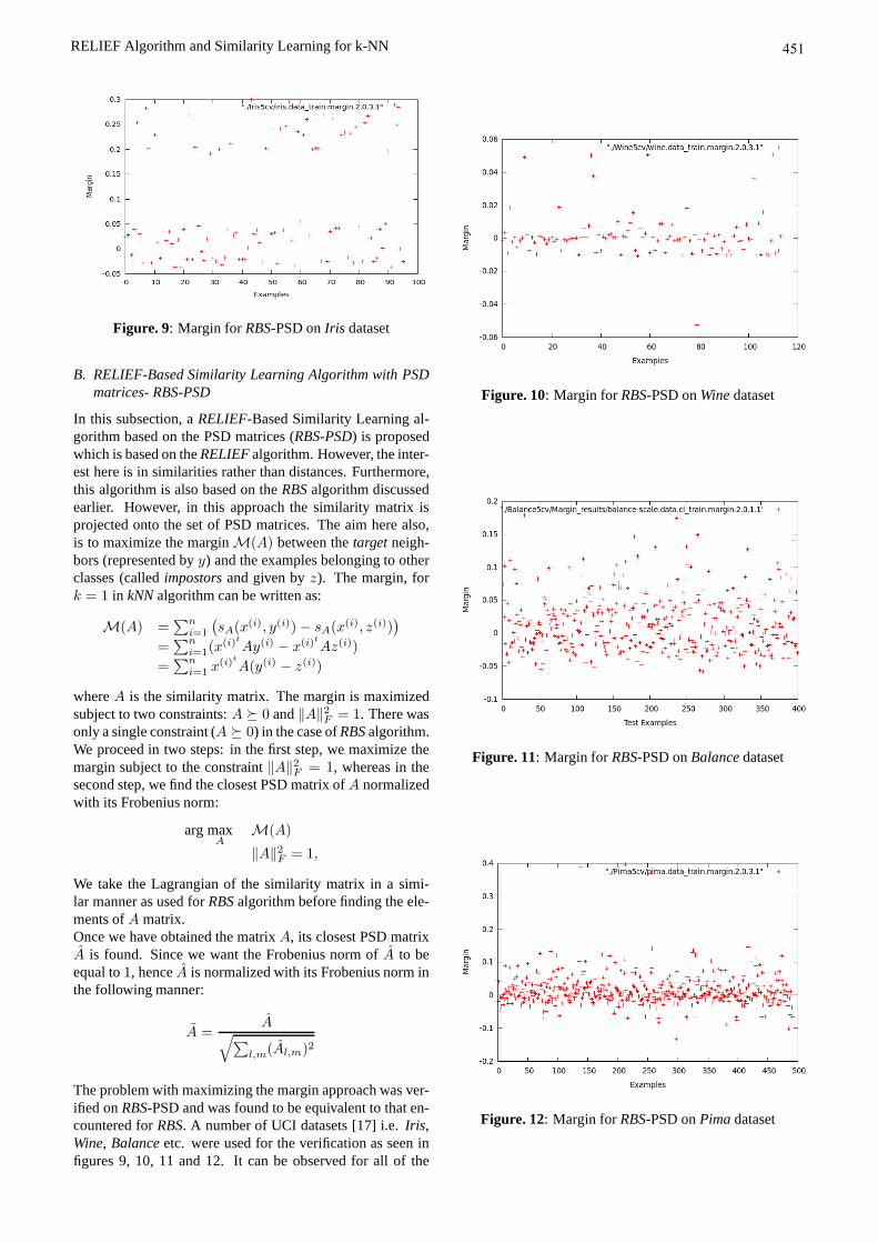
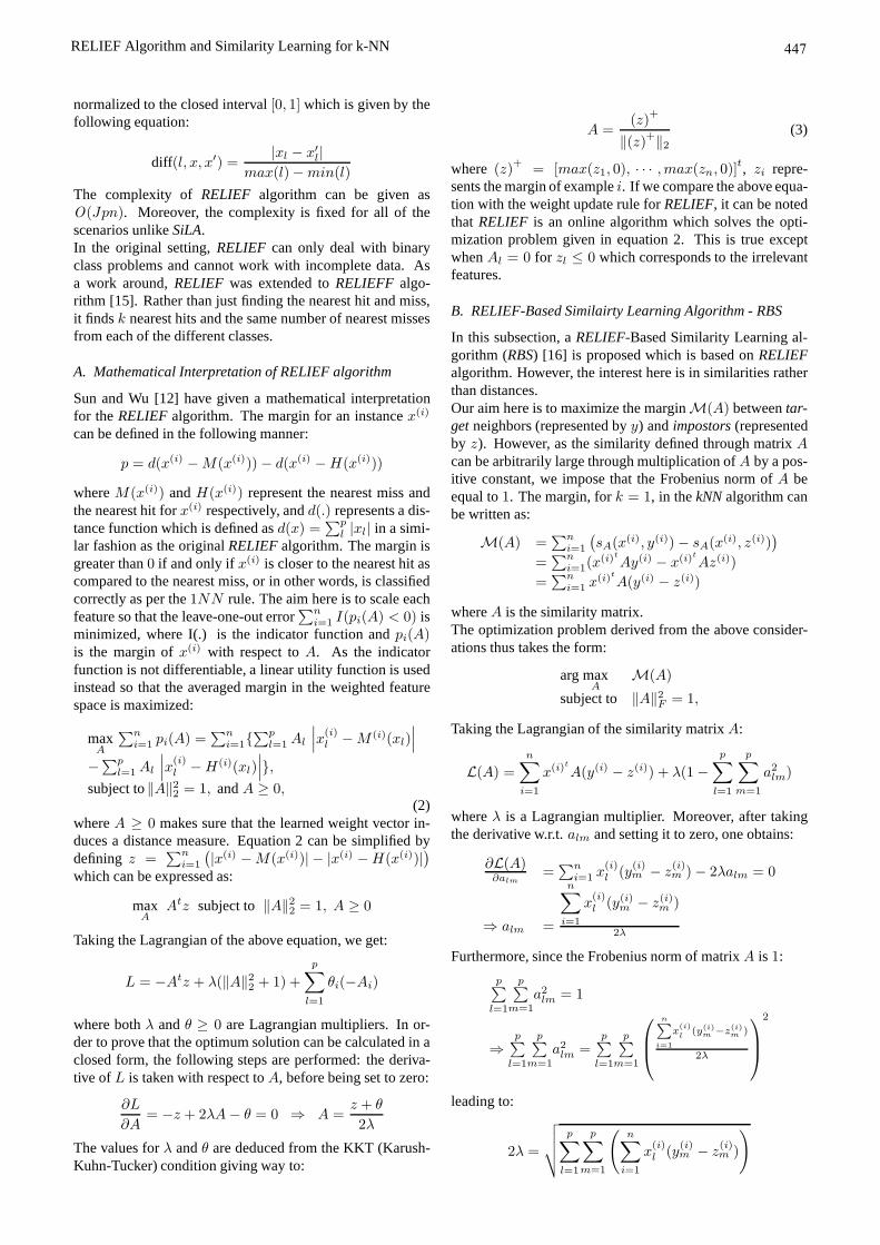
Figure. 9: Margin forRBS-PSD onIris dataset

B. RELIEF-Based Similarity Learning Algorithm with PSDmatrices- RBS-PSD

In this subsection, aRELIEF-Based Similarity Learning al-gorithm based on the PSD matrices (RBS-PSD) is proposedwhich is based on theRELIEFalgorithm. However, the inter-est here is in similarities rather than distances. Furthermore,this algorithm is also based on theRBSalgorithm discussedearlier. However, in this approach the similarity matrix isprojected onto the set of PSD matrices. The aim here also,is to maximize the marginM(A) between thetargetneigh-bors (represented byy) and the examples belonging to otherclasses (calledimpostorsand given byz). The margin, fork = 1 in kNNalgorithm can be written as:

M(A) =∑n

i=1

(

sA(x(i), y(i))− sA(x

(i), z(i)))

=∑n

i=1(x(i)tAy(i) − x(i)tAz(i))

=∑n

i=1 x(i)tA(y(i) − z(i))

whereA is the similarity matrix. The margin is maximizedsubject to two constraints:A � 0 and‖A‖2F = 1. There wasonly a single constraint (A � 0) in the case ofRBSalgorithm.We proceed in two steps: in the first step, we maximize themargin subject to the constraint‖A‖2F = 1, whereas in thesecond step, we find the closest PSD matrix ofA normalizedwith its Frobenius norm:

arg maxA

M(A)

‖A‖2F = 1,

We take the Lagrangian of the similarity matrix in a simi-lar manner as used forRBSalgorithm before finding the ele-ments ofA matrix.Once we have obtained the matrixA, its closest PSD matrixA is found. Since we want the Frobenius norm ofA to beequal to 1, henceA is normalized with its Frobenius norm inthe following manner:

A =A

√

∑

l,m(Al,m)2

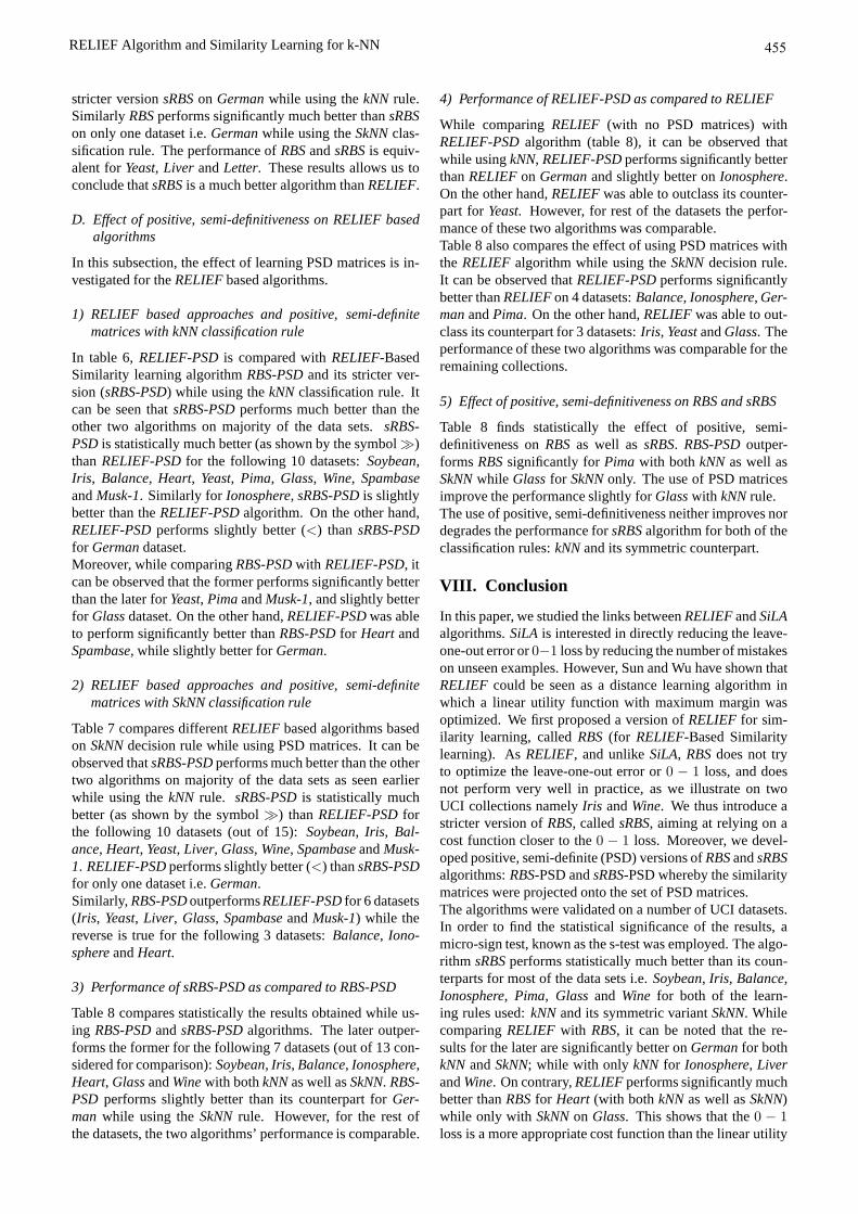
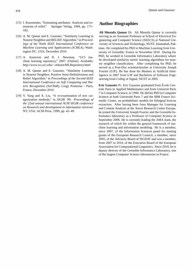
The problem with maximizing the margin approach was ver-ified onRBS-PSD and was found to be equivalent to that en-countered forRBS. A number of UCI datasets [17] i.e.Iris,Wine, Balanceetc. were used for the verification as seen infigures 9, 10, 11 and 12. It can be observed for all of the

Figure. 10: Margin forRBS-PSD onWinedataset

Figure. 11: Margin forRBS-PSD onBalancedataset

Figure. 12: Margin forRBS-PSD onPimadataset


datasets that the average margin remains positive despite thepresence of a number of mistakes, since the positive marginis much greater than the negative one for the majority of thetest examples. For example, the values of negative margin inthe case ofIris is in the range of0.05−0.10 whereas most ofthe positive margin values are greater than0.15. Similarly,for Wine, most of the negative margin values lie in the rangebetween0 and−0.04 while the positive margin values aredispersed in the range0 − 0.08. So, despite the fact that theoverall margin is large, a lot of examples are misclassified.This explains the fact that the algorithmsRELIEF-PSDandRBS-PSDdid not perform quite well on different standardtest collections as can be seen in Section VII.

VI. A stricter version of RBS-PSD:sRBS-PSD

The same work around used in the case ofsRBSalgorithmto improve the performance ofRELIEFbased methods wasused in the case ofRELEIF-PSD andRBS-PSD: to directlyuse the leave-one-out error or0 − 1 loss like theSiLAalgo-rithm [8] where the aim is to reduce the number of mistakeson unseen examples. The resulting algorithm is a stricter ver-sion ofRBS-PSD and is termed assRBS-PSD. It is called asa stricter version as we do not try to maximize the overallmargin but are interested in reducing the individual errorsonthe unseen examples.sRBS-PSD algorithm is exactly the same assRBSexcept thefact that in the former case, the similarity matrix is projectedonto the set of PSD matrices.We proceed in two steps in the case ofsRBS-PSD: in thefirst step we find theA matrix for which the cost functionis minimized. In the second step, we find the closest PSDmatrix ofA which should have a low cost.

sRBS-PSD - TrainingInput: training set(x(1), c(1)), · · · , (x(n), c(n)) of n vectorsin Rp, A1

lm denotes the element ofA1 at row l and columnm

Output:Matrix A

Initialization t = 1, A(1) = 1 (Unity matrix)RepeatJ times (epochs)for all of the featuresl,m

Minuslm = 0

for i = 1, · · · , n

for all of the featuresl,m

Minuslm + = ∂Qi(At)

∂alm

αt = 1t

At+1 = At − αt

n∗ Minus

If there exist strictly positive eigenvalues ofAt+1, thenAt+1 =

∑

r,λr>0 λrurutr (whereλr andur are the eigen-

values and eigenvectors ofAt+1)Error otherwiseif∑

lm |At+1lm −At

lm| ≤ 0.001

Stop

Figures 13, 14, 15 and 16 show the margin values on thetraining data forsRBS-PSDfor the datasetsIris, Wine andBalance. Comparing these results with the earlier ones for

Figure. 13: Margin forsRBS-PSD onIris dataset

Figure. 14: Margin forsRBS-PSD onWinedataset

Figure. 15: Margin forsRBS-PSD onBalancedataset


Figure. 16: Margin forsRBS-PSD onPimadataset

kNN-cosine kNN-Euclidean

Soybean 1.0± 0.0 1.0± 0.0Iris 0.987± 0.025 0.973± 0.029Letter 0.997± 0.002 0.997± 0.002Balance 0.954± 0.021≫ 0.879± 0.028Wine 0.865± 0.050≫ 0.819± 0.096Ionosphere 0.871± 0.019 0.854± 0.035Glass 0.899± 0.085 0.890± 0.099Pima 0.630± 0.041 0.698± 0.024≫Liver 0.620± 0.064 0.620± 0.043German 0.594± 0.040 0.615± 0.047Heart 0.670± 0.020 0.656± 0.056Yeast 0.911± 0.108 0.912± 0.108Spambase 0.858± 0.009 0.816± 0.007Musk-1 0.844± 0.028 0.848± 0.018

Table 2: Comparison between cosine similarity and Euclidean dis-tance based on s-test

RBS-PSD, one can see the importance of using a cost func-tion closer to the0− 1 loss. The margin is positive for mostof the training examples in this case.

VII. Experimental Validation

Fifteen datasets from the UCI database ([17]) were used toassess the performance of the different algorithms. These arestandard collections which have been used by different re-search communities (machine learning, pattern recognition,statistics etc.). The information about the datasets is summa-rized in Table 1 whereBal stands forBalancewhereasIonorefers toIonosphere.Table 2 compares the performance of cosine similarity andthe Euclidean distance for all of the datasets.The matrices learned by all of the algorithms can be usedto predict the class(es) to which a new example should beassigned. Two basic rules for prediction were considered: thestandardkNNrule and its symmetric variant (SkNN). SkNNisbased on the consideration of the same number of examplesin the different classes. The new example is simply assignedto the closest class, the similarity with a class being definedas the sum of the similarities between the new example andits k nearest neighbors in the class.Furthermore, all of the algorithms can be used in either a bi-nary or multi-class mode. There are a certain number of ad-vantages in the binary version. First, it allows using the two

prediction rules given above. Moreover, it allows learninglocal matrices, which are more likely to capture the varietyof the data. Finally, its application in prediction resultsin amulti-label decision.5-fold nested cross-validation was used to learn the singleweight vector in case ofRELIEF andRBSalong with theirPSD counterparts, and the matrix sequence(A1, · · · , An) incase ofsRBSandsRBS-PSD for all of the datasets. 20 per-cent of the data was used for test purpose for each of thedataset. Of the remaining data, 80 percent was used forlearning whereas 20 percent for the validation set. In caseof RELIEF, RBSand their PSD versions, the validation setis used to find the best value ofk, whereas in the case ofsRBSandsRBS-PSD, it is used to estimate the values ofk,λ andβ. Micro-sign test (s-test), earlier used by Yang andLiu [19] was performed to assess the statistical significanceof the different results.

A. Comparison between different RELIEF algorithms basedon kNN decision rule

While comparingRELIEF with its similarity based variant(RBS) based on the simplekNN classification rule, it is ev-ident that the later performs significantly much better onlyon Germanand slightly better onSoybeanas shown in ta-ble 3. HoweverRELIEF outperformsRBSfor Heart whileusingkNN.It can be further verified from table 3 that the algorithmsRBSperforms significantly much better (≫) than theRELIEFal-gorithm for eight out of twelve datasets i.e.Soybean, Iris,Balance, Ionosphere, Heart, Pima, GlassandWine. This al-lows one to deduce safely thatsRBSin general is a muchbetter choice thanRELIEFalgorithm.

B. Comparison between different RELIEF algorithms basedon SkNN decision rule

While comparingRELIEF with its similarity based variant(RBS) based on theSkNN-A rule, it can be seen from table 4that the later performs significantly much better onIono-sphere, German, Liver andWinecollections. On the otherhand,RELIEFperforms significantly much better thanRBSonHeart andGlass.It can further observed thatsRBSperformed significantlymuch better thanRELIEFon majority of the datasets (9 outof a total of 12) i.e.Soybean, Iris, Balance, Ionosphere,Heart, German, Pima, Glass and Wine. On Liver, sRBSperformed slightly better than theRELIEFalgorithm. ThussRBSoutperformsRELIEF in general forSkNNas seen pre-viously forkNN.

C. Performance of sRBS as compared to RBS

Furthemore, the twoRELIEF based similarity learning al-gorithms i.e.RBSandsRBSare compared using bothkNNas well asSkNN as shown in table 5. On majority ofthe datasets, the algorithmsRBSoutperformsRBSfor bothkNNandSkNN. sRBSperforms significantly much better (asshown by≪) than its counterpart on the following datasets:Soybean, Iris, Balance, Ionosphere, Heart, Pima, GlassandWinefor the two classification rules (kNNandSkNN). On theother hand,RBSwas able to perform slighty better than its


Iris Wine Bal Iono Glass Soy Pima Liver Letter German Yeast Heart Magic Spam Musk-1

Learn 96 114 400 221 137 30 492 220 12800 640 950 172 12172 2944 304Valid. 24 29 100 56 35 8 123 56 3200 160 238 44 3044 737 77Test 30 35 125 70 42 9 153 69 4000 200 296 54 3804 920 95Class 3 3 3 2 6 4 2 2 26 2 10 2 2 2 2Feat. 4 13 4 34 9 35 8 6 16 20 8 13 10 57 168

Table 1: Characteristics of datasets

kNN-A (RELIEF) kNN-A (RBS) kNN-A (sRBS)

Soybean 0.711± 0.211 0.750± 0.197> 1.0± 0.0≫

Iris 0.667± 0.059 0.667± 0.059 0.987± 0.025≫

Balance 0.681± 0.662 0.670± 0.171 0.959± 0.016≫

Ionosphere 0.799± 0.062 0.826± 0.035 0.866± 0.015≫

Heart 0.556± 0.048 0.437± 0.064≪ 0.696± 0.046≫

Yeast 0.900± 0.112 0.900± 0.112 0.905± 0.113

German 0.598± 0.068 0.631± 0.020≫ 0.609± 0.016

Liver 0.574± 0.047 0.580± 0.042 0.583± 0.015

Pima 0.598± 0.118 0.583± 0.140 0.651± 0.034≫

Glass 0.815± 0.177 0.821± 0.165 0.886± 0.093≫

Letter 0.961± 0.003 0.961± 0.005 0.997± 0.002

Wine 0.596± 0.188 0.630± 0.165 0.834± 0.077≫

Table 3: Comparison between differentRELIEFbased algorithms while usingkNN-A method based on s-test

SkNN-A (RELIEF) SkNN-A (RBS) SkNN-A (sRBS)

Soybean 0.756± 0.199 0.750± 0.197 0.989± 0.034≫

Iris 0.673± 0.064 0.667± 0.059 0.987± 0.025≫

Balance 0.662± 0.200 0.672± 0.173 0.967± 0.010≫

Ionosphere 0.681± 0.201 0.834± 0.031≫ 0.871± 0.021≫

Heart 0.526± 0.085 0.430± 0.057≪ 0.685± 0.069≫

Yeast 0.900± 0.113 0.900± 0.112 0.908± 0.110

German 0.493± 0.115 0.632± 0.021≫ 0.598± 0.038≫

Liver 0.539± 0.078 0.580± 0.042≫ 0.588± 0.021>

Pima 0.585± 0.125 0.583± 0.140 0.665± 0.044≫

Glass 0.833± 0.140 0.816± 0.171≪ 0.884± 0.084≫

Letter 0.957± 0.047 0.961± 0.005 0.997± 0.002

Wine 0.575± 0.198 0.634± 0.168≫ 0.840± 0.064≫

Table 4: Comparison between differentRELIEFbased algorithms while usingSkNN-A based on s-test


stricter versionsRBSon Germanwhile using thekNN rule.Similarly RBSperforms significantly much better thansRBSon only one dataset i.e.Germanwhile using theSkNNclas-sification rule. The performance ofRBSandsRBSis equiv-alent forYeast, Liver andLetter. These results allows us toconclude thatsRBSis a much better algorithm thanRELIEF.

D. Effect of positive, semi-definitiveness on RELIEF basedalgorithms

In this subsection, the effect of learning PSD matrices is in-vestigated for theRELIEFbased algorithms.

1) RELIEF based approaches and positive, semi-definitematrices with kNN classification rule

In table 6,RELIEF-PSDis compared withRELIEF-BasedSimilarity learning algorithmRBS-PSDand its stricter ver-sion (sRBS-PSD) while using thekNNclassification rule. Itcan be seen thatsRBS-PSDperforms much better than theother two algorithms on majority of the data sets.sRBS-PSDis statistically much better (as shown by the symbol≫)thanRELIEF-PSDfor the following 10 datasets:Soybean,Iris, Balance, Heart, Yeast, Pima, Glass, Wine, SpambaseandMusk-1. Similarly for Ionosphere, sRBS-PSDis slightlybetter than theRELIEF-PSDalgorithm. On the other hand,RELIEF-PSDperforms slightly better (<) than sRBS-PSDfor Germandataset.Moreover, while comparingRBS-PSDwith RELIEF-PSD, itcan be observed that the former performs significantly betterthan the later forYeast, PimaandMusk-1, and slightly betterfor Glassdataset. On the other hand,RELIEF-PSDwas ableto perform significantly better thanRBS-PSDfor Heart andSpambase, while slightly better forGerman.

2) RELIEF based approaches and positive, semi-definitematrices with SkNN classification rule

Table 7 compares differentRELIEFbased algorithms basedon SkNNdecision rule while using PSD matrices. It can beobserved thatsRBS-PSDperforms much better than the othertwo algorithms on majority of the data sets as seen earlierwhile using thekNN rule. sRBS-PSDis statistically muchbetter (as shown by the symbol≫) thanRELIEF-PSDforthe following 10 datasets (out of 15):Soybean, Iris, Bal-ance, Heart, Yeast, Liver, Glass, Wine, SpambaseandMusk-1. RELIEF-PSDperforms slightly better (<) thansRBS-PSDfor only one dataset i.e.German.Similarly,RBS-PSDoutperformsRELIEF-PSDfor 6 datasets(Iris, Yeast, Liver, Glass, SpambaseandMusk-1) while thereverse is true for the following 3 datasets:Balance, Iono-sphereandHeart.

3) Performance of sRBS-PSD as compared to RBS-PSD

Table 8 compares statistically the results obtained while us-ing RBS-PSDandsRBS-PSDalgorithms. The later outper-forms the former for the following 7 datasets (out of 13 con-sidered for comparison):Soybean, Iris, Balance, Ionosphere,Heart, GlassandWinewith bothkNNas well asSkNN. RBS-PSD performs slightly better than its counterpart forGer-man while using theSkNNrule. However, for the rest ofthe datasets, the two algorithms’ performance is comparable.

4) Performance of RELIEF-PSD as compared to RELIEF

While comparingRELIEF (with no PSD matrices) withRELIEF-PSDalgorithm (table 8), it can be observed thatwhile usingkNN, RELIEF-PSDperforms significantly betterthanRELIEFon Germanand slightly better onIonosphere.On the other hand,RELIEFwas able to outclass its counter-part for Yeast. However, for rest of the datasets the perfor-mance of these two algorithms was comparable.Table 8 also compares the effect of using PSD matrices withthe RELIEF algorithm while using theSkNNdecision rule.It can be observed thatRELIEF-PSDperforms significantlybetter thanRELIEFon 4 datasets:Balance, Ionosphere, Ger-manandPima. On the other hand,RELIEFwas able to out-class its counterpart for 3 datasets:Iris, YeastandGlass. Theperformance of these two algorithms was comparable for theremaining collections.

5) Effect of positive, semi-definitiveness on RBS and sRBS

Table 8 finds statistically the effect of positive, semi-definitiveness onRBSas well assRBS. RBS-PSDoutper-formsRBSsignificantly forPima with bothkNN as well asSkNNwhile Glassfor SkNNonly. The use of PSD matricesimprove the performance slightly forGlasswith kNNrule.The use of positive, semi-definitiveness neither improves nordegrades the performance forsRBSalgorithm for both of theclassification rules:kNNand its symmetric counterpart.

VIII. Conclusion

In this paper, we studied the links betweenRELIEFandSiLAalgorithms.SiLA is interested in directly reducing the leave-one-out error or0−1 loss by reducing the number of mistakeson unseen examples. However, Sun and Wu have shown thatRELIEF could be seen as a distance learning algorithm inwhich a linear utility function with maximum margin wasoptimized. We first proposed a version ofRELIEF for sim-ilarity learning, calledRBS(for RELIEF-Based Similaritylearning). AsRELIEF, and unlikeSiLA, RBSdoes not tryto optimize the leave-one-out error or0 − 1 loss, and doesnot perform very well in practice, as we illustrate on twoUCI collections namelyIris andWine. We thus introduce astricter version ofRBS, calledsRBS, aiming at relying on acost function closer to the0 − 1 loss. Moreover, we devel-oped positive, semi-definite (PSD) versions ofRBSandsRBSalgorithms:RBS-PSD andsRBS-PSD whereby the similaritymatrices were projected onto the set of PSD matrices.The algorithms were validated on a number of UCI datasets.In order to find the statistical significance of the results, amicro-sign test, known as the s-test was employed. The algo-rithm sRBSperforms statistically much better than its coun-terparts for most of the data sets i.e.Soybean, Iris, Balance,Ionosphere, Pima, Glass and Wine for both of the learn-ing rules used:kNNand its symmetric variantSkNN. WhilecomparingRELIEF with RBS, it can be noted that the re-sults for the later are significantly better onGermanfor bothkNN andSkNN; while with only kNN for Ionosphere, LiverandWine. On contrary,RELIEFperforms significantly muchbetter thanRBSfor Heart (with bothkNNas well asSkNN)while only with SkNNon Glass. This shows that the0 − 1loss is a more appropriate cost function than the linear utility


kNN-A (RBS) / kNN-A (sRBS) SkNN-A (RBS) / SkNN-A (sRBS)

Soybean ≪ ≪

Iris ≪ ≪

Balance ≪ ≪

Ionosphere ≪ ≪

Heart ≪ ≪

Yeast = =German > ≫

Liver = =Pima ≪ ≪

Glass ≪ ≪

Letter = =Wine ≪ ≪

Table 5: Comparison betweenRBSandsRBSbased on s-test

kNN-A (RELIEF-PSD) kNN-A (RBS-PSD) kNN-A (sRBS-PSD)

Soybean 0.739± 0.192 0.733± 0.220 1.0± 0.0≫

Iris 0.664± 0.058 0.667± 0.059 0.987± 0.025≫

Balance 0.665± 0.193 0.670± 0.171 0.959± 0.016≫

Ionosphere 0.839± 0.055 0.826± 0.035 0.880± 0.015>

Heart 0.556± 0.048 0.437± 0.036≪ 0.693± 0.047≫

Yeast 0.893± 0.132 0.900± 0.112≫ 0.911± 0.109≫

German 0.637± 0.017 0.624± 0.015< 0.609± 0.016<

Liver 0.574± 0.034 0.580± 0.042 0.606± 0.034

Pima 0.593± 0.077 0.661± 0.024≫ 0.651± 0.034≫

Glass 0.819± 0.164 0.835± 0.138> 0.886± 0.093≫

Letter 0.961± 0.005 0.961± 0.005 0.997± 0.002

Wine 0.608± 0.185 0.630± 0.165 0.834± 0.077≫

Magic 0.516± 0.085 0.360± 0.007 0.767± 0.009

Spambase 0.618± 0.031 0.611± 0.020≪ 0.855± 0.009≫

Musk-1 0.698± 0.055 0.851± 0.033≫ 0.838± 0.024≫

Table 6: Comparison between differentRELIEFbased algorithms usingkNN-A and PSD matrices

SkNN-A (RELIEF-PSD) SkNN-A (RBS-PSD) SkNN-A (sRBS-PSD)

Soybean 0.783± 0.163 0.733± 0.220 0.983± 0.041≫

Iris 0.571± 0.164 0.667± 0.059≫ 0.987± 0.025≫

Balance 0.708± 0.175 0.672± 0.173≪ 0.967± 0.010≫

Ionosphere 0.886± 0.028 0.834± 0.031≪ 0.889± 0.011

Heart 0.533± 0.067 0.437± 0.036≪ 0.685± 0.069≫

Yeast 0.897± 0.122 0.900± 0.112≫ 0.914± 0.106≫

German 0.625± 0.035 0.624± 0.015 0.598± 0.038<

Liver 0.528± 0.085 0.580± 0.042≫ 0.609± 0.035≫

Pima 0.659± 0.027 0.658± 0.030 0.665± 0.044

Glass 0.768± 0.235 0.835± 0.138≫ 0.884± 0.084≫

Letter 0.961± 0.008 0.961± 0.004 0.997± 0.002

Wine 0.606± 0.177 0.634± 0.168 0.840± 0.064≫

Magic 0.539± 0.109 0.360± 0.007 0.777± 0.009

Spambase 0.583± 0.075 0.611± 0.020≫ 0.857± 0.010≫

Musk-1 0.712± 0.037 0.857± 0.029≫ 0.842± 0.010≫

Table 7: Comparison between differentRELIEFbased algorithms usingSkNN-A and PSD matrices


Table 8: Comparison between different algorithms based on s-test

RELIEF / RELIEF-PSD RBS / RBS-PSD sRBS / sRBS-PSD RBS-PSD / sRBS-PSD

kNN-A SkNN-A kNN-A SkNN-A kNN-A SkNN-A kNN-A SkNN-A

Soybean = = = = = = ≪ ≪

Iris = ≫ = = = = ≪ ≪

Balance = ≪ = = = = ≪ ≪

Ionosphere < ≪ = = = = ≪ ≪

Heart = = = = = = ≪ ≪

Yeast ≫ ≫ = = = = = =German ≪ ≪ = = = = = >

Liver = = = = = = = =Pima = ≪ ≪ ≪ = = = =Glass = ≫ < ≪ = = ≪ ≪

Letter = = = = = = = =Wine = = = = = = ≪ ≪

Musk-1 = =

function used byRELIEF. While comparing the PSD algo-rithms with their counterparts,RELIEF-PSD performed wellas compared toRELIEF. However, for the rest of the algo-rithms, the effect of projection onto the set of PSD matriceswas minimal e.g. in the case ofsRBS, the use of PSD matri-ces neither improves neither degrades the performance.

Acknowledgments

Ali Mustafa would like to thank the French Ministry ofHigher Education and Research for the PhD grant.

References

[1] M. Diligenti, M. Maggini, and L. Rigutini, “Learningsimilarities for text documents using neural networks,”in Proceedings of International Workshop on ArtificialNeural Networks in Pattern Recognition (ANNPR), Flo-rence, Italy, 2003.

[2] L. Baoli, L. Qin, and Y. Shiwen, “An adaptive k-nearest neighbor text categorization strategy,”ACMTransactions on Asian Language Information Process-ing (TALIP), vol. 3, no. 4, pp. 215–226, 2004.

[3] S. Shalev-Shwartz, Y. Singer, and A. Y. Ng, “Onlineand batch learning of pseudo-metrics,” inICML ’04:Proceedings of the twenty-first International Confer-ence on Machine learning. New York, NY, USA:ACM, 2004, p. 94.

[4] K. Q. Weinberger and L. K. Saul, “Distance metriclearning for large margin nearest neighbor classifica-tion,” Journal of Machine Learning Research, vol. 10,pp. 207–244, Feb 2009.

[5] Y. Chen, E. K. Garcia, M. R. Gupta, A. Rahimi, andL. Cazzanti, “Similarity-based classification: Conceptsand algorithms,”Journal of Machine Learning Re-search, vol. 10, pp. 747–776, March 2009.

[6] S. Melacci, L. Sarti, M. Maggini, and M. Bianchini,“A neural network approach to similarity learning,”in Proceeding of Third IAPR Workshop on Artifi-cial Neural Networks in Pattern Recognition, ANNPR,Paris, France, ser. Lecture Notes in Computer Science.Springer, 2008, pp. 133–136.

[7] M. R. Peterson, T. E. Doom, and M. L. Raymer, “GA-facilitated knn classifier optimization with varying sim-ilarity measures,” inEvolutionary Computation, 2005.The 2005 IEEE Congress on, vol. 3, Sept. 2005, pp.2514–2521.

[8] A. M. Qamar, E. Gaussier, J.-P. Chevallet, and J. H.Lim, “Similarity learning for nearest neighbor classifi-cation,” inProceedings of International Conference onData Mining (ICDM), 2008, pp. 983–988.

[9] M. P. Umugwaneza and B. Zou, “A novel similar-ity measure using a normalized hausdorff distance fortrademarks retrieval based on genetic algorithm,”Inter-national Journal of Computer Information Systems andIndustrial Management Applications (IJCISIM), vol. 1,pp. 312–320, 2009.

[10] P. Porwik, R. Doroz, and K. Wrobel, “A new signaturesimilarity measure based on windows allocation tech-nique,” International Journal of Computer InformationSystems and Industrial Management Applications (IJ-CISIM), vol. 2, pp. 297–305, 2010.

[11] K. Kira and L. A. Rendell, “A practical approach to fea-ture selection,” inML92: Proceedings of the ninth in-ternational workshop on Machine learning. San Fran-cisco, CA, USA: Morgan Kaufmann Publishers Inc.,1992, pp. 249–256.

[12] Y. Sun and D. Wu, “A RELIEF based feature extractionalgorithm,” in Proceedings of the SIAM InternationalConference on Data Mining, SDM, Atlanta, USA, 2008,pp. 188–195.

[13] Y. Freund and R. E. Schapire, “Large margin classifica-tion using the perceptron algorithm,”Machine Learn-ing, vol. 37, no. 3, pp. 277–296, 1999.

[14] M. Collins, “Discriminative training methods for hid-den markov models: theory and experiments with per-ceptron algorithms,” inEMNLP ’02: Proceedings ofthe ACL-02 conference on Empirical methods in natu-ral language processing, Morristown, NJ, USA, 2002,pp. 1–8.


[15] I. Kononenko, “Estimating attributes: Analysis and ex-tensions of relief.” Springer Verlag, 1994, pp. 171–182.

[16] A. M. Qamar and E. Gaussier, “Similarity Learning inNearest Neighbor and RELIEF Algorithm,” inProceed-ings of the Ninth IEEE International Conference onMachine Learning and Applications (ICMLA), Wash-ington DC, USA, December 2010.

[17] A. Asuncion and D. J. Newman, “UCI ma-chine learning repository,” 2007. [Online]. Available:http://www.ics.uci.edu/∼mlearn/MLRepository.html

[18] A. M. Qamar and E. Gaussier, “Similarity Learningin Nearest Neighbor; Positive Semi-Definitiveness andRelief Algorithm,” in Proceedings of the Second IEEEInternational Conference on Soft Computing and Pat-tern Recognition (SoCPaR), Cergy Pointoise / Paris,France, December 2010.

[19] Y. Yang and X. Liu, “A re-examination of text cat-egorization methods,” inSIGIR ’99: Proceedings ofthe 22nd annual international ACM SIGIR conferenceon Research and development in information retrieval.NY, USA: ACM Press, 1999, pp. 42–49.

Author Biographies

Ali Mustafa Qamar Dr. Ali Mustafa Qamar is currentlyserving as an Assistant Professor at School of Electrical En-gineering and Computer Science (SEECS) at National Uni-versity of Sciences and Technology, NUST, Islamabad, Pak-istan. He completed his PhD in Machine Learning from Uni-versity of Grenoble, France in November 2010. During hisPhD, he worked in Grenoble Informatics Laboratory wherehe developed similarity metric learning algorithms for near-est neighbor classification. After completing his PhD, heserved as a Post-Doc scientist/teacher at University JosephFourier (UJF). He has done his Masters in Artificial Intel-ligence in 2007 from UJF and Bachelors of Software Engi-neering from Colleg of Signal, NUST in 2005.

Eric Gaussier Pr. Eric Gaussier graduated fromEcole Cen-trale Paris in Applied Mathematics and from Universit Paris7 in Computer Science, in 1990. He did his PhD in ComputerScience at both Universite Paris 7 and the IBM France Sci-entific Center, on probabilistic models for bilingual lexiconextraction. After having been Area Manager for Learningand Content Analysis at the Xerox Research Centre Europe,he joined the Universite Joseph Fourier and the Grenoble In-formatics laboratory as a Professor of Computer Science inSeptember 2006. He is currently leading the AMA team, theresearch of which fits within the general framework of ma-chine learning and information modeling. He is a member,since 2007, of the Information Sciences panel for startinggrants of the European Research Council, a member, since2005, of the Advisory Board of SIGDAT and was a member,from 2007 to 2010, of the Executive Board of the EuropeanAssociation for Computational Linguistics. Since 2010, heisdeputy director of the Grenoble Informatics Laboratory, oneof the largest Computer Science laboratories in France.

458

Qamar and Gaussier

relief algorithm and similarity learning for k-nn · relief algorithm and similarity learning for...

Documents