Relative Labor Productivity and the Real Exchange Ratein the Long Run: Evidence for a Panel of OECD Countries

by

Matthew B. Canzoneri, Robert E. Cumby and Behzad Diba

Georgetown University

Revised July 1997

ABSTRACT

The Balassa-Samuelson model, which explains real exchange rate movements in terms ofsectoral productivities, rests on two components. First, it implies that the relative price ofnontraded goods in each country should reflect the relative productivity of labor in the traded andnontraded goods sectors. Second, it assumes purchasing power parity holds for traded goods. Wetest both of these using a panel of OECD countries. Our results suggest that relative pricesgenerally reflect relative labor productivities in the long run. The evidence on purchasing powerparity in traded goods is less favorable, at least when we look at U.S. dollar exchange rates.

2

Changes in real exchange rates—defined as the relative price of national outputs—have

been so persistent that they question the very notion of purchasing power parity (PPP). Even the

evidence suggesting that deviations from PPP are temporary points to a half life of four to five

years.1 Explanations of persistent real exchange rate changes have often followed the lead of

Balassa (1964) and Samuelson (1964), who divide national output into traded and nontraded

goods and explain real exchange rates in terms of sectoral productivity. The Balassa-Samuelson

hypothesis divides real exchange rate movements into two components. Competitive behavior

implies that the relative price of nontraded goods depends on the ratio of the marginal costs in

the two sectors, and we will show that for a wide class of technologies the ratio of marginal costs

is proportional to the ratio of average labor products in the two sectors. So, the first component

of the hypothesis is the assumption that the relative price of nontradeables is proportional to the

ratio of average labor products. The second component is the assumption of PPP for traded

goods.

The two components combine to produce a simple model of real exchange rate

movements. If, for example, the ratio of traded goods productivity to nontraded goods

productivity is growing faster at home than abroad, then the relative price of nontraded goods

must be growing faster at home than abroad, and the price of home national output must be rising

relative to the price of foreign national output (since by assumption the prices of traded goods

equalize). In other words, if traded good productivity relative to nontraded good productivity is

growing faster at home than abroad, then the home country should experience a real appreciation.

How well does the Balassa-Samuelson model explain real exchange rate movements? In

figure 1 we plot four bilateral real exchange rates along with the ratio of labor productivity in the

3

traded and nontraded goods sectors for each country. The Balassa-Samuelson hypothesis clearly

fails to explain the short run movements in real exchange rates and figure 1 suggests that there

may also be problems in explaining the long run movements, especially where the U.S. dollar is

concerned. Relative traded goods productivity has risen much faster in the United States than in

Germany, especially since the late-1970s. This should have led to a real appreciation of the

dollar (a fall in the real exchange rate as plotted in figure 1); instead, the dollar has depreciated.

And the negligible difference between U.S. and Japanese productivity trends has little hope of

explaining the real depreciation of the dollar against the yen. The Balassa-Samuelson hypothesis

does seem to fare better with DM real exchange rates. Since the mid-1970s, relative traded

goods productivity has been growing more rapidly in both Italy and Japan than it has in Germany,

and both the lira and the yen have appreciated in real terms against the DM.

Figure 1 points to some problems with the Balassa-Samuelson hypothesis, but it does not

reveal the source of the problems. Nor does it explain why there might be a problem with the

dollar real exchange rates. Either component of the hypothesis can be challenged, and the special

problem with the dollar—if one exists—could reside in either place.

In this paper we examine the two components of the Balassa-Samuelson hypothesis using

a panel of 13 OECD countries. We do not require that either part of the hypothesis holds in the

short run. In fact, both theory and a substantial body of evidence suggest that short-run deviations

from both can be substantial. Instead, we focus our tests on long-run or trend behavior.

Two unfortunate facts have combined to plague the time series literature on long run real

exchange rates: we typically only have 20 to 30 years of data on any pair of countries, and unit

root tests have notoriously low power in small samples to distinguish between series that are

4

nonstationary and series that are stationary but highly persistent.2 Recently developed techniques

allow us to deal with nonstationary data in heterogeneous panels, and in fact combining the data

from 13 countries yields substantial benefits. We are able to confirm the existence of a long run

(or cointegrating) relationship between the relative price of nontradeables and the ratio of average

labor products, and we are able to estimate its parameters with a surprising degree of precision.

The precision is so great that we are seemingly able to reject the first component of

Balassa-Samuelson model. This leads us to perform some Monte Carlo experiments to show that

the remaining small sample bias is capable of explaining our apparent rejection of the model.

We will argue that this firmly establishes the first component of the Balassa-Samuelson

hypothesis.

We will argue instead that the problems with the Balassa-Samuelson hypothesis lie in the

failure of PPP to explain traded goods prices, especially for the U.S. dollar. Once again, using

panel data we are able to establish that the appropriate long run (or cointegrating) relationship

exists, but our estimates of its parameters are much less precise, and none of the parameter

estimates are close to the values implied by PPP. And, as figure 1 would seem to suggest, we

find that the failure of PPP to hold for traded goods may be largely a U.S. dollar phenomenon.

These large and persistent deviations from PPP in traded goods dominate U.S. dollar real

exchange rate movements and it is therefore difficult to explain those movements with

differences in sectoral productivities.3 When we use the DM as reference currency, the results

are much more favorable.

The plan of the paper is as follows. In section 2 we describe our notation and set out the

two components of the Balassa-Samuelson hypothesis. We review the econometric methods we

5

MX / ML X

MH / ML H'

W / P X

W / P H'

P H

P X' q (1)

MX / ML X

MH / ML H'

n (X / L X )

R (H / L H)(2)

X ' F(K X) (L X)n , H ' G(K H) (L H)R (3)

use in section 3, we present our empirical results in section 4. In section 5 we offer some

concluding remarks.

2. The Analytical Framework

We begin with the link between the relative price of nontraded goods and the relative

productivities in the traded and nontraded goods sectors. The analytical framework we use is

quite general. In each country, capital and labor are employed in the production of traded goods,

X, and non-traded goods, H. Competition implies that labor is paid the value of its marginal

product, and labor mobility implies that the nominal wage rate, W, is equal in the two sectors.

Equation (1) states the familiar condition that the relative price of nontraded goods, which we

denote as q, is equal to the slope of the production possibility curve.

To measure the marginal products we assume that the marginal product of labor is

proportional to the average product of labor in each sector.

With Cobb Douglas technologies, n and R are the labor shares in value added in the traded and

nontraded goods sectors. But equation (2) will hold under assumptions that are much less

restrictive than Cobb Douglas. Average and marginal products will be proportional if the

production functions can be expressed as,

6

q 'P H

P X'

nR

X / L X

H / L H'

nR

xh

(4)

ln (qi, t) ' lnni

Ri

% lnxi, t

hi, t

(5)

where F(.) and G(.) are arbitrary functions that may, for example, depend on inputs other than the

firms' choices of labor and capital as in the endogenous growth literature.4 Moreover, if labor

and capital are both mobile across sectors, then (2) holds in equilibrium even for some

technologies that cannot be represented in the form of (3). For example, CES production

functions with constant returns to scale satisfy (3) in equilibrium if both factors are mobile.

When average and marginal products are proportional, the relative price of non-traded

goods, q, is proportional to the ratio of the average products of labor, x/h, in the two sectors:

Adding subscripts to denote country i at date t and taking logarithms, we get

Although the model described above does not distinguish short-run and long-run fluctuations, in

our empirical tests, we interpret equation (5) as a restriction on the long-run trends in the relative

price of non-traded goods and relative labor productivity in the two sectors. Thus, in Section 4

we test whether ln(q) and ln(x/n) are cointegrated and whether the cointegrating slope is one.

The recent literature has often focused on total factor productivity (TFP), reflecting an

interest in assessing the relative importance of supply shocks (as proxied by TFP) and demand

shocks (as proxied by government expenditures, etc.) in explaining real exchange rate

movements.5 Instead, we follow Hsieh (1982), Marston (1987), and others and use average

products of labor. We therefore implicitly allow both supply and demand shocks to affect real

exchange rates. We make this choice for four reasons. First, interpreting movements in Solow

7

ri,t 'P T

1,t

P Ti,t

(6)

residuals as exogenous supply shocks is problematic.6 Second, we don't need data on sectoral

capital stocks, which are likely to be less reliable than data on sectoral employment and value

added. Third, we have shown that our development of the first component of the Balassa-

Samuelson hypothesis holds for a broader class of technologies than the Cobb-Douglas

production function, which is used to compute Solow residuals. And finally, our specification

allows a sharper test of the first component of the Balassa-Samuelson hypothesis; in particular,

we do not need to rely on outside estimates of labor's share in production.7

We now turn the second part of the Balassa-Samuelson model, the assumption that traded

goods prices are characterized by purchasing power parity. Let Ei,t be the nominal exchange rate

of currency i relative to currency 1 (the reference currency) at time t. If Ei,t is expressed in units

of the reference currency per unit of currency i, purchasing power parity implies that

. If we define the PPP exchange rate for country i at date t asEi,t P Ti,t ' P T

1,t

purchasing power parity implies that the nominal exchange rate is equal to the PPP exchange

rate. As is well known, purchasing power parity fails dramatically in the short run. The

interesting question is whether it holds in the long run for traded goods. We therefore test

whether ln(Ei,t) and ln(ri,t) are cointegrated and whether the cointegrating slope is unity.8

3. A Brief Review of the Econometric Methods

Because the tests that we consider focus on the long-run or trend behavior of the relative

prices, relative productivities and nominal and PPP exchange rates, we begin by examining the

long-run or trend behavior of each of the series and then test the restrictions that the hypotheses

8

Nt̄ N & aT

bT

(7)

imply on that long-run behavior. In all of the tests that we implement, we allow the short-run

dynamics to be relatively unconstrained and focus only on the long-run behavior of the data.

In order to determine whether each of the series is better characterized by stationary

deviations from a deterministic trend or by stochastic trends, or possibly by both a deterministic

and stochastic trend we carry out augmented Dickey-Fuller (1979) unit root tests.9 Im, Pesaran

and Shin (1995) propose testing for a of a unit root in a heterogeneous panel that is based on the

average over the N cross sections of the ADF t-ratio, ¯tN. They show that the statistic,

is distributed asymptotically as a standard normal. The mean and variance of ¯tN, aT and bT

depend only on T and the average lag length and are tabulated by Im, Pesaran, and Shin.10

If the data contain stochastic trends, the Balassa-Samuelson model implies that pairs of

series must share the same stochastic trend. That is, they must be cointegrated. For each

country, we test for cointegration using both standard, residual-based tests and the panel tests

proposed by Pedroni (1995). We estimate the regression, yi,t = "i + $i zi,t + ,i,t and test the null

hypothesis that the estimated residuals have a unit root as suggested by Engle and Granger (1987)

and Phillips and Ouliaris (1990). Pedroni (1995) proposes a series of tests of cointegration in

heterogeneous panels that can be viewed as extensions of these single-equation tests.11 Two of

his tests extend the semiparametric Phillips-Ouliaris (1990) tests. The third extends the ADF

test.12

The Balassa-Samuelson model implies not only that pairs of variables should be

cointegrated, but also that the slopes, $i, of the cointegrating relationships should have the

9

)yi,t ' 61,i % 81,i (yi,t&1 & zi,t&1 ) % jsi

j'1N1,i,j)yi,t&j % j

si

j'1R1,i,j)zi,t&j % <1,i,t

)zi,t ' 62,i % 82,i (yi,t&1 & zi,t&1 ) % jsi

j'1N2,i,j)yi,t&j % j

si

j'1R2,i,j)zi,t&j % <2,i,t

(8)

common value of 1.0. We explore this hypothesis in two ways. First, we impose $i = 1.0 and

test whether that restriction is consistent with the data. Next, we compute the Phillips-Hansen

fully modified OLS estimates of $ and the corresponding standard errors and test the null

hypothesis that $i = 1.0 both country-by-country and with the panel tests proposed by Pedroni

(1996).

We test whether the restriction $i = 1.0 is consistent with the data in two ways. First, we

test for unit roots in the difference yi,t - zi,t using ADF tests for each cross section along with the

Im-Pesaran-Shin tests for the panel. In addition, as proposed by O’Connell (1997), we pool the

data and estimate a common value of the coefficient on yi,t-1 - zi,t-1 in the ADF regressions using a

GLS estimator to take account of cross-equation correlation in the errors. We then do panel unit

root test proposed by Levin and Lin (1992). Second, we carry out tests proposed by Horvath and

Watson (1995) that are valid when the cointegrating vector contains known parameters. Their

test is based on the error correction representation,

Under the null hypothesis that the variables are not cointegrated with $i = 1.0, 81,i = 82,i = 0. If the

constant terms are zero, the Wald and likelihood ratio statistics have standard distributions. But,

as is the case here, when the constants are non-zero, the test statistics have a non-standard

distribution that is tabulated by Horvath and Watson. Unfortunately, the properties of a panel

Horvath-Watson test have not yet been derived so we are restricted to country-by-country tests.

The fully modified OLS tests are based on the representation,

10

yi, t ' "1, i % $i zi, t % ,i, t

)zi, t ' "2, i % Hi, t

(9)

where we make no assumptions about the exogeneity of the regressors. The FMOLS estimates

correct for both endogeneity and serial correlation in the errors. Pedroni (1996) proposes two

tests of the hypothesis that the (common) cointegrating slope for heterogenous panels, $, is equal

to some value, $0. Both tests can be thought of as extensions of fully modified OLS to

heterogeneous panels in which the intercepts "1,i and "2,i can differ across i as can the dynamics

of 0i,t = (,i,t, .i,t)’. The first is the group-mean t-ratio (as in Im, Pesaran, and Shin (1995)) and

the second is based on a t-ratio from the pooled data. Both have standard normal distributions.

4.Empirical Results

Before examining the hypotheses of interest, we examine the trend behavior of each

series, and find little evidence against the null hypothesis of a unit root in relative productivities,

relative prices of nontraded goods, nominal exchange rates, or PPP exchange rates.13 Because

the evidence points overwhelmingly to unit roots we proceed to look at cointegrating

relationships.

4.1 Relative Prices and Relative Productivities

We begin with the hypothesis that, in the long run, the relative price of nontraded goods

reflects relative productivities in the traded and nontraded goods sectors. Table 1 contains the

results of tests of the null hypothesis that relative prices and relative productivities are not

cointegrated. The tests using individual country data yield mixed evidence. The ADF-type tests

reject the null hypothesis of no cointegration for 8 of the 13 countries at the 10 percent level, and

7 of these 8 test statistics are also significant at the 5 percent level. The other two tests provide

11

less evidence against the null. The panel tests provide strong evidence that relative prices and

relative productivities are, in fact, cointegrated. We reject the null of no cointegration at the 5

percent level with the ADF-type tests and at the 10 percent level with the semiparametric t-tests.

We conclude from table 1 that the relative prices of nontraded goods and the relative

productivities in the traded and nontraded goods sectors are cointegrated as the Balassa-

Samuelson model predicts. In tables 2 and 3 we turn to the stronger predictions of the Balassa-

Samuelson model that the slope in the cointegrating relationship is 1.0. In table 2 we report the

results of tests of the null hypothesis that there is a unit root in the difference between the (log)

relative price and the (log) relative productivities and tests of whether the coefficients on the

lagged differences are jointly zero in the error correction representation. Once again the evidence

is mixed when we look at the individual country tests. The ADF tests reject the null hypothesis of

a unit root in the difference at the 5 percent level for only two of the 13 countries and at the 10

percent level for three additional countries. Similarly, the Horvath-Watson tests reject the null

hypothesis that the series are not cointegrated with $i = 1 at the five percent level for only three

countries and at the ten percent level for an additional country. Once again, the gain in power

from the panel tests is clear. When we include common time dummies, we reject the null

hypothesis of a unit root at the 5 percent level for all countries and for the G-7 countries.14

Monte Carlo evidence presented by Im, Pesaran, and Shin (1995) suggests that their test

is generally quite reliable even for relatively small values of N and T (provided the lag length is

chosen correctly) but that size distortions can arise for some types of serial correlation in the

data. In order to determine how the test performs in samples like our unbalanced panel, we do

Monte Carlo experiments in which the data are generated with a unit root and serial correlation

12

that matches our data. In experiments with 2000 replications in which the lag length is data

determined, we find only slight size distortions. The tests reject 6.25% of the time at the five

percent level and 10.35% of the time at the ten percent level. Small sample problems with the

tests do not appear to be responsible for the results in table 2.

The evidence in table 2 is consistent with the long-run proportionality of relative prices

and relative productivities. An alternative means of testing whether the slope of the cointegrating

relationship is 1.0 is to estimate the slope and do a t-test. We report the results of these tests in

table 3. With three exceptions, Denmark, Britain, and Sweden, the slope coefficients are

generally close to 1.0. The average fully modified OLS slope estimate is roughly 0.8. Excluding

the three countries with slopes around 0.5, the average is nearly 0.9. The slopes are fairly

precisely estimated, however, and we can reject the null hypothesis that the slope is 1.0 at the 5

percent level for 10 of the 13 countries. The panel tests confirm these results. When we include

common time dummies the t-ratio for the null that $ = 1.0 is around -7.0 when we use all of the

countries in the sample, although it is considerably lower when we use only the G-7 countries.

The results of the formal tests are reflected in figure 2 where we plot the (log) relative

price of nontraded goods and the (log) relative labor productivities in traded and nontraded goods

(normalized so that 1970=0) for four countries: Germany, Japan, Italy, and the United States.

The differences between the two series appear to be transitory but the data for the United States

and Italy exhibit a tendency, common to many of the countries we examine, for the relative

productivities to grow by more than the relative price. This tendency is reflected in the slope

estimates, which are generally less than one.

4.2 Monte Carlo Experiments

13

Tables 2 and 3 contain contradictory results. The results in table 2 are consistent with a

slope of 1.0 while the result from table 3 are not. One explanation for the difference is that the

unit root tests in table 2 have low power against alternatives with $i … 1(as suggested by Evans

and Lewis 1994). Another is the small sample properties of the FMOLS estimator. Phillips and

Hansen (1990) find that FMOLS estimates can exhibit considerable small sample bias when ,

and . (from (9)) are persistent and when they are highly correlated. We explore whether small

sample problems might be responsible for the differences between the results in tables 2 and 3,

with a series of Monte Carlo experiments. First we verify that the FMOLS estimates perform

well in time series of 25 observations when , and . are iid. Then we choose three countries: one

(United States) with a slope estimate around 0.9, one (Belgium) with a slope estimate around 0.8,

and one (Denmark) with a slope estimate around 0.5. For each, we estimate a VAR for 0=(,, .)’

and use the parameters and error covariance matrix to generate 15,000 samples of 25

observations in which the true value of $ is 1.0. We also examine the small sample properties of

the pooled tests statistics from the corresponding 1,000 panels of 15 countries and 25

observations.

In all three cases we find that the FMOLS estimate of the slope is biased and that using

the asymptotic distribution would lead to rejecting the null hypothesis of $=1.0 too frequently.

The mean FMOLS estimates of $ are: 0.90 when we use the U.S. parameters, 0.77 when we use

the Belgian parameters, and 0.86 when we use the Danish parameters. Thus for two of the three

we find that our point estimate from table 3 is roughly equal to the mean value from the Monte

Carlos in which the true value of $ is unity. The point estimate computed from the Danish data

(0.54) is below the average for the third and is significantly different from 1.0 at the 5 percent

14

level even using the empirical Monte Carlo distribution. The tendency for the FMOLS estimates

to reject the null of $ = 1.0 too frequently is also reflected in the panel test statistics.

The Monte Carlo evidence suggest that one would tend to find slope estimates below 1.0

(relative productivity changes outstripping relative price changes) even if the true slope was, in

fact, 1.0. Thus the test statistics reported in table 3 should probably not be taken as evidence

against the null hypothesis that $ is one.15

Figure 2, the results in tables 1, 2 and 3, and the Monte Carlo experiments taken together

lend support to the first part of the Balassa-Samuelson hypothesis. The relative prices of

nontraded goods and the relative productivities in traded and nontraded goods appear to be

cointegrated and the slopes of the cointegrating relationships are close to 1.0 as the hypothesis

predicts. Thus relative prices and relative productivities appear to be proportional in the long

run.

4.3 Purchasing Power Parity in Traded Goods

Next we turn to testing long run purchasing power parity in traded goods. In order to

determine if any our tests are sensitive to the choice of reference currency, we carry out all tests

using both the U.S. dollar and the DM.16

Table 4 presents the results of tests of the hypothesis that the nominal and PPP exchange

rates are not cointegrated. The tests carried out on the data from individual countries yield mixed

evidence. The ADF tests reject the null hypothesis of no cointegration at the 5 percent level for

five of the twelve currencies when the dollar is the reference currency. When the DM is used as

the reference currency we reject the null at the five percent level for the three Scandinavian

countries and at the ten percent level for one additional country. The benefit of pooling the data

15

in the panel tests is, once again, clearly apparent. When we include common time dummies, all

three tests reject the null of no cointegration at the 5 percent level for both reference currencies.17

The results in table 4 suggest that nominal exchange rates and PPP exchange rates are

cointegrated. If purchasing power parity holds for traded goods, they should be cointegrated with

a cointegrating slope of 1.0. Next we test this stronger restriction of purchasing power parity and

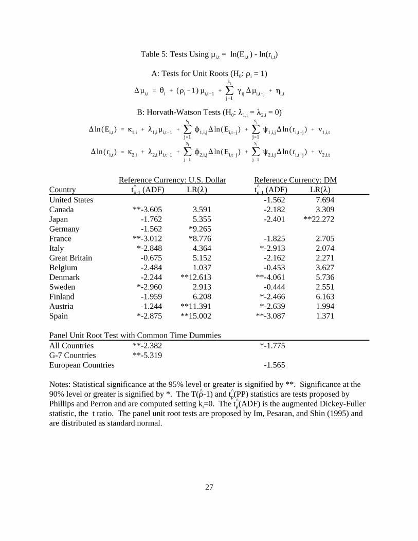
report the results in tables 5 and 6. If purchasing power parity holds in the long run for traded

goods, the difference between the nominal exchange rate and the PPP exchange rate should be

stationary. In table 5 we report the results of tests of the null hypothesis that there is a unit root

in the difference as well as the Horvath-Watson tests of the null hypothesis that nominal and PPP

exchange rates are not cointegrated with a slope of 1.0. The tests using the data from each

country individually again provide mixed evidence. Regardless of whether the dollar or the DM

is the reference currency, the ADF tests reject at the ten percent level for five of the twelve

currencies. The evidence from the Horvath-Watson tests is also mixed, with more evidence

against the null when the dollar is used as the reference currency than when the DM is used. The

panel test points to a rejection of the null hypothesis when common time dummies are used.18

In table 6 we present estimates of the slopes of the cointegrating relationships along with

tests of the hypothesis that the slope is 1.0. When we use the dollar as the reference currency, we

reject the null hypothesis that the slope is 1.0 for eight of the twelve countries. Not surprisingly,

the panel test also points to a rejection of the null hypothesis that the slopes are jointly equal to

one. We also find a large number of rejections of the null when we look at the cointegrating

slopes for relative prices and relative productivities. But there the rejections arise because the

slope estimates, which are fairly close to 1.0, are precisely estimated. In contrast, here the point

16

estimates are generally far from 1.0 and we reject the null despite fairly large standard errors. The

wide range of point estimates that we report in table 6 is roughly consistent with previous work.

Froot and Rogoff (1995) report that it is common in the literature to find slopes that vary widely

across countries and are frequently far from the value of 1.0 implied by purchasing power parity.

Could these results also be due to the small-sample properties of the FMOLS estimates?

Monte Carlo evidence suggests that it is not. We choose six countries, three with estimated

slopes exceeding one (Japan, Germany, and Austria) and three with estimated slopes below one

(France, Britain, and Finland). For each, we estimate a VAR for 0=(,, .)’ and use the parameters

and error covariance matrix to generate 15,000 samples of 25 observations in which the true

value of $ is 1.0. Although we find evidence that the FMOLS estimates are biased, the bias is

not sufficient to explain either the dispersion or the magnitudes of the estimated slopes in table 6.

In all six experiments the mean slope is below one, so that small sample problems cannot explain

the estimated slopes that exceed one. The FMOLS standard errors understate the dispersion of

the slopes found in the experiments. Using the empirical distribution of slopes, we reject the null

of a unit slope at the 95 percent level for two countries (Japan and France), at the 90 percent level

for two countries (Germany and Austria) and at levels below 90 percent for the other two.

In contrast, when we use the DM as the reference currency, the point estimates are much

closer to 1.0 than are those obtained using the dollar.19 Even though we can reject the null

hypothesis for some currencies, the point estimates are close to one. Interestingly, the point

estimates do not indicate that purchasing power parity in traded goods is any more likely to hold

for European currencies than for non-European currencies relative to the DM.

The results in tables 4 - 6 lend somewhat favorable support for the hypothesis of

17

purchasing power parity in traded goods, especially when the DM is the reference currency.

Nominal exchange rates and PPP exchange rates appear to be cointegrated. Our estimates

suggest that the slopes of the cointegrating relationships are far from the hypothesized value of

unity when the dollar is used as the reference currency. But nominal and PPP exchange rates are

nearly proportional when the DM is used as the reference currency.

In figure 3 we plot the (logs of the) nominal and PPP exchange rates for the DM and yen

relative to the U.S. dollar and the lira and yen relative to the DM. Again, we normalized so that

1970 = 0. Large and long-lasting deviations from PPP in traded goods are evident for both

exchange rates relative to the U.S. dollar. As is consistent with the formal tests, these deviations

are smaller and less persistent when we examine the two exchange rates relative to the DM.

5. Concluding Remarks

How well does the Balassa-Samuelson model explain the behavior of real exchange

rates? The evidence from a panel of 13 OECD countries supports the hypothesis that the relative

price of nontraded goods reflects the relative labor productivities in the traded and nontraded

goods sectors. The results suggest that the relative prices of nontraded goods and the relative

productivities in the traded and nontraded goods sectors are cointegrated and that the slope of the

cointegrating relationship is generally close to 1.0. For some countries, growth in relative

productivities appears to outstrip growth in relative prices (or equivalently the slope is less than

1.0), but Monte Carlo evidence suggests that this difference is within the range of sampling

variation in a sample like ours. Thus relative prices and relative productivities appear to be

proportional in the long run.

The Balassa-Samuelson model also assumes that traded goods prices are characterized by

18

purchasing power parity. As is consistent with the evidence presented in Engel (1995), we find

large and long-lived deviations from PPP in traded goods when we look at U.S. dollar exchange

rates. Although nominal exchange rates and PPP exchange rates appear to be cointegrated we

find that the slopes of the cointegrating regressions vary widely and differ substantially from one.

But when we examine DM exchange rates the evidence is considerably more favorable to

purchasing power parity in traded goods. Nominal and PPP exchange rates appear to be

cointegrated and the slopes of the cointegrating regressions are generally close to one.

19

Appendix: THE DATA

Nominal exchange rates are from International Financial Statistics (line ae). For

Belgium, Canada, Denmark, Great Britain, Finland, France, Germany, Italy, Japan, Sweden, and

the U.S., sectoral price and productivity data come from the OECD International Sectoral

Database, 1995. For Austria and Spain, they come from national statistics. (Francisco de Castro

of the Bank of Spain collected and documented the data.) These sources provide annual data on

nominal and real value added and number of employees. Sectoral prices are implicit deflators.

Traded goods consist of the "manufacturing" and "agriculture, hunting forestry and

fishing" sectors. Non-traded goods consist of the "wholesale and retail trade, restaurants and

hotels", "transport, storage and communication", "finance, insurance, real estate and business

services", "community social and personal services", "non-market services" sectors. "Non-market

services" include the "producers of government services" and "other producers" subsectors.

Data consistency is always an issue. We are aware of these anomalies in the OECD data:

(1) The German market services employment figures do not include the "real estate and business

services" sector; value added figures do. (2) The Italian, British and Belgian value added and

employment figures do not include "real estate and business services" sector. (3) British value

added and employment figures consist of the "producers of government services" sector.

The productivity data allow us to begin in 1960 for 3 countries (the United States,

Germany, and Finland), in 1961 for Canada, in 1964 for Spain, in 1967 for Denmark, and in

1970 for the remainder. The data end in 1993 for all countries except Canada, Austria, Spain (all

1992), Great Britain (1991), and Belgium (1990). Apart from Germany, where the post-

unification data are problematic, we use all available data for estimation.

Acknowledgments

Helpful discussions with José Vinals and generous assistance and numerous suggestions fromPeter Pedroni along with the comments of seminar participants at Johns Hopkins University,Indiana University, North Carolina State University, the University of Maryland, and theUniversity of Pennsylvania, the referees and the editor are acknowledged with thanks.

References

Asea, P.K. and E.G. Mendoza, 1994, The Balassa-Samuelson model: A general equilibriumappraisal, Review of International Economics 2, 244-267.

Balassa, B., 1964, The purchasing power parity doctrine: A reappraisal, Journal of PoliticalEconomy 72, 584-596.

Chinn, M.D. and L. Johnston, 1996, Real exchange rate levels, productivity and demand shocks:Evidence from a panel of 14 countries, working paper, Department of Economics, University ofCalifornia, Santa Cruz.

Canzoneri, M.B., R.E. Cumby, and B.T. Diba, 1996, Relative labor productivity and the realexchange rate in the long run: Evidence for a panel of OECD countries, NBER working paper no.5676.

De Gregorio, J., A. Giovannini, and T. Krueger, 1994, The behavior of nontradable goods pricesin Europe: Evidence and interpretation, Review of International Economics 2, 284-305.

De Gregorio, J., A. Giovannini, and H. Wolf, 1993, “International evidence on tradables andnontradables inflation,” European Economic Review 38, 1225-1244.

Dickey, D.A. and W.A. Fuller, 1979, Distribution of the estimators for autoregressive time serieswith a unit root, Journal of the American Statistical Association 74, 427-431.

Edison, H.J., J.E. Gagnon, and W.R. Melick, 1997, Understanding the empirical literature onpurchasing power parity: The post-Bretton Woods era, Journal of International Money andFinance 16, 1-17.

Engle, R.F. and C.W.J. Granger, 1987, Co-integration and error correction: representation,estimation, and testing, Econometrica 55, 251-276.

Engel, C., 1995, Accounting for U.S. real exchange rate changes,” NBER working paper no.5394.

Engel, C., M.K. Hendrickson, and J.H. Rogers, 1997, Intra-national, intra-continental, and intra-planetary PPP, NBER working paper no. 6069.

21

Evans, C., 1992, Productivity shocks and real business cycles, Journal of Monetary Economics29, 191-208.

Evans, M.D.D. and K.K. Lewis, 1994, Do stationary risk premia explain it all? Evidence fromthe term structure, Journal of Monetary Economics 33, 285-318.

Frankel, J.A. and A.K. Rose, 1996, A panel project on purchasing power parity: Mean reversionwithin and between countries, Journal of International Economics 40, 209-224.

Frenkel, J.A., 1981, Flexible exchange rates, prices, and the role of “news”: Lessons from the1970s, Journal of Political Economy 89, 665-705.

Froot, K. and K. Rogoff, 1995, Perspectives on PPP and long-run real exchange rates, in G.Grossman and K. Rogoff, eds., Handbook of international economics, Vol. 3 (North-Holland,Amsterdam) 1647-1688.

Hall, A., 1994, Testing for a unit root in time series with pretest data-based model selection,Journal of Business and Economic Statistics 12, 461-470.

Hakkio, C.S., 1984, A re-examination of purchasing power parity: A multi-country and multi-period study, Journal of International Economics 17, 265-277.

Horvath, M.T.K., and M.W. Watson, 1995, Testing for cointegration when some of thecointegrating vectors are prespecified, Econometric Theory 11, 984-1014.

Hsieh, D.A., 1982, The determination of the real exchange rate: The productivity approach,Journal of International Economics 12, 355-362.

Im, K., M.H. Pesaran, and Y. Shin, 1995, Testing for unit roots in heterogeneous panels, workingpaper, Department of Applied Economics, University of Cambridge.

Jorion, P. and R.D. Sweeney, 1996, Mean reversion in real exchange rates: Evidence andimplications for forecasting, Journal of International Money and Finance 15, 535-550.

Levin, A. and C.F. Lin, 1992, Unit root tests in panel data: Asymptotic and finite sampleproperties, working paper, Department of Economics, University of California, San Diego.

Lothian, J., 1997, Multi-country evidence on the behavior of purchasing power parity under thecurrent float, Journal of International Money and Finance 16, 19-35.

Marston, R., 1987, Real exchange rates and productivity growth in the United States and Japan,”in S. Arndt and J.D. Richardson, eds., Real and financial linkages among open economies (MITPress, Cambridge).

22

Newey, W.K. and K.D. West, 1994, Automatic lag selection in covariance matrix estimation,Review of Economic Studies 61, 631-653.

Ng, S. and P. Perron, 1995, Unit root tests in ARMA models with data-dependent methods forthe selection of the truncation lag, Journal of the American Statistical Association 90, 268-281.

O’Connell, P., 1997, The overvaluation of purchasing power parity, Journal of InternationalEconomics, forthcoming.

Papell, D.H., 1997, Searching for stationarity: purchasing power parity under the current float,Journal of International Economics, forthcoming.

Papell, D.H. and H. Theodoridis, 1997, The choice of numeraire currency in panel tests ofpurchasing power parity, working paper, Department of Economics, University of Houston.

Pedroni, P., 1995, Panel cointegration: Asymptotic and finite sample properties of pooled timeseries tests with an application to the PPP hypothesis,” working paper, Department ofEconomics, Indiana University.

Pedroni, P., 1996, Fully Modified OLS for Heterogeneous Panels, working paper, Department ofEconomics, Indiana University.

Phillips, P.C.B. and B.E. Hansen, 1990, Statistical inference in instrumental variables regressionswith I(1) processes, Review of Economic Studies 57, 99-125.

Phillips, P.C.B. and S. Ouliaris, 1990, Asymptotic properties of residual based tests forcointegration, Econometrica 58, 165-193.

Phillips, P.C. B. and P. Perron, 1988, Testing for a unit root in time series regression, Biometrika 75, 335-346.

Samuelson, P., 1964, Theoretical notes on trade problems, Review of Economics and Statistics46, 145-154.

Wei, S.J. and D.C. Parsley, 1995, Purchasing power dis-parity during the floating rate period:Exchange rate volatility, trade barriers, and other culprits,” working paper, Kennedy School ofGovernment.

23

ln (qi,t ) ' "i % $i ln (xi,t /hi,t ) % ,i,t

),̂i,t ' (Di&1) ,̂i,t&1 % jki

j'1(ij ),̂i,t&j % <i,t

Table 1: Tests for Cointegration of ln(qi,t ) and ln(xi,t / hi,t )

Country T( ^D-1) t^D(PP) t^D (ADF) United States *-18.361 *-3.378 **-3.859Canada -11.419 -2.451 **-4.664Japan -8.643 -3.052 **-3.521Germany -15.629 *-3.173 **-3.837France -8.943 -2.339 -2.972Italy -5.009 -1.536 -2.842Great Britain -4.969 -1.276 -1.356Belgium -17.931 **-4.161 **-4.254Denmark -6.184 -1.728 -1.796Sweden -7.142 -1.882 **-4.278Finland -15.888 -3.034 **-3.852Austria -11.102 -3.021 -3.066Spain -9.809 -2.494 *-3.403

Panel Tests of Cointegration with Common Time DummiesAll Countries -19.508 *-8.267 **-8.803G-7 Countries -14.360 -5.621 **-6.950

Notes: Significance at the 95% and 90% levels are noted by ** and *, respectively. The T( ^D-1)and t^D(PP) statistics are Phillips-Perron tests applied to the residuals from the first regression andare computed with ki=0. The t^D(ADF) is the augmented Dickey-Fuller statistic. Critical valuesare taken from the tables compiled by Phillips and Ouliaris (1990). The panel cointegration testsare those proposed by Pedroni (1995), which is the source of the critical values.

24

)*i,t ' 2i % (Di&1) *i,t&1 % jki

j'1(ij )*i,t&j % 0i,t

) ln (qi,t ) ' 61,i % 81,i*i,t&1 % jsi

j'1N1,i,j) ln (qi,t&j ) % j

si

j'1R1,i,j) ln (xi,t&j /hi,t&j ) % <1,i,t

) ln (xi,t /hi,t ) ' 62,i % 82,i*i,t&1 % jsi

j'1N2,i,j) ln (qi,t&j ) % j

si

j'1R2,i,j) ln (xi,t&j /hi,t&j ) % <2,i,t

Table 2: Tests Using *i,t = ln(qi,t ) - ln(xi,t / hi,t )

A: Tests for Unit Roots (H0: Di = 1)

B: Horvath-Watson Tests (H0: 81,i = 82,i = 0)

Country t^D-1 (ADF) LR(8)

United States -2.245 8.069Canada *2.669 7.557Japan -1.742 5.758Germany *-2.875 **14.433France -1.716 4.810Italy **-3.361 **15.630Great Britain -1.149 5.319Belgium -0.199 6.022Denmark -1.570 4.488Sweden -2.452 4.977Finland -1.003 **11.296Austria *-2.709 *9.198Spain **-3.819 3.632

Panel Unit Root Test with Common Time DummiesAll Countries **-3.762G-7 Countries **-2.422

Notes: Significance at the 95% and 90% levels is noted by ** and*, respectively. The t^D-1(ADF)is the augmented Dickey-Fuller statistic and LR(8) is the Horvath-Watson likelihood ratio test. The joint tests are the panel unit root tests proposed by Im, Pesaran, and Shin (1995) and aredistributed as standard normal.

25

ln (qi, t ) ' "i % $i ln (xi, t /hi, t ) % ,i,t

Table 3: Estimates of the Cointegrating Slope Coefficient of ln(qi,t ) and ln(xi,t / hi,t )

Country ^$i,OLS^$i,FMOLS t( ^$i,FMOLS=1)

United States 0.877 0.869 **-4.209Canada 0.633 0.675 **-2.602Japan 1.237 1.181 **3.145Germany 1.074 1.063 1.570France 0.802 0.779 **-3.297Italy 0.900 0.922 -1.212Great Britain 0.412 0.443 **-7.002Belgium 0.773 0.763 **-12.219Denmark 0.552 0.510 **-7.888Sweden 0.624 0.571 **-3.713Finland 0.804 0.770 **-3.194Austria 0.959 0.929 -1.398Spain 0.895 0.859 **-2.141

Panel Tests of ^$ = 1 with Common Time Dummies

t^$ N t̄All Countries **-7.309 **-6.206G-7 Countries **-2.055 *-1.693

Notes: The second column contains the ordinary least squares estimates of the slope coefficient. Column 3 contains the Phillips-Hansen (1990) fully modified OLS estimates of the slope and column 4 contains the t-ratio formed by subtracting one from the fully modified OLS estimate ofthe slope and dividing by the corresponding standard error. The numbers of lags used incomputing the fully modified OLS estimate are chosen using the data dependent procedureproposed by Newey and West (1994). The panel tests are those proposed by Pedroni (1996).

26

ln (Ei, t ) ' "i % $i ln ( ri, t ) % ,i, t

),̂i, t ' (Di&1) ,̂i, t&1 % jki

j'1(ij ),̂i, t&j % <i, t

Table 4: Tests for Cointegration of ln(Ei,t ) and ln(ri,t )

Reference Currency: U.S. Dollar Reference Currency: DMCountry T( ^D-1) t^D(PP) t^D (ADF) T( ^D-1) t^D(PP) t^D (ADF)Canada -10.196 -2.294 **-3.459 -8.261 -2.052 -2.404Japan -9.062 -2.404 -2.466 -9.193 -2.221 -2.663Germany - 8.261 -2.052 -2.404 -13.245 -2.661 -2.178France -10.345 -2.321 **-3.481 -8.285 -2.325 -2.096Italy -8.695 -2.112 -3.074 -9.870 -2.729 -2.995Great Britain -15.880 -3.049 **-4.713 -8.863 -2.311 -2.673Belgium -7.141 -1.822 -2.635 -0.476 -0.439 -0.793Denmark -7.166 -1.909 -2.740 *-20.531 **-4.817 **-4.170Sweden -7.081 -1.863 -2.414 -17.552 **-5.591 **-5.881Finland -12.350 -2.400 **-3.602 *-18.882 **-3.486 **-4.114Austria -7.618 -2.025 -2.071 -10.713 -2.679 -2.728Spain -8.692 -2.094 **-3.668 -15.143 -3.055 *-3.119

Panel Tests of Cointegration with Common Time DummiesAll Countries **-45.769 **-9.839 **-10.587 **-45.448 **-9.827 **-11.782G-7 Countries **-40.717 **-9.475 **-11.169European Countries **-38.040 **-8.824 **-10.349

Notes: Statistical significance at the 95% level or greater is signified by **. Significance at the90% level or greater is signified by *. The T( ^D-1) and t^D(PP) statistics are Phillips and Perrontests applied to the residuals from the first regression and are computed from regressions settingki=0 in the second regression. The t^D(ADF) is the augmented Dickey-Fuller statistic. Significance levels for these tests are taken from the tables compiled by Phillips and Ouliaris(1990). The joint tests are the panel cointegration tests proposed by Pedroni (1995). Significance levels for these tests are computed from tables compiled by Pedroni.

27

)µ i,t ' 2i % (Di&1) µ i,t&1 % jki

j'1(ij )µ i,t&j % 0i,t

) ln (Ei,t ) ' 61,i % 81,i µ i,t&1 % jsi

j'1N1,i,j) ln (Ei,t&j ) % j

si

j'1R1,i,j) ln ( ri,t&j ) % <1,i,t

) ln ( ri,t ) ' 62,i % 82,i µ i,t&1 % jsi

j'1N2,i,j) ln (Ei,t&j ) % j

si

j'1R2,i,j) ln ( ri,t&j ) % <2,i,t

Table 5: Tests Using µ i,t = ln(Ei,t ) - ln(ri,t)

A: Tests for Unit Roots (H0: Di = 1)

B: Horvath-Watson Tests (H0: 81,i = 82,i = 0)

Reference Currency: U.S. Dollar Reference Currency: DMCountry t^D-1 (ADF) LR(8) t^D-1 (ADF) LR(8)United States -1.562 7.694Canada **-3.605 3.591 -2.182 3.309Japan -1.762 5.355 -2.401 **22.272Germany -1.562 *9.265France **-3.012 *8.776 -1.825 2.705Italy *-2.848 4.364 *-2.913 2.074Great Britain -0.675 5.152 -2.162 2.271Belgium -2.484 1.037 -0.453 3.627Denmark -2.244 **12.613 **-4.061 5.736Sweden *-2.960 2.913 -0.444 2.551Finland -1.959 6.208 *-2.466 6.163Austria -1.244 **11.391 *-2.639 1.994Spain *-2.875 **15.002 **-3.087 1.371

Panel Unit Root Test with Common Time DummiesAll Countries **-2.382 *-1.775G-7 Countries **-5.319European Countries -1.565

Notes: Statistical significance at the 95% level or greater is signified by **. Significance at the90% level or greater is signified by *. The T( ^D-1) and t^D(PP) statistics are tests proposed byPhillips and Perron and are computed setting ki=0. The t^D(ADF) is the augmented Dickey-Fullerstatistic, the t ratio. The panel unit root tests are proposed by Im, Pesaran, and Shin (1995) andare distributed as standard normal.

28

ln (Ei, t ) ' "i % $i ln ( ri, t ) % ,i,t

Table 6: Estimates of the Cointegrating Slope Coefficient of ln(Ei,t ) and ln(ri,t )

Reference Currency: U.S. Dollar Reference Currency: DM Country ^$i,OLS

^$i,FMOLS t( ^$i,FMOLS=1) ^$i,OLS^$i,FMOLS t( ^$i,FMOLS=1)

United States 1.888 1.592 1.357Canada 0.651 0.610 **-2.615 1.455 1.322 *1.874Japan 1.657 1.521 1.912 1.416 1.169 0.707Germany 1.888 1.592 1.357France 0.495 0.390 **-3.072 1.337 1.242 **2.703Italy 0.868 0.973 -0.221 1.040 1.037 0.923Great Britain 0.506 0.497 **-7.104 0.954 0.886 *-1.754Belgium 0.422 0.116 **-2.857 -1.045 -0.563 -0.672Denmark -0.060 -0.032 **-3.341 1.058 1.043 *1.680Sweden 0.727 0.734 -0.927 1.159 1.133 **4.229Finland 0.322 0.308 **-6.328 0.861 0.850 **-3.822Austria 2.118 1.912 **2.234 1.058 1.017 0.036Spain 0.652 0.635 **-2.784 1.023 1.005 0.184

Panel Tests of ^$ = 1 with Common Time Dummies

t^$ t^$N t̄ N t̄All Countries **-2.948 **-4.587 -0.849 -0.815G-7 Countries **-5.671 **-10.296European Countries **-6.696 **-6.600

Notes: The second and fifth columns contain the ordinary least squares estimates of the slopecoefficient. Columns 3 and 6 contains the Phillips-Hansen (1990) fully modified OLS estimatesof the slope, and columns 4 and 7 contain the t-ratio formed by subtracting one from the fullymodified OLS estimate of the slope and dividing by the corresponding standard error. Thenumbers of lags used in computing the fully modified OLS estimate and its standard error arechosen using the data dependent procedure proposed by Newey and West (1994). The panel testsare those proposed by Pedroni (1996).

29

Figure 1: Real Exchange Rates and Relative Labor Productivities

30

Figure 2: Relative Productivities and Relative Prices

31

Figure 3: Nominal and Purchasing Power Parity Exchange Rates

32

1. Frankel and Rose (1996) and Lothian (1997) report half lives of this magnitude using

aggregate price levels as do Wei and Parsley (1995) using sectoral prices.

2. Hakkio (1984) is the first to exploit the benefits of pooling when examining PPP.

3. Engel (1995) examines real exchange rate variability over various horizons and reaches the

same conclusion. Our results suggest that his conclusions might be sensitive to the choice of

reference currency.

4. The production functions specified in (3) are the general solutions to the differential

equations: MX/MLX = n(X/LX) and MH/MLH = R(H/LH). We require only that they satisfy the

standard properties of production functions.

5. De Gregorio, Giovannini, and Wolf (1993), De Gregorio, Giovannini, and Krueger (1994),

and Chinn and Johnston (1996) are examples.

6. Evans (1992), for example, shows that measured Solow residuals are Granger caused by

money, interest rates, and government spending and finds that one fourth to one half of their

variation is attributable to variations in aggregate demand.

7. Asea and Mendoza (1994) also examine the link between relative prices and relative

productivities. They find that the coefficient on total factor productivity has the correct sign and

that its magnitude is reasonable given other estimates of factor shares. Our setup, using average

products, yields the sharper hypothesis that the slope is unity.

8. We use two reference currencies, the U.S. dollar and the DM. Because we include a constant

term in our estimates, we consider relative, not absolute, purchasing power parity.

9. We use the general-to-specific procedures suggested by Hall (1994) and Ng and Perron (1995)

to determine the number of lags and do tests both with and without deterministic trends.

10. As they suggest, we use common time dummies to account for correlation across cross

33

section units. Our cross sections differ in the number of observations that we have available so

we use all of the available data to compute the t-ratios for each cross section.

11. The parameters "i and $i in the cointegrating regression for each cross section are allowed to

differ as are the dynamics of yi,t and zi,t.

12. Our test statistics are a slight modification of Pedroni’s that allows for a different number of

time series observations in each cross section. Again, we account for cross section correlation by

using common time dummies to remove shocks common to all cross sections.

13. The results are available in Canzoneri, Cumby, and Diba (1996). Post-unification German

data present a problem—there is a sharp divergence of relative productivities and relative prices.

This could be due to a data problem associated with unification or to transition-related

developments. The question needs further study once the data issues are more settled.

14. We also reject the null hypothesis of a unit root in the difference both for all countries and

for the G-7 countries at the 95 percent level when we use GLS estimates to account for cross

sectional dependence.

15. Pedroni (1996) presents extensive evidence on the panel tests’ small sample properties.

16. Some existing evidence suggests that it might. Frenkel (1981) finds that PPP held more

closely in the 1970s when the DM is used as the reference currency than when the dollar is used.

More recently, Jorion and Sweeney (1996), Papell (1997), Papell and Theodoridis (1997), and

Edison, Gagnon, and Melick (1997) all find a similar influence of the choice of reference

currency in their samples.

17. The similarity of the panel test statistics across the two reference currencies is no accident.

Changing the reference currency amounts to adding the same log exchange rate to each cross-

34

sectional unit, it will have no impact on tests computed using deviations from cross-section

means, at least for large N. With N=12, a change of reference currency results in only minimal

changes to the test statistics. See O’Connell (1997) and Engel, Hendrickson, and Rogers (1997).

18. The test statistics differ slightly for the two reference currencies. These differences arise

from slight difference in sample size (as we note in the data appendix, we do not use post-

unification German data) and because N=12. In addition, Papell and Theodoridis (1997) argue

that panel tests will be invariant to the choice of reference currency only when the same number

of lags is used for all currencies. Once again, the unit root tests using GLS to account for cross-

sectional dependence reject the null hypothesis at the 95 percent level.

19. The one notable exception is the Belgian franc regression where we obtain a negative point

estimate and a large standard error. The slopes for the U.S. dollar - DM exchange rate are, of

course, identical.