NASA Technical Memorandum 104824

Flight Test Results from Real-Time

Relative Global Positioning System

Flight Experiment on STS-69

Young W. Park

Jack P. Brazzel, Jr.

J. Russell Carpenter

Heather D. Hinkel

James Ho Newman

November 1996

https://ntrs.nasa.gov/search.jsp?R=19970001337 2019-06-04T07:56:58+00:00Z

NASATechnical Memorandum 104824

Flight Test Results from Real-Time

Relative Global Positioning System

Flight Experiment on STS-69

Young W. Park

Jack P. Brazzell, Jr.

McDonnell Douglas

Houston, Texas

J. Russell CarpenterHeather D. Hinkel

James H. Newman

Lyndon B. Johnson Space Center

Houston, Texas

November 1996

This publication is available from the NASA Center for Aerospace Information, 800 Elkridge LandingRoad, Linthicum Heights, MD 21090-2934, (301) 621-0390

Contents

Abstract................................................................................................................................. 1

Introduction ........................................................................................................................... 1

Mission Summary and Objectives ......................................................................................... 1

Crew Member Comments ...................................................................................................... 2

Flight Experiment Setup ........................................................................................................ 2

Integration of RPOP and RGPS ........................................................................................... 4

Relative GPS Kalman Filter Design ...................................................................................... 6

Single-Vehicle Mode ............................................................................................................ 7Dual-Vehicle Mode ............................................................................................................... 9

Results ................................................................................................................................... 9

Real-Time Onboard Processing ............................................................................................ 10Single-Vehicle Mode .................................................................................................................. 10Dual-Vehicle Mode ..................................................................................................................... 11

Postflight Processing of Recorded Data .............................................................................. 13TurboRogue Receiver Clock Offset Problem ................................................................................... 13Single-Vehicle Mode .................................................................................................................. 14Dual.Vehicle Mode Playback ........................................................................................................ 16

Conclusions ........................................................................................................................... 18

Acknowledgments ................................................................................................................. 19

References ............................................................................................................................. 19

..°

111

Figures

1 Onboard laptop computer setup ............................................................................................ 32 Orbiter GPS antenna locations ............................................................................................. 33 RPOP relative motion display using recorded dam ................................................................... 44 RPOP zoomed-in relative motion display using recorded data ..................................................... 55 RPOP state vector configuration dialog box ........................................................................... 66 RGPS filter architecture ..................................................................................................... 67 Real-time onboard SVM results ........................................................................................... 10

8a SMA comparison during near-real-time processong of snapshot data ........................................... 118b SMA parameters duringnear-real-lime processing of snapshot data ............................................. 128c Number of channels tracked by each receiver snapshot .............................................................. 129 TurboRogue receiver clock offset ......................................................................................... 1310 SVM position and SMA differences from postflight processing ................................................. 1411 Comparison of SMA estimates ............................................................................................ 1512 Target-centered relative motion plot ...................................................................................... 16

13 DVM position and SMA difference from posttlight processing .................................................. 1714 Common satellite availability from postflight processing ......................................................... 18

iv

Acronyms

AT_

BET

C/A

cg

DVM

ESA

FOM

GPC

GPS

GUI

ISS

JPL

LVLH

MCC

RGPS

RNAVRPOP

SA

SMA

STS

SVM

TDRSS

TRAD

• UT/CSR

WSF

automated uansfer vehicle

best estimated trajectory

coat.acquisition

center of gravity

dual-vehicle mode

European Space Agency

figure of merit

general-purpose computer

global positioning system

graphical user interface

International Space Station

Jet Propulsion Laboratory

local vertical/local horizontal

Mission Control Center

relative global positioning system

rendezvous navigation

rendezvous and proximity operations program

selective availability

semimajotaxis

Space Transportation System (the Space Shuttle)

single-vehicle mode

tracking and data relay satellite system

tools for rendezvous and docking

University of Texas Center of Space Research

Wake Shield Facility

V

Abstract

A real-time relative global positioning system (GPS) Kalman ftlter has been developed in support of automated

rendezvous with the International Space Station (ISS). The filter is integrated with existing Space Shuttle ren-dezvous software running on a 486 laptop computer under Windows ®. In this work we present real-time and

postflight results achieved with the filter on Space Shuttle mission STS-69. This experiment used GPS data

from an Osborne/Jet Propulsion Laboratory (JPL) TurboRogue receiver carried on the Wake Shield Facility

(WSF) free-flyer and a Rockwell Collins 3M receiver carried on the Orbiter. Real-time filter results, processed

onboard the Shuttle and replayed in near-real-time on the ground, are based on single-vehicle mode operation and

on 5 to 20 minute snapshots of telemetry provided by WSF for dual-vehicle mode operation. Postflight results

were achieved by running the ftlter in a real-time mode using data recorded during the mission.

Orbiter and WSF state vectors calculated using our filter compare favorably with precise reference orbits deter-

mined by the University of Texas Center for Space Research. The reference orbits were generated by double-

differencing GPS data flom both vehicles along with data from GPS ground stations. The lessons learned from

this experiment will be used in conjunction with future experiments to mitigate the technology risk posed by

automated rendezvous and docking to the ISS.

Introduction

We have developed a real-time relative global positioning system (RGPS) extended Kalman filter insupport of automated rendezvous with the International Space Station (ISS) (ref. 1), based in part on earlier work

by Montez and Zyla (ref. 2). The filter design exploits common satellite tracking by both chaser and target ve-

hicle receivers, and optimizes its performance during periods of asynchronous tracking. The filter is integrated

with existing Space Shuttle rendezvous support software running on a 486 laptop computer under Windows*.

The filter is designed to support a wide variety of global positioning system (GPS) receivers under adverse

selective availability (SA) conditions. Handover at close range to a proximity operations sensor precludes the

need for sub-decameter solution accuracy. Therefore, the filter processes coarse/acquisition (C/A) code pseudo-range measurements only.

To mitigate the technology risk posed by automated rendezvous and docking to the ISS, an RGPSexperiment will be performed on STS-80. STS-69 provided an opporamity for incremental software develop-

ment, early software validation, and valuable experience processing real-time RGPS data prior to this important

milestone. We will apply the lessons learned from the experiment on STS-69 to ensure successful results onSTS-80.

In this work, we will present real-time and posltlight results achieved with the filter on Space Shuttle

mission STS-69. We will first present a summary of the experiment mission plan and objectives. Then we willinclude crew member comments, flight experiment setup, and challenges encountered. Next, we will discuss the

integration of the filter into the rendezvous and proximity operations program (RPOP). Following this discus-sion will be a description of the filter design itself. We will then present results for single- and dual-vehicle filter

operation, both from real-time processing and from postflight analysis, by running the filter in a real-time mode

using data recorded during the mission. We will present a comparison of the Orbiter and Wake Shield Facility

(WSF) state vectors calculated using our filter to those from precise reference orbits determined by the University

of Texas Center of Space Research (UT/CSR) (tel 3). Finally, we will conclude with a summary of results andlessons learned.

Mission Summary and Objectives

The experiment involved a GPS receiver on both the Orbiter and the WSF free-flyer. Throughout this

paper we will use Orbiter and "chaser" mterchangeably and WSF and "target" mterehangeably. Orbiter GPS data

were available onboard continuously throughout the mission, while the WSF GPS data were only available inter-

mittently. The plans for real-time relative GPS data collection during WSF free-flight consisted of several short

snapshots of WSF GPS data followed by continuous data during the rendezvous. The snapshots were intended to

test the space-to-space communications link and to make a quick assessment of the WSF GPS data. The contin-uous data period was intended to prove the operation and accuracy of the real-time RGPS filter in a rendezvous

environment. Unfortunately, continuous WSF GPS data transmission did not occur because of a failure in the

power supply to the receiver. Fortunately, 19 hours of WSF GPS data were recorded onboard the free-flyer prior

to the power supply failure. These problems reslricted the filter operation to single-vehicle mode (SVM) during

mat of the mission. The snapshots provided limited operation in dual-vehicle mode (DVM), however. Theexperiment objects, specified by Hinkel et al. (ref. 1), are fisted below:

1. Collect flight experiment GPS data that will support the European Space Agency (ESA) m validating the

automated Wansfer vehicle (ATV) ground verification facilities (specilically GPS models used in the facility).

2. Determine the accuracy of GPS relative navigation, including usable ranges.

3. Learn the effect of common versus non-common satellite tracking between two different receivers.

4. Gain experience m passing GPS data through a space-to-space communications link for real-time navigation.

Unfortunately, all objectives were not met during the mission. Most of the objectives were achieved,

however, by processing both WSF and Orbiter GPS data post-mission. Objective 1 was accomplished by re-

cording significant amounts of GPS data onboard each vehicle. Objective 2 was partially achieved by comparing

the RGPS filter resalts to a best estimated trajectory (BET). The anticipated accuracy was not achieved owing to

unexpected marginal GPS receiver performance. Objective 3 was met by quantifying the negative effect of non-

common satellite tracking between two different receivers using the flight data. The first part of Objective 4

was met by successfully transmitting WSF GPS data through the space-to-space communications link during thesnapshots. To fulfill Objective 4 completely, successful onboard real-time relative navigation was required. This

did not occur, however, and postflight analysis operating the filter with recorded data allowed the rest of Objective

4 to be partially fulfilled. Although all objectives were not completely achieved, we learned many lessons andgained valuable experience in preparation for STS-80.

Crew Member Comments

Mission Specialist Jim Newman operated the experiment inside the Orbiter cockpit throughout the

STS-69 mission. Following is a commentary on the experiment from Dr. Newman's perspective:"STS-51 was the fLrSt time a GPS unit was flown on the Shuttle, successfully determining Orbiter state

vectors (ref. 4). STS-51 also included another GPS unit on a deployed satellite, ORFEUS-SPAS. Although the

GPS data were displayed on an onboard laptop, no attempt was made to do true relative GPS state vector deter-

mination at that time. But it was clear that GPS had tremendous potential. Although the primary emphasis on

STS-69 is application to automated rendezvous, Shuttle crews expect to benefit as well. The addition of GPS

and relative GPS sensor information to the suite of available rendezvous and proximity operations tools may help

reduce propellant budget and increase our margin for mission success. Opera_g this experiment on orbit was

time-consuming and somewhat frnswating because of a number of unforeseen anomalies. However, it is still felt

that the efforts were worthwhile for this step in the development of GPS as a standard method for accurate orbitand relative position determination."

Flight Experiment SetupTo fulfill onboard real-time data processing objectives, three Orbiter laptop computers were linked

to route the data for processing, as shown in Figure 1. Rt_P with the integrated RGPS filter (RPOP/RGPS)

2

PCDecom ComputerGPC and WSF GPSData Extraction andTransmission toRPOP/RGPS Computer

RPOP/RGPS ComputerRelative navigation,display and datarecording software

Shuttle GPS ComputerGPS Data recordingsoftware and datatransmission across

serial port

RS-422

RS-232

RS-422

Data

Comm

to WSF

GPS

Figure 1: Onboard laptop computer setup

resided on one laptop computer. It received WSF GPS measurements and solutions, Orbiter GPS measurements

and solutions, and navigation data from the Orbiter general-purpose computer (GPC). A second laptop contain-

ing a software package called PCDecom stripped the real-time GPC and WSF GPS data from the telemetry,

decommutated the original data, and transmitted formatted data packets to RPOP/RGPS via RS-422 serial

connection. The third laptop, containing the Orbiter GPS receiver command, control, and display software,transmitted the Orbiter GPS data to RPOP/RGPS via RS-232 serial connection.

The experiment used GPS data from an eight-channel Osborne/Jet Propulsion Laboratory (JPL)

TurboRogue receiver carried by the WSF flee-flyer, and a Rockwell Collins 3M receiver carried on the Orbiter,

as described by Schutz et al. (ref. 5). A single GPS antenna was mounted on the WSF free-flyer. Two GPS

antennas were mounted on the Orbiter. One of the GPS antennas is located on top of the Orbiter and the other on

the bottom of the orbiter, as seen in Figure 2. The 3M receiver takes inputs from both antennas and selects a set

of four GPS satellites based on the selection algorithm. The receiver does not know which antenna is trackingwhich GPS satellites, so the antenna-to-center of gravity (eg) offset is not precisely known.

Figure 2: Orbiter GPS antenna locations

Integration of RPOP and RGPSTo accomplish Objective 4 of the flight experiment- performing relative GPS data filtering in real

time onboard the Space Shuttle - we integrated the RGPS filter into an already existing Shuttle flight-certifiedsoftware program called RPOP. We chose to integrate RGPS into RPOP because:

• Rt_P was flight certified and used as a standard tool on every Shuttle rendezvous and deploy mission

* the STS-69 crew was very familiar with RPOP and had used it on previous rendezvous flights* RI_P had the framework for a GPS data interface

• RPOP was originally designed to allow easy integration of new sensors, such as GPS

• Rt_P provides a long-term platform for GPS data processing onboard the Shuttle

RPOP is a Windows ® application that runs on a laptop computer in the Shuttle's cockpit during ren-dezvous, docking, and deploy missions. RPOP provides useful information, not available on standard Orbiter

displays, to assist the Shuttle crew during rendezvous and proximity operations with other spacecraft. RPOP

displays navigation and guidance information based on Orbit_ data and sensor measurements. In addition, RPOP

is the heart of the Shuttle tools for rendezvous and docking (TRAD) system used for Shuttle-to-Mir and, eventu-

ally, for Shuttle-to-ISS rendezvous and docking missions.

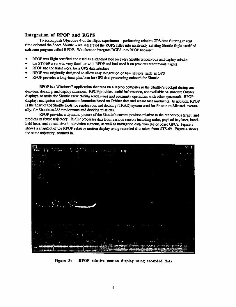
RPOP provides a dynamic picture of the Shuttle's current position relative to the rendezvous target, and

predicts its future trajectory. RPOP processes data from various sensors including radar, payload bay Laser,hand-

held laser, and closed-circuit television cameras, as well as navigation data from the onboard GPCs. Figure 3

shows a snapshot of the RI_P relative motion display using recorded data taken from STS-69. Figure 4 showsthe same trajectory, zoomed in.

Figure 3: RPOP relative motion display using recorded data

4

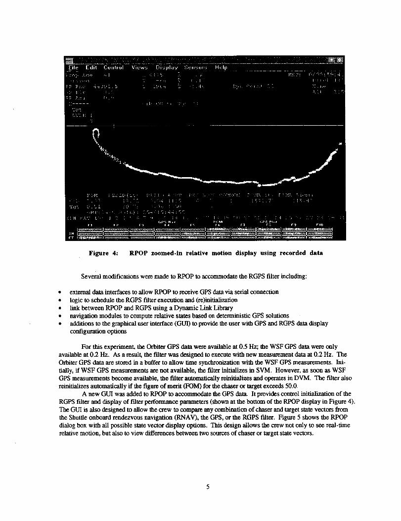
Figure 4: RPOP zoomed-in relative motion display using recorded data

Several modifications were made to Rt_P to accommodate the RGPS filter including:

• external data interfaces to allow RPOP to receive GPS data via serial connection

• logic to schedule the RGPS filter execution and (re)initialization

* link between RPOP and RGPS using a Dynamic Link Library

• navigation modules to compute relative states based on deterministic GPS solutions• additions to the graphical user interface (GLrl) to provide the user with GPS and RGPS data display

configuration options

For this experiment, the Orbiter GPS data were available at 0.5 Hz; the WSF GPS data were only

available at 0.2 Hz. As a result, the filter was designed to execute with new measurement data at 0.2 Hz. TheOrbiter GPS data are stored in a buffer to allow time synchronization with the WSF GPS measurements. Ini-

tially, if WSF GPS measurements are not available, the filter initializes in SVM. However, as soon as WSF

GPS measurements become available, the filter automatically reinitializes and operates in DVM. The filter alsoreinitializes automatically if the figure of merit (FOM) for the chaser or target exceeds 50.0.

A new GUI was added to RPOP to accommodate the GPS data. It provides control initialization of the

RGPS filter and display of filter performance parameters (shown at the bottom of the Rt_P display in Figure 4).

The GUI is also designed to allow flae crew to compare any combination of chaser and target state vectors from

the Shuttle onboard rendezvous navigation (RNAV), the GPS, or the RGPS filter. Figure 5 shows the RPOP

dialog box with all possible state vector display options. This design allows the crew not only to see real-time

relative motion, but also to view differences between two sources of chaser or target state vectors.

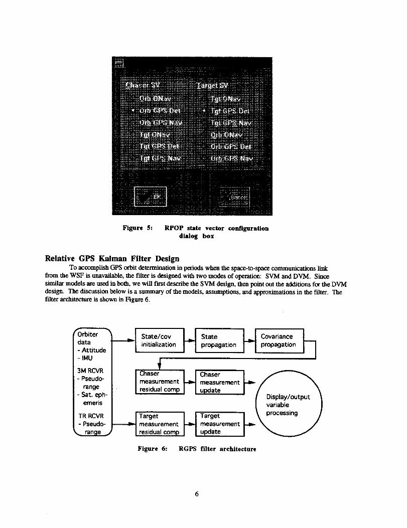
Figure 5: RPOP state vector configuration

dialog box

Relative GPS Kalman Filter DesignTo accomplish GPS orbit determination in periods when the space-to-space communications link

from the WSF is unavailable, the filter is designed with two modes of operation: SVM and DVM. Since

similar models are used in both, we will fast describe the SVM design, then point out the additions for the DVMdesign. The discussion below is a summary of the models, assumptions, and approximations in the filter. The

filter architecture is shown in Figure 6.

_0rbiter _

data

- Attitude

- IMU

3M RCVR

- Pseudo-

range

- Sat. eph-emeris

TR RCVR

- Pseudo-

[ state/ o" H State H C° ' ia°cehinitialization propagation propagation

Chaser H Chasermeasurement measurement

residual comp update

_t Target H Targetmeasurement measurement

residual comp update

Figure 6: RGPS filter architecture

Single-VehicleModeTheRGPSfilteroperatesin Earth-centered, Earth-fixed coordinates. It assumes the following model for

the time evolution of the Orbiter position and velocity.

i:c (t) = i' c (t) = fnm (rc (t)) + roe x 0_E x r c (t)- 203E x v c (t) + a s (t) + _a u (t) + w d (t)

E[wd(t)]=0, E[Wd(t)wT(v)]=o'2wd<3(t - T)I(1)

In (1), t represents time, the variable over which the differentiation indicated by the overdots occurs, rc is the

chaser vehicle (Orbiter) position, vc is the chaser velocity relative to the Earth-fixed rotation flame, roE is the

Earth's angular velocity vector, and the symbol x represents the cross-product operator. Also, f_ is a truncation

of the GEM-10 gravitational force model (ref. 6) to degree n and order m; although we typically operate the filter

with n = m = 4, the filter has coefficients up to degree and order 30. The acceleration sensed by accelerometers

onboard the orbiter during powered flight is a,. The remaining two terms are random disturbances. The first of

these, &t,, we refer to as "unmodeled acceleration." We tune this to accommodate other time-correlated forcesacting on the vehicle such as drag, continuous or relatively long-duration vehicle venting, and gravity model

errors. The unmodeled acceleration is assumed to evolve as a vector of uncorrelated first-order Gauss-Markov

process (ref. 7, pp. 81-82), equally distributed among its three coordinates. We include the second term, w_,

termed direct process noise, to model timewise uncorrelated forces, including short-duration vents and uncoupled

attitude maintenance maneuvers, among others. In specifying the statistics of Wd,we denote the expectation op-

erator by the letter E, the transpose operation by the superscript T, the identity matrix by I, and the Dirac delta

function by 6(t - x). The variable (r2d is the noise variance.

The filter processes a discrete sequence of pseudorange measurements for the chaser, from up to fourGPS satellite vehicles at a time, that we assume are modeled as follows:

Psvi(tj)=lrc(tj)-rsvi(tj +&T)[ +c(tj)+ lsvi(tj)+bsvi(tj)+ vj,

¢Yv_jk, J = 1,2,K

(2)

In (2), tj is the jth measurement time tag, Psvi is the corresponding pseudorange measurement from the ith GPSsatellite vehicle, rsv_ is the position of SVi based on its broadcast ephemeris, and &r is a correction to the time

tag, also based on broadcast parameters, accounting for the time at which the measurement signal was transmit-

ted. The notation _ [] denotes the Euclidean norm. The remaining terms in (2) describe corruptions to the meas-

urement: c is the chaser receiver clock bias, also accommodating any biases common to all receiver channels,

and bs_ is a range bias parameter unique to each SVi, tuned to accommodate SA and other unmodeled radio

frequency propagation biases unique to a given receiver channel. Is_ is a correction for single-frequency iono-

spheric refraction based on a model due to Lear (ref. 8, pp. 6-1 to 6-7 and A-1 to A-10), and vj is a noise se-

quence. In specifying the statistics of v j, 6_ denotes the Kronecker delta function, and the variable o{v is the

noise variance. We assume that the measurement noises from each of the SVi are uncorrelawA. To model the

clock bias, we assume that it is the integral of a drift variable, d. The drift, d, is modeled as a first-order Gauss-

Markov process. First-order Ganss-Markov processes are also the models we choose for each of the four range

bias variables, which we assume are uncorrelated and equally distributed.SVM for the filter is based on (1) and (2). In this mode, the filter state vector is based on the unknown

variables in these two equations. Therefore, the filter must estimate these variables. The 15-element state vector

for this mode, x,,, is defined as

r,.,, vT, ¢, d, .SAT, bT] TXsng = [ c

where the range biases for the four channels of the chaser receiver have been collected m the vector b<. This

vector is ini "tmliz_ propagated, and updated in an extended Kalman filter recursion (ref. 7, pp. 182-188). When-

ever satellite switching occurs on a given receiver channel, the later state corresponding to that channel's range

bias is reini_ed. Next we will describe relevant details of our implementation of the models described abovein the Kalman filter.

The state vector is analytically propagated between measurements, except for the chaser position and

velocity elements, integrated numerically using the "Super-G" integrator (ref. 9, p. 4-130). The Kalman filter

recursion also requires that we propagate the covariance malrix corresponding to state vector estimation errors,

(3)

where P(tj)isthecovariancejustpriortoincorporatingthemeasurements att_intothestateand I'(tj_,)

isthecov i cejust incorporatingthemeasurementsatt..Them trafunctionsS(At) are based on (1), but we make several assumptions and approximations in deriving them. The matrix

• , corresponding to the state error transition, is nominally the solution of the matrix differential equation

_:_(tj,tj_ l )= F(Ij )_(tj,tj_i), O(tj-l,tj-l)=I where F(t/) is the Jacobian mall'ix of the state vector, evaluated

at the latest estimate. However, we approximate the upper six-by-six partition of F by assuming a spherical

Earth. Assuming F is constant over the propagation interval, the solution for • is given by the matrix

exponential e Fat. For the upper six-by-six partition, we approximate the exponential with a second-order

truncation of its representation as an infinite series (ref. 10, p. 55). The remaining diagonal elements of O

correspond to state transitions of In'st-order Ganss-Markov processes except in the case of the clock bias, which

is the integral of the drift. Since for any ftrst-order Gauss-Markov process the state transition is e -_/_r, we

can easily show the state transition for the clock bias and the rift elements of • has the form

Ci,clock(At) = I10 Z'(1-- e-_¢/¢) 1e-At/r 1

Clearly, most of the elements of el, are zeros. We exploit this structure by using sparse matrix operations incoding (3).

Most of the discrete process noise matrix S in (3) results from an analytic solution of the well-known

integral (e.g., ref. 7, p. 77) f o O(t, s)GQGT_T(t, s)ds, where the matrix Q is the spectral density of the

11-element process noise vector (3 for direct process noise, 1 for clock drift, 3 for tmmodeled acceleration, and

4 for the range biases), and G is a matrix of ones and zeros mapping these 11 terms into the 15-element state

vector. The exception is the upper six-by-six partition involving the state transition of the position and velocityand the direct process noise spectral density. Following an approach similar to Lear's (ref. 11, p. 172), we dis-

lense with the continuous time model shown in (1) and instead assume the direct process noise is a discrete

sequence of step functions, constant over the filter propagation interval. The result has the following simpleform:

=...2 r_t4/413 _3/313]

Swa ,.,waL_3/313 AtZl3 J

where 13 is the three-by-three identity matrix. As with the state transition matrix, we exploit sparsity in theprocess noise matrix in coding (3).

In addition to using the covariance for the standard Kalman gain calculations, we use it for measure-

ment screening. Prior to incorporating a measurement, the filter differences it with its predicted value, based onthe latest state estimate. This difference is often called the filter innovation, and its variance is computed as part

of the standard filter recursion. We divide the filter innovation by its variance and reject any measurements ex-

ceeding a given dimensionless threshold. For our filter, we chose 10 as the threshold.

Dual-Vehicle Mode

When RPO receives target GPS measurements, the filter automatically reinitializes and transitions

to DVM. At this point, the filter augments its state vector and covariance with target position and velocity

elements, target receiver clock bias and drift, and 8 additional range biases for the 8 channels in the TurboRogue

receiver, bringing the total number of states to 31. The filter state time is referenced to the chaser state time for

both vehicle states. The model described in (1) for chaser position and velocity propagation is used for the target

vehicle as well, except we do not employ modeled acceleration for the target, and different tuning parameters

may be specified. The target receiver clock model, as well as the additional range biases for the target receiver,

employ the same models as the chaser range biases, but the clock model may have different tuning parameters.

An explicit relative state is not estimated by the filter. Rather, it generates an estimate of the chaser and target

inertial states, and RPOP computes the relative side.

A key filter performance discriminator and element of the filter design is exploitation of satellite com-monality between the target and the chaser. Whenever the two receivers are tracking a common GPS satellite,

the same range bias element of the state vector is used for both. This is the only direct coupling between targetand chaser states in the filter. As shown by Montez and Zyla (ref. 2), when two vehicles are in moderately close

proximity, simultaneously estimating a common range bias from pseudorange measurements is an effective

strategy for nullifying the effects of SA. When four common satellites are tracked by both receivers, only those

common channels are processed. Whenever there are less than four common satellites the filter processes all

available measurements from the receivers on both vehicles. During the periods of uncommon satellite tracking,

the range bias estimation performance is important to minimize the effect of SA on the relative state accuracy.

The relative state performance is also sensitive to the minimum number of satellites available for proc-

essing from each GPS receiver. Pseudoranges from an least four satellites must be processed for both chaser and

target filter paths to ensure the expected orbit estimation accuracy. Additionally, the receiver clock bias and drift

rate estimation hinges on the stability of the clocks. The clock drift rates are modeled essentially as randomconstants, exponentially correlated random processes with the lime constant value of 200,000 sec. Based on

preflight experience with Osbome/JPL TurboRogue GPS data collected from another orbital mission and during

an integrated test perfomaed at the Kennedy Space Center, the time constant value of the receiver clock drift rate

of the target filter was lowered to 2000 sec. This was necessary to accommodate the occasional oscillatory be-havior of the clock bias estimates from the TurboRogue receiver. Other performance discriminators include the

likeness of modeling filter state noise, ionospheric correction, and the inertial measurement unit (IMU) data proc-

essing effect between two filter paths.Once the transition to DVM has occurred, the filter cannot switch back to SVM unless it is manually

reiniti_lized. If all target measurements drop out, the filter will continue to process any available chaser measure-

ments. During these data dropouts, the filter propagates the state and covariance for the target position and

velocity and the additional range biases. This strategy avoids filter reinitialization and the resulting inaccurate

transient solutions during periods of intermittent communications between the vehicles.

Results

The flight experiment produced a significant amount of GPS data from the receivers of both the Orbiter

and the WSF, including over 5 days of 3M GPS data and about 19 hours of TurboRogue receiver data. Posttlight

replay and the RGPS filter performance studies will use these data. In addition, the ground test facilities for ATVand ISS will also use these data for model validation and design analysis. Below, we will first present results

from real-time onboard data processing and from near-real-time analysis performed in the Mission Control Center

(MCC). Then we will present the results obtained by running the filter in a real-time mode using recorded data.

Real-Time Onboard Processing

This section wil show and explain results from data generated in real time onboard by the RGPS filter

during the mission. The SVM results will be followed by the DVM results.

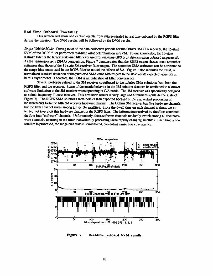
Single-Vehicle Mode. During most of the data collection periods for the Orbiter 3M GPS receiver, the 15-state

SVM of the RGPS filter performed real-time orbit determination in SVM. To our knowledge, the 15-state

Kalman filter is the largest state-size filter ever used for real-time GPS orbit determinalion onboard a spacecraft.

As the semimajor axis (SMA) comparison, Figure 7 demonstrates that the RGPS output shows much smoother

estimates than those of the 11-state 3M receiver filter output. The smoother SMA estimates can be auributed to

the range bias states used in the RGPS filter to model the effects of SA. Figure 7 also includes the FOM, a

normalized standard deviation of the predicted SMA error with respect to the steady-state expeewal value (75 m

in this experimen0. Therefore, the FOM is an indication of filter convergence.Several problems related to the 3M receiver contributed to the inferior SMA solutions from both the

RGPS filter and the receiver. Some of the erratic behavior in the 3M solution data can be attributed to a known

software limitation in the 3M receiver when operating in C/A mode. The 3M receiver was specifically designedas a dual-frequency, P-code receiver. This limitation results in very large SMA transients (outside the scale of

Figure 7). The RGPS SMA solutions were noisier than expected because of the inadvertent processing ofmeasurements from the fifth 3M receiver hardware channel. The Collins 3M receiver has five hardware channels,

but the fifth channel roves among all visible satellites. Since the dwell time on each channel is short, we in-

tended not to exploit this hardware channel in the RGPS filter. The information received by the filter contained

the fL"St four "software" chamzels. Unforlmmtely, these software channels randomly switch among all five hard-

ware channels, resulting in the filter inadvertently processing these rapidly changing satellites. Each time a new

satellite is processed, the range bias state is reinifi,liTed, preventing range bias convergence.

SMA Comparison

678417 T :i i=: = :r ¥ : _ • smaFl_

0

30

i=°L0

so of..a 20° 2so

, , , , , .L---;--- , , -q- --

0 50 Nolo(_'hanneis A_I tO Fltr: _ 250 300

4

2

00 50 100 150 200 250 300

Mins elapsed from LIT 1995 255:11: 1: 1

Figure 7: Real-time onboard SVM results

10

Dual-Vehicle Mode. A few snapshots of WSF GPS data became available during the WSF free-flight. However,hands-off operation of the RGPS filter did not transition from SVM to successful DVM operation, owing to an

unexpected set of stale data that preceded fresh WSF GPS data at the beginning of each snapshot. The filter target

state was repeatedly initialized using several hours-old solutions, causing all target GPS measurements to be

rejected. Successful DVM operation could have been achieved with a manual reinitialization of the filter. Note,

the snapshots were intended to allow a quick assessment of WSF GPS receiver performance. DVM operation

in this period was not intended to demonstrate filter performances since the data availability interval was plannedto be too short for filter convergence. Ground examination of downlinked GPS data uncovered this stale leftover

data problem. The filter successfully processed the snapshot data in DVM during near-real-time RPOP/RGPSexecution of these downlinked data in the MCC. This was achieved by delaying the reinitialization of the falteruntil fresh data amved.

Figure 8a shows the SMA solutions from the receivers and the RGPS filter during this short snapshot

period. Figure 8b shows the SMA FOM in the transient phase for the target and the chaser, and the correspond-

ing relative SMA filtered error standard deviation. Figure 8c shows the number of channels tracked by each

receiver during the snapshot. As Figure 8c shows, the number of satellites being tracked by each receiver was

low, resulting in very poor common satellite tracking during this period. The brevity of the WSF GPS snapshot

availability did not allow the filter enough time to converge. The combination of these two effects resulted in

rather high SMA FOM values during this period. Note that the SMA estimate convergence takes 20 to

30 minutes of filter operation under the minimum of four-satellite coverage.

68O0SMA Comparison

(D

Eo__

6795

6790

6785

6780

67752

X

i

o smaFItrChs_x smaRcvrChlsr

smaFItrTarc; I

+ smaRcvrTafg

x •

.'"" . . "i....._-- _" _d_'3m_' _•i ._ ._ ............. '.

...u_., ,..L..... _ ._1(-. "_ "_"" "t_ "1_" i'" '. ...+

. • X...X-_× x

I I I I I

3 4 5 6 7Mins elapsed from UT 1995 254:23:11:25

Figure 8a: SMA comparison during near-real-time processing

of snapshot data

8

11

30

25

o

2o

15

102

5000

4000

£

E

2O0O

10002

SMA Figure of Medt Comparison1 r T

&"m

BBIIB-l- n--- i! .ill- ol- IL

cp

°'"°ooo. o.o.. o.o..o.o.."'0"0 ..................... 0" ,0- 0¢_0 O0--O

1 I I ! I

3 4 5 6 7Mins elapsed from UT 1995 254:23:11".25

"_--;--- ............. -._-,-wu.u.-_4 5 6 7 8

Mins etal:_ed from UT 1995 254:23:11:25

Relative SMA Sigmai i v i

Figure 8b: SMA parameters during near-real-time processingof snapshot data

4 i

2 [ ooo...oooo.._> o

t% 3

if o. Q:' 'o ,' o"

I

02 3

4 i

2[ Q'_. ....

0 .... c2 3

Number of Channels Avail to Filter: Orbiter Rcvr

i i u

.O.O- • O, ._O ..................... '0- - -O -GO00C/'"

I I I I

4 5 6 7Mins elapsed from LIT 1995 254:23:11:25

Number of Channels Avail to Filter: WSF Rcvr

i i n I

.0 -0- - • _ .0-0., .0 0 O.. -0o .... o-o ..................... o" 'o...' "o'

ol I I I

4 5 6 7Mins elapsed from UT 1995 254:23:11:25

Number of Common GPS SVs in Fltr Soln

u u n i

0 ..................... 0"'0"0 000.-0

CC _C O" i i 0 i4 5 6 7

Mins elapsed from UT 1995 254:23:11:25

Figure 8c: Number of channels tracked by each receiver snapshot

t8

8

t8

12

Postflight Processing of Recorded Data

As previously explained, continuous WSF GPS data never became available during WSF rendezvous.

To complete the performance analysis, we ran RPOP/RGPS in a real-time mode using recorded data. Results

from these RI_P/RGPS runs were compared to the BET generated by UT/CSR described by Schroeder et al.

(ref. 3). At the time of this publication, the BET was only available for approximately 4 hours of the time

just following WSF deploy. However, we limited our comparisons to approximately 1 hour because of the

unexpected clock bias behavior of the TurboRogue receiver. Below we will explain the TurboRogue clock bias

behavior, and then compare SVM and DVM results to the BET.

TurboRogue Receiver Clock Offset Problem. The postflight analysis revealed unexpectedly inferior behavior

in the TurboRogue clock offset. Figure 9 shows an almost periodic random behavior of substantial magnitude.

This behavior may be due to a feedback loop present in the receiver clock-steering algorithm. The second-order

Markov clock model and the associated tuning parameters used in the RGPS filter assume a slowly drifting clock

behavior common to the majority of GPS receiver docks. We, therefore, limited our comparisons to a segment

of relatively mild clock behavicn'.

TurboRogueClockOffsetEstimate60 i i i i J t i

4O

o 20

2

E

0a=

o

80-20

-40

-606

i

612 I I I I I I I I

6.4 6.6 6.8 7 7.2 7.4 7.6 7.8Hrselapsed sinceUT 1995254: 9:1:32.000

Figure 9: TurboRogue receiver clock offset

13

Single-Vehicle Mode. Figure 10 presents the results of SVM operations compared to the BET. The plots in

the left column of Figure 10 reveal the position differences in UVW (radial, downtrack, and cross-track) coordi-

nates as well as the SMA differences between the SVM solutions and the BET. In the fight column, the 3Mreceiver and the Space Shuttle RNAV solutions are compared to the BET. Note that the state estimates from

RGPS filters are superior.

RGPS-UT/CSR BET chaser pos diffs, mtrs 3M Rcvr(o) and ONav(+) - UT/CSR BET pos diffs, mtrs

_ ! ! ! ! ! 2001 ! !! ! ! ! 'I" _' i ! i i i I i iO _O : : '

-o ' " _---_'" -' ' _ 0 ...._ i '

"i i i -200

i.... i i i ::: t [ iL_ : i !..I: : : ' :

,- ......... i ....... ::......... i...... i ..... !.... t 2ool-....... _-. _!...... i...t'---- ._. : : : _ / _ :0 : : _= : I

; i i ; _ -2001 i i - ; _- ; I

Semi-major axis diffs, mtrs Semi-major axis diffs, rntrs

1000 _ ..... 1000 ' • - oil 0l'-, i i i i :: I I i i i::i ::=_i: _i_l

v l'_r "" ": __._-m'_--- _; ...... :--2r uE_:_,_. ....... "'_-, ..... ._.-_--1 ...... ! " ..../, _-':--- ._'_ : : : I I,.I¢I :_ _::! 3111Dw _1_1__ l[Ir:::;:.'_" _l

-1000 : ; _ ; ; J_IOOOI=IP ' " g :: : : : :_ _ :i "r0 10 20 30 40 50 0 10 20 30 40 50

Mins elapsed since 254:14:49:50.951 Mins elapsed since 254:14:49:54.951

Figure 10: SVM position and SMA differences from

postflight processing

14

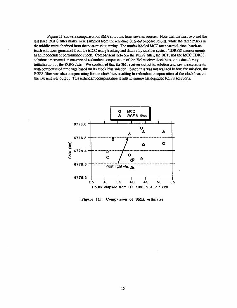
Figure 11 shows a comparison of SMA solutions from several sources. Note that the fast two and the

last three RGPS filter marks were sampled from the real-time STS-69 onboard results, while the three marks in

the middle were obtained from the post-mission replay. The marks labeled MCC are near-real-time, batch-to-

batch solutions generated from the MCC using tracking and data relay satellite system (TDRSS) measurements

as an independent performance cheek. Comparisons between the RGPS filter, the BET, and the MCC TDRSS

solutions uncovered an unexpected redundant compensation of the 3M receiver clock bias on its data duringinitialization of the RGPS filter. We confLrmed that the 3M receiver output its solution and raw measurements

with compensated time tags based on its clock bias solution. Since this was not realized before the mission, the

RGPS filter was also compensating for the clock bias resulting in redundant compensation of the clock bias on

the 3M receiver outpuL This redundant compensation results in somewhat degraded RGPS solutions.

6778.6

6778.5 -

E

< 6778.4 -

I O MCC,& .qGPS fi!ter

I I I I

O,&

,&Z_

6778.3 ..........................................................................................................Postflight --_

6778.2 I I I I I25 30 35 40 45 50 55

Hours elapsed from UT 1995 254:01:13:20

Figure 11: Comparison of SMA estimates

15

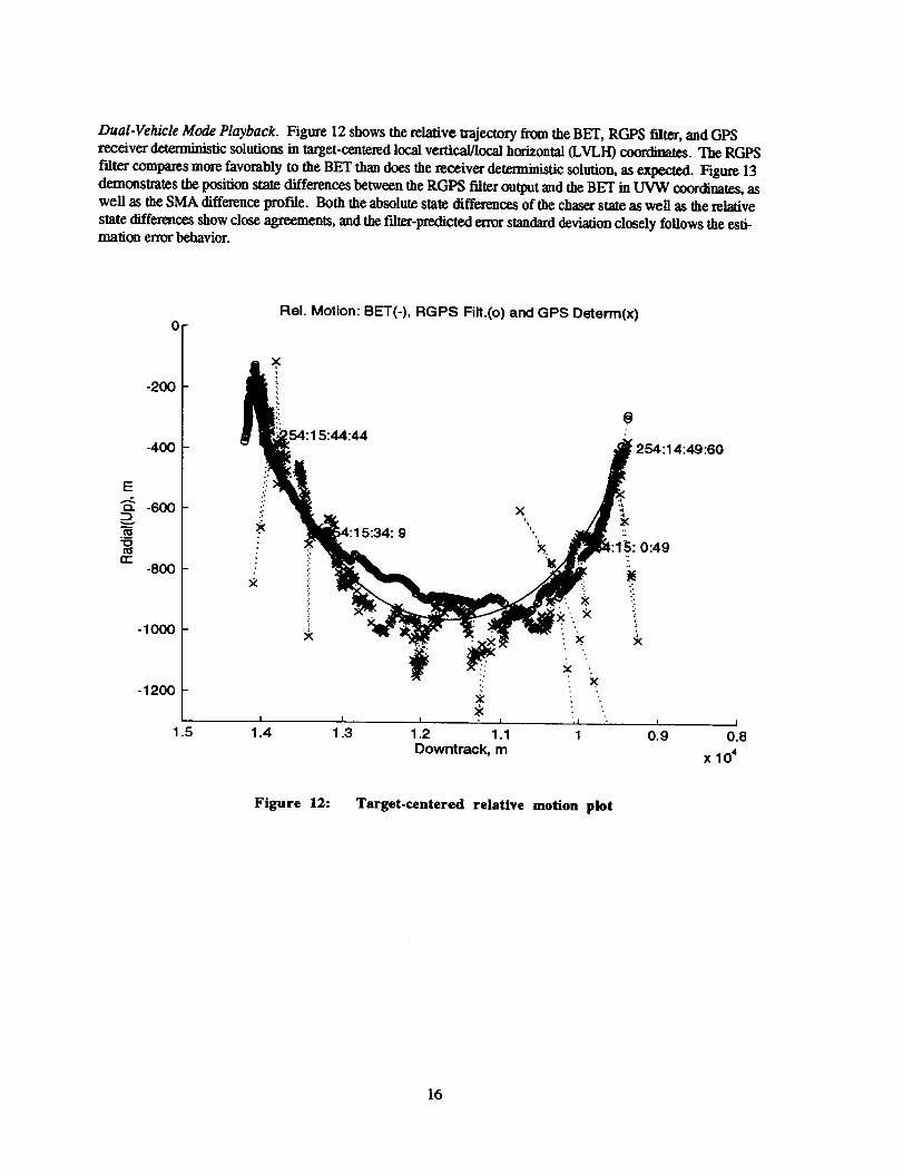
Dual-Vehicle Mode Playback. Figure 12 shows the relative trajectory from the BET, RGPS filter, and GPS

receiver deterministic solutions in target-centered local vertical/local horizontal (LVLH) coordinates. The RGPS

toter compares more favorably to the BET than does the receiver deterministic solution, as expected. Hgute 13

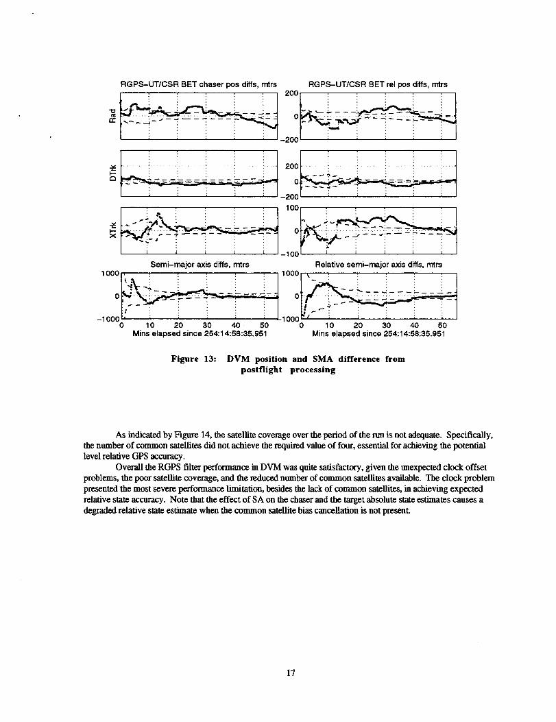
demonstrates the position state differences between the RGPS filter output and the BET in UVW coordinates, as

well as the SMA difference profile. Both the absolute state differences of the chaser state as well as the relative

state differences show close agreements, and the filter-predicted error standard deviation closely follows the esti-mation error behavior.

E

::>

._m

rr-

-2OO

-4OO

-6OO

-8OO

-IO00

-12OO

.5

Rol. Motion: BET(-), RGPS Filt.(o) and GPS De_erm(x)

'54:15:44:44

9

X

X

I I -1

1.4 1.3 1.2 1.1 1Downtrack, m

0

254:14:49:60

I

0.9 0.8

x 104

Figure 12: Target-centered relative motion plot

16

RGPS-UT/CSR BET chaser pos diffs, mtrs RGPS-UT/CSR BET rel pos diffs, mtrs

2OO

_ .........i.........i.........i..... i........i.... 200........i ......i........}........i.........i....

; ; ; i i 1-2oo' ......

: _ i.... i i i 1001 ! ! ! ! ! I

Semi-major axis dills, mtrs Relative semi-major axis dills, rntrs10001' : : : : : I 10001 k '. : : : I

:;I : : : : : ; _ : : : : '.

_1ooof[ _' "_ :, Llooo_, -_:, :, :, :_ i I0 10 20 30 40 50 0 10 20 30 40 50

Mins elapsed since 254:14:58:35.951 Mins elapsed since 254:14:58:35.951

Figure 13: DVM position and SMA difference frompostflight processing

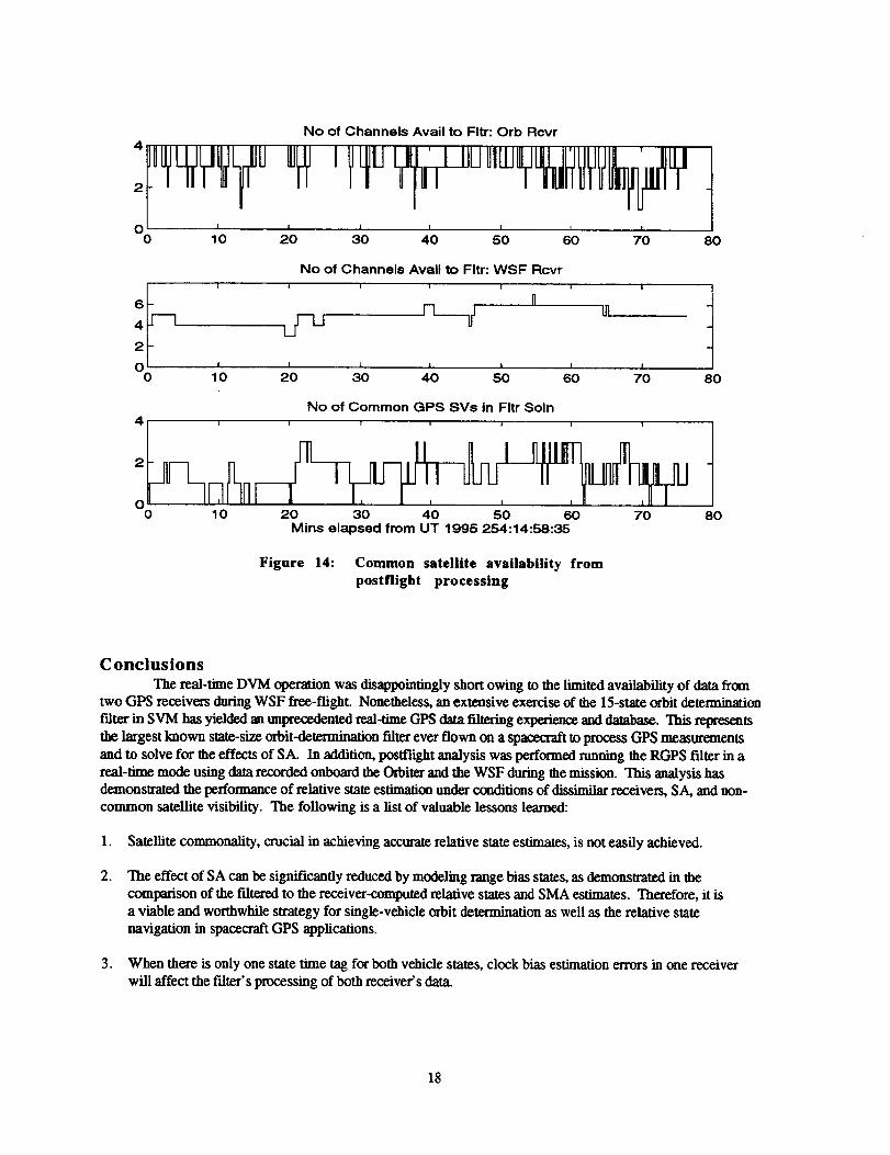
As indicated by Figure 14, the satellite coverage over the period of the run is not adequate. Specifically,the number of common satellites did not achieve the required value of four, essential for achieving the potential

level relative GPS accuracy.

Overall the RGPS filter performance in DVM was quite satisfactory, given the unexpected clock offset

problems, the poor satellite coverage, and the reduced number of common satellites available. The clock problem

presented the most severe performance limitation, besides the lack of common satellites, in achieving expected

relative state accuracy. Note that the effect of SA on the chaser and the target absolute state estimates causes a

degraded relative state estimate when the common satellite bias cancellation is not present.

17

0 10

No of ChanneLs Avail to Fltr: Orb Rcvr

I I I I I I

20 :30 40 50 60 70

No of Channels Avail to Fltr: WSF Rcvr

' ' ' ' ' '

6 J-L__ n I_,

O I I I I I I I

0 10 20 30 40 50 60 70

No of Common GPS SV$ in Fltr Soln4 i i i i i i !

o I

0 10 20 30 40 50 60 70Mine elapsed from UT 1995 254:14:58:35

Figure 14: Common satellite availability from

postflight processing

80

80

80

Conclusions

The real-time DVM operation was disappointingly short owing to the limited availability of data fromtwo GPS receivers during WSF free-fright. Nonetheless, an extensive exercise of the 15-state orbit detemfination

filter in SVM has yielded an unprecedented real-time GPS data filtering experience and database. This represents

the largest known state-size orbit-determination filter ever flown on a spacecraft to process GPS measurements

and to solve for the effects of SA. In addition, postflight analysis was performed running the RGPS filter in a

real-time mode using data recorded onboard the Orbiter and the WSF during the mission. This analysis hasdemonstrated the performance of relative state estimation under conditions of dissimilar receivers, SA, and non-

common satellite visibility. The following is a list of valuable lessons learned:

1. Satellite commonality, crucial in achieving accurate relative state estimates, is not easily achieved.

. The effect of SA can be significantly reduced by modeling range bias states, as demonstrated in the

comparison of the filtered to the receiver-computed relative states and SMA estimates. Therefore, it is

a viable and worthwhile strategy for single-vehicle orbit determination as well as the relative statenavigation in spacecraft GPS applications.

3. When there is only one state time tag for both vehicle states, clock bias estimation errors in one receiver

will affect the filter's processing of both receiver's data.

18

4. Real-timedatacanbehaveunpredictably.Emphasismustbeplaced on efforts to protect against as manydata failure situations as possible.

. For the class of GPS receivers with a clock steering algorithm, the dock parameter modeling presents a

significant challenge. To overcome this problem for orbital applications, disabling the clock steeringalgorithm may be required.

Despite many hardware and software glitches encountered during the mission, valuable lessons have been learned.The next opportunity to fly this experiment will be later this year (1996) on STS-80.

Acknowledgments

The project, the results of which are reported here, was supported and funded by the ISS Phase One

Risk Mitigation Office. Also, without the contributions of the following people our results could never have

been achieved: P. A. M. Abusali, Antha Adkins, Nick Combs, Gene Cook, Mike Cooke, Scott Cryan, Brent

Disselkoen, Charley Dunn, Courtney Duncan, Mike Exner, Ron Flanary, Bill Jackson, Jim Ledet, Kevin Lee,

Stephanie Lowery, Rick McCloskey, Samantha McDonald, Charlene Madden, Tom Manning, Scott Merkle, "l_ma

Minnix, Moises Montez, Dave Mulcihy, Tri Nguyen, Ray Nuss, John Riehl, Penny Saunders-Roberts, Christie

Schroeder, Bob Schutz, Tom Silva, Charles Simmons, Scott Tamblyn, and Dave Walker.

References

1. Hinkel, H. D., Y.-W. Park, and W. Fehse, "Realtime GPS Relative Navigation Flight Experiment,"

Proceedings of the National Technical Meeting, The Institute of Navigation, January 1995, pp. 593-601.

2. Montez, M., and L. Zyla, "Use of Two GPS Receivers in Order to Perform Space Vehicle OrbitalRendezvous," Proceedings of the ION GPS-93, The Institute of Navigation, September 1993, pp. 301-312.

3. Schroeder, C., B. Schutz, and P. Abusali, "STS-69 Relative Positioning GPS Experiment," AAS/AIAAConference, Paper No. AAS 96-180, February 1996.

4. Saunders, P. E., et al., "The First Flight Tests of GPS on the Space Shuttle," Proceedings of the 1994 ION

National Technical Meeting, The Institute of Navigation, January 24-26, 1994.

5. Schutz, B., et al., "GPS Tracking Experiment of a Free-Flyer Deployed from Space Shuttle," Proceedings ofthe ION GPS-95, The Institute of Navigation, September 1995, pp. 229-235.

6. March, J. G., et al., "Gravity Model Improvements Using Geos 3 (GEM 9 and GEM 10)," Journal ofGeophysical Research, Vol. 84, No. BS, July 30, 1979.

7. Gelb, Arthur (ed.), Applied Optimal Estimation, The M.I.T. Press, Cambridge, Mass., 1974.

8. Lear, W. M., "Proposed Simplified GPS Navigation Filters," JSC-25468 (Rev. 1), NASA Johnson SpaceCenter, Houston, Texas, 1993.

9. "Space Shuttle Operational Level C Functional Subsystem Software Requirements: Guidance, Navigation,

and Control: Part B: Onorbit Navigation," STS 83-0006H (OI-24), Rockwell International Space SystemsDivision, 1993.

10. Chen, C.-T., Linear System Theory and Design, Holt, Rinehart, & Winston, Inc., New York, 1984.

11. Lear, W. M., "Kalman Filtering Techniques," JSC-20688, NASA Johnson Space Center, Houston, Texas,1985.

19

FormApprovedREPORT DOCUMENTATION PAGE OMB No.0704-0188

Public reporting burd_q for this collection of tnfommtion is estimated to average 1 hour per responso, including the time for reviewing instructions. =marching existing data sources, gathering andmaintaining the data needed, and coml_stJng and reviewing the collection of Information. Send commerds regarding inis burden estimate or any other aspect of 1his coCe_ion of inform=tion.including suggestions fo¢ reducing this burden, to Washington Headquarters Services. Directorate for infommtion Operations and Re_oorts. 1215 Jeffer=on Davis Highway. Suite 1204. Arlington.VA 22202-430_. and to the Office of M_ and Budget. Papef_od¢ Reduction Project (0704-0188). Washington. DC 2&-uO3.

1. AGENCY USE ONLY (Leave Blank) 2. REPORT DATE 3. REPORT TYPE AND DATES COVEREDNovember 1996 NASA Technical Memorandum

4. TITLE AND SUBTITLE 5. FUNDING NUMBERS

Flight Test Results from Real-Time Relative Global Positioning System HightExperiment on STS-69

6. AUTHOR(S)

Young W. Park*; Jack P. Brazzel*; J. Russell Carpenter; Heather D. Hinkel;James H. Newman

7. PERFORMING ORGANIZATION NAME(S) AND ADDRESS(ES)

Lyndon B. Johnson Space CenterAeroscience and Hight Mechanics DivisionHouston, Texas 77058

9. SPONSORING/MONITORING AGENCY NAME(S) ANDADDRESS(ES)

National Aeronautics and Space AdministrationWashington, D.C. 20546-0001

8. PERFORMING ORGANIZATIONREPORT NUMBERS

S-821

10. SPONSORING/MONITORINGAGENCY REPORT NUMBER

TM- 104824

11. SUPPLEMENTARY NOTES

*McDonnell Douglas Aerospace, Houston, Texas

12a. DISTRIBUTION/AVAILABILITY STATEMENTUnclassified/Unlimited

Available from the NASA Center for AeroSpace Information (CASI)800 Elkridge Landing RoadLinthieum Heights, MD 21090-2934(301) 621-0390 Subject Category: 17

12b. DISTRIBUTIONCODE

13. ABSTRACT (Maximum200 words)A real-time global positioning system (GPS) Kalman filter has been developed to support automated rendezvous with theInternational Space Station (ISS). The filter is integrated with existing Shuttle rendezvous software running on a 486 laptopcomputer under Windows*. In this work we present real-time and postflight results achieved with the filter on STS-69. Theexperiment used GPS data from an Osborne/Jet Propulsion Laboratory TurboRogue receiver carried on the Wake Shield Facility(WSF) free-flyer and a Rockwell Collins 3M receiver carried on the Orbiter. Real-time filter results, processed onboard theShuttle and replayed in near-real time on the ground, are based on single-vehicle mode operation and on 5 to 20 minute snapshotsof telemetry provided by WSF for dual-vehicle mode operation. Postflight results were achieved by running the filter in real-timemode using data recorded during the mission. Orbiter and WSF state vectors calculated using our filter compare favorably withprecise reference orbits determined by the University of Texas Center for Space Research. The lessons learned from thisexperiment will be used in conjunction with future experiments to mitigate the technology risk posed by automated rendezvousand docking to the ISS.

*Trademark

14. SUBJECT TERMSglobal positioning system; space rendezvous; real time operation; Kalman filters

17. SECURITY CLASSIFICATION :18. SECURITY CLASSIFICATIONOF REPORT OF THIS PAGE

Unclassified Unclassified

NSN 7540-01-280-5500

15. NUMBEROF PAGES25

16. PRICE CODE

19. SECURITYCLASSIFICATIONOF ABSTRACT

Unclassified

20. LIMITATION OF ABSTRACT

Unlimited

StandardForm298 (Rev 2-89)Prescribed by ANSI Std. 239-18298-10_