1

Relative Efficiency of Modern Small Scale Industries in India:

An Inter-State Comparison*

Hiranya K Nath Southern Methodist University

I. Introduction

Persistent efforts have been made to promote small-scale industries (SSIs

hereafter) in India as a source of large-scale employment generation and equitable

distribution of income. There has been substantial growth of these industries over

last few decades1. Whether this growth has achieved the intended goals is subject

to empirical scrutiny. However it has been observed that the growth and

expansion of the small-scale sector have been uneven across the states2. It is in

this context that the present paper intends to measure relative efficiency of SSIs in

different states and to inquire into inter-state differences in these measures. An

index of relative efficiency (based on the concept of total factor productivity) is

used in this paper. This index gives a measure of efficiency of a SSI in a state

compared to its counterpart in other states.

The rest of this paper is organized as follows. A brief review of the earlier

studies on efficiency of SSIs in India is presented in the second section. The third

2

section discusses the database and the methodology used in the present study. In

the fourth section, we present the measures of relative efficiency of selected SSIs

in fifteen major states of India. Reasons for inter-state differences in efficiency

are investigated in the fifth section. The last section summarizes the major

findings of this study.

II. Review of Earlier Studies

A number of studies on efficiency of SSIs in India were undertaken.

Among the interesting ones were Dhar and Lydall3 (1961); Hajra4 (1965);

Sandesara5,6 (1966 and 1969); Mehta7 (1969); Bhavani8,9 (1980 and 1991);

Goldar10,11 (1985 and 1988); Little, Mazumdar and Page12 (1987) and

Ramaswamy13 (1990). Most of the earlier studies used the partial productivity

ratios for a measure of the relative efficiency of SSIs.

Dhar and Lydall, Hajra, Sandesara (1966 and 1969) and Mehta use

CMI/ASI14 data for their analysis. The first four studies report a positive

relationship between size and output-capital ratio. This is attributed to economies

of scale and better management in the relatively bigger units. Mehta’s conclusion

is contrary to those of others. However, he uses a different criterion for size

classification of the firms : he classifies the firms into different size classes

according to the value of fixed assets. Earlier studies, on the other hand, use

employment as the criterion for size classification. Also, Dhar –Lydall-Sandesara

use total productive capital (fixed plus working capital) as a measure of capital

input while Mehta uses fixed capital. However it is difficult to fully understand

3

the reasons for contradictory conclusions arrived at by these studies. It is possible

that ‘since the ratio of working capital to fixed capital is high in small scale units,

efficiency comparisons based on fixed capital favor small scale units’15.

Bhavani’s study (1980) is an improvement over the previous studies in the

sense that the basic data source for her study is the census of SSI units (CSSI),

conducted by the Development Commissioner of Small Scale Industries (DCSSI)

in 1973-74, which has a wider coverage than CMI/ASI does. A comparison

between the census sector16 of the ASI, the sample sector17 of the ASI and the

CSSI reveals that the capital productivity of SSI units is lower than that of large

scale units suggesting efficiency differences in line with the findings of Dhar-

Lydall-Sandesara.

Goldar, in his 1985 study, estimates a frontier production function (of

Cobb-Douglas form) using firm level data from CSSI for the small scale Washing

Soap industry to obtain measures of technical efficiency. Measures of partial and

total factor productivity, and an analysis of technical efficiency reveal that tiny

units are inefficient compared to relatively bigger units within the small scale

Washing Soap industry. The positive relationship between unit size and

efficiency, and high capital intensity of relatively larger units suggest a trade off

between output gain and employment loss.

Little et al (1987) discover very little regularity in the patterns of partial

and total factor productivity, and in their relationship with firm size in five SSIs

when size is measured either by number of workers employed, or by the value of

fixed assets. An analysis of technical efficiency, based on a three factor translog

4

production function, reveals that there are wide variations in total factor

productivity. Within each of the five industries, variation in technical inefficiency

(measured by the difference between actual and predicted output) is substantial

and there is no systematic relationship between employment size and technical

efficiency. Only in Machine Tools industry, technical efficiency is correlated with

firm size. As for the sources of variations in technical efficiency, four variables:

the average experience of the labor force, the age of the capital stock, the

experience of the entrepreneur and the level of capacity utilization, are found to

be significant in one or more industries.

Goldar (1988) uses a total factor productivity index based on the Cobb-

Douglas production function, to assess relative efficiency of 37 three-digit

industries of the NIC18. The data for this study are drawn from the statistical

reports of a sample survey of SSI units undertaken by the Reserve Bank of India

(RBI), with 1976-77 as the reference year. Data on large-scale industries are

drawn from census sector results of the ASI for 1976-77. It is observed that in

almost all industries labor productivity in small-scale units is less than that in

large-scale units. On the other hand, capital productivity in small units is higher in

22 industries when gross invested capital is used and in fifteen industries when

net invested capital is used as a measure of capital input. The relative efficiency

index which is a weighted average of partial productivity indexes, is less than

unity for 34 out of 37 industries suggesting that the SSIs are relatively less

efficient than large scale units. The study observes that economies of scale (as

captured by relative size) and better management (as captured by the ratio of

5

closing stock to consumption of raw materials) are significant sources of

efficiency for large units. Similarly higher relative efficiency can also be

attributed to mechanized technologies.

Ramaswamy (1990) estimates partial productivity of labor and of capital,

and relative efficiency using unit level data for four industries: Motor Vehicle

Parts, Agricultural Machinery and Parts, Machine Tools and Parts, and Plastic

Products. He uses the same relative efficiency index as Goldar (1985) does. His

analysis indicates that capital intensity and partial productivity are sensitive to

alternative measures of firm size. There is little regularity in the behavior of

capital-labor ratio and employment size. Partial factor productivity of labor and of

capital also do not exhibit any significant relationship with firm size when size is

measured in terms of employment. However, a positive relationship is observed

between capital-labor ratio and investment size of the unit. Labor productivity

rises while capital productivity falls as the investment size of the unit increases.

Efficiency indexes show neither systematic nor substantial differences between

employment or investment size classes of units. Ramaswamy’s analysis suggests

existence of increasing returns to scale and thus rejects the assumption of constant

returns to scale. His results are consistent with those reported by Little et al

(1987).

Using firm level data drawn from CSSI, Bhavani (1991) makes an attempt

to measure technical efficiency of 4 four-digit level metal products industries

using a translog production frontier with three inputs, viz. capital, labor and

materials. It is observed that for all the four metal products industries and five size

6

groups within each one of them, the average level of efficiency is quite high and

that efficiency measures increase with the increase in size upto a size class and

then decreases.

III. Database and Methodology

Database

The basic source of data for the present study is the Report on the Second

All India Census of Small Scale Industrial Units. State level data are obtained

from the corresponding state-wise volumes of the report. The census was

conducted in 1988-89, taking 1987-88 as the reference year, by the Development

Commissioner of Small Scale Industries (DCSSI) in association with the

Directorates of Industries (DI) of the states. The census data relate to SIDO units19

registered with the state DIs upto March 31, 1988. A `modern small scale

industrial unit’ was then defined as one with investment in plant and machinery

(original value) not exceeding Rs 3.5 million and Rs. 4.5 million in case of

ancillary unit20.

Most of the data were reported for the two-digit level disaggregation21 of

the SSIs. Data on gross output, investment in fixed assets, gross value added, net

value added and employment are reported for top 100 industries - in order of their

contribution to gross output - at four-digit level of disaggregation for India as a

whole, as well as for the states. We are considering nine industries in fifteen

major states in this study. These nine industries constitute the intersection of the

samples of 100 industries in each of the fifteen states. The choice of the level of

7

disaggregation is dictated by the availability of data.

Gross value added is taken as the measure of output22. Gross value added

is that part of the value of the products, which is created in the unit and is

obtained by deducting total value of inputs from the value of gross output.

Investment in fixed assets is taken as the measure of capital. ‘Fixed assets are

those which are of permanent nature like land, building, plant and machinery,

transport equipment, tools etc. which have normal production life of more than

one year’23. Investment in fixed assets is reported at original purchase prices.

Since the vintages of these assets are not known, no adjustment could be made for

price changes.

Number of employees is taken as the measure of labor input. Employment

comprises own account workers, direct workers and contract/casual employees.

Own account workers are those self-employed, i.e., proprietor, partners, or

members of the family of the owner, who work (whether paid or not) in the unit

regularly or casually. A direct worker, according to the Factories Act, is a person

employed directly, whether for wages or not, and engaged in any manufacturing

process or in any kind of work incidental to or connected to manufacturing

process. A contract or casual employee is one who is engaged through some

agency. This measure of labor input, however, doesn’t take into account the

quality differences. Moreover, preponderance of casual workers highly inflates

the measure of labor input.

Intermediate inputs include `value of raw materials, fuels, packing

materials, consumable stores etc. consumed and other incidental expenses

8

incurred by the unit, like sales expenses, hostage expenses, stationary charges,

publicity expenses, legal fees, insurance etc.’24.

Total wages paid to the persons employed were reported for the SSIs at

two-digit disaggregation level of industries. To obtain total wages paid to the

employees in the four-digit level industries, wages per employee have been

calculated for the corresponding two-digit level industry first, and then they are

multiplied by the number of persons employed at the four-digit level. However

there could be wide differences in wage rates among the four-digit industries

within the two-digit level industry group. Moreover, in SSIs the own account

workers are not paid a fixed amount.

Methodology

The analysis of efficiency is grounded in the theory of production. A

production function, by definition, gives the maximum possible output that can be

produced from given combination of inputs with a given level of technology.

Production is said to be efficient if there is no way to produce more output with

the same inputs or to produce the same output with less inputs. Based on this

theoretical framework, Farrell’s seminal paper25 of 1957 furnished measures of

efficiency. Farrell’s measure of technical efficiency is given by the ratio of inputs

needed to produce a given level of output to the inputs actually used to produce

that level. After Farrell, efficiency measurement has grown into a voluminous

literature and over the years has added to its richness and sophistication. For

empirical work, the Farrell indexes as proposed in the 1957 paper entail two

measures of efficiency. The first is given by the extent to which actual total factor

9

productivity (TFP hereafter) differs from a potential or maximal TFP and the

second measure is given by the extent to which TFP of a firm/industry differs

from that of another.

In empirical works, two approaches are usually taken to measure

efficiency as envisaged by Farrell. A frontier or best practice production function

is estimated to predict the maximum output which could be obtained from a set of

production inputs which are actually observed in the sample. The difference

between this predicted output and the actual output of the firm is considered to be

due to technical inefficiency in production. In the specification of the production

function either a one-sided negative error term or a stochastic error term is

included. In the first case the estimates of the error represent technical

inefficiency. In the second case, on the other hand, the error term consists of two

components: one represents technical inefficiency which is assumed to be

negative and the other represents measurement error and other statistical noise

and which could be positive or negative or zero. The second approach is to

calculate a weighted average of partial productivity indices of various inputs. The

first approach is used to obtain the first measure of efficiency as described above.

The second approach can be used for both the measures.

Given the availability of data and their inadequacies, the frontier

production function approach is not appropriate. First, the data source doesn’t

provide information on various characteristics of the SSIs at sufficiently

disaggregated level. Even four-digit level disaggregation that has been used in this

study leaves room for heterogeneity of products, which in turn has crucial

10

implications for technology which is captured by the hypothesized production

function. Second, as we have already seen, the measures of capital and labor are

grossly inadequate. Absence of vintage information pertaining to capital stock

measures and lack of information on hours worked and quality of workers could

account for a large part of the deviations from the best practice production

frontier. Under such circumstances, the role of production frontier as an efficiency

standard is questionable.

Since the aim of the present study is to investigate inter-state differences

in efficiency of SSIs we are focusing on the second measure implied by the

Farrell index. As we have seen that the frontier production function approach

might involve serious problems we are using the total factor productivity

approach. This is not to say that we can do away with the problems created by

data inadequacy in this approach. Moreover this approach has its own limitations.

Nevertheless the measures obtained by using this approach are good

approximations and the whole exercise is a useful first step in analyzing inter-

state differences in efficiency of SSIs in India. First we discuss the measure to be

used and then comment on its merits and demerits.

We are using gross value added per employee as the measure of labor

productivity and the ratio of gross value added to investment in fixed assets as the

measure of capital productivity. For each industry, relative productivity of labor

and capital in a state (say, in the ith state) are obtained by dividing productivity of

labor and of capital in the ith state by those in `all other states’. The relative

efficiency index for the jth industry in the ith state, denoted by REji (a ratio of

11

total factor productivity in the ith state to that in all other states), is computed as a

weighted average of relative productivity of labor and of capital26. Thus,

RELP

LP

KP

KPji j

i

jA i

wji

jA i

r

=⎛

⎝

⎜⎜

⎞

⎠

⎟⎟

⎛

⎝

⎜⎜

⎞

⎠

⎟⎟− −

where

w w wi A i=

+ −( )2

r r ri A i=

+ −( )2

w + r = 1

where LP and KP denote productivity of labor and of capital respectively.

Subscript j refers to the jth industry and superscripts i and A-i refer to `ith state’

and `all but the ith state’. w and r are the income shares of labor and capital

respectively.

This measure of relative efficiency assumes that there is constant returns

to scale and competitive equilibrium prevails in the market. The efficiency

measure described above is based on the Cobb-Douglas production function.

Using the logarithmic transformation we can write

InRE wInLP

LPr

KP

KPji j

i

jA i

ji

jA i

=⎛

⎝

⎜⎜

⎞

⎠

⎟⎟+

⎛

⎝

⎜⎜

⎞

⎠

⎟⎟− −

ln

The vintages of capital might vary widely across the states but while

computing relative productivity of capital, taking average over all the states

excepting the one for which relative productivity is being calculated has taken

care of the effect of extreme cases. Similarly, there could be wide variations of

12

hours worked among the states but even in this case taking average has reduced

the effect of extreme cases sufficiently.

As we have already mentioned, measures of technical efficiency based on

total factor productivity involve problems, particularly when they are used to

make comparisons between firms or industries that use different technologies. It is

very difficult to separate out the effects of technological differences. This problem

is relevant because within each industry group the composition of product-

specific industries might vary widely across states and so might their technology.

Another problem27of determining relative levels of total factor productivity

consists in establishing the productivity differential between firms which use

different levels of inputs and produce different levels of output. The problem in

this case is to separate the effect of different input levels among the firms.

IV. Empirical Measures of Relative Efficiency

Relative Labor Productivity

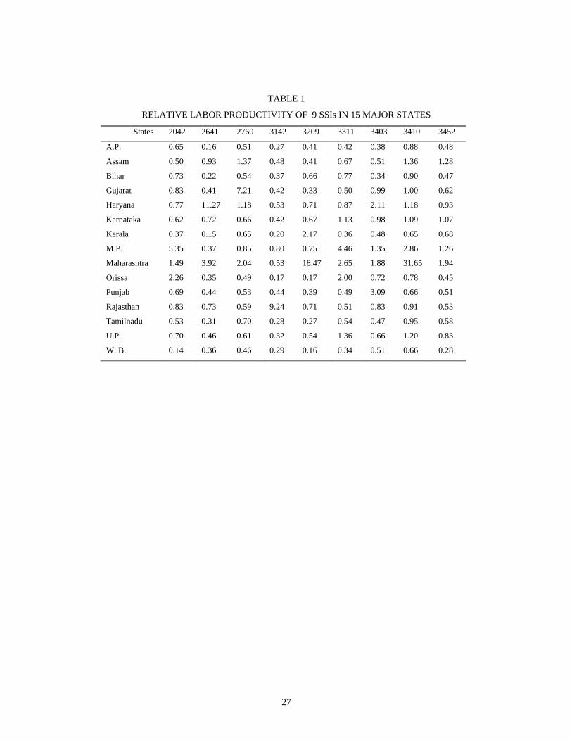
Table 1 shows relative labor productivity of SSIs in different states. It is

seen from the table that in Maharashtra labor is relatively more productive than in

other states as a whole, in case of eight industries. It may be noted that in

Maharashtra labor in the Non-ceramic Bricks industry (3209) is more than

eighteen times, and in the Structural Metal Products industry (3410), more than

thirty one times as productive as in other states. Besides, the Utensils industry

(3452) has the highest labor productivity in this state. Maharashtra is followed by

Madhya Pradesh with five industries which exhibit higher labor productivity

13

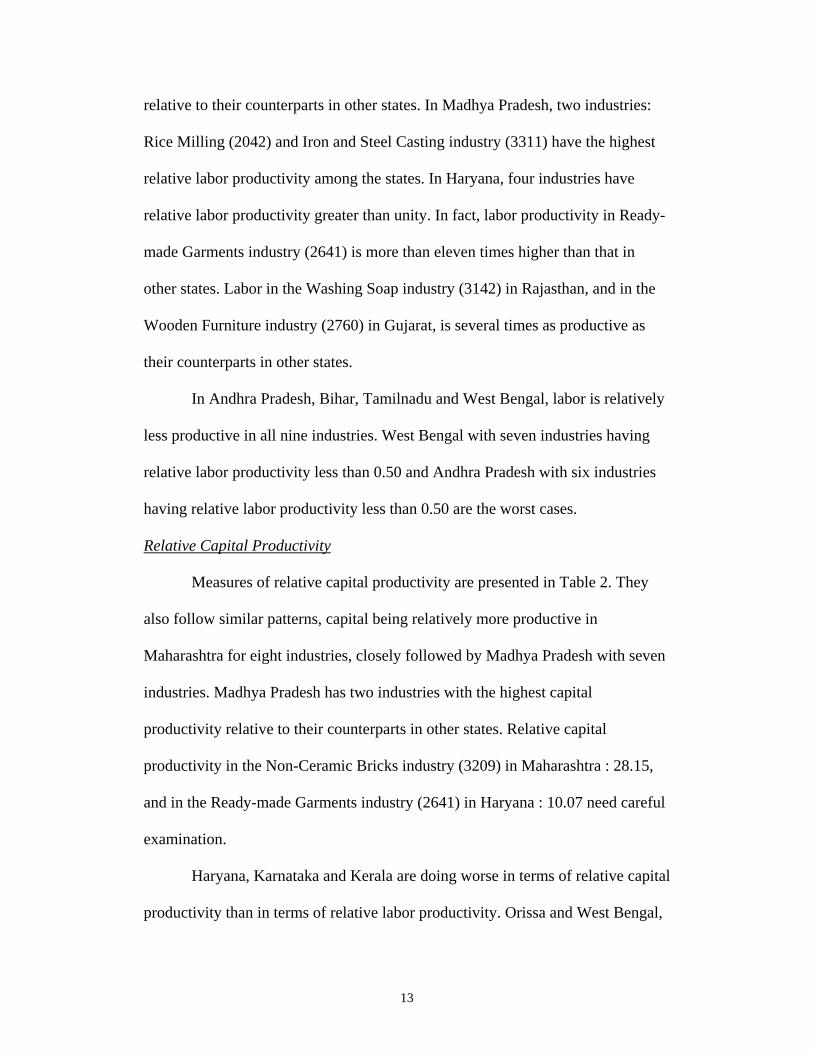
relative to their counterparts in other states. In Madhya Pradesh, two industries:

Rice Milling (2042) and Iron and Steel Casting industry (3311) have the highest

relative labor productivity among the states. In Haryana, four industries have

relative labor productivity greater than unity. In fact, labor productivity in Ready-

made Garments industry (2641) is more than eleven times higher than that in

other states. Labor in the Washing Soap industry (3142) in Rajasthan, and in the

Wooden Furniture industry (2760) in Gujarat, is several times as productive as

their counterparts in other states.

In Andhra Pradesh, Bihar, Tamilnadu and West Bengal, labor is relatively

less productive in all nine industries. West Bengal with seven industries having

relative labor productivity less than 0.50 and Andhra Pradesh with six industries

having relative labor productivity less than 0.50 are the worst cases.

Relative Capital Productivity

Measures of relative capital productivity are presented in Table 2. They

also follow similar patterns, capital being relatively more productive in

Maharashtra for eight industries, closely followed by Madhya Pradesh with seven

industries. Madhya Pradesh has two industries with the highest capital

productivity relative to their counterparts in other states. Relative capital

productivity in the Non-Ceramic Bricks industry (3209) in Maharashtra : 28.15,

and in the Ready-made Garments industry (2641) in Haryana : 10.07 need careful

examination.

Haryana, Karnataka and Kerala are doing worse in terms of relative capital

productivity than in terms of relative labor productivity. Orissa and West Bengal,

14

on the other hand, are doing better in terms of capital productivity. For example,

in West Bengal none of the industries has labor productivity higher than in other

states. But two industries: Drums-Tanks-and-Metal Products industry (3403) and

Utensils industry (3452) have relative capital productivity greater than unity in

this state. Because of the shortcoming of the measure of capital as mentioned

earlier, it is possible that higher relative capital productivity indicates that the

fixed assets are of old vintages.

It is seen that there is strong positive correlation between relative labor

productivity and relative capital productivity in each of the industries across states

and across industries in each of the states. This suggests that labor and capital are

complementary rather than substitutes to each other. This is further reinforced by

a strong positive correlation between capital and labor inputs.

Relative Efficiency

Relative efficiency measures are presented in Table 3. It is observed that

relative efficiency index is less than unity for all nine industries in five states :

Andhra Pradesh, Bihar, Kerala, Tamilnadu and West Bengal. That is, SSIs in

these states are less efficient than their counterparts in other states. In fact, in

Andhra Pradesh, Kerala and Tamilnadu, none of the nine industries has a relative

efficiency index greater than 0.90. In five other states: Gujarat, Karnataka,

Punjab, Rajasthan and Uttar Pradesh, only one industry each (Wooden Furniture

industry (2760) in Gujarat; Drums-Tanks-and-Metal Products industry (3403) in

Punjab; Washing Soap industry (3142) in Rajasthan and Iron and Steel Casting

industry (3311) in Karnataka and Uttar Pradesh) is relatively more efficient than

15

in other states. Similarly, Haryana and Orissa have got two industries each with

relative efficiency indexes greater than unity.

Madhya Pradesh and Maharashtra have only one industry each, out of the

nine considered here, which is relatively less efficient than in other states. In

Maharashtra, Non-Ceramic Bricks industry (3209) is more than four times, and

Structural Metal Products industry (3410) is more than two and half times as

efficient as those in other states. This is not surprising given the fact that relative

labor and capital productivity of those two industries are quite high in this state.

On the other hand, in Madhya Pradesh Rice Milling (2042) is almost two and a

half times as efficient as in other states. In fact, Rice Milling (2042) and Iron and

Steel Casting industry (3311) in this state have the highest relative efficiency

indexes among the states.

The Ready-made Garments industry (2641) in Haryana, the Wooden

Furniture industry (2760) in Gujarat and the Washing Soap industry (3142) in

Rajasthan have the highest relative efficiency indexes among the states. The

pattern of labor and capital productivity estimates discussed above is a pointer to

these results.

A use-based classification of industries and estimates of coefficient of

variation (CV) of the relative efficiency measures of the industries would throw

lights on a few other aspects of the inter-state differences in relative efficiency

measures. A three category classification puts Rice Milling (2042), Ready-made

Garments (2641) and Washing Soap (3142) into the category `consumer non-

durables’; Wooden Furniture (2760), Drums- Tanks-and-Metal Products (3403)

16

and Utensils (3452) into `consumer durables’ and Non-Ceramic Bricks (3209),

Iron and Steel Casting(3311), and Structural Metal Products (3410) into

`intermediate products’ category. As Table 4 shows, the intermediate product

industries and the consumer non-durable industries have greater variations of

relative efficiency indexes among the states. The consumer durable industries

have the highest average efficiency indexes and relatively smaller CVs. It could

be inferred that there is greater diffusion of technical knowledge, more uniform

demand for the products and greater uniformity of efficiency of these industries

across the states. Intermediate goods industries have some of the highest CVs. It

is possible that there is wide variation in technological knowledge and in

opportunities of vertical integration for, say, Non-Ceramic Bricks industry or

Structural Metal Products industry across the states. Among the intermediate

product industries, Non-ceramic Bricks industry has the widest dispersion of

relative efficiency indexes.

In order to test for the appropriateness of the two-factor production

function implied by the measure used in this study we obtain relative efficiency

measures of the SSIs by an alternative method based on weighted average of

relative productivity indexes of three factors of production: capital, labor and

intermediate inputs. Broadly the pattern of efficiency measures doesn’t change.

However, for those industries and for those states where relative indexes were

higher than unity the new indexes are slightly lower in magnitude than the earlier

ones though not less than unity. On the other hand, for those industries and for

those states where relative indexes were lower than unity the new indexes are

17

slightly higher in magnitude than the earlier ones thus reducing the dispersion of

these measures.

V. Reasons for Inter-State Differences in Relative Efficiency

Measures of relative efficiency presented in Table 3 show considerable

variations across states. An analysis of these variations would be useful for

understanding the causes of inefficiency of SSIs in various states. The explanatory

variables chosen for this purpose are discussed below.

Several studies [including Dhar and Lydall,1961 and Sandesara, 1966 &

1969] suggest that higher efficiency could be attributed to economies of scale. To

capture the effect of economies of scale on relative efficiency, three different

measures of relative size are used : first, value of production per unit in a state

divided by value of production per unit in other states (RS1); second, fixed

investment per unit in a state divided by fixed investment per unit in other states

(RS2); third, employment per unit in a state divided by employment per unit in

other states (RS3). States with higher average relative firm size are expected to

have higher relative efficiency indexes.

Better management could be a source of higher efficiency. Goldar (1988)

uses the ratio of closing stock of raw materials to consumption as the measure of

quality of management in SSIs.`This ratio indicates how efficiently small scale

units manage their inventories’28. But our data source does not provide the

relevant information on inventories. Therefore percentage capacity utilization has

been taken as the measure of quality of management. It is assumed that this ratio

18

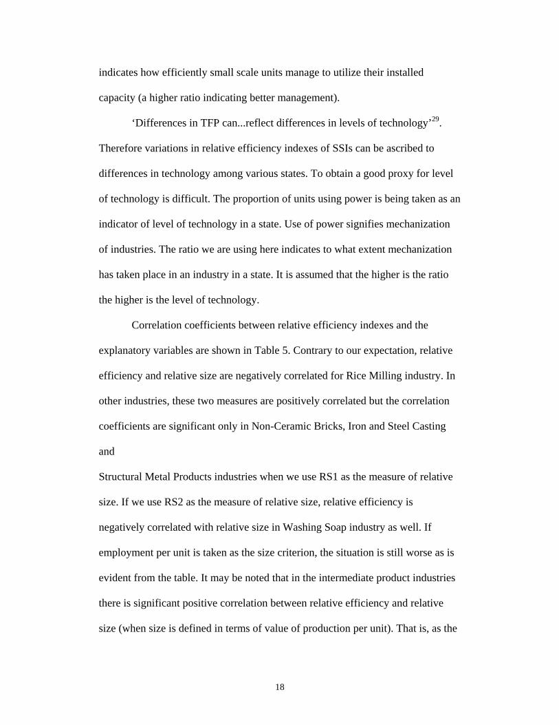
indicates how efficiently small scale units manage to utilize their installed

capacity (a higher ratio indicating better management).

‘Differences in TFP can...reflect differences in levels of technology’29.

Therefore variations in relative efficiency indexes of SSIs can be ascribed to

differences in technology among various states. To obtain a good proxy for level

of technology is difficult. The proportion of units using power is being taken as an

indicator of level of technology in a state. Use of power signifies mechanization

of industries. The ratio we are using here indicates to what extent mechanization

has taken place in an industry in a state. It is assumed that the higher is the ratio

the higher is the level of technology.

Correlation coefficients between relative efficiency indexes and the

explanatory variables are shown in Table 5. Contrary to our expectation, relative

efficiency and relative size are negatively correlated for Rice Milling industry. In

other industries, these two measures are positively correlated but the correlation

coefficients are significant only in Non-Ceramic Bricks, Iron and Steel Casting

and

Structural Metal Products industries when we use RS1 as the measure of relative

size. If we use RS2 as the measure of relative size, relative efficiency is

negatively correlated with relative size in Washing Soap industry as well. If

employment per unit is taken as the size criterion, the situation is still worse as is

evident from the table. It may be noted that in the intermediate product industries

there is significant positive correlation between relative efficiency and relative

size (when size is defined in terms of value of production per unit). That is, as the

19

firm size increases efficiency also increases thus suggesting that intermediate

product industries might have substantial economies of scale.

There is positive correlation between relative efficiency and capacity

utilization indexes except in two industries: Wooden Furniture industry and

Utensils. However the correlation coefficient is significantly different from zero

only in the Ready-made Garments industry. In seven out of nine industries, there

is positive correlation between relative efficiency and proportion of power using

units. The coefficient is, however, not significantly different from zero in most of

the cases suggesting a weak relationship between efficiency and level of

technology. These two measures have significant positive correlation only in

Non-Ceramic Bricks industry.

Examining the correlation coefficients, we have decided to regress relative

efficiency indexes on three variables: relative size (RS1), level of capacity

utilization (CU) and level of technology (TECH). The regression results are

presented in Table 6.

The coefficient of the explanatory variable: relative size is positive and

significant for six industries. It supports the hypothesis that there are some

economies of scale in these industries. The coefficient of relative size is negative

but not significant in rice milling industry. In other two industries, the estimated

coefficients are smaller and not significantly different from zero. In these

industries small firms could be the most efficient ones and at higher level of

production there could be decreasing returns to scale.

Level of capacity utilization, which has been taken as a measure of the

20

quality of management, is a significant source of variations in relative efficiency

only in the Ready-made Garments industry. The coefficient of level of capacity

utilization is positive in five other industries but are not significant. It is surprising

to note that the relationship between relative efficiency and level of technology-as

measured by the proportion of power using units- is negative in most industries

and in one or two cases, this is even significant. Only in Rice Milling, the

elasticity of efficiency with respect to level of technology is positive and

significant at 0.10 level. It is possible that since in most states, particularly in

relatively less developed states, power supply is irregular and insufficient, as the

number of units using power increases their efficiency suffers. This hypothesis is

substantiated by the fact that average consumption of power is low in relatively

backward states even if the proportion of power using units may be high30.

A test for heteroscedasticity31 based on the regression of the squared

residuals on squared fitted values has been carried out and the F-statistics are

found to be insignificant for all nine regressions. Thus it is reasonable to use

ordinary least square estimates under the assumption that the error terms are

homoscedastic.

VI. Conclusion

The relative efficiency measures presented in this paper indicate that only

in seven states we observe some general patterns: in Maharashtra and Madhya

Pradesh, most of the SSIs are relatively more efficient than in other states. On the

other hand, in Andhra Pradesh, Bihar, Kerala, Tamilnadu and West Bengal they

21

are relatively less efficient. In other states, some industries have efficiency

indexes greater than unity and others have less than unity. A use-based

classification of industries reveals that consumer durable industries have some of

the highest average efficiency indexes and relatively smaller coefficient of

variations. It could be because of greater diffusion of technical knowledge, more

uniform demand for the products across the states. On the other hand, the

intermediate product industries and the consumer non-durable industries have

wider variations in their relative efficiency indexes across states. In case of the

intermediate product industries, it could be ascribed to greater variation in

technological knowledge and opportunities for vertical integration among the

states.

Relative efficiency is positively correlated with relative size, but is

significantly so only in three industries: Non-Ceramic Bricks, Iron and Steel

Casting and Structural Metal Products. The index has positive correlation with the

level of capacity utilization in seven out of nine industries. The correlation

coefficient, however, is significant only in the Ready-made Garments industry.

The proportion of SSI units using power-which has been taken as a proxy for the

level of technology, is found to be positively correlated with relative efficiency in

seven industries. A careful perusal of the data on this important ratio will reveal

that in industrially developed states like Maharashtra, the industries with higher

proportion of power using units are relatively more efficient. However, even if

this proportion is high, with irregular and insufficient supply of power the

industries may be relatively inefficient as it is the case in some backward states.

22

The multiple regression analysis involving three explanatory variables:

relative size, level of capacity utilization and level of technology, shows that

relative size of the firm is the most important explanatory variable. It explains

inter-state differences in relative efficiency of six industries. It may be noted that

intermediate product industries have scale advantages. The level of capacity

utilization is a significant source of efficiency differences only in the Ready-made

Garments industry. The level of technology explains inter-state differences in

efficiency only in Rice Milling.

The results of this study have policy implications. The decade of nineties

has witnessed widespread economic reforms in India. Higher growth has been the

primary objective of these reform measures. In a liberalized environment the SSIs

are facing competition and there is an apprehension that some of them might have

to close down. But given the social and economic condition of India the relevance

and role of small-scale sector can’t be looked down upon. It can be instrumental

in containing rising inequalities. Also, in the transition of backward regions from

predominantly agriculture-based economic activities to industrial activities SSIs

can play the role of a catalyst by creating an infrastructure for the growth of

industries, in terms of capital formation and entrepreneurship development. In this

context, this study provides important guidelines to the policy-makers who wish

to achieve growth by smooth restructuring of the economy and without increasing

regional disparities in India.

23

Notes * This paper is based on my M Phil. dissertation at the Jawaharlal Nehru

University, New Delhi, India. Comments from A. N. Bhat, H. Mukhopadhyay,

Esfandiar Maasoumi and Tom Fomby are gratefully acknowledged. I also thank

the seminar participants at the Texas Camp Econmetrics III held at Lago Vista in

1998. However, any error that remains is my responsibility.

1. For a discussion on the growth of SSIs in India see J. C. Sandesara,

‘Modern Small Industry, 1972 and 1987-88 : Aspects of Growth and Structural

Change’, Economic and Political Weekly, February 6, 1993; and K. V.

Ramaswamy, ‘Small Scale Manufacturing Industries : Some Aspects of Size,

Growth and Structure’, Economic and Political Weekly, February 26, 1994.

2. See Hiranya K. Nath, “Relative Efficiency of Modern Small Scale

Industries in India : An Inter-State Comparison” (M. Phil. dissertation, Delhi :

Jawaharlal Nehru University, 1996) and National Council of Applied Economic

Research and Fredrich Naumann-Stifling, Structure and Promotion of Small Scale

Industry in India : Lessons for Future Development, (New Delhi : NCAER, 1993)

3. P. N. Dhar and H. F. Lydall, The Role of Small Scale Enterprises in

Indian Economic Development, (Bombay: Asia Publishing House, 1961)

4. S. Hajra, “Firm Size and Efficiency in Measuring Industries”, Economic

and Political Weekly, August,1965.

5. J. C. Sandesara, “Scale and Technology in Indian Industry”, Oxford

Bulletin of Economics and Statistics, Vol.28, 1966.

6. J. C. Sandesara, “Size and Capital Intensity in Indian Industry: Some

Comments”, Oxford Bulletin of Economics and Statistics, Vol.31, No.1, 1969.

24

7. B. V. Mehta, “Size and Capital Intensity in Indian Industry”, Oxford

Bulletin of Economics and Statistics, Vol.31, No.3, 1969.

8. D. A. Bhavani, Relative Efficiency of the Modern Small Scale Industry

in India, (M.Phil dissertation, Delhi: University of Delhi, 1980)

9. D. A. Bhavani, ‘Technical Efficiency in Indian Modern Small Scale

Sector: An application of Frontier Production Function’, Indian Economic

Review, Vol. 26, No.2, 1991.

10. B. N. Goldar, ‘Unit Size and Economic Efficiency: A Study of Small

Scale Washing Soap Industry in India’, Artha Vijnana, Vol.27, No.1,1985.

11. B. N. Goldar, “Relative Efficiency of Small Scale Industries in India”

in K. B. Suri (ed.) Small Scale Enterprises in Industrial Development: The Indian

Experience (New Delhi : Sage Publications, 1988).

12. I. M. D. Little, Dipak Mazumdar and John M Page, Jr. Small

Manufacturing Enterprises: A Comparative Study of India and Other Economies,

(Washington, D.C.: World Bank, 1987).

13. K. V. Ramaswamy, Technical Efficiency in Modern Small Industry in

India, (Ph.D. thesis, Delhi: University of Delhi, 1990)

14. CMI = Census of Manufacturing Industries

ASI = Annual Survey of Industries

15. B. N. Goldar, “Relative Efficiency of Small Scale Industries in India”

in K. B. Suri (ed.) Small Scale Enterprises in Industrial Development: The Indian

Experience (New Delhi : Sage Publications, 1988).

16. Census sector includes all those units registered under the Factories

25

Act. A factory has been defined as one with 10 workers and use of power, or one

with 20 workers and without use of power.

17. Sample sector includes a sample of units which are not registered

under the Factories Act but registered with one or more of the government

organizations or departments.

18. NIC = National Industrial Classification

19. Those units which are registered with the Small Industries

Development Organization (SIDO).

20. Development Commissioner of Small Scale Industries, Report on the

Second All India Census of Small Scale Industrial Units, (New Delhi:

Government of India, 1992).This definition since then has changed.

21. This is according to the National Industrial Classification (NIC). As

the number of digits in level of disaggregation increases the industry group

becomes more product specific.

22. For a discussion, see Z. Griliches and V. Ringstad, Economies of

Scale and the Form of Production Function, (Amsterdam : North Holland

Publishing Co, 1971).

23. Development Commissioner of Small Scale Industries.

24. ibid.

25. M. J. Farrell, “The Measurement of Production Efficiency”, Journal of

Royal Statistical Society, No.A120, 1957.

26. S. Ho, “Small Scale Enterprises in Korea and Taiwan” (World Bank

Staff Working Paper 384, Washington, D.C.: World Bank,1980) and B. N.

26

Goldar, “Relative Efficiency of Small Scale Industries in India” in K. B. Suri

(ed.) Small Scale Enterprises in Industrial Development : The Indian Experience

(New Delhi : Sage Publications, 1988) use similar index.

27. This was pointed out by Little et al.

28. B. N. Goldar, “Relative Efficiency of Small Scale Industries in India”

in K. B. Suri (ed.) Small Scale Enterprises in Industrial Development : The Indian

Experience (New Delhi : Sage Publications, 1988).

29. Little et al

30. Nath

31. This is the test built in the package ‘MICROFIT’ that has been used

for estimation in this paper.

27

TABLE 1

RELATIVE LABOR PRODUCTIVITY OF 9 SSIs IN 15 MAJOR STATES States 2042 2641 2760 3142 3209 3311 3403 3410 3452

A.P. 0.65 0.16 0.51 0.27 0.41 0.42 0.38 0.88 0.48

Assam 0.50 0.93 1.37 0.48 0.41 0.67 0.51 1.36 1.28

Bihar 0.73 0.22 0.54 0.37 0.66 0.77 0.34 0.90 0.47

Gujarat 0.83 0.41 7.21 0.42 0.33 0.50 0.99 1.00 0.62

Haryana 0.77 11.27 1.18 0.53 0.71 0.87 2.11 1.18 0.93

Karnataka 0.62 0.72 0.66 0.42 0.67 1.13 0.98 1.09 1.07

Kerala 0.37 0.15 0.65 0.20 2.17 0.36 0.48 0.65 0.68

M.P. 5.35 0.37 0.85 0.80 0.75 4.46 1.35 2.86 1.26

Maharashtra 1.49 3.92 2.04 0.53 18.47 2.65 1.88 31.65 1.94

Orissa 2.26 0.35 0.49 0.17 0.17 2.00 0.72 0.78 0.45

Punjab 0.69 0.44 0.53 0.44 0.39 0.49 3.09 0.66 0.51

Rajasthan 0.83 0.73 0.59 9.24 0.71 0.51 0.83 0.91 0.53

Tamilnadu 0.53 0.31 0.70 0.28 0.27 0.54 0.47 0.95 0.58

U.P. 0.70 0.46 0.61 0.32 0.54 1.36 0.66 1.20 0.83

W. B. 0.14 0.36 0.46 0.29 0.16 0.34 0.51 0.66 0.28

28

TABLE 2

RELATIVE CAPITAL PRODUCTIVITY OF 9 SSIs IN 15 MAJOR STATES

States 2042 2641 2760 3142 3209 3311 3403 3410 3452

A. P. 0.75 0.24 0.73 0.21 0.55 0.46 0.36 0.21 0.66

Assam 0.41 1.01 1.37 0.24 0.65 0.46 0.55 0.28 1.33

Bihar 0.62 0.28 0.80 0.39 0.96 0.74 0.53 0.21 0.45

Gujarat 0.65 0.48 4.84 0.49 0.35 0.53 0.73 0.19 0.32

Haryana 0.75 10.07 0.69 0.50 0.30 0.59 2.43 0.21 0.42

Karnataka 0.45 0.79 0.73 0.48 0.27 1.20 0.84 0.18 0.66

Kerala 0.32 0.23 0.48 0.18 0.16 0.23 0.50 0.12 0.48

M. P. 7.89 0.77 2.13 1.12 1.72 3.15 1.96 0.74 1.22

Maharashtra 1.19 3.03 1.46 0.60 28.15 1.94 1.55 3.65 1.15

Orissa 3.12 0.65 0.88 0.22 0.48 1.91 0.55 0.18 0.97

Punjab 0.64 0.36 0.34 0.39 0.32 0.58 3.62 0.12 0.40

Rajasthan 0.69 0.64 0.45 6.56 0.42 0.42 0.98 0.17 0.47

Tamilnadu 0.64 0.50 0.80 0.33 0.23 0.47 0.65 0.21 0.53

Uttar Pradesh 0.54 0.26 0.51 0.23 0.24 1.08 0.65 0.25 0.45

West Bengal 0.29 0.94 0.96 0.64 0.39 0.67 1.09 0.21 1.40

29

TABLE 3

MEASURES OF RELATIVE EFFICIENCY OF 9 SSIs IN 15 MAJOR STATES

States 2042 2641 2760 3142 3209 3311 3403 3410 3452

A.P. 0.88 0.50 0.83 0.53 0.74 0.71 0.65 0.63 0.79

Assam 0.69 1.00 1.15 0.57 0.77 0.74 0.77 0.70 1.13

Bihar 0.82 0.56 0.86 0.66 0.95 0.88 0.73 0.61 0.71

Gujarat 0.84 0.72 2.04 0.72 0.62 0.75 0.89 0.62 0.67

Haryana 0.88 2.74 0.89 0.74 0.66 0.82 1.46 0.63 0.75

Karnataka 0.71 0.90 0.86 0.72 0.64 1.08 0.93 0.59 0.88

Kerala 0.61 0.49 0.76 0.49 0.56 0.56 0.73 0.55 0.77

M.P. 2.43 0.85 1.24 1.03 1.15 1.68 1.31 1.03 1.09

Maharashtra 1.09 1.64 1.22 0.79 4.10 1.36 1.23 2.61 1.12

Orissa 1.62 0.78 0.87 0.50 0.56 1.33 0.79 0.59 0.88

Punjab 0.83 0.66 0.66 0.67 0.63 0.78 1.74 0.53 0.70

Rajasthan 0.86 0.83 0.73 2.30 0.73 0.70 0.98 0.58 0.73

Tamilnadu 0.82 0.70 0.89 0.61 0.54 0.73 0.80 0.63 0.77

Uttar Pradesh 0.78 0.66 0.77 0.55 0.59 1.05 0.83 0.68 0.76

West Bengal 0.53 0.89 0.86 0.75 0.54 0.78 0.97 0.61 0.87

30

TABLE 4

SUMMARY OF THE RELATIVE EFFICIENCY MEASURES FOR 9 SSIs IN INDIA

Ind/Measures Mean Std.Dev. C.V. Min. Max.

2042 0.96 0.46 0.48 0.53(WB) 2.43(MP)

2641 0.93 0.55 0.60 0.49(Ker) 2.74(Har)

2760 0.98 0.33 0.34 0.66(Pun) 2.04(Guj)

3142 0.78 0.43 0.55 0.49(Ker) 2.30(Raj)

3209 0.92 0.87 0.94 0.54(TN) 4.10(Mah)

3311 0.93 0.30 0.32 0.70(Raj) 1.68(MP)

3403 0.99 0.30 0.30 0.65(AP) 1.74(Pun)

3410 0.77 0.50 0.65 0.53(Pun) 2.61(Mah)

3452 0.84 0.15 0.18 0.70(Pun) 1.13(Asm)

Notes: The states in brackets refer to those states where the efficiency indexes are minimum or

maximum as the case may be.

Std. Dev. = Standard Deviation

Min. = Minimum

Max. = Maximum

31

TABLE 5 CORRELATION COEFFICIENTS BETWEEN RELATIVE EFFICIENCY

AND EXPLANATORY VARIABLES

Industry RS1 RS2 RS3 CU TECH

2042 -0.03 -0.26 -0.43 0.15 0.32

2641 0.49 0.30 0.12 0.83 ** 0.04

2760 0.29 0.08 0.18 -0.02 0.40

3142 0.16 -0.05 -0.24 0.31 0.04

3209 0.95 ** 0.50 0.25 0.41 0.53 *

3311 0.72 ** 0.13 0.11 0.09 0.02

3403 0.24 0.11 -0.16 0.15 -0.16

3410 0.90 ** 0.70 ** 0.52 * 0.38 0.31

3452 0.44 0.26 0.29 -0.03 -0.07

Note: * significant at 10 % significance level. ** significant at 5 % level.

32

TABLE 6

REGRESSION RESULTS

Industry Intercept RS1 CU TECH Observ- -ations

R-square F-Statistic

FStatistic for Heteroscedasticity Test

2042 -4.55 -0.16 (-0.84)

0.14 (0.61)

0.88 (1.42 *)

15 0.19 0.84 0.06

2641 -0.18 0.36 (4.40 **)

0.51 (3.12**)

-0.56 (-4.74)

15 0.82 16.53 * 0.19

2760 0.13 0.11 (0.82)

-0.17 (-0.47)

0.12 (0.37)

15 0.20 0.92 1.08

3142 0.11 0.23 (0.72)

0.18 (0.54)

-0.28 (-0.40)

15 0.20 0.94 1.22

3209 -1.14 0.69 (3.16 **)

0.37 (1.19)

-0.15 (-0.56)

15 0.58 5.12 * 0.76

3311 0.74 0.35 (2.72 **)

-0.02 (-0.11)

-0.18 (-0.60)

15 0.40 2.49 2.95

3403 1.65 0.23 (1.63 *)

0.26 (1.04)

-0.64 (-1.91)

15 0.31 1.67 0.97

3410 0.67 0.47 (2.61 **)

0.16 (0.50)

-0.37 (-0.88)

15 0.43 2.76 0.37

3452 0.83 0.15 (1.61 *)

-0.07 (-0.43)

-0.17 (-0.79)

15 0.20 0.93 0.80

Notes: * significant at 10 % significance level

** significant at 5 % level.