regularization of portfolio allocation · the mean-variance optimization (mvo) theory of markowitz...

Electronic copy available at: http://ssrn.com/abstract=2767358

Regularization of Portfolio Allocation∗

Benjamin BruderQuantitative Research

Lyxor Asset Management, [email protected]

Nicolas GausselChief Investment Officer


Jean-Charles RichardQuantitative Research


Thierry RoncalliQuantitative Research


June 2013

Abstract

The mean-variance optimization (MVO) theory of Markowitz (1952) for portfolioselection is one of the most important methods used in quantitative finance. Thisportfolio allocation needs two input parameters, the vector of expected returns and thecovariance matrix of asset returns. This process leads to estimation errors, which mayhave a large impact on portfolio weights. In this paper we review different methodswhich aim to stabilize the mean-variance allocation. In particular, we consider recentresults from machine learning theory to obtain more robust allocation.

Keywords: Portfolio optimization, active management, estimation error, shrinkage esti-mator, resampling methods, eigendecomposition, norm constraints, Lasso regression, ridgeregression, information matrix, hedging portfolio, sparsity.

JEL classification: G11, C60.

1 IntroductionThe mean-variance optimization (MVO) framework developed by Markowitz (1952) is cer-tainly the most famous model used in asset management. This model is generally associatedto the CAPM theory of Sharpe (1964). This explains why Harry M. Markowitz and WilliamF. Sharpe have shared1 the Nobel Prize in 1990. However, the two models are used differ-ently by practitioners.

The CAPM theory considers the Markowitz model from the viewpoint of micro analysisin order to deduce the price formation for financial assets. In this model, the key conceptis the market portfolio, which is uniquely defined. In the Markowitz model, optimizedportfolios depend on expected returns and risks. Moreover, the optimal portfolio is notunique and depends on the investor’s risk aversion. As a consequence, these two models∗We are grateful to Clément Le Bars for his helpful comments.1with Merton H. Miller.


pursue different purposes. While the CAPM theory is the foundation framework of passivemanagement, the Markowitz model is the relevant framework for active management.

Nevertheless, even if the Markowitz model is a powerful model to transform the viewsof the portfolio manager into investment bets, it has suffered a lot of criticism because it isparticularly dependent on estimation errors (Michaud, 1989). In fact, the Markowitz modelis an aggressive model of active management (Roncalli, 2013). By construction, it does notmake the distinction between real arbitrage factors and noisy arbitrage factors. The goal ofportfolio regularization is then to produce less aggressive portfolios by reducing noisy bets.

The paper is organized as follows. Section two presents the motivations to use regu-larization methods. In particular, we illustrate the instability of mean-variance optimizedportfolios. In section three, we review the different approaches of portfolio regularization.They concern the introduction of weight constraints, the use of resampling techniques or theshrinkage of covariance matrices. We also consider penalization methods of the objectivefunction like Lasso or ridge regression and show how these methods may be used to regularizethe inverse of the covariance matrix, which is the most important quantity in portfolio opti-mization. In section four, we consider different applications in order to illustrate the impactof regularization on portfolio optimization. Section five offers some concluding remarks.

2 Motivations2.1 The mean-variance portfolioLet us consider a universe of n risky assets. Let µ and Σ be the vector of expected returnsand the covariance matrix of asset returns2. We note r the risk-free asset. A portfolioallocation consists in a vector of weights x = (x1, . . . , xn) where xi is the percentage of thewealth invested in the ith asset. Sometimes, we may assume that all the wealth is investedmeaning that the sum of weights is equal to one. Moreover, we may also add some otherconstraints on the weights. For instance, we may impose that the portfolio is long-only. Letus now define the quadratic utility function U of the investor which only depends of theexpected returns µ and the covariance matrix Σ of the assets:

U (x) = x> (µ− r1)− φ

2x>Σx

where φ is the risk tolerance of the investor. The mean-variance optimized (or MVO)portfolio x? is the portfolio which maximizes the investor’s utility. The optimization problemcan be reformulated equivalently as a standard QP problem:

x? = arg min 12x>Σx− γx> (µ− r1)

where γ = φ−1. Without any constraints, the solution yields the well known formula:

x? = 1φ

Σ−1 (µ− r1) = γΣ−1 (µ− r1)

It comes that the Sharpe ratio of the MVO portfolio is:

SR (x? | r) = x?> (µ− r1)√x?>Σx?

=√

(µ− r1)>Σ−1 (µ− r1)2In this paper, we adopt the formulation presented in the book of Roncalli (2013).


We deduce that the optimal utility of the investor is:

U (x?) = x?> (µ− r1)− φ

2x?>Σx?

= 12φ (µ− r1)> Σ−1 (µ− r1)

= 12φ SR2 (x? | r)

Maximizing the mean-variance utility function is then equivalent to maximizing the ex-anteSharpe ratio of the allocation.

Remark 1 Without lack of generality, we assume that the risk-free rate r is equal to zeroin the rest of the paper.

In practice, we cannot reach the optimal allocation because we don’t know µ and Σ.That is why we have to estimate these two quantities. Let Rt = (R1,t, . . . , Rn,t) be thevector of historical returns for the different assets at time t. We then estimate µ and Σ bymaximum likelihood method:

µ = 1T

T∑t=1

Rt

Σ = 1T

T∑t=1

(Rt − µ) (Rt − µ)>

We can therefore use the estimates µ and Σ in place of µ and Σ in mean-variance optimiza-tion. This estimation step is very easy. As mentioned by Roncalli (2013), “we could thinkthat the job is complete. However, the story does not end here”.

2.2 Evidence of mean-variance instabilityEstimating the input parameters of the optimization program necessarily introduces esti-mation errors and instability in the optimal solution. This stability issue with estimatorsbased on historical figures has been largely studied by academics3. Before going into thedetails of this subject, we propose to illustrate the stability problem of the MVO portfoliowith the following example.

Example 1 We consider a universe of four assets. The expected returns are µ1 = 5%,µ2 = 6%, µ3 = 7% and µ4 = 8% whereas the volatilities are equal to σ1 = 10%, σ2 = 12%,σ3 = 14% and σ4 = 15%. We assume that the correlations are the same and we haveρi,j = ρ = 70%.

We solve the mean-variance problem without constraints using the parameters givenin Example 1. The risk tolerance parameter φ is calibrated in order to target an ex-antevolatility4 equal to 10%. In this case the optimal portfolio is x?1 = 23.49%, x?2 = 19.57%,

3See for instance Michaud (1989), Jorion (1992), Broadie (1993) Ledoit and Wolf (2004) or more recentlyDeMiguel et al. (2011).

4Let σ? be the ex-ante volatility. We have:

φ =

√µ>Σ−1µ

σ?

x?3 = 16.78% and x?4 = 28.44%%. In Table 1, we indicate how a small perturbation of inputparameters changes the optimized solution. For instance, if the volatility of the second assetincreases by 3%, the weight on this asset becomes −14.04% instead of 19.57%. If the realizedreturn of the first asset is 6% and not 5%, the optimal weight of the first asset is almostthree times larger (63.19% versus 23.49%). As a consequence, the optimized solution is verysensitive to estimation errors.

Table 1: Sensitivity of the MVO portfolio to input parameters

ρ 70% 80% 80%σ2 12% 15% 15%µ1 5% 6%x?1 23.49% 19.43% 36.55% 39.56% 63.19%x?2 19.57% 16.19% −14.04% −32.11% 8.14%x?3 16.78% 13.88% 26.11% 28.26% 6.98%x?4 28.44% 32.97% 37.17% 45.87% 18.38%

The stability problem comes from the solution structure. Indeed, the solution involvesthe inverse of the covariance matrix I = Σ−1 called the information matrix. The eigenvectorsof the two matrices are the same but the eigenvalues of I are equal to the inverse of theeigenvalues of Σ (Roncalli, 2013).

Example 2 We consider our previous example but with another correlation matrix:

C =

1.000.50 1.000.40 0.30 1.00−0.50 0.20 0.10 1.00

In Table 2, we consider Example 2 and report the eigenvectors vj and the eigenvalues λj

of the covariance and information matrices. Results show that the most important factor5

of the information matrix is the less important factor of the covariance matrix. However thesmallest factors of the covariance matrix are generally considered noise factors because theyrepresent a small part of the total variance. This explains why MVO portfolios are sensitiveto input parameters because small changes in the covariance matrix dramatically modifythe nature of smallest factors. Despite the simplicity of the mean-variance optimization, thestability of the allocation is then a real problem. In this context, Michaud suggested thatmean-variance maximization is in fact ‘error maximization’:

“The unintuitive character of many optimized portfolios can be traced to thefact that MV optimizers are, in a fundamental sense, estimation error maxi-mizers. Risk and return estimates are inevitably subject to estimation error.MV optimization significantly overweights (underweights) those securities thathave large (small) estimated returns, negative (positive) correlations and small(large) variances. These securities are, of course, the ones most likely to havelarge estimation errors” (Michaud, 1989, page 33).

In a dynamic framework, estimation errors can then dramatically change the weights leadingto high turnover and/or high transaction costs. Moreover, the diversifiable risk is supposed

5The jth factor is represented by the eigenvector vj and the importance of the factor is given by theeigenvalue λj .

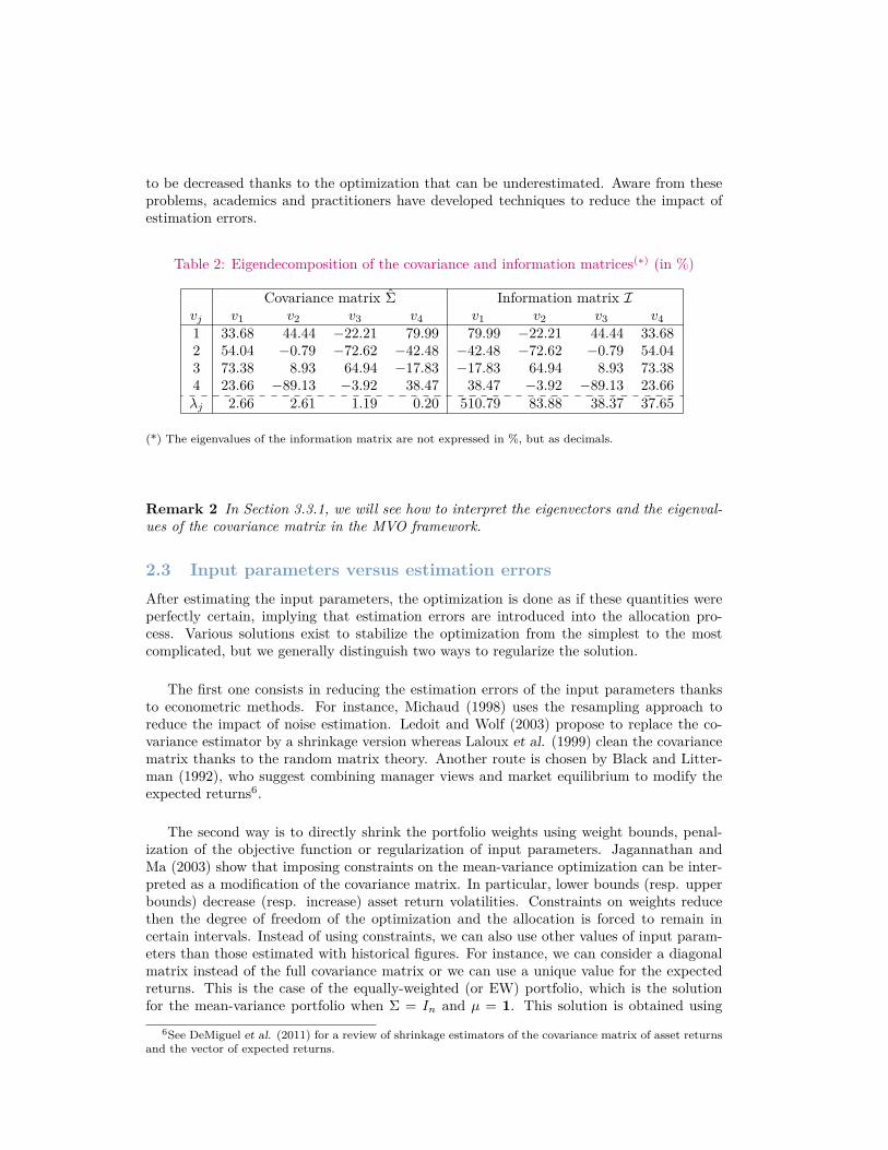
to be decreased thanks to the optimization that can be underestimated. Aware from theseproblems, academics and practitioners have developed techniques to reduce the impact ofestimation errors.

Table 2: Eigendecomposition of the covariance and information matrices(∗) (in %)

Covariance matrix Σ Information matrix Ivj v1 v2 v3 v4 v1 v2 v3 v41 33.68 44.44 −22.21 79.99 79.99 −22.21 44.44 33.682 54.04 −0.79 −72.62 −42.48 −42.48 −72.62 −0.79 54.043 73.38 8.93 64.94 −17.83 −17.83 64.94 8.93 73.384 23.66 −89.13 −3.92 38.47 38.47 −3.92 −89.13 23.66λj 2.66 2.61 1.19 0.20 510.79 83.88 38.37 37.65

(*) The eigenvalues of the information matrix are not expressed in %, but as decimals.

Remark 2 In Section 3.3.1, we will see how to interpret the eigenvectors and the eigenval-ues of the covariance matrix in the MVO framework.

2.3 Input parameters versus estimation errorsAfter estimating the input parameters, the optimization is done as if these quantities wereperfectly certain, implying that estimation errors are introduced into the allocation pro-cess. Various solutions exist to stabilize the optimization from the simplest to the mostcomplicated, but we generally distinguish two ways to regularize the solution.

The first one consists in reducing the estimation errors of the input parameters thanksto econometric methods. For instance, Michaud (1998) uses the resampling approach toreduce the impact of noise estimation. Ledoit and Wolf (2003) propose to replace the co-variance estimator by a shrinkage version whereas Laloux et al. (1999) clean the covariancematrix thanks to the random matrix theory. Another route is chosen by Black and Litter-man (1992), who suggest combining manager views and market equilibrium to modify theexpected returns6.

The second way is to directly shrink the portfolio weights using weight bounds, penal-ization of the objective function or regularization of input parameters. Jagannathan andMa (2003) show that imposing constraints on the mean-variance optimization can be inter-preted as a modification of the covariance matrix. In particular, lower bounds (resp. upperbounds) decrease (resp. increase) asset return volatilities. Constraints on weights reducethen the degree of freedom of the optimization and the allocation is forced to remain incertain intervals. Instead of using constraints, we can also use other values of input param-eters than those estimated with historical figures. For instance, we can consider a diagonalmatrix instead of the full covariance matrix or we can use a unique value for the expectedreturns. This is the case of the equally-weighted (or EW) portfolio, which is the solutionfor the mean-variance portfolio when Σ = In and µ = 1. This solution is obtained using

6See DeMiguel et al. (2011) for a review of shrinkage estimators of the covariance matrix of asset returnsand the vector of expected returns.

wrong estimators. However, these estimators have a null variance and minimize the impactof estimation errors on the optimized portfolio.

The correction of estimation errors is such difficult task that several studies tend to showthat heuristic allocations perform better than mean-variance allocations in terms of theSharpe ratio. For example, DeMiguel et al. (2009) compare the performances of 14 differentportfolio models and the equally-weighted portfolio on different datasets and conclude thatsophisticated models are not better than the EW portfolio. More recently, Tu and Zhou(2011) propose to combine the EW portfolio with optimized allocation to outperform naivestrategies. In a similar way, Dupleich et al. (2012) combine MVO portfolios with differentlag windows to remove model uncertainty. By mixing stable noisy portfolios, the authorsseek to improve the stability of the allocation. In fact, we will see that most of mixingschemes are equivalent to denoising input parameters.

3 Regularization methods for portfolio optimizationIn what follows, we present the most popular techniques used to solve the problem of esti-mation errors. The first three paragraphs concern weight constraints, resampling methodsand shrinkage procedures of the covariance matrix. We then consider the penalization ap-proach of the objective function. Finally, the stability of hedging portfolios based on theinformation matrix is explained in the last paragraph.

3.1 Using weight constraintsAdding constraints is certainly the first approach that has been used by portfolio managersto regularize optimized portfolios, and it remains today the most frequent method to avoidmean-variance instability.

Let us consider the optimization problem with the normalization constraint:

x? (γ) = arg max 12x>Σx− γx>µ

u.c. 1>x = 1

The constraint 1>x = 1 means that the sum of weights is equal to one. It is easy to showthat the optimized portfolio is then:

x? (γ;λ) = γΣ−1µ

where µ = µ+ (λ/γ) · 1 and λ is the Lagrange coefficients associated to the constraint. Wenotice that imposing a portfolio that is fully invested with a leverage equal to exactly one isequivalent to regularize the vector of expected returns. The constraint

∑ni=1 xi = 1 is then

already a regularization method.

Example 3 We consider a universe of four assets. The expected returns are µ1 = 8%,µ2 = 9%, µ3 = 10% and µ4 = 8% whereas the volatilities are equal to σ1 = 15%, σ2 = 20%,σ3 = 25% and σ4 = 30%. The correlation matrix is the following:

C =

1.000.10 1.000.40 0.70 1.000.50 0.40 0.60 1.00

If we suppose that γ = 0.5, we obtain results reported in Table 3. If there is no constraint,the portfolio is highly leveraged. For instance, the weight of the first asset is equal to207.05%. By adding the simple constraint

∑ni=1 xi = 1, the dispersion of optimized weights

is smaller7. We also notice that the regularized expected returns are lower, because λ isequal to −2.65%.

Table 3: Optimized portfolio with the constraint∑ni=1 xi = 1

Unconstrained Constrainedµi x? (γ) µi x? (γ;λ)

1 8.00% 207.05% 2.69% 64.61%2 9.00% 136.24% 3.69% 42.06%3 10.00% −22.75% 4.69% 11.55%4 8.00% −32.28% 2.69% −18.22%

The previous framework may be generalized to other constraints. For instance, Jagan-nathan and Ma (2003) show that adding a long-only constraint is equivalent to regularizingthe covariance matrix. This result also holds for any equality or inequality constraints(Roncalli, 2013). If we consider our previous example and add a long-only constraint, theoptimized portfolio is x?1 = 52.23%, x?2 = 42.41%, x?3 = 1.36% and x?4 = 0.00%. In thiscase, the regularized vector of expected returns µ and the regularized covariance matrix Σare given in Table 4. We notice that the long-only constraint is equivalent to decrease thevolatility and the correlation of the fourth asset in order to eliminate its short exposure.

Table 4: Regularized parameters µ and Σ

Asset µi σi ρi,j1 2.83% 15.00% 100.00%2 3.83% 20.00% 10.00% 100.00%3 4.83% 25.00% 40.00% 70.00% 100.00%4 2.83% 26.72% 32.90% 27.49% 53.43% 100.00%

Remark 3 Portfolio managers generally find the optimal portfolio by sequential steps. Theyperform the portfolio optimization, analyze the solution to define some regularization con-straints, design a new optimization problem by considering these constraints, analyze the newsolution and add more satisfying constraints, etc. This step-by-step approach is then verypopular, because portfolio managers implicitly regularize the parameters in a coherent waywith their expectations for the solution. The drawback may be that the regularized parame-ters are no longer coherent with the initial parameters. Moreover, the constrained solutionis generally overfitted.

3.2 Resampling methodsResampling techniques are based on Monte Carlo and bootstrapping methods. Jorion (1992)was the first to apply these techniques to portfolio optimization. The idea is to create morerealistic allocation by introducing uncertainty in the decision process of the allocation. For

7The weight of the first asset is then equal to 64.61%.

that, we consider a universe of n assets. Let µ and Σ be the estimates of the expected re-turns and the covariance matrix of assets returns. The efficient frontier computed with thesestatistics is an estimation of the true efficient frontier. Michaud (1998) proposed then av-eraging many realizations of optimized MV solutions to improve out-of-sample performancethanks to the statistical diversification.

The procedure is the following. We generate K samples of asset returns from the originaldata using Monte Carlo or bootstrap methods:

• Monte CarloThe returns are simulated according to a multivariate Gaussian distribution with meanµ and covariance matrix Σ.

• BootstrapThe returns are drawn randomly from the original sample with replacement.

We assume that the MV solution is computed for a given value of the risk tolerance. Wethen calculate the mean µ(k) and the covariance matrix Σ(k) of the k-th simulated sample.We also calculate the MVO portfolios for a grid of risk tolerance. Finally, we average theweights with respect to the grid and estimate the resampled efficient frontier.


C =

1.000.10 1.000.40 0.20 1.00−0.10 −0.10 −0.20 1.00

We illustrate the resampling procedure in Figure 1 by considering Example 4. MVO

portfolios are computed under the constraints 1>x = 1 and 0 ≤ xi ≤ 1. We consider500 simulated samples and 60 points for the grid. The estimated frontier is calculatedwith µ and Σ statistics. The averaged frontier corresponds to the average of the differentefficient frontiers obtained for each sample of simulated asset returns. It is different from theresampled frontier, which corresponds to the frontier of resampled portfolios. For instance,we report one optimal resampled portfolio (designed by the red star symbol) which is theaverage of the 500 resampled portfolios (indicated with the blue cross symbol).

The resampled efficient frontier in Figure 2 is performed with S&P 100 asset returnsduring the period from January 1, 2011 to December 31, 2011. The resampled frontieris largely below the estimated and averaged efficient frontiers. Moreover, portfolios withhigh returns are unattainable on the resampled frontier, meaning that these portfolios areextreme points on the estimated efficient frontier and are purely due to estimation noises.

Remark 4 Resampling techniques have faced some criticisms (Scherer, 2002). The firstone concerns the procedure itself, because the resampled portfolio always contains estimationerrors since it is computed with the initial parameters µ and Σ. The second criticism is thelack of theory. Resampling techniques is more an empirical method which seems to correctsome biases, because portfolio averaging produces more diversified portfolios. However, theydo not solve the robustness question concerning optimized portfolios.

Figure 1: Simulated resampled efficient frontier (Monte Carlo approach)

Figure 2: S&P 100 resampled efficient frontier (Bootstrap approach)

3.3 Regularization of the covariance matrix3.3.1 The eigendecomposition approach

The goal of this method is to reduce the instability of the covariance matrix estimator Σ.For that, we consider the eigendecomposition Σ = V ΛV > where Λ = diag (λ1, · · · , λn) isthe diagonal matrix of the eigenvalues with λ1 > λ2 > · · · > λn and V is an orthogonalmatrix where each column vj is an eigenvector. With this decomposition, also known asprincipal components analysis, we can build endogenous factors Ft = Λ−1/2V >Rt. In thiscase, the cleaning process consists in deleting some noise factors Fj,t.

Let m be the number of relevant factors. We can then keep the most informative factors,i.e. the factors with the largest eigenvalues. In this case, factors with low eigenvalues areconsidered as noise factors and we have:

m = max {j : λj ≥ (λ1 + · · ·+ λn)/n}

Another solution consists in computing the implicit exposures of the portfolio to these fac-tors. For instance, we can reformulate the MVO portfolio as follows:

x? = γΣ−1µ = V Λ−1/2β

where β = γΛ−1/2V >µ. If we compute the return of the portfolio’s investor, we obtain:

Rt (x?) = x?>Rt = β>Λ−1/2V >Rt = β>Ft

We deduce that βj is exactly the exposure of the investor to the PCA factor Fj,t. We noticethat the weights β of the factors in the MVO portfolio are inversely proportional to thesquare root of the eigenvalues: βj ∝

√λj . Thus the optimized portfolio can be strongly

exposed to low variance factors, meaning that some noise factors may have a high impacton the MVO solution.

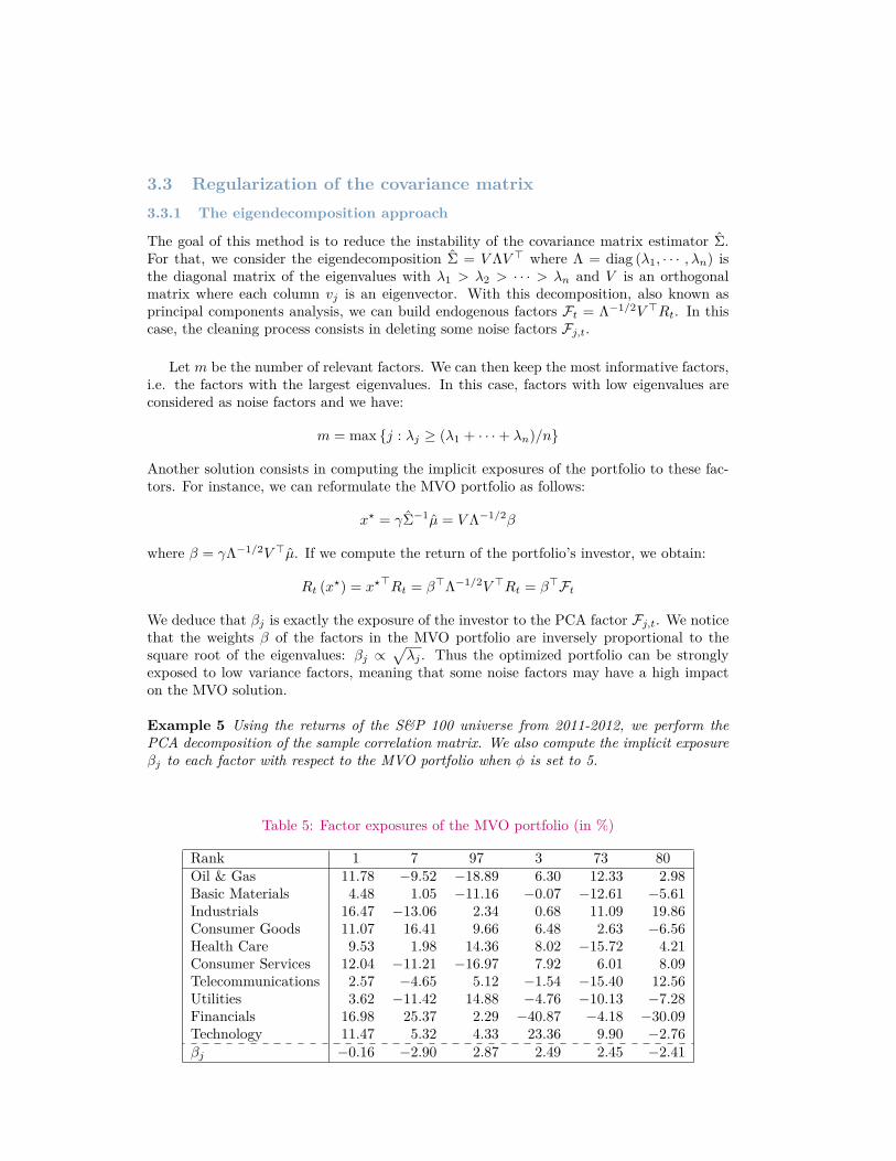
Example 5 Using the returns of the S&P 100 universe from 2011-2012, we perform thePCA decomposition of the sample correlation matrix. We also compute the implicit exposureβj to each factor with respect to the MVO portfolio when φ is set to 5.

Table 5: Factor exposures of the MVO portfolio (in %)

Rank 1 7 97 3 73 80Oil & Gas 11.78 −9.52 −18.89 6.30 12.33 2.98Basic Materials 4.48 1.05 −11.16 −0.07 −12.61 −5.61Industrials 16.47 −13.06 2.34 0.68 11.09 19.86Consumer Goods 11.07 16.41 9.66 6.48 2.63 −6.56Health Care 9.53 1.98 14.36 8.02 −15.72 4.21Consumer Services 12.04 −11.21 −16.97 7.92 6.01 8.09Telecommunications 2.57 −4.65 5.12 −1.54 −15.40 12.56Utilities 3.62 −11.42 14.88 −4.76 −10.13 −7.28Financials 16.98 25.37 2.29 −40.87 −4.18 −30.09Technology 11.47 5.32 4.33 23.36 9.90 −2.76βj −0.16 −2.90 2.87 2.49 2.45 −2.41

Results are reported in Table 5. For each factor, we give the loading coefficients withrespects to ICB classification8. The second column is the eigenvector with the largest eigen-value. You can see that it is a proxy of a sector-weighted portfolio9. It may be viewed asa market factor. The other reported factors are the top five most important factors of theMVO portfolio in terms of beta exposures. These factors correspond to long-short portfoliosof industry sectors. We notice that the factor with the highest beta is ranked 7, whereasthe second most important factor corresponds to the factor ranked 97, which is certainly anoise factor. We verify that the beta exposure of the market factor is very small10. Thisexample illustrates how some factors can introduce noise in the MVO solution and how aninvestor can be exposed to non significant factors. A way to reduce this noise is then to setto 0 the weight of these noisy factors.

A last solution consists in using random matrix theory to regularize eigenvalues of thecorrelation matrix. Thanks to the random matrix theory, Laloux et al. (1999) showed thatthe eigenvalues of the estimated correlation matrix are generally more dispersed than the trueones. A first consequence for the MVO allocation is the overweighing of some assets. Indeedthe optimization focuses on some low eigenvalues whereas these eigenvalues were equal to theothers in the true correlation matrix. Random matrix theory allows to test if the dispersionof the eigenvalues is significant or just due to noise. As a consequence, regularizing theestimated correlation matrix would be either to delete or equalize the eigenvalues, which arenot significant. Laloux et al. (1999) studied the estimated correlation matrix of n identicalindependent asset returns based on T observations and showed that the eigenvalues followa Marcenko-Pastur (MP) distribution11:

ρ (λ) = Q

2πσ2

√(λmax − λ) (λ− λmin)

λ

where Q = T/n. The maximum and minimum eigenvalues are then given by:

λmaxmin = σ2

(1±

√1/Q

)2

It is therefore difficult to distinguish the true eigenvalues from noisy eigenvalues for a ma-trix whose eigenvalue distribution looks like the MP distribution. On the other hand, theeigenvalue spectrum outside this distribution could represent real information.

Example 6 We compute the theoretical distribution of λ for different value of T whenn = 100. We also simulate the eigenvalue distribution of independent asset returns withn = 100 and T = 260. We finally consider the eigenvalue distribution of S&P 100 assetreturns for the year 2011.

In the first panel in Figure 3, we report on the Marcenko-Pastur distribution of theeigenvalues. In the second panel, we compare the histogram of simulated independent assetreturns (red bars) and the theoretical MP distribution (blue line). The last panel correspondsto the eigenvalues of the correlation matrix in the case of the S&P 100 universe. For that,we remove the first eigenvalue which represents 60% of the total variance. If we consider the99 remaining eigenvalues, we observe that their histogram is close to the MP distribution,

8The ICB repartition of the 100 stocks is the following: Energy (11), Basic Materials (4), Industrials(15), Consumer Goods (12), Health Care (10), Consumer Services (13), Telecommunications (3), Utilities(4), Financials (16) and Technology (12).

9The weight of the sector is closed to the frequency of stocks belonging to it.10It is equal to −0.16%.11See Marcenko and Pastur (1967).

Figure 3: Eigenvalue distribution

except for seven eigenvalues which are outside the dashed blue line. Denoising the correlationmatrix can then be performed by replacing all the eigenvalues under the dashed blue lineby their mean.

3.3.2 The shrinkage approach

This method was popularized by Ledoit and Wolf (2003). They propose do define theshrinkage estimator of the covariance matrix as a combination of the sample estimator ofthe covariance matrix Σ and a target covariance matrix Φ:

Σα = αΦ + (1− α) Σ

where α is a constant between 0 and 1. We know that Σ is a non-biased estimator, butits convergence is slow. The underlying idea is then to combine it with a biased estimatorΦ, but which converges faster. As a result, the mean squared error of the estimator isreduced. This approach is very close to the principle of bias and variance trade-off wellknown in regression analysis (James and Hastie, 1997). Ledoit and Wolf (2003) use thebias-variance decomposition with respect to the Frobenius norm to propose an optimalshrinkage parameter α?. The loss function considered by Ledoit and Wolf is the following:

L (α) =∥∥∥αΦ + (1− α) Σ− Σ

∥∥∥2

By solving the minimization problem α? = arg minE [L (α)], they give an analytical expres-sion of α?.

Ledoit and Wolf (2003) consider the single-factor model of Sharpe (1963). In this case,the vector of asset returns Rt can be written as a function of the market return Rm,t and

uncorrelated Gaussian residuals εt ∼ N (0, D):

Rt = βRm,t + εt

where β is the vector of market betas, σm is the volatility of the market portfolio andD = diag

(σ2

1 , . . . , σ2n

)is the covariance of specific risks. The covariance matrix Φ of the

single-factor model is then:Φ = σ2

mββ> +D

Assuming that the first eigenvector of Σ is the market factor, we obtain12:

Σα ' λ1v1v>1 +

n∑i=2

((1− α)λi + ασ2) viv>i

The expression (1− α)λi + ασ2 shows that shrinking toward the single-factor matrix isequivalent to modifying the distribution of eigenvalues. The highest eigenvalue is unchangedwhereas the other eigenvalues are forced to be closer to specific risks. Others models can beconsidered like the constant correlation matrix (Ledoit and Wolf, 2004), but the result ofthe shrinkage approach is always to reduce the dispersion of eigenvalues.

3.4 Penalization methodsThe idea of using penalizations comes from the regularization problem of linear regres-sions. These techniques have been largely used in machine learning in order to improveout-of-sample forecasting (Tibshirani, 1996; Zou and Hastie, 2005). Since mean-varianceoptimization is related to linear regression (Scherer, 2007), regularizations may improve theperformance of MVO portfolios. For instance, DeMiguel et al. (2010) consider the followingnorm-constrained problem:

x? (λ) = arg min 12x>Σx+ λ ‖x‖

u.c. 1>x = 1

where ‖x‖ is the norm of the portfolio x. In particular they proved that the solution of the L1norm-constrained MV problem is the same as the short-sale constrained minimum-varianceportfolio analyzed in Jagannathan and Ma (2003). They also demonstrate that using theL2 norm is equivalent to combine MV and EW portfolios.

3.4.1 The L1 constrained portfolio

The L1 norm or the Lasso approach is one of the most famous regularization procedures.The penalty consists to constrain the sum of the absolute values of the weights. We have13:

x? (γ, λ) = arg min 12x>Σx− γx>µ+ λ ‖x‖ (1)

The L1 penalty has useful properties. It improves the sparsity and thus the selection ofassets in large portfolio. Moreover, it stabilizes the problem by imposing size restriction onthe weights. Even there is no closed solution of Equation (1), it can be easily solved with QP

12See Appendix A.1 for computational details. We also assume that the idiosyncratic volatilities are equal(σ1 = . . . = σn = σ).

13The L1 norm is defined as follows: ‖x‖ =∑n

i=1 |xi|. It may be interpreted as the portfolio leverage.

algorithm. If the covariance matrix is the identity, we obtain an analytical formula whichgives insight on the effect on the L1 norm. The solution is14:

x? (γ, λ) = sgn (µ) · (γ |µ| − λ)+

The L1 norm corresponds then to a soft-thresholding operator of the expected return.

The L1 penalty is also well adapted to portfolio optimization under transaction or liquid-ity costs (Scherer, 2007). Let c be the vector of transaction costs and x0 the initial portfolio.The transaction cost paid by the investor is c>|x?−x0| and may be easily introduced into themean-variance optimization. Another way to use the L1 norm is to perform asset selection.The investor may then choose the parameter λ which corresponds to the given number mof selected assets.

Example 7 We consider the asset returns of the S&P 100 universe for the period January2011 – December 2011. We compute the regularized L1 MVO portfolio for different valuesof λ.

Results are reported in Figure 4. In the first panel, we indicate the number of selectedstocks. The optimized value of the utility function (or the ex-ante Sharpe ratio) is givenin the second panel. We also report the weight evolution of the consumer services stocks.Finally, we indicate the leverage

∑ni=1 |xi| of the portfolio in the last panel. This example

illustrates the sparsity property when λ increases. We also notice the impact of λ in theleverage of the portfolio. For instance, if λ = 0.2%, the leverage is divided by a factor largerthan six whereas the decrease of the utility function is equal to 28%. As a result, we mayobtain more sparse portfolios with limited impacts on the ex-ante Sharpe ratio.

3.4.2 The L2 constrained portfolio

The L2 constrained MVO problem is defined as follows:

x? (γ, λ) = arg min 12x>Σx− γx>µ+ 1

2λx>x

= arg min 12x>(

Σ + λIn

)x− γx>µ

x? (γ, λ) is then a MVO portfolio with a modified covariance matrix Σ = Σ +λIn. Imposingthe L2 constraint is equivalent to adding the same amount λ to the diagonal elements of thecovariance matrix. This approach is therefore very close to the shrinkage method of Ledoitand Wolf (2003).

Remark 5 The L2 constraint may be viewed as an eigenvalue shrinkage method. Indeed,we have Σ = V ΛV > and Σ = V (Λ + λIn)V > because V V > = In. The parameter λ is thususeful to stabilize the small eigenvalues of the covariance matrix.

14We notice that sgn (x?) = sgn (µ). The first order condition is x− γµ+ λ sgn (µ) = 0. We deduce that:

• If µi ≥ 0, the first order condition becomes xi − γµi + λ = 0 and we have:

x?i = γµi − λ= sgn (µi) · (γ |µi| − λ)+

• If µi < 0, the first order condition becomes xi − γµi − λ = 0 and we have:

x?i = γµi + λ

= sgn (µi) · (γ |µi| − λ)+

Figure 4: Illustration of the L1 norm-constrained portfolio optimization

The solution can be written as a linear combination of the MVO solution x? (γ):

x? (γ, λ) = γ(

Σ + λIn

)−1µ

=(In + λΣ−1

)−1x? (γ)

Using the eigendecomposition Σ = V ΛV >, the solution can be expressed in a simple form:

x? (γ, λ) =(V V > + λV Λ−1V >

)−1x? (γ)

= V ΛV >x? (γ)

where Λ is a diagonal matrix with elements Λj = Λj/ (Λj + λ). We notice that the weightsare equal to 0 when λ = +∞.

Instead of using the identity matrix, we can consider a general matrix A to define theL2 norm:


2λx>Ax

= arg min 12x>(

Σ + λA)x− γx>µ

The solution is then:

x? (γ, λ) = γ(

Σ + λA)−1

µ

=(In + λΣ−1A

)−1x? (γ)

In the case of L2 identity constraint, the covariance matrix is shrunken toward theidentity matrix. If A is the diagonal matrix of asset variances (A = υ), the shrinkage isbased on the correlation matrix15. This approach is sometimes used by portfolio managerswhen they reduce the correlations even if they don’t realize it. Indeed, we have:

x? (γ, λ) = γ(

Σ + λυ)−1

µ

= γ

1 + λ

(ηΣ + (1− η) υ

)−1µ

with η = (1 + λ)−1. In this case, the solution x? (γ, λ) is an optimized portfolio where wekeep a percentage η of the correlations.

Example 8 To illustrate the L2 approach, we consider a universe of four assets. Thecorrelation matrix is:

C =

1.000.60 1.000.20 0.20 1.00−0.20 −0.20 −0.20 1.00

The expected returns are 10%, 0%, 5% and 10% whereas the volatilities are the same andare equal to 10%.

Figure 5: Weights with respect to λ

15See Appendix A.2.1.

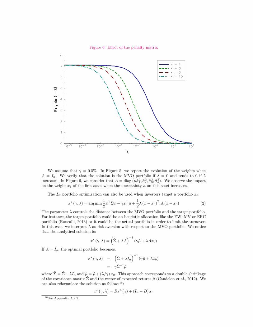
Figure 6: Effect of the penalty matrix

We assume that γ = 0.5%. In Figure 5, we report the evolution of the weights whenA = In. We verify that the solution is the MVO portfolio if λ = 0 and tends to 0 if λincreases. In Figure 6, we consider that A = diag

(κσ2

1 , σ22 , σ

23 , σ

24). We observe the impact

on the weight x1 of the first asset when the uncertainty κ on this asset increases.

The L2 portfolio optimization can also be used when investors target a portfolio x0:


2λ (x− x0)>A (x− x0) (2)

The parameter λ controls the distance between the MVO portfolio and the target portfolio.For instance, the target portfolio could be an heuristic allocation like the EW, MV or ERCportfolio (Roncalli, 2013) or it could be the actual portfolio in order to limit the turnover.In this case, we interpret λ as risk aversion with respect to the MVO portfolio. We noticethat the analytical solution is:

x? (γ, λ) =(

Σ + λA)−1

(γµ+ λAx0)

If A = In, the optimal portfolio becomes:

x? (γ, λ) =(

Σ + λIn

)−1(γµ+ λx0)

= γΣ−1µ

where Σ = Σ +λIn and µ = µ+ (λ/γ)x0. This approach corresponds to a double shrinkageof the covariance matrix Σ and the vector of expected returns µ (Candelon et al., 2012). Wecan also reformulate the solution as follows16:

x? (γ, λ) = Bx? (γ) + (In −B)x0

16See Appendix A.2.2.

where B =(In + λΣ−1

)−1. The optimal portfolio is then a linear combination between the

MVO portfolio and the target portfolio, and coincides with classical allocation policy. Forexample, when an investor considers a 50/50 allocation policy, B is equal to In/2 and weobtain:

x? (γ, λ) = 12x

? (γ) + 12x0

Example 9 We consider a universe of three assets. The expected returns are 5%, 6% and7% whereas the volatilities are 10%, 15% and 20%. The correlation matrix is:

C =

1.000.50 1.000.20 −0.30 1.00

The risk aversion parameter γ is set to 30%. We assume that the target portfolio is the EWportfolio.

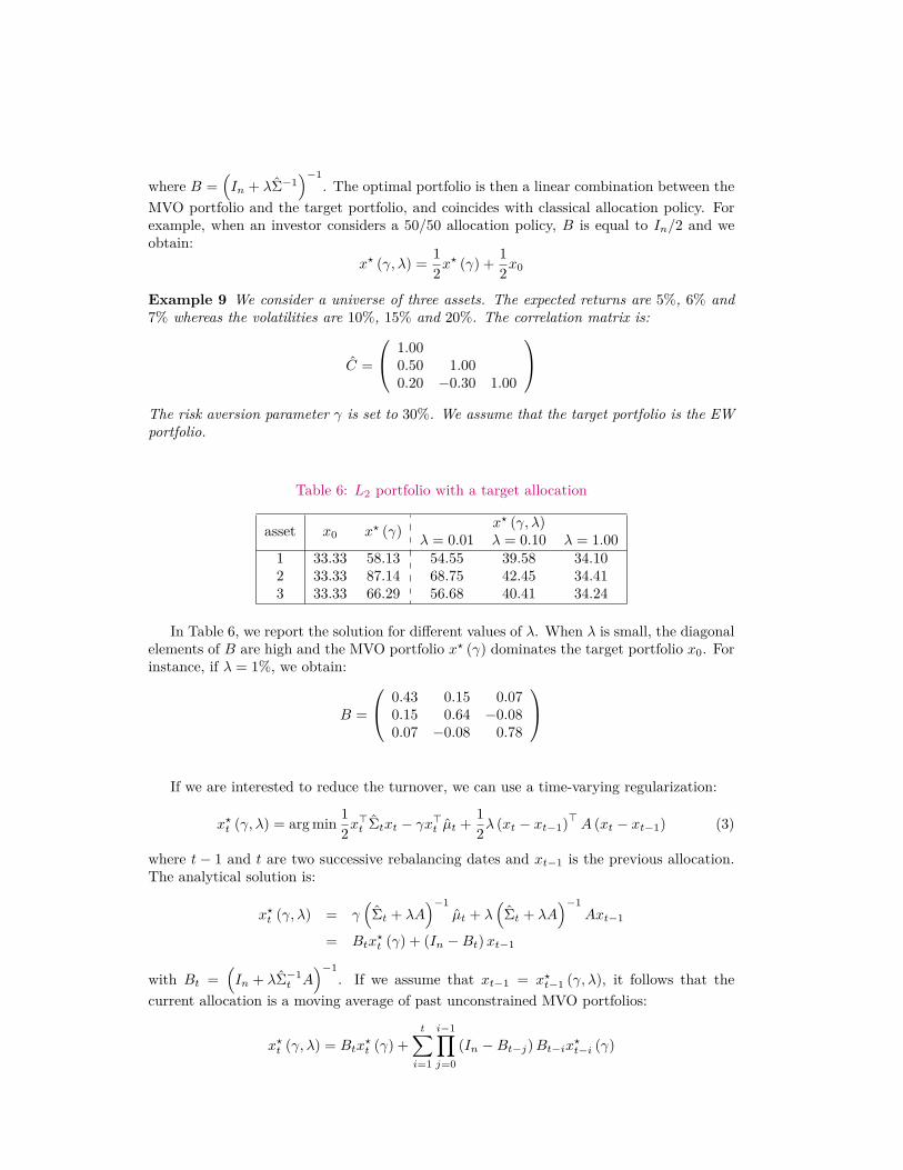
Table 6: L2 portfolio with a target allocation

asset x0 x? (γ) x? (γ, λ)λ = 0.01 λ = 0.10 λ = 1.00

1 33.33 58.13 54.55 39.58 34.102 33.33 87.14 68.75 42.45 34.413 33.33 66.29 56.68 40.41 34.24

In Table 6, we report the solution for different values of λ. When λ is small, the diagonalelements of B are high and the MVO portfolio x? (γ) dominates the target portfolio x0. Forinstance, if λ = 1%, we obtain:

B =

0.43 0.15 0.070.15 0.64 −0.080.07 −0.08 0.78

If we are interested to reduce the turnover, we can use a time-varying regularization:

x?t (γ, λ) = arg min 12x>t Σtxt − γx>t µt + 1

2λ (xt − xt−1)>A (xt − xt−1) (3)

where t − 1 and t are two successive rebalancing dates and xt−1 is the previous allocation.The analytical solution is:

x?t (γ, λ) = γ(

Σt + λA)−1

µt + λ(

Σt + λA)−1

Axt−1

= Btx?t (γ) + (In −Bt)xt−1

with Bt =(In + λΣ−1

t A)−1

. If we assume that xt−1 = x?t−1 (γ, λ), it follows that thecurrent allocation is a moving average of past unconstrained MVO portfolios:

x?t (γ, λ) = Btx?t (γ) +

t∑i=1

i−1∏j=0

(In −Bt−j)Bt−ix?t−i (γ)

Remark 6 Suppose that Σt = Σt−1 and A = diag(σ2

1 , . . . , σ2n

). If asset returns are not

correlated, we obtain:

x?i,t (γ, λ) = γ

σ2i + λσ2

i

µi,t + λσ2i

σ2i + λσ2

i

x?i,t−1 (γ, λ)

= αx?i,t (γ) + (1− α)x?i,t−1 (γ, λ)

where α = 1/(1 + λ). The solution is an exponentially weighted moving average filter.Calibrating λ is then equivalent to choosing the holding period to turn the portfolio.

3.5 Information matrix and hedging portfoliosThe previous methods are focused on the covariance matrix. However, the important quan-tity in mean-variance optimization is the information matrix I = Σ−1, i.e. the inverse of thecovariance matrix (Scherer, 2007; Roncalli, 2013). Stevens (1998) gives a new interpretationof the information matrix using the following regression framework:

Ri,t = β0 + β>i R(−i)t + εi,t (4)

where R(−i)t denotes the vector of asset returns Rt excluding the ith asset and εi,t ∼ N (0, s2

i ).Let R2

i be the R-squared of the linear regression (4) and β be the matrix of OLS coefficientswith rows β>i . Stevens (1998) shows that the diagonal elements of the information matrixare given by:

Ii,i = 1σ2i (1−R2

i )whereas the off-diagonal elements are:

Ii,j = − βi,jσ2i (1−R2

i )= − βj,i

σ2j

(1−R2

j

)Using this expression of I, we obtain a new formula of the MVO portfolio:

x?i (γ) = γµi − β>i µ(−i)

σ2i (1−R2

i )

Scherer (2007) interprets µi − β>i µ(−i) as the excess return after regression hedging and

σ2i

(1−R2

i

)as the non-hedging risk. We remind that R2

i = 1− s2i /σ

2i . We finally obtain:

x?i (γ) = γµi − β>i µ(−i)

s2i

From this equation, we deduce the following conclusions:

1. The better the hedge, the higher the exposure. This is why highly correlated assetsproduces unstable MVO portfolios.

2. The long-short position is defined by the sign of µi − β>i µ(−i). If the expected returnof the asset is lower than the conditional expected return of the hedging portfolio, theweight is negative.

It has been shown that the linear regression can be improved using norm constraints (Hastieet al., 2009). For example we can use the L2 regression to improve the predictive power ofthe hedging relationships. We can also estimate the hedging portfolios with the L1 penalty.


C =

1.000.50 1.000.50 0.50 1.000.60 0.50 0.40 1.00

In Table 7, we have reported the results of the hedging portfolios. The OLS coefficients

βi, the coefficient of determination R2i and the standard error si of residuals are computed

thanks to the formulas given in Appendix A.4. We also have computed the conditionalexpected return17 µi = µi − β>i µ(−i). We can then deduce the corresponding informationmatrix I and the MVO portfolio x? for γ = 0.5. We finally obtain a very well balancedallocation, because the weights range between 19.28% and 69.80%. Let us now change thevalue of the correlation between the third and fourth assets. If ρ3,4 = 95%, we obtain resultsgiven in Table 8. In this case, the story is different, because the optimized portfolio is notwell balanced. Indeed, because two assets are strongly correlated, some hedging relationshipspresent high value of R2. The information matrix is then very sensitive to these hedgingportfolios. This explains that the weights are now in the range between −168.70% and239.34%!

Table 7: Hedging portfolios when ρ3,4 = 40%

Asset βi R2i si µi x?

1 0.139 0.187 0.250 45.83% 11.04% 1.70% 69.80%2 0.230 0.268 0.191 37.77% 14.20% 2.06% 51.18%3 0.409 0.354 0.045 33.52% 16.31% 2.85% 53.66%4 0.750 0.347 0.063 41.50% 19.12% 1.41% 19.28%

Table 8: Hedging portfolios when ρ3,4 = 95%

Asset βi R2i si µi x?

1 0.244 −0.595 0.724 47.41% 10.88% 3.16% 133.45%2 0.443 0.470 −0.157 33.70% 14.66% 2.23% 52.01%3 −0.174 0.076 0.795 91.34% 5.89% 1.66% 239.34%4 0.292 −0.035 1.094 92.38% 6.90% −1.61% −168.67%

4 Some applicationsIn this section, we look at three applications which are directly linked to the previousframework. The first application concerns the relationship between the MVO portfolioand the principal portfolios derived from PCA analysis. The second application shows theusefulness of the L2 covriance matrix regularization. We finally illustrate how the Lassoapproach may improve the robustness of the information matrix and hedging portfolios inthe third application.

17We note that µi is also equal to the intercept β0 of the linear regression.

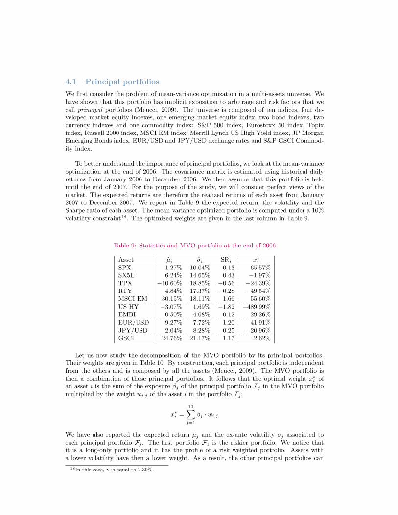
4.1 Principal portfoliosWe first consider the problem of mean-variance optimization in a multi-assets universe. Wehave shown that this portfolio has implicit exposition to arbitrage and risk factors that wecall principal portfolios (Meucci, 2009). The universe is composed of ten indices, four de-veloped market equity indexes, one emerging market equity index, two bond indexes, twocurrency indexes and one commodity index: S&P 500 index, Eurostoxx 50 index, Topixindex, Russell 2000 index, MSCI EM index, Merrill Lynch US High Yield index, JP MorganEmerging Bonds index, EUR/USD and JPY/USD exchange rates and S&P GSCI Commod-ity index.

To better understand the importance of principal portfolios, we look at the mean-varianceoptimization at the end of 2006. The covariance matrix is estimated using historical dailyreturns from January 2006 to December 2006. We then assume that this portfolio is helduntil the end of 2007. For the purpose of the study, we will consider perfect views of themarket. The expected returns are therefore the realized returns of each asset from January2007 to December 2007. We report in Table 9 the expected return, the volatility and theSharpe ratio of each asset. The mean-variance optimized portfolio is computed under a 10%volatility constraint18. The optimized weights are given in the last column in Table 9.

Table 9: Statistics and MVO portfolio at the end of 2006

Asset µi σi SRi x?iSPX 1.27% 10.04% 0.13 65.57%SX5E 6.24% 14.65% 0.43 −1.97%TPX −10.60% 18.85% −0.56 −24.39%RTY −4.84% 17.37% −0.28 −49.54%MSCI EM 30.15% 18.11% 1.66 55.60%US HY −3.07% 1.69% −1.82 −489.99%EMBI 0.50% 4.08% 0.12 29.26%EUR/USD 9.27% 7.72% 1.20 41.91%JPY/USD 2.04% 8.28% 0.25 −20.96%GSCI 24.76% 21.17% 1.17 2.62%

Let us now study the decomposition of the MVO portfolio by its principal portfolios.Their weights are given in Table 10. By construction, each principal portfolio is independentfrom the others and is composed by all the assets (Meucci, 2009). The MVO portfolio isthen a combination of these principal portfolios. It follows that the optimal weight x∗i ofan asset i is the sum of the exposure βj of the principal portfolio Fj in the MVO portfoliomultiplied by the weight wi,j of the asset i in the portfolio Fj :

x∗i =10∑j=1

βj · wi,j

We have also reported the expected return µj and the ex-ante volatility σj associated toeach principal portfolio Fj . The first portfolio F1 is the riskier portfolio. We notice thatit is a long-only portfolio and it has the profile of a risk weighted portfolio. Assets witha lower volatility have then a lower weight. As a result, the other principal portfolios can

18In this case, γ is equal to 2.39%.

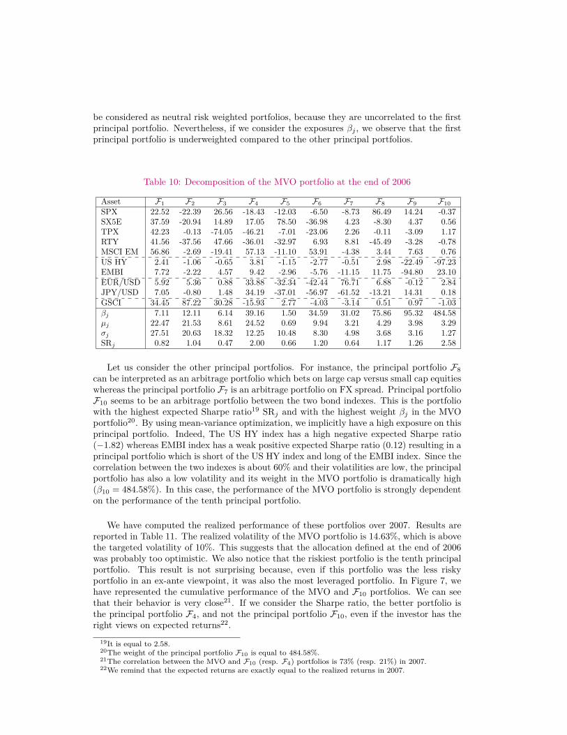
be considered as neutral risk weighted portfolios, because they are uncorrelated to the firstprincipal portfolio. Nevertheless, if we consider the exposures βj , we observe that the firstprincipal portfolio is underweighted compared to the other principal portfolios.

Table 10: Decomposition of the MVO portfolio at the end of 2006

Asset F1 F2 F3 F4 F5 F6 F7 F8 F9 F10SPX 22.52 -22.39 26.56 -18.43 -12.03 -6.50 -8.73 86.49 14.24 -0.37SX5E 37.59 -20.94 14.89 17.05 78.50 -36.98 4.23 -8.30 4.37 0.56TPX 42.23 -0.13 -74.05 -46.21 -7.01 -23.06 2.26 -0.11 -3.09 1.17RTY 41.56 -37.56 47.66 -36.01 -32.97 6.93 8.81 -45.49 -3.28 -0.78MSCI EM 56.86 -2.69 -19.41 57.13 -11.10 53.91 -4.38 3.44 7.63 0.76US HY 2.41 -1.06 -0.65 3.81 -1.15 -2.77 -0.51 2.98 -22.49 -97.23EMBI 7.72 -2.22 4.57 9.42 -2.96 -5.76 -11.15 11.75 -94.80 23.10EUR/USD 5.92 5.36 0.88 33.88 -32.34 -42.44 76.71 6.88 -0.12 2.84JPY/USD 7.05 -0.80 1.48 34.19 -37.01 -56.97 -61.52 -13.21 14.31 0.18GSCI 34.45 87.22 30.28 -15.93 2.77 -4.03 -3.14 0.51 0.97 -1.03βj 7.11 12.11 6.14 39.16 1.50 34.59 31.02 75.86 95.32 484.58µj 22.47 21.53 8.61 24.52 0.69 9.94 3.21 4.29 3.98 3.29σj 27.51 20.63 18.32 12.25 10.48 8.30 4.98 3.68 3.16 1.27SRj 0.82 1.04 0.47 2.00 0.66 1.20 0.64 1.17 1.26 2.58

Let us consider the other principal portfolios. For instance, the principal portfolio F8can be interpreted as an arbitrage portfolio which bets on large cap versus small cap equitieswhereas the principal portfolio F7 is an arbitrage portfolio on FX spread. Principal portfolioF10 seems to be an arbitrage portfolio between the two bond indexes. This is the portfoliowith the highest expected Sharpe ratio19 SRj and with the highest weight βj in the MVOportfolio20. By using mean-variance optimization, we implicitly have a high exposure on thisprincipal portfolio. Indeed, The US HY index has a high negative expected Sharpe ratio(−1.82) whereas EMBI index has a weak positive expected Sharpe ratio (0.12) resulting in aprincipal portfolio which is short of the US HY index and long of the EMBI index. Since thecorrelation between the two indexes is about 60% and their volatilities are low, the principalportfolio has also a low volatility and its weight in the MVO portfolio is dramatically high(β10 = 484.58%). In this case, the performance of the MVO portfolio is strongly dependenton the performance of the tenth principal portfolio.

We have computed the realized performance of these portfolios over 2007. Results arereported in Table 11. The realized volatility of the MVO portfolio is 14.63%, which is abovethe targeted volatility of 10%. This suggests that the allocation defined at the end of 2006was probably too optimistic. We also notice that the riskiest portfolio is the tenth principalportfolio. This result is not surprising because, even if this portfolio was the less riskyportfolio in an ex-ante viewpoint, it was also the most leveraged portfolio. In Figure 7, wehave represented the cumulative performance of the MVO and F10 portfolios. We can seethat their behavior is very close21. If we consider the Sharpe ratio, the better portfolio isthe principal portfolio F4, and not the principal portfolio F10, even if the investor has theright views on expected returns22.

19It is equal to 2.58.20The weight of the principal portfolio F10 is equal to 484.58%.21The correlation between the MVO and F10 (resp. F4) portfolios is 73% (resp. 21%) in 2007.22We remind that the expected returns are exactly equal to the realized returns in 2007.

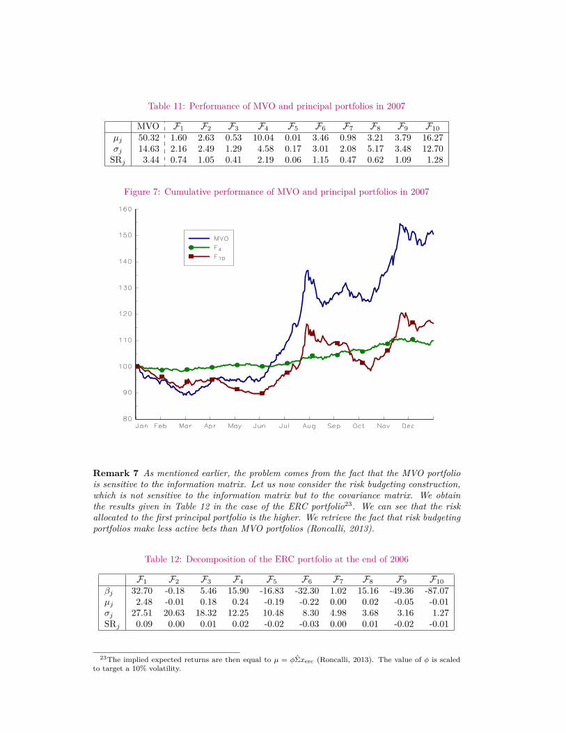
Table 11: Performance of MVO and principal portfolios in 2007

MVO F1 F2 F3 F4 F5 F6 F7 F8 F9 F10µj 50.32 1.60 2.63 0.53 10.04 0.01 3.46 0.98 3.21 3.79 16.27σj 14.63 2.16 2.49 1.29 4.58 0.17 3.01 2.08 5.17 3.48 12.70

SRj 3.44 0.74 1.05 0.41 2.19 0.06 1.15 0.47 0.62 1.09 1.28

Figure 7: Cumulative performance of MVO and principal portfolios in 2007

Remark 7 As mentioned earlier, the problem comes from the fact that the MVO portfoliois sensitive to the information matrix. Let us now consider the risk budgeting construction,which is not sensitive to the information matrix but to the covariance matrix. We obtainthe results given in Table 12 in the case of the ERC portfolio23. We can see that the riskallocated to the first principal portfolio is the higher. We retrieve the fact that risk budgetingportfolios make less active bets than MVO portfolios (Roncalli, 2013).

Table 12: Decomposition of the ERC portfolio at the end of 2006

F1 F2 F3 F4 F5 F6 F7 F8 F9 F10βj 32.70 -0.18 5.46 15.90 -16.83 -32.30 1.02 15.16 -49.36 -87.07µj 2.48 -0.01 0.18 0.24 -0.19 -0.22 0.00 0.02 -0.05 -0.01σj 27.51 20.63 18.32 12.25 10.48 8.30 4.98 3.68 3.16 1.27SRj 0.09 0.00 0.01 0.02 -0.02 -0.03 0.00 0.01 -0.02 -0.01

23The implied expected returns are then equal to µ = φΣxerc (Roncalli, 2013). The value of φ is scaledto target a 10% volatility.

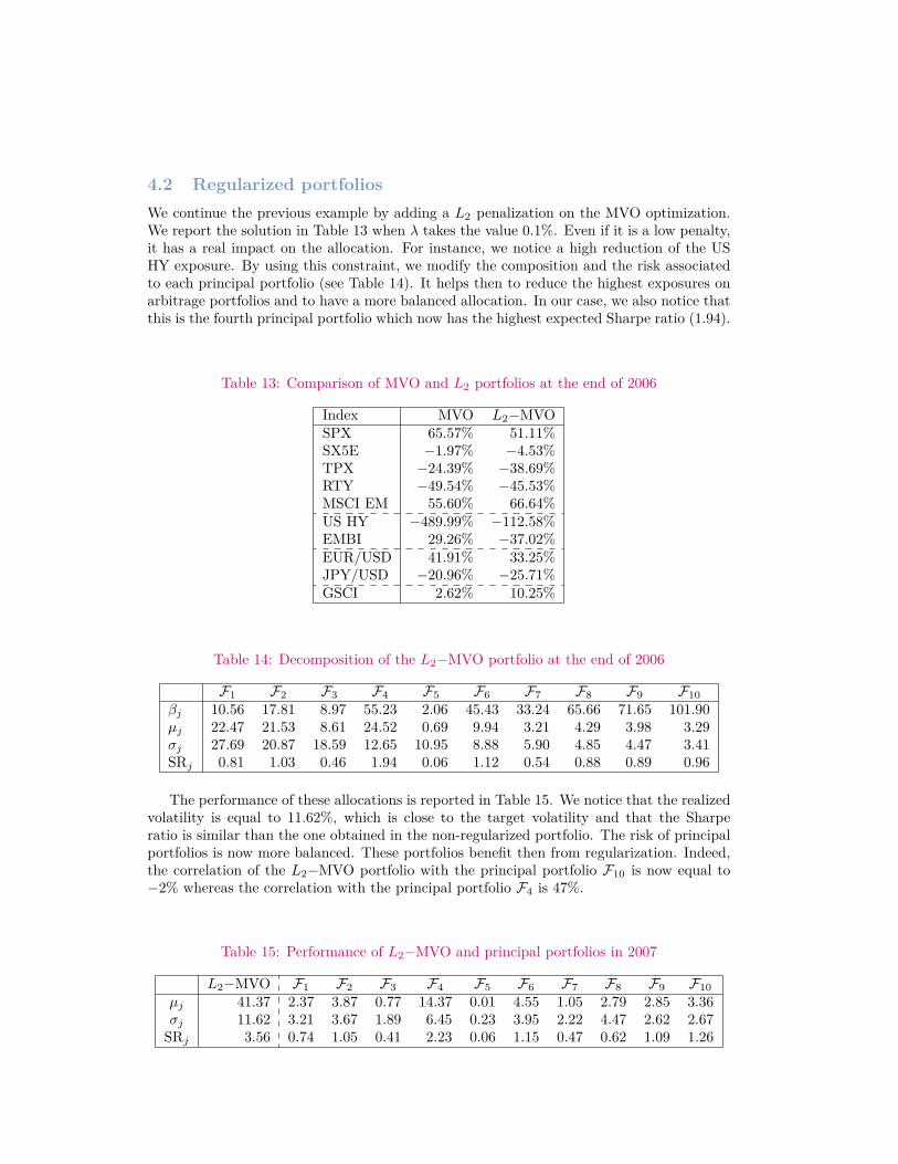
4.2 Regularized portfoliosWe continue the previous example by adding a L2 penalization on the MVO optimization.We report the solution in Table 13 when λ takes the value 0.1%. Even if it is a low penalty,it has a real impact on the allocation. For instance, we notice a high reduction of the USHY exposure. By using this constraint, we modify the composition and the risk associatedto each principal portfolio (see Table 14). It helps then to reduce the highest exposures onarbitrage portfolios and to have a more balanced allocation. In our case, we also notice thatthis is the fourth principal portfolio which now has the highest expected Sharpe ratio (1.94).

Table 13: Comparison of MVO and L2 portfolios at the end of 2006

Index MVO L2−MVOSPX 65.57% 51.11%SX5E −1.97% −4.53%TPX −24.39% −38.69%RTY −49.54% −45.53%MSCI EM 55.60% 66.64%US HY −489.99% −112.58%EMBI 29.26% −37.02%EUR/USD 41.91% 33.25%JPY/USD −20.96% −25.71%GSCI 2.62% 10.25%

Table 14: Decomposition of the L2−MVO portfolio at the end of 2006

F1 F2 F3 F4 F5 F6 F7 F8 F9 F10βj 10.56 17.81 8.97 55.23 2.06 45.43 33.24 65.66 71.65 101.90µj 22.47 21.53 8.61 24.52 0.69 9.94 3.21 4.29 3.98 3.29σj 27.69 20.87 18.59 12.65 10.95 8.88 5.90 4.85 4.47 3.41SRj 0.81 1.03 0.46 1.94 0.06 1.12 0.54 0.88 0.89 0.96

The performance of these allocations is reported in Table 15. We notice that the realizedvolatility is equal to 11.62%, which is close to the target volatility and that the Sharperatio is similar than the one obtained in the non-regularized portfolio. The risk of principalportfolios is now more balanced. These portfolios benefit then from regularization. Indeed,the correlation of the L2−MVO portfolio with the principal portfolio F10 is now equal to−2% whereas the correlation with the principal portfolio F4 is 47%.

Table 15: Performance of L2−MVO and principal portfolios in 2007

L2−MVO F1 F2 F3 F4 F5 F6 F7 F8 F9 F10µj 41.37 2.37 3.87 0.77 14.37 0.01 4.55 1.05 2.79 2.85 3.36σj 11.62 3.21 3.67 1.89 6.45 0.23 3.95 2.22 4.47 2.62 2.67

SRj 3.56 0.74 1.05 0.41 2.23 0.06 1.15 0.47 0.62 1.09 1.26

Figure 8: Cumulative performance of L2-MVO and principal portfolios in 2007

Remark 8 We modify the previous example by considering unperfect views. Suppose thatwe have wrong expected returns for the bond indexes, i.e. 3.07% for the US HY index and−0.5% for the EMBI index. In this case, exposures change slightly except for the principalportfolio F10, which becomes −452%. We have reported in Table 16 the performance of theoptimized and principal portfolios. We can see that having the wrong views has a big impacton the MVO portfolio. Its return is reduced by 81%! For the L2−MVO portfolio, the returnonly decreases by 29%.

Table 16: Performance of optimized and principal portfolios in 2007 with wrong views

L2−MVO F1 F2 F3 F4 F5 F6 F7 F8 F9 F10MVO

µj 11.19 1.69 2.76 0.55 10.64 0.01 3.60 1.05 3.42 3.56 -14.38σj 17.57 2.28 2.62 1.35 4.84 0.17 3.13 2.24 5.51 3.27 11.85

SRj 0.64 0.74 1.05 0.41 2.20 0.06 1.15 0.47 0.62 1.09 -1.21L2−MVO

µj 32.43 2.39 3.88 0.76 14.53 0.01 4.52 1.08 2.84 2.55 -2.96σj 12.91 3.23 3.68 1.88 6.52 0.22 3.93 2.29 4.56 2.35 2.38

SRj 2.51 0.74 1.05 0.41 2.23 0.06 1.15 0.47 0.62 1.09 -1.24

4.3 Hedging portfoliosWe recall that the MVO portfolio involves the inverse of the covariance matrix. Since theinformation matrix reflects the hedging relationships, we illustrate how penalization methodsmay be used to obtain better hedging portfolios. For that, we impose a L1 constraint on

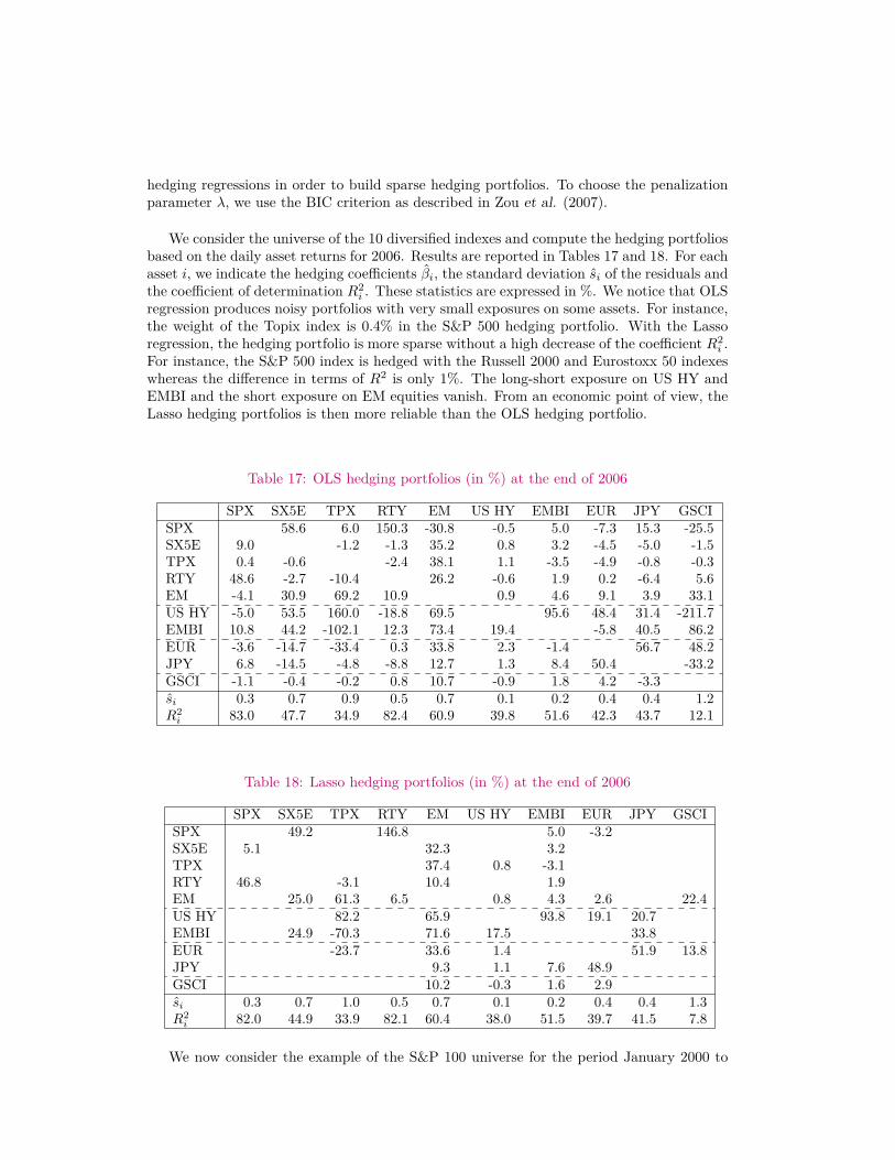
hedging regressions in order to build sparse hedging portfolios. To choose the penalizationparameter λ, we use the BIC criterion as described in Zou et al. (2007).

We consider the universe of the 10 diversified indexes and compute the hedging portfoliosbased on the daily asset returns for 2006. Results are reported in Tables 17 and 18. For eachasset i, we indicate the hedging coefficients βi, the standard deviation si of the residuals andthe coefficient of determination R2

i . These statistics are expressed in %. We notice that OLSregression produces noisy portfolios with very small exposures on some assets. For instance,the weight of the Topix index is 0.4% in the S&P 500 hedging portfolio. With the Lassoregression, the hedging portfolio is more sparse without a high decrease of the coefficient R2

i .For instance, the S&P 500 index is hedged with the Russell 2000 and Eurostoxx 50 indexeswhereas the difference in terms of R2 is only 1%. The long-short exposure on US HY andEMBI and the short exposure on EM equities vanish. From an economic point of view, theLasso hedging portfolios is then more reliable than the OLS hedging portfolio.

Table 17: OLS hedging portfolios (in %) at the end of 2006

SPX SX5E TPX RTY EM US HY EMBI EUR JPY GSCISPX 58.6 6.0 150.3 -30.8 -0.5 5.0 -7.3 15.3 -25.5SX5E 9.0 -1.2 -1.3 35.2 0.8 3.2 -4.5 -5.0 -1.5TPX 0.4 -0.6 -2.4 38.1 1.1 -3.5 -4.9 -0.8 -0.3RTY 48.6 -2.7 -10.4 26.2 -0.6 1.9 0.2 -6.4 5.6EM -4.1 30.9 69.2 10.9 0.9 4.6 9.1 3.9 33.1US HY -5.0 53.5 160.0 -18.8 69.5 95.6 48.4 31.4 -211.7EMBI 10.8 44.2 -102.1 12.3 73.4 19.4 -5.8 40.5 86.2EUR -3.6 -14.7 -33.4 0.3 33.8 2.3 -1.4 56.7 48.2JPY 6.8 -14.5 -4.8 -8.8 12.7 1.3 8.4 50.4 -33.2GSCI -1.1 -0.4 -0.2 0.8 10.7 -0.9 1.8 4.2 -3.3si 0.3 0.7 0.9 0.5 0.7 0.1 0.2 0.4 0.4 1.2R2i 83.0 47.7 34.9 82.4 60.9 39.8 51.6 42.3 43.7 12.1

Table 18: Lasso hedging portfolios (in %) at the end of 2006

SPX SX5E TPX RTY EM US HY EMBI EUR JPY GSCISPX 49.2 146.8 5.0 -3.2SX5E 5.1 32.3 3.2TPX 37.4 0.8 -3.1RTY 46.8 -3.1 10.4 1.9EM 25.0 61.3 6.5 0.8 4.3 2.6 22.4US HY 82.2 65.9 93.8 19.1 20.7EMBI 24.9 -70.3 71.6 17.5 33.8EUR -23.7 33.6 1.4 51.9 13.8JPY 9.3 1.1 7.6 48.9GSCI 10.2 -0.3 1.6 2.9si 0.3 0.7 1.0 0.5 0.7 0.1 0.2 0.4 0.4 1.3R2i 82.0 44.9 33.9 82.1 60.4 38.0 51.5 39.7 41.5 7.8

We now consider the example of the S&P 100 universe for the period January 2000 to

December 2011. We compute the minimum variance portfolio using the hedging relation-ships:

x?i (γ) = γ1− β>i 1

s2i

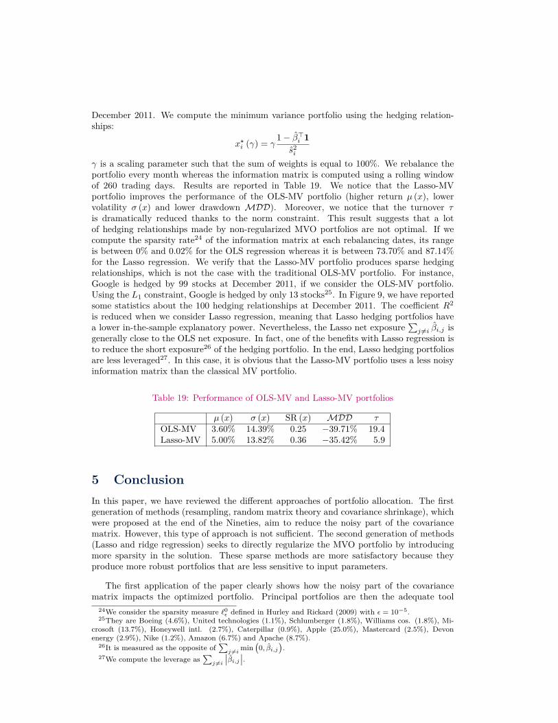
γ is a scaling parameter such that the sum of weights is equal to 100%. We rebalance theportfolio every month whereas the information matrix is computed using a rolling windowof 260 trading days. Results are reported in Table 19. We notice that the Lasso-MVportfolio improves the performance of the OLS-MV portfolio (higher return µ (x), lowervolatility σ (x) and lower drawdown MDD). Moreover, we notice that the turnover τis dramatically reduced thanks to the norm constraint. This result suggests that a lotof hedging relationships made by non-regularized MVO portfolios are not optimal. If wecompute the sparsity rate24 of the information matrix at each rebalancing dates, its rangeis between 0% and 0.02% for the OLS regression whereas it is between 73.70% and 87.14%for the Lasso regression. We verify that the Lasso-MV portfolio produces sparse hedgingrelationships, which is not the case with the traditional OLS-MV portfolio. For instance,Google is hedged by 99 stocks at December 2011, if we consider the OLS-MV portfolio.Using the L1 constraint, Google is hedged by only 13 stocks25. In Figure 9, we have reportedsome statistics about the 100 hedging relationships at December 2011. The coefficient R2

is reduced when we consider Lasso regression, meaning that Lasso hedging portfolios havea lower in-the-sample explanatory power. Nevertheless, the Lasso net exposure

∑j 6=i βi,j is

generally close to the OLS net exposure. In fact, one of the benefits with Lasso regression isto reduce the short exposure26 of the hedging portfolio. In the end, Lasso hedging portfoliosare less leveraged27. In this case, it is obvious that the Lasso-MV portfolio uses a less noisyinformation matrix than the classical MV portfolio.

Table 19: Performance of OLS-MV and Lasso-MV portfolios

µ (x) σ (x) SR (x) MDD τOLS-MV 3.60% 14.39% 0.25 −39.71% 19.4Lasso-MV 5.00% 13.82% 0.36 −35.42% 5.9

5 ConclusionIn this paper, we have reviewed the different approaches of portfolio allocation. The firstgeneration of methods (resampling, random matrix theory and covariance shrinkage), whichwere proposed at the end of the Nineties, aim to reduce the noisy part of the covariancematrix. However, this type of approach is not sufficient. The second generation of methods(Lasso and ridge regression) seeks to directly regularize the MVO portfolio by introducingmore sparsity in the solution. These sparse methods are more satisfactory because theyproduce more robust portfolios that are less sensitive to input parameters.

The first application of the paper clearly shows how the noisy part of the covariancematrix impacts the optimized portfolio. Principal portfolios are then the adequate tool

24We consider the sparsity measure `0ε defined in Hurley and Rickard (2009) with ε = 10−5.25They are Boeing (4.6%), United technologies (1.1%), Schlumberger (1.8%), Williams cos. (1.8%), Mi-

crosoft (13.7%), Honeywell intl. (2.7%), Caterpillar (0.9%), Apple (25.0%), Mastercard (2.5%), Devonenergy (2.9%), Nike (1.2%), Amazon (6.7%) and Apache (8.7%).

26It is measured as the opposite of∑

j 6=i min(0, βi,j

).

27We compute the leverage as∑

j 6=i

∣∣βi,j∣∣.

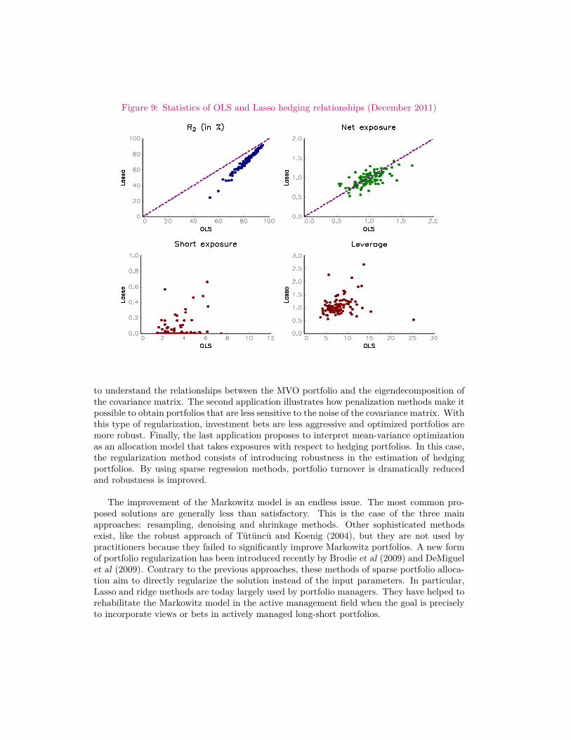
Figure 9: Statistics of OLS and Lasso hedging relationships (December 2011)

to understand the relationships between the MVO portfolio and the eigendecomposition ofthe covariance matrix. The second application illustrates how penalization methods make itpossible to obtain portfolios that are less sensitive to the noise of the covariance matrix. Withthis type of regularization, investment bets are less aggressive and optimized portfolios aremore robust. Finally, the last application proposes to interpret mean-variance optimizationas an allocation model that takes exposures with respect to hedging portfolios. In this case,the regularization method consists of introducing robustness in the estimation of hedgingportfolios. By using sparse regression methods, portfolio turnover is dramatically reducedand robustness is improved.

The improvement of the Markowitz model is an endless issue. The most common pro-posed solutions are generally less than satisfactory. This is the case of the three mainapproaches: resampling, denoising and shrinkage methods. Other sophisticated methodsexist, like the robust approach of Tütüncü and Koenig (2004), but they are not used bypractitioners because they failed to significantly improve Markowitz portfolios. A new formof portfolio regularization has been introduced recently by Brodie et al (2009) and DeMiguelet al (2009). Contrary to the previous approaches, these methods of sparse portfolio alloca-tion aim to directly regularize the solution instead of the input parameters. In particular,Lasso and ridge methods are today largely used by portfolio managers. They have helped torehabilitate the Markowitz model in the active management field when the goal is preciselyto incorporate views or bets in actively managed long-short portfolios.

A Mathematical results

A.1 The single-factor model

We assume that the first factor of the covariance matrix corresponds to the market factor andthat the idiosyncratic volatilities are equal (σ1 = . . . = σn = σ). In terms of eigenvectors,we have:

v1 = β√∑ni=1 β

2i

Because V V > = I and λ1 ' σ2m

∑ni=1 β

2i + σ2, we obtain the following expression of Σα:

Σα = αΦ + (1− α) Σ= α

(σ2mββ

> +D)

+ (1− α)V ΛV >

= α(σ2mββ

> +DV V >)

+ (1− α)n∑i=1

λiviv>i

' ασ2mββ

> + αDV V > + (1− α)λ1ββ>∑ni=1 β

2i

+ (1− α)n∑i=2

λiviv>i

=(ασ2

m + (1− α) λ1∑ni=1 β

2i

)ββ> + (1− α)

n∑i=2

λiviv>i + αDV V >

It follows that:

Σα '(ασ2

m + (1− α) λ1∑ni=1 β

2i

)ββ> + (1− α)

n∑i=2

λiviv>i +

α

(σ2 ββ>∑n

i=1 β2i

+n∑i=2

σ2viv>i

)

=(ασ2

m + (1− α) λ1∑ni=1 β

2i

+ ασ2∑ni=1 β

2i

)ββ> +

(1− α)n∑i=2

λiviv>i + α

n∑i=2

σ2viv>i

= λ1ββ>∑ni=1 β

2i

+n∑i=2


= λ1v1v>1 +

n∑i=2


A.2 Analytical solutions of L2 portfolio optimization

A.2.1 The case of variance penalization

We have the following optimization program:

x? (γ, λ) = arg min 12x>(

Σ + λA)x− γx>µ

We assume that A is the covariance matrix without correlations. We have A = υ =diag

(σ2

1 , . . . , σ2n

). It follows that:

Σ = Σ + λυ

= υ1/2Cυ1/2 + λυ1/2υ1/2

= υ1/2(C + λIn

)υ1/2

By setting y = υ1/2x, we get:

y? (γ, λ) = arg min 12y>(C + λIn

)y − γy>s

where s is the vector of expected Sharpe ratios. The solution is then:

x? (γ, λ) = υ−1/2y? (γ, λ)

= γυ−1/2(C + λIn

)−1s

When λ tends to ∞ and when we renormalize the solution, we retrieve the analytical ex-pression of Merton (1969):

limλ→∞

x?i (γ, λ) ∝ γ µiσ2i

A.2.2 The case of a target portfolio

We remind that:x? (γ, λ) =

(Σ + λIn

)−1(γµ+ λx0)

We see that:

In −(In + λΣ−1

)−1=

(In + λΣ−1

)−1 (In + λΣ−1

)−(In + λΣ−1

)−1

=(In + λΣ−1

)−1λΣ−1

We then obtain:

x? (γ, λ) =(

Σ + λIn

)−1γµ+

(Σ + λIn

)−1λx0

=(In + λΣ−1

)−1x? (γ) +

(In + λΣ−1

)−1λΣ−1x0

= Bx? (γ) + (In −B)x0

where B =(In + λΣ−1

)−1.

A.3 Relationship between penalization and robust portfolio opti-mization

A.3.1 Robust portfolio optimization

Robust optimization is a technique designed to build a portfolio that performs well in a num-ber of different scenarios including the extreme ones. For instance, a portfolio manager may

apply a confidence interval on each coefficients of the estimated covariance matrix. Halldórs-son and Tütüncü (2003) have extensively studied this problem and define the uncertaintyset U as follows:

U ={

Σ : Σ− ≤ Σ ≤ Σ+,Σ � 0}

where Σ− and Σ+ are extreme values of the set U . In the case of the MVO problem, weobtain:

x? (γ;U) = arg min maxΣ∈U

12x>Σx− γx>µ

Under the constraint x ≥ 0, we notice that the solution is:

x? (γ;U) = γ(Σ+)−1

µ

A.3.2 QP formulation of the optimization problem

By decomposing the weights as xi = x+i − x

−i with x+

i ≥ 0 and x−i ≥ 0, we obtain:

12x>Σx− γx>µ = 1

2

n∑i=1

n∑j=1

Σi,jxixj − γx>µ

= 12

n∑i=1

n∑j=1

Σi,jx+i x

+j + 1

2

n∑i=1

n∑j=1

Σi,jx−i x−j

−n∑i=1

n∑j=1

Σi,jx+i x−j − γx

>µ

Let us consider the following function:

m (x) = maxΣ∈U

12x>Σx− γx>µ

For a given set of weights x, the worst covariance matrix among U is the highest (resp. thelowest) element of U if xixj ≥ 0 (resp. xixj ≤ 0). It comes that:

m (x) = 12 x>Σx− γx>µ

with:x =

(x+

x−

), Σ =

(Σ+ −Σ−−Σ− Σ+

)and µ =

(µ−µ

)We finally obtain:

x? (γ;U) = arg min 12 x>Σx− γx>µ

u.c. x ≥ 0

This problem can be solved using classical QP algorithm under the condition that Σ ispositive definite.

A.3.3 L1 formulation of the optimization problem

Robust estimation is not frequently used in practice, because it is time consuming and it isextremely difficult to define the set U . If we omit the definite positive condition Σ � 0, we

can nevertheless use the L1 approach to solve a similar problem with the set U defined asfollows:

U ={

Σ : Σ−A ≤ Σ ≤ Σ +A}

where A is a positive definite matrix of noise. We have28:

x>Σx = x>(

Σ +A −Σ +A

−Σ +A Σ +A

)x

= x>(

Σ −Σ−Σ Σ

)x+ x>

(A AA A

)x

=(x+ − x−

)> Σ(x+ − x−

)+(x+ + x−

)>A(x+ + x−

)= x>Σx+ |x|>A |x|

We deduce that the minmax problem can be reformulated as follows:

x? (γ;A) = arg min 12x>Σx− γx>µ+ 1

2 |x|>A |x| (5)

Using a confidence interval on the empirical covariance matrix implies then a penalizationon the squared L1 norm.

Remark 9 If A = cIn with c a scalar, the optimization problem (5) is a L2 constrainedproblem. In this case, we have:

U ={

Σ : V (Λ−A)V > ≤ Σ ≤ V (Λ +A)V >}

where V ΛV > is the eigendecomposition of Σ. As a result, the L2 constraint is also a minmaxproblem with uncertain eigenvalues. This gives some intuitions to choose the L2 shrinkageparameter λ equal to the average of diagonal elements of A.

A.4 Relationship between the conditional normal distribution andthe linear regression

Let us consider a Gaussian random vector defined as follows:(YX

)∼ N

((µyµx

),

(Σyy ΣyxΣxy Σxx

))The conditional distribution of Y given X = x is a multivariate normal distribution. Wehave (Roncalli, 2013):

µy|x = E [Y | X = x]= µy + ΣyxΣ−1

xx (x− µx)

and:

Σyy|x = σ2 [Y | X = x]= Σyy − ΣyxΣ−1

xxΣxy

We deduce that:Y = µy + ΣyxΣ−1

xx (x− µx) + u

28Since Σ and A are two positive definite matrices, Σ is also a positive definite matrix.

where u is a centered Gaussian random variable with variance s2 = Σyy|x. It follows that:

Y =(µy − ΣyxΣ−1

xxµx)︸︷︷︸

β0

+ ΣyxΣ−1xx︸︷︷︸

β>

x+ u

We recognize the linear regression of Y on X:

Y = β0 + β>x+ u

Moreover, we have:

R2 = 1− s2

Σyy

= ΣyxΣ−1xxΣxy

Σyy

References[1] Black F. and Litterman R.B. (1992), Global Portfolio Optimization, Financial An-

alysts Journal, 48(5), pp. 28-43.

[2] Broadie M. (1993), Computing Efficient Frontiers using Estimated Parameters, Annalsof Operations Research, 45(1), pp. 21-58.

[3] Brodie J., Daubechies I., De Mol C., Giannone D. and Loris I. (2009), Sparse andStable Markowitz Portfolios, Proceedings of the National Academy of Sciences, 106(30),pp. 12267-12272.

[4] Candelon B., Hurlin C. and Tokpavi S. (2012), Sampling Error and Double Shrink-age Estimation of Minimum Variance Portfolios, Journal of Empirical Finance, 19(4),pp. 511-527.

[5] DeMiguel V., Garlappi L., Nogales F.J. and Uppal R. (2009), A GeneralizedApproach to Portfolio Optimization: Improving Performance by Constraining PortfolioNorms, Management Science, 55(5), pp. 798-812.

[6] DeMiguel V., Garlappi L. and Uppal R. (2009), Optimal Versus Naive Diversifica-tion: How Inefficient is the 1/N Portfolio Strategy?, Review of Financial Studies, 22(5),pp. 1915-1953.

[7] DeMiguel V., Martin-Utrera A. and Nogales F.J. (2011), Size Matters: Opti-mal Calibration of Shrinkage Estimators for Portfolio Selection, SSRN, www.ssrn.com/abstract=1891847.

[8] Dupleich Ulloa M.R., Giamouridis D. and Montagu C. (2012), Risk Reductionin Style Rotation, Journal of Portfolio Management, 38(2), pp. 44-55.

[9] El Ghaoui L., Oks M. and Oustry F. (2003), Worst-Case Value-at-Risk and RobustPortfolio Optimization: A Conic Programming Approach, Operations Research, 51(4),pp. 543-556.

[10] Halldórsson B.V. and Tütüncü R.H. (2003), An Interior-Point Method for a Classof Saddle-Point Problems, Journal of Optimization Theory and Applications, 116(3),pp. 559-590.

[11] Hastie T., Tibshirani R. and Friedman J. (2009), The Elements of Statistical Learn-ing, Second Edition. Springer.

[12] Hurley N. and Rickard S. (2009), Comparing Measures of Sparsity, IEEE Transac-tions on Information Theory, 55(10), pp. 4723-4741.

[13] Jagannathan R. and Ma T. (2003), Risk Reduction in Large Portfolios: Why Impos-ing the Wrong Constraints Helps, Journal of Finance, 58(4), pp. 1651-1684.

[14] James G. and Hastie T. (1997), Generalizations of the Bias/Variance Decompositionfor Prediction Error, Technical Report, Department of Statistics, Stanford University.

[15] Jorion P. (1992), Portfolio Optimization in Practice, Financial Analysts Journal,48(1), pp. 68-74.

[16] Laloux L., Cizeau P., Bouchaud J-P. and Potters M. (1999), Noise Dressing ofFinancial Correlation Matrices, Physical Review Letters, 83(7), pp. 1467-1470.

www.ssrn.com/abstract=1891847

www.ssrn.com/abstract=1891847

[17] Ledoit O. and Wolf M. (2003), Improved Estimation of the Covariance Matrix ofStock Returns With an Application to Portfolio Selection, Journal of Empirical Fi-nance, 10(5), pp. 603-621.

[18] Ledoit O. and Wolf M. (2004), A Well-conditioned Estimator for Large-dimensionalCovariance Matrices, Journal of Multivariate Analysis, 88(2), pp. 365-411.

[19] Ledoit O. and Wolf M. (2004), Honey, I Shrunk the Sample Covariance Matrix,Journal of Portfolio Management, 30(4), pp. 110-119.

[20] Marchenko V.A. and Pastur L.A. (1967), Distribution of Eigenvalues for Some Setsof Random Matrices, Mathematics of the USSR-Sbornik, 72(4), pp. 507-536.

[21] Markowitz H. (1952), Portfolio Selection, Journal of Finance, 7(1), pp. 77-91.

[22] Michaud R.O. (1989), The Markowitz Optimization Enigma: Is ‘Optimized’ Optimal?,Financial Analysts Journal, 45(1), pp. 31-42.

[23] Michaud R.O. (1998), Efficient Asset Management: A Practical Guide to Stock Port-folio Management and Asset Allocation, Financial Management Association, Surveyand Synthesis Series, HBS Press.

[24] Merton R.C. (1969), Lifetime Portfolio Selection under Uncertainty: The Continuous-Time Case, Review of Economics and Statistics, 51(3), pp. 247-257.

[25] Roncalli T. (2013), Introduction to Risk Parity and Budgeting, Chapman & Hall/CRCFinancial Mathematics Series.

[26] Scherer B. (2002), Portfolio Resampling: Review and Critique, Financial AnalystsJournal, 58(6), pp. 98-109.

[27] Scherer B. (2007), Portfolio Construction & Risk Budgeting, Third edition, RiskBooks.

[28] Sharpe W.F. (1963), A Simplified Model for Portfolio Analysis, Management Science,9(2), pp. 277-293.

[29] Stevens G.V.G. (1998), On the Inverse of the Covariance Matrix in Portfolio analysis,Journal of Finance, 53(5), pp. 1821-1827.

[30] Tibshirani R. (1996), Regression Shrinkage and Selection via the Lasso, Journal ofthe Royal Statistical Society B, 58(1), pp. 267-288.

[31] Tu J. and Zhou G. (2011), Markowitz meets Talmud: A Combination of Sophisticatedand Naive Diversification Strategies, Journal of Financial Economics, 99(1), pp. 204-215.

[32] Tütüncü R.H. and Koenig M. (2004), Robust Asset Allocation, Annals of OperationsResearch, 132(1-4), pp. 157-187.

[33] Zou H. and Hastie T. (2005), Regularization and Variable Selection via the ElasticNet, Journal of the Royal Statistical Society B, 67(2), pp. 301-320.

[34] Zou H., Hastie T. and Tibshirani R. (2007), On the "Degrees of Freedom" of theLasso, Annals of Statistics, 35(5), pp. 2173-2192.

regularization of portfolio allocation · the mean-variance optimization (mvo) theory of markowitz...

Documents