regression and classification with r

Regression and Classification with R

Yanchang Zhao

http://www.RDataMining.com

30 September 2014

1 / 44

http://www.RDataMining.com

Outline

Introduction

Linear Regression

Generalized Linear Regression

Decision Trees with Package party

Decision Trees with Package rpart

Random Forest

Online Resources

2 / 44

Regression and Classification with R 1

I build a linear regression model to predict CPI data

I build a generalized linear model (GLM)

I build decision trees with package party and rpart

I train a random forest model with package randomForest

1Chapter 4: Decision Trees and Random Forest & Chapter 5: Regression,in book R and Data Mining: Examples and Case Studies.http://www.rdatamining.com/docs/RDataMining.pdf

3 / 44

http://www.rdatamining.com/docs/RDataMining.pdf

Regression

I Regression is to build a function of independent variables (alsoknown as predictors) to predict a dependent variable (alsocalled response).

I For example, banks assess the risk of home-loan applicantsbased on their age, income, expenses, occupation, number ofdependents, total credit limit, etc.

I linear regression models

I generalized linear models (GLM)

4 / 44

Outline

Introduction

Linear Regression




Random Forest

Online Resources

5 / 44

Linear Regression

I Linear regression is to predict response with a linear functionof predictors as follows:

y = c0 + c1x1 + c2x2 + · · · + ckxk ,

where x1, x2, · · · , xk are predictors and y is the response topredict.

I linear regression with function lm()

I the Australian CPI (Consumer Price Index) data: quarterlyCPIs from 2008 to 2010 2

2From Australian Bureau of Statistics, http://www.abs.gov.au.6 / 44

http://www.abs.gov.au

The CPI Data

year <- rep(2008:2010, each = 4)

quarter <- rep(1:4, 3)

cpi <- c(162.2, 164.6, 166.5, 166, 166.2, 167, 168.6, 169.5, 171,

172.1, 173.3, 174)

plot(cpi, xaxt = "n", ylab = "CPI", xlab = "")

# draw x-axis, where 'las=3' makes text vertical

axis(1, labels = paste(year, quarter, sep = "Q"), at = 1:12, las = 3)

162

164

166

168

170

172

174

CPI

2008

Q1

2008

Q2

2008

Q3

2008

Q4

2009

Q1

2009

Q2

2009

Q3

2009

Q4

2010

Q1

2010

Q2

2010

Q3

2010

Q4

7 / 44

Linear Regression

## correlation between CPI and year / quarter

cor(year, cpi)

## [1] 0.9096

cor(quarter, cpi)

## [1] 0.3738

## build a linear regression model with function lm()

fit <- lm(cpi ~ year + quarter)

fit

##

## Call:

## lm(formula = cpi ~ year + quarter)

##

## Coefficients:

## (Intercept) year quarter

## -7644.49 3.89 1.17

8 / 44

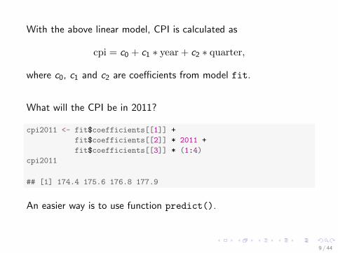
With the above linear model, CPI is calculated as

cpi = c0 + c1 ∗ year + c2 ∗ quarter,

where c0, c1 and c2 are coefficients from model fit.

What will the CPI be in 2011?

cpi2011 <- fit$coefficients[[1]] +

fit$coefficients[[2]] * 2011 +

fit$coefficients[[3]] * (1:4)

cpi2011

## [1] 174.4 175.6 176.8 177.9

An easier way is to use function predict().

9 / 44

More details of the model can be obtained with the code below.

attributes(fit)

## $names

## [1] "coefficients" "residuals" "effects"

## [4] "rank" "fitted.values" "assign"

## [7] "qr" "df.residual" "xlevels"

## [10] "call" "terms" "model"

##

## $class

## [1] "lm"

fit$coefficients

## (Intercept) year quarter

## -7644.488 3.888 1.167

10 / 44

Function residuals(): differences between observed values andfitted values

# differences between observed values and fitted values

residuals(fit)

## 1 2 3 4 5 6 ...

## -0.57917 0.65417 1.38750 -0.27917 -0.46667 -0.83333 -0.40...

## 8 9 10 11 12

## -0.66667 0.44583 0.37917 0.41250 -0.05417

summary(fit)

##

## Call:

## lm(formula = cpi ~ year + quarter)

##

## Residuals:

## Min 1Q Median 3Q Max

## -0.833 -0.495 -0.167 0.421 1.387

##

## Coefficients:

## Estimate Std. Error t value Pr(>|t|)

## (Intercept) -7644.488 518.654 -14.74 1.3e-07 ***

## year 3.888 0.258 15.06 1.1e-07 ***

## quarter 1.167 0.189 6.19 0.00016 ***

## ---

## Signif. codes: 0 '***' 0.001 '**' 0.01 '*' 0.05 '.' 0.1 ' ' 1

##

## Residual standard error: 0.73 on 9 degrees of freedom

## Multiple R-squared: 0.967, Adjusted R-squared: 0.96

## F-statistic: 133 on 2 and 9 DF, p-value: 2.11e-07

11 / 44

3D Plot of the Fitted Model

library(scatterplot3d)

s3d <- scatterplot3d(year, quarter, cpi, highlight.3d = T, type = "h",

lab = c(2, 3)) # lab: number of tickmarks on x-/y-axes

s3d$plane3d(fit) # draws the fitted plane

2008 2009 2010

160

165

170

175

1

2

3

4

year

quar

ter

cpi

12 / 44

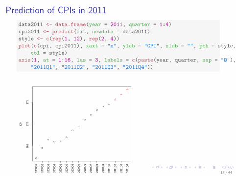
Prediction of CPIs in 2011

data2011 <- data.frame(year = 2011, quarter = 1:4)

cpi2011 <- predict(fit, newdata = data2011)

style <- c(rep(1, 12), rep(2, 4))

plot(c(cpi, cpi2011), xaxt = "n", ylab = "CPI", xlab = "", pch = style,

col = style)

axis(1, at = 1:16, las = 3, labels = c(paste(year, quarter, sep = "Q"),

"2011Q1", "2011Q2", "2011Q3", "2011Q4"))

165

170

175

CPI

2008

Q1

2008

Q2

2008

Q3

2008

Q4

2009

Q1

2009

Q2

2009

Q3

2009

Q4

2010

Q1

2010

Q2

2010

Q3

2010

Q4

2011

Q1

2011

Q2

2011

Q3

2011

Q4

13 / 44

Outline

Introduction

Linear Regression




Random Forest

Online Resources

14 / 44

Generalized Linear Model (GLM)

I Generalizes linear regression by allowing the linear model to berelated to the response variable via a link function andallowing the magnitude of the variance of each measurementto be a function of its predicted value

I Unifies various other statistical models, including linearregression, logistic regression and Poisson regression

I Function glm(): fits generalized linear models, specified bygiving a symbolic description of the linear predictor and adescription of the error distribution

15 / 44

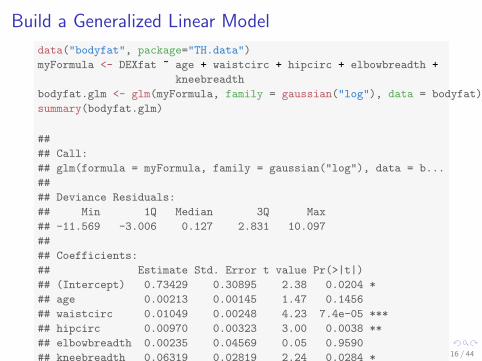
Build a Generalized Linear Model

data("bodyfat", package="TH.data")

myFormula <- DEXfat ~ age + waistcirc + hipcirc + elbowbreadth +

kneebreadth

bodyfat.glm <- glm(myFormula, family = gaussian("log"), data = bodyfat)

summary(bodyfat.glm)

##

## Call:

## glm(formula = myFormula, family = gaussian("log"), data = b...

##

## Deviance Residuals:

## Min 1Q Median 3Q Max

## -11.569 -3.006 0.127 2.831 10.097

##

## Coefficients:

## Estimate Std. Error t value Pr(>|t|)

## (Intercept) 0.73429 0.30895 2.38 0.0204 *

## age 0.00213 0.00145 1.47 0.1456

## waistcirc 0.01049 0.00248 4.23 7.4e-05 ***

## hipcirc 0.00970 0.00323 3.00 0.0038 **

## elbowbreadth 0.00235 0.04569 0.05 0.9590

## kneebreadth 0.06319 0.02819 2.24 0.0284 *

## ---

## Signif. codes: 0 '***' 0.001 '**' 0.01 '*' 0.05 '.' 0.1 ' ' 1

##

## (Dispersion parameter for gaussian family taken to be 20.31)

##

## Null deviance: 8536.0 on 70 degrees of freedom

## Residual deviance: 1320.4 on 65 degrees of freedom

## AIC: 423

##

## Number of Fisher Scoring iterations: 5

16 / 44

Prediction with Generalized Linear Regression Model

pred <- predict(bodyfat.glm, type = "response")

plot(bodyfat$DEXfat, pred, xlab = "Observed", ylab = "Prediction")

abline(a = 0, b = 1)

10 20 30 40 50 60

2030

4050

Observed

Pred

ictio

n

17 / 44

Outline

Introduction

Linear Regression




Random Forest

Online Resources

18 / 44

The iris Data

str(iris)

## 'data.frame': 150 obs. of 5 variables:

## $ Sepal.Length: num 5.1 4.9 4.7 4.6 5 5.4 4.6 5 4.4 4.9 ...

## $ Sepal.Width : num 3.5 3 3.2 3.1 3.6 3.9 3.4 3.4 2.9 3.1...

## $ Petal.Length: num 1.4 1.4 1.3 1.5 1.4 1.7 1.4 1.5 1.4 1...

## $ Petal.Width : num 0.2 0.2 0.2 0.2 0.2 0.4 0.3 0.2 0.2 0...

## $ Species : Factor w/ 3 levels "setosa","versicolor",....

# split data into two subsets: training (70%) and test (30%); set

# a fixed random seed to make results reproducible

set.seed(1234)

ind <- sample(2, nrow(iris), replace = TRUE, prob = c(0.7, 0.3))

train.data <- iris[ind == 1, ]

test.data <- iris[ind == 2, ]

19 / 44

Build a ctree

I Control the training of decision trees: MinSplit, MinBusket,MaxSurrogate and MaxDepth

I Target variable: Species

I Independent variables: all other variables

library(party)

myFormula <- Species ~ Sepal.Length + Sepal.Width + Petal.Length +

Petal.Width

iris_ctree <- ctree(myFormula, data = train.data)

# check the prediction

table(predict(iris_ctree), train.data$Species)

##

## setosa versicolor virginica

## setosa 40 0 0

## versicolor 0 37 3

## virginica 0 1 31

20 / 44

Print ctree

print(iris_ctree)

##

## Conditional inference tree with 4 terminal nodes

##

## Response: Species

## Inputs: Sepal.Length, Sepal.Width, Petal.Length, Petal.Width

## Number of observations: 112

##

## 1) Petal.Length <= 1.9; criterion = 1, statistic = 104.643

## 2)* weights = 40

## 1) Petal.Length > 1.9

## 3) Petal.Width <= 1.7; criterion = 1, statistic = 48.939

## 4) Petal.Length <= 4.4; criterion = 0.974, statistic = ...

## 5)* weights = 21

## 4) Petal.Length > 4.4

## 6)* weights = 19

## 3) Petal.Width > 1.7

## 7)* weights = 32

21 / 44

plot(iris_ctree)

Petal.Lengthp < 0.001

1

≤ 1.9 > 1.9

Node 2 (n = 40)

setosa

0

0.2

0.4

0.6

0.8

1

Petal.Widthp < 0.001

3

≤ 1.7 > 1.7

Petal.Lengthp = 0.026

4

≤ 4.4 > 4.4

Node 5 (n = 21)

setosa

0

0.2

0.4

0.6

0.8

1

Node 6 (n = 19)

setosa

0

0.2

0.4

0.6

0.8

1

Node 7 (n = 32)

setosa

0

0.2

0.4

0.6

0.8

1

22 / 44

plot(iris_ctree, type = "simple")

Petal.Lengthp < 0.001

1

≤ 1.9 > 1.9

n = 40y = (1, 0, 0)

2Petal.Widthp < 0.001

3

≤ 1.7 > 1.7

Petal.Lengthp = 0.026

4

≤ 4.4 > 4.4

n = 21y = (0, 1, 0)

5n = 19

y = (0, 0.842, 0.158)

6

n = 32y = (0, 0.031, 0.969)

7

23 / 44

Test

# predict on test data

testPred <- predict(iris_ctree, newdata = test.data)

table(testPred, test.data$Species)

##

## testPred setosa versicolor virginica

## setosa 10 0 0


## virginica 0 0 14

24 / 44

Outline

Introduction

Linear Regression




Random Forest

Online Resources

25 / 44

The bodyfat Dataset

data("bodyfat", package = "TH.data")

dim(bodyfat)

## [1] 71 10

# str(bodyfat)

head(bodyfat, 5)

## age DEXfat waistcirc hipcirc elbowbreadth kneebreadth

## 47 57 41.68 100.0 112.0 7.1 9.4

## 48 65 43.29 99.5 116.5 6.5 8.9

## 49 59 35.41 96.0 108.5 6.2 8.9

## 50 58 22.79 72.0 96.5 6.1 9.2

## 51 60 36.42 89.5 100.5 7.1 10.0

## anthro3a anthro3b anthro3c anthro4

## 47 4.42 4.95 4.50 6.13

## 48 4.63 5.01 4.48 6.37

## 49 4.12 4.74 4.60 5.82

## 50 4.03 4.48 3.91 5.66

## 51 4.24 4.68 4.15 5.91

26 / 44

Train a Decision Tree with Package rpart

# split into training and test subsets

set.seed(1234)

ind <- sample(2, nrow(bodyfat), replace=TRUE, prob=c(0.7, 0.3))

bodyfat.train <- bodyfat[ind==1,]

bodyfat.test <- bodyfat[ind==2,]

# train a decision tree

library(rpart)

myFormula <- DEXfat ~ age + waistcirc + hipcirc + elbowbreadth +

kneebreadth

bodyfat_rpart <- rpart(myFormula, data = bodyfat.train,

control = rpart.control(minsplit = 10))

# print(bodyfat_rpart£cptable)

print(bodyfat_rpart)

plot(bodyfat_rpart)

text(bodyfat_rpart, use.n=T)

27 / 44

The rpart Tree

## n= 56

##

## node), split, n, deviance, yval

## * denotes terminal node

##

## 1) root 56 7265.0000 30.95

## 2) waistcirc< 88.4 31 960.5000 22.56

## 4) hipcirc< 96.25 14 222.3000 18.41

## 8) age< 60.5 9 66.8800 16.19 *

## 9) age>=60.5 5 31.2800 22.41 *

## 5) hipcirc>=96.25 17 299.6000 25.97

## 10) waistcirc< 77.75 6 30.7300 22.32 *

## 11) waistcirc>=77.75 11 145.7000 27.96

## 22) hipcirc< 99.5 3 0.2569 23.75 *

## 23) hipcirc>=99.5 8 72.2900 29.54 *

## 3) waistcirc>=88.4 25 1417.0000 41.35

## 6) waistcirc< 104.8 18 330.6000 38.09

## 12) hipcirc< 109.9 9 69.0000 34.38 *

## 13) hipcirc>=109.9 9 13.0800 41.81 *

## 7) waistcirc>=104.8 7 404.3000 49.73 *

28 / 44

The rpart Tree|waistcirc< 88.4

hipcirc< 96.25

age< 60.5 waistcirc< 77.75

hipcirc< 99.5

waistcirc< 104.8

hipcirc< 109.92e+01n=9

2e+01n=5 2e+01

n=62e+01

n=33e+01

n=83e+01

n=94e+01

n=9

5e+01n=7

29 / 44

Select the Best Tree

# select the tree with the minimum prediction error

opt <- which.min(bodyfat_rpart$cptable[, "xerror"])

cp <- bodyfat_rpart$cptable[opt, "CP"]

# prune tree

bodyfat_prune <- prune(bodyfat_rpart, cp = cp)

# plot tree

plot(bodyfat_prune)

text(bodyfat_prune, use.n = T)

30 / 44

Selected Tree|waistcirc< 88.4

hipcirc< 96.25

age< 60.5 waistcirc< 77.75

waistcirc< 104.8

hipcirc< 109.92e+01

n=92e+01

n=52e+01

n=63e+01n=11 3e+01

n=94e+01

n=9

5e+01n=7

31 / 44

Model Evalutation

DEXfat_pred <- predict(bodyfat_prune, newdata = bodyfat.test)

xlim <- range(bodyfat$DEXfat)

plot(DEXfat_pred ~ DEXfat, data = bodyfat.test, xlab = "Observed",

ylab = "Prediction", ylim = xlim, xlim = xlim)

abline(a = 0, b = 1)

10 20 30 40 50 60

1020

3040

5060

Observed

Pred

ictio

n

32 / 44

Outline

Introduction

Linear Regression




Random Forest

Online Resources

33 / 44

R Packages for Random Forest

I Package randomForestI very fastI cannot handle data with missing valuesI a limit of 32 to the maximum number of levels of each

categorical attribute

I Package party : cforest()I not limited to the above maximum levelsI slowI needs more memory

34 / 44

Train a Random Forest

# split into two subsets: training (70%) and test (30%)

ind <- sample(2, nrow(iris), replace=TRUE, prob=c(0.7, 0.3))

train.data <- iris[ind==1,]

test.data <- iris[ind==2,]

# use all other variables to predict Species

library(randomForest)

rf <- randomForest(Species ~ ., data=train.data, ntree=100,

proximity=T)

35 / 44

table(predict(rf), train.data$Species)

##

## setosa versicolor virginica

## setosa 36 0 0


## virginica 0 1 34

print(rf)

##

## Call:

## randomForest(formula = Species ~ ., data = train.data, ntr...

## Type of random forest: classification

## Number of trees: 100

## No. of variables tried at each split: 2

##

## OOB estimate of error rate: 2.88%

## Confusion matrix:

## setosa versicolor virginica class.error

## setosa 36 0 0 0.00000

## versicolor 0 31 1 0.03125

## virginica 0 2 34 0.05556

attributes(rf)

## $names

## [1] "call" "type" "predicted"

## [4] "err.rate" "confusion" "votes"

## [7] "oob.times" "classes" "importance"

## [10] "importanceSD" "localImportance" "proximity"

## [13] "ntree" "mtry" "forest"

## [16] "y" "test" "inbag"

## [19] "terms"

##

## $class

## [1] "randomForest.formula" "randomForest"

36 / 44

Error Rate of Random Forest

plot(rf, main = "")

0 20 40 60 80 100

0.00

0.05

0.10

0.15

0.20

trees

Erro

r

37 / 44

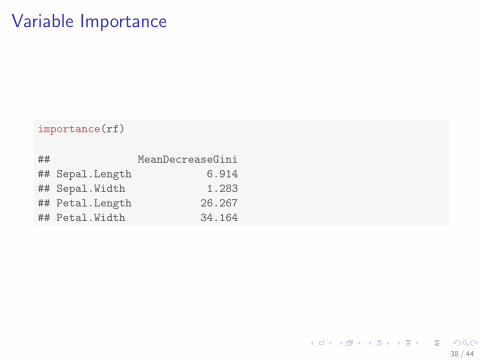
Variable Importance

importance(rf)

## MeanDecreaseGini

## Sepal.Length 6.914

## Sepal.Width 1.283

## Petal.Length 26.267

## Petal.Width 34.164

38 / 44

Variable Importance

varImpPlot(rf)

Sepal.Width

Sepal.Length

Petal.Length

Petal.Width

0 5 10 15 20 25 30 35

rf

MeanDecreaseGini

39 / 44

Margin of Predictions

The margin of a data point is as the proportion of votes for thecorrect class minus maximum proportion of votes for other classes.Positive margin means correct classification.

irisPred <- predict(rf, newdata = test.data)

table(irisPred, test.data$Species)

##

## irisPred setosa versicolor virginica

## setosa 14 0 0


## virginica 0 1 11

plot(margin(rf, test.data$Species))

40 / 44

Margin of Predictions

0 20 40 60 80 100

0.0

0.2

0.4

0.6

0.8

1.0

Index

x

41 / 44

Outline

Introduction

Linear Regression




Random Forest

Online Resources

42 / 44

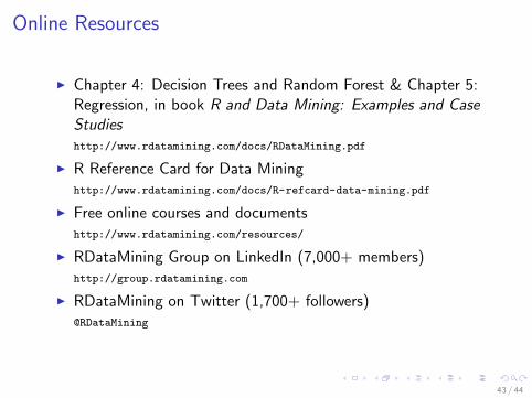
Online Resources

I Chapter 4: Decision Trees and Random Forest & Chapter 5:Regression, in book R and Data Mining: Examples and CaseStudieshttp://www.rdatamining.com/docs/RDataMining.pdf

I R Reference Card for Data Mininghttp://www.rdatamining.com/docs/R-refcard-data-mining.pdf

I Free online courses and documentshttp://www.rdatamining.com/resources/

I RDataMining Group on LinkedIn (7,000+ members)http://group.rdatamining.com

I RDataMining on Twitter (1,700+ followers)@RDataMining

43 / 44

http://www.rdatamining.com/docs/RDataMining.pdf

http://www.rdatamining.com/docs/R-refcard-data-mining.pdf

http://www.rdatamining.com/resources/

http://group.rdatamining.com

@RDataMining

The End

Thanks!

Email: yanchang(at)rdatamining.com

44 / 44

http://www.rdatamining.com/books/rdm

http://www.rdatamining.com/books/dmar

regression and classification with r

Technology