(Cluster Analysis) &

(Classification And Regression Trees = CART)

James McCreightmccreigh >at< gmail >dot< com

1

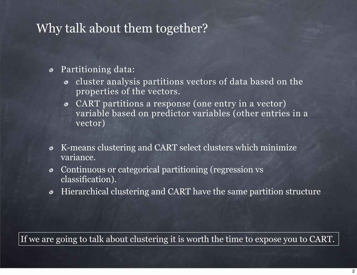
Why talk about them together?

Partitioning data:cluster analysis partitions vectors of data based on the properties of the vectors.CART partitions a response (one entry in a vector) variable based on predictor variables (other entries in a vector)

K-means clustering and CART select clusters which minimize variance. Continuous or categorical partitioning (regression vs classification).Hierarchical clustering and CART have the same partition structure

If we are going to talk about clustering it is worth the time to expose you to CART.

2

Cluster Analysis

Cluster analysisFrom Wikipedia, the free encyclopedia

Cluster analysis or clustering is the task of assigning a set of objects into groups (called clusters) so that the objects in the same cluster are more similar (in some sense or another) to each other than to those in other clusters.

Clustering is a main task of explorative data mining, and a common technique for statistical data analysis used in many fields, including machine learning, pattern recognition, image analysis,information retrieval, and bioinformatics.

Cluster analysis itself is not one specific algorithm, but the general task to be solved. It can be achieved by various algorithms that differ significantly in their notion of what constitutes a cluster and how to efficiently find them. 

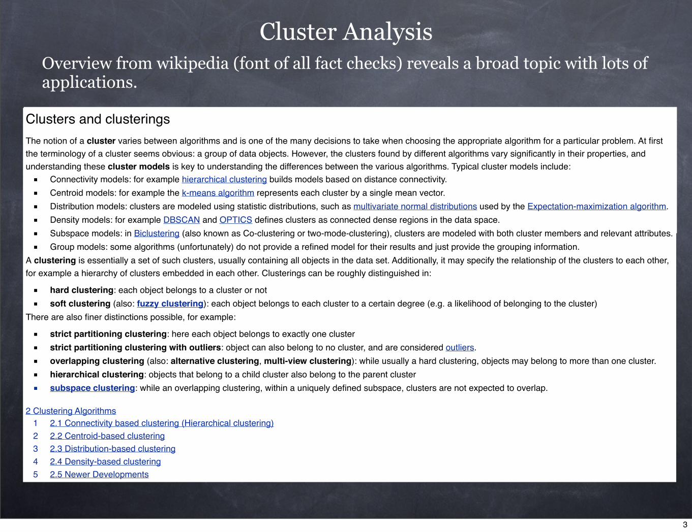
Overview from wikipedia (font of all fact checks) reveals a broad topic with lots of applications.

Clusters and clusteringsThe notion of a cluster varies between algorithms and is one of the many decisions to take when choosing the appropriate algorithm for a particular problem. At first the terminology of a cluster seems obvious: a group of data objects. However, the clusters found by different algorithms vary significantly in their properties, and understanding these cluster models is key to understanding the differences between the various algorithms. Typical cluster models include:■ Connectivity models: for example hierarchical clustering builds models based on distance connectivity.■ Centroid models: for example the k-means algorithm represents each cluster by a single mean vector.■ Distribution models: clusters are modeled using statistic distributions, such as multivariate normal distributions used by the Expectation-maximization algorithm.■ Density models: for example DBSCAN and OPTICS defines clusters as connected dense regions in the data space.■ Subspace models: in Biclustering (also known as Co-clustering or two-mode-clustering), clusters are modeled with both cluster members and relevant attributes.■ Group models: some algorithms (unfortunately) do not provide a refined model for their results and just provide the grouping information.

A clustering is essentially a set of such clusters, usually containing all objects in the data set. Additionally, it may specify the relationship of the clusters to each other, for example a hierarchy of clusters embedded in each other. Clusterings can be roughly distinguished in:

■ hard clustering: each object belongs to a cluster or not■ soft clustering (also: fuzzy clustering): each object belongs to each cluster to a certain degree (e.g. a likelihood of belonging to the cluster)

There are also finer distinctions possible, for example:

■ strict partitioning clustering: here each object belongs to exactly one cluster■ strict partitioning clustering with outliers: object can also belong to no cluster, and are considered outliers.■ overlapping clustering (also: alternative clustering, multi-view clustering): while usually a hard clustering, objects may belong to more than one cluster.■ hierarchical clustering: objects that belong to a child cluster also belong to the parent cluster■ subspace clustering: while an overlapping clustering, within a uniquely defined subspace, clusters are not expected to overlap.

2 Clustering Algorithms1 2.1 Connectivity based clustering (Hierarchical clustering)2 2.2 Centroid-based clustering3 2.3 Distribution-based clustering4 2.4 Density-based clustering5 2.5 Newer Developments

3

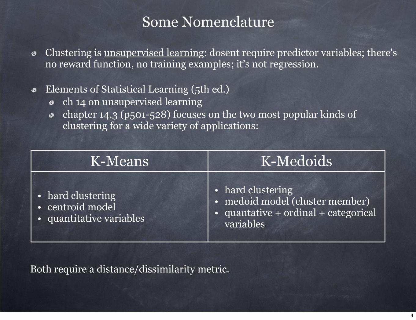
Some Nomenclature

K-Means K-Medoids

• hard clustering• centroid model• quantitative variables

• hard clustering• medoid model (cluster member)• quantative + ordinal + categorical

variables

Both require a distance/dissimilarity metric.

Clustering is unsupervised learning: dosent require predictor variables; there's no reward function, no training examples; it’s not regression.

Elements of Statistical Learning (5th ed.) ch 14 on unsupervised learningchapter 14.3 (p501-528) focuses on the two most popular kinds of clustering for a wide variety of applications:

4

Outline

1-d non-example: the idea of variance and clusters

2-d example, dissimilarity/variance in 2-d

Dissimilarity / variance in N-d

The algorithm

Problem of a priori selection of K

hierarchical clustering

5

1-D Clusters and Variance

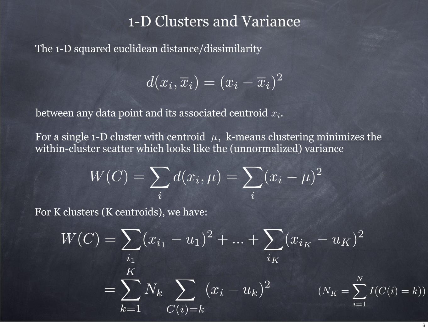
The 1-D squared euclidean distance/dissimilarity

For a single 1-D cluster with centroid , k-means clustering minimizes the within-cluster scatter which looks like the (unnormalized) variance

d(xi, xi) = (xi − xi)2

W (C) =�

i

d(xi, µ) =�

i

(xi − µ)2

µ

For K clusters (K centroids), we have:

W (C) =�

i1

(xi1 − u1)2 + ...+

�

iK

(xiK − uK)2

=K�

k=1

Nk

�

C(i)=k

(xi − uk)2

xibetween any data point and its associated centroid .

(NK =N�

i=1

I(C(i) = k))

6

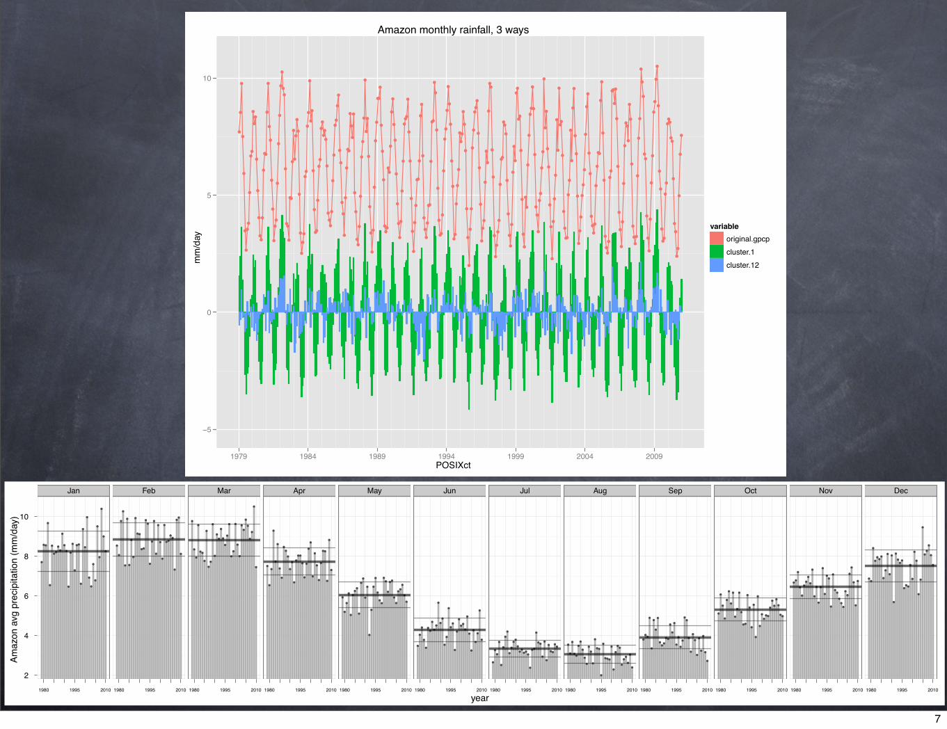
Intuitive 1-D non-example

year

Amaz

on a

vg p

reci

pita

tion

(mm

/day

)

2

4

6

8

10

Jan

●

●●

●

●

●

●●

●●

●

●

●

●

●

●

●

●●

●

●

●

●

●

●

●

●

●

●

●

●

●

1980 1995 2010

Feb

●

●

●

●

●

●

●

●

●

●

●●

●●

●●

●

●

●

●

●

●

●

●

●●

●●

●

●●

●

1980 1995 2010

Mar

●

●

●

●

●●

●

●

●

●

●

●

●

●

●

●

●

●

●

●

●

●

●

●

●

●

●

●

●

●

●

●

1980 1995 2010

Apr

●

●

●

●

●

●

●

●

●●

●

●

●

●

●

●●

●

●

●

●

●

●

●

●

●

●

●●

●

●

●

1980 1995 2010

May

●

●

●

●

●

●

●●

●

●

●

●

●

●

●

●

●

●

●●

●●

●

●●

●

●

●●

●

●

●

1980 1995 2010

Jun

●

●

●

●

●

●●

●

●

●

●

●

●

●

●

●

●●

●

●

●

●●

●

●

●

●

●

●

●

●

●

1980 1995 2010

Jul

●

●

●

●

●

●

●

●

●

●

●●

●

●●●●

●

●

●●

●

●●

●

●

●

●

●●

●●

1980 1995 2010

Aug

●

●

●

●●

●

●

●

●

●

●

●

●

●

●●

●

●

●●●

●

●

●

●●

●

●●

●

●

●

1980 1995 2010

Sep

●

●●

●

●

●

●

●

●●●

●●

●

●

●

●

●

●

●

●●

●

●

●

●

●

●

●

●

●

●

1980 1995 2010

Oct

●

●

●

●

●

●

●

●

●

●

●

●

●●

●

●

●

●

●

●

●

●

●●●

●

●

●

●

●

●●

1980 1995 2010

Nov

●●

●

●

●

●

●

●

●

●

●

●

●

●

●

●

●●

●

●

●●

●

●●

●

●

●

●

●

●

●

1980 1995 2010

Dec

●●

●

●●●●

●

●

●

●

●

●

●

●●●

●●●

●

●

●

●

●

●

●

●●

●

●

●

1980 1995 2010

Amazon monthly rainfall, 3 ways

POSIXct

mm

/day

−5

0

5

10

●

● ●

●

●

●

● ●

●●

●

●

●

●

●

●

●

● ●

●

●

●

●

●

●

●

●

●

●

●

●

●

●

●

●

●

●

●

●

●

●

●

● ●

● ●

●●

●

●

●

●

●

●

●

●

● ●

●●

●

●●

●

●

●

●

●

● ●

●

●

●

●

●

●

●●

●

●

●

●

●

●

●

●

●

●

●●

●

●

●

●

●

●●

●

●

●

●

●

●

●

●●

●

●

●

●

●

● ●

●

●

●

●

●

●

●

●

●

●

● ●

●

●

●

●

●

●

●

●

●●

●

●

●●

●

●

●

●

●

●

●

●●

●●

●

● ●

●

●

●●

●

●

●

●

●

●

●

●

●●

●

●●

●

●●

●

●

●

●●

●

●

●

● ●

●

●

●

●

●

●

●

●

●

●

●●

●

●

●

●

●

●

●

●●

●

●●

● ●●

●

● ●

●

● ●

●

●

●

●

● ●

●●

●

●

●

●●

●●

●

●

●

●

●

●

●

● ●

●

●

● ● ●

●

●

●

● ●

●

●●

●

●

●

●● ●

●

●

●

●

●

●●

●

● ●

●

●

●

●

●

●

●

●●

●

●

●

●

●

●

●

●

●

●

●

●

●

●

●

●

●

●

●

●

●

●

● ●

●

●

●

●

●

●

●

●

●● ●

●

●

●

●

●

● ●

●●

●

●

●

●●

●

●

●

●

●

●

●

●

●

●●

●

●

●●

●●

●

●●

●

●

●

●

●●

●

●

●●

●●

●

●

●

●

●

●

●

●●

●

●● ●

●

●

●

●

●

●

●

●●

●

●

●

1979 1984 1989 1994 1999 2004 2009

variable● original.gpcp

Amazon monthly rainfall, 3 ways

POSIXct

mm

/day

−5

0

5

10

●

● ●

●

●

●

● ●

●●

●

●

●

●

●

●

●

● ●

●

●

●

●

●

●

●

●

●

●

●

●

●

●

●

●

●

●

●

●

●

●

●

● ●

● ●

●●

●

●

●

●

●

●

●

●

● ●

●●

●

●●

●

●

●

●

●

● ●

●

●

●

●

●

●

●●

●

●

●

●

●

●

●

●

●

●

●●

●

●

●

●

●

●●

●

●

●

●

●

●

●

●●

●

●

●

●

●

● ●

●

●

●

●

●

●

●

●

●

●

● ●

●

●

●

●

●

●

●

●

●●

●

●

●●

●

●

●

●

●

●

●

●●

●●

●

● ●

●

●

●●

●

●

●

●

●

●

●

●

●●

●

●●

●

●●

●

●

●

●●

●

●

●

● ●

●

●

●

●

●

●

●

●

●

●

●●

●

●

●

●

●

●

●

●●

●

●●

● ●●

●

● ●

●

● ●

●

●

●

●

● ●

●●

●

●

●

●●

●●

●

●

●

●

●

●

●

● ●

●

●

● ● ●

●

●

●

● ●

●

●●

●

●

●

●● ●

●

●

●

●

●

●●

●

● ●

●

●

●

●

●

●

●

●●

●

●

●

●

●

●

●

●

●

●

●

●

●

●

●

●

●

●

●

●

●

●

● ●

●

●

●

●

●

●

●

●

●● ●

●

●

●

●

●

● ●

●●

●

●

●

●●

●

●

●

●

●

●

●

●

●

●●

●

●

●●

●●

●

●●

●

●

●

●

●●

●

●

●●

●●

●

●

●

●

●

●

●

●●

●

●● ●

●

●

●

●

●

●

●

●●

●

●

●

1979 1984 1989 1994 1999 2004 2009

variable● original.gpcp● cluster.1

Amazon monthly rainfall, 3 ways

POSIXct

mm

/day

−5

0

5

10

●

● ●

●

●

●

● ●

●●

●

●

●

●

●

●

●

● ●

●

●

●

●

●

●

●

●

●

●

●

●

●

●

●

●

●

●

●

●

●

●

●

● ●

● ●

●●

●

●

●

●

●

●

●

●

● ●

●●

●

●●

●

●

●

●

●

● ●

●

●

●

●

●

●

●●

●

●

●

●

●

●

●

●

●

●

●●

●

●

●

●

●

●●

●

●

●

●

●

●

●

●●

●

●

●

●

●

● ●

●

●

●

●

●

●

●

●

●

●

● ●

●

●

●

●

●

●

●

●

●●

●

●

●●

●

●

●

●

●

●

●

●●

●●

●

● ●

●

●

●●

●

●

●

●

●

●

●

●

●●

●

●●

●

●●

●

●

●

●●

●

●

●

● ●

●

●

●

●

●

●

●

●

●

●

●●

●

●

●

●

●

●

●

●●

●

●●

● ●●

●

● ●

●

● ●

●

●

●

●

● ●

●●

●

●

●

●●

●●

●

●

●

●

●

●

●

● ●

●

●

● ● ●

●

●

●

● ●

●

●●

●

●

●

●● ●

●

●

●

●

●

●●

●

● ●

●

●

●

●

●

●

●

●●

●

●

●

●

●

●

●

●

●

●

●

●

●

●

●

●

●

●

●

●

●

●

● ●

●

●

●

●

●

●

●

●

●● ●

●

●

●

●

●

● ●

●●

●

●

●

●●

●

●

●

●

●

●

●

●

●

●●

●

●

●●

●●

●

●●

●

●

●

●

●●

●

●

●●

●●

●

●

●

●

●

●

●

●●

●

●● ●

●

●

●

●

●

●

●

●●

●

●

●

1979 1984 1989 1994 1999 2004 2009

variable● original.gpcp● cluster.1● cluster.12

7

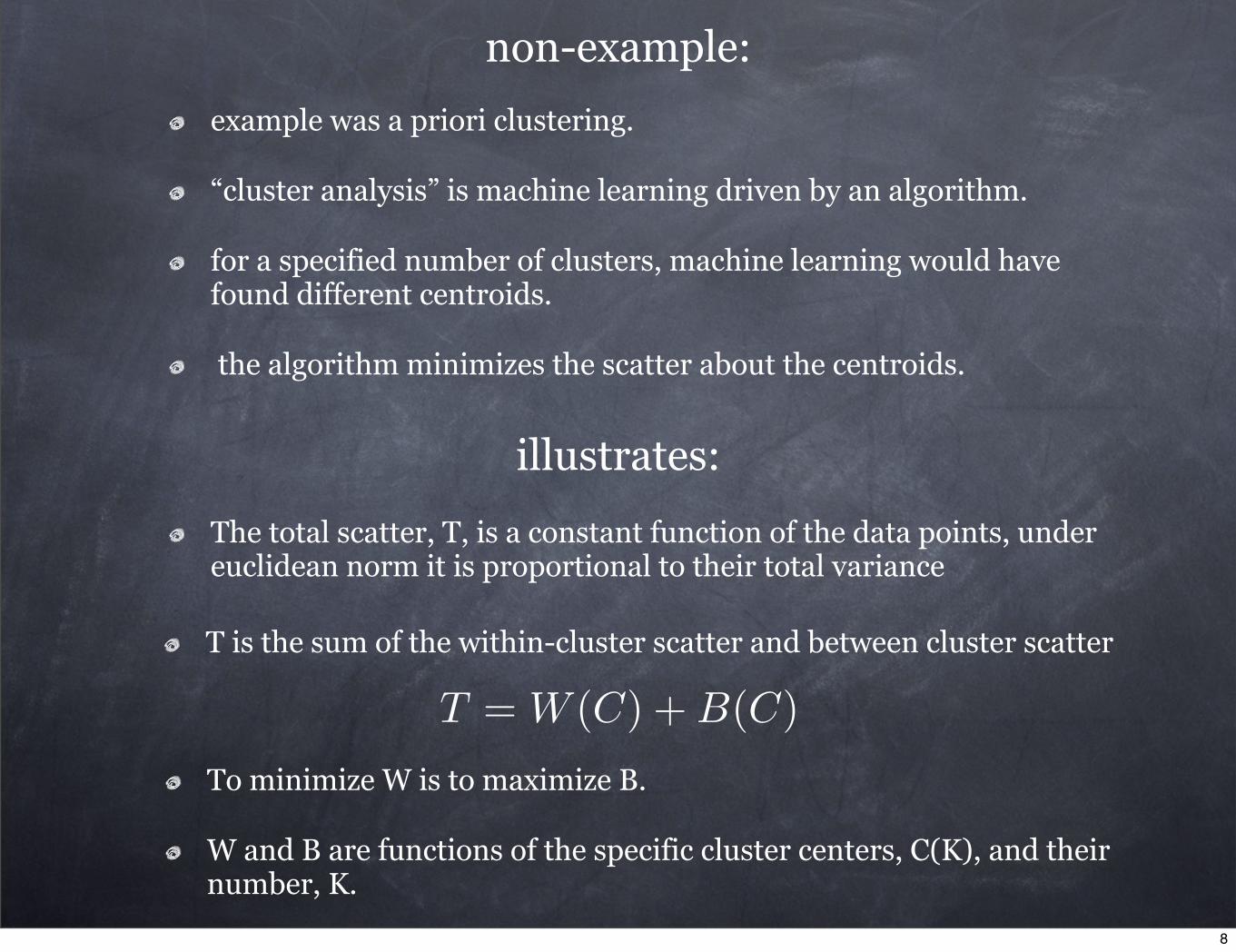
The total scatter, T, is a constant function of the data points, under euclidean norm it is proportional to their total variance

non-example:

example was a priori clustering.

“cluster analysis” is machine learning driven by an algorithm.

for a specified number of clusters, machine learning would have found different centroids.

the algorithm minimizes the scatter about the centroids.

T = W (C) +B(C)

illustrates:

T is the sum of the within-cluster scatter and between cluster scatter

To minimize W is to maximize B.

W and B are functions of the specific cluster centers, C(K), and their number, K.

8

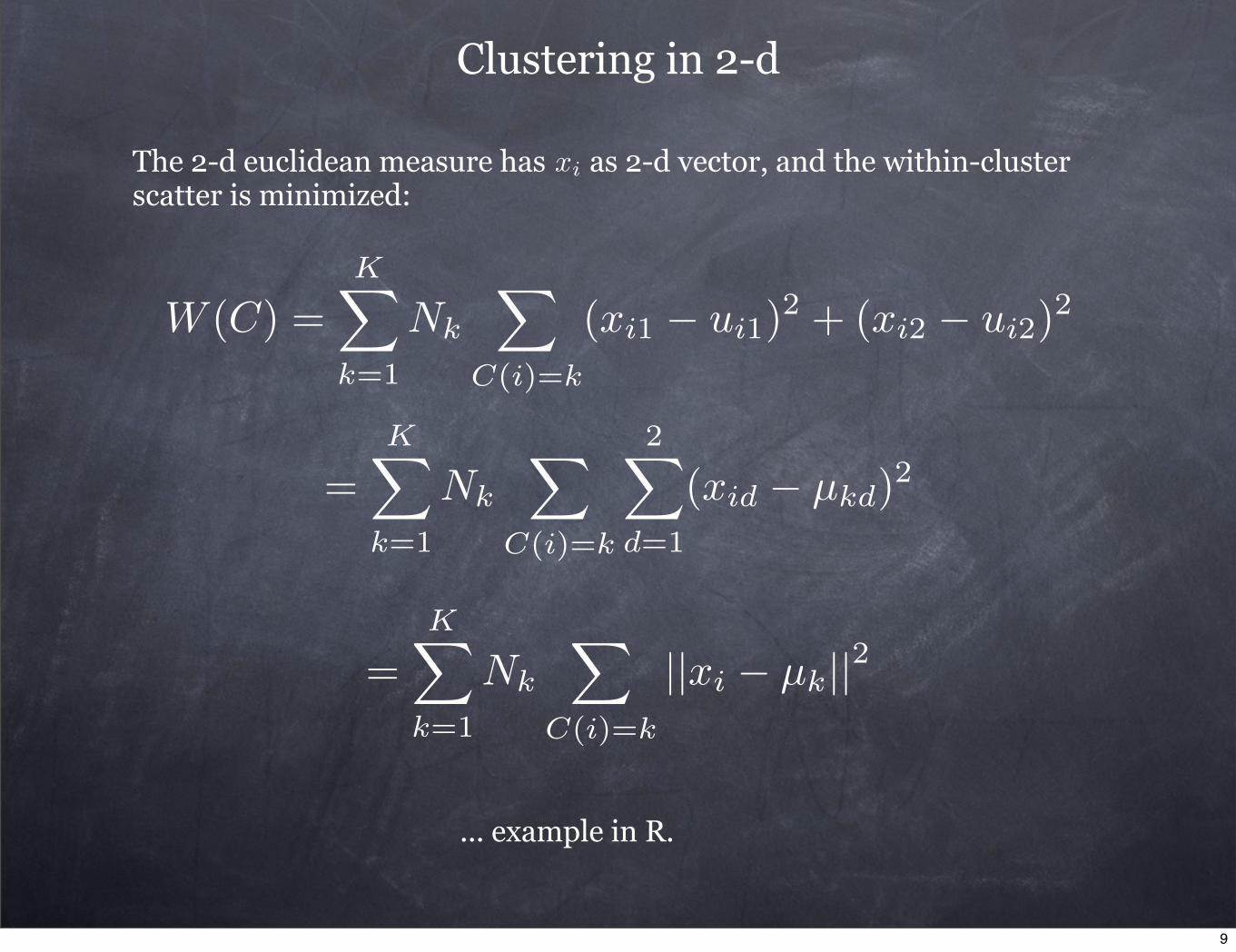
Clustering in 2-d

The 2-d euclidean measure has as 2-d vector, and the within-cluster scatter is minimized:

xi

... example in R.

W (C) =K�

k=1

Nk

�

C(i)=k

(xi1 − ui1)2 + (xi2 − ui2)

2

=K�

k=1

Nk

�

C(i)=k

2�

d=1

(xid − µkd)2

=K�

k=1

Nk

�

C(i)=k

||xi − µk||2

9

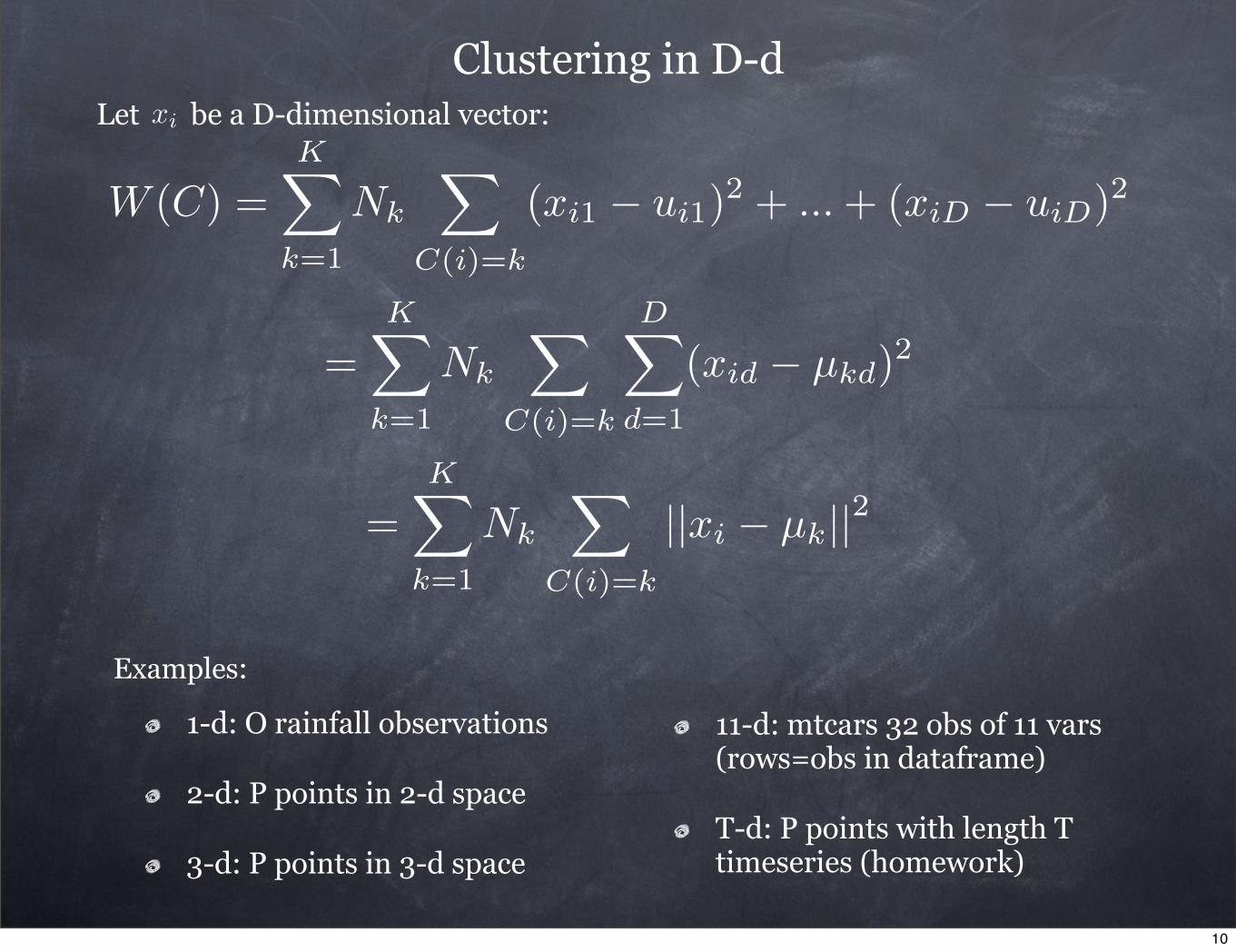
Clustering in D-dLet be a D-dimensional vector:xi

=K�

k=1

Nk

�

C(i)=k

||xi − µk||2

W (C) =K�

k=1

Nk

�

C(i)=k

(xi1 − ui1)2 + ...+ (xiD − uiD)2

=K�

k=1

Nk

�

C(i)=k

D�

d=1

(xid − µkd)2

1-d: O rainfall observations

2-d: P points in 2-d space

3-d: P points in 3-d space

11-d: mtcars 32 obs of 11 vars (rows=obs in dataframe)

T-d: P points with length T timeseries (homework)

Examples:

10

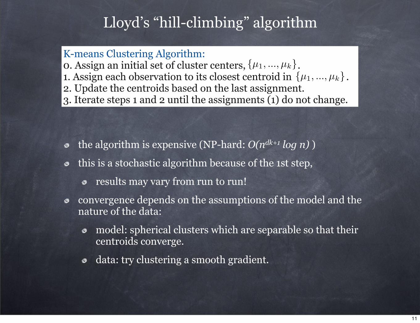
Lloyd’s “hill-climbing” algorithm

K-means Clustering Algorithm: 0. Assign an initial set of cluster centers, .1. Assign each observation to its closest centroid in . 2. Update the centroids based on the last assignment.3. Iterate steps 1 and 2 until the assignments (1) do not change.

{µ1, ..., µk}{µ1, ..., µk}

the algorithm is expensive (NP-hard: O(ndk+1 log n) )

this is a stochastic algorithm because of the 1st step,

results may vary from run to run!

convergence depends on the assumptions of the model and the nature of the data:

model: spherical clusters which are separable so that their centroids converge.

data: try clustering a smooth gradient.

11

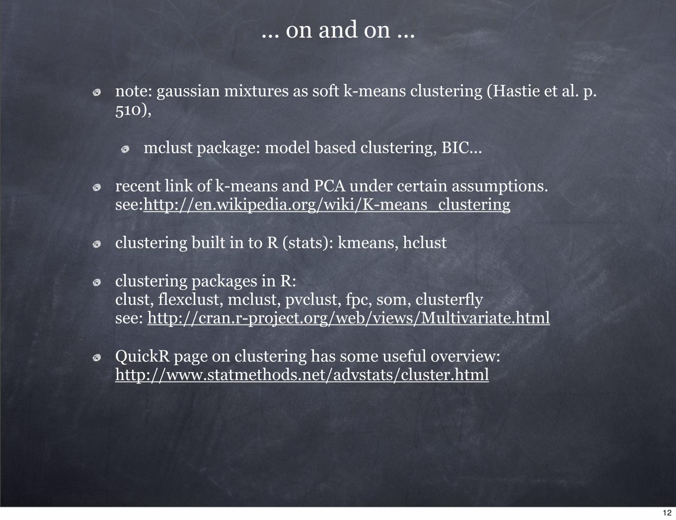
... on and on ...

note: gaussian mixtures as soft k-means clustering (Hastie et al. p. 510),

mclust package: model based clustering, BIC...

recent link of k-means and PCA under certain assumptions. see:http://en.wikipedia.org/wiki/K-means_clustering

clustering built in to R (stats): kmeans, hclust

clustering packages in R: clust, flexclust, mclust, pvclust, fpc, som, clusterfly see: http://cran.r-project.org/web/views/Multivariate.html

QuickR page on clustering has some useful overview: http://www.statmethods.net/advstats/cluster.html

12

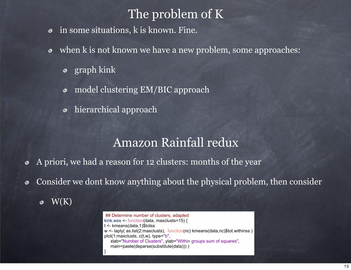
The problem of Kin some situations, k is known. Fine.

when k is not known we have a new problem, some approaches:

graph kink

model clustering EM/BIC approach

hierarchical approach

Amazon Rainfall redux

A priori, we had a reason for 12 clusters: months of the year

Consider we dont know anything about the physical problem, then consider

W(K)

## Determine number of clusters, adaptedkink.wss <- function(data, maxclusts=15) {t <- kmeans(data,1)$totssw <- laply( as.list(2:maxclusts), function(nc) kmeans(data,nc)$tot.withinss )plot(1:maxclusts, c(t,w), type="b", xlab="Number of Clusters", ylab="Within groups sum of squares", main=paste(deparse(substitute(data))) )}

13

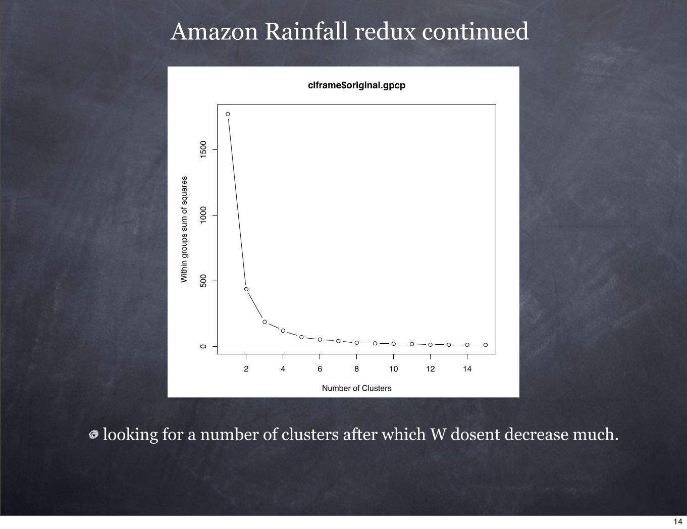
Amazon Rainfall redux continued

●

●

●

●

●● ● ● ● ● ● ● ● ● ●

2 4 6 8 10 12 14

050

010

0015

00

clframe$original.gpcp

Number of Clusters

With

in g

roup

s su

m o

f squ

ares

looking for a number of clusters after which W dosent decrease much.

14

aside...EOF/PCA vs Cluster Analysis

Dominant variability (modes) vs similar observations (clusters),

one chooses the # of clusters but not the # of modes.

EOF/PCA: data subspaces which explain maximum variance.

Cluster analysis: similarities/differences in observations

identify observations which vary similarly,

decompose non-stationarity, homogenize a variable.

15

5 10 15 20

−185

0−1

800

−175

0−1

700

−165

0

number of components

BIC

EV

2 4 6 8 10

0.05

0.10

0.15

0.20

dens

ity

Density

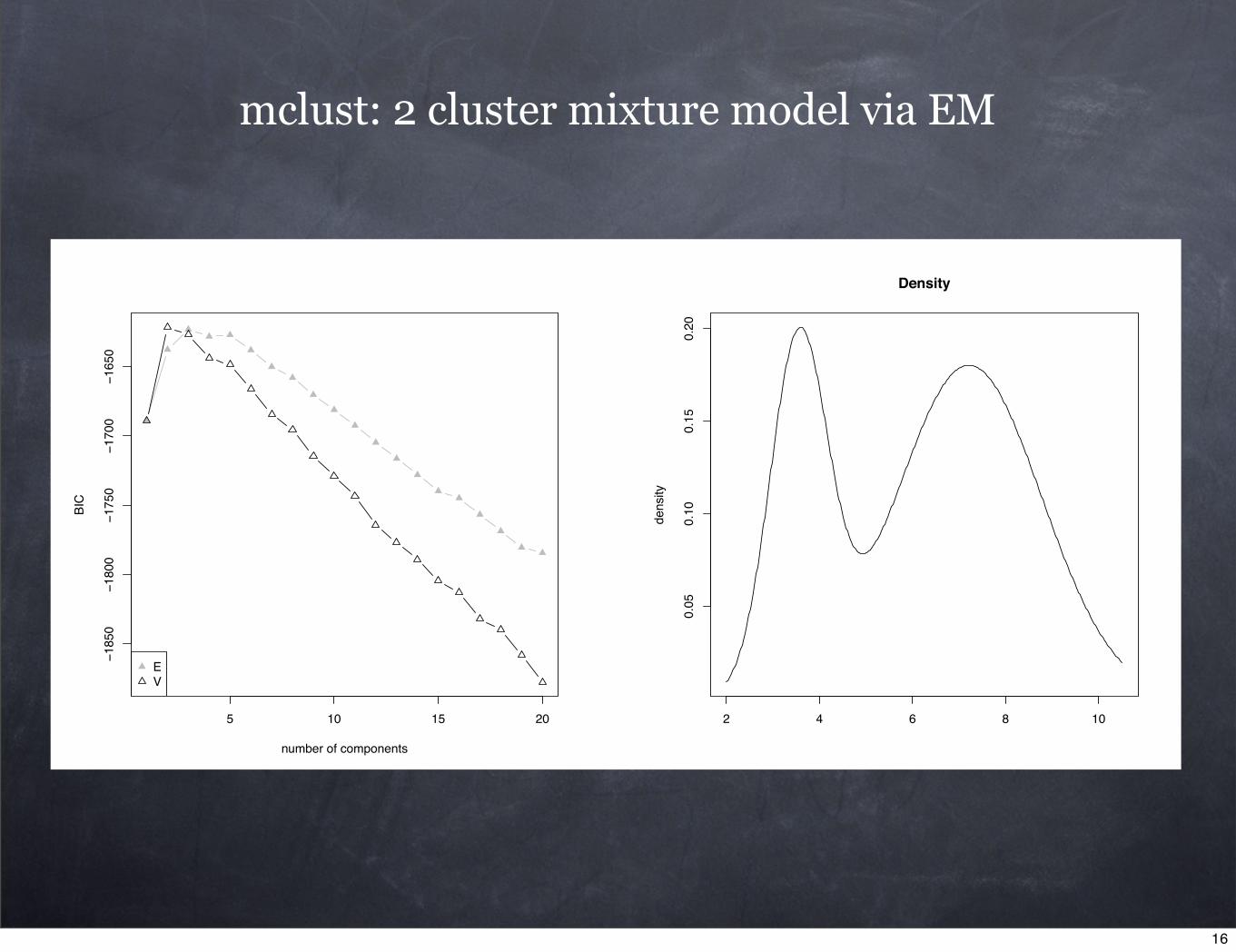
mclust: 2 cluster mixture model via EM

16

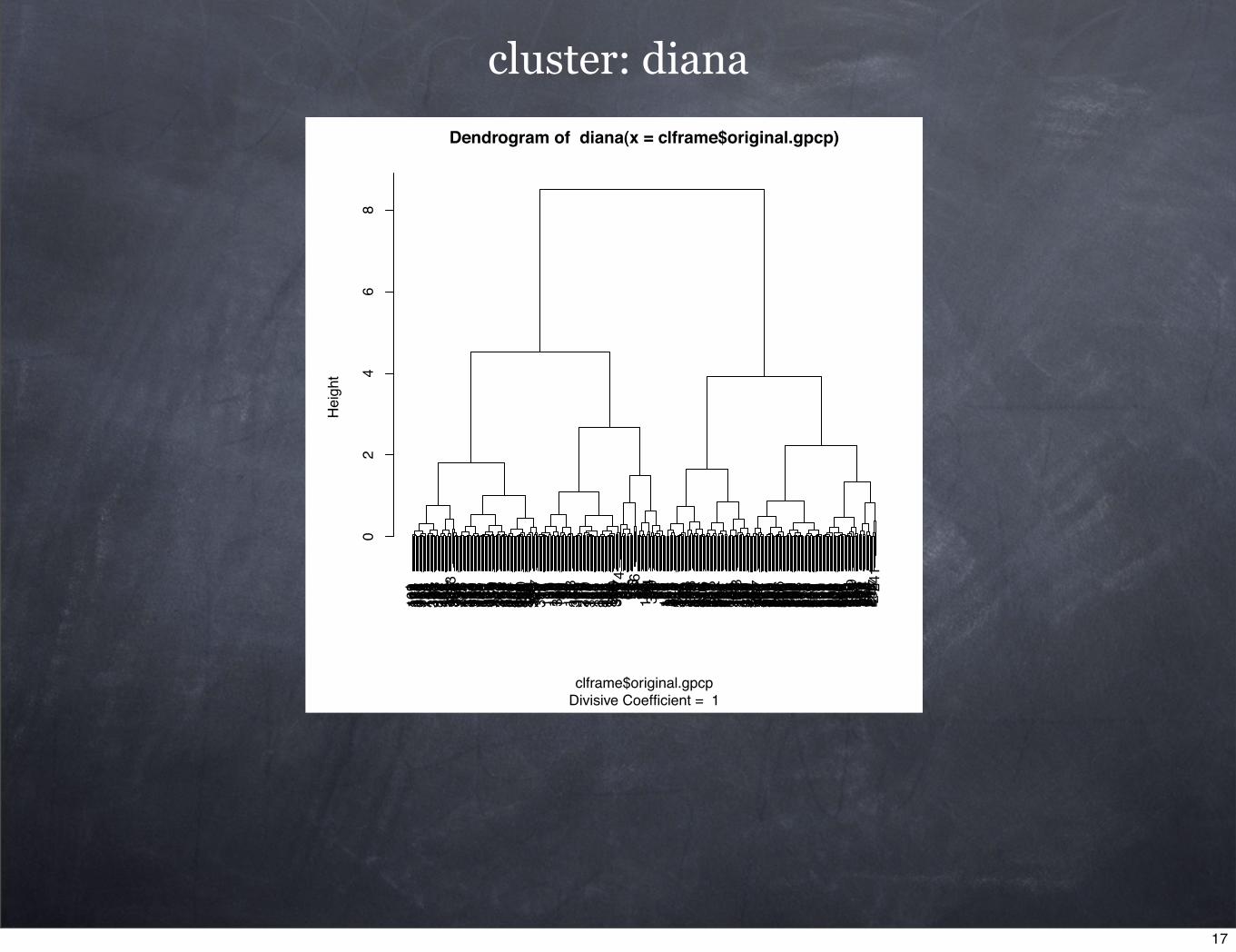
cluster: diana

110

911

412

336

8 71 356

376

111

369 74 101 26 49 116 37 121 39 384

373 73 97 17 361

128 61 330 99 108 96 349

103

335 323

337

340

363

348 5 98 371

158

326 14 144

141 25 372

332

334 20 329

110

350

321

138 24 104

145

149

360

139

338

353

374

115

328

119 27 322

153

122

378

126

352

354

150

152

327

132

336

377

146

296

342

299

134

303

347

159

325

290

308

331

135

156

294

346

151

341

136

370

324

157 2 81 3 382 12 18 6 33 16 102 19 87 9 22 105 46 117

355 40 127 60 80 78 93 50 57 54 118 58 7 52 366 64 362

120 15 70 8 69 375 10 13 106

124

381 32 85 125 45 66 29 41 357 84 107

359 88 34 383 76 112

113

364

380 55 358

367 67

423 63 38 42 35 51 65 47 62 91 3

0 95 36

11 43 44 77 31 59 82 72 100 90 94 21 79 379

28 92 53 68 56 89 48 75 83 86 129

154

140

147

293

315

317

343

131

155

148

344

171

333

295

160

365

130

300

143

191

298

176

304

314

339

345

291

316

318

351

306

133

319

310

137

289

185

297

313

320

312

173

292

311

260

264

277

181

262

278

163

177

305

166

169

263

184

188

168

172

272

178

183

302

170

182

309

270

301

142

258

162

186

190

281

167

180

200

214

271

164

192

204

257

238

269

276

282

175

307

274

199

259

286

268

279

284

161

230

249

205

220

266

165

202

250

239

261

198

224

246

235

275

174

225

273

223

216

242

267

189

227

196

203

218

231

215

265

179

194

207

212

232

187

285

213

240

201

208

206

209

236

280

222

248

287

221

195

210

255

283

226

228

229

217

253

233

243

193

237

254

197

251

234

219

288

244

245

252

211

256

247 24

1

02

46

8

Dendrogram of diana(x = clframe$original.gpcp)

Divisive Coefficient = 1clframe$original.gpcp

Hei

ght

17

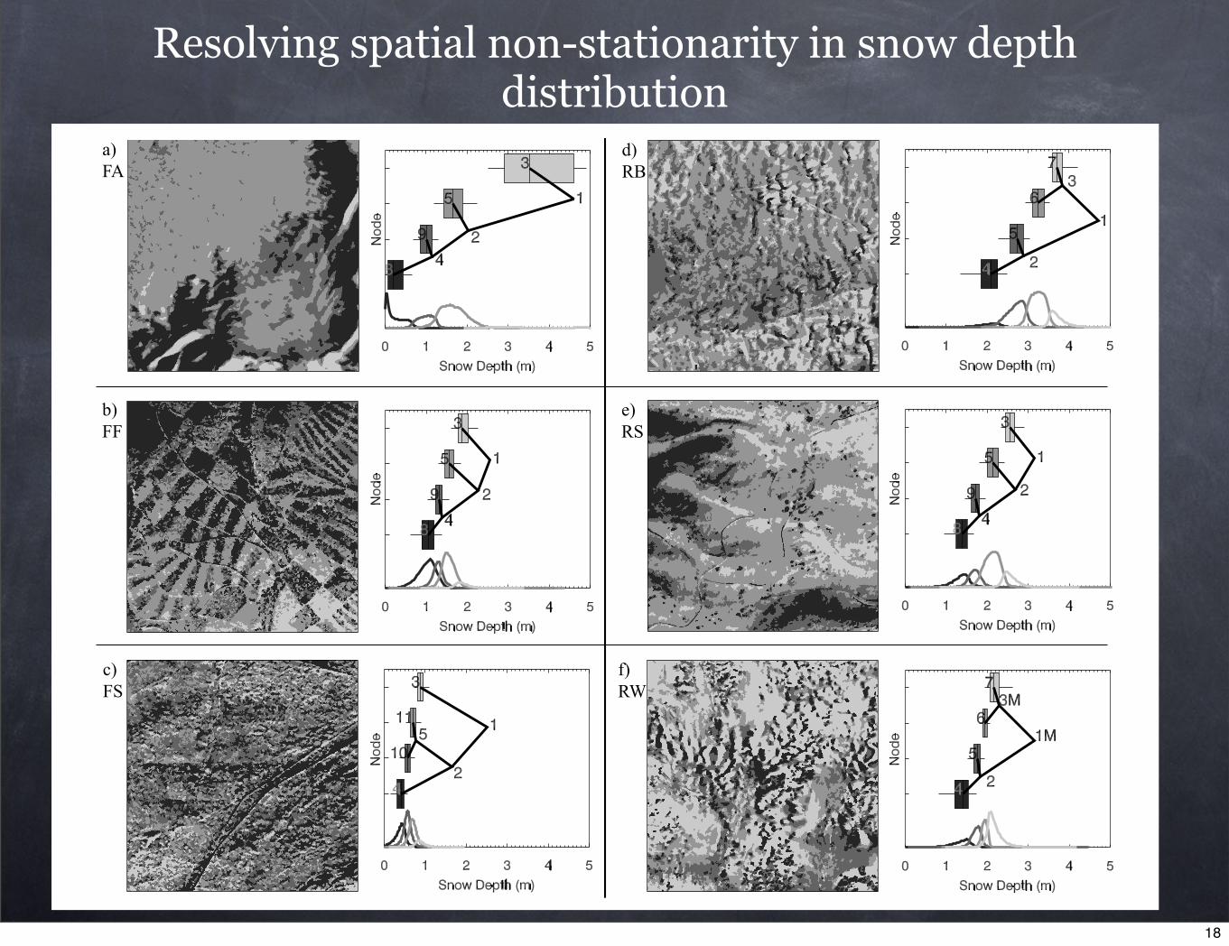
Resolving spatial non-stationarity in snow depth distribution

!"#$

%"#&

'"#(

)"*+

,"**

-"*&

18

New Observations

But what does that get you??

Typically we want an estimate or prediction of some variable from new data, not just a classification.

Classification: assign a new observation to its closest centroid of an existing clustering.

-> CART

19

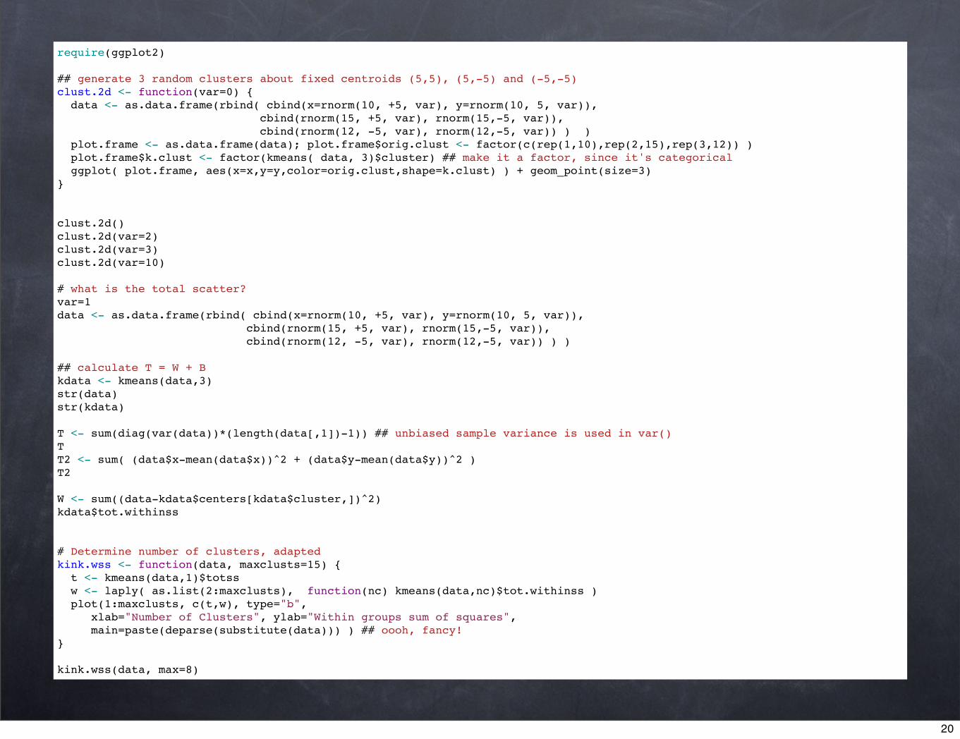
require(ggplot2)

## generate 3 random clusters about fixed centroids (5,5), (5,-5) and (-5,-5)clust.2d <- function(var=0) { data <- as.data.frame(rbind( cbind(x=rnorm(10, +5, var), y=rnorm(10, 5, var)), cbind(rnorm(15, +5, var), rnorm(15,-5, var)), cbind(rnorm(12, -5, var), rnorm(12,-5, var)) ) ) plot.frame <- as.data.frame(data); plot.frame$orig.clust <- factor(c(rep(1,10),rep(2,15),rep(3,12)) ) plot.frame$k.clust <- factor(kmeans( data, 3)$cluster) ## make it a factor, since it's categorical ggplot( plot.frame, aes(x=x,y=y,color=orig.clust,shape=k.clust) ) + geom_point(size=3)}

clust.2d()clust.2d(var=2)clust.2d(var=3)clust.2d(var=10)

# what is the total scatter?var=1data <- as.data.frame(rbind( cbind(x=rnorm(10, +5, var), y=rnorm(10, 5, var)), cbind(rnorm(15, +5, var), rnorm(15,-5, var)), cbind(rnorm(12, -5, var), rnorm(12,-5, var)) ) )

## calculate T = W + Bkdata <- kmeans(data,3)str(data)str(kdata)

T <- sum(diag(var(data))*(length(data[,1])-1)) ## unbiased sample variance is used in var()TT2 <- sum( (data$x-mean(data$x))^2 + (data$y-mean(data$y))^2 )T2

W <- sum((data-kdata$centers[kdata$cluster,])^2)kdata$tot.withinss

# Determine number of clusters, adaptedkink.wss <- function(data, maxclusts=15) { t <- kmeans(data,1)$totss w <- laply( as.list(2:maxclusts), function(nc) kmeans(data,nc)$tot.withinss ) plot(1:maxclusts, c(t,w), type="b", xlab="Number of Clusters", ylab="Within groups sum of squares", main=paste(deparse(substitute(data))) ) ## oooh, fancy!}

kink.wss(data, max=8)

20