regional policy and economic …rri.wvu.edu/wp-content/uploads/2013/07/fullpaper_2.c.1.pdfrate as a...

RECONSIDERING THE REGIONAL EMPLOYMENT CONVERGENCE PROBLEM IN

TURKEY: SPATIAL PANEL DATA ESTIMATION IN AN SUR FRAMEWORK

Pelin AKÇAGÜN Nadir ÖCAL Jülide YILDIRIM Middle East Technical University Middle East Technical University TED University

Department of Economics Department of Economics Department of Economics

Ankara, Turkey Ankara, Turkey Ankara, Turkey

June, 2013

FIRST DRAFT: PLEASE DO NOT QUOTE

Abstract

Even though convergence in regional employment has been a highly debated issue

in the literature, the discussion still remains incomplete as far as sectoral and

spatial interactions are concerned. This paper is an attempt to uncover the

employment convergence problem in Turkey via incorporating time, space and

sectoral heterogeneity under the same framework. For comparison purposes,

standard absolute convergence model as well as an interaction model which

accounts for the sectoral connections is utilized. The model without any spatial,

time and sectoral interaction effects indicates convergence in the agriculture and

industry sectors whereas no significant divergence and convergence are recorded

in the services sector. We argue that exclusion of the relevant factors causes a bias

in the estimated effect of initial employment on the growth rate. Hence, for each

sectoral equation, the neighborhood and time effects are included via spatial panel

data framework. The feasible generalized three stage least squares estimation of

random effects panel data model with spatial error components yields similar

outcomes as to the simple pooled OLS model. Subsequently, we further allow for

the existence of correlation between the estimated spatial panel data models and

employ a spatial panel seemingly unrelated regression model, in which each

sectoral employment convergence equation is related through the

contemporaneous correlation in the disturbances. The estimation results point out

a divergent pattern in the agriculture sector and a convergent trend in the services

sector, which is in line with the preliminary data analysis and the expectations.

Moreover, the interaction model estimated in a spatial panel SUR framework

posits that a lower level of agricultural employment in the initial year has ended

up with higher levels of employment in services sector.

Keywords: Sectoral employment dynamics, spatial panel, spatial panel SUR,

Turkey.

JEL Codes: C33; E24; R12

FIRST DRAFT

Please do not quote

2

1. INTRODUCTION

The persistent disparities in aggregate growth and the large differences in the wealth of Eastern

and Western regions has been the main concern of policy makers in Turkey. Even though the

issue of regional differences and economic development of Turkish economy have been widely

investigated, there is still limited empirical evidence regarding the dynamics of regional

employment. Empirical research on employment in Turkey has been mainly focusing on female

labor force participation (Tunali (1997), Özar and Senesen (1998) and Tansel (2002)). Quite

recently there is a rising interest in the sectoral and regional employment problem as well. Temel

et.al. (2005) uses Markov chain model to show that in the long run convergence clubs are likely

to occur in the agriculture and industry sectors whereas in the services sector global convergence

is expected in Turkey. Öcal and Yıldırım (2008) perform a geographically weighted regression

(GWR) model and observe that there is divergence in the employment rates of provinces for the

1985-2000 period. Filiztekin (2009) uses spatial and nonparametric techniques to show that over

1980-2000 period the gap between the provincial unemployment rates are widening with the

emergence of spatial clusters across Turkey. Berument et. al. (2009) examines the responses of

unemployment rates to various macroeconomic shocks in the economy. They find that

unemployment in agriculture and manufacturing responds in different ways.

This paper is an attempt to uncover the employment convergence problem in Turkey via

incorporating time, space and sectoral heterogeneity under the same framework; focusing on how

the concentration of sectoral employment across 26 Turkish regions has changed over the period

2004-2011. First, a beta convergence analysis of the regional employment rates for

manufacturing, agriculture and services sectors are performed by employing a seemingly

unrelated regression model (SUR). Then this model is extended in order to capture the spatial

aspects of employment dynamics, where spatial dependence is handled in alternative ways.

Spatial variations in the sectoral relationships are examined by means of panel data with spatial

error components and random effects as well as panel SUR model with spatial error components

and random effects. Feasible generalized spatial three stage least squares estimations point out

that the outcomes of the spatial panel SUR model are in line with the preliminary data analysis

and the expectations.

In the literature, it is a common practice to use growth equations in order to investigate the

employment dynamics across regions. However, the discussion would remain incomplete if the

FIRST DRAFT

Please do not quote

3

sectoral and especially the spatial connections are not taken into account. Across the regions,

there are close economic linkages caused by the interdependencies through the access to the

common markets. First of all, these regions often have similar industrial composition and

production technologies. Hence, employment in any region may depend to some extent on the

employment in another region. Any possible shock that could affect one region may possibly

affect other regions that produce similar goods for the consumption at the common marketplace.

A shock to a producer in one region may affect suppliers of intermediate goods in the

neighboring area. Therefore, it can be argued that if there is substantial spatial correlation among

regions, its ignorance may result in biased and inconsistent estimates of the employment

dynamics. Thus, incorporating spatial effects into the analysis may have a significant impact on

the estimated convergence parameters.1

To account for this effect, some scholars employ spatial SUR models as a tool for integrating

limited heterogeneity in the model. These models present spatial equations for different time

periods and allow for correlation between their disturbances, in line with the SUR setting (see

Anselin (1988) for a theoretical discussion; Fingleton (2001), LeGallo & Dall’erba (2006) for

empirical models). In another strand of the literature, panel SUR models are discussed which

include both time and individual effects for each equation and further, a correlation between the

error components of these SUR equations (Avery(1977), Baltagi (1980)). Recently, some studies

consider the spatial extension of this panel SUR system. Wang and Kockelman (2007) employ a

spatial panel SUR model to analyze the crash rates in the transportation of Chinese cities. Baltagi

& Pirotte (2011) make an important contribution by considering various estimators for panel

SUR model with spatial error correlation. Baltagi & Bresson (2011) extend this work by

incorporating spatially lagged dependent variable and proposing Lagrange multiplier tests.

As for the regional employment problem, previous studies mostly handle the issue by forming an

SUR system in which each equation represents different time periods. Hence, they build a space-

time system with variations on time T and cross-section N. On the other hand, this paper aims to

constitute a framework which incorporates an additional dimension: key sectors in the economy.

In this sense it would be an (NTxG) system where G stands for the number of equations in the

system, i.e. three sectors: agriculture, industry and services. The contemporaneous correlation in

1 See for example Glendon and Vigdor (2003), Desmet and Fafchamps (2006) for the importance of spatiality in

employment dynamics.

FIRST DRAFT

Please do not quote

4

the disturbances of each equation will give an idea about the movements of employment across

different sectors.

The paper is composed of five sections: In section 2, we present a brief overview of the labor

market developments in Turkey for the time period under consideration. Econometric

methodology is summarized in section 3. Section 4 presents the empirical results for the

employment convergence problem of Turkey and section 5 concludes.

2. LABOUR MARKET DEVELOPMENTS IN TURKEY

Even though the Turkish population growth rate declined over the last decade, Turkey still has

one of the highest values among the OECD countries. With an average of 1.286 per cent over the

2001-2011 period, the population growth reached the level of 1.343 per cent in 2009 and 1.323

per cent in 2010 (whereas OECD averages are 0.565 and 0.883 per cent respectively)2. In early

1970s Turkey had one of the highest employment rates among the OECD countries, whereas in

2000 the employment rate fell below 50 per cent and under the OECD averages. Employment

rate as a percentage of working age population was 46.3 per cent in 2010 and 48.4 per cent in

2011, as compared to the OECD average of 64.8%. Employment growth over the last two years

has relatively been high, however still lacking behind compensating for high unemployment

rates. Taken as a percentage change from the previous year, employment growth was reported to

be 6.1 per cent in 2010 and 5.9 per cent in 2011 whereas the OECD average was 1.2%. On the

other hand, unemployment rates were recorded as 12.1 per cent and 10.0 per cent in 2010 and

2011 respectively. The historically low participation and employment rates can be attributed not

only to demographic issues and entry problems in the labor market but also to recessions and

structural shifts.

The Turkish labor market has experienced significant changes parallel to the macroeconomic

environment in the country. Until 1980s, Turkey has implemented an import substitution policy

for economic growth. From the early 1980s onwards there has been a change in the

industrialization strategy towards an export-led growth regime via an orthodox structural

adjustment program, aiming the integration of the country into the global economy. Even though

2

The values are derived from various issues of OECD Employment Outlook and OECD Historical Statistics. 2011

values for population growth rate are not announced for some OECD countries; hence for the sake of comparison

2010 values are reported here. However, the descriptive analysis of this study covers the period 2001-2011 in

general.

FIRST DRAFT

Please do not quote

5

export growth increased in post-1980 period, there has been a decrease in the growth rate of

employment compared to the import-substitution period, with a drastic decline in real wages.3

Before 1980 both wages and employment generally moved together. However this parallel

movement has been reversed after 1980s without any significant improvement in the employment

growth. In 1989, following the liberalization of capital movements, government was able to

increase its spending with the help of foreign capital entries. Thus after 1990, increases in real

wages were recorded. Onaran (1999) argues that wage demands of the trade unions were found

acceptable by the employers for two reasons: First, an increase in public spending indicated an

increase in domestic demand. Second, there has been a decline in non-labor input costs due to the

appreciation of the domestic currency so that wages could be increased without undermining

profits. However, with the 1994 financial crisis exchange rate has depreciated sharply with large

interest rate rises, reducing the real wage gains of post-1989 period.

Overall, the suppressed real wages and increased labor market flexibility have not encouraged

high employment growth rates in the post-1980 period. Compared to the import-substitution

period, a lower rate of growth in employment was recorded even though there has been an

increase in export growth. The strategy of export promotion that is based on wage suppression

has not been successful in stimulating new investments which may be due to the volatility of

growth and, consequently, employment growth has been weak in the absence of industrial

restructuring.

During 2000s, this trend of high unemployment rates and low employment generation capacity

persisted, even deteriorated further. The macroeconomic environment of the country had

significantly worsened following the 2001 crisis. In 2001 real GNP fell by 7.4 per cent, consumer

price inflation increased up to 54.9 per cent and Turkish lira (TL) has lost 51% of its value

against foreign currencies. As a result, unemployment rate rose to levels higher than 10 percent

and real wages were reduced by 20 per cent (Yeldan, 2011). In the post-2001 crisis period, poor

job creation, high interest rates, huge appreciation of TL and expanding current account deficits

became the basic patterns of the economy. The elasticity of employment, i.e. percentage gain in

employment with respect to percentage change in GDP growth, was relatively low. International

Labor Organization employment report (Yeldan, 2011) shows that, for the 1989-2008 period,

3 See Onaran and Stockhammer (2005), Voyvoda and Yeldan (2001), Onaran (2000) and Taymaz (1999) for a

review of labor market developments in Turkey.

FIRST DRAFT

Please do not quote

6

employment elasticity is found to be 0.25. But considering two sub-periods, we observe that

during 1989-2000, elasticity was 0.39 whereas between 2002 and 2008, it fell down to 0.14. At

the sectoral level, the effects were far from being homogeneous: the structure of the labor force

has been transforming together with movements out of rural areas to urban areas, resulting a

decrease in agricultural employment and an increase in services employment.

There has been a considerable increase in the employment share of services sector since the

beginning of 2000s. In 2000 even half of the employed people were located in services sector and

this climbed up until 2010 (Figure 1). The agriculture sector, on the other hand has been losing its

significance especially after 2004, holding an employment share within the range of 23 to 30 per

cent. Based on these figures, it can be argued that unemployed labor in the agricultural sector

might have found employment opportunities in the services sector during 2000s. Employment

share in industry sector had a relatively smooth pattern, varying from 23 to 27 per cent over

2004-2011.

Figure 1: Sectoral employment shares in Turkey (2000-2012)

Notes: sersh, indsh and agrsh stand for the employment rates in services sector, industry

and agriculture respectively. Source: Authors’ calculations from Turkish Statistical Institute database.

In this period employment rates at the sectoral level were also non-homogeneous across the

regions. Two immediate observations follow from Figure 2, which presents the regional sectoral

employment rates in 2004 and 20114. First, in both years welfare disparities among regions of

Turkey exhibit themselves in sectoral employment rates as well. Eastern regions and Central

4 Because of the limitations in data availability, the period under investigation is constrained to be 2004-2011. Before

this period, there is lack of data both at regional and sectoral level.

FIRST DRAFT

Please do not quote

7

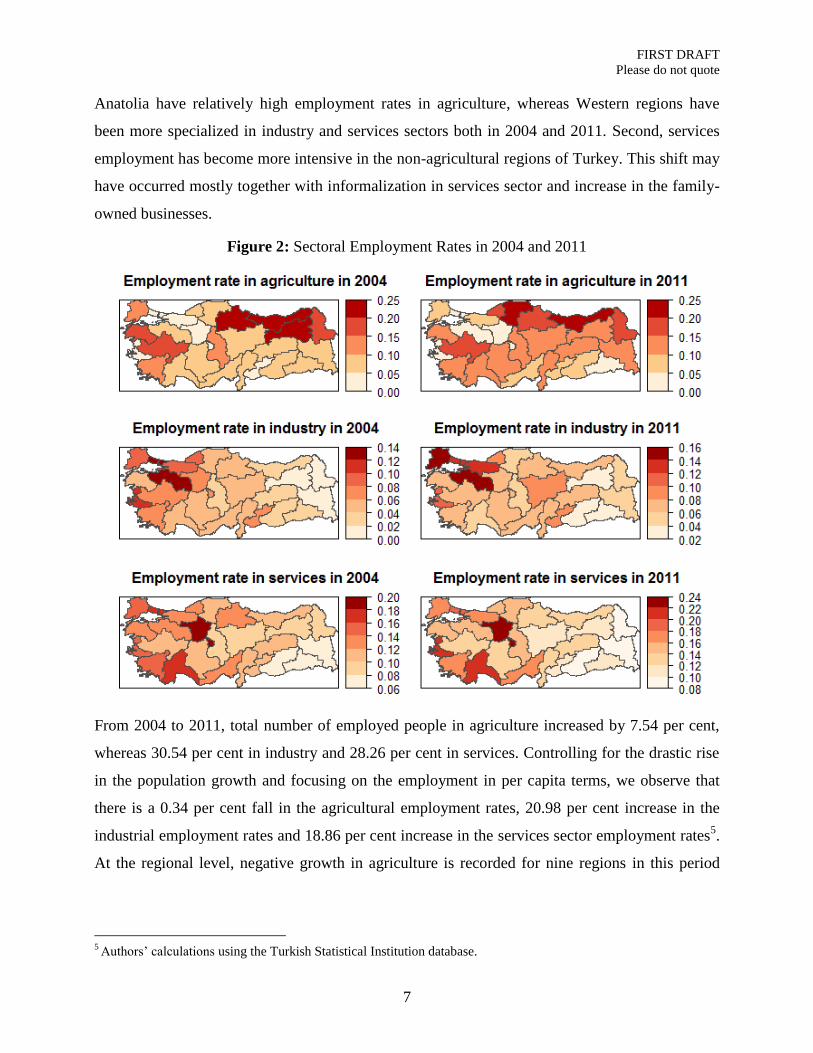
Anatolia have relatively high employment rates in agriculture, whereas Western regions have

been more specialized in industry and services sectors both in 2004 and 2011. Second, services

employment has become more intensive in the non-agricultural regions of Turkey. This shift may

have occurred mostly together with informalization in services sector and increase in the family-

owned businesses.

Figure 2: Sectoral Employment Rates in 2004 and 2011

From 2004 to 2011, total number of employed people in agriculture increased by 7.54 per cent,

whereas 30.54 per cent in industry and 28.26 per cent in services. Controlling for the drastic rise

in the population growth and focusing on the employment in per capita terms, we observe that

there is a 0.34 per cent fall in the agricultural employment rates, 20.98 per cent increase in the

industrial employment rates and 18.86 per cent increase in the services sector employment rates5.

At the regional level, negative growth in agriculture is recorded for nine regions in this period

5 Authors’ calculations using the Turkish Statistical Institution database.

FIRST DRAFT

Please do not quote

8

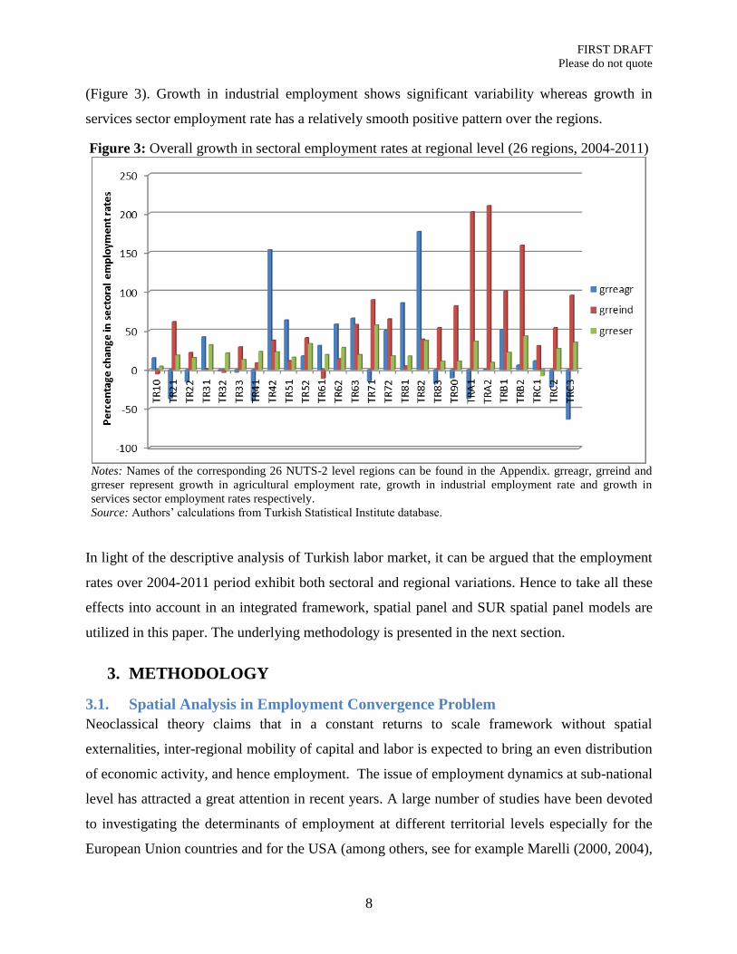
(Figure 3). Growth in industrial employment shows significant variability whereas growth in

services sector employment rate has a relatively smooth positive pattern over the regions.

Figure 3: Overall growth in sectoral employment rates at regional level (26 regions, 2004-2011)

Notes: Names of the corresponding 26 NUTS-2 level regions can be found in the Appendix. grreagr, grreind and

grreser represent growth in agricultural employment rate, growth in industrial employment rate and growth in

services sector employment rates respectively.

Source: Authors’ calculations from Turkish Statistical Institute database.

In light of the descriptive analysis of Turkish labor market, it can be argued that the employment

rates over 2004-2011 period exhibit both sectoral and regional variations. Hence to take all these

effects into account in an integrated framework, spatial panel and SUR spatial panel models are

utilized in this paper. The underlying methodology is presented in the next section.

3. METHODOLOGY

3.1. Spatial Analysis in Employment Convergence Problem

Neoclassical theory claims that in a constant returns to scale framework without spatial

externalities, inter-regional mobility of capital and labor is expected to bring an even distribution

of economic activity, and hence employment. The issue of employment dynamics at sub-national

level has attracted a great attention in recent years. A large number of studies have been devoted

to investigating the determinants of employment at different territorial levels especially for the

European Union countries and for the USA (among others, see for example Marelli (2000, 2004),

FIRST DRAFT

Please do not quote

9

Boeri and Terrel (2002), Perugini and Signorelli (2004), Desmet and Fafchamps, (2005, 2006)).

Beta convergence analysis has generally been employed in order to investigate convergence

across economies or regions using cross-sectional data, implementing the following equation:

0

0

log logiti i

i

EE u

E

(1)

where Eit denotes employment rate at time t, Ei0 denotes employment rate at some initial time 0;

is the intercept term, which may incorporate any rate of technological progress; u is random

error term distributed i.i.d.(0,2), which may represent random shocks to technology or tastes. A

negative value of signifies the beta convergence. However, this approach assumes that all

regions or economies under consideration have the same steady state income path. This is a

highly restrictive assumption and may induce significant heterogeneity bias in estimates of

convergence coefficient. Thus, to control for these effects, panel data counterparts to the

employment convergence problem have been employed. Besides controlling for individual

heterogeneity, panel data models are superior to cross-section models also in the sense that it

allows more informative data, more variability, more degrees of freedom and more efficiency

(Baltagi, 2010a).

Another dimension of the convergence analysis is that regional employment growth may follow a

spatial pattern. Even though the neoclassical model assumes perfect mobility of factors of

production between economies, there may be significant adjustment costs or barriers to mobility

of labor and possibly of capital. When regions pursue their own growth promoting policies, there

may be spillover effects from those regions to the adjacent regions which may affect

employment. Cheshire and Gordon (1998) point that economic rents from research and

development and other sources may more likely to accrue locally, where regions are more self-

contained. Moreover, Fagerberg et al. (1996) claim that rates of technological diffusion may

follow a spatial pattern as regions may have different capacities to create or absorb new

technologies. Thus, incorporating spatial effects into the analysis may have a significant impact

on the estimated convergence parameters.

Hence for the employment convergence problem given in equation (1), the spatial panel data

alternatives are offered for each employment equation. This can be handled in a number of ways.

First, the panel data model can be specified either as fixed effects, where the individual effects

FIRST DRAFT

Please do not quote

10

are constant; or random effects, where the individual effects are allowed to change across cross-

sections. The shortcoming of fixed effects model is that time-invariant variables are wiped out

from the model during the within transformation6. Moreover, there is a great loss in the degrees

of freedom as it needs introducing dummy variables and hence there are too many parameters to

estimate. In this paper, the initial employment rate variable is fixed at 2004 level (time- invariant)

in the original convergence model. Also, as there are data limitations, in order not to lose any

degrees of freedom, a random effects specification has been utilized.

The spatiality can also be introduced into the model in different ways. First, the spatial error

model denotes that the spatial dependence operates through the error process, where any random

shock follows a spatial pattern, so that shocks are correlated across adjacent regions. In this case

the spatial correlation is brought in the error terms of equation (1) through the multiplication of

the spatial weight matrix. Second, the spatial lag (or spatial autoregressive) model examines the

extent to which regional growth rates depend on the growth rates of adjacent regions,

conditioning on the level of initial employment. This model necessitates direct enforcement of

the spatial weight matrix multiplied by the dependent variable as a regressor term. Third, spatial

cross-regressive (or spatial Durbin) model allows any spatial spillovers to be reflected in the

initial levels of employment. In other words, whereas the spatial autoregressive model only takes

the spatial lag of the dependent variable, the spatial Durbin model also takes the spatial lag of the

independent variable. Lastly, a spatial autoregressive model with autoregressive disturbances

(SARAR, or alternatively SAC model as Le Sage (2009) puts it) can be formed. In this case, the

model contains both the spatial error and the spatially lagged dependent variable term. For our

purposes, the spatial dimension is introduced into the model by means of spatial error terms.

Intuitively, this makes much sense regarding the characteristics of the employment problem

mentioned above. A shock to a producer in one region may affect suppliers of intermediate goods

in the surrounding regions (Glendon & Vigdor, 2003). Further, in cases where regions produce

similar goods for consumption in the global market, when the demand for the certain product

changes due to a shock, employment changes tend to occur in several neighboring regions.

Therefore, due to the nature of the employment problem, taking spatial dependence through the

error components of the employment model is found to be convenient.

6 See Elhorst (2003, 2010) and Baltagi (2010b) for a discussion on fixed effects spatial panel data models.

FIRST DRAFT

Please do not quote

11

3.2. Spatial Panel Data Model

The spatial autocorrelation can be introduced into the error component in different ways. Baltagi

et.al. (2003) specifies a SAR process for ,t i whereas Kapoor et.al. (2007) applies the SAR

process to ,t iu first and then take the error components specification to its remainder error term

,t i . In terms of the error component structure, this paper follows the Kapoor et.al.(2007) method.

The random effects spatial error model for employment convergence equation of each sector can

be written as follows:

, , ,

, , , ,

1

, ,

1,..., 1,...,

t i i t i t i

n

t i i j t i t i

j

t i i t i

y X u

u w u i N t T

v

(2)

where ,

,

0,

ln( )t i

t i

i

Ey

E is the growth of employment rate, , 0,ln( )t i iX E is the initial employment

rate for the given sector. ,

1

n

i j

j

w

correspond to each element of the WNxN spatial weights matrix;

,t iu is the spatially autocorrelated error component; 2~ . . (0, )i i i d is the unobservable individual

specific effect, 2

, ~ . . (0, )t i i i d is specified as a one-way error component model and

2

, ~ . . (0, )t i vv i i d vary over both cross-sections and time periods. In line with the random effects

specification, we assume that the individual effects i are uncorrelated with the other explanatory

variables. Note that the spatial autoregressive parameter satisfies 1 .

In stacked form this model can be re-written as:

y X u (3.1)

( )Tu I W u (3.2) (3)

( )T NI v (3.3)

where y denotes the (NTx1) vector of dependent variable, X denotes the (NTxk) vector of

independent variables including the constant term, W denotes the (NxN) spatial weight matrix,

FIRST DRAFT

Please do not quote

12

NI and TI correspond to the identity matrix of order (NxN) and (TxT) respectively; T is the

(Tx1) column matrix of ones and denotes the usual Kronecker product . Hence, from (3.2)

1[ ( ) ]T Nu I I W (4)

and the variance-covariance matrix of u is,

1 1[ ( ) ] [ ( ) ]T

u T N T NI I W I I W

(5)

where TW is the transpose of the spatial weight matrix. The variance-covariance matrix of the

one-way error component model is,

2 2

0 1 1vQ Q (6)

where the usual transformation is applied7:

2 2 2

1

0

1

( )

( )

v

T

T TT N

T

T TN

T

Q I IT

Q IT

(7)8

Kapoor et. al. (2007) show that for 2T , the following moment conditions can be used for the

GMM estimation of the parameters:

7

Note that the model is adopted to the different ordering of the data. Contrary to the usual panel data literature, in

spatial panel data the observations are sorted so that time t is the slow running index and cross-section i is the fast

running index; i.e. the spatial panel data are stacked first by time period, and then by cross-section (see Millo & Piras

(2012) for details).

8 The term

T

T T is usually referred to as TJ in the literature which is in fact a (TxT) matrix of ones.

FIRST DRAFT

Please do not quote

13

0

2

02

0

2

1

12

1

1

1

1

( 1)

1

1( 1)( )

10( 1)

1

1( )

1

0

1

T

vT

T

v

T

T

T

T

T

QN T

QN T

tr W WN

QN TE

QN

tr W WN

QN

QN

(8)

where ( )T Nu I W u ; ( )T Nu I W u ; u u and u u . The first three

moment conditions can be used to compute the initial estimators and 2

v . Based on these initial

estimators and the fourth moment condition,2

1 can be estimated. As a second step one can re-

estimate the parameters using the other set of moment conditions to obtain ̂ ,2ˆv and

2

1̂ . In the

third step the spatial feasible generalized least square estimator for can be obtained, after

transforming the model twice. Initially, the spatial Cochrane-Orcutt transformation is carried out

such that

* 1

* 1

( ) [ ( ) ]

( ) [ ( ) ]

T N

T N

y I I W y

X I I W X

(9)

Then, the model in (9) is further transformed via premultiplying it by 1NTI Q where1

1 v

.

Applying OLS to this transformed model yields the estimator of the final parameter .

For the application, rather than using the full set of moments; the initial estimators based on the

first three moment conditions or the simplified weighting schemes, in which each sample

moment is given equal weights, can also be used. In this paper, though computationally it

complicates the model, using the full set of moment conditions is preferred. Based on this GMM

procedure (or equivalently feasible generalized spatial three stage least squares estimation in our

case), each employment equation is estimated separately for each sector. In other words; for

agriculture, industry and services sectors random effects spatial error models are estimated one

FIRST DRAFT

Please do not quote

14

by one using the described methodology. In the next section, these three estimated sectoral

equations are further allowed to be related via contemporaneous correlation among disturbances.

Hence, it will be possible to observe sectoral interactions through the heterogeneity described by

the error terms of each model.

3.3. Spatial Panel SUR Model

Suppose that the spatial panel data models estimated in section 3.2. for each sector are further

correlated with each other through their disturbance terms. Hence we have the following (NTxG)

system of equations:

, , , ,

, , , ,

1

, , ,

1,..., 1,..., 1,...,

g ti g i g g ti g ti

n

g ti g g ij g ti g ti

j

g ti g i g ti

y X u

u w u i N t T g G

v

(10)

where g=1,…,G is the number of equations (G=3 corresponding to three sectors in our empirical

model, but we solve for the general case in this part); the other variables and estimators described

as before. For an SUR model, the correlations between the disturbances of equations should be

specified. For the error components of this system, we have

, ,

, ,

[ ]

[ ] ,

gh

gh

g i h i

g it h it v

E i and g h

E v v i t and g h

(11)

In order to have an analogous expression to model in (3) we stack the observations over time and

cross sections:

y X u (12.1)

( )g g TG g gu I W u (12.2) (12)

( )g T NG g gI v (12.3)

Note that the subscript “g” is not used for the weight matrix W since the neighborhood relation

does not change over the equations. This can be generalized as gW for different empirical

problems, but for our specific purposes the assumption 1.,..,gW W for g G holds, i.e. for

each employment equation we use the same regions whose neighbors are specified by the same

weight matrix.

FIRST DRAFT

Please do not quote

15

The model in (12) is different from Wang & Kockelman (2007) model in the sense that the

spatial autocorrelation exists in tiu rather than ti . It is more like Kapoor et.al. (2007) spatial panel

model, but revised for an SUR setting. A similar error component structure has been considered

by Baltagi & Bresson (2011); but unlike the one specified here, their model includes a spatial lag

term. The spatially autocorrelated error component in (12.2) can be re-written as:

1[ ( ) ]g TG NG g g

B

u I I W (13)

with

1

.

.

T

T G

I B

B

I B

and g N gB I W

The variance-covariance matrix of u would be

1 1( )T

u B B

(14)

And the variance-covariance matrix of the error component is

0 1 1vQ Q with

1

0

1

v

T

T TT N

T

T TN

T

Q I IT

Q IT

(15)

and

1 12 1

21 2 2

1 2

2

2

2

...

...

. . . .

. . . .

...

G

G

G G G

1 12 1

21 2 2

1 2

2

2

2

...

...

. . . .

. . . .

...

G

G

G G G

v v v

v v v

v

v v v

The estimation of this system requires the estimation of the spatial panel data model. More

concretely, for each equation in the system, the spatial panel data estimation described above will

be applied. Subsequently, the residuals of these estimated equations will be further correlated as

they belong to an SUR system at this time. Hence, after applying GMM estimation for every

FIRST DRAFT

Please do not quote

16

equation (as we did above in part 3.2), we take the estimated disturbances and apply FGLS. The

resulting estimators will be quite informative as it comes from the model that allows for time,

cross-section and equation (i.e. sector) heterogeneity at the same time.

4. EMPIRICAL RESULTS

In this section sectoral employment dynamics are considered for three sectors, namely

agriculture, industry9 and services. These three main sectors are investigated as they constitute

the largest employment shares with their sum giving the total employment in the country (see

Figure 1). Data on the employment levels for the agriculture, industry, services sectors and non-

institutional working age population are obtained from the Turkish Statistical Institute (TurkStat,

2012). We collect data at NUTS-2 level for 26 regions of Turkey over 2004-2011. All variables

are taken as thousand person and sectoral employment rates are calculated based on non-

institutional working age population of each region10

. The empirical analysis incorporates the

sectoral employment rates rather than levels, in order to control for the drastic changes in

population.

The random effects model with spatial error components and its SUR counterpart are estimated

as described in Section 3. For the sake of comparison, the pooled OLS and pooled SUR results

are also provided. The system estimation approach, i.e. seemingly unrelated regression (SUR), is

suggested on the grounds that error terms might be correlated across equations due to the

omission of variables. SUR provides parameter estimates that are asymptotically more efficient

than ordinary least squares estimates when there is contemporaneous correlation between

disturbances of different equations11

. Accordingly, a three equation system is estimated by SUR

in which each equation represents one of the key sectors in the economy:

,

10 11 0 1

, 1

log logi t

i i

i t

EAGREAGR u

EAGR

,

20 21 0 2

, 1

log logi t

i i

i t

EINDEIND u

EIND

(16)

9 Construction is included in the industry sector, during the analysis.

10 Note that the employment rate is the ratio of employed persons to the non-institutional working age population (the

population 15 years of age and over within the non-institutional population, i.e. the population excluding the

residents of dormitories of universities, orphanage, rest homes for elderly persons, special hospitals, prisons and

military barracks etc ). 11

See Zellner (1962).

FIRST DRAFT

Please do not quote

17

,

30 31 0 3

, 1

log logi t

i i

i t

ESERESER u

ESER

where EAGR, EIND and ESER denote employment rates in agriculture, industry and services

sectors, respectively. Moreover, in order to capture any interaction effects among the sectors, an

alternative model has also been considered for each of the specifications:

,

10 11 0 12 0 13 0 1

, 1

log log log logi t

i i i i

i t

EAGREAGR EIND ESER u

EAGR

,

20 21 0 22 0 23 0 2

, 1

log log log logi t

i i i i

i t

EINDEAGR EIND ESER u

EIND

(17)

,

30 31 0 32 0 33 0 3

, 1

log log log logi t

i i i i

i t

ESEREAGR EIND ESER u

ESER

where changes in employment dynamics in each sector are conditioned not only on that sector’s

initial employment rate, but also on other sectors’ initial employment rates.

For the base model introduced in (16) and the interaction model presented in (17), the pooled

OLS and pooled SUR estimation results are presented in Table 1 and Table 2.

Table 1: Pooled OLS estimation results of employment rate convergence model

(with initial employment rates)

Agriculture Industry Services

Coefficients Base Interaction Base Interaction Base Interaction

Intercept -0.050 -0.015 -0.128*** -0.272** -0.005 -0.029

(0.146) (0.943) (0.001) (0.016) (0.928) (0.685)

log(reagr04) -0.024* -0.021 -0.007 -0.003

(0.083) (0.270) (0.481) (0.635)

log(reind04) 0.016 -0.065*** -0.058*** -0.001

(0.654) (0.000) (0.002) (0.936)

log(reser04) -0.009 -0.084 -0.013 -0.022

(0.938) (0.153) (0.659) (0.568)

Residual standard error 0.206 0.208 0.107 0.107 0.068 0.068

N 182 182 182 182 182 182

DF 180 178 180 178 180 178

SSR 7.673 7.664 2.058 2.034 0.833 0.832

MSE 0.043 0.043 0.011 0.011 0.005 0.005

RMSE 0.206 0.208 0.107 0.107 0.068 0.068

FIRST DRAFT

Please do not quote

18

Multiple R-squared 0.017 0.018 0.106 0.116 0.001 0.002

Note: Dependent variables are the logarithms of the yearly growth in employment rates, for each sector. The

values reported in parentheses are p-values. (*), (**), (***) denote significance at 10%, 5% and 1% respectively.

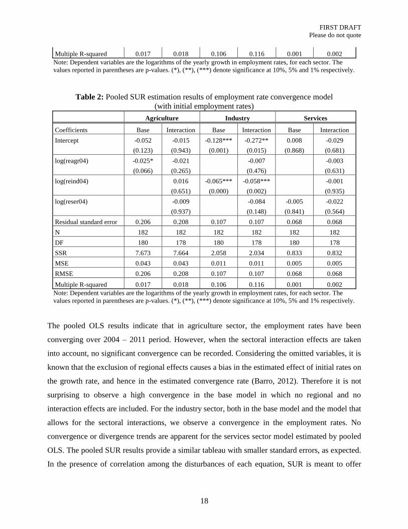
Table 2: Pooled SUR estimation results of employment rate convergence model




Intercept -0.052 -0.015 -0.128*** -0.272** 0.008 -0.029

(0.123) (0.943) (0.001) (0.015) (0.868) (0.681)

log(reagr04) -0.025* -0.021 -0.007 -0.003

(0.066) (0.265) (0.476) (0.631)

log(reind04) 0.016 -0.065*** -0.058*** -0.001

(0.651) (0.000) (0.002) (0.935)

log(reser04) -0.009 -0.084 -0.005 -0.022

(0.937) (0.148) (0.841) (0.564)


N 182 182 182 182 182 182

DF 180 178 180 178 180 178

SSR 7.673 7.664 2.058 2.034 0.833 0.832

MSE 0.043 0.043 0.011 0.011 0.005 0.005

RMSE 0.206 0.208 0.107 0.107 0.068 0.068




The pooled OLS results indicate that in agriculture sector, the employment rates have been

converging over 2004 – 2011 period. However, when the sectoral interaction effects are taken

into account, no significant convergence can be recorded. Considering the omitted variables, it is

known that the exclusion of regional effects causes a bias in the estimated effect of initial rates on

the growth rate, and hence in the estimated convergence rate (Barro, 2012). Therefore it is not

surprising to observe a high convergence in the base model in which no regional and no

interaction effects are included. For the industry sector, both in the base model and the model that

allows for the sectoral interactions, we observe a convergence in the employment rates. No

convergence or divergence trends are apparent for the services sector model estimated by pooled

OLS. The pooled SUR results provide a similar tableau with smaller standard errors, as expected.

In the presence of correlation among the disturbances of each equation, SUR is meant to offer

FIRST DRAFT

Please do not quote

19

more efficient results than the OLS outcome. However, these outcomes are still far from being

sufficient as they ignore the time effects as well as neighborhood effects in the model.

Therefore the spatial panel alternative is presented in Table 3. The neighborhood between the

regions is introduced into the model using the binary contiguity weight matrix12

. FGS3SLS

results are obtained using the methodology described in section 3.2.

Table 3: Spatial panel estimation results of employment rate convergence model




Intercept -0.048* -0.028 -0.125*** -0.278*** -0.004 -0.026

(0.063) (0.870) (0.000) (0.000) (0.860) (0.450)

log(reagr04) -0.023** -0.021

-0.007 -0.003

(0.031) (0.150) (0.173) (0.380)

log(reind04) 0.013 -0.064*** -0.057*** -0.0005

(0.630) (0.000) (0.000) (0.930)

log(reser04) -0.011

-0.089*** -0.012 -0.021

(0.900) (0.006) (0.370) (0.240)

Spatial error component

(rho) -0.125 -0.118 0.122 0.147 0.093 0.084

Note: Dependent variables are the logarithms of the yearly growth in employment rates, for each sector. Random

effects model with spatial error components is estimated by feasible generalized spatial three stage least squares;

full set of moments are used in the estimation. The values reported in parentheses are p-values. (*), (**), (***)

denote significance at 10%, 5% and 1% respectively.

The estimated random effects spatial error model shows that in the agriculture sector there are

convergence dynamics across the regions. Nonetheless, when the initial employment rates in the

other sectors are taken into account, the model indicates neither convergence nor divergence in

the agriculture sector. The effects of other sectors’ initial employment on the agriculture sector

are not significant either. For the industry sector, there is evidence of convergence: the regions

that start over with lower levels of industrial employment show higher rates of growth in

employment rates, i.e. less industrial-labor-endowed regions are catching up the others. The

interaction model shows that agriculture and services sector employment rates in 2004 have a

negative impact on the industrial employment changes in 2004-2011. In the services sector no

12

The neighboring regions take the value of one, whereas the non-neighboring regions take the value zero in the

matrix. The diagonal elements are zero since a region cannot be a neighbor of itself. The weight matrix is row-

standardized so that sum of the elements in each row will add up to one.

FIRST DRAFT

Please do not quote

20

clear evidence of convergence or divergence can be reported as a result of spatial panel model

estimation.

Subsequently, we further allow for the existence of correlation between the estimated spatial

panel data models and estimate a spatial panel SUR model as described before. The SUR

estimation outcomes with random effects and spatial error components are presented in Table 4.

We observe substantial changes in the employment convergence model estimation results of each

sector.

Table 4: Spatial panel SUR estimation results of industrial employment rate convergence model




Intercept 0.008 1.326*** -0.027 -0.120 0.038 -0.250***

(0.820) (0.000) (0.660) (0.405) (0.440) (0.007)

log(reagr04) 0.003 0.104*** 0.035** -0.022**

(0.880) (0.000) (0.012) (0.011)

log(reind04) 0.202* -0.027 0.341*** -0.019

(0.054) (0.240) (0.000) (0.575)

log(reser04) 0.323* -0.649*** 0.012 -0.096*

(0.065) (0.000) (0.680) (0.068)


(rho) -0.125 -0.118 0.123 0.147 0.093 0.084

Note: Dependent variables are the logarithms of the yearly growth in employment rates, for each sector. SUR

model with random effects and spatial error components is estimated by feasible generalized spatial three stage

least squares; full set of moments are used in the estimation. The values reported in parentheses are p-values. (*),

(**), (***) denote significance at 10%, 5% and 1% respectively.

For each sector, base models do not provide any evidence of convergence or divergence in the

employment rates. On the other hand, when the interactions among sectors are introduced,

significant dynamics are documented. In the agriculture sector, the employment rates in the

regions follow a divergent pattern. Likewise, the initial employment rates in industry and services

sectors have a positive impact on the growth of agricultural employment rates. In the industry

sector, also, the model indicates divergence in the employment rates. In fact, these results are in

line with the preliminary data analysis and the descriptive information provided before. What is

more, the spatial autocorrelation in the agricultural equation is negative, which implies that the

regions are conversely affecting each other. This can be regarded as a trend towards clustering in

agricultural employment rather than a homogenization among the regions.

FIRST DRAFT

Please do not quote

21

In the services sector, on the other hand, employment rates show evidence of convergence across

the regions. The agricultural employment rate in the initial year has a negative effect on the

growth in services sector employment rate. This implies that regions with a lower level of

agricultural employment in the initial year has ended up with higher levels of employment in

services over 2004-2011. The results are parallel with the initial observations: the agriculture

sector is more clustered in interior regions and the eastern provinces. The services employment

on the other hand is increasing as a general trend in all regions -though with more concentration

in the western parts of the country. Hence the agriculture and services sectors seem like being on

different sides of the coin.

As a further step, we investigate whether taking the initial employment rate variable in a dynamic

manner would affect the results. To this end, we take the lagged initial employment rate as a

regressor and consider the following two specifications which are analogous to equations (16)

and (17):

,

10 11 , 1 1

, 1

log logi t

i t i

i t

EAGREAGR u

EAGR

,

20 21 , 1 2

, 1

log logi t

i t i

i t

EINDEIND u

EIND

(18)

,

30 31 , 1 3

, 1

log logi t

i t i

i t

ESERESER u

ESER

And the interaction model becomes:

,

10 11 , 1 12 , 1 13 , 1 1

, 1

log log log logi t

i t i t i t i

i t

EAGREAGR EIND ESER u

EAGR

,

20 21 , 1 22 , 1 23 , 1 2

, 1

log log log logi t

i t i t i t i

i t

EINDEAGR EIND ESER u

EIND

(19)

,

30 31 , 1 32 , 1 33 , 1 3

, 1

log log log logi t

i t i t i t i

i t

ESEREAGR EIND ESER u

ESER

The modified base and interaction models have a dynamic initial employment rate variable. The

beta convergence parameters show also the short-run response of the growth rates to the

FIRST DRAFT

Please do not quote

22

employment rates, i.e. the effect from one year to the next can be controlled. The estimation

results of these alternative models are given in Tables 5-8.

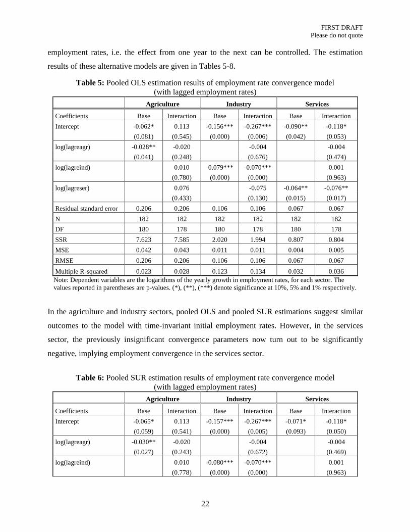
Table 5: Pooled OLS estimation results of employment rate convergence model

(with lagged employment rates)



Intercept -0.062* 0.113 -0.156*** -0.267*** -0.090** -0.118*

(0.081) (0.545) (0.000) (0.006) (0.042) (0.053)

log(lagreagr) -0.028** -0.020 -0.004 -0.004

(0.041) (0.248) (0.676) (0.474)

log(lagreind) 0.010 -0.079*** -0.070*** 0.001

(0.780) (0.000) (0.000) (0.963)

log(lagreser) 0.076 -0.075 -0.064** -0.076**

(0.433) (0.130) (0.015) (0.017)


N 182 182 182 182 182 182

DF 180 178 180 178 180 178

SSR 7.623 7.585 2.020 1.994 0.807 0.804

MSE 0.042 0.043 0.011 0.011 0.004 0.005

RMSE 0.206 0.206 0.106 0.106 0.067 0.067




In the agriculture and industry sectors, pooled OLS and pooled SUR estimations suggest similar

outcomes to the model with time-invariant initial employment rates. However, in the services

sector, the previously insignificant convergence parameters now turn out to be significantly

negative, implying employment convergence in the services sector.

Table 6: Pooled SUR estimation results of employment rate convergence model




Intercept -0.065* 0.113 -0.157*** -0.267*** -0.071* -0.118*

(0.059) (0.541) (0.000) (0.005) (0.093) (0.050)

log(lagreagr) -0.030** -0.020 -0.004 -0.004

(0.027) (0.243) (0.672) (0.469)

log(lagreind) 0.010 -0.080*** -0.070*** 0.001

(0.778) (0.000) (0.000) (0.963)

FIRST DRAFT

Please do not quote

23

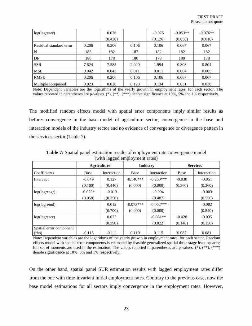
log(lagreser) 0.076 -0.075 -0.053** -0.076**

(0.428) (0.126) (0.036) (0.016)


N 182 182 182 182 182 182

DF 180 178 180 178 180 178

SSR 7.624 7.585 2.020 1.994 0.808 0.804

MSE 0.042 0.043 0.011 0.011 0.004 0.005

RMSE 0.206 0.206 0.106 0.106 0.067 0.067




The modified random effects model with spatial error components imply similar results as

before: convergence in the base model of agriculture sector, convergence in the base and

interaction models of the industry sector and no evidence of convergence or divergence pattern in

the services sector (Table 7).

Table 7: Spatial panel estimation results of employment rate convergence model




Intercept -0.049 0.127 -0.140*** -0.260*** -0.030 -0.051

(0.100) (0.440) (0.000) (0.000) (0.360) (0.260)

log(lagreagr) -0.023* -0.013 -0.004 -0.003

(0.058) (0.350) (0.487) (0.550)

log(lagreind) 0.012 -0.073*** -0.062*** -0.002

(0.700) (0.000) (0.000) (0.840)

log(lagreser) 0.073 -0.081** -0.028 -0.035

(0.390) (0.022) (0.140) (0.150)


(rho) -0.115 -0.111 0.110 0.115 0.087 0.081

Note: Dependent variables are the logarithms of the yearly growth in employment rates, for each sector. Random

effects model with spatial error components is estimated by feasible generalized spatial three stage least squares;

full set of moments are used in the estimation. The values reported in parentheses are p-values. (*), (**), (***)

denote significance at 10%, 5% and 1% respectively.

On the other hand, spatial panel SUR estimation results with lagged employment rates differ

from the one with time-invariant initial employment rates. Contrary to the previous case, now the

base model estimations for all sectors imply convergence in the employment rates. However,

FIRST DRAFT

Please do not quote

24

keeping in mind that these models show only absolute convergence and disregard the presence of

any conditional variable, they may still be suffering from omitted variable bias. The interaction

models are expected to give more precise outcomes not only because of this reason, but also as

they are capable of demonstrating the transition between sectors.

Table 8: Spatial panel SUR estimation results of industrial employment rate convergence model




Intercept -0.068* 1.091*** -0.072 -0.252 -0.153*** -0.711***

(0.097) (0.001) (0.224) (0.151) (0.001) (0.000)

log(lagreagr) -0.031* 0.069** 0.001 -0.055***

(0.081) (0.032) (0.939) (0.000)

log(lagreind) 0.099 -0.046** 0.061 -0.051*

(0.227) (0.049) (0.134) (0.051)

log(lagreser) 0.404*** -0.267*** -0.101*** -0.281***

(0.008) (0.000) (0.000) (0.000)


(rho) -0.115 -0.111 0.110 0.115 0.087 0.081

Note: Dependent variables are the logarithms of the yearly growth in employment rates, for each sector. SUR

model with random effects and spatial error components is estimated by feasible generalized spatial three stage

least squares; full set of moments are used in the estimation. The values reported in parentheses are p-values. (*),

(**), (***) denote significance at 10%, 5% and 1% respectively.

The interaction models estimated by spatial panel SUR shows again the divergence in the

agricultural employment and convergence in the services employment. In the industry sector, the

modified model does not show a significant divergent pattern as before. Hence, industrial

employment at the regional level may have diverged from its value of 2004, but this pattern is not

obvious when yearly changes in the employment rates are accounted for. The effect of services

sector employment in 2004 on the growth rate of industrial employment is found to be

significantly negative.

5. CONCLUSION

This study investigates the regional convergence dynamics of sectoral employment rates in

Turkey over 2004-2011. First, the effects of initial employment rates on the yearly growth in

employment rates are estimated by random effects model with spatial error components, for each

sector. Then, considering the possible contemporaneous correlation between these sectoral

FIRST DRAFT

Please do not quote

25

models, a spatial panel SUR regression is employed. As a further exercise, the initial employment

rates are taken to be dynamic in a modified model with lagged employment rates. For all

specifications, the base model in which the growth in sectoral employment is explained only by

its own initial employment rate and the interaction model in which it is explained also by the

other sectors’ employment rates are compared to the pooled OLS and pooled SUR results.

It is observed that the panel seemingly unrelated regression model with spatial error components

model represents the observed changes in the sectoral employment shares better than the

alternatives. This result is in line with expectations since it offers a comprehensive framework

where time, cross-section and sectoral relations are mutually incorporated. The feasible

generalized spatial three stage least squares estimation outcomes indicate that even though beta

divergent trend is observed in agricultural sector employment for 2004-2011 period, mixed

results are obtained for industry sector employment. In the services sector, there exists evidence

of convergence, which is in line with expectations. The descriptive analyses as well as the

econometric estimations suggest that over the last decade Turkey has experienced a shift towards

services sector, which affects its employment rates positively in all regions. On the other hand,

the agriculture sector is losing its significance and over time it has become more concentrated in

particular regions.

FIRST DRAFT

Please do not quote

26

References

Anselin L. 1988. Spatial Econometrics: Methods and Models. Kluwer Academic Publishers, Dordrecht,

The Netherlands.

Avery R. 1977. “Error Components and Seemingly Unrelated Regressions”. Econometrica 45(1): 199–

208.

Baltagi B. & Bresson G. 2011. “Maximum Likelihood Estimation and Lagrange Multiplier Tests for Panel

Seemingly Unrelated Regressions with Spatial Lag and Spatial Errors: An Application to Hedonic

Housing Prices in Paris”. Journal of Urban Economics 69(1): 24–42.

Baltagi B. & Pirotte A. 2011. “Seemingly Unrelated Regressions with Spatial Error Components”.

Empirical Economics 40: 5-49.

Baltagi B. H. Song, S. H & Koh, W. 2003 “Testing Panel Data Regression Models with Spatial Error

Correlation”. Journal of Econometrics 117: 123-150.

Baltagi B.H. 1980. “On Seemingly Unrelated Regressions with Error Components”. Econometrica 48(6):

1547-1551.

Baltagi, B.H. 2010a. Econometric Analysis of Panel Data, 4th edition, John Wiley&Sons Inc.: Great

Britain.

Baltagi B.H. 2010b. “Spatial Panels”, in Ullah A. and Giles D.E.A. (eds), Handbook of Empirical

Economics and Finance, Chapter 15, Chapman and Hall/CRC, 435-454.

Barro R. J. 2012. “Convergence and Modernization Revisited”. Paper prepared for presentation at the

Nobel Symposium on Growth and Development, Stockholm, September 3-5, 2012.

Berument M.H. Dogan N. & Tansel A. 2009. “Macroeconomic Policy and Unemployment by Economic

Activity: Evidence from Turkey”. Emerging Markets Finance and Trade 45(3): 21-34.

Boeri T, & Terrel K. 2002. “Institutional determinants of labor reallocation in transition”. Journal of

Economic Perspectives 16: 51-76.

Cheshire P.C. & Gordon I.R. 1998. “Territorial competition: some lessons for policy”. The Annals of

Regional Science 32: 321-346.

Desmet K. & Fafchamps M. 2005. “Changes in the spatial concentration of employment across U.S.

counties: A sectoral analysis 1972-2000”. Journal of Economic Geography 5: 261-84.

Desmet K. & Fafchamps M. 2006. “Employment concentration across U.S. counties”. Regional Science

and Urban Economics 36: 482-509.

Elhorst J.P. 2003. “Specification and Estimation of Spatial Panel Data Models”. International Regional

Science Review 26: 244.

Elhorst J.P. 2010. “Spatial Panel Data Models”, in Fischer, M.M. and Getis, A. (eds.), Handbook of

Applied Spatial Analysis: Software Tools, Methods and Applications, Springer-Verlag: Berlin.

FIRST DRAFT

Please do not quote

27

Fagerberg J. Verspagen B. & Marjolein C. 1996. “Technology, growth and unemployment across

European regions”. Regional Studies 31: 457-466.

Filiztekin A. 2009. “Regional Unemployment in Turkey”. Papers in Regional Science 88(4): 863-879.

Fingleton B. 2001. “Theoretical Economic Geography and Spatial Econometrics: Dynamic Perspectives”.

Journal of Economic Geography 1(2): 201–225.

Glendon P.S. Vigdor J.L. 2003. “Thy neighbor’s job: geography and labour market dynamics”. Regional

Science and Urban Economics 33: 663-693.

Kapoor M. Kelejian H. H. & Prucha, I. R. 2007, “Panel Data Models with Spatially Correlated Error

Components”, Journal of Econometrics, 140: 97-130.

Le Gallo J. & Dall’Erba S. 2006. “Evaluating the Temporal and Spatial Heterogeneity of the European

Convergence Process, 1980–1999”. Journal of Regional Science 46(2): 269–288.

LeSage J.P. & Pace R.K. 2009. Introduction to Spatial Econometrics, CRC Press: Boca Raton, FL.

Marelli E. 2000. “Convergence and asymmetries in the dynamics of employment: the case of European

regions”. Jahrbuch fur Regionalwissenschaft/Rev. Reg. Res: 20.

Marelli E. 2004. “Evolution of employment structures and regional specialization in the EU”. Economic

Systems 28.

Millo G. & Piras G. 2012. “splm: Spatial Panel Data Models in R”, Journal of Statistical Software 47(1):

1-38.

OECD Employment Outlook: Various Issues.

OECD Historical Statistics: Various Issues.

Onaran Ö. & Stockhammer E. 2005. “Two different export-oriented growth strategies: distribution and

accumulation a la Turca and a la South Korea”. Emerging Markets Finance and Trade 41(1): 65-

89.

Onaran Ö. 1999. “The wage setting mechanism in private manufacturing industry and its effect on the

flexibility of the labor market in Turkey”. ITU Discussion papers in Management Engineering:

99/5.

Onaran Ö. 2000. “Labor market flexibility during structural adjustment in Turkey”. ITU Discussion

papers in Management Engineering: 00/1.

Öcal N. & Yıldırım, J. 2008. “Employment Performance of Turkish Provinces: A Spatial Data Analysis”.

İktisat İşletme ve Finans 23(266): 5-20.

Özar S. & Günlük-Senesen G. 1998. “Determinants of female (non) participation in the urban labor force

in Turkey”. METU Studies in Development 25(2): 311-328.

Perugini C. & Signorelli M. 2004. “Employment performance and convergence in the European countries

and regions”. The European Journal of Comparative Economics 1(2): 243-278.

FIRST DRAFT

Please do not quote

28

Tansel A. 2002. “Economic development and female labor force participation in Turkey: time-series

evidence and cross-province estimates”. Middle East Technical University, ERC Working Papers

in Economics 01/05.

Taymaz E. 1999. “Trade liberalization and employment generation: the experience of Turkey in the 1980s

in Turkey: Economic Reforms, Living Standards, and Social Welfare Study”, Ana Revenga (ed):

Vol II Technical Papers. Washington D.C.: World Bank.

Temel T., Tansel A. & Güngör N.D. 2005. “Convergence of Sectoral Productivity in Turkish Provinces:

Markov Chains Model”. International Journal of Applied Econometrics and Quantitative Studies

2(2): 65-98.

Tunali I. 1997. “To work or not to work: an examination of female labor force participation rates in urban

Turkey”. Mimeo: Koç University.

TurkStat. 2012. Labor Force Statistics. online data accessed on 9/10/2012. www.tuik.gov.tr

Voyvoda E. & Yeldan E. 2001. “Patterns of productivity growth and the wage cycle in Turkish

manufacturing”. International Review of Applied Economics 15(4): 375-396.

Wang X. & Kockelman K. M. 2007. “Specification and Estimation of a Spatially and Temporally

Autocorrelated Seemingly Unrelated Regression Model: Application to Crash Rates in China”,

Transportation 281–300.

Yeldan E. 2011. “Macroeconomics of Growth and Employment: The Case of Turkey”. International

Labour Organization Employment Sector: Employment Working Paper No.108.

Zellner A. 1962. “An Efficient Method of Estimating Seemingly Unrelated Regressions and Tests for

Aggregation Bias”. Journal of American Statistical Association 57(298): 348–368.

FIRST DRAFT

Please do not quote

29

APPENDIX

NUTS-2 Level Regions and Provinces in Turkey (2004-2011)

NUTS-2 regions Provinces

TR10 İstanbul

TR21 Tekirdağ, Edirne, Kırklareli

TR22 Balıkesir, Çanakkale

TR31 İzmir

TR32 Aydın, Denizli, Muğla

TR33 Manisa, Afyon, Kütahya, Uşak

TR41 Bursa, Eskişehir, Bilecik

TR42 Kocaeli, Sakarya, Düzce, Bolu, Yalova

TR51 Ankara

TR52 Konya, Karaman

TR61 Antalya, Isparta, Burdur

TR62 Adana, Mersin

TR63 Hatay, Kahramanmaraş, Osmaniye

TR71 Kırıkkale, Aksaray, Niğde, Nevşehir, Kırşehir

TR72 Kayseri, Sivas, Yozgat

TR81 Zonguldak, Karabük, Bartın

TR82 Kastamonu, Çankırı, Sinop

TR83 Samsun, Tokat, Çorum, Amasya

TR90 Trabzon, Ordu, Giresun, Rize, Artvin, Gümüşhane

TRA1 Erzurum, Erzincan, Bayburt

TRA2 Ağrı, Kars, Iğdır, Ardahan

TRB1 Malatya, Elazığ, Bingöl, Tunceli

TRB2 Van, Muş, Bitlis, Hakkari

TRC1 Gaziantep, Adıyaman, Kilis

TRC2 Şanlıurfa, Diyarbakır

TRC3 Mardin, Batman, Şırnak, Siirt

Total number: 26 Total number: 81

regional policy and economic …rri.wvu.edu/wp-content/uploads/2013/07/fullpaper_2.c.1.pdfrate as a...

Documents