1

Regional Convergence and Divergence in Europe. Patterns and regularities.

By Per Botolf Maurseth*

July 2013

Key words: Economic growth, convergence, technological change, regional development, spatial dynamics. JEL Classification: 047, 03, R11, R12

Abstract Many studies have focused on spatial patterns in economic growth. For the case of Europe, these studies have indicated that growth is spatially dependent and that clustering as well as de-clustering are parts of economic development processes. The distribution dynamics approach has revealed important characteristics of regional growth. This paper adds to the literature in three ways. First,conditional income distributions are used in a novel way as a basic tool for empirical growth studies. By conditioning income on averages of subsets of the sample, new dimensions of the impact of covariates can be revealed. Second, by applying this methodology on geographical distance, new results on spatial growth patterns in Europe are obtained. It is demonstrated that convergence is pronounced between regions that are far away from each other while there is no convergence between neighbor regions. Third, it is shown how the conditional σ-convergence approach can be extended to other dimensions than the spatial one.

* Department of Economics, Norwegian School of Management (BI) and Department for International Economics, NUPI. email: PerB.Maurseth@nupi.no. Comments and suggestions from Espen Moen, Jørgen Juel Andersen and Roman Römisch and seminar participants at IFN, Stockholm, is greatfully appreciated. The preparation of this paper was supported by the MICRO-DYN project (www.micro-dyn.eu), an independent research project funded by the EU sixth Framework Program.

2

1. Introduction Do income differences between regions and across countries decrease over time or does economic dynamics produce increased and new income differences? These questions are of great importance for understanding economic development and economic growth. In the case of Europe, it is also of interest whether the clustered economic landscape, with clusters of adjacent rich regions and adjacent poor regions, is becoming strengthened or weakened as the consequence of economic integration and enlargement of the European Union. In empirical growth economics, growth regressions constitute the standard approach for revealing driving forces in growth processes. This approach implies regressing growth rates in a cross section or panel data set of regions or countries on a set of potential explanatory variables. Sometimes spatial interdependence and interaction effects are also taken into account. Studies based on regression methodology have revealed many important regularities about cross-sectional patterns of growth. Among these are the existence of conditional convergence and the contributions to growth from many explanatory variables. It has been underlined, however, that the regression approach is only able to reveal parts of the underlying income distribution dynamics: the (conditional) mean. The regression approach is more silent about other aspects of the income distribution (standard deviation, higher order moments, multiple peaks etc). It follows that the relations between these aspects of the distribution dynamics and other variables are not revealed too. A rich research tradition has supplemented the regression approach. One avenue has been to calculate the standard deviation of the income distribution and to report its dynamics (σ-convergence). It is a main result that conditional convergence from the regression approach (β-convergence) does not necessarily imply collapsing income distributions or even decreasing income differences. β-convergence is a necessary but not a sufficient condition for σ-convergence. Danny Quah (e.g. 1993) pioneered a research tradition that focuses on the dynamics of the income distribution itself. He demonstrates how analyses of the distribution dynamics supplement results based on the regression approach. In particular, he estimates discrete fractile Markov chain models for the cross-country income distribution. Quah shows that most observation units stay within their fractile over time. This indicates relative stability in the income distribution despite significant β-convergence revealed by the regression approach. In Quah (1996) the distribution dynamics between geographical neighbors is compared to the distribution dynamics in full samples for European regions. The results indicate that

3

the income distribution between neighbors is tighter (with smaller standard deviation) and has a different dynamics as compared to income distribution for the larger sample. The differing regularities between neighbor conditional income distributions and the unconditional income distributions indicate that growth processes are characterized by spatial interactions. In the last decade, several authors have investigated spatial regularities in growth processes. Fingleton (2001), Fingleton and McCombie (1998) and Rey and Montouri (1999) are early contributions. López-Bazo et al (2004), Rey and Janikas (2005) and Magrini (2004) present overviews of the literature. The existing literature has revealed important results about spatial characteristics of the income distribution dynamics. An important regularity is that growth is spatially contagious. Some results point in the direction that economic dynamics are characterized by both clustering and de-clustering. From empirical studies it seems that spatial patterns in growth processes depend on conditioning variables such as country dummy variables, economic integration, technological factors, industrial composition and geographical localization. These are important research issues since the extent to which such conditioning variables explain spatial patterns of growth indicates whether determinants of growth have spatial patterns or whether growth itself is spatially contagious. In this paper conditional income distributions are used to reveal new aspects about regional growth in Europe. In the next section, the dataset and some basic results are presented, mainly for comparison with the existing literature. In order to ease comparison with this literature, the period analyzed here is from 1995 to 2004. In the third section, relative income distributions normalized along geographical distances are introduced. The conditional income distributions are estimated and compared with each other. The standard deviation of these distributions are calculated and used to infer about conditional σ-convergence and other characteristics of the conditional income distributions. In the fourth section some results based on the above is presented. In section five the conditional relative distributions are calculated for a restricted set of other dimensions than geography (like technology, service specialization and investments). Section six concludes. 2) Basic results. Convergence or divergence? Figures 1 and 2 show basic and well known results for European economic development in recent years. Those figures are based on the regional dataset provided by Eurostat. The data used are income per capita in 255 NUTS 2 level regions among the 25 EU member countries. The time span covered by the data is for the period from 1995 to 2004. The regions are listed in the appendix.1

1 The data are used extensively in the literature. Generally, there is a tradeoff between the numbers of observations and the number of variables since many variables are available for some regions only. In sections 2-4 in this paper, coverage in terms of number of regions is prioritized. When additional variables

4

The first figure show the relationship between average annual growth rates in income per capita and (the log of) initial income levels.2 Also graphed are the linear regression lines. This is a classic figure in the convergence literature. The figure shows whether there is any tendency that initially poor regions grow faster than initially rich regions, a necessary (though not sufficient) condition for income to converge. Figure 1. Convergence or divergence?

.02

.04

.06

.08

.1

8 8.5 9 9.5 10 10.5lgdpc95

growth full samplenew old

The figure reveals a clear and significant negative relationship. This is demonstrated by the downward sloping regression line for the full sample (the steepest regression line). Thus, in the ten years period following 1995 poor regions tended to have higher growth rates than richer regions. Convergence of this type is denoted β-convergence (β denotes the estimated coefficient of initial income levels). This regression result is reported in the first column in table 1 below. During the period covered in the figure the formerly planned economies in Eastern Europe were integrated into the Western European market economy and many countries joined the European Union. In the figure, also separate regression lines for the new member states and the old ones are included. Membership status in the European Union

are included, the number of regions is lower. In section 5 some extra variables are added to the analysis and the coverage of the dataset is therefore lower. The data used in this paper are discussed in appendix 5. 2 The data is for purchasing power parity adjusted gross regional product per capita. See appendix 1 for data description.

5

according to inclusion of these countries will be used as dummy variable on many occasions throughout this paper.3 The figure shows that convergence is present among the old member states but not among the new. In the period covered here, the new member states diverged in their per capita income levels. This is revealed by the positively sloped regression line in the figure which is for a separate regression for the new members. Still the regression line is steeper for the full sample than it is for the regions in the old member states only. The reason is that the new member states are poorer but have higher growth rates than the old member states (on average). Figure 2 shows the development in the standard deviation of (log of) income per capita in the 255 regions sample during the period. There is a clear decrease in the standard deviation over time. This is denoted σ-convergence. Figure 2

Sigma-convergence in Europe

0.35

0.37

0.39

0.41

0.43

0.45

1994 1995 1996 1997 1998 1999 2000 2001 2002 2003 2004 2005

In table 1, a summary of regression results are presented. The dependent variable is annual growth rates in gdp per capita. In all regressions (log of) gdp per capita in the initial year (1995) is included as explanatory variable. The first column reports results when (log of) initial income is the only explanatory variable. The regression line is the one reported for the full sample in figure1. The negative and significant regression

3 The new member states are defined as those that joined the EU in 2004 and in 2007. These are Bulgaria, Cyprus, The Czech Republic, Estonia, Hungary, Latvia, Lithuania, Poland, Slovenia and Slovakia. Those that joined in 1995 (Sweden, Finland and Austria) are denoted ‘old’ together with the remaining countries. Appendix B provides a list of the regions included in the analysis.

6

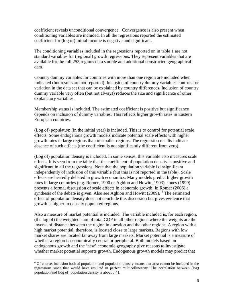
coefficient reveals unconditional convergence. Convergence is also present when conditioning variables are included. In all the regressions reported the estimated coefficient for (log of) initial income is negative and significant. The conditioning variables included in the regressions reported on in table 1 are not standard variables for (regional) growth regressions. They represent variables that are available for the full 255 regions data sample and additional constructed geographical data. Country dummy variables for countries with more than one region are included when indicated (but results are not reported). Inclusion of country dummy variables controls for variation in the data set that can be explained by country differences. Inclusion of country dummy variable very often (but not always) reduces the size and significance of other explanatory variables. Membership status is included. The estimated coefficient is positive but significance depends on inclusion of dummy variables. This reflects higher growth rates in Eastern European countries. (Log of) population (in the initial year) is included. This is to control for potential scale effects. Some endogenous growth models indicate potential scale effects with higher growth rates in large regions than in smaller regions. The regression results indicate absence of such effects (the coefficient is not significantly different from zero). (Log of) population density is included. In some senses, this variable also measures scale effects. It is seen from the table that the coefficient of population density is positive and significant in all the regressions. Note that the population variable is insignificant independently of inclusion of this variable (but this is not reported in the table). Scale effects are heatedly debated in growth economics. Many models predict higher growth rates in large countries (e.g. Romer, 1990 or Aghion and Howitt, 1993). Jones (1999) presents a formal discussion of scale effects in economic growth. In Romer (2006) a synthesis of the debate is given. Also see Aghion and Howitt (2009). 4 The estimated effect of population density does not conclude this discussion but gives evidence that growth is higher in densely populated regions. Also a measure of market potential is included. The variable included is, for each region, (the log of) the weighted sum of total GDP in all other regions where the weights are the inverse of distance between the region in question and the other regions. A region with a high market potential, therefore, is located close to large markets. Regions with low market shares are located far away from large markets. Market potential is a measure of whether a region is economically central or peripheral. Both models based on endogenous growth and the ‘new’ economic geography give reasons to investigate whether market potential supports growth. Endogenous growth models may predict that

4 Of course, inclusion both of population and population density means that area cannot be included in the regressions since that would have resulted in perfect multicollinearity. The correlation between (log) population and (log of) population density is about 0.41.

7

regions being close to large markets receive more technology spillovers than peripheral regions and therefore grow faster. In models such as Romer (1986) and Romer (1990) such predictions follow if one allows technology spillovers to depend on geographical distance. For a specification for regional economic development, see López-Bazo et al. (2004). Jaffe et al. (1993) and Maurseth and Verspagen (2002) (for the case of European regions) give empirical support for geographically bounded spillovers. Economic geography models predict higher income levels in economically central regions and (potentially) agglomeration effects from economic integration (see e.g. Krugman, 1991 a and b). The results reported in table 1 indicate that the effects are the reverse of these predictions: Peripheral regions (in the economic sense) grow faster than other regions. These results support the idea that peripheral regions may benefit from economic integration or, alternatively, that EU regional policies counteract potential centripetal forces. The higher growth rates in peripheral regions is part of the European convergence process. It seen from the table that initial income is negative and significant also when additional explanatory variables are included. But higher growth in peripheral regions weakens the centre-periphery pattern in Europe where the central regions are also the richest ones. In figure A2 in appendix 3 (log of) initial income per capita is graphed against market potential. The figure reveals a positively sloped relationship. The results reported in table 1 indicate that this pattern has weakened over time.5 Last, latitude and longitude (in degrees) are included in the regressions. The estimated coefficients indicate higher growth in northern regions and in eastern regions. Note that this result does not ‘survive’ inclusion of country dummy variables. In some growth empirics, geography is hypothesized as a potential ‘deep’ cause of growth in the sense that it explains both growth and growth’s causes. Frankel and Romer (1999) is one main contribution. A more critical assessment is given by Rodrik et al. (2004). Inclusion of these variables here does not check for such effects, but they serve to map growth processes in Europe and therefore as an extra check for significance of country dummy variables and of market potential. Figures A3 and A4 in appendix 3 indicate that central regions in Europe are the richest ones. The figures reveal an inverse U shape between income per capita and localization along the North-South direction (A3) and along the East-West direction (A4). The geographical data included are based on using a full distance matrix for all regions. Distances in kilometers, dij, for all pairs of regions based on the localization of their main cities were calculated. The resulting distances were used to construct row standardized distance weights of the type:

∑=

= n

j ij

ijij

d

dw

1

1

1 )1

5 Hanson (2005) analyzes market potential in models of economic geography and estimates market potential functions.

8

The weights are the inverse of the distance between two regions weighted by the row sum of all distances. The row standardization makes it possible to construct weighted averages of other variables. The distance weight given in eq. 1) is used as weights in spatial lags regression model. Such a model is of the type:

uWgg )2 +++= γρα X Above, g denotes annual average growth rates. W denotes the distance weight matrix and ρ the spatial autocorrelation coefficient to be estimated. X is the vector of explanatory variables and γ is its vector of coefficients. α is the constant term and u is the residual. A regression model of the type described in eq. 2 cannot be consistently estimated by means of least squares. Instead a maximum likelihood procedure was applied. In table 1 results both when spatial autocorrelation is included and when it is not are reported. In the three last columns, spatial regression results are reported. It is seen from table 1 that when only (log of) initial income is included, spatial lags are present, large and significant. This result remains when other explanatory variables are included. This indicates clustered growth patterns in Europe. Regions that are close to each other seem to have similar growth rates. This result does not, however, remain when country dummy variables are included. Thus, the cluster effects revealed by the positive and significant coefficient of ρ may be a country effect. Some authors do not report results when country dummies are included (see e.g. López-Bazo et al., 2004). In fact, when country dummy variables are included, the spatial autoregressive effect is negative (though not significant). This is counter evidence to spatial growth effects reported by others in the literature. In fact, this result seems more in line with the ‘backwash’ effect proposed by Gunnar Myrdal (1957) than with cluster effects hypothesized in new growth or economic geography economics. One such effect ‘backwash’ effect is that fast growing regions attract inputs (of which skilled labor is one) at the expense of its neighbors.

9

Table 1: Regression results. 1. 2. 3. 4. 5. 6. Lgdpc95 -0.014

(0.000) -0.011 (0.002)

-0.008 (0.024)

-0.011 (0.000)

-0.009 (0.004)

-0.008 (0.018)

Lpop95 -0.001 (0.148)

-0.000 (0.417)

-0.001 (0.259)

-0.001 (0.389)

New 0.008 (0.051)

0.016 (0.222)

0.006 (0.110)

0.016 (0.194)

Lmp -0.008 (0.000)

-0.001 (0.775)

-0.006 (0.001)

-0.001 (0.731)

Lpopdens 0.004 (0.000)

0.003 (0.001)

0.003 (0.001)

0.003 (0.000)

Lat 0.057 (0.000)

0.008 (0.597)

0.046 (0.000)

0.001 (0.563)

Lon -0.015 (0.092)

-0.000 (0.968)

-0.012 (0.136)

-0.000 (0.976)

Dummies No No Yes No No Yes Rho 0.91

(0.000) 0.87

(0.000) -0.08

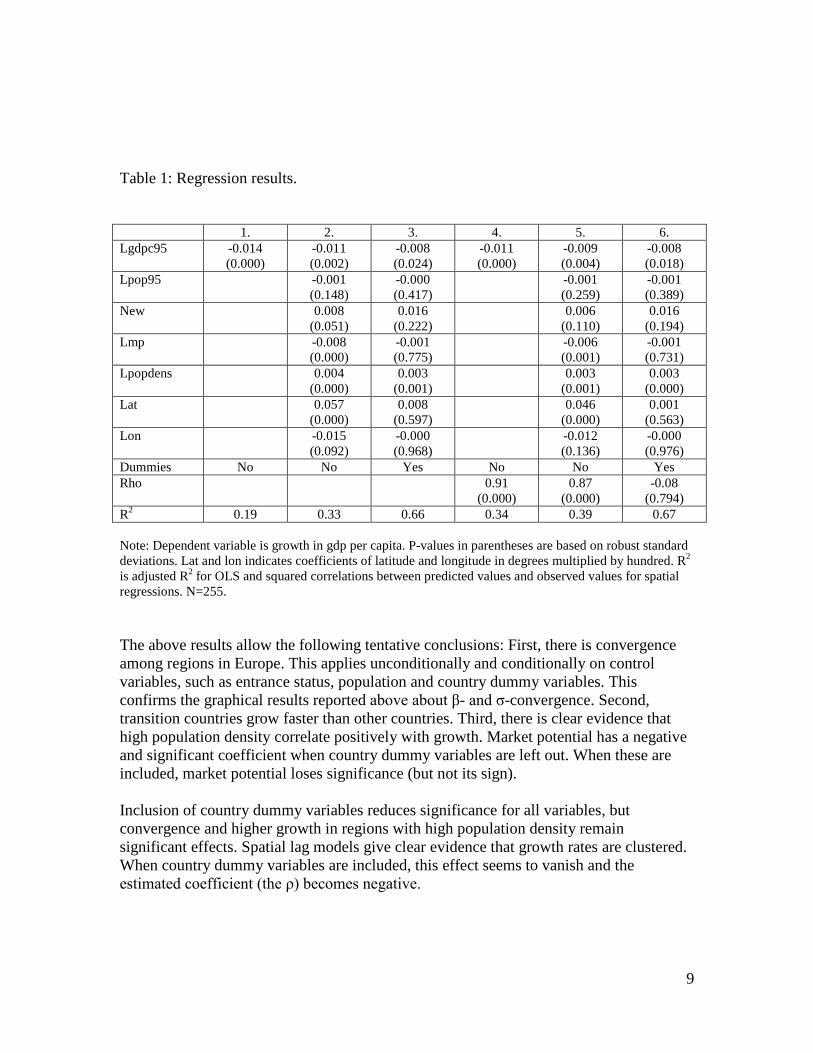
(0.794) R2 0.19 0.33 0.66 0.34 0.39 0.67 Note: Dependent variable is growth in gdp per capita. P-values in parentheses are based on robust standard deviations. Lat and lon indicates coefficients of latitude and longitude in degrees multiplied by hundred. R2 is adjusted R2 for OLS and squared correlations between predicted values and observed values for spatial regressions. N=255. The above results allow the following tentative conclusions: First, there is convergence among regions in Europe. This applies unconditionally and conditionally on control variables, such as entrance status, population and country dummy variables. This confirms the graphical results reported above about β- and σ-convergence. Second, transition countries grow faster than other countries. Third, there is clear evidence that high population density correlate positively with growth. Market potential has a negative and significant coefficient when country dummy variables are left out. When these are included, market potential loses significance (but not its sign). Inclusion of country dummy variables reduces significance for all variables, but convergence and higher growth in regions with high population density remain significant effects. Spatial lag models give clear evidence that growth rates are clustered. When country dummy variables are included, this effect seems to vanish and the estimated coefficient (the ρ) becomes negative.

10

Other contributions have revealed other regularities. As mentioned above, the regressions reported in table is very much dictated by data availability. Table 2 reports results which are more similar to others’ contributions. The regressions reported in table 2 standard variables in growth regressions are included in addition to the ones that were included in the regressions reported in table 1. This comes at the cost of reducing the number of observations. The data used for the regressions in table 2 are constructed to minimize the decrease in the number of observations while including standard variables in the regressions. The data resulted from taking the average over the available yearly observations in the original data set for the each of the new variables introduced in the new regressions. Thus data availability was maximised. The resulting dataset consists of 229 regions. Details of the data construction are reported in the appendix. Capital formation as share of value added is included in the regressions. This variable reflects regions’ investment in physical capital. It’s ‘candidate status’ in growth regressions follows from many growth models both in the neoclassical and the endogenous growth literature tradition.6 Patents per capita are included in log-form. The choice of patents rather than R&D was made because patents are available for more observations than R&D. In addition patents seem to add more explanatory power to the regressions. Share of services in value added is also included. High shares of services may indicate modern economies.7 Table 2 reports five regression results. The first two are OLS regressions when the above variables are included for the cases without (column one) and with (column two) country dummy variables included. The results are qualitatively similar as for the larger data set for the original variables, but the new variables enter with the expected signs. For investments and innovation, the estimated coefficients are significant. The coefficient for share of services in the economy is not significant, however. The third column reports a spatial reference regression. It is run with the same variables as in table 1, but for the smaller dataset. It should be compared with the fifth column in table 1. The results indicate that only small changes in the results occur due to the reduced number of observations. Explanatory power (R2) is larger and the dummy variable for the new member states is less significant. The reference regression is included to illustrate the effect of decreasing the size of the data set. Also the two spatial regressions reported on in column four and five are qualitatively similar to the results reported in table 1. Initial income, the dummy for new member states, market potential (when country dummy variables are not included), population

6 Inclusion of capital formation is more controversial according to for instance Keynesian or some Schumpeterian approaches to economic growth. See e.g. Fagerberg (1994) for an overview. 7 It was experimented with inclusion also of share of agriculture and manufacturing separatively and together. The chosen specification proved to be the one with highest explanatory power and most significant results.

11

density have expected signs and they are significant. When country dummy variables are included, there is significant spatial autocorrelation while this coefficient is negative and insignificant when country dummies are included. The significance of latitude and longitude depends on inclusion of country dummy variables. The new variables in the reduced dataset enter with the expected signs. Investment shares have positive and significant coefficients in all specifications. So have patents per capita. Specialisation in services is almost significant when country dummy variables are absent but not when they are included. Explanatory power of the regression is high. It is seen that the model explains about half of the variation in the data when country dummy variables are not included and three fourth when dummies are included. Comparing column two and three in table 1 with column one and two in table 2 shows that inclusion of investments, technology and service specialisation adds significantly to the explanatory power of the models. Table 2: Regression results. 1. 2. 3. 4. 5. Lgdpc95 -0.017

(0.000) -0.007

(0.022) -0.011

(0.000) -0.015

(0.000) -0.007 (0.014)

Lpop95 -0.001 (0.349)

0.000 (0.841)

-0.001 (0.275)

-0.000 (0.610)

0.000 (0.845)

New 0.013 (0.003)

0.026 (0.000)

0.007 (0.050)

0.010 (0.008)

0.026 (0.000)

Lmp -0.006 (0.000)

-0.004 (0.165)

-0.005 (0.004)

-0.005 (0.005)

-0.004 (0.138)

Lpopdens 0.003 (0.005)

0.002 (0.046)

0.003 (0.001)

0.002 (0.018)

0.002 (0.027)

Lat 0.044 (0.004)

0.017 (0.257)

0.041 (0.001)

0.034 (0.014)

0.017 (0.226)

Lon -0.018 (0.077)

0.004 (0.566)

-0.001 (0.152)

-0.015 (0.096)

0.004 (0.550)

Invest. 0.046 (0.010)

0.053 (0.032)

0.046 (0.005)

0.055 (0.022)

L(pathab) 0.002 (0.004)

0.001 (0.078)

0.002 (0.005)

0.001 (0.062)

Services 0.018 (0.104)

0.011 (0.243)

0.017 (0.085)

0.011 (0.238)

Dummies No Yes No No Yes Rho 0.89

(0.000) 0.88

(0.000) -0.17

(0.531) Adj. r2 0.51 0.75 0.51 0.56 0.75 Note: Dependent variable is growth in gdp per capita. P-values in parentheses are based on robust standard deviations. Lat and lon indicates coefficients of latitude and longitude in degrees multiplied by hundred. R2 is adjusted R2 for OLS and squared correlations between predicted values and observed values for spatial regressions. N=229.

12

As mentioned in the introduction many have raised objections against regression based methodology. Growth regressions are useful for many purposes, but the following are regarded as important arguments why also supplementary methodology should be used. First: spatial lags and any types of interaction between regions contradict regressions based methodology. The OLS regressions reported in tables 1 and 2 have as basic premise that the observations are independent from each other. Any textbook in econometrics underlines the premise that the residuals are independent of each other. Naturally, they are not. Labour, capital, services, physical goods and ideas flow across and between regions. Thus growth rates in one region depends on growth rates in other regions. Spatial regression techniques are one way to capture such interaction. Interaction between regions and countries, however, is not always correctly described with spatial regressions techniques. The above estimations of ρ depend on very restrictive assumptions about the growth dynamics. Second: regression models capture (conditional) average tendencies. Higher order dimensions of the income distributions are not described with regression based methodology. Neither bias nor kurtosis is evaluated with regressions techniques. Even though innovative regions on average are richer and grow faster than other regions, that result does not preclude multiple peaked distributions or other types of anomalies for subsets of the data. There have been many attempts at exploring other dimensions of income distribution dynamics in the literature on cross country and cross region economic development. See e.g. Quah (1996 and 1997), Johnson (2000) and Juessen (2009) or the overview provided by Magrini (2004). One such tradition in the literature is illustrated with figure 3. That figure shows Kernel distribution density estimates figures for regional income distribution developments in Europe. The methodology on which the figure is constructed can be compared with an advanced histogram in which the bars are made as advanced moving averages of each other. Kernel distributions approximate a hypothesised real (logarithmic) income distribution (see e.g. STATA, 2007).

13

Figure 3. Kernel density figures for income across regions in Europe.

0.5

11.

5

-1.5 -1 -.5 0 .5 1lrel95

density: lrel95 density: lrel04

The figure is constructed for (log of) relative income levels but so that so that the average is zero (see Section 3). The figure graphs these estimated kernel distributions for 1995 and for 2004. The figure indicates that what was observed as convergence in Europe in the time span considered here was a mass shift from the left tail towards the centre of the distribution. Of course, this reflects high growth in transition countries (partly reflected by the effect of the dummy variable New member above). Obviously, the above figure reveals supplementary aspects of income distribution dynamics as compared to figures 1 and 2. It is seen that the regional income distribution in Europe is in transformation from a doubled peaked distribution to a single peaked distribution. The distribution has become tighter with the (highest) peak becoming higher. Note that the (highest) peak in the distribution has shifted a bit leftwards. This represents a mass shift and should not be confused with changing means. The mean is normalised to be equal to zero. A large literature has emerged employing methodology similar to the type figure 3 is based upon (see the references cited above). In the next section, a novel methodology for constructing figures like the one above for conditioned income distributions is proposed. It consists of constructing relative income distributions conditioned on explanatory variables. Thus, conditional convergence or divergence can be explored also for higher order moments (than the first) of the income distribution.

14

3. Methodology Above, normalising with the average gave rise to a distribution with zero mean and with some interesting dynamics over time. Let yi denote income per capita in region i. The distribution graphed in figure 3 is the one given by equation 1. This is different (rescaled) from the commonly used distribution in many studies of economic convergence which is simply the logarithm of the ratio of income per capita to the mean. The standard distribution used in the literature is given by equation 2. This standard distribution is normally distributed when income is lognormal. Generally however, income is not exactly lognormal. The approach taken here (eq. 1) ensures distributions that are scaled so that their means equal zero. Below, where income distributions are conditioned on other variables, this becomes crucial in order to compare effects of such conditioning. This is further discussed in appendix 2.

( ) ( ) ( ) ( )

( ) ( ) ( )

( ) ( ) ( ) ( )yyyn

y

yn

yy

yn

yyy

n

jji

n

jji

n

jjiii

lnlnln1ln yyln-

yyln )3

1lnlnlnyln yyln )2

ln1lnlnln )1

1

ii

1i

i

1

+−−=

−=−=

−=−

∑

∑

∑

=

=

=

Note that eq.1) is the same as eq. 3). Normalising with the average is not the only normalisation possible however. One can normalise with many other types of variables. In that case, eq. 3 is the recipe for rescaling distributions to common means. The methodology is simple and can be explained as follows: Take a variable characterising a pair of regions, qij. This variable can be dichotomous, so that it defines regions belonging to the same country or to different countries . In this case qij can equal one or zero. qij can qualitative characteristics of the data (such as if both, none or only one of the two regions belong to new member countries in the EU). But qij can also be a measure of interaction between the two regions, like trade, technology spillovers or it can just be geographical distance. And qij can be a constructed variable of how the two regions differ with respect to any explanatory variable. In total there will be n2 observations of qij, where n is the number of observations of regions or countries.8 The observations of qij can be partitioned into discrete values according to their value. Assign such discretisised values of qij to any pair of regions. On the basis of this assignment, new relative income per capita distributions can be constructed for each discrete value of qij according to the formula:

8 There are n2 observations. For many purposes (like for some applications reported on below) use only of the n2-n variables for different regions is the obvious choice.

15

∑∑∑

∑

−

=−=

=

=

==

±±∗

=

±

n

iqn

jiqj

i

i

iqn

jiqj

i

iiqiqiq

n

jiqj

i

iiq

ii

i

yn

yny

n

yyyy

yn

yy

11

1

1ln1

1ln )5

Q1,...,q ,1

ln 4)

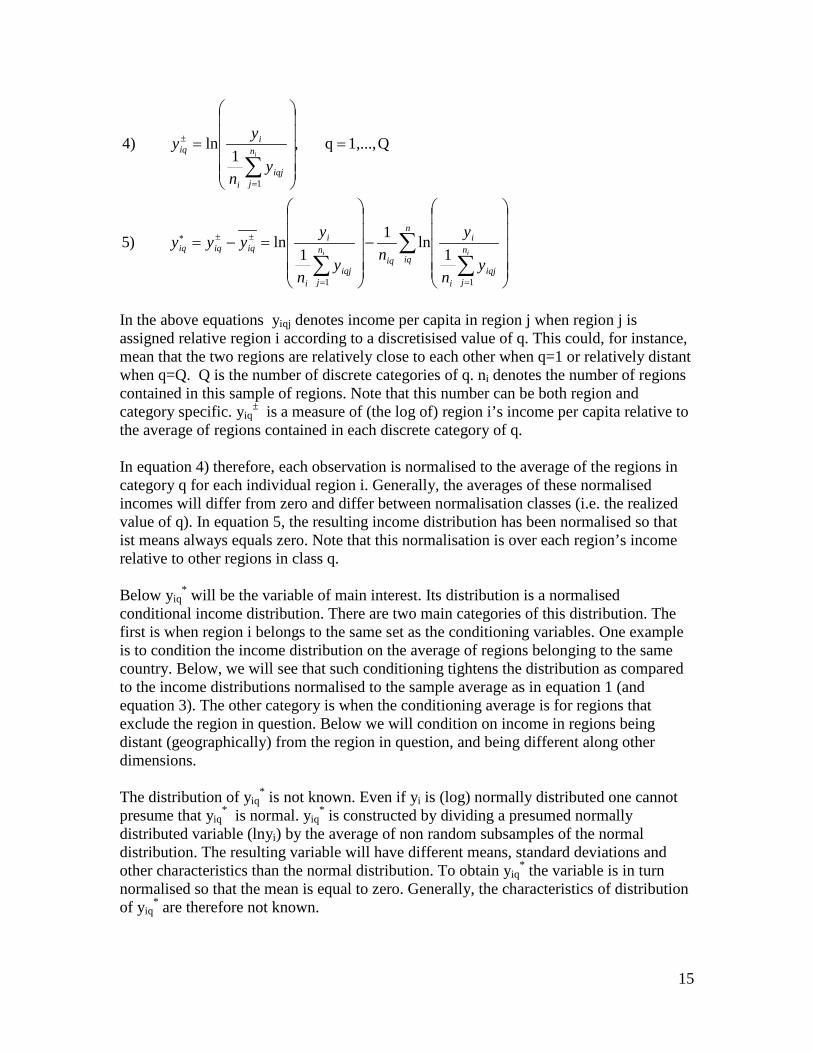
In the above equations yiqj denotes income per capita in region j when region j is assigned relative region i according to a discretisised value of q. This could, for instance, mean that the two regions are relatively close to each other when q=1 or relatively distant when q=Q. Q is the number of discrete categories of q. ni denotes the number of regions contained in this sample of regions. Note that this number can be both region and category specific. yiq

± is a measure of (the log of) region i’s income per capita relative to the average of regions contained in each discrete category of q. In equation 4) therefore, each observation is normalised to the average of the regions in category q for each individual region i. Generally, the averages of these normalised incomes will differ from zero and differ between normalisation classes (i.e. the realized value of q). In equation 5, the resulting income distribution has been normalised so that ist means always equals zero. Note that this normalisation is over each region’s income relative to other regions in class q. Below yiq

* will be the variable of main interest. Its distribution is a normalised conditional income distribution. There are two main categories of this distribution. The first is when region i belongs to the same set as the conditioning variables. One example is to condition the income distribution on the average of regions belonging to the same country. Below, we will see that such conditioning tightens the distribution as compared to the income distributions normalised to the sample average as in equation 1 (and equation 3). The other category is when the conditioning average is for regions that exclude the region in question. Below we will condition on income in regions being distant (geographically) from the region in question, and being different along other dimensions. The distribution of yiq

* is not known. Even if yi is (log) normally distributed one cannot presume that yiq

* is normal. yiq* is constructed by dividing a presumed normally

distributed variable (lnyi) by the average of non random subsamples of the normal distribution. The resulting variable will have different means, standard deviations and other characteristics than the normal distribution. To obtain yiq

* the variable is in turn normalised so that the mean is equal to zero. Generally, the characteristics of distribution of yiq

* are therefore not known.

16

By means of bootstrapping methodology, some of the characteristics of the distribution of yiq

* may be explored, however. Bootstrapping methodology essentially means constructing a large sample from the empirical sample by drawing subsamples (with replacement) from the empirical sample (many) several times. The resulting samples are then observations from the larger (theoretical) sample. Based on those observations, some characteristics of the underlying distributions can be revealed. Of particular interest is the standard deviation of yiq

* and its development over time. For the purpose of this paper, the standard deviation obtained after bootstrapping is of particular importance. This standard deviation is used to construct confidence intervals for the standard deviations of the conditional income distributions. Reduced standard deviation is denoted conditional σ-convergence. Conditional σ-convergence implies reduced dispersion of income between regions belonging to specific values of qij. Differences in the standard deviation of yiq

* can easily be explored by means of bootstrapping. The resulting confidence intervals can be used to test whether changes in standard deviations in the conditional distributions are significant. The construction of yiq

* therefore make it possible to study σ-convergence systematically along various dimensions. The methodology proposed here differs from the standard conditional income distribution approach in the literature. That approach most often analyse the extent to which income distributions tightens when conditioning on common characteristics for the observational units. Many have for instance analysed the fact that neighbours have a tighter income distribution than the unconditional distribution (Quah, 1996) or that country conditional income distributions (income divided by national averages) are tight (Boldrin and Canova, 2001). Closer to the present methodology is (Quah, 1997) in which two dimensional stochastic kernel distributions are presented. There, for instance trade between countries are used as conditioning variables. Trade patterns are not used to draw inferences on the income distribution. Rather the conditioning scheme is used to establish that “rich countries trade mostly with other rich ones: and, interestingly, the very poorest countries, mostly with rich ones again.” In Magrini (2004) and in Quah (1997) two dimensional kernel distributions are presented and it is demonstrated that neighbours have tighter income distributions than the (unconditioned) mean conditioned distributions. The existing literature therefore, often reports results for the cases when Q=1 in equation 4, but is more silent about the distributions for which Q=2 and Q has higher values. 4. Convergence and geography Figure 4 shows a typical result from using the methodology described in section 3. The kernel density estimates are for two alternative income distributions for 1995. The first is when it is normalised according to the full sample average, like in figure 3. The second is when income is normalised to each region’s national average. As such this figure also exemplifies standard approaches in the existing literature.

17

Figure 4 shows that conditioning income to the national average tightens the income distribution. Note that the averages (means) of the two distributions by construction are the same and equal to zero. Country belonging explains a fair amount of income differences between regions. This reflects the regression result reported in table 1. There, inclusion of country dummy variables increased explanatory power in the regression at the cost of significance of all other variables. But figure 4 adds information: In essence, the country conditional distribution has a higher peak and it is more symmetric than the distribution for the whole sample. The different localisations of the distributions’ peaks are due to different symmetry, not different means. The distribution for the full sample seems to double peaked. This, of course, reflects the new member states. In appendix 4, bootstrapping estimates for standard deviations of the conditioned income distributions are reported. Also 95 per cent confidence intervals are reported. A strict but intuitive test for significance of differences in standard deviations is when 95 per cent confidence intervals do not overlap. In this paper, this will be the chosen criterion for testing whether standard deviations are different. For our full sample the 95 per cent confidence interval for the standard deviation is (0.40, 0.48). For the country conditioned income distribution, the confidence interval is (0.19, 0.24).The standard deviations are therefore significantly different. Figure 4 Kernel estimates for unconditioned and country conditioned income.

0.5

11.

52

2.5

-1.5 -1 -.5 0 .5 1gdp 95

density: gdp 95 density: country conditioned gdp 95

The separate distributions for the new and the old member states in 1995 are shown in figure 5. That figure shows that regions in the new member states have a wider income distribution than regions in the old member states. Again, the means are similar, so the different locations of the peaks are because the distributions are not symmetric. The confidence intervals for the standard deviations of the two regions are just barely overlapping. Therefore, the two distributions indicate larger (but not significantly so)

18

income differences among the new members states as compared income differences among the old ones. Figure 5. Kernel estimates for new and old member states.

0.5

11.

52

-1.5 -1 -.5 0 .5 1gdp 95

density: lcrelN95 density: lcrelO95

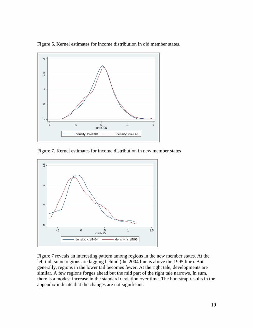
Figures 6 and 7 show developments over time. In figure 3 the distribution for the full sample in 1995 and in 2004 was compared. That figure reveals modest convergence in the sense that the distribution tightened during the period covered here. Poor regions in the left tale of the distributions become fewer in numbers. Figure 6 and 7 show that convergence is absent for the separate distributions for new and old member states. Regions in the new and the old member states do not converge. For the old member states (figure 6) the estimated distribution is remarkable stable. The observed convergence in the full sample, therefore, is because differences among the newcomers grow when some of them have high growth rates and reach high income levels (cfr. figure 7).9 Since these regions initially were generally poor, the consequence is reduced differences in the full sample. The bootstrap results reported in the appendix show that these developments are not statistically significant, however. Income distributions (both in 1995 and in 2004) among the new member countries display statistically significantly higher standard deviations than the ones for regions belong to the old member countries.

9 This is the Kuznets mechanism studied in detail in Kuznets (1973).

19

Figure 6. Kernel estimates for income distribution in old member states.

0.5

11.

52

-1 -.5 0 .5 1lcrelO95

density: lcrelO04 density: lcrelO95

Figure 7. Kernel estimates for income distribution in new member states

0.5

11.

5

-.5 0 .5 1 1.5lcrelN95

density: lcrelN04 density: lcrelN95

Figure 7 reveals an interesting pattern among regions in the new member states. At the left tail, some regions are lagging behind (the 2004 line is above the 1995 line). But generally, regions in the lower tail becomes fewer. At the right tale, developments are similar. A few regions forges ahead but the mid part of the right tale narrows. In sum, there is a modest increase in the standard deviation over time. The bootstrap results in the appendix indicate that the changes are not significant.

20

In section 3 it was demonstrated that income can be conditioned also with respect to geographical distance (and other variables). Figure 8 through 14 shows results based on this idea. The 255*254 distance matrix (excluding the diagonal elements) (or really long list, in panel data terminology) was divided into ten equally numbered parts (centiles) according to increasing distances between the regions.10 Regions in the first centile are close to each other. Regions in the tenth centile are far away from each other. Figures 8, 9 and 10 show distance conditioned income distributions for 1995 for distance classes 1, 5 and 10 respectively compared with the distribution for the full sample. Figure 8. Kernel estimates for regions that are ‘neighbours’ compared to the full sample.

0.5

11.

52

-1.5 -1 -.5 0 .5 1gdp 95

density: lcrel951 density: gdp 95

Figure 9. Kernel estimates for regions that have mid-distances between them compared to the full sample.

0.5

11.

5

-1.5 -1 -.5 0 .5 1gdp 95

density: lcrel955 density: gdp 95

10 The number of observations is 255x254 since zero observations were excluded, so that the region in question did not enter the conditioning mean.

21

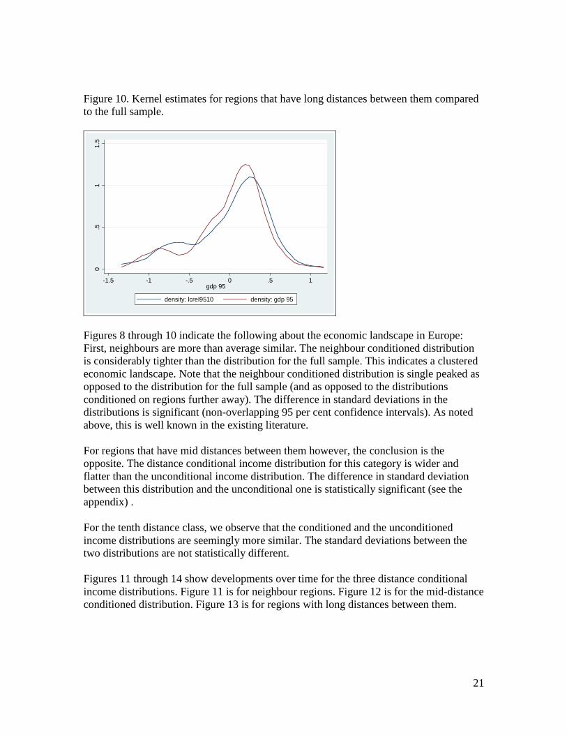
Figure 10. Kernel estimates for regions that have long distances between them compared to the full sample.

0.5

11.

5

-1.5 -1 -.5 0 .5 1gdp 95

density: lcrel9510 density: gdp 95

Figures 8 through 10 indicate the following about the economic landscape in Europe: First, neighbours are more than average similar. The neighbour conditioned distribution is considerably tighter than the distribution for the full sample. This indicates a clustered economic landscape. Note that the neighbour conditioned distribution is single peaked as opposed to the distribution for the full sample (and as opposed to the distributions conditioned on regions further away). The difference in standard deviations in the distributions is significant (non-overlapping 95 per cent confidence intervals). As noted above, this is well known in the existing literature. For regions that have mid distances between them however, the conclusion is the opposite. The distance conditional income distribution for this category is wider and flatter than the unconditional income distribution. The difference in standard deviation between this distribution and the unconditional one is statistically significant (see the appendix) . For the tenth distance class, we observe that the conditioned and the unconditioned income distributions are seemingly more similar. The standard deviations between the two distributions are not statistically different. Figures 11 through 14 show developments over time for the three distance conditional income distributions. Figure 11 is for neighbour regions. Figure 12 is for the mid-distance conditioned distribution. Figure 13 is for regions with long distances between them.

22

Figure 11. Kernel density estimates for neighbours’ income distribution, 1995 and 2004.

0.5

11.

52

-1.5 -1 -.5 0 .5 1gdp 95

density: lcrel951 density: lcrel041

Figure 12. Kernel density estimates for income distribution for regions with mid distances between them, 1995 and 2004.

0.2

.4.6

.81

-1.5 -1 -.5 0 .5 1gdp 95

density: lcrel955 density: lcrel045

23

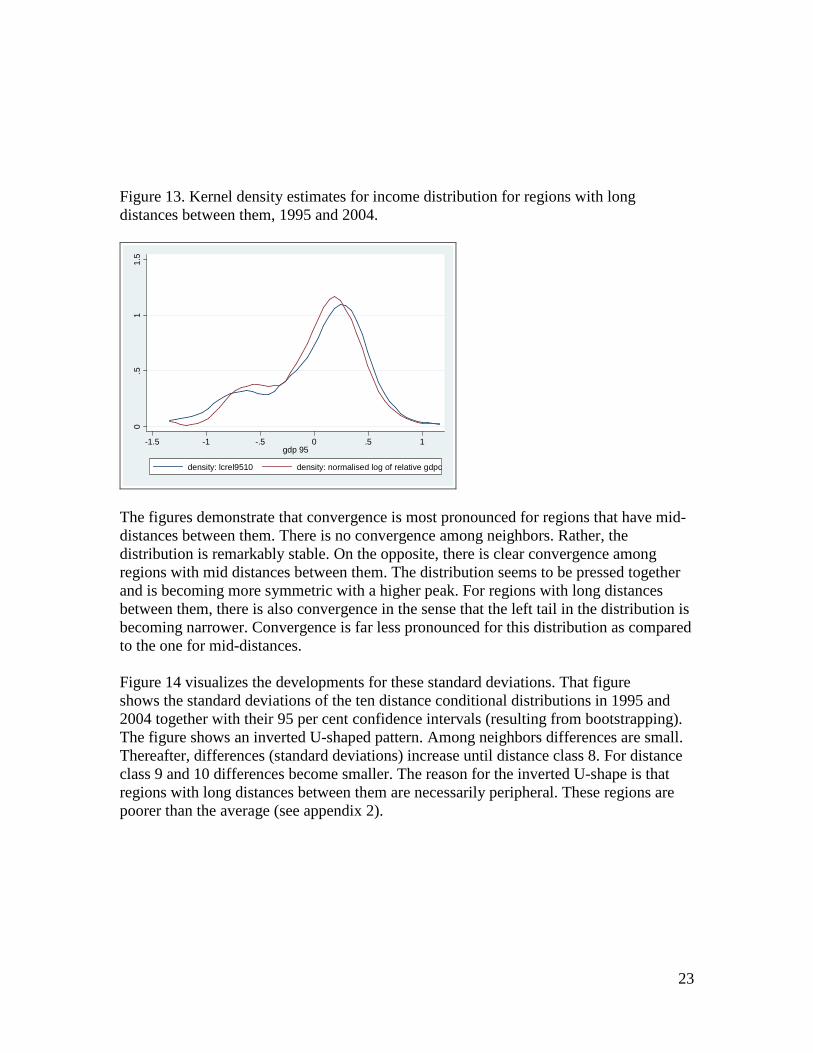
Figure 13. Kernel density estimates for income distribution for regions with long distances between them, 1995 and 2004.

0.5

11.

5

-1.5 -1 -.5 0 .5 1gdp 95

density: lcrel9510 density: normalised log of relative gdpc

The figures demonstrate that convergence is most pronounced for regions that have mid-distances between them. There is no convergence among neighbors. Rather, the distribution is remarkably stable. On the opposite, there is clear convergence among regions with mid distances between them. The distribution seems to be pressed together and is becoming more symmetric with a higher peak. For regions with long distances between them, there is also convergence in the sense that the left tail in the distribution is becoming narrower. Convergence is far less pronounced for this distribution as compared to the one for mid-distances. Figure 14 visualizes the developments for these standard deviations. That figure shows the standard deviations of the ten distance conditional distributions in 1995 and 2004 together with their 95 per cent confidence intervals (resulting from bootstrapping). The figure shows an inverted U-shaped pattern. Among neighbors differences are small. Thereafter, differences (standard deviations) increase until distance class 8. For distance class 9 and 10 differences become smaller. The reason for the inverted U-shape is that regions with long distances between them are necessarily peripheral. These regions are poorer than the average (see appendix 2).

24

Figure 14. Distance-conditional convergence in Europe.

.2.3

.4.5

.6

0 2 4 6 8 10distance

high95/low95 high04/low04stdev95 stdev04

Note: The two inverted U-shaped grpahs indicate standard deviation of distance conditioned income levels. The vertical lines are the estiamted 95 per cent confidence interval based on bootstrapping. It is also seen that convervence is strongest for regions with mid-distances between them, Convergence is absent for neighbour regions (as was indicated in figure 11). The confidence intervals for the standard deviations between the two periods are almost everywhere overlapping. Still, the pattern is clear: There is convergence in Europe and most so for regions that are located at some distance apart from each other. Thus, Europe is becoming de-clustered in the spatial sense. Figure 15 and 16 qualifies this conclusion. These figures are Moran scatter plots of regional GDP per capita in 1995 and 2004. Moran scatter plots show (normalised) income levels among the regions along the horisontal axis and a normalised distance-weighted average of the other regions GDP per capita along the veritcal axis. The distance weights used here are the same as the one used for the spatial regression results reported in table 1. Regions in the upper-right quadrant are rich regions with rich neighbours. Regions in the lower-right quadrant are rich regions with poor neighbours. Regions in the lower-left quadrant are poor regions with poor neighbours. The interpretation of the fourth quadrant follows.

25

Figure 15: Moran scatter plot. GDP per capita 1995.

Moran scatterplot (Moran's I = 0.189)gdp 95

Wz

z-3 -2 -1 0 1 2 3

-2

-1

0

1

Figure 16: Moran scatter plot. GDP per capita 2004.

Moran scatterplot (Moran's I = 0.178)gdp 04

Wz

z-4 -3 -2 -1 0 1 2 3 4

-1

0

1

26

Moran’s I is higher for 1995 than for 2004. Thus, spatial clustering is less pronounced in 2004 than in 1995. In the appendix, this conclusion is qualified by a set of Moran scatter plots based on income and growth rates conditioned on country averages and membership status. Those figures show that country belonging and membership status (to a less extent) explains a fair amount of the spatial distribution of income in Europe. 5. Convergence in other dimensions Figures 4 through 7 show kernel density estimates for income per capita relative to country averages and averages among new and old member states, respectively. These are other conditioning dimensions than distance is. Distance is the conditioning variable for figures 8 through 16. Distance measures a characteristic of pairs of regions. Of course, pairs of regions also have other characteristics. Thus, the methodology used above can be used also for income distributions relative to other characteristics than geographical distance. For the purpose of this paper, three alternative distance measures have been constructed. These are differences in regions’ number of patents per capita, differences in regions’ specialization in service production and differences in regions’ investments as share of their total income levels. These are the same variables that were used as additional explanatory variables in the regressions reported on in table 2. The alternative ‘distance’ weights were row-standardized similarly to the geographical distance weights. Thus the methodology for using the alternative distances is parallel to the case with geographical distance. The alternative ‘distance measures’ are used for exploring trends in the income distribution dynamics. A caution is appropriate at this stage however: On many instances, spatial dependence has clear and well established interpretations. Spatial dependence means that (often independently of other explanatory variables) a phenomenon tends to show distinct geographical patterns. Often a phenomenon is demonstrated to be geographically contagious. Technology spillovers may be spatially dependent and explain economic cluster occurrence. If growth rates themselves are spatially contagious, cluster occurrence may be inherent in growth processes even if growth’s explanatory variables are not. Gunnar Myrdal’s ‘backwash effect’ would imply the opposite and give a scattered economic landscape. In other disciplines than economics, it has been noted that crime, spread of diseases and other variables depend on distance (see e.g. Anselin, 1988). People are in contact with each other depending on the distance between them and learn from each other or are infected by each others characteristics. Increasing distance means less contact. Thomas Schelling (1978) shows how geographical neighborhoods may end up with clear patterns because of minor preferences for being neighbor to persons of the same kind as one self. Such interpretations are not, however, necessarily obvious for the cases of dependence along other dimensions than geographical distance. If regions perform similar in their patenting (per capita) are also similar in their gdp per capita, the obvious interpretation is that patenting and gdp are related (which is not the case with distance as such and gdp). Similarly, if similarity in industrial composition of gdp (e.g. similar shares of service

27

specialization) has a relationship with similarity in gdp per capita, the intuitive interpretation is that industrial specialization is related to gdp. However, a possible interpretation is the same as for geographical distance: similarity may help transmission of other causal variables for gdp levels or economic growth. Thus, whether relationships between economic performance and differences in performance of variables between pairs of regions reflect these variables’ causal effects of whether they reflect improved transmissions for other causal variables, are not revealed by using these variables. Still, use of distance along other dimensions than geography may reveal interesting patterns in growth processes. Figures 17 through 19 show Moran scatter plots for income per capita in 1995 for the three alternative distance measures. Figure 17. Moran scatter plot. GDP per capita 1995. Differences in patents as distance measure.

Moran scatterplot (Moran's I = 0.567)lgdpc95

Wz

z-3 -2 -1 0 1 2 3

-3

-2

-1

0

1

2

28

Figure 18. Moran Scatter plot. GDP per capita 1995. Differences in service specialization as distance measure.

Moran scatterplot (Moran's I = 0.313)lgdpc95

Wz

z-3 -2 -1 0 1 2 3

-3

-2

-1

0

1

2

Figure 19. Moran Scatter plot. GDP per capita 1995. Differences in investments as share of income as distance measure.

Moran scatterplot (Moran's I = 0.082)lgdpc95

Wz

z-3 -2 -1 0 1 2 3

-2

-1

0

1

2

Figures 17 through 19 indicates clustering in the data in the following sense: The alternative distance measures describes how regions are different. The spatial weights used are similar in principle to the one defined by eq. 1. Thus weights are low for regions that are ‘far away’ from each other according to our alternative distances. The Moran scatter plots show regions’ normalized income per capita along the horizontal axis. Along

29

the vertical axis the weighted average of other regions’ income per capita were the weights fall with the alternative distance are shown. Thus, figure 17 shows that there is a clear correlation between income in regions and income in other regions with similar performance in patents. This indicates that patenting is of importance for explaining economic performance. In the spatial geography version of Moran scatter plots, the interpretation is that regions are similar to their geographical neighbors. Here (figure 17) the interpretation is that regions are similar in terms of gdp per capita to regions for which they are also similar in terms of technological strength. Figure 18 and 19 show weaker but still positive correlations between regions’ economic performance and performance in regions that do similarly according to specialization in service production (figure 18) and in investments as share of income (figure 19). It is clear, though, that the scatter plots for service specialization and for investments show far less significant correlation than does the one for patents. Moran scatter plots give some indications of the underlying conditional distributions. Figures 20 through 22 show kernel density estimates for income distributions conditioned on the first discrete distance centiles and the tenth for three conditioning variables, respectively. Thus, figure 20 shows the income distribution of incomes relative to regions with about the same numbers of patents (the first centile) and for very different numbers of patents (the tenth centile). The unconditioned income distribution (conditioned only with the sample mean) is included as reference line (dotted line). Figure 20 shows that conditioning on similarity in patenting tightens the income distribution. Conditioning on large differences, however, widens the distribution. It is seen that both these distributions are fairly symmetric and similar in shape as the reference income distribution. Figure 20. Kernel density income distributions, 1995, small and large differences in patents and reference distribution.

0.5

11.

52

-1 -.5 0 .5 1lrel95

density: lrel95 density: lrelpat951density: lrelpat9510

30

Figure 21. Kernel density income distributions, 1995, small and large differences in specialization in services and reference distribution.

0.5

11.

5

-2 -1 0 1 2lrelserv9510

density: lrel95 density: lrelserv951density: lrelserv9510

The figure for differences in service specialization looks different. The income distribution conditioned on small differences is tighter than the unconditioned distribution. In shape the two look fairly similar, however. The distribution conditioned on large differences is asymmetric and displays very large spread. Thus, being very different in specialization in service production is important for differences in income per capita between regions. Figure 22. Kernel density income distributions, 1995, small and large differences in investments as share of income and reference distribution.

31

0.5

11.

5

-1 -.5 0 .5 1lrel95

density: lrel95 density: lrelgfc951density: lrelgfc9510

For differences in investments, there is a similar picture as the one for patents: Conditioning on similarity tightens the distribution. Conditioning on differences widens it. The shapes of the distributions are fairly similar in the case of investments conditioning, however. Figure 14 showed the standard deviation for the distance conditioned income distribution in 1995 and in 2004. That figure displayed an inverse U-shaped relation. Thus, differences in the space dimension increase with the distance between regions, reach a peak and thereafter differences decrease with distance. In figure 23 the 1995 values for that figure is displayed together with the standard deviation of the three other conditional distributions. Figure 23. Conditional standard deviations, 1995, distance, patents, service specialization and investments shares

32

The four conditional standard deviations show different patterns. For investments, the shape is almost flat. This indicates that the differences between regions that are similar in investments and regions that are different are almost the same. This reflects the similar shapes of the kernel density estimates reported in figure 22 above. For patents, standard deviation is markedly smaller for small differences in patenting. The standard deviation increases with differences in patenting up until centile 4 and becomes flatter for higher centiles. For differences in specialization in services, it is evident that large differences are important. Regions that differ very much in terms of their specialization in services are also doing economically very differently. Figure 14 also demonstrated that conditional sigma convergence in European regions was pronounced for regions being far away from each other while there was no convergence among neighbor regions. In the appendix (Figures A9 – A11) the dynamics for the standard deviation for the three other conditional distributions are displayed. Those graphs show different trends. For patents, convergence is strongest for regions that are different. For regions that have the same number of patents, there is only modest convergence. This indicates in some senses that technological strength (as measured by patents) has become less important for explaining income differences between European regions. For specialization in services, the pattern is the opposite: Convergence is weakest for regions that differs the most (10 centile). For investment shares, convergence is uniform. Thus, standard deviations for the ten conditional income distributions decrease by about the same amount. 6. Summary The convergence literature has revealed much important regularity about regional growth in Europe. There is unconditional and conditional convergence. Country belonging explain a large share of income differences and of growth. New member states have higher growth rates than the old member states so that the large income differences in Europe that was due to low performance in the formerly planned economies are being gradually reduced. Technology (performance in innovation), economic specialization and investments are well-known explanatory variables for growth. Location, as evidenced by market potential, has been revealed to correlate with growth (so that peripheral regions have higher growth rates). Also spatial correlation has been revealed by some authors, but such autocorrelation is generally insignificant (and negative) when country dummy variables are included in the analyses. Here, it has been revealed that also population density is positively, robustly and significantly correlated with growth. It was suggested that the significant and positive effects of population density reflect scale effects, but clear conclusions require further research. Location according to latitude or longitude reveals higher growth rates in northern and eastern regions, but these effects are not significant when country dummy variables are included.

33

In recent years the convergence literature has benefitted from studies devoted to distribution dynamics. Regression analyses reveal the dynamics of the (conditional) mean in the income distribution but are silent about other characteristics of the distribution. Also, developments in standard deviations (to evaluate σ-convergence) only reveal limited aspects of the distribution dynamics. Therefore, some contributions have estimated kernel densities of distributions. Income distribution in Europe was double peaked but high growth rates in (some) formerly planned economies transforms the income distribution to a single peaked distribution. Also, tighter income distributions among neighbor regions have been revealed in the existing literature (Quah, 1996). This paper adds to the distribution dynamics literature. In the existing literature, developments in normalized income distributions have been discussed. As has been underlined repeatedly, normalizing with respect to the mean is only one alternative. In this paper, normalizing according to many dimensions in the data has been proposed. The results indicate that distance is important for Europe’s regional income distributions. Europe is clustered in the sense that regions that are neighbors are more similar than other regions. Standard deviations for income distributions for regions further apart from each other increase as a function of distance up to a maximum and then they decrease. The reason is lower income differences for peripheral regions. σ-convergence is absent for neighbors however, so that economic development in Europe involves de-clustering. For other conditional variables, like patents per capita, specialization in services and investments, differences (as revealed by standard deviation of the conditioned income distributions) increase (but according to different patterns) with differences in performance in the conditioning variables. Conditional σ-convergence thus shows different patterns. The construction of conditioned income distributions comes at the cost that any known initial income distribution is distorted. Thus, even if the initial income distribution is (log) normal, one cannot presume (log) normality of the conditioned distributions. Statistical inference must therefore be limited to non- or quasi-parametric methodology. Here, bootstrapping was used to infer about standard deviations and for constructing confidence intervals. References Aghion, P. and P. Howitt (1992) “A Model of Growth through Creative Destruction” Econometrica 60, 323-351. Aghion, P. and P. Howitt (2009) The Economics of Growth MIT Press, Cambridge, Massachusetts. Anselin, L. (1988) Spatial Econometrics Methods and Models. Kluwer Academic Publishers, Dordrecht.

34

Anselin, L. (1992) SpaceStat Tutorial. Technical Report S-92-1, National Centre for Geographic Information and Analysis, University of California, Santa Barbara, California. Boldrin, M. and F. Canova (2001) “Europe’s regions – Income disparities and regional policies” Economic Policy April, 207-253. Fagerberg, J. (1994) “Technology and international differences in growth rates” Journal of Economic Literature, 32, 1147-1175. Frankel, J., A. and D. Romer (1999) “Does Trade Cause Growth?” American Economic Review 89 (3) 379-399. Hanson, G. H. (2005) “Market potential, increasing returns and geographic concentration” Journal of International Economics 67, 1-24. Jaffe, A. B., M. Trajtenberg and R. Henderson (1993) “Geographic Localization of Knowledge Spillovers as Evidenced by Patent Citations” Quarterly Journal of Economics 108, 577-598. Johnson, P. A. (2000) “A nonparametric analysis of income convergence across the US states” Economics Letters 69, 219-223. Jones, C. I. (1999) “Growth: With or without scale effects” American Economic Review (89) May, 139-144. Juessen, F. (2009) A Distribution Dynamics Approach to Regional GDP convergence in Unified Germany IZA DP No 4177 (forthcoming in Empirical Economics). Krugman, P. (1991a) Geography and Trade, MIT Press, Cambridge, Massachusetts. Krugman, P. (1991b) “Increasing Returns and Economic Geography” Journal of Political Economy 99, 3, 483-499. Kuznets, S. (1973) “Modern Economic Growth: Findings and Reflections” American Economic Review, 63, June, 247-258. López-Bazo, E., E. Vayá and M. Artís (2004) “Regional Externalities and Growth: Evidence form European Regions” Journal of Regional Science, 44, (1), 43-73. Magrini, S. (2004) “Regional (Di)Convergence” in Hendersen, V. and J.-F. Thisse (eds) Handbook of Urban and Regional Economics, vol. 4. Amsterdam, New York and Oxford: Elsevier Science, North Holland, 2004. Maurseth, P. B. (2001) “Geography, Technology and Convergence” Structural Change and Economic Dynamics 12, 247-276.

35

Maurseth, P. B. and B. Verspagen (2002) “Knowledge Spillovers in Europe: A Patent Citations Analysis” 104, 4, 531-545. Myrdal, G. (1957) Economic Theory and Under-Development Regions Duckworth, London. Quah, D. (1993) “Galton’s Fallacy and Tests for the Convergence Hypothesis” Scandinavian Journal of Economics 95, 4, 427-443. Quah, D. (1996) “Empirics for Growth and Convergence” European Economic Review 40, 6, 1353-1375. Quah D. (1997) “Empirics for Growth and Distribution: Stratification, Polarization, and Convergence Clubs” Journal of Economic Growth 2, 27-59. Rodrik, D., A. Subramanian and F. Trebbi (2004) “Institutions Rule: The Primacy of Institutions Over Geograohy and Integration in Economic Development” Journal of Economic Growth, 9, 131-165. Romer, D. (2006) Advanced Macroeconomics Mac Graw-Hill Irvin, New York. Romer, P. (1986) “Increasing returns and long-run growth” Journal of Political Economy 94, 1002-1038. Romer, P. (1990) “Endogenous Technological Change” Journal of Political Economy 98, 5, 71-102. Schelling, T. (1978) Micromotives and macrobehavior W. W. Norton, New York.

36

Appendices Appendix 1. Data construction The data used in this paper are from the well known regional data set provided by Eurostat. They are downloaded from http://epp.eurostat.ec.europa.eu/portal/page/portal/eurostat/home/. From the same source detailed descriptions of the construction of the data is available. For the purpose of this paper, data on NUTS level 2 was used. The following variables for the period from 1995 to 2004 were used:

• Gross domestic product per capita in purchasing power parities. These data are comparable over time and across countries.

• Population in the regions. • Population density in the regions.

The above variables were available for the full 255 regions dataset. Also distances for the full 255*255 matrix was constructed on the basis of the latitude and longitude of each region (mostly their capital cities) were constructed. The distance measure used is full circle distance measured in kilometers (see the formulae in e.g. Anselin (1992)). Latitude and longitude was also used directly to control for potential growth effects of each region’s location. The distance data was used to construct the distance weights presented in equation 1. These distance weights are row-standardized (so that their row sums are 1) and inverse with the distance between regions. On the basis of the distance measure also a measure of market potential was constructed. This measure is the standard one given by

∑≠

=ij ij

ji d

YMP A1)

Above, Yj, denotes total GDP (in purchasing power parities) in region j and dij denotes the distance between region i and region j. Market potential measures a region’s economic localisation. Central regions, located close to large markets, have high market potential. Peripheral regions have low market potential. The above data, together with dummy variables, were used for the regressions reported in table 1 (and for the other results). Data on patents, specialisation in services and investments were included. The data on patents are patent applications to EPO by priority year. Construction of patents per capita follows. Also patents in different technological classes are available. In particular, this is

37

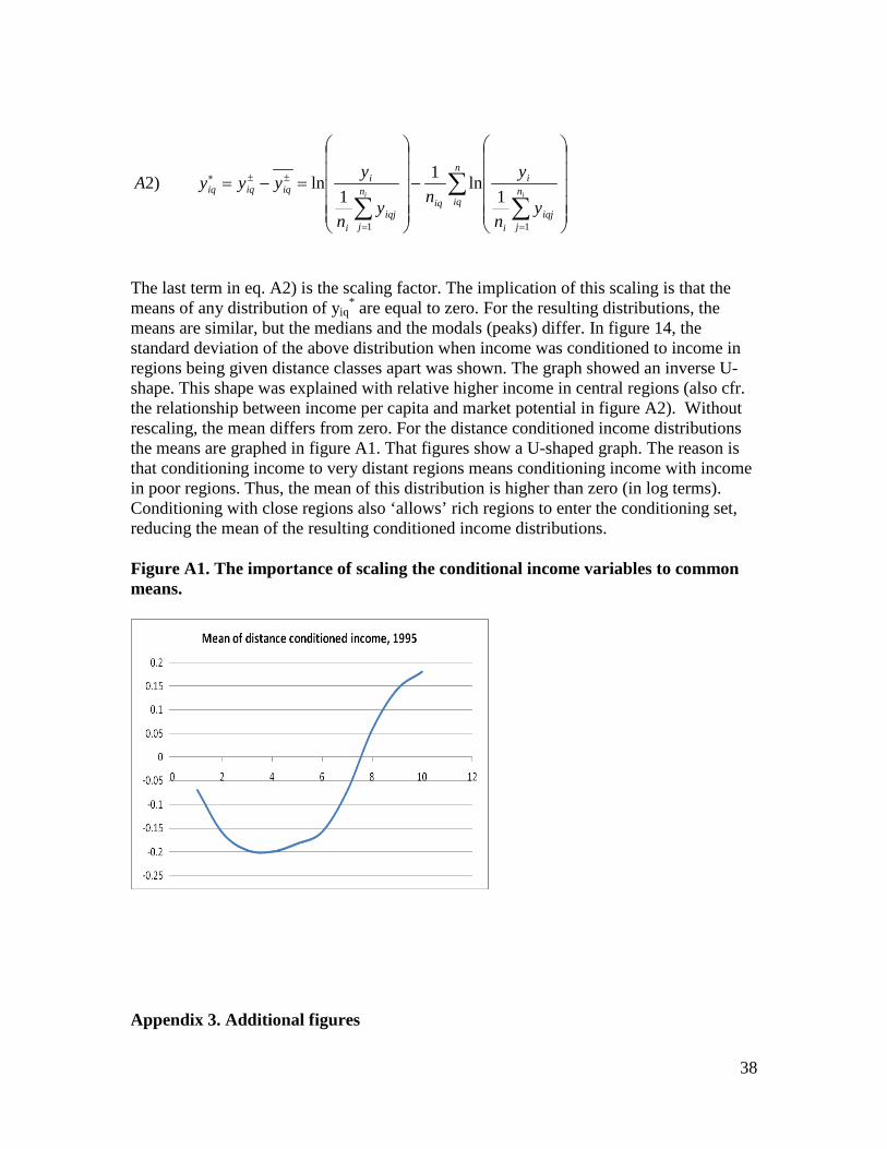
the case for patents in ICT. These correlated to a high degree with the other patent data and did not yield additional significant results. Therefore, only patents per capita were used. The patent data have different availability. For instance, for 1995 patent data are available for 203 regions, for 2000 they are available for 230 regions while availability for 2004 is for 15 regions only. The strategy chosen here was to take the average over patents per capita for all years from 1995 to 2004 for which data was available. The region specific averages are therefore for different years. This approach was chosen because the data show high correlations overt time. For the 167 regions for which patent data was available for all years from 1995 to 2003, all correlations were above 0.9. Averaging gives a variable available for 242 regions. Data on investments are gross fixed capital formation for all industries and broken down at agriculture, manufacturing and services. Also value added for all industries are available. The investment variables used in the analysis is capital formation as share of total value added. Also for capital formation, data availability varies. For instance for 1995, gross fixed capital formation is available for 161 regions, for 2001, it is available for 201 regions and for 2004 only for 157 regions. Averaging as described above gives a variable available for 236 regions. Correlations for the years 1995 to 2003 for the 148 regions for which capital formation is available for all these years are above one half. Gross value added is available for the three main industries (services, manufacturing and agriculture). For this paper, only value added in services was used. Using all gives high collinearity (in principle they sum to total GDP) while services was the one of them that added the highest explanatory variable to the regressions. Also, high production of services may indicate modernized economies. This is more important since the dataset included regions both from Western and from Eastern Europe. The averaging procedure as described above was also used for service production as share of total GDP. Service production is available for almost all regions in the dataset (above 200 for every year). Their correlation is above 0.9 for all years. The averaged variable completes the dataset and is available for 255 regions. Inclusion of the three variables averaged as described above, gives a dataset consisting of 229 regions. Those regions that are not included in the smaller dataset are market by * in the list of regions in appendix 5. Appendix 2. The importance of scaling conditional income to common means. The conditional income distributions introduced in the text are scaled to have common means equal to zero. The formulae is:

38

∑∑∑

−

=−=

==

±±∗n

iqn

jiqj

i

i

iqn

jiqj

i

iiqiqiq ii

yn

yny

n

yyyyA

11

1ln1

1ln )2

The last term in eq. A2) is the scaling factor. The implication of this scaling is that the means of any distribution of yiq

* are equal to zero. For the resulting distributions, the means are similar, but the medians and the modals (peaks) differ. In figure 14, the standard deviation of the above distribution when income was conditioned to income in regions being given distance classes apart was shown. The graph showed an inverse U- shape. This shape was explained with relative higher income in central regions (also cfr. the relationship between income per capita and market potential in figure A2). Without rescaling, the mean differs from zero. For the distance conditioned income distributions the means are graphed in figure A1. That figures show a U-shaped graph. The reason is that conditioning income to very distant regions means conditioning income with income in poor regions. Thus, the mean of this distribution is higher than zero (in log terms). Conditioning with close regions also ‘allows’ rich regions to enter the conditioning set, reducing the mean of the resulting conditioned income distributions. Figure A1. The importance of scaling the conditional income variables to common means.

Appendix 3. Additional figures

39

Figure A2. Income per capita and market potential

88.

59

9.5

1010

.5lg

dpc9

5

0 10000 20000 30000 40000MP

Figure A3. Income per capita and latitude

88.

59

9.5

1010

.5lg

dpc9

5

30 40 50 60 70lat

Figure A4. Income per capita and longitude

40

88.

59

9.5

1010

.5lg

dpc9

5

-20 0 20 40 60lon

Figure A5: Moran scatterplot of gdp per capita relative to country average, 1995.

Moran scatterplot (Moran's I = 0.011)country conditioned gdp 95

Wz

z-3 -2 -1 0 1 2 3 4 5

-1

0

1

2

41

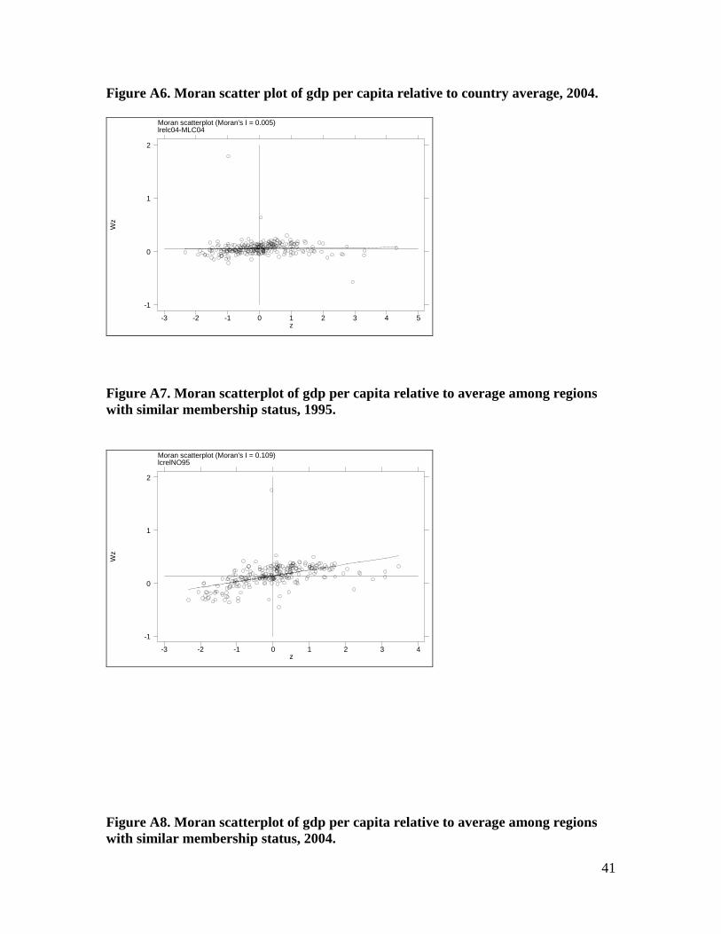
Figure A6. Moran scatter plot of gdp per capita relative to country average, 2004.

Moran scatterplot (Moran's I = 0.005)lrelc04-MLC04

Wz

z-3 -2 -1 0 1 2 3 4 5

-1

0

1

2

Figure A7. Moran scatterplot of gdp per capita relative to average among regions with similar membership status, 1995.

Moran scatterplot (Moran's I = 0.109)lcrelNO95

Wz

z-3 -2 -1 0 1 2 3 4

-1

0

1

2

Figure A8. Moran scatterplot of gdp per capita relative to average among regions with similar membership status, 2004.

42

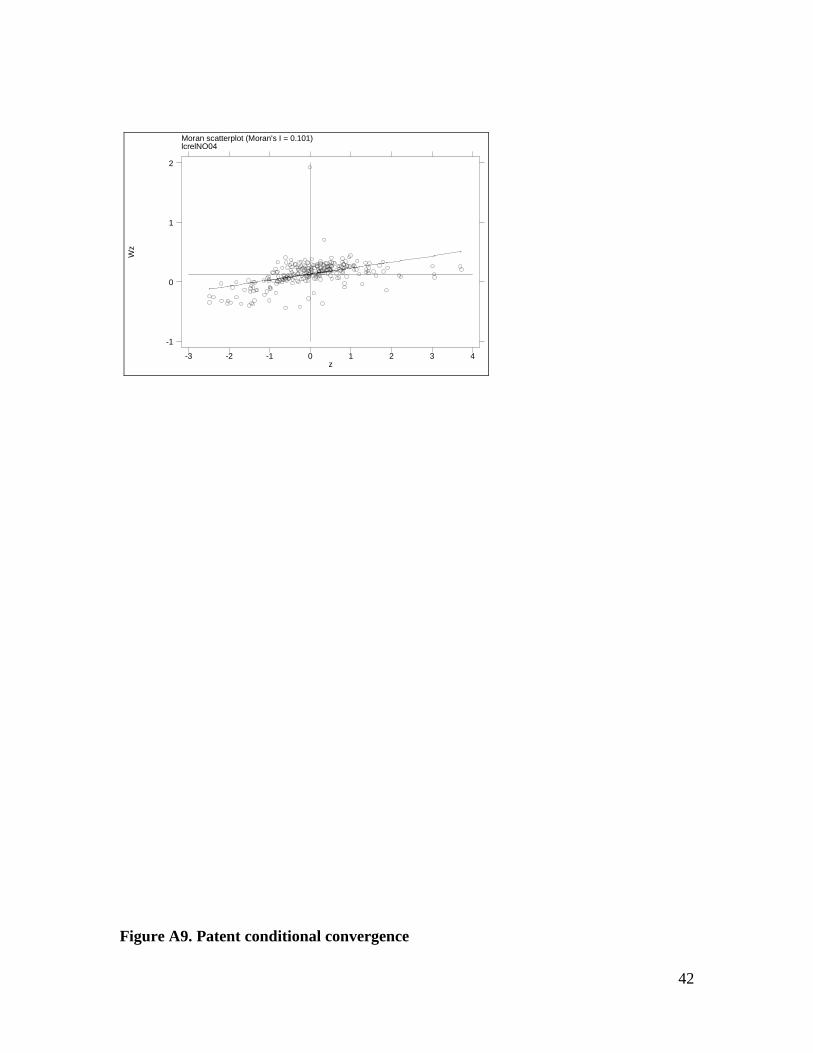
Moran scatterplot (Moran's I = 0.101)lcrelNO04

Wz

z-3 -2 -1 0 1 2 3 4

-1

0

1

2

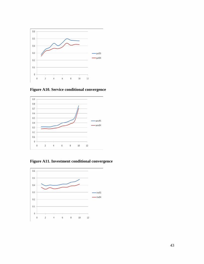
Figure A9. Patent conditional convergence

43

Figure A10. Service conditional convergence

Figure A11. Investment conditional convergence

44

Appendix 4: Standard deviations of relative income measures and their confidence intervals based on bootstrapping. Bootstrapping results based on 1000 reps.

Conditioning variable, year

Standard deviation

Normal based 95 % confidence interval

Sample mean, 95 0.44 0.40 0.48 Sample mean, 04 0.40 0.36 0.44 National mean, 95 0.22 0.19 0.24 National mean, 04 0.23 0.20 0.26 Old member, 95 (N=209) 0.27 0.24 0.31 Old member, 04 (N=209) 0.27 0.23 0.30 New member, 95 (N=46) 0.35 0.28 0.43 New member, 04, (N=46) 0.38 0.29 0.48 Distance=1, 95 0.25 0.22 0.28 Distance=1,04 0.25 0.22 0.28 Distance=2, 95 0.34 0.30 0.37 Distance=2, 04 0.32 0.29 0.35 Distance=3, 95 0.42 0.38 0.45 Distance=3, 04 0.38 0.35 0.43 Distance=4, 95 0.46 0.42 0.50 Distance=4, 04 0.40 0.36 0.44 Distance=5, 95 0.52 0.47 0.56 Distance=5, 04 0.45 0.41 0.49 Distance=6, 95 0.52 0.47 0.56 Distance=6, 04 0.45 0.41 0.50 Distance=7, 95 0.54 0.48 0.59 Distance=7, 04 0.47 0.43 0.52 Distance=8, 95 0.57 0.52 0.62 Distance=8, 04 0.52 0.47 0.57 Distance=9, 95 0.54 0.49 0.59 Distance=9, 04 0.52 0.47 0.57 Distance=10, 95 0.49 0.44 0.53 Distance=10, 04 0.45 0.40 0.50 Patent dist=1, 95 0.28 0.25 0.31 Patent dist=1, 04 0.26 0.22 0.29 Patent dist=2, 95 0.35 0.31 0.40 Patent dist=2, 04 0.33 0.29 0.36 Patent dist=3, 95 0.38 0.34 0.42 Patent dist=3, 04 0.34 0.31 0.38 Patent dist=4, 95 0.44 0.39 0.48 Patent dist=4, 04 0.37 0.33 0.40 Patent dist=5, 95 0.40 0.36 0.44 Patent dist=5, 04 0.36 0.32 0.40 Patent dist=6, 95 0.44 0.40 0.48 Patent dist=6, 04 0.38 0.35 0.42 Patent dist=7, 95 0.50 0.45 0.55 Patent dist=7, 04 0.44 0.40 0.48 Patent dist=8, 95 0.48 0.43 0.52 Patent dist=8, 04 0.41 0.37 0.45 Patent dist=9, 95 0.47 0.42 0.53 Patent dist=9, 04 0.42 0.38 0.47 Patent dist=10, 95 0.47 0.42 0.52

45

Patent dist=10, 04 0.42 0.38 0.46 Service dist=1, 95 0.32 0.28 0.35 Service dist=1, 04 0.27 0.25 0.30 Service dist=2, 95 0.32 0.28 0.35 Service dist=2, 04 0.28 0.25 0.30 Service dist=3, 95 0.31 0.28 0.35 Service dist=3, 04 0.27 0.24 0.30 Service dist=4, 95 0.33 0.30 0.37 Service dist=4, 04 0.28 0.26 0.31 Service dist=5, 95 0.35 0.31 0.39 Service dist=5, 04 0.30 0.27 0.33 Service dist=6, 95 0.40 0.36 0.44 Service dist=6, 04 0.33 0.30 0.36 Service dist=7,95 0.41 0.37 0.45 Service dist=7, 04 0.35 0.31 0.38 Service dist=8, 95 0.45 0.41 0.49 Service dist=8, 04 0.38 0.34 0.42 Service dist=9, 95 0.51 0.46 0.55 Service dist=9, 04 0.44 0.40 0.47 Service dist=10, 95 0.76 0.71 0.82 Service dist=10, 04 0.71 0.67 0.75 Invest dist=1, 95 0.42 0.38 0.47 Invest dist=1, 04 0.37 0.33 0.41 Invest dist=2, 95 0.39 0.35 0.44 Invest dist=2, 94 0.34 0.31 0.38 Invest dist=3, 95 0.40 0.35 0.45 Invest dist=3, 04 0.36 0.32 0.41 Invest dist=4, 95 0.40 0.36 0.44 Invest dist=4, 04 0.35 0.31 0.39 Invest dist=5, 95 0.40 0.35 0.45 Invest dist=5, 04 0.36 0.32 0.40 Invest dist=6, 95 0.41 0.37 0.46 Invest dist=6, 04 0.37 0.33 0.41 Invest dist=7, 95 0.42 0.37 0.46 Invest dist=7, 04 0.37 0.33 0.41 Invest dist=8, 95 0.44 0.40 0.48 Invest dist=8, 04 0.39 0.35 0.43 Invest dist=9, 95 0.45 0.41 0.49 Invest dist=9, 04 0.39 0.36 0.43 Invest dist=10, 95 0.48 0.44 0.52 Invest dist=10, 04 0.41 0.38 0.45

46

Appendix 5. Regions included in analysis. Regions included in large, but not in small dataset are marked with *.

Region name Region code Country code Region name Region code Country code

Burgenland at11 At Hamburg de60 de Niederösterreich at12 At Darmstadt de71 de Wien at13 At Gießen de72 de Kärnten at21 At Kassel de73 de Steiermark at22 At Mecklenburg-Vorpommern de80 de Oberösterreich at31 At Braunschweig de91 de Salzburg at32 At Hannover de92 de Tirol at33 At Lüneburg de93 de Vorarlberg at34 At Weser-Ems de94 de Région de Bruxelles-Capitale be10 Be Düsseldorf dea1 de Prov. Antwerpen be21 Be Köln dea2 de Prov. Limburg (B) be22 Be Münster dea3 de Prov. Oost-Vlaanderen be23 Be Detmold dea4 de Prov. Vlaams Brabant be24 Be Arnsberg dea5 de Prov. West-Vlaanderen be25 Be Koblenz deb1 de Prov. Brabant Wallon be31 Be Trier deb2 de Prov. Hainaut be32 Be Rheinhessen-Pfalz deb3 de Prov. Liège be33 Be Saarland dec0 de Prov. Luxembourg (B) be34 Be Chemnitz ded1 de Prov. Namur be35 be Dresden ded2 de Severozapaden* bg31 bg Leipzig ded3 de Severen tsentralen* bg32 bg Dessau dee1 de Severoiztochen* bg33 bg Halle dee2 de Yugoiztochen* bg34 bg Magdeburg dee3 de Yugozapaden* bg41 bg Schleswig-Holstein def0 de Yuzhen tsentralen* bg42 bg Thüringen deg0 de Cyprus cy00 cy Denmark dk00 dk Praha cz01 cz Estonia ee00 ee Strední Cechy cz02 cz Galicia es11 es Jihozápad cz03 cz Principado de Asturias es12 es Severozápad cz04 cz Cantabria es13 es Severovýchod cz05 cz Pais Vasco es21 es Jihovýchod cz06 cz Comunidad Foral de Navarra es22 es Strední Morava cz07 cz La Rioja es23 es Moravskoslezsko cz08 cz Aragón es24 es Stuttgart de11 de Comunidad de Madrid es30 es Karlsruhe de12 de Castilla y León es41 es Freiburg de13 de Castilla-la Mancha es42 es Tübingen de14 de Extremadura es43 es Oberbayern de21 de Cataluña es51 es Niederbayern de22 de Comunidad Valenciana es52 es Oberpfalz de23 de Andalucia es61 es Oberfranken de24 de Región de Murcia es62 es Mittelfranken de25 de Itä-Suomi fi13 fi Unterfranken de26 de Etelä-Suomi fi18 fi Schwaben de27 de Länsi-Suomi fi19 fi Berlin de30 de Pohjois-Suomi fi1a fi Brandenburg - Nordost de41 de Åland fi20 fi Brandenburg - Südwest de42 de Île de France fr10 fr Bremen de50 de

47

Appendix 5, cont. Regions included in analysis

Region name Region code Country code Region name Region code Country code

Champagne-Ardenne fr21 fr Liguria itc3 it Picardie fr22 fr Lombardia itc4 it Haute-Normandie fr23 fr Provincia Aut. Bolzano-Bozen itd1 it Centre fr24 fr Provincia Autonoma Trento itd2 it Basse-Normandie fr25 fr Veneto itd3 it Bourgogne fr26 fr Friuli-Venezia Giulia itd4 it Nord - Pas-de-Calais fr30 fr Emilia-Romagna itd5 it Lorraine fr41 fr Toscana ite1 it Alsace fr42 fr Umbria ite2 it Franche-Comté fr43 fr Marche ite3 it Pays de la Loire fr51 fr Lazio ite4 it Bretagne fr52 fr Abruzzo itf1 it Poitou-Charentes fr53 fr Molise itf2 it Aquitaine fr61 fr Campania itf3 it Midi-Pyrénées fr62 fr Puglia itf4 it Limousin fr63 fr Basilicata itf5 it Rhône-Alpes fr71 fr Calabria itf6 it Auvergne fr72 fr Sicilia itg1 it Languedoc-Roussillon fr81 fr Sardegna itg2 it Provence-Alpes-Côte d'Azur fr82 fr Lithuania lt00 lt Corse fr83 fr Luxembourg (Grand-Duché)* lu00 lu Guadeloupe (FR) fr91 fr Latvia lv00 lv Martinique (FR) fr92 fr Groningen nl11 nl Guyane (FR) fr93 fr Friesland nl12 nl Reunion (FR) fr94 fr Drenthe nl13 nl Anatoliki Makedonia, Thraki* gr11 gr Overijssel nl21 nl Kentriki Makedonia* gr12 gr Gelderland nl22 nl Dytiki Makedonia* gr13 gr Flevoland nl23 nl Thessalia* gr14 gr Utrecht nl31 nl Ipeiros* gr21 gr Noord-Holland nl32 nl Ionia Nisia* gr22 gr Zuid-Holland nl33 nl Dytiki Ellada* gr23 gr Zeeland nl34 nl Sterea Ellada* gr24 gr Noord-Brabant nl41 nl Peloponnisos* gr25 gr Limburg (NL) nl42 nl Attiki* gr30 gr Lódzkie pl11 pl Voreio Aigaio* gr41 gr Mazowieckie pl12 pl Notio Aigaio* gr42 gr Malopolskie pl21 pl Kriti* gr43 gr Slaskie pl22 pl Közép-Magyarország hu10 hu Lubelskie pl31 pl Közép-Dunántúl hu21 hu Podkarpackie pl32 pl Nyugat-Dunántúl hu22 hu Swietokrzyskie pl33 pl Dél-Dunántúl hu23 hu Podlaskie pl34 pl Észak-Magyarország hu31 hu Wielkopolskie pl41 pl Észak-Alföld hu32 hu Zachodniopomorskie pl42 pl Dél-Alföld hu33 hu Lubuskie pl43 pl Border, Midlands and Western* ie01 ie Dolnoslaskie pl51 pl Southern and Eastern* ie02 ie Opolskie pl52 pl Piemonte itc1 it Kujawsko-Pomorskie pl61 pl Valle d'Aosta/Vallée d'Aoste itc2 it Warminsko-Mazurskie pl62 pl Pomorskie pl63 pl

48

Appendix 5, cont. Regions included in analysis

Region name Region code Country code Region name Region code

Country code

Norte pt11 pt South Yorkshire uke3 uk Algarve pt15 pt West Yorkshire uke4 uk Centro (PT) pt16 pt Derbyshire Nottinghamshire ukf1 uk Lisboa pt17 pt Leicesters., Rutland, Nort. ukf2 uk Alentejo pt18 pt Lincolnshire* ukf3 uk Região Autónoma dos Açores * pt20 pt Herefords., Worces, Warks ukg1 uk Região Autónoma da Madeira pt30 pt Shropshire and Staffordshire ukg2 uk Stockholm se01 se West Midlands ukg3 uk Östra Mellansverige se02 se East Anglia ukh1 uk Sydsverige se04 se Bedfordshire, Hertfordshire ukh2 uk Norra Mellansverige se06 se Essex ukh3 uk Mellersta Norrland se07 se Inner London uki1 uk Övre Norrland se08 se Outer London uki2 uk Småland med öarna se09 se Berksh, Bucks and Oxf ukj1 uk Västsverige se0a se Surrey, East and West Sussex ukj2 uk Slovenia si00 si Hampshire and Isle of Wight ukj3 uk Bratislavský kraj sk01 sk Kent ukj4 uk Západné Slovensko sk02 sk Gloucesters., Wilts., North So ukk1 uk Stredné Slovensko sk03 sk Dorset and Somerset ukk2 uk Východné Slovensko sk04 sk Cornwall and Isles of Scilly ukk3 uk Tees Valley and Durham ukc1 uk Devon ukk4 uk Northumberland, Tyne and Wear ukc2 uk West Wales and The Valleys ukl1 uk Cumbria* ukd1 uk East Wales ukl2 uk Cheshire ukd2 uk North Eastern Scotland ukm1 uk Greater Manchester ukd3 uk Eastern Scotland* ukm2 uk Lancashire ukd4 uk South Western Scotland* ukm3 uk Merseyside ukd5 uk Highlands and Islands ukm4 uk East Riding and North Lincoln uke1 uk Northern Ireland ukn0 uk North Yorkshire uke2 uk