reeftemp next generation - cawcr | · reeftemp next generation l.a. garde1, c.m spillman1, ......

The Centre for Australian Weather and Climate Research

A partnership between CSIRO and the Bureau of Meteorology

ReefTemp Next Generation

L.A. Garde, C.M Spillman, L. Majewski, C. Griffin, G. Kruger and H. Beggs

CAWCR Technical Report No. 063

July 2013


L.A. Garde1, C.M Spillman1, L. Majewski2, C. Griffin2, G. Kruger1, 2 and H. Beggs1

1 Centre for Australian Weather and Climate Research (CAWCR)

- a partnership between CSIRO and the Bureau of Meteorology

2Observations and Engineering Branch

CAWCR Technical Report No. 063

July 2013

ISSN: 1835-9884

National Library of Australia Cataloguing-in-Publication entry

Author: L.A. Garde, C.M Spillman, L. Majewski, C. Griffin, G. Kruger and H. Beggs

Title: ReefTemp Next Generation

ISBN: 978-1-4863-0123-2

Series: CAWCR technical report CRT 063

Enquiries should be addressed to:

Luke Garde

Climate and Water Division | Climate Information Services | Climate Prediction

Bureau of Meteorology

GPO Box 1289, Melbourne

Victoria 3001, Australia

[email protected]

Copyright and Disclaimer

All images reproduced in grayscale. A colour version of CAWCR Technical Report No.063

is available online: http://www.cawcr.gov.au/publications/technicalreports.php

© 2013 CSIRO and the Bureau of Meteorology. To the extent permitted by law, all rights are reserved

and no part of this publication covered by copyright may be reproduced or copied in any form or by

any means except with the written permission of CSIRO and the Bureau of Meteorology.

CSIRO and the Bureau of Meteorology advise that the information contained in this publication

comprises general statements based on scientific research. The reader is advised and needs to be aware

that such information may be incomplete or unable to be used in any specific situation. No reliance or

actions must therefore be made on that information without seeking prior expert professional,

scientific and technical advice. To the extent permitted by law, CSIRO and the Bureau of Meteorology

(including each of its employees and consultants) excludes all liability to any person for any

consequences, including but not limited to all losses, damages, costs, expenses and any other

compensation, arising directly or indirectly from using this publication (in part or in whole) and any

information or material contained in it.

ReefTemp Next Generation i

Contents

1. Abstract ............................................................................................................. 1

2. Introduction ....................................................................................................... 2

3. The ReefTemp Next Generation system .......................................................... 5

3.1 Data Acquisition ......................................................................................................... 8

3.1.1 L3S Spatial Coverage and SST Mosaic .............................................................. 10

3.1.2 IMOS L3S Quality Level and Error Bias .............................................................. 13

3.2 Calculation of Climatologies.................................................................................... 14

3.2.1 L3S Maximum Gap Persistence ......................................................................... 17

3.3 Product Development ............................................................................................. 19

3.3.1 Sea Surface Temperature .................................................................................. 19

3.3.2 Sea Surface Temperature Anomaly.................................................................... 20

3.3.3 Degree Heating Days ......................................................................................... 21

3.3.4 Mean Positive Summer Anomaly ........................................................................ 23

3.3.5 Thermal Stress Product Interpretation ................................................................ 25

3.4 Product Visualisation and Delivery.......................................................................... 25

4. Future Development ....................................................................................... 29

5. Summary .......................................................................................................... 31

6. Acknowledgments .......................................................................................... 32

References ................................................................................................................ 33

ii ReefTemp Next Generation

List of Figures

Fig. 1 Schematic overview of the ReefTemp Next Generation program. Calculation of thermal stress is only conducted during the extended summer period (1 Dec – 31 March inclusive). IMOS SST data has been used to generate RTNG products. ........... 7

Fig. 2 (a) GBR night-time L3S-01day SST data for the 1 January 2012. (b) Infrared satellite image taken from the MTSAT-2 platform for 1 January 2012 (16:32 UTC), highlighting cloud cover in the north-eastern parts of the Coral Sea. Note that in (a) gray regions represent land and white regions represent missing data, or data of insufficient quality. GBR Marine Park boundary is illustrated as a solid black line (a) and a white line in (b). .................................................................................................. 10

Fig. 3 Simple representation of how the ReefTemp Next Generation SST mosaic is generated. In this example, only the data from 3 days is shown.................................. 11

Fig. 4 Example GBR region IMOS L3S-01day SST grids for (a) 8 January and (b) 24 January 2012. (c) and (d) represent the 14-day SST mosaic and (e) and (f) represent the mosaic pixel age for the two dates 8 and 24 of January respectively. ... 12

Fig. 5 Example Quality Level (QL) images for (a) 8 January and (b) 24 January 2012. SSES Bias images for (c) 8 January and (d) 24 January 2012. ................................... 13

Fig. 6 December climatology using (a) IMOS L3S-01day (2002-2011) and (b) CSIRO SST data (1993-2002), and the (c) difference (IMOS – CSIRO). January climatology using (d) IMOS L3S-01day (2002-2011), and (e) CSIRO SST data (1993-2002) and the (f) difference. February climatology using (g) IMOS L3S-01day (2002-2011) and (h) CSIRO SST data (1993-2002), and the (i) difference. ............................................ 16

Fig. 7 Number of data points per grid cell, expressed as a percentage of the total number of days that form the climatological period for (a) December (n=310), (b) January (n=310) and (c) February (n=282) IMOS climatologies. Note that the colour scale is limited to 50%. .............................................................................................................. 17

Fig. 8 Example night-time L3S-01day gap persistence counts (days) for (a) December 2003, (b) January 2004, (c) February 2004, (d) December 2008, (e) January 2009, (f) February 2009, (g) December 2011, (h) January 2012 and (i) February 2012. The Australian coastline and GBR marine park boundary are indicated by solid white lines. .................................................................................................................... 18

Fig. 9 Example of the IMOS (a) L3S-01day and (b) 14-day mosaic SST products generated by RTNG for 11 February 2012. .................................................................. 19

Fig. 10 Example RTNG SSTA products for 11 February 2012. IMOS 1-day SST referenced to (a) IMOS climatology and (b) CSIRO climatology. 14-day SST mosaic referenced to (c) IMOS climatology and (d) CSIRO climatology. ................................................... 20

Fig. 11 Flow diagram representing how the IMOS 1-day and 14-day mosaic DHD grids are calculated. .................................................................................................................... 21

Fig. 12 Example L3S-01day DHD stress index products for 31 March 2012 using (a) IMOS climatology, (b) IMOS climatology DHD counts, (c) CSIRO climatology and (d) CSIRO climatology DHD counts................................................................................... 22

Fig. 13 DHD stress index products using 14-day SST IMOS mosaic for 31 March 2012: (a) IMOS climatology, (b) IMOS climatology DHD counts, (c) CSIRO climatology and (d) CSIRO climatology DHD counts ............................................................................. 23

ReefTemp Next Generation iii

Fig. 14 Example MPSA products for 11 February 2012 for (a) IMOS climatology, (b) CSIRO climatology, 14-day SST mosaic product using (c) the IMOS climatology and (d) the CSIRO climatology ........................................................................................................ 24

Fig. 15 Screenshot of the ReefTemp Next Generation webpage (screenshot captured during the development phase). DHD data for 31 March 2012 shown. ........................ 26

Fig. 16 Screenshot of the RTNG Google EarthTM display illustrating the IMOS 1-day SST product for 31 March 2012. ........................................................................................... 27

Fig. 17 Screenshot of the eReefs Marine Water Quality Dashboard, highlighting the RTNG layers (screenshot captured during the development phase). Red squares on the map represent the trajectory of TC Yasi (2011). GBRMPA boundaries are also indicated by the wide (and blue) outlines. ..................................................................... 28

List of Tables

Table 1: Comparison between ReefTemp coral bleaching thermal stress monitoring systems: Legacy (RT1) and ReefTemp Next Generation (RTNG). ............................................... 3

Table 2: Comparison between ReefTemp coral bleaching thermal stress products: Legacy (RT1) and ReefTemp Next Generation (RTNG). ............................................................ 4

Table 3: ReefTemp Next Generation module dependencies ........................................................ 5

Table 4: ReefTemp Next Generation running scripts and user developed functions. Note that functions indicated by * are not used in the daily execution of the RTNG suite .............. 6

Table 5: ReefTemp Next Generation netCDF output configuration (yyyy = year, mm = month, dd = day) ......................................................................................................................... 8

iv ReefTemp Next Generation

ReefTemp Next Generation 1

1. ABSTRACT

Mass coral bleaching events are primarily triggered by elevated ocean temperatures. ReefTemp

produces high resolution satellite based nowcasts of sea surface temperature (SST), thermal

stress and associated bleaching risk for the Great Barrier Reef (GBR). The ReefTemp Next

Generation (RTNG) system is based on new state-of-the-art Integrated Marine Observing

System (IMOS) Level 3 super-collated (L3S) multi-sensor composite satellite SST products.

Derived SST products are delivered daily online via static images, Google EarthTM and a

sophisticated data portal, providing an improved ability to monitor thermal stress over the Great

Barrier Reef.

The original ReefTemp system was a collaborative project between Commonwealth Scientific

and Industrial Research Organisation (CSIRO) Marine and Atmospheric Research, the Great

Barrier Reef Marine Park Authority and the Australian Bureau of Meteorology (the Bureau).

The ReefTemp Next Generation system has been developed and operationalized within the

Bureau and is funded by eReefs, under the National Plan for Environmental Information

(NPEI).

Continuous SST monitoring provides researchers and management with necessary tools to

inform decisions and plan in advance for the complex interactions leading to coral bleaching.

When bleaching conditions occur, this tool can be used to support both bleaching response

plans and strategic reef management decisions. Development of real-time reef-scale monitoring

systems with 24/7 support is extremely important as the frequency and severity of coral

bleaching is expected to increase under future climate change.

2 ReefTemp Next Generation

2. INTRODUCTION

Coral reefs are among the most diverse ecosystems in the world and are often referred to as the

‘rainforests of the sea’ (Liu et al. 2006). The Great Barrier Reef (GBR) is the largest coral reef

system in the world, composed of over 2,900 individual reefs and 900 islands stretching 2500

km, covering an area of approximately 344,400 km2. The GBR is managed by the Great Barrier

Reef Marine Park Authority (GBRMPA) and is a World Heritage Site. However, despite best

management practices, climate change is expected to have serious impacts on the reef in the

coming decades (Hennessy et al. 2007). Coral bleaching in particular is expected to increase in

frequency and severity as ocean temperatures rise under global warming (Hoegh-Guldberg

1999; Donner et al., 2005; Frieler et al. 2012), presenting many challenges for reef management

worldwide (Hoegh-Guldberg et al., 2007; Donner et al., 2009).

Coral bleaching has been observed sporadically since 1982 on the GBR, with mass bleaching

events occurring in 1997/1998 and 2002 and a more localised but severe event in 2006,

affecting the southern GBR (Hoegh-Guldberg 1999; Berkelmans et al. 2004; Weeks et al.

2008). No mass coral bleaching events were observed prior to 1979 (Glynn 1993; Hoegh-

Guldberg 1999). Mass coral bleaching events are caused primarily by anomalously warm sea

temperatures (Brown 1997; Hoegh-Guldberg 1999; Lesser 2004) and have caused significant

damage and mortality when thermal stress has been prolonged and/or severe.

As water temperatures increase, coral bleaching can occur. This process is characterised by the

expulsion of zooxanthellae from the coral host. Zooxanthellae are microscopic photosynthetic

organisms which live within the coral tissues and provide the coral with nutrients and, due to

their pigments, give corals their vibrant colours. In addition to protection, coral provide

zooxanthellae with metabolic and respiratory by-products. The loss of zooxanthellae often

results in coral turning white, hence the term ‘coral bleaching’ (Jones et al. 1998). Corals

become white because their tissue without zooxanthellae is nearly transparent, revealing the

coral skeleton. Loss of reef-building corals, changes in benthic habitat and reef fish populations

are just a few of the long-term impacts as a result of severe bleaching events. Anomalously high

sea surface temperature (SST) conditions have also been linked to coral disease frequency

(Hoegh-Guldberg 1999; Beeden et al. 2011; Heron et al., 2012). Although corals can re-

establish themselves under favourable conditions, it can take one to two decades for severely

bleached reefs to fully recover (Baker et al., 2008; Wilkinson, 2008).

ReefTemp is a customised remote sensing application for the monitoring of local SST

conditions that may lead to coral bleaching (Maynard et al., 2009) and was first developed in

2007 through a collaboration between GBRMPA, Commonwealth Scientific and Industrial

Research Organisation (CSIRO) and the Australian Bureau of Meteorology (the Bureau;

Maynard et al., 2008). The system is utilised on a daily-to-weekly time scale throughout the

year by GBRMPA, with particular attention to the summer months, to monitor the current SST

conditions and associated thermal stress across the GBR. Continuous near-real time monitoring

of the SST conditions provides reef management with the capability to effectively employ

limited resources for the best outcome of both individual reefs and the entire reef system. As

part of a broader early warning system, these monitoring tools can indicate the levels of likely

impact across the entire reef and, in conjunction with other observations, support response

plans and management decisions (Maynard et al. 2009).

However, the ReefTemp system (herein now referred to as RT1) is essentially an experimental

system, run in research mode at CSIRO and not operationally supported by the Bureau. RT1


derived products are based on the Bureau legacy 14-day Advanced Very High Resolution

Radiometer (AVHRR) Mosaic SST product (Rea 2004). This product is soon to be superseded

by new satellite SST products developed under the Integrated Marine Observing System

(IMOS; Paltoglou et al. 2010). Additionally, the legacy software has not been updated since its

initial development in 2007, nor has the system been kept in line with the latest scientific

developments. Furthermore, the RT1 codebase uses legacy tools and methods that are not

appropriate for operational implementation within the Bureau.

During 2012, with funding from eReefs under the National Plan for Environmental Information

(NPEI), a new operational version of RT1, known as ReefTemp Next Generation (RTNG), was

designed, developed and launched at the Bureau. There were several motivations behind the

development of the new RTNG system. The first was to deliver a nowcast system based on the

latest scientific advances and new state-of-the-art, multi-sensor composite AVHRR SST

products. The second was to run the system in an operational environment (i.e. 24/7 supported)

using a modern portable programming language suitable for operational deployment, within the

National Meteorological and Oceanographic Centre (NMOC) at the Bureau. The third was to

rethink both the design and delivery of the thermal stress products to best address the needs of

the reef managers. Table 1 and Table 2 directly compares the RT1 and RTNG systems and their

products.

Table 1: Comparison between ReefTemp coral bleaching thermal stress monitoring systems:

Legacy (RT1) and ReefTemp Next Generation (RTNG).

Item Legacy ReefTemp

(2007)


(2012)

SST Input Product Bureau Legacy 14-day mosaic

SST IMOS 1-day L3S SST product

Grid Resolution 0.018° x 0.018° 0.02° x 0.02°

SST Dataset 14-day (day+night) composite 1-day night-time

Climatology Dataset CSIRO SST

(Griffin et al. 2004)

IMOS L3S SST

(Paltoglou et al., 2010)

CSIRO SST

(Griffin et al. 2004)

Climatology Baseline 1993 – 2003 2002 – 2011

Climatology

Calculation 65th percentile, day + night Monthly means, night only

Climatology

Resolution 0.042° x 0.036° 0.02° x 0.02°

Degree Heating Day

Calculation

Monthly climatologies

Monthly climatologies:

IMOS

CSIRO

Degree Heating Day

analysis period 1 Dec to 28 Feb 1 Dec to 31 Mar

System Deployment Experimental at CSIRO Operational at the Bureau (24/7)


Table 2: Comparison between ReefTemp coral bleaching thermal stress products: Legacy (RT1)

and ReefTemp Next Generation (RTNG).

Legacy ReefTemp

(2007)


(2012)

Sea Surface

Temperature (SST)

SST Anomaly

Degree Heating Days

(DHD)

Heating Rate

1-day IMOS SST

(IMOS climatology)

1-day IMOS SST

(CSIRO climatology)

SST

Quality Level (QL)

Gap analysis

Single Sensor Error

Statistics Bias

SST anomaly

Degree Heating Day (DHD)

DHD count

Mean Positive Summer

Anomaly

SST anomaly


DHD count


Anomaly

14-day mosaic IMOS SST

(IMOS Climatology)

14-day mosaic IMOS SST

(CSIRO climatology)

SST

Grid Age

SST anomaly


DHD count


Anomaly

SST anomaly


DHD count


Anomaly


3. THE REEFTEMP NEXT GENERATION SYSTEM

The new RTNG system has been developed using the Python programming language

(specifically Python 2.7.2), which is a high-level, open-source cross platform programming

language. This choice of language supersedes the original experimental RT1 system which is

based on a mixture of outdated software. RTNG module dependencies and functions are

summarised in Table 3 and Table 4 respectively.

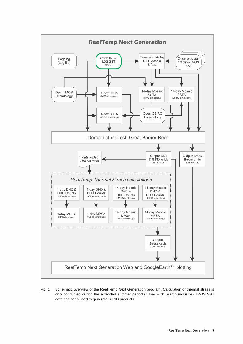
One of the advantages of RTNG is that the whole system is contained within the one

programming environment to aid in the transition to an operational environment. Figure 1

provides an overarching view of how each of the RTNG products is calculated. RTNG has been

developed to operate in two execution modes, ‘Real-time’ and ‘Hindcast’. By developing the

code in this way, users are able to run RTNG in an operational real-time mode or run for a

period in the past, targeting a specific date range.

Once created, RTNG products are then output to three netCDF files (CF1.5 compliant). For

each analysis date, the SST, error and thermal stress gridded data is plotted for both the web

and visualisation within Google EarthTM. Additionally, the RTNG netCDF files are also served

online in real-time to the eReefs Marine Water Quality Dashboard via an OPeNDAP (Open-

source Project for a Network Data Access Protocol) server. This provides end users with a user

friendly interface where the grids from RTNG can be visualised with other eReefs products

such as Marine Water Quality. The contents of the RTNG netCDF files are listed in Table 5.

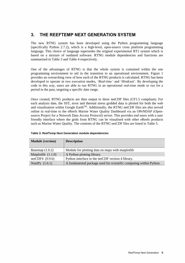
Table 3: ReefTemp Next Generation module dependencies

Module (version)

Description

Basemap (1.0.2) Module for plotting data on maps with matplotlib

Matplotlib (1.1.0) A Python plotting library.

netCDF4 (0.9.6) Python interface to the netCDF version 4 library.

NumPy (1.6.1) A fundamental package used for scientific computing within Python.


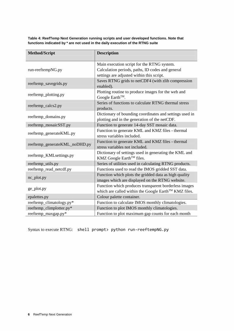
Table 4: ReefTemp Next Generation running scripts and user developed functions. Note that

functions indicated by * are not used in the daily execution of the RTNG suite

Method/Script

Description

run-reeftempNG.py

Main execution script for the RTNG system.

Calculation periods, paths, ID codes and general

settings are adjusted within this script.

reeftemp_savegrids.py Saves RTNG grids to netCDF4 (with zlib compression

enabled).

reeftemp_plotting.py Plotting routine to produce images for the web and

Google EarthTM.

reeftemp_calcs2.py Series of functions to calculate RTNG thermal stress

products.

reeftemp_domains.py Dictionary of bounding coordinates and settings used in

plotting and in the generation of the netCDF.

reeftemp_mosaicSST.py Function to generate 14-day SST mosaic data.

reeftemp_generateKML.py Function to generate KML and KMZ files - thermal

stress variables included.

reeftemp_generateKML_noDHD.py Function to generate KML and KMZ files - thermal

stress variables not included.

reeftemp_KMLsettings.py Dictionary of settings used in generating the KML and

KMZ Google EarthTM files.

reeftemp_utils.py Series of utilities used in calculating RTNG products.

reeftemp_read_netcdf.py Functions used to read the IMOS gridded SST data.

nc_plot.py Function which plots the gridded data as high quality

images which are displayed on the RTNG website.

ge_plot.py Function which produces transparent borderless images

which are called within the Google EarthTM KMZ files.

epalettes.py Colour palette container.

reeftemp_climatology.py* Function to calculate IMOS monthly climatologies.

reeftemp_climplotter.py* Function to plot IMOS monthly climatologies.

reeftemp_maxgap.py* Function to plot maximum gap counts for each month

Syntax to execute RTNG: shell prompt> python run-reeftempNG.py


Fig. 1 Schematic overview of the ReefTemp Next Generation program. Calculation of thermal stress is

only conducted during the extended summer period (1 Dec – 31 March inclusive). IMOS SST

data has been used to generate RTNG products.


Table 5: ReefTemp Next Generation netCDF output configuration (yyyy = year, mm = month, dd =

day)

NetCDF file name

NetCDF file variable contents

Variable Long name Short name

RT2_yyyymmdd_SST.nc4 1-day IMOS SST

14-day SST Mosaic

1-day IMOS SSTA

1-day Legacy SSTA

14-day SSTA IMOS Mosaic

14-day SSTA Legacy Mosaic

sst1day

sst_mosaic

ssta1day

ssta_leg1day

ssta_mosaic_imos

ssta_mosaic_leg

RT2_yyyymmdd_DHD.nc4 1-day IMOS DHD

1-day Legacy DHD

14-day DHD IMOS Mosaic

14-day DHD Legacy Mosaic

1-day IMOS DHD counts

1-day Legacy DHD counts

14-day DHD IMOS Mosaic counts

14-day DHD Legacy Mosaic counts

1-day IMOS MPSA

1-day Legacy MPSA

14-day MPSA IMOS Mosaic

14-day MPSA Legacy Mosaic

dhd1

dhd1_leg

dhd_mosaic_imos

dhd_mosaic_leg

dhdc1

dhdc1_leg

dhdc_mosaic_imos

dhdc1_mosaic_leg

mpsa1

mpsa1_leg

mpsa_mosaic_imos

mpsa_mosaic_leg

RT2_yyyymmdd_ERR.nc4 Persistence Gap counter

IMOS L2P mask flags

14-day SST IMOS Mosaic Pixel Age

1-day IMOS QL

1-day IMOS SSES Bias

gap_counter

l2p_flags

mosaic_age

ql_1day

sses_bias_1day

3.1 Data Acquisition

The SST analyses produced by RTNG show the ocean skin temperatures for that day. The

Group for High Resolution Sea Surface Temperature (GHRSST) define SST skin temperatures

as the temperature within the conductive diffusion-dominated sub-layer at a depth of

approximately 10-20 µm (see www.ghrsst.org/ghrsst-science/sst-definitions for details). These

temperatures are measured by an infrared radiometer typically operating at wavelengths of 3.7-

12 µm.

SST processing upgrades implemented by the Bureau now adhere to international best practices

and comply with GHRSST data processing specification v2.0 (Paltoglou et al., 2010; Casey et

http://www.ghrsst.org/ghrsst-science/sst-definitions


al., 2011). By measuring brightness temperatures in five spectral bands, National Oceanic and

Atmospheric Administration (NOAA) satellites (NOAA-11, 12, 14, 15, 16, 17, 18, 19) are used

to produce state-of-the-art multi-sensor composite High Resolution Picture Transmission

(HRPT) AVHRR skin SST products (Paltoglou et al., 2010), from 1992 to present. Raw HRPT

data, received by ground receiving stations across Australia and Antarctica, are used to

generate a level 2 pre-processed (L2P) geolocated, single swath dataset. This is then re-mapped

to a standard Level 3 un-collated gridded product (L3U). A new level 3 collated product (L3C)

is created from a combination of multiple swaths from a single sensor. Finally a multi-sensor,

multi-swath (L3S or 'super-collated') product is produced. An overview of the Bureau’s

GHRSST-format products is provided at http://imos.org.au/sstproducts.html (accessed 2 March

2013) and Casey et al. (2011) provides detailed information regarding the content and format of

these products.

The L3S SST product is a super-collated, multi-sensor gridded product at 0.02° x 0.02° spatial

resolution, with no spatial or temporal smoothing to fill in missing data. Daily L3S data used in

RTNG are produced by the Bureau as a contribution to the Integrated Marine Observing

System (IMOS; www.imos.org.au). During 2012, the Bureau’s Observations and Engineering

Branch (OEB) were storing daily, day-time and night-time grids at the following FTP location:

ftp://aodaac2-cbr.act.csiro.au/imos/GHRSST/L3S-01day/night/

Currently, the RTNG system is based on the L3S 1-day night-time only product (Table 1). The

night-only SST limitation was chosen to avoid observations that are affected by daily surface

warming caused by solar heating and/or solar glare effects (Gentemann et al., 2003). Satellite

retrievals measure temperatures at the surface layer and thus these warming effects will have

strong influences in their measurements (Gentemann et al., 2003). The relationship with deeper

bulk temperature, is the same on average during the night and during the day for wind speed

conditions of > ~6 m s-1 (Donlon et al., 2002; Minnett, 2003). But under low winds the

relationship is very variable vertically, horizontally and temporally (Ward, 2006). Night-time

SSTs also correlate with in situ SSTs at one meter depth (Montgomery and Strong, 1995).

An important stage in the creation of the L3S grids is in the identification of clouds. Following

an extensive study, clouds are identified using a carefully calibrated set of radiance, uniformity

and 2-channel thresholds (Paltoglou et al., 2010). Paltoglou et al., (2010) state that cloud

contamination will result in a negative temperature bias at affected grid cells in the dataset

because observations contaminated by cloud have lower temperatures than the ocean surface.

Consequently, particular effort has been made to ensure that all suspect pixels are identified

and masked out. Conversely, it is also important to ensure that pixels are not needlessly masked

out during this process, as spatial coverage is also a factor for consideration (Paltoglou et al.,

2010).

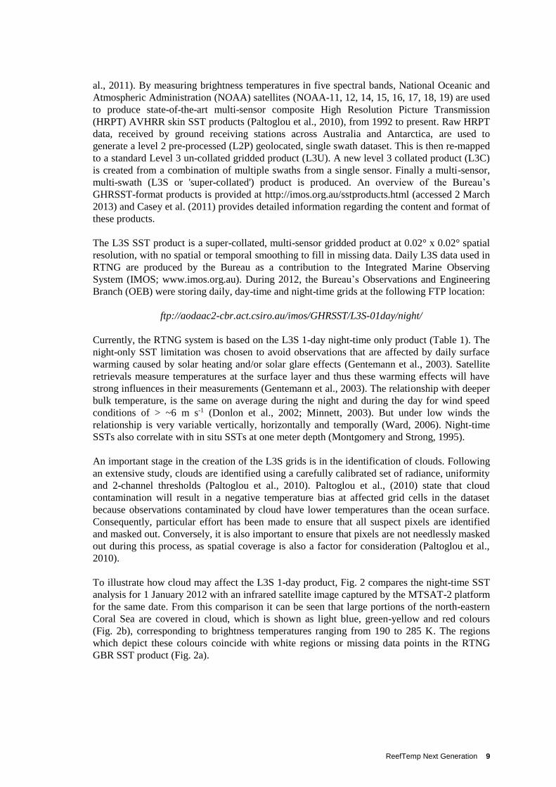
To illustrate how cloud may affect the L3S 1-day product, Fig. 2 compares the night-time SST

analysis for 1 January 2012 with an infrared satellite image captured by the MTSAT-2 platform

for the same date. From this comparison it can be seen that large portions of the north-eastern

Coral Sea are covered in cloud, which is shown as light blue, green-yellow and red colours

(Fig. 2b), corresponding to brightness temperatures ranging from 190 to 285 K. The regions

which depict these colours coincide with white regions or missing data points in the RTNG

GBR SST product (Fig. 2a).


Fig. 2 (a) GBR night-time L3S-01day SST data for the 1 January 2012. (b) Infrared satellite image

taken from the MTSAT-2 platform for 1 January 2012 (16:32 UTC), highlighting cloud cover in the

north-eastern parts of the Coral Sea. Note that in (a) gray regions represent land and white

regions represent missing data, or data of insufficient quality. GBR Marine Park boundary is

illustrated as a solid black line (a) and a white line in (b).

3.1.1 L3S Spatial Coverage and SST Mosaic

As IMOS L3S daily SST data does not contain any smoothing to fill spatial gaps, there was a

concern that poor coverage would lead to an underestimate of the total accumulated thermal

stress. This is of major concern to GBRMPA management as this would prevent appropriate

and timely action regarding a current bleaching episode. This underestimate is further

compounded when SST data is restricted to higher quality levels (will be discussed in Section

3.1.2).

To address this issue, a gap-filled SST mosaic product was developed based on the IMOS L3S

1-day product. The SST mosaic generation followed the methodology of the Bureau legacy

SST mosaic (Rea 2004); i.e., filling each missing-data grid cell in the current day using the

most-recent daily SST for that grid cell from up to 13 days ago. Figure 3 is a simple

representation of the RTNG mosaic generation process. Initially, the scheme determines the

locations of all missing or insufficient data. Data from the previous day are then selected to fill

in those locations. If grids are still missing data, an additional preceding day is sourced for data.

This process is repeated until all grids are filled, or historical data has been sourced from as far

back as 13 days. If data is still missing, these locations remain empty.


Fig. 3 Simple representation of how the ReefTemp Next Generation SST mosaic is generated. In this

example, only the data from 3 days is shown.

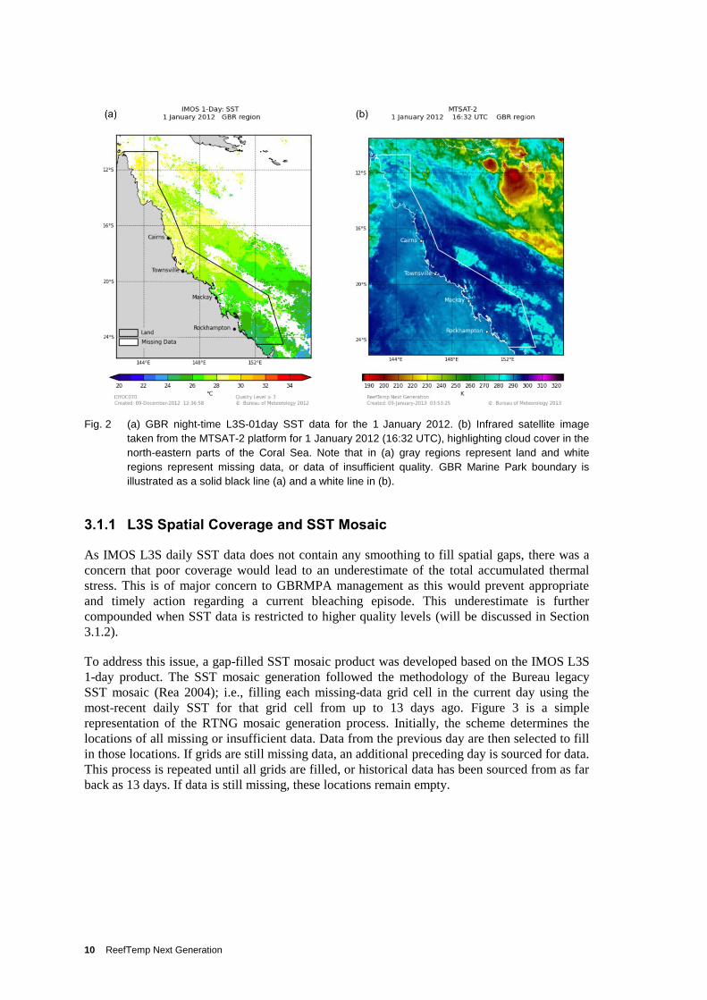
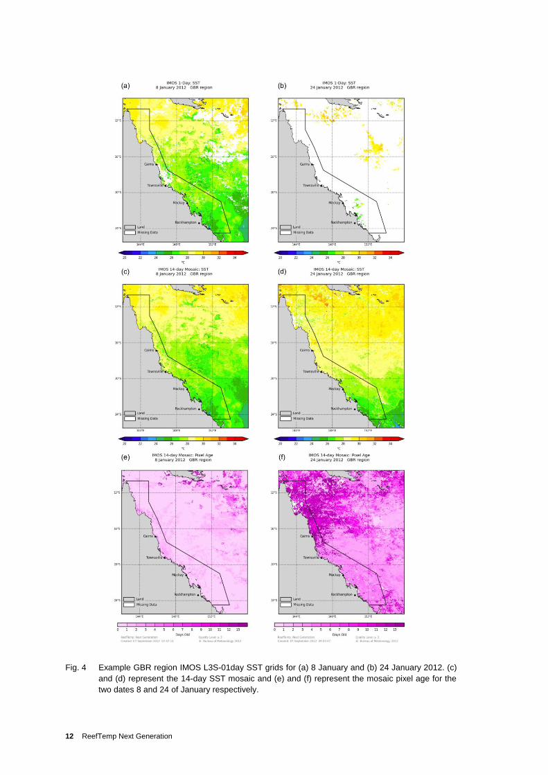
Figure 4 illustrates the data coverage for two example dates, 8 January and 24 January 2012

with varying spatial coverage due to monsoonal cloud cover. Figures 4a and 4b represent the

output from the 1-day IMOS SST product, whilst Fig. 4c and 4d represent the output from the

14-day IMOS SST mosaic product for the two dates respectively. It can be seen that the mosaic

product has markedly improved spatial coverage.

Whilst a more complete SST image is available using the mosaic method, the generated SST

field can be spatially inhomogeneous as data recorded over the space of up to 14 days is mixed

in a single image. It is possible that neighbouring pixels within the final mosaic grid may

contain SST variations which do not represent current conditions. However, this product serves

to improve spatial coverage, ensuring that the thermal stress is accumulated and not simply

masked due to cloud. Although not representing the real world, this product meets the needs of

reef management who are more concerned by under prediction of bleaching events than over

prediction.

To quantify this effect, a new product which accounts for when missing data points were filled

was developed. This is known as Pixel Age and can be thought of as temporal error bars for

each SST grid value. This product represents the age of the SST data at each grid cell, with an

age of zero days representing current data (Figs 4e-f; indicated by light tones). Figure 4e

illustrates that the SST mosaic that was generated for 8 January 2012, contains more current

day data as compared to the mosaic generated for 24 January 2012, which contains SST data

from up to 13 days previously in the northern GBR region.


Fig. 4 Example GBR region IMOS L3S-01day SST grids for (a) 8 January and (b) 24 January 2012. (c)

and (d) represent the 14-day SST mosaic and (e) and (f) represent the mosaic pixel age for the

two dates 8 and 24 of January respectively.


3.1.2 IMOS L3S Quality Level and Error Bias

The IMOS L3S satellite data files contain information regarding the quality level (QL) and

sensor specific error statistics (SSES) for each SST value by pixel. The QL is based on

proximity to cloud (distance to cloud), satellite zenith angle and day/night. The SSES comprise

bias and standard deviation estimates for each QL based on rolling 60 day match-ups with

drifting buoy SST observations (Paltoglou et al., 2010).

IMOS L3S metadata states that pixels at QL 3, 4, and 5 are of low, acceptable and best quality

respectively (Paltoglou et al. 2010). To ensure the best spatial coverage, RTNG uses all QL

pixels (QL 3, 4 and 5). Figure 5 illustrates the contribution of each QL and SSES for the dates

shown in Fig. 2 (8 and 24 January 2012 respectively). Even when cloud cover is minimal and

data coverage is good as for 8 January (Fig. 5a), resulting in improved data coverage, some

pixels may still be of low quality. For this specific date, the likely explanation for the swath of

low quality data is a result of high satellite sensor viewing angle. These would be removed if

specific QL threshold was set to acceptable or above only.

Fig. 5 Example Quality Level (QL) images for (a) 8 January and (b) 24 January 2012. SSES Bias

images for (c) 8 January and (d) 24 January 2012.


3.2 Calculation of Climatologies

The RTNG SST anomaly (SSTA) and thermal stress products are calculated using new monthly

IMOS climatologies. These climatologies use the L3S-01day nightly grids covering the 2002 to

2011 period. A monthly climatology refers to the long term monthly mean, i.e. January

climatology is the average of all January monthly means within a specified period. First,

monthly means were calculated for all months within 2002 – 2011, before an average was

calculated across the 10 years for each month. To ensure consistency with the real-time SST

data, all QL data (QL 3, 4 and 5), as described in Section 3.1.2, were included.

To assess the impact of using a new climatology on RTNG products, the IMOS and CSIRO

legacy climatologies were compared for December, January and February (Fig. 6). The RT1

system utilises the CSIRO SST climatology for 1993 – 2003, generated using day and night

HRPT AVHRR SST data from NOAA polar-orbiting satellites, calibrated to around 20 – 30 cm

depth by using observations from global drifting buoys (Griffin et al., 2004; Maynard et al.,

2008). The IMOS HRPT AVHRR SSTs forming the IMOS climatology were calibrated to the

ocean skin at around 10 – 20 micron depth by first regressing the AVHRR brightness

temperatures against drifting buoy SST observations over the Australian region, followed by

conversion from buoy depths to the cool skin by subtraction of 0.17C (Paltoglou et al., 2010).

In the CSIRO SST processing system, the removal of anomalous values caused by cloud and

diurnal surface warming is achieved by removing all the SST values above the 65th percentile of

the cumulative frequency distribution (Maynard et al., 2008). In contrast, the IMOS processing

system uses a set of brightness temperature, uniformity and 2-channel thresholds to identify

cloud (Paltoglou et al., 2010).

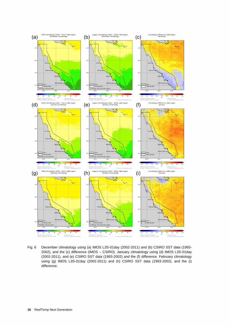
Generally, the IMOS climatology is warmer than the CSIRO climatology across most of the

GBR region (Fig. 6), with the exception of the far northern GBR and inshore regions. This is in

spite of the 0.17C cold offset between the IMOS skin SST and CSIRO sub-skin SST and the

use of night-time only data for the IMOS climatology. Two possible explanations which help

explain why the IMOS climatology is warmer on average as compared to the CSIRO

climatology are:

1. The climatologies are calculated for two different decades. SSTs in the Australian

region were the warmest on record during the recent decade as compared to the 1961 –

1990 average using NOAA Extended Reconstruction SSTs (Australian Bureau of

Meteorology, 2011). Lough (2008) showed that the trend in SST of coastal waters off

north-eastern Australia was to increase at 0.12°C/decade for the period 1950-2007.

2. The cloud quality control methods differ between the IMOS and CSIRO products. The

CSIRO SST product utilises a cloud detection mask which is generated using the

Saunders and Kribel (1998) algorithm. Griffin et al. (2004) states that approximately

40% of thin cloud at night is not detected by the Saunders and Kribel algorithm. This

would result in a cooler SST for the CSIRO SST climatology although the effect is at

least partially offset by using the 65th percentile median SST. For the IMOS SST and

climatology, Paltoglou et al. (2010) states that a new threshold test based on brightness

temperature measured from thermal infrared channels was found to be very effective at

identifying cloud.

We postulate that the observed differences could be due to these combined factors. However, it

is worth highlighting that the GBR had shown very little difference (± 0.5°C) between

climatologies, which is of importance to the primary management users of the RTNG product.


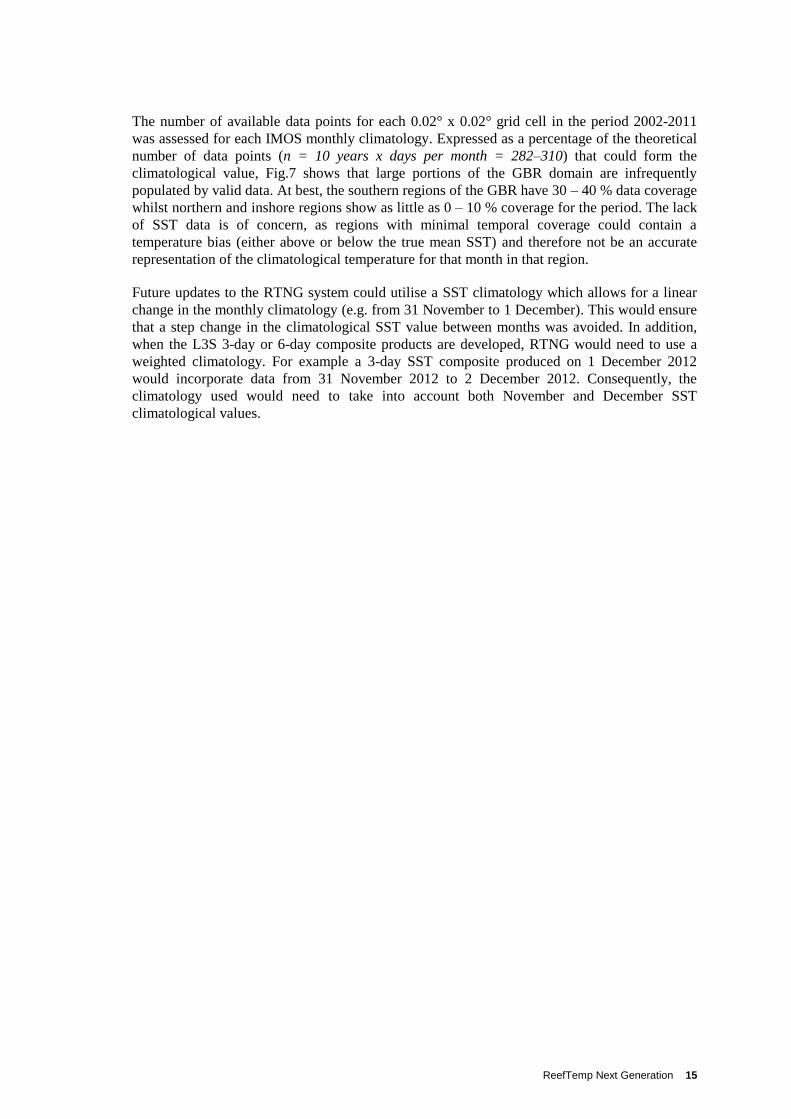
The number of available data points for each 0.02° x 0.02° grid cell in the period 2002-2011

was assessed for each IMOS monthly climatology. Expressed as a percentage of the theoretical

number of data points (n = 10 years x days per month = 282–310) that could form the

climatological value, Fig.7 shows that large portions of the GBR domain are infrequently

populated by valid data. At best, the southern regions of the GBR have 30 – 40 % data coverage

whilst northern and inshore regions show as little as 0 – 10 % coverage for the period. The lack

of SST data is of concern, as regions with minimal temporal coverage could contain a

temperature bias (either above or below the true mean SST) and therefore not be an accurate

representation of the climatological temperature for that month in that region.

Future updates to the RTNG system could utilise a SST climatology which allows for a linear

change in the monthly climatology (e.g. from 31 November to 1 December). This would ensure

that a step change in the climatological SST value between months was avoided. In addition,

when the L3S 3-day or 6-day composite products are developed, RTNG would need to use a

weighted climatology. For example a 3-day SST composite produced on 1 December 2012

would incorporate data from 31 November 2012 to 2 December 2012. Consequently, the

climatology used would need to take into account both November and December SST

climatological values.


Fig. 6 December climatology using (a) IMOS L3S-01day (2002-2011) and (b) CSIRO SST data (1993-

2002), and the (c) difference (IMOS – CSIRO). January climatology using (d) IMOS L3S-01day

(2002-2011), and (e) CSIRO SST data (1993-2002) and the (f) difference. February climatology

using (g) IMOS L3S-01day (2002-2011) and (h) CSIRO SST data (1993-2002), and the (i)

difference.


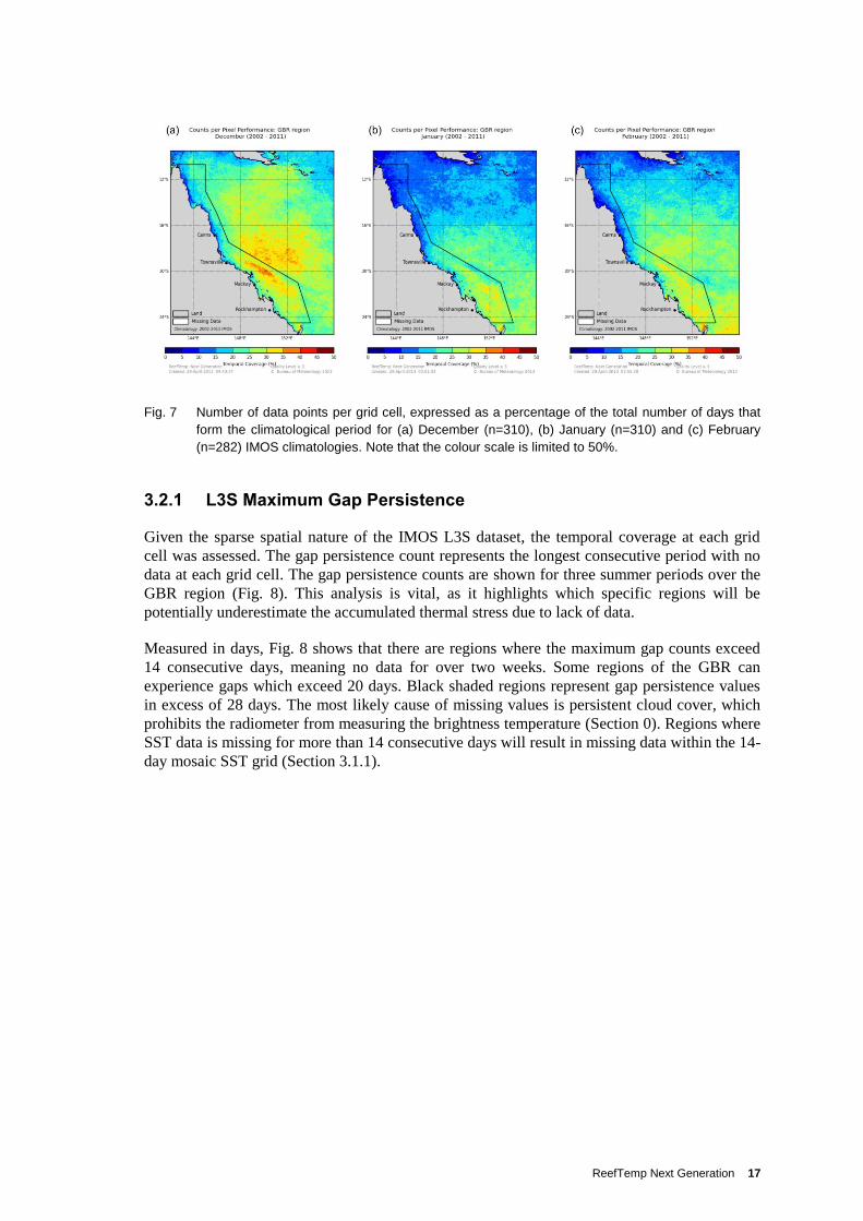
Fig. 7 Number of data points per grid cell, expressed as a percentage of the total number of days that

form the climatological period for (a) December (n=310), (b) January (n=310) and (c) February

(n=282) IMOS climatologies. Note that the colour scale is limited to 50%.

3.2.1 L3S Maximum Gap Persistence

Given the sparse spatial nature of the IMOS L3S dataset, the temporal coverage at each grid

cell was assessed. The gap persistence count represents the longest consecutive period with no

data at each grid cell. The gap persistence counts are shown for three summer periods over the

GBR region (Fig. 8). This analysis is vital, as it highlights which specific regions will be

potentially underestimate the accumulated thermal stress due to lack of data.

Measured in days, Fig. 8 shows that there are regions where the maximum gap counts exceed

14 consecutive days, meaning no data for over two weeks. Some regions of the GBR can

experience gaps which exceed 20 days. Black shaded regions represent gap persistence values

in excess of 28 days. The most likely cause of missing values is persistent cloud cover, which

prohibits the radiometer from measuring the brightness temperature (Section 0). Regions where

SST data is missing for more than 14 consecutive days will result in missing data within the 14-

day mosaic SST grid (Section 3.1.1).


Fig. 8 Example night-time L3S-01day gap persistence counts (days) for (a) December 2003, (b)

January 2004, (c) February 2004, (d) December 2008, (e) January 2009, (f) February 2009, (g)

December 2011, (h) January 2012 and (i) February 2012. The Australian coastline and GBR

marine park boundary are indicated by solid white lines.


3.3 Product Development

There are four primary products that comprise ReefTemp Next Generation (RTNG). These are:

1. Sea Surface Temperature (SST)

2. Sea Surface Temperature Anomaly

(SSTA)

3. Degree Heating Days (DHD)

4. Mean Positive Summer Anomaly

(MPSA)

These products are each generated using both IMOS-based 1-day L3S SST data and 14-day

SST mosaic products. Furthermore, all RTNG products are generated from daily night-time

only observations as discussed in Section 3.1.

3.3.1 Sea Surface Temperature

Daily SST values, derived directly from IMOS L3S 1-day products, are shown spatially over

the GBR, using the range 20-35°C in 1°C increments (Fig. 9). During the climatological period

of 2002-2011, SST values tend to peak around 29°C in the northern GBR and 26°C in the

southern GBR during the summer months. Temperatures in the low to mid-twenties (°C) are

common during the winter months.

Fig. 9 Example of the IMOS (a) L3S-01day and (b) 14-day mosaic SST products generated by RTNG

for 11 February 2012.


3.3.2 Sea Surface Temperature Anomaly

SSTA is calculated at each grid cell as the difference between the current SST condition and

the relevant monthly climatology. Figure 10 shows the four RTNG SSTA products, which

utilise IMOS 1-day and 14-day mosaic input SST grids, as well as IMOS and CSIRO

climatologies. The SSTA product temperature range is from -4°C to 4°C in increments of

0.5°C.

Fig. 10 Example RTNG SSTA products for 11 February 2012. IMOS 1-day SST referenced to (a) IMOS

climatology and (b) CSIRO climatology. 14-day SST mosaic referenced to (c) IMOS climatology

and (d) CSIRO climatology.


3.3.3 Degree Heating Days

Degree Heating Days (DHD) is a measure of the accumulation of heat stress from 1 December,

to 31 March each year. One DHD is calculated as 1°C above the relevant monthly climatology

for one day at a particular grid point (x, y). DHD can represent a broad range of heat stress, in

that 3 weeks at 1°C above the local long-term average results in the same number of DHDs as 1

week at 3°C, the latter representing more severe stress to corals. Mathematically, DHD can be

written as the following:

todayt

t yxyx SSTADHD1

st0 Dec 1 ,, C0 where SSTA (Equation 1)

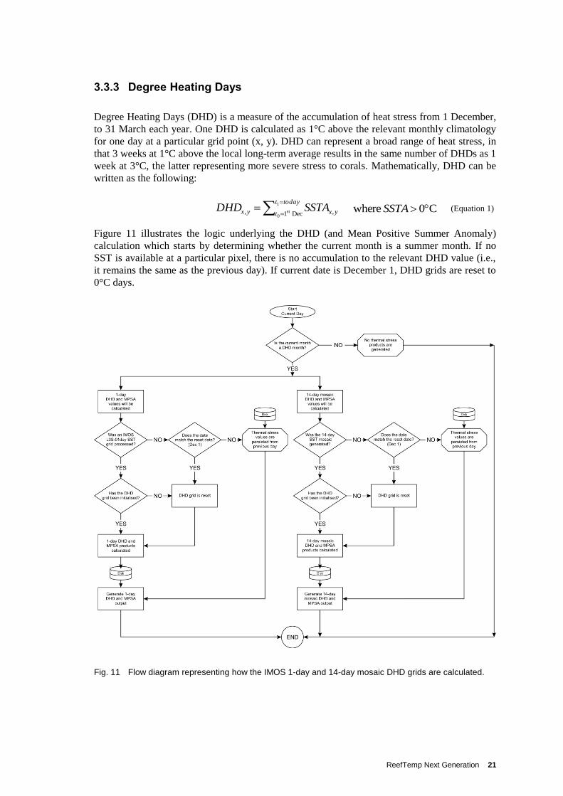
Figure 11 illustrates the logic underlying the DHD (and Mean Positive Summer Anomaly)

calculation which starts by determining whether the current month is a summer month. If no

SST is available at a particular pixel, there is no accumulation to the relevant DHD value (i.e.,

it remains the same as the previous day). If current date is December 1, DHD grids are reset to

0°C days.

Fig. 11 Flow diagram representing how the IMOS 1-day and 14-day mosaic DHD grids are calculated.


RTNG also produces a complementary product which illustrates occurrences, called DHD

counts. This product represents the number of days where the SSTA is greater than 0°C. As a

guide, DHD values above 60 generally are a cause of concern for GBRMPA, and are linked to

moderate-to-severe bleaching observations (Maynard et al., 2008). Figures 12 and 13 present

example DHD values using the L3S-01day and 14-day SST mosaic products respectively. DHD

value visualisation range is 0 – 240°C days in increments of 20°C days and DHD counts range

from 0 – 120 days in increments of 10 days.

Fig. 12 Example L3S-01day DHD stress index products for 31 March 2012 using (a) IMOS climatology,

(b) IMOS climatology DHD counts, (c) CSIRO climatology and (d) CSIRO climatology DHD

counts.


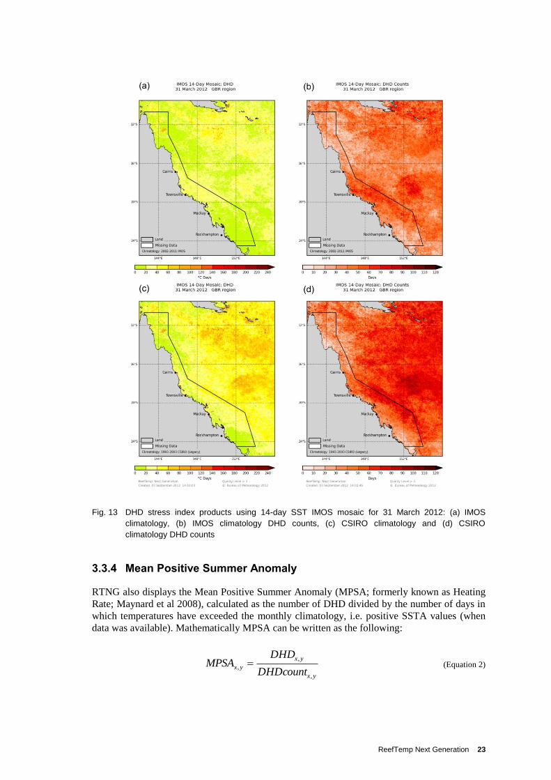
Fig. 13 DHD stress index products using 14-day SST IMOS mosaic for 31 March 2012: (a) IMOS

climatology, (b) IMOS climatology DHD counts, (c) CSIRO climatology and (d) CSIRO

climatology DHD counts

3.3.4 Mean Positive Summer Anomaly

RTNG also displays the Mean Positive Summer Anomaly (MPSA; formerly known as Heating

Rate; Maynard et al 2008), calculated as the number of DHD divided by the number of days in

which temperatures have exceeded the monthly climatology, i.e. positive SSTA values (when

data was available). Mathematically MPSA can be written as the following:

yx

yx

yxDHDcount

DHDMPSA

,

,

, (Equation 2)


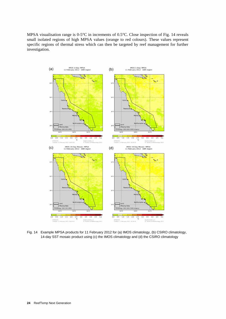
MPSA visualisation range is 0-5°C in increments of 0.5°C. Close inspection of Fig. 14 reveals

small isolated regions of high MPSA values (orange to red colours). These values represent

specific regions of thermal stress which can then be targeted by reef management for further

investigation.

Fig. 14 Example MPSA products for 11 February 2012 for (a) IMOS climatology, (b) CSIRO climatology,

14-day SST mosaic product using (c) the IMOS climatology and (d) the CSIRO climatology


3.3.5 Thermal Stress Product Interpretation

In comparing Figures 12 and 13, it is apparent that DHDs calculated based on the IMOS 1-day

SST product do not accumulate to the same magnitude as compared to the 14-day SST mosaic

SST product. As shown in Fig. 11, in the event that a daily SST grid is missing, the DHD

values remain the same. However, as the 14-day SST mosaic has historical data to draw on and

so better spatial coverage, its DHD are allowed to continue accumulating. As stated previously,

care must be taken when using the mosaic DHD products as the accumulated DHD may not be

a true representation of the current thermal stress.

The observed changes in baseline between the monthly climatologies have implications in the

way the thermal stress indices are calculated and how they should be interpreted. As discussed

in Section 3.2 (Fig. 6), for most of the GBR region, the IMOS climatology is warmer than the

CSIRO climatology. It is therefore not surprising that the DHD values will be higher when

using the CSIRO climatology, as it is more likely to observe a positive SSTA and therefore

accumulate DHD.

Given the inhomogeneous mosaic concerns raised in Section 3.1.1, it is advised that further

research could be targeted at developing a more accurate back-filled daily SST product. Spatial

interpolation techniques could be employed which would result in improved spatial coverage.

To complement this, at times where no daily SST data are available, the SSTA could be

persisted and damped from the previous day. This method would allow DHD values to continue

to accumulate instead of being persisted from the previous analysis. However, sensitivity and

performance evaluations are needed to measure the accuracy of such a technique.

3.4 Product Visualisation and Delivery

RTNG real-time and historical SST, SSTA and thermal stress products can be viewed online in

multiple ways. Delivery methods include:

1. Static images through specific RTNG web pages and Google EarthTM displays

2. eReefs – Marine Water Quality dashboard and OPeNDAP server

1. RTNG website and Google EarthTM

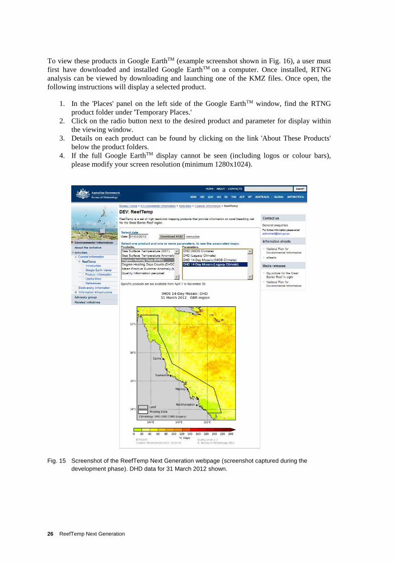
As shown in Fig. 15, the RTNG website (development site) provides an introduction to the

system as well as a simple user interface. By selecting a date from the top-left calendar, current

or historical RTNG products can be viewed. Multiple parameters can be viewed for a selected

product by selecting each parameter. In addition, Google EarthTM KMZ files can be

downloaded by clicking on the ‘Download KMZ’ button. Useful links, references and product

information can be viewed by clicking on the respective link under ReefTemp on the left hand

side.

Viewing RTNG products in Google EarthTM provides an interface in which users are able to

search, zoom and navigate to specific locations, change the viewing angle, and bookmark

favourite locations. Google Earth’s built in ocean layers also allow users to toggle GBR Marine

Park boundaries and reef outlines.


To view these products in Google EarthTM (example screenshot shown in Fig. 16), a user must

first have downloaded and installed Google EarthTM on a computer. Once installed, RTNG

analysis can be viewed by downloading and launching one of the KMZ files. Once open, the

following instructions will display a selected product.

1. In the 'Places' panel on the left side of the Google EarthTM window, find the RTNG

product folder under 'Temporary Places.'

2. Click on the radio button next to the desired product and parameter for display within

the viewing window.

3. Details on each product can be found by clicking on the link 'About These Products'

below the product folders.

4. If the full Google EarthTM display cannot be seen (including logos or colour bars),

please modify your screen resolution (minimum 1280x1024).

Fig. 15 Screenshot of the ReefTemp Next Generation webpage (screenshot captured during the

development phase). DHD data for 31 March 2012 shown.


Fig. 16 Screenshot of the RTNG Google EarthTM display illustrating the IMOS 1-day SST product for 31

March 2012.

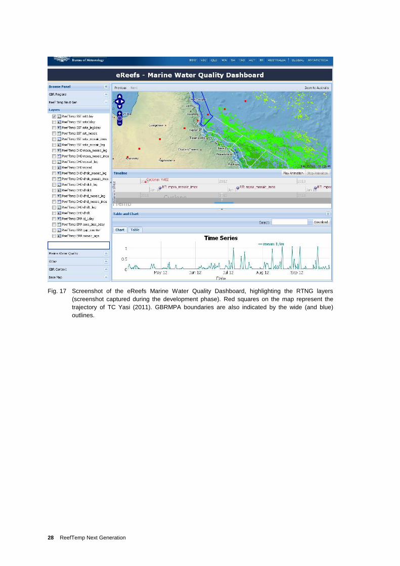
2. Dashboard and OPeNDAP server

The eReefs – Marine Water Quality dashboard visualises products from the RTNG system. By

selecting ‘Reef Temp Next Gen’ from the Browse Panel, a RTNG product can be selected by

clicking on the appropriate checkbox (Fig. 17). Once selected, the user can overlay GBRMPA

management zones, additional layers or change the map background. In addition, a user can

select a GBR region of interest which is then highlighted on the map. The dashboard backend

has the ability to source the netCDF data and calculate an area average of a parameter for that

region. A time series is generated and displayed. Animations can also be controlled via the

dashboard which is important as it allows users to visualise the accumulation of thermal stress.

This user interface will see major development throughout 2013.

RTNG netCDF files are also being served via the Bureau OPeNDAP (Open-source Project for a

Network Data Access Protocol) server which allows users to use data which are stored

remotely with visualisation client software. This server architecture is widely used within the

earth sciences community. To use this service, the OPeNDAP URL is simply entered into the

client’s software.


Fig. 17 Screenshot of the eReefs Marine Water Quality Dashboard, highlighting the RTNG layers

(screenshot captured during the development phase). Red squares on the map represent the

trajectory of TC Yasi (2011). GBRMPA boundaries are also indicated by the wide (and blue)

outlines.


4. FUTURE DEVELOPMENT

The development of RTNG has provided the launching pad for additional research. Reef

managers are particularly interested in products that document risk of coral disease (e.g. White

Syndrome, Black Band disease) as well as cross validation of current RTNG products with

coral bleaching data. Additional requests included increased spatial coverage, extension of the

RTNG geographical domain beyond the GBR and the facilitation of virtual stations, which are

analyses that are targeted at specific reef locations.

Enhancements to this system could include new products for diurnal warming and coral

bleaching risk. In its current form, RTNG utilises night-only IMOS L3 1-day data to produce

SST products. The capability to capture diurnal warming (warming over the course of the day)

would create more refined functionality and provide the first real-time products documenting

diurnal warming over the GBR. Coral disease risk can be estimated using SST conditions and

coral cover and would be valuable information for management. New RTNG disease risk

products could facilitate quick response reef management teams to attend locations of concern

within the GBR. The product would also provide an historical overview of disease risk as

related to temperature to aid climate change research.

Additional products could include 6-10 day composite and day+night products for greater

spatial coverage. Currently a mosaic product has been built to provide a gap-filled SST product

for managers, using the L3S 1-day data over the past 14 days. However whilst effective, this

approach can produce spatially inhomogeneous results. The next step would be to utilise new

IMOS L3S 6-day or 10-day products which provide a more sophisticated weighted average of

SST values over the past 6 or 10 days. Likewise, day+night products would incorporate a

greater volume of data and would increase the spatial coverage currently possible in the RTNG

products.

The RTNG domain is currently limited to the GBR. The geographic region covered could be

expanded to the wider Australian region, [70-190°E; 20-70°S], including Ningaloo Reef, Scott

Reef, Lord Howe Island, the Coral Sea and the Western Pacific. The expansion of the RTNG

domain will significantly increase both functionality and the number of users and applications

of RTNG. It will also facilitate comparison with complementary NOAA Coral Reef Watch

satellite products over a wider geographic domain.

Nowcasts from RTNG present high resolution SST, SSTA and thermal stress distributions over

the GBR at the daily timescale. These nowcasts show current conditions at a 2 km spatial scale,

allowing assessment of the current risk of bleaching in particular reef regions. Linking in

seamlessly with the daily nowcasts, would be multi-week and seasonal forecasts of coral

bleaching risk, generated using the dynamical prediction system POAMA (Prediction Ocean

Atmosphere Model for Australia). Seasonal POAMA forecasts of bleaching risk for the GBR

are currently already produced operationally at the Bureau and are the first in the world to

utilise a dynamical GCM (General Circulation Model) in the prediction of coral bleaching

conditions (Spillman 2011a; 2011b) . They are an important component in management plans

and strategic frameworks for the GBR, including the GBRMPA Early Warning System for

coral bleaching (Maynard et al. 2009).

This multi-scale reef information presentation would allow reef managers to assess the current

thermal conditions at the reef scale then move forward in time to predicted regional

temperatures to enable them to plan their activities for the upcoming season. The provision of

both the observation-based nowcasts and forecasts on different spatial scales in real-time


provides reef management to the most up-to-date information and hence facilitates proactive

management. Forecasts on a weekly to seasonal timescale are particularly useful for reef

managers as they provide advance notice of potential bleaching conditions, allowing for

implementation of management strategies prior to bleaching onset (Spillman and Alves 2009).

This would also synergise with other projects looking at intra-seasonal to seasonal climate risk

products.


5. SUMMARY

RTNG is a sophisticated new state-of-the-art nowcast remote sensing system that monitors

ocean temperature and associated coral bleaching risk over the GBR. The development and

operational support for these types of systems is extremely important as the frequency and

severity of coral bleaching is expected to increase due to climate change.

RTNG is based on the new multi-sensor composite AVHRR SST L3S 1-day night-only product

developed as part of IMOS. RT1 products have been reconfigured in the new system to use this

new data stream and updated climatologies. These products include SST, SSTA, DHD and

MPSA. New 14-day SST mosaic products have also been developed to address the issue of

missing data. Additionally, new products have been created to provide complementary

information as to the number of data points used to construct climatologies, length and

persistence of data gaps and data errors. Products are available online as static images through

tailored RTNG web pages, in Google EarthTM and in the new Marine Water Quality dashboard.

This research also presented an opportunity to rethink both the design and delivery of the

thermal stress products to best address the needs of the reef managers. This was undertaken in

close consultation with end users, such as the GBRMPA and NOAA, to ensure that the new

system addressed user needs. RTNG provides reef management with the means of better

monitoring thermal stress events and when coral bleaching is likely, targeting both response

actions and in-situ observations of stress impacts.


6. ACKNOWLEDGMENTS

The authors would like to acknowledge Dr. Oscar Alves, Dr. Debbie Hudson, Aurel Griesser,

Elaine Miles, Griffith Young, Kevin Keay (Centre for Australian Weather and Climate

Research, Australian Bureau of Meteorology), Dr. Scott Heron (National Oceanic and

Atmospheric Administration), Roger Beeden (Great Barrier Reef Marine Park Authority) and

Dr. Jeffrey Maynard (Maynard Marine Consulting) for their guidance, helpful discussion and

suggestions given to the authors during the preparation of this manuscript. Thanks is also

extended to the staff at GBRMPA for their support and feedback during the ReefTemp Next

Generation development process. The authors also thank the reviewers of this document for the

comments and suggestions.

Data was sourced from the Integrated Marine Observing System (IMOS). IMOS is supported

by the Australian Government through the National Collaborative Research Infrastructure

Strategy and the Super Science initiative. Raw HRPT AVHRR SST data was collected by the

Australian Bureau of Meteorology in collaboration with Australian Institute of Marine Science

(AIMS) and CSIRO Marine and Atmospheric Research. Finally, thanks also to the reviewers of

this manuscript. Funding provided by eReefs/NPEI.


REFERENCES

Australian Bureau of Meteorology 2011: Annual Climate Summary 2010. January 2011. pp 20

Baker, A., Glynn, P.W. and Riegl, B. 2008: Climate change and coral reef bleaching: An

ecological assessment of long-term impacts, recovery trends and future outlook. Estuar. Coast.

Shelf Sci. 80, 435–71

Beeden, R.J., Maynard, J.A., Marshall, P., Heron, S. and Willis, B. 2011: A framework for

responding to coral disease outbreaks that facilitates adaptive management. Environmental

Management, 1-11-11. http://dx.doi.org/10.1007/s00267-011-9770-9

Berkelmans, R., De’ath, G., Kininmonth, S. and Skirving, W. J. 2004: A comparison of the

1998 and 2002 coral bleaching events on the Great Barrier Reef: spatial correlation, patterns,

and predictions. Coral Reefs, 23, 74–83. doi:10.1007/s00338-003-0353-y

Brown, B.E. 1997: Coral bleaching: causes and consequences. Coral Reefs. 16,

doi:10.1007/s003380050249

Casey, K., Donlon, C. and the GHRSST Science Team. 2011. The recommended GHRSST

Data Specification (GDS) 2.0, Revision 4 [online], 7 November 2011, 123 pp.

https://www.ghrsst.org/documents/q/category/gds-documents/operational/

Donlon, C.J., Minnett, P.J. Gentemann, C. Nightingale, T. J. Barton, I. J. Ward, B. and Murray,

J. 2002: Toward improved validation of satellite sea surface skin temperature measurements for

climate research. Journal of Climate, 15, 353-69

Donner S.D., Skiving, W., Little C.M., Oppenheimer M. and Hoegh-Guldberg O. 2005: Global

assessment of coral bleaching and required rates of adaptation under climate change. Global

Change Biology, 11, 1-15, doi: 10.1111/j.1365-2486.2005.01073.x

Donner S. D. 2009: Coping with Commitment: Projected Thermal Stress on Coral Reefs under

Different Future Scenarios. PLoS ONE 4(6): e5712. doi:10.1371/journal.pone.0005712

Frieler, K., Meinshausen, M., Golly, A., Mengel, M., Lebek, K., Donner, S.D. and Hoegh-

Guldberg, O. 2012: Limiting global warming to 2°C is unlikely to save most coral reefs. Nature

Climate Change, 2(9), 1–6. doi:10.1038/nclimate1674

Gentemann, C.L., Donlon, C.J., Stuart-Menteth, A. and Wentz, F.J. 2003: Diurnal signals in

satellite sea surface temperature measurements, Geophs. Res. Lett., 30, 1140,

doi:10.1029/2002GL016291

Glynn, P.W. 1993: Coral reef bleaching: ecological perspectives. Coral Reefs, 12, 1-17

Griffin, D.A., Rathbone, C.E., Smith, G.P., Suber, K.D. and Turner, P.J. 2004: A Decade of

SST Satellite Data. Final Report for the National Oceans Office, Contract NOOC2003/020, 1-8

Hennessy, K., Fitzharris, B., Bates, B.C., Harvey, N., Howden, S.M., Hughes, L., Salinger J.

and Warrick, R. 2007: Australia and New Zealand. Climate Change 2007: Impacts, Adaptation

and Vulnerability. Contribution of Working Group II to the Fourth Assessment Report of the

http://dx.doi.org/10.1007/s00267-011-9770-9


Intergovernmental Panel on Climate Change, M.L. Parry, O.F. Canziani, J.P. Palutikof, P.J. van

der Linden and C.E. Hanson, Eds., Cambridge University Press, Cambridge, UK, 507-40

Heron, S. et al. 2012: Developments in understanding relationships between environmental

conditions and coral disease. Proceedings of the 12th International Coral Reef Symposium,

Cairns, Australia, 9-13 July 2012 (pp. 9–13)

Hoegh-Guldberg, O. 1999: Climate change, coral bleaching and the future of the world’s coral

reefs. CSIRO: Marine and Freshwater Research, 50, 839-66

Hoegh-Guldberg, O., Mumby P.J., Hooten A.J., Steneck R.S., Greenfield P., Gomez E.,

Hardvell C.D., Sale P.F., Edwards A.J., Caldeira K., Knowlton N., Eakin C.M.,Iglesias-Prieto

R., Muthiga N., Bradbury R.H., Dubi A. and Hatziolos M.E. 2007: Coral Reefs Under Rapid

Climate Change and Ocean Acidification. Science. 318, 1737-1742, doi:

10.1126/science.1152509

Jones, R.J, Hoegh-Guldberg, O., Larkum, A.W.D. and Schreiber, U. 1998: Temperature-

induced bleaching of corals begins with impairment of the CO2 fixation mechanism in

zooxanthellae. Plant, Cell and Environment. 21, 1219-30

Lesser, M. P. 2004: Experimental biology of coral reef ecosystems. Journal of Experimental

Marine Biology and Ecology. 300, 217-52

Liu, G., Strong, A.E., Skirving W. and Arzayus. L.F. 2006: Overview of NOAA Coral Reef

Watch Program’s near-real time global satellite coral bleaching monitoring activities. Proc. 10th

Int. Coral Reef Symp., Okinawa, Japan, 1783-93

Lough, J.M. 2008: Shifting climate zones for Australia’s tropical marine ecosystems,

Geophysical Research Letters, 35, L14708, doi: 10.1029/2008GL034634

Maynard, J.A., Turner, P.J., Anthony, K.R.N., Baird, A.H., Berkelmans, R., Eakin, C.M.,

Johnson, J., Marshall, P.A., Packer, G.R., Rea A. and Willis, B.L. 2008: ReefTemp: An

interactive monitoring system for coral bleaching using high-resolution SST and improved

stress predictors. Geophysical Research Letters, 35, L05603, doi:10.1029/2007GL032175

Maynard, J.A., Johnson, J.E., Marshall, P.A., Eakin, C.M., Goby, G., Schuttenberg, H. and

Spillman, C.M. 2009: A strategic framework for responding to coral bleaching events in a

changing climate. Environmental Management, 44, 1-11, doi:10.1007/s00267-009-9295-7

Minnett, P.J. 2003: Radiometric measurements of the sea–surface skin temperature—the

competing roles of the diurnal thermocline and the cool skin. International Journal of Remote

Sensing, 24 (24), 5033–47

Montgomery, R.S. and Strong, A. 1995: Coral bleaching threatens ocean, life, EOS, 75, 145-7

Paltoglou, G., Beggs H. and Majewski, L. 2010: New Australian High Resolution AVHRR SST

Products from the Integrated Marine Observing System, In: Extended Abstracts of the 15th

Australasian Remote Sensing and Photogrammetry Conference, Alice Springs, 13-17

September, 2010. http://imos.org.au/srsdoc.html

Rea, A. 2004: Recent Improvements to the NOAA AVHRR SST Product at the Australian

Bureau of Meteorology, Presented to the Fifth GODAE High Resolution SST Pilot Project


Science Team Workshop, Townsville, Australia, 25-30th July, 2004,

http://imos.org.au/srsdoc.html

Saunders, R.W. and Kriebel, K.T. 1998: An improved method for detecting clear sky and

cloudy radiances from AVHRR data. International Journal of Remote Sensing, 9, 123-50

Spillman, C.M. 2011a: Advances in forecasting coral bleaching conditions for reef

management. Bulletin of the American Meteorological Society, 94, 1426-31

Spillman, C.M. 2011b: Operational real-time seasonal forecasts for coral reef management.

Journal of Operational Oceanography, 4, 13-22

Spillman C.M. and Alves, O. 2009: Dynamical seasonal prediction of summer sea surface

temperatures in the Great Barrier Reef. Coral Reefs, 28, 197-206

Ward, B. 2006. Near-surface ocean temperature. Journal of Geophysical Research, 111,

C02005

Weeks, S. J., Anthony, K.R.N., Bakun, A., Feldman, G.C. and Hoegh-Guldberg, O. 2008:

Improved predictions of coral bleaching using seasonal baselines and higher spatial resolution.

Limnology and Oceanography, 53, 1369–75. doi:10.4319/lo.2008.53.4.1369

Wilkinson, C. 2008: Status of coral reefs of the world: 2008. Global Coral Reef Monitoring

Network and Reef and Rainforest Research Centre, Townsville, Australia, 296 p

reeftemp next generation - cawcr | · reeftemp next generation l.a. garde1, c.m spillman1, ......

Documents