reducing scientific computing problems to...
TRANSCRIPT
UNIVERSITY OF TARTUFaculty of Mathematics and Computer Science
Institute of Computer Science
Pelle Jakovits
Reducing scientific computing problems to MapReduce
Masters thesis
Supervisor Satish Srirama
Author ldquohellipldquo May 2010Supervisor ldquohellipldquo May 2010
Permission for defenceProfessor ldquohellipldquo May 2010
TARTU 2010
Table of Contents
Acknowledgements5
1 Introduction6
2 Scientific computing on the cloud8
3 Hadoop1131 What is Hadoop1132 Hadoop Distributed File System1133 Hadoop MapReduce13
331 Map and Reduce14332 Execution15333 Combining intermediate results and preserving task state17334 Keys and values 20
34 Other Hadoop Projects21
4 Algorithms2341 Choice of algorithms2342 Conjugate gradient method24
421 CG in MapReduce27422 Matrix-vector multiplication in MapReduce27423 Result28
43 K-medoids30431 Partitioning Around Medoids30432 PAM in MapReduce31433 Clustering large applications33434 CLARA in MapReduce34435 Comparison37
44 RSA breaking41441 Integer factoring algorithm42442 Integer factoring algorithm in MapReduce43443 Result44
5 Conclusion47
Kokkuvotildete48
References49
Appendices51
2
Index of FiguresFigure 1 Replicating and distributing file blocks on HDFS12Figure 2 Asking file block location from the namenode13Figure 3 Word count example MapReduce algorithm15Figure 4 MapReduce framework16Figure 5 Word count without combiner18Figure 6 Word count with combiner19Figure 7 Commutativity of a function19Figure 8 Associativity of a function19Figure 9 Word count map method20Figure 10 An example Java class Pair21Figure 11 System of linear equations24Figure 12 Matrix form of a linear system24Figure 13 Conjugate Gradient algorithm25Figure 14 Map method of the matrix vector multiplication28Figure 15 Reduce method of the matrix vector multiplication28Figure 16 PAM process31Figure 17 Sequential part of PAM MapReduce 31Figure 18 Mapper (PAM)32Figure 19 Reducer (PAM)32Figure 20 Sequential part CLARA MapReduce34Figure 21 Map method (first CLARA MapReduce job)34Figure 22 Reduce method (first CLARA MapReduce job)35Figure 23 Map method (second CLARA MapReduce job)36Figure 24 Reduce method (second CLARA MapReduce job)36Figure 25 PAM iteration 437Figure 26 PAM iteration 137Figure 27 PAM iteration 738Figure 28 PAM iteration 1038Figure 29 PAM final iteration38Figure 30 CLARA result 139Figure 31 CLARA result 239Figure 32 CLARA result 339Figure 33 CLARA best result39Figure 34 Algorithm to find the smallest factor43Figure 35 Map method of the RSA factoring MapReduce algorithm43Figure 36 Reduce method of the RSA factoring MapReduce algorithm44
3
Index of TablesTable 1 Runtime of the CG MapReduce and the original CG algorithm29Table 2 Runtime comparison for PAM and CLARA40Table 3 Runtime table for RSA45Table 4 Parallel speedup for RSA45Table 5 Parallel efficiency for RSA45
4
Acknowledgements
First I thank my supervisor Satish Srirama for introducing me to cloud computing and MapReduce Hes help and suggestions with the research in this topic and writing this thesis has been invaluable Secondly I would like to thank everyone in the Distributed Systems Group in Tartu University Over the years I got a lot of experience in writing and presenting topics in the weekly seminars of Distributed Systems and this has helped me immensely I would also like to thank the Tartu University for providing an excellent education and my friends and family for supporting me while I was writing this thesis
5
Chapter 1
IntroductionScientific computing[1] should not be confused with computer science It is a field of
study that applies computer science to solve scientific problems Scientific computing is most often associated with large scale computer simulation and modelling However a considerable effort in scientific computing is actually devoted to studying the numerical methods and algorithms on which the simulations and models depend on
The computer simulation problems that scientific computing deals with are often very large scale from modelling climate to simulating a star going supernova Because such simulations generally require large amount of computing resources scientific computing has always been strongly connected to distribute computing adapting to any advances done in this field and gradually progressing from doing computations on clusters to grids and from grids to clouds
Clouds are the latest direction in distributed computing Companies like Google Amazon and Microsoft are building huge data centres on which to provide cloud services like Google App engine Gmail Windows Azure and Amazon EC2 As a result cloud computing has become more and more popular as a platform to provide services on Apart from offering services for external clients these cloud resources are also used internally for these companies own needs for distributed computing Google has developed a MapReduce[2] model and framework to process very large amounts of raw data that can no longer be managed with normal means The amount of data Google has to deal with daily basis like indexed internet documents and web requests logs grows every day To cope with this Google uses a cloud computing platform which consists of large number of commodity computers in their data centres to run MapReduce jobs
MapReduce is a programming model and a distributed computing framework to process extremely large data It can be used to write auto scalable distributed applications in a cloud environment In the MapReduce model programmers have to reduce an algorithm into iterations of map and reduce functions known from Lisp[3] and other functional programming languages Writing an algorithm only consisting of these two functions can be a complicated task but MapReduce framework is able to automatically scale and parallelize such algorithms The framework takes care of partitioning the input data scheduling synchronising and handling failures allowing the programmers to focus more on developing the algorithms and less on the background tasks Making it easier for prog-rammers without extensive experience with parallel programming to write applications for large distributed systems
In Tartu University the Distributed Systems Group is working on a project called Scientific Computing on the Cloud[4] (SciCloud) The goal of this project is to study establishing private clouds using the existing resources of university computer networks and using the resources of these clouds to solve different large scale scientific and mathematical problems A section of this project deals with MapReduce and its goal is to study how to apply MapReduce programming model to solve scientific problems This thesis is the first work on this topic (in the context of SciCloud project) and its goal is to study what steps are needed to reduce different computationally intensive algorithms to MapReduce model and what can affect the efficiency and scalability of the results
6
Additional goal is to lay the grounds for further work in this direction establishing a general idea of which kind of scientific computing problems can be solved using MapReduce and what kinds of complications can arise The algorithms that are reduced to MapReduce model in the course of this thesis are Conjugate Gradient breaking RSA[56]
using integer factorization and two different k-medoid[7] clustering algorithms Partitioning Around Medoids[7] and Clustering Large Applications[7]
The Google MapReduce implementation is proprietary and could not be employed for this thesis Instead an open source Hadoop[8] implementation of MapReduce framework was chosen Apache Hadoop is a Java software framework inspired by Googles MapReduce and Google File System[9] (GFS) Hadoop project is being actively developed and is widely used both commercially and for research It is also very suitable for this thesis because it is under free licence has a large user base and very adequate documentation
The structure of this thesis consists of four chapters First is the introduction The second chapter introduces scientific computing domain and cloud computing It gives a brief overview of the problems the scientific computing deals with and explains its connection to distributed computing on clouds It also tries to explain the advantages of using cloud computing as a platform for solving scientific problems The third chapter introduces the open source cloud computing framework called Hadoop describes its components Hadoop MapReduce and Hadoop Distributed File System (HDFS)[10] and also gives a very brief overview of other Hadoop projects The fourth and last chapter outlines the algorithms that were implemented in MapReduce framework for this thesis Each sub chapter introduces one algorithm describing it and the steps taken to reduce the algorithm to MapReduce programming model Also the scalability of each of the reduced algorithms is analysed to find how well their implementations would work in large clouds Additionally the appendix contains the source code compiled Java code and Javadoc for the algorithms presented in this thesis
This thesis is addressed to readers who are interested in scientific computing and want to learn more about reducing different algorithms to auto scalable parallel application framework called MapReduce
7
Chapter 2
Scientific computing on the cloudScientific computing[1] (SC) is a field of study dealing with the construction of mat-
hematical models for computer simulations and using numerical methods to solve different scientific and engineering problems Weather forecasting nuclear explosion simulation and the simulation of air plane aerodynamics are some of the examples of computer modelling problems that SC deals with Also a substantial effort in SC is devoted to studying the numerical and computational methods and algorithms needed to simulate such models
The problems the scientific computing deals with are often very large and require to process massive amounts of data To solve such large scale problems the resources of a single computer is not enough and the use of distributed systems is required However writing efficient and precise algorithms for distributed systems is often a very complex task Methods and algorithms that work on a single computer might not be scalable for distributed environments or a lot of effort is required to parallelize them including organising the distribution of data managing synchronization and communication achieving fault tolerance and avoiding race conditions Thus because of the large size of the problems it deals with scientific computing is greatly influenced by other fields of study dealing with parallel computing Like distributed computing[11] parallel programming[12] and cloud computing[13]
Last one of these three the cloud computing is relatively new and is more focused on the commercial side of distributed computing and on providing services to outside clients It is difficult to define what cloud computing exactly is A cloud can be described as a large collection of commodity computers connected through a network and forming a computing platform where the resources of the individual computers are shared However the same description could be used for both grids and clusters[14] What mainly makes the clouds different is the use of virtualization[15] technology which allows more flexible use of the computer resources in the cloud Virtualization allows to hide the actual characteristics of a cloud hardware and instead of giving limited access to the actual machines in the cloud users are given full access to virtual machines (VM) that are executed in the cloud Different VMs can have different configurations and operating systems and it is possible to limit how much resources each VMs is able to access
In grids and clusters each individual machines must be configured to cater all possible needs of the users be it different programming language compilers libraries or programs But in clouds the individual machines only need to have a basic cloud configuration and the ability to run multiple virtual machines at once Not only does this make managing the cloud easier it also gives users complete control over the computing environment Users can choose what operation system they need for their VM fully configure it and freely install any software or libraries they need Once they have configured the virtual machine they can run it on the cloud and save or delete the VM when they are done
Clouds can be divided to public clouds which are available to general public and private clouds which refer to closed clouds belonging to businesses universities or other organizations Public clouds offer their services on demand as utilities in the sense that users are able to request cloud resources and pay for exactly how much they use treating the cloud resources as quantity measured services like gas or electricity Also similarly
8
with gas and electricity clouds try to provide an illusion of infinite amount of computing resources being available at any time To achieve this the Cloud infrastructure must be very flexible and reliable Considering that the hardware used in clouds is mostly composed of commodity computers extra measures must be taken to achieve reliability at any time To achieve fault tolerance all data in the cloud must be replicated so even if some computers fail no data is lost The structure of a cloud must also be dynamic so that failure of a few machines in the cloud does not interrupt the whole system and it would be possible to switch out and add new machines without stopping the cloud services
The availability of nearly infinite amount computing resources on demand provides cloud users with an ability to scale their applications more easily For example a company which is just starting out can rent the initial computing resources they need from the cloud and increase or decrease the amount of resources dynamically when the demand changes They no longer need to make huge initial investments to plan for the future demand and can simply pay for what they use lowering the start up costs and risks of starting a new business
Also in the public cloud it does not matter if one computer is used for 10000 hours or 1000 computers are used for 10 hours it still costs the same for the user This provides cloud users the perfect means to do short term experiments which require a huge amount of resources without having to invest into the hardware themselves If the experiments are long and done frequently then investing into private hardware might be useful However if the experiments are done infrequently but still require a lot of computer resources then it is often more cost effective to use a cloud resources and pay for how much was used rather than to invest into expensive hardware when most of the time this hardware might not even be used
The commercial applicability of cloud computing is one of the main reasons why cloud computing is becoming more and more popular A large amount of money is invested into cloud technologies and infrastructure every year by Google Amazon Microsoft IBM and other companies Apart from providing services to others cloud computing is also used by these companies for their own large scale computing needs For example Google uses a framework called MapReduce for their computing tasks which is able to automatically parallelize certain types of algorithms and run them on the cloud It takes care of the data data distribution synchronisation and communication allowing the programmer to design algorithms for cloud systems without having to manage these background tasks
Google developed MapReduce framework because the raw data Google collects on daily basis has grown so large that it is no longer possible to manage and process it by normal means MapReduce was specifically designed to deal with huge amount of data by dividing the algorithms into map and reduce tasks that can be executed on hundreds or thousands of machines concurrently in the cloud Google uses MapReduce for many different problems including large-scale indexing graph computations machine learning and extracting specific data from a huge set indexed web pages[2] Already in 2008 the MapReduce framework was used by Google to process more than 20 petabytes of data every day[16] Other related work[17] shows that MapReduce can be successfully used for graph problems like finding graph components barycentric clustering enumerating rectangles and enumerating triangles And also for scientific problems[18] like Marsaglia polar method for generating random variables integer sort conjugate gradient fast Fourier transform and block tridiagonal linear system solver It shows that MapReduce can be used for wide range of problems However this previous work has also indicated that MapReduce is more suited for embarrassingly parallel algorithms and has problems with iterative ones As a result it was decided that this thesis concentrates more on iterative
9
algorithms to further study this result
The structure of algorithms written for MapReduce framework is rather strict but the potential of automatic parallelization high scalability and the ability to process huge amount of data could be very useful for scientific computing This makes it important to study what kind of algorithms can be applied using the MapReduce framework Because Googles MapReduce implementation is not freely available the Hadoop distributed computing framework was chosen as platform on which to implement and study algorithms for this thesis The next chapter takes a closer look on Hadoop and describes its architecture and its MapReduce implementation in more detail
10
Chapter 3
HadoopThis section gives an overview of the Hadoop software framework It describes the file
system of Hadoop which is used to store very large data in a distributed manner and describes the Hadoop implementation of MapReduce which is used to execute scalable parallel applications This chapter will also briefly introduce other cloud computing applications that are developed under the Hadoop project
31 What is HadoopHadoop is a free licence Java software framework for cloud computing distributed by
Apache[19] It implements Hadoop Distributed File System (HDFS) to store data across hundreds of computers and MapReduce framework to run scalable distributed applications Both HDFS and Hadoop MapReduce are open source counterparts of Google File System and Google MapReduce Hadoop also includes other cloud computing applications like Hive[20] Pig[21] and Hbase[22] Hadoop is in active development and has been tested to run on up to 2000 nodes for example to sort 20TB of data[23]
The architecture of Hadoop is designed so that any node failures would be automatically handled by the framework In HDFS all data is replicated to multiple copies so even if some machines fail and their data is lost there always exist another replica of the data somewhere else in the cloud In MapReduce framework the node failures are managed by re-executing failed or very slow tasks So if a node fails and a MapReduce task was running on it the framework will keep track of this and re-execute the task on some other machine in the cloud The framework is also able to detect tasks that are running very slow and re-execute them elsewhere
32 Hadoop Distributed File SystemHDFS is an open source counterpart of the proprietary Google File System It is
designed to reliably store very large files across multiple nodes in a cloud network HDFS is also designed to be deployed on cheap commodity hardware and therefore it is almost guaranteed that there will be hardware failures especially if the cloud consists of hundreds or thousands of machines Because of this the fault tolerance is the most important goal of the HDFS
HDFS has a masterslave architecture Master of a HDFS cluster is called a namenode and slave is called a datanode Namenode handles the file system directory structure regulates access to files and manages the file distribution and the replication All changes to the file system are performed through namenode however the actual data is always moved between the client and the datanode and never through the namenode All other nodes in a HDFS cluster act as datanodes which is where the actual data on the HDFS is stored Each machine in the cloud acting as a datanode allocates and serves part of its local disc space as a storage for the HDFS
11
Fault tolerance in the HDFS is achieved by dividing each file into a sequence of file blocks of the same size and replicating each such block Each such replica is then distributed across different datanodes across the HDFS The default size of the file block is 64 MB and the default number of file block replicas is 3 Both of these settings can be changed by the user and can be different for each file on the HDFS File block size must be set when the file is created and can not be changed but the number of replicas can change at any time A sample file division into blocks and their replication and distribution is described on the figure 1
How exactly the replicas are distributed is very important for HDFS performance and fault tolerance If all replicas are very close to each other then a large failure could cause a permanent data loss However if all replicas are very far from each other and spread across many machines then reading a file from the HDFS can be slowed down considerably HDFS tries to distribute the replicas so that two replicas are located on nodes in the same rack and another replica is located on other racks in the cloud So even if a network equipment failure brings down a whole rack the data would still be accessible
When a user or an application wants to read a file on the HDFS they first have to ask for the file block locations from the namenode For each file block the namenode will reply with the file block identification and with the identification of the datanode where the data block is located The client then contacts the datanode and asks the file block data This process is also described on the figure 2
When a location of a file block is asked from the HDFS namenode it knows locations of multiple replicas for that block Namenode always tries to supply the location of a replica that is closest to the request location to minimize the global bandwidth and latency This can be very helpful when the cloud network is very large and machines are located on different computer racks or even in different buildings For an application running on a cloud it is always faster to read data from the same machine or from a neighbouring one
12
Figure 1 Replicating and distributing file blocks across different datanodes in the HDFS
HDFS uses two types of messages to keep track of the condition of the distributed file system These two messages are heartbeat and block report and they are sent to the namenode by each of the datanodes in the cloud The heartbeat message is sent periodically to let the namenode know that the datanode is still reachable If some of the datanodes fail to send the heartbeat message they are marked as unreachable and no new file read and write requests are forwarded to them by the namenode This also causes all the file block replicas in those datanodes to be lost and to preserve the required number of replicas for each file block the namenode has to manage the creation and distribution of replacement replicas The second message block report is sent by the datanodes when they start up It contains a list of all the HDFS data blocks the datanode has stored in its local file system The namenode uses the block reports to keep track of the data block locations and if it notices that some data blocks do not have enough replicas it will initiate a process to create additional replicas
33 Hadoop MapReduceMapReduce is a programming model for designing auto scalable distributed computing
applications on clouds However in the context of Hadoop MapReduce is also a framework where the distributed applications are implemented Using the same term for both the model and the framework can be confusing but its meaning is strictly dependant on the context When talking about algorithm design then MapReduce refers to a model When talking about executing distributed applications in a cloud then it refers to the framework
Hadoop MapReduce framework is written in Java programming language and is designed for applications processing vast amounts of data in parallel in a cloud network Because clouds often consist of commodity hardware the MapReduce framework must provide reliable and fault tolerant execution of distributed applications
In the MapReduce model all algorithms consist of two methods map and reduce To write auto scalable distributed applications for cloud computing all the user has to do is to define these two methods The Hadoop MapReduce framework is able to automatically parallelize such applications taking care of all the background tasks including data distribution synchronisation communication and fault tolerance This allows programmers
13
Figure 2 Asking file block location from the namenode and reading the file block data from the location given by the namenode
to easily write distributed applications for cloud computing without having any previous experience with parallel computing
This sub chapter introduces the MapReduce model and the Hadoop MapReduce framework It also gives a basic idea how to write MapReduce algorithms and how they are executed on the framework
331 Map and Reduce
MapReduce model is inspired by the map and reduce functions commonly used in functional programming Map method in the functional programming typically takes a function and a list as an argument applies the function to each element in the list and returns the new list as a result An example of a map in functional programming is
map f [1234] = [f(1) f(2) f(3) f(4)] == [12 22 32 42] = [2 4 6 8]
where f is a function in this example f(x) = x2
Reduce method in the functional programming can be defined as a accumulator method that takes a function f a list l and a initial value i as the arguments The values in the list l are accumulated using the accumulator function f and starting from the initial value i An example of a reduce method in functional programming is
reduce f 0 [1234] = f(4 f(3 f(2 f(1 0)))) == 4 + (3 + (2 + (1 + 0))) = 10
where f is a function in this example f(x y) = x + yIn the MapReduce model the map and reduce methods work similarly but there are few
differences The main difference is that both map and reduce work on a list of key and value pairs instead of just a list of values Also the user defined function used in map and in reduce does not have to output just one value per input it can return any number of key and value pairs including none The general signatures for map and reduce methods are
map (kv) =gt [(kv)]reduce (k [v]) =gt [(kv)]
Input to a map function is a pair that consists of a key and a value and output is a list of similar pairs Input to a reduce is a key and a list of values and output is a list consisting of key and value pairs
The main purpose of map method is to perform operations on each data object separately and to assign a specific key scheme on its output The map output is grouped by the keys and all such groups form a pair of a key and a list of all values assigned to this key As a result the map output is distributed into subgroups and each such subgroup is an input for the reduce method Reduce gets a key and a list of values as an input and its general purpose is to aggregate the list of values For example it could sum multiply or find maximum value of the elements in the input list However the aggregation is not required reduce method could simply output all the values in the input list Reduce method that simply outputs its input values is often called identity reducer and is used in cases where all the work in the algorithm is done by the map method
14
So to design a MapReduce algorithm the user has to define the following
bull How the map method processes each input key and value pair
bull What scheme the map method uses to assign keys to its output meaning how exactly the the map output is divided into subgroups
bull And how the reduce method processes each subgroup
These three choices form the core of the MapReduce algorithm design
To better explain this process lets look at an example There is a list of documents and the goal is to count how many times each word in the document occurs The solution to this problem is an algorithm called word count which goes through all documents one word at a time and counts how many times each word is found But how to solve it using the MapReduce model Map method can be defined to output every word in the document and the reduce method can be defined to sum all the occurrences of one word But how to make sure the reduce method receives all occurrences of one word To achieve this the map can be defined to output the word as a key and 1 as a value indicating that this word was seen once The reduce method gets a key and all values assigned to this key as input Because the key is a word reduce method gets a list of all occurrences of one word and can simply sum all the values in the list and output the sum The pseudo code for this example MapReduce algorithm is following
123456
map(document id document) for word in document
emit(word 1)reduce(word counts) counts is a list in this example [1 1 1 1]
emit (word sum(counts))
Figure 3 Word count example MapReduce algorithm
It is often very hard or even impossible to reduce complex algorithms to a single MapReduce job consisting of one map and one reduce method In such cases a sequence of different MapReduce jobs can be used each job performing a different subtask in the algorithm This adds yet another aspect to consider when designing MapReduce algorithms how to decompose a complex algorithm into subtasks each consisting of a different MapReduce job
332 Execution
The MapReduce framework takes care of all the background tasks like scheduling communication synchronization and fault tolerance and the user only has to define the map and reduce methods However the efficiency and the scalability of MapReduce applications is always dependant on the background tasks that the framework performs Without knowing how the framework works it is very hard to determine what can affect the performance of a MapReduce algorithm This sub chapter gives an overview of the tasks that are performed by the framework every time a MapReduce application is executed
15
Parallelization in the MapReduce framework is achieved by having multiple map and reduce tasks run concurrently on different nodes on the network as described on the following figure
The input to a Hadoop MapReduce applications is a list of key and value pairs This list is stored on a Hadoop Distributed File System (HDFS) as one or more files On HDFS a file is stored as a sequence of blocks and each block is replicated and distributed across different machines on the network When a MapReduce application starts a different map task is created for each of the input file blocks To reduce the remote reading of the file blocks on the HDFS each individual map task is moved to the location of the input file block and executed there This is important because moving the task is much cheaper than moving the data especially when the size of the dataset is huge Not moving the data helps to minimise the network traffic and to increase the overall throughput of the system The number of different map tasks executed by the framework can be modified by the user but it is not possible to set it lower than the number of actual input file splits
Map task processes the input key and value pairs one at a time and outputs one or more key and value pairs The resulting pairs with the same key are collected together and stored as files on the local file system which will be used as an input to reduce tasks MapReduce framework uses a partitioner method to decide how to distribute the map output between different reduce tasks Partitioner uses a hash function which gets the key as an argument and outputs the reduce task number indicating to which reduce task the data with this key is assigned This will effectively divide the whole key space between reduce tasks
The data that has to be moved between map and reduce tasks is called intermediate data The size of the intermediate data has a large effect on the efficiency of the MapReduce jobs because most of the time this data is remotely read over the network and this is relatively slow To reduce the size of the intermediate data and thus the network traffic and latency between map and reduce tasks a user defined combiner method can be used on the map output before its written to the local file system How exactly combiner works is
16
Figure 4 MapReduce framework
described in the next sub chapter
Before a reduce task is executed all data that was partitioned to this reduce task is read remotely over the network and stored on the local disk The data is then grouped and sorted by keys in the ascending order The reduce task processes the data one group at a time each group consisting of a key and a list of all values assigned to this key and outputs a number of key and value pairs as a result How many different reduce tasks will be executed can also be defined by the user but this is often left for the framework to decide Reduce tasks are usually executed on the same machines with the map tasks to utilize the locality of data as much a possible But this only has a small effect because reduce tasks often need data from many map tasks each located on a different machine in the network The output of the MapReduce job consists of the combined output of all the reduce tasks and is written on HDFS Each reduce task creates and writes its output to a separate file
Fault tolerance in Hadoop MapReduce framework is achieved by re-executing failed or very slow tasks When a map task fails either because a node or a network failure the framework can simply re-execute the task on another node that has a replica of the same input data Thus thanks to file block replication of the HDFS no extra file transfer is need in such case When a reduce task fails it is a bit more complicated situation Framework can re-execute the reduce task on another node but it means that all the intermediate data this reduce task needs has to be collected again from multiple finished map tasks The framework also keeps track of tasks that are very slow and re-executes them on another node in the cloud However this can be a problem with certain algorithms where the calculations are supposed to take long time to finish In such cases extra care must be taken to make sure that the framework does not start to re-execute slow but still valid tasks
333 Combining intermediate results and preserving task state
In distributed computing one of the factors which greatly affects the efficiency of the parallel applications is the communication between concurrent processes In Hadoop MapReduce framework the communication between different tasks mainly involves remote reading the intermediate results The output of the map tasks is first stored on the local file system and the files are then remotely read by the reduce tasks If the amount of intermediate data is really large it can greatly reduce the efficiency of the whole application because network operations are relatively slow Therefore it makes sense to try to decrease the size of the intermediate results and it is very important to consider this when designing MapReduce algorithms
One way to reduce the size of intermediate results is to aggregate them using the MapReduce combiner method After each map task finishes it has generated a number of key and value pairs as an output The output will be grouped by the key in the memory and before it is stored on the local disk (so that the Reduce processes can read them remotely) it is possible to execute a combiner on the grouped output Combiner acts very similarly to a reduce method and can be considered a mini reduce task in the sense that it only runs on the output of one map task Combiner gets a key and a list of all values assigned to this key as an input and outputs the key and the result of aggregating the list of values How exactly the values are aggregated is defined by the programmer and is specific to each algorithm Very often the reduce method itself can be used as a combiner to pre-reduce the intermediate data
17
To illustrate this lets look at a sample example of word count MapReduce algorithm that was discussed earlier The goal of the word count algorithm is to find how many times each word appeared in a document The map function processes the document one word at a time and emits ltword 1gt for each of the words If a word appears in a document 7 times then 7 such pairs are emitted The input to the reduce function is a word as the key and a list of ones as a value It sums the values in the list together to get the total count of how many times this word appeared in the document The following figure provides an example word count process
On the figure it is possible to see that the map task output consists of all the occurrences of every single words that appeared in the map input Consider performing a word count on thousands of documents the size of the intermediate results would be enormous However if the reduce method is used as a combiner to pre-reduce the map output the process would look different as shown on the figure 6
As a result of using the reduce method also as a combiner to calculate subtotals the output from the first map task is lowered from 8 words to 5 cutting the size of the intermediate data to almost half for this map task This example is very small so the gain from using the combiner here is minimal however if the size and the number of documents is very large then the gain from using a combiner can be invaluable
18
Figure 5 Word count without combiner
There are a few restrictions when using a combiner A combiner can be used when the combiner function is both commutative and associative In this context commutativity means the order of input data does not matter Commutativity can be expressed with the following formula
f(a b) == f(b a)
Figure 7 Commutativity of a function
Associativity in this context means that the result does not change if the combiner function is used on the whole data set or on some subgroups of the data set separately and then on the intermediate subgroup results Formulas explaining this are on the figure 7
f(abcd) == f(a f(b f(cd)))f(abcd) == f(f(ac) f(bd))
Figure 8 Associativity of a function
For example if reduce and combine functions perform summing operation the order of data does not matter and its possible to first sum some sub groups of the data set and then the results without changing the final result However if the reduce performs division or exponentiation operation then the order of elements is very important and it is no longer possible to divide the data set to sub groups and to apply these operations first in the subgroup without changing the final result
19
Figure 6 Word count with combiner
Another way to reduce the amount of the intermediate results is to do the counting inside the map task itself by using the ability of the map task to preserve its state across multiple inputs One map task usually processes many objects one at a time and in the Hadoop MapReduce Java implementation each map or reduce task is a separate Java instance For each input a map or reduce method of the instance is called and in between these calls the Java instance is able to store data in the memory allowing the map and reduce tasks to preserve their state across multiple inputs
In word count example instead of emitting a word right away it is possible to construct an associative array where the array index is the word and the value is the how many times the word has been encountered so far For each word in the input the associative array is checked to see if it already contains this word If it does then the count for this word is increased by one but if it does not then a new word entry is added to the array with count equal to one Once the map task has finished processing all its input a method called cleanup() is executed automatically by the MapReduce framework This method can be defined to emit all words with their counts from the associative array as a map output Pseudo code explaining this algorithm is on the following figure
12345678910
class Mapper words = new AssociativeArray() map(document id document) if wordsexists(word) wordsset(word) = wordsget(word) + 1 else wordsset(word) = 1 cleanup() for word count in words emit(word count)
Figure 9 Word count map method which uses the associative array to count intermediate words
This gives exactly the same result as using a combiner from the previous example except that the combining of words is done inside the map process and not after Using such technique is usually faster than using a combiner because less values are emitted and thus less objects have to be stored in the memory However there are also a few problems with this approach Doing the aggregating inside the map method breaks the map and reduce concepts and makes writing and debugging such programs more difficult Another problem is that the whole associative array has to fit into the memory and thus its size is limited
Weather it is possible to aggregate intermediate results or not depends on the algorithm But if it is possible to effectively use aggregation to reduce the amount of intermediate data it should certainly be considered
334 Keys and values
Both keys and values in a MapReduce applications can be user defined data objects however the key object must implement the Hadoop WritableCompareable[24] Java interface and a value must implement either Writable[25] or WritableCompareble Java interface To implement Writable interface a data object must define two functions write and readFields Write function writes the object data to file and readFields reads the object
20
data from file To implement WritableCompareble interface the object must implement the same functions as Writable but it also has to define two additional methods compareTo and hashCode CompareTo method compares the data object to another and decides which of the two is larger or if they are both equal CompareTo method is used when sorting objects The hashCode method returns an integer hash representation of the data object and is used for example in partitioner A following is an example Java class implementing WritableCompareble
12345678910111213141516171819102122
class Pair implements WritableComparable int x
int ypublic void write (DataOutput out)
outwriteInt(x)outwriteInt(y)
public void readFields (DataInput in)
x = inreadInt()y = inreadInt()
public int compareTo (Pair o)
if (thisx lt ox) return -1else if (thisx gt ox) return +1else if (thisy lt oy) return -1else if (thisy gt oy) return +1else return 0
public int hashCode ()
return x ltlt 16 + y
Figure 10 A Java class Pair which implements WritableComparable and can thus act as a key object in Hadoop MapReduce applications
34 Other Hadoop ProjectsApart from MapReduce Hadoop also includes other distributed computing frameworks
dealing with large data This sub chapter introduces three Hadoop sub projects Hive Pig and Hbase
Hive[20] is a data warehouse infrastructure which provides tools to analyse summarise and query large distributed datasets stored on the HDFS It includes its own query language HiveQL which is based on Structured Query Language[26] (SQL) and allows to use similar queries on the distributed data The actual queries on the distributed data are executed using MapReduce
Pig[21] is a framework for analysing large distributed datasets on HDFS Pig also has its own language called Pi Latin which can be used to specify different operations on the dataset like data transformations filtering grouping and aggregating Programs written in Pig Latin are converted into MapReduce jobs and run on the distributed data sets
Pig and Hive are very similar the main difference is in the language they use HiveQL
21
is stricter language and puts more restriction on the data structure For example it is easier to handle unstructured and nested data with Pig Latin At the same time HiveQL is based on SQL so it is easier to learn it for many users who have previous experience with SQL Both Pig an Hive can be extended with user defined MapReduce functions to perform operations which may not be supported by the built in capabilities of their respective languages
Hbase[22] is open source project under Hadoop to provide distributed database on top of HDFS It is inspired by Bigtable[27] which is Googles distributed storage system on Google File System In Hbase the data is stored in tables rows and columns The tables can be very large and can be distributed on HDFS across multiple or even hundreds of machines Each row in the table has a sortable key and an arbitrary number of columns The columns are divided to families which represent a logical grouping of values which should be stored close to each other on HDFS when the data is distributed Hbase allows both scanning through the whole row range and retrieving column values specific to a certain row While Pig and Hive use MapReduce to perform queries on data and have high latency because of that Hbase is optimised for real time queries and has much lower latency As a result Hbase is actively used as a cloud database for different web applications[28]
22
Chapter 4
AlgorithmsThis chapter describes the algorithms that were reduced to MapReduce model provides
the steps needed to implement them and analyses the efficiency of running the results on the Hadoop MapReduce framework
41 Choice of algorithmsFour algorithms were selected to illustrate the different designs choices and problems
that arise when dealing with similar scientific computing problems Three out of the four algorithms have an iterative structure because scientific computing often uses iterative methods to solve problems The algorithms that are implemented in MapReduce model are
bull Conjugate gradient (CG)bull Two different k-medoid clustering algorithms
bull Partitioning Around Medoids (PAM)bull Clustering Large Application (CLARA)
bull Breaking RSA prime number factoring
Conjugate Gradient is a classical iterative algorithm very often used in scientific computing to solve systems of linear equations CG is a very complex algorithm and it is practically impossible to write the complete algorithm as only one MapReduce job Instead the operations used in CG algorithm are reduced to MapReduce model and executed in parallel As a result the algorithm itself is changed minimally
Partitioning Around Medoids and Clustering Large Medoids are two different k-medoid clustering algorithms PAM is also a iterative algorithm like CG however compared to CG where the basic operations are written in MapReduce model it is possible to write the content of a whole iteration as a MapReduce algorithm As a result the PAM algorithm consists of multiple iterations of a single MapReduce algorithm
CLARA was designed as an optimisation of the PAM k-medoid clustering algorithm Compared to PAM it is a lot less computationally intensive because it uses random sampling and performs the actual clustering only on small subsets of the data The original CLARA algorithm is also iterative however in contrast to CG and PAM the order of iterations is not strict This allows to break up the order and content of the iterations and recombine them into several different MapReduce jobs As a result instead of using a number of iterations a constant number of different MapReduce jobs are executed each performing a different task
Prime number factoring used in breaking RSA is not a complex algorithm and can be considered embarrassingly parallel It was specifically chosen to illustrate that MapReduce is also suited for problems which do not require processing large amounts of data but still require very intensive calculations
23
42 Conjugate gradient methodConjugate gradient[29] (CG) is an iterative linear system solver It solves specific linear
systems whose matrix representation is symmetric and positive-definite[30] A linear system consists of unknown variables the coefficients of the unknown variables and the right-hand side values A sample linear system is on the following figure
Figure 11 System of linear equations
To solve a linear system using CG it first has to be represented in matrix form A linear system in the matrix form is expressed as
Ax=b
where A is a known matrix b is a known vector and x is an unknown vector To represent a linear system in the matrix form it is decomposed into one matrix and two vectors Unknown variables and the right-hand side values form two separate vectors and the coefficients of the unknown variables form a matrix The decomposition of the example linear system from the figure 11 is shown on the figure 12
Figure 12 Matrix form of a linear system
Such matrix representation makes it easier to store the linear system in the computer memory and allows to perform matrix operations on the system
As discussed above the matrix representation of a linear system must be both symmetric and positive-definite or it is not possible to use CG to solve it Matrix A is symmetric if it has equal number of rows and columns and for each element in the matrix the following condition is true
a i j=a j i
Matrix A with n rows and n columns is positive-definite if for all non zero vectors v of length n the value of the following dot product
vTsdotAsdotv0
is larger than zero T denotes a matrix transpose operation
24
asdotxbsdotycsdotzdsdotw = efsdotxgsdotyhsdotzisdotw = jksdotxlsdotymsdotznsdotw = plsdotxrsdotyssdotztsdotw = u
A=a b c df g h ik l m nq r s t b = e
jpu x = x
yzw
The basic idea of CG which solves the linear system
Ax=b
is to guess the value of the vector x As the first step the CG algorithm performs an initial guess of vector x values denotes it x(0) and calculates r(0) using the formula
r0=bminusAx0
Vector r(0) is the vector difference between the real result b and the result obtained by using the initial guess x(0) The goal of the CG algorithm is to improve the the guess of the vector x by minimizing the vector r values because the smaller the vector r is the closer the vector x guess must be to the real vector x For example if the vector r value becomes 0 then
0=bminusAx0=AxminusAx0
Ax=Ax0
The complete CG algorithm is shown on the following figure
Figure 13 Conjugate Gradient algorithm
Explaining the mathematical background of how exactly the CG algorithm works is out of the scope of this paper but this is explained in detail in the paper ldquoAn Introduction to the Conjugate Gradient Method Without the Agonizing Painrdquo written by Jonathan R Shewchuk[31] Remainder of this sub chapter outlines the operations used in the CG algorithm
The matrix and vector operations used in the CG algorithm are
bull Matrix-vector multiplicationbull Two vector addition
25
r0=bminusAx0 where x 0 is the initial guess of the resultRepeat until riminus1 is suficiently small
z i=ri
iminus1= riminus1 T z iminus1
if i=1 p1 =z0
else
iminus1=iminus1
iminus2
pi =z iminus1iminus1 p iminus1
qi =Ap i
i=iminus1
pi T
x i= x iminus1i p i
ri =r iminus1minusi qi
bull Dot product bull Vector and scalar multiplication
Matrix-vector multiplication is an operation of multiplying a matrix with a vector This can be expressed as Amiddotx = b where A is a matrix with n rows and m columns x is a vector of length m and b is a vector of length n Result vector b elements are calculated using the following formula
bi=sum ja i jsdotx j
where i is the row index of matrix A and j is column index Following is an example to illustrate the matrix vector multiplication process Let matrix A and vector x be
A=[ 1 2 34 5 67 8 9
10 11 12] x=[minus210]
then the solution Amiddotx = b is calculated in the following way
b=Asdotx=[ 1 2 34 5 67 8 9
10 11 12]sdot[minus210] = [ minus2sdot11sdot20sdot3
minus2sdot41sdot50sdot6minus2sdot71sdot80sdot9
minus2sdot101sdot110sdot12] = [ 0minus3minus6minus9]
Each matrix A element aij is multiplied with xi and all the elements in the same row are summed together producing a vector b = (0 -3 -6 -6)
Dot product is an operation of multiplying two vectors It takes two same length vectors multiplies the elements with same vector index and sums the multiplication results
asdotb=a1sdotb1a2sdotb2ansdotbn=sumiaisdotbi
Dot product can also be called scalar product or inner product
Two vector addition is an operation that takes two vectors as an argument and performs a pairwise sum of the vector values in the same position It outputs the resulting vector
a=a1 a2 an b=b1 b2 bnc=ab=a1b1 a2b2 anbn
Vector and scalar multiplication is a vector operation where each of the vector elements are multiplied by a scalar
a=a1 a2 anc=alowastb=a1lowastb a2lowastb anlowastb
These four matrix and vector operations are the core of the CG algorithm The next sub chapter describes how this algorithm is implemented using the MapReduce model
26
421 CG in MapReduce
CG is a very complex algorithm Apart from consisting of four different vector or matrix operations it is also iterative and each following iteration strictly depends on the result of the previous iteration Because of this it is not possible to to perform the iterations concurrently for example as separate map or reduce tasks In cases like this when dealing with iterative algorithms and its not possible to divide the iterations between different tasks it might be possible to reduce the content of one iteration into a MapReduce job and execute multiple iterations of such jobs instead However this is also a problem for CG because each iteration consists of multiple executions of different matrix or vector operations and combining them into one map and one reduce method is extremely complex or even an impossible task An alternative solution was to reduce the operations used in each CG iteration into MapReduce model
When solving a linear system with n unknowns each matrix-vector multiplication operation in CG algorithm performs nn multiplications and nn additions Dot product performs n multiplications plus n additions and both adding two vectors and vector and scalar multiplication operations do n operations Thus the most expensive operation in CG algorithm is matrix-vector multiplication which has a quadratic time complexity O(n2) compared to linear complexity O(n) of the other operations in relation to the number of unknowns in the linear system
CG is an iterative algorithm Reducing all four vector and matrix operations to MapReduce model would mean executing multiple MapReduce jobs at every CG iteration However each MapReduce job has a high latency it takes time for the framework to start up and finish the job regardless of the size of the input data Because of this it was decided that only the Matrix vector multiplication would be implemented in MapReduce model as it is the single most expensive operation in CG especially when the size of the linear system is huge For example when dealing with a linear system of 5 000 unknowns the vector operations do around 5 000 to 10 000 operations while the matrix vector multiplication must do around 50 million operations
When dealing with linear systems whose matrix representation is sparse it might be useful to also reduce other operations used in CG to MapReduce model Sparse matrix is a matrix consisting of mostly zeros The number of operations performed to calculate a matrix vector multiplication can be lowered excessively when most of the matrix elements are zeros As a result the ratio of computations performed by the other operations in CG will increase in contrast However when dealing with dense matrices adding additional MapReduce jobs that only work on very small subset of the data actually slows down the whole algorithm because of the job latency
As a result of only changing the basic operations in CG the algorithm itself was not changed However from the implementation point of view the only operation performed on the matrix A is the matrix vector multiplication This means that the CG algorithm itself does not have to know anything about the matrix A other than to provide the location of the matrix A data to the matrix vector operation In case of Hadoop MapReduce implementation it only has to provide the path to the matrix A data on the HDFS This frees the CG implementation from having to read the whole matrix A into memory
422 Matrix-vector multiplication in MapReduce
Input to a matrix vector multiplication algorithm is matrix A and vector x and the goal of
27
the algorithm is to calculate vector b in the following way
bi=sum ja i jsdotx j
The algorithm consists of multiplying each matrix A value aij with a vector x value xj where j is the column index of the matrix A element and summing all the results that have the same row index
The definition of map in MapReduce model is to perform operation on each data object separately and the definition of reduce method is to perform aggregation on the map method output In case of this algorithm the map method can be defined to perform the multiplication and the reduce method can be defined to perform the summing operation Additionally the key scheme must be defined so that the reduce method would receive all map output values corresponding to one matrix row
12345
class Mapperglobal values distributed with MapReduce configurationglobal xmethod Map(ltijgt value)
emit(ivaluex[j])
Figure 14 Map method of the matrix vector multiplication
Input to the map method (Figure 14) is the row and column index as a key and the matrix element as a value Map multiplies the matrix element with the corresponding vector x value and assigns the row index of the matrix element as a key
123
class Reducermethod Reduce(i values)
emit(i sum(values))
Figure 15 Reduce method of the matrix vector multiplication
The input to the reduce method is a key and a list of all values assigned to this key Because the key is the row index of the matrix the input list must include all values in one row of the matrix and all the reduce has to do is sum the elements in the list together and output the result The reduce method is also used as a combiner to calculate subtotals one each map task output decreasing the size of the intermediate results
But how does the map method get the vector x values As the first step when the MapReduce algorithm is executed the HDFS file containing the vector x is distributed across all nodes in the cloud network where the map task is run This means each separate map task gets a copy of the file with the vector x values and can read it into the memory
Also should note that this algorithm works for both dense and sparse input matrices In case of sparse matrices all vector x and matrix A values equal to zero can be removed without affecting the result
423 Result
The execution times of GC MapReduce algorithm were measured in a Cloud cluster composed of one master and three slave nodes Both the master and slaves acted as task
28
nodes resulting in a 4 parallel worker nodes where the MapReduce algorithm could run on Each node was a virtual machine with 500MB RAM and 22 GHz CPU The total size of the HDFS was 8 GB Algorithm was tested on different random linear systems where the number of unknowns were 10 100 500 1000 2000 4000 and 6000 unknowns For the largest linear system with 6000 unknowns the number elements in the of representation matrix was 36 million and the matrix file size on the HDFS was 727 MB As a comparison a non parallel CG algorithm was also timed to illustrate how long it takes for the algorithm to run when the whole problem fits into the memory of one machine
Nr of unknowns 10 100 500 1000 2000 4000 6000 20000Sequential 0003 0025 0052 0078 0178 0518 1074 Out of memoryMapReduce 194 231 253 314 430 588 802
Table 1 Runtime(sec) of the CG MapReduce and the original algorithm
It took 194 seconds to solve a system with only 10 unknowns using the MapReduce algorithm while it only took 3 milliseconds with original algorithm on one computer as shown on the table 1 194 seconds is definitely too slow for such a small linear system The main problem here is the number of different MapReduce jobs One job is started for each CG iteration and the total number of iterations was 10 In Hadoop MapReduce framework every MapReduce job takes a certain time to start and finish independent on the size of the input or calculations performed This can be viewed as a job latency and it especially affects the algorithms that include multiple iterations of MapReduce jobs like CG The job lag was around 19 seconds per job based on these runtime records
Unfortunately the rest of the tests also showed that CG MapReduce algorithm is unreasonably slow For example the linear system with 6000 unknowns took more than 25 minutes to solve using the MapReduce algorithm and it took only 1 second for the sequential algorithm This illustrates that Hadoop MapReduce can not compete with sequential algorithms as long as problems still fit in the memory of one machine However the regular algorithm ran out of memory at 20 000 unknowns when the matrix representation of the linear system had 400 million elements showing that it can not handle very large problems
The advantages of the MapReduce CG algorithm is that the memory requirement is much lower because the whole representation matrix of the linear system is never stored in the memory and that the MapReduce framework is able to scale most expensive computations across many machines in the cloud As a result it is able to solve much larger linear systems than the original algorithm on one machine However the time required to solve very large systems would likely be too unreasonable for any real world application and further study is needed to investigate how to lower the job latency
29
43 K-medoidsThis sub chapter introduces two different k-medoid algorithms describes their
implementation in MapReduce model and compares them These k-medoids algorithms are Partitioning Around Medoids (PAM) and Clustering Large Applications (CLARA)
The k-medoid is a classical partitioning clustering method Its function is to cluster a data set of n objects into k different clusters This is achieved by minimising the distances between all objects in a cluster and the most central object of cluster called medoid A medoid can be defined as the representative of the cluster the object whose average dissimilarity to all the other objects in the cluster is minimal In contrast to a similar clustering algorithm called k-means[31] the k-medoids algorithm must choose an existing data point as the centre (or medoid) of the cluster which makes it more robust to noise and outliers as compared to k-means
PAM is an exhaustive clustering algorithm that randomly chooses k data objects as the initial medoids uses these k medoids to cluster the dataset and tries to improve the clustering by iteratively minimising the average distance of all data objects and the medoid of the cluster they belong to
CLARA is a clustering algorithm that uses random sampling of data to find the best clustering of a large dataset It takes a small sample of objects from the dataset and uses PAM algorithm on the sample to find a candidate set of k medoids The candidate set is then used to divide the large dataset to clusters and the quality of this clustering is calculated This process is repeated multiple times and the candidate set with the best quality is returned as the result of the CLARA algorithm
431 Partitioning Around Medoids
Partitioning Around Medoids is an algorithm first devised by Kaufman and Rousseeuw in 1987 A particularly nice property of PAM is that in contrast to k-means it allows clustering with respect to any specified distance metric This means Partitioning Around Medoids can cluster any kind of objects as long as the pairwise distance or similarity for the objects is defined In addition the medoids are robust representations of the cluster centres which is important in the common context that many elements do not belong well to any cluster Such outliers can greatly affect the clustering if their distance from the rest of the objects is extreme
To cluster a set of objects into k different clusters the PAM algorithm first chooses k random objects as the initial medoids As a second step for each object in the dataset the distances from each of the k medoids is calculated and the object is assigned to the cluster with the closest medoid effectively dividing the whole dataset into clusters At the next step the PAM algorithm recalculates the medoid positions for each of the clusters choosing the most central object as the new medoid This process of dividing the objects into clusters and recalculating the cluster medoid positions is repeated until there is no change from the previous iteration meaning the the clusters become stable
The exact PAM algorithm consists of the following steps
1 Randomly select k of the n dataset objects as the starting medoids 2 Associate each object to the closest medoid forming k different clusters 3 For each of the clusters recalculate its medoid position
30
bull For each object o associated with medoid m swap m and o and compute the cost of the cluster
bull Select the object with the lowest cost as the new medoid 4 Repeat steps 2 to 3 until there is no change in the medoids
The cost of the cluster is defined as the sum of all distances between the medoid and all the data objects in the cluster The algorithm steps 2 and 3 are also visually described on the following figure
432 PAM in MapReduce
The MapReduce version of the PAM algorithm is very similar the original one It is divided into two logical units the sequential part and the MapReduce job The sequential part chooses k starting medoids and runs MapReduce job to recalculate the medoid positions The MapReduce job is repeated until the medoid positions no longer change
12345678
pick k random objectsmedoids = pickRandom(dataset k)repeat
run the MapReduce jobnewMedoids = runMapReduceJob(dataset medoids)if(medoids == newMedoids) breakmedoids = newMedoids
return medoids
Figure 17 Sequential part of PAM MapReduce
The second part is the MapReduce job It uses k medoids to divide the dataset into clusters and then recalculates the medoid position for each of the clusters The map method of this MapReduce job takes a key and value pair as an argument where the value is a object of the dataset and the key is the previous cluster it belonged to Map function calculates the distances from this object to each of the k medoids and outputs the index of
31
Figure 16 PAM process Picking random 3 medoids dividing data into clusters and re-calculating the medoid positions
the medoid which was the closest This index acts as an identification of the cluster the object belongs to
123456789101112
class MapperGlobal values are distributed with the MapReduce job configurationglobal medoidsmethod Map (key object)
min = distance(medoids[0] object)best = 0for (i = 1 i lt medoidslength i++)
distance = distance(medoids[i] object) if(distance lt min)
min = distancebest = i
emit (best object)
Figure 18 Mapper (PAM)
Reduce function takes a key and list of values as an argument where the key is the cluster identification and the values are the objects belonging to this cluster It looks through all the objects in the list choosing each of them as a temporary medoid and calculates the cost of the cluster for it The cost of the cluster is defined as the sum of all distances between the medoid and all the data objects in the cluster The temporary medoid with the lowest cost is chosen as the new medoid for this cluster The output of the reduce is the identification of this cluster as a key and the new medoid as a value
1234567891011121314151617
class Reducermethod Reduce (key objects)
bestMedoid = objects[0]bestCost = findCost(bestMedoid objects)for (i = 1 i lt objectslength i++)
medoid = objects[i]cost = findCost(medoid objects)if(cost lt bestCost)
bestCost = costbestMedoid = medoid
emit (key bestMedoid)
method findCost(medoid objects)sum = 0for (i = 0 i lt objectslength i++)
sum += distance(medoid object[i])return sum
Figure 19 Reducer (PAM)
The MapReduce PAM algorithm works almost the same way as the original PAM algorithm The most computationally exhaustive portion of the algorithm was rewritten as a MapReduce job but the actual algorithm steps performed inside the job did not change
The MapReduce job can be automatically parallelized by the MapReduce framework however there is a limit on how efficient this parallelization is While there is no limit on the number of concurrent map processes run on the input data other than the number of
32
input file blocks the number of reduce tasks is limited to the total number of clusters which is equal to k This is because one reduce method must work with all the values in one cluster and there are only k clusters in total It greatly limits the scalability of the PAM implementation in the MapReduce framework because running it on more than k nodes results in a very little efficiency increase Because of this limitation the PAM implementation in MapReduce is not able to take full advantage of a large cloud computing platform It is also one of the reasons why another k-medoid clustering algorithm was chosen as the third algorithm for this thesis
433 Clustering large applications
Clustering Large Application was first devised by Kaufman and Rousseeuw in 1990[7] In contrast to the PAM algorithm CLARA can deal with much larger datasets because it is not exhaustive and performs the actual clustering only on small samples of the data Like PAM CLARA also tries to find k medoids that are more or less centrally located in the cluster they define But instead of clustering the whole dataset it considers only data subsets of fixed size so that the overall computation time becomes linear in the total number of objects rather than quadratic
The main idea in CLARA algorithm is to perform a number of random experiments Each experiment finds one possible clustering of the dataset and the best of them is chosen as the output An experiment consists of two steps First is finding a candidate set of k medoids For this a random sample of size S (for example[7] S = 40+2k where k is the number of clusters) is drawn from the dataset and the PAM k-medoid algorithm is used on the sample to cluster it As a result of the clustering PAM returns k medoids which are noted as the candidate medoids for the dataset Second step is finding the quality of the candidate set The medoids in the candidate set are used to divide the whole dataset into clusters by assigning each object in the dataset to the cluster of its closest medoid And the total cost of such clustering is calculated which is defined as the sum of all pairwise distances between the objects in the dataset and the medoid of the cluster they are assigned to This allows to compare the different candidate sets and CLARA chooses the one with the lowest cost
There are also other ways to measure the quality of a clustering in general Instead of total sum of distances it is possible to use average or maximum distance or to consider the shape of the clusters by comparing the ratio of the maximum distance in a cluster and the minimum distance to a medoid of another cluster However in the context of this thesis using the sum of all distances is sufficient to compare the different clusterings of the same dataset
The exact CLARA algorithm consists of the following steps
bull Q = number of experiments to dobull Repeat Q times
bull Draw a sample S of 40 + 2k objects randomlybull Cluster the sample S with PAM to find a set of k medoidsbull Use the medoids from the previous step to divide the main dataset to
clusters and find the cost of this clusteringbull Choose the clustering with the lowest cost
CLARA is generally faster than PAM algorithm because the actual clustering is only performed on small samples of data randomly chosen from the dataset However it is also
33
less accurate because a good clustering based on the samples will not necessarily represent a good clustering of the whole dataset To increase the accuracy it is possible increase the sample size and the number of samples but doing so will decrease the efficiency of the algorithm Finding a good balance between the efficiency and the accuracy is the main difficulty in using CLARA algorithm in real applications but this is out of the scope of this thesis
434 CLARA in MapReduce
CLARA implementation in MapReduce consists of three logical units The sequential main application and two different MapReduce jobs The main part of the application is a non parallel code that manages the two MapReduce jobs and chooses the best set of k medoids to output
1234567891011121314
Q = 10 number of samplessampleSize = 40+2kFirst MapReduce jobcandidates = findCandidatesMR(Q sampleSize dataset)Second MapReduce joblistOfCosts = findCostsMR(candidates dataset)choosing the best candidatebest = candidates[0]bestCost = listOfCosts[0]for (i = 1 i lt Q i++)
if(listOfCosts[i] lt bestCost)bestCost = listOfCosts[i]best = candidates[i]
return best
Figure 20 Sequential part of CLARA MapReduce
The first MapReduce job randomises the order of objects in the dataset and picks Q different samples of size S = 40+2k It then uses PAM algorithm on the samples clustering them to find a set of k medoids for each of the samples The first MapReduce job outputs the Q different sets of k medoids as candidates
1234
class Mappermethod Map(key object)
rand = random()emit (rand object)
Figure 21 Map method of the first CLARA MapReduce job
The map method of the first MapReduce job does not process the input objects but simply assigns a random key to each of them By the time these objects reach the reduce method their order has been randomized because the MapReduce framework groups and orders the keys of the reduce task input Pseudo code for the map method is on the figure 21
The reduce method has to pick S = 40 + 2k random objects for a sample but because the order of objects is now randomized it can simply choose the first S objects As a side effect of assigning each object a random key the number of different keys is very large and
34
depending on the dataset size each key might only have a few objects assigned to it This means that the reduce task might have to collect objects across multiple keys to have enough objects to make up a whole sample of size S The reduce task is able to do this because it has persistent memory in the duration of one reduce task and is able to store previously processed objects in the memory
The reduce method of the first MapReduce job stores objects in a global list until it has collected a sample of size S and ignores all following objects A method called cleanup is automatically executed every time a reduce task finishes and in this algorithm it is used to apply PAM clustering algorithm on the collected sample The PAM algorithm clusters the sample to find and output a set of k medoids Pseudo code for the reduce method is on the figure 22
123456789101112131415
class ReducerGlobal values are distributed with the MapReduce job configurationglobal sampleglobal Sthis method is run when reducer has finishedmethod cleanup()
Use PAM algorithm on the samplemedoids = PAM(sample)for (i = 0 i lt medoidslength i++)
emit (key medoids[i])method Reduce(key objects)
Add S objects into sample setfor (i = 0 i lt objectslength i++)
if(samplelength == S) breaksampleadd(object[i])
Figure 22 Reduce method of the first CLARA MapReduce job
The goal of the second MapReduce job is to find the quality for all the different candidates from the previous MapReduce job This is done by using each candidate to divide the whole dataset into clusters and then calculating the sum of all pairwise distances between all objects and their closest medoid
The Map method of the second MapReduce job processes one object at a time and for each object it looks through Q different candidate sets Each candidate set consists of k medoids and the algorithm finds which of these medoids is closest to the object The distance from the closest medoid is returned for each of the Q candidate sets Map method also maps each calculated distance with a key corresponding the the candidate set so that the distances with same key can be summed together later Pseudo code for the map method is shown on the Figure 23
The reduce method of the second job performs a simple summing operation which gets a key and a list of values and outputs the same key and the sum of all the values in the list It is also used as a combiner to calculate subtotals on each map task output to reduce the size of the intermediate results Pseudo code for the reduce method is on the figure 24
35
123456789101112
class MapperGlobal values are distributed with the MapReduce job configurationGlobal medoidSetsmethod Map(key object)
for (i = 0 i lt medoidsSetslength i++)medoids = medoisSets[i]min = distance(medoids[0] object)for (j= 1 j lt medoidslength j++)
distance = distance(medoids[j] object) if(distance lt min)
min = distanceemit (i min)
Figure 23 Map method of the second CLARA MapReduce job
123
class Reducer method Reduce(keyobjects)
emit (key sum(objects))
Figure 24 Reduce method of the second CLARA MapReduce job It is also used as a combiner
As the Map method outputs values with Q different keys and the Reduce sums only the elements with one key the second MapReduce is able to calculate Q different sums (one for each of the samples) looking through the dataset only once These quality values found in the second MapReduce job are then used to decide which of the Q candidates results in the best clustering for the whole dataset The best candidate which consists of k medoids is returned as the result of the CLARA algorithm
The CLARA MapReduce algorithm is very similar to the original CLARA algorithm as the basic operations stay the same But most of the iterative part of the algorithm was removed Instead of using Q iterations to pick random samples to find the candidates and to calculate the quality of each of the candidates it uses one MapReduce job to find Q different candidates and another MapReduce job to find the quality measurement for all of them The removal of the iterations and combining the work into concurrent tasks was possible because in contrast to the PAM algorithm the order of the iterations in the original CLARA do not matter and the results of the iterations are independent of each other
The tasks in these two MapReduce jobs are almost fully parallelizable by the framework but there are few issues that can affect the efficiency and the scalability of this solution While the map process of the first MapReduce job can be distributed between any number of nodes in the cloud the number of different reduce tasks is limited to Q This is because each reduce task executes PAM algorithm on one sample set to find a candidate set and there is only Q sample sets in total Increasing the number of reduce tasks over this value has no effect as the algorithm does not need more candidates
In the second MapReduce job finding the quality for each of the Q candidates can be distributed to any number of concurrent map tasks each working on a subset of the input data However similarly with the first job the number of concurrent reduce tasks is limited to the number of candidates Q as this is how many different sums will be calculated But in contrast to the first MapReduce job it affects the efficiency of the whole job less because bulk of the work in the second MapReduce job is done by the map tasks and the
36
reduce task just sum up the results Also a combiner method is used to calculate the sub totals on the map output before the data is directed to the reduce tasks greatly decreasing the number of calculations that reduce tasks must perform
435 Comparison
This sub chapter compares the PAM and CLARA algorithms In the first subsection the clustering steps of the both algorithms are visualised and compared The second subsection compares the efficiency of the two algorithm implementations in MapReduce
Visualisation To better demonstrate the results of the two different k-medoid algorithms a dataset of
5000 two dimensional points was generated and clustered using both PAM and CLARA algorithms
All the intermediate and final results were saved in a text format and later visualised using a Python[32] library called Easyviz[33] Easyviz is a interface written in Python with the purpose of scientific visualization and plotting of two and three dimensional data points Use of Python scripting language was preferred to Java programming language because Python is a higher level programming language and allows faster development of code Thanks to Python libraries like Easyviz it is very easy to write short visualization scripts much faster than in Java even though the Python code might run slower but in this case it is not important
The generated dataset has 6 different rectangle shaped dense regions The number of clusters for the both algorithms is also chosen to be 6 Expected result for the both algorithms is to cluster each of the dense regions into different clusters
PAMA visual snapshot was made for each of the iteration in the PAM MapReduce
application The total number of iterations was 12 and 5 of them are shown on the following figures
37
Figure 26 PAM iteration 1 Figure 25 PAM iteration 4
First iteration starts with a random guess of 6 different medoids divides the data into 6 clusters which are in different colours on the figures
At each of the following iterations the medoid positions and the division of the points into clusters are recalculated trying to find a stable clustering
The final result on the figure 29 is as expected All the six different dense regions are clustered into different separate clusters It is possible to see there is a slight overlap between the two middle clusters so the clustering is not quite perfect but it is still very close to what was expected
CLARAA visual snapshot was made for each of the candidate clusterings in the CLARA
MapReduce application In contrast to PAM algorithm each of the results are completely random and not dependent on each other in any way Out of the 10 candidates 2 were very similar to the PAM result and the best result of the CLARA algorithm was almost identical
38
Figure 27 PAM iteration 7 Figure 28 PAM iteration 10
Figure 29 PAM final iteration
to the final result of the PAM algorithm Four of the ten snapshots are shown on the following figures with the last being the final result chosen by the algorithm
The medoid positions on the PAM final result (Figure 29) are almost exactly in the middle of the dense areas while in CLARA (Figure 33) they more or less in random position near the centre of the dense areas This indicates that PAM is much more accurate but in this example the clustering is still almost exactly as expected when trying to cluster 6 dense regions into 6 different clusters
The figure 32 shows a clustering which seems almost perfect It actually looks more accurate to a human eye than the best clustering chosen by both the CLARA and PAM algorithms (figures 29 and 33) It is well known that human eye and mind has extremely good ability to cluster objects based on the shapes they form and it is very hard for any kind of algorithm to match it but at least on this example both PAM and CLARA performed very well
39
Figure 30 CLARA random result 1 Figure 31 CLARA random result 2
Figure 32 CLARA random result 3 Figure 33 CLARA best result
Runtime comparisonThe execution times of PAM and CLARA MapReduce algorithms were compared in a
Cloud cluster with one master node and three slave nodes Both the master and slaves acted as a task nodes resulting in a 4 parallel worker nodes where the MapReduce algorithms could run on Both algorithms were tested on different dataset sizes which were 5 000 10 000 15000 25 000 50 000 and 100 000 objects CLARA was also tested on additional data sizes of 250 000 1 000 000 and 5 000 000 objects to illustrate its scalability Both algorithms were run on a randomly generated dataset which was clustered into 6 clusters For CLARA the number of samples was 10 and the sample size was 112
5 000 10 000 15 000 25 000 50 000 100 000 250 000 1 000 000 5 000 000
PAM 255 317 342 575 833 3489 - - -
CLARA 52 57 65 63 69 68 74 117 219
Table 2 Runtime comparison (sec)
From the results in table 2 it is possible to see that CLARA MapReduce algorithm works much faster than PAM especially when the number of objects in the dataset increases PAM is not able to handle datasets larger than 100 000 objects while CLARA can cluster datasets consisting of millions and tens of millions of objects However the sample size for CLARA was not increased when the dataset size was so the actual accuracy of CLARA clustering may have decreased in the process
It should also be noted that the time to cluster the smallest dataset is quite large for both CLARA and PAM This is because the background tasks of MapReduce framework are relatively slow to start so each separate MapReduce job that is started slows down the whole algorithm This affects PAM more greatly than CLARA because PAM consists of many MapReduce job iterations while in CLARA only uses two MapReduce jobs
Comparison resultThe Partitioning Around Medoids algorithm implementation in the MapReduce was
straightforward The final MapReduce algorithm was almost identical to the original A part of the algorithm was rewritten in MapReduce to achieve parallelization but the actual algorithm steps used remained the same
The work inside each iteration in PAM MapReduce algorithm is parallelized but while the work can be divided between potentially unlimited number of map tasks the number of different reduce tasks is limited to k Because the bulk of the work in PAM MapReduce algorithm is done in the reduce method the scaling of this algorithm is problematic It might be possible to improve the algorithm to use more than k different reduce tasks meaning using more than one reduce task to find the new medoid for a cluster but it is out of the scope of this thesis The problematic scalability of PAM is also one of the reasons why a second k-medoid algorithm CLARA was included in this thesis to illustrate that to reduce a complex problem to MapReduce model it is often useful to consider alternate approaches which might be better suited for MapReduce
The implementation of CLARA algorithm was not as straightforward The iterative portion of the algorithm was removed and the bulk of the work was divided into two different MapReduce jobs First MapReduce job randomly selects Q samples of size 40+2k
40
and uses PAM algorithm on each of those samples concurrently to find q different sets of k medoids as candidates The second MapReduce job calculates the quality measurements for each of the candidate sets on the whole data set The application outputs the candidate set of k medoids with the best quality
Removing the iterations in the CLARA MapReduce application and incorporating multiple tasks into two MapReduce jobs results in a better scaling of the application and allows to take full advantage of the parallel computing on the Hadoop framework The same could not be done for PAM algorithm because each following iteration strictly depends on the result of the previous iteration
Comparing the results of PAM and CLARA on datasets with different sizes clearly shows that CLARA is much faster than PAM However is still unclear what is the best amount and size of samples for the CLARA algorithm to get a good clustering Still using a test data set of 5000 two dimensional points and clustering it into 6 different clusters using CLARA with 10 samples of size of 100+2k gave a rather good results with at least 2 candidates out of 10 returning almost identical clustering to PAM on the same data set
44 RSA breakingRSA is named after its inventors R Rivest A Shamir and L Adleman and was
designed in 1978 with the purpose of providing privacy to electronic mail messages and to allow signing them by the senders RSA is currently the most widely used public-key encryption used for both encrypting data and signing digital signatures Security in the RSA is based on the difficulty of the factorization of very large integers
First step in RSA is to generate the secret and public keys which are used for encrypting and decrypting The algorithm to generate the keys is following
1 Generate two large random primes p and q each roughly the same size but distinct2 Compute n = pq and find φ = (p minus 1)(q minus 1) 3 Select a random integer e in range 1 lt e lt φ such that the global common delimiter
of e and φ equals 1 (gcd(e φ) = 1)4 Find the unique integer d in range 1 lt d lt φ such that ed equiv 1 (mod φ) (For
example using the extended Euclidean algorithm[34])5 The pair (n e) is considered as public key and the integer d is the private key
The public key can be known for anyone and is used to encrypt messages The private key is used for decryption and must stay secret To encrypt an integer m the following formula is used
c = me mod n
There are few limits when using this formula To encrypt a text message it first has to be represented as an integer The integer can then be encrypted however the value of the integer must be smaller than n because in RSA all calculations are done in modulo n Any larger values will be divided by n and replaced with the remainder of the division To solve this problem the original message will be split into smaller blocks and each such block will be encrypted separately
The decryption uses the same formula as encryption but the exponent used in the
41
formula is not the public key e but instead the secret key d meaning that secret key must be known to decrypt a message The exact formula used to decrypt an integer c is following
m = cd mod n
There are multiple different methods to break the RSA encryption like forward search attack common modulus attack cycling attacks message concealing or factoring of the public modulus n[35] The attack method that is used in this thesis is the factoring of the RSA public modulus n to find p and q
n = pq
Once p and q are found it is possible to find the secret key d by simply following the original algorithm using the now known values of p q n and e This attack is simple by its design however the complexity of breaking RSA comes from using very large prime numbers as p and q The larger the prime numbers are the longer it takes to factor n It is currently suggested[36] that the size of n should be 2048 bits long to make factoring public modulus impractical The cost and time involved would simply be too high
441 Integer factoring algorithm
Factor an integer n means finding a set of prime numbers f1 f2 fm so that
f1 f2 hellip fm = n
f1 f2 fm are called the factors of n To find these factors it is possible to use trial division which is a brute force method to find a divisor of an integer There are faster methods to factor a number like the Number Field Sieve[37] but in the context of this thesis using the trial division is sufficient
To find the factors of n using the trial division the n will be divided by all values in the range from 2 to n2 one by one If a certain number in the range divides the n evenly without leaving a remainder then it is one of the factors of n However because this algorithm is used specifically to find the factors for the RSA modulus it is possible to make some simple optimisations RSA modulus n only has two large prime factors p and q meaning it is not needed to check any even numbers because all even numbers are divisible by 2 and thus can not be prime Also because n only has two factors it is possible to find one of the factors and calculate the second one by dividing n with the first factor As a result it is not necessary to check the whole range from 3 to n2 and can check the range from 3 to n instead to find just one of the factors The range can be limited to n because at least one of the factors must be smaller or equal to n Otherwise if both p and q are larger than n then the multiplication of the two must also be larger than n But this is not possible because the product of p and q is strictly equal to n
So to find one of the factors of RSA public modulus n all odd numbers in range 3 ton should be checked to see if they divide the number n evenly The second factor can
then be found by dividing the number n with the first Algorithm to find one of the factors of the RSA public modulus n is shown on the following figure
42
1234567
method factor(n)m = sqrt(n)try = 3while try lt= m
if m try == 0return try
try += 2
Figure 34 Algorithm to find the smallest factor of the RSA public modulus n
442 Integer factoring algorithm in MapReduce
The factoring of integers using trial division is a relatively simple algorithm but few things need to be considered before it can be reduced to the MapReduce model The goal is to divide the calculations between multiple map or reduce tasks which could be executed parallel on multiple nodes in the cloud This can be achieved by dividing the range (in which the factors are checked for) between the concurrent tasks each task checking for factors in a smaller sub range The integer factorization algorithm can be reduced to MapReduce model by defining the map method to divide the initial range into multiple sub ranges and defining reduce method to check for the factors in those sub ranges It is also important each sub range would be assigned a unique key to guarantee that more than one reduce task can be used
The input to the map method of the MapReduce application is an arbitrary key and the number that needs to be factored Map calculates n and divides the range from 3 to n into k smaller ranges For each smaller range the map emits a unique key and a data
object consisting of three values
bull Start of the rangebull End of the rangebull Number n
The key of the map output must be unique for each smaller range to make sure that each range can be assigned to a different reduce task The value of k is the number of reduce tasks and must be chosen by the user The pseudo code for the map method is on the following figure
1234567891011
class Mapperglobal k k= number of reduce tasksmethod Map(key n)
m = squareRoot(n) block = mkfor (i = 0 i lt k i++)
start = block iif(i == 0) start = 3end = block (i + 1) ndash 1if(i == k-1) end = memit (i ltstart end ngt)
Figure 35 Pseudo code for the map method of the RSA factoring MapReduce algorithm
The reduce method gets a key and a list of data objects as an argument each data object
43
consists of the start of the range the end of the range and the number n that will be factored The reduce method checks all odd numbers in the input range to see if one of them divides n evenly If one of the numbers does then the reduce method outputs it as a factor of n If no factors are found in this range then the reduce method does not output anything If the number n has factors then at least one of the reduce tasks will output it Following figure shows the pseudo code for the reduce method
12345678
class Reducermethod Reduce(key ranges)
for ltstart end ngt in rangesmake sure the start of the range is oddif(start 2 == 1) start++for (i = start i lt= end i += 2)
if i divides n evenly then output n and iif(n i == 0) emit(n i)
Figure 36 Pseudo code for the reduce method of the RSA factoring MapReduce algorithm
The RSA MapReduce application has extremely small input compared to most MapReduce applications This can be a problem because the MapReduce framework uses the size of the input to decide how many map processes should be executed and the size of the intermediate results to decide how many reduce processes can be executed Because the size of the intermediate data is very small the Hadoop MapReduce framework is not able to decide the right number of reduce tasks for this algorithm Thus the user has to specifically decide how many reduce tasks will be used to parallelize the execution of RSA MapReduce application The number of map processes does not need to be increased because the input is only one number It is actually possible to use more than one number as an input and as a result factor multiple numbers at once
This distributed MapReduce algorithm can be considered to be embarrassingly parallel because there is almost no data operations needed The size of the input intermediate and output data is insignificant so the network use is minimal There is also almost no limit for the number of reduce tasks as it is possible to divide the range (in where the factors are checked in) to practically any number of sub ranges So it is theoretically possible to utilize any number of parallel cloud nodes to achieve a high parallel efficiency for this algorithm
443 Result
The execution times of RSA breaking MapReduce algorithm were measured in a Cloud cluster composed of one master and three slave nodes Both the master and slaves acted as task nodes resulting in a 4 parallel worker nodes where the MapReduce algorithm could run on Each node was a virtual machine with 500MB RAM and 22 GHz CPU The total size of the HDFS was 8 GB Algorithm was tested on different sized numbers ranging from 1014 from 1020 and for each number it was tested with 1 2 and 4 reduce tasks The MapReduce framework automatically parallelized the algorithm if the number reduce tasks was set above 1 The calculated runtime numbers are on the table 3
44
1014 1015 1016 1017 1018 1019 1020
1 tasks 20 26 44 86 242 642 31212 tasks 21 26 32 57 135 359 16824 tasks 22 24 29 49 104 253 958
Table 3 Runtime table Column value is the size of the factored number
Compared to previous algorithms where the number of parallel workers depended on the input size and the size of the intermediate result it was possible to strictly regulate the number of workers by increasing the number of reduce tasks As a result it was possible to calculate speedup and efficiency for the RSA modulus factoring Speedup is calculated using the formula
speedup m =T 1
T m
where m is the number of nodes T1 is the runtime for one node execution and Tm is the runtime for execution with m nodes Speedup measures how many times the parallel execution is faster than the non parallel one If it is larger than 1 it means there is at least some gain from doing the work in parallel Speedup equal to m is considered an ideal and means the algorithm has the perfect scalability Calculated speedup is shown on the table 4
1014 1015 1016 1017 1018 1019 1020
2 tasks 095 100 000 151 179 179 1864 tasks 091 108 152 176 233 254 326
Table 4 Parallel speedup
Efficiency is calculated using the formula
efficiency m =T 1
T msdotm
where m is the number of nodes T1 is the runtime for one node execution and Tm is the runtime for execution with m nodes Efficiency measures how well the multiple parallel workers are utilized If it is equal to 1 then it means that 100 of parallel workers were utilized properly It it is lower than 1 then it means a part of of the runtime was wasted for background tasks and slowed down the parallel calculations Calculated efficiency is on the table 5
1014 1015 1016 1017 1018 1019 1020
2 tasks 048 050 069 075 090 089 0934 tasks 023 027 038 044 058 063 081
Table 5 Parallel efficiency
From the table 4 and 5 it is possible to see that when the factored number is small there is no advantage of using multiple workers in parallel The speedup is below 1 and efficiency is also very low This is because the number of calculations done was relatively small compared to the job latency caused by the MapReduce framework However with
45
the increase of the size of the input number both the speedup and the efficiency started to grow significantly When the modulus size was 1020 the efficiency for two and four node executions were 093 and 081 and the speedup were 186 and 326 showing that there is significant gain from using multiple nodes to find the factors when the size of the modulus is large enough
The calculated speedup and efficiency numbers indicate that this algorithm has a good scalability and that similar algorithms with very little input and intermediate data are very suitable for MapReduce framework
46
Chapter 5
ConclusionThe MapReduce model and framework has been successfully used by Google for
various problems dealing with massive amount of data The Google MapReduce implementation of is proprietary but thanks to open source cloud computing framework Hadoop MapReduce is also available for both commercial applications and for research
This work contributes to the SciCloud project which is carried out by the distributed systems group in the Tartu University SciCloud project studies the scope of establishing private clouds at universities by utilizing the existing university computer resources and using these resources to solve large scale scientific and mathematical problems The purpose of the thesis is to study how to reduce various algorithms to MapReduce model what can affect the efficiency of the resulting algorithms and to provide a foundation for further work in this field For both the author and for the SciCloud project To achieve this four algorithms with different characteristics are chosen and reduced to the MapReduce model The four algorithms are Conjugate gradient Partitioning Around Medoids Clustering Large Application and Breaking RSA Each of the algorithms is studied implemented on MapReduce model and the implementation result is analysed to investigate its scalability
The main problem with MapReduce is latency caused by the relatively slow execution of MapReduce jobs This greatly affects iterative algorithms like Conjugate Gradient and Partitioning Around Medoids which need to run many iterations of MapReduce jobs in sequence Because of this it is crucial to determine if the order of iterations is absolute when reducing iterative algorithms to MapReduce model If the order of iterations can be changed then it might be possible to parallelize the iterative algorithm by executing the content of the iterations concurrently in multiple map or reduce tasks A good example of this is the Clustering Large Application algorithm where the original algorithm is iterative however the different iterations are independent of each other As a result it is possible to restructure the iterative part of the algorithm and instead of doing Q different iterations a two different MapReduce jobs is used The content of the Q iterations is decomposed into smaller tasks and executed in multiple concurrent map and reduce tasks in parallel Greatly reducing the effect of the job latency
Because of the job latency MapReduce is more suited for non iterative algorithms that process massive amount of data However it is also very suitable for algorithms like integer factorization for RSA breaking which have almost non existent input and intermediate data but have to do massive number of calculations MapReduce unsuitability for iterative algorithms is a great concern for scientific computing as scientific computing often uses iterative methods to solve problems Because of this further study focused specifically on reducing iterative algorithms to MapReduce model is necessary
Author plans to continue work in this field by widening the range of different algorithms to study but at the same time concentrating more on problems that deal with massive amounts of data The longer term goal is to apply this research to implement applicable large scale cloud computing solutions
47
Teadusarvutuse probleemide taandamine MapReduce raamistikule
Magistritoumlouml (30 EAP)
Pelle Jakovits
KokkuvotildeteTeadusarvutused tegelevad peamiselt arvutisimulatsioonide ja teadusarvutuslike
eksperimentide laumlbi viimisega nagu naumliteks naftamaardlate simulatsioon laevade kaumlitumine lainetes votildei kliimamuutuste modelleerimine Sellised simulatsioonid on tihti vaumlga suuremahulised ning nende laumlbi viimiseks ei piisa uumlksiku arvuti votildeimsusest On vaja rakendada kas superarvutit mis on uumllikallis votildei paralleelarvutusi paljudel omavahel uumlhendatud arvutitel Selle totildettu on teadusarvutused alati olnud tugevalt seotud paralleelarvutuste ning paralleelprogrammeerimisega
Programmide kirjutamine paralleelarvutuste jaoks on uumlldjuhul kuumlllaltki keeruline kuna lisaks programmi algoritmile on vaja paika panna ka andmete jagamine kommunikatsioon ning arvutuste kordineerimine erinevate arvutite vahel MapReduce on Google poolt loodud paralleelarvutuse raamistik suuremahuliste arvutuste jaoks mis on votildeimeline teatud struktuuriga algoritme paralleelselt kaumlivitama nii et raamistik ise hoolitseb andmete jagamise kommunikatsiooni ning kordineerimise eest Programmeerija peab vaid algoritmi valmis kirjutama ja raamistik hoolitseb ise kotildeige uumllejaumlaumlnu eest mis lihtsustab oluliselt paralleelprogrammide kirjutamist ning teeb selle raamistiku teadusarvutuste jaoks huvitavaks
Algoritmid mida MapReduce raamistik on votildeimeline paralleelselt kaumlivitama peavad olema kindla struktuuriga koosnedes kahest erinevast meetodist map ja reduce mis kaumlivitatakse paralleelselt erinevates arvutites Kaumlesoleva toumlouml eesmaumlrgiks on uurida kuidas taandada erinevaid teadusarvutuse poolt kasutatavaid meetodeid MapReduce raamistikule Valitakse neli erinevat algoritmi taandatakse need MapReduce raamistikule ja uuritakse millised probleemid votildeivad tekkida selle protsessi kaumligus ning mis votildeiks motildejutada tulemuse paralleelset efektiivsust Toumlouml kaumligus taandatud algoritmid on Kaasgradientide meetod (Conjugate Gradient) kaks erinevat k-medoid klasterdamise algoritmi ning RSA kruumlptosuumlsteemi murdmine Tulemuseks on nende algoritmide baaskood dokumentatsioon (Javadoc) ning MapReduce raamistikul kaumlivitatav programmkood
Toumlouml kaumligus selgus et MapReduce raamistikul on probleeme keeruliste algoritmidega mis on iteratiivsed ning kus erinevate iteratsioonide jaumlrjekorda ei ole votildeimalik muuta See on probleem teadusarvutuste jaoks kuna suur osa teadusarvutuste poolt kasutatavatest meetoditest on iteratiivsed
48
References1 Wikipedia Scientific computing httpenwikipediaorgwikiComputational_science
[20052010]2 Jeffrey Dean Sanjay Ghemawat Simplified data processing on large clusters In
Proc of the 6th OSDI Dec 20043 Wikipedia Lisp httpenwikipediaorgwikiLisp_28programming_language29
[20052010]4 S N Srirama O Batrashev E Vainikko SciCloud Scientific Computing on the
Cloud 10th IEEEACM International Symposium on Cluster Cloud and Grid Computing (CCGrid 2010) May 17-20 2010 pp 579 IEEE Computer Society
5 Oorschot Menezes Scott Vanstone Handbook of Applied Cryptography Chapter 82 CRC Press 1996
6 R L Rivest A Shamir L Adleman A method for obtaining digital signatures and public-key cryptosystems Communications of the ACM Feb 1978
7 L Kaufman P J Rousseeuw Finding groups in data an introduction to cluster analysis in Wiley Series in Probability and Mathematical Statistics Applied Probability and Statistics New York US Wiley 1990 vol 28 p 125
8 Hadoop wiki Hadoop httpwikiapacheorghadoop [18052010]9 Sanjay Ghemawat Howard Gobioff and Shun-Tak Leung The Google File System
19th ACM Symposium on Operating Systems Principles Lake George NY October 2003
10 Apache Hadoop HDFS httphadoopapacheorgcommondocscurrenthdfs_designhtml [14052010]
11 Wikipedia Distributed computing httpenwikipediaorgwikiDistributed_computing [20052010]
12 Wikipedia Parallel programming httpenwikipediaorgwikiParallel_computing[20052010]
13 Wikipedia Cloud Computing httpenwikipediaorgwikiCloud_computing[23052010]
14 Greg Pfister In Search of Clusters Prentice Hall 199815 Paul Barham Boris Dragovic Keir Fraser Steven Hand Tim Harris Alex Ho Rolf
Neugebauer Ian Pratt Andrew Warfield Xen and the art of virtualization Proceedings of the nineteenth ACM symposium on Operating systems principles October 19-22 2003 Bolton Landing NY USA
16 Jeffrey Dean Sanjay Ghemawat MapReduce simplified data processing on large clusters Communications of the ACM v51 n1 January 2008
17 Jonathan Cohen Graph Twiddling in a MapReduce World Computing in Science and Engineering vol 11 no 4 pp 29-41 JulyAug 2009
18 Chris Bunch Brian Drawert Matthew Norman MapScale A Cloud Environment for Scientific Computing Computer Science Department University of California Santa Barbara 2009
49
19 Apache httpwwwapacheorg [14052010]20 Hadoop wiki Hive httpwikiapacheorghadoopHive [15052010]21 Hadoop wiki Pig httpwikiapacheorgpig [15052010]22 Hadoop wiki Hbase httpwikiapacheorghadoopHbase [15052010]23 Hadoop wiki Hadoop FAQ httpwikiapacheorghadoopFAQA3 [22052010]24 Hadoop API WritableCompareble
httphadoopapacheorgcommondocscurrentapiorgapachehadoopioWritableComparablehtml [23052010]
25 Hadoop API WritablehttphadoopapacheorgcommondocscurrentapiorgapachehadoopioWritablehtml [23052010]
26 Mike Chapple SQL Fundamentals Aboutcom Databaseshttpdatabasesaboutcomodsqlasqlfundamentalshtm [19052010]
27 Fay Chang Jeffrey Dean Sanjay Ghemawat Wilson C Hsieh Deborah A Wallach Mike Burrows Tushar Chandra Andrew Fikes Robert E Gruber Bigtable a distributed storage system for structured data Proceedings of the 7th USENIX Symposium on Operating Systems Design and Implementation p15-15 November 06-08 2006 Seattle WA
28 Hbase Applications powered by Hbase httpwikiapacheorghadoopHbasePoweredBy [15052010]
29 Jonathan R Shewchuk An Introduction to the Conjugate Gradient Method Without the Agonizing Pain Carnegie Mellon University Pittsburgh PA 1994
30 Chia-Ping Chen Positive Definite Matrices Notes on Linear Algebra Department of Computer Science and Engineering National Sun Yat-Sen University Kaohsiung Taiwan ROC
31 David MacKay An Example Inference Task Clustering Information Theory Inference and Learning Algorithms Cambridge University Press pp 284ndash292 2003
32 Python programming language httpwwwpythonorg [23052010]33 Scitools wiki Easyviz
httpcodegooglecompscitoolswikiEasyvizDocumentation [19052010]34 Wikipedia Extended Euclidean algorithm
httpenwikipediaorgwikiExtended_Euclidean_algorithm [23052010]35 Oorschot Menezes Scott Vanstone Handbook of Applied Cryptography Chapter
822 CRC Press 199636 RSA Laboratories How large a key should be used in the RSA cryptosystem Public-
Key Cryptography Standards (PKCS) httpwwwrsacomrsalabsnodeaspid=2218 [11052010]
37 Carl Pomerance A Tale of Two Sieves Notices of the AMS 43 (12) 1473ndash1485 December 1996
50
Appendices
Appendix A Source Code
Appendix B Implemented algorithms
Appendix C Javadoc
51
Appendix A
Source code
Source code is on an external DVD in the folder source It includes source code for both the algorithms and for the PAM and CLARA visualization python scripts DVD is provided with this thesis
52
Appendix B
Implemented algorithms
Jar file containing the compiled algorithms is on an external DVD in the folder compiled The folder also includes a readmepdf file containing instructions how to run the algorithms DVD is provided with this thesis
53
Appendix C
Javadoc
Javadoc is on an external DVD in the folder sourcesciCoToMRdoc DVD is provided with this thesis
54
- Acknowledgements
- Introduction
- Scientific computing on the cloud
- Hadoop
-
- 31 What is Hadoop
- 32 Hadoop Distributed File System
- 33 Hadoop MapReduce
-
- 331 Map and Reduce
- 332 Execution
- 333 Combining intermediate results and preserving task state
- 334 Keys and values
-
- 34 Other Hadoop Projects
-
- Algorithms
-
- 41 Choice of algorithms
- 42 Conjugate gradient method
-
- 421 CG in MapReduce
- 422 Matrix-vector multiplication in MapReduce
- 423 Result
-
- 43 K-medoids
-
- 431 Partitioning Around Medoids
- 432 PAM in MapReduce
- 433 Clustering large applications
- 434 CLARA in MapReduce
- 435 Comparison
-
- 44 RSA breaking
-
- 441 Integer factoring algorithm
- 442 Integer factoring algorithm in MapReduce
- 443 Result
-
- Conclusion
- Kokkuvotildete
- References
- Appendices
-
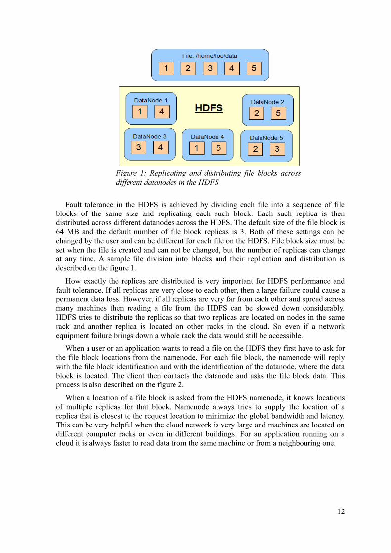
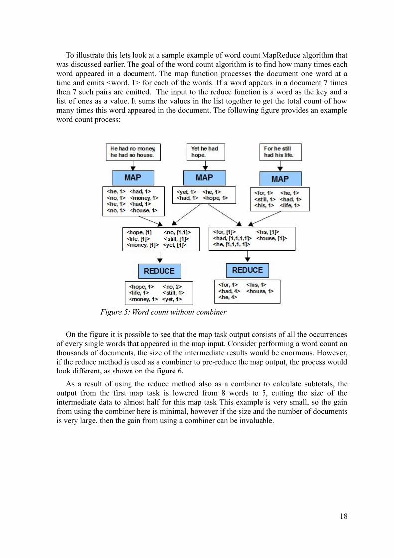
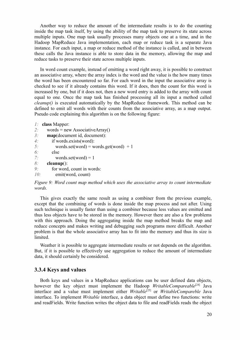
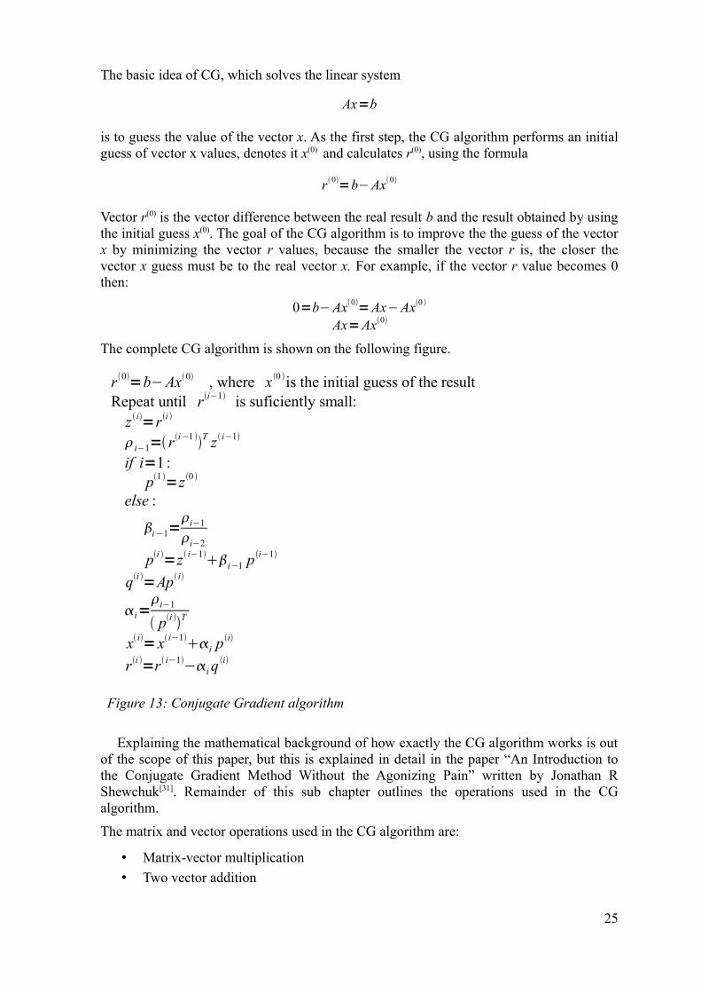
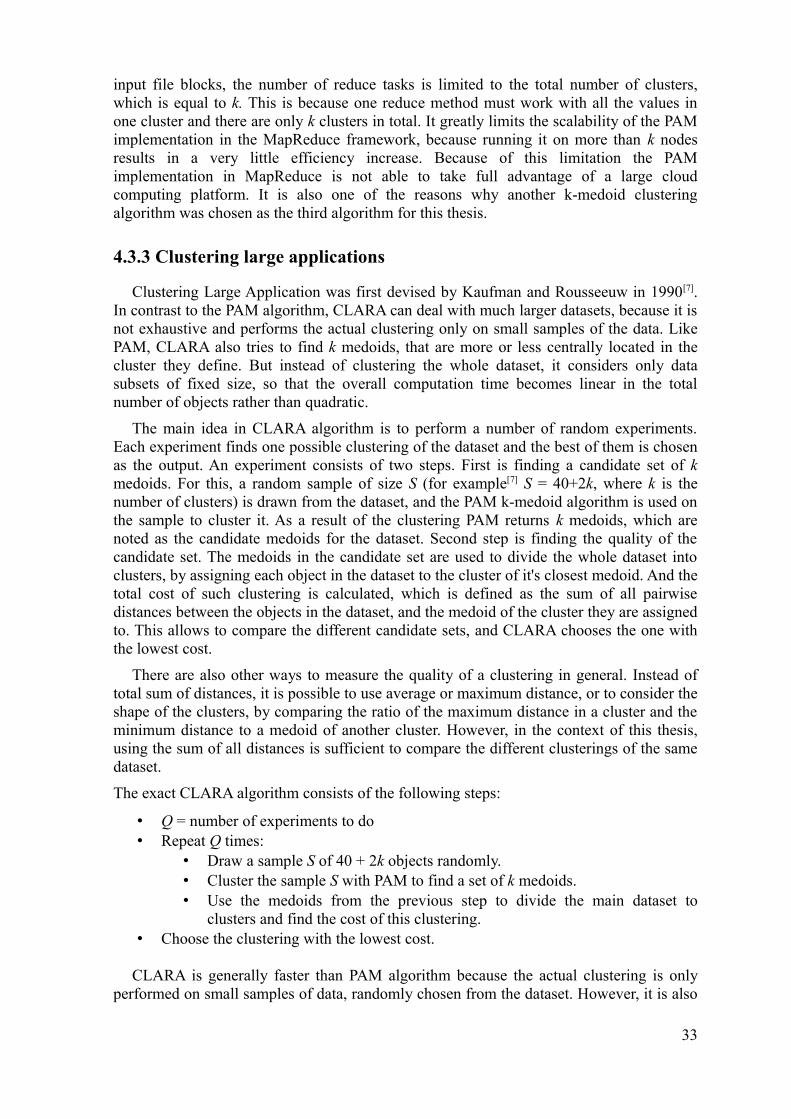
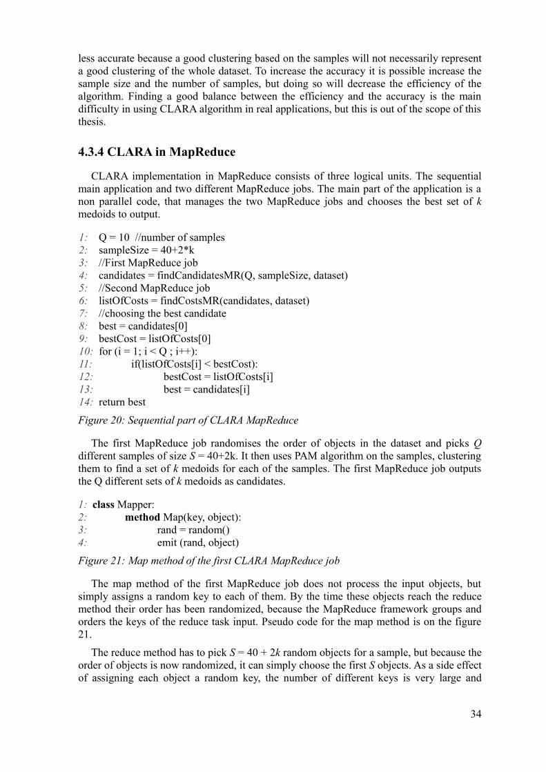
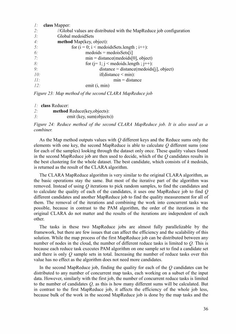
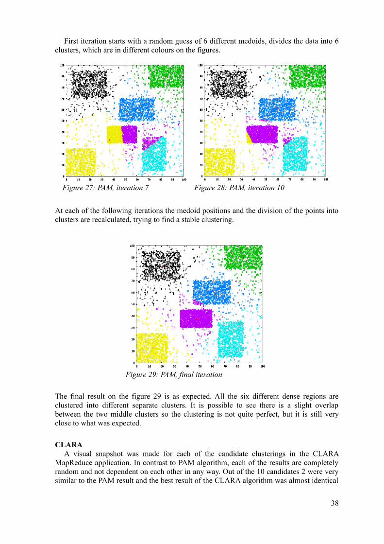
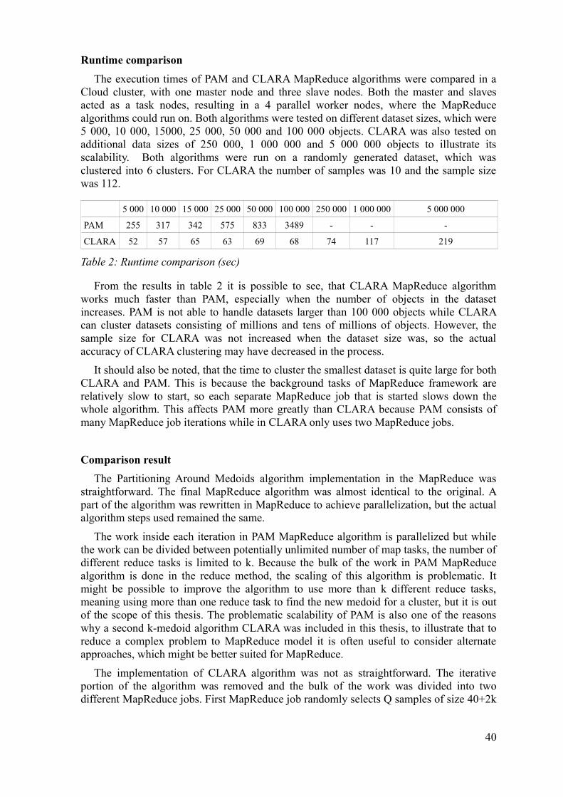
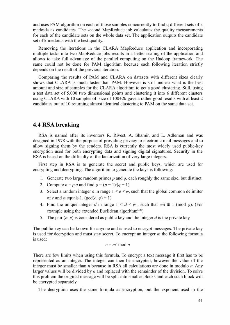
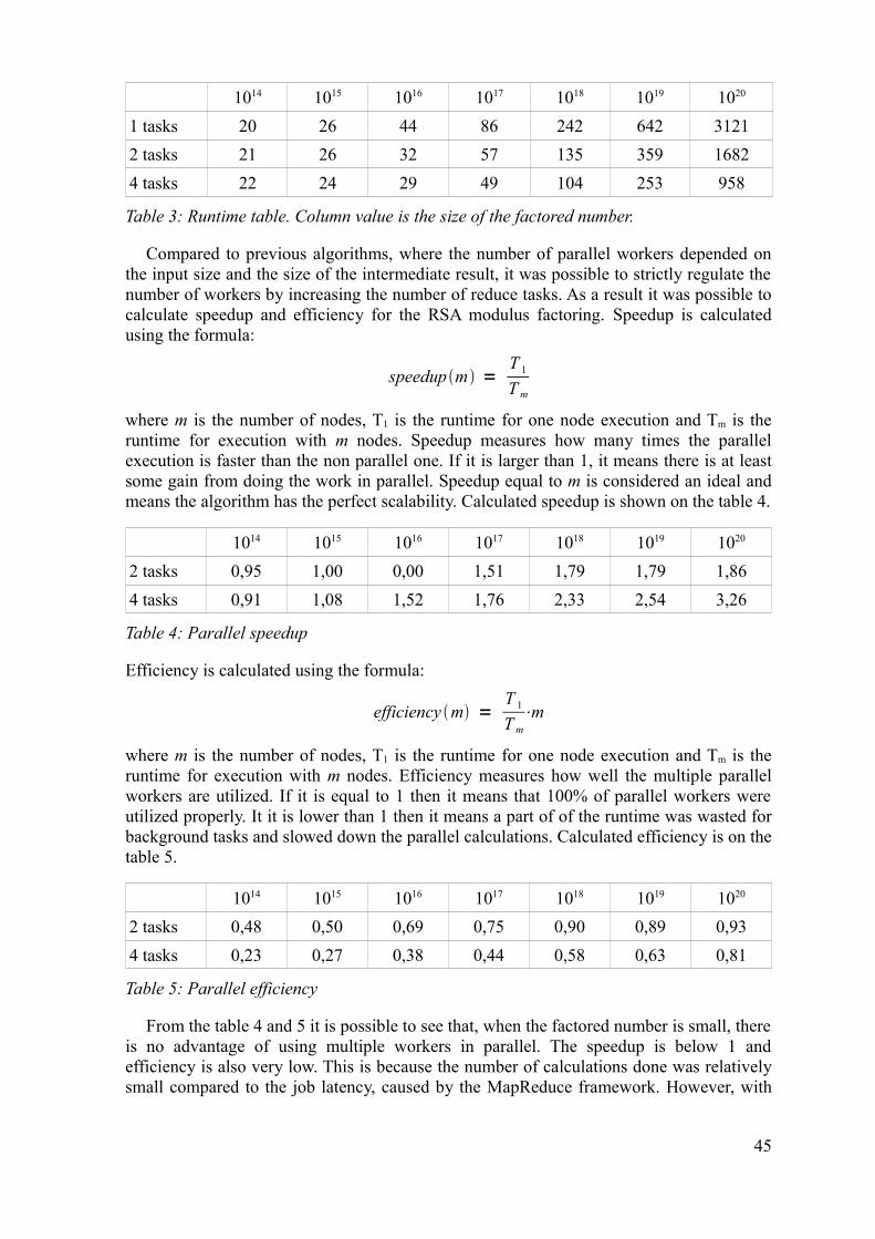
1014 1015 1016 1017 1018 1019 1020
1 tasks 20 26 44 86 242 642 31212 tasks 21 26 32 57 135 359 16824 tasks 22 24 29 49 104 253 958
Table 3 Runtime table Column value is the size of the factored number
Compared to previous algorithms where the number of parallel workers depended on the input size and the size of the intermediate result it was possible to strictly regulate the number of workers by increasing the number of reduce tasks As a result it was possible to calculate speedup and efficiency for the RSA modulus factoring Speedup is calculated using the formula
speedup m =T 1
T m
where m is the number of nodes T1 is the runtime for one node execution and Tm is the runtime for execution with m nodes Speedup measures how many times the parallel execution is faster than the non parallel one If it is larger than 1 it means there is at least some gain from doing the work in parallel Speedup equal to m is considered an ideal and means the algorithm has the perfect scalability Calculated speedup is shown on the table 4
1014 1015 1016 1017 1018 1019 1020
2 tasks 095 100 000 151 179 179 1864 tasks 091 108 152 176 233 254 326
Table 4 Parallel speedup
Efficiency is calculated using the formula
efficiency m =T 1
T msdotm
where m is the number of nodes T1 is the runtime for one node execution and Tm is the runtime for execution with m nodes Efficiency measures how well the multiple parallel workers are utilized If it is equal to 1 then it means that 100 of parallel workers were utilized properly It it is lower than 1 then it means a part of of the runtime was wasted for background tasks and slowed down the parallel calculations Calculated efficiency is on the table 5
1014 1015 1016 1017 1018 1019 1020
2 tasks 048 050 069 075 090 089 0934 tasks 023 027 038 044 058 063 081
Table 5 Parallel efficiency
From the table 4 and 5 it is possible to see that when the factored number is small there is no advantage of using multiple workers in parallel The speedup is below 1 and efficiency is also very low This is because the number of calculations done was relatively small compared to the job latency caused by the MapReduce framework However with
45
the increase of the size of the input number both the speedup and the efficiency started to grow significantly When the modulus size was 1020 the efficiency for two and four node executions were 093 and 081 and the speedup were 186 and 326 showing that there is significant gain from using multiple nodes to find the factors when the size of the modulus is large enough
The calculated speedup and efficiency numbers indicate that this algorithm has a good scalability and that similar algorithms with very little input and intermediate data are very suitable for MapReduce framework
46
Chapter 5
ConclusionThe MapReduce model and framework has been successfully used by Google for
various problems dealing with massive amount of data The Google MapReduce implementation of is proprietary but thanks to open source cloud computing framework Hadoop MapReduce is also available for both commercial applications and for research
This work contributes to the SciCloud project which is carried out by the distributed systems group in the Tartu University SciCloud project studies the scope of establishing private clouds at universities by utilizing the existing university computer resources and using these resources to solve large scale scientific and mathematical problems The purpose of the thesis is to study how to reduce various algorithms to MapReduce model what can affect the efficiency of the resulting algorithms and to provide a foundation for further work in this field For both the author and for the SciCloud project To achieve this four algorithms with different characteristics are chosen and reduced to the MapReduce model The four algorithms are Conjugate gradient Partitioning Around Medoids Clustering Large Application and Breaking RSA Each of the algorithms is studied implemented on MapReduce model and the implementation result is analysed to investigate its scalability
The main problem with MapReduce is latency caused by the relatively slow execution of MapReduce jobs This greatly affects iterative algorithms like Conjugate Gradient and Partitioning Around Medoids which need to run many iterations of MapReduce jobs in sequence Because of this it is crucial to determine if the order of iterations is absolute when reducing iterative algorithms to MapReduce model If the order of iterations can be changed then it might be possible to parallelize the iterative algorithm by executing the content of the iterations concurrently in multiple map or reduce tasks A good example of this is the Clustering Large Application algorithm where the original algorithm is iterative however the different iterations are independent of each other As a result it is possible to restructure the iterative part of the algorithm and instead of doing Q different iterations a two different MapReduce jobs is used The content of the Q iterations is decomposed into smaller tasks and executed in multiple concurrent map and reduce tasks in parallel Greatly reducing the effect of the job latency
Because of the job latency MapReduce is more suited for non iterative algorithms that process massive amount of data However it is also very suitable for algorithms like integer factorization for RSA breaking which have almost non existent input and intermediate data but have to do massive number of calculations MapReduce unsuitability for iterative algorithms is a great concern for scientific computing as scientific computing often uses iterative methods to solve problems Because of this further study focused specifically on reducing iterative algorithms to MapReduce model is necessary
Author plans to continue work in this field by widening the range of different algorithms to study but at the same time concentrating more on problems that deal with massive amounts of data The longer term goal is to apply this research to implement applicable large scale cloud computing solutions
47
Teadusarvutuse probleemide taandamine MapReduce raamistikule
Magistritoumlouml (30 EAP)
Pelle Jakovits
KokkuvotildeteTeadusarvutused tegelevad peamiselt arvutisimulatsioonide ja teadusarvutuslike
eksperimentide laumlbi viimisega nagu naumliteks naftamaardlate simulatsioon laevade kaumlitumine lainetes votildei kliimamuutuste modelleerimine Sellised simulatsioonid on tihti vaumlga suuremahulised ning nende laumlbi viimiseks ei piisa uumlksiku arvuti votildeimsusest On vaja rakendada kas superarvutit mis on uumllikallis votildei paralleelarvutusi paljudel omavahel uumlhendatud arvutitel Selle totildettu on teadusarvutused alati olnud tugevalt seotud paralleelarvutuste ning paralleelprogrammeerimisega
Programmide kirjutamine paralleelarvutuste jaoks on uumlldjuhul kuumlllaltki keeruline kuna lisaks programmi algoritmile on vaja paika panna ka andmete jagamine kommunikatsioon ning arvutuste kordineerimine erinevate arvutite vahel MapReduce on Google poolt loodud paralleelarvutuse raamistik suuremahuliste arvutuste jaoks mis on votildeimeline teatud struktuuriga algoritme paralleelselt kaumlivitama nii et raamistik ise hoolitseb andmete jagamise kommunikatsiooni ning kordineerimise eest Programmeerija peab vaid algoritmi valmis kirjutama ja raamistik hoolitseb ise kotildeige uumllejaumlaumlnu eest mis lihtsustab oluliselt paralleelprogrammide kirjutamist ning teeb selle raamistiku teadusarvutuste jaoks huvitavaks
Algoritmid mida MapReduce raamistik on votildeimeline paralleelselt kaumlivitama peavad olema kindla struktuuriga koosnedes kahest erinevast meetodist map ja reduce mis kaumlivitatakse paralleelselt erinevates arvutites Kaumlesoleva toumlouml eesmaumlrgiks on uurida kuidas taandada erinevaid teadusarvutuse poolt kasutatavaid meetodeid MapReduce raamistikule Valitakse neli erinevat algoritmi taandatakse need MapReduce raamistikule ja uuritakse millised probleemid votildeivad tekkida selle protsessi kaumligus ning mis votildeiks motildejutada tulemuse paralleelset efektiivsust Toumlouml kaumligus taandatud algoritmid on Kaasgradientide meetod (Conjugate Gradient) kaks erinevat k-medoid klasterdamise algoritmi ning RSA kruumlptosuumlsteemi murdmine Tulemuseks on nende algoritmide baaskood dokumentatsioon (Javadoc) ning MapReduce raamistikul kaumlivitatav programmkood
Toumlouml kaumligus selgus et MapReduce raamistikul on probleeme keeruliste algoritmidega mis on iteratiivsed ning kus erinevate iteratsioonide jaumlrjekorda ei ole votildeimalik muuta See on probleem teadusarvutuste jaoks kuna suur osa teadusarvutuste poolt kasutatavatest meetoditest on iteratiivsed
48
References1 Wikipedia Scientific computing httpenwikipediaorgwikiComputational_science
[20052010]2 Jeffrey Dean Sanjay Ghemawat Simplified data processing on large clusters In
Proc of the 6th OSDI Dec 20043 Wikipedia Lisp httpenwikipediaorgwikiLisp_28programming_language29
[20052010]4 S N Srirama O Batrashev E Vainikko SciCloud Scientific Computing on the
Cloud 10th IEEEACM International Symposium on Cluster Cloud and Grid Computing (CCGrid 2010) May 17-20 2010 pp 579 IEEE Computer Society
5 Oorschot Menezes Scott Vanstone Handbook of Applied Cryptography Chapter 82 CRC Press 1996
6 R L Rivest A Shamir L Adleman A method for obtaining digital signatures and public-key cryptosystems Communications of the ACM Feb 1978
7 L Kaufman P J Rousseeuw Finding groups in data an introduction to cluster analysis in Wiley Series in Probability and Mathematical Statistics Applied Probability and Statistics New York US Wiley 1990 vol 28 p 125
8 Hadoop wiki Hadoop httpwikiapacheorghadoop [18052010]9 Sanjay Ghemawat Howard Gobioff and Shun-Tak Leung The Google File System
19th ACM Symposium on Operating Systems Principles Lake George NY October 2003
10 Apache Hadoop HDFS httphadoopapacheorgcommondocscurrenthdfs_designhtml [14052010]
11 Wikipedia Distributed computing httpenwikipediaorgwikiDistributed_computing [20052010]
12 Wikipedia Parallel programming httpenwikipediaorgwikiParallel_computing[20052010]
13 Wikipedia Cloud Computing httpenwikipediaorgwikiCloud_computing[23052010]
14 Greg Pfister In Search of Clusters Prentice Hall 199815 Paul Barham Boris Dragovic Keir Fraser Steven Hand Tim Harris Alex Ho Rolf
Neugebauer Ian Pratt Andrew Warfield Xen and the art of virtualization Proceedings of the nineteenth ACM symposium on Operating systems principles October 19-22 2003 Bolton Landing NY USA
16 Jeffrey Dean Sanjay Ghemawat MapReduce simplified data processing on large clusters Communications of the ACM v51 n1 January 2008
17 Jonathan Cohen Graph Twiddling in a MapReduce World Computing in Science and Engineering vol 11 no 4 pp 29-41 JulyAug 2009
18 Chris Bunch Brian Drawert Matthew Norman MapScale A Cloud Environment for Scientific Computing Computer Science Department University of California Santa Barbara 2009
49
19 Apache httpwwwapacheorg [14052010]20 Hadoop wiki Hive httpwikiapacheorghadoopHive [15052010]21 Hadoop wiki Pig httpwikiapacheorgpig [15052010]22 Hadoop wiki Hbase httpwikiapacheorghadoopHbase [15052010]23 Hadoop wiki Hadoop FAQ httpwikiapacheorghadoopFAQA3 [22052010]24 Hadoop API WritableCompareble
httphadoopapacheorgcommondocscurrentapiorgapachehadoopioWritableComparablehtml [23052010]
25 Hadoop API WritablehttphadoopapacheorgcommondocscurrentapiorgapachehadoopioWritablehtml [23052010]
26 Mike Chapple SQL Fundamentals Aboutcom Databaseshttpdatabasesaboutcomodsqlasqlfundamentalshtm [19052010]
27 Fay Chang Jeffrey Dean Sanjay Ghemawat Wilson C Hsieh Deborah A Wallach Mike Burrows Tushar Chandra Andrew Fikes Robert E Gruber Bigtable a distributed storage system for structured data Proceedings of the 7th USENIX Symposium on Operating Systems Design and Implementation p15-15 November 06-08 2006 Seattle WA
28 Hbase Applications powered by Hbase httpwikiapacheorghadoopHbasePoweredBy [15052010]
29 Jonathan R Shewchuk An Introduction to the Conjugate Gradient Method Without the Agonizing Pain Carnegie Mellon University Pittsburgh PA 1994
30 Chia-Ping Chen Positive Definite Matrices Notes on Linear Algebra Department of Computer Science and Engineering National Sun Yat-Sen University Kaohsiung Taiwan ROC
31 David MacKay An Example Inference Task Clustering Information Theory Inference and Learning Algorithms Cambridge University Press pp 284ndash292 2003
32 Python programming language httpwwwpythonorg [23052010]33 Scitools wiki Easyviz
httpcodegooglecompscitoolswikiEasyvizDocumentation [19052010]34 Wikipedia Extended Euclidean algorithm
httpenwikipediaorgwikiExtended_Euclidean_algorithm [23052010]35 Oorschot Menezes Scott Vanstone Handbook of Applied Cryptography Chapter
822 CRC Press 199636 RSA Laboratories How large a key should be used in the RSA cryptosystem Public-
Key Cryptography Standards (PKCS) httpwwwrsacomrsalabsnodeaspid=2218 [11052010]
37 Carl Pomerance A Tale of Two Sieves Notices of the AMS 43 (12) 1473ndash1485 December 1996
50
Appendices
Appendix A Source Code
Appendix B Implemented algorithms
Appendix C Javadoc
51
Appendix A
Source code
Source code is on an external DVD in the folder source It includes source code for both the algorithms and for the PAM and CLARA visualization python scripts DVD is provided with this thesis
52
Appendix B
Implemented algorithms
Jar file containing the compiled algorithms is on an external DVD in the folder compiled The folder also includes a readmepdf file containing instructions how to run the algorithms DVD is provided with this thesis
53
Appendix C
Javadoc
Javadoc is on an external DVD in the folder sourcesciCoToMRdoc DVD is provided with this thesis
54
- Acknowledgements
- Introduction
- Scientific computing on the cloud
- Hadoop
-
- 31 What is Hadoop
- 32 Hadoop Distributed File System
- 33 Hadoop MapReduce
-
- 331 Map and Reduce
- 332 Execution
- 333 Combining intermediate results and preserving task state
- 334 Keys and values
-
- 34 Other Hadoop Projects
-
- Algorithms
-
- 41 Choice of algorithms
- 42 Conjugate gradient method
-
- 421 CG in MapReduce
- 422 Matrix-vector multiplication in MapReduce
- 423 Result
-
- 43 K-medoids
-
- 431 Partitioning Around Medoids
- 432 PAM in MapReduce
- 433 Clustering large applications
- 434 CLARA in MapReduce
- 435 Comparison
-
- 44 RSA breaking
-
- 441 Integer factoring algorithm
- 442 Integer factoring algorithm in MapReduce
- 443 Result
-
- Conclusion
- Kokkuvotildete
- References
- Appendices
-