reducing plug loads in office spaces - nrel · pdf fileblcc building life cycle cost ... these...
TRANSCRIPT

NREL is a national laboratory of the U.S. Department of Energy, Office of Energy Efficiency & Renewable Energy, operated by the Alliance for Sustainable Energy, LLC.
Contract No. DE-AC36-08GO28308
National Renewable Energy Laboratory 15013 Denver West Parkway Golden, CO 80401 303-275-3000 • www.nrel.gov
Reducing Plug Loads in Office Spaces Hawaii and Guam Energy Improvement Technology Demonstration Project M. Sheppy, I. Metzger, D. Cutler, and G. Holland National Renewable Energy Laboratory
A. Hanada Naval Facilities Engineering Command
Technical Report NREL/TP-5500-60382 January 2014
Produced under direction of Naval Facilities Engineering Command (NAVFAC) by the National Renewable Energy Laboratory (NREL) under Interagency Agreement 11-01829 and Task No. WFK3.1020.

NREL is a national laboratory of the U.S. Department of Energy, Office of Energy Efficiency & Renewable Energy, operated by the Alliance for Sustainable Energy, LLC.
Contract No. DE-AC36-08GO28308
National Renewable Energy Laboratory 15013 Denver West Parkway Golden, CO 80401 303-275-3000 • www.nrel.gov
Reducing Plug Loads in Office Spaces Hawaii and Guam Energy Improvement Technology Demonstration Project M. Sheppy, I. Metzger, D. Cutler, and G. Holland National Renewable Energy Laboratory
A. Hanada Naval Facilities Engineering Command
Prepared under Task No. WFK3.1020
Technical Report NREL/TP-5500-60382 January 2014

NOTICE This manuscript has been authored by employees of the Alliance for Sustainable Energy, LLC (“Alliance”) under Contract No. DE-AC36-08GO28308 with the U.S. Department of Energy (“DOE”). This report was prepared as an account of work sponsored by an agency of the United States government. Neither the United States government nor any agency thereof, nor any of their employees, makes any warranty, express or implied, or assumes any legal liability or responsibility for the accuracy, completeness, or usefulness of any information, apparatus, product, or process disclosed, or represents that its use would not infringe privately owned rights. Reference herein to any specific commercial product, process, or service by trade name, trademark, manufacturer, or otherwise does not necessarily constitute or imply its endorsement, recommendation, or favoring by the United States government or any agency thereof. The views and opinions of authors expressed herein do not necessarily state or reflect those of the United States government or any agency thereof.
Printed on paper containing at least 50% wastepaper, including 10% post consumer waste.

iii
This report is available at no cost from the National Renewable Energy Laboratory (NREL) at www.nrel.gov/publications.
Acknowledgments The authors would like to thank the Naval Facilities Engineering Command (NAVFAC) energy team for their dedicated support of the project, especially Amy Hanada, Chelsea Goto, and Rochelle Trueblood. We would also like to thank the occupants of building A4 at Joint Base Pearl Harbor-Hickam (JBPHH), including Capt. Jeffrey W. James, joint base commander, and Col. David Kirkendall, deputy joint base commander.
We would like to thank content contributors Lynn Billman (NREL) and Rachel Gelman (NREL), who both authored the “Commercial Readiness Qualitative Assessment” section. We would also like to thank the peer reviewers for their time and constructive feedback, including Jeffrey Dominick (NREL) and Gene Holland (NREL), who reviewed this report during its development. Lastly, thanks to Marjorie Schott (NREL) for providing assistance with creating figures.

iv
This report is available at no cost from the National Renewable Energy Laboratory (NREL) at www.nrel.gov/publications.
List of Abbreviations and Acronyms A ampere
AC alternating current
APS advanced power strip
ASHRAE American Society of Heating, Refrigerating and Air-Conditioning Engineers
BLCC building life cycle cost
CIO command information officer
COTS commercial, off-the-shelf technology
CT current transducer
DC direct current
DOD U.S. Department of Defense
DOE U.S. Department of Energy
EIA U.S. Energy Information Administration
eROI energy return on investment
ESPC energy savings performance contract
FY fiscal year
GSA U.S. General Services Administration
HVAC heating, ventilation, and air conditioning
IPT integrated project team
JBPHH Joint Base Pearl Harbor-Hickam
JRM Joint Region Marianas
kW kilowatt
kWh kilowatt-hour
NAVFAC Naval Facilities Engineering Command
NEPA National Environmental Policy Act

v
This report is available at no cost from the National Renewable Energy Laboratory (NREL) at www.nrel.gov/publications.
NIST National Institute of Standards and Technology
NREL National Renewable Energy Laboratory
O&M operation and maintenance
RFI radio frequency interference
SIOH supervision, inspection, and overhead
SIR savings to investment ratio
TRL technology readiness level
UL Underwriters Laboratories
W Watt
vi
This report is available at no cost from the National Renewable Energy Laboratory (NREL) at www.nrel.gov/publications.
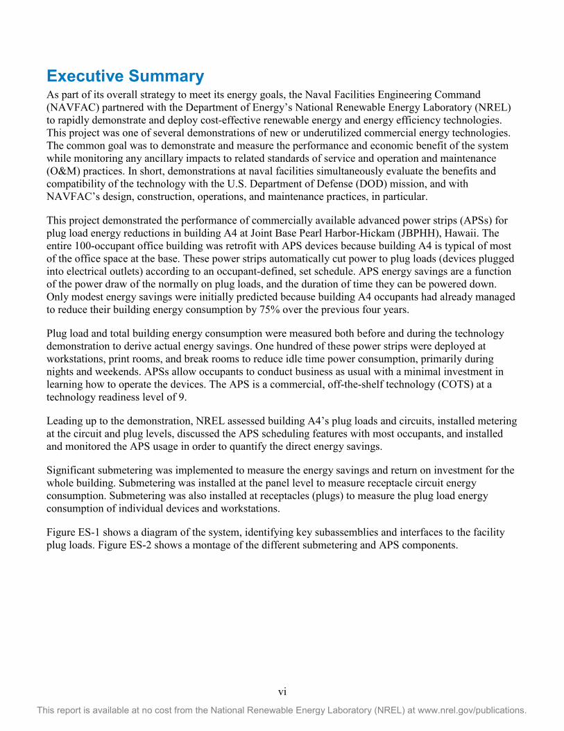
Executive Summary As part of its overall strategy to meet its energy goals, the Naval Facilities Engineering Command (NAVFAC) partnered with the Department of Energy’s National Renewable Energy Laboratory (NREL) to rapidly demonstrate and deploy cost-effective renewable energy and energy efficiency technologies. This project was one of several demonstrations of new or underutilized commercial energy technologies. The common goal was to demonstrate and measure the performance and economic benefit of the system while monitoring any ancillary impacts to related standards of service and operation and maintenance (O&M) practices. In short, demonstrations at naval facilities simultaneously evaluate the benefits and compatibility of the technology with the U.S. Department of Defense (DOD) mission, and with NAVFAC’s design, construction, operations, and maintenance practices, in particular.
This project demonstrated the performance of commercially available advanced power strips (APSs) for plug load energy reductions in building A4 at Joint Base Pearl Harbor-Hickam (JBPHH), Hawaii. The entire 100-occupant office building was retrofit with APS devices because building A4 is typical of most of the office space at the base. These power strips automatically cut power to plug loads (devices plugged into electrical outlets) according to an occupant-defined, set schedule. APS energy savings are a function of the power draw of the normally on plug loads, and the duration of time they can be powered down. Only modest energy savings were initially predicted because building A4 occupants had already managed to reduce their building energy consumption by 75% over the previous four years.
Plug load and total building energy consumption were measured both before and during the technology demonstration to derive actual energy savings. One hundred of these power strips were deployed at workstations, print rooms, and break rooms to reduce idle time power consumption, primarily during nights and weekends. APSs allow occupants to conduct business as usual with a minimal investment in learning how to operate the devices. The APS is a commercial, off-the-shelf technology (COTS) at a technology readiness level of 9.
Leading up to the demonstration, NREL assessed building A4’s plug loads and circuits, installed metering at the circuit and plug levels, discussed the APS scheduling features with most occupants, and installed and monitored the APS usage in order to quantify the direct energy savings.
Significant submetering was implemented to measure the energy savings and return on investment for the whole building. Submetering was installed at the panel level to measure receptacle circuit energy consumption. Submetering was also installed at receptacles (plugs) to measure the plug load energy consumption of individual devices and workstations.
Figure ES-1 shows a diagram of the system, identifying key subassemblies and interfaces to the facility plug loads. Figure ES-2 shows a montage of the different submetering and APS components.

vii
This report is available at no cost from the National Renewable Energy Laboratory (NREL) at www.nrel.gov/publications.
Figure ES-1. Diagram of sub-metering, control, and occupancy monitoring components that were installed
and demonstrated in Building A4. Illustration by Marjorie Schott, NREL
Figure ES-2. Close-up views of sub-metering, control, and occupancy monitoring components that were
installed and demonstrated in Building A4. Illustration by Marjorie Schott, NREL
The measured energy savings from deploying this technology in building A4 is 28%1 for plug loads and 8%2 for the whole building. Economic results of this demonstration indicate application of the APS technology can yield appreciable energy and cost savings at a relatively small investment. For the demonstrated system, we calculate an energy return on investment (eROI) value of 18.6, with net savings projected at $14,000 over a 5-year lifetime and $80,000 for a 20-year lifetime. A pre- and post-demonstration survey confirmed that the technology was generally accepted by building occupants and caused minimal disruptions, which were contained to the first week of installation. When asked how NAVFAC would prefer to deploy this technology in the future, Amy Hanada from the NAVFAC Hawaii energy team recommended that a third party install the APSs. For this type of future
1 Extrapolated from measured plug load data from building A4. 2 Based on energy model. Model was informed by measured plug load data and utility bills from building A4.
viii
This report is available at no cost from the National Renewable Energy Laboratory (NREL) at www.nrel.gov/publications.
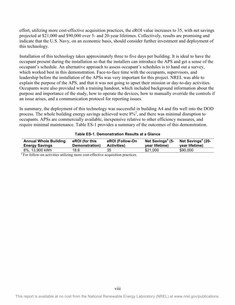
effort, utilizing more cost-effective acquisition practices, the eROI value increases to 35, with net savings projected at $21,000 and $90,000 over 5- and 20-year lifetimes. Collectively, results are promising and indicate that the U.S. Navy, on an economic basis, should consider further investment and deployment of this technology.
Installation of this technology takes approximately three to five days per building. It is ideal to have the occupant present during the installation so that the installers can introduce the APS and get a sense of the occupant’s schedule. An alternative approach to assess occupant’s schedules is to hand out a survey, which worked best in this demonstration. Face-to-face time with the occupants, supervisors, and leadership before the installation of the APSs was very important for this project. NREL was able to explain the purpose of the APS, and that it was not going to upset their mission or day-to-day activities. Occupants were also provided with a training handout, which included background information about the purpose and importance of the study, how to operate the devices, how to manually override the controls if an issue arises, and a communication protocol for reporting issues.
In summary, the deployment of this technology was successful in building A4 and fits well into the DOD process. The whole building energy savings achieved were 8%2, and there was minimal disruption to occupants. APSs are commercially available, inexpensive relative to other efficiency measures, and require minimal maintenance. Table ES-1 provides a summary of the outcomes of this demonstration.
Table ES-1. Demonstration Results at a Glance
Annual Whole Building Energy Savings
eROI (for this Demonstration)
eROI (Follow-On Activities)
Net Savingsa (5-year lifetime)
Net Savingsa (20-year lifetime)
8%, 13,900 kWh 18.6 35 $21,000 $90,000 a For follow-on activities utilizing more cost-effective acquisition practices.

ix
This report is available at no cost from the National Renewable Energy Laboratory (NREL) at www.nrel.gov/publications.
Table of Contents Acknowledgments ..................................................................................................................................... iii List of Abbreviations and Acronyms ....................................................................................................... iv Executive Summary ................................................................................................................................... vi List of Figures ............................................................................................................................................ xi List of Tables .............................................................................................................................................. xi 1 Introduction ........................................................................................................................................... 1
1.1 Background ...................................................................................................................................... 1 2 Demonstration Objective ..................................................................................................................... 2
2.1 Technology Description ................................................................................................................... 2 3 Demonstration Design ......................................................................................................................... 4
3.1 Site Selection ................................................................................................................................... 4 3.2 Pretest Preparation and Inventory .................................................................................................... 4 3.3 Sensor and Related Equipment Installation ..................................................................................... 6 3.4 Sampling Protocol ........................................................................................................................... 8 3.5 Equipment Calibration and Data Quality Issues .............................................................................. 8 3.6 Baseline Characterization ................................................................................................................ 8 3.7 Operational Testing ......................................................................................................................... 8 3.8 Modeling and Simulation ................................................................................................................ 9 3.9 Summary of Performance Objectives .............................................................................................. 9 3.10 Description of Performance Objectives .................................................................................. 10
4 Technical Performance Analysis and Assessment ........................................................................ 11 4.1 Overview........................................................................................................................................ 11 4.2 Baseline Results and Findings ....................................................................................................... 11 4.3 Control Period Results and Findings ............................................................................................. 12 4.4 Energy Model and Simulation of Whole Building Energy Savings .............................................. 15 4.5 Utility Meter Evidence .................................................................................................................. 18 4.6 Occupant Surveys .......................................................................................................................... 19 4.7 Assessment of Performance Objectives Results ............................................................................ 19
5 Economic Performance Analysis and Assessment ........................................................................ 21 6 Project Management Considerations ............................................................................................... 25
6.1 Site Approval, National Environmental Policy Act, and DD1391 ................................................ 26 6.2 Contracts and Procurement ............................................................................................................ 26 6.3 Design ............................................................................................................................................ 27 6.4 Installation and Construction ......................................................................................................... 28 6.5 Operation and Maintenance ........................................................................................................... 29 6.6 Training ......................................................................................................................................... 29
7 Commercial Readiness Qualitative Assessment ............................................................................ 29 7.1 Primary Manufacturers .................................................................................................................. 30 7.2 Product Availability ....................................................................................................................... 30 7.3 Policy ............................................................................................................................................. 31 7.4 Price of Advanced Power Strips .................................................................................................... 32 7.5 Usability and Functionality ............................................................................................................ 32
7.5.1 Energy Savings ............................................................................................................... 32 8 Recommended Next Steps ................................................................................................................ 34 Appendix 1: Floor Plans ........................................................................................................................... 36 Appendix 2: Plug Load Participant Exit Survey..................................................................................... 37 Appendix 3: Normalizing .......................................................................................................................... 38 Appendix 4: Descriptions of Performance Objectives .......................................................................... 40 Appendix 5: Power Usage—Average Daily Profiles .............................................................................. 42 Appendix 6: Occupancy—Average Daily Profiles ................................................................................. 44
Space Types ......................................................................................................................................... 44 Occupant Types .................................................................................................................................... 47

x
This report is available at no cost from the National Renewable Energy Laboratory (NREL) at www.nrel.gov/publications.
Appendix 7: Exit Survey Results ............................................................................................................. 50 Appendix 8: Demonstration Economic Analysis and Cost Details ..................................................... 52
Cost Information .................................................................................................................................. 52 Demonstration Costs (Actuals) ...................................................................................................... 52 Estimated Costs for Future (Follow-On) Technology Deployment............................................... 53
Economic Analysis Information ........................................................................................................... 56 Energy Return on Investment Analyses ......................................................................................... 56 Building Life Cycle Cost Analysis ................................................................................................ 57
Appendix 9: Manager Training Nov. 13, 2012 ........................................................................................ 58 Appendix 10: Occupant Training—Using the APC Power Strip........................................................... 59
Directions for Altering Preprogrammed Schedules ............................................................................. 59 To Change a Single Day Schedule ................................................................................................ 59 To Add Another Schedule ............................................................................................................. 59
Directions for Overriding the Power Strip ........................................................................................... 60

xi
This report is available at no cost from the National Renewable Energy Laboratory (NREL) at www.nrel.gov/publications.
List of Figures Figure ES-1. Diagram of sub-metering, control, and occupancy monitoring components
that were installed and demonstrated in Building A4. ................................................................... vii Figure ES-2. Close-up views of sub-metering, control, and occupancy monitoring
components that were installed and demonstrated in Building A4. ............................................. vii Figure 1. Diagram of submetering, control, and occupancy monitoring components that
were installed and demonstrated in building A4 .............................................................................. 7 Figure 2. Close-up views of submetering, control, and occupancy monitoring components
that were installed and demonstrated in building A4 ....................................................................... 7 Figure 3. Comparison of panel-level power data to receptacle-level power data
(baseline period) ................................................................................................................................. 12 Figure 4. Whole building plug loads for baseline and control period (weekday and weekend
profiles shown) ................................................................................................................................... 13 Figure 5. Comparison of panel-level power data to receptacle-level power data
(control period) ................................................................................................................................... 15 Figure 6. Building A4 energy model representation ............................................................................. 16 Figure 7. Building A4 actual and modeled monthly electrical use (kWh) ........................................... 17 Figure 8. Building A4 energy model calibrated baseline results for annual energy use .................. 17 Figure 9. Building A4 energy model simulated plug load energy profile for baseline and
controlled phases ............................................................................................................................... 18 Figure 10. Net savings estimates for a five-year economic life on installation of APS over
an electricity price range between $0.325/kWh to $0.525/kWh ...................................................... 23 Figure A-1. Electrical panel locations on the first floor ........................................................................ 36 Figure A-2. Electrical panel locations on the second floor .................................................................. 36
List of Tables Table ES-1. Demonstration Results at a Glance ................................................................................... viii Table 1. Total Space Types Present in Building A4 ................................................................................ 5 Table 2. Total Plug Load Inventory for Building A4 ................................................................................ 6 Table 3. Performance Objectives ............................................................................................................ 10 Table 4. Percent Energy Savings by Space Type .................................................................................. 14 Table 5. Percent Energy Savings by Occupant Type ............................................................................ 14 Table 6. Annual Energy Savings for Building A4 .................................................................................. 18 Table 7. Performance Objectives and Outcomes .................................................................................. 20 Table 8. Summary of Economic Results and Key Analysis Inputs...................................................... 22 Table 9. Summary of Programmatic Elements of this Project ............................................................. 25 Table 10. Example List of Manufacturers of APSs ................................................................................ 30 Table 11. Example List of APS Retailers ................................................................................................ 31 Table 12. High Scoring APSs Currently on the Market ......................................................................... 32 Table A-1. Summary Breakout of Costs as Accounted in Performance of the Technology
Demonstration .................................................................................................................................... 52 Table A-2. Detailed Breakout of Equipment Procured and Service-Related Purchase Orders
Executed on this Project ................................................................................................................... 53 Table A-3. Summary Breakout of Costs as Estimated for Future, Follow-On Deployments of
the Technology at JBPHH ................................................................................................................. 54 Table A-4. Basis of Estimate Breakout per Estimated Cost Element for Future, Follow-On
Deployments of the Technology at JBPHH ..................................................................................... 55 Table A-5. Key Information Regarding eROI Analyses Performed for this Report ............................ 56 Table A-6. Key Information Regarding BLCC Analyses Performed for this Report .......................... 57

1
This report is available at no cost from the National Renewable Energy Laboratory (NREL) at www.nrel.gov/publications.
1 Introduction As part of its overall strategy to meet its energy goals, the Naval Facilities Engineering Command (NAVFAC) partnered with Department of Energy’s National Renewable Energy Laboratory (NREL) to rapidly demonstrate and deploy cost-effective renewable energy and energy efficiency technologies. This was one of several demonstrations of new or underutilized commercial energy technologies. The common goal was to demonstrate and measure the performance and economic benefit of the system while monitoring any ancillary impacts to related standards of service and operation and maintenance (O&M) practices. In short, demonstrations at naval facilities simultaneously evaluate the benefits and compatibility of the technology with the U.S. Department of Defense (DOD) mission, and with NAVFAC’s design, construction, operations, and maintenance practices, in particular.
1.1 Background Efficiency gains in building lighting and heating, ventilation, and air conditioning (HVAC) systems have resulted in plug loads becoming a greater percentage of building energy use. In a minimally code-compliant office building, plug loads typically account for 25% of the total electrical load. In an ultra-efficient office building, plug loads can account for more than 50% of the total electrical load.3 Plug load reduction strategies are needed to continue progress toward NAVFAC’s energy goals. Plug load efficiency strategies are different than other building efficiency strategies because they involve small electronics distributed throughout the building. These loads typically move around in the building when reorganizations and office configuration changes are made, so these loads may shift between circuits over time.
This project demonstrated the performance of commercially available advanced power strips (APSs) and occupant education/training for plug load energy reductions in building A4 at Joint Base Pearl Harbor-Hickam (JBPHH) in Hawaii. APSs allow occupants to conduct business as usual with a minimal investment in learning how to operate the devices. The demonstrated APS is a commercial, off-the-shelf technology (COTS) at a technology readiness level of 9.
The goal of this demonstration was a reduction in plug loads, thereby reducing the overall building load. Plug load and total building energy consumption were measured both before and during the technology demonstration to derive actual energy savings. APSs were deployed at workstations, print rooms, and break rooms to reduce idle time power consumption, primarily during nights and weekends.
3 C. Lobato, S. Pless, M. Sheppy, P. Torcellini. “Reducing Plug and Process Loads for a Large Scale, Low Energy Office Building: NREL’s Research Support Facility.” NREL/CP-5500-49002. February 2011.

2
This report is available at no cost from the National Renewable Energy Laboratory (NREL) at www.nrel.gov/publications.
2 Demonstration Objective NREL demonstrated a whole building application of schedule-based APSs to measure total plug load energy use and the resulting plug load energy savings. The APS devices cut power to plug loads according to an occupant-defined set schedule.
The goal of this demonstration was to reduce the plug loads by 20% or more, thereby reducing the overall building load by 5% or more. Plug load and total building energy consumption were measured both before and during the technology demonstration to derive actual energy savings.
The demonstration was designed to quantify total plug loads in a typical DOD office building and the percentage of energy consumption due to plug loads, compare workstation occupancy patterns to energy consumption, and measure the effectiveness of inexpensive plug load controls.
2.1 Technology Description Plug load efficiency strategies are different than other building efficiency strategies because they involve small electronics distributed throughout the building. These loads typically move around in the building when reorganizations and office configuration changes are made, so these loads may shift between circuits over time. This project applied simple, effective APSs and occupant education/training to achieve maximum plug load energy savings.
The amount of savings that can be achieved with this technology is dependent on the size of the load being controlled and how long that load can be turned off each day. For instance, the savings from turning off a desktop computer (100 Watt [W] average load) for 12 hours a night, will be triple compared to turning off a laptop (30 W average load) for 12 hours a night.4
Currently, the top four control approaches for APS technologies on the market utilize master control, load-sensing, schedule-based, and occupancy-based controls.
• Master and load-sensing controls work off a “master” and “slave” relationship. When a device plugged into the “master” outlet goes above/below a power threshold, the “slave” outlets are automatically energized/de-energized. A master device must turn completely off before cutting power to the slave outlets, while a load-sensing device has a power threshold.
• Schedule-based control applies user programmed schedules to energize/de-energize outlets.
• Occupancy-based control energizes/de-energizes outlets automatically depending on the feedback from an attached occupancy sensor, which monitors whether a specific space is occupied or unoccupied.
A recent Green Proving Ground technology demonstration conducted at eight U.S. General Services Administration (GSA) field offices found that schedule-based timer controls had the shortest payback period and highest user acceptance in typical office space applications compared to other control methods.5 In addition, schedule-based control is the most mature type of APS on the market. Therefore,
4 For additional resources on how to calculate the energy impact of APSs in a building, see http://www.nrel.gov/docs/fy13osti/54175.pdf and http://www.nrel.gov/buildings/docs/office_ppl_reduction_tool.xlsx. 5 “Plug Load Control.” U.S. General Services Administration, 2013. Accessed July 7, 2013: http://www.gsa.gov/portal/content/121203.

3
This report is available at no cost from the National Renewable Energy Laboratory (NREL) at www.nrel.gov/publications.
schedule-based APSs were selected for demonstration at a whole building scale within building A4 at JBPHH.
This report focuses on installation of APSs in existing buildings. However, it is worth mentioning the automatic receptacle control (paragraph 8.4.2) requirement from the American Society of Heating, Refrigerating and Air-Conditioning Engineers (ASHRAE) standard 90.1–2010 indicates that at least 50% of all receptacles be controlled by an automatic control device in new construction. The standard indicates that switched outlets may be controlled by a programmable time clock, occupancy sensor, or some other similar means. The schedule-based plug load control strategy demonstrated in this project could be used to meet this ASHRAE 90.1–2010 requirement. A few caveats are that the schedules could not be overridden by occupants, and the control device would have to be affixed to the building in a permanent way.
4
This report is available at no cost from the National Renewable Energy Laboratory (NREL) at www.nrel.gov/publications.
3 Demonstration Design This technology demonstration project hypothesized that simple and inexpensive schedule-based APSs deployed throughout DOD office buildings would achieve significant energy and cost savings, and short payback periods. The variable that changes from plug load to plug load is the time of use. Input data included occupancy, energy consumption, and time of use. Outputs were energy savings and occupant acceptance. Calculated variables included data statistics, cost savings, and simple payback period. Controlled variables were location, existing plug load devices, control approach, control devices, building characteristics, and building operation. Uncontrolled variables included occupant behavior and personnel changes.
The demonstration progressed through a series of phases, including site selection, pretest preparation, baseline measurements, equipment and sensor installation, commissioning, data collection, data analysis, and report writing.
3.1 Site Selection Building A4 at JBPHH, located at Marshall Road, Pearl Harbor, Hawaii 96860, has a square footage of 18,818 and was constructed in July 1946. This building was selected as the demonstration site based on the rationale listed below:
• Building A4 has approximately 90 occupants. This provided an acceptable statistical sample size to test out a number of plug load reduction strategies. Also, the occupants are representative of typical Navy personnel.
• This building has accessible electrical panels that were conducive to capturing the energy use of all workstations, kitchens, conference rooms, print rooms, and other plug loads.
• Occupants have clearly defined work schedules, which allowed for simple, inexpensive schedule-based controls to be used.
• There are no classified or mission-critical functions being done in the building, so building access is relatively easy, and there is no chance of the APSs powering down mission-critical devices.
It should be noted that many of the occupants in building A4, including the NAVFAC Hawaii commanding officer, were eager to participate in this demonstration due to the energy conservation culture already instilled in the base.
3.2 Pretest Preparation and Inventory As part of pretest preparation, NREL audited the building to categorize the space types and inventory the plug loads. This facility offers a typical DOD office environment representative of the larger building stock with several different space types, such as cubicles, offices, kitchens, print rooms, and conference rooms.
Table 1 quantifies the total number of space types in building A4.

5
This report is available at no cost from the National Renewable Energy Laboratory (NREL) at www.nrel.gov/publications.
Table 1. Total Space Types Present in Building A4
Quantity Space Type 1st Floor 2nd Floor Total Libraries 0 1 1 Cubicles 5 52 57 Offices 20 10 30 Kitchens 1 2 3 Open Areas (hallways) 5 7 12 Print Rooms 0 1 1 Conference Rooms 1 1 2 Mail Rooms 1 0 1 Reception Areas 1 0 1
Some space types, such as offices and cubicles, contain personal-use plug loads. Personal-use plug loads are devices that are the direct responsibility of an occupant, such as computers, monitors, and task lights. Other space types, such as break rooms, print rooms, and conference rooms, contain shared plug loads. Shared plug loads are devices that are not the direct responsibility of any individual occupant, such as plug-in air conditioning units, coffee machines, printers, microwaves, drinking fountains, and vending machines.
There are a total of 689 plug loads in building A4. Table 2 shows the inventory of plug loads in building A4. The different space types and associated plug loads each require customized controls.

6
This report is available at no cost from the National Renewable Energy Laboratory (NREL) at www.nrel.gov/publications.
Table 2. Total Plug Load Inventory for Building A4
Plug Load Count Monitors 129 Phones and Accessories 95 Audio 91 Miscellaneous 51 Hard Drives 46 Desktop Computers 43 Printers/Copiers/Scanners 37 Laptops 35 AC Units (plug in) 32 Docking Stations 32 Task Lights 31 Fans 20 Pencil Sharpeners 17 Microwaves 11 Clocks 6 Refrigerators 5 Coffee Machines 4 Drinking Fountains 2 Vending Machines 2 Total 689
Schedule-based plug strips allow the flexibility to customize the schedule for each plug strip depending on the usage patterns. For this demonstration, 100 schedule-based APSs and 115 receptacle submeters were deployed in building A4 to capture the 689 plug loads listed above. These APSs allow each occupant to program custom schedules for their personal plug loads, as well as shared plug loads.
3.3 Sensor and Related Equipment Installation To measure the baseline energy consumption and to verify the performance of the APSs, submetering equipment was installed. Submetering was installed at the panel level to measure receptacle circuit energy consumption, and installed at receptacles (plugs) to measure the plug load energy consumption of individual devices and workstations.
The visual depiction in Figure 1 shows a block diagram of the system, identifying key subassemblies and interfaces to the facility plug loads. Figure 2 shows a montage of the different submetering and APS components.
7
This report is available at no cost from the National Renewable Energy Laboratory (NREL) at www.nrel.gov/publications.
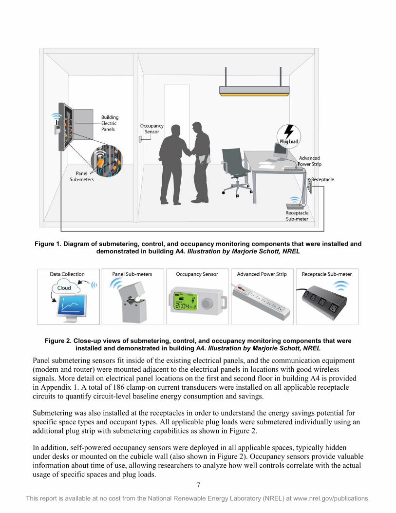
Figure 1. Diagram of submetering, control, and occupancy monitoring components that were installed and demonstrated in building A4. Illustration by Marjorie Schott, NREL
Figure 2. Close-up views of submetering, control, and occupancy monitoring components that were
installed and demonstrated in building A4. Illustration by Marjorie Schott, NREL
Panel submetering sensors fit inside of the existing electrical panels, and the communication equipment (modem and router) were mounted adjacent to the electrical panels in locations with good wireless signals. More detail on electrical panel locations on the first and second floor in building A4 is provided in Appendix 1. A total of 186 clamp-on current transducers were installed on all applicable receptacle circuits to quantify circuit-level baseline energy consumption and savings.
Submetering was also installed at the receptacles in order to understand the energy savings potential for specific space types and occupant types. All applicable plug loads were submetered individually using an additional plug strip with submetering capabilities as shown in Figure 2.
In addition, self-powered occupancy sensors were deployed in all applicable spaces, typically hidden under desks or mounted on the cubicle wall (also shown in Figure 2). Occupancy sensors provide valuable information about time of use, allowing researchers to analyze how well controls correlate with the actual usage of specific spaces and plug loads.

8
This report is available at no cost from the National Renewable Energy Laboratory (NREL) at www.nrel.gov/publications.
Measurements collected by the submeters were transmitted to NREL via a series of data loggers, wireless routers, and cellular modems. The APSs and APS metering system components were located entirely within building A4, with no interfacing with DOD information systems. Data was communicated through a separate wireless network setup within the office space. Data was transferred from the metering devices to a wireless router, and then through a modem that securely transmitted data to the internet via a cellular signal. Wireless routers and hubs transmit measured data from the current transducers (CTs) and plug load meters to a secure data repository via a cellular modem. In building A4, six cellular modems were installed on windowsills or near windows.
3.4 Sampling Protocol The sampling protocol describes the collection of relevant and sufficient data to validate the technology cost and performance under real-world conditions. Power data at the circuit and receptacle level were collected at one-minute intervals, and 15-minute averages were transmitted through a secure network to an online database accessible only to NREL researchers. Occupancy data was collected at 15-minute intervals and stored on the sensor, requiring periodic manual collection locally by NREL researchers and on-site personnel.
A survey was conducted before and after the project to determine occupant acceptance and interaction with the control devices. There were insufficient responses (only six) to the pre-project survey, so the results are not included in this report. However, there were sufficient responses to the post-project survey. Questions from the post-project survey are provided in Appendix 2.
3.5 Equipment Calibration and Data Quality Issues The APSs and occupancy sensors were programmed to have the correct date and time, and were maintained periodically as needed.
NREL conducted statistically sound analysis to quantify energy savings for the whole building. Data were filtered and normalized for equal comparison of data sets between research phases. Discrepancies caused by holidays, loss of communication signals, or incorrect data were removed. The normalization process is discussed in more detail in Appendix 3.
3.6 Baseline Characterization Using the equipment described in Section 3.3, Baseline data (power and occupancy) were collected at the circuit level and at the plug level at 15-minute intervals for a period of six weeks each. Researchers used the baseline measurement period to quantify the typical operating conditions prior to implementing the APS control device. Baseline estimations include normalization due to length of data collection, weather anomalies, and schedule discrepancies (such as holidays). Control phase was directly compared to baseline energy consumption to quantify reductions in energy usage.
3.7 Operational Testing The operational testing was initiated by replacing the existing plug strips with APSs, leaving all of the baseline data collection equipment (plug load meters, panel meters, routers, etc.) in place. Once the APSs were installed and the occupants trained in their use, operational testing consisted of data collection and monitoring. Energy usage was monitored 24 hours per day and seven days per week for six weeks. The length of data collection was selected to adequately capture normal operating conditions, including variations in weather, occupancy, and schedules. Occupancy sensors were used to determine occupied and unoccupied periods.
9
This report is available at no cost from the National Renewable Energy Laboratory (NREL) at www.nrel.gov/publications.
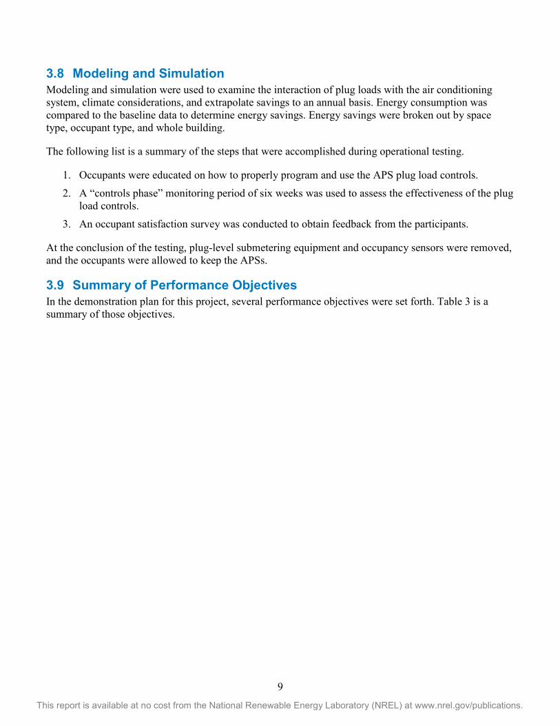
3.8 Modeling and Simulation Modeling and simulation were used to examine the interaction of plug loads with the air conditioning system, climate considerations, and extrapolate savings to an annual basis. Energy consumption was compared to the baseline data to determine energy savings. Energy savings were broken out by space type, occupant type, and whole building.
The following list is a summary of the steps that were accomplished during operational testing.
1. Occupants were educated on how to properly program and use the APS plug load controls.
2. A “controls phase” monitoring period of six weeks was used to assess the effectiveness of the plug load controls.
3. An occupant satisfaction survey was conducted to obtain feedback from the participants.
At the conclusion of the testing, plug-level submetering equipment and occupancy sensors were removed, and the occupants were allowed to keep the APSs.
3.9 Summary of Performance Objectives In the demonstration plan for this project, several performance objectives were set forth. Table 3 is a summary of those objectives.

10
This report is available at no cost from the National Renewable Energy Laboratory (NREL) at www.nrel.gov/publications.
Table 3. Performance Objectives
Performance Objective Metric Data Requirements Success Criteria
Quantitative Performance Objectives 1 Quantify whole
building energy savings and energy savings by space type from deploying schedule-based advanced power strips
Energy savings (% reduction) by space type and for the whole building, and simple payback period (years)
Receptacle-level and electrical panel-level power and energy data with a resolution of no more than 15 minutes, and an accuracy of plus or minus 5%. Occupancy sensor data with a resolution of no more than five minutes, and an accuracy of plus or minus 5%. Baseline energy savings will be measured and used for comparison to quantify energy savings from the APS.
Determination of baseline energy, identification of inefficiencies, and determination of energy savings resulting from APS. Reductions of 20% or more (thereby reducing the overall building load by 5% or more). Payback period less than five years.
Qualitative Performance Objectives 1 User satisfaction
with the demonstrated advanced power strips
Degree of Satisfaction
Survey 75% satisfaction rate
2 Occupant acceptance and comprehension of training on plug load energy saving strategies
Degree of acceptance and comprehension
Survey 75% acceptance and comprehension rates
3.10 Description of Performance Objectives For a detailed description of each performance objective, Please see Appendix 4 for a detailed description of each performance objective.

11
This report is available at no cost from the National Renewable Energy Laboratory (NREL) at www.nrel.gov/publications.
4 Technical Performance Analysis and Assessment 4.1 Overview Demonstration data was collected during an 11-week period from February 15 to May 4. The first five weeks of data collection (February 15 to March 22) were designated as the baseline period. No controls were implemented during these five weeks, and the data that was collected was representative of the typical operation of building A4. The last six weeks of the study were designated the control period. At the beginning of the control period, all 100 of the APSs were programmed to energize and de-energize based on a schedule defined by the occupant (or building management for shared spaces). The default schedule, if the occupant did not request an alteration, was 6 a.m. to 6 p.m. weekdays. The schedule based controls were expected to reduce plug level energy use during weekend and nighttime hours when equipment was not in use, therefore reducing building energy consumption without impacting the building occupants.
The principal goal of this study was to demonstrate greater than 20% reduction in whole-building plug-level energy consumption due to implementation of the schedule-based APSs. To effectively measure plug-level energy reduction due to the APS installation, three data sources were monitored in building A4:
1. Plug-level power/energy consumption 2. Panel-level power/energy consumption of plug load circuits
3. Occupancy data at each plug location.
Occupancy and power consumption for every APS device were measured every minute, and 15-minute average data was transmitted to NREL for data analysis purposes. In addition to these measurements, NAVFAC provided monthly whole building energy consumption data.
To accurately quantify whole building energy reduction, every plug-in device in the building was monitored at the plug level (data source one from above). To verify that all of the plug-in devices were accurately captured, all of the plug load circuits were monitored at the panel level using current transducers embedded in the panel (data source two from above). This enabled a second check of the savings that were recorded at the plug level. The fact that every plug load in the building was monitored before and after controls were implemented via the APSs allowed for quantification of the impact of the schedule-based APS on plug-level energy use.
4.2 Baseline Results and Findings The five weeks of baseline plug load data were analyzed to produce hourly power consumption profiles for an average weekday and an average weekend day. Figure 3 shows the plug load power profiles for all of building A4 using both the plug and circuit-level power measurements.
12
This report is available at no cost from the National Renewable Energy Laboratory (NREL) at www.nrel.gov/publications.
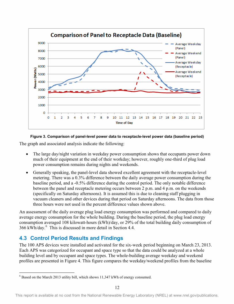
Figure 3. Comparison of panel-level power data to receptacle-level power data (baseline period)
The graph and associated analysis indicate the following:
• The large day/night variation in weekday power consumption shows that occupants power down much of their equipment at the end of their workday; however, roughly one-third of plug load power consumption remains during nights and weekends.
• Generally speaking, the panel-level data showed excellent agreement with the receptacle-level metering. There was a 0.3% difference between the daily average power consumption during the baseline period, and a -0.5% difference during the control period. The only notable difference between the panel and receptacle metering occurs between 2 p.m. and 4 p.m. on the weekends (specifically on Saturday afternoons). It is assumed this is due to cleaning staff plugging in vacuum cleaners and other devices during that period on Saturday afternoons. The data from those three hours were not used in the percent difference values shown above.
An assessment of the daily average plug load energy consumption was performed and compared to daily average energy consumption for the whole building. During the baseline period, the plug load energy consumption averaged 108 kilowatt-hours (kWh)/day, or 29% of the total building daily consumption of 366 kWh/day.6 This is discussed in more detail in Section 4.4.
4.3 Control Period Results and Findings The 100 APS devices were installed and activated for the six-week period beginning on March 23, 2013. Each APS was categorized for occupant and space type so that the data could be analyzed at a whole building level and by occupant and space types. The whole-building average weekday and weekend profiles are presented in Figure 4. This figure compares the weekday/weekend profiles from the baseline
6 Based on the March 2013 utility bill, which shows 11,347 kWh of energy consumed.

13
This report is available at no cost from the National Renewable Energy Laboratory (NREL) at www.nrel.gov/publications.
to the weekday/weekend profiles from the control period. The profiles for various space types and occupant types are presented in Appendix 5.
Figure 4. Whole building plug loads for baseline and control period (weekday and weekend profiles shown)
It can be noted that the approximate 3 kilowatt (kW) night and weekend load during the baseline period was reduced significantly during the control period to approximately 0.9 kW. There are also significant reductions in energy use during the shoulder periods of the day (late afternoon and early morning).
As expected, APS use lowered the power consumption during nights and weekends, and that reduction translates to energy savings. During the control period, the plug load energy consumption averaged 78 kWh/day.
As mentioned in Section 3.5, all of the control period power consumption data was normalized with respect to occupancy. This ensures the energy savings that are described in this report are due to the implementation of APS control and are not simply a byproduct of a reduction (or increase) in building occupancy during the control period. The occupancy normalization is described in Appendix 3, and occupancy profiles are included in Appendix 6.
Average energy savings were calculated at the whole-building level and for each space and occupant types identified in building A4. The different space types identified were: open office, private office, print stations, conference rooms, reception areas, hallways, and break rooms. The different occupant types identified were technical staff, managerial staff, administrative staff, and all other staff.
The formula used to quantify energy use reduction was:
𝐸�𝑏𝑎𝑠𝑒𝑙𝑖𝑛𝑒,𝑑𝑎𝑖𝑙𝑦 − 𝐸�𝑐𝑜𝑛𝑡𝑟𝑜𝑙,𝑑𝑎𝑖𝑙𝑦 (1)
14
This report is available at no cost from the National Renewable Energy Laboratory (NREL) at www.nrel.gov/publications.
Where:
• 𝐸�𝑏𝑎𝑠𝑒𝑙𝑖𝑛𝑒,𝑑𝑎𝑖𝑙𝑦 is the average daily energy consumption during the baseline period
• 𝐸�𝑐𝑜𝑛𝑡𝑟𝑜𝑙,𝑑𝑎𝑖𝑙𝑦 is the average daily energy consumption during the control period.
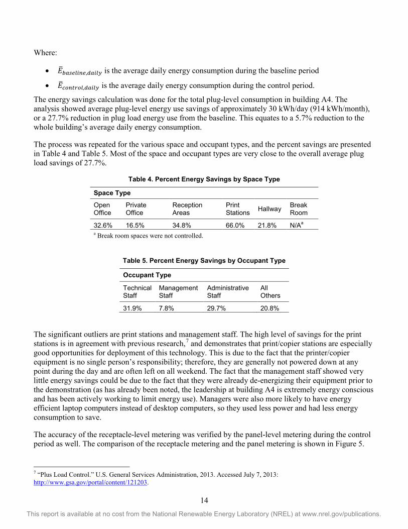
The energy savings calculation was done for the total plug-level consumption in building A4. The analysis showed average plug-level energy use savings of approximately 30 kWh/day (914 kWh/month), or a 27.7% reduction in plug load energy use from the baseline. This equates to a 5.7% reduction to the whole building’s average daily energy consumption.
The process was repeated for the various space and occupant types, and the percent savings are presented in Table 4 and Table 5. Most of the space and occupant types are very close to the overall average plug load savings of 27.7%.
Table 4. Percent Energy Savings by Space Type
Space Type
Open Office
Private Office
Reception Areas
Print Stations Hallway Break
Room
32.6% 16.5% 34.8% 66.0% 21.8% N/Aa a Break room spaces were not controlled.
Table 5. Percent Energy Savings by Occupant Type
Occupant Type
Technical Staff
Management Staff
Administrative Staff
All Others
31.9% 7.8% 29.7% 20.8%
The significant outliers are print stations and management staff. The high level of savings for the print stations is in agreement with previous research,7 and demonstrates that print/copier stations are especially good opportunities for deployment of this technology. This is due to the fact that the printer/copier equipment is no single person’s responsibility; therefore, they are generally not powered down at any point during the day and are often left on all weekend. The fact that the management staff showed very little energy savings could be due to the fact that they were already de-energizing their equipment prior to the demonstration (as has already been noted, the leadership at building A4 is extremely energy conscious and has been actively working to limit energy use). Managers were also more likely to have energy efficient laptop computers instead of desktop computers, so they used less power and had less energy consumption to save.
The accuracy of the receptacle-level metering was verified by the panel-level metering during the control period as well. The comparison of the receptacle metering and the panel metering is shown in Figure 5.
7 “Plus Load Control.” U.S. General Services Administration, 2013. Accessed July 7, 2013: http://www.gsa.gov/portal/content/121203.

15
This report is available at no cost from the National Renewable Energy Laboratory (NREL) at www.nrel.gov/publications.
The agreement between the two data sources is very good (excluding the Saturday spike attributed to cleaning energy use), with a -0.5% difference on the daily energy consumption.
Figure 5. Comparison of panel-level power data to receptacle-level power data (control period)
In summary, the baseline and control measurements enabled the calculation of energy savings directly attributable to the APSs. Plug loads were determined to be 108 kWh/day or 29% of the total building load, and during the six-week control period, the APS devices saved an average of 30 kWh/day.8 There are also additional air conditioning savings associated with reducing the internal heat load in the building. The following section describes how total annual savings were calculated.
The demonstration of savings by space/occupant type provides additional information for the Navy that would inform implementation of this technology. It is shown that certain space types or occupant types are better suited for the APS technology evaluated. This can be useful in deciding which buildings and/or occupants should be selected for deployment of APS technology.
4.4 Energy Model and Simulation of Whole Building Energy Savings The 11 weeks of directly measured plug load energy consumption was used to inform a building model to calculate total annual energy savings. The total annual energy savings are a combination of 12 months of plug load savings, plus savings in air conditioning energy consumption as a result of the lower internal load in the building.
Building energy modeling was used to determine the energy use of NAVFAC Hawaii building A4, which included: examining the interactions between plug loads and the air conditioning system, analyzing climate considerations, and quantifying annual energy savings for the project. The building characteristics and operating conditions of HVAC systems were modeled, including current operating schedules and, as
8 Based on the April 2013 utility bill, which shows 9348 kWh of energy consumed.

16
This report is available at no cost from the National Renewable Energy Laboratory (NREL) at www.nrel.gov/publications.
much as possible, equipment operational characteristics determined from discussion with the facilities team.
A graphical representation of the building energy model developed is shown in Figure 6. The geometry of the buildings was simplified for modeling purposes to accurately simulate energy transfer through all surfaces in the building.
Figure 6. Building A4 energy model representation
The NREL team used the data gathered during the site visits to develop the energy model. The baseline energy model for building A4 was calibrated to within approximately 1% of the annual energy use from the existing electricity utility data for 2012. Figure 7 graphically displays the calibration for monthly electricity use. Baseline model calibration consists of adjusting model parameters that are somewhat difficult to measure, such that the modeled energy-use profile corresponds with actual utility-use data.
17
This report is available at no cost from the National Renewable Energy Laboratory (NREL) at www.nrel.gov/publications.
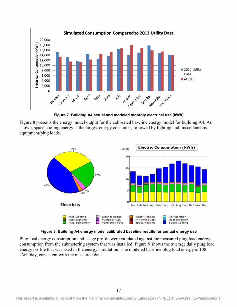
Figure 7. Building A4 actual and modeled monthly electrical use (kWh)
Figure 8 presents the energy model output for the calibrated baseline energy model for building A4. As shown, space cooling energy is the largest energy consumer, followed by lighting and miscellaneous equipment/plug loads.
Figure 8. Building A4 energy model calibrated baseline results for annual energy use
Plug load energy consumption and usage profile were validated against the measured plug load energy consumption from the submetering system that was installed. Figure 9 shows the average daily plug load energy profile that was used in the energy simulation. The modeled baseline plug load energy is 108 kWh/day, consistent with the measured data.

18
This report is available at no cost from the National Renewable Energy Laboratory (NREL) at www.nrel.gov/publications.
Figure 9. Building A4 energy model simulated plug load energy profile for baseline and controlled phases
The annual energy savings are calculated by comparing the modeled baseline energy consumption to the modeled energy consumption of the building using the APS plug load control schedule. Table 6 shows the annual energy savings results for plug loads and air conditioning, as well as the percent reduction from baseline.
Table 6. Annual Energy Savings for Building A4
Annual Electricity (kWh/year) Savings % Reduction from Baseline
Plug Loads 9,890 28%
Cooling 4,010 5% Total 13,900 8%
The annual energy savings, which was extrapolated from the measured reduction in plug load energy resulting from the deployment of schedule-based APSs in building A4, was calculated to be a 28% reduction in plug load energy and 8% reduction in whole building energy consumption. These results meet and exceed the objectives of this project, which was to achieve a 20% reduction in plug loads and a 5% reduction in whole building energy.
4.5 Utility Meter Evidence Although variation in utility bills can be a factor of weather and other factors, it was hoped that at least some of the APS’s estimated 8% reduction would be apparent at the building electric meter. Weather normalization of utility bill data generally requires three years prior and one year post-retrofit utility data, so more cursory observations were made. Building A4 utility meter readings from April and May 2013 were compared to the same months in 2012, and an average reduction of 21% was observed. This high reduction in whole building loads is due to our APS demonstration, as well as other ongoing efforts of the NAVFAC Hawaii energy team.

19
This report is available at no cost from the National Renewable Energy Laboratory (NREL) at www.nrel.gov/publications.
4.6 Occupant Surveys Energy savings are meaningless if they result in reduced productivity of the building occupants. Two surveys were delivered to the occupants of building A4 (one prior to install and one upon removal of the metering equipment) to gauge occupant acceptance of the technology. The entry survey was designed to capture any preconceived notions on energy use in an office space, how the APS devices would impact their work, and general occupant schedules. The exit survey was designed to assess the usability of the product for the occupants, assess the impact that it had on their daily work schedules, and their perception of savings achieved through use of the APS. The exit survey is included in Appendix 2, and its results are graphed in Appendix 7. It should be noted that both of the surveys were passed through the central DOE Internal Review Board, and was not deemed under their purview for human subject research.
In general, the exit survey shows that occupants were satisfied with and accepted the APSs. The notable outcomes of the exit survey are:
• 69% of occupants said the APS did not change their productivity
• 84% of occupants would recommend that APSs be deployed throughout JBPHH.
4.7 Assessment of Performance Objectives Results Table 7 lists the performance objectives for this demonstration and the outcomes that were achieved.

20
This report is available at no cost from the National Renewable Energy Laboratory (NREL) at www.nrel.gov/publications.
Table 7. Performance Objectives and Outcomes
Performance Objective Metric Data Requirements Success Criteria Outcome
Quantitative Performance Objectives 1 Quantify whole
building energy savings and energy savings by space type from deploying schedule-based advanced power strips
Energy savings (% reduction) by space type and for the whole building, and simple payback period (years)
Receptacle-level and electrical panel-level power and energy data with a resolution of no more than 15 minutes, and an accuracy of plus or minus 5%. Occupancy sensor data with a resolution of no more than five minutes, and an accuracy of plus or minus 5%. Baseline energy savings will be measured and used for comparison to quantify energy savings from the APS.
Determination of baseline energy, identification of inefficiencies, and determination of energy savings resulting from APS. Reductions of 20% or more (thereby reducing the overall building load by 5% or more). Payback period less than five years.
Accomplished. See Section 4.4. Achieved plug load reductions of 28%, thereby reducing the overall building load by 8%. Payback period less than two years.
Qualitative Performance Objectives Outcome 1 User satisfaction
with the demonstrated advanced power strips
Degree of Satisfaction
Survey 75% satisfaction rate
Accomplished. See Section 4.6.
2 Occupant acceptance and comprehension of training on plug load energy saving strategies
Degree of acceptance and comprehension
Survey 75% acceptance and comprehension rates
Accomplished. See Section 4.6.

21
This report is available at no cost from the National Renewable Energy Laboratory (NREL) at www.nrel.gov/publications.
5 Economic Performance Analysis and Assessment Economic results of this demonstration indicate application of the APS technology can yield appreciable energy and cost savings at a relatively small investment. For the demonstrated system, we calculate an eROI value of 18.6, with net savings projected at $14,000 over a five-year lifetime and $80,000 for a 20-year lifetime. For follow-on activities utilizing more cost-effective acquisition practices, the eROI value increases to 35, with net savings projected at $21,000 and $90,000 over five- and 20-year lifetimes. Collectively, results are promising and indicate that the U.S. Navy, on an economic basis, should consider further investment and deployment of this technology.
Table 8 provides a full summary of economic results, in addition to key analysis inputs. Estimates for net savings, savings to investment ratio (SIR), and simple payback were calculated using the latest version of the National Institute of Standards and Technology-developed Building Life Cycle Cost (BLCC) program. eROI values were provided using the latest available version of the Neptune eROI calculator, as provided by NAVFAC.

22
This report is available at no cost from the National Renewable Energy Laboratory (NREL) at www.nrel.gov/publications.
Table 8. Summary of Economic Results and Key Analysis Inputs
DD1391 Estimatea Demo Actualsb Projected Follow-Onc
Economic Analysis Results
eROI Value 3.2 18.6 35.0
Net Savings, Five-Year Life -$68,000 $14,000 $21,000
SIR, Five-Year Life 0.2 2.0 3.4
Net Savings, 20-Year Life -$40,000 $80,000 $90,000
SIR, 20-Year Life 0.6 6.7 10.0
Simple Payback None < 3 years < 2 year
Key Analysis Inputs
Annual Energy Savings 13,500 kWh 14,960 kWh 14,960 kWh
Electricity Priced $0.24/kWh $0.425/kWh $0.425/kWh
Initial Investment Cost $83,070 $16,918 $8,672
Units Installede 100 100 100 a DD1391 estimate column reflects analysis as performed as part of site approval/DD1391 process in July 2012. b Demo actuals column reflects economic results based on actual, realized costs of procurement and installation, as well as measured energy savings results. c Projected follow-on column reflect estimated results for future installations of this technology using a more efficient acquisition strategy than executed in the demonstration. d Electricity pricing for demo actuals and projected follow-on reflect the average price of fiscal year (FY) 13 and FY14 rates at JBPHH. According to the U.S. Energy Information Administration (EIA), in June 2013, the average electricity rate in the United States was $0.105/kWh. e One hundred units were installed; however, an additional 30 spare units were also procured in the demonstration and are included in demonstration actuals and projected follow-on initial investment costs
Economic results were reviewed to evaluate potential sources of error and/or uncertainty in the estimates provided. Four issues were identified and described below.
• Utility electricity rate volatility. Significant volatility in JBPHH utility rates from FY12 through FY14 indicate analysis results as presented may be susceptible to uncertainty in projecting future year utility rate pricing. More specifically, utility rates have jumped from $0.24/kWh in FY12 to $0.58/kWh in FY14. The expectation, based on discussions with NAVFAC Hawaii personnel, is for utility rates to decline in FY15, but an exact value remains uncertain. This volatility in pricing must be considered in evaluating economic results of the APS technology, as applied to JBPHH.

23
This report is available at no cost from the National Renewable Energy Laboratory (NREL) at www.nrel.gov/publications.
A preliminary sensitivity analysis was performed to evaluate the effect of electricity pricing uncertainty on economic yield. Figure 10 shows net savings estimates for a five-year economic life on installation of APS over an electricity price range between $0.325/kWh to $0.525/kWh. This range encompasses as +/- $0.10/kWh sensitivity band around the nominal rate applied to our economic analysis.9 As indicated by the figure, electricity pricing has a significant impact on savings. APS technology savings, however, remain appreciable, even at a conservative price of electricity of $0.325/kWh. Although net savings will be highly dependent upon electricity pricing, economic yields for implementation of the APS technology should remain significant enough to warrant U.S. Navy interest in investment over the full range of potential, long-term electricity prices.
Figure 10. Net savings estimates for a five-year economic life on installation of APS over an electricity price
range between $0.325/kWh to $0.525/kWh
• Technology design life. The APS devices as demonstrated include a four-year parts warranty, providing the manufacturer’s confidence in device longevity. These devices, however, include a device-specific battery that will likely need replacement every four to five years. A five-year economic life is provided as a conservative, base estimate of economic yield. A 20-year economic life is also provided to evaluate long-term benefits of these devices. For the 20-year economic life, the analysis accounts for batteries being replaced every five years at an assumed replacement value of 25% of initial APS procurement cost.
• DD1391 estimate, investment cost. The projected economic yield of the DD1391 estimates, as shown in Table 9, are not consistent with demonstration actuals nor projected results for follow-on deployment of this technology. This is largely attributed to an incorrect inclusion of procurement and installation costs of demonstration monitoring equipment in the initial estimate, as apparent in Table 8.
9 The nominal rate of $0.425/kWh is the average rate between FY13 and FY14 known rates.

24
This report is available at no cost from the National Renewable Energy Laboratory (NREL) at www.nrel.gov/publications.
• Follow-on installations, investment cost. The projected investment cost for follow-on procurement and installation activities is significantly less than costs realized in performance of the technology demonstration (see Table 8). This differential in costs is attributed to recommended adjustment in acquisition strategy. For the demonstration, NREL staff performed installation of the APS devices as an interrelated element of the overall demonstration setup. This required significant labor costing of high-labor grade scientists and associated travel. These requirements were necessary for demonstration purposes but are not required for general implementation of this technology. Follow-on investment costs assume implementation activities are performed by a local contractor, significantly reducing total labor hours and labor category, without requiring travel to and from the contiguous United States.
Some measure of uncertainty is inherent to projecting future installation costs of this technology; however, overall reduction from realized demonstration costs should be significant and projected costs, as presented, are in line with this expectation.
More details on the cost analysis are found in Appendix 8.

25
This report is available at no cost from the National Renewable Energy Laboratory (NREL) at www.nrel.gov/publications.
6 Project Management Considerations Execution of this technology demonstration was straightforward from a programmatic basis. Acquisition and deployment of these devices required limited time and resources owing to the commercial availability and simplicity of the technology. Table 9 provides a summary of programmatic elements of this project and a high-level timeline of events.
Table 9. Summary of Programmatic Elements of this Project
The project life cycle was composed of four sequential tasks, as described below:
1) Site identification. To initiate this project, an appropriate facility was needed to demonstrate the technology. The Integrated Project Team (IPT) developed a listing of site criteria for an ideal location for the demonstration, which was then distributed to NAVFAC Hawaii and Joint Region Marianas (JRM) facility and energy managers. Upon identification of candidate sites, IPT researchers visited these sites and recommended the preferred location for the demonstration. The selection criteria are listed in Section 3.
2) Site approval. Upon selection of the site, the IPT performed site approval, DD1391, and National Environmental Policy Act (NEPA) determination activities.
3) Procurement/installation. The majority of the procurement and installation activities were related to the unique nature of the project as a technology demonstration. These activities included design and installation of monitoring equipment, baseline building performance measurements, and remote monitoring application and implementation. In contrast, installation of the APS devices, as required for standard deployments, required minimal effort with procurement performed over a few weeks and installation performed in less than one week of on-site activity.
4) Demonstration. Upon completion of installation activities and baseline measurements of facility performance, the APS devices were setup and their performance monitored over several months. Upon completion of the demonstration period, IPT personnel removed the demonstration monitoring equipment form the site, with APS devices remaining in operation.
Programmatic challenges experienced on this project were limited. Those observed were nontechnical in nature and due largely to the demonstration-specific objectives of this project. Examples include maneuvering through the approval process for using a cellular modem for remote monitoring.
Programmatic Summary Implementation Method NREL procure and install Key Contractors None Period of Performance One year, three months Project Timeline Site identification: February 2012 - April 2012
Site approval: April 2012 - August 2012
Procurement/installation: August 2012 - March 2013
Demonstration: March 2013 - May 2013

26
This report is available at no cost from the National Renewable Energy Laboratory (NREL) at www.nrel.gov/publications.
Similarly, in evaluating the project schedule, the majority of project time was spent on demonstration-specific activities. The project experienced a lengthy site approval/NEPA process due to installation of demonstration monitoring equipment interfacing the facility’s electrical system. In addition, several months of facility baseline energy measurements were required prior to installing the APS devices to evaluate device benefits. These types of demonstration-specific activities significantly extended the project deadline.
In summary, when evaluating the project from a programmatic basis, the majority of its lengthiest activities and challenges were directly attributable to its nature as a technology demonstration. It should be emphasized that standard deployment of this technology in a nondemonstration setting can be executed with relative ease, over a significantly shorter timeline.
6.1 Site Approval, National Environmental Policy Act, and DD1391 Site approval, NEPA, and DD1391 activities were required for this project due to its nature as a technology demonstration. Specifically, evaluation of APS and building energy performance required installing monitoring equipment interfacing the building’s electrical system. In tandem with building A4’s listing as a historical building, installation of the monitoring equipment gave cause for a relatively lengthy process for assessing environmental impacts and receiving site approval.
NAVFAC Pacific has determined, however, that future, standard deployments of this technology without need for facility monitoring equipment will not require site approval. Further, such activities would fall under a categorical exclusion regarding a NEPA determination.
As a cursory note, this demonstration also required remote access/networking capabilities for monitoring of device performance. A cellular modem was installed on-site, requiring coordination with appropriate site personnel and submittal of a communications plan. It should be emphasized, however, that the APS technology does not require network communications to operate. The cellular modem was only required for purposes of demonstration monitoring.
6.2 Contracts and Procurement NREL and NAVFAC personnel self-performed the majority of the procurement and installation activities for this demonstration, excluding installation of submetering monitoring equipment, which was performed by a U.S. licensed, master electrician. Rationale for self-performance of APS installation was based on the marginal scope of APS installation activities in addition to overall efficiency of performing APS installation activities in parallel with other site-related demonstration activities (such as facility personnel training, monitoring equipment installation, surveys of site personnel, etc.). Appendix 8 presents a detailed accounting of equipment procured and service-related purchase orders executed under this project. This appendix also delineates between technology and demonstration specific, cost elements.
For standard deployments of this technology, the preferred implementation strategy is dependent upon the scale of the activity. Based on the cost estimates presented in Section 5 and Appendix 8, total pricing for deployment of APS device technologies in an office building similar to building A4 may be prohibitively small to generate interest for a competitively selected, contractor-performed implementation. Consequently, office or small building implementations may have to be self-performed by facility personnel or NAVFAC public works.
In contrast, for larger deployments of this technology, implementation by a competitively selected contractor is recommended for the reasons listed below:

27
This report is available at no cost from the National Renewable Energy Laboratory (NREL) at www.nrel.gov/publications.
• Resource constraints. Although installation of the APS devices is not technically challenging, it can be labor intensive. Large-scale implementation may require resources not available by site personnel.
• Quality control. APS installations when self-performed by office residents typically yields a wide range of performance results. Office personnel may not install the devices properly or may not even install the devices. Utilization of a contractor helps ensure a consistent level of quality control in implementation of this device technology.
• Training and troubleshooting. Although the APS devices are simple to use, they may still require some handling from office residents for proper function over extended periods. A contractor can provide standardized training to office personnel. Additionally, a contractor can be required to be readily accessible for troubleshooting support that may not be available under a U.S. Navy, self-performed implementation.
• Economy-of-scale pricing benefits. For large-scale deployments, the U.S. Navy should see pricing efficiencies, especially in reuse of training materials for APS implementation at several facilities, general requirements for site access, and optimal utilization of contract labor resources for installation, training, and troubleshooting activities.
If the U.S. Navy has flexibility regarding the scale of the technology acquisition, the recommended best approach to implementation would be large-scale implementation (> 500 APS devices), and utilizing a local contractor for procurement, installation, and training. This recommendation is based on evaluation of demonstration results, past experience, and concurring comments made by facility personnel.10 In utilizing this approach, a task order agreement/indefinite delivery, indefinite quantity contracting structure may have best value for applications at the base or regional levels.
6.3 Design Little to no design is required for this technology; however, the APS equipment selection options are dependent on the existing equipment in the space. Master-slave and load-sensing APSs might be better alternatives to schedule-based APSs when a device (such as a computer with automatic low-power savings settings enabled) can act as the master device. For example, if the laptop computers in a given building are set to automatically transition into a standby/sleep state after 15 minutes of idle time, they could be used as “master” devices. When these laptops transition to a low-power state, the connected “slave” devices, such as monitors and task lights, would automatically be powered off as well. Master-slave APSs have the added advantage of not interrupting power to computers, allowing software updates during unoccupied periods (this is Anderson Air Force Base’s current strategy for updates). Schedule-based APS implementation must be coordinated with the command chief information officer to ensure the scheduled load controls are compatible with software update strategies (users can override the schedules when notified of a software push event).
High power-draw plug loads, such as window air conditioners, may require specialized APSs.
It is a one-for-one replacement with the existing standard power strips, and controls are managed locally by the occupants. Certain specifications should be considered during procurement, such as:
10 At the end of this demonstration, IPT team member Amy Hanada from NAVFAC Hawaii indicated that installation by a local contractor was her preferred approach for future deployments.
28
This report is available at no cost from the National Renewable Energy Laboratory (NREL) at www.nrel.gov/publications.
• Control type (i.e., schedule-based, load sensing, etc.)
• Number of outlets (i.e., ≥ 8 total outlets, ≥ 2 constant hot outlets, ≥ 6 switched outlets)
• Manual on/off or user override control
• Power qualities: o Surge protection with electromagnetic interference/radio frequency interference (RFI) filter
rated ≥ 1080 joule surge protection and ≥ 72,000 ampere (A) protection, and RFI filter to 75 decibels
o Rated to handle a 15 A load; Underwriters Laboratories (UL)-required 15 A and UL voltage protection rating; clamping voltage 400 volts and maximum spike voltage 6 kilovolts
o 110-volt alternating current (AC), 60 Hertz, 15 A, and ≥ 6 foot power cable
o Must be UL listed with Electrical Testing Laboratories certification of UL 1449 3rd edition, UL 1363 3rd edition.
• Outlet orientation (i.e., oriented and spaced to accommodate multiple AC to direct current power supplies without blocking other outlets)
• Statement of offered “commercial/standard” lifetime warranty
• Statement of offered “connected equipment” warranty (i.e., $50,000)
• Contain easy-to-understand user instructions
• Item must meet Executive Order 13221; device uses ≤ 1 Watt in standby power consuming mode
• Wire management (i.e., retractable power cords)
• Mounting (i.e., Velcro or two-sided tape to hold device securely in place on desktop).
6.4 Installation and Construction Installation of the APS devices is straightforward and can be performed by a general, untrained labor force. Basic activity requires straightforward replacement of existing standard power strips with APS devices. APS timers will need to be preprogrammed to a default schedule prior to deployment, with occupants then able to customize settings post-installation.
Installations can be performed by one person. Two people working together may be more efficient, however, to accommodate visibility and physical lifting constraints posed by some office environments. Based on time to perform APS installations on this project, expectation should be to install around four devices per hour per installer.
A key factor in the installation process is coordination with building occupants. Buy-in from the building’s occupants is critical to correct operation of the APS devices, which in turn translates to realized energy savings. It is important the occupants understand the value and function of the APS devices, and that the devices will not adversely affect their ability to perform their jobs. The IPT believes that training and face-to-face time with the occupants, supervisors, and facility leadership were key contributors to the demonstration’s success. We strongly recommend similar training and educational activities be provided in future deployments of this technology.
29
This report is available at no cost from the National Renewable Energy Laboratory (NREL) at www.nrel.gov/publications.
Similarly, when installing the devices, preference is to have the occupant present soon after the installation. The installer can then introduce the device to the occupant and help them customize timer settings. Installing APS devices during lunchtime or other planned, short term work break is ideal, allowing the installer not to interfere with occupants’ workday while also allowing for a post-installation introduction to the device. We realize, however, this may not be a practical option, especially for deployment of a large number of these devices.
6.5 Operation and Maintenance In general, APS devices are similar to standard plug strips and do not require regular maintenance. Some devices may, however, have unique features requiring recurring maintenance or replacement, such as batteries. Because of the device’s low procurement cost, nonrecurring maintenance activities, such as repair of poorly operating or malfunctioning units, may not be cost-effective. Replacement of malfunctioning units might be the more pragmatic and cost-effective solution.
Specific to the demonstration at building A4, the IPT installed 100 APS devices and procured 30 spare units. Spare units were provided to ensure malfunctioning devices could be easily replaced, ensuring maximum building energy savings over an extended economic life. Standard deployment of APS devices may also benefit from procurement of spare devices, providing margin for malfunctioning and lost devices at limited additional cost.
The APS devices demonstrated also include batteries for device memory. These batteries will likely need to be replaced. Each device comes with a four-year parts warranty, indicating this recurring replacement activity will likely occur every four to five years of operational life. Unique issues of different APS devices such as this one should be considered when moving forward with future APS procurement activities.
6.6 Training As indicated in Section 6.4, proper training of building occupants is a key factor in realizing the full operational potential of the APS devices.
NREL provided training to site facility managers and energy managers on how the system would be configured and operated throughout the study. Site managers were given access to the online dashboard for real-time feedback of the data being collected. Training also included troubleshooting techniques that may be required from on-site personnel.
In addition, NREL provided training to all occupants receiving an APS control device. The training included background information about the purpose and importance of the study, how to operate the devices, how to manually override the controls if an issue arises, and communication protocol for reporting issues.
Appendix 9 and Appendix 10 include the manager training and occupant training, respectively, which were developed for this demonstration project.
7 Commercial Readiness Qualitative Assessment Automatic power strips are a mature but underutilized commercially available technology provided by multiple manufacturers and vendors. The various types of APSs are described in Section 2.1, and a representative listing of manufacturers are listed below.

30
This report is available at no cost from the National Renewable Energy Laboratory (NREL) at www.nrel.gov/publications.
7.1 Primary Manufacturers Table 10 captures some of the manufacturers who make APSs.
Table 10. Example List of Manufacturers of APSs
Source: Information gathered from www.google.com/shopping on May 10, 2013.
7.2 Product Availability APS devices are widely available from a variety of retailers, including hardware, electronic, big box retail, and online merchants. Table 11 lists some of the retailers were APSs can be purchased.
ApproximateSelected Manufacturers Products Price Range
APC Several Master-Control and Timer models $20
BelkinSeveral Master-Control and Timer models, some with a remote control
$25-$45
BITs Master-Control models with 7-10 outlets $25-$40TrickleStar Master-Control models with 6-12 outlets $25-$50TrippLite Master-Control models with 8-12 outlets $30-$50Coleman Cable, Inc Master-Control models with 6-10 outlets $25-$40EcoStrip One Master-Control model with 6 outlets $25
EtherealLoad sensing model with an informational LED display and 8 outlets
$130
iGoGreenMaster-Control model with 4 outlets and a load sensing 8 outlet model with USB interface
$25, $50
Monster Power Master-Control models with 6-8 outlets $40-$60NuGiant Master-Control models with 6-8 outlets $20-$40Rocketfish Master-Control models with 7-12 outlets $20-$30
Watt Stopper (Legrand)Load sensing model with an occupancy sensor and 8 outlets
$70-$85
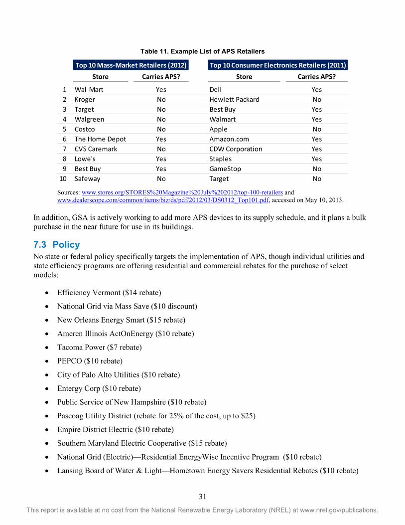
31
This report is available at no cost from the National Renewable Energy Laboratory (NREL) at www.nrel.gov/publications.
Table 11. Example List of APS Retailers
Sources: www.stores.org/STORES%20Magazine%20July%202012/top-100-retailers and www.dealerscope.com/common/items/biz/ds/pdf/2012/03/DS0312_Top101.pdf, accessed on May 10, 2013.
In addition, GSA is actively working to add more APS devices to its supply schedule, and it plans a bulk purchase in the near future for use in its buildings.
7.3 Policy No state or federal policy specifically targets the implementation of APS, though individual utilities and state efficiency programs are offering residential and commercial rebates for the purchase of select models:
• Efficiency Vermont ($14 rebate)
• National Grid via Mass Save ($10 discount)
• New Orleans Energy Smart ($15 rebate)
• Ameren Illinois ActOnEnergy ($10 rebate)
• Tacoma Power ($7 rebate)
• PEPCO ($10 rebate)
• City of Palo Alto Utilities ($10 rebate)
• Entergy Corp ($10 rebate)
• Public Service of New Hampshire ($10 rebate)
• Pascoag Utility District (rebate for 25% of the cost, up to $25)
• Empire District Electric ($10 rebate)
• Southern Maryland Electric Cooperative ($15 rebate)
• National Grid (Electric)—Residential EnergyWise Incentive Program ($10 rebate)
• Lansing Board of Water & Light—Hometown Energy Savers Residential Rebates ($10 rebate)
Top 10 Mass-Market Retailers (2012) Top 10 Consumer Electronics Retailers (2011)Store Carries APS? Store Carries APS?
1 Wal-Mart Yes Dell Yes2 Kroger No Hewlett Packard No3 Target No Best Buy Yes4 Walgreen No Walmart Yes5 Costco No Apple No6 The Home Depot Yes Amazon.com Yes7 CVS Caremark No CDW Corporation Yes8 Lowe's Yes Staples Yes9 Best Buy Yes GameStop No
10 Safeway No Target No

32
This report is available at no cost from the National Renewable Energy Laboratory (NREL) at www.nrel.gov/publications.
• Port Angeles Public Works & Utilities—Commercial and Industrial Energy Efficiency Rebate Program ($20 rebate).
7.4 Price of Advanced Power Strips Prices for APSs typically range from $15 to $50, with the majority of units around the $30 price mark. These types of units will have a range of four to 10 outlets. Compared to the price of a standard surge suppressor of $10-$50, the price premium for an APS is no more than $5.
A price barrier is present when compared with the price of a compact fluorescent light bulb, which may be purchased for as little as $1 at many national retailers. However, when combined with utility and efficiency program rebates (outlined in Section 7.3), the price premium for an APS is essentially nonexistent.
7.5 Usability and Functionality Historically, APS usability has been a key barrier to energy savings. As mentioned in Section 6.6, training of building occupants in the use and benefits of the technology is key to overcoming those issues.
Of the 20 APS tested in a study by NREL (Earle & Sparn, 2012), only four received perfect scores based on functionality (whether the device worked as expected) and usability (user interaction necessary for desired performance). Of the four devices that received perfect scores, only three appear to be commercially available today and are listed in Table 12.
Table 12. High Scoring APSs Currently on the Market
Source: www.aceee.org/files/proceedings/2012/data/papers/0193-000005.pdf.
If users are required to take too many extra steps or the APS requires a change in habit, users are less likely to be consistent with the actions necessary to reduce consumption and will revert to traditional power strips. Training is key to get the most out of an APS.
The specification provided in Section 6.3 addresses key APS features that contribute to its usability, and the specification can be modified to address NAVFAC-specific needs.
7.5.1 Energy Savings Two federal agencies have already estimated or measured the energy savings from APS use in their facilities.
• GSA. In 2012, the GSA monitored plug load consumption in eight buildings and found that a schedule timer was most effective in an office setting, resulting in energy savings of 48% in
Approximate Total ControlledBrand Model Cost Category Outlets Outlets Image
BelkinBelkin Conserve Smart AV Surge Suppressor
$30 Master Control 8 5
NuGiant Energy Saving Smart Surge $22 Master Control 6 4
Rocketfish RF-HTS105 Surge Suppressor $20 Master Control 7 4

33
This report is available at no cost from the National Renewable Energy Laboratory (NREL) at www.nrel.gov/publications.
printer rooms and kitchens and 26% at workstations. Particularly when applied to devices that are powered 24 hours a day, including copiers and small kitchen appliances, significant energy savings may be achieved with timer controls.11
• U.S. Air Force. In 2012, the U.S. Air Force purchased over 75,000 APSs specifically for use in workstations. They chose a TrickleStar master control model with seven total outlets, four of which are controlled. The Air Force has estimated this upgrade will allow them to reduce energy usage by 8 million kWh annually and save them $5.4 million over 10 years. Although it is likely the Air Force received a discount for purchasing so many units, assuming each unit cost approximately $30 (the current retail price) this implies a payback period of five years.12
The results found by the GSA and the U.S. Air Force are corroborated by this demonstration in terms of energy savings and payback. In summary, APSs are a low-risk, mature, inexpensive technology that can offer significant savings when implemented with a proper installation and training process.
11 “Plug Load Control: Findings.” U.S. General Services Administration, 2012. www.gsa.gov/portal/content/121203. 12 Buczynski, B. “Advanced Power Strips Will Save the Air Force $5.4 Million.” Earth Techling, 2012. www.earthtechling.com/2012/12/advanced-power-strips-will-save-the-air-force-5-4-million/.

34
This report is available at no cost from the National Renewable Energy Laboratory (NREL) at www.nrel.gov/publications.
8 Recommended Next Steps The APS technology deployed during this demonstration performed exceptionally well. The demonstration exceeded the quantitative goals laid out in Section 3.9. The APS’s achieved 27.7%13 savings with regards to plug-level energy consumption, and 8%14 savings on a whole-building level. The feedback from the occupants demonstrates overall success on the qualitative goals that were set for the project (see Section 3.9). The low upfront cost for this technology led to short payback periods and almost immediate savings for the U.S. Navy at building A4.
This technology is at a technology readiness level 9 (TRL-9). It has been proven through successful operation and is a commercially available product that can be procured through various different manufacturers and distributors. The technology is probably best categorized as COTS rather than partner technology because it has reached maturity, is commercially available, and has demonstrated high potential impact to U.S. Navy shore energy goals.
It is recommended that the U.S. Navy transition this COTS technology to office and other building types having numerous plug loads. Its savings are maximized where electricity costs are high, and in warm climate zones where reductions in internal loads result in larger air conditioning savings.
Key elements that should be addressed for successful adoption of APS technology are:
• Establishing standardized procurement and installation procedures
• Communication and integration with NAVFAC’s CIO organization to minimize interference with off-hours computer software updates
• Training and occupant buy-in. This is not an exhaustive list, and the recommendations are based solely on the experience of this demonstration and other research performed by the authors. The following discussion explains each of these components of an APS installation, and presents methods for avoiding any potential barriers associated with them.
• It is important to implement appropriate procurement and installation procedures. It has been the experience of the authors that if the APSs are left with the building occupants for installation, the vast majority of the devices are not installed or not installed correctly. As an anecdotal example, two APS strips were left with occupants for personal installation. These strips were not installed at the next site visit and had to be installed by the authors at that point in time.
• It is critical to establish acceptable protocol with regards to NAVFAC CIO. It is important to consider the necessary software pushes that the operating systems require. It should also be noted that new operating systems with power management settings can increase energy savings and can function in a similar manner as the APS system that was deployed at building A4. This is only true if the computer power settings are consistently used. Schedule-based controls are a proven alternative but can interfere with off-hours software updates if not properly coordinated. It will be important to consider how to best leverage the combined capabilities of advanced computer power management and APS control.
13 Extrapolated from measured plug load data from building A4. 14 Based on energy model. Model was informed by measured plug load data and utility bills from building A4.
35
This report is available at no cost from the National Renewable Energy Laboratory (NREL) at www.nrel.gov/publications.
• Training and occupant buy-in are critical for the success of the APS system. The occupant needs to be informed about how the APS system works, and if applicable, how to override the system should the strip be de-energized when he/she arrives at work and how to schedule their personal start times and stop times. This will ensure both familiarity with the system, appropriate operation, and optimal operation of the system.
In addition, the following concerns presented by NAVFAC were addressed by the authors:
• “Disappearing” APS devices. The authors heard concerns that the installed APS devices would disappear from building A4. Based on the experience of the NAVFAC Hawaii energy team, this has not been a problem. There have been no observed incidents of power strips missing.
• Occupants defeating automatic controls. The authors heard concerns that the schedule controls would be overridden by occupants. Based on the experience of the NAVFAC Hawaii energy team, this has not happened except for when the occupants have been asked to do so to receive computer updates.
• Installing APS devices through an energy savings performance contract (ESPC). The authors have been asked whether APS devices could be procured and installed through an ESPC. The answer to that question is yes, but the extra costs of measurement and verification would have to be taken into consideration.
It should be noted that schedule-based plug load control was demonstrated during this technology demonstration, but there are other types of plug load control that could be successful at U.S. Navy installations (load-sensing control and occupancy-based control). Schedule-based control was selected for this project due to previous studies indicating a high level of achievable energy savings combined with low capital cost for this technology. The schedule-based control is also the most mature of the various types of plug load control.

36
This report is available at no cost from the National Renewable Energy Laboratory (NREL) at www.nrel.gov/publications.
Appendix 1: Floor Plans
Figure A-1. Electrical panel locations on the first floor
Figure A-2. Electrical panel locations on the second floor

37
This report is available at no cost from the National Renewable Energy Laboratory (NREL) at www.nrel.gov/publications.
Appendix 2: Plug Load Participant Exit Survey 1. Did you adjust the schedule on your advanced power strip? If so, what changes did you make?
2. If you did make changes to the schedule, please rate the usability of the advanced power strip on a scale of 1 to 10 (10 being easy to use, and 1 being difficult to use)?
N/A (Difficult) 1 2 3 4 5 6 7 8 9 10 (Easy)
3. How did the advanced power strip affect your productivity? a. Significantly improved my productivity b. Improved my productivity c. No change d. Reduced my productivity e. Significantly reduced my productivity
4. Did you use the manual override on the advanced power strip? If so, how often?
5. How much energy savings do you think the advanced power strips yielded in the building?
a. Plug load energy reduction _________ % b. Whole building energy reduction _________ %
6. Would you recommend advanced power strips be deployed throughout the whole base?
a. Yes b. No
7. Additional comments:

38
This report is available at no cost from the National Renewable Energy Laboratory (NREL) at www.nrel.gov/publications.
Appendix 3: Normalizing The principal variable affecting plug-level energy use that was not possible to control for in this study was occupancy. It was not possible to enforce the occupants of the building to maintain the exact same schedule before and after the controls were implemented. Occupancy levels can have a direct impact on plug-level energy use, especially if the occupant turns his/her plug loads on and off when he/she comes and goes. As an example, if the average occupancy in the office was 25% lower during the control period than the baseline period, one would expect to see a reduction in energy use in the control period. This reduction in energy use would not necessarily be connected to the implementation of controls via the advanced power strips (APSs). It could be related solely to the change in occupancy. Therefore, it was necessary to normalize the control period energy consumption to the occupancy levels of the baseline. The occupancy normalization was done using the occupancy data that was recorded at each plug location.
As noted above, one important assumption inherent in Equation 1 is that the occupancy during the baseline period and the control period are identical. Essentially, this equation requires that the only variable impacting energy reduction is the implementation of plug strip controls. During actual operation this is impossible to achieve. Occupants have variations in their daily schedules due to personal time off, holidays, and standard variation in day-to-day schedules. To account for this variation, the concurrently logged occupancy data was used to normalize the energy consumption data.
The occupancy normalization was accomplished by normalizing the control period energy data to the baseline occupancy levels. The measured energy usage during the control period was divided by the ratio of occupancy during the control period (at the exact time step correlating to the energy data) to occupancy during the baseline period [the average baseline occupancy for that time step (e.g., 3 p.m. Tuesday)]. Occupancy normalization was done for each space type, each occupant type, and for the whole building. This is shown in the formula below. Therefore, if occupancy during the control period was less than occupancy during baseline, the control period energy usage is divided by a fraction, and the measured energy during the control period is adjusted up (and vice versa if the occupancy was higher). The average weekly occupancy profile from the baseline period was used to generate this ratio and normalize the energy use data.
The steps in occupancy normalization were as follows:
1. Establish relationship between a percent change in occupancy and a percent change in power consumption.
This is not a one-to-one relationship; a 50% reduction of occupancy will not necessarily result in a 50% reduction in the power consumption of the building. This is due to the fact that occupants do not turn off every device when they leave their desk. To establish the relationship between occupancy and power consumption, percent of peak occupancy was plotted against percent of peak power. This relationship (along with the linear regression line) yielded a regression factor, 𝑚𝑟𝑒𝑔𝑟𝑒𝑠𝑠𝑖𝑜𝑛, of 0.606.
2. Generate an average week of occupancy for the baseline.
The five weeks of the baseline occupancy data were averaged to generate a single “typical” week of baseline occupancy data. This was done for each occupancy sensor in the study.
3. Map the average baseline occupancy profile to the average control occupancy for each time step.

39
This report is available at no cost from the National Renewable Energy Laboratory (NREL) at www.nrel.gov/publications.
Each time step of the six weeks of control period data (averaged across the whole building) was mapped to the appropriate day/time of the average baseline occupancy profile generated in Step 2 above; if the control period data was recoded at 2:30 on a Tuesday, it was associated with the average baseline occupancy data for Tuesday at 2:30.
4. Calculate the percent difference between the average baseline and average control occupancy (at each time step) and normalize control period power consumption.
The percent difference between control and baseline was calculated for each time step in the control period. This was then multiplied by the slope of the regression line from Step 1to give us the percent difference in power consumption that is attributable to the change in occupancy. This percent difference in power consumption (attributable to occupancy) was used to normalize the control period power consumption. This is shown in Equation 2.
𝐸𝑐𝑡𝑟𝑙,𝑛𝑜𝑟𝑚 = 𝐸𝑐𝑡𝑟𝑙,𝑎𝑐𝑡 + 𝐸𝑐𝑡𝑟𝑙,𝑎𝑐𝑡 × (𝑂𝑐𝑐𝑐𝑡𝑟𝑙,𝑎𝑐𝑡−𝑂𝑐𝑐𝑏𝑎𝑠𝑒𝑙𝑖𝑛𝑒,𝑎𝑣𝑔)(𝑂𝑐𝑐𝑐𝑡𝑟𝑙,𝑎𝑐𝑡+𝑂𝑐𝑐𝑏𝑎𝑠𝑒𝑙𝑖𝑛𝑒,𝑎𝑣𝑔)/2
× 𝑚𝑟𝑒𝑔𝑟𝑒𝑠𝑠𝑖𝑜𝑛
(2)
Occupancy normalization was done for each space type (except hallways, print areas, and break rooms, where occupancy does not directly affect energy use), each occupant type, and for the whole building.
Once the control period energy usage was normalized, it was used to calculate the daily average energy savings due to implementation of the APS.

40
This report is available at no cost from the National Renewable Energy Laboratory (NREL) at www.nrel.gov/publications.
Appendix 4: Descriptions of Performance Objectives Quantitative Performance Objectives
Quantitative Performance Objective 1: Quantify whole building energy savings and energy savings by space type from deploying schedule-based APSs.
• Purpose. Currently, DOD does not have a clear understanding of the magnitude of plug load energy consumption in their office buildings. In building A4 and other surveyed buildings, occupants are directly plugging into receptacles or using conventional power strips at workstations and common areas. The National Renewable Energy Laboratory (NREL) will advise occupants on which pairings of schedule-based advanced power strips and DOD office electronics yield the largest energy savings and allow users to program a customized schedule to fit their needs. NREL will quantify energy savings from inexpensive schedule-based APSs. Energy savings will be discriminated between various space types and for the whole building. Occupancy data will be trended to quantify potential and realized savings.
• Metric. Energy savings (% reduction) by space type and for the whole building. Simple payback period (years).
• Measured data. Receptacle-level and electrical panel-level power and energy data with a resolution of no more than 15 minutes, and an accuracy of plus or minus 5%. Occupancy sensor data with a resolution of no more than five minutes and an accuracy of plus or minus 5%.
• Analytical methodology. Baseline energy consumption will be measured at the panel and at the receptacle levels. Occupants will be trained on how to program schedule-based controls into the APSs. Occupants will be advised to include targeted inefficiencies revealed by the baseline energy consumption results. Measured energy consumption of the APS will be compared to the baseline period energy consumption. Energy and cost savings will be calculated and categorized by space type, whole building, and occupancy.
• Success criteria. Success of performance objective 1 will be achieved through the quantification of the total plug loads in building A4, as well as whole building electricity consumption. Baseline energy use by space type and occupancy, as well as inefficiencies, will be identified to estimate maximum potential savings. Successful APSs will have a simple payback of less than five years. Successful plug load energy consumption will be reduced by 20% or more, and reduce the overall building load by 5% or more [per energy return on investment (eROI) analysis)].
Qualitative Performance Objectives
Qualitative Performance Objective 1: User satisfaction with the demonstrated APSs.
• Purpose. To determine if there are any usability issues with the demonstrated APSs.
• Metric. Degree of satisfaction.
• Measured Data. Likert scale survey.
• Analytical methodology. Occupants will be provided with a Likert scale survey at the end of this demonstration.
• Success criteria: Success will be achieved with a 75% rate of satisfaction or higher.

41
This report is available at no cost from the National Renewable Energy Laboratory (NREL) at www.nrel.gov/publications.
Qualitative Performance Objective 2: Occupant acceptance and comprehension of training on plug load energy saving strategies.
• Purpose. To determine how effective training is at reducing plug load energy consumption.
• Metric. Degree of acceptance and comprehension of training.
• Measured data. Likert scale survey.
• Analytical methodology. Occupants will be provided with a Likert scale survey at the end of this demonstration.
• Success criteria. Success will be achieved with a 75% rate of acceptance and comprehension or higher.

42
This report is available at no cost from the National Renewable Energy Laboratory (NREL) at www.nrel.gov/publications.
Appendix 5: Power Usage—Average Daily Profiles Power consumption was metered at every receptacle in building A4. Each receptacle was identified as both a space type (open office, private office, administrative, print area, hallway, conference, and break room) and an occupant type (technical staff, managerial staff, administrative staff, and all others).
Average daily power use profile for open offices are presented below, followed by the power use profile for technical staff. The other space types and occupant types are not included below due to their smaller statistical sample size.

43
This report is available at no cost from the National Renewable Energy Laboratory (NREL) at www.nrel.gov/publications.

44
This report is available at no cost from the National Renewable Energy Laboratory (NREL) at www.nrel.gov/publications.
Appendix 6: Occupancy—Average Daily Profiles Occupancy was metered at all locations where there was receptacle-level metering. Each receptacle was identified as both a space type (open office, private office, administrative, print area, hallway, conference, and break room) and an occupant type (technical staff, managerial staff, administrative staff, and all others).
Average daily occupancy profiles for the different space types are presented below, followed by the occupancy profiles for the different occupant types identified.
Space Types

45
This report is available at no cost from the National Renewable Energy Laboratory (NREL) at www.nrel.gov/publications.

46
This report is available at no cost from the National Renewable Energy Laboratory (NREL) at www.nrel.gov/publications.

47
This report is available at no cost from the National Renewable Energy Laboratory (NREL) at www.nrel.gov/publications.
Occupant Types

48
This report is available at no cost from the National Renewable Energy Laboratory (NREL) at www.nrel.gov/publications.

49
This report is available at no cost from the National Renewable Energy Laboratory (NREL) at www.nrel.gov/publications.
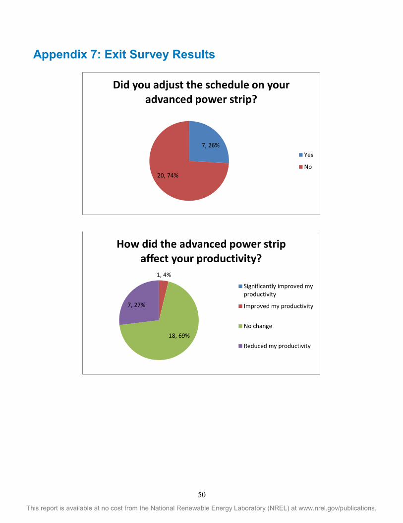
50
This report is available at no cost from the National Renewable Energy Laboratory (NREL) at www.nrel.gov/publications.
Appendix 7: Exit Survey Results
7, 26%
20, 74%
Did you adjust the schedule on your advanced power strip?
Yes
No
1, 4%
18, 69%
7, 27%
How did the advanced power strip affect your productivity?
Significantly improved myproductivity
Improved my productivity
No change
Reduced my productivity
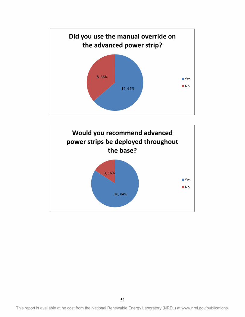
51
This report is available at no cost from the National Renewable Energy Laboratory (NREL) at www.nrel.gov/publications.
14, 64%
8, 36%
Did you use the manual override on the advanced power strip?
Yes
No
16, 84%
3, 16%
Would you recommend advanced power strips be deployed throughout
the base?
Yes
No
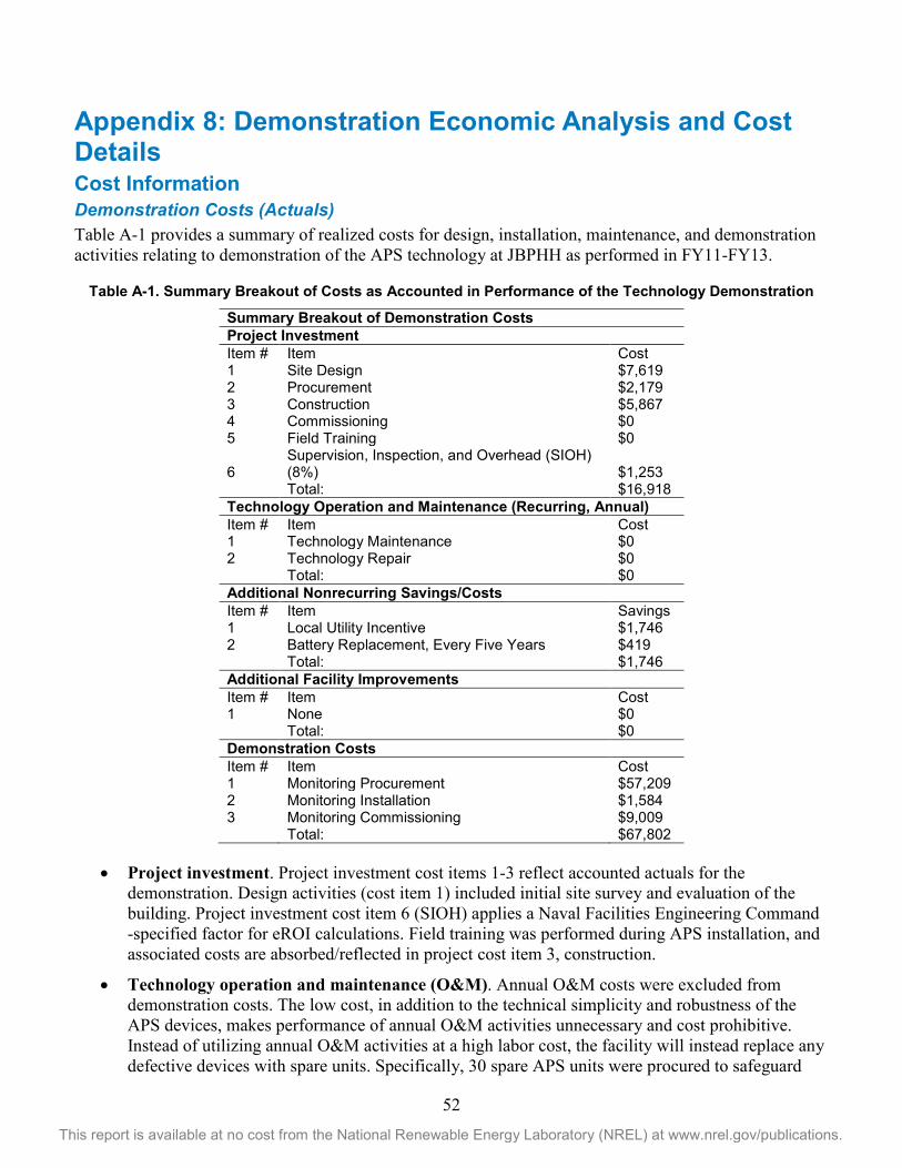
52
This report is available at no cost from the National Renewable Energy Laboratory (NREL) at www.nrel.gov/publications.
Appendix 8: Demonstration Economic Analysis and Cost Details Cost Information Demonstration Costs (Actuals) Table A-1 provides a summary of realized costs for design, installation, maintenance, and demonstration activities relating to demonstration of the APS technology at JBPHH as performed in FY11-FY13.
Table A-1. Summary Breakout of Costs as Accounted in Performance of the Technology Demonstration
Summary Breakout of Demonstration Costs Project Investment Item # Item Cost 1 Site Design $7,619 2 Procurement $2,179 3 Construction $5,867 4 Commissioning $0 5 Field Training $0
6 Supervision, Inspection, and Overhead (SIOH) (8%) $1,253
Total: $16,918 Technology Operation and Maintenance (Recurring, Annual) Item # Item Cost 1 Technology Maintenance $0 2 Technology Repair $0 Total: $0 Additional Nonrecurring Savings/Costs Item # Item Savings 1 Local Utility Incentive $1,746 2 Battery Replacement, Every Five Years $419 Total: $1,746 Additional Facility Improvements Item # Item Cost 1 None $0 Total: $0 Demonstration Costs Item # Item Cost 1 Monitoring Procurement $57,209 2 Monitoring Installation $1,584 3 Monitoring Commissioning $9,009 Total: $67,802
• Project investment. Project investment cost items 1-3 reflect accounted actuals for the demonstration. Design activities (cost item 1) included initial site survey and evaluation of the building. Project investment cost item 6 (SIOH) applies a Naval Facilities Engineering Command -specified factor for eROI calculations. Field training was performed during APS installation, and associated costs are absorbed/reflected in project cost item 3, construction.
• Technology operation and maintenance (O&M). Annual O&M costs were excluded from demonstration costs. The low cost, in addition to the technical simplicity and robustness of the APS devices, makes performance of annual O&M activities unnecessary and cost prohibitive. Instead of utilizing annual O&M activities at a high labor cost, the facility will instead replace any defective devices with spare units. Specifically, 30 spare APS units were procured to safeguard
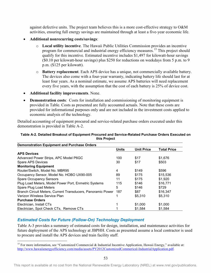
53
This report is available at no cost from the National Renewable Energy Laboratory (NREL) at www.nrel.gov/publications.
against defective units. The project team believes this is a more cost-effective strategy to O&M activities, ensuring full energy savings are maintained through at least a five-year economic life.
• Additional nonrecurring costs/savings: o Local utility incentive. The Hawaii Public Utilities Commission provides an incentive
program for commercial and industrial energy efficiency measures.15 This project should qualify for this incentive. Estimated incentive includes $1,497 for kilowatt-hour savings ($0.10 per kilowatt-hour savings) plus $250 for reductions on weekdays from 5 p.m. to 9 p.m. ($125 per kilowatt).
o Battery replacement. Each APS device has a unique, not commercially available battery. The devices also come with a four-year warranty, indicating battery life should last for at least four years. As a nominal estimate, we assume APS batteries will need replacement every five years, with the assumption that the cost of each battery is 25% of device cost.
• Additional facility improvements. None.
• Demonstration costs: Costs for installation and commissioning of monitoring equipment is provided in Table. Costs as presented are fully accounted actuals. Note that these costs are provided for informational purposes only and are not included in the investment costs applied to economic analysis of the technology.
Detailed accounting of equipment procured and service-related purchase orders executed under this demonstration is provided in Table A-2.
Table A-2. Detailed Breakout of Equipment Procured and Service-Related Purchase Orders Executed on this Project
Demonstration Equipment and Purchase Orders Units Unit Price Total Price APS Devices Advanced Power Strips, APC Model P6GC 100 $17 $1,676 Spare APS Devices 30 $17 $503 Monitoring Equipment Router/Switch, Model No. MBR95 4 $149 $596 Occupancy Sensor, Model No. HOBO UX90-005 89 $175 $15,536 Spare Occupancy Sensors 11 $175 $1,920 Plug Load Meters, Model Power Port, Enmetric Systems 115 $146 $16,771 Spare Plug Load Meters 5 $146 $729 Branch Circuit Meters, Current Transducers, Panoramic Power 187 $87 $16,347 Verizon Wireless Service Plan 1 $5,310 $5,310 Purchase Orders Electrician, Install CTs 1 $1,000 $1,000 Electrician, Spot Check CTs, Remove CTs 1 $1,584 $1,584
Estimated Costs for Future (Follow-On) Technology Deployment Table A-3 provides a summary of estimated costs for design, installation, and maintenance activities for future deployment of the APS technology at JBPHH. Costs as presented assume a local contractor is used to procure and install the APS devices and train facility staff. 15 For more information, see “Customized Commercial & Industrial Incentive Application, Hawaii Energy,” available at: http://www.hawaiienergyefficiency.com/media/assets/PY2012CustomizedCommerical-IndustrialApplication.pdf.

54
This report is available at no cost from the National Renewable Energy Laboratory (NREL) at www.nrel.gov/publications.
Table A-3. Summary Breakout of Costs as Estimated for Future, Follow-On Deployments of the Technology at JBPHH
Summary Breakout of Projected Costs Project Investment Item # Item Cost 1 Site Design/General Requirements $2,205 2 Procurement $2,179 3 Construction $3,544 4 Commissioning $0 5 Contingency (5%) $286 6 SIOH (8%) $458 Total: $8,672 Technology Operation and Maintenance (Recurring, Annual) Item # Item Cost 1 Technology Maintenance $0 2 Technology Repair $0 Total: $0 Additional Nonrecurring Savings/Costs Item # Item Savings 1 Battery Replacement, Every 5 Yrs $419 Total: $419
• Project investment. Basis of estimate for how the project investment costs were derived is provided in Table A-4.

55
This report is available at no cost from the National Renewable Energy Laboratory (NREL) at www.nrel.gov/publications.
Table A-4. Basis of Estimate Breakout per Estimated Cost Element for Future, Follow-On Deployments of the Technology at JBPHH
Project Investment Costs: Basis of Estimate Table Site Design Costs
No. Item Units Unit Price Total Basis of Estimate
1 Labor—Site Assessment and General Requirementsa 30 $42 $1,260 Engineering judgment
2 Burden [Fringe, Insurance, Etc. (75%)]c N/A N/A $945 Engineering judgment Total: $2,205 Procurement Costs
No. Item Units Unit Price Total Basis of Estimate
1 Advanced Power Strips, APC Model P6GC 100 $17 $1,676 Historical data
2 Spare APS Devices, APC Model P6GC 30 $17 $503 Historical data Total: $2,179 Construction (Installation) Costs
No. Item Units Unit Price Total Basis of Estimate
1 Labor—Installation (4 devices per hour)b 25 $24 $600 Historical data/engineering judgment
2 Labor—Mobilization 8 $24 $192 Engineering judgment
3 Labor—Training Preparation 20 $42 $840 Historical data/engineering judgment
4 Labor—Training 8 $42 $336 Historical data/engineering judgment
5 Burden [Fringe, Insurance, Etc. (75%)]d N/A N/A $1,476 Engineering judgment 6 Travel 1 $100 $100 Engineering judgment Total: $3,544
a Hourly labor rates: Hourly labor rates for items 1.1, 3.3, and 3.4 are estimated as the mean hourly wage for management occupations for the State of Hawaii, as provided by the U.S. Bureau of Labor Statistics for FY12. Hourly labor rates for items 2.1, 2.2, 3.1, and 3.2 are estimated as the mean hourly wage for installation, maintenance, and repair occupations for the State of Hawaii, as provided by the U.S. Bureau of Labor Statistics for FY12.16 b Total labor estimates: Total labor hours required for 3.1, 3.3, and 3.4 based upon comparison to actuals realized in performance of this demonstration. Total labor hours for 1.1 and 3.2 based upon general experience and technical scope of this activity. c Burden: Fringe is estimated at 55%, as defined for Laborer II, Davis Bacon Wages Hawaii for Buildings;17 additional overhead cost factor of 20% applied (this is an assumed value based on general experience) yielding an aggregate applied burden of 75%. d Procurement costs: Procurement costs reflect actuals, as realized in performance of this demonstration.
• Technology O&M. Annual O&M costs were excluded from demonstration costs. The low cost, in
addition to the technical simplicity and robustness of the APS devices, makes performance of annual O&M activities unnecessary and cost-prohibitive. Instead of utilizing annual O&M activities at a high labor cost, we assume the facility will replace any defective devices with spare units. Specifically, 30 spare APS units were included in the procurement estimate to safeguard against defective units. The project team believes this is a more cost-effective strategy to O&M activities, ensuring full energy savings are maintained through at least a five-year economic life.
16 For more information, see U.S. Bureau of Labor Statistics website at http://www.bls.gov/. 17 For more information, see the Wage Determinations OnLine website at http://www.wdol.gov/dba.aspx.
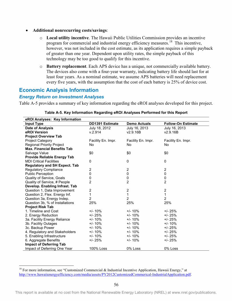
56
This report is available at no cost from the National Renewable Energy Laboratory (NREL) at www.nrel.gov/publications.
• Additional nonrecurring costs/savings: o Local utility incentive. The Hawaii Public Utilities Commission provides an incentive
program for commercial and industrial energy efficiency measures.18 This incentive, however, was not included in the cost estimate, as its application requires a simple payback of greater than one year. Dependent upon utility rates, the simple payback of this technology may be too good to qualify for this incentive.
o Battery replacement. Each APS device has a unique, not commercially available battery. The devices also come with a four-year warranty, indicating battery life should last for at least four years. As a nominal estimate, we assume APS batteries will need replacement every five years, with the assumption that the cost of each battery is 25% of device cost.
Economic Analysis Information Energy Return on Investment Analyses Table A-5 provides a summary of key information regarding the eROI analyses developed for this project.
Table A-5. Key Information Regarding eROI Analyses Performed for this Report
eROI Analyses: Key Information Input Type DD1391 Estimate Demo Actuals Follow-On Estimate Date of Analysis July 18, 2012 July 16, 2013 July 16, 2013 eROI Version v.2.914 v2.9.16B v2.9.16B Project Overview Tab Project Category Facility En. Impr. Facility En. Impr. Facility En. Impr. Regional Priority Project No No No Max. Financial Benefits Tab Salvage Value $0 $0 $0 Provide Reliable Energy Tab MDI Critical Facilities 0 0 0 Regulatory and SH Expect. Tab Regulatory Compliance 2 2 2 Public Perception 0 0 0 Quality of Service, Goals 0 0 0 Quality of Service, # People 2 2 2 Develop. Enabling Infrast. Tab Question 1, Data Improvement 2 2 2 Question 2, Flex. Energy Inf. 1 1 1 Question 3a, Energy Indep. 2 2 2 Question 3b, % of Installations 25% 25% 25% Project Risk Tab 1. Timeline and Cost +/- 10% +/- 10% +/- 25% 2. Energy Reduction +/- 25% +/- 10% +/- 25% 3a. Facility Energy Reliance +/- 10% +/- 10% +/- 25% 3b. Facility Outages +/- 10% +/- 10% +/- 10% 3c. Backup Power +/- 10% +/- 10% +/- 25% 4. Regulatory and Stakeholders +/- 10% +/- 10% +/- 25% 5. Enabling Infrastructure +/- 10% +/- 10% +/- 25% 6. Aggregate Benefits +/- 25% +/- 10% +/- 25% Impact of Deferring Tab Impact of Deferring One Year 100% Loss 0% Loss 0% Loss
18 For more information, see “Customized Commercial & Industrial Incentive Application, Hawaii Energy,” at http://www.hawaiienergyefficiency.com/media/assets/PY2012CustomizedCommerical-IndustrialApplication.pdf.

57
This report is available at no cost from the National Renewable Energy Laboratory (NREL) at www.nrel.gov/publications.
Building Life Cycle Cost Analysis Table A-6 provides a summary of key information regarding the building life cycle costs (BLCC) analyses developed for this project.
Table A-6. Key Information Regarding BLCC Analyses Performed for this Report
BLCC Analyses: Key Information Input Type Value Report Type MilCon BLCC Version 5.3 Location Hawaii Discounting Convention Mid-year Analysis Type Constant dollars Base Date Feb. 1, 2013 Beneficial Occupancy Feb. 1, 2013 Length of Study Five, 20 years Energy Usage Indice 100% throughout economic life Investment Cost, Cost-Phasing 0% Major Repair and Replacement Costs
At five years $419 At 10 years $419 At 15 years $419
Energy Escalation Factor: 0%

58
This report is available at no cost from the National Renewable Energy Laboratory (NREL) at www.nrel.gov/publications.
Appendix 9: Manager Training Nov. 13, 2012

59
This report is available at no cost from the National Renewable Energy Laboratory (NREL) at www.nrel.gov/publications.
Appendix 10: Occupant Training—Using the APC Power Strip This document provides instructions on how to adjust/program the controls on your APC power strip. The power strip was delivered with five schedules (one for each day of the work week) preprogrammed into the strip. Each daily schedule (Monday through Friday) is set to turn on at 6:00am and turn off at 6:00pm. The preprogrammed schedules will also keep your devices de-energized during the weekend (both Saturday and Sunday).
If you are able to refine this predefined schedule to more accurately reflect your workweek, that will help improve the current study and will reduce energy use in the building.
Examples of reasons to refine the predefined schedules:
• You actually arrive at work at 9 a.m. and leave at 5 p.m.
• You work from home one or more days in the week
• You work later than the default setting of 6 p.m. If any of these examples apply to your particular work schedule, please follow the directions below to customize the control of your power strip.
Directions for Altering Preprogrammed Schedules To Change a Single Day Schedule Note: The number of each schedule has been set to correspond with a day of the week. For example, 1 corresponds to Monday, 2 corresponds with Tuesday, and so on, until 5, which controls Friday. Each schedule also has an “on” time setting and an “off” time setting.
1. Press the “timer” button (#9 in diagram below) until you reach the day/number that you wish to alter (e.g., press timer until you see 2ON to alter the start time for the Tuesday schedule).
2. Use the H+ button (#11 in diagram) to adjust the hour the plug strip will turn on. Note that there is an “a” and “p” at the right end of the screen that denote a.m. and p.m.
3. Use the M+ button (#12 in diagram) to adjust the minute at which the plug strip will turn on.
4. Press the “timer” button once more to adjust the time when you want the plug strip to turn off that day (e.g., if you are adjusting the Tuesday schedule, you will want to see 2OFF).
5. Repeat Steps 2 and 3 to adjust the time you want the plug strip to turn off.
6. Repeat Steps 1 through 5 with a different schedule number to adjust another day of the week.
To Add Another Schedule 1. Schedule 6 has been left empty to accommodate another schedule. Press the “timer” button (#9 in
diagram) until you reach 6ON.

60
This report is available at no cost from the National Renewable Energy Laboratory (NREL) at www.nrel.gov/publications.
2. Press the “day” button (#10 in diagram) until you reach the day you want to control. Note that there are options for controlling both Saturday and Sunday with the same schedule.
3. Follow Steps 2 and 3 from the “To Change a Single Day Schedule” section to set the time you wish the power strip to turn on.
4. Press the “timer” button again (#9 in diagram) to adjust the time when you want the plug strip to turn off (you will want to see 6OFF).
5. Follow Steps 2 and 3 from the “To Change a Single Day Schedule” section to set the time you wish the power strip to turn off.
For more details on the power strip programming, please refer to the user manual, found online at: http://www.apcmedia.com/salestools/SCON-7RJP3D_R0_EN.pdf.
Directions for Overriding the Power Strip If you come to work during the weekend or between 6 p.m. and 6 a.m. on a weekday, you will probably find that the devices you need to use will be powered off for energy savings. To turn the devices back on:
1. Press the “override” button (#4 in diagram) once on the power strip.
2. You should notice that the devices have turned back on.
Note: If the “override” button is pressed when the devices are already turned on, the power strip will turn them all off.
3. Refer to the “Directions for Altering Preprogrammed Schedules” section to make changes to the preprogrammed schedules.