recognition of circular-arc graphs and some subclasses · abstract in this work we present three...
TRANSCRIPT
TEL-AVIV UNIVERSITY
RAYMOND AND BEVERLY SACKLER
FACULTY OF EXACT SCIENCES
SCHOOL OF COMPUTER SCIENCE
Recognition of Circular-Arc Graphs andSome Subclasses
This thesis was submitted in partial fulfillment of the requirements for the M.Sc. degree in
the School of Computer Science, Tel-Aviv University
by
Yahav Nussbaum
The research work for this thesis has been carried out at Tel-Aviv University
under the supervision of Prof. Haim Kaplan
February 2007

Acknowledgements
I would like to thank my supervisor, Prof. Haim Kaplan, for his guidance and support.
I wish to thank my family for their love and encouragement.
And thanks to anyone else who helped, cared or asked.
i

Abstract
In this work we present three new recognition algorithms for circular-arc graphs and for two sub-
classes of this graph class.
We give a linear-time recognition algorithm for circular-arc graphs based on the algorithm of
Eschen and Spinrad [ES93, Esc97]. Our algorithm is simpler than the earlier linear-time recognition
algorithm of McConnell [McC03], which is the only linear time recognition algorithm previously
known.
We give new characterizations of proper circular-arc graphs and of unit circular-arc graphs
which are based on characterizations of Tucker [Tuc71, Tuc74]. These characterizations lead to
two new linear-time algorithms for recognizing proper circular-arc graphs and for recognizing unit
circular-arc graphs. Both algorithms either provide a model for the input graph, or a certificate
that such a model does not exist. No other previous algorithm for each of these two graph classes
provides a certificate for its result.
ii

Contents
Abstract ii
1 Introduction 1
1.1 Circular-arc graphs . . . . . . . . . . . . . . . . . . . . . . . . . . . . . . . . . . . . . 1
1.2 Proper circular-arc graphs and unit circular-arc graphs . . . . . . . . . . . . . . . . . 4
1.3 Certifying algorithms . . . . . . . . . . . . . . . . . . . . . . . . . . . . . . . . . . . . 5
1.4 Our contribution . . . . . . . . . . . . . . . . . . . . . . . . . . . . . . . . . . . . . . 6
2 Preliminaries 9
2.1 Graphs . . . . . . . . . . . . . . . . . . . . . . . . . . . . . . . . . . . . . . . . . . . . 9
2.2 Circular-arc graphs . . . . . . . . . . . . . . . . . . . . . . . . . . . . . . . . . . . . . 10
2.3 Matrices . . . . . . . . . . . . . . . . . . . . . . . . . . . . . . . . . . . . . . . . . . . 12
2.4 Representation . . . . . . . . . . . . . . . . . . . . . . . . . . . . . . . . . . . . . . . 13
3 Circular-Arc Graphs 15
3.1 Preprocessing . . . . . . . . . . . . . . . . . . . . . . . . . . . . . . . . . . . . . . . . 15
3.2 Splitting into cases . . . . . . . . . . . . . . . . . . . . . . . . . . . . . . . . . . . . . 16
3.3 Stage 1: dividing the circle into sections . . . . . . . . . . . . . . . . . . . . . . . . . 17
3.3.1 Finding a maximal independent set . . . . . . . . . . . . . . . . . . . . . . . . 17
3.3.2 The single-arc and the two-arcs requirements . . . . . . . . . . . . . . . . . . 19
3.3.3 More requirements are required . . . . . . . . . . . . . . . . . . . . . . . . . . 25
3.3.4 The cross-path requirements . . . . . . . . . . . . . . . . . . . . . . . . . . . 26
3.3.5 Every valid order of I is consistent with a circular-arc model . . . . . . . . . 33
iii

CONTENTS iv
3.4 Stage 2: placing the endpoints of the arcs in the sections . . . . . . . . . . . . . . . . 44
3.5 Stage 3: Arranging the endpoints in each section . . . . . . . . . . . . . . . . . . . . 56
3.6 Verifying the result . . . . . . . . . . . . . . . . . . . . . . . . . . . . . . . . . . . . . 61
4 Proper Circular-Arc Graphs 62
4.1 Characterization of proper circular-arc graphs . . . . . . . . . . . . . . . . . . . . . . 62
4.2 The complement of G is not bipartite . . . . . . . . . . . . . . . . . . . . . . . . . . 65
4.3 The complement of G is bipartite . . . . . . . . . . . . . . . . . . . . . . . . . . . . . 66
4.4 Authentication algorithm . . . . . . . . . . . . . . . . . . . . . . . . . . . . . . . . . 68
5 Unit Circular-Arc Graphs 69
5.1 Characterization of unit circular-arc graphs . . . . . . . . . . . . . . . . . . . . . . . 69
5.2 Pairs of arcs that cover the circle . . . . . . . . . . . . . . . . . . . . . . . . . . . . . 72
5.2.1 Co-bipartite unit circular-arc graphs . . . . . . . . . . . . . . . . . . . . . . . 73
5.3 The algorithm . . . . . . . . . . . . . . . . . . . . . . . . . . . . . . . . . . . . . . . . 73
5.4 The certificate and the authentication algorithm . . . . . . . . . . . . . . . . . . . . 78
6 Future Work 83
Bibliography 85
Hebrew Synopsis ℵ
Chapter 1
Introduction
1.1 Circular-arc graphs
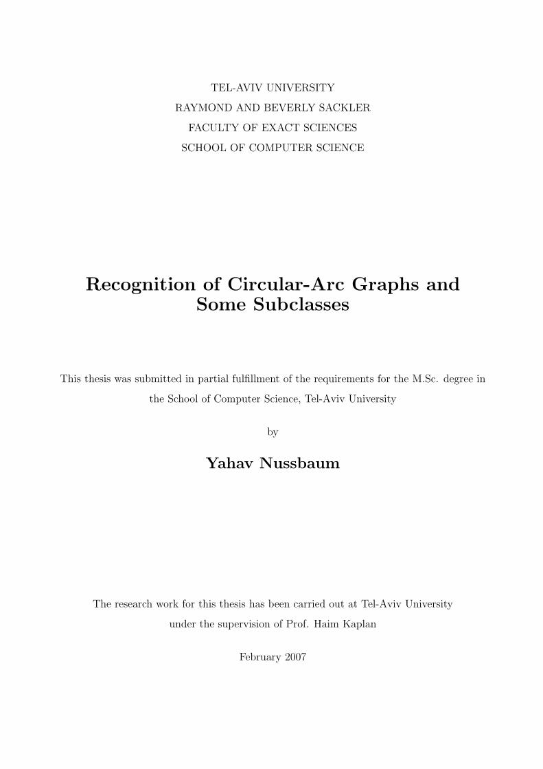
A Circular-arc graph (see Figure 1.1) is an intersection graph of arcs on the circle. That is, every
vertex is represented by an arc, such that two vertices are adjacent if and only if the corresponding
arcs intersect. The arcs constitute a circular-arc model of the graph. Circular-arc graphs generalize
interval graphs which are the intersection graphs of intervals on the line. An extensive overview of
circular-arc graphs can be found in the book by Spinrad [Spi03]. Circular-arc graphs can be used
to model objects of a circular or a repetitive nature. Recent applications of circular-arc graphs are
in modeling ring networks [SE04] and item graphs of combinatorial auctions [CDS04].
The class of circular-arc graphs and the corresponding recognition problem was first defined by
Hadwiger, Debrunner and Klee [HDK64, Kle69]. The problem of finding a recognition algorithm
a
bc
d
e
a
b d
c
e
Figure 1.1: A circular-arc graph and a circular-arc model of it. The model and the graph are alsoproper circular-arc and unit circular-arc.
1

CHAPTER 1. INTRODUCTION 2
for circular-arc graphs was solved only after finding a recognition algorithm for interval graphs.
Classical recognition algorithms for interval graphs [BL76] rely on the fact that any clique in an
interval graph corresponds to a nonempty intersection of the corresponding intervals in the interval
model. This property of interval graphs is called the Helly property. Due to the Helly property,
the number of maximal cliques in an interval graph is linear. In contrast, arcs associated with a
clique in a circular-arc graph do not have the Helly property. Furthermore, the number of maximal
cliques in a circular-arc graph may be exponential in the size of the graph. Another difference
between interval graphs and circular-arc graphs is that two arcs on the circle can intersect from
two different directions.
The first characterizations of circular-arc graphs were given by Tucker [Tuc71] and by Gavril
[Gav74]. These characterization did not lead to an efficient recognition algorithm.
Tucker [Tuc80] gave the first polynomial time recognition algorithm for circular-arc graphs.
This algorithm splits into one of two cases according to whether G is bipartite (G is co-bipartite).
In case G is not bipartite the algorithm finds an odd length induced cycle in G, and further splits
into one of two subcases according to whether the cycle it found is of length 3 or of length at least
5. Using Tucker’s terminology we refer to the first case where G is co-bipartite as Case I. We refer
to the subcase where we found in G a cycle of length 3, and therefore we found in G an independent
set of size 3, as Subcase IIa. We refer to the subcase where we found in G an induced cycle of
length at least 5 as Subcase IIb.
Tucker showed how to implement his algorithm in O(n3) time. One of the bottlenecks in
Tucker’s implementation is a preprocessing phase where we identify containment relations between
the neighborhoods of the vertices. Specifically, for every pair of vertices v and u we determine
whether the neighborhood of v is contained in the neighborhood of u or vice versa. Furthermore,
Tucker runs his algorithm recursively on particular graphs and this recursive structure also leads
to cubic running time.
Spinrad [Spi88] simplified Case I in Tucker’s algorithm – the case where G is co-bipartite. Spin-
rad reduced this case to the problem of recognizing two dimensional posets [SV83]. We construct
the poset using particular relations between the vertices of G. Two vertices are related in the
poset if their corresponding arcs are either disjoint, one is contained in the other, or together they
cover the circle. The relations between the arcs are determined from the relations between the

CHAPTER 1. INTRODUCTION 3
neighborhoods of the vertices. In case G is a circular-arc graph then from any two total orders that
represent the poset we can construct a representation for G. Spinrad showed that this algorithm
runs in O(n3) time.
Eschen and Spinrad [ES93, Esc97] gave an O(n2) algorithm for recognizing circular-arc graphs
by addressing the two bottlenecks in Tucker’s implementation. Eschen and Spinrad show how to
compute neighborhood containment relations in O(n2) time. Specifically, they construct two graphs
such that if G is indeed circular-arc graph then one of the graphs is an interval graph and the other
graph is a chordal bipartite graph. These graphs are constructed such that from the neighborhood
containment relation between two vertices in these graphs we can determine the neighborhood
containment relation between the same vertices in G. The quadratic time bound follows since one
can compute neighborhood containment relations in interval graphs and chordal bipartite graphs
in quadratic time [MS91, ES93, Esc97].
Eschen and Spinrad also showed that in Case I of the algorithm, when G is co-bipartite, we
can use a reduction similar to the reduction that we used to determine neighborhood containment
relations to determine all pair of arcs that can cover circle in a model of G in O(n2) time. Since this
was the only bottleneck in Spinrad’s algorithm for this case, we obtain an O(n2) implementation
of Case I.
To implement Subcase IIa and Subcase IIb in O(n2) time, Eschen and Spinrad changed the
recursive structure of Tucker’s algorithm. They show how to implement the algorithm such that
each recursive call is on a co-bipartite graph (Case I) and therefore does not trigger further recursion.
Since the sum of the sizes of the graphs in all recursive calls is proportional to the size of G, the
quadratic bound follows. Unfortunately, as we show in this work, the algorithm of Eschen and
Spinrad for Subcase IIa has a flaw.
Recently, McConnell [McC03] presented the first recognition algorithm for circular-arc graphs
that runs in linear time. The algorithm reduced the problem to an interval graph recognition prob-
lem where specific intersection types between the intervals are specified. McConnell’s algorithm
uses the same preprocessing stage of Eschen and Spinrad where it computes neighborhood con-
tainment relations. To establish the linear time bound, McConnell tightens the analysis of Eschen
and Spinrad’s preprocessing stage. He shows that this preprocessing stage can be implemented in
linear time since we are interested only in neighborhood containment relations between adjacent

CHAPTER 1. INTRODUCTION 4
vertices, and the associated chordal bipartite graphs cannot be too large.
McConnell’s algorithm is quite involved. Its most complicated computation is to find a partition
of a graph into a particular kind of modules called ∆ modules. These ∆ modules are used to turn
the input circular-arc graph into an interval graph with specific types of intersections between the
intervals, and to find a model for this interval graph. McConnell first presents an implementation
that runs in O(m + n log n) time. To get the linear time bound, a more complicated partitioning
procedure has to be adapted from the linear-time transitive orientation algorithm of McConnell
and Spinrad [MS99] which is by itself quite involved. This algorithm also uses probe interval graphs
to find pairs of arcs that can cover the circle in linear time.
Hsu [Hsu95] presented a different recognition algorithm for circular-arc graphs. Hsu’s algorithm
runs in O(mn) time and reduces the problem to recognition of circle graphs.
1.2 Proper circular-arc graphs and unit circular-arc graphs
A circular-arc model in which no arc contains another arc is called a proper circular-arc model.
A circular-arc graph that has a proper circular-arc model is a proper circular-arc graph. Tucker
gave characterizations of proper circular-arc graphs, in terms of the adjacency matrix [Tuc71], and
forbidden subgraphs [Tuc74]. Skrien [Skr82] and Deng, Hell and Huang [DHH96] gave characteri-
zations that use orientation of the edges. The characterization of [DHH96] leads to a linear-time
recognition algorithm for sparse proper circular-arc graphs. For dense graphs the algorithm of
[DHH96] uses an implementation of [Tuc71]. Spinrad [Spi03] showed how to implement the char-
acterization of [Tuc71] to construct a linear-time recognition algorithm for all proper circular-arc
graphs.
A circular-arc model in which all arcs are of the same length is called a unit circular-arc model.
A circular-arc graph that has a unit circular-arc model is a unit circular-arc graph. By definition,
every unit circular-arc graph is a proper circular-arc graph. Tucker [Tuc74] gave a characterization
of proper circular-arc graphs which are not unit circular-arc graph. Recently, Duran, Gravano,
McConnell, Spinrad, and Tucker [DGM+06] presented a quadratic recognition algorithm for unit
circular-arc graphs, based on this characterization. This algorithm does not provide a unit circular-
arc model for a unit circular-arc graph. Even more recently, Lin and Szwarcfiter [LS06b] gave a new

CHAPTER 1. INTRODUCTION 5
characterization of unit circular-arc graphs based on the length of the arcs in a proper circular-arc
model. They used this characterization to derive a linear-time recognition algorithm that constructs
a unit circular-arc model if the input is a unit circular-arc graph.
1.3 Certifying algorithms
A certifying algorithm is an algorithm that provides a certificate together with its answer. A
certificate is an evidence that can be used to authenticate the correctness of the answer (cf. [MN99,
KMMS06]). An authentication algorithm is an algorithm that checks the validity of the certificate.
Certifying algorithms reduce the risk of erroneous answer, caused by bugs in the implementation.
For example, a recognition algorithm for bipartite graphs can provide a 2-coloring of the graph
as a certificate when the graph is bipartite, and an odd cycle as a certificate when the graph is not
bipartite. Other graph classes that have certifying recognition algorithms include chordal graphs
[TY85], planar graphs [MN99], interval graphs and permutation graphs [KMMS06], proper interval
graphs [HH04a, Mei05] and proper interval bigraphs [HH04a].
Given an implementation of a certifying algorithm, we have a simple way to prove whether every
output it provides is correct or not, if the authentication algorithm is correct. This is important
since software is prone to errors. In addition, the ability to validate every output allows us test an
implementation of a certifying algorithm on any input, not limiting ourselves to a specific set of
inputs with known expected outputs.
Kratsch, McConnell, Mehlhorn, and Spinrad discuss the requirements from a good certificate
[KMMS06]. First, it is clear that the authentication algorithm that authenticates the certificate
should be simpler than an algorithm for solving the problem itself, because otherwise, the correct-
ness of the result may be at risk because of an error in the implementation of the authentication
algorithm. Additionally, the proof of the correctness of the authentication algorithm should be
easy to understand. Given a certifying algorithm with an authentication algorithm, it is enough to
trust the authentication algorithm, since it proves the correctness of every output of the certifying
algorithm. Moreover, if we have a correct authentication algorithm, then the certifying algorithm
can be trusted even without knowing it.
The last two requirements from certificates and authentication algorithms are not formal. A

CHAPTER 1. INTRODUCTION 6
formal way to measure the quality of a certificate and an authentication algorithm is the time
complexity it takes to validate the certificate. A certificate is defined by [KMMS06] to be a strong
certificate, if the time bound of its authentication algorithm is asymptotically smaller than the
time bound of the best known algorithm for solving the problem itself. A certificate may be a good
certificate even if it is not a strong certificate, this holds when the authentication algorithm, given
the certificate, has some other advantages over solving the problem from scratch.
There are no previously known certifying algorithms for circular-arc graphs, proper circular-arc
graphs or unit circular-arc graphs. Current algorithms construct a model of the input graph if it
belongs to the appropriate graph class, but fail to provide a certificate otherwise. Moreover, even if
we disregard the cost of the computation, there is no known certificate that can prove that a graph
is not a circular-arc graph.
1.4 Our contribution
In Chapter 3, we give a new recognition algorithm for circular-arc graphs. This algorithm is based
on the algorithm of Eschen and Spinrad, and runs in linear time. Our algorithm either finds an
independent set of size 3, in which case the algorithm of Eschen and Spinrad applies Subcase IIa,
or it concludes that the graph has Θ(n2) edges and then the algorithm of Eschen and Spinrad in
fact runs in linear time. The fact that a graph which does not have an independent set of size 3
has Θ(n2) edges is an implication of Mantel’s Theorem from 1907, which is considered to be the
first result in extremal graph theory (cf. Bollobas [Bol78]).
Eschen and Spinrad find in Subcase IIa a particular maximal independent set and place the
corresponding arcs on the circle. We show that there is a flaw in the way Eschen and Spinrad
place the arcs of the independent set on the circle. We present a correction to this flaw, and
describe a linear-time implementation of the correct placement algorithm. Our implementation
then continues as the implementation of Eschen and Spinrad, but we tighten their analysis to show
that the running time is linear. Our main new insight is that each subgraph considered by the
algorithm while placing and ordering the arcs on the circle is dense. That is, the number of edges
that each subgraph contains is quadratic in the size of its vertex set. Furthermore, the total size
of these subgraphs is linear in the size of the input graph.

CHAPTER 1. INTRODUCTION 7
Our algorithm also performs a preprocessing phase where neighborhood containment relations
are computed. As proved by McConnell [McC03] this can be done in linear time. As all previous
algorithms, we also require a postprocessing verification step where we check that the representation
we obtain is indeed a representation of G. McConnell [McC03] gave a straightforward linear-time
implementation of this postprocessing step, which we also describe for completeness.
We describe a linear-time implementation of Subcase IIa. Subcase IIb can also be implemented
in linear time in a similar way. We do not describe it here since we apply Subcase IIb only when
we are sure that G has Θ(n2) edges. Our implementation is simpler than McConnell’s algorithm.
Hsu [Hsu95] defined normalized model of a circular-arc graph G. A circular-arc model % of
G is normalized if every arc that contains another arc in some circular-arc model of G, contains
it also in %, and every pair of arcs that covers the circle in some circular-arc model of G, covers
the circle also in %. The circular-arc recognition algorithms of [Tuc80, Spi88, ES93, Hsu95, Esc97]
construct a normalized model, but the linear-time algorithm of [McC03] does not. The model
which our algorithm produces is a normalized model. Normalized models of circular-arc graphs
take part in the circular-arc graph isomorphism algorithm of Hsu [Hsu95], and in the recent linear-
time algorithm for recognizing circular-arc graphs which admit the Helly property of Lin and
Szwarcfiter [LS06a].
In Chapters 4 and 5, we present new characterizations of proper circular-arc graphs and unit
circular-arc graphs which are based on characterizations of Tucker [Tuc71, Tuc74] for the two graph
classes and on a characterization of McConnell [McC04] for the consecutive-ones property. The new
characterizations provide certificates for graphs that are not proper circular-arc graphs or not unit
circular-arc graphs.
The two new characterizations lead to linear-time certifying algorithms for recognizing proper
circular-arc graphs and unit circular-arc graphs. If the input graph is a member of the graph class,
then the algorithms provide an appropriate model for it. Otherwise, if the input graph is not a
member of the graph class, then the algorithm provides a certificate for this answer. None of the
two graph classes previously had a certifying recognition algorithm.
The certificates that prove that the input graph is not a proper circular-arc graph or a unit
circular-arc graph can be authenticated in O(n) time, where n is the number of vertices in the

CHAPTER 1. INTRODUCTION 8
graph. This time bound is asymptotically better than the optimal O(n + m) time bound of the
recognition algorithm when the number of edges in superlinear in the number of vertices, so the
certificates are strong certificates.
Our algorithm for proper circular-arc graphs splits into two cases, according to whether the
graph is co-bipartite or not, just like the algorithm for circular-arc graphs. In each case, the
algorithm is based on a different certifying algorithm for another problem.
Our algorithm for unit circular-arc graphs is based on the ideas of the recent algorithm of
Duran, Gravano, McConnell, Spinrad, and Tucker [DGM+06]. We show an algorithm that runs
in linear time without the complex data structures which they use, and in addition we provide a
certificate for the result of the algorithm. The algorithm was found independently from the recent
linear-time algorithm of [LS06b].
To build our certifying algorithms, we combined elements from a number of previous results on
the topic. We hope that our work will help to establish this new and important algorithm design
philosophy.
In addition of being the first certifying algorithms for proper circular-arc graphs and unit
circular-arc graphs, we believe that our algorithms are also easier to implement than earlier recog-
nition algorithms for these graph classes. This is because we do not use any complex subproblem
or data structure, except of the certifying algorithm for recognizing the consecutive-ones prop-
erty of McConnell [McC04]. If a simple algorithm is necessary and a certificate for graphs that
are not proper circular-arc graphs is not required, then we can plug into our algorithm a simpler
circular-ones or consecutive-ones recognition algorithm (e.g. [HM03]).
Preliminary version of the results of Chapter 3 appeared at the 10th Scandinavian Workshop
on Algorithm Theory (SWAT) [KN06b]. Preliminary version of the results of Chapters 4 and 5
appeared at the 32nd International Workshop on Graph-Theoretic Concepts in Computer Science
(WG) [KN06a].
Chapter 2
Preliminaries
2.1 Graphs
We consider a finite simple graph G = (V, E), where |V (G)| = n and |E(G)| = m. For a vertex v
in a graph, the (closed) neighborhood of v, denoted by N [v] = v ∪ u | vu ∈ E(G) is the set of
all vertices adjacent to v together with v itself. If N [v] = V (G), then we call v a universal vertex.
For a set of vertices U we define NU [v] to be N [v] ∩U . For u, v ∈ V (G), if uv /∈ E(G) then we say
that uv is a non-edge.
The sequence P = (v1, v2, . . . vk) with vivi+1 ∈ E(G) for i = 1, . . . , k is a path. If vkv1 ∈ E(G)
then P is also a cycle. The sequence P = (v1, v2, . . . vk) with vivi+1 /∈ E(G) for i = 1, . . . , k is a
co-path. If vkv1 /∈ E(G) then P is also a co-cycle. The length of a path or a co-path P , is denoted
by |P |. A path, cycle, co-path or co-cycle in which all the vertices are distinct is simple.
If there are k cliques in G that span all the vertices of G then G is covered by k cliques.
A graph that can be partitioned into two independent sets is called bipartite. If G is not bipartite
then it must have an odd-length induced cycle. If G, the complement of G, is bipartite then G is
called co-bipartite, and its vertices are covered by two cliques.
A bipartite graph G with the bipartition (X, Y ) is an interval bigraph if it can be represented
by intervals on the line, such that the interval of x ∈ X intersects the interval of y ∈ Y if and only
if x and y are adjacent in G. Two intervals corresponding to two vertices in X or to two vertices
in Y , may or may not intersect. Muller [Mul97] gave a polynomial time recognition algorithm for
interval bigraphs.
9

CHAPTER 2. PRELIMINARIES 10
An interval bigraph that has a model in which no arc contains another, is a proper interval
bigraph. Hell and Huang [HH04b] showed that the class of proper interval bigraphs, is exactly
the class of the complements of co-bipartite proper circular-arc graphs. These graph classes are
known to be equivalent to many other well known graph classes including bipartite permutation
graphs, bipartite AT-free graphs and bipartite trapezoid graphs (cf. [BLS99, Spi03]). Hell and
Huang [HH04a] also gave a simple linear-time certifying algorithm for recognizing proper interval
bigraphs.
2.2 Circular-arc graphs
A circular-arc model of a graph G is a mapping from the vertices of G to arcs on the circle, such that
two vertices are adjacent if and only if the corresponding arcs intersect. A graph G is a circular-arc
graph if it has a circular-arc model. Note that a circular-arc graph may have more than one model.
A circular-arc model in which no arc covers another arc is a proper circular-arc model. A graph G
is a proper circular-arc graph if it has a proper circular-arc model. A circular-arc model in which
all arcs are of the same length is a unit circular-arc model. A graph G is a unit circular-arc graph
if it has a unit circular-arc model. Every unit circular-arc graph is a proper circular-arc graph.
There are four possible types of intersections between two arcs x and y [Tuc80, Hsu95]:
• Cross: Arc x contains a single endpoint of arc y (see Figure 2.1(a)).
• Cover the circle: Arcs x and y jointly cover the circle and each contains both endpoints of
the other (see Figure 2.1(b)).
• Arc x is contained in arc y.
• Arc x contains arc y (see Figure 2.1(c)).
In addition, if x and y do not intersect then they are disjoint (see Figure 2.1(d)).
If x and y either cross or cover the circle, we say that x and y overlap. In a proper circular-arc
model, every pair of arcs that intersect, overlap each other. The relations between the different
intersection types is illustrated in Figure 2.2.
Let u and v be a pair of adjacent vertices in G. The arc representing u can contain the arc
representing v in a circular-arc model of G if and only if N [u] ⊆ N [v]. Such a relation between u

CHAPTER 2. PRELIMINARIES 11
x y
(a) Cross
x y
(b) Cover the circle
x y
(c) Containment
x y
(d) Disjoint
Figure 2.1: Intersection types of two arcs in circular-arc model.
HH
HH
HHH
HH
HH
HHH
HH
HH
HHH
Pair of arcs
Disjoint Intersect
Containment Overlap
Cover the circle Cross
Figure 2.2: The relations between intersection types of arcs in a circular-arc model.

CHAPTER 2. PRELIMINARIES 12
and v is called a neighborhood containment relation. The arc representing u can cover the circle
with the arc representing v in a circular-arc model of G if and only if for every w /∈ N [u] the arc
representing w can be contained in the arc representing u.
Hsu [Hsu95] showed that if G is a circular-arc graph without a universal vertex, and without
pair of vertices with the identical neighborhoods, then G has a circular-arc model % such that for
every pair of arcs x and y, if x can contain y then it does so in %, and if x can cover there circle
with y then it does so in %. Such a circular-arc model is called a normalized model.
For convenience, we refer to the vertices of G as arcs even before we decide if G is a circular-
arc graph and find a model for it. We say that two adjacent vertices intersect even before we
have a model, because the arcs of adjacent vertices must intersect in every model. If G has a
normalized model we say that v contains u when N [u] ⊂ N [v], even before we have found a model.
Additionally, if the arcs representing u and v cover the circle in a normalized model of G, we say
that u and v cover the circle. We also say that two vertices overlap when they intersect but do not
contain each other. If u and v overlap but do not cover the circle we would say that u and v cross.
To simplify we refer to the clockwise direction as right and to the counterclockwise direction as
left, as we view them if we stand at the center of the circle.
In a circular-arc graph G with a circular-arc model %, every vertex v ∈ V (G) has an arc in %
with two endpoints. We denote the left endpoint of v by `(v) and the right endpoint of v by r(v).
If the arc x crosses the arc y and covers r(y) then x overlaps the right side of y. Analogously, if
the arc x crosses the arc y and covers `(y) then x overlaps the left side of y
The arcs in circular-arc models and proper circular-arc models may be either open or closed.
For unit circular-arc models it makes a difference if an arc is open or closed [Tuc74]. We assume
that all arcs are closed. Our results also hold when all arcs are open. If arcs may be either open or
closed then every proper circular-arc graphs is a unit circular-arc graph [Tuc74].
2.3 Matrices
The adjacency matrix of a graph G, denoted by M(G), has 1 in position (i, j) if vivj ∈ E(G), and
0 otherwise. The augmented adjacency matrix of G is the adjacency matrix of G with 1’s on the
main diagonal, that is M∗(G) = M(G) + I, where I is the identity matrix. We refer to the row in

CHAPTER 2. PRELIMINARIES 13
M∗(G) that corresponds to the vertex v as row v. Likewise, we refer to the column in M∗(G) that
corresponds to the vertex v as column v.
A (0, 1)-matrix has the consecutive-ones property if its columns can be ordered so that in every
row the 1’s are consecutive. The consecutive-ones property can be recognized in time proportional
to sum of the number of columns, the number of rows, and number of 1’s in the matrix [BL76].
McConnell [McC04] gave a linear-time certifying algorithm for this property. A (0, 1)-matrix has
the circular-ones property if its columns can be ordered so that in every rows the 1’s are circularly
consecutive. The circular-ones property can be reduced to the consecutive-ones property [Tuc71]
(see Section 4.2) and there are also algorithms that find it directly [HM03].
2.4 Representation
The desired graph representation for certifying algorithms on graphs is discussed in [KMMS06].
We use, as [KMMS06], an ordered adjacency list representation of graphs. This representation
allows us to get the list of neighbors of a given vertex in constant time, and to certify adjacency of
two vertices in constant time. An edge is certified by its location in the ordered adjacency list. A
non-edge is certified by the location in the adjacency list of its predecessor, if it would have been
an edge. To collect the locations of O(n) edges and non-edges, we radix sort them, and scan the
sorted list together with the adjacency lists of the graph. The running time for this sort and scan
is O(n + m).
We represent a circular-arc model or a proper circular-arc model by a cyclic order of the end-
points of its arcs. The 2n endpoints in the model are indexed according to their ranks in the order,
starting at any arbitrary endpoint and going right. Each arc has the indices of its two endpoints.
The type of intersection between two arcs can be determined, in constant time, by the order of
their endpoints [Gol80] (see Table 2.1). Arcs in a unit circular-model also obey length constraint,
so the exact location of the endpoints on the circle is also required.
We represent (0, 1)-matrices in a sparse way, similar to the graph representation by ordered
adjacency lists. This representation allows algorithms that process matrices to run in time propor-
tional to the sum of the number of columns, number of rows, and number of 1’s in the matrix. For
M∗(G) the number of 1’s is O(n + m).

CHAPTER 2. PRELIMINARIES 14
Endpoints order (left to right) Intersection type Figure
[`(x), `(y), r(x), r(y)] x overlaps the left side of y 2.1(a)[`(x), r(y), r(x), `(y)] x overlaps the right side of y[`(x), r(y), `(y), r(x)] x and y cover the circle 2.1(b)[`(x), `(y), r(y), r(x)] x contains y 2.1(c)[`(x), r(x), r(y), `(y)] x is contained in y[`(x), r(x), `(y), r(y)] x and y are disjoint 2.1(d)
Table 2.1: Intersection types of two arcs in circular-arc model by the cyclic order of their endpoints.

Chapter 3
A Simpler Linear-Time Recognition of
Circular-Arc Graphs
3.1 Preprocessing
An arc representing a universal vertex can be placed on the circle in O(1) time by placing its right
endpoint anywhere on the circle and its left endpoint immediately to the right side of it. It is easy
to find all universal vertices of G in linear time. Thus, we may assume that G does not have any
universal vertices.
Let x be an arc that have the same neighborhood as another arc y that was already placed on
the circle. The arc x can be placed on the circle by placing its endpoints next to the endpoints of
y, in O(1) time. McConnell [McC03] showed how to find vertices with the identical neighborhoods
in linear time using a simple process called radix partitioning, which is similar to radix sort. Thus,
we may assume that there are no two vertices in G that have the same neighborhood.
If G is a circular-arc graph that has no universal vertices and there is no pair of vertices with
the same neighborhood in G, then G has a normalized circular-arc model [Hsu95]. The circular-arc
model of G which our algorithm produces is normalized.
Before running our algorithm we preprocess the graph and for every pair of adjacent vertices v
and u we check whether v contains u or u contains v, that is whether N [v] ⊆ N [u] or N [u] ⊆ N [v].
Recall that Eschen and Spinrad [ES93, Esc97] showed how to compute neighborhood containment
15
CHAPTER 3. CIRCULAR-ARC GRAPHS 16
relations in O(n2) time, and McConnell [McC03] tightened the analysis to show that this can be
done in linear time. For more details of this part, which are not complicated, see [McC03, Section
7.1].
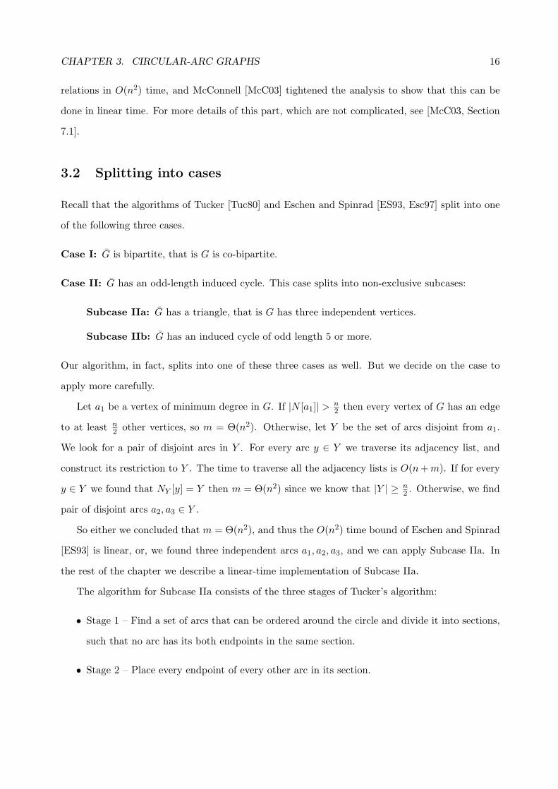
3.2 Splitting into cases
Recall that the algorithms of Tucker [Tuc80] and Eschen and Spinrad [ES93, Esc97] split into one
of the following three cases.
Case I: G is bipartite, that is G is co-bipartite.
Case II: G has an odd-length induced cycle. This case splits into non-exclusive subcases:
Subcase IIa: G has a triangle, that is G has three independent vertices.
Subcase IIb: G has an induced cycle of odd length 5 or more.
Our algorithm, in fact, splits into one of these three cases as well. But we decide on the case to
apply more carefully.
Let a1 be a vertex of minimum degree in G. If |N [a1]| > n2 then every vertex of G has an edge
to at least n2 other vertices, so m = Θ(n2). Otherwise, let Y be the set of arcs disjoint from a1.
We look for a pair of disjoint arcs in Y . For every arc y ∈ Y we traverse its adjacency list, and
construct its restriction to Y . The time to traverse all the adjacency lists is O(n + m). If for every
y ∈ Y we found that NY [y] = Y then m = Θ(n2) since we know that |Y | ≥ n2 . Otherwise, we find
pair of disjoint arcs a2, a3 ∈ Y .
So either we concluded that m = Θ(n2), and thus the O(n2) time bound of Eschen and Spinrad
[ES93] is linear, or, we found three independent arcs a1, a2, a3, and we can apply Subcase IIa. In
the rest of the chapter we describe a linear-time implementation of Subcase IIa.
The algorithm for Subcase IIa consists of the three stages of Tucker’s algorithm:
• Stage 1 – Find a set of arcs that can be ordered around the circle and divide it into sections,
such that no arc has its both endpoints in the same section.
• Stage 2 – Place every endpoint of every other arc in its section.
CHAPTER 3. CIRCULAR-ARC GRAPHS 17
• Stage 3 – Order the endpoints within each section.
We describe each of these stages in the following three sections.
3.3 Stage 1: dividing the circle into sections
The algorithm begins by finding an independent set of arcs, I, that can be embedded around the
circle, in an order consistent with some model of G. This set of arcs divides the circle into sections,
such that no arc has its two endpoints in the same section.
3.3.1 Finding a maximal independent set
The algorithm of Tucker uses a maximal independent set of arcs I of size at least 3 that obeys two
requirements. First, no arc of I contains any other arc of G. Second, there is no arc x ∈ I and two
disjoint arcs y, z /∈ I such that y and z overlap x and do not overlap any other arc in I. We begin
by constructing a maximal independent set I ′ greedily, which satisfies the first requirement, and
then change it to an independent set I that satisfies the second requirement as well.
Before constructing I ′, we eliminate any arc that contains another arc from G, since these arcs
cannot be in I. Let G′ be the induced subgraph of G without these arcs. Every pair of intersecting
arcs in G′ overlaps, since no arc of G′ contains another. In order to construct I ′ we maintain a set
J consisting of every arc in G′ that is disjoint from every arc already in I ′. For every arc x in G′
we maintain a counter of the number of arcs in I ′ that x intersects.
Let a1, a2, a3 be the independent set that we found in Section 3.2. We initialize I ′ to be
a′1, a′2, a
′3 where a′i is an arc from G′ and may be either ai or a minimal arc contained in ai. The
set I ′ is an independent set in G′, since a1, a2, a3 is an independent set in G. For every a′i ∈ I ′,
we remove N [a′i] from J and increase the counters of the members of N [a′i].
As long as J is not empty, we pick an arbitrary arc x ∈ J and add x to I ′. We increase the
counter of every arc y that overlaps x, and set J = J \ y. When J is empty, I ′ is a maximal
independent set.
Next we construct I from I ′. For every arc x ∈ I ′ such that there are two disjoint arcs y1
and y2 in G′ which overlaps only x in I ′, we add y1 and y2 to I. If such y1 and y2 do not exist,
we add x to I. To do so in linear time, we find all arcs in G′ that overlap only x by scanning

CHAPTER 3. CIRCULAR-ARC GRAPHS 18
N [x], and identifying all neighbors of x whose counters are equal to one. Let Y ⊂ N [x] consist of
these neighbors. For every y ∈ Y we scan N [y] and construct NY [y], if NY [y] 6= Y then we find
y′ ∈ Y \ NY [y] which is disjoint from y.
The following lemma proves that I satisfies the two requirements stated above.
Lemma 3.1. If G is a circular-arc graph then I is a maximal independent set in G and we cannot
get a larger independent set by replacing an arc y1 ∈ I with two disjoint arcs z1, z2 /∈ I that intersect
y1.
Proof. First note that I ′ is a maximal independent set in G, since it is a maximal independent set
in G′, and every arc in G which is not in G′ contains an arc in G′.
We now prove that I is a maximal independent set in G. Assume otherwise, then there is an
arc z /∈ I which is disjoint from every arc of I. We may assume that z is in G′, as otherwise we
can replace z by an arc which z contains. The arc z cannot be in I ′ because otherwise z or an arc
that intersects z would be inserted to I. Then, since I ′ is maximal independent set, z must overlap
some x ∈ I ′, such that x /∈ I and x was replaced by y1, y2 in I. It follows that y1, y2, z is an
independent set of three arcs that overlap x, but this is impossible since each of them should cover
an endpoint of x, and x has only two endpoints.
We next prove that we cannot get a larger independent set by replacing an arc y1 ∈ I with two
disjoint arcs z1, z2 /∈ I that overlap y1. Assume that y1 ∈ I can be replaced by two disjoint arcs
z1, z2 /∈ I that overlap y1 but do not overlap any other arc in I. The arc y1 cannot be a member
of I ′, since otherwise we would have added z1, z2 to I instead of y1. Therefore there are arcs x ∈ I ′
and y2 ∈ I such that y1 and y2 are disjoint and overlap x. Arcs z1 and z2 do not overlap any arc
x′ 6= x, x′ ∈ I ′, because if they do, they must overlap some arc different from y1 in I. Since I ′
is maximal, the two arcs z1 and z2 must intersect x. Again, we got independent set of three arcs
y2, z1, z2, that should overlap x, but x has only two endpoints.
Note that if G is not a circular-arc graph, I might not satisfy the requirements stated in Lemma
3.1. In this case our algorithm continues and will detect that G is not a circular-arc graph later on.
In the following subsections we show how to place the arcs of I on the circle. We label the arcs
of I by a1, . . . , a|I| according to their cyclic order around the circle, where a1 is some arbitrary arc
in I. The endpoints of the arcs split the circle into sections. Each section is either an arc of I or a

CHAPTER 3. CIRCULAR-ARC GRAPHS 19
gap between two consecutive arcs of I. Let S be a section. The two endpoints of the arcs of I that
define S are called the endpoints of S. We assume that a section contains its left endpoint, but
does not contain its right endpoint. We denote by S2i the section of arc ai. We denote by S2i+1
the section which is the gap between S2i and S2(i+1). Arithmetic on subscripts of arcs is modulo
|I| and arithmetic on subscripts of sections is modulo 2|I|.
Let Ic be the set of arcs of G not in I. The following lemma shows that each arc has its
endpoints in two different sections.
Lemma 3.2. [Tuc80] Let x ∈ Ic. In a model of G consistent with the placement of I, the endpoints
of x are in different sections.
Proof. Assume that arc x has both its endpoints in the same section S2i. Then either x is contained
in ai or every arc that x does not intersect is contained in ai. The first option is impossible, since
ai ∈ G′, and therefore it cannot contain any arc. To see that the second option is impossible recall
that there are no universal arcs in G. So, there is an arc that x does not intersect, and this arc is
not contained in ai by the way we define I.
Assume that for some arc x both endpoints are in the gap section S2i+1. Then either x is
disjoint from every arc of I, or every arc that x does not intersect is disjoint from every arc of I.
These options are also impossible since I is a maximal independent set, and x cannot be a universal
arc.
3.3.2 The single-arc and the two-arcs requirements
We now place the arcs of I around the circle. Using the adjacencies between arcs in I and arcs in
Ic, we find a cyclic order of I such that there exists a circular-arc model of G consistent with this
order.
Let x ∈ Ic. In any circular-arc model of G, the neighborhood of x in I, NI [x] should be
consecutive around the circle. For every arc y ∈ Ic that intersects x, the arcs NI [x] ∪ NI [y]
should also be consecutive around the circle. If x and y have a common neighbor in I, then the
consecutiveness of NI [x] and the consecutiveness of NI [y] imply the consecutiveness of NI [x]∪NI [y].
In order to deal with the case where x and y do not have a common neighbor in I, we define D(x)
to be the set consisting of every arc y ∈ NIc [x] such that NI [x] ∩ NI [y] = ∅. Note that y ∈ D(x) if

CHAPTER 3. CIRCULAR-ARC GRAPHS 20
b
c
d
e
a8
a7
a6a5
a4
a3
a2
a1
Figure 3.1: The contained neighborhood. Arcs of I are drawn in boldface. C(d) = a4 is the arccontained in d, C(b) = a1 is NI [b], C(e) = ∅. C(d) is in the middle of NI [d]. C(b)∪C(c) = a1, a2is consecutive in any circular-arc model of the same graph.
and only if x ∈ D(y).
The intersection types between x and the arcs of NI [x] affect the order of the arcs within the
consecutive set of arcs NI [x]. The arcs that x overlaps should be at the ends of the set NI [x] and
the arcs that x contains should be in the middle of NI [x], in any circular-arc model of G. We
expand this observation for the neighborhood of two intersecting arcs. In the consecutive set of
arcs NI [x] ∪ NI [y], the arcs which x or y contains should be in the middle. For most cases, the
consecutiveness of the arcs in I that x or y contains implies the consecutiveness of NI [x] ∪ NI [y],
because of the consecutiveness of the sets NI [x] and NI [y]. The exception for that is when x or y do
not contain any arc of I. If x does not contain any arc of I then either |NI [x]| = 1 or |NI [x]| = 2.
If x does not contain any arc of I and |NI [x]| = 2 then x overlaps two arcs of I, so it has both of
its endpoints inside arcs of I, and then every arc that intersects x also intersects one of the arcs of
NI [x], hence D(x) = ∅. We define C(x) to be the set of arcs of I that x contains if |NI [x]| ≥ 2, or
equal to NI [x] if |NI [x]| = 1, and call it the contained neighborhood of x in I. See Figure 3.1.
We define the following types of requirements:
Single-arc requirements For each arc x ∈ Ic, the neighborhood of x in I, NI [x], is consecutive
around the circle, with C(x), the contained neighborhood, in the middle and NI [x] \ C(x),
the arcs that overlap x, at the ends.
Two-arcs requirements For each pair of intersecting arcs x, y ∈ Ic, such that y ∈ D(x) and
x ∈ D(y), the set of arcs C(x) ∪ C(y) is consecutive around the circle.
The single-arc requirements are also defined by Eschen and Spinrad [ES93, Esc97]. Instead

CHAPTER 3. CIRCULAR-ARC GRAPHS 21
b
c
d
e
f
ga4 a3
a2a1
Figure 3.2: Our version of the two-arcs requirements. Arcs of I are drawn in boldface. Arcs ofC(b)∪C(c) = a1, a4 must be consecutive, it is not enough to require NI [b]∪NI [c] = a1, a2, a3, a4to be consecutive.
of the two-arcs requirements as defined above, Eschen and Spinrad required NI [x] ∪ NI [y] to be
consecutive around the circle for every x, y ∈ Ic such that such that y ∈ D(x) and x ∈ D(y). The
example in Figure 3.2 shows that these requirements are not sufficient.
In the graph in the example, the vertices a1 and a4 are of minimum degree. Our algorithm
chooses one of them, say a1, and finds an independent set of size three, say a1, a2, a3. The graph
then falls into Subcase IIa. Our algorithm then sets a1, a2, a3, a4 to be I, since these arcs do
not contain any other arc and form a maximal independent set consistent with the requirements
of the algorithm. The two-arcs requirements, as we present them, force C(b) ∪ C(c) = a1, a4
to be consecutive, while in the set of requirements that Eschen and Spinrad present, there is no
requirement that forces these arcs to be consecutive.
Unfortunately, even with our modification, the single-arc and the two-arcs requirements of
Eschen and Spinrad do not suffice, as we show in the next section. Later, we add an additional
type of requirements, the cross-path requirements. Then, we show that every cyclic order of I that
satisfies all of the requirements is consistent with some circular-arc model of G.
We construct a (0, 1)-matrix M such that from a circular-ones arrangement of M we can define
the order of I. Every arc of I corresponds to a column of M and every single-arc, two-arcs or
cross-path requirement corresponds to one or three rows of M . We arrange the matrix such that
the ones in every row are cyclically consecutive. Then, the order of the columns gives us an order
of I that is consistent with all the requirements.
Hsu an McConnell [HM03] used the PC-tree data structure to find and represent all possible
circular-ones arrangements of the columns of a matrix. A PC-tree corresponding to a (0, 1)-matrix

CHAPTER 3. CIRCULAR-ARC GRAPHS 22
x
bc
d
Figure 3.3: D(x) and Dm(x). Arcs of I are drawn in boldface. b, c, d ∈ D(x). Also, b, c ∈ Dm(x)but d /∈ Dm(x), since C(b) ⊂ C(d).
M is an unrooted tree where each leaf corresponds to a column of M . There is a cyclic order
defined on the edges incident to each internal vertex. This cyclic order at every vertex induces
a cyclic order on the leaves. The cyclic order of the leaves is a circular-ones arrangement of M .
Each internal node of the PC-tree is labeled either as a P-node or as a C-node. Every circular-ones
arrangement of M can be obtained by arbitrarily permuting the order of the edges incident to
P-nodes or inverting the order of the edges incident to C-nodes. A PC-tree of M can be found in
time linear in the sum of the number of columns of M , the number of rows of M , and the number
of 1’s in M . The PC-tree is an unrooted version of the PQ-tree data structure of Booth and Lueker
[BL76].
Let x ∈ Ic and consider the contained neighborhood in I of the arcs in D(x). Let Dm(x) be
the subset of D(x) consisting of every arc y′ ∈ D(x) such that there is no arc y ∈ D(x) for which
C(y) ⊂ C(y′) (see Figure 3.3). In any circular-arc model of G, every arc y ∈ D(x) covers one
endpoint of x and stretches away from x. So, the set C(y) consists of a member of I next to x in
the model, followed by zero or more members of I consecutively after it, in the direction in which
y stretches. Therefore, the arcs of D(x) form at most two chains with respect to the contained
neighborhood in I, each chain consisting of arcs that cover the same endpoint of x. So, there are at
most two distinct contained neighborhoods in I for arcs in Dm(x). For example, in the illustration
of Figure 3.3, C(b) and C(c) are the two distinct contained neighborhoods in I for arcs in Dm(x).
Using the set Dm(x) instead of D(x), the following lemma allows us to reduce the number of
pairs of arcs to which we apply a two-arcs requirement.
Lemma 3.3. Assume that G is a circular-arc graph. Let π be an cyclic order of I that satisfies the

CHAPTER 3. CIRCULAR-ARC GRAPHS 23
single-arc requirement of any arc x′ ∈ Ic and the two-arcs requirement with respect to every pair of
arcs x′, y′ ∈ Ic such that y′ ∈ Dm(x′) and x′ ∈ Dm(y′). Then, π satisfies the two-arcs requirement
with respect to every pair of intersecting arcs x, y ∈ Ic, such that y ∈ D(x) and x ∈ D(y).
Proof. Let x, y ∈ Ic be a pair of intersecting arcs such that y ∈ D(x) and x ∈ D(y). Since π
satisfies the single-arc requirements, then the arcs of C(x) and the arcs of C(y) are consecutive
in π. If y /∈ Dm(x) we replace it with an arc that is in Dm(x). Since y ∈ D(x), there is an arc
y1 ∈ Dm(x) such that C(y1) ⊂ C(y). If x /∈ Dm(y1), we replace it with an arc that is in Dm(y1).
The arc y1 ∈ D(x), so x ∈ D(y1), therefore there is an arc x1 ∈ Dm(y1) such that C(x1) ⊂ C(x).
It is not necessarily true that y1 ∈ Dm(x1). We repeat the process until we get ys and xs such
that ys ∈ Dm(xs) and xs ∈ Dm(ys). By the condition of the lemma the arcs of C(xs) ∪ C(ys) are
consecutive in π, and since C(x) and C(y) are also consecutive, and C(xs)∪C(ys) ⊆ C(x)∪C(y),
we get that C(x) ∪ C(y) is consecutive in π.
We create rows in M for the single-arc requirements. For each arc x ∈ Ic we create a row that
have 1’s in the columns of the arcs in NI [x]. This row forces the consecutiveness of NI [x]. If G
is a circular-arc graph then there are at most two arcs in I that x overlaps. For each such arc,
ai ∈ NI [x] \ C(x), we create a row that have 1’s only in the columns of NI [x] \ ai. These rows
will force NI [x] to be ordered so that the contained neighborhood in I of x, C(x), is in the middle
and the arcs that x overlaps, NI [x] \ C(x), are at the ends. If for some x there are more than two
arcs in I that it overlaps then we halt since G is not a circular-arc graph. We created at most three
rows for each arc, and a total of at most 3n rows with less than 3m ones. We denote the current
value of the matrix M by M1.
Next, we add rows to M for the two-arcs requirements. By Lemma 3.3, it is enough to add
rows only for x and y such that x ∈ Dm(y) and y ∈ Dm(x).
In order to find D(x) and Dm(x), we decide for each pair of arcs x, y ∈ Ic whether NI [x]∩NI [y] =
∅ and whether C(x) ⊆ C(y). To do so, we find a PC-tree of M1 which gives us a circular-ones
arrangement of the columns. This arrangement gives us a preliminary cyclic order π1 of the arcs
of I. If such an arrangement does not exist then G is not a circular-arc graph, and we halt.
Let J be a non-empty proper subset of I such that the arcs of J are consecutive in π1. We
denote by h(J) the first arc of J in the cyclic order π1 of I. We denote by t(J) the last arc of J in

CHAPTER 3. CIRCULAR-ARC GRAPHS 24
the cyclic order π1 of I. In order to find the arcs h(J) and t(J), we pick an arc z ∈ I \ J and make
the cyclic order π1 linear by making z the first arc. The arc h(J) is the first arc of J and the arc
t(J) is the last arc of J also in the linear order that we obtained. Suppose that the arcs of I are
numbered according to their position in π1 starting from an arbitrary arc. Let p(x) be the position
of x ∈ I in π1. Then h(J) is the arc x ∈ J which minimize (p(x) − p(z)) mod |I|, and t(J) is the
arc y ∈ J which maximize (p(y)− p(z)) mod |I|. Therefore, finding h(J) and t(J) takes time linear
in |J |.
For each pair of intersecting arcs in Ic we can detect if NI [x]∩NI [y] = ∅ by looking at h(NI [x]),
t(NI [x]), h(NI [y]), and t(NI [y]). Note that if NI [x] = I then h(NI [x]) and t(NI [x]) are not defined,
but in this case, for every y ∈ Ic we have NI [y]∩NI [x] 6= ∅. For each pair of intersecting arcs in Ic
we can detect if C(x) ⊆ C(y) by looking at h(C(x)), t(C(x)), h(C(y)), and t(C(y)). Note that for
any x ∈ Ic, C(x) 6= I, since otherwise x would be a universal arc. Also, if C(x) = ∅ then detecting
if C(x) ⊆ C(y) is trivial. Finding h(NI [x]), t(NI [x]), h(C(x)), and t(C(x)) for every x ∈ Ic takes
O(m) time.
For each arc x ∈ Ic, we go through D(x) to find Dm(x). We find Dm(x) partitioned into two
sets, each consisting of arcs with the same contained neighborhood in I. We consider the elements
in D(x) one by one, in an arbitrary order. While scanning D(x) we maintain at most two sets
of minimal elements with respect to the contained neighborhood in I. We denote these sets by
D1(x) and D2(x). The sets D1(x) and D2(x) are initially empty. For the next arc y ∈ D(x) in
the scan and for i = 1, 2, if C(y) = C(mi) for mi ∈ Di(x), we add y to Di(x). If C(y) ⊂ C(mi)
for mi ∈ Di(x), we replace Di(x) by y. If C(mi) ⊂ C(y) for mi ∈ Di(x), we skip y. If none of
the above holds and one of D1(x) or D2(x) is empty, we put y into the empty set. Otherwise, the
relation does not form two chains and thus G is not a circular-arc graph and we halt. When we
finish scanning D(x), we have identified Dm(x) partitioned into two sets D1(x) and D2(x), each
set consists of all elements with the same contained neighborhood in I.
According to Lemma 3.3, for every pair of arcs x, y ∈ Ic such that x ∈ Dm(y) and y ∈ Dm(x),
we should add a row to M with 1’s in the columns of C(x)∪C(y). Although there could be Ω(n2)
pairs x, y ∈ Ic such that x ∈ Dm(y) and y ∈ Dm(x), the number of distinct sets C(x) ∪ C(y) is
at most n. This is because for every arc x ∈ Ic, the members of Dm(x) have at most two distinct
contained neighborhoods in I. We identify these distinct rows to add to M as follows.

CHAPTER 3. CIRCULAR-ARC GRAPHS 25
d
e
b
ca4 a3
a2a1
(a) Model of the graph
d
b
ca4 a3
a1a2
(b) The arc e cannot be embed-ded into this model
Figure 3.4: A circular-arc graph for which the single-arc and the two-arcs requirements are notenough.
For every x ∈ Ic, we traverse these among D1(x) and D2(x) which are not empty. For each
y ∈ D1(x) we check if x ∈ Dm(y). If indeed x ∈ Dm(y), we add a row to M with 1’s in the columns
of C(x) ∪ C(y). In this case we also set D1(x) to be empty and stop the traversal, since all other
arcs in D1(x) have the same neighborhood in I as y. We do the same for each y ∈ D2(x). To check
if x ∈ Dm(y) in constant time, we pick an arbitrary arc z from each set among D1(y) and D2(y)
that is not empty, and check if C(x) = C(z), by checking if C(x) ⊆ C(z) and C(x) ⊇ C(z).
After adding all two-arcs requirements, we restore the sets D1(x) and D2(x) for every x ∈ Ic to
their original value, before we emptied them, so we can use them later again.
Since we use the neighborhood of each arc to define at most two rows, and each row consists
of the neighborhood of two arcs, we add to M at most n rows containing at most 2m ones. The
running time is O(n + m). We denote the current value of the matrix M by M2.
3.3.3 More requirements are required
The single-arc and the two-arcs requirements are not enough. In this section we show a circular-arc
graph G for which there is an order of I that satisfies these requirements but is not consistent with
any circular-arc model of G.
Let G be the circular-arc graph whose model is given in Figure 3.4(a). The vertices a1 and a4 are
of minimum degree in G. Our algorithm chooses one of them, say a1, and find an independent set of
size three, say a1, a2, a3. The graph then falls into Subcase IIa. Our algorithm sets a1, a2, a3, a4
to be the set I, since these are the only arcs that do not contain any other arc.

CHAPTER 3. CIRCULAR-ARC GRAPHS 26
From the single-arc requirement of arc b we have that the set a2 is consecutive. From the
single-arc requirement of arc c we have that the set a4 is consecutive. These two requirements
are meaningless because the size of each set is one.
From the single-arc requirement of arc d we have that the set a1, a2 is consecutive. From the
single-arc requirement of arc e we have that the set a3, a4 is consecutive.
From the two-arcs requirement of arcs b and e we have that the set a2, a3, a4 is consecutive.
From the two-arcs requirement of arcs c and d we have that the set a1, a2, a4 is consecutive.
These two requirements are meaningless, since every subset of size three is consecutive in a cyclic
order of four arcs. There are no additional two-arcs requirements.
Therefore, the only constraints on the order of I imposed by the single-arc and the two-arcs
requirements are that the set a1, a2 is consecutive and the set a3, a4 is consecutive. So, we may
arrange I as in Figure 3.4(b).
Let us consider a circular-arc model % of G, in which the cyclic order of I is as in Figure 3.4(b).
The arc b must intersect the arc a2 in %, and the arc c must intersect the arc a4. The arc d intersects
both arcs a1 and c, so it must contain in % either the arc b or the arc a3 which are between the
arcs a1 and c in the model, from two different sides. Since the arcs d and a3 are disjoint, the arc
d contains the arc b in %. The arc e should intersect the arc b, but not d, this is impossible in %
because the arc d contains the arc b in this model. It follows that % cannot exist.
3.3.4 The cross-path requirements
We define the cross-path requirements that forbid an order of I that is not consistent with any
model of G, as in the example in the previous section.
Let F = x ∈ IC | NI [x] = C(x), the set of arcs in Ic that for which the contained neighbor-
hood is equal to the neighborhood in I. We compute a partition Π of F into subsets FJ , where
x ∈ FJ if and only if NI [x] = J . To compute Π, we associate a key with each arc x ∈ F . The key is
the pair (h(NI [x]), t(NI [x])). We then sort the arcs of F lexicographically by their keys so all arcs
in a particular set FJ ∈ Π are consecutive. For each set FJ ∈ Π, we determine if also FI\J ∈ Π. To
do so, we associate two keys k1(FJ), k2(FJ) with each set FJ in Π. The key k1(FJ) is equal to the
key of an arc in FJ , that is (h(J), t(J)), and the key k2(FJ) is (h(I \ J), t(I \ J)), where h(I \ J) is
the arc of I that follows t(J) and t(I \ J) is the arc of I that precedes h(J) . We look for pairs of

CHAPTER 3. CIRCULAR-ARC GRAPHS 27
b
c
d
e
Figure 3.5: FJ and BJ . Arcs of I are drawn in boldface. Arcs of J are dotted. b ∈ FJ , c ∈ FI\J ,d ∈ BJ , e ∈ BI\J .
sets J and K such that k1(FJ) = k2(FK). We can discover these pairs of sets by sorting the sets
FJ by k1(FJ) and by k2(FJ).
For every J such that both FJ and FI\J are in Π, let BJ be the set containing every arc x such
that the neighbors of x in I are all in J , the contained neighborhood of x is not equal to J , and the
arc x has a neighbor in FI\J . That is BJ = x ∈ Ic | (NI [x] ⊆ J)∧(C(x) ⊂ J)∧(FI\J ∩N [x] 6= ∅).
See Figure 3.5. We find BJ by traversing all members of FI\J . For every y ∈ FI\J and for every
z ∈ D(y), we have z ∈ BJ if and only if C(z) ⊂ C(x0) where x0 is an arbitrary member of FJ .
We are interested in pairs J and I \ J that satisfy the following three conditions.
Condition (1) Both FJ and FI\J are in Π.
Condition (2) Both BJ and BI\J are not empty.
Condition (3) There is no single-arc or two-arcs requirement that forces a non-empty proper
subset of J to be consecutive to a non-empty proper subset of I \ J .
Lemma 3.4. We can find all pairs that satisfy the three conditions above in linear time.
Proof. It is straightforward to determine whether a pair J and I\J satisfies the first two conditions.
For Condition (3) we need to check that there is no single-arc or two-arcs requirement that includes
both an arc of J and an arc of I \J , and does not include at least one arc of J and one arc of I \J .
We find a circular-ones arrangement of M2 and get a cyclic order π2 of I consistent with all the
single-arc and two-arcs requirements. For each pair J and I \J that satisfies Condition (1) we find
the first and last members of J in π2 as we found h(NI [x]) and t(NI [x]) for every x ∈ Ic in π1. For
every such pair J and I \ J that satisfies Condition (1), this computation takes O(|J |) time. Since

CHAPTER 3. CIRCULAR-ARC GRAPHS 28
FJ 6= ∅ for such set J we can charge this time to the edges incident to an arc x ∈ FJ . Therefore
the computation for all such pairs takes O(m) time.
Let K(c) be the subset of arcs of I corresponding to the columns having a 1 in row c of M2. For
every row c in M2 we find the first and last members of K(c) in π2 as before. This computation
takes time linear in the number of 1’s in M2 which is O(m).
The pair J and I \J satisfies Condition (3) if and only if for every row c in M2, either K(c) ⊆ J ,
or K(c) ⊆ I \ J , or K(c) ⊇ J , or K(c) ⊇ I \ J . It takes O(n) time to go over all rows for each pair
J and I \ J . Since by Condition (1), FJ 6= ∅ and FI\J 6= ∅, we can charge this time to the edges
incident to an arc x ∈ FJ and an arc y ∈ FI\J . There are sufficiently many edges to charge since
every arc of G intersects either x or y and so |N [x]| + |N [y]| = Θ(n). This shows that the total
running time for all pairs J , I \ J is O(m).
In the following discussion we consider a pair of sets J and I \ J that satisfy these three
conditions. We repeat this process for every such pair J and I \ J .
Lemma 3.5. If G is a circular-arc graph then |J | ≥ 2 and |I \ J | ≥ 2.
Proof. By Condition (2), BJ is not empty. So, there is an arc x ∈ BJ such that C(x) ⊂ J . By
the definition of contained neighborhood, C(x) = ∅ only if |NI [x]| = 2 and x overlaps both arcs of
NI [x]. In this case, the arc x must appear between the arcs of NI [x] in any normalized circular-arc
model of G, and is disjoint from every arc which is disjoint from an arc of NI [x]. But, since x ∈ BJ ,
it intersects an arc of FI\J . So, |C(x)| ≥ 1 and thus |J | ≥ 2. Similarly, BI\J is not empty, and if
G is a circular-arc graph then |I \ J | ≥ 2.
If |J | = 1 or |I \ J | = 1 then G is not a circular-arc graph and we halt.
Let GJ be the subgraph of G induced by h(J), t(J), h(I \J), t(I \J)∪FJ ∪FI\J ∪BJ ∪BI\J . If
G is a circular-arc graph then GJ is also a circular-arc graph. Let us denote the number of vertices
in GJ by nJ , and the number of edges by mJ .
Lemma 3.6. If G is a circular-arc graph, then mJ = Θ(n2J).
Proof. In a normalized circular-arc model of G, every arc of FJ covers both h(J) and t(J). Fur-
thermore, every arc of BJ covers either the endpoint of h(J) closest to the arcs of I \ J , or the

CHAPTER 3. CIRCULAR-ARC GRAPHS 29
endpoint of t(J) closest to the arcs of I \ J . It follows that h(J), t(J) ∪ FJ ∪ BJ is covered by
two cliques and similarly h(I \ J), t(I \ J) ∪ FI\J ∪ BI\J is also covered by two cliques. Hence,
GJ is covered by four cliques and mJ must be at least nJ
4 (nJ
4 − 1) if G is a circular-arc graph.
We check if mJ ≥ nJ
4 (nJ
4 − 1). By Lemma 3.6, if this inequality does not hold then G is not a
circular-arc graph and our algorithm stops. Otherwise we continue and we know that mJ = Θ(n2J).
Lemma 3.7. The total number of edges in all the graphs GJ ,∑
mJ , is O(m).
Proof. Since I is an independent set every edge of GJ is incident to an arc in FJ ∪FI\J ∪BJ ∪BI\J .
To prove the claim, we show that every x ∈ Ic belongs to at most three graphs.
An arc x ∈ Ic can be a member of at most one set FJ ∈ Π. Also, since J and I \ J satisfy
Condition (3), for every x ∈ BJ we have that ∅ 6= D1(x) ⊆ FI\J or ∅ 6= D2(x) ⊆ FI\J . Therefore x
can belong to at most two sets of the type BJ .
Recall that a pair of arcs x and y covers the circle in a normalized circular-arc model if and
only if every arc that is disjoint from x is contained in y. Hence, two overlapping arcs x and y cover
the circle in a normalized circular-arc model of GJ only if the arcs among h(J), t(J), h(I \ J), and
t(I \J) that are disjoint from x are contained in y. It follows that either x is in FJ and y is in FI\J
or vice-versa.
Lemma 3.8. Two arcs x ∈ FJ and y ∈ FI\J cover the circle in a normalized circular-arc model of
G if and only if they cover the circle in a normalized circular-arc model of GJ .
Proof. We show that any arc z that is in G but is not in GJ either intersects x or is contained in
y in G.
Assume that z is disjoint from x in G and is not in GJ .
If z ∈ I then z ∈ I \ NI [x] = I \ J = C(y). From Lemma 3.5, we know that |C(y)| ≥ 2, so by
the definition of the contained neighborhood, y contains every arc in C(y). Thus, z is contained in
y.
Let z ∈ Ic and let w be an arc that intersects z. We show that w also intersects y. From this
follows that z is contained in y.

CHAPTER 3. CIRCULAR-ARC GRAPHS 30
y’
y
x
HyLrHyL
Hy’L rHy’L
Figure 3.6: Adding y′ to GJ . The arc x and y cover the circle if and only if x contains y′.
Since C(x) = J , we have C(z) ⊆ NI [z] ⊆ I \ J . However, z in not in GJ and in particular not
in FI\J so either C(z) ⊂ NI [z] or NI [z] ⊂ I \ J , and in any case C(z) ⊂ I \ J . From this, and since
z /∈ BI\J , follows that w /∈ FJ . Therefore, either NI [w] 6= J or C(w) 6= J .
Assume C(w) 6= J . Since C(z) ⊂ I \ J it follows from Condition (3) that C(w) 6⊂ J . Thus,
C(w) ∩ (I \ J) 6= ∅ and w intersects y.
Otherwise, assume C(w) = J . In this case, NI [w] 6= J and therefore NI [w] ⊃ J . It follows that
NI(w) ∩ (I \ J) 6= ∅ and w intersects y.
Using Lemma 3.8, for every x ∈ FJ and y ∈ FI\J such that x and y overlap, we determine if x
and y cover the circle or cross each other in a normalized circular-arc model of G, by determining
if they cover the circle in a normalized model of GJ . For every y ∈ FI\J , we add to GJ vertex y′
that intersects every vertex that y does not contain, including y itself. We denote the new graph
which we obtain by G′J . An arc x ∈ FJ cover the circle with y ∈ FI\J , if and only if N [y′] ⊆ N [x]
in G′J . Otherwise, x and y must cross.
We can run the neighborhood containment computation as in Section 3.1 on G′J since G′
J is
a circular-arc graph if GJ is a circular-arc graph. Indeed, we can get a circular-arc model of G′J
from a circular-arc model of GJ by adding the arcs y′ | y ∈ FI\J. For each such y′, we put `(y′)
immediately to the left of r(y) and r(y′) immediately to the right of `(y). See Figure 3.6.
By Lemma 3.8 we discovered for each pair of overlapping arcs x ∈ FJ and y ∈ FI\J whether
they cross or cover the circle in G. The running time is linear in the size of GJ , since we can
construct G′J in O(n2
J) = O(mJ) time, and computing the neighborhood containment relations in
G′J takes time linear in the size of G′
J . The following lemma follows.

CHAPTER 3. CIRCULAR-ARC GRAPHS 31
b
c
s
(a) s is to the right
b
c
t
(b) t is to the right
b
c
t
(c) t is to the left
Figure 3.7: Intersection between s, t and arcs of FJ ∪ FI\J .
Lemma 3.9. It takes O(mJ) time to find for each pair of arcs in GJ whether they cover the circle
in G.
We look for a path P = (s = x0, . . . , xk−1 = t) in GJ from an arbitrary arc s ∈ BJ to an
arbitrary arc t ∈ BI\J such that every pair of consecutive arcs xi−1 and xi cross, and in every triple
of consecutive arcs xi−2, xi−1, and xi, the arcs xi−2 and xi do not cross. In order to find such a
path P , we compute the connected components of the subgraph of GJ induced by edges between
arcs that cross. If there is component with an arc s ∈ BJ and an arc t ∈ BI\J we let P be a shortest
path from s to t in this component. If there is no such component then P does not exist and we
do not add a constraint for J and I \ J .
Since s ∈ BJ , it intersects an arc of FI\J , so in any circular-arc model of G the arcs of C(s)
are either to the right of all other arcs of J or to the left of all other arcs of J . Similarly, since
t ∈ BI\J , it intersects some arc of FJ , so in any circular-arc model of G the arcs of C(t) are either
the right of all other arcs of I \ J or to the left of all other arcs of I \ J . The existence of the path
P implies that the position of C(s) in J forces a particular position for C(t) in I \ J .
Assume that the arcs of C(s) are to the right of all other arcs of J in some normalized circular-arc
model of GJ . Recall that for every i, the arcs xi−1 and xi cross. We traverse P while maintaining
for each arc xi ∈ P the endpoint of the arc xi−1 which xi covers in the same model.
We start with the endpoint of s = x0 that the arc x1 covers. If x1 ∈ FJ then it covers the left
endpoint of s (see the arc b in Figure 3.7(a)), and if x1 ∈ FI\J then it covers the right endpoint of
s (see the arc c in Figure 3.7(a)).
We decide which endpoint of xi−1, xi covers according to the intersection type between xi and

CHAPTER 3. CIRCULAR-ARC GRAPHS 32
xi-1
xi-2
Figure 3.8: Arcs xi−2 covers the left endpoint of xi−1. Arcs that contains or are contained in xi−2
cover the left endpoint of xi−1 as well. Arcs that cover the circle with or disjoint from xi−2 coverthe right endpoint of xi−1.
xi−2. If xi and xi−2 are disjoint or cover the circle then xi covers the endpoint of xi−1 that xi−2 does
not cover. Otherwise, if one of xi and xi−2 contains the other, then xi covers the same endpoint of
xi−1 that xi−2 covers. See Figure 3.8.
At the end of the path we know which endpoint of xk−2, the arc t = xk−1 crosses. If xk−2 ∈ FJ
and t covers the right endpoint of xk−2 then the arcs of C(t) must be to the left of all other arcs
of I \ J (see the arc b in Figure 3.7(c)). If xk−2 ∈ FJ and t covers the left endpoint of xk−2 then
the arcs of C(t) must be to the right of all other arcs of I \ J (see the arc b in Figure 3.7(b)). If
xk−2 ∈ FI\J and t covers the right endpoint of xk−2 then the arcs of C(t) must be to the right of
all other arcs of I \ J (see the arc c in Figure 3.7(b)). If xk−2 ∈ FI\J and t covers the left endpoint
of xk−2 then the arcs of C(t) must be to the left of all other arcs of I \ J (see the arc c in Figure
3.7(c)).
If we find that the arcs of C(t) are to the left of all other arcs of I \ J then C(s) ∪ C(t) must
be consecutive in any cyclic order of I. If the arcs of C(t) are to the right of all other arcs of I \ J ,
then C(s) ∪ ((I \ J) \ C(t)) must be consecutive in any cyclic order of I. This is the cross-path
requirement of J and I \ J . We add an appropriate row to M that represents this requirement.
The time bound to process each graph GJ is O(mJ) and so by Lemma 3.7 the total time bound
is O(m). We add one row to M for each FJ and FI\J , so there are at most n/2 new rows and
the total number of ones in the new rows is at most m since the union of the neighborhood of a
member of FJ with the neighborhood of a member of FI\J contains I.
We denote the current value of the matrix M (with the single-arc, two-arcs and cross-path
requirements) by M3. We find a circular-ones arrangement for M3 in O(n + m) time. If such an

CHAPTER 3. CIRCULAR-ARC GRAPHS 33
arrangement does not exist then G is not a circular-arc graph. Otherwise, we denote by π the cyclic
order of the columns of M3, in its circular-ones arrangement.
We call a cyclic order of I that is consistent with all of the single-arc, two-arcs and cross-path
requirements valid. In particular, the order π is valid.
We place the arcs of I by the order of π from left to right around the circle. We keep the
sections S1, . . . , S2|I| that are formed by the endpoints of arcs of I in an ordered cyclic list.
3.3.5 Every valid order of I is consistent with a circular-arc model
We show that π, the valid cyclic order of I that we found, is consistent with some circular-arc
model of G.
If G is a circular-arc graph, then it has a normalized circular-arc model %. Let γ be the cyclic
order of the arcs of I in %. The order γ must satisfy all the requirements above, hence γ must
be a valid cyclic order of I. From a PC-tree of M3 that is consistent with γ, we can obtain π by
repetitively permuting the order of the edges of a P-node, or inverting the order of the edges of a
C-node.
Let ϕ be a valid cyclic order of I and let ϕ′ be another valid cyclic order of I that we obtain from
ϕ either by permuting the order of the edges of a P-node, or by inverting the order of the edges of
a C-node. We show how to obtain a normalized model consistent with ϕ′ from a normalized model
consistent with ϕ.
Recall that a circular-arc model is represented by a cyclic order of the endpoints of the arcs of
G. A segment K in a model % is a set of endpoints that are consecutive in %. An arc x crosses
a segment K if only one endpoint of x is in K. A segment K is uncrossed if every arc either has
both of its endpoints in K or both of its endpoints not in K. Otherwise, we say that K is crossed.
We invert a segment by reversing the order of the endpoints in it and making every left endpoint
a right endpoint and vice-versa. Let K be a segment in a normalized circular-arc model of G. If
K is uncrossed, then the new cyclic order of the endpoints that we obtain by inverting K is also a
normalized circular-arc model of G. This is because the inversion does not change the intersection
type between any pair of arcs.
If % is partitioned into several uncrossed segments, then any permutation on the order of the
segments will produce a circular-arc model of G, since it does not change the intersection type of

CHAPTER 3. CIRCULAR-ARC GRAPHS 34
b
c
d
Figure 3.9: Intersection types between a set in Π and an arc. Arcs of I are drawn in boldface. Arcsof X ∈ Π are dotted. The arcs b, c and d intersect X. The arc b contains X, and the arc c overlapsX.
any pair of arcs.
The next lemma addresses the case when we permute the order of the edges incident to a
P-node.
Lemma 3.10. Let % be a normalized circular-arc model of G with a cyclic order ϕ of the arcs of I.
Let ϕ′ be another valid order of the arcs of I that is obtained from ϕ by permuting the cyclic order
of the edges incident to a P-node in a PC-tree of M3. There is a normalized circular-arc model %′
of G that is consistent with ϕ′.
To prove Lemma 3.10 we need the following notation.
Let p be the P-node that we permute the order of its edges in order to get ϕ′ from ϕ. We partition
I into subsets, each subset contain all arcs of I that are connected to p through a particular edge.
We denote this partition of I by Π. Since p is a P-node, any permutation of Π in ϕ will produce
a valid order of I. We assume that |Π| > 3, because otherwise, permuting the cyclic order of Π is
the same as inverting the cyclic order of Π and we consider p as a C-node.
We define intersection types between a set X ∈ Π, and an arc y, similar to the way we defined
intersection types between arcs. We say that y intersects X if there is x ∈ X such that y intersects
x or if y ∈ X. We say that y contains X if for every x ∈ X the arc y contains x. If y intersects X,
and y does not contain X, and there is an arc z such that z intersects y but z does not intersect
X, then y overlaps X. See Figure 3.9.
There are two possible types for any arc u (see Figure 3.10):
• Arc u contains all but one member X of Π. For each X ∈ Π we accumulate these arcs in a
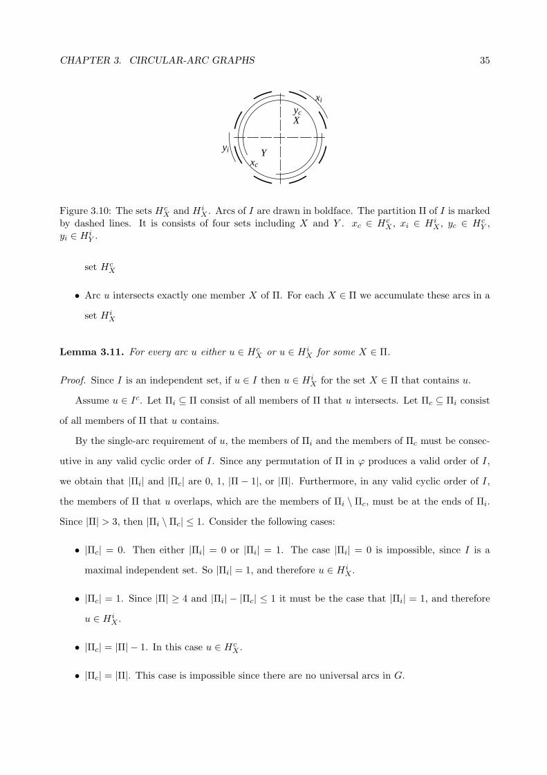
CHAPTER 3. CIRCULAR-ARC GRAPHS 35
xi
xc
yi
ycX
Y
Figure 3.10: The sets HcX and H i
X . Arcs of I are drawn in boldface. The partition Π of I is markedby dashed lines. It is consists of four sets including X and Y . xc ∈ Hc
X , xi ∈ H iX , yc ∈ Hc
Y ,yi ∈ H i
Y .
set HcX
• Arc u intersects exactly one member X of Π. For each X ∈ Π we accumulate these arcs in a
set H iX
Lemma 3.11. For every arc u either u ∈ HcX or u ∈ H i
X for some X ∈ Π.
Proof. Since I is an independent set, if u ∈ I then u ∈ H iX for the set X ∈ Π that contains u.
Assume u ∈ Ic. Let Πi ⊆ Π consist of all members of Π that u intersects. Let Πc ⊆ Πi consist
of all members of Π that u contains.
By the single-arc requirement of u, the members of Πi and the members of Πc must be consec-
utive in any valid cyclic order of I. Since any permutation of Π in ϕ produces a valid order of I,
we obtain that |Πi| and |Πc| are 0, 1, |Π − 1|, or |Π|. Furthermore, in any valid cyclic order of I,
the members of Π that u overlaps, which are the members of Πi \ Πc, must be at the ends of Πi.
Since |Π| > 3, then |Πi \ Πc| ≤ 1. Consider the following cases:
• |Πc| = 0. Then either |Πi| = 0 or |Πi| = 1. The case |Πi| = 0 is impossible, since I is a
maximal independent set. So |Πi| = 1, and therefore u ∈ H iX .
• |Πc| = 1. Since |Π| ≥ 4 and |Πi| − |Πc| ≤ 1 it must be the case that |Πi| = 1, and therefore
u ∈ H iX .
• |Πc| = |Π| − 1. In this case u ∈ HcX .
• |Πc| = |Π|. This case is impossible since there are no universal arcs in G.

CHAPTER 3. CIRCULAR-ARC GRAPHS 36
If x ∈ HcX ∪ H i
X then we say that x is associated with X. From Lemma 3.11, we know that
every arc x is associated with a single set X ∈ Π. The following lemma classifies the intersection
types between two arcs that are associated with different members of Π.
Lemma 3.12. The intersection type between an arc that is associated with X and an arc that is
associated with Y , such that X 6= Y , is as follows (see Figure 3.10):
(A) If x ∈ H iX and y ∈ H i
Y then x and y are disjoint.
(B) If x ∈ HcX and y ∈ H i
Y then x contains y.
(C) If x ∈ HcX and y ∈ Hc
Y then x and y cover the circle.
Proof. (A) Let x ∈ H iX and y ∈ H i
Y . Since x intersects X and y intersects Y , the arcs x and y
cannot contain each other. If x overlaps y then X and Y must be consecutive in any order
of I by the two-arcs requirement of x and y. However, since |Π| > 3, there are valid orders of
I in which X and Y are not consecutive. Therefore x and y are disjoint.
(B) Let x ∈ HcX and y ∈ H i
Y , the arc x is disjoint only from arcs of H iX , since it contains I \ X.
By statement (A), y does not intersect the arcs of H iX , so x contains y.
(C) Let x ∈ HcX and y ∈ Hc
Y , the arc x is disjoint only from arcs of H iX . By statement (B) the
arcs of H iX are contained in y, so x and y cover the circle.
In the next lemma we define KX to be the minimal segment of % that contains the endpoints
of all arcs that are associated with X. By definition, every x ∈ X intersects X, so x is associated
with X, therefore, in particular KX contains all endpoints of the arcs of X.
Lemma 3.13. There exists a segment KX that contains all endpoints of arcs associated with X
and only such endpoints.
Proof. Let K0 be the minimal segment that contains all endpoints of arcs in X, and no endpoint
of an arc in I \X. Every arc that has an endpoint in K0 intersects X but does not contain X, and
thus it is associated with X.

CHAPTER 3. CIRCULAR-ARC GRAPHS 37
Let K be a segment that contains K0 and does not contain any endpoint of an arc that is not
associated with X. We show that if K does not contain all endpoints of the arcs that are associated
with X, then either the endpoint immediately to the left of K or the endpoint immediately to the
right of K is an endpoint of an arc associated with X.
This shows that the minimal segment containing K0, and all endpoints of arcs associated with
X, satisfies the requirements of the lemma.
Let K be a segment as above, and let x be an arc associated with X with an endpoint outside
of K. Assume by contradiction that the endpoint ey immediately to the left of K is an endpoint
of an arc y which is associated with Y 6= X and that the endpoint ey′ immediately to the right of
K is an endpoint of an arc y′ which is associated with Y ′ 6= X (it might be the case that Y = Y ′
or y = y′).
If the arc x is in H iX , then since x intersects X, either x crosses K, or x covers all endpoints
in K. Therefore, x covers either ey or ey′ . If x covers ey, then x cannot be contained in y and
cannot be disjoint from y, in contradiction with Lemma 3.12. Similarly, we get a contradiction
with Lemma 3.12 also if x covers ey′ .
If the arc x is in HcX , then since x does not contain X, either x crosses K or does not cover any
endpoint in K. Therefore, x does not cover either ey or ey′ . If x does not cover ey the x cannot
contain y and cannot cover the circle with y, in contradiction with Lemma 3.12. Similarly, we get
a contradiction with Lemma 3.12 also if x does not covers ey′ .
The segments that we defined allow us to prove Lemma 3.10. We have %, a normalized circular-
arc model of G with a cyclic order ϕ of the arcs of I. We also have ϕ′, another valid order of the
arcs of I that is obtained from ϕ by permuting Π. We show a model %′ of G that is consistent with
ϕ′.
Proof of Lemma 3.10. Recall that any segment KX contains all the endpoints of the arcs in X.
Also, by Lemma 3.13 the segments are pairwise disjoint and their union is the entire circle. There-
fore, we can get a model %′ of G, which is consistent with ϕ′ by rearranging the segments KX
according to ϕ′.
By Lemma 3.13, any segment KX is uncrossed. So, rearranging the segments does not change
the intersection type between any pair of arcs. Therefore the model %′ that we get is a normalized

CHAPTER 3. CIRCULAR-ARC GRAPHS 38
K0
K’
Figure 3.11: The segments K0 and K ′. Arcs of I are drawn in boldface. Arcs of J are dotted. Thesegments are indicated on the circle.
model of G.
In order to prove a lemma analogous to Lemma 3.10 for C-nodes we first prove the following.
Lemma 3.14. Let % be a normalized circular-arc model of G with a cyclic order ϕ of the arcs of
I. Let ϕ′ be another valid order of the arcs of I that is obtained from ϕ by inverting a consecutive
subset of I. There is a model %′ of G that is consistent with ϕ′.
To prove this lemma we use the following definitions and lemmas.
We denote by J the consecutive subset of I that we invert in order to get ϕ′ from ϕ. We assume
that |J | > 1, because otherwise ϕ′ is the same as ϕ. We also assume that |I \ J | > 1, because
otherwise, %′ can be obtained by inverting the entire model %.
We find in % an uncrossed segment K, that contains all endpoints of arcs of J , but none of the
endpoints of arcs of the I \ J . Inverting K converts % to %′.
Let K0 be the minimal segment that contains all endpoints of arcs of J and does not contains
any endpoint of an arc of I \ J . The segment K0 is spanned form the leftmost endpoint of J , and
in the right direction to the rightmost endpoint of J . Let K ′ be the minimal possible segment that
covers all arcs of I \ J and does not contain any endpoint of an arc of J . See Figure 3.11.
We start with K = K0. As long as K is crossed, we extend K as follows. If K is crossed then
there is an arc x with one endpoint inside of K and one endpoint outside of K. If x does not cross
K ′, then we extend K to contain both endpoints of x, in the direction that will not cause K to
intersect K ′. We show that there is never an arc x with one endpoint inside K and the other inside
K ′, that is an arc that crosses both K and K ′. Therefore, when we cannot extend K anymore, it
is uncrossed.

CHAPTER 3. CIRCULAR-ARC GRAPHS 39
b
c
d
e
Figure 3.12: FJ , BJ and B′J . Arcs of I are drawn in boldface. Arcs of J are dotted. b ∈ FJ ,
c ∈ FI\J , d ∈ B′J , e ∈ BI\J .
b
c
d
e
Figure 3.13: B′J and RJ . Arcs of I are drawn in boldface. Arcs of J are dotted. b ∈ B′
J , c ∈ RJ ,d ∈ B′
I\J , e ∈ RI\J .
Recall that FJ is the set containing every arc that contains all arcs of J and is disjoint from
every arc of I \ J . Recall that BJ is the set containing every arc that crosses K0, is disjoint from
every arc of I \ J , and intersects some arc of FI\J . We denote by B′J the set containing every arc
that crosses K0, is disjoint from every arc of I \ J , and also, is disjoint from every arc of FI\J . We
define B′I\J symmetrically. See Figure 3.12. We denote by RJ the set containing every arc that
crosses K0 and contains all I \ J . We define RI\J symmetrically. See Figure 3.13.
Lemma 3.15. Let x be an arc that crosses K0 then x ∈ RJ ∪ BJ ∪ B′J . Symmetrically, let x′ be
an arc that crosses K ′ then x ∈ RI\J ∪ BI\J ∪ B′I\J .
Proof. Let x be an arc that crosses K0. Since x crosses K0 it cannot contain all arcs of J and so
C(x) ∩ J ⊂ J .
Assume C(x) ∩ J = ∅. Since x crosses K0, there is a single arc y ∈ J which x overlaps. By
the definition of C(x), if |NI [x]| = 1 then C(x) = NI [x], and since C(x) ∩ J = ∅, there must be an
arc z ∈ I \ J that x intersects. Recall that the cyclic order ϕ′ of I is obtained from ϕ by inverting

CHAPTER 3. CIRCULAR-ARC GRAPHS 40
the arcs of J . Therefore, the order of (I \ J) ∪ y in ϕ and in ϕ′ is the same except that either
in ϕ or in ϕ′ the arc y is the rightmost arc of (I \ J) ∪ y, and in the other order of I the arc y
is the leftmost arc of (I \ J) ∪ y. By the single-arc requirement of x, if y is the rightmost arc
of (I \ J) ∪ y then every arc of I \ J to the right of z in ϕ (and also in ϕ′) is contained in x.
Similarly, if y is the leftmost arc of (I \ J) ∪ y then every arc of I \ J to the left of z in ϕ (and
also in ϕ′) is contained in x. By repeating the same argument using z′ 6= z in I \ J we obtain that
z is also contained in x. So, x contains all arcs of I \ J . Thus, x ∈ RJ .
Otherwise, assume C(x) ∩ J 6= ∅. By the single-arc requirements, there is no arc that contains
both a proper subset of J and a proper subset of I \ J . Therefore, either I \ J ⊂ C(x), or
(I \ J) ∩ C(x) = ∅. If I \ J ⊂ C(x) then x ∈ RJ . Otherwise, in the case where (I \ J) ∩ C(x) = ∅,
if x overlaps an arc y of I \ J , then using an argument as in the case where C(x) ∩ J = ∅ with
I \ J instead of J , we get that x contains all arcs of J . This is impossible since C(x) ∩ J ⊂ J . So,
NI [x] ⊆ J and x ∈ BJ ∪ B′J .
We prove the claim about K ′ symmetrically.
The following lemma shows the intersection types between arcs in the sets discussed above.
Lemma 3.16. The following intersection types hold:
(A) Let x ∈ FJ and y ∈ B′J , then x contains y (see Figure 3.12).
(B) Let x ∈ FI\J and y ∈ B′J , then x and y are disjoint (see Figure 3.12).
(C) Let x ∈ BJ ∪B′J and y ∈ BI\J ∪B′
I\J , then x and y are disjoint (see Figure 3.5, Figure 3.12,
and Figure 3.13).
(D) Let x ∈ RJ and y ∈ RI\J , then x and y cover the circle (see Figure 3.13).
(E) Let x ∈ BJ ∪ B′J and y ∈ RI\J , then x is contained in y (see Figure 3.13).
Statements (A)-(E) also hold when replacing J and I \ J .
Proof. (A) Assume that there is an arc z which intersects y but does not intersect x. Since x
contains every arc of J , we get that NI [z] ⊆ I \ J . Because y ∈ B′J we know that z /∈ FI\J .
Therefore, C(z) ⊂ I \ J . The arcs y and z create a two-arcs requirement that prevent the
inversion of J . This is a contradiction.
CHAPTER 3. CIRCULAR-ARC GRAPHS 41
(B) By the definition of B′J .
(C) Assume that x and y intersect. We know that C(x) ⊂ J and C(y) ⊂ I \J . So, x and y create
a two-arcs requirement that prevents the inversion of J . This is a contradiction.
(D) Let z be an arc that is disjoint from x. Since x covers I \ J and intersects at least one arc of
J , we have NI [z] ⊂ J . Similarly, if w and y are disjoint then NI [w] ⊂ I \ J . If z intersects w
we get a two-arcs requirement that forbids the inversion of J . So, every arc such as w that
is disjoint from y is also disjoint from z, and therefore, y contains z. Thus, y contains every
arc that is disjoint from x and the claim follows.
(E) We know that C(x) ⊂ J . Let z be an arc which is disjoint from y. As in statement (D), we
have NI [z] ⊂ I \J . If z intersects x we get a two-arcs requirement that prevents the inversion
of J . So x is disjoint from every arc that y is disjoint from, therefore y contains x.
All the proofs above hold also when replacing J and I \ J .
As we extend K as described above, every arc that crosses K at some point either crosses K0
or crosses an arc that we previously used to extend K. An arc that none of its endpoints is in K0
or K ′ is in FJ or FI\J . This follows since such an arc contains every arc in J or every arc in I \ J ,
and is disjoint from every arc of I \J or every arc of J , respectively. Since we never use an arc that
crosses K ′ to extend K, every arc that we use to extend K either crosses K0 or is in FJ ∪ FI\J .
Lemma 3.17. Assume that at some point while extending K there is an arc xs that crosses both
K and K ′. Then, there is a path P = (x0, . . . , xs−1, xs) such that:
1. For i = 1, . . . , s, the arc xi crosses the arc xi−1.
2. x0 ∈ RJ ∪ BJ .
3. xs ∈ RI\J ∪ BI\J .
4. For i = 1, . . . s − 1, we have xi ∈ FJ ∪ FI\J .
5. |P | ≥ 3.
Proof. Assume that at some point while extending K there is an arc xs that crosses both K and
K ′. By Lemma 3.15, we have xs ∈ RI\J ∪BI\J ∪B′I\J . Also follows from Lemma 3.15 that the arc

CHAPTER 3. CIRCULAR-ARC GRAPHS 42
xs cannot cross K0, since (RJ ∪BJ ∪B′J)∩ (RI\J ∪BI\J ∪B′
I\J) = ∅. So, there is an arc xs−1 that
we used to extend K which xs crosses.
By Lemma 3.16(C)-(E), since xs−1 crosses xs, we get that xs−1 /∈ RJ ∪BJ ∪B′J , so by Lemma
3.15, xs−1 does not cross K0. So, there is an arc xs−2 which crosses xs−1 that we used to extend
K before xs−1. Also, since xs−1 does not cross K0 or K ′, it follows that xs−1 ∈ FJ ∪ FI\J .
We can trace back in this way a path P = (x0, . . . , xs−1, xs) such that xi crosses xi−1 for
i = s, . . . , 1, until we get to an arc x0 ∈ RJ ∪BJ ∪B′J which crosses K0. The length of P is at least
3. For i = 1, . . . s − 1, we have xi ∈ FJ ∪ FI\J , since they do not cross K0 or K ′.
Since x1 ∈ FJ ∪ FI\J we get from Lemma 3.16(A)-(B) that x1 does not cross any arc of B′J .
Therefore, x0 /∈ B′J . Similarly, since xs−1 ∈ FJ ∪ FI\J we get that xs /∈ B′
I\J .
The following lemma shows that if a path P as in Lemma 3.17 exists, then there is also a path
P ′ satisfying the same conditions as in Lemma 3.17 and in addition P ′ starts with an arc of BJ
and ends with an arc of BI\J .
Lemma 3.18. Let P = (x0, . . . , xs−1, xs) be as in Lemma 3.17. There is an arc x′0 ∈ BJ that
crosses x1. Similarly, there is an arc x′s ∈ BI\J that crosses xs−1.
Proof. By Lemma 3.17, x0 ∈ BJ ∪ RJ and x1 ∈ FJ ∪ FI\J . Also, the arcs x0 and x1 cross.
If x0 ∈ BJ , we let x′0 = x0.
Assume x0 ∈ RJ and x1 ∈ FI\J . The arcs x0 and x1 cross, so there is an arc z that intersects
x1 but not x0. Since z and x0 are disjoint, we have NI [z] ⊂ J , and because z intersects x1 we have
z ∈ BJ . We let x′0 = z.
Assume x0 ∈ RJ and x1 ∈ FJ . The arc x0 contain every arc of I \ J , and the arc x1 contains
every arc of J . Therefore, every arc that is disjoint from x0, intersects x1. The arcs x0 and x1 do
not cover the circle, so there is an arc z disjoint from x0 which is not contained in x1. Thus, the
arc z crosses x1. Since z and x0 are disjoint, we have NI [z] ⊂ J . Since z crosses x1, it intersects
an arc w which is disjoint from x1, such that NI [w] ⊆ I \ J . Since there is no two-arcs requirement
that contains both a proper subset of J and a proper subset of I \ J , we know that C(w) = I \ J .
Therefore, w ∈ FI\J and z ∈ BJ . We let x′0 = z.
We prove the claim about x′s symmetrically.

CHAPTER 3. CIRCULAR-ARC GRAPHS 43
We can now prove Lemma 3.14.
Proof of Lemma 3.14. Assume that at some point while extending K we have an arc that crosses
both K and K ′. By Lemma 3.17 and Lemma 3.18, there is a path P ′ = (x′0, x1, . . . , xs−1, x
′s) such
that each arc crosses the previous arc, and all arcs of P ′ are in BJ ∪BI\J ∪FJ ∪FI\J . The path P ′
impose a cross-path requirement that forbids the inversion of the arcs of J in ϕ, in the sense that
ϕ′ is not valid. This is a contradiction, so there is never an arc that crosses both K and K ′.
It follows that we can extend K until it is uncrossed. When K is uncrossed, it does not contain
any endpoint of an arc of I \ J . We invert K in % and get a normalized circular-arc model %′ of G
in which the cyclic order of I is ϕ′.
The following lemma shows that Lemma 3.14 can be used for C-nodes.
Lemma 3.19. Let ϕ be a valid cyclic order of I. Let c be a C-node in a PC-tree of M3, and x be a
vertex in the tree adjacent to c. Let X be the set of arcs of I such that the path connecting each of
them to c in the tree contains x. The order ϕ′ which is obtained from ϕ by inverting I \X is valid.
Proof. Let T be a PC-tree of M3 such that the leaves of T are ordered as in ϕ. We show how by
permuting the order of the edges of P-nodes and inverting the order of the edges of C-nodes, we
can obtain a PC-tree T ′ in which the leaves are ordered as in ϕ′. From this the claim would follow.
Let Tc be the connected subtree of T containing c that we would have obtained if we deleted x.
We obtain T ′ by traversing the vertices of Tc in T , and inverting the order of the edges incident to
every internal node.
The next lemma addresses the case when we invert the order of the edges incident to a C-node.
Lemma 3.20. Let % be a normalized circular-arc model of G with a cyclic order ϕ of the arcs of I.
Let ϕ′ be another valid order of the arcs of I that is obtained from ϕ by inverting the cyclic order
of the edges incident to a C-node in a PC-tree of M3. There is a normalized circular-arc model %′
of G that is consistent with ϕ′.
Proof. Let c be the C-node that we invert the order of its edges to get ϕ′ from ϕ. We partition I
into subsets, each subset contains all arcs of I that are connected to c through a particular edge.

CHAPTER 3. CIRCULAR-ARC GRAPHS 44
We denote this partition of I by Γ. We assume that |Γ| > 1, because otherwise, inverting the cyclic
order of Γ is meaningless.
Let X be an arbitrary member of Γ. Lemma 3.19 allows us to use Lemma 3.14 and produce
from % a model %1 of G, in which the order of I \X is inverted. In %1, the order of the members of
Γ is inverted, but %1 is not consistent with ϕ′, since we also inverted the order of the arcs inside Y
for every Y ∈ Γ \ X. To fix that, we need to invert back the arcs of Y for each such Y .
Let Y be a set in Γ \ X, and let y be the vertex adjacent to c such that the path between c
and any member of Y contains y.
If y is a leaf then |Y | = 1 and we do not need to invert it.
If y is a C-node then we can apply Lemma 3.19 and Lemma 3.14 to invert back the order of
the arcs in Y .
If y is a P-node then there is a partition Π of I as in Lemma 3.10 that is defined by the edges
incident to y. The members of Π are I \ Y and subsets of Y . We use Lemma 3.10 to invert the
order of Π, this inverts the order of any pair of arcs each in a different subset of Y . We continue
recursively and invert the order of arcs inside each of the subsets of Y .
From Lemma 3.10 and Lemma 3.20 the main theorem of this section follows.
Theorem 3.21. Let G be a circular-arc graph. Let I be a maximal independent set as above, and
let π be a valid cyclic order of I. Then, G has a normalized circular-arc model in which the cyclic
order of I is consistent with π.
3.4 Stage 2: placing the endpoints of the arcs in the sections
Consider π, the order of I found in Section 3.3. For every arc x ∈ Ic, the members of NI [x] are
consecutive on the circle. Since there are no universal arcs in G, and I is a maximal independent
set, x cannot contain all arcs of I and NI [x] 6= ∅. Also, x overlaps at most two arcs of I, since
otherwise G is not a circular-arc graph and we should have detected it in Stage 1.
Let x ∈ Ic, the way we place the endpoints of x into their sections depends on the relation
between x and the arcs of I. In most cases these relations suffice to determine the sections, and
in the other cases we apply the algorithm recursively on an appropriate graph. The arc x satisfies

CHAPTER 3. CIRCULAR-ARC GRAPHS 45
b
c
d
e
ai
Figure 3.14: Ui, Wi, Aei and Ac
i . Arcs of I are drawn in boldface. b ∈ Ui, c ∈ Wi, d ∈ Aei and e ∈ Ac
i .
one of the following cases.
• Arc x overlaps an arc ai ∈ I and does not intersect any other arc in I. For every ai ∈ I we
accumulate these arcs in a set which we call Ui (see Figure 3.14).
• Arc x contains an arc ai ∈ I and does not intersect any other arc in I. In this case `(x) is
placed in S2i−1 and r(x) is placed in S2i+1. For every ai ∈ I we accumulate all arcs that
contain it and does not intersect any other arc of I in a set which we call Aei (see Figure 3.14).
• Arc x intersects at least two arcs of I and does not intersect at least one. For all these arcs we
identify in NI [x] the leftmost arc ai, and the rightmost arcs aj . We do that as we identified
h(NI [x]) and t(NI [x]) of every arc in the preliminary order π1 of I in Section 3.3. If x contains
ai then `(x) is in S2i−1, if x overlaps ai then this endpoint is in S2i. Similarly, if x contains
aj then r(x) is in S2j+1, if x overlaps aj then this endpoint in S2j . For every arc ai ∈ I we
accumulate every arc that contains all arcs in I except ai, and does not intersect ai, in a set
which we call Aci (see Figure 3.14).
• Arc x overlaps two consecutive arcs ai, ai+1 ∈ I and contains all other arcs of I. In this case,
we place `(x) in S2(i+1) and r(x) in S2i.
• Arc x overlaps one arc ai ∈ I and contains all other arcs of I. For each ai ∈ I we accumulate
these arcs in a set Wi (see Figure 3.14).
At this point we placed the endpoints of all arcs in Ic into their sections except arcs in Ui and
Wi for i = 1, . . . , |I|. Consider any arc ai ∈ I and the associated sets Ui and Wi. Each arc in
Ui ∪ Wi has one endpoint in S2i and the other in S2i−1 or in S2i+1. Furthermore, all arcs of Ui

CHAPTER 3. CIRCULAR-ARC GRAPHS 46
must form a clique, as otherwise we can get from I a larger independent set by replacing ai by two
disjoint arcs in Ui, contradicting Lemma 3.1.
We place the endpoints of the arcs of Ui∪Wi in the sections S2i−1, S2i and S2i+1 for each ai ∈ I
separately, by solving a new problem recursively on a graph Gi. The graph Gi which we construct
is identical to the graph that Eschen [Esc97] constructs1. This graph is co-bipartite and therefore
when we run the algorithm on Gi, Case I applies and there would not be further recursion. We
contribute the following observations. If G is a circular-arc graph then the recursive application of
the algorithm on Gi takes time linear in the size of Gi. Furthermore, the sum of the sizes of all
Gi’s is proportional to the size of G.
Let Cai be the set of arcs ai ∪ Ui ∪ Ae
i . The set Cai forms a clique in G, since Ui forms a
clique and all the arcs of Aei intersect every arc that ai intersects. The clique Ca
i consists of all arcs
contained in the union of the sections S2i−1, S2i and S2i+1. Furthermore, since these arcs cannot
cover the circle, there must be a point pa which all arcs in Cai cover. Let Qi be the set of arcs that
intersect some but not all arcs in Cai , and are not members of Ac
i ∪ Wi.
To define Gi we first define a subgraph of G which we denote by G′i. The graph G′
i is also a
subgraph of Gi. The graph G′i is the subgraph induced by Ca
i ∪ Aci ∪ Wi ∪ Qi.
We find Qi by scanning the adjacency list of each x ∈ Cai . We maintain a set Y of arcs
encountered during the scan. For each arc y ∈ Y , we also keep a counter that counts the number
of neighbors of y in Cai . When we finish scanning the adjacency list of every x ∈ Ca
i , the arcs of
y ∈ Y whose counters are smaller than |Cai | are the arcs of Ac
i ∪ Wi ∪ Qi. We construct G′i by
scanning the adjacency list of each arc in it and restricting the list to contain only arcs inside G′i.
The following lemma proves that all G′i’s are constructed in linear time.
Lemma 3.22. [Esc97] Every arc x participates in a constant number of graphs G′i.
Proof. From the definition of the sets Ui, Aei , A
ci , Wi, it follows that an arc x can belong to at most
one such set. So, it remains to show that x can belong to at most constant number of sets Qi.
Suppose that x ∈ Qi for some i, then x intersects an arc y ∈ Cai such that NI [y] = ai. By
the single-arc requirement of x or the two-arcs requirement of x and y, the subset ai ∪ C(x) is
consecutive in π. Assume ai ∈ NI [x], since by the definition of Qi, ai is not contained in x, then
1Note that this graph is different from the one of [ES93] which seems to have an error.
CHAPTER 3. CIRCULAR-ARC GRAPHS 47
ai must be the leftmost or the rightmost arc of NI [x] in π. Assume ai /∈ NI [x], then either the
leftmost or the rightmost arc of NI [x] in π must be next to ai in this order. In either case one of
the arcs ai−1, ai, ai+1 must be the leftmost or the rightmost arc of NI [x] in the cyclic order of I.
So, x can belong to Qi only if one of ai−1, ai or ai+1 is its rightmost or leftmost neighbor in the
cyclic order of I.
Let n′i be the number of vertices in G′
i, and let m′i be the number of edges in G′
i. Every arc in G′i
covers at least one of the four endpoints of the three consecutive sections S2i−1, S2i, S2i+1. Therefore,
the arcs of G′i are covered by four cliques, one for each endpoint. One of these cliques should have
at leastn′
i
4 vertices and therefore has at leastn′
i
4 (n′
i
4 − 1) edges. So we check if m′i ≥
n′
i
4 (n′
i
4 − 1). If
this inequality does not hold then G is not a circular-arc graph and we halt. Otherwise, we know
that m′i = Θ(n′2
i ).
We construct Gi from G′i by adding a constant number of new vertices and O(n′2
i ) = O(m′i) edges
as we describe below. So if ni and mi denote the number of vertices and edges in Gi respectively,
then we also have that mi = Θ(m′i) = Θ(n′2
i ) = Θ(n2i ).
Since mi = Θ(n2i ), the recursive application of our algorithm to Gi takes O(mi) time. Since by
Lemma 3.22 each arc of G belongs to at most a constant number of graphs Gi, then each edge of
G can belong to at most a constant number of graphs Gi. Therefore,∑
mi = O(m) and the linear
time bound for Stage 2 follows.
To construct Gi for some i = 1, . . . , |I|, we add to G′i a vertex bi which represents I \ ai. We
make bi adjacent to every arc in G′i that intersects either ai−1 or ai+1 in G, these arcs are exactly
those arcs in Aci ∪ Wi ∪ Qi. We make Gi co-bipartite by making bi ∪ Ac
i ∪ Wi ∪ Qi a clique. We
call this clique Cbi . Note that since the arcs in bi ∪Ac
i ∪Wi already intersect all the arcs of Cbi (they
all contain ai−1 and ai+1), in order to make Cbi a clique we only add intersections between arcs in
Qi. Since every arc of Gi is either in Cai or in Cb
i , then Gi is co-bipartite.
Intuitively, we construct Gi such that a circular-arc model of Gi corresponds to a model of G in
the following sense. Consider the arcs ai and bi in a circular-arc model of Gi. These arcs partition
the circle into four sections – the section of the arc ai, which we denote by T (i)2i, the section of the
arc bi, which we denote by T (i)′, and the two sections of the gaps between ai and bi, denoted by
T (i)2i−1 and T (i)2i+1. The sections T (i)2i−1, T (i)2i, and T (i)2i+1 correspond to the sections S2i−1,

CHAPTER 3. CIRCULAR-ARC GRAPHS 48
c
d
e
ara
br b
ai
bi
Figure 3.15: The construction of Gi. c ∈ Ui, d ∈ Wi. Since e intersects c but not ai, it is in Qi.The arc ar is disjoint from e and forces e to overlap bi from the side that ar does not cover.
S2i, and S2i+1 respectively. More formally, all endpoints including these of the arcs of Ui∪Wi, that
are contained in one of the sections T (i)2i−1, T (i)2i or T (i)2i+1, are in the corresponding section
S2i−1, S2i or S2i+1 in the model which we construct for G.
The construction of Gi up to this point is not sufficient to guarantee that the position of the
endpoints of the arcs of Qi in a model of Gi is consistent with the model we construct for G. An
arc in Qi has one endpoint in S2i−1, S2i or S2i+1, so in Gi we should force it to have the same
endpoint (and only this endpoint) in T (i)2i−1, T (i)2i or T (i)2i+1 respectively. Note that no arc of
Cbi can contain ai, so for x ∈ Cb
i the endpoint `(x) cannot be in S2i−1 and the endpoint r(x) cannot
be in S2i+1.
To complete the construction of Gi we add four more vertices a`, ar, b` and br (see Figure 3.15).
We also add the edges a`ar, arb`, b`br, bra` so these vertices form a chordless cycle. We add a` and
ar to the clique Cai , and b` and br to the clique Cb
i . In addition, we make a` adjacent to every arc
in Cbi , except arcs of Qi with left endpoint already placed in one of the sections S2i, S2i+1 or arcs in
Ui+1. Symmetrically, we make ar adjacent to every arc in Cbi , except arcs of Qi with right endpoint
already placed in one of the sections S2i−1, S2i or arcs in Ui−1. The arcs a` and ar overlap both
ai and bi, so in a model of Gi each of them covers either T (i)2i−1 or T (i)2i+1. The arcs b` and br
guarantee that a` and ar cover different sections. We let T (i)2i−1 be the section covered by a` and
T (i)2i+1 be the section covered by ar. The arcs a` and ar force the arcs of Qi which they do not
intersect, to overlap bi from the side which they do not cover.
Note that two arcs of Qi that overlap bi from different sides, cannot overlap each other outside
of bi. This is because otherwise at least one of them will cover pa, the point covered by all arcs of

CHAPTER 3. CIRCULAR-ARC GRAPHS 49
Cai , which would contradict the fact that these arcs are in Qi. However, a` and ar do not prevent
two arcs in Qi to intersect inside bi. This means that if x and y are two arcs of Qi that are not
adjacent in G, and we added an edge between them in Gi, the common part of the two arcs on the
circle is not in T (i)2i−1, T (i)2i or T (i)2i+1.
For each graph Gi we apply Case I and get a normalized circular-arc model %i. From %i we
get the sections T (i)2i−1, T (i)2i and T (i)2i+1 as defined above. The next lemma shows that these
sections are consistent for each i = 1, . . . , |I|.
Lemma 3.23. Let G be a circular-arc graph. Let e be an endpoint of an arc x in G. If e ∈
T (i)p ∩ T (j)q for some i 6= j, then p = q.
Proof. Assume that e is already placed in a section Sr. That is, there is no k such that x ∈ Wk or
x ∈ Uk. Then, the four-vertices chordless cycle of Gi forces e to be in T (i)r, and the four-vertices
chordless cycle of Gj forces e to be in T (j)r, so p = r = q.
Otherwise, if we have not placed e in a section, then either x ∈ Wk or x ∈ Uk for some
k = 1, . . . , |I|.
Assume that x ∈ Wk. We claim that x does not belong to any Gi for i 6= k, from this follows
that x cannot be both in Gi and in Gj since i 6= j. Assume that i 6= k. The arc x is not ai, and
x cannot be in Ui, Aei , Ac
i or Wi by the definitions of these sets. Furthermore, x /∈ Qi, since every
arc in Qi is disjoint from an arc y ∈ Cai , and therefore cannot contain ai, but x does contain ai.
Assume now that x ∈ Uk for some k = 1, . . . , |I|. Assume also that k 6= i and k 6= j. Each
arc of G which is also in Gi is in one of the sets ai, Ui, Aei , Ac
i , Wi or Qi. Since Qi is the only
set which is not necessarily disjoint from Uk, x ∈ Qi. Therefore, there is an arc z ∈ Cai which
intersects x. Since x ∈ Uk we have NI [x] = ak, and since z ∈ Cai we have NI [z] = ai. So, we
have a two-arcs requirement corresponding to x and z that forces ai and ak to be consecutive in
π. Let % be a normalized circular-arc model of G consistent with π. The arc x overlaps the arc ak
and the arc z in %, so x covers the endpoint of ak which is closer to ai. Using the same argument,
we get that the arcs aj and ak are also consecutive in π, and that in the model % the arc x covers
the endpoint of ak which is closer to aj . The endpoint of ak which is closer to aj is different from
the endpoint of ak which is closer to ai. So, x covers both endpoints of ak, and thus x contains
ak. But, since x ∈ Uk, x does not contain ak. From this contradiction follows that if x ∈ Uk then
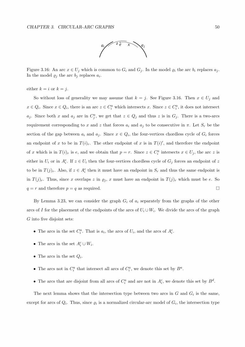
CHAPTER 3. CIRCULAR-ARC GRAPHS 50
ai a jz xe
Figure 3.16: An arc x ∈ Uj which is common to Gi and Gj . In the model %i the arc bi replaces aj .In the model %j the arc bj replaces ai.
either k = i or k = j.
So without loss of generality we may assume that k = j. See Figure 3.16. Then x ∈ Uj and
x ∈ Qi. Since x ∈ Qi, there is an arc z ∈ Cai which intersects x. Since z ∈ Ca
i , it does not intersect
aj . Since both x and aj are in Caj , we get that z ∈ Qj and thus z is in Gj . There is a two-arcs
requirement corresponding to x and z that forces ai and aj to be consecutive in π. Let Sr be the
section of the gap between ai and aj . Since x ∈ Qi, the four-vertices chordless cycle of Gi forces
an endpoint of x to be in T (i)r. The other endpoint of x is in T (i)′, and therefore the endpoint
of x which is in T (i)r is e, and we obtain that p = r. Since z ∈ Cai intersects x ∈ Uj , the arc z is
either in Ui or in Aei . If z ∈ Ui then the four-vertices chordless cycle of Gj forces an endpoint of z
to be in T (j)r. Also, if z ∈ Aei then it must have an endpoint in Sr and thus the same endpoint is
in T (j)r. Thus, since x overlaps z in %j , x must have an endpoint in T (j)r which must be e. So
q = r and therefore p = q as required.
By Lemma 3.23, we can consider the graph Gi of ai separately from the graphs of the other
arcs of I for the placement of the endpoints of the arcs of Ui ∪Wi. We divide the arcs of the graph
G into five disjoint sets:
• The arcs in the set Cai . That is ai, the arcs of Ui, and the arcs of Ae
i .
• The arcs in the set Aci ∪ Wi.
• The arcs in the set Qi.
• The arcs not in Cai that intersect all arcs of Ca
i , we denote this set by Ba.
• The arcs that are disjoint from all arcs of Cai and are not in Ac
i , we denote this set by Bd.
The next lemma shows that the intersection type between two arcs in G and Gi is the same,
except for arcs of Qi. Thus, since %i is a normalized circular-arc model of Gi, the intersection type

CHAPTER 3. CIRCULAR-ARC GRAPHS 51
between two arcs, which are not in Qi, in %i is the same as in a normalized circular-arc model of G.
Lemma 3.24. Let G be a circular-arc graph. Let x and y be two arcs that are both in G and Gi,
such that x, y /∈ Qi. The intersection type of x and y in Gi is the same as in G.
Proof. First note that two arcs x and y which are both in G and in Gi and at least one of them is
not in Qi are adjacent in G if and only if they are adjacent in Gi. So we only have to prove that
x and y have a neighborhood containment relation in Gi if and only if they have a neighborhood
containment relation in G, and that they cover the circle in Gi if and only if they cover the circle
in G.
The arcs that are in G but not in Gi are arcs of Ba and arcs of Bd. The arcs that are in Gi but
not in G are the arcs of the four-vertices chordless cycle, a`, ar, b`, br, and bi. Therefore, in order to
compare the intersection types between two arcs in G and Gi, we need to consider their adjacencies
to a`, ar, b`, br, bi, and to arcs of Ba and Bd.
We split the proof into cases according to which of the sets Cai and Ac
i ∪ Wi contain x an y.
Case 1: Arcs x, y ∈ Cai . The arcs x and y intersect both in G and in Gi since they are both
in the clique Cai . In the graph G, both x and y are disjoint from the arcs of I \ ai, therefore x
and y do not cover the circle. In the graph Gi, both x and y are disjoint from bi, therefore x and
y do not cover the circle also in this graph. The neighbors of x in Gi are a`, ar and its neighbors
in G, without the arcs in Ba. Similarly, the neighbors of y in Gi are a`, ar and its neighbors in G,
without the arcs in Ba. So it follows that x and y have a neighborhood containment relation in
Gi if and only if they have a neighborhood containment relation in G. Therefore, the intersection
type between x and y in Gi is the same as in G.
Case 2: Arc x ∈ Cai and arc y ∈ Ac
i ∪ Wi. Assume that x intersects y in G, and therefore also
in Gi. In the graph G, the arc x is disjoint from the arcs of I \ ai. The arc y covers every arc of
I \ai, therefore there is an arc z ∈ Cai which y does not intersect, because otherwise y would be a
universal arc. The arc x intersects z, thus there is no neighborhood containment relation between
x and y. All the arcs that are in G but not in Gi intersect y in G, and all the arcs that are in Gi
and not in G intersect y in Gi. So it follows that x and y cover the circle in Gi if and only if they
cover the circle in G. Therefore, the intersection type between x and y in Gi is the same as in G.
Case 3: Arcs x, y ∈ Aci ∪Wi. In this case, x and y intersect both in G and in Gi since they both

CHAPTER 3. CIRCULAR-ARC GRAPHS 52
cover I \ai. Since there are no universal arcs, there are arcs z, z′ ∈ Cai such that z is disjoint from
x and z′ is disjoint from y. Either z = z′, or z intersects z′, in both cases we get that y does not
contain z and therefore x and y do not cover the circle both in G and in Gi. All the arcs that are in
G but not in Gi intersect both x and y in G, and all the arcs that are in Gi and not in G intersect
both x and y in Gi. So it follows that x and y have a neighborhood containment relation in Gi if
and only if they have a neighborhood containment relation in G. Therefore, the intersection type
between x and y in Gi is the same as in G.
Lemma 3.24 deals with the intersection type between two arcs of ai ∪ Ui ∪ Aei ∪ Ac
i ∪ Wi
in normalized circular-arc models of G and Gi. In the next lemma we consider the order of the
endpoints in the sections T (i)2i−1, T (i)2i and T (i)2i+1 of %i, and in the sections S2i−1, S2i and S2i+1
of %. Note that when we talk about the relative order of endpoints we refer to their relative order
either within T (i)2i−1, T (i)2i and T (i)2i+1 or within S2i−1, S2i and S2i+1, so phrases such as “e is
to the left of e′” are well-defined.
Lemma 3.25. Let G be a circular-arc graph. Let % be a normalized circular-arc model of G
consistent with the placement of endpoints done so far. Let %i be a normalized circular-arc model
of Gi. Let ej and ek be endpoints of arcs in ai ∪ Ui ∪ Aei ∪ Ac
i ∪ Wi such that ej is to the left of
ek in % and ek is to the left of ej in %i. Then, every endpoint e between ej and ek in % is of an arc
in ai ∪ Ui ∪ Aei ∪ Ac
i ∪ Wi.
Proof. For the proof we split the arcs in ai ∪ Ui ∪ Aei ∪ Ac
i ∪ Wi into two sets - Cai and Ac
i ∪ Wi,
and the other arcs into three sets - Qi, Ba and Bd. Let ej , e, and ek be endpoints of arcs xj , x, and
xk respectively such that ej is to the left of ek in %, ek is to the left of ej in %i, and e is between ej
and ej in %.
Recall that pa is a point on the circle which is covered by all arcs of Cai . Such a point exists
both in % and in %i. If z ∈ Cai then `(z) is to the left of pa and r(z) is to the right of pa. For every
arc z ∈ Aci ∪ Wi there is an arc z′ ∈ Ca
i which z does not intersect, since otherwise z is a universal
arc, thus z does not cover pa. So, if z ∈ Aci ∪Wi, r(z) is to the left of pa and `(z) is to the right of
pa. Thus, if ej is to the left of pa and ek is to the right of pa in %, then ej and ek have the same
order in %i. So, we assume that ej and ek are both to the left of pa. If both ej and ek are to the
right of pa the proof is symmetric.

CHAPTER 3. CIRCULAR-ARC GRAPHS 53
If x ∈ Qi, then since x cannot cover pa, e = r(x). Assume x ∈ Ba, we show that there is an
endpoint e′ of an arc x′ ∈ Cai which is to the right of e. The arc x′ can be either xk if xk ∈ Ca
i , or
an arc which xk does not intersect, if xk ∈ Aci ∪ Wi. Since x intersects x′, the endpoint e is `(x).
Assume that x ∈ Bd, then since x cannot cover pa, e = r(x). If xj ∈ Cai then e is to the left of ej
since x is disjoint from xj . If xj ∈ Aci ∪ Wi then all arcs that xj does not intersect are arcs of Ca
i ,
which are disjoint from x. Thus, x is contained in xj and e must be to the left of ej . So e cannot
be between ej and ek and therefore x /∈ Bd.
The rest of the proof is split into cases according to the sets containing xj and xk as follows.
Case 1: Arcs xj , xk ∈ Cai . In this case ej = `(xj) and ek = `(xk).
Assume x ∈ Qi (see Figure 3.17(a)), then e = r(x). The arc x intersects xj since e is to the
right of ej in %, but x is disjoint from xk since e is to the left of ek in %. Therefore, the order
between ej , e and ek should be the same in %i, in contradiction to the way we defined ej and ek.
Assume that x ∈ Ba (see Figure 3.17(b)), then, e = `(x). Since e is to the left of ek, x contains
xk in %. Also, x does not contain xj , since ej is not covered by x (% is a normalized circular-arc
model). So, there is an arc x′ which intersects xj but is disjoint from x, such that x′ has an endpoint
e′ between ej and e. Since x contains ek, the arc x′ is disjoint from xk. Thus, x′ ∈ Qi, and by the
previous argument e′ cannot exist and we obtain a contradiction.
Case 2: Arc xj ∈ Aci ∪ Wi and arc xk ∈ Ca
i . In this case ej = r(xj) and ek = `(xk).
Assume x ∈ Qi (see Figure 3.17(c)), then e = r(x). The arc x is not contained in xj in %,
therefore there is an arc x′ with an endpoint between ej and e which intersects x and is disjoint
from xj . Since x′ is disjoint from xj , it must be in Cai . Since e is between e′ and ek, then according
to Case 1, e′ is to the left of ek also in %i. Since xj is disjoint from x′, ej is to the left of ek in %i,
in contradiction to the way we defined ej and ek.
Assume that x ∈ Ba (see Figure 3.17(d)), then e = `(x). Since xj and x do not cover the circle
in %, there is an arc x′ which xj does not intersect and x does not contain, with an endpoint e′
between ej and e. Again, x′ must be an arc of Cai and using Case 1 we obtain a contradiction.
Case 3: Arc xj ∈ Cai and arc xk ∈ Ac
i ∪ Wi. In this case ej = `(xj) and ek = r(xk).
Assume x ∈ Qi (see Figure 3.17(e)), then e = r(x). The arc xk contains x in %. The arcs xj
and x intersect in %, therefore ej is to the left of e also in %i. Since ek is to the left of ej in %i we
obtain that ek is to the left of e in %i. It follows that there is an arc x′ in Gi which x intersects but

CHAPTER 3. CIRCULAR-ARC GRAPHS 54
e j e ek pa
(a) xj ∈ Cai , x ∈ Qi, xk ∈ Ca
i
e j e’ e ek pa
(b) xj ∈ Cai , x ∈ Ba, xk ∈ Ca
i
e j e’ e ek pa
(c) xj ∈ Aci ∪ Wi, x ∈ Qi, xk ∈ Ca
i
e j e’ e ek pa
(d) xj ∈ Aci ∪ Wi, x ∈ Ba, xk ∈ Ca
i
e j e’ e ek pa
(e) xj ∈ Cai , x ∈ Qi, xk ∈ Ac
i ∪ Wi
e j e’ e ek pa
(f) xj ∈ Cai , x ∈ Ba, xk ∈ Ac
i ∪ Wi
e j e’ e ek pa
(g) xj ∈ Aci ∪Wi, x ∈ Qi, xk ∈ Ac
i ∪Wi
e j e’ e ek pa
(h) xj ∈ Aci ∪Wi, x ∈ Ba, xk ∈ Ac
i ∪Wi
Figure 3.17: The different cases of the proof of Lemma 3.25.
CHAPTER 3. CIRCULAR-ARC GRAPHS 55
xk does not intersect. The arc x′ must be in Cai and therefore also in the graph G. But this is a
contradiction because xk contains x in %.
Assume that x ∈ Ba (see Figure 3.17(f)), then e = `(x). Since ej is to the left of e, there is an
arc x′ in % which intersects xj and is disjoint form x, with an endpoint e′ between ej and e. The
arc x′ must be in Qi, and by the previous argument e′ cannot exist and we obtain a contradiction.
Case 4: Arcs xj , xk ∈ Aci ∪ Wi. In this case ej = r(xj) and ek = r(xk).
Assume x ∈ Qi (see Figure 3.17(g)), then e = r(x). The arc x is not contained in xj in %, thus
there is an arc x′ which intersects x but does not intersect xj with an endpoint e′ between ej and
e. The arc x′ must be in Cai , and using Case 3 we obtain a contradiction.
Assume that x ∈ Ba (see Figure 3.17(h)), then, e = `(x). Since xj and x do not cover the circle
in %, there is an arc x′ which xj does not intersect and x does not contain, with an endpoint e′
between ej and e. Again, x′ must be an arc of Cai and using Case 3 we obtain a contradiction.
Now, we show that we can place the endpoints of arcs of Ui ∪ Wi which are in T (i)2i−1, T (i)2i
and T (i)2i+1 into S2i−1, S2i and S2i+1 respectively. This completes Stage 2 of the algorithm.
Lemma 3.26. Let G be a circular-arc graph. Let F2i−1, F2i and F2i+1 be the endpoints of arcs
in Ui ∪ Wi that are in T (i)2i−1, T (i)2i and T (i)2i+1, respectively, in some normalized circular-arc
model of Gi. There is a normalized model of G, consistent with the placement of endpoints done
so far, such that the endpoints in F2i−1, F2i and F2i+1 are in S2i−1, S2i and S2i+1, respectively.
Proof. Let % be a normalized circular-arc model of G consistent with π, the cyclic order of I, and
with the placement of endpoints we have done so far. Let %i be a normalized circular-arc model
of Gi. We change the order of endpoints in %, and get another circular-arc model %′ of G in which
F2i−1, F2i and F2i+1 are in S2i−1, S2i and S2i+1, respectively.
We change the order of the endpoints of arcs in ai ∪ Ui ∪ Aei ∪ Ac
i ∪ Wi in %, so it will be the
same as in %i, by repeatedly exchanging consecutive endpoints of arcs in ai ∪ Ui ∪ Aei ∪ Ac
i ∪ Wi
that are in different order in %i. By Lemma 3.25 there is no endpoint of an arc in Qi ∪ Ba ∪ Bd
between two endpoint of arcs of ai ∪Ui ∪Aei ∪Ac
i ∪Wi that have different order in % and %i. We
denote the resulting model by %′.
Examine the sections S2i−1, S2i and S2i+1 in %′. The two endpoints of ai separate these three
sections. The order of the endpoints of ai and the arcs of ai ∪ Ui ∪ Wi in %′ is the same as in %i.

CHAPTER 3. CIRCULAR-ARC GRAPHS 56
So, every endpoint of an arc of Ui ∪ Wi in T (i)2i−1 is to the left of `(ai), and therefore is in S2i−1.
Every endpoint of an arc of Ui∪Wi in T (i)2i is between `(ai) and r(ai), and therefore in S2i. Every
endpoint of an arc of Ui ∪ Wi in T (i)2i+1 is to the right of r(ai), and therefore in S2i+1.
Next we show that %′ is a normalized circular-arc model of G. Recall that we divide the arcs of
G into five sets Cai , Ac
i ∪ Wi, Qi, Ba and Bd.
Assume that x is an arc in any of the five sets and y ∈ Qi ∪ Ba ∪ Bd. Then, the order of the
endpoints of x and y in %′ is the same as in %, since we did not changed the order between the
endpoints of x and y in the construction of %′. Thus, the intersection type between x and y in %′
is the same as in % which is a normalized circular-arc model of G.
Assume that x, y ∈ Cai ∪Ac
i ∪Wi. Then, the order of the endpoints of x and y in %′ is the same
as in %i. By Lemma 3.24, the intersection type between x and y in %i is the same as in a normalized
circular-arc model of G.
3.5 Stage 3: Arranging the endpoints in each section
We now know which sections contain the endpoints of every arc. Next we arrange the endpoints
inside each section. We follow the algorithm of Eschen and Spinrad [ES93, Esc97], but provide a
tighter analysis of it.
Our algorithm goes through the sections and tries to split each section S into ordered list of
subsections. If S is split into subsections, then these subsections replace S in the cyclic order of
sections. When we cannot split sections anymore then each section S has a corresponding section
S′ such that all arcs that have one endpoint in S have their other endpoint in S′ and vice versa.
We then use recursion to order the endpoints inside sections containing more than one endpoint.
Our initial list of sections, S1, . . . , S2|I|, are the sections of the previous stages. Let ni be the
number of arcs that have an endpoint in Si, and let mi be the number of edges in G between these
arcs. If G is a circular-arc graph then the arcs that have their right endpoint in Si form a clique
in G, since they all cover the left endpoint of Si. Similarly, the arcs that have their left endpoint
in Si also form a clique in G. So for each of the initial sections mi should be at least ni
2 (ni
2 − 1).
We check for all i = 1, . . . , 2|I| that indeed mi ≥ ni
2 (ni
2 − 1), and if it does not hold for some i,
then G is not a circular-arc graph. Note that since each arc has endpoints in exactly two sections,

CHAPTER 3. CIRCULAR-ARC GRAPHS 57
∑mi = O(m).
We split sections in the same way as Eschen and Spinrad [ES93, Esc97] did. Intuitively, since
the order of the endpoints inside a particular section S is not affected by any arc that does not
have an endpoint in S, it suffices to determine the order between pairs of endpoints in the same
section. Therefore as we show below, we can split the sections in O(∑
n2i ) time. Since O(
∑n2
i ) =
O(∑
mi) = O(m) this time is linear in the size of G.
Let e be an endpoint of an arc x. We denote by c(e) the other endpoint of x. If e = `(x) then
c(e) = r(x) and if e = r(x) then c(e) = `(x).
We can split a section S, if c(e) for every e ∈ S, are not all in the same section. Let e and f be
two endpoints in S, such that c(e) and c(f) are in different sections. We say that e is to the left
of f in S, and denote it by e ≺ f , if e should be to the left of f inside S in a normalized model
of G consistent with our construction so far. The following set of rules [Esc97] shows how we can
determine if e ≺ f or f ≺ e.
• Case 1: e and f are both right endpoints. Let e = r(x) and f = r(y). In this case x and y
intersect, since they cover the same endpoint of S. Furthermore, they do not cover the circle,
since they do not cover the other endpoint of S.
– If y contains x, then e ≺ f .
– If y crosses x and x extends further than y to the left (if we go left from S, we will
encounter `(y) before `(x)), then e ≺ f .
– Otherwise, f ≺ e.
• Case 2: e and f are both left endpoints. This case is symmetric to the previous case. Let
e = `(x) and f = `(y)
– If y contains x then f ≺ e.
– If y crosses x and x extends further than y to the right then f ≺ e.
– Otherwise, e ≺ f .
• Case 3: e is a right endpoint and f is a left endpoint. Let e = r(x) and f = `(y) In this case
x does not contain y, and y does not contain x, since each of them covers an endpoint of S
that the other does not cover.

CHAPTER 3. CIRCULAR-ARC GRAPHS 58
– If y and x are disjoint then e ≺ f .
– If y and x overlap and they intersect outside of S (r(y) is to the right of `(x)), in this
case if y and x cannot cover the circle then e ≺ f .
– Otherwise, f ≺ e.
For Case 3 we have to know if x and y may cover the circle for x and y such that r(x) and `(y)
are in S, and x and y intersect outside of S. We find this in a way similar to the way we do it for
Lemma 3.9. Recall that x and y cover the circle if and only if every arc that is disjoint from x is
contained in y. Let GS be the subgraph of G induced by arcs with an endpoint in S.
Lemma 3.27. Let x and y be a pair of arcs such that r(x) and `(y) are in S, and x and y intersect
outside of S. Then, x and y cover the circle in a normalized circular-arc model of G if and only if
they cover the circle in a normalized circular-arc model of GS.
Proof. The graph GS is an induced subgraph of G, so if x and y cover the circle in a model of G,
they can also cover the circle in a model of GS .
For the other direction, let z be an arc that is disjoint from x. Since x and y intersect outside
of S, either z is contained in y, or `(z) is in S and therefore z is in GS . Thus, x and y cover the
circle in a model of G if they cover the circle in a model of GS .
So we check for each such pair of arcs x and y if they cover the circle in GS . For every arc y
with an endpoint `(y) in S, we add to GS a vertex y′ that intersects every vertex that y does not
contain, including y itself. We denote the new graph we obtain by G′S . An arc x with r(x) in S
covers the circle with an arc y with `(y) in S if and only if N [y′] ⊆ N [x] in G′S . The graph G′
S is
a circular-arc graph if the graph GS is, similarly to the graph G′J in Lemma 3.9. So, we run the
neighborhood containment computation as in Section 3.1 on G′S and find for every such x and y if
they cover the circle in a normalized model of G.
We should do this computation only for the original sections S1, . . . , S2|I|, since any pair that
appears together in the same section that we produce by splitting sections, also appears together
in one of the initial sections. So it takes O(∑
n2i ) time to determine which pair of arcs of this kind
covers the circle.
CHAPTER 3. CIRCULAR-ARC GRAPHS 59
In order to split the sections, we maintain a queue Q of sections that should be split. Each
section is either marked or unmarked. A section would be marked when we discover that we do
not have enough information to split it. The queue Q is initialized to contain the initial sections
S1, . . . , S2|I|, in an arbitrary order, all unmarked. We will go through Q, split the sections in the
queue, and take out those that cannot be split. Each newly created section is inserted at the end
of Q. We repeat this process until Q is empty.
Let S be the next section in Q. We remove S from Q and try to split it. Let F be the set of
endpoints in S. We divide F into disjoint sets F1, F2, . . . , Fr, each containing all endpoints x ∈ F
with c(x) in the same section. We pick an arbitrary endpoint x ∈ F , for which c(x) is in section S′,
and traverse the set F . Every endpoint y ∈ F such that c(y) is in S′, including x itself, is removed
from F and inserted into F1. We repeat the process until F is empty, to construct F2, . . . , Fr. If
we end up with only one set F1, we do not have enough information to split S. If S is not marked,
we mark it, and insert it at the end of Q. Otherwise, if S is already marked, then it would not be
split anymore.
We now split S into subsections, such that each subsection contains endpoints from the same
set Fi. We maintain a list L of subsections, ordered from left to right. For every subsection, B, we
maintain a set K(B), of all endpoints that are not in a subsection yet, and should be immediately
to the left of B. We also maintain a set K, of all endpoints that are not in a subsection yet, and
should be to the right of all subsections.
We initialize L and K to be empty. Let Fi be the next set of endpoints to scan. For every
endpoint x ∈ Fi we traverse L. Let B be the next subsection in L that we traverse. If for every
b ∈ B, b ≺ x then x should be to the right of B and we continue to traverse the next subsection. If
for every b ∈ B, x ≺ b then x should be to the left of B, we add x to K(B) and stop the traversal.
Otherwise, we split B into two subsections. Every b ∈ B such that x ≺ b is taken out of B and
inserted into a new subsection B′. We insert B′ to L immediately to the right of B. The endpoint
x should be between B and B′. Therefore, we add x to K(B′) and stop the traversal. If for some
x we traversed all the subsections in L, and x should be to the right of all of them, then we add x
to K. When we know the location of each x ∈ Fi, we form a new subsection for every set K(B)
and for K. We place K(B) before B in L and place K last in L.
When we finish scanning all sets Fi, we replace the section S with the ordered list of subsections

CHAPTER 3. CIRCULAR-ARC GRAPHS 60
L in the cyclic order of sections. We also insert all subsections in L to Q, unmarked.
We show that splitting the sections takes linear time. The time to split a section S is propor-
tional to the number of pairs of endpoints in S that end up in different subsections of S. Since
each pair of endpoints separates to different sections once and endpoints can be compared only if
they are in the same initial section, the total number of comparisons is O(∑
ni2).
We now analyze the time it takes to divide F , the set of endpoints of S, into subsets F1, . . . , Fr.
If we have at least two subsets F1 and F2, then we split S, and the time to divide F is dominated
by the time it takes to split S. If we get only one subset F1 and S is already marked then S is
not returned to Q, this can happen to any endpoint at most once. Our marking scheme guarantees
that we scan F at most once without splitting S or removing it from Q. Therefore the total time
we spend on dividing sets F is dominated by the time of splitting, and by the size of G.
Correctness of the splitting follows from the following lemma.
Lemma 3.28. [Tuc80] Let S be a section that we did not split. Then there is a section S′ containing
exactly all other endpoints of arcs that have an endpoint in S.
Proof. Consider the two times that we encountered S in Q. In the first time we marked S, because
there was a section S′′ such that for all endpoints x in S, c(x) was in S′′. If for every endpoint y
in S′′, c(y) is in S then the lemma follows. Otherwise, S′′ is split into subsections, each subsection
Sa has a unique section Sb such that for every y in Sa, c(y) is in Sb. Since S is not split also in the
second time we encounter it in Q, we know that there is only one subsection S′ of S′′ that contains
c(x) for endpoints x in S, and only them.
The last step of the arrangement is to order the endpoints inside the sections that we did not
split and contain more than one endpoint. Let S be such section. By Lemma 3.28 all arcs that
have an endpoint in S, and only these arcs, have their other endpoint in the same section S′. We
arrange the endpoints in S and S′ together. Every arc that does not have its endpoints in S or
S′ cannot affect the order of the endpoints inside S or S′. So, we order S and S′ by solving a
separate circular-arc recognition problem, on GS , the subgraph of G induced by the arcs that have
an endpoint in S.
Each arc of GS covers one endpoint of S, therefore the arcs of GS can be partitioned into
two cliques. Since the graph GS is co-bipartite we find a normalized circular-arc model of GS by

CHAPTER 3. CIRCULAR-ARC GRAPHS 61
running Case I of the algorithm, and no further recursion can be triggered.
The running time of the recursion is proportional to the square of the number of arcs in GS ,
which is the number of endpoints in S. So the total time is O(∑
ni2).
3.6 Verifying the result
Now we have a circular-arc model. If G is a circular-arc graph then this must be a model of G,
since at any step we place the arcs in a way that is consistent with some model of G. But, we
may also get a model when G is not circular-arc graph. Therefore, we must verify that the model
corresponds to the graph, that is, intersections of arcs fit adjacencies of vertices.
McConnell [McC03] showed how to do this in linear time. We initialize an empty list of inter-
sections. We start at an arbitrary point on the circle, and produce a (doubly-linked) list L of all
arcs that contain this point by going to the right and around the circle. Every arc whose right
endpoint is traversed before its left endpoint is inserted to L. Then we go, again around the circle,
in the same direction, maintaining L to be the list of arcs that cover the endpoint we traverse next.
Let x be the next endpoint which we traverse. If x is a left endpoint we add the corresponding
arc to L, and if x is a right endpoint we remove the corresponding arc from L. In both cases we
add intersections between the arc of x and every arc of L to the list of intersections. We stop
accumulating intersections either when we have more than 4m of them, or when we return to our
starting point on the circle.
If we found more than 4m intersections then the model cannot be of G, because each pair of
arcs has a total of four endpoints, and each intersection is found at most once for each endpoint.
Otherwise, we compare the list of intersections that we found to the list of adjacencies in G, by
radix sorting both lists and eliminating duplicates.

Chapter 4
Certifying Algorithm for Recognizing
Proper Circular-Arc Graphs
4.1 Characterization of proper circular-arc graphs
We define an incompatibility graph for proper circular-arc graphs, in a way similar to the definitions
of incompatibility graphs for the consecutive-ones property [McC04] and for permutation graphs
[KMMS06], as follows.
Let % be a proper circular-arc model of G, and v0 be a fixed vertex in G. If we start at r(v0),
traverse the circle to the right, and list the vertices according to the order in which we meet their
right endpoints, we get a traversal order (v0, v1, . . . , vn−1) of the vertices. This order defines a
traversal order relation R = (vi, vj) | i < j.
Consider the traversal order of an arbitrary proper circular-arc model for G. For every x, y ∈
V (G), (x, y) and (y, x) cannot both appear in the same traversal order relation. We say that (x, y)
is incompatible with (y, x). For every w ∈ V (G), the right endpoints of all the vertices in N [w]
must be consecutive around the circle. Assume that v0 /∈ N [w]. Then, in a traversal order that
starts with v0 the vertices of N [w] must be consecutive. Therefore, if x, z ∈ N [w] and y /∈ N [w],
the vertex y cannot be between x and z. So (x, y) and (y, z) are incompatible, with w as a witness.
Now, assume that v0 ∈ N [w], in this case the vertices of N [w] are not necessarily consecutive in a
traversal order that starts with v0, because it might be that vn−1 is also in N [w]. But V (G)−N [w]
62

CHAPTER 4. PROPER CIRCULAR-ARC GRAPHS 63
must be consecutive in this traversal order, so if x, z /∈ N [w] and y ∈ N [w] then (x, y) and (y, z)
are incompatible, with w as a witness.
The incompatible pairs define the incompatibility graph IC(G; v0) of G with starting vertex v0.
The vertex set of IC(G; v0) is (x, y) | x, y ∈ V (G), x 6= y, which are all possible members in
a traversal order relation. The edge set of IC(G; v0) are edges of the forms (x, y)(y, x), edges of
the form (x, y)(y, z) such that x, z ∈ N [w], y /∈ N [w] for some w /∈ N [v0], and edges of the form
(x, y)(y, z) such that y ∈ N [w], x, z /∈ N [w] for some w ∈ N [v0].
The definition of IC(G; v0) is analogous to the definition of the incompatibility graph for the
consecutive-ones property IC(M), presented by McConnell [McC04]. Since a consecutive-ones
arrangement is linear, we do not need a starting point to define IC(M). The edge set of IC(M)
are (x, y)(y, x), for every pair of columns x and y, and (x, y)(y, z) such that there is a row w,
with ones in the column of x, z but not in the column of y. Actually, the incompatibility graph
that we define for a proper circular-arc graph is an extension of the incompatibility graph for the
consecutive-ones property to an incompatibility graph for the circular-ones property.
Theorem 4.1. Let G be a proper circular-arc graph. For any v0 ∈ V (G), the incompatibility graph
IC(G; v0) is bipartite.
Proof. Let % be a proper circular-arc model of G, let v0 ∈ V (G) and let R be the traversal order
relation defined by the traversal order of % that starts with v0. The relation R is made of half of the
vertices of IC(G; v0) since for every x 6= y either (x, y) ∈ R or (y, x) ∈ R. The relation R cannot
have any incompatible pairs, so the vertices of R are an independent set in IC(G; v0). Let %′ be a
proper circular-arc model of G that is obtained by replacing the right and left directions of %. Let
R′ be the traversal order relation defined by the traversal order of %′ starting with v0. Any vertex
in IC(G; v0) that is not in R is in R′. The vertices of R′ are also an independent set, and therefore
IC(G; v0) is bipartite.
To certify that G is not a proper circular-arc graph we can provide a odd cycle in one of its
incompatibility graphs. We do so without explicitly constructing the entire incompatibility graph,
since the size of this graph is at least Ω(n2), and might be as large as Θ(n4). Note however, that
IC(G; v0) might be bipartite even when G is not a proper circular-arc graph.

CHAPTER 4. PROPER CIRCULAR-ARC GRAPHS 64
Figure 4.1: Forbidden subgraphs.
Our certifying algorithm for proper circular-arc graphs consists of two cases, depending on
whether G is co-bipartite or not. In the first case, when G is not co-bipartite, we use the following
theorem of Tucker [Tuc71].
Theorem 4.2. [Tuc71] Let G be a graph which is not co-bipartite. Then, G is a proper circular-arc
graph if and only if M∗(G) has the circular-ones property.
To check if M∗(G) has the circular-ones property, we use a reduction to the problem of check-
ing the consecutive-ones property and use the certifying algorithm of McConnell [McC04] for the
consecutive-ones property.
In the second case of our algorithm, when G is co-bipartite, we use the following forbidden
subgraphs characterization of Tucker [Tuc74].
Theorem 4.3. [Tuc74] Let G be a co-bipartite graph. Then, G is a proper circular-arc graph if
and only if G does not contain an induced even cycle of length ≥ 6, and any of the graphs in Figure
4.1 as an induced subgraph.
Since any induced subgraph of a proper circular-arc graph is also a proper circular-arc graph
we can use the following theorem to provide a certificate.
Theorem 4.4. [Tuc74] Let G be a graph. If G contains an induced even cycle of length ≥ 6 or
one of the graphs in Figure 4.1, then G is not a proper circular-arc graph.
Hell and Huang [HH04b] gave a list of graph classes that are equivalent to bipartite interval
graphs.
Theorem 4.5. [HH04b] Let G be a co-bipartite graph. Then, G is a proper circular-arc graph if
and only if G is a proper interval bigraph.

CHAPTER 4. PROPER CIRCULAR-ARC GRAPHS 65
Therefore, we may use the certifying algorithm for recognizing proper interval bigraph of Hell
and Huang [HH04a] on G. Note that the graphs in Theorem 4.4 are exactly the graphs that the
certifying algorithm for recognizing proper interval bigraphs [HH04a] uses as certificates.
The certificate for an answer of the algorithm is of one of three kinds. If G is a proper circular-
arc graph, the certificate is a proper circular-arc model for it. If G is not a proper circular-arc
graph then we use either Theorem 4.1 or Theorem 4.4 to provide a certificate. In this case, the
certificate is either an odd length cycle in an incompatibility graph of G, or a complement of one
of the graphs in Figure 4.1 as an induced subgraph in G.
We begin the algorithm by deciding whether G is co-bipartite. If G is co-bipartite, then it is
covered by two cliques. At least one of these cliques should cover half of V (G), so m ≥ n2 (n
2 − 1).
If this inequality does not hold then G is not co-bipartite. Otherwise, m = Θ(n2), and we check if
G is bipartite in O(n2) = O(m) time.
4.2 The complement of G is not bipartite
If G is not co-bipartite, then we use Theorem 4.2 and check whether M∗(G) has the circular-ones
property. We use the following reduction from testing the circular-ones property to testing the
consecutive-ones property.
Theorem 4.6. [Tuc71] Let M1 be a (0, 1)-matrix. Fix a column j. Form the matrix M2 by
complementing those rows with 1 in column j of M1. Then M1 has the circular-ones property if
and only if M2 has the consecutive-ones property.
Let v0 be a vertex of minimum degree in G. To perform the reduction of Theorem 4.6 in linear
time, we complement the rows of M∗(G) which have one in the column of v0. Since the degree of
v0 is O(m/n), we complement O(m/n) rows. It takes O(n) time to complement a single row, so we
perform the entire reduction in O(m) time. We denote by M the new matrix that we obtain.
After the reduction we run the algorithm of McConnell [McC04] to test if M has the consecutive-
ones property. If M has a consecutive-ones arrangement, we order the columns of M∗(G) in the
same way, to get a circular-ones arrangement for M∗(G). We order the rows of M∗(G) accordingly,
since it is an adjacency matrix. Tucker [Tuc74] showed how to produce a proper circular-arc
CHAPTER 4. PROPER CIRCULAR-ARC GRAPHS 66
model of G from a circular-ones arrangement of M∗(G). Tucker’s algorithm can be implemented
in O(n + m) time.
If M does not have the consecutive-ones property, then the algorithm of [McC04] produces a
certificate for this fact. This certificate is an odd cycle C of length at most n + 2 in the incompati-
bility graph IC(M). Next, we show that all edges of C exist in IC(G; v0) so C is also an odd cycle
in the incompatibility graph IC(G; v0).
Edges of C in IC(M) have one of two forms. Edges of the form (x, y)(y, x) always exist in
IC(G; v0). Consider an edge (x, y)(y, z) with a witness w, where w is a row in M such that the
columns of x and z have 1 in this row, but the column of y has 0 in it. If w /∈ N [v0] then the row
of w in M is the same as in M∗(G). So, x, z ∈ N [w] while y /∈ N [w] and therefore (x, y)(y, z) is
an edge of IC(G; v0), with arc w /∈ N [v0] as a witness. Otherwise, if w ∈ N [v0], then the row of w
in M is the complement of the row of w in M∗(G). So, y ∈ N [w] while x, z /∈ N [w] and therefore
(x, y)(y, z) is an edge of IC(G; v0), with arc w ∈ N [v0] as a witness.
We provide the odd cycle C in IC(G; v0), together with v0 as a certificate. To complete the
certificate, we need to add a certificate for all edges and non-edges of G that are involved in it. For
an edge (x, y)(y, z) with a witness w in IC(G; v0), we need to provide a certificate for the edges or
non-edges xw, yw, zw and wv0 in G. The length of the cycle in IC(G; v0) is O(n), and thus there
are O(n) edges or non-edges to certify.
4.3 The complement of G is bipartite
Recall that in this case, by Theorem 4.5, G is a proper circular-arc graph if and only if G is a proper
interval bigraph. We use the certifying algorithm of Hell and Huang [HH04a] for proper interval
bigraphs on G. The graph G is covered by two cliques, one of these two cliques must cover at least
n/2 of the vertices of G, therefore m = Θ(n2). So we can produce G from G in O(n2) = O(m)
time.
If G is an interval bigraph, we get an interval bigraph model for it, and we use an algorithm of
Hell and Huang [HH04b] to construct a proper circular-arc model of G, from this model of G.
Otherwise, if G is not an interval bigraph, then we have one of graphs in Figure 4.1, or an even
cycle of length ≥ 6, induced in G as a certificate. For a graph of Figure 4.1, we use its complement

CHAPTER 4. PROPER CIRCULAR-ARC GRAPHS 67
x0
x1
x2
x3
x4
x5
x6
x7
(a) r = 4
x0
x1
x2
x3
x4
x5
(b) r = 3
Figure 4.2: Transforming the even cycle in G to an odd cycle in IC(G; x1). An arrow from xi toxj corresponds to the vertex (xi, xj) in the odd cycle in IC(G; x1).
to certify that G is not a proper circular-arc graph.
If we have an induced even cycle of length ≥ 6 as a certificate that G is not a proper interval
bigraph, we transform it into an odd cycle in an incompatibility graph of G. We do so for two
reasons. First, a straightforward authentication of an even length cycle takes O(n+m) time, while
authentication of an odd cycle in an incompatibility graph takes O(n) time. Second, we reduce the
number of cases that the authentication algorithm, which should be simple, has to deal with, since
it has to verify an odd cycle in an incompatibility graph for the case where G is not co-bipartite.
Note that authentication of an induced cycle which is not necessarily even can be done by the
authentication of a chordless path of length 4 in any cycle [KMMS06]. This method however, does
not work in our case, because it does not guarantee that the induced cycle is of even length.
Let (x0, x1, . . . , x2r−1) be an even induced cycle in G of length ≥ 6. For every i = 0, . . . , 2r− 1,
and for every j 6= i±1, we have that (xi, xj) ∈ E(G), where arithmetic on subscripts of the vertices
is modulo 2r. We find an odd cycle C in the incompatibility graph IC(G; x1).
In the case where r is even (see Figure 4.2(a)), r ≥ 4, we start the cycle C in the incompatibility
graph with (x0, xr). From the vertex (xi, xj) in C, we continue to (xj , xi+2). We can use xi+1 as a
witness for the edge (xi, xj)(xj , xi+2), since if we start with (x0, xr), we always have xi+1 ∈ N [x1]
and xi, xi+2 /∈ N [xi+1] while xj ∈ N [xi+1]. After r edges we get to (xr, x0), we add an edge
(xr, x0)(x0, xr) to complete C as an odd cycle of length r + 1.
If r is odd (see Figure 4.2(b)), r ≥ 3, we start the cycle C in the incompatibility graph with
(x0, xr+1). Again, from the vertex (xi, xj) in the C, we continue to (xj , xi+2). As before, we can use
xi+1 as a witness for the edge (xi, xj)(xj , xi+2), since if we start with x0 and xr+1, we always have
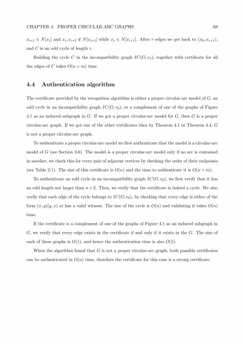
CHAPTER 4. PROPER CIRCULAR-ARC GRAPHS 68
xi+1 ∈ N [x1] and xi, xi+2 /∈ N [xi+1] while xj ∈ N [xi+1]. After r edges we get back to (x0, xr+1),
and C is an odd cycle of length r.
Building the cycle C in the incompatibility graph IC(G; x1), together with certificate for all
the edges of C takes O(n + m) time.
4.4 Authentication algorithm
The certificate provided by the recognition algorithm is either a proper circular-arc model of G, an
odd cycle in an incompatibility graph IC(G; v0), or a complement of one of the graphs of Figure
4.1 as an induced subgraph in G. If we got a proper circular-arc model for G, then G is a proper
circular-arc graph. If we got one of the other certificates then by Theorem 4.1 or Theorem 4.4, G
is not a proper circular-arc graph.
To authenticate a proper circular-arc model we first authenticate that the model is a circular-arc
model of G (see Section 3.6). The model is a proper circular-arc model only if no arc is contained
in another, we check this for every pair of adjacent vertices by checking the order of their endpoints
(see Table 2.1). The size of this certificate is O(n) and the time to authenticate it is O(n + m).
To authenticate an odd cycle in an incompatibility graph IC(G; v0), we first verify that it has
an odd length not larger than n + 2. Then, we verify that the certificate is indeed a cycle. We also
verify that each edge of the cycle belongs to IC(G; v0), by checking that every edge is either of the
form (x, y)(y, x) or has a valid witness. The size of the cycle is O(n) and validating it takes O(n)
time.
If the certificate is a complement of one of the graphs of Figure 4.1 as an induced subgraph in
G, we verify that every edge exists in the certificate if and only if it exists in the G. The size of
each of these graphs is O(1), and hence the authentication time is also O(1).
When the algorithm found that G is not a proper circular-arc graph, both possible certificates
can be authenticated in O(n) time, therefore the certificate for this case is a strong certificate.

Chapter 5
Certifying Algorithm for Recognizing
Unit Circular-Arc Graphs
5.1 Characterization of unit circular-arc graphs
In this section we present the structure theorem of Tucker [Tuc74] for unit circular-arc graphs. We
also present a similar theorem that our algorithm uses. Note that every proper circular-arc graph
has a proper circular-arc model in which no pair of arcs covers the circle [Tuc74, Gol80], we discuss
this further in the next section, and assume that all models we work with here satisfy this property.
Let G be a proper circular-arc graph with a proper circular-arc model %. First we define two types
of sets of vertices in a proper circular-arc graph.
Let C = (x0, . . . , xs−1) be a simple cycle in G, such that for i = 1, . . . , s− 1, the arc xi overlaps
x0
x1
x2
x3
x4
(a) Bounding cycle
y0
y1
y2
y3
y4
(b) Bounding co-cycle
Figure 5.1: Bounding cycle and bounding co-cycle, both with ratio 5/2.
69

CHAPTER 5. UNIT CIRCULAR-ARC GRAPHS 70
the right side of xi−1, and the arc x0 overlaps the right side of xs−1, in %. We call such a cycle C,
a bounding cycle. Assume that we traverse the cyclic list of endpoints of %, starting immediately
after `(x0), going right to r(x0) and continuing from r(xi) to r(xi+1) until we get to r(xs−1). We
call the list of endpoints that we encounter in this traversal the walk of C. The number of times
that C goes around the circle is the number of times that the walk of C hits `(x0), we denote this
number by w(C). The ratio of C, denoted by p(C), is |C|/w(C). (See Figure 5.1(a)). We call Cm
a minimum bounding cycle if there is no other bounding cycle C with p(C) < p(Cm). We denote
the ratio of a minimum bounding cycle by p(Cm). If the union of the arcs in % does not cover the
circle, then there are no bounding cycles. In this case, we let p(Cm) = ∞.
Let I = (y0, . . . , yt−1) be a simple co-cycle in G. We call I a bounding co-cycle. We define the
walk of I as we defined it for bounding cycles. To compute w(I), the number of times that I goes
around the circle, we add 1 to the number of times that the walk of I hit `(y0), to count also the
last partial turn. The ratio of I, denoted by p(I), is |I|/w(I). (See Figure 5.1(b)). We call IM a
maximum bounding co-cycle if there is no other bounding co-cycle I with p(I) > p(IM ). We denote
the ratio of a maximum bounding co-cycle by p(IM ).
The circumference of a unit circular-arc model of closed arcs with a bounding cycle C can be
at most p(C). On the other hand, the circumference of a unit circular-arc model with a bounding
co-cycle I must be strictly greater than p(I). So for any unit circular-arc model p(IM ) < p(Cm).
The following theorem shows that this condition is also sufficient. Furthermore, the bounds do not
depend on the specific model.
Theorem 5.1. [Tuc74] Let G be a proper circular-arc graph. If there exists a proper circular-arc
model of G with no pair of arcs that covers the circle, such that p(IM ) < p(Cm), then G is a unit
circular-arc graph. If G is a unit circular-arc graph, then in every proper circular-arc model of G
with no pair of arcs that covers the circle, p(IM ) < p(Cm).
The following lemma tells us about the structure of a minimum bounding cycle and a maximum
bounding co-cycle if G is a proper circular-arc graph but not a unit circular-arc graph.
Lemma 5.2. [Tuc74] Let G be a proper circular-arc graph. Let Cm be a minimum bounding cycle
and let IM be a maximum bounding co-cycle in a proper circular-arc model of G with no pair of
arcs that covers the circle. If p(IM ) ≥ p(Cm) then p(IM ) = p(Cm), |IM | = |Cm|, and also Cm and

CHAPTER 5. UNIT CIRCULAR-ARC GRAPHS 71
IM do not share a common vertex.
Given a proper circular-arc model %, the algorithm of Duran et al. [DGM+06] finds minimum
bounding cycles and maximum bounding co-cycles that begin with every arc in the model. To do
so in linear time they use complicated data structures.
We relax the definitions of a bounding cycle and a bounding co-cycle, in two ways, in order to
get a simple implementation. First, we allow repetitions of vertices. Second, we use paths instead
of cycles.
Let P = (x0, . . . , xs−1) be a path of vertices in G, not necessarily simple, such that for i =
1, . . . , s − 1, the arc xi overlaps the right side of xi−1, in %. The path P is a bounding path. We
define the walk of P and count the number of times that P goes around the circle, denoted by
w(P ), in the same way as we do it for bounding cycles. The ratio of P is p(P ) = |P |/w(P ). Note
that since a bounding path is not necessarily a cycle, it might be that w(P ) = 0, in this case we
assume that p(P ) = ∞.
Let Q = (y0, . . . , yt−1) be a co-path of vertices in G, not necessarily simple. We call Q a
bounding co-path. We define the walk of Q and count the number of times that Q goes around the
circle, denoted by w(Q), in the same way as we do it for bounding co-cycles. The ratio of Q is
p(Q) = |Q|/w(Q).
As for bounding cycles and bounding co-cycles, the circumference of a unit circular-arc model
with a bounding path P , and a bounding co-path Q, can be at most p(P ) and must be strictly
greater than p(Q). So in any unit circular-arc model, for every bounding path P and bounding
co-path Q we have p(Q) < p(P ). The following theorem is analogous to Theorem 5.1.
Theorem 5.3. Let G be a proper circular-arc graph. If there exists a proper circular-arc model
of G with no pair of arcs that covers the circle, such that for every bounding path P and every
bounding co-path Q, p(Q) < p(P ), then G is a unit circular-arc graph. If G is a unit circular-arc
graph, then in every proper circular-arc model of G with no pair of arcs that covers the circle, for
every bounding path P and every bounding co-path Q, p(Q) < p(P ).
Proof. Let G be a proper circular-arc graph with a circular-arc model %. Assume that in % for
every bounding path P and bounding co-path Q, we have p(P ) < p(Q). Since minimum bounding

CHAPTER 5. UNIT CIRCULAR-ARC GRAPHS 72
cycle is also a bounding path and maximum bounding co-cycle is also a bounding co-path, we have
p(IM ) < p(Cm). So, by Theorem 5.1, G is a unit circular-arc graph.
Now assume that G is a unit circular-arc graph. For any proper circular-arc model % of G
without pair of arcs that covers the circle, there is a unit circular-arc model of G, with the same
order of the endpoints [Tuc74]. So every bounding path P and bounding co-path Q in % are also
a bounding path and a bounding co-path, respectively, in a unit circular-arc model of G, and
therefore p(Q) < p(P ).
5.2 Pairs of arcs that cover the circle
In the previous section we presented a characterization of unit circular-arc graphs that is defined
for proper circular-arc models with no pair of arcs that covers the circle. The following theorem
shows that this requirement is valid for any proper circular-arc graph.
Theorem 5.4. [Tuc74, Gol80] If G is a proper circular-arc graph, then G has a proper circular-arc
model in which no pair of arcs covers the circle.
Let x and y be a pair of arcs that covers the circle in %. Any arc in % that is disjoint from x
must be contained in y, but since % is a proper circular-arc model, there is no such arc. So every
arc in a pair that covers the circle represents a universal vertex in G.
Let u be a universal vertex in G. In any proper circular-arc model of G, every arc must either
cover `(u) or r(u). The vertices of the arcs that cover each of the endpoints of u defines a clique in
G. Therefore, G is co-bipartite.
In the algorithm of Chapter 4, if we receive as an input a co-bipartite graph G then we use the
algorithms of [HH04b] to construct a proper circular-arc model for it. The algorithm of [HH04b]
always builds a proper circular-arc model without a pair of arcs that covers the circle. Therefore,
our algorithm never constructs a model with a pair of arcs that covers the circle.
We can use the observation that every arc in a pair that covers the circle is a universal arc to
give a simple O(n) time algorithm to eliminate pairs of arcs that cover the circle in a given proper
circular-arc model. We go around the circle twice, in the left to right direction. In the first round,
we count the number of arcs that cover the starting point, this is the number of arcs for which
we traversed the right endpoint before the left endpoint. In the second round, we find the number

CHAPTER 5. UNIT CIRCULAR-ARC GRAPHS 73
of arcs that cover each endpoint. We maintain a counter of the open arcs. When we encounter a
left endpoint we increment the counter. When we encounter a right endpoint we decrement the
counter. Since any arc which is not a universal arc cannot cover the circle with another arc, the
sum of the values of the counter at the endpoints of an arc x is greater or equal to n − 1, if and
only if x is a universal arc. After we identified all the universal arcs, we pick an arbitrary universal
arc, and put all other universal arcs in the same place on the circle, with a slight shift.
5.2.1 Co-bipartite unit circular-arc graphs
From the discussion above we conclude that the class of co-bipartite proper circular-arc graphs is
equivalent to the class of co-bipartite unit circular-arc graph.
Theorem 5.5. A graph G is a co-bipartite proper circular-arc graph if and only if G is a co-bipartite
unit circular-arc graph.
Proof. Assume that G is a co-bipartite proper circular-arc graph. For any proper circular-arc model
of G, p(IM ) = 2. This is because we can traverse at most two disjoint arcs in any turn around the
circle. For any proper circular-arc model of G without pair of arcs that covers the circle, p(Cm) > 2,
such a model exists by Theorem 5.4. From Theorem 5.1 it follows that G is a co-bipartite unit
circular-arc graph.
Assume that G is a co-bipartite unit circular-arc graph. Since every unit circular-arc graph is
a proper circular-arc graph it follows that G is a proper circular-arc graph.
The class of the complements of co-bipartite proper circular-arc graphs is known to be equivalent
to many other well-known graph classes including bipartite permutation graphs, bipartite AT-free
graphs and bipartite trapezoid graphs (cf. [BLS99, Spi03]).
5.3 The algorithm
Every unit circular-arc graph is a proper circular-arc graph, so we start by testing whether G is
a proper circular-arc graph using the algorithm of Chapter 4. If G is not a proper circular-arc
graph then it is also not a unit circular-arc graph, and the algorithm of Chapter 4 certifies that.
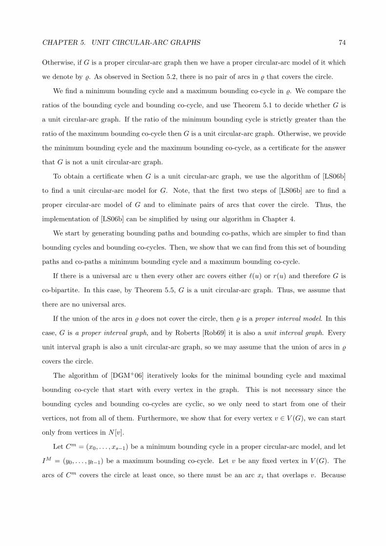
CHAPTER 5. UNIT CIRCULAR-ARC GRAPHS 74
Otherwise, if G is a proper circular-arc graph then we have a proper circular-arc model of it which
we denote by %. As observed in Section 5.2, there is no pair of arcs in % that covers the circle.
We find a minimum bounding cycle and a maximum bounding co-cycle in %. We compare the
ratios of the bounding cycle and bounding co-cycle, and use Theorem 5.1 to decide whether G is
a unit circular-arc graph. If the ratio of the minimum bounding cycle is strictly greater than the
ratio of the maximum bounding co-cycle then G is a unit circular-arc graph. Otherwise, we provide
the minimum bounding cycle and the maximum bounding co-cycle, as a certificate for the answer
that G is not a unit circular-arc graph.
To obtain a certificate when G is a unit circular-arc graph, we use the algorithm of [LS06b]
to find a unit circular-arc model for G. Note, that the first two steps of [LS06b] are to find a
proper circular-arc model of G and to eliminate pairs of arcs that cover the circle. Thus, the
implementation of [LS06b] can be simplified by using our algorithm in Chapter 4.
We start by generating bounding paths and bounding co-paths, which are simpler to find than
bounding cycles and bounding co-cycles. Then, we show that we can find from this set of bounding
paths and co-paths a minimum bounding cycle and a maximum bounding co-cycle.
If there is a universal arc u then every other arc covers either `(u) or r(u) and therefore G is
co-bipartite. In this case, by Theorem 5.5, G is a unit circular-arc graph. Thus, we assume that
there are no universal arcs.
If the union of the arcs in % does not cover the circle, then % is a proper interval model. In this
case, G is a proper interval graph, and by Roberts [Rob69] it is also a unit interval graph. Every
unit interval graph is also a unit circular-arc graph, so we may assume that the union of arcs in %
covers the circle.
The algorithm of [DGM+06] iteratively looks for the minimal bounding cycle and maximal
bounding co-cycle that start with every vertex in the graph. This is not necessary since the
bounding cycles and bounding co-cycles are cyclic, so we only need to start from one of their
vertices, not from all of them. Furthermore, we show that for every vertex v ∈ V (G), we can start
only from vertices in N [v].
Let Cm = (x0, . . . , xs−1) be a minimum bounding cycle in a proper circular-arc model, and let
IM = (y0, . . . , yt−1) be a maximum bounding co-cycle. Let v be any fixed vertex in V (G). The
arcs of Cm covers the circle at least once, so there must be an arc xi that overlaps v. Because

CHAPTER 5. UNIT CIRCULAR-ARC GRAPHS 75
Cm is a cycle, we may assume that xi is x0, hence, x0 ∈ N [v]. Assume that v is not adjacent to
every vertex of IM , we can add v to IM and get a bounding co-cycle I, with w(I) = w(IM ) and
|I| = |IM | + 1, and therefore p(I) > p(IM ), contradicting the fact that IM is maximum. Because
IM is a co-cycle, we may assume that y0 ∈ N [v].
For a particular vertex u, we find n bounding paths, of lengths 1 to n, each starting with the arc
u, using the following greedy algorithm. Let u0 = u. We start with P1 = (u0) as a bounding path
with w(P1) = 0. For i = 1, . . . , n−1, we generate Pi+1 = (u0, . . . , ui) by adding to Pi the vertex ui,
where `(ui) is the rightmost left endpoint covered by the arc ui−1. Such an endpoint `(ui) exists,
since otherwise the circle is not covered by the union of the arcs. We let w(Ci) = w(Ci−1)+1, if the
arc ui covers `(u0), and otherwise w(Ci) = w(Ci−1). We stop after generating Pn. We represent
the n bounding paths by the list of arcs in Pn and the list of the values w(Pi) for i = 1, . . . , n.
Similarly, we find n bounding co-paths, of lengths 1 to n, each starting with u, using the
following greedy algorithm. Let u0 = u. We start with Q1 = (u0) as a bounding co-path with
w(Q1) = 1. For i = 1, . . . , n − 1, we generate Qi+1 = (u0, . . . , ui) by adding to Qi the vertex ui,
where `(ui) is the leftmost left endpoint not covered by the arc ui−1. We know that ui−1 and ui
are not adjacent, since otherwise ui−1 would be a universal arc. We let w(Qi) = w(Qi−1)+1, if the
arc ui covers `(u0), and otherwise w(Qi) = w(Qi−1). We stop after generating Qn. We represent
the n bounding co-paths by the list of arcs in Qn and the list of the values w(Qi) for i = 1, . . . , n.
To implement these algorithms in O(n) time, we identify in advance, for every arc, the rightmost
left endpoint that it covers, and the leftmost left endpoint that it does not cover. We do so by
going around the circle from left to right, starting at some left endpoint, and maintaining `(x), the
last left endpoint we encountered. When we encounter a right endpoint r(y), the rightmost left
endpoint that the arc y covers is `(x). We can find the leftmost left endpoint following each arc in
the same way, by going around the circle from right to left.
Let v0 ∈ V (G) be a vertex with a minimum degree, so |N [v0]| = O(m/n). We find n bounding
paths and n bounding co-paths that start with each of the arcs of vertices in N [v0], by the greedy
algorithms described above. This takes O(n|N [v0]|) = O(n · m/n) = O(m) time and O(m) space.
We then find among the O(m) bounding paths, the bounding path Pm for which p(Pm) is the
smallest, if there is more than one bounding path with the same ratio we take the shortest. We
also find the bounding co-path QM for which p(QM ) is the largest, and if there is more than one

CHAPTER 5. UNIT CIRCULAR-ARC GRAPHS 76
bounding co-path with the same ratio we take the shortest.
Lemma 5.6. For the bounding path Pm and the bounding co-path QM that we have found, we have
p(Pm) ≤ p(Cm) and p(IM ) ≤ p(QM ).
Proof. Let Cm be a minimum bounding cycle, starting with x0 ∈ N [v0]. Let s = |Cm|, since Cm is
a simple cycle, s ≤ n. Let Ci be the prefix of Cm with |Ci| = i. The path Ci is a bounding path.
Let Pi be the bounding path of length i stating at x0 that our greedy algorithm found. We prove by
induction on i, that the walk of Ci is a prefix of the walk of Pi. It follows that for every i = 1, . . . , s,
we have w(Ci) ≤ w(Pi), and so p(Ci) ≤ p(Pi). In particular p(Cm) = p(Cs) ≥ p(Ps) ≥ p(Pm), as
required.
For i = 1, Ci = Pi, and thus the walks of C1 and P1 are identical. Assume that the walk of Ci
is prefix of the walk of Pi. To get Ci+1, we add to Ci a vertex xi such that the last occurrence of
`(xi) in the walk of Ci is not followed by an occurrence of r(xi). The walk of Ci+1 starts with the
walk of Ci and continues until r(xi). To get Pi+1, we add to Pi the vertex ui such that `(ui) is the
last left endpoint in the walk of Pi. The walk of Pi+1 starts with the walk of Pi and continues until
r(ui). Since by induction the walk of Ci is a prefix of the walk of Pi, the last occurrence of `(xi) in
the walk of Ci corresponds to an occurrence of `(xi) in the walk of Pi preceding or equal to the last
occurrence of `(ui) in the walk of Pi. Therefore the last occurrence of r(xi) in Ci+1 corresponds to
an occurrence of r(xi) in the walk of Pi+1 preceding or equal to the last occurrence of r(ui) in the
walk of Pi+1. Thus, the walk of Ci+1 is a prefix of the walk of Pi+1.
Let IM be a maximum bounding co-cycle starting with y0 ∈ N [v0]. Let t = |IM | and let Qt
be the bounding co-path of length t starting from y0 that our greedy algorithm found. We can
prove similarly by induction that the walk of Qt is a prefix of the walk of IM . Therefore, we have
p(IM ) ≤ p(Qt) ≤ p(QM ).
Lemma 5.7. For the bounding path Pm and the bounding co-path QM that we have found, Pm is
a minimum bounding cycle and QM is a maximum bounding co-cycle.
Proof. Let Pm = (x0, . . . xs−1) and let QM = (y0, . . . yt−1). By Lemma 5.6 it suffices to prove that
Pm is a simple path with its last arc xs−1 covers `(x0), and that QM is a simple co-cycle.
Assume that Pm is not a simple path. So, there is x ∈ V (G) such that xi = x and xj = x, but
i 6= j. Let j be the smallest index for which there exists an index i < j such that xi = xj . Let

CHAPTER 5. UNIT CIRCULAR-ARC GRAPHS 77
C = (xi+1, . . . , xj). The path C is simple by the way we chose xi and xj . Furthermore, C is a cycle
since xj = xi, and since C consists of vertices which are consecutive in Pm, it is a bounding cycle.
Let P = (x0, . . . , xi, xj+1, . . . xs−1) (if j = s − 1, then the last vertex of P would be xi), the path
obtained from Pm by taking out the vertices of C. The way that our greedy algorithm chooses
the successor of each vertex does not depend on its location along the path, so xj+1 = xi+1 and
P = (x0, . . . , x(s−1)−(j−i)). The value of w(P ) is the number of occurrences of `(x0) in the walk
of Pm that are not in the walk of C. The walk of C goes around the circle w(C) times starting
after `(xi+1) and ending at r(xj), so every endpoint appears w(C) times in this walk, except of the
endpoints that are after the last occurrence of `(xi+1) which appear w(C) + 1 times. The latter
endpoints are the endpoints that follow `(xi+1) and precede r(xj) = r(xi) when going right. By
the way that our greedy algorithm works, there are no such left endpoints, so the number of times
that the walk of C hits `(x0) is w(C). It follows that, w(P ) = w(Pm) − w(C). We also know that
|P | = |Pm| − |C|. By Lemma 5.6, we have p(C) ≥ p(Cm) ≥ p(Pm). Therefore, p(P ) ≤ p(Pm)
contradicting the definition of Pm, to be the shortest path with the maximal ratio that the greedy
algorithm found. Similarly, we can show that QM is a simple co-path.
We show that |Pm| > 1 and |QM | > 1, from this we conclude that x0 6= xs−1 and y0 6= yt−1.
Assume |Pm| = 1 then w(Pm) = 0 and thus p(Pm) = ∞. Because the union of the arcs in % covers
the circle, we have p(Cm) 6= ∞, and by Lemma 5.6, p(Pm) 6= ∞. We got a contradiction, therefore
|Pm| > 1. Since there are no universal vertices, there is a pair of vertices which are not adjacent.
This pair forms a bounding co-cycle with ratio 2, so we have 2 ≤ p(IM ) ≤ p(QM ), and therefore
|QM | > 1.
Now, assume that the arc xs−1 does not cover `(x0). In this case, the arc xs−1 does not start a
new turn of Pm around the circle. Let P be the prefix of Pm of length s − 1. We have |P | < |Pm|
but w(P ) = w(Pm) therefore p(P ) < p(Pm). That is a contradiction to the definition of Pm.
Assume that QM is not a co-cycle. It follows that the arc yt−1 overlaps y0 and thus covers
either `(y0) or r(y0). If the arc yt−1 covers r(y0) then yt−2 covers `(y0), because otherwise the
greedy algorithm would have chosen yt−1 to be y0. Since QM is a co-path but not a co-cycle then
|QM | > 2, let Q be the prefix of QM of length t − 2. Since there is one arc less in Q that covers
`(y0), we have w(Q) = w(QM )−1. And since p(QM ) ≥ 2 we have p(QM ) ≤ p(Q), which contradict
the way we define QM .
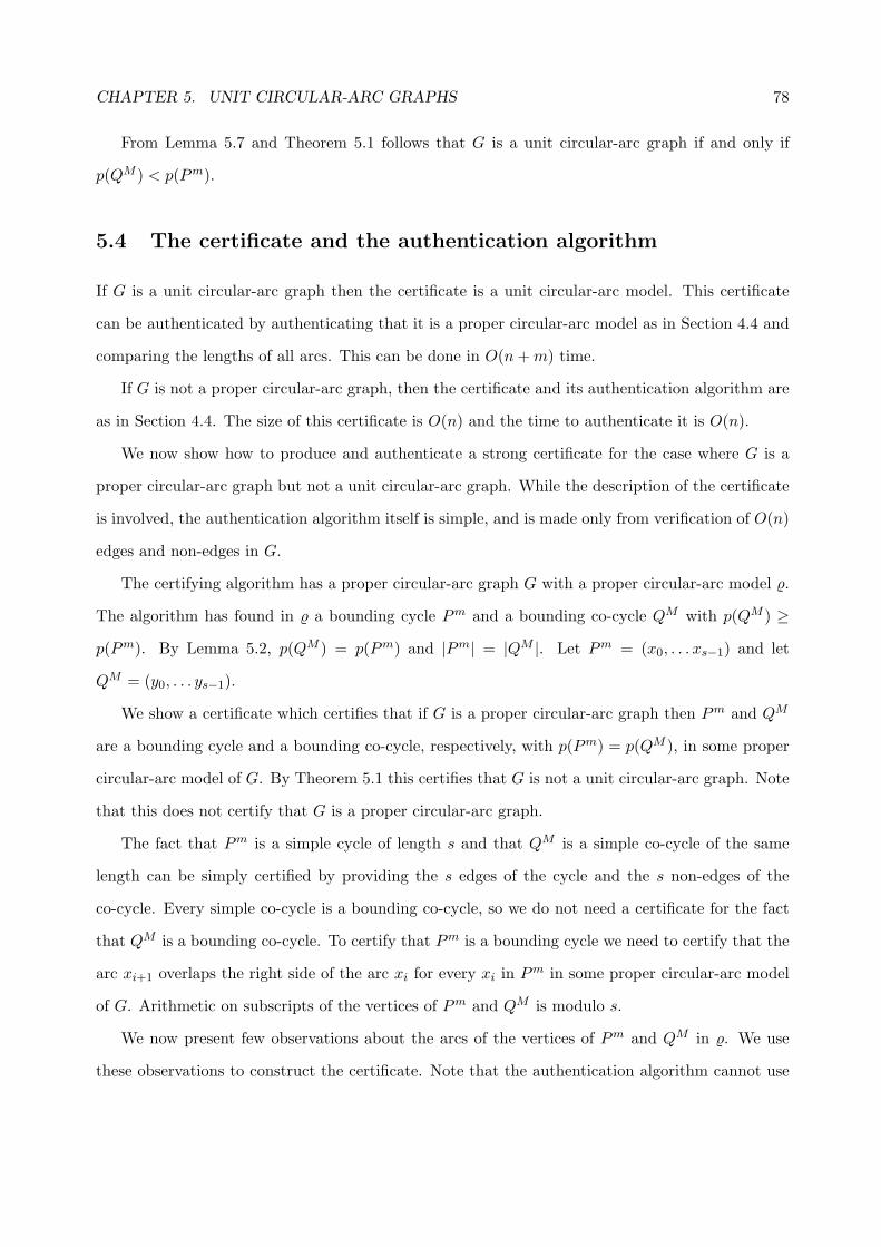
CHAPTER 5. UNIT CIRCULAR-ARC GRAPHS 78
From Lemma 5.7 and Theorem 5.1 follows that G is a unit circular-arc graph if and only if
p(QM ) < p(Pm).
5.4 The certificate and the authentication algorithm
If G is a unit circular-arc graph then the certificate is a unit circular-arc model. This certificate
can be authenticated by authenticating that it is a proper circular-arc model as in Section 4.4 and
comparing the lengths of all arcs. This can be done in O(n + m) time.
If G is not a proper circular-arc graph, then the certificate and its authentication algorithm are
as in Section 4.4. The size of this certificate is O(n) and the time to authenticate it is O(n).
We now show how to produce and authenticate a strong certificate for the case where G is a
proper circular-arc graph but not a unit circular-arc graph. While the description of the certificate
is involved, the authentication algorithm itself is simple, and is made only from verification of O(n)
edges and non-edges in G.
The certifying algorithm has a proper circular-arc graph G with a proper circular-arc model %.
The algorithm has found in % a bounding cycle Pm and a bounding co-cycle QM with p(QM ) ≥
p(Pm). By Lemma 5.2, p(QM ) = p(Pm) and |Pm| = |QM |. Let Pm = (x0, . . . xs−1) and let
QM = (y0, . . . ys−1).
We show a certificate which certifies that if G is a proper circular-arc graph then Pm and QM
are a bounding cycle and a bounding co-cycle, respectively, with p(Pm) = p(QM ), in some proper
circular-arc model of G. By Theorem 5.1 this certifies that G is not a unit circular-arc graph. Note
that this does not certify that G is a proper circular-arc graph.
The fact that Pm is a simple cycle of length s and that QM is a simple co-cycle of the same
length can be simply certified by providing the s edges of the cycle and the s non-edges of the
co-cycle. Every simple co-cycle is a bounding co-cycle, so we do not need a certificate for the fact
that QM is a bounding co-cycle. To certify that Pm is a bounding cycle we need to certify that the
arc xi+1 overlaps the right side of the arc xi for every xi in Pm in some proper circular-arc model
of G. Arithmetic on subscripts of the vertices of Pm and QM is modulo s.
We now present few observations about the arcs of the vertices of Pm and QM in %. We use
these observations to construct the certificate. Note that the authentication algorithm cannot use

CHAPTER 5. UNIT CIRCULAR-ARC GRAPHS 79
x0
x1x2
x3
y0
y1
y2
y3
Figure 5.2: A bounding cycle and a bonding co-cycle with the same ratio 4/1 in the same model.
these observations, since it does not have %, moreover, the authentication algorithm does not know
whether G is a proper circular-arc graph or not. An example of a bounding cycle and a bounding
co-cycle with the same ratio in the same model is illustrated in Figure 5.2.
Observation 5.8. For every arc xi of a vertex in Pm, there is an arc yj of a vertex in QM , such
that xi does not overlap yj.
Proof. Assume that xi overlaps all the arcs of the vertices of QM . Then, QM can be partitioned
into two cliques, one consisting of the vertices whose arcs cover `(xi) and the other consisting of the
vertices whose arcs cover r(xi). So every time the walk of QM go around the circle, it traverse at
most two arcs of QM , therefore p(QM ) = 2. On the other hand, there is no pair of arcs that covers
the circle, so p(Pm) > 2. We got a contradiction since p(QM ) = p(Pm), therefore there exists an
arc yj that does not overlap xi.
Observation 5.9. For every arc yj and two arcs xi and xi+1, if yj covers r(xi) then yj also covers
`(xi+1). Similarly, if yj covers `(xi+1) then yj also covers r(xi).
Proof. Both arcs yj and xi+1 covers r(xi), therefore the two arcs overlap each other. Assume yj
overlaps the right side of both xi and xi+1. In this case, we can replace xi+1 with yj in Pm and
get a minimum bounding cycle that shares a vertex with QM , contradicting Lemma 5.2. See for
example i = 0 and j = 0 in Figure 5.2. The second claim is proved symmetrically.
Observation 5.10. For every arc xi and two arcs yj and yj+1, if yj covers `(xi) then yj+1 covers
r(xi). Similarly, if yj+1 covers r(xi) then yj covers `(xi).

CHAPTER 5. UNIT CIRCULAR-ARC GRAPHS 80
Proof. Assume that xi does not intersect yj+1, then we can replace yj with xi in QM , contra-
dicting Lemma 5.2. See for example i = 0 and j = 3 in Figure 5.2. The second claim is proved
symmetrically.
Observation 5.11. The arc xi overlaps yj if and only if xi+1 overlaps yj+1.
Proof. Assume that the arc xi overlaps yj . If yj covers `(xi) then yj+1 covers r(xi) by Observation
5.10, and therefore yj+1 covers `(xi+1) by Observation 5.9. See for example i = 0 and j = 3 in
Figure 5.2. Otherwise, If yj covers r(xi) then yj covers `(xi+1) by Observation 5.9 and therefore
yj+1 covers r(xi+1) by Observation 5.10. See for example i = 0 and j = 0 in Figure 5.2. The other
direction is proved symmetrically.
Observation 5.12. For any arc xi, let yj be the first arc, to its right, which is disjoint from xi
out of the arcs of vertices of QM . Then, yj overlaps the right side of xi+1. Symmetrically, for any
arc xi, the rightmost arc, which is disjoint from xi, out of the arcs of vertices of QM , overlaps the
left side of xi−1.
Proof. Assume that yj is disjoint from, xi+1. Then, by Observation 5.11, the arc yj−1 does not
overlap xi. So, we can add xi to QM between yj−1 and yj , and get a bounding co-cycle with a
greater ratio, contradicting the fact that QM is maximum. See for example i = 0 and j = 1 in
Figure 5.2. The second claim is proved symmetrically.
Now we show how to construct the certificate for the fact that x2 overlaps the right side of x1.
Consider the arc x1 in %. This arc overlaps the right side of the arc x0. So, by Observation 5.8
and Observation 5.12 there is an arc yb which is disjoint from x0 and overlaps the right side of x1.
Also, by Observation 5.11 the arc yb+1 is disjoint from x1. Symmetrically, the arc x2 overlaps the
right side of x1, so, there is an arc ya such that ya is disjoint from x2 and overlaps the left side
of x1. Also, the arc ya−1 is disjoint from x1. Note that ya−1 and yb+1 may be the same arc. The
arcs x0 and ya cover the same endpoint of x1 so they overlap each other. So does x2 and yb. (See
Figure 5.3). We provide the vertices x0, x1, x2, ya, yb, ya−1, yb+1 and the edges between them as
a certificate that x2 overlaps the right side of x1.
If G is a proper circular-arc graph, then there must be a model of G where the arc x1 overlaps
the right side of the arc x0. Thus, the authentication algorithm can fix the direction in which the

CHAPTER 5. UNIT CIRCULAR-ARC GRAPHS 81
x1
x0 x2
ya yb
ya-1 yb+1
Figure 5.3: Arcs of the certificate for x2 overlaps the right side of x1.
x1
x0 ya
ya-1
(a) The union of x0 and ya must contain x1.
x1
x0 ya
x1
x2yb
(b) The union of x2 and yb also contains x1.
Figure 5.4: x1 overlaps the right side of both x0 and x2.
arc x1 overlaps the arc x0 to be right.
We now show how the authentication algorithm can verify that in a proper circular-arc model
of G in which the arc x1 overlaps the right side of the arc x0, it must be the case that the arc x2
overlaps the right side of x1, given the adjacencies between the set of vertices described above.
Assume for a contradiction that there is a proper circular-arc model in which x1 overlaps the
right side of both x0 and x2 (see Figure 5.4). In this model ya overlaps the right side of x1, since
ya and x2 are not adjacent. The arc yb also overlaps the right side of x1, since yb and x0 are not
adjacent. The arcs x0 and ya overlap each other, since the vertices x0 and ya are adjacent. The
arcs x0 and ya cover different endpoints of x1, so the union of these arcs either contains x1 or covers
the part of the circle that is not covered by x1. The arcs x1 and ya−1 are disjoint, so if the union of
the arcs x0 and ya cover the part of the circle that is not covered by x1, then this union contains
ya−1. The arc x0 cannot contain the arc ya−1, in addition ya and ya−1 are not adjacent. Therefore,
the union of the arcs x0 and ya cannot contain ya−1. So, the union of the arcs x0 and ya contains
the arc x1, and hence the common part of the arcs is covered by x1 (see Figure 5.4(a)). Similarly,
the vertices x2 and yb are adjacent. From this we get that the union of the arcs x2 and yb also
contains x1, since it cannot contain yb+1, and the common part of the arcs is covered by x1 (see
Figure 5.4(b)). Since x0 and ya are not adjacent to yb and x2 respectively, we get a contradiction.
Therefore, we verified that in a proper circular-arc model of G in which the arc x1 overlaps the
right side of the arc x0, it must be the case that the arc x2 overlaps the right side of x1.

CHAPTER 5. UNIT CIRCULAR-ARC GRAPHS 82
We can continue by induction and certify that if the arc xi+1 overlaps the right side of the arc
xi in a proper circular-arc model of G, then in the same model the arc xi+2 overlaps the right side
of xi+1. As a certificate we provide the vertices xi, xi+1, xi+2, ya+i, yb+i, ya−1+i, yb+1+i and the
edges between them.
We find ya and yb in O(n) time, and from them we find the rest of the vertices that are involved
in the certificate in O(n) time. For each xi we provide seven vertices and the edges between them
in the certificate, altogether we provide O(n) edges and non-edges. The entire certificate can be
constructed in O(n + m) time.
The authentication algorithm just verifies that every edge is indeed an edge and every non-edge
is indeed a non-edge. This takes O(n) time.
To complete the authentication, we need to show that p(Pm) = p(QM ), in some proper circular-
arc model of G. We show that the verification done so far by the authentication algorithm is
enough to verify this equality. By Lemma 5.2, we know that if G is a proper circular-arc graph
then p(Pm) ≤ p(QM ), so it is enough to verify that p(Pm) ≥ p(QM ). Since |Pm| = |QM |, it is
enough to verify that w(Pm) ≤ w(QM ). Since QM is a co-cycle, we may assume that its first vertex
is ya. For every i, it was verified that the arc ya+i overlaps the right side of xi and overlaps the
left side of xi+1. The walk of Pm starts after `(x0) and ends at r(xs−1). In this walk, the endpoint
r(ya+i) occurs between r(xi) and r(xi+1). The walk of QM starts after `(ya) and ends at r(ya−1).
These two walks have a common part that starts after `(ya) and ends at r(xs−1), let us denote
this common part by S. The number of times that `(x0) occurs in S is w(Pm), since the part of
the walk of Pm which is not in S is the beginning of the walk, up to the first occurrence of `(ya),
and this part is just after `(x0). The number of times that `(ya) occurs in S is w(QM ) − 1, since
the part of the walk of QM which is not in S is covered by ya−1 which is not adjacent to ya, as
was verified. The endpoints `(x0) and `(ya) occur at S alternately, therefore `(x0) appears at most
once more than `(ya). We got that w(Pm) ≤ w(QM ), as required.
When the algorithm found that G is not a unit circular-arc graph, all possible certificates can
be authenticated in O(n). Therefore, the certificate for this case is a strong certificate.

Chapter 6
Future Work
We presented in Chapter 3 a new linear-time algorithm for recognition circular-arc graphs. While
our circular-arc algorithm is simpler than the only previously known linear-time algorithm of Mc-
Connell [McC03], it is still involved. Our algorithm is based on the three stages of Tucker’s algorithm
[Tuc80], each performed separately. We can find similarities between the three stages, after finding
an odd length induced cycle in G, all three stages in a sense refine a partition of the vertices of G
(they are various forms of partition refinement, cf. [Spi03]). It might be possible to unify the three
stages, by defining a partition that can be found in a single step. This partition should be aware
of the type of intersections between arcs, much like the ∆ tree that is used for interval matrices
[McC03] and probe interval graphs [MS02]. The ∆ tree cannot deal with a set of arcs that cover
the circle, which makes it difficult to derive a simple algorithm for recognizing circular-arc graphs
that uses it.
A natural question that is left open is to find a certifying recognition algorithm for circular-arc
graphs. The only known characterizations of circular-arc graphs are these of Tucker [Tuc71] and
Gavril [Gav74], but it is not clear how to derive from these characterizations a certificate for a
graph which is not a circular-arc graph. So, the first step towards finding a certifying algorithm
for circular-arc graphs would be finding a new characterization of circular-arc graphs from which
we can derive a certificate when the graph is not a circular-arc graph.
For proper circular-arc graphs, our certificate for a graph that is not a proper circular-arc is
of one of two possible kinds. It is either a odd length cycle in the incompatibility graph, or an
induced subgraph of constant size. The characterizations that we use for proper circular-arc graphs,
83

CHAPTER 6. FUTURE WORK 84
Theorem 4.1 and Theorem 4.4, do not provide one simple condition that fits all graphs. However,
the characterization of Skrien [Skr82] and the characterization of Deng, Hell and Huang [DHH96] do
provide such a condition. It is an open question whether it is possible to derive a certifying algorithm
for proper circular-arc graph based on these or other characterizations that do not split into two
cases. The number of different kinds of certificates even increases for unit circular-arc graphs, which
is based on recognizing whether a proper circular-arc graph is a unit circular-arc graph, like other
characterizations and recognition algorithms for unit circular-arc graphs [Tuc74, DGM+06, LS06b].
For unit circular-arc graphs we use, in fact, two recognition algorithms, the algorithm of Lin and
Szwarcfiter [LS06b] and our algorithm in Chapter 5. The former is used to give a certificate when
the input graph is a unit circular-arc graph and the latter is used to give a certificate otherwise.
Therefore every unit circular-arc graph is recognized twice. It is an open problem to find one
algorithm that can provide both certificates.
Another important problem related to graph recognition is graph isomorphism. An O(mn)
graph isomorphism algorithm for circular-arc graphs was presented by Hsu [Hsu95]1. As suggested
by Eschen [Esc97], the recognition algorithm presented here may lead to a more efficient graph
isomorphism algorithm for circular-arc graphs. Eschen [Esc97] showed an O(n2) graph isomorphism
algorithm for co-bipartite circular-arc graphs. For the same reasons as in Chapter 3, this O(n2) time
bound is in fact linear in the size of the input graph. For proper circular-arc graphs, our algorithm
in Chapter 4 also may lead to a linear-time isomorphism algorithm. This algorithm requires an
isomorphism algorithm for the circular-ones property of the augmented adjacency matrices. Such
an isomorphism algorithm might be based on isomorphism of the PC-trees [HM03] of matrices,
similar to the isomorphism algorithm of PQ-trees [LB79].
1According to some sources [ES93, Hsu95, Esc97], Wu presented another algorithm, based on the recognitionalgorithm of Tucker [Tuc80], which we could not retrieve. Later, Eschen [Esc97] claimed to find a flaw in it.

Bibliography
[BL76] K. S. Booth and G. S. Lueker. Testing for the consecutive ones property, interval graphs,
and graph planarity using PQ-tree algorithms. J. Comput. Syst. Sci., 13(3):335–379,
1976.
[BLS99] A. Brandstadt, V. B. Le, and J. P. Spinrad. Graph Classes: A Survey. SIAM Mono-
graphs on Discrete Mathematics and Applications 3. SIAM, 1999.
[Bol78] B. Bollobas. Extremal Graph Theory. London Mathematical Society monographs 11.
Academic Press, 1978.
[CDS04] V. Conitzer, J. Derryberry, and T. Sandholm. Combinatorial auctions with structured
item graphs. In Proceedings of the Nineteenth National Conference on Artificial Intel-
ligence, pages 212–218, 2004.
[DGM+06] G. Duran, A. Gravano, R. M. McConnell, J. P. Spinrad, and A. Tucker. Polynomial
time recognition of unit circular-arc graphs. J. Algorithms, 58(1):67–78, 2006.
[DHH96] X. Deng, P. Hell, and J. Huang. Linear-time representation algorithms for proper
circular-arc graphs and proper interval graphs. SIAM J. Comput., 25(2):390–403, 1996.
[ES93] E. M. Eschen and J. P. Spinrad. An O(n2) algorithm for circular-arc graph recognition.
In SODA ’93: Proceedings of the fourth annual ACM-SIAM Symposium on Discrete
algorithms, pages 128–137, 1993.
[Esc97] E. M. Eschen. Circular-arc graph recognition and related problems. PhD thesis, De-
partment of Computer Science, Vanderbilt University, 1997.
85

BIBLIOGRAPHY 86
[Gav74] F. Gavril. Algorithms on circular-arc graphs. Networks, pages 357–369, 1974.
[Gol80] M. C. Golumbic. Algorithmic Graph Theory and Perfect Graphs. Academic Press, 1980.
[HDK64] H. Hadwiger, H. Debrunner, and V. Klee. Combinatorial geometry in the plane. Holt,
Rinehart & Winston, 1964.
[HH04a] P. Hell and J. Huang. Certifying LexBFS recognition algorithms for proper interval
graphs and proper interval bigraphs. SIAM J. Discrete Math., 18(3):554–570, 2004.
[HH04b] P. Hell and J. Huang. Interval bigraphs and circular arc graphs. J. Graph Theory,
46(4):313–327, 2004.
[HM03] W.-L. Hsu and R. M. McConnell. PC-trees and circular-ones arrangements. Theor.
Comput. Sci., 296(1):99–116, 2003.
[Hsu95] W.-L. Hsu. O(mn) algorithms for the recognition and isomorphism problems on
circular-arc graphs. SIAM J. Comput., 24(3):411–439, 1995.
[Kle69] V. Klee. What are the intersections graphs of arcs in a circle? Amer. Math. Monthly,
76(7):810–813, 1969.
[KMMS06] D. Kratsch, R. M. McConnell, K. Mehlhorn, and J. P. Spinrad. Certifying algorithms
for recognizing interval graphs and permutation graphs. SIAM J. Comput., 36(2):326–
353, 2006.
[KN06a] H. Kaplan and Y. Nussbaum. Certifying algorithms for recognizing proper circular-
arc graphs and unit circular-arc graphs. In Graph-Theoretic Concepts in Computer
Science: 32nd International Workshop WG 2006, Lecture Notes in Computer Science
4271, pages 289–300, 2006.
[KN06b] H. Kaplan and Y. Nussbaum. A simpler linear-time recognition of circular-arc graphs.
In 10th Scandinavian Workshop on Algorithm Theory (SWAT), Lecture Notes in Com-
puter Science 4059, pages 41–52, 2006.
[LB79] G. S. Lueker and K. S. Booth. A linear time algorithm for deciding interval graph
isomorphism. J. ACM, 26(2):183–195, 1979.

BIBLIOGRAPHY 87
[LS06a] M. C. Lin and J. L. Szwarcfiter. Characterizations and linear time recognition of
helly circular-arc graphs. In The Twelfth Annual International Computing and Com-
binatorics Conference (COCOON’06), Lecture Notes in Computer Science 4112, pages
73–82, 2006.
[LS06b] M. C. Lin and J. L. Szwarcfiter. Efficient construction of unit circular-arc models. In
SODA ’06: Proceedings of the seventeenth annual ACM-SIAM symposium on Discrete
algorithm, pages 309–315, 2006.
[McC03] R. M. McConnell. Linear-time recognition of circular-arc graphs. Algorithmica,
37(2):93–147, 2003.
[McC04] R. M. McConnell. A certifying algorithm for the consecutive-ones property. In SODA
’04: Proceedings of the fifteenth annual ACM-SIAM symposium on Discrete algorithms,
pages 768–777, 2004.
[Mei05] D. Meister. Recognition and computation of minimal triangulations for AT-free claw-
free and co-comparability graphs. Discrete Applied Math., 146(3):193–218, 2005.
[MN99] K. Mehlhorn and S. Naeher. The LEDA Platform for combinatorial and geometric
computing. Cambridge University Press, 1999.
[MS91] T.-H. Ma and J. P. Spinrad. Avoiding matrix multiplication. In Graph-Theoretic
Concepts in Computer Science: 16th International Workshop WG ’90, Lecture Notes
in Computer Science 484, pages 61–71, 1991.
[MS99] R. M. McConnell and J. P. Spinrad. Modular decomposition and transitive orientation.
Discrete Mathematics, 201(1-3):189–241, 1999.
[MS02] R. M. McConnell and J. P. Spinrad. Construction of probe interval models. In SODA
’02: Proceedings of the thirteenth annual ACM-SIAM symposium on Discrete algo-
rithms, pages 866–875, 2002.
[Mul97] H. Muller. Recognizing interval digraphs and interval bigraphs in poly-
nomial time. Discrete Applied Math., 78(1-3):189–205, 1997. Erratum,
http://www.comp.leeds.ac.uk/hm/patch.ps.

BIBLIOGRAPHY 88
[Rob69] F. S. Roberts. Indifference graphs. In Proof techniques in graph theory: proceedings of
the second Ann Arbor Conference, pages 139–146, 1969.
[SE04] S. Stefanakos and T. Erlebach. Routing in all-optical ring networks revisited. In
Proceedings of the 9th IEEE Symposium on Computers and Communication, pages
288–293, 2004.
[Skr82] D. J. Skrien. A relationship between triangulated graphs, comparability graphs, proper
interval graphs, proper circular-arc graphs, and nested interval graphs. J. Graph The-
ory, 6:309–316, 1982.
[Spi88] J. P. Spinrad. Circular-arc graphs with clique cover number two. Journal of Combina-
torial Theory Series B, 44(3):300–306, 1988.
[Spi03] J. P. Spinrad. Efficient Graph Representations. Fields Institute Monographs 19. Amer-
ican Mathematical Society, 2003.
[SV83] J. P. Spinrad and J. Valdes. Recognition and isomorphism of two dimensional partial
orders. In Automata, Languages and Programming, 10th Colloquium, Lecture Notes in
Computer Science 154, pages 676–686, 1983.
[Tuc71] A. Tucker. Matrix characterizations of circular-arc graphs. Pacific J. Math., 39(2):535–
545, 1971.
[Tuc74] A. Tucker. Structure theorems for some classes of circular-arc graphs. Discrete Math.,
7:167–195, 1974.
[Tuc80] A. C. Tucker. An efficient test for circular-arc graphs. SIAM J. Comput., 9(1):1–24,
1980.
[TY85] R. E. Tarjan and M. Yannakakis. Addendum: Simple linear-time algorithms to test
chordality of graphs, test acyclicity of hypergraphs, and selectively reduce acyclic hy-
pergraphs. SIAM J. Comput., 14(1):254–255, 1985.
(circular-arc graph)
(arcs)edge
model
proper circular-arc graph
unit circular-arc graph
(certifying algorithm)(certificate)
(authentication algorithm)
Eschen and SpinradES93, Esc97
Eschen and Spinrad
McConnellMcC03
normalized
TuckerTuc71, Tuc74

M.Sc.