Receiver Noise and Sensitivity

Abdul Rehman

Receiver Noise

• Optical receivers convert incident optical powerinto electric current through photodiode

• The relation I p = R ⋅ Pin assumes that such aconversion is noise free but this is not true evenfor a perfect receiver

• Two fundamental mechanisms are– Shot noise– Thermal noise

• This causes fluctuations in the current evenwhen the incident optical power has a constantpower. Additional noise is generated if inputpower is fluctating

PPhotocurrentt

average

I p = R ⋅ Pin

• This relation still holds good if we consider photocurrentas the average current

• Electrical noise induced by current fluctuations affectsthe receiver performance

4.4 RECEIVER NOISE

Shot noise

Thermal noise

I p = R ⋅ Pin

SNR4.4.1 Noise mechanisms4.4.1.1 Shot noise

Spectral Density: It is often called simply the spectrum of the signal. Intuitively, the spectral density captures the frequency content of a stochastic process and helps identify periodicities

Average current

−∞

∞

∫ )

Ip

Constant optical power

I (t ) = I p + i s (t )

I p = RPin

is(t)

stationary random process

Poisson statistics

Gaussian

Wiener-Khinchin theorem

i s (t )i s (t + τ) =

Autocorrelation function

S S (f e i 2 πfτdf

Spectral density

is(t)

t

Theory Of StochasticsProcess

In a stochastic or random process there is some indeterminacy in its future evolution described by probability distributions. This means that even if the initial condition (or starting point) is known, there are many possibilities the process might go to, but some paths may be more probable and others less so.

THEORY OF POISSONSTATISTICS

• A sequence of independent random events is onein which the occurrence of any event has no effecton the occurrence of any other. One example issimple radioac-tive decay such as the emission of

663 KeV photons by a sample of 137Cs. In contrast,the fissions of nuclei in a critical mass of 235U arecorrelated events in a ‘chain re- action" in whichthe outcome of each event, the number of neutronsreleased, affects the outcome of subsequent

Negative Frequency

The concept of negative frequency is purely mathematical. This can be easily proven by some simple trigonometric math. However in comms systems the 'negative' frequencies is simply copies of you signal symetric about the sampling frequency. Thus if you sample (for the carrier) at 433MHz and your data sits at 433.1MHz then you see an image at 432.9Mhz as well. If you move this to the 0Hz point negative frequencies needs to be used.

However, as mentioned negative frequency is not a physical phenomenan. Imagine a sime wave of -100Hz - I can't.

s s

White noise SS(f)Two-sided

qIp

f

One-sided

2qIp

fNoise variance τ=0

δ2 = i 2 (t ) =∞

∫ S s (f )df−∞

= 2qI p ∆f

HT (f )2

2 2

SS(f)

qIp

SS(f)

2qIp

−∆f ∆ff

0 ∆ff

effective noise bandwidth

At output of photodiode: bandwidth of photodiodeInput to decision circuit: bandwidth of receiver

Preamp Amp

One − sided

Photodiode Filter

S s (f ) = 2qI p HT (f )

σs

∞

= ∫ 2qI p HT (f )0

df∞

= 2qI p ∫ HT0

(f ) 2 df

⇒ ⎬ dark current

s

∆fd ∞

= ∫ HT0

(f ) 2 df

Stray light ⎫

Thermal generation ⎭(also shot noise )

σ 2 = 2q (I p + I d )∆fcan be reduced bylow pass filter

4.4.1.2 Thermal noiseRandom thermal motion of electrons in RL

IT(t)

Ip is iT CT RL

2

2

∆

2

Thermal noiseI (t ) = I p + I s (t ) + I t (t )

thermal

iT(t): stationary Gaussian random processflat up to ∼ 1THz

ST (f ) =2k BT

RL

(Two − sided ) kB=1,38⋅10-23 J/K

σT = i T2 (t ) =∞

∫ S T (f )df−∞

=∆f

−∫f

2k BTR L

df =4k BT ⋅ ∆fR L

σT independent of I p

∆f =∞

∫ HT (f )0

df

σT =

i s (t ) ⎫

iT (t )⎭

2 2 2

Also thermal noise from pre-ampfield effectbipolar

Amplifier noise figure2 4k BTFn ∆f

R L

⎬ : independent random processes (Gaussian )

Total variance

σ = σ s + σT = 2q (I p + I d )∆f +4k BTFn ∆f

R L

2I p

σ

=

4.4.2 p-i-n ReceiversSNR

Neglect CT:

Ip is iT RL

SNR = 2 =

Thermal limit

R 2Pin2

2q (RPin + I d ) ∆ f +4 k BTFn ∆fRL

SNR ≈ R 2Pin2

4k BTFn ∆ fRL

R 2Pin2R L

4k BTFn ∆ fSNR ∝ Piin2

SNR ∝ R L (C L neglected )

=

2

NEP: Noise Equivalent Power

RLR 2Pin2

4k BTFn ∆f= 1

Pin2 4k BTFn

∆f RLR 2

NEP =Pin

∆f=4k BTFn

RLR 2

=hν

ηq4k BTFn

RL

Pin = NEP ⋅ ∆f

Shot noise limit σs>>σT

σ s = 2q (I p + I d )∆f = 2q (RPin + I d ) ∆ f

Increases linearly with Pin

Obtained for large Pin

Id neglected

ηq

=

thttdw'(==)1p

d

h'(t=)1

∞

hdTT==

−∫

−

−

SNR ≅ R 2Pin2

2qRPin ∆ f= RPin

2q ∆ f= hν Pin

2q ∆ f

ηPin

2hν∆f Shot noise limit SNR ∝ Pin

E p = Pin TB

E p = Area in a bit

E p

E p

= PinT B =

= N p hν

Pin

B

Pin = BE p = BN p hν

∆f =B

2(Nyquist )

Piin= 2∆f ⋅ N p hν

SNR ≅η ⋅ 2∆f ⋅ N p hν2hν∆f

= ηN p Shot noise limit

η 1≅

Np=100SNR=100

SNRdB=10log10SNR=10⋅log100 dB=20dB

Thermal noise dominates Np≈1000

2

⎛⎟

s

4.4.3 APD Receivers

Higher SNR (for same Pin)

Ip=MRPin=RAPD ⋅Pin

Also multiplication noiseThermal noise the sameShot noise changes due to multiplicationM is a random variable

p − i − n diode

APDExcess noise factor

F A = k A M + (1 − k A ) ⎜ 2 −⎝

σ 2 = 2q (RPin + I d )∆f

σ s = 2qM 2F A (RPin + I d )∆f

1 ⎞

M ⎠

Electrons initiate and

Holes initiate and

αe > αh

αh > αe

k A =

k A =

αh

αe

αe

αh

2

2 2

2

2

k A = 0

k A = 1

F A = 2 −

F A = M

1M

Fig. 4.14

Small kA best

SNR = I p

σ s + σT

= (MRPiin )2qM F A (RPin + I d )∆f+ 4k BTFn ∆f

RL

=

2 =

ηq

Thermal noise limit

SNR ≅M 2R 2Pin2

4 k BTFn ∆fRL

RLR 2

4k BTFn ∆fM 2Pin2

improved by M 2

Shot noise limit

SNR ≅ M 2R 2Pin2

2qM F ARPin ∆fRPin

2qF A ∆f

= hν Pin

2qF A ∆f= ηPin

2hνF A ∆f

reduced by F A

There is optimum Mopt that maximizes SNR

22

⎡ ⎛2

⎝⎣

⎞⎤

⎠⎦

3 2 2 2

B [k M + (1 − k )(2M − M )]+ C

SNR =

dSNRdM

A

2

SNR = M (RPin )

2q (RPin + I d )∆f ⋅ M ⎢k A M + (1 − k A ) ⎜ 2 −1

M ⎥ +4 k BTFn ∆f

RL

AM 2

B [k AM 3 + (1 − k A )(2M 2 − M )]+ C= B [k AM + (1 − k A )(2M − M )]+ C 2AM − AM B [3k AM2 + (1 − k A )(4M − 1)] = 0

3 2A A

B [kM 3 + (1 − k A )(2M 2 − M )] + C 2 − MB [3k A M 2 + (1 − k A )(4M − 1)] = 0

M 3 (Bk A − B 3k A ) + M 2 [B (1 − k A )4 − B (1 − k A )4] + M [− B (1 − k A )2 + B (1 − k A )] + 2C = 0

Bk A M 3 + B (1 − k A )M − 2C = 0

3 RL=k A M + (1 − k A )M =2C

B

2 4k BTFn ∆f

2q (RPin + I d )∆f

= 4k BTFn

qRL (RPin + I d)

1.55 µm

APD receiver:

RL=1kΩ

Fn=2

R=1A/W

Id=2nA

Fig. 4.15 Pin (dBm)

⎛ 4k BTFn ⎞= ⎜

13

⎠⎝

Neglect (1-kA)M:

M opt ⎜ k AqRL (RPin + I d ) ⎟

critical

Si APD:GaInAs APD:

kA<<1kA ≈0,7

Mopt≈100Mopt ≈10

4.5 RECEIVER SENSITIVITY

BERBER ≤ 10−9

Sensitivity : Prec ⇒ BER = 10− 9

4.5.1 Bit-Error Rate

PDF ! !

12

12

I>IDI<ID

⇒⇒

bit 1bit 0

I<IDI>ID

for bit 1⇒for bit 0⇒

errorerror

p(1):p(0):

probability of receiving 1probability of receiving 0

P(0/1): probability of deciding 0 when 1 is receivedP(1/0): probability of deciding 1 when 0 is received

BER = p (1) ⋅ P (0 / 1) + p (0) ⋅ P (1 / 0)

p (1) = p (0) =

BER = [P (0 / 1) + P (1 / 0)]Thermal noise: Gaussian, zero mean, variance σT2

2APD :s

2s

2

0

2

∫

D

0

Shot noise:

p − i − n : Gaussian , zero mean ,

Gaussian ?, zero mean ,

σ2 = 2q (I p + I d )∆f

σs = 2qM 2F A (RPin + I d )∆f

σ2 = σT + σ2

bit 1 and 0 have different average value and variance

bit − 1 :

bit − 0 :

σ1

σ2

P (0 / 1) =I D

−∞ σ1

1

2πe

−(I −I 1 )2

2σ1dI

P (1 / 0) =∞

I∫ σ0

1

2πe

−(I −I 0 )2

2 σ2dI

= ⋅1 22

1

P (0 / 1) =

I D − I12σ1

∫−∞

1

σ1 2πe−y 2

2σ1dy

1 2

2 π

I D − I12σ1

∫ e−∞

−y dy = ⋅2 π

∞

∫ eI1 − I D

2σ1

−y 2dy

= erfc2

I 1 −I D

2σ1

y =I − I 0

2σ0

dy =dI

2σ0

∞

∫

[1 I 1 −I 0

4]

P (1 / 0) =∞

∫I D − I 0

2σ 0

1

σ 0 2πe−y 2

2σ 0dy

1 2 −y 2 1= ⋅ e dy = erfc2 π I D − I 0 2

2σ 0

BER = erfc + erfc2σ1

I D −I 0

2σ 0

I D −I 0

2σ0

12

20

σ0

σ1

P(0/1)I0 ID I1

P(1/0)

minimum for:

BER = [P (0 / 1) + P (1 / 0)]

1

σ0 2πe

−(I D −I 0 )2

2 σ2=1

σ1 2πe

−(I D −I 1 )2

2 σ1

2 2

=2 2

=2 2 ≈ 2

+ ln σ0 +(I D − I 0 )2

2σ0= + ln σ1 +

(I D − I 1 )2

2σ1

(I D − I 0 )2 (I 1 − I D )2

2σ0 2σ1+ ln σ1 − ln σ0

(I D − I 0 )2 (I 1 − I D )2

σ0 σ1

+ 2 lnσ1 (I 1 − I D )2

σ0 σ1

I 1 − I D

σ1

=I D − I 0

σ0

= Q

σ0I 1 − σ0I D = σ1I D − σ1I 0

σ0I 1 + σ1I 0 = I D (σ0 + σ1 )

I D =

=

1 ⎡

4 ⎣ ⎦

σ 0I 1 + σ 1I 0

σ 0 + σ 1

σ1 =σ0 ⇒ I D =σ0 I 1 +σ0 I 0 I 1 + I 0

2σ0 2

For I 1 − I D

σ1

=I D − I 0

σ0

= Q

Holds for p-i-n receivers, where σT2>>σS2

BER = ⎢erfcQ

2+ erfc

Q ⎤ 1

2 = ⎥ 2 erfcQ

2

Q =I 1 − I D

σ1

=I 1 −σ0I 1 + σ1I 0

σ0 + σ1

σ1

=σ0I 1 + σ1I 1 − σ0I 1 − σ1I 0

σ1 (σ0 + σ1 )

= I 1 − I 0

σ1 + σ0

1 Q 1

erfc ≅1

x πe− x 2 x >> 1

BER = erfc2

≈ ⋅2 2 Q

2

1

πe

−Q 2

2

=1

2πQe

−Q 2

2

Reasonable for Q>3

Q = 6 ⇒ BER ≈ 10−9

1 1

2 2 2

2 2

2

2

2 2

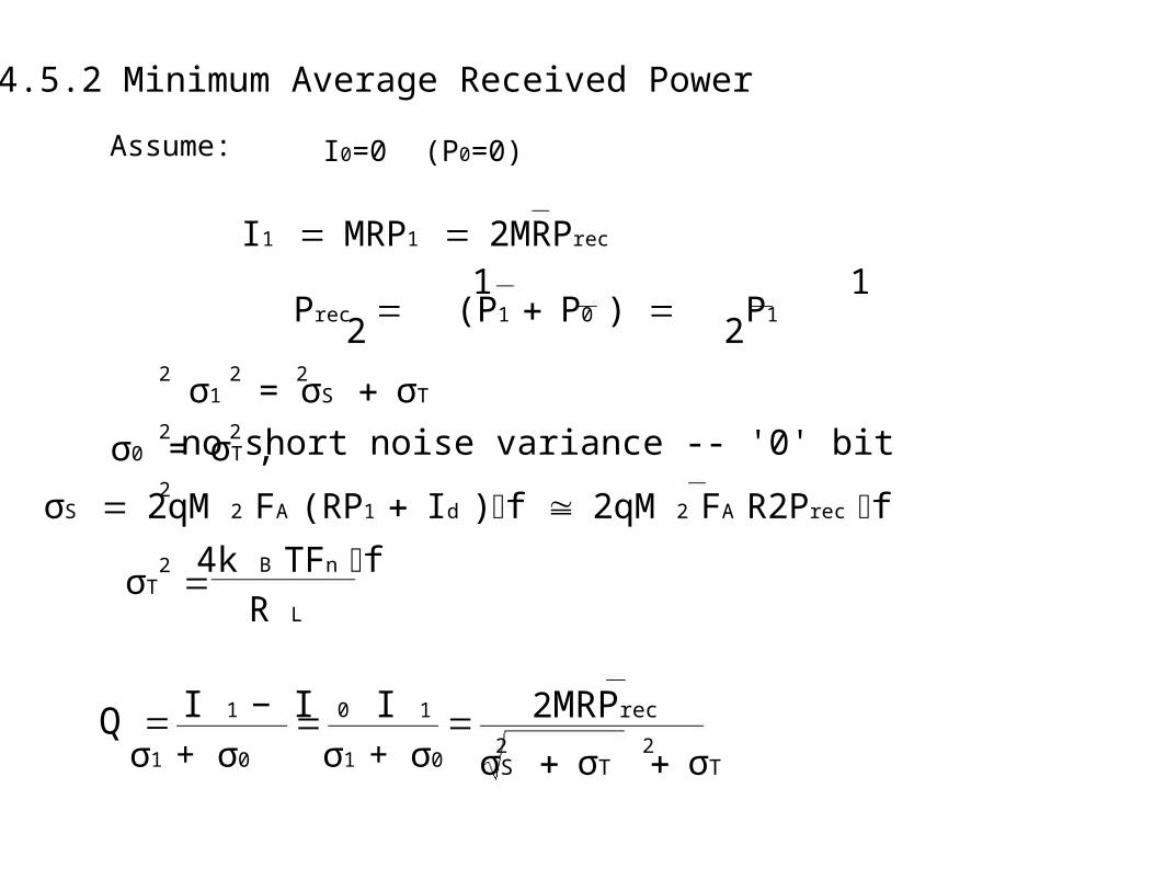
4.5.2 Minimum Average Received Power

Assume: I0=0 (P0=0)

I1 = MRP1 = 2MRPrec

Prec = (P1 + P0 ) = P12 2

σ1 = σS + σT

σ0 = σT , no short noise variance -- '0' bit

σS = 2qM 2 FA (RP1 + Id )∆f ≅ 2qM 2 FA R2Prec ∆f

σT =4k B TFn ∆f

R L

Q = I 1 − I 0

σ1 + σ0

= I 1

σ1 + σ0

= 2MRPrec

σS + σT + σT

1

2

2

2

⎛ 2MRPrec ⎞2 2

⎜ Q2

2

22

2

BER = erfc2

Q2

BER ⇒ Q ⇒ Prec

Q σ S + σT2 + Q ⋅ σT = 2MRPrec

Q σ S + σT2 = 2MRPrec − Q ⋅ σT

σ S + σT2 =2MRPrec

Q− σT

σ S + σT = ⎜ ⎝ ⎠

+ σT −4MRPrec σT

Q

2qM F AR 2Prec ∆f =4M 2R 2

QPrec −

4MRPrec σT

Q

2

⋅

Q ⎛R ⎝

σ ⎞

QR

MRQ

Prec = qMF A ∆f +σT

Q

Prec =Q 2

MRqMF A ∆f +

Q 2 σT

MR Q

Prec= ⎜QqFA ∆f+ T

M ⎠

p-i-n receiverM=1, σT dominates

Prec ≈ σT =Q

R4k BTFn ∆f

RL

∝ B

16

dBm

Q ⎛R ⎝

⎟

⎛ 1 ⎞

M ⎠

Numerical example R = 1 A /W

σT = 0,1 µAQ = 6 (BER = 10− 9 )

Prec ≈⋅ 0,1 ⋅ 10−6W = 0,6 µW

Prec = 10 log0,6 ⋅ 10−6

10−3dBm = 10 log 6 ⋅ 10−4 dBm

= −32,2 dBm

APD receiver:

Prec= ⎜QqF A ∆f +σT ⎞

M ⎠

If σT dominant ⇒ Prec reduced by factor MBut also shot noise contributes

F A = k AM + (1 − k A ) ⎜ 2 − ⎟⎝

⎟⎥ + ⎬⎝⎣

dPrec Q ⎧ ⎡ ⎛ 1 ⎞⎤ σT ⎫dM R ⎩ ⎝ M ⎠⎦ M ⎭⎣

2

2

2

⎣ ⎦

Prec =Q

R⎧⎨Qq∆f⎩

⎡ ⎛ 1⎢k AM + (1 − k A ) ⎜ 2 − M

⎞⎤ σT ⎫

⎠⎦ M ⎭

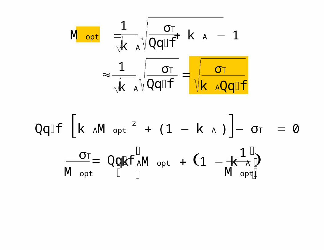
Optimum M

= ⎨Qq∆f ⎢k A + (1 − k A ) + ⎜ 2 − ⎟⎥ 2 = ⎬ 0

Qq∆f [k AM 2 + (1 − k A )] − σT = 0

k AM+ (1 − k A ) = σT

Qq∆f

k AM = σT

Qq∆f− (1 − k A )

M = 1 σ⎡ T ⎤k A ⎢Qq∆f + k A − 1⎥

2

⎡ ⎤⎥⎥⎦⎣

M opt =1

k A

σT

Qq∆f+ k A − 1

≈1

k A

σT

Qq∆f= σT

k AQq∆f

Qq∆f [k AM opt + (1 − k A )]− σT = 0

σT

M opt

= Qq∆f⎢k AM opt + (1 − k A )⎢

1

M opt

Q ⎧⎜

1 ⎞ ⎤ ⎡

M opt ⎟ ⎥Prec

⎩ ⎣ ⎢

⎪

⎥ ⎪

σM

Q ⎣ ⎦

= ⎣ ⎦

⎢⎣

=

Q

= ⎨Qq∆fR ⎪

⎡ ⎛ ⎢ k A M opt + (1 − k A ) ⎜ 2 − ⎢ ⎝

⎟ ⎥ + Qq∆f ⎢ k A M opt + (1 − k A ) ⎠ ⎦ ⎣

1 ⎤ ⎫ ⎥ ⎬

M opt ⎦ ⎭

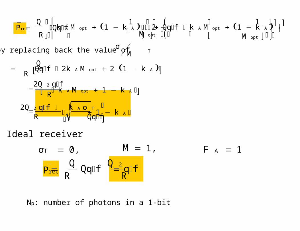
by replacing back the value of T

= Qq∆f ⎡ 2k A M opt + 2 (1 − k A )⎤R

2Q 2 q∆f

R ⎡ k A M opt + 1 − k A ⎤

2Q 2 q∆f ⎡ k A σ T

R Qq∆f

Ideal receiver

⎤+ 1 − k A ⎥

⎦

σT = 0, M = 1, F A = 1

Prec= Qq∆f =R

Q 2

Rq∆f

Np: number of photons in a 1-bit

=

2

Thermal noise limitσ0 = σ1

I 0 = 0

Q = I1 − I0 I1

σ1 + σ0 2σ1

SNR =I 12

σ1

= 4Q 2 BER = 10−9 ⇒ Q = 6

SNR = 4 ⋅ 36 = 144

SNRdB = 10 log144dB = 21,6dB

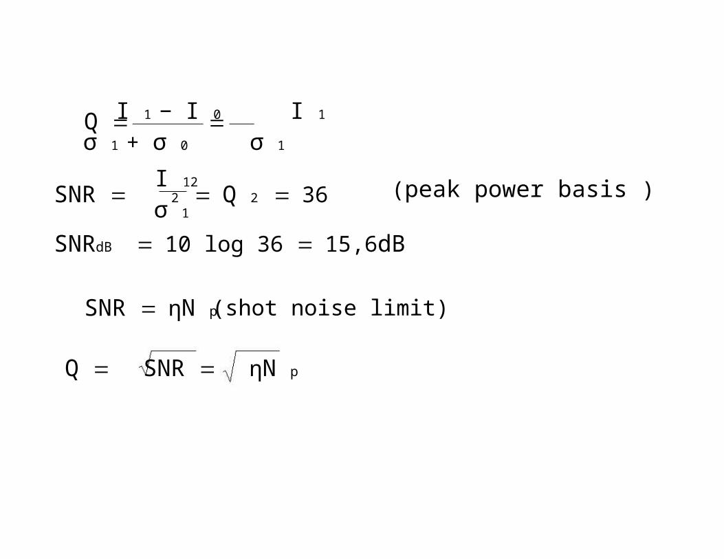
Shot noise limit

σ0 = 0

σ1 = σS

I 0 = 0

=

I 12

σ 1

Q = I 1 − I 0 I 1

σ 1 + σ 0 σ 1

SNR = 2 = Q 2 = 36

SNRdB = 10 log 36 = 15,6dB

(peak power basis )

SNR = ηN p (shot noise limit)

Q = SNR = ηN p

1 Q 1BER = erfc

2= erfc

2 2η = 1

ηN p

2

BER = 10− 9 or Q = 6

N p = Q 2 = 36

In practice Np≈1000, limited by thermal noise

1 ηN p

2144424443

m

12

4.5.3 Quantum Limit of Photodetection

BER = erfc

assumes Gaussian statistics

Shot noise limit

Small number of photons in a bitPoisson statisticsNp.: average number photons in a bit 1Probability of generating m electron-hole pairs

Pm =N p

m!e−N p

BER = [P (0 / 1) + P (1 / 0)]

0

1 −N p

1 −N p

P (1 / 0) = 0because N p = 0 for bit 0

P (0 / 1) =N p

0!e−N p= e−N p for bit 1

BER = e2

BER = e2

= 10−9

− ln 2 − N p = −9 ln10

N p = 9 ln10 − ln 2 = 20,03 ≈ 20

12

=

c 3 ⋅ 108 m s 3

Quantum limit: Each 1-bit must contain 20 photons:

P1 =N p hν

TB= N p hνB

Prec =P1 + P0

2= P1 =

N p

2hνB = N p hνB

N p =N p 20

2 2= 10 average number of photons per bit

Numerical example

λ = 1,55 µm

ν = = =λ 1,55 ⋅ 10−6 m 1,55

⋅ 1014 Hz

= 1,94 ⋅ 1014 Hz ≈ 2 ⋅ 1014 Hz = 200.000GHz= 200THz

hν = 6,626 ⋅ 10−34 Js ⋅ 1,94 ⋅ 1014 s −1 = 12,85 ⋅ 10−20 J

= 1,285 ⋅ 10−19 J

−3

B = 1Gbit / s

Prec = 10 ⋅ 1,285 ⋅ 10−19 ⋅ 109W = 1,285 ⋅ 10−9W

Prec ,dBm= 10 log1,285 ⋅ 10−9

10dBm = −58,9dBm

In practice:20dB more power is required10⋅100=1000 photons per bit

4.6 RECEIVER DEGRADATION

So far: Noise only degrading mechanismIdeal sensitivityPractice: More power needed. Power penalty!Several sources:Extinction ratio

Intensity noise (in transmitter)Timing jitter

4.6.1 Extinction Ratio

Energy carried by 0-bitsLaser biased above threshold P0>0

rex =P0

P1

P1

P0

1 0 1 1

Prec =

Q = =

⋅=

Find power penalty

Q = I 1 − I 0

σ 1 + σ 0

I 1 = RP1

I 0 = RP0

P1 + P0

2

R (P1 − P0 ) (P1 − P0 ) R (P1 + P0 )σ1 + σ0 P1 + P0 σ1 + σ0

1 − rex R ⋅ 2Prec

1 + rex σ1 + σ0

⋅ = ⋅

Prec (rex ) = ⋅

σT QR

δex = =

p-i-n receiver: σ1 ≈ σ0 = σT

Q =1 − rex R ⋅ 2 ⋅ Prec 1 − rex RPrec

1 + rex 2σT 1 + rex σT

1 + rex σT Q1 − rex R

Prec (0) =

Prec (rex ) 1 + rex

Prec (0) 1 − rex

increases with rex

δex ,dB = 10 log1 + rex

1 − rex

dB Power penalty

Fig. 4.18

rex

Laser biased below threshold: rex≈0,05

δex ,dB= 10 log1 + 0,05

0,95dB = 0,43dB

Laser biased above threshold:δex,dB significant

APD receiver: Power penalty larger by factor of 2 for same rex

2s I

2

2

2

∞

rI2 ∫

4.6.2 Intensity noise

Assumption - optical power incident on the receiver does not fluctuate !

So far:Practice:

No intensity noiseIntensity noise causes current fluctuation extra noise

Simple approach:

σ 2 = σ 2 + σ T + σ 2

σI = R

d

rI =

∆Pin =

∆Pin

Pin

∆Pin

Pin⋅ RPin = rI RPin

∞

= ∫ RIN (f )df =−∞

1

2π −∞RIN (ω)dωRelative Intensity Noise

σ1 ⎫

σ0 ⎭

rI =1

SNR

Typically SNRdB>20dB SNR>100 rI<0,01

Q = I 1 − I 0

σ1 + σ0

reduced because ⎬increased because of σI

Q should be the sameincident power must be increased (i.e. power penalty)

Assume : I 0 = 0 ⇒ σ0 = σT

I 1 = RP1 = 2RPrec

2s I

s

2

4k BTFn ∆f 2 2 2

RL

Q = I 1 − I 0

σ1 + σ 0= 2RPrec

σ 2 + σT + σ 2 + σT

σ2 = 2qRP1 ∆f = 2qR 2Prec ∆f

σs = 2 qRPrec ∆f

σI = rI RPin = rI R 2Prec

σT =4k BTFn ∆f

RL

σT =

Q =

4k BTFn ∆fR L

4qRPrec ∆f +

2RPrec

+ rI R 4Prec +4k BTFn ∆fRL

2

2 2 ⎤2 2

2 2 2

2 2

2 2 2

[

Q 4qRPrec ∆f +4k BTFn ∆f

RL+ rI2R 2 4Prec

= 2RPrec − Q4k BTFn ∆f

RL

⎡Q ⎢4qRPrec ∆f +

⎣

4k BTFn ∆fRL

+ rI R 4Prec ⎥⎦

= 4R Prec + Q4k BTFn ∆f

RL− 4RPrec Q

Rk BTFn ∆fRL

Q q∆f + rI RPrec ] = RPrec − Q

Prec [R − Q rI R ] = Q q∆f + Q

4k BTFn ∆fRL

4k BTFn ∆fRL

+ Q 2q∆fQ

Q

=

Prec (rI ) =4k B Fn ∆f

RL

R (1 − rI2Q 2 )

Prec (0) =4k BTFn ∆f

RL

R

+ Q 2q∆f

Prec (rI ) 1Prec (0) 1 − rI2Q 2

δI ,dB= 10 logPrec (rI )Prec (0)= −10 log(1 − rI2Q 2 )

1 244 3for

Fig. 4.19

Intensity noise parameter rex

δI ,dB < 0,02dB rI < 0,01normal for transmitters

Intensity noise negligible for most digital receiversCan become limiting factor for analog systems

4.6.3 Timing jitter

Fig. 4.10

Timing jitter Fluctuation in signalTiming jitter as random variableSNR reduced Power penaltyAssume:

p-i-n receiverdominated by thermal noisezero extinction ratio

2j

∆ij:σj:

(t)

Q = I 1 − I 0

σ1 + σ0

=(I 1 − ∆i j ) − 0

σT + σ2 + σT

current fluctuation induced by timing jitterrms value of current fluctuation ∆ij

I1hout()

I1hout(0)

0 ∆t

I1hout(∆t)∆ij

4.7 RECEIVER PERFORMANCE

Receiver sensitivity , Prec : Power needed forBER = 10− 9

Fig. 4.21

Bit Rate (Gbit/s)Long sequence of pseudo-random bits (215-1)

Quantum limit

Prec = Ν p hνB = 10hνB

Practical receivers: 20dB worse than quantum limit

Most degradation due to thermal noise

Some degradation due to dispersion

degradation∝BL

Biterrate

rror

InGaAs APD1,3 µm8 Gbit/s

Fig. 4.22

1,5dB dispersion penalty

Received optical power (dBm)

5-6dB improvement with APD over p-i-n

InGaAs APD≈

Quantum limit ≈

Si APD ≈

1000 photons/bit

10 photons/bit

400 photons/bit, 0,8-0,9 µm

Eye diagram – simple way to monitor a system

1.55 µm2.5 Gbit/s

0 km

120 km

Fig. 4.23

So far: direct detection receiversCoherent detection (or heterodyne) receiverswithin 5dB of quantum limit

Received signal

LO laser

But optical preamplifiers also give good sensitivity

PDFA probability density function is any function f(x) thatdescribes the probability density in terms of the inputvariable x in a manner described below.• f(x) is greater than or equal to zero for all values of x• The total area under the graph is 1:

The actual probability can then be calculated by takingthe integral of the function f(x) by the integration intervaof the input variable x.For example: the variable x being within the interval 4.3< x < 7.8 would have the actual probability of