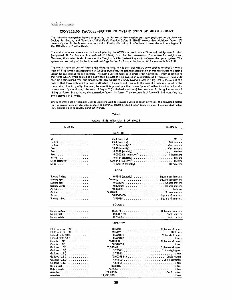
rec-erc-72-28 - bureau of reclamation · ms-230 (8-70) bureau of re clama tion technical report...

iJ

J

REC-ERC-72-28

John J. Cassidy Engineering and Research Center Bureau of Reclamation

September 1972

··;. '\ ~ .

MS-230 (8-70 ) Bureau o f R e clama tio n TECHNICAL REPORT STANDARD TITLE PAGE

1. REPORT NO .

REC-ERC-72-28 4. TITLE AND SUBTITLE

Control of Surging in Low-Pressure Pipelines

7. AUTHOR(S)

John J . Cassidy

9 . PERFORMING ORGANIZATION NAME AND ADDRESS

Engineering and Research Center Bureau of Reclamation Denver, Colorado 80225

12 . SPONSORING AGENCY NAME AND ADDRESS

Same

15 . SUPPLEMENTARY NOTES

16. ABSTRACT

3 . RECIPIENT'S CATALOG NO .

5 . REPORT DATE

Sep 72 6 . PERFORMING ORGANIZATION CODE

8 . PERFORMING ORGANIZATION REPORT NO.

REC-ERC-72-28

10 . WORK UNIT NO .

11. CONTRACT OR GRANT NO .

13 . TYPE OF REPORT AND PERIOD COVERED

14. SPO!'<SOR I NG AGENCY CODE

Review and analysis of available information regarding surging in low-pressure pipelines indicated that such lines, designed to operate with the hydraulic gradeline roughly parallel to the ground surface at design discharge, will undergo a fluid motion which is underdamped when operating at flow rates below the design value. An analytical study of the dynamics of surging flow enumerated the significant design and operation parameters. Numerical values of these parameters were obtained and are tabulated in the report. Through use of these tabulated values, low-pressure pipelines may be designed to minimize the amplitude of flow oscillations.

17 . KEY WORDS AND DOCUMENT ANALYSIS

a . DESCRIPTORS- - I *pipelines/ *surges/ closed conduit flow/ fluid flow/ fluid mechanics/ hydraulics/ oscillations/ *water pipes/ momentum

b . IDENT/F /£RS-- / *pipeline surges/ Canadian River Project, Tex

c . COSATI Field / Group Field/Group

18. DISTRIBUTION STATEMENT

Available from the Na t ional Technical /n(ornia t ion Serv i ce, Operations Division, Springfield , Virginia 22151 .

19 . SECURITY CLASS 21 . NO. OF PAGE (THIS REPORT)

UNCLASSIFIED 37

20 . SECURITY CLASS 22 . PRICE (THIS PAGE)

UNCLASSIFIED

REC-ERC-72-28

CONTROL OF SURGING IN LOW-PRESSURE PIPELINES

by John J. Cassidy

September 1972

Hydraulics Branch Division of General Research Engineering and Research Center Denver, Colorado

UNITED STATES DEPARTMENT OF THE INTERIOR Rogers C. B. Morton Secretary

* BUREAU OF RECLAMATION Ellis L. Armstrong Commissioner

ACKNOWLEDGMENT

This study was conducted by the writer, Professor of Civil Engineering at the University .of Missouri, while working as a Ford-Foundation Engineering Resident with the Hydraulics Branch, Division of General Research. All work was conducted using Bureau of Reclamation facilities.

Conversations with Messrs. C. C. Crawford, R. L. Vance, L. H. Burton, and D. F. Nelson of the Division of Design; and with D. Colgate, R. B. Dexter, and R. A. Dodge of the Division of General Research greatly aided in reviewing past work and in establishing objectives of this study.

Figure

10-11

12-13

14-15

16-17

18-19

20-21

22-23

24-25

26-27

CONTENTS-Continued

Dimensionless discharge variations as a function of dimensionless time . . . . . . . . . .



Range of dimensionless discharge as a function of the dimensionless discharge cutback ratio . . . . .

Range of dimensionless discharge as a function of the dimensionless discharge cutback ratio . . . . .

Range of dimensionless discharge as a function of the dimensionless discharge cutback ratio . . .

Surge amplitudes as a function of the resistance coefficient . . . . . . . . . . . .



ii

Page

15

16

17

18

19

20

21

22

23

Nomenclature Purpose Conclusions Applications Background Equations of Motion

Development Interpretation The Actual Surge Problem

Analysis

Stability Periodic Inflow Changes in Inflow Rate

Correlation With Field Experience

Previous Field Tests Canadian River Tests, 1968 Canadian River Tests, 1969

CONTENTS

Simultaneous Consideration of Several Reaches References . . . . . . . . . . . . . Appendix: Computer Programs . . . . . . Conversion Factors-British to Metric Units of Measurement

Table

I II

111

Figure

1 2 3

3a 4 5

6-7

8-9

LIST OF TABLES

Data on Canadian River pipes and structures Dimensionless discharge ratios from a surging model

pipeline . . . . . Canadian River surge data

LIST OF FIGURES

Typical pipe-check and pipe-stand structures Definition sketch for flow in a pipe reach Typical types of unsteady flow . . . . . Damped oscillations due to an oscillating inflow Magnitude of discharge surges . . . . . . Effect of resistance on the flow rate . . . . Dimensionless discharge variations as a function of

dimensionless time . . . . . . . . . . Dimensionless discharge variations as a function of

dimensionless time . . . . . . . . . .

Page

iii 1 1 1 1 2

2 3 5

5

5 6 7

10

10 10 10

11 12 27 39

4

7 11

1 2 6 6 7 8

13

14

Symbol

A123---D''

f F g

H

ht k

L123---Q''

t V X

Y1 Y1max

Y2 D.y I:K

'Y p

NOMENCLATURE

Cross-sectional areas Diameter

Definition

Darcy-Weisbach resistance coefficient Frequency Gravitational acceleration Total head Head loss Roughness height Pipe lengths Discharge Steady design discharge Final steady discharge Discharge entering a pipe reach Fluctuating discharge with period

TO superimposed on Qs Steady - state discharge Dimensionless resistance coefficient Distance along pipe centerline Natural period of reach Period of superimposed fluctuation

or period of first upstream reach Time Mean velocity Horizontal coordinate Depth of water at inlet Maximum possible value of Y1 Depth of water at outlet Y1 max -Y2 Combined resistance coefficient

(hL = ~K v2/2g) Specific weight Density

*M = mass; F = force; L = length; T = time

iii

Dimensions*

T-1

L/T2

L L L L L3/T L3/T L3/T L3/T L3/T

L3/T

L T T

T LIT L L L L L

flow rate was decreased to a final discharge substantially below the design value.

As a result of the experiences on the Coachella and Canadian Rivers, considerable study was initiated, some of which has already been noted, 1, 2, 3, 4 . This

study represents an attempt to analyze the problem

of unsteady flow in low-pressure pipe distribution

systems as a problem in dynamics. A review was made

of all available published and unpublished results in

order to arrive at representative system parameters and to isolate at least a portion of the problem which

had not been thoroughly studied. A summary of previous work is incorporated where the particular work seemed to fit into the current analysis best.

The results of the analysis are set forth in a form

which should be useful to designers interested in the

analysis of unsteady flow in a low-pressure pipe

distribution system.

All results have been computed and displayed in a dimensionless fashion in order to completely

generalize the analysis and results. The dimensionless

parameters have been defined and can readily be

computed from the dimensional properties normally

used by designers.

Not all possible combinations of parameters have

been included in these numerical results. However, a

listing of the program is included in the appendix and can readily be used to make further analyses as

required.

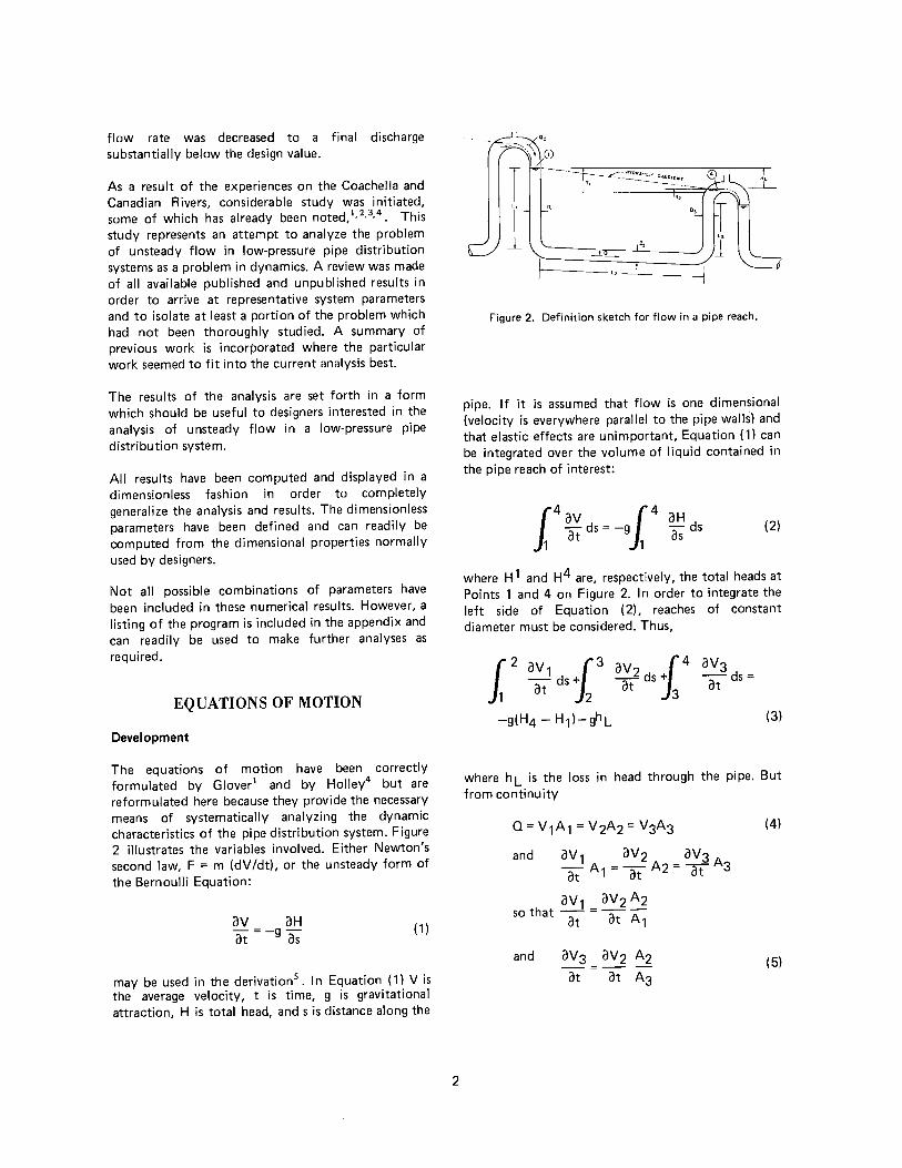
EQUATIONS OF MOTION

Development

The equations of motion have been correctly formulated by Glover1 and by Holley4 but are

reformulated here because they provide the necessary means of systematically analyzing the dynamic

characteristics of the pipe distribution system. Figure 2 illustrates the variables involved. Either Newton's second law, F = m (dV /dt), or the unsteady form of

the Bernoulli Equation:

(1)

may be used in the derivation 5 . In Equation (1) Vis the average velocity, t is time, g is gravitational

attraction, H is total head, and s is distance along the

2

Figure 2. Definition sketch for flow in a pipe reach.

pipe. If it is assumed that flow is one dimensional

(velocity is everywhere parallel to the pipe walls) and

that elastic effects are unimportant, Equation ( 1) can

be integrated over the volume of liquid contained in

the pipe reach of interest:

14 av ds = -g1,4 at 1

aH ds as

(2)

where H 1 and H4 are, respectively, the total heads at Points 1 and 4 on Figure 2. In order to integrate the

left side of Equation (2), reaches of constant

diameter must be considered. Thus,

_1 ds+ a/ ds + 12 av £3 av £4 at 2 3

-g(H4 - H1)-ghL

aV3 --ds= at

(3)

where h L is the loss in head through the pipe. But

from continuity

Q = V1A1 = V2A2 = V3A3

and av, av2 aV3 at A1 = at A2 = at A3

av 1 av2 A2 so that -- = ---

at at A1

and

(4)

(5)

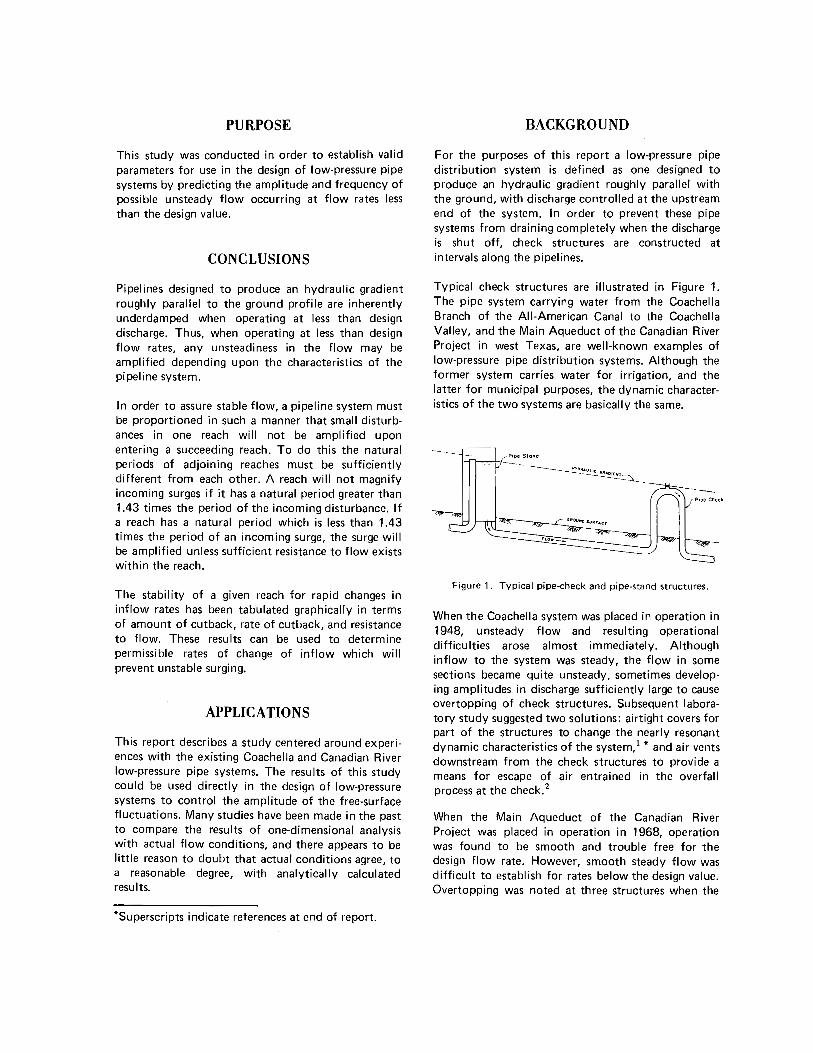
PURPOSE

This study was conducted in order to establish valid parameters for use in the design of low-pressure pipe systems by predicting the amplitude and frequency of possible unsteady flow occurring at flow rates less than the design value.

CONCLUSIONS

Pipelines designed to produce an hydraulic gradient roughly parallel to the ground profile are inherently underdamped when operating at less than design discharge. Thus, when operating at less than design flow rates, any unsteadiness in the flow may be amplified depending upon the characteristics of the pipeline system.

In order to assure stable flow, a pipeline system must be proportioned in such a manner that small disturbances in one reach will not be amplified upon entering a succeeding reach. To do this the natural periods of adjoining reaches must be sufficiently different from each other. A reach will not magnify incoming surges if it has a natural period greater than 1.43 times the period of the incoming disturbance. If a reach has a natural period which is less than 1.43 times the period of an incoming surge, the surge will be amplified unless sufficient resistance to flow exists within the reach.

The stability of a given reach for rapid changes in inflow rates has been tabulated graphically in terms of amount of cutback, rate of cutback, and resistance to flow. These results can be used to determine permissible rates of change of inflow which will prevent unstable surging.

APPLICATIONS

This report describes a study centered around experiences with the existing Coachella and Canadian River low-pressure pipe systems. The results of this study could be used directly in the design of low-pressure systems to control the amplitude of the free-surface fluctuations. Many studies have been made in the past to compare the results of one-dimensional analysis with actual flow conditions, and there appears to be little reason to doubt that actual conditions agree, to a reasonable degree, with analytically calculated results.

*Superscripts indicate references at end of report.

BACKGROUND

For the purposes of this report a low-pressure pipe distribution system is defined as one designed to produce an hydraulic gradient roughly parallel with the ground, with discharge controlled at the upstream end of the system. In order to prevent these pipe systems from draining completely when the discharge is shut off, check structures are constructed at intervals along the pipelines.

Typical check structures are illustrated in Figure 1. The pipe system carrying water from the Coachella Branch of the All-American Canal to the Coachella Valley, and the Main Aqueduct of the Canadian River Project in west Texas, are well-known examples of low-pressure pipe distribution systems. Although the former system carries water for irrigation, and the latter for municipal purposes, the dynamic characteristics of the two systems are basically the same.

Figure 1. Typical pipe-check and pipe-stand structures.

When the Coachella system was placed in operation in 1948, unsteady flow and resulting operational difficulties arose almost immediately. Although inflow to the system was steady, the flow in some sections became quite unsteady, sometimes developing amplitudes in discharge sufficiently large to cause overtopping of check structures. Subsequent laboratory study suggested two solutions: airtight covers for part of the structures to change the nearly resonant dynamic characteristics of the system, 1 * and air vents downstream from the check structures to provide a means for escape of air entrained in the overfall process at the check. 2

When the Main Aqueduct of the Canadian River Project was placed in operation in 1968, operation was found to be smooth and trouble free for the design flow rate. However, smooth steady flow was difficult to establish for rates below the design value. Overtopping was noted at three structures when the

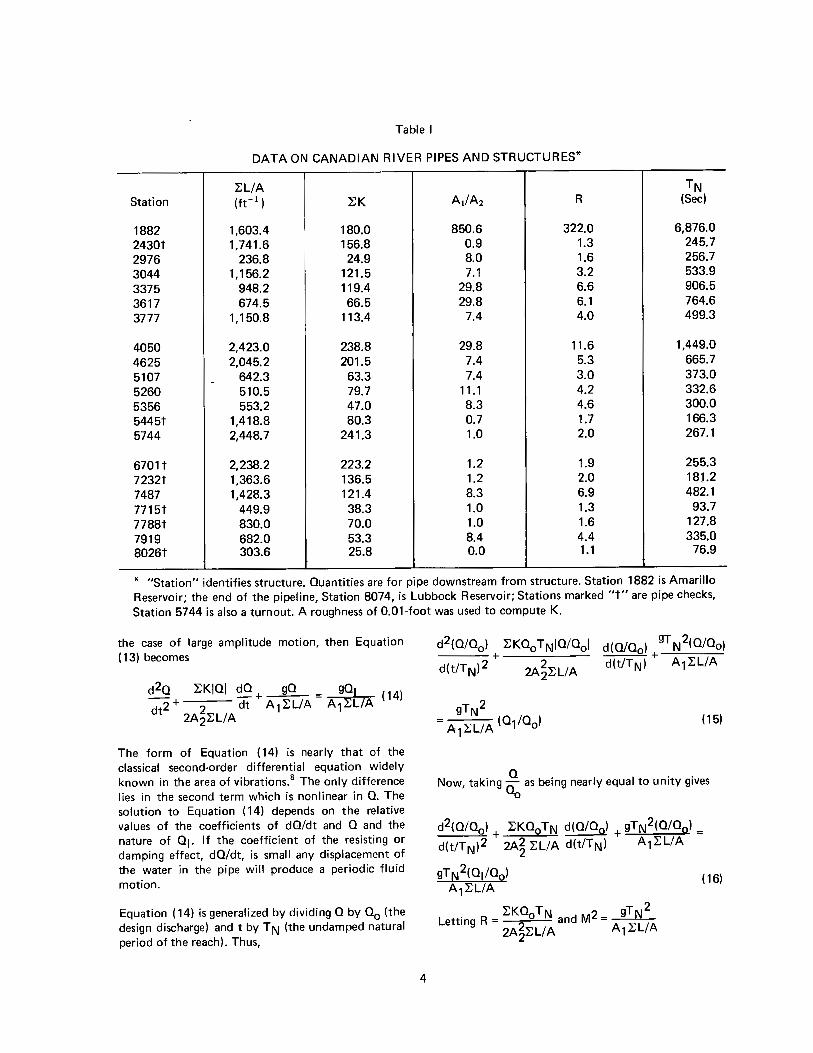
Table I

DATA ON CANADIAN RIVER PIPES AND STRUCTURES*

'E,L/A TN Station (ft- 1) 'E,K A1/A2 R (Sec)

1882 1,603.4 180.0 850.6 322.0 6,876.0

2430t 1,741.6 156.8 0.9 1.3 245.7

2976 236.8 24.9 8.0 1.6 256.7 3044 1,156.2 121.5 7.1 3.2 533.9

3375 948.2 119.4 29.8 6.6 906.5

3617 674.5 66.5 29.8 6.1 764.6

3777 1,150.8 113.4 7.4 4.0 499.3

4050 2,423.0 238.8 29.8 11.6 1,449.0

4625 2,045.2 201.5 7.4 5.3 665.7

5107 - 642.3 63.3 7.4 3.0 373.0

5260 510.5 79.7 11.1 4.2 332.6

5356 553.2 47.0 8.3 4.6 300.0

5445t 1,418.8 80.3 0.7 1.7 166.3

5744 2,448.7 241.3 1.0 2.0 267.1

6701t 2,238.2 223.2 1.2 1.9 255.3

7232t 1,363.6 136.5 1.2 2.0 18J.2

7487 1,428.3 121.4 8.3 6.9 482.1

7715t 449.9 38.3 1.0 1.3 93.7

7788t 830.0 70.0 1.0 1.6 127.8

7919 682.0 53.3 8.4 4.4 335.0 8026t 303.6 25.8 0.0 1.1 76.9

* "Station" identifies structure. Quantities are for pipe downstream from structure. Station 1882 is Amarillo

Reservoir; the end of the pipeline, Station 8074, is Lubbock Reservoir; Stations marked "t" are pipe checks,

Station 5744 is also a turnout. A roughness of 0.01-foot was used to compute K.

the case of large amplitude motion, then Equation (13) becomes

d2a 'E,KIOI dQ gQ gQI -+----+ = A1'E,L/A (14) dt2 2 dt A1'E,L/A

2A2'f,L/A

The form of Equation ( 14) is nearly that of the classical second-order differential equation widely known in the area of vibrations.8 The only difference lies in the second term which is nonlinear in Q. The solution to Equation (14) depends on the relative values of the coefficients of dQ/dt and Q and the nature of 01. If the coefficient of the resisting or damping effect, dQ/dt, is small any displacement of the water in the pipe will produce a periodic fluid motion.

Equation ( 14) is generalized by dividing Q by 0 0 (the design discharge) and t by TN (the undamped natural period of the reach). Thus,

4

d2(0/Qo) 'E,KOa TNIO/Oal d(Q/Q0 ) gT N2(0/0o)

d(t/TN)2 + 2A~'E,L/A d(t/TN) + A1'E,L/A

(15)

Now, taking~ as being nearly equal to unity gives

d2(Q/Qo) + 'E,KQo TN d(Q/Qo) + gTN2(Q/9c,) =

d(t/TN)2 2A~ 'E,L/A d(t/TN) A1'E,L/A

gTN2(01/Clg) A1r,L/A

(16)

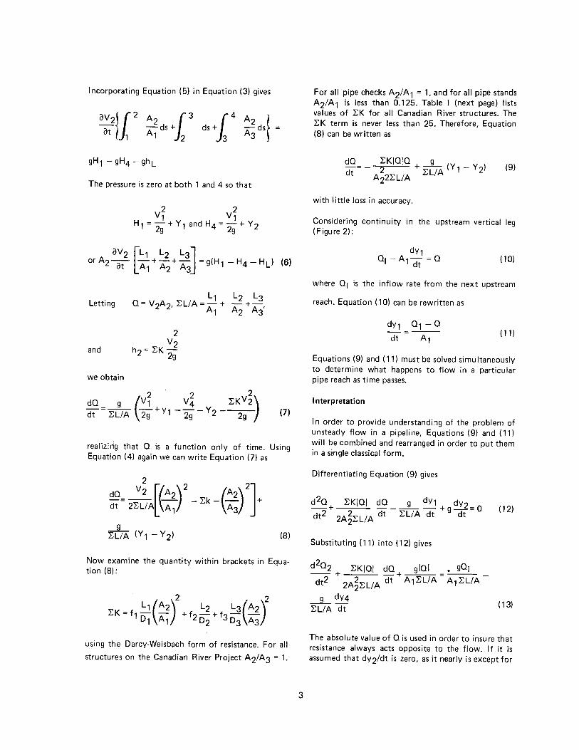
Incorporating Equation (5) in Equation (3) gives

av2JJ, 2 A2 +J,3 l 4

A2 ! at A ds ds + A3 ds = 1 l 2

The pressure is zero at both 1 and 4 so that

Letting

and

we obtain

2 2 2 dO g (V1 V4 "f,KV2\ dt - "f, L/ A 2g + y 1 - 2g - y 2 - 2g J (7)

realizing that Q is a function only of time. Using Equation (4) again we can write Equation (7) as

(8)

Now examine the quantity within brackets in Equation (8):

using the Darcy-Weisbach form of resistance. For all

structures on the Canadian River Project A2/A3 = 1.

3

For all pipe checks A2/A1 = 1, and for all pipe stands A2/A1 is less than 0.125. Table I (next page) lists values of "f,K for all Canadian River structures. The "f,K term is never less than 25. Therefore, Equation (8) can be written as

dO dt

"f,KIOIO g (Y y l 2 +-- 1- 2 A22"f,L/A "f,L/A

with little loss in accuracy.

(9)

Considering continuity in the upstream vertical leg (Figure 2):

dy1 O1-A1- =Q

dt (10)

where 01 is the inflow rate from the next upstream

reach. Equation ( 10) can be rewritten as

( 11)

Equations (9) and ( 11) must be solved simultaneously to determine what happens to flow in a particular pipe reach as time passes.

Interpretation

In order to provide understanding of the problem of unsteady flow in a pipeline, Equations (9) and ( 11) will be combined and rearranged in order to put them in a single classical form.

Differentiating Equation (9) gives

d2Q+ "f,KIOI dO __ g_ dy1 +gdy2=o dt2 2A~"f,L/A dt "f,L/A dt dt

(12)

Substituting (11) into (12) gives

d 2O2 "f,KIOI dO glOI • gO1 -- +--- -+---dt2 2A~"f,L/A dt A1"f,L/A A1"f,L/A

g dy4 "f,L/A dt (13)

The absolute value of Q is used in order to insure that resistance always acts opposite to the flow. If it is assumed that dy2/dt is zero, as it nearly is except for

01 is changed (dO1/dt) is also of importance. If dO1/dt is very small, then the resulting unsteady flow will have an insignificant amplitude. As the absolute value of dO1/dt is made larger, the resulting unsteady flow will have a larger amplitude.

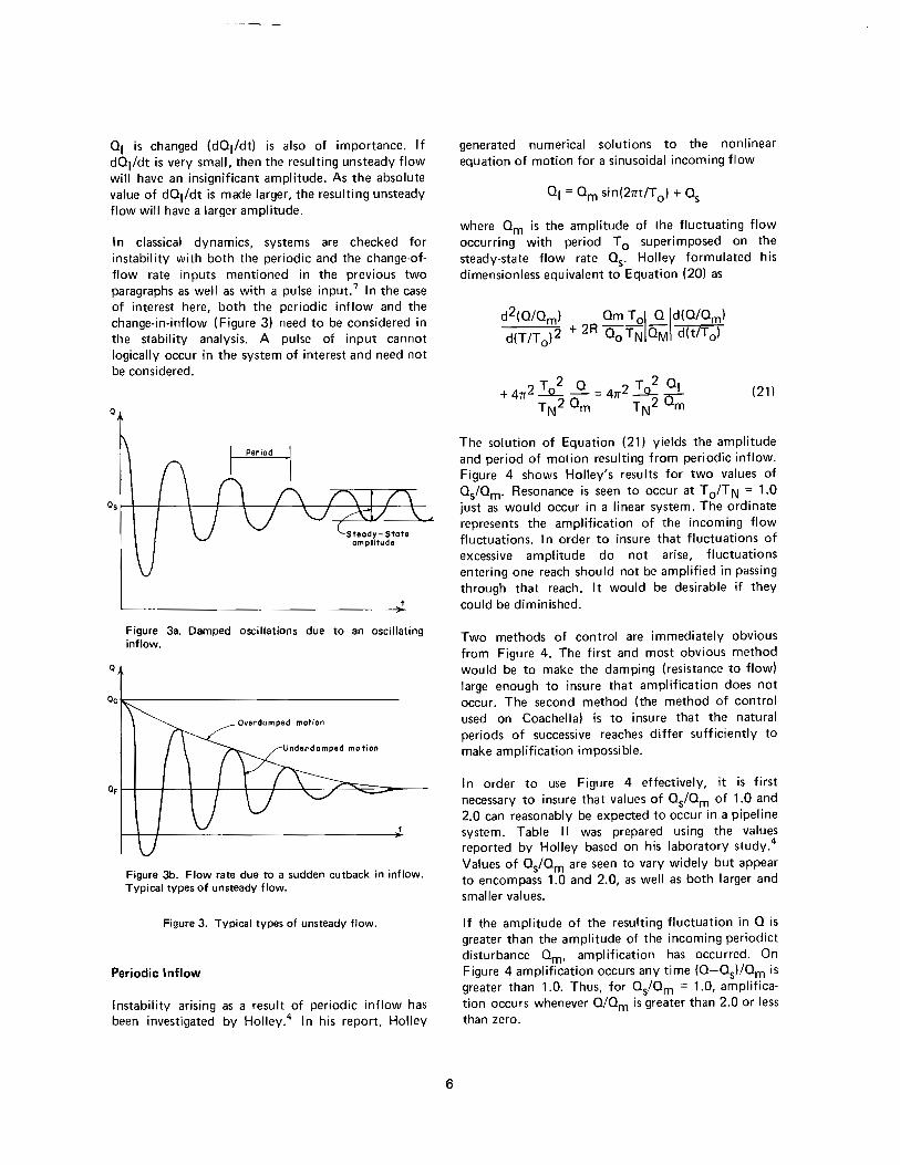
In classical dynamics, systems are checked for instability with both the periodic and the change-offlow rate inputs mentioned in the previous two paragraphs as well as with a pulse input.7 In the case of interest here, both the periodic inflow and the change-in-inflow (Figure 3) need to be considered in the stability analysis. A pulse of input cannot logically occur in the system of interest and need not be considered.

Q

Q

Figure 3a. Damped oscillations due to an oscillating inflow.

Figure 3b. Flow rate due to a sudden cutback in inflow. Typical types of unsteady flow.

Figure 3. Typical types of unsteady flow.

Periodic Inflow

Instability arising as a result of periodic inflow has been investigated by Holley.4 In his report, Holley

6

generated numerical solutions to the nonlinear equation of motion for a sinusoidal incoming flow

01 = Om sin(21rt/T 0 ) + Os

where Om is the amplitude of the fluctuating flow occurring with period TO superimposed on the steady-state flow rate Os. Holley formulated his dimensionless equivalent to Equation (20) as

(21)

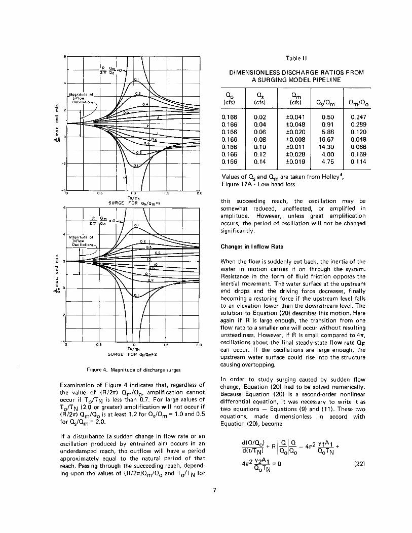
The solution of Equation (21) yields the amplitude and period of motion resulting from periodic inflow. Figure 4 shows Holley's results for two values of OsfOm· Resonance is seen to occur at T 0 /T N = 1.0 just as would occur in a linear system. The ordinate represents the amplification of the incoming flow fluctuations. In order to insure that fluctuations of excessive amplitude do not arise, fluctuations entering one reach should not be amplified in passing through that reach. It would be desirable if they could be diminished.

Two methods of control are immediately obvious from Figure 4. The first and most obvious method would be to make the damping (resistance to flow) large enough to insure that amplification does not occur. The second method (the method of control used on Coachella) is to insure that the natural periods of successive reaches differ sufficiently to make amplification impossible.

In order to use Figure 4 effectively, it is first necessary to insure that values of OsfOm of 1.0 and 2.0 can reasonably be expected to occur in a pipeline system. Table 11 was prepared using the values reported by Holley based on his laboratory study.4

Values of OsfOm are seen to vary widely but appear to encompass 1.0 and 2.0, as well as both larger and smaller values.

If the amplitude of the resulting fluctuation in Q is greater than the amplitude of the incoming periodict disturbance Om, amplification has occurred. On Figure 4 amplification occurs any time (O-Os)/Om is greater than 1.0. Thus, for OsfOm = 1.0, amplification occurs whenever O/Om is greater than 2.0 or less than zero.

Equation ( 16) becomes

d2(0/0ol + R d(O/Ool + M2 (0/0a) = d(t/TN) 2 d(t/TN) '

M2 (01/00 ) (17)

Solutions to Equation (17) are well known6 • If R = O then the motion of the system will be undamped and any disturbance of the flow wm produce a motion with the natural period.

(18)

Thus, Equation ( 17) can be written as

d2(0/0ol + R d(O/Ool + 47r2(0/0a) = d(t/TN) 2 d(t/TN)

47r2(01/0ol (19)

The solutions to Equation (19) Will yield considerable insight into the behavior of disturbed flow in the pipeline.

If R > 411' the system is said to be overdamped or stable against oscillations. Any sudden change in discharge will produce a flow in the reach which exponentially approaches the final steady-state value. The flow in the reach produced by a periodically fluctuating inflow will also be periodic. However, the amplitude of the incoming fluctuations may or may not be amplified depending upon the relative magnitude of the period of the incoming flow and the natural period of the reach.

In order to adapt this discussion and analysis to the problem of interest, the magnitudes of R, TN, and T 0

which can occur in the real system need to be known. Table I shows the values of TN and R as calculated for , pipe reaches in the Main Aqueduct of the Canadian River Project as originally constructed.

There is only one reach in which R is seen to be greater than 411'. Hence, that is the only reach in which oscillations should not be expected as a result of a rapid change in flow rate. All other reaches are underdamped and may possibly amplify incoming flow osciallations depending Lipon the incoming frequency.

The Actual Surge Problem

As was shown in the preceding section, considerable qualitative understanding of unsteady pipeline flow

5

can be gleaned from studying solutions of the linear Equation (19). However, quantitative information is obtained from solutions of Equation (15). Using the previous definitions of R and TN, Equation ( 15) can be written as

d2(0/00) IOld(0/00 ) 2 _ d(t/TN)2 + R Ood(t/TN) + 411' (0/0ol -

47r2(01/0a) (20)

The second term in Equation (20) represents the rate at which energy is dissipated by pipe friction. The term Q/00 is equal to unity when the flow rate Q is exactly equal to the design discharge, 0 0 •

Because of design procedures the pipe runs full throughout when Q = .00 , and the hydraulic gradient passes through the top of each structure as shown in Figure 1. In Equation ( 9), the first term on the right of the equal sign shows that the dissipation rate is proportional to the square of discharge. Thus, if the discharge is descreased below 0 0 the damping decreases more rapidly than does 0. A pipe reach which had a large enough R value to just be stable when flow was taking place at design conditions could then become quite unstable if the flow rate were decreased below 0 0 •

ANALYSIS

Stability

As noted in the previous section, Equation (20), which is characteristic of the motion of water in a given pipe reach, can be expected to predict an underdamped motion for the practical case. As well as being dependent upon R, the resulting motion is also dependent upon the inflow 01. If 01 is periodic, the linear Equation ( 19) predicts an exponentially damped harmonic motion which, as time increases, developes a constant period and amplitude governed by the period and amplitude of 01. This motion is illustrated in Figure 3a.

The nonlinear Equation (20) can be expected to give a somewhat similar result. If 01 is abruptly changed, the linear Equation (19) predicts a resulting motion which will be overdamped or underdamped depending upon R. If 01 is changed from one constant value to a second constant value, a harmonic motion is produced for the underdamped case. The harmonic motion is damped out as time increases, eventually producing a constant flow Q equal to 01. Such a motion is illustrated in Figure 3b. The rate at which

and (23)

A Runge-Kutta method of solution was used in the numerical simultaneous solutions of Equations (22) and (23). 8 The program used is listed in the Appendix. Actually the solution of Equations (22) and (23) is a six-parameter problem. The parameters are Q/Q0 , t/TN, A1/A2, QF/00 , R, and d(01/00 )

d(t/TN) where

Looking at Equation (23) one might expect Y1A1 /00 TN and Y2A1 /00 TN to also be parameters. However, Y1 - Y2 is fixed by the head loss occurring between the two structures at the design flow 0 0 .

The dimensionless elevation Y1A1/00 TN is determined by Q/Q0 and t/T N and, thus, is not independent.

Two occurrences are of interest in the solution of Equations (22) and (23). First, if the flow becomes negative (moving upstream), it will unwater the downstream tower rapidly. Second, if the upstream water surface rises to the top of the upstream structure, overtopping will occur.

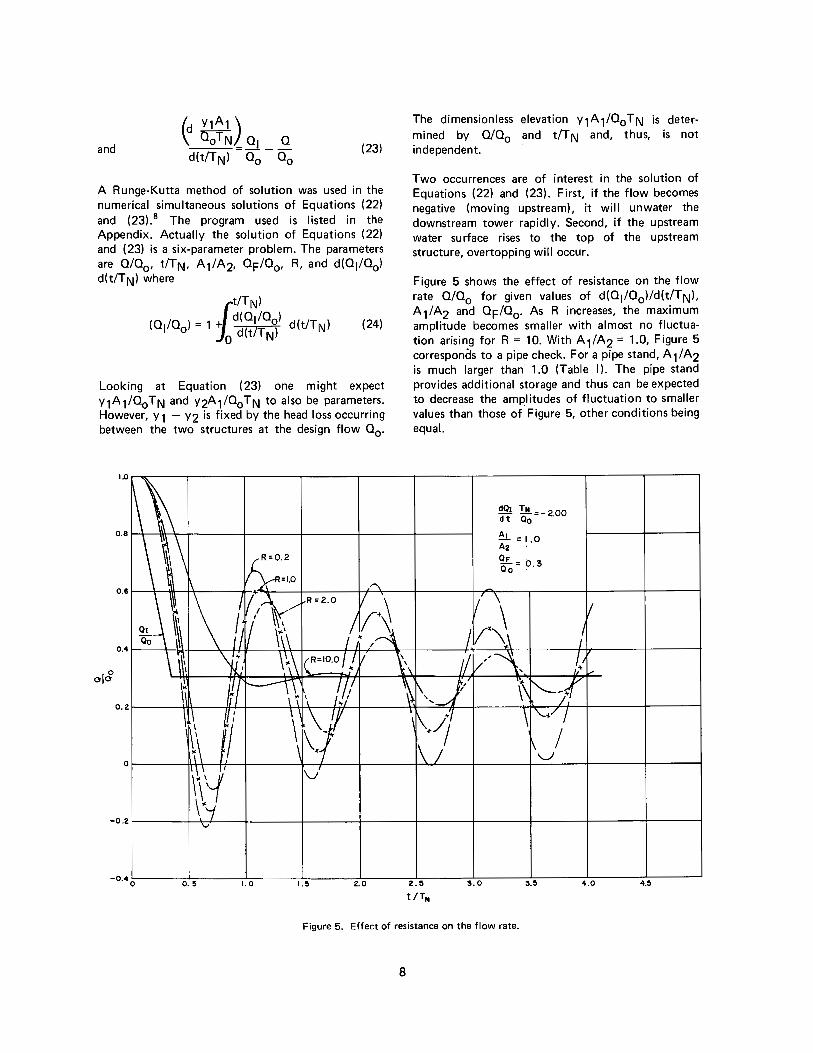
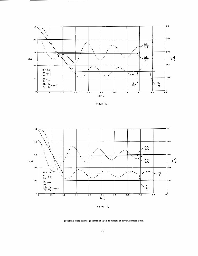
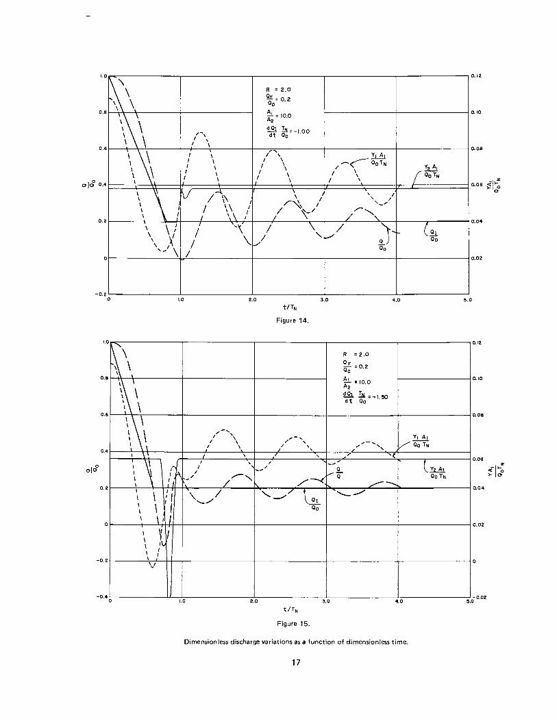
Figure 5 shows the effect of resistance on the flow rate Q/Q0 for given values of d(01/00 )/d(t/TNl. A1/A2 and QF/00 • As R increases, the maximum amplitude becomes smaller with almost no fluctuation arising for R = 10. With A1/A2 = 1.0, Figure 5 corresponds to a pipe check. For a pipe stand, A1/A2 is much larger than 1.0 (Table I). The pipe stand provides additional storage and thus can be expected to decrease the amplitudes of fluctuation to smaller values than those of· Figure 5, other conditions being equal.

1.0 ~~-~---~-------~----,----..--------,------,,-----,

dQ1 TN =-200 d t Oo .

~ = 1.0 A2

9£.=0.3 Oo ·

-0.21----~H_J_---1----+-----l-----+---+----+----+----+----l

o. 5 1.0 1.5 2. 0 3.0 3.5 4.0 4.5

Figure 5. Effect of resistance on the flow rate.

8

,, C 0

c

6

4

-2

6

4

IR QJ . \ 27T ao=O~

~\ ' II "' ~ MoQnitude of 0.2 Inflow v_ ~ ~ Oscillations} 0.4 -

~V L.. ""'~ I --~ • 2

~ ~ i---_,

~ ---..P-6 -r--.... 0_4

\\ ~ 0.2 v-/

1 ~; ~

I o• ,~ i• 2.0

To/Tn SURGE FOR Qs/Qm•I

I \ R Om •O 27T Qo 7/ ~ L'..

Magnitude or I/_ --~ Inflow 0.2 Osei I lot ions-., -- ~ 0.3 .,._

I,,'"~ n.& I~

·e 2 I

,, C 0

,i

~ ~ 10

0.

2 .._ " E ol& O

~"--\" ki./ V

-2

-4 0

1 I I

0.5 1.0 1.5 2.0 To/Tn

SURGE FOR Os/Qm•2

Figure 4. Magnitude of discharge surges

Examination of Figure 4 indicates that, regardless of the value of (R/21r) Om/00 , amplification cannot occur if T 0 /TN is less than 0.7. For large values of T 0 /T N (2.0 or greater) amplification will not occur if ( R/21r) Om/00 is at least 1.2 for OsfOm = 1.0 and 0.5 for OsfOm = 2.0.

If a disturbance (a sudden change in flow rate or an oscillation produced by entrained air) occurs in an underdamped reach, the outflow will have a period approximately equal to the natural period of that reach. Passing through the succeeding reach, depending upon the values of ( R/21r)Om/Clo and T 0 /T N for

7

Table II

DIMENSIONLESS DISCHARGE RATIOS FROM A SURGING MODEL PIPELINE

Clo Os Om (cfs) (cfs) (cfs) Os/Om

0.166 0.02 ±0.041 0.50 0.166 0.04 ±0.048 0.91 0.166 0.06 ±0.020 5.88 0.166 0.08 ±0.008 16.67 0.166 0.10 ±0.011 14.30 0.166 0.12 ±0.028 4.00 0.166 0.14 ±0.019 4.75

Values of Os and Om are taken from Holley4,

Figure 17 A - Low head loss.

Om!Oo

0.247 0.289 0.120 0.048 0.066 0.169 0.114

this succeeding reach, the oscillation may be somewhat reduced, unaffected, or amplified in amplitude. However, unless great amplification occurs, the period of oscillation will not be changed significantly.

Changes in Inflow Rate

When the flow is suddenly cut back, the inertia of the water in motion carries it on through the system. Resistance in the form of fluid friction opposes the inertial movement. The water surface at the upstream end drops and the driving force decreases, finally becoming a restoring force if the upstream level falls to an elevation lower than the downstream level. The solution to Equation (20) describes this motion. Here again if R is large enough, the transition from one flow rate to a smaller one will occur without resulting unsteadiness. However, if R is small compared to 41T, oscillations about the final steady-state flow rate OF can occur. If the oscillations are large enough, the upstream water surface could rise into the structure causing overtopping.

In order to study surging caused by sudden flow change, Equation (20) had to be solved numerically. Because Equation (20) is a second-order nonlinear differential equation, it was necessary to write it as two equations - Equations (9) and (11). These two equations, made dimensionless in accord with Equation (20), become

(22)

CORRELATION WITH FIELD EXPERIENCE

Previous Field Tests

The Coachella and Canadian River systems provide the bulk of the history which can be related to the phenomenon of surging in low-pressure pipeline systems. As mentioned earlier, the Coachella system was constructed with pipe reaches having almost identical natural periods, and a resonant condition was reached. The recommended remedy involved placing covers over adjacent pipe stands to effectively change the natural periods of the reaches. 1 A review of the Project Record for Coachella for 1955 and 1958 shows that this system of control has not always been successful, but that the operators have learned how to avoid trouble in most cases.

Examination of Figure 4 can yield a possible explanation for the failure of airtight lids to work in all cases. If the period of a reach is effectively increased, an oscillation entering it may not be amplified. However, when passing into a following reach, amplification can take place since at that point T 0/TN will be greater than unity, and R is small. Project records also indicate that problems with surging arise when discharges are changed.

The Canadian River system was tested by personnel from the Hydraulics Branch and the Project in 1968. Observations showed that flow occurred smoothly and trouble free at design flow. However, upon cutting back from design flow, surges developed which overtopped four structures. Two of the overtopped pipe-check structures were subsequently replaced with pipe-stand structures (large A1/A2), Subsequent tests by project personnel in 1969 produced overtopping of only one pipe-check structure when the flow rate was changed.

Canadian River Tests, 1968

Table Ill shows values of (R/21rlOm/Cla, T 0/TN, and amplification factors as computed for the Main Aqueduct of the Canadian River system as they existed in 1968. A value of Om/Clo = 0.29 was assumed in computing (R/21r) Om/O0 since that is the maximum value indicated in Table II. T 0/TN was computed as the ratio of the natural periods (TN) of each pipe reach and the reach immediately preceding it (T 0). Maximum amplification factors are also shown in Table 111 ROm/21rO0 = 0 to indicate the possible range of amplification.

Examination of the maximum amplification factors contained in Table Ill indicates five reaches in which

10

severe amplification might have been expected (Stations 2976, 3617, 5260, 5356, and 6701). Of these five, only Station 6701 overtopped in actual operation. When the amplification factors computed with Om/Clo = 0.29 are examined, only Stations 6701 and 2976 indicate possible trouble due to resonance. No trouble was observed with Station 2976. However, it was near the upstream end of the system and was probably not subject to incoming oscillations as severe as those entering structures farther downstream.

During operation, overtopping of structures also occurred at Stations 5445, 7788, and 7919. At none of these locations could resonance with the structure i~mediately upstream have been a problem. Station 5445 probably overtopped because of the combined amplification occurring through the structures upstream from it. Overtopping of the structures at Stations 7788 and 7919 appears to be more subtle. Amplification factors for these structures do not appear to be severe.

However, no consideration is given to resonance with structures farther than one reach upstream. Table I indicates that several reaches upstream have periods nearly in resonance with Station 7788 or 7919. A periodic surge generated upstream could pass through several reaches without being amplified before reaching one where large amplification occurs. Thus, a disturbance generated at Station 5260 or 5356 might very well receive large amplification at Station 7919 since, unless overtopping occurred somewhere between these two stations, the period of the surge would remain relatively unchanged. Similarly, a disturbance generated at Station 5445 or 7232 might cause severe problems at Station 7788.

Canadian River Tests, 1969

A review of the discharge records for the 1969 Canadian River tests as recorded at the Kress flowmeter at Station 5080 show that a change of discharge from 40 to O cfs took place in about 4-1 /2 minutes. For that reach the rate corresponds to dimensionless cutback rate d(O1/O0)/d(t/TN) = -0.50. Using the values of R shown in Table I, Figure 27 indicates that none of the structures should have been overtopped. Only the structure at Station 8026 was overtopped, and that only slightly. However, the ratio T 0 /TN is 4.4 for the reach following Station 8026 and the value of ROm/2O0 is 0.48 as seen in Table Ill. Figure 4 shows that amplification might well be expected in that reach. Thus, overtopping of that structure might have been expected.

Figures 6 through 15 (at end of report) show Q/Q0

and Y1A1/00 TN for various combinations of R, QF/0 0 , A1/A2 and the cutback rate d(01/00 )/d(t/T Nl- Not all solutions obtained are represented in the figures. Only those depicting special conditions were graphed. In all solutions, except where Q became negative, Y2 was taken to be constant. Actually, it will vary somewhat since the downstream structure acts as a weir and Y2 must be relatively large for large positive flow rates. However, it is Y1 - Y2 which is really important in the solution since this elevation difference represents the driving force. Because Y1 undergoes large changes with respect to time, the minor change of Y2 for positive flows was neglected. Figure 12 shows a case where Y2 actually decreased because the flow rate Q became negative. Figures 9 and 15 illustrate more drastic cases.

In Figures 6 through 15, wherever Y1A1/00 TN rises above its value at t/T N = 0, overflow of the upstream structure is predicted. In some cases such as that represented by Figure 8, overflow occurs despite the fact that 0/0a never becomes negative. However, that is a case of rapid cutback of inflow and low resistance such as might be expected in a short reach.

The periods of flow in Figures 6 through 15 are seen to be nearly equal to the natural undamped frequency of the system. Although damping decreases the natural period, in the cases shown, damping is small in comparison to the inertial forces and, hence, has a relatively small influence.

The relative influence of cutback rate is demonstrated in comparing Figures 13 and 15. Slow cutback rate is seen to produce almost no fluctuation (Figure 13) while rapid cutback (Figure 15) produces large fluctuations and even negative flow.

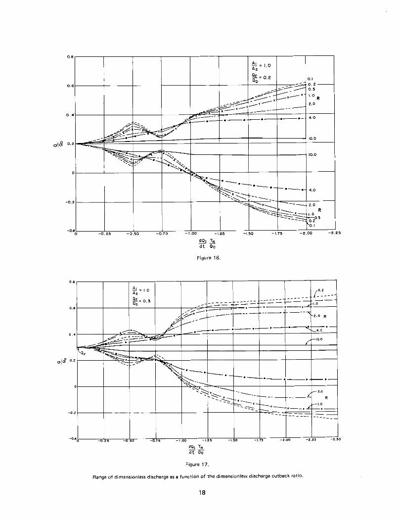
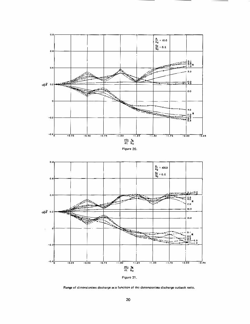
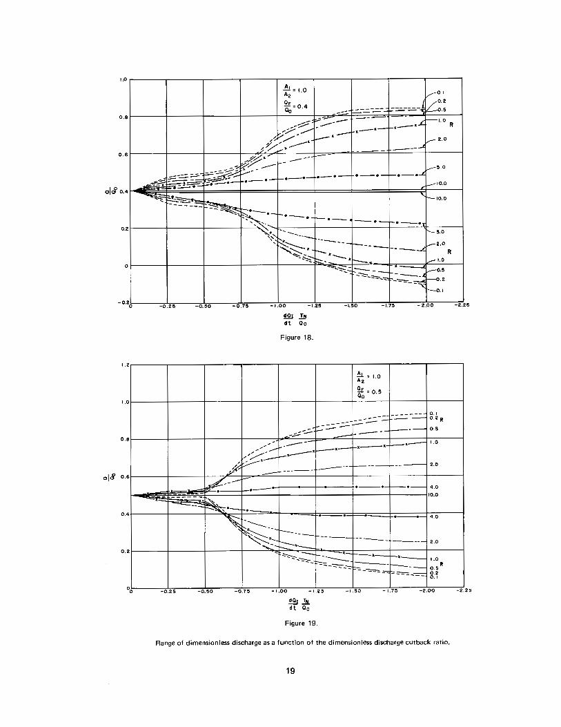
Maximum and minimum values of Q/Q0 are summarized in Figures 16 through 21 for all solutions obtained. Those figures show the extreme values of Q/Q0 for the values of R, A1/A2, QF/00 , and cutback rate. Magnitudes of extreme values of O/Oa are seen to be increased as the cutback rate is increased, as R becomes smaller, as QF/Q0 becomes smaller, and as A1/A2 becomes smaller.

However, as demonstrated by Figure 16 there are cases where magnitudes of extreme fluctuations are reduced as d(01/00 )/d(t/TN) is made larger. For instance, in Figure 16 with R = 0.5, the maximum value of Q/Q0 is 0.32 for d(01/00 )/d(t/TN) = -0.5 and 0.24 for d(01/00 )/d(t/T Nl = -0. 75.

9

When a cutback in flow rate is started, the system is immediately set into unsteady motion with natural period TN. The cutback reinforces a decreasing flow rate and diminishes an increasing one. If the cutback rate is very slow, its effect is distributed over many periods, and thus its net effect is a small oscillation. If the cutback rate is large, its effect is felt over only a fraction of a total period, and a relatively large oscillation occurs.

However, there is a small range in cutback rate at which the accelerating effect of the cutback, occurring during the first half of the first period in which discharge is falling, is counteracted by the decelerating effect during the second half of the first period. If the cutback rate is slightly less than this, it acts over more than one accelerating period, producing a slightly larger fluctuation.

As pointed out in an earlier section, the overtopping of a structure occurs when Y1 rises to the top of the structure. Thus, critical values of cutback rate can be observed by looking at the motion pattern shown in Figures 6 through 15, where Y1A1/0a TN curves with flat tops such as Figure 12 indicate that overtopping of the upstream structure would occur.

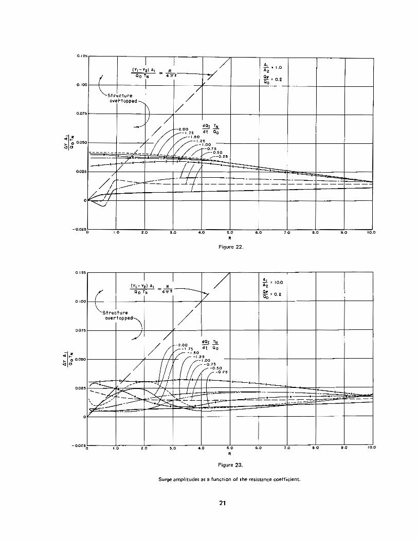
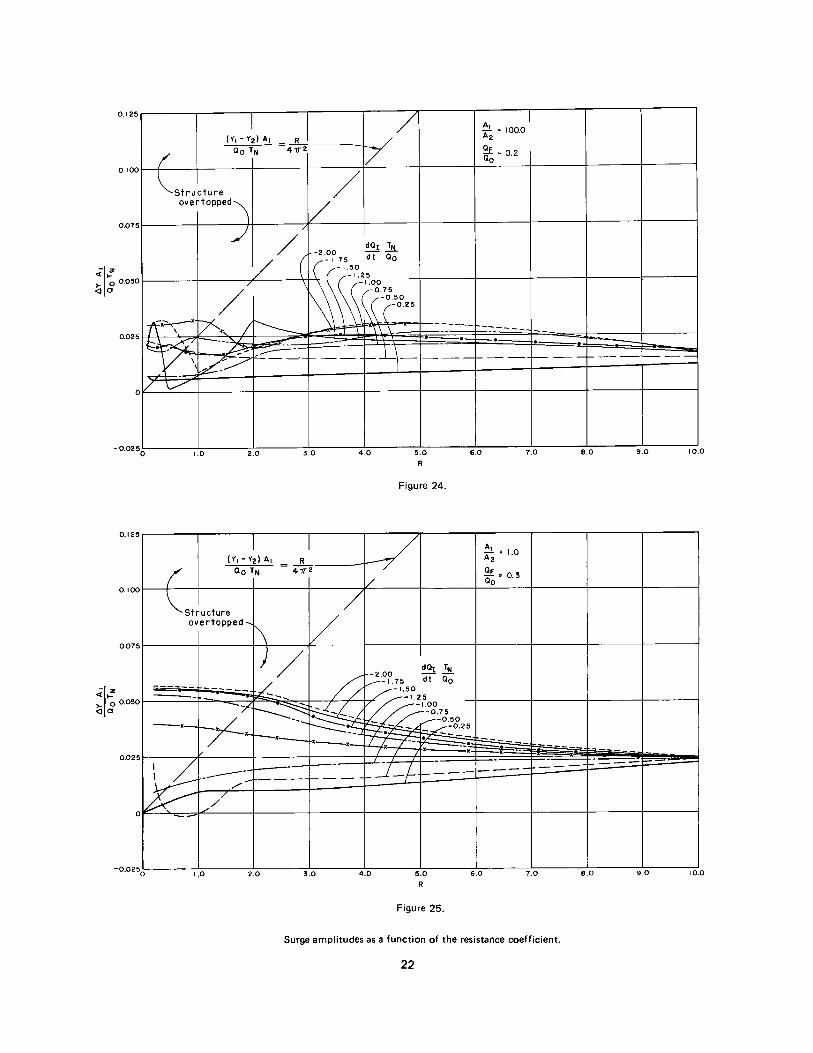
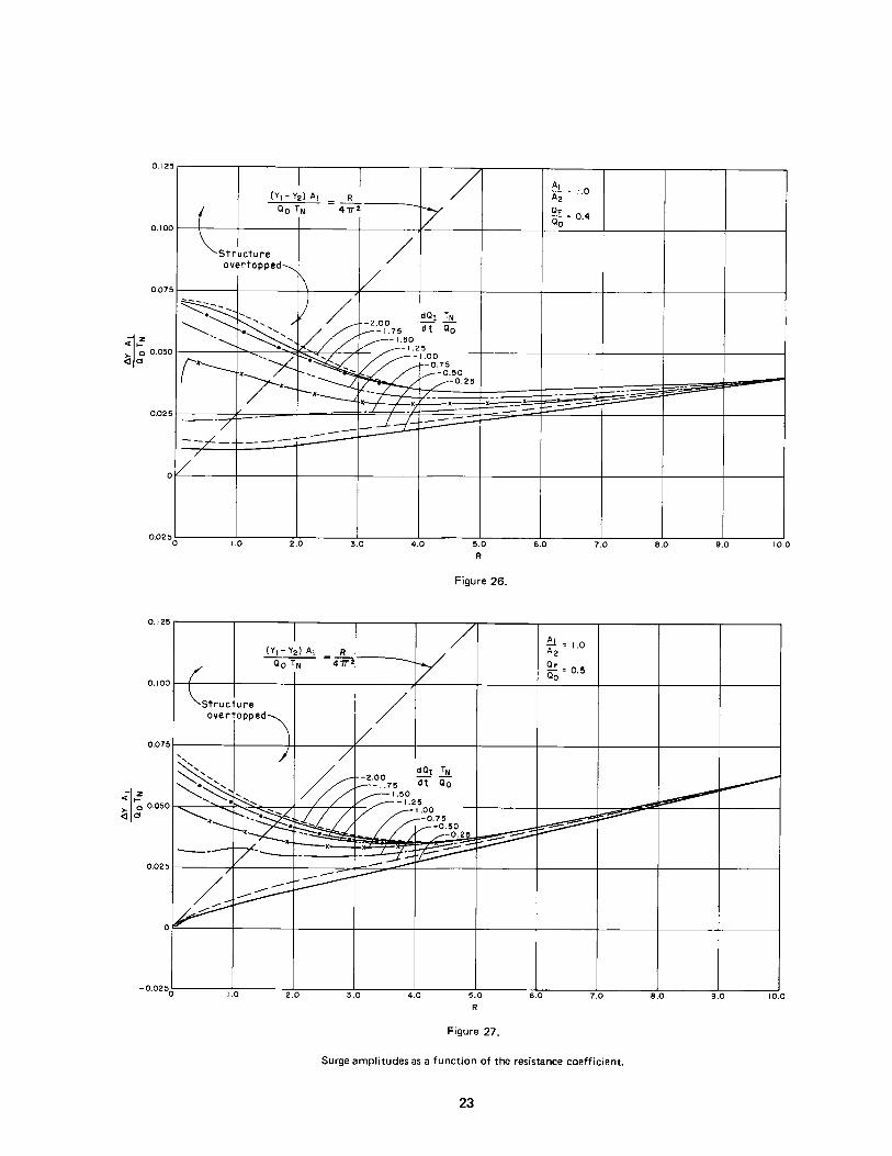
The extreme movements of the upstream water surface have been summarized in Figures 22 through 27. In those figures the diagonal line going upward to the right is the difference between the tops of the upstream and downstream structures for steady flow [Equation (22) with d(Oi/00 )/d(t/TN) set equal to zero] . As Equation (22) indicates, this difference in elevation (in dimensionless form) is determined by R alone with D(Q/00 )/d(t/TN) is zero (steady flow) and Q/00 = 1 (design flow).

The other lines in Figures 22 through 27 are the extreme rises in upstream water surface elevations produced by particular cutback rates for particular values of R, QF, and A1/A2. Whenever a line for a particular cutback rate crosses to the left of the diagonal line, overtopping has occurred.

The effect of increasing storage in the upstream riser (making A1/A2 larger) in general makes it possible to cut back at a faster rate without overtopping than could be done with a pipe-check structure. The effect of the resistance (R) is already seen. For a design situation, a cutback rate could be chosen at which overtopping would not occur in a pipe reach for which the values of R, A1/A2, and QF/00 have been calculated.

REFERENCES

1. Hale, C. S., Terrell, P. W., Glover, R. E., and Simmons, W. P., Surge Control on the Coachella Pipe Distribution System, Engineering Monograph No. 17, U.S. Department of the Interior, Bureau of

Reclamation, Denver Federal Center, Denver, Colorado, January 1954.

2. Colgate, D. C., "Hydraulic Model Studies of the Flow Characteristics and Air Entrainment in the Check Towers of the Main Aqueduct, Canadian River Project, Texas," Report No. HYD-555, U.S. Department of the Interior, Bureau of Reclamation, Hydraulics Branch, September 1967.

3. Taylor, E. H., Pillsbury, A. F., Ellis, T. 0., and Bekey, G. A., "Unsteady Flow in Open-type Pipe Irrigation Systems," Transactions ASCE, v 121, 1956.

12

4. Holley, E. R., "Surging in a Laboratory Pipeline with Steady Inflow," Report No. HYD-580, U.S. Department of the Interior, Bureau of Reclamation, Hydraulics Branch, September 1967.

5. Rouse, H. (Editor), Engineering Hydraulics, John Wiley, New York, 1953

6. Sokolnikoff, I. S. and Redheffer, R. M., Mathematics of Physics and Modern Engineering, McGraw-Hill, 1958.

7. Ayre, R., Mechanical Vibrations, McGraw-Hill, New York, 1964.

8. McCracken, D. D., and Dorn, W. S., Numerical Methods and Fortran Programming, John Wiley, New York, 1964.

Table Ill

CANADIAN RIVER SURGE DATA

Amplificationt

(Omax - Osl/Om RO

Maximum Using ______!!! 21rO0

Station Oo ROm To (Rom) from (ft) (cfs) 21rO0 TN 21rOo = 0 Column 3

1882 92 +2430 92 0.06 29.0 1.4 1.0

2976 92 0.08 1.0 ~5.0 ~5.0 3044 92 0.15 0.5 0.4 0.3 3275 92 0.06 0.6 0.5 0.4 3617 92 0.34 1.2 ~5.0 1.6 3777 92 0.27 1.5 1.9 1.3

4050 92 0.54 0.3 0.2 0.2 4625 92 0.24 2.2 1.4 1.0 5107 92 0.14 1.8 1.5 1.2 5260 92 0.20 1.1 ~5.0 2.1 5356 92 0.22 1.1 ~5.0 2.0

+5445* 92 0.08 1.8 1.5 1.3 5744 92 0.09 0.6 0.6 0.4

+6701* 85 0.09 1.0 ~5.0 ~5.0 7232* 85 0.09 1.4 1.9 1.7 7487 85 0.32 0.4 0.3 0.3 7715* 85 0.06 5.2 1.4 1.0

+7788* 85 0.08 0.7 1.2 0.9 +7919 85 0.20 0.4 0.3 0.3

8026* 95 0.48 4.4 1.4 1.0

t Amplification factors from O/Om = 1.0 curves, Figure 4a * Check structures + Structures which experienced overflow during the 1968 tests

SIMULTANEOUS CONSIDERATION OF SEVERAL REACHES

At the outset of this study it was planned to consider several reaches simultaneously to see what the mutual effect of one reach was on the remainder. However, when this problem was formulated mathematically, it was found that the system of equations was singular. Practical consideration of the problem showed that this should have been expected. The only way a downstream reach can affect an upstream reach is for

11

flow to move upstream into the upper reach. That condition already violates the desired design conditions. In other words, the surge is already beyond tolerable limits, and it is of little consequence to know how much worse it gets.

Thus, the condition of interest is only the effect of inflow on any given reach. If the reach does not surge excesively for the frequency and rate of decrease expected in the inflow, it will be satisfactory. Consideration of each reach for these conditions should result in a satisfactory overall design.

1,0

0.8

0.6

\\ R = 0.2

~=O 2 Oo .

~=100 0

~\

A2 .

'!Bl .!l!.:-1 oo Y1 A1

dt Oo . ( _,,,..- Oo TN

Y2A1

' r -----, r- ----, r -- --, /'Oo'iN

'

018 0.4

\

\ I I I I I

I

I I I I I I I

I I I I I I I I I I

I I I I I I I I I I I I I I I I I I I

0.2

0

-0.2 0

1.0

'

I I I I I I I

\ \

\ ,_,

0.8 \\

0.6 '· \ \ 0.4

0.2

0

-0.2

-0.4 0

I I I I I \\ I \ I I I I

I

\ I I I \ I I I I I I I I I

\ I \ I ,}

\~ /''\ I ~\,, \ I

I I--.. \ I

I \ I I I \' I

\ I I _,

I \ I -, ,,.-B.! V I \ I oo

I

" I I \ I \ ,,, \ \ \ I I I \ \ I \ I \ Q I, ,~ ,--'U'"o

\.., \...1 '--

1.0 2.0 3.0 4.0

Figure 8.

R = 0.2

QF = 02 Oo .

~ = 100.0 A2

dQI .Tu. =-1.75 dt Qo Y2A1

r-----"'\ r--- --, r-----, (OoTN

~ \ ,' I I \

\ I \ Y1 A1 I \ I

\ I \ ,___..-QoTN

I \ I \ I \< \ I

I \ I \ I \

I ' .' ' _, I I Q

I -~ I / ' /' 1/"'( .,....0o

\ ,f , I I \ / \ I

I I I \ I

\ I \ ' \ I I I

I \ 'I 01

\ I I '-..,/

,_,, ~-Qo

V1 \, -,~ \ I

1.0 2.0 3.0 4.0

Figure 9.

Dimensionless discharge variations as a function of dimensionless time.

14

0.10

0.08

0.06

-.,_z 0.04 ~Io

0

0.02

0

-0.02 5.0

0.10

0.08

0.06

0.04

0.02

0

-0.02

-0.04 5.0

-1~ C( 0 >- 0

1.0

0.8

I~ R • 0.10

~ a. Oo , 0.2

'-~ ~-100 Az •

Y1A 1

0.6 ~ dOx TN •-0.25

/ ---dt 0 0

OoTN

'-

0.4

0.2

0 0

,.o

' ' ' ' , , ,

', _,

0.5

:~ ~

-, ,. ' ' ' ' ' ' ... --

1.0 1.5

",~ ~ -- ---... ~ ,,.- ... , .... _.,, _,, ,,,

... _ --~

~~ Oz i--0o

""' 2.0 2.5

tfr.

Figure 6.

R ' 0.2 a. Co° '0.2

' r-/

3.0 3.5

--

Q

,,, -voo

4.0

o.e ,'-::::, ~ • 1.00

~ Az

0.6 ........

0.4

0.2

0 0

' ' ' ' / ,.

/

' -,.

0.5

- ' ... ' ' ' ' ...

1.0

Q V-- Oo dOx r. •-0.25

dt Oo

"-~

'-~ - ............... - -... ,. - ' -,

, __ _,,,., -.......:

~-,, ,. __ ,.

"r---... ~ ~--- I

1.5 2.0 2.S

t/TN

Figure 7.

,_

3.0

Y1A1 V OoT•

,---~ ,

o, /'Oo -/

-/

4.0


13

'\ '- Y2A 1

OoTN

4.5

\ I'--- Y2A1

OoTN

4.5

0.10

0.08

0.06

0.04

0.02

0 5.0

0.10

o.oe

0.06

0.04

0.02

0 5.0

-, z ...... >- 0

0

...... -1Z >- 0 0

1.0

0.8 \\

0.8

ola' o.4

0.2

0

-0.2 0

1.0

'\ \ \ '. \ \ \

'

\ \ '. '

I \ I I I I \ I

I I I I I

I 1 I

I y I I

\ ,'\ J \

0.5

...

I I I LOverflow to Preceding Reach

r- - .... r --~ .' --, I I I I I I I I \

I I I I I I I I I I I I I I I I I

I I I I I I I I I ' v

I\\ I I I I I I I I I " I

I i \ I I / \ I I

I '. I I

I I I '. I

I I I I I I\ I I I I I \ I \ .\/ I I I I I

I I \ I

I

\ I I I \) \

\ I \ , '- ..I I I R = 1.0 \

I o,

-../ Oo • 0.3 I

A1 '--' Az • 1.0

dQI TN dt ao=-1.2s

1.0 1.5 2.0 3.0

Figure 12.

I ,

\ \ ' I , .. ,.....__Y1A1

\ I I °<)TN I I

I I I

I " I I I , Y2A·1 I I \

I I °<)TN I / "'\\ I

,_

I\ - o,

\ I Oo

' I ' ----\_ ..._ ~

Oo

3.5 4.0

R • 2.0 0 ~' o,

' Oo •0.2

0.8

0.8

0.4

0.2

0 0

' ' ', ' ............

0.5

~ :: • 10.0

' Oz

/oo ~ TN •-0.25 .... ___ ~

dt Oo

--.... ' '~

-, Q Y1A1 ----- ~ /Oo ,,--,/ VooTN - ---~../ -- , ' ,

~---- , -... __ .,,

~ ~ ----

..... -- --1.0 1.5 2.0 3.0 3.5 4,0

Figure 13.


16

4.5

\ '- Y2 A 1

OoTN

4.5

0.10

0.08

0.08

-,z 0.04 : 8

0.02

0

-0.02 5.0

0.12

0.10

0,08

0.08

0.04

0.02 5.0

1.0

N\ 0.8

Q.6

0.4

0.2

0 0

\ \ '\

~ \ \

~ \

\

\ \

\ __ ,,,~\ --'

""'" ',,,_ ,

'\ R • 1.0 ~ o, Oo , 0. 3

\

A1 -· 1.0 A2

dOr T••-0.5 dt Qo

0.5 1.0 1.5

, , , , , I

I

I I

I I ,

I

I "' /

-' ' \

\ I

\ ,

\ I

\ \ I

\ I I \ ,

' -

/---.. I " I' ,__...

z.o

Figure 10.

- Y1A1 , \ ~QoTN , '

, -'

, \

,

' ,

' , , \ ' \ i's-- YzA 1 - , OoTN

-" / ' V

/ '--- ........ ..-{

Q Oo

3.0 3.5 4.0

\ \

[\___~ Oo

4.5

0.10

o.oe

0.06

0.04

0.02

0 5.0

1.0 -------,-----,------.------,------,-----,------,,-----,-------,------, 0.10

['\\ a.a t-->-----'<--1-t-----+-----+-----+------+-----1-------i-----+-----+------10.oa

\\1 ~\ , , YzA1

/ '' ; --.., / 0oTN ' I \ ,I ' ~,,,- ... ' I \ \ ,' \ ,I' /'

0.6 ~==-==l~====t:=;!===+='~===!::::J.'.:::' ===:t::::='~==+::;::====t====t:::::.:t;-----,----i 0.06

' \/ ,' \,_,, / ',,_, , '---<__ ;;:: I \ I I

0.4 r----....... --..,.....,,_-+-----;------;-----+-----t------1-----+------;-------10.04 ', ,\' \ V '-

0.2

R = 1.00 - , \ \'t----;-'--/+--".......,+---"'-+i,------'...:.....;,.....+--__,,..._"-1""--_'-_,.--:-!-.£~r--- Or o, , 0 _, -.. / " / '--- , ) 00 Oo ~ '....._/ ,____.. ,...____, \

~ , 1.o f-----1-----+-----+-----+------+------11-------lf------1 a.oz

A2

~ TN •-0.75 dt Oo

0 0'-----o-.-s----,~.o-----,.Ls----2~.-0----2~.,-----3.Lo----3~_-,----4~.o-----4~.s----,~_g

t!r.

Figure 11.


15

.. I--1 z >- g

0.8

~=I 0 A2 .

0.6

0.4

ol8 o.2

Qj, -Q6 - 0.2 0.1 - 0.2-

~~ c:::_;:.;..:::- 0.5 r_--

~~--i-·-· 1.0 R

-;;.:::: - ----· 2.0 ---~ .--· -~: r-.--1.---_ ------L.------

~ ~:.-----

._ _____ c....-e-~---- 4.0

.,,v-. ~' ~ -·-L~ ~ ~· ~ ~ ~~ -- 10.0

~ ......

0

-0.2

-··~--== ~-~ "'~, 10.0

,~; ~., ---~ ~-t',, _, ·"~ .,.~ -~ .... -- . -----~ ~-----~ ..._

', ~,::,....-t ___ ·-· 4.0

'--:..~ -----<~~----- ---- 2.0

~~-:;:: -t R --- :...:::::::::-:----- 1.0 --::-::-:.~ ~0.5

~'.2 .I

-0.25 -0.50 -0.75 -1.00 -1.25 -1.50 -1.75 -2.00 -2.25

Figure 16.

0.8

0.6

0.4

~=I 0 /0.2 ___ A2 .

t= 0.3 -- - - - ------- --=-=-=~~-- ------- --- --- -x----x---x-L

1.0

,,/.:::--1---i ·-,,.~. --- ---- ----- ----, <j . - -- 2.0 R

L----

..!..._-_/_,.,,.--- 1--·-·---·- '---•-.....

' •-

--- .- t--4.0 L. •

-- --c v~~~-~ --i- /

L-10.0

ol8 o.2

0

-0.2

I\QF ---~--::-:,..... .. _,,.::: ... , ... :::--x -_-.,,., ~-,:::_

~ i-. -. i----. --~ ~--- -·-L...·-·----·--·-~---:--.... -----~ .... ---.:::::::::-. ------ __ __L 1-- 2.0 ..__. ___

----:::-:::-;;;....-._ R -- 1----._ 1--1.0 ----- •--,..L ,__,_ --- I---._

----- - --::-:: ------- ----

-0.25 -0.50 -0.75 -1.00 -1.25 -1.50 -1.75 -2.00 -2.25 -2.50

Figure 17.

Range of dimensionless discharge as a function of the dimensionless discharge cutback ratio.

18

1.0

0.8

0.6

016' 0.4

~ r- \ .

·~ \ \ ,-\ \ I \

\ I \

\~ ' I I

I I

\ \ I I I I I

I I

0.2

I

\ V ;-\" I I i \\ I I

I I I I \\

0

\

\ '/ I

''(, I \ I I ,.,. \

I

-0.2 0 1.0

1.0

0.8

0.6

\\ I \

\ \ \ \ \

,,-, I '

R = 2.0

~=O 2 Qo .

i; = 10.0

dQi Tu.:-1 00 dt Qo ·

,., Y1 A 1 I ' I \

--~QoTN I \ \ / \

I \ I \ I I I \

I' \ ·, I

' / I I /"'-\, I

,_,, I / \_/ --....... I

I

I \. l//

2.0

t/TN

Figure 14.

.. - ..

\

' .,/

3.0

/ ' / J'-

Qo

4.0

R = 2.0

~~ = 0.2

~=100 A2 •

dQ1 :!ti. =-I 50 dt Qo ·

Y2 A1

(QoTN

(!b.. Qo

Y1 A1 \\ \ \ / \ ,, ' .. - .. / QoTN \ I I \ I ' ,, ' , ' , ' 0.4

016'

0.2

0

-0.2

-0.4 0

I I

I I I I I

I I I I

I' I

' I I

( '-\, I

I _, I I

\ I

\. I I \ I I

_ __,,,

\ I I I y ; I i\. I I I

I I \v/

1.0

/

' I ' ~' ', , _.,. ., ,,

Q .. , ,,-" /-<'

---o"

/ ' ,.. ,_,,,,, ~~

.....__.,,,

2.0

t/TN

Figure 15.

Qo

3.0

'(

.,,.,--...

4.0


17

l~ QoTN

0.12

0.10

0.08

-1.,_z 0.06 ..: 0 >- 0

0.04

0.02

5.0

0.12

0.10

0.08

0.06

0.04

0.02

0

-0.02 5.0

o.er------,.------,-----.-----.----..,.----..,.------,-------.------,

°ii • 10.0

t •0.2 0.61------+-----+-----1------+-----+-----1-----+-----+-----1

-o·40::-------o::,.'::2c:5---_...,o:!.'=s-:::o---_-,o='".-=1-=s---_-,1c'.o::co::c----_-:1·.2"'s=----_-:,.,__5"'0=----_-:-,-'-:_7:-:5=------=2-'-=.o"'o,----_-:'2_25

~..!ri dt Oo

Figure 20.

o.e,-----..... -----.------,r-----,------.------,r-----,------r-----, ~ • 100.0 A2

t • 0.2 0.61------l------4-------1------+-----+-----+-----+------+------I

-o·40!-------o=".2c,..,,5---_-o=-'."'s"'o ____ ...,o,-,..""1""s---_...,,.,__o'"o=----_-:1-'-:.2:cs=----_-:-,.1.:_5:-:o,----_-:-,L::_7"'5,---_-2=".'=o"'o ____ ...,2='.2s

Figure 21.


20

1.0 .-----~----~-------,.-----~----~----~-------,.-----~----,

·-· ·----~. ~~

ol-----+----+-----l-----+-----'-l"'""-,~-,,.....1--=-

------- ---------

0.1

.5

2.0

5.0

2.0

R

R 1.0

0.5

0.2

0.1

- 0·20=-------=o".~2~5---_...,o=-."'5-=0------=o".1=5=----_....,..1...,o-=o,----_...,1..,_2'"'5,----_-1'"'.5!-o=----_...,1-!.1'"'5----_-2=-.'=o-=o,----_-=2~:25

dQ1 .!ti dt Qo

Figure 18.

1.2.-----,-------.---------.-----,------,-------.---------.-----,------,

~•I 0 A2 .

~ • 0 5 Oo .

I .0 t-----+------+-----+-----t-----+------+-----t-----1--------t

00 -0.25 -0.50 -0.75 -1.00 - 1.25

Figure 19.

------- 0.1 --..::-

----+•---•

-1.50 - 1.75

0.2 R

0.5

4.0

10.0

1.0 R

0.5 0.2 0.1

-2.00


19

-2.25

0.12 5

0.100

0.075

<t ,__ -, z >- 0 0.050

<J 0

0.025

I I / (Y1 -Y2) A1 = R

( Qo TN 4772 7 1.,

~Structure /

over-topped--.._ / I\ / l/ /

------~t2 dQI TN

-200 - -1,.-----115 dt Qo

~:~25 / 1/-1.00 -0.75 ---- - __ L __

1.,.,---0.50 -- . - .. --- -~( .,.,--0.25

J--X L X .,___, ·-~.L..? I : ~-•-~ -·--·-[7 / --- - --_:;:::.---r---- --- ----

~=I 0 A2 .

t = 0.2

--• ·-~ ---- - -----------------

0

:?±f:_ /,; ~/;

-0.0250 1.0 2.0 3.0 4.0 5.0 6.0 7.0 8.0 9.0 10.0

R

Figure 22.

0.125 ,--------,-----...------r-------r----..,...-------r------,r-----.-----,-----, ~ = 100 A2 .

t = 0.2

0.1001-+---lf------+-----+-----.1".-----+-----+-------jf-----t-----+----7

-0.0250 1.0 2.0 3.0

-2.00 • 1. 75

-1.50 -1 .25

-1.00

4.0

-0.75 -0.50

-0.25

·-·

5.0

R

Figure 23.

6.0 7.0

Surge amplitudes as a function of the resistance coefficient.

21

8.0 9.0 10.0

0.125

0.100

0.075

<I I--1 z >- 0 0.050 <I 0

0.025

0

0.125

0.100

0.075

<I I--, z >- 0 0.050 <I 0

0.025

0

I R I / ~ : 1000

(Y1 - Y2) A1

V A2 .

/' QO TN =4,r2

~: 02 Qo .

~Structure / over topped"\ /

~ /

V/( -2 oo dQr 1 (- I 75 d t QO

/ \ ~\\(J·i,, / tfx~x t?<--~, I r--. ------ ----.-f \\\ ---~-- - --L A , --' /

~ . . - ----- ·-v\ /~ . _ _L\----~

,.:::.._ __ ._ e---- ----+--- r-- ---e-----~--

I/ \../

1.0 2.0 3.0 4.0 5.0 6.0 7.0 8.0 9.0 10.0

R

Figure 24.

I I -/ ~: I 0 (Y1 - Y2) A1 R

A2 .

( 0o TN = 47r2 3f: 0 3

I/ ao ·

~Structure /

overtopped,

I\ V ) / dQl TN

~ -200 - -

- - - -- L __ ,..---1.15 dt Qo -1.50 -- tc2-I 25 --/ ~ ~ v--100 r---: ___ -0.75 -----~ -o 50 -·--/- ------=::::.· ---::z ~-.....-----0.25

·-1---._ t:t-• • ---"--x-f4 7-- --· - ---,, I , • • ..

~ - --- -

0 - - . - . --- -

/- ----- - -- -. ,,,,,-/

~/ --0.0250

1.0 2.0 3.0 4.0 5.0

R

6.0 7.0 8.0 9.0 10.0

Figure 25.


22

0.125 ,----,------r------r------.----....,..-------.----~-----.------~---~

~L I o A2 ,

~ = 04 0.100 t---t-----i-----+-----+----+----+-----1-a--'o'---·-+----+-----1-------l

/

-2.00 - I. 75

-1.50 -1.25

-1.00 -0.75

-0.50 -0.25

0i"-------l-----+----+----+-----+-----f------+-----+----+-----j

0·025 o'-----1.1._0 _____ 2.,__0,-----3--'_o-----4...J_c.0 _____ 5.L.o-----,6.L..o,-----,7--'.o:-----,e:-'_-:-o----9-::-.'=o------,1-=-'o.o

R

Figure 26.

0.125 .------~----~----~-----r----~----~----~-------.----~:-----~

~=I 0 A2 .

~ = 0.5 0.100 l--+----+-----+-----+-----.,f-------+-----+-----+------+------11-------t

Structure over topped /

0.0751-----+-----++-----,f------+------+-----+-----+------+------1-------t

0F-----+-----+------+-----+------+-----+-----+------+------,-------t

- 0-0250:-----1~.o=------2--'.o-----3--'_..,.o-----4_'-::o-----5-'-_o-----6~.o:-------,7--'_o-----e--'.""o----9,,-_"=o------,1-=-'o.o

R

Figure 27.


23

APPENDIX

COMPUTER PROGRAMS FOR DIMENSIONLESS AQUADUCT PARAMETERS AND AGUADUCT SURGE CHARACTERISTICS

T A fl L E 0 f CO.NTf'NTS

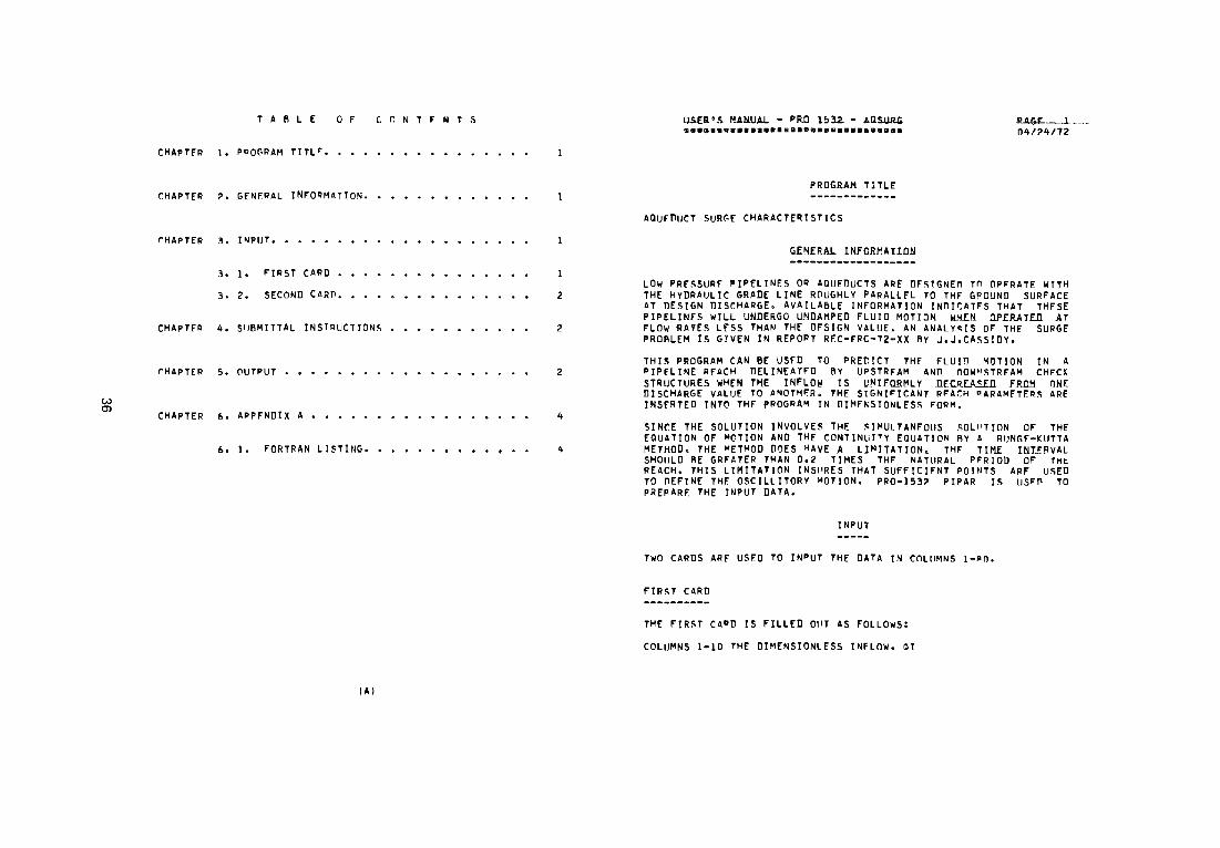
CHAPTER 1. PROGRAM TITLf.

CHAPTER 2. PURPOSE •• • • • • • ••••••••••••

CHAPTER 3. MfTHOD •• • • • • • ••••••••••••

CHAPTER 4. TNPUT-OUTPUT • • • • • •• • ••••••••

CHAPTER 5. LTMITATIONS. • • • • ••• • •••••••• l

lAl

PROGRAM DE SCRIP HON - PRO 1532 - P !PAR. ••••••••••••••••••••••••••••••••••••••

PROGRAM TITLE

DIMFNSIONLESS AQUEDUCT PARAMETERS

PURPOS.E

.e..A.G.£ l 04/?4172

THE PROGRAM CONVERTS IIASIC Dtt'ENSIONS OF' A "-TllllE SHAPED PIPFLINf OR AQUEDUCT REACH TO DIMENSIONLESS QU~NTITIF.S. THE QUANTITIES ARF USEF'UL IN EXAMINING SURGF. CHARACTERTSTICS OF' THE AOUFDUCT SYSTEM AS OUTL!NED IN REPOQT uc-Fac.-12-u BY J.J.CASSIOY. TH£ QUANTITIES ARE ALSO INPUT VARIABLF TO PR0-1~32 AQSU"IG.

METHrD

THE PROGRAM COMBINES THE rcIVEN QUANTITIES INTO DIMENSIONLFSS PARAMETFRS r.IVEN IN THE ABOVE REFF.RF.Nr.F U~INr. fLF.MENTARY MATHEMATICAL OPERATIO~S.

I NPUT-01,TF UT

THE INPUT CONSISTS OF': THF STATION. DISr.HARGFo RESISTANCE COEFFICIENT. PERTINENT ELEVATIONS ANO PIPELTNF DIAMETERS.

THE OUTPUT CONSISTS OF: THE STATION, DE~Ir.N DTSCHARr.E. THE ~IGNIFICANT DIMENSIONLESS PARAMETFRS.

LIMITATIONS

TH'E PROGRAM TS NOT LIM!TF.'D BY THE NUMBER OF TNPIJTS. HOWF.VFR, THEY MUST ALL BE NON ZF.RO.

Rl.lREAll (')F' RECLAMATJ('IN ENGH..E'fRtNG COMPIITF'R ~-YSTFM

-------------------------------------------------

CLASSIFifATION - HYDRAULTC.S

PROGRAM DESrRTPTION - PRC 15~~ - PTPAP

n•••••••••••••••••••••••••••••••••••••

PROGR.A.~. RY

J. J. CA~SIDY

norUMFNTAlION RY

H. T. FALVEY

11NITfD STATES DE.PARTMFNT OF THF INTFQil"R

~URFAII OF RfrLAMATION

~ENFRAL RfSFARCH

HVOPAULTCS RRANCH

ENGINEERTNr, ANn RFS~ARCH CFNTFR

nFNVER~ COLORAno 04/?4/'72

27

T A B L E 0 F' C O N T E N T S

C'HAPT£R 1. PROGRAM TITLF.

CHAPTER 2, r.FNERAL INFORMATION, , • , • , ••• , • , •

CHAPTER 3, INPUT• • •

3, 1. HEAOER CARD.

3, ?. DATA DESCRIPTION CARD,

CHAPTER 4, SUBMITTAL INSTRUCTIONS. ,

CHAPTE~ 5, OUTPUT• , • • • , • • •• • • •••••••

CHAPTER 6. AOPf'NDIX A. •

6, l, DEF'INITl'IN SKETCH OF PIPE REACH,

CHAPTER 7. APPF.NDIX II, •

1. 1. FORTRAN LISTING,

IA)

2

2

4

5

5

IISFA•S MANUAL - PRO 1532 - PJPAR ••••••••••••••••••••••••••••••••

PROGRAM TITLF

DIMFNSIO'ILESS AQUEDUCT PARAMETERS

GE'IERAL INF'r,R•'ATION

PAGF: l 041'4172

TN GENFRAL. TWO F'LOW C'ONDITIONS NFEn Tn RF FXAMJNE'D WHEN ANALYZING A PJPE'LINF OP. AQUEDUCT SYSTFM FOR SIIRIHN"• THESE ARF A SINUSOIDAL IN.PUT ANO A RAMP INPUT. CURVES FnR enTH OF THFSE' CONDITIONS HAVE BEEN PREPARF.D AND THEY ARF APPLICABLF TO ANY PIPEL INF SYSTF:M WHICH HA~ 11-TUIIE SHAPED RUr.HFS. I" 'lR'lF'R TO IISF THE CURVES, T~E DATA DESrRlblNG T~r P~YSICAL PRO•ERTIFS OF' THF REAr.HES "4llST ALSO Bf IN ll1"4~NSIONLF.SS F'ORM.

THIS PROGRAM USF'S THE BA~lr. PIPELINF GFOMFTRV TO COMPUTF TH£ NECFSSARY DIMrNSIONLESS PAPAMETER TO BE USFD TN THF ANALYSIS

INPUT

THE INPUT DATA ARE PUNCHED ON TwO CARns. A Hr.AOEP 01( P~OJFCT TITI.F. CARO A~·n A DATA nE~CPIPT!ON CARO.

HEAOER rARD

THE HEADER CARD IS FILLEII nur AS FOLLOWS:

C'OLUMNS 1-80 TH£ TITLE OR IIESCRIPTION OF' THF PROJFrT IS AR~ANGED TO eE CFNT£Rfll TN THE 80 SPACES ON THF CARO.

IIATA DESCRIPTtON CAPO

THE DATA DFSCPIPTtON CAR" IS FTLLFD OUT AS FOLLnws:

BUREAU OF RECLAMATION ENGINEERTNr; COMPtlTFR ~YSTFM

-------------------------------------------------

CLASSirirATION. ~YDRAULICS

IJSER 1 S MANIIAL - Pi;O PB? - PIPAR ••••••••••••••••••••••••••••••••

PROGRAM BY

J. J. CASSIDY

nor.uMENTATION 8Y

H. T. FALVEY

U~ITED STATE~ nEPARTMFNT OF THF INTFRinR

BUR!:AII OF RECL~MATION

GE~ERAL RESFARCH

HYD~AULICS RRANCH

ENGINEERTN~ AND RFSfAPC~ CFNTFR

nF.NVf.R, COLOP.Ano 04/?4/.,2

29

USER•~ MANUAL• P~O 1532 • PIPAR ..•.•.....•...........•......•..

APPrnDI X A

DEFINITION SKETCH OF PIPE REACH

__ {!_A

fj._fi_ __ l -

I I I-<--- --- - - JJ.

Ir D =O fhen D, '., D:;.

el. D

:-.r----1- - _§_. C ___ _j I I

I-<- -1 ~

Ir D.,=0 then IJ,, ~ 1)2

PAGE 4 04/24177

C C C

USER'S MANUAi. • PRO 1532 • P !PAR •...•..•..•.....................

APPENDIX 8

FORTRAN LISTING

n!MENS!ONLESS AQUEDUCT PARAMfTERS

flIMENSION TI U.l READ(?, 11 (T (NI ,N=l, 161 FORP'ATl16A5l rALL fOFINOl !FINO.EQ,llCALL EXIT wRTTE13,200l lTINl ,N:J,161

?00 FORHATl1Hl,IX,16A5l WRTTE13,20ll

201 FORMATC66H STA, SUMIL/Al SUMK A1/A4 R T~ VIM 1 Y2M Y2A//)

7 READl?,100lSTA,OO,RK,ELA,ELB,ELC,fL[,Dl,P2,D?,P,,n3 100 FORMATl2F6,0,IOF6,ll

Dl:ELA•ELB P4=ELD•FLC ~2=3.141600?002/4, f2:l,/12,oALOGln!P.2/RKl+l,14)007 J.F rr.1 l 3,2,6

2 nl=D2 6 A1=3,141600JoOJ/4,

fl:l,/12,oALOGlO!Ol/RKl+l,14)002 If ID3l 3,3,4

3 !14=02 A4=A2 F4:f2 SUMLA=Pl/Al+P?/A2+P4/A4 ~UMK:f!O(A2/A!)OO?OP1/Dl+f20P2/D2+f40(A?/A4)0020P4/D4 r.0 TO S

4 A3=3,!4160D300314. 114=03 A4:A3 SUP'LA:Pl/Al+P?/A2+P3/A3+P4/A4 F3:l,/12,•ALOGIOID3/RK)+l,14)002 SUMK:flO(A2/Alloozop1/Dl+f;>oP2/D2+F3o(A7/A3)oo;>o(p,+P4l/n~

5 TN:6,28320SQRTIAl•SUMLA/32,2l R=SUMKOTNOQ0/(?.,0A20A2•SUMLA> PAR=At/lQOOTNl YlM=rrLA+D2-EL~)OPAR YlB=IFLD•ELBloPAR Y2M=D40PAR Y2B=IFLD•ELC)OPAR AR=Al/A4 WRTTE 13,202) STA .ao. SUMLA, SIIMK ,AR, R, TN, Y lM, vu,. Y::>M. Y2~

202 ~0RMATIF6,0,F8,n,2Fa.1,3F7,J,4F8,4) GO TO 7 FND

p= s 04/24172

YIB

IJSER•S IIANUAL - PIIO 1532 - PIPAR ••••••••••••••••••••••••••••••••

COLUMt,S 1-6 STATION OF THE UPSTIIHM LFG OF THF PIPr, STA

7-1? DESIGN n1sCHARGE IN RFACH, Qr.

13•16 FRICTION LOSS COEFr1r1ENT FFO~ MOODY DIAGRAM, RK

19•?4 MAXIMU" UPSTREAM ELEVATION, E'LA

'-5•30 MINIMU~ UPSTRFAM ELEVATION, ELB

31•36 MINIMUM ~"WNSTREAM ELEVATIO~, ELC

37•42 MAXIMUM DOWNSTREAM HEVATIO~, ELD

43•48 UPSTRFA~ VERTICAL PIPE DIAMFTER, Dl

47•54 LFNGTH OF HORIZONTAL PIPE WITH OIAMFTFR D?, D?

53•60 HORIZONTAL PIPE DIAMFTER, D2

61•66 LFNGTH OF HORIZONTAL PIPE WITH r.lAMFTFR D,, 03

PAGE 2 Q4/2ltl72

67-72 HORIZONTAL PIPE n1AHETER, DJ. IF THFRE IS ONLY nNF. DIAMETER OF HORIZONTAL PIPF, THEN P3:0, THE nlAMETER OF THF nowNSTRFAM VF.RTICAL PIPE IS SUBTITUTED FOR 03,

SUBMITTAL INSTRUCTIONS

THE FIRST CAPJ'I IN THE nATA SET SHOIJI D BF THF HF"ADrR r.ARD, THE NEXT N CARDS ARE THE DATA DESCRIPTION CARDS, ~HEPE N IS ANY POSITIVE INTFGEq,

OUTPt,T

THE DATA OUTPUT IS IN THF. FORM OF" A TARLF WHF.Rr THF COLl™N HEADINGS ARF ~EFTNEO A~ FOLLOWS:

STA= STATION OF VERTICAL CENTERLtNF AT UPSTRFAM LrG OF REACH

Q = DESIGN DISCHARGE IN PEACH

SUHIL/AI : SllMMATION OF ALL LENGTH TO AREA RATIOS IN RF"ACH

$UMK = SUMMATION OF FRICTION COEFFICIFNT TIMFS LFNTH TO AREA

llSFR 1 S MANUAL - PRO 1532 - PIPAR ••••••••••••••••••••••••••••••••

RATIOS RELATIVE TO THE HORl70NTAL P!PF ARFA IN THE pfAr.H.

Al/A4 = AREA RATIO BETWEEN UPST~EAM AND DOWNSUEAN IIU?JCAL LEGS,

R = DIMENSIONLESS DAMPINGIFRICTIONI FACTOR

TN: NATURAL PERIOD OF Tl'F REACH

YlM = IIAXIMUM UPSTREAM WATFR SURFACE !N DIMFN~IONLFSS FORM

YIB = MINIMUM UPSTREAM WATER SURFACE IN DIMFN~IONLFSS F"ORH

Y2M = Mn I MUM DOWNSTREAM WATER SUPFACF IN OIMFN"!ONLF.SS FORM

Y2B = 141N!MUII DOWNSTREAM WATER SU~FACE IN OIMFN\IONLES\ FORM

T A 8 L E O F C O N T E N T S

CHAPTER 1. PROGRAM TITLF.. • • • • ••• • ••• • • • • l

CHAPTER 2. PURPOSE •• • • •••••••••••••••

CHAPTER 3. ~FTHOD •• • • •••••• • • • • • • • • • l

CHAPTER 4. INPUT-OUTPUT ••••••••••••••••

CHAPTER ~. LIMITATIONS •••••••••••••••••

(Al

PROGRAM DESCRIPTION - PPO 1532 - AQSURG •••••••••••••••••••••••••••••••••••••••

PROGRAM TITLE

AQUFDUCT SURGE CHARACTERISTTCS

PURPOSE

!'AGE. l 04/24172

TO !IOLVF THF NONLINEAR SUR«;£ EQUATION OF FLOW IN A u-TllBF !'IHAPED PIPELINF SYSTFM FOR A GIVFN DECREASF TN THF INFLOW RATF.

METHOD

THE PROGRAM SOLVES THE ONE-DIMENSIONAL EQUATION OF MCTION AND THE CONTINUITY FQUATION ~IMULTANEOUSLV 8V A RIINGE-KUTTA MFTHOD OF NUMERICAL INTEGRATION.

lNPUT-011TPUT

THE INPUT CONSISTS OF TWO CARDS WHICH CONTAIN: nIMFNSIOtlLESS AQUFDUCT PARAMETERS, AND DIMENSIO~LESS FLOW PARAMETERS.

THE OUTPUT CONSISTS OF: FLO~ AND WATFR !IURFACF. PAQAMFTFR!I AT DISr.RETF TIME INTERVALS.

LIMITATIONS

THE SilF. OF THE TIME INTFRVAL MUST 8E CHOSEN TO BE LE55 THAN 0.2 TIMFS THE NATURAL PERIOD OF THE P!PELTNF RFAr.H AEI~G ANALY7FD.

RURFAU OF RECLAMATION ENG I tl!EER T NG COMPIITF~ ~ VS TFM - --------------------------------------------------

CLASSI~ICATION - HYDRAULICS

PRO~RAM DESCP.IPTION - PRO 1532 • AQ~URr. •••••••••••••••••••••••••••••••••••••••

PROGHAM AV

J. J. CASSIDY

nocUMF.NTATION BY

H. T. FALVEY

~NITFD STATES nEPARTMFNT OF THF INTFRIOR

f\URf.Afl OF RECLAMATION

GENERAL RESEARCH

HYOPAULICS ~RANCH

FNGINEERTNr. AND RESEARCH CENTFR

T!F'NVF.R, COLORAno 04/?.4/"'').

33

T A II L E 0 F C O N T F N T S

CHAPTFR 1. Pl'IOGRAM TITLF.

CHAPTER ?. GENERAL INFORMATION •••••••••••••

rHAPTER

CHAPTE'l'I

rHAPTER

CHAPTER

3. INPUT •••••

3. 1. FIRST CARD

3. 2. SECOND CAR~.

4. SIJIIMITTAL INSTl'IUCTION!i

5. OUTPUT •• • • •••••••••••••••

6. APPFNDIX A • ••••

6, 1. FORTRAN LISTING. • • • • • 9 • • 9 I • •

CAI

2

2

2

4

tJ.S£a•s MAN.l!Al - PRO \!,32. - AQSUJU; •••••••••••••••aaamm••••••maawama

PROGUK TITLE

AQUFOUCT SURGE CHARACTERISTICS

6..E.N.ERAL lNFO.RMAUON

~-l. --·-04/?4172

LOW PRFSSURF PIPELINES OR AQUEDUCTS AR~ DFSTGNEn Tn OPFRATE WTTH THE HYDRAULIC GRADE LINE ROUGHLY PARALLEL TO THF GPOUND SURFACE AT TIESIGN DISCHARGE. AVAILABLE INFORMATION INTII~ATFS THAT THFSE PIP.ELINFS WILL l!NllERGO U-"IDAMPED FLUID MOTION .WM.EN. OP.ERAJ.ED AT FLOW ~ATES LFSS THAN THE DFSIGN VALUE. AN ANALY~IS OF THE SURGE PRORLEM IS GIVEN IN REPORT REC-FRC-72-XX BY J.J,CASSIDY,

IN A CHFCK

ON.I::

THIS PROGRAM CAN BE USFD TO PREDICT THF FLUID MOTION PIPELINE REACH DELINEATFD BY UPSTRFAM ANO now~sTRFAM STRUCTU.RE.S WllEN THE IN.F'LOl!I IS UNIFORl'ILY DE<:R.E.A.5..E11 FROM DISCHARGE VALUE TO ANOTHER, THE SIGNIFICANT RFACH DARAMFTERS INSFRTED INTO THE PROGRA~ IN DIMF~SIONLESS FQ1lM.

ARE

SINr.E THE SOLUTION INVOLVE!I THE SIMUL TANF'OUS SOLl•TION OF THE EQUATION OF MOTION AND THE CONTINUITY EQUATION AY A RUNGE-KUTTA METHOD, THE METl-!OD OOES MAVE A LlMITATION. THF Til1.E INT.Ef!VAL SHOULD AE GRFATER Tl-!AN 0.2 TIMES THF NATURAL PFRIOU OF THt REACH, THIS LIMITATION INSl'RES THAT SUFFICIFNT POINTS ARF USED TO nEFJNE THE OSCILLITORY MOTION. PR0-153? PlPAR IS usFn TO PREPARE THE INPUT DATA.

INPUT

TWO CARDS ARE USF.D TO INPUT THE DATA IN COLUMNS 1-110.

FIRST CARD

THE FIRST CAP.D IS FILLED OIIT AS FOLLOWS:

COLUMNS 1-10 THE DIMENSIONLESS INFLOW, QI

RUREALI OF' RECLAMATION ENGI~EfRTNG COMPIITFR 5VSTFM

-------------------------------------------------

CLASSI~ICATION • HYDRAULIC~

USER I S MA~UAL - PRC 1532 - AQSIJRr. •••••••••••••••••••••••••••••••••

PROGRAt-. AY

J. J. CASSIDY

DO('lJMfNTATTON BY

H. T. F~LVEY

IINJTf.D STATES T"EPARTMfNT OF THF JNTFRif'R

BURF.AII OF RECLAMATION

r.ENERAL RFSEAPCH

HYDRAULICS BRANCH

ENGINEERTNr. AND RFS~ARCH CFNTFR

PfNVER. COLORAno 04/'?4/7?

35

USER'S MANUAL - PRO 1532 - AQSUPG •••••••••••••••••••••••••••••••••

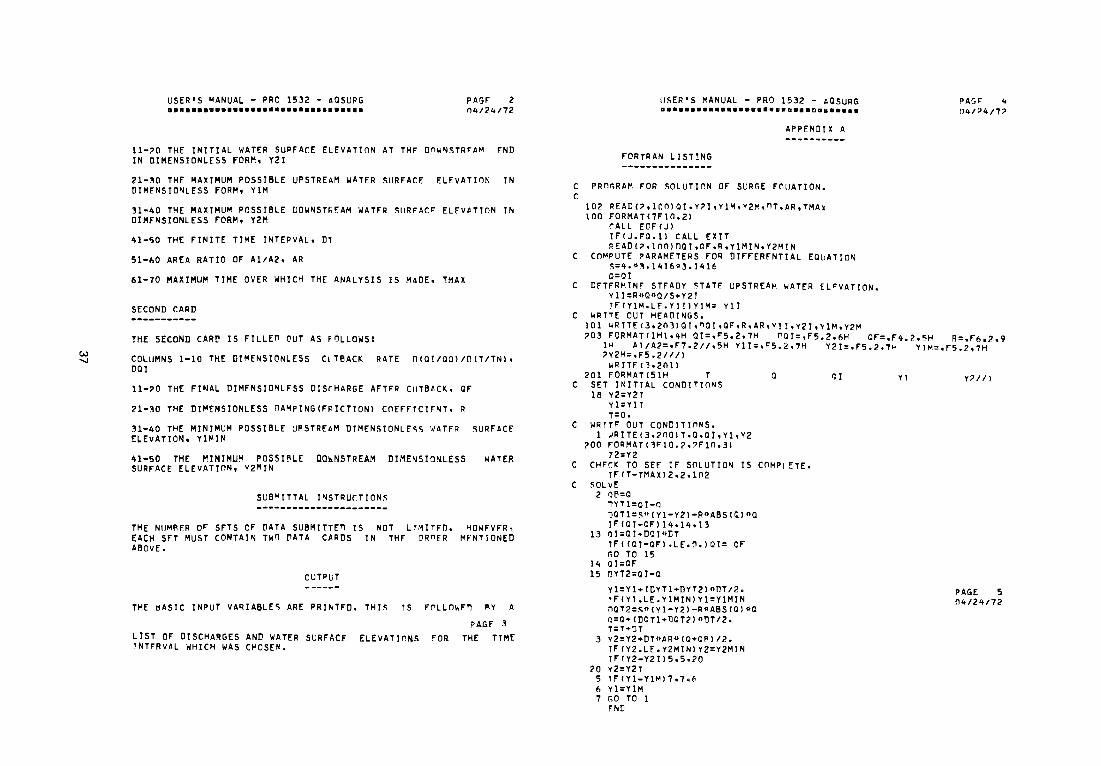
PAliF 2 04/24172

11-20 THE INITIAL WATER SUPFACE ELEVATION AT THF onwNSTRFAM FND IN DIMENSIONLESS FORM. Y2I

21-30 THE MAXIMUM POSSIBLE UPSTREAM WATE'R SURFACE ELEVATION IN OIMFNSIONLESS FORM, YlM

31-40 THE MAXIMUM POSSIBLE DOWNSTl<F.AM WATFR SIIRFACF' ELFVATtnN IN DIMfNSIONLESS FORM, Y2M

41-50 THE FINITE TIME INTEPVAL, Dt

51-~0 AREA RATIO OF Al/A2, AR

6-1-70 MAXIMUM TIME OVER WHICH THE ANALYSIS IS MADE, TMAX

SECOND CARD

TH! SECOND CARD IS FILLEO OUT AS FOLLOWS:

COLUMNS 1-10 THE DIMENSIONLESS Cl TBACK RATE O(QI/QOI/OIT/TNI, DQI

11-20 THE FINAL DIME'NSIONLFSS DISrHARGE AFTFR CUTBACK, QF

21-30 THE DIME'NSIONLESS OAMPINGIFPICTIONI COE'FFTCIFNT, R

31-40 THE MIN?MUM POSSIBLE UPSTREAM D?MENSTONLF~S WATFR SURFACE' ELEVATION, YlMIN

41-50 THE MINIMUM POSSil'ILE DO~N.STREAM DIMENSIONL.ESS SURFACE ELEVATION, Y2MIN

WATE.R

SUBMTTTAL INSTRUCTIONS

THE NUMAER OF' SFTS OF DATA SUBMITTEl'l IS NOT LTMITFD, HOWFVFR, EACH SET MUST CONTAIN TWO ~ATA CARDS IN THF OAnEA MfNTiONED ABOVE,

OUTPUT

THE ~ASIC INPUT VARIABLE~ ARE PAI~TFD. THIS TS

LIST OF DISCHARGES AND WATE'R SURFACE ELEVATIONS ?NTFRVAL WHICH WAS CHOSEN.

Fl"'LLOWl'Tl AY A

PA.Gf 3 !'"OR THE TIME

USER'S MANUAL - PRO 1532 - AQSURG m••••••••••••••••••••a•••mma•••••

APPENDIX A

FORTRAN LIST!NG

PA.GF 4 04/?4/7?

C PRn~RAM FOR SOLUTION OF SURGE FOUATION. C

C

C

C

C

C

C

C

102 READ(?,lOOIQI,Y2I,YlM,Y2M,1'1T,AR,TMAk 100 FORMATl7Fl0.2l

CALL E'OFIJI IFIJ.FQ. ll CALL EXIT P.EADl?,1nn1nar,0F,R,Y1MIN,Y2MIN

COMPUTE PARAMETERS FOR DIFFEAF'NTIAL EQUATION 5:4.03.141603.1416 a=OI

DF.TFRMINF STFADY 5TATF. UPSTREAM WATER ELF'VATION. Y1I=R<>QOQ/S+Y21 !F(YlM,LF.,YlTIYlM= YlI

WRITE OUT HEADINGS. 101 wRITE13,203lQI,nQI,QF,R,AA,YJl,Y2I,YlM,Y2M 203 FORMAT(lH1,4H QI=,F'5,2,7H nQI=,F5.2,6H QF=,F4.2,~H R=,F6,2,9

1H AI/A?.=,F7,2//,5H YlI:,F'5,2,7H Y2I=,F5.2,7H YIM=,F5,2,7H 2Y2M=,F5,2///l

wRITF. 13,?.0l l 201 FOP.MATl51H T

SET INITIAL CONDITIONS 18 Y2=Y2T

vl=YI I T=O,

WRTTF' OUT CONDITIONS. 1 wRITE13,200IT,Q,QI,Yl,Y2

?.00 FORMAT(~F'lO,?.,,Fl0,31 72:Y2

Q

CHFCK TO SEE IF SOLUTION IS COMPLETE, IFIT-TMAX12,2,102

SOLVE 2 lll'l=Q

nYTl=aI-o nQTl:S<>(Yl-Y2)-ROA8S(Q)<>Q 1F(QI-QF'll4,14,13

13 llI=QI+DOI<>OT !Fl IQI-QFI ,LE,0,IQI: QF r.O TO 15

14 OI=QF 15 DYT2=QI-Q

Yl:Yl+IDYTl+DYT2)oDT/2, TF'IYl.LE',YlMINIYl=YlMIN nQT2:s<>(Yl-Y2)-ROABS(Q)<>Q o=D•IDDTl+naT210DT12. r:T+DT

3 v2=Y2+DT<>ARO(Q+OAl/2, IFIY2.LE',Y2MINIY2=Y2MIN TFIY2-Y2Il5,5,?.0

20 Y2=Y2T 5 TFIYl-YlMl7,7,~ 6 Yl=YlM 7 r.O TO 1

FND

Yl Y'U/1

PAGE. 5 04/24172

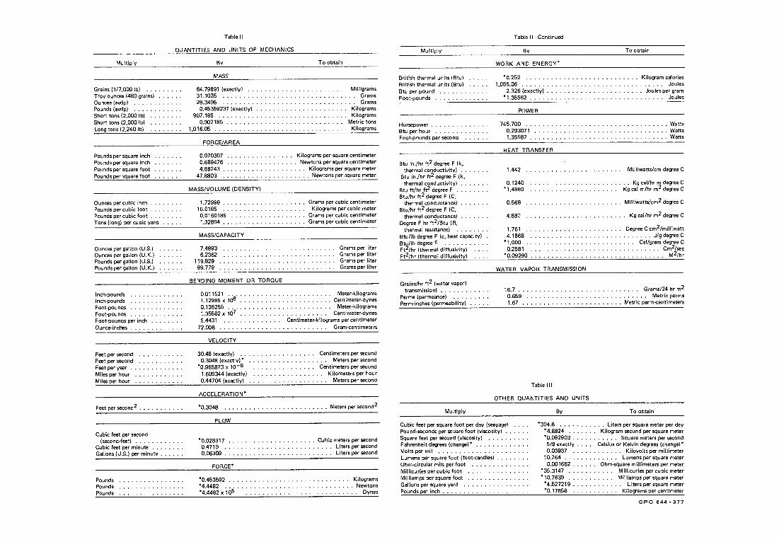
Table II

QUANTITIES AND UNITS OF MECHANiCS

Multiply

Grains (1/7,000 lb) ........ . Troy ounces (480 grains) ..... . Ounces (avdp) ........... . Pounds (avdp) •........... Short tons (2,000 lb) Short tons (2,000 lb) Long tons (2,240 lb)

Pounds per square inch Pounds per square inch Pounds per square foot Pounds per square foot

Ounces per cubic inch ....... . Pounds per cubic foot ....... . Pounds per cubic foot ....... . Tons (long) per cubic yard .... .

Ounce!. per gallon (U.S.) Ounces per gallon (U.K.) Pounds per gallon (U.S.) Pounds per gallon (U.K.)

I nch-?ounds ............ . Inch-pounds ............ . Foot-pounds ............ . Foot-pounds ............ . Foot-pounds per inch ....... . Ounce-inches ............ .

Feet per second .. Feet per second .. Feet per year .... Miles per hour Miles per hour , ....

Feet per second2 .•••.......

Cubic feet per second (second-feet) .... .

Cubic feet per minute ....... . Gallons (U.S.) per minute .•....

Pounds Pounds Pounds

By

MASS

64.79891 (exactly) 31.1035 ......... . 28.3495 ......... .

0.45359237 (exactly) 907.185 ........ .

0.907185 ... . 1,016.05 ...... .

FORCE/AREA

0.070307 . , 0.689476 .. 4.88243 ...

To obtain

. . . . . . . . . . . . . . . Milligrams

. . . . . . . . . . . . . . . . . Grams

. ................ Grams . ................... Kilograms

. . . . . . . . . Kilograms Metric tons

. Kilograms

Kilograms per square centimeter . Newtons per square centimeter . . . Kilograms per square meter

47.8803 ....•.......•.. . . . . . . Newtons per square meter

MASS/VOLUME (DENSITY)

1.72999 .. . 16.0185 .. . 0.0160185 . 1.32894 ...

MASS/CAPACITY

7.4893 6.2362

119.829 99.779

Grams per cubic centimeter Kilograms per cubic meter

Grams per cubic centimeter Grams per cubic centimeter

Grams per liter Grams per liter Grams per liter Grams per liter

BENDING MOMENT OR TORQUE

0.011521 . . . . . . • • . . . . • . . . . . • • . . . . . Meter-kilograms 1.12985 x ,06 ......•••............. Centimeter-dynes 0.138255 . . . . • • . . . . . . . . . . . . . . . . . . . Meter-kilograms 1.35582 x 107 .•..••................ Centimeter-dynes 5.4431 . . . . . . . . . . . . . . Centimeter-kilograms per centimeter

72.008 ...... .

VELOCITY

30.48 (exactly) 0.3048 (exactly)•

*0.965873 X 10-6 1.609344 (exactly) . 0.44704 (exactly)

ACCELERATION*

Gram-centimeters

Centimeters per second Meters per second

Centimeters per second Kilometers per hour

. . . . . Meters per second

*0.3048 ..... , . , ................. Meters per second2

FLOW

•o.028317 ..........•.......... Cubic meters per second 0.4719 . . . . . . . . • . . . . . . . . . . . . . . . . . Liters per second 0.06309 . . . • • • . . . . . • . • . . . . . . . . . . . . Liters per second

FORCE*

*0.453592 . , *4,4482 ... *4.4482 X 105

.... , . . . . . . . . . . . . . . . Kilograms

. . . . . . . . . . . . . . . . . Newtons

. . . . . . . . . . . . . . . . . . . . . . Dynes

Multiply

British thermal units (Btu) .... . British thermal units (Btu) .... . Btu per pound ........... . Foot-pounds ............ .

Horsepower ...... . Btu per hour Foot-pounds per second

Btu in./hr tt2 degree F (k, thermal conductivity) ..

Btu in./hr tt2 degree F (k, thermal conductivity) ... .

Btu ft/hr tt2 degree F .... . Btu/hr tt2 degree F (C,

thermal conductance) Btu/hr tt2 degree F (C,

thermal conductance) Degree F hr tt2/Btu ( R,

thermal resistance) ....... . Btu/lb degree F (c, heat capacity) . Btu/lb degree F .......... . Ft2/hr (thermal diffusivity) Ft2/hr (thermal diffusivity)

Grains/hr tt2 (water vapor) transmission) ........... .

Perms (permeance) ........ . Perm-inches (permeability) .... .

Multiply

Table I I-Continued

By To obtain

WORK AND ENERGY•

*0.252 ........................... Kilogram calories 1,055.06 . . . . . . . . . . . . . . . . . . . . . . . . . . . . . . . . . . Joules

2.326 (exactly) ....................... Joules per gram • 1 .35582 . . . . . . . . • . • . • . . . . . . . . . . . . Joules

POWER

745.700 .. 0.293071 1,35582 .

HEAT TRANSFER

1.442 ........ .

0.1240 *1.4880

Watts Watts Watts

Milliwatts/cm degree C

. . Kg cal/hr m degree C Kg cal m/hr m2 degree C

0.568 ................... Milliwatts/cm2 degree C

4.882 . , . . . . . . . • . . . Kg cal/hr m2 degree C

1.761 .....•................. Degree Ccm2/milliwatt 4. 1868 . . . . . . . . . . . . J/9 degree C

• 1 .000 . . . . . . . . . . . . . . . . . . . . . Cal/gram degree C 0.2581 . . . . . . . . . .......... , , . . . . . . . . Cm2/sec

*0.09290 ............. , . , , . , . . . M2/hr

WATER VAPOR TRANSMISSION

16.7 . . . . . . . . . . . . . . . . . . . . . . • . . . . . . Grams/24 hr m2 0.659 . . . . . . . . . . . . . . . . . . . . . Metric perms 1.67 ........................ Metric perm-centimeters

Table Ill

OTHER QUANTITIES AND UNITS

By To obtain

Cubic feet per square foot per day (seepage) Pound-seconds per square foot (viscosity) ..

*304.8 . . . . . . . . Liters per square meter per day * 4.8824 . . . . . . . Kilogram second per square meter *0.092903 . . . . . . . • . . . Square meters per second 5/9 exactly . . . . Celsius or Kelvin degrees (change)* 0.03937 ... , . , , . . . . . Kilovolts per millimeter

10.764 . . . . . . . . . . . . . Lumens per square meter

Square feet per second (viscosity) ..... . Fahrenheit degrees (change)* ............ . Volts per mil .............•........ Lumens per square foot (foot-candles) ....... . Ohm-circular mils per foot ..... . 0.001662 ...... Ohm-square millimeters per meter Millicuries per cubic foot ...... . *35.3147 . . . . . . Millicuries per cubic meter

Milliamps per square foot ... . *10.7639 . . . . . .... Milliamps per square meter

Gal Ions per square yard * 4.527219 . . . Liters per square meter

Pounds per inch . *0.17858 . , . . . . . . . . . Kilograms per centimeter

GPO 844-377

7-1750(3-71) Bureau of Reclamation

CONVERSION FACTORS-BRITISH TO METRIC UNITS OF MEASUREMENT

The following conversion factors adopted by the Bureau of Reclamation are those published by the American Society for Testing and Materials (ASTM Metric Practice Guide, E 380-68) except that additional factors (*) commonly used in the Bureau have been added. Further discussion of definitions of quantities and units is given in the ASTM Metric Practice Guide.

The metric units and conversion factors adopted by the ASTM are based on the "International System of Units" (designated SI for Systeme International d'Unites), fixed by the International Committee for Weights and Measures; this system is also known as the Giorgi or MKSA (meter-kilogram (mass)-second-ampere) system. This system has been adopted by the International Organization for Standardization in ISO Rec;ommendation R-31.

The metric technical unit of force is the kilogram-force; this is the force which, when applied to a body having a mass of 1 kg, gives it an acceleration of 9.80665 m/sec/sec, the standard acceleration of free fall toward the earth's center for sea level at 45 deg latitude. The metric unit of force in SI units is the newton (N), which is defined as that force which, when applied to a body having a mass of 1 kg, gives it an acceleration of 1 m/sec/sec. These units must be distinguished from the (inconstant) local weight of a body having a mass of 1 kg, that is, the weight of a body is that force with which a body is attracted to the earth and is equal to the mass of a body multiplied by the acceleration due to gravity. However, because it is general practice to use "pound" rather than the technically correct term "pound-force," the term "kilogram" (or derived mass unit) has been used in this guide instead of "kilogram-force" in expressing the conversion factors for forces. The newton unit of force will find increasing use, and is essential in SI units.

Where approximate or nominal English units are used to express a value or range of values, the converted metric units in parentheses are also approximate or nominal. Where precise English units are used, the converted metric units are expressed as equally significant values.

Multiply

Mil ................ . Inches .............. . Inches .............. . Feet .............. .. Feet .............. .. Feet ............... . Yards .............. . Miles (statute) ......... . Miles ............... .

Square inches .......... . Square feet . . . . . . . . . . . . Square feet . . . . . . . . . . . . Square yards . . . . . . . . . . . Acres ............... . Acres ............... . Acres ............... . Square miles . . . . . . . . . . .

Cubic inches . . . . . . . . . . . Cubic feet ............ . Cubic yards . . . . . . . . . . . .

Fluid ounces (U.S.) ...... . Fluid ounces (U.S.) ...... . Liquid pints (U.S.) ....... . Liquid pints (U.S.) ....... . Quarts (U.S.) .......... . Ouarts (U.S.) .......... . Gallons (ll.S.) .......... . Gallons (U.S.) .......... . Gallons (U.S.) .......... . Gallons (U.S.) .......... . Gallons (U.K.) ......... . Gallons (U.K.) .....•.... Cubic feet ............ . Cubic yards . . . . . . . . . . . . Acre-feet ..•.....•.... Acre-feet ............ .

Table I

QUANTITIES AND UNITS OF SPACE

By To obtain

LENGTH

25.4 (exactly) . . . . . . . . . . . . . . . . . . . . . . Micron 25.4 (exactly) . . . . . . . . . . . . . . . . . . . Millimeters

2.54 (exactly)* . . . . . . . . . . . . . . . . . . Centimeters 30.48 (exactly) . . . . . . . . . . . . . . . . . . Centimeters

0.3048 (exactly)* . . . . . . . . . . . . . . . . . . . Meters 0.0003048 (exactly)* . . . . . . . . . . . . . . Kilometers 0.9144 (exactly) . . . . . . . . . • . . . . . . . . . . Meters

1,609.344 (exactly)* .................... Meters 1.609344 (exactly) . . . . . . . . . . . . . . . Kilometers

AREA

6.4516 (exactly) ............. Square centimeters *929.03 . . . . . . . . . . . . . . . . . . . . Square centimeters

0.092903 .................... Square meters 0.836127 .................... Square meters

*0.40469 . . . . . . . . . . . . . . . . . . . . . . . . Hectares *4,046.9 ........................ Square meters

*0.0040469 . . . . . . . . . . . . . . . . Square kilometers 2.58999 . . . . . . . . . . . . . . . . . . Square kilometers

VOLUME

16.3871 . . . . . . . . . . . . . . . . . . . Cubic centimeters 0.0283168 . . . . . . . . . . . . . Cubic meters 0. 764555 . . . . . . . . . . . . . . . . . . . . Cubic meters

CAPACITY

29.5737 . . . . . . . . . . . . . . . , . . . Cubic centimeters 29.5729 . . . . . . . . . • . . . . . . . . . . . . . . Milliliters

0.473179 . . . . . . . . . . . . . . . . . . Cubic decimeters 0.473166 . . . . . . . . . . . . . . . . . . . . . . • . Liters

*946.358 . . . . . . . . . . . . . . . . . . . Cubic centimeters *0.946331 . . . . . . . . . . . . . . . . . . . . . . . . Liters

*3,785.43 . . . . . . . . . . . . . . . . . . . . Cubic centimeters 3. 78543 . . . . . . . . . . . . . . . . . . . Cubic decimeters 3. 78533 . . . . . . . . . . . . . . . . . . . . . . . . . Liters

*0.00378543 . . . . . . . . . . • . . • . . . . . Cubic meters 4.54609 . . . . . . . . . . . . . . . . . . . Cubic decimeters 4.54596 . . . . . . . . . . . . . . . . . . . . . . . . . Liters

28.3160 . . . . . . . . . . . . . . . . . . . . . . . . . . Liters *764.55 . . . . . . . . . . . . . . . . . . . . . . . . . . . Liters

* 1,233.5 . . . . . . . . . . . . . . . • . . . . . . . • Cubic meters * 1,233,500 . . . . . . . . . . . . . . . . . . . . . . . . . . . . . Liters

39

REC-ERC-72-28 Cassidy, J J CONTROL OF SURGING IN LOW-PRESSURE PIPELINES Bur Reclam Rep REC-ERC-72-28, Div Gen Res, September 1972. Bureau of Reclamation, Denver, 37 p, 27 fig, 3 tab, 8 ref, append

DESCRIPTORS-/ *pipelines/ *surges/ closed conduit flow/ fluid flow/ fluid mechanics/ hydraulics/ oscillations/ *Water pipes/ momentum IDENTIFIERS-/ *pipeline surges/ Canadian River Project, Tex







························································~·································~·············i··························~·· ........................... , ...... .

ABSTRACT


. . .

-· ABSTRACT


, .••••..••..••••..••••.•.••.......•............••.................................... ···················································································· •

ABSTRACT


.

ABSTRACT


rec-erc-72-28 - bureau of reclamation · ms-230 (8-70) bureau of re clama tion technical report...

Documents