reassessing effective protection rates in a trade in tasks perspective
TRANSCRIPT

REASSESSING EFFECTIVE PROTECTION RATES
IN A TRADE IN TASKS PERSPECTIVE:
EVOLUTION OF TRADE POLICY IN "FACTORY ASIA"
Antonia Diakantoni and Hubert Escaith ‡
Abstract: With international trade moving from "trade in (final) goods" to "trade in tasks", effective
protection rates (EPRs) are back to the stage, allowing us to measure the overall protection of a
product or sector by including the production structure and the origin of the inputs -domestic or
imported. Input-output matrices are used in this paper to monitor the production structure of 10
Asian-Pacific countries between 1995 and 2005, and to calculate sectorial EPRs. The paper proposes
a series of counter-factual simulation methods aimed at isolating the specific contribution of changes
in tariff policies, in production structure or in real exchange rates. Working on international input-
output matrices allowed also to compute and compare the average propagation length of a cost-push
linked to a sudden change in tariff duties, identifying those sectors that are the most deeply
interconnected, both in the intensity and in the length of their inter-industrial foreign relationships.
Keywords: Tariff, Effective Protection, Trade in Value Added, International Outsourcing, Asian
Input-Output.
JEL classifications: F13, F23
_____________________________ ‡
Economic Research and Statistics Division, World Trade Organization. Forthcoming (September
2012) as WTO Staff Working Paper ERSD-2012-11. The authors thank Feifei Zhang for her statistical
assistance during the preparation of the underlying data base and the participants of the WIOD final
conference (Groningen, April 2012) for their comments and suggestions on an earlier draft; they
retain all responsibility for remaining errors and short-comings. The opinions expressed are personal
and do not represent an official position of the WTO or its Secretariat.

2
I. INTRODUCTION
The spread of international production networks and the increased geographical fragmentation of
supply chains profoundly changed the nature of world trade. Today, intermediate goods dominate
trade flows and the rapid industrialization of developing countries often results from the successful
insertion of developing countries in these global value chains. One of these most remarkable case is
the emergence of “factory Asia”, where developed and developing countries at different stages of
development and with different resource endowments have created complementary industrial
relationships to emerge as the world manufacturing powerhouse (WTO and IDE-JETRO, 2012).
Goods produced within these supply chains are traded across several countries, incorporating at each
stage an additional layer of value added. The shipments of intermediate goods between the
participating counties and industries provide the material support for this “trade in tasks”. This
explains why trade in tasks is much more sensible to the tariff duties imposed on those international
transactions, and especially when –due to tariff escalation—the duties charged on relatively
elaborated parts and components is high. At the difference of the import-substitution industrial
policies which drove steep tariff escalation, in a world dominated by global value chains, firms that
produce final goods often produce intermediate components as well. Firms lobbying for protection in
final goods may therefore have an incentive to protect upstream production, leading to flatter nominal
tariff schedules.
International Input-Output (I-O) matrices provide a particularly interesting tool for analysing the
impact of trade policy on these supply chains. Indeed, one of the main challenges facing the
statisticians producing such inter-linked tables is to estimate the flows of intermediate goods and
services between the countries and their respective industrial sectors. The increasing availability of
international I-O matrices provides a new perspective for revisiting one of the most vibrant issues of
international economics in the late 1960s and the 1970s: the role of effective protection rates (EPRs)
in trade and industrial policies.
We argue also that the concept of EPR is particularly adapted to analyse protection in today’s
international economics, where countries do not trade final goods anymore, but “trade in tasks”. As a
matter of fact, it can be shown that EPR does not measure protection on goods, but protection on
value-added, which is the way I-O matrices measure the domestic content of trade goods and services
(it can be shown that EPR is the percentage increase in sectoral value added per unit of output, which
is made possible by the nominal tariff schedule relative to a situation of free trade).
After briefly reviewing this debate and the main criticisms that are opposed by economists to the
effectiveness of EPRs in predicting ex-ante the changes in industrial structure, the paper will reverse
the order of the arguments and proposes a series of decomposition techniques to investigate, from an
ex-post perspective (i.e., once all substitutions induced by changes in prices have taken place), what
were the respective contributions of changes in trade policy, on the one hand, and in production
structure on the other one, in explaining the observed changes in EPRs.
The paper combines market access statistics with I-O matrices to show the increasing interconnection
of the Asian economies in a regional production network, and describe the main changes in trade
policy that accompanied this closer regional integration. The methodology derives from comparative
static analysis between 1995 (conclusion of the Uruguay Round), 2000 (before China joins WTO) and
2005 (latest benchmark year for I-O matrices). To analyse the source of variations in effective
protection, a series of counterfactual simulations will isolate the respective contributions of nominal
protection (changes in tariff schedules), productive structure (changes in technology and productive
linkages) and exchange rates. A conclusion will summarize the main results as well as highlight the
interest and limitation of the method for analysing trade policy from inter-temporal and inter-country
perspectives.

3
II. EFFECTIVE PROTECTION: DEFINITION, LIMITATIONS AND RENEWED
INTEREST WHEN TRADING IN VALUE ADDED
After having fell in relative obscurity, at least from a normative perspective, effective protection rates
(EPRs) may be back to the central stage as international trade moves from "trade in (final) goods" to
"trade in tasks".
A. TARIFF ESCALATION AND TRADE POLICY
Originally, EPRs were used as an analytical indicator of tariff escalation (the difference between low
and high duties). Discriminating between high and low taxed imports was used for two distinct goals.
The first one was closely linked to industrial policy, particularly the import substitution strategy
followed by most developing countries in the post WW2 era. Protecting infant industries was
achieved by raising high tariff barriers for their products, while keeping their supply costs competitive
through lower tariff on their imported inputs. In this theoretical framework, tariff escalation would be
typically biased in favour of processed final goods, while raw material and semi-processed inputs
would have lower duty rates.
The second motive was related to trade theory, as a country was supposedly able to improve its terms
of trade and welfare through the imposition of higher tariffs on goods with lower export elasticity or
where it had significant market power as importer. In this conjuncture, tariff peaks were not linked to
the degree of processing but only to the market power the high tariff country was enjoying for this
product, either as an importer or as an exporter. Nevertheless, even in the terms of trade approach, we
should also expect a higher probability of tariff peak for processed goods, due to the effect of product
differentiation. Indeed, individual countries have lower market power in goods with high elasticity of
substitution with respect to price, i.e., for commodities. At the contrary, the possibility of substitution
is lower for specialized or differentiated goods. Building on Rauch (1999) classification of goods into
three categories (commodities, reference priced goods and differentiated goods), Broda at al. (2007)
find higher market power on the latter category. 1 They also find that market power strongly affects
the trade policy of large countries, such as the USA, redounding in higher tariffs for goods in which
there is significant market power.
All in all, the theory of tariff escalation and effective protection remains closely linked to the first
motive of industrial policy, particularly aimed at substituting imports of manufactured goods. It can
be shown that a tariff escalation where tariffs rise in function of the degree of processing magnifies
the return to investment in upstream production sectors. At the contrary, the terms-of-trade approach
does not imply any functional relationship between a high level of tariff for a given products and
lower ones for the inputs required for its production, at least in the absence of strong economies of
scale and scope. 2
Actually, from a growth accounting perspective, EPRs can be closely associated to the production
function in a simplified KLEMS framework which distinguishes capital, labour, material and services
inputs:
[1]
1 Rauch classifies as 'reference priced goods' processed products that can be quoted without mentioning
the name of the manufacturer, as the information on price is found to be sufficiently useful by buyers. 2 Effectively, it could be argued from the perspective of the new trade theory (Krugman, 1979) that
when those scale effects are present, an initial protection of the (infant) industry would help acquiring a
dominant market position that could open the possibility of manipulating terms of trade.

4
Where Q is the output, K the capital inputs, L stands for labour inputs and M are the intermediate
inputs. 3 In the Leontief technology which underlies the I-O matrices used in the present analysis,
material inputs always enter in fixed proportions to produce a unit of output and the contribution of K
and L are bundled together as value added.
∑ [2]
Where stands for the value added in sector "j" (remuneration of the primary inputs such as capital,
labour, plus net taxes) and are the intermediate consumptions (domestic and imported) used by
the sector "j" from sector "i". ∑ stands for "Sum from i = 1 to n", where n is the total number of
sectors, including "j" itself as an industry may use some of its own output in the production process.
In a national account framework, and are observed, and is computed by differences, after
imputing net taxes. 4
In an open economy, intermediate consumptions can also be imported from trade partners. If all trade
partners are included in an international I-O matrix, the equation [2] can be rewritten as:
∑
[3]
Where superscript "c" designs the importing country (left side and first part of right-hand side) and
includes also its trade partners (second part of right-hand side). For simplicity, the following
discussion will disregard superscripts "c", with no loss of generality.
Assuming that all applied tariffs are MFN (most favoured nations) and do not discriminate between
trade partners, the effective tariff EPR for sector "j" is the difference between the nominal protection
enjoyed on the output minus the weighted average of tariff paid on the required inputs. It is given by:
∑
∑ [4]
With [ ∑ ] 0, where
(elements of the matrix A of technical coefficients in a
Leontief model), is the nominal protection on sector "j" and the nominal protection on inputs
purchased from sector "i". It should be noted that "i" can be equal to "j", as a firm from a given
industry may require purchasing inputs from other firms of the same sector of activity. In an inter-
country framework, "i" includes also the partner dimension [c] as inputs from sector "i" might be
domestic or imported.
Note that tariff duties do influence the domestic price of all inputs, be they imported or domestically
produced. In effect, domestic producers of tradable goods will be able to raise their own prices up to
the level of the international price plus the tariff duty, without running the risk of being displaced by
imports. Thus, any domestic industry "j" will benefit directly from the tariff applied to the goods it
produces ( ) but will suffer an additional cost equal to the weighted average of its intermediate
consumption (∑ ), including those purchased domestically.
3 The complete KLEMS model differentiates various categories of intermediate inputs: energy, material
goods and services. The present work focuses only on the tariff duties assigned to these inputs rather than on
their industrial classification. 4 For the readers unfamiliar with input-output notations, the standard notation show in line "i" the uses
(or destination) of sectoral output "i" for intermediate or final demand (including exports), while the column "j"
indicate the requirements of intermediate inputs from the various domestic sectors of origin, plus the imports.
Thus, an analysis in terms of production function is done according to the column index, "j".

5
The relationship between EPRs and the "price" of value added is patent, when noting that [ ∑ ] is the rate of sectoral value added per unit of output, when EPRs are computed according to
the Balassa (1965) formulation.5 Therefore, and under the simplifying assumption that are
exogenously given by the production technology and strictly complementary (Leontief production
functions do not contemplate substitution effects), EPRs can be interpreted as the ratio of the value
added obtained considering the given (applied) tariff schedules compared to a situation of free trade
and no tariff (MFN-0).
[5]
Where Vj and V*j are the value added in the activity "j" as measured at protection-inclusive domestic
prices and world prices, respectively. EPRs can also be expressed as a percentage of the domestic
value added margin (Flatters, 2003) by rewriting formula [5] as follows:
[6]
This reformulation measures EPR as the percentage by which a country's trade barriers increase the
industries' value added per unit of output as compared to value added at prevailing world prices.
The absolute magnitude of effective protection (the numerator of equation [4]) derives arithmetically
from a linear combination of applied tariff duties, negatively weighted when they apply to inputs
(weights being equal to their contribution in the total output). Intuitively, the higher the nominal
protection on the output (NP), the higher the absolute effective protection (AEP); similarly, the higher
the tariffs on inputs or the higher the weight of intermediate inputs in the production costs, the lower
the AEP. The latter could be reformulated as: "for a given tariff schedule, the higher the rate of value-
added, the higher the absolute magnitude of effective protection ". 6
Thus, a few properties of effective protection can be already derived from [4], [5] and [6]:
(a) Effective protection for an industry can be negative, even if its output benefits from a strictly
positive nominal rate of protection (tj>0).
(b) The effective rate of protection will be less than the nominal protection (and even negative), if
the nominal protection on an activity’s output is smaller than on its inputs.
(c) EPR will be higher (i) the larger the nominal tariff on the output and the lower the nominal
protection of the inputs required in its production, and (ii) the smaller the value added at
world prices.
(d) If the inputs required are all non-tradable (e.g., services), EPR is higher than nominal
protection when the Balassa formula is used. 7
(e) If the nominal tariff schedule is flat (all tariffs are similar across all sectors of activity), then
the EPR is equal to the nominal protection and identical for all products.
(f) A positive EPR creates an anti-export bias, as the value added obtained by selling on the
domestic market is higher than selling at international prices, even when the exporter is able
to get reimbursed from the tax duties paid on the corresponding imported inputs (drawbacks).8
5 An alternative formulation, commonly used in tariff analysis, was proposed by Corden (1996) and
excludes non traded inputs from the "A" matrix. Those inputs are therefore implicitly treated as domestic value
added. The appropriate treatment of non-traded inputs was the object of an abundant literature in the 1970s. The
present paper adopted the Balassa approach for its closer relationship with the national accounts concepts as
used in official statistics. 6 Note that the result does not always apply for EPRs, as the higher the value added (without
considering tariffs), the larger the denominator of EPR equation [4]. 7 The Corden approach, which treats non-tradable inputs as part of the domestic value-added, leads in
this case to an EPR equal to nominal tariff (Corden, 1985).

6
B. THE DEMISE OF EPR IN TRADE THEORY AND THEIR RESILIENCE IN APPLIED TRADE AND
"TRADE IN TASKS" ANALYSIS
After their formulation in the 1960s, EPRs gained rapidly a wide audience, and became regarded not
only as a key indicator of the structure of protection, but also as a predictor for policy appraisal, in
particular in developing countries. High positive EPRs create an anti-export bias, but they can be used
to redirect investment to targeted industrial sectors by providing artificially high factorial returns (the
value added measured at domestic prices) for these activities. Thus they were attractive tools for
import substitution industrialization policies (ISI), such as those adopted in Latin America up to the
1980s. Yet, theoretical criticisms arose almost as quickly as the EPR theory had emerged.
1. Theoretical shortcoming in a general equilibrium context
A key assumption of EPRs when used as predictors (and not as descriptors) is the hypothesis of fixed
coefficients in the production function, as it is implicitly the case in the Leontief model, which
assumes perfect complementarity between production factors K, L and M (equation [1]). While this
assumption has some validity in short-term economics, it is no more the case when long-term effects
have to be modelled. When long-run effects are considered in a general equilibrium context, two
forces counteract to reduce the "effectiveness" of EPRs as predictors: substitution and scale effects.
The possibility of substitution widens the choices open to each industry. When the domestic price of a
domestic product rises, its demand will be lower; the greater the substitution effects, the faster
demand shifts to lower-priced products. The situation is even more complex when traded and non-
traded goods and services are substitute. 9 Thus, the effective positive protection provided to the
priority sectors will be overstated by the EPR formula, while it will be the opposite for negative EPRs.
Moreover, when primary and intermediate inputs are substitutes, in particular when effective
protection changes the demand for labour in some sectors, it may lead to changes in the relative costs
of labour and capital across the board, inducing further substitution effects. Finally, in presence of
significant scale effects, the lower demand resulting from higher nominal protection may reduce
production volumes and increase production costs per unit in such a way as to considerably mitigate
(or even reverse) the intended subsidy on the sectorial value added. 10
Because of these theoretical
shortcomings, EPRs fell out of fashion in the late 1970s.
2. A widely applied measure devoted of theory?
The possibility of substitutability clearly undermines the analytical capabilities of EPR theory.
Despite these shortcomings, effective rate of protection remains widely used by practitioners and
policy analysts. There are several reasons behind EPR resilience.
First, EPRs remain a synthetic descriptor of the past or present arbitrages caused by the applied tariff
schedule on each sector of the economy. The I-O matrix observed in a certain point of time is the
outcome of the resources and technology available at that time, plus the end result from all the
substitution effects that took place due to changes in relative prices and in the nominal tariff structure.
Provided that the base year chosen for establishing the national accounts is close to a normal state
(free to recent real or nominal shocks such as natural disasters, changes in tariff duties or nominal
8 Due to the upward bias induced by nominal tariffs on the prices of domestic inputs, domestic costs
will always be higher than in a free trade situation. Moreover, most regional trade agreements limit drawbacks
on inputs imported from third countries. This anti-competitiveness bias is compounded by the impact of
protection on the price of non-tradable products and on the real exchange rate (the treatment of these effects is
beyond the scope of the present paper). 9 For example, in agriculture production, it is possible to replace the use of herbicides used for
controlling weeds by employing more labour. 10
Remember that value added is a residual, calculated as the difference between the market value of
the output and the cost of production, excluding primary inputs (labour and capital). When there are positive
returns to the scale of production, the value added by unit of product increases as production expands.

7
exchange rate), the EPRs calculated with the observed I-O coefficients give a synthetic and unbiased
picture of the net economic impact of nominal tariffs on productive sectors. 11
In particular, it provides
a good estimate of transfer of income across sectors and the resulting anti-export bias resulting from
the nominal tariff schedule. It is also a relatively simple measure to understand, compared to other
"simulated" estimates of market distortions. 12
Thus it is, from a purely descriptive point of view, an
excellent aggregated tariff indicator.
Second, the standard definition can still apply to partial equilibrium economic models, often used by
applied economists. Moreover, the increasing availability of computable general equilibrium (CGE)
models in the 1980s reinserted EPRs as bona fide indicators. CGE models simulate the substitution
effects that changes in nominal protection will determine in the economy, re-operationalizing the use
of EPRs in comparative statics. In particular, CGEs make possible the conduct of sensibility analysis
for measuring the impact of substitution effects on the predictive power of EPRs.
3. Vertical specialization and trade in value added
Recent developments in the very nature of international trade are providing an additional
attractiveness for this indicator. Globalization has changed manufacturing and business models; today
an increasing share of manufacture production is internationally fragmented. Before reaching their
final stage, "manufactures in process" transit through international supply chains in the form of
intermediate goods; at each stage, value added is incorporated (embodied) in the product then shipped
to the next step, often in a different country. We are therefore in a situation where countries do not
trade final goods anymore, but trade "manufacturing or business services". This is the reason why
Grossman and Rossi (2006) qualified the phenomenon as "trade in tasks".
From a national account perspective, what is internationally traded is value added (the primary inputs)
and the adequate measure of trade distortion is no more the nominal tariff structure on the output but
the effective rate of "protection" on value added. In this case, high positive EPRs are a bad omen for
the "beneficiary" sector, as it indicates a strong anti-export bias in a trade in task perspective as the
domestic cost of the sectorial value added is much higher than the international cost.
Trade in intermediate is both the blood stream of global value chains and the glue which ties together
the individual I-O matrices in an international I-O table. Therefore, for any given export by an
industry "j" in a country "c", it is possible to decompose the total exported value into (i) the domestic
value-added generated in its production, both directly from the main producing industry, and
indirectly via transactions between domestic industries; and (ii) the imported value-added generated in
producing the imports used in production (OECD-WTO, 2012).
Therefore, using international I-O matrices allows additional refinements in the computation of the
traditional EPR indicators, as the origin of imported inputs is identified, thus MFN tariffs may be
adjusted for preferential treatments, when relevant. On the other hand, the formula [4] can be adjusted
in order to capture both the direct and indirect value added embodied in the export of intermediate and
final goods. While the proper measure of the domestic factor content of trade is still subject to debate
in the literature (Koopman et al. 2011 and Stehrer, 2012), a first approach would be to add the indirect
consumption of inputs in the original definition of EPRs. Using Leontief instead of the technical
coefficients in equation [4] would capture these indirect consumptions of intermediate inputs.
Disregarding country subscript, it gives:
∑
∑ [7]
Where results from the Leontief inverse for all i≠j, and the Leontief coefficient minus one when
i=j.
11
We will measure in the paper the possible bias generated by short-term nominal exchange rate
movements, under the assumption that real exchange rates tend to return to their initial value. 12
Most alternative indicators are based on some estimate of the welfare cost of tariffs, and include
elasticities of substitution in partial or general equilibrium framework.

8
L" = (I-A)-1
- I [8]
Where I stands for the identity matrix of same rank than A, the matrix of technical coefficients.
In a first step, our analysis will capture only the first part of additional information provided by
international I-O matrices (allocating the sectoral consumption on imported inputs by trade partners).
In a second step, indirect effects and the international dimensions will be introduced to measure
average propagation length and compute EPRs as in equation [8].
III. THE DATA
A. THE ASIAN INTERNATIONAL INPUT-OUTPUT MATRICES
Technical coefficients
are calculated as a share of the intermediate inputs, domestic and
imported, in the final output. The relative weights [ of intermediate inputs [M] compared to
primary inputs ([K] and [L] in the production function [1]) is doubly important when measuring
EPRs. At the numerator of [4], they are used to correct NP with the weighted average of duties paid
on inputs (Absolute Effective Protection); at the denominator, they determine the rate of value added.
The technical coefficients are sourced (or derived when not available at the required disaggregation)
from the Asian international input-output (AIO) matrices developed by the Institute of Developing
Economies, JETRO. The matrices are available for three reference years 1995, 2000 and 2005 and
cover ten economies, namely China, Indonesia, Japan, Korea, Malaysia, Philippines, Singapore,
Chinese Taipei, Thailand, and the USA. 13
The AIO matrices have the same structure as the national ones, and include in addition trade in
intermediate goods and services. The original tables for 1995 and 2000 include 76 sectors of activity,
that we aggregated into 64 sectors to match the tariff data for the calculation of the nominal protection
rates. The 2005 64 sectors table results from our estimate, based on IDE-JETRO 26 sectors. The
computation of EPRs as in [4] is done on the domestic part of the AIO matrix.
The monetary data (domestic and foreign transactions) are expressed in US dollars. Imports are
valued FOB for China, Indonesia, Japan, Korea, Malaysia, Philippines, Singapore, Chinese Taipei,
Thailand, and the USA and CIF for the Rest of the World. Freight and insurance data are distributed
to partner countries with FOB data by applying the respective a CIF/FOB factor to each sector to
obtain a harmonised data set valued CIF for all countries.
The relative weight of intermediate inputs and its domestic or foreign origin is particularly important
from a trade in task perspective. It depends both of the "downstreamness" of each sector of activity,
the level of development of the national economy and its insertion in global supply chains (also called
"vertical specialization"). Downstream industries (e.g. manufactures) tend to rely more on
intermediate consumption than upstream extractive sectors, while given industries in developed
countries are usually more integrated (stronger backward linkages) than their counterparts in
developing economies (Graph 1).
Over the years, we observed a net increase in the magnitude of use of domestic inputs for all
countries, except for Singapore in Agriculture and Manufactures and Indonesia, Japan, Taipei and the
USA in Manufactures in 2005 compared to 1995 (Graph 1). This evolution is consistent with the
increased inter-industrial linkage to be expected when developing countries transit towards deeper
13
At the time of writing the paper, the final AIO 2005 matrix was not yet available at its most
disaggregated level, and the authors derived their own estimates when needed. For this reason, 2005 results have
to be considered with precaution.

9
industrialisation. The evolution of imported inputs presents a more diversified profile. In
manufactures we see an upward trend except maybe for Malaysia and the Philippines, and mixture of
tendencies in raw materials and in agriculture, especially when we look at 2000.
Graph 1: Domestic and imported contents of exports, by main category
Source: Author's calculations, on the basis of IDE-JETRO's I-O matrices and own estimates. The imported
content is under-estimated because only direct content is taken into account (see WTO and IDE-JETRO
2011).
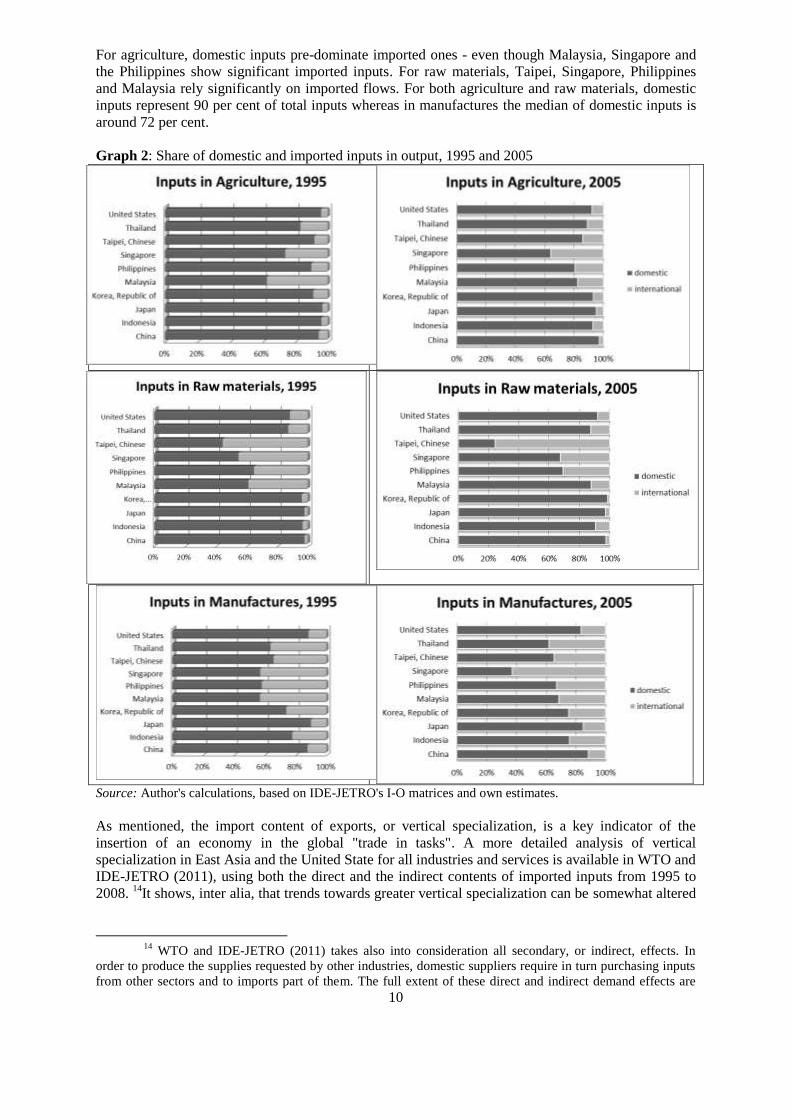
Even though magnitudes increase globally, shares remain balanced as shown in Graph 2. Domestic
inputs are pre-dominant in all product categories for the majority of countries, except for Chinese
Taipei in Raw materials and for Singapore in Manufactures. Generally, we do not observe a
significant change in the share of domestic inputs over the years, with the exception of Malaysia,
Philippines, Singapore and Chinese Taipei.
10
For agriculture, domestic inputs pre-dominate imported ones - even though Malaysia, Singapore and
the Philippines show significant imported inputs. For raw materials, Taipei, Singapore, Philippines
and Malaysia rely significantly on imported flows. For both agriculture and raw materials, domestic
inputs represent 90 per cent of total inputs whereas in manufactures the median of domestic inputs is
around 72 per cent.
Graph 2: Share of domestic and imported inputs in output, 1995 and 2005
Source: Author's calculations, based on IDE-JETRO's I-O matrices and own estimates.
As mentioned, the import content of exports, or vertical specialization, is a key indicator of the
insertion of an economy in the global "trade in tasks". A more detailed analysis of vertical
specialization in East Asia and the United State for all industries and services is available in WTO and
IDE-JETRO (2011), using both the direct and the indirect contents of imported inputs from 1995 to
2008. 14
It shows, inter alia, that trends towards greater vertical specialization can be somewhat altered
14
WTO and IDE-JETRO (2011) takes also into consideration all secondary, or indirect, effects. In
order to produce the supplies requested by other industries, domestic suppliers require in turn purchasing inputs
from other sectors and to imports part of them. The full extent of these direct and indirect demand effects are

11
when foreign direct investment and offshoring substitute some imports of parts and components with
local production.
B. NOMINAL AND EFFECTIVE PROTECTION RATES
The calculation of the effective protection rates is a two-step calculation which requires first the
computation of the nominal rates of protection, as shown in formula [4] of the previous section. The
nominal rate of protection is the percentage tariff imposed on a product as it enters the country.
Nominal protection (NP) is computed for the 53 good-producing sectors and partners included in the
I-O matrices, by first calculating the weighted tariff average by product and partner at the Harmonized
System (HS) 6-digits level; then HS6 results are aggregated at the AIO sectorial level. 15
NPs were
calculated for the three years 1995, 2000 and 2005; only MFN applied rates are used, as preferential
schemes were not available for all countries or reference years. The raw data for the calculation of
NPs —MFN duty rates and import statistics at disaggregated level of the Harmonized System (HS)—
were sourced from the WTO Integrated Data Base. Standard concordance tables were used (i) to
handle differences in versions of the various HS classifications used in tariff schedules and (ii) to
correlate HS tariff data to the ISIC industrial sectors.
From 1995 to 2005 we observe a trend towards lower applied tariffs, reflecting undoubtedly the effect
of the multilateral trade negotiations and the conclusion of the Uruguay Round, plus China and
Chinese Taipei joining the WTO. 16
This trend can also point towards an increase in productivity in
developing countries (Hansen, 2010) and a smaller productivity gap with industrialised economies
lowering the demand for nominal protection from domestic industrial groups.
It may also represent a shift away from traditional imports' substitution policies in developing
countries and greater emphasis on export competitiveness. Although high NP on imported goods
protects domestic producers, it increases the production costs of domestic manufacturers who use
those goods as inputs. The net effect is captured by EPR, measuring the net overall protection of a
sector in the basis of the production structure.
EPRs were computed based on equation [4]. We associated the World NP (applied MFN tariffs) to
domestic intermediate inputs as we suppose that the domestic price of domestic products that are
internationally tradable compete with World prices. Imported intermediate goods were calculated on
the basis of the composition of the transactions with the importing partner. EPRs were further
aggregated to the three major product categories, Agriculture (AIO sectors 1-7), Raw materials
(sectors 8-11) and Manufactures (sectors 12-53). When required, a further disaggregation of
Manufacture was performed to isolate sectors particularly involved in global supply chains.
IV. INITIAL DATA EXPLORATION
The objective of this section is to provide some empirical evidences and stylised facts about the
distribution of the observations across time and across sectors.
A. LOOKING AT ABSOLUTE FREQUENCIES
Table 1 distinguishes between sectors which truly benefit from the tariff schedule (their EPR is higher
than their nominal protection) from those which are relative or net losers (effective protection lower
captured by the Leontief matrix (as in equation [7]). Indirect imported content refers to the share of foreign
value-added in domestically sourced inputs. 15
Services sectors (AIO codes 54 to 64) do not benefit from tariff protection. 16
The Uruguay Round concluded in 1995; albeit GATT-WTO only deals with bound tariffs, many
applied duties were reduced in this opportunity, especially in developed countries. In addition, newcomers, such
as China (2001) and Chinese Taipei (2002) had to open their economies when negotiating their accession to
WTO (on a typology of bound and applied tariffs by countries and sectors, see Diakantoni and Escaith, 2009).

12
than the nominal one, or even negative). Note that Singapore has been excluded from all calculations,
as its tariff schedule is flat and equal to 0, leading to a similar flat EPR-0 profile. Altogether, the first
two panels exhaust almost all possible cases. 17
The third panel shows, among the sectors receiving
less effective than nominal protection, those which suffer from a negative EPR.
Table 1: Effective protection relative to nominal one, absolute counts of sectors by main type of
activity (all years) (1) EPR greater tha n NP ( 2 ) E P R l o w e r t h a n N P ( 3 ) E P R n e g a t i v e
¦ DVG DVD Total
------+----------------------------
Agr ¦ 65 21 86
Man ¦ 618 156 774
Raw ¦ 12 0 12
------+----------------------------
Total ¦ 695 177 872
¦ DVG DVD Total
------+----------------------------
Agr ¦ 82 21 103
Man ¦ 264 96 360
Raw ¦ 70 24 94
------+----------------------------
Total ¦ 416 141 557
¦ DVG DVD Total
------+----------------------------
Agr ¦ 49 15 64
Man ¦ 148 69 217
Raw ¦ 55 22 77
------+----------------------------
Total ¦ 252 106 358
Note: EPR: Effective protection rate; NP: Nominal protection (applied tariffs); Agr: agriculture, Man:
manufactures, Raw: raw material. DVG: developing countries, DVD: developed economies.
No sector producing raw material benefited from enhanced effective protection in developed
economies; as a matter of fact, in their large majority (92 per cent), they suffered from negative
protection. The situation is barely better for these sectors when they operate in developing countries,
67 per cent of them suffering from negative EPR.
On the other side of the spectrum, manufactures' sectors usually enjoy a positive EPR higher than
their nominal protection. Over the period 1995-2005, it was the case for 70 and 62 per cent of them in
developing and developed countries, respectively, when looking at the disaggregated data.
Nevertheless, a significant number of manufacturing sectors suffers from negative protection. Some
of those manufacturing sectors are relatively close to raw materials (such as timber, or pulp and
paper). Others are much more downstream in the production chain (printing and publishing,
electronics, motor cycles). When this is the case, the pattern is more typical of the Asian developing
economies, which is unexpected and may be linked to the export-orientation of their industrial policy
or to the reliance on non-tariff measures to protect their domestic market.
Agriculture stands in-between with EPRs usually lower than its nominal protection, particularly in
developing economies (66 per cent of the cases); in developed economies, the odds are better as the
sectors split equally between the two cases.
Table 2: Absolute frequency of negative EPRs by sector, 1995-2005 1995 2005
Sector¦ DVG DVD Total
Agr ¦ 14 5 19
Man ¦ 45 21 66
Raw ¦ 19 7 26
Total ¦ 78 33 111
Sector¦ DVG DVD Total
Agr ¦ 18 5 23
Man ¦ 61 26 87
Raw ¦ 19 8 27
Total ¦ 98 39 137
Note: see table 1.
Interestingly, the number of sectors suffering from negative protection rose between 1995 and 2005,
in both developing and developed countries (table 2). The change is almost entirely due to the
incidence of negatives in the manufacturing sector, particularly in developing countries. As a positive
EPR is usually associated with a disincentive to export, this may point to a more export-led
orientation of the trade policy. The next section will go further in the analysis, moving away from a
pure count of sectors and looking at the numerical value behind the respective nominal and effective
protection rates.
17
There are only two cases where effective and nominal protections are both equal to 0, occurring in
the Philippines for sector 009 (iron ore) in 2000 and 2005.

13
B. FURTHER EXPLORATORY STATISTICS
Table 3 provides additional insights on the respective level and distribution of nominal and effective
protection rates, by sector, years and development status. First, in all cases sectors producing raw
materials appear as enjoying very low nominal protection and suffering also from a negative rate of
effective protection. This is almost a mechanical consequence of the sectors (which are also their
suppliers of inputs) enjoying higher nominal protection. Nevertheless, this negative EPR has been
decreasing in developing countries (from -2.1 to 0.8 per cent), in line, as we shall see, with a
symmetrical variation in the (positive) EPRs enjoyed by agriculture and manufactures.
While both agriculture and manufactures enjoy a high rate of nominal and effective protection in the
Asian developing countries, it is striking to see that the asymmetrical distribution of those rates
(approximated by the difference between the arithmetic mean and the median) is much higher in
agriculture than in manufactures. EPR is, in average, higher for agriculture than manufactures in
developing countries (up to 2005), while the median is much lower. This signal a clear asymmetrical
distribution: while a few agricultural sectors may benefit from very high EPR, the majority of them
has a lower protection than in manufactures. In the case of developing countries, up to 2005, effective
protection was always higher for manufactures than for agriculture. The situation reversed in 2005 (a
similar situation was observed for the sub-group of developing economies).
Table 3: Median and mean of nominal and effective protection rates, by sector, years and
development status
AGRICULTURE RAW MATERIAL MANUFACTURES
DVG DVD DVG DVD DVG DVD
1995 NP EPR
NP EPR NP EPR
NP EPR NP EPR
NP EPR
Median 6.5 4.9
1.3 0.9 1.2 -0.4
0.0 -0.5 9.2 14.7
2.3 3.5
Mean 27.2 29.6
2.0 1.1 3.2 -2.1
0.1 -0.5 15.9 26.3
4.0 8.3
2000
Median 3.8 2.9
1.2 1.1 1.0 -0.5
0.0 -0.4 7.5 11.7
1.9 2.5
Mean 24.3 30.1
1.8 1.5 1.6 -1.2
0.1 -0.4 10.0 17.6
3.3 6.6
2005
Median 3.9 2.6
1.9 3.1 0.1 -0.5
0.0 -0.3 6.2 10.6
1.3 1.8
Mean 11.9 15.5 2.1 3.9 1.1 -0.8 0.1 -0.4 7.8 16.6 2.9 5.8
Notes: DVG and DVD stand for developing and developed countries, respectively. NP: nominal protection;
EPR: Effective protection rate (in per cent).
The other important observation is the sharp decrease in both nominal and effective protections
recorded in the group of Asian developing countries in agriculture and manufactures. The drop is
particularly important in agriculture, exceeding 50 per cent for both nominal and effective protections
between 1995 and 2005. At the same time, NP in agriculture remained more or less constant in the
two developed countries (Japan and USA), at least on an MFN basis, while effective protection
increased by almost 3 percentage points. This said, both nominal and effective protections remain
much lower in developed than in developing countries.
Additional statistical analysis was performed to further explore the structure of the data and identify
possible patterns and correlations. Table 4 shows the correlation between EPR, nominal protection on
the output (NP) and the weight of intermediate inputs in the production costs (Inputs).
All sectors show a positive correlation with NP, as expected. Raw materials in both developed and
developing countries show both (i) the weakest positive correlation with NP and (ii) a negative
correlation between EPR and their reliance on intermediate inputs, as should be expected in a
situation of steep tariff escalation. The situation is similar for agriculture, but to a much lower extent.
14
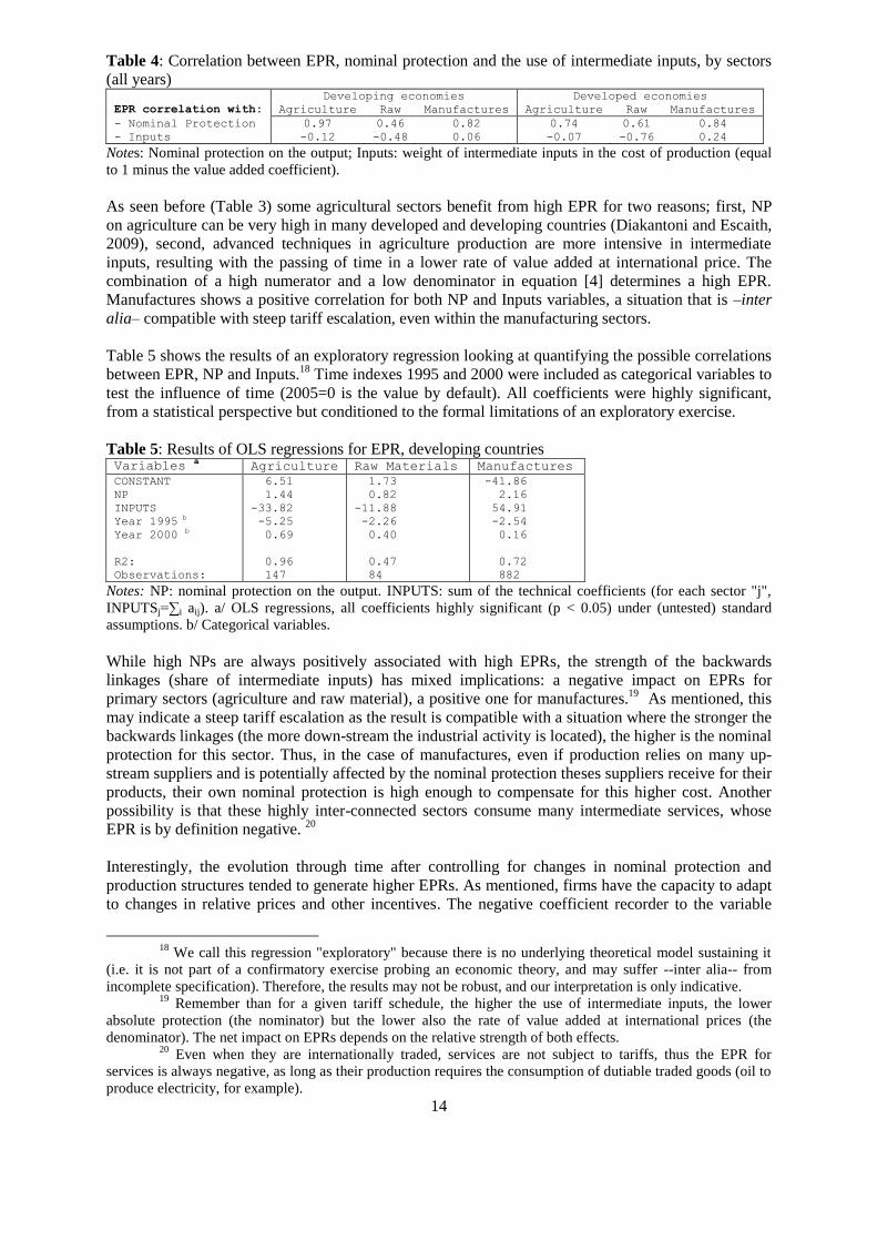
Table 4: Correlation between EPR, nominal protection and the use of intermediate inputs, by sectors
(all years) Developing economies Developed economies
EPR correlation with: Agriculture Raw Manufactures Agriculture Raw Manufactures
- Nominal Protection 0.97 0.46 0.82 0.74 0.61 0.84
- Inputs -0.12 -0.48 0.06 -0.07 -0.76 0.24
Notes: Nominal protection on the output; Inputs: weight of intermediate inputs in the cost of production (equal
to 1 minus the value added coefficient).
As seen before (Table 3) some agricultural sectors benefit from high EPR for two reasons; first, NP
on agriculture can be very high in many developed and developing countries (Diakantoni and Escaith,
2009), second, advanced techniques in agriculture production are more intensive in intermediate
inputs, resulting with the passing of time in a lower rate of value added at international price. The
combination of a high numerator and a low denominator in equation [4] determines a high EPR.
Manufactures shows a positive correlation for both NP and Inputs variables, a situation that is –inter
alia– compatible with steep tariff escalation, even within the manufacturing sectors.
Table 5 shows the results of an exploratory regression looking at quantifying the possible correlations
between EPR, NP and Inputs.18
Time indexes 1995 and 2000 were included as categorical variables to
test the influence of time (2005=0 is the value by default). All coefficients were highly significant,
from a statistical perspective but conditioned to the formal limitations of an exploratory exercise.
Table 5: Results of OLS regressions for EPR, developing countries Variables
a Agriculture Raw Materials Manufactures
CONSTANT
NP
INPUTS
Year 1995 b
Year 2000 b
R2:
Observations:
6.51
1.44
-33.82
-5.25
0.69
0.96
147
1.73
0.82
-11.88
-2.26
0.40
0.47
84
-41.86
2.16
54.91
-2.54
0.16
0.72
882
Notes: NP: nominal protection on the output. INPUTS: sum of the technical coefficients (for each sector "j",
INPUTSj=∑i aij). a/ OLS regressions, all coefficients highly significant (p < 0.05) under (untested) standard
assumptions. b/ Categorical variables.
While high NPs are always positively associated with high EPRs, the strength of the backwards
linkages (share of intermediate inputs) has mixed implications: a negative impact on EPRs for
primary sectors (agriculture and raw material), a positive one for manufactures.19
As mentioned, this
may indicate a steep tariff escalation as the result is compatible with a situation where the stronger the
backwards linkages (the more down-stream the industrial activity is located), the higher is the nominal
protection for this sector. Thus, in the case of manufactures, even if production relies on many up-
stream suppliers and is potentially affected by the nominal protection theses suppliers receive for their
products, their own nominal protection is high enough to compensate for this higher cost. Another
possibility is that these highly inter-connected sectors consume many intermediate services, whose
EPR is by definition negative. 20
Interestingly, the evolution through time after controlling for changes in nominal protection and
production structures tended to generate higher EPRs. As mentioned, firms have the capacity to adapt
to changes in relative prices and other incentives. The negative coefficient recorder to the variable
18
We call this regression "exploratory" because there is no underlying theoretical model sustaining it
(i.e. it is not part of a confirmatory exercise probing an economic theory, and may suffer --inter alia-- from
incomplete specification). Therefore, the results may not be robust, and our interpretation is only indicative. 19
Remember than for a given tariff schedule, the higher the use of intermediate inputs, the lower
absolute protection (the nominator) but the lower also the rate of value added at international prices (the
denominator). The net impact on EPRs depends on the relative strength of both effects. 20
Even when they are internationally traded, services are not subject to tariffs, thus the EPR for
services is always negative, as long as their production requires the consumption of dutiable traded goods (oil to
produce electricity, for example).

15
1995 shows that the adaptation of firms to changes over a ten year period resulted in pushing up
effective protection, even if, in fine, the influence of other variables had more weight. The mutation
was particularly strong in the case of the agricultural sector. This result will be further explored in a
following section, where we test the separate effects of the evolution of production and tariff structure
on EPRs.
Table 6 shows similar results for the two developed economies, Japan and the USA. The influence of
the time dimension is much less prevalent, and nil in the case of manufactures where the coefficients
associated with the years were not significantly different form 0 at any reasonable level of confidence,
despite the high number of observations (252). Again, EPR is always positively correlated with NP,
but the strength of backward linkages plays a different role for primary sectors (agriculture, raw
material) and secondary activities (manufactures). Nevertheless, this pattern is much less prevalent
than in the case of developing countries; the values of the coefficients are lower and not significant in
the case of agriculture.
Table 6: Results of OLS regressions for EPR, industrialised countries Variables
Agriculture Raw Materials Manufactures
CONSTANT
NP
INPUTS
Year 1995 b
Year 2000 b
R2:
Observations:
0.72
1.95 a
-5.04
-1.27
-0.43
0.59
42
1.18
1.27 a
-3.52 a
-0.22 a
0.05 a
0.90
24
-16.42
2.38 a
23.98 a
-
-
0.75
252
Note: See Table 5.
a/ coefficient highly significant (p < 0.05).
b/ Categorical variable.
V. DETANGLING STRUCTURAL AND TARIFF EFFECTS
As we saw in the previous sections, changes in the applied tariff schedules induce high variance in
effective protection. Obviously, other external factors, such as technological progress and changes in
domestic and external demands, are expected to modify the structure of production and affect the
resulting EPRs.
A. DIFFERENTIATING REAL AND NOMINAL EFFECTS
To disentangle the respective contribution a change in the trade policy (nominal tariff schedule) and
the change in the inter-industrial productive structure (input-output matrix), we distinguish two
effects. The first effect is the change in EPR explained by the trade policy (nominal duty rates on
output and inputs, the "tj and ti " in equation [4]); the second effect is the variation in EPR due to
changes in the production structure (the technical coefficients " aij").
It should be noted that changes in production structure (input-output matrix) include not only the
effect of technological or "real" changes (relative contribution of individual sectors to total output and
their respective production functions) but also the effect of variations in international and domestic
prices. Because input-output matrices are constructed at nominal prices, these nominal variations can
induce important fluctuations in the relative weight of domestic or external suppliers, irrespective of
the changes in quantities purchased. This bias will be addressed at a later stage.
1. Counterfactual simulation
A first approach to compare the relative contribution of changes in duty schedules and technologies is
to simulate a situation where only one of the parameters changes. By including the notion of time for
year 0 the EPR formula [4] can be written as follows,

16
∑
∑
∑
[9]
Where is the Value added in year 0 for sector j.
Allowing only changes in technologies but keeping the same duty schedules as in year 0 provides for
a first simulation:
(∑
)
[9.a]
Similarly, keeping the initial technologies but applying to them the new tariff schedule provides for a
second simulation:
(∑
)
[9.b]
Comparing the results obtained in [9] with the two simulations [9.a] and [9.b] gives an indication of
the respective contributions of production technologies (especially the change in the use of inputs)
and applied tariffs. Graph 3 presents the results obtained by comparing observed results in base year
1995 with counterfactual simulations using 2005 values.
Graph 3: EPR 1995 - Results of counterfactual simulations
Note: Based on equations [9], [9.a] and [9.b] with T0=1995 and T1=2005
Keeping duties as they were in 1995, technological changes would have pushed up EPRs in
developing countries. But a closer analysis shows that most of this effect is due to a lower
denominator vj1 in [9.a]. In other words, the rate of sectorial value added per unit of output has
decreased between 1995 and 2005 due to a more intense use of intermediate inputs in the production
process. The effect of a change in applied duties is strongly negative for both agriculture and
manufactures' sectors, indicating that tariffs were the main drivers of changes.

17
For industrialised countries, agriculture and manufactures show different patterns. Changes in
technology had almost no impact in manufactures, at the difference of agriculture where the impact is
also more on the denominator vj1 in [9.a]. Agriculture benefited also from the decrease in applied
tariffs, which affected more its inputs than its output.
2. Decomposing the variation between two benchmark years
Because the variation between two benchmark years is discrete and covers quite a long time-span (5
or 10 years), we need to weight accordingly the two sources of change (tariffs and production
structure) in order to avoid introducing a bias in favour of either the initial or the final period. To do
so, we use a simple average of both initial and final structures for the purpose of weighting variations. 21
Additionally, we further simplify the analysis by looking only at the numerator of equation [9], the
absolute effective protection (AEP). The changes in the denominator of [9] are only affected by the
changes in the total use of inputs, irrespective of the tariff structure.
Discarding cross-effects between changes in tariffs and changes in production structure, the relative
variation in AEP between two benchmark years, say 1995 and 2005, can be decomposed in three
parts: (i) the variation in nominal protection of the output, weighted by an average of its respective
weights in 1995 and 2005 (1 in both cases); (ii) the variation of the nominal protection on inputs (each
one weighted by an average of the technical coefficients aij in 1995 and 2005); and (iii) the variation
of the technical coefficients themselves (weighted by the average of the respective tariffs in both
years).
(
) Part1
∑
(
)
Part2
∑
(
)
Part3 [10]
Parts 1 and 2 provide the net effects of tariffs variations and Part 3 measures the contribution of
changes in production structure.
The analysis looks for specific patterns differentiating developed and developing countries, or across
sectors, and addresses the long-term changes between 1995 and 2005. Because of the limited number
of countries, the results are more illustrative than indicative.
The average variation in AEP is smaller than for EPR (table 7), as expected (the denominator in EPR
is smaller than 1) but of same sign. As already mentioned, the largest changes were observed in
developing countries. Because the drop in nominal protection affected almost all products, the effect
on Part1 (reduction of protection on output) is partially compensated by a reduction in Part2 (lower
duty taxes on inputs). In average, the shifts in production structure (real changes) tended also to
reduce the effective protection, which indicates that, per unit of output, relatively more inputs were
used in 2005 than in 1995. This is particularly true for developing economies, as improved production
technologies are usually less labour intensive than traditional ones, and require more intermediate
inputs. Similarly, the mean values are usually much higher than the median in the case of developing
countries, indicating a wide and asymmetric distribution of individual sectoral cases.
21
Intuitively, one can illustrate the issue of discrete variations using the simple example of an
arithmetic rate of growth. If A is 50 in time 0 and reaches 100 in time 2, the variation is 100% when weighted
on the initial year, or only 50% from the final year perspective. Normalizing the discrete variation by an average
of the initial and final weight is one of the most often solutions used in shift-share analysis.

18
Table 7: Decomposition of the 1995-2005 variation of effective protection by country grouping Change NP Change Tariffs Net effect Shift
¦ AEP EPR Outputa Inputs
b Tariffs
c Coefficients
d
a. Developing countries e
----------------+---------------------------------------------------------------------------
Median ¦ -1.3 -2.0 -2.4 -1.4 -1.0 -0.1
Arithmetic Mean ¦ -5.4 -9.5 -8.6 -3.5 -5.1 -0.2
b. Developed countries
e
----------------+---------------------------------------------------------------------------
Median ¦ -0.2 -0.4 -0.6 -0.3 -0.2 0.0
Arithmetic Mean ¦ -0.6 -1.6 -0.9 -0.3 -0.6 -0.1
Notes: a/ and b/ correspond to Part1 and Part2 of equation [10], respectively. c/ Part1 minus Part2. d/ Part 3
of equation [10]. e/ eight developing countries corresponding to a total of 371 sector; two developed economies
(106 sectors). The identity AEP=Part1-Part2+Part3 does not hold for the median due to statistical reasons.
To analyse more finely sectorial impacts, the manufactures sector is subdivided into selected sub-
sectors that are expected to be more intensive in the use of supply chains (Textile and Clothing,
Chemicals, Metals, Electronics and Motor vehicles).
Table 8: Decomposition of the 1995-2005 variation of effective protection by sectors, developing
countries Developing ¦ Change NP Change Tariffs Net effect Shift
Countries ¦ AEP EPR Outputa Inputs
b Tariffs
c Coefficients
d
----------------+-----------------------------------------------------------------------------
Agriculture
Median e ¦ -0.7 -0.3 -1.3 -1.5 -0.8 -0.1
Arithmetic Mean ¦-13.4 -14.1 -15.3 -2.5 -12.8 -0.6
----------------+---------------------------------------------------------------------------
Raw Materials
Median e ¦ -0.2 0.6 0.0 -0.7 0.3 -0.2
Arithmetic Mean ¦ -0.4 1.3 -2.0 -2.1 0.1 -0.5
----------------+---------------------------------------------------------------------------
Textile and Clothing
Median e ¦ -3.6 -7.6 -4.0 -1.9 -2.4 -0.3
Arithmetic Mean ¦ -8.7 -20.7 -13.6 -5.3 -8.3 -0.4
----------------+---------------------------------------------------------------------------
Chemicals
Median e ¦ -0.8 1.1 -1.6 -1.4 -0.4 -0.2
Arithmetic Mean ¦ -2.2 -1.4 -5.1 -3.4 -1.7 -0.5
----------------+---------------------------------------------------------------------------
Metals
Median e ¦ -1.8 -5.5 -3.1 -1.7 -1.6 -0.1
Arithmetic Mean ¦ -3.0 -7.8 -5.4 -2.4 -3.0 0.0
----------------+---------------------------------------------------------------------------
Electronics
Median e ¦ -1.1 -2.2 -3.1 -2.1 -0.7 0.0
Arithmetic Mean ¦ -3.3 -8.7 -7.7 -4.7 -3.0 -0.3
----------------+---------------------------------------------------------------------------
Motor vehicles
Median e ¦ 1.1 7.7 0.1 -0.9 1.3 -0.1
Arithmetic Mean ¦ -3.2 -1.5 -7.2 -3.9 -3.2 0.1
----------------+----------------------------------------------------------------------------
Manufactures, others
Median e ¦ -1.9 -4.5 -3.2 -1.2 -1.7 0.0
Arithmetic Mean ¦ -4.4 -9.8 -8.0 -3.6 -4.4 0.0
----------------+----------------------------------------------------------------------------
Notes: a/ and b/ correspond to Part1 and Part2 of equation [10], respectively. c/ Part1 minus Part2; d/ Part 3
of equation [10]. e/ The identity AEP=Part1-Part2+Part3 does not hold for the median.
Labour intensive activities such as Agriculture and Textile & Clothing had their effective production
greatly reduced between 1995 and 2005, most effects being attributed to the changes in nominal
protection on the output (Table 8). Raw material production is the sole clear example where the drop
in nominal protection on output (Part1 of [10]) was more than compensated by lower costs on inputs

19
(Part2), even if the total effect remains negative due to the changes in production techniques (Part3).
Motor vehicles and Electronics and electrical equipment benefited also from a positive impact of the
reduction of the costs of their inputs, even if the net effects of the changes in tariff schedules remained
negative. In all cases, but one (Motor vehicles) the average effect of the change in the production has
been negative (see below for a closer analysis of the concomitant changes between tariffs and
production structures).
Table 9 provides similar results for the two developed countries, Japan and USA. The changes
occurred during the 1995-2005 decade are much smaller in absolute magnitude, indicating that the
nominal tariffs in the initial period were already much lower than in the case of developing countries.
In the case of agriculture and raw material, the decrease in tariffs affected principally the inputs used
by those sectors of activity, leading to a modest increase in the effective protection. Changes in
technical coefficients had either no impact or a minor negative one. Textile and clothing is an
exception, were the impact was negative but relatively large, in magnitudes comparable to what was
observed in the case of developing countries (Table 8 above).
Table 9: Decomposition of the 1995-2005 variation of effective protection by sectors, developed
countries Developed ¦ Change NP Change Tariffs Net effect Shift
Countries ¦ AEP EPR Outputa Inputs
b Tariffs
c Coefficients
d
----------------+-----------------------------------------------------------------------------
Agriculture
Median e ¦ 0.0 0.0 0.0 -0.1 0.0 0.0
Arithmetic Mean ¦ 0.3 2.9 0.1 -0.2 0.3 0.0
----------------+---------------------------------------------------------------------------
Raw Material
Median e ¦ 0.1 0.2 0.0 -0.1 0.1 0.0
Arithmetic Mean ¦ 0.1 0.1 -0.1 -0.2 0.1 0.0
----------------+----------------------------------------------------------------------------
Textile and Clothing
Median e ¦ -1.5 -1.6 -1.5 -0.8 -0.9 -0.3
Arithmetic Mean ¦ -1.5 -1.6 -1.7 -0.7 -1.0 -0.5
----------------+---------------------------------------------------------------------------
Chemicals
Median e ¦ -0.7 -1.6 -1.4 -0.5 -0.8 0.0
Arithmetic Mean ¦ -0.9 -1.8 -1.5 -0.5 -0.9 0.0
----------------+---------------------------------------------------------------------------
Metals
Median e ¦ -0.2 -0.2 -0.6 -0.5 -0.2 0.0
Arithmetic Mean ¦ -0.4 -1.3 -0.9 -0.5 -0.4 0.0
----------------+---------------------------------------------------------------------------
Electronics
Median e ¦ -0.1 -0.3 -0.3 -0.2 -0.1 0.0
Arithmetic Mean ¦ -0.1 -0.5 -0.4 -0.3 -0.1 0.0
----------------+---------------------------------------------------------------------------
Motor vehicles
Median e ¦ 0.1 0.1 0.0 -0.2 0.1 -0.1
Arithmetic Mean ¦ -0.1 -0.2 -0.3 -0.2 0.0 -0.1
----------------+---------------------------------------------------------------------------
Manufacures, others
Median e ¦ -0.2 -0.4 -0.6 -0.3 -0.2 0.0
Arithmetic Mean ¦ -0.8 -3.2 -1.1 -0.3 -0.8 0.0
----------------+----------------------------------------------------------------------------
Notes: same as Table 8 .
The decomposition of the discrete absolute variation is somewhat blurred by the scale effect between
tariffs and technical coefficients. One option to avoid this bias is to compute the correlation
coefficients between the three parts of equation [10]. Table 10 shows the correlation of a change in
technical coefficients between 1995 and 2005 (Part3 of equation 10) with changes in tariffs applied to
output (Part 1) and to inputs (Part2). The second panel shows the results obtained for the developing
countries alone, where technological changes are expected to be relatively more important during the
period.

20
Results are very similar between the two panels. With the exception of Raw Materials (a clear outlier
in most of the cases), the correlation of Part3 with changes due to tariffs (Pats 1 and 2) is often
negative or nil. As already observed during the decomposition process, motor vehicles appear as a
special case. In this sector, a change in effective protection due to tariffs is compensated by (i.e.,
shows negative correlation with) a change in technology.
Assuming that the change of tariff policy is exogenous to the industry and the change of technology
results from endogenous business decisions, those results may indicate that the production function in
Motor vehicles has adjusted to compensate a drop of revenue due to lower nominal protection. But
this remains a conjecture, as the data do not allow testing for the existence of a causality running from
the policy variable to the technological adaptations.
Table 10: Correlation of the contribution of technical coefficients with changes in output and input
tariffs, 1995-2005
Ag
ricultu
re
(p)
Raw
Mat.
(p)
Oth
er Man
uf.
(p)
Tex
tile & C
lo.
(p)
Ch
emicals
(p)
Metal p
rod
.
(p)
Electro
nics
(p)
Mo
tor v
ehicl.
(p)
All countries
No. of observations 63
36
234
45
36
27
18
18
Change in Part1 -0.1 (1.0) 0.4 (0.0) -0.1 (1.0) -0.1 (1.0) 0.1 (1.0) 0.5 (0.0) 0.1 (1.0) -0.8 (0.0)
Change in Part2 0.6 (0.0) 0.0 (1.0) 0.2 (0.0) -0.3 (0.3) 0.2 (0.8) 0.5 (0.0) 0.2 (1.0) -0.8 (0.0)
Change in Part 1-2 a -0.1 (0.3) 0.6 (0.0) -0.2 (0.0) 0.0 (0.8) 0.0 (0.9) 0.5 (0.0) 0.0 (0.9) -0.8 (0.0)
Developing countries only No. of observations 49 28 182 45 36 21 14 14
Change in Part1 -0.1 (1.0) 0.4 (0.1) -0.1 (1.0) -0.1 (1.0) 0.1 (1.0) 0.5 (0.1) 0.0 (1.0) -0.8 (0.0)
Change in Part2 0.6 (0.0) 0.0 (1.0) 0.3 (0.0) -0.3 (0.4) 0.2 (1.0) 0.5 (0.1) 0.1 (1.0) -0.7 (0.0)
Change in Part 1-2 a -0.2 (0.3) 0.6 (0.0) -0.2 (0.0) 0.0 (0.8) 0.0 (0.9) 0.5 (0.0) -0.1 (0.8) -0.8 (0.0)
Notes: "p" statistics in parenthesis. A value close to 1.0 indicates that the correlation is probably nil.
a/ Part1 minus Part2 of equation [10].
B. CHANGES IN THE USE OF DOMESTIC AND IMPORTED INPUTS
The changes in simulated EPRs observed previously in Graph 3 were particularly affected by a lower
value of vj1 in equation [9.a]. When looking at the disaggregated data, we observe that value added
has decreased for the majority of sectors (48 out of 53) in 2005, attesting of an increasing
interconnection between sectors and countries as trade of intermediate goods has grown.
Sectors including Machinery, Iron and steel, Non-ferrous metals, Chemicals and Textiles and
Clothing are particularly affected by a lower rate of value added in both developing and developed
countries, highlighting the increasing interconnection of these sectors in 2005. Inversely, value added
per unit of output has increased for a few developing countries' sectors, such as Tobacco, Livestock
and poultry, Milled grain and flour, and Crude petroleum and natural gas,

21
Graph 4: Sectors and countries with increased used of both domestic and imported inputs between
1995 and 2005.
In some agricultural sectors like Fishery, Non-food crops and Paddy, we observe increasing inflows
of intermediate goods in 2005. The relative use of imported inputs decreased in many developing
countries, showing a shift to domestic inputs reflecting a relative cost of the imported inputs with
respect to the output price (or both) (Graph 4). The use of domestic inputs in Textiles and Clothing
sectors has increased in developing counties but decreased in developed countries for the benefit of
imported inputs obviously available at a lower cost than the domestic ones.
Of particular interest are the situations where the intensity of use of domestic inputs does not coincide
with the trend for imported inputs for some sectors and countries. For instance increasing domestic
inputs besides decreasing imported inputs indicate situations where domestic suppliers of intermediate
goods have increased their market share with respect to imported supplies. China and Korea have 27
industries with these characteristics followed by Malaysia with 26 sectors (Table 11). As can be
expected in countries that are in process of industrialization, this occurs more in developing
economies, while it remains relatively rare in mature economies.

22
Table 11: Sectors and countries with increased use of domestic inputs and decreased use of imported
inputs, between 1995 and 2005
To
tal
Ag
ricu
ltu
re
Ra
w m
ate
ria
ls
Ma
nu
fact
ure
s
Developing countries
China 27 5 1 21
Indonesia 11 1 0 10
Korea, Rep. 27 2 2 23
Malaysia 26 2 2 22
Philippines 23 0 1 22
Taipei, Ch. 16 2 0 14
Thailand 21 3 0 18
Developed countries
Japan 3 0 0 3
United States 6 1 1 4
Note: Occurrences (number of sectors where the situation was observed)
This situation reflects an increase in the competitiveness of domestic suppliers, which are able to
displace imported inputs, but can conversely result from a higher price of domestic inputs relative to
imported ones following, for example, a higher inflation or a revaluation of the currency, and be the
prelude for a future drop in market share. The following section looks further into these aspects.
VI. DETANGLING NOMINAL EXCHANGE RATES AND INFLATION EFFECTS
EPRs provide a good synthetic indicator of the net sectorial protection as long as the base years used
for rebasing national accounts can be considered as representative. In particular, they should be far
enough from any significant external shocks which may have skewed relative prices and real
exchange rates. This is unfortunately not always the case, as base years in official statistics are fixed
independently of macroeconomic considerations: input-output coefficients are estimated every five
years, finishing in "0" or "5". When the base year falls relatively close to a major shock, such was the
case in Asia in 2000 after the major crisis of 1997, it may arise that the real economy did not have
enough time to adjust to major changes in relative prices, in particular to changes in exchange rate.
Thus, I-O coefficients, including the weight of imported inputs, while supposed to reflect the state of
production technologies (real factors) are sensitive to these sources of nominal variations. A large
devaluation may inflate in the very short run the relative weight of imported inputs, while the reverse
would occur in the medium term, as long as domestic inflation has not adjusted to international prices.
Additionally, important dissimilarities exist between countries in terms of foreign exchange policies,
which can reduce the validity of inter-country comparisons. As an example, when we compare the
2005 exchange rates to the 1995 ones, we see that China exchange rate decreased (an appreciation)
while Philippines' has more than doubled (a devaluation, resulting -in the short-term- in costlier
imported inputs in domestic currency). Thus, in a pure Leontief production function with no
possibility of substituting inputs, the relative weights of imported inputs would have decreased in
China while they would have doubled in the Philippines. Similarly, differences in domestic inflation
rate are other sources of short-term biases. To filter out such biases, one option is to apply
differentiated deflators to the I-O coefficients.
A. THE METHOD FOR IMPUTING NOMINAL DEFLATORS
In open economies, inflation and exchange rates are not independent. For instance, Indonesia with a
high annual rate of inflation had to devaluate periodically to offset the difference between national

23
inflation and inflation of its main trading partners. Thus, the relative weight of the imported inputs
would not have doubled in this country because of devaluation, as the costs of domestic inputs
increased also because of high inflation. Our purpose here is to provide an evaluation of the impact of
divergent evolution of domestic and international prices on EPRs.
The domestic price of imported inputs should move as the rate of World inflation and the variation in
nominal effective exchange rate; the price of domestic inputs is expected to move according to the
domestic CPI. 22
In order to evaluate the possible bias presented in the previous section, we
recalculated the main coefficients (relative weight of imported vs. domestic inputs; effective
protection rate) under the hypothesis of the long-run stability of the bilateral real exchange rates
(REER).
Taking 1995 as our base year, supposing that the law of one price prevails (all similar tradable
products have identic price irrespective of their origin) and USA is the price-setter dominant economy
in the sub-sample, in any subsequent base year (2000 and 2005), prices of domestic and imported
inputs, expressed in national currency, were supposed to move according to the following:
(i) Imported inputs move as international inflation (i.e., the US one) and changes in nominal
exchange rate vis à vis the US dollar.
(ii) Domestic inputs move as the domestic rate of inflation.
In a context of constant REER, the relative prices of imported and domestic inputs should move in
parallel, as long as nominal protection rates are constant. Short-term frictional adjustments may lead
to deviations from this long-term equilibrium pattern, resulting in bias for year-to-year comparisons of
EPRs. In order to factor-in these perturbations, we deflated the imported and domestic value of inputs
in 2000 and 2005 by the expected inflationary factors defined in (i) and (ii). The adjusted results
provide an estimate of the frictional effects, by specifying EPRs that would have resulted if
production and tariff structure had changed as observed, but REER had remained constant at their
1995 value.
Differentiating between base year (0) and a subsequent period (1), equation [2] can be written as
follow:
∑ ( ) ∑
[11]
Where =
M0d
and M0m
stand for domestic and imported inputs in year 0; ∆CPId
and ∆CPIUSA
are the relative changes in domestic and imported inflation between 0 and 1, and
∆XRATE the variation in exchange rate during the same period.
Thus, for years t = 2000 and 2005, Qjt was recalculated by deflating the observed value of Vj and M
dij
at time "t" by (1+∆CPId), and the price of imported inputs M
mij by (1+∆CPI
USA). (1+∆XRATE).
Note that, if the law of one price holds and prices and exchange rates move in accordance to the law
of constant purchasing parity, observed domestic process should behave as our simulation and the
respective left and right members of equation [4] and [11] should be the same.
( ) [12]
Correcting for exchange rates and inflation will change our results only if actual prices did not behave
according to [12], and REER deviated from its 1995 value. Note also that the end result (EPR) does
not depend on the monetary unit used as it is a ratio of two absolute values.
22
For simplicity, the USA, being the largest economy in the sub-sample, is expected to be the
international price maker. Because national accounts and IO matrices are initially computed in domestic
currency, the relative weight of imported vs. domestic inputs is based of valuation in each domestic currency.

24
B. COMPARING ADJUSTED VS. NON ADJUSTED EPRS
Differences between observed and adjusted EPRs may come from two sources. If domestic inflation is
higher than the international one (adjusted by variation in exchange rate), the relative weight of
domestic inputs (including primary factors measured in the value added) will tend to be higher in the
observed situation. If, at the contrary, the country experienced a real devaluation, the relative price of
imported inputs will be higher and the rate of value added (valued at domestic prices) will be lower.
As, in our simulations, the USA are the reference for international prices, they are not affected by this
exercise and excluded from the calculation.
Graph 5: Histogram of differences between observed and adjusted EPRs in 2000 and 2005 by sector
When differentiating between groups of countries, we observe that the difference when adjusting for
prices and exchange rate variations are more significant for developing countries. The operated
adjustment has a significant impact to imported inputs for Indonesia, Malaysia and Thailand for 2000
and in addition for Philippines, Korea and Japan in 2005. As in equation [12], when domestic
inflation and exchange rates tend to move in accordance to the law of constant purchasing parity, the
adjustment factor tends towards 1. For China we found the highest adjustment factor of 0.97 and 0.93
in 2000 and 2005, in contrast to Indonesia with the lowest adjustment factor of 0.54 and 0.64.
Graph 5 demonstrates similarities within sector, and highlights three clusters of Manufactures (large
positive impact), Agriculture (also positive, but small or nil) and Raw materials (negative impact).
Looking at each country, similar patterns emerge and adjusted input coefficients resulted for all
observed countries in lower simulated EPRs in agriculture and manufactures, but higher for raw
materials (except for the Philippines, Graph 6).
Adjusted EPRs could be interpreted like protection corrected for any real appreciation/devaluation
effects. In the context of a real devaluation, the observed EPR corresponds to weak domestic prices
and its difference with the adjusted EPR shows the incident of such a devaluation effect for the sector.
As shown in Graph 6, in manufactures the incident of the devaluation accounts for 0 to 5 per cent with
the largest values for Malaysia and the Philippines. These variations are probably related to the
important shares of imported inputs in the manufacturing sector of these countries. In agriculture the
effect is almost zero, confirming the reliance of the sector to domestic inputs, whereas we observe an
appreciation effect on raw materials.

25
Graph 6: Differences between observed and adjusted EPRs in 2000 and 2005 by country and sector
One can also observe more important changes in 2000, a pattern that is probably related to the effects
of devaluation of the 1997-98 Asian financial crisis, which affected principally Indonesia, South
Korea and Thailand. Malaysia and the Philippines were also hurt by the recession. China and the
Chinese Taipei were less affected.
VII. AVERAGE PROPAGATION LENGTH OF A TARIFF HIKE
Up to now, the international sourcing of inputs was relevant only for determining the relevant rate of
tariff duty. The present section goes one step further and considers the inter-industrial relationships
across countries and the potential effect of a tariff hike on trade partners through the international
supply chains. Indeed, globalization has been changing business models and increasing international
fragmentation of production. Companies divide their operations across the world, from the design of
the product and manufacturing of components, to assembly and marketing, so creating international
production chains.
As highlighted by OECD and WTO (2012), more and more products are ‘made in the world’ rather
than in any particular country. A change in NP modifies production costs, particularly when
drawbacks on tariffs paid on imports are not allowed. These variations in costs are expected to be
transmitted from country to country through the supply chain. For example, Yi (1999) analyses the
non-linear trade response to tariff variations when countries are vertically specialised. When trade
partners do not have the possibility of substituting their source of supply (typically, the short-term

26
perspective considered in Leontief models), a tariff hike in one of the partners will potentially
generate a supply shock, through an increase in the cost of the related product. 23
The scale of the impact depends on the length of the supply chain; in an input-output setting, a rough
measure of the depth of supply chains could be given by the average propagation length (APL) of a
shock. Based on the property of an inverse Leontief or Ghosh matrix to trace both direct and indirect
impacts, APL is formulated as a weighted average of the number of production stages which the
impact from industry "j" goes through until it ultimately reaches industry "i" (Dietzenbacher and
Romero, 2007). At each iteration, the net impact is used as a weight; it tends to zero when the
number of iterations increases. APL is closely related to the notion of vertical integration, as shown
by Inomata (2008).
Average propagation length (APL) measures, in a forward-looking cost-push model proper to Ghosh
matrices, the average number of steps it takes a cost-push in one sector to affect the output value of
others. It should be noted than APLs are symmetric in the demand and supply domain, and both
Leontief and Ghosh approaches yield the same result.
APL= G.(G-I)●(1/G) [13]
With G=(I-B)-1
and (I-B)-1
: the Ghosh Inverse Matrix;
● denotes the Hadamard product; in this case, H●(1/G)= (hij/gij).
APLs are usually inversely correlated to the intensity of the linkage. As mentioned by Dietzenbacher
and Romero (2007), many linkages with a large APL are often also almost irrelevant in terms of size.
In order to limit this bias, we follow Escaith and Gonguet (2011) and rescale each of APLs
coefficients using the strength of its respective backwards or forwards linkage:
APL# = APL ● (L-I) [14]
APL# = APL ● (G-I) [15]
It should be noted that, while the calculation of APL is not affected by the use of Leontief or Gosh
inverse matrix (L or G), it is no more the case for APL#. When L are used as weights, as in equation
[14], individual APL are weighted according to their importance for the importing countries --
demand approach--; when equation [15] is used, the weights are those of the exporting markets for a
given producer. Equation [14] will give a higher weight to relatively large countries, in direct
proportion of the share of their exports of intermediate goods that are used by partner countries.
Equation [15] will, at the contrary, favour small export-oriented countries as the share of their exports,
related to their total output, is usually much higher than for the large economies, where most output is
used domestically. 24
Because we are interested in tracking the propagation of an increase in nominal tariff, we use equation
[14], which is more representative of the economic weight of the transactions. APL# are calculated for
2005 and only for foreign trade (i.e., excluding the domestic part of the propagation, which is usually
dominant), using the aggregated 26-sector Asian Input-Output produced by IDE-JETRO. The results
exclude domestic impacts and were rescaled to an index equal to 100 for the maximum value, to
23
In the short-term, we assume that the suppliers can impose to their foreign customers an increase in
price proportional to the raise in nominal protection they benefit on their domestic market. Obviously, this is an
oversimplifying assumption unless the size of the domestic market is large enough to influence world prices. 24
The forward looking formula [15] may also highlight the relevance of some specific export markets
from a producer perspective; it is in particular the case for the export of oil derivatives by Korea, which are
widely used in the region.

27
facilitate comparisons. 25
The results, shown in table 12, provide a measure of the economic relevance
of the average propagation length, by sector and country.
Table 12: Sectorial Average Propagation Length (APL#), 2005
China
Japan
USA
Korea
Taipei
Malaysia
Indonesia
Singapore
Thailand
Philippines
Average
Median
Paddy 1.2 0.4 0.0 0.3 0.0 0.1 1.2 0.0 0.7 0.2 0.4 0.2
Other agricultural products 8.2 0.7 6.3 0.4 0.2 3.8 3.8 0.0 3.8 0.7 2.8 2.2
Livestock and poultry 5.3 0.6 2.2 0.3 0.2 1.8 1.1 0.0 0.5 0.1 1.2 0.5
Forestry 1.4 0.2 2.6 0.1 0.0 2.1 1.2 0.0 0.7 0.1 0.8 0.4
Fishery 1.7 0.3 0.0 0.2 0.2 0.3 0.6 0.0 0.4 0.1 0.4 0.2
Crude petroleum and natural gas 11.5 0.3 17.5 1.3 0.1 16.3 18.1 0.0 2.7 0.2 6.8 2.0
Other mining 26.0 0.9 3.0 0.5 0.7 0.3 9.8 0.0 0.5 1.3 4.3 0.8
Food, beverage and tobacco 9.6 4.6 6.9 1.7 0.6 7.0 5.3 0.6 3.6 1.3 4.1 4.1
Textile, leather, and other 18.5 4.2 2.3 3.7 3.7 1.3 2.7 0.3 1.9 0.3 3.9 2.5
Wooden furniture and other 7.1 1.5 2.4 0.5 0.2 3.3 2.5 0.1 0.7 0.3 1.9 1.1
Pulp, paper and printing 11.5 17.2 11.1 4.1 2.8 2.2 5.8 2.0 2.0 0.3 5.9 3.5
Chemical products 40.7 66.8 45.0 27.3 23.5 8.8 6.0 15.7 6.7 0.9 24.1 19.6
Petroleum and petrol products 22.5 11.3 9.7 12.9 10.7 12.5 5.8 21.8 8.5 1.6 11.7 11.0
Rubber products 3.7 3.3 1.0 0.7 0.6 3.9 0.6 0.2 1.1 0.1 1.5 0.9
Non-metallic mineral products 9.6 7.2 2.6 2.1 1.5 1.3 0.8 0.4 1.0 0.3 2.7 1.4
Metals and metal products 75.8 100.0 27.3 31.6 17.8 6.9 6.2 4.1 3.6 1.8 27.5 12.3
Industrial machinery 20.7 23.1 9.5 3.8 2.6 2.5 1.3 2.2 2.3 0.5 6.8 2.5
Computers and electronic equipment 25.2 43.1 19.3 18.1 20.3 9.9 1.6 12.9 5.7 8.8 16.5 15.5
Other electrical equipment 25.2 25.7 23.2 8.4 8.5 5.5 1.7 4.3 2.6 2.2 10.7 6.9
Transport equipment 10.5 29.0 10.4 3.8 0.6 1.3 3.3 1.1 3.5 0.5 6.4 3.4
Other manufacturing products 18.1 17.6 8.4 3.8 3.0 2.8 1.2 2.0 1.3 0.4 5.9 2.9
Average 16.9 17.0 10.0 6.0 4.7 4.5 3.8 3.2 2.6 1.0 7.0 4.5
Median 11.5 4.6 6.9 2.1 0.7 2.8 2.5 0.4 2.0 0.4 4.3 2.5
Note: APL# = APL ● (L-I); Index 100 = highest sectorial value, non-domestic effects only
Source: Authors calculations based on IDE-JETRO data.
From a sectorial perspective, "chemical products" and "metals and metal products" are by far the
sectors generating most of the depth in inter-industrial connections, when both the intensity and the
length of the relationship are considered. Computers and electronic equipment are also highly
interconnected. Petroleum products and other electrical equipment conform a second group of
industries, with relatively strong connections, both in volume and length of the inter-connections. In
other terms, an increase in the nominal protection of these sectors would be widely transmitted
through the regional production networks. At the other end of the spectrum, we find food industries
which are typically oriented towards their domestic market, or with little international inter-industry
linkages (paddy, fisheries).
From a country perspective, China is the main hub for inter-industrial connections, when both
intensity and length are pondered. Albeit Japan comes as a close second in terms of average APL#
indexes, this is due to the high value of some sectors (metals, chemical products, computers) while
China's APL# large indexes are spread over a larger number of sectors. Indeed, the median value for
Chinese sectors is about 12, compared to only 4 for Japan, while their sectoral averages are quite
similar (17 and 16, respectively). The USA is the third most important economy from a sectoral APL#
perspective. A cost-push shock due to an increase in the average nominal tariff of these economies
would diffuse to other countries and industries, due to both the size of these economies and the
deepness of their production networks. Korea and Chinese Taipei present characteristics that are
similar to Japan: the strength and depth of their inter-industrial connections is concentrated in a few
sectors. Outside these particular industries, a modification of the national tariff schedule would have
little impact on their trade partners, from a supply-chain perspective. 26
25
Excluding the domestic part of shock transmission, all APL#
coefficients are very low. The
maximum, recorded for the Japanese metal industry, is about 0.04. In other words, despite the increasing
industrial inter-connection, most transactions occur domestically. 26
Note that in this section, only trade in intermediate products is considered. The impact of a change in
tariffs on trade in final products (consumption and investment) is not taken into account.

28
Those results do not take into consideration the institutional capacity for each WTO member to raise
its nominal tariff. This capacity is given by the tariff water, or the difference between bound (the
maximum tariff that countries are authorised to charge imported products from other WTO members)
and applied tariffs (see Diakantoni and Escaith, 2009). Indonesia, Malaysia, Thailand and the
Philippines could theoretically increase their applied duties as they globally benefit from significant
tariff water. Some important sectors, highly interconnected with foreign countries like petroleum and
petrol products, wooden furniture and pulp and paper sector, are even not fully bound and allow
potentially for an unlimited unilateral increase of the nominal protection. However, when looking at
the countries with the highest interconnection profiles like China, USA and Japan, we see difficulties
in increasing their applied duties as they have practically no tariff water.
The Computer and electronic equipment sector, a highly interconnected to foreigner countries sector,
is rather well regulated by the WTO Information Technology Agreement (ITA). The agreement
covers 97 per cent of world trade in information technology products and allows participants to trade
ITA products duty free. This sector is largely insulated from protectionist activism and cannot
contaminate any other inter-connected industry/country.
VIII. CONCLUSIONS
With international trade moving from "trade in (final) goods" to "trade in tasks", effective protection
rates (EPRs) are back to the stage, allowing a measure of the overall protection of the value-added
imbedded in traded product. EPRs go beyond nominal rates of protection and highlight the impact of
trade policy because they take into account the interconnectivity of a sector with other domestic and
foreign industries. The increasing availability of time series of international input-output matrices
opens the way for a deeper analysis of the respective economic and trade policy factors behind
changes in EPRs and the implications for partner countries.
The findings of this paper can be summarised as follows: First, monitoring the production structure of
10 Asian-Pacific countries between 1995 and 2005 showed an increasing use of intermediate inputs
and a diversification towards imported ones. In particular downstream industries (e.g. manufactures)
tend to rely more on intermediate consumption than upstream extractive sectors, while given
industries in developed countries are usually more integrated than their counterparts in developing
economies. Over the years, even though magnitudes increased globally, shares remained balanced
with domestic inputs accounting for 90 per cent in Agriculture and Raw materials and, 72 per cent in
Manufactures. Machinery, Metals, Chemicals, Textiles and Clothing show increased interconnection
in contrast to Tobacco, Livestock and poultry, Milled grains. In particular Textiles and Clothing in
developing counties enlarged the use of domestic inputs but in developed countries, imported inputs
became more prevalent with time.
Second, the paper confirms the decrease of NPs and EPRs from 1995 to 2005, reflecting the effect of
multilateral trade negotiations, the accession of China and Chinese Taipei to the WTO and the general
world trend towards lower applied tariffs. Manufactures benefit from the highest EPR in average,
followed by Agriculture and Raw materials. Manufacturing sectors usually enjoy an enhanced EPR,
compared to their nominal protection whereas Raw materials suffer from negative protection.
Agriculture stands in-between with EPRs usually lower than nominal protection. The decrease of
EPRs was particularly intense in developing Asia where a rising number of sectors suffered from
negative protection between 1995 and 2005, especially in manufactures. As positive EPRs are
associated with a disincentive to export, trade policies seem to be a more export-led orientated.
Third, counter-factual simulations have shown that EPRs would have been higher if the nominal tariff
schedules had not changed. Tariff policies tended to reduce domestic rents (as measured by high
EPRs) and moved towards more open and less discriminatory policies. Labour intensive activities in
developing countries, such as Agriculture and Textile & Clothing, had their effective protection
greatly reduced, most effects being attributed to the changes in nominal protection on the output. Raw

29
materials is the only clear example where the drop in nominal protection on output is compensated by
lower costs on inputs, even if the total effect remains negative due to the changes in production
techniques. Motor vehicles is the sole sector where changes in effective protection due to tariffs have
been partially compensated by a change in production technology.
Simulations adjusting EPRs for nominal exchange rates and inflation effects show positive frictional
effects in Manufactures, no changes in Agriculture and negative impact in Raw materials. In the
context of a real devaluation, the observed EPR corresponds to weak domestic prices and its
difference with the adjusted EPR shows the incident of such a devaluation/appreciation effect for the
sector. In manufactures the incidence of the devaluation accounts for 0 to 5 per cent of EPRs, with the
largest values for Malaysia and the Philippines dues to the important shares of imported inputs. In
agriculture the effect is almost nil, confirming the reliance of the sector to domestic inputs, whereas
an appreciation effect is observed for raw materials.
Finally, the calculation of the average propagation length (APL) showed that Chemical products,
Metals, Computers and electronic equipment and Petroleum are the industries which are the most
deeply interconnected in production chains, both in intensity and in length of their inter-industrial
foreign relationships. Any increase in the nominal protection of these sectors would create a cost-push
shock that would be widely transmitted through the regional production networks. China confirms its
status of the main hub for inter-industrial connections, followed by Japan and the USA implying that
any significant increase of the average protection in these economies would increase production costs
and would quickly spread to other countries and industries, due to both, the size of these economies
and the deepness of their production networks. However, this scenario is highly unrealistic as these
countries have practically no tariff water and cannot increase much their applied tariffs under their
WTO commitments.

30
BIBLIOGRAPHY
Balassa, B. (1965) 'Tariff Protection in Industrial Countries: An Evaluation' The Journal of Political
Economy, vol LXXIII, pp. 573-594, December.
Broda, Ch, N. Limão and D. Weinstein (2006), 'Optimal Tariffs: The Evidence' NBER Working
Paper No. 12033.
Cipollina, M and L. Salvatici (2007) 'Measuring protection: mission impossible?' TradeAG Working
Paper 06/07 (http://tradeag.vitamib.com).
Corden, W.M (1966) 'The structure of a tariff system and the effective protection rate' The Journal of
Political Economy, vol LXXIV, pp. 221-237, June.
Diakantoni, A. and H. Escaith (2009) 'Mapping the tariff waters' WTO Staff Working Paper ERSD-
2009-13.
Dietzenbacher, E. and Romero, I. (2007) 'Production chains in an interregional framework:
Identification by means of average propagations lengths' International Regional Science Review,
30: 362-383.
Escaith, H and F. Gonguet (2011) 'International Supply Chains Trade as Real Transmission Channels
of Financial Shocks' Journal of Financial Transformation, 31st edition, pp 83-97.
Flatters, F. (2003) 'Measuring the Impacts of Trade Policies: Effective Rates of Protection' mimeo.
Greenaway, D. and C. Milner (2003) 'Effective Protection, Policy Appraisal and Trade Policy Reform'
The World Economy Vol 6, pp. 441–456.
Grossman, G. and E. Rossi-Hansberg (2006) 'The rise of offshoring: it's not wine for cloth anymore'
Proceedings, Federal Reserve Bank of Kansas City.
Hertwich1 E. and GP. Peters (2010) 'Multiregional Input-Output Database' OPEN:EU Technical
Document.
IDE-JETRO (2006) 'How to make Asian Input-Output Tables'.
Inomata, S. (2008) 'A New Measurement for International Fragmentation of the Production Process:
An International Input-Output Approach' IDE Discussion Papers No.175.
Koopman, R., W. Powers, Z. Wang and S.-J. Wei (2011) 'Give credit to where credit is due: tracing
value added in global production chains' NBER Working Papers Series 16426, revised
September.
Krugman, P (1979) 'Increasing returns, monopolistic competition, and international trade'. Journal of
International Economics 9, pp. 469–79.
Lamy, P. (2010) Inaugural speech at the Conference 'Globalization of the Industrial Production
Chains and Measuring International Trade in Value Added' WTO-French Senate, Paris.
OECD-WTO (2012) 'Trade in value-added: concepts, methodologies and challenges' e-document in
'Made in the World' website.
Pearson, S., C. Gotsch, and S. Bahri (2003) 'Applications of the Policy Analysis Matrix'.
Rauch, J (1999) 'Networks versus markets in international trade' Journal of International Economics
48, pp. (1999) 7–35].
Stehrer, R. (2012) ‘Trade in Value Added and the Value Added in Trade’, WIOD Working Paper 8.
WTO and IDE-JETRO (2011) ‘Trade patterns and global value chains in East Asia: From trade in
goods to trade in tasks', Geneva.
WTO 'Integrated Data Base' (online database)
Yi, K-M (1999) 'Can Vertical Specialization Explain the Growth of World Trade?' International
Research, Federal Reserve Bank of New York (revised 2001).

31
ANNEX
MAIN PRODUCT CATEGORIES AND SECTORS
Category Sector Description A
gri
cult
ure
001 Paddy
002 Other grain
003 Food crops
004 Non-food crops
005 Livestock and poultry
006 Forestry
007 Fishery
Raw
mat
eria
ls 008 Crude petroleum and natural gas
009 Iron ores
010 Other metallic ores
011 Non-metallic ores and quarrying
Man
ufa
ctu
res
012 Milled grain and flour
013 Fish products
014
Slaughtering, meat products and dairy
products
015 Other food products
016 Beverages
017 Tobacco
018 Spinning
019 Weaving and dyeing
020 Knitting
021 Wearing apparel
022 Other made-up textile products
023 Leather and leather products
024 Timber
025 Wooden furniture
026 Other wooden products
027 Pulp and paper
028 Printing and publishing
029 Synthetic resins and fibres
030 Basic industrial chemicals
031 Chemical fertilizers and pesticides
032 Drugs and medicines
Sector Description
033 Other chemical products
034 Refined petroleum and its products
035 Plastic products
036 Tires and tubes
037 Other rubber products
038 Cement and cement products
039 Glass and glass products
040 Other non-metallic mineral products
041 Iron and steel
042 Non-ferrous metal
043 Metal products
044 Boilers, Engines and turbines
045 General machinery
046 Heavy Electrical equipment
047 Electronics and electronic products
048 Other electric machinery and appliance
049 Motor vehicles
050 Motor cycles and other transport equipment
051 Shipbuilding
052 Precision machines
053 Other manufacturing products
Ser
vic
es
054 Electricity, gas and water supply
055 Building construction
056 Other construction
057 Wholesale and retail trade
058 Transportation
059 Telephone and telecommunication
060 Finance and insurance
061 Other services
062 Education and research
063 Unclassified
064 Public administration