Real Time Visual Tracking using Spatial-Aware Temporal Aggregation Network

Tao Hu Lichao Huang Xianming Liu Han ShenHorizon Robotics Inc

{tao,hu, lichao.huang, xianming.liu, han.shen}@horizon.ai

Abstract

More powerful feature representations derived from deepneural networks benefit visual tracking algorithms widely.However, the lack of exploitation on temporal informa-tion prevents tracking algorithms from adapting to appear-ances changing or resisting to drift. This paper proposes acorrelation filter based tracking method which aggregateshistorical features in a spatial-aligned and scale-awareparadigm. The features of historical frames are sampledand aggregated to search frame according to a pixel-levelalignment module based on deformable convolutions. Inaddition, we also use a feature pyramid structure to han-dle motion estimation at different scales, and address thedifferent demands on feature granularity between trackinglosses and deformation offset learning. By this design, thetracker, named as Spatial-Aware Temporal Aggregation net-work (SATA), is able to assemble appearances and mo-tion contexts of various scales in a time period, resultingin better performance compared to a single static image.Our tracker achieves leading performance in OTB2013,OTB2015, VOT2015, VOT2016 and LaSOT, and operatesat a real-time speed of 26 FPS, which indicates our methodis effective and practical. Our code will be made publiclyavailable at https://github.com/ecart18/SATA.

1. IntroductionAs a fundamental problem in computer vision, visual ob-

ject tracking, which aims to estimate locations of a visualtarget at each frame within a video sequence [31], has beenapplied extensively on navigation, security and defense ar-eas. Correlation filter based (CF) trackers have shown greatpotential on this task due to its impressive speed in thelast decade. It attempts to get the best match positionof objects from frame to frame and solves a ridge regres-sion problem efficiently in Fourier frequency domain [17].Hand-crafted features are usually adopted in canonical CFtrackers [17, 5, 18, 11] until deep learning features becomeprevalent [9, 4]. To further improve the feature correlation,several fully convolutional network based correlation filter

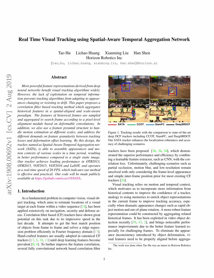
SATA CCOT SiamFC DeepSRDCF

Figure 1. Tracking results with the comparison to state-of-the-artdeep DCF trackers including CCOT, SiamFC, and DeepSRDCF.Our SATA tracker enhances the localization robustness and accu-racy of challenging scenarios.

trackers have been proposed [16, 36, 34], which demon-strated the superior performance and efficiency by combin-ing a learnable feature extractor, such as CNN, with the cor-relation loss. Unfortunately, challenging scenarios such aspartial occlusion, motion blur, and low-resolution remainunsolved with only considering the frame-level appearanceand simple inter-frame position prior for most existing CFtrackers [24].

Visual tracking relies on motion and temporal context,which motivates us to incorporate more information fromhistorical contents to improve the confidence of a tracker,analogy to using memories to enrich object representationsin the current frame to improve tracking accuracy, espe-cially when dramatic appearance changes such as rapid ob-ject motion and out-of-plane rotation. A more robust featurerepresentation could be constructed by aggregating relatedhistorical frames. It has been exploited in video object de-tection recently [39, 43, 2], and brings noticeable perfor-mance improvements due to the better feature learned es-pecially for challenging frames. To eliminate the appear-ance inconsistency introduced by object deformation, vi-sual features need to be properly aligned before aggrega-

The work was done when Tao Hu was an intern in Horizon RoboticsInc.

1

arX

iv:1

908.

0069

2v1

[cs

.CV

] 2

Aug

201

9

tion. The explored alignment methods include pixel-wisecorrelation [39], optical flow warping [43] or deformableconvolution sampling [2]. Compared to applying an optical-flow based warping method [44], which requires intensivecomputation by extracting features in an extra branch anddense flow prediction [14, 20], we attempt to utilize de-formable convolution networks [6] to estimate the motiontransformation and conduct the spatial alignment in a morecomputational efficient manner.

In terms of scales of feature to align, shallow layers ofCNN favor fine-grained spatial details and help locate pre-cise object location [4, 22], while deeper layers maintainsemantic patterns that are robust to variation and motionblur. Recent deep tracker [25] employs multiple convolu-tional layers in a hierarchical weighted ensemble of inde-pendent CF models. However, such naive feature ensemblestill lacks full use of multi-level semantics.

In this work, we present a novel spatial-aware tempo-ral feature aggregation network for visual object tracking asshown in Figure 2. The intuition is to find out a pixel-levelalignment among historical frames and explore an elegantfusion of multi-resolution feature maps. The features ofdifferent layers from historical frames are aligned to theircorresponding feature layers of the template frame throughAlign Module, and then aggregated by Aggregation Mod-ule. The features from different layers are combined grad-ually top-down to produce final predicted CF features. Ournetwork architecture is able to balance the need of track-ing for shallow layer features from CF loss and the need oftranslation invariance for deep semantic features aroused bydeformable offset learning. As illustrated in Figure 1, ourmethod enhances the localization robustness and accuracyin scenarios of intra-class variation and motion blur.

The key contributions of this paper are summarized asfollows:

• We apply a pixel-wise ”align-and-aggregate” temporalfusion paradigm to the visual tracking task. Withoutusing extra annotated data, the method can exploit in-formation from previous frames to enhance both accu-racy and robustness of the tracking algorithm.

• We propose a sequential multi-level feature aggrega-tion mechanism which balances spatial details and se-mantic invariant properly.

• This network is trained end-to-end and significantlyboosts the performance on VOT2015, VOT2016,OTB-2013, OTB-2015 and LaSOT. We conduct exten-sive ablation studies and show significant enhancementachieved by each component. Our code will be madepublicly available.

2. Related Work

In this section, we give a brief overview on the CF basedvisual tracking and spatial-temporal fusion approaches re-lated to our method.

2.1. Discriminative Correlation Filter BasedTracker

Discriminative correlation filter (DCF) based tracker isone of the most import methods in visual tracking for itsimpressive performance and speed [9, 10]. In these meth-ods, the filters are trained by minimizing the least-squaresloss for all circular shifts of a training template patch, andthe new location for object in the search patch are obtainedthrough finding the maximize value in the correlation re-sponse map [5]. The matching formulation is simple whichmakes the features become rather important, and many re-searchers start from this aspect to optimize the tracking per-formance. For example, CN [11] combines the Color Nameand grayscale features to describe the object. KCF [17] usesmulti-channel HOG feature maps to extend single-channelgray features. Recently, deep neural networks like CNNhave attached more and more attention to researchers inthe field of visual tracking [9]. ImageNet [13] pre-traineddeep CNN models are utilized in DCF based methods to ex-tract the features to correlate [25]. However, the achievedtracking performance may not be sufficient because the pre-trained features are extracted independently with the corre-lation tracking process. To address this issue, several meth-ods [16, 36, 34, 3] interpret CF as a layer of the fully con-volutional network based on Siamese architecture and trainit with video detection datasets [29] from scratch. The in-tegration of DCF with features from CNNs has achievedexciting performance boosting [35]. However, these ap-proaches have an inherent limitation When dealing withchallenging scenario such as illumination changes, motionblur in practice.

2.2. Feature Aggregation in Video Analysis

Feature aggregation is proposed to utilize motion cuesand improve performance for video analysis task suchas video object detection and video object segmenta-tion(VOS) [1, 32]. There are two mainstream categoriesmethods of feature aggregation: recurrent neural networks(RNNs) based approaches and spatial-temporal convolutionbased approaches. Ballas et al. [1] proposes convolutionalgated recurrent units (ConvGRU) which model the video se-quence in spatial and temporal dimension simultaneously.This network shows the significant advantage of captur-ing long-distance dependencies and makes remarkable im-provements in video object detection tasks [39].

Another direction to fuse the motion dynamic acrossframes is the spatial-temporal convolution-based methods.

Such methods have been widely used in VOS, which is de-fined as a one-shot video object learning problem similarto visual object tracking. CRN [19] takes the inter-framemotion as a guidance to generate an accurate segmentationbased on cascaded refinement network. OSMN [41] uses aspatial modulator to integrate historical object location in-formation in its segmentation framework. By introducinga distance transform layer, MoNet [40] separates motion-inconstant feature in historical frames to refine segmenta-tion results. FGFA [43] aggregates temporal features byusing weighted summation directly. However, as a typicalvideo analysis task, visual object tracking has been less ben-efited from these advances in temporal feature aggregation.In fact, given more temporal context, it provides the po-tential to improve the robustness of the tracking algorithm.Besides, it is also consistent with the pattern of how humaneyes track objects. These intuitions drive us to employ tem-poral feature aggregation in the visual tracking task.

2.3. Motion Estimation by Deep Learning

Motion estimation in videos requires correspondences inpixel-level of raw image or features-level to find the rela-tionship between consecutive frames [33]. Optical flow iswidely used to estimate precise per-pixel localization be-tween two input frames. Early attempts for estimating op-tical flow have focused on variational and combinatorialmatching approaches [33]. Recently, many works haveshown that optical flow estimation can be solved as a super-vised learning problem through CNNs [14, 20, 28]. How-ever, such flow estimation networks are always integrated asa bypass branch, which makes the training procedure morechallenging when the task loss is not consistent with theflow loss. In addition, training a flow network usually re-quires large amounts of flow data, which is difficult andexpensive to obtain. Instead, some recent works find thecorrespondences implicitly, without the need for extra an-notations to supervise the model. STMN [39] proposes apixel-wise correlation module to learn the object motionbetween features of neighboring frames. STSN [2] usesseveral stacked deformable sampling modules to align thehigh-level features. Nevertheless, the tasks of detection andtracking are quite different, such that when high-level fea-tures work on detection tasks whereas not the case on track-ing task because the latter often addresses the appearancedetails.

The work most related to ours in visual tracking is Flow-Tracker [44]. It proposes a temporal feature aggregationmethod based on optical flow. Though good performanceachieved, their network is quite inefficient because it trainsand extracts the optical flow field on the raw image. In ad-dition, this method operates on fixed-length temporal win-dows, which has difficulty modeling variable motion dura-tion and the long-term temporal information.

3. Spatial-Aware Temporal Aggregation Net-work

In this section, we first describe the overall architectureof this spatial-aware temporal aggregation network. Thenwe introduce each individual module in detail including theAlignment Module, the Aggregation Module and correla-tion filter layer.

3.1. Multi-scale Feature Aggregation Mechanism

In a deep neural network like CNN, features of differ-ent layers show different patterns [42]. Generally, low levelfeatures contain sufficient appearance details, which haspresent better performance in localization, especially for vi-sual tracking [16, 10]. Respectively, the high layer featurespresent semantic patterns to deal with the intra-class varia-tion, which play an important role when the context varieswith time. To take advantage of the feature in both shal-low and deep layers, we propose a multi-scale feature ag-gregation mechanism to learn the alignment across framesadaptively inspired by FPN [23].

As shown in Figure 2, our framework adopts the Siamesenetwork architecture, which consists of search and templatebranches. Given the input video frames {It} , t = 1, ., N ,we define the search frame index and its feature as t and Ftrespectively, and the historical frame feature as Ft−τ , whereτ = 1, 2...T is a integer large than zero in online tracking.Template frame, which is different from the history framesand the search frame, is selected randomly near the searchframe.

In the search branch, we construct a feature pyramidfor the search frame It and historical frame It−τ throughthe backbone feature extraction network. Without loss ofgenerality, we set the number of pyramid layers to l = 3,where l represents the deepest layer of the feature pyramidfor aggregation. The feature pyramid consists of three pro-portionally sized feature maps, named

{P lt , P

l−1t , P l−2t

}and

{P lt−τ , P

l−1t−τ , P

l−2t−τ}

from deep layer to shallow layerfor search and historical frame respectively. Then, theAlignment Module (see details in section 3.2) are usedto learn the relative offsets

{Ol, Ol−1, Ol−2

}for every

feature map layer in{P l, P l−1, P l−2

}between It and

It−τ . After that,{Ol, Ol−1, Ol−2

}are used to gener-

ate the aligned feature{P lt−τ→t, P

l−1t−τ→t, P

l−2t−τ→t

}with

deformable ConvNets. Note that the Alignment Mod-ule is tailor-made for multi-scale pyramid feature to learnthe motion dynamics and appearance change hierarchi-cally. Finally, the

{P lt−τ→t, P

l−1t−τ→t, P

l−2t−τ→t

}are aggre-

gated to{P lt , P

l−1t , P l−2t

}by temporal feature aggregation

(see details in section 3.3) and then merged through top-down pathway as FPN.

In template branch, the feature maps of the templateframe is extracted and the outputs of both branches are fed

Aggregation module

t-k frame

Tem

pora

l inf

rom

atio

n

Search (t) frame

Spatial infromation

...

Aggmodule

AlignModule

EmbeddingFeature

Cosinesimilarity

... ...

ConvFeatureConcat

...

Offsets DeformConv

Aggregation module

Alignment module

CF layer

Template frame

Gaussionresponse

...

Feature extraction

AlignModule

Aggmodule

AlignModule

Aggmodule

Historical frame

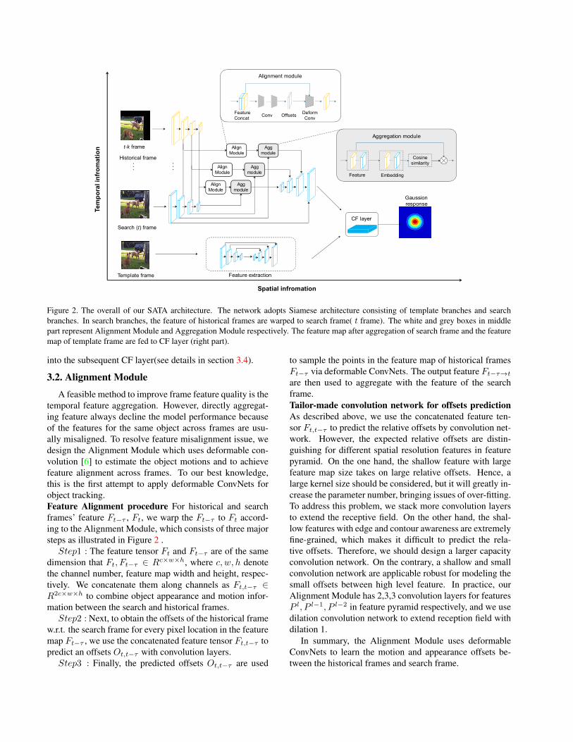
Figure 2. The overall of our SATA architecture. The network adopts Siamese architecture consisting of template branches and searchbranches. In search branches, the feature of historical frames are warped to search frame( t frame). The white and grey boxes in middlepart represent Alignment Module and Aggregation Module respectively. The feature map after aggregation of search frame and the featuremap of template frame are fed to CF layer (right part).

into the subsequent CF layer(see details in section 3.4).

3.2. Alignment Module

A feasible method to improve frame feature quality is thetemporal feature aggregation. However, directly aggregat-ing feature always decline the model performance becauseof the features for the same object across frames are usu-ally misaligned. To resolve feature misalignment issue, wedesign the Alignment Module which uses deformable con-volution [6] to estimate the object motions and to achievefeature alignment across frames. To our best knowledge,this is the first attempt to apply deformable ConvNets forobject tracking.Feature Alignment procedure For historical and searchframes’ feature Ft−τ , Ft, we warp the Ft−τ to Ft accord-ing to the Alignment Module, which consists of three majorsteps as illustrated in Figure 2 .Step1 : The feature tensor Ft and Ft−τ are of the same

dimension that Ft, Ft−τ ∈ Rc×w×h, where c, w, h denotethe channel number, feature map width and height, respec-tively. We concatenate them along channels as Ft,t−τ ∈R2c×w×h to combine object appearance and motion infor-mation between the search and historical frames.Step2 : Next, to obtain the offsets of the historical frame

w.r.t. the search frame for every pixel location in the featuremap Ft−τ , we use the concatenated feature tensor Ft,t−τ topredict an offsets Ot,t−τ with convolution layers.Step3 : Finally, the predicted offsets Ot,t−τ are used

to sample the points in the feature map of historical framesFt−τ via deformable ConvNets. The output feature Ft−τ→tare then used to aggregate with the feature of the searchframe.Tailor-made convolution network for offsets predictionAs described above, we use the concatenated feature ten-sor Ft,t−τ to predict the relative offsets by convolution net-work. However, the expected relative offsets are distin-guishing for different spatial resolution features in featurepyramid. On the one hand, the shallow feature with largefeature map size takes on large relative offsets. Hence, alarge kernel size should be considered, but it will greatly in-crease the parameter number, bringing issues of over-fitting.To address this problem, we stack more convolution layersto extend the receptive field. On the other hand, the shal-low features with edge and contour awareness are extremelyfine-grained, which makes it difficult to predict the rela-tive offsets. Therefore, we should design a larger capacityconvolution network. On the contrary, a shallow and smallconvolution network are applicable robust for modeling thesmall offsets between high level feature. In practice, ourAlignment Module has 2,3,3 convolution layers for featuresP l, P l−1, P l−2 in feature pyramid respectively, and we usedilation convolution network to extend reception field withdilation 1.

In summary, the Alignment Module uses deformableConvNets to learn the motion and appearance offsets be-tween the historical frames and search frame.

3.3. Temporal Feature Aggregation

The Alignment Module is applied for all selected his-torical frames in the specified range. After that, we ob-tain a series of complementary feature maps of historicalframes which include diverse appearance information forthe object being tracked. Inspired by the method in flow-guide feature aggregation network(FGFA) [43], we use theadaptive weights to aggregate historical frames feature tosearch frames at each spatial location. The aggregation re-sults could be formulated as:

F agg =

T∑τ=1

wt−τ→tFt−τ→t (1)

Where T is predefined range for historical frames andwt−τ→t is an adaptive weights mask for different spatial lo-cations in the feature map Ft−τ→t. To compute the weightwt−τ→t, we use a 3-layer fully convolutional bottleneckembedding network E to compute the feature representa-tion et−τ→t for Ft−τ→t firstly. Then cosine similarity areused to measure the similarity of each corresponding pointlocation between et−τ→t and search frame embedding fea-ture et. We calculate the weights wt−τ→t by applying anexponential function on cosine similarity, and normalize allweights wt−τ→t, τ ∈ [1, 2, · · ·T ] for all selected range ofhistorical frames. The wt−τ→t could be formulated as:

wt−τ→t(p) =exp( et−τ→t·et

|et−τ→t|·|et| )∑Tτ=1 exp(

et−τ→t·et|et−τ→t|·|et| )

(2)

where p is spatial location in feature map Ft−τ→t.

3.4. Correlation Filter Layer

Discriminative correlation filter is one of the most pop-ular solution for visual object tracking. Motivated by [16,36, 34], we interpret correlation filter as a learnable layerembedded in the whole siamese tracking network.

In the standard DCF tracking framework for multi-dimensional feature, the goal is to learn series correlationfilters wd, d ∈ {1, 2...D} from training sample feature Fxand the ideal response y. Here, feature tensor Fx, extractedfrom CNN, has D channels and spatial size m× n, and theideal response tensor y which is a Gaussian function peakedat the center has the same spatial size m × n. The correla-tion filter wd could be obtained by minimizing the outputridge loss:

L =

∥∥∥∥∥D∑d=1

wd ? F dx − y

∥∥∥∥∥2

+ λ

D∑d=1

∥∥wd∥∥2 (3)

Where wd and F dx refers to the dth channel of filter w andfeature map of x respectively, ? denotes circular correla-tion operation. The λ in the second term of equation is reg-ularization coefficient. Theoretically, the solution can be

formed as:

wd =F dx � y∗∑D

d=1 Fdx �

(F dx

)∗+ λ

(4)

where the ∧ symbol and the ∗ symbol represents discreteFourier transform and complex conjugate of a complex re-spectively, and the symbol � denotes Hadamard products.

In the tracking process, we crop a search patch z andobtain the corresponding feature tensor Fz , then the corre-lation response map g for the search patch is calculated as:

g = F−1(

D∑d=1

wd∗ � Fzd

)(5)

Finally, the translation offsets could be obtained by search-ing the location of the maximum value of response map g.In the Siamese framework, we train network parameters wwith template patch x, and calculate the loss with searchpatch z. The loss function for training is defined as:

l = ‖g − y‖2 + λ ‖θ‖2 (6)

θ represents parameters in CNN. Note that we embed cor-relation filters as a learnable layer for end-to-end training.The details of the derivation for back propagation could befound in [16, 36].

4. Training & InferenceIn this section, we detail the pipeline of the proposed

SATA tracker for training and inference.

4.1. Training

During the training phase, the input data fed to thissiamese network architecture are clips of the video se-quences, which consist of historical frames, search frameand template frame. More specifically, we randomly samplehistorical frames before the search frame, and randomly se-lect another frame near the search frame as template frame.The backbone feature extraction network is applied on in-dividual frame to produce the multi-scale feature maps.The Alignment Module in Section 3.2 is used to estimatethe sampling offsets between the historical frames and thesearch frame, and the feature maps from historical framesare sampled to the search frame according to the predictedsampling offsets in multi-scale layer. The sampled featuremaps, as well as its own feature maps on the search frame,are aggregated through Aggregation Module in Section 3.3.Finally, the resulting aggregated feature maps of the searchframe and the feature of template frame are then fed to thecorrelation filter layer to produce the tracking result. To ex-plore more feature data for training Alignment Module, dataaugmentations are adopted including affine transformationto history frames. All the modules in this framework aretrained end-to-end.

4.2. Inference

After off-line training, the learned network is used toperform online tracking. We fix backbone feature extrac-tion network and other CNN layer but update parameters incorrelation filter layer during the online tracking. The firstframe of a video is set as template frame in tracking. Givena new frame, we crop and resize a search patch centeredat the estimated position in the last frame. The historicalframes are selected from previous frames of the search im-age with fixed window size T . Then the feature pyramid ofhistorical frames are warped and aggregated to search patchwith Alignment Module and Aggregation Module respec-tively. The estimation location of the search patch is ob-tained by finding the maximum value in the response scoremap of CF layer. To make tracker adaptive to appearancevariations, we update our CF layer network frame-by-frameas [8]. To handle the scale changes, we carry out scale esti-mation followed the approach in [8] and use scale pyramidwith the scale factors

{αs|s =

⌊−S−12

⌋, ...,

⌊S−12

⌋}.

5. ExperimentsIn this section, we first introduce the implementation de-

tails of experiments. Then, we perform in-depth analysisof SATA on various benchmark datasets including OTB-2013 [37], OTB-2015 [38], VOT-2015 and VOT-2016 [21].All the tracking results use the reported results to ensurea fair comparison. Finally, we present extensive ablationstudies on the effect of spatial and temporal aggregation.

5.1. Implementation details

Training We implement the pre-trained VGG-16model [30] as the backbone feature extraction net-work. Specifically, the output feature map of the Conv2,Conv4, Conv7, Conv10 layer are used to constructedfeature pyramid. We apply 3 × 3 × 64 convolution layeras lateral to reduce and align the the channels of featurepyramid to 64. The feature map size for P 1, P 2, P 3 are62,31,15 respectively, The final output feature map sizeand response map size are both 125 × 125. Align Moduleimplement as described in section 3.2. Embedding sub-network in spatial attention consists of three convolutionlayers (1×1×32, 3×3×32, 1×1×64 ). The lateral layer,Align Module and embedding sub-network are initializedrandomly. The parameters in backbone feature extractorare fixed after pre-trained using ImageNet [13]. We applystochastic gradient descent (SGD) with momentum of 0.9to end-to-end train the network and set the weight decayrate to 0.0005. The model is trained for 50 epochs witha learning rate of 10−5 and mini-batch size of 32. Theregularization coefficient λ for CF layer is set to 1e-4 andthe Gaussian spatial bandwidth is 0.1.Data dimensions Our training data comes from ILSVRC-

2015 [29], which consist of training and validation set. Foreach training samples, we randomly pick a pair of imageas template and search image within the nearest 10 frames.Historical frames are selected among the nearest 20 framesof the search frame randomly. The historical frame numberof aggregation is set to 3 in training. In each frame, patch iscropped around ground truth with a 2.0 padding and resizedinto 125× 125.Inference In online tracking, scale step a and number Sis set to 1.03 and 3, scale penalty and model updatingrate is set to 0.993 and 0.01 for scale estimation. Hyper-parameters in CF layer are seted as training. The learningrate for updating CF layer is 0.01. The proposed SATA-NET is implemented using Pytorch 4.0 [27] on a PC withan Intel i7 6700 CPU, 48 GB RAM, Nvidia GTX TITANX GPU. Average tracking speed of the SATA is 26 FPS andthe code will be made publicly available.

5.2. Results on OTB

OTB is a standard and popular tracking benchmark withcontains 100 fully annotated videos. OTB-2013 contains50 sequences, and OTB-2015 is the extension of OTB2013which contains other 50 more difficult tracking video se-quences. The evaluation of OTB is based on two metrics:center location error and bounding box overlap ratio. Wefollow the standard evaluation approaches of OTB and re-port the results based on success plots and precision plots ofone-pass evaluation (OPE). We present the results on bothOTB-2013 and OTB-2015.OTB-2013 OPE is employed to compare our algorithm withthe other 17 trackers from OTB-2013 benchmark, whichincluding CCOT [12], ECO-HC [7], DeepSRDCF [10],SiamFC [3], et al. Figure 3 shows the results from all com-pared trakcers, our SATA tracker performs favorably againststate of art trackers in both overlap and precision success.In the success plot, our approach obtain an AUC score of0.698, significantly outperforms the winner of VOT2016(CCOT). In the precision plot, our approach obtains a high-est score of 0.920. For detailed performance analysis, wealso report the performance under five video challenge at-tributes using one-pass evaluations in OTB2013 Figure 5demonstrate that our SATA tracker effectively handles largeappearance variations well caused by low resolution, illumi-nation variations, in-plane and out-of-plane rotations whileother trackers obtain lower scores.OTB-2015 In this experiment, we compare our methodagainst recent trackers on the OTB-2015 benchmark. Fig-ure 4 illustrates the success and precision plots of OPE re-spectively. The results shows that our SATA tracker over-all performs well. Specifically, our method achieves a suc-cess score of 0.661, which is far superior to other meth-ods combining correlation filter and deep learning such asDeepSRDCF(0.635) and CFNet(0.568) [34].

SATA CCOT MDNet SiamFCEAO 0.319 0.331 0.257 0.277Accuracy 0.544 0.539 0.541 0.549Robustness 0.243 0.238 0.337 0.382

Table 1. Comparison with the state-of-the-art trackers on the VOT2016 dataset. The results are evaluated with expected averageoverlap (EAO), accuracy (mean overlap) and robustness (averagenumber of failures).

5.3. Results on VOT

For completeness, we also present the evaluation resultson benchmark datasets VOT-2015 and VOT-2016, whichboth consists of 60 identical challenging videos but theground truth has been re-annotated in VOT-2016.

In VOT2015, we present a state-of-the-art comparison tothe top 20 participants in the challenge under the evaluationmetric expected average overlap (EAO). Figure 6 show thatthe performance of SATA ranks 2nd after MDNet [26] onlywhich is trained on OTB.

In VOT2016, we compare our SATA tracker withother state-of-the-art trackers including CCOT, MDNet andSiamFC. The performance of SATA is comparable to CCOTand better than SiamFC and MDNet. VOT-2016 report [21]defined the lower bound EAO of state-of-the-art tracker as0.251. SATA tracker shows state-of-the-art performance ac-cording to this definition.

5.4. Results on LaSOT

To further validate SATA on a larger and more challeng-ing scenario in the wild, we conduct experiments on LaSOT

0 0.2 0.4 0.6 0.8 1

Overlap threshold

0

0.1

0.2

0.3

0.4

0.5

0.6

0.7

0.8

0.9

1

Suc

cess

rat

e

Success plots of OPE

SATA [0.698]CCOT [0.672]SINT_flow [0.655]SRDCFdecon [0.653]ECO-HC [0.652]DeepSRDCF [0.641]SINT_noflow [0.635]LCT [0.628]SRDCF [0.626]SiamFC [0.612]SiamFC_3s [0.608]Scale_DLSSVM [0.608]CF2 [0.605]HDT [0.603]Staple [0.600]FCNT [0.599]CNN-SVM [0.597]DLSSVM [0.589]

0 10 20 30 40 50

Location error threshold

0

0.1

0.2

0.3

0.4

0.5

0.6

0.7

0.8

0.9

1

Pre

cisi

on

Precision plots of OPE

SATA [0.920]CCOT [0.899]CF2 [0.891]HDT [0.889]SINT_flow [0.882]ECO-HC [0.874]SRDCFdecon [0.870]Scale_DLSSVM [0.861]FCNT [0.856]CNN-SVM [0.852]SINT_noflow [0.851]DeepSRDCF [0.849]LCT [0.848]SRDCF [0.838]MEEM [0.830]DLSSVM [0.829]SiamFC [0.815]SiamFC_3s [0.809]

Figure 3. Success and precision plots on OTB2013. The num-bers in the legend indicate the representative the area-under-curvescores for success plots and precisions at 20 pixels for precisionplots.

0 0.2 0.4 0.6 0.8 1

Overlap threshold

0

0.1

0.2

0.3

0.4

0.5

0.6

0.7

0.8

0.9

1

Suc

cess

rat

e

Success plots of OPE

CCOT [0.671]SATA [0.661]DeepSRDCF [0.635]SRDCFdecon [0.627]SRDCF [0.598]Staple [0.581]HDT [0.564]CF2 [0.562]LCT [0.562]CNN-SVM [0.554]SAMF [0.553]MEEM [0.530]DSST [0.513]KCF [0.477]

0 10 20 30 40 50

Location error threshold

0

0.1

0.2

0.3

0.4

0.5

0.6

0.7

0.8

0.9

1

Pre

cisi

on

Precision plots of OPE

CCOT [0.898]SATA [0.872]DeepSRDCF [0.851]HDT [0.848]CF2 [0.837]SRDCFdecon [0.825]CNN-SVM [0.814]SRDCF [0.789]Staple [0.784]MEEM [0.781]LCT [0.762]SAMF [0.751]KCF [0.696]DSST [0.680]

Figure 4. Precision and success plots on OTB2015.

SATA ECO ECO HC SATA (No agg)Success rate 0.331 0.324 0.304 0.300Precision 0.344 0.338 0.320 0.311

Table 2. Comparison with the state-of-the-art trackers on the La-SOT dataset. The results are evaluated with AUC score of successrate and precision as OTB.

without any parameters fine-tune [15]. The LaSOT datasetprovides a large-scale annotations with 1,400 sequences andmore 3.52 millions frames in the testing set. Table 2 reportsthe results of SATA on LaSOT testing set with protocol I.Without bells and whistles, the SATA achieves competitiveresults compared to recent outstanding trackers. Specifi-cally, SATA increases AUC of success rate and precisionsignificantly comoared to the baseline (SATA No agg).

5.5. Ablation study

In this section, we conduct ablation study on OTB2013to illustrate the effectiveness of proposed components.Wefirst analyze the contributions of multi-spatial feature ag-gregation. Then we illustrate how the number of historicalframes affects visual object tracking performance.Multi-scale feature aggregation analysis. To verify thesuperiority of proposed multi-scale feature aggregationstrategy and to assess the contributions of feature aggre-gation on different layer in our algorithm, we implementand evaluate six variations of our approach. Two metricare used to evaluate the performance of different architec-tures, AUC means area under curve (AUC) of each successplot and FPS stands for mean speed. At first, the baselineis implemented that no aggregation is utilized (denoted byNo Agg). Then the influence of number of layer for featureaggregation are tested. Historical frame number for this ab-lation experiments is T = 3. We present our results in Table3, where P l, P l−1 and P l−2 represent aggregation layer infeature pyramid. The algorithm P lP l−1 Agg, which assem-bles two highest layer feature aggregation, gains the per-formance with more than 0.05 compared to the version ofbaseline(No Agg). However, the performance boosting isnot obvious but along with speed decreasing when we usedmore aggregation feature layer (P lP l−1P l−2 Agg gains0.006 than P lP l−1 Agg). P lP l−1 Agg makes a trade-offbetween speed and performance. P lP l−1 Agg operate onreal time speed 26 FPS and AUC 0.677 when set T = 3(last line in Table 3). As shown in 7, the shallow aggrega-tion could favor fine-grained spatial details and the deep ag-gregation maintains semantic patterns, which demonstratesour coarse-to-fine fusion paradigm in spatial is important topreserve the location information and improve the activa-tion for motion blur.

In a word, our comparison results show that the aggrega-tion of lower-resolution and strong semantic feature mapscould increase tracking robustness and performance.

0 0.2 0.4 0.6 0.8 1

Overlap threshold

0

0.1

0.2

0.3

0.4

0.5

0.6

0.7

0.8

0.9

1

Suc

cess

rat

e

Success plots of OPE - low resolution (4)

SATA [0.642]SINT_noflow [0.596]SINT_flow [0.587]SiamFC [0.566]CCOT [0.562]CF2 [0.557]HDT [0.551]ECO-HC [0.536]FCNT [0.514]SiamFC_3s [0.499]CNN-SVM [0.461]Staple [0.438]SRDCFdecon [0.436]DLSSVM [0.430]SRDCF [0.426]Scale_DLSSVM [0.418]DSST [0.408]SAMF [0.388]

(a) Low resolution

0 0.2 0.4 0.6 0.8 1

Overlap threshold

0

0.1

0.2

0.3

0.4

0.5

0.6

0.7

0.8

0.9

1

Suc

cess

rat

e

Success plots of OPE - illumination variation (25)

SATA [0.669]SINT_flow [0.637]CCOT [0.637]SINT_noflow [0.630]SRDCFdecon [0.624]ECO-HC [0.612]FCNT [0.598]DeepSRDCF [0.589]LCT [0.588]SRDCF [0.576]Staple [0.568]Scale_DLSSVM [0.564]DSST [0.561]CF2 [0.560]HDT [0.557]CNN-SVM [0.556]SiamFC [0.542]DLSSVM [0.540]

(b) Illumination variations

0 0.2 0.4 0.6 0.8 1

Overlap threshold

0

0.1

0.2

0.3

0.4

0.5

0.6

0.7

0.8

0.9

1

Suc

cess

rat

e

Success plots of OPE - scale variation (28)

SATA [0.703]CCOT [0.658]SRDCFdecon [0.634]DeepSRDCF [0.628]ECO-HC [0.627]SINT_flow [0.624]SINT_noflow [0.609]SiamFC [0.603]SiamFC_3s [0.601]SRDCF [0.587]FCNT [0.558]LCT [0.553]Staple [0.551]DSST [0.546]Scale_DLSSVM [0.531]CF2 [0.531]HDT [0.523]CNN-SVM [0.513]

(c) Scale variations

0 0.2 0.4 0.6 0.8 1

Overlap threshold

0

0.1

0.2

0.3

0.4

0.5

0.6

0.7

0.8

0.9

1

Suc

cess

rat

e

Success plots of OPE - in-plane rotation (31)

SATA [0.659]SINT_flow [0.631]CCOT [0.625]SINT_noflow [0.601]SRDCFdecon [0.598]DeepSRDCF [0.596]LCT [0.592]ECO-HC [0.589]CF2 [0.582]SiamFC [0.582]HDT [0.580]Staple [0.580]Scale_DLSSVM [0.580]CNN-SVM [0.571]SiamFC_3s [0.570]SRDCF [0.566]DSST [0.563]DLSSVM [0.556]

(d) In plane rotation

0 0.2 0.4 0.6 0.8 1

Overlap threshold

0

0.1

0.2

0.3

0.4

0.5

0.6

0.7

0.8

0.9

1

Suc

cess

rat

e

Success plots of OPE - out-of-plane rotation (39)

SATA [0.677]CCOT [0.659]SINT_flow [0.638]SRDCFdecon [0.633]ECO-HC [0.632]DeepSRDCF [0.630]LCT [0.624]SINT_noflow [0.612]SRDCF [0.599]Scale_DLSSVM [0.591]SiamFC_3s [0.590]SiamFC [0.588]CF2 [0.587]HDT [0.584]DLSSVM [0.582]CNN-SVM [0.582]FCNT [0.581]Staple [0.575]

(e) Out of plane rotation

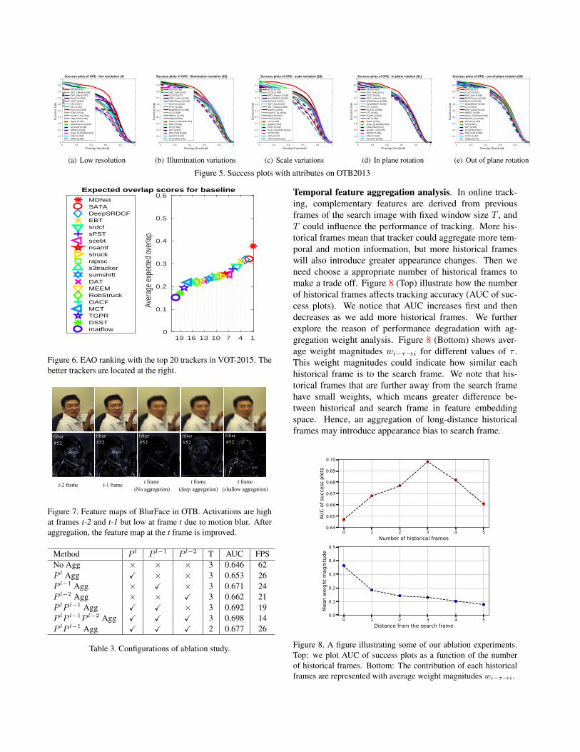
Figure 5. Success plots with attributes on OTB2013

14710131619

Order

0

0.1

0.2

0.3

0.4

0.5

0.6

Aver

age

expe

cted

over

lap

Expected overlap scores for baseline

MDNetSATADeepSRDCFEBTsrdcfsPSTscebtnsamfstruckrajsscs3trackersumshiftDATMEEMRobStruckOACFMCTTGPRDSSTmatflow

Figure 6. EAO ranking with the top 20 trackers in VOT-2015. Thebetter trackers are located at the right.

t frame (No aggregation)

t-2 frame t-1 frame t frame(deep aggregation)

filter #58 filter #58 filter #58

filter#52

filter#52

filter#52

t frame(shallow aggregation)

filter#52

filter#52

Figure 7. Feature maps of BlurFace in OTB. Activations are highat frames t-2 and t-1 but low at frame t due to motion blur. Afteraggregation, the feature map at the t frame is improved.

Method P l P l−1 P l−2 T AUC FPSNo Agg × × × 3 0.646 62P l Agg X × × 3 0.653 26P l−1 Agg × X × 3 0.671 24P l−2 Agg × × X 3 0.662 21P lP l−1 Agg X X × 3 0.692 19P lP l−1P l−2 Agg X X X 3 0.698 14P lP l−1 Agg X X X 2 0.677 26

Table 3. Configurations of ablation study.

Temporal feature aggregation analysis. In online track-ing, complementary features are derived from previousframes of the search image with fixed window size T , andT could influence the performance of tracking. More his-torical frames mean that tracker could aggregate more tem-poral and motion information, but more historical frameswill also introduce greater appearance changes. Then weneed choose a appropriate number of historical frames tomake a trade off. Figure 8 (Top) illustrate how the numberof historical frames affects tracking accuracy (AUC of suc-cess plots). We notice that AUC increases first and thendecreases as we add more historical frames. We furtherexplore the reason of performance degradation with ag-gregation weight analysis. Figure 8 (Bottom) shows aver-age weight magnitudes wi−τ→i for different values of τ .This weight magnitudes could indicate how similar eachhistorical frame is to the search frame. We note that his-torical frames that are further away from the search framehave small weights, which means greater difference be-tween historical and search frame in feature embeddingspace. Hence, an aggregation of long-distance historicalframes may introduce appearance bias to search frame.

0 1 2 3 4 5Number of historical frames

0.64

0.65

0.66

0.67

0.68

0.69

0.70

AUC

of su

cces

s plo

ts

0 1 2 3 4 5Distance from the search frame

0.0

0.1

0.2

0.3

0.4

0.5

Mea

n we

ight

mag

nitu

de

Figure 8. A figure illustrating some of our ablation experiments.Top: we plot AUC of success plots as a function of the numberof historical frames. Bottom: The contribution of each historicalframes are represented with average weight magnitudes wi−τ→i.

6. ConclusionIn this work, we propose a end-to-end spatial-aware

Temporal Aggregation Network for Visual Object Track-ing(SATA) which makes use of the rich information frommulti-scale and variable-length temporal windows of his-torical frames. We developed a Aligned Module usingdeformable ConvNets to estimate the motion changing ofmulti-spatial resolution feature map across frames, and fea-tures of historical frame are sampled and aggregated tosearch frame with pixel-level alignment and multi-scale ag-gregation. In experiments, our method achieves leadingperformance in OTB2013, OTB2015, VOT2015, VOT2016and LaSOT and operates at real time speed of 26 FPS.

References[1] N. Ballas, L. Yao, C. Pal, and A. C. Courville. Delving

deeper into convolutional networks for learning video rep-resentations. In 4th International Conference on LearningRepresentations, ICLR 2016, San Juan, Puerto Rico, May2-4, 2016, Conference Track Proceedings, 2016. 2

[2] G. Bertasius, L. Torresani, and J. Shi. Object detectionin video with spatiotemporal sampling networks. In Com-puter Vision - ECCV 2018 - 15th European Conference, Mu-nich, Germany, September 8-14, 2018, Proceedings, PartXII, pages 342–357, 2018. 1, 2, 3

[3] L. Bertinetto, J. Valmadre, J. F. Henriques, A. Vedaldi, andP. H. S. Torr. Fully-convolutional siamese networks for ob-ject tracking. In Computer Vision - ECCV 2016 Workshops- Amsterdam, The Netherlands, October 8-10 and 15-16,2016, Proceedings, Part II, pages 850–865, 2016. 2, 6

[4] G. Bhat, J. Johnander, M. Danelljan, F. S. Khan, and M. Fels-berg. Unveiling the power of deep tracking. In ComputerVision - ECCV 2018 - 15th European Conference, Munich,Germany, September 8-14, 2018, Proceedings, Part II, pages493–509, 2018. 1, 2

[5] D. S. Bolme, J. R. Beveridge, B. A. Draper, and Y. M. Lui.Visual object tracking using adaptive correlation filters. InThe Twenty-Third IEEE Conference on Computer Vision andPattern Recognition, CVPR 2010, San Francisco, CA, USA,13-18 June 2010, pages 2544–2550, 2010. 1, 2

[6] J. Dai, H. Qi, Y. Xiong, Y. Li, G. Zhang, H. Hu, and Y. Wei.Deformable convolutional networks. In IEEE InternationalConference on Computer Vision, ICCV 2017, Venice, Italy,October 22-29, 2017, pages 764–773, 2017. 2, 4

[7] M. Danelljan, G. Bhat, F. S. Khan, and M. Felsberg. ECO:efficient convolution operators for tracking. In 2017 IEEEConference on Computer Vision and Pattern Recognition,CVPR 2017, Honolulu, HI, USA, July 21-26, 2017, pages6931–6939, 2017. 6

[8] M. Danelljan, G. Hager, F. S. Khan, and M. Felsberg. Ac-curate scale estimation for robust visual tracking. In BritishMachine Vision Conference, BMVC 2014, Nottingham, UK,September 1-5, 2014, 2014. 6

[9] M. Danelljan, G. Hager, F. S. Khan, and M. Felsberg. Con-volutional features for correlation filter based visual tracking.

In 2015 IEEE International Conference on Computer VisionWorkshop, ICCV Workshops 2015, Santiago, Chile, Decem-ber 7-13, 2015, pages 621–629, 2015. 1, 2

[10] M. Danelljan, G. Hager, F. S. Khan, and M. Felsberg. Learn-ing spatially regularized correlation filters for visual track-ing. In 2015 IEEE International Conference on ComputerVision, ICCV 2015, Santiago, Chile, December 7-13, 2015,pages 4310–4318, 2015. 2, 3, 6

[11] M. Danelljan, F. S. Khan, M. Felsberg, and J. van de Wei-jer. Adaptive color attributes for real-time visual tracking.In 2014 IEEE Conference on Computer Vision and PatternRecognition, CVPR 2014, Columbus, OH, USA, June 23-28,2014, pages 1090–1097, 2014. 1, 2

[12] M. Danelljan, A. Robinson, F. S. Khan, and M. Felsberg.Beyond correlation filters: Learning continuous convolutionoperators for visual tracking. In Computer Vision - ECCV2016 - 14th European Conference, Amsterdam, The Nether-lands, October 11-14, 2016, Proceedings, Part V, pages472–488, 2016. 6

[13] J. Deng, W. Dong, R. Socher, L. Li, K. Li, and F. Li. Im-agenet: A large-scale hierarchical image database. In 2009IEEE Computer Society Conference on Computer Vision andPattern Recognition (CVPR 2009), 20-25 June 2009, Miami,Florida, USA, pages 248–255, 2009. 2, 6

[14] A. Dosovitskiy, P. Fischer, E. Ilg, P. Hausser, C. Hazirbas,V. Golkov, P. van der Smagt, D. Cremers, and T. Brox.Flownet: Learning optical flow with convolutional networks.In 2015 IEEE International Conference on Computer Vision,ICCV 2015, Santiago, Chile, December 7-13, 2015, pages2758–2766, 2015. 2, 3

[15] H. Fan, L. Lin, F. Yang, P. Chu, G. Deng, S. Yu, H. Bai,Y. Xu, C. Liao, and H. Ling. Lasot: A high-qualitybenchmark for large-scale single object tracking. CoRR,abs/1809.07845, 2018. 7

[16] E. Gundogdu and A. A. Alatan. Good features to corre-late for visual tracking. IEEE Trans. Image Processing,27(5):2526–2540, 2018. 1, 2, 3, 5

[17] J. F. Henriques, R. Caseiro, P. Martins, and J. Batista. High-speed tracking with kernelized correlation filters. IEEETrans. Pattern Anal. Mach. Intell., 37(3):583–596, 2015. 1,2

[18] J. F. Henriques, R. Caseiro, P. Martins, and J. P. Batista. Ex-ploiting the circulant structure of tracking-by-detection withkernels. In Computer Vision - ECCV 2012 - 12th EuropeanConference on Computer Vision, Florence, Italy, October 7-13, 2012, Proceedings, Part IV, pages 702–715, 2012. 1

[19] P. Hu, G. Wang, X. Kong, J. Kuen, and Y. Tan. Motion-guided cascaded refinement network for video object seg-mentation. In 2018 IEEE Conference on Computer Visionand Pattern Recognition, CVPR 2018, Salt Lake City, UT,USA, June 18-22, 2018, pages 1400–1409, 2018. 3

[20] E. Ilg, N. Mayer, T. Saikia, M. Keuper, A. Dosovitskiy, andT. Brox. Flownet 2.0: Evolution of optical flow estimationwith deep networks. In 2017 IEEE Conference on ComputerVision and Pattern Recognition, CVPR 2017, Honolulu, HI,USA, July 21-26, 2017, pages 1647–1655, 2017. 2, 3

[21] M. Kristan, J. Matas, A. Leonardis, M. Felsberg, L. Cehovin,G. Fernandez, T. Vojır, G. Hager, G. Nebehay, and R. P.

Pflugfelder. The visual object tracking VOT2015 challengeresults. In 2015 IEEE International Conference on ComputerVision Workshop, ICCV Workshops 2015, Santiago, Chile,December 7-13, 2015, pages 564–586, 2015. 6, 7

[22] H. Li, Y. Li, and F. Porikli. Deeptrack: Learning discrimina-tive feature representations online for robust visual tracking.IEEE Trans. Image Processing, 25(4):1834–1848, 2016. 2

[23] T. Lin, P. Dollar, R. B. Girshick, K. He, B. Hariharan, andS. J. Belongie. Feature pyramid networks for object detec-tion. In 2017 IEEE Conference on Computer Vision andPattern Recognition, CVPR 2017, Honolulu, HI, USA, July21-26, 2017, pages 936–944, 2017. 3

[24] H. Lu, P. Li, and D. Wang. Visual object tracking: A survey.Pattern Recognition and Artificial Intelligence, 31(1):61–76,2018. 1

[25] C. Ma, J. Huang, X. Yang, and M. Yang. Hierarchical con-volutional features for visual tracking. In 2015 IEEE Inter-national Conference on Computer Vision, ICCV 2015, San-tiago, Chile, December 7-13, 2015, pages 3074–3082, 2015.2

[26] H. Nam and B. Han. Learning multi-domain convolutionalneural networks for visual tracking. In 2016 IEEE Confer-ence on Computer Vision and Pattern Recognition, CVPR2016, Las Vegas, NV, USA, June 27-30, 2016, pages 4293–4302, 2016. 7

[27] A. Paszke, S. Gross, S. Chintala, and G. Chanan. Pytorch:Tensors and dynamic neural networks in python with stronggpu acceleration. PyTorch: Tensors and dynamic neural net-works in Python with strong GPU acceleration, 2017. 6

[28] A. Ranjan and M. J. Black. Optical flow estimation using aspatial pyramid network. In 2017 IEEE Conference on Com-puter Vision and Pattern Recognition, CVPR 2017, Hon-olulu, HI, USA, July 21-26, 2017, pages 2720–2729, 2017.3

[29] O. Russakovsky, J. Deng, H. Su, J. Krause, S. Satheesh,S. Ma, Z. Huang, A. Karpathy, A. Khosla, M. S. Bernstein,A. C. Berg, and F. Li. Imagenet large scale visual recog-nition challenge. International Journal of Computer Vision,115(3):211–252, 2015. 2, 6

[30] K. Simonyan and A. Zisserman. Very deep convolutionalnetworks for large-scale image recognition. In 3rd Interna-tional Conference on Learning Representations, ICLR 2015,San Diego, CA, USA, May 7-9, 2015, Conference Track Pro-ceedings, 2015. 6

[31] Y. Song, C. Ma, X. Wu, L. Gong, L. Bao, W. Zuo, C. Shen,R. W. H. Lau, and M. Yang. VITAL: visual tracking viaadversarial learning. In 2018 IEEE Conference on ComputerVision and Pattern Recognition, CVPR 2018, Salt Lake City,UT, USA, June 18-22, 2018, pages 8990–8999, 2018. 1

[32] S. Tripathi, Z. C. Lipton, S. J. Belongie, and T. Q. Nguyen.Context matters: Refining object detection in video withrecurrent neural networks. In Proceedings of the BritishMachine Vision Conference 2016, BMVC 2016, York, UK,September 19-22, 2016, 2016. 2

[33] Z. Tu, W. Xie, D. Zhang, R. Poppe, R. C. Veltkamp, B. Li,and J. Yuan. A survey of variational and cnn-based opticalflow techniques. Sig. Proc.: Image Comm., 72:9–24, 2019.3

[34] J. Valmadre, L. Bertinetto, J. F. Henriques, A. Vedaldi, andP. H. S. Torr. End-to-end representation learning for correla-tion filter based tracking. In 2017 IEEE Conference on Com-puter Vision and Pattern Recognition, CVPR 2017, Hon-olulu, HI, USA, July 21-26, 2017, pages 5000–5008, 2017.1, 2, 5, 6

[35] N. Wang, W. Zhou, Q. Tian, R. Hong, M. Wang, and H. Li.Multi-cue correlation filters for robust visual tracking. In2018 IEEE Conference on Computer Vision and PatternRecognition, CVPR 2018, Salt Lake City, UT, USA, June 18-22, 2018, pages 4844–4853, 2018. 2

[36] Q. Wang, J. Gao, J. Xing, M. Zhang, and W. Hu. Dcfnet:Discriminant correlation filters network for visual tracking.CoRR, abs/1704.04057, 2017. 1, 2, 5

[37] Y. Wu, J. Lim, and M. Yang. Online object tracking: Abenchmark. In 2013 IEEE Conference on Computer Visionand Pattern Recognition, Portland, OR, USA, June 23-28,2013, pages 2411–2418, 2013. 6

[38] Y. Wu, J. Lim, and M. Yang. Object tracking benchmark.IEEE Trans. Pattern Anal. Mach. Intell., 37(9):1834–1848,2015. 6

[39] F. Xiao and Y. J. Lee. Video object detection with an alignedspatial-temporal memory. In Computer Vision - ECCV 2018- 15th European Conference, Munich, Germany, September8-14, 2018, Proceedings, Part VIII, pages 494–510, 2018. 1,2, 3

[40] H. Xiao, J. Feng, G. Lin, Y. Liu, and M. Zhang. Monet: Deepmotion exploitation for video object segmentation. In 2018IEEE Conference on Computer Vision and Pattern Recogni-tion, CVPR 2018, Salt Lake City, UT, USA, June 18-22, 2018,pages 1140–1148, 2018. 3

[41] L. Yang, Y. Wang, X. Xiong, J. Yang, and A. K. Katsaggelos.Efficient video object segmentation via network modulation.In 2018 IEEE Conference on Computer Vision and PatternRecognition, CVPR 2018, Salt Lake City, UT, USA, June 18-22, 2018, pages 6499–6507, 2018. 3

[42] J. Yosinski, J. Clune, A. M. Nguyen, T. J. Fuchs, and H. Lip-son. Understanding neural networks through deep visualiza-tion. CoRR, abs/1506.06579, 2015. 3

[43] X. Zhu, Y. Wang, J. Dai, L. Yuan, and Y. Wei. Flow-guidedfeature aggregation for video object detection. In IEEE In-ternational Conference on Computer Vision, ICCV 2017,Venice, Italy, October 22-29, 2017, pages 408–417, 2017.1, 2, 3, 5

[44] Z. Zhu, W. Wu, W. Zou, and J. Yan. End-to-end flow cor-relation tracking with spatial-temporal attention. In 2018IEEE Conference on Computer Vision and Pattern Recog-nition, CVPR 2018, Salt Lake City, UT, USA, June 18-22,2018, pages 548–557, 2018. 2, 3