real-time object detection for autonomous driving …
TRANSCRIPT

REAL-TIME OBJECT DETECTION FOR AUTONOMOUS DRIVING BASEDON DEEP LEARNING
A Thesis
by
GUANGRUI LIU
BS, Beijing University of Technology, China, 2011
Submitted in Partial Fulfillment of the Requirements for the Degree of
MASTER OF SCIENCE
in
COMPUTER SCIENCE
Texas A&M University-Corpus ChristiCorpus Christi, Texas
May 2017

c©GUANGRUI LIU
All Rights Reserved
May 2017

REAL-TIME OBJECT DETECTION FOR AUTONOMOUS DRIVING BASEDON DEEP LEARNING
A Thesis
by
GUANGRUI LIU
This thesis meets the standards for scope and quality ofTexas A&M University-Corpus Christi and is hereby approved.
Dr. Maryam Rahnemoonfar Dr. Longzhuang LiChair Committee Member
Dr. Mohammed BelkhoucheCommittee Member
May 2017

ABSTRACT
Optical vision is an essential component for autonomous cars. Accurate detec-
tion of vehicles, pedestrians and road signs could assist self-driving cars to drive as
safely as humans. However, object detection has been a challenging task for decades
since images of objects in the real world environment are affected by illumination,
rotation, scale, and occlusion. Recently, many Convolutional Neural Network (CNN)
based classification-after-localization methods have improved detection results in var-
ious conditions. However, the slow recognition speed of these two-stage methods
limits their usage in real-time situations. Recently, a unified object detection model,
You Only Look Once (YOLO) [20], was proposed, which could directly regress from
input image to object class scores and positions. Its single network structure pro-
cesses images at 45 fps on PASCAL VOC 2007 dataset [7] and has higher detection
accuracy than other current real-time methods. However, when applied to auto-
driving object detection tasks, this model still has limitations. It processes images
individually despite the fact that an object's position changes continuously in the
driving scene. Thus, the model ignores a lot of important information between con-
tinuous frames. In this research, we applied YOLO to three different datasets to
test its general applicability. We fully analyzed its performance from various aspects
on KITTI dataset [10] which is specialized for autonomous driving. We proposed
a novel technique called memory map, which considers inter-frame information, to
strengthen YOLO's detection ability in driving scene. We broadened the model's
applicability scope by applying it to a new orientation estimation task. KITTI is our
main dataset. Additionally, ImageNet [5] dataset is used for pre-training, and three
other datasets. And Pascal VOC 2007/2012 [7], Road Sign [2], and Face Detection
Dataset and Benchmark (FDDB) [15] were used for other class domains.
v

TABLE OF CONTENTS
CONTENTS PAGE
ABSTRACT . . . . . . . . . . . . . . . . . . . . . . . . . . . . . . . . . . . . v
TABLE OF CONTENTS . . . . . . . . . . . . . . . . . . . . . . . . . . . . . vi
LIST OF TABLES . . . . . . . . . . . . . . . . . . . . . . . . . . . . . . . . . x
LIST OF FIGURES . . . . . . . . . . . . . . . . . . . . . . . . . . . . . . . . x
1 INTRODUCTION . . . . . . . . . . . . . . . . . . . . . . . . . . . . . . . 1
1.1 Motivation . . . . . . . . . . . . . . . . . . . . . . . . . . . . . . . . . 1
1.2 Research Questions . . . . . . . . . . . . . . . . . . . . . . . . . . . . 2
1.3 My Contribution . . . . . . . . . . . . . . . . . . . . . . . . . . . . . 2
1.4 Literature Review . . . . . . . . . . . . . . . . . . . . . . . . . . . . . 3
1.4.1 Evolution Of Image Recognition . . . . . . . . . . . . . . . . . 3
1.4.2 CNN Based Object Detection . . . . . . . . . . . . . . . . . . . 5
1.4.2.1 Regions-based Convolutional Neural Network (R-CNN)
[12] . . . . . . . . . . . . . . . . . . . . . . . . . . . . . . 6
1.4.2.2 Spatial Pyramid Pooling Network (SPP-Net) [13] . . . . 7
1.4.2.3 Fast Region-based Convolutional Network (Fast R-
CNN) [11] . . . . . . . . . . . . . . . . . . . . . . . . . . 8
1.4.2.4 Faster-RCNN [21] . . . . . . . . . . . . . . . . . . . . . . 9
1.4.3 Real-Time Object Detection . . . . . . . . . . . . . . . . . . . 9
1.4.3.1 Volia Jones [29] (2001) . . . . . . . . . . . . . . . . . . . 9
1.4.3.2 Deformable Parts Model - 30hz (DPM) . . . . . . . . . . 10
2 BACKGROUND . . . . . . . . . . . . . . . . . . . . . . . . . . . . . . . . 11
2.1 Neural Network . . . . . . . . . . . . . . . . . . . . . . . . . . . . . . 11
2.1.1 Neuron . . . . . . . . . . . . . . . . . . . . . . . . . . . . . . . 11
2.1.2 Structure of Neural Networks . . . . . . . . . . . . . . . . . . . 12
2.1.3 How Neural Networks Make Complex Designs . . . . . . . . . . 13
2.1.4 Cost Function and Training . . . . . . . . . . . . . . . . . . . . 13
2.2 Convolutional Neural Network (CNN) . . . . . . . . . . . . . . . . . . 14
vi

2.2.1 Partial Connected Manner . . . . . . . . . . . . . . . . . . . . 15
2.2.2 Pooling . . . . . . . . . . . . . . . . . . . . . . . . . . . . . . . 16
2.2.3 CNN for Image Classification . . . . . . . . . . . . . . . . . . . 16
2.2.4 General Object Detection Model . . . . . . . . . . . . . . . . . 17
2.3 Unified Detection Model - YOLO . . . . . . . . . . . . . . . . . . . . 18
2.3.1 Structure of YOLO . . . . . . . . . . . . . . . . . . . . . . . . 18
2.3.2 Network Structure . . . . . . . . . . . . . . . . . . . . . . . . . 20
3 SYSTEM DESIGN AND METHODOLOGY . . . . . . . . . . . . . . . . 21
3.1 System Design . . . . . . . . . . . . . . . . . . . . . . . . . . . . . . . 21
3.1.1 Neural Network Parameter Setting . . . . . . . . . . . . . . . . 21
3.1.2 Cost Function . . . . . . . . . . . . . . . . . . . . . . . . . . . 21
3.2 Gridding Size Effect on Detection Result . . . . . . . . . . . . . . . . 23
3.3 Memory Map . . . . . . . . . . . . . . . . . . . . . . . . . . . . . . . 23
3.3.1 Design of Memory Map . . . . . . . . . . . . . . . . . . . . . . 24
3.3.2 Sum Fucntion of Memory Map . . . . . . . . . . . . . . . . . . 24
3.3.3 Network Structure with Memory Map . . . . . . . . . . . . . . 25
3.4 Orientation Estimation . . . . . . . . . . . . . . . . . . . . . . . . . . 26
3.4.1 Quantification of Orientation . . . . . . . . . . . . . . . . . . . 27
3.4.2 Design of Cost Function . . . . . . . . . . . . . . . . . . . . . . 27
3.5 Evaluation Criteria . . . . . . . . . . . . . . . . . . . . . . . . . . . . 28
4 EXPERIMENTS . . . . . . . . . . . . . . . . . . . . . . . . . . . . . . . 31
4.1 Datasets . . . . . . . . . . . . . . . . . . . . . . . . . . . . . . . . . . 31
4.1.1 KITTI . . . . . . . . . . . . . . . . . . . . . . . . . . . . . . . 31
4.1.2 ImageNet . . . . . . . . . . . . . . . . . . . . . . . . . . . . . . 33
4.1.3 Pascal VOC 2007/2012 . . . . . . . . . . . . . . . . . . . . . . 34
4.1.4 Road Sign . . . . . . . . . . . . . . . . . . . . . . . . . . . . . 35
4.1.5 Face Detection Dataset and Benchmark (FDDB) . . . . . . . . 35
4.2 Global System Setting . . . . . . . . . . . . . . . . . . . . . . . . . . 37
4.3 Pre-training with ImageNet . . . . . . . . . . . . . . . . . . . . . . . 38
4.3.1 Data Preparation . . . . . . . . . . . . . . . . . . . . . . . . . 39
4.3.2 Label file format for Pascal VOC, Road sign and FDDB datasets 39
4.3.3 Extension label file format for KITTI dataset . . . . . . . . . . 39
4.3.4 Conversation Coordinates from Pixel to Ratio. . . . . . . . . . 40
4.3.5 Generating training file list . . . . . . . . . . . . . . . . . . . . 40
vii

4.4 YOLO on Pascal VOC, Road Sign, FDDB Datasets . . . . . . . . . . 41
4.4.1 Object Detection Results on FDDB Dataset . . . . . . . . . . . 41
4.4.2 Object Detection Results on Road Sign Dataset . . . . . . . . . 41
4.4.3 Object Detection Results on Pascal VOC Dataset . . . . . . . 43
4.4.4 Summary . . . . . . . . . . . . . . . . . . . . . . . . . . . . . . 43
4.5 YOLO on KITT Dataset . . . . . . . . . . . . . . . . . . . . . . . . 44
4.5.1 Training Configuration . . . . . . . . . . . . . . . . . . . . . . 44
4.5.2 Results and Discussions . . . . . . . . . . . . . . . . . . . . . . 44
4.5.2.1 Results of KITTI Testing Images . . . . . . . . . . . . . 44
4.5.2.2 Wild Testing on Our Own Images . . . . . . . . . . . . . 46
4.5.3 Results Analysis . . . . . . . . . . . . . . . . . . . . . . . . . . 48
4.5.3.1 Training Batches' Effect . . . . . . . . . . . . . . . . . . 48
4.5.3.2 Training Batches' Effect on Class . . . . . . . . . . . . . 49
4.5.3.3 Training Batches' Effect on Difficulty Levels . . . . . . . 52
4.6 Gridding Size's Effect on Detection Result . . . . . . . . . . . . . . . 53
4.6.1 Implementation and Configuration . . . . . . . . . . . . . . . . 53
4.6.2 Results and Discussions . . . . . . . . . . . . . . . . . . . . . . 53
4.6.2.1 Overall Precision and Recall by Gridding Size . . . . . . 54
4.6.2.2 Gridding Size Affects Each Class . . . . . . . . . . . . . 54
4.6.2.3 Gridding size affects each difficulty level object . . . . . 56
4.6.3 Summary . . . . . . . . . . . . . . . . . . . . . . . . . . . . . . 57
4.7 Memory Map on KITTI Dataset . . . . . . . . . . . . . . . . . . . . 58
4.7.1 Implementation and Configuration . . . . . . . . . . . . . . . . 58
4.7.2 Validation Dataset . . . . . . . . . . . . . . . . . . . . . . . . . 60
4.7.3 Results Analysis . . . . . . . . . . . . . . . . . . . . . . . . . . 60
4.7.3.1 Overall Recall and Precision with Memory Map . . . . . 60
4.7.3.2 Class Recall and Precision with Memory Map . . . . . . 60
4.7.3.3 Summary . . . . . . . . . . . . . . . . . . . . . . . . . . 62
4.8 Orientation Estimation on KITTI Dataset . . . . . . . . . . . . . . . 63
4.8.1 Implementation . . . . . . . . . . . . . . . . . . . . . . . . . . 63
4.8.2 Visualization of Orientation . . . . . . . . . . . . . . . . . . . . 63
4.8.3 Results and Discussions . . . . . . . . . . . . . . . . . . . . . . 64
4.8.4 Evaluation . . . . . . . . . . . . . . . . . . . . . . . . . . . . . 66
4.8.4.1 Evaluation by Directions . . . . . . . . . . . . . . . . . . 67
4.8.4.2 Evaluation by Classes . . . . . . . . . . . . . . . . . . . 67
4.8.4.3 Evaluation by Difficulty Levels . . . . . . . . . . . . . . 68
viii

4.9 Comparison of Object Detection with State-Of-The-Art Methods . . 70
5 CONCLUSION . . . . . . . . . . . . . . . . . . . . . . . . . . . . . . . . 73
5.1 Summary . . . . . . . . . . . . . . . . . . . . . . . . . . . . . . . . . 73
5.2 Contribution . . . . . . . . . . . . . . . . . . . . . . . . . . . . . . . . 73
6 FUTURE WORK . . . . . . . . . . . . . . . . . . . . . . . . . . . . . . . 75
REFERENCES . . . . . . . . . . . . . . . . . . . . . . . . . . . . . . . . . . . . . 76
ix

LIST OF TABLES
TABLES PAGE
I Information of Datasets. . . . . . . . . . . . . . . . . . . . . . . . . . 31
II Description of Parameters of KITTI Labels [10]. . . . . . . . . . . . . 33
III Definition of Difficulty Levels. . . . . . . . . . . . . . . . . . . . . . . 34
IV Information of Datasets. . . . . . . . . . . . . . . . . . . . . . . . . . 37
V Information of Datasets. . . . . . . . . . . . . . . . . . . . . . . . . . 39
VI Information of Datasets. . . . . . . . . . . . . . . . . . . . . . . . . . 40
VII Gridding Size and Maxmium Predictions. . . . . . . . . . . . . . . . 53
VIII Class Precision of Different Frames of Memory Map on KITTI. . . . 70
IX Class Recall of Different Frames of Memory Map on KITTI. . . . . . 70
X Overall Accuracy of Object Detection on KITTI Car. . . . . . . . . 71
XI Overall Accuracy of Object Detection on KITTI Pedestrian. . . . . 71
XII Overall Accuracy of Object Detection on KITTI Cyclist. . . . . . . 72
x

LIST OF FIGURES
FIGURES PAGE
1 Structure of Perceptron. . . . . . . . . . . . . . . . . . . . . . . . . 11
2 Activation Functions . . . . . . . . . . . . . . . . . . . . . . . . . . . 12
3 Fully Connected Neural Network . . . . . . . . . . . . . . . . . . . . 13
4 Visualization of Training Process . . . . . . . . . . . . . . . . . . . . 14
5 Partial Connected between Layers . . . . . . . . . . . . . . . . . . . 15
6 Max-pooling . . . . . . . . . . . . . . . . . . . . . . . . . . . . . . . 16
7 Visualization of CNN Feature Filters . . . . . . . . . . . . . . . . . . 17
8 Structure of CNN Based Object Detection Model . . . . . . . . . . . 18
9 YOLO Model . . . . . . . . . . . . . . . . . . . . . . . . . . . . . . . 19
10 YOLO Network Structure . . . . . . . . . . . . . . . . . . . . . . . . 20
11 Network with Different Gridding Size. . . . . . . . . . . . . . . . . . 24
12 Memory Map. . . . . . . . . . . . . . . . . . . . . . . . . . . . . . . 25
13 Revised Network with Memory Map Component. . . . . . . . . . . 26
14 Quantification of Orientation. . . . . . . . . . . . . . . . . . . . . . 27
15 Precision and Recall. . . . . . . . . . . . . . . . . . . . . . . . . . . 29
16 Samples from KITTI Dataset. . . . . . . . . . . . . . . . . . . . . . 32
17 Samples from ImageNet Dataset. . . . . . . . . . . . . . . . . . . . . 34
18 Samples from Pascal VOC Dataset. . . . . . . . . . . . . . . . . . . 35
19 Samples from Road Sign Dataset. . . . . . . . . . . . . . . . . . . . 36
xi

20 Samples from FDDB Dataset. . . . . . . . . . . . . . . . . . . . . . 36
21 Label Conversation at Running Time. . . . . . . . . . . . . . . . . . 40
22 FDDB Results. . . . . . . . . . . . . . . . . . . . . . . . . . . . . . 42
23 Road Sign Results . . . . . . . . . . . . . . . . . . . . . . . . . . . . 42
24 Pascal VOC Results . . . . . . . . . . . . . . . . . . . . . . . . . . . 43
25 Results of KITTI - Car . . . . . . . . . . . . . . . . . . . . . . . . . 44
26 Results of KITTI - Car Occluded . . . . . . . . . . . . . . . . . . . . 45
27 Results of KITTI - Car Failure . . . . . . . . . . . . . . . . . . . . . 45
28 Results of KITTI - Pedestrian . . . . . . . . . . . . . . . . . . . . . . 45
29 Wild Test - Main Road . . . . . . . . . . . . . . . . . . . . . . . . . 46
30 Wild Test - Campus Road . . . . . . . . . . . . . . . . . . . . . . . . 47
31 Wild Test - Parking Lot . . . . . . . . . . . . . . . . . . . . . . . . . 47
32 Precision and Recall by Training Batches. . . . . . . . . . . . . . . . 49
33 Each Class's Recall by Training Batches. . . . . . . . . . . . . . . . 50
34 Each Class's Precision by Training Batches. . . . . . . . . . . . . . 51
35 Training Batches Affects Recall by Difficulty Levels. . . . . . . . . . 52
36 Precision and Recall by Gridding Size. . . . . . . . . . . . . . . . . 54
37 Gridding Size Affects Each Class Recall. . . . . . . . . . . . . . . . 55
38 Gridding Size Affects Each Class Precision. . . . . . . . . . . . . . . 56
39 Gridding Size Affects Recall of Each Difficulty Level. . . . . . . . . . 57
40 Memory Map Workflow . . . . . . . . . . . . . . . . . . . . . . . . . 59
xii

41 Overall Precision and Recall Change with Memory Map. . . . . . . 61
42 Class Recall with Memory Map. . . . . . . . . . . . . . . . . . . . . 61
43 Class Precision with Memory Map. . . . . . . . . . . . . . . . . . . 62
44 Orientation Visualization . . . . . . . . . . . . . . . . . . . . . . . . 63
45 Orientation Results of Car . . . . . . . . . . . . . . . . . . . . . . . . 64
46 Orientation Results of Car, Pedestrian and Pedestrian . . . . . . . . 65
47 Orientation Results of Pedestrian and Cyclist . . . . . . . . . . . . . 66
48 Orientation Accuracy by Object Directions . . . . . . . . . . . . . . 67
49 Orientation Accuracy by Object Classes . . . . . . . . . . . . . . . . 68
50 Orientation Accuracy by Object Difficulty Levels . . . . . . . . . . . 69
xiii

CHAPTER 1
INTRODUCTION
The goal of this research is to improve a CNN based real-time object detection model,
YOLO [20], to better fit self-driving system by proposing a new technology called
memory map. Also, we will explore YOLO's potential in estimating the orientation
of an object. Moreover, we will validate the model's performance by adjusting a
key parameter, namely gridding size, and by training on three other datasets with
different class domains.
1.1 Motivation
Autonomous driving has been a promising industry in recent years. Both car man-
ufactories and IT companies are competitively investing to self-driving field. Com-
panies like Google, Uber, Ford, BMW have already been testing their self-driving
vehicles on the road. Optical vision is an essential component of autonomous car.
Accurate real-time object detection, such as vehicles, pedestrians, animals, and road
signs, could accelerate the pace of building a self-driving car as safe as human drivers.
Image understanding has been a challenging task for decades. Unlike geometric fig-
ures, objects in the real world are always irregular figures. And the same object
appears in various shapes when capturing from different angles or the object itself
is changing its shape. Besides, images of objects in the real world environment are
variant to illumination, rotation, scale and occlusion, which makes object detection
task more challenging. In recent years, a large improvement in image recognition was
made by a series of CNN based solutions. In ImageNet Large Scale Visual Recog-
nition Competition (ILSVRC, 2015), computers were doing better than human in
1
image classification task. In 2016, a fast object detector, YOLO, was proposed to
expand object detection to real-time situation. Thus, we are motivated to apply
YOLO to object detection task for autonomous driving.
1.2 Research Questions
The goal of this research is object detection for autonomous driving. To perform real-
time object detection, the detection speed (30 frames per second or better) is a prime
factor while choosing the object detection model. The very first research question of
this study is to verify whether YOLO is a good model for general object detection
or not. Moreover, whether it is a potential candidate for autonomous driving system
or not. Later, the question is, whether there is any scope for improving YOLO for
self-driving situation. Lastly, whether YOLO can be applied to other tasks rather
than object detection such as orientation estimation.
1.3 My Contribution
Our contribution includes four parts. Firstly, to check whether YOLO is a good
model for general object detection, we trained the model on three different datasets
namely, Pascal VOC [7], Road Sign [2], and FDDB [15]. Experiment results reveal
that YOLO performs well for all the three datasets.
Secondly, we performed a comprehensive analysis of YOLO over KITTI - object de-
tection and orientation estimation benchmark. The results reveal that the YOLO is
an excellent model for detecting objects required for autonomous driving systems.
However, YOLO processes the images individually and cannot be applied to real-
time autonomous driving system without further modifications. To fill this gap,
the most important contribution of this research lies in proposing a novel technique
2

called memory map to make YOLO suitable for real-time object detection in video
streaming.
Lastly, YOLO was originally designed for object detection. To explore its other
potentials, our second important contribution is to apply YOLO on orientation es-
timation. We discovered that YOLO can effectively estimate the orientations of the
detected objects, which is very crucial for a real-time autonomous driving system.
1.4 Literature Review
In this section, we will first go over the evolution of image recognition in recent years.
Later, we will review some dominant approaches for object detection. These methods
can be divided into two classes namely, traditional (Non-CNN based) methods and
CNN based methods. We will discuss the pros and cons in two aspects, detection
accuracy, detecting speed.
1.4.1 Evolution Of Image Recognition
Before 2012, object detection methods follow the feature-extraction-plus-classifier
paradigm. First, people need to deliberately define specific feature for a category of
objects in order to accurately represent the object. After extracting enough features
from training dataset, the object can be represented by a vector of features, which is
used to train a classifier in training time and also can be used to perform detection
task in testing time. If people want to build a multiple objects detector, more con-
sideration is needed in choosing a general feature so that the common feature can
fit different objects. The disadvantage is obvious since the feature definition is so
complex and the model is hard to extend when new object is added to the detecting
list. Besides, the detecting accuracy is unsatisfactory.
3

In Large Scale Visual Recognition Challenge 2012 (ILSVRC, 2012), Krizhevsky's
CNN based model outperformed all the other models by a big margin[16]. Even the
similar CNN structure was presented in 1990s, its potential was hidden by the lack
of training examples and weak hardware. In ILSVRC (2012), a subset of ImageNet
[5] was used for classification which contains 1.2 million images from 1,000 cate-
gories. Moreover, GPUs became more powerful. With sufficient training images and
powerful GPUs, Krizhevsky's experiment proved CNN's powerful ability in images
classification. The main advantage that CNN has over traditional methods, is the
ability to construct feature filters during the training process. Researchers are set
free from tedious feature engineering work. Benefited from the self-learning ability,
CNN models are much more friendly to extend to other categories if enough training
data is provided. From then on, CNN became the major tool for image classification
task. And, people made better results in image classification related problems.
Since CNN has proved its huge advantage on image classification, people began to
revise previous CNNs to realize image localization and classification. The simple
recipe for localization-plus-classification model is to attach another group of fully-
connected layers (regression head) to the current CNN model. The new regression
head is trained separately to predict 4 coordinates. Thus, the CNN has a classifica-
tion head and a regression head. At test time, two heads are working together, one
for predicting class score and one for position. From 2012 to 2015, Researches succes-
sively drafted regression head to the present remarkable CNNs, such as Overfeat-Net
[24], VGG-Net [25] and ResNet [14], reducing the single object localization error from
34% to 9%. Obviously, CNN based methods have done very well in localization-plus-
classification task.
Later in 2014, researchers began to move to multiple objects detection task. There
4

are more than one object in a single image and the system needs to find out each
object's class and location. Many CNN based region proposals-plus-classification
approaches came out [12] [13] [11] [21]. The main idea is to utilize region proposal
methods to generate candidate regions that possibly contain objects, and later per-
form classification on each of the regions. In practice, these region-proposals-plus-
classification approaches could achieve very high precision [24] [25] [14]. However,
the region proposal part is very time consuming, that slows down the speed of the
whole system. The slow detection speed prevents these methods from applying to
time critical applications, such as auto-driving, surveillance system etc.
Recently, a unified object detection model, YOLO [20], was proposed by Joseph et.
[20]. It frames detection as a regression problem [20]. The model directly regresses
from input image to a tensor which represents object class score and digits of each
object's position. The input images just need to go through the network once and
as a result, the model processes images faster. YOLO has achieved an accuracy over
50 percent in real-time detection on VOC 2007 and 2012 dataset, which makes it the
best choice for any real-time object detection tasks.
1.4.2 CNN Based Object Detection
Unlike image classification, object detection requires multi-object localization. Be-
cause regression tool is used to predict fixed number of outputs, the classification
network cannot be used to directly regress from the input image to objects' location.
In this case, the network does not know how many objects are present in the input
images. Thus, researchers repurposed the current single object classifier to perform
multiple objects detection and came up with region proposal-plus-classification so-
lutions to change the new task to familiar single object classification. Many models
5

were proposed following this two-stage solution.
1.4.2.1 Regions-based Convolutional Neural Network (R-CNN) [12]
Girshick, Ross et al. (2014) proposed a multi-stage approach following classification
using regions paradigm. The system consists of three components, region proposal
component, feature vector extraction by CNN and Support Vector Machine (SVM)
as classifier. During training time, the CNN is supervised pre-trained on a large
dataset (ILSVRC) and fine-tuned on a small dataset (PASCAL). Therefore, the CNN
is more efficient to extract feature vectors for both positive ground truth regions and
negative regions from background and save to disk for next training step. Then,
these feature vectors are used to train SVM classifier. At test time, an external re-
gion proposal component, Selective Search [28], is utilized to generate 2000 fixed-size
category-independent regions that possibly contain objects. Then the well-trained
CNN extractor will convert all the potential regions into feature vectors, base on
which the SVM is used for domain-specific classification. At the end, a linear re-
gression model is used to refine the bounding box and apply a greedy non-maximum
suppression to eliminate duplicate detections as well base on the intersection-over-
union (IOU) overlap with a higher scoring region.
R-CNN achieves excellent detection accuracy comparing to other method at that
time. However, R-CNN's complex multi-stage pipeline bring with notable draw-
backs as well. The CNN components plays as a classifier. The region prediction
still relies on external region proposal method, which is very slow and slow down
the whole system on both training and detecting periods. Besides, the separated
training manner of each components results in the CNN part is hard to optimize.
Namely, when training the SVM classifier, the CNN part cannot be updated.
6

1.4.2.2 Spatial Pyramid Pooling Network (SPP-Net) [13]
The SPP-Net was proposed for speeding up convolution computation and remove
the constrain of fixed-size input. Before SPP-Net, CNNs required fixed-size input
images. In general, a CNN always consists of two parts, Convolutional layers for
outputting feature map and Fully-connected (FC) layers or a SVM for classification.
Inside the Convolutional layers, there are always alternatively layout convolutional
layer and pooling (Sliding Window Pooling) layer. In fact, the Convolutional layers
can process any size of input images. on the other hand, the FC layers or SVM
requires fixed-size input. Thus, the whole network can only process fixed-size input
images. To fulfill this requirement, the common practice is to either crop or warp
the region proposals before feeding them into the Convolutional layers. Both the so-
lutions could affect the CNNs' performance. It is easy to understand that cropping
part of the object may result in failing to recognize the object, and the consequence
of warping is loss of the original ratio which is essential information for ratio sensitive
objects.
The first progress that SPP-Net made is to remove the constrain of fixed-size input.
In SPP-Net, they replaced the last sliding window pooling layer of Convolutional
part with a spatial pyramid pooling (SPP) layer. Spatial pyramid pooling can be
thought of the spatial version of Bag of Words (BoW) [18] which can extract feature
at multi scales. The number of bins is fixed to the input size of FC layers or SVM
rather than considering the input image size. Therefore, SPP-Net, and the whole
network can accept images of arbitrary sizes.
Another advantage of this spatial pooling after convolution manner of SPP-Net is
sharing the computation of all the region proposals. As mentioned earlier, previous
CNNs crop or warp the regions first and let each of them go through the Convolu-
7

tional layers to extract features. The duplicate computing of overlap regions wastes
a lot of time. In SPP-Net, let the whole image go through the Convolutional layers
just once to generate a feature map, and use projecting function to project all the
regions to the last convolutional layer. So, the feature extraction of each region is
only performed on the feature map. The idea of SPP-Net could in general speed up
all CNN-based image classification methods at that time.
Even SPP-Net has made such an improvement to the CNNs in speed and detection
accuracy, just like R-CNN, it still has same drawbacks. Region proposals still rely
on external methods. The multi stage structure require the Convolutional layers and
classifier to be trained individually. Since SPP layers does not allow the loss error
back-propagation, the Convolutional layers still cannot get updated.
1.4.2.3 Fast Region-based Convolutional Network (Fast R-CNN) [11]
The Fast R-CNN was built to realize the training and testing end-to-end. It can be
thought as the extension of R-CNN and SPP-Net. Just as SPP-Net, Fast R-CNN
swaps the order of extracting region feature and running through the CNN for shar-
ing computation. It also revises the last pooling later in order to process any size
input images. But, the difference from SPP-Net is that Fast R-CNN only uses a
region of interest (RoI) pooling layer to pool at one scale, in contrast to SPP-Net's
multi-scale pooling. This trick is quite important for training, since loss error can
back-propagate through RoI pooling layers to update the Convolutional layers. Also,
Fast R-CNN use multi-task loss on each labeled RoI by combining the class score
loss and bounding box loss. Thus, the whole network can be trained end-to-end.
In practice, the results prove that these innovations are efficient in accelerating train-
ing time and testing time while also improving detection accuracy. At the same time,
8

fast running time in networks exposes slow region proposal as a bottleneck.
1.4.2.4 Faster-RCNN [21]
Faster R-CNN mainly solved the slow region proposal problem. Instead of using
external region proposals methods, a Region Proposal Network (RPN) was intro-
duced to perform the region proposal task, which shares the image convolutional
computation with the detection network. A RPN basically is a class-agnostic Fast
R-CNN. The feature map is divided by n x n grid and at each region give out 9
region proposals of different ratios and scale. All the regions proposals will be fed
in to RPN to predict existence score of objects and their positions. Then, let the
high-score output regions of RPN be the input of the second Fast R-CNN to further
perform class-specific classification and bounding box refinement. Now, all the region
proposal work and classification work is done within the network and the training
is end-to-end. As the result, The Faster R-CNN achieved state-of-the-art object de-
tection accuracy on multiple dataset at that time, and it became the foundation of
subsequence outstanding detection methods. Even the detection speed is about 10
fps, it is the fastest detection model comparing to other models with same accuracy.
1.4.3 Real-Time Object Detection
1.4.3.1 Volia Jones [29] (2001)
This paper proposed an object detection approach which processes image near real-
time. At that time, CNN had not caught common attention and this approach
still rely on engineered feature to represent image and multi-level classifier to in-
crease accuracy. Three main contributions were made by this paper. Firstly, in
order to compute Harr-like feature at different scale rapidly, it introduced integral
9

image, which was computed once and allows Harr-like feature computation in con-
stant time. Secondly, using AdaBoost [9] to select critical features to construct a
classifier, which ensure fast classification. Lastly, constructing a cascading classifier
to speed up detection time by fast focus on promising regions. In the real-time face
detection application, the system could run at 15 fps, which is comparable to the
best contemporaneous systems.
1.4.3.2 Deformable Parts Model - 30hz (DPM)
In [23], a revised DPM [8] was implemented with a variety of speed up strategies.
They used (Histogram of oriented gradients) (HoG) features at few scales to re-
duce the feature computation time. Then a hierarchical vector quantization method
compresses the HoG features for further HoG templates evaluation. And the HoG
templates will be evaluated by hash-table methods to identify the most useful lo-
cations which would be stored to several template priority lists. A cascade frame
work was also utilized to improve detecting speed. As the fast speed and high accu-
racy cannot obtain at same time, the method achieved 30 fps with mAP of 26% on
PASCAL 2007 object detection.
10

CHAPTER 2
BACKGROUND
In this chapter, we will review the basic concepts of general neural networks. Next,
we are going to explain a subclass of neural network, Convolution Neural Network
(CNN), which is widely used in image recognition. Later, we will describe a specific
CNN based object detection model, YOLO [20], which is the most accurate real-time
object detector.
The neural networks we are talking in this thesis especially means feed-forward neural
networks, in which information is transmitted in a feedforward manner.
2.1 Neural Network
2.1.1 Neuron
Neuron is the atomic element of neural networks. It origins from perceptron which
was proposed in 1950s. A perceptron has many inputs and one output as shown in
Figure 1. It weights up the inputs and compares the sum to a given threshold to
output binary value. Equation 2.1 gives the mathematic expression of the perceptron.
Figure 1. Structure of Perceptron.
11

output =
0 if∑
ωjχj > threshold
1 if∑
ωjχj ≤ threshold(2.1)
where ωj is the weight for input χj.
Since the outputs of a perceptron follow the step function curve. Only when the sum
of inputs changes near the threshold, the output will jump between 0 and 1. Other-
wise, small change of input will not be reflected on the output. To produce gradient
outputs from 0 to 1, activation function was introduced to revise the perceptron
model. And the revised model was renamed as neuron. Figure 2 gives two activa-
tion functions, sigmoid function and tanh function. Through the function curves, we
could find that every small change in the inputs will be reflected on the outputs.
Figure 2. Activation functions. (1)The left curve is a sigmold function curve. (2)
the right one is a tanh function curve.
2.1.2 Structure of Neural Networks
Neural networks typically consist of multiple layers as shown in Figure 3. The first
layer is called input layer, the last layer is called output layer, and all the middle
layers are hidden layers. Each layer has many neurons. Neurons between adjacent
layers are connected for passing information. In general neural networks, neurons
are fully connected as shown in Figure 3. Between any two adjacent layers, every
12

pair of neurons have a connection. For example, if two adjacent layers respectively
have m and n neurons, the total number of connections will be m x n.
Figure 3. A sample of fully connected neural network. In practice, there are many
hidden layers. This figure only shows one hidden layer.
2.1.3 How Neural Networks Make Complex Designs
In a neural network, outputs from the previous layers become the inputs of next lay-
ers. When the network in active state, the fist layer only makes simple decisions and
pass them to the second layer as inputs. Based on the simple decisions, the second
layer can make smarter decisions. In this way, as information passes through more
layers, the network can make better and better decisions. In practice, researchers
have proved that a deep neural network can solve various sophisticated problems,
such as automatic speech recognition, natural language processing, biomedical infor-
matics and recommendation systems.
2.1.4 Cost Function and Training
Training is the process that a neural network learns to perform a task. To be specific,
a neural network learns from the errors between the predictions and ground truths
by updating its parameters (weights). A cost function defines how to compute the
13

prediction error. In an effective training, the network will gradually reduce the error
to a small range. When the error does not change obviously, the training process
is finished. Figure 4 gives a visualization of training process. In the bowl- shape
error surface, the red dot, which means prediction error, moves from the edge to the
bottom where the error reaches the minimum value.
Figure 4. Visualization of Training process [1]. In the bowl-shape error surface, the
total error slides from the edge to the bottom where the minimum error
locates.
2.2 Convolutional Neural Network (CNN)
The concept of Convolution Neural Network (CNN) was first brought out at 1998 [17],
but was proved to be an efficient tool for image classification in 2012 at Large Scale
Visual Recognition Challenge. Two main characters that CNN's structure differs
from traditional fully connected neural network are: partial connected manner and
pooling operation, which make CNN very suitable for image recognition tasks.
14

2.2.1 Partial Connected Manner
Inspired by animal visual cortex, an individual cortical neuron only responds to a
restricted field of image, known as local receptive field. In a CNN, neurons in the
same layer are arranged in two-dimension array layout. Each neuron is connected to
a small interest field of the previous layer defined by a m x n feature filter. Usually
the feature filter is square. In Figure 5, the size of the feature filter is 5 x 5.
Figure 5. Partial Connected between Layer. Feature filter size is 5 x 5.
In active states, a feature filter will slide on the input layer to perform convolution
operation and generate a feature map. The layer that performs convolution is called
convolutional layer, and the networks with convolutional layers are named as Convo-
lutional Neural Networks. Essentially, the feature filter searches for a specific pattern
among the input layer. In the training state, the searching process is to learn to rec-
ognize a pattern. While in the testing state, the searching process is to check if a
specific pattern exists. One feature filter represents one type of pattern, thus, all the
neurons in the feature map can share one feature filter. The sharing feature weights
behavior greatly reduces the number of parameters that used to define connections
between adjacent layers. In practice, there always be many feature filters to learn
different patterns.
15

2.2.2 Pooling
After each convolution operation, there always follows a pooling operation to further
simplify the information. The pooling process compresses previous feature maps to
condensed feature maps. There are two common pooling methods, average-pooling
and max-pooling. Average-pooling means to output the average value among the
pooling filed, and max-pooling is to select the maximum value. Figure 6 shows a
max-pooling operation with a 2 x 2 pooling filter. The size of the feature map is
reduced from 24 x 24 to 12 x 12. In most CNN models, the most widely used pooling
method is max-pooling.
Figure 6. Max-pooling. Pooling from 24 x 24 to 12 x 12.
2.2.3 CNN for Image Classification
As mentioned in Chapter 2.1.3, the front layers make simple designs. Then middle
layers make better designs base on the previous simple designs. In this way, the
last layer can make sophisticated designs. CNN has the similar cumulative process.
16

Instead making designs, its layers learn to recognize patterns. As shown in Figure 7,
the beginning layers are sensitive to specific colors or edges. Middle layers could
recognize basic patterns, like corners, arcs or basic color patterns. The rear layers
are able to recognize parts of object, like eyes.
Figure 7. Visualization of CNN Feature Filters [33]. From left to right, these feature
filters from front layers, middle layers and rear layers.
2.2.4 General Object Detection Model
The current dominant CNN based object detectors have the similar structure, which
has a region proposal component followed by a CNN classifier as shown in Figure 8.
Researchers use region proposal methods to produce a bunch of candidate regions,
each of which may contain one kind of object. Then, let each region go through the
CNN to do classification. The essential idea behind this structure is to convert a
multiple object detection problem into a single object classification problem. How-
ever, these region proposal methods are much slower than classification part, which
becomes the bottleneck of the whole system. The drawback of this structure is that
17

we cannot trade off accuracy for detection speed in time critical applications [27].
Figure 8. Structure of CNN Based Object Detection Model. External region pro-
posal to generate candidate regions, then let each region go through the
CNN classifier.
2.3 Unified Detection Model - YOLO
YOLO is a recent, unified CNN based object detection model, proposed by Joseph
et. in 2016 [20]. It explores to use a single network to predict both objects' positions
and class scores at one time. The motivation is to reframe detection problem as
regression problem, which regresses from input image directly to class probabilities
and locations. Benefit from the unified design, YOLO's detection speed is about 10
times faster than other state-of-the-art methods [20].
2.3.1 Structure of YOLO
Regression model requires fixed size outputs. However, when an input image comes,
the network does not know how many objects to predict. To solve this confliction,
what YOLO does is to predict a large fixed number of objects and sets a threshold
to eliminate predictions with low probabilities. As shown in Figure 9, the model
18

divides the input images into S x S grids. And each grid predicts B bounding boxes
(width, height, box center x and y) and each box's probability of containing an object
P (Object). Each grid also predicts C (C is the total amount of classes) conditional
class probabilities P (Classi |Object) which is conditioned on the grid containing an
object. Overall, the network predicts a S x S x ( B x 5 + C ) tensor. The digit 5
means each box has 4 coordinates and 1 object probability.
Figure 9. YOLO Model [20].
At test time, it computes class-specific scores for each box by using Equation 2.2. For
a given threshold Pmin , the system outputs the detection objects whose PClass ≥ Pmin.
In post-processing stage, Non-maximal suppression is used to eliminate duplicated
detection of the same object.
P (Classi) = P (Classi |Object) ∗ P (Object) (2.2)
Where P (Classi) is the probability of the ith class. P (Object) is the probability
19

of containing an object in a grid and P (Classi |Object) is the conditional class
probability of the ith class which is conditioned on P (Object).
2.3.2 Network Structure
Yolo's structure is inspired by GoogLeNet [26]. The network has 24 convolutional
layers for feature extraction and 2 fully connected layers for output class scores and
location coordinates as shown in Figure 10. The input images are resized to 448 x
448 with RGB three channels. There are 64 feature filters, with the size of 7 x 7,
that apply convolution operation on each channel of the input images. The moving
stride is 2. The size of output feature maps is 224 x 224 (input size / stride), and
the depth is 192 (3 channels x 64 filters). Then a 2 x 2 max-pooling reduces the size
to 112 x 112. After 24 convolutional layers and 2 fully connected layers, the output
is a 7 x 7 x 30 vector, of which 7 x 7 is the gridding size of the input images, and 30
is from 3 boxes x 5 + 20 classes. The threshold Pmin is 0.2. The model achieved the
mAP of 63.4% at 45 FPS on PASCAL VOC 2007 dataset.
Figure 10. YOLO Network Structure [20].
20

CHAPTER 3
SYSTEM DESIGN AND METHODOLOGY
Our neural network is based on YOLO model. However, in Section 3.3, we will attach
memory map component to the end of neural network. When we validate the effect
of gridding size, the size of last layer will be changed to multiple sizes. In orientation
estimation experiment, we will revise the cost function, so that the network could
learn to distinguish objects' orientations. In the remaining part of this chapter, we
will separately explain: system design; memory map for increasing detection accuracy
in video; different gridding size's effect; applying YOLO on orientation estimation
task.
3.1 System Design
3.1.1 Neural Network Parameter Setting
The network consists of 24 convolutional layers and 2 fully connected layers. The
system can read any size of images and resize them to 448 x 448 before feeding to the
network. The input images are divided into 7 x 7 grids. For each grid, the network
predicts 3 bounding boxes (each box has 4 coordinates and 1 probability) and 20
class scores. So, the output is a 7 x 7 (3 x 5 + 30) tensor.
3.1.2 Cost Function
As explained in Chapter 2.1.4, a cost function defines what ability a neural network is
going to learn. In the object detection task, the network needs to predict class scores
and bounding box. Thus, the overall cost Costtotal consists of class cost Costclass and
bounding box cost CostIOU as shown in Equation 3.1. Class cost is the difference
21

between class probability and ground truth values (0 or 1). Bounding box cost is
computed from Intersection of Union (IOU) between the predicting box and the
ground truth box.
Costtotal = Costclass + CostIOU (3.1)
In actual system, the cost computing is much complex. In our object detection exper-
iment, the cost is computed as Equation 3.2. The scale parameters (noobject scale,
object scale and class scale) are used to adjust the weights of different cost. The
total cost is the sum of SxS grids' cost. And each grid's cost consists of N boxes'
object existence cost, C class cost and best predicting box's IOU cost. All kinds of
cost are using squared error. Notice that, only when an object is present in that grid
cell (isObj = 1), the cost function will penalize class classification error by adding
class cost and best IOU cost.
Cost =
S∗S∑
m=0
{
N∑
n=0
noobject scale ∗ P 2object,n
+ isObj ∗{
− noobject scale ∗ P 2object,best prediction
+ object scale ∗ (1 − Pobject,best predict)2
+ (1 − IOUbest predict)2
+C
∑
i=0
(
class scale ∗ (Pclass,i − Ptruth,i)2)
}
}
(3.2)
Where S is the gridding size, N is the number of bounding boxes predicted in one grid.
C is the number of classes. Parameters noobject scale, object scale and class scale
are used to adjust the weights of each partial cost. Pobject,n is the probability of
exiting an object in the nth box of the mth grid. isObj represents if an object
22

presents in current box decided by ground truth. Pobject,best predict is the Pobject,n with
the best IOU prediction among n boxes. IOUbest predict is the Intersection of Union
between ground truth bounding box and best prediction bounding box in grid m.
Pclass,i is the prediction class probability for class i and Ptruth,i is the ground truth
class probability for class i in grid m, which is 0 or 1.
3.2 Gridding Size Effect on Detection Result
In YOLO model, the input images are divided into 7 x 7 grids and each grid only
predicts 3 bounding boxes and one dominant class score, more detain is explained in
Chapter 2.3.1. The limitation of this model is that when different objects are present
in the same grid, the model could only predict one class with the highest score and
leave out the other objects. The gridding size could affect the maximum number of
predicting classes, and therefore may affect the prediction accuracy. Thus, to study
the extent to which gridding size effects the detection accuracy, we will train several
models with different gridding size and validate the performance.
Changing gridding size actually changes the output size of the last layer. As shown
in Figure 11, we will set the output size to 7 x 7, 9 x 9, 11 x 11 and 14 x 14 and
trained four models. Then compute the recall and precision of each gridding size for
comparison.
3.3 Memory Map
YOLO's detection speed is more than 30 fps, which makes it the best detector for
autonomous driving system. As we know, in driving situations, objects in the vehi-
cle's camera view moves continuously between frames. As YOLO processes images
separately, rich temporary inter-frame information is wasted. In this thesis, the
23

Figure 11. Network with Different Gridding Size.
memory map technique is introduced to remember the temporary inter-frame infor-
mation. A M-frames memory map can remember previous M-1 frames' detection
results. Therefore, when predicts current frame, the system can combine the past M
frames' outputs.
3.3.1 Design of Memory Map
The memory map is designed to remember the predictions of each grid's last M − 1
frames. Its structure is a two-dimension array, of which the length is S2 and the
width is M . As shown in Figure 12, for each grid, the memory map maintains a
vector of previous M − 1 predictions.
3.3.2 Sum Fucntion of Memory Map
We use a sum function to combine the results of m frames. Notice that, only the class
probabilities will be added through M frames. Objects' bounding boxes directly use
24

Figure 12. Memory Map.
the current frame results. Equation 3.3 gives the equation of the sum function.
Ci =
m−1∑
t=0
wt ∗ Ci,t (3.3)
Where t is set from 0 to M −1, which represents t frames earlier than current frame.
Ci,t is the probability of class i at frame t. wt is the weight for frame t. In this
experiment, wt is a decreasing arithmetic sequence from 1 to 0.
In a m frames memory map, the weights for each frame will be (m−0)m
, (m−1)m
, (m−2)m
, ..., 2m
, 1m
.
And the the sum function will be Equation 3.4
Sum =C0 ∗ (m − 0)
m+
C1 ∗ (m − 1)
m+
C2 ∗ (m − 2)
m+, ..., +
Cm−2 ∗ 2
m+
Cm−1 ∗ 1
m
(3.4)
3.3.3 Network Structure with Memory Map
We attached memory map component to the last layer of the original network as
shown in Figure 13. The memory map only works at testing time, which means it
does not need to be trained. The training process keeps the same as YOLO training.
In testing stage, the predictions of the most recent M frames will be cached in the
memory. Predictions which are M − 1 frames earlier than current prediction will be
25

discarded.
Figure 13. Revised Network with Memory Map Component.
3.4 Orientation Estimation
In an autonomous driving system, the object detector helps make navigation decision
by providing objects' classes and locations. In addition to classes and locations,
if extra objects' orientations can be provided, the self-driving system can predict
objects' patterns of motion, and make smarter decisions. For example, in driving
scenarios, if an autonomous car notices other vehicles are all facing opposite to its
own direction, that probably means this vehicle is going on a wrong direction or
wrong lane. Or if one car's orientation is perpendicular to its own orientation,
that probably means that car is turning. Thus, in autonomous driving subarea,
orientation estimation rises as new research topic.
26

3.4.1 Quantification of Orientation
We quantify orientation in radians from -π to π as shown in Figure 14. We define
the camera's front direction as -π/2, left direction as - π or π and right direction as
0.
Figure 14. Quantification of Orientation.
3.4.2 Design of Cost Function
As mentioned Chapter 3.1.2, cost function defines what the neural networks learn
to recognize. To enable the network to learn to estimate an object's orientation, we
revised the cost function by adding the orientation cost as shown in the Equation 3.5.
Cost = CostClass + CostIOU + CostOrientation (3.5)
Where Costtotal is the overall cost, Costclass is the class cost, CostIOU is the bounding
box cost and CostOrientation is the orientation cost.
Equation 3.6 gives detail design of orientation cost, which is the square of difference
between prediction angle and ground truth angle. After we adding orientation cost,
27
the overall cost function becomes Equation 3.7. The class cost and IOU cost are
same with those in the object detection cost function, detail information is explained
in Chapter 3.1.2, Equation 3.2.
CostOrientation = (alphatruth − alphabestpredict)2 (3.6)
Where alphabestpredict is the best prediction orientation value in radians and alphatruth
is the ground truth orientation value.
Cost =S∗S∑
m=0
{
N∑
n=0
noobject scale ∗ P 2object,n
+ isObj ∗{
− noobject scale ∗ P 2object,best prediction
+ object scale ∗ (1 − Pobject,best predict)2
+ (1 − IOUbest predict)2
+
C∑
i=0
(
class scale ∗ (Pclass,i − Ptruth,i)2)
+ orientation scale∗(alphatruth − alphabestpredict)2}
}
(3.7)
3.5 Evaluation Criteria
To validate object detection results, we use three criteria, overall precision, overall
recall and orientation accuracy. Precision and recall is to validate object detection
results. Orientation accuracy is to validate the results of orientation estimation
tasks. Figure 15 gives the visualization of the overall precision and recall. Only
overall precision is used in comparison with other state-of-art methods.
28
Figure 15. Precision and Recall.
The computation of precision and recall is given in Equation 3.8. The actual meaning
of precision is how many predicting items are relevant elements, and Recall represents
how many relevant elements are predicted.
precision =tp
tp + fprecall =
tp
tp + fn(3.8)
To validate orientation, we use orientation accuracy, which is defined by Equation 3.9.
αpredict is the predicting orientation value and αtruth is the ground truth value. Notice
that, we validate the orientation results on the top of correct detections, which
29

requires correct class and IOU over 50%.
orientationaccuracy = 1 −1
n
∑n
1
‖αpredict − αtruth‖
π(3.9)
Where n is number of objects in all testing images. αpredict is the predicting
orientation value in radians and αtruth is the ground truth orientation value.
30
CHAPTER 4
EXPERIMENTS
In this chapter, we will give a detail introduction about the datasets we are using, we
will present the implementation of the methodology discussed in Chapter 3 followed
by the analysis of each experiment result.
4.1 Datasets
Five datasets were involved in this experiment, KITTI [10], ImageNet [5], Pascal
VOC 2007/2012 [7], road sign [2], and Face Detection Dataset and Benchmark
(FDDB) [15]. Detail information about datasets are given in Table I.
Name Classes Number Size
KITTI [10] 80 7481 6.2GB
ImageNet[5] 1000 1.2 million -
Pascal VOC [7] 20 21088 2.77G
Road Sign [2] 2 530 35.7MB
FDDB [15] 1 2845 552 MB
Table I. Information of Datasets.
4.1.1 KITTI
The KITTI Vision Benchmark Suite is specialized for autonomous driving. By driv-
ing the car equipped with multiple sensors around in mid-size city, rural areas and on
highways, they collected rich data, including images and optical flow from camera,
points cloud from laser scanner and odometry information from a GPS. KITTI also
31

extract benchmarks for 2D/3D object detection, object tracking and pose estimation.
In this thesis, we used the object detection and orientation estimation benchmark.
This benchmark includes 7481 labeled images from 80 classes. Single image size is
800kb to 900kb and total size of 7481 images is 6.2GB. Among these classes, only the
frequent objects (car, truck, pedestrian, cyclist, tram, and sitting people) are labeled
independently, all the other classes are labeled as 'Misc' or 'DontCare' class. The
7481 images were divided into 70% (5237 images) for training and 30% (2244 images)
for testing. Figure 16 shows the samples from KITTI datasets.
Figure 16. Samples from KITTI Dataset.
The label files contain the following parameters, class type, truncation, occlusion,
32

orientation and bounding box. Their descriptions are given in Table II.
Values Name Description
1 type
Describes the type of object: ’Car’, ’Van’,
’Truck’,’Pedestrian’, ’Person sitting’, ’Cyclist’,
’Tram’,’Misc’ or ’DontCare’
1 truncationFloat from 0 (non-truncated) to 1 (truncated), where
truncated refers to the object leaving image boundaries
1 occlusion
Integer (0,1,2,3) indicating occlusion state: 0 = fully
visible, 1 = partly occluded, 2 = largely occluded, 3 =
unknown
1 orientation Observation angle of object, ranging [-π - π]
4 bbox2D bounding box of object in the image: contains left,
top, right, bottom coordinates in pixel
Table II. Description of Parameters of KITTI Labels [10].
In the object detection and orientation estimation benchmark, objects are subdivided
into three difficulty levels, easy, moderate and hard by their occlusion and truncation
and height. Table III gives the definition. For example, easy objects are those
whose heights are larger than 40 pixels, fully visible and with at most 15% of body
truncated.
4.1.2 ImageNet
A subset of ImageNet [5] that contains 1.2 million images over 1000 classes is used
for pre-training. In Chapter 4.3, we will explain the importance of pre-training.
33

Level Min. bounding box heightMax.
occlusion level
Max.
truncation
Easy 40 Px Fully visible 15%
Moderate 25 Px Partly occluded 30%
Hard 25 Px Difficult to see 50%
Table III. Definition of Difficulty Levels.
Figure 17 shows the samples from KITTI datasets.
Figure 17. Samples from ImageNet Dataset.
4.1.3 Pascal VOC 2007/2012
Pascal VOC [7] dataset is an important foundation of Pascal VOC Challenge, which
has promoted the development of image classification and object detection. The
dataset used in this thesis are from Pascal VOC 2007 Challenge and 2012 Challenge,
which respectively includes 9,963 (875MB) and 11,125 images (1.9GB) of 20 classes.
Figure 18 shows the samples from Pascal VOC dataset.
34
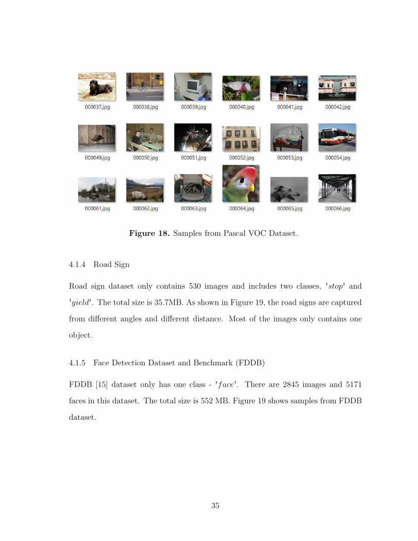
Figure 18. Samples from Pascal VOC Dataset.
4.1.4 Road Sign
Road sign dataset only contains 530 images and includes two classes, 'stop' and
'yield'. The total size is 35.7MB. As shown in Figure 19, the road signs are captured
from different angles and different distance. Most of the images only contains one
object.
4.1.5 Face Detection Dataset and Benchmark (FDDB)
FDDB [15] dataset only has one class - 'face'. There are 2845 images and 5171
faces in this dataset. The total size is 552 MB. Figure 19 shows samples from FDDB
dataset.
35

Figure 19. Samples from Road Sign Dataset.
Figure 20. Samples from FDDB Dataset.
36
4.2 Global System Setting
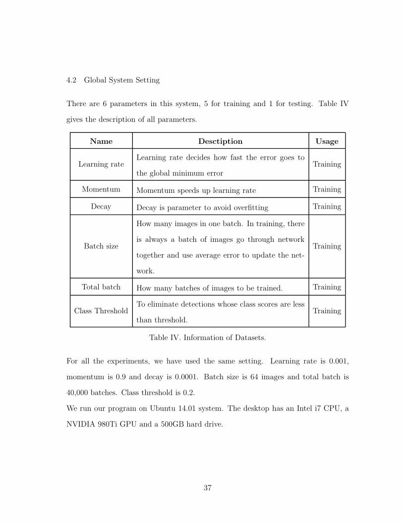
There are 6 parameters in this system, 5 for training and 1 for testing. Table IV
gives the description of all parameters.
Name Desctiption Usage
Learning rateLearning rate decides how fast the error goes to
the global minimum errorTraining
Momentum Momentum speeds up learning rate Training
Decay Decay is parameter to avoid overfitting Training
Batch size
How many images in one batch. In training, there
is always a batch of images go through network
together and use average error to update the net-
work.
Training
Total batch How many batches of images to be trained. Training
Class ThresholdTo eliminate detections whose class scores are less
than threshold.Training
Table IV. Information of Datasets.
For all the experiments, we have used the same setting. Learning rate is 0.001,
momentum is 0.9 and decay is 0.0001. Batch size is 64 images and total batch is
40,000 batches. Class threshold is 0.2.
We run our program on Ubuntu 14.01 system. The desktop has an Intel i7 CPU, a
NVIDIA 980Ti GPU and a 500GB hard drive.
37

4.3 Pre-training with ImageNet
Usually, when we want to train a neural network to perform a task on a dataset. We
start training from scratch with random weights. Once the training process is done,
we save the weights of the neural network to somewhere. When we are interested in
another task with a different dataset, we do not want to repeat the training process
from scratch. Instead, we use the weights that are trained before and optimize those
on the new dataset, which is called fine-tuning. In contrast, we refer the behavior of
training network from random weights as pre-training.
Nowadys, the common way to apply a network on a new dataset is to supervised
pretrain the network on a large dataset with broad categories. Then remove the
weights of fully connected layers and attach new layers with random weights. There
are two advantage of pre-training a network with large dataset.
First, it is a very helpful to gain good result on small dataset. Training a deep neural
network requires a large dataset. However, large datasets are not always available
in every researching field. The good thing is that objects in our world have similar
general features, such as edges, arcs, circles and colors patterns. Thus, from one large
dataset with broad categories, the pre-training network can learn a variety of general,
basic features. When applying the pre-trained network to a new small dataset, we
just need fine-tuning process.
Second, working on a pretrained general purpose network can save plenty of time.
Even today's GPUs are very fast with thousands of cores, fully trained a network
from scratch could still take days to weeks. It is a suffer to wait for a long time every
time when people revise network structure.
In our experiments, to save time, we downloaded the extraction model pretrained
on ImageNet classification task. We kept the 24 convolutional layers and replace the
38

last 2 fully connected layers with random weights. All our experiments are fine-tuned
from the pre-training network.
4.3.1 Data Preparation
Training data consists of images and labels. Our network is compatible with most
image formats, like .png and .jpeg. However, the label files are in different formats.
We converted the label files into an unified format that the network can understand.
In our system, label files have the same name as images, but extension is .txt.
4.3.2 Label file format for Pascal VOC, Road sign and FDDB datasets
In label files, one line with 5 values (1 class value and 4 coordinates) represents one
object. Table V gives the list and two samples. The first object's class is 2, locates
in the center with the 1/4 width and 1/10 height. And the second object's class is
3, locates in right - bottom rapped by a box with 1/10 image width and 1/10 image
height.
Class Center-X (ratio) Center-Y (ratio) Width (ratio) Height (ratio)
2 0.5 0.5 0.25 0.1
3 0.9 0.8 0.1 0.1
Table V. Information of Datasets.
4.3.3 Extension label file format for KITTI dataset
The extension label file includes three more values, 'Orientation', 'Occlusion' and
'Truncation' as shown in Table VI. For description, please refer to Chapter 4.1.1.
39

Class X Y Width Height Orientation Truncation Trunc
Table VI. Information of Datasets.
4.3.4 Conversation Coordinates from Pixel to Ratio.
The coordinates (Center − X, Center − Y, Width, Height) of a bounding box are
in pixel values. We need to convert them to ratio by dividing image length and
width. For FDDB, PASCAL VOC and Road Sign, we wrote a Python script to
convert pixel coordinates to ratio coordinates. However, KITTI label file does not
contain the image width and height, we cannot use Python script to covert during
data preparation stage. Instead, we covert KITT's coordinates at training time. As
shown in Figure 21, we changed the program to load image with width and height.
Then, the program will read label files and at the same time convert coordinates
from pixel values to ratio values.
Figure 21. Label Conversation at Running Time.
4.3.5 Generating training file list
Once the label files and the image files are prepared. We need to create two file path
lists, which respectively contains training files and testing files. Instead of relative
40

path, we used absolute path. A sample is given below.
misc/file/gliu1/darknet/kitti/training/image/000000.png
4.4 YOLO on Pascal VOC, Road Sign, FDDB Datasets
In this section, we trained three YOLO models on three different datasets, FDDB
[15], road Sign [2], and Pascal VOC 2007/2012 [7]. To get a comprehensive evalu-
ation, we validated the results of on three different datasets separately, which are
single-class dataset (FDDB), double-class dataset (Road Sign) and multiple-class
dataset (Pascal VOC). ImageNet was used for pre-training the model from struc-
ture. The setting we used is mentioned in Chapter 4.2.
4.4.1 Object Detection Results on FDDB Dataset
In FDDB benchmark, we have 2845 labeled images including 5171 faces. Same
partition rule as KITTI, we used 30%, 853 images for testing and 70%, 1992 images
for training. We got an overall precision of 95.32% and recall of 94.21%, with the
detection speed of 0.031 seconds per image. As shown in Figure 22, Most of the faces
were correctly predicted. However, several small face and occluded faces were left
out.
4.4.2 Object Detection Results on Road Sign Dataset
The Road Sign dataset contains 530 images (264 stop sign images and 266 yield sign
images). The model was trained with 371 images (30%) and tested on 159 images
(30%). We got an overall precision of 94.47% and recall of 92.53%. As shown in
Figure 23, samples are captured from different environments. YOLO has a good
performance on this dataset. The right two images are failure results because the
41

Figure 22. FDDB Results.
signs are too small.
Figure 23. Road Sign Results
42

4.4.3 Object Detection Results on Pascal VOC Dataset
We separated the Pascal VOC dataset (15680 images) into training part (70% 10976
images) and testing part (30% 4704 images). Same setting with previous experi-
ments, 40,000 batches and 50 hours. After validating on the testing images, we got
a precision of 87.96% and recall of 77.34% with detection speed of 0.033 seconds per
image. As shown in Figure 24, Even various classes are present in this dataset, such
as vehicles, planes, humans and animals, YOLO's detection results is acceptable.
Figure 24. Pascal VOC Results
4.4.4 Summary
Through validating the model on three datasets with different class domains, we
saw YOLO's good detection ability with all the classes, face detection, stop sign or
animals. We can initially infer that YOLO has a general object detection potentiality.
43
4.5 YOLO on KITT Dataset
We trained YOLO dataset on KITTI dataset. It this section we will give the training
configuration, results and discussions and analysis. Besides, the comparison with
state-of-the-art methods is given in Chapter 4.9.
4.5.1 Training Configuration
In this experiment, the setting we used is mentioned in Chapter 4.2. Batch size is 64.
We have trained 40,000 batches for about 50 hours. KITTI dataset includes 5237
images (70%) for training and 2244 images (30%) for testing. For detail information
about KITTI, please refer to Chapter 4.1.1.
4.5.2 Results and Discussions
Our model has achieved 85% overall precision and 62% overall recall with detection
speed of 0.03s per images. In this section, we will show samples of detection results
of KITTI testing images and wild test results on our captured images.
4.5.2.1 Results of KITTI Testing Images
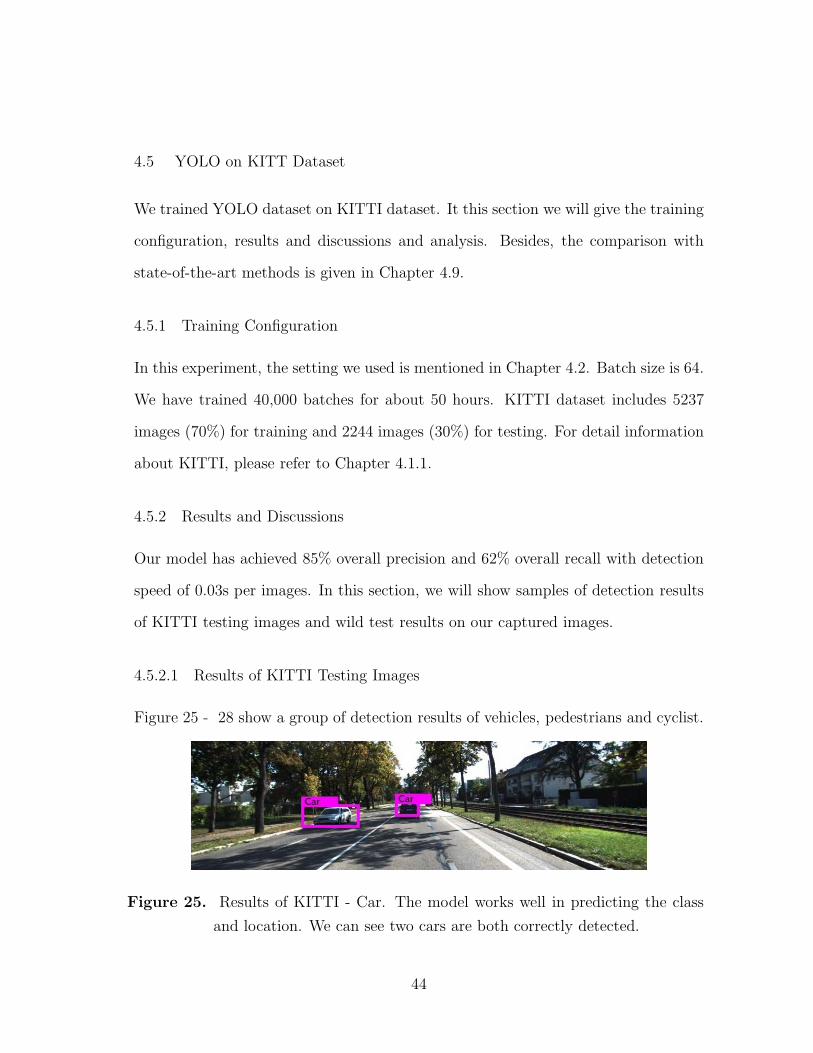
Figure 25 - 28 show a group of detection results of vehicles, pedestrians and cyclist.
Figure 25. Results of KITTI - Car. The model works well in predicting the class
and location. We can see two cars are both correctly detected.
44

Figure 26. Results of KITTI - Car occluded. Even the car on the right side is
hidden by the wall, the system still successfully detects it.
Figure 27. Results of KITTI - Car Failure. The near large vehicles are all detected
correctly, but the far and small car are left out.
Figure 28. Results of KITTI - Pedestrian. This is a true positive detection.
45

4.5.2.2 Wild Testing on Our Own Images
Wild testing means training a model on one dataset while testing on another dataset.
In this case, we use the model which trained on KITTI dataset, to test on our images.
These images were captured by the car recorder. We could subjectively check if the
model works. However, without ground truth, we cannot do validation on these
images. Below are samples of images from main road, campus road and park lot.
Figure 29. Wild Test - Main Road. The image was took from main road off campus.
A white car was successfully detected.
46

Figure 30. Wild Test - Campus Road. Image shows small road in campus. In the
center of image, both coming car and leaving car are detected. Also, our
recording car is also detected at the right bottom.
Figure 31. Wild Test - Parking Lot. In park lot. This situation is more complexity
since there more than 10 vehicles in the camera view and our model
detected 9 of them.
47

4.5.3 Results Analysis
In this section, we are going to analyze how training batches affect detection results.
We will give the recall and precision changes at each training batches. We also
compute each class's recall and precision precision by classes and by difficulty levels.
How to compute recall and precision is introduced in Chapter 3.5.
4.5.3.1 Training Batches' Effect
Training batch is an important parameter that affects the detection result. Training
batch is defined in Chapter 4.2. Theoretically, the more batches, the better results
we get, also takes longer time. In the section, we will analyze the relation between
training batches and results, to find out the best batch settings for a tuning model
and a final model. Figure 32 shows the recall and precision tendency as training
images increase. From this chart, we found the recall and precision increase rapidly
before 10,000 batches. After that, two criteria increase slowly until 40,000 batches.
Thus, we summarized two training points in our later experiments. First, we use
5,000 or 10,000 batches for fast testing new model's applicability. Second, when we
valid a model's best performance, we use 40,000 batches.
48

Figure 32. Precision and Recall by Training Batches.
4.5.3.2 Training Batches' Effect on Class
In this section, we are going to analysis how training batches affect each class's recall
and precision.
Figure 33 gives each class's over recall at different training patches. Throughout all
training stages, car always has the highest recall than pedestrian and cyclist, which
means car is the easiest class to detect in this dataset. And pedestrian is the hardest
class to detect. We also found that the recalls of car and cyclist increase rapidly at
early training and slow down after 25,000 batches. But pedestrian' recall suffered a
flat period from 10,000 to 30,000 batches and increased at later batches. We infer
that the network learned faster to detect car and cyclist than to detect pedestrian.
49

Figure 33. Each Class's Recall by Training Batches.
50

Figure 34 shows the precision change as training batches increase. Precision of car
increases stable, which again proves that car is easier to detect than pedestrian and
cyclist. In this figure, pedestrian's precision does not increase or even decreases from
10,000 batches to 35,000 batches. Which means during the middle of the training,
the network predicts more false positives. Thus, we conclude that more training
batches could increase recall, but might also reduce precision.
Figure 34. Each Class's Precision by Training Batches.
51

4.5.3.3 Training Batches' Effect on Difficulty Levels
As define in Chapter 4.1.1 - Table III, KITTI has three difficulty levels objects, hard,
moderate and hard, which defined by object's hight, occlusion degree and truncation
percentage. In this experiment, objects' difficulty levels match their recalls as shown
in Figure 35. The easy level object always has the highest recall; moderate objects
rank secondly and hard objects get the lowest recall.
Figure 35. Training Batches Affects Recall by Difficulty Levels.
52

4.6 Gridding Size's Effect on Detection Result
In YOLO model, the input images are divided into grids, and the network predicts a
fixed number of objects for each grid. In fact, the gridding size defines the maximum
amount that a network cal predict. For more detail aboug gridding size, please refer
to Chapter 3.2. In this section, we trained 4 neural networks with different gridding
sizes on the same dataset and analyzed the relation between the performance and
gridding sizes.
4.6.1 Implementation and Configuration
In this experiment, we used general setting which is mentioned in Chapter 4.2. As
the gridding size changes, the maximum amount of predicting objects also changes,
which is shown in Table VII.
Gridding size 7x7 9x9 11x11 14x14
Maxmium predictions 147 243 363 588
Table VII. Gridding Size and Maxmium Predictions.
4.6.2 Results and Discussions
In this section, we will analyze how training batches affect detection results. We
still use overall recall and overall precision, by classes and by difficulty levels. The
definitions of recall and precision are introduced in Chapter 3.5.
53

4.6.2.1 Overall Precision and Recall by Gridding Size
In Figure 36, as the gridding size increases from 7x7 to 14x14, the precision decreases
slightly but not obvious. And the recall goes down a little bit and then goes up.
11x11 is the best gridding size in KITTI dataset. However, since the tendency of
recall is not stable, we could conclude that gridding size has little effect on network's
performance.
Figure 36. Precision and Recall by Gridding Size.
4.6.2.2 Gridding Size Affects Each Class
Figure 37 shows each class's recall change at different gridding size. We found that
9x9 and 14x14 gridding sizes are not good choices because Pedestrian and Cyclist
get lower recall at these two points. 11x11 is a good selection for better recall.
54

Figure 37. Gridding Size Affects Each Class Recall.
Figure 38 gives each class's precision at 4 gridding sizes. Car class reaches lowest
precision at 14x14 gridding size and gets best precision at 7x7. Pedestrian class's
precision slightly increases as the gridding size changes. Cyclist class gets most effect
by gridding size. When the size is 9x9, the precision dropped 41 percentage points.
Thus, from this figure, we found that 7x7 and 11x11 are better gridding sizes.
55
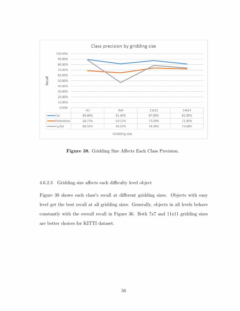
Figure 38. Gridding Size Affects Each Class Precision.
4.6.2.3 Gridding size affects each difficulty level object
Figure 39 shows each class's recall at different gridding sizes. Objects with easy
level get the best recall at all gridding sizes. Generally, objects in all levels behave
constantly with the overall recall in Figure 36. Both 7x7 and 11x11 gridding sizes
are better choices for KITTI dataset.
56

Figure 39. Gridding Size Affects Recall of Each Difficulty Level.
4.6.3 Summary
From this part of experiment, we found that 7x7 and 11x11 are the better gridding
size for KITTI dataset. The precision and recall reaches highest point either at 7x7
gridding size or 11x11. In our experiment, we chose 7x7 as our gridding size because
network at this setting has the least outputs and uses the shortest computing time.
However, the recall difference and precision different between different gridding sizes
are not obvious. We suspect that gridding size has weak effect on the network's
performance.
57

4.7 Memory Map on KITTI Dataset
Memory map is the most important contribution in our research. It considers inter-
frame information to improve detecting performance in video stream. More details
is explained in Chapter 3.3. In this section, we will give the implementation and
results analysis.
4.7.1 Implementation and Configuration
In this experiment, the setting we used is mentioned in Chapter 4.2. We computed
the overall recall and precision of models considering different frames of memory.
The methodology of memory map is explained in Chapter 3.3.3. Figure 40 shows the
work flow of the object detection with with M frames. At the beginning, initialize
an array MemoryMap with the length of M . Read a frame F from video stream. If
the current frame F is not empty, perform the detection on it and store the current
result to the MemoryMap at location P . Move the pointer P to the next location.
At the end, use sum function to compute the final detection result by considering all
the past M frames predictions. When finish current frame, loop to read next frame.
Chapter 3.3.2 gives the definition of sum function.
Below is the pseudocode for memory map algorithm:
Initialize a M-frame MemoryMap [M].
Set index pointer P = 0;
Begin loop ( read current frame, if it is not empty)
Predict current frame;
Store current result to MemoryMap [P];
Pointer P++ % M;
58

Figure 40. Memory Map Workflow
Compute current result by using sum function and matching function;
End loop;
59

4.7.2 Validation Dataset
Memory map is proposed to improve model's detection accuracy on video or live
stream. Lack of labels video on KITTI dataset is a challenge. So, we use labels
images to generate labeled video by sticking images together, each image continually
appears 10 frames in the video. Then, we validate the model with memory map on
the created video.
4.7.3 Results Analysis
This section shows the recall and precision of different frames of memory map.
4.7.3.1 Overall Recall and Precision with Memory Map
From Figure 41, we can easily find out that as the network has more frames of
memory map, it has higher recalls. Which means, the network predicts more ground
truth. However, we lose some precision at the same time. The reason is that memory
map can accumulate class probabilities, which help predict more true positive false
and positive results.
4.7.3.2 Class Recall and Precision with Memory Map
The class recall and precision are shown in Figure 42 and Figure 43. In accordance
with the overall result, the recall of each class increase as the system adding more
frames of memory map. Also, more frames of memory map bring more false positive
results, and decrease the class precision.
60

Figure 41. Overall Precision and Recall Change with Memory Map.
Figure 42. Class Recall with Memory Map.
61

Figure 43. Class Precision with Memory Map.
4.7.3.3 Summary
Memory map is a mechanism which accumulates class-confidence for temporal frames.
The higher class-confidence leads to more predictions for objects, which increases re-
call while reduces precision to some extent. Thus, Memory map provides a way
that precision can trade off for recall. If the task is aiming at higher recall without
considering precision, longer memory map will be a better choice. On the side, if
the task requires both good precision and recall, set up less memory map or even
without memory map is the best choice.
62

4.8 Orientation Estimation on KITTI Dataset
YOLO is a neural network model only designed for object detection. However, in
this section, we will explore whether YOLO can be used for predicting orientation
in addition to an object's class and bounding box, which is our second important
contribution. We will talk about implementation, visualization of orientation and
analysis of results.
4.8.1 Implementation
To apply the current model on the orientation task, we revised the cost function
by adding the orientation cost. The design of cost function is explained in Chapter
3.4.2. For system setting, we used common setting as given in Chapter 4.2.
4.8.2 Visualization of Orientation
Orientation value varies from -π to π as defined in Chapter 3.4.1. The front direction
of the camera view is -π/2, left direction is -π or π, right is 0. To visualize orientation
in image, we designed a circle icon to represent the orientation as shown in Figure 44.
For an object, its orientation circle center coincides with the center of its bounding
box. And the arrow points to the object's orientation.
Figure 44. Orientation Visualization
63

4.8.3 Results and Discussions
In Figures 45, 46 and 47, we display samples of both ground truth and prediction
orientations. Validation of orientation results is performed on the top of correct
object detections. So, in this part, we focus on the orientations of objects that are
correctly detected. We got an orientation precision of 84.89% with the processing
speed of 0.031 seconds per image.
Figure 45. Orientation Results of Car. The top image is prediction and the bottom
one is ground truth. For three cars, the model correctly predicts the
class, locations and orientations.
64

Figure 46. Orientation Results of Pedestrian and Cyclist. The top image is predic-
tion and the bottom one is ground truth. Among the objects in predic-
tion image, 4 cars, 1 cyclist and 1 pedestrian are predicted with correct
orientations.
65

Figure 47. Orientation Results of Pedestrian and Cyclist]. The top image is ground
truth and the bottom one is prediction. The left motorcycle is correctly
predicted. The cyclist and pedestrian in the middle are also predicted
with the right orientations. The right cyclist is recognized as pedestrian,
but its orientation is right.
4.8.4 Evaluation
We use orientation accuracy to validate the experiment results. Computing equa-
tion of orientation accuracy is given in Chapter 3.5. We separately compute the
orientation accuracy by directions, by classes and by difficulty levels. Validation
of orientation results is performed on the top of correct object detections, which
requires correct class and the IOU over 50%.
66

4.8.4.1 Evaluation by Directions
From the Figure 48- Left, we can easily find out that there are two peaks of the
accuracy trend from -π to π, which are near -π/2 and π/2. By checking the Figure 48-
Right, we know both -π/2 and π/2 are parallel with camera orientation. The only
different is -π/2 is in the same direction with camera orientation, while π/2 is opposite
to the camera orientation. While, in both -π/π and 0 directions, we get the lowest
accuracy, which are perpendicular to camera orientation. From this form, we can
conclude that the model predicts best orientation when objects' orientations are
parallel with camera orientation. As objects' orientation rotate away from parallel
direction, the prediction results become worse till worst at perpendicular orientation.
Figure 48. Left: orientation accuracy by object directions. Right: orientation defi-
nition
4.8.4.2 Evaluation by Classes
In this section, we will show the orientation accuracy by categories, Car, Pedestrian,
Cyclist and Misc (all other not important objects and we will not discuss it). From
the Figure 49, we found Caris much easy to predict the orientation than other
67

classes. Cyclist ranks second and Pedestrian is the hardest class. We think of two
possible factors that affect the orientation estimation. The first one is the objects'
size because larger size is easy to extract features and therefore get better result.
By common sense, a car is much larger than a human, and a cyclist's size is in the
middle, which match their accuracies Another possible factor is the structure of the
objects. Since the orientation is decided by horizontal lines or patterns on an object's
surface, flat objects with longer horizontal lines and patterns are easy to predict its
orientation than thin tall object. However, the speculative reasons need elaborate
experiments for further proof.
Figure 49. Orientation Accuracy by Object Classes
4.8.4.3 Evaluation by Difficulty Levels
Figure 50 gives the orientation accuracy by difficulty levels. For definition of difficulty
level, refer to Chapter. The easy level objects get the best accuracy, while hard level
objects get the worst accuracy. The validation result is reasonable since easy objects
68

have contribute larger features for network to predict. Even the difficulty level affects
the orientation prediction, the maximum difference between the best result and the
worst result is 3 percentage points. Accuracy of all levels are good and over 80%.
Figure 50. Orientation Accuracy by Object Difficulty Levels
69

4.9 Comparison of Object Detection with State-Of-The-Art Methods
Table VIII shows our object detection precisions with different frames of memory
map, and Table IX shows the class recall of object detection.
class without 3 frames 5 frames 7 frames 9 frames
Car 89.46 % 82.31 % 78.03 % 75.54 % 74.38 %
Pedestrian 68.75 % 61.05 % 56.43 % 53.15 % 51.73 %
Cyclist 88.32 % 78.79 % 72.16 % 68.05 % 66.19 %
Table VIII. Class Precision of Different Frames of Memory Map on KITTI.
class without 3 frames 5 frames 7 frames 9 frames
Car 66.19 % 73.81 % 76.25 % 77.22 % 77.79 %
Pedestrian 43.44 % 46.68 % 48.33 % 49.32 % 50.18 %
Cyclist 50.60 % 53.37 % 54.40 % 55.61 % 56.22 %
Table IX. Class Recall of Different Frames of Memory Map on KITTI.
We compared our 5-frames precision with other state-of-the-art methods as shown
in Table X, Table XI and Table XII. Other methods focus on accuracy rather than
speed. In three classes detection, our overall accuracy is at the end. But it is the
fastest model. It is almost 10 times faster than the second fast models (MS-CNN and
SDP+RPN, 0.4 second). Besides, our method is the only one that achieves real-time
performance (0.031 seconds per image/ 32 frames per second).
70

Method Overall precision Runtime
DeepStereoOP [19] 93.45 % 3.4 s / GPU
Mono3D [4] 92.33 % 4.2 s / GPU
SubCNN [31] 90.81 % 2 s / GPU
SDP+RPN [32] 90.14 % 0.4 s / GPU
MS-CNN [3] 90.03 % 0.4 s / GPU
Faster R-CNN [22] 86.71 % 2 s / GPU
Regionlets [30] 84.75 % 1 s / 8 cores
Our Method with 5MM 78.03 % 0.03 s / GPU
Vote3Deep [6] 76.79 % 1.5 s / 4 cores
Table X. Overall Accuracy of Object Detection on KITTI Car.
Method Overall precision Runtime
MS-CNN [3] 83.92 % 0.4 s / GPU
SubCNN [31] 83.28 % 2 s / GPU
DeepStereoOP [19] 81.82 % 3.4 s / GPU
Mono3D [4] 80.35 % 4.2 s / GPU
SDP+RPN [32] 80.09 % 0.4 s / GPU
Faster R-CNN [22] 78.86 % 2 s / GPU
Regionlets [30] 73.14 % 1 s / 8 cores
Vote3Deep [6] 68.39 % 1.5 s / 4 cores
Our Method with 5MM 56.43 % 0.03 s / GPU
Table XI. Overall Accuracy of Object Detection on KITTI Pedestrian.
71

Method Overall precision Runtime
MS-CNN [3] 84.06 % 0.4 s / GPU
SDP+RPN [32] 81.37 % 0.4 s / GPU
Vote3Deep [6] 79.92 % 1.5 s / 4 cores
SubCNN [31] 79.48 % 2 s / GPU
DeepStereoOP [19] 79.58 % 3.4 s / GPU
Mono3D [4] 76.04 % 4.2 s / GPU
Faster R-CNN [22] 72.26 % 2 s / GPU
Our Method with 5MM 72.16 % 0.03 s / GPU
Regionlets [30] 70.41 % 1 s / 8 cores
Table XII. Overall Accuracy of Object Detection on KITTI Cyclist.
72

CHAPTER 5
CONCLUSION
5.1 Summary
In Chapter 1, we first introduced the motivation of researching on object detection
problems, reviewed the traditional detectors and CNN based detectors, and proposed
our research plan. In Chapter 2, we provided the background information of the
fully connected neural network, CNN and YOLO. In Chapter 3, we explained how to
design the overall system and the methodology adapted. In Chapter 4, we presented
the experiment result for all the datasets that we considered in this research.
5.2 Contribution
We trained the model on three different datasets namely, Pascal VOC [7], Road Sign
[2], and FDDB [15]. Experiment results reveal that YOLO performs well for all the
three datasets.
By performing a comprehensive analysis of YOLO over KITTI dataset, we found
that YOLO can achieve 85% precision with 62% recall at 30 frames per second. The
results are encouraging and suggest that YOLO is an excellent model for detecting
objects required for autonomous driving systems.
However, YOLO processes the images individually despite the fact that there is con-
tinuous information in video stream in real-time driving situation. YOLO needs
further modifications to better fit real-time driving system. To fill this gap, the most
important contribution of this research lies in proposing a novel technique called
memory map to make YOLO suitable for real-time video streaming. The memory
map mechanism, which accumulates class-confidence throughout temporal frames,
73

helps increase recall while reduce precision.
By comparing with state-of-the-art methods, our revised model with memory map
got a little lower detection precision. However, our methods won the first place in
detection speed. Our detection speed is 0.03 seconds per image, which is 10 times
faster than the best methods. Our modified model is the only one that achieve real-
time, 30 frames per second, which can be used in driving situation.
In the orientation estimation section, we found that YOLO works well in predicting
an object's orientation. In an auto-driving system, predicting an object's direction
is crucial for the system to be able to make correct decisions.
Through our experiments, we proved that YOLO has great performance in image-
level object detection and orientation estimation. Our novel memory map improve-
ment makes YOLO much suitable in driving situation, that makes it the best choice
for autonomous driving system.
74

CHAPTER 6
FUTURE WORK
In YOLO network, the input images are divided into unique-sized grids to predict
objects with various sizes. Thus, the unique-sized grid may affect the bounding box
accuracy of smaller or larger objects. In the future, we will try to divide the input
images into multiple sizes and select the best results from overlapping grids.
In our experiments, we observed an increase in recall as an impact of using memory
map. However, the memory map component does not need training process currently
and the weights for each frame are engineered. In the future, we can add memory
map to training process to learn the optimum weights.
KITTI dataset has multiple ground truth data, 2D and 3D. In our experiments,
we only used 2D information to train the network. In the future, both 2D and 3D
data can be used to train the neural network for object detection and orientation
estimation.
Currently, our system can only run on a single GPU. In the future, we can revise the
system to make it run on multiple GPUs to get higher detection speed. That will
enable the network to work better in high speed driving situations.
75

REFERENCES
[1] A brief introduction to gradient descent. https://alykhantejani.github.io/
a-brief-introduction-to-gradient-descent/. Accessed: 2017-04-06.
[2] Start training yolo with our own data. http://guanghan.info/blog/en/
my-works/train-yolo/. Accessed: 2017-04-06.
[3] Cai, Z., Fan, Q., Feris, R. S., and Vasconcelos, N. A unified multi-
scale deep convolutional neural network for fast object detection. In European
Conference on Computer Vision (2016), Springer, pp. 354–370.
[4] Chen, X., Kundu, K., Zhang, Z., Ma, H., Fidler, S., and Urtasun,
R. Monocular 3d object detection for autonomous driving. In Proceedings
of the IEEE Conference on Computer Vision and Pattern Recognition (2016),
pp. 2147–2156.
[5] Deng, J., Berg, A., Satheesh, S., Su, H., Khosla, A., and Fei-Fei, L.
Imagenet large scale visual recognition competition 2012 (ilsvrc2012), 2012.
[6] Engelcke, M., Rao, D., Wang, D. Z., Tong, C. H., and Posner, I.
Vote3deep: Fast object detection in 3d point clouds using efficient convolutional
neural networks. arXiv preprint arXiv:1609.06666 (2016).
[7] Everingham, M., and Winn, J. The pascal visual object classes challenge
2011 (voc2011) development kit. Pattern Analysis, Statistical Modelling and
Computational Learning, Tech. Rep (2011).
[8] Felzenszwalb, P. F., Girshick, R. B., McAllester, D., and Ra-
manan, D. Object detection with discriminatively trained part-based models.
76

IEEE transactions on pattern analysis and machine intelligence 32, 9 (2010),
1627–1645.
[9] Freund, Y., and Schapire, R. E. A desicion-theoretic generalization of
on-line learning and an application to boosting. In European conference on
computational learning theory (1995), Springer, pp. 23–37.
[10] Geiger, A., Lenz, P., Stiller, C., and Urtasun, R. Vision meets
robotics: The kitti dataset. The International Journal of Robotics Research
(2013), 0278364913491297.
[11] Girshick, R. Fast r-cnn. In Proceedings of the IEEE International Conference
on Computer Vision (2015), pp. 1440–1448.
[12] Girshick, R., Donahue, J., Darrell, T., and Malik, J. Rich feature
hierarchies for accurate object detection and semantic segmentation. In Proceed-
ings of the IEEE conference on computer vision and pattern recognition (2014),
pp. 580–587.
[13] He, K., Zhang, X., Ren, S., and Sun, J. Spatial pyramid pooling in
deep convolutional networks for visual recognition. In European Conference on
Computer Vision (2014), Springer, pp. 346–361.
[14] He, K., Zhang, X., Ren, S., and Sun, J. Deep residual learning for image
recognition. arXiv preprint arXiv:1512.03385 (2015).
[15] Jain, V., and Learned-Miller, E. G. Fddb: A benchmark for face detec-
tion in unconstrained settings. UMass Amherst Technical Report (2010).
77

[16] Krizhevsky, A., Sutskever, I., and Hinton, G. E. Imagenet classifica-
tion with deep convolutional neural networks. In Advances in neural information
processing systems (2012), pp. 1097–1105.
[17] LeCun, Y., Bottou, L., Bengio, Y., and Haffner, P. Gradient-based
learning applied to document recognition. Proceedings of the IEEE 86, 11
(1998), 2278–2324.
[18] Mikolajczyk, K., and Schmid, C. A performance evaluation of local de-
scriptors. IEEE transactions on pattern analysis and machine intelligence 27,
10 (2005), 1615–1630.
[19] Pham, C. C., and Jeon, J. W. Robust object proposals re-ranking for
object detection in autonomous driving using convolutional neural networks.
Signal Processing: Image Communication 53 (2017), 110–122.
[20] Redmon, J., Divvala, S., Girshick, R., and Farhadi, A. You only look
once: Unified, real-time object detection. In Proceedings of the IEEE Conference
on Computer Vision and Pattern Recognition (2016), pp. 779–788.
[21] Ren, S., He, K., Girshick, R., and Sun, J. Faster r-cnn: Towards real-
time object detection with region proposal networks. In Advances in neural
information processing systems (2015), pp. 91–99.
[22] Ren, S., He, K., Girshick, R., and Sun, J. Faster r-cnn: Towards real-
time object detection with region proposal networks. In Advances in neural
information processing systems (2015), pp. 91–99.
[23] Sadeghi, M. A., and Forsyth, D. 30hz object detection with dpm v5. In
European Conference on Computer Vision (2014), Springer, pp. 65–79.
78

[24] Sermanet, P., Eigen, D., Zhang, X., Mathieu, M., Fergus, R., and
LeCun, Y. Overfeat: Integrated recognition, localization and detection using
convolutional networks. arXiv preprint arXiv:1312.6229 (2013).
[25] Simonyan, K., and Zisserman, A. Very deep convolutional networks for
large-scale image recognition. arXiv preprint arXiv:1409.1556 (2014).
[26] Szegedy, C., Liu, W., Jia, Y., Sermanet, P., Reed, S., Anguelov,
D., Erhan, D., Vanhoucke, V., and Rabinovich, A. Going deeper with
convolutions. In Proceedings of the IEEE Conference on Computer Vision and
Pattern Recognition (2015), pp. 1–9.
[27] Szegedy, C., Reed, S., Erhan, D., and Anguelov, D. Scalable, high-
quality object detection. arXiv preprint arXiv:1412.1441 (2014).
[28] Uijlings, J. R., van de Sande, K. E., Gevers, T., and Smeulders,
A. W. Selective search for object recognition. International journal of computer
vision 104, 2 (2013), 154–171.
[29] Viola, P., and Jones, M. Rapid object detection using a boosted cascade
of simple features. In Computer Vision and Pattern Recognition, 2001. CVPR
2001. Proceedings of the 2001 IEEE Computer Society Conference on (2001),
vol. 1, IEEE, pp. I–511.
[30] Wang, X., Yang, M., Zhu, S., and Lin, Y. Regionlets for generic object
detection. In Proceedings of the IEEE International Conference on Computer
Vision (2013), pp. 17–24.
[31] Xiang, Y., Choi, W., Lin, Y., and Savarese, S. Subcategory-aware con-
volutional neural networks for object proposals and detection. arXiv preprint
79

arXiv:1604.04693 (2016).
[32] Yang, F., Choi, W., and Lin, Y. Exploit all the layers: Fast and accurate
cnn object detector with scale dependent pooling and cascaded rejection classi-
fiers. In Proceedings of the IEEE Conference on Computer Vision and Pattern
Recognition (2016), pp. 2129–2137.
[33] Zeiler, M. D., and Fergus, R. Visualizing and understanding convolutional
networks. In European conference on computer vision (2014), Springer, pp. 818–
833.
80