1

3D Object Detection for Autonomous Driving: ASurvey

Rui Qian, Xin Lai, and Xirong LiRenmin University of China

Beijing, China{rui-qian, laixin, xirong}@ruc.edu.cn

Abstract—Autonomous driving is regarded as one of the mostpromising remedies to shield human beings from severe crashes.To this end, 3D object detection serves as the core basis of suchperception system especially for the sake of path planning, motionprediction, collision avoidance, etc. Generally, stereo/monocularimages with corresponding 3D point clouds are already standardlayout for 3D object detection, out of which point clouds areincreasingly prevalent with accurate depth information beingprovided. Despite existing efforts, 3D object detection on pointclouds is still in its infancy due to high sparseness and irregularityof point clouds by nature, misalignment view between cameraview and LiDAR bird’s eye of view for modality synergies,occlusions and scale variations at long distances, etc. Recently,profound progress has been made in 3D object detection, witha large body of literature being investigated to address thisvision task. As such, we present a comprehensive review of thelatest progress in this field covering all the main topics includingsensors, fundamentals, and the recent state-of-the-art detectionmethods with their pros and cons. Furthermore, we introducemetrics and provide quantitative comparisons on popular publicdatasets. The avenues for future work are going to be judiciouslyidentified after an in-deep analysis of the surveyed works. Finally,we conclude this paper.

Index Terms—3D object detection, Autonomous driving, Pointclouds

I. INTRODUCTION

WHY is automonous driving? The rise of AutomonousDriving (AD) is sure to benefit the whole society from

the following aspects: 1) Safety. The paramount aim for ADis to address the problem of safety. According to NationalHighway Traffic Safety Administration (NHTSA) [1, 2], about36,560 people died in the U.S. in 2018, as a consequence ofmotor vehicle-related crashes. What’s more, 94% of severecrashes are owe to human error. The continuing evolutionof AD is poised to save lives and change the car insuranceindustry in essence. 2) Economic benefits. A NHTSA studyreveals $242 billion is spent on motor vehicle crashes in 2010,involved in disentangling traffic accidents and treating thewounded. 3) Efficiency and convenience. With AD system,traffic flow could be smoothed with the help of big data,the time for daily commutes can be radically reduced. 4)Mobility. Automonous vehicles will provide new mobilityoptions, creating new employment opportunities for peoplewith disabilities. More details can be found in [1–3].

X. Lai contributes equally to this work and should be considered as co-firstauthor. Xirong Li contributes equally to this work and is the correspondingauthor.

Manuscript received Jun 19, 2021; revised ** ** , 2021.

2009 2010 2011 2012 2013 2014 2015 2016 2017 2018 2019Year

0

50

100

150

200

250

Num

ber o

f pub

licat

ions

267

223

116

84

64697565

5748

27

The number of publications in 3D object detection

(a) The increasing number of publications in 3D object detection from 2009to 2019. (Data from Google scholar advanced search: allintitle: “3D objectdetection”.)

10-Ja

n

10-N

ov

11-S

ep

12-Ju

l

13-M

ay

14-M

ar

15-Ja

n

15-N

ov

16-S

ep

17-Ju

l

18-M

ay

19-M

ar

20-Ja

n

0

20

40

60

80

100

Heat

The trend of heat change with time

(b) The trend of heat change with time from 2010 to 2020.(Data from Googletrends by searching key word: “3d object detection autonomous driving”.)

Fig. 1: The increasing number of publications from 2009 to2019 and the heat trends from January 2010 to June 2020.Note that 3D object detection is getting its popularity.

What is automonous driving? Universally acknowledged, 5levels exist at present. The biggest demarcation of AD happensat Level 3, with completely certain safety-critical functionsbeing shifted to the vehicle under certain traffic conditions.

Level 0: The driver (human) does all the driving: steering,brakes, and power, etc.

Level 1: An advanced driver assistance system (ADAS) au-tomatically assists the human driver with specific and limitedfunctions, (e.g., steering or braking). Note that the driver stillcontrols almost all the behaviours.

Level 2: In level 2, the driver assistance system actually

arX

iv:2

106.

1082

3v1

[cs

.CV

] 2

1 Ju

n 20

21

2

controls both steering and acceleration/deceleration under cer-tain circumstances. Full human attention is still needed in caseof emergency.

Level 3: Drivers are still indispensable to intervene ifnecessary, but are able to shift all the functions to the vehicle.

Level 4: This is so called “fully autonomous”. Vehicles per-form all driving functions, which is limited to the “operationaldesign domain (ODD)” for an entire trip.

Level 5: A fully-autonomous system is expected to functionas good as a human driver, coping with various unconstraineddriving scenarios. The occupants of the vehicles are justpassengers in the foreseeable future.

What is 3D object detection? 3D object detection is to detectphysical objects from 3D sensor data, with oriented 3D bound-ing boxes being estimated and with specific categories beingassigned. 3D object detection serves as the core of 3D sceneperception and understanding. Thousands of downstream ap-plications, such as autonomous driving, housekeeping robots,and augmented/virtual reality, etc., have sprung up with theavailability of various types of 3D sensors [4]. Generally, threetypes of 3D representations commonly exist, including pointclouds 2(a), meshes 2(b), volumetric grids 2(c), out of whichpoint clouds are the preferred representation in many cases.Point clouds neither consume storages as much as meshes thatconsist of a large number of faces, nor lose original geometricinformation like volumetric grids due to quantization. Pointclouds are close to raw LiDAR sensor data 4.

(a) Point Clouds (b) Meshes (c) Volumetric Grids

Fig. 2: Three types of commonly existing 3D representations.Image from Qi et al. [5].

3D object detection [6–8] has made remarkable progress,though, it has still trailed its 2D counterpart thus far[9–18]. 3Dobject detection looks into detecting visual objects of a certainclass with accurate geometric, shape and scale information:3D position, orientation, and occupied volume [19], providinga better understanding of surroundings for machines, andposing a difficult technological challenge simultaneously. It isgenerally believed that the key to the success of ConvolutionNeural Networks is the capability of leveraging spatially-local correlations in dense representations [20]. However,directly applying CNNs kernels against point clouds inevitablycontributes to desertion of shape information and variance topoint ordering [20]. On this basis, this paper carefully analyzesthe recently state-of-the-art 3D object detection methods.

Last but not least, it is also important to note that modernautomonous driving system relies heavily on deep learning.Whereas, deep learning methods have already been proved tobe vulnerable to forgeries. As such, this poses an inherent

security risk(e.g., sabotage, adverse conditions, and blindspots, etc.) to the automated industry. Ultimately, adversarialattacks with regard to 3D object detection are largely in theirinfancy [21].

Compared to the existing literature, we summarize ourcontributions as follows:

1) A survey with new taxonomy which is more fine-grained: Compared with [6, 7], we dig in further toprovide more fine-grained classification on the existingefforts [6, 7] which facilitates readers to grasp thecharacteristics of each method intuitively and concretely.For instance, point cloud-based methods are meant to beexhaustive, but when we group point cloud-based meth-ods further into multi-view-based, voxel-based, point-based, and point-voxel-based methods on the basis ofrepresentation learning, readers should be able to iden-tify the main ideas of point cloud-based methods withouteffort.

2) A survey with new taxonomy which is more sys-tematic: As shown in Fig. 2 and Fig. 6, the outbreakhappening after 2018 has undergone a profound transi-tion, regardless of social concerns and effectiveness ofthe method itself. 3D perception system has witnesseda process of continuous self-improvement, which is notreally established until high-performance detectors areproposed after 2018, e.g., PointRCNN [22], PV-RCNN[23]. Whereas, literature [7] only covers the progressbefore 2018. Besides, to the best of our knowledge,only a handful of literature is associated with 3D pointclouds, not to mention the far unexplored fields focusingon autonomous driving.

3) A survey with new taxonomy which is more inclusive:In [8], Guo et al. grouped Part-A2 [24], PV-RCNN[23], Point-GNN [25] into “Other Methods”, leaving theproblem unsolved. Studies [6, 7, 26] have discussed thetaxonomy carefully, but when it comes to multimodalfusion, they only introduced the basic concept of earlyfusion, late fusion, and deep fusion, without identify-ing which category each method belongs to explicitly.Whereas, we defined two new paradigms to adapt toongoing changes.

4) A survey with new taxonomy which is a supplemen-tary rather than an alternative: As opposed to existingsurvey [8], we specifically focus on 3D object detectionin the context of autonomous driving, rather than allrelated subtopics of 3D point clouds, (e.g., 3D shapeclassification, 3D point cloud segmentation and tracking,etc.) Given that the limited space available, one cannot delve into such details, with all the materials beinginvolved. Instead, we start with quite basic concepts,providing a glimpse of evolution of 3D object detec-tion in terms of autonomous driving under our definedparadigms, together with comprehensive comparisons onpublicly available datasets being manifested, with prosand cons being judiciously presented.

The rest of this paper is organized as follows. In SectionII, we discuss the commonly used 3D sensors. In Section III,

3

TABLE I: Advantages and disadvantages of different sensors.

Sensors Advantages Disadvantages Publications

MonocularCamera

•cheap and available for multiple situations •no depth or range detecting feature [27], [28], [29]•informative color and texture attributes •susceptible to weather and light conditions [30], [31], [32]

StereoCamera

•depth information provided •computationally expensive [33], [34], [35]•informative color and texture attributes •sensitive to weather and light conditions•high frame rate •limited Field-of-View(FoV)

LiDAR•accurate depth or range detecting feature •high sparseness and irregularity by nature [22, 23, 36–39], [25]•less affected by external illumination •no color and texture attributes [40], [41], [42, 43]•360◦ FoV •expensive and critical deployment [44, 45], [24, 46, 47]

Solid StateLiDAR

•more reliable compared with surround viewsensors

•error increase when different points ofview are merged in real time

-

•cost decrease •Still under development and limited FoV -

we introduce basic concepts and notations. In Section IV, wereview the latest existing state-of-the-art 3D object detectionmethods with their corresponding pros and cons in the contextof autonomous driving. Commonly used metrics, comprehen-sive comparsions of the state-of-the-arts, and publicly availabledatasets are summarized in Section V. Afterwards, we identifyfuture research directions. In Section VI, we conclude thispaper.

II. SENSORS

We human beings leverage visual and auditory systemsto perceive the real world when driving, so how about au-tonomous vehicles? If they were to drive like a human, thento identify what they see on the road constantly is the way togo. To this end, sensors matter. It is sensors that empowervehicles a series of abilities: obstacles perception, overtak-ing, automatic emergency braking, collision avoidance, ride-hailing, traffic light and pedestrian detection, etc. In general,the most commonly used sensors can be divided into twocategories: passive sensors and active sensors. The on goingdebate among industry experts is whether or not to just equipvehicles with camera systems (no LiDAR), or deploy LiDARtogether with on-board camera systems. Currently, Waymo,Uber and Velodyne are in support of LiDAR, while Tesla hasbeen outnumbered, in favor of camera systems. Given thatcamera is considered to be one of the typical representatives ofpassive sensors, and LiDAR is regarded as a representative ofactive sensors, we first introduce the basic concepts of passivesensors and active sensors, then take camera and LiDAR asan example to discuss how they serve the automonous drivingsystem, together with pros and cons being manifested in tableII.

A. Passive Sensors

Passive sensors are anticipated to receive natural emissionsemanating from both the Earth’s surface and its atmosphere.These natural emissions could be natural light or infrared rays.For instance, a camera directly grabs a bunch of color pointsfrom the optics in the lens and arranges them into an imagearray that is often referred to as a digital signal for sceneunderstanding. Inspired by recent advancements in computervision algorithms to analyze over image signals, 2D/3D object

detection has undergone profound progress. So far Tesla hasbeen successfully leveraging camera systems (no LiDAR) toobtain a 360 degree view for its autonomous vehicles (as ofthis main text in June 2021). Primarily, a monocular cameralends itself well to informative color and texture attributes,better visual recognition of text from road signs, and highframe rate at a negligible cost, etc. Whereas, it is lack of depthinformation, which is crucial for accurate position estimationin the real world. To overcome this, a stereo camera usesmatching algorithms to align correspondences in both left andright images for depth recovery. While cameras have shownpotentials as a reliable visioning system, it is hardly sufficientas a standalone system. Specifically, a camera is prone todegrade its accuracy in cases where luminosity is low at night-time or rainy weather conditions occur. As a consequence,Tesla has to use auxiliary sensors to fall-back onto in casethat camera system should malfunction or disconnect.

B. Active Sensors

Active sensors are expected to measure reflected signals thatare transmitted by the sensor, which are bounced by the Earth’ssurface or its atmosphere. Typically, LiDAR (Light DetectionAnd Ranging) is a point-and-shoot device with three basiccomponents of len, laser and detector, which spits out lightpulses that will bounce off the surroundings in the form of3D points, referred to as “point clouds”. High sparseness andirregularity by nature and the absence of texture attributes arethe primary characteristics of a point cloud, which is welldistinguished from image array. Since we have already knownhow fast light travels, the distance of obstacles could be deter-mined without effort. LiDAR system emits thousands of pulsesthat spin around in a circle per second, with a 360 degree viewof surroundings for the vehicles being provided. For example,Velodyne HDL-64L produces 120 thousand points per framewith a 10 Hz frame rate. Obviously, LiDAR is less affectedby external illumination conditions (e.g., at night-time), giventhat it emits light pulses by itself. Although LiDAR systemhas been hailed for high accuracy and reliability comparedwith camera system, it does not always hold true. Specifically,wavelength stability of LiDAR is susceptible to variationsin temperature, while adverse weather (e.g., snow or fog) isprone to result in poor SNR (Signal-to-Noise Ratio) in the

4

LiDAR’s detector. Another issue with LiDAR is the high costof deployment. A conservative estimate according to Velodyne,so far, is about $70,000 [7]. In the foreseeable future ofLiDAR, how to decrease cost and how to increase resolutionand range are where the whole community is to march ahead.As for the former, the advent of Solid State LiDAR is expectedto address this problem of cost decrease, with the help ofseveral stationary lasers that emit light pulses along a fixedfield of view. As for the latter, the newly announced VelodyneVLS-128 featuring 128 laser pulses and 300m radius range hasbeen on sale, which is going to significantly facilitate betterrecognition and tracking in terms of public safety.

C. Discussion

Fatalities occurred with autonomous vehicles have alreadyincreased the society’s grave concern about safety. if au-tonomous vehicles were to hit the road legally, they at leastneed to satisfy three basic characteristics: high accuracy, highcertainty, and high reliability. To this end, sensor fusion incor-porating the merits of two worlds (camera vs LiDAR) is goingto be necessary. From a sensor standpoint, LiDAR providedepth information close to linearity error with a high level ofaccuracy, but it is susceptible to adverse weather (e.g., snow orfog). Camera is intuitively much better at visual recognitionin cases where color or texture attributes are available (seeFig. 16), but they are not sufficient as a standalone systemas aforementioned. Note that certainty is still an importantyet largely unexplored problem. A combination of LiDARand camera is anticipated to ensure detection accuracy andimprove prediction certainty. With regard to reliability, twofacets should be considered: sensor calibration and systemredundancy. Sensor calibration undoubtedly increases the dif-ficulty of deployment and directly affects the reliability of thewhole system. Studies [48–50] have looked into calibratingsensors to avoid drift over time. System redundancy is to havea secondary sensor to fall-back onto in case of a malfunction oroutage. The community should be keenly aware of the safetyrisk of over-reliance on a single sensor. More details will bediscussed in Section IV-C.

III. FUNDAMENTALS

In this section, we formulate 3D object detection problem,list commonly used notations, and introduce basic coordinatetransformation.

A. Problem Formulation

Unless otherwise stated, notations used in this survey aremanifested in Table II. Given that all the methods associatedbellow are based on KITTI dataset for comparisons, wefollow the camera coordinate system adopted by the project ofKarlsruhe Institute of Technology and Toyota TechnologicalInstitute (KITTI) [19, 51] in the remainder of main text:it is a right-handed coordinate system, when x-axis pointsto right, y-axis points down with regard to the 2D imageplane, z-axis stands for depth and is perpendicular to the 2Dimage plane. Denote by {{Bi, Ci} = Φ (Di; Θ) : i = 1, ...,M}

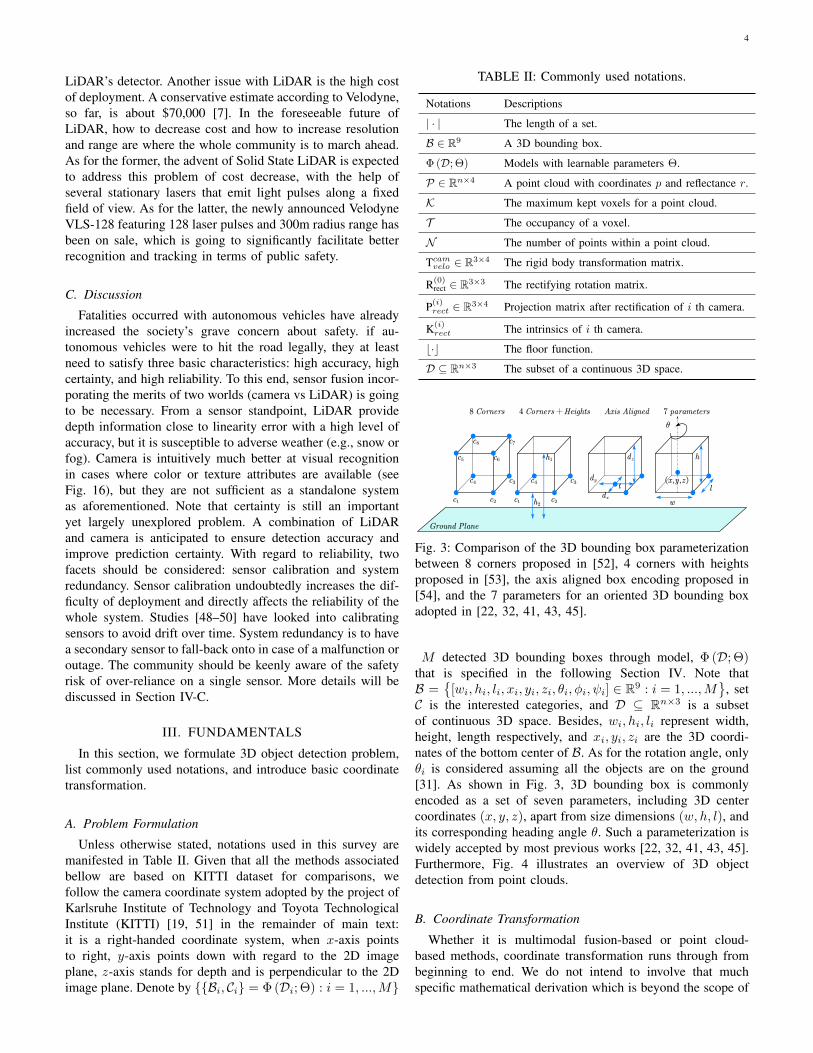
TABLE II: Commonly used notations.

Notations Descriptions

| · | The length of a set.

B ∈ R9 A 3D bounding box.

Φ (D; Θ) Models with learnable parameters Θ.

P ∈ Rn×4 A point cloud with coordinates p and reflectance r.

K The maximum kept voxels for a point cloud.

T The occupancy of a voxel.

N The number of points within a point cloud.

Tcamvelo ∈ R3×4 The rigid body transformation matrix.

R(0)rect ∈ R3×3 The rectifying rotation matrix.

P(i)rect ∈ R3×4 Projection matrix after rectification of i th camera.

K(i)rect The intrinsics of i th camera.

b·c The floor function.

D ⊆ Rn×3 The subset of a continuous 3D space.

Fig. 3: Comparison of the 3D bounding box parameterizationbetween 8 corners proposed in [52], 4 corners with heightsproposed in [53], the axis aligned box encoding proposed in[54], and the 7 parameters for an oriented 3D bounding boxadopted in [22, 32, 41, 43, 45].

M detected 3D bounding boxes through model, Φ (D; Θ)that is specified in the following Section IV. Note thatB =

{[wi, hi, li, xi, yi, zi, θi, φi, ψi] ∈ R9 : i = 1, ...,M

}, set

C is the interested categories, and D ⊆ Rn×3 is a subsetof continuous 3D space. Besides, wi, hi, li represent width,height, length respectively, and xi, yi, zi are the 3D coordi-nates of the bottom center of B. As for the rotation angle, onlyθi is considered assuming all the objects are on the ground[31]. As shown in Fig. 3, 3D bounding box is commonlyencoded as a set of seven parameters, including 3D centercoordinates (x, y, z), apart from size dimensions (w, h, l), andits corresponding heading angle θ. Such a parameterization iswidely accepted by most previous works [22, 32, 41, 43, 45].Furthermore, Fig. 4 illustrates an overview of 3D objectdetection from point clouds.

B. Coordinate Transformation

Whether it is multimodal fusion-based or point cloud-based methods, coordinate transformation runs through frombeginning to end. We do not intend to involve that muchspecific mathematical derivation which is beyond the scope of

5

Fig. 4: An overview of 3D object detection from point clouds. 3D object detection is to detect physical objects from 3D sensordata, with oriented 3D bounding boxes being estimated and with specific categories being assigned. Note that Fig. 4 are inLiDAR coordinates.

this survey, but it is necessary to give its basic concepts giventhat it is indeed an essential prerequisite of preprocessing (e.g.,data augmentation). Since most of the existing researches arebased on KITTI dataset, we will take KITTI dataset as anexample to introduce the main principles which holds true forits counterparts. In general, LiDAR and camera coordinate sys-tems are defined as: 1) LiDAR coordinates: x=forward, y=left,z=up. 2) Camera coordinates: x=right, y=down, z=forward.

Given a 3D point p = (x, y, z, 1)T in LiDAR coordinates,

its corresponding point y = (u, v, 1)T in the i-th camera image

is given as:y = P(i)

rect R(0)rect Tcamvelo p, (1)

where i ∈ {0, 1, 2, 3} is the camera index in the KITTI sensorsetups, out of which camera 0 is the reference coordinates.Tcamvelo ∈ R3×4 is the rigid body transformation from LiDARcoordinates to camera coordinates, R(0)

rect ∈ R3×3 is the recti-fying rotation matrix, and P(i)

rect ∈ R3×4 is projection matrixafter rectification. Note that all four camera centers are alignedto the same x/y − plane. In particular,

P(i)rect =

f(i)u 0 c

(i)u −f (i)u b

(i)x

0 f(i)v c

(i)v 0

0 0 1 0

, (2)

with

K(i)rect =

f(i)u 0 c

(i)u

0 f(i)v c

(i)v

0 0 1

. (3)

here, b(i)x is the baseline with respect to reference camera 0,f(i)u and f

(i)v denote camera focal length from u-axis and v-

axis in camera coordinates respectively. In fact, K(i)rect denotes

camera intrinsics. We refer readers to [19, 51] for more details.

IV. 3D OBJECT DETECTION METHODS2D object detection has a catalytic effect in spurring

progress in 3D object detection somewhat. As shown inFig. 6, 3D object detection methods can be categoried intomonocular/stereo image-based IV-A, point cloud-based IV-Band multimodal fusion-based methods IV-C in terms of themodality of input data. Note that point cloud-based meth-ods which predominate in 3D object detection, can furtherbe classified into multi-view-based, voxel-based, point-based,and point-voxel-based methods on the basis of representationlearning. Multimodal fusion-based methods have been gettingpopularity nowadays, but it is no-trivial to exploit the synergiesof different domains (i.e., images and point clouds). To ex-plicitly distinguish diverse multimodal fusion-based methods,

6

Fig. 5: Pipeline of 3D Object Detection in General. Generally, image-based methods either exploit carefully manual featureengineering to exhaustively search templates via machine learning (e.g., SVM) [27, 28, 35, 55] or leverage considerable domainexpertise to roughly estimate 3D pose via geometric properties from empirical observation, with high-quality 2D bounding boxesbeing provided via the off-the-shelf 2D detectors [29, 31, 33]. Nevertheless, standard point cloud-based methods commonlyconsists of three conponents: 1) Point cloud representation; 2) Backbone, 3) Detection headers. Given exceptions [22, 25, 39]directly take raw point clouds as input leaving feature learning implicitly, we use dotted line to reveal optional operation. Ina sequel, on the basis of image-based and point cloud-based methods, multimodal fusion-based methods have become eventhriving, with numerous literature being proposed [52, 56–58].

we define two new categories of fusion strategies: sequentialfusion-based methods and parallel fusion-based methods. Weintroduce monocular/stereo image-based methods, point cloud-based methods, and multimodal fusion-based methods in linewith the chronological order in which each method emerges.We put multimodal fusion-based methods at last since it’son the basis of the others. Now, we analyze each categoryindividually in deep in the following subsections.

A. Monocular/Stereo Image-based MethodsThese methods which are the most similar stream in spirit

to 2D object detection among those in 3D, only take monocu-lar/stereo images as input to predict 3D object instances. Gen-erally two lines exist: Templates Matching based Methodsand Geometric Properties based Methods. As for the former,region proposals are the essential ingredients of this line. Infact, how to propose high-quality regions where objectnessmay exist in 2D object detection has been extensively studied[59], varying from traditional hand-crafted grouping (e.g.,SelectiveSearch [60]) and window scoring (e.g., EdgeBoxes[61]) methods to recently Region Proposal Network (RPN)[13] accompanying with the success of CNNs. Methods toobtain region proposals are meant to be exhaustive. Neverthe-less, the purpose of extracting regional coorresponding priors(i.e., segmentation, shape, and free space, etc.) of images toexhaustively score and match 3D representative templates isalways with consistency [27, 28, 35, 55]. Whereas, the latercan be reduced to the perspective n-point problem (PnP) [62]to roughly estimate 3D pose via geometric properties fromempirical observation, with high-quality 2D bounding boxesbeing provided via the off-the-shelf 2D detectors [11–18].Recently, inspired by the encouraging success of point cloud-based methods, another attempt occurs by reprojecting image

coordinates back into 3D space via computing disparity tomimic LiDAR signal (hereafter called pseudo LiDAR), andthen resorts to high-performance point cloud-based methods.We name it Pseudo LiDAR based Methods.

Templates Matching based Methods. These methods areprone to perform 2D/3D matching via exhaustively samplingand scoring 3D proposals as representative templates.

Templates matching based methods are typically exempli-fied by the early and well known 3DOP [55] proposed byChen et al., which consumes a stereo image pair as input toestimate depth and compute a point cloud via reprojectingpixel-wise coordinates in the image plane back into 3D space.3DOP formulates the problem of proposal generation as en-ergy minimization of a Markov Random Field (MRF) withrespect to carefully designed potentials (e.g., object size priors,ground plane, and point cloud density, etc.). With a diverseset of 3D object proposals being obtained, 3DOP resortsFast R-CNN [11] pipeline to jointly regress object locations.Subsequently, on the possible occasions when cars are onlyequipped with a single camera, Chen et al. proposed Mono3D[27] to achieve on par performance through using a monocularcamera only instead of stereo one. Different from 3DOP,Mono3D directly samples 3D object candidates from 3D spacethrough the usage of sliding windows without computing depthinformation, assuming the ground plane where objects liesshould be orthogonal to the image plane to reduce search ef-forts. Potentials, for instance, semantic segmentation, instancelevel segmentation as well as location priors are exploitedto exhaustively score candidates in the image plane to selectthe most promising one before conducting detections via FastR-CNN [11] pipeline specified in 3DOP [55]. Either 3DOP[55] or Mono3D [27] outputs class-specific proposals, whichmeans potentials needs to be newly designed for each category

7

Part-� (Shi et al. TPAMI) 78.49

A2

Deep3DBox (Mousavian et al. CVPR) n.a.Deep MANTA (Chabot et al. CVPR) n.a.

MF3D (Xu et al. CVPR) n.a.3DOP* (Chen et al. TPAMI) n.a.

One Stage Detectors Two Stage Detectors

VeloFCN (Li et al. Robotics) Mono3D (Chen et al. CVPR) 2.31

MV3D (Chen et al. CVPR) 63.63

PointPainting (Vora et al. CVPR) 71.70

PVRCNN (Shi et al. CVPR) 81.43

Pseudo-LiDAR (Wang et al. CVPR) 34.05

Pseudo-LiDAR++ (You et al. ICLR) 42.43

3D-CVF (Jin et al. ECCV) 80.05

SASSD (He et al. CVPR) 79.79

Point-GNN (Shi et al. CVPR) 79.47

Voxel-FPN (Wang et al. CVPR) 76.70

HVNet (Ye et al. CVPR) n.a.

Fast Point RCNN (Chen et al. CVPR) 77.40

STD (Yang et al. ICCV) 79.71

Stereo R-CNN (Li et al. CVPR) 30.23

GS3D (Li et al. CVPR) 2.9

PointRCNN (She et al. CVPR) 75.64

Mono3D-PLiDAR (Weng et al. ICCV) 7.5

MMF （Liang et al. CVPR) 77.43

FConvnet (Wang et al. IROS) 76.39

3DSSD (Yang et al. CVPR) 79.57

PointPillars (AH Lang et al. CVPR) 74.31

AVOD (Ku et al. IROS) 66.47

3DOP (Chen et al. NeurIPS) n.a.

Frustum PointNets (Qi et al. CVPR) 69.79

ContFuse (Ming et al. ECCV) 68.78

SECOND (Yan et al. sensors) 75.96

VoxelNet (Zhou et al. CVPR) 64.17

PIXOR (Yang et al. CVPR) n.a.

2018

Monocular/Stereo Image-based MethodsPoint Cloud-based MethodsMultimodal Fusion-based Methods3D results NOT available

2016

2017

2019

2020

2015

Fig. 6: Chronological axis of 3D object detection. Detectors inthis figure: 3DOP [35, 55], Mono3D [27], Deep MANTA [28],Deep3DBox[29], GS3D [31], Stereo R-CNN [33], MF3D [30],Mono3D-PLidar [32], VeloFCN [36], PIXOR [37], VoxelNet[45], SECOND [41], PointPillars [43], Voxel-FPN [44], Part-A2 [24], HVNet [47], PointRCNN [22], 3DSSD [39], Point-GNN [25], Fast Point R-CNN [63], STD [38], PV-RCNN[23], SA-SSD [40], Frustum PointNets [56], F-ConvNet [46],PointPainting [57], Pseudo-LiDAR [64], Pseudo-LiDAR++[65], MV3D [52], AVOD [53], ContFuse [58], MMF [66],3D-CVF [67].

separately. Nevertheless, over-reliance on careful engineeringand considerable domain expertise limit the generalizabilityof these models for complex scenarios. Another attempt isseen in Deep MANTA [28] proposed by Chabot et al., whichutilizes a customized 2D detector to output 2D boundingboxes, associated with 2D part coordinates, part visibility and3D template similarity supervised by a large CAD database of3D models. With the best corresponding 3D template beingchosen from a template database according to the predicted3D template similarity, 2D/3D matching in [68] is conductedto recover 3D geometry. The drawbacks are: Deep MANTAneeds to maintain a huge CAD database of 3D models which

is ill-suited to be generalized to the category which is absentfrom the database.

Geometric Properties based Methods. Instead of requiringextensive proposals to achieve high recall, these methods startwith accurate 2D bounding boxes directly to roughly estimate3D pose from geometric properties obtained by empiricalobservation.

Mousavian et al. proposed Deep3DBox[29], leveraging thegeometric properties that the perspective projection of 3D cor-ners should tightly touch at least one side of the 2D boundingbox. Li et al. proposed GS3D [31], which detects complete3D instances via monocular RGB image only, without extradata or label being introduced. Specifically, GS3D adds anextra branch of orientation prediction on the basis of the FasterRCNN [13] framework to predict reliable 2D bounding boxesand observation orientations, referred to as 2D+O subnet. ThenGS3D obtains coarse 3D boxes, referred to as guidances,based on the empirical evidence in the context of autonomousdriving, that the 3D box top center is approximately closeto the top midpoint of its coorresponding 2D bounding box.Last, features extracted from both 2D box and three visiblesurfaces of 3D box are fused to eliminate the problem ofrepresentation ambiguity before fed into 3D subnet for furtherrefinement. Although GS3D shows a significant performancegain over existing monocular image-based methods, GS3Ddepends upon the empirical knowledge, which is inaccurateand vulnerable to the ranges and sizes of the objects. Anotherexample of utilizing projection relationships between 2D and3D is Stereo R-CNN [33]. Li et al. proposed Stereo R-CNN [33], which fully exploits semantic properties as wellas dense constraints in stereo imagery. In particular, StereoR-CNN adopts weight-share network, namely ResNet-101[69] and FPN [70] as backbone, to extract both left andright image features respectively, then a Region of Interest(RoI) alignment operation is applied, with corresponding RoIproposals being cropped. Next, these selected RoI features arefused via concatenation before fed into a stereo regressionbranch. Simultaneously, four semantic keypoints are predictedby mimicking Mask R-CNN [18], with RoI features of leftbranch being utilized. Last, the 3D box estimation can beartfully addressed resorting to geometric constraints, that is,the projection relationships between 3D corners and 2D boxesas well as the predicted keypoints.

Pseudo LiDAR based Methods. These methods first per-form depth estimation and then resort to existing point cloud-based methods.

Xu et al. proposed MF3D [30], which performs multi-level fusion for image features and pseudo LiDAR. Specif-ically, MF3D first computes the disparity via a stand-alonemonocular depth estimation module to obtain a pseudo Li-DAR. Simultaneously, a standard 2D region proposal networkis employed taking as input RGB images fused with theconverted front view (see algorithm 3) features obtained bythe disparity map. With 2D region proposals being obtained,features both from RGB images and pseudo LiDAR are fusedby concatenation for further refinement. Recently, Weng et al.proposed Mono3D-PLiDAR [32], which lifts the input imageinto 3D camera coordinates, namely, pseudo-LiDAR points,

8

Evolution of Monocular/Stereo Image-based Methods

Year: 2010 2015 2016 2017 2018 2019 2020

Templates matching

1. Templates matching 2. Geometric properties 3. Pseudo LiDAR

2D bbox

3D bbox

Pseudo LiDAR

Geometric properties with CNNs

Pseudo LiDAR@3DOP(Chen et al.—NeuralPS2015),@Mono3D(Chen et al.—CVPR2016),@Deep MANTA(Chabot et al.—CVPR2017)@3DOP*(Chen et al.—TPAMI2018), …

@Deep3DBox(Mousavian et al.—CVPR2017),@GS3D(Li et al.—CVPR2019),@Stereo R-CNN(Li et al.—CVPR2019), …

@MF3D(Xu et al.—CVPR2018),@Mono3D-PLidar(Weng et al.—ICCV2019), …

✔

✘

✘

Fig. 7: Evolution of monocular/stereo image-based methods: 1) Templates matching, 2) Geometric properties, 3) Pseudo LiDAR.Detectors in this figure: 3DOP [35, 55], Mono3D [27], Deep MANTA [28], Deep3DBox[29], GS3D [31], Stereo R-CNN [33],MF3D [30], Mono3D-PLidar [32].

via monocular depth estimation (e.g., DORN [71]). Then a 3Dobject detector, called Frustum PointNets [56] is applied withthe pseudo-LiDAR. Weng et al. reveals that Pseudo LiDARhas a large amount of noise due to the error of monoculardepth estimation, which reflects in two aspects: a local mis-alignment w.r.t the LiDAR points and a problem of depthartifacts. To overcome the former, Mono3D-PLiDAR uses a2D-3D bounding box consistency loss (BBCL) to supervise thetraining. To alleviate the latter, Mono3D-PLiDAR adopts theinstance mask predicted by Mask-RCNN [18] instead of the2D bounding box to reduce irrelevant points within frustum.We refer the interested reader to Fig. 15(f) for details offrustum architecture. Pseudo LiDAR based methods indeedobtain an promising performance gain in accuracy, whichsomehow provide enlightenments for exploring the synergiesof two modalities, that is, images and point clouds.

In summary 7, monocular/stereo image-based methods havetheir pros and cons. These methods take images only asinputs, which provide color attributes as well as textureinformation. Typically, they rely on a considerable amountof domain expertise to design vector representation. As theabsence of depth information, one possible remedy is toinvestigate depth estimation algorithm. For an automonoussystem, redundancy is indispensible to guarantee safty apartfrom economic concerns, so image-based methods are poisedto make a continuing impact over the next few years.

B. Point Cloud-based Methods

The essence of CNNs is sparse interaction and weightsharing, whose kernels have been proved to be effective inexploiting spatially-local correlations in regular domains [20],that is, euclidean structure, by a weighted sum of centerpixel and its adjacent pixels. Whereas, CNNs is ill-suited incases where data is represented in irregular domains, (e.g.,social networks, point clouds, etc.). Since a point cloud isirregular and unordered, directly convolving against it suffersfrom “desertion of shape information and variance to pointordering” [20], as Li et al. notes. As shown in Fig. 8,suppose set F =

{fi ∈ RF : i = a, b, c, d

}in (i)-(iv) denotes

four point features. Except (i), each points in (ii)-(iv) isassociated with an order index, coordinates, and a feature,let K =

{ki ∈ RF : i = α, β, γ, δ

}is the convolution kernel,

Conv (·, ·) is a weighted element-wise sum. Traditionallyconvolving against irregular domains can be denoted as:

fii = Conv(

K, [fa, fb, fc, fd]T)

fiii = Conv(

K, [fa, fb, fc,fd]T)

fiv = Conv(

K, [fc, fa, fb, fd]T).

(4)

Note that fii ≡ fiii holds true for all cases which desertsshape information, while fiii 6= fiv holds true for mostcases which reveals variance to point ordering. Hence, featurelearning from irregular domains is the core of point cloud-based methods. Specifically, these methods can be further

9

divided into four categories: multi-view-based, voxel-based,point-based, and point-voxel-based methods on the basis ofrepresentation learning from point clouds.

𝑓𝑎 𝑓𝑏

𝑓𝑑𝑓𝑐

1

𝑓𝑎

3

𝑓𝑐

2

𝑓𝑏

4

𝑓𝑑

1

𝑓𝑎

2

𝑓𝑏

4

𝑓𝑑3

𝑓𝑐

2

𝑓𝑎

3

𝑓𝑏

4

𝑓𝑑1

𝑓𝑐

i ii iii iv

Fig. 8: The effects of convolving against regular grids (i) andpoint clouds (ii-iv) [20].

Fig. 9: Visualization of point clouds from front view. Frontview with a shape of 3 × W × H encodes height, distance,and reflectance intensities. Front view can be obtained by thealgorithm 3 under LiDAR coordinates. The original imagecorresponding to the visualized point cloud can be found in 4.

Density mapHeight map Intensity mapBEV map

Fig. 10: Visualization of point clouds from bird’s eye of view.Height map encodes height information of z-axis, intensitymap encodes LiDAR reflection intensity of each LiDARpoints, and density map encodes statistics within each grid cell.These maps have a shape of 1×W×H. BEV map with a shapeof 3 ×W × H is the concatenation of three aforementionedmaps. All these maps can be obtained by the algorithm 2 underLiDAR coordinates. The original image corresponding to thevisualized point cloud can be found in 4.

Multi-view-based Methods. These methods first convert asparse point cloud into either front view (see algorithm 3)or Bird’s Eye View (BEV) (see algorithm 2) representation,which is densely in grids. The idea is intuitive and simplefor the sake of leveraging CNNs and standard 2D detectionpipeline.

Li et al. proposed VeloFCN [36], which converts a pointcloud into front-view 2D feature map, then resorts to theoff-the-shelf 2D detectors. To alleviate the problem of oc-clusions due to overlaps, Yang et al. proposed PIXOR [37],which rasterizes the point cloud into more compact 2D BEVrepresentation. Once discretization, a standard 2D detectionpipeline is applied. PIXOR benefits from conversion of pointclouds in BEV perspective with an advantage of less scaleambiguity and minimal occlusions. Whereas, according to

algorithm 2, considerable information on vertical axis maybe neglected when generating a BEV map. Hence, it is maynot a feasible choice for pedestrians, road signs, and objectsunder overpasses, etc., since these enumerated cases from sucha perspective may only be a few points after sampling ata certain height (see algorithm 2), which is obviously notconducive to the network feature extraction.

Voxel-based Methods. These methods generally transformthe irregular point clouds to the volumetric representationsin compact shape to efficiently extract point features for 3Ddetection via 3D Convolutional Neural Networks (3D CNNs).It is believed that voxel-based methods are computationallyefficient, at the cost of degrading the fine-grained localizationaccuracy because of the information loss during discretization[23, 40].

Before introducing specific methods, we first must startwith several basic concepts, because they run throughthe whole process of voxel-based Methods. Let p bea point in a point cloud P with the 3D coordi-nates (x, y, z) and reflectance intensities r, where P ={pi = [xi, yi, zi, ri] ∈ R4 : i = 1, ..., N

}. A point cloud P is

first evenly divided into spatial resolution of L×W ×H . Letv = {pi = [xi, yi, zi, ri]

T ∈ R4 : i = 1, ..., t} be a non-emptyvoxel comprising t points(t ≤ T ) and [vL, vW , vH ] ∈ R3 bethe spatial volume of a voxel, the voxel indices of each point piin P is denoted as {pi =

(b xi

vLc, b yivW c, b

zivHc)

: i = 1, ..., N},where b·c indicates floor function, then iteratively determinewhich voxel a certain point pi belongs to according to theassociated index. If the points within each voxel reaches theoccupancy T of a voxel, discard pi directly, otherwise, assignthe point pi to the voxel. Such a many-to-one mapping algo-rithm (hereafter called hard voxelization) is widely adoptedby SECOND [41], Pointpillars [43] and all their successors,which by nature presents three intrinsic limitations [42]: 1)Given points and voxels are thrown away when they exceedthe allocated capacity, useful information for detection couldpossiblely be forsaken. 2) Non-deterministic voxel embeddingswith points and voxels being stochastically dropped, could leadto jitteriness of detection models. 3) Unavailing zero-paddingsquanders unnecessary computation somewhat. For simplicity,SA-SSD [40] directly quantizes each point pi to tensor indexby regarding each pi as a nonzero entry. The shared indexof multiple points will be overwritten in place by the latestpoint. Recently, Zhou et al. [42] proposed a novel dynamicvoxelization to overcome preceding limitations, The differ-ences between hard voxelization and dynamic voxelization areillustrated in Fig. 11.

Voxel-wise representation is nothing but aggregate point-wise features into voxel-wise features. As far as we know,there exists three operators at present. As shown in Fig. 12,1) Mean operator. All inside point features with the 3Dcoordinates and reflectance intensities of a certain voxel aredirectly calculated for the mean, (i.e., the centroid), denotedas (cx, cy, cz). (e.g., SECOND[41]) 2) Random sampling. Apoint within the voxel is randomly selected on behalf of thevoxel feature. (e.g., SA-SSD [40]) 3) MLP operator. Thepoint-wise features pi within v are then transformed by a

10

Fig. 11: Comparisons of hard voxelization and dynamic vox-elization [42]. Specifically, assume that 3D space is evenlydivided into four voxels, which is indexed as v1, v2, v3, v4.Hard voxelization may randomly drops 3 points in v1 anddiscards v2 with 15f memory usage if we set the occupancyof a voxel T to 5 and the maximum kept voxels K to 3 for awhole point cloud for memory cost saving. Whereas, dynamicvoxelization gets rid of unstable voxel embeddings via keepingall points during voxelization with memory usage 15f .

Mean Operator Random Sampling

MLPs

……

…… …

Max Pooling

MLP Operator

Fig. 12: Illustration of voxel-wise representations via threeaggregation operators.

PointNet [5] block to generate voxel-wise high level semanticfeatures as:

f = max {MLP (G (pi)) ∈ Rm : i = 1, ..., T } (5)

Optionally, the initial voxel representation can be augmentedby the relative offset of the centroid (cx, cy, cz) as: v = {pi =[xi, yi, zi, ri, xi − cx, yi − cy, zi − ci]T ∈ R7 : i = 1, ..., t},where G (·) denotes randomly sampling at most T points inorder to keep the number of points within each voxel bethe same. MLP(·) denotes a stacked multi-layer perceptronnetwork composed of a linear layer, a Batch Normalization(BN) layer, and a Rectified Linear Unit (ReLU) layer. Thealong-channel max-pooling operation max (·) aggregates allinside point-wise features into voxel-wise features f (e.g.,Voxelnet [45], Pointpillar [43], and F-ConvNet [46], etc.).

Zhou et al. took the first lead to propose an end-to-end train-able network named VoxelNet [45], as shown in Fig. 15(a).Instead of manual feature engineering as most previous worksdo, VoxelNet learns a informative feature representation by

three components: (1) Feature learning network, (2) Convolu-tional middle layers, and (3) Region proposal network. Featurelearning network divides a point cloud into equally spaced3D voxels, and newly introduce a PointNet-like Voxel FeatureEncoding (VFE) layer to transform a set of points into avector that encodes the shape of the surface within each voxel.The convolutional middle layers introduces more contextualshape description by aggregating voxel-wise features withinan expanding receptive field. Finally, the Region ProposalNetwork (RPN) takes as input the 3D CNN feature volumesand outputs the encouraging 3D detection results. Althoughthe VoxelNet is the seminal work in 3D object detection, itsdrawbacks are: the cubically computational complexity of 3Dconvolutional network imposes increased memory usage andefficiency burdens on the computing platform. Later on, Yan etal. proposed SECOND [41] to reduce memory consumptionand accelerate computational speed via sparse convolutionaloperation. As illustrated in Fig. 15(b), They first gatheredthe original sparse data directly in an ordered fashion withits corresponding coordinates being recorded, then they per-formed a General Matrix Multiplication (GEMM) algorithm toconvolve against the gathered data before scattering the databack. Sparse convolutional operation opts to take advantageof the sparsity of a point cloud to only convolve against non-empty voxels rather than perform on all voxels as traditional3D convolutions do. Although SECOND leverages sparseconvolution operation to get rid of unnecessary computa-tion squandered by unavailing zero-padding voxels comparedwith VoxelNet [45], the expensive 3D convolutions remain,hindering the further improvement of speed. Subsequently,Pointpillars was proposed to remove this bottleneck. H. Langet al. proposed PointPillars [43], which encoded point cloudsinto vertical columns, namely, pillars, a special partition ofvoxels in essence, in order to take advantages of standard2D convolutional detection pipeline. PointPillars consists ofthree main conponents as VoxelNet does: (1) A feature encodernetwork, (2) a 2D convolutional backbone, and (3) A detectionheader. The feature encoder network organizes a point cloud invertical columns, then scattering the pillars back to its originallocalization to create a pseudo-image in a BEV perspective.The 2D convolutional backbone comprises two sub-networks:one downsamples the pseudo-image while the other upsamplesand concatenates the downsampled features. The detectionheader regresses 3D boxes the same as its 2D counterpart.Albeit Pointpillars achieves a 2-4 fold runtime improvement at62 FPS1 via getting rid of traditional 3D convolutions used inVoxelNet [45], it suffers poor information perception problemin pillar partition. As a result, the subsequent literature is proneto encode a point cloud into voxels instead of pillars in thelight of tradeoff between efficiency and accuracy [44].

Shi et al. proposed Part-A2 [24]. Motivated by the observa-tion that intra-object part locations can be provided by the 3Dbounding box annotations accurately without any occlusions,two stages are delicate designed: the part-aware stage and thepart-aggregation stage. Specifically, Part-A2 utilizes a UNet-like [72] architecture to convolve and deconvolve non-empty

1FPS denotes Frames Per Second.

11

voxels for foreground points segmentation and part prediction.Simultaneously, coarse 3D proposals are generated via anextra RPN header. In the part-aggregation stage, a subtle RoI-grid pooling module is presented to eliminate the ambiguityof 3D bounding boxes and learn the spatial correlations ofthe points within 3D proposals. Last, 3D sparse convolution[41] is applied to aggregate the part information for scoringand refining locations. Ye et al. proposed HVNet [47], whichconsists of three components:1) Multi-scale voxelization andfeature extraction 2) Multi-scale feature fusion and dynamicfeature projection 3) A detection header. Specifically, HVNetvoxelizes a point cloud at different scales first, then for eachscale, a voxel-wize feature is computed by aggregating theinformation of each point within a voxel, resorting to anAttentive Voxel Feature Encoder (AVFE). Then these highlevel semantic features are scattered back to their originallocalization, forming a pseudo-image according to the coor-responding index records. Last, HVNet employs FPN [70]as the backbone to predict final instances. These strategiesenable HVNet to outperform all existing LiDAR-based one-stage methods in terms of Cyclist on KITTI benchmark with areal time inference speed of 31FPS. Although HVNet ranks 1st

on the KITTI test server associated with the Cyclist category,there still exists a far cry from the state-of-the-art LiDAR-based methods on the Car leaderboard. Given that the carcategory predominates the whole KITTI dataset [19, 51], itwill be more persuasive to compare on the Car category.

Point-based Methods. These methods generally consumeraw point clouds leveraging two types of backbone: Point-Net(++) and its variants or Graph Neural Networks (GNNs).Usually, they retain the geometry of the original point cloud asmuch as possible. Nevertheless, point retrieval in 3D space ishostile to efficient hardware implementations compared withvolumetric grids [73].

concat concat

(a)Multi-scale grouping(MSG) (b)Multi-resolution grouping(MRG)(a) Multi-scale grouping(MSG)

concat concat

(a)Multi-scale grouping(MSG) (b)Multi-resolution grouping(MRG)(b) Multi-resolution grouping(MRG)

Fig. 13: PointNet(++)[74] applies PointNet [5] recursively in ahierarchical manner. In particular, the density adaptive layers,i.e., the Multi-Scale Grouping(MSG) and Multi-ResolutionGrouping(MRG), enable PointNet and its variants to adap-tively capture local structures and fine-grained patterns of pointclouds.

In 2017, Qi et al. proposed PointNet [5], which is a pioneerin terms of learning over point sets. PointNet enables thenetwork to directly consume raw point clouds and learn3D representations from a point cloud for classification andsegmentation without converting a point cloud into volumetric

grids or other formats. As shown in 13, the improved version,PointNet(++) [74], applies PointNet recursively in a hierarchi-cal manner. In particular, the density adaptive layers, i.e., theMulti-Scale Grouping (MSG) and Multi-Resolution Grouping(MRG), enable PointNet and its variants to adaptively capturelocal structures and fine-grained patterns of point clouds. Lateron, a series of point-based methods sprang up for 3D objectdetection on the basis of PointNet due to its generalizabilityto complex scenes. Hence, point-based methods (e.g., PointR-CNN [22], 3DSSD [39]) are powered by PointNet(++) [5, 74]and its variants to directly extract discriminative features fromraw point clouds. In this paradigm, usually Set Abstraction(SA) layers are utilized for downsampling points and FeaturePropagation (FP) layers are applied for broadcasting featuresto the whole scene via upsampling. Afterwards, they leverage a3D region proposal network to generate high-quality proposalscentered at each point for the further refinement in the finalstage. These methods could obtain flexible receptive field bythe stacked SA modules at the price of higher computationcost compared with voxel-based methods.

Algorithm 1 Farthest Points Sampling

Require: P = {p1, p2, · · · , pN } is a set of point cloud data,where N is the number of points. Each point is presentedby a C-length vector. k ∈ N is the number of samples.D = (D1, D2, · · · , DN ) is a distance vector containingthe distance of each point from a sampled point set. SetDn = +∞, n = 1, 2, · · · ,N .

Ensure:1: Randomly sample the first point pi1 ∈ P, i1 ∈{1, 2, · · · ,N}.

2: for s = 1, 2, · · · , k − 1 do3: for n = 1, 2, · · · ,N do4: d(n, is+1) =

∑Cj=1(pn(j)− pis+1

(j))2.5: if d(n, is+1) < d(n, is) then6: Dn = d(n, is+1).7: end if8: end for9: Sample the next farthest point’s index:

is+1 = arg maxn∈{1,2,··· ,N}

Dn.

10: end for11: return Sampled farthest points (pi1 , pi2 , · · · , pik).

Shi et al. proposed PointRCNN [22], as shown in Fig.15(c). PointRCNN is a typical point-based two-stage detectionframework, elegantly transplants the idea of classical 2Ddetector, Faster RCNN [13], into 3D detection task, takingpoint clouds only as input: (1) Since 3D object instances inpoint clouds are well separated by annotated 3D boundingboxes, PointRCNN directly performs semantic segmention onthe whole scene via PointNet(++) architecture to achieve fore-ground points, generating a set of high-quality 3D proposals ina bottom-up fashion. (2) PointRCNN leverages 3D region ofinterest pooling operation to pool points and coorrespondingsemantic features of each proposal for further box refinementand confidence prediction. The limitation of PointRCNN is

12

the inference time: both the backbone, PointNet(++), andrefinement modules in stage two are time consuming. Yang etal. proposed 3DSSD [39]. The main contributions of 3DSSDare: (1) It safely removes FP layers, which is regard as themain bottleneck of speed for point-based methods, via fusingEuclidean metrics (refer to as D-FPS* in 3DSSD [39]) andfeatures metrics(refer to as F-FPS* in 3DSSD [39]) togetherwhen performing Furthest Point Sampling (FPS*)2 specified inalgorithm 1 to make up the loss of interior points of differentforeground instances during downsampling. (2) An anchor-freeregression header is developed to reduce memory consumptionand boost the accuracy further. 3DSSD is more than 25 FPS,2× faster than PoinRCNN, around 13 FPS, which makes itpossible to be widely used in real-time systems.

A large body of literature [75–79] has looked into leveragingGNNs for classification and semantic segmentation from pointclouds. Since GNNs has a strong reasoning ability over Non-Euclidean data (e.g., Point Clouds) [80]. Point cloud-based3D object detection is another area in which graph-basedmethods are poised to make a large impact over the nextfew years. Currently, using GNNs for 3D object detectionis still largely unexplored [81, 82], nevertheless. Shi et al.proposed Point-GNN [25], which utilizes GNNs to preservethe irregularity of a point cloud without quantization. Point-GNN leverages a graph neural network to encode a point cloudby regarding each point within the point cloud as graph vertex.Points that lie within a given cut-off distance are connectedto form the graph edges. Point-GNN comprises three steps:(1) Constructing graph from a downsampled point cloud, (2)Updating each vertex so that the message can flow betweenneighbors for detecting the category and localization, and (3)Merging 3D bounding boxes from multiple vertices. AlthoughPoint-GNN pioneered a new stream line for 3D object detec-tion, its challenges are tricky: the time of constructing graphand inference within iterations are usually intolerable and ittakes almost one week to completely train the model claimedin the paper. Note that point-based methods are sensitive totranslation variance. To alleviate the dilemma, Point-GNNproposed an auto-registration mechanism to predict alignmentoffsets appended to neighbors’ relative coordinates via struc-tural features of the center vertex. 3DSSD predicts shifts forforeground points supervised by the relative locations betweenthose interior points and their corresponding center within ainstance.

Point-voxel-based Methods. Point-voxel-based methodsrepresent a new growing trend for learning representationsfrom a point cloud. In 2019, Liu et al. proposed PVConv[73], PVConv fuses the merits of voxels and points together.On the one hand, voxel-based methods are vulnerable to theparameters of voxels, e.g., low resolution results in coarse-grained localization accuracy, whereas, high resolution in-creases cubical computation cost. On the other hand, point-based methods can easily preserve the irregularity and localityof a point cloud opting to either set abstraction or PointNet-like block, providing fine-grained neighborhood information.In fact, such integration has been proved to be effective by

2We name Furthest Point Sampling FPS* to avoid ambiguity.

Voxelization

3D Convs. Backbone

To BEV 2D Convs. Backbone

3D

Det

ecti

on

Bo

xes

a: VoxelNet End-to-End Learning for Point Cloud Based 3D Object Detection (VoxelNet)

Voxelization

3D Sparse Convs. Backbone

To BEV 2D Convs. Backbone

3D

Det

ecti

on

Bo

xes

b: SECOND Sparsely Embedded Convolutional Detection (SECOND)

PointNet++

PointsPool

3D

Det

ecti

on

Bo

xes

d: Sparse-to-Dense 3D Object Detector (STD)

Point-wise Scores & Features

Shperical Anchors

Vo

xeliz

atio

n

VFE3D Region

Proposals

IoUBranch

Box Pred

Branch

Voxelization3D Convs. Backbone

To BEV 2D Convs. Backbone

3D

Det

ecti

on

Bo

xes

e: Point-Voxel Feature Set Abstraction for 3D Object Detection (PV-RCNN)

Voxel Set Abstraction

RPN

Point-wise Feature Vector

RoI-gridPooling

PointNet++

RoIpooling

3D

Det

ecti

on

Bo

xes

c: PointRCNN 3D Object Proposal Generation and Detection from Point Cloud (PointRCNN)

Canonical 3D Box

Refinement

Point CloudSegmentation

Bottom-up 3DProposal Generation

3D ProposalGeneration

…

RGB Image

3D RoIs

3D

Det

ecti

on

Bo

xes

g: End-to-End Multi-View Fusion for 3D Object Detection in LiDAR Point Clouds (MV3D)

2D CNN

RGB ImageProjection & Pooling

Bird’s Eye View

Front View

Bird’s Eye ViewProjection & Pooling

Front ViewProjection & Pooling

Fusion

Stereo/Mono Images

3D

Det

ecti

on

Bo

xes

h: Pseudo-LiDAR from Visual Depth Estimation Bridging the Gap in … (Pseudo-LiDAR)

Stereo/Mono depth

LiDAR-basedDetection

Depth estimation Pseudo LiDAR

RGB Image

3D

Det

ecti

on

Bo

xes

f: Frustum PointNets for 3D Object Detection from RGB-D Data (Frustum-PointNets)

Frustum-wise Feature Vector

2D ImageDetector 2D RoIs Region

To Frustum

Fig. 15: Representatives of 3D object detectors. From top tobottom: a) VoxelNet [45], b) SECOND [41], c) PointRCNN[22], d) STD [38], e) PV-RCNN [23], f) Frustum-PointNets[56], g) MV3D [52], h) Pseudo-LiDAR [64].

multiple literature [23, 38, 40, 63] in practice.Chen et al. proposed Fast Point R-CNN [63], which benefits

from volumetric representation and raw dense coordinatesrespectively. The first stage, termed VoxelRPN, generates a

13

Evolution of Point Cloud-based Methods

Year: 2010 2015 2016 2017 2018 2019 2020

Multi view

1. Voxel grids 2. Point set 3. Point voxel hybrid

Voxel-wise feature

Point-wise feature

LiDAR signal

Voxel grids

Point set

Point voxel hybrid

@VeloFCN(Li et al.—Robotics2016),@PIXOR(Yang et al.—CVPR2018), …

@VoxelNet(Zhou et al.—CVPR2018),@SECOND(Yan et al.—CVPR2018),@PointPillars(H. Lang et al.—CVPR2019),@Voxel-FPN(Wang et al.—CVPR2019),@Part –𝐴2(Shi et al.—TPAMI2020),@HVNet(Ye et al.—CVPR2020), …

@PointRCNN(Shi et al.—CVPR2019),@3DSSD(Yang et al.—CVPR2020),@Point-GNN(Shi et al.—CVPR2020), …

@Fast Point R-CNN(Chen et al.—CVPR2019),@STD(Yang et al.—ICCV2019), @PV-RCNN(Shi et al.—CVPR2020),@SA-SSD(He et al.—CVPR2020), …

PointNet

Graph

Fig. 14: Evolution of point cloud-based methods: 1) Voxel grids, 2) Point set, 3) Point voxel hybrid. Detectors in this figure:VeloFCN [36], PIXOR [37], VoxelNet [45], SECOND [41], PointPillars [43], Voxel-FPN [44], Part-A2 [24], HVNet [47],PointRCNN [22], 3DSSD [39], Point-GNN [25], Fast Point R-CNN [63], STD [38], PV-RCNN [23], SA-SSD [40].

small set of high-quality proposals via voxelizing the wholescene into regular grids in a bottom-up fashion. Given theinitial predictions, a light-weight PointNet, RefinerNet, isclosely designed to effectively fuse the interior points and theircorresponding convolution feature via attention mechanism,with the loss of localization information in the first stage beingsupplemented. Fast Point R-CNN runs at 15 FPS. Yang et al.proposed STD [38], as shown in Fig. 15(d). The pipeline ofSTD is very similar to PointRCNN. The main innovations ofSTD is spherical anchor, which is more generic to achieve ahigh recall than rectangular one, regardless of heading angle.STD possesses excellent performance, especially on the hardset. Shi et al. proposed PV-RCNN [23], as shown in Fig.15(e), which deeply integrates the effectiveness of 3D SparseConvolution [41] and the flexible receptive fields of PointNet-based set abstraction to learn more discriminative point cloudfeatures. Specifically, PV-RCNN utilizes a 3D sparse con-volution as the backbone to encode the whole scene, thesame as SECOND [41]. Then two innovative operations, thevoxel-to-keypoint scene encoding and key-point-to-grid RoIfeature abstraction are applied for computation cost saving andlocalization refinement. In particular, the Voxel Set Abstraction(VSA) module is adopted to aggregate the multi-scale seman-tic voxel-wise features from 3D CNNs into keypoint features.Note that the keypoints are selected via FPS* algorithm 1from the original point cloud. PV-RCNN ranks 1st on the Car3D detection leaderboard and outperforms the second by alarge margin as of Jul. 10th, 2020. The absolute improvements

demonstrate the effectiveness of integrating the best of twoworlds, that is, point-based methods and voxel-based methodstogether. He et al. proposed SA-SSD [40]. SA-SSD explicitlyleverages the geometric information of a 3D point cloud viaa auxiliary network. Specifically, SA-SSD first progressivelydownscales point clouds in a sparse convolutional fashion.Then the downscaled convolutional features are discretizedevenly to point-level representations with primitive voxel-wizeunit. Next, the points within a 3D ground truth boundingbox, along with the offsets from the box center providepoint-level supervisions for jointly optimizing the auxiliarynetwork: the former forces the features to be sensitive tothe object boundary while the latter establish the intra-objectrelationships between voxels. It is ingenious for the auxiliarynetwork to detach after training, running at 25 FPS and withno extra computation overhead being introduced in the infer-ence stage. All along, the mismatching problem between theclassification score and coorresponding localization accuracyis salient, regardless of 3D object detection [23, 38, 40] orits 2D counterpart [83]. As GS3D [31] notes, given that theclassification and box regression branch are trained in parallel,Non Maximum Suppression (NMS) is likely to remove high-quality bounding boxes with low classification score. Toalleviate the discordance, STD [38] adds a 3D Intersection-over-Union (IoU) prediction branch to multiply each box’sconfidence with its predicted 3D IoU. PV-RCNN [23] directlyuses 3D IoU as the training targets. SA-SSD [40] developsa part-sensitive warping operation to sample features along

14

channels for the mean in order to perform further classificationto relief such discrepancy.

In summary 14, voxel-based methods are easily amenableto efficient hardware implementations with distinguished ac-curacy and latency, but inevitablely suffering quantizationloss considering that a number of points beyond the voxeloccupancy will be discarded. At the same time, the process ofvoxelization is more sensitive to the selection of parameters,i.e., the length, width and height of a voxel; Point-basedmethods more reasonably retain the original geometry infor-mation of a point cloud. For methods powered by pointent(++),the critical modules, FPS* and feature propagation layers aremore time-consuming than voxelization in terms of consuminga point cloud; as for those powered by GNNs, intuitively,not only the correlations between points, but also the moreintricate spatially-local structure, that is, the “vertex-edge”information is captured simultaneously. The 3D shape will bemore easily perceived, at the cost of taking longer feedforwardtime than those taking pointent(++) as the backbone.

C. Multimodal Fusion-based Methods

Nowadays, 3D object detection for autonomous drivinglargely relies on LiDARs in the light of providing informativesurrounding information. Albeit precise, it is not sensibleenough to be over-reliant on a single sensor due to an inherentsafety risk(e.g., sabotage, adverse conditions, and blind spots,etc.). In addition, the low resolution of a point cloud atthe long ranges and poor texture information also pose agreat challenge. Naturally, the most promising candidate ison-board stereo or monocular cameras, which provide fine-grained texture as well as RGB attributes simultaneously.Cameras suffer depth ambiguity by nature, though. Besides,stereo or monocular cameras are several orders of magnitudecheaper than LiDARs, with a high frame rate and a densedepth map. One persuasive case is illustrated in Fig. 16, itis more difficult to distinguish the pedestrian and signpostin the LiDAR modality when it comes to a long distance.Obviously, each sensor type has its defects, the joint treatmentis seen as a possible remedy to failure modes. Literature [84]even states that multimodal fusion provides redundancy duringdifficult conditions rather than just complementary. Althoughexploiting the synergies is a compelling research hotspot, still,it is non-trivial to consolidate the best of two worlds at presentin the light of misalignment view, namely, camera view andLiDAR bird’s eye of view.

MethodmAP Car Pedestrian CyclistMod. Easy Mod. Hard Easy Mod. Hard Easy Mod. Hard

PointPillars [11] 73.78 90.09 87.57 86.03 71.97 67.84 62.41 85.74 65.92 62.40Painted PointPillars 76.27 90.01 87.65 85.56 77.25 72.41 67.53 81.72 68.76 63.99

Delta +2.50 -0.08 0.08 -0.47 +5.28 +4.57 +5.12 -4.02 +2.84 +1.59

VoxelNet [34, 29] 71.83 89.87 87.29 86.30 70.08 62.44 55.02 85.48 65.77 58.97Painted VoxelNet 73.55 90.05 87.51 86.66 73.16 65.05 57.33 87.46 68.08 65.59

Delta +1.71 +0.18 +0.22 +0.36 +3.08 +2.61 +2.31 +1.98 +2.31 +6.62

PointRCNN [21] 72.42 89.78 86.19 85.02 68.37 63.49 57.89 84.65 67.59 63.06Painted PointRCNN 75.80 90.19 87.64 86.71 72.65 66.06 61.24 86.33 73.69 70.17

Delta +3.37 +0.41 +1.45 +1.69 +4.28 +2.57 +3.35 +1.68 +6.10 +7.11Table 1. PointPainting applied to state of the art lidar based object detectors. All lidar methods show an improvement in bird’s-eye view(BEV) mean average precision (mAP) of car, pedestrian, and cyclist on KITTI val set, moderate split. The corresponding 3D results areincluded in Table 7 in the Supplementary Material where we observe a similar improvement.

Figure 3. Example scene from the nuScenes [1] dataset. Thepedestrian and pole are 25 meters away from the ego vehicle.At this distance the two objects appears very similar in the pointcloud. The proposed PointPainting method would add semanticsfrom the image making the lidar detection task easier.

number of channels dedicated to reading the point cloud.For methods using hand-coded features [30, 22], some ex-tra work is required to modify the feature encoder.

PointPainting is sequential by design which means that itis not always possible to optimize, end-to-end, for the finaltask of 3D detection. In theory, this implies sub-optimalityin terms of performance. Empirically, however, PointPaint-ing is more effective than all other proposed fusion meth-ods. Further, a sequential approach has other advantages:(1) semantic segmentation of an image is often a usefulstand-alone intermediate product, and (2) in a real-time 3Ddetection system, latency can be reduced by pipelining theimage and lidar networks such that the lidar points are deco-rated with the semantics from the previous image. We showin ablation that such pipelining does not affect performance.

We implement PointPainting with three state of the artlidar-only methods that have public code: PointPillars [11],VoxelNet (SECOND) [34, 29], and PointRCNN [21]. Point-Painting consistently improved results (Figure 1) and in-deed, the painted version of PointRCNN achieves state ofthe art on the KITTI leaderboard (Table 2). We also showa significant improvement of 6.3 mAP (Table 4) for PaintedPointPillars+ on nuScenes [1].

Contributions. Our main contribution is a novel fusionmethod, PointPainting, that augments the point cloud withimage semantics. Through extensive experimentation weshow that PointPainting is:• general – achieving significant improvements when

used with 3 top lidar-only methods on the KITTI andnuScenes benchmarks;• accurate – the painted version of PointRCNN

achieves state of the art on the KITTI benchmark;• robust – the painted versions of PointRCNN and

PointPillars improved performance on all classes onthe KITTI and nuScenes test sets, respectively.• fast – low latency fusion can be achieved by pipelining

the image and lidar processing steps.

2. PointPainting ArchitectureThe PointPainting architecture accepts point clouds and

images as input and estimates oriented 3D boxes. It consistsof three main stages (Fig. 2). (1) Semantic Segmentation:an image based sem. seg. network which computes thepixel wise segmentation scores. (2) Fusion: lidar points arepainted with sem. seg. scores. (3) 3D Object Detection: alidar based 3D detection network.

2.1. Image Based Semantics Network

The image sem. seg. network takes in an input imageand outputs per pixel class scores. These scores serve ascompact summarized features of the image. There are sev-eral key advantages of using sem. seg. in a fusion pipeline.First, sem. seg. is an easier task than 3D object detectionsince segmentation only requires local, per pixel classifi-cation, while object detection requires 3D localization andclassification. Networks that perform sem. seg. are eas-ier to train and are also amenable to perform fast inference.Second, rapid advances are being made in sem. seg. [4, 36],which allows PointPainting to benefit from advances in bothsegmentation and 3D object detection. Finally, in a robotics

Fig. 16: A scene from the nuScenes [84] where the pedestrianand signpost are clearly identifiable in image modality. Imagefrom Vora et al. CVPR2020 [57].

Deep neural networks exploit the property of compositionalhierarchies from natural signals [85], in which fusion strategiesmay vary. Generally, two classes of fusion schemes exist,namely, early fusion and late fusion [6, 7, 26, 52, 86].The former combines multimodal features before fed intoa supervised learner, whereas the latter integrates semanticfeatures abtained by separatly trained supervised learners [86],as illustrated in Fig. 17.

Visual Features

Extraction

Auditory Features

Extraction

Textual Features

Extraction

Multimodal Features

Extraction

Supervised Learner

Data flow conventions:

Multimedia raw data

Feature vectorConcept scoreAnnotations

Data flow conventions:

Multimedia raw data

Feature vectorConcept scoreAnnotations

Visual Features Extraction

Auditory Features Extraction

Textual Features Extraction

Multimodal Features

Extraction

Supervised Learner

Supervised Learner

Supervised Learner

Supervised Learner

(a) General scheme for early fusion.

Visual Features

Extraction

Auditory Features

Extraction

Textual Features

Extraction

Multimodal Features

Extraction

Supervised Learner

Data flow conventions:

Multimedia raw data

Feature vectorConcept scoreAnnotations

Data flow conventions:

Multimedia raw data

Feature vectorConcept scoreAnnotations

Visual Features Extraction

Auditory Features Extraction

Textual Features Extraction

Multimodal Features

Extraction

Supervised Learner

Supervised Learner

Supervised Learner

Supervised Learner

(b) General scheme for late fusion.

Fig. 17: Two traditional fusion schemes for modalities

Note that diverse fusion variants consistently emerges in 3Dobject detection, the schemes aforementioned may not apply.For instance, pointpainting [57] is a sequential fusion method,which neither applies to early fusion nor late one. Hence,we define two new categories: sequential fusion and parallelfusion. In the sequel, we first give a definition for each scheme,and then judiciously analyze corresponding methods under ournewly defined paradigms.

Sequential Fusion-based Methods. These methods exploitmulti-stage features in a sequential manner, in which thecurrent feature extraction depends heavily on the previousstage.

Qi et al. proposed Frustum PointNets [56], as shown inFig. 15(f). Frustum PointNets first leverages a standard 2DCNN object detector to extract 2D regions, then transforms2D regional coordinates to the 3D space to crop frustumproposals. Next, each point within the frustum is segmentedby a PointNet-like block to obtain interest points for furtherregression. Frustum PointNets resorts to mature 2D detection

15

methods to provide prior knowledge which to a certain ex-tent, reduces the 3D search space and inspires its succes-sors(e.g., F-ConvNet [46]). Although Frustum PointNets isvery innovative, the drawbacks of such a cascade approachare: Frustum PointNets heavily relies on the accuracy of2D detectors. Vora et al. proposed PointPainting [57], whichleverages semantic segmentation information from images toconsolidate point clouds. Specifically, PointPainting first turnsto semantics network for per pixel classification, and then therelevant segmentation score, which in fact serves as compactsummarized features of the image is appended to the LiDARpoints via projecting the LiDAR points into the segmentationmask directly, “painting”, vividly. Last, an arbitrary LiDAR-based 3D detector is deployed for instance localization andclassification. Although PointPainting consistently enhancesthe existing networks (e.g., PoinRCNN [22], SECOND [41],Pointpillar [43]) by utilizing segmentation scores instead ofRGB attributes. PointPainting is not an end-to-end training.Besides, low semantic segmentation accuracy will deterioratethe model itself.

Another attempt is Pseudo-LiDAR. Wang et al. proposedPseudo-LiDAR [64], as illustrated in Fig. 15(h), which firstuses the pyramid stereo matching network (PSMNET) [87] toobtain depth estimation. Then it back-projects all the pixels inthe image into 3D coordinates in space via the disparity map,which is referred to as pseudo-LiDAR signals. At last, existingLiDAR-based detector is applied. It is reported that Pseudo-LiDAR increases image-based performance within 30m rangeby 52% (from 22% to an unprecedented 74% ) on the popularKITTI benchmark. The idea of Pseudo-LiDAR is simple butcompelling. It argues that it is the data representation not thediscrepancy in depth estimation that matters, which mainlyresults in the performance gap between stereo images andLiDARs. Pseudo-LiDAR helps us reexamine the off-the-shelfmonocular/stereo-based detectors and sensors, which providessome important enlightenments to the current 3D perceptionsystems. Although pseudo-LiDAR signals are a promisingalternative, a notable performance gap still exists comparedwith the real LiDAR signals, according to the experiments.Later, You et al. proposed Pseudo-LiDAR++ [65]. The Pseudo-LiDAR++ was proposed to align the faraway objects, giventhat the depth estimation error grows quadratically at longranges. The main contribution of Pseudo-LiDAR++ is that itpresented a Graph-based Depth Correction (GDC) algorithm,which leverages sparse but accurate LiDAR points (e.g.,the 4 laser beams) to de-bias stereo-based depth estimation.Specifically, they project a small portion of sparse LiDARpoints, namely “landmarks”, onto pixel locations, and assignthem to corresponding 3D Pseudo-LiDAR points as “groundtruth” LiDAR depth. Note that the depth of 3D Pseudo-LiDARpoints is obtained by stereo depth estimation (PSMNET) [87].To correct depth values, Pseudo-LiDAR++ first constructsa local graph via k Nearest Neighbors (kNN), then updategraph weight under the supervision of “landmarks”. Last, theinformation propagates over the entire graph at negligible cost.Although Pseudo-LiDAR++ subtly explored a hybrid approachto correct depth bias, it is not an end-to-end approach. Suchan issue is then well addressed by Pseudo-LiDAR E2E [88]

in 2020.Parallel Fusion-based methods. These methods fuse

modalities in feature space to obtain one multimodal repre-sentation before fed into a supervised learner.

Chen et al. proposed MV3D [52], as shown in Fig. 15(h).MV3D takes a multi-view representation, that is, the bird’seye view and the front view as well as images as inputs.MV3D first generates a handful set of accurate 3D candidateboxes by utilizing a bird’s eye view representation of a pointcloud. Given the high-quality 3D proposals, MV3D cropsthe corresponding regions from multiple views according tothe coordinates of 3D Proposals. Then, a deep multi-viewfusion network is employed to fuse the RoI-wise features.Although MV3D exploits multiple view representations ofa point cloud, its drawbacks are: MV3D resorts to hand-craft features, which hinders its further improvement andis surpassed by its successors soon. Besides, MV3D doesnot work well for small objects since they only occupy afraction of a pixel in the course of progressively downscaling.Later on, Ku et al. proposed AVOD [53]. AVOD is slightlydifferent from MV3D [52] in that it further extends fusionstrategy to the early region proposal stage. Specifically, givena set of predefined 3D boxes which are referred to as anchorboxes, two corresponding regions are cropped and resizedfrom both image and BEV feature maps at the top of featurepyramids respectively, and then fused by an element-wisemean operation, then AVOD feeds the fused features into fullyconnected layers to detect objects. AVOD argues that sucha delicate operation allows to generate high recall proposalsand benefit localization accuracy, especially for small objects.Although AVOD advanced the fusion strategy resulting in afurther improvement of proposal quality, such a regional fusiononly happens at the top of the feature pyramids. Whereas,intermediate features can be important for detection [89].Note that both MV3D and AVOD are RoI-wise level fusionstrategies, then pixel-wise fusion is subsequently proposed forsynergies in deep. ContFuse is proposed to further fuses multi-scale convolutional features via continuous convolution in apixel-wise fashion.

Ming et al. proposed ContFuse [58]. which leverages contin-uous convolution layers, to perform multi-sensor fusion at mul-tiple scales. Such a fusing operation is non-trivial, however,e.g., quite a few discrete pixels in LiDAR BEV feature map areunobservable in camera view as one captures the world’s native3D structure while the other represents the world onto 2D cam-era plane. Hence, ContFuse first finds k nearest LiDAR pointsfor each pixel in LiDAR BEV feature map, then retrievesthe k corresponding image features by bilinear interpolationaccording to the coordinates of the source LiDAR pointsprojected onto the images. Next, ContFuse leverages MLPoperation to encode interpolated image features, together withcontinuous 3D geometry offsets between k nearest LiDARpoints and the target pixel in LiDAR BEV feature map, togenerate the final representation for the target LiDAR BEVpixel. Note that the relative offset is aimed for modelingeach point’s contribution to the final representation. AlthoughContFuse pioneered the modality fusion in terms of leveragingimage feature maps and BEV feature maps, such fusion is

16

@MV3D(Chen et al.—CVPR2017),@AVOD(Ku et al.—IROS2018), …

@ContFuse(Ming et al.—ECCV2018),@MMF(Liang et al.—CVPR2019),…

Evolution of Multimodal Fusion-based Methods

Year: 2010 2015 2016 2017 2018 2019 2020

Sequential fusion

1. RoI-wise fusion 2. Pixel-wise fusion

Image feature map

Lidar feature map

LiDAR signal

Parallel fusion

RoI-wise fusion

RoI-Pixel-wise fusion

@F-PointNets(Qi et al.—CVPR2018),@F-ConvNet(Wang et al.—IROS2019),@Pseudo-LiDAR(Wang et al.—CVPR2019),@Pseudo-LiDAR++(You et al.—ICLR2019),@Pseudo-LiDAR E2E(Qian et al.—CVPR2020),@PointPainting(Vora et al.—CVPR2020), …

RoI-Pixel-wise fusion+Attention aligned

@3D-CVF(Jin et al.—ECCV2020), …

Lidar BEV map KNN search

Project & retrieve

MLP

Fig. 18: Evolution of multimodal fusion-based methods: 1) RoI-wise fusion, 2) Pixel-wise fusion. Detectors in this figure:Frustum PointNet [56], F-ConvNet [46], PointPainting [57], Pseudo-LiDAR [64], Pseudo-LiDAR++ [65], Pseudo-LiDAR E2E[88], MV3D [52], AVOD [53], ContFuse [58], MMF [66], 3D-CVF [67].

likely to suffer the problem of sparsity at long range in thatLiDAR signals are by nature constrained to the 64 or 128sparse rotating laser beams.

Liang et al. proposed MMF [66], which is a multi-taskand multi-sensor fusion architecture. MMF exploits multiplerelated tasks (e.g., ground estimation, depth completion, and2D/3D object detection). It turns out that these tasks arecomplementary for better representation learning via informa-tion fusion of various levels. Specifically, MMF implementsthe fusion at two levels: point-wise feature fusion and RoI-wise feature fusion. The former utilizes LiDAR points as theintermediate bridge: for each pixel in the BEV feature map,MMF retrieves the corresponding image feature via projectingthe nearest LiDAR points onto the image. The latter performsROIAlign operation on the image and BEV feature mapsrespectively to extract regions of interest for fusion and furtherrefinement. In addition, the auxiliary tasks, ground estimationand depth completion, facilitate feature fusion via providinggeometric priors and cross-modality correlations. MMF runsat 10 FPS. Although MMF integrates multi-task to benefit 3Ddetection task, its drawbacks are: Depth completion indeeddensifies the LiDAR points, especially at long ranges, butto what extent the estimation error will affect the robustnessof the system is agnostic. Jin et al. proposed 3D-CVF [67].Specifically, 3D-CVF first downscales point clouds 8× in a3D sparse convolution fashion after voxelization to encode 3Dfeature volumes into 2D birds view feature maps, and resortsto pre-trained ResNet-18 [69] to extract the coorresponding

image features in parallel. One of the most challenges to fusethese two modalities is misalignment view. To this end, the firststage of 3D-CVF presents auto-calibrated feature projection,which is a simplified version of continuous fusion layer [58]in essence, to align camera view and LiDAR BEV view.Particularly, in ContFuse [58], k nearest LiDAR points areextracted for each pixel as a bridge in LiDAR BEV featuremap, then these k LiDAR points are projected to cameraview to retrieve pixel-wise image features. And to obtain thefinal coorresponding feature, a PointNet-like block is appliedto the k pixel-wise image features. Nevertheless, as for 3D-CVF, the center coordinate of voxel grid is directly projectedonto image plane to interpolate the camera features. Simulta-neously, 3D-CVF employs an adaptive attention mechanism tofilter information from image features and convolved 3D pointclouds features. Given the proposals in the first stage, 3D RoIgrid pooling is utilized to transfer and fuse image featuresto the aligned LiDAR BEV feature map for RoI-wise fusion,with more spatial information being supplemented. Although3D-CVF shows significant performance gains over existingfusion-based works, gap still exists compared to LiDAR basedmethods (e.g., PV-RCNN). Note that “feature blurring” [57] isa common problem existing in all pixel-wise fusion methods,that is, two LiDAR points in 3D space that are far away fromeach other may roughly correspond to the same pixel in theimage location, which contributes to bias inevitablely.

In summary 18, there is no consensus on which paradigmis better. Sequential fusion-based methods integrate features

17

in a sequential fashion, in which current phase is dependenton previous one. In such a paradigm, model architectureusually can not be trained end-to-end in the light of highmemory requirements. Besides, a tighter coupling betweendifferent stages is one of typical characteristics existing inall sequential fusion-based methods, that is, poor performancein the previous stage could deteriorate the remaining stages.In addition, informative intermediate features are largely for-saken, which is plausibly crucial for object detection. Parallelfusion-based methods integrate features in one multimodalrepresentation. Only one learning phase is required. Whereas,view misalignment among sensors is usually tricky.

V. BENCHMARK EVALUATION

This section covers commonly used metrics, and extensiveapples-to-apples comparison of the state-of-the-arts. Finally,the future research directions are going to be judiciouslyidentified based on aforementioned analysis of the surveyedworks, together with emerging datasets.KITTI [19, 51]: Since all methods specified in Section

IV perform their experiments on the basis of KITII, we bringKITTI out alone from emerging datasets. KITTI dates backto 2012, covering most of the 3D tasks (e.g., lane detection,depth estimation and completion, object tracking, and domainadaptation, etc.). In addition, each track has expedites abundantopen resources. Its protocol has inspired almost all subsequentdatasets (e.g., nuScences [84], Lyft dataset [90], Waymo opendataset [91], and Applloscape dataset [92]) somewhat. Hence,the pioneering KITTI Dataset has become the industry defacto intended for the autonomous driving: equipped with fourhigh resolution video cameras, a Velodyne laser scanner and aGPS/IMU localization unit[19], KITTI acquires 7,481 trainingimages and 7,518 held-out testing images in addition to thecorresponding raw point clouds with three categories of Car,Pedestrian and Cyclist. These three categories are furtherdivided into three levels of difficulty, easy, moderate andhard, according to the level of occlusion and truncation.

A. Metrics

The ideology of object detection derived from the sameorigin, regardless of 2D/3D object detection, so do the metrics.In fact, the well established Average Precision (AP) describedin [93] is the most common metric used to evaluate theperformance of an object detector. Before introducing AP,some basic concepts should be reviewed in the the scope ofobject detection.

Rotated Intersection over Union (IoU3D) As shownin Fig. 19, the rotated IoU3D evaluates the rotated overlapbetween a ground-truth bounding box Bgt(in green) and adetected bounding box Bp (in red), that is:

J (Bp,Bgt) = IoU3D =rotated 3D area (Bp ∩ Bgt)rotated 3D area (Bp ∪ Bgt)

. (6)

Using the IoU stated above, we can define what TruePositive (TP) and False Positive (FP) are: a detection isconsidered as TP with IoU ≥ threshold, otherwise is FP. (e.g.,for KITTI, the threshold is set to 0.7 for car, 0.5 for pedestrians

Fig. 19: Illustration of rotated overlap between a ground-truthbounding box (in green) and a detected bounding box (in red).

and cyclists, respectively) In addition, an undetected ground-truth bounding box is regarded as False Negative (FN). Notethat true negative (TN) does not apply since there exist infinitepossible candidates. Further, the precision P and recall R isformulated as follow:

P =TP

TP + FP=

TPall det ections

R =TP

TP + FN=

TPall ground truths

.(7)

By plotting the Precision × Recall Curve (PRC), thearea under the curve tends to indicate the performanceof a detector. In practical cases, however, zigzag-likePRC poses challenges to accurately calculate its area. Assuch, KITTI adopted AP@SN Metric as an alternativeto circumvent the calculations directly. We presume S =[q0, q0 + q1−q0

N−1 , q0 + 2(q1−q0)N−1 , ..., q1

], where we denote by S

a subset of N equally spaced recall levels,

AP =1

N

∑

r∈SPinterpolate (r), (8)

withPinterpolate (r) = max

r:r≥rP (r) . (9)

Instead of taking the precision at each point into account, theprevious version of KITTI benchmark performs evaluation onAP@S11 Metric via taking the maximum precision whoserecall is greater than r, denote by Pinterp (r), of which S11 =[0, 0.1, 0.2, ..., 1] is considered. It is important to note that,KITTI updates its protocol on 08.10.2019 for fairly assessingthe performance of a detector via using AP@S40 Metric[94], with 40 recall levels being evaluated, of which S40 =[1/40, 2/40, 3/40, ..., 1]. The mean AP (mAP) can be easilyobtained by averaging AP over all classes in a certain dataset,that is:

mAP =1

|C|

|C|∑

i=1

APi. (10)

where C is a subset of interested categories, APi denotesthe AP of i-th class. Take KITTI [19, 51] for example,the Average Precision (AP) is the official KITTI evaluationprotocol. Specifically, the rotated 3D IoU of 0.7, 0.5, and 0.5

18

0 20 40 60 80AP(%)

Mono3DVeloFCN

MV3DAVOD

VoxelNetFrustum PointNet

SECONDContFuse

Stereo RCNNPointPillarsPointRCNN

3DSSDFast Point RCNN

STDMMF

FConvnetHVNet

partA^2VoxelFPNPVRCNN

PointGNNPointPainting

SASSD3DCVF

Mod

els

2D object detection3D object detectionBEV object detectionone-stagetwo-stage

Fig. 20: The performance of Car category of moderate diffi-culty on 2D, 3D and BEV object detection for each state-of-the-art method. 2D object detection is drawn as blue triangles,BEV object detection is drawn as green circles and 3D objectdetection is drawn as red squares. Two-stage methods is drawnas solid lines and one-stage methods is drawn as dotted lines.

is for the categories of car, cyclist, and pedestrian respectively.Note that the performance of moderate difficulty is paramountin terms of evaluation. We refer readers to [19, 51, 93, 95]therein for more specific details.

B. Comprehensive Comparsion of the State-of-the-arts

In this section, we exploit a series of quantitative analysison the basis of AP on the publicly available benchmark KITTIdataset. Table III and Table IV summarize the results of3D object detection and bird’s eye view detection on theKITTI test server, respectively. Point cloud-based methodsstill predominate the benchmark at present, though multi-modal fusion-based methods are closing the gap somewhat.As forementioned above, fusing these two modalities togtheris non-trivial due to view misalignment. On the one hand,the monocular or stereo cameras indeed bring extra sourceinformation as a supplementary, which circumvent the risk ofover-reliance on a single sensor. On the other hand, multiplesensors hinder the runtime and make it hard to deploy giventhe requirement of continuous synchronization. As such, trade-off exists all the time. Note that although depth ambiguitycan be mitigated by 3D depth estimation, the empirical errorgrows quadratically as the depth increases in the context ofstereo-based 3D depth estimation. Hence, the performance ofimage-based method is still far from satisfactory.

All along, detectors have been seeking a balance betweenspeed and accuracy. Runtime is vital to real-time system. Fig.21(a) and Fig. 21(b) manifest 3D detection performance andbird’s eye view performance vs runtime on KITTI test [19, 51]set. For 3D detection, PV-RCNN [23] outperforms all othermethods by a large margin in terms of Car category. Whereas,SA-SSD [40] and 3DSSD [39] have shown a possibility ofbeing able to trade off both speed and accuracy, especiallyfor point-based methods, such a result is encouraging andpromising. Remarkably, SA-SSD [40] still rank 1st place in

0 10 20 30 40 50 60Runtime (Hz)

63

68

73

78

83

Perf

orm

ence

(AP

in %

)

VoxelNet

SECOND

PointPillars

VoxelFPN

3DSSDPointGNN

SA-SSD

ContFuse

partA^2

PointRCNN

Fast Point RCNN

STD

PV-RCNN

MV3D

Frustum-PointNet

AVOD

MMF

PointPainting

F-Convnet

Car

Single stage detectorsTwo stage detectors

0 10 20 30 40 50 60Runtime (Hz)

25

30

35

40

45

50

55

60

65

Perf

orm

ence

(AP

in %

)

PointPillars

3DSSDPointGNNpartA^2

PointRCNN

STD

PV-RCNN

Frustum-PointNet

AVOD

PointPainting

F-Convnet

Pedestrain

Single stage detectorsTwo stage detectors

0 10 20 30 40 50 60Runtime (Hz)

40

45

50

55

60

65

70

Perf

orm

ence

(AP

in %

) PointPillars

3DSSDPointGNN

part^2

PointRCNN

STDPV-RCNN

Frustum-PointNet

AVOD

F-Convnet

F-Convnet

Cyclist

Single stage detectorsTwo stage detectors

(a) 3D detection performance vs runtime in KITTI test [19, 51] set. Two-stagemethods drawn as blue circles and one-stage methods drawn as red triangles.SA-SSD [40] and 3DSSD [39] are well balanced both speed and accuracy.PV-RCNN [23] outperforms all other methods by a large margin.

0 10 20 30 40 50 60Runtime (Hz)

78

83

88

93

Perf

orm

ence

(AP

in %

)

VoxelNet

SECOND PointPillars

HVNet

Voxel-FPN

3DSSDPointGNN

SA-SSD

ContFuse

partA^2PointRCNN

Fast Point RCNN

STD

PV-RCNN

MV3D

Frustum-PointNetAVOD

MMF

PointPainting

F-Convnet

Car

Single stage detectorsTwo stage detectors

0 10 20 30 40 50 60Runtime (Hz)

30

35

40

45

50

55

60

Perf

orm

ence

(AP

in %

) PointPillarsHVNet3DSSD

PointGNN

partA^2

PointRCNN

STD

PV-RCNN

Frustum-PointNet

AVOD

PointPainting

F-Convnet

Pedestrain

Single stage detectorsTwo stage detectors

0 10 20 30 40 50 60Runtime (Hz)

54

59

64

69

74

Perf

orm

ence

(AP

in %

)

PointPillars

HVNet

3DSSD

PointGNN

partA^2

PointRCNN

STD

PV-RCNN

Frustum-PointNet

AVOD

PointPaintingF-Convnet

Cyclist

Single stage detectorsTwo stage detectors

(b) Bird’s eye view performance vs runtime in KITTI test [19, 51] set. Two-stage methods drawn as blue circles and one-stage methods drawn as redtriangles. SA-SSD [40] rank 1st place in KITTI BEV bechmark for car categorycurrently. Both HVNet [47] and [57] have achieved the state of the art, butgiven the runtime, HVNet is more likely to deploy in real-time systems.

Fig. 21: Performance vs Runtime. We report AP unless other-wise noted.

KITTI BEV bechmark for Car category of moderate difficultyas of Apr. 17th, 2021.

Furthermore, In Fig. 20, we plotted the performance of allreviewed state-of-the-art methods in the context of 2D, 3D, andBEV object detection. Single-state methods have been closingthe gap with the two stage methods ever since last year. Still,Fig. 20 reveals a disparity between 3D object detection andits counterpart, namely, 2D object detection.

Given that calculating the 11-point/40-point interpolationcircumvents the estimation of area directly, we plot theprecision-recall curve for more intuitive comparsion of thestate-of-the-art methods manifested in Section IV on the3D/BEV detection leaderboard in Appendix VI and AppendixVII. It can be seen intuitively from the precision-recall curve,the detection performance of pedestrian and cyclist still existsa far cry from car detection. On the one hand, car categoryis more resilient to occlusion compared with the other twocategories, on the other hand, hyper-parameters need to befine-tuned for the specific category rather than using the sameset of hyper-parameters as Car category.

19

TABLE III: Comprehensive comparsion of the state-of-the-art 3D object detection AP3D (in %) on KITTI test split bysubmitting to official test server. All these methods follow the official KITTI evaluation protocol, i.e., the rotated 3D IoUof 0.7, 0.5, and 0.5 is for the categories of Car, Cyclist, and Pedestrian respectively. Note that the symbol ‘-’ means theresults are unavailable.

Input Methods Speed(fps)

Cars Pedestrians CyclistsEasy Moderate Hard Easy Moderate Hard Easy Moderate Hard

Images

Monocular-basedMethods

Deep MANTA [28] - - - - - - - - - -Deep3DBox [29] - - - - - - - - - -

MF3D [30] - - - - - - - - - -Mono3D [27] - 2.53 2.31 2.31 - - - - - -

GS3D [31] - 4.47 2.9 2.47 - - - - - -Mono3D-PLiDAR [32] - 1.76 7.5 6.1 - - - - - -

Stereo-basedMethods

3DOP [35, 55] - - - - - - - - - -Stereo R-CNN [33] - 47.58 30.23 23.72 - - - - - -

Point clouds

Multi-view-based Methods

VeloFCN [36] 1.0 - - - - - - - - -PIXOR [37] 28.6 - - - - - - - - -

Voxel-basedMethods

HVNet [47] 31 - - - - - - - - -VoxelNet [45] 2.0 77.82 64.17 57.51 - - - - - -

PointPillars [43] 62.0 82.58 74.31 68.99 51.45 41.92 38.89 77.10 58.65 51.92SECOND [41] 26.3 84.65 75.96 68.71 - - - - - -

Voxel-FPN [44] 50 85.48 76.70 69.44 - - - - - -Part-A2 [24] 12.5 87.81 78.49 73.51 53.10 43.35 40.06 79.17 63.52 56.93

Point-basedMethods

PointRCNN [22] 10 86.96 75.64 70.70 47.98 39.37 36.01 74.96 58.82 52.53Point-GNN [25] 1.7 88.33 79.47 72.29 51.92 43.77 40.14 78.60 63.48 57.08

3DSSD [39] 25.0 88.36 79.57 74.55 54.64 44.27 40.23 82.48 64.10 56.90

Point-VoxelMethods

Fast Point R-CNN [63] 16.7 85.29 77.40 70.24 - - - - - -STD [38] 12.5 87.95 79.71 75.09 53.29 42.47 38.35 78.69 61.59 55.30

SA-SSD [40] 25.0 88.75 79.79 74.16 - - - - - -PV-RCNN [23] 12.5 90.25 81.43 76.82 52.17 43.29 40.29 78.60 63.71 57.65

Images &Point clouds(Multimodal

fusion)

Sequentialfusion-based

Methods

Pseudo-LiDAR [64] - 54.53 34.05 28.25 - - - - - -Pseudo-LiDAR++ [65] - 61.11 42.43 36.99 - - - - - -

Pseudo-LiDAR E2E [88] - 64.75 43.92 38.14 - - - - - -Frustum PointNets [56] 5.9 82.19 69.79 60.59 50.53 42.15 38.08 72.27 56.12 49.01

PointPainting [57] 2.5 82.11 71.70 67.08 50.32 40.97 37.87 77.63 63.78 55.89F-Convnet [46] 2.1 87.36 76.39 66.69 52.16 43.38 38.80 81.98 65.07 56.54

Parallelfusion-based

Methods

MV3D [52] 2.8 74.97 63.63 54.00 - - - - - -AVOD [53] 12.5 76.39 66.47 60.23 36.10 27.86 25.76 57.19 42.08 38.29

ContFuse [58] 16.7 83.68 68.78 61.67 - - - - - -MMF [66] 12.5 88.40 77.43 70.22 - - - - - -

3D-CVF [67] - 89.20 80.05 73.11 - - - - - -

C. Emerging Datasets

With the rapid evolution in the field of autonomous driving,many top tier technology companies have open-sourced theirrelated datasets. In fact, autonomous driving covers all aspectsof scene perception. Usually, the financial, material, andhuman resources needed for the acquisition of data are notaffordable for ordinary individuals. To a certain extent, thesedatasets greatly promote the research process of autonomousdriving. Here, we only manifest several typical ones as repre-sentatives in relation with 3D object detection for autonomousdriving.

nuScenes [84]: NuScenes dataset comprises 1000 scenes,with 23 object classes and 8 attributes being fully annotated. Itis the first to collect 3D data from entire autonomous vehiclesensor kit.(e.g., 6 cameras, 1 LiDAR, 5 RADAR, GPS, IMU)The full released dataset consists 1.4M object bounding boxesapproximately. As a result, it is 7x more object annotationsand 100x more images than the pioneering KITTI dataset.It is gathered from Boston and Singapore where the heavyand challenging driving situations are well-known. NuScenespresented a new evaluation metric, referred to as nuScenesdetection score (NDS).

Waymo open dataset [91]: Waymo dataset containsapproximately 3000 driving records for a total of 16.7 hours,with each 20s long. As a whole, it contains 600,000 frames, 3x

as many scenes as the nuScenes dataset, with about 25 million3D bounding boxes and 22 million 2D bounding boxes beingannotated. In addition, Waymo open dataset diversifies itselfby taking into account weather conditions, periods of day andnight, downtown and suburbs, etc.Lyft dataset [90]: The Lyft dataset is captured by 10 host

cars on the roads of Palo Alto, California. Each host car hasseven cameras on the roof in order to capture images of sur-rounding environment at different fixed view points, providing55,000 human-labeled 3D annotations on cars, pedestrians,bicycles. Besides, each host car is also equipped with oneLiDAR sensor, shooting lasers all-around to acquire exact 3Dspatial geometric information.H3D dataset [96]: The Honda Research Institute 3D

Dataset (H3D) collected in San Francisco Bay Area is a large-scale 3D multi-object detection and tracking dataset for 3Dscene perception. H3D consists of 160 crowded traffic scenes.1,071,302 3D bounding box labels among 8 object classes ismanually annotated.Applloscape dataset [97]: Appllo scape is a large-scale

dataset for urban areas in China collected under variouslighting conditions and traffic densities. Apollo scape defines26 object classes in the dataset, with 100K 1920 × 1080 RGBimages and around 1000km trajectories for complex movingtraffic agents.

20

TABLE IV: Comprehensive comparsion of the state-of-the-art BEV object detection APBEV (in %) on KITTI test split bysubmitting to official test server. All these methods follow the official KITTI evaluation protocol, i.e., the rotated 3D IoU of0.7, 0.5, and 0.5 is for the categories of Car, Cyclist, and Pedestrian respectively. Note that the symbol ‘-’ means the resultsare unavailable.

Input Methods Speed(fps)

Cars Pedestrians CyclistsEasy Moderate Hard Easy Moderate Hard Easy Moderate Hard

Images

Monocular-basedMethods

Deep MANTA [28] - - - - - - - - - -Deep3DBox [29] - - - - - - - - - -

MF3D [30] - - - - - - - - - -Mono3D [27] - 5.20 5.20 4.10 - - - - - -

GS3D [31] - 8.41 6.08 4.94 - - - - - -Mono3D-PLiDAR [32] - 21.27 13.92 11.25 - - - - - -

Stereo-basedMethods

3DOP [35, 55] - - - - - - - - - -Stereo R-CNN [33] - 61.92 41.31 33.42 - - - - - -

Point clouds

Multi-view-based Methods

VeloFCN [36] 1.0 - - - - - - - - -PIXOR [37] 28.6 - - - - - - - - -

Voxel-basedMethods

VoxelNet [45] 2.0 87.95 78.39 71.29 - - - - - -SECOND [41] 26.3 91.81 86.37 81.04 - - - - - -

PointPillars [43] 62.0 90.07 86.56 82.81 57.60 48.64 45.78 79.90 62.73 55.58Voxel-FPN [44] 50 92.75 87.21 79.82 - - - - - -

Part-A2 [24] 12.5 91.70 87.79 84.61 59.04 49.81 45.92 83.43 68.73 61.85HVNet [47] 31 92.83 88.82 83.38 54.84 48.86 46.33 83.97 71.17 63.65

Point-basedMethods

PointRCNN [22] 10 92.13 87.39 82.72 54.77 46.13 42.84 82.56 67.24 60.283DSSD [39] 25.0 92.66 89.02 85.86 60.54 49.94 45.73 85.04 67.62 61.14

Point-GNN [25] 1.7 93.11 89.17 83.90 55.36 47.07 44.61 81.17 67.28 59.67

Point-VoxelMethods

Fast Point R-CNN [63] 16.7 90.87 87.84 80.52 - - - - - -STD [38] 12.5 94.74 89.19 86.42 60.02 48.72 44.55 81.36 67.23 59.35

PV-RCNN [23] 12.5 94.98 90.65 86.14 59.86 50.57 46.74 82.49 68.89 62.41SA-SSD [40] 25.0 95.03 91.03 85.96 - - - - - -

Images &Point clouds(Multimodal

fusion)

Sequentialfusion-based

Methods

Pseudo-LiDAR [64] - 67.30 45.00 38.40 - - - - - -Pseudo-LiDAR++ [65] - 78.31 58.01 51.25 - - - - - -

Pseudo-LiDAR E2E [88] - 79.58 58.84 52.06 - - - - - -Frustum PointNets [56] 5.9 91.17 84.67 74.77 57.13 49.57 45.48 77.26 61.37 53.78

F-Convnet [46] 2.1 91.51 85.84 76.11 57.04 48.96 44.33. 84.16 68.88 60.05PointPainting [57] 2.5 92.45 88.11 83.36 58.70 49.93 46.29 83.91 71.54 62.97

Parallelfusion-based

Methods

MV3D [52] 2.8 86.62 78.93 69.80 - - - - - -AVOD [53] 12.5 89.75 84.95 78.32 42.58 33.57 30.14 64.11 48.15 42.37

ContFuse [58] 16.7 94.07 85.35 75.88 - - - - - -MMF [66] 12.5 93.67 88.21 81.99 - - - - - -

3D-CVF [67] - 93.52 89.56 82.45 - - - - - -

Argoverse dataset [92]: Argoverse dataset contains 3Dtracking annotations, with 113 scenes being manually labeled.Each scene is composed of a sequence of 15 to 30 seconds.There are more than 10,000 object tracking labels in total. Be-sides, Argoverse dataset extracted 324,557 interesting vehicletrajectories from over 1,000 driving hours. It is noteworthythat Argoverse is the first released dataset with high-definition(HD) maps.

Autonomous driving involves multiple subtasks such as2D/3D object detection, semantic/instance segmentation, lanedetection, depth estimation and completion, object tracking,and domain adaptation, etc. It is easier for beginners to getstarted with KITTI dataset, since it covers most of the tasksaforementioned, with abundant open resources in each track.In addition, nuScences keeps up with the pace. The experi-ments in many papers are based on these two datasets and thesubsequent ones are trying to adapt to their data structure andevaluation protocol. In terms of scale and diversity, Waymoopen dataset undoubtedly dominates, however, such a hugedataset is still hostile to computing resources for academia.

D. Research Challenges and Opportunities

The future directions of 3D object detection should beelaborated based on the challenges posed in the previousreviewed literature.

1) First, image-based methods still exist a far cry fromthe state-of-the-art LiDAR-based methods due to lackof depth information, which is of great significance foraccurate 3D perception. Stereo or monocular camerasare several orders of magnitude cheaper than LiDAR,with discriminative texture information being available.Besides, having a secondary sensor to fall-back onto incase of an outage can circumvent the safety risk ofover-reliance on a single sensor. To this end, image-based method is still a compelling research hotspot.

2) Second, multimodal fusion is an increasingly populartrend. Intuitively, multimodal fusion should yield bet-ter results when more source information has beenmade available. Nevertheless, multimodal fusion-basedmethods lag behind point cloud-based at present. Infact, exploiting the synergies is non-trivial in the lightof viewpoint misalignment. In addition, synchronizingand calibrating all sensors to avoid drift over time alsoposes a great challenge for applications of fusion-basedmethods. How to bring the best of two worlds togetheris still a tricky yet largely unexplored problem.

3) Third, GNNs are proposed to reason on Non-Euclideandata, its efficiency has been proved in classification andsegmentation task. However, little research has lookedinto using GNNs for 3D object detection in the context

21

TABLE V: A summary of publicly available datasets for 3D object detection in the context of autonomous driving

Dataset Name Year Scenes Classes 360◦ cameras Size Frames 3D Boxes Cites

KITTI [19, 51] 2012 50 8 × 43.67(train) 15K 200K 5011nuScenes [84] 2019 1K 23 X 75.75(train+val) 40K 1.4M 225Lyft L5 [90] 2019 1805 9 X 102.34(train) 46K 1.3M -H3D [96] 2019 160 8 × 86.02(train+val+test) 27K 1.1M 31Applloscape 2019 103 26 × 206.16(train) 100K - 78Argoverse [92] 2019 113 15 X 97.81(train+val+test) 44K 993K 88Waymo [91] 2020 1K 4 X 336.62(train+val) 200K 12M 31

of autonomous driving as far as we know until Shi et alproposed Point-GNN [25].

4) Fourth, 3D convolution has not been the bottleneck oflatency ever since Yan et al proposed SECOND [41]. Assuch, voxel-based methods tend to pay more attentionto accuracy improvement. Simultaneously, point-basedmethods are exhausted with computation cost though,they could more easily capture fine-grained semantics. Itis also important to note that the performance of existingpoint-based two stage methods drop dramatically com-pared with voxel-based methods [39] when faced withconsiderable points, e.g., nuScenes [84]. Point-voxel-based methods (e.g., PV-RCNN [23], SA-SSD [40]) arelikely the one of most promising research directions atpresent. There still remains much to be done.

5) Last but not least, pseudo LiDAR indeed provides en-lightenments on dealing with image data and broadensthe source information. Besides, fusion of LiDAR andpseudo-LiDAR is also a new direction that is worthtrying. Ultimately, adversarial attacks in 3D object detec-tion should not be forsaken by the mainstream computervision communities along with the continuing evolutionof 3D object detection.

VI. CONCLUSIONRemarkable achievements have been made in 3D object

detection over recent years. This survey extensively reviewsthe latest representative detectors, with close analysis oftheir pros and cons. Our taxonomy is based on sensormodality: monocular/stereo image-based, point cloud-basedand multimodal fusion-based methods. Furthermore, we clas-sify point cloud-based methods into multi-view-based, voxel-based, point-based, and point-voxel-based from the perspectiveof representation learning. We also provide commonly usedmetrics, evolutions of 3D object detection in the context ofautonomous driving, and comprehensive comparsions of thestate-of-the-arts, together with insightful observations beingmanifested. We hope that this survey is a stepping stone in thedirection of 3D object detection and is inspiring more follow-up literature in this area.

REFERENCES

[1] “2018 fatal motor vehicle crashes: Overview,” 2019.[Online]. Available: https://crashstats.nhtsa.dot.gov/Api/Public/ViewPublication/812826

[2] “Automated vehicles for safety,” 2019. [Online].Available: https://www.nhtsa.gov/technology-innovation/automated-vehicles-safety

[3] “Self-driving cars:the impact on peo-ple with disabilities,” 2019. [Online].Available: https://rudermanfoundation.org/white papers/self-driving-cars-the-impact-on-people-with-disabilities/

[4] Z. Liang, Y. Guo, Y. Feng, W. Chen, L. Qiao, L. Zhou,J. Zhang, and H. Liu, “Stereo matching using multi-levelcost volume and multi-scale feature constancy,” TPAMI,2019.

[5] C. R. Qi, H. Su, K. Mo, and L. J. Guibas, “Pointnet:Deep learning on point sets for 3d classification andsegmentation,” in CVPR, 2017.

[6] M. M. Rahman, Y. Tan, J. Xue, and K. Lu, “Recentadvances in 3d object detection in the era of deep neuralnetworks: A survey,” TIP, 2019.

[7] E. Arnold, O. Y. Al-Jarrah, M. Dianati, S. Fallah,D. Oxtoby, and A. Mouzakitis, “A survey on 3d objectdetection methods for autonomous driving applications,”IEEE Transactions on Intelligent Transportation Systems,2019.

[8] Y. Guo, H. Wang, Q. Hu, H. Liu, L. Liu, and M. Ben-namoun, “Deep learning for 3d point clouds: A survey,”TPAMI, 2019.

[9] L. Jiao, F. Zhang, F. Liu, S. Yang, L. Li, Z. Feng,and R. Qu, “A survey of deep learning-based objectdetection,” IEEE Access, 2019.

[10] Z. Zou, Z. Shi, Y. Guo, and J. Ye, “Object detection in20 years: A survey,” arXiv preprint arXiv:1905.05055,2019.

[11] R. Girshick, “Fast r-cnn,” in ICCV, 2015.[12] K. He, X. Zhang, S. Ren, and J. Sun, “Spatial pyramid

pooling in deep convolutional networks for visual recog-nition,” in ECCV, 2014.

[13] S. Ren, K. He, R. B. Girshick, and J. Sun, “FasterR-CNN: towards real-time object detection with regionproposal networks,” in NeurIPS, 2015.

[14] J. Redmon, S. K. Divvala, R. B. Girshick, and A. Farhadi,“You only look once: Unified, real-time object detection,”in CVPR, 2016.

[15] J. Redmon and A. Farhadi, “YOLO9000: better, faster,stronger,” CoRR, 2016.

[16] W. Liu, D. Anguelov, D. Erhan, C. Szegedy, S. E. Reed,C. Fu, and A. C. Berg, “SSD: single shot multibox

22

detector,” in ECCV, 2016.[17] T.-Y. Lin, P. Goyal, R. Girshick, K. He, and P. Dollar,

“Focal loss for dense object detection,” in ICCV, 2017.[18] K. He, G. Gkioxari, P. Dollar, and R. B. Girshick, “Mask

R-CNN,” in ICCV, 2017.[19] A. Geiger, P. Lenz, and R. Urtasun, “Are we ready for

autonomous driving? the kitti vision benchmark suite,”in CVPR, 2012.

[20] Y. Li, R. Bu, M. Sun, W. Wu, X. Di, and B. Chen,“Pointcnn: Convolution on x-transformed points,” inNeurIPS, 2018.

[21] J. Tu, M. Ren, S. Manivasagam, M. Liang, B. Yang,R. Du, F. Cheng, and R. Urtasun, “Physically realizableadversarial examples for lidar object detection,” in CVPR,2020.

[22] S. Shi, X. Wang, and H. Li, “Pointrcnn: 3d objectproposal generation and detection from point cloud,” inCVPR, 2019.

[23] S. Shi, C. Guo, L. Jiang, Z. Wang, J. Shi, X. Wang, andH. Li, “PV-RCNN: point-voxel feature set abstraction for3d object detection,” CVPR, 2019.

[24] S. Shi, Z. Wang, J. Shi, X. Wang, and H. Li, “From pointsto parts: 3d object detection from point cloud with part-aware and part-aggregation network,” 2020.

[25] W. Shi and R. R. Rajkumar, “Point-gnn: Graph neuralnetwork for 3d object detection in a point cloud,” inCVPR, 2020.

[26] D. Feng, C. Haase-Schutz, L. Rosenbaum, H. Hertlein,C. Glaeser, F. Timm, W. Wiesbeck, and K. Dietmayer,“Deep multi-modal object detection and semantic seg-mentation for autonomous driving: Datasets, methods,and challenges,” IEEE Transactions on Intelligent Trans-portation Systems, 2020.

[27] X. Chen, K. Kundu, Z. Zhang, H. Ma, S. Fidler, andR. Urtasun, “Monocular 3d object detection for au-tonomous driving,” in CVPR, 2016.

[28] F. Chabot, M. Chaouch, J. Rabarisoa, C. Teuliere, andT. Chateau, “Deep MANTA: A coarse-to-fine many-task network for joint 2d and 3d vehicle analysis frommonocular image,” in CVPR, 2017.

[29] A. Mousavian, D. Anguelov, J. Flynn, and J. Kosecka,“3d bounding box estimation using deep learning andgeometry,” in CVPR, 2017.

[30] B. Xu and Z. Chen, “Multi-level fusion based 3d objectdetection from monocular images,” in CVPR, 2018.

[31] B. Li, W. Ouyang, L. Sheng, X. Zeng, and X. Wang,“Gs3d: An efficient 3d object detection framework forautonomous driving,” in CVPR, 2019.

[32] X. Weng and K. Kitani, “Monocular 3d object detectionwith pseudo-lidar point cloud,” in ICCV, 2019.

[33] P. Li, X. Chen, and S. Shen, “Stereo r-cnn based 3d objectdetection for autonomous driving,” in CVPR, 2019.

[34] X. Chen, K. Kundu, Y. Zhu, A. G. Berneshawi, H. Ma,S. Fidler, and R. Urtasun, “3d object proposals foraccurate object class detection,” in NeurIPS, 2015.

[35] X. Chen, K. Kundu, Y. Zhu, H. Ma, S. Fidler, andR. Urtasun, “3d object proposals using stereo imageryfor accurate object class detection,” TPAMI, 2018.

[36] B. Li, T. Zhang, and T. Xia, “Vehicle detection from3d lidar using fully convolutional network,” in Robotics,2016.

[37] B. Yang, W. Luo, and R. Urtasun, “Pixor: Real-time 3dobject detection from point clouds,” in CVPR, 2018.

[38] Z. Yang, Y. Sun, S. Liu, X. Shen, and J. Jia, “Std: Sparse-to-dense 3d object detector for point cloud,” in ICCV,2019.

[39] Z. Yang, Y. Sun, S. Liu, and J. Jia, “3dssd: Point-based3d single stage object detector,” CVPR, 2020.

[40] C. He, H. Zeng, J. Huang, X.-S. Hua, and L. Zhang,“Structure aware single-stage 3d object detection frompoint cloud,” in CVPR, 2020.

[41] Y. Yan, Y. Mao, and B. Li, “Second: Sparsely embeddedconvolutional detection,” Sensors, 2018.

[42] Y. Zhou, P. Sun, Y. Zhang, D. Anguelov, J. Gao,T. Ouyang, J. Guo, J. Ngiam, and V. Vasudevan, “End-to-end multi-view fusion for 3d object detection in lidarpoint clouds,” in Conference on Robot Learning. PMLR,2020.

[43] A. H. Lang, S. Vora, H. Caesar, L. Zhou, J. Yang,and O. Beijbom, “Pointpillars: Fast encoders for objectdetection from point clouds,” in CVPR, 2019.

[44] B. Wang, J. An, and J. Cao, “Voxel-fpn: multi-scale voxelfeature aggregation in 3d object detection from pointclouds,” 2019.

[45] Y. Zhou and O. Tuzel, “Voxelnet: End-to-end learning forpoint cloud based 3d object detection,” in CVPR, 2018.

[46] Z. Wang and K. Jia, “Frustum convnet: Sliding frustumsto aggregate local point-wise features for amodal 3dobject detection,” in IROS, 2019.

[47] M. Ye, S. Xu, and T. Cao, “Hvnet: Hybrid voxel networkfor lidar based 3d object detection,” 2020.

[48] Y. Park, S. M. Yun, C. S. Won, K. Cho, K. Um,and S. Sim, “Calibration between color camera and3d LIDAR instruments with a polygonal planar board,”Sensors, 2014.

[49] R. Ishikawa, T. Oishi, and K. Ikeuchi, “Lidar and cameracalibration using motions estimated by sensor fusionodometry,” in IROS, 2018.

[50] W. Lee, C. Won, and J. Lim, “Unified calibration formulti-camera multi-lidar systems using a single checker-board,” in IROS, 2020.

[51] A. Geiger, P. Lenz, C. Stiller, and R. Urtasun, “Visionmeets robotics: The kitti dataset,” The International Jour-nal of Robotics Research, 2013.

[52] X. Chen, H. Ma, J. Wan, B. Li, and T. Xia, “Multi-view3d object detection network for autonomous driving,” inCVPR, 2017.

[53] J. Ku, M. Mozifian, J. Lee, A. Harakeh, and S. L.Waslander, “Joint 3d proposal generation and objectdetection from view aggregation,” in IROS, 2018.

[54] S. Song and J. Xiao, “Deep sliding shapes for amodal3d object detection in RGB-D images,” in CVPR, 2016.

[55] X. Chen, K. Kundu, Y. Zhu, A. G. Berneshawi, H. Ma,S. Fidler, and R. Urtasun, “3d object proposals foraccurate object class detection,” in NeurIPS, 2015.

[56] C. R. Qi, W. Liu, C. Wu, H. Su, and L. J. Guibas,

23

“Frustum pointnets for 3d object detection from rgb-ddata,” in CVPR, 2018.

[57] S. Vora, A. H. Lang, B. Helou, and O. Beijbom, “Point-painting: Sequential fusion for 3d object detection,” inCVPR, 2020.

[58] M. Liang, B. Yang, S. Wang, and R. Urtasun, “Deepcontinuous fusion for multi-sensor 3d object detection,”in ECCV, 2018.

[59] J. H. Hosang, R. Benenson, P. Dollar, and B. Schiele,“What makes for effective detection proposals?” TPAMI,2016.

[60] K. E. A. van de Sande, J. R. R. Uijlings, T. Gevers, andA. W. M. Smeulders, “Segmentation as selective searchfor object recognition,” in ICCV, 2011.

[61] C. L. Zitnick and P. Dollar, “Edge boxes: Locating objectproposals from edges,” in ECCV. Springer.

[62] F. Moreno-Noguer, V. Lepetit, and P. Fua, “Accurate non-iterative o(n) solution to the pnp problem,” in ICCV,2007.

[63] Y. Chen, S. Liu, X. Shen, and J. Jia, “Fast point R-CNN,”in ICCV, 2019.

[64] Y. Wang, W.-L. Chao, D. Garg, B. Hariharan, M. Camp-bell, and K. Q. Weinberger, “Pseudo-lidar from visualdepth estimation: Bridging the gap in 3d object detectionfor autonomous driving,” in CVPR, 2019.

[65] Y. You, Y. Wang, W. Chao, D. Garg, G. Pleiss, B. Hari-haran, M. E. Campbell, and K. Q. Weinberger, “Pseudo-lidar++: Accurate depth for 3d object detection in au-tonomous driving,” in ICLR, 2020.

[66] M. Liang, B. Yang, Y. Chen, R. Hu, and R. Urtasun,“Multi-task multi-sensor fusion for 3d object detection,”in CVPR, 2019.

[67] J. H. Yoo, Y. Kim, J. S. Kim, and J. W. Choi, “3d-cvf:Generating joint camera and lidar features using cross-view spatial feature fusion for 3d object detection,” 2020.

[68] V. Lepetit, F. Moreno-Noguer, and P. Fua, “Epnp: Anaccurate O(n) solution to the pnp problem,” Int. J.Comput. Vis., 2009.

[69] K. He, X. Zhang, S. Ren, and J. Sun, “Deep residuallearning for image recognition,” in CVPR, 2016.

[70] T. Lin, P. Dollar, R. B. Girshick, K. He, B. Hariharan,and S. J. Belongie, “Feature pyramid networks for objectdetection,” in CVPR, 2017.

[71] H. Fu, M. Gong, C. Wang, K. Batmanghelich, andD. Tao, “Deep ordinal regression network for monoculardepth estimation,” in CVPR, 2018.

[72] O. Ronneberger, P. Fischer, and T. Brox, “U-net: Con-volutional networks for biomedical image segmentation,”in MICCAI, 2015.

[73] Z. Liu, H. Tang, Y. Lin, and S. Han, “Point-voxel CNNfor efficient 3d deep learning,” in NeurIPS, 2019.

[74] C. R. Qi, L. Yi, H. Su, and L. J. Guibas, “Pointnet++:Deep hierarchical feature learning on point sets in ametric space,” in NeurIPS, 2017.

[75] Y. Wang, Y. Sun, Z. Liu, S. E. Sarma, M. M. Bronstein,and J. M. Solomon, “Dynamic graph cnn for learning onpoint clouds,” TOG, 2019.

[76] L. Wang, Y. Huang, Y. Hou, S. Zhang, and J. Shan,

“Graph attention convolution for point cloud semanticsegmentation,” in CVPR, 2019.

[77] X. Qi, R. Liao, J. Jia, S. Fidler, and R. Urtasun, “3d graphneural networks for RGBD semantic segmentation,” inICCV, 2017.

[78] T. N. Kipf and M. Welling, “Semi-supervised classifica-tion with graph convolutional networks,” in ICLR, 2017.

[79] W. L. Hamilton, Z. Ying, and J. Leskovec, “Inductiverepresentation learning on large graphs,” in NeurIPS,2017.

[80] Z. Wu, S. Pan, F. Chen, G. Long, C. Zhang, and P. S.Yu, “A comprehensive survey on graph neural networks,”2019.

[81] M. Feng, S. Z. Gilani, Y. Wang, L. Zhang, and A. Mian,“Relation graph network for 3d object detection in pointclouds,” TIP, 2021.

[82] J. Zarzar, S. Giancola, and B. Ghanem, “Pointrgcn:Graph convolution networks for 3d vehicles detectionrefinement,” 2019.

[83] S. Wu, X. Li, and X. Wang, “Iou-aware single-stageobject detector for accurate localization,” arXiv preprintarXiv:1912.05992, 2019.

[84] H. Caesar, V. Bankiti, A. H. Lang, S. Vora, V. E. Liong,Q. Xu, A. Krishnan, Y. Pan, G. Baldan, and O. Beijbom,“nuscenes: A multimodal dataset for autonomous driv-ing,” arXiv preprint arXiv:1903.11027, 2019.

[85] Y. LeCun, Y. Bengio, and G. Hinton, “Deep learning,”nature, 2015.

[86] C. G. Snoek, M. Worring, and A. W. Smeulders, “Earlyversus late fusion in semantic video analysis,” in ACMMM, 2005.

[87] J. Chang and Y. Chen, “Pyramid stereo matching net-work,” in CVPR, 2018.

[88] R. Qian, D. Garg, Y. Wang, Y. You, S. Belongie,B. Hariharan, M. Campbell, K. Q. Weinberger, and W.-L. Chao, “End-to-end pseudo-lidar for image-based 3dobject detection,” in CVPR, 2020.

[89] W. Liu, D. Anguelov, D. Erhan, C. Szegedy, S. E. Reed,C. Fu, and A. C. Berg, “SSD: single shot multiboxdetector,” in ECCV, 2016.

[90] R. Kesten, M. Usman, J. Houston, T. Pandya, K. Nad-hamuni, A. Ferreira, M. Yuan, sB. Low, A. Jain, P. On-druska, S.Omari, S. Shah, A. Kulkarni, A. Kazakova,C. Tao, L. Platinsky, W. Jiang, and V. Shet., “Lyft level5 av dataset 2019,” in None, 2019.

[91] P. Sun, H. Kretzschmar, X. Dotiwalla, A. Chouard,V. Patnaik, P. Tsui, J. Guo, Y. Zhou, Y. Chai, B. Caine,V. Vasudevan, W. Han, J. Ngiam, H. Zhao, A. Timofeev,S. Ettinger, M. Krivokon, A. Gao, A. Joshi, Y. Zhang,J. Shlens, Z. Chen, and D. Anguelov, “Scalability in per-ception for autonomous driving: Waymo open dataset,”in CVPR, 2020.

[92] M.-F. Chang, J. W. Lambert, P. Sangkloy, J. Singh,S. Bak, A. Hartnett, D. Wang, P. Carr, S. Lucey, D. Ra-manan, and J. Hays, “Argoverse: 3d tracking and fore-casting with rich maps,” in CVPR, 2019.

[93] M. Everingham, L. Van Gool, C. K. I. Williams, J. Winn,and A. Zisserman, “The PASCAL Visual Object Classes

24

Challenge 2012 (VOC2012) Results.”[94] A. Simonelli, S. R. Bulo, L. Porzi, M. Lopez-Antequera,

and P. Kontschieder, “Disentangling monocular 3d objectdetection,” in ICCV, 2019.

[95] R. Padilla, S. L. Netto, and E. A. B. da Silva, “A surveyon performance metrics for object-detection algorithms,”in IWSSIP, 2020.

[96] A. Patil, S. Malla, H. Gang, and Y.-T. Chen, “Theh3d dataset for full-surround 3d multi-object detectionand tracking in crowded urban scenes,” in InternationalConference on Robotics and Automation, 2019.

[97] Y. Ma, X. Zhu, S. Zhang, R. Yang, W. Wang, andD. Manocha, “Trafficpredict: Trajectory prediction forheterogeneous traffic-agents,” in AAAI, 2019.

[98] P. Hu, J. Ziglar, D. Held, and D. Ramanan, “What yousee is what you get: Exploiting visibility for 3d objectdetection,” 2019.

[99] D. Zhou, J. Fang, X. Song, C. Guan, J. Yin, Y. Dai, andR. Yang, “Iou loss for 2d/3d object detection,” in 3DV,2019.

VII. APPENDIX

We provide details omitted in the main text.• Appendix A: Bird’s Eye of View Algorithm (Section IV

of the main paper).• Appendix B: Front View Algorithm (Section IV of the

main paper).• Appendix C: Details of the Precision-recall Curve on the

3D/BEV Detection Leaderboard (Section V of the mainpaper).

• Appendix D: Details of 3D Object Detection Implemen-tation (Section III of the main paper).

A. Bird’s Eye of View Algorithm

B. Front View Algorithm

C. Precision-Recall Curve on 3D/BEV Detection Leaderboard

We also plotted the precision-recall curve for more intu-itive comparsion of the state-of-the-art methods manifested inSection IV on 3D detection leaderboard VI and BEV detectionleaderboard VII.

Fig. 22: (a) represents the original LiDAR point cloud. (b)shows naively “pasted” new objects (red) in the scene. Imagefrom Hu et al. [98]D. Implementation Details

1) Data Augmentation:Data augmentation is indispensable during training. Aug-

mentation methods may vary, but the “ground truth augmen-tor” first proposed by SECOND[41] is regarded as the goldrule adopted by most previous works. In particular, the essence

Algorithm 2 Bird’s Eye of View

Require: P is a N × 4 matrix of point cloud data withN points. Each point is denoted as (x, y, z, r), wherex, y, z is the coordinates of the point in the 3D space,r stands for the reflection intensity of LiDAR. Let p :=(px, py, pz, pr) ∈ P . Let d ∈ N be the step size fordiscretization, h,w ∈ N be the height and width of thedesired bird’s eye image.

Ensure:1: Initialize a height map H , an intensity map I and a density

map D as zero matrixes with size (w, h).2: Discretize the point cloud.

px = bpxdc, py = bpy

dc.

3: Sort the points by priority of −pz, py, px.4: Let P(x,y) be the set of points at (x, y). The top point at

(x, y) is:top(x,y) = arg max

p∈P(x,y)

pz.

5: Compute the values at (x, y):6: Height map

Hxy = top(x,y)z ;

Intensity mapIxy = top(x,y)r ;

Density map

Dxy = min{1, ln(|P(x,y)|+ 1)

ln 64},

where |P(x,y)| denotes the number of points in set P(x,y).7: return Bird’s eye view image BEVw×h×3, whereBEV (x, y) = (Dxy, Hxy, Ixy).

Algorithm 3 Front View

Require: P is a N × 4 matrix of point cloud data withN points. Each point is denoted as (x, y, z, r), wherex, y, z are the coordinates of points in the 3D space, rstands for the reflection intensity of LiDAR. Let p :=(px, py, pz, pr) ∈ P .Denote h,w ∈ N as the height andwidth of the output front view image.

Ensure:1: Mask the point cloud. Only preserve points within a range

of interest. The masked point cloud is denoted as P2: For every point p ∈ P :

pθ = arctanpypx,

pφ = arctanpz√p2x + p2y

.

3: Let θmin, θmax, φmin, φmax denote the minimum andmaximum of all pθ and pφ, respectively.

4: Let F be a image with size (h,w). For every point p ∈ P :

pfvx = (h− 1)−[pφ − φminφmax − φmin

(h− 1)

],

pfvy = (w − 1)−[pθ − θminθmax − θmin

(w − 1)

],

where [ · ] denotes a rounding operation. Then for allp ∈ P , the value of F (pfvx , pfvy ) is

(pz,√p2x + p2y + p2z, pr).

Pixels not specified are set as (0, 0, 0).5: return Front view image F .

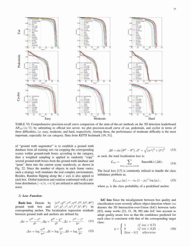
25

Car

0.0 0.2 0.4 0.6 0.8 1.0Recall

0.0

0.2

0.4

0.6

0.8

1.0

Prec

ision

PointPaintingFastPointR-CNNSECONDSTDPoint-GNNF-ConvNet3D-CVFPointPillarsMMFAVOD3DSSDVoxelNetF-PointNetSA-SSDPV-RCNNPartA^2PointRCNN

0.0 0.2 0.4 0.6 0.8 1.0Recall

0.0

0.2

0.4

0.6

0.8

1.0

Prec

ision

PointPaintingFastPointR-CNNSECONDSTDPoint-GNNF-ConvNet3D-CVFPointPillarsMMFAVOD3DSSDVoxelNetF-PointNetSA-SSDPV-RCNNPartA^2PointRCNN

0.0 0.2 0.4 0.6 0.8 1.0Recall

0.0

0.2

0.4

0.6

0.8

1.0

Prec

ision

PointPaintingFastPointR-CNNSECONDSTDPoint-GNNF-ConvNet3D-CVFPointPillarsMMFAVOD3DSSDVoxelNetF-PointNetSA-SSDPV-RCNNPartA^2PointRCNN

Pede

stra

in

0.0 0.2 0.4 0.6 0.8 1.0Recall

0.0

0.2

0.4

0.6

0.8

1.0

Prec

ision

PointPaintingSTDPoint-GNNF-ConvNetPointPillarsAVOD3DSSDF-PointNetPV-RCNNPartA^2PointRCNN

0.0 0.2 0.4 0.6 0.8 1.0Recall

0.0

0.2

0.4

0.6

0.8

1.0

Prec

ision

PointPaintingSTDPoint-GNNF-ConvNetPointPillarsAVOD3DSSDF-PointNetPV-RCNNPartA^2PointRCNN

0.0 0.2 0.4 0.6 0.8 1.0Recall

0.0

0.2

0.4

0.6

0.8

1.0

Prec

ision

PointPaintingSTDPoint-GNNF-ConvNetPointPillarsAVOD3DSSDF-PointNetPV-RCNNPartA^2PointRCNN

Cyc

list

0.0 0.2 0.4 0.6 0.8 1.0Recall

0.0

0.2

0.4

0.6

0.8

1.0

Prec

ision

PointPaintingSTDPoint-GNNF-ConvNetPointPillarsAVOD3DSSDF-PointNetPV-RCNNPartA^2PointRCNN

0.0 0.2 0.4 0.6 0.8 1.0Recall

0.0

0.2

0.4

0.6

0.8

1.0

Prec

ision

PointPaintingSTDPoint-GNNF-ConvNetPointPillarsAVOD3DSSDF-PointNetPV-RCNNPartA^2PointRCNN

0.0 0.2 0.4 0.6 0.8 1.0Recall

0.0

0.2

0.4

0.6

0.8

1.0

Prec

ision

PointPaintingSTDPoint-GNNF-ConvNetPointPillarsAVOD3DSSDF-PointNetPV-RCNNPartA^2PointRCNN

Easy Moderate Hard

TABLE VI: Comprehensive precision-recall curve comparsion of the state-of-the-art methods on the 3D detection leaderboardAP3D (in %) by submitting to official test server. we plot precision-recall curve of car, pedestrain, and cyclist in terms ofthree difficulties, i.e. easy, moderate, and hard, respectively. Among these, the performance of moderate difficulty is the mostimportant, especially for car category. Data from KITTI bechmark [19, 51].

of “ground truth augmentor” is to establish a ground truthdatabase from all training sets via cropping the correspondingscenes within ground-truth boxes according to the category,then a weighted sampling is applied to randomly “copy”several ground-truth boxes from the ground truth database and“paste” them into the current scene seamlessly, as shown inFig. 22. Since the number of objects in each frame varies,such a strategy well simulates the real complex environments.Besides, Random flipping along the x axis is also appied toeach box. Global transition and rotation conformed with a uni-form distribution [−π/4,+π/4] are utilized to add localizationnoise.

2) Loss Function:

Basic loss Denote by (xgt, ygt, zgt, wgt, lgt, hgt, θgt)ground truth box and (xa, ya, za, wa, la, ha, θa) itscorresponding anchor. The localization regression residualsbetween ground truth and anchors are defined by:

∆x =xgt − xa

da, ∆y =

ygt − yada

, ∆z =zgt − zaha

(11)

∆w = logwgt

wa, ∆l = log

lgt

la, ∆h = log

hgt

ha(12)

∆θ = sin(θgt − θa

), da =

√(wa)

2+ (la)

2 (13)

as such, the total localization loss is:

Lloc =∑

b∈(x,y,z,w,l,h,θ)SmoothL1 (∆b). (14)

The focal loss [17] is commonly utilized to handle the classimbalance problem as,

Lfocal (pt) = −αt (1− pt)γ log (pt) , (15)

where pt is the class probability of a predefined anchor.

IoU loss Since the misalignment between box quality andclassification score severely affects object detection where ioudenotes the 3D Intersection-over-Union (IoU) between tasks[83], many works [23, 31, 38, 99] take IoU into account toadopt quality aware loss so that the confidence predicted foreach class is consistent with that of the corresponding targetclass:

q =

1 if iou > 0.750 if iou < 0.252iou− 0.5 otherwise

. (16)

26

Car

0.0 0.2 0.4 0.6 0.8 1.0Recall

0.0

0.2

0.4

0.6

0.8

1.0

Prec

ision

PointPaintingFastPointR-CNNSECONDSTDPoint-GNNF-ConvNet3D-CVFPointPillarsMMFAVOD3DSSDVoxelNetF-PointNetSA-SSDPV-RCNNPartA^2PointRCNN

0.0 0.2 0.4 0.6 0.8 1.0Recall

0.0

0.2

0.4

0.6

0.8

1.0

Prec

ision

PointPaintingFastPointR-CNNSECONDSTDPoint-GNNF-ConvNet3D-CVFPointPillarsMMFAVOD3DSSDVoxelNetF-PointNetSA-SSDPV-RCNNPartA^2PointRCNN

0.0 0.2 0.4 0.6 0.8 1.0Recall

0.0

0.2

0.4

0.6

0.8

1.0

Prec

ision

PointPaintingFastPointR-CNNSECONDSTDPoint-GNNF-ConvNet3D-CVFPointPillarsMMFAVOD3DSSDVoxelNetF-PointNetSA-SSDPV-RCNNPartA^2PointRCNN

Pede

stra

in

0.0 0.2 0.4 0.6 0.8 1.0Recall

0.0

0.2

0.4

0.6

0.8

1.0

Prec

ision

PointPaintingSTDPoint-GNNF-ConvNetPointPillarsAVOD3DSSDF-PointNetPV-RCNNPartA^2PointRCNN

0.0 0.2 0.4 0.6 0.8 1.0Recall

0.0

0.2

0.4

0.6

0.8

1.0

Prec

ision

PointPaintingSTDPoint-GNNF-ConvNetPointPillarsAVOD3DSSDF-PointNetPV-RCNNPartA^2PointRCNN

0.0 0.2 0.4 0.6 0.8 1.0Recall

0.0

0.2

0.4

0.6

0.8

1.0

Prec

ision

PointPaintingSTDPoint-GNNF-ConvNetPointPillarsAVOD3DSSDF-PointNetPV-RCNNPartA^2PointRCNN

Cyc

list

0.0 0.2 0.4 0.6 0.8 1.0Recall

0.0

0.2

0.4

0.6

0.8

1.0

Prec

ision

PointPaintingSTDPoint-GNNF-ConvNetPointPillarsAVOD3DSSDF-PointNetPV-RCNNPartA^2PointRCNN

0.0 0.2 0.4 0.6 0.8 1.0Recall

0.0

0.2

0.4

0.6

0.8

1.0

Prec

ision

PointPaintingSTDPoint-GNNF-ConvNetPointPillarsAVOD3DSSDF-PointNetPV-RCNNPartA^2PointRCNN

0.0 0.2 0.4 0.6 0.8 1.0Recall

0.0

0.2

0.4

0.6

0.8

1.0

Prec

ision

PointPaintingSTDPoint-GNNF-ConvNetPointPillarsAVOD3DSSDF-PointNetPV-RCNNPartA^2PointRCNN

Easy Moderate Hard

TABLE VII: Comprehensive precision-recall curve comparsion of the state-of-the-art methods on the BEV detection leaderboardAPBEV (in %) by submitting to official test server. we plot precision-recall curve of car, pedestrain, and cyclist in terms ofthree difficulties, i.e., easy, moderate, and hard, respectively. Among these, the performance of moderate difficulty is the mostimportant, especially for Car category. Data from KITTI bechmark[19, 51].

ground-truth boxes and their corresponding 3D RoIs:

Liou = − [q log (p) + (1− q) log (1− p)] , (17)

where p is the predicted score, and thus, the total loss issummarized as :

L =1

Npos(βlocLloc + βiouLiou) . (18)

Corner loss Corner loss minimizes the differences betweenthe predicted 8 corners and assigned groundtruth [38, 56],denoted by:

Lcorner =

8∑

k=1

‖Pk −Gk‖. (19)

Bin-based loss As shown in Fig. 23, the region along x-axis and z-axis of each interest point is discretized into a seriesof bins. By transforming the original regression task into binclassification and a small residual regression, the complexity ofdirect regression is dramatically mitigated, especially in termsof the angle regression[22, 29, 30, 46].

Bin-based 3D bounding box generation. As we men-tioned above, a box regression head is also appended for si-multaneously generating bottom-up 3D proposals with theforeground point segmentation. During training, we onlyrequire the box regression head to regress 3D bounding boxlocations from foreground points. Note that although boxesare not regressed from the background points, those pointsalso provide supporting information for generating boxesbecause of the receptive field of the point-cloud network.

A 3D bounding box is represented as (x, y, z, h, w, l, θ)in the LiDAR coordinate system, where (x, y, z) is the ob-ject center location, (h,w, l) is the object size, and θ is theobject orientation from the bird’s view. To constrain thegenerated 3D box proposals, we propose bin-based regres-sion losses for estimating 3D bounding boxes of objects.

For estimating center location of an object, as shown inFig. 3, we split the surrounding area of each foregroundpoint into a series of discrete bins along the X and Z axes.Specifically, we set a search range S for each X and Z axisof the current foreground point, and each 1D search range isdivided into bins of uniform length δ to represent differentobject centers (x, z) on the X-Z plane. We observe that us-ing bin-based classification with cross-entropy loss for theX and Z axes instead of direct regression with smooth L1loss results in more accurate and robust center localization.

The localization loss for the X or Z axis consists of twoterms, one term for bin classification along each X and Zaxis, and the other term for residual regression within theclassified bin. For the center location y along the vertical Yaxis, we directly utilize smooth L1 loss for the regressionsince most objects’ y values are within a very small range.Using the L1 loss is enough for obtaining accurate y values.

The localization targets could therefore be formulated as

bin(p)x =

⌊xp − x(p) + S

δ

⌋, bin(p)

z =

⌊zp − z(p) + S

δ

⌋,

res(p)u

u∈{x,z}=

1

C

(up − u(p) + S −

(bin(p)

u · δ +δ

2

)), (2)

res(p)y = yp − y(p)

where (x(p), y(p), z(p)) is the coordinates of a foregroundpoint of interest, (xp, yp, zp) is the center coordinates of itscorresponding object , bin(p)

x and bin(p)z are ground-truth bin

assignments along X and Z axis, res(p)x and res(p)

z are theground-truth residual for further location refinement withinthe assigned bin, and C is the bin length for normalization.

The targets of orientation θ and size (h,w, l) estimationare similar to those in [25]. We divide the orientation 2π

into n bins, and calculate the bin classification target bin(p)θ

and residual regression target res(p)θ in the same way as x or

z prediction. The object size (h,w, l) is directly regressedby calculating residual (res(p)

h , res(p)w , res(p)

l ) w.r.t. the aver-age object size of each class in the entire training set.

Figure 3. Illustration of bin-based localization. The surroundingarea along X and Z axes of each foreground point is split into aseries of bins to locate the object center.

In the inference stage, for the bin-based predicted param-eters, x, z, θ, we first choose the bin center with the high-est predicted confidence and add the predicted residual toobtain the refined parameters. For other directly regressedparameters, including y, h, w, and l, we add the predictedresidual to their initial values.

The overall 3D bounding box regression loss Lreg withdifferent loss terms for training could then be formulated as

L(p)bin =

∑

u∈{x,z,θ}(Fcls(bin

(p)

u , bin(p)u ) + Freg(res(p)

u , res(p)u )),

L(p)res =

∑

v∈{y,h,w,l}Freg(res(p)

v , res(p)v ), (3)

Lreg =1

Npos

∑

p∈pos

(L(p)

bin + L(p)res

)

where Npos is the number of foreground points, bin(p)

u andres(p)

u are the predicted bin assignments and residuals of theforeground point p, bin(p)

u and res(p)u are the ground-truth

targets calculated as above, Fcls denotes the cross-entropyclassification loss, and Freg denotes the smooth L1 loss.

To remove the redundant proposals, we conduct non-maximum suppression (NMS) based on the oriented IoUfrom bird’s view to generate a small number of high-qualityproposals. For training, we use 0.85 as the bird’s view IoUthreshold and after NMS we keep top 300 proposals fortraining the stage-2 sub-network. For inference, we use ori-ented NMS with IoU threshold 0.8, and only top 100 pro-posals are kept for the refinement of stage-2 sub-network.

3.2. Point cloud region poolingAfter obtaining 3D bounding box proposals, we aim at

refining the box locations and orientations based on the pre-viously generated box proposals. To learn more specific lo-cal features of each proposal, we propose to pool 3D pointsand their corresponding point features from stage-1 accord-ing to the location of each 3D proposal.

For each 3D box proposal, bi = (xi, yi, zi, hi, wi,li, θi), we slightly enlarge it to create a new 3D box

4

Fig. 23: Illustration of bin-based localization. The originalregression problem is simply transformed into a series ofdiscrete bin classification and residual regression. Image fromShi et al. [98]