Real option analysis in a replicating portfolioperspective

Wouter van Heeswijk�, Reinoud Joosteny, Kuno Huismanz

& Christian Bosx

December 10, 2013

Abstract

In the last decades, a vast body of literature has arisen on realoption analysis (ROA). The use of di¤erent approaches and the oftenimplicit adoption of major assumptions may cause confusion on whatROA precisely entails, or in which situations it may be applied.We assess the �eld of real option analysis by explicitly linking ROA

to the basic principles of option pricing theory and the replicatingportfolio concept. From this perspective, we explain how real optionsadjust to the varying risk pro�les of a project, a feature not available inother valuation methods. We also clarify how non-market risks can bedealt with in ROA. We show that a combination of option pricing anddecision tree analysis enables us to treat a broad range of investmentproblems, in a manner that is consistent with pricing theory.Keywords: Real option analysis, private risk, risk-neutral valuation,replicating portfolio.

1 Introduction

Black & Scholes [1973] introduced an option pricing model allowing mar-ket participants to value �nancial options by applying risk-neutral valuationunder a set of restrictive assumptions. This model and subsequent workhad a large impact on �nancial markets; traders started to rely more onmathematical valuation and the implications of market prices. Not long af-ter the introduction of the Black-Scholes model, Myers [1977] recognized itspotential to describe real-world investment opportunities under uncertainty

�IEBIS, School of Management & Governance, University of Twente.yContact: IEBIS, School of Management & Governance, University of Twente.

Email: r.a.m.g.joosten@utwente.nl.zCentER, Department of Econometrics and Operations Research, Tilburg University

and ASML Netherlands B.V.xPetroleum Geosciences, TNO Utrecht

1

as well. By considering the value of a project as the underlying asset, therequired investment as the strike price, and the opportunity to defer a deci-sion as the right to invest, one could apply option pricing techniques to realinvestment opportunities. This approach was baptized �real�option pricingas it applied option theory to real-world projects instead of �nancial assets.

As authors from di¤erent research areas rallied to develop real optionanalysis (ROA) further, a vast body of literature exists by now, containingmany variants as well as theoretical assessments (see e.g., Dixit & Pindyck[1994], Trigeorgis [1996], Copeland & Antikarov [2001]). However, ROA isstill waiting for a major breakthrough in corporate decision making. Webelieve one of the reasons for this may be that there is little consensus onwhat ROA stands for precisely, making it unclear to a practitioner whichversion should be applied to an investment problem at hand.

The state of the �eld is that many di¤erent approaches to ROA coex-ist, often without the underlying assumptions and their implications beingpointed out explicitly. Decision makers may sense that the assumptions re-quired for �nancial option valuation are too rigid to apply in the real world,and do not see their concerns addressed in literature (Smith & McCardle[1999]). Also they may not understand in what aspects ROA could yield animprovement over the advanced decision tools they are using already.

When practitioners try to apply ROA on an investment problem usinga standard option valuation model, e.g., Black-Scholes, vital assumptionsare rarely satis�ed for real-world projects. Most importantly, option the-ory presumes that all risks are liquidly traded on the �nancial market, andcan therefore be hedged, which does not hold for most projects. In general,investment problems are much too complex to be modeled as a standardoption, hence the option model must be tailor-made, with standard as-sumptions no longer applicable. So, application of ROA requires a set ofassumptions not as restrictive as for �nancial options, while retaining themerits of structuring investment problems as real options.

To contribute to solving these impediments for practitioners, we �rst aimto provide a better insight in what ROA stands for, under which assumptionsit can be applied, and how it solves inconsistencies existing in other decisiontools. To do this, we return to the basics of option pricing theory, namely theconcepts of risk-neutral valuation and replicating portfolios. From this per-spective, we compare ROA with the net present valuation (NPV) techniquesdominating state-of-the-art practice. NPV techniques have a fundamentaltheoretical �aw by assuming a constant risk pro�le for projects incorporatingmanagerial �exibility, and we show that ROA solves this shortcoming.

Next, we point out which approaches can be used for ROA, and whattheir implications are, based on Borison [2005]. We limit our assessment ofdi¤erences between these methods to the treatment of non-tradable (�pri-vate�) risk, and expand on the ROA approach of Smith & Nau [1995] to valueprojects comprising both market and private risk consistent with theory.

2

1.1 More on real option analysis

Real option analysis is a methodology to value real-world projects by mod-eling decisions in an option pricing framework. Its application is based onthe theory used to value options on �nancial assets (Luenberger [1998]). In�nance, a standard option is the right, but not the obligation, to buy (calloption) or sell (put option) an asset at a prede�ned price, called a strike(price). This allows the holder of the option to defer the investment deci-sion up to a certain date, waiting for new market information (i.e., the assetprice) to arrive. A rational holder of an option will only exercise the optionif the asset price exceeds the prede�ned strike price at the decision point.

If the option is not exercised before maturity, the investor loses the cost ofthe option itself. The so-called �classic�ROA uses an approach highly similarto that of �nancial options. When the underlying risk of a project behavesas if it is traded, we can apply option pricing theory on real investmentdecisions. Two conditions required to apply option theory are that theuncertainty associated with the project is market risk (the value-in�uencingfactors are liquidly traded) and that the decision maker has the managerial�exibility to make investment decisions based on new information. In theview we deploy here, pure option theory should only be applied to the partof a project�s risk that is actually traded on the market.

We now illustrate the analogy between �nancial options and real optionsby the Black-Scholes option pricing model, which is an application of risk-neutral pricing under strict assumptions (Black & Scholes [1973]). Merton[1998] warned against the application of option theory to real world prob-lems. He stressed to consider the limitations of the model, and keep in mindwhat purpose it serves. The main limitations and assumptions of classicreal option pricing will be assessed in detail in the remainder, along withalternatives that are less restrictive.

The Black-Scholes formula can be used to obtain the value of a Euro-pean option, i.e., one that can be exercised only at maturity. The majorassumptions for the Black-Scholes model and the resulting formula, are thefollowing.

� No arbitrage opportunities exist.

� Cash can be borrowed and lent at a constant risk-free interest rate.

� Buying and short-selling of the underlying asset is unrestricted.

� No transaction costs exist.

� The underlying asset�s price follows a lognormal distribution.

� The underlying asset does not pay dividends.

3

Under these assumptions we can create a hedged position, so that thevalue of the portfolio does not depend on the price of the underlying asset.We do this by constructing a portfolio consisting of the option, the underly-ing and cash (including negative amounts due to short-selling), so that pricechanges of the asset are o¤set by the other instruments. It is then possibleto apply risk-neutral valuation.

Translated to real options, a call option is the possibility to undertakea project; a put option is the possibility to abandon it, or rather to abstainfrom it. In real options, the term �asset�should be viewed in a broad sense.It is the value of the project, should it be taken up. We present modi�cationsof the original Black-Scholes formula for the value of call and put options attime t, including the e¤ect of continuous dividend payments as well, as theyform an integral part of many options. The formulas are the following:

call = Ste��(T�t)N(d1)�Xe�rf (T�t)N(d2);

put = Xe�rf (T�t)N(�d2)� Ste��(T�t)N(�d1); with

� N(�) : the CDF of a standard-normal distribution,

� d1 =ln�StX

�+(rf��+0:5�2)(T�t)

�pT�t , d2 =

ln�StX

�+(rf���0:5�2)(T�t)

�pT�t :

The meanings of the other symbols in terms of �nancial and real options areprovided in Table 1 (Leslie & Michaels [1997]).

Symbol Financial options Real options

X Strike price Present value (PV) of required expen-ditures to exercise the option

St Stock price PV of expected net cash �ows at t� Volatility of St Volatility of Stt Current period Current periodT Time to expiry Time that decision is deferredrf Risk-free interest rate Risk-free interest rate� Fixed cash dividends Costs to preserve the option

Table 1: Symbols of the Black-Scholes model in �nancial and real options.

Nielsen [1993] provides a detailed explanation of the logic behind theBlack-Scholes model. We restrict ourselves to a brief rationale for the calloption; the one for put options is comparable. For the call option, N(d2)is the risk-adjusted probability that the option will be exercised, such thatthe strike price must be paid. N(d1) can be viewed as the factor by whichthe expected payo¤ exceeds the current stock price. As exercise occurs atmaturity, payo¤ and strike price are discounted for dividends and interestrespectively. The di¤erence between both terms is the option�s value.

4

In real options St represents the present value at time t of the expectednet cash �ows, should the option be exercised. The strike price X describesthe present value of the expenditures required to exercise the option (Carls-son & Fullér [2003]). These costs are only incurred if the option is actuallyexercised, such as the costs to acquire an asset (call option) or to abandona project (put option).

The volatility � is de�ned as the square root of the variance of theproject returns based on the free cash �ows. Returns are assumed to followa Geometric Brownian Motion (i.e., normally distributed and unrelated overtime, standard deviation remains constant). The option value increases withvolatility, as an option holder pro�ts from favorable movements of the valueof the underlying, while downside risk is limited to losing the option value.

In line with option pricing theory, cash �ows in ROA are discountedusing the risk-free interest rate rf . Finally, for real options, �dividends�� represent the costs to preserve the option, or the money draining awayduring the lifetime of the option (Leslie & Michaels [1997]).

Clearly, the rigid structure of the Black-Scholes model does not suitmany real-world investment problems well. We discuss common points ofcritique on the assumptions posed, and explain how these may be overcomeby adopting a less restrictive approach. In the �nal section of this paper wediscuss potential discrepancies between ROA valuation and practice.

A simple European call- or put option can be exercised at the maturitydate only, generally making these options un�t to capture the �exibilities em-bedded in a project. The project might comprise exercise and abandonmentdecisions at di¤erent time points, multiple investment opportunities, strikeprices variable over time, time-varying volatility, etc. (Trigeorgis [1993a],Mun [2002]). Consequently, often no analytical solutions can be found. In-stead, numerical approaches such as a binomial tree or simulation should beapplied (Cortazar [2000], Wood [2007], Fuji et al. [2011]). These methodsapproximate the option value by dividing its partial di¤erentials in manysteps, and allow much more �exibility than analytical methods to valuecomplex options. Therefore, even strong deviations from standard optionmodels need not be considered an obstacle when applying ROA.

The risk-free rate rf is the (theoretical) return required when an invest-ment has no possibility of default, providing a compensation for the time theinvested capital is tied up only. We treat the subject of discounting in detailin Section 3. We apply risk-neutral probabilities to calculate the expectedrisk-neutral cash �ows before discounting them. However, as follows fromthe assumptions, a hedged position can only be formed for assets which areliquidly traded on the market. Private risk cannot be hedged and as suchshould not be discounted by rf ; the exposure to riskiness calls for a higherdiscount rate. We address this signi�cant problem in Section 4, and describea hybrid between option valuation and decision tree analysis applicable toboth market and private risks in a manner consistent with theory. In Section

5

5, we discuss the practical implementation of risk-neutral pricing, makinguse of futures�contracts to estimate risk-neutral drifts.

Examples of dividends in ROA are payments to preserve productionrights and money lost through competition. In practice, it might be di¢ cultto forecast and estimate the leakage of cash over the length of the option.Also, losses are generally not constant over time (Trigeorgis [1996]). Somereal option practitioners therefore act as if no dividend payments exist, thatis, � = 0 (Davis [1998]). However, for liquidly traded risks it is possible toestimate dividends based on information embedded in futures prices, as weshow in Section 6. Furthermore, it should be noted that �exible valuationtechniques such as simulation are very well capable of incorporating evencomplex dividend patterns.

A �nal di¤erence between �nancial options and real options we wish topoint out is that competitors may have a signi�cant impact on the value of areal option. As opposed to �nancial options, strategic decision-making (e.g.,acting as a leader or a follower) could therefore in�uence the value of realoptions as well. Chevalier-Roignant & Trigeorgis [2011], Grenadier [2000],and Huisman [2001] describe how real option analysis and game theory canbe combined to address such problems. We do not further treat this subjectin this paper, but one should be aware of the in�uence of strategic decision-making in project valuation.

For the remainder of the paper we take a broad view on ROA, in line withauthors such as Dixit & Pindyck [1994] and Dias [2012a]. We do not considerROA as a pricing technique such as the Black-Scholes model, but rather as amethodology based on risk-neutral valuation. We support the view of Smith& Nau [1995], who modify the concept of risk-neutral valuation to make itapplicable to projects containing both market and private risk. We expandon this approach later.

2 Comparing ROA and discount-based approaches

The most commonly used valuation methods are based on discounted cash�ow (DCF) principles (Drury [2008]). Using such methods, the expectedcash �ows during the lifetime of the project are estimated and subsequentlydiscounted over time. The discount rate applied should incorporate both thetime value of money and compensation for uncertainty of future cash �ows(Robichek & Myers [1966]). This rate has a profound impact on the NPV ofa long-term project. In this section we address the theoretical backgroundof discount rates and point out the theoretical �aw in DCF methods andits implications for risk adjustment. In the next section, we show how risk-neutral valuation as used in ROA resolves these issues.

It is nearly impossible to obtain a discount rate able to re�ect accuratelyall the risks a project is subject to (Mun [2002]). To mention some, a

6

project�s value may be in�uenced by in�ation, the size of the company,credit risk, country risk, shareholder decisions, etc. Many random eventscan occur during the lifetime of a project, making it very hard to derive aproper discount rate analytically. Therefore, we generally resort to discountrates which try to capture how the capital providers perceive the risk theyare subject to when investing in the project.

In practice, the most commonly used discount rate is the Weighted Aver-age Cost of Capital (WACC). This is the average cost of capital for the com-pany or the project. In its basic form the WACC assumes that a company isfunded with one source of equity and one source of debt, both demanding asingle constant return. In reality, companies may raise money from multiplesources requiring di¤erent expected returns (e.g., preferred stocks, warrants,etc.); more expansive versions of the WACC could then be applied. Interestcosts are deducted from corporate pro�ts, hence the inclusion of corporatetax in the equation. This boils down the following formula:

WACC =

�E

E +D

�� re +

�D

E +D

�� rd � (1� C) with

� E;D : the market value of equity respectively debt,

� re; rd : the cost of equity respectively debt,

� C : the corporate tax rate.

We advocate to calculate the WACC for the project itself, regardless ofthe way it is funded. First, suppose that a project is funded separately, andalso pays o¤ as a standalone project. The project must at least earn itsWACC to satisfy owners, stock holders and creditors. If the project failsto do so, by assumption rational investors would not be willing to investin it. Hence, a project discounted at the WACC should at least have anNPV of 0 in order to be attractive to capital providers. The project mayhave a di¤erent risk pro�le than the company as a whole, meaning thatinvestors would require a di¤erent return than the WACC of the company(Mun [2002], Smith [2005]). Alternatively, a project might not be fundedseparately, but instead have a budget allocated from the company�s means.If this is the case, the project will alter the overall risk pro�le of the company,because it changes the investment portfolio.1 By estimating the correlationof the project with market risk, the discount rate can be adjusted better toa speci�c project (Constantinides [1978], Magni [2007]). Hence, regardlessof the manner of funding, using a discount rate based on the project itselfyields more accurate and insightful results.

1Recalculating the �rm�s � and WACC is rather straightforward and will not yield largedi¤erences provided the project�s requirements in assets is small relative to the �rm�s.

7

To calculate the cost of equity, models such as the Capital Asset PricingModel (CAPM) may be applied. The CAPM states that the expected returnof an asset is equal to the risk-free rate plus a market risk premium dependingon the relationship between the volatility of the asset�s return and that of themarket return (Sharpe [1964], Merton [1973b]). The underlying reasoningof the model is that investors only care about the systemic risk (related tothe movements of the market as a whole) of the asset, as all other risks canbe diversi�ed away. Diversi�cation means that private risks are o¤set byholding many uncorrelated assets in a portfolio. The expected return underthe CAPM is denoted as

E (re) = rf + � (E (rm)� rf ) with

� rm; rf : the market return respectively the risk-free interest rate,

� � = cov(re;rm)var(rm)

; the ratio of the covariance of the asset return andmarket return, and the variance of the market return.

So, � can be viewed as capturing the volatility of the asset relative to thevolatility of the market. In other words, it is a measure for part of the asset�sriskiness that cannot be removed through diversi�cation. The risk premiumfor the asset is given by the term � (E (rm)� rf ). It follows that an appro-priate discount rate for a project depends on the market return, the risk-freerate, and the beta of the project (Ang & Liu [2004]). Though treated asconstants, these factors are all variable over time in reality, implying thatthe discount rate should be time-varying as well. The use of a constantdiscount rate might be rationalized to some extent by assuming that theportfolio investment opportunity and the systemic risk exposure (i.e., �)remain constant over time (Merton [1973b], Fama & Schwert [1997]).

By incorporating stochastic forecasting models on the aforementionedfactors, we could obtain a more realistic re (Geltner & Mei [1995], Schul-merich [2010]). Generally, the theoretical parameters rf and rm are esti-mated with bond yields and market indices. The bond should approximatean investment which never defaults, with the same maturity and in the samecurrency as the investment to exclude currency risk. The market index cho-sen should represent the portfolio of the investment as well as possible; yetit should be kept in mind that this portfolio should be well-diversi�ed toapply the CAPM.

To �nish our assessment of the discount rate, it is essential to note thatthe risk premium is calculated for the asset (by analogy, the project value);the opportunity to invest in the project (i.e., the option) is subject to adi¤erent risk pro�le, varying with the decisions made. So, the discount ratefor a project with embedded �exibilities should be adjusted accordingly.ROA applies risk-neutral valuation instead; by already accounting for riskwhen estimating the cash �ows, rf can always be used as the discount rate.

8

We brie�y discuss two discount-based methods, Net Present Value (NPV)analysis and Decision Tree Analysis (DTA). Traditional DCF analysis as-sumes that future cash �ows are deterministic, as soon as the investmentdecision is made. To re�ect both the time value and the riskiness of theproject, a constant discount rate is applied to future cash �ows. This re-sults in the Net Present Value (NPV), the net worth of the project at timeof initial investment. Usually the WACC of the �rm is used as the discountrate, and sum of discounted cash �ows is the NPV of the project. A positiveNPV may be interpreted as a signal to accept the project.

Similar to ROA, Decision Tree Analysis (DTA) incorporates uncertain-ties and intermediate decision-making in valuation. The nodes are connectedin a graph, which paths indicate the change of the project value over time. Adistinction is made between decision nodes and uncertainty nodes. Projectoptions are de�ned as decision nodes to allow managerial �exibility, whileuncertainty nodes re�ect chance events with certain probabilities assigned.So, decisions may depend on the outcome of chance events. Similar to DCF,future cash �ows are discounted by a single discount rate, so DTA can beseen as an enhanced version of DCF (Piesse et al. [2004]). Instead of evalu-ating a single aggregated scenario, each path is viewed as a possible scenario.As stated before, the discount rate re�ects both time value and riskiness.

Traditional DCF assumes that decisions are irreversible, with new infor-mation getting available at a later time not altering the cash �ows or inter-mediate decisions made. This is often not realistic, as management has theopportunity to reallocate capital based on the performance and prospects ofthe project. Active risk management may allow both increasing upside po-tential and limiting downside potential, leading to a higher expected projectvalue. These e¤ects are ignored in traditional DCF (Prasanna Venkatesan[2005]), making this method un�t for projects with embedded �exibilities.

Real options address several aspects ignored in DCF (Triantis & Borison[2001], Van de Putte [2005]). A real option values �exibility as it includesthe possibility to alter the course of the project at the decision points inorder to maximize pro�t or minimize losses given the information availableat that time (Copeland & Keenan [1988], Mun [2002], Brandão et al. [2005]).

Compared to ROA, DTA falls short when it comes to risk-adjustment.In a decision tree, chance events and decisions are represented by nodes. A�aw in the DTA approach is that the decisions made over time alter therisk pro�le of the project, which con�icts with the application of a singlerisk-adjusted discount rate used to calculate the present value (Brandão etal. [2005]). Investors expect compensation in line with the degree of riskthey are exposed to; if the company decides to change course, this willa¤ect expectations. In ROA, this adjustment takes place via risk-neutralvaluation, such that an opportunity is valued in line with its risk pro�le.We clarify this adjustment in the next sections, hence the present examplewill be continued there for the ROA part.

9

Example 1 We now illustrate the valuation techniques of NPV and DTA.Say that we have the right to exploit an oil �eld of unknown size, i.e., itmay be �small� (10m barrels), �medium�(20m barrels) or �large� (40m bar-rels). The associated probabilities are 1

2 ;14 and

14 , respectively. At the costs

of 50 million dollar (m$), this �eld may be explored to determine how muchoil is present in year 0. If the �eld is to be exploited, an investment of 800m$ in year 1 (regardless of �eld size) is necessary. All cash �ows are, forthe sake of simplicity, assumed to be end of the year cash �ows.In addition, future oil prices are unknown; with probabilities 1

2 prices maybe �low�(80$ per barrel) or �high�(120$ per barrel) during exploitation. De-pending on technological advance, a new technology may be available at thestart of the project to reduce extraction costs. The variable extraction costsmay be 60$ or 40$ per barrel with a probability of 80% respectively 20%. The�eld is to be exploited in three years; 20% in year 1, 50% in year 2, and 30%in year 3. Finally, the WACC is 10%.

E

NEE

NEE

NEE

NEE

NEE

NEE

NEE

NEE

NEE

NEE

NEENE

Medium

Large

Small

High

Low

High

Low

High

Low

New

Old

New

Old

New

Old

New

Old

New

Old

New

Old

Figure 1: Structure of the investment scenario for DTA. Dark squares indi-cate chance events, light squares indicate decision moments, the open circlesindicate outcomes. The discounted pro�ts depend on the �eld size (Large,Medium, Small), the price of oil (High, Low), the technology (New, Old)and the decision whether to exploit (E) the �eld or not (NE).

With traditional net present valuation, we take the expected values for the�eld size (20m barrels), oil price (100$ per barrel) and variable costs (56$ perbarrel). In the subsequent three years, we then get expected annual cash �owsof 4�44�800 = �624 m$; 10�44 = 440 m$ and 6�44 = 264 m$. Hence, these

10

cash �ows result (WACC = 0:1) in an NPV of �6241:1 +4401:12

+ 2641:13

= �5:289 3m$. Based on this criterion the project should not be taken up.Next, we apply DTA to the same investment problem; see Figure 1 for thecorresponding decision tree, where a crucial assumption is that the decisionto test has already been taken in advance and was positive.2 For DTA, wenow calculate the NPV for each branch in the tree, and optimize our deci-sion for each branch. The actual numbers and calculations may be found inthe Appendix. Thus, it is possible to determine the discounted project valuewhen accounting for the option to cancel the project after exploration. In ourexample, the value of the project under DTA and the testing-�rst assump-tion increases to approximately 177 m$. This signi�cant improvement of thevalue found under DTA and NPV stems from the added value of �exibility.Under DTA the project would stand a good chance of being taken up.

3 Risk-neutral valuation

An essential concept in option pricing is risk-neutral valuation to obtain thevalue of derivatives (Appeddu et al. [2012]). Recall that the Black-Scholesmodel is an application of risk-neutral valuation under strict assumptions.We focus on the main principles of risk-neutral valuation, providing an intu-itive insight why it is used. For the mathematical properties of risk-neutralvaluation, we refer to Luenberger [1998] or Bingham & Kiesel [2004].

To calculate the present value of an asset, one could take the expectedreturn of an asset, and then discount it based on the preferences of the in-vestor. However, it is di¢ cult to estimate the future growth rate of an asset�svalue. Risk-neutral valuation provides a methodology which does not requireestimating this rate (Miller & Park [2002]). The application of risk-neutralvaluation requires two major assumptions. First, the market must be com-plete, meaning that every good can be exchanged by any participant in themarket without transaction costs (Merton [1973a], Constantinides [1978]).Every agent has perfect market information, so no trader has an advantagethrough knowledge. Also short-selling and borrowing are unrestricted andcan be done at the risk-free rate. Second, arbitrage opportunities are absent;there are no imbalances in the market which allow for the possibility of arisk-free pro�t at zero cost. When these assumptions hold, a derivative canbe replicated by holding a linearly weighted combination of �nancial instru-ments (Gisiger [2010]). As arbitrage opportunities cannot exist, this linearcombination must have the exact same value as the derivative. If this werenot the case, an investor could buy the cheaper of the two and sell the more

2DTA would be analogous but considerably more involved as now also an optimaltiming issue arises for when to do the test, or whether to do the test at all. Without goinginto much detail, we found that such an analyis yields a value of 198 m$, a considerableimprovement over the number found under the asumption of testing in advance.

11

expensive one, thus making a risk-free pro�t without a cost (Tilley [1992]).Risk-neutral valuation provides the unique arbitrage-free price of the deriv-ative based on this principle. It does so by using the arti�cial concept ofrisk-neutral probabilities.

We provide an example based on Gisiger [2010] to explain this concept.Suppose that the economy can be in one of n states at time t, with a speci�cstate denoted as j 2 I = f1; :::; ng. For every state a unique so-calledArrow security is available, which pays o¤ a positive amount xj to theholder of the security when the asset reaches state j and zero otherwise.The real probability that the asset state will shift from an arbitrary state ito state j is denoted by pij , with

Pj2I pij = 1. We do not assume interest

yet. Each security has a price representing the value the market places onthis state. This means that the state price needs not to be equal to itsrationally expected payo¤ pij � xj ; the market incorporates risk preferences.A security paying o¤ in a certain state could be perceived as a more valuableaddition to one�s portfolio (for example because it pays o¤ in a decliningmarket), therefore being priced higher than its rationally expected payo¤.The discrete payo¤ structure described here is illustrated in Figure 2.

Asset statetime t

Transitionprobability

Asset statetime t+1

Security payoff

State i

 State 2

State n­1

State n

pi,1

pi,1

pi,2 p

i,j

pi,n­1

pi,n

x1

x2

xj

xn­1

xn

State 1

State j

time t+1

Figure 2: Example of a discrete payo¤ structure in an economy with n Arrowsecurities (based on Gisiger [2010]).

Now we introduce a derivative, which returns the payo¤ of the securitymatching state j. This derivative can be considered as a portfolio of allArrow securities, priced by using risk-neutral valuation, denoting its valueas �i. Contrary to what its name may indicate, risk-neutral valuation doesnot assume investors to be indi¤erent to risk. Risk-neutral probabilities canbe viewed as the sum of state prices (i.e., incorporating risk preferences)compounded to 1; denote these probabilities by aij : Multiplying each risk-neutral probability with the corresponding payo¤ x in state j provides the

12

value of the derivative. Note that the real probabilities pij are not requiredfor this, as their information is incorporated in the security prices. Forexample, a security yielding a high payo¤ with large probabilities will mostlikely have a high price as well, though such a relation need not be linear.

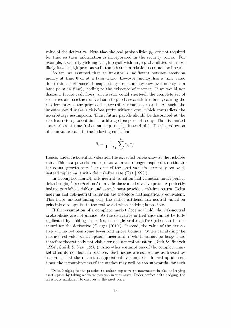
So far, we assumed that an investor is indi¤erent between receivingmoney at time 0 or at a later time. However, money has a time valuedue to time preference of people (they prefer money now over money at alater point in time), leading to the existence of interest. If we would notdiscount future cash �ows, an investor could short-sell the complete set ofsecurities and use the received sum to purchase a risk-free bond, earning therisk-free rate as the price of the securities remain constant. As such, theinvestor could make a risk-free pro�t without cost, which contradicts theno-arbitrage assumption. Thus, future payo¤s should be discounted at therisk-free rate rf to obtain the arbitrage-free price of today. The discountedstate prices at time 0 then sum up to 1

1+rfinstead of 1. The introduction

of time value leads to the following equation:

�i =1

1 + rf

nXj=1

aijxj :

Hence, under risk-neutral valuation the expected prices grow at the risk-freerate. This is a powerful concept, as we are no longer required to estimatethe actual growth rate. The drift of the asset value is e¤ectively removed,instead replacing it with the risk-free rate (Kat [1998]).

In a complete market, risk-neutral valuation and valuation under perfectdelta hedging3 (see Section 5) provide the same derivative price. A perfectlyhedged portfolio is riskless and as such must provide a risk-free return. Deltahedging and risk-neutral valuation are therefore mathematically equivalent.This helps understanding why the rather arti�cial risk-neutral valuationprinciple also applies to the real world when hedging is possible.

If the assumption of a complete market does not hold, the risk-neutralprobabilities are not unique. As the derivative in that case cannot be fullyreplicated by holding securities, no single arbitrage-free price can be ob-tained for the derivative (Gisiger [2010]). Instead, the value of the deriva-tive will lie between some lower and upper bounds. When calculating therisk-neutral value of an option, uncertainties which cannot be hedged aretherefore theoretically not viable for risk-neutral valuation (Dixit & Pindyck[1994], Smith & Nau [1995]). Also other assumptions of the complete mar-ket often do not hold in practice. Such issues are sometimes addressed byassuming that the market is approximately complete. In real option set-tings, the incompleteness of the market may well be too substantial for such

3Delta hedging is the practice to reduce exposure to movements in the underlyingasset�s price by taking a reverse position in that asset. Under perfect delta hedging, theinvestor is indi¤erent to changes in the asset price.

13

an assumption to hold. Though some authors provide rationales to applyoption pricing on an incomplete market, it is theoretically more correct toapply risk-neutral valuation only on risks traded on the market. Section 5goes in more detail about handling non-hedgeable risks.

Though the assumptions of risk-neutral valuation may sound strong,they are no more restrictive than those adopted for discount-based ap-proaches. In fact, the assumptions for the CAPM and risk-neutral valu-ation are the same (Birge & Zhang [1998], Cudica [2012]). Thus, acceptingDCF methods based on CAPM principles means that the assumptions forrisk-neutral valuation should be accepted as well. Next, we show how thepossibility to hedge risk allows using risk-neutral valuation in practice.

4 Replicating portfolio concept in ROA

Risk-neutral pricing presumes that a perfect hedge can be constructed forthe portfolio held. If this assumption holds, it is possible to construct areplicating portfolio for the project. In that case, holding a portfolio con-sisting of �nancial instruments should provide the exact same payo¤ as theproject itself at all times and in all states. We can then also construct aperfect hedging portfolio by mirroring the replicating portfolio (short-sellingmay be required for this), allowing to apply risk-neutral valuation.

To retain the equivalence between the real project and the replicat-ing portfolio, (continuous) adjustment of the portfolio might be required.We can do this under the assumption that no transaction costs exist in acomplete market (Tilley [1992]). In reality, transaction costs are of coursepresent in trading. Therefore, some argue that the rigid complete market as-sumption signi�cantly a¤ects the validity of the theory (e.g., Mayshar [1981],Haug & Taleb [2011]). Constantinides [1986] justi�es the assumption of notransaction costs by stating that the existence of transaction costs does notsigni�cantly alter the asset proportions held compared to the theoreticalproportions. At the very least, we should keep in mind that we assume theabsence of transaction costs when applying option pricing (Merton [1987]).

Another deviation from the complete market observed in practice isthe presence of arbitrage opportunities arising from market imperfections.Such opportunities tend to be quickly corrected by the market itself (Tham[2001]), this phenomenon in fact justi�es the assumption that a single correctmarket price exists.

In reality a complete replicating portfolio is rarely found for a project,as only part of the factors in�uencing its value is traded on the market. Onecan distinguish market risk and private risk. Market risk can be replicatedby �nancial instruments; it is assumed that individual companies have noin�uence on it. Market information is revealed over time, thereby solvinguncertainty. An example of such risk is the one caused by changing com-

14

modity prices. It can be hedged by taking a position in these assets.Private risk comprises all sources of uncertainty that cannot be replicated

by �nancial instruments (Amram & Kulatilaka [2002], Piesse et al. [2004]).Merton [1998] provides a formal de�nition of private risk, stating that privaterisk can be measured as the tracking error of the portfolio representing theunderlying asset. Mathematically the tracking error can be de�ned by dSt

St�

dPtPtwhere St is the project value (the underlying) and Pt is the value of the

tracking portfolio, both at time t. As such, the di¤erence between the valueof the replicating portfolio and the value of the underlying asset is consideredprivate risk. Borison [2005] distinguishes �ve real option approaches, whichdi¤er regarding their perspective on dealing with both types of risk. Wefocus only on their theoretical fundaments, ignoring di¤erences such as thetechniques applied. In our view the integrated approach is the most correctapplication of ROA, and is preferable over the other methods.

Classic ROA is based on the assumption that the project can be repli-cated by a portfolio of market-driven instruments that is exactly equivalent(Brennan & Schwartz [1985], Amram & Kulatilaka [1999]). As stated before,such projects rarely exist. Two rationales are used to justify incorporatinga certain degree of private risk in classic ROA. It may be presumed that pri-vate risk is only minor after the option has been exercised, and will not havea great impact on the payo¤ (i.e., the market is approximately complete).The tracking error then increases with the amount of private risk. The al-ternative rationale is to include such uncertainties in the valuation process,but assume that they can be hedged as well. It might be possible to diversifyaway private risk by trading it with comparable risks, even though these arenot liquidly traded on the market (Mattar & Cheah [2006]).

We argue that these rationales fall short for projects containing a sig-ni�cant amount of private risk, and do not recommend using the classicapproach in these cases. In an attempt to solve this shortcoming, the re-vised classic approach proposes to use decision tree analysis when privaterisk is dominating and option pricing when market risk is dominating. Thisapproach provides only a crude approximation to the project value, and isunable to solve the described theoretical issues.

Some assume that a replicating portfolio can also be derived by subjec-tively estimating the market value of the project (e.g., Copeland & Antikarov[2001], Amram & Kulatilaka [2002], Brealey et al. [2008]). They justify thesubjectively derived asset value by adopting a shareholder view. Their val-uation assesses how much a project contributes to the value of the �rm,thereby considering the project itself as if it were a traded asset (Borison[2005]). They value the project with traditional DCF (hence without incor-porating �exibility) to obtain a subjective estimate of the market value ofthe project. Some authors deem this value to be the best unbiased estimate,coining the assumption Market Asset Disclaimer or MAD. Although the un-

15

derlying of a real option is generally not liquidly traded, one may chooseto treat it as if it were a �nancial asset. The rationale is that we seek thearbitrage-free value of the project, as this is comparable to the added valueof the project to the market value of the company (Benaroch & Kaufmann[1999]). Wrongly valuing the project would eventually result in arbitrageopportunities which are corrected by the market.

Although the subjective approaches4 are not as restrictive as the classicone, market completeness remains crucial. Note that using both notionsis con�icting by nature; if the market were indeed complete, we would notneed subjective estimates but market data to obtain the correct marketprice. The subjective approach is therefore internally inconsistent, makingit hard to justify using this form of ROA.

Finally, the integrated approach considers the market to be partiallycomplete when private risk is incorporated in the project (Smith & Nau[1995], Smith [2005]. Cox et al. [1985] provide a description of a marketmodel which allows applying integrated ROA in a theoretically consistentmanner. They adopt the viewpoint of a rational and well-diversi�ed share-holder as described in the CAPM framework.

This shareholder approach is in line with maximizing the market valueof the company, which we consider to be a rational objective for real optionvaluation. Shareholders are assumed to agree with the subjective assess-ment of management of private risk. Under the assumption that sourcesof private risk are uncorrelated with the market, their real probability dis-tributions estimated by management are consistent with the risk-neutralapproach for well-diversi�ed shareholders. This follows from having � = 0in the CAPM, so that shareholders require no additional return on privaterisk. The risk-neutral distribution is then equivalent to the real distribution.Though not requiring a premium on private risk, reducing private risk leadsto better investment decisions, as such increasing value to investors. There-fore private risk should de�nitely not be viewed as unimportant; yet from aportfolio point of view, the private risks of many assets tend to be (partly)uncorrelated, resulting in a reduced risk of the total portfolio, relative to itsexpected return. An issue often not assessed in literature is that risk maybe correlated with the market, but that no derivative exists for it (Kauf-man & Mattar [2002]). For this type of risk, the probability distributionlies between the real distribution and the risk-neutral distribution. We dothis by subtracting the risk premium from the drift of the private risk forthe part correlated to the market. Within the described market model, theintegrated method results in a single theoretically correct option price.

The risk-neutral integrated approach is consistent with a shareholdersperspective, and should maximize value for this group. However, projectsare not necessarily funded by rational, well-diversi�ed shareholders who are

4Borison [2003] distinguishes subjective from MAD approaches.

16

only exposed to systemic risk. Instead, a project may be funded by one ormore investors who invest a signi�cant portion of their capital, making themunable to diversify away private risk. In that case the risk-free discount ratewould no longer apply to non-systemic risk. The risk preferences of theinvestors then become of importance, as they have to make an individualassessment of the trade-o¤ between risk and expected return.

The recognition that private risk may not always be diversi�ed awayis important to accept the use of real options as a decision tool. It allowsremoving the assumption that private risk requires no premium if applicable,so that we may apply ROA on a much broader range of investment problems.

Smith & Nau [1995] and Luenberger [1998] propose to perform so-called�buying price analysis�in the case of non-diversi�able private risk, makinguse of an personal exponential utility function to obtain the unique certaintyequivalent of cash �ows. We describe this utility function as

U(ST ) = �e� (1+rf )T�tST

where U(�) describes the utility function, ST is the stochastic project valueat maturity T , ST is the risk-neutral value of the project value, and isa risk aversion coe¢ cient larger than 0. We �nd the risk-neutral projectvalue by setting equal U(ST ) = E[U(ST )]. This exponential utility functionimplies a constant absolute risk aversion. It follows that the slope of ourutility function decreases when ST increases, i.e., our marginal added valuediminishes. This is in line with a risk-averse perspective of the investor.Utility is adjusted for time, this is because the value ST would be worthmore when received at an earlier time. We may discount the obtained risk-neutral values at the risk-free rate, as they are corrected for risk preferences.This way, we can obtain the real option value by using risk-neutral valuation.

5 Cash �ow risk adjustment by futures contracts

The essential characteristic of ROA is that it adjusts the discount rate to thevarying risk pro�les of the project (Triantis & Borison [2001], Mun [2002],Arnold & Crack [2004]). The expected future cash �ows are adjusted fortheir risk, obtaining their risk-neutral equivalent instead. In such a waya risk-neutral distribution is created, allowing for risk-neutral valuation bydiscounting the risk-adjusted cash �ows at the risk-free interest rate. Asan option is a leveraged instrument, it has a more risky pro�le than theunderlying asset (Cudica [2012], Dias [2012b]).

If we were to work with real probabilities, the discount rates would haveto be consistent with the varying risk pro�le of the option to obtain the samevalue as with risk-neutral valuation (Birge & Zhang [1998]). Risk-neutralvaluation is generally much easier to implement. Later on we explain how touse the information embedded in futures contracts when performing ROA.

17

The cash �ows of a project can partially be replicated by one or moremarket assets for which we are required to estimate the risk-neutral growthrate; recall that private risks are estimated subjectively in the integratedapproach. We illustrate the concept of risk-adjustment with the CAPM,showing how the expected growth rate of an asset is composed. Say thatwe have an asset with return ra and volatility �, and rf is constant. Recallthat the expected return on an asset is given by rf + �(E(rm)� rf ).

For a correctly priced asset, the future cash �ows generated by the asset,discounted at the calculated discount rate, should result in the spot price. Ifthis were not the case, the no-arbitrage assumption would be contradicted.It follows that if we presume the spot price of an asset to be correct, theCAPM provides its expected growth rate, here denoted as �. The CAPMrisk premium may also be expressed as ��, such that we get � = rf + ��(Smith [2005], Samis et al. [2007]). The market price of risk � is de�nedby the Sharpe ratio, which essentially measures the excess return receivedfor the volatility the investor is subject to (Constantinides [1978], Sharpe[1994], Saénz-Diez & Gimeno [2008]):

� =E (ra � rf )

�:

For risk-neutral valuation, we are required to estimate future cash �owsbased on risk-neutral growth rates of the market assets. To obtain the risk-neutral growth of an asset, we should remove the risk premium from theexpected real growth rate of this asset (Tilley [1992], Trigeorgis [1993b]).The risk premium is often assumed to be constant over time, in the discus-sion we revisit this assumption. After calculating the risk-neutral projectcash �ows, we can discount them at the riskless interest rate, thereby ob-taining the present value of the project (Schwartz & Trigeorgis [2001]). Weshow how we can observe implied risk premiums for forthcoming cash �owsbased on futures contracts. For common stocks, under the risk-neutral mea-sure, the expected price simply grows at the risk-free rate, leaving out theneed to estimate the real-world drift (Cox & Ross [1976]). However, thismethod is generally not applicable to commodities or stocks paying divi-dends. As commodity prices are often relevant in real option settings (e.g.,raw materials), we describe a general and practical solution to estimate theirrisk-neutral drifts based on futures contracts.

Users who physically hold a commodity may be able to pro�t from tem-porary shortages. This so-called gross convenience yield �uctuates over time,and is based on an inverse relation with inventory levels (Gibson & Schwartz[1990]). Furthermore, when physically holding a commodity, storage costsdecrease the return value. Possible costs when holding a commodity are thecosts for the storage facility, maintenance, insurance, etc. Deducting thestorage costs from the convenience yield provides a cash �ow comparable to

18

a dividend payment, sometimes referred to as the net convenience yield:

� = gross convenience yield � storage costs.

We need to account for this dividend-like payment (usually but not nec-essarily positive) when estimating the drift of commodities. We illustratethis procedure with a set of equations (Trigeorgis [1996], Dias [2012b]). Thetotal expected growth rate for an investor holding the commodity is givenby � = �+�, with � describing the real drift for commodity price itself (i.e.,when only virtually holding the commodity). We previously established thatthe growth rate of an asset can also be expressed as � = rf +��. By settingequal these equations, it follows that � � �� = rf � �. We know that therisk-neutral drift (denoted as b�) of an asset is equal to its real drift minusits market-risk premium. Thus, the risk-neutral drift of a dividend-payingasset is given by b� = �� �� = rf � �:Historical observations may be used to forecast these parameters, but donot necessarily incorporate insights in future developments. Also there issubjectivity in constructing the forecasting models. Estimating the risk-neutral drift based on historical data may therefore not always be in linewith the expectations of the market.

A more convenient method to determine b� is to assess futures contractson the commodity, because they implicitly contain information about therisk-neutral drift (Trigeorgis [1996], Luenberger [1998], Casassus [2004]). Afutures contract (or simply �futures�) is an agreement between two partiesto trade an underlying asset at a speci�ed maturity date for a speci�edprice. Futures are standardized contracts traded on the exchange, and oftenused as a hedging instrument. Settlement of the contract takes place atmaturity either physically or �nancially, the contracts are often traded manytimes during their lifetime. To ensure that neither party has an advantagewhen making the initial agreement, there are no up-front costs to enterinto a futures contract except for the transaction costs. In a liquid market,the futures price will therefore be adjusted so that the present value of allexpected cash �ows is equal to 0, otherwise inducing arbitrage opportunities.

First we will consider this mechanism while ignoring dividends. To pre-vent arbitrage, the futures price should be equal to the expected spot priceat maturity (Mandler [2003]). If this were not the case, a risk-free pro�tcould be made by taking a position in the futures contract and an inverseposition in the underlying. If the futures price exceeds the current spot priceplus the risk-free return until maturity, the investor is cheaper o¤ by buyingthe underlying now, missing out only on the interest rate had the moneybeen invested in a risk-free bond instead.

A similar rationale applies when the future price is less than the currentspot price growing with the risk-free rate. It follows that the futures price

19

discounted at the risk-free rate must equal the current spot price. Hence, thefutures price implies the risk-neutral drift of the asset until maturity, so thatwe may simple deduce this drift from readily available futures contracts.

For commodities, the relationship between spot price and futures price isoften more complex due to the convenience yield (Trigeorgis [1996], Dinceleret al. [2005]). As the commodity is not physically held when holding afutures contract, the �dividend�component should be subtracted from thegrowth rate rf ; provided b� = rf��. When futures contracts on commoditiesin plentiful supply are liquidly traded, their real prices are therefore equiv-alent to the risk-neutral expectation of the spot prices at time T . Hence,we can infer the risk-neutral growth rate b� when prices of futures contractswith di¤erent maturity dates T are available.

Say that the prices of two futures contracts (F1 and F2) are known,with maturity dates T1 and T2 respectively (with T1 < T2). Expressed as afunction of the spot price growing with the risk-neutral drift until maturity,assuming continuous compounding, the values of these contracts are thengiven by:

Fk = Seb�Tk for k = 1; 2:

All values except for b� are known, so between T1 and T2b� = lnF2 � lnF1

T2 � T1:

The spot price can be considered as a special case of a futures contract,i.e., one at maturity (future and spot prices converge to the same level atthe maturity date to avoid arbitrage). So, F1 may be substituted with Stas well. The calculated drift depends on the futures contracts used in theequation. When many futures contracts with di¤erent maturities are avail-able, a futures curve can be constructed which represents the risk-neutralprice development over time. The corresponding curve of the expected realspot price lies above the futures curve by a risk premium ��.

We have illustrated all steps necessary to perform ROA, we now applyit on the example analyzed earlier under NPV and DTA.

Example 2 In Example 1, we implicitly assumed that the oil price is cur-rently 100$ per barrel, has a volatility of 20% and a real drift of 0%. Sup-pose that the correlation of the oil price with the market is 0.5, we then getb� = �� �� = 0� 0:5 � 0:2 = �0:1.Presenting another computation method, suppose we know that the totalgrowth rate � for a commodity holder is 15%. Combined with the real driftwe can deduce that � = 0:15, resulting in b� = rf � � = 0:05� 0:15 = �0:1:As these methods require estimating the parameter values in the future, itmight prove cumbersome to obtain an accurate value for b� using these equa-tions. It is more convenient and more consistent with market expectations

20

to estimate the risk-neutral drift based on liquidly traded future contracts.Suppose that a futures�contract maturing in one year exists for a barrel ofoil, having a value of 90$. Setting F1 = St, we obtain

b� = lnF2 � lnF1T2 � T1

=ln 90� ln 100

1� 0 � 0:105 36 � �0:1:

This number slightly deviates from the other outcomes because we assumecontinuous compounding in our formula, which we do not in our example.After obtaining the risk-neutral drift we can calculate the risk-neutral equiv-alents for the oil price, using the actual volatility of the price.We get

100 + (100 � �0:1) + 0:5 � (100 � 0:2) = 90 + 20 = 110;

100 + (100 � �0:1) + 0:5 � (100 � �0:2) = 90� 20 = 70;

as the risk-neutral oil prices for the example. Having e¤ectively removed themarket risk component, we may discount these prices at the risk-free ratefor the remainder of the analysis.As we now use arbitrage pricing, the expected oil prices grow by the risk freerate rf instead of their actual drift. We furthermore assume that techno-logical advance is independent from the market. We apply ROA with thesenew settings. For this, we use the decision tree structure as shown in Figure1, modify the oil prices to the risk-neutral equivalents 110$ and 70$; anduse the risk-free discount rate of 5%. Remaining calculations may be foundagain in the Appendix. We �nd a value of the project of 133 m$. The di¤er-ence between DTA and ROA is caused by each path in the decision structurealtering the risk pro�le for which DTA does not adapt.

6 Discussion

In comparison to traditional DCF, real option analysis has some distinctadvantages. Most importantly, it values �exibility, allowing to respond tonew information dynamically. However, more advanced decision tools suchas DTA are able to deal with stochastic processes and decision optimizationjust as well as real options do. It would therefore be incorrect to state thatreal options bring a decisive advantage with respect to embedding �exibilityin general. From an academic point of view, we still prefer ROA over DTA,since the latter is theoretically �awed due its application of a constant dis-count rate on projects with varying risk pro�les. The beta in the CAPMis based on the covariance of the project returns with those of the market.As this covariance di¤ers for each decision path, it is inconsistent to applya single discount rate. In fact, the only fundamental aspect in which ROAdi¤ers from advanced applications of DTA is the risk adjustment towards

21

the di¤erent risk pro�les, which is done by applying risk-neutral valuation.ROA is therefore more consistent with pricing theory.

The risk-neutral approach used for market risks in ROA has some fa-vorable elements. It allows estimating the risk-neutral asset drift based onfutures contracts, while the discount rate can be based on government bondyields. This objective approach incorporating market information is theo-retically superior to subjective estimation of real drifts and discount rates,which can be strongly in�uenced by personal beliefs and preferences andmay deviate from how investors would value the project. The applicationof ROA should lead to investment decisions which are more in line withthe expectations of investors, and consequently to decisions which help tomaximize the value of the company.

The integrated ROA is precise and theoretically solid, yet requires eachsource of risk to be evaluated individually. For a correct implementation, thedecision maker should take great care in identifying and modeling risk factorsthat impact the project value. Such a detailed analysis is not always possibleor required; in these cases the use of cruder methods may be justi�ed, beit another form of ROA or DTA. Real options are best suited for projectswith large market uncertainties and the managerial �exibility to respond tothem (Van de Putte [2005], Kodukula & Papudesu [2006]). When it comesto decision making, real options are particularly useful when the NPV ofthe project without �exibility is close to 0, so that decisions taken are morelikely to have a signi�cant impact on the project value. For decisions whichare obviously good or bad beforehand, �exibility provides little additionalvalue. It is important that the decision maker actually has the opportunityto respond in a �exible way to new information becoming available. If thisis not possible, an approach such as DCF may have a better �t.

The assumption of a constant risk-free rate and market risk premium is�awed, especially when considering projects with a long time horizon. Treat-ing these factors as stochastic variables could increase realism in projectvaluation. More research on such stochastic models and their implicationsis required. In particular, codependencies between the risk-free rate and therisk premium may have profound implications for ROA. Analysis of histor-ical futures contracts in conjunction with changes in the historical risk-freerate might provide fruitful insights on this matter.

A single project may contain more than �exibility; an option to defer aninvestment, an option to switch, an option to expand, etc. Having multipleoptions on a project could be considered as a portfolio of options. We haveshown that the individual assessment of individual options is well possible.However, the value of the portfolio is generally non-additive due to interde-pendencies between the options. This means that the total value of �exibilityis di¤erent from the sum of individual option values; they can be sub- as wellas superadditive (Trigeorgis [1993b], Trigeorgis [1996]). Combining multipleinteracting options in a single framework may be highly complex or require

22

long computation times. Gamba [2002] provides some structure for dealingwith complex capital budgeting problems, mapping them as a sequence ofsimple real options, mutually exclusive options and independent options.This approach allows decomposing a complex option into a set of simpleones that can be solved independently.

The risk pro�le of both the project at hand and the portfolio itself un-dergo continuous change. Managerial decisions, changes in asset values,�uctuations in the risk-free rate etc., are events requiring the discount rateto be modi�ed. Clearly, it is not possible to do this all the time (semi-continuously). However, in order to obtain insightful results, the risk pro�leof the full portfolio should indeed be recalculated rather frequently. Makingdecisions based on an outdated perception of the portfolio may very wellundermine the potential accuracy bene�ts of ROA.

For some practitioners, the frequent violation of option theory assump-tions might make it di¢ cult to defend the use of ROA for their investmentproblems. Though the calculation of the WACC required for traditionalmethods is partially based on the same principles, these principles becomemore prominent when applying risk-neutral valuation. These issues mayto some extent explain why real option valuation has not been adopted ona large scale in practice so far. The integral method does not require thearti�cial construct of a complete market, thereby taking away some keyobjections against ROA.

We stress that it is not necessary to resort to restrictive option pricingtechniques such as the Black-Scholes model, or binomial trees. From amethodological point of view there is no constraint on the techniques usedfor ROA, allowing to incorporate complex processes in the same manner asany other advanced decision tool. We based our explanations partially onthe CAPM and its assumptions, for the sake of simplicity. It should be notedthat more sophisticated asset price models have been developed, providinga better �t with reality.

Finally, the incorporation of utility functions permits decision makers toapply ROA as well on investment problems requiring a signi�cant proportionof capital, strongly expanding the range of problems on which real optionscan be applied. Hence, ROA may be used for many practical investmentproblems. The insights o¤ered by ROA touch upon the very core of therationale behind project valuation, giving real option analysis the potentialto increase the �t between project management and investment decisions.

7 Appendix

Computations for Example 1 Below, all relevant numbers for the DTAof Example 1 are provided: S is the size of the oil �eld, Margin denotes thecontribution margin per unit, PV is the present value of the exploitation for

23

the end of the year amounts presented. For the computation of the presentvalue, the yearly amounts are divided by (1 +WACC)t where t = 1; 2; 3refers to the corresponding year. Recall that in the �rst year 20% of thetotal size is exploited, then 50% and in the �nal year 30%.

S Margin PV Year 1 Year 2 Year 310 40 �399 2 � 40� 800 = �720 5 � 40 = 200 3 � 40 = 12010 20 �563 2 � 20� 800 = �760 5 � 20 = 100 3 � 20 = 6010 80 �71 2 � 80� 800 = �640 5 � 80 = 400 3 � 80 = 24010 60 �235 2 � 60� 800 = �680 5 � 60 = 300 3 � 60 = 18020 40 �71 4 � 40� 800 = �640 10 � 40 = 400 6 � 40 = 24020 20 �399 4 � 20� 800 = �720 10 � 20 = 200 6 � 20 = 12020 80 585 4 � 80� 800 = �480 10 � 80 = 800 6 � 80 = 48020 60 257 4 � 60� 800 = �560 10 � 60 = 600 6 � 60 = 36040 40 585 8 � 40� 800 = �480 20 � 40 = 800 12 � 40 = 48040 20 �71 8 � 20� 800 = �640 20 � 20 = 400 12 � 20 = 24040 80 1898 8 � 80� 800 = �160 20 � 80 = 1600 12 � 80 = 96040 60 1242 8 � 60� 800 = �320 20 � 60 = 1200 12 � 60 = 720The computation of the project�s value is straightforward if the decision toperform the test is taken �rst and then the prices of oil and the associatedunit costs become known. In case a negative PV arises in the table above,the decision is not to exploit the resource, and the PV of the associated caseis set equal to zero. Note that the probabilities of the twelve outcomes are�0:05 0:2 0:05 0:2 0:025 0:1 0:025 0:1 0:025 0:1 0:025 0:1

�;

(1)where e.g., the �rst probability is the likelihood that the �rst case occurs,i.e., the �eld happens to be small with probability 0:5, the price is 80 withprobability 0:5 and cost are low (40) with probability 0:2, hence the proba-bility of these three events occurring simultaneously is 0:5� 0:5� 0:2:

Five subcases yield a positive present value, hence the value of the ex-ploitation phase of the project is the inner product of (1) and�

0 0 0 0 0 0 585 257 585 0 1898 1242�>;

which amounts to 226:6. For the project a test with costs 50 was performedright at the start, hence these costs should be subtracted from the latterfound value. So, using DTA to determine the value of the project, we �nda value of approximately 177.

Computations for Example 2 For the computation of the present value,the yearly amounts are divided by (1 + rf )

t where t = 1; 2; 3 refers to thecorresponding year.

24

S Margin PV Year 1 Year 2 Year 310 30 �491 2 � 30� 800 = �740 5 � 30 = 150 3 � 30 = 9010 10 �672 2 � 10� 800 = �780 5 � 10 = 50 3 � 10 = 3010 70 �130 2 � 70� 800 = �660 5 � 70 = 350 3 � 70 = 21010 50 �310 2 � 50� 800 = �700 5 � 50 = 250 3 � 50 = 15020 30 �220 4 � 30� 800 = �680 10 � 30 = 300 6 � 30 = 18020 10 �581 4 � 10� 800 = �760 10 � 10 = 100 6 � 10 = 6020 70 502 4 � 70� 800 = �520 10 � 70 = 700 6 � 70 = 42020 50 141 4 � 50� 800 = �600 10 � 50 = 500 6 � 50 = 30040 30 322 8 � 30� 800 = �560 20 � 30 = 600 12 � 30 = 36040 10 �401 8 � 10� 800 = �720 20 � 10 = 200 12 � 10 = 12040 70 1767 8 � 70� 800 = �240 20 � 70 = 1400 12 � 70 = 84040 50 1044 8 � 50� 800 = �400 20 � 50 = 1000 12 � 50 = 600Here, we calculated the column of present values for a risk-free rate of 5%.Five cases yield positive cash �ows and computations with the same proba-bilities given by (1) and the new vector of PVs�

0 0 0 0 0 0 502 141 322 0 1767 1044�>

we �nd the value of this project to be equal to approximately 183�50 = 133;deducting test costs from the expected present value.

8 References

Amram, M. & Kulatilaka, N. (1999). �Real options: Managing strategicinvestment in an uncertain world�, Harvard Business School Press, Boston,MA.Amram, M. & Kulatilaka, N. (2002). Strategy and shareholder valuecreation: The real option frontier, J Applied Corporate Finance 13, 8-21.Ang, A. & Liu, J. (2004). How to discount cash�ows with time-varyingexpected returns, J Finance 59, 745-2783.Appeddu, A., Licari, J.M. & Suárez-Lledó, J. (2012). A macro-�nance view on stress-testing, Moody�s Analytics, London, UK.Arnold, T. & Crack, T.F. (2004). Using the WACC to value real options,Financial Analysts Journal 60, 78-82.Benaroch, M. & Kaufmann, R.J. (1999). A case for using real optionspricing analysis to evaluate information technology project investments, In-formation Systems Research 10, 70-86.Bingham, N.H. & Kiesel, R. (2004). �Risk-neutral valuation: Pricingand hedging of �nancial derivatives�, Springer-Verlag, London, UK.Birge, J.R. & Zhang, R.Q. (1998). Risk-neutral option pricing methodsfor adjusting constrained cash �ows, The Engineering Economist 44, 36-49.Black, F. & Scholes, M. (1973). The pricing of options and corporateliabilities, J Political Economy 81, 637-654.

25

Borison, A. (2005). Real options analysis: Where are the emperor�sclothes? J Applied Corporate Finance 17, 17-32.Brandão, L.E., Dyer, J.S. & Hahn, W.J. (2005). Using binomial treesto solve real option valuation problems, J Decision Analysis 2, 69-88.Brealey, R.A., Myers, S.C. & Allen, F. (2008). �Principles of corporate�nance�(9th ed.), McGraw-Hill, New York.Brennan, M.J. & Schwartz, E.S. (1985). Evaluating natural resourceinvestments, J Business 58, 135-157.Carlsson, C. & Fullér, R. (2003). A fuzzy approach to real option valu-ation, Fuzzy Sets and Systems 139, 297-312.Casassus, J. (2004). �Stochastic behavior of spot and futures commodityprices: Theory and evidence�. PhD Thesis Carnegie Mellon University,Pittsburgh, PA.Chevalier-Roignant, B. & L. Trigeorgis. (2011). �Competitive strat-egy: Options and games�, The MIT Press, Cambridge, MA.Constantinides, G.M. (1978). Market risk adjustment in project valua-tion, J Finance 33, 603-116.Constantinides, G.M. (1986). Capital market equilibrium with transac-tion costs, J Political Economy 94, 842-862.Copeland, T.E. & Keenan, P.T. (1998). Making real options real, TheMcKinsey Quarterly 3, 128-141.Copeland, T.E. & Antikarov, V. (2001) �Real options: A practitioner�sguide�, Texere LLC, New York, NY.Cortazar, G. (2000). Simulation and numerical methods in real optionsvaluation. In: L. Schwartz & E.S. Trigeorgis [2000], pp. 601-620.Cox, J.C. & Ross, S.A. (1976). The valuation of options for alternativestochastic processes, J Financial Economics 3, 145-166.Cox, J.C., Ingersoll, J.E. & Ross, S.A. (1985). An intertemporalgeneral equilibrium model of asset prices, Econometrica 53, 363-384.Cudica, M. (2012). Understanding risk-neutral probability, 05-02-2012:http://www.ma.utexas.edu/users/mcudina/.Davis, G.A. (1998). Estimating volatility and dividend yield when valuingreal options to invest or to abandon, Quarterly Review Economics & Finance38, 725-754.Dias, M.A.G. (2012a). FAQ Number 0: What is the real options approachto capital budgeting?, 05-02-2012: http://www.puc-rio.br/marco.ind/faq0.html.Dias, M.A.G. (2012b). FAQ Number 4: Risk-neutral valuation and simu-lation, 05-13-2012: http://www.puc-rio.br/marco.ind/faq4.html.Dixit, A. & Pindyck, R. (1994). �Investment under uncertainty�, Prince-ton University Press, Princeton, NJ.Dinceler, C., Khokher, Z. & Simin, T. (2005). An empirical analysis ofcommodity convenience yields, 06-27-2012: http://ssrn.com/abstract=748884.Drury, C. (2008). �Management and cost accounting�(7th ed.), CengageLearning EMEA, London, UK.

26

Fama, E.F. & Schwert, G.W. (1977). Asset returns and in�ation, JFinancial Economics 5, 115-146.Fuji, M., Matsumoto, K. & Tsubota, K. (2011). Simple improvementmethod for upper bound of American option. Stochastics: International JProbability & Stochastic Processes 83, 449-466.Gamba, A. (2002). Real options valuation: A Monte Carlo approach.Presented at the EFA 2002 Berlin Meetings, Germany, 10-24-2012, fromhttp://papers.ssrn.com/sol3/papers.cfm?abstract_id=302613.Geltner, D. & Mei, J. (1995). The present value model with time-varyingdiscount rates: Implications for commercial property valuation and invest-ment decisions, J Real Estate, Finance & Economics 11, 119-235.Gibson, R. & Schwartz, E.S. (1990). Stochastic convenience yield andthe pricing of oil contingent claims, J Finance 45, 959-976.Gisiger, N. (2010). Risk-neutral probabilities explained, 04-11-2012, fromhttp://papers.ssrn.com/sol3/papers.cfm?abstract_id=1395390.Grenadier, S.R. (2000). �Game choices: The intersection of real optionsand game theory�, Risk Books, London, UK.Haug, E.G. & Taleb, N.N. (2011). Options traders use (very) sophis-ticated heuristics, never the Black-Scholes-Merton formula. J EconomicBehavior & Organization 77, 97-106.Huisman, K.J.M. (2001). �Technology investment: A game-theoretic realoptions approach�, Kluwer Academic Publishers, Dordrecht, The Nether-lands.Kat, H.M. (1998). �Structured equity derivatives��, John Wiley & Sons,Chichester, UK.Kaufman, G.M. & Mattar, M.H. (2002). Private risk, Working Paper,MIT, Cambridge, MA.Kodukula, P. & Papudesu, C. (2006). �Project valuation using realoptions: A practitioner�s guide�, J. Ross Publishing Inc, Fort Lauderdale,FL.Leslie, K.J. & Michaels, M.P. (1997). The real power of real options.The McKinsey Quarterly 3.Luenberger, D.G. (1998). �Investment science�, Oxford University Press,UK.Magni, C.A. (2007). Project valuation and investment decisions: CAPMversus arbitrage. Applied Financial Economics Letters 3, 137-140.Mandler, M. (2003). �Market expectations and option prices�, Physica-Verlag, Heidelberg.Mattar, M.H. & Cheah, C.Y.J. (2006). Valuing large engineeringprojects under uncertainty: private risk e¤ects and real options, Construc-tion Management & Economics 24, 847-860.Mayshar, J. (1981). Transaction costs and the pricing of assets, J Finance36, 583-597.

27

Merton, R.C. (1973a). Theory of rational option pricing, Bell J Economics& Management Science 4, 141-183.Merton, R.C. (1973b). An intertemporal capital asset pricing model,Econometrica 41, 867-887.Merton, R.C. (1987). A simple model of capital market equilibrium withincomplete information, J Finance 42, 483-510.Merton, R.C. (1998). Applications of option-pricing theory: Twenty-�veyears later, American Economic Review 88, 323-349.Miller, L.T. & Park, C.S. (2002). Decision making under uncertainty:Real options to the rescue? The Engineering Economist 47, 105-150.Mun, J. (2002). �Real options analysis�, John Wiley & Sons Inc, Hoboken,NJ.Myers, S.C. (1977). Determinants of corporate borrowing, J FinancialEconomics 5, 147-175.Nielsen, L.T. (1993). Understanding N(d1) and N(d2): Risk-adjustedprobabilities in the Black-Scholes model, Revue Finance 14, 95-106.Piesse, J., Présiaux, C. & Putte, A. van de (2004). Economic valua-tion of complex projects exhibiting both technical and economic uncertainty,05-08-2012: www.�nancialanalyst.org/article13.pdf.Prasanna Venkatesan, C. (2005). �Real options = real value�, A.T.Kearney Inc, Chicago, IL.Putte, A. van de (2005). �Rational valuation under uncertainty: Valua-tion handbook�, Rouen Institute of Finance, Rouen, France.Robichek, A.A. & Myers, S.C. (1966). Conceptual problems in the useof risk-adjusted discount rates. J Finance 21, 727-730.Sáenz-Diez, R. & Gimeno, R. (2008). Simulation and risk adjustmenton a real options valuation model: A case study of an e-commerce company,J Applied Corporate Finance 20, 129-143.Samis, M.R., Davis, G.S. & Laughton, D.G. (2007). Using sto-chastic discounted cash �ow and real option Monte Carlo simulation toanalyse the impacts of contingent taxes on mining projects. Paper pre-sented at the Project Evaluation Conference, Melbourne, Australia, 10-24-2012: http://inside.mines.edu/~gdavis/Papers/AusIMM.pdfSchulmerich, M. (2010). �Real options valuation: The importance of in-terest rate modelling in theory and practice�(2nd ed.), Springer, Heidelberg,Germany.Schwartz, E.S. & Trigeorgis, L. (2001). �Real options and investmentunder uncertainty: Classical readings and recent contributions�, MIT Press,Cambridge, MA.Sharpe, W.F. (1964). Capital asset prices: A theory of market equilibriumunder conditions of risk, J Finance 19, 425-442.Sharpe, W.F. (1994). The Sharpe ratio, J Portfolio Management 21,49-58.

28

Smith, J.E. & Nau R. (1995). Valuing risky projects: Option pricingtheory and decision analysis, Management Science 14, 795-816.Smith, J.E. & McCardle, K.F. (1999). Options in the real world:Lessons learned in evaluating oil and gas investments. Operations Research47, 1-15.Smith, J.E. (2005). Alternative approaches for solving real-options prob-lems, J Decision Analysis 2, 89-102.Tham, J. (2001). Risk-neutral valuation: A gentle introduction (1), SSRNWorking Paper Series.Tilley, J.A. (1992). An actuarial layman�s guide to building stochasticinterest rate generators, Transactions of Society of Actuaries 44, 509-564.Triantis, A. & Borison, A. (2001). Real options: State of the practice,J Applied Corporate Finance 14.2, 8-24.Trigeorgis, L. (1993a). Real options and interactions with �nancial �exi-bility, Financial Management 22, 202-224.Trigeorgis, L. (1993b). The nature of option interactions and the valua-tion of investments with multiple real options, J Financial & QuantitativeAnalysis 28, 1-20.Trigeorgis, L. (1996). �Real options: Managerial �exibility and strategyin resource allocation�, MIT Press, Cambridge, MA.Wood, T. (2007). Numerical Option Pricing, Working Paper, Universityof Oxford, UK.

29