1

Real Options – Introduction

Amsterdam, June 4th, 2002

Portfolion Group

2

Summary

I. Why should CEOs worry about “real” options – what are they?

II. Examples in Pharma, Oil & Gas, Semiconductors, Energy, Aircraft

III. Current trends; quotes from Copeland, Myers, et al.

IV. What are differences between NPV analysis, Decision Analysis, and Real Option Analysis? A quick overview.– Risk adjusted discount rate, twin security– Replicating portfolio and arbitrage arguments

V. Methods to calculate option value– Pros and cons of each approach– No discussion of stochastic processes or stochastic control theory

Sources: Copeland, Trigeorgis, Schwartz, Amram, Luenberger, Myers

3

Why should CEOs worry about “real” options

n The right, but not the obligation, to take an action at a pre-determined cost (exercise price), for a pre-determined period of time (time to expiration). Applies to strategic, as well as financial options.

– Defer, expand, contract, abandon a project over time

n NPV analysis underestimates project value !

– Every project has embedded real options

n CEOs will miss opportunities if they ignore option value

– In bidding contests, a bidder needs to know full value of investment opportunity, for itself and for other bidders

– In screening investment opportunities, low risk projects incorrectly get precedence over higher flexibility projects with increased risk.

– CEOs intuitively understand value of flexibility – but there is a disconnect with CFOs that pre-dominantly use static DCF analyses

I. Why & What

4

What is real about “real” options

n Financial options can be valued using arbitrage arguments– Replicate pay-offs using dynamic portfolio of traded underlying

asset(s) and risk-free bond– Since portfolio pay-offs are equivalent to option pay-offs in each

state of nature, price is the same as well

n Real options have two unique characteristics– Some or all of the underlying asset(s) are not traded (priced)– Underlying assets might, or might not have correlation with other

traded assets

n Real Options Analysis (ROA) generally used for strategic decision making, traditional option analysis most used in trading

– ROA provides plan of action contingent on future events

I. Why & What

5

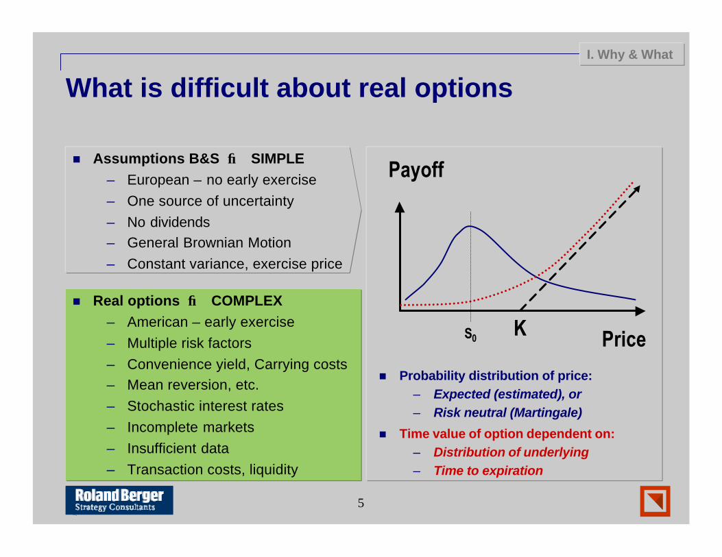
What is difficult about real options

n Assumptions B&S → SIMPLE– European – no early exercise– One source of uncertainty– No dividends– General Brownian Motion– Constant variance, exercise price

n Probability distribution of price:– Expected (estimated), or– Risk neutral (Martingale)

n Time value of option dependent on:– Distribution of underlying– Time to expiration

K

Payoff

Price

I. Why & What

S0

n Real options → COMPLEX– American – early exercise– Multiple risk factors– Convenience yield, Carrying costs– Mean reversion, etc.– Stochastic interest rates– Incomplete markets– Insufficient data– Transaction costs, liquidity

6

Types of options on projects/investments

n Defer an investment for later, contingent on new information– An American call option

n Expand, extend the life of a project– A portfolio of American calls

n Scale back, abandon a project– A portfolio of American puts

n Switch between two fuel types, two modes of operation– A portfolio of American calls and puts– Trade-off the cost of flexibility versus the value of option to switch

n Invest in phase II, contingent on investment in phase I– Compound options

I. Why & What

7

Drivers of real option value, relevance of ROA

n Increased project uncertainty

– Chance options in-the- money

n Increased room for management flexibility (modularity)

n NPV without flexibility close to 0

n Relevance of ROA

I. Why & What

Moderate High

Low Moderate

L Uncertainty H

L

Flex

ibili

ty

H

Likelihood for new info

Abili

ty to

resp

ondn Longer time to expiration

– Investment horizon

n Increased interest rates

– Option to defer, contract more valuable

n Less competition (game theory)

– Option to defer more valuable

8

Simple example of valuing a startup

A FINANCIAL CALL OPTION

n Option price

n Exercise price (K)

n Exercise date

n Current stock price (S)

n Return standard deviation

OPTION TO LAUNCH (EUROPEAN)

n PV of development costs

n Cost of launch (K)

n Launch date

n Current expectation of value (S)

n Firm value volatility

II. Examples

BUSINESS IDEA:

n Costs are known for sure:

– Product development: $4M (2y)

– Launch costs: $12M (after 2y)

n Expected sales: $6M per year

– Value established firm: $22M(revenue multiple of 3.66)

STATIC NPV:

n PV development (6%) $3.8M

n PV launch (6%) $10.9M

n PV business (21%) $14.5M\

Net Present Value: ($200,000)

(DCF analysis ignores flexibility)

9

Simple example of valuing a startup (contd.)

n Launch decision is call option– Product development cost is

price of this option– Launch if in 2 years:

PV firm > Launch costs

n Black & Scholes:– Cost of launch (K): $12.0M– Firm value (S): $14.5M– Firm volatility: 40%– Risk free rate: 6%OPTION VALUE: $5.0M

n ROA analysis: $5M - $3.8M= $1,200,000

n Add option to abandon project

– American; solve numerically

– Include both options in analysis

n Value of options: $5.6M

n ROA analysis = $1,750,000

n Determine firm volatility using simulation of static DCF model(without management flexibility)

– Volatility of firm is not the same as volatility of underlying

– Examples of underlying: price, market size, etc…

II. Examples

10

Example in Aircraft sales – embedded options

n Airbus and Boeing compete for long term orders in a cyclical capacity driven industry

– Aggressive market share targets to recoup aircraft model costs– Time lag between orders and delivery

n Traditional “approach”: the more purchase rights (options) handed out (at a certain exercise price) the more orders follow …

– These options are more valuable to airlines with higher volatilities– Segment market – discriminate smaller more volatile airlines– Also control time to expiration

n Other practical issues to value embedded options:– Mean reversion, lead time after exercise– Yield on each aircraft (analogous to dividends)– Swap between aircraft types: switching options

II. Examples

11

Compound (rainbow) options

n Large capital, R&D, Marketing outlays upon revelation of new information in each project phase

– Semi-conductor manufacturing– Pharmaceuticals– Oil & gas

D Fully Commit

• Design• R&D• Exploration

Abandon

D Fully Commit

• Build• FDA approval• Build wells

Abandon

D

Aggressive• Commercialization• Production

Abandon project

Current +1 year +2 years

Cost Market size

…

CompetitionPrice

…

II. Examples

Defensive• Commercialization• Production

12

Examples in Gas & Power

VALUING A POWERPLANT

n Gas powerplant can be turned on and off based on demand

n Two stochastic price processes; spread is what matters most

– Electricity demand varies with weather, etc.

– Fuel cost varies with gas-supply, related to local storage and transportation capacity

n Powerplant is series of calls; switch on when Price > MC

– If two fuel types: incorporates a series of switching options

VIRTUAL STORAGE

n Sell the ability to store gas when prices are low

n One stochastic process: gas price (mean reversion?)

n No simple solution– Path dependency– Constraints: empty and full

n Value using stochastic dynamic programming approach

– Storage empty at end of lease– DP works backward in time– Storage empty at start of lease

II. Examples

13

Quotes…

n “Many unspoken assumptions in standard corporate finance textbooks”, Myers (2002)

n “It took decades for DCF analysis to replace payback period analysis, the same will happen for real option analysis”, Copeland (2001)

n “Airbus management was slowly persuaded of competitive advantages of valuation of embedded options in contracts”, Stonier (2001)

n “A key advantage of ROA is that it is a gradual improvement, inherently incorporating DCF analysis”, Antikarov (2001)

III. Trends

14

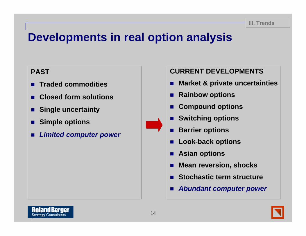
Developments in real option analysis

PAST

n Traded commodities

n Closed form solutions

n Single uncertainty

n Simple options

n Limited computer power

CURRENT DEVELOPMENTS

n Market & private uncertainties

n Rainbow options

n Compound options

n Switching options

n Barrier options

n Look-back options

n Asian options

n Mean reversion, shocks

n Stochastic term structure

n Abundant computer power

III. Trends

15

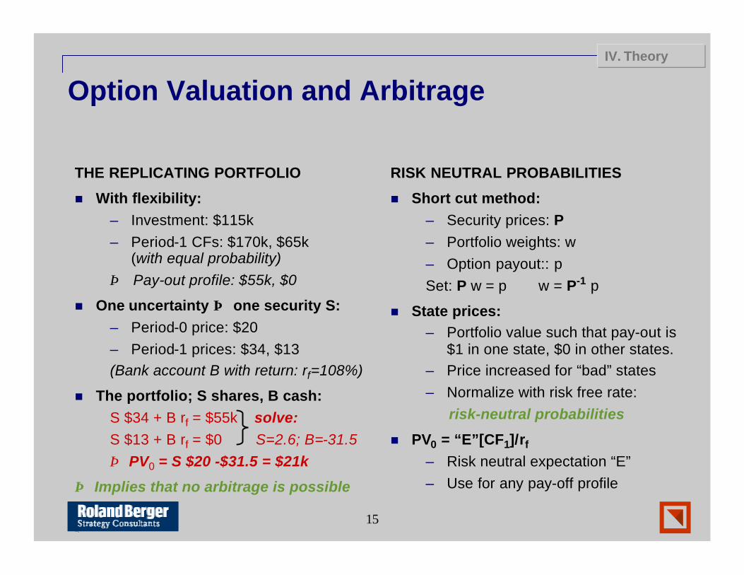
Option Valuation and Arbitrage

THE REPLICATING PORTFOLIO

n With flexibility:– Investment: $115k– Period-1 CFs: $170k, $65k

(with equal probability)⇒ Pay-out profile: $55k, $0

n One uncertainty ⇒ one security S:– Period-0 price: $20– Period-1 prices: $34, $13(Bank account B with return: rf=108%)

n The portfolio; S shares, B cash:S $34 + B rf = $55k solve:S $13 + B rf = $0 S=2.6; B=-31.5⇒ PV0 = S $20 -$31.5 = $21k

⇒ Implies that no arbitrage is possible

RISK NEUTRAL PROBABILITIES

n Short cut method:– Security prices: P– Portfolio weights: w– Option payout:: pSet: P w = p ⇒ w = P-1 p

n State prices:– Portfolio value such that pay-out is

$1 in one state, $0 in other states. – Price increased for “bad” states– Normalize with risk free rate:⇒ risk-neutral probabilities

n PV0 = “E”[CF1]/rf

– Risk neutral expectation “E”– Use for any pay-off profile

IV. Theory

16

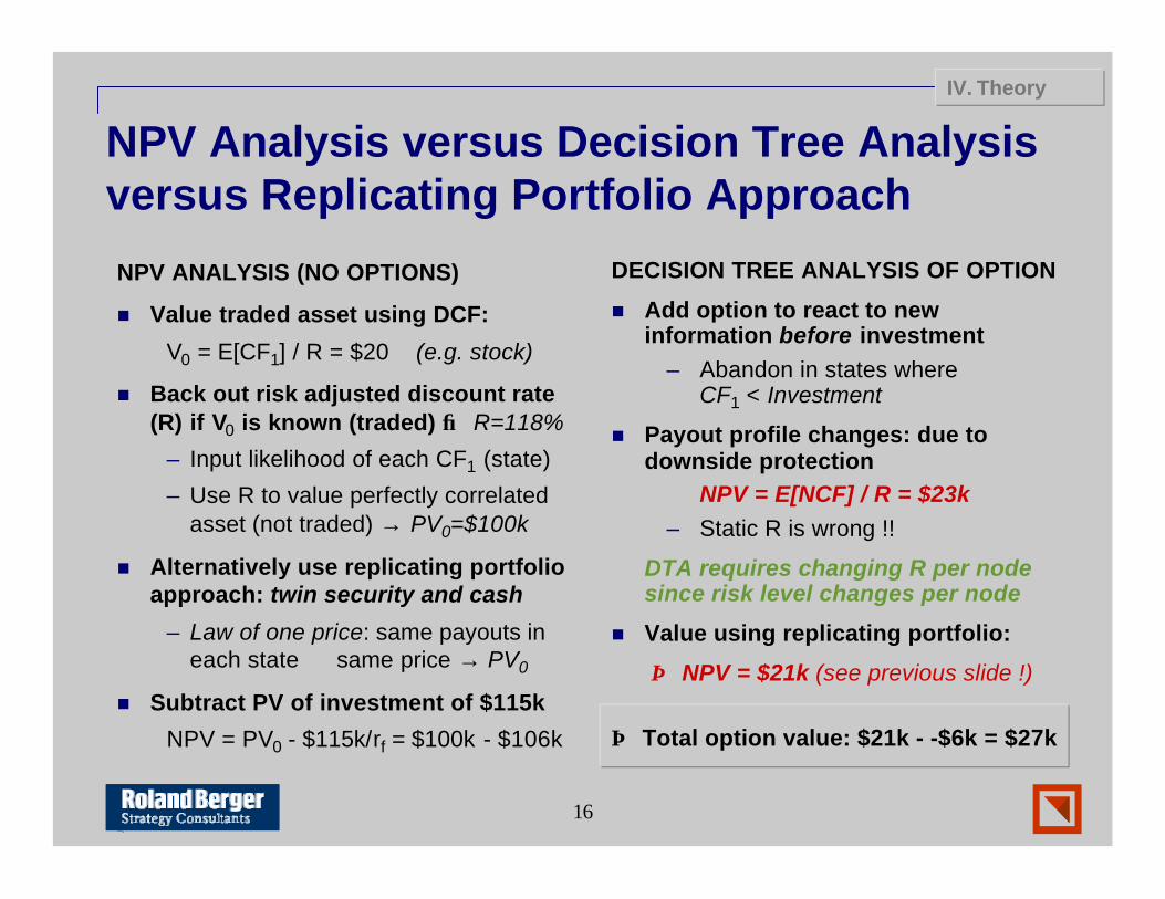
NPV Analysis versus Decision Tree Analysis versus Replicating Portfolio Approach

NPV ANALYSIS (NO OPTIONS)

n Value traded asset using DCF:

V0 = E[CF1] / R = $20 (e.g. stock)

n Back out risk adjusted discount rate (R) if V0 is known (traded) → R=118%

– Input likelihood of each CF1 (state)

– Use R to value perfectly correlated asset (not traded) → PV0=$100k

n Alternatively use replicating portfolio approach: twin security and cash

– Law of one price: same payouts in each state ⇔ same price → PV0

n Subtract PV of investment of $115k

NPV = PV0 - $115k/rf = $100k - $106k

DECISION TREE ANALYSIS OF OPTION

n Add option to react to new information before investment

– Abandon in states whereCF1 < Investment

n Payout profile changes: due to downside protection

⇒ NPV = E[NCF] / R = $23k – Static R is wrong !!

DTA requires changing R per node since risk level changes per node

n Value using replicating portfolio:

⇒ NPV = $21k (see previous slide !)

⇒ Total option value: $21k - -$6k = $27k

IV. Theory

17

Example in Oil & Gas – private uncertainty

n Risk neutral probabilities …– Are determined from a no arbitrage

condition on traded securities– Do not require subjective

probabilities, or an assessment of expected return (!)

– Can be used in multi-period setting

n Incomplete markets …– If no solution to: w = P-1 p– For example technology risk, or oil

reserve risk

n Solve with traditional DTA:– Use private probabilities– If fully uncorrelated with market:

use risk free rate (CAPM)

n Exploration and Production– Future oil prices, and total

reserves are unknown– Phased approach: 1. Seismic, 2.

Well logs, 3. Production

n Build multi-dimensional lattice– Two risk factors– Mixed real- and risk neutral

probabilities for private and market risks respectively

– Discount using risk-free rate

n Mean reversion in oil-prices can easily be incorporated

– Parameters can be inferred from historical data, or traded securities (Options and futures on oil)

IV. Theory

18

Closed form versus simulation

n Black & Scholes – closed form solution of Differential Equation

– No early exercise, etc…

– Many extensions; most need to be solved numerically

n Trees and lattices

– Binomial, quadranomial, multi-dimensional

– Lattice branches recombine; computational tractability

n Finite differences

– Similar to lattice approach, but directly solves differential equation

n Stochastic control. Dynamic Stochastic Programming

– Portfolio management; limit state space to wealth level

IV. Methods