Real estate ownership and the demand for cars in Denmark

- A pseudo-panel analysis

Jens Erik Nielsen

jen@dtf.dk

COST

11-10-2006

2

Start End

Introduction

• What affects the demand for cars?– Income– Household structure (adults and children)– Urbanization– Access to public transport

• But what about ‘wealth’– In Denmark the housing prices have increased drastically during the

last 10 years– The interest rate have dropped from around 10% to around 5% in 10

years

– This means that it is possible to capitalize the wealth accumulated in the households and this can be done without increasing the monthly mortgage payments.

Intro

3

Start End

Introduction

Source: www.jp.dk

We see large differences in the development in housing prices in Denmark

Largest increases in the large cities

Small increases (or falling) in small cities and on the countryside

Intro

4

Start End

Some facts from Denmark

0

200

400

600

800

1000

1200

1992 1993 1994 1995 1996 1997 1998 1999 2000 2001 2002

Prices onapartments

Prices onone-familyhouses

Real estate values (www.statistikbanken.dk)

0

20000

40000

60000

80000

100000

120000

140000

1992 1993 1994 1995 1996 1997 1998 1999 2000 2001 2002

Number of cars (www.statistikbanken.dk)

Some facts

5

Start End

Some facts from Denmark

0

10000

20000

30000

40000

50000

60000

70000

1994 1995 1996 1997 1998 1999 2000 2001 2002 2003 2004

Lending activity (www.statistikbanken.dk)

0

2

4

6

8

10

12

1992 1993 1994 1995 1996 1997 1998 1999 2000 2001 2002 2003 2004

Interest rate (www.statistikbanken.dk)

Some facts

6

Start End

An example

• Initial situation:– Need 1.000.000 DKr. In 30-year bond with annual interest rate of 8%– Value of the bond: 98– You need to borrow: 1.020.408

– Mortgage payments per year: 90.640

• New situation (after 3 years)– Value of real estate: 1.300.000 DKr.– Have paid back some money and has debt of 979.818 DKr.– You have accumulated 320.192 DKr.– The 30-year bond now has 27 years left. Value of the bond is now 105

but you can always pay back at 100.– The interest rate has dropped to 6%– Value of new bond is: 100

Example

7

Start End

An example

• Situation now– Wealth accumulated in real estate: 320.192 DKr.– Interest rate: 6%– Value of 30-year bond: 10– Yearly mortgage payment: 90.640

– How much can the household borrow without increasing its expenses?

– Maximum debt: 1.247.647 DKr.– Value of real estate: 1.300.000 DKr.– Remaining debt: 979.818 DKr.

– The household can capitalize: 267.829 DKr. (appr. 35.000 Euro)

Example

8

Start End

Can economic theory help?

• Investment theory?– One asset increase in value. – In order to keep the same risk-profile one has to diversify the

investment

• Households are short-sighted– Households only care about monthly expenses.– The total debt is not important

– As the example showed: Households get “free money”.

Theory?

9

Start End

The question?

• Have the following influenced car demand in Denmark:

– Increasing real estate prices– Falling interest rate

The question

10

Start End

The Data

• Danish Transport Diary Survey• Number of cars in households• Income• Number of adults and number of children• Cohort• Municipality• Real estate owner or tenant

• Statistics Denmark• Average value of real estate in municipalities• Annual interest rate

The data

11

Start End

Pseudo-panel

• Deaton (1985) Panel data from time series of cross sections, Journal of Econometrics 30, 109-126

• Result• It is possible to construct a ”pseudo-panel”

– Year of birth

• It is possible to include macro-variables

Pseudo-panel

12

Start End

Pseudo-panel

• Deaton (1985) Panel data from time series of cross sections, Journal of Econometrics 30, 109-126

• Result• It is possible to construct a ”pseudo-panel”

– Year of birth

• It is possible to include macro-variables

Pseudo-panel

13

Start End

Observations

Observations

Cohort. Year of birth Urban – owner

Rural - owner Urban – tenant Rural - tenant

1234567891011

1920-241925-291930-341935-391940-441945-491950-541955-591960-641965-691970-74

47971390610791463177215301592159315431125

13232079256532144254518448184567445838312104

688767720715714800702834109316082162

48261751947551060458461074910301299

Average 1254 3491 982 680

14

Start End

Car availability – real estate owners

Some information

15

Start End

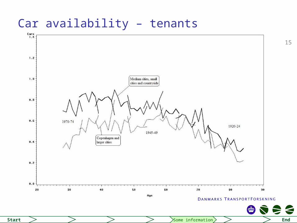
Car availability – tenants

Some information

16

Start End

Model variables

Model variables

Variabel Source Description

CarsIncome (log)AdultsCohortIncreasing valueInterest rateUrbanization

TUTUTUTUDSTDSTTU

Number of cars in the householdTotal household incomeNumber of adults in the householdCohort numberLast years increase in real estate value30-year interest rateLiving in urban area

17

Start End

The model

• C: cars

• Y: income

• W: real estate value

• R: interest rate

• I: adults

• G: Cohort

• U: urbanization

The model

1log( )i i i ii i i it t tt tt Y W E U R I t G C tC Y W E U R I G C

18

Start End

Estimates

Estimation

Variable M-all M-owners M-tenants

InterceptReal estate ownerUrbanizationValue increaseInterest rateIncome (log)Generation (cohort)AdultsCars (t-1)AR1 (βγ)

R2

Log LikelihoodSSEMSE

-0.1815 (-1.30)0.0650 (6.10)

-0.0625 (-5.36)0.0003 (2.46)

-0.0458 (-4.84)0.0756 (3.99)0.0040 (3.36)0.0659 (4.50)

0.7221 (21.39)0.2872 (4.90)

0.9966-305.8879131.3977

0.4409

-0.2403 (-0.76)

-0.0968 (-4.17)0.0007 (3.05)

-0.0565 (-4.18)0.1105 (4.20)0.0036 (2.27)0.0627 (3.50)

0.6737 (13.53)0.2270 (2.55)

0.9958-160.8236

72.77330.5019

-0.0239 (-0.08)

-0.0524 (-3.08)-0.0002 (-0.95)-0.0564 (-3.56)

0.1040 (2.82)0.0030 (1.14)0.0490 (1.31)

0.6797 (12.09)0.3941 (4.91)

0.9486-135.0271

52.01740.3587

19

Start End

Estimates

Variable M-rural M-urban

InterceptReal estate ownerValue increaseInterest rateIncome (log)Generation (cohort)AdultsCars (t-1)AR1 (βγ)

R2

Log LikelihoodSSEMSE

-0.8894 (-3.32)0.1145 (6.41)

-0.0799 (-5.42)0.0009 (3.33)0.1589 (5.62)0.0075 (4.91)0.0932 (5.37)0.4280 (6.86)0.1426 (1.58)

0.9971-132.952050.68300.3495

-0.6061 (-1.99)0.0668 (4.30)

-0.0685 (-4.44)0.0000 (0.18)0.1188 (3.64)

-0.0028 (-1.02)0.0656 (2.15)

0.6936 (11.93)0.3782 (4.65)

0.9800-148.667662.10460.4283

Estimation

20

Start End

Income elasticities

Elasticities

M-owners M-tenants

Mean car availability in the group[1]

Short term0.1008

Long term0.3090

Short term0.1952

Long term0.6094

[1] The average for real estate owners is 1.0960 cars and for tenants it is 0.5326.

M-rural M-urban

Mean car availability in the group[1]

Short term0.1506

Long term0.2631

Short term0,1653

Long term0.5395

[1] The total average for rural households is 1.0549 cars and for urban hosueholds it is 0.7188.

21

Start End

Other elasticities

Interest rate Real estate values

Real estate ownersTenantsLow increase (100.000 DKr.)High increase (300.000 DKr.)

Short term-0.2576-0.5395

Long term-0.7902-1.6843

Short term

0.06390.1916

Long term

0.19580.5873

The average for real estate owners is 1.0960 cars and for tenants it is 0.5326. The average increase in housing prices in the period has been around 200.000 DKr. per year. The interest rate is assumed to be 5%.

Elasticities

22

Start End

Conclusion

• Rising real estate values have increased car ownership for real estate owners.

• Rising real estate values have not affected tenants

• Both real estate owners and tenants have increased their car ownership due to the falling interest rate

• BUT– It would be nice to have register data to investigate further– Moving patterns are not included– The elasticities for the increasing real estate prices seems high– Income elasticities seems to be low– We do not accound for correlation between real estate prices and interest rate– A theoretical model is needed

End

http://www.dtf.dk

Thank you for your attention! Thank you for your attention! Jens Erik Nielsen

jen@dtf.dk