L������� �� E������� I���������

Debraj Ray, University of Warwick, Summer ����

Inequality and Divergence

Slides �: Introduction

Slides �: Occupational Choice

Slides �: Economic Growth and the Capital Share

Inequality and Con�ict

Slides �: Polarization and Fractionalization

Slides �: Some Empirical Findings

Slides � (preliminary): Notes on Class Con�ict

P�����������, F���������������� ��� C�������

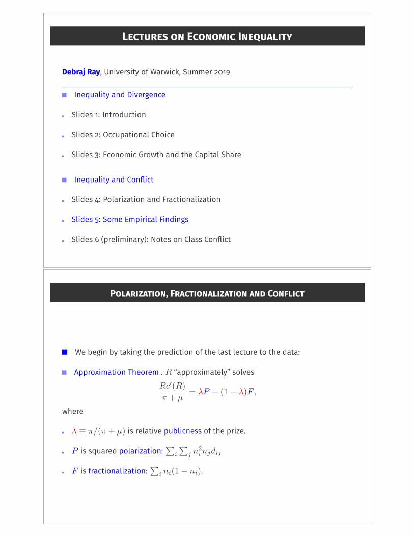
We begin by taking the prediction of the last lecture to the data:

Approximation Theorem . R “approximately” solves

Rc0(R)

⇡ + µ= �P + (1� �)F ,

where

� ⌘ ⇡/(⇡ + µ) is relative publicness of the prize.

P is squared polarization:P

i

Pj n

2injdij

F is fractionalization:P

i ni(1� ni).

E�������� I������������

(Esteban, Mayoral and Ray AER ����, Science ����)

��� countries over ����–���� (pooled cross-section).

�rio��: ��� battle deaths in the year. [Baseline]

�riocw: �rio�� � total exceeding ���� battle-related deaths.

�rio����: �,���� battle-related deaths in the year.

�rioint: weighted combination of above.

�sc: Continuous index, Banks (����), weighted average of � di�erent

manifestations of co�ict.

G�����

Fearon database: “culturally distinct” groups in ��� countries.

based on ethnolinguistic criteria.

Ethnologue: information on linguistic groups.

�,��� living languages � group sizes.

P���������� ��� D��������

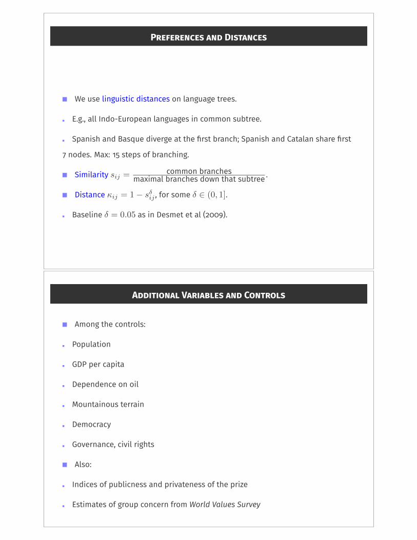
We use linguistic distances on language trees.

E.g., all Indo-European languages in common subtree.

Spanish and Basque diverge at the �rst branch; Spanish and Catalan share �rst

� nodes. Max: �� steps of branching.

Similarity sij = common branchesmaximal branches down that subtree .

Distance ij = 1� s�ij , for some � 2 (0, 1].

Baseline � = 0.05 as in Desmet et al (����).

A��������� V�������� ��� C�������

Among the controls:

Population

GDP per capita

Dependence on oil

Mountainous terrain

Democracy

Governance, civil rights

Also:

Indices of publicness and privateness of the prize

Estimates of group concern from World Values Survey

Want to estimate

⇢c0(⇢)it = X1ti�1 +X2it�2 + "it

X1it distributional indices.

X2it controls (including lagged con�ict)

With binary outcomes, latent variable model:

P (�rioxit = 1|Zit) = P (⇢c0(⇢) > W⇤|Zit) = H(Zit� �W

⇤)

where Zit = (X1i, X2it)

Baseline: uses max likelihood logit (results identical for probit).

p-values use robust standard errors adjusted for clustering.

Baseline with �rio��, Fearon groupings

Var [1] [2] [3] [4] [5] [6]

P ⇤⇤⇤ 6.07(0.002)

⇤⇤⇤ 6.90(0.000)

⇤⇤⇤ 6.96(0.001)

⇤⇤⇤ 7.38(0.001)

⇤⇤⇤ 7.39(0.001)

⇤⇤⇤ 6.50(0.004)

F ⇤⇤⇤ 1.86(0.000)

⇤⇤ 1.13(0.029)

⇤⇤ 1.09(0.042)

⇤⇤ 1.30(0.012)

⇤⇤ 1.30(0.012)

⇤⇤ 1.25(0.020)

�op ⇤⇤ 0.19(0.014)

⇤⇤ 0.23(0.012)

⇤⇤ 0.22(0.012)

0.13(0.141)

0.13(0.141)

0.14(0.131)

�dppc - ⇤⇤⇤- 0.40(0.001)

⇤⇤⇤- 0.41(0.002)

⇤⇤⇤- 0.47(0.001)

⇤⇤⇤- 0.47(0.001)

⇤⇤- 0.38(0.011)

�il/diam - - 0.06(0.777)

0.04(0.858)

0.04(0.870)

- 0.10(0.643)

�ount - - - 0.01(0.134)

0.01(0.136)

0.01(0.145)

�cont - - - ⇤⇤ 0.84(0.019)

⇤⇤ 0.85(0.018)

⇤⇤⇤ 0.90(0.011)

�emoc - - - - - 0.02(0.944)

0.02(0.944)

�xcons - - - - - - 0.13(0.741)

�utocr - - - - - 0.14(0.609)

�ights - - - - - 0.17(0.614)

�ivlib - - - - - 0.16(0.666)

�ag ⇤⇤⇤ 2.91(0.000)

⇤⇤⇤ 2.81(0.000)

⇤⇤⇤ 2.80(0.000)

⇤⇤⇤ 2.73(0.000)

⇤⇤⇤ 2.73(0.000)

⇤⇤⇤ 2.79(0.000)

Residual scatters.

!"#$%

!"#&%

!"#'%

"#'%

"#&%

"#$%

"#(%

"#)%

!"#"(% !"#"*% "#"&% "#"+% "#'&% "#'+%

PRIO

25 R

esid

uals

Polarization (Residuals) !"#$%

!"#&%

!"#'%

"#'%

"#&%

"#$%

"#(%

"#)%

!"#*$% !"#&$% !"#+$% !"#'$% !"#"$% "#"$% "#'$% "#+$% "#&$% "#*$%

PRIO

25 (R

esid

uals

)

Fractionalization (Residuals)

P (20 ! 80), �rio�� ���! ���.

F (20 ! 80), �rio�� ���! ���.

R��������� C�����

Alternative de�nitions of con�ict

Alternative de�nition of groups: Ethnologue

Binary versus language-based distances

Con�ict onset

Region and time e�ects

Other ways of estimating the baseline model

Di�erent de�nitions of con�ict, Fearon groupings

Variable �rio�� �riocw �rio���� �rioint �sc

P ⇤⇤⇤ 7.39(0.001)

⇤⇤⇤ 6.76(0.007)

⇤⇤⇤10.47(0.001)

⇤⇤⇤ 6.50(0.000)

⇤⇤⇤25.90(0.003)

F ⇤⇤ 1.30(0.012)

⇤⇤ 1.39(0.034)

⇤ 1.11(0.086)

⇤⇤⇤ 1.30(0.006)

2.27(0.187)

�dp ⇤⇤⇤- 0.47(0.001)

⇤- 0.35(0.066)

⇤⇤⇤- 0.63(0.000)

⇤⇤⇤- 0.40(0.002)

⇤⇤⇤- 1.70(0.001)

�op 0.13(0.141)

⇤ 0.19(0.056)

0.13(0.215)

0.10(0.166)

⇤⇤⇤ 1.11(0.000)

�il/diam 0.04(0.870)

0.06(0.825)

- 0.03(0.927)

- 0.04(0.816)

- 0.57(0.463)

�ount 0.01(0.136)

⇤⇤ 0.01(0.034)

0.01(0.323)

0.00(0.282)

⇤⇤ 0.04(0.022)

�cont ⇤⇤ 0.85(0.018)

0.62(0.128)

⇤ 0.78(0.052)

⇤ 0.55(0.069)

⇤⇤⇤ 4.38(0.004)

�emoc - 0.02(0.944)

- 0.09(0.790)

- 0.41(0.230)

- 0.03(0.909)

0.06(0.944)

�ag ⇤⇤⇤ 2.73(0.000)

⇤⇤⇤ 3.74(0.000)

⇤⇤⇤ 2.78(0.000)

⇤⇤⇤ 2.00(0.000)

⇤⇤⇤ 0.50(0.000)

P (20 ! 80), �rio�� ���–���, �riocw ��–���, �rio���� ��–���.

F (20 ! 80), �rio�� ���–���, �riocw ��–���, �rio���� ��–��.Di�erent de�nitions of con�ict, Ethnologue groupings

Variable �rio�� �riocw �rio���� �rioint �sc

P ⇤⇤⇤ 8.26(0.001)

⇤⇤⇤ 8.17(0.005)

⇤⇤10.10(0.016)

⇤⇤⇤ 7.28(0.001)

⇤⇤⇤27.04(0.008)

F 0.64(0.130)

0.75(0.167)

0.51(0.341)

0.52(0.185)

- 0.58(0.685)

�dp ⇤⇤⇤- 0.51(0.000)

⇤⇤- 0.39(0.022)

⇤⇤⇤- 0.63(0.000)

⇤⇤⇤- 0.45(0.000)

⇤⇤⇤- 2.03(0.000)

�op ⇤ 0.15(0.100)

⇤⇤ 0.24(0.020)

0.15(0.198)

0.12(0.118)

⇤⇤⇤ 1.20(0.000)

�il/diam 0.15(0.472)

0.21(0.484)

0.10(0.758)

0.08(0.660)

- 0.06(0.943)

�ount ⇤ 0.01(0.058)

⇤⇤ 0.01(0.015)

0.01(0.247)

⇤ 0.01(0.099)

⇤⇤ 0.04(0.013)

�cont ⇤⇤ 0.72(0.034)

0.49(0.210)

0.50(0.194)

0.44(0.136)

⇤⇤⇤ 4.12(0.006)

�emoc 0.03(0.906)

0.00(0.993)

- 0.32(0.350)

0.03(0.898)

0.02(0.979)

�ag ⇤⇤⇤ 2.73(0.000)

⇤⇤⇤ 3.75(0.000)

⇤⇤⇤ 2.83(0.000)

⇤⇤⇤ 2.01(0.000)

⇤⇤⇤ 0.50(0.000)

Binary variables don’t work well with Ethnologue.

Can compute pseudolikelihoods for � as in Hansen (����).

Onset vs incidence, Fearon and Ethnologue groupings

Variable �nset� �nset� �nset� �nset� �nset� �nset�

P ⇤⇤⇤ 7.85(0.000)

⇤⇤⇤ 7.41(0.000)

⇤⇤⇤ 7.26(0.000)

⇤⇤⇤ 8.83(0.000)

⇤⇤⇤ 8.84(0.000)

⇤⇤⇤ 8.71(0.000)

F ⇤ 0.94(0.050)

0.72(0.139)

0.62(0.204)

0.39(0.336)

0.20(0.602)

0.15(0.702)

�dp ⇤⇤⇤- 0.60(0.000)

⇤⇤⇤- 0.65(0.000)

⇤⇤⇤- 0.68(0.000)

⇤⇤⇤- 0.64(0.000)

⇤⇤⇤- 0.70(0.000)

⇤⇤⇤- 0.73(0.000)

�op 0.01(0.863)

0.03(0.711)

0.03(0.748)

0.06(0.493)

0.05(0.588)

0.05(0.619)

�il/diam ⇤⇤ 0.54(0.016)

⇤⇤ 0.46(0.022)

⇤⇤ 0.47(0.025)

⇤⇤⇤ 0.64(0.004)

⇤⇤⇤ 0.56(0.005)

⇤⇤⇤ 0.57(0.007)

�ount 0.00(0.527)

0.00(0.619)

0.00(0.620)

0.00(0.295)

0.00(0.410)

0.00(0.424)

�cont ⇤⇤⇤ 0.74(0.005)

⇤⇤ 0.66(0.010)

0.42(0.104)

⇤⇤ 0.66(0.012)

⇤⇤ 0.63(0.017)

0.40(0.120)

�emoc - 0.06(0.816)

0.06(0.808)

0.08(0.766)

- 0.02(0.936)

0.09(0.716)

0.10(0.704)

�ag 0.32(0.164)

- 0.08(0.740)

- 0.08(0.751)

0.29(0.214)

- 0.13(0.618)

- 0.13(0.622)

Fearon Fearon Fearon Eth Eth Eth

Region and time e�ects, Fearon groupings

Variable reg.dum. no Afr no Asia no L.Am. trend interac.

P ⇤⇤⇤ 6.64(0.002)

⇤⇤ 5.36(0.034)

⇤⇤⇤ 7.24(0.001)

⇤⇤⇤ 9.56(0.001)

⇤⇤⇤ 7.39(0.001)

⇤⇤⇤ 7.19(0.001)

F ⇤⇤⇤ 2.03(0.001)

⇤⇤⇤ 2.74(0.001)

⇤⇤ 1.28(0.030)

⇤⇤⇤ 1.49(0.009)

⇤⇤ 1.33(0.012)

⇤⇤⇤ 1.76(0.001)

�dp ⇤⇤⇤- 0.72(0.000)

⇤⇤⇤- 0.69(0.000)

⇤⇤- 0.39(0.024)

⇤⇤⇤- 0.45(0.006)

⇤⇤⇤- 0.49(0.001)

⇤⇤⇤- 0.60(0.000)

�op 0.05(0.635)

0.09(0.388)

0.06(0.596)

⇤ 0.17(0.087)

0.14(0.125)

0.06(0.543)

�il/diam 0.12(0.562)

0.14(0.630)

0.10(0.656)

0.10(0.687)

0.05(0.824)

0.15(0.476)

�ount 0.00(0.331)

- 0.00(0.512)

0.01(0.114)

⇤⇤ 0.01(0.038)

0.01(0.109)

0.01(0.212)

�cont ⇤⇤ 0.87(0.018)

⇤ 0.75(0.064)

⇤⇤ 0.83(0.039)

0.62(0.134)

⇤⇤ 0.82(0.025)

⇤⇤ 0.77(0.040)

�emoc 0.08(0.761)

- 0.03(0.932)

- 0.23(0.389)

0.10(0.716)

0.08(0.750)

0.13(0.621)

�ag ⇤⇤⇤ 2.68(0.000)

⇤⇤⇤ 2.83(0.000)

⇤⇤⇤ 2.69(0.000)

⇤⇤⇤ 2.92(0.000)

⇤⇤⇤ 2.79(0.000)

⇤⇤⇤ 2.74(0.000)

Other estimation methods, Fearon groupings.

Variable Logit OLog(CS) Logit(Y) RELog OLS RC

P ⇤⇤⇤ 7.39(0.001)

⇤⇤⇤11.84(0.003)

⇤⇤ 4.68(0.015)

⇤⇤⇤ 7.13(0.000)

⇤⇤⇤ 0.86(0.004)

⇤⇤⇤ 0.95(0.001)

F ⇤⇤ 1.30(0.012)

⇤⇤⇤ 2.92(0.001)

⇤⇤⇤ 1.32(0.003)

⇤⇤⇤ 1.27(0.005)

⇤⇤ 0.13(0.025)

⇤⇤⇤ 0.16(0.008)

�dp ⇤⇤⇤- 0.47(0.001)

⇤⇤⇤- 0.77(0.001)

⇤⇤- 0.29(0.036)

⇤⇤⇤- 0.46(0.000)

⇤⇤⇤- 0.05(0.000)

⇤⇤⇤- 0.06(0.000)

�op 0.13(0.141)

0.03(0.858)

0.14(0.123)

⇤⇤ 0.14(0.090)

⇤⇤ 0.02(0.020)

⇤⇤ 0.02(0.032)

�il/diam 0.04(0.870)

⇤⇤ 0.94(0.028)

0.29(0.280)

0.04(0.850)

0.00(0.847)

0.01(0.682)

�ount 0.01(0.136)

0.01(0.102)

0.00(0.510)

0.01(0.185)

0.00(0.101)

0.00(0.179)

�cont ⇤⇤ 0.85(0.018)

⇤⇤⇤ 1.51(0.007)

⇤ 0.62(0.052)

⇤⇤⇤ 0.83(0.002)

⇤⇤ 0.09(0.019)

⇤⇤⇤ 0.10(0.006)

�emoc - 0.02(0.944)

- 0.48(0.212)

- 0.09(0.690)

- 0.02(0.941)

0.01(0.788)

0.01(0.585)

�ag ⇤⇤⇤ 2.73(0.000)

- ⇤⇤⇤ 4.69(0.000)

⇤⇤⇤ 2.69(0.000)

⇤⇤⇤ 0.54(0.000)

⇤⇤⇤ 0.45(0.000)

I����-C������ V��������� �� P��������� ��� C�������

con�ict per-capita ' ↵⇥�P + (1� �)F

⇤,

Relax assumption that � and ↵ same across countries.

Privateness: natural resources; use per-capita oil reserves (oilresv).

Publicness: control while in power (pub), average of

Autocracy (Polity IV)

Absence of political rights (Freedom House)

Absence of civil liberties (Freedom House)

⇤ ⌘ (���*gdp)/(���*gdp+ �������).

Country-speci�c public good shares and group cohesion

Variable �rio�� �rioint �sc �rio�� �rioint �sc

P - 3.31(0.424)

- 1.93(0.538)

- 9.21(0.561)

- 3.01(0.478)

- 1.65(0.630)

-13.04(0.584)

F 0.73(0.209)

0.75(0.157)

- 2.27(0.249)

1.48(0.131)

1.51(0.108)

⇤⇤- 6.65(0.047)

P⇤ ⇤⇤⇤17.38(0.001)

⇤⇤⇤13.53(0.001)

⇤⇤⇤60.23(0.005)

F (1� ⇤) ⇤⇤⇤ 2.53(0.003)

⇤⇤⇤ 1.92(0.003)

⇤⇤⇤11.87(0.000)

P⇤A ⇤⇤23.25(0.021)

⇤⇤19.16(0.019)

⇤72.22(0.083)

F (1� ⇤)A ⇤⇤ 4.02(0.013)

⇤⇤⇤ 2.92(0.003)

⇤⇤⇤26.03(0.000)

�dp ⇤⇤⇤- 0.62(0.000)

⇤⇤⇤- 0.50(0.000)

⇤⇤⇤- 2.36(0.000)

⇤⇤⇤- 0.65(0.000)

⇤⇤⇤- 0.53(0.003)

⇤⇤⇤- 3.68(0.000)

�op 0.10(0.267)

0.09(0.243)

⇤⇤⇤ 0.99(0.000)

0.08(0.622)

0.09(0.448)

0.33(0.565)

�ag ⇤⇤⇤ 2.62(0.000)

⇤⇤⇤ 1.93(0.000)

⇤⇤⇤ 0.47(0.000)

⇤⇤⇤ 2.40(0.000)

⇤⇤⇤ 1.79(0.000)

⇤⇤⇤ 0.42(0.000)

S������ S� F��

Exclusionary con�ict as important as distributive con�ict, maybe more.

O�en made salient by the use of ethnicity or religion.

Do societies with “ethnic divisions” experience more con�ict?

We developed a theory of con�ict that generates an empirical test.

The notions of polarization and fractionalization are central to this theory

Convex combination of the two distributional variables predicts con�ict.

Theory appears to �nd strong support in the data.

Other predictions: interaction e�ects on shocks that a�ect rents and

opportunity costs.

B��W��� A���� E������� I���������?

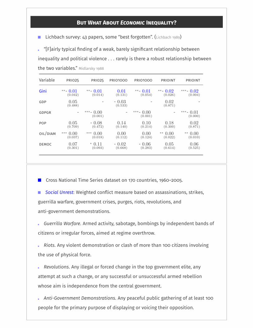
Lichbach survey: �� papers, some “best forgotten”. (Lichbach ����)

“[F]airly typical �nding of a weak, barely signi�cant relationship between

inequality and political violence . . . rarely is there a robust relationship between

the two variables.” Midlarsky ����

Variable ������ ������ �������� �������� ������� �������

Gini ⇤⇤- 0.01(0.042)

⇤⇤- 0.01(0.014)

0.01(0.131)

⇤⇤- 0.01(0.054)

⇤⇤- 0.02(0.026)

⇤⇤⇤- 0.02(0.004)

��� 0.05(0.488)

- - 0.03(0.533)

- 0.02(0.871)

-

����� - ⇤⇤⇤- 0.00(0.001)

- ⇤⇤⇤- 0.00(0.001)

- ⇤⇤⇤- 0.01(0.000)

��� 0.05(0.709)

- 0.08(0.472)

0.14(0.140)

0.10(0.214)

0.18(0.300)

0.02(0.871)

���/���� ⇤⇤⇤ 0.00(0.037)

⇤⇤⇤ 0.00(0.018)

0.00(0.112)

0.00(0.124)

⇤⇤ 0.00(0.022)

⇤⇤ 0.00(0.010)

����� 0.07(0.301)

⇤ 0.11(0.093)

- 0.02(0.668)

- 0.06(0.283)

0.05(0.614)

0.06(0.525)

Cross National Time Series dataset on ��� countries, ����–����.

Social Unrest: Weighted con�ict measure based on assassinations, strikes,

guerrilla warfare, government crises, purges, riots, revolutions, and

anti-government demonstrations.

Guerrilla Warfare. Armed activity, sabotage, bombings by independent bands of

citizens or irregular forces, aimed at regime overthrow.

Riots. Any violent demonstration or clash of more than ��� citizens involving

the use of physical force.

Revolutions. Any illegal or forced change in the top government elite, any

attempt at such a change, or any successful or unsuccessful armed rebellion

whose aim is independence from the central government.

Anti-Government Demonstrations. Any peaceful public gathering of at least ���

people for the primary purpose of displaying or voicing their opposition.

United States

CanadaCuba

Haiti

Dominican Rep

JamaicaTrinidad

Mexico

Guatemala

Honduras

El Salvador

Nicaragua

Costa Rica

Panama

Colombia

Venezuela

Guyana

Ecuador

Peru

Brazil

Bolivia

Paraguay

Chile

Argentina

Uruguay

United Kingdom

IrelandNetherlandsBelgium

France

Switzerland

Spain

Portugal

GermanyGermanyPoland

AustriaHungary

Czechoslovakia

Czech RepublicSlovak Republic

Italy

AlbaniaMacedoniaCroatia

Serbia Bosnia

Serbia

Slovenia

Greece

CyprusBulgaria

Moldova

Romania

Russia

Russia

EstoniaLatviaLithuaniaUkraine

Belarus

Armenia

Georgia

Azerbaijan

FinlandSwedenNorway Denmark

Guinea-Bissau

GambiaMali

Senegal

Benin MauritaniaNigerIvory Coast

Guinea Burkina Faso

Liberia Sierra Leone

GhanaTogoCameroon

Nigeria

Gabon

Central African Republic

Chad

Congo Brazzaville

Congo Kinshasa

Uganda

KenyaTanzania

Burundi

Rwanda

Somalia

Djibouti

Ethiopia

Ethiopia

Angola

Mozambique

Zambia

Zimbabwe

Malawi

South Africa

Namibia

Lesotho

BotswanaSwazilandMadagascar

Comoros

Mauritius

Morocco

Algeria

Tunisia

Sudan

Iran

TurkeyIraq

Egypt

Lebanon

Jordan

Israel

YemenTurkmenistan

Tajikistan

Kyrgyzstan

Uzbekistan

Kazakhstan

China

MongoliaTaiwan

Korea South

Japan

India

Bhutan

Pakistan

Pakistan

Bangladesh

Sri Lanka

Nepal

Thailand

Cambodia

Laos

Vietnam

Malaysia

Singapore

Philippines

Indonesia

Australia

Papua New Guinea

New ZealandFiji

010

0020

0030

0040

0050

00So

cial

unr

est (

aver

age)

.3 .4 .5 .6 .7Gini (average)

010

000

2000

0So

cial

Unr

est

.2 .4 .6 .8Gini

Social Unrest, ����–����

[1] [2] [3] [4]

���� -����* �.��� ***����� *��.���

(�.���) (�.���) (�.���) (�.���)

����2 ***-����� *-��.���

(�.���) (�.���)

��� �.��� -�.��� ��.��� -�.���

(�.���) (�.���) (�.���) (�.���)

��� ���.��� �.��� ���.��� �.���

(�.���) (�.���) (�.���) (�.���)

����� [�������] -�.��� -�.��� -��.��� -�.���

(�.���) (�.���) (�.���) (�.���)

��� ***�.��� ***�.��� ***�.��� ***�.���

(�.���) (�.���) (�.���) (�.���)

c -���� �.��� -���� -�.���

(�.���) (�.���) (�.���) (�.���)

Estimation OLS Neg. Bin OLS Neg. Bin

Country FE

Year FE

R2 �.��� �.�� �.��� �.���

Obs ���� ���� ���� ����

Interpretation (col �):

�st! ��th Gini �-tile:

social unrest " ���

��th! ��th Gini �-tile:

social unrest # ���

Components of Social Unrest, ����–����

[1] [2] [3] [4]

Guerrilla Riots Revolutions Demos

���� **�.��� **�.��� �.��� *�.���

(�.���) (�.���) (�.���) (�.���)

����2 **-�.��� **-�.��� *-�.��� *-�.���

(�.���) (�.���) (�.���) (�.���)

��� -�.��� -�.��� -�.��� �.���

(�.���) (�.���) (�.���) (�.���)

��� -�.��� �.��� �.��� ***�.���

(�.���) (�.���) (�.���) (�.���)

����� [�������] -�.��� -�.��� -�.��� ***-�.���

(�.���) (�.���) (�.���) (�.���)

Lag

C �.��� -�.��� -�.��� **-�.���

(�.���) (�.���) (�.���) (�.���)

Country FE

Year FE

R2 �.��� �.��� �.��� �.���

Obs ���� ���� ���� ����

������ ������

050

010

00So

cial

Unr

est (

fitte

d va

lues

)

.2 .4 .6 .8Gini

�������������� ��������� �������

.2.3

.4.5

.6.7

Anti-

Gov

ernm

ent D

emon

stra

tions

(fitte

d va

lues

)

.2 .4 .6 .8Gini

0.0

5.1

.15

.2G

uerri

lla W

arfa

re

.2 .4 .6 .8Gini

����������� �����

0.0

5.1

.15

Rev

olut

ions

(fitte

d va

lues

)

.2 .4 .6 .8Gini

0.2

.4.6

.8R

iots

(fitte

d va

lues

)

.2 .4 .6 .8Gini

T�� A�������� �� I���������

The Grabbing and Opportunity Cost E�ects Dube-Vargas ����, Mitra-Ray ����

An increase in rival income increases violence directed against rival group.

An increase in own income reduces violence directed against rival group.

Motive Versus Means Esteban-Ray ����, ����, Huber-Mayoral ����

The class marker is a two-edged sword:

it breeds resentment, but harder for the poor to revolt

ethnic division) perverse synergy of money and labor (���� Gujarat)