PATE OF RETURN, COST OF CAPITAL AND VALUATION

RATIO IN FINNISH MANUFACTURING 1960 - 1979*

Heikki Koskenkvld

Research Department

Bank of Finland

May 1981

* Paper to be preserited at the M.I.T. Rate of

ReturnConference, June19.81. This paper is a

revised version of an earlier draft from

September 1980 (see references).

CONTENTS

page

Introduction1.

2. Development of Total Capital, Own Capital

4

4

11

14

and the Rate of Profit

2.1. Total Capital and Its Components

2.2. Own Capital and Debt Ratios

2.3. Profit, Taxes and the Effective Tax Rate

3. Development of the Rate of Return on Total

Capital and on Own Capital

3.1. The Rate of Return on Total Capital

3.2. The Rate of Return on Own Capital

4. The Rate uf Return to Investors

5. The Valuation Ratio and the Cost of Capital

6. Determinants of the Rate of Return and

the Effective Tax Rate

7. Conclusions

Footnotes

Statistical Appendix

List of Symbols

References

20

20

29

35

40

53

62

66

73

83

86

1

4 1

1. INTRODUCTION*

The international background of this investigation is

the ongoing debate and argument that started in the

mid-1970s about the development and possible decline

in the rate of return on corporate capital in most

western countries. The potential significance of the

behaviour of corporate profitability is clear, but its

actual development has raised many theoretical and

empirical issues.

W. Nordhaus laid the ground for this discussion by

concluding that in the post-war period (1948 - 1970)

the rate of return revealed a downtrend in corporate

profitability in the U.S.A.1 Feldstein and Summers

(1977), on the other hand, disputed this finding,

their conclusion being that "our analysis of these

rates of return provides no support for the view that

there has been a gradual decline in the rate of return

over the post-war period." Von Furstenberg and

Malkiel (1977) also doubt the argument for the overall3

decline in profitability. They emphasize the import-

ance of the reduction in real indebtedness on the

development of profit and retained earnings.

Holland and Myers (1978, 1980) have very carefully

analyzed the performance of U.S. nonfinancial corpora-

tions since the war by using both rates of return to

investors and rates of return on capital.4 They concludE

that these corporations have fared poorly since the

mid-1960s, but they, too, were unable to find evidence

of a long-term downtrend.

* The collection of statistical data and the calcula-tions used in this paper were carried out by IlkkaSalonen. Seija Leino typed this paper, and thelanguage was checked by Malcolm Waters.

1. See Footnotes.

1

14 A 2

In many other countries researchers in this field have

found a significant downtrend in corporate profit-

ability over the last decade and especially following

the first oil crisis in 1973. Reference can be made

here to the studies made in the United Kingdom and

Sweden.5 International organizations have also devoted

attention to the development and measurement of

company profitability in the latter half of the 1970s

(OECD, etc.). 6

Against this background the principal objective of

this study is the analysis of the performance of

the Finnish manufacturing sector in the period 1960 -

1979. The analysis is restricted to manufacturing

companies because of data limitations. The performance

of these companies is examined by means of various

indicators. Our main emphasis is on the movements in

and measurement of rates of return on capital, although

we also make some calculations of the returns to

investors in these companies. Our second purpose is to

analyze the behaviour of capital costs in the manu-

facturing sector. Finally, we attempt to discover

statistically whether profitability has behaved in a

trendwise manner.

The basic data used in the calculations of this report

is taken from official national income accounts, but

use is also made of firms' balance sheet data (book

accounts), industrial statistics and capital market

data. In addition, some self-constructed data is used

in the calculations of capital stock figures.

The contents of the paper are organized as follows:

at 3

In Chapter 2 various estimates of total capital,

physical capital and own capital as well as figures

for debt-equity ratios are presented. We also discuss

the basic formulas for calculating the economic rate

of profit, or operating income, and the official

(statutory) and effective tax rates for manufacturing

industries.

Chapter 3 attempts to trace the development of real

profitability in manufacturing by developing various

estimates of the real rate of return on total and own

capital.

In Chapter 4 we provide some preliminary estimates of

investors rates of return on total and eauity capital.

These are used as additional evidence in considering

the general performance of the manufacturing sector.

Chapter 5 provides an analysis of the development of

the cost of capital and the valuation ratio (Tobin's

q-variable) in relation to the real rate of return.

Finally, in Chapter 6 we perform some simple regression

analysis of the determinants of the rate of return and

try to discover whether or not there has occurred

trendwise behaviour. Similar tests are also carried

out for effective tax rates.

3

14 4

2. DEVELOPMENT OF TOTAL CAPITAL, OWN CAPITAL AND

THE RATE OF PROFIT

2.1. Total Capital and Its Components

The concept and measurement of capital is a compli-

cated task both from the theoretical and the empirical

point of view, the main problems usually arising in

connection with the stock of physical assets, that is,

real capital plus inventories. It is generally felt

that financial assets can be estimated rather reliably

from official statistics. In this paper estimates of

total capital in manufacturing have had to be drawn

from a variety of statistical sources and earlier

Finnish studies. However, we believe that the esti-

mates so obtained are quite reliable, especially for

the manufacturing sector. In recent years, various

measures of the fixdd capital stock of Finnish manu-

facturing have been developed. The basic measure used i:

this investigation is that of net replacement cost

value. The capital stock series is based on an esti-

mate of 5.4 per cent for true economic depreciation.

This rate of depreciation is calculated with the aid

of fire insurance values for the manufacturing capital

stock.

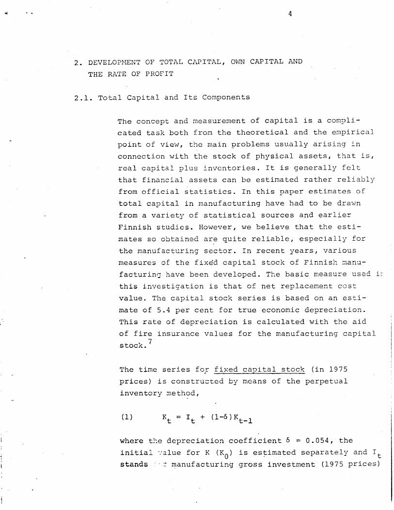
The time series for fixed capital stock (in 1975

prices) is constructed by means of the perpetual

inventory method,

(1) Kt =t + (1-6) Kt-1

where the depreciation coefficient 6 = 0.054, the

initial -alue for K (K0 ) is estimated separately and Itstands manufacturing gross investment (1975 prices)

4

5

and is taken from the national income statistics. The

current value of this net capital stock is obtained

through multiplying by the price index of investment

goods.

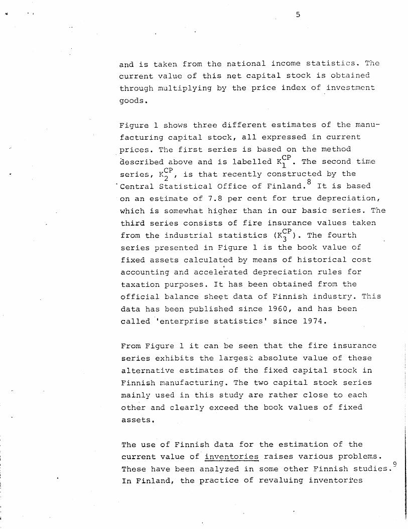
Figure 1 shows three different estimates of the manu-

facturing capital stock, all expressed in current

prices. The first series is based on the methodCP

described above and is labelled K C. The second time

series, K CP is that recently constructed by the2 ie8

Central Statistical Office of Finland. It is based

on an estimate of 7.8 per cent for true depreciation,

which is somewhat higher than in our basic series. The

third series consists of fire insurance values takenCP

from the industrial statistics (K3 ). The fourth

series presented in Figure 1 is the book value of

fixed assets calculated by means of historical cost

accounting and accelerated depreciation rules for

taxation purposes. It has been obtained from the

official balance sheet data of Finnish industry. This

data has been published since 1960, and has been

called 'enterprise statistics' since 1974.

From Figure 1 it can be seen that the fire insurance

series exhibits the largesL absolute value of these

alternative estimates of the fixed capital stock in

Finnish manufacturing. The two capital stock series

mainly used in this study are rather close to each

other and clearly exceed the book values of fixed

assets.

The use of Finnish data for the estimation of the

current value of inventories raises various problems.

These have been analyzed in some other Finnish studies.

In Finland, the practice of revaluing inventori'es

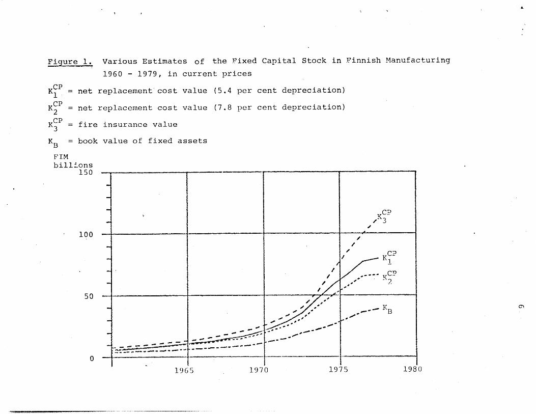
Figure 1. Various Estimates of the Fixed Capital Stock in Finnish Manufacturing

1960 - 1979, in current prices

K CP = net replacement cost value (5.4 per cent depreciation)1

K = net replacement cost value (7.8 per cent depreciation)

CPK = fire insurance value3

KB = book value of fixed assets

FIMbillions

150

CD

K

100 -

101

CP

- ... K

------ B

0-

1970 1975 19801965

7

according to the so-called FIFO (first-in-first-out)

principle is applied in taxation. It is, however,

permissible to enter into the accounts certain future

inventory expenses; i.e., the inventories can be

undervalued. Since 1969, the maximum rate of under-

valuation has been 50 per cent of the acquisition cost

of inventories. Earlier the maximum rate was 100 per

cent. In effect this undervaluation means that

nowadays 50 per cent of the value of inventories (at

historic cost) can be regarded as expenses when

calculating the taxable income.

In this way, companies can create "hidden reserves",

or tax credits, which can at least to some extent be

regarded as comparable to other components of own

capital. This question will be discussed in the next

section when estimating the own capital of Finnish

manufacturing companies. The rationale behind this

undervaluation lies partly in the fact that during

inflationary periods the FIFO principle operates in

such a way that the increase in the value of inventorieE

is transferred to sales income and hence becomes

taxable income. Undervaluation is designed to at

least partially prevent these nominal capital gains

being subject to corporate income taxation. It is

worth mentioning that during the 1970s companies'

profitability levels did not allow full use of under-

valuation.

Figure 2 shows the book value of inventories (VO ) andCP 0

the estimated current value of inventories (VO ).

In addition, Figure 2 shows the value of the financial

assets of manufacturing companies. This series has

been taken directly from the enterprise statistics

(balance sheet data), but can be regarded as reliable

Figure 2. Various Estimates of Inventories and Financial Assets in Finnish

Manufacturing 1960 - 1979

VOCP = current value of inventories

VOB = book value of inventories

RO = value of all financial assetsnet

RO = value of net financial assets

FIMbillions

40

30 UrOP

2- B

10

1965 1970 1975 1980

9

data. The series RO includes all financial assets,

that is, cash, all kinds of deposits, accounts

receivables and some other financial items. The second

series shown in Figure 2, RO net, is gross financial

assets less accounts payable and it is regarded as an

approximation of financial assets for net working

capital purposes.

We are now in a position to present our estimates for

total capital. The concept of total capital used in

this study includes

total physical assets, i.e., the stock of

fixed assets (K) and inventories (VO)

all financial assets (RO)

Thus tota] capital (at current prices) is the sum of

these three components,

(2) TC = K + VO + RO

In addition, we employ some other definitions of

capital in the rate of return calculations. Total

physical capital is defined as

(3) TFC =K + VO

Figure 3 shows various estimates of total capital. The

time series TC is based on the fixed capital stockCP

estimate K1 , whereas the series TC is based on the1 2CP

value of K2 Figure 3 also shows the value for total

physical capital (TFC) and the book value of total

capital (TC B employed by Finnish manufacturing

.pi 10companies.-

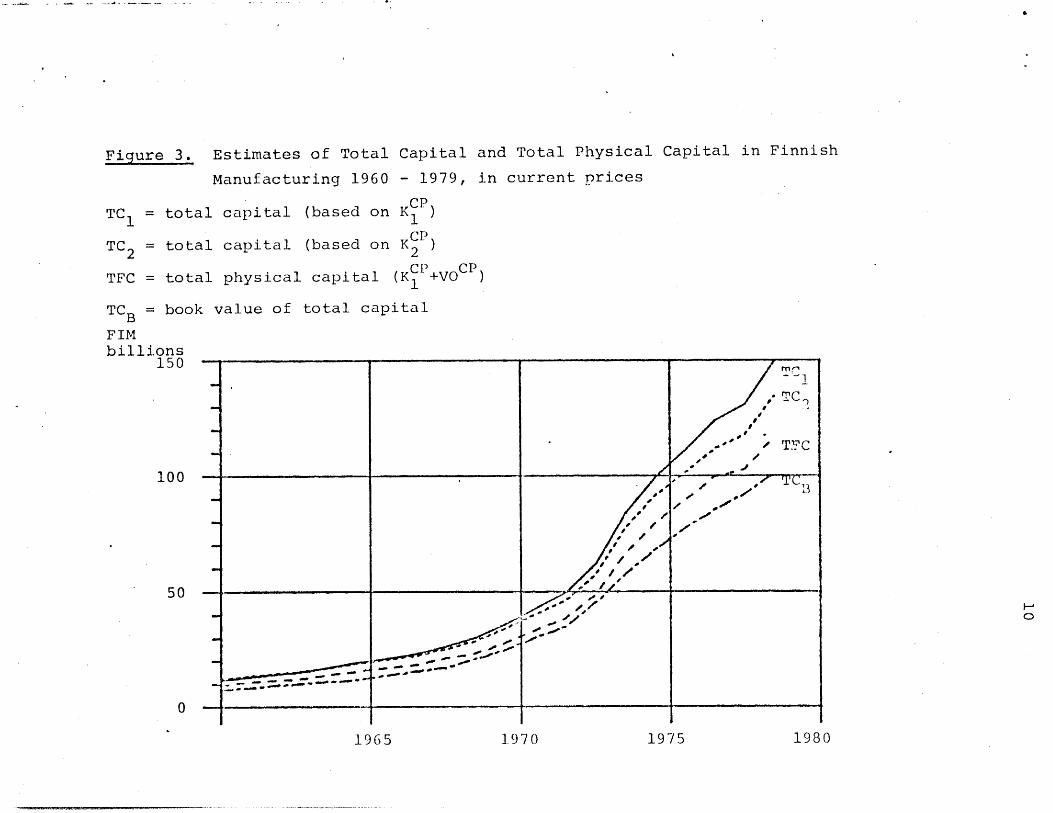
Figure 3. Estimates of Total Capital and Total Physical Capital in Finnish

Manufacturing 1960 - 1979, in current prices

CPTC = total capital (based on KC )

11CP

TC = total capital (based on K2 )2 C

TFC = total physical capital (K1 +VO )

TCB = book value of total capital

FIMbillions

150

100 T(

50

0

1970 19751965 1980

11

2.2. Own Capital and Debt Ratios

The analysis in the previous section provides the

basis for estimating the "true" value of the own

capital of Finnish manufacturing companies. In section

2.1 we developed various estimates of the net replace-

ment value of total capital and we found that these

were much greater than the book value of total capital.

A reliable estimate of the value of the total debt of

the same companies can be obtained from the official

enterprise statistics. The measure of debt capital

includes all short- and long-term credits as well as

domestic and foreign debt.

The difference between the current replacement and

book values of total capital is an estimate of the

total amount of various "hidden reserves" held by

manufacturing companies. It could be argued that part

of these reserves belong to own capital and part are

due to deferred tax liabilities in the form of tax

credits. An extreme view which has been put forward is

that all these reserves should be included in the

concept of total own capital.1 1

Figure 4 shows various estimates of own capital held

by manufacturing companies. The lowest value is

obtained for an estimate of pure equity capital (E)

taken directly from the enterprise statistics. Equity

capital forms the basis for the dividend payments of

manufacturing corporations. The second measure shown

in Figure 4 is the total value of own capital as taken

from the enterprise statistics (OC1 ). In addition to

equity capital this concept also includes various

"official" reserves and financial transfer and valua-

tion items.12 It can be seen that the share of'these

Figure 4. Estimates of Own Capital in Finnish Manufacturing 1960 - 1979,

in current prices

E = equity capital (book value)

OC = total own capital (b'ok value)

OC2 = estimated own capital (maximum value)

OC = estimated own capital (half of hidden reserves included in own capital)

FIMbillions

80

60

40

20

0

0C

- .OC

.00 ,

oo 0oO

/E

1975 19801965 1970

13

items in total "official own capital" has risen con-

tinuously, being currently over 50 per cent.

The third measure of total own capital (OC) is the

basis for most of our calculations in this paper. It

represents a compromise between the extreme interpreta-

tions of the role of total "hidden reserves" (see

footnote 11). We have assumed that one half of these

reserves belong to own capital and one half to debt

capital in the form of interest-free loans.1 3

The last measure of total own capital (OC 2) is based

on the extreme assumption that all "hidden reserves"

belong to own capital. The magnitude of these reserves

is mainly attributable to inventory undervaluation and

accelerated depreciation rules. The size of inventory

reserves can be roughly seen from Figure 2 as the

difference between VO ~ and VOB. Depreciation charges

for tax purposes have on average exceeded true econ-

omic depreciation at-replacement cost value.

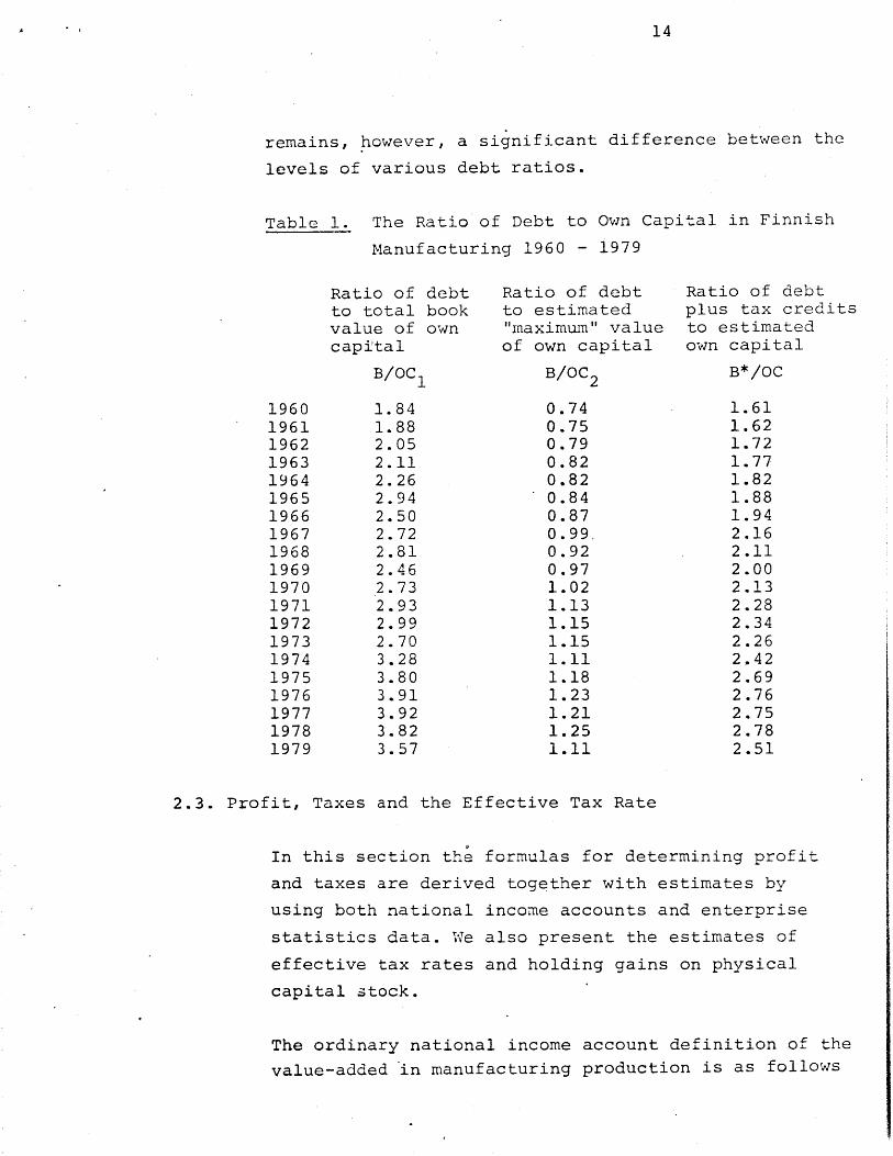
Table 1 shows three different measures of the ratio of

debt to own capital. The highest value for this ratio

is obtained when own capital includes only the

"official" amount as shown in book accounts. This

ratio is denoted as B/O C where B is total debt at

book value. The lowest value for debt to own capital

ratio results when all "hidden reserves" are included

in own capital (B/OC2). The mean value for this ratio

is obtained when half of the reserves are included in

debt (B*/OC). 12

From Table 1 it can be seen that all of these debt

ratios have increased in a trendwise manner. There

14

remains, however, a significant difference between the

levels of various debt ratios.

Table 1. The Ratio of Debt to Own Capital in Finnish

Manufacturing 1960 - 1979

Ratio of debtto total bookvalue of owncapital

B/OC1

1.841.882.052.112.262.942.502.722.812.462.732.932.992.703.283.803.913.923.823.57

Ratio of debtto estimated"maximum" valueof own capital

B/OC2

0.740.750.790.820.820.840.870.99.0.920.971.021.131.151.151.111.181.231.211.251.11

Ratio of debtplus tax creditsto estimatedown capital

B*/OC

1.611.621.721.771.821.881.942.162.112.002.132.282.342.262.422.692.762.752.782.51

2.3. Profit, Taxes and the Effective Tax Rate

In this section the formulas for determining profit

and taxes are derived together with estimates by

using both national income accounts and enterprise

statistics data. We also present the estimates of

effective tax rates and holding gains on physical

capital stock.

The ordinary national income account definition of the

value-added in manufacturing production is as follows

19601961196219631964196519661967196819691970197119721973197419751976197719781979

15

pQ = W + Deb + IR + 7b A,

e

= current price value-added production

= sum of wage- and social security payments

(total labour costs)

= economic value of depreciation

IR = net interest expenses'bTr = gross profit, i.e. profit before taxes

The values for the variables pQ and W are taken from

the national income accounts data for the manufacturing

sector. An estimate of economic depreciation charges

is calculated along with the fixed capital stock

estimates. The series for net interest expenses (all

interest payments minus interest receipts) originate

from the enterprise statistics.

From the basic formula for value-added production, the

variable "profit before taxes" becomes following

(5) 7b = pQ - W - Deb - IR

The variables pQ, W and IR are the same in all our

calculations, but the variable Deb varies according to

which depreciation coefficient is used (5.4 or 7.8 per

cent, see section 2.1).

Operating income (net) is defined as

(6) OI = 7a + T + IR

where

,a = profit after taxes

T = direct corporate taxes (paid)

(4)

wher

pQ

W

Deb

16

We thus have

b =7a + T(7)

Table 2 shows the percentage distribution of operating

income into its three components.

Table 2. The Distribution of Operating Income into

Its Components (percentage)

Net profit

72.5171.1862.1264.6964.2258.4553.3252.6061.6772.8972.7758.9360.3663.7269.7945.7332.2122.1246.8657.98

Taxes

17.7417.7021.4318.4717.6619.2621.3818.4413.64

9.618.58

11.029.198.546.46

11.5715.0414.028.568.27

Interest

9.7511.1216.4516.8418.1322.2925.3028.9624.6917.5018.6530.0630.4527.7423.7542.7052.7563.8544.5833.75

It can be seen from Table 2 that the relative propor-

tion of interest expenses has risen continuously

reflecting the trendwise increase in the debt-own

capital ratio (see Table 1).

We next present the estimates of actual and effective

tax rates for Finnish manufacturing companies. The

actual tax rate is as follows

19601961196219631964196519661967196819691970197119721973197419751976197719781L79

17

(8)TU TI

where

T = paid taxes

TI = taxable income (profit before taxes) at book

value

The effective tax rate is

(9)T

f 7T=

thus it is the share of paid company taxes in econ-

omic (true) profit before taxes. Table 3 presents

estimates of these tax rates.13

Table 3. Actual and Effective Tax Rates in Finnish

Manufacturing

Actualtax rate

U

0.450.560.600.560.550.560.600.590.550.490.460.500.440.410.430.640.791.520.690.46

Effectivetax rate(based ondepreciationcoefficient5.4 per cent)

U f

0.200.200.260.220.220.250.290.260.180.120.110.160.130.120.080.200.320.390.150.12

Effectivetax rate(depreciationcoefficient7.8 per cent)

Uf2

0.230.230.310.270.260.310.360.330.220.130.120.190.160.140.100.270.480.760.190.14

19601961196219631964196519661967196819691970197119721973197419751976197719781979

18

It can be seen that the effective tax rates are only

about half the actual rates. This is due to the fact

that taxable income is reduced by accelerated deprecia-

tion and inventory undervaluation as compared to the

estimates of "true" profit before taxes.

In calculating the values of "true" profit in this

section we have not taken into account the effect of

capital gains or holding gains on existing capital

stock. This is done separately here because the role

of holding gains on physical capital is a matter of

some dispute. The nominal relative holding gain on

total physical capital (TFC) is defined as

(l+g CUR)(10) 1 + g =

(gCON)

where

CUR = annual rate of increase of the current value of

total physical capital (TFC)

CON = annual rate of increase of the volume of TFC

(1975 prices)

Thus the variable g is the annual rate of increase in

the implicit price index for total physical capital. 4

Relative real holding gains are measured by the formula

(11) g= (1+cj)r (l+gCP)

Hence real holding gains are measured relative to the

rise in the general price level (gCP = rate of

increase in the consumer price index).

In Table 4 are shown the percentage nominal and real

holding gains. The absolute values of these ficures

are given in the Appendix (Table A3) in addition to

19

the estimates for holding gains on fixed capital

stock. It can be seen that if real holding gains are

zero then operating income as calculated above equals

total real income. The role of holding gains will also

be discussed in the next section when calculating real

and nominal rates of return on total capital.

Table 4. Nominal and Real Holding Gains in Finnish

Manufacturing 1961 - 1979, per cent

NHG, RHG,per cent per cent

1961 1.63 -0.181962 3.61 -0.821963 4.74 -0.121964 5.52' -4.381965 5.60 0.751966 2.11 -1.761967 6.26 1.631968 10.44 0.801969 4.71 2.441970 8.22 5.341971 10.25 3.531972 11.78 4.791973 19.78 8.181974 24.60 6.551975 13.50 -3.671976 10.28 -3.541977 10.56 -1.851978 10.74 2.961979 9.14 1.72

We can observe from Table 4 that percentage nominal

holding gains increased rather rapidly in the 1970s

compared to the 1960s. Real holding gains were on

average almost zero in the 1960s and amounted to less

than two per cent on average in the 1970s. Although

the relative size of real holding gains seems to be

rather low, they have been quite large in absolute

terms in some years. The year-to-year variations in

holding gain estimates should, however, be regarded

with caution because of difficulties in the measurement

of the composite price index for the total fixed

capital stock.

20

3. DEVELOPMENT OF THE RATE OF RETURN

ON TOTAL CAPITAL AND OWN CAPITAL

3.1. The Rate of Return on Total Capital

In this section we present the estimates of the real

rate of return on total capital for Finnish manu-

facturing companies in the period 1960 - 1979. The

main results are shown in Tables 5 and 6 and in

Figures 5 - 7, while some alternative estimates are

given in the Appendix. The means and standard devia-

tions for both sets of estimates are presented in

Table 7.

The nominal rate of return on total capital before

taxes is

bNB _ + IR + NHG

(12) RR - TTC

where the variables are measured as described in the

previous section. The absolute value of nominal hold-

ing gains on total physical capital is obtained by

multiplying the current value of TFC by the relative

nominal holding gains. The absolute values for NHG are

given in the Appendix (Table A3). The after-tax

nominal rate of return (RR NA) is obtained by replacing

7b in formula (12) with post-tax profit (7 a). Total

capital as well as other concepts of capital used are

the averages of the beginning- and end-of-year values

of the corresponding-capital measures.

When g is the proportional rate of increase in the

implicit price index of total physical capital, then

NHG = gTC and we get the standard expression for the

real rate of return

21

(13) RRB = RR NB- g

and the equivalent formula for the real rate of returnRA

after taxes (RR ). Strictly speaking we should also

consider the effect of price changes on the value of

financial assets, but this is not taken into account

here because we are mainly interested in the value of

the appreciation of fixed capital and total physical

capital. From expressions (12) and (13), we obtain an

equivalent formula for the real rate of return on

-total capital (before taxes)

bRB _ + ±IR

(14) RR C=TC

which is the ratio of operating income to total

capital. In the formulas (13) and (14) it is assumed

that real holding gains are zero. The equivalentRA b a

formula for RR is obtained by replacing 7 with Tr

It was pointed out in section 2.3 that operating

income equals real total income only if real holding

gains on capital stock and inventories are zero. This

means that the composite price index of this stock

value rises at exactly the same rate as prices

generally. Including real holding gains (or losses) in

the measure of real income gives the second basic

formula for the real rate of return

RB _ Tb + IR + RHG(15) RR = _______

TC

and, taking into account the fact that the absolute

value of real holding gains equals g r TC (see equation

11), we obtair also a second formula for the relation-

ship between real and nominal rates of return

(16) RRRB = RRNB _ 9CP'#

-j22

where gCP. is the rate of increase in the general price

level (usually assumed to be the consumer goods price

level) .15

In all of the above cases, the real rate of returnRA

after taxes (RR ) is obtained by deducting taxes

actually paid from the estimated profit before taxes

to get post-tax profit (see section 2.3).

These general principles have been used to calculate

the real rate of return on alternative estimates of

total capital and total physical capital. In these

alternative estimates we have varied the concepts of

total assets and the depreciation coefficient on

fixed capital stock (see Table A4 in the Appendix).

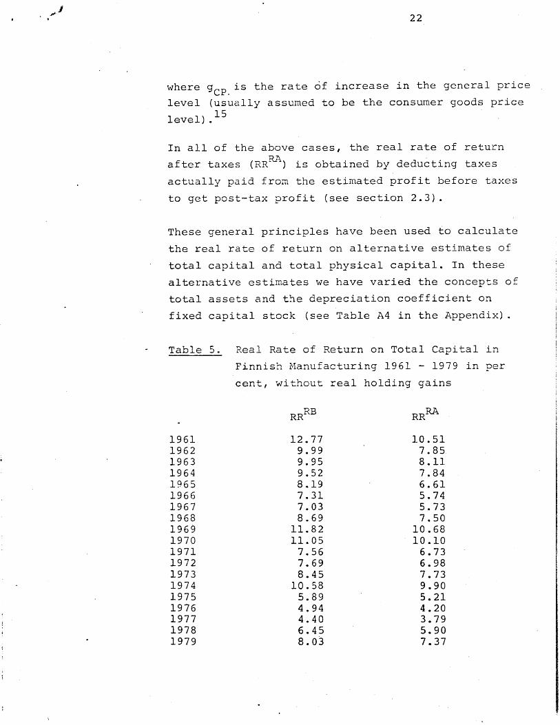
Table 5. Real Rate of Return on Total Capital in

Finnish Manufacturing 1961 - 1979 in per

cent, without real holding gains

RRRB RR

1961 12.77 10.511962 9.99 7.851963 9.95 8.111964 9.52 7.841965 8.19 6.611966 7.31 5.741967 7.03 5.731968 8.69 7.501969 11.82 10.681970 11.05 10.101971 7.56 6.731972 7.69 6.981973 8.45 7.731974 10.58 9.901975 5.89 5.211976 4.94 4.201977 4.40 3.791978 6.45 5.901979 8.03 7.37

23

Table 6. Real Rate of Return on Total Capital in

Finnish Manufacturing 1961 - 1979 in per

cent, including real holding gains

19611962196319641965196619671968,19691970197119721973197419751976197719781979

RRRB

12.619.289.855.798.835.828.379.37

13.8415.5910.5511.7015.6116.58

2.711.932.838.849.47

RRRA

10.357.148.014.117.264.257.108.19

12.7114.65

9.7210.9914.8915.90

2.031.182.218.288.80

From Tables 5 and 6 it can be seen that the average

effect of real holding gains on the estimates of the

real rate of return on total capital is not very large

(less than 1 per cent), but that the year-to-year

effects are much greater. The fairly small difference

between the levels of before- and after-tax measures

reflects the fact that the effective rate of taxation

on corporate income has been rather low (see section

2.3). These estimates of the "true" rate of return on

total capital are almost twice the size of the rate of

return on total capital at book-values.

Figure 5 shows the development of the real rate of

return on total capital (before and after taxes) and

of total physical capital (after taxes) including real

24

holding gains. Figure 6 shows the development of the

same series without holding gains. Figure 7 shows the

effect of real holding gains on the rate of return on

total capital after taxes on a year-to-year basis.

From these figures it can be seen that the annual

fluctuations in the real rate of return on total

capital in Finnish manufacturing have been very large.

On average, these series seem to reflect very well the

general cyclical fluctuations of the manufacturing

sector as well as the whole Finnish economy. As is

well-known, the year-to-year variations in the GDP of

the Finnish economy are among the highest of the OECD

countries.

In Table 7 we present means and standard deviations

for .selected measures of the real rate of return in

the Finnish manufacturing sector.

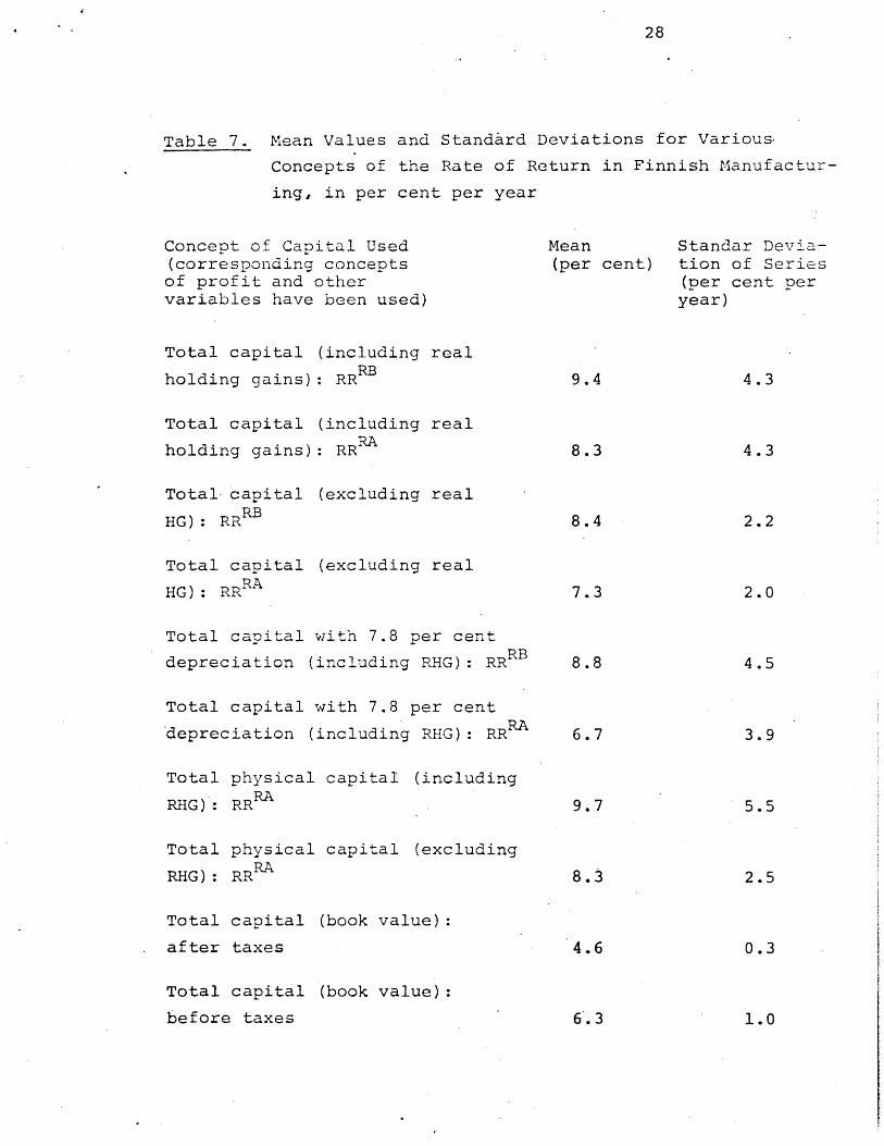
Some interesting observations can be made from Table 7.

The average real rate of return on total capital or

total physical capital before taxes varies between 8.4

and 9.4 per cent. The corresponding range for after-

tax figures is somewhat larger. We can thus safely

conclude that our measures for real rate of return are

rather insensitive to the choice of the estimate for

the capital variable. It can also be seen that the

standard deviations of estimates including real hold-

ing gains are about twice as large as those without.

There does not at present seem to be any method for

evaluating the reliability of the estimates of real

holding gains. However, we are tempted to express

some doubts about the year-to-year variations in RHG.

The third interesting observation is that the rate of

return on total capital measured at book value does

not vary very much. This is basically due to the fact

that, during periods of weak profit development,

Figure 5. Real Rate of Return on Total Capital in Finnish Manufacturing

1961 - 1979, in per cent, including real holding gains

RRTCB = total capital before taxes

RRTCA = total capital after taxes

RRTFCA = total physical capital after taxes

RR, %

20

15

RRTFQA

20 - - RRTCB\ \RRTICA

i-/0, P

I,'

5| A||

0 Odle

0

1965 1970 1975 1980

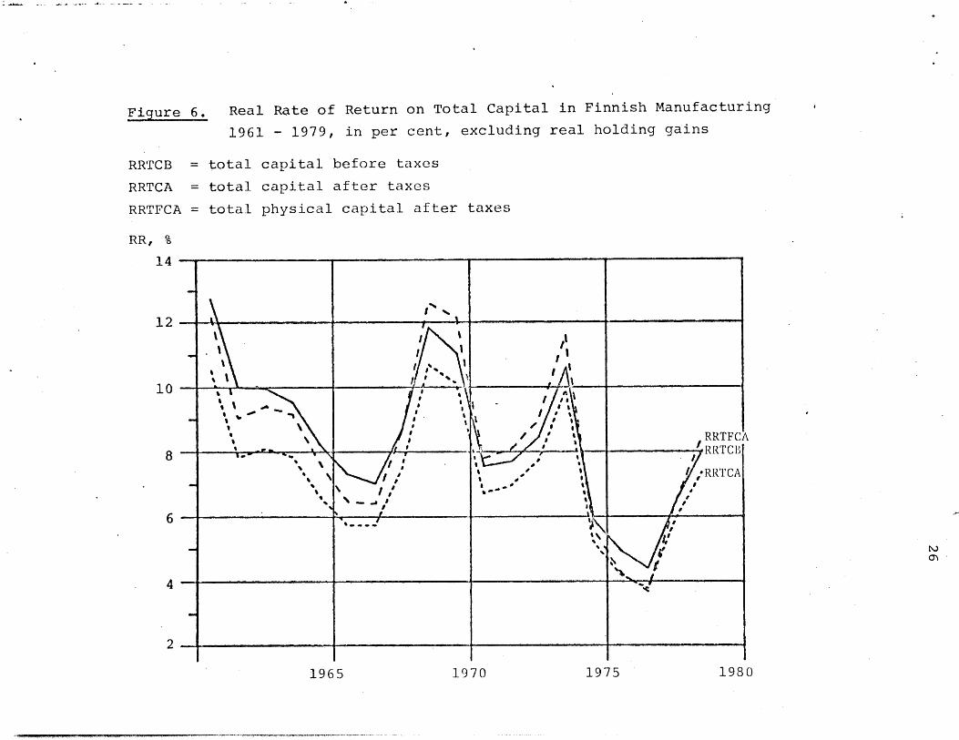
Figure 6. Real Rate of Return on Total Capital in Finnish Manufacturing

1961 - 1979, in per cent, excluding real holding gains

RRTCB = total capital before taxes

RRTCA = total capital after taxes

RRTFCA = total physical capital after taxes

RR, %

14

12

10 - -

\ -

RRTFCA

RRTCB

2

1965 1970 1975 1980

Figure 7. The Effect of Real Holding Gains on the Real Rate of Return

on Total Capital in Finnish Manufacturing 1961 - 1979

RRTCG = rate of return including RHG (after taxes)

RRTC = rate of return excluding RHG (after taxes)

RR, %

20

15

10

- PRRTCG

I , RRTC

5

0P

1965 1970 1975 1980

28

Table 7. Mean Values and Standard Deviations for Various.

Concepts of the Rate of Return in Finnish Manufactur-

ing, in per cent per year

Concept of Capital Used(corresponding conceptsof profit and othervariables have been used)

Total capital (including real

holding gains): RRRB

Total capital (including real

holding gains): RR RA

Total- capital (excluding real

HG): RRRB

Total capital (excluding real

HG): RRRA

Total capital with 7.8 per cent

depreciation (including RHG): RRRB

Total capital with 7.8 per cent

depreciation (including RHG): RR RA

Total physical capital (including

RHG): RRR

Total physical capital (excluding

RHG): RR

Total capital (book value):

after taxes

Total capital (book value):

before taxes

Mean Standar Devia-(per cent) tion of Series

(per cent peryear)

9.4 4.3

8.3 4.3

8.4 2.2

7.3 2.0

8.8 4.5

6.7 3.9

9.7 5.5

8.3 2.5

4.6 0.3

6.3 1.0

29

net interest expenses have risen sharply both in

absolute and relative terms.

3.2. The Rate of Return on Own Capital

The rate of return on own capital has been estimated

by means of two different methods. The first is based

on the ratio of profits to estimated own capital. This

calculation is analogous to that of the rate of return

on total capital. The basic formula for the rate of

return on own capital is thus

R Tr(17) RR O '

where 7 is estimated profit (after taxes) and OC is

the current value of own capital (see section 2.2).

The results derived by formula (17) can be interpreted

as values for the "real" rates of return on own

capital. The nominal rate of return could in principle

be calculated by adding the rate of increase in the

general price level to the values given by (17).

Table 8 shows the results for selected values of own

capital. In section 2.2 we discussed the methodol-

ogical questions connected with various concepts of

the estimates of own capital (see also footnote 11).

30

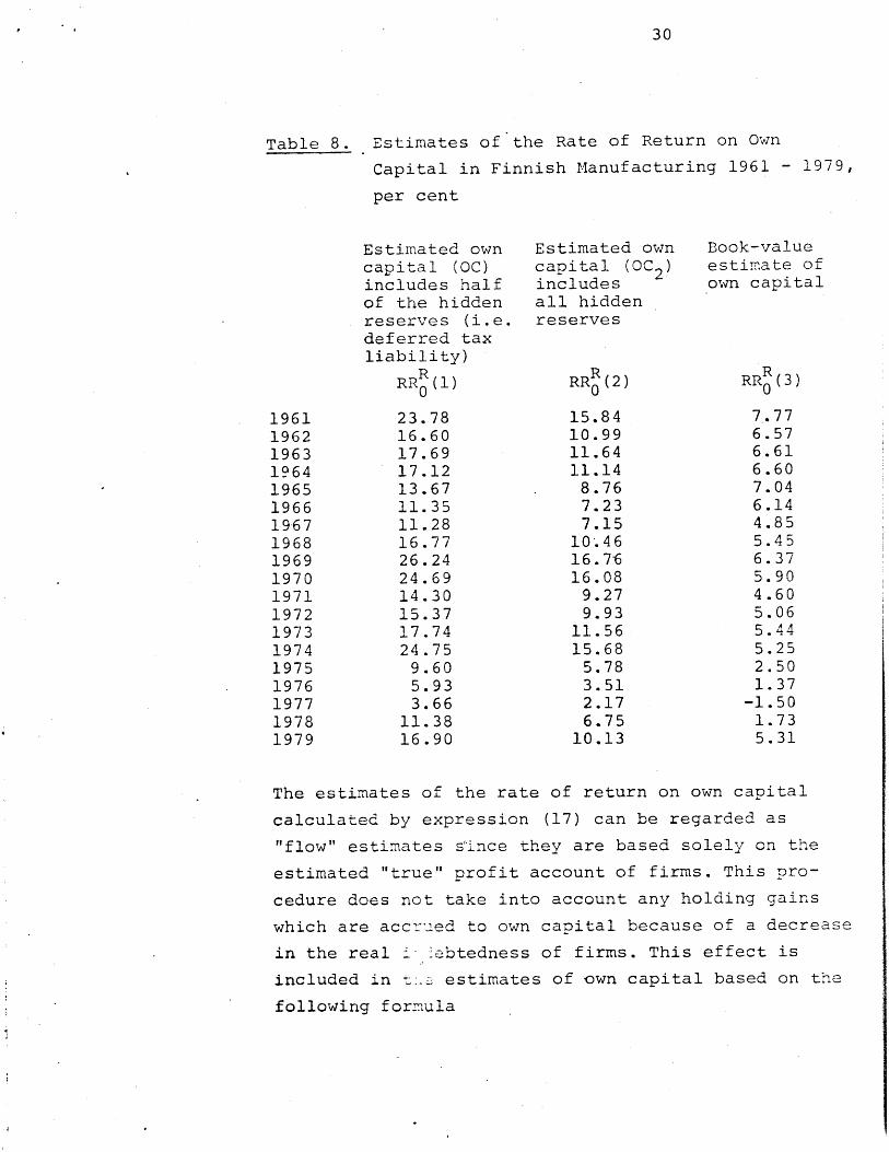
Table 8. Estimates of the Rate of Return on Own

Capital in Finnish Manufacturing 1961 - 1979,

per cent

Estimated owncapital (OC)includes halfof the hiddenreserves (i.e.deferred taxliability)

RRR (1)

23.7816.6017.6917.1213.6711.3511.2816.7726.2424.6914.3015.3717.7424.759.605.933.66

11.3816.90

Estimated owncapital (OC 2)includesall hiddenreserves

RR (2)

15.8410.9911.6411.148.767.237.15

10.4616.7-616.089.279.93

11.5615.685.783.512.176.75

10.13

Book-valueestimate ofown capital

RR (3)

7.776.576.616.607.046.144.855.456.375.904.605.065.445.252.501.37

-1.501.735.31

The estimates of the rate of return on own capital

calculated by expression (17) can be regarded as

"flow" estimates s'ince they are based solely on the

estimated "true" profit account of firms. This pro-

cedure does not take into account any holding gains

which are accrued to own capital because of a decrease

in the real icbtedness of firms. This effect is

included in t. estimates of own capital based on the

following formula

1961196219631964196519661967196819691970197119721973197419751976197719781979

31

R RR x TC- r x B(18) RROC TC- B

where

RR = real rate of return on total capital

TC = total capital

r = real rate of interest

B = total debt

This general formula can be shown to lead to the

following form

R R R B(19) RR c- RR + (RRR-r)

The real rate of interest (r) is defined as usual by

the expression

(20) r =1 + p

where

i = nominal rate of interest

p = rate of increase in the general price level

(taken to be gCP, see formula (11))

From formula (19) it can be seen that the rate of

return on own capital exceeds the rate of return on

total capital if the latter is greater than the rate

of interest.16 In that case, an increase in leverage

(B/OC) also tends to increase the return on own

capital.

The difference between the rate of return estimates

of own capital obtained by formulas (17) and (19) is

largely due to the factor ( )B, which measures the1+p 17decrease in the real indebtedness of firms.

32

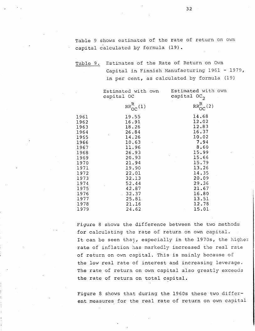
Table 9 shows estimates of the rate of return on own

capital calculated by formula (19).

Table 9. Estimates of the Rate of Return on Own

Capital in Finnish Manufacturing 1961 - 1979,

in per cent, as calculated by formula (19)

Estimated withcapital OC

RR C(1)C

19.5516.9118.2626.8414.2610.6311.9626 . 9320.9321.9419.9022.0132.1352.4442.8732.3725.8121.1624.62

own Estimated with owncapital OC 2

RR C(2)

14.6812.0212.8316.3710.02

7.948.60

15.9915.6615.7913.2614 .3520.0929.3621.6716.8013.5112.7815.01

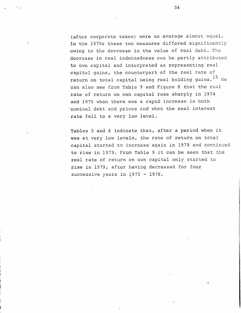
Figure 8 shows the difference between the two methods

for calculating the rate of return on own capital.

It can be seen that, especially in the 1970s, the higher

rate of inflation has markedly increased the real rate

of return on own capital. This is mainly because of

the low real rate of interest and increasing leverage.

The rate of return on own capital also greatly exceeds

the rate of return on total capital.

Figure 8 shows that during the 1960s these two differ-

ent measures for the real rate of return on own capital

1961196219631964195519661967196819691970197119721973197419751976197719781979

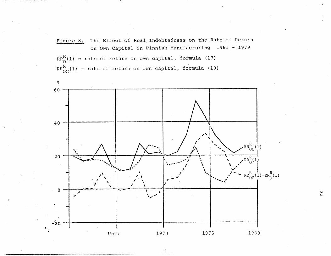
Figure 8. The Effect of Real Indebtedness on the Rate of Return

on Own Cap-ital in Finnish Manufacturing 1961 - 1979

RR (1) rate of return on own capital, formula (17)0

RR (1) = rate of return on own capital, formula (19)OC

60

40

RR 0C

20 \ ,RR (1

/ R R

000 %-RR RC(1)-RROR(1

0 \

-20.U

1970 1975 19801-965

34

(after corporate taxes) were on average almost equal.

In the 1970s these two measures differed significantly

owing to the decrease in the value of real debt. The

decrease in real indebtedness can be partly attributed

to own capital and interpreted as representing real

capital gains, the counterpart of the real rate of18

return on total capital being real holding gains. We

can also see from Table 9 and Figure 8 that the real

tate of return on own capital rose sharply in 1974

and 1975 when there was a rapid increase in both

nominal debt and prices and when the real interest

rate fell to a very low level.

Tables 5 and 6 indicate that, after a period when it

was at very low levels, the rate of return on total

capital started to increase again in 1978 and continued

to rise in 1979. From Table 9 it can be seen that the

real rate of return on own capital only started to

rise in 1979, after having decreased for four

successive years in 1975 - 1978.

35

4. RATE OF RETURN TO INVESTORS

In. the previous chapter we based the analysis of move-

ments in real profitability on the real rate of return

on total and own capital. The calculation of these

rates was based on the joint use of national income

accounts, industrial statistics and enterprise (balance

sheet) data. The rate of return measures can be inter-

preted as reflecting the attitudes and interests of

the companies themselves. In this chapter, we turn to

the use of capital market data. The behaviour of the

stock market can in principle be assumed to reflect

the attitude of the owners of the companies.

It is, however, important to emphasize that the capital

market does not play a very important role in the

financing of operations (investment) by Finnish manu-

facturing companies. The share of equity capital in

total capital (at book value) was about 10 per cent in

the 1970s. However, only part of the total equity

capital owned by manufacturing companies was quoted on

the stock exchange. In 1978, for example, the nominal

value of total equity capital in the manufacturing

sector was 8.3 billion marks (FIM). The nominal

(taxable) value of equity capital quoted on the stock

exchange was 3.0 billion marks, the market value being

4.3 billion marks.

The nominal rate of return to investors in companies

is calculated by the-formula

M(21) 1 RI = DIV + IRE + AE

MV

36

where

DIV = dividends

IRE = interest payments

AEM = change in the market value of equity capital

MV = total market value

Total market value is defined as

(22) MV EM + (OC -E) + B + TB

where

0C = total value of own capital (book value)

E = equity capital (book value)

B = total debt (book value)

TB = total amount of hidden reserves

EM = market value of equity capital (E)

The market value of the equity capital of the total

manufacturing sector is estimated by the formula

(23) EM = f x E

where f is the ratio of market value to nominal value

for manufacturing companies quoted on the stock

exchange. 19

The real rate of return to investors is calculated by

the usual formula

R(24) RI = RI - gCP

where

CP = rate of increase in the consumer goods

price index

37

Movements in nominal and real rates of return to

investors over the period 1961 - 1978 are shown in

Table 10.

Table 10. Nominal and Real Rates of Return to

Investors in Finnish Manufacturing

1961 - 1978, in per cent

RI RIR(nominal) (real)

1961 0.53 -1.281962 3.76 -0.701963 3.89 -0.981964 2.47 -7.891965 1.52 -3.291966 0.52 -3.411967 2.10 -2.451968 6.29 -3.281969 5.74 3.531970 6.16 3.431971 4.61 -1.881972 9.21 2.541973 8.19 -2.541974 0.43 -16.511975 2.42 -15.411976 1.96 -12.371977 2.85 -9.801978 4.99 -2.58

Average 3.76 . -4.16

As can be seen, the real rate of return has been

negative in most years. It was about -1.5 per cent in

the 1960s, but decreased sharply in the latter half of

the 1970s. This result is perhaps not very surprising

because the real interest rate on ordinary deposits

was also negative in- the same period (about -2 per

cent). We have also calculated the real rate of return

to investors by omitting the total amount of hidden

reserves from the market value. The result was by and

large similar, although the rates were somewhat higher

(-0.3 per cent in the 1960s and -5.7 per cent in the

1970s).

38

The nominal and real rates of return to equity owners

were calculated by the formulas

(25) REI DIV + AEM

EM

(26) REIR = REI -CP

The results are shown in Table 11.

Table 11. Nominal and Real Rates of Return to Equity

Owners in Finnish Manufacturing 1961 - 1978,

in per cent

REI RER(nominal) (real)

1961 -5.55 -7.361962 11.89 7.431963 11.98 7.111964 3.89 -6.461965 -3.42 -8.241966 -13.95 -17.891967 -2.59 -7.141968 33.04 23.481969 25.10 22.901970 27.02 24.291971 15.48 8.991972 37.19 30.521973 29.94 19.211974 -15.08 -32.021975 -2.02 -19.841976 -10.77 -25.101977 ,-4.42 -17.071978 19.83 12.27

Average 8.75 0.84

Table 11 shows that the rate of return on equity

capital has been much higher than the rate of return

on total invested capital (Table 10). It was positive

(0.84 per cent) on average over the whole period,

whereas the real rate of interest on ordinary deposits

39

was negative on average. From 1961 to 1973 the real

rate of return to equity investors averaged about 10

per cent, but in the period 1974 - 1977 it became

negative. This was a period of very poor economic

performance by the Finnish economy and, as we have

seen earlier (Chapter 3), the real rates of return on

total and own capital also declined appreciably. In

1978 the real rate of return on equity capital again

rose and became positive (12.27 per cent), as did also

the real rate of return on total capital (see Tables 5

and 6). Since 1978 the development of the Finnish

economy has been very favourable, with GDP rising 7 per

cent in 1979 and 5.5 per cent in 1980.

To some extent c h a n g e s in the real rate of

return to investors show similarities with the move-

ments of real profitability, although zhe levels of

these two sets of measures of manufacturing performance

are very different. We believe, however, that the

estimates of investors' rate of return should be

regarded as preliminary, and especially the analysis

of the development of real profitability in Finnish

manufacturing should be based on the real rate of

return on total and own capital (Chapter 3).

40

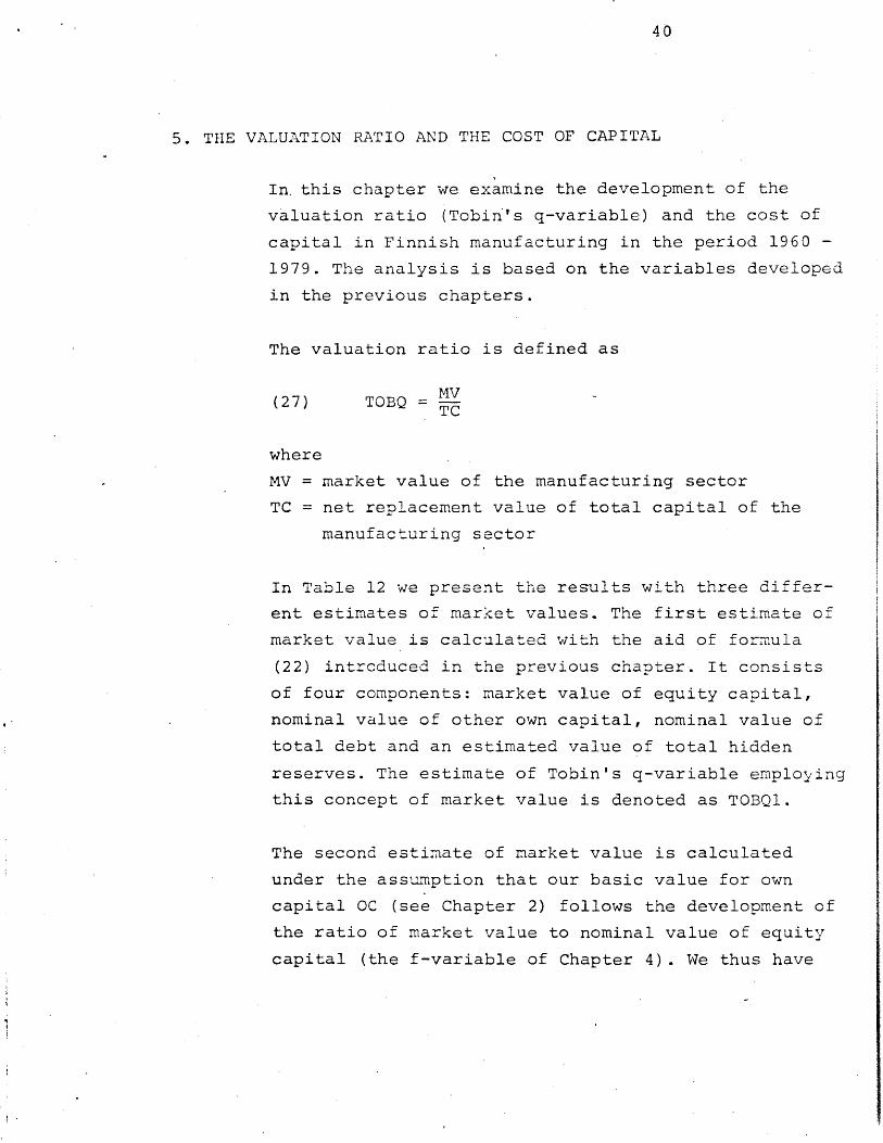
5. THE VALUATION RATIO AND THE COST OF CAPITAL

In. this chapter we examine the development of the

valuation ratio (Tobin's q-variable) and the cost of

capital in Finnish manufacturing in the period 1960 -

1979. The analysis is based on the variables developed

in the previous chapters.

The valuation ratio is defined as

(27) TOBQ MV

where

MV = market value of the manufacturing sector

TC = net replacement value of total capital of the

manufacturing sector

In Table 12 we present the results with three differ-

ent estimates of market values. The first estimate of

market value is calculated with the aid of formula

(22) introduced in the previous chapter. It consists

of four components: market value of equity capital,

nominal value of other own capital, nominal value of

total debt and an estimated value of total hidden

reserves. The estimate of Tobin's q-variable employing

this concept of market value is denoted as TOBQ1.

The second estimate of market value is calculated

under the assumption that our basic value for own

capital OC (see Chapter 2) follows the development of

the ratio of market value to nominal value of equity

capital (the f-variable of Chapter 4). We thus have

41

(28) MV2 = OCM + B + TB*

where

OCM = market value of estimated own capital OC

(includes total book value of own capital plus

half of the total hidden reserves)

B = total debt

TB* = estimated value of tax credits (half of the

value of total hidden reserves, i.e., deferred

tax liability)

The series for Tobin's q-variable calculated by means

of MV2 is denoted as TOBQ2.

The third measure of market value is defined as

(29) MV3 = OC +'B

where

OC M= market value of total book value of own capital

In this third measure of MV we have thus assumed that

the total book value of own capital (OC1) follows the

development of the f-variable. It has further been

assumed that "hidden reserves" do not affect the

market value. With this latter assumption we wanted to

check the effect of "hidden reserves" on the estimates

of market value. Tobin's q-variable based on the

estimate of MV3 is denoted as TOBQ3.

All three estimates of the valuation ratio are based

on our basic value for total capital (TCl), which

includes the net replacement cost value of fixed

capital and inventories as well as financial assets.

Estimates of the valuation ratio based on total physica.

capital are presented in the Appendix (see Table A7).

42

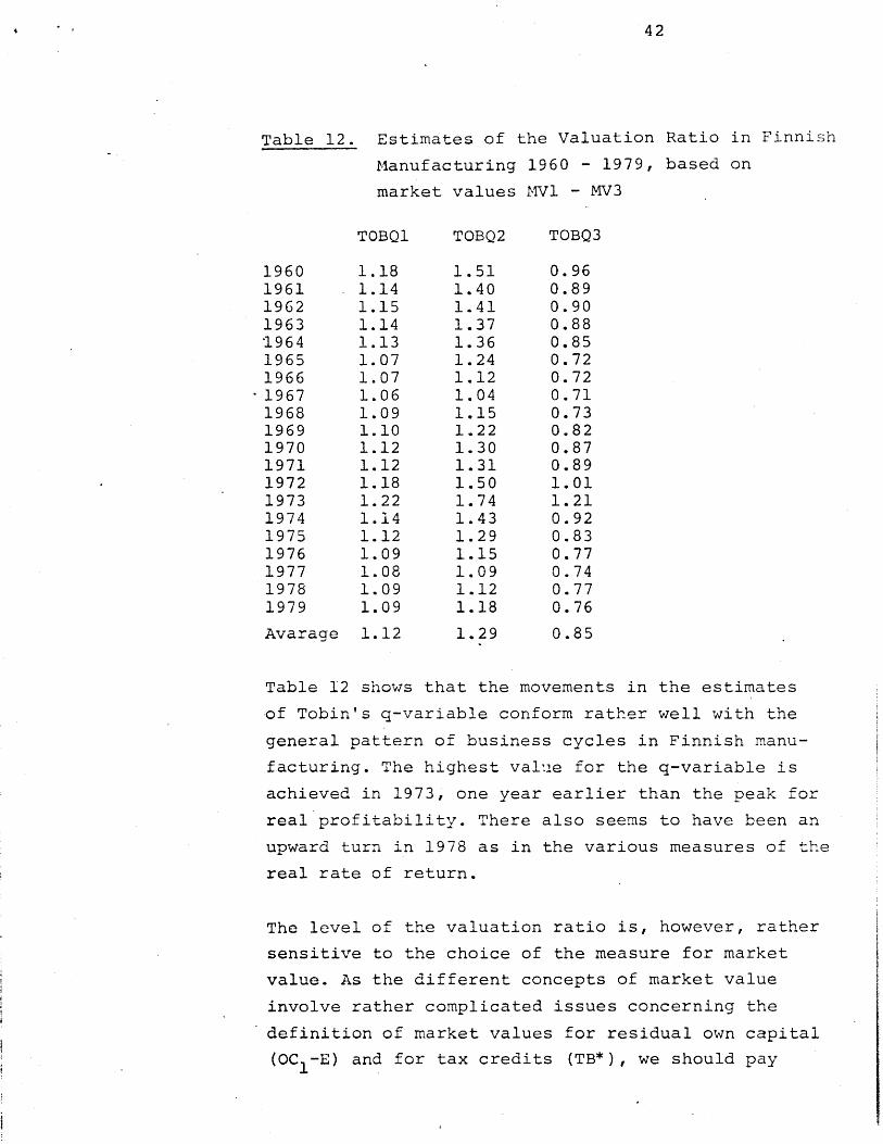
Table 12. Estimates of the Valuation Ratio in Finnish

Manufacturing 1960 - 1979, based on

market values MV1 - MV3

TOBQ1 TOBQ2 TOBQ3

1960 1.18 1.51 0.961961 1.14 1.40 0.891962 1.15 1.41 0.901963 1.14 1.37 0.881964 1.13 1.36 0.851965 1.07 1.24 0.721966 1.07 1.12 0.72

-1967 1.06 1.04 0.711968 1.09 1.15 0.731969 1.10 1.22 0.821970 1.12 1.30 0.871971 1.12 1.31 0.891972 1.18 1.50 1.011973 1.22 1.74 1.211974 1.14 1.43 0.921975 1.12 1.29 0.831976 1.09 1.15 0.771977 1.08 1.09 0.741978 1.09 1.12 0.771979 1.09 1.18 0.76

Avarage 1.12 1.29 0.85

Table 12 shows that the movements in the estimates

of Tobin's q-variable conform rather well with the

general pattern of business cycles in Finnish manu-

facturing. The highest value for the q-variable is

achieved in 1973, one year earlier than the peak for

real profitability. There also seems to have been an

upward turn in 1978 as in the various measures of the

real rate of return.

The level of the valuation ratio is, however, rather

sensitive to the choice of the measure for market

value. As the different concepts of market value

involve rather complicated issues concerning the

definition of market values for residual own capital

(OC -E) and for tax credits (TB*), we should pay

43

attention primarily to' the. c h a n g e s in the q-

variables (marginal q).

Figure 9 shows the development of TOBQ variables in

the period 1960 - 1979, while Figure 10 shows the

development of TOBQ2 and the real rate of return on

total capital (before taxes) over the same period.

Figure 10 indicates that changes in the q-variable and

the real rate of return have been rather similar during

the whole period. It can further be noticed that the

recovery of the manufacturing sector after its very

poor performance in the latter half of the 1970s has

been much better in terms of real profitability (RRR

than in terms of the valuation ratio.

We next turn to the analysis of the behaviour of the

cost of capital (discount rate) in Finnish manu-

facturing in the period 1961 - 1979. Basic financial

theory shows that the market value of a company equals

the capitalized value of the long-run income from

present assets (Y/p) plus the present value of future

growth opportunities (PVGO).21 Market value is hence

defined as

(30) MV = + PVGOp

Income (earnings) are defined by the expression

(31) Y = RR x TC

where

RR = rate of return

TC = total capital

Neglecting the PVGO term, we get the following formula

for Tobin's q-variable

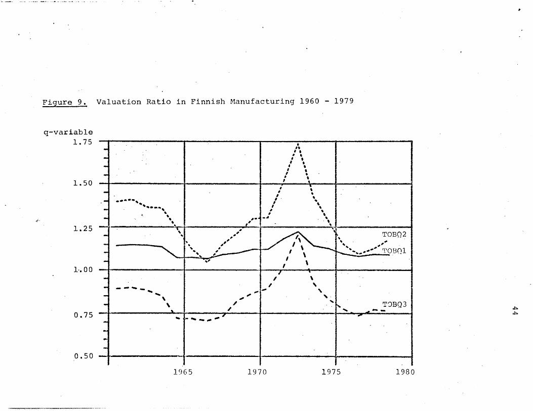
Figure 9. Valuation Ratio in Finnish Manufacturing 1960 - 1979

q-variable

1.75d9M

1.50\*, S

1.25

d *

1-. 0o0

1.00

0 .75 A

0.50

1965 1970 1975 1980

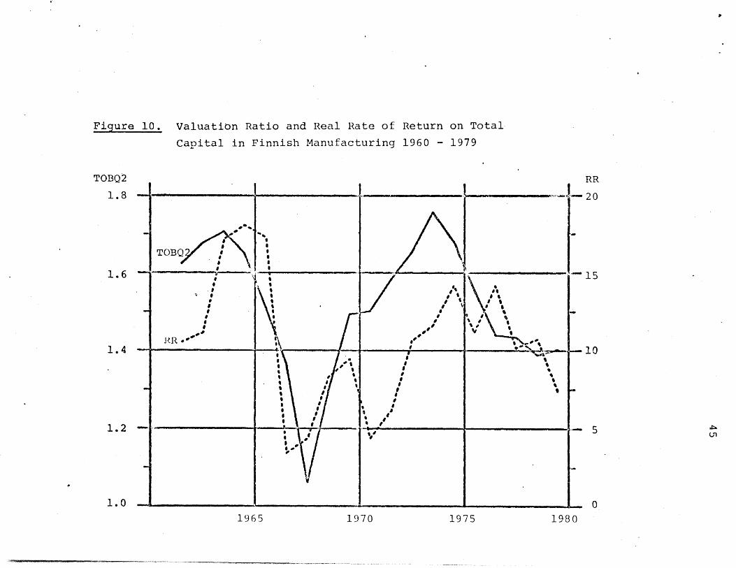
Figure 10.

TOBQ2

1.8

1.6

1.4

1.2

1.0

Valuation Ratio and Real Rate of Return on Total

Capital in Finnish Manufacturing 1960 - 1979

RR

20

15

10

5

0

1965 1970 1975 198 0

46

PR(32) q=

which for the cost of capital gives2 2

(33) p = RRq

In Table 13 are shown the estimates of the real cost

of capital in the case where the real rate of return

(RR R) includes real holding gains on total physical

capital. As the values for the real rate of return

are before corporate taxes, the real cost of capital

estimates are a pre-tax series. Measures of the post-

tax real cost of capital are provided in the Appendix

(see Tables A8 - A9). The three estimates of the real

cost of capital are calculated by means of the corre-

sponding estimates of the valuation ratio (TOBQ1-

TOBQ3). Table 13 also shows the real interest rate

(average 'ending rate).

Table 13. Estimates of the Real Cost of Capital and

the Real Rate of Interest in Finnish

Manufacturing 1961 - 1979, in per cent,

including real holding gains

P i P 2 p 3 r

1961 11.06 9.03 14.13 5.091962 8.10 6.58 10.35 2.461963 8.61 7.22 11.17 2.171964 5.11 4.26 6.80 -2.811965 8.27 7.11 12.28 2.531966 5.43 5.19 8.10 3.461967 7.88 8.04 11.87 2.871968 8.61 8.16 12.87 -1.701969 12.61 11.39 16.86 5.381970 13.91 12.02 18.03 4.901971 9.41 8.08 11.81 2.111972 9.90 7.78 11.55 1.411973 12.77 8.99 12.94 -1.601974 14.53 11.57 17.97 -6.071975 2.41 2.11 3.25 -6.621976 1.76 1.67 2.49 -3.671977 2.62 2.59 3.84 -2.361978 8.11 7.86 11.47 0.881979 8.70 8.06 12.39 1.14

Average 8.41 7.25 11.06 0.50Standard devi'-ation 3.71 3.26 4.50 .3.08

47

Table 13 shows that the movements in the real cost of

capital follow closely the development of real

profitability because there is more variability in the

real rate of return than in the q-variables. It can

also be seen that the real rate of interest is on

average much lower than the real cost of capital. This

is partly due to the fact that the real rate of return

on own capital is on average much higher than the real

rate of return on total capital (see sections 3.1 and

3.2).

Table 14 shows the estimates of the real cost of

capital in the case where the real rate of return on

total capital excludes real holding gains.

Table 14. Estimates of the Real Cost of Capital in

Finnish Manufacturing 1961 - 1979, in per

cent, excluding real holding gains

pl P 2 p3

1961 11.19 9.14 14.311962 8.72 7.08 11.141963 8.70 7.29 11.281964 8.40 7.00 11.181965 7.66 6.60 11.391966 6.82 6.52 10.181967 6.60 6.74 9.951968 7.98 7.57 11.931969 10.76 9.72 14.391970 9.86 8.52 12.781971 6.74 5.79 8.461972 6.51 5.11 7.591973 6.91 4.86 7.001974 9.28 7.38 11.471975 5.24 4.58 7.071976 4.52 4.29 6.391977 4.08 4.03 5.971978 5.92 5.73 8.371979 7.38 6.83 10.51

Average 7.54 6.56 10.07Standard deviation 1.94 1.58 2.53

48

From Table 14 it can be seen that changes in the real

cost of capital (excluding RHG) are very similar to

the P-variable which includes RHG. The most noticeable

difference between these two series for the cost of

capital is the much lower standard deviation in the

case where real holding gains are excluded.

Figures 11 and 12 show the development of the real

cost of capital (before taxes) with and without real

holding gains. In the mid-1970s the real cost of

capital fall to a rather low level, but it has been

rising again since 1978. There seems to be some indica-

tion of a declining trend in the cost of capital

without RHG, but no trend in the measure which in-

cludes RHG. Figure 13 shows the development of the

real cost of capital after corporate taxes. We could

argue that from the point of view of investment behav-

iour what matters is the behaviour of real profit-

ability relative to real capital costs. The average

real rate of return on total capital in Finnish manu-

facturing in the whole period 1961 - 1979 was 8.3

per cent (including RHG) and 7.3 per cent (excluding

RHG) after corporate taxes. The average values for the

real cost of capital measure P1 are almost the same,

i.e., 8.4 per cent and 7.5 per cent, respectively.

Because a lower value for P would imply a capital

shortage, it seems reasonable to state that "an

equilibrium situation" has existed in this sense in

the manufacturing sector. It also seems justified to

assume that the availability of or possibility to

acquire tax credits which are non-interest bearing has

been rather important in this respect.

During the period of very weak performance by the

Finnish economy (1976 - 1978), real profitability

Figure 11.

20

15

10

5

0

Real Cost of Capital in Finnish Manufacturing

1961 - 1979, in per cent, including real holding gains

and before corporate taxes

1975 19801965 1970

Figjure 12. Real Cost of Capital in Finnish Manufacturing

1961 - 1979, in per cent, excluding real holding gains

and before corporate taxes

15. 0

12.5

%4 2

10.0

% '4

ON ' \I% 0 I

c>

5.0

2.5

1970 1975 19801965

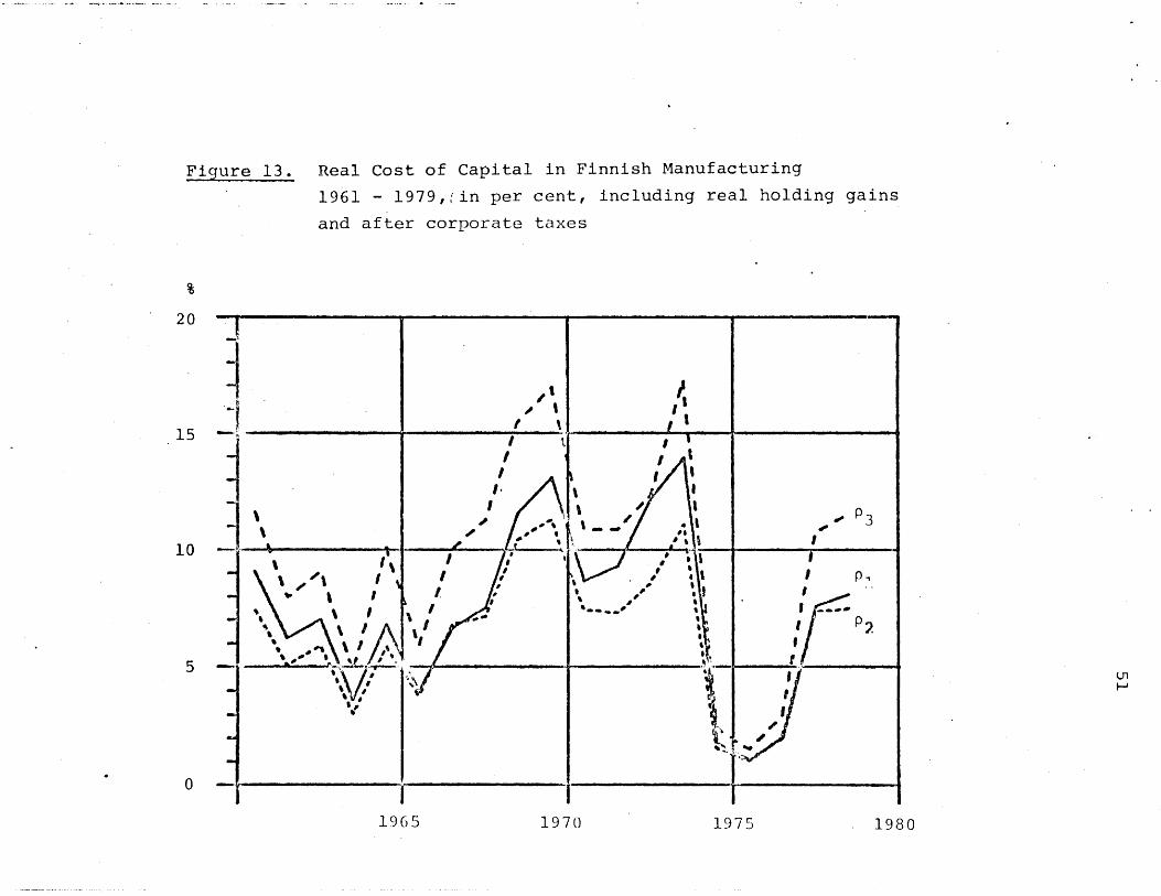
Figure 1-3. Real Cost of Capital in Finnish Manufacturing

1961 - 1979,; in per cent, including real holding gains

and after corporate taxes

20

15

I I

10 1410

5 -

0

1965 1970 1975 1980

52

declined proportionally more than the real cost of

capital. It is possible that this behaviour con-

tributed to the sharp decline in manufacturing invest-

ment during those years. It should, however, be

emphasized that the development of the cost of capital

relative to real profitability is not enough to

determine the behaviour of real investment outlays.

Most important in this respect is the behaviour of

real profitability as measured by the real rate of

return on total, capital (RR R) relative to the real

user cost of fixed capital stock. The real cost of

capital only measures the capital costs as regards the

use of financial capital, but not the cost of real

capital invested by the companies. The analysis of the

development of user cost in Finnish manufacturing is,

however, beyond the scope of this investigation.

53

6. DETERMINANTS OF THE RATE OF RETURN AND

THE EFFECTIVE TAX RATE

In this chapter we perform some statistical tests in

order to discover whether there has been trendwise

behaviour in the real rate of return on total and own

capital as well as in the effective tax rate. This is

done by means of standard regression analysis of the

determinants of the rate of return and the effective

tax rate.

The aim is not a thoroughgoing analysis of the factors

affecting the behaviour of these explanatory variables

because we think this would be rather difficult using

the single equation method. It can be assumed that

both the rate of return and the effective tax rate

depend upon the development of various price and cost

factors as well as economic policy variables. We shall

try to capture the effect of the general business

fluctuations in the manufacturing sector by two

variables, namely the annual percentage chance in the

GDP of this sector and the rate of capacity utiliza-

tion in the whole economy.23

In addition to a trend variable (time), we also use

the rate of price changes, which can take the form of

different price indexes. Our hypothesis is that the

price variable might reflect to a large extent the

impact of inflation on effective corporation income

tax rates. It could also be argued that the inflation

rate takes into account the impact of holding gains

in the case of the return on total capital and capital

gains (decrease in the real value of debt) in the case

of own capital. We have, however, also directly ex-

perimented with the tax rate variable as an independent

54

variable. Finally, similar models are tried with the

effective tax rate as the dependent variable.

Table 15 shows the results for the real rate of

return on total capital before (RR RB) and after taxes

(RR ) excluding real holding gains. Table 16 shows

the results for the rate of return including real

holding gains. The models are estimated by the ordinary

least squares method.

Tables 15 and 16 show that our equations explaining RR

are rather effective but crude. Profitability responds

to more than just inflation and the growth of GDP or

capacity utilization. This can be interpreted from the

rather low D-W statistics. Table 15 reveals almost

uniformally that the real rate of return on total

capital has behaved in a trendwise manner downwards,

as inspection of Figure 6 would have led us to expect

(p. 27). Both the production and the CU variables

seem to capture equally well the general business

fluctuations. Neither of the inflation rate variables

proves to be significant.

An interesting fact emerging from Table 16 in compariso

with the results of Table 15 is that there does not

seem to be any time trend in.real profitability if

real holding gains are included in the rate of return

measure. In this respect the role of capital gains (or

holding gains) is again rather crucial for our results

(see also Figure 5). Capacity utilization now seems

to capture the cyclical variations a little better

than the change in GDP. Generally there is not much

evidence of a significant price effect, although the

investment goods price variable has a positive effect

in two equations (2a and 2b).

Determinants of the Real Rate of Return on Total Capital in Finnish Manufacturing

1961 - 1979, RR excluding real holding gains

EquationNo.

la

lb

2a -

Dependentvariable

RR RB

RR

RRRB

RR

RRRB

RR

RRRB

RRRA

2b

3a

3b

4a

4b

Independent variables

Trend

-0.24(3.43)

-0.16(2.19)

-0.24(3.90)

-0.16(*2.62)

-0.15(1.94)

-0.06(0.76)

-0.14(1.80)

-0.05(0.70)

Production1 CU2

0.26(3.85)

0. 37(3.94)

0.31(4.27)

0.31

(4.50)

35.94(3.18)

39.34(3.66)

40.38(3.28)

42.81(3.65)

Inflation/

CP 3

0.12(1.22)

0.13(1.29)

Inflation/

IP4

0.11(1.71)

0.12(2.07)

-0.05(0.53)

-0.04(0.46)

-0.04(0.56)

-0.03(0.45)

Note:

t statistics appear in parentheses under the coefficients.1. Annual percentage change in real GDP of manufacturing sector.

2. Rate of capacity utilization.3. Annual percentage change in consumer price index.

4. Annual percentage change in investment goods price index.

0.70

0.62

0.72

0.67

0.64

0.59

0.64

0.59

D-W

1.50

1.50

1.50

1.63

1.27

1.34

1.27

1.34

Table 15.

the Real Rate of Return on Total

1961 - 1979, RR including real holding gains

EquationNo.

2a

2b'

Dependentvariable

RRRB

RR RA

RRRB

RR

RRRB

RR RA

RRRB

RRRA

3b

4b

Independent variables

Trend

-0.06(0.30)

0.03(0.16)

-0.20(1.48)

-0.11(0. 84)

0.16(1.15)

0.16(1.04)

0.15(1.13)

0.16(1.04)

Production CU

0.70(2.87)

0.71(2.84)

0.71(4.58)

0.71(4.57)

102.85(4.91)

108.37(4.62)

104.11(4.32)

108.37(4.62)

CP

0.10(0.37)

0.11(0.39)

0.41(3.06)

0.42(3.16)

-0.18(1.05)

-0.17(1.01)

0.04(0.61)

0.03(0.25)

LU,CT)

Note: see Table 15.

IP -

0.44

0.42

0.66

0.67

0.67

0.67

0.66

0.65

D-W

1.61

1.57

2.31

2.32

1.86

1.90

1.80

1.81

Capital in Finnish ManufacturingTable 16. Determinants of

57

As a general remark we can state that the GDP (or CU)

variable accounts for about 40 - 50 per cent of the

explanation and the trend variable for about 30 per

cent in the models of Table 15. The equivalent per-

centages in Table 16 are 50 - 60 and 10 - 2-0,

respectively.

We also carried out some tests with the effective tax

rate as an independent variable. It proved to be

significantly negative and took the role of GDP (or

CU) as a measure of general business fluctuations.

This can be interpreted to mean that the effective tax

rate behaves in a countercyclical manner. This latter

aspect was tested with a direct model of the effective

tax rate. The result can be seen from the following

equation:

UFl = 2.17 - 0.006TREND - 1.98 CU(5.66) (2.56) (5.09)

R = 0.63 D-W = 1.81

The explanatory variable was UFl (see Table 3, Chapter

2) and the independent variables are as in Table 15.

The estimation period was 1961 - 1979. This equation

shows that there is a downtrend in the effective tax

rate and that UF varies countercyclically (see also

Table 3, p. 17).

Finally, we used regression methods to examine the

determinants of the real rate of return on own

capital. The dependent variables are those constructed

in Chapter 3 (section 3.2). The results for the real

rate of return calculated by formula (17) are shown in

Table 17. It should be remembered that this formula

does not take into account the effect of capital gains

58

for the rate of return on own capital. Capital gains

are taken into account by formula (19), in which case

an-increase in leverage (debt-equity ratio) raises the

rate of return on own capital if the rate of return on

total capital exceeds the real rate of interest. TheR

results produced by formula (19) with RROC as an ex-

planatory variable are given in Table 18.

RTable 17 shows some evidence of a downtrend in RR0 ,

although the trend factor is not significant in all

the equations. Changes in the production and the

capacity utilization variables seem to reflect equally

well business variations, and the inflation rate is

not significant. We also tried the other price

variable used in Tables 15 and 16, but it also

proved not to be uniformally significant.

Table 18 shows that the trend variable is either in-

significant or shows some sign of uptrend, contrary to

the results of Table 17 with RR variables. Capac-iy

utilization seems to better reflect general business

conditions than the production variable. The most

interesting observation is that the inflation rate

now has a positive effect on the real rate of return

on own capital. This effect is especially strong if

the price variable is the price index used in the

calculation of holding gains. Thus it seems likely

that the inflation rate reflects the effect of real

capital gains due to the decline in the value of the

real debt burden of the manufacturing sector.

The RROC variables used in the equations of Table 18

were calculated by means of the real rate of return on

total capital including real holding gains (see

formula (19)). Similar models were also tested in the

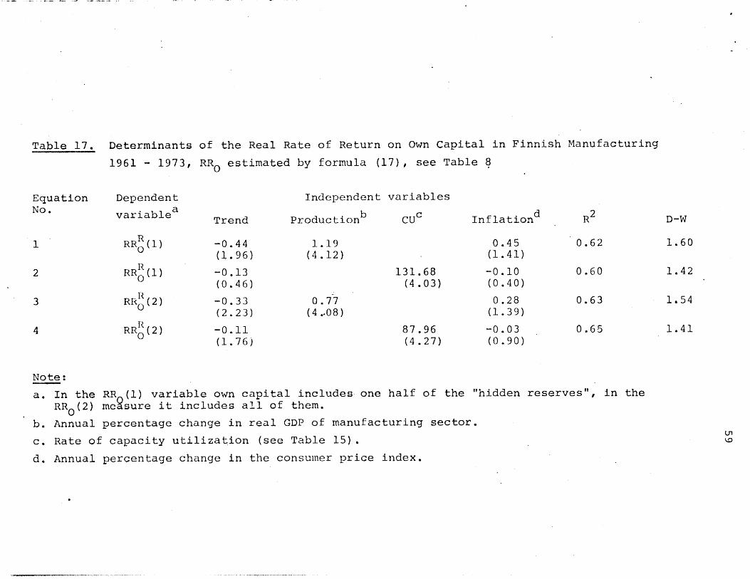
of the Real Rate of Return on Own Capital in Finnish Manufacturing

1961 - 1973, RR0 estimated by formula (17), see Table 8

EquationNo'

2

3

4

Dependent

variablea

RR (1)0

RRR (1)0

RRR(2)

RR (2)

Trend

-0.44(1.96)

-0.13(0.46)

-0.33(2.23)

-0.11(1.76)

Independent

Productionb

variables

CUc

1.19(4.12)

131.68(4.03)

0.77(4..08)

87.96(4.27)

Inflationd

0.45(1.41)

-0.10(0.40)

0.28(1.39)

-0.03(0.90)

Note:

a. In the RR (1) variable own capital includes oneRR0 (2) measure it includes all of them.

half of the "hidden reserves", in the

b. Annual percentage change in real GDP of manufacturing sector.

c. Rate of capacity utilization (see Table 15).

d. Annual percentage change in the consumer price index.

0.62

0.60

0.63

0.65

D-W

1.60

1.42

1.54

1.41

Table 17. Determinants

Table 18. Determinants

1961 - 1979,

of the Real Rate of Return on Own Capital in Finnish Manufacturing

RROC estimated by formula (19), see Table 9

EquationNo.

1

2

3

4

5a

Dependentvariable

RR C(1)OC

RR (1)

OC.

RR RC(2)

RR (2)

RROc(2)

Trend

0.40(0.65)

1.10(2.42)

0.21(0.52)

0.67(2.34)

0.05(0.21)

Independent

Production

variables

CU

2.15(2.67)

334.58(5.00)

1.41(2.68)

223.80(5.29)

148.31(4.02).

Inflation

2.44(2.75)

1.62(3.01)

1.16(2.11)

0.63(1.86)

2.31(8.80)

Note: see Table 17.

0.61

0.75

0.50

0.70

0.94

D-W

1.58

1.95

1.50

1.91

1.51

61

case where real holding gains were excluded. The

results conformed with those of Table 18. With respect

to declining trends in the real rate of return on own

capital, we can rather safely conclude that there is

no trend.

62

7. CONCLUSIONS

Our principal objective was to analyze the development

of real profitability in the Finnish manufacturing

sector in the period 1960 - 1979. Various measures of

the real rate of return were used for this purpose.

In addition, a variety of factors which are closely

linked to the rate of return were examined and finally

we attempted to discover the basic determinants of the

rate of return. We shall comment briefly here on the

main results of this study.

(1) The debt ratios (debt to own capital ratios)

have risen in a trendwise manner during the

period 1960 - 1979. The level of this ratio,

however, largely depends upon the measure of

own capital used.

(2) The effective tax rate has experienced a

downtrend and it also seems to vary in a

countercyclical way. This rate has been less

than 20 per cent in the 1970s, whereas the

statutory corporate income tax rate has been

about 60 per cent.

(3) Real profitability as measured by the real

rate of return on total capital at replace-

ment cost value has been at a rather high

level during the whole period.

It, however, declined considerably after the

mid-1970s, but has risen again in.1978 -

1979. The real rate of return before taxes

has been on average about 8 - 9 per cent and

the post-tax rate about one percentage point

63

lower. This small difference is due to the

low effective tax rate.

On average, real holding gains are of little

importance for the level of real profitability,

but they have quite a substantial effect on

the year-to-year fluctuations in the real

rate of return. Including real holding gains

in the measures of the real rate of return

increases the variability of this rate con-

siderably.

The role of real holding gains is also rather

crucial for the trend behaviour of the rate

of return. Without real holding gains, there

is some evidence of a downtrend, whereas

there is no trend in the real rate of return

on total capital when they are included.

(4) The real rate of return on own capital has on

average been at a much higher level than the

corresponding rate for total capital. Capital

gains on own capital are the result of a

decrease in real indebtedness. This effect

has been very impurtant in the 1970s, in

particular, and it has prevented the real

rate of return from declining in a trendwise

manner.

(5) The real rate of return to investors in the

manufacturing sector has been negative on

average, and it has also exhibited marked

annual variations. The real rate of return

. to equity investors in the period 1961 -

1973 was about as high as the real rate of

64

return on total capital, but it has declined

considerably in the latter half of the 1970s.

Even so, we do not believe that the measures

of investors' rate of return are a very

reliable indicator of real profitability.

(6) The average valuation ratio (Tobin's q-

variable) has reflected quite well the general

business fluctuations in the manufacturing

sector. The variations in this ratio have

been smaller than those of real profitability.

The estimates of the q-variable are rather

sensitive to the measure of market value

employed.

Our estimates of the real cost of capital

have on average been about the same as the

real rate of return. The fluctuations in the

real cost of capital follow closely the real

rate of return. The real rate of interest has

been much lower than the real cost of

capital.

(7) Annual changes in the real rates of return on

total and own capital can be explained quite

satisfactorily by changes in GDP or by capacity

utilization. There is also some evidence that

the rate of inflation has had a positive

impact on the rate of return. The inflation

rate probably captures the effect of holding

or capital gains on the rate of return. It

should, however, be emphasized that our

analysis has been of partial equilibrium

character and rather tentative in this respect.

In particular, we have not taken into account

65

the effect of decreasing price competitiveness

on the manufacturing sector, which relies

heavily on foreign demand (exports).

As an overall conclusion we may say that

the performance of Finnish manufacturing

companies was rather good in the period

1961 - 1979, at least in light of the develop-

ment of real profitability. The annual

fluctuations in the real rate of return have,

however, been very large and this may have

also exacerbated the otherwise severe business

cycle problems of the Finnish economy. Book

values do not constitute a reliable basis for

the analysis of the development of real

profitability. Current replacement cost

values of total capital and the equivalent

measures of real income (profit) are necessarv

for this kind of analysis.

66

FOOTNOTES

1. See W. Nordhaus (1974) in references.

2. See Feldstein and Summers (1977), p. 225.

3. See von Furstenberg and Malkiel (1977).

4. See Holland and Myers (1978) and (1980).

5. 'The Bank of England has, since the mid-1970s, published

various articles on company profitability in its

Quarterly Bulletin. Of the Swedish studies on profit-

ability, we can mention especially those by the IUI

(The Industrial Institute for Economic and Sosical

Research); for example, "Att vdlja 80-tal", Stockholm

1979, p. 204 - 210. See references.

6. See, for example, T.P. Hill (1979) in references.

7. The calculation of this capital stock series is

described in Koskenkyl. (1979), see references.

8. This series is published at current and fixed prices

(1975) for the years 1965 - 1977. We have extended

this series forwards and backwards by using a constant

depreciation coefficient (7.8 per cent annually) which

was estimated from the capital stock series by using

gross investment data.

9. See especially the studies by S. Salo (1977) and P.

Ylti-Anttila (1980) in references. We have used the

book value of inventories as the basic series and

converted this to the corrected value by using the

undervaluation percentages shown in Yla-Anttila!'s.

67

study. The series thus obtained is interpreted as the

current value of inventories. The volume version of thi:

series is obtained by using the price index for stocks

constructed by Salo and calculated since 1977 by means

of the price index of value-added production. It

should be mentioned that the ratio of total sales

(gross) to the corrected value of inventories was

nearly three in the 1970s. This means that the

velocity of inventories has been rather high. We can

thus assume that at the end of each year the value of

inventories resembles that of the current value of new

products and raw materials.

10. The notion "basic series" usually refers here to the

estimate of total capital based on the fixed capitalCP

stock series K 1

11. This extreme position has been taken by, for example,

the IUI in its profitability calculations of own

capital, see references "Att vdlja 80-tal", p.- 207.

This procedure produces the "maximum value" of an

estimate of own capital. In the calculations of the

rate of return on own capital, the numerator should in

this case include an estimate of the value of profit

after taxes. If, however, part (or all) of the "hidden

reserves" are regarded as interest-free tax credits,

then theoretically the correct way to measure the rate

of return on total capital and on own capital (before

taxes) would be to include some present value esti-

mate of future tax payments in the definition of the

numerator. This is, however, rather difficult to do,

and hence the interpretation of the role of these

reserves usually only leads to various estimates of

total own capital and thereby directly affects the

levels of the rate of return calculations for own

capital. The denominator of the measures for the rate

68

of return on total capital is, however, unaffected by

the interpretation of the role of these reserves. The

method of using the corporate tax rate multiplied by

total hidden reserves as a measure of tax credits has

been used by Valvanne' and Lassila (1965, references),

and also in the Bank of England studies (1981).

12. This "residual" part of balance sheet own capital

includes such items as reserves for bad debts and

guarantees, reserve funds, investment funds, other

funds and various valuation items. It is interesting

to note that the share of total own capital in total

capital (at book values) was, in the 1930s, over 50

per cent in a rather representative sample of Finnish

manufacturing companies (see references A.E. Tudeer,

1938).

13. For Finnish corporations, the statutory income tax

rate in state taxation was 43 per cent in the 1970s,

while the local and church taxes amounted to about

17 per cent. Thus, the total tax rate was about 60 per

cent. In principle, this would mean that the share of

tax credits should be somewhat higher than that of own

capital. Because the actual tax rates (the ratio of

paid taxes to taxable income) have varied around 50

per cent, we have used this "half-half" assumption.

It should be noticed that up to the year 1968 there

was also a wealth tax on companies' net property. The

actual tax rate presented in Table 3 takes into account

both the corporate income taxes and wealth taxes before

1968. There was a temporary wealth tax also in 1976.

It' should also be mentioned that since 1969 corporate

income taxation has been based on a split-rate principle

meaning that retained and distributed earnings are

taxed on a different basis.

69

14. The same procedure has also been used by Holland and

Myers (1978) . They conclude, however, that on average

real holding gains are zero in the U.S. non-financial

corporation sector. In section 2.1 we described the

calculation of the volumes of fixed capital stock and

inventories.

15. Strictly speaking relative real holding gains are

g = 1 + g CP (see formula 11). In deriving formula (16),

*we have used the general approximation, gr =9 CP'R rCIn this case, the expression for RR is

R 71b + IR + (g-gCP)TCRR =T TC

which gives the result of (16).

16. Formula (19) can be shown to be equivalent to the

following expression

R R TC(19)' RRO = r + (RR -r)

The effects of various factors on the rate of return

on own capital in these formulas have been analyzed

in Finland by K. Alho (1980). The results for the

Swedish manufacturing industry have been presented by

the IUI (Att vdlja 80-tal, p. 207 - 208). In the U.S.A.,

the effect of a decrease in real indebtedness has been

analyzed and emphasized by von Furstenberg and Malkiel

(1977).

17. See references von Furstenberg and Malkiel (1977),

Felstein and Summers (1977).

70

18. In this paper we have only calculated the rate of

return on own capital after corporate taxes. The same

concept, but before company taxes, could be estimated

just as well by adding paid taxes to the numerator. In

principle our measure RR (2) in Table 8 is a rather0general approximation to the pre-tax and post-tax rate

of return on own capital, if in the former case taxes

are included in the numerator. In the post-tax case

the problematic question is whether, apart from the

paid taxes, some estimate of tax accruals (future)

should also be deducted from the numerator. An esti-

mate of contingent tax liability (tax accruals due to

deferred taxation) has been calculated in the U.K.

studies (see Fleming et al., 1976 and Williams, 1981).

They have also estimated the deferred taxation by

multiplying the difference between replacement and

book values of fixed capital stock by the corporate

income tax rate.

19. The series for market and nominal values of the equity

capital of industrial companies quoted on the stock

exchange have been provided by Kim Lindstrbm (Union

Bank of Finland). When cal-culating EM we have assumed

that the ratio f for companies quoted on the stock

exchange approximates the behaviour of all manufactur-

ing companies. It has further been assumed that the

nominal values of residual own capital (OC -E) and

debt (B) are equivalent to their market values. The

components of OC -E are described in footnote 12. Only

a very small proportion of debt is quoted on the stock

market in Finland. The total amount of TB is estimated

as' the difference between total capital at replacement

cost and the book value of total capital (see Chapter

2). It could be argued that the residual component of

own capital and that part of the hidden reserves which

71

can be attributed to own capital also have market

values similar to equity capital. This approach has

been used when calculating the Tobin q-variables in

Chapter 5.

20. K. Alho (1980) has estimated the real rate of return

to equity owners (before personal taxes) for indus-

trial companies to be 11.1 per cent in the period

1960 - 1973 and 3.9 per cent (negative values for

years 1974 - 1978) for the period 1960 - 1979. See

references, Alho, p. 114.

21. See references, Holland and Myers (1978) and (1980).

It can be assumed that the effect of the growth factor

(PVGO) might be rather important in a growing and

profitable firm (or sector). However, we have no

reliable estimates for the present value of future

growth possibilities. If this factor remains constant,

then our reasures of the cost of capital can be regarded

as reliable estimates for changes in the discount

factor.

22. It is difficult to separate the effects of RR and P

on the q-variable, because we lack a reliable direct

estimate of p. With formula (33) we can, however,

obtain a rough measure of the cost of capital. In

effect expression (33) means that p is the ratio of

operating income (01) to market value. This ratio can

be thought of as a "generalized earnings-price" ratio.

MV is an approximation for "price" and real operating

income is an approximation for "earnings". There

remains, however, the question of whether real operat-

ing income should also be included (or excluded) in

real holding gains. Both approaches have been tested

here.

72

In effect this method for calculating the real cost of

capital implies that the cost of capital is a weighted

average of real rates of return on own capital, debt

capital and deferred tax liability. The weights are

the proportional shares of these components in the

total market value. We could have alternatively

calculated other estimates of the cost of capital by

making various assumptions about these proportional

shares.

23. We could not test the effect of capacity utilization

in the manufacturing sector, because this measure was

not available up to the year 1979. An estimate of

capacity utilization in the whole economy has been

constructed by Ilkka Salonen of the Bank of Finland's

Research Department.

73

STATISTICAL APPENDIX

In this Appendix we tabulate the estimates of some

basic variables used in the calculations of rate of

return and the related figures. The series presented

here are based on various data sources, national

income accounts, industrial statistics, enterDrise

data (profit and loss and balance sheet data),

financial market statistics and capital market data.

All of the series presented here are concerned with

Finnish manufacturing in the period 1961 - 1979

(or 1960 - 1979).

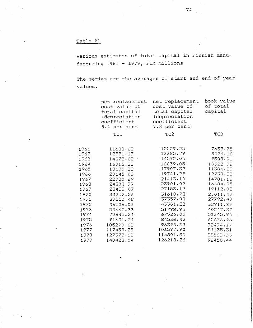
74

Table Al

Various estimates of total capital in Finnish manu-

facturing 1961 - 1979, FIM millions

The series are the averages of start and end of year

values.

net replacementcost value oftotal capital(depreciationcoefficient5.4 per cent

TCl

1168.6212991.1714372.82 '1 60 .15 +221310", 3220145.0622030.6924808.7923428. 0733257.2639553.4846206.03

55662.3372845.2491631 . 74105270 .02117458 .28127372 .6 21404234

net replacementcost value oftotal capital(depreciationcoefficient7.8 per cent)

TC2

12229.251 y 7)-

14592.0416039.0517907.3219741 . 2921413.1023901.0227183.1231610.7837357.0843301 .2351798.9567526.0084533.429639 .53

106597. 9011480 1 .85126218.26

book valueof totalcapital

TCB

8526.169503.0110522.7311384.2312733. 214701.1,16484, Z519112.0223011.4327792.4932911.89

40247.3951345.9462676.9672474. 1731135 .31

96450.44

1961196219631964196519661967196819691970197119721973197419751976197719781979

75

Table A2

Estimates of operating income in Finnish manufacturing

1960 - 1979, FIM millions

operating incomebased on the 5.4per cent deprecia-tion coefficient

OIl

1332.611492.091298.071430.251525.141432.401471.731548.962154.673359.013675.602989,813553.734702.997710.535401 ,.695198.765170.968214.03

11276.33

19601961196219631964196519661967196319691970197119721973197419751976197719781979

based on the 7.8per cent deprecia-tion coefficient

012

1164.941311.501104.681229.311316.791257.801237.141304.291881.513075.493350.112612.203119.214197.547065.114639.204358.254261.177337.9210356.76

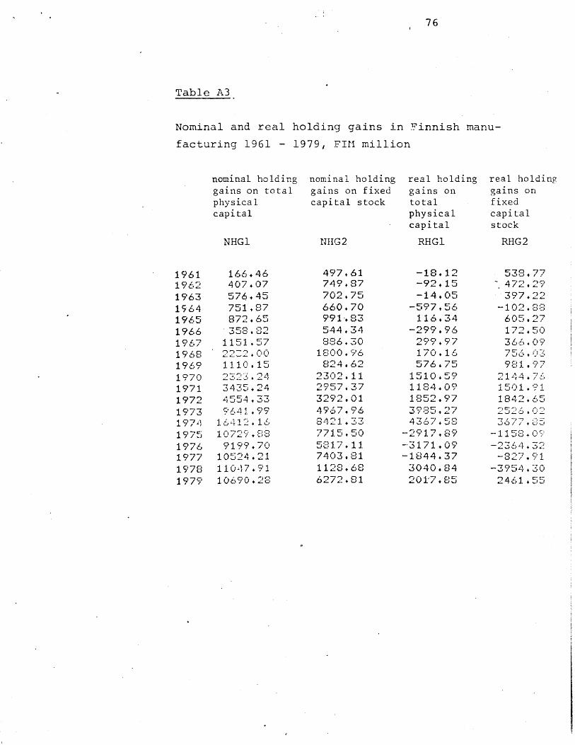
76

Table A3

Nominal and real holding gains in Finnish manu-

facturing 1961 - 1979, FIMI million

nominal holdinggains on totalphysicalcapital

NHG1

166.46407.07576.45751 .87872.65358 .82

1151.5722 2. C:1110.152 3231.243435.244554.339641.99

16412. 1610729.839199.70

10524.2111047.9110690.28

nominal holdinggains on fixedcapital stock

NHG2

497. 61749 .37702.75660.70991-.83544. 34836.30

1800.96824.62

2302.11295.7 3292.014967.968421.337715.505317.117403.811128.686272.8

real holdinggains ontotalphysicalcapital

RHG1l

-18.12-924 15-14.05

-597.56116.34

-299.96299.97170. 16576.75

1510.5?1134.091852.973985.274367.58

-2917.89--3171.09-1844.373040.84201-7.85

real holdinggains onfixedcapitalstock

RHG 2

533477. 472. 29397.22102. 605.27172.50366.09756 . 03981 .97

2144.761501.911842.652526.02

-11583 .0--2364 .3 2

-827.91-3954.30

2461. , 55

196119621963156419651966197 0196819691970197119721973197419751976197719781979

77

Table A4

Estimates of real rate of return on total capital

in Finnish manufacturing 1961 - 1979, per cent

B refers to before taxes and A

real rate of return ontotal physical capital(fixed capital stockat 5.4 per centdepreciation plusinventories)

RRTFCRB RRTFC

1961196219631964196519661967196819691970197119721973197419751976197719781979

14.6910.7811.56

10.37

9.7110.9916.651 9.2112.7114.1219.0220.032.521 .43

10.1011.10

11 .78.209.314.528.414.658.099.52

15.21 .17.9911.6413.2218.1019.161.660.511.749.41

10.25

to after taxes values.

real rate of return ontotal capital(7.8 per cent deprecia-tion coefficient)

RR2 RB

10.587,568.334.487.674.757,498.58

13.4415.3810.1611.4815.8016.932.041.232.279.049.80

RR2R

8.425.496.522.81

6.033.156.167.35

12.2514 . 3,9.2810.7315.0216.19

1 . 300.421.598.439.07

78

Table A5

Estimates of real rate of return on own capital in

Finnish manufacturing 1961 - 1979, per cent

RRR (1) and RRR (2) are calculated by formula (19)OC OC

by excluding RHG from RR (see section 3.2)

1961.1962196319641.965196619671968196919701971

1972197319741975197619771978f1979

RRR (1)OC

19.1514.9817.9916.3116.116.2616.2729.0627.0136. 1729.7135 .4055.4972.9331.1121. 0519.9230.1829.66

RRR (2)OC-

14.4010.7512.659,5911.205.15

11.3117.3119.6524.9819.64

C;,6

35.4541.9914.7410.0710.0418.1618.05

Note:R

In RRR (2) all hidden reserves are included in theOC

measure of own capital.R

In RR (1) half of these reserves are added to

total debt as an estimate for tax credits.

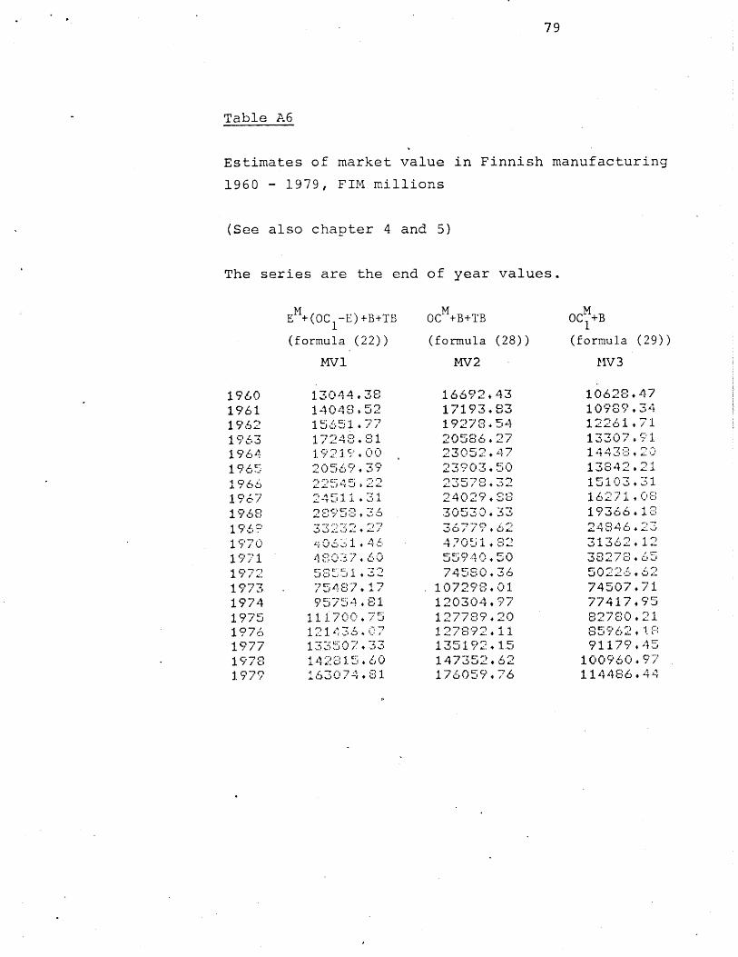
79

Table A6

Estimates of market value in Finnish manufacturing

1960 - 1979, FIM millions

(See also chapter 4 and 5)

The series are the end of year values.

E +(OC -E)+B+TB

(formula (22))

MVl

OC +B+TB 0C +B

(formula (28)) (formula (29))

MV2 MV3

13044.3814048.5215651.7717243. 3119219.0020569.3922545. 2224511 .312J.A. 4 5 . -

06,U:,J 1 - 4 6

5r-51. *32

175487.1795754.81

1i 7 0 . 75121436.07133507. 3 ,14 23 1. 5 . 60163074.31

16692.4317193.8319270.5420586.27252 . 47 .

239,03.502

24029, *S3053). 33

47051 . 62

107293.01120304.97127789.20127892.11135192.15147352.62176059.76

10628.4710989.3412261.7113307. 911 443 3213342.2115103.3116271 . .819366.13

31362. 12

3~ 2 7 3 . 6 55 0226.6*41274507.7177417.9532730 . 2185962.1891179.45100960.97114486.44

196019611962196319641965196 619671968

1970197119721973197419751976197719781.979

80

Table A7

Estimates of Tobin's q-variable in Finnish

facturing 1960 - 1979

Market values MVl - MV3

total physical capital.

TOBQF1

19601961196219631964196519661967196819691970197119721973197419751976197719781979Average

1.4421.371.391.421.411.321.321.331.351.411.441.431.511.551 .441.411.361,.341.391 . 391.40

are divided by the value of

TOBQF2

.81

.68

.71

.69

.69

.53

.38

.31

.43

.56

.66

.67

.93

.20

.80

.61

.43

.36

.43

.50

.62

TOBQF3

1,151.081.091.101,060.890.890.880 . 911.051.111.141.301.53.1.161.040.960.920.980.981.06

manu-

81

Table A8

Estimates of real cost of capital in Finnish manu-

facturing 1961 - 1979, per cent

Based on the real rate of return on total capital

after taxes and including real holding gains.

Market values are MVl - MV3.

1961196219631964196519661967196819691970197119721973197419751976197719781979

CClA

9.076.237.013.636.793.976.667.52

11.5713.078.679.3112.1813.931.801.082.057.608.09

CC2A

7.415.065.873.025.843.806.807.13

10.4611.297.457.318.57

11.091.581.032.037,377.49

CC3A

11.607.969.084.8310.09

5~ 4 9 '-p

10.0411.2415. 4016.9310.8 :10 .8512.3417.232.431.533.01

10.7511.52

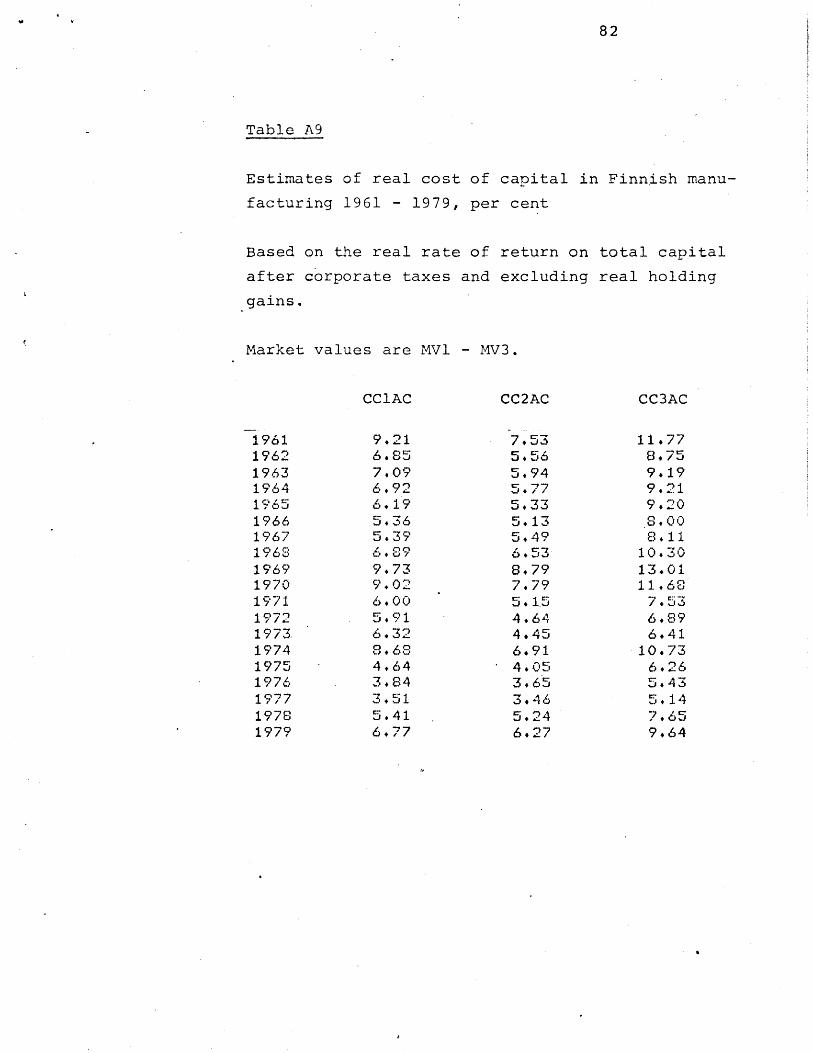
82

Table A9

Estimates of real cost of capital in Finnish manu-

facturing 1961 - 1979, per cent

Based on the real rate of return on total capital

after corporate taxes and excluding real holding

gains.

Market values are MVl - MV3.

1961196219631964196519661967196819691970197119721973.197419751976197719781979

CClAC

9.216.857.096.926.195.365.396.899,739.026.005 .916.328.684.643,843.515.416.77

CC2AC

7.535565.945.775,335.135.496.538.797.795.1.54.644.456.914.053.653,465.246,27

CC3AC

11.778.759.199.219.208.008.11

10.3013.011 1.68

7.536.896.41

10.736.265.435.147.659.64

I

83

LIST OF SYMBOLS

CPK = fixed capital stock (5.4 per cent depreciation),1 current cost value

K2C = fixed capital stock (7.8 per cent depreciation),2 current cost value

KCP = fire insurance value of fixed capital stock3

KB = book value of fixed assets

VO C = estimated value of inventories

VO B = book value of inventories

RO = book value of financial assets

ROnet = book value of net financial assets

B = book value of total debt

E = book value of equity capital

OC = book value of total own capital

TC total capital, replacement cost value

TFC = total physical capital, replacement cost value

TC = K + VO + RO (also TCl)

TC = book value of total capital

TB = total value of hidden reserves (TC-TC )B

TB* = tax credits, i.e., deferred tax liability

OC = estimated value of own capital (TC-B-TB*)

OC2 = estimated value of own capital (TC-B)

B* = estimated total debt (B+TB*)

pQ = value-added of production

W = total labour costs

Deb = economic value of depreciation

IR = net interest expenses

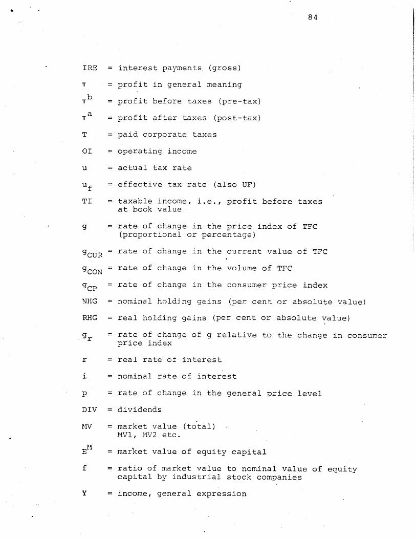
84

IRE = interest payments, (gross)

iT = profit in general meaning

7b = profit before taxes (pre-tax)

7Ta = profit after taxes (post-tax)

T = paid corporate taxes

0I = operating income

u = actual tax rate

u = effective tax rate (also UF)

TI = taxable income, i.e., profit before taxesat book value

g = rate of change in the price index of TFC(proportional or percentage)

gCUR = rate of change in the current value of TFC

gCON = rate of change in the volume of TFC

gCP = rate of change in the consumer price index

NHG = nominal holding gains (per cent or absolute value)

RHG = real holding gains (per cent or absolute value)

g = rate of change of g relative to the change in consumerprice index

r = real rate of interest

i = nominal rate of interest

p = rate of change in the general price level

DIV = dividends

MV = market value (total) -

MVl, MV2 etc.

E = market value of equity capital

f = ratio of market value to nominal value of equitycapital by industrial stock companies

Y = income, general expression

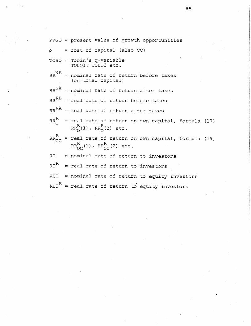
85

PVGO = present value of growth opportunities

p = cost of capital (also CC)

TOBQ = Tobin's q-variableTOBQl, TOBQ2 etc.

RRNB = nominal rate of return before taxes(on total capital)

RRNA = nominal rate of return after taxes

RBRR = real rate of return before taxes

RRRA = real rate of return after taxes

RRR = real rate of return on own capital, formula (17)

RR (1), RR (2) etc.

RRR = real rate of return on own capital, formula (19)

RROC(1), RR~OC(2) etc.

RI = nominal rate of return to investors

RIR = real rate of return to investors

REI = nominal rate of return to equity investors

RREI = real rate of return to equity investors

86

REFERENCES

T. Airaksinen

K. Alho

T.A. Clark and

N.P. Williams

G. Eliasson et al.

M. Feldstein and

L. Summers

G.M. von Furstenberg and

B.G. Malkiel

T.P. Hill

D.M. Holland and

S.C. Myers

Tutkimus kannattavuuden mittaami-

sesta ja komponoimisesta, sovellu-

tuksena Suomen tehdasteollisuus

vuosina 1960 - 1975, Teollistamis-

rahasto Oy, B:1, 1978.

Pauoman tuottoaste, korko ja kansan-

talouden padomanmuodostus, Etla B:26,

Helsinki 1980.

"Measures of real profitability",

Bank of England Quarterly Bulletin,

1978, 18(4).

Att vdlja 80-tal,- IUI, Stockholm

1979.

"Is the Rate of Profit Fallina?"

Brookings Papers on Economic Activity

1977:1, p. 211 - 227.

"Financial Analysis in an Inflationar

Environment", The Journal of Finance,

Vol. XXXII, No. 2, May 1977,

p. 575 - 587.

Profits and Rates of Return, OECD,

Paris 1979.

Trends in Corporate Profitability

and Capital Costs, MIT, WP 999-78,

May 1978.

87

D.M. Holland and

S.C. Myers

H. Koskenkyls

H. Koskenkyld

W.D. Nordhaus

Salo, S.

A.'E. Tudeer

H. Valvanne and

J. Lassila

"Profitability and Capital Costs

for Manufacturing Corporations and

All Nonfinancial Corporations",

The American Economic Review, Vol.

70 No. 2, May 1980.

The Definition and Measurement of

Capital and Its Role in the Invest-

ment Function, TU 4/1979, Bank of

Finland, Helsinki.

Profitability, the Cost of Capital

and the Valuation Ratio in Finnish

Manufacturing 1960 - 1977, Bank of

Finland, Research Papers 6/80.

"The Falling Share of Profit.s",

Brookings Papers on Economic

Activity 1974:2, p. 169 - 308.

Suomen teollisuuden varastot v.

1960 - 1975 (Finnish industrial

inventories, 1960 - 75), Etla B:15,

Helsinki 1977.

"Suomen teollisuusyhti5iden pusoma-

suhteet ja kannattavuus seks suh-

danteiden vaikutus niihin", Kansan-

taloudellinen aikakauskirja, 1938:1.

The Taxation of Business Enterprises

and the Development of Financial

Markets in Finland, Bank of Finland

Publications D:4, Helsinki 1965.

88

Vihavainen - Valppu -

Suokko - Bj5rk

N.P.. Williams

N.P. Williams

Yld-Anttila,' P. and

Heikkild, A.

Pddomakanta vuosina 1965 - 1977,

Tilastokeskus, Tutkimuksia n:o 58,

Helsinki 1980.

"The Profitability of UK Industrial

Sectors", Bank of England Quarterly

Bulletin, 1979, 19(4).

Influences on the profitability of

twenty-two industrial sectors,

Bank of England, Discussion Paper

No. 15, March 1981.

Teollisuuden kannattavuus toimialoit-

tain (Profitability in Finnish

industry by branches), Etla B:24,

Helsinki 1980.