Essays in Public Finance and Labor Economics

By

Elizabeth Oltmans Ananat

B.A. Political Economy and MathematicsWilliams College, 1999

Master of Public PolicyUniversity of Michigan, 2001

SUBMITTED TO THE DEPARTMENT OF ECONOMICS IN PARTIALFULFILLMENT OF THE REQUIREMENTS FOR THE DEGREE OF

DOCTOR OF PHILOSOPHY IN ECONOMICSAT THE

MASSACHUSETTS INSTITUTE OF TECHNOLOGY

JUNE 2006

02006 Elizabeth Oltmans Ananat. All rights reserved.

The author hereby grants to MIT permission to reproduce and to distribute publicly paperand electronic copies of this thesis document in whole or in part in any medium now

known or hereafter created.

Signature of Author:I

D) Department of EconomicsMay 15, 2006

Certified by:

Certified by: (

CL lr/ C6Jonathan Gruber

Professor of Economics

sY ')o 6David Autor

Professor of EconomicsMay 15, 2006

Accepted by:Peter Temin

Professor of EconomicsChairman, Committee for Graduate Students

MASSHUSMT8 IlWSTfrOF TECHNOLOGY

JUN 06 2006I

LIBRARIES

1

ARCHIVES

_. ._I5 _50(

%.I I -v

Essays in Public Finance and Labor Economics

By

Elizabeth Oltmans Ananat

Submitted to the Department of Economics on May 15, 2006 in partial fulfillment of therequirements for the degree of Doctor of Philosophy in Economics

Abstract

This thesis examines three questions of causality relevant to public finance and laboreconomics: the effect of racial segregation on city characteristics, the effect of divorce onwomen's economic outcomes, and the effect of abortion legalization on completedfertility.

Chapter one examines the effect of segregation on cities. There is a strikingly negativecity-level correlation between residential racial segregation and population outcomes-particularly for black residents-but it is widely recognized that this correlation may notbe causal. This chapter provides a novel test of the causal relationship betweensegregation and population outcomes by exploiting the arrangements of railroad tracks inthe 19th century to isolate plausibly exogenous variation in a city's susceptibility tosegregation. I show that, conditional on miles of railroad track laid, the extent to whichtrack configurations physically subdivided cities strongly predicts the level of segregationthat ensued after the Great Migration of African-Americans to northern and western citiesin the 20th century. Prior to the Great Migration, however, track configurations wereuncorrelated with racial concentration, income, education and population, indicating thatreverse causality is unlikely. Instrumental variables estimates find that segregation leadsto negative characteristics for blacks and high-skilled whites, but positive characteristicsfor low-skilled whites. Segregation could generate these effects either by affecting humancapital acquisition of residents of different races and skill groups ('production') or byinducing sorting of race and skill groups into different cities ('selection'). I develop amodel to distinguish between production and selection effects. The findings are mostconsistent with the view that more segregated cities produce better outcomes for low-skilled whites and that more segregated cities are in less demand among both blacks andwhites, implying that Americans on average value integration.

Chapter two, coauthored with Guy Michaels, examines the effect of divorce on women'seconomic outcomes. Having a female firstborn child significantly increases theprobability that a woman's first marriage breaks up. We exploit this exogenous variationto measure the effect of marital breakup on women's economic outcomes. We findevidence that divorce has little effect on a woman's average household income, butsignificantly increases the probability that her household will be in the lowest incomequartile. While women partially offset the loss of spousal earnings with child support,

2

welfare, combining households, and substantially increasing their labor supply, divorcesignificantly increases the odds of household poverty on net.

Chapter three, coauthored with Jonathan Gruber and Phillip B. Levine, examines theeffect of abortion legalization on completed fertility. Previous research has convincinglyshown that abortion legalization in the early 1970s led to a significant drop in fertility atthat time. But this decline may have either represented a delay in births from a pointwhere they were "unintended" to a point where they were "intended," or they may haverepresented a permanent reduction in fertility. We combine data from the 1970 U.S.Census and microdata from 1968 to 1999 Vital Statistics records to calculate lifetimefertility of women in the 1930s through 1960s birth cohorts. We examine whether thosewomen who were born in early legalizing states and who passed through the early 1970sin their peak childbearing years had differential lifetime fertility patterns compared towomen born in other states and in different birth cohorts. We consider the impact ofabortion legalization on both the number of children ever born as well as the distributionof number of children ever born. Our results indicate that much of the reduction infertility at the time abortion was legalized was permanent in that women did not havemore subsequent births as a result. We also find that this result is largely attributable toan increase in the number of women who remained childless throughout their fertileyears.

Thesis Supervisor: Jonathan GruberTitle: Professor of Economics

Thesis Supervisor: David AutorTitle: Associate Professor of Economics

3

Acknowledgements

I thank my advisors, David Autor and Jon Gruber, for their constant support, advice, andfeedback and for their talent at answering email at any hour-without them, needless tosay, I could not have completed this dissertation. I also thank Michael Greenstone, whoin my fifth year took on many of the responsibilities but not the dissertation-signing gloryof an advisor.

I am indebted to the Jacob K. Javits Fellowship for support in my first and second yearsand to the National Institute on Aging (through grant number T32-AG00186 to theNational Bureau of Economic Research) for research support in my fifth year.

Many people have contributed in important ways to the completion of this project.Sheldon Danziger encouraged and guided me towards economics and MIT. The entireMIT economics department-but especially Dave Abrams, Josh Fischman, GuyMichaels, and Sarah Siegel-provided intellectual and emotional support. Mypredecessors Joanna Lahey and Ebonya Washington let me exploit the hard-won wisdomthey gained through experience at every step of the way.

Daniel Sheehan and Lisa Sweeney of GIS Services at MIT and David Cobb and PatrickFlorance of the Harvard Map Library provided indispensable aid for the research inchapter one by creating the digital map images and teaching me how to use them.

My family, which includes many friends, has been a constant and essential source ofsupport throughout these past five years. For Ryan's presence there aren't words-that'swhat John Coltrane is for. For Jane, may it suffice to say that in my life most credit isdue to her, and all mistakes remain my own.

And, of course, without Hubris, nothing is possible.

4

The Wrong Side(s) of the Tracks:Estimating the Causal Effects of Racial Segregation on City Outcomes

Elizabeth Oltmans Ananat

5

Abstract

There is a strikingly negative city-level correlation between residential racial segregationand population outcomes-particularly for black residents-but it is widely recognizedthat this correlation may not be causal. This paper provides a novel test of the causalrelationship between segregation and population outcomes by exploiting thearrangements of railroad tracks in the 19t century to isolate plausibly exogenousvariation in a city's susceptibility to segregation. I show that, conditional on miles ofrailroad track laid, the extent to which track configurations physically subdivided citiesstrongly predicts the level of segregation that ensued after the Great Migration ofAfrican-Americans to northern and western cities in the 20th century. Prior to the GreatMigration, however, track configurations were uncorrelated with racial concentration,income, education and population, indicating that reverse causality is unlikely.Instrumental variables estimates find that segregation leads to negative characteristics forblacks and high-skilled whites, but positive characteristics for low-skilled whites.Segregation could generate these effects either by affecting human capital acquisition ofresidents of different races and skill groups ('production') or by inducing sorting of raceand skill groups into different cities ('selection'). I develop a model to distinguishbetween production and selection effects. The findings are most consistent with the viewthat more segregated cities produce better outcomes for low-skilled whites and that moresegregated cities are in less demand among both blacks and whites, implying thatAmericans on average value integration.

6

I. Introduction

Residential segregation by race is one of the most visible characteristics of many

American cities. Although African-Americans represent just over one-tenth of the U.S.

population, the average urban African-American lives in a neighborhood that is majority

black (Glaeser and Vigdor 2001). Cities vary in the extent to which their black

populations live in black neighborhoods, and more segregated cities on average have

worse characteristics than less segregated cities, on measures ranging from infant

mortality to educational achievement (Massey and Denton 1993).

This correlation is difficult to interpret, however. In what ways, if any, racial

segregation causally affects outcomes is a longstanding question in social science. Two

conceptual obstacles complicate identifying the answer. First, some economic, political,

or other attributed may lead some cities to have more segregation and also more negative

city characteristics. This will cause omitted variable bias when estimating the bivariate

relationship between segregation and city outcomes. Instrumenting for a city's level of

segregation can help address this problem, thereby allowing the effect of segregation on

macro city-level outcomes to be estimated.

A second conceptual obstacle arises from the fact that, although segregation must

affect aggregate city characteristics through some effect on individuals, there at least two

different ways it can do so. First, segregated cities may be less productive, leading to

lower accumulation of capital (human and otherwise) for its citizens. Second, people

may respond to segregation itself, and to any effects segregation has on production, by

sorting between cities in ways that alter average city characteristics. Both of these

phenomena are of economic interest, but only the first can be considered a causal effect

' For example, greater political corruption or a more industrial economy.

of segregation on the outcomes of people. The combination of the two, which is easier to

observe, must be considered an effect of segregation on places.

In this paper I address concerns about omitted variable bias by using 19th-century

railroad configurations to instrument for the extent to which cities became segregated as

they developed African-American populations during the 20th century. I show that the

proverbial convention of the "wrong side of the tracks" is helpful in identifying

segregation; the more subdivided a city was by railroads (i.e., the more total "sides" there

were to the tracks) the more segregated the city became during the Great Migration.

As a city began to develop a significant black population during the Great

Migration, African-Americans became isolated in ghettoes in part because demand

among the broader community for residential segregation grew (Weaver 1955). As the

black population continued to expand, the physical size of a ghetto had to increase if

segregation was going to be maintained. Since railroads generate neighborhood

divisions, cities that were subdivided by railroads into many small insular neighborhoods

could expand a ghetto by one neighborhood at a time and still practice "containment,"

whereby the black population remained concentrated and contiguous. On the other hand,

in cities where expanding a ghetto meant breaching a main divide, then as the black

population increased segregation could no longer be as easily maintained.2

Figure 1 illustrates this concept. Binghamton, NY, and York, PA, were similar in

total quantity of railroad tracks laid by 1900 (shown in red, circumscribed by a four

kilometer-radius circle). They also had similar industrial bases and substantial changes in

2 The proverb does not explain why it is that railroads tend to define neighborhood boundaries, although inmany cases it is self-evident that they do. One likely possibility is that a railroad provides a cleardemarcation that facilitates collective agreement on neighborhood boundaries by residents, real estateagents, police, and others. When a community is interested in remaining separate from a certain group,railroads could facilitate collective action in enforcing segregation by reducing coordination costs.

8

African-American population (these characteristics are discussed in detail later in the

paper). But York's railroads were configured such that they created many insular

neighborhoods, particularly in the center of the city. Its Census tracts, in the year 2000,

show a black population more concentrated in this set of small, railroad-defined

neighborhoods (tract percent black is represented by darkness of tract shading). In

Binghamton, on the other hand, railroads are tightly clustered, leaving some areas too

long and narrow to encompass neighborhoods and others too wide open to create

meaningful population restrictions. In contrast to York, Binghamton's year 2000 Census

tracts show its black population dispersed lightly and evenly throughout much of the city.

My research design relies on the assumption that the variation I observe in the

railroad subdivision of neighborhoods, conditional on total track laid in a city, is

exogenous. I provide a variety of tests of the validity of this assumption. Under this

assumption, instrumentation allows me to identify the extent to which cities that initially

are randomly assigned greater segregation end up having more negative characteristics

overall. That is, it identifies the causal effect of segregation on places.

To identify the effect of segregation on people, it is necessary to determine how

much of a city's characteristics result from the production effects of segregation and how

much from the migration effects. I develop a simple model in which cities' equilibrium

characteristics are driven by race, tastes, production effects of segregation, and relative

housing demand. This model produces implications that I am then able to test

empirically, providing some speculative estimates that decompose the macro effects of

segregation on places into the effects on people and the effects on migration.

9

A number of other papers have attempted to measure the effects of segregation on

outcomes (cf. Massey and Denton 1993, Wilson 1996, Polednak 1997). An influential

contribution by Cutler and Glaeser (1997), which includes a rich discussion of the

problems of omitted variable bias and endogenous migration, is significantly limited in

its ability to address those problems because they lack a plausible instrument. In place of

an instrument they impose a variety of exclusion restrictions. Their main empirical

estimates depend on the identifying restriction that segregation has no effect on whites, so

that within cities white outcomes provide a counterfactual for what black outcomes

would be in the absence of segregation. My results, by contrast, suggest that segregation

has significant effects on whites and that assuming otherwise produces incorrect

estimates of the effects of segregation on blacks.3

In some specifications, Cutler and Glaeser use an approach more similar in spirit

to that used here, instrumenting for a city's level of segregation with its number of rivers.

In practice, however, my approach, using railroads, is quite different. Railroads, unlike

rivers, predict division on a small scale-at the neighborhood rather than municipal level.

This means, first, that unlike rivers (Hoxby 1994) railroads do not separately predict

confounding metropolitan characteristics such as intergovernmental competition.

Secondly, it means that railroads identify neighborhood-level segregation, which is the

level that the literature has generally considered relevant and is the level that segregation

indices measure. Most importantly, railroad division strongly and robustly predicts

segregation. Therefore, I argue that the use of railroad division provides ex-ante a more

compelling answer to the question of the effects of segregation on places than has

3 For example, I find that Cutler and Glaeser's results overstate the negative effects of segregation on low-skilled blacks because their strategy misses the positive effects of segregation on low-skilled whites.

10

previously been proposed. It can then allow research to proceed to the next important

question-the effects of segregation on people.

My results on the overall effects of instrumented segregation suggest that,

consistent with observed correlation, greater segregation causes cities to have black

populations with worse present-day characteristics, both at the top and the bottom of the

education/income distribution. Within the white population, segregation results in worse

characteristics at the top of the skill distribution and better characteristics at the bottom.

This relationship is obscured in ordinary least squares estimation, possibly because other

omitted local characteristics that lead to broader inequality also lead to more segregation.

My results when looking separately at production and migration suggest that

segregation actually leads to better outcomes for low-skilled whites. For other groups, it

is not possible to distinguish between direct effects of segregation on individual outcomes

and effects on average group characteristics due to selective migration. For all groups,

there is no evidence of preferences for segregated cities, and there is some evidence that

Americans on average have tastes for integration.

II. Some facts about U.S. segregation

The history of urban American racial segregation can be divided into four periods.

In the 19th century, very few African-Americans lived outside of the South. This changed

rapidly during the Great Migration (roughly 1915 to 1950), when large numbers of

African-Americans migrated into Northern and Western cities from the South. Cities

became highly segregated as their urban black populations grew (Cutler et al. 1999).

Much of this segregation resulted not from market forces but from deliberate government

11

policies and collective action by white residents (Massey and Denton 1993).

Government policy towards segregation then changed gradually during the civil rights

era, and a clear break in housing policy came in 1968 with the Fair Housing Act.

Subsequent stated government policies on housing segregation have been neutral or have

explicitly endorsed integration, but cities today continue overwhelmingly to exhibit high

degrees of neighborhood segregation (Cutler et al. 1999). Segregation appears to persist

despite the fact that significant proportions of Americans now state preferences for

integrated neighborhoods (Ananat and Siegel 2002) and that, at a macro level, the U.S.

population has in recent years been migrating to less-segregated cities (Glaeser and

Vigdor 2001).

Two explanations can reconcile the survey and macro evidence that people prefer

integration with the micro-level evidence (Emerson et al. 2001, Bayer et al. 2005,

Goering et al. 2002) that within cities they continue to choose segregated neighborhoods.

First, attempts to provide integration for people who have tastes for it may suffer from a

collective action problem (Schelling 1971, Ananat and Siegel 2002). Second, integrated

cities may be more efficient than segregated cities, at least for some people. For

example, if there are neighborhood effects on individual outcomes and the black and

white populations differ in their distribution of skill types, then blacks and whites will

have different outcomes in more segregated cities. If these types are substitutes in the

production of neighborhood effects, then separating blacks from whites in neighborhood

production will be inefficient, causing people to sort away from less-productive

segregated cities.

12

In theory, the productivity of segregation relative to integration is ambiguous in

sign. For example, Tiebout sorting suggests that, if demand for neighborhood public

goods varies less within race than within an entire city, then segregation is efficient.

Segregation of blacks (relatively low-skilled) from whites (relatively high-skilled) would

also be efficient if the high-skilled are complements in the production of public goods.

Productivity effects of and tastes for segregation may act in tandem. For

example, after initial assignment to a city with a given level of segregation, rational

agents sort away from that city based both on tastes and on any efficiency cost or benefit

of segregation. If, for example, people have tastes for integration and integration is

efficient, then, since willingness to pay is a function of income, high types will select into

integrated cities, which will further reinforce the correlation of integration and positive

outcomes.

III. Research Design

The ideal approach to identifying the effects of segregation on people and on

places would require actual random assignment within an experimental framework. The

experimental design would involve two otherwise identical cities with small open

economies, one that would be kept perfectly residentially segregated by race (the

treatment city), and another that would be kept perfectly integrated (the control city).

At time zero, each city would receive the same total number of blacks and the

same total number of whites, with individuals assigned randomly to one city or the other.

By virtue of random assignment, each city's within-race and overall skill distribution

would start out equal to that of the other city. Restricting individuals from moving, one

13

could then observe, over generations, the overall and within-race outcomes in each city.4

Absent migration, differences in these outcomes would reflect both the effect of

segregation on individuals and the effect on the population characteristics of places-

since population would be fixed, the two effects would not be conceptually different.

Within-race outcomes would identify whether segregation was beneficial or harmful for

each group; which city had better aggregate outcomes would identify whether

segregation is more or less efficient than integration for society as a whole.

The quasi-experiment generated by railroad division

The actual quasi-experiment that railroads provide does not perfectly follow the

framework described above. Instead of a technology that results in being either perfectly

segregated or perfectly integrated, railroad technology for segregation varies by degrees.

To accept the estimates of segregation effects I derive, it is necessary to assume that the

effects are monotonic. In addition, whites and blacks were not randomly assigned to

cities; it is necessary to assume that individuals did not sort selectively based on railroad

division. However, as I will show, there is no evidence of pre-period differences in cities

based on railroad division that would cause individuals to sort selectively; they would

have had to predict the effects of railroad division subsequent to black inflows, which

seems unlikely.

4 The standard model (Roback 1982) of the way wages and rents adjust for city consumption amenities thatare productive (e.g. temperate climate) or unproductive (e.g. clean air) is inapplicable here. It requires thatan amenity have the same productivity effects for all residents, a restriction that is inappropriate in the caseof segregation. It is much more plausible to assume, to the contrary, that segregation has the effect ofconcentrating resources in the white community, making segregation more productive for whites than forblacks. This will be true both because the skill and resource distribution of whites dominates that of blacksand because whites typically outnumber blacks, with the political result of redistribution towards the whitecommunity. Moreover, the clearest way to model the effects of differential resources over time is with amultigenerational model rather than the one-period model in Roback (1982). Therefore I opt to model theproduction of type in the next generation, with type-specific wages fixed across cities, rather than city-determined productivity conditional on type.

14

To believe that railroad division can identify the effect of segregation on people, it

is necessary to assume that individuals do not move. This assumption is plainly not

credible; however, it is also not necessary to identify effect on places.

IV. Empirical Strategy

Segregation can be modeled as a classic endogenous regressor affecting outcomes

at the city level,

(1)Seg = aZ + 2X + U

(2) Y = l,Seg + 2X +,

and then estimated using two-stage least squares analysis. The right-hand side variable of

interest in equation (2), Seg , represents a city's current level of segregation. Segregation

is captured by a dissimilarity index, which measures the difference between the

distribution of blacks by neighborhood and their total representation in the metropolitan

area as a whole. Dissimilarity is defined as

N I black. nonblack i(3) Index of dissimilarity = 2 , blacks - nonblackii= blackotal nonblacktota,

where i = l... N is the array of census tracts in the area. It can be considered the answer

to the question, "What percent of blacks (or non-blacks) would have to move to a

different census tract in order for the proportion black in each neighborhood to equal the

proportion black in the city as a whole?" Note that an index of zero is improbable in the

absence of central planning.

Outcomes, represented by Y in equation (2), include the proportions of a city's

blacks and whites who are poor, unemployed, high-school dropouts, college graduates, or

who have household incomes above $150,000. The first three outcomes should reflect

15

primarily characteristics of a city's low-skilled population, who are more likely to be on

the margin of poverty, unemployment, and dropping out of high school. The last two

outcomes should reflect primarily characteristics of a city's high-skilled population.

The instrument, Z, is a measure of a city's railroad-induced potential for

segregation. Z quantifies the extent to which the city's land is divided into smaller units

by railroads. I define a "railroad division index," or RDI, which is a variation on a

Herfindahl index that measures the dispersion of city land into subunits.

(4) RDI =1 areaighborhoodiareatotal

If a city were completely undivided by railroads, so that the area of its single

neighborhood was 100% of the total city area, the RDI would equal 0. If a city were

infinitely divided by railroads, so that each neighborhood had area near zero, the RDI

would equal 1. The more subdivided a city, the more "sides" there are to its tracks, and

the more possible boundaries between groups are available to use as barriers enforcing

segregation. In particular, if railroads created many small neighborhoods that adjoin each

other, it would have been possible during the Great Migration to relieve pent-up housing

demand by allowing a ghetto to expand into an adjacent neighborhood, while still

maintaining a new railroad barrier between the ghetto and the rest of the city. This

should have facilitated persistent segregation even as the black population increased.

For variation in track configuration to be a valid instrument for segregation, it

must result from random factors, such as minor variations in gradient, natural resource

location, or direction to the next city-factors that amount to noise in aggregate. Any

factors that drive both railroad configuration and city outcomes must be included as

controls. X denotes a vector of city characteristics that affect railroad configuration and

16

city outcomes. The most important of these is total track length, because there is a

mechanical correlation between the total length of track and the division of the city by

track. If total length of track is related to other features of the city, such as industrial

composition or land quality, then length of track may predict city outcomes on its own,

not because of the way track divides the city. Therefore all regressions in the paper

control for total track length.

Other possible confounding factors include: manufacturing share-more

manufacturing-oriented cities may differ in their routing of railroads; region-cities in

the Northeast or Midwest may have different geography and different outcomes from

those in the West; and black population inflows-African-Americans may have chosen

cities based on different tastes for railroad breakup. I perform specification checks to test

for explanatory power of these possible confounders. I run regressions including either

1920 manufacturing share or region dummies. I also instrument for black population

inflows using data from Dresser (1994). She demonstrates that during World War II,

some cities received larger war contracts per capita than others, leading to larger labor

shortages in some cities than in others. She further shows that larger per-capita war

contracts predicted higher inflows of African-Americans during World War II. I draw on

Dresser's work by using per-capita war contracts as an instrument for greater black

inflows during the Great Migration and including it in reduced form as a control in the

analysis.5

5 Railroad-induced segregation technology should have proved differentially useful in cities with highexogenous inflows of blacks. In cities with large exogenous changes in African-American population,which therefore had high demand for segregation, available segregation technology would have made moreof a difference in the resultant degree of separation of blacks and whites. In cities with low inflows, wheresegregation did not become a salient demand, differences in the technology for producing segregationwould have been less relevant to the equilibrium dispersion of blacks and whites and to city outcomes.This has the empirical implication that railroad subdivision should matter more in cities where a rapidly

17

The chronology of the Great Migration provides a further specification check.

The validity of railroad division as an instrument relies on the assumption that division

affected cities only by facilitating segregation of significant African-American

populations. Therefore there would be cause for concern about validity if railroad

division predicted city outcomes prior to the Great Migration. To test this assumption, I

estimate equations (1) and (2) using pre-Great Migration city characteristics as dependent

variables. These pre-period "outcomes" include manufacturing, labor force participation

rate, average income, population, physical city size, percent black, and literacy rate. The

ideal year to measure these characteristics would be 1910, the last Census year before the

beginning of the Great Migration, when nearly 90% of African-Americans still lived in

slave states. Measuring later, however, should bias specification tests toward failure, to

the extent that cities may have already begun to differ due to segregation; my estimates,

which use 1920 characteristics, therefore provide an especially strong test of the validity

of the instrument.

I examine the characteristics of cities' black and white populations separately,

since these groups would not be expected to respond identically to segregation. The two-

stage least squares estimate allows me to measure the effect of railroad-induced

segregation on city outcomes. The difference between the two-stage and ordinary least

squares estimates can provide a sense of whether segregation that occurs endogenously is

obscuring or intensifying the observed correspondence between segregation and group

characteristics.

18

increasing black population increased whites' utility of segregation. Unfortunately, the railroad divisionindex and the proxy for WWII labor shortage do not provide enough power to estimate that interaction. Itherefore confine my estimates to the main effect of each, by controlling for per-capita war contracts in thestandard regression specification.

I test whether the population flows of each race are positive or negative, and also

whether individuals of each race face relatively higher or lower rent and mortgage costs

in more segregated cities. Differences in housing costs would not be a valid measure of

city demand if they are driven by variation in the cost of living or by the amount of

housing consumed in more versus less segregated cities. To test for this possibility, I

examine costs as a percent of income and I examine household crowdedness.

Differences between the overall change in a city's skill distribution and that

explained by migration represent the city's production of skill. For example, the percent

change in a city's population of young high school dropouts, conditional on net migration

of young high school dropouts, can provide an upper bound for the effect of city

production on the size of the low-skill population. A similar argument holds for college

graduates. By breaking down these differences by race, the race-specific production

effects of segregation can be bounded. I therefore examine population change and net

migration by race and education.

V. Data

Sample

My major data sources are U.S. Census Bureau reports on metropolitan

demographics (various years), information on 19th century railroad configuration

extracted from archival maps, measures of metropolitan segregation from Cutler and

Glaeser (1997), and a replication of Dresser's data using city-level total war contracts and

total population information from the 1947 County Data Book.

My ideal sample would include all places outside the South that were

incorporated prior to the Great Migration, so that they were potential destinations for

19

African-Americans leaving the South. Then the growth of the place itself into an MSA

could be treated as an outcome of its potential segregation. Because the Census only

provides data for large places, however, it is not possible to get pre-period information

for places that were small at the time of the Great Migration.

My sample of cities is chosen as follows. Cutler and Glaeser (1997) provide data

for MSAs with at least 1000 black residents. Of these MSAs, I include only those in

states that were not slave-owning at the time of the Civil War, because these were the

states that had few African-Americans prior to the Great Migration.6 Further, my sample

was limited by the set of historical maps held by the Harvard Map Library. The library

depends on donations and estate purchases, etc., to collect maps, and therefore there are

gaps in its collection. I have compared the full non-South Cutler and Glaeser (1997)

sample to the sample available from the Harvard Map Library. The cities for which the

library could not provide maps tend to have been smaller cities in the 19th century but

otherwise do not appear different in either historical or current characteristics. My final

sample consists of 134 urban areas.

Maps

The maps that provide railroad placement information were created by the U.S.

Geological Survey as part of an effort to document the country's topography, beginning

in the 1880s.7 These maps display elevation, bodies of water, roads, railroads, and (in

6 Specifically, I exclude Delaware, Maryland, Washington, DC, Virginia, West Virginia, North Carolina,South Carolina, Georgia, Florida, Alabama, Mississippi, Louisiana, Tennessee, Kentucky, Missouri, Texas,and Arkansas. Nearly 90% of African-Americans resided in one of these states in 1910 (author'scalculation from 1910 IPUMS data).7 The median map year in my sample is 1909, prior to the start of the Great Migration. The observations inthe maps should primarily reflect 19t century railroads, since 75% of the total track laid in the UnitedStates was in place by 1900 (Atack and Passell 1994, p. 430)

20

many cases) individual representations of non-residential buildings and private homes.8

The edges of a 15-minute map are exogenously defined in round 15-minute units, so that,

for example, a map will extend from -90°30'00" longitude and 43045'00 ' latitude (in the

southeast corner) to -90045'00' longitude and 44000'00' latitude (in the northwest corner)

Because the Harvard Map Library collection is incomplete, there are 77 cities in

non-South states available in the Cutler and Glaeser data for which I do not have the

necessary map observations. In addition, in 15 cities I observe only some fraction of the

four-kilometer-radius land area I wish to observe, since the cities overlap two or more 15-

minute areas and I have maps only for some subset of those areas. Finally, in 40 cases

the city overlaps multiple areas and I observe all of the areas.

The process of extracting railroad information from the maps is illustrated in

Figure 2. For each city, its map or maps were used first to identify its physical size,

shape and location at the time its map was made. A Geographic Information Systems

program, ArcGIS, was used to create a convex polygon that was the smallest such

polygon that could contain the entire densely inhabited urban area. Dense habitation,

defined as including any area with houses and frequent, regular cross-streets, was

identified by visual examination. ArcGIS was then used to identify the centroid of this

polygon, and this point was defined as the historical city center. A four-kilometer radius

circle around this point became the level of observation for the measurement of railroads.

This approach meant that differences in initial city area would not distort the

measurement of initial railroads: cities that were, at the time, very small would still be

coded with railroads that affected later development, after the population had expanded;

8 In some cities with relatively dense areas, some center-city blocks are marked as continuously inhabited,rather than showing individual structures. The outskirts of every inhabited area, however, do showindividual structures.

21

cities that were already large would have only those railroads in their center cities

included. It should be noted, however, that about 75% of the cities were smaller than 16a

square kilometers when mapped, and many were much smaller, so for most cities this

measure includes railroads that were laid on unoccupied land without need to consider

habitation.

Visual examination reveals that the historical city center created in this way is

typically quite close to what would be identified as the current city center if using a

current map. Within this four-kilometer circle, every railroad was identified, its length

measured, and the area of the "neighborhoods" created by its intersections with each

other railroad calculated. Historical railroads predict the borders of current

neighborhoods as identified by the Census quite well. The actual land area within the

circle was also calculated, so that measurement could be adjusted for available observed

land when working with maps that truncate city observations or include substantial

bodies of water.

Segregation Indices

I use the Cutler/Glaeser/Vigdor segregation data provided online by Vigdor

(2001). These data come from various decennial Censuses, and include 19 th and 20t

century historical segregation indices and metropolitan characteristics from Cutler and

Glaeser (1997), 1990 GIS-dependent measures of segregation based on Census data from

Cutler et al. (1999), and additional data from the 2000 Census from Glaeser and Vigdor

(2001). These data include dissimilarity indices for every decade from 1890 to 2000. In

addition, they provide four other measures of segregation, all based on those developed in

22

Massey and Denton (1988). These include an index of isolation, available for every

decade from 1890 to 2000, which provides a different way to organize the same

information contained in the dissimilarity index and is highly correlated with the

dissimilarity index. Supplementary measures of clustering, concentration, and

centralization-all of which rely on geographical data about the proximity, size, and

location of a city's census tracts-are available for 1990. Dissimilarity is the standard

measure of segregation in the literature, and I use the dissimilarity index throughout the

paper, while also testing the robustness of my instrument to alternative segregation

measures.

Census Measures of Urban Characteristics

I collect city outcomes from published Census reports (U.S. Census Bureau

2005). Although at the time that tracks were laid each of these cities was physically

separated by open space from other cities, over the last century urban growth has meant

that many once-distinct metropolitan areas are now conglomerates. To surmount this

problem, I collect data for the reporting area which best centers on the original city center

without containing other original city centers.

Thus I use MSA-level data for the 64 cities that have remained independent

MSAs. For MSAs in which multiple city centers are each in a separate county, I assign

to each city the characteristics for the county that holds that city's original urban center.

Doing so allows me to differentiate between the effect of an original center on its county

level outcomes and the combined effect of several centers on MSA-level outcomes (e.g.

outcomes for the New York-Northern New Jersey-Long Island Consolidated MSA).

23

Fifty-three cities are in unique counties but share an MSA with at least one other city.

Finally, for the 17 cities that share a single county with another city, I assign the

characteristics of the politically-defined city itself to the observation.

I use Census data collected at these MSA, county, or municipal levels to derive

city outcomes by race. These outcomes include education, labor force characteristics,

poverty, distribution of income, median rent and mortgage costs, housing costs as a

percent of income, percent of households with more than one person per room, and

proportion of residents who are new to the area.

VI. Results

First stage

Table 1 shows that, controlling for track per square kilometer in the historical city

center, the neighborhood RDI generated by the configuration of track strongly predicts

the metropolitan dissimilarity index in 1990. Adding a control for pre-period

manufacturing composition does not significantly affect the relationship between railroad

division and current segregation.9 Nor does adding per-capita war contracts as a proxy

for exogenous black inflows. The regression in column 4 includes Census region

dummies; the coefficient on the RDI remains positive and significant. As seen in Table

2, the RDI similarly positively predicts other aspects of segregation, including isolation,

clustering, concentration, and centralization. The effects of the RDI on three of these

four facets of segregation are highly significant.

9 Regressions that instead use later measures of manufacturing share (1970 and 1998) produce similarresults. These regressions should, if anything, bias the effect of manufacturing on outcomes toward greatersignificance (Acemoglu, Johnson, and Robinson 2001).

24

Specification checks

Table 3 displays the results of regressions that use railroad division to predict city

characteristics prior to the time when cities experienced significant African-American inflows. I

use data from 1920, which is just after the start of the Migration, but using data from such a late

date should merely bias specification tests toward failure. As shown in Table 3, the RDI predicts

neither 1920 labor force participation, average income, population, physical city size, nor percent

black. The RDI has a marginally significant relationship with literacy rate in an unexpected

direction-more railroad subdivision corresponds to higher literacy.

Main results: The impact of segregation on city outcomes

Table 4 shows ordinary least squares and two-stage least squares estimates of the

effects of racial segregation on a variety of current urban characteristics. Black outcomes

and white outcomes are shown separately. Table 4 also includes overall city outcomes,

but these are strongly driven by white outcomes, since white populations numerically

dominate black populations.

The top panel of Table 4 demonstrates that RDI-induced segregation causes a

city's low-skilled whites to have better characteristics. White unemployment and poverty

are lower, and whites are less likely to be high-school dropouts; the former two effects

are significant. In contrast, RDI-induced segregation causes a city's black population to

have worse characteristics; in particular, they have much higher poverty rates. The

effects of segregation on black unemployment and proportion of adults who are high-

school dropouts, however, are not significant.

25

The bottom panel of Table 4 shows that RDI-induced segregation has negative

effects on the characteristics at the upper end of the skill distribution. Segregation

significantly lowers the fractions of a city's blacks and whites who are college graduates,

as well as the fractions of white and black households with more than $150,000 in

income. The negative effects on these characteristics for whites are as large as or larger

than for blacks.

Table 5 shows migration and housing market characteristics by race from 2000 Census

statistics reported at the urban level. Cities with more RDI-induced segregation have

significantly fewer new residents, both black and white. The effect on black in-migration is

larger than the effect for whites.

Unfortunately, because the Census does not supply data on out-migration, I cannot

distinguish between low demand and low supply as explanations for this result. It may be that

there are fewer new residents because out-migration is lower, leading to few vacancies.

However, the evidence on housing values in Table 5 suggests that segregated cities are in fact in

less demand. First, more segregated places have significantly lower rents, lower mortgage costs,

and lower home values. These effects do not appear to be driven by lower cost of living in more

segregated cities, since rents are as low or lower as a fraction of income (significantly lower for

whites). Second, lower expenditures on housing also do not seem to reflect lower consumption

of housing in more segregated cities; blacks and whites in more segregated cities are

significantly less likely to live in crowded homes (that is, homes with more than one person per

room).

VII. The effects of segregation on individual outcomes

26

To what extent are these differences in present-day city characteristics driven by

sorting of individuals across cities in response to segregation? To what extent are they

driven by the direct effect of segregation on the production of health, human capital, and

productivity? To distinguish between the effects of segregation on individuals and

equilibrium sorting of individuals by race and skill, it is helpful to briefly examine the

theoretical relationships between tastes, skills, production, and residential choice.

Theory of Skill Production and Endogenous Migration

Assume two small open-economy cities that exist for two generations. City I has

railroad technology such that it will have two perfectly racially integrated tracts, while

city S has railroad technology such that it will have two perfectly racially segregated

tracts (See Figure 4a for an illustration). In all other ways, these two cities are identical.

At time zero, corresponding to the Great Migration, each city is randomly

assigned the same population of measure one, ,8 of which is black and 1- ,/ white.

There are two types of residents, high and low, such that the high types receive wage H,

relative to a low-type wage that is normalized to 1. Even assuming some wage

discrimination, it is appropriate to infer from the data that at time of the Great Migration

the proportion of blacks who are high types, Phb,, is lower than the proportion of whites

who are high types, Ph,,

Production of types in the next generation depends on the type mix of current

neighborhood residents. This implies that type is a neighborhood-level public good. It

could represent education, health, connectedness to a job network, political influence-

anything that varies at the individual level but might depend on the mix of characteristics

27

of a neighborhood's elder generation. In particular, consider the following public-good

production function:

PH2 APH I

where a > 0, l is a scaling parameter, and PHI and PH2 are a neighborhood's

proportion high-type in the first and second generations, respectively.

The parameter a reflects the complementarity or substitutability of types in the

production of next-generation type. If a < 1, the production of high-type offspring is

concave in the percent high type in the current generation, meaning that types are

substitutes. If a > 1, the production of high-type offspring is convex in the percent high

type in the current generation, meaning that types are complements. (See Figure 4b for

an illustration.) The complementarity or substitutability of types has important

implications for the economic efficiency of segregation.

If residents cannot move between cities-i.e., moving costs are greater than high-

skilled income-we need go no further. Tastes or distastes for integration will be

irrelevant, the high-skilled will not be able to migrate differently from the low-skilled,

and housing demand will not differ by city. Observed differences in proportion high-

skilled in the second generation can be interpreted as resulting from the relative

productivity of segregation. As long as a > 0, whites in S will have higher PH2 than

whites and blacks in I, who in turn will have higher PH2 than blacks in S. If a > 1, so

that types are complements, then the weighted average PH2 in S will be greater than the

weighted average PH2 in I-implying that segregation is more efficient than integration.

If a < 1, so that types are substitutes, then the weighted average PH2 in S will be smaller

28

than the weighted average PH2 in I-implying that integration is more efficient than

segregation.

However, if moving cost C is low enough that migration between cities occurs,

then the picture becomes more complicated. Race, income, tastes or distastes for

integration, intergenerational altruism, and the elasticity of housing supply will affect

individuals' choice of city. To explore these complications, allow a parameter a to

represent taste (if positive) or distaste (if negative) for integration, and assume that

individual utility is:

U = ln(wage) + (a I residenceinI)

Consistent with survey evidence, a varies continuously, takes on both positive and

negative values, and is distributed differently by race. A simple parameterization that

captures these attributes is to define a as distributed uniformly on the interval [a w, d w]

for whites and [a b, 6 b] for blacks.

In the absence of housing discrimination and with a flexible neighborhood

delineation, we can assume that the housing market clears on the city level. Initially, with

equal population of measure 1 in each city, the price of housing in city I relative to city S

can be normalized to 0. To avoid an unrealistic corner solution in which everyone resides

in one city or the other, it is desirable that the relative price of housing in city I approach

infinity as city population approaches 2 and approach negative infinity as city population

approaches 0. A simple parameterization that captures these three characteristics of the

housing market is:

(T(T - 1)

29

where R is the rent that must be paid (or subsidy received) each generation, q is a scaling

parameter, and T is the total population of city I (see Figure 4c for an illustration).

To capture individuals' interests in the difference in public goods production by

segregation and race, assume that each individual is altruistic towards an offspring in the

second generation who shares taste parameter a. The individual's problem, then, is to

maximize, by choosing I or S, the value of his own utility plus the expected value of his

offspring's utility, which is discounted at rate S.

In equilibrium, the proportion of each of the four groups of individuals (high- and

low-type blacks and whites) choosing I should be in the interval (0,1), since we never in

fact observe cities entirely missing one of these demographics. Within race and type,

individuals will sort by preferences, so that the individual with preference a* is

indifferent between the two cities, while those with a>a* choose city I and those with

a<a* choose city S.

Thus we have four indifference equations and four unknowns-the proportions

(bH, WH, bL, and WL) of each group that choose the integrated city-so we can solve for

the equilibrium populations, generation 2 proportion high-type, and rent differential:

b = ln(H -C-R[T+ ln(H-R[T]+ 1 (PhbbH + (1 -l)PhwWH ln(H-R[T])

_+ _PPhbbH +( - )PhwWH ln(l-R[T])-ln(H -C)-Xln(H)

I+a ( 1-bPhb b ( hb-Pb)

30

H =l21n(H - C- R[Tb + Xln(H - R[T)+- I + -)P wH--

+ (1 fpb, +(1- )pw,) Iln(l-R[T])-/ln(H-C)-/ln(H)

I + a (1 WH P h (1 -w )iL=/ i H -CI hw I n(H)+ 2 (-w )-' Phw-- L W-

bL=V1n1C[b+}f+ 1 pP(hbbH +(- P)PhwH ln(H-R[T])

I~~~~+a T

I8 HI (p + (1- )phH Ph)(

WHb)Phw a ln()+ -2+ aWL = Y n(1- C - R[Tb + Xln(l - R[T + l (phbH +n(H - R[T)1 ( (1-wH)Phw ' () 2 + (1- w )1+a l-WHPhw -WL(t -Phw) 1+

Because these equations are of the form xln(x), they do not have closed-form solutions.

Instead, they can be solved numerically for given parameter values.

Without making parametric assumptions necessary to solve the model, several

implications are clear. If, in equilibrium, rents are lower in cities with more exogenous

segregation, then either segregation is unproductive or people on average have strong

tastes for integration. If, in addition, it is observed that in equilibrium a racial group has

more positive outcomes in more segregated cities and faces lower rent in these cities, it is

evident that segregation is productive for that group, but that the group has average tastes

31

in favor of integration. On the other hand, if a group has worse outcomes in more

segregated cities and pays lower rents, it is unclear whether those with lower

unobservable type are sorting into more segregated cities because of the lower costs or

whether the cities actually produce worse outcomes. Finally, the model has a specific

prediction in terms of the relative production effects by race: since blacks start out with a

lower type distribution, segregation must produce relatively worse outcomes for blacks

than for whites. Any effect on white characteristics that is more negative than the

corresponding effect on blacks must be due to sorting.

Extrapolating to an multigenerational context, sorting recurs every generation,

since type is not perfectly inherited. That is, migration persists even in equilibrium, as

offspring who find themselves with different type than their parents re-sort so that the

housing market clears. The signed equilibrium conditions for outcomes, rents, and

migration can be used to make inferences from the patterns that emerge in the empirical

results.

Empirical Estimates of Outcomes by Race and Type

To apply the equilibrium conditions concerning prices and housing demand by

race and skill to the data, segregation is again treated as an endogenous regressor

affecting outcome Y, as in equations (1) and (2). Here, however, these outcomes are city

average housing prices and net population flows for particular demographic groups. I test

whether the population flows of young people of each race or race and skill group are

positive or negative, and also whether the group faces relatively high or low rent and

mortgage costs.

32

The difference between the overall change in a city's skill distribution, estimated

earlier, and that explained by migration represents the city's production of skill. For

example, the percent change in a city's population of young high school dropouts,

conditional on net migration of young high school dropouts, can provide an upper bound

for the effect of city production on the size of the low-skill population. A similar

argument holds for college graduates. By breaking down these differences by race, the

race-specific production effects of segregation can be measured, which in turn allows the

testing of the equilibrium conditions derived above.

Aggregate Census data do not allow me to distinguish racial migration patterns by

education level. They also do not report out-migration, which is required to identify net

migration (since population change data combine in- and out-migration with births and

deaths). To identify the out-migration and characteristics of young people by race-skill

group, I use Census microdata (Ruggles et al. 2004) on 22- to 30-year-olds that I

aggregate to the urban level. However, Census microdata only identify a subset of urban

locations, and represent a 5% sample of the population. Both of these limitations reduce

the precision of my estimates.

Table 6 shows migration data by race and education for young adults age 22 to

30. Consistent with the aggregate data in Table 5, individual-level data also show lower

rents in more segregated cities. Unfortunately, the microdata cannot give precise enough

estimates to distinguish total population change from that change induced by net

migration. Therefore, these data cannot separately identify production effects and the

effects of general equilibrium sorting by race and education. I hope to further explore

these separate effects using restricted-use Census microdata in future research.

33

Combining these results with the aggregate results derived earlier, low-skilled

whites are better off in more segregated cities: they are less likely to be poor or

unemployed, and they pay lower rent for better housing. Nonetheless, they do not appear

to be migrating towards segregated cities-the estimates of the effects of RDI-induced

segregation on migration of white high-school graduates and dropouts are negative and

insignificant. This suggests that more segregated cities produce better outcomes for low-

skilled whites. The mechanism or mechanisms through which this production occurs

remains an open question.

More segregated cities have a higher percentage of blacks who are poor. Their

white and black populations have fewer college graduates and fewer households with

very high income. The data cannot distinguish with certainty between sorting and

production explanations for these groups. However, the fact that the quasi-experimental

estimates for high-skilled white education and income are as large as or larger in

magnitude than those for high-skilled blacks suggest, according to the model, that at least

some of the white effect is due to migration.

VIII. Discussion

To what extent does racial segregation cause worse city level outcomes? This

question has been difficult to answer because of the confounding effects of endogenous

segregation and endogenous migration. This paper addresses the first of these two

obstacles: it separates endogenous relationships between segregation and city

characteristics (such as their correlations with more manufacturing and larger black

population) from relationships induced by quasi-experimental variation, and

34

demonstrates thatRDI-induced segregation causes cities to have low-skilled whites with

better characteristics and other populations with worse characteristics. It also sheds light

on the second concern: it identifies the effects of segregation on low-skilled whites as

results of differential production rather than migration; it suggests that at least some of

the effects on high-skilled white characteristics occur through migration.

OLS estimates overstate the negative effects of segregation on low-skilled whites

and blacks and overstate the positive effects on high-skilled whites. This suggests that

other city characteristics that result in greater inequality also imply more endogenous

segregation. Such a correlation could arise, for example, if cities that have lower tastes

for redistribution also have lower tastes for neighborhood mixing. It does, however,

appear that on average Americans have tastes for more integrated cities-such cities are

more crowded, demand higher rents, and attract more new residents.

35

References

Acemoglu, Daron; Johnson, Simon; Robinson, James A. "The Colonial Origins ofComparative Development: An Empirical Investigation." American Economic Review,91(5): 1369-1401.Ananat, Elizabeth Oltmans; Siegel, Sarah Y. (2002). "Schelling Revisited: An Agent-Based Segregation Model with Empirical Design." Mimeograph, MIT.Atack, Jeremy; Passell, Peter (1994). A New View of American Economic History, 2nd

Edition. New York, NY: W.W. Norton and Company.Bayer, Patrick; Fang, Hanming; McMillan, Robert (2005). "Separate When Equal? RacialInequality and Residential Segregation." NBER Working Paper no. 11507.Bobo, L.; Johnson, J.; Oliver, M.; Farley, R.; Bluestone, B.; Browne, I.; Danziger, S.;Green, G.; Holzer, H.; Krysan, M.; Massagli, M.; C. Charles, C.; J. Kirschenman, J.;Moss, P.; Tilly, C. (1994). Multi-City Study of Urban Inequality. Ann Arbor, MI: Inter-University Consortium for Political and Social Research Study #2535.http://data.fas.harvard.eduCard, David; Rothstein, Jesse (2005). "Racial Segregation and the Black-White TestScore Gap." NBER Working Paper no. ????.Cutler, David M.; Glaeser, Edward L. (1997). "Are Ghettoes Good or Bad?" QuarterlyJournal of Economics, 112( 3): 827-72.Cutler, David M.; Glaeser, Edward L.; Vigdor, Jacob L. (1999). "The Rise and Decline ofthe American Ghetto." Journal of Political Economy, 107(3): 455-506.Cutler, David M.; Glaeser, Edward L.; Vigdor, Jacob L. (1997). "The Rise and Decline ofthe American Ghetto." NBER Working Paper no. 5881.Dresser, Laura (1994). "Changing Labor Market Opportunities of White andAfrican-American Women in the 1940s and the 1980s." Ph.D. dissertation,University of Michigan.Emerson, Michael O.; Chai, Karen J.; Yancey, George (2001). "Does Race Matter inResidential Segregation? Exploring the Preferences of White Americans." AmericanSociological Review 66(6):922-935.Glaeser, Edward L.; Vigdor, Jacob L. (2001). "Racial Segregation in the 2000 Census:Promising News." Washington, DC: Brookings Institution Center on Urban andMetropolitan Policy Survey Series.Goering, John; Feins, Judith D.; Richardson, Todd M (2002). "A Cross-Site Analysis ofInitial Moving to Opportunity Demonstration Results." Journal of Housing Research13(1):1-30.Hoxby, C. M. (1994)."Does Competition among Public Schools Benefit Students andTaxpayers?" NBER Working Paper No. 4979.Massey, Douglas S.; Denton, Nancy (1993). American Apartheid: Segregation and theMaking of the Underclass. Cambridge, MA: Harvard University Press.Massey, Douglas S.; Denton, Nancy (1988). "The Dimensions of ResidentialSegregation." Social Forces 67(2):281-316.National Center for Health Statistics (various years). Data File Documentations, BirthCohort Linked Birth/Infant Death, 1995-1999 (machine readable data file anddocumentation, CD-ROM Series 20, Nos. 12a-17a), National Center for HealthStatistics, Hyattsville, Maryland.

36

Polednak, Anthony P. (1997). Segregation, poverty, and mortality in urban AfricanAmericans. New York: Oxford University Press.Ruggles, Steven; Sobek, Matthew; Alexander, Trent; Fitch, Catherine A.; Goeken,Ronald; Hall, Patricia Kelly; King, Miriam; Ronnander, Chad (2004) Integrated PublicUse Microdata Series: Version 3.0. [machine readable database] Minneapolis, MN:Minnesota Population Center [producer and distributor].http://www.ipums.org.Schelling, Thomas C. (1971). "Dynamic Models of Segregation." Journal ofMathematical Sociology 1(1971):143-186.Taylor, George Rogers; Neu, Irene D. (1956). The American Railroad Network, 1861-1890. Cambridge, MA: Harvard University Press.U.S. Census Bureau (2005). "American Factfinder" database, generated by author usingAmerican Factfinder software, August 2005.http://factfinder.census.gov.U.S. Dept. of Justice, Federal Bureau of Investigation. "Uniform Crime ReportingProgram Data: [United States], 1975-2002" [Computer file]. Compiled by the U.S. Dept.of Justice, Federal Bureau of Investigation. ICPSR09028-v4. Ann Arbor, MI: Inter-university Consortium for Political and Social Research [producer and distributor], 2005-04-15.Weaver, Robert C. (1955). "The Effect of Anti-Discrimination Legislation upon theFHA- and VA-Insured Housing Market in New York State." Land Economics, 31(4):303-313.Wellington, Arthur Mellen (1911).The Economic Theory of the Location of Railways, 6'hEdition. New York, NY: John Wiley and Sons.Wilson, William Julius (1996). When Work Disappears: The World of the New UrbanPoor. New York, NY: Vintage Books.

37

For figures in color, seehttp://econ-www.mit. edu/g raduate/candidates/download_res.php ?id=250

Figure 1.

Binghamton, NY York, PA

19th century railroads, shown in red within the 4-kilometer radius historical city center,divide York, PA into a larger number of smaller neighborhoods than do the railroads inBinghamton, NY. Thus, even though the two cities had similar total lengths of track,similar World War II labor shortages, and similar manufacturing bases (in fact,Binghamton was somewhat more industrial than York), York became more segregated,as can be seen from the smaller, more concentrated area of African-Americans near therailroad-defined neighborhoods at the city's center. Rivers are shown in blue.

38

Figure 2. Measuring the railroads of Anaheim, CA

Figure 2a. 1894 15' map showing Anaheim, CA, which is marked in green.

Figure 2b. The outline of the densely occupied area of Anaheim, defined as densehousing (each house is represented by a dot) and regular streets. The centroid of theoccupied area is marked in blue.

39

Figure 2c. The historical city center is defined as the 4 kilometer-radius circle around thecentroid of the historical city, and is shown here in red.

Figure 2d. Every railroad within the 4-kilometer circle is marked and measured-detailis shown here in violet.

40

Figure 2e. Neighborhoods are defined as polygons created by the intersection ofrailroads with each other and with the perimeter. Anaheim contains five neighborhoods,shown here in orange. The area of each neighborhood is calculated and used to calculatea RDI measuring the subdivision of the historical city center.

Figure 2f. Year 2000 census tracts are shown in green. Note that current neighborhoodborders, as defined by the US Census Bureau in 2000, closely follow historical railroadtracks.

41

Figure 4. Illustrations for model

:ITS

Figure 4a. City I is perfectly integrated (blacks and whites have the same outcomes,determined by the overall city characteristics ). City S is perfectly segregated (blacks andwhites have different outcomes, determined only by the characteristics of those of theirrace living in the city.)

PHA PH

0 100n>1: segregation dominates

0n<l:

100integration dominates

Figure 4b. The convexity of the skill production function with regard to proportionhigh-skilled in the current generation will determine whether the separating (segregation)or pooling (integration) outcome is more efficient in producing second generation skill.Note, however, that the proportion of high-skill in the next generation is alwaysincreasing with the current proportion of skill, so that it is always desirable for anindividual to be in a higher-skilled neighborhood. In the absence of perfect markets,then, low-skilled people may be unable to fully compensate high-skilled people to livewith them even if pooling is more efficient.

42

_IL

L

iI

in I

% population in I11)0%

Figure 4c. A basic rent function. Note that the parameter tI will determine for whatrange of populations rent will rise less than population (housing supply is elastic) and at

what threshold level rent will begin rising faster (housing supply is inelastic). A smallerlq implies elastic housing over a broader range of populations.

43

IIIIIIIIIIIIIII l

II

I

l

Il

l

l

Table 1. First stage: Railroad division index as a predictor of current segregation

(dissimilarity index)

(1) (2) (3) (4)Railroad division index

track length (km/km2)

Per-capita WWII war contracts

0.3915**

(0.081)

18.7881*

(9.235)

% of employment in manufacturing

1920

0.3407**

(0.083)

19.5858*

(9.078)

0.0101*

(0.004)

0.3458**

(0.073)

13.7753+

(8.300)

0.2332**

(0.076)

13.7068+

(8.068)

0.2752**

(0.047)

Region dummies

R-squared 0.21 0.28 0.37

X

0.42

Standard errors in parentheses. N=134.

+ significant at 10%; * significant at 5%; ** significant at 1%

Table 2. First stage with Alternative Segregation Measures: Railroad subdivision index as a

predictor of current segregation

(1) (2) (3) (4) (5)

Dependent Dissimilarity Isolation Clustering Concentration Centralization

variable:

Railroad division 0.3407** 0.3596** 0.4299** 0.3875* 0.2335

index(0.0825) (0.1046) (0.1345) (0.1529) (0.1414)

Observations 134 134 121 121 121

R-squared 0.24 0.29 0.28 0.16 0.05

All regressions control for total track length per square kilometer and per-capita WWII war contracts.

Standard errors in parentheses. + significant at 10%; * significant at 5%; ** significant at 1%

44

Table 3. Falsification Tests: 1920 Outcomes

(1) (2) (3) (4) (5) (6)Labor Force Average Literacy Population Area (mi2) Percent

Participation Income Rate Black

Rate Category

Railroad division 0.0403 -0.0887 0.0429+ 312,242 1,036 -0.0029index

(0.0279) (0.1329) (0.0241) (305,958) (27,741) (0.032)Observations 134 134 134 78 72 49

R-squared 0.03 0.01 0.05 0.03 0.00 0.49

All regressions control for total track length per square kilometer and per-capita WWII war contracts.

Standard errors in parentheses. + significant at 10%; * significant at 5%; ** significant at 1%

Table 4. The Effect of Segregation on Current City Characteristics

Overall Blacks Whites

Dependent variable OLS 2SLS OLS 2SLS OLS 2SLS

A. Lower-tail characteristics

Poverty rate -0.0165 -0.1711+ 0.2291** 0.3573* -0.0497* -0.1721*(0.0287) (0.0930) (0.0511) (0.1536) (0.0217) (0.0711)

Unemployment rate 0.0028 -0.0794+ 0.1119** 0.0222 -0.0105 -0.0657+

(0.0142) (0.0467) (0.0270) (0.0824) (0.0105) (0.0338)

Fraction of adults who are

high school dropouts 0.0480 -0.1751 0.3436** 0.0971 0.0602 -0.0701

(0.0475) (0.1509) (0.0546) (0.1724) (0.0404) (0.1232)

B. Upper-tail characteristics

Fraction of adults who are -0.1956** -0.3303+ -0.3352** -0.4035** -0.1695* -0.4614*college graduates

(0.0557) (0.1670) (0.0440) (0.1302) (0.0619) (0.1967)

Fraction of households with -0.0341* -0.0960+ -0.0311** -0.0496+ -0.0277 -0.1347*

more than $150,000 inincome

(0.0169) (0.0521) (0.0085) (0.0255) (0.0210) (0.0675)

All regressions control for total track length per square kilometer and per-capita WWII war contracts.

Standard errors in parentheses. N=134. + significant at 10%; * significant at 5%; ** significant at 1%

45

Table 5. Effect of segregation on migration and housing by race, from aggregate Census data

Outcome variable

Proportion of residents who arenew to the city since 1995

Median monthly rent

Median home value

Median home expenses

w/mortgage

Median percent of income that

goes to rent

Proportion of HHs w/more than 1

person per room

-412.6272** -770.3659** -348.2157** -847.8479**(73.42) (234.33) (89.18) (291.62)

-198,549**(34,273)

-1,007**(198)

-3.3789

(2.41)

-0.0771**

(0.02)

-404,682**

(113,725)

-2,243**(662)

-3.1139

(7.07)

-0.1577*

(0.07)

-137,381**

(46,467)

-490*(222)

-7.8383**

(1.25)

-0.0510**

(0.01)

-463,138**(160,093)

-1,972**

(755)

-17.0297**

(4.38)

-0.1166*

(0.05)

All regressions control for total track length per square kilometer and per-capita WWII war contracts.

Standard errors in parentheses. N=134. + significant at 10%; * significant at 5%; ** significant at 1%

46

Blacks

OLS

-0.3783**

(0.0683)

Whites

2SLS

-0.5804**

(0.2070)

OLS

-0.1705**

(0.0260)

2SLS

-0.2175**

(0.0774)

P c n

co

C)0 C

0c(C

a

Co

co0)

ov

.

c2 Co

/ c)C TO Cf Z,

> 00 o

on o

a0 C 7za0)a)U> a< w

o '

oo {

Co o

cO CoO I-C) CN

O4 CO

9 60)o

- CO

6 ,

ccco ,

oco

- CDcO

d d

CD60)oot.oooo

N-

C)C\J cno

oo to m

6 co d

t n>ioa

U-) -ocicOcoI-

Co.'-0)Coccsm o~

a,-)0

Z . (-) n

r jRCo cCO ..9 !ET:

0)co

CO CDo C

6-

C-oooC)

r-

6o2

- CD-

LOCo*C

cn cno ,

Co ,

,= O-

, C

C

-J

C

Is

CIzC

C

cI

V

V

I)5)3D5

N c04 oC CD

o oco

I

e-

c

CII

CI

a2CcC,c

CC

EaC. .CCE

c

C,aCE

a,-r_

0

0CaCmrx

-oI-cu

la0(0

a)

-0cu

Co-00cr

UU/)

C,

c)),U)

2

_0ca

, ,(U

EC)CD

0

co

cn

a)E

0C

a)

E0

a,(U0)oo U

a)

-CC O

a,.0(U(UCU

U) U) CIr

o~lv

co C c, CO9 6

Coco6

C(.0coCo

Co6~

00 COCO C)9 NC)

U)CoCr

aCOC)Coc:)

v

U)Lo0

LC)rl.:U'(=>

C

--- U ~~ )

rdL)mn

P)

ai

-

The Effect of Marital Breakup on the Income and Povertyof Women with Children

Elizabeth 0. AnanatGuy Michaels

48

Abstract

Having a female firstborn child significantly increases the probability that a woman'sfirst marriage breaks up. We exploit this exogenous variation to measure the effect of maritalbreakup on women's economic outcomes. We find evidence that divorce has little effect on awoman's average household income, but significantly increases the probability that herhousehold will be in the lowest income quartile. While women partially offset the loss ofspousal earnings with child support, welfare, combining households, and substantially increasingtheir labor supply, divorce significantly increases the odds of household poverty on net.

49

Introduction and Motivation

The poverty rate for single mothers fell substantially between 1974 and 2002. Over the

same period, the poverty rate for married mothers remained virtually unchanged. Given these

facts, one might assume that women with children are less likely to be poor than they were 30

years ago. In fact, however, the overall poverty rate for women with children rose slightly over

this period (Figure 1).

A clue to resolving this puzzle may be found in the fact that divorce and single

parenthood have been increasing dramatically over the past several decades throughout the

developed world. In the United States, the proportion of mothers who are single rose from about

16 percent in 1974 to roughly 26 percent in 2002 (Figure 2). It appears that in the absence of this

trend, overall poverty rates would have decreased, rather than increased.

In order to establish this argument, however, one would need to demonstrate a causal

relationship between divorce and poverty. Current political discussions commonly assume that

marriage has causal beneficial effects on women and children. In particular, recent welfare

legislation encourages marriage as a method of increasing income and reducing the need or

eligibility for welfare. President Bush's 2005 budget proposal earmarks $1.2 billion of its

Temporary Assistance to Needy Families (TANF, or welfare) budget for a five-year initiative

"supporting healthy marriages"'°; five states allocate some of their general TANF budget to

marriage promotion activities, and ten states provide cash marriage incentives in the structure of

their TANF benefits".

10 U.S. Department of Health and Human Services, "FY2005 Budget in Brief."http://www.hhs.gov/budget/05budget/acf.html11 Gardiner, Karen, Michael Fishman, Plamen Nikolov, Asaph Glosser, and Stephanie Laud."State Policies to Promote Marriage: Final Report." U.S. Department of Health and Human

50

Despite the assumptions made in popular debate, a causal relationship between economic well-

being and marriage preservation has not been established. Indeed, there are reasons to suspect that the

correlation between marital breakup and poverty overstates the causal effect of divorce. For example,

negative household income shocks such as job loss or falling real wages may increase marital tension

and thereby increase the likelihood of divorce, so that poverty causes divorce rather than divorce driving

poverty. In addition, women with worse earnings opportunities may be less attractive marriage partners,

which would mean that women who get divorced have lower income, but not simply because they got

divorced. Of course, the possibility also exists that the causal relation is understated.

This paper uses an instrumental variables (IV) approach to separate the causal effects of

divorce from its well-known correlations. Using the 1980 U.S. Census, we document that having

a female first-born child slightly, but robustly, increases the probability that a woman's first

marriage breaks up. We find that the likelihood that a woman's first marriage is broken is 0.63

percentage points higher if her first child is a girl, representing a 3.7 percent increase from a base

likelihood of 17.2 percentage points. This result, which we will argue implies that sons have a

stabilizing effect on the family unit, is consistent with the finding (established in the psychology

and sociology literature) that fathers bond more with sons.

When we use child sex as an instrumental variable to measure the effect of divorce on

economic outcomes, we find that the marital breakup driven by having a girl does not

significantly affect mean household income. Marital breakup does, however, significantly affect

the household income distribution; in particular, it dramatically increases the probability that a

mother will end up with very low income. While child support, welfare, and an increase in her

Services Assistant Secretary for Planning and Evaluation, 2002.http://aspe.hhs. gov/hsp/marriageO2f/report.htm

51

own earnings (due to a substantially increased labor supply) go some way towards alleviating the

loss of her husband's earnings, they often do not prevent poverty status. We also find some

evidence that women who divorce may be slightly more likely to end up at the top of the income

distribution, possibly due to re-marriage.

Several concerns might reasonably be raised about causal interpretation of the

relationships between child sex, marital breakup, and economic outcomes. First, one might be

concerned that the observed relationship between child sex and divorce is in fact an artifact of

differential custody rates; women are more likely to lose custody of their boys in divorce, leading

to divorced women being observed with fewer boys. However, we find highly comparable

estimates in Current Population Survey (CPS) supplements that provide detailed fertility

histories, which lends evidence that our results are not due to bias in observed household

composition. Second, biologists (Trivers and Willard 1973) argue that child sex is endogenous

to resources-that is, that natural selection has favored the ability of parents to have more girls in

bad economic times. We find, however, that in our sample there is no difference between the

economic resources of mothers of boys and mothers of girls when their first child is born; rather,

the difference in income builds up over time, as does the difference in divorce rates. Third, one

might worry that sex of the first-born child affects economic outcomes through channels other

than divorce. For example, parents may work harder when they have a son. But we find a

negligible effect of child sex on economic outcomes in a sample of women with a low exogenous

probability of divorce, which provides evidence that child sex is not affecting economic

outcomes through a channel other than marital breakup.

After discussing our findings, we consider the potential macro implications of the

relationship we identify between divorce and poverty. In recent decades, mothers' poverty rates

52

have failed to decline as much as the overall rate. Can the increase in the proportion of divorced

women in the U.S. explain this stagnation? We calculate that, in fact, the poverty rate of women

with children today is substantially higher than it would be if divorce had not risen over the post-

1980 period.

The paper proceeds as follows. In section 2, we set our findings in the context of

previous research. In section 3, we describe the data and the sample we use. In section 4, we

describe the estimation strategy for analyzing mean outcomes and describe the results. In section

5, we develop a framework for estimating distributional outcomes and discuss the results. In

section 6, we conclude.

Divorce and Children's Gender

Previous research has established the need for instrumental variables when examining the

effect of marital status on women's outcomes, both in theory (e.g. Becker, Landes, and Michael

1977; Becker 1985) and empirically (e.g. Angrist and Evans 1998). In particular, Gruber (2000)

emphasizes the necessity of alternatives to cross-sectional analysis when measuring the effect of

divorce on child outcomes.

We instrument for the breakup of a woman's first marriage using the sex of the first-born child.

Having a first-born girl could be positively correlated with breakup of the first marriage for one or more

reasons involving both the husband and the wife. First, a man with a daughter may be less interested in

sustaining marriage than a man with a son. He may intrinsically value a son more, perceiving him as an

"heir." Or he may have more in common with a boy than with a girl, and therefore bond better over

time. Second, a woman with a daughter may be less interested in sustaining marriage than a woman

with a son. For example, she may believe a son needs his father as a role model, and therefore work

53

harder to retain her husband. Or she may get better companionship from a daughter, and therefore place

less weight on her relationship with her husband.

The previous literature supports the idea that fathers tend to bond more with their sons. Aldous,

Mulligan and Bjarnason (1998), using data from the U.S. National Surveys of Families and Households,

find that fathers spend more time with boys than with girls, and that the gender gap in paternal attention

increases as the child ages. This supports the idea of increased bonding over time. Harris, Furstenberg

and Marmer (1998) construct a "parental involvement index" and find that fathers' involvement with

their adolescent children is higher with sons than with daughters, while mothers' involvement does not

differ by child sex. This supports the claim that fathers bond more with sons, but does not lend evidence

that mothers get better companionship from daughters. Thus the literature is more consistent with the

theory that fathers bond more with sons, and that this has a stabilizing effect on the family unit.

Previous work (e.g. Angrist and Evans 1998) considers child sex as an exogenous variable when

analyzing U.S. data and after conditioning on race. This seems particularly plausible when considering

only births that took place prior to the 1980's, when ultrasound was limited to problematic pregnancies

(Campbell 2000). Nevertheless, concern has been raised by some that child sex is endogenous to

resource levels. Trivers and Willard (1973) argue that a male is likely to out-reproduce a female if both

are in good condition, and vice versa if both are in bad condition. They argue that natural selection may

therefore have favored parental ability to adjust sex ratios so that more girls are born in bad times, and

they argue that data from mammals support their hypothesis. Our findings, however, are not consistent

with the Trivers and Willard hypothesis. We find no relationship between economic circumstances at

birth and child sex. Our findings are consistent with the hypothesis that the sex of the eldest child is

exogenous.

54

Dahl and Moretti (2004), in simultaneous research, examine the relationship between

child sex and divorce-that is, our first stage. They too find a significant relationship between

having female children and divorce, although our estimates of the effect size are smaller because

we address serious selection problems that otherwise overstate the relationship.

In related research, Bedard and Deschenes (2003) use the same instrumental variable for

divorce: gender of the first child. When we use specifications similar to theirs, our results are

generally consistent with their findings: they, like we, find that divorce has no significant

negative causal effect on women's mean economic outcomes and that the cross-sectional

relationship between divorce and household income at the mean is due to selection.

However, when we look beyond the mean to consider the way in which marital breakup affects

the entire income distribution of women with children, we arrive at a different conclusion. Namely, we

find that marital breakup has significant negative consequences for many women; in particular, it

increases the probability that a woman lives in poverty.

We also find some evidence that women who remarry may actually become "better off'

in terms of income after the end of their first marriages. This is consistent with an earlier

literature that does not attempt to establish causality or deal with selection into remarriage:

Mueller and Pope (1980) and Jacobs and Furstenberg (1986) find that women who remarry do

better in terms of their husbands' education level and SES score. Duncan and Hoffman (1985)

find that five years after their divorce, women who remarried gained in terms of family income.

12

12 Both Jacobs and Furstenberg and Duncan and Hoffman argue that this is largely due to lifecycle effects, so that if the man these women divorced is similar to the average person in his agegroup, he would have made similar gains from the time of his divorce until the time we observethe woman's second husband. We suspect, however, that in our case the men who divorce are

55

Previous literature has not emphasized the relationship between divorce and inequality,

although both have increased substantially over the past three decades. Much of the recent

literature on the causes of inequality has focused on wage inequality and the forces that may be

affecting it, such as: technology (Acemoglu 2002); the decline of labor market institutions

(DiNardo, Fortin, and Lemieux 1996); and the rise of international trade. Our findings suggest

that the decline of the traditional family unit as an institution may have contributed to the rise in

income inequality.

Data

We use data on women living with minor children from the 5 percent 1980 Census file,

which allow us sufficient power to identify the effect of sex of the first-born child on marital

breakup.' 3 We limit our sample to white women who are living with all of their children, whose

eldest child is under 17, who had their first birth after marriage, after age 18 and before age 45,

and had a single first birth. These limitations are necessary in order to create a sample for which

measurement error in the sex of the observed first-born child has a classical structure. In

particular it is important to consider only women who live with all their children, since by doing

so we avoid any spurious correlation between child sex and household structure due to

differential maternal custody rates of boys and girls. For further discussion of the sample

construction, see the Appendix.

negatively selected, so it is plausible that women who re-married did somewhat improve theireconomic situation.13 While earlier censuses have these measures, in previous decades the divorce rate was verylow. Subsequent censuses, on the other hand, don't have all of the necessary measures. We did,however, try similar specifications using 1990 data and found similar patterns to those reportedhere; this finding lends evidence that cohort-specific effects are not driving the relationshipbetween firstborn sex and divorce.

56

Table 1 shows summary statistics for our full sample and subsamples relative to the

overall population of women with minor children. Our sample is quite similar to the overall

population except in terms of age and marital status. Our sample is younger than average,

consistent with the requirement that a woman's eldest child is under 17. The women in our

sample are slightly less likely to be divorced, both because they are younger and because we

require that they have custody of all children. And of course, unlike the overall population,

women in our sample cannot be never-married. On other characteristics, however, the two

groups differ little: women in our sample have slightly more education and household income

than the overall population and work and earn slightly less.

In addition to estimating our model on the full sample, we look specifically at two

subsamples that we use in specification checks: those who are at high risk of having ever

divorced and those at low risk of having ever divorced. We create an index of exogenous risk

for divorce, which is orthogonal to the sex of the eldest child (see Appendix). The high-risk

subsample includes women whose predicted risk is in the top quartile; the low-risk subsample

includes women whose predicted risk is in the bottom quartile.

The high-predicted divorce subsample is much older on average than the low-predicted

divorce subsample, consistent with more years of exposure to risk of divorce. They are also less

educated, but they have higher own and household income-probably due to lifecycle effects.

The two subsamples allow us to test the validity of our IV strategy. As Table 1 shows,

women in the high-predicted divorce subsample are much more likely to have undergone divorce

by the time we observe them, so if the responsiveness to the child-sex instrument is proportional

to the overall level of divorce then we would expect the first stage to be bigger for this group.

Moreover, the high predicted-divorce subsample has lower years of schooling and thus may be,

57

on average, of lower SES; below, we conjecture that our instrument may play a larger role in

marital breakup decisions for this group. Thus we expect the first stage to be stronger for the

high-divorce subsample than for the low-divorce subsample. As a consequence, the two-stage

effect of child sex on outcomes should also be more precise for the high-divorce subsample, if

indeed our IV strategy is valid and child sex is affecting outcomes through divorce rather than

through other channels.

Estimation of the Effect of Marital Breakup on Average Economic Outcomes

Estimation Framework

We begin our investigation of the causal effects of divorce by considering a simple econometric

model. In this model, income is affected by the breakup of the first marriage, which is treated as a

classic endogenous regressor:

(1) D = aZ + X 2 + Ua3 + u

(2) Y = AD + X 2+ U 3 +

The right-hand-side variable of interest in equation (2), D, is a dummy for the breakup of

the first marriage. We define a woman as having her first marriage intact if she reported both

that she was "currently married with spouse present" and that she had been married exactly once.

We define as having her first marriage broken any woman who: has been married multiple times,

58

is married but currently not living with her husband, is currently separated from her husband, is

currently divorced, or is currently widowed. 14

Our outcomes, Y, are total others' income, defined as total household income less total

own income; household income; a measure of household poverty; and in some specifications

hours worked last year. The change in others' income measures the direct effect on a woman of

losing her husband as a source of income (to the extent that the husband is not replaced by other

wage earners). The change in total household income captures this direct effect but also includes

the indirect effects of divorce on income: transfers from the ex-husband in the form of alimony

and child support1 5; transfers from the state in the form of cash assistance; and income generated

by the woman's own labor supply response. 16

Our controls, denoted by X, are a vector of pre-determined demographic variables including

age, age squared, age at first birth and a dummy for high-school dropouts. 17 While our Ordinary Least

Squares (OLS) estimates of the relationship between marital breakup and income may be sensitive to

14 We have run the analysis with ever-divorced, rather than first marriage broken, as theexplanatory variable: in this case, widows and those separated from or not living with their firsthusband are coded as 0 rather than 1. Our results are not sensitive to this difference incategorization.

It is not possible to systematically remove widows from the sample, since the data do not allowus to identify those whose first marriage ended in death among those who have had multiplemarriages. In any event, since widowhood is endogenous to both socioeconomic status andmarital duration, it is probably not desirable to exclude widows.15 The 1980 Census question reads: "Unemployment compensation, veterans' payments,pensions, alimony or child support, or any other sources of income received regularly... Excludelump-sum payments such as money from an inheritance or the sale of a home."16 We have also looked at various intermediate outcomes, such as the level of alimony and childsupport, the level of welfare, the woman's own earnings, and the woman's hours. All of theanalyses gave results highly consistent with the results presented here, and are available from theauthors upon request.17 Since we look only at women who gave birth to their first child after age 19, we canreasonably assume that the decision on whether to graduate from high school is made prior to therealization of the sex of the first-born child.

59

their inclusion, our IV specifications are robust to controls (results without controls are available upon

request). We think of U as representing unobserved factors such as human capital, views on gender

roles, and taste for non-market work relative to market work and leisure. Finally, our instrumental

variable, Z, is an indicator for having a girl as one's firstborn child.

As discussed above, there are two major problems with estimating equation (2) with OLS. The

first, correlation of U and D, can be seen as omitted variables bias or a selection problem, and it induces

a bias of indeterminate direction. Women with worse earnings opportunities may be less attractive

marriage partners: this would imply negative selection into marital breakup and upward bias in the

estimated cost of marital breakup for women. On the other hand, women with worse earnings

opportunities may be more interested in sustaining marriage. Or a stronger preference for household

work relative to market work may cause a woman to work harder at staying married. In this case, the

women who stay married would have supplied fewer hours of labor had their marriage broken up, and

their earnings would have been lower.

The second major problem with OLS estimates of equation (2) is reverse causality.

Conditional on a woman's observed and unobserved characteristics, a negative income shock to

the household may increase marital tension and thereby raise the likelihood of divorce.

To address concerns both about omitted variable bias and about reverse causality, we

estimate equation (2) using two-stage least squares, using the sex of the eldest child (Z ) as an

instrument for whether the first marriage is broken (D). Angrist and Imbens (1994) show that in

60

the absence of covariates and given the standard two-stage least squares assumptions,1 8 the IV

approach identifies the local average treatment effect:

(3) fl]., = Cov(D,Y) = E[Y I Z = 1] - E[Y Z = ] E[ -Y ID > D]Var(D) E[D I Z = 1]- E[D I Z = 0]

Here Y. and Y0 denote the income (or other dependent variable) for women whose first

marriage is broken and intact, respectively. D is an indicator for whether a woman would

divorce if her first child were a girl; Do is an indicator for whether she would divorce if her first

child were a boy. D and Do are, of course, just hypothetical constructs; in practice we can only

observe the indicator for the child sex that is realized.

filv therefore measures the change in income due to divorce for women whose first

marriage breaks up if they have a girl and remains intact if they have a boy. That is, two-stage

least squares estimates the average effect of divorce only for that part of the population for whom

the treatment is equal to the instrument ( D, > Do), the group known as "compliers." As one

might imagine, this group is typically not a random subsample of the population, and in fact we

will show below that those who comply with sex of the first-born child tend to be of low socio-

economic status (SES).' 9

18 The assumptions are: conditional independence of Z, exclusion of the instrument, existence ofa first stage and monotonicity - see Abadie (2002). The result can be generalized for the casewith covariates.19 Note that AeIv can only be interpreted as the causal effect of divorce for the average complier

to the extent that the sample is not contaminated with "defiers". Defiers are women for whomDo > Di, that is, women whose first marriage would dissolve only if their firstborn is a boy. We

have run first-stage regressions for a variety of sub-populations and found no significant signreversals in the coefficient of child sex on divorce, suggesting that defiers, if any, are a verysmall group.

61

First Stage Results: Child Sex and Marital Breakup

The first stage results for the entire population as well as for the full sample and various

subsamples are presented in Table 2. When equation (1) is estimated for all women living with minor

children, the coefficient on child sex is 1.13 percent. We believe that this figure overstates the actual

effect of child sex on marital breakup, because endogeneity in the sex of the eldest child residing with a

woman will create a spurious correlation between living with an eldest girl and being divorced.2 0 That

is, since women are more likely to end up with custody of girls than boys in the event of divorce, living

with a girl is cross-sectionally correlated with being divorced above and beyond the causal effect of

having a girl on marital breakup.

The second column gives the estimated relationship for our sample, which is constructed in order

to close the custody channel, so that the relationship between child sex and marital breakup is causal.

We find that the average effect of the first child being a girl on the breakup of the first marriage is about

0.63 percent, which is substantially smaller than the full-population estimate, but still highly significant.

Furthermore, as discussed below, we replicate our result using data from the Current Population Survey,

which identifies the sex of a woman's actual firstborn child (and hence requires no sample restrictions).

The CPS results are highly similar to those from our Census sample.

The effect increases with the age of the eldest child, suggesting, sensibly, that the sex of the first

child affects the hazard rate of divorce and separation.21 This can also be seen in Figures 3 and 4, each

presenting the results from 17 separate regressions by the age (0 to 16) of the eldest child. We also find

20 In fact, a regression similar to those in Table 2 for a sample of women with all of ourrestrictions except that she must reside with all of her children gives an estimate of .010. Thisresult is much closer to the estimate in column 1 than in column 2, suggesting that the factordriving the difference between the estimates in the full population and in our sample is theendogeneity of child residence.21 The base hazard rate of divorce may also change with the length of the relationship, which iscorrelated with the age of the eldest child.

62

that the effect size varies by the woman's education-high-school dropouts exhibit the strongest effect,

and the effect size diminishes as education increases. This suggests that our instrument primarily

provides us insight on the effects of marital breakup particularly for low-SES women.

Finally, we find a larger and more significant effect on those at higher exogenous risk of

divorce: the quarter of our sample with the highest predicted risk of divorce has a first stage of

1.13 percent (highly significant), and the group that is least likely to divorce has a first stage of

0.36 percent (marginally significant). The differential effect by underlying probability of divorce

lends evidence that the instrument is acting in the way we would anticipate.

One further implication of the figures should also be noted: a comparison between

Figures 3 and 4 reveals that the effects of sex of the eldest child on the breakup of the first

marriage are bigger than those on being currently divorced. Much of this difference comes from

the fact that some of the women who divorced due to the instrument have since remarried. In

addition, some of those who have not re-married have instead moved in with other adults (such

as their parents). We find that having an eldest girl increases the probability that a woman is the

head of household by only about half as much as the increase in probability that her first

marriage is broken (result not shown).2 2 It is therefore important to keep in mind that we are not

estimating the effect of being currently divorced or of residing in a mother-only household on

economic outcomes. Rather, we are estimating the effect of having ever been divorced on current

outcomes.

22 Note that this will not capture all avenues of combining households, since a woman may sharea household and be identified as its head.

63

Specification Checks

While the lack of over-identification implies that we cannot formally test the validity of our

instrument, we do bring to bear some evidence that the instrument is not correlated with other omitted

variables. First, we test the Trivers and Willard hypothesis that adverse conditions cause women to give

birth to a higher proportion of girls. We have examined the income of mothers who were never married,

and found that the income distribution in this group was very similar whether the eldest was a girl or a

boy. We have also examined the income of women who were married when their first child was born

and whose first marriage was still intact, and similarly found that the income distribution in this group

was virtually the same whether the eldest was a girl or a boy. (Results not shown.)

This is still not a conclusive refutation of the endogenous sex hypothesis for our sample: the first

group, those who were never married, are not included in our sample (we limit to those whose first birth

occurred after their first marriage); the second group includes women who remain married after having a

girl (i.e. those who do not respond to our instrument, and thus for whom we cannot measure the causal

effect of divorce). But we have also found that the reduced-form effect of the instrument on household

income and on others' income is small and statistically insignificant shortly after the child is born.

Rather, the effect of the instrument increases with time.23 This suggests that child sex is not the result of

resources, but rather that later resources are the result of child sex, through its effect on marital

breakup-note that the effect of sex on breakup similarly builds over time (see Figures 3 and 4).

If child sex is not the result of resources, we can interpret as causal the reduced-form

relationship between having an eldest girl and economic outcomes. But child sex may affect

outcomes through paths other than divorce, so that our IV estimate of the effect of divorce on

23 We also regressed the sex of the eldest child on household income and controls for motherswhose children were aged 0-1 and found no significant effect of household income on child sex.

64

outcomes is misstated. There are various possible reasons why either or both parents might work

more or less in response to the sex of the eldest child.24 We again cannot refute these

possibilities directly. However, when we looked at the sample of women whose marriages

remain intact, the income distribution and labor supply of mothers did not substantially differ by

the sex of the eldest child. Similarly, if child sex affects economic outcomes through channels

other than marital breakup, we would expect differences in outcomes by firstborn sex for the

group that is predicted to have a low divorce rate. But we do not find any significant effects for

this subsample.

We might also overestimate the cost of divorce if fathers pay differential child support by

the sex of the eldest child. It is possible that fathers of boys transfer more money to the mother

of their child, even if they are no longer married to her. In this case, again, having a girl would

be negatively correlated with women's outcomes, but not solely through marital breakup. To

check this possibility, we examined the Census "other income" variable (which includes child

support and alimony) for women who are currently divorced and for women who are ever

divorced. We found that other income did not differ by the sex of the eldest child (results not

shown).2 5

24 For example, parents may work harder in the labor market when they have a boy. Lundbergand Rose (2002) find that men's labor supply and wage rates increase more in response to thebirths of sons than to the births of daughters. In addition, having a girl may, even in the absenceof divorce, cause increased marital conflict, which could in turn negatively impact economicoutcomes. In either case, having a girl would be negatively correlated with women's outcomes,but not solely through marital breakup, and using it as an instrument would cause anoverstatement of the cost of divorce. Alternatively, women may increase their labor supply as a"defensive investment" in anticipation that their marriage may be less stable (Weiss 1997) iftheir first child is a girl.25 Dahl and Moretti (2003) find that divorced mothers of multiple children who are all girls aremarginally significantly less likely to receive child support than those whose children are allboys. They, however, use a much less restricted sample, and use the gender of all children.

65

A final caveat remains for using the sex of the eldest child as an instrument for marital

breakup: having a son as one's eldest child may affect the likelihood of re-marriage after the first

marriage was broken. Note, again, that this would not invalidate the causal interpretation of the

reduced-form estimates, but could cause us to overstate the direct effects of divorce. Again, we

cannot rule out the existence of such a causal effect. However, when we regress a dummy for

being currently married on having an eldest girl for ever-divorced women in our sample, the

coefficient is indeed negative, but is not statistically significant (t-statistic=0.67).

As an additional check on the validity of the relationship between child sex and marital

breakup, we replicate our Census estimates using CPS data. We do so to address potential

concern about the reliability of our Census sample-that despite our best effort to restrict our

sample to women for whom error in observed eldest child sex is uncorrelated with marital status,

some error remains and is contaminating our estimate. We address this concern by using CPS

fertility supplements. Because they record a woman's fertility history regardless of whether her

children are still in the household, we do not have to worry about bias in the sex of the children

still in the household.

Four June CPS supplements (1980, 1985, 1990, and 1995) record the sex of a woman's

first-born child. In this sample, we need only restrict to women who are white, had their first

birth after their first marriage, and had a single first birth-we need not make any of the Census

restrictions that were geared towards assuring that we accurately observe the sex of the first

child.26 When we pool these supplements (N=107,519), we again find that having an eldest girl

Even within their sample and methodology, when they examine all family sizes they do not finda significant effect.26 Compared to the census data, the CPS has drawbacks as well as advantages. On the one hand,the CPS allows us to look at older women, whose eldest children left their house after their full

66

significantly increases the probability of marital breakup. In fact, we find that having an eldest

girl causes a 0.68 percent increase in the probability that the first marriage breaks up (t-

statistic=2.31). We consider the similarity of the point estimates from both samples (the Census

estimate is 0.63 percent) an encouraging sign that our results reflect a real and significant effect

of the sex of the first child on the probability of marital breakup.

The effect of marital breakup on mean outcomes

Cross-sectional (OLS) regressions of income and labor supply on marital breakup (Table

3), which admit no causal interpretation, show that breakup of the first marriage is correlated

with large losses in income and large increases in labor supply. Both of these relationships

confirm the conventional view that women whose first marriages end are significantly worse off

than women whose first marriages remain intact.

Two-stage least squares estimates, on the other hand, suggest that the mean effect of

marital breakup on material well-being is quite different from the cross-sectional results. The

two-stage estimate of the effect of divorce on others' income is negative but insignificant, though

still within two standard deviations of the OLS estimates, as is the two-stage estimate for log

household income.

The two-stage estimate of the effect of divorce on household income level, however, is

significantly more positive than the OLS estimate-while the coefficient is not statistically

different from zero, it is more than two standard deviations from the negative OLS estimate. The

impact on marital stability had been realized, thus increasing the potential causal effect. On theother hand, older women are less likely to have experienced divorce (due to cohort effects) andwidowhood may be higher, attenuating the estimated effect of child sex on marital breakup.Finally, in order to get a large enough sample, we needed to look at more recent data, since theCPS recorded women's fertility history only in the four samples we used.

67

same is true for the high predicted-divorce subsample. For the low predicted-divorce subsample

our first stage is barely significant, so the two-stage least squares estimate cannot rule out zero

effect or an effect equal to the cross-sectional effect. (The absence of significant estimates for

the low predicted divorce subsample in all of our IV specifications is consistent with the fact that

the first stage is only marginally significant for this group, supporting our hypothesis that child

sex affects outcomes only through divorce).

Taken together, these results imply that on average there is negative selection into

divorce-women who would have had low income anyway are more likely to divorce, creating a

negative cross-sectional correlation between income and divorce-and that there is no significant

causal effect of divorce on mean income. The lack of significant effect on others' income is

probably due to the fact that most women compensate for the loss of their husbands' income by

re-marriage or by moving in with other adults. Moreover, we find a very large increase in mean

hours worked (about 1,000 hours a year), which is more than double the cross-sectional effect

and clearly helps offset the loss of husband income in the measure of household income.2 7

As the labor supply results indicate, the stability of mean income should not be taken to

imply that there is no mean welfare loss from divorce. The increase in work without a

significant increase in income could imply a welfare loss for women, since they experience a

mean decrease in leisure without an expansion of consumption possibilities. In addition, it may

imply adverse consequences for children; for example, if parents are not perfectly altruistic they

may divorce even if doing so disrupts joint household production, including childrearing. Our

27 Our results thus far are broadly consistent with those of Bedard and Deschenes (2003), despiteour use of different sample restrictions and specifications, lending further evidence of therobustness of the relationships we analyze.

68

results indicate that on average children receive no gain in consumption but likely experience a

decrease in time with their mother (and probably with their father as well).

Estimation of the Effect of Marital Breakup on the Income Distribution

Estimation Framework

The difference in sign between the IV estimates of the effect of divorce on mean log

income and on mean level of income leads us to investigate the possibility that there are

important effects of marital breakup on the income distribution, particularly at the bottom, that

aren't evident at the mean. In fact, it makes intuitive sense that the effect of divorce on the

income distribution would be to fatten the lower tail, rather than to shift the entire distribution

uniformly downward. After all, divorce-and the implied withdrawal of the husband's

income-represents a discrete fall in income. To the extent that women remarry, move in with

other relatives, or have high earning potential, many may end up as well off financially as before

(or even better off)-resulting in little effect of divorce on the mean of the distribution. And yet

a subset of women who cannot recover from the loss would experience a much greater than

average effect of divorce, falling near the bottom of the distribution.

To address this possibility, we consider more flexible specifications in which we estimate

the effect of marital breakup on the probability that a woman's income is below various

thresholds. This enables us to identify the marginal effect of marital breakup on the cumulative

distribution function (CDF). In addition, we obtain estimators of the CDF itself for those whose

first marriage is broken and for those whose first marriage is intact. Doing so allows us to

evaluate the magnitude of the effect of divorce on the income distribution.

69

Recall that the local average treatment effect formula in equation (3) gave the causal effect of

treatment on the compliers. Similarly, Abadie (2002, 2003) demonstrates that in absence of covariates

and with the same assumptions as the standard two-stage least squares model:28

E[(1 - D)Y I Z = 1] - E[(1 - D)Y I Z = 0]E[(1 - D) I Z = 1]- E[(1- D) I Z = 0]

We can similarly estimate the following equation using two-stage least squares with controls,

using the sex of the eldest child as an instrument:

(5) (1- D)Y = y( - D) + X + u

This strategy gives a consistent estimator:

(6) 'v - ry= E[Y I X;D > Do]

That is, y gives the expected value of Y for compliers who have a boy (and whose marriage

therefore remains intact). When we apply this method to the case where Y is the CDF of the income

distribution we can effectively trace out the CDF for compliers who have boys. Similarly, we could

estimate the CDF for compliers who have girls.29 But a standard two-stage least squares estimate of the

effect of marital breakup on an indicator for a given income level gives the difference between the two

CDFs. Thus, by summing the standard coefficient and the estimate of equation (6), we can likewise

2 8 Proof of equation (4): Z = i > D = Dz = Y = Yz for i = 0,1, so the numerator is:

E[(1- D)Y I Z = 1] - E[(1- D)Y I Z = 01] = E[(1- D )Yl - (1- D)Y 0 ]

By the monotonicity assumption this equals:E[(1-DI)Y -(1-D)Y I D > Do]P[DI > Do] = E[Yo I D > Do]P[DI > Do]

Dividing by the denominator yields: E[Yo I DI > Do].

Since X is discrete, this proof can be extended to the case where we add controls.

29 By estimating the equation: DY = OD + Xp + q we can get I - 8 = E[Y I X;D, > Do] . The

proof is similar.70

trace out the CDF for compliers who have girls. Finally, we also estimate equation (6) using OLS, and

compare it to the instrumental variables estimate.

The effect of marital breakup on the distribution of outcomes

In each of Tables 4, 5, and 6, the columns of results labeled "First marriage intact" report

the CDF for those who remain married, estimated using the method described above. (Recall

that in the two-stage least squares regressions, the CDFs are estimated for the specific group of

women-"compliers"-who divorce or stay married in response to the sex of the first-born

child.) The columns labeled "Difference in CDFs: broken - intact" report the estimated

difference in CDFs between the compliers who have divorced and those who stay married, which

is the standard coefficient on breakup in the OLS or two-stage least squares estimation.

OLS estimates of the difference in distribution of income by marital breakup (first two columns

in Tables 4 and 5) tell a familiar story. In cross-section, those with broken first marriages have income

distributions -both household and others'- that are first-order stochastically dominated by those of

women with intact first marriages. That is, divorce is correlated with a uniform shift downward in

income at every point in the income distribution.3 0

The two-stage least squares estimates in Tables 4 and 5 give a more nuanced picture.3'

We do in fact find a large effect of marital breakup on the probability of being at the bottom of

the income distribution: women whose first marriage is broken are 42 percentage points more

30 Note also that the estimated income distribution for compliers whose first marriage remainsintact is first-order stochastically dominated by the income distribution for the full sample. Thisresult, which holds throughout Tables 4-6, is consistent with the view that the people whorespond to the instrument are typically of relatively low SES.31 Note that the estimation of linear probability models results in some estimates that are slightlyoutside the [0,1] interval, though always well within two standard errors of this interval. Despitethis drawback, we prefer to follow this methodology because of its transparency.

71

likely (about twelve times as likely) to have less than $5000 in others' income, and 23

percentage points more likely (about 80 percent more likely) to have less than $10,000. While

legal transfers (which include child support and mean-tested transfers) reduce the number of

compliers with no income, over a quarter of the divorced compliers have no unearned income

even after accounting for transfers-compared to virtually none of the compliers who stay

married (results not shown).

The analysis of household income similarly shows a large effect of marital breakup on

the density at the bottom of the income distribution. Roughly one in six of those who experience

marital breakup have less than $5000 in household income, compared to virtually none of those

who remain married.32 Results follow a similar pattern for the high predicted-divorce

subsample, as expected. For the low predicted-divorce subsample, the effects are not significant

and do not demonstrate any consistent pattern, also as expected.

Interestingly, the two-stage estimates also show that those who divorce due to the

instrument (in both the full sample and the high predicted-divorce subsample) are somewhat

more likely to have income near the top of the distribution, although the differences are not

statistically significant. The reversal in the sign of the difference occurs at (in the case of others'

income) or below (in the case of household income) the mean of the distribution, explaining why

models for the mean find little effect of marital breakup on income. Previous literature (e.g.

Mueller and Pope 1980, Jacobs and Furstenberg 1986) finds that when divorced women remarry,

their second husband is typically more educated and has a higher occupational SES score

32 Although they cannot earn enough to make up for the loss in others' income, divorcedcompliers do have a very large labor supply response to the loss. Since the distributional effecton hours does not differ markedly from the mean responsiveness, a separate analysis is notincluded here.

72

(although at least some of this is due to life-cycle effects). In addition, Bedard and Deschenes

(2003) argue that many divorced mothers co-reside with their parents, who likely have higher

joint incomes than their husbands. The reversal in sign is more substantial for total household

income than for others' income, probably because that also includes top-end variation in

women's earnings as well as sources of other income (such as alimony and child support).

The results discussed thus far ignore one important aspect of divorce-namely, it reduces

family size. Thus even though income decreases at the bottom with divorce, women may not

necessarily end up worse off; on the other hand, if income gains at the top come primarily

through remarriage, the effect may be neutralized by increased family size. To estimate the

effect of divorce on the ratio of income to needs, we divide each woman's total household

income by the poverty line for a household of that size.

As shown in Table 6, we find that changes in family size do not mitigate our results. The

OLS estimates still indicate that marital breakup decreases normalized household income at all

levels. The two-stage least squares results indicate that virtually none of those still in their first

marriage have household income below the poverty line, while nearly a quarter of those whose

first marriage ended are below poverty. Compliers whose first marriage ended are, however,

significantly more likely to be above 400 percent of poverty than are compliers whose first

marriage remains intact. The results for the high-predicted divorce subsample are similar -

divorce significantly increases the probability of poverty and the effect reverses at the top of the

distribution, although the effect is not significant for the subsample. As always, the low-poverty

subsample shows no significant effect and no discernable pattern, consistent with our hypothesis.

73

Discussion

Our results suggest that negative selection into divorce accounts for the observed

relationship between marital breakup and lower mean income. Yet marital breakup does have a

significant causal effect on the distribution of income: divorce increases the percent of women at

the bottom-and perhaps at the top-tail of the income distribution. In net, divorce causally

increases poverty, and perhaps inequality more generally, for women with children.

What would have been the poverty rate of women with children in 1995 had the fraction

of ever-divorced mothers not changed since 1980? In 1995 (the most recent year for which we

have data on marital history, from the CPS), the poverty rate for women with our sample

characteristics who are still in their first marriage was 8.7 percent, while the rate for women who

have ever divorced was 21.7 percent. Thus if divorce had stayed at its 1980 prevalence (17.2

percent ever divorced), the overall poverty rate in this sample would be:

Counterfactual poverty rate = (% ever divorced 1980)*(poverty rate I ever divorced 1995)

+ (% never divorced 1980)*(poverty rate I never divorced 1995)

= 0.172*0.217 + (1-0.172)*0.087 = 0.109,

or 10.9 percent. Because the prevalence of divorce rose to 28.6 percent, the poverty rate became:

Actual poverty rate = (% ever divorced 1995)*(poverty rate I ever divorced 1995)

+ (% never divorced 1995)*(poverty rate I never divorced 1995)

= 0.286*0.217 + (1-0.286)*0.087 = 0.124,

74

or 12.4 percent. Thus the increase in divorce may potentially have caused an increase of 1.5

points, or 13.8 percent, in the poverty rate for women with our sample characteristics. If we

assume that the effect holds outside of those with our sample characteristics, we can conclude

that nearly 1.4 million more women and children were in poverty in 1995 than would have been

if the divorce rate had remained at its 1980 level.

We conclude by noting that our findings do not have clear-cut policy implications. While

some might interpret them as evidence for the importance of traditional family structures, others

may conclude that they emphasize the need for more generous welfare policies.

75

References

Acemoglu, Daron. "Technical Change, Inequality, and the Labor Market." Journal ofEconomic Literature 40 (March 2002): 7-72.

Abadie, Alberto. "Semiparametric Instrumental Variable Estimation of Treatment ResponseModels." Journal of Econometrics 113 (April 2003): 231-63.

------. "Bootstrap Tests for Distributional Treatment Effects in Instrumental VariableModels." Journal of the American Statistical Association 97 (March 2002): 284-292.

Aldous, Joan; Mulligan, Gail M.; and Bjarnason, Thoroddur. "Fathering over Time: WhatMakes the Difference?" Journal of Marriage and the Family 60 (November 1998): 809-820.

Angrist, Joshua D. "Estimation of Limited Dependent Variable Models With DummyEndogenous Regressors: Simple Strategies for Empirical Practice." Journal of Businessand Economic Statistics 19 (January 2001): 2-16.

Angrist, Joshua D. and Evans, William S. "Children and their Parents' Labor Supply:Evidence from Exogenous Variation in Family Size." American Economic Review 88(June 1998): 450-477.

Angrist, Joshua D. and Imbens, Guido. "Identification and Estimation of Local AverageTreatment Effects." Econometrica 62 (March 1994): 467-476.

Becker, Gary S. "Human Capital, Effort, and the Sexual Division of Labor." Journal ofLabor Economics 3 (January 1985): S33-58.

------. A Treatise on the Family. Cambridge, MA and London: Harvard University Press,1981

Becker, Gary S.; Landes, Elizabeth M.; and Michael, Robert T. "An Economic Analysis ofMarital Instability." Journal of Political Economy 85 (December 1977): 1141-87

Bedard, Kelly, and Deschenes, Olivier. "Sex Preferences, Marital Dissolution, and theEconomic Status of Women.", mimeo, University of California at Santa Barbara, 2003.http://www.econ.ucsb.edu/-olivier/papers.html

Campbell, Stuart. "History of Ultrasound in Obstetrics and Gynecology." presented at 2000International Federation of Obstetrics and Gynecology, Washington, D.C.http://www.obgyn.net/avtranscripts/FIGO historycampbell.htm

Dahl, Gordon, and Moretti, Enrico. "The Demand for Sons: Evidence from Divorce, Fertility,and Shotgun Marriage.", Working Paper No. 10281, Cambridge, MA: National Bureauof Economic Research, 2004.

DiNardo, John; Fortin, Nicole M.; and Lemieux, Thomas. "Labor Market Institutions and theDistribution of Wages, 1973-1992: A Semiparametric Approach." Econometrica 64(September 1996): 1001-44.

Duncan, Greg J., and Hoffman, Saul D. "A Reconsideration of the Economic Consequencesof Marital Dissolution." Demography 22 (November 1985): 485-497.

Gruber, Jonathan. "Is Making Divorce Easier Bad for Children? The Long Run Implicationsof Unilateral Divorce." Working Paper no. 7968. Cambridge, MA: National Bureau ofEconomic Research, 2000.

Harris, Kathleen M.; Furstenberg, Frank F.; and Marmer, Jeremy M. "Paternal Involvementwith Adolescents in Intact Families: The Influence of Fathers over the Life Course."Demography 35 (May 1998): 201-216

76

Jacobs, Jerry A., and Furstenberg, Frank F. "Changing Places: Conjugal Careers andWomen's Marital Mobility." Social Forces 64 (March 1986): 714-732.

Lundberg, Shelly, and Rose, Elaina "The Effects of Sons and Daughters on Men's LaborSupply and Wages." Review of Economics and Statistics v84, n2 (May 2002): 251-68

Mueller, Charles W., and Pope, Hallowell. "Divorce and Female Remarriage Mobility: Dataon Marriage Matches after Divorce for White Women." Social Forces 3 (March 1980):726-738.

Ruggles, Steven; Sobek, Matthew; et al. Integrated Public Use Microdata Series: Version3.0. Minneapolis: Historical Census Projects, University of Minnesota, 2003 .http://www.ipums.org

Trivers, Robert L., and Willard, Dan E. "Natural Selection of Parental Ability to Vary theSex of Offspring." Science 179 (January 1973): 90-92.

US Bureau of the Census.http://www.census.gov/population/socdemo/hh-fam/tabMS-l .xls

Weiss, Yoram "The Formation and Dissolution of Families: Why Marry? Who MarriesWhom? and What Happens upon Divorce." Amsterdam; New York and Oxford: ElsevierScience, North-Holland. Handbook of population and family economics. Volume 1A(1997): 81-123.

77

Data Appendix

The 5 percent 1980 Census data contain several measures that allow us to analyze a

woman's fertility history. These include the number of children ever born to a woman, the

number of marriages, the quarter as well as year of first birth, and the quarter and year of first

marriage. This information permits us to identify the sex of the first-born child for most women,

although not for women whose eldest child has left the household.

A substantial drawback of using cross-sectional data is the fact that we can only observe the sex

of the eldest child residing with a woman, whereas our true characteristic of interest is the sex of the

firstborn child. It is imperative that we create a sample of women for whom measurement error in the

sex of the observed first-born child has a classical structure.

To that end, we attempt to restrict the sample to those women observed with all their

biological children. We do so in order to limit the risk that our results will be affected by

differential attrition of boys and girls. In particular, we are concerned that boys may be

differentially likely to end up in the custody of their fathers in the event of marital breakup. In

fact, as Table A, panel 1, shows, girls are significantly less likely than boys to be living with

their father and not their mother. This pattern could lead to endogeneity of our instrument if the

sample were left uncorrected. If, in the event of divorce, fathers keep the sons and mothers keep

the daughters, there will be a spurious positive correlation in the overall sample between marital

breakup and the eldest observed child being a girl.

To address this issue, we exclude any woman for whom the number of children ever born

does not equal the number of children living with her. If a mother lives with stepchildren or

adopted children in a number that exactly offsets the number of her own children that are not

78

living with her, this rule will fail to exclude her. We therefore further minimize the possibility of

including women who have non-biological children "standing in" for biological children by

including only women whose age at first birth is measured as between 19 and 44.

Limiting our sample to women who are living with all of their children reduces but does not

eliminate the threat that differential custody rates could bias our result-because we could still be more

likely to include divorced women with two girls than those with one boy and one girl or those with two

boys. We find, however, that mothers living with all their children and mothers in the overall population

are equally likely to be observed with a girl as the eldest child, which suggests that sex of the eldest

child is not a major determinant of living with all of one's children (See Table A, panel 2).

Second, we limit our sample to women whose first child was born after their first marriage, since

breakup of the first marriage is our focus. If instead we included out-of-wedlock births, we would be

concerned that the sex of the first child affected selection into the first marriage. To the extent that

people could learn the sex of the child before it was born and thereby select into "shotgun marriages,"

we may still have selection into first marriage. But ultrasound technology was not yet widely used in

1980 (Campbell 2000), so this threat is not of particular concern. In addition, because we can only

identify the beginning of the first marriage and not the end, we may include some women whose first

child was born after the breakup of the first marriage. But this should create only classical measurement

error in our first stage estimation.

Third, we look only at mothers whose eldest child is a minor, since those who still live with their

adult children may be a select group. Further, since girls are differentially likely to leave home early (at

ages 17 and 18), we restrict to mothers whose eldest child is under age 17. Fourth, we limit our sample

to white women because black women's childbearing and marital decisions may be quite different, and

fully modeling the differences would greatly complicate the analysis. Finally, we leave out women

79

whose first child was a twin, both because different-sex twins would complicate our instrument and

because twins increase the number of children a woman has.

Selection into our restricted sample might be cause for concern, just as selection into the

labor market is cause for concern when measuring labor outcomes. To test for such a problem,

we generated the predicted probability that a woman was included in our sample based on age

and birthplace dummies. Then we re-ran our two-stage estimates, treating a woman's predicted

probability of inclusion as an endogenous regressor. Our first- and second-stage estimates were

quite stable with and without this variable.

To create our high- and low-predicted divorce subsamples, we create an exogenous risk

index (Table A, panel 3) by predicting "ever divorced" using age, age squared, age at first birth,

and dummies for place of birth and for high school dropout (recall that our sample includes only

women whose first birth occurs after age 19, so the decision on whether to graduate from high

school can be treated as pre-determined).

In summary, the limitations we place on the sample are designed to create a group of

women for whom we can measure the sex of the firstborn child with only classical measurement

error. These restrictions weaken the power of our first stage, but we believe this compromise is

necessary in order to minimize concerns about endogeneity of our instrument.

80

C.,ltl~f cl q00-

00 cl~

00-Cl \t"l00 c,3

cql

OO o- cl

if Xc Cl4tCl l0 < 0\. N-~~jto t s ayv:3C cs> n

to0C',J

c 0

0 COac

E to C)a) ¢< >

ICtC

(I

I

CIC

\D

) C 00 o-Cl4 trfl 007 00 0

ac 00o C) 0\ Cl 00000000) C4 0D

C) C l C oo00 0

0 0t N 00oddo000~Xq o o q_ o o) o o CD

Cl 0 I I mo "t 00oo -c~oooooo000 0

0

C-o C

a C

01

~~~~0uuuwi,X ,, e8 X

C

01)

-C0

-oSU

0z,

C

14

~0)

oC

, A

-L -

0)0 5-o -

C'SS-F o C)Ctaj

-on 2C0

c 00 (L

"g sC C'sso )

;-3 >~-a sX

to C, -7-0)-o2X U: E

0.) bD 0

-o

0)0* o

-o

0) ~. X X

-i -

z S

00

0L)00X

B

gC-o0m)0.

._aH(L13CZ

S000

C

0,Ec

o

0)

C)c)a., C:

-.

00

<

E

CZ

-o

-0C )

:; C l - C

j o o: 0 :o C) cq

cqr

0

3 0\

ON0C) Co t10 "

o o O

6 6 G

, o

00 0oo.lcoc , vq 4

oo.0o '.

- v

C)C o

Y

.2 --20.2

C) --'I°°C, C

O -0*.p

t 0 00o00 0 0 t.~o o ,.00 r--00 r

r- V'( CA -

00q q C~

I- rcn 0 o 0o o.s

'(N -00Cl

33

C)

o "O

VX O

O s-1C) -0o -._1

0c0.3

c 50

=a

-o- 0 -o

00

o

0 ~0O X t3^o -M

-,~0 o

o) t

C Cl)

-. )

ScW .f n

o s

-c 5Sd Y

3 Q ,

. a,30<o

= oo

NZE

00

D oo V)00 i, ' n) o ij o 0

Clo00

x

03o

0)00u7:(1

P.

0

"CC~

I\c

C

C;C

E0)

-o

0

0-e

C)bi

00o.

cl~r-clr-

NV-1Ci00

C)000o

-'0)

m

C

EE

C

C0

-4

-"0L~

©d

"0q-0I

4z

[.-

C[I-

- Co c0o C0)

vW

90

0

C

-000

4,4

;t-jz0)0)0r00

0a

C

o

)

o©

I

i

r- r,I 00

o- n_/

ty 00

Cr

I

't " C., 11D°O -t - ;° CD D * 0 D cC5 ' _/ ' 00

0oo nI N NNMC6 00 , C' 'It.s -)

c

Nr

d-

0 N 0O - rr-dbr

00(NO

C) I-- 00 0c n,N'- ,t- " a""- kl kf) 0 0o , a c V - m

O) 'tN >'n - q N N -0 t * N t

u0

0 .

.S O01~0 -e0 - O

O 'Ao 00 r 1:o

O <00X

'tc-4', -'

C)

-o

0-e00

0

Ct001tcO

04.

0

z(L)

-C

E

O1

4,

0 -. B0

c 0

't Q i E U _

4 0.

4 ,

0 c . 0a. 0 0)0 D O c >t

0 fo-~,5 eD e;O

.N *- 0O M0 .~ ~ -001i

-00 o

00C a -0-0 0o~

0, 0~

05a10k - a~0 " ~--~ L.. o1 m

010 000 ~

0

00

o\O,t.0

0

0

C)0aj

uu

uQ

(L)0000s-o)02020u

0.

00

Vi -

CQ U

u

V

C,

-0CIl

I,

EC

C

C.

FEC

C4C.-

aC

C

FC

0

H

Hurleuc,cleF-.q

0,fIzSCO

00

0nS0000

0!QCO

0-0:0

51 XE

- 00 nIICC

V

C

0h

C

00 C ' 0 C" V) 0 0_ 0000 ON Oo o 0000 N oc

fl . .D. n C C) ~.0 - C) -e inIninh _ -00 '.0 t 00 ON I 00 '.IOn 0 C O 00 --I en oo In O66-0 \ 66O \

00 N - - O 0 'W

occ ooC) c00 c n O O 0O666 6666DO~l

r- O 00 _ cs csv) t o00

t-- 000 '.o r- C Ct n O 0o66~~ ON OoO '08

00 In 0 0 ̂ - O crce C- 00 - >- In _ ' Cl

e Cl b - 00 c ^00 Cl -00 0-o66666-46

00 C 0 V) C' t t OC- I- C_ N CI _0 W 000 N O 0 - Oc O c O -O -0 O

OOO O O O O O

ON

00 O n 0 0

0O 0 00 0

O O OO O O

VI VI Vl

-o )VI

a '.a dC) 00

C.)u01)

0

tt

c.)

.tI0

C.)u0)

JCd

u0cd

uC.)

xC)a)

U

00)'0,C)

C.)

0'0'0

V)

V)

00

0

C.).

I C )Cd ·~

v to a)..C E

C).

Q 'nk .~C) a )0 =

Cd E01).C I 1 000~ o

;- CdCO5

. Lr .C- Nd

e0 0 2.dc+I 0.).

U Cac4 E c

0)

· .~a o2 0

Z ·

.,

a)=o

0)

v,.

Co0C's

E

oo

o5:

S

0v,

0oo

oCij(.)

,-E0

U-,o

H

6toCd

0

I- laE s t Z I..Ya, C'= (1r o

4 -ri |O cv,

-30 = Cii; tor Cdr-I6

o C.)_ ;u

.Cd00

= OUC. C )-n 0-)

r

Cd) C d

0C =I- *1) - 0Ca

O., 0C 0 .. 7 C d

33~4. C)0 ;. =

;. 11)

*3 < "

-E o00

OO3 s CdW Cd

0 )

osis o5-0

0 .. o

. o " C o 0Cd Cd

S C d

H W

00gZ t4 O

0)

Cs00W

vl

0)

SCd00

vIr2Z

.

O oo °V)"t Cr ^ m -E00 Ne CS V; °°0

01 0 0 0 °, 00 O ONm 00 000 m

crC N 00 Cl l oO- cP 0 l a tD 0 o trkrNCl ~c It N 0000 OA N O 6 0 06 0 AO

o'1 m (°, o 'o00 o . o o c

O . Ic 00 00 .

o00cC 0 oo C 6 6666666X

O \c O t- ' C- 0000 C N_dodd o, o°o,'-

c \D r c"" OI O 0 0 O -

- 0 00066666 6

C, o o - -r 00 o-00o0o O n 00 -0 o oCl - 00

ON

N -00 o o CC O O o C o CD CD

0O O Oo o o

o VI VI VIoo Zoof o

o o oVD ° O

00

aS

coYCM aE g

aL) -5

I

= 0

. a)!: Cqj

-~ -oa)

t0= =1O c

C)

-o 0- ouo = t .u, 3= ,

ta 5

0c~(a)=3s.C) CIn (1 ~tit = In.= _ C.

C) 0S t"= 'n 73Q C)

.

o a 0-m3 ,

)-o

3 ct Co ocd X }

o~ ed '

r2Qa)

O000

;O

EgC'si(i30r

0C)u

.0

0a)0.u

a/)oa)i..U0:1Xo

a.),

0a)Pgaa

cE:

-oa;EC

o

o

O)

-ca

[..

cn

00Cl

©0

a)

eu o-

r -

a-1 a).r

4- .k :.S

a)a

3, t

" .1,u o r1rn-a))

-J. t~

, cIr-) = S

lu~.

..a

a

CI U)6 t E.

- E

a)

) 0.

-14

u 0 = .0 .

C.) )

a)

11)

a)a)a)

0

000Rcn

(CIa)S

00==1

::

I.

Ž.4

00

C0

0u

0

C

-0UC

IIL

In

0c)

o0

.2cuLrl

vJC

0-

crC4.

t, .1 C1 $

a) 0

u ES

I , .C 0

0.0(1 , = -I. -

.14

U E

C.

r. , r. -

C)C) C

!;2 bo

c . C'

c- -

I Iu E

IDrcu ''I E " =6

0

I-C4

.

0 a'

U E

00 100 t-Cl0

.~00mtn C 0 \o- r- -0 Cl l

Clr~~~l0o S Cl 0

C0 C0Cl0

oo oo , ~ _'t

~ 00 if)O~ C~ ,-4 0..~ o i > 0o00 m c,0 - In - C)

v v v o o t x I E <78 o C e

CO 00 0 000O 0 - t 00 0 >

h C06 00C ?~ 000>

0 0 ON 00 C

O O O O O 0 - 0

C, - C -I 0 - 0 -l - n00

00 0 I 0 0

0 - 0C

VI VI VI

-f=~o o

P. tVI z

'I00

;:3"4EI c]

t/)

00t:

0

~0P-44.'Sr-.2

-0.r

;3

EU

116a"

HO

a;

tSo

crO iCa)

;t O C)

C) X t'n t c D0 tD tDc a) oa~a)

I-i 0'

0O-t) 0

bo~-o C-

) C) O~ 0j

·s .=

)O

00

o ,- tD CI-m P Ci2

a)_-D0

0 -~ 0o._~

a

S-o~

C- o C)3 o -o

oo

0-.tDj ed°

.~CCCSt-o50 °aL) 00 C

.0- C<.. % , NZ<

··

I

bn

zd

.;-, I 1

'51

III I

Table A. Specification Checks and Sample Construction

Panel 1 Dependent variable: Child is a girlChild lives with father and not with

mother -0.0501(0.0022)

Constant 0.4888

(0.0003)Observations 2,810,256

Panel 2 Dependent variable: Eldest child is a girlMother lives with all her children 0.0000

(0.0013)Constant 0.4871

(0.0011)Observations 790,746

Panel 3 Dependent variable: Ever divorcedAge 0.0264

(0.0003)Age squared + 100 -0.0305

(0.0005)Age at first birth -0.0025

(0.0001)Dummy for high school dropout 0.0947

(0.0012)Observations 1,092,433

NOTES: The sample in panel 1 includes white children under age 19 (the unit of observation is a child)The sample in panel 2 includes women meeting the set of restrictions imposed throughout the paper, exceptthat we do not restrict to mothers living with all their children. That is, it includes white mothers who hadtheir first birth after marriage after age 18 and before age 45, had a single first birth, and whose eldest childis under 17.

The sample in panel 3 includes white women who had their first birth after marriage, after age 18, andbefore age 45, and had a single first birth. Controls also include birthplace dummies (147 categories)Robust standard errors in brackets

87

d d o

0000

CE

0Cl.

0a0Cl

(ON¢

Cn

C,.Ea)P4.Cd

-

a'A0E

t

a)'S0

a)o

41

CT;-4a

0ai0

.2

I:

,It

O0

(o0000

00Io

CL'oo

~c00

00C'00

o

ooN0

\oN-0ll

t-N\

0\o'I o

0rto

boa.)0I..

0C,,

0

a.)a.)

C-ia.

0O

00

000CO0OOOO

00011

0C00N

000

00

00ci

00'C00

0N00

ON

crN\

0 0 0 0 0 0E) 0 tn 0 ') 0Cl Cl ,,- 4 0 06 C5 C5 6 C5 6

Abortion Legalization and Lifecycle Fertility

Elizabeth Oltmans AnanatJonathan GruberPhillip B. Levine

90

Abstract

Previous research has convincingly shown that abortion legalization in the early 1970sled to a significant drop in fertility at that time. But this decline may have either represented adelay in births from a point where they were "unintended" to a point where they were"intended," or they may have represented a permanent reduction in fertility. We combine datafrom the 1970 U.S. Census and microdata from 1968 to 1999 Vital Statistics records to calculatelifetime fertility of women in the 1930s through 1960s birth cohorts. We examine whether thosewomen who were born in early legalizing states and who passed through the early 1970s in theirpeak childbearing years had differential lifetime fertility patterns compared to women born inother states and in different birth cohorts. We consider the impact of abortion legalization onboth the number of children ever born as well as the distribution of number of children ever born.Our results indicate that much of the reduction in fertility at the time abortion was legalized waspermanent in that women did not have more subsequent births as a result. We also find that thisresult is largely attributable to an increase in the number of women who remained childlessthroughout their fertile years.

91

I. Introduction

The ability to control one's fertility through legal abortion is one of the most profound

changes in family planning of the last fifty years. The significant change in the cost of abortion

brought about by its legalization enabled women to abort pregnancies that would otherwise have

resulted in an unwanted birth. Past research has shown that women responded very strongly to

this incentive when abortion was legalized in the early 1970s, reducing their fertility by at least 4

percent (Levine et al., 1999).

The immediate drop in the birth rate in response to legal abortion does not, however,

necessarily indicate that women have fewer children over the rest of their childbearing years.

Many of the women who chose to abort rather than have an unwanted birth still had a number of

fertile years remaining. If the births that did not occur were "replaced" by additional births

subsequently, then women would not experience a net reduction in lifetime fertility. Therefore,

the short-run impacts on birth rates estimated in earlier work may not represent long-run

reductions in birth rates and completed fertility.33

It is important to understand the extent to which the short-run fertility is permanent

because of the different implications for subsequent child outcomes. For instance, in response to

the legalization of abortion, Gruber et al. (1999) find improvements in child well-being and

Donohue and Levitt (2001) report a reduction in crime when those children mature. One

explanation for these findings is that those children who were born are differentially selected

among those who could have been born if abortion had not been legal. But if births are just

33 Angrist and Evans (1999) raise this issue as well in their analysis of the longer term outcomes for teens, whosefertility fell dramatically when abortion was legalized in the early 1970s. Our approach is partially aided by thepassage of more time since abortion was legalized, so that completed fertility (or "virtually" completed fertility) canbe addressed for more birth cohorts. In addition, our use of Vital Statistics Microdata in addition to Census datasubstantially improves the precision of our estimates.

timed differently, then any selection effect would strongly depend upon whether children's

outcomes are determined by the fixed characteristics of mothers or the age at which those

mothers give birth. If it is the mother's fixed characteristics that matter, then the effects reported

in Gruber et al. (1999) and Donahue and Levitt (2001) should diminish over time since the

children those mothers would have had will eventually be born. If it is the age of the mother that

matters, then even the delay will lead to lasting improvements in child well-being.

The purpose of this paper is to estimate the impact of abortion legalization on lifecycle

fertility, beginning from the point at which abortion was legalized through the remainder of

women's childbearing years. We combine data from the 1970 U.S. Census and microdata from

1968 to 1999 Vital Statistics records to calculate lifetime fertility of women in cohorts born in

the 1930s through 1960s. We examine whether those women who were born in early legalizing

states and who passed through the early 1970s in their peak abortion and childbearing years had

differential lifetime fertility patterns compared to women born in other states and in different

birth cohorts. We consider the impact of abortion legalization on both the number of children

ever born as well as the distribution of number of children ever born.

We find that much of the reduction in fertility at the time abortion was legalized was

permanent; women did not have many more subsequent births as a result. We also find that this

result is attributable to an increase in the number of women who remained childless throughout

their fertile years.

II. Background

The process by which abortion was legalized in the United States in the early 1970s is an

integral component of the identification strategy we employ. A detailed description of the events

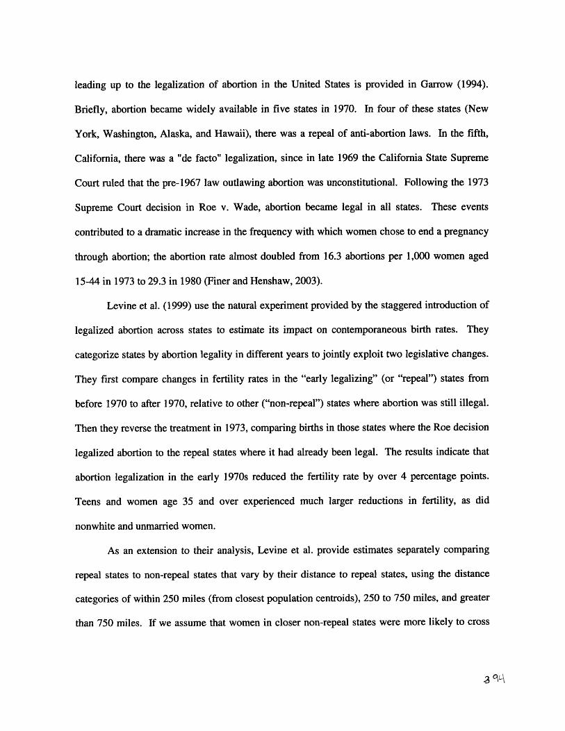
leading up to the legalization of abortion in the United States is provided in Garrow (1994).

Briefly, abortion became widely available in five states in 1970. In four of these states (New

York, Washington, Alaska, and Hawaii), there was a repeal of anti-abortion laws. In the fifth,

California, there was a "de facto" legalization, since in late 1969 the California State Supreme

Court ruled that the pre-1967 law outlawing abortion was unconstitutional. Following the 1973

Supreme Court decision in Roe v. Wade, abortion became legal in all states. These events

contributed to a dramatic increase in the frequency with which women chose to end a pregnancy

through abortion; the abortion rate almost doubled from 16.3 abortions per 1,000 women aged

15-44 in 1973 to 29.3 in 1980 (Finer and Henshaw, 2003).

Levine et al. (1999) use the natural experiment provided by the staggered introduction of

legalized abortion across states to estimate its impact on contemporaneous birth rates. They

categorize states by abortion legality in different years to jointly exploit two legislative changes.

They first compare changes in fertility rates in the "early legalizing" (or "repeal") states from

before 1970 to after 1970, relative to other ("non-repeal") states where abortion was still illegal.

Then they reverse the treatment in 1973, comparing births in those states where the Roe decision

legalized abortion to the repeal states where it had already been legal. The results indicate that

abortion legalization in the early 1970s reduced the fertility rate by over 4 percentage points.

Teens and women age 35 and over experienced much larger reductions in fertility, as did

nonwhite and unmarried women.

As an extension to their analysis, Levine et al. provide estimates separately comparing

repeal states to non-repeal states that vary by their distance to repeal states, using the distance

categories of within 250 miles (from closest population centroids), 250 to 750 miles, and greater

than 750 miles. If we assume that women in closer non-repeal states were more likely to cross

-3 %\

state lines to obtain an abortion (e.g. those in New Jersey crossing into New York), then the

effects of abortion legalization should be strongest for those living farthest from the early repeal

states. They also find that this effect was much larger when early repeal states are compared to

more distant comparison states, suggesting that travel between states dampened the estimated

impact.

III. Methodology

To examine the impact of abortion legalization on life-cycle fertility, we will again

exploit the quasi-experiment provided by the variation across states in the exact timing of

abortion legalization in the early 1970s. The main methodological extension in the present

analysis is to convert the focus on period effects that Levine et al. estimated to a focus on cohort

effects. The period effect analysis operated by comparing women at different ages at the time of

the law changes (either early repeal or Roe v. Wade), and measuring their current fertility rates.

The cohort analysis instead compares women who passed through these different legal states at

the time when they were most likely to be affected by abortion availability, and examines

measures of completed fertility.

A. Defining "Treatment Cohorts"

We focus on those cohorts who were most likely to be affected by changes in abortion

law in the early 1970s based on their age at that time. Women in these cohorts from repeal states

experienced greater exposure to legal abortion and may have had different fertility patterns over

the remainder of their lives as a result. Once these "treatment cohorts" are defined, the

methodological approach is analogous to that based on period effects. Women in the different

sets of states in cohorts before the treatment cohorts and after the treatment cohorts should have

been equally affected by changes in abortion policy; abortion would have either been uniformly

illegal (for the earlier cohorts) or uniformly legal (for the later cohorts) during the years in which

they were most at-risk of unwanted pregnancies.

To define our "treatment cohorts," we extend the analysis in Levine et al. to examine the

impact of abortion legalization by exact age, rather than by broad age groups, using Vital

Statistics microdata between 1968 and 1980 (described in the next section). Comparable to

Levine et al.'s findings (albeit with greater age-specificity), we find that legalized abortion had

the biggest relative impact on births to teens and to older women. The impact is largest at age

15, declines to zero by age 28, and then rises again.34

For the purposes of the present analysis, however, these results are somewhat misleading

because they reflect the impact on relative birth rates. In 1970, birth rates are highest between

the late teens and late 20s, peaking at age 23, and are low in the early teens and into the 30s and

40s. Therefore, the large relative impact of abortion legalization on births at older ages needs to

be tempered by the fact that the base is relatively low. The absolute impact on the number of

births is small at older ages.

To address the absolute impact on fertility, we repeat Levine et al.'s estimating strategy,

but replace the natural logarithm of the birth rate as the dependent variable with the birth rate in

levels. As such, parameter estimates represent the absolute effect on the birth rate rather than the

relative effect based on the percentage change. When we make this change, we see that ages 16

through 26 represent the peak ages at which the number of births was affected.35 At these ages,

births fell by roughly 6 per 1,000 women in response to abortion legalization. Therefore, we

34 Detailed results are provided in Ananat et al. (2004).35 Detailed results of this analysis are provided in Ananat et al. (2004) as well.

would expect the largest impact on lifecycle fertility to hit those cohorts who passed through the

early 1970s between the ages of 16 and 26.

The next step requires transitioning from these age-specific period effects to a definition

of the treatment cohorts. We know that abortion laws differed between repeal and other states

over the 1970 to 1972 period, which, given the nine month delay of pregnancy, largely applies to

births in 1971 to 1973. We can combine this information with the fact that the peak ages of

abortion legalization's impact was 16 to 26. This means that the birth cohorts of the later 1940s

and earlier 1950s were the ones whose fertility was most directly affected by abortion

legalization. As an approximation, in our analysis we define the 1946 to 1955 birth cohorts to

represent the treatment cohorts.36 If abortion legalization in the early 1970s reduced fertility at

those ages for these women, any permanent impact on lifetime fertility would show up as a gap

in children ever born between those who lived in early repeal states and others. Women born

after 1955 would have entered childbearing ages following the Roe decision, so they would have

faced a lifetime of exposure to legal abortion regardless of their state of residence. Similarly,

women born in the 1930s and earlier 1940s were in their later stages of childbearing by the early

1970s. These women passed through their peak childbearing years with no legal abortion access,

regardless of where they lived.

B. Empirical Model

These results bring us to an empirical specification of our model of completed fertility.

We estimate models of the form:

36 Our results are not sensitive to small changes in the start and end date of the treatment cohort. We alsoexperimented with alternative specifications within the 1946-1955 cohort window (like breaking it up into twowindows - one from 1946-1950 and one from 1951-1955), but found no pattern strong enough to statisticallydistinguish.

CF, = pl*REPEAL*D4655 + P2 *REPEALs*D(post55) (1)

+ 8s + 8c + 8s*TREND + Ccs

where CF,, represents alternative measures of completed fertility in cohort c in state s, D4655 is

an indicator of the 1946-1955 birth cohorts and D(post55) is an indicator of post-1955 birth

cohorts. We include state-specific (s) and cohort-specific (c) fixed effects to capture

longstanding differences in fertility patterns across states over time as well as aggregate patterns

of changing fertility preferences over time. We also allow the state-specific differences to trend

over time. The omitted term here is the difference before 1946 between repeal and non-repeal

states, which is captured by the set of state fixed effects. The coefficient 1 measures the

difference in completed fertility between repeal and non-repeal states for those women born in

the 1946-1955 period (the treatment cohorts), relative to those born before 1946 (who were

beyond prime childbearing age when abortion was legalized). The coefficient p2 measures the

difference in completed fertility between repeal and non-repeal states for the set of women born

after 1955 (for whom there should be no effect since they were all subject to legal abortion

throughout their childbearing years), relative to those born before 1946. As with the period tests

of Levine et al., this framework provides two tests for the effect of abortion legalization: that 01

is negative, and that 32 is zero.

It is important to recognize the additional power that we obtain by including the

interaction for the post-1955 cohort. Without it we would be unable to differentiate an early

repeal effect from a differential trend by repeal versus non-repeal states. That is, the early repeal

of abortion, followed by Roe v. Wade, allows researchers to go beyond the typical "difference-

in-difference" setup, in which it is difficult to distinguish policy-induced changes from

underlying trends. By finding both an effect on fertility for the treatment cohort and that there is

no effect for later cohorts, we are able to confirm that there is a causal effect of abortion

availability and not an underlying trend that differs between these sets of states.

There are two other important differences in this model relative to standard difference-in-

difference models, like Levine et al. (1999), which rely on contemporaneous data. First, states

no longer represent the state where the birth occurred since states are designed to identify the

mother's state of residence in the early 1970s. As described below, however, it is impossible to

determine states of residence in the early 1970s from the available data, so we use mothers'

states of birth instead. Using state of birth has two advantages for our purposes: it is exogenous

to any mobility decisions related to abortion availability37; and it is a fixed characteristic that

allows us to merge the two data sources we use below. Second, we no longer are able to control

for other time varying, state-specific covariates. In the cohort context, individuals are potentially

influenced by some complex function of social conditions since they were born and it is unclear

how to specifically control for them in a regression framework.38 Instead, we rely on state of

birth fixed effects along with linear trends within states of birth to control for these other

factors. 3 9

37 Implicitly, we use repeal status of the state of birth to instrument for repeal status of the state a woman lived induring her childbearing years. If migration between repeal and non-repeal states increased over time, then state ofbirth would be a weaker instrument for later cohorts, causing our estimate of P2 to be biased toward zero andoverstating the evidence for our hypothesis. However, migration rates between early-legalizing and other stateshave not changed significantly over the period in question: in 1980, 90.02% of women of childbearing age wereliving in a state whose repeal status was the same as that of their state of birth; in 2000, the analogous proportionwas 90.21%. Therefore legalization timing in a woman's state of birth appears to be an equally strong instrumentfor exposure to legalization in older and younger cohorts.38 One type of time varying, state-specific covariate that is more easily incorporated into this framework is exposureto other relevant social policies during women's childbearing years. We experimented with two such variables:number of years of exposure to legal access to contraception between the ages of 18 and 20 (derived from the data inBailey, 2006) and the number of years of exposure to Medicaid funding of abortion (derived from the data inLevine, 2004). These policies both varied over states and time, so women in different state/year of birth cohortswould have different exposure to these policies over their childbearing years. Since these policies are also related toabortion access, they have the potential to bias our results. Nevertheless, when we included these additionalvariables neither were statistically significant and including them had very little impact on the estimated repeal/yearinteractions. As a result, we chose to report the results omitting these variables.

39 The findings reported later in the paper are similar when we control for state-specific quadratic trends.

In addition to estimating models of this form, we also follow Levine et al. and estimate

models comparing completed fertility to women in repeal states to women in non-repeal states

who differ in their distance to repeal states. If travel between states occurred in response to the

early legalization of abortion in repeal states, then the estimated impacts should be greater when

comparing repeal states to more distant non-repeal states.

IV. Description of the Data

Based on this discussion, we need data providing measures of women's completed

fertility for different birth cohorts of women along with geographical identifiers that can isolate

those women exposed to the early legalization of abortion in repeal states. No single dataset

provides all of this information. We rely on the Public Use Micro Sample from the 1970 Census

and data from the Vital Statistics Natality Detail Files between 1968 and 1999 to construct

measures of completed fertility for birth cohorts beginning in the 1930s and going through the

1960s. This combination provides a unique opportunity to examine the life-cycle fertility of the

relevant treatment and control cohorts.

The Vital Statistics data represent individual records on births that took place in the

United States between 1968 and 1999.40 Microdata prior to 1968 are not publicly available.

These data are invaluable because they specify the parity of the birth, the mother's age (from

which we can estimate the year she was born), and the mother's state of birth.4 ' With these data,

40 From 1985 onward, these data represent a complete count of births. Prior to 1972, births were sampled at a 50percent rate nationwide. In the intervening period, some states sampled at a 50 percent rate and others included allbirths. In our analysis, we applied appropriate weights to provide estimates of all births.41 For a very small number of births, this information is missing. These births are not included in the analysis.These data also contain information regarding whether the birth was a singleton or part of a multiple birth. Theissue of multiple births is an interesting one in the present context, because fertility treatments over time haveincreased the likelihood of multiple births and may have made it more difficult to achieve "optimal" family size ifmultiple births result from a pregnancy for which only one child was intended. To pursue this issue, we estimatedrates of singleton births for 1971 and 1999 separately for repeal and non-repeal states. Our results indicate that

amoOa

we can attribute every birth that takes place in the United States to the mothers' state/year of

birth cohort.42 Moreover, we can use the information available on the parity of each birth to help

formulate the distribution of the number of births to each woman over her childbearing years.43

For those women born in the mid 1950s and later, these Vital Statistics microdata contain

a record of every birth they have had. Since fertility trails off considerably after age 35 and is

very low after age 40, birth records for the 1968 through 1999 period will capture most, if not all

all births to women born as recently as the mid 1960s. Therefore, these data on their own are

sufficient to measure completed (or almost completed) fertility for roughly a decade's worth of

birth cohorts. But these data are inadequate for capturing completed fertility for women born

before the mid 1950s since they will already have given birth to at least some of their children

prior to 1968. If they give birth to additional children after 1968, we will see them in the Vital

Statistics data from later years, but we would miss any women whose fertility is completed

before 1968.

To count births prior to 1968 we use data from the 1970 Census, which provides

information on both women's state of birth and their children ever born.44 Based on these data,

we can count children ever born who are more than two years old, and thus were born before

1968, by mothers' birth cohort and state. This becomes a baseline to which we can add

information on later births from the Vital Statistics data. For example, consider the cohort of

women born in 1940. We use the 1970 census data to measure how many children those women

singleton births have declined slightly over time (from 98 to 97 percent) and that there is no difference in thesevalues between repeal and non-repeal states.42 Another minor limitation of these data is that births to women who were born in the United States but gave birthin another country would not be captured in these data. It is our impression that this is a very infrequent event andwe ignore it here.43 Each birth at a given level of parity contributes to the counts in a cumulative birth distribution, which can then beconverted to a probability distribution.44 The Census data we use come from the standardized Minnesota Integrated Public Use Microdata Series (Rugglesand Sobek 2003).

101

had through 1967. We then use the Vital Statistics data to track the additional births to this

cohort that occurred in 1968 or later. Since both sources of data are sorted by state of birth, we

can be sure that we are tracking the same women.

We use these combined Census and Vital Statistics microdata to create measures of

lifetime fertility for women born in the 1930s through the 1960s.45 For the earliest of these

cohorts, the Census data captures virtually all of their fertility.4 6 For those born after the mid

1950s their fertility history is virtually entirely captured by the Vital Statistics microdata. For the

intervening cohorts, these two data sources are combined to create complete fertility histories.

Using the available data, we are able to construct measures of the number of children ever born

by age 25, by age 30, by age 35, and then total completed fertility.47 We convert counts of births

by these ages to measures of children ever born per woman by incorporating estimates from the

1970 Census on the number of women in each state/year of birth cohort. In addition, we have

constructed distributions of the number of children born to each woman in each state/year of

birth cohort and focus, in particular, on the percentage of women who never have children.4 8

45 Although the approach we use to construct these data provides what we believe is the best method available, it isnot without limitations. First, the Vital Statistics data do not contain information on mother's state of birth in 1968,1969, and 1972. To overcome this, we estimate the number of births in those years by mother's state of birth byusing rates of migration between birth states and state of residence computed from the 1970, 1971, and 1973 data. Asecond limitation of the Census data is that it only provides information on an individual's age and quarter of birth,without specific birth dates. We employ an algorithm that assumes all responses were filed on April 1St to determinethe number of children born since the beginning of 1968 and then take the difference between this and children everborn to determine the number born prior to 1968. These issues are described in greater detail in Ananat et al.(2004); we do not believe that they have any systematic effect on our results.46 For example, the 1933 birth cohort would have been 35 years old in 1968. Their completed fertility included anaverage of 3.17 children; 3.04 of them were born by age 35.47 Where sufficient data are available, we define total completed fertility to include births up to age 44. In someinstances, however, we use births up to age 39 since so little fertility takes place after that. We have tested thesensitivity of our results to including births up to age 39 for all cohorts and found little difference to that reportedhere.48 All of these data can be constructed separately for white women and non-white women (blacks or other race)separately. We have done so and estimated all the models reported subsequently separately by race. Notsurprisingly, results for white women look very similar to those for the whole population because whites represent alarge majority of the population. Point estimates for non-whites were also similar, but they lacked the precision tobe able to draw strong conclusions.

10-

V. Results

Initial Evidence

Before presenting estimation results from equation (1) using our constructed data on

completed fertility, we first present an analysis that relies exclusively on contemporaneous age-

specific birth rates beginning in 1968 from the Vital Statistics microdata. We attribute births at

each age in each year to the relevant birth cohort of the mother, defined as the year of birth

minus mother's age. For example, we can construct a birth history for the 1959 birth cohort by

using birth rates at age 15 from 1974, age 16 from 1975, age 17, from 1976, and so on. We then

plot the percentage difference in age-specific birth rates between women in repeal states and

other states for three selected cohorts. For the 1959 birth cohort, the differential timing across

states in abortion legalization would have had no impact on the difference in birth rates since

these women would not have reached their childbearing years until after Roe v. Wade.

Therefore, this cohort can serve as a control group.

The results of this analysis are plotted in Figure 1 for the 1949, 1954, and 1959 birth

cohorts. Women in repeal states are more likely to have their births at later ages, as indicated by

the general upward slope of these lines. The treated cohorts are those born in 1954 and 1949,

who would have been 17 and 22 years old in 1971, respectively, when abortion was legalized in

the early repeal states. The trends in age-specific fertility for these cohorts clearly show the

period effects that past research has found. Age-specific birth rates for women in repeal states in

the 1954 birth cohort show a clear drop exactly at age 17 relative to women in non-repeal states

and to other birth cohorts. This drop lasts for the few years in which abortion laws differed

across states and then reverts back to the pattern for the control cohorts. Similarly, births to

women in repeal states in the 1949 birth cohort fall exactly at age 22, which corresponds to their

12,

births in 1971, and remain lower just for the three years in which abortion policies differed

across states. 4 9

The advantage of this figure is that it enables us to compare births at later ages for these

cohorts that were clearly contemporaneously affected by differential abortion access. The

impression one would take away from this figure is that the contemporaneous reduction in births

did not alter childbearing patterns at later ages. The age-profile in the difference in births for the

1954 cohort is no different after the early 20s from that of the control cohort. If anything,

women in the 1949 birth cohorts from repeal states had fewer births over the remainder of their

main childbearing years compared to women in other states and the control cohort. These results

provide the first evidence that the reduction in period fertility attributable to abortion legalization

may have been permanent.

Main Results

Figure 2 and the top panel of Table 1 present the main results of our cohort-based

analysis examining the impact of abortion legalization on children ever born. Figure 2 focuses

on children ever born throughout the childbearing years and Table 1 separately considers

children ever born by age 25, 30, 35, and completed fertility (by age 44, or age 39 for cohorts

who have not yet reached 44 in 1999).50 As we described earlier, we are looking for a gap to

49 Note that births for the 1949 cohort are only reported beginning at age 19, which corresponds to their fertility in1968, the first year in which Vital Statistics microdata are available.50 All fertility information before 1968 comes from the 1970 Census, which only includes data on children ever bornwhen the Census was completed. It is impossible to date when births occurred prior to that year in those data. Thisexplains why data on births by age 25 and age 30 are only available as far back as the 1943 and 1938 birth cohorts,respectively. To maintain at least some balance to our sample, we do not use birth cohorts prior to 1933 since wewould not be able to date births by age 35 prior to that year. At the other extreme, births by age 35 are onlyavailable through the 1964 birth cohort since our micro Vital Statistics data ends in 1999. In addition, children everborn represents births to age 44, except for the 1956 through 1960 birth cohorts in which births to age 39 are usedsince these birth cohorts had not yet reached age 44 by 1999. We have estimated all of our models using data for

13 lo1L

emerge in the difference in children ever born between women in repeal and other states

beginning around the 1946 birth cohorts that would then disappear for the post-1955 birth

cohorts.

Figure 2 displays the difference in children ever born between women born in repeal

states and other states over time. The results indicate a clear upward trend in this difference, as

illustrated by the trend line added to the figure. Apparently, it used to be the case that women in

non-repeal states had more children than women in repeal states, but this difference has been

slowly going away. This highlights the need to consider the deviation from state-specific trends.

Such a deviation from trend is clearly apparent for the relevant birth cohorts, those born between

1946 and 1955. For that set of cohorts, there is a sharp reduction in the differential of children

ever born between repeal and non-repeal states.

This conclusion is confirmed in the top panel of Table 1. By the end of childbearing (the

final column), we see that abortion legalization reduced children ever born by 0.054.51

Moreover, the difference in children ever born that emerged for the 1946 to 1955 birth cohorts in

repeal states was statistically eliminated in the post-1955 cohorts. The coefficient for that cohort

is statistically and substantively insignificant. This further confirms the causal interpretation of

our finding. The effects we estimate here are present only for the 1946-1955 cohorts, relative to

both cohorts born before 1946 (the omitted group), and cohorts born after 1955; these are not just

trends in differential state fertility behavior.

Evidence in the top panel of Table 1 also suggests that the similar reductions in fertility

are observed by ages 25, 30, and 35. By each of those ages, we see that children ever born to

i4- 1o3

just the 1943 through 1960 birth cohorts, which provide relevant information for children ever born by each age (andassuming that "completed fertility" ends at age 39) and obtained results comparable to those reported below.51 To provide some perspective on the magnitude of this number, roughly 3 million women were born between 1946and 1955 in repeal states. If the each had 0.054 fewer children, this would amount to about 150,000 fewer children.

women in repeal states had fallen by .07 relative to women in non-repeal states in the 1946 to

1955 birth cohorts. Importantly, this gap is statistically and substantively insignificant in the

post 1955 cohorts (except, perhaps, by age 25). Although these point estimates for the 1946 to

1955 birth cohorts by age 35 are slightly larger than that by the end of childbearing, they are not

statistically different. These results suggest that the reduction in births associated with abortion

legalization in the early 1970s was essentially permanent. It does not appear that much, if any,

of it was made up in the form of additional births at later ages.

As a rough assessment of the validity of these findings, we estimated models comparable

to that in Levine et al. (1999) using age-specific birth rates estimated from 1968 to 1980 Vital

Statististics microdata. We then applied the estimates of the impact of abortion legalization on

these birth rates (a 6.7% reduction) to the 1970 age-specific birth rates to determine the steady

state impact on children ever born. The results suggest that children ever born would have fallen

by 0.043, which is comparable to (and not significantly different from) our estimate in Table 1 of

0.054 by the end of childbearing.

Distance Estimates

A means of confirming this striking finding is to take advantage of the fact that the non-

repeal states are better "controls" the farther they were from the repeal states (due to the

possibility of travel to the repeal states from nearby states). Following Levine et al., we can

divide the non-repeal states into those within 250 miles, between 250 and 750 miles, and more

than 750 miles from repeal states.52 By doing so, we can assess whether our results are stronger

for the farther away set of control states, as we would expect.

52 States in each category include:Repeal: AK, CA, HI, NY, and WADistance < 250: AZ, CT, DE, DC, ME, MD, MA, MI, NV, NH, NJ, OH, OR, PA, RI, VTDistance > 250 and < 750: CO, GA, ID, IL, IN, IA, KY, MN, MS, MT, NM, NC, SC, TN, UT, VA, WV, WI, WY

5 0(0

Figure 3 and the remainder of Table 1 report the results of our analysis, separately for

control states of different distances to the repeal states. Figure 3 displays the difference in

children ever born by the end of childbearing to women in repeal states relative to women in

each of these distance categories by mother's birth cohort. Again, this figure shows that women

in repeal states historically had fewer births, but it also shows that the difference is greater when

they are compared to further away states. In each case the general trend is toward a narrowing of

the gap. But for far away non-repeal states, another clear pattern is the break from trend that

occurs in the difference in children ever born among cohorts born in the late 1940s and early

1950s. No such trend is apparent when comparing children ever born between repeal states and

the nearest group of comparison states.

These assessments are confirmed in the bottom three panels of Table 1. By age 25,

children ever born to women in repeal states born between 1946 and 1955 fell by an insignificant

amount relative to women in the closest group of comparison states, by 0.085 children relative to

the middle distance group, and by 0.099 children relative to the most distant group of

comparison states. Moreover, the estimates are roughly stable throughout the remainder of the

childbearing years. And, for all distances, the results are largely insignificant for the cohorts

born after 1955.53 These results provide further evidence of a causal and largely permanent

impact of abortion legalization on children ever born.

Distribution of Children Ever Born

We turn our attention now to the impact of abortion legalization on the distribution of

children ever born rather than just the count. We pay particular attention to the percentage of

*W106

Distance > 750: AL, AR, FL, KS, LA, MS, NE, ND, OK, SD, TX.53 The coefficient on the post-1955 interaction for the middle distance states is statistically significant, contrary tothe model's predictions. In a table estimating this many coefficients, one might expect random variation to providean occasional odd result and this would be our interpretation of this finding.

childless women, which is of primary importance since it is the only point in this distribution for

which we have an unambiguous prediction; more women should remain childless. Since the

remainder of the distribution should be shifting to the left, it is difficult to tell whether the flow

out of a particular level should be greater than the flow in from a larger value (e.g. the share of

women who only had one child will be falling as those who otherwise would have one child

move to zero children, but it will also be rising as those who otherwise would have two children

move to one child).

The main results of this analysis are reported in Figure 4 and in the top panel of Table 2.

Figure 4 displays the difference in the percentage of childless women between repeal and non-

repeal states by birth cohort. For all birth cohorts before the mid 1940s, this difference is

reasonably stable. But by the mid 1940s we begin to see a sizeable jump in the number of

childless women in repeal states relative to non-repeal states. The gap widens through the early

1950s and then recedes, just as we would predict if the cause of the gap was differential abortion

access. By 1956, the difference is at the same level as before the "treatment" cohort began in

1946.

Table 2 presents a regression-based version of these results that also includes the

percentage of women with different numbers of children. The results presented here confirm our

observations from Figure 2 in that abortion legalization is estimated to have increased the

number of childless women in the treatment cohort by 3.47 percent. Once again, there is no

significant impact on the post-1955 cohort, consistent with the causal interpretation of this

finding. 5 4

54 Another interesting simulation estimates the number of children that those who became childless would have hadif abortion were not legalized. If the number of women having children fell by 3.47 percentage points and thisreduction led to a reduction in children ever born by 0.054, then it must have been the case that these women whoremain childless otherwise would have had .054/.0347 = 1.57 children if abortion remained illegal.

1- is

The evidence regarding the impact at other points in this distribution is not that strong.

Although we see a reduction in the number of women with one child and two children in the

1946 to 1955 repeal cohorts, a similar reduction is also observed for the later birth cohorts in

those states. Therefore, it is difficult to attribute this change to abortion legalization itself as

compared to some other ongoing trend that differed across states in the later birth cohorts.

Figure 5 and the remainder of Table 2 conduct the analogous exercises differentiating

comparison states by their distance to repeal states. In Figure 5 we see that the difference in the

percentage of childless women between repeal states and the closest set of non-repeal states was

stable across birth cohorts. But as the distance increases across comparison states, we see the

gap in the percentage of childless women for the late 1940s and early 1960s birth cohorts grow.

The bottom three panels of Table 2 confirm these impressions. Relative to the closest

group of comparison states, there was no statistically significant increase in the percentage of

childless women among women born in repeal states between 1946 and 1955. Relative to the

middle distance and farthest distance groups, however, these women are estimated to be 3.89

percent and 5.45 percent more likely to be childless. The pattern by repeal status, birth cohort,

and distance to repeal states provides strong evidence that this finding is causally related to

abortion legalization.

Discussion and Implications of Lifecycle Fertility Results

The results from this analysis tell a very consistent story: the early availability of abortion

in the repeal states led to a decline not only in contemporaneous but in permanent fertility. This

reduction in lifetime fertility is largely attributable to an increase in the number of women who

complete their fertile years without having any children. This finding is clear both graphically

and statistically. And it is confirmed both by the absence of any differential effect for cohorts

born after 1955, and by the fact that the effect is much stronger the farther away the control

states were from the early repeal states.

These results are also substantively large. The 1945 birth cohort, which had already

passed through its peak childbearing years by the time abortion was legalized, averaged about

2.4 births per women; about 11.3 percent had no children at all.55 By the 1960 birth cohort,

which was fully exposed to legalized abortion in all states at the time they hit childbearing age,

each woman had 1.9 children on average; 18.2 percent had no children. Our overall estimates

imply that abortion availability lowered the number of children ever born by 0.054, and the odds

of being childless by 3.6 percent. These figures account for 11 and 52 percent of the time series

changes in these variables.

Moreover, this calculation likely provides a lower bound of the effect of legalized

abortion because it does not account for the fact that some women in non-repeal states traveled to

repeal states prior to the Roe decision. Using our estimates based on the control states farthest

from the early repeal states, we would be able to explain 17 and 79 percent of the time series

change in these variables.

Other Outcomes for Women

The fact that abortion availability had such a fundamental impact on the lifecycle fertility

patterns of women raises the issue of whether legalization had impacts on other aspects of these

women's lives as well. Women who reduced the total number of children they had or chose

never to have any at all may have invested in more education and worked more, which would

have led to higher wages. Their marital decisions may have been altered as well. Changes in

55 This estimate is based on the data employed in this project. Estimates based on data from Current PopulationFertility Supplements are more like 14 percent.

both earnings and family composition effects also may have affected their poverty rates and

welfare participation.

We attempted to investigate this by looking at measures of these outcomes available in

the decennial Census. In order to focus on the full effects of reduced fertility, we looked at

outcomes for women aged 35 to 44, for whom most childbearing is complete.56 We observed the

outcomes of the various cohorts of interest at these ages by pooling multiple Censuses.

Observations for women born between 1930 and 1935 come from the 1970 Census, so that the

outcomes of those born in 1930, for example, are measured at age 40, while the outcomes of the

1935 cohort are measured at age 35. For the 1936 to 1945 cohorts, observations come from the

1.980 Census; for the 1946 to 1955 cohorts, from the 1990 Census; and for the 1956 to 1960

cohorts, from the 2000 Census.

We estimated models comparable in format to those reported earlier regarding children

ever born to assess the impact of abortion legalization on women's outcomes, categorizing

women according to state and year of birth and then examining the patterns in outcomes over

time between women born in repeal and non-repeal states. The outcomes examined include: the

probability of having completed high school or having completed college; current labor force

participation; poverty status, and household income as a percent of the poverty line. Using these

samples, we were unable to identify effects of increased fertility control on any of these

outcomes, but our results were not sufficiently precise to rule out such effects. Apparently, the

availability of virtually universal Vital Statistics data on fertility provided statistical power in our

earlier analysis that we were unable to attain relying exclusively on the 5 percent samples (or, in

the 1970 Census, a 4 percent sample) available in the Census data.

56 Ideally, we would focus on a somewhat older age range, but the youngest of treated women, who were 15 in 1970,had only reached age 45 by 2000.

o I(I

VI. Conclusions

It is clear from past research that the legalization of abortion in the U.S. induced a major

change in fertility. Estimates from past research, replicated here, suggest that total fertility fell

by roughly 5 percent when abortion was legalized. Previous research on fertility has emphasized

the importance of decomposing fertility changes into temporary fertility (timing) effects and

permanent (completed fertility) effects. Yet this has not been done for this critical change in the

nature of birth planning.

In this paper, we directly investigate the impact of abortion legalization on the lifecycle

pattern of fertility of cohorts affected by legalization. The power of our analysis derives from

the observation that abortion legalization had its primary effects on those aged 16 to 26; for

younger and older ages, there was either a sufficiently small effect of abortion access, or

sufficiently low baseline fertility. Those ages 16 to 26 in the early 1970s, when abortion laws

differed across states, were mainly in the cohorts born between 1946 and 1955. Thus, by

comparing differences in children ever born between women in early repeal states to women in

other states during the 1946 to 1955 window relative to the analogous difference for women born

before and after those years, we can provide a causal estimate of the impact of abortion

legalization on lifetime fertility.

Our results are striking. It appears that the response of fertility to legalization was largely

composed of reductions in completed fertility, not changes in timing. Moreover, abortion

legalization is found to have led to a very large rise in childless women in these treatment

cohorts. The causal nature of our findings is confirmed by the comparison to other cohorts

surrounding the treatment cohort, and by the fact that the relationship is strongest relative to the

most distant states whose residents could not benefit from early legalization.

There are several important implications of these findings. First, they suggest that

improved fertility control does not simply lead to changes in fertility timing, as suggested by

some other papers. Indeed, the majority of the effect of abortion legalization was permanent and

not attributable to timing effects. Second, they suggest that the availability of abortion can

explain a sizeable share of the time series trend in reduced completed fertility and in childless

women over these birth cohorts. Finally, there are potentially important implications for the

long-term well-being of these cohorts of mothers from the improved fertility control. We were

unable to draw strong conclusions about these implications from the available data, but this is a

worthy goal for future research.

S2 23

References

Ananat, Elizabeth Oltmans, Jonathan Gruber, and Phillip B. Levine. AAbortion Legalizationand Lifecycle Fertility.@ National Bureau of Economic Research working paper 10705, August2004.Angrist, Joshua and William N. Evans. "Schooling and Labor-Market Consequences of the 1970State Abortion Reforms," in Solomon Polachek and John Robst (eds.), Research in LaborEconomics. Vol. 18 (1999). pp. 75-114.Bailey, Martha J. "More Power to the Pill: The Impact of Contraceptive Freedom on Women'sLifecycle Labor Supply," Quarterly Journal of Economics, forthcoming.Donahue III, John J., and Steven D. Levitt. "The Impact of Legalized Abortion on Crime."Quarterly Journal of Economics. Vol. 116, No. 2 (May 2001). pp. 379-420.Finer, Lawrence B. and Stanley K. Henshaw. "Abortion Incidence and Services in the UnitedStates." Perspectives on Sexual and Reproductive Health. Vol. 35, No. 1 (January/February2003). pp. 6-15.Garrow, David J., Liberty and Sexuality: The Right to Privacy and the Making of Roe v. Wade.New York, NY: Macmillan Publishing Company. 1994.Gruber, Jonathan, Phillip B. Levine, and Douglas Staiger. "Abortion Legalization and ChildLiving Circumstances: Who is the "Marginal Child?" Quarterly Journal of Economics. February1999. pp. 2 6 3-2 9 2 .Levine, Phillip B., Douglas Staiger, Thomas J. Kane, and David J. Zimmerman. "Roe v. Wadeand American Fertility." American Journal of Public Health. February 1999. pp. 199-203.Levine, Phillip B. Sex and Consequences: Abortion, Public Policy, and the Economics ofFertility. Princeton, NJ: Princeton University Press. 2004.Ruggles, Steven and Matthew Sobek et al. Integrated Public Use Microdata Series, Version 3.0.Minneapolis: Historical Census Projects, University of Minnesota, 2003.http://www.ipums.umn.edu/

23- 1 1

Table 1: Estimated Impact of Abortion Legalization on Children Ever Born, by Age

Children Ever Born by:

End ofAge 25 Age 30 Age 35 Childbearing

Mean of Dependent Variable (all states) 1.10 1.73 2.16 2.48

Repeal States Relative to All Non-Repeal States

Repeal*1946-1955 birth cohorts

Repeal*post-1955 birth cohorts

Sample Size (birth cohorts*states)

-0.068(0.012)

-0.030(0.018)

1,377

-0.070(0.018)

0.006(0.030)

1,632

-0.070(0.023)

0.002(0.029)

1,632

-0.054(0.012)

-0.002(0.018)

1,377

Repeal States Relative to Non-Repeal States within 250 Miles of a Repeal State

Repeal* 1946-1955 birth cohorts

Repeal*post-1955 birth cohorts

-0.030(0.019)

-0.015(0.022)

Sample Size (birth cohorts*states) 567

-0.010(0.022)

0.017(0.032)

672

-0.007(0.030)

0.006(0.038)

672

-0.007(0.022)

-0.009(0.026)

567

Repeal States Relative to Non-Repeal States between 250 and 750 Miles from a Repeal State

Repeal*1946-1955 birth cohorts

Repeal*post-1955 birth cohorts

Sample Size (birth cohorts*states)

-0.085(0.016)

-0.042(0.021)

648

-0.098(0.021)

-0.005(0.033)

768

-0.095(0.025)

-0.006(0.035)

768

-0.073(0.013)

-0.008(0.027)

648

Repeal States Relative to Non-Repeal States greater than 750 Miles from a Repeal State

Repeal* 1945-1955 birth cohorts

Repeal*post- 1955 birth cohorts

-0.093(0.023)

-0.028(0.032)

-0.108(0.030)

0.009(0.047)

-0.114(0.026)

0.016(0.039)

-0.087(0.019)

0.028(0.033)

Sample Size (birth cohorts*states) 432 512 512 432Notes: The dependent variable in each regression represents the average children ever born to women by each age.The "end of childbearing" is defined to be the oldest age for which births occur. For younger cohorts additional birthsare likely to result after the period for which data is available here. To address this, I only include the 1960 andearlier birth cohorts whose fertility at least through age 39 is recorded. Since so few births occur after that, I definelifetime births to equal the births that have occurred through the last age observed. All specifications include stateand cohort-specific fixed effects along with state-specific trends. Standard errors are corrected for heteroskedasticityand an arbitrary covariance structure within birth states (i.e. clustered on state of birth).

z 2.4-

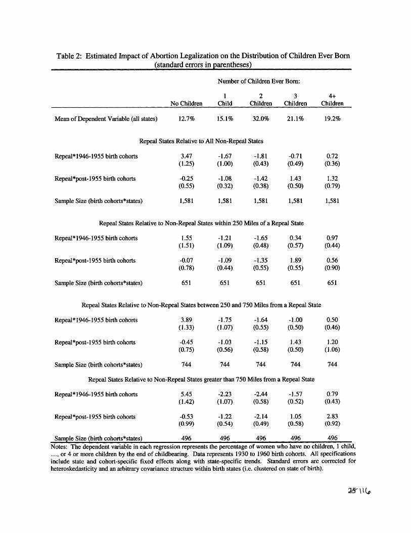
Table 2: Estimated Impact of Abortion Legalization on the Distribution of Children Ever Born(standard errors in parentheses)

Number of Children Ever Born:

1 2 3 4+No Children Child Children Children Children

Mean of Dependent Variable (all states) 12.7% 15.1% 32.0% 21.1%

Repeal States Relative to All Non-Repeal States

Repeal*1946-1955 birth cohorts

Repeal*post-1955 birth cohorts

Sample Size (birth cohorts*states)

3.47(1.25)

-0.25(0.55)

1,581

-1.67(1.00)

-1.08(0.32)

1,581

-1.81(0.43)

-1.42(0.38)

1,581

-0.71(0.49)

1.43(0.50)

1,581

Repeal States Relative to Non-Repeal States within 250 Miles of a Repeal State

Repeal*1946-1955 birth cohorts 1.55 -1.21 -1.65 0.34(1.51) (1.09) (0.48) (0.57)

Repeal*post-1955 birth cohorts -0.07 -1.09 -1.35 1.89(0.78) (0.44) (0.55) (0.55)

Sample Size (birth cohorts*states) 651 651 651 651

Repeal States Relative to Non-Repeal States between 250 and 750 Miles from a Repeal State

Repeal*1946-1955 birth cohorts 3.89 -1.75 -1.64 -1.00(1.33) (1.07) (0.55) (0.50)

Repeal*post-1955 birth cohorts -0.45 -1.03 -1.15 1.43(0.75) (0.56) (0.58) (0.50)

651

0.50(0.46)

1.20(1.06)

Sample Size (birth cohorts*states) 744 744 744 744 744

Repeal States Relative to Non-Repeal States greater than 750 Miles from a Repeal State

Repeal*1946-1955 birth cohorts 5.45 -2.23 -2.44 -1.57 0.79(1.42) (1.07) (0.58) (0.52) (0.43)

Repeal*post-1955 birth cohorts -0.53 -1.22 -2.14 1.05 2.83(0.99) (0.54) (0.49) (0.58) (0.92)

Sample Size (birth cohorts*states) 496 496 496 496 496

Notes: The dependent variable in each regression represents the percentage of women who have no children, I child,... , or 4 or more children by the end of childbearing. Data represents 1930 to 1960 birth cohorts. All specificationsinclude state and cohort-specific fixed effects along with state-specific trends. Standard errors are corrected forheteroskedasticity and an arbitrary covariance structure within birth states (i.e. clustered on state of birth).

19.2%

0.72(0.36)

1.32

(0.79)

1,581

0.97(0.44)

0.56(0.90)

_ . . _ . .

~ *00 0

\~00

* C

0 - -'

00 rhm Ch

Ionc~ o

c 0

) )

a 0

u I_

In00

. _

t

I.,..tu'E;)

-o0)

(0)zC

0

0

I0)

00)

o0P.)C'stov26u

CD

0

S

v:

r_cj 01

C

C0)-FIC

UtLCR

t i

-

0[-)

0

Ev00

zr.

cO

cws

a)01)0)P

z

0)

t

0)

co

-G

040)r0C)c

40O X

-o O

,B -o

C)

-

I

II

0

ct

t

. - V)

a o

1) aQ

O C

$ _4C 0 c

(1) 0--

Q)

4

(1)

40

O o o o O o o 0 0 o oIn It Ci i i (IedoI-uoN - eodI) ouaooJJ!a oiUluoZJ3d

,-Ito

ooeeh

{n00m

Ccrm

mW)cn

.. _mc

Cr'

m

om

tC'

C-

Nl

Cl4cl

CACl

=C

QC,

I-okr)Co0

0oCallo0'

+

Cl4

C)

C4'

00

F-

IN

kr)

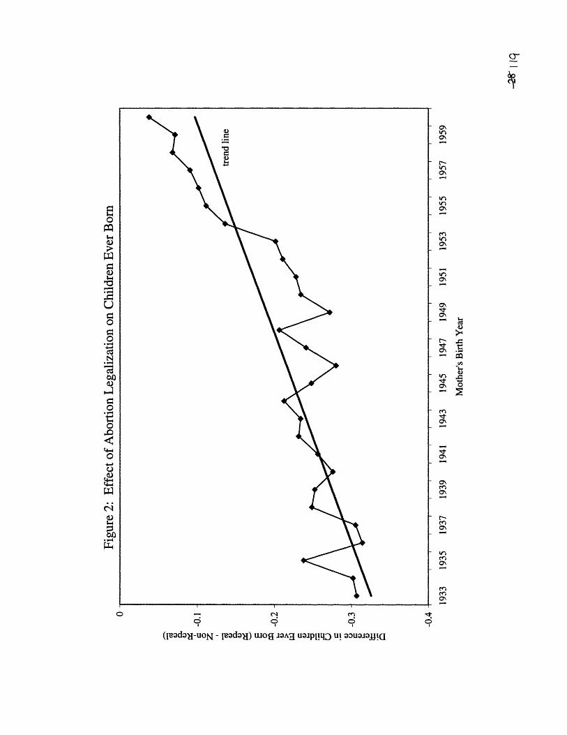
c.1

"O

I C6 o9c

(leadma-uoN - loado) UJOt gAI uaOpIp!qj U! QuJJ!Jl

o-

0

0

.--

C)tq

. .©

.0

oas

--*

tr

InON

- -4-m

-

'e

-

-It

in

ev~eeCf)

To

0I 1 _·

I I I I I -

ho\IciF C:W)

iON

C

W)ON-4

0-4

a

-0.4

-4 0VR

~t U

W0

0)

0IS0 o

0'0'4-40t

o 6 ) c 6 c(leoada-uou - gladao) gtH ui aouaoJajja

CO

O,-C

NC

co*S

Q)

Ec

an

N

ioantUXA

'I

oC)

V

9

ma-

1-

_ __ ~ ~ ~ --- ---- - ------ --I I

i

I

U~

i w.:

leodo-I-uoN - luodod) a3uaojJJla

C

C

0,al

U00-0

gI0CA

4)

C4

o

\00

inI,.

tr

- 0

C

0.00

- N- n

oo0 (1

__ __

�I - �I -- ·

I III I I I I rI

oll'r-Cre

ON

t

0.'

mN

- In

It

ONto4- V) 00'

'Fm

-{,

m

0.'

- lrj

- inma,Cr1Cr0.'

00oo \ Cl 0 00 \C I Cl O Cl

(IeadaJ-uou - leoada) aouaojj!

cly

0(e~D

c{

coO -

oO

F,

0bt2e: )

O rd

O -¢

,o <6

3.. D

0

0Lr o(D(D .% Wo)

Ct

CIO

AOin

m

or-AV)

CA

Nv

��--�------�----��---"��--�-�-- --I-

II

I