AD-762 148

CHAPMAN-KIRK REDUCTION OF FREE-FLIGHT RANGE DATA TO OBTAIN NONLINEAR AERO- DYNAMIC COEFFICIENTS

Roberr H. Whyte, et al

Ballistic Research Laboratories Aberdeen Proving Ground, Maryland

May 1973

DISTRIBUTED BY:

urn National Technical Information Service U. S. DEPARTMENT OF COMMERCE 5285 Port Royal Road, Springfield Va. ?2151

QP

a: CD

00

(M CO

Q

BRL |AD_

MEMORANDUM REPORT NO. 2298

CHAPMAN-KIRK REDUCTION OF FR"E-FUGHT

RANGE DATA TO OBTAIN NONLINEAR

AERODYNAMIC COEFFICIENTS

by

Robert H. Whyte Angela Jeung

James W. Bradley ^ rD P c

; M 28 1973

May 1973 ;J u LJC^

Approved for public release; distribution unlimited.

NATIONAL TECHNICAL INFORMATION SERVICE

USA BALLISTIC RESEARCH LABORATORIES ABERDEEN PROVING GROUND, MARYLAND

.-rv

Destroy this report when it is no longer needed. Do not return it to the originator.

Secondary distribution of this report by originating or sponsoring activity is prohibited.

Additional copies of this report may be obtained from the National Technical Information Service, U.S. Department of Commerce, Springfield, Virginia 22151.

-F - l"1 ''

a

M ti:il11!CTIM/««U«Un C0D3

tun. i^uit/m snan.

The findings in this report are not to be construed as an official Department of the Army loaition, unless so designated by other authorized do uments.

IINUASÜinil] jgcurtt» Cl«tiific«iion

DOCUMENT CONTROL DATA ■ R & D (Security claaatlumtion ol »!/>. body of mbittm* i «nd indmuing mnnolatior mual 6# mnt^r+d whmn th» wtmll fpfl I» clmtmUlmdj

I ORIGINATING ACTIVITV iCorpoff aufflMJ

U. S. Army Ballistic Research Laboratories Aberdeen Proving Ground, Maryland 21005

im. RcronT •■CURITV cuAttiFic*TiOM

Unclassified Mb. &HOUP

> ««POKT T) TL E

CHAPMAN-KIRK RHDUCTION OF FRIiE-FLIGHT HANCF. ÜATA TO OBTAIN NONLINEAR AERODYNAMIC COEFFICIENTS

4 DEtcniPTivKNOTKS ( 7>;'» of tmpotl mnä Inctumivm dmf»)

I AUTHONIII (Ftfinmm*. mlitott» Inltlml. Immt n»m»)

Robert H. Whyte Angela Jeung J;iines W. Bradley

• RCPOMT OATt

MAY 1973 7«. TOTAL NO ,0* PAGK1

^r.sS 7b. NO OF RtF»

19 •«. CONTRACT Om GRANT NO.

». PROJECT NO RDT^E 1T061102A33D

»S OfliaiNATOH** RtPOMT NUMVENIII

BRL MEMORANDUM REPORT NO. 2298

•6. OTHER REPORT HOili (Any ottyr numt*r» Hlml mmr bm m»ml0fd Ihtm fport)

)0 DIlTRiauTlON STATEMENT

Approved for public release; distribution unlimited,

11 SUPPLEMENT ART NOTES 12 SPONSORING MILITARY ACTIVITY

U. S. Army Materiel Command Washington, I). C. 20315

The Chapman-kirk technique for obtaining the parameters in a system of differential equations was applied to time, position and orientation measurements taken along the trajectories of twelve rounds fired in the BRL Transonic Range. The twelve rounds represent four spin-stabilized projectile types: the M7I, the M329A1 with and with- out extension and the M329A1EI. The rounds were previously reduced at BRL by standard, linear reduction techniques; the Chapman-Kirk reduction .'as carried out by the General Electric Company under contract to BRL. A comparison uf the BRL and GE results shows good agreement in the linear coefficients. The Chapman-Kirk technique has the advantage - particularly for large yaw rounds, where the linear analysis breaks down - that it can determine from a single trajectory the values of the nonlinear coefficients present in the equations of motion.

MPMW 4 4*70 »«PLAC» DO PO«M I IM*VM14/0 OMOLMT« POR A««iT

At», I JIM M, «MICK I« u*a. UNCLASSIFIED

■•cufiiy BBS38SSB

BALLISTIC RESEARCH LABORATORIES

MEMORANDUM REPORT NO. 2298

RHWhyte/AJeung/JWBradley/ds Aberdeen Proving Ground, Md. May 1973

CHAPMAN-KIRK REDUCTION OF FREE-FLIGHT RANGE DATA TO OBTAIN NONLINEAR AERODYNAMIC COEFFICIENTS

ABSTRACT

The Chapman-Kirk technique for obtaining the parameters in a system of differential equations was applied to time, position and orientation measurements taken along the trajectories of twelve rounds fired in the BRL Transonic Range. The twelve rounds represent four spin-stabilized projectile types: the M71, the M329A1 with and without extension and the M329A1E1. The rounds were previously reduced at BRL by standard, linear reduction techniques; the Chapman-Kirk reduction was carried out by the General Electric Company under contract to BRL. A comparison of the BRL and GE results shows good agreement in the linear coefficients. The Chapman-Kirk technique has the advantage - particularly for large yaw rounds, where the linear analysis breaks down - that it can determine from a single trajectory the values of the nonlinear coefficients present in the equations of motion.

Preced/nf page Wan*

TABLE OF CONTENTS

Page

ABSTRACT 3

LIST OF TABLES 7

LIST OF SYMBOLS 9

I. INTRODUCTION 15

II. THE CHAPMAN-KIRK TECHNIQUE 17

III. INPUT DATA, COORDINATE SYSTEMS AND YAW VARIABLES 23

IV. THE EQUATIONS OF MOTION 27

A. The Drag Equation 27

B. The Roll Equation 31

C. The Yaw Equations 34

D. The CG Equations 38

V. RESULTS 42

A. Background 42

B. Drag Results 43

C. Yaw Results 44

D. CG Results 45

VI. CONCLUSIONS AND RECOMMENDATIONS 45

FIGURES 47

REFERENCES 59

DISTRIBUTION LIST 61

Preceding page blank

LIST OF TABLES

Table Page

I. Physical Parameters and Environment 51

II. Drag Reduction Results 52

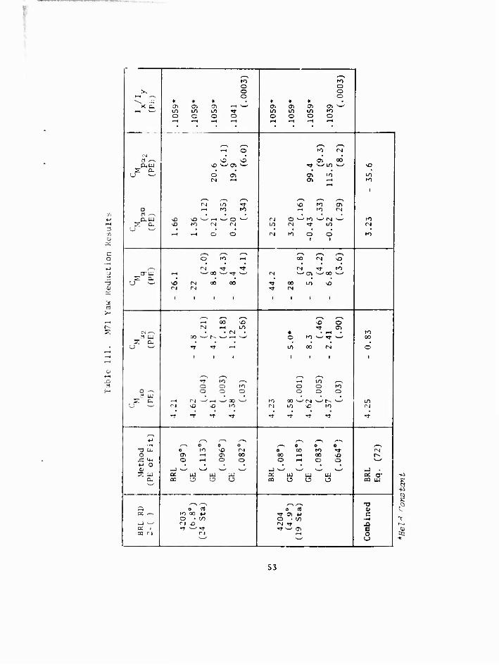
III. M71 Yaw Reduction Results S3

IV. M329A1 (w/ext) Yaw Reduction Results S4

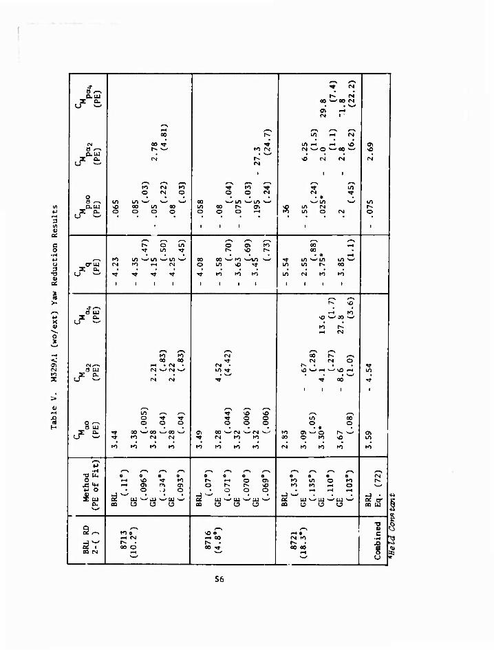
V. M329A1 (wo/ext) Yaw Reduction Results 56

VI. M3^9A1E1 Yaw Reduction Results -7

VII. M329A1E1 CG Reduction Results 58

Preceding page blank

2

3

1 2 3

LIST OF SYMBOLS

vector of the N23 parameters a to be determined

^ fL-1! i

Vr1 tL'2J y

A. VA C0 [L-l] 8 I "i

a the r.-th unknown constant parameter to be determined n (n = 1. 2, . . . N23)

aR tan"1 (y/xj, see Fig. 2c

a ,& ,a coefficients in an expansion of time as a cubic in distance. eq. (36)

B vector from the range system origin in the direction of the positive X-axis, see Fig. 2a

C Coriolis acceleration, eq. (64a,b)

CA Ai CD Vo [T1]. eq. (38)

C drag coefficient, ldraB forcel > eqi (30) m A V2

1

Cp. coefficient of 63 (j = 0, 2) in the expansion of CL

Cp. axial drag coefficient, (1 - 52) C-

CDA. coefficient of 6J (j = 0, 2) in the expansion of CL.

CDR BRL range value of CL, eq. (36)

CD average value of CL, eq. (35)

C roll damping moment coefficient, ± ll'^l damping moment^ p m d2 A V p

eq. (47) 9

Preceding page blank

LIST OF SYMBOLS (Continued)

C. Magnus moment coefficient. ± l^gnus fSSSSll , eq. (51) pa m d2 A V p 6

(L. coefficient of 6J (j = 0, 1, 2, 4, 6, 8) in the expansion poj of C^j

pa

C. damping moment coefficient, ± [damping moment] ^ q m d2 A V |e + i iji cos e|

eq. (51)

CM coefficient of 6* (j = 0, 2) in the expansion of C. qj q

„ , rr- . Istatic momentl ,_-« C. static moment coefficient, ± -1 L , eq. (51) ^a m d A V2 6

1

Cu coefficient of 5^ (j = o. 2, 4) in the expansion of Cu M M aj a

(^ Magnus force coefficient, ± ^—^r v0rC6 ' eqs• (59, 66)

pa j P

t, coefficient of 6^ (j » 0, 2) in the expansion of C, paj pa

C. normal force coefficient, ± J L > eqS, (59f 66) a m A V2 6

1

(I. coefficient of 6^ (j »0, 2) in the expansion of CL. aj a

t~ centripetal acceleration, eq. (63), [LT-2]

Cy 2 (1^ , the Magnus force coefficient of Reference 14 pa pa

0 Nl x N4 matrix of measurements d. lm

t drag force, eq. (30), [MLT"2]

d reference diameter, [L]

d. the measured value of y. at x = x im '1 m

10

LIST OF SYMBOLS (Continued)

ER sin"1 (z/V), see Fig. 2c

sum of the aerodynamic forces acting on the projectile, [MLT-2]

Fy.Fy»''? range components of f X* Y'"Z

F ,F ,F fixed-plane components of P 12 3

f.( ) single-valued elementary function

(£ gravitational force, eq. (21), [MLT-2]

g magnitude of the gravitational acceleration, [LT~2]

I ,1 axial and transverse moments of inertia, [ML2] x y

L angular momentum vector, [ML2!-1]

L ,L ,L fixed-plane components of L, eq. (42) 12 3

M sum of the aerodynamic moments acting on the projectile, [ML2!"2]

M ,M ,M fixed-plane components of M, eq. (43) 12 3

m mass, [M]

Nl the number of measured dependent variables in a system of equations

N2 the total number of dependent variables in a system of differential equations

N3 the number of unknown parameters appearing explicitly in a system of differential equations

N4 the number of measurements taken on each of the Nl depen- dent variables

N23 N2 ♦ N3, the number of unknown constants in a system of equations

n rifling, [cal/rev], Table I

11

LIST OF SYMBOLS (Continued)

PE probable error

a yi P. -5 , the influence (or sensitivity) coefficients, eq. (3) in da n

p the X -component of the angular velocity of the missile-

fixed system with respect to the range system, eqs. (40- 41), [rad/sec]

R position vector of the missile's CG, [L]

r arclength along the trajectory of the missile's CG, [M]

t time

t* value of time at x = x*

u ,u ,u fixed-plane components of V, [LT"1] 12 3

v velocity vector, [LT-1]

V magnitude of ^, [LT-1]

X vector of the N4 values x of the independent variable at

which measurements are taken

XYZ the axes of a range (earth-fixed) coordinate systeo»; the X-axis is directed down-range along the intersection of a horizontal plane with the vertical plane contain- ing the gun; the Y-axis lies in this horizontal plane, directed to the left of an observer facing downrange; the Z-axis is directed upward.

XXX the axes of a fixed-plane coordinate system; the X -axis 12 3 r 1

lies along the missile's longitudinal axis, directed from the CG (origin) to the nose; the X -axis is con-

2 strained to lie in the horizontal plane, directed to the left of an observer facing in the direction of the positive X -axis; the X -axis is directed upward.

1 3

X X'X' the axes of the fixed-plane system of References 1 and 2, 1 2 3 where X' = - X , X7 = - X .

2 2 3 3

12

LIST OF SYMBOLS (Continued)

x the independent variable of a system of equations

x,y,z range components of R

• • • -t x,y,z range components of V

x the value of the independent variable x at which the m-th measurement is taken, m = 1,2, . . . N4

x* the mid-range value of the down-range coordinate x

y. the dependent variables of a system of equations

o . the coefficients of the increments A? in the differential nk u K corrections normal equations, see eqs. (6-7)

ä . the (n, k)-th element of the inverse of matrix (O-j.)

ou, the yaw angle, the total angle of attack, measured (in the XXX system) from the velocity vector to the X -axis. 12 3 1

ß the terms on the right-hand side of the differential correc- tions normal equations, see eqs. (6, 8)

y. a possible replacement for a . , suggested by Marquardt,

eq. (15)

Aa. the increments by which the parameters are changed in the differential corrections process

6 sine of the yaw angle, eq. (17)

e the sum of the squares of the residuals in a least squares fit, eq. (2)

6 an Euler angle; see Fig. 2a

9 azimuth of the line-of-fire, that is, the angle measured clockwise from North to the down-range axis (192° for the BRL Transonic Range)

0 latitude of the range, considered positive in the Northern hemisphere (39° 26' at BRL)

6 the missile's angle of yaw; see Fig. 2a and eq. (26)

13

5 .? 2 3

"S (S ) 1 2

LIST OF SYMBOLS (Continued)

a constant in Marquardt's scheme, eq. (IS)

- u /V, - u /V 2 3

air density, considered constant, [ML"3]

the earth's angular velocity vector, eq. (64a)

magnitude of t, 0.00007292 rad/sec E

(where S and S can be FP, R or R') angular velocity of 12

the S coordinate system with respect to the S coor- 1 2

dinate system

Subscripts:

( ) FP

OR

OR,

d^

dt2

components in a fixed-plane (XXX) system 1 2 3

components in a range (XYZ) system

components in an intermediate (X'Y'Z') system

second derivative of R in an inertial syst em

( ), initial condition, taken here to be the value at the first data station

14

I. INTRODUCTION

In free flight studies, the main task is to determine from obser- vations of a missile's motion the values of the aerodynamic coefficients appearing in the differential equations describing that motion. For normal enclosed-range firing conditions (symmetric shell, nearly hori- zontal flight, small yaw, constant or only slowly varying spin, etc.), we can approximate the solution to the differential equations quite adequately by convenient closed-form expressions. These expressions involve certain constants directly related to the aerodynamic coeffi- cients. The values of these constants are determined by a least squares fit of the observed data to the closed-form expressions.

For the past two decades, the general technique of fitting observed data to convenient closed-form expressions has been the heart of free- flight, enclosed-range data reduction1*2*. Highly successful results have been obtained for a variety of missile shapes and sizes. Over the Xears, the technique has been gradually refined and extended to cov?r many types of force and moment nonlinearities. Unfortunately, such extension often requires that a number of rounds be fired at different Mach numbers, yaw levels, and so on, to obtain a single set of coeffi- cients. The process can be costly in dollars and time. Moreover, the technique can be stretched only so far; an occasional round has defied analysis by conventional procedures.

It is relatively easy in these troublesome nonlinear situations to specify - by experience and by cunning - the sort of nonlinear terms that must appear in the differential equations of motion in ordsr to produce the observed behavior. It is much more difficult to find convenient pseudo-solutions that Will (1) represent the motion adequately and (2) contain constants that can be easily related to the coefficients of the differential equations. What we need in these situations is a method that doesn't require any knowledge or assumptions on our part regarding the form of the solution to the differential equation.

The problem is essentially one of parameter optimization. We are given

a. the form of a set of differential equations involving unknown constant parameters (coefficients and initial conditions);

b. a set of first estimates for the parameters;

c. a set of discrete measurements on one or more of the dependent variables;

d. a criterion function of the parameters (say, the sum of the squares of the residuals for a given fit).

tReferenoee ewe lieted on page 59.

15

The problem is to devise a routine for adjusting the parameters luto- matically so as to minimize the criterion function.

The problem has received much attention, particularly in recent years with the proliferation of high-speed computers, and many ingenious schemes for optimizing the parameters have been proposed. For continuous rather than discrete input data, Meissinger3t1* approached the criterion function minimum by a path of approximately steepest descent, using an analog computer. On the other hand, the techniques devised by Goodman5"7

and by the team of Chapman and Kirk° to handle discrete data are better suited to the digital computer. In this paper, we will be concerned primarily with the Chapman-Kirk technique. The Goodman and Chapman- Kirk methods are quite similar, although Chapman and Kirk were unaware of Goodman's work when they presented their own results at the AIM Seventh Aerospace Sciences Meeting, New York, 1969. From the stand- point of the aerodynamicist. Chapman and Kirk's contribution was to apply the process successfully to representative aerodynamic cases and, perhaps more important, to present their results at the meeting and later in a journal8 where it came to aerodynamicists* attention. (It is unfortunate but often true that when a pertinent article such as Goodman's appears in a mathematical journal, the aerodynamicist either overlooks it or fails to recognize its applicability to his work.)

Applications9-13 of the Chapman-Kirk technique are growing more and more sophisticated. The present report documents one such appli- cation carried out by the Armament Depaitment, General Electric Company, Burlington, Vermont, for the U. S. Army Aberdeen Research and Development Center (ARDC), Aberdeen Proving Ground, Maryland, under Government Contract No. DAAD0S-71-C-0265 during the period 4 February to 20 April 1971. The results of this work have also been issued as a General Electric report1*1.

The raw data for this study consisted of time, position and orien- tation measurements at discrete points along the trajectory for twelve rounds fired in the Transonic Free Flight Range15, Ballistic Research Laboratories (BRLj. The twelve rounds consisted of four spin-stabilized projectile types (see Table I and Figuve 1). Each of the rounds had been previously reduced11'16 by the usual range technique (with varying deg »es of success) and each was hand-picked for the present assignment.

Sotu ot the twelve rounds could be fitted by assuming relatively simple fcue and moment systems; these rounds were chosen to enable the Chapman-Kirk technique to get a foot in the door. Other rounds of the twelve were oddities that had already annoyed and frustrated a team of data analysts; these rounds were chosen to give the Chapman-Kirk tech- nique a good work-out. The primary purpose of the present study was to see how well the Chapman-Kirk technique could determine the values of the nonlinear coefficients present in the force and moment expres- sions.

16

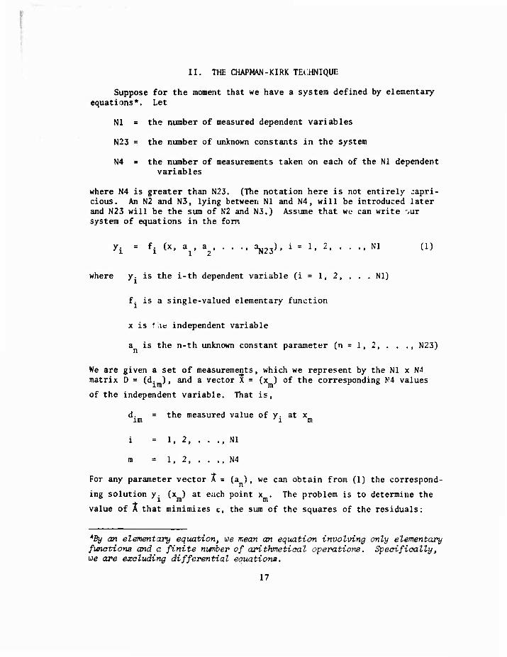
II. THE CHAPMAN-KIRK TECHNIQUE

Suppose for the moment that we have a system defined by elementary equations*. Let

Nl = the number of measured dependent variables

N23 = the number of unknown constants in the system

N4 = the number of measurements taken on each of the Nl dependent variables

where N4 is greater than N23. (The notation here is not entirely :apri- cious. An N2 and N3, lying between Nl and N4, will be introduced later and N23 will be the sum of N2 and N3.) Assume that we can write our system of equations in the fom

yi = ^ (x, a , a , . . ., a^j), i = 1, 2, . . ., Nl (1)

where y. is the i-th dependent variable (i = 1, 2, . . . Nl)

f. is a single-valued elementary function

x is riie independent variable

a is the n-th unknown constant parameter (n = 1, 2, . . ., N23)

We are given a set of measurements, which we represent by the Nl x N4 matrix D = (d. ), and a vector X = (x ]

inr v m of the independent variable. That is.

matrix D = (d. ), and a vector X = (x ) of the corresponding N4 values im m

d. = the measured value of y. at x im 'i m

i = 1. 2. . . ., Nl

m = 1, 2, . . ., N4

For any parameter vector A = (a ) , we can obtain from (1) the correspond-

ing solution y. (x ) at each point x . The problem is to determine the i m r m r

value of A that minimizes e, the sum of the squares of the residuals:

*By an elementary equation, we mean an equation involving only elementary funationa and a finite nwtber of arithmetiaal operations. Specifioally, we are excluding differential equationa.

17

N4 Nl

■ L a [di». - yi (VJ; (2)

m=l i-1

(For convenience, we omit weighting factors in (2) and the succeeding discussion; such factors might be needed, for example, to insure that the terms in (2) are dimensionally equal.) Now e will be at a minimum only when its partial derivatives with respect to each of the para- meters is zero. We introduce a conveniert notation for these partial derivatives:

3 yi (3) Fin 3an

i = 1. 2, . . ., Nl

n = 1. 2, . . ,, N23

Because they reflect the influence of each parameter change, the P.

are sometimes called "influence" (or "sensitivity") coefficients. For a minimim E, we must have

N4 Nl

—- = - 2 > ) [d. - y. (x )] P. =0 (4) 3 a / . / , l im 'i l nrJ m K J

n •;—r* m=l i=l

Equations (4) constitute a set of N23 equations in the N23 unknown param- eters; the values of the parameters satisfying (4) are the desired optimum values.

If the functions f. are linear in the parameters a :

fi ' a1 ♦i, W ♦ a2 i^ (x) ♦ . . . ♦ ^j ^^j (x)

then Pin " hn^

and set (4) is also linear in the parameters; hence (4) is easily solvable (in theory). If the functions f. are nonlinear in the para-

meters, owever, then solving (4) can be quite difficult. The usual way of 5 this difficulty is to approximate the variables y. by their

18

linearly truncated Taylor expansions about a given set of values for the parameters:

y^

N23

(5)

k=l

where the circumflex (") denotes evaluation at the given parameter values and where Aa, is an indicated change in the given value of a,.

If (5) is substituted in (4), and if the P. in (4) are replaced

by P. , we have

N4 Nl

m=l i-l

N23

din. * ^i " ZZ 'ik k=l

Aa, Pin = 0

or

N23

L k=l

JZJ ankAalc = ßn. "= 1. 2. . . .. N23 (6)

where

N4 Nl

ank -ItZYZ 'in CV ^ik **> m=l i=l

(7)

N4 Nl INt INI p.

n = ZZ ZZ dim " yi (xm^ m=l i-l L J

P. (x ) in v mJ (8)

Equation (6) represents a set of N23 linear equations in the ^23 incre- ments Aa . Hence we can solve (6) for the increments:

N23

Aa = } a n C. I k=l

nk ök' n - L 2. , N23 (9)

19

where

8 . = the (n, k)-th element of the inverse of matrix (a k)

cofactor of element a . _^__^ nk determinant of matrix (a .)

The new value of a is then obtained by adding Aa to the old value, n n

If the initial estimates of the parameters are "close enough" to the "true" va.'ues. (5) will be an adequate approximation and the new values of the parameters will produce a smaller criterion function e. The process can then be repeated as many times as necessary until some convergence criterion is satisfied. The probable error of the fit at the end of any iteration is given by

PE = 0.6745 __-^__ (10) 0-6745 Un M7 KiTfl Nl x N4 - N23 I

and an estimate of the probable error in a is given by

E C«n) • (ä^ • PE (11)

This, in brief, is the well-known process of "differential corrections," as applied to elementary equations that are nonlinear in the parameters.

For a system of ordinary differential equations, the situation is naturally more complicated. Assume that the given system of differential equations has been reduced to a system of N2 first order, possibly non- linear eouations*:

-^ • fj (x.y^, . . ., yN2, ai,a2 a^)

yj (xo) = ^3 + j

j = 1, 2, . . ., N2

>(12)

*It ie not neaeeeary when oarrying out the Chapman-Kirk technique to reduce the given syetem to firet order equations; this was done here merely to aid the exposition.

20

where

N2 = the total number of dependent variables in the system

N3 = the number of unknown parameters appearing explicitly in the differential equations

and where Nl and N4 are defined as before. Note that we have juggled the notation so that while only N3 parameters appear explicitly in (12), there are still N23 (= N2 + N3) parameters to be determined:

a , a , . . ., a^ (the N3 explicit parameters)

a^. , a^, 2' • • '' ** 2S ^t^e N^ un'cnown initial conditions)

where

1 < Nl «S N2 < N23 < N4 (13)

The same differential correction technique that was applied to (1) can be applied to (12). Equations (6-11), which depend only on the definition (2) of the criterion function e, are still valid. However, a new difficulty arises when the given set of equations are ordinary differential equations: how do we evaluate the dependent variables and their partial derivatives appearing in (7) and (8)? For the case of non-differential equations, this was no problem; we were presumably given explicit expressions for each of the variables and could easily write down expressions for the required partials. For a given set of differential equations, however, we will not, in general, know the form of the solution. Values of the dependent variables can be obtained by some numerical integration scheme, but part of the problem remains: how do we obtain the required values of the partial derivatives?

Chapman and Kirk tried various schemes for evaluating these partial derivatives and finally settled on the method* of "parametric different- iation." This method consists of formally differentiating the given set (12) of differential equations with respect to each of the N23 constants to be determined. We have

3 an V dx J 3 f. 1 3 a

n

*The method ie not neu. It was used, for example, by the previously cited Meieainger and Goodman (and apparently by Knalder17, with whose work we are unfamiliar but who is referenced in References 10 and 12).

21

or, assuming that the y. are continuous in x and a , so that the order

of differentiation can be interchanged,

d P. 3 f. -,-& . —i j . 1, 2 , N2 (14a)

n

where

P. (x ) = 1 jn v oJ

j • 1, 2, . • • f N2

n = 1, 2, . • • > N23

(if n - j = N3)

(otherwise) = 0 (otherwise) (14b)

The somewhat strange-looking initial conditions (14b) merely reflect the fact that P. is initially 1 if and only if a represents the initial

value of y.. By (12), this occurs if and only if a « a^. + j; hence

if and only if n = N3 + j.

What we have done above is to derive an auxiliary set of N2 x N3 equations (14) whose solutions are the partials P. , some of which

(those for j < Nl) are needed in solving (6). For a given set of estimates of the parameters and initial conditions, we can integrate by some numerical scheme both the original set of equations (12) and the auxiliary set (14). (The original set may or may not be linear; the auxiliary set will always be linear.) The numerical integration yields the values of the dependent variables and the influence coefficients required to solve (6) for the parameter changes.

Except for this more laborious way of determining y (x ) and

P. (xm)• the procedure for determining the unknown constants of a

set of differential equations is the same as for non-differential equations.

As a final aside, we note a possible future improvement. In the N23-dimensional parameter space, the truncated Taylor series technique proceeds from a given point (whose coordinates are the given estimates of the N23 constants) in the direction of the vector AA = (Aa ) ' v n obtained by solving (6). The method of steepest descent, on the other hand, proceeds from the given point in the direction of the negative gradient of e. Marquardt18•19 points out that these two directions are nearly perpendicular, while the optimum direction lies somewhere in between. To proceed in approximately the optimum direction, he suggests replacing a. in (6) by

22

r \n

(1 + X) a, for k

kn for k ^ n (15)

where X is a fudge factor constant whose value should be changed from one iteration to the next according to a few simple rules (the rules are listed - in slightly different form - in References 18 and 19). Using Marquardt's magic X, the Chapman-Kirk process often converges for initial guesses far outside the previous region of convergence. The Marquard alg rithm was pointed out to us by Chapman himself, who has used it (subsequent to the work reported on in Reference 8) with great success in hitherto .Intractable cases. The algorithm was not used in the investigation covered by this report because we were not aware of it at the time.

III. INPUT DATA, COORDINATE SYSTEMS AND YAW VARIABLES

A missile fired in the BRL Transonic Range is observed at twenty- five spark-photography stations distributed along a 680-foot portion of the trajectory. The observed data at each station consists of

a. the elapsed time t, reckoned from the instant the spark at the first station was triggered by the passing missile. The time error in a properly functioning timer is estimated to be no more than one micro- second. Only about two-thirds of the stations are instrumented at present to furnish timing data.

b. (x,y,z) : the position vector of the missile's CG in a range

(earth-fixed) coordinate system XYZ. The X-axis is directed down-range along the intersection of a horizontal plane with the vertical plane containing the gun; the Y-axis lies in this horizontal plane, directed to the left of an observer facing downrange; the Z-axis is directed up- ward. The error in any position measurement should be no greater than 0.003 meter.

c (0, ? , C )cn: the yaw vector in a fixed-plane coordinate 2 3 rr » system XXX. The X -axis lies along the missile's longitudinal axis,

12 3 1 directed from the CG (the origin of the fixed-plane system) to the nose; the X -axis is constrained to lie in the horizontal plane, directed to

the left of au observer facing in the direction of the positive X -axis;

the X -axis is directed according to the right-hand rule (that is, up-

ward) . If u ,u ,u are the velocity components in the fixed-plane 12 3 r

system, then

23

u u

where V is the magnitude of the velocity vector. The minus signs in (16) appear because in range studies the yaw angle is measured from the velocity vector to the X -axis*. The magnitude 6 of the yaw is

given by

r ML f"2 + "2 )h

ä - f^*^] ^ Z v = sin a,. (17)

where a is the yaw angle, the so-called total angle of attack. The

angular measurements that yield the yaw components are usually accurate to within 0.002 radian.

Although differential equations describing the yawing motion can be written in terms of e and C , we found it more convenient to work with

2 3 the related Euler angles I|I and 6. These angles appear in the trans- formation matrix that converts from range to fixed-plane coordinates. To derive this matrix, assume the existence of a vector B extending from the range system origin in the direction of the positive X -axis

(see Figure 2a). Rotate the range system XYZ about the Z-axis by the angle ty so that X' (the rotated X-axis) coincides with the projection of the vector B on the XY-plane. The magnitude of i/( is not to exceed 180°; if this requires a counterclockwise rotation about the 2-axis (as in Figure 2a), i/i is considered positive and if clockwise, then i|i is considered negative. Then we have

*In References 1 and 2, a fixed-plane aystem X X'X' is uaedj where the

X'- and X'-axee have oppoeite direations to the X - and X -axee. reepeo- ^3 2 3

ttvely. In this X X'X7 ayetem, the you angle ie measured from the X -

axie to the velocity vector. If v «u7 .u' are the velocity aomponenta 12 3

and 0,%,' ,$,' are the yau aomponenta in the X X7 X' ayetem, then 2 3 12 3

u' u

2 V V S

and eimilarly, ?' « £ . That ia3 the you components in the tuo fixed-

plane systems are identical.

24

COS l|) sin i* 0\ /x - sin i(i cos i|; 0 y

0 0 1 z (18)

Next, rotate the intermediate system X'Y'Z' about the Y7-axis so that X" (the rotated X-axis) coincides with vector B. Let 6 denote the angle from Z' to B, where |e| < 90°. If the rotation is counterclockwise about the Y'-axis, 6 is considered positive; if the rotation is clock- wise (as in Figure 2a), 6 is negative. Then we have

(

cos e 0 - sin e\ / *' 0 1 0 y*

sin 9 0 cos e / \ z' FP \ / \ / R' (19)

This final system X'T'I" has the orientation of the fixed-plane system XXX. Thus the transformation matrix from range to fixed-plane co- 12 3

ordinates is the product of the 6-matrix and the ip-matrix:

' cos 9 cos ty cos 9 sin ty - sin 9*

- sin i</ cos 0 0

sin 9 cos iji sin 9 sin I|I cos 9/ V z/D (20) \ / \ / K

For an assumed flat, nonrotating earth, the gravitational force G has the form

S = (0, 0, - mg)R (21a)

where the gravitational acceleration g is constant for range firings. Substituting the right-hand side of (21a) in (20), we see that the fixed-plane components of G depend on the Euler angle 9:

5 = (mg sin 9, 0, - mg cos 9)pp (21b)

Note that by the definitions of the two Euler angles, the angular velocity of the intermediate R' (X'Y'Z7) system with respect to the range system is

V(R) " (0' '*' ^R*

25

Substituting this vector in (19), we obtain the angular velocity of the fixed-plane system with respect to the range system

aw,,, = (- ij. sin 6, e. ^ cos 6)__ (22) UFP(R) v y Ji" "' "' ^ w" ^FP

The above discussion gives us the physical interpretation of ^ and 6, but in ^rder to work with these angles, we needed explicit equations relating IJJ and 6 to the given yaw components C and £ . By some elemen-

2 3 tary but cumbersome vector analysis, it can be shown that the desired relations are

('in*H\ sin"1 -^—^ + aD (23)

/sin^\

\cos ^j 9 = eM - sin'1 [ ^^i | (24)

where ij».. and eM are the missile's pitch and yaw angles, respectively

(see Figure 2b):

*M = sin'1 [- v^-J = sin'1 C«2) C")

\^l " 'sinl y^j eM " tan"1 I T^l = " sin'J IT^TV 1 (26)

where aR and ER are the azimuth and elevation angles, respectively, of

the velocity vector in the range system (see Figure 2c):

aD = tan-1 / f 1 (27j

ft)

(0 ER - sin-1 | $ J (28)

where x,y,z are the velocity components in the range system.

26

For the present analysis of range firings, we made the simpliiying assumption that the angles a and E could be ignored. Letting

a= ED = 0, equations (23) and (24) reduce to K K

* = iPM (23a)

e = eM (24a)

By equations (17), (25) and (26), the magnitude & of the yaw can be expressed in terms of the pitch and yaw angles:

& = (sin2 ik. + cos2 ^ sin2 8M)^ (29)

IV. THE EQUATIONS OF MOTION

In this section, the working forms of the equations of motion are derived (albeit briefly) from the basic expressions for Newton's Second Law. By writing out this derivation, we can point out where and what kinds of assumptions and simplifications were made and thus facilitate future changes.

The interdependence of the various equations and of the three distinct reductions (drag, yaw and CG) are indicated in Figure 3.

A. The Drag Equation

The classic drag equation has the form

* + (J. m ^ dt2

[MLT-2]

I

(30)

where

D ■ drag force

= - (m A CD V) V

1 tr

7T P d2

8m [L- l]

gravitational force

27

R = position vector of the missile's CG

and where the subscript I denotes vector differentiation in an inertial system. For enclosed-range studies, the density p and hence A are

known constants. The drag coefficient C is in general a function of

Mach number and o: 62. For each of the twelve Transonic Range rounds studied here, however, we could ignore the Mach number variation over the observed trajectory and assume a linear* dependence of C^ on <S2:

S = CD +CD 62 (31) O 2

We seek the X-component of (30) in the range system. For the pur- pose of performing the drag reduction, we can assume that the range system is an inertial system and hence ignore the centripetal and Coriolis accelerations that arise in any earth-fixed system. Then the X-component of (30) can be written as

A Cn V x 1 D

Al CDX V2 (32)

where

■(l)cD CDX = \V jCD " CDCOsERCOSaR

= down-range drag coefficient

For the present Transonic Range studies, (32) has the disadvantage that the independent variable t - which should be known exactly at each point - is obtained only at about two-thirds of the spark stations (and obtained with sufficient accuracy at a considerably smaller fraction). On the other hand, the down-range coordinate x of the missile's CG is usually known very accurately at each station. Thus a reasonable course of action is to convert the independent variable in (32) from t to x. We have

^Provision was made in the coding to hco die C^ as a quadratic in Ö2,

but the higher-order term woe never needed.

28

dt dx

dx

1

X

- A1 CD V - A

"DX J (33)

The presence in (33) of the velocity V is a nuisance for as yet we have no equation for generating V. For the nearly horizontal flights en- countered in ballistic ranges, the distinction between V and

x (= V

can write (33) in the final form:

cos E cos a ) and between C and Cn5. can be ignored. Thus we

dt 1 dx V

dV dx "

(C»o * \ S2) A V

1 M34)

Hie drag reduction - that i technique to (34) - is normally this stage we know the values of (namely, at each spark station), tained additional input values 0 polation. (After the yaw reduct reduction could be re-done, usin the raw plus interpolated-raw va wasn't necessary.)

s, the application of the Chapman-Kirk done before the yaw reduction and so at 62 only at certain discrete points From these scattered valuer, we ob-

f 62 at selected values of x by inter- ion has been performed, the drag g the fitted values of 62 rather than lues. For the present study, this

In addition to the yaw data, the required input for a given round consisted of the measured times t, the measured x values and initial estimates of the two explicit parameters fc , C \ and the two initial

conditions (t , V ), where we defined initial conditions as the con- o o ditions at the first spark station. The output consisted of

a. the least squares values of the explicit parameters and initial conditions;

b. appropriate error estimates in the above;

c. a reliable correlation of time with distance, so that in the remaining equations of motion, time could be used as the independent variable. Of course, it was not absolutely necessary to revert to a

29

I • iwnttivw,..,

time base. For theoretical work, the arclength r along the trajectory 0f the missile's CC (or a nondimensional length r/d) is often a more convenient independent variable than either time or down-range distance. The equations of motion (in particular, the yaw equations) assume

simpler forms when r is the independent variable. Since r = V, our

approximation x a V is equivalent to ignoring the distinction between x and r. We could, then, have written all the equations with respect to this convenient length variable which we measure as x but are free to interpret as r. One reason we didn't is that the present study, while interesting in itself, is also regarded as preliminary, getting- our-feet-wet training for more ambitious studies that will require a time-based set of equations. By working with time-based equations in the present study, we could save considerable coding effort. Compre- hensive computer programs, capable of handling the larger problems, were able to handle the current problem as a special case.

One additional bit of information can be gleaned from our reduction: a representative Cn value for each round, obtained by replacing 62 in

(31) by its mean value:

CD = CD + CD F (35) O 2

Although a value for J2 was available for each round from the BRL yaw

reduction, the quantities a_ = sin'Vy ^Jlisted in Tables II - VI were

obtained by a slightly different averaging process than used by BRL. Thus these listed values differ slightly (by less than 4%) from the BRL values. Each representative drag coefficient Cn car. be compared

with the range value, C obtained at BRL by fitting time as a cubic UK f

(x - x*)2 + a (x - x*)3

3

in down-range distance x:

t = t* + a (x - x*) + a

CDR =

2 a 2

A a 1 l

= range value of C[) itftt, x, V) = (t*, x*, 1/a J]

J

(36)

where x* is the given mid-range value of x.

As we will see, the variabie V appears in the yaw and CG equations and the question arises: how should we generate it there? We could.

30

of course, store the large number of discrete velocity values available when we integrate the drag equation (34) numerically. This would be both tedious and unnecessary. Instead, we made a reasonable assumption: for purposes of performing the yaw reduction* on the given Transonic Range rounds, V can be represented adequately over the observed tra- jectory by a known quadratic in time:

V = V + V (t - t ) + V (t - t )2 (37) O i v 0 2 0

Values for V and V in (37) can be obtained in various ways. For 1 2 _

example, if we replace CD with CD in the drag equation, the solution

can be written at once:

V - V^xp [- A^p (x-xo)]

where

V

' ! + CA ^ - V

c = A cn v [r1] A i D o L '

(38)

with the truncated series expansion:

V = Vo [1 - CA (t - to) ♦ C* (t - to)2] (37a)

B. The Roll Equation

Consider a missile-fixed coordinate system XXX, where <-he X - 1 i» 5 1

axis lies along the missile's longitudinal axis (as in the XXX fixed- 12 3

plane system) and where the X and X axes are rigidly attached tu the

missile in a right-handed system. Then the angular velocity of this missile-fi/ed system relative to the fixed-plane system is given by

^MFfFP) = (*• 0, 0)Fp (39)

*The OBBumption is not neaeasary for the CG equations where, as we shall see, V can be generated handily.

31

where $ is the roll angle (the angle between the X X axes and the X X

axes). By (22) and (39), we can write an expression for the angular velocity of the missile-fixed system with respect to the range system:

"Ww " "MFtFP) * "FPW

= (P, e, i^ cos e) FP (40)

where

• • p = $ - ii sin 6 (41)

The angular momentum of a missile with rotational symmetry is then

t 2 (L . l2, L3)Fp = (Ix p. Iy 6. Iy i> cos 9)Fp [ML2!"1] (42)

The sum of the moments acting on the missile is equal to the time deriv- ative of the angular momentum:

3 5 (M^ M2> M3)Fp = ^ [ML2T"2]

• • = [C^. L2. L3) * wFp(R) xt]Fp M43)

where again the range system is considered an inertial system. Hence by (22) and (42),

M I P x r (44)

M =ie+(lp+Iij; sin 6) ty cos 6 2 y ^ x

(45)

I <ii cos e-(I p*2I iji sin 6) 6 y x y (46)

Equation (44) is the roll equation; (45) and (46) constitute the yaw equations.

The roll equation does not depend on the other two moment equations and hence can be solved separately. We define the axial momfnt as

32

Mi - (P ^) (^) W) (^ ) C, [ML2T-2] (47)

where C is the roli damping moment coefficient*. Tlien the roll equa- P

tion (44) becomes

A3 p V [T-2] (48)

where

H) *, (ft ] clp (L--!

For the present study, A can be considered constant. If we were given 3

sufficient spin data (obtained, say, by measuring the position on each spark photograph of two distinguishable pins placed in the base of the missile), we could obtain the "best" values of p and A by the Chapman-

Kirk technique or by a fit of the data to the solution of (48):

p = p0 exp [A3 (x - xo)] (49)

In the present study, however, such spin data was unavailable. Yet the roll rate p was needed in the yaw equations. We resolved this problem by assuming that p is a known linear function of time:

P = po f1 * A3 Vo (t - V1 (50)

where p = 2 n V /(nd), rad/sec

n = rifling, cal/rev (see Table I)

and where A was evaluated by assuming C. = - .013 for all twelve P

rounds.

*In some texts (e.g., in Referenoee 13 and 14), the combination pd/(2V)

P is preferred to pd/V and in those texts the C must be interpreted

accordingly:

vpj- > p

33

C. The Yaw Equations

The yaw equations describe the wobbling motion of the missile's longitudinal axis A jjbout the tangent to the trajectory, that i^, about the velocity vector V. Any two variables sufficient to orient V with respect to A can serve as the dependent variables. IT. the usual BRL Transonic Range reduction, the dependent variables are the yaw components £; and 5 ; here we use the Euler angles iji and 9 and the governing equa-

2 3 tions (45) and (46). We define the cross-moments acting on the missile as follows*:

V'V (^){^)W)-\ ['''i ?cos e> \ [ML2T-2]

(51)

where**

C ^V

M

pa

S 62 + C 32

s + c pao

■ C. + c. qo

M pa2

62

»i 92

M «it

+ C M pa!»

> (52)

^Provision was made in the aomputer program to cape with an aeyrmetriaal missile by including some trim terms not shown in (51) above. These terrtiS were not used in the present study.

**Note that C in (61) is multiplied by the nondimensional spin pd/V, Mpa

so that the remarks on C in a previous footnote apply to C, as well. P pa

That is.

\ * 2 (C, pa

$

M pa

Likewise, C, as defined here is half the CM of References 12 a,id 14, q q

34

Substituting (51) in (45) and (46), we obtain the final form of the yaw equations:

e = A [(V u ) a. ♦ (u p d) a. + (d v e) cM | 3 a 2 pa qj

- [(I /I ) p + ♦ sin 8] i(i cos e A 7

(53)

(V U ) Cj, ♦ (u p d) CM + (d V t/» cos 6) (^ 2 a ' pa q

♦ [(Ix/Iy) p + 2 * sin 6] 9 ^ /cos 6 '} (54)

where A is a known constant: 2

n p d3

8 I [L-2]

Equations (53) and (54) involve four initial conditions, the eight aero- dynamic parameters indicated in (52) and (possibly) one physical param- eter. I /I . Thus a maximum of thirteen constants could be determined

' x y for each round by an application of the Chapman-Kirk technique to (53) and (54). However, for any computer run, any one or more of the eight aerodynamic constants in (52) could be treated as a known constant rather than as a parameter to be determined. For example, (L. was

fixed at zero (that is, ignored) in all the present computer runs.

Note that in addition to 6, \p and their derivatives, (53) and (54) involve five dependent variables:

V, p, 62, u and u 2 3

We have already given equations adequate for simulating V and p as functions of time, namely, (37) and (50), respectively. The squared yaw can be obtained by (17):

(u2 + u2) /V2

2 3 (17a)

provided we know u and u . Thus the ability to solve (53) and (54) 2 3

hinges now on our ability to generate u and u . We proceed now to 2 3

derive the required equations. Let

35

? £ ^X' F2' F3)FP

■ the aerodynamic force vector

and assume that the only forces acting on the missile are the aerodynamic and gravitational forces. Then the force equation is

f*t m dV mat

• • m [Oy u2. u3) * ^HR) xVlFp

or. by (21b) and (22),

-(55)

F + mg sin 6 = m (u - u i cos 9 + u 9) 1 12 3

(56)

m (u + u it sin 6 + u ii cos 6) 2 3 1

(57)

F - mg cos 9 = m(u -u 9-u iji sin 9) 3 3 12

(58)

We assume that the fixed-plane components of the aerodynamic force are given by

m A Cn V u 1 D l

F + i F 2 3 '\{\ V + i CVI pd (u + i u )

pa / z .(59)

where for the present purposes, C. and C are considered known N N a pa constants*. Then equations (57) ar.d (58) can be written as:

Ms with C , CM and C. , we have P P« w = 2 S

El 2V

pa gd v

36

u = - A 2 , [(v v v (M "3' sj

- (u cos 6 + u sin b) * (60) 1 3

u = - A 3 . [(v v \'(p d ^ v]

• •

where

u

+ u 6 + u ifi sin 6 - g cos 8 (61) 12

.2^ (V2 - u2 - u2)^ = (1 - 62) V 1 2 3

Thus we generate u and u by assigning values to C., , C., , u and u ? 3 NN2O 30 ti a pa ':u JU

and then solving (60) and (61) simultaneously with the yaw equations (53) and (54).

An alternative method for generating u and u follows at once from

assumptions (23a) and (24a) that 4) = iK. and 6 = 0... By (16), (25) and

(26) we have

u = - V sin ii 2

u = V cos ij/ sin 9 3

These expressions eliminate the need for (60) and (61). The only draw- back is that the resulting computer program couldn't be used in future cases where assumptions (23a) and (24a) are invalid.

While we didn't use this simplification, we did ease the labor of computation by modifying the auxiliary set of yaw equations produced by parametric differentiation"! That is, we replaced the functions f.

in equation (14) by approximating exprfsions. The validity of this procedure depends, of course, on the adequacy of the approximations.

One final remark: a by-product of the yaw reduction is 62 as a function of time. As mentioned in section IV A, a second drag reduc- tion could be performed with this computed a2 as input. If the out- put of the second drag reduction differs significantly from the

37

original drag output, a second yaw reduction based on the new drag data should then be run. For the present study, none of this was necessary,

D. The CG Equations

The motion of the missile's CG along the trajectory is defined by the force equation:

1U2 = m^ dt2

(62)

We are interested in the range components of (62). Whereas in (30) and (55) we could treat the range system as an inertial system, here such simplification is not as defensible. For the range (earth-fixed) system, the acceleration is given by

d^

dt2 [(x,y,z) + t + tj.^ (63)

where C is the centripetal acceleration, which we promptly ignore, and

where C is the Coriolis acceleration, which we retain:

s = 2:Ex^

where

Up = the earth's angular velocity vector

= Up (cos 6 cos 6 , cos 6 sin 6 , sin e.)R

u = 2 IT radians/sidereal day

* 0.00007292 rad/sec

and where 6. and 6. are known constants defined in the List of Symbols.

If we make the approximation

^ - U.y.z)R ^ (v, o, o)R

38

then the Coriolis acceleration is given by

? = 2 uE V (0, sin eL, - cos eL sin eA)R (64b)

Defining

* = (Fx. Fr FZ)R = (F^ F2. F3)Fp

and using (21a), (63) and (64b), we can write (62) in the form

x = Fx/«

y = FY/m - (2 Ug sin eL) V

z = F_/in + (2 oj cos 6 sin 6.) V - g <65)

To obtain expressions ui ^ , FY and F , we assume that the fixed-plane

components of F have the form already indicated in (59):

F = - m A €_, V u 1 1 D 1

- m A Cn. V2

1 DA

-mA1 (S V+ iCN Pd) (U2 1 \ o pa / ^

F2 + iF3 -»A^C, V.i^pdjtu^iu^ V(66)

where

■ {»- CDA ^ 1/ / CD V -52)CD

axial drag coefficient

For the yaw reduction, CN and CN were considered known constants and a pa

F wasn't needed; here we assume 1

39

^A = CDAo + CDA2 &

CN +CN 62

aO 02

:N = S +CN 62 pa pao paa

where the six coefficients on the right-hand side are unknown constants to be determined by the Chapman-Kirk technique*. The range components of the aerodynamic force are obtained by multiplying the fixed-plane components by the transpose of the transformation matrix given in equation (20):

F„ = F cos 9 cos ü/ - F sin ^ + F sin 9 cos di x 1 2 3

F„ = F cos 9 sin ^ + F cos ij/ + F sin 9 sin to Y 1 2 3

F sin 9 ♦ F cos 9 1 3

r (67)

Substituting (66) and (67) in (65) we obtain the final form of the CG equations:

A -i 1 (v2 s*) cos 9 cos ii

(V u ) CN - (pd u ) CN si 2 a 3 paj

in i-

-»• (V u ) CN + (pd u ) C ! sin 9 cos I|I

L 3 a 2 paj (68)

'Since CDA = (1 - 62) ^ - CDo + (c^ - CDo ) 6^ - C^ &\ where CDo

and Cn are well-deterrrr^^d from the drag reduction, we could, as an 2

alternative, consider CDA a knaJn function of 6ZJ thus reducing to four

the number of aerodynamic coefficients to be determined by the CG equations,

40

A •< 1 (v! c»)

. [(V u3, CNo . Cpd u;, CNp J

cos 6 sin \i)

COS Ijl

sin 6 sin i))

(2 wE sin 9L) V (69)

z = A sin 9 .IK) (V u3) CN * (pd u2) C^ ■

cos 6

+ (2 uE cos 9L sin eA) V - g (70)

The right-hand sides of equations (68 - 70) involve six dependent variables:

V, p, u , u , 9 and i*.

The first of these can be generated internally:

V ■ (x2 + y2 * z2)*5

The other five must be brought in from outside. For the spin p, we used the linear expression given in (50). The variables u , u , 6 and

2 3 i^ were obtained from the yaw reduction, as described in the previous subsection.

The aerodynamic coefficients and initial conditions of equations (68 - 70) were adjusted by the Chapman-Kirk technique until the solution of the equations was a least squares fit to the measured (x,y,z) values

of the CG.

41

■

V. RESULTS

The results obtained in the present study can be interpreted better in the light of a little background on the four shell types.

A. Background

The 90iiun M71 HE shell was designed to be fired from a 1/32 twist gun at Mach 2.4; at lower muzzle velocities, the shell was known to perform unsatisfactorily. The two rounds studied here (round 2-4203 at 7° average yaw and round 2-4204 at 5°) were fired at about Mach 0.93. At that muzzle velocity and a 1/32 twist, the gyroscopic stability factor s was slightly less than unity at launch, so that the shell was gyro-

scopically unstable when it emerged from the tube. However, the situ- ation fiike the shell) took some turns for the better. As the shell travelled downrange, (.a) the velocity decay exceeded the spin decay and (b) the static moment coefficient decreased with decreasing Mach number. As a result, s increased, eventually crossing the value 1.0, so that

thp shell became and remained gyroscopically stable.

The M71 rounds were fired and initially reduced in 1956, but the values obtained for some of the coefficients were known to be nonsense. The photographic plates were reread several times in the next four years in a largely unsuccessful attempt to improve the linear theory fit. One positive result of all these readings is that the probable errors of the fit in the present study are smaller for the two M71 rounds than for any of the other rounds.

Before applying the Chapman-Kirk technique to the two M71 rounds, we simulated their motion on an analog computer, using partial1./ linear- ized equations of motion. This side investigation served two purposes: it satisfied our curiosity as to the behavior of a shell flying along the borderline of gyroscopic stability - instability ard it provided accurate estimates of the initial conditions required by the Chapman- Kirk technique. For the other three shell types, however, we were satisfied to use a simple digital subprogram to obtain the needed first estimates.

The M329A1 shell without extension was a 4.2-inch (107mm) spin- stabilized mortar shell to which a subcaliber cylindrica after-body - a boom - had been attached at the base (see Figure 1). This boom, about 0.35 caliber in diameter and 0.7 caliber long, was used to carry the ignition and propelling charge and to provide needed volume. The boom served no aerodynamic purpose and it was hoped at the time that the boom would have negligible aerodynamic effect on the shell's per- formance. Careful experiments11 proved otherwise.

42

The M329A1 shell with extension carried, as its name might imply, an extension to the original boom, bringing the total boom length to 1.35 calibers (see Figure 1). Tests11 comparing the M329A1 with and without the extension clearly indicated that the added length affected the aerodynamics, decreasing the stability and increasing the drag and the shell's tendency to fly erratically now and then.

The M329A1E1 shell differed from the two previous types in that it had a longer ogive, a shorter body, a boattail rather than a square base and a shorter over-all length (see Figure 1). The boom was about 0.31 caliber in diameter and 0.75 caliber long.

B. Drag Results

A comparison of the BRL drag results with those of the GE Chapman- Kirk approach is given in Table II. The last column lists the BRL values of C and C. for each of the foui projectile types, obtained

o 2

by a least squares fit of the data for each round of the given type to the equation

CDR = CD + CD ^BRL (71)

o 2

Although additional rounds of each Oi ehe four shell types were avail- able for fitting BRL data to equation ,1), it was considered a fairer comparison to work solely with the twelve given rounds. As a result, the fits for the M71 and M329A1E1 - where there are only two rounds each - are exact and unreliable. To make matters worse, the yaw levels of the two M71 rounds are roughly the same, so that we can expect the slope to be poorly determined. In fact, only for type M329A1 with extension, where there are five rounds (albeit only three yaw levels), can we iegard the results of the fit with any semblance of confidence. In spite of all this, the BRL fitted values of C aid CD and the GE

o 2

Chapman-Kirk values are not wildly dissimilar - they are, so to speak, in the same ball park - and perhaps that is all we can expect from such a meager number of rounds.

One encouraging feature of the GE lata is that the values of Cn o

and Cn obtained arc approximately the same for each round of a given 2

type. This seems a necessary if not sufficient condition for trusting the results. For each round, we can also compare C (from equation 35)

with the BRL range value C- shewn in the next to last column of Table

II. Here we find that the agreement is quite good when the yaw is small ana poorer when the yaw is large.

43

*

C. Yaw Results

The yaw results are shown in Tables III - VI. The BRL values of Cu , Cu and Cu shown for each round are - for the small yaw rounds - MM M a q pa

the values obtained by the standard BRL epicycle yaw reduction1'2. For the large yaw rounds (8615, 8618, 8621 and 8721), the BRL reduction values were corrected to compensate for the fact that certain geometrical terms in the yaw reduction - terms which are only significant for large yr.w angles - are ignored in the BRL reduction.

Again it should be noted that all the coefficients C. and C. q pa

shown in these tables, both BRL and GE values, are defined (see equation 51) as half the coefficients designated by the same symbols in, for example. References 9, 13 and 14. This disparity is unfortunate but necessary if the present paper is to be consistent with other BRL reports.

For most of the rounds, more than one GE case per round is shown in the tables. These cases differ in the selection of which parameters were fixed (indicated by an asterisk) and which were allowed to seek out their optimum values. As might be expected, the more parameters fitted, the smaller (with a few exceptions) was the probable error of the fit. For three rounds (8713, 8716 and 8981), GE assumed in one case per round that all the moment coefficients were constant. This affords a direct comparison with the BRL values.

The last row in Tables III - VI lists the four coefficients obtain- ed by fitting the BRL data for each round of the given type to the equa- tions

-\

URL Si +CM 6e ao a2

CM +CM 6e pQl'BRL pa0 pci2

L(72)

where the constant 62 is an effective squared yaw, obtained as a by-

product of the BRL yaw reduction. The previous remarks on the fit to Equation (71) apply with equal force to Equation (72) : the results of the fit are not too trustworthy but are least suspect for the M329A1 with extension (Table IV).

Round 8618 and to a lesser extent round 8621 (Table IV) revealed a very strong Magnus moment nonlinearity. In fact, by a separate computer curve fit program, we determined that the expansion

44

po pao pa2 pai«

+ CM 6* + C,, 68 (73) Poe Pas

was needed in these two rounds to obtain a reasonable fit to the given data. Accordingly, our main program was modified to allow for the last terms in (73) - terms that are missing in equation (52). Unfortu- nately, we were unable to determine values for the two new coefficients; the process diverged on every attempt. That is, it was not possible with the present technique and/or the available data to determine more than three terms of the Magnus moment coefficient expansion.

This situation should be investigated further. A first step would be to analyze by the present technique the output of a six-degrees-of- freedom program that simulates the motion of a projectile with a highly nonlinear Magnus moment. In this way, the quantity and the quality of the experimental data needed to obtain a satisfactory fit for this type of noniinearity could be determined.

D. CG Results

The CG equations (68-70) were applied only to the two M329A1E1 rounds (see Table VII). The values obtained for the normal force coefficient are in good agreement with each other and with the BRL values. The Magnus force coefficient (which is less by that ubiquitous factor of two than the coefficient labelled C, in Reference 14) is

pa not very well determined. The BRL values of the axial drag coefficient shown in Table VII were obtained by the approximation

(4 :c-L ■ ""p) c™ using the C values in Table III.

UK

VI. CONCLUSIONS AND RECOMMENDATIONS

We have shown that for twelve problem rounds the Chapman-Kirk technique could be applied satisfactorily to free-flight, enclosed- range data. However, before we can safely apply the technique on a steady, production basis to high-yaw rounds, additional theoretical study is needed. A systematic investigation should be made, whereby a variety of trajectories are computer-generated, suitable noise is intro- duced and the resultant data fed to the Chapman-Kirk system.

45

Some force and moment coefficients are more easily determined than others; for example, those depending mainly on the frequencies of the motion are more easily pinpointed than those related to the damping. For a given force or moment expansion in 62, the coefficients naturally become less reliable as the order of the term increases and shortly a limit is reached; when any term of order higher than this limit is in- cluded in the analysis, the process fails to converge (or, worse yet, converges to wrong answers). This limit is a function of the number and accuracy of the observations, so that any improvement in these factors (up to some point of diminishing return) would be helpful.

It might be possible to determine hign order terms more accurately for a given set of data if the lowest order terms are fixed at good values. In particular, low yaw rounds (say, cü, < 3°) should establish

adequate zero-yaw coefficients for use with the high yaw rounds. In general, the fewer the number of coefficients to be determined, the less likely that computational instabilities will arise.

46

^ M 329 AI W/EXT

4.80

] 035

— 1.35-H

9 M329AI W/OEXT

J 0.35

0.75 .»4075 U-

NOTE: ALL DIMENSIONS ARE IN CALIBERS

FIGURE I SIMPLIFIED SKETCH OF THE FOUR PROJECTILE TYPES

47

FIG. 2a i IS POSITIVE FOR A COW ROTATION OFTHE XY-PLANE ABOUT Z (THUS f AS SHOWN IN THE FIGURE IS POSITIVE}

9 IS POSITIVE FOR A COW ROTATION OF THE Z'X'-PLANE ABOUT Y'(THUS 9 AS SHOWN IN THE FIGURE IS NEGATIVE)

48

a* z Ü.

/. : s ; u

Ul

Q.

Q

a:

i UJ

< a: <

Ü

3 QQ

a ÜJ

CO

o

49

?

c

o u • r-l > c tu

s

u a.

■S

•a §^ o u M 41

i^ 1^ ^t o> (N O t^ O ai in vO CSI

F- 00 CO LO r~ oo' I-- ^f m T)- ^■ d ^H

M3? to ro S to 5; rO to 10 ^ •O to to s V ^- § > oi »■H > r—i

Z m o Pvl ro vO IT O vO 0 t ^H 0 r^ tu Z r- (N ^• Ul CM r- n 0 f-H 00 ■«t <N

a^ r~- 1^ o CO 00 00 0 00 00 O» 10 m o i-H i-H (N r-1 PH ^H (N |H ^H f-H ^H f-H

M • • • • • • • • • • • • ^H i-H FH r-t FH f-H ^H f-H rH f-H ^H t-H

60 r-,

c > ■H V -i u ^•^ (N rj 00 co 00 CO 00 co 00 OO O O ■ H ■-< M ro f-H f—* f-H rH t-H f-H f-H t-H (N (N

M a II u c •—'

r-\ • U

•-I V) at o "W <NI ai T O rM Oi t-~ ^H ^H t^ t^

U c r^. \0 (N to t 10 00 o» LT. >o 00 co a» Oi O o O O o> 0» CTl o> ^> '» (N (N to to to to (N CN ri CM (N (Nl

U K.

^ (M

w _

2 CM t-- r- U1 • LO 00 f-H CO ^T TT lO to ? s vO O to 00 LO ^H r-~ en r-- r^ <N (N c? Xi O o r^ OP r« CO 00 vD r^ r~. O O ^ M U i-H #—4 to to to 10 t (N to to to IO a. S ^H f—* <NI (Nl (N (N CM (N CM CM t-H ^H

u

ö »—i fu* o O r~ ul LO ,-H ^H 00 to to O 0 V) CM CM fN (M ^H VD f-H CO n r^ r- 00 CO

fe i t-. r- (N fM ^H rsi t^ (N vO vO 0 0 X l »-H (-H 00 00 00 CO 00 00 00 00 LO LO

a. i-i u i-H r-H i—t *-* f-H f-H fH »H •—* t-H •-H t-H

M o o o o 0 O O O O O O O ^" • " • 1 ' " ' * ' '

t ro 00 CO (M (>l 00 to to to >o <N (—i FH (N o> a> O O o> O) ai a> 0 O s u vO <o co 00 Ui cri 00 t^ r^ r~- 0 O X • ■ • • • • • •

o 1—(

o f-H f-H

f-H f-H

^H ^H

t-H f-H 3 f-H

f-H f-H f-H

0 ^H

O t-H

<o vO to LO 00 to to to to to O O <N (N t t to 3 'T T 1 ^» •«• Tf

r-^ o> o> vO vO vO <e >o vO vO vO O T) S 00 00 o o O 0 0 0 0 O 0 O

1—1 O o I-H ^H f-H ^H f-H f-H f-H t-H >H t-H

2 fM M «» Irt r- 00 ^H ^■ to vD f-H 00 o o t-4 f-H F-^ (N O f-H t-H <M 00 00

äö (M «N £ >o vO vO 1^ r~ r- r^ o» CTl Tt •t 00 00 CO 00 00 00 00 00 CO

00 2

^H ■H 4-* r-H < ♦J < X <

1 Si i) 's,

IN

s 3

«71

3 —i U

51

Preceding page blank

3 01

c o

u 3

T3

Q

J2

H

^-^ • cg^->

Q -^ _) t^ • /^^ * /—\ * /** * r*%

m K) o a» tO CTl in oo '" O D- oo in o> m IN t^ rt Tt a uj ^H p^ IN • »—1 •

j ^^ • (N . to . IN • M *-• IM^ v—^ N«/

/—s ca vO

OS K5 at T (N r~- o> in oo to -H O» Tt O Q -H © t-^ to 00 i-l to IN to r^ r^ CM

J cr (N (N to rg to 00 IN K) CNI «t pH I—t

U) ■ • • ■ . • • • • • •

^ in to r-i en <N O IN CTl -H 00 IN IN o en

, Q (S o\ o> ^t iH »N. <» IN IO fNl 00 <N U (T (N ^H tO (N Tt r- IN to PNI m >—> r-l

UJ > . . ■ • • ■ • • • • • \—/ y—N /—^ ^-\ >—\ (•^ ^v oo in /-^

CM,—, in ro o o IN o m a u IH (N « ♦ o * IN • O to

u w o> • 1^ . o in o NO • in O • -1 IN O • • + p-H ^-' (Nl ^—' O (N IN i-H v—' i-H ^ »—' to N-^ o ^—' O »-'O

t m' to to to to to to to to IN IN

^^ /^ to \o oo /-N in *~> / N r~. Tt (N (N o O O rH o NO in 00 o

Ul o ^ O O o O O rt o o ^ o o H Q UJ o o o o o o o o o« o o _J U D. CM • O • 1-^ • (N . ^- . r-~ . t^- . o • O) • m o» • r- • 3 \Q ^^ \0 w/ O v-'-< ^^ O ^^ CTl ^-^ O ^-^ Csl •—' o ■~' —1 IN N—' *—1 N '

CO ^-( ^H CM (N IN ^l IN IN IN IN t-H »—1

s * ' • ' ■ • • • ■ • * ' /ä\

Q u u /—\ ^> '—\ /—v /-^ *"■> / N HH O OJ / N / S r-^ Tt- o) IN in ,-^ r^ rt f— i—< m i/i to o to vo r^ o> m ^-N ^-N NO O NO CJ ■%. ^. o o o O O -H o M to O ^H O 5 z E a o o to o t o r-~ o to o to o IN o o o 3 o

NO -00 .00 • in o NO o

o O UJ

in • o • m • in • m -IN .oo . O • NO •

in t>N -H ci rf rt »o NO to to IN in < > a. <N IN IN —1 iH FH fH r-t p-H i-H Ol IN o H ^—' hO to (N IN IN IN IN IN IN IN —> IN i CO

^s Z-S /—S /—^ /—N /—» *"% /—^ / N ^-N /-, a 5 u o

(N PM "* IN "3- ^> ^-v IN O

t^ NO CJ> IN IN

UJ U V) (N »-^ -^ (N 00 tO LT» NO 0> 00 vO ^^ O ^H NO to t^ -H O t oo in oo Tt O m V) 1 ro v—' fN ^-' tO -^ -H ^—' in N—* o N^ in N-_^ rt N_, ,0 _/ 00 N_/ 00 wo N_/

s 3 Ol Ol 00 \0 t-^ o r^ t-^ r^ r^ O) Tt > i-H »—< -H IN r-t O <N IN IN IN IN IN —1 o - o o o o o o o o o o o o < 4-> UJ > a.

1 1 1 1 1 1 1 1 1 1 1

•> -—» ♦J /—\ /Ä\ /—\ /—^ ^—N /—N /—N r-N ^-^ /•—N /~N •M rt t to T O ■-• /-\ ^ IN IN IN tO Tt u. U *J r-t ^H —* ■H <-» O) lH 1-4 i-t PH -H FH

V CO W >_/ v_^ N—^ ^^ ^^ ^—^ ^^ ^ tn O 00 a> r^ NO t IN Tt to oo to o O i • • •

3 O (N (N tO Tt NO o r^ tO -H NO Tt NO' UJ z ^H »^ a. >-'

i /-> n ac ^-^ /—N /—^ ^-^ /—N ^-^ ^-s /—N /-^ /—^ /—. <—>

4) oo a> IN tO O NO O^ IN 00 IO fM in

§^ vO <«' t in «t «t in d »t oo o> ^ i to --'rr x-' in -< r^ 1—' 00 »-« ^H IN *t ^-^ tO rH NO ^ -^ rt -H N_^00 ^-^ 8

ä\t O O i-H '—' »-H ^ N_/ M ^^O l-l N_^ ^H IN V_/ oo oo fl fM fN vO ^> \0 NO r^ r*- t». i"« Oi T.

0Q ^-^ ■«r ■• oo oo oo oo oo 00 00 00 00 JC

^> «—i "1 *J -H

< «J < X Tt "a V W X O) 0) o> -< Kl ^ IN IU IN ^, IN UJ V

^ 2V go to X *

52

c o

-3

>-

.1

/ s ro K) o o

X o o o o

"«v .y « « ♦ « * « K C Oi Ol CT. —i ^—- o^ & d ai ,—^

t—i ^s LO tO LO Tj 1/1 LO LO M o c o o o o o o

^H ^-4 r-t r-H rH i-H «—« i-H

/—\ , « -H O to rsi

04 . ■ a ^ O vD O) 00 auj vo --^ a> ^^ Tt ^—' LO ^^ O

s: ft. . . . U ^-' O CTl (7) LO LO

rj ^ p—t

to

I

/-% /—\ ^-\ /—% / S / N

(NJ LO T \D to CTl o ^H Kl hO ^ to CM a ,-, * • ctu sO \0 *—' <—( ^—' O *—' rj o ^-z to ^-z (Si >^ to

S ft. \0 to rj (-4 LO (N TJ- LO (SI l_) ^-z . > . .... .

-H —1 O O (Nl to o o 1 1

to

r-\ r-% i^-N '—s /—v / V O M rH 00 (N vO

^-^ (N Tt ■<* <N ^ to Q'UJ M v_/ QO >_^ n- ^-^ rsi v—' ai *—' oo ^—*

Z ft. ■ . tj w vD ra oo oo n oo LO ^

i i i i

t IN

1 1 > 1

^ _ ^ ^ ^ ri 00 \0 o o rsi rH LO TT Oi

<M^^ . (S| . * • -H • to 8 UJ 00 v_^^ ^, ^ ^^ O to ^ Tf w 00

Z ft. * • • . . * u ^ If Tf 1-1

1 1 1

lO 00 (N

1 1 1

o 1

/ N , V

T ro ^-~ ^ LO ^s O O ^ o o to

o — o o o o o o a UJ

" a ~-i rt —' ^H ^^ oo ^^ to oo ^ (si >-^ r-^ ^ LO U w rj vo O 'O ri in \D to r-i

T T I- t «9- T T TT T

^^ 4J (^-N ' » / N ^^ -—\ / N

z—\ 0 o 0 r^ 0 o o -3 U. o rO O rg o 00 to «»■ ISI O ty> rH a» oo 00 -H 00 vO i^ £ I« O •-• O O o ^ o o v^/ «-> o V J . T: UJ 06 Ui (U Ui S U) u u a: a-

a. CO u u o CO u u o ca u ^

/—^ -*-N z—\ /-^ T3 a o m o rt 4) OS /-< tl 00 4-1 T CTl *J c

O • C/l o • w •I-* J *-' r-i o (S| Tt ja Q: I Tf W/ ^ t ^ o> I CO ri rj n o '— 1~-' u

53

3

4) o: c o

u 3 ■a

OS

S

X

<

J- y—^ /-^ 8 ^ o o

_O.UJ O 00 00 o

J8 &

00

O ^-^ to ^^ <N (N

1 1

CM O fM /—N r~\ 00 f o • to • a ^> • • 00 00 . • . K> • i-l

_Ci.ai CN m O Tf UO TJ- l~- IO tO i-4 O) •-<

J5 & (N <--

1 1

rH 91 B »-. CXUJ to (N

J8 e. ■ ^

PH

<—\ y^'s /"^ /—^ »—^ fO /—^ /—s t^ IO o ^t vO <N o r^. IO

o tn (N to oo t^. vo m to CT> tooMvoro .(or^Tto 0 ^ ■-H i-s • O l<>.tr). O »M • 00 • 00 rH tO . \0 .

_o.w • • ^-> • . wv • ^—/ Z a. f-H r-| i-H t-H •-H rH (N (N (N

U ^ 1 1 l 1 1

^^ r-\ c^t i-s /—\ lO z-^ /—N /^ tO (N «s- 00 (N hO (N Cl T» CTl tO \0

lO . • • 00 (N • f^ .00 • VO • cr^ r-^ ro ro rM to i-< —( —t vO vO .(NIOTJ-tOOltovOfM

J« s • ^—' . ^—' . ^> . v-/ . ^/ . ^_^ . v_/ . v_/ <NI O to in \o i-H (M -H (N (N to

i 1 i i < 1 1 1

^■^

(N

-J ^^ fN S Ul «» —I

Z tx . ^/ u ^-^

2

/—> r^ 1^- i-H IO h~ IO Ol CTl 1^ • <7i r^ r~. vo

OJ/—N u t^ t^ o> • o • n • oi • oo -H 8 Ul • —■ • ^^

J2 S: ai I'M

1

oo oi oo f^ r^

11(11

/—^ t7> /-v o 00 o o> -H Ol 00 00 o

_a'-« 00 vO O CM ^ O ^f O LT) O-Ht0O>0OOO00-H

J^ s .—< t—( ^ • •» -to -to • \o • v*^ hO TT ^r Tt- TJ- to » <♦ ^ ♦ V yÄ^

4-> •H ^-N '-^ *—\ /-*s /«\ / V

-a u. a o o a a O o o o e e o r^ (N to oo (O *•* <N ai ui to r^

JS <« rg <N ►o o> o> l/l vO <N fM rt a» <-> o rsi f—( -H O O rg >-( rt ^< ^ o ^W ^^ (t] ^ 2 ^-^ m *-^ uj s^ Öw f I] ^—/ jy ^^^ JJJ v^^ [M s.^ JJJ v_/

a. 09 u oo u u CO O O U U (J km*f

/-> <—\ §^ e ^—\ o

LO (N 1^ o 00 vO ^ ■ -H ro |M«

ÖT S 00 in s CO CM Vw/ ^^ ^-/

13 (U 3 C

54

T3

C

a o 'J

3 (A Ü at

c o

u 3

O

cd >>

< r l

td H

^^ #^N CTl K1

-J • • 8 ^ vO f^ ^-t O O.U . »H • (N

Z a. O) ^-z ro v_/

U w <N vD

to CM O 00 • o> a <-. (N • Tf . 1- o P.IU . ui . r^ <N

S D. O ^^ M -—' LO w vO U ^ (N tO

1

fT^ _B.W Z d. u ^

.—"^ /—\ /—t (N r^ vO (N

o r—t ^r oo O CM IO Ol a ^ vO r- . TT • .-H O» • >—* &.IU . v^ . ^-z

S D. (N O »N o o o U >-'

1 1

i / N « o> r^ L0 IO IO 00 ^^ t 1^ CT> <N oo r~ •

ITUJ • • y^ • • \s

S 0. LO m o LO LO Ü

1 1 1 1

»—S /—N J-r-> LO vO O UJ • •

J" t \0 —i fi to . v—/ . ^—'

oo -H i-H

) ^ i 00 LO o tO •

eg/—N —C . 1-^ -H •H rt o a uJ • v—/ • s—/ > v ' •

z a. vO vO vO ^o C_) ^

1 1 1

' V

1

O /-v l/l I/) LO —1 vO rg o i-H

a in t^ 00 00 . t-H ;-J • r-4

X EL. • * • ^v • • ^—■ • U ^ i—t to to t ■* t

^^ 4-> •rl /^ /—\ ^> *—N r-> >~N U. 0 0 o o 0 tN

o in oo to r-- r- IM Tt t-~ to to w >—' 0 • (N (N -i o

_] -i • OS w UJ w

-J • LU at >-> Ol ^ IU ^-z Ji cr a. to U U CQ U CQ UJ v—'

^ •H Q 0 -^ a> OS ,-> f—t >o f o e

(M o o> ■ H J ^ vO t r- . £ C< 1 oo (N 00 LO 0Q (N ^—/

" u

55

3

<u OS

§

a

x CD

O 3

■a

^\ s-* J- •* fN a ,-« O.UJ r^ CM

J1 ^ 00 ^ 00 (N • • »—' a» -H (N >

^^ ^^* /-N

m ^H (N

fM oo ^r * LO •—1 I-H \0 o> 0 ^ 1^ «-^ hO <M (SI v-^ O ^-' 00 •—' o P.W • • N-^ ■ • •

J1 & CM

O

(M

1

^t (O * O O (N

\0 (N (N IN

o • ■ . « Ö --^ I/) L/) ^ ^-^ ^u/ oo >—' LO >-'l/l ^^ >—' Irt v-^ 10 P.UJ vO 00 LO 00 irt ee f- O) vO m N r^

Z o- o o o o o O O -H »o IT) O (N o U w

• 1 1 1 l 1

/—> /-s f /—N r** #-^ /—\ ^^ r- o U1 o o> M 00 ^H T m Tf t^ vO C^. OO

• * t-l /—s IO l/> ^^ Lrt w l/> v^ 00 oo »—' fo ^i/> ^^ Tl- l/> >—'L0 U1 ^^

o-ai (N ro i-l (N o L0 VO »* LO in t^ 00 Z a. • • • • • • • •

u ^ Tt Tf Tf Tf

1 1 1 1 1

K» M «O

I i i

U1 M K) tO

1 1 1

/—i ^> t-~ \0

J-/—> ■ •

a tu ■-( to Z a. O t-s 90 ^ J~ ^

00 00 CM

to r-- il CM

(N <N O rsl/^ r* . <N • (M . 1^ . ^ a UJ (N «-'(N v—^ LO t *0 **-' »-^ ^—' ^O «-i to

J^ e^ • • • v-s • • s^ (N (N t i- 00

1 1 1 1

r** ^-N /"> LO ^-N ^—^ Tf VO VO /—N f~\ o n n s § § in oo

§w O O o o o • • • > • ♦

J1 & Tt 00 w 00 w 00 v ' o\ 00 ^-^ (N >—' (N •—' ro o» ^-' o r-« w Ol * 1*» IN N •* <N to (O JO o to ^ irt

ro M ro M ro IO tO fO (N to to to to

*^\ *J •rt f~\ /—\ *-% r-\ /•^ y^N /"S ^^ ^^ ^ ^-s ^^

•fl U, • 0 • 0 e o e o O 0 0 0 (N 0 . -H VO t (O 1^ ^ O (71 to m o to r»

JS ^ •-H O» r>> Ci O r^ r- vo •o K) iH O VM'

4-> o O .i O o o o • -H rH p-<

Ü« oc uj ^-^ aj ^^ uj w ^ m v_^ QJ W^ Ml ~s 5 UJ w^ UJ ^-^ uj v^ 00 UJ a. co u a U OQ U U (J ca U (J o 8 ^^ -a

S "9 Cj

§^ ^~\ ^-s /^\ 4) <o ►0 a v£) a ■-I e C FH <N ^H 00 (N to •H T3 gv I"~ • r» • r^ • A r^i 00 o 00 »* 00 00 1 1)

CO (SI ^H SM/ ll *! ^■rf w u (r

56

ü 3

-a o et

>-

IN

z

/-\ /—^ K> l/l

J- 00 -H o ^ -H tn

O.UJ r^ * vO v—^

Z 0. -< o U -—s

O (N • • /—, ,—^ /—\

00 t^ -H rsi (si

CNJ 00 >-^ •—' T IO LO 3 ^N ui ro ^^ oi w rj ^ Cl

OiU • • • • • Z a. tO O Tf a> r«. IN

U ^-'

1 1 1 i i 1

f~* r~\ i~~. r-s f^ (N vO O •t ■n o fN r~- •V T

o O LO v—' ^ >_^ IO ^—' sO ^—' o 8 ,-^ ao t^ U) « ^r o r^ U1

CXUJ ^H i-H O LO 00 ^H rf to IN

Z CL • • > ■

u ^ f—(

1 1 1

fl /*> ^ /—\ i—s ^~^ rH t^ ^ Tf in Tt tO Tt M t^ t^ t^

C"ttJ tN vOv-^tO*—'»-H^^t1—^ \o ^j- w\e v_/ z o. t0 00 t^ to (N O 00 t^

d ^ ■ • • rsl (N (N (N »-H

1 1 1 1 1

tO fN tN

1 1 1

^—s ^^ ^^ ^^ tO —1 rH IO

r-I O rn' oo TT v-/ tO ^-'00 ^-^ \^j a>

CM^-> ♦ 00 O tS) r^ 8 IJJ • • ■ •

ü* t I to (N

1 1 1

in

1

r-\ ^ r~\ *-\ CTi *-% o t t O l~- o o o o o

o ^ • • a tu LO «>>-'<—'* w tO LO ^ ^ ^/

ü* ^ r^ oo r-- rg \0 'S- t —" o o> a> o ^ o f-H »-* O (N

(N <N to IO tO to to to tO

^^ frj /~* ,—% f-~\ •H O O 0 O 0 O 0 0

T3 IM ■* O cn <N r^ tO LO LO ^^ O O O CTl ff> 00 o> o o IN

JC <*-, -H rt O O O O ^ -i r- *J O D

K CU U (U IU

taj **-/ ^ v«^ _1 • Z W S w u a a-

EL, CQ U U U C.T 0Q U O CO IU »^-^ v—'

■a

2^ /—N C-N ti -H o 00 o e 00 <S| oo un • H

-J w o> • CTl • Ja OS 1 00 CTl oo Tt CQ <N w^ v*-rf

u

57

U1 ♦J i-H

3 IA <U

DC

g •H *-> o 3

U

< fN

>

'S

O ^

a a.

.170

.117* 1.08*

.117 1.08

(.01

3) (.54)

.143 (.00

05)

.115 1.10

(.01

2) (.

58)

.117* 1.

08*

.128

.122

- .295

(.009) (1

.53)

.120 (.0005)

.121 (.00

05)

CM a /-> a tu

Z a. u «-^

o

.0566

- .5

* 14

.7 (2.4

) .0435 (.

075)

.0585 (.

072)

1.27 -

34.8

(.41

) (12)

1.04 -

29.0

(.37) (11)

- .64

- .555 (.

17)

- .555 (.

17)

- 2.

655 22

8 (1.14) (1

23)

CM/-N a w

z o.

o ^ a uj

J2 e^

1.40

3

1.39

6 (.01

2)

1.41

2 (.01

3)

1.40

2 (.01

1)

1.36

4 2.

88

(.068) (2.2)

1.44

4 (.010)

1.40

2

1.40

0 (.026)

1.401 (.

026)

1.31

5 (.033)

■H •o U.

*i o

a. BRL (.

0019)

GE (.

0023

) GE (.

0021)

GE (.

0020)

GE (.

0017

) GE (.

0017

)

BRL (.

0019)

GE (.

0023

) GE (.

0023

) GE (.

0022)

»J *-- oc i 00 (N

8981

(9.2

°)

aoo oo to o> • oo ■*• ***

58

REFERENCES

1. c:. II. Murphy, "Data Reduction for the Free Flight Spark Ranges," Ballistic Research Laboratories Report No. 900, 1954, AÜ 35833.

2. C. H. Murphy, "Free Flight Motion of Symmetric Missiles," Ballistic Research Laboratories Report 1216, 1963, AD 442757.

3. II. F. Meissinger, "The Use of Parameter Influence Coefficients in Computer Analysis of Dynamic Systems," Proc. Western Joint Computer Conference, San Francisco, California, May I960, pp. 181-192.

4. G. A. Bekey and W. J. Karplus, Hybrid Computation, John Wiley 5 Sons, Ind., New York, 1968.

5. T. R. Goodman, "System Identification and Prediction - An Algorithm Using a Newtonian Iteration Procedure," Quarterly of Applied MaUcmatias, 24, No. 3, 1966, pp. 249-255.

b. T, K Goodman and T. P. Sargent, "A Method for Identifying Nonlinear Systems with Applications to Vehicle Dynamics and Chemical Kinetics," Oceanics, Inc., Technical Report No. 71-83, 1971.

7. J. W. Bradley, "CHLOE: a FORTRAN Subroutine for Fitting Ordinary Differential Equations to Observed Data," Ballistic Research Laboratories Memorandum Report 2184, 1972, AD 743878.

8. G. T. Chapman and D. B. Kirk, "A New Method for Extracting Aero- dynamic Coefficients from Free-Flight Data," AIAA Journal, &_, Ho. 4, 1970, pp. 753-758.

9. R. II. Whyte and J. G. Beliveau, "Non-Linear Free Flight Aerodynamic Reduction Using Angle of Attack or Angular Rate Data," General Electric Report No. GE T1SR69APB6, Armament Department, Burlington, Vermont, 1969.

10. D. R. Cormier, "Numerical Integration Method for Computing Stability Coefficients," Department of Aerospace and Mechanical Engineering, University of Notre Dame, Notre Dame, Indiana, 1969.

11. L. C. MicAllister, V. Oskay, B. J. Reiter, R. Klein and W. Gazdayka, "The Effect of a Subcaliber Cylindrical After-Body on the Behavior of Spin-Stabilized Projectiles," AIAA Paper No. 70-558, AIAA Atmosphere Flight Mechanics Conference, Tullahoma, Tennessee, 1970.

12. T. E. Bullock, M. H. Clarkson and D. C. Daniel, "Preliminary Report On Extracting Aerodynamic Coefficients From Dynamic Data," University of Florida Technical Report AFATL-TR-72-52 under con- tract with the Air Force Armament laboratory (DLGC), Eglin Air Force Base, Florida, 1972.

59

REFERENCES (condinued)

13. R. H. Whyte and W. H. Mermagen, "A Method for Obtaining Aerodynamic Coefficients from Yawsonde and Radar Data," AIAA Paper No. 72-978, AIAA 2nd Atmospheric Flight Mechanics Conference, Palo Alto, California, 1972.

14. R. H. Whyte and A. Jeung, "Aerodynamic Reduction of Free Flight Transonic Range Data Utilizing Numerical Integration," General Electric Report No. GE 71APB514, Armament Department, Burlington, Vermont, 1971.

15. W. K. Rogers, Jr., "The Transonic Free Flight Range," Ballistic Research Laboratories Report 1044, 1958, AD 200177.

16. E. D. Boyer, "Aerodynamic Properties of the 90mm HE M-71 Shell," Ballistic Research Laboratories Memorandum Report 1475, 1963, AD 411804.

17. C. E. Knadler, Jr., "A Method for Determining the Parameters of Ordinary Differential Equations," NOL TR 68-1972, 1968.

18. D. W. Marquardt, "An Algorithm for Least-Squares Estimation of Nonlinear Paraneters," J. Soa. Indmt. Appl. Math., 11_, No. 2, June 1963, pp. 431-441.

19. P. R. Bevington, Data Reduction and Error Analysis for the Physical Saienaes, McGraw-Hill Book Co., New York, 1969.

60