baker kirk
TRANSCRIPT

8/8/2019 Baker Kirk
http://slidepdf.com/reader/full/baker-kirk 1/243
MULTILINGUAL DISTRIBUTIONAL LEXICAL SIMILARITY
DISSERTATION
Presented in Partial Fulfillment of the Requirements for
the Degree Doctor of Philosophy in the
Graduate School of The Ohio State University
By
Kirk Baker, B.A., M.A.
*****
The Ohio State University2008
Dissertation Committee: Approved by
Chris Brew, Advisor
James Unger
Mike White Advisor
Graduate Program in Linguistics

8/8/2019 Baker Kirk
http://slidepdf.com/reader/full/baker-kirk 2/243
c Copyright byKirk Baker
2008

8/8/2019 Baker Kirk
http://slidepdf.com/reader/full/baker-kirk 3/243
ABSTRACT
One of the most fundamental problems in natural language processing involves words
that are not in the dictionary, or unknown words. The supply of unknown words
is virtually unlimited – proper names, technical jargon, foreign borrowings, newly
created words, etc. – meaning that lexical resources like dictionaries and thesauri
inevitably miss important vocabulary items. However, manually creating and main-
taining broad coverage dictionaries and ontologies for natural language processing is
expensive and difficult. Instead, it is desirable to learn them from distributional lex-
ical information such as can be obtained relatively easily from unlabeled or sparsely
labeled text corpora. Rule-based approaches to acquiring or augmenting repositories
of lexical information typically offer a high precision, low recall methodology that fails
to generalize to new domains or scale to very large data sets. Classification-based ap-
proaches to organizing lexical material have more promising scaling properties, but
require an amount of labeled training data that is usually not available on the neces-
sary scale.
This dissertation addresses the problem of learning an accurate and scalable
lexical classifier in the absence of large amounts of hand-labeled training data. One
approach to this problem involves using a rule-based system to generate large amountsof data that serve as training examples for a secondary lexical classifier. The viability
of this approach is demonstrated for the task of automatically identifying English
loanwords in Korean. A set of rules describing changes English words undergo when
ii
8/8/2019 Baker Kirk
http://slidepdf.com/reader/full/baker-kirk 4/243
they are borrowed into Korean is used to generate training data for an etymological
classification task. Although the quality of the rule-based output is low, on a sufficient
scale it is reliable enough to train a classifier that is robust to the deficiencies of the
original rule-based output and reaches a level of performance that has previously been
obtained only with access to substantial hand-labeled training data.
The second approach to the problem of obtaining labeled training data uses the
output of a statistical parser to automatically generate lexical-syntactic co-occurrence
features. These features are used to partition English verbs into lexical semantic
classes, producing results on a substantially larger scale than any previously reported
and yielding new insights into the properties of verbs that are responsible for their
lexical categorization. The work here is geared towards automatically extending the
coverage of verb classification schemes such as Levin, VerbNet, and FrameNet to other
verbs that occur in a large text corpus.
iii

8/8/2019 Baker Kirk
http://slidepdf.com/reader/full/baker-kirk 5/243
ACKNOWLEDGMENTS
I am indebted primarily to my dissertation advisor Chris Brew who supported me for
four years as a research assistant on his NSF grant “Hybrid methods for acquisition
and tuning of lexical information”. Chris introduced me to the whole idea of statistical
machine learning and its applications to large-scale natural language processing. He
gave me an enormous amount of freedom to explore a variety of projects as my
interests took me, and I am grateful to him for all of these things. I am grateful
to James Unger for generously lending his time to wide-ranging discussions of the
ideas in this dissertation and for giving me a bunch of additional ideas for things
to try with Japanese word processing. I am grateful to Mike White for carefully
reading several drafts of my dissertation, each time offering feedback which crucially
improved both the ideas contained in the dissertation and their presentation. His
questions and comments substantially improved the overall quality of my dissertation
and were essential to its final form.
I am grateful to my colleagues at OSU. Hiroko Morioka contributed substan-
tially to my understanding of statistical modeling and to the formulation of many of
the ideas in the dissertation. Eunjong Kong answered a bunch of my questions about
English loanwords in Korean and helped massively with revising the presentation of the material in Chapter 2 for other venues. I am grateful to Jianguo Li for lots of
discussion about automatic English verb classification, and for sharing scripts and
data.
iv

8/8/2019 Baker Kirk
http://slidepdf.com/reader/full/baker-kirk 6/243
VITA
1998 . . . . . . . . . . . . . . . . . . . . . . . . . . . . . . . . . . . . . . . . B. A . , Li ngui st i c s ,University of North Carolina at ChapelHill
2001 . . . . . . . . . . . . . . . . . . . . . . . . . . . . . . . . . . . . . . . . M . A . , Li ngui st i c s ,
University of North Carolina at ChapelHill
2003 - 2007 . . . . . . . . . . . . . . . . . . . . . . . . . . . . . . . . . Research Assistant,The Ohio State University
2008 . . . . . . . . . . . . . . . . . . . . . . . . . . . . . . . . . . . . . . . . Presidential Fellow,The Ohio State University
PUBLICATIONS
1. Kirk Baker and Chris Brew (2008). Statistical identification of English loan-words in Korean using automatically generated training data. In Proceedingsof The Sixth International Conference on Language Resources and Evaluation (LREC). Marrakech, Morocco.
FIELDS OF STUDY
Major Field: Linguistics
Specialization: Computational Linguistics
v
8/8/2019 Baker Kirk
http://slidepdf.com/reader/full/baker-kirk 7/243

8/8/2019 Baker Kirk
http://slidepdf.com/reader/full/baker-kirk 8/243
3.2.1.3 Kang and Kim (2000) . . . . . . . . . . . . . . . . . 343.2.2 Phoneme-Based English-to-Korean Transliteration Models . . 35
3.2.2.1 Lee (1999); Kang (2001) . . . . . . . . . . . . . . . . 353.2.2.2 Jung, Hong, and Paek (2000) . . . . . . . . . . . . . 37
3.2.3 Ortho-phonemic English-to-Korean Transliteration Models . . 39
3.2.3.1 Oh and Choi (2002) . . . . . . . . . . . . . . . . . . 393.2.3.2 Oh and Choi (2005); Oh, Choi, and Isahara (2006) . 42
3.2.4 Summary of Previous Research . . . . . . . . . . . . . . . . . 443.3 Experiments on English-to-Korean Transliteration . . . . . . . . . . . 47
3.3.1 Experiment One . . . . . . . . . . . . . . . . . . . . . . . . . 483.3.1.1 Purpose . . . . . . . . . . . . . . . . . . . . . . . . . 483.3.1.2 Description of the Transliteration Model . . . . . . . 483.3.1.3 Experimental Setup . . . . . . . . . . . . . . . . . . 523.3.1.4 Results and Discussion . . . . . . . . . . . . . . . . . 52
3.3.2 Experiment Two . . . . . . . . . . . . . . . . . . . . . . . . . 543.3.2.1 Purpose . . . . . . . . . . . . . . . . . . . . . . . . . 543.3.2.2 Description of the Model . . . . . . . . . . . . . . . . 553.3.2.3 Experimental Setup . . . . . . . . . . . . . . . . . . 563.3.2.4 Results and Discussion . . . . . . . . . . . . . . . . . 56
3.3.3 Experiment Three . . . . . . . . . . . . . . . . . . . . . . . . 583.3.3.1 Purpose . . . . . . . . . . . . . . . . . . . . . . . . . 583.3.3.2 Description of the Model . . . . . . . . . . . . . . . . 593.3.3.3 Experimental Setup . . . . . . . . . . . . . . . . . . 633.3.3.4 Results and Discussion . . . . . . . . . . . . . . . . . 64
3.3.4 Error Analysis . . . . . . . . . . . . . . . . . . . . . . . . . . . 683.3.5 Conclusion . . . . . . . . . . . . . . . . . . . . . . . . . . . . . 69
4 Automatically Identifying English Loanwords in Korean . . . . . 734.1 Overview . . . . . . . . . . . . . . . . . . . . . . . . . . . . . . . . . . 734.2 Previous Research . . . . . . . . . . . . . . . . . . . . . . . . . . . . . 744.3 Current Approach . . . . . . . . . . . . . . . . . . . . . . . . . . . . . 76
4.3.1 Bayesian Multinomial Logistic Regression . . . . . . . . . . . 774.3.2 Naive Bayes . . . . . . . . . . . . . . . . . . . . . . . . . . . . 86
4.4 Experiments on Identifying English Loanwords in Korean . . . . . . . 874.4.1 Experiment One . . . . . . . . . . . . . . . . . . . . . . . . . 87
4.4.1.1 Purpose . . . . . . . . . . . . . . . . . . . . . . . . . 874.4.1.2 Experimental Setup . . . . . . . . . . . . . . . . . . 87
4.4.1.3 Results . . . . . . . . . . . . . . . . . . . . . . . . . 884.4.2 Experiment Two . . . . . . . . . . . . . . . . . . . . . . . . . 89
4.4.2.1 Purpose . . . . . . . . . . . . . . . . . . . . . . . . . 894.4.2.2 Experimental Setup . . . . . . . . . . . . . . . . . . 894.4.2.3 Results . . . . . . . . . . . . . . . . . . . . . . . . . 90
4.4.3 Experiment Three . . . . . . . . . . . . . . . . . . . . . . . . 91
vii

8/8/2019 Baker Kirk
http://slidepdf.com/reader/full/baker-kirk 9/243
4.4.3.1 Purpose . . . . . . . . . . . . . . . . . . . . . . . . . 914.4.3.2 Experimental Setup . . . . . . . . . . . . . . . . . . 914.4.3.3 Results . . . . . . . . . . . . . . . . . . . . . . . . . 92
4.5 Conclusion . . . . . . . . . . . . . . . . . . . . . . . . . . . . . . . . . 93
5 Distributional Verb Similarity . . . . . . . . . . . . . . . . . . . . . . 955.1 Overview . . . . . . . . . . . . . . . . . . . . . . . . . . . . . . . . . . 955.2 Previous Work . . . . . . . . . . . . . . . . . . . . . . . . . . . . . . 97
5.2.1 Schulte im Walde (2000) . . . . . . . . . . . . . . . . . . . . . 975.2.2 Merlo and Stevenson (2001) . . . . . . . . . . . . . . . . . . . 985.2.3 Korhonen, Krymolowski, and Marx (2003) . . . . . . . . . . . 1005.2.4 Li and Brew (2008) . . . . . . . . . . . . . . . . . . . . . . . . 100
5.3 Current Approach . . . . . . . . . . . . . . . . . . . . . . . . . . . . . 1015.3.1 Scope and Nature of Verb Classifications . . . . . . . . . . . . 1015.3.2 Nature of the Evaluation of Verb Classifications . . . . . . . . 1025.3.3 Relation to Other Lexical Acquisition Tasks . . . . . . . . . . 103
5.3.4 Advantages of the Current Approach . . . . . . . . . . . . . . 1045.4 Components of Distributional Verb Similarity . . . . . . . . . . . . . 105
5.4.1 Representation of Lexical Context . . . . . . . . . . . . . . . . 1065.4.2 Bag-of-Words Context Models . . . . . . . . . . . . . . . . . . 1065.4.3 Grammatical Relations Context Models . . . . . . . . . . . . . 107
5.5 Evaluation . . . . . . . . . . . . . . . . . . . . . . . . . . . . . . . . . 1095.5.1 Application-Based Evaluation . . . . . . . . . . . . . . . . . . 1095.5.2 Evaluation Against Human Judgments . . . . . . . . . . . . . 1105.5.3 Evaluation Against an Accepted Standard . . . . . . . . . . . 111
5.5.3.1 Levin (1993) . . . . . . . . . . . . . . . . . . . . . . 112
5.5.3.2 VerbNet . . . . . . . . . . . . . . . . . . . . . . . . . 1135.5.3.3 FrameNet . . . . . . . . . . . . . . . . . . . . . . . . 1135.5.3.4 WordNet . . . . . . . . . . . . . . . . . . . . . . . . 1135.5.3.5 Roget’s Thesaurus . . . . . . . . . . . . . . . . . . . 1145.5.3.6 Comparison of Verb Classification Schemes . . . . . . 114
5.6 Measures of Distributional Similarity . . . . . . . . . . . . . . . . . . 1225.6.1 Set-Theoretic Similarity Measures . . . . . . . . . . . . . . . . 124
5.6.1.1 Jaccard’s Coefficient . . . . . . . . . . . . . . . . . . 1255.6.1.2 Dice’s Coefficient . . . . . . . . . . . . . . . . . . . . 1255.6.1.3 Overlap Coefficient . . . . . . . . . . . . . . . . . . . 1265.6.1.4 Set Cosine . . . . . . . . . . . . . . . . . . . . . . . . 126
5.6.2 Geometric Similarity Measures . . . . . . . . . . . . . . . . . . 1265.6.2.1 L1 Distance . . . . . . . . . . . . . . . . . . . . . . . 1275.6.2.2 L2 Distance . . . . . . . . . . . . . . . . . . . . . . . 1275.6.2.3 Cosine . . . . . . . . . . . . . . . . . . . . . . . . . . 1285.6.2.4 General Comparison of Geometric Measures . . . . . 128
5.6.3 Information Theoretic Similarity Measures . . . . . . . . . . . 129
viii

8/8/2019 Baker Kirk
http://slidepdf.com/reader/full/baker-kirk 10/243
5.6.3.1 Information Radius . . . . . . . . . . . . . . . . . . . 1305.7 Feature Weighting . . . . . . . . . . . . . . . . . . . . . . . . . . . . 131
5.7.1 Intrinsic Feature Weighting . . . . . . . . . . . . . . . . . . . 1315.7.1.1 Binary Vectors . . . . . . . . . . . . . . . . . . . . . 1315.7.1.2 Vector Length Normalization . . . . . . . . . . . . . 132
5.7.1.3 Probability Vectors . . . . . . . . . . . . . . . . . . . 1325.7.2 Extrinsic Feature Weighting . . . . . . . . . . . . . . . . . . . 133
5.7.2.1 Correlation . . . . . . . . . . . . . . . . . . . . . . . 1335.7.2.2 Inverse Feature Frequency . . . . . . . . . . . . . . . 1345.7.2.3 Log Likelihood . . . . . . . . . . . . . . . . . . . . . 135
5.8 Feature Selection . . . . . . . . . . . . . . . . . . . . . . . . . . . . . 1365.8.1 Frequency Threshold . . . . . . . . . . . . . . . . . . . . . . . 1365.8.2 Conditional Frequency Threshold . . . . . . . . . . . . . . . . 1375.8.3 Dimensionality Reduction . . . . . . . . . . . . . . . . . . . . 138
6 Experiments on Distributional Verb Similarity . . . . . . . . . . . 139
6.1 Data Set . . . . . . . . . . . . . . . . . . . . . . . . . . . . . . . . . . 1406.1.1 Verbs . . . . . . . . . . . . . . . . . . . . . . . . . . . . . . . . 1406.1.2 Corpus . . . . . . . . . . . . . . . . . . . . . . . . . . . . . . . 142
6.2 Evaluation Measures . . . . . . . . . . . . . . . . . . . . . . . . . . . 1426.2.1 Precision . . . . . . . . . . . . . . . . . . . . . . . . . . . . . . 1436.2.2 Inverse Rank Score . . . . . . . . . . . . . . . . . . . . . . . . 145
6.3 Feature Sets . . . . . . . . . . . . . . . . . . . . . . . . . . . . . . . . 1476.3.1 Description of Feature Sets . . . . . . . . . . . . . . . . . . . . 1476.3.2 Feature Extraction Process . . . . . . . . . . . . . . . . . . . . 150
6.4 Experiments . . . . . . . . . . . . . . . . . . . . . . . . . . . . . . . . 157
6.4.1 Similarity Measures . . . . . . . . . . . . . . . . . . . . . . . . 1586.4.1.1 Set Theoretic Similarity Measures . . . . . . . . . . . 1586.4.1.2 Geometric Measures . . . . . . . . . . . . . . . . . . 1606.4.1.3 Information Theoretic Measures . . . . . . . . . . . . 1626.4.1.4 Comparison of Similarity Measures . . . . . . . . . . 164
6.4.2 Feature Weighting . . . . . . . . . . . . . . . . . . . . . . . . 1666.4.3 Verb Scheme . . . . . . . . . . . . . . . . . . . . . . . . . . . 1696.4.4 Feature Set . . . . . . . . . . . . . . . . . . . . . . . . . . . . 171
6.5 Relation Between Experiments and Existing Resources . . . . . . . . 1746.6 Conclusion . . . . . . . . . . . . . . . . . . . . . . . . . . . . . . . . . 176
7 Conclusion . . . . . . . . . . . . . . . . . . . . . . . . . . . . . . . . . . 1787.1 Transliteration of English Loanwords in Korean . . . . . . . . . . . . 1787.2 Identification of English Loanwords in Korean . . . . . . . . . . . . . 1797.3 Distributional Verb Similarity . . . . . . . . . . . . . . . . . . . . . . 180
Appendices . . . . . . . . . . . . . . . . . . . . . . . . . . . . . . . . . . . . 183
ix
8/8/2019 Baker Kirk
http://slidepdf.com/reader/full/baker-kirk 11/243
A English-to-Korean Standard Conversion Rules . . . . . . . . . . . . . 183B Distributed Calculation of a Pairwise Distance Matrix . . . . . . . . . 187C Full Results of Verb Classification Experiments using Binary Features 191D Full Results of Verb Classification Experiments using Geometric Mea-
sures . . . . . . . . . . . . . . . . . . . . . . . . . . . . . . . . . . . . 196
E Full Results of Verb Classification Experiments using Geometric Mea-sures . . . . . . . . . . . . . . . . . . . . . . . . . . . . . . . . . . . . 201
F Results of Verb Classification Experiments using Inverse Rank Score . 206
Bibliography . . . . . . . . . . . . . . . . . . . . . . . . . . . . . . . . . . . 212
x
8/8/2019 Baker Kirk
http://slidepdf.com/reader/full/baker-kirk 12/243
LIST OF FIGURES
Figure Page
2.1 Example loanword alignment . . . . . . . . . . . . . . . . . . . . . . . . 102.2 Correlation between number of loanword vowel spellings in English and
Korean . . . . . . . . . . . . . . . . . . . . . . . . . . . . . . . . . . . . . 26
3.1 Feature representation of English graphemes . . . . . . . . . . . . . . . . 43
3.2 Example rule-based transliteration automaton for cactus . . . . . . . . . 563.3 Performance of three transliteration models as a function of training data
size . . . . . . . . . . . . . . . . . . . . . . . . . . . . . . . . . . . . . . . 653.4 Example probabilistic transliteration automaton for cactus . . . . . . . . 663.5 Performance of the statistical decision list model producing multiple translit-
eration candidates as a function of training data size . . . . . . . . . . . 673.6 Number of unique Roman letter words by number of Chinese characters
in the Chinese Gigaword Corpus (CNA 2004) . . . . . . . . . . . . . . . 72
4.1 Standard logistic sigmoid function . . . . . . . . . . . . . . . . . . . . . . 804.2 Normal probability distribution densities for two possible values of µ . . 83
4.3 Density of the normal (dashed line) and Laplacian distributions with thesame mean and variance . . . . . . . . . . . . . . . . . . . . . . . . . . . 84
4.4 Classifier accuracy trained on pseudo-English loanwords and classifyingactual English loanwords . . . . . . . . . . . . . . . . . . . . . . . . . . . 90
4.5 Classifier accuracy trained on pseudo-English loanwords and pseudo-Koreanitems . . . . . . . . . . . . . . . . . . . . . . . . . . . . . . . . . . . . . . 92
5.1 Distribution of verb senses assigned by the five classification schemes. Thex-axis shows the number of senses and the y-axis shows the number of verbs115
5.2 Distribution of class sizes. The x-axis shows the class size, and the y-axisshows the number of classes of a given size . . . . . . . . . . . . . . . . . 117
5.3 Distribution of neighbors per verb. The x-axis shows the number of neigh-bors, and the y-axis shows the number of verbs that have a given numberof neighbors . . . . . . . . . . . . . . . . . . . . . . . . . . . . . . . . . . 119
6.1 Precision at levels of k for three verbs . . . . . . . . . . . . . . . . . . . . 1446.2 Feature growth rate on a log scale . . . . . . . . . . . . . . . . . . . . . . 156
xi

8/8/2019 Baker Kirk
http://slidepdf.com/reader/full/baker-kirk 13/243
C.1 Classification results for Levin verbs using binary features . . . . . . . . 191C.2 Classification results for VerbNet verbs using binary features . . . . . . . 192C.3 Classification results for FrameNet verbs using binary features . . . . . . 193C.4 Classification results for Roget verbs using binary features . . . . . . . . 194C.5 Classification results for WordNet verbs using binary features . . . . . . 195
D.1 Classification results for Levin verbs using geometric distance measures . 196D.2 Classification results for VerbNet verbs using geometric distance measures 197D.3 Classification results for FrameNet verbs using geometric distance measures198D.4 Classification results for WordNet verbs using binary features . . . . . . 199D.5 Classification results for Roget verbs using binary features . . . . . . . . 200
E.1 Classification results for Levin verbs using information theoretic distancemeasures . . . . . . . . . . . . . . . . . . . . . . . . . . . . . . . . . . . . 201
E.2 Classification results for VerbNet verbs using information theoretic dis-tance measures . . . . . . . . . . . . . . . . . . . . . . . . . . . . . . . . 202
E.3 Classification results for FrameNet verbs using information theoretic dis-tance measures . . . . . . . . . . . . . . . . . . . . . . . . . . . . . . . . 203E.4 Classification results for WordNet verbs using information theoretic dis-
tance measures . . . . . . . . . . . . . . . . . . . . . . . . . . . . . . . . 204E.5 Classification results for Roget verbs using information theoretic distance
measures . . . . . . . . . . . . . . . . . . . . . . . . . . . . . . . . . . . . 205
xii

8/8/2019 Baker Kirk
http://slidepdf.com/reader/full/baker-kirk 14/243
LIST OF TABLES
1.1 Example lexical feature representation for loanword identification experi-ments . . . . . . . . . . . . . . . . . . . . . . . . . . . . . . . . . . . . . 3
1.2 Example verb-subject frequency co-occurrence matrix . . . . . . . . . . . 5
2.1 Example of labeled and unlabeled German loanwords . . . . . . . . . . . 92.2 Example of unlabeled English loanwords . . . . . . . . . . . . . . . . . . 102.3 Romanization key for transliteration of Korean words into English . . . . 122.4 Hoosier Mental Lexicon and CMUDict symbol mapping table. . . . . . 15
2.5 Accuracy by phoneme of phonological adaptation rules. Mean = 0.97 . . 202.6 Contingency table for the transliteration of ‘s’ in English loanwords inKorean . . . . . . . . . . . . . . . . . . . . . . . . . . . . . . . . . . . . . 21
2.7 Contingency table for the transliteration of /j/ in English loanwords inKorean . . . . . . . . . . . . . . . . . . . . . . . . . . . . . . . . . . . . . 22
2.8 Contingency table for the transliteration of ‘i’ in English loanwords inKorean . . . . . . . . . . . . . . . . . . . . . . . . . . . . . . . . . . . . . 23
2.9 Average number of transliterations per vowel in English loanwords in Korean 232.10 Correlation between acoustic vowel distance and transliteration frequency 252.11 Examples of final stop epenthesis after long vowels in English loanwords
in Korean . . . . . . . . . . . . . . . . . . . . . . . . . . . . . . . . . . . 27
2.12 Vowel epenthesis after voiceless final stop following Korean /o/. † indicatesepenthesis . . . . . . . . . . . . . . . . . . . . . . . . . . . . . . . . . . . 27
2.13 Relation between voiceless final stop epenthesis after » Ó » ‘’ and whetherthe Korean form is based on English orthography ‘o’ or phonology » » .χ2 = 107.57; df = 1; p < .001 . . . . . . . . . . . . . . . . . . . . . . . . . 28
3.1 Feature representation for transliteration decision trees used in Kang andChoi (2000a, b) . . . . . . . . . . . . . . . . . . . . . . . . . . . . . . . . 34
3.2 Example English-Korean transliteration units from (Jung, Hong, and Paek,2000: 388–389, Tables 6-1 and 6-2) . . . . . . . . . . . . . . . . . . . . . 37
3.3 Greek affixes considered in Oh and Choi (2002)to classify English loanwords 41
3.4 Example transliteration rules considered in Oh and Choi (2002) . . . . . 413.5 Feature sets used in Oh and Choi (2005) for transliterating English loan-
words in Korean . . . . . . . . . . . . . . . . . . . . . . . . . . . . . . . 433.6 Summary of previous transliteration results . . . . . . . . . . . . . . . . 453.7 Feature bundles for transliteration of target character ‘p’ . . . . . . . . . 63
xiii
8/8/2019 Baker Kirk
http://slidepdf.com/reader/full/baker-kirk 15/243
4.1 Frequent English loanwords in the Korean Newswire corpus . . . . . . . 93
5.1 Correlation between number of verb senses across five classification schemes1205.2 Correlation between number of neighbors assigned to verbs by five classi-
fication schemes . . . . . . . . . . . . . . . . . . . . . . . . . . . . . . . . 120
5.3 Correlation between neighbor assignments for intersection of verbs in fiveverb schemes . . . . . . . . . . . . . . . . . . . . . . . . . . . . . . . . . 1215.4 An example contingency table used for computing the log-likelihood ratio 135
6.1 Number of verbs included in the experiments for each verb scheme . . . . 1406.2 Average number of neighbors per verb for each of the five verb schemes . 1416.3 Chance of randomly picking two verbs that are neighbors for each of the
five verb schemes . . . . . . . . . . . . . . . . . . . . . . . . . . . . . . . 1426.4 Examples of Subject-Type relation features . . . . . . . . . . . . . . . . 1526.5 Examples of Object-Type relation features . . . . . . . . . . . . . . . . . 1526.6 Examples of Complement-Type relation features . . . . . . . . . . . . . . 153
6.7 Examples of Adjunct-Type relation features . . . . . . . . . . . . . . . . 1546.8 Example of grammatical relations generated by Clark and Curran (2007)’sCCG parser . . . . . . . . . . . . . . . . . . . . . . . . . . . . . . . . . . 155
6.9 Average maximum precision for set theoretic measures and the 50k mostfrequent features of each feature type . . . . . . . . . . . . . . . . . . . . 159
6.10 Average maximum precision for geometric measures using the 50k mostfrequent features of each feature type . . . . . . . . . . . . . . . . . . . . 161
6.11 Average maximum precision for information theoretic measures using the50k most frequent features of each feature type . . . . . . . . . . . . . . 163
6.12 Measures of precision and average number of neighbors yielding maximumprecision across similarity measures . . . . . . . . . . . . . . . . . . . . . 164
6.13 Nearest neighbor average maximum precision for feature weighting, usingthe 50k most frequent features of type labeled dependency triple . . . . . 167
6.14 Average number of Roget synonyms per verb class . . . . . . . . . . . . . 1706.15 Nearest neighbor precision with cosine and inverse feature frequency . . . 1726.16 Coverage of each verb scheme with respect to the union of all of the verb
schemes and the frequency of included versus excluded verbs . . . . . . . 1746.17 Expected classification accuracy. The numbers in parentheses indicate raw
counts used to compute the baselines . . . . . . . . . . . . . . . . . . . . 175
F.1 Average inverse rank score for set theoretic measures, using the 50k mostfrequent features of each feature type . . . . . . . . . . . . . . . . . . . . 207
F.2 Average inverse rank score for geometric measures using the 50k mostfrequent features of each feature type . . . . . . . . . . . . . . . . . . . . 208
F.3 Average inverse rank score for information theoretic measures using the50k most frequent features of each feature type . . . . . . . . . . . . . . 209
F.4 Inverse rank score results across similarity measures . . . . . . . . . . . . 210
xiv

8/8/2019 Baker Kirk
http://slidepdf.com/reader/full/baker-kirk 16/243
F.5 Inverse rank score with cosine and inverse feature frequency . . . . . . . 210F.6 Nearest neighbor average inverse rank score for feature weighting, using
the 50k most frequent features of type labeled dependency triple . . . . . 211
xv
8/8/2019 Baker Kirk
http://slidepdf.com/reader/full/baker-kirk 17/243
CHAPTER 1
INTRODUCTION
1.1 Overview
One of the fundamental problems in natural language processing involves words that
are not in the dictionary, or unknown words. The supply of unknown words is vir-
tually unlimited – proper names, technical jargon, foreign borrowings, newly created
words, etc. – meaning that lexical resources like dictionaries and thesauri inevitably
miss important vocabulary items. However, manually creating and maintaining broad
coverage dictionaries and ontologies for natural language processing is expensive and
difficult. Instead, it is desirable to learn them from distributional lexical information
such as can be obtained relatively easily from unlabeled or sparsely labeled text cor-pora. Rule-based approaches to acquiring or augmenting repositories of lexical infor-
mation typically offer a high precision, low recall methodology that fails to generalize
to new domains or scale to very large data sets. Classification-based approaches to
organizing lexical material have more promising scaling properties, but require an
amount of labeled training data that is usually not available on the necessary scale.
This dissertation addresses the problem of learning accurate and scalable lex-
ical classifiers in the absence of large amounts of hand-labeled training data. It
considers two distinct lexical acquisition tasks:
• Automatic transliteration and identification of English loanwords in Korean.
1
8/8/2019 Baker Kirk
http://slidepdf.com/reader/full/baker-kirk 18/243
• Lexical semantic classification of English verbs on the basis of automatically
derived co-occurrence features.
The approach to the first task exploits properties of phonological loanword adaptation
that render them amenable to description by a small number of linguistic rules. The
basic idea involves using a rule-based system to generate large amounts of data that
serve as training examples for a secondary lexical classifier. Although the precision
of the rule-based output is low, on a sufficient scale it represents the lexical patterns
of primary statistical significance with enough reliability to train a classifier that is
robust to the deficiencies of the original rule-based output. The approach to the
second task uses the output of a statistical parser to assign English verbs to lexical
semantic classes, producing results on a substantially larger scale than any previously
reported and yielding new insights into the properties of verbs that are responsible
for their lexical categorization.
1.2 General Methodology
The task of automatically assigning words to semantic or etymological categories
depends on two things – a reference set of words whose classification is already known,
and a mechanism for comparing an unknown word to the reference set and predicting
the class it most likely belongs to. The basic idea is to build a statistical model
of how the known words are contextually distributed, and then use that model to
evaluate the contextual distribution of an unknown word and infer its membership in
a particular lexical class.
2

8/8/2019 Baker Kirk
http://slidepdf.com/reader/full/baker-kirk 19/243
1.2.1 Loanword Identification
In the loanword identification task, a word’s contextual distribution is modeled in
terms of the phoneme sequences that comprise it. Table 1.1 contains an example of
the type of lexical representation used in the loanword identification task. Statistical
Source Word Phonemes
t* u k* ¾ Æ k p a c e l i s th½
Korean / Ø ¶ Ù ¶ ¾ Æ / 1 1 1 1 1Korean / Ø ¶ ¾ Ô Ô / 1 1 1 2 1English / Ð Ð × ½ Ø
½ / 1 1 2 1 1 1 2English / Ô Ð Ð ¾ × ½ Ø
½ / 1 1 2 1 1 2 1
Table 1.1: Example lexical feature representation for loanword identification experi-ments
differences in the relative frequencies with which certain sets of phonemes occur in
Korean versus English-origin words can be used to automatically assign words to one
of the two etymological classes. For example, aspirated stops such as / Ø
/ and the
epenthetic vowel / ½ / tend to occur more often in English loanwords than in Korean
words.
1.2.2 Distributional Verb Similarity
Many people have noted that verbs often carry a great deal of semantic informa-
tion about their arguments (e.g., Levin, 1993; McRae, Ferretti, and Amyote, 1997),
and have proposed that children use syntactic and semantic regularities to bootstrap
knowledge of the language they are acquiring (e.g., Pinker, 1994). For example, un-
derstanding a sentence like Jason ate his nattou with a fork requires using knowledge
about eating events, people, forks and their inter-relationships to know that Jason
is an agent, nattou is the patient and fork is the instrument. These relations are
3

8/8/2019 Baker Kirk
http://slidepdf.com/reader/full/baker-kirk 20/243
mediated by the verb eat , and knowing them allows us to infer that nattou , the thing
being eaten by a person with a fork, is probably some kind of food.
Conversely, when we encounter a previously unseen verb, we can infer some-
thing about the semantic relationships of its arguments on the basis of analogy to
similar sentences we have encountered before to figure out what the verb probably
means. For example, the verb in a sentence like I IM’d him to say I was running about
5 minutes late can be understood to be referring to some means of communication
on the basis of an understanding of what typically happens in a situation like this.
Because verbs are central to people’s ability to understand sentences and also play a
central role in several theories of the organization of the lexicon (e.g., McRae et al.,
1997: and references therein), the second lexical acquisition problem this dissertation
looks at is automatic verb classification – more specifically, how previously unknown
verbs can be automatically assigned a position in a verbal lexicon on the basis of their
distributional lexical similarity to a set of known verbs. In order to examine this prob-
lem, we compare several verb classification schemes with empirically determined verb
assignments.
For the verb classification task, context was defined in terms of grammatical
relations between a verb and its dependents (i.e., subject and object). Table 1.2
contains a representation of verbs in such a feature space. The features in this space
are grammatical subjects of the verbs in column 2 of the table. The values of the
features are the number of times each noun occurred as the subject of each verb, as
obtained from an automatically parsed version of the New York Times subsection of
the English Gigaword corpus (Graff, 2003). The verb class assignments in Table 1.2come from the ESSLLI 2008 Lexical Semantics Workshop verb classification task and
are based on Vinson and Vigliocco (2007).
4

8/8/2019 Baker Kirk
http://slidepdf.com/reader/full/baker-kirk 21/243
Verb Class Verb Subjects of Verb
bank company stock share child womanexchange acquire 362 2047 46 38 56 40exchange buy 2844 7405 300 308 166 711
exchange sell 3893 17065 681 634 104 340motionDirection rise 684 2437 20725 35166 23 213motionDirection fall 881 2580 19289 31907 299 431bodyAction cry 2 26 0 1 191 190bodyAction listen 12 55 1 1 187 121bodyAction smile 0 2 0 3 29 125
Table 1.2: Example verb-subject frequency co-occurrence matrix
In Table 1.2, bank and company tend to occur relatively often as subjects of
the exchange verbs acquire, buy and sell . Similarly, the values for share and stock tend
to be highest when they correspond to subjects of motionDirection verbs, whereas the
bodyAction verbs tend to be associated with higher counts for child and woman . This
systematic variability in the frequencies with which certain nouns appear as subjects
of verbs of different classes can be used to classify verbs. In essence, the frequency
information associated with each noun can serve to predict something about which
class a verb belongs to – i.e., high counts for child and woman are indicators for
membership in the bodyAction class. When an unknown verb is encountered, its
distribution of values for these nouns can be assessed to assign it to the most likely
class.
1.3 Structure of Dissertation and Summary of Contributions
The remainder of this dissertation is structured as follows. Chapters 2 – 4 deal with
the transliteration and identification of English loanwords in Korean. Chapter 2
5
8/8/2019 Baker Kirk
http://slidepdf.com/reader/full/baker-kirk 22/243
describes the preparation of the data set and the results of large scale quantitative
analysis of English loanwords in Korean. The primary contributions of Chapter 2
include:
• The preparation of a freely available set of 10,000 English-Korean loanword
pairs that are three-way aligned at the character level (English orthography,
English phonology, Korean orthography).
• A quantitative analysis of a set of phonological adaptation rules which shows
that consonant adaptation is fairly regular but that vowel adaptation is much
less predictable.
• A quantification of the extent to which English orthography influences loanword
adaptation in Korean, particularly with respect to vowel transliteration.
• The identification of an interaction between English orthography and Korean
phonological processes as they relate to epenthesis following word final voiceless
stops.
Chapter 3 deals with the automatic transliteration of English loanwords in
Korean. The primary contributions of Chapter 3 include:
• The implementation of a statistical transliteration model which is robust to
small amounts of training data.
• A modified version of the statistical transliteration model which incorporates
observations about the variability of vowel adaptation to generate a ranked list
of transliteration candidates that obtains substantially higher precision than
previous n-best transliteration models.
Chapter 4 deals with automatically identifying English loanwords in Korean.The primary contributions of Chapter 4 include:
• A demonstration of the suitability of a sparse logistic regression classifier to the
task of automatic loanword identification.
6
8/8/2019 Baker Kirk
http://slidepdf.com/reader/full/baker-kirk 23/243
• A highly efficient solution to the problem of obtaining labeled training data that
utilizes generative phonological rules to create large amounts of pseudo-training
data. These data are used to train a classifier that distinguishes actual English
and Korean words as accurately as one trained entirely on hand-labeled data.
Chapters 5 and 6 cover distributional verb similarity. Chapter 5 describes
previous studies on automatic verb classification which provide a springboard for the
current research and describes in general terms the elements that go into determining
distributional verb similarity. Chapter 6 contains the results of a series of experi-
ments that deal with various aspects of assigning and evaluating distributional verb
similarity. The parameters explored here can be used to extend the coverage of verb
classification schemes such as Levin, VerbNet, and FrameNet to unclassified verbs
that occur in a large text corpus. The primary contributions of Chapter 6 include:
• A comparison of 5 lexical semantic verb classification schemes – Levin (1993),
VerbNet, FrameNet, Roget’s Thesaurus, and WordNet – in terms of how each
partitions verbs into classes.
• An examination of interactions between a larger number of the parameters that
determine empirical verb similarity – feature sets, similarity measures, feature
weighting, and feature selection – than has previously been considered in studies
of distributional verb similarity.
• A quantification of the extent to which synonymy influences verb assignments
in Levin’s, VerbNet’s, and FrameNet’s classifications of verbs.
Chapter 7 concludes the dissertation.
7
8/8/2019 Baker Kirk
http://slidepdf.com/reader/full/baker-kirk 24/243
CHAPTER 2
DESCRIPTIVE ANALYSIS OF ENGLISH LOANWORDS IN KOREAN
This chapter presents a large scale quantitative analysis of English loanwords in Ko-
rean. The analysis is based on a list of 10,000 orthographically and phonologically
aligned English words attested as loanwords in Korean, and it details a number of
previously unreported effects of orthography on the phonological adaptation of En-
glish loanwords in Korean. The loanwords analyzed here are also used as data in
a series of experiments on English-Korean transliteration 3 and identifying English
loanwords in Korean 4.
The remainder of this chapter describes the data set and aspects of English
loanword adaptation in Korean. Section 2.1 deals with details of the construction
of the data set including criteria for inclusion, data formatting, obtaining English
phonological representations, and aligning orthographic and phonological forms. Sec-
tion 2.2 presents an analysis of how orthography influences the adaptation of English
loanwords in Korean, particularly with respect to vowels.
2.1 Construction of the Data Set
This analysis is based on a list of 10,000 English words attested as loanwords in Ko-
rean. The majority of the words (9686) come from the National Institute of the Ko-
rean Language’s (NIKL) list of foreign words (NIKL, 1991) after removing duplicate
entries, proper names and non-English words. Entries considered duplicates in the
8
8/8/2019 Baker Kirk
http://slidepdf.com/reader/full/baker-kirk 25/243
NIKL list are spelling variants like traveller/traveler , analog/analogue, hippy/hippie,
etc. The remainder (314) were manually extracted from a variety of online Korean
text sources.
The original NIKL list of foreign words used in Korean contains 20,420 items
from a number of languages, including Italian, French, Japanese, Greek, Latin, Hindi,
Hebrew, Mongolian, Russian, German, Sanskrit, Arabic, Persian, Spanish, Viet-
namese, Malaysian, Balinese, Dutch, and Portuguese. Non-English words are often
labeled according to their etymological source, whereas English words (the majority)
are not labeled.
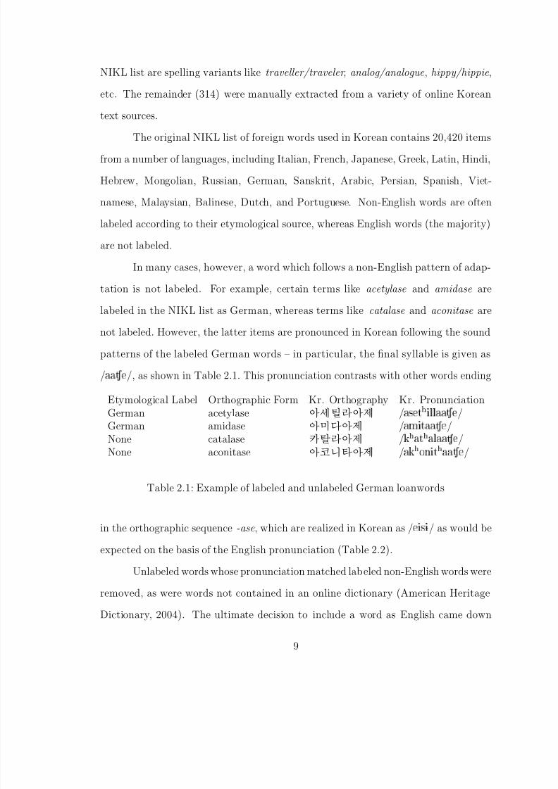
In many cases, however, a word which follows a non-English pattern of adap-
tation is not labeled. For example, certain terms like acetylase and amidase are
labeled in the NIKL list as German, whereas terms like catalase and aconitase are
not labeled. However, the latter items are pronounced in Korean following the sound
patterns of the labeled German words – in particular, the final syllable is given as
/ /, as shown in Table 2.1. This pronunciation contrasts with other words ending
Etymological Label Orthographic Form Kr. Orthography Kr. Pronunciation
German acetylase [j9]j / × Ø
Ð Ð
/German amidase p]j / Ñ Ø /None catalase »1Ï]j /
Ø
Ð /None aconitase ïm]j /
Ó Ò Ø
/
Table 2.1: Example of labeled and unlabeled German loanwords
in the orthographic sequence -ase, which are realized in Korean as / × ½ / as would be
expected on the basis of the English pronunciation (Table 2.2).Unlabeled words whose pronunciation matched labeled non-English words were
removed, as were words not contained in an online dictionary (American Heritage
Dictionary, 2004). The ultimate decision to include a word as English came down
9

8/8/2019 Baker Kirk
http://slidepdf.com/reader/full/baker-kirk 26/243
Etymological Label Orthographic Form Kr. Orthography Kr. PronunciationNone periclase o9þtYUsÛ¼ /Ô
Ö
½ Ð × ½ /None base ZsÛ¼ /Ô × ½ /
Table 2.2: Example of unlabeled English loanwords
to a subjective judgment: if the word was recognized as familiar, it was included;
otherwise, it was discarded.
Each entry in the list corresponds to an orthographically distinct English word
and consists of four tab-separated fields: English spelling, English pronunciation,
linearized hangul transliteration, and orthographic hangul transliteration. The first
three fields in each entry are aligned at the the character level. An example entry is
shown below.
s-pi-der s-pY-dX- s|paid^- Û¼s8
Figure 2.1: Example loanword alignment
The list is stored in a single, UTF-8 encoded text file, with one entry per line.
UTF-8 is a variable length character encoding for Unicode symbols that uses one byte
to encode the 128 US-ASCII characters and uses three bytes for Korean characters.
Because it is a plain text file, it is not tied to any proprietary file format and can be
opened with any modern text editor.
2.1.1 Romanization
Korean orthography is based on an alphabetic system that is organized into syllabic
blocks containing two to four characters each. In standard Korean character encodings
such as EUC-KR or UTF-8, each syllabic block is itself coded as a unique character.
10
8/8/2019 Baker Kirk
http://slidepdf.com/reader/full/baker-kirk 27/243
This means that there is no longer an explicit internal representation of the individual
orthographic characters composing that syllable. For example, in UTF-8 the Korean
characters , a, and are represented as ‘\u1112’, ‘\u1161’, and ‘\u1102’,
respectively. However, the Korean syllable composed of these characters, ôÇ, is not
represented as ‘\u1112\u1161\u1102’ but as its own character ‘\uD55C’. Therefore,
determining character-level mappings (i.e., phoneme-to-phoneme or letter-to-letter)
between Korean and English words is possible only by converting the syllabic blocks
of Korean orthography into a linear sequence of characters. One way to do this is to
convert hangul representations into an ASCII-based character representation.
For romanization of the data set, priority was given to a one-to-one mapping
from hangul letters to ASCII characters because this simplifies many string-based
operations like aligning and searching. Multicharacter representations such as Yale
romanization (Martin, 1992) or phonemic representations like those in the CMU Pro-
nouncing Dictionary (Weide, 1998) require additional processing or an additional
delimiter between symbols. Furthermore, the symbol delimiter must be distinct from
the word delimiter.
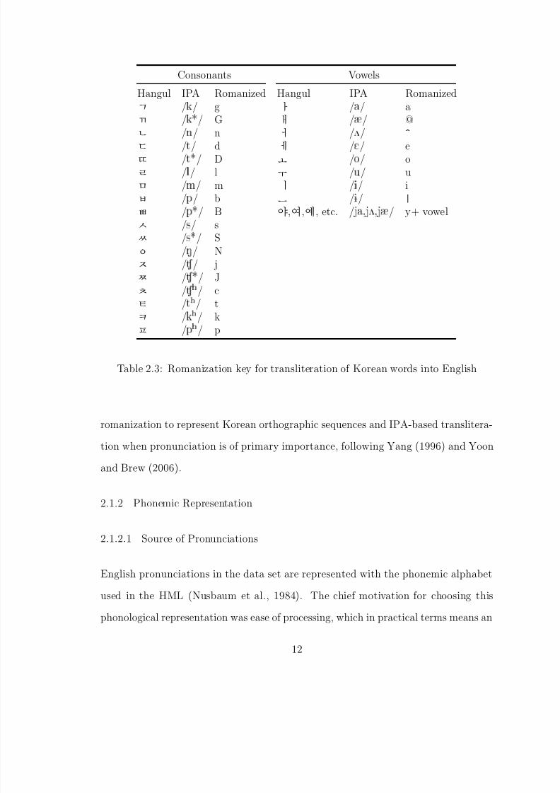
As much as possible, romanization of the data set is phonemic in the sense
that it uses ASCII characters that are already in use as IPA symbols. Consonant
transliteration follows Yoon and Brew (2006), which in turn is based on Revised
Romanization of Korean. We modified this transliteration scheme so that tense con-
sonants are single character and velar nasal is single character. Table 2.3 (left column)
shows the list of consonant equivalences. Vowels were romanized on the basis of the
IPA transliterations given in Yang (1996: 251, Table III), using the ASCII equiva-lents from the Hoosier Mental Lexicon (HML) (Nusbaum, Pisoni, and Davis, 1984).
Vowel equivalents are shown in Table 2.3, right column. This dissertation uses Yale
11
8/8/2019 Baker Kirk
http://slidepdf.com/reader/full/baker-kirk 28/243
Consonants Vowels
Hangul IPA Romanized Hangul IPA Romanized / / g a / / a / ¶ / G b / / @
/Ò
/ ne
/¾
/^
/Ø / d f / / e /Ø ¶ / D i /Ó / o /Ð / l n /Ù / u /Ñ / m u / / i /Ô / b s /½ / |
/Ô ¶ / B ,#,\V, etc. / ¸ ¾ ¸ / y+ vowel /× / s /× ¶ / S /Æ / N / / j
/ ¶ / J /
/ c /Ø
/ t /
/ k /Ô
/ p
Table 2.3: Romanization key for transliteration of Korean words into English
romanization to represent Korean orthographic sequences and IPA-based translitera-
tion when pronunciation is of primary importance, following Yang (1996) and Yoon
and Brew (2006).
2.1.2 Phonemic Representation
2.1.2.1 Source of Pronunciations
English pronunciations in the data set are represented with the phonemic alphabet
used in the HML (Nusbaum et al., 1984). The chief motivation for choosing this
phonological representation was ease of processing, which in practical terms means an
12

8/8/2019 Baker Kirk
http://slidepdf.com/reader/full/baker-kirk 29/243
ASCII-based, single character per phoneme pronunciation scheme. Pronunciations for
English words were derived from two main sources: the HML (Nusbaum et al., 1984)
and the Carnegie Mellon Pronouncing Dictionary (CMUDict) (Weide, 1998). The
HML contains approximately 20,000 words, and CMUDict contains approximately
127,000. Loanwords contained in neither of these two sources were transcribed with
reference to pronunciations given in the American Heritage Dictionary (2004).
2.1.2.2 Standardizing Pronunciations
There are several differences between the transcription conventions used in the HML
and CMUDict which had to be standardized for consistent pronunciation. Therelevant differences are briefly summarized below, followed by the procedure used for
normalizing these differences and standardizing pronunciations.
1. Different alphabets. CMUDict uses an all-capital phoneme set, with many
phonemes represented by two characters (e.g., AA /a/, DH » » , etc.). Two-
character phones requires using an additional delimiter to separate unique sym-
bols. The HML uses upper and lower case letters, with only one character perphoneme, which does not require an additional delimiter.
2. CMUDict represents three levels of lexical stress with indices 0, 1, or 2 at-
tached to vowel symbols; the HML does not explicitly represent suprasegmen-
tal stress. For example, chestnut CEsn^t (HML) versus CH EH1 S N AH2 T
(CMUDict).
3. The HML distinguishes two reduced vowels (| / ½ / vs. x / /); CMUDict treats
both as unstressed schwa (AH0 / /). For example, wicked wIk|d (HML) and
W IH1 K AH0 D (CMUDict) versus zebra zibrx (HML) and Z IY1 B R AH0
(CMUDict).
13
8/8/2019 Baker Kirk
http://slidepdf.com/reader/full/baker-kirk 30/243
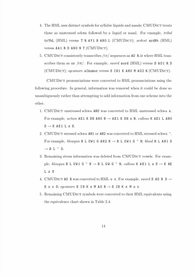
4. The HML uses distinct symbols for syllabic liquids and nasals; CMUDict treats
these as unstressed schwa followed by a liquid or nasal. For example, tribal
trYbL (HML) versus T R AY1 B AH0 L (CMUDict); ardent ardNt (HML)
versus AA1 R D AH0 N T (CMUDict).
5. CMUDict consistently transcribes / Ó / sequences as AO R Ç where HML tran-
scribes them as or /Ó /. For example, sword sord (HML) versus S A O 1 R D
(CMUDict); sycamore sIkxmor versus S IH1 K AH0 M AO2 R (CMUDict).
CMUDict pronunciations were converted to HML pronunciations using the
following procedure. In general, information was removed when it could be done so
unambiguously rather than attempting to add information from one scheme into the
other.
1. CMUDict unstressed schwa AH0 was converted to HML unstressed schwa x.
For example, action AE1 K SH AH0 N → A E 1 K S H x N; callous K AE1 L AH0
S → K A E 1 L x S.
2. CMUDict stressed schwa AH1 or AH2 was converted to HML stressed schwa ^.
For example, blowgun B L OW1 G AH2 N → B L O W 1 G ^ N; blood B L A H 1 D
→ B L ^ D.
3. Remaining stress information was deleted from CMUDict vowels. For exam-
ple, blowgun B L O W 1 G ^ N → B L O W G ^ N; callous K A E 1 L x S → K AE
L x S
4. CMUDict AO R was converted to HML o r. For example, sword S AO R D →
S o r D; sycamore S I H K x M A O R → S IH K x M o r.
5. Remaining CMUDict symbols were converted to their HML equivalents using
the equivalence chart shown in Table 2.4.
14
8/8/2019 Baker Kirk
http://slidepdf.com/reader/full/baker-kirk 31/243
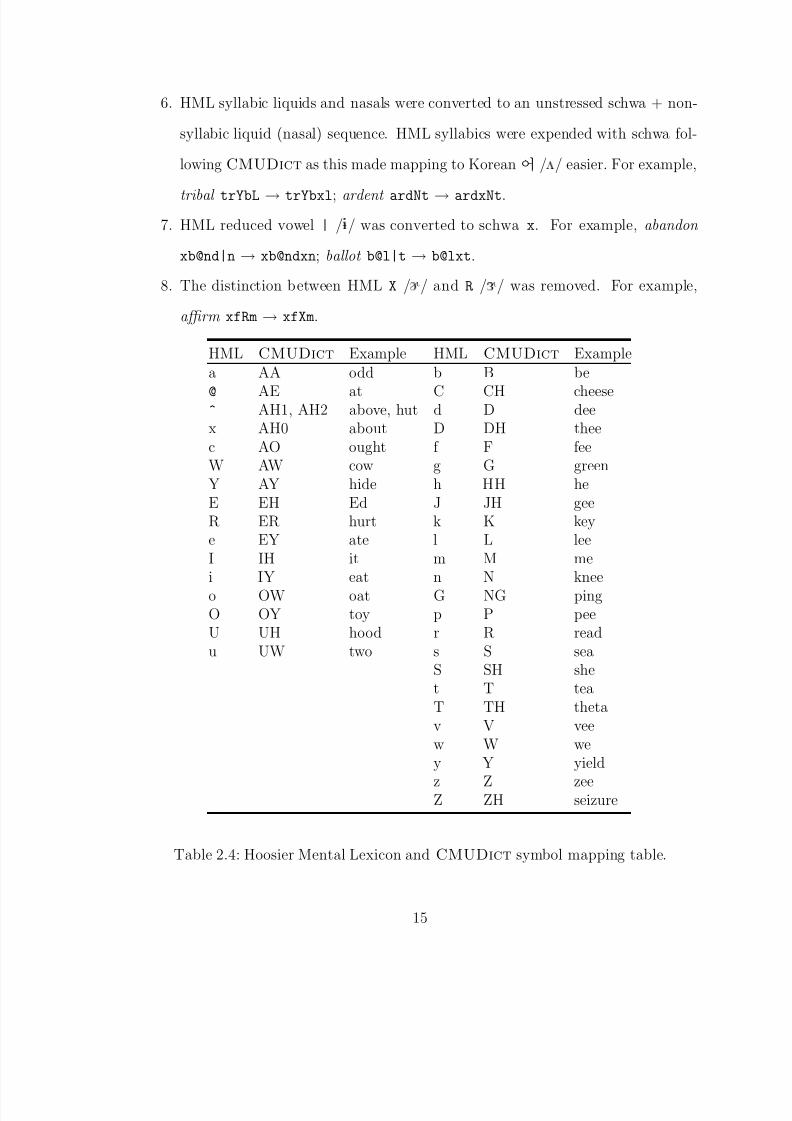
6. HML syllabic liquids and nasals were converted to an unstressed schwa + non-
syllabic liquid (nasal) sequence. HML syllabics were expended with schwa fol-
lowing CMUDict as this made mapping to Korean#Q /¾ / easier. For example,
tribal trYbL → trYbxl; ardent ardNt → ardxNt.
7. HML reduced vowel | / ½ / was converted to schwa x. For example, abandon
xb@nd|n → xb@ndxn; ballot b@l|t → b@lxt.
8. The distinction between HML X / / and R / / was removed. For example,
affirm xfRm → xfXm.
HML CMUDict Example HML CMUDict Examplea AA odd b B be
@ AE at C CH cheese^ AH1, AH2 above, hut d D deex AH0 about D DH theec AO ought f F feeW AW cow g G greenY AY hide h HH heE EH Ed J JH geeR ER hurt k K keye EY ate l L leeI IH it m M mei IY eat n N kneeo OW oat G NG pingO OY toy p P peeU UH hood r R readu UW two s S sea
S SH shet T teaT TH thetav V veew W wey Y yield
z Z zeeZ ZH seizure
Table 2.4: Hoosier Mental Lexicon and CMUDict symbol mapping table.
15
8/8/2019 Baker Kirk
http://slidepdf.com/reader/full/baker-kirk 32/243
2.1.3 Alignments
In order to look at the influence of both orthography and pronunciation on English
loanwords in Korean, we wanted a three-way, character level alignment between an
English orthographic form, its phonemic representation, and corresponding linearized
Korean transliteration. English spellings were automatically aligned with their pro-
nunciations using the iterative, expectation-maximization based alignment algorithm
detailed in Deligne, Yvon, and Bimbot (1995). The Korean transliteration was aligned
with the English pronunciation using a simplified version of the edit-distance proce-
dure detailed in Oh and Choi (2005). The algorithm described in Oh and Choi (2005)
assigns a range of substitution costs depending on a set of conditions that describe
the relation between a source and target symbol. For example, if the source and
target symbol are phonetically similar, a cost of 0 is assigned; an alignment between
a vowel and a semi-vowel incurs a cost of 30; an alignment between phonetically dis-
similar vowels costs 100, and aligning phonetically dissimilar consonants costs 240.
Manually constructed phonetic similarity tables are used to determine the relation
between source and target symbols.We tried a simpler strategy of assigning consonant-consonant or vowel-vowel
alignments a low cost consonant-vowel alignments a high cost and found that values
of 0 and 10, respectively, performed reasonably well. These costs were determined by
trial and error on a small sample. Because there are symbols in one representation
that don’t have a counterpart in the other (e.g., Korean epenthetic vowels or English
orthographic characters that are not pronounced), it is necessary to insert a special
null symbol indicating a null alignment. The null symbol is ‘-’. The resulting align-
ments are all the same length. The costs assigned determine alignments that tend to
obey the following constraints.
16

8/8/2019 Baker Kirk
http://slidepdf.com/reader/full/baker-kirk 33/243
8/8/2019 Baker Kirk
http://slidepdf.com/reader/full/baker-kirk 34/243
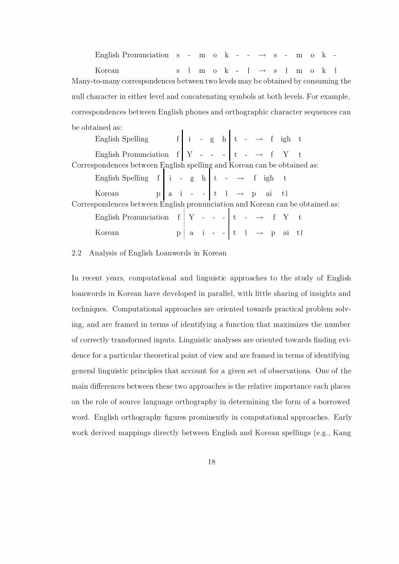
English Pronunciation s - m o k - - → s - m o k -
Korean s | m o k - | → s | m o k |
Many-to-many correspondences between two levels may be obtained by consuming the
null character in either level and concatenating symbols at both levels. For example,correspondences between English phones and orthographic character sequences can
be obtained as:
English Spelling f i - g h t - → f igh t
English Pronunciation f Y - - - t - → f Y t
Correspondences between English spelling and Korean can be obtained as:
English Spelling f i - g h t - → f igh t
Korean p a i - - t|
→ p ai t|
Correspondences between English pronunciation and Korean can be obtained as:
English Pronunciation f Y - - - t - → f Y t
Korean p a i - - t | → p ai t|
2.2 Analysis of English Loanwords in Korean
In recent years, computational and linguistic approaches to the study of English
loanwords in Korean have developed in parallel, with little sharing of insights andtechniques. Computational approaches are oriented towards practical problem solv-
ing, and are framed in terms of identifying a function that maximizes the number
of correctly transformed inputs. Linguistic analyses are oriented towards finding evi-
dence for a particular theoretical point of view and are framed in terms of identifying
general linguistic principles that account for a given set of observations. One of the
main differences between these two approaches is the relative importance each places
on the role of source language orthography in determining the form of a borrowed
word. English orthography figures prominently in computational approaches. Early
work derived mappings directly between English and Korean spellings (e.g., Kang
18
8/8/2019 Baker Kirk
http://slidepdf.com/reader/full/baker-kirk 35/243
and Choi, 2000a), while later work considers the joint contribution of orthographic
and phonological information (e.g., Oh and Choi, 2005).
Many linguistic analyses of loanword adaptation, however, consider orthogra-
phy a confound, as in Kang (2003: 234):
“problem of interference from normative orthographic conventions”
or uninteresting, as in Peperkamp (2005: 10):
“Given the metalinguistic character of orthography, adaptations that are
(partly) based on spelling correspondences are of course of little interest
to linguistic analyses”
Linguistic accounts of English loanword adaptation in Korean instead focus on
whether the mechanisms of loanword adaptation are primarily phonetic or phono-
logical. Other analyses of loanword adaptation in other languages acknowledge that
orthography interacts with these mechanisms (e.g., Smith (2008) on English loanword
adaptation in Japanese).
This section looks at some influences of orthography on English loanwords
in Korean, and shows that English spelling accounts for substantially more of thevariation in Korean vowel adaptation than phonetic similarity does. The relevance
of this correlation is illustrated for the case of variable vowel epenthesis following
word final voiceless stops, and discussed more generally for understanding English
loanword adaptation in Korean.
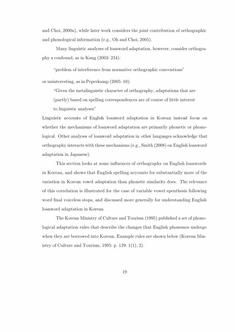
The Korean Ministry of Culture and Tourism (1995) published a set of phono-
logical adaptation rules that describe the changes that English phonemes undergo
when they are borrowed into Korean. Example rules are shown below (Korean Min-
istry of Culture and Tourism, 1995: p. 129: 1(1), 2).
19

8/8/2019 Baker Kirk
http://slidepdf.com/reader/full/baker-kirk 36/243
1. after a short vowel, word-final voiceless stops ([p], [t], [k]) are written as codas
(p, s, k)
book bÍ k] → Ô Ù
2.½
is inserted after word-final and pre-consonantal voiced stops ([b], [d], [g])
signal sÁ gn l] → × ½ Ò Ð
These rules were implemented as regular expressions in a Python script and
applied to the phonological representations of English words in the data set (this
procedure is explained in detail in Chapter 3 Section 3.3.1). The output of the
program was compared to the attested Korean forms, and the proportion of times
the rule applied as predicted was calculated for each English consonant. These results
are shown in Table 2.5.
Stops Fricatives Nasals Glides
p 0.990 f 0.999 m 1.000 r 0.988t 0.989 v 0.985 n 0.997 l 0.987k 0.990 Ì 0.978 Æ 0.983 w 0.967b 0.996 1.000 j 0.859d 0.996 s 0.975g 0.984 z 0.733
Ë 0.985 1.000 0.951 0.969h 0.983
Table 2.5: Accuracy by phoneme of phonological adaptation rules. Mean = 0.97
In general the rules do a good job of predicting the borrowed form of English
consonants in Korean. On average, consonants were realized as predicted by the
phonological conversion rules 97% of the time. The prediction rates for /z/ and /j/
were substantially below the mean at 0.73 and 0.86, respectively. Based on Korean
20

8/8/2019 Baker Kirk
http://slidepdf.com/reader/full/baker-kirk 37/243
Ministry of Culture and Tourism (1995: p. 129: 2, 3(1)) the following rules for the
adaptation of English » Þ » in Korean loanwords were implemented:
1. word-final and pre-consonantal Þ ℄ → ݼ ½
jazz Þ ℄ → Fݼ / ½ /
2. otherwise, Þ ℄ → / /
zigzag Þ Á Þ ℄ → tÕªFÕª / ½ ½ /
» Þ » occurred 704 times in English words in the data set; it was realized accord-
ing to the rule as 512 times and realized as × 188 times. In 117 of these cases,
the unpredicted form corresponds to English word-final » Þ » representing the plural
morpheme (orthographic ‘-s’). Examples include words like users / Ù Þ Þ / → Ä»$
Û¼ / Ù ¾ × ½ /, broncos / Ö Æ Ó Þ / → ÚÔ2xïÛ¼ /Ô ½ Ð Ó Æ
Ó × ½ /, and bottoms / Ø Ñ Þ /
→ Ð)3Û¼ /Ô Ó Ø
¾ Ñ × ½ /. The contingency table in 2.6 shows how often » Þ » is real-
ized as predicted with respect to the English grapheme spelling it. The χ2 signifi-
cance test indicates that » Þ » is significantly more likely to become s in Korean
when the English spelling contains a corresponding ‘s’ than when it does not (Yates’
χ2
= 100.547, df = 1, p < 0.001).
s ¬s English Orthography» Þ »
→ 300 212» Þ »
→ × 185 3
Table 2.6: Contingency table for the transliteration of ‘s’ in English loanwords inKorean
Although this result indicates that English spelling is a more reliable indicatorof the adapted form of » Þ » than its phonological identity alone, it does not tease apart
the question of whether low level phonetics or morphological knowledge of English
is responsible for this adaptation pattern. English word-final » Þ » often devoices (e.g.
21

8/8/2019 Baker Kirk
http://slidepdf.com/reader/full/baker-kirk 38/243
Smith, 1997); if the adaptation of these words is based on × ℄ rather than » Þ » , these
cases would be regularly handled under the rule for the adaptation of English » × » .
Alternatively, these borrowed forms may represent knowledge of the morphological
structure of the English words, in which a distinction between
and ×
is
maintained in the borrowed forms.
The following rule predicts the appearance of English / / in English loanwords
in Korean (Korean Ministry of Culture and Tourism, 1995):
[j] → y .
/ / occurred 368 times in English loanwords in the data set; 275 of these cases
were adapted as the predicted j (e.g., yuppie / ¾ Ô / → #x / ¾ Ô
/), while 35 were
adapted as i (e.g., billion / Á Ð Ò / →yn=o /Ô Ð Ð ¾ Ò /) and 58 were adapted as ∅ (e.g.,
cellular /× Ð Í Ð / → !sqÀÒQ /× Ð Ð Ù Ð Ð ¾ /). These cases are examined separately in the
χ2 tables 2.7 and 2.8. Table 2.7 shows how often English » » transliterates as Korean
s / / with respect to whether the English spelling contains a corresponding ‘i’. The
i ¬i
→ 7 64
→∅ 29 4
Table 2.7: Contingency table for the transliteration of /j/ in English loanwords inKorean
results of the χ2 test indicate that when the English orthography contains the vowel ‘i’,
» » is more likely to be transliterated ass / / (Yates’ χ2 = 57.192, df = 1, p < 0.001).
Table 2.8 shows how often English » » is produced in the adapted form with respect
to whether the English orthography contains a corresponding character. The results
of the χ2 test indicate that » » shows a tendency to drop when the orthography does
not support its inclusion (e.g, cellular ) (χ2 = 4.725, df = 1, p ≤ 0.03).
22

8/8/2019 Baker Kirk
http://slidepdf.com/reader/full/baker-kirk 39/243
y ∅
→ 54 204 → ∅ 5 53
Table 2.8: Contingency table for the transliteration of ‘i’ in English loanwords inKorean
Whereas the behavior of English consonants in loanwords in Korean is reliably
expressed with a handful of phonological rules, the behavior of vowels is considerably
less constrained. Table 2.9 shows the number of transliterations found in the data set
for each English vowel. The average number of transliterations per vowel is 8.46.
English Vowel Number of Korean Transliterationsa 7 6Ç 6e 11Í 5Á 9o 10i 9u 6 15 12 9¾ 5
Table 2.9: Average number of transliterations per vowel in English loanwords inKorean
Korean Ministry of Culture and Tourism (1995) does not provide phonological
rules describing the adaptation of English vowels to Korean. However, Yang (1996)
provides acoustic measurements of the English and Korean vowel systems. Based on
this data, it is possible to estimate the acoustic similarity of the English and Korean
23

8/8/2019 Baker Kirk
http://slidepdf.com/reader/full/baker-kirk 40/243
vowels, and examine the relation between the cross language vowel similarity and
transliteration frequency. The prediction is that acoustically similar Korean vowels
will be substituted for their English counterparts more frequently than non-similar
vowels. Recognizing that acoustic similarity is not necessarily the best predictor of
perceptual similarity (e.g., Yang, 1996), we nonetheless applied two measures of vowel
distance and correlated each with transliteration frequency.
The first measurement was the Euclidean distance between vowels using F1
through F3 measurements for English and Korean vowels from Yang (1996):
(2.1)
3i=1
(F E i − F K i)2
The notion of a perceptual F 2′ has been recognized as relevant since Carlson,
Granstrom, and Fant (1970) introduced it for accounting for the perceptual integra-
tion of the higher formants. We calculated F 2′ according to the formula in Padgett
(2001: 200):
(2.2) F 2′ = F 2 +F 3 − F 2
2×
F 2 − F 1
F 3 − F 1
and applied the Euclidean distance formula in 2.3 to calculate vowel distance:
(2.3) (F E 1 − F K 1)2 + (F E 2′ − F K 2′)2
The correlation between vowel distance and frequency of transliteration in an
acoustic-perceptual space is very weak. Table 2.10 shows the associated correlations
between each of the distance measures and vowel transliteration frequency.
24
8/8/2019 Baker Kirk
http://slidepdf.com/reader/full/baker-kirk 41/243
Measure CorrelationEuclidean -0.256F 2′ -0.331
Table 2.10: Correlation between acoustic vowel distance and transliteration frequency
However, in many cases the Korean vowel corresponds to a normative “IPA
reading” of the English orthographic vowel, regardless of its actual pronunciation.
A much stronger correlation is found between the number of ways a vowel is writ-
ten in English and the number of adaptations of that vowel in Korean (r = 0.92).
For example,
is represented orthographically in a variety of ways in English (e.g.,
action, Atlanta, cricket, coxswain, instrumentalism) and shows a variety of realiza-
tions in loanwords in Korean (e.g., Óo ayksy e n , Ed¦½ aythullaynth a , ß¼oHàÔ
khulik ey thu , 9qÛ¼J? khoksuw ey in , Û¼àÔÀÒF'p_Oo7£§ insuthul wu meynthellicum ).
This correlation is depicted graphically in Figure 2.2.
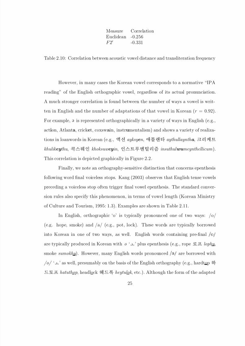
Finally, we note an orthography-sensitive distinction that concerns epenthesis
following word final voiceless stops. Kang (2003) observes that English tense vowels
preceding a voiceless stop often trigger final vowel epenthesis. The standard conver-
sion rules also specify this phenomenon, in terms of vowel length (Korean Ministry
of Culture and Tourism, 1995: 1.3). Examples are shown in Table 2.11.
In English, orthographic ‘o’ is typically pronounced one of two ways: /o/
(e.g. hope, smoke) and /a/ (e.g., pot, lock). These words are typically borrowed
into Korean in one of two ways, as well. English words containing pre-final » Ó »
are typically produced in Korean with o ‘i’ plus epenthesis (e.g., rope ÐáÔ lophu ,
smoke sumokhu ). However, many English words pronounced » » are borrowed with
/o/ ‘i’ as well, presumably on the basis of the English orthography (e.g., hardtop
×¼ÐáÔ hatuthop, headlock K×¼2¤ heytulok , etc.). Although the form of the adapted
25

8/8/2019 Baker Kirk
http://slidepdf.com/reader/full/baker-kirk 42/243
0 5 10 15 20 25 30
0
5
1 0
1 5
No. of English vowel spellings
N o .
o f K o r e a n v o w e
l s p e
l l i n g s
a
æO
e
U
I
o
i
u
Ç
@
E
2
Figure 2.2: Correlation between number of loanword vowel spellings in English andKorean
vowel is the same in both cases, epenthesis is significantly less likely to occur for
orthographically derived /o/ than when /o/ corresponds to the English pronunciation
as well (Yates’ χ2 = 107.57; df = 1; p < .0001). Examples are given in Table 2.12,
which contains a breakdown of the epenthesis data for /o/ by identity of the following
stop. For /k/ and /p/, epenthesis is very unlikely when the English letter ‘o’ is
pronounced /a/; for /t/, orthographically derived /o/ is as likely to epenthesize as
pronunciation-based /o/1. In essence, the Korean phonology preserves a distinction
1This difference may reflect morphophonemic constraints on final /t/ in Korean nouns (Kang,2003).
26
8/8/2019 Baker Kirk
http://slidepdf.com/reader/full/baker-kirk 43/243
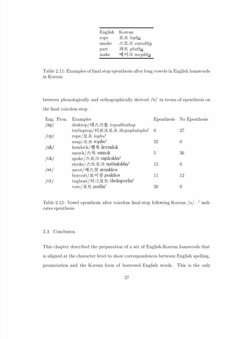
English Koreanrope ÐáÔ lophu smoke ۼ߼ sumokhu part àÔ phathu make Bjsß¼ meyikhu
Table 2.11: Examples of final stop epenthesis after long vowels in English loanwordsin Korean
between phonologically and orthographically derived » Ó » in terms of epenthesis on
the final voiceless stop.
Eng. Pron. Examples Epenthesis No Epenthesis» Ô » desktop/X<ۼ߼dv teysukhuthop
turboprop/'ÐáÔÐáÔ thepophulophu † 0 27» Ó Ô » rope/ÐáÔ lophu †
soap/èáÔ × Ó Ô Ù
† 32 0» » hemlock/Ùכ2¤ Ý Ñ Ð Ó
smock/Û¼3lq × Ù Ñ Ó 5 36» Ó » spoke/Û¼íß¼ × Ù Ô Ó Ù
†
stroke/Û¼àÔÐß¼ × Ù Ø Ù Ð Ó Ù
† 15 0» Ø » ascot/EÛ¼9w Ý × Ù Ó ×
boycott/Ðs9w Ô Ó Ó × 11 12» Ó Ø » tugboat/'ÕªÐàÔ Ø Ù Ô Ó Ø Ù
†
vote/ÐàÔ Ô Ó Ø Ù
† 26 0
Table 2.12: Vowel epenthesis after voiceless final stop following Korean /o/. † indi-cates epenthesis
2.3 Conclusion
This chapter described the preparation of a set of English-Korean loanwrods that
is aligned at the character level to show correspondences between English spelling,
prounciation and the Korean form of borrowed English words. This is the only
27

8/8/2019 Baker Kirk
http://slidepdf.com/reader/full/baker-kirk 44/243
resource of its kind that is freely available for unrestricted download: http://purl.
org/net/kbaker/data. Several analyses of the data were presented which highlight
previously unreported observations about the influence of orthography on English
loanword adaptation in Korean. Orthography has a particularly noticeable influence
on the realization of vowel in English loanwords in Korean. Vowel adaptation is not
reliably predicted form the phonological representation of vowels in English source
words in the absence of orthographic information, whereas consonant transliteration
is reliably captured by a small set of phonological conversion rules.
The analysis presented here also identified cases where English orthography
interacts with the Korean phonological process of word final vowel epenthesis follow-
ing voiceless stops. These findings are important for accounts of English loanword
adaptation in Korean because they provide a quantification of the extent to which
orthography influences the form of borrowed words, and indicate that accounts of
loanword adaptation which focus exclusively on the phonetics or phonology of the
adaptation process are overlooking important factors that shape the realization of
English loanwords in Korean. The next chapters use the data set described here in a
series of experiments on automatic English-Korean transliteration and foreign word
identification.
» » » Ó » English pronunciation of ‘o’Korean /o/ ‘i’, with Epenthesis 16 73Korean /o/ ‘i’, no Epenthesis 75 0
Table 2.13: Relation between voiceless final stop epenthesis after » Ó » ‘i’ andwhether the Korean form is based on English orthography ‘o’ or phonology » » .
χ2
= 107.57; df = 1; p < .001
28
8/8/2019 Baker Kirk
http://slidepdf.com/reader/full/baker-kirk 45/243
CHAPTER 3
ENGLISH-TO-KOREAN TRANSLITERATION
3.1 Overview
3.2 Previous Research on English-to-Korean Transliteration
Three types of automatic English-to-Korean transliteration models have been pro-
posed in the literature: grapheme-based models (Lee and Choi, 1998; Jeong, Myaeng,
Lee, and Choi, 1999; Kim, Lee, and Choi, 1999; Lee, 1999; Kang and Choi, 2000a;
Kang and Kim, 2000; Kang, 2001), phoneme-based models (Lee, 1999; Jung et al.,
2000), and ortho-phonemic models (Oh and Choi, 2002, 2005; Oh, Choi, and Isa-
hara, 2006b). Grapheme-based models work by directly transforming source language
graphemes into target language graphemes without explicitly utilizing phonology in
the bilingual mapping. Phoneme-based models, on the other hand, do not utilize
orthographic information in the transliteration process. Phoneme-based models are
generally implemented in two steps: first obtaining the source language pronunci-
ation and then converting that representation into the target language graphemes.
Ortho-phonemic models consider the joint influence of orthography and phonology
on the transliteration process. They also involve a two-step process, but rather than
discarding the orthographic information after the pronunciation of a source word has
been determined, they utilize it as part of the transliteration process.
29
8/8/2019 Baker Kirk
http://slidepdf.com/reader/full/baker-kirk 46/243
8/8/2019 Baker Kirk
http://slidepdf.com/reader/full/baker-kirk 47/243
dei-t- , etc. Maximum likelihood estimates specifying the probability with which each
English graphone maps onto each Korean graphone are obtained via the expectation
maximization algorithm (Dempster, Laird, and Rubin, 1977).
The probability of a particular Korean graphone sequence K = (k1, . . . , kL) oc-
curing is represented as a first-order Markov process (Manning and Schutze, 1999: Ch.
9) and is estimated as the product of the probabilities of each graphone ki (Equation
3.2):
(3.2) P (K ) ∼= P (k1)Li=2
p(ki|ki−1)
The probability of observing an English graphone sequence E = (e1, . . . , eL) given a
Korean sequence K is estimated from the observed graphone alignment probabilities
as
(3.3) P (E |K ) ∼=
ni=1
p(ei|ki)
This approach suffers from two drawbacks (Oh, Choi, and Isahara, 2006a; Oh
et al., 2006b). The first is the enormous time complexity involved in generating all
possible graphone sequences for words in both English and Korean. There are an
exponential number of ordered substrings to consider for a string of length L (e.g.,
string |L| has 2|L|−1 possible ordered subsequences). Because this number of substrings
must be considered for both languages, the approach is impossible to implement for
a large number of transliteration pairs. The second consideration involves the nature
of the alignment procedure for identifying within-language graphones. Alignment
errors in this stage propagate to the cross-language alignments, leading to incorrect
transliterations that might otherwise be avoided. This model obtained recall of 0.47
31
8/8/2019 Baker Kirk
http://slidepdf.com/reader/full/baker-kirk 48/243
when evaluating the 20 best transliteration candidates per word in a comparison
reported in Jung et al. (2000: 387, Table 3; trained on 90% of an 8368 word data set
and tested on 10%). Recall is defined as the number of correctly transliterated words
divided by the number of words in the test set.
3.2.1.2 Kang and Choi (2000a,b)
Kang and Choi (2000a, b) describes a grapheme-based transliteration model that uses
decision trees to convert an English word into its Korean transliteration. Like Lee
and Choi (1998) and Lee (1999), it is based on alignments between source and target
language graphones. However, this approach differs in terms of how the alignmentsare obtained.
Kang and Choi (2000a, b) explicitly mentions some of the steps undertaken
to mitigate the exponential growth of the graphone mapping problem, noting that
the number of combinations can be greatly reduced by disallowing many-to-many
mappings and null correspondences from English to Korean. Furthermore, Kang
and Choi (2000a, b) does not apply an initial English grapheme-phoneme alignment
step, but directly aligns English and Korean graphones. Character alignments are
automatically obtained using a modified version of a depth-first search alignment
algorithm based on Covington (1996).
Covington (1996)’s alignment procedure is a variant of the string edit-distance
algorithm (Levenshtein, 1966) that treats string alignment as a way of stepping
through two words performing a match or skip operation at each step. Kang and Choi
(2000a, b) extends Covington’s algorithm by adding a bind operation that removes
null mappings in the alignment and allows many-to-many correspondences between
source and target characters. For example, Covington’s edit distance algorithm aligns
board and /Ô Ó Ø ½
/ as
32

8/8/2019 Baker Kirk
http://slidepdf.com/reader/full/baker-kirk 49/243
b o a r d -
p o - - t ½
which produces null mappings (the ‘-’ symbol) in both the source and target strings.
Kang and Choi’s modifications produce the following alignmentb oar d
p o t½
in which the null mapping has been replaced by a binding operation that produces
many-to-many correspondences. Kang and Choi further modify the original align-
ment procedure by assigning different costs to matching symbols on the basis of their
phonetic similarity (i.e., phonetically dis-similar alignments such as consonant-vowel
receive higher penalties than an alignment between phonetically similar consonants
such as /f/ and / Ô
/). The penalties are heuristic in nature and are based on the
following two observations:
• English consonants tend to transliterate as Korean consonants, and English
vowels tend to transliterate as Korean vowels;
• there are typical Korean transliterations of most English characters.
These heuristics are implemented in terms of penalties involving the matching, skip-
ping, or binding of specific classes of English and Korean characters (Kang and Choi,
2000a: 1139, Table 2).
Kang and Choi (2000a, b) models the transliteration process in terms of a
bank of decision trees that decide, for each English letter, the most likely Korean
transliteration on the basis of seven contextual English graphemes (the left three,
the target, and the right three). For example, given the word board and its Korean
transliteration <potu >, 5 decision trees would attempt to predict the Korean output
on the basis of the representations in Table 3.1.
Kang and Choi (2000a, b) used ID3 (Quinlan, 1986), a decision tree learning
algorithm that splits attributes with the highest information gain first. Information
33
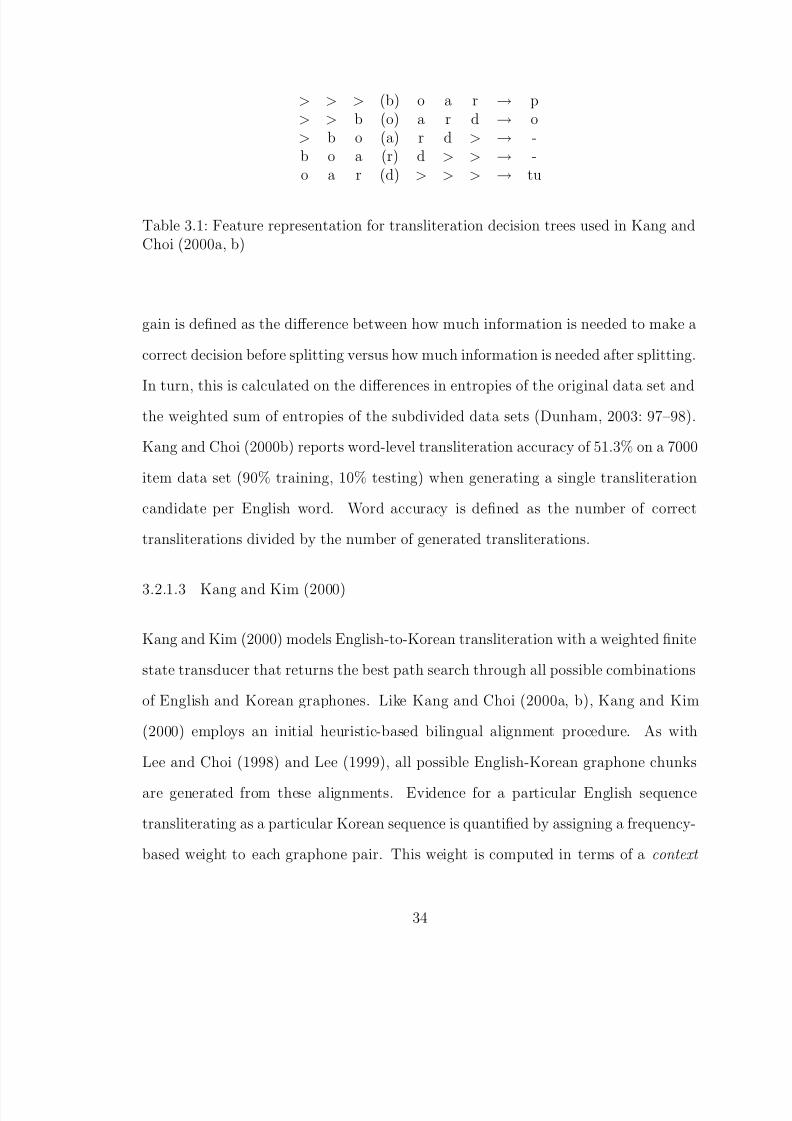
8/8/2019 Baker Kirk
http://slidepdf.com/reader/full/baker-kirk 50/243
> > > (b) o a r → p> > b (o) a r d → o> b o (a) r d > → -b o a (r) d > > → -o a r (d) > > > → tu
Table 3.1: Feature representation for transliteration decision trees used in Kang andChoi (2000a, b)
gain is defined as the difference between how much information is needed to make a
correct decision before splitting versus how much information is needed after splitting.
In turn, this is calculated on the differences in entropies of the original data set andthe weighted sum of entropies of the subdivided data sets (Dunham, 2003: 97–98).
Kang and Choi (2000b) reports word-level transliteration accuracy of 51.3% on a 7000
item data set (90% training, 10% testing) when generating a single transliteration
candidate per English word. Word accuracy is defined as the number of correct
transliterations divided by the number of generated transliterations.
3.2.1.3 Kang and Kim (2000)
Kang and Kim (2000) models English-to-Korean transliteration with a weighted finite
state transducer that returns the best path search through all possible combinations
of English and Korean graphones. Like Kang and Choi (2000a, b), Kang and Kim
(2000) employs an initial heuristic-based bilingual alignment procedure. As with
Lee and Choi (1998) and Lee (1999), all possible English-Korean graphone chunks
are generated from these alignments. Evidence for a particular English sequence
transliterating as a particular Korean sequence is quantified by assigning a frequency-
based weight to each graphone pair. This weight is computed in terms of a context
34

8/8/2019 Baker Kirk
http://slidepdf.com/reader/full/baker-kirk 51/243
and an output , where context refers to an English graphone ei and output refers to an
aligned Korean graphone ki as in Equation 3.4 (Kang and Kim, 2000: 420, Equation
4),
(3.4)
weight(context : output) =C (output)
C (context)len(context)
= weight(ei : ki) =C (ki ∩ ei)
C (ei)len(ei)
where C (x) refers to the number of times x occured in the training set. The weight
is multiplied by the length of the English graphone sequence so that longer chunks
receive more weight than shorter chunks.
A transliteration network is constructed as a finite state transducer where
arcs between nodes are weighted with the weights obtained from the aligned training
data. The best transliteration is found via the Viterbi algorithm (Forney, 1973) as
the optimal path through the network.
3.2.2 Phoneme-Based English-to-Korean Transliteration Models
Phoneme-based transliteration models map directly from English phonemes to Korean
graphemes.
3.2.2.1 Lee (1999); Kang (2001)
Oh et al. (2006a, b) summarizes two phoneme-based transliteration model originally
proposed by Lee (1999) and Kang (2001). Lee (1999)’s model generates Korean
transliterations from English words through a two-step process. The first step in-
volves the statistical segmentation of English words into graphones using the align-
ment procedure described in Section 3.2.1.1. At this point, instead of taking the
35
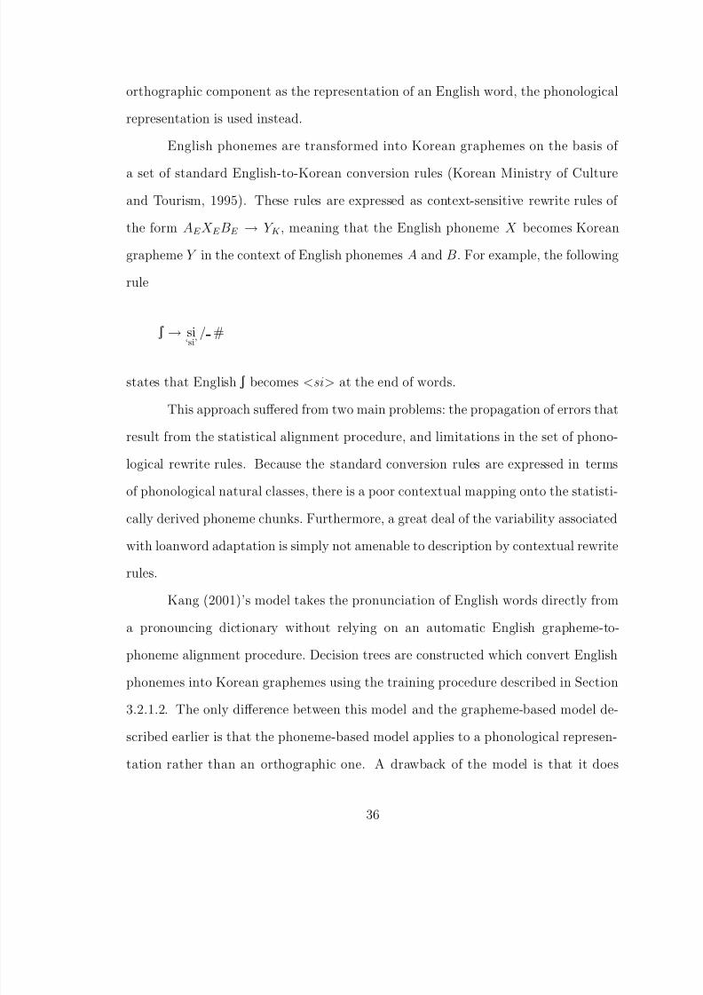
8/8/2019 Baker Kirk
http://slidepdf.com/reader/full/baker-kirk 52/243
orthographic component as the representation of an English word, the phonological
representation is used instead.
English phonemes are transformed into Korean graphemes on the basis of
a set of standard English-to-Korean conversion rules (Korean Ministry of Culture
and Tourism, 1995). These rules are expressed as context-sensitive rewrite rules of
the form AE X E BE → Y K , meaning that the English phoneme X becomes Korean
grapheme Y in the context of English phonemes A and B. For example, the following
rule
Ë → si‘si’
/ #
states that English Ë becomes <si > at the end of words.
This approach suffered from two main problems: the propagation of errors that
result from the statistical alignment procedure, and limitations in the set of phono-
logical rewrite rules. Because the standard conversion rules are expressed in terms
of phonological natural classes, there is a poor contextual mapping onto the statisti-
cally derived phoneme chunks. Furthermore, a great deal of the variability associatedwith loanword adaptation is simply not amenable to description by contextual rewrite
rules.
Kang (2001)’s model takes the pronunciation of English words directly from
a pronouncing dictionary without relying on an automatic English grapheme-to-
phoneme alignment procedure. Decision trees are constructed which convert English
phonemes into Korean graphemes using the training procedure described in Section
3.2.1.2. The only difference between this model and the grapheme-based model de-
scribed earlier is that the phoneme-based model applies to a phonological represen-
tation rather than an orthographic one. A drawback of the model is that it does
36

8/8/2019 Baker Kirk
http://slidepdf.com/reader/full/baker-kirk 53/243
not provide a method for estimating the pronunciation of English words not in the
dictionary, making it impossible to generalize to a larger set of transliteration pairs.
3.2.2.2 Jung, Hong, and Paek (2000)
Jung et al. (2000) presents a phoneme-based approach to English-to-Korean translit-
eration that models the process with an extended Markov window consisting of the
current English phoneme, the preceding and following English phoneme, and the cur-
rent and preceding Korean grapheme. The first step of the transliteration process
involves converting an English word to a pronunciation string using a pronouncing
dictionary. A transcription automaton is used to generate pronunciations for wordsnot contained in the dictionary. The next step involves constructing a phonological
mapping table that links English and Korean pronunciation units. Pronunciation
units may consist of vowel or consonant singletons, or larger units made up of combi-
nations of consonant and vowel sequences. Mappings are based on hand-crafted rules
that come from examining a set of English-Korean transliteration pairs. For each
English pronunciation unit, a list of possible Korean transliterations is determined.
Some examples are shown in Table 3.2 (Jung et al., 2000: 388–389, Tables 6-1 and
6-2).
English pronunciation unit Korean orthographic unit(s)
/p/ ,,áÔ, ‘p,b,p½ ,bb’/s/ ,Û¼,,, ‘s,s½ ,j,ss,jj’» Ù Ö » n#Q,0> ‘u ,w ’
Table 3.2: Example English-Korean transliteration units from (Jung et al., 2000: 388–389, Tables 6-1 and 6-2)
English pronunciations are aligned with Korean orthographic strings in a two
step heuristic-based process. In the first stage, English and Korean consonants are
37
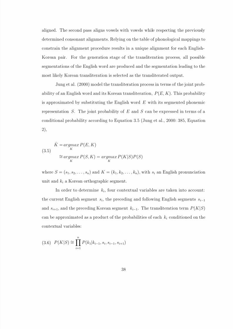
8/8/2019 Baker Kirk
http://slidepdf.com/reader/full/baker-kirk 54/243
aligned. The second pass aligns vowels with vowels while respecting the previously
determined consonant alignments. Relying on the table of phonological mappings to
constrain the alignment procedure results in a unique alignment for each English-
Korean pair. For the generation stage of the transliteration process, all possible
segmentations of the English word are produced and the segmentation leading to the
most likely Korean transliteration is selected as the transliterated output.
Jung et al. (2000) model the transliteration process in terms of the joint prob-
ability of an English word and its Korean transliteration, P (E, K ). This probability
is approximated by substituting the English word E with its segmented phonemic
representation S . The joint probability of E and S can be expressed in terms of a
conditional probability according to Equation 3.5 (Jung et al., 2000: 385, Equation
2),
(3.5)
K = argmaxK
P (E, K )
∼= argmaxK
P (S, K ) = argmaxK
P (K |S )P (S )
where S = (s1, s2, . . . , sn) and K = (k1, k2, . . . , kn), with si an English pronunciation
unit and ki a Korean orthographic segment.
In order to determine ki, four contextual variables are taken into account:
the current English segment si, the preceding and following English segments si−1
and si+1, and the preceding Korean segment ki−1. The transliteration term P (K |S )
can be approximated as a product of the probabilities of each ki conditioned on the
contextual variables:
(3.6) P (K |S ) ∼=
ni=1
P (k1|ki−1, si, si−1, si+1)
38

8/8/2019 Baker Kirk
http://slidepdf.com/reader/full/baker-kirk 55/243
The probability of a given English phonemic segmentation S is estimated from a
bigram language model:
(3.7) P (S )∼=
ni=1 P (s1|si−1)
Jung et al. (2000) describes further enhancements to the basic model in terms
of estimating backoffs to combat data sparsity and redundancies in feature predic-
tion. In comparing their model to the grapheme-based approach, the authors note
that grapheme-based models may have an advantage in transliterating proper names,
which are often absent from pronouncing dictionaries (Jung et al., 2000: 388). This
model obtains word level transliteration accuracy, defined as the number of correct
transliterations divided by the number of generated transliterations of 53% on a data
set containing 8368 items (90% training, 10% testing).
3.2.3 Ortho-phonemic English-to-Korean Transliteration Models
More recent research has explored models that combine orthographic and phonemic
information in the transliteration process. In general, models that incorporate ortho-
graphic and phonemic information outperform models that include only one source
of conditioning information.
3.2.3.1 Oh and Choi (2002)
Oh and Choi (2002) considered the joint influence of English orthography and pronun-
ciation on the transliteration process in the form of ortho-phonemic transliteration
rules. Oh and Choi’s model begins by applying the heuristic bilingual alignment pro-
cedure described in Kang and Choi (2000a, b). English phonological representations
are taken from the Carnegie Mellon Pronouncing Dictionary (CMUDict) (Weide,
39
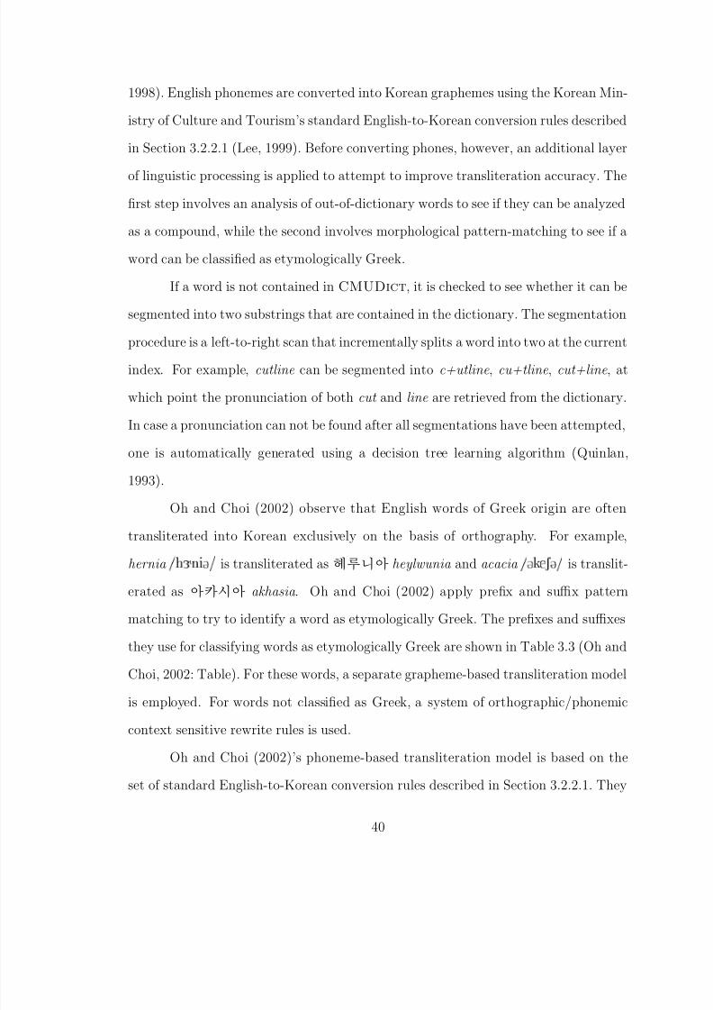
8/8/2019 Baker Kirk
http://slidepdf.com/reader/full/baker-kirk 56/243
1998). English phonemes are converted into Korean graphemes using the Korean Min-
istry of Culture and Tourism’s standard English-to-Korean conversion rules described
in Section 3.2.2.1 (Lee, 1999). Before converting phones, however, an additional layer
of linguistic processing is applied to attempt to improve transliteration accuracy. The
first step involves an analysis of out-of-dictionary words to see if they can be analyzed
as a compound, while the second involves morphological pattern-matching to see if a
word can be classified as etymologically Greek.
If a word is not contained in CMUDict, it is checked to see whether it can be
segmented into two substrings that are contained in the dictionary. The segmentation
procedure is a left-to-right scan that incrementally splits a word into two at the current
index. For example, cutline can be segmented into c+utline, cu+tline, cut+line, at
which point the pronunciation of both cut and line are retrieved from the dictionary.
In case a pronunciation can not be found after all segmentations have been attempted,
one is automatically generated using a decision tree learning algorithm (Quinlan,
1993).
Oh and Choi (2002) observe that English words of Greek origin are often
transliterated into Korean exclusively on the basis of orthography. For example,
hernia » Ò » is transliterated asKÀÒm heylwunia and acacia » Ë » is translit-
erated as r akhasia . Oh and Choi (2002) apply prefix and suffix pattern
matching to try to identify a word as etymologically Greek. The prefixes and suffixes
they use for classifying words as etymologically Greek are shown in Table 3.3 (Oh and
Choi, 2002: Table). For these words, a separate grapheme-based transliteration model
is employed. For words not classified as Greek, a system of orthographic/phonemiccontext sensitive rewrite rules is used.
Oh and Choi (2002)’s phoneme-based transliteration model is based on the
set of standard English-to-Korean conversion rules described in Section 3.2.2.1. They
40
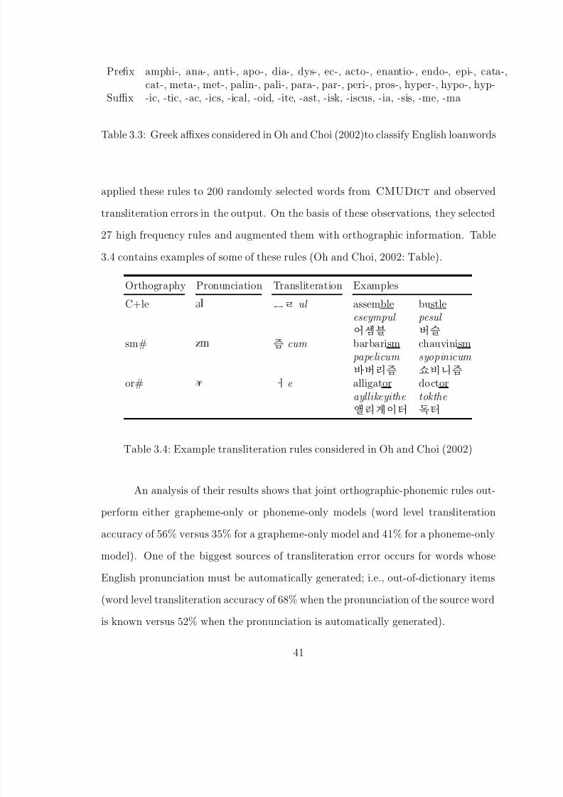
8/8/2019 Baker Kirk
http://slidepdf.com/reader/full/baker-kirk 57/243
Prefix amphi-, ana-, anti-, apo-, dia-, dys-, ec-, acto-, enantio-, endo-, epi-, cata-,cat-, meta-, met-, palin-, pali-, para-, par-, peri-, pros-, hyper-, hypo-, hyp-
Suffix -ic, -tic, -ac, -ics, -ical, -oid, -ite, -ast, -isk, -iscus, -ia, -sis, -me, -ma
Table 3.3: Greek affixes considered in Oh and Choi (2002)to classify English loanwords
applied these rules to 200 randomly selected words from CMUDict and observed
transliteration errors in the output. On the basis of these observations, they selected
27 high frequency rules and augmented them with orthographic information. Table
3.4 contains examples of some of these rules (Oh and Choi, 2002: Table).
Orthography Pronunciation Transliteration Examples
C+le Ð s ul assemble bustleeseympul pesul #Q!lr¦ !Q_þt
sm# Þ Ñ 7£§ cum barbarism chauvinismpapelicum syopinicum !Qo7£§ ®éqm7£§
or# e e alligator doctorayllikeyithe toktheîqo>s' 1lq'
Table 3.4: Example transliteration rules considered in Oh and Choi (2002)
An analysis of their results shows that joint orthographic-phonemic rules out-
perform either grapheme-only or phoneme-only models (word level transliteration
accuracy of 56% versus 35% for a grapheme-only model and 41% for a phoneme-only
model). One of the biggest sources of transliteration error occurs for words whose
English pronunciation must be automatically generated; i.e., out-of-dictionary items
(word level transliteration accuracy of 68% when the pronunciation of the source word
is known versus 52% when the pronunciation is automatically generated).
41

8/8/2019 Baker Kirk
http://slidepdf.com/reader/full/baker-kirk 58/243
3.2.3.2 Oh and Choi (2005); Oh, Choi, and Isahara (2006)
Oh and Choi (2005); Oh et al. (2006b) presents a generalized framework for combining
orthographic and phonemic information into the transliteration process. Oh and Choi
(2005) applies three different machine learning methods (maximum entropy modeling,
decision tree learning, and memory-based learning) to the transliteration task and
evaluates the results.
Oh and Choi’s method begins with establishing alignments between English
graphemes and phonemes, and then alignments from English grapheme-phoneme pairs
to Korean graphemes. English phonological representations are taken from CMU-
Dict (Weide, 1998). Alignments are obtained automatically using a heuristically
weighted version of the edit distance algorithm (Levenshtein, 1966). The cost schemes
are borrowed from Kang and Choi (2000a, b). The first step involves aligning English
graphemes with English phonemes (GE → P E ) and then aligning English phonemes
with Korean graphemes (P E → GK ). Using the English phoneme as a pivot, English
graphemes are aligned with Korean graphemes (GE → P E → GK ). The (GE → P E )
alignments are used to construct training data for a procedure that can be used togenerate the pronunciation of words that are not in CMUDict (the actual procedure
is not specified).
Oh and Choi model the transliteration process in terms of a function that
maps a set of source language contextual features onto a target language grapheme.
Four types of features are used: graphemes, phonemes, generalized graphemes, and
generalized phonemes. These features are described in Table 3.5 (Oh and Choi,
2005: 1743, Table 6).
Figure 3.1 (Oh and Choi, 2005: 1744, Figure 6) illustrates the principle of
using these features to predict the transliteration of the word board (Ð×¼ ‘bo-d½ ’).
42

8/8/2019 Baker Kirk
http://slidepdf.com/reader/full/baker-kirk 59/243
Feature Possible Values
English Graphemes {a , b , c , . . . , x , y , z}English Phonemes {/AA/,/AE/,... }Generalized Graphemes Consonant (C),Vowel (V)
Generalized Phonemes Consonant (C),Vowel (V),Semi-vowel (SV),Silence (∅
)
Table 3.5: Feature sets used in Oh and Choi (2005) for transliterating English loan-words in Korean
The grapheme currently being transliterated is represented in the center of a context
of three preceding and three following features. It can be described in terms of a 28-
feature vector consisting of the current grapheme plus six contextual graphemes, the
current phoneme plus six contextual phonemes, the current generalized grapheme plus
six generalized graphemes, and the current generalized phoneme plus six generalized
phonemes.
L3 L2 L1 ▽ R1 R2 R3G = ( ∅ ∅ ∅ b o a r )P = ( ∅ ∅ ∅ /b/ /o/ ∅ /r/ )
GG = ( ∅ ∅ ∅ C V V C )GP = ( ∅ ∅ ∅ C V ∅ C )
→ ‘b’
Figure 3.1: Feature representation of English graphemes
Oh and Choi apply three machine learning models to the feature representa-
tion described in Figure 3.1: maximum entropy modeling, decision tree learning, and
memory based learning. The maximum entropy model (Jaynes, 1991; Berger, Pietra,
and Pietra, 1996) is a probabilistic framework for integrating information sources. It
43

8/8/2019 Baker Kirk
http://slidepdf.com/reader/full/baker-kirk 60/243
is based on the constraint that the expected value of each feature in the final maxi-
mum entropy model must equal the expectation of that same feature in the training
set. Training the model consists of finding the probability distribution subject to
the constraints that has the maximum entropy distribution (Manning and Schutze,
1999: Chapter 16, 589–591). For the decision tree, Oh and Choi used C4.5 (Quin-
lan, 1993), a variant of the ID3 model described in Section 3.2.1.2 (Kang and Choi,
2000a, b). Memory-based learning is a k-nearest neighbors classifier (Hastie, Tibshi-
rani, and Friedman, 2001). Training instances are stored in memory, and a similarity
metric is used to compare a new instance with items in memory. The k most similar
items are stored, and the majority class label is assigned to the new instance. Oh
and Choi used TiMBL (Tilburg Memory-Based Learner) (Daelemans, Zavrel, van
der Sloot, and van den Bosch, 2003), an efficient knn implementation geared towards
NLP applications. The results of these comparisons are shown in Table 3.6.
3.2.4 Summary of Previous Research
Table 3.6 contains a summary of the results of previous English-to-Korean translit-
eration experiments. The reported results are for 1-best transliteration accuracy,
defined as the number of correct transliterations divided by the number of gener-
ated transliterations, and include a mixture of words whose English pronunciation
was automatically generated and words whose English pronunciation was found by
dictionary lookup. Because not all results are reported over the same data set using
the same methodology, they should be interpreted as representative of the various
approaches to English-Korean transliteration rather than as strict comparisons. In
general, the combined models outperform models that only include one source of in-
formation in the transliteration process. On average, the grapheme-based models are
44
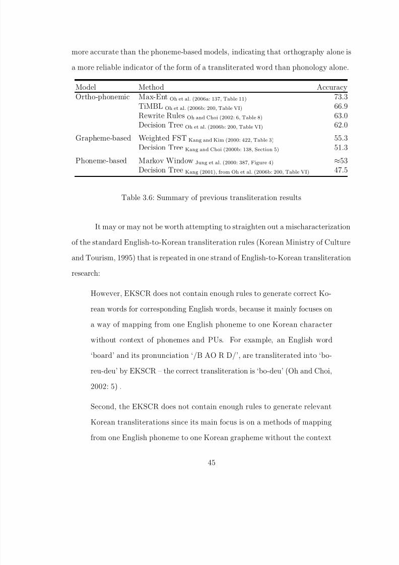
8/8/2019 Baker Kirk
http://slidepdf.com/reader/full/baker-kirk 61/243
more accurate than the phoneme-based models, indicating that orthography alone is
a more reliable indicator of the form of a transliterated word than phonology alone.
Model Method Accuracy
Ortho-phonemic Max-Ent Oh et al. (2006a: 137, Table 11) 73.3TiMBL Oh et al. (2006b: 200, Table VI) 66.9Rewrite Rules Oh and Choi (2002: 6, Table 8) 63.0Decision Tree Oh et al. (2006b: 200, Table VI) 62.0
Grapheme-based Weighted FST Kang and Kim (2000: 422, Table 3) 55.3Decision Tree Kang and Choi (2000b: 138, Section 5) 51.3
Phoneme-based Markov Window Jung et al. (2000: 387, Figure 4) ≈53Decision Tree Kang (2001), from Oh et al. (2006b: 200, Table VI) 47.5
Table 3.6: Summary of previous transliteration results
It may or may not be worth attempting to straighten out a mischaracterization
of the standard English-to-Korean transliteration rules (Korean Ministry of Culture
and Tourism, 1995) that is repeated in one strand of English-to-Korean transliteration
research:
However, EKSCR does not contain enough rules to generate correct Ko-rean words for corresponding English words, because it mainly focuses on
a way of mapping from one English phoneme to one Korean character
without context of phonemes and PUs. For example, an English word
‘board’ and its pronunciation ‘/B AO R D/’, are transliterated into ‘bo-
reu-deu’ by EKSCR – the correct transliteration is ‘bo-deu’ (Oh and Choi,
2002: 5) .
Second, the EKSCR does not contain enough rules to generate relevant
Korean transliterations since its main focus is on a methods of mapping
from one English phoneme to one Korean grapheme without the context
45

8/8/2019 Baker Kirk
http://slidepdf.com/reader/full/baker-kirk 62/243
of graphemes and phonemes. For example, the English word board and
its proununciation /B AO R D/ are incorrectly transliterated into ‘bo-
reu-deu’ by EKSCR. However, the correct one, ‘bo-deu’, can be acquired
when their contexts are considered (Oh and Choi, 2005: 1740).
The other problem is that EKSCRs does not contain enough rules to
generate relevant Korean transliterations for all the corresponding English
words since its main focus is on mapping from one English phoneme to
one Korean grapheme without considering the context of graphemes and
phonemes. For example, the English word board and its proununciation /B
AO R D/ are incorrectly transliterated into “boreudeu” by EKSCRs. If
the contexts are considered, they are correctly transliterated into “bodeu”
(Oh et al., 2006b: 191).
While it is true that the standard conversion rules do not adequately encap-
sulate the various ways in which English phonemes transliterate into Korean, the
characterization of them as focusing mainly on a one-to-one bilingual mapping in the
absence of contextual information is misleading. It is also incongruent with the de-scription of the transliteration rules as “context-sensitive rewrite rules” given in (Oh
et al., 2006a: 123). Instead, the rules are expressed in traditional phonological terms
of phonologically conditioned sound change.
However, there is no rule that explicitly deals with the conversion of / » /r/
into Korean in this context. This is because the rules focus on alternations in the
pronunciation of English phonemes, i.e., environmentally conditioned changes. /Ö /
is always dropped in this context, so no rule is included. Nothing predicts that
board would transliterate as polutu . On the other hand, there are lots of examples of
46
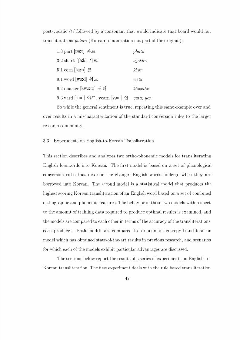
8/8/2019 Baker Kirk
http://slidepdf.com/reader/full/baker-kirk 63/243
post-vocalic /Ö / followed by a consonant that would indicate that board would not
transliterate as polutu (Korean romanization not part of the original):
1.3 part Ô Ø ℄
àÔ phatu
3.2 shark Ë ℄ ß¼ syakhu
5.1 corn Ó Ò ℄
BH khon
9.1 word Û ℄
0>×¼ wetu
9.2 quarter Û Ç Ø ℄
3$' khwethe
9.3 yard ℄
×¼, yearn Ý Ò ℄
yatu, yen
So while the general sentiment is true, repeating this same example over and
over results in a mischaracterization of the standard conversion rules to the larger
research community.
3.3 Experiments on English-to-Korean Transliteration
This section describes and analyzes two ortho-phonemic models for transliterating
English loanwords into Korean. The first model is based on a set of phonological
conversion rules that describe the changes English words undergo when they are
borrowed into Korean. The second model is a statistical model that produces the
highest scoring Korean transliteration of an English word based on a set of combined
orthographic and phonemic features. The behavior of these two models with respect
to the amount of training data required to produce optimal results is examined, and
the models are compared to each other in terms of the accuracy of the transliterations
each produces. Both models are compared to a maximum entropy transliteration
model which has obtained state-of-the-art results in previous research, and scenarios
for which each of the models exhibit particular advantages are discussed.
The sections below report the results of a series of experiments on English-to-
Korean transliteration. The first experiment deals with the rule based transliteration
47
8/8/2019 Baker Kirk
http://slidepdf.com/reader/full/baker-kirk 64/243

8/8/2019 Baker Kirk
http://slidepdf.com/reader/full/baker-kirk 65/243
as input and produces a Korean transliteration of it as output. The programming
language used was Python1, although any language which provides regular expression
support is suitable.
In this experiment, the transliteration process was modeled in three steps.
First, a preprocessing step is applied to the English phonological representations
that expands the single character representation of diphthongs used by the Hoosier
Mental Lexicon (Nusbaum et al., 1984) into two vowel symbols. This step is per-
formed because it reduces the number of symbols and transformation rules needed
for transliteration. The second step consists of the successive application of a sequence
of regular expression substitutions which transform a string of English phonemes into
a Korean phonological representation. Finally, an optional post-processing step may
be performed to syllabify the Korean string and convert it to hangul.
This transliteration model assumes the definition of the following two character
classes.
:shortvowel: = IE@aUcx^
:vowel: = ieou + :shortvowel:
In addition to these definitions, a set of intermediate vowel symbols was used to handle
word boundaries and epenthesis and /Ö / deletion. # is inserted at the beginning and
end of words; ∼ serves as a placeholder for deleted / Ö /, and ! and % stand for the
epenthetic vowels / ½ / and / /, respectively. Reserving extra symbols for epenthetic
vowels facilitates the application of the phonological conversion rules such that rules
that apply later are not inadvertently triggered by a vowel that was not present in
the input. The preprocessing step consists of the following six character expansions.
Y -> ai
1Distributed under an open source license: http://www.python.org.
49

8/8/2019 Baker Kirk
http://slidepdf.com/reader/full/baker-kirk 66/243

8/8/2019 Baker Kirk
http://slidepdf.com/reader/full/baker-kirk 67/243
([sTf])([^:vowel:]) -> \1!\2
%% e.g., ‘first’ #fx~st!# -> #fx~s!t!#
4. voiced obstruent/affricate epenthesis
([vbdzg])([^:vowel:]) -> \1!\2 %% e.g., ‘cape’ #keip# -> #keip!#
([CJSZ])([^:vowel:]) -> \1%\2 %% e.g., ‘church’ #Cx~C# -> #Cx~C%#
5. short vowel voiceless stop substitution
([:shortvowel:])p([^:vowel:]) -> \1b\2
%% e.g., ‘apt’ #@pt!# -> #@bt!#
([:shortvowel:])t([^:vowel:]) -> \1d\2
([:shortvowel:])k([^:vowel:]) -> \1g\2
6. /Ð / gemination
([:vowel:~!%])l([:vowel:]) -> \1ll\2
%% e.g., ‘clasp #k!l@s!p!# -> #k!ll@s!p!#
7. unconditioned consonant substitutions
f - > p
v - > b
T - > s
D - > d
[zZ] -> J
8. unconditioned vowel substitutions
c - > o
I - > i
51
8/8/2019 Baker Kirk
http://slidepdf.com/reader/full/baker-kirk 68/243
x - > ^
[U|] -> u
@ - > E
3.3.1.3 Experimental Setup
This experiment used the list of 10,000 English-Korean loanword pairs described in
2.1. The phonological representation of each English item in the list was transliterated
via the rule based model and the resulting form was compared to the actual Korean
adaptation of that English source word. Because the rule based model does not
require training data, it was applied to all of the items in the data set.
3.3.1.4 Results and Discussion
The first evaluation of the rule based transliteration model measured transliteration
accuracy in terms of the number of transliterated items that exactly matched the
actual Korean form. Overall transliteration accuracy, measured as
# of correct transliterations# of actual transliterations
was 49.2%. A strict comparison between the current work and previous research is
not feasible given the range of approaches represented therein on different data sets 2.
However, these results are in line with previous phoneme-based approaches (≈ 53%
reported in Jung et al., 2000; 47.5% reported in Kang, 2001).
Based on the analysis of English loanwords in Korean provided in 2.1, it is
known that vowel transliteration is harder to predict by phonological rule than con-
sonant transliteration (Table 2.5). Therefore, we also examined the performance of
2Repeated efforts to obtain access to previously used data sets were unsuccessful.
52

8/8/2019 Baker Kirk
http://slidepdf.com/reader/full/baker-kirk 69/243

8/8/2019 Baker Kirk
http://slidepdf.com/reader/full/baker-kirk 70/243
The congruence of the full word transliteration results with previous models
and the disparity between full word transliteration and consonant sequence transliter-
ation reported here suggest that the phonological information represented in this data
set alone does not convey sufficient information to reliably predict the transliterated
form of vowels in English loanwords in Korean. On the basis of this observation and
the analysis of English loanwords in Chapter 2.1, we modified the rule based model to
incorporate orthographic information into the transliteration of vowels. This modified
rule based transliteration model is described in the next section.
3.3.2 Experiment Two
Previous researchers have examined the performance of transliteration models that
produce a set of transliteration candidates for a given input string (Lee, 1999; Jung
et al., 2000; Kang and Kim, 2000). The motivation for this approach to transliteration
is spelled out in Kang and Choi (2000b), which points out that multiple translitera-
tions of the same English word are often found in large document collections, creating
problems for information retrieval. For example, the English word digital appears var-
iously in Korean as ticithel , ticithal , and ticithul even though ticithel is the standard
transliteration (Kang and Choi, 2000b: 133). Following this strand of research, this
experiment examines the performance of a rule based model that produces a set of
transliteration candidates.
3.3.2.1 Purpose
The purpose of this experiment is to investigate the performance of an ortho-phonemic
rule based transliteration model for generating sets of transliteration candidates for
English loanwords in Korean.
54
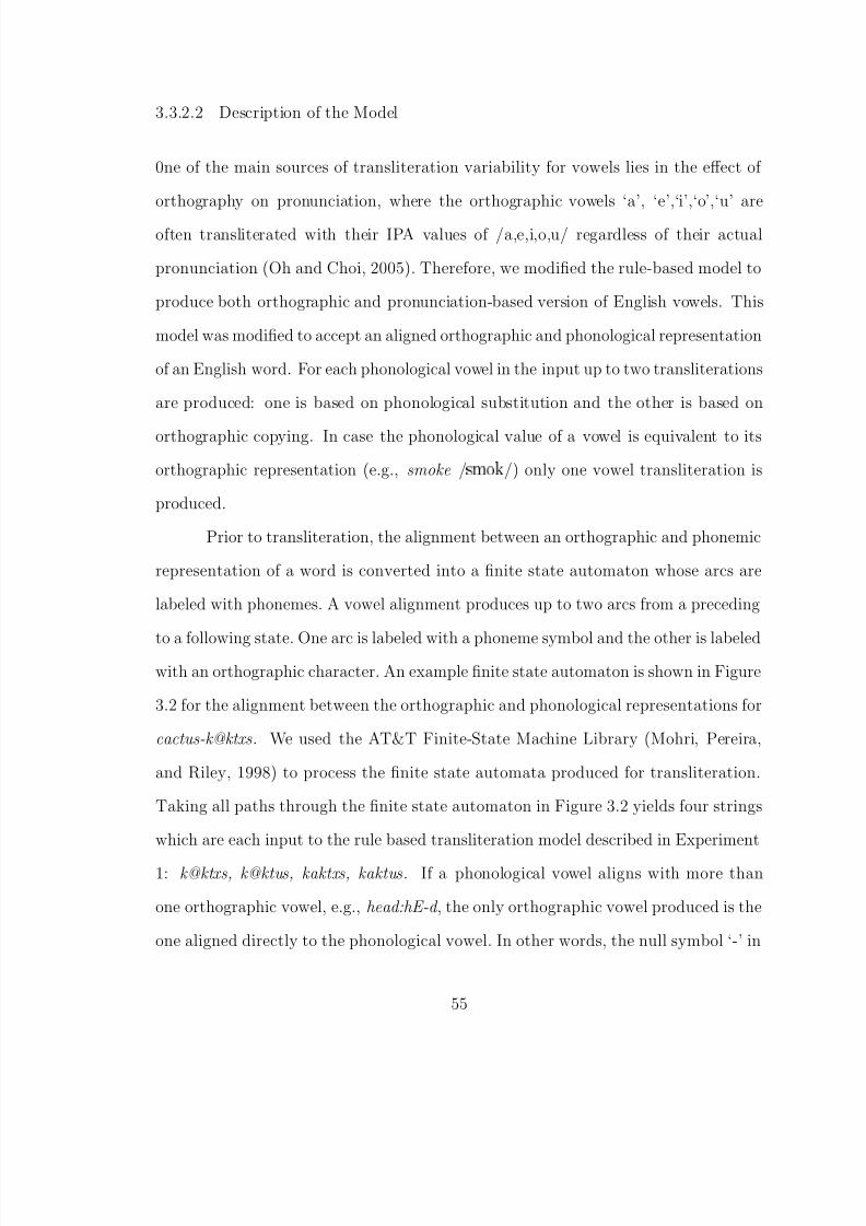
8/8/2019 Baker Kirk
http://slidepdf.com/reader/full/baker-kirk 71/243

8/8/2019 Baker Kirk
http://slidepdf.com/reader/full/baker-kirk 72/243
8/8/2019 Baker Kirk
http://slidepdf.com/reader/full/baker-kirk 73/243
8/8/2019 Baker Kirk
http://slidepdf.com/reader/full/baker-kirk 74/243
of transliteration candidates. Inputs that are likely to exhibit greater variation pro-
duce larger candidate sets. Finally, we are able to offer a direct comparison between
the current approach and previous ones in terms of the precision given a correctly
generated transliteration. On average, when the correct transliteration appears in the
candidate set the ortho-phonemic rule based model generates 2.85 candidates, giving
a precision when correct of 1/2.85 = 0.35. The size of the candidate set considered
by previous researchers varies – Lee (1999) evaluated transliteration accuracy on the
basis of the 20 most likely transliteration candidates, giving a precision when correct
of 0.05; Jung et al. (2000) considered the top 10 transliteration candidates giving a
precision when correct of 0.10, and Kang and Kim (2000) used the top 5, giving a
precision when correct of 0.20, all of which are considerably lower than the current
results.
Although the relative performance of the ortho-phonemic transliteration model
represents an improvement over previous work, its overall precision is quite low. A
further disadvantage of the model is that it does not rank transliteration candidates
by any measure of goodness. Many statistical models do allow an ordering of a set of
transliteration candidates. Therefore, we conducted a third experiment with a statis-
tical transliteration model that produces a ranked list of transliteration candidates,
and compare its performance to the rule based models.
3.3.3 Experiment Three
3.3.3.1 Purpose
The purpose of this experiment is to examine the performance of a statistical translit-
eration model and compare it to the ortho-phonemic rule based model in terms of
ranking transliteration candidates.
58

8/8/2019 Baker Kirk
http://slidepdf.com/reader/full/baker-kirk 75/243
3.3.3.2 Description of the Model
In this experiment we model the task of producing a transliterated Korean character
in terms of the probability of that character being generated by a given sequence of
graphones and phonemes. Under this approach, the task of transliterating an English
word into Korean can be formulated as the problem of finding an optimal alignment
between three streams of symbols
GE = g1,...,gL
ΦE = ϕ1,...,ϕL
K = κ1,...,κL
where GE is a sequence of English graphemes, ΦE is a sequence of English phonemes,
and K is a sequence of Korean graphemes. We assume that the three sequences have
equal length (L) due to the insertion of a null symbol (‘-’) when necessary, and assume
a one-to-one alignment between symbols in the three strings. For example, the English
word ‘first’ and its Korean transliteration (Û¼àÔ /Ô
¾ × ½ Ø
½
/ can be represented as
GE = f i r s − t −
ΦE = f − s − t −
K = Ô
1 ¾ 2 −3 s4 ½ 5 t
6 ½ 7
with the symbol alignments (f , f , ph), (i, , ¾ ), (r, −, −), etc.
We are interested in obtaining the Korean string K that receives the highestscore given (GE , ΦE , K ). Computing the score of (GE , ΦE , K ) can be formulated as a
decoding problem that consists of finding the highest scoring Korean string K given
the aligned sequences of English graphemes and phonemes GE and ΦE .
59
8/8/2019 Baker Kirk
http://slidepdf.com/reader/full/baker-kirk 76/243
The score of a particular Korean string given GE and ΦE is the product of the
scores of the alignments comprising the three sequences:
Score(K |GE , ΦE ) =
Li=1
p(κi|gi, ϕi)
In order to account for context effects of adjacent graphemes and phonemes on the
transliteration of a particular English grapheme-phoneme pair, we define gi and ϕi
as subsequences of GE and ΦE , respectively, centered at i and containing elements
<gi−2,...,gi+2> and <ϕi−2,...,ϕi+2>, respectively. For example, if κ4 = s in the
preceding example, then g4 = <i,r,s, −, t> and ϕ4 = < , −, s, −, t>. Positions
i < 1 and i > L are understood to contain a boundary symbol (#) to allow modeling
context at word starts and ends. We estimate the probability of κi given subsequences
gi and ϕi with relative frequency counts:
p(κi|gi,ϕi) =p(gi,ϕi, κi)
p(gi,ϕi)≈
c(gi,ϕi, κi)
c(gi,ϕi).
Given the relatively large context window (2 preceding and 2 following ortho-
graphic phoneme pairs), the chance of encountering an unseen feature in the test set
is relatively high. In order to mitigate the effect of data sparsity on the transliter-
ation model described above, we modified it to use a backoff strategy that involved
successively decreasing the size of the context window centered at the Korean charac-
ter currently being predicted until a trained feature was found. The specific backoff
strategy used in this model is to search for features in the following order starting at
the top of the list, where S i represents the source orthographic-phoneme pair at the
index of the Korean letter being predicted and si represent preceding and following
ortho-phonemic pairs:
60

8/8/2019 Baker Kirk
http://slidepdf.com/reader/full/baker-kirk 77/243
si−2si−1S isi+1si+2
si−2si−1S isi+1
si−1S isi+1si+2
si−1S isi+1
si−2si−1S i
S isi+1si+2
si−1S i
S isi+1
S i
As soon as a trained feature is found, iteration stops and the most highly ranked
Korean target corresponding to that feature is produced. In the event that no feature
corresponding to S i is found, no prediction is made. This backoff strategy was based
on the intuition that larger contextual units provide more reliable statistical cues tothe transliteration of an English segment; it was determined prior to assessing its
performance on any of the data and was not altered in response its performance on
the data.
In order to establish a comparison between previous statistical transliteration
approaches and the current work, we also applied a maximum entropy model (Berger
et al., 1996; Pietra, Pietra, and Lafferty, 1997) that was demonstrated to outperform
other machine learning approaches to English-Korean transliteration in previous com-
parisons (Oh and Choi, 2005; Oh et al., 2006a). The maximum entropy model is a
61
8/8/2019 Baker Kirk
http://slidepdf.com/reader/full/baker-kirk 78/243
conditional probability model that incorporates a heterogenous set of features to con-
struct a statistical model that represents an empirical data distribution as closely as
possible (Berger et al., 1996; Zhang, 2004). In the maximum entropy model, events
are represented by a bundle of binary feature functions that map an outcome even y
and a context x to {0, 1}. For example, the event of observing the Korean letter ‘p’
in the context of ##boa in a word like board can be represented as
f (x, y) =
1 if y=p and x=##boa
0 otherwise.
Once a set of features has been selected, the corresponding maximum entropy
model can be constructed by adding features as constraints to the model and adjusting
their weights. The model must satisfy the constraint that the empirical expectation
of each feature in the training data equals the expectation of that feature with respect
to the model distribution. Among the models that meet this constraint is one with
maximum entropy. Generally, this maximum entropy model is represented as
p(y|x) =1
Z (x)exp
ki=1
λif i(x, y)
where p(y|x) denotes the conditional probability of outcome y given contextual feature
x, k is the number of features, f i(x, y) are feature functions, and λi is a weighting
parameter for each feature. Z (x) is a normalization factor defined as
62
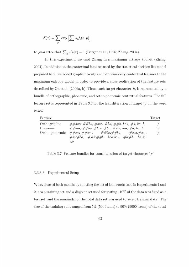
8/8/2019 Baker Kirk
http://slidepdf.com/reader/full/baker-kirk 79/243
Z (x) =y
exp
λif i(x, y)
to guarantee thaty p(y|x) = 1 (Berger et al., 1996; Zhang, 2004).
In this experiment, we used Zhang Le’s maximum entropy toolkit (Zhang,
2004). In addition to the contextual features used by the statistical decision list model
proposed here, we added grapheme-only and phoneme-only contextual features to the
maximum entropy model in order to provide a close replication of the feature sets
described by Oh et al. (2006a, b). Thus, each target character ki is represented by a
bundle of orthographic, phonemic, and ortho-phonemic contextual features. The full
feature set is represented in Table 3.7 for the transliteration of target ‘p’ in the word
board .
Feature Target
Orthographic ##boa, ##bo, #boa, #bo, ##b, boa, #b, bo, b ‘p’Phonemic ##bo-, ##bo, #bo-, #bo, ##b, bo-, #b, bo, b ‘p’Ortho-phonemic ##boa:##bo-, ##bo:##bo, #boa:#bo-,
#bo:#bo, ##b:##b, boa:bo-, #b:#b, bo:bo,
b:b
‘p’
Table 3.7: Feature bundles for transliteration of target character ‘p’
3.3.3.3 Experimental Setup
We evaluated both models by splitting the list of loanwords used in Experiments 1 and
2 into a training set and a disjoint set used for testing. 10% of the data was fixed as a
test set, and the remainder of the total data set was used to select training data. The
size of the training split ranged from 5% (500 items) to 90% (9000 items) of the total
63

8/8/2019 Baker Kirk
http://slidepdf.com/reader/full/baker-kirk 80/243
data set in 5% intervals. Each training split was tested on the same 10% test set. This
procedure was repeated 10 times, and the results were averaged. Following Oh and
Choi (2005), we trained the maximum entropy model using the default Gaussian prior
of 0; in addition we used 30 iterations of the default L-BFGS method of parameter
estimation and did not change any other default settings. However, we note that a
training regime which utilizes development data to tune the Gaussian parameter and
uses more training iterations may produce better results than those obtained here.
3.3.3.4 Results and Discussion
The first evaluation of the statistical transliteration models is reported in terms of 1-best whole word transliteration accuracy, defined as
# of correct transliterations
# of actual transliterations.
Figure 3.3 depicts transliteration accuracy for the two statistical models as a function
of size of the training set. This figure also shows the performance of the rule based
model for comparison. Because the rule based model does not require training data,
its performance is flat. For both statistical models, transliteration accuracy clearly
depends on the amount of training data. As the amount of training data increases,
the performance of the maximum entropy model and the statistical model proposed
here nearly converge, but for all trials reported here the performance of the maximum
entropy model never exceeds the performance of the newly proposed model.
The best transliteration accuracy obtained by the statistical transliteration
model and the maximum entropy models is 73.4% and 71.9%, respectively. The
proposed model is relatively robust even to small amounts of training data, performing
better than the rule based model with as few as 500 training items (5% training data).
64
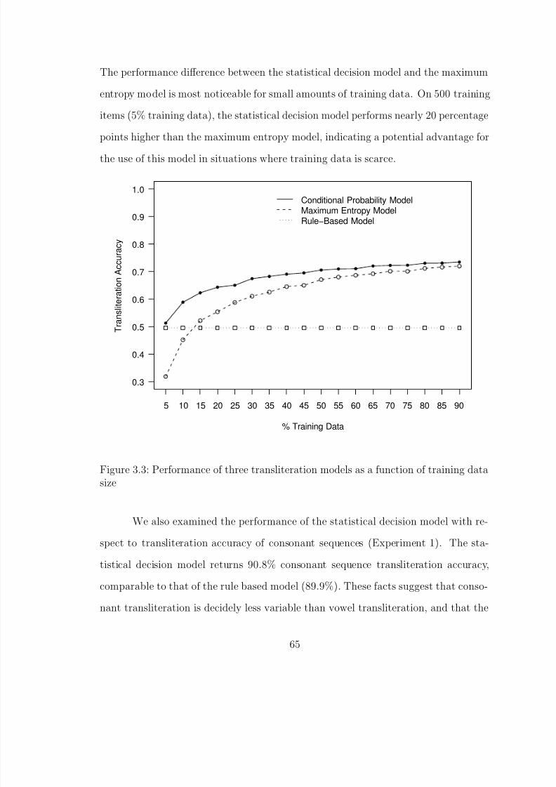
8/8/2019 Baker Kirk
http://slidepdf.com/reader/full/baker-kirk 81/243
The performance difference between the statistical decision model and the maximum
entropy model is most noticeable for small amounts of training data. On 500 training
items (5% training data), the statistical decision model performs nearly 20 percentage
points higher than the maximum entropy model, indicating a potential advantage for
the use of this model in situations where training data is scarce.
0.3
0.4
0.5
0.6
0.7
0.8
0.9
1.0
% Training Data
T r a n s
l i t e r a
t i o n
A c c u r a c y
5 10 15 20 25 30 35 40 45 50 55 60 65 70 75 80 85 90
Conditional Probability ModelMaximum Entropy ModelRule−Based Model
Figure 3.3: Performance of three transliteration models as a function of training datasize
We also examined the performance of the statistical decision model with re-
spect to transliteration accuracy of consonant sequences (Experiment 1). The sta-
tistical decision model returns 90.8% consonant sequence transliteration accuracy,
comparable to that of the rule based model (89.9%). These facts suggest that conso-
nant transliteration is decidely less variable than vowel transliteration, and that the
65
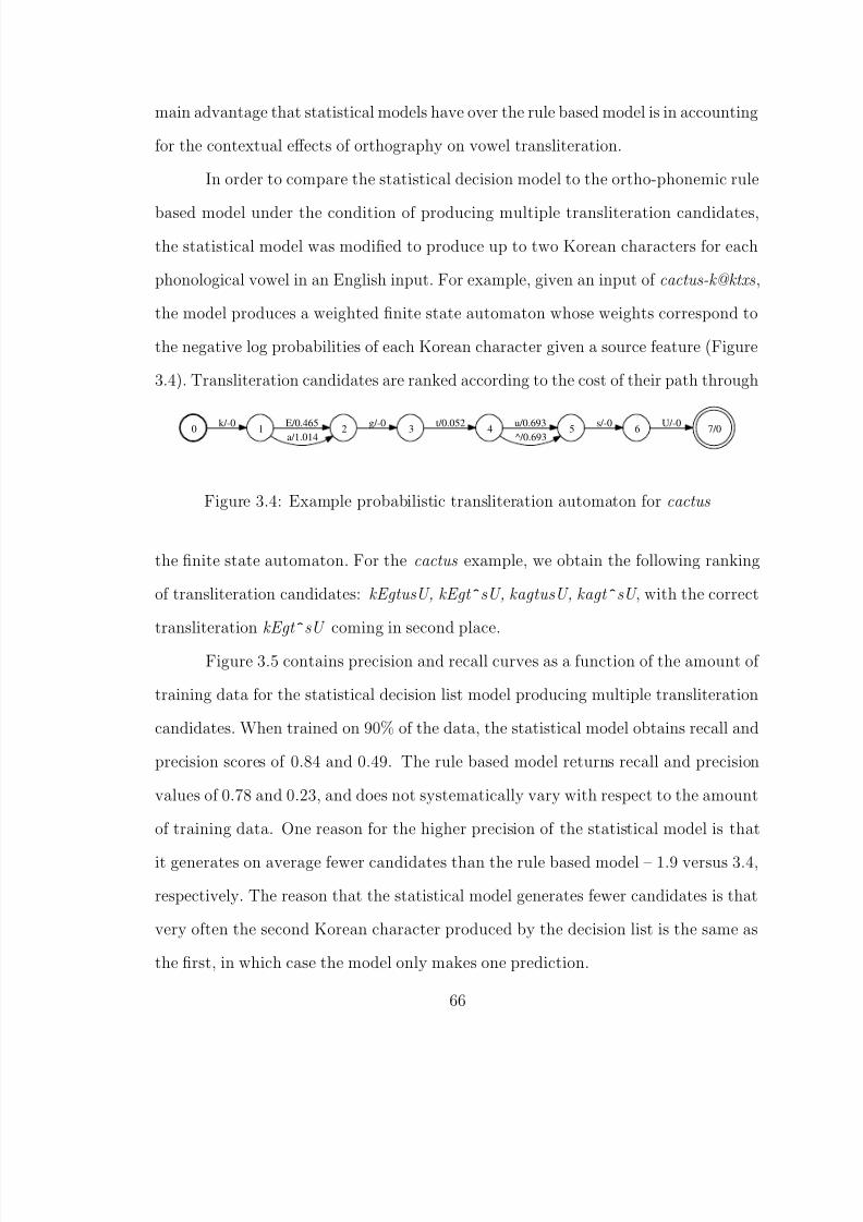
8/8/2019 Baker Kirk
http://slidepdf.com/reader/full/baker-kirk 82/243
main advantage that statistical models have over the rule based model is in accounting
for the contextual effects of orthography on vowel transliteration.
In order to compare the statistical decision model to the ortho-phonemic rule
based model under the condition of producing multiple transliteration candidates,
the statistical model was modified to produce up to two Korean characters for each
phonological vowel in an English input. For example, given an input of cactus-k@ktxs,
the model produces a weighted finite state automaton whose weights correspond to
the negative log probabilities of each Korean character given a source feature (Figure
3.4). Transliteration candidates are ranked according to the cost of their path through
0 1k/-0 2E/0.465a/1.014
3g/-0 4t/0.052 5u/0.693^/0.693
6s/-0 7/0U/-0
Figure 3.4: Example probabilistic transliteration automaton for cactus
the finite state automaton. For the cactus example, we obtain the following ranking
of transliteration candidates: kEgtusU, kEgt sU, kagtusU, kagt sU , with the correct
transliteration kEgt sU coming in second place.
Figure 3.5 contains precision and recall curves as a function of the amount of
training data for the statistical decision list model producing multiple transliteration
candidates. When trained on 90% of the data, the statistical model obtains recall and
precision scores of 0.84 and 0.49. The rule based model returns recall and precision
values of 0.78 and 0.23, and does not systematically vary with respect to the amount
of training data. One reason for the higher precision of the statistical model is that
it generates on average fewer candidates than the rule based model – 1.9 versus 3.4,
respectively. The reason that the statistical model generates fewer candidates is that
very often the second Korean character produced by the decision list is the same as
the first, in which case the model only makes one prediction.
66
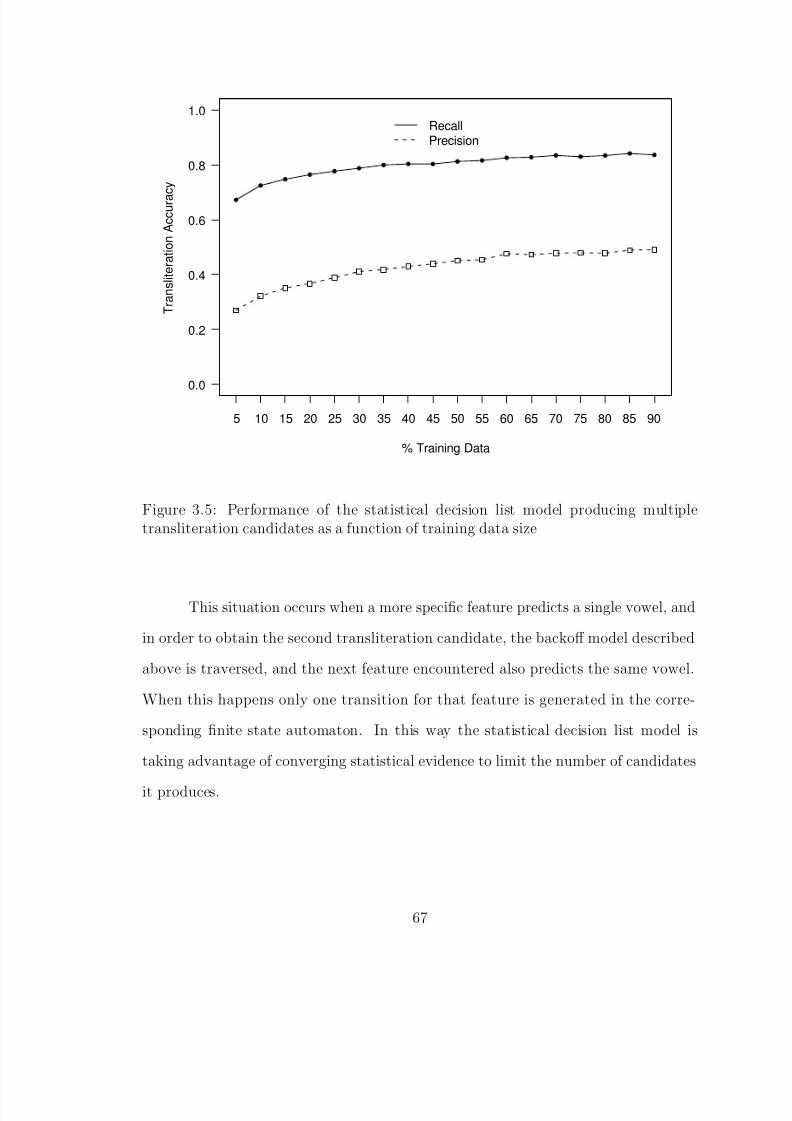
8/8/2019 Baker Kirk
http://slidepdf.com/reader/full/baker-kirk 83/243
0.0
0.2
0.4
0.6
0.8
1.0
% Training Data
T r a n s
l i t e r a
t i o n
A c c u r a c y
5 10 15 20 25 30 35 40 45 50 55 60 65 70 75 80 85 90
RecallPrecision
Figure 3.5: Performance of the statistical decision list model producing multipletransliteration candidates as a function of training data size
This situation occurs when a more specific feature predicts a single vowel, and
in order to obtain the second transliteration candidate, the backoff model described
above is traversed, and the next feature encountered also predicts the same vowel.
When this happens only one transition for that feature is generated in the corre-
sponding finite state automaton. In this way the statistical decision list model is
taking advantage of converging statistical evidence to limit the number of candidates
it produces.
67

8/8/2019 Baker Kirk
http://slidepdf.com/reader/full/baker-kirk 84/243
The statistical decision list model also offers an advantage over the ortho-
phonemic rule based model in that it is capable of producing a ranked list of translit-
eration candidates, with the best candidate appearing at the beginning of the list.
In order to compare the statistical model with the rule based model in terms of
candidate ranks, we computed the mean reciprocal rank. The reciprocal rank of a
transliteration candidate is the multiplicative inverse of the rank of that candidate.
For example, if the correct transliteration occurred as the second candidate in the
list, that item’s reciprocal rank is 1/2 = 0.5. The mean reciprocal rank is the average
of the reciprocal ranks of each transliterated item. In case the correct answer does
not appear in the list of transliteration candidates for a given item, a reciprocal rank
of 0 is assigned. The mean reciprocal rank for the statistical model is 0.77 versus 0.54
for the rule based model3.
3.3.4 Error Analysis
Examination of transliterations missed by the statistical model shows that many of
these items are ones for which vowel transliteration follows an orthographic translit-
eration, e.g., oxalis → /Ó × Ð Ð × ½ /, orangutan → /Ó Ð Æ Ù Ø
Ò /, ketene → /
Ø Ò /,
antivitamin → / Ò Ø
Ô Ø
Ñ Ò /, delphi → /Ø Ð Ô
/, lazuli → /Ð Ù Ð Ð /, alkali →
/ Ð
Ð Ð /. An alternative explanation for orthographic transliteration is that the
word is not borrowed directly from English but is borrowed in both languages from
another source or has come to Korean from English via Japanese (Kang, Kenstowicz,
and Ito, 2007). Although the ability to assess a detailed etymological history of newly
encountered foreign words is difficult to implement in an automatic transliteration
system, knowledge of the frequency of a word’s usage in non-English text (such as
3The rule based model does not impose a ranking on transliteration candidates, so the defaulthash order of the Python dictionary object was used to order candidates in the rule based model.
68
8/8/2019 Baker Kirk
http://slidepdf.com/reader/full/baker-kirk 85/243
would be available, e.g., from Google estimates of language specific document counts
for a word) could be explored for its utility in influencing the expectation of an En-
glish phonological versus orthographic transliteration. Work along these lines remains
for future research.
A second area where both the statistical and rule-based models had difficulty
is consonant transliteration corresponding to internal word boundaries in compounds
like taphole, spillover, blackout, kickout, locknut , and cakework . In these cases the
actual transliterations mark the presence of the internal word boundary by applying
the expected end of word transliteration rule. For example, in the transliteration
of the word black , the final / / becomes an unaspirated coda in Korean: /Ô ½ Ð Ð /.
In intervocalic position, English voiceless stops typically aspirate and are realized
as syllable onsets. For example in the word Utah , the English / Ø / becomes Ko-
rean /Ø
/, as in/ Ý Ù Ø
/. In compound words like blackout , however, the intervocalic
stop follows the end of word transliteration pattern and becomes / Ô ½ Ð Ð Ù × /. This
transliteration is unexpected if only the segmental context is considered, where the
intervocalic consonant would typically become an onset of the following syllable black-
out → */ Ô ½ Ð Ð
Ù × /). Applying a module to pre-identify potential compound words
and insert a word boundary symbol (e.g., blackout → #black#out#) is one way to
incorporate additional morphological knowledge into the transliteration process and
would be expected to improve transliteration accuracy in these cases.
3.3.5 Conclusion
This chapter presented two novel transliteration models, both of which are robust
to small amounts of data and are parsimonious in terms of the number of parame-
ters required to estimate them and the number of outputs they produce. The rule
69
8/8/2019 Baker Kirk
http://slidepdf.com/reader/full/baker-kirk 86/243
based model is defined by a small set of regular expressions and requires no train-
ing data. By modifying it to produce both orthographic and pronunciation based
vowel transliterations, its coverage is substantially increased. Relative to previous
n-best transliteration models, its precision is high; however, its precision is substan-
tially lower than that of the statistical decision list model when the latter model is
modified to produce multiple transliteration candidates as well.
The statistical decision list model achieves reasonable results on small amounts
of training data. As the amount of training data increases, the performance of the
two statistical models becomes much closer, although the simpler statistical model
slightly outperforms the maximum entropy model on all trials in the experiments
reported here. However, the maximum entropy model provides greater flexibility
for incorporating multiple sources of information, and its performance may increase
given a richer feature set for which the statistical decision list model is less suited.
Furthermore, its performance may improve given a suitable Gaussian penalty. These
possibilities remain to be explored in future research.
The rule based and statistical models lend themselves to situations where
bilingual training data is scarce or unavailable. Although the cost of developing an
aligned list of loanwords for an arbitrary pair of languages may be lower than the cost
of developing a richer lexical resource such as a large syntactically and semantically
annotated corpus, it is not negligible. We are not aware of any accounts of the cost of
developing a list of aligned English-Korean loanwords from scratch, but can provide
an estimate of the amount of data that would be required to produce a similar list of
English loanwords in Chinese.Chinese is similar to Korean in that it has recently begun importing English
loanwords into its lexicon as well (Riha and Baker, 2008a, b). However, in Chinese,
70

8/8/2019 Baker Kirk
http://slidepdf.com/reader/full/baker-kirk 87/243
these words are often borrowed “as is”, i.e., in the original English orthography. Be-
cause these words occupy a distinct range of character codes when stored in electronic
orthographic form, they are easy to extract from Chinese text using standard regular
expression utilities (e.g., Perl or grep). Figure 3.6 displays the number of unique
Roman letter strings in the 2004 CNA subsection4 of the Chinese gigaword corpus
(Graff, 2007) against the number of Chinese characters read before encountering each
new instance. For example, the figure shows that in order to come across 5,000 unique
Roman letter words, 17 million Chinese characters have to be read (conservatively,
4.25 million words on the basis of estimates average length of Chinese words in Tea-
han, Wen, Mcnab, and Witten 2000); in order to extract 10,000 unique Roman letter
words, 37 million Chinese characters (9.25 million words) have to be read.
For language pairs that are not as well attested (e.g., Danish-Korean, Italian-
Korean), the amount of material required to produce similar lists would be substan-
tially greater or non-existent at the requisite scale. However, phonological accounts of
loanword adaptation such as that provided by Li (2005) contain phonological conver-
sion rules for adapting loanwords into Korean from many languages, including Danish,
Italian, Thai, Romanian, and Swedish among others. Furthermore, it is possible to
find similar accounts for additional pairs of languages like French and Vietnamese
(Barker, 1969). In such situations, the cost and time required to develop even a
moderately sized list of aligned loanwords for each of these language pairs is likely
to exceed the cost and time required to deploy a rule based transliteration model.
The next chapter demonstrates the utility of a low precision rule based transliteration
model for bootstrapping a statistical model that classifies words according to theiretymological source.
4This is the section of the corpus with the highest percentage of Roman letter words (Riha andBaker, 2008a, b).
71
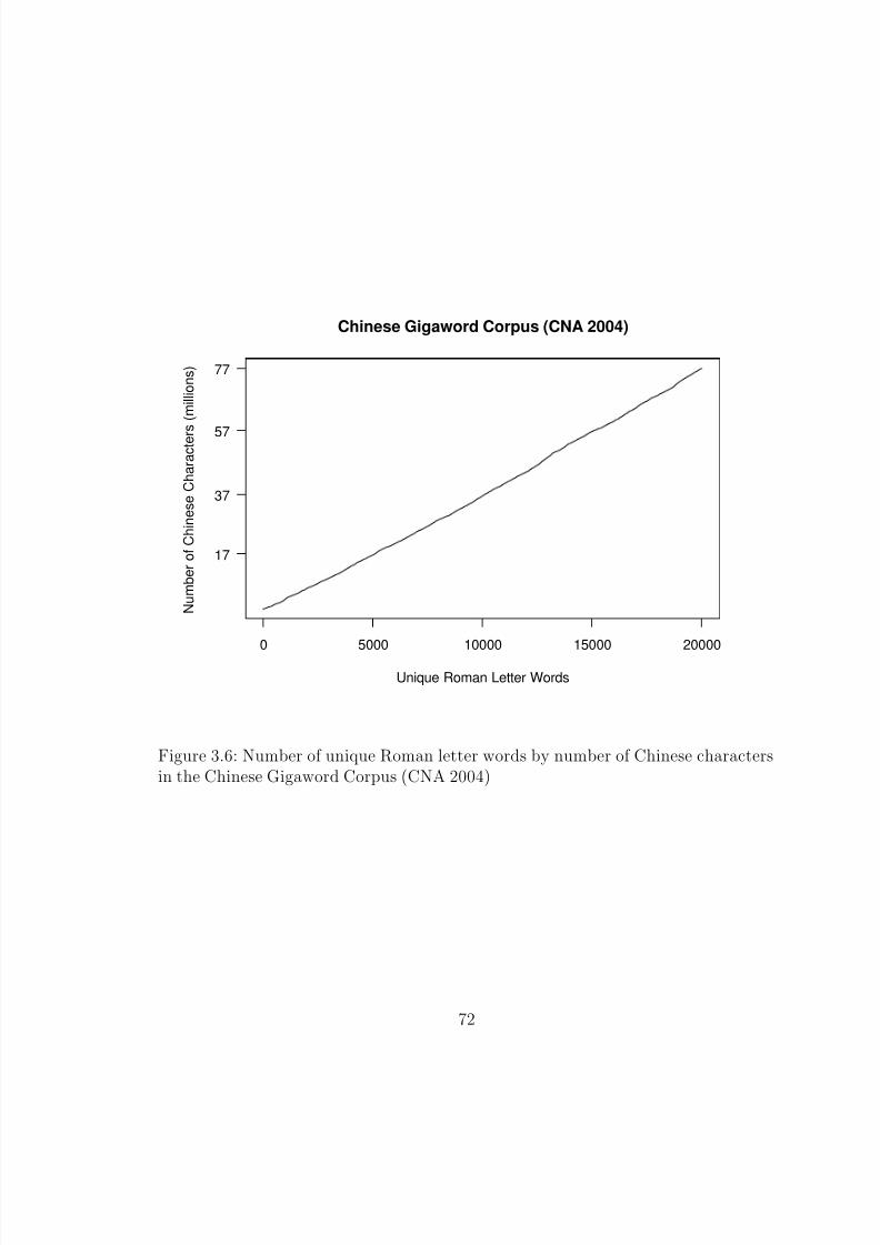
8/8/2019 Baker Kirk
http://slidepdf.com/reader/full/baker-kirk 88/243
0 5000 10000 15000 20000
Chinese Gigaword Corpus (CNA 2004)
Unique Roman Letter Words
N u m
b e r o
f C h i n e s e
C h a r a c
t e r s
( m i l l i o n s
)
17
37
57
77
Figure 3.6: Number of unique Roman letter words by number of Chinese charactersin the Chinese Gigaword Corpus (CNA 2004)
72

8/8/2019 Baker Kirk
http://slidepdf.com/reader/full/baker-kirk 89/243
CHAPTER 4
AUTOMATICALLY IDENTIFYING ENGLISH LOANWORDS IN KOREAN
4.1 Overview
This chapter deals with the task of automatically classifying unknown words ac-
cording to their etymological source. It focuses on identifying English loanwords in
Korean, and presents an approach for automatically generating training data for use
by supervised machine learning techniques. The main innovation of the approach
presented here is its use of generative linguistic rules to produce large quantities of
training data, circumventing the need for manually labeled resources.
Being able to automatically identify the etymological source of an unknown
word is important for a wide range of NLP applications. For example, automaticallytranslating proper names and technical terms is a notoriously difficult task because
these items can come from anywhere, are often domain-specific and are frequently
missing from bilingual dictionaries (e.g., Knight and Graehl, 1998; Al-Onaizan and
Knight, 2002). In the case of borrowings across languages with unrelated writing sys-
tems and dissimilar phonemic inventories (i.e., English and Korean), the appropriate
course of action for an unknown word may be transliteration or back-transliteration
(Knight and Graehl, 1998). However, in order to transliterate an unknown word cor-
rectly, it is necessary to first identify the originating language of the unknown word.
Etymological classification also plays a role in information retrieval and cross-lingual
73

8/8/2019 Baker Kirk
http://slidepdf.com/reader/full/baker-kirk 90/243
information retrieval systems where finding equivalents between a source word and
its various target language realizations improves indexing of search terms and subse-
quently document recall (e.g., Kang and Choi, 2000b; Oh and Choi, 2001; Kang and
Choi, 2002).
Source language identification is also a necessary component of speech syn-
thesis systems, where the etymological class of a word can trigger different sets of
letter-to-sound rules (e.g., Llitjos and Black, 2001; Yoon and Brew, 2006). In Korean,
for example, a phonological consonant tensification rule applies to semantically trans-
parent compounds of Sino-Korean origin. For example, the Sino-Korean syllable #î
pyeng corresponds to two homographic morphemes illness and anger , both of which
have two pronunciations in compounds: untensed initial /p/ (e.g., o#î hwapyeng
[ Û Ô Ý Æ ] vase, ño#î holipyeng [ Ó Ê Ý Æ ] genie’s bottle and t#î cipyeng [ Ý Æ ]
terminal illness and tensed initial /p/ (e.g., c+t#î khollapyeng [
Ó Ð Ô ¶ Ý Æ ] o
#î hwapyeng [ Û Ô ¶ Ý Æ ] anger disease and )o#î helipyeng [ Ð Ô ¶ Ý Æ ] backache)
(Yoon and Brew, 2006: 367). In addition, words of English origin often undergo /s/-
tensification that is not orthographically indicated (e.g., [j{9 seyil [× ¶ Ð ] ‘sale’, OÛ¼
phelsu [Ô
Ð × ½ ] ‘pulse’ (Yoon and Brew, 2006: 372).
The sections that follow describe and evaluate statistical approaches to identi-
fying English loanwords in Korean. Section 4.2 describes previous work on identifying
English loanwords in Korean. Section 4.3 lays out the current approach and describes
the supervised learning algorithm used in the experiments that are presented in Sec-
tion 4.4.
4.2 Previous Research
Identifying foreign words is similar to the task of language identification (e.g., Beesley,
1988), in which documents or sections of documents are classified according to the
74

8/8/2019 Baker Kirk
http://slidepdf.com/reader/full/baker-kirk 91/243
language in which they are written. However, foreign word identification is made more
difficult by the fact that words are nativized by the target language phonology and
the fact that differences in character encodings are removed when words are rendered
in the target language orthography. For example, French and German words are often
written in English just as they appear in the original languages – e.g., tete or außer-
halb. In these cases, characters like e and ß provide reliable cues to the etymological
source of the foreign word. However, when these same words are transliterated into
Korean, such character level differences are no longer maintained: tete becomes_àÔ
theytu and außerhalb becomes ĺ"f½+ÉáÔ awusehalpu (Li, 2005: 132). Instead, in-
formation such as transition frequencies between characters or the relative frequency
of certain characters in known Korean words versus known French or German words
can be used to distinguish these classes of words.
Oh and Choi (2001) describes an approach along these lines to automatically
identifying and extracting English words from Korean text. Oh and Choi (2001)
formulates the problem in terms of a syllable tagging problem – each syllable in a
hangul orthographic unit is identified as foreign or Korean, and each sequence of
foreign-tagged syllables is extracted as an English word. Hangul strings are modeled
by a hidden Markov model where states represent a binary indication of whether a
syllable is Korean or not. Transitional probabilities and the probability of a syllable
being English or Korean are calculated from a corpus of over 100,000 words in which
each syllable was manually tagged as foreign or Korean. Oh and Choi (2001) reports
precision and recall values ranging from 96% to 98% for identifyin foreign word tokens
in their corpus, but is not clear whether these values are obtained from a disjointtrain/test split of the data or indicate performance of their system on trained data.
Kang and Choi (2002) employs a similar Markov-based approach that alle-
viates the burden of manually syllable tagging an entire corpus, but relies instead
75
8/8/2019 Baker Kirk
http://slidepdf.com/reader/full/baker-kirk 92/243
on a foreign word dictionary, a native word dictionary, and a list of 2000 function
words obtained from a manually POS-tagged corpus. Kang and Choi (2002) uses
their method to extract a set of 799 potential foreign terms from their corpus, and
restrict their analysis to this set of terms. Kang and Choi (2002) reports precision
and recall for foreign word extraction over this candidate set of 84% and 92%, respec-
tively. While these results are promising, the burden of manually labeling data has
not been eliminated, but deflected to external resources.
The experiments presented in the next section describe an accurate, easily
extensible method for automatically classifying unknown foreign words that requires
minimal monolingual resources and no bilingual training data (which is often difficult
to obtain for an arbitrary language pair). It does not require tagging and uses corpus
data that is easily obtainable from the web, for example, rather than hand-crafted
lexical resources.
4.3 Current Approach
While statistical approaches have been successfully applied to the language identifica-
tion task, one drawback to applying a statistical classifier to loanword identification
is the requirement for a sufficient amount of labeled training examples. Amassing a
large list of transliterated foreign words is expensive and time-consuming. We address
this issue by using phonological conversion rules to generate potentially unlimited
amounts of pseudo training data at very low cost. Although the rules themselves are
not highly accurate, a classifier trained on sufficient amounts of this automatically
generated data performs as well as one trained on actual examples. The classifier
used here is a sparse logistic regression model. The sparse logistc regression model
has been shown to provide state of the art classification results on a range of natural
language classification tasks such as author identification (Madigan, Genkin, Lewis,
76
8/8/2019 Baker Kirk
http://slidepdf.com/reader/full/baker-kirk 93/243
Argamon, Fradkin, and Ye, 2005a), verb classification (Li and Brew, 2008), and ani-
macy classification (Baker and Brew, accepted). This model is described in the next
section.
4.3.1 Bayesian Multinomial Logistic Regression
At a very basic level of description, learning is about observing relations that hold
between two or more variables and using this knowledge to adapt future behavior
under similar circumstances. Regression analysis models this type of learning in
terms of the way that one variable Y varies as a function of a vector of variables
X . This function is represented in terms of the conditional distribution of Y givenX and a set of weighted parameters β . Bayesian approaches to regression modeling
involve setting up a distribution on the parameter vector β that encodes prior beliefs
about the elements of β . The prior distribution should be strong enough to allow
accurate estimation of the model parameters without overfitting the model to the
training data (e.g., Genkin, Lewis, and Madigan, 2004; Gelman, Carlin, Stern, and
Rubin, 2004: 354). The statistical inference task involves estimating the parameters β
conditioned on X and Y (Gelman et al., 2004: 354). The simplest and most flexible
regression model is the normal linear model (Hays, 1988; Gelman et al., 2004), which
states that each value of Y is equal to a weighted sum of the corresponding values of
the predictors in X :
(4.1a) Y i = β 0 +P
p=1
β pX ip
In Equation (4.1a), i indexes over examples in the training set, and β0 is the y-
intercept or bias, which is analogous to the prior probability of class k in a naive
Bayes model. This formulation assumes that the true relationship between Y and X
77
8/8/2019 Baker Kirk
http://slidepdf.com/reader/full/baker-kirk 94/243
falls on a straight line, and that the actual observations of these variables are normally
distributed around it. Equation (4.1a) is often expressed in equivalent notation as
(4.1b) Y i =
P p=0
β pX ip where X i0 ≡ 1
or in matrix notation as
(4.1c) Y i = βX i where X i0 ≡ 1.
The regression function for model (4.1a) expresses the expected value of Y as a
function of the weighted predictors X :
(4.2) E {Y i} = β 0 +P p=1
β pX ip
In simple linear regression the expected value of Y i ranges over the set of real numbers.
However, in classification problems of the type considered here, the desired output
ranges over a finite set of discrete categories. The solution to this problem involves
treating Y i as a binary indicator variable where a value of 1 indicates membership
in a class and a value of 0 indicates not belonging to that class.
When Y i is a binary random variable, the expected outcome E {Y i} has a
special meaning. The probability distribution of a binary random variable is defined
as follows:
Y i Probability1 P (Y i = 1) = πi0 P (Y i = 0) = 1 − πi
Applying the definition of expected value of a random variable (Kutner, Nachtsheim,
78
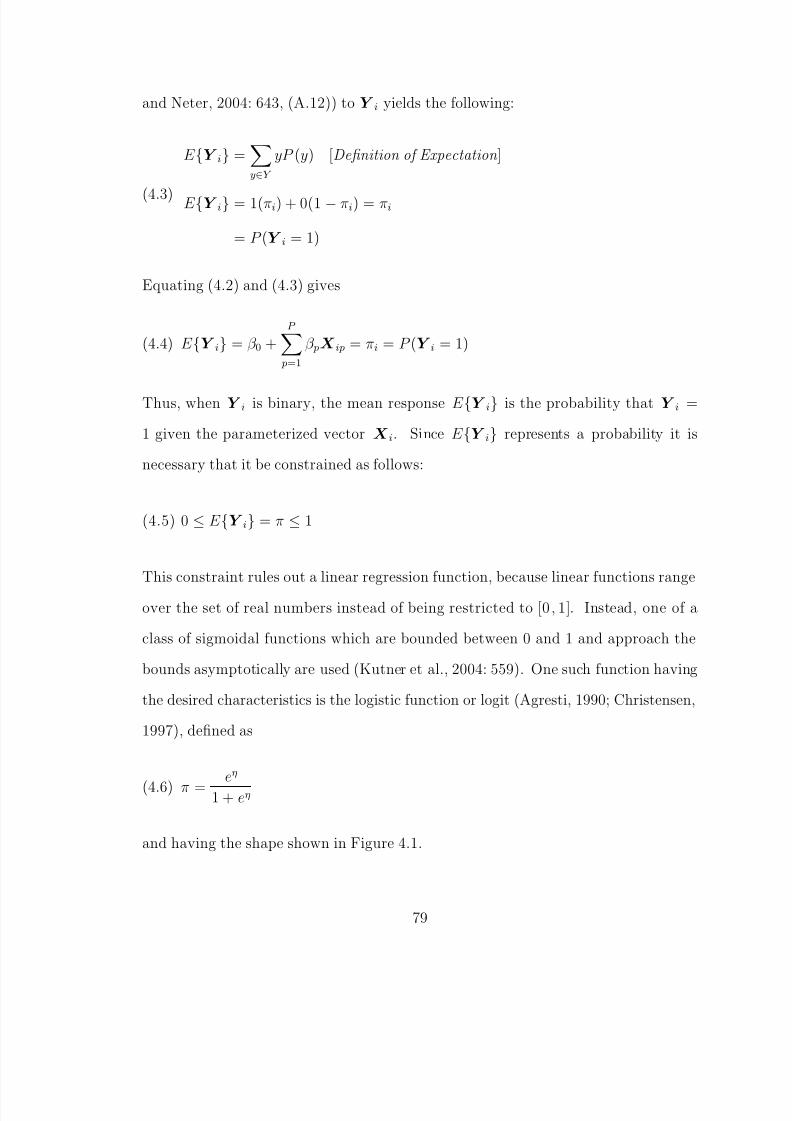
8/8/2019 Baker Kirk
http://slidepdf.com/reader/full/baker-kirk 95/243
and Neter, 2004: 643, (A.12)) to Y i yields the following:
(4.3)
E {Y i} =y∈Y
yP (y) [Definition of Expectation ]
E {Y i} = 1(πi) + 0(1 − πi) = πi
= P (Y i = 1)
Equating (4.2) and (4.3) gives
(4.4) E {Y i} = β 0 +P p=1
β pX ip = πi = P (Y i = 1)
Thus, when Y i is binary, the mean response E {Y i} is the probability that Y i =
1 given the parameterized vector X i. Since E {Y i} represents a probability it is
necessary that it be constrained as follows:
(4.5) 0 ≤ E {Y i} = π ≤ 1
This constraint rules out a linear regression function, because linear functions range
over the set of real numbers instead of being restricted to [0, 1]. Instead, one of a
class of sigmoidal functions which are bounded between 0 and 1 and approach the
bounds asymptotically are used (Kutner et al., 2004: 559). One such function having
the desired characteristics is the logistic function or logit (Agresti, 1990; Christensen,
1997), defined as
(4.6) π =eη
1 + eη
and having the shape shown in Figure 4.1.
79
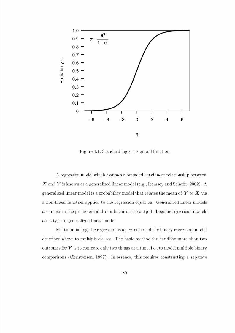
8/8/2019 Baker Kirk
http://slidepdf.com/reader/full/baker-kirk 96/243
η
P r o
b a
b i l i t y π
−6 −4 −2 0 2 4 6
0
0.1
0.2
0.3
0.4
0.5
0.6
0.7
0.8
0.9
1.0
π =eη
1 + eη
Figure 4.1: Standard logistic sigmoid function
A regression model which assumes a bounded curvilinear relationship between
X and Y is known as a generalized linear model (e.g., Ramsey and Schafer, 2002). A
generalized linear model is a probability model that relates the mean of Y to X via
a non-linear function applied to the regression equation. Generalized linear models
are linear in the predictors and non-linear in the output. Logistic regression models
are a type of generalized linear model.
Multinomial logistic regression is an extension of the binary regression model
described above to multiple classes. The basic method for handling more than two
outcomes for Y is to compare only two things at a time, i.e., to model multiple binary
comparisons (Christensen, 1997). In essence, this requires constructing a separate
80

8/8/2019 Baker Kirk
http://slidepdf.com/reader/full/baker-kirk 97/243
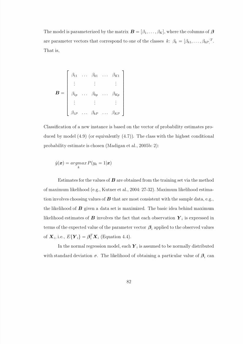
8/8/2019 Baker Kirk
http://slidepdf.com/reader/full/baker-kirk 98/243
8/8/2019 Baker Kirk
http://slidepdf.com/reader/full/baker-kirk 99/243
be assessed with respect to the probability of seeing that value given a normal dis-
tribution with mean E {Y i}. Maximum likelihood estimation uses the density of the
probability distribution at Y i as an estimate for the probability of seeing that ob-
servation. For example, Figure 4.2 shows the densities of the normal distribution for
two possible parameterizations of βi. If Y i is in the tail (4.2b), it will be assigned
µ = βi X i
Y i Y i
µ′ = β′i X i
Figure 4.2: Normal probability distribution densities for two possible values of µ
a low probability of occurring. On the other hand, if it is closer to the center of the
distribution (4.2a), it will be assigned a higher probability of occurrence. The method
of maximum likelihood estimates for βi involves choosing values of βi that favor a
value of Y i that is near the center of its probability distribution. The parameters
must be optimized over all of the observations in the training sample.
Bayesian approaches to logistic regression involve specifying a distribution on
B that reflects prior beliefs about about likely values of the parameters. In the typical
classification setting involving large data sets in a high dimensional feature space, a
reasonable prior distribution for B is one that assigns a high probability that most
83
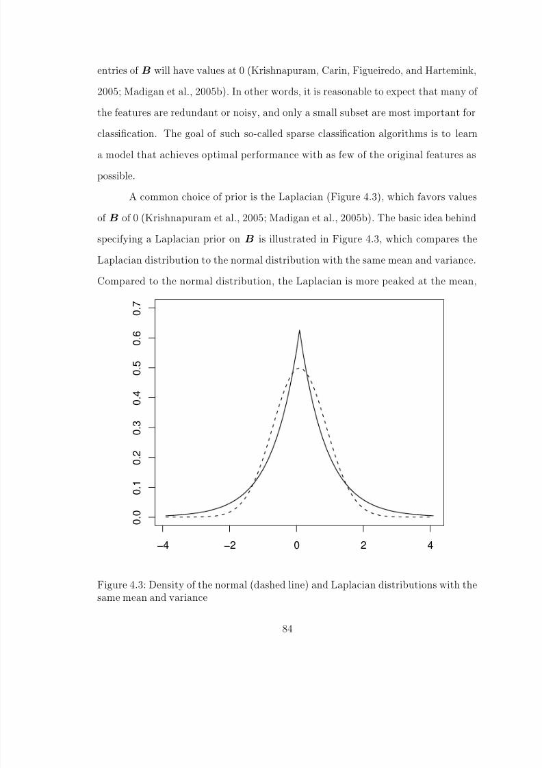
8/8/2019 Baker Kirk
http://slidepdf.com/reader/full/baker-kirk 100/243
entries of B will have values at 0 (Krishnapuram, Carin, Figueiredo, and Hartemink,
2005; Madigan et al., 2005b). In other words, it is reasonable to expect that many of
the features are redundant or noisy, and only a small subset are most important for
classification. The goal of such so-called sparse classification algorithms is to learn
a model that achieves optimal performance with as few of the original features as
possible.
A common choice of prior is the Laplacian (Figure 4.3), which favors values
of B of 0 (Krishnapuram et al., 2005; Madigan et al., 2005b). The basic idea behind
specifying a Laplacian prior on B is illustrated in Figure 4.3, which compares the
Laplacian distribution to the normal distribution with the same mean and variance.
Compared to the normal distribution, the Laplacian is more peaked at the mean,
0 . 0
0 . 1
0 . 2
0 . 3
0
. 4
0 . 5
0 . 6
0 . 7
−4 −2 0 2 4
Figure 4.3: Density of the normal (dashed line) and Laplacian distributions with thesame mean and variance
84
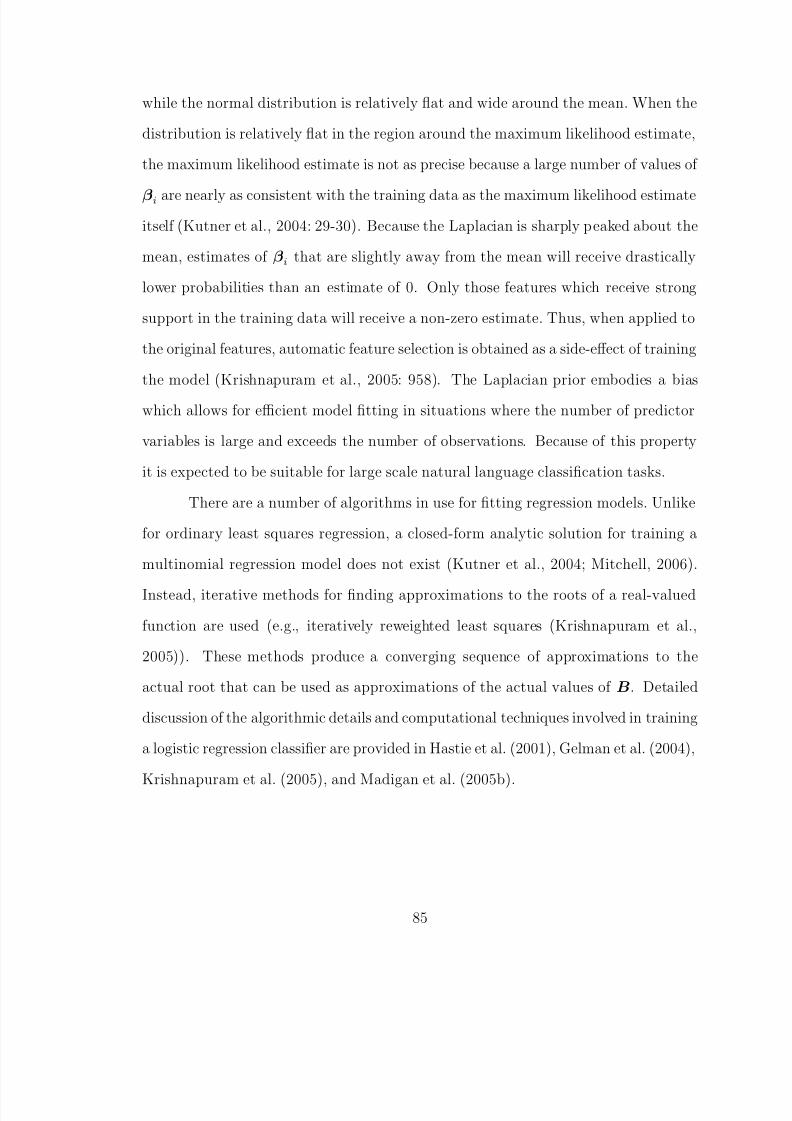
8/8/2019 Baker Kirk
http://slidepdf.com/reader/full/baker-kirk 101/243
while the normal distribution is relatively flat and wide around the mean. When the
distribution is relatively flat in the region around the maximum likelihood estimate,
the maximum likelihood estimate is not as precise because a large number of values of
βi are nearly as consistent with the training data as the maximum likelihood estimate
itself (Kutner et al., 2004: 29-30). Because the Laplacian is sharply peaked about the
mean, estimates of βi that are slightly away from the mean will receive drastically
lower probabilities than an estimate of 0. Only those features which receive strong
support in the training data will receive a non-zero estimate. Thus, when applied to
the original features, automatic feature selection is obtained as a side-effect of training
the model (Krishnapuram et al., 2005: 958). The Laplacian prior embodies a bias
which allows for efficient model fitting in situations where the number of predictor
variables is large and exceeds the number of observations. Because of this property
it is expected to be suitable for large scale natural language classification tasks.
There are a number of algorithms in use for fitting regression models. Unlike
for ordinary least squares regression, a closed-form analytic solution for training a
multinomial regression model does not exist (Kutner et al., 2004; Mitchell, 2006).
Instead, iterative methods for finding approximations to the roots of a real-valued
function are used (e.g., iteratively reweighted least squares (Krishnapuram et al.,
2005)). These methods produce a converging sequence of approximations to the
actual root that can be used as approximations of the actual values of B. Detailed
discussion of the algorithmic details and computational techniques involved in training
a logistic regression classifier are provided in Hastie et al. (2001), Gelman et al. (2004),
Krishnapuram et al. (2005), and Madigan et al. (2005b).
85

8/8/2019 Baker Kirk
http://slidepdf.com/reader/full/baker-kirk 102/243
4.3.2 Naive Bayes
For comparison purposes, we also use a naive Bayes classifier in the first experiment
below. The motivation for including the naive Bayes classifier is its simplicity and
the fact that it is often competitive with more sophisticated models on a wide range
of classification tasks (Mitchell, 2006). The naive Bayes classifier is a conditional
probability model of the form
P (C |F 1, . . . , F n)
where C stands for the class we are trying to predict and F 1, . . . , F n represent thefeatures used for prediction. The class-conditional probabilities can be estimated
using maximum likelihood estimates that are approximated with relative frequenices
from the training data. Therefore, the conditional distribution over the class variable
C can be written
P (C |F 1, . . . , F n) ≈ P (C )n
i=1
P (F i|C )
This rewrite is possible only under the assumption that the features are independent.
When used for classification, we are interested in obtaining the most likely class given
a particular set of values of the input features, i.e.,
classify(f i, . . . , f n) = argmaxc
P (C = c)ni=1
P (F i = f i|C = c)
In the experiments reported here we use a balanced data set (i.e., the same number
of English and Korean words) and therefore do not include the prior probability of a
word being English or Korean in the model.
86
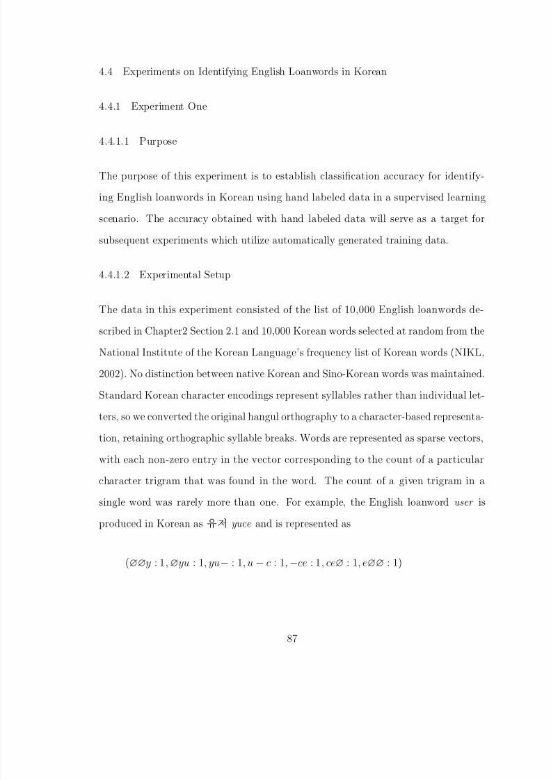
8/8/2019 Baker Kirk
http://slidepdf.com/reader/full/baker-kirk 103/243
4.4 Experiments on Identifying English Loanwords in Korean
4.4.1 Experiment One
4.4.1.1 Purpose
The purpose of this experiment is to establish classification accuracy for identify-
ing English loanwords in Korean using hand labeled data in a supervised learning
scenario. The accuracy obtained with hand labeled data will serve as a target for
subsequent experiments which utilize automatically generated training data.
4.4.1.2 Experimental Setup
The data in this experiment consisted of the list of 10,000 English loanwords de-
scribed in Chapter2 Section 2.1 and 10,000 Korean words selected at random from the
National Institute of the Korean Language’s frequency list of Korean words (NIKL,
2002). No distinction between native Korean and Sino-Korean words was maintained.
Standard Korean character encodings represent syllables rather than individual let-
ters, so we converted the original hangul orthography to a character-based representa-
tion, retaining orthographic syllable breaks. Words are represented as sparse vectors,
with each non-zero entry in the vector corresponding to the count of a particular
character trigram that was found in the word. The count of a given trigram in a
single word was rarely more than one. For example, the English loanword user is
produced in Korean as Ä»$ yuce and is represented as
(∅∅y : 1, ∅yu : 1, yu− : 1, u − c : 1, −ce : 1, ce∅ : 1, e∅∅ : 1)
87

8/8/2019 Baker Kirk
http://slidepdf.com/reader/full/baker-kirk 104/243
where ∅ is a special string termination symbol and ‘-’ indicates an orthographic
syllable boundary.
The decision to use trigrams instead of syllables as in Oh and Choi (2001)
and Kang and Choi (2002) was based on the intuition that segment level transitions
provide important cues to etymological class that are lost by only considering syllable
transitions. Unigrams or bigrams are not as likely to be sufficiently informative, while
going to 4-grams or higher results in severe problems with data sparsity. This feature
representation resulted in 2276 total features; English words contained 1431 unique
trigrams and Korean words contained on 1939 unique trigrams.
This experiment used a 10-fold, 90/10 train/test split. We report identification
accuracy, which is computed as the number of correctly classified words in the test
set divided by the total number of words in the test set, averaged over ten trials.
Baseline accuracy for all experiments is 50%.
4.4.1.3 Results
Mean classification accuracy using labeled data was 91.1% for the Bayes classifier
and 96.2% for the regression classifier. This is expected, in accordance with the
observation that discriminative models typically perform better than generative ones
(Ng and Jordan, 2002). Taking these results as a reasonable baseline for what can be
expected using hand-labeled data, the next experiment looks at using phonological
rules to automatically generate English training data.
88

8/8/2019 Baker Kirk
http://slidepdf.com/reader/full/baker-kirk 105/243
4.4.2 Experiment Two
4.4.2.1 Purpose
The purpose of this experiment is to use phonological transliteration rules to generate
a set of possible but unattested English loanwords in Korean and train a classifier to
automatically distinguish actual English loanwords from actual Korean words.
4.4.2.2 Experimental Setup
This experiment applied the phonological rule based transliteration model presented
in Chapter 3 Section 3.3.1 to the pronunciations of English words in the CMU Pro-
nouncing Dictionary (Weide, 1998) to create a set of possible but unattested English
loanwords in Korean. These items served as training data for the distinction between
actual English loanwords and Korean words. The number of pseudo-English train-
ing instances ranged from 10,000 to 100,000. The test items were all 20,000 items
from the experiment above. The training data did not include any of the test items.
This means that if the phonological conversion rules produced a form that was ho-
mographic with any of the actual English loanwords, this item was removed from the
training set. Note that this is conservative: in practical situations we would expect
that the conversion rules would sometimes manage to duplicate actual loanwords,
with the possibility of improved performance. We had a total of 62688 labeled actual
Korean words (Sino-Korean plus native Korean). In order to keep the same number
of items in the English and Korean classes, i.e., in order to avoid introducing a bias in
the training data that was not reflected in the test data, we used a random sampling
with replacement sampling model for the Korean words.
89
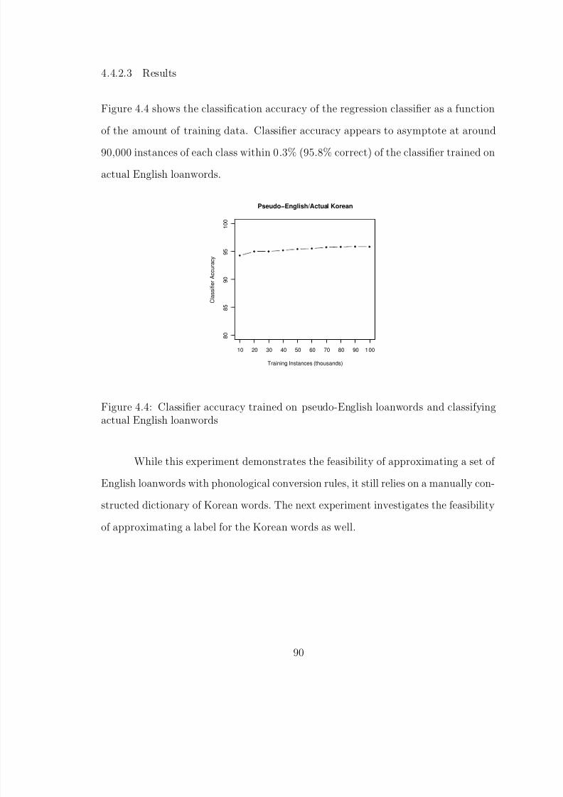
8/8/2019 Baker Kirk
http://slidepdf.com/reader/full/baker-kirk 106/243
4.4.2.3 Results
Figure 4.4 shows the classification accuracy of the regression classifier as a function
of the amount of training data. Classifier accuracy appears to asymptote at around
90,000 instances of each class within 0.3% (95.8% correct) of the classifier trained on
actual English loanwords.
8 0
8 5
9 0
9 5
1 0 0
Pseudo−English/Actual Korean
Training Instances (thousands)
C l a s s
i f i e r A c c u r a c y
10 20 30 40 50 60 70 80 90 100
Figure 4.4: Classifier accuracy trained on pseudo-English loanwords and classifying
actual English loanwords
While this experiment demonstrates the feasibility of approximating a set of
English loanwords with phonological conversion rules, it still relies on a manually con-
structed dictionary of Korean words. The next experiment investigates the feasibility
of approximating a label for the Korean words as well.
90
8/8/2019 Baker Kirk
http://slidepdf.com/reader/full/baker-kirk 107/243
4.4.3 Experiment Three
4.4.3.1 Purpose
The purpose of this experiment is to examine the performance of the loanword iden-
tifier on distinguishing actual English loanwords from actual Korean words when it
is trained on pseudo-English loanwords and unlabeled items that serve as examples
of Korean words.
4.4.3.2 Experimental Setup
Based on observations of English loanwords in Japanese (Graff and Wu, 1995) and
Chinese (Graff, 2007) newswires, we believe that the majority of these items will occur
relatively infrequently in comparable Korean text. This means that we are assuming
that there is a direct relationship between word frequency and the likelihood of a word
being Korean, i.e., the majority of English loanwords will occur very infrequently.
Accordingly, we sorted the items in the Korean Newswire corpus (Cole and Walker,
2000) by frequency on the assumption that Korean words will tend to dominate the
higher frequency items, and examined the effects of using these as a proxy for known
Korean words.
We identified 23406254 Korean orthographic units (i.e., eojeol ) in the Korean
Newswire corpus (Cole and Walker, 2000). Because we believe that high frequency
items are more likely to be Korean words, we applied a sampling without replacement
sampling scheme to the instances extracted from the corpus. This means that the
frequencies of items in our extracted subset approximately match those in the actual
corpus, i.e., we have repeated items in the training data. Thus, the classifier for this
experiment was trained on automatically generated pseudo-English loanwords as the
91
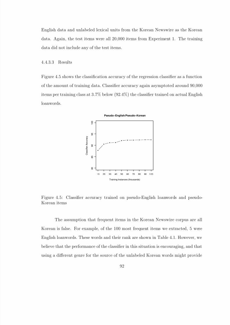
8/8/2019 Baker Kirk
http://slidepdf.com/reader/full/baker-kirk 108/243
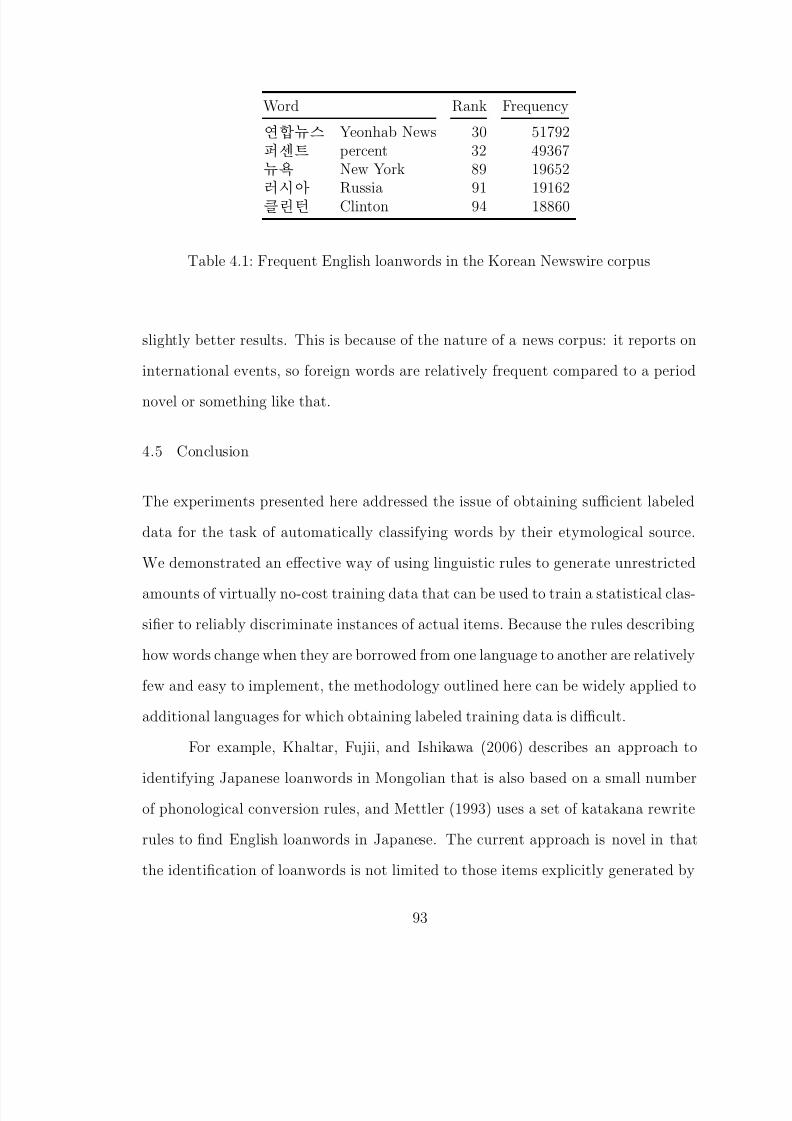
8/8/2019 Baker Kirk
http://slidepdf.com/reader/full/baker-kirk 109/243
Word Rank Frequency
½+˾»Û¼ Yeonhab News 30 51792(G'pàÔ percent 32 49367¾»6¤ New York 89 19652Qr
Russia 91 191629þt2; Clinton 94 18860
Table 4.1: Frequent English loanwords in the Korean Newswire corpus
slightly better results. This is because of the nature of a news corpus: it reports on
international events, so foreign words are relatively frequent compared to a period
novel or something like that.
4.5 Conclusion
The experiments presented here addressed the issue of obtaining sufficient labeled
data for the task of automatically classifying words by their etymological source.
We demonstrated an effective way of using linguistic rules to generate unrestricted
amounts of virtually no-cost training data that can be used to train a statistical clas-
sifier to reliably discriminate instances of actual items. Because the rules describing
how words change when they are borrowed from one language to another are relatively
few and easy to implement, the methodology outlined here can be widely applied to
additional languages for which obtaining labeled training data is difficult.
For example, Khaltar, Fujii, and Ishikawa (2006) describes an approach to
identifying Japanese loanwords in Mongolian that is also based on a small numberof phonological conversion rules, and Mettler (1993) uses a set of katakana rewrite
rules to find English loanwords in Japanese. The current approach is novel in that
the identification of loanwords is not limited to those items explicitly generated by
93
8/8/2019 Baker Kirk
http://slidepdf.com/reader/full/baker-kirk 110/243
the conversion rules, but generalizes beyond a specific set of input items to identify
loanwords that are not contained in the training material. As a point of comparison
on the current data set, we can take the performance of the rule-based translitera-
tion models described in Chapter 3 as indicative of a direct rule-based approach to
identifying English loanwords on this data set. The phonological rule-based model
correctly transliterates (i.e., identifies) about 49% of the loanwords in the data set,
and the ortho-phonemic rule-based model finds 78%. The identification model trained
on the output of the phonological rule-based model and approximated Korean labels
performs about 15% higher than the ortho-phonemic model would, and the model
trained on pseudo-English and actual Korean words performs about 18% higher.
94

8/8/2019 Baker Kirk
http://slidepdf.com/reader/full/baker-kirk 111/243
CHAPTER 5
DISTRIBUTIONAL VERB SIMILARITY
5.1 Overview
The idea of lexical similarity provides the basis for the description of a wide range
of linguistic phenomena. For example, morphological overgeneralizations resulting
in new forms such as dived for dove proceed by analogy to existing irregular inflec-
tional paradigms (Prasada and Pinker, 1993). Priming studies show that people are
quicker to respond to a target word after very brief exposure to a phonologically or
semantically related stimulus (e.g., O’Seaghdha and Marin, 1997). The concept of
syntactic category can be approached in terms of classes of words that appear in
similar structural configurations (e.g., Radford, 1997), and lexical semantic relationslike synonymy and hyponymy are often understood in terms of words that can be
substituted for one another without changing the truth conditions of a sentence (e.g.,
Cruse, 1986).
One particular strand of research has focused attention more narrowly on un-
derstanding and describing patterns of lexical similarity among verbs. Of specific
interest here is research that looks at ways to automatically assess lexical similarity
of verbs in terms of their contextual distribution in large text corpora. This research
is motivated by the idea, expressed as early as Harris (1954), that words that occur in
95

8/8/2019 Baker Kirk
http://slidepdf.com/reader/full/baker-kirk 112/243

8/8/2019 Baker Kirk
http://slidepdf.com/reader/full/baker-kirk 113/243
5.2 Previous Work
A substantial body of research deals with the task of automatically classifying verbs
according to their membership in lexical semantic classes on the basis of features
extracted from their distribution in a large text corpus (e.g., Lapata and Brew, 1999;
Stevenson and Merlo, 1999; Schulte im Walde, 2000; Joanis, 2002; Schulte im Walde
and Brew, 2002; Tsang, Stevenson, and Merlo, 2002; Joanis and Stevenson, 2003;
Lapata and Brew, 2004; Li and Brew, 2008). This section provides an overview of
several studies which serve as a springboard for the current research. In particular,
the types of features which have been used by these studies for extracting Levin’s
classification of English verbs from empirical data are relevant to the current study 1.
5.2.1 Schulte im Walde (2000)
Schulte im Walde (2000) explores the hypothesis that verbs can be clustered seman-
tically on the basis of their syntactic alternations. Schulte im Walde applies two
unsupervised hierarchical clustering algorithms to 153 English verbs selected from 30
Levin classes. 103 of these verbs belong to a single Levin class, 35 of these verbs be-
long to exactly two classes, 9 belong to exactly three classes, and 6 belong to exactly
four classes. Each verb is represented by a distribution over subcategorization frames
extracted from the British National Corpus (Clear, 1993) using a statistical parser
(Carroll and Rooth, 1998). Schulte im Walde investigates the features relevant to au-
tomatic verb clustering by evaluating three different components of subcategorization
frames:
• syntactic frames, which are relevant to capturing argument alternations (e.g.
NP-V-PP)
1Portions of Section 5.2 were co-authored with Jianguo Li.
97
8/8/2019 Baker Kirk
http://slidepdf.com/reader/full/baker-kirk 114/243
• prepositions, which are able to distinguish, e.g., directions from locations (e.g.
NP-V-PP(into), NP-V-PP(on ))
• selectional preferences, which encode participant roles (e.g. NP(PERSON)-V-
PPon (LOCATION)).
Using Levin’s verb classification as a basis for evaluation, 61% of the verbs
are correctly classified into semantic classes. The best clustering result is achieved
when when using subcategorization frames enriched with PP information. Adding
selectional preferences actually decreases the clustering performance, a finding which
is attributed to data sparsity that results from the specificity of the features produced
when selectional preferences are incorporated.
5.2.2 Merlo and Stevenson (2001)
Merlo and Stevenson (2001) describes an automatic classification of three types of En-
glish intransitive verbs including unergatives, unaccusatives, and object-drop. They
select 60 verbs with 20 verbs from each verb class. However, verbs in these three se-
lected classes show similarities with respect to their argument structure in that theycan all be used as transitives and intransitives. Therefore, syntactic cues alone can-
not effectively distinguish the classes. Merlo and Stevenson define five linguistically-
motivated verb features that describe the thematic relations between subject and
object in transitive and intransitive usage. These features are collected from an au-
tomatically tagged corpus (primarily the Wall Street Journal corpus (LDC, 1995)).
Each verb is represented as a five-feature vector on which a decision tree classifier
is trained. Merlo and Stevenson (2001) reports 69.8% accuracy for a task with a
baseline of 33.3%, and an expert-based upper bound of 86.5%.
98

8/8/2019 Baker Kirk
http://slidepdf.com/reader/full/baker-kirk 115/243
The approach described in Merlo and Stevenson (2001) requires deep linguistic
expertise to identify the five verb features, which are crucial for the success of the
classification experiments. The need for such linguistic expertise limits the applica-
bility of the method because these features are designed specifically to the particular
class distinctions investigated, and are unlikely to be effective when applied to other
classes. Later work has proposed an analysis of possible class distinctions exhibited
by Levin verbs that generalizes Merlo and Stevenson’s features to a larger space of
features that potentially cover any verb classes (Joanis, 2002; Joanis and Stevenson,
2003; Joanis, Stevenson, and James, 2006). These more general features fall into four
groups:
• syntactic slots,
• slot overlaps,
• tense, voice and aspect, and
• animacy of NPs.
These features are extracted from BNC using the chunker described in Abney (1991).
This more general feature space is potentially applicable to any class distinction
among Levin classes and is relatively inexpensive in that it requires only a POS
tagger and chunker. Joanis et al. (2006) presents experiments on classification tasks
involving 15 verb classes and 835 verbs using a support vector machine with the
proposed feature space. These experiments achieve a rate of error reduction ranging
from 48% to 88% over a chance baseline, across classification tasks of varying difficulty.
In particular, these experiments yield classification accuracy comparable to or even
better than that of the feature sets manually selected for each particular task.
99

8/8/2019 Baker Kirk
http://slidepdf.com/reader/full/baker-kirk 116/243
5.2.3 Korhonen et al. (2003)
Korhonen et al. (2003) presents an investigation of English verb classification that
concentrates on polysemic verbs. Korhonen et al. employs an extended version of
Levin’s verb classification that incorporates 26 classes introduced by Dorr (1997), and
57 additional classes described in Korhonen and Briscoe (2004) . 110 test verbs are
chosen, most of which belong to more than one verb class. After obtaining subcatego-
rization frame frequency information from the British National Corpus (Clear, 1993)
using the parser described in Briscoe and Carroll (1997), two clustering methods are
applied: 1) a naive method that collects the nearest neighbor of each verb, and 2) an
iterative method based on the information bottleneck method (Tishby, Pereira, and
Bialek, 1999). Neither of these clustering methods allow the assignment of a single
verb to multiple verb classes.
In analyzing the impact of polysemy on cluster assignments, Korhonen et al.
(2003) makes a distinction between regular and irregular polysemy. A verb is said
to display regular polysemy if it shares its full set of Levin class memberships with
at least one other verb. A verb is said to display irregular polysemy if it does notshare its full set of Levin class memberships with any other verb. Korhonen et al.
finds that polysemic verbs with one predominant sense and those with similar regular
polysemy are often assigned to the same clusters, while verbs with irregular polysemy
tend to resist grouping are likely to be assigned to singleton clusters.
5.2.4 Li and Brew (2008)
Li and Brew (2008) evaluates a wide range of feature types for performing Levin-style
verb classification using a sparse logistic regression classifier Genkin et al. (2004) on
a substantially larger set of Levin verbs and classes than previously considered. In
100
8/8/2019 Baker Kirk
http://slidepdf.com/reader/full/baker-kirk 117/243
addition to a replication of the feature set used in Joanis et al. (2006), this study ex-
amined a number of additional feature sets that focus attention on ways to combine
syntactic and lexical information. These additional feature sets include dependency
relations, contextual co-occurrences, part-of-speech tagged contextual co-occurrences,
and subcategorization frames plus co-occurrence features. All features are extracted
automatically from the English gigaword corpus (Graff, 2003) using Clark and Cur-
ran’s (2007) CCG parser. Results are reported over 48 Levin verb classes involving
around 1300 single-class verbs. For the 48-way classification task, Li and Brew (2008)
reports a best classification accuracy of 52.8% obtained with features derived from a
combination of subcategorization frames plus co-occurrence features.
5.3 Current Approach
The current research also deals with automatic verb classification, but represents a
departure from the work described above in two fundamental ways. The first way in
which the current study differs from previous work relates to the scope and nature
of the class structure assumed to be at work in organizing the structure of the verb
lexicon. The second difference has to do with the type of evaluation that is applied
to assessing distributional verb similarity. These differences are discussed below.
5.3.1 Scope and Nature of Verb Classifications
Previous research has tended to focus on assigning verbs to classes based directly
on or derived from Levin (1993), investigating either a small number of verbs (e.g.,
Schulte im Walde, 2000) or a small number of classes (e.g., Joanis et al., 2006), but
see Li and Brew (2008) for consideration of a larger set of Levin verbs. Rather
than restricting the assessment of distributional verb similarity to a single linguistic
101

8/8/2019 Baker Kirk
http://slidepdf.com/reader/full/baker-kirk 118/243
classification, the current study analyzes distributional verb similarity with respect
to multiple verb schemes. Three of these Levin (1993) – VerbNet (Kipper, Dang, and
Palmer, 2000), and FrameNet (Johnson and Fillmore, 2000) – explicitly incorporate
some form of frame-based syntactic information into their organization of verbs, while
the other two – WordNet (Fellbaum, 1998) and an online version of Roget’s Thesaurus
(Roget’s Thesaurus, 2008) – are organized primarily around the semantic relations
of synonymy and antonymy. Furthermore, the first three classification schemes place
verbs into a comparatively small number of classes on the basis of shared semantic
components such as MOTION or COGNITION. This type of class structure has no
direct analogy in Roget or WordNet, which essentially create separate classes for each
lexical entry (e.g., run heads its own class of synonyms, draw heads its own class,
etc).
5.3.2 Nature of the Evaluation of Verb Classifications
The differences in organizational structure discussed above and the goal of obtaining
a consistent comparison across classification schemes lead to the second way in which
the current research departs from previous work. Rather than training a classifier
to assign verbs to a predefined set of classes or clustering verbs with respect to a
particular taxonomy, the current study approaches the evaluation of distributional
verb similarity from the standpoint of obtaining a pairwise matrix of similarities
between all of the verbs under consideration. This conceptualization of the problem
of measuring distributional lexical similarity is found as well in work on automatic
thesaurus construction (e.g., Lin, 1998a; Curran and Moens, 2002; Weeds, 2003),
which typically deals with techniques for grouping nouns into sets of lexically related
items.
102
8/8/2019 Baker Kirk
http://slidepdf.com/reader/full/baker-kirk 119/243
5.3.3 Relation to Other Lexical Acquisition Tasks
In many ways the task of extracting distributionally similar words from a corpus
is analogous to the classic information retrieval task of retrieving documents from
a collection in response to a query. For example, the vector-based representation
of a target word can be considered a query and the vector-based representations of
other words in the corpus can be treated as documents that are ranked by order of
decreasing similarity to the target. This conceptualization of the task of assessing
distributionally similar lexical items lends itself to evaluation techniques commonly
used in information retrieval such as precision, recall, and F1. However, one differ-
ence between the evaluation of distributionally similar lexical items and information
retrieval is that the former is primarily concerned with the quality of the first few
highly ranked words (precision) rather than extracting all items that belong to the
same class as the target word (recall).
Representative work on automatic thesaurus extraction (e.g., Lin, 1998a; Cur-
ran and Moens, 2002; Weeds, 2003; Gorman and Curran, 2006) adopts measures that
reflect the importance of correctly classifying the top few items such as inverse rank(Curran and Moens, 2002; Gorman and Curran, 2006) or precision-at-k (Lin (1998a);
Curran and Moens (2002), Manning, Raghavan, and Schutze (2008: 148) without em-
phasizing recall of the entire set of class members. Other more general applications of
distributional similarity that emphasize the quality of a small subset of highly ranked
class members over exhaustive identification of all class members include dimension-
ality reduction techniques that preserve local structure (e.g., Roweis and Saul, 2000;
Saul and Roweis, 2003) and semisupervised learning techniques that rely on the iden-
tification of a lower dimensional manifold in a high dimension ambient space (e.g.,
Belkin and Niyogi, 2003, 2004).
103
8/8/2019 Baker Kirk
http://slidepdf.com/reader/full/baker-kirk 120/243
5.3.4 Advantages of the Current Approach
The points of departure from previous research outlined above present the follow-
ing opportunities for increasing our understanding of the application of automatic
classification techniques to distributional verb similarity.
• Taking the union of verbs that occur in multiple classification schemes greatly
increases the number of verbs that can be included for evaluation. Many previ-
ous verb classification studies have examined a relatively small number of verbs
belonging to relatively few classes (e.g., Schulte im Walde, 2000; Joanis, 2002;
Joanis et al., 2006). One problem with such restrictions is not knowing how well
those findings extend to other verbs in the classification that were excluded from
the study.
• Considering a broader range of verb classification criteria allows us to tease
apart some of the elements that are responsible for the organization of the
various verb schemes.
Levin and VerbNet verbs are grouped according to similarity in both syntactic
behavior and meaning, but it is not always clear which of these criteria are actually
responsible for placing an individual verb in a certain class (Baker and Ruppenhofer,
2002). For example, the BUTTER verbs (Levin, 1993: 120) comprise a semantically
diverse class, including items such as asphalt, buttonhole, lipstick, mulch, poison,
sulphur , and zipcode on the basis of their behavior with respect to the locative and
conative alternations (*Lora stained tea on the shirt/Lora stained the shirt with tea;
Lora stained the shirt/*Lora stained at the shirt ).
For other classes of verbs Levin explicitly indicates that the syntactic alterna-
tion forming the basis of their grouping only applies to some members of the class.
For example, for the the DRIVE verbs, comprised of barge, bus, cart, drive, ferry,
104
8/8/2019 Baker Kirk
http://slidepdf.com/reader/full/baker-kirk 121/243
fly, row, shuttle, truck, wheel , and wire (money)), Levin indicates that the dative al-
ternation only applies to “some verbs” (Levin, 1993: 136) but does not specify which
ones. The current study, which separately considers synonymy as a potential selec-
tion criteria for verb classification, will shed light on the extent to which semantic
similarity versus syntactic similarity influences automatic verb classification.
5.4 Components of Distributional Verb Similarity
A number of interdependent factors go in to the process of determining distributional
lexical similarity. The factors considered in this dissertation and discussed in the
following sections are• how to determine the features over which lexical similarity is measured,
• how to determine an appropriate numeric representation of those features,
• how to determine an appropriate measure of distributional similarity,
• and how to evaluate the results of ranking items according to their empirically
determined similarity.
Implicit in the concept of lexical similarity is a method for comparing words along
some set of characteristics that are relevant to the particular distinction being made
(e.g., phonological, semantic, etc.). A procedure for doing this can be operationalized
in terms of a vector X over which observations of a word are made. Under this sce-
nario, a word can be conceptualized as a distribution of values over X , and similarity
between two words y1 and y2 can be computed by application of a similarity metric
to their respective distributional vectors X 1 and X 2. When the task involves deter-
mining lexical semantic similarity, the relevant characteristics are generally taken to
be those words which co-occur with a target item. The following section describes
various approaches to defining context in terms of word co-occurrences.
105
8/8/2019 Baker Kirk
http://slidepdf.com/reader/full/baker-kirk 122/243
5.4.1 Representation of Lexical Context
In computational approaches to determining word similarity, distributional similarity
is typically defined in terms of a word’s context, and words are said to be distribution-
ally similar to the extent that they occur in similar contexts. Applying this definition
to corpus data often yields word classes that overlap the classifications assigned by
traditional lexical semantic relations such as synonymy and hyponymy. For example,
Lin (1998a) describes a method for automatically extracting synonyms from corpus
data that yields word classes such as {brief, affidavit, petition, memorandum, depo-
sition, slight, prospectus, document, paper, . . . } (p. 770). Just as often, applying
this definition yields sets of words whose relation is best described in terms of topical
associations. For example, Kaji and Morimoto (2005) describes a procedure for auto-
matic word sense disambiguation using bilingual corpus data that groups words into
lexical neighborhoods such as {air, area, army, assault, battle, bomb, carry, civilian,
commander, . . . } (p. 290 (a)). In this example, the common thread among these
words is that they all co-occurred with the words tank and troop. Broadly speak-
ing, the context representations which give rise to a distinction between topicallyassociated and semantically similar words fall into two categories: models that use a
bag-of-words representation, and those that model grammatical relations.
5.4.2 Bag-of-Words Context Models
Bag-of-words models take the context of a word to be some number of words preced-
ing and following the target word. The order of items within this context is often not
considered. The context of a target word can be delimited by index (i.e., n words
before or after the target) or structurally (i.e., the paragraph or document the target
106
8/8/2019 Baker Kirk
http://slidepdf.com/reader/full/baker-kirk 123/243
occurs in). For example, Schutze (1998) describes a method for automatically dis-
criminating word senses that uses a 50-word context window centered on the target
word, and (Gale, Church, and Yarowsky, 1992) use a 100-word window.
In the Hyperspace Analogue to Language approach to word similarity (Lund,
Burgess, and Audet, 1996), context is defined as a window of 10 words preceding
and following a target word. Word order is weakly accounted for in this model by
assigning a weight to context words which is inversely proportional to their distance
from the target. In the Latent Semantic Analysis (Deerwester, Dumais, Landauer,
Furnas, and Harshman, 1990) approach to lexical similarity, context is defined as an
entire document, and word co-occurrences are calculated in a document space. One
of the main advantages of the bag-of-words context model is its relative simplicity
when applied to languages that naturally delimit words with whitespace – in its
most basic form, no corpus pre-processing is required to determine a context window.
However, a series of pre-processing steps are typically applied before the context
model is constructed. These steps involve procedures such as word stemming, text
normalization, stopword removal, and lemmatization that are designed to obtain a
more consistent representation of items in the corpus.
5.4.3 Grammatical Relations Context Models
A second approach to modeling distributional context is to define it in terms of gram-
matical dependency relations. Lin (1998a) defines context on the basis dependency
relations between words in a sentence. For example, in the sentence “I have a brown
dog”, the context of dog can be represented as the set of dependency triples {(dog Obj-
of have), (dog Adj-mod brown), (dog Det a)} (Lin, 1998a: 769, (2)). Other approaches
to automatic lexical acquisition that consider the role that syntactic relationships play
in determining distributional word similarity include work on noun clustering (e.g.,
107
8/8/2019 Baker Kirk
http://slidepdf.com/reader/full/baker-kirk 124/243
Pereira, Tishby, and Lee, 1993; Caraballo, 1999; Weeds, 2003) and verb classification
(e.g. Lapata and Brew, 1999; Stevenson and Merlo, 1999; Schulte im Walde, 2000; Li
and Brew, 2008).
Applying a grammatical relations context model requires a deeper level of lin-
guistic extraction than flat context models, and this analysis invariably entails most
of the pre-processing steps involved in the bag-of-words model before grammatical
relations can be extracted. Tools for extracting grammatical relations range from rel-
atively straightforward Bayesian models (e.g., Curran and Moens, 2002) to full-blown
parsers like MiniPar (Lin, 1998b) and the C&C CCG Parser (Clark and Curran, 2007).
The extra linguistic processing has been justified through direct comparison to bag-
of-words models (e.g., Pado and Lapata, 2007) and in terms of a distinction between
“loose” and “tight” thesauri (Weeds, 2003: 19) that are automatically derived from
bag-of-words and grammatical relations context models, respectively. Previous work
has claimed to show that using grammatical relation data yields sets of words which
are semantically related (e.g., Kilgarriff and Yallop, 2000; Weeds, 2003), whereas flat
context models generate word sets that are topically related.
However, it is not always easy to disentangle semantic similarity from topical
similarity, and all lexical context models group items according to a variety of asso-
ciational relations. Following Weeds (2003) we take the position that grammatical
relations are a sufficient information resource to allow for meaningful study of the
process of calculating and assessing distributional lexical similarity. Accordingly, this
dissertation focuses on using grammatical relations to define context models.
108

8/8/2019 Baker Kirk
http://slidepdf.com/reader/full/baker-kirk 125/243
5.5 Evaluation
This section describes some common approaches to evaluating a set of empirically
determined lexical similarity scores. The three approaches considered are application-
based evaluation, comparison to human judgments, and comparison to an accepted
standard. This dissertation primarily deals with evaluation by comparison to an
accepted standard.
5.5.1 Application-Based Evaluation
Application-based evaluation tasks evaluate distributional lexical similarity scores by
judging their usefulness in some other NLP application. For example, in information
retrieval, the primary objective is to retrieve documents that are related to a user
query. Query expansion (Xu and Croft, 1996) is a technique for augmenting a given
query with similar terms so that a greater number of relevant documents can be
found. In this case, the performance of the information retrieval system could be
evaluated with and without using query expansions based on distributionally similar
words to assay the utility of the lexical similarity matrix.
Many additional applications of distributional lexical similarity scores are dis-
cussed in (Weeds, 2003: Chapter 2, Section 2). Some of these include language mod-
eling, where the probability estimate of a previously unseen co-occurrence can be
generated from the co-occurrence probability of distributionally similar items; prepo-
sitional phrase attachment, where the likelihood of a particular syntactic configuration
can be estimated from smoothed estimates obtained from clusters of distributionally
similar items; and spelling correction, where the detection of real word spelling errors
(e.g., principle for principal ) can be enhanced when distributionally-defined semantic
plausibility is considered.
109

8/8/2019 Baker Kirk
http://slidepdf.com/reader/full/baker-kirk 126/243
5.5.2 Evaluation Against Human Judgments
Evaluations against human judgments look at the correlation between distributional
similarity scores and human similarity judgments for the same set of items. For
example, McDonald and Brew (2004) presents a computational model of contextual
priming effects that is based on a probabilistic distribution of word co-occurrences
in the British National Corpus (Clear, 1993). These data are compared to lexical
decision response times for a set of 96 prime-target pairs taken from Hodgson (1991)
that represent a range of lexical relations including synonyms, antonyms, phrasal and
conceptual associates, and hyper/hyponyms (McDonald and Brew, 2004: 21).
Pado and Lapata (2007) presents a general framework for constructing dis-
tributional lexical models that define context on the basis of grammatical relations.
Model selection is based on correlations between empirical similarities and a set of
human similarity judgments from Rubenstein and Goodenough (1965). These data
consist of ordinal similarity ratings for a set of 65 noun-noun pairs that ranged from
highly synonymous to unrelated (Pado and Lapata, 2007: 177). Additional research
making use of the same data set is referenced in (Pado and Lapata, 2007: 177).In general, evaluations against human judgments involve comparisons between
small data sets, chiefly due to the time and cost involved in gathering the requisite
judgments from human subjects. Furthermore, the stimuli used in human subjects ex-
periments may not be well-attested in the corpus being used for evaluating automatic
word similarity measures (e.g, McDonald and Brew (2004) discarded 48 potential
pairs due to low frequency), leading to a potential confound between low frequency
items and the performance of the automatic technique.
110
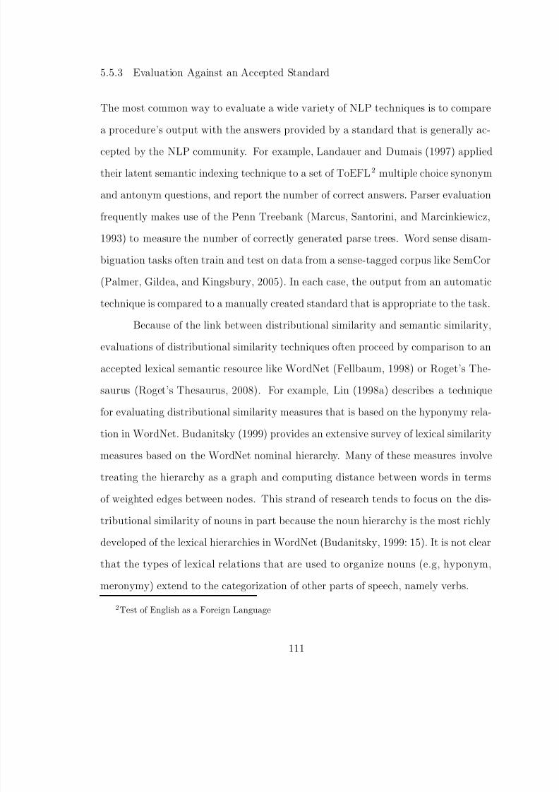
8/8/2019 Baker Kirk
http://slidepdf.com/reader/full/baker-kirk 127/243
5.5.3 Evaluation Against an Accepted Standard
The most common way to evaluate a wide variety of NLP techniques is to compare
a procedure’s output with the answers provided by a standard that is generally ac-
cepted by the NLP community. For example, Landauer and Dumais (1997) applied
their latent semantic indexing technique to a set of ToEFL2 multiple choice synonym
and antonym questions, and report the number of correct answers. Parser evaluation
frequently makes use of the Penn Treebank (Marcus, Santorini, and Marcinkiewicz,
1993) to measure the number of correctly generated parse trees. Word sense disam-
biguation tasks often train and test on data from a sense-tagged corpus like SemCor
(Palmer, Gildea, and Kingsbury, 2005). In each case, the output from an automatic
technique is compared to a manually created standard that is appropriate to the task.
Because of the link between distributional similarity and semantic similarity,
evaluations of distributional similarity techniques often proceed by comparison to an
accepted lexical semantic resource like WordNet (Fellbaum, 1998) or Roget’s The-
saurus (Roget’s Thesaurus, 2008). For example, Lin (1998a) describes a technique
for evaluating distributional similarity measures that is based on the hyponymy rela-tion in WordNet. Budanitsky (1999) provides an extensive survey of lexical similarity
measures based on the WordNet nominal hierarchy. Many of these measures involve
treating the hierarchy as a graph and computing distance between words in terms
of weighted edges between nodes. This strand of research tends to focus on the dis-
tributional similarity of nouns in part because the noun hierarchy is the most richly
developed of the lexical hierarchies in WordNet (Budanitsky, 1999: 15). It is not clear
that the types of lexical relations that are used to organize nouns (e.g, hyponym,
meronymy) extend to the categorization of other parts of speech, namely verbs.
2Test of English as a Foreign Language
111

8/8/2019 Baker Kirk
http://slidepdf.com/reader/full/baker-kirk 128/243
A second strand of research has dealt with the classification of verbs. In this
setting, empirically defined similarities between verbs are typically evaluated with
respect to a lexical semantic verb classification such as that given in (Levin, 1993),
VerbNet (Kipper et al., 2000), or FrameNet (Johnson and Fillmore, 2000). This
dissertation evaluates a number of distributional similarity measures against 5 widely
used lexical semantic standards: Levin (1993), VerbNet, FrameNet, WordNet and
Roget’s Thesaurus. The next sections outline the organizational principles behind
each and quantify some of the similarities and differences among them with respect
to how they organize the same set of verbs.
5.5.3.1 Levin (1993)
Levin’s classification of English verbs rests on the hypothesis that a verb’s meaning
determines the syntactic realization and interpretation of its arguments (e.g., Lapata
and Brew, 2004: references therein). Levin argues that verbs which participate in the
same diathesis alternations share certain components of meaning and form seman-
tically coherent classes. The converse of the hypothesis Levin assumes is that the
syntactic behavior of verbs can be used to provide clues to aspects of their mean-
ing. Levin groups verbs into classes of items that participate in the same syntactic
alternation.
For example, the dative alternation, exemplified below,
(1) a. Brian passed DJ the ball.
b. Brian passed the ball to DJ.
involves an alternation between the double object construction (1-a) and a preposi-
tional phrase headed by to (1-b). Verbs that participate in the alternation, like give,
feed, rent, sell, trade etc., are all grouped into the the class of GIVE verbs. Levin
112

8/8/2019 Baker Kirk
http://slidepdf.com/reader/full/baker-kirk 129/243
identifies around 77 such syntactic alternations and uses them to group 3,004 verbs
into 191 classes such as SEND (FedEx, UPS, slip, smuggle, etc.) and CLING (adhere,
cleave, cling ).
5.5.3.2 VerbNet
VerbNet closely follows Levin’s classification, adding some verbs (3626 total) and
classes (237 total). In addition, VerbNet specifies selectional preferences for some
verbs (e.g., ±ANIMATE, ±LOCATION) that are not explicitly expressed in Levin’s
original classification.
5.5.3.3 FrameNet
Verbs in FrameNet are organized around semantic frames, which are schematic rep-
resentations of situation types that tie lexical units to frames of semantic knowledge.
For example, the GIVING frame relates the subject, object, and indirect object of
a verb like give to the donor , theme, and recipient semantic roles. Other verbs that
evoke the GIVING frame are bequeath, donate, endow, fob off, foist, gift, give out,
hand, hand in, hand out, hand over, pass, pass out , and treat . FrameNet classifies
2307 verbs into 321 classes.
5.5.3.4 WordNet
WordNet arranges specific senses of nouns, verbs, adjectives, and adverbs into syn-
onym sets that express a distinct concept. Synonym sets are further linked by a
number of lexical relations like hyponymy, antonymy, coordinate terms, etc. For ex-
ample, the verb brachiate is synonymous with swing and sway and is a hyponym of
move back and forth . WordNet organizes 11529 verbs in 13767 synonym sets. In
113

8/8/2019 Baker Kirk
http://slidepdf.com/reader/full/baker-kirk 130/243
addition to synonymy, WordNet defines hyponymy relations between verbs, which
often correspond to Roget synonyms. For example, Roget synonyms of argue such as
quibble, quarrel, dispute, and altercate are classified as hyponyms by WordNet.
5.5.3.5 Roget’s Thesaurus
Roget’s Thesaurus (2008) is an online thesaurus published by Lexico Publishing
Group. It contains around 14,000 verbs, and each entry consists of an indication
of its part of speech, a dictionary-style definition, synonyms and possibly antonyms.
An example entry for gargle is shown below:
Main Entry: gargle
Part of Speech: verb
Definition: rinse
Synonyms: irrigate, swash, trill, use mouthwash
Querying the online thesaurus for verbs contained in the previously described verb
classification schemes returned synonym sets for 3786 entries.
5.5.3.6 Comparison of Verb Classification Schemes
The fact that multiple classification schemes have been proposed and instantiated
for a reasonably large number of English verbs suggests that the optimal criteria for
determining verbs categories are open to debate. At the very least, the existence
of multiple categorization schemes suggests that the criteria for verb classification
differ according to the particular aspect of lexical similarity that is of interest to the
lexicographer. One of the purposes of this dissertation is to examine distributionally
114

8/8/2019 Baker Kirk
http://slidepdf.com/reader/full/baker-kirk 131/243
similar verb assignments with respect to multiple verb classification schemes. Before
doing so, it is useful to quantify the extent to which the five schemes outlined above
agree on their assignments of verbs to lexical classes.
Figure 5.1 compares the five schemes in terms of the number of senses each
assigns to verbs. For WordNet, senses are explicitly distinguished and labeled in a
0 10 20 30 40 50 60
0
500
1000
1500
2000
Levin
0 10 20 30 40 50 60
0500
10001500
20002500
VerbNet
0 10 20 30 40 50 60
0
500
1000
1500
FrameNet
0 10 20 30 40 50 60
0500
1000150020002500
Roget
0 10 20 30 40 50 60
0100020003000400050006000
WordNet
Figure 5.1: Distribution of verb senses assigned by the five classification schemes.The x-axis shows the number of senses and the y-axis shows the number of verbs
115

8/8/2019 Baker Kirk
http://slidepdf.com/reader/full/baker-kirk 132/243
verb’s entry, for example
Synonyms/Hypernyms of verb run
Sense 1: run
Sense 2: scat, run, scamper, turn tail, . . .
Sense 3: run, go, pass, lead, extend
...
Sense 39: melt, run, melt down
Sense 40: ladder, run
Sense 41: run, unravel
Roget’s Thesaurus also distinguishes verb senses in the form of multiple entries headed
by the same item with distinct definitions (e.g., run 1: move fast, run 2: flow, run 3:
operate, run 4: manage, run 5: continue, run 6: be candidate). For Levin, VerbNet,
and FrameNet, we treat the number of classes to which a verb is assigned as the
number of senses of that verb. For example, Levin and VerbNet assign run to the
PREPARING, SWARM, MEANDER, and RUN classes (4 senses); FrameNet as-
signs run to the SELF MOTION, LEADERSHIP, IMPACT, FLUIDIC MOTION,
and CAUSE IMPACT classes (5 senses).
As Figure 5.1 shows, Levin, VerbNet, FrameNet, and Roget’s Thesaurus are
quite similarly distributed, and do not assign more than 10 senses to any verb. The
overall distribution of senses to verbs is similar in WordNet as well, but WordNet
makes substantially more sense distinctions (up to 59) for a small number of verbs.
Figure 5.2 compares Levin, VerbNet, and FrameNet in terms of how the size
of the verb classes each defines. Because Roget’s Thesaurus and WordNet do notexplicitly define verb classes, only sets of synonyms, they are not included in this
figure. Overall, the distribution of class sizes between Levin and VerbNet is similar, as
is expected since VerbNet is based on Levin’s original classification. The largest Levin
116
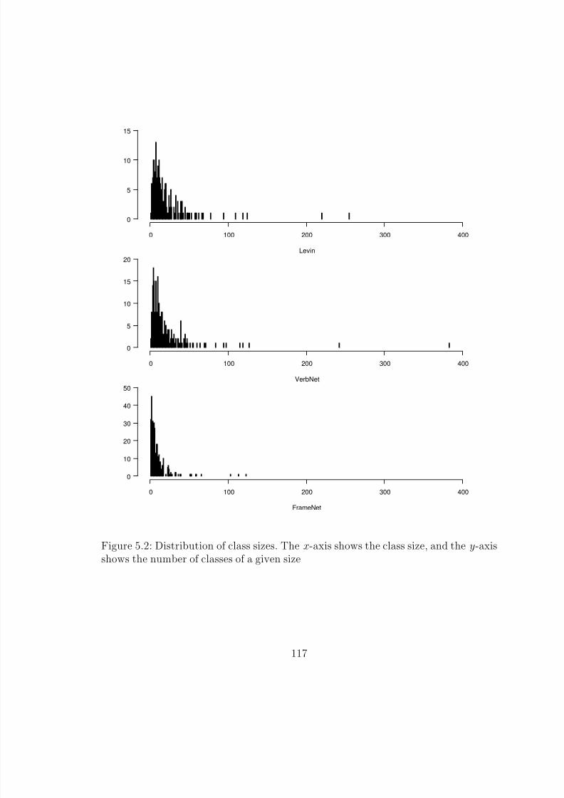
8/8/2019 Baker Kirk
http://slidepdf.com/reader/full/baker-kirk 133/243
0 100 200 300 400
0
5
10
15
Levin
0 100 200 300 400
0
5
10
15
20
VerbNet
0 100 200 300 400
0
10
20
30
40
50
FrameNet
Figure 5.2: Distribution of class sizes. The x-axis shows the class size, and the y-axis
shows the number of classes of a given size
117
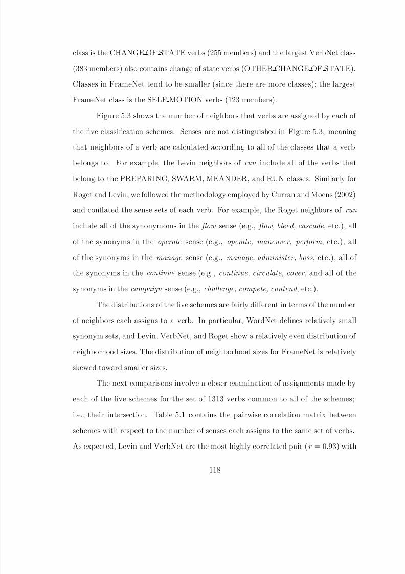
8/8/2019 Baker Kirk
http://slidepdf.com/reader/full/baker-kirk 134/243
class is the CHANGE OF STATE verbs (255 members) and the largest VerbNet class
(383 members) also contains change of state verbs (OTHER CHANGE OF STATE).
Classes in FrameNet tend to be smaller (since there are more classes); the largest
FrameNet class is the SELF MOTION verbs (123 members).
Figure 5.3 shows the number of neighbors that verbs are assigned by each of
the five classification schemes. Senses are not distinguished in Figure 5.3, meaning
that neighbors of a verb are calculated according to all of the classes that a verb
belongs to. For example, the Levin neighbors of run include all of the verbs that
belong to the PREPARING, SWARM, MEANDER, and RUN classes. Similarly for
Roget and Levin, we followed the methodology employed by Curran and Moens (2002)
and conflated the sense sets of each verb. For example, the Roget neighbors of run
include all of the synonymoms in the flow sense (e.g., flow, bleed, cascade, etc.), all
of the synonyms in the operate sense (e.g., operate, maneuver, perform , etc.), all
of the synonyms in the manage sense (e.g., manage, administer, boss, etc.), all of
the synonyms in the continue sense (e.g., continue, circulate, cover , and all of the
synonyms in the campaign sense (e.g., challenge, compete, contend , etc.).
The distributions of the five schemes are fairly different in terms of the number
of neighbors each assigns to a verb. In particular, WordNet defines relatively small
synonym sets, and Levin, VerbNet, and Roget show a relatively even distribution of
neighborhood sizes. The distribution of neighborhood sizes for FrameNet is relatively
skewed toward smaller sizes.
The next comparisons involve a closer examination of assignments made by
each of the five schemes for the set of 1313 verbs common to all of the schemes;i.e., their intersection. Table 5.1 contains the pairwise correlation matrix between
schemes with respect to the number of senses each assigns to the same set of verbs.
As expected, Levin and VerbNet are the most highly correlated pair (r = 0.93) with
118
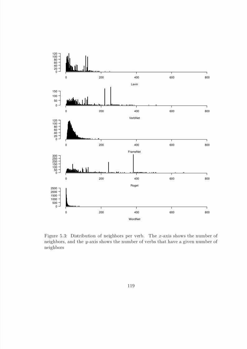
8/8/2019 Baker Kirk
http://slidepdf.com/reader/full/baker-kirk 135/243
0 200 400 600 800
020406080
100120
Levin
0 200 400 600 800
0
50
100
150
VerbNet
0 200 400 600 800
020406080
100120
FrameNet
0 200 400 600 800
050
100150200250300
Roget
0 200 400 600 800
0
500
1000
1500
2000
2500
WordNet
Figure 5.3: Distribution of neighbors per verb. The x-axis shows the number of neighbors, and the y-axis shows the number of verbs that have a given number of neighbors
119
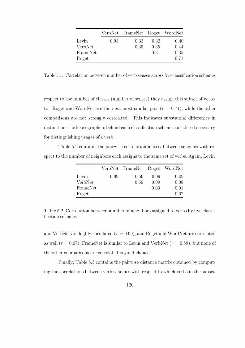
8/8/2019 Baker Kirk
http://slidepdf.com/reader/full/baker-kirk 136/243
VerbNet FrameNet Roget WordNet
Levin 0.93 0.33 0.32 0.40VerbNet 0.35 0.35 0.44FrameNet 0.31 0.35
Roget 0.71
Table 5.1: Correlation between number of verb senses across five classification schemes
respect to the number of classes (number of senses) they assign this subset of verbs
to. Roget and WordNet are the next most similar pair (r = 0.71), while the other
comparisons are not strongly correlated. This indicates substantial differences in
distinctions the lexicographers behind each classification scheme considered necessary
for distinguishing usages of a verb.
Table 5.2 contains the pairwise correlation matrix between schemes with re-
spect to the number of neighbors each assigns to the same set of verbs. Again, Levin
VerbNet FrameNet Roget WordNet
Levin 0.99 0.59 0.09 0.09
VerbNet 0.59 0.09 0.08FrameNet -0.03 -0.01Roget 0.67
Table 5.2: Correlation between number of neighbors assigned to verbs by five classi-fication schemes
and VerbNet are highly correlated (r = 0.99), and Roget and WordNet are correlated
as well (r = 0.67). FrameNet is similar to Levin and VerbNet (r = 0.59), but none of
the other comparisons are correlated beyond chance.
Finally, Table 5.3 contains the pairwise distance matrix obtained by comput-
ing the correlations between verb schemes with respect to which verbs in the subset
120
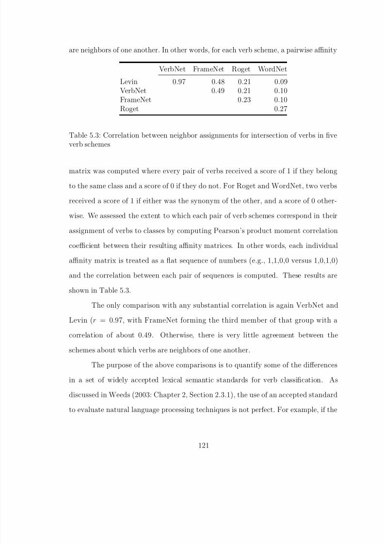
8/8/2019 Baker Kirk
http://slidepdf.com/reader/full/baker-kirk 137/243
are neighbors of one another. In other words, for each verb scheme, a pairwise affinity
VerbNet FrameNet Roget WordNet
Levin 0.97 0.48 0.21 0.09VerbNet 0.49 0.21 0.10FrameNet 0.23 0.10Roget 0.27
Table 5.3: Correlation between neighbor assignments for intersection of verbs in fiveverb schemes
matrix was computed where every pair of verbs received a score of 1 if they belong
to the same class and a score of 0 if they do not. For Roget and WordNet, two verbs
received a score of 1 if either was the synonym of the other, and a score of 0 other-
wise. We assessed the extent to which each pair of verb schemes correspond in their
assignment of verbs to classes by computing Pearson’s product moment correlation
coefficient between their resulting affinity matrices. In other words, each individual
affinity matrix is treated as a flat sequence of numbers (e.g., 1,1,0,0 versus 1,0,1,0)
and the correlation between each pair of sequences is computed. These results are
shown in Table 5.3.
The only comparison with any substantial correlation is again VerbNet and
Levin (r = 0.97, with FrameNet forming the third member of that group with a
correlation of about 0.49. Otherwise, there is very little agreement between the
schemes about which verbs are neighbors of one another.
The purpose of the above comparisons is to quantify some of the differences
in a set of widely accepted lexical semantic standards for verb classification. As
discussed in Weeds (2003: Chapter 2, Section 2.3.1), the use of an accepted standard
to evaluate natural language processing techniques is not perfect. For example, if the
121
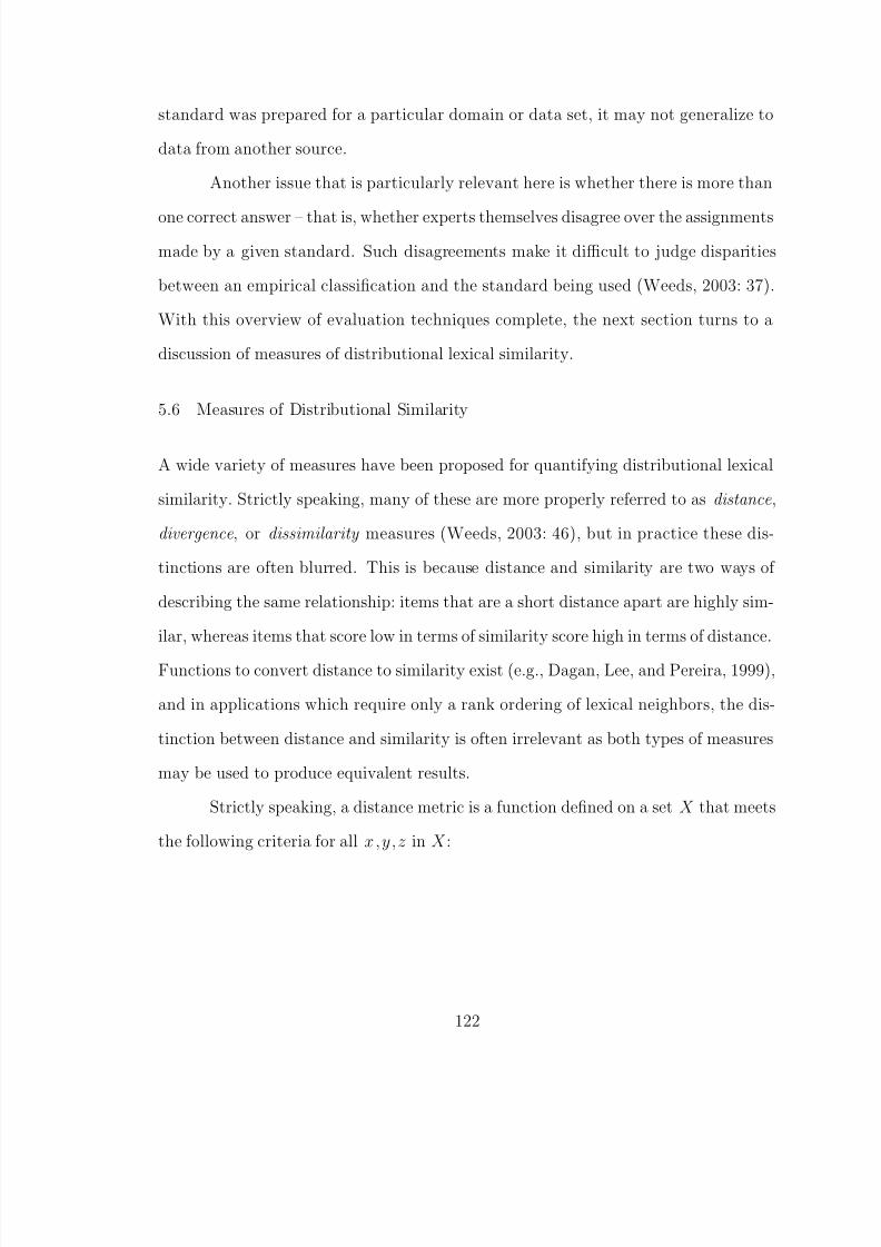
8/8/2019 Baker Kirk
http://slidepdf.com/reader/full/baker-kirk 138/243
standard was prepared for a particular domain or data set, it may not generalize to
data from another source.
Another issue that is particularly relevant here is whether there is more than
one correct answer – that is, whether experts themselves disagree over the assignments
made by a given standard. Such disagreements make it difficult to judge disparities
between an empirical classification and the standard being used (Weeds, 2003: 37).
With this overview of evaluation techniques complete, the next section turns to a
discussion of measures of distributional lexical similarity.
5.6 Measures of Distributional Similarity
A wide variety of measures have been proposed for quantifying distributional lexical
similarity. Strictly speaking, many of these are more properly referred to as distance,
divergence, or dissimilarity measures (Weeds, 2003: 46), but in practice these dis-
tinctions are often blurred. This is because distance and similarity are two ways of
describing the same relationship: items that are a short distance apart are highly sim-
ilar, whereas items that score low in terms of similarity score high in terms of distance.
Functions to convert distance to similarity exist (e.g., Dagan, Lee, and Pereira, 1999),
and in applications which require only a rank ordering of lexical neighbors, the dis-
tinction between distance and similarity is often irrelevant as both types of measures
may be used to produce equivalent results.
Strictly speaking, a distance metric is a function defined on a set X that meets
the following criteria for all x,y,z in X :
122
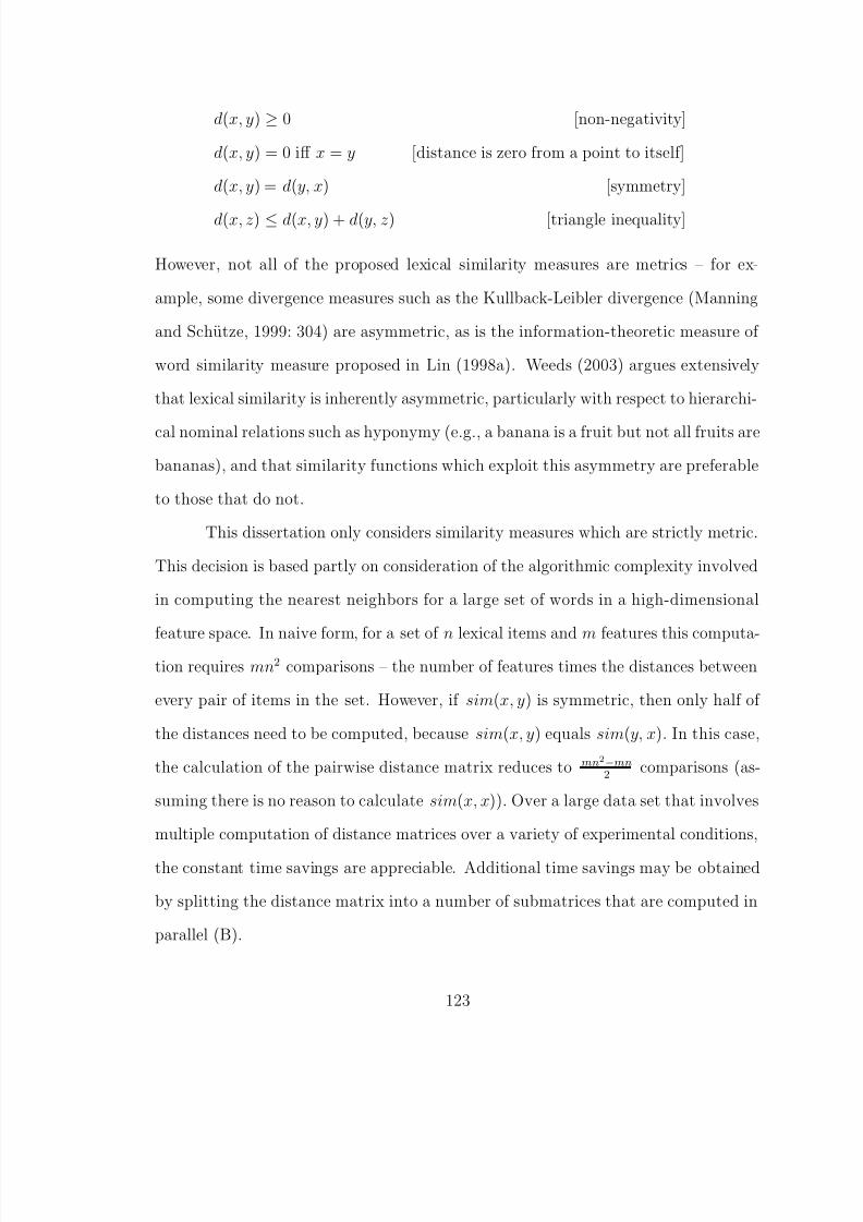
8/8/2019 Baker Kirk
http://slidepdf.com/reader/full/baker-kirk 139/243
d(x, y) ≥ 0 [non-negativity]
d(x, y) = 0 iff x = y [distance is zero from a point to itself]
d(x, y) = d(y, x) [symmetry]
d(x, z) ≤ d(x, y) + d(y, z) [triangle inequality]
However, not all of the proposed lexical similarity measures are metrics – for ex-
ample, some divergence measures such as the Kullback-Leibler divergence (Manning
and Schutze, 1999: 304) are asymmetric, as is the information-theoretic measure of
word similarity measure proposed in Lin (1998a). Weeds (2003) argues extensively
that lexical similarity is inherently asymmetric, particularly with respect to hierarchi-
cal nominal relations such as hyponymy (e.g., a banana is a fruit but not all fruits are
bananas), and that similarity functions which exploit this asymmetry are preferable
to those that do not.
This dissertation only considers similarity measures which are strictly metric.
This decision is based partly on consideration of the algorithmic complexity involved
in computing the nearest neighbors for a large set of words in a high-dimensional
feature space. In naive form, for a set of n lexical items and m features this computa-tion requires mn2 comparisons – the number of features times the distances between
every pair of items in the set. However, if sim(x, y) is symmetric, then only half of
the distances need to be computed, because sim(x, y) equals sim(y, x). In this case,
the calculation of the pairwise distance matrix reduces to mn2−mn
2 comparisons (as-
suming there is no reason to calculate sim(x, x)). Over a large data set that involves
multiple computation of distance matrices over a variety of experimental conditions,
the constant time savings are appreciable. Additional time savings may be obtained
by splitting the distance matrix into a number of submatrices that are computed in
parallel (B).
123
8/8/2019 Baker Kirk
http://slidepdf.com/reader/full/baker-kirk 140/243
However, the primary reason that we restrict ourselves to similarity (distance)
metrics has to do with the difficulty of applying clustering or classification techniques
when sim(x, y) = sim(y, x). In order to deal with this confound previous researchers
have adopted a variety of strategies for converting asymmetric measures into de facto
metrics. For example, Lin (1998a, c) proposes an asymmetric measure of similarity,
and considers two words w1 and w2 neighbors if and only if the maximally similar
neighbor of w1 is w2, and the maximally similar neighbor of w2 is w1. Using skew
divergence, Brew and Schulte im Walde (2002) computes similarity in both directions
and takes the larger of sim(w1, w2),sim(w2, w1) as the measure of two words’ similar-
ity. Information radius (Section 5.6.3.1) takes the average similarity between ( w1, w2)
and (w2, w1). Although we are not averse to the claim that lexical similarity is in-
herently asymmetric, we do not explicitly adopt this approach here for the reasons
outlined above.
The various lexical similarity metrics can be grouped into classes according
to their conceptualization of the computation of similarity. Although the distinction
blurs in practice, this dissertation groups similarity measures into three classes – set-
theoretic, geometric, and information-theoretic – each of which is discussed in the
following sections.
5.6.1 Set-Theoretic Similarity Measures
Set-theoretic measures conceive of similarity between items on the basis of the cardi-
nality of shared versus unshared features. In their basic instantiation, these measures
are based solely on the concept of set membership, meaning that the number of times
a feature occurs with a target word does not contribute to the measure of similar-
ity (although numerous frequency-weighted variants have been proposed (e.g., Curran
124

8/8/2019 Baker Kirk
http://slidepdf.com/reader/full/baker-kirk 141/243
and Moens, 2002)). Most set-theoretic similarity measures consider the ratio of shared
features to some combination of shared and unshared features.
5.6.1.1 Jaccard’s Coefficient
Jaccard’s coefficient is defined as the ratio of the intersection of two feature sets to
their union (Manning and Schutze 1999: 299, Table 8.7; Weeds 2003: 3.1.3.1 and
references therein):
|A ∩ B|
|A ∪ B|
5.6.1.2 Dice’s Coefficient
Dice’s coefficient is similar to Jaccard’s coefficient, but takes the total number of
elements as the denominator. Multiplying by 2 scales the measure to [0 , 1]:
2|A ∩ B|
|A| + |B|
Dice’s coefficient and Jaccard’s coefficient are monotonically equivalent3 in terms
of the relative similarities they assign to a group of objects (Evert, 2000; Weeds,
2003). However, similarity drops off faster with Jaccard’s coefficient than with Dice’s
coefficient. Dice’s coefficient penalizes a small number of shared features less than
Jaccard’s coefficient does (Manning and Schutze, 1999: 299), and in general assigns
higher similarity scores than Jaccard’s coefficient.
3Jaccard = Dice
2−Dice
125
8/8/2019 Baker Kirk
http://slidepdf.com/reader/full/baker-kirk 142/243
5.6.1.3 Overlap Coefficient
The overlap coefficient measures the ratio of the intersection of two sets to the mini-
mum cardinality of those sets (Manning and Schutze, 1999: 299, Table 8.7):
|A ∩ B|
min(|A|, |B|)
The overlap coefficient has a value of 1 if either set is a subset of the other, and a
value of 0 if no entries are shared between the two sets.
5.6.1.4 Set Cosine
The set cosine is defined as the ratio of the intersection of two sets to the square root
of the product of their cardinality (Manning and Schutze, 1999: 299, Table 8.7):
|A ∩ B| |A| × |B|
The set cosine is identical to Dice’s coefficient for sets with the same number of
elements (Manning and Schutze, 1999: 299), but penalizes less when the cardinality
of the sets is very different (i.e, because of the square root in the denominator).
5.6.2 Geometric Similarity Measures
Geometric measures express similarity in terms of the distance between points or the
angle between vectors and as such assume an underlying real-valued geometric space.
Within this framework features represent the dimensions of the space and the number
of features determines its dimensionality. In general, the value of each dimension for a
given item contains a count of how many times that feature occurred with the target
126

8/8/2019 Baker Kirk
http://slidepdf.com/reader/full/baker-kirk 143/243
item. Some scaling procedure is typically applied to count vectors before similarity
is computed.
5.6.2.1 L1 Distance
L1 distance (variously called Manhattan distance, city block distance, or taxicab
distance among others) represents the distance between two points traveling only in
orthogonal directions (i.e., walking around the block without taking any shortcuts).
It can be computed as
ni=1
|xi − yi|
5.6.2.2 L2 Distance
L2 distance, more widely known as Euclidean distance, yields the straight line distance
between two points. It can be calculated as
ni=1
(xi − yi)2
If only the rank ordering is import, the square root can be treated as a constant and
removed. L1 and L2 distance are particular instances of the more general class of the
generalized Lm or Minkowski distance measure (Black, 2006), defined as
ni=1
|xi − yi|m 1
m
127
8/8/2019 Baker Kirk
http://slidepdf.com/reader/full/baker-kirk 144/243
Both measures are widely used in computing distributional lexical similarity (Weeds,
2003: 48). L2 distance is more sensitive to large differences in the number of non-
zero elements between two vectors, because it squares differences in each dimension,
and for some applications is less effective than L1 distance (Weeds, 2003: 48, and
references therein).
5.6.2.3 Cosine
In its geometric interpretation, the cosine measure returns the cosine of the angle
between two vectors. The cosine is equivalent to the normalized correlation coeffi-
cient (i.e., Pearson’s product moment correlation coefficient) (Manning and Schutze,1999: 300), and as such is a measure of similarity rather than distance. The cosine is
bounded between [-1,1]; when applied to vectors whose elements are all greater than
or equal to zero, it is bounded between [0,1] with 1 being identity and 0 being orthog-
onal vectors. The cosine of the angle between real-valued vectors can be calculated
as (Manning and Schutze, 1999: 300, (8.40))
ni=1 xiyi ni=1 x2i
ni=1 y2i
The set cosine (Section 5.6.1.4) is equivalent to applying the above definition of cosine
to binary vectors. In general, real valued vectors result in the term in the denominator
being larger, so that the value of cosine based on real-valued vectors tend to be smaller
than the corresponding binary measure.
5.6.2.4 General Comparison of Geometric Measures
In general, differences in ranking produced by the various distance measures are influ-
enced by how differences in values along shared and unshared features are calculated.
128
8/8/2019 Baker Kirk
http://slidepdf.com/reader/full/baker-kirk 145/243
For example, in calculating cosine, corresponding elements between two vectors are
multiplied; L1 distance subtracts corresponding elements and L2 squares the difference
between corresponding elements. In large, sparse feature spaces, it is often the case
that an element with a non-zero value in one vector has a corresponding value of zero
in another vector. For cosine, these differences essentially cancel out because of the
multiplication by zero. For L1 and L2, larger differences between vectors accumulate
along these unshared dimensions.
Because of the normalization factor in its denominator, cosine is invariant
to constant scalings of a vector, e.g., it returns the same score for a vector of raw
counts as for unit vectors or probability vectors. Weightings which alter the ratio of
values within a vector such as binary, log-likelihood, etc., impact the assignment of
rankings given by cosine. Euclidean and L1 distance are sensitive to all weightings
of the data in that they do not contain a normalization factor. For unit vectors,
Euclidean(x, y) = 2(1 − cos(x, y)), so the order of proximities coincide (Manning and
Schutze, 1999: 301).
5.6.3 Information Theoretic Similarity Measures
Information theoretic measures assume an underlying probability space, and are based
on a comparison of two probability distributions. For example, the relative entropy
(also known as Kullback-Leibler divergence, information gain, among others) of two
probability mass functions p and q is defined as (Manning and Schutze, 1999: 72,
(2.41))
D( p||q) =i
pilog piqi
129

8/8/2019 Baker Kirk
http://slidepdf.com/reader/full/baker-kirk 146/243
and measures the average number of bits (when log = log2) required to express events
drawn from distribution p in terms of q. D( p||q) ranges from [0, ∞] when 0log 0q
≡ 0
and plog p0 ≡ ∞. However, this is problematic when applied to the sparse vectors
typically associated with distributions of lexical co-occurrences, because zeros in one
distribution or the other are so common that nearly everything ends up with a distance
of ∞. Furthermore, D( p||q) is asymmetric, doubling the necessary computation
of a pairwise distance matrix and requiring some further decision when D( p||q) =
D(q|| p). One option for producing a symmetric version of relative entropy is to use
a variant known as Jensen-Shannon divergence or information radius.
5.6.3.1 Information Radius
Information radius is defined as (Lin, 1991)
IRad( p,q) = D p|| p + q
2
+ Dq|| p + q
2
=i
pilogpi
12 pi +
12qi
+i
qilogqi
12 pi +
12qi
and overcomes two problems with using relative entropy in a sparse vector space.
First, it is symmetric, and second, because we are not interested in events which have
zero probability under both p and q, pi + qi is greater than zero, and pi+q
i
2 > 0
which eliminates the problem of division by zero. Information radius ranges from 0
for identical distributions to 2log2 for maximally different distributions, and measures
the amount of information lost if two words represented by p and q are described by
their average distribution (Manning and Schutze, 1999: 304).
Although information radius is the only information theoretic measure con-
sidered in this dissertation, nothing in practice prevents vector space measures from
being applied to probability vectors. For example, applying cosine to probability
130
8/8/2019 Baker Kirk
http://slidepdf.com/reader/full/baker-kirk 147/243
vectors yields results identical to those obtained for vectors scaled by any other con-
stant factor (e.g., unit vectors, which have been normalized to have vector length 1).
When L1 distance is applied to probability vectors, the result can be interpreted as
the expected proportion of events that differ between p and q (Manning and Schutze,
1999: 305).
5.7 Feature Weighting
The basic representation of words as a distribution of lexical co-occurrences is a vector
whose elements are counts of the number of times features f 1, . . . , f n occurred in the
context of target word wi. The assumption is that the frequency with which certainsubsets of features co-occur with particular groups of words is an indication of those
words’ lexical similarity. However, using raw co-occurrence counts is not the most ef-
fective method of weighting features (Manning and Schutze, 1999: 542), because gross
differences in the frequency of two target words can overwhelm subtler distributional
patterns. Therefore, feature weighting schemes which rely on some transformation of
the original frequency counts are used. We divide these transformation schemes into
two classes: intrinsic feature transformations, which use only frequency information
which is contained in an individual target word’s vector, and extrinsic feature trans-
formations, which consider the distribution of a feature over all of the target words
in addition to its local frequency information.
5.7.1 Intrinsic Feature Weighting
5.7.1.1 Binary Vectors
The simplest feature weighting scheme is to disregard all frequency information and
replace co-occurrence counts with a binary indication of presence versus absence.
131
8/8/2019 Baker Kirk
http://slidepdf.com/reader/full/baker-kirk 148/243
This is the distributional representation assumed by set theoretic measures of lexical
similarity 5.6.1.
5.7.1.2 Vector Length Normalization
A common transformation procedure is to convert a vector to a unit vector, which is
done by dividing every element in the vector by the length of the vector, defined as
|x| =
ni=1
x2i
A unit vector has unit length according to the Euclidean norm
|x| =ni=1
x2i = 1
Working with unit vectors yields a couple of useful properties. The cosine of two unit
vectors is equal to their dot product
cos(x,y) = x · y
=ni=1
xiyi
which provides for an efficient calculation of the cosine and gives the same ranking
as the Euclidean distance metric when applied to unit vectors with no values smaller
than 0.
5.7.1.3 Probability Vectors
Converting a vector of counts to a vector of probabilities is done by dividing every
element in the vector by the sum of all elements in the vector.
132
8/8/2019 Baker Kirk
http://slidepdf.com/reader/full/baker-kirk 149/243
Other intrinsic transformation procedures are available; for example in Latent
Semantic Analysis, a vector is scaled by the entropy of the vector (Landauer, Foltz,
and Laham, 1998). However, constant scalings of a vector do not change the relative
ordering of similarities produced by the measures considered in this dissertation, with
the exception of L1 and L2 distance.
5.7.2 Extrinsic Feature Weighting
Extrinsic feature weighting schemes try to capture the strength of the association be-
tween a feature and a target word relative to all of the target words. The assumption
is that a feature that occurs very frequently with a small set of target words is impor-tant and should be weighted more highly than a feature that occurs frequently with
all of the target words. Numerous approaches have been described, and many of these
are summarized in Curran and Moens (2002) and Weeds (2003). This dissertation
considers three representative ones.
5.7.2.1 Correlation
Rohde, Gonnerman, and Plaut (submitted) propose a feature weighting method based
on the strength of the correlation between a word a and a feature b, defined as (Rohde
et al., submitted: 3, (Table 4)):
w′a,b =
T wa,b− j wa,j ·
iwi,b
( j wa,j · (T −
j wa,j) ·
iwi,b · (T −
iwi,b))
1
2
T =i j
wi,j
The intuition behind using correlation to weight features is that the conditional rate
of co-occurrence is more useful than raw co-occurrence. Correlation addresses the
133
8/8/2019 Baker Kirk
http://slidepdf.com/reader/full/baker-kirk 150/243
question of whether feature f occurs more or less often in the context of word w
than it does in general (Rohde et al., submitted: 6). Values of features weighted by
correlation are in [−1, 1]. Following Rohde et al. (submitted), we eliminate features
that are negatively correlated with a word on the basis of their observation that
retaining negatively correlated features hurts performance.
Rohde et al. (submitted) find that correlation outperforms other weighting
schemes for modeling human word pair similarity judgments and Li and Brew (2008)
also reports success using correlation as a feature weight in an automatic classification
study of Levin verbs.
5.7.2.2 Inverse Feature Frequency
Inverse feature frequency is a family of weighting schemes taken from the field of
information retrieval which are characterized by term co-occurrence weights, docu-
ment frequency weights, and a scaling component (Manning and Schutze, 1999: 543).
We adapt the scheme defined in Manning and Schutze (1999: 543, (15.5)) for use in
distributional lexical similarity:
1 + log(freq(f, w))log W words(f )
if freq(f, w) ≥ 1
0 if freq(f, w) = 0
where freq(f, w) is the number of times feature f occurs with word w, W is the total
number words, and words(f ) is the number of words that f occurs with.
134

8/8/2019 Baker Kirk
http://slidepdf.com/reader/full/baker-kirk 151/243
5.7.2.3 Log Likelihood
A third approach to feature weighting is based on hypothesis testing, where the
strength of the relation between a word and a feature is expressed in terms of the ex-
tent to which their co-occurrence is greater than chance. A number of parametric sta-
tistical tests have been applied to the task of identifying above-chance co-occurrences,
notably the t-test (e.g., Church and Hanks, 1989) and Pearson’s χ2 test (e.g., Church
and Gale, 1991).
Dunning (1993) introduced the log-likelihood ratio (G-test) as an alternative
to the χ2 test that is more appropriate for sparse data that violates the assumption of
normality. Like the χ2 test, the log-likelihood ratio can be applied to a contingency
table like Table 5.4, and measures the ratio of the frequency observed in a cell to the
Word ¬WordFeature a b a + b
¬Feature c d c + da + c b + d N = a + b + c + d
Table 5.4: An example contingency table used for computing the log-likelihood ratio
expected frequency of that cell if the null hypothesis is true.
The general formula for G is (Wikipedia, 2008)
G = 2i
Oi · lnOi
E i
135
8/8/2019 Baker Kirk
http://slidepdf.com/reader/full/baker-kirk 152/243
which can be calculated in terms of Table 5.4 as (Rayson, Berridge, and Francis,
2004: 929)
G = 2(alna + blnb + clnc + dlnd + N lnN −
(a + b)ln(a + b) − (a + c)ln(a + c) − (b + d)ln(b + d) − (c + d)ln(c + d)).
5.8 Feature Selection
Automatic lexical acquisition tasks that take data from large corpora have to deal with
an enormous number of potential features – on the order of hundreds of thousands
to millions. Of this potential feature set, a small fraction provides nearly all of its
discriminatory power, meaning that most of the feature do no work at all or even
obscure potential patterns of relatedness. Therefore, it is common or even necessary
to eliminate features that are not expected to contribute to the desired classification.
All feature reduction techniques rely in their core on frequency information
contained in the feature set. The simplest reduction technique is to apply a frequency
threshold to the feature set. An alternative to this relies on class-conditional frequen-
cies, and a third choice, dimensionality reduction, indirectly incorporates frequency
information into a matrix approximation of the original feature set.
5.8.1 Frequency Threshold
Applying a frequency threshold to a data set simply means removing any items that
occur less than a specified number of times. In the early days of statistical NLP (i.e.,
the early 1990’s), a frequency cutoff was applied more because of physical storage
and processing limitations than anything else. There is no principled justification for
choosing a particular cutoff value; however, the intuitive justification is that extremely
136
8/8/2019 Baker Kirk
http://slidepdf.com/reader/full/baker-kirk 153/243
low frequency features provide little or no generalizability and should be discarded
to improve some downstream processing. For example, a feature that occurs only
one time with one word in the whole data set does not relate to any other item in
the data set, and retaining it only serves to increase the distance between all points.
This reasoning extends from 1 to some arbitrary cutoff. Because of the frequency
distribution of words in language, where there are a few high frequency items, more
medium frequency items, and lots of low frequency items (e.g., Zipf’s law; Manning
and Schutze, 1999: 24), relatively low frequency thresholds can drastically reduce the
size of a lexical feature set.
5.8.2 Conditional Frequency Threshold
A similar approach to feature selection uses class-conditional frequency information
to order features by their ability to partition the data set into the desired classes.
For example, the ID3 technique for constructing a decision tree (e.g., Quinlan, 1986)
selects features with the highest information gain, which is defined in terms of the
reduction of entropy achieved by splitting on that feature (Dunham, 2003: 97-98).
The Rainbow text classifier (McCallum, 1996) provides a similar utility for selecting
features with the highest class-conditional average mutual information.
Other statistical techniques for data reduction in general and feature selection
in particular include class-based correlation and covariance (Richeldi and Rossotto,
1997). However, all of these techniques rely on prior knowledge of class assignments
for their computation, and therefore may not be applicable in machine learning set-
tings where class labels are either unknown or, as in the case of determining a word’s
nearest lexical neighbors, irrelevant.
137
8/8/2019 Baker Kirk
http://slidepdf.com/reader/full/baker-kirk 154/243

8/8/2019 Baker Kirk
http://slidepdf.com/reader/full/baker-kirk 155/243
CHAPTER 6
EXPERIMENTS ON DISTRIBUTIONAL VERB SIMILARITY
This chapter describes a series of experiments that deal with various aspects of as-
signing and assessing lexical similarity scores to a set of English verbs on the basis
of their distributional context in the English gigaword corpus. These experiments
simultaneously varied four parameters that influence distributional lexical similarity
with respect to five different verb classification schemes. The verb classifications con-
sidered were Levin (1993), VerbNet, FrameNet, Roget’s Thesaurus, and WordNet.
The parameters considered were choice of feature set, measure of lexical similarity,
feature weighting, and feature selection. The purpose of this series of experiments
is to examine interactions between these parameters with respect to the five verb
schemes mentioned above and described in Chapter 5.
The remainder of this chapter is organized as follows. Section 6.1 describes the
set of verbs and corpus used in the experiments. Section 6.2 describes two measures
for evaluating distributional lexical similarity used in the experiments. Section 6.3
discusses the feature sets and procedures for extracting features from the corpus.
Section 6.4 describes the experiments performed.
139
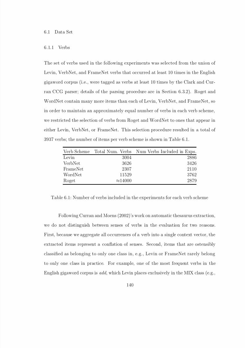
8/8/2019 Baker Kirk
http://slidepdf.com/reader/full/baker-kirk 156/243
6.1 Data Set
6.1.1 Verbs
The set of verbs used in the following experiments was selected from the union of
Levin, VerbNet, and FrameNet verbs that occurred at least 10 times in the English
gigaword corpus (i.e., were tagged as verbs at least 10 times by the Clark and Cur-
ran CCG parser; details of the parsing procedure are in Section 6.3.2). Roget and
WordNet contain many more items than each of Levin, VerbNet, and FrameNet, so
in order to maintain an approximately equal number of verbs in each verb scheme,
we restricted the selection of verbs from Roget and WordNet to ones that appear ineither Levin, VerbNet, or FrameNet. This selection procedure resulted in a total of
3937 verbs; the number of items per verb scheme is shown in Table 6.1.
Verb Scheme Total Num. Verbs Num Verbs Included in Exps.Levin 3004 2886VerbNet 3626 3426FrameNet 2307 2110WordNet 11529 3762
Roget ≈14000 2879
Table 6.1: Number of verbs included in the experiments for each verb scheme
Following Curran and Moens (2002)’s work on automatic thesaurus extraction,
we do not distinguish between senses of verbs in the evaluation for two reasons.
First, because we aggregate all occurrences of a verb into a single context vector, the
extracted items represent a conflation of senses. Second, items that are ostensibly
classified as belonging to only one class in, e.g., Levin or FrameNet rarely belong
to only one class in practice. For example, one of the most frequent verbs in the
English gigaword corpus is add , which Levin places exclusively in the MIX class (e.g.,
140

8/8/2019 Baker Kirk
http://slidepdf.com/reader/full/baker-kirk 157/243
combine, join, link, merge, etc.). However, in the English gigaword corpus, this verb
is used most often as a synonym for say (e.g., “I don’t think I’ll really fully realize
the impact until I swear in,” Bush added.), and FrameNet places it exclusively in
the STATEMENT class. Because of the recognized difficulties in establishing an
inventory of senses for verbs in particular and words in general (e.g., Manning and
Schutze, 1999: 229-231), we conflated senses in the verb schemes and defined items
as neighbors as follows.
1. Levin, VerbNet, FrameNet: two items are neighbors if the intersection of the
classes they belong to is non-empty; e.g., they share at least one sense which
puts them in the same class. For example, for VerbNet link ∈ {MIX, TAPE}
and harness ∈ {BUTTER, TAPE} are neighbors because {MIX, TAPE} ∩
{BUTTER, TAPE} = {TAPE}.
2. Roget, WordNet: two words are neighbors if either is listed as a synonym of the
other.
Table 6.2 shows the average number of neighbors per verb in our study for
each of the verb schemes using these criteria. Table 6.3 contains the baselines that
Levin VerbNet FrameNet Roget WordNetMean (Std. Dev.) 86.3 (85.0) 103.5 (120.5) 40.4 (41.9) 31.9 (20.1) 12.6 (10.9)Max 513 669 248 185 76Median 49 48 23 39 10Min 2 1 1 4 1
Table 6.2: Average number of neighbors per verb for each of the five verb schemes
indicate the chance that two verbs in our study selected at random are neighbors.
For all five schemes, the baseline is less than 3%.
141
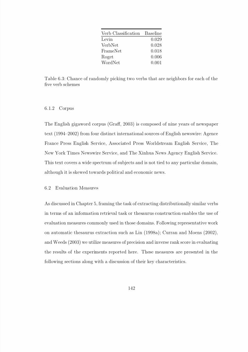
8/8/2019 Baker Kirk
http://slidepdf.com/reader/full/baker-kirk 158/243
Verb Classification BaselineLevin 0.029VerbNet 0.028FrameNet 0.018Roget 0.006
WordNet 0.001
Table 6.3: Chance of randomly picking two verbs that are neighbors for each of thefive verb schemes
6.1.2 Corpus
The English gigaword corpus (Graff, 2003) is composed of nine years of newspaper
text (1994–2002) from four distinct international sources of English newswire: Agence
France Press English Service, Associated Press Worldstream English Service, The
New York Times Newswire Service, and The Xinhua News Agency English Service.
This text covers a wide spectrum of subjects and is not tied to any particular domain,
although it is skewed towards political and economic news.
6.2 Evaluation Measures
As discussed in Chapter 5, framing the task of extracting distributionally similar verbs
in terms of an information retrieval task or thesaurus construction enables the use of
evaluation measures commonly used in those domains. Following representative work
on automatic thesaurus extraction such as Lin (1998a); Curran and Moens (2002),
and Weeds (2003) we utilize measures of precision and inverse rank score in evaluating
the results of the experiments reported here. These measures are presented in the
following sections along with a discussion of their key characteristics.
142
8/8/2019 Baker Kirk
http://slidepdf.com/reader/full/baker-kirk 159/243
6.2.1 Precision
Following the methodologies for evaluating distributional lexical similarity reported
in, e.g., Lin (1998a), Curran and Moens (2002), and Weeds (2003), one evaluation
measure that we report here is precision at k, where k is a fixed, usually low level
of retrieved results. We report precision at k for k = 1, 5, 10. However, Manning
et al. (2008: 148) point out that the highest point on the precision recall curve can
be of no less interest than mean single point summaries such as F1, R-precision,
or mean average precision. For the purposes of comparing feature sets and distance
measures across verb schemes, we report microaveraged maximum precision (MaxP),
defined as the point on the precision recall curve at which precision is the highest.
We compute maximum precision for each individual verb and report the average of
these values. It is always the case in our study that the trends reported for MaxP
also hold for k = 1, 5, 10.
When precision is high and k is relatively large, this indicates that many same
class items are clustered within the most highly ranked neighbors of a target verb
(e.g., appeal in Figure 6.1). Low precision values associated with large k indicatethat very few of the distributionally most similar items belong to the same class as
the target (enshrine in Figure 6.1). High precision and small k suggest that only
a few of the actual same-class items are contained within the set of highly ranked
empirical neighbors (reply in Figure 6.1), or that the size of the class is small. The
relative size of the class is shown in the precision curve by those portions of the curve
that jag upwards, indicating that a cluster of same-class items has been retrieved
at some lower value of k. However, precision alone does not account for the overall
distribution of matches within the ranked set of results. A measure that does a better
143
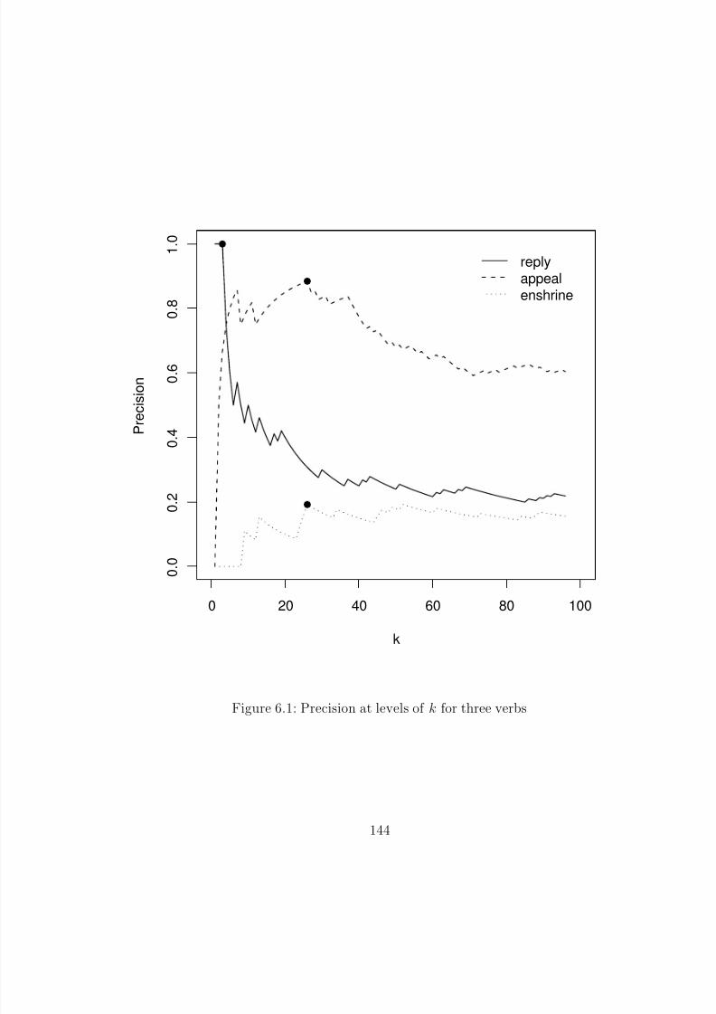
8/8/2019 Baker Kirk
http://slidepdf.com/reader/full/baker-kirk 160/243
0 20 40 60 80 100
0 . 0
0 . 2
0 . 4
0 . 6
0 . 8
1 . 0
k
P r e c
i s i o n
replyappealenshrine
Figure 6.1: Precision at levels of k for three verbs
144
8/8/2019 Baker Kirk
http://slidepdf.com/reader/full/baker-kirk 161/243
job of accounting for the relative positions of matches within the total set of results
is the inverse rank score.
6.2.2 Inverse Rank Score
Following Curran and Moens (2002); Gorman and Curran (2006), we also evaluate
distributional similarity in terms of inverse rank score, which is the sum of the inverse
of the rank of each same class item in the top ranked m items:
InvR =mk=1
xkk
where xk is an indicator variable defined as
xk =
1 if the class of the kth item matches the target class
0 otherwise.
For example, if items at rank 2, 3, and 5 match the target class, the inverse rank
score is 1
2
+ 1
3
+ 1
5
= 1.03. In the experiments reported here, only the 100 most highly
ranked items were retained, so the maximum InvR score is 5.19. InvR is a useful
measure because it distinguishes between result lists that contain the same number of
same-class items but rank them differently. InvR assigns higher scores to result lists
in which same-class items are highly ranked. For example, a result list containing 5
matches at ranks 1, 2, 3, 5, 8 receives an InvR score of 2.16; another list containing
the same 5 items at rank 3, 4, 5, 6, 7 receives an InvR score of 1.09.
As with MaxP, discretion is required in interpreting InvR in the current
study. For example, if one word has five synonyms and another has ten synonyms,
and both sets are returned as the highest ranked items, the inverse rank score of
145

8/8/2019 Baker Kirk
http://slidepdf.com/reader/full/baker-kirk 162/243
the second word will be higher than the score for the first word without indicating a
difference in the quality of the ranked synonyms. Similarly, a word with many lowly
ranked synonyms can receive a higher InvR score than a word with only a few highly
ranked synonyms. For example, a word with only five synonyms ranked in positions
2–6 would receive an InvR score of 1.45; a word with eleven synonyms in positions
1, 15–24 would receive an InvR score of 1.48.
146
8/8/2019 Baker Kirk
http://slidepdf.com/reader/full/baker-kirk 163/243
Finally, because InvR is sensitive to the number of matched items, we cannot use it
to compare across verb schemes that assign different numbers of neighbors to each
verb. In this case, we only report measures of precision.
6.3 Feature Sets
This section describes the feature sets used here for assessing distributional verb sim-
ilarity1. We evaluated four different feature sets for their effectiveness in extracting
classes of distributionally similar verbs: Syntactic Frames, Labeled Dependency Rela-
tions, Unlabeled Dependency Relations, and Lexicalized Syntactic Frames. Syntactic
frames contain mainly syntactic information, whereas the other three feature setsencode varying combinations of lexical and syntactic information. Each of these fea-
ture types has been used extensively in previous research on automatic Levin verb
classification.
6.3.1 Description of Feature Sets
Syntactic Frames. Syntactic frames have been used extensively as features in early
work on automatic verb classification due to their relevance to the alternation be-
haviors which are crucial for Levin’s verb classification (e.g., Schulte im Walde, 2000;
Brew and Schulte im Walde, 2002; Schulte im Walde and Brew, 2002; Korhonen et al.,
2003). Syntactic frames provide a general feature set that can in principle be applied
to distinguishing any number of verb classes. However, using syntactic information
alone does not allow for the representation of semantic distinctions that are also rele-
vant in verb classification. Work in this area has been primarily concerned with verbs
taking noun phrase and prepositional phrase complements. To this end, prepositions
1Portions of Section 6.4.4 were co-authored with Jianguo Li.
147
8/8/2019 Baker Kirk
http://slidepdf.com/reader/full/baker-kirk 164/243
have played an important role in defining relevant syntactic frames. However, only
knowing the identity of prepositions is not always enough to represent the desired
distinctions.
For example, the semantic interpretation of the syntactic frame NP-V-PP(with )
depends to a large extent on the NP argument selected by the preposition with . In
(1), the same surface form NP-V-PP(with ) corresponds to three different underlying
meanings. However, such semantic distinctions are totally lost if lexical information
is disregarded.
(1) a. I ate with a fork . [INSTRUMENT]
b. I left with a friend . [ACCOMPANIMENT]
c. I sang with confidence. [MANNER]
Lexicalized Frames. This deficiency of unlexicalized subcategorization frames has
led researchers to incorporate lexical information into the feature representation. One
possible improvement over subcategorization frames is to enrich them with lexical
information. Lexicalized frames are usually obtained by augmenting each syntactic
slot with its head noun (2).
(2) a. I ate with a fork . [INSTRUMENT] → NP(I )-V-PP(with:fork )
b. I left with a friend . [ACCOMPANIMENT] → NP(I )-V-PP(with:friend )
c. I sang with confidence. [MANNER] → NP(I )-V-PP(with:confidence)
148

8/8/2019 Baker Kirk
http://slidepdf.com/reader/full/baker-kirk 165/243
The analysis of feature sets previously used in automatic verb classification suggests
that both syntactic and lexical information are relevant in determining meaning of
Levin verbs (e.g., Li and Brew, 2008). This agrees with the findings in previous
studies on WSD (Lee and Ng, 2002) that although syntactic information on its own
is not very informative in automatic word sense disambiguation, its combination with
lexical information results in improved disambiguation. The next two feature types
focus on various ways to mix syntactic and lexical information.
Dependency relations. Recall that subcategorization frames are limited as verb
features in the properties of verb behaviors they tap into. Lexicalized frames, with
potentially improved discriminatory power, suffer from increased exposure to data
sparsity. One way to overcome data sparsity is to break lexicalized frames into depen-
dency relations. Dependency relations contain both syntactic and lexical information
(3).
(3) a. SUBJ(I ), PP(with:fork )
b. SUBJ(I ), PP(with:friend )
c. SUBJ(I ), PP(with:confidence)
However, since we augment prepositional phrases with the head nouns selected by
prepositions, as in PP(with:fork ), the data sparsity problem still exists. We therefore
break all prepositional phrases in the form PP(preposition:noun) into two separate
dependency relations: PP(preposition) and PP-noun, as shown in (4).
(4) a. SUBJ(I ), PP(with ), PP- fork
b. SUBJ(I ), PP(with ), PP- friend
c. SUBJ(I ), PP(with ), PP-confidence
149
8/8/2019 Baker Kirk
http://slidepdf.com/reader/full/baker-kirk 166/243
Although dependency relations have proved effective in a range of lexical acquisition
tasks such as word sense disambiguation (McCarthy, Koeling, Weeds, and Carroll,
2004), construction of a lexical semantic space (Pado and Lapata, 2007), and detection
of polysemy (Lin, 1998a), their utility in automatic verb classification has not been
as thoroughly examined.
Unlabeled Dependency Relations. In order to further examine the separate
contributions of lexical and syntactic information, we removed the syntactic tag from
the labeled dependency relations, leaving a feature set that consists only of lexical
items that were selected on the basis of their structural relation to the verb. However,
the distinction between, e.g., Subject, Object, and Prepositional Object is no longer
explicitly represented in the unlabeled feature set. The representation of the examples
above using this feature set is shown in (5).
(5) a. I ate with a fork → {I, with, fork}
b. I left with a friend → {I, with, friend}
c. I sang with confidence → {I, with, confidence}
6.3.2 Feature Extraction Process
The experiments reported here used Clark and Curran’s (2007) CCG parser, a log-
linear parsing model for an automatically extracted lexicalized grammar, to automat-
ically extract the features described above from the English gigaword corpus (Graff,
2003). The lexicalized grammar formalism used by the parser is combinatory cate-
gorial grammar (CCG) (Steedman, 1987; Szabolcsi, 1992), and the grammar is auto-
matically extracted from CCGbank (Hockenmaier and Steedman, 2005). The parser
produces several output formats; we use grammatical relations (Briscoe, Carroll, and
150

8/8/2019 Baker Kirk
http://slidepdf.com/reader/full/baker-kirk 167/243
Watson, 2006) and employ a post-processing script to extract four types of grammat-
ical relations that are relevant to verbs: Subject-Type, Object-Type, Complement-
Type, and Modifier-Type.
The primary feature type that we extract from the parser’s output is lexicalized
syntactic frame. Syntactic frames are defined in terms of the syntactic constituents
used in the Penn Treebank (Marcus et al., 1993) style parse trees. For example, a
double object frame exemplified by a sentence like Sam handed Tom the flute can be
represented as NP1-V-NP2-NP3. A lexicalized syntactic frame augments the struc-
tural information represented by a syntactic frame with the lexical head of each
constituent, e.g., NP1(Sam )-V(hand )-NP2(Tom )-NP3( flute).
Extracting Subject-Type Relations. Table 6.4 illustrates the three types of
Subject-Type relations extracted from the parser’s output. The first column indi-
cates the relation, the second column contains and example of the relation, the third
column contains representative output from the parser, and the fourth column con-
tains the lexicalized frame that is extracted as a result of processing the parser’s
output.
Each relation is represented by the parser as a quadruple, with the first element
in the quadruple always containing the name of the relation. The order of the other
elements depends on the type of relation. For Subject-Type, the verb is always the
second element of the quadruple. Each lexical entry in the parser’s output is indexed
according to its position in the input sentence.
This index also points to each item’s position in a lemmatized, part-of-speech
tagged representation of the sentence that is also part of the parser’s output. In orderto extract features from the ncsubj relation, we combine the lemmatized form of the
verb with the lemmatized form of the third element in the quadruple. Similary, in or-
der to extract features from the xsubj and csubj relations, we combine the lemmatized
151
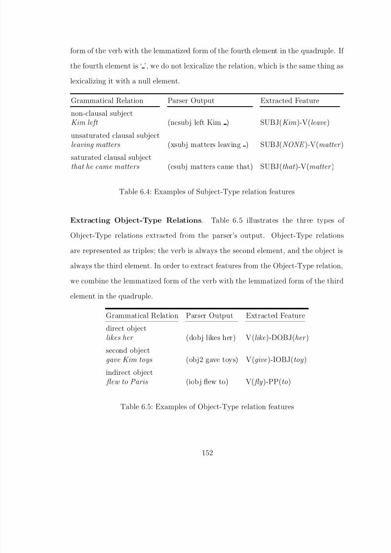
8/8/2019 Baker Kirk
http://slidepdf.com/reader/full/baker-kirk 168/243
form of the verb with the lemmatized form of the fourth element in the quadruple. If
the fourth element is ‘ ’, we do not lexicalize the relation, which is the same thing as
lexicalizing it with a null element.
Grammatical Relation Parser Output Extracted Feature
non-clausal subjectKim left (ncsubj left Kim ) SUBJ(Kim )-V(leave)
unsaturated clausal subjectleaving matters (xsubj matters leaving ) SUBJ(NONE )-V(matter )
saturated clausal subjectthat he came matters (csubj matters came that) SUBJ(that )-V(matter )
Table 6.4: Examples of Subject-Type relation features
Extracting Object-Type Relations. Table 6.5 illustrates the three types of
Object-Type relations extracted from the parser’s output. Object-Type relations
are represented as triples; the verb is always the second element, and the object is
always the third element. In order to extract features from the Object-Type relation,
we combine the lemmatized form of the verb with the lemmatized form of the third
element in the quadruple.
Grammatical Relation Parser Output Extracted Feature
direct objectlikes her (dobj likes her) V(like)-DOBJ(her )
second objectgave Kim toys (obj2 gave toys) V(give)-IOBJ(toy )
indirect object flew to Paris (iobj flew to) V( fly )-PP(to)
Table 6.5: Examples of Object-Type relation features
152
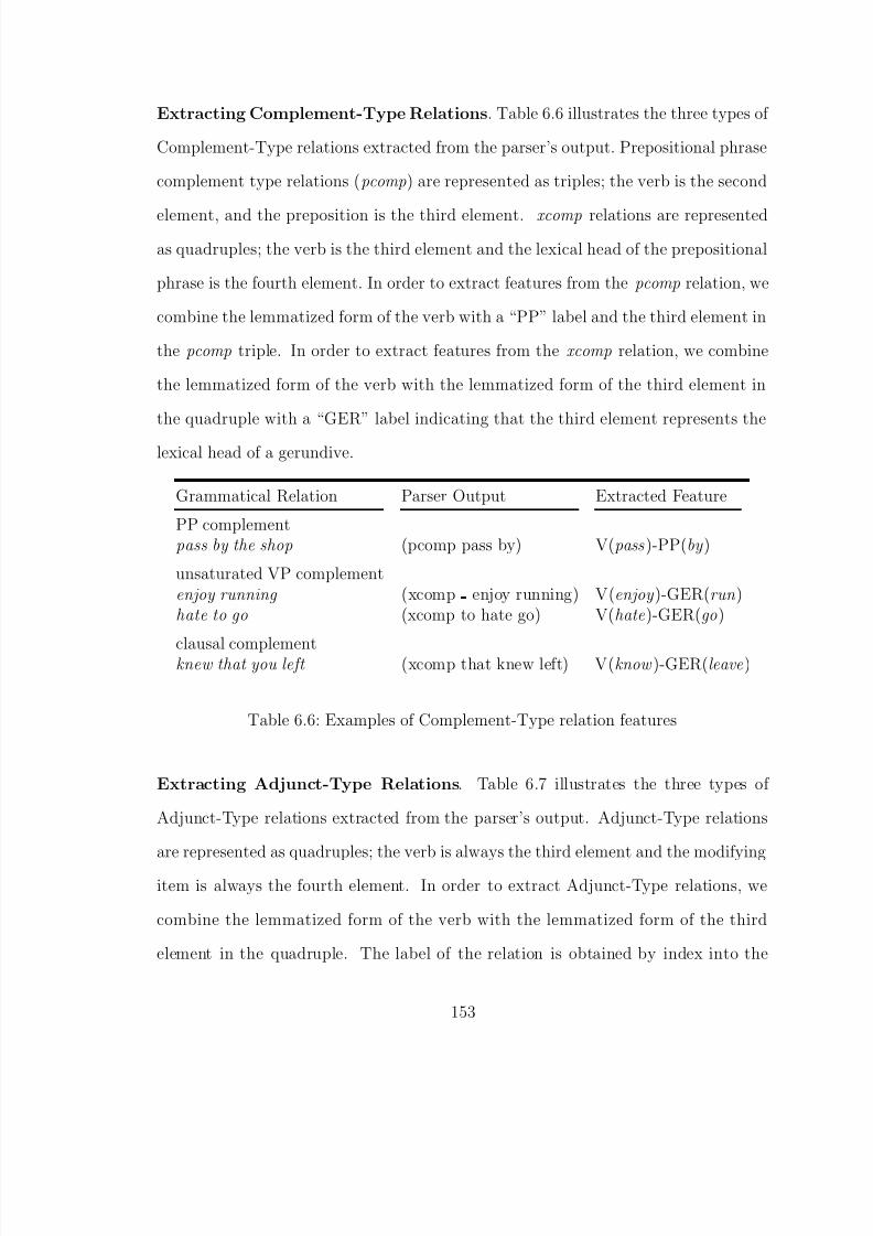
8/8/2019 Baker Kirk
http://slidepdf.com/reader/full/baker-kirk 169/243
Extracting Complement-Type Relations. Table 6.6 illustrates the three types of
Complement-Type relations extracted from the parser’s output. Prepositional phrase
complement type relations (pcomp) are represented as triples; the verb is the second
element, and the preposition is the third element. xcomp relations are represented
as quadruples; the verb is the third element and the lexical head of the prepositional
phrase is the fourth element. In order to extract features from the pcomp relation, we
combine the lemmatized form of the verb with a “PP” label and the third element in
the pcomp triple. In order to extract features from the xcomp relation, we combine
the lemmatized form of the verb with the lemmatized form of the third element in
the quadruple with a “GER” label indicating that the third element represents the
lexical head of a gerundive.
Grammatical Relation Parser Output Extracted Feature
PP complementpass by the shop (pcomp pass by) V(pass)-PP(by )
unsaturated VP complementenjoy running (xcomp enjoy running) V(enjoy )-GER(run )hate to go (xcomp to hate go) V(hate)-GER(go)
clausal complementknew that you left (xcomp that knew left) V(know )-GER(leave)
Table 6.6: Examples of Complement-Type relation features
Extracting Adjunct-Type Relations. Table 6.7 illustrates the three types of
Adjunct-Type relations extracted from the parser’s output. Adjunct-Type relations
are represented as quadruples; the verb is always the third element and the modifying
item is always the fourth element. In order to extract Adjunct-Type relations, we
combine the lemmatized form of the verb with the lemmatized form of the third
element in the quadruple. The label of the relation is obtained by index into the
153
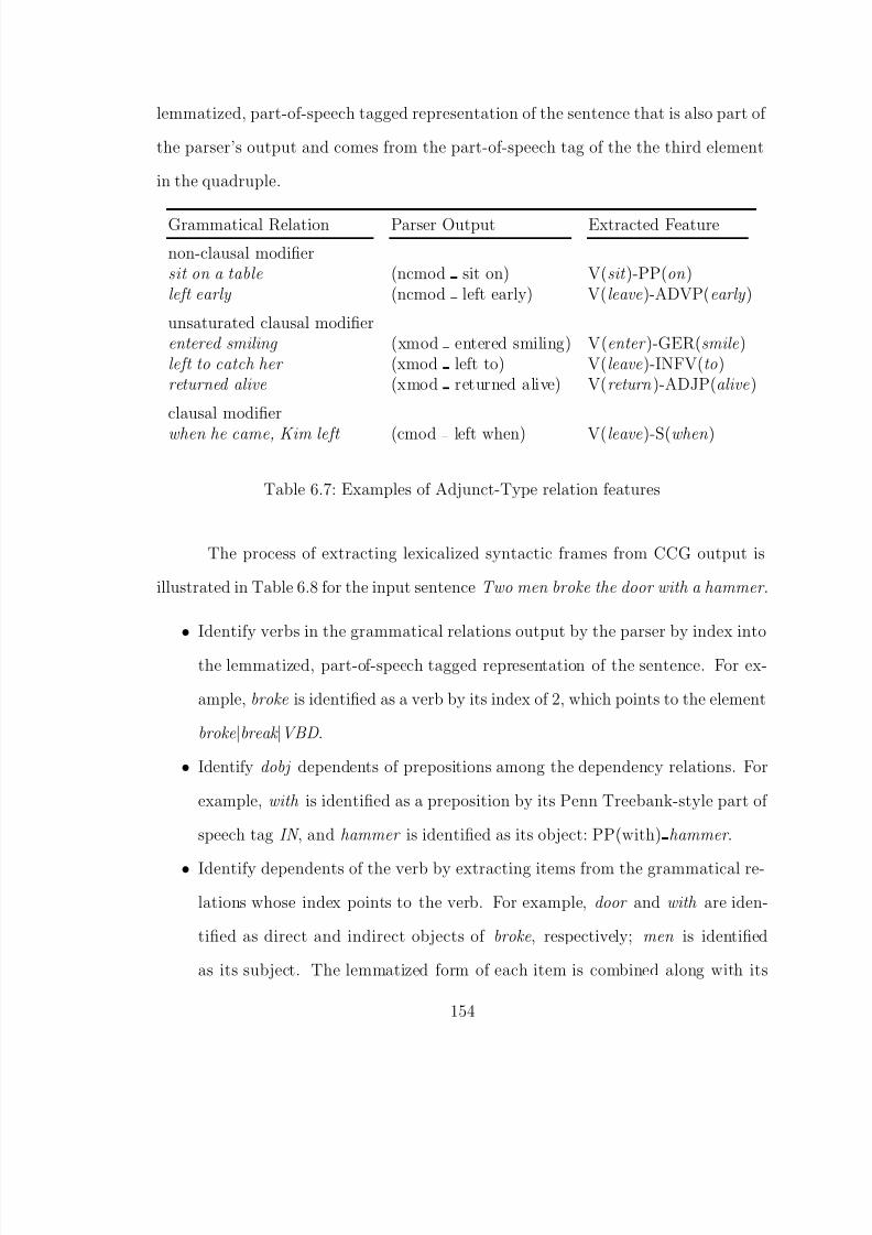
8/8/2019 Baker Kirk
http://slidepdf.com/reader/full/baker-kirk 170/243
lemmatized, part-of-speech tagged representation of the sentence that is also part of
the parser’s output and comes from the part-of-speech tag of the the third element
in the quadruple.
Grammatical Relation Parser Output Extracted Feature
non-clausal modifiersit on a table (ncmod sit on) V(sit )-PP(on )left early (ncmod left early) V(leave)-ADVP(early )
unsaturated clausal modifierentered smiling (xmod entered smiling) V(enter )-GER(smile)left to catch her (xmod left to) V(leave)-INFV(to)returned alive (xmod returned alive) V(return )-ADJP(alive)
clausal modifier
when he came, Kim left (cmod left when) V(leave)-S(when )
Table 6.7: Examples of Adjunct-Type relation features
The process of extracting lexicalized syntactic frames from CCG output is
illustrated in Table 6.8 for the input sentence Two men broke the door with a hammer .
• Identify verbs in the grammatical relations output by the parser by index into
the lemmatized, part-of-speech tagged representation of the sentence. For ex-
ample, broke is identified as a verb by its index of 2, which points to the element
broke|break |VBD .
• Identify dobj dependents of prepositions among the dependency relations. For
example, with is identified as a preposition by its Penn Treebank-style part of
speech tag IN , and hammer is identified as its object: PP(with) hammer .
• Identify dependents of the verb by extracting items from the grammatical re-
lations whose index points to the verb. For example, door and with are iden-
tified as direct and indirect objects of broke, respectively; men is identified
as its subject. The lemmatized form of each item is combined along with its
154
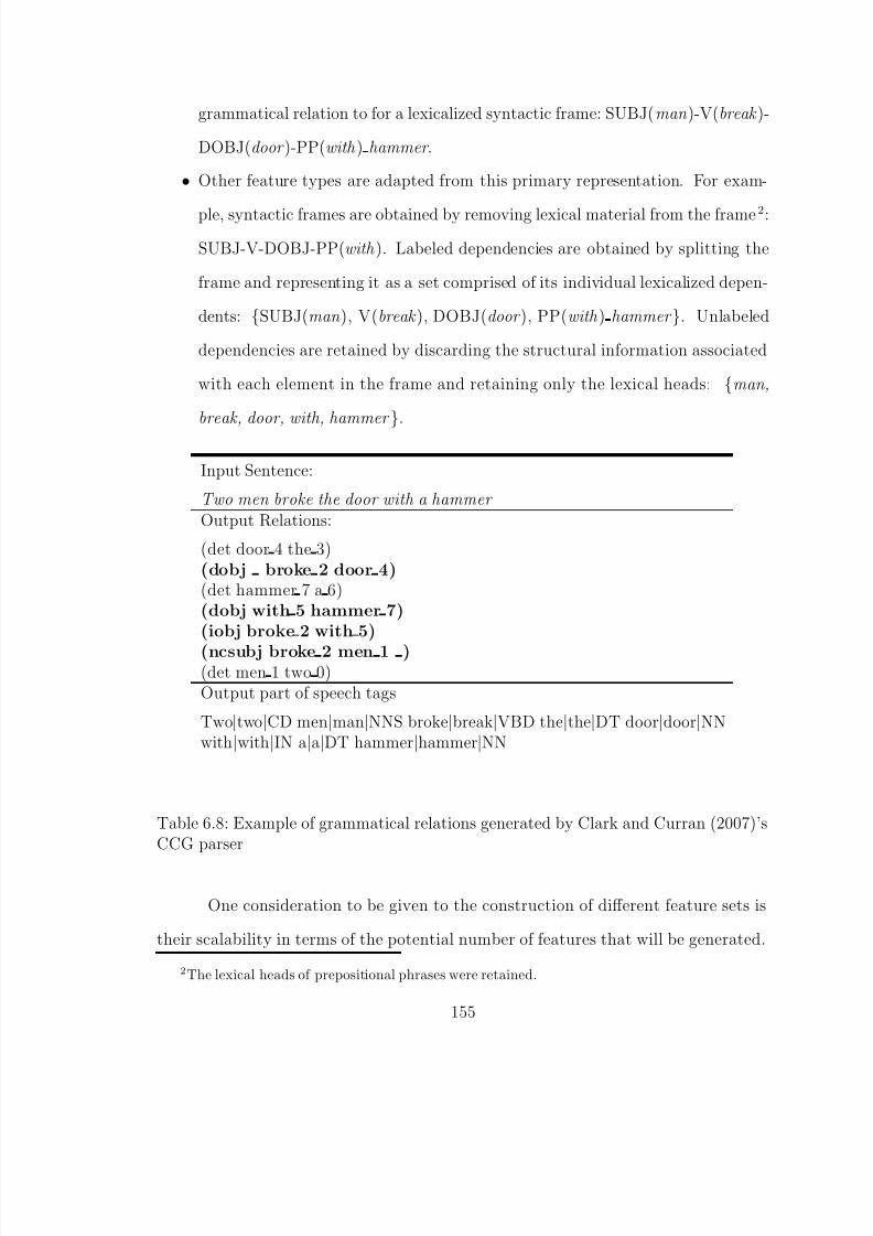
8/8/2019 Baker Kirk
http://slidepdf.com/reader/full/baker-kirk 171/243
grammatical relation to for a lexicalized syntactic frame: SUBJ(man )-V(break )-
DOBJ(door )-PP(with ) hammer .
• Other feature types are adapted from this primary representation. For exam-
ple, syntactic frames are obtained by removing lexical material from the frame2
:
SUBJ-V-DOBJ-PP(with ). Labeled dependencies are obtained by splitting the
frame and representing it as a set comprised of its individual lexicalized depen-
dents: {SUBJ(man ), V(break ), DOBJ(door ), PP(with ) hammer }. Unlabeled
dependencies are retained by discarding the structural information associated
with each element in the frame and retaining only the lexical heads: {man,
break, door, with, hammer }.
Input Sentence:
Two men broke the door with a hammer Output Relations:
(det door 4 the 3)(dobj broke 2 door 4)(det hammer 7 a 6)(dobj with 5 hammer 7)(iobj broke 2 with 5)
(ncsubj broke 2 men 1 )(det men 1 two 0)Output part of speech tags
Two|two|CD men|man|NNS broke|break|VBD the|the|DT door|door|NNwith|with|IN a|a|DT hammer|hammer|NN
Table 6.8: Example of grammatical relations generated by Clark and Curran (2007)’sCCG parser
One consideration to be given to the construction of different feature sets is
their scalability in terms of the potential number of features that will be generated.
2The lexical heads of prepositional phrases were retained.
155

8/8/2019 Baker Kirk
http://slidepdf.com/reader/full/baker-kirk 172/243
The main motivation for using a large corpus like the English gigaword corpus is that
relatively infrequent items may still be attested often enough to allow generalizations
that would not be possible using a smaller resource. A potential downside of using
such a large corpus is the bulk of data that will be generated and must be processed.
Most similarity metrics run in time linear to the number of non-zero elements in two
vectors being compared. Therefore, the more features, the longer the run time for
finding nearest neighbors. Figure 6.2 shows the increase in the number of features
as a function of the number of verb instances encountered in the English gigaword
corpus.
Number of Instances
N u m
b e r o
f F e a
t u r e s
10^3
10^4
10^5
10^6
10^7
10^4 10^5 10^6 10^7 10^8
SyntaxLexLexSynFrames
Figure 6.2: Feature growth rate on a log scale
156
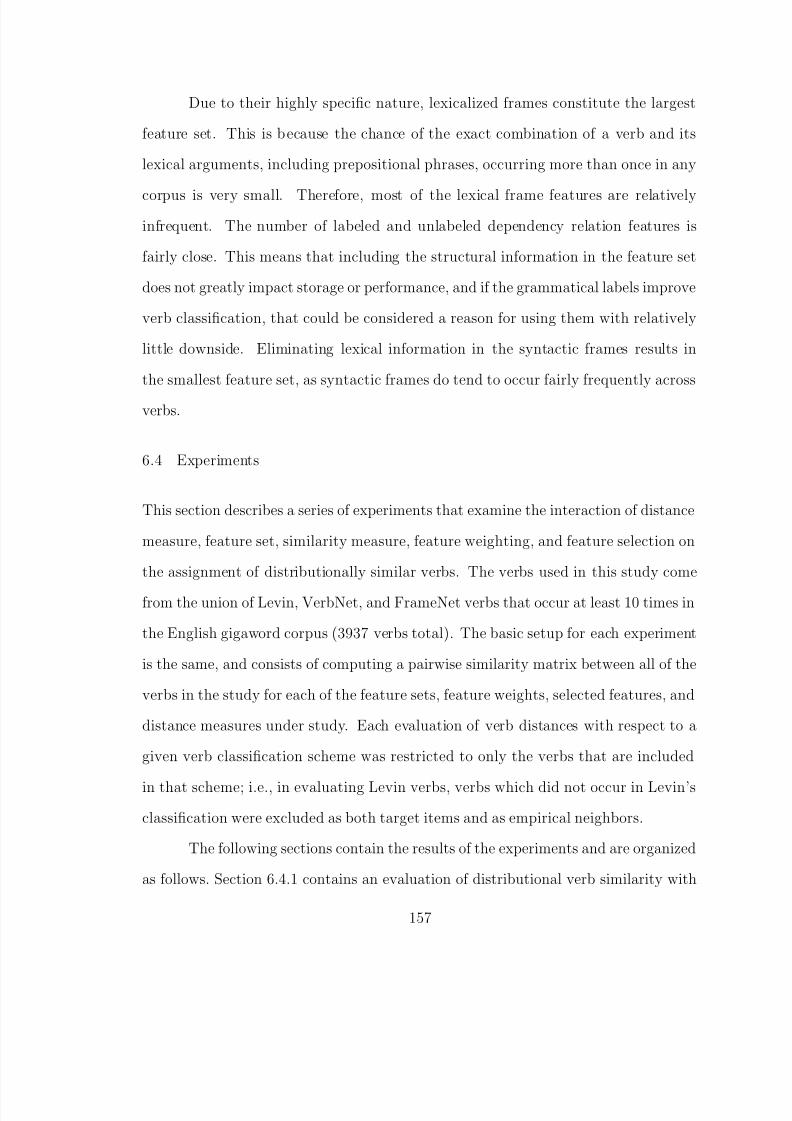
8/8/2019 Baker Kirk
http://slidepdf.com/reader/full/baker-kirk 173/243
Due to their highly specific nature, lexicalized frames constitute the largest
feature set. This is because the chance of the exact combination of a verb and its
lexical arguments, including prepositional phrases, occurring more than once in any
corpus is very small. Therefore, most of the lexical frame features are relatively
infrequent. The number of labeled and unlabeled dependency relation features is
fairly close. This means that including the structural information in the feature set
does not greatly impact storage or performance, and if the grammatical labels improve
verb classification, that could be considered a reason for using them with relatively
little downside. Eliminating lexical information in the syntactic frames results in
the smallest feature set, as syntactic frames do tend to occur fairly frequently across
verbs.
6.4 Experiments
This section describes a series of experiments that examine the interaction of distance
measure, feature set, similarity measure, feature weighting, and feature selection on
the assignment of distributionally similar verbs. The verbs used in this study come
from the union of Levin, VerbNet, and FrameNet verbs that occur at least 10 times in
the English gigaword corpus (3937 verbs total). The basic setup for each experiment
is the same, and consists of computing a pairwise similarity matrix between all of the
verbs in the study for each of the feature sets, feature weights, selected features, and
distance measures under study. Each evaluation of verb distances with respect to a
given verb classification scheme was restricted to only the verbs that are included
in that scheme; i.e., in evaluating Levin verbs, verbs which did not occur in Levin’s
classification were excluded as both target items and as empirical neighbors.
The following sections contain the results of the experiments and are organized
as follows. Section 6.4.1 contains an evaluation of distributional verb similarity with
157
8/8/2019 Baker Kirk
http://slidepdf.com/reader/full/baker-kirk 174/243
respect to the choice of distance measure. Section 6.4.2 evaluates the effect of feature
weighting on distributional verb similarity. Section 6.4.3 compares the different verb
schemes described early with respect to how well their respective classifications match
distributionally similar verbs, and Section 6.4.4 compares feature sets.
6.4.1 Similarity Measures
The purpose of this analysis is to examine the performance of different distance mea-
sures on identifying distributionally similar verbs. Three types of distance measure
– set theoretic, geometric, and information theoretic – are compared across verb
schemes and feature sets. For each type of distance measure only one feature weight-ing was employed: the set theoretic measures were applied to binary feature vectors,
the geometric distance measures were applied to vector-length normalized count vec-
tors, and the information theoretic measures were applied to count vectors normalized
to probabilities.
6.4.1.1 Set Theoretic Similarity Measures
Table 6.9 contains the precision results of the nearest neighbor classifications for three
set theoretic measures of distributional similarity, using the 50,000 most frequently
occurring features of each feature type. The full set of precision results using a range
of feature frequencies is given in Appendix C, Figures C.1 – C.5. Table F.1 (Appendix
F) contains the corresponding inverse rank scores.
Overall, for MaxP cosine returned the best results across feature types and
verb classifications (MaxP = 0.43); Jaccard’s coefficient performed close to cosine
(MaxP = 0.40), and overlap performed substantially lower (MaxP = 0.10). Similarly
for InvR, cosine gave the overall best results (InvR= 0.81), followed by Jaccard’s
158

8/8/2019 Baker Kirk
http://slidepdf.com/reader/full/baker-kirk 175/243
Verb Classification Feature Type Distance Measure Meancosine Jaccard overlap
Levin Syntactic Frame 0.40 0.39 0.14 0.31Lexical 0.50 0.47 0.08 0.35
Dep. Triple 0.57 0.56 0.10 0.41Lex. Frame 0.49 0.48 0.11 0.36
Mean 0.49 0.48 0.11
VerbNet Syntactic Frame 0.38 0.38 0.15 0.30Lexical 0.48 0.45 0.08 0.34Dep. Triple 0.55 0.53 0.10 0.39Lex. Frame 0.48 0.46 0.11 0.35
Mean 0.47 0.46 0.11
FrameNet Syntactic Frame 0.36 0.35 0.09 0.27
Lexical 0.48 0.44 0.07 0.33Dep. Triple 0.54 0.51 0.10 0.38Lex. Frame 0.49 0.46 0.11 0.35
Mean 0.47 0.44 0.09
Roget Syntactic Frame 0.28 0.27 0.06 0.20Lexical 0.52 0.47 0.08 0.36Dep. Triple 0.61 0.53 0.10 0.41Lex. Frame 0.54 0.49 0.11 0.38
Mean 0.49 0.44 0.09
WordNet Syntactic Frame 0.13 0.12 0.04 0.10Lexical 0.23 0.20 0.06 0.17Dep. Triple 0.28 0.25 0.11 0.22Lex. Frame 0.24 0.22 0.10 0.19
Mean 0.22 0.20 0.08
Table 6.9: Average maximum precision for set theoretic measures and the 50k mostfrequent features of each feature type
coefficient (InvR= 0.74) and overlap (InvR= 0.23). In terms of verb scheme, focusing
just on the cosine measure, Roget, Levin, VerbNet, and FrameNet perform nearly
identically (MaxP≈0.48), followed by WordNet at MaxP = 0.22.
159
8/8/2019 Baker Kirk
http://slidepdf.com/reader/full/baker-kirk 176/243
For MaxP, the best performing feature type across verb scheme and distance
measure is lexically specified dependency triples. Again focusing on the cosine, across
verb schemes dependency triples return around 0.51 maximum precision, followed
by unlabeled dependents and lexicalized frames MaxP≈0.44, and finally syntactic
frames (MaxP≈0.31). These trends are mirrored in the InvR results.
6.4.1.2 Geometric Measures
Table 6.10 contains the MaxP results of the nearest neighbor classifications for three
geometric measures of distributional similarity, using the 50,000 most frequently oc-
curring features of each feature type. The context vectors were vectors of counts,normalized by vector length. The full set of MaxP results using a range of feature
frequencies are given in Appendix D, figures D.1 – D.5. Table F.2 (Appendix F)
contains results of the geometric measures as evaluated by InvR.
Overall, the neighbors assigned by cosine similarity (mean MaxP = 0.35;
mean InvR = 0.63) resemble the given verb classifications more than the neighbors
assigned by L1 distance (mean MaxP = 0.25; InvR=0.41) for both evaluation mea-
sures. In terms of feature type, for MaxP frame-based features did not perform as
well as lexical-based features for either distance measure. For cosine, labeled and
unlabeled lexical dependents performed at a very similar rate across verb schemes
(mean MaxP = 0.40 for lexical-only versus mean MaxP = 0.39 for labeled depen-
dency triples). These trends are mirrored in the InvR results.
For L1, the difference between lexical-only and labeled dependency triples
was more pronounced: MaxP = 0.33 versus MaxP = 0.23, respectively. These
trends are mirrored in the InvR results. This difference is likely due to the fact
that the labeled dependency triples form a relatively sparser feature space than the
unlabeled feature space and differences in how the two measures handle zeros when
160
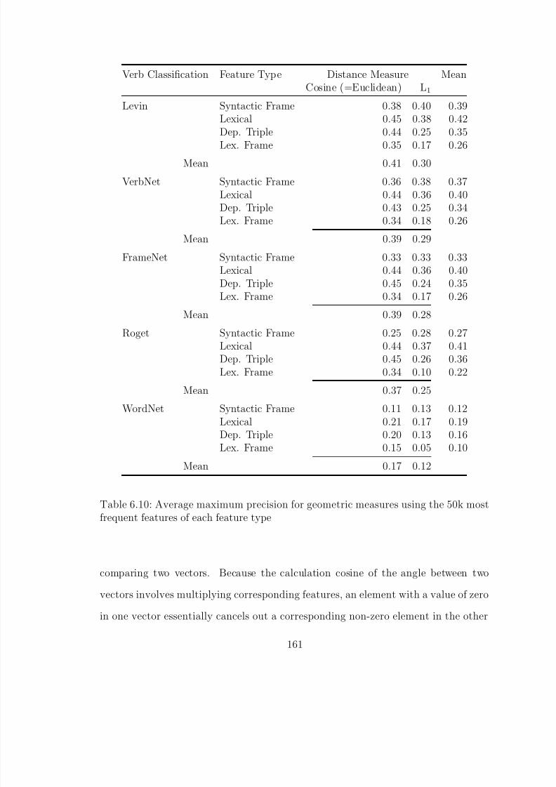
8/8/2019 Baker Kirk
http://slidepdf.com/reader/full/baker-kirk 177/243
Verb Classification Feature Type Distance Measure MeanCosine (=Euclidean) L1
Levin Syntactic Frame 0.38 0.40 0.39Lexical 0.45 0.38 0.42
Dep. Triple 0.44 0.25 0.35Lex. Frame 0.35 0.17 0.26
Mean 0.41 0.30
VerbNet Syntactic Frame 0.36 0.38 0.37Lexical 0.44 0.36 0.40Dep. Triple 0.43 0.25 0.34Lex. Frame 0.34 0.18 0.26
Mean 0.39 0.29
FrameNet Syntactic Frame 0.33 0.33 0.33
Lexical 0.44 0.36 0.40Dep. Triple 0.45 0.24 0.35Lex. Frame 0.34 0.17 0.26
Mean 0.39 0.28
Roget Syntactic Frame 0.25 0.28 0.27Lexical 0.44 0.37 0.41Dep. Triple 0.45 0.26 0.36Lex. Frame 0.34 0.10 0.22
Mean 0.37 0.25
WordNet Syntactic Frame 0.11 0.13 0.12Lexical 0.21 0.17 0.19Dep. Triple 0.20 0.13 0.16Lex. Frame 0.15 0.05 0.10
Mean 0.17 0.12
Table 6.10: Average maximum precision for geometric measures using the 50k mostfrequent features of each feature type
comparing two vectors. Because the calculation cosine of the angle between two
vectors involves multiplying corresponding features, an element with a value of zero
in one vector essentially cancels out a corresponding non-zero element in the other
161
8/8/2019 Baker Kirk
http://slidepdf.com/reader/full/baker-kirk 178/243
vector. For L1, a zero element is subtracted from the corresponding non-zero element,
and larger differences accumulate along the many zero dimensions. In a sparse space
with many zeros, differences along non-shared dimensions overwhelm similarity along
shared dimensions. Since the labeled and unlabeled dependency triples represent
much of the same contextual information, but the ambient space is slightly denser for
the unlabeled triples, L1 distance performs better in that space, while the cosine is
relatively unaffected.
Using geometric measures of similarity, Levin verbs are picked up slightly
more often than the other classes, with MaxP of 0.41 versus MaxP = 0.39 for
VerbNet and FrameNet. Roget verbs are identified slightly less often at MaxP =
0.37, while WordNet synonyms are relatively unlikely to appear in the top-ranked set
of distributionally similar verbs (MaxP = 0.17).
6.4.1.3 Information Theoretic Measures
Table 6.11 contains the results of the nearest neighbor classifications for two informa-
tion theoretic measures of distributional similarity, using the 50,000 most frequently
occurring features of each feature type. The context vectors were vectors of proba-
bilities of counts. When L1 distance is applied to vectors of probabilities, the result
can be interpreted as the expected proportion of events that differ between the two
probability distribution (Manning and Schutze, 1999: 305), and is included here for
comparison. The full set of results using a range of feature frequencies are given in
Appendix E, figures E.1 – E.5. Table F.3 (Appendix F) contains the corresponding
inverse rank scores.
Overall, information radius and L1 distance performed similarly across feature
types and verb schemes for both MaxP and InvR (MaxPinforad = 0.45; MaxPL1 =
0.44; InvRinforad = 0.81; InvRL1 = 0.87).
162
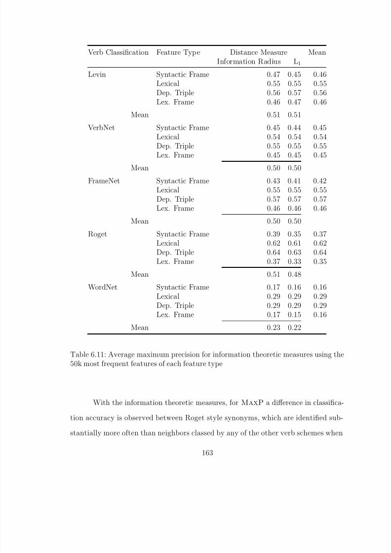
8/8/2019 Baker Kirk
http://slidepdf.com/reader/full/baker-kirk 179/243
Verb Classification Feature Type Distance Measure MeanInformation Radius L1
Levin Syntactic Frame 0.47 0.45 0.46Lexical 0.55 0.55 0.55
Dep. Triple 0.56 0.57 0.56Lex. Frame 0.46 0.47 0.46
Mean 0.51 0.51
VerbNet Syntactic Frame 0.45 0.44 0.45Lexical 0.54 0.54 0.54Dep. Triple 0.55 0.55 0.55Lex. Frame 0.45 0.45 0.45
Mean 0.50 0.50
FrameNet Syntactic Frame 0.43 0.41 0.42
Lexical 0.55 0.55 0.55Dep. Triple 0.57 0.57 0.57Lex. Frame 0.46 0.46 0.46
Mean 0.50 0.50
Roget Syntactic Frame 0.39 0.35 0.37Lexical 0.62 0.61 0.62Dep. Triple 0.64 0.63 0.64Lex. Frame 0.37 0.33 0.35
Mean 0.51 0.48
WordNet Syntactic Frame 0.17 0.16 0.16Lexical 0.29 0.29 0.29Dep. Triple 0.29 0.29 0.29Lex. Frame 0.17 0.15 0.16
Mean 0.23 0.22
Table 6.11: Average maximum precision for information theoretic measures using the50k most frequent features of each feature type
With the information theoretic measures, for MaxP a difference in classifica-
tion accuracy is observed between Roget style synonyms, which are identified sub-
stantially more often than neighbors classed by any of the other verb schemes when
163
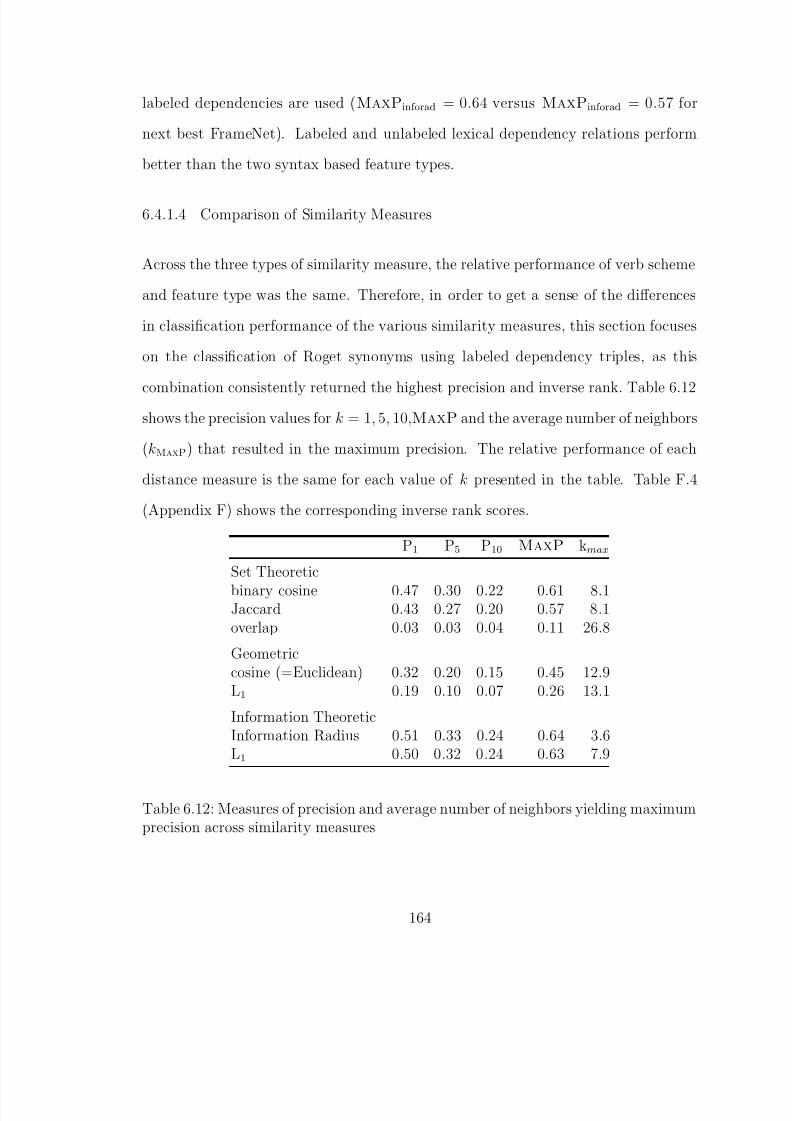
8/8/2019 Baker Kirk
http://slidepdf.com/reader/full/baker-kirk 180/243
labeled dependencies are used (MaxPinforad = 0.64 versus MaxPinforad = 0.57 for
next best FrameNet). Labeled and unlabeled lexical dependency relations perform
better than the two syntax based feature types.
6.4.1.4 Comparison of Similarity Measures
Across the three types of similarity measure, the relative performance of verb scheme
and feature type was the same. Therefore, in order to get a sense of the differences
in classification performance of the various similarity measures, this section focuses
on the classification of Roget synonyms using labeled dependency triples, as this
combination consistently returned the highest precision and inverse rank. Table 6.12shows the precision values for k = 1, 5, 10,MaxP and the average number of neighbors
(kMaxP) that resulted in the maximum precision. The relative performance of each
distance measure is the same for each value of k presented in the table. Table F.4
(Appendix F) shows the corresponding inverse rank scores.
P1 P5 P10 MaxP kmax
Set Theoretic
binary cosine 0.47 0.30 0.22 0.61 8.1Jaccard 0.43 0.27 0.20 0.57 8.1overlap 0.03 0.03 0.04 0.11 26.8
Geometriccosine (=Euclidean) 0.32 0.20 0.15 0.45 12.9L1 0.19 0.10 0.07 0.26 13.1
Information TheoreticInformation Radius 0.51 0.33 0.24 0.64 3.6L1 0.50 0.32 0.24 0.63 7.9
Table 6.12: Measures of precision and average number of neighbors yielding maximumprecision across similarity measures
164
8/8/2019 Baker Kirk
http://slidepdf.com/reader/full/baker-kirk 181/243
Several trends are evident from the data in Tables 6.12 and F.4. First, overlap
performs substantially worse than any of the other distance measures. Secondly,
binary cosine, information radius, and L1 have very similar MaxP values. From this
point of view, binary cosine can be considered an information theoretic measure in
the sense that it is computing the correlation between two distributions of numbers,
and the fact that it is applied to binary vectors can be considered a particular feature
weighting scheme. That is, the calculation of cosine does not change when it is applied
to binary vectors, only the feature weighting.
Although binary cosine, information radius, and L1 distance all achieve the
same average maximum precision, they do so at different values of k. Information
radius tops out with k around 3.6, while binary cosine and L1 are between 8.1 and 7.6.
Pairwise t-tests, adjusted for multiple comparisons, show that on average, information
radius tops out significantly earlier than binary cosine and L1 distance, which are not
significantly different from each other. This means that although the precision is the
same, L1 distance returns just under twice as many actual neighbors as information
radius does for the same precision. For k = 1, 5, 10, the three measures are nearly
equal.
The geometric measures, i.e., cosine and L1 applied to normalized count vec-
tors, return lower precision values than the information theoretic measures do. How-
ever, whereas the feature weighting for set theoretic and information theoretic mea-
sures is fixed at {0,1} and Prob(f ), respectively, many other feature weightings are
available to which the more general geometric measures can be applied. The next
section considers the effect of feature weighting on the performance of geometric sim-ilarity measures.
165

8/8/2019 Baker Kirk
http://slidepdf.com/reader/full/baker-kirk 182/243
6.4.2 Feature Weighting
This section considers six feature weighting schemes and their interaction with lexical
similarity measures. Three of the weightings (binary, normalized, and probabilities),
were considered in the context of comparing distance measures. The other three, log-
likelihood, correlation, and inverse feature frequency, are introduced into this study
here. The three distance measures considered are cosine, Euclidean distance, and L1
distance.
Within verb schemes and across feature sets, the relative performance of the
different feature weighting schemes remained constant. Overall, labeled dependency
triples performed the best, followed by unlabeled triples, lexicalized frames, and syn-
tactic frames.
Tables 6.13 and F.6 show precision results for verb classifications using labeled
dependency triples. Across verb schemes, the trends between feature weight and
distance measure hold fairly consistently. Overall, the best performing combination
of feature weight and distance measure was achieved by applying the cosine to vectors
weighted by inverse feature frequency: 58% of the 1-nearest neighbors computed withthis combination are classified as synonyms by Roget’s thesaurus, with a maximum
precision of 71%. This combination performed the best for the other verb schemes as
well, ranging from MaxP = 63% for Levin to MaxP = 34% for WordNet.
In terms of the interactions between feature weight and distance measure, the
following tendencies are observed. For Euclidean distance, the following ranking of
feature weights in terms of precision approximately holds:
normalized > probability > iff > binary, log-likelihood, correlation
166

8/8/2019 Baker Kirk
http://slidepdf.com/reader/full/baker-kirk 183/243
Feature Weighting Distance MeasureCosine Euclidean L1
P1 MaxP kmax P1 MaxP kmax P1 MaxP kmax
Levin binary 0.43 0.57 8.8 0.19 0.29 7.7 0.19 0.29 7.7probability 0.31 0.44 12 0.28 0.40 14 0.43 0.57 9.5normalized 0.31 0.44 12 0.31 0.44 12 0.17 0.25 9.9
log-likelihood 0.44 0.58 8.9 0.19 0.29 7.8 0.19 0.29 7.8correlation 0.38 0.55 10 0.20 0.27 6.4 0.10 0.15 5.6inv feat freq 0.49 0.63 7.7 0.27 0.38 6.1 0.19 0.28 6.4
VerbNet binary 0.43 0.55 10 0.19 0.29 9.5 0.19 0.29 9.5probability 0.30 0.43 14 0.27 0.39 15 0.41 0.55 11normalized 0.30 0.43 14 0.30 0.43 14 0.17 0.25 14log-likelihood 0.41 0.56 10 0.19 0.30 9.1 0.19 0.29 9.1correlation 0.37 0.54 11 0.22 0.29 7.1 0.12 0.16 6.3inv feat freq 0.47 0.62 8.8 0.27 0.38 7.1 0.19 0.29 8.2
FrameNet binary 0.41 0.54 7.7 0.18 0.28 4.3 0.18 0.26 4.3probability 0.33 0.45 10 0.29 0.40 11 0.45 0.58 8.7normalized 0.33 0.45 10 0.33 0.45 10 0.18 0.24 9.2log-likelihood 0.42 0.55 7.6 0.17 0.26 4.3 0.17 0.26 4.3correlation 0.42 0.57 7.6 0.16 0.22 2.3 0.02 0.06 2.6
inv feat freq 0.49 0.61 6.8 0.27 0.36 3.5 0.18 0.26 3.7Roget binary 0.47 0.61 8.1 0.19 0.25 4.9 0.19 0.25 4.9
probability 0.32 0.45 12.9 0.29 0.42 14.2 0.50 0.63 7.9normalized 0.32 0.45 12.9 0.32 0.45 12.9 0.19 0.26 13.1log-likelihood 0.48 0.62 7.7 0.19 0.26 3.7 0.19 0.26 3.7correlation 0.43 0.60 8.6 0.19 0.24 5.9 0.03 0.04 2.8inv feat freq 0.58 0.71 6.1 0.28 0.35 3.5 0.19 0.24 3.0
WordNet binary 0.19 0.28 10 0.08 0.12 5.4 0.08 0.12 5.4probability 0.13 0.20 12 0.12 0.19 13 0.21 0.29 9.6normalized 0.13 0.20 12 0.13 0.20 12 0.09 0.13 9.9log-likelihood 0.19 0.29 10 0.07 0.12 4.8 0.08 0.12 4.8correlation 0.18 0.28 11 0.08 0.11 4.8 0.01 0.03 3.2inv feat freq 0.24 0.34 9.3 0.11 0.16 4.7 0.08 0.11 4.7
Table 6.13: Nearest neighbor average maximum precision for feature weighting, usingthe 50k most frequent features of type labeled dependency triple
For Euclidean distance, the tendency for normalized vectors to produce better neigh-
bors can be explained by the fact that Euclidean distance is quadratic in the un-
shared terms; normalized vectors exhibit the smallest absolute feature values of the
six weights considered, so these differences will be minimized.
167
8/8/2019 Baker Kirk
http://slidepdf.com/reader/full/baker-kirk 184/243
Interestingly, inverse feature frequency performs better than the other three
weights although the average feature weight is much larger than for binary, log-
likelihood, or correlation. This suggests that inverse feature frequency does a better
job of capturing the relevance of the association between a verb and a feature than
log-likelihood or correlation.
For L1 distance, the following ranking of feature weights holds:
probability ≫ binary, log-likelihood, iff > normalized ≫ correlation
Probability vectors outperform any of the other weighting methods by a substan-
tial margin (nearly 2:1), lending credence to its interpretation as a measure of the
difference between probability distributions. The differences between binary, log-
likelihood, and inverse feature frequency were slight and varied unpredictably across
verb schemes. Once again, weighting by correlation performed poorly.
For cosine, the following ranking of feature weights was found:
iff > log-likelihood, binary, correlation ≫ normalized, probability
In this combination, inverse feature frequency returned appreciably better results
across the verb schemes. As with Euclidean distance, binary feature weights perform
just as well as log-likelihood and correlation, which in turn outperform normal vector
scalings.
These results indicate that two ingredients are needed for successful nearest
neighbor identification of verbs. One is an extrinsic weighting method which models
the relative strength of the association between a verb and a feature as a function of
both co-occurrence frequency and its proclivity to occur with other verbs. The second
consideration is an appropriate scaling of the magnitude of the feature weights. In
168

8/8/2019 Baker Kirk
http://slidepdf.com/reader/full/baker-kirk 185/243

8/8/2019 Baker Kirk
http://slidepdf.com/reader/full/baker-kirk 186/243
to distributionally similar verb assignments than its stricter definitions of synonymy.
Exploring these more finely grained lexical distinctions is left for future research.
Levin, VerbNet, and FrameNet place verbs into classes based on both simi-
larity in meaning and similarity along more schematic representations of syntactic
or semantic behavior such as alternations (Levin, VerbNet) or participation in se-
mantic frames (FrameNet). In an effort to tease apart the independent criteria of
semantic and syntactic similarity, we can look at the proportion of items in a class
that are independently classified as synonyms by a thesaurus, and compare this to
the proportion of empirical neighbors that are either synonyms or not by the same
standard.
The left column in Table 6.14 shows the average number of synonyms that are
found within a verb class for Levin, VerbNet, and FrameNet.
Verb Scheme %Synonyms in Class %Synonyms in k-nn
k = 1 5 10Levin 23 71 57 48VerbNet 23 73 58 50FrameNet 38 76 65 56
Table 6.14: Average number of Roget synonyms per verb class
This number was calculated from the number of same class items that are
listed as synonyms in Roget’s online thesaurus; i.e., on average 23% of a Levin verb’s
neighbors are recognized as synonyms by the thesaurus. The right column shows
the average percentage of empirically determined 1-nearest neighbors that are also
synonyms. For example, of the empirically determined 1-nearest neighbors that are
put into the same class by Levin, 71% turn out to be synonyms by Roget’s thesaurus;
this figure is slightly higher for VerbNet and FrameNet. This means that when highly
similar Levin-style neighbors are identified empirically, they are over three times more
170
8/8/2019 Baker Kirk
http://slidepdf.com/reader/full/baker-kirk 187/243
likely to be synonyms than would be expected based on the prior class probability
of being synonyms; similarly for VerbNet. The fact that a greater percentage of
FrameNet verbs are synonyms is to be expected given that FrameNet emphasizes
semantic relatedness and does not explicitly include participation in syntactic alter-
nations as a criterion for partitioning verbs into classes (Baker, Fillmore, and Lowe,
1998; Baker and Ruppenhofer, 2002). Also apparent in Table 6.14 is the fact that
as k increases, the number of synonyms decreases for all three verb schemes. Again
this points to the interpretation that highly distributionally similar items are likely
to be synonyms, and that the additional grouping criteria used Levin, VerbNet, and
FrameNet are not represented as well using the feature sets examined here.
The upshot of this analysis is that regardless of the four feature sets applied
here, distributionally similar verbs assignments correspond to thesaurus style syn-
onyms more than they correspond to the groupings in Levin, VerbNet, and FrameNet.
As noted above, distributionally similar verbs do not correspond well to WordNet’s
more restrictive definitions of synonymy. This is most likely due to the fact that
WordNet is conservative in assigning synonymy to verbs, and makes subtler lexical
distinctions than Roget’s thesaurus does.
6.4.4 Feature Set
Tables 6.15 and F.5 show the performance of the four feature sets across verb classes
for the best performing feature weight/distance measure combination of inverse fea-
ture frequency and cosine. In this setting, the following ranking of feature sets in
terms of precision of empirically determined nearest neighbors holds:
labeled dependencies > unlabeled dependencies > lex. frames > syntactic frames
171
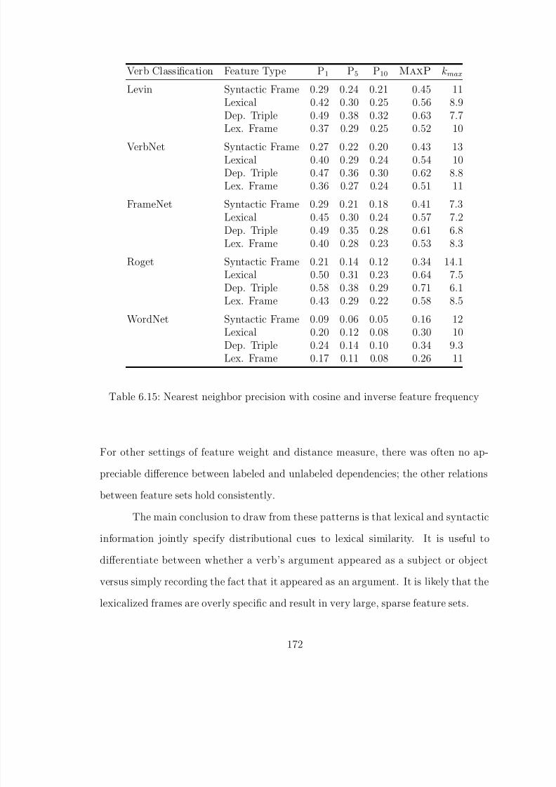
8/8/2019 Baker Kirk
http://slidepdf.com/reader/full/baker-kirk 188/243
Verb Classification Feature Type P1 P5 P10 MaxP kmax
Levin Syntactic Frame 0.29 0.24 0.21 0.45 11Lexical 0.42 0.30 0.25 0.56 8.9Dep. Triple 0.49 0.38 0.32 0.63 7.7Lex. Frame 0.37 0.29 0.25 0.52 10
VerbNet Syntactic Frame 0.27 0.22 0.20 0.43 13Lexical 0.40 0.29 0.24 0.54 10Dep. Triple 0.47 0.36 0.30 0.62 8.8Lex. Frame 0.36 0.27 0.24 0.51 11
FrameNet Syntactic Frame 0.29 0.21 0.18 0.41 7.3Lexical 0.45 0.30 0.24 0.57 7.2Dep. Triple 0.49 0.35 0.28 0.61 6.8Lex. Frame 0.40 0.28 0.23 0.53 8.3
Roget Syntactic Frame 0.21 0.14 0.12 0.34 14.1
Lexical 0.50 0.31 0.23 0.64 7.5Dep. Triple 0.58 0.38 0.29 0.71 6.1Lex. Frame 0.43 0.29 0.22 0.58 8.5
WordNet Syntactic Frame 0.09 0.06 0.05 0.16 12Lexical 0.20 0.12 0.08 0.30 10Dep. Triple 0.24 0.14 0.10 0.34 9.3Lex. Frame 0.17 0.11 0.08 0.26 11
Table 6.15: Nearest neighbor precision with cosine and inverse feature frequency
For other settings of feature weight and distance measure, there was often no ap-
preciable difference between labeled and unlabeled dependencies; the other relations
between feature sets hold consistently.
The main conclusion to draw from these patterns is that lexical and syntactic
information jointly specify distributional cues to lexical similarity. It is useful to
differentiate between whether a verb’s argument appeared as a subject or object
versus simply recording the fact that it appeared as an argument. It is likely that the
lexicalized frames are overly specific and result in very large, sparse feature sets.
172

8/8/2019 Baker Kirk
http://slidepdf.com/reader/full/baker-kirk 189/243
Other researchers have noted this problem of data sparsity, (e.g., Schulte im
Walde, 2000), and have explored the additional use of selectional preference features
by augmenting each syntactic slot with the concept to which its head noun belongs in
an ontology (e.g. WordNet). For example, replacing a frame like eat, <Joe, Subj >,
<corn, Obj > with eat, <Person, Subj >, <Plant, Obj > provides a level of general-
ization that overcomes some of the data sparsity problem. Although the problem of
data sparsity can be mitigated through the use of such techniques, these features have
generally not been shown to improve classification performance (Schulte im Walde,
2000; Joanis, 2002).
It is not surprising that syntactic frames perform worse than the other feature
sets. A lexically unspecified syntactic frame conveys relatively little information, and
any given frame may be shared by many verbs regardless of their semantic class or
synonym set. The fact that syntactic information alone can achieve around 40%
precision on a semantic classification task with a negligible baseline provides support
for semantic theories that relate syntactic structure to verb meaning. It is interesting
that syntactic frames do a better job of identifying Roget synonyms, which are not
explicitly organized around syntactic behavior, than of identifying Levin neighbors,
which do explicitly incorporate syntactic behavior. However, Levin’s classification
involves specific syntactic alternations that preserve meaning rather than general
syntactic frames that are not tied to a given semantic interpretation. The failure
of syntactic frames to identify Levin neighbors more precisely is probably due to a
mismatch between the information they represent and the criteria used in Levin’s
original classification.
173

8/8/2019 Baker Kirk
http://slidepdf.com/reader/full/baker-kirk 190/243
6.5 Relation Between Experiments and Existing Resources
One application of the techniques developed here would be to assist in extending
existing verb schemes such as VerbNet, FrameNet, or Roget’s thesaurus by suggesting
neighbors of unclassified verbs. In order to estimate the coverage of the five verb
schemes studied here, we compared the number of verbs in each scheme that occur at
least 10 times in the English gigaword corpus to the number of verbs in the union of the
five verbs schemes. There are 7206 verbs in the union of Levin, VerbNet, FrameNet,
Roget, and WordNet that occur at least 10 times in the English gigaword corpus 3.
Table 6.16 contains these comparisons. For each verb scheme, the average frequency
of verbs included in that scheme is indicated along with the average frequency of
verbs not included in that scheme.
Verb Scheme Contained MissingLevin 2886 4320
Avg. Freq 47231 23479
VerbNet 3426 3780Avg. Freq 44504 22558
FrameNet 2110 5096Avg. Freq 94374 7577
Roget 5660 1546Avg. Freq 61915 1151
WordNet 7110 96Avg. Freq 33433 351
Table 6.16: Coverage of each verb scheme with respect to the union of all of the verb
schemes and the frequency of included versus excluded verbs
3The reason that there are more Roget and WordNet verbs here than in the experiments is thatthe experiments used the union of Levin, VerbNet, and FrameNet and extracted Roget and WordNetsynonyms from those; here we are looking at the union of all five verb schemes.
174
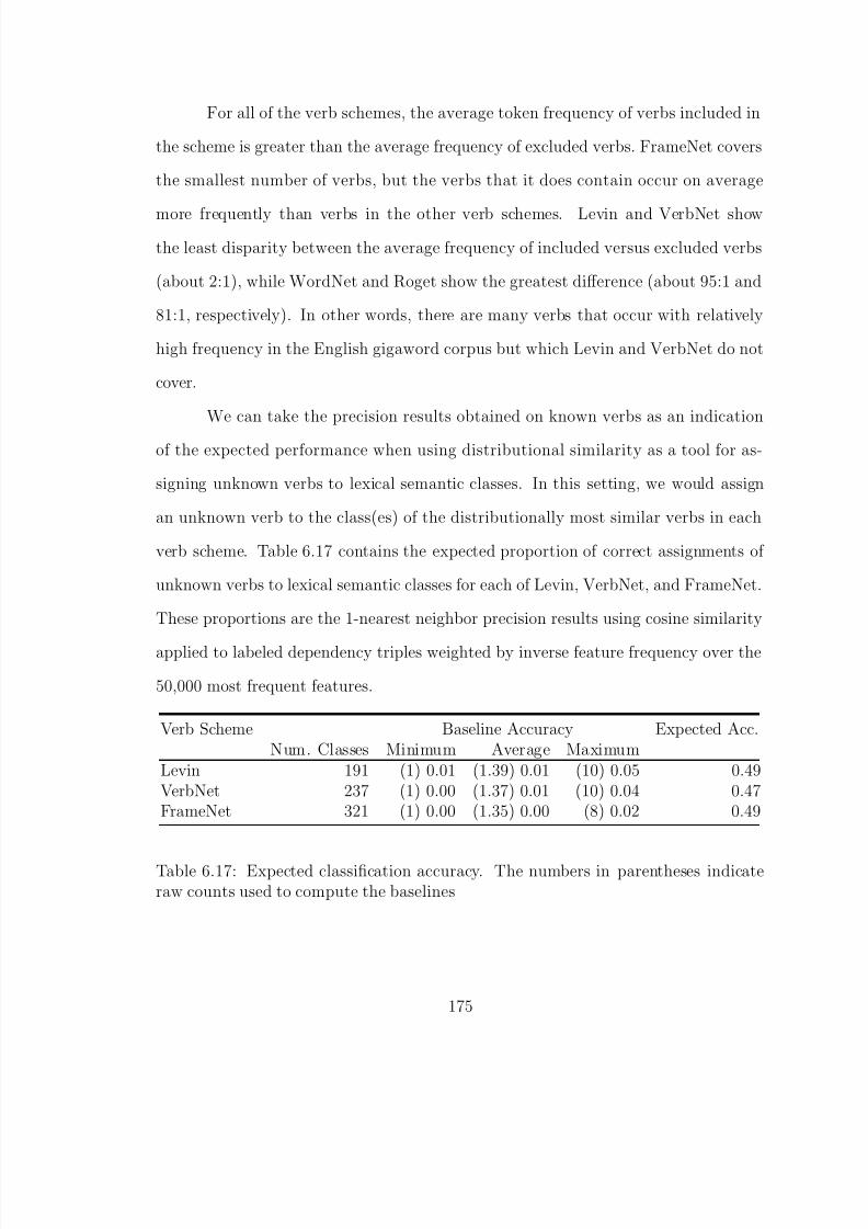
8/8/2019 Baker Kirk
http://slidepdf.com/reader/full/baker-kirk 191/243
For all of the verb schemes, the average token frequency of verbs included in
the scheme is greater than the average frequency of excluded verbs. FrameNet covers
the smallest number of verbs, but the verbs that it does contain occur on average
more frequently than verbs in the other verb schemes. Levin and VerbNet show
the least disparity between the average frequency of included versus excluded verbs
(about 2:1), while WordNet and Roget show the greatest difference (about 95:1 and
81:1, respectively). In other words, there are many verbs that occur with relatively
high frequency in the English gigaword corpus but which Levin and VerbNet do not
cover.
We can take the precision results obtained on known verbs as an indication
of the expected performance when using distributional similarity as a tool for as-
signing unknown verbs to lexical semantic classes. In this setting, we would assign
an unknown verb to the class(es) of the distributionally most similar verbs in each
verb scheme. Table 6.17 contains the expected proportion of correct assignments of
unknown verbs to lexical semantic classes for each of Levin, VerbNet, and FrameNet.
These proportions are the 1-nearest neighbor precision results using cosine similarity
applied to labeled dependency triples weighted by inverse feature frequency over the
50,000 most frequent features.
Verb Scheme Baseline Accuracy Expected Acc.Num. Classes Minimum Average Maximum
Levin 191 (1) 0.01 (1.39) 0.01 (10) 0.05 0.49VerbNet 237 (1) 0.00 (1.37) 0.01 (10) 0.04 0.47FrameNet 321 (1) 0.00 (1.35) 0.00 (8) 0.02 0.49
Table 6.17: Expected classification accuracy. The numbers in parentheses indicateraw counts used to compute the baselines
175
8/8/2019 Baker Kirk
http://slidepdf.com/reader/full/baker-kirk 192/243
For each verb scheme, we also indicate baseline classification accuracy. Be-
cause we have conflated verb senses, the 1-nearest neighbor precision results indicate
that a verb was correctly classified if it belongs to any one of the classes that its
distributionally most similar neighbor belongs to. Therefore, for each verb scheme
we show three baselines:
• The most restrictive case, when the distributionally most similar known verb
belongs to exactly one class, defined as 1 divided by the total number of classes
in the verb scheme.
• The average case, defined as the average number of classes to which a verb
belongs divided by the total number of classes.
• The least restrictive case, defined as the maximum number of classes any verb
in the verb scheme belongs to divided by the total number of classes.
6.6 Conclusion
This chapter presented the results of a large-scale comparison of a variety of pa-
rameters which determine distributional lexical similarity over five lexical semantic
classifications of English verbs. The main findings are summarized below.
• Of the distance measures considered here, cosine (viz. correlation coefficient)
yielded the best results.
• Of the feature sets considered here, labeled dependency triples yielded the best
results.
• Of the feature weightings considered here, inverse feature frequency yielded the
best results.
• Using the parameters studied here, distributionally similar verb assignments
correspond more closely to Roget-style synonyms than to Levin, VerbNet, or
FrameNet classes or WordNet synonyms.
176
8/8/2019 Baker Kirk
http://slidepdf.com/reader/full/baker-kirk 193/243
• The parameters explored here can be used to extend the coverage of Levin,
VerbNet, and FrameNet to other verbs that occur in a large text corpus with
an expected accuracy of around 49% (over a baseline accuracy of about 5%).
Based on these findings, we conclude more generally that:
• Syntactically informed lexical co-occurrence features do a better job of identify-
ing synonyms than of identifying neighbors based on the other lexical semantic
criteria that Levin, VerbNet, and FrameNet rely on (e.g., shared components of
meaning such as MOTION or COVERING; participation in semantic frames).
• Extrinsic feature weightings, which quantify the association between a feature
and a target verb with respect to that feature’s overall distribution among verbs,
do a better job of identifying neighbors than feature weightings which do not
account for overall feature distribution.
• In addition to extrinsic feature weightings, scaling a weighted context vector
(i.e., via cosine or vector length normalization) improves neighbor identification.
177
8/8/2019 Baker Kirk
http://slidepdf.com/reader/full/baker-kirk 194/243
CHAPTER 7
CONCLUSION
This dissertation addressed the problem of learning accurate and scalable lexical
classifiers in the absence of large amounts of hand-labeled training data. It considered
two distinct lexical acquisition tasks, both of which rely on an appropriate definition
of distributional lexical similarity:
• Automatic transliteration and identification of English loanwords in Korean.
For this problem, lexical similarity was defined over phonological co-occurrence
features.
• Lexical semantic classification of English verbs on the basis of automatically
derived co-occurrence features. For this problem, similarity was defined in terms
of grammatical relations.
7.1 Transliteration of English Loanwords in Korean
The first task focused on ways to mitigate the effort of obtaining large amounts of
labeled training data for transliterating and identifying English loanwords in other
languages, using Korean as a case study. The key ideas that emerged from the
transliteration task are:
• Consonant transliteration is highly regular and can be expressed reliably using
a small number of phonological adaptation rules.
178

8/8/2019 Baker Kirk
http://slidepdf.com/reader/full/baker-kirk 195/243

8/8/2019 Baker Kirk
http://slidepdf.com/reader/full/baker-kirk 196/243
• A highly efficient solution to the problem of obtaining labeled training data for
etymological classification.
• A demonstration of the fact that automatically generated pseudo-data can be
used to train a classifier that distinguishes actual English and Korean words as
accurately as one trained entirely on hand-labeled data.
Three experiments were conducted which systematically varied the quantity
and quality of labeled training data. The first experiment, conducted entirely on
hand-labeled training data, obtained classification accuracy of 96.2%. The second
experiment used the rule-based transliteration model from Chapter 3 to produce
large amounts of pseudo-English loanwords that were used in conjunction with actual
Korean words to train a classifier capable of identifying actual English loanwords with
95.8% accuracy. The third experiment used pseudo-English loanwords and unlabeled
items that served as examples of Korean words to train a classifier that identified
actual English loanwords with 92.4% accuracy.
7.3 Distributional Verb Similarity
The second lexical acquisition task considered in this dissertation was the assignment
of English verbs to lexical semantic classes on the basis of their distributional context
in a large text corpus. The approach to this task used the output of a statistical
parser to automatically generate a feature set that was used to assign English verbs
to lexical semantic classes. This study produced results on a substantially larger scale
than any previously reported and yielded new insights into the properties of verbs
that are responsible for their lexical categorization. A series of experiments were
conducted which examined the interactions between a number of parameters that
influence empirical determinations of distributional lexical similarity. The parameters
examined were:
180

8/8/2019 Baker Kirk
http://slidepdf.com/reader/full/baker-kirk 197/243
• Similarity measure. Three classes of similarity measure were considered – set
theoretic, geometric, and information theoretic.
• Feature type. Four feature types based on grammatical dependencies were
examined – syntactic frames, labeled and unlabeled dependency relations, and
lexicalized syntactic frames.
• Feature weighting. Intrinsic weightings such as vector length normalization were
compared to extrinsic weighting schemes such as correlation.
• Feature selection. Feature selection was limited to cutoff by frequency.
These parameters were further evaluated with respect to five verb classification
schemes – Levin, VerbNet, FrameNet, Roget’s Thesaurus, and WordNet. The main
picture that emerged from this analysis is that a combination of cosine similarity
measure with labeled dependency triples and inverse feature frequency consistently
yielded the best results in terms of how closely empirical verb similarities matched
the labels of the five verb schemes. Performance asymptotes at around 50,000 of the
most frequent features of each type.
Simultaneously considering multiple verb classification schemes allowed for
a comparison of the criteria used by each scheme for grouping verbs. One of the
main findings along these lines is that using the feature sets considered here, verbs
within a given classification scheme that are related by synonymy are identified more
reliably than verbs related by criteria such as diathesis alternations or participation
in semantic frames. This approach also allowed for an examination of the relation
between each verb scheme and empirically determined verb similarities. Here we
saw that Roget synonyms were identified more reliably than Levin, VerbNet, andFrameNet verbs. Extrapolating the precision of empirical neighbor assignments for
each of the five verb schemes to unknown verbs allowed an estimate of the expected
accuracy that would be obtained for automatically extending the coverage of each
181

8/8/2019 Baker Kirk
http://slidepdf.com/reader/full/baker-kirk 198/243
scheme to new verbs. Using the best performing combination of parameters mentioned
in the preceding paragraph, Roget synonyms were correctly identified 58% of the
time; Levin, VerbNet, and FrameNet verbs obtained approximately 49% accuracy,
and WordNet synonyms were correctly identified 24% of the time. Together, these
findings indicate that we should pay closer attention to the relation between the
various criteria used in each verb scheme and which of those criteria are primarily
reflected in the feature sets commonly used in automatic verb classification.
182
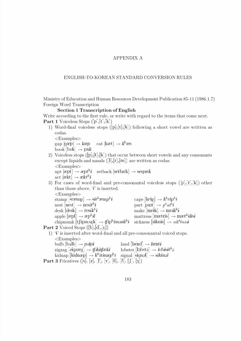
8/8/2019 Baker Kirk
http://slidepdf.com/reader/full/baker-kirk 199/243
APPENDIX A
ENGLISH-TO-KOREAN STANDARD CONVERSION RULES
Ministry of Education and Human Resources Development Publication 85-11 (1986.1.7)Foreign Word Transcription
Section 1 Transcription of EnglishWrite according to the first rule, or write with regard to the items that come next.Part 1 Voiceless Stops ( Ô ℄ ¸ Ø ℄ ¸ ℄ )
1) Word-final voiceless stops ( Ô ℄ ¸ Ø ℄ ¸ ℄ ) following a short vowel are written ascodas.<Examples>gap [ Ô ] → Ô cat [ Ø ] →
×
book Í ℄ → Ô Ù
2) Voiceless stops ( Ô ℄ ¸ Ø ℄ ¸ ℄ ) that occur between short vowels and any consonantsexcept liquids and nasals ´ Ð ℄ ¸ Ö ℄ ¸ Ñ ℄ µ are written as codas.<Examples>apt [ Ô Ø ] →
Ô Ø
½ setback [× Ø ] →× × Ô
act [ Ø
] → Ø
½
3) For cases of word-final and pre-consonantal voiceless stops ( Ô ℄ ¸ Ø ℄ ¸ ℄ ) otherthan those above, ‘½ ’ is inserted.<Examples>stamp × Ø Ñ Ô ℄ → × ½ Ø
Ñ Ô
½ cape Ô ℄ →
Ô
½
nest Ò × Ø ℄ → Ò × ½ Ø
½ part Ô Ø ℄ → ph at h ½
desk × ℄ → Ø × ½
½ make Ñ ℄ → Ñ
½
apple Ô Ð ℄
→ Ô
½ Ð mattress Ñ Ø Ö × ℄
→Ñ Ø
½ Ð × ½
chipmunk Ø Ë Ô Ñ ¾ Æ ℄
→ Ô
½ Ñ Ò
½ sickness × Ò × ℄
→ sik h ½ nis½
Part 2 Voiced Stops ´ ℄ ¸ ℄ ¸ ℄ µ
1) ‘½ ’ is inserted after word-final and all pre-consonantal voiced stops.
<Examples>bulb ¾ Ð ℄ → Ô Ð Ô ½ land Ð Ò ℄ → Ð Ò Ø ½
zigzag Þ Þ ℄ → ½ ½ lobster Ð Ç × Ø ℄ → Ð Ó ½ × ½ Ø
kidnap Ò Ô ℄ →
Ø ½ Ò Ô
½ signal × Ò Ð ℄ → × ½ Ò Ð
Part 3 Fricatives ( × ℄ ¸ Þ ℄ ¸ ℄ ¸ Ú ℄ ¸ Ì ℄ ¸ ℄ ¸ Ë ℄ ¸ ℄ )
183
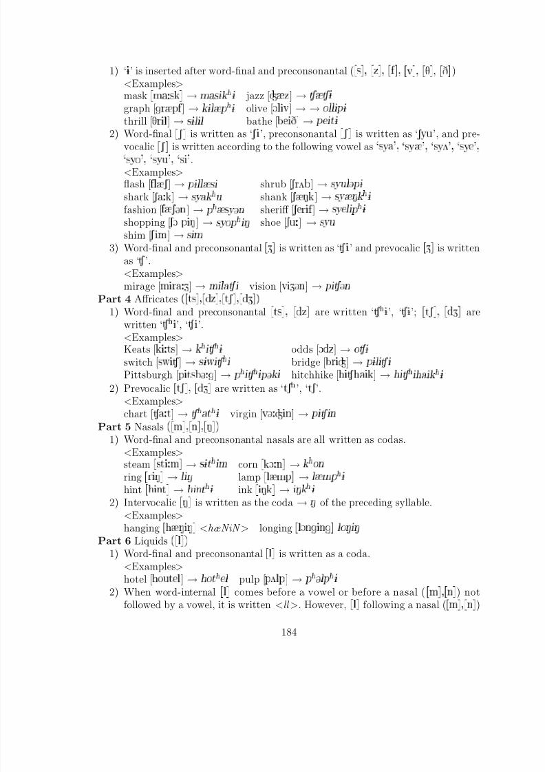
8/8/2019 Baker Kirk
http://slidepdf.com/reader/full/baker-kirk 200/243
1) ‘½ ’ is inserted after word-final and preconsonantal ( × ℄ ¸ Þ ℄ ¸ ℄ ¸ Ú ℄ ¸ Ì ℄ ¸ ℄ )<Examples>mask Ñ × ℄
→Ñ × ½
½ jazz [ Þ ] → ½
graph [ Ö Ô ] → ½ Ð Ô
½ olive [Ç Ð Ú ] → →Ó Ð Ð Ô ½
thrill [Ì Ö Ð ] →× ½ Ð Ð bathe [ ] →
Ô Ø ½
2) Word-final Ë ℄
is written as ‘ Ë
’, preconsonantal Ë ℄
is written as ‘ Ë Ý Ù
’, and pre-vocalic Ë ℄ is written according to the following vowel as × Ý ³ ¸ × Ý ³ ¸ × Ý ¾ ³ ¸ × Ý ³ ¸
× Ý Ó ³ ¸ × Ý Ù ³ ¸ × ³ .<Examples>flash [ Ð Ë ] → Ô ½ Ð Ð × shrub [ Ë Ö ¾ ] → × Ý Ù Ð Ô ½
shark [ Ë ] → × Ý
Ù shank [ Ë Æ ] → × Ý Æ
½
fashion [ Ë Ò ] → Ô
× Ý Ò sheriff [ Ë Ö ] → × Ý Ð Ô
½
shopping [ Ë Ç Ô Æ ] → × Ý Ó Ô
Æ shoe [ Ë Ù ] → × Ý Ù
shim [ Ë Ñ ] →× Ñ
3) Word-final and preconsonantal ℄ is written as ‘ ’ and prevocalic ℄ is writtenas ‘ ’.
<Examples>mirage [Ñ Ö ] → Ñ Ð vision [Ú Ò ] → Ô Ò
Part 4 Affricates ´ Ø × ℄ ¸ Þ ℄ ¸ Ø Ë ℄ ¸ ℄ µ
1) Word-final and preconsonantal Ø × ℄ ¸ Þ ℄ are written ‘
½ ’, ‘ ½ ’; Ø Ë ℄ ¸ ℄ arewritten ‘
’, ‘ ’.<Examples>Keats [ Ø × ] →
½ odds [Ç Þ ] → Ó ½
switch [× Û ] → × ½ Û
bridge [ Ö ] → Ô ½ Ð
Pittsburgh [Ô Ø × ] → Ô
½ Ô ½ hitchhike [ ] →
½
2) Prevocalic Ø Ë ℄ ¸ ℄ are written as ‘ Ø Ë
’, ‘Ø Ë ’.
<Examples>chart [ Ø ] →
Ø
½ virgin [Ú Ò ] → Ô Ò
Part 5 Nasals ´ Ñ ℄ ¸ Ò ℄ ¸ Æ ℄ µ
1) Word-final and preconsonantal nasals are all written as codas.<Examples>steam × Ø Ñ ℄ → × ½ Ø
Ñ corn Ç Ò ℄ →
Ó Ò
ring Ö Æ ℄ → Ð Æ lamp Ð Ñ Ô ℄ → Ð Ñ Ô
½
hint Ò Ø ℄ → Ò Ø
½ ink Æ ℄ → Æ
½
2) Intervocalic Æ ℄ is written as the coda →Æ of the preceding syllable.
<Examples>hanging Æ Æ ℄ <hæNiN > longing Ð Ç Ò Ò ℄ Ð Ó Æ Æ
Part 6 Liquids ´ Ð ℄ µ
1) Word-final and preconsonantal Ð ℄ is written as a coda.<Examples>hotel [ Ó Ù Ø Ð ] → Ó Ø
Ð pulp [Ô ¾ Ð Ô ] → Ô
Ð Ô
½
2) When word-internal Ð ℄ comes before a vowel or before a nasal ( Ñ ℄ ¸ Ò ℄ ) notfollowed by a vowel, it is written <ll >. However, Ð ℄ following a nasal ( Ñ ℄ ¸ Ò ℄ )
184
8/8/2019 Baker Kirk
http://slidepdf.com/reader/full/baker-kirk 201/243
is written <l > even if it comes before a vowel.<Examples>slide [× Ð ] →
× ½ Ð Ð Ø ½ film [ Ð Ñ ] →Ô
Ð Ð ½ Ñ
helm [ Ð Ñ ] → Ð Ð ½ Ñ swoln [× Û Ó Ù Ð Ò ] →
× ½ Û Ð Ð ½ Ò
Hamlet [ Ñ Ð Ø ] → Ñ Ð × Henley [ Ò Ð ] →
Ò Ð
Part 7 Long VowelsThe length of a long vowel is not separately transcribed.<Examples>team [Ø Ñ ] → Ø
Ñ route [Ö Ù Ø ] → Ð Ù Ø
½
Part 8 Diphthongs ´ ℄ ¸ Ù ℄ ¸ ℄ ¸ Ç ℄ ¸ Ó Ù ℄ ¸ Ù ℄ µ
For diphthongs, the phonetic value of each monophthong is realized andwritten separately, but Ó Ù ℄ is written as <o> and Ù ℄ is written as<aw ¾ >.<Examples>time [Ø Ñ ] → Ø
Ñ house [ Ù × ] → Ù × ½
skate [× Ø ] → × Ù Ý Ø Ù oil [Ç Ð ] → Ó Ð
boat [ Ó Ù Ø ] → Ô Ó Ø Ù tower [Ø Ù ] → Ø
Û
Part 9 Semivowels ´ Û ℄ ¸ ℄ µ
1) Û ℄ is written according to the following vowel as Û ℄ ¸ Û Ç ℄ ¸ Û Ó Ù ℄ become<w ¾ >, Û ℄ becomes <wa >, Û ℄ becomes <wæ>, Û ℄ becomes <we>, Û ℄
becomes <wi >, and Û Ù ℄ becomes <u >.<Examples>word [Û ] →
Û Ø ½ want [Û Ç Ò Ø ] →Û Ò Ø
½
woe [Û Ó Ù ] → Û wander [Û Ò ] → Û Ò Ø
wag [Û ] → Û ½ west [Û × Ø ] → Û × ½ Ø ½
witch [Û ] → Û
wool [Û Ù Ð ] → Ù Ð
2) When Û ℄ occurs after a consonant, two separate syllables are written; however, Û ℄ ¸ Û ℄ ¸ Û ℄ are written as a single syllable.<Examples>swing
× Û Æ ℄
→× ½ Û Æ
twist Ø Û × Ø ℄
→Ø
½ Û × ½ Ø
½
penguin Ô Æ Û Ò ℄
→Ô
Æ Û Ò whistle Û × Ð ℄
→ Û × ½ Ð
quarter Û Ç Ø ℄
→
Û Ø
3) The semivowel ℄ combines with the following vowel to be written <ya >,<yæ>, <y ¾ >, <ye>, <yo>, <yu >, <i >. However, ℄ following ℄ ¸ Ð ℄ ¸
Ò ℄ is written individually as <di-¾ >, <li-¾ >, <ni-¾ >.<Examples>yard [ ] → Ý Ø ½ yank Æ ℄ → Ý Æ
½
yearn Ý Ò ℄
→Ý Ò
yellow Ð Ó Ù ℄
→Ý Ð Ð Ó
yawn Ý Ç Ò ℄ → Ý Ó Ò you Ù ℄ → Ý Ù
year ℄ →
Indian Ò Ò ℄
→ Ò Ø Ò
battalion Ø Ð Ý Ò ℄
→Ô Ø
Ð Ð Ò
union Ù Ò Ò ℄
→Ý Ù Ò Ò
Part 10 Compound Words
185

8/8/2019 Baker Kirk
http://slidepdf.com/reader/full/baker-kirk 202/243
1) In a compound, words that can stand alone that have combined to form thecompound are written as they are when they occur independently.<Examples>cuplike ¾ Ô Ð ℄
→
Ô Ð
½ bookend Ù Ò ℄
→Ô Ù Ò Ø ½
headlight Ð Ø ℄
→ Ø ½ Ð Ø
½ touchwood Ø ¾ Ø Ë Û Ù ℄
→Ø
Ù Ø ½
sit-in × Ø Ò ℄
→× × Ò
bookmaker Ù Ñ ℄
→Ô Ù Ñ
flashgun Ð Ë ¾ Ò ℄
→Ô
½ Ð × Ò topknot Ø Ç Ô Ò Ç Ø ℄
→Ø
Ó Ô Ò Ó ×
2) Words written with spaces in the source language may be written with or with-out spaces in Korean.<Examples>Los Alamos Ð Ç × Ð Ñ Ó Ù × ℄ → Ð Ó × ½ Ð Ð Ñ Ó × ½ » Ð Ó × ½ Ð Ð Ñ Ó × ½
top class Ø Ç Ô Ð × ℄ → Ø
Ó Ô
½ Ð Ð × ½ » Ø
Ó Ô
½ Ð Ð × ½
186

8/8/2019 Baker Kirk
http://slidepdf.com/reader/full/baker-kirk 203/243
APPENDIX B
DISTRIBUTED CALCULATION OF A PAIRWISE DISTANCE MATRIX
The basic idea for distributing the task of computing one half of a symmetric pairwise
distance matrix in a set of p independent processes each consisting of an approximately
equal number of comparisons is illustrated as follows. Assuming a proper distance
metric and five items [1, 2, 3, 4, 5], the minimum set of comparisons needed to compute
the distance between every pair of points is
187

8/8/2019 Baker Kirk
http://slidepdf.com/reader/full/baker-kirk 204/243
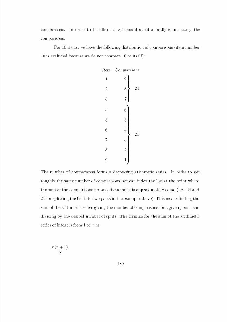
8/8/2019 Baker Kirk
http://slidepdf.com/reader/full/baker-kirk 205/243
comparisons. In order to be efficient, we should avoid actually enumerating the
comparisons.
For 10 items, we have the following distribution of comparisons (item number
10 is excluded because we do not compare 10 to itself):
Item Comparisons
1
2
3
9
8
7
24
4
5
6
7
8
9
6
5
4
3
2
1
21
The number of comparisons forms a decreasing arithmetic series. In order to get
roughly the same number of comparisons, we can index the list at the point where
the sum of the comparisons up to a given index is approximately equal (i.e., 24 and
21 for splitting the list into two parts in the example above). This means finding the
sum of the arithmetic series giving the number of comparisons for a given point, and
dividing by the desired number of splits. The formula for the sum of the arithmetic
series of integers from 1 to n is
n(n + 1)
2
189
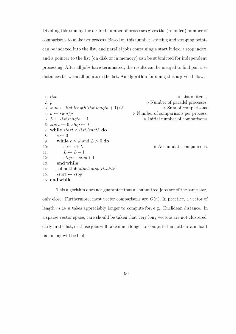
8/8/2019 Baker Kirk
http://slidepdf.com/reader/full/baker-kirk 206/243
Dividing this sum by the desired number of processes gives the (rounded) number of
comparisons to make per process. Based on this number, starting and stopping points
can be indexed into the list, and parallel jobs containing a start index, a stop index,
and a pointer to the list (on disk or in memory) can be submitted for independent
processing. After all jobs have terminated, the results can be merged to find pairwise
distances between all points in the list. An algorithm for doing this is given below.
1: list ⊲ List of items.2: p ⊲ Number of parallel processes.3: sum ← list.length(list.length + 1)/2 ⊲ Sum of comparisons.4: k ← sum/p ⊲ Number of comparisons per process.5: L ← list.length − 1 ⊲ Initial number of comparisons.6: start ← 0, stop ← 07: while start < list.length do8: c ← 09: while c ≤ k and L > 0 do
10: c ← c + L ⊲ Accumulate comparisons.11: L ← L − 112: stop ← stop + 113: end while14: submitJob(start, stop, listP tr)
15: start ← stop16: end while
This algorithm does not guarantee that all submitted jobs are of the same size,
only close. Furthermore, most vector comparisons are O(n). In practice, a vector of
length m ≫ n takes appreciably longer to compute for, e.g., Euclidean distance. In
a sparse vector space, care should be taken that very long vectors are not clustered
early in the list, or those jobs will take much longer to compute than others and load
balancing will be bad.
190

8/8/2019 Baker Kirk
http://slidepdf.com/reader/full/baker-kirk 207/243
APPENDIX C
FULL RESULTS OF VERB CLASSIFICATION EXPERIMENTS USING
BINARY FEATURES
Syntactic Frames
No. of Features
M a x
P r e c
i s i o n
Binary Cosine
JaccardOverlap
5 0 0
1 k
5 k
1 0 k
1 5 k
2 0 k
2 5 k
3 0 k
3 5 k
4 0 k
4 5 k
5 0 k
1 0 0 k
0
0.2
0.4
0.6
0.8
1Unlabeled Dependents
No. of Features
M a x
P r e c
i s i o n
Binary Cosine
JaccardOverlap
5 0 0
1 k
5 k
1 0 k
1 5 k
2 0 k
2 5 k
3 0 k
3 5 k
4 0 k
4 5 k
5 0 k
1 0 0 k
0
0.2
0.4
0.6
0.8
1
Labeled Dependents
No. of Features
M a x
P r e c
i s i o n
Binary CosineJaccardOverlap
5 0 0
1 k
5 k
1 0 k
1 5 k
2 0 k
2 5 k
3 0 k
3 5 k
4 0 k
4 5 k
5 0 k
1 0 0 k
0
0.2
0.4
0.6
0.8
1 Lexical Frames
No. of Features
M a x
P r e c
i s i o n
Binary CosineJaccardOverlap
5 0 0
1 k
5 k
1 0 k
1 5 k
2 0 k
2 5 k
3 0 k
3 5 k
4 0 k
4 5 k
5 0 k
1 0 0 k
0
0.2
0.4
0.6
0.8
1
Figure C.1: Classification results for Levin verbs using binary features
191

8/8/2019 Baker Kirk
http://slidepdf.com/reader/full/baker-kirk 208/243

8/8/2019 Baker Kirk
http://slidepdf.com/reader/full/baker-kirk 209/243
Syntactic Frames
No. of Features
M a x P
r e c
i s i o n
Binary CosineJaccardOverlap
5 0 0
1 k
5 k
1 0 k
1 5 k
2 0 k
2 5 k
3 0 k
3 5 k
4 0 k
4 5 k
5 0 k
1 0 0 k
0
0.2
0.4
0.6
0.8
1Unlabeled Dependents
No. of Features
M a x P
r e c
i s i o n
Binary CosineJaccardOverlap
5 0 0
1 k
5 k
1 0 k
1 5 k
2 0 k
2 5 k
3 0 k
3 5 k
4 0 k
4 5 k
5 0 k
1 0 0 k
0
0.2
0.4
0.6
0.8
1
Labeled Dependents
No. of Features
M a x
P r e c
i s i o n
Binary CosineJaccard
Overlap
5 0 0
1 k
5 k
1 0 k
1 5 k
2 0 k
2 5 k
3 0 k
3 5 k
4 0 k
4 5 k
5 0 k
1 0 0 k
0
0.2
0.4
0.6
0.8
1Lexical Frames
No. of Features
M a x
P r e c
i s i o n
Binary CosineJaccard
Overlap
5 0 0
1 k
5 k
1 0 k
1 5 k
2 0 k
2 5 k
3 0 k
3 5 k
4 0 k
4 5 k
5 0 k
1 0 0 k
0
0.2
0.4
0.6
0.8
1
Figure C.3: Classification results for FrameNet verbs using binary features
193

8/8/2019 Baker Kirk
http://slidepdf.com/reader/full/baker-kirk 210/243
Syntactic Frames
No. of Features
M a x P
r e c
i s i o n
Binary CosineJaccardOverlap
5 0 0
1 k
5 k
1 0 k
1 5 k
2 0 k
2 5 k
3 0 k
3 5 k
4 0 k
4 5 k
5 0 k
1 0 0 k
0
0.2
0.4
0.6
0.8
1Unlabeled Dependents
No. of Features
M a x P
r e c
i s i o n
Binary CosineJaccardOverlap
5 0 0
1 k
5 k
1 0 k
1 5 k
2 0 k
2 5 k
3 0 k
3 5 k
4 0 k
4 5 k
5 0 k
1 0 0 k
0
0.2
0.4
0.6
0.8
1
Labeled Dependents
No. of Features
M a x
P r e c
i s i o n
Binary CosineJaccard
Overlap
5 0 0
1 k
5 k
1 0 k
1 5 k
2 0 k
2 5 k
3 0 k
3 5 k
4 0 k
4 5 k
5 0 k
1 0 0 k
0
0.2
0.4
0.6
0.8
1Lexical Frames
No. of Features
M a x
P r e c
i s i o n
Binary CosineJaccard
Overlap
5 0 0
1 k
5 k
1 0 k
1 5 k
2 0 k
2 5 k
3 0 k
3 5 k
4 0 k
4 5 k
5 0 k
1 0 0 k
0
0.2
0.4
0.6
0.8
1
Figure C.4: Classification results for Roget verbs using binary features
194
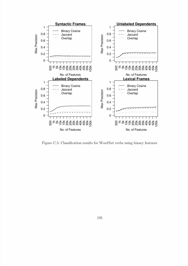
8/8/2019 Baker Kirk
http://slidepdf.com/reader/full/baker-kirk 211/243

8/8/2019 Baker Kirk
http://slidepdf.com/reader/full/baker-kirk 212/243
APPENDIX D
FULL RESULTS OF VERB CLASSIFICATION EXPERIMENTS USING
GEOMETRIC MEASURES
Syntactic Frames
No. of Features
M a x
P r e c
i s i o n
Cosine
L1
5 0 0
1 k
5 k
1 0 k
1 5 k
2 0 k
2 5 k
3 0 k
3 5 k
4 0 k
4 5 k
5 0 k
1 0 0 k
0
0.2
0.4
0.6
0.8
1Unlabeled Dependents
No. of Features
M a x
P r e c
i s i o n
Cosine
L1
5 0 0
1 k
5 k
1 0 k
1 5 k
2 0 k
2 5 k
3 0 k
3 5 k
4 0 k
4 5 k
5 0 k
1 0 0 k
0
0.2
0.4
0.6
0.8
1
Labeled Dependents
No. of Features
M a x
P r e c
i s i o n
CosineL1
5 0 0
1 k
5 k
1 0 k
1 5 k
2 0 k
2 5 k
3 0 k
3 5 k
4 0 k
4 5 k
5 0 k
1 0 0 k
0
0.2
0.4
0.6
0.8
1 Lexical Frames
No. of Features
M a x
P r e c
i s i o n
CosineL1
5 0 0
1 k
5 k
1 0 k
1 5 k
2 0 k
2 5 k
3 0 k
3 5 k
4 0 k
4 5 k
5 0 k
1 0 0 k
0
0.2
0.4
0.6
0.8
1
Figure D.1: Classification results for Levin verbs using geometric distance measures
196

8/8/2019 Baker Kirk
http://slidepdf.com/reader/full/baker-kirk 213/243

8/8/2019 Baker Kirk
http://slidepdf.com/reader/full/baker-kirk 214/243
Syntactic Frames
No. of Features
M a x P
r e c
i s i o n
CosineL1
5 0 0
1 k
5 k
1 0 k
1 5 k
2 0 k
2 5 k
3 0 k
3 5 k
4 0 k
4 5 k
5 0 k
1 0 0 k
0
0.2
0.4
0.6
0.8
1Unlabeled Dependents
No. of Features
M a x P
r e c
i s i o n
CosineL1
5 0 0
1 k
5 k
1 0 k
1 5 k
2 0 k
2 5 k
3 0 k
3 5 k
4 0 k
4 5 k
5 0 k
1 0 0 k
0
0.2
0.4
0.6
0.8
1
Labeled Dependents
No. of Features
M a x
P r e c
i s i o n
CosineL1
5 0 0
1 k
5 k
1 0 k
1 5 k
2 0 k
2 5 k
3 0 k
3 5 k
4 0 k
4 5 k
5 0 k
1 0 0 k
0
0.2
0.4
0.6
0.8
1Lexical Frames
No. of Features
M a x
P r e c
i s i o n
CosineL1
5 0 0
1 k
5 k
1 0 k
1 5 k
2 0 k
2 5 k
3 0 k
3 5 k
4 0 k
4 5 k
5 0 k
1 0 0 k
0
0.2
0.4
0.6
0.8
1
Figure D.3: Classification results for FrameNet verbs using geometric distance mea-sures
198
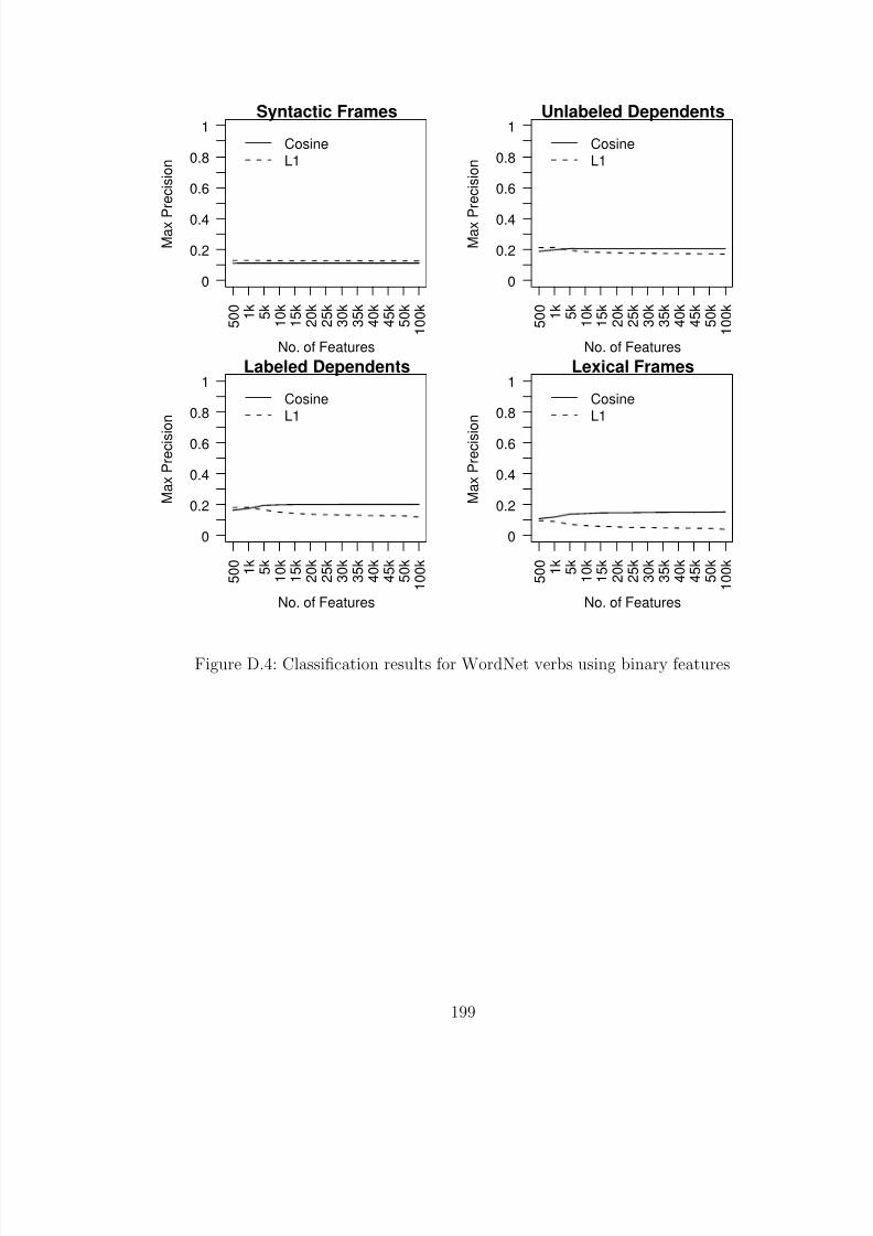
8/8/2019 Baker Kirk
http://slidepdf.com/reader/full/baker-kirk 215/243
Syntactic Frames
No. of Features
M a x P
r e c
i s i o n
CosineL1
5 0 0
1 k
5 k
1 0 k
1 5 k
2 0 k
2 5 k
3 0 k
3 5 k
4 0 k
4 5 k
5 0 k
1 0 0 k
0
0.2
0.4
0.6
0.8
1Unlabeled Dependents
No. of Features
M a x P
r e c
i s i o n
CosineL1
5 0 0
1 k
5 k
1 0 k
1 5 k
2 0 k
2 5 k
3 0 k
3 5 k
4 0 k
4 5 k
5 0 k
1 0 0 k
0
0.2
0.4
0.6
0.8
1
Labeled Dependents
No. of Features
M a x
P r e c
i s i o n
CosineL1
5 0 0
1 k
5 k
1 0 k
1 5 k
2 0 k
2 5 k
3 0 k
3 5 k
4 0 k
4 5 k
5 0 k
1 0 0 k
0
0.2
0.4
0.6
0.8
1Lexical Frames
No. of Features
M a x
P r e c
i s i o n
CosineL1
5 0 0
1 k
5 k
1 0 k
1 5 k
2 0 k
2 5 k
3 0 k
3 5 k
4 0 k
4 5 k
5 0 k
1 0 0 k
0
0.2
0.4
0.6
0.8
1
Figure D.4: Classification results for WordNet verbs using binary features
199
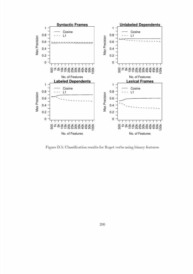
8/8/2019 Baker Kirk
http://slidepdf.com/reader/full/baker-kirk 216/243
Syntactic Frames
No. of Features
M a x P
r e c
i s i o n
CosineL1
5 0 0
1 k
5 k
1 0 k
1 5 k
2 0 k
2 5 k
3 0 k
3 5 k
4 0 k
4 5 k
5 0 k
1 0 0 k
0
0.2
0.4
0.6
0.8
1Unlabeled Dependents
No. of Features
M a x P
r e c
i s i o n
CosineL1
5 0 0
1 k
5 k
1 0 k
1 5 k
2 0 k
2 5 k
3 0 k
3 5 k
4 0 k
4 5 k
5 0 k
1 0 0 k
0
0.2
0.4
0.6
0.8
1
Labeled Dependents
No. of Features
M a x
P r e c
i s i o n
CosineL1
5 0 0
1 k
5 k
1 0 k
1 5 k
2 0 k
2 5 k
3 0 k
3 5 k
4 0 k
4 5 k
5 0 k
1 0 0 k
0
0.2
0.4
0.6
0.8
1Lexical Frames
No. of Features
M a x
P r e c
i s i o n
CosineL1
5 0 0
1 k
5 k
1 0 k
1 5 k
2 0 k
2 5 k
3 0 k
3 5 k
4 0 k
4 5 k
5 0 k
1 0 0 k
0
0.2
0.4
0.6
0.8
1
Figure D.5: Classification results for Roget verbs using binary features
200
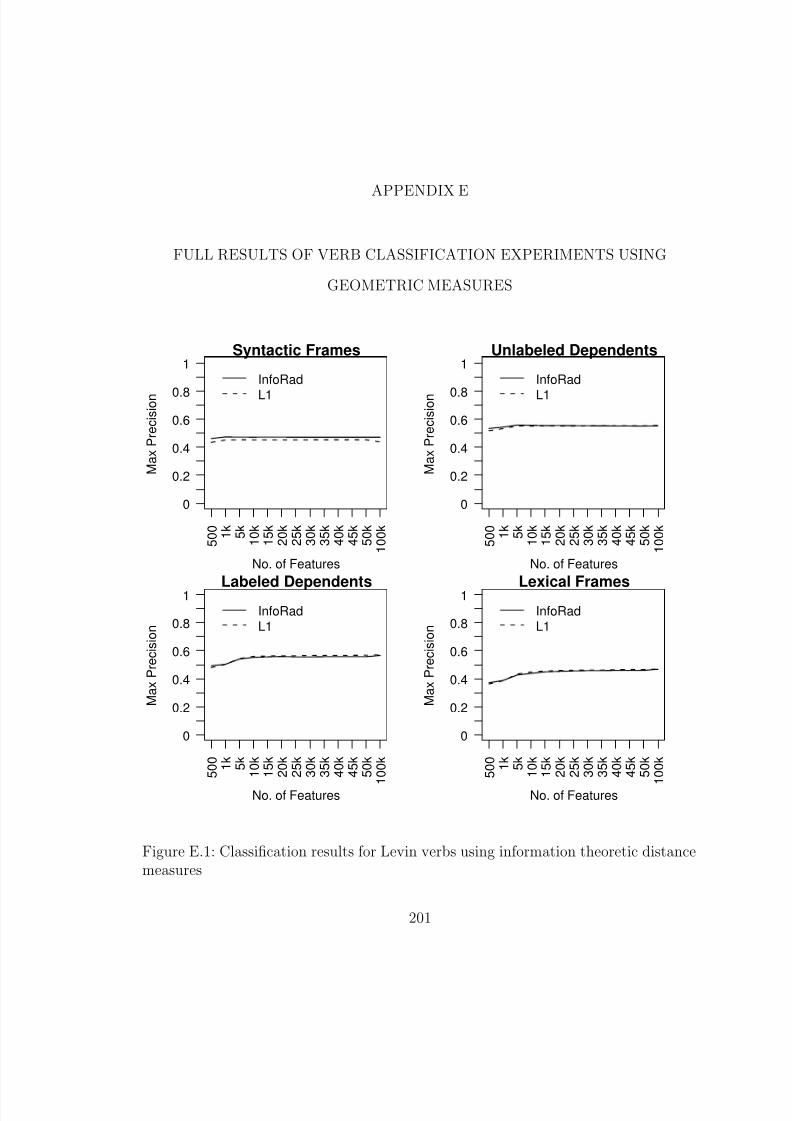
8/8/2019 Baker Kirk
http://slidepdf.com/reader/full/baker-kirk 217/243
APPENDIX E
FULL RESULTS OF VERB CLASSIFICATION EXPERIMENTS USING
GEOMETRIC MEASURES
Syntactic Frames
No. of Features
M a x
P r e c
i s i o n
InfoRad
L1
5 0 0
1 k
5 k
1 0 k
1 5 k
2 0 k
2 5 k
3 0 k
3 5 k
4 0 k
4 5 k
5 0 k
1 0 0 k
0
0.2
0.4
0.6
0.8
1Unlabeled Dependents
No. of Features
M a x
P r e c
i s i o n
InfoRad
L1
5 0 0
1 k
5 k
1 0 k
1 5 k
2 0 k
2 5 k
3 0 k
3 5 k
4 0 k
4 5 k
5 0 k
1 0 0 k
0
0.2
0.4
0.6
0.8
1
Labeled Dependents
No. of Features
M a x
P r e c
i s i o n
InfoRadL1
5 0 0
1 k
5 k
1 0 k
1 5 k
2 0 k
2 5 k
3 0 k
3 5 k
4 0 k
4 5 k
5 0 k
1 0 0 k
0
0.2
0.4
0.6
0.8
1 Lexical Frames
No. of Features
M a x
P r e c
i s i o n
InfoRadL1
5 0 0
1 k
5 k
1 0 k
1 5 k
2 0 k
2 5 k
3 0 k
3 5 k
4 0 k
4 5 k
5 0 k
1 0 0 k
0
0.2
0.4
0.6
0.8
1
Figure E.1: Classification results for Levin verbs using information theoretic distancemeasures
201
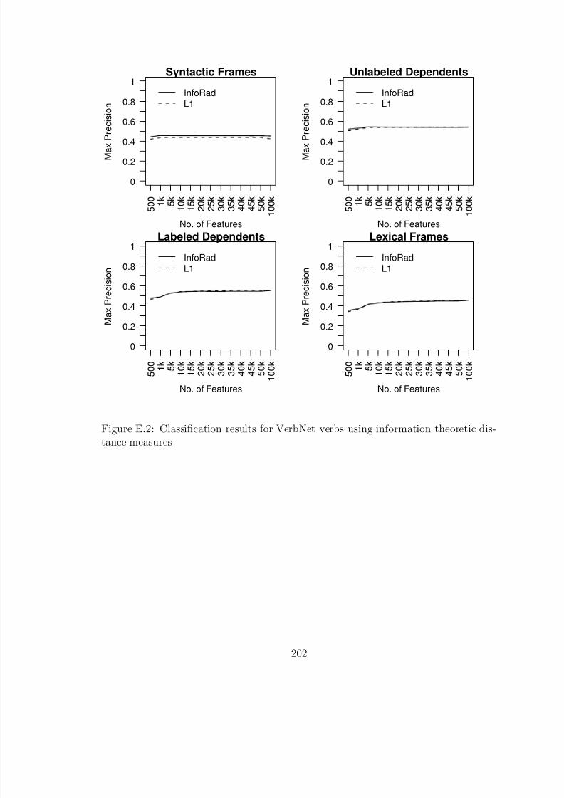
8/8/2019 Baker Kirk
http://slidepdf.com/reader/full/baker-kirk 218/243
Syntactic Frames
No. of Features
M a x P
r e c
i s i o n
InfoRadL1
5 0 0
1 k
5 k
1 0 k
1 5 k
2 0 k
2 5 k
3 0 k
3 5 k
4 0 k
4 5 k
5 0 k
1 0 0 k
0
0.2
0.4
0.6
0.8
1Unlabeled Dependents
No. of Features
M a x P
r e c
i s i o n
InfoRadL1
5 0 0
1 k
5 k
1 0 k
1 5 k
2 0 k
2 5 k
3 0 k
3 5 k
4 0 k
4 5 k
5 0 k
1 0 0 k
0
0.2
0.4
0.6
0.8
1
Labeled Dependents
No. of Features
M a x
P r e c
i s i o n
InfoRadL1
5 0 0
1 k
5 k
1 0 k
1 5 k
2 0 k
2 5 k
3 0 k
3 5 k
4 0 k
4 5 k
5 0 k
1 0 0 k
0
0.2
0.4
0.6
0.8
1Lexical Frames
No. of Features
M a x
P r e c
i s i o n
InfoRadL1
5 0 0
1 k
5 k
1 0 k
1 5 k
2 0 k
2 5 k
3 0 k
3 5 k
4 0 k
4 5 k
5 0 k
1 0 0 k
0
0.2
0.4
0.6
0.8
1
Figure E.2: Classification results for VerbNet verbs using information theoretic dis-tance measures
202
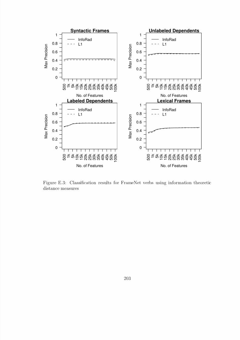
8/8/2019 Baker Kirk
http://slidepdf.com/reader/full/baker-kirk 219/243
Syntactic Frames
No. of Features
M a x P
r e c
i s i o n
InfoRadL1
5 0 0
1 k
5 k
1 0 k
1 5 k
2 0 k
2 5 k
3 0 k
3 5 k
4 0 k
4 5 k
5 0 k
1 0 0 k
0
0.2
0.4
0.6
0.8
1Unlabeled Dependents
No. of Features
M a x P
r e c
i s i o n
InfoRadL1
5 0 0
1 k
5 k
1 0 k
1 5 k
2 0 k
2 5 k
3 0 k
3 5 k
4 0 k
4 5 k
5 0 k
1 0 0 k
0
0.2
0.4
0.6
0.8
1
Labeled Dependents
No. of Features
M a x
P r e c
i s i o n
InfoRadL1
5 0 0
1 k
5 k
1 0 k
1 5 k
2 0 k
2 5 k
3 0 k
3 5 k
4 0 k
4 5 k
5 0 k
1 0 0 k
0
0.2
0.4
0.6
0.8
1Lexical Frames
No. of Features
M a x
P r e c
i s i o n
InfoRadL1
5 0 0
1 k
5 k
1 0 k
1 5 k
2 0 k
2 5 k
3 0 k
3 5 k
4 0 k
4 5 k
5 0 k
1 0 0 k
0
0.2
0.4
0.6
0.8
1
Figure E.3: Classification results for FrameNet verbs using information theoreticdistance measures
203
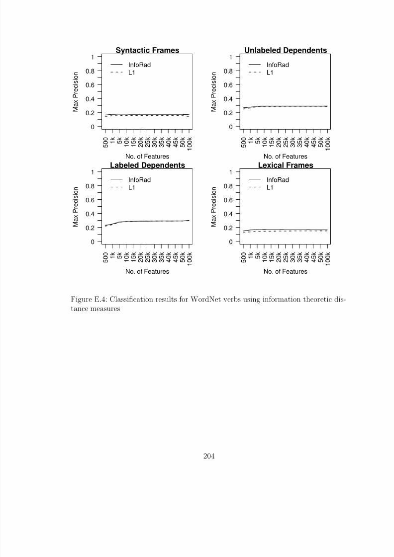
8/8/2019 Baker Kirk
http://slidepdf.com/reader/full/baker-kirk 220/243
Syntactic Frames
No. of Features
M a x P
r e c
i s i o n
InfoRadL1
5 0 0
1 k
5 k
1 0 k
1 5 k
2 0 k
2 5 k
3 0 k
3 5 k
4 0 k
4 5 k
5 0 k
1 0 0 k
0
0.2
0.4
0.6
0.8
1Unlabeled Dependents
No. of Features
M a x P
r e c
i s i o n
InfoRadL1
5 0 0
1 k
5 k
1 0 k
1 5 k
2 0 k
2 5 k
3 0 k
3 5 k
4 0 k
4 5 k
5 0 k
1 0 0 k
0
0.2
0.4
0.6
0.8
1
Labeled Dependents
No. of Features
M a x
P r e c
i s i o n
InfoRadL1
5 0 0
1 k
5 k
1 0 k
1 5 k
2 0 k
2 5 k
3 0 k
3 5 k
4 0 k
4 5 k
5 0 k
1 0 0 k
0
0.2
0.4
0.6
0.8
1Lexical Frames
No. of Features
M a x
P r e c
i s i o n
InfoRadL1
5 0 0
1 k
5 k
1 0 k
1 5 k
2 0 k
2 5 k
3 0 k
3 5 k
4 0 k
4 5 k
5 0 k
1 0 0 k
0
0.2
0.4
0.6
0.8
1
Figure E.4: Classification results for WordNet verbs using information theoretic dis-tance measures
204
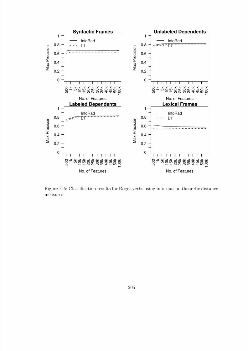
8/8/2019 Baker Kirk
http://slidepdf.com/reader/full/baker-kirk 221/243
Syntactic Frames
No. of Features
M a x P
r e c
i s i o n
InfoRadL1
5 0 0
1 k
5 k
1 0 k
1 5 k
2 0 k
2 5 k
3 0 k
3 5 k
4 0 k
4 5 k
5 0 k
1 0 0 k
0
0.2
0.4
0.6
0.8
1Unlabeled Dependents
No. of Features
M a x P
r e c
i s i o n
InfoRadL1
5 0 0
1 k
5 k
1 0 k
1 5 k
2 0 k
2 5 k
3 0 k
3 5 k
4 0 k
4 5 k
5 0 k
1 0 0 k
0
0.2
0.4
0.6
0.8
1
Labeled Dependents
No. of Features
M a x
P r e c
i s i o n
InfoRadL1
5 0 0
1 k
5 k
1 0 k
1 5 k
2 0 k
2 5 k
3 0 k
3 5 k
4 0 k
4 5 k
5 0 k
1 0 0 k
0
0.2
0.4
0.6
0.8
1Lexical Frames
No. of Features
M a x
P r e c
i s i o n
InfoRadL1
5 0 0
1 k
5 k
1 0 k
1 5 k
2 0 k
2 5 k
3 0 k
3 5 k
4 0 k
4 5 k
5 0 k
1 0 0 k
0
0.2
0.4
0.6
0.8
1
Figure E.5: Classification results for Roget verbs using information theoretic distancemeasures
205

8/8/2019 Baker Kirk
http://slidepdf.com/reader/full/baker-kirk 222/243
APPENDIX F
RESULTS OF VERB CLASSIFICATION EXPERIMENTS USING INVERSE
RANK SCORE
206
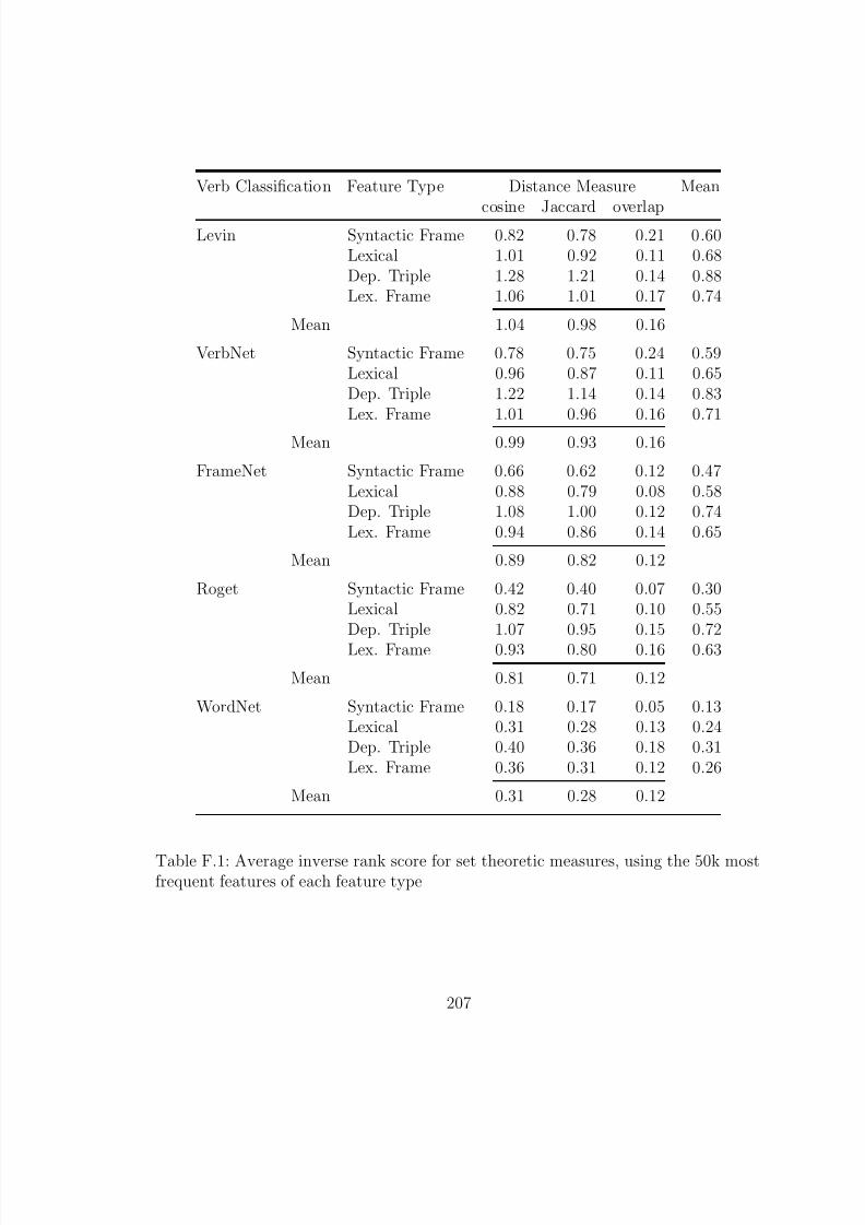
8/8/2019 Baker Kirk
http://slidepdf.com/reader/full/baker-kirk 223/243

8/8/2019 Baker Kirk
http://slidepdf.com/reader/full/baker-kirk 224/243
Verb Classification Feature Type Distance Measure Mean
Cosine (=Euclidean) L1
Levin Syntactic Frame 0.78 0.80 0.79Lexical 0.93 0.68 0.81Dep. Triple 0.95 0.45 0.70Lex. Frame 0.70 0.28 0.49
Mean 0.84 0.55
VerbNet Syntactic Frame 0.75 0.78 0.76Lexical 0.88 0.64 0.76Dep. Triple 0.91 0.45 0.68Lex. Frame 0.66 0.29 0.48
Mean 0.80 0.54
FrameNet Syntactic Frame 0.60 0.59 0.59Lexical 0.83 0.59 0.71Dep. Triple 0.90 0.40 0.65Lex. Frame 0.61 0.27 0.44
Mean 0.73 0.46
Roget Syntactic Frame 0.36 0.41 0.39Lexical 0.68 0.55 0.61Dep. Triple 0.72 0.37 0.55
Lex. Frame 0.45 0.13 0.29
Mean 0.55 0.36
WordNet Syntactic Frame 0.14 0.16 0.15Lexical 0.27 0.23 0.25Dep. Triple 0.27 0.17 0.22Lex. Frame 0.18 0.05 0.12
Mean 0.22 0.15
Table F.2: Average inverse rank score for geometric measures using the 50k mostfrequent features of each feature type
208
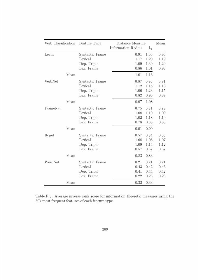
8/8/2019 Baker Kirk
http://slidepdf.com/reader/full/baker-kirk 225/243
Verb Classification Feature Type Distance Measure Mean
Information Radius L1
Levin Syntactic Frame 0.91 1.00 0.96Lexical 1.17 1.20 1.19Dep. Triple 1.09 1.30 1.20Lex. Frame 0.86 1.01 0.93
Mean 1.01 1.13
VerbNet Syntactic Frame 0.87 0.96 0.91Lexical 1.12 1.15 1.13Dep. Triple 1.06 1.23 1.15Lex. Frame 0.82 0.96 0.89
Mean 0.97 1.08
FrameNet Syntactic Frame 0.75 0.81 0.78Lexical 1.08 1.10 1.09Dep. Triple 1.02 1.18 1.10Lex. Frame 0.78 0.88 0.83
Mean 0.91 0.99
Roget Syntactic Frame 0.57 0.54 0.55Lexical 1.08 1.06 1.07Dep. Triple 1.09 1.14 1.12Lex. Frame 0.57 0.57 0.57
Mean 0.83 0.83
WordNet Syntactic Frame 0.21 0.21 0.21Lexical 0.43 0.42 0.43Dep. Triple 0.41 0.44 0.42Lex. Frame 0.22 0.23 0.23
Mean 0.32 0.33
Table F.3: Average inverse rank score for information theoretic measures using the50k most frequent features of each feature type
209
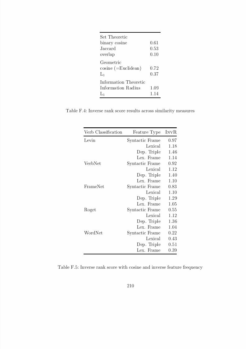
8/8/2019 Baker Kirk
http://slidepdf.com/reader/full/baker-kirk 226/243
Set Theoreticbinary cosine 0.61Jaccard 0.53overlap 0.10
Geometriccosine (=Euclidean) 0.72L1 0.37
Information TheoreticInformation Radius 1.09L1 1.14
Table F.4: Inverse rank score results across similarity measures
Verb Classification Feature Type InvR
Levin Syntactic Frame 0.97Lexical 1.18
Dep. Triple 1.46Lex. Frame 1.14
VerbNet Syntactic Frame 0.92Lexical 1.12
Dep. Triple 1.40
Lex. Frame 1.10FrameNet Syntactic Frame 0.83Lexical 1.10
Dep. Triple 1.29Lex. Frame 1.05
Roget Syntactic Frame 0.55Lexical 1.12
Dep. Triple 1.36Lex. Frame 1.04
WordNet Syntactic Frame 0.22Lexical 0.43
Dep. Triple 0.51Lex. Frame 0.39
Table F.5: Inverse rank score with cosine and inverse feature frequency
210

8/8/2019 Baker Kirk
http://slidepdf.com/reader/full/baker-kirk 227/243
Feature Weighting Distance MeasureCosine Euclidean L1
Levin binary 1.28 0.50 0.50probability 0.95 0.81 1.30normalized 0.95 0.95 0.45log-likelihood 1.29 0.52 0.52correlation 1.25 0.40 0.18inv feat freq 1.46 0.68 0.48
VerbNet binary 1.22 0.53 0.53probability 0.91 0.77 1.23normalized 0.91 0.91 0.45log-likelihood 1.23 0.54 0.54
correlation 1.21 0.45 0.22inv feat freq 1.40 0.68 0.50
FrameNet binary 1.08 0.40 0.40probability 0.90 0.75 1.18normalized 0.90 0.90 0.40log-likelihood 1.09 0.41 0.41correlation 1.18 0.31 0.07inv feat freq 1.29 0.58 0.40
Roget binary 1.07 0.39 0.39probability 0.72 0.64 1.14normalized 0.72 0.72 0.37
log-likelihood 1.09 0.40 0.40correlation 1.12 0.32 0.04inv feat freq 1.36 0.56 0.38
WordNet binary 0.40 0.16 0.16probability 0.27 0.26 0.44normalized 0.27 0.27 0.17log-likelihood 0.42 0.16 0.16correlation 0.39 0.12 0.02inv feat freq 0.51 0.21 0.15
Table F.6: Nearest neighbor average inverse rank score for feature weighting, usingthe 50k most frequent features of type labeled dependency triple
211
8/8/2019 Baker Kirk
http://slidepdf.com/reader/full/baker-kirk 228/243
8/8/2019 Baker Kirk
http://slidepdf.com/reader/full/baker-kirk 229/243
Belkin, Mikhail and Partha Niyogi. 2003. Laplacian eigenmaps for dimension-ality reduction and data representation. Neural Computation , 15(6). 1373–1396.
Belkin, Mikhail and Partha Niyogi. 2004. Semi-supervised learning on Rie-mannian manifolds. Machine Learning , 56. 209–239.
Berger, Adam L., Stephen Della Pietra, and Vincent J. Della Pietra .1996. A maximum entropy approach to natural language processing. Computational Linguistics, 22(1). 39–71.
Bisani, Maximilian and Hermann Ney. 2002. Investigations on jointmultigrammodels for grapheme-to-phoneme conversion. Proceedings of the 7th International Conference on Spoken Language Processing , volume 1, 105–108.
Black, Paul E. 2006. Lm distance. In Dictionary of Algorithms and Data
Structures [online], Paul E. Black, ed., U.S. National Institute of Standardsand Technology. 31 May 2006. (accessed April 3, 2008.) Available from: http:
//www.nist.gov/dads/HTML/lmdistance.html .
Brew, Chris and Sabine Schulte im Walde. 2002. Spectral clustering forGerman verbs. Proceedings of the Conference on Empirical Methods in Natural Language Processing , 117–124. Philadelphia, PA.
Briscoe, Ted and John Carroll. 1997. Automatic extraction of subcategoriza-tion from corpora. In Proceedings of the 5th ACL Conference on Applied Natural Language Processing , 356–363.
Briscoe, Ted, John Carroll, and Rebecca Watson. 2006. The second releaseof the rasp system. Proceedings of the COLING/ACL on Interactive presentation sessions, 77–80.
Budanitsky, Alexander. 1999. Lexical semantic relatedness and its applicationin natural language processing. Technical Report CSRG-390, Department of Com-puter Science, University of Toronto.
Caraballo, S. 1999. Automatic construction of a hypernym-labeled noun hier-
archy from text. Proceedings of the 37th Annual Meeting of the Association for Computational Linguistics, 120–126.
Carlson, Rolf, Bjorn Granstrom, and Gunnar Fant. 1970. Some studiesconcerning perception of isolated vowels. Speech Transmission Laboratory Quarterly Progress and Status Report, Royal Institute of Technology, Stockholm, 2–3 , 19–35.
213
8/8/2019 Baker Kirk
http://slidepdf.com/reader/full/baker-kirk 230/243
Carroll, Glenn and Mats Rooth. 1998. Valence induction with a head-lexicalized pcfg. In Proceedings of the 3rd Conference on Empirical Methods in Natural Language Processing , 36–45.
Christensen, Ronald. 1997. Log-Linear Models and Logistic Regression . Springer,
second edition.
Church, Kenneth W. and William A. Gale. 1991. Concordances for paral-lel texts. Proceedings of the 7th Annual Conference for the New OED and Text Research, Oxford .
Church, Kenneth Ward and Patrick Hanks. 1989. Word association norms,mutual information and lexicography. Proceedings of the 27th Annual Meeting of the Association for Computational Linguistics, 76–83.
Clark, Stephen and James R. Curran. 2007. Formalism-independent parserevaluation with CCG and DepBank. Proceedings of the 45th Annual Meeting of the
Association for Computational Linguistics.
Clear, Jeremy H. 1993. The British national corpus. The Digital Word: Text-based Computing in the Humanities, 163–187. Cambridge, MA, USA: MIT Press.
Cole, Andy and Kevin Walker. 2000. Korean Newswire. Linguistic Data Con-sortium, Philadelphia. LDC2000T45.
Cook, Paul, Afsaneh Fazly, and Suzanne Stevenson. 2007. Pulling their
weight: Exploiting syntactic forms for the automatic identification of idiomaticexpressions in context. Proceedings of the Workshop on A Broader Perspective on Multiword Expressions, 41–48. Prague, Czech Republic: Association for Computa-tional Linguistics.
Covington, Michael A. 1996. An algorithm to align words for historical compar-ison. Computational Linguistics, 22(4). 481–496.
Cruse, D. Alan. 1986. Lexical Semantics. Cambridge University Press.
Curran, James R. and Marc Moens. 2002. Improvements in automatic the-saurus extraction. Unsupervised Lexical Acquisition: Proceedings of the Workshopof the ACL Special Interest Group on the Lexicon (SIGLEX), 59–66.
214

8/8/2019 Baker Kirk
http://slidepdf.com/reader/full/baker-kirk 231/243
Daelemans, Walter, Jakub Zavrel, Ko van der Sloot, and Antal van
den Bosch. 2003. TiMBL: Tilburg Memory Based Learner, version 5.0, Refer-ence Guide. ILK Technical Report 03-10. http://ilk.uvt.nl/downloads/pub/
papers/ilk0310.pdf.
Dagan, Ido, Lillian Lee, and Fernando C. N. Pereira. 1999. Similarity-based models of word cooccurrence probabilities. Machine Learning , 34(1-3). 43–69.
Deerwester, Scott C., Susan T. Dumais, Thomas K. Landauer,
George W. Furnas, and Richard A. Harshman. 1990. Indexing by la-tent semantic analysis. Journal of the American Society of Information Science,41(6). 391–407.
Deligne, Sabine, Francois Yvon, and Frederic Bimbot. 1995. Variable-length sequence matching for phonetic transcription using joint multigrams. Fourth European Conference on Speech Communication and Technology (EUROSPEECH 1995), 2243–2246.
Dempster, Arthur, Nan Laird, and Donald Rubin. 1977. Maximum likeli-hood from incomplete data via the em algorithm. Journal of the Royal Statistical Society, Series B , 39(1). 1–38.
Dorr, Bonnie J. 1997. Large-scale dictionary construction for foreignlanguagetutoring and interlingual machine translation. Machine Translation , 12(4). 271–322.
Dunham, Margaret H. 2003. Data Mining: Introductory and Advanced Topics.Prentice Hall.
Dunning, Ted E. 1993. Accurate methods for the statistics of surprise and coinci-dence. Computational Linguistics, 19(1). 61–74.
Evert, Stefan. 2000. Association measures. Electronic document. http://www.
collocations.de/AM/section5.html. Accessed April 2, 2008.
Fellbaum, Christiane, editor. 1998. WordNet: An Electronic Lexical Database.
Cambridge, MA: The MIT Press.
Forney, G. David. 1973. The Viterbi algorithm. Proceedings of the IEEE , vol-ume 61, 268–278.
215
8/8/2019 Baker Kirk
http://slidepdf.com/reader/full/baker-kirk 232/243
Gale, William, Kenneth Church, and David Yarowsky. 1992. One senseper discourse. Proceedings of the DARPA Speech and Natural Language Workshop,233–237.
Gelman, Andrew, John B. Carlin, Hal S. Stern, and Donald B. Rubin.
2004. Bayesian Data Analysis. Chapman & Hall/CRC, second edition.
Genkin, Alexander, David D. Lewis, and David Madigan. 2004. Large-scaleBayesian logistic regression for text categorization. DIMACS Technical Report .
Gorman, James and James R. Curran. 2006. Scaling distributional similar-ity to large corpora. ACL-44: Proceedings of the 21st International Conferenceon Computational Linguistics and the 44th annual meeting of the Association for Computational Linguistics, 361–368.
Graff, Dave. 2007. Chinese gigaword third edition. Linguistic Data Consortium,Philadelphia. LDC2007T38.
Graff, David. 2003. English Gigaword. Linguistic Data Consortium, Philadelphia.LDC2003T05.
Graff, David and Zhibiao Wu. 1995. Japanese Business News Text. LinguisticData Consortium, Philadelphia. LDC95T8.
Harris, Zellig. 1954. Distributional structure. Word , 10(23). 146–162.
Hastie, Trevor, Robert Tibshirani, and Jerome Friedman. 2001. TheElements of Statistical Learning: Data Mining, Inference, and Prediction . Springer.
Hays, William T. 1988. Statistics. Holt, Rinehart and Winston, Inc., fourthedition.
Hockenmaier, Julia and Mark Steedman. 2005. CCGbank. Linguistic DataConsortium, Philadelphia. LDC2005T13.
Hodgson, J. M. 1991. Informational constraints on pre-lexical priming. Language
and Cognitive Processes, 6. 169–205.
Jaynes, Edwin T. 1991. Notes on present status and future prospects. Jr. Wal-ter T. Grandy and Leonard H. Schick, editors, Maximum Entropy and Bayesian Methods, 1–13. Kluwer Academic Publishers.
216

8/8/2019 Baker Kirk
http://slidepdf.com/reader/full/baker-kirk 233/243
Jeong, Kil Soon, Sung Hyun Myaeng, Jae Sung Lee, and Key-Sun Choi.1999. Automatic Identification and Back-Transliteration of Foreign Words forInformation Retrieval. Information Processing and Management , 35(4). 523–540.
Joanis, Eric. 2002. Automatic verb classification using a general feature space.
Master’s thesis, University of Toronto.
Joanis, Eric and Suzanne Stevenson. 2003. A general feature space for auto-matic verb classification. Proceedings of the 10th Conference of the EACL (EACL2003), 163–170.
Joanis, Eric, Suzanne Stevenson, and David James. 2006. A general featurespace for automatic verb classification. Natural Language Engineering , 14(03). 337–367.
Johnson, Christopher and Charles J. Fillmore. 2000. The FrameNet tagsetfor frame-semantic and syntactic coding of predicate-argument structure. Pro-
ceedings of the 1st Meeting of the North American Chapter of the Association for Computational Linguistics (ANLP-NAACL 2000), 56–62.
Jung, Sung Young, SungLim Hong, and Eunok Paek. 2000. An English toKorean Transliteration Model of Extended Markov Window. Proceedings of The18th Conference on Computational Linguistics, 383–389. Association for Compu-tational Linguistics.
Kaji, Hiroyuki and Yasutsugu Morimoto. 2005. Unsupervised word sense
disambiguation using bilingual comparable corpora. IEICE Transactions on Infor-mation and Systems E88 , D(2). 289–301.
Kang, Byung Ju. 2001. A resolution of word mismatch problem caused by foreign word transliterations and English words in Korean information retrieval . Ph.D.thesis, Computer Science Department, KAIST.
Kang, Byung-Ju and Key-Sun Choi. 2000a. Automatic transliteration and back-transliteration by decision tree learning. Proceedings of the 2nd International Con-
ference on Language Resources and Evaluation , 1135–1411.
Kang, Byung-Ju and Key-Sun Choi. 2000b. Two approaches for the resolutionof word mismatch problem caused by English words and foreign words in Koreaninformation retrieval. Proceedings of the Fifth International Workshop on Infor-mation Retrieval with Asian Languages, 133–140.
217
8/8/2019 Baker Kirk
http://slidepdf.com/reader/full/baker-kirk 234/243
8/8/2019 Baker Kirk
http://slidepdf.com/reader/full/baker-kirk 235/243
Korean Ministry of Culture and Tourism. 1995. English to Korean stan-dard conversion rules. Electronic Document. http://www.hangeul.or.kr/nmf/
23f.pdf. Accessed February 13, 2008.
Korhonen, Anna and Ted Briscoe. 2004. Extended lexical-semantic classifica-
tion of english verbs. Dan Moldovan and Roxana Girju, editors, HLT-NAACL 2004:Workshop on Computational Lexical Semantics, 38–45. Boston, Massachusetts,USA: Association for Computational Linguistics.
Korhonen, Anna, Yuval Krymolowski, and Zvika Marx. 2003. Clusteringpolysemic subcategorization frame distributions semantically.
Krishnapuram, Balaji, Lawrence Carin, Mario A. T. Figueiredo, and
Alexandar J. Hartemink. 2005. Sparse multinomial logistic regression: fastalgorithms and generalization bounds. IEEE Transactions on Pattern Analysisand Machine Intelligence, 27.
Kutner, Michael H., Christopher J. Nachtsheim, and John Neter. 2004.Applied Linear Regression Models. McGraw Hill, fourth edition.
Landauer, Thomas, P. W. Foltz, and D. Laham. 1998. Introduction to latentsemantic analysis. Discourse Processes, 25. 259–284.
Landauer, Thomas K. and Susan T. Dumais. 1997. A solution to Plato’sproblem: The latent semantic analysis theory of acquisition, induction, and repre-sentation of knowledge. Psychological Review , 104(2). 211–240.
Lapata, Mirella and Chris Brew. 1999. Using subcategorization to re-solve verb class ambiguity. Pascale Fung and Joe Zhou, editors, Proceedings of WVLC/EMNLP , 266– 274.
Lapata, Mirella and Chris Brew. 2004. Verb class disambiguation using infor-mative priors. Computational Linguistics, 30(2). 45–73.
LDC. 1995. ACL/DCI. Linguistic Data Consortium, Philadelphia. LDC93T1.
Lee, Ahrong. 2006. English coda /s/ in Korean loanword phonology. Blake Rodgers,editor, LSO Working Papers in Linguistics. Proceedings of WIGL 2006 , volume 6.
Lee, Jae Sung. 1999. An English-Korean transliteration and retransliteration model for cross-lingual information retrieval . Ph.D. thesis, Computer Science Depart-ment, KAIST.
219
8/8/2019 Baker Kirk
http://slidepdf.com/reader/full/baker-kirk 236/243
Lee, Jae Sung and Key-Sun Choi. 1998. English to Korean statistical translit-eration for information retrieval. International Journal of Computer Processing of Oriental Languages, 12(1). 17–37.
Lee, Yoong Keok and Hwee Tou Ng. 2002. An empirical evaluation of knowl-
edge sources and learning algorithms for word sense disambiguation. Proceedings of the Conference on Empirical Methods in Natural Language Processing (EMNLP),41–48.
Levenshtein, Vladimir. 1966. Binary codes capable of correcting deletions, inser-tions, and reversals. Soviet Physics Doklady , 10. 707–710.
Levin, Beth. 1993. English Verb Classes and Alternations: A Preliminary Investi-gation . Chicago, IL: University of Chicago Press.
Li, Eui Do. 2005. Principles for transliterating roman characters and foreign wordsin Korean. Proceedings of the 9th Conference for Foreign Teachers of Korean ,
95–147.
Li, Jianguo and Chris Brew. 2007. Disambiguating levin verbs using untaggeddata. Proceedings of Recent Advances In Natural Language Processing (RANLP-07).
Li, Jianguo and Chris Brew. 2008. Which are the best features for automaticverb classification. Proceedings of the 46th Annual Meeting of the Assoication for Computational Linguistics.
Lin, Dekang. 1998a. Automatic retrieval and clustering of similar words. COLING-ACL, 768–774.
Lin, Dekang. 1998b. Dependency-based evaluation of MINIPAR. Workshop on theEvaluation of Parsing Systems.
Lin, Dekang. 1998c. An information-theoretic definition of similarity. Proceedingsof the 15th International Conference on Machine Learning , 296–304.
Lin, Jianhua. 1991. Divergence measures based on the Shannon entropy. IEEE Transactions on Information Theory , 37(1). 145–150.
Llitjos, Ariadna Font and Alan Black. 2001. Knowledge of language originimproves pronunciation of proper names. Proceedings of EuroSpeech-01, 1919–1922.
220
8/8/2019 Baker Kirk
http://slidepdf.com/reader/full/baker-kirk 237/243
Lund, K., C. Burgess, and C. Audet. 1996. Dissociating semantic and as-sociative relationships using high-dimensional semantic space. Cognitive ScienceProceedings, 603–608. LEA.
Madigan, David, Alexander Genkin, David D. Lewis, Shlomo Argamon,
Dmitriy Fradkin, and Li Ye. 2005a. Author identification on the large scale.Proceedings of The Classification Society of North America (CSNA).
Madigan, David, Alexander Genkin, David D. Lewis, and Dmitriy Frad-
kin. 2005b. Bayesian multinomial logistic regression for author identification. DI-MACS Technical Report .
Manning, Christopher D., Prabhakar Raghavan, and Hinrich Schutze.2008. Introduction to Information Retrieval . Cambridge University Press.
Manning, Christopher D. and Hinrich Schutze. 1999. Foundations of Sta-tistical Natural Language Processing . Cambridge, Massachusetts: The MIT Press.
Marcus, Mitchell P., Beatrice Santorini, and Mary Ann
Marcinkiewicz. 1993. Building a large annotated corpus of English: ThePenn treebank. Computational Linguistics, 19(2). 313–330.
Martin, Samuel Elmo. 1992. A Reference Grammar of Korean: A CompleteGuide to the Grammar and History of the Korean Language. Rutland, Vermont:Charles E. Tuttle.
McCallum, Andrew Kachites. 1996. Bow: A toolkit for statistical languagemodeling, text retrieval, classification and clustering. http://www.cs.cmu.edu/
~ mccallum/bow.
McCarthy, Diana, Rob Koeling, Julie Weeds, and John Carroll. 2004.Finding predominant senses in untagged text.
McDonald, Scott and Chris Brew. 2004. A distributional model of semanticcontext effects in lexical processing. Proceedings of the 42nd Annual Meeting on Association for Computational Linguistics, 17–24.
McRae, Ken, Todd R. Ferretti, and Liane Amyote. 1997. Thematic roles asverb-specific concepts. Language and Cognitive Processes: Special Issue on Lexical Representations in Sentence Processing , 12. 137–176.
221
8/8/2019 Baker Kirk
http://slidepdf.com/reader/full/baker-kirk 238/243
8/8/2019 Baker Kirk
http://slidepdf.com/reader/full/baker-kirk 239/243
Oh, Jong-Hoon and Key-Sun Choi. 2005. Machine learning based English-to-Korean transliteration using grapheme and phoneme information. IEICE Transac-tions on Information and Systems, E88-D(7). 1737–1748.
Oh, Jong-Hoon, Key-Sun Choi, and Hitoshi Isahara. 2006a. A comparison of
different machine transliteration models. Journal of Artificial Intelligence Research ,27. 119–151.
Oh, Jong-Hoon, Key-Sun Choi, and Hitoshi Isahara. 2006b. A machinetransliteration model based on correspondence between graphemes and phonemes.ACM Transactions on Asian Language Processing , 5(3). 185–208.
O’Seaghdha, Padraig G. and Joseph W. Marin. 1997. Mediated semantic-phonological priming: Calling distant relatives. Journal of Memory and Language,36(2). 226–252.
Padgett, Jaye. 2001. Contrast dispersion and Russian palatalization. ElizabethHume and Keith Johnson, editors, The Role of Speech Perception in Phonology .Academic Press.
Pado, Sebastian and Mirella Lapata. 2007. Dependency-based constructionof semantic space models. Computational Linguistics, 33. 161–199.
Palmer, Martha, Dan Gildea, and Paul Kingsbury. 2005. The propositionbank: a corpus annotated with semantic roles. Computational Linguistics, 31(1).71–106.
Park, Hanyong. 2007. Varied adaptation patterns of English stops and fricativesin Korean loanwords: The influence of the P-map. IULC Working Papers Online.
Peperkamp, Sharon. 2005. A psycholinguistic theory of loanword adaptations.Marc Ettlinger, Nicholas Fleisher, and Mischa Park-Doob, editors, Proceedings of the 30th Annual Berkeley Linguistics Society , volume 30.
Pereira, Fernando C. N., Naftali Tishby, and Lillian Lee. 1993. Distri-butional clustering of english words. Meeting of the Association for Computational
Linguistics, 183–190.
Pietra, Stephen Della, Vincent Della Pietra, and John Lafferty. 1997.Inducing features of random fields. IEEE Transactions on Pattern Analysis and Machine Intelligence, 19. 380–393.
223

8/8/2019 Baker Kirk
http://slidepdf.com/reader/full/baker-kirk 240/243
Pinker, Steven. 1994. The Language Instinct . New York: W Morrow and Co.
Prasada, Sandeep and Steven Pinker. 1993. Generalisation of regular andirregular morphological patterns. Language and Cognitive Processes, 8(1). 1–56.
Quinlan, J. Ross. 1986. Induction of decision trees. Machine Learning , 1. 81–106.
Quinlan, J. Ross. 1993. C4.5: Programs for Machine Learning . Morgan KaufmannPublishers, Inc.
Radford, Andrew. 1997. Syntactic theory and the structure of English: A mini-malist approach . Cambridge University Press.
Ramsey, Fred L. and Daniel W. Schafer. 2002. The Statistical Sleuth: ACourse in Methods of Data Analysis. Pacific Grove, CA: Duxbury.
Rayson, Paul, Damon Berridge, and Brian Francis. 2004. Extending theCochran rule for the comparison of word frequencies between corpora. Volume II of Purnelle G., Fairon C., Dister A. (eds.) Le poids des mots: Proceedings of the7th International Conference on Statistical analysis of textual data (JADT 2004),926–936.
Richeldi, Marco and Mauro Rossotto. 1997. Combining statistical tech-niques and search heuristics to perform effective feature selection. GholamrezaNakhaeizadeh and Charles C. Taylor, editors, Machine Learning and Statistics:The Interface, 269–291. Wiley.
Riha, Helena and Kirk Baker. 2008a. The morphology and semantics of romanletter words in Chinese. Paper presented at the 13th International MorphologyMeeting 2008. Vienna, Austria.
Riha, Helena and Kirk Baker. 2008b. Tracking sociohistorical trends in theuse of Roman letters in Chinese newswires. Paper presented at the AmericanAssociation for Corpus Linguistics (AACL 2008). Provo, Utah.
Roget’s Thesaurus. 2008. Roget’s New Millennium Thesaurus, First Edition (v
1.3.1). Lexico Publishing Group, LLC. http://thesaurus.reference.com.
Rohde, Douglas L. T., Laura M. Gonnerman, and David C. Plaut. sub-mitted. An improved model of semantic similarity based on lexical co-occurrence.Cognitive Science.
224

8/8/2019 Baker Kirk
http://slidepdf.com/reader/full/baker-kirk 241/243
Roweis, Sam and Lawrence Saul. 2000. Nonlinear dimensionality reduction bylocally linear embedding. Science, 290(5500). 2323–2326.
Rubenstein, Herbert and John B. Goodenough. 1965. Contextual correlatesof synonymy. Communications of the ACM , volume 8, 627–633.
Sahlgren, Magnus, Jussi Karlgren, and Gunnar Eriksson. 2007. SICS: Va-lence annotation based on seeds in word space. Proceedings of Fourth International Workshop on Semantic Evaluations (SemEval-2007), 4. Prague, Czech Republic.
Saul, Lawrence K. and Sam T. Roweis. 2003. Think globally, fit locally: un-supervised learning of low dimensional manifolds. Journal of Machine Learning Research , 4. 119–155.
Schulte im Walde, Sabine. 2000. Clustering verbs semantically according to their
alternation behaviour. COLING , 747–753.
Schulte im Walde, Sabine. 2003. Experiments on the choice of features forlearning verb classes. Proceedings of EACL 2003 , 315–322.
Schulte im Walde, Sabine and Chris Brew. 2002. Inducing German semanticverb classes from purely syntactic subcategorisation information. Proceedings of the 40th Annual Meeting of the Association for Computational Linguistics, 223–230. Philadelphia, PA.
Schutze, Hinrich. 1998. Automatic word sense discrimination. Computational
Linguistics, 24(1). 97–123.
Smith, Caroline L. 1997. The devoicing of /z/ in american english: effects of localand prosodic context. Journal of Phonetics, 25(4). 471–500.
Smith, Jennifer. 2008. Source similarity in loanword adaptation: Correspondencetheory and the posited source-language representation. Steve Parker, editor, Phono-logical Argumentation: Essays on Evidence and Motivation . London: Equinox.
Steedman, Mark. 1987. Combinatory grammars and parasitic gaps. Natural Lan-
guage and Linguistic Theory , 5.
Stevenson, Suzanne and Paola Merlo. 1999. Automatic verb classificationusing distributinos of grammatical features. Proceedings of the Ninth Conferenceof the European Chapter of the Association for Computational Linguistics, 45–52.
225
8/8/2019 Baker Kirk
http://slidepdf.com/reader/full/baker-kirk 242/243
Szabolcsi, Anna. 1992. Combinatory grammar and projection from the lexicon.Ivan Sag and Anna Szabolcsi, editors, Lexical Matters. CSLI Lecture Notes 24,241–269. Stanford, CSLI Publications.
Teahan, W. J., Yingying Wen, Rodger Mcnab, and Ian H. Witten. 2000.
A compression-based algorithm for chinese word segmentation. Computational Lin-guistics, 26. 375–393.
Tishby, Naftali, Fernando C. Pereira, and William Bialek. 1999. Theinformation bottleneck method. In Proceedings of the 37th Annual Allerton Con-
ference on Communication, Control and Computing , 368–377.
Tsang, Vivian, Suzanne Stevenson, and Paola Merlo. 2002. Crosslinguistictransfer in automatic verb classification. Proceedings of the 19th International Conference on Computational Linguistics (COLING 2002), 1–7.
Vinson, David P. and Gabriella Vigliocco. 2007. Semantic feature productionnorms for a large set of objects and events. Behavior Research Methods, 40. 183–190.
Weeds, Julie. 2003. Measures and Applications of Lexical Distributional Similarity .Ph.D. thesis, Department of Informatics, University of Sussex.
Weide, J. W. 1998. The Carnegie Mellon Pronouncing Dictionary v. 0.6. ElectronicDocument, School of Computer Science, Carnegie Mellon University, Pittsburgh,PA. http://www.speech.cs.cmu.edu/cgi-bin/cmudict .
Wikipedia. 2008. G-test. Wikipedia, The Free Encyclopedia. http://en.
wikipedia.org/w/index.php?title=G-test&oldid=186838098 . Accessed April5, 2008.
Xu, Jinxi and W. Bruce Croft. 1996. Query expansion using local and globaldocument analysis. SIGIR ’96: Proceedings of the 19th annual international ACM SIGIR conference on Research and development in information retrieval , 4–11.
Yang, Byunggon. 1996. A comparative study of American English and Korean
vowels produced by male and female speakers. Journal of Phonetics, 24(2). 245–261.
Yoon, Kyuchul and Chris Brew. 2006. A linguistically motivated approachto grapheme-to-phoneme conversion for Korean. Computer Speech and Language,2(4). 357–381.
226

8/8/2019 Baker Kirk
http://slidepdf.com/reader/full/baker-kirk 243/243
Zhang, Le. 2004. Maximum entropy modeling toolkit for python and C++. http:
//homepages.inf.ed.ac.uk/s0450736/maxent_toolkit.html .