random trees: an interplay between combinatorics and
TRANSCRIPT
W


To Gabriela, Heidi, Hanni and Peter

Preface
Trees are a fundamental object in graph theory and combinatorics as well asa basic object for data structures and algorithms in computer science. Duringthe last years research related to (random) trees has been constantly increasingand several asymptotic and probabilistic techniques have been developed inorder to describe characteristics of interest of large trees in different settings.
The purpose of this book is to provide a thorough introduction into variousaspects of trees in random settings and a systematic treatment of the involvedmathematical techniques. It should serve as a reference book as well as a basisfor future research. One major conceptual aspect is to connect combinatorialand probabilistic methods that range from counting techniques (generatingfunctions, bijections) over asymptotic methods (singularity analysis, saddlepoint techniques) to various sophisticated techniques in asymptotic probabil-ity (convergence of stochastic processes, martingales). However, the readingof the book requires just basic knowledge in combinatorics, complex analysis,functional analysis and probability theory of master degree level. It is alsopart of concept of the book to provide full proofs of the major results even ifthey are technically involved and lengthy.
Due to the diversity of the topic of the book it is impossible to present anexhaustive treatment of all known models of random trees and of all importantaspects that have been considered so far. For example, we do not deal with thesimulation of random trees. The choice of the topics reflects the author’s tasteand experience. It is slightly leaning on the combinatorial side and analyticmethods based on generating functions play a dominant role in most of theparts of the book. Nevertheless, the general goal is to describe the limitingbehaviour of large trees in terms of continuous random objects. This rangesfrom central (or other) limit theorems for simple tree statistics to functionallimit theorems for the shape of trees, for example, encoded by the horizontalor vertical profile. The majority of the results that we present in this book isvery recent.
There are several excellent books and survey articles dealing with someaspects on combinatorics on trees and graphs resp. with probabilistic meth-
VIII Preface
ods in these topics which complement the present book. One of the first oneswas Harary and Palmer book Graphical enumeration [98]. Around the sametime Knuth published the first three volumes of The Art of Computer Pro-gramming [128, 129, 130] where several classes of trees related to algorithmsfrom computer science are systematically investigated. His books with GreenMathematics for the analysis of algorithms [96] and the one with Graham andPatashnik Concrete Mathematics [95] complement this programme. In parallelasymptotic methods in combinatorics, many of them based on generating func-tions, became more and more important. The articles by Bender Asymptoticmethods in enumeration [7] and Odlyzko Asymptotic enumeration methods[165] are excellent surveys on this topic. This development is highlighted byFlajolet and Sedgewick’s recent (monumental) monograph Analytic Combina-torics [84]. Computer science and in particular the mathematical analysis ofalgorithms was always a driving force for developing concepts for the asymp-totic analysis of trees (see also the books by Kemp [122], Hofri [102], Sedgewickand Flajolet [191], and by Szpankowski [197]). Moreover, several concepts ofrandom trees arose naturally in this scientific process (see for example Mah-moud’s book Evolution of random search trees [146], and Pittel’s, Devroye’sor Janson’s work).
However, combinatorics and problems of computer science, though impor-tant, are not the only origin of random tree concepts. There was at leasta second (and almost independent) line of research concerning conditionedGalton-Watson trees. Here one starts with a Galton-Watson branching processand conditions on the size of the resulting trees. For example, Kolchin’s bookRandom Mappings [132] summarises many results from the Russian school.This work is complemented by the American school represented by Aldous[3, 5] and Pitman [171] where stochastic processes related to the Brownianmotion play an important role. The invention of the continuum random treeas well as the ISE (integrated super-Brownian excursion) by Aldous are break-throughs. Actually these continuous limit objects are quite universal concepts.It seems that they also appear as limit objects for several kinds of randomplanar maps and other related discrete objects. There are even more generalsettings where Levy processes are used (see the recent survey articles RandomTrees and Applications [135] and Random Real Trees [136] by Le Gall and thebook Probability and Real Trees [75] by Evans). By the way, the study of ran-dom graphs is completely different from that of random trees (compare withthe books by Bollobas [21], Janson, �Luczak and Rucinski [116], and Kolchin[133]). Nevertheless, there is a very interesting paper The Birth of the Gi-ant Component [115] which uses analytic methods that are very close to treemethods.
This book is divided into nine chapters. The first two of them are providingsome background whereas the remaining chapters 3–9 are devoted to morespecific and (more or less) self contained topics on random trees and on related
Preface IX
subjects. Of course, they will use basic notions from Chapter 1 and some ofthe methods from Chapter 2.
In Chapter 1 we survey several classes of random trees that are consideredhere: combinatorial tree classes like planted plane trees, Galton-Watson trees,recursive trees, and search trees including binary search trees and digital trees.
Chapter 2 is a second introductory chapter. It collects some basic facts oncombinatorics with generating functions and provides an analytic treatmentof generating functions that satisfy a functional equation (or a system offunctional equations) leading to asymptotics and central limit theorems. It isprobably not necessary to study all parts of this chapter in a first reading butto use it as a reference chapter.
The first purpose of Chapter 3 is tree counting, to obtain explicit for-mulas for the numbers of trees of given size with possible and asymptoticinformation on these numbers in those cases, where no or no simple explicitformula is available. The analysis of several combinatorial classes of trees andalso of Galton-Watson trees is based on generating functions and their analyticproperties that are discussed in Chapter 2. The recursive structure of (rooted)trees usually leads to a functional equation for the corresponding generatingfunctions. By extending these counting procedures with the help of bivariategenerating functions one can also study (so-called) additive statistics on thesetree classes like the number of nodes of given degree or more generally thenumber of occurrences of a given pattern. In all these cases we derive a centrallimit theorem.
The general topic of Chapters 4–7 is the limiting behaviour of the profileand related statistics of different classes of random trees. Starting from anatural (vertex) labelling on a discrete object, for example the distance to aroot vertex in a tree, the profile is the value distribution of the labels. Moreprecisely, if a random discrete object has size n then the profile (Xn,k) isgiven by the numbers Xn,k of vertices with label k. The idea behind is thatthe profile (Xn,k) describes the shape of the random object. It is thereforenatural to search for a proper limiting object of the profile after a properscaling.
In Chapter 4 we discuss the depth profile (induced by the distance tothe root) of Galton-Watson trees with bounded offspring variance which canbe approximated by the local time of the Brownian excursion of duration1. This property is closely related to the convergence of normalised Galton-Watson trees to the continuum random tree introduced by Aldous [2, 3, 4].The proof method that we use here follows the same principles as those ofthe previous chapters. We use multivariate generating functions and analyticmethods. Interestingly these methods can be applied to unlabelled rootedtrees, too, where we obtain the same approximation result. And the onlysuccessful approach to the latter class of trees – also called Polya trees – isbased on generating functions in combination with Polya’s theory of counting.Thus, Polya trees look like Galton-Watson trees although they are definitelynot of that kind.
X Preface
Chapter 5 considers again Galton-Watson trees but a different kind of pro-file that is induced by a random walk on the tree. We fix an integer valueddistribution η with zero mean. Then, given a tree T , every edge e of T is en-dowed with an independent copy ηe of η. The label of a node is then definedas the sum of ηe over all edges e on the path to the root. There are severalmotivations to study such random models. For example, if η has only values±1 or 0 and ±1 then the resulting trees are closely related to random trian-gulations and quadrangulations. Furthermore, the random variables ηe can beseen as random increments in an embedding of the tree in the space. This ideais originally due to Aldous [5] and gave rise of the ISE, the integrated super-Brownian excursion, which acts as the limiting occupation measure of theinduced label distribution. The final result is that the corresponding profilecan be approximated by the (random) density of the ISE. This result reachesvery far and is out of scope of this book but, nevertheless, there are specialcases which are of particular interest and capable for the framework of thepresent book. By the use of explicit generating functions of unexpected formthe analysis recovers one-dimensional versions of the functional limit theoremand also leads to integral representations for several parameters of the ISE.These observations are due to Bousquet-Melou [23].
Chapter 6 deals with recursive trees and their variants (plane orientedrecursive trees, binary and m-ary search trees). The interesting feature ofthese kinds of trees is that they can be seen from different points of views:They can be seen as a combinatorial object (where usual counting proceduresapply) as well as the result of a (stochastic) growth process. Interestingly theirasymptotic structure is completely different from that of Galton-Watson trees.They are so-called logn trees which means that their expected height is oforder logn (in contrast to Galton-Watson trees with expected height of order√n). We provide a unified approach to several basic statistics like the degree
distribution. However, the main focus is again the profile. Here one observesthat most vertices are concentrated around few levels so that a (possible)limiting object of the normalised project is not related to some functional ofthe Brownian motion. Nevertheless, the normalised profileXn,k/EXn,k can beapproximated by X(k/ logn), where X(t) is now a random analytic function.We also deal with the height and its concentration properties.
Tries and digital search trees are two other classes of logn trees which arediscussed in Chapter 7. Their construction is based on digital keys and noton the order structure of the keys as in the case of binary search trees. Again,most vertices are concentrated around few levels of order logn but the profilebehaves differently. It is even more concentrated around its mean value thanthe profile of binary search trees or recursive trees. The normalised profileXn,k/EXn,k (of tries) converges to 1 and we observe a central limit theorem.
Chapter 8 is devoted to the so-called contraction method which was devel-oped to handle stochastic recurrence relations which naturally appear in thestochastic analysis of recursive algorithms like Quicksort. Such recurrencesalso appear in the analysis of the profile of recursive trees and binary search

Preface XI
trees (and their variants). The idea is that after normalisation the recur-rence relation stabilises to a (stochastic) fixed point equation that can besolved uniquely by Banach’s fixed point theorem in a properly chosen Banachspace setting. Here we restrict ourselves to an L2 setting with the Wasser-stein metric. We mainly follow the work by Rosler, Ruschendorf, Neininger[158, 161, 162, 186, 187].
The final Chapter 9 deals with planar graphs. At first sight planar graphsand trees have nothing in common but there are strong similarities in the com-binatorial and asymptotic analysis. For example the 2-connected parts of aconnected (planar) graph have a tree structure which is reflected by the struc-ture of the corresponding generating functions. In particular in the asymptoticanalysis one can use the same techniques from Chapter 2 as for combinatorialtree classes in Chapter 3. Besides the asymptotic counting problem the ma-jor goal of this chapter is to study the degree distribution of random planargraphs or equivalently the expected number of vertices of given degree wherewe can again use asymptotic tree counting techniques. This chapter is basedon recent work by Gimenez, Noy and the author [63, 64].
Of course, such a book project cannot be completed without help andsupport from many colleagues and friends. In particular I am grateful toMireille Bousquet-Melou, Luc Devroye, Philippe Flajolet, Bernhard Gitten-berger, Alexander Iksanov, Svante Janson, Christian Krattenthaler, Jean-Francois Marckert, Marc Noy, Ralph Neininger, Alois Panholzer, and WojciechSzpankowski. I also thank Frank Emmert-Streib for helping me to design thebook cover.
Finally I want to thank Veronika Kraus, Johannes Morgenbesser, andChristoph Strolz for their careful reading of the manuscript and for severalhints to improve the presentation and Barbara Dolezal-Rainer for her supportin type setting. I also want to thank Stephen Soehnlen from Springer Verlagfor his constant support in this book project and his patience.
I am especially indebted to my family to whom this book is dedicated.
Vienna, November 2008 Michael Drmota

Contents
1 Classes of Random Trees . . . . . . . . . . . . . . . . . . . . . . . . . . . . . . . . . . 11.1 Basic Notions . . . . . . . . . . . . . . . . . . . . . . . . . . . . . . . . . . . . . . . . . . . 2
1.1.1 Rooted Versus Unrooted trees . . . . . . . . . . . . . . . . . . . . . . . 21.1.2 Plane Versus Non-Plane trees . . . . . . . . . . . . . . . . . . . . . . . 31.1.3 Labelled Versus Unlabelled Trees . . . . . . . . . . . . . . . . . . . . 3
1.2 Combinatorial Trees . . . . . . . . . . . . . . . . . . . . . . . . . . . . . . . . . . . . . 41.2.1 Binary Trees . . . . . . . . . . . . . . . . . . . . . . . . . . . . . . . . . . . . . . 51.2.2 Planted Plane Trees . . . . . . . . . . . . . . . . . . . . . . . . . . . . . . . 61.2.3 Labelled Trees . . . . . . . . . . . . . . . . . . . . . . . . . . . . . . . . . . . . 71.2.4 Labelled Plane Trees . . . . . . . . . . . . . . . . . . . . . . . . . . . . . . . 81.2.5 Unlabelled Trees . . . . . . . . . . . . . . . . . . . . . . . . . . . . . . . . . . 81.2.6 Unlabelled Plane Trees . . . . . . . . . . . . . . . . . . . . . . . . . . . . . 91.2.7 Simply Generated Trees – Galton-Watson Trees . . . . . . . 9
1.3 Recursive Trees . . . . . . . . . . . . . . . . . . . . . . . . . . . . . . . . . . . . . . . . . 131.3.1 Non-Plane Recursive Trees . . . . . . . . . . . . . . . . . . . . . . . . . 131.3.2 Plane Oriented Recursive Trees . . . . . . . . . . . . . . . . . . . . . 141.3.3 Increasing Trees . . . . . . . . . . . . . . . . . . . . . . . . . . . . . . . . . . . 15
1.4 Search Trees . . . . . . . . . . . . . . . . . . . . . . . . . . . . . . . . . . . . . . . . . . . . 171.4.1 Binary Search Trees . . . . . . . . . . . . . . . . . . . . . . . . . . . . . . . 181.4.2 Fringe Balanced m-Ary Search Trees . . . . . . . . . . . . . . . . . 191.4.3 Digital Search Trees . . . . . . . . . . . . . . . . . . . . . . . . . . . . . . . 211.4.4 Tries . . . . . . . . . . . . . . . . . . . . . . . . . . . . . . . . . . . . . . . . . . . . . 22
2 Generating Functions . . . . . . . . . . . . . . . . . . . . . . . . . . . . . . . . . . . . . . 252.1 Counting with Generating Functions . . . . . . . . . . . . . . . . . . . . . . . 26
2.1.1 Generating Functions and Combinatorial Constructions 272.1.2 Polya’s Theory of Counting . . . . . . . . . . . . . . . . . . . . . . . . . 332.1.3 Lagrange Inversion Formula . . . . . . . . . . . . . . . . . . . . . . . . 36
2.2 Asymptotics with Generating Functions . . . . . . . . . . . . . . . . . . . . 372.2.1 Asymptotic Transfers . . . . . . . . . . . . . . . . . . . . . . . . . . . . . . 382.2.2 Functional Equations . . . . . . . . . . . . . . . . . . . . . . . . . . . . . . 43
XIV Contents
2.2.3 Asymptotic Normality and Functional Equations . . . . . . 462.2.4 Transfer of Singularities . . . . . . . . . . . . . . . . . . . . . . . . . . . . 542.2.5 Systems of Functional Equations . . . . . . . . . . . . . . . . . . . . 62
3 Advanced Tree Counting . . . . . . . . . . . . . . . . . . . . . . . . . . . . . . . . . . 693.1 Generating Functions and Combinatorial Trees . . . . . . . . . . . . . . 70
3.1.1 Binary and m-ary Trees . . . . . . . . . . . . . . . . . . . . . . . . . . . . 703.1.2 Planted Plane Trees . . . . . . . . . . . . . . . . . . . . . . . . . . . . . . . 713.1.3 Labelled Trees . . . . . . . . . . . . . . . . . . . . . . . . . . . . . . . . . . . . 733.1.4 Simply Generated Trees – Galton-Watson Trees . . . . . . . 753.1.5 Unrooted Trees . . . . . . . . . . . . . . . . . . . . . . . . . . . . . . . . . . . 773.1.6 Trees Embedded in the Plane . . . . . . . . . . . . . . . . . . . . . . . 81
3.2 Additive Parameters in Trees . . . . . . . . . . . . . . . . . . . . . . . . . . . . . 823.2.1 Simply Generated Trees – Galton-Watson Trees . . . . . . . 843.2.2 Unrooted Trees . . . . . . . . . . . . . . . . . . . . . . . . . . . . . . . . . . . 87
3.3 Patterns in Trees . . . . . . . . . . . . . . . . . . . . . . . . . . . . . . . . . . . . . . . . 903.3.1 Planted, Rooted and Unrooted Trees . . . . . . . . . . . . . . . . . 913.3.2 Generating Functions for Planted Rooted Trees . . . . . . . 923.3.3 Rooted and Unrooted Trees . . . . . . . . . . . . . . . . . . . . . . . . . 993.3.4 Asymptotic Behaviour . . . . . . . . . . . . . . . . . . . . . . . . . . . . . 101
4 The Shape of Galton-Watson Trees and Polya Trees . . . . . . . 1074.1 The Continuum Random Tree . . . . . . . . . . . . . . . . . . . . . . . . . . . . . 108
4.1.1 Depth-First Search of a Rooted Tree . . . . . . . . . . . . . . . . . 1084.1.2 Real Trees . . . . . . . . . . . . . . . . . . . . . . . . . . . . . . . . . . . . . . . . 1094.1.3 Galton-Watson Trees and the Continuum Random Tree 111
4.2 The Profile of Galton-Watson Trees . . . . . . . . . . . . . . . . . . . . . . . . 1154.2.1 The Distribution of the Local Time . . . . . . . . . . . . . . . . . . 1184.2.2 Weak Convergence of Continuous Stochastic Processes . 1204.2.3 Combinatorics on the Profile of Galton-Watson Trees . . 1254.2.4 Asymptotic Analysis of the Main Recurrence . . . . . . . . . 1264.2.5 Finite Dimensional Limiting Distributions . . . . . . . . . . . . 1294.2.6 Tightness . . . . . . . . . . . . . . . . . . . . . . . . . . . . . . . . . . . . . . . . 1344.2.7 The Height of Galton-Watson Trees . . . . . . . . . . . . . . . . . . 1394.2.8 Depth-First Search . . . . . . . . . . . . . . . . . . . . . . . . . . . . . . . . 149
4.3 The Profile of Polya Trees . . . . . . . . . . . . . . . . . . . . . . . . . . . . . . . . 1544.3.1 Combinatorial Setup . . . . . . . . . . . . . . . . . . . . . . . . . . . . . . . 1544.3.2 Asymptotic Analysis of the Main Recurrence . . . . . . . . . 1564.3.3 Finite Dimensional Limiting Distributions . . . . . . . . . . . . 1644.3.4 Tightness . . . . . . . . . . . . . . . . . . . . . . . . . . . . . . . . . . . . . . . . 1684.3.5 The Height of Polya Trees . . . . . . . . . . . . . . . . . . . . . . . . . . 177
Contents XV
5 The Vertical Profile of Trees . . . . . . . . . . . . . . . . . . . . . . . . . . . . . . . 1875.1 Quadrangulations and Embedded Trees . . . . . . . . . . . . . . . . . . . . 1885.2 Profiles of Trees and Random Measures . . . . . . . . . . . . . . . . . . . . 196
5.2.1 General Profiles . . . . . . . . . . . . . . . . . . . . . . . . . . . . . . . . . . . 1965.2.2 Space Embedded Trees and ISE . . . . . . . . . . . . . . . . . . . . . 1965.2.3 The Distribution of the ISE . . . . . . . . . . . . . . . . . . . . . . . . . 204
5.3 Combinatorics on Embedded Trees . . . . . . . . . . . . . . . . . . . . . . . . 2075.3.1 Embedded Trees with Increments ±1 . . . . . . . . . . . . . . . . 2075.3.2 Embedded Trees with Increments 0,±1 . . . . . . . . . . . . . . 2145.3.3 Naturally Embedded Binary Trees . . . . . . . . . . . . . . . . . . . 216
5.4 Asymptotics on Embedded Trees . . . . . . . . . . . . . . . . . . . . . . . . . . 2195.4.1 Trees with Small Labels . . . . . . . . . . . . . . . . . . . . . . . . . . . . 2195.4.2 The Number of Nodes of Given Label . . . . . . . . . . . . . . . . 2255.4.3 The Number of Nodes of Large Labels . . . . . . . . . . . . . . . 2295.4.4 Embedded Trees with Increments 0 and ±1 . . . . . . . . . . . 2355.4.5 Naturally Embedded Binary Trees . . . . . . . . . . . . . . . . . . . 235
6 Recursive Trees and Binary Search Trees . . . . . . . . . . . . . . . . . . 2376.1 Permutations and Trees . . . . . . . . . . . . . . . . . . . . . . . . . . . . . . . . . . 238
6.1.1 Permutations and Recursive Trees . . . . . . . . . . . . . . . . . . . 2396.1.2 Permutations and Binary Search Trees . . . . . . . . . . . . . . . 246
6.2 Generating Functions and Basic Statistics . . . . . . . . . . . . . . . . . . 2476.2.1 Generating Functions for Recursive Trees . . . . . . . . . . . . . 2486.2.2 Generating Functions for Binary Search Trees . . . . . . . . . 2496.2.3 Generating Functions for Plane Oriented Recursive
Trees . . . . . . . . . . . . . . . . . . . . . . . . . . . . . . . . . . . . . . . . . . . . 2516.2.4 The Degree Distribution of Recursive Trees . . . . . . . . . . . 2536.2.5 The Insertion Depth . . . . . . . . . . . . . . . . . . . . . . . . . . . . . . . 262
6.3 The Profile of Recursive Trees . . . . . . . . . . . . . . . . . . . . . . . . . . . . . 2656.3.1 The Martingale Method . . . . . . . . . . . . . . . . . . . . . . . . . . . . 2666.3.2 The Moment Method . . . . . . . . . . . . . . . . . . . . . . . . . . . . . . 2756.3.3 The Contraction Method . . . . . . . . . . . . . . . . . . . . . . . . . . . 278
6.4 The Height of Recursive Trees . . . . . . . . . . . . . . . . . . . . . . . . . . . . 2806.5 Profile and Height of Binary Search Trees and Related Trees . . 291
6.5.1 The Profile of Binary Search Trees and Related Trees . . 2916.5.2 The Height of Binary Search Trees and Related Trees . . 300
7 Tries and Digital Search Trees . . . . . . . . . . . . . . . . . . . . . . . . . . . . . 3077.1 The Profile of Tries . . . . . . . . . . . . . . . . . . . . . . . . . . . . . . . . . . . . . . 308
7.1.1 Generating Functions for the Profile . . . . . . . . . . . . . . . . . 3087.1.2 The Expected Profile of Tries . . . . . . . . . . . . . . . . . . . . . . . 3117.1.3 The Limiting Distribution of the Profile of Tries . . . . . . . 3217.1.4 The Height of Tries . . . . . . . . . . . . . . . . . . . . . . . . . . . . . . . . 3237.1.5 Symmetric Tries . . . . . . . . . . . . . . . . . . . . . . . . . . . . . . . . . . . 324
7.2 The Profile of Digital Search Trees . . . . . . . . . . . . . . . . . . . . . . . . . 325
XVI Contents
7.2.1 Generating Functions for the Profile . . . . . . . . . . . . . . . . . 3257.2.2 The Expected Profile of Digital Search Trees . . . . . . . . . . 3277.2.3 Symmetric Digital Search Trees . . . . . . . . . . . . . . . . . . . . . 337
8 Recursive Algorithms and the Contraction Method . . . . . . . . 3438.1 The Number of Comparisons in Quicksort . . . . . . . . . . . . . . . . . . 3458.2 The L2 Setting of the Contraction Method. . . . . . . . . . . . . . . . . . 350
8.2.1 A General Type of Recurrence . . . . . . . . . . . . . . . . . . . . . . 3508.2.2 A General L2 Convergence Theorem . . . . . . . . . . . . . . . . . 3528.2.3 Applications of the L2 Setting . . . . . . . . . . . . . . . . . . . . . . 357
8.3 Limitations of the L2 Setting and Extensions . . . . . . . . . . . . . . . 3618.3.1 The Zolotarev Metric . . . . . . . . . . . . . . . . . . . . . . . . . . . . . . 3628.3.2 Degenerate Limit Equations . . . . . . . . . . . . . . . . . . . . . . . . 363
9 Planar Graphs . . . . . . . . . . . . . . . . . . . . . . . . . . . . . . . . . . . . . . . . . . . . . 3659.1 Basic Notions . . . . . . . . . . . . . . . . . . . . . . . . . . . . . . . . . . . . . . . . . . . 3669.2 Counting Planar Graphs . . . . . . . . . . . . . . . . . . . . . . . . . . . . . . . . . 368
9.2.1 Outerplanar Graphs . . . . . . . . . . . . . . . . . . . . . . . . . . . . . . . 3689.2.2 Series-Parallel Graphs . . . . . . . . . . . . . . . . . . . . . . . . . . . . . . 3769.2.3 Quadrangulations and Planar Maps . . . . . . . . . . . . . . . . . . 3829.2.4 Planar Graphs . . . . . . . . . . . . . . . . . . . . . . . . . . . . . . . . . . . . 389
9.3 Outerplanar Graphs . . . . . . . . . . . . . . . . . . . . . . . . . . . . . . . . . . . . . 3969.3.1 The Degree Distribution of Outerplanar Graphs . . . . . . . 3969.3.2 Vertices of Given Degree in Dissections . . . . . . . . . . . . . . . 4009.3.3 Vertices of Given Degree in 2-Connected Outerplanar
Graphs . . . . . . . . . . . . . . . . . . . . . . . . . . . . . . . . . . . . . . . . . . . 4049.3.4 Vertices of Given Degree in Connected Outerplanar
Graphs . . . . . . . . . . . . . . . . . . . . . . . . . . . . . . . . . . . . . . . . . . . 4069.4 Series-Parallel Graphs . . . . . . . . . . . . . . . . . . . . . . . . . . . . . . . . . . . . 408
9.4.1 The Degree Distribution of Series-Parallel Graphs . . . . . 4089.4.2 Vertices of Given Degree in Series-Parallel Networks . . . 4159.4.3 Vertices of Given Degree in 2-Connected Series-Parallel
Graphs . . . . . . . . . . . . . . . . . . . . . . . . . . . . . . . . . . . . . . . . . . . 4169.4.4 Vertices of Given Degree in Connected Series-Parallel
Graphs . . . . . . . . . . . . . . . . . . . . . . . . . . . . . . . . . . . . . . . . . . . 4199.5 All Planar Graphs . . . . . . . . . . . . . . . . . . . . . . . . . . . . . . . . . . . . . . . 420
9.5.1 The Degree of a Rooted Vertex . . . . . . . . . . . . . . . . . . . . . 4219.5.2 Singular Expansions . . . . . . . . . . . . . . . . . . . . . . . . . . . . . . . 4259.5.3 Degree Distribution for Planar Graphs . . . . . . . . . . . . . . . 4299.5.4 Vertices of Degree 1 or 2 in Planar Graphs . . . . . . . . . . . 433
Appendix . . . . . . . . . . . . . . . . . . . . . . . . . . . . . . . . . . . . . . . . . . . . . . . . . . 439
References . . . . . . . . . . . . . . . . . . . . . . . . . . . . . . . . . . . . . . . . . . . . . . . . . . . . . 445

Contents XVII
Index . . . . . . . . . . . . . . . . . . . . . . . . . . . . . . . . . . . . . . . . . . . . . . . . . . . . . . . . . . 455

1
Classes of Random Trees
In this first chapter we survey several types of random trees. We start withbasic notions on trees and the description of several concepts of tree countingproblems. In particular we distinguish between rooted and unrooted, planeand non-plane, and labelled and unlabelled trees. It is also possible to modifythe counting procedure by putting certain weights on trees, for example, byusing the degree distribution.
We consider classical combinatorial tree classes like planted plane trees orlabelled rooted trees. Furthermore we discuss simply generated trees whichcan be also considered as conditioned Galton-Watson trees and cover sev-eral classes of the classical (rooted) trees. We introduce unlabelled trees (alsocalled Polya trees) that do not fall into this class but behave similarly tosimply generated trees. Recursive trees (and more generally increasing trees)are labelled rooted trees where each path starting at the root has increasinglabels. All these kinds of trees give rise to a natural probability distributionbased on combinatorics by assuming that every tree of size n (of a certainclass) is equally likely.
Trees occur also in the context of algorithms from computer science, forexample, as data structures. Here the structure of the tree is determined bythe input data of the algorithm. Prominent examples are binary search trees,digital search trees or tries. From a combinatorial point of view these kinds oftrees are just binary trees. However, if we assume some probability distributionon the input data this induces a probability distribution on the correspondingtrees. Moreover, one usually has a tree evolution process by inserting moreand more data.
2 1 Classes of Random Trees
1.1 Basic Notions
Trees are defined as connected graphs without cycles, and their properties arebasics of graph theory. For example, a connected graph is a tree, if and only ifthe number of edges equals the number of nodes minus 1. Furthermore, eachpair of nodes is connected by a unique path.
The degree d(v) of a node v in a tree is the number of nodes that areadjacent to v or the number of neighbours of v.
Nodes of degree ≤ 1 are usually called leaves or external nodes and theremaining ones internal nodes.
1.1.1 Rooted Versus Unrooted trees
r
r
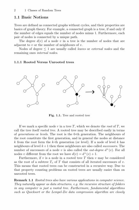
Fig. 1.1. Tree and rooted tree
If we mark a specific node r in a tree T , which we denote the root of T , wecall the tree itself rooted tree. A rooted tree may be described easily in termsof generations or levels. The root is the 0-th generation. The neighbours ofthe root constitute the first generation, and in general the nodes at distancek from the root form the k-th generation (or level). If a node of level k hasneighbours of level k+ 1 then these neighbours are also called successors. Thenumber of successors of a node v is also called the out-degree d+(v). For allnodes v different from the root we have d(v) = d+(v) + 1.
Furthermore, if v is a node in a rooted tree T then v may be consideredas the root of a subtree Tv of T that consists of all iterated successors of v.This means that rooted trees can be constructed in a recursive way. Due tothat property counting problems on rooted trees are usually easier than onunrooted trees.
Remark 1.1 Rooted trees also have various applications in computer science.They naturally appear as data structures, e.g. the recursive structure of foldersin any computer is just a rooted tree. Furthermore, fundamental algorithmssuch as Quicksort or the Lempel-Ziv data compression algorithm are closely
1.1 Basic Notions 3
related to rooted trees, namely to binary and digital search trees which are alsoused to store (and search for) data. Rooted trees even occur in informationtheory. For example, prefix free codes on an alphabet of order m are encodedas the set of leaves in m-ary trees.
1.1.2 Plane Versus Non-Plane trees
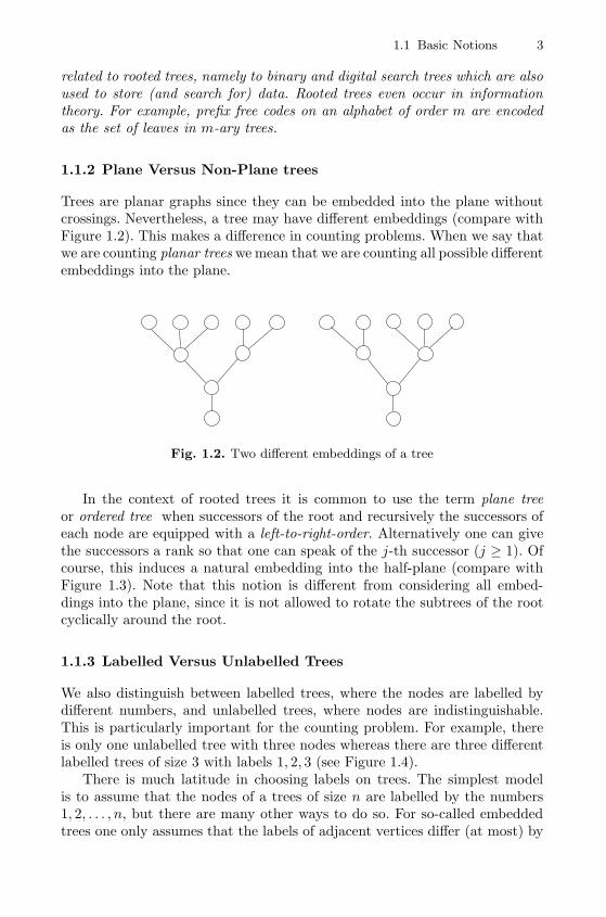
Trees are planar graphs since they can be embedded into the plane withoutcrossings. Nevertheless, a tree may have different embeddings (compare withFigure 1.2). This makes a difference in counting problems. When we say thatwe are counting planar trees we mean that we are counting all possible differentembeddings into the plane.
Fig. 1.2. Two different embeddings of a tree
In the context of rooted trees it is common to use the term plane treeor ordered tree when successors of the root and recursively the successors ofeach node are equipped with a left-to-right-order. Alternatively one can givethe successors a rank so that one can speak of the j-th successor (j ≥ 1). Ofcourse, this induces a natural embedding into the half-plane (compare withFigure 1.3). Note that this notion is different from considering all embed-dings into the plane, since it is not allowed to rotate the subtrees of the rootcyclically around the root.
1.1.3 Labelled Versus Unlabelled Trees
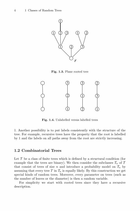
We also distinguish between labelled trees, where the nodes are labelled bydifferent numbers, and unlabelled trees, where nodes are indistinguishable.This is particularly important for the counting problem. For example, thereis only one unlabelled tree with three nodes whereas there are three differentlabelled trees of size 3 with labels 1, 2, 3 (see Figure 1.4).
There is much latitude in choosing labels on trees. The simplest modelis to assume that the nodes of a trees of size n are labelled by the numbers1, 2, . . . , n, but there are many other ways to do so. For so-called embeddedtrees one only assumes that the labels of adjacent vertices differ (at most) by
4 1 Classes of Random Trees
r
1
1
1
1
2
2 23
3
Fig. 1.3. Plane rooted tree
1
3
2 1
3
2 1
3
2
Fig. 1.4. Unlabelled versus labelled trees
1. Another possibility is to put labels consistently with the structure of thetree. For example, recursive trees have the property that the root is labelledby 1 and the labels on all paths away from the root are strictly increasing.
1.2 Combinatorial Trees
Let T be a class of finite trees which is defined by a structural condition (forexample that the trees are binary). We then consider the subclasses Tn of Tthat consist of trees of size n and introduce a probability model on Tn byassuming that every tree T in Tn is equally likely. By this construction we getspecial kinds of random trees. Moreover, every parameter on trees (such asthe number of leaves or the diameter) is then a random variable.
For simplicity we start with rooted trees since they have a recursivedescription.
1.2 Combinatorial Trees 5
1.2.1 Binary Trees
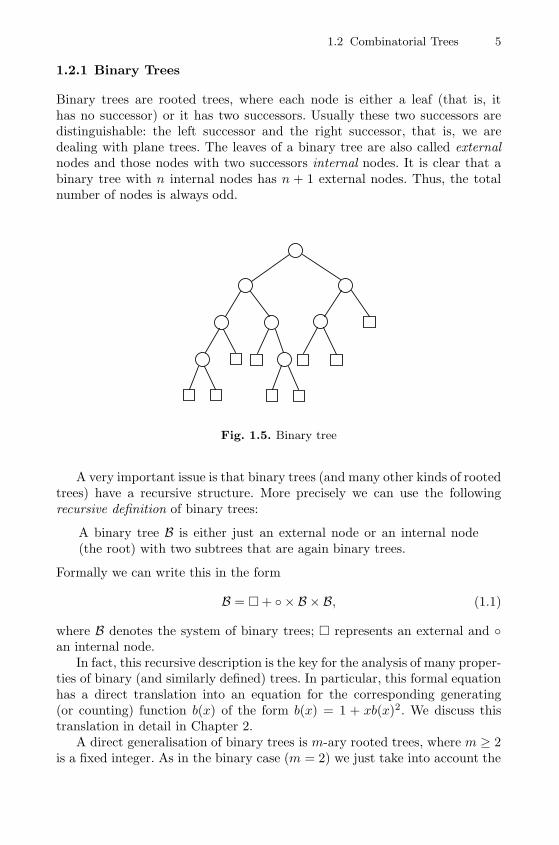
Binary trees are rooted trees, where each node is either a leaf (that is, ithas no successor) or it has two successors. Usually these two successors aredistinguishable: the left successor and the right successor, that is, we aredealing with plane trees. The leaves of a binary tree are also called externalnodes and those nodes with two successors internal nodes. It is clear that abinary tree with n internal nodes has n + 1 external nodes. Thus, the totalnumber of nodes is always odd.
Fig. 1.5. Binary tree
A very important issue is that binary trees (and many other kinds of rootedtrees) have a recursive structure. More precisely we can use the followingrecursive definition of binary trees:
A binary tree B is either just an external node or an internal node(the root) with two subtrees that are again binary trees.
Formally we can write this in the form
B = � + ◦ × B × B, (1.1)
where B denotes the system of binary trees; � represents an external and ◦an internal node.
In fact, this recursive description is the key for the analysis of many proper-ties of binary (and similarly defined) trees. In particular, this formal equationhas a direct translation into an equation for the corresponding generating(or counting) function b(x) of the form b(x) = 1 + xb(x)2. We discuss thistranslation in detail in Chapter 2.
A direct generalisation of binary trees is m-ary rooted trees, where m ≥ 2is a fixed integer. As in the binary case (m = 2) we just take into account the
6 1 Classes of Random Trees
number n of internal nodes. The number of leaves is then given by (m−1)n+1and the total number of nodes by mn+ 1.
Interestingly it is relatively easy to find explicit formulas for the numbers
b(m)n of m-ary trees with n internal nodes:
b(m)n =
1
(m− 1)n+ 1
(mn
n
).
The set Tn of m-ary trees with n internal nodes then constitutes a set ofrandom trees if we assume that everym-ary tree in Tn is equally likely, namely
of probability 1/b(m)n .
Note that in the binary case the number of trees is precisely the n-thCatalan number
Cn =1
n+ 1
(2n
n
).
It is also possible to consider binary and more generallym-ary trees, wherethe left-to-right-order of the successors is not taken into account. However,the counting problem of these classes of trees is much more involved (comparewith Sections 1.2.5 and 3.1.5).
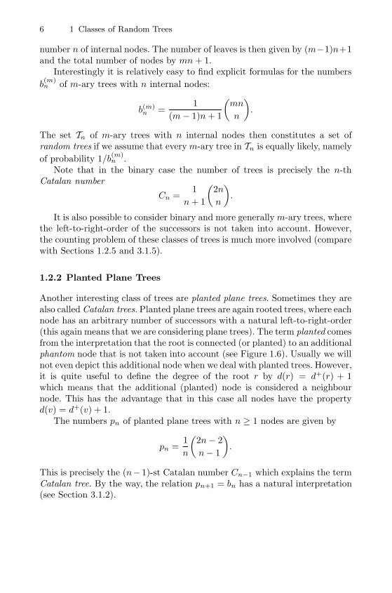
1.2.2 Planted Plane Trees
Another interesting class of trees are planted plane trees. Sometimes they arealso called Catalan trees. Planted plane trees are again rooted trees, where eachnode has an arbitrary number of successors with a natural left-to-right-order(this again means that we are considering plane trees). The term planted comesfrom the interpretation that the root is connected (or planted) to an additionalphantom node that is not taken into account (see Figure 1.6). Usually we willnot even depict this additional node when we deal with planted trees. However,it is quite useful to define the degree of the root r by d(r) = d+(r) + 1which means that the additional (planted) node is considered a neighbournode. This has the advantage that in this case all nodes have the propertyd(v) = d+(v) + 1.
The numbers pn of planted plane trees with n ≥ 1 nodes are given by
pn =1
n
(2n− 2
n− 1
).
This is precisely the (n−1)-st Catalan number Cn−1 which explains the termCatalan tree. By the way, the relation pn+1 = bn has a natural interpretation(see Section 3.1.2).
1.2 Combinatorial Trees 7
r
r
Fig. 1.6. Planted plane tree
1.2.3 Labelled Trees
We recall that a tree T of size n is labelled if the n nodes are labelled by1, 2, . . . , n.1 The counting problem of labelled trees is different from that ofunlabelled trees. There is, however, an easy connection between rooted and un-rooted labelled trees. There are exactly n different ways to make an unrootedtree to a rooted one by choosing one of the labelled nodes. Thus, the numberof rooted labelled trees of size n equals the number of unrooted labelled treesexactly n times. Consequently it is sufficient to consider rooted labelled treeswhich has the advantage that one can use the recursive structure.
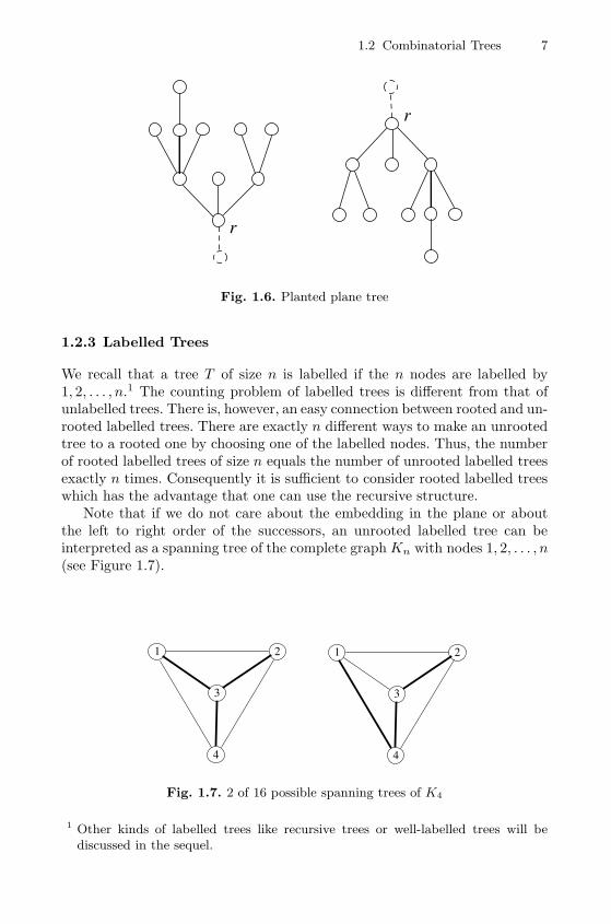
Note that if we do not care about the embedding in the plane or aboutthe left to right order of the successors, an unrooted labelled tree can beinterpreted as a spanning tree of the complete graphKn with nodes 1, 2, . . . , n(see Figure 1.7).
1 2
3
4
1 2
3
4
Fig. 1.7. 2 of 16 possible spanning trees of K4
1 Other kinds of labelled trees like recursive trees or well-labelled trees will bediscussed in the sequel.
8 1 Classes of Random Trees
It is a well known fact that the number of unrooted labelled trees of size nequals nn−2 (usually called Cayley’s formula). Hence, there are nn−1 differentrooted labelled trees of size n. Sometimes these trees are called Cayley trees(but this term is also used for infinite regular trees).
1.2.4 Labelled Plane Trees
It is also of interest to count the number of different planar embeddings oflabelled trees. There is even an explicit formula, namely for n ≥ 2 there are
(2n− 3)!
(n− 1)!
different planar embeddings of labelled trees of size n (and n(2n−3)!/(n−1)!different planar embeddings of rooted labelled trees of size n). For example,for n = 4 there are 42 = 16 different labelled trees but 5!/3! = 20 differentplanar embeddings.
1.2.5 Unlabelled Trees
Let T denote the set of unlabelled unrooted trees and T be the set of unla-belled rooted trees. Here we do not care about the possible embeddings intothe plane. We just think of trees in the graph-theoretical sense.
These kinds of trees are relatively difficult to count. Let us denote by tnand tn the corresponding numbers of those trees of size n, for example wehave
t1 = 1, t2 = 1, t3 = 1, t4 = 2 and t1 = 1, t2 = 1, t3 = 2, t4 = 4.
However, if there is no direct recursive relation one has to take into accountall symmetries. Nevertheless, this problem can be solved by using generatingfunctions and Polya’s theory of counting [176] (see Section 3.1.5). For thatreason these trees are also called Polya trees.
In order to give an impression of the kind of problems one has to face wejust state that the generating functions
t(x) =∑n≥1
tnxn and t(x) =
∑n≥1
tnxn
satisfy the relations
t(x) = x exp
(t(x) +
1
2t(x2) +
1
3t(x3) + · · ·
)(1.2)
and
t(x) = t(x) − 1
2t(x)2 +
1
2t(x2). (1.3)
It seems that there is no proper explicit formula for tn and tn. However, thereare asymptotic expansions for them and by using extensions of the mentionedcounting procedure it is also possible to study several shape characteristics ofthese kinds of trees.
1.2 Combinatorial Trees 9
1.2.6 Unlabelled Plane Trees
We already mentioned that a tree usually has several different embeddingsinto the plane. Planted plane trees are, in particular, designed to take intoaccount all possible planar embeddings of planted rooted trees.
It is, however, another non-trivial step to count all embeddings of unla-belled rooted trees and all embeddings of unlabelled trees. Again we haveto take into account symmetries. Fortunately Polya’s theory can be appliedhere, too. As in the case of unlabelled trees we do not get explicit formulasbut asymptotic expansions (see Section 3.1.6).
1.2.7 Simply Generated Trees – Galton-Watson Trees
Simply generated trees are weighted versions of rooted trees and have beenintroduced by Meir and Moon [151]. The idea is to put a weight to a rootedtree according to its degree distribution.
Let φj , j ≥ 0, be a sequence of non-negative real numbers, called theweight sequence. Usually one assumes that φ0 > 0 and φj > 0 for some j ≥ 2.We then define the weight ω(T ) of a finite rooted ordered tree T by
ω(T ) =∏
v∈V (T )
φd+(v) =∏j≥0
φDj(T )j ,
where d+(v) denotes the out-degree of the vertex v (or the number of succes-sors) and Dj(T ) the number of nodes in T with j successors. The numbers
yn =∑|T |=n
ω(T )
are then the weighted numbers of trees of size n. It is natural to define aprobability distribution on the set Tn by
πn(T ) =ω(T )
yn(T ∈ Tn). (1.4)
It is convenient to introduce the generating series
Φ(x) = φ0 + φ1x+ φ2x2 + · · · =
∑j≥0
φjxj .
In Section 3.1.4 we will show that the generating function y(x) =∑
n≥1 ynxn
satisfies the equationy(x) = xΦ(y(x)).
This equation is the key for the asymptotic analysis of these kinds of trees.If we replace φj by φj = abjφj , which is the same as replacing Φ(x) by
Φ(x) = aΦ(bx) for two numbers a, b > 0, then ω(T ) is replaced by
10 1 Classes of Random Trees
ω(T ) =∏j≥0
(abjφj
)Dj(T )= a|T |b|T |−1ω(T ).
Note that∑
j jDj(T ) = |T | − 1. Hence, yn = anbn−1yn and the probability
distribution πn on Tn is the same for Φ(x) and Φ(x) (for every n). Usuallyonly these distributions are important, and we may then freely make this typeof modification of φj .
Simply generated trees generalise several of the above examples of combi-natorial trees.
Example 1.2 If φj = 1 for all j ≥ 0, that is, Φ(x) = 1/(1 − x), then allplanted plane trees have weight ω(T ) = 1 and yn is the number of plantedplane trees. Thus, πn is the uniform distribution on planted plane trees ofsize n.
Example 1.3 Binary trees (counted according to their internal nodes) arealso covered by this approach. If we set φ0 = 1, φ1 = 2, φ2 = 1, and φj = 0for j ≥ 3, that is, Φ(x) = (1+x)2, then nodes with one successor get weight 2.This takes into account that binary trees (where external nodes are disregarded)have two kinds of nodes with one successor, namely those with a left branchbut no right branch and those with a right branch but no left branch. Thus,πn is the uniform distribution on all binary trees with n internal nodes.
Similarly, m-ary trees are covered with the help of the weights φj =(mj
)or with Φ(x) = (1 + x)m.
Example 1.4 If φ0 = φ1 = φ2 = 1 and φj = 0 for j ≥ 3 or Φ(x) = 1+x+x2,then we get so-called Motzkin trees. Here only rooted trees, where all nodeshave less than 3 successors, get (a non-zero) weight ω(T ) = 1: yn is thenumber of Motzkin trees with n nodes and πn is the uniform distribution onMotzkin trees of size n.
Example 1.5 If we set φj = 1/j! then
n! · yn = nn−1
denotes precisely the number of labelled rooted non-plane trees. The weightφj = 1/j! disregards all possible orderings of the successors of a vertex ofout-degree j and the factor n! corresponds to all possible labellings of n nodes.Hence, πn yields the uniform distribution on labelled rooted trees.
Interestingly there is an intimate relation to Galton-Watson branching pro-cesses. Let ξ be a non-negative integer-valued random variable, the so-calledoffspring distribution. The Galton-Watson branching process starts with asingle individual (generation 0); each individual has a number of children dis-tributed as independent copies of ξ. If Zk denotes the size of the generationk, then a formal description of the process (Zk)k≥0 is Z0 = 1, and for k ≥ 1
1.2 Combinatorial Trees 11
Zk =
Zk−1∑j=1
ξ(k)j ,
where the (ξ(k)j )k,j are i.i.d.2 random variables distributed as ξ.
It is clear that Galton-Watson branching processes can be represented byordered (finite or infinite) rooted trees T such that the sequence Zk is just thenumber of nodes at level k and
∑k≥0 Zk (which is called the total progeny)
is the number of nodes |T | of T . We denote by ν(T ) the probability that aspecific tree T occurs. If P{ξ = 0} = 0 then the total progeny is infinite withprobability 1. Thus we always assume that P{ξ = 0} > 0.
The generating function y(x) =∑
n≥1 ynxn of the numbers
yn = P{|T | = n} =∑|T |=n
ν(T )
satisfies the functional equation
y(x) = xΦ(y(x)),
whereΦ(t) = E tξ =
∑j≥0
φjtj
with φj = P{ξ = j}. Observe that
ν(T ) =∏j≥0
φDj(T )j = ω(T ).
The weight of T is now the probability of T .If we condition the Galton-Watson tree T on |T | = n, we thus get the
probability distribution (1.4) on Tn. Hence, the conditioned Galton-Watsontrees are simply generated trees with φj = P{ξ = j} as above. We havehere Φ(1) =
∑j φj = 1, but this is no real restriction. In fact, if (φj)j≥0
is any sequence of non-negative weights satisfying the very weak conditionΦ(x) =
∑j≥0 φjx
j <∞ for some x > 0, then we can replace (as above) φj by
abjφj with b = x and a = 1/Φ(x) and thus the simply generated tree is thesame as the conditioned Galton-Watson tree with offspring distribution P{ξ =j} = φjx
j/Φ(x). Consequently, for all practical purposes, simply generatedtrees are the same as conditioned Galton-Watson trees.
The argument above also shows that the distribution of a conditionedGalton-Watson tree is not changed if we replace the offspring distribution ξby ξ with P{ξ = j} = P{ξ = j} = τ j/Φ(τ) and thus Φ(x) = Φ(τx)/Φ(τ) forany τ > 0 with Φ(τ) <∞. (Such modifications are called conjugate or tilteddistributions.)
2 The letters “i.i.d.” abbreviate “independent and identically distributed”.
12 1 Classes of Random Trees
Note thatμ = Φ′(1) = E ξ
is the expected value of the offspring distribution. If μ < 1, the Galton-Watsonbranching process is called sub-critical, if μ = 1, then it is critical, and if μ > 1,then it is supercritical. From a combinatorial point of view we do not haveto distinguish between these three cases. Namely, if we replace the offspringdistribution by a conjugate distribution as above, the new expected value is
Φ′(1) =τΦ′(τ)
Φ(τ).
We can thus always assume that the Galton-Watson process is critical, pro-vided only that there exists τ > 0 with
τΦ′(τ) = Φ(τ) <∞,
a weak condition that is satisfied for all interesting classes of Galton-Watsontrees.
It is usually convenient to choose a critical version, which explains whythe equation τΦ′(τ) = Φ(τ) appears in most asymptotic results. A heuristicreason is that the probability of the event |T | = n that we condition ontypically decays exponentially in the subcritical and supercritical cases butonly as n−1/2 in the critical case, and it seems advantageous to condition onan event of not too small probability.
Example 1.6 For planted plane trees (as in Example 1.2) we start withΦ(x) = 1/(1 − x). The equation τΦ′(τ) = Φ(τ) is τ(1 − τ)−2 = (1 − τ)−1,which is solved by τ = 1
2 . Random planted plane trees are thus conditionedGalton-Watson trees with the critical offspring distribution given by Φ(x) =(1 − x/2)−1/2 = 1/(2 − x), or P{ξ = j} = 2−j−1 (for j ≥ 0), a geometricdistribution.
Example 1.7 Similarly random binary trees are obtained with a binomialoffspring distribution Bi(2, 1/2) with Φ(x) = (1 + x)2/4, and more generallyrandom m-ary trees are obtained with offspring law Bi(m, 1/m) with Φ(x) =((m− 1 + x)/m)
m.
Example 1.8 For Motzkin trees the critical offspring distribution ξ is uni-form on {0, 1, 2} with Φ(x) = (1 + x+ x2)/3.
Example 1.9 For uniform rooted labelled trees the critical ξ has a Poissondistribution Po(1) with Φ(x) = ex−1.
Finally we remark that for a critical offspring distribution ξ, its varianceis given by
σ2 = Var ξ = E ξ2 − 1 = E(ξ(ξ − 1)) = Φ′′(1).
1.3 Recursive Trees 13
Starting with an arbitrary sequence (φj)j≥0 and modifying it as above the geta critical probability distribution, we obtain the variance
σ2 = Φ′′(1) =τ2Φ′′(τ)
Φ(τ),
where τ > 0 is such that τΦ′(τ) = Φ(τ) < ∞ (assuming this is possible). Wewill see that this quantity appears in several asymptotic results.
1.3 Recursive Trees
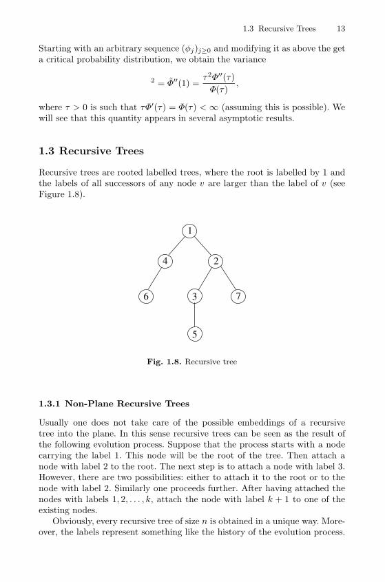
Recursive trees are rooted labelled trees, where the root is labelled by 1 andthe labels of all successors of any node v are larger than the label of v (seeFigure 1.8).
1
2
3
4
5
6 7
Fig. 1.8. Recursive tree
1.3.1 Non-Plane Recursive Trees
Usually one does not take care of the possible embeddings of a recursivetree into the plane. In this sense recursive trees can be seen as the result ofthe following evolution process. Suppose that the process starts with a nodecarrying the label 1. This node will be the root of the tree. Then attach anode with label 2 to the root. The next step is to attach a node with label 3.However, there are two possibilities: either to attach it to the root or to thenode with label 2. Similarly one proceeds further. After having attached thenodes with labels 1, 2, . . . , k, attach the node with label k + 1 to one of theexisting nodes.
Obviously, every recursive tree of size n is obtained in a unique way. More-over, the labels represent something like the history of the evolution process.
14 1 Classes of Random Trees
Since there are exactly k ways to attach the node with label k + 1, there areexactly (n− 1)! possible trees of size n.
The natural probability distribution on recursive trees of size n is to assumethat each of these (n− 1)! trees is equally likely. This probability distributionis also obtained from the evolution process by attaching successively each newnode to one of the already existing nodes with equal probability.
Remark 1.10 Historically, recursive trees appear in various contexts. Theyare used to model the spread of epidemics (see [155]) or to investigate andconstruct family trees of preserved copies of ancient manuscripts (see [157]).Other applications are the study of the schemes of chain letters or pyramidgames (see [88]).
1.3.2 Plane Oriented Recursive Trees
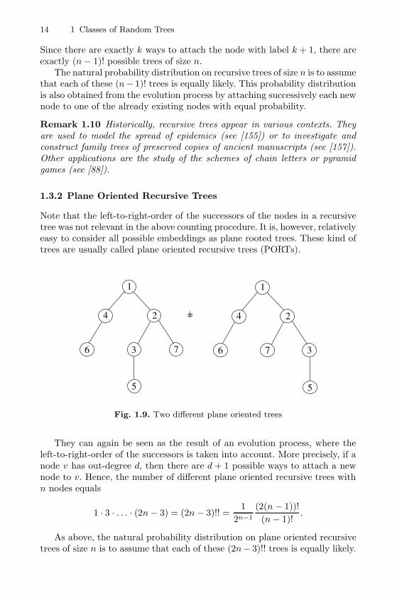
Note that the left-to-right-order of the successors of the nodes in a recursivetree was not relevant in the above counting procedure. It is, however, relativelyeasy to consider all possible embeddings as plane rooted trees. These kind oftrees are usually called plane oriented recursive trees (PORTs).
1
2
3
4
5
6 7
1
2
3
4
5
6 7
=
Fig. 1.9. Two different plane oriented trees
They can again be seen as the result of an evolution process, where theleft-to-right-order of the successors is taken into account. More precisely, if anode v has out-degree d, then there are d + 1 possible ways to attach a newnode to v. Hence, the number of different plane oriented recursive trees withn nodes equals
1 · 3 · . . . · (2n− 3) = (2n− 3)!! =1
2n−1
(2(n− 1))!
(n− 1)!.
As above, the natural probability distribution on plane oriented recursivetrees of size n is to assume that each of these (2n− 3)!! trees is equally likely.
1.3 Recursive Trees 15
This probability distribution is also obtained from the evolution process byattaching each node with probability proportional to the out-degree plus 1 tothe already existing nodes.
1.3.3 Increasing Trees
The probabilistic model of simply generated trees was to define a weight thatreflects the degree distribution of rooted trees. The same idea can be appliedto recursive and to plane oriented recursive trees. The resulting classes oftrees are called increasing trees. They have been first introduced by Bergeron,Flajolet, and Salvy [12].
As above we define the weight ω(T ) of a recursive or a plane orientedrecursive tree T by
ω(T ) =∏
v∈V (T )
φd+(v) =∏j≥0
φDj(T )j ,
where d+(v) denotes the out-degree of the vertex v (or the number of suc-cessors) and Dj(T ) the number of nodes in T with j successors. Then weset
yn =∑
T∈Jn
ω(T ),
where Jn denotes the set of recursive or plane oriented recursive trees of sizen. The natural probability distribution on the set Jn of increasing trees isthen given by
πn(T ) =ω(T )
yn(T ∈ Jn).
As in the case of simply generated trees it is also possible to introducegenerating series. We set
Φ(x) = φ0 + φ1x+ φ2x2
2!+ φ2
x3
3!+ · · ·
in the case of recursive trees and
Φ(x) = φ0 + φ1x+ φ2x2 + φ3x
3 + · · ·
in the case of plane oriented recursive trees. The generating function
y(z) =∑n≥0
ynzn
n!
satisfies the differential equation
y′(z) = Φ(y(z)), y(0) = 0.
In the interest of clarity we state how the general concept specialises.
16 1 Classes of Random Trees
1. Recursive trees (that is, every non-planar recursive tree gets weight 1) aregiven by Φ(x) = ex. Here yn = (n− 1)! and y(z) = log(1/(1− z)).
2. Plane oriented recursive trees are given by Φ(x) = 1/(1− x). This meansthat every planar recursive tree gets weight 1. Here yn = (2n − 3)!! =1 · 3 · 5 · · · (2n− 3) and y(z) = 1−
√1− 2z.
3. Binary recursive trees are defined by Φ(x) = (1 + x)2. We have yn = n!and y(z) = 1/(1 − z). The probability model that is induced by this(planar) binary increasing trees is exactly the standard permutation modelof binary search trees that is discussed in Section 1.4.1.
Note that the probability distribution on Jn is not automatically given byan evolution process as it is definitely the case for recursive trees and planeoriented recursive trees. It is interesting that there are precisely three familiesof increasing trees, where the probability distribution πn is also induced by a(natural) tree evolution process.
1. Φ(x) = φ0eφ1φ0
xwith φ0 > 0, φ1 > 0.
2. Φ(x) = φ0
(1− φ1
rφ0x
)−r
for some r > 0 and φ0 > 0, φ1 > 0.
3. Φ(x) = φ0 (1 + (φ1/(dφ0))x)d
for some d ∈ {2, 3, . . .} and φ0 > 0, φ1 > 0.
The corresponding tree evolution process runs as follows:3 The starting pointis (again) a node (the root) with label 1. Now assume that a tree T of size n ispresent. We attach to every node v of T a local weight ρ(v) = (k+1)φk+1φ0/φk
when v has k successors and set ρ(T ) =∑
v∈V (T ) ρ(v). Observe that in a
planar tree there are k + 1 different ways to attach a new (labelled) nodeto an (already existing) node with k successors. Now choose a node v in Taccording to the probability distribution ρ(v)/ρ(T ) and then independentlyand uniformly one of the k+ 1 possibilities to attach a new node there (whenv has k successors). This construction ensures that in these three particularcases a tree T of size n, which occurs with probability proportional to ω(T ),generates a tree T ′ of size n + 1 with probability that is proportional toω(T )φk+1φ0/φk, which equals ω(T ′). Thus, this procedure induces the sameprobability distribution on Jn as the one mentioned above, where a tree T ∈Jn has probability ω(T )/yn.
Note that if we are only interested in the distributions πn, then we canwork (without loss of generality) with some special values for φ0 and φ1. It issufficient to consider the generating functions
1. Φ(x) = ex,2. Φ(x) = (1− x)−r for some r > 0,3. Φ(x) = (1 + x)d for some d ∈ {2, 3, . . .}.
The first class is just the class of recursive trees. The second class can beinterpreted as generalised plane oriented recursive trees, since the probability
3 In the interest of brevity we only discuss the plane version.
1.4 Search Trees 17
of choosing a node with out-degree j is proportional to j + r. For r = 1 weget (usually) plane oriented recursive trees. The trees in the third class areso-called d-ary recursive trees; they correspond to an interesting tree evolutionprocess that we shortly describe for d = 3.
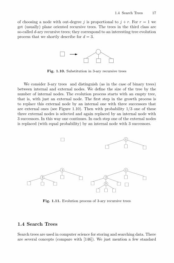
Fig. 1.10. Substitution in 3-ary recursive trees
We consider 3-ary trees and distinguish (as in the case of binary trees)between internal and external nodes. We define the size of the tree by thenumber of internal nodes. The evolution process starts with an empty tree,that is, with just an external node. The first step in the growth process isto replace this external node by an internal one with three successors thatare external ones (see Figure 1.10). Then with probability 1/3 one of thesethree external nodes is selected and again replaced by an internal node with3 successors. In this way one continues. In each step one of the external nodesis replaced (with equal probability) by an internal node with 3 successors.
1
1
2
1
2
3
Fig. 1.11. Evolution process of 3-ary recursive trees
1.4 Search Trees
Search trees are used in computer science for storing and searching data. Thereare several concepts (compare with [146]). We just mention a few standard
18 1 Classes of Random Trees
probabilistic models that are used to analyse these kinds of trees and thealgorithms that are related with them.
1.4.1 Binary Search Trees
The origin of binary search trees dates to a fundamental problem in computerscience: the dictionary problem. In this problem a set of records is given whereeach can be addressed by a key. The binary search tree is a data structureused for storing the records. Basic operations include insert and search.
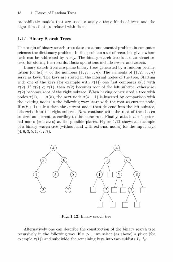
Binary search trees are plane binary trees generated by a random permu-tation (or list) π of the numbers {1, 2, . . . , n}. The elements of {1, 2, . . . , n}serve as keys. The keys are stored in the internal nodes of the tree. Startingwith one of the keys (for example with π(1)) one first compares π(1) withπ(2). If π(2) < π(1), then π(2) becomes root of the left subtree; otherwise,π(2) becomes root of the right subtree. When having constructed a tree withnodes π(1), . . . , π(k), the next node π(k + 1) is inserted by comparison withthe existing nodes in the following way: start with the root as current node.If π(k + 1) is less than the current node, then descend into the left subtree,otherwise into the right subtree. Now continue with the root of the chosensubtree as current, according to the same rule. Finally, attach n + 1 exter-nal nodes (= leaves) at the possible places. Figure 1.12 shows an exampleof a binary search tree (without and with external nodes) for the input keys(4, 6, 3, 5, 1, 8, 2, 7).
1
2
3
4
5
6
7
8 1
2
3
4
5
6
7
8
Fig. 1.12. Binary search tree
Alternatively one can describe the construction of the binary search treerecursively in the following way. If n > 1, we select (as above) a pivot (forexample π(1)) and subdivide the remaining keys into two sublists I1, I2:
1.4 Search Trees 19
I1 = (x ∈ {π(2), . . . , π(n)} : x < π(1)) and
I2 = (x ∈ {π(2), . . . , π(n)} : x > π(1)) .
The pivot π(1) is put to the root and by recursively applying the same proce-dure, the elements of I1 constitute the left subtree of the root and the elementsof I2 the right subtree. This is precisely the standard Quicksort algorithm.
At the moment there is no randomness involved. Every input sequenceinduces uniquely and deterministically a binary search tree. However, if weassume that the input data follow some probabilistic rule, then this inducesa probability distribution on the corresponding binary search trees. The mostcommon probabilistic model is the random permutation model, where oneassumes that every permutation of the input data 1, 2, . . . , n is equally likely.
By assuming this standard probability model, there is, however, a com-pletely different point of view to binary search trees, namely the tree evolutionprocess of 2-ary recursive trees (compare with the description of 3-ary recur-sive trees in Section 1.3.3). Here one starts with the empty tree (just consistingof an external vertex). Then in a first step this external node is replaced by aninternal one with two attached external nodes. In a second step one of thesetwo external nodes is again replaced by an internal one with two attachedexternal nodes. In this way one continues. In each step one of the existingexternal nodes is replaced by an internal one (plus two externals) with equalprobability.
It is easy to explain that these two models actually produce the same kindsof random trees. Suppose that the keys 1, . . . , n are replaced by n real numbersx1, . . . , xn that are ordered, that is, x1 < x2 < · · · < xn. Suppose that we havealready constructed a binary search tree T according to some permutation πof x1, . . . , xn. The choice of an external node of T and replacing it by aninternal one corresponds to the choice of one of the n+ 1 intervals (−∞, x1),(x1, x2), . . ., (xn,∞) and choosing a number x∗ of one of these intervals andworking out the binary search tree algorithm to the list of n + 1 elements,where x∗ is appended to the list π (compare with Figure 1.12). However, thisprocedure also produces equally likely random permutations of n+1 elementsfrom a random permutation of n elements.
1.4.2 Fringe Balanced m-Ary Search Trees
There are several generalisations of binary search trees. The search trees thatwe consider here, are characterised by two integer parameters m ≥ 2 andt ≥ 0. As binary search trees they are built from a set of n distinct keystaken from some totally ordered sets such as real numbers or integers. For ourpurposes we again assume that the keys are the integers 1, . . . , n. The searchtree is an m-ary tree where each node has at most m successors; moreover,each node stores one or several of the keys, up to at most m− 1 keys in eachnode. The parameter t affects the structure of the trees; higher values of t
20 1 Classes of Random Trees
tend to make the tree more balanced. The special case m = 2 and t = 0corresponds to binary search trees.
To describe the construction of the search tree, we begin with the simplestcase t = 0. If n = 0, the tree is empty. If 1 ≤ n ≤ m− 1 the tree consists of aroot only, with all keys stored in the root. If n ≥ m we select m− 1 keys thatare called pivots. The pivots are stored in the root. The m− 1 pivots split theset of the remaining n−m+1 keys into m sublists I1, . . . , Im: if the pivots arex1 < x2 < · · · < xm−1, then I1 := (xi : xi < x1), I2 := (xi : x1 < xi < x2),. . . , Im := (xi : xm−1 < xi). We then recursively construct a search tree foreach of the sets Ii of keys (ignoring it if Ii is empty), and attach the roots ofthese trees as children of the root in the search tree from left to right.
In the case t ≥ 1, the only difference is that the pivots are selected ina different way. We now select mt + m − 1 keys at random, order them asy1 < · · · < ymt+m−1, and let the pivots be yt+1, y2(t+1), . . . , y(m−1)(t+1). Inthe case m ≤ n < mt+m−1, when this procedure is impossible, we select thepivots by some supplementary rule (depending only on the order properties ofthe keys). Usually one aims that the corresponding subtree that is generatedhere is as balanced as possible. This explains the notion fringe balanced tree.In particular, in the case m = 2, we let the pivot be the median of 2t + 1selected keys (when n ≥ 2t+ 1).
The standard probability model is again to assume that every permutationof the keys 1, . . . , n is equally likely. The choice of the pivots can then bedeterministic. For example, one always chooses the first mt +m − 1 keys. Itis then easy to describe the splitting at the root of the tree by the randomvector Vn = (Vn,1, Vn,2, . . . , Vn,m), where Vn,k := |Ik| is the number of keysin the k-th subset, and thus the number of nodes in the k-th subtree of theroot (including empty subtrees).
We thus always have, provided n ≥ m,
Vn,1 + Vn,2 + · · ·+ Vn,m = n− (m− 1) = n+ 1−mand elementary combinatorics, counting the number of possible choices of themt + m − 1 selected keys, showing that the probability distribution is, forn ≥ mt+m− 1 and n1 + n2 + · · ·+ nm = n−m+ 1,
P{Vn = (n1, . . . , nm)} =
(n1
t
)· · ·(nm
t
)(n
mt+m−1
) . (1.5)
(The distribution of Vn for m ≤ n < mt+m− 1 is not specified.)In particular, for n ≥ mt + m − 1, the components Vn,j are identically
distributed, and another simple counting argument yields, for n ≥ mt+m−1and 0 ≤ � ≤ n− 1,
P{Vn,j = �} =
(�t
)(n−�−1
(m−1)t+m−2
)(n
mt+m−1
) . (1.6)
For usual binary search tree with m = 2 and t = 0 we have Vn,1 and Vn,2 =n− 1− Vn−1 which are uniformly distributed on {0, . . . , n− 1}.
1.4 Search Trees 21
1.4.3 Digital Search Trees
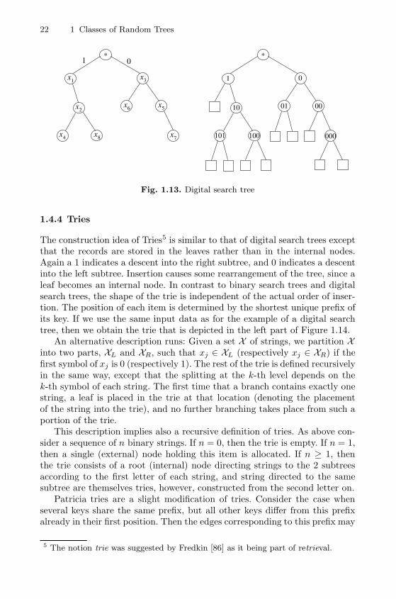
Digital search trees are intended for the same kind of problems as binarysearch trees. However, they are not constructed from the total order structureof the keys for the data stored in the internal nodes of the tree but from digitalrepresentations (or binary sequences) which serve as keys.
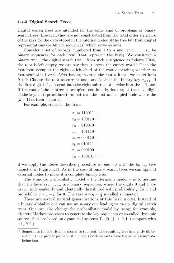
Consider a set of records, numbered from 1 to n and let x1, . . . , xn bebinary sequences for each item (that represent the keys). We construct abinary tree – the digital search tree – from such a sequence as follows. First,the root is left empty, we can say that it stores the empty word.4 Then thefirst item occupies the right or left child of the root depending whether itsfirst symbol is 1 or 0. After having inserted the first k items, we insert itemk + 1: Choose the root as current node and look at the binary key xk+1. Ifthe first digit is 1, descend into the right subtree, otherwise into the left one.If the root of the subtree is occupied, continue by looking at the next digitof the key. This procedure terminates at the first unoccupied node where the(k + 1)-st item is stored.
For example, consider the items
x1 = 110011 · · ·x2 = 100110 · · ·x3 = 010010 · · ·x4 = 101110 · · ·x5 = 000110 · · ·x6 = 010111 · · ·x7 = 000100 · · ·x8 = 100101 · · · .
If we apply the above described procedure we end up with the binary treedepicted in Figure 1.13. As in the case of binary search trees we can appendexternal nodes to make it a complete binary tree.
The standard probabilistic model – the Bernoulli model – is to assumethat the keys x1, . . . , xn are binary sequences, where the digits 0 and 1 aredrawn independently and identically distributed with probability p for 1 andprobability q = 1− p for 0. The case p = q = 1
2 is called symmetric.There are several natural generalisations of this basic model. Instead of
a binary alphabet one can use an m-ary one leading to m-ary digital searchtrees. One can also change the probabilistic model by using, for example,discrete Markov processes to generate the key sequences or so-called dynamicsources that are based on dynamical systems T : [0, 1] → [0, 1] (compare with[41, 206]).
4 Sometimes the first item is stored to the root. The resulting tree is slightly differ-ent but (in a proper probabilistic model) both variants have the same asymptoticbehaviour.
22 1 Classes of Random Trees
x
*
1
x2
x3
x6 x5
x7x4 x8
1 0
1
*
01
0
000
00
101
10
100
Fig. 1.13. Digital search tree
1.4.4 Tries
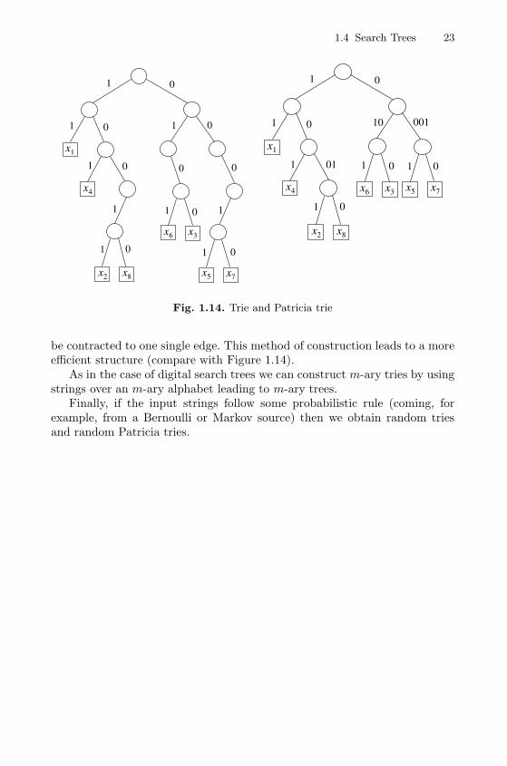
The construction idea of Tries5 is similar to that of digital search trees exceptthat the records are stored in the leaves rather than in the internal nodes.Again a 1 indicates a descent into the right subtree, and 0 indicates a descentinto the left subtree. Insertion causes some rearrangement of the tree, since aleaf becomes an internal node. In contrast to binary search trees and digitalsearch trees, the shape of the trie is independent of the actual order of inser-tion. The position of each item is determined by the shortest unique prefix ofits key. If we use the same input data as for the example of a digital searchtree, then we obtain the trie that is depicted in the left part of Figure 1.14.
An alternative description runs: Given a set X of strings, we partition Xinto two parts, XL and XR, such that xj ∈ XL (respectively xj ∈ XR) if thefirst symbol of xj is 0 (respectively 1). The rest of the trie is defined recursivelyin the same way, except that the splitting at the k-th level depends on thek-th symbol of each string. The first time that a branch contains exactly onestring, a leaf is placed in the trie at that location (denoting the placementof the string into the trie), and no further branching takes place from such aportion of the trie.
This description implies also a recursive definition of tries. As above con-sider a sequence of n binary strings. If n = 0, then the trie is empty. If n = 1,then a single (external) node holding this item is allocated. If n ≥ 1, thenthe trie consists of a root (internal) node directing strings to the 2 subtreesaccording to the first letter of each string, and string directed to the samesubtree are themselves tries, however, constructed from the second letter on.
Patricia tries are a slight modification of tries. Consider the case whenseveral keys share the same prefix, but all other keys differ from this prefixalready in their first position. Then the edges corresponding to this prefix may
5 The notion trie was suggested by Fredkin [86] as it being part of retrieval.
1.4 Search Trees 23
1 0
1
1
1
1
1
1
1
0
00 0
0
0 0
1x
4x
2x 8x
6x 3x
5x 7x
0
1
1 0
1
1
1
10
1 1
0
01 0
0
0
1x
4x
2x 8x
6x 3x 5x 7x
001
Fig. 1.14. Trie and Patricia trie
be contracted to one single edge. This method of construction leads to a moreefficient structure (compare with Figure 1.14).
As in the case of digital search trees we can construct m-ary tries by usingstrings over an m-ary alphabet leading to m-ary trees.
Finally, if the input strings follow some probabilistic rule (coming, forexample, from a Bernoulli or Markov source) then we obtain random triesand random Patricia tries.

2
Generating Functions
Generating functions are not only a useful tool to count combinatorial objectsbut also an analytic object that can be used to obtain asymptotics. They canbe used to encode the distribution of random variables that are related tocounting problems and, hence, asymptotic methods can be applied to obtainprobabilistic limit theorems like central limit theorems.
In this chapter we survey some properties of generating functions followingthe mentioned categories above. First we collect some useful facts on gener-ating functions in relation to counting problems, in particular, how certaincombinatorial constructions have their counterparts in relations for generat-ing functions. Next we provide a short introduction into singularity analysisof generating functions and its applications to asymptotics.
One major goal is to provide analytic and asymptotic properties of a gen-erating function when it satisfies a functional equation and more generallywhen it is related to the solution of a system of functional equations. This sit-uation occurs naturally in combinatorial problems with a recursive structure(as in tree counting problems) because a recursive relation usually translatesinto a functional equation for the corresponding generating function.
It turns out that solutions of functional equations typically have a finiteradius of convergence R and – what is even more remarkable – that the kindof singularity at x = R is of so-called square root type. This means thatthe generating function can be represented as a power series in
√R− x. This
explains that square root type singularities are omnipresent in the asymptoticsof tree enumeration problems.
26 2 Generating Functions
2.1 Counting with Generating Functions
Generating functions are quite natural in the context of tree counting since(rooted) trees have a recursive structure that usually translates to recurrencerelations for corresponding counting problems. Besides generating functionsare a proper tool for solving recurrence equations.
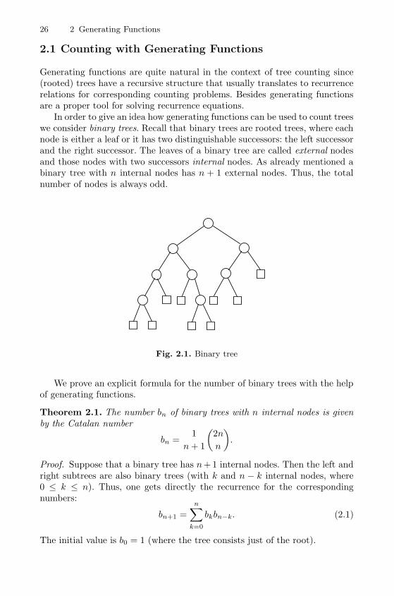
In order to give an idea how generating functions can be used to count treeswe consider binary trees. Recall that binary trees are rooted trees, where eachnode is either a leaf or it has two distinguishable successors: the left successorand the right successor. The leaves of a binary tree are called external nodesand those nodes with two successors internal nodes. As already mentioned abinary tree with n internal nodes has n + 1 external nodes. Thus, the totalnumber of nodes is always odd.
Fig. 2.1. Binary tree
We prove an explicit formula for the number of binary trees with the helpof generating functions.
Theorem 2.1. The number bn of binary trees with n internal nodes is givenby the Catalan number
bn =1
n+ 1
(2n
n
).
Proof. Suppose that a binary tree has n+ 1 internal nodes. Then the left andright subtrees are also binary trees (with k and n − k internal nodes, where0 ≤ k ≤ n). Thus, one gets directly the recurrence for the correspondingnumbers:
bn+1 =
n∑k=0
bkbn−k. (2.1)
The initial value is b0 = 1 (where the tree consists just of the root).
2.1 Counting with Generating Functions 27
This recurrence can be solved using the generating function
b(x) =∑n≥0
bnxn.
By (2.1) we find the relation
b(x) = 1 + xb(x)2 (2.2)
and consequently an explicit representation of the form
b(x) =1−
√1− 4x
2x. (2.3)
Hence (by using the notation [xn]a(x) = an for the n-th coefficient of a powerseries a(x) =
∑n≥0 anx
n) we obtain
bn = [xn]1−
√1− 4x
2x
= −1
2[xn+1](1− 4x)
12
= −1
2
( 12
n+ 1
)(−4)n+1
=1
n+ 1
(2n
n
).
By inspecting the proof of Theorem 2.1 one observes that the recurrencerelation (2.1) – together with its initial condition – is exactly a translationof a recursive description of binary trees (that was given in Section 1.2.1: abinary tree B is either just an external node or an internal node (the root)with two subtrees that are again binary trees.
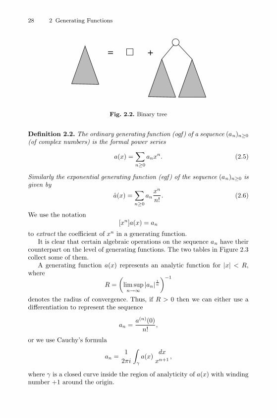
It is also worth mentioning that the formal restatement of this recursivedefinition,
B = � + ◦ × B × B = � + ◦ × B2, (2.4)
leads to a corresponding relation (2.2) for the generating function:
b(x) = 1 + xb(x)2,
compare also with the schematic Figure 2.2.
2.1.1 Generating Functions and Combinatorial Constructions
We will now provide a more systematic treatment of combinatorial construc-tions and generating functions. The presentation is inspired by the work ofFlajolet and his co-authors (see in particular the monograph [84] where thisconcept is described in much more detail).
28 2 Generating Functions
= +
Fig. 2.2. Binary tree
Definition 2.2. The ordinary generating function (ogf) of a sequence (an)n≥0
(of complex numbers) is the formal power series
a(x) =∑n≥0
anxn. (2.5)
Similarly the exponential generating function (egf) of the sequence (an)n≥0 isgiven by
a(x) =∑n≥0
anxn
n!. (2.6)
We use the notation[xn]a(x) = an
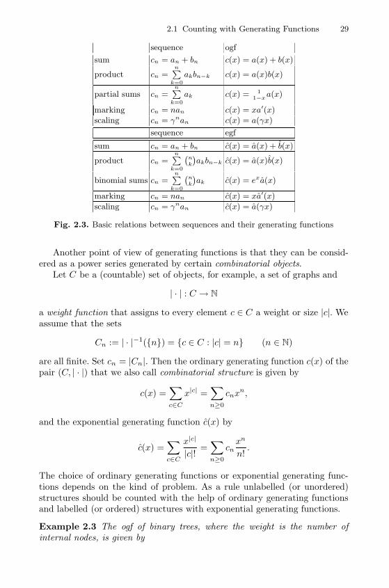
to extract the coefficient of xn in a generating function.It is clear that certain algebraic operations on the sequence an have their
counterpart on the level of generating functions. The two tables in Figure 2.3collect some of them.
A generating function a(x) represents an analytic function for |x| < R,where
R =
(lim sup
n→∞|an|
1n
)−1
denotes the radius of convergence. Thus, if R > 0 then we can either use adifferentiation to represent the sequence
an =a(n)(0)
n!,
or we use Cauchy’s formula
an =1
2πi
∫γ
a(x)dx
xn+1,
where γ is a closed curve inside the region of analyticity of a(x) with windingnumber +1 around the origin.
2.1 Counting with Generating Functions 29
sequence ogf
sum cn = an + bn c(x) = a(x) + b(x)
product cn =nP
k=0
akbn−k c(x) = a(x)b(x)
partial sums cn =nP
k=0
ak c(x) = 11−x
a(x)
marking cn = nan c(x) = xa′(x)
scaling cn = γnan c(x) = a(γx)
sequence egf
sum cn = an + bn c(x) = a(x) + b(x)
product cn =nP
k=0
`nk
´akbn−k c(x) = a(x)b(x)
binomial sums cn =nP
k=0
`nk
´ak c(x) = exa(x)
marking cn = nan c(x) = xa′(x)
scaling cn = γnan c(x) = a(γx)
Fig. 2.3. Basic relations between sequences and their generating functions
Another point of view of generating functions is that they can be consid-ered as a power series generated by certain combinatorial objects.
Let C be a (countable) set of objects, for example, a set of graphs and
| · | : C → N
a weight function that assigns to every element c ∈ C a weight or size |c|. Weassume that the sets
Cn := | · |−1({n}) = {c ∈ C : |c| = n} (n ∈ N)
are all finite. Set cn = |Cn|. Then the ordinary generating function c(x) of thepair (C, | · |) that we also call combinatorial structure is given by
c(x) =∑c∈C
x|c| =∑n≥0
cnxn,
and the exponential generating function c(x) by
c(x) =∑c∈C
x|c|
|c|! =∑n≥0
cnxn
n!.
The choice of ordinary generating functions or exponential generating func-tions depends on the kind of problem. As a rule unlabelled (or unordered)structures should be counted with the help of ordinary generating functionsand labelled (or ordered) structures with exponential generating functions.
Example 2.3 The ogf of binary trees, where the weight is the number ofinternal nodes, is given by
30 2 Generating Functions
b(x) =1−
√1− 4x
2x.
Example 2.4 The egf of permutations of finite sets, where the weight is thesize of the finite set, is given by
p(x) =∑n≥0
n!xn
n!=
1
1− x .
One major aspect in the use of generating functions is that certain combi-natorial constructions have their counterparts in relations of the correspondinggenerating functions. The recursive description of binary trees (2.4) is a niceexample to support this statement.
We again use the notation A,B,C, . . . for sets of combinatorial objectswith corresponding size functions | · |. First suppose that the objects that weconsider are (in some sense) unlabelled or unordered. We have the followingbasic operations:
1. If A and B are disjoint then C = A+B = A ∪B denotes the union of Aand B.
2. C = A × B denotes the Cartesian product. The size function of a pairc = (a, b) is given by |c| = |a|+ |b|.
3. Suppose that A contains no object of size 0 and that the sets A, A × A,A×A×A, . . . are disjoint. Then
C = A∗ := {ε}+A+A×A+A×A×A+ · · ·
is the set of (finite) sequences of elements of A (ε denotes the empty objectof size zero).
4. Let C = Pfin(A) denote the set of all finite subsets of A. The size of asubset {a1, a2, . . . , ak} ⊆ A is given by |{a1, a2, . . . , ak}| = |a1| + |a2| +· · ·+ |ak|.
5. Let C = Mfin(A) denote the set of all finite multisets {aj11 , a
j22 , . . . , a
jk
k }of A, that is, the element ai is taken ji times (1 ≤ i ≤ k). Its size is givenby |{aj1
1 , aj22 , . . . , a
jk
k }| = j1|a1|+ j2|a2|+ · · ·+ jk|ak|.6. Suppose that B has no object of zero size. Then the composition C =A(B) of A and B is given by
C = A(B) := A0 +A1 ×B +A2 ×B ×B + · · · ,
where An = {a ∈ A | |a| = n}. The size of (a, b1, b2, . . . , bn) ∈ An×B×B×· · ·×B is defined by |b1|+|b2|+· · ·+|bn|. The combinatorial interpretationof this construction is that an element a ∈ A of size |a| = n is substitutedby an n-tuple of elements of B.
As already indicated these combinatorial constructions have counterpartsin relations of generating functions:
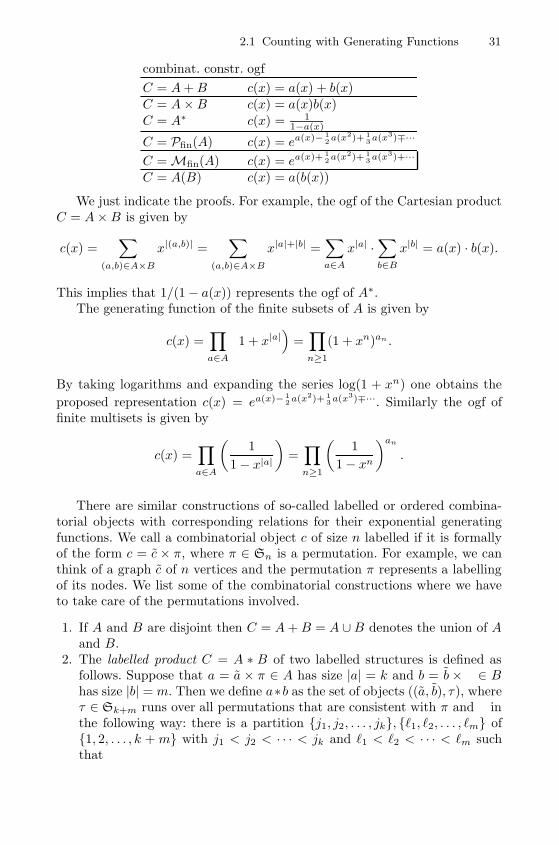
2.1 Counting with Generating Functions 31
combinat. constr. ogf
C = A+B c(x) = a(x) + b(x)C = A×B c(x) = a(x)b(x)C = A∗ c(x) = 1
1−a(x)
C = Pfin(A) c(x) = ea(x)− 12 a(x2)+ 1
3 a(x3)∓···
C = Mfin(A) c(x) = ea(x)+ 12 a(x2)+ 1
3 a(x3)+···
C = A(B) c(x) = a(b(x))
We just indicate the proofs. For example, the ogf of the Cartesian productC = A×B is given by
c(x) =∑
(a,b)∈A×B
x|(a,b)| =∑
(a,b)∈A×B
x|a|+|b| =∑a∈A
x|a| ·∑b∈B
x|b| = a(x) · b(x).
This implies that 1/(1− a(x)) represents the ogf of A∗.The generating function of the finite subsets of A is given by
c(x) =∏a∈A
(1 + x|a|
)=∏n≥1
(1 + xn)an .
By taking logarithms and expanding the series log(1 + xn) one obtains the
proposed representation c(x) = ea(x)− 12 a(x2)+ 1
3 a(x3)∓···. Similarly the ogf offinite multisets is given by
c(x) =∏a∈A
(1
1− x|a|)
=∏n≥1
(1
1− xn
)an
.
There are similar constructions of so-called labelled or ordered combina-torial objects with corresponding relations for their exponential generatingfunctions. We call a combinatorial object c of size n labelled if it is formallyof the form c = c × π, where π ∈ Sn is a permutation. For example, we canthink of a graph c of n vertices and the permutation π represents a labellingof its nodes. We list some of the combinatorial constructions where we haveto take care of the permutations involved.
1. If A and B are disjoint then C = A+B = A ∪B denotes the union of Aand B.
2. The labelled product C = A ∗ B of two labelled structures is defined asfollows. Suppose that a = a × π ∈ A has size |a| = k and b = b× σ ∈ Bhas size |b| = m. Then we define a∗b as the set of objects ((a, b), τ), whereτ ∈ Sk+m runs over all permutations that are consistent with π and σ inthe following way: there is a partition {j1, j2, . . . , jk}, {�1, �2, . . . , �m} of{1, 2, . . . , k +m} with j1 < j2 < · · · < jk and �1 < �2 < · · · < �m suchthat
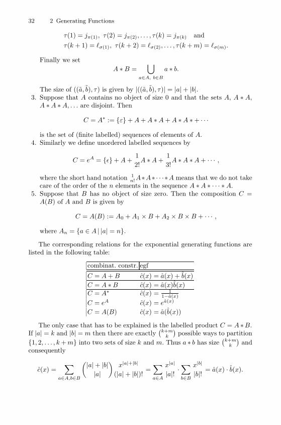
32 2 Generating Functions
τ(1) = jπ(1), τ(2) = jπ(2), . . . , τ(k) = jπ(k) and
τ(k + 1) = �σ(1), τ(k + 2) = �σ(2), . . . , τ(k +m) = �σ(m).
Finally we set
A ∗B =⋃
a∈A, b∈B
a ∗ b.
The size of ((a, b), τ) is given by |((a, b), τ)| = |a|+ |b|.3. Suppose that A contains no object of size 0 and that the sets A, A ∗ A,A ∗A ∗A, . . . are disjoint. Then
C = A∗ := {ε}+A+A ∗A+A ∗A ∗+ · · ·
is the set of (finite labelled) sequences of elements of A.4. Similarly we define unordered labelled sequences by
C = eA = {ε}+A+1
2!A ∗A+
1
3!A ∗A ∗A+ · · · ,
where the short hand notation 1n!A∗A∗ · · · ∗A means that we do not take
care of the order of the n elements in the sequence A ∗A ∗ · · · ∗A.5. Suppose that B has no object of size zero. Then the composition C =A(B) of A and B is given by
C = A(B) := A0 +A1 ×B +A2 ×B ×B + · · · ,
where An = {a ∈ A | |a| = n}.
The corresponding relations for the exponential generating functions arelisted in the following table:
combinat. constr. egf
C = A+B c(x) = a(x) + b(x)
C = A ∗B c(x) = a(x)b(x)C = A∗ c(x) = 1
1−a(x)
C = eA c(x) = ea(x)
C = A(B) c(x) = a(b(x))
The only case that has to be explained is the labelled product C = A ∗B.If |a| = k and |b| = m then there are exactly
(k+m
k
)possible ways to partition
{1, 2, . . . , k+m} into two sets of size k and m. Thus a ∗ b has size(k+m
k
)and
consequently
c(x) =∑
a∈A,b∈B
(|a|+ |b||a|
)x|a|+|b|
(|a|+ |b|)! =∑a∈A
x|a|
|a|! ·∑b∈B
x|b|
|b|! = a(x) · b(x).
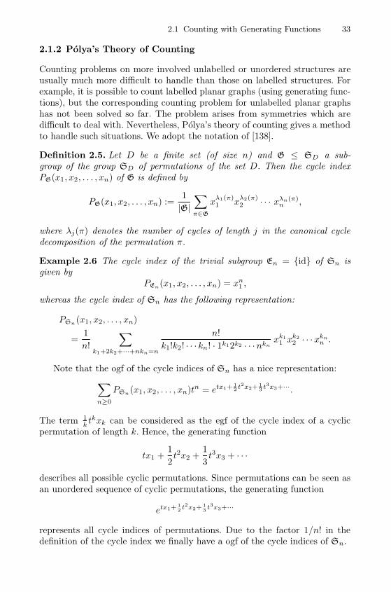
2.1 Counting with Generating Functions 33
2.1.2 Polya’s Theory of Counting
Counting problems on more involved unlabelled or unordered structures areusually much more difficult to handle than those on labelled structures. Forexample, it is possible to count labelled planar graphs (using generating func-tions), but the corresponding counting problem for unlabelled planar graphshas not been solved so far. The problem arises from symmetries which aredifficult to deal with. Nevertheless, Polya’s theory of counting gives a methodto handle such situations. We adopt the notation of [138].
Definition 2.5. Let D be a finite set (of size n) and G ≤ SD a sub-group of the group SD of permutations of the set D. Then the cycle indexPG(x1, x2, . . . , xn) of G is defined by
PG(x1, x2, . . . , xn) :=1
|G|∑π∈G
xλ1(π)1 x
λ2(π)2 · · · xλn(π)
n ,
where λj(π) denotes the number of cycles of length j in the canonical cycledecomposition of the permutation π.
Example 2.6 The cycle index of the trivial subgroup En = {id} of Sn isgiven by
PEn(x1, x2, . . . , xn) = xn1 ,
whereas the cycle index of Sn has the following representation:
PSn (x1, x2, . . . , xn)
=1
n!
∑k1+2k2+···+nkn=n
n!
k1!k2! · · ·kn! · 1k12k2 · · ·nknxk1
1 xk22 · · ·xkn
n .
Note that the ogf of the cycle indices of Sn has a nice representation:∑n≥0
PSn(x1, x2, . . . , xn)tn = etx1+12 t2x2+
13 t3x3+···.
The term 1k t
kxk can be considered as the egf of the cycle index of a cyclicpermutation of length k. Hence, the generating function
tx1 +1
2t2x2 +
1
3t3x3 + · · ·
describes all possible cyclic permutations. Since permutations can be seen asan unordered sequence of cyclic permutations, the generating function
etx1+12 t2x2+
13 t3x3+···
represents all cycle indices of permutations. Due to the factor 1/n! in thedefinition of the cycle index we finally have a ogf of the cycle indices of Sn.
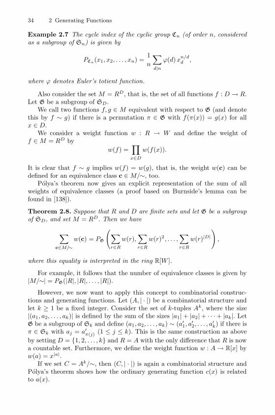
34 2 Generating Functions
Example 2.7 The cycle index of the cyclic group Cn (of order n, consideredas a subgroup of Sn) is given by
PCn(x1, x2, . . . , xn) =1
n
∑d|nϕ(d)x
n/dd ,
where ϕ denotes Euler’s totient function.
Also consider the set M = RD, that is, the set of all functions f : D → R.Let G be a subgroup of SD.
We call two functions f, g ∈ M equivalent with respect to G (and denotethis by f ∼ g) if there is a permutation π ∈ G with f(π(x)) = g(x) for allx ∈ D.
We consider a weight function w : R → W and define the weight off ∈M = RD by
w(f) =∏x∈D
w(f(x)).
It is clear that f ∼ g implies w(f) = w(g), that is, the weight w(c) can bedefined for an equivalence class c ∈M/∼, too.
Polya’s theorem now gives an explicit representation of the sum of allweights of equivalence classes (a proof based on Burnside’s lemma can befound in [138]).
Theorem 2.8. Suppose that R and D are finite sets and let G be a subgroupof SD, and set M = RD. Then we have
∑c∈M/∼
w(c) = PG
(∑r∈R
w(r),∑r∈R
w(r)2, . . . ,∑r∈R
w(r)|D|),
where this equality is interpreted in the ring R[W ].
For example, it follows that the number of equivalence classes is given by|M/∼| = PG(|R|, |R|, . . . , |R|).
However, we now want to apply this concept to combinatorial construc-tions and generating functions. Let (A, | · |) be a combinatorial structure andlet k ≥ 1 be a fixed integer. Consider the set of k-tuples Ak, where the size|(a1, a2, . . . , ak)| is defined by the sum of the sizes |a1|+ |a2|+ · · ·+ |ak|. LetG be a subgroup of Sk and define (a1, a2, . . . , ak) ∼ (a′1, a
′2, . . . , a
′k) if there is
π ∈ Sk with aj = a′π(j) (1 ≤ j ≤ k). This is the same construction as above
by setting D = {1, 2, . . . , k} and R = A with the only difference that R is nowa countable set. Furthermore, we define the weight function w : A→ R[x] byw(a) = x|a|.
If we set C = Ak/∼, then (C, | · |) is again a combinatorial structure andPolya’s theorem shows how the ordinary generating function c(x) is relatedto a(x).
2.1 Counting with Generating Functions 35
Theorem 2.9. Let (A, | · |) be a combinatorial structure and C = Ak/∼ bedefined as above. Then the ordinary generating function c(x) is given by
c(x) = PG(a(x), a(x2), . . . , a(xk)). (2.7)
Proof. The proof is immediate. We only have to note that Theorem 2.8 for-mally extends to countable sets R. For example, we first apply Theorem 2.8for RN = {a ∈ A : |a| ≤ N} and MN = Rk
N . This leads to a correspondingformula
cN (x) = PG(aN (x), aN (x2), . . . , aN(xk)),
where aN (x) and cN (x) are the ogf’s of AN and CN = RkN/∼. Obviously we
have [xn]aN (x) = [xn]a(x) and [xn]cN (x) = [xn]c(x) for all n ≤ N . Thus, wecan formally let N →∞ and obtain (2.7).
In particular, we can apply this construction to the cyclic group Ck andthe symmetric group Sk:
c(x) = PCk(a(x), a(x2), . . . , a(xk)), (2.8)
orc(x) = PSk
(a(x), a(x2), . . . , a(xk)). (2.9)
If we use the cyclic group then C can be interpreted as the set of cycles oflength k of elements of A and if we use the whole group Sk then C can beseen as the set of multisets (of total size k) of elements of A. Note that therepresentation (2.9) can also be deduced from the multiset construction ofunlabelled structures:
ea(x)+ 12! a(x2)+ 1
3! a(x3)+···.
If we introduce another variable t then the k-th coefficient
[tk]eta(x)+t2 12! a(x2)+t3 1
3! a(x3)+···
=1
k!
∑�1+2�2+···+k�k=k
k!
�1!�2! · · · �k! · 1�12�2 · · · k�ka(x)�1a(x2)�2 · · · a(xk)�k
= PSk(a(x), a(x2), . . . , a(xk))
collects all multisets of size k.It is also of interest to consider k-tuples (a1, a2, . . . , ak) of different ele-
ments a1, a2, . . . , ak ∈ A. There is no general result here as for the unrestrictedcase. Nevertheless there are some particular cases that can be treated simi-larly. For example, if C denotes the set of k-tuples (a1, a2, . . . , ak) with theproperty that all aj are different we have
c(x) = a(x)k −k∑
�=2
(−1)�
(k
l
)a(x)k−�a(x�).
36 2 Generating Functions
This is just a direct application of the principle of inclusion and exclusion.Finally, if C denotes the sets of size k of elements of A (that is, we consider
k-tuples (a1, a2, . . . , ak) with the property that all aj are different and the fullgroup Sk) we obtain
c(x) = PSk(a(x),−a(x2), . . . , (−1)k−1a(xk)).
Here we just have to observe that this generating function is given by the k-thcoefficient
[tk]eta(x)−t2 12! a(x2)+t3 1
3! a(x3)∓···.
2.1.3 Lagrange Inversion Formula
Let a(x) =∑
n≥0 anxn be a power series with a0 = 0 and a1 = 0. The
Lagrange inversion formula provides an explicit representation of the coeffi-cients of the inverse power series a[−1](x) which is defined by a(a[−1](x)) =a[−1](a(x)) = x.
Theorem 2.10. Let a(x) =∑n≥0
anxn be a formal power series with a0 = 0
and a1 = 0. Let a[−1](x) be the inverse power series and g(x) an arbitrarypower series. Then the n-th coefficient of g(a[−1](x)) is given by
[xn]g(a[−1](x)) =1
n[un−1]g′(u)
(u
a(u)
)n
(n ≥ 1).
In tree enumeration problems the following variant is more appropriate.
Theorem 2.11. Let Φ(x) be a power series with Φ(0) = 0 and y(x) the(unique) power series solution of the equation
y(x) = xΦ(y(x)).
Then y(x) is invertible and the n-th coefficient of g(y(x)) (where g(x) is anarbitrary power series) is given by
[xn]g(y(x)) =1
n[un−1]g′(u)Φ(u)n (n ≥ 1).
Theorems 2.10 and 2.11 are equivalent. If a(x) = x/Φ(x) then a[−1](x) = y(x),where y(x) satisfies the equation y(x) = xΦ(y(x)).
We give an immediate application of Theorem 2.11. We have already ob-served that the generating function b(x) of binary trees satisfies the functionalequation (2.2). If we set b(x) = b(x)− 1 then
b(x) = x(1 + b(x))2.
By Theorem 2.11 with Φ(x) = (1 + x)2 we obtain (for n ≥ 1)
2.2 Asymptotics with Generating Functions 37
bn = [xn]b(x) =1
n[un−1](1 + u)2n
=1
n
(2n
n− 1
)=
1
n+ 1
(2n
n
).
Proof. Since Theorems 2.10 and 2.11 are equivalent, we only have to proveTheorem 2.10. We just present an analytic proof for complex coefficients. Theresulting analytic identities are formal ones, too.
We start with Cauchy’s formula and use the substitution u = a[−1](x).Note that if γ is a contour with winding number 1 around the origin thenγ′ = a[−1](γ) has the same property:
[xn]g(a[−1](x)) =1
2πi
∫γ
g(a[−1](x))
xn+1dx
=1
2πi
∫γ′g(u)
a′(u)
a(u)n+1du.
Since (g(u)
1
a(u)n
)′= g′(u)
1
a(u)n− n g(u)
a′(u)
a(u)n+1,
it follows that ∫γ′g(u)
a′(u)
a(u)n+1du =
1
n
∫γ′g′(u)
1
a(u)ndu,
and consequently
[xn]g(a[−1](x)) =1
n
∫γ′g′(u)
un
a(u)n
du
un
=1
n[un−1]g′(u)
(u
a(u)
)n
.
2.2 Asymptotics with Generating Functions
Generating functions a(x) =∑
n≥0 anxn can be considered, too, as power
series in a complex variable x. If the radius of convergence is positive thenone can apply Cauchy’s formula
an =1
2πi
∫γ
a(x)dx
xn+1,
where the contour γ is contained in the region of analyticity of a(x) andencircles the x = 0 once. Thus, the analytic behaviour of a(x) can be usedto obtain information on the order of magnitude of an. In what follows wefollow this idea by showing that certain kinds of singularities of a(x) induce
38 2 Generating Functions
corresponding asymptotics for the coefficients an. This singularity analysiswas introduced in a systematic way by Flajolet and Odlyzko [83] and will bethe starting point of the following treatment. However, the main focus will bethe analysis of functions y(x) that satisfy a functional equation of the formy(x) = F (x, y(x)). We determine the kind of singularity (that will be of squareroot type) and extend this concept to a combinatorial central limit theorem(Theorem 2.23).
Note that Lagrange’s inversion formula can be used to obtain explicitrepresentations for the coefficients of the solution of the functional equationy = xΦ(y). The functional equation y = F (x, y) mentioned above is thereforea natural generalisation that occurs frequently in tree enumeration problems,too.
2.2.1 Asymptotic Transfers
The basic property that allows an asymptotic transfer between the analyticbehaviour of a generating function a(x) and to its coefficients is the so-calledTransfer Lemma by Flajolet and Odlyzko [83]. Note that an essential assump-tion is that a(x) has an analytic continuation to a so-called Delta-domain Δthat is depicted in Figure 2.4.
Lemma 2.12. Leta(x) =
∑n≥0
anxn
be analytic in a region
Δ = Δ(x0, η, δ) = {x : |x| < x0 + η, | arg(x/x0 − 1)| > δ},
in which x0 and η are positive real numbers and 0 < δ < π/2. Furthermoresuppose that there exists a real number α such that
a(x) = O((1− x/x0)−α
)(x ∈ Δ).
Thenan = O
(x−n
0 nα−1).
Proof. One uses Cauchy’s formula
an =1
2πi
∫γ
a(x)
xn+1dx,
where γ is a suitable chosen path of integration around the origin. In partic-ular, one can use γ = γ1 ∪ γ2 ∪ γ3 ∪ γ4, where (see also Figure 2.4)
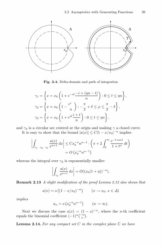
2.2 Asymptotics with Generating Functions 39
Δ
x0
Δ
x0
γ
Fig. 2.4. Delta-domain and path of integration
γ1 =
{x = x0
(1 + e−iδ−i+ (ηn− t)
n
): 0 ≤ t ≤ ηn
},
γ2 =
{x = x0
(1− e
iϕ
n
): −π
2+ δ ≤ ϕ ≤ π
2− δ},
γ3 =
{x = x0
(1 + eiδ
i+ t
n
): 0 ≤ t ≤ ηn
},
and γ4 is a circular arc centred at the origin and making γ a closed curve.It is easy to show that the bound |a(x)| ≤ C|1 − x/x0|−α implies∣∣∣∣∫
γ1∪γ2∪γ3
a(x)
xn+1dx
∣∣∣∣ ≤ Cx−n0 nα−1 ·
(π + 2
∫ ∞0
e−t cos δ
1 + tαdt
)= O(x−n
0 nα−1)
whereas the integral over γ4 is exponentially smaller:∣∣∣∣∫γ4
a(x)
xn+1dx
∣∣∣∣ = O((x0(1 + η))−n).
Remark 2.13 A slight modification of the proof Lemma 2.12 also shows that
a(x) = o((1− x/x0)−α
)(x→ x0, x ∈ Δ)
impliesan = o
(x−n
0 nα−1)
(n→∞).
Next we discuss the case a(x) = (1 − x)−α, where the n-th coefficientequals the binomial coefficient (−1)n
(−αn
).
Lemma 2.14. For any compact set C in the complex plane C we have
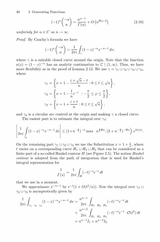
40 2 Generating Functions
(−1)n
(−αn
)=nα−1
Γ (α)+O(n�α−2)
(2.10)
uniformly for α ∈ C as n→∞.
Proof. By Cauchy’s formula we have
(−1)n
(−αn
)=
1
2πi
∫γ
(1− x)−αx−n−1 dx,
where γ is a suitable closed curve around the origin. Note that the functiona(x) = (1 − x)−α has an analytic continuation to C \ (1,∞). Thus, we havemore flexibility as in the proof of Lemma 2.12. We use γ = γ1 ∪ γ2 ∪ γ3 ∪ γ4,where
γ1 =
{x = 1− i+
√n− tn
: 0 ≤ t ≤√n
},
γ2 =
{x = 1− 1
ne−iϕ : −π
2≤ ϕ ≤ π
2
},
γ3 =
{x = 1 +
i+ t
n: 0 ≤ t ≤
√n
},
and γ4 is a circular arc centred at the origin and making γ a closed curve.The easiest part is to estimate the integral over γ4:∣∣∣∣∣∣ 1
2πi
∫γ4
(1− x)−αx−n−1 dx
∣∣∣∣∣∣ ≤ (1+n−12 )−n max
(n
12�α, (2 + n−
12 )−�α)e2π|α|.
On the remaining part γ1 ∪ γ2 ∪ γ3 we use the Substitution x = 1 + tn , where
t varies on a corresponding curve H1 ∪H2 ∪H3 that can be considered as afinite part of a so-called Hankel contourH (see Figure 2.5). The notion Hankelcontour is adopted from the path of integration that is used for Hankel’sintegral representation for
1
Γ (s)=
1
2πi
∫H
(−t)−se−t dt
that we use in a moment.We approximate x−n−1 by e−t(1 + O(t2/n)). Now the integral over γ1 ∪
γ2 ∪ γ3 is asymptotically given by
1
2πi
∫γ1∪γ2∪γ3
(1− x)−αx−n−1 dx =nα−1
2πi
∫H1∪H2∪H3
(−t)−αe−t dt
+nα−2
2πi
∫H1∪H2∪H3
(−t)−αe−t · O(t2) dt
= nα−1I1 + nα−2I2.
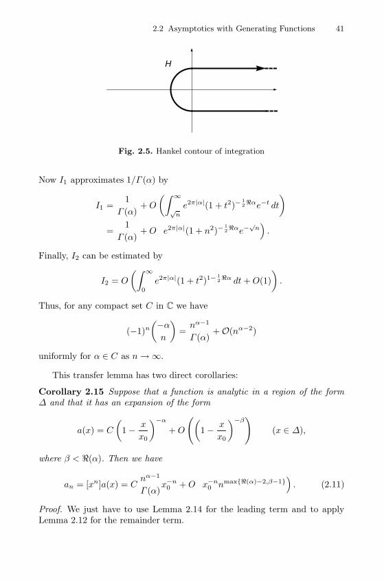
2.2 Asymptotics with Generating Functions 41
H
Fig. 2.5. Hankel contour of integration
Now I1 approximates 1/Γ (α) by
I1 =1
Γ (α)+O
(∫ ∞√
n
e2π|α|(1 + t2)−12�αe−t dt
)=
1
Γ (α)+O(e2π|α|(1 + n2)−
12�αe−
√n).
Finally, I2 can be estimated by
I2 = O
(∫ ∞0
e2π|α|(1 + t2)1−12�α dt+O(1)
).
Thus, for any compact set C in C we have
(−1)n
(−αn
)=nα−1
Γ (α)+O(nα−2)
uniformly for α ∈ C as n→∞.
This transfer lemma has two direct corollaries:
Corollary 2.15 Suppose that a function is analytic in a region of the formΔ and that it has an expansion of the form
a(x) = C
(1− x
x0
)−α
+O
((1− x
x0
)−β)
(x ∈ Δ),
where β < �(α). Then we have
an = [xn]a(x) = Cnα−1
Γ (α)x−n
0 +O(x−n
0 nmax{�(α)−2,β−1}). (2.11)
Proof. We just have to use Lemma 2.14 for the leading term and to applyLemma 2.12 for the remainder term.

42 2 Generating Functions
Corollary 2.16 Suppose that a(x) is analytic in a Delta-region Δ such that
a(x) ∼ C(
1− x
x0
)−α
for x → x0 with x ∈ Δ, where α is a complex number different from{0,−1,−2, . . .}. Then, as n→∞
[xn]a(x) ∼ Cnα−1
Γ (α)x−n
0 .
Proof. Instead of Lemma 2.12 we now use the properties mentioned in Re-mark 2.13 for estimating the remainder term.
Remark 2.17 Transfer principles like the one presented in Corollary 2.16are not only valid for functions that behave like C(1 − x/x0)−α. For exampleone can add slowly varying factors (compare with [83]). In particular, if it isa purely logarithmic behaviour of the form
a(x) ∼ C log
(1− x
x0
)for x ∈ Δ then we have
[xn]a(x) ∼ C
nx−n
0 .
Another important issue is that in fact all estimates in the proof ofLemma 2.12 are explicit and, thus, we obtain uniform estimates if we have anadditional parameter.
Lemma 2.18. Suppose that a(x;w) is a power series in x and a parameterw ∈W such that there is an expansion of the form
a(x;w) = C(w)
(1− x
x0(w)
)−α(w)
+O
((1− x
x0(w)
)−β(w)),
that is uniform for w ∈ W and x ∈ Δ(x0(w)) with functions C(w), x0(w),α(w), and β(w) that remain bounded and satisfy β(w) < �(α(w)) for allw ∈W . Then we get
[xn]a(x;w) = C(w)nα(w)−1
Γ (α(w))x0(w)−n +O
(x0(w)−nnmax{�(α(w))−2,β(w)−1}
)(2.12)
uniformly for w ∈W as n→∞.
Proof. We just have to use two facts. First, the expansion (2.10) holds uni-formly if α varies in some compact subset of the complex plane. Second, theestimates of Lemma 2.12 are explicit and also uniform.
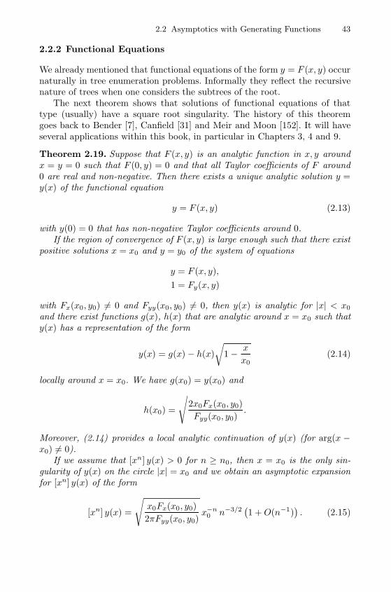
2.2 Asymptotics with Generating Functions 43
2.2.2 Functional Equations
We already mentioned that functional equations of the form y = F (x, y) occurnaturally in tree enumeration problems. Informally they reflect the recursivenature of trees when one considers the subtrees of the root.
The next theorem shows that solutions of functional equations of thattype (usually) have a square root singularity. The history of this theoremgoes back to Bender [7], Canfield [31] and Meir and Moon [152]. It will haveseveral applications within this book, in particular in Chapters 3, 4 and 9.
Theorem 2.19. Suppose that F (x, y) is an analytic function in x, y aroundx = y = 0 such that F (0, y) = 0 and that all Taylor coefficients of F around0 are real and non-negative. Then there exists a unique analytic solution y =y(x) of the functional equation
y = F (x, y) (2.13)
with y(0) = 0 that has non-negative Taylor coefficients around 0.If the region of convergence of F (x, y) is large enough such that there exist
positive solutions x = x0 and y = y0 of the system of equations
y = F (x, y),
1 = Fy(x, y)
with Fx(x0, y0) = 0 and Fyy(x0, y0) = 0, then y(x) is analytic for |x| < x0
and there exist functions g(x), h(x) that are analytic around x = x0 such thaty(x) has a representation of the form
y(x) = g(x)− h(x)
√1− x
x0(2.14)
locally around x = x0. We have g(x0) = y(x0) and
h(x0) =
√2x0Fx(x0, y0)
Fyy(x0, y0).
Moreover, (2.14) provides a local analytic continuation of y(x) (for arg(x −x0) = 0).
If we assume that [xn] y(x) > 0 for n ≥ n0, then x = x0 is the only sin-gularity of y(x) on the circle |x| = x0 and we obtain an asymptotic expansionfor [xn] y(x) of the form
[xn] y(x) =
√x0Fx(x0, y0)
2πFyy(x0, y0)x−n
0 n−3/2(1 +O(n−1)
). (2.15)
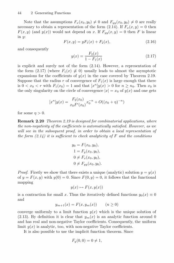
44 2 Generating Functions
Note that the assumptions Fx(x0, y0) = 0 and Fyy(x0, y0) = 0 are reallynecessary to obtain a representation of the form (2.14). If Fx(x, y) = 0 thenF (x, y) (and y(x)) would not depend on x. If Fyy(x, y) = 0 then F is linearin y:
F (x, y) = yF1(x) + F2(x), (2.16)
and consequently
y(x) =F2(x)
1− F1(x)(2.17)
is explicit and surely not of the form (2.14). However, a representation ofthe form (2.17) (where F1(x) ≡ 0) usually leads to almost the asymptoticexpansions for the coefficients of y(x) in the case covered by Theorem 2.19.Suppose that the radius r of convergence of F1(x) is large enough that thereis 0 < x0 < r with F1(x0) = 1 and that [xn]y(x) > 0 for n ≥ n0. Then x0 isthe only singularity on the circle of convergence |x| = x0 of y(x) and one gets
[xn]y(x) =F2(x0)
x0F ′(x0)x−n
0 +O((x0 + η)−n)
for some η > 0.
Remark 2.20 Theorem 2.19 is designed for combinatorial applications, wherethe non-negativity of the coefficients is automatically satisfied. However, as wewill see in the subsequent proof, in order to obtain a local representation ofthe form (2.14) it is sufficient to check analyticity of F and the conditions
y0 = F (x0, y0),
1 = Fy(x0, y0),
0 = Fx(x0, y0),
0 = Fyy(x0, y0).
Proof. Firstly we show that there exists a unique (analytic) solution y = y(x)of y = F (x, y) with y(0) = 0. Since F (0, y) = 0, it follows that the functionalmapping
y(x) �→ F (x, y(x))
is a contraction for small x. Thus the iteratively defined functions y0(x) ≡ 0and
ym+1(x) = F (x, ym(x)) (n ≥ 0)
converge uniformly to a limit function y(x) which is the unique solution of(2.13). By definition it is clear that ym(x) is an analytic function around 0and has real and non-negative Taylor coefficients. Consequently, the uniformlimit y(x) is analytic, too, with non-negative Taylor coefficients.
It is also possible to use the implicit function theorem. Since
Fy(0, 0) = 0 = 1,
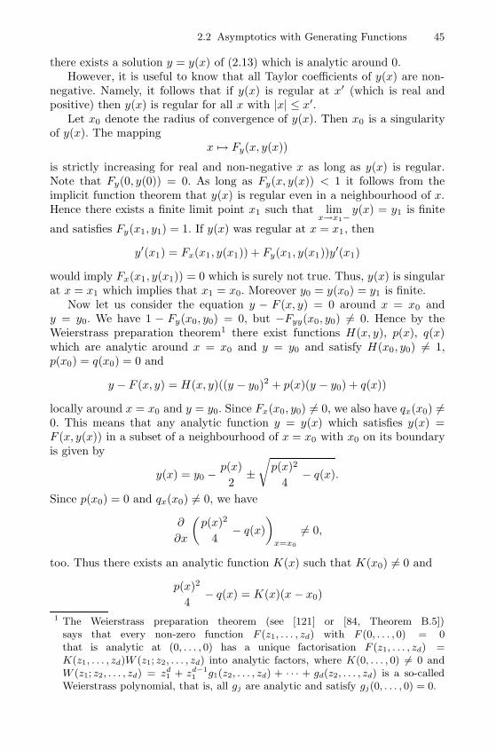
2.2 Asymptotics with Generating Functions 45
there exists a solution y = y(x) of (2.13) which is analytic around 0.However, it is useful to know that all Taylor coefficients of y(x) are non-
negative. Namely, it follows that if y(x) is regular at x′ (which is real andpositive) then y(x) is regular for all x with |x| ≤ x′.
Let x0 denote the radius of convergence of y(x). Then x0 is a singularityof y(x). The mapping
x �→ Fy(x, y(x))
is strictly increasing for real and non-negative x as long as y(x) is regular.Note that Fy(0, y(0)) = 0. As long as Fy(x, y(x)) < 1 it follows from theimplicit function theorem that y(x) is regular even in a neighbourhood of x.Hence there exists a finite limit point x1 such that lim
x→x1−y(x) = y1 is finite
and satisfies Fy(x1, y1) = 1. If y(x) was regular at x = x1, then
y′(x1) = Fx(x1, y(x1)) + Fy(x1, y(x1))y′(x1)
would imply Fx(x1, y(x1)) = 0 which is surely not true. Thus, y(x) is singularat x = x1 which implies that x1 = x0. Moreover y0 = y(x0) = y1 is finite.
Now let us consider the equation y − F (x, y) = 0 around x = x0 andy = y0. We have 1 − Fy(x0, y0) = 0, but −Fyy(x0, y0) = 0. Hence by theWeierstrass preparation theorem1 there exist functions H(x, y), p(x), q(x)which are analytic around x = x0 and y = y0 and satisfy H(x0, y0) = 1,p(x0) = q(x0) = 0 and
y − F (x, y) = H(x, y)((y − y0)2 + p(x)(y − y0) + q(x))
locally around x = x0 and y = y0. Since Fx(x0, y0) = 0, we also have qx(x0) =0. This means that any analytic function y = y(x) which satisfies y(x) =F (x, y(x)) in a subset of a neighbourhood of x = x0 with x0 on its boundaryis given by
y(x) = y0 −p(x)
2±√p(x)2
4− q(x).
Since p(x0) = 0 and qx(x0) = 0, we have
∂
∂x
(p(x)2
4− q(x)
)x=x0
= 0,
too. Thus there exists an analytic function K(x) such that K(x0) = 0 and
p(x)2
4− q(x) = K(x)(x − x0)
1 The Weierstrass preparation theorem (see [121] or [84, Theorem B.5])says that every non-zero function F (z1, . . . , zd) with F (0, . . . , 0) = 0that is analytic at (0, . . . , 0) has a unique factorisation F (z1, . . . , zd) =K(z1, . . . , zd)W (z1; z2, . . . , zd) into analytic factors, where K(0, . . . , 0) �= 0 andW (z1; z2, . . . , zd) = zd
1 + zd−11 g1(z2, . . . , zd) + · · · + gd(z2, . . . , zd) is a so-called
Weierstrass polynomial, that is, all gj are analytic and satisfy gj(0, . . . , 0) = 0.
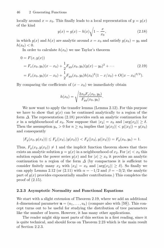
46 2 Generating Functions
locally around x = x0. This finally leads to a local representation of y = y(x)of the kind
y(x) = g(x)− h(x)
√1− x
x0, (2.18)
in which g(x) and h(x) are analytic around x = x0 and satisfy g(x0) = y0 andh(x0) < 0.
In order to calculate h(x0) we use Taylor’s theorem
0 = F (x, y(x))
= Fx(x0, y0)(x− x0) +1
2Fyy(x0, y0)(y(x) − y0)2 + · · · (2.19)
= Fx(x0, y0)(x− x0) +1
2Fyy(x0, y0)h(x0)2(1− x/x0) +O(|x− x0|3/2).
By comparing the coefficients of (x− x0) we immediately obtain
h(x0) =
√2x0Fx(x0, y0)
Fyy(x0, y0).
We now want to apply the transfer lemma (Lemma 2.12). For this purposewe have to show that y(x) can be continued analytically to a region of theform Δ. The representation (2.18) provides such an analytic continuation forx in a neighbourhood of x0. Now suppose that |x2| = x0 and | arg(x2)| ≥ δ.Then the assumption yn > 0 for n ≥ n0 implies that |y(x2)| < y(|x2|) = y(x0)and consequently
|Fy(x2, y(x2))| ≤ Fy(|x2|, |y(x2)|) < Fy(|x2|, y(|x2|)) = Fy(x0, y0) = 1.
Thus, Fy(x2, y(x2)) = 1 and the implicit function theorem shows that thereexists an analytic solution y = y(x) in a neighbourhood of x2. For |x| < x0 thissolution equals the power series y(x) and for |x| ≥ x0 it provides an analyticcontinuation to a region of the form Δ (by compactness it is sufficient toconsider finitely many x2 with |x2| = x0 and | arg(x2)| ≥ δ). So finally wecan apply Lemma 2.12 (or (2.11) with α = −1/2 and β = −3/2; the analyticpart of g(x) provides exponentially smaller contributions.) This completes theproof of (2.15).
2.2.3 Asymptotic Normality and Functional Equations
We start with a slight extension of Theorem 2.19, where we add an additionalk-dimensional parameter u = (u1, . . . , uk) (compare also with [59]). This con-cept turns out to be useful for studying the distribution of tree parameterslike the number of leaves. However, it has many other applications.
The reader might skip most parts of this section in a first reading, since itis quite technical, and should focus on Theorem 2.23 which is the main resultof Section 2.2.3.
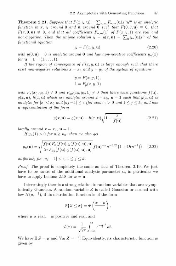
2.2 Asymptotics with Generating Functions 47
Theorem 2.21. Suppose that F (x, y,u) =∑
n,m Fn,m(u)xnym is an analyticfunction in x, y around 0 and u around 0 such that F (0, y,u) ≡ 0, thatF (x, 0,u) ≡ 0, and that all coefficients Fn,m(1) of F (x, y, 1) are real andnon-negative. Then the unique solution y = y(x,u) =
∑n yn(u)xn of the
functional equationy = F (x, y,u) (2.20)
with y(0,u) = 0 is analytic around 0 and has non-negative coefficients yn(1)for u = 1 = (1, . . . , 1).
If the region of convergence of F (x, y,u) is large enough such that thereexist non-negative solutions x = x0 and y = y0 of the system of equations
y = F (x, y,1),
1 = Fy(x, y,1)
with Fx(x0, y0, 1) = 0 and Fyy(x0, y0,1) = 0 then there exist functions f(u),g(x,u), h(x,u) which are analytic around x = x0, u = 1 such that y(x,u) isanalytic for |x| < x0 and |uj − 1| ≤ ε (for some ε > 0 and 1 ≤ j ≤ k) and hasa representation of the form
y(x,u) = g(x,u)− h(x,u)
√1− x
f(u)(2.21)
locally around x = x0, u = 1.If yn(1) > 0 for n ≥ n0, then we also get
yn(u) =
√f(u)Fx(f(u), y(f(u),u),u)
2πFyy(f(u), y(f(u),u),u)f(u)−nn−3/2
(1 +O(n−1)
)(2.22)
uniformly for |uj − 1| < ε, 1 ≤ j ≤ k.
Proof. The proof is completely the same as that of Theorem 2.19. We justhave to be aware of the additional analytic parameter u, in particular wehave to apply Lemma 2.18 for w = u.
Interestingly there is a strong relation to random variables that are asymp-totically Gaussian. A random variable Z is called Gaussian or normal withlaw N(μ, σ2), if its distribution function is of the form
P{Z ≤ x} = Φ
(x− μσ
),
where μ is real, σ is positive and real, and
Φ(x) =1√2π
∫ x
−∞e−
12 t2 dt.
We have EZ = μ and VarZ = σ2. Equivalently, its characteristic function isgiven by
48 2 Generating Functions
E eitZ = eiμt− 12 σ2t2 .
A random vector Z = (Z1, . . . , Zk) is normally distributed with mean μ andcovariance matrix Σ (with law N(μ,Σ)), if and only if all linear forms aTZ =a1Z1+· · ·+akZk are normally distributed with mean aTμ and variance aTΣa.
The Gaussian distribution is important because it is a universal law thatappears as a limiting distribution for sums of independent and weakly depen-dent random variables.
We say, that a sequence of random variables Xn satisfies a central limittheorem with (scaling) mean μn and (scaling) variance σ2
n, if
P{Xn ≤ μn + x · σn} = Φ(x) + o(1)
as n→∞. In terms of weak convergence2 this is equivalent to
Xn − μn
σn
d−→ N(0, 1). (2.23)
For example, if Xn is the sum ξ1 + ξ2 + · · ·+ ξn of i.i.d. random variables ξj(with finite second moment) we have (2.23) with μ = E ξj and σ =
√Var ξj .
This can be checked easily by Levy’s criterion. Note that the characteristicfunction of Xn is just the n-th power of the characteristic function of ξj :
E eitXn = E eit(ξ1+ξ2+···+ξn) =(E eitξj)n.
We state (and prove) a multivariate version of the so-called Quasi PowerTheorem by H.-K. Hwang [104] (see also [84], similar theorems can be foundin [6, 10]), which is very useful to prove a central limit theorem. The ideais that if the characteristic function of a sequence of random variables Xn
behaves almost like powers of a function, then the distribution of Xn shouldbe approximated by a corresponding sum of i.i.d. random variables and, thus,one can expect a central limit theorem. Note that the so-called probabilitygenerating function EuX is related to the characteristic function by settingu = eit.
We also include simple tail estimates. (There exists a more precise largedeviation result for the univariate case [105].)
Theorem 2.22. Let Xn be a k-dimensional random vector with the propertythat3
2 A sequence of random variables Xn converges weakly to a random variableX, if limn→∞ P{Xn ≤ x} = P{X ≤ x} holds for all points of continuity of
FX(x) = P{X ≤ x}. This is denoted by Xnd−→ X. Another possible definition
is that limn→∞ E F (Xn) = E F (Xn) for all bounded continuous functions F . Itis sufficient to check this condition for exponential functions F (x) = eitx. Hence,
Xnd−→ X, if and only if limn→∞ E eitXn = E eitX (for all real numbers t) which
is Levy’s criterion. Corresponding properties hold for random vectors.3 If u = (u1, . . . , uN ) and x = (x1, . . . , xN) are vectors of real (or complex) numbers
then ux abbreviates ux11 ux2
2 · · ·uxNN .
2.2 Asymptotics with Generating Functions 49
EuXn = eλn·A(u)+B(u)
(1 +O
(1
φn
))(2.24)
holds uniformly in a complex neighbourhood of u = 1, where λn and φn aresequences of positive real numbers with λn → ∞ and φn → ∞, and A(u)and B(u) are analytic functions in this neighbourhood of u = 1 with A(1) =B(1) = 0. Then Xn satisfies a central limit theorem of the form
1√λn
(Xn − EXn)d−→ N (0,Σ) (2.25)
and we haveEXn = λnμ +O (1 + λn/φn)
andCovXn = λnΣ +O
((1 + λn/φn)
2),
whereμ = Au(1) = (Auj (1))1≤j≤k
andΣ = (Auiuj (1) + δijAuj (1))1≤i,j≤k .
Finally if we additionally assume that λn = φn there exist positive constantsc1, c2, c3 such that
P
{‖Xn − EXn‖ ≥ ε
√λn
}≤ c1e−c2ε2 (2.26)
uniformly for ε ≤ c3√λn.
Proof. We first consider the univariate case k = 1, that is, we have
EuXn = eλn·a(u)+b(u)
(1 +O
(1
φn
)). (2.27)
By assumption, we obtain for t in a neighbourhood of t = 0
E eitXn = eitλnμ− 12 t2λnσ2+O(λnt3)+O(t)
(1 + O
(1
φn
)),
where μ = a′(1) and σ2 = a′(1) + a′′(1). Set Yn = (Xn − λnμ)/√λn. Then,
replacing t by t/√λn, one gets
E eitYn = e−σ2
2 t2+O(t3/√
λn)+O(t/√
λn)
(1 +O
(1
φn
)).
Thus, Yn is asymptotically normal with mean zero and variance σ2.Next set fn(u) = EuXn . Then f ′n(1) = EXn. On the other hand, by
Cauchy’s formula, we have
50 2 Generating Functions
f ′n(1) =1
2πi
∫|u−1|=ρ
fn(u)
(u− 1)2du.
In particular, we use the circle |u − 1| = 1/λn as the path of integration andget
EXn =
1
2πi
∫|u−1|=1/λn
1 + (λna′(1) + b′(1))(u − 1) +O(λn(u− 1)2)
(u − 1)2
(1 +O
(1
φn
))du
= λna′(1) +O
(1 +
λn
φn
).
We can manage the variance similarly. Set gn(u) = fn(u)u−λna′(1)−b′(1).Then VarXn = g′′n(1) +O
(1 + λ2
n/φ2n
). By using the approximation
exp (λn(a(u)− a′(1) log u) + (b(u)− b′(1) log u)
= 1 + (λn(a′′(1) + a′(1)) + (b′′(1) + b′(1)))(u − 1)2
2
+O(λn(u− 1)3) +O(λ2n(u− 1)4)
and a similar calculation as above one obtains
g′′n(1) = λn(a′′(1) + a′(1)) +O
(1 +
λn
φn
)and consequently
VarXn = λn(a′′(1) + a′(1)) +O(
(1 + λn/φn)2).
If σ2 > 0, then Yn/σ and (Xn − EXn)/√
VarXn have the same limitingdistribution. Hence, the central limit theorem follows.
In order to obtain tail estimates we proceed as follows. Suppose that λn =φn. Then we get (similarly as above)
E et(Xn−E Xn)/√
λn = eσ2
2 t2+O(t3/√
λn)+O(t/√
λn)
(1 +O
(1
λn
)).
Hence, there exist positive constants c′, c′′, c′′′ with
E et(Xn−E Xn)/√
λn ≤ c′ec′′t2
for real t with |t| ≤ c′′′√λn. By a Chernov type argument we get for every
t > 0 the inequality
P{|Y | ≥ ε} ≤(E etY + E e−tY
)e−εt.
2.2 Asymptotics with Generating Functions 51
We also get (2.26) (for k = 1) by choosing c1 = 2c′, t = ε/(2c′′), c2 = 1/(4c′′),and c3 = 2c′′c′′′.
Now recall that a random vector Y is normally distributed with mean zeroand covariance matrix Σ, if and only if aTY = a1Y1 + · · ·+ akYk is normallydistributed with mean zero and variance aTΣa.
Hence, if we assume that a sequence of random vectors Xn satisfies(2.24) then the random variable Xn(a) = aTXn satisfies (2.27) with a(u) =A(ua1 , . . . , uak) and b(u) = B(ua1 , . . . , uak). Consequently Xn(a) is asymp-totically normal with EXn(a) = λnμ + O (1 + λn/φn) and VarXn(a) =λnσ
2 +O (1 + λn/φn), where
μ = a′(1) = aTμ and σ2 = a′(1) + a′′(1) = aTΣa.
The tail estimate (2.26) can also be derived from the one-dimensional casek = 1.
If ‖Xn − EXn‖ ≥ ε√λn, then there exists j with ‖X (j)
n − EX(j)n ‖ ≥
ε√λn/
√k. Hence
P
{‖Xn − EXn‖ ≥ ε
√λn
}≤ kc1e−c2ε2/k.
Thus, we also get (2.26) in the multidimensional case. We just have to adjustc1 and c2.
By combining Theorems 2.21 and 2.22 we immediately obtain the followingcombinatorial central limit theorem. (For simplicity we just state a univariateversion and discuss the multivariate version afterwards.)
Theorem 2.23. Suppose that Xn is a sequence of random variables such that
EuXn =[xn] y(x, u)
[xn] y(x, 1),
where y(x, u) is a power series, that is the (analytic) solution of the func-tional equation y = F (x, y, u), where F (x, y, u) satisfies the assumptions ofTheorem 2.21. In particular, let x = x0 > 0 and y = y0 > 0 be the (minimal)solution of the system of equations
y = F (x, y, 1),
1 = Fy(x, y, 1)
and set
μ =Fu
x0Fx,
σ2 = μ+ μ2 +1
x0F 3xFyy
(F 2
x (FyyFuu − F 2yu)− 2FxFu(FyyFxu − FyxFyu)
+ F 2u (FyyFxx − F 2
yx)),
52 2 Generating Functions
where all partial derivatives are evaluated at the point (x0, y0, 1). Then wehave
EXn = μn+O(1) and VarXn = σ2n+O(1)
and if σ2 > 0 thenXn − EXn√
VarXn
d−→ N(0, 1).
Proof. By Theorem 2.21 we have uniformly for u in a complex neighbourhoodof 1
EuXn =[xn] y(x, u)
[xn] y(x, 1)
=
√f(u)Fx(f(u), y(f(u), u), u)Fyy(x0, y0, 1)
Fyy(f(u), y(f(u), u), u)x0Fx(x0, y0, 1)
(x0
f(u)
)n (1 +O(n−1)
).
Thus, we can apply Theorem 2.22 with A(u) = − log(f(u)/x0), where f(u) =x(u) and y(u) are the solutions of the system
y = F (x, y, u),
1 = Fy(x, y, u).
In particular the constants μ and σ2 are given by
μ = −x′(1)
x0and σ2 = μ+ μ2 − x
′′(1)
x0.
By implicit differentiation one gets (with some algebra)
x′(1) = −Fu(x0, y0, 1)
Fx(x0, y0, 1)= −Fu
Fx
and
x′′(1) = − 1
Fx
(Fxxx
′(1)2 + Fxyx′(1)y′(1) + 2Fuxx
′(1) + Fuyy′(1) + Fuu
),
where
y′(1) = −Fxyx′(1) + Fuy
Fyy.
The explicit representations for μ and σ2 follow immediately.
Remark 2.24 If we have several variables (u1, . . . , uk) =: u and a sequenceof random vectors Xn with
EuXn =[xn] y(x,u)
[xn] y(x,1),
2.2 Asymptotics with Generating Functions 53
where y(x,u) is a power series, which is the solution of the function equationy = F (x, y,u), then we get
EXn = μn+O(1) and Cov Xn = Σn+O(1),
where μ = (μ1, . . . , μk) and Σ = (σij)1≤i,j≤k can be calculated by
μi =Fui
x0Fx,
σij = μiμj + μiδi,j
+1
x0F 3xFyy
(F 2
x (FyyFuiuj − FyuiFyuj )− FxFui(FyyFxuj − FyxFyuj )
− FxFuj (FyyFxui − FyxFyui) + FuiFuj (FyyFxx − F 2yx)),
and we also have a central limit theorem of the form
1√n
(Xn − EXn)d−→ N (0,Σ) .
We finally state a useful variant of a central limit theorem for randomvariables which are defined with the help of generating functions.
Theorem 2.25. Suppose that a sequence of k-dimensional random vectorsXn satisfies
EuXn =cn(u)
cn(1),
where cn(u) is the coefficient of xn of an analytic function
f(x,u) =∑n≥0
cn(u)xn
that has a local singular representation of the form
f(x,u) = g(x,u) + h(x,u)
(1− x
ρ(u)
)α
for some real α ∈ R \ N and functions g(x,u), h(x,u) = 0 and ρ(u) = 0 thatare analytic around x = x0 > 0 and u = 1. Suppose also that x = ρ(u) is theonly singularity of f(x, u) on the disc |x| ≤ |ρ(u)|, if u is sufficiently closeto 1 and that there exists an analytic continuation of f(x,u) to the region|x| < |ρ(u)|+ δ, | arg(x− ρ(u))| > ε for some δ > 0 and ε > 0.
Then Xn satisfies a central limit theorem
1√n
(Xn − EXn)d−→ N (0,Σ)
with
54 2 Generating Functions
EXn = μn+O(1) and Cov Xn = Σn+O(1),
where
μ = −ρu(1)
ρ(1)
and
Σ = −ρuu(1)
ρ(1)+ μμT + diag(μ).
Furthermore there exist positive constants c1, c2, c3 such that
P{‖Xn − EXn‖ ≥ ε
√n}≤ c1e−c2ε2
uniformly for ε ≤ c3√n.
Proof. By Lemma 2.18 we get the asymptotic expansion
cn(u) =h(ρ(u),u)
Γ (−α)n−α−1ρ(u)−n
(1 +O
(1
n
))that is uniform for u in a complex neighbourhood of u = 1. Hence,
EuXn =cn(u)
cn(1)
=h(ρ(u),u)
h(ρ(1),1)
(ρ(1)
ρ(u)
)n(1 +O
(1
n
))and consequently the result follows from Theorem 2.22.
2.2.4 Transfer of Singularities
The main objective of this section is to consider analytic functions f(x, u)that have a local representation4
f(x, u) = g(x, u)− h(x, u)
√1− x
ρ(u)(2.28)
that holds in a (complex) neighbourhood U ∈ C2 of (x0, u0) with x0 = 0,u0 = 0 and with ρ(u0) = x0 (we only have to cut off the half lines {x ∈ C :arg(x−ρ(u)) = 0} in order to have an unambiguous value of the square root).
We derive certain closure properties which will be mainly used in Chapter 9for the asymptotic analysis of planar graphs. It might be skipped in a firstreading.
The functions g(x, u) and h(x, u) are analytic in U and ρ(u) is analyticin a neighbourhood of u0. In our context we can usually assume that x0 and
4 The reason for the negative sign in front of h(x, u) is that the coefficients ofp1 − x/ρ(u) are negative (if ρ(u) > 0) so that the coefficients of f(x, u) in x are
non-negative (provided that h(x, u) > 0, too).
2.2 Asymptotics with Generating Functions 55
u0 are positive real numbers. In Section 2.2.2 we have shown that solutionsf(x, u) of functional equations (usually) have a local expansion of this form.
Note that a function f(x, u) of the form (2.28) can also be represented as
f(x, u) =∑�≥0
a�(u)
(1− x
ρ(u)
)�/2
=∑�≥0
a�(u)X�, (2.29)
where X =√
1− x/ρ(u). The analytic function g(x, u) and h(x, u) are givenby
g(x, u) =∑k≥0
a2k(u)
(1− x
ρ(u)
)k
=∑k≥0
(−1)ka2k(u)ρ(u)−k(x− ρ(u)
)k,
and
h(x, u) =∑k≥0
a2k+1(u)
(1− x
ρ(u)
)k
=∑k≥0
(−1)ka2k+1(u)ρ(u)−k(x− ρ(u)
)k.
In particular, the coefficients a�(u) are analytic in u (for u close to u0) andthe power series ∑
�≥0
a�(u)X�
converges uniformly and absolutely, if u is close to u0 and |X | < r (for someproperly chosen r > 0). It also represents an analytic function of u and X (inthat range).
In the following passage we analyse some properties of functions that havea singular expansion of the form (2.28).
Lemma 2.26. Suppose that f(x, u) has a singular expansion of the form(2.28) and that H(x, u, z) is a function that is analytic at (x0, u0, f(x0, u0))such that
Hz(x0, u0, f(x0, u0)) = 0.
ThenfH(x, u) = H(x, u, f(x, u))
has the same kind of singular expansion, that is
fH(x, u) = g(x, u)− h(x, u)
√1− x
ρ(u)
for certain analytic functions g(x, u) and h(x, u).If ρ(u) = 0 and f(x, u) has an analytic continuation to the region |x| ≤
|ρ(u)|+ε, arg(x/ρ(u)−1) = 0 for some ε > 0, and if H(x, u, z) is also analyticfor |x| < x0 + ε, |u| < u0 + ε and |z| < f(x0, u0)+ ε, then f(x, u) and fH(x, u)have power series expansions
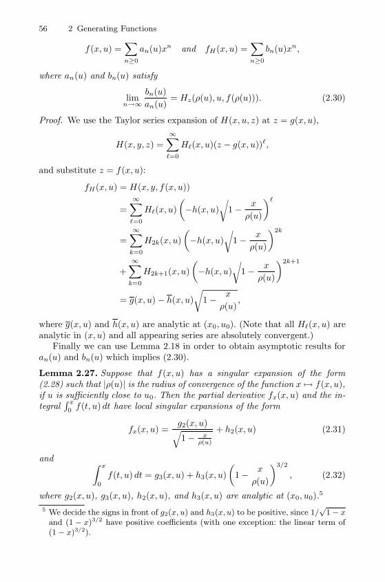
56 2 Generating Functions
f(x, u) =∑n≥0
an(u)xn and fH(x, u) =∑n≥0
bn(u)xn,
where an(u) and bn(u) satisfy
limn→∞
bn(u)
an(u)= Hz(ρ(u), u, f(ρ(u))). (2.30)
Proof. We use the Taylor series expansion of H(x, u, z) at z = g(x, u),
H(x, y, z) =
∞∑�=0
H�(x, u)(z − g(x, u))�,
and substitute z = f(x, u):
fH(x, u) = H(x, y, f(x, u))
=
∞∑�=0
H�(x, u)
(−h(x, u)
√1− x
ρ(u)
)�
=∞∑
k=0
H2k(x, u)
(−h(x, u)
√1− x
ρ(u)
)2k
+
∞∑k=0
H2k+1(x, u)
(−h(x, u)
√1− x
ρ(u)
)2k+1
= g(x, u)− h(x, u)
√1− x
ρ(u),
where g(x, u) and h(x, u) are analytic at (x0, u0). (Note that all H�(x, u) areanalytic in (x, u) and all appearing series are absolutely convergent.)
Finally we can use Lemma 2.18 in order to obtain asymptotic results foran(u) and bn(u) which implies (2.30).
Lemma 2.27. Suppose that f(x, u) has a singular expansion of the form(2.28) such that |ρ(u)| is the radius of convergence of the function x �→ f(x, u),if u is sufficiently close to u0. Then the partial derivative fx(x, u) and the in-tegral∫ x0f(t, u) dt have local singular expansions of the form
fx(x, u) =g2(x, u)√1− x
ρ(u)
+ h2(x, u) (2.31)
and ∫ x
0
f(t, u) dt = g3(x, u) + h3(x, u)
(1− x
ρ(u)
)3/2
, (2.32)
where g2(x, u), g3(x, u), h2(x, u), and h3(x, u) are analytic at (x0, u0).5
5 We decide the signs in front of g2(x, u) and h3(x, u) to be positive, since 1/√
1 − xand (1 − x)3/2 have positive coefficients (with one exception: the linear term of(1 − x)3/2).
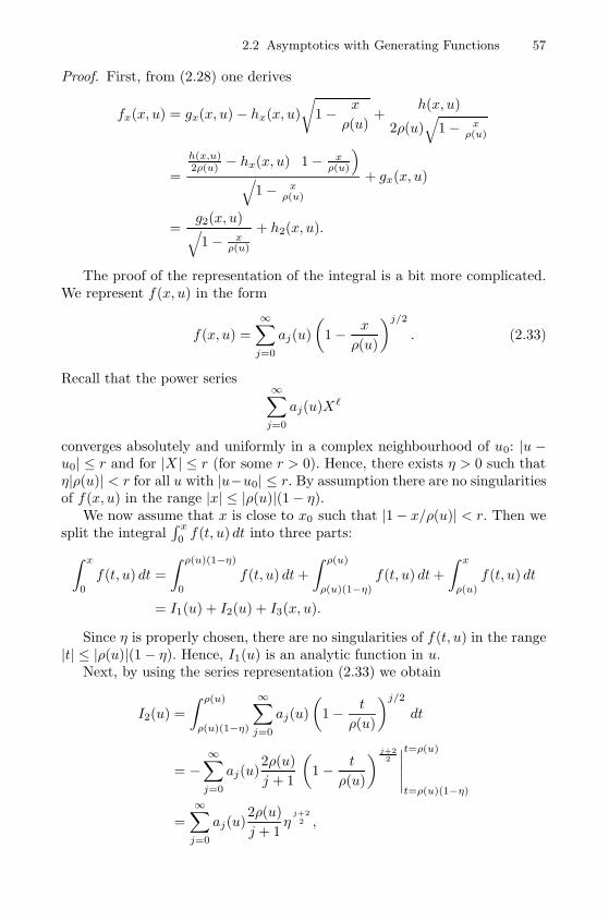
2.2 Asymptotics with Generating Functions 57
Proof. First, from (2.28) one derives
fx(x, u) = gx(x, u)− hx(x, u)
√1− x
ρ(u)+
h(x, u)
2ρ(u)√
1− xρ(u)
=
h(x,u)2ρ(u) − hx(x, u)
(1− x
ρ(u)
)√
1− xρ(u)
+ gx(x, u)
=g2(x, u)√1− x
ρ(u)
+ h2(x, u).
The proof of the representation of the integral is a bit more complicated.We represent f(x, u) in the form
f(x, u) =
∞∑j=0
aj(u)
(1− x
ρ(u)
)j/2
. (2.33)
Recall that the power series∞∑
j=0
aj(u)X�
converges absolutely and uniformly in a complex neighbourhood of u0: |u −u0| ≤ r and for |X | ≤ r (for some r > 0). Hence, there exists η > 0 such thatη|ρ(u)| < r for all u with |u−u0| ≤ r. By assumption there are no singularitiesof f(x, u) in the range |x| ≤ |ρ(u)|(1− η).
We now assume that x is close to x0 such that |1− x/ρ(u)| < r. Then wesplit the integral
∫ x
0 f(t, u) dt into three parts:∫ x
0
f(t, u) dt =
∫ ρ(u)(1−η)
0
f(t, u) dt+
∫ ρ(u)
ρ(u)(1−η)
f(t, u) dt+
∫ x
ρ(u)
f(t, u) dt
= I1(u) + I2(u) + I3(x, u).
Since η is properly chosen, there are no singularities of f(t, u) in the range|t| ≤ |ρ(u)|(1− η). Hence, I1(u) is an analytic function in u.
Next, by using the series representation (2.33) we obtain
I2(u) =
∫ ρ(u)
ρ(u)(1−η)
∞∑j=0
aj(u)
(1− t
ρ(u)
)j/2
dt
= −∞∑
j=0
aj(u)2ρ(u)
j + 1
(1− t
ρ(u)
) j+22
∣∣∣∣∣t=ρ(u)
t=ρ(u)(1−η)
=
∞∑j=0
aj(u)2ρ(u)
j + 1η
j+22 ,
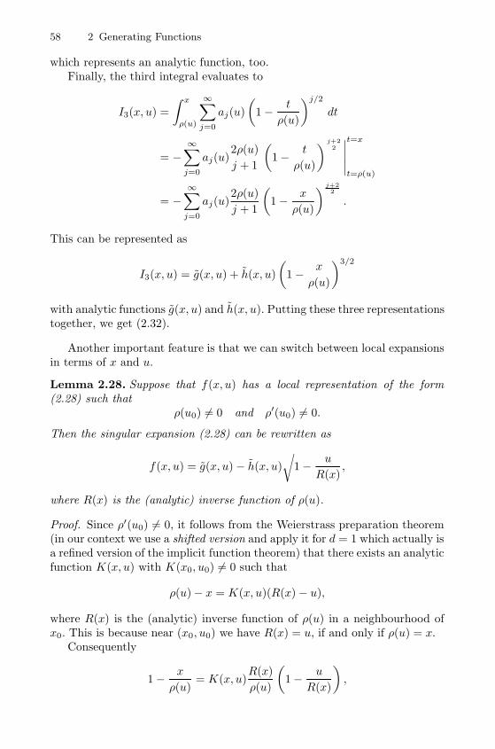
58 2 Generating Functions
which represents an analytic function, too.Finally, the third integral evaluates to
I3(x, u) =
∫ x
ρ(u)
∞∑j=0
aj(u)
(1− t
ρ(u)
)j/2
dt
= −∞∑
j=0
aj(u)2ρ(u)
j + 1
(1− t
ρ(u)
) j+22
∣∣∣∣∣t=x
t=ρ(u)
= −∞∑
j=0
aj(u)2ρ(u)
j + 1
(1− x
ρ(u)
) j+22
.
This can be represented as
I3(x, u) = g(x, u) + h(x, u)
(1− x
ρ(u)
)3/2
with analytic functions g(x, u) and h(x, u). Putting these three representationstogether, we get (2.32).
Another important feature is that we can switch between local expansionsin terms of x and u.
Lemma 2.28. Suppose that f(x, u) has a local representation of the form(2.28) such that
ρ(u0) = 0 and ρ′(u0) = 0.
Then the singular expansion (2.28) can be rewritten as
f(x, u) = g(x, u)− h(x, u)
√1− u
R(x),
where R(x) is the (analytic) inverse function of ρ(u).
Proof. Since ρ′(u0) = 0, it follows from the Weierstrass preparation theorem(in our context we use a shifted version and apply it for d = 1 which actually isa refined version of the implicit function theorem) that there exists an analyticfunction K(x, u) with K(x0, u0) = 0 such that
ρ(u)− x = K(x, u)(R(x)− u),
where R(x) is the (analytic) inverse function of ρ(u) in a neighbourhood ofx0. This is because near (x0, u0) we have R(x) = u, if and only if ρ(u) = x.
Consequently
1− x
ρ(u)= K(x, u)
R(x)
ρ(u)
(1− u
R(x)
),
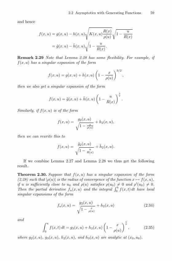
2.2 Asymptotics with Generating Functions 59
and hence
f(x, u) = g(x, u)− h(x, u)
√K(x, u)
R(x)
ρ(u)
√1− u
R(x)
= g(x, u)− h(x, u)
√1− u
R(x).
Remark 2.29 Note that Lemma 2.28 has some flexibility. For example, iff(x, u) has a singular expansion of the form
f(x, u) = g(x, u) + h(x, u)
(1− x
ρ(u)
)3/2
,
then we also get a singular expansion of the form
f(x, u) = g(x, u) + h(x, u)
(1− u
R(x)
) 32
.
Similarly, if f(x, u) is of the form
f(x, u) =g2(x, u)√1− x
ρ(u)
+ h2(x, u),
then we can rewrite this to
f(x, u) =g2(x, u)√1− u
R(x)
+ h2(x, u).
If we combine Lemma 2.27 and Lemma 2.28 we thus get the followingresult.
Theorem 2.30. Suppose that f(x, u) has a singular expansion of the form(2.28) such that |ρ(u)| is the radius of convergence of the function x �→ f(x, u),if u is sufficiently close to u0 and ρ(u) satisfies ρ(u0) = 0 and ρ′(u0) = 0.Then the partial derivative fu(x, u) and the integral
∫ u0 f(x, t) dt have local
singular expansions of the form
fu(x, u) =g2(x, u)√1− x
ρ(u)
+ h2(x, u) (2.34)
and ∫ u
0
f(x, t) dt = g3(x, u) + h3(x, u)
(1− x
ρ(u)
) 32
, (2.35)
where g2(x, u), g3(x, u), h2(x, u), and h3(x, u) are analytic at (x0, u0).
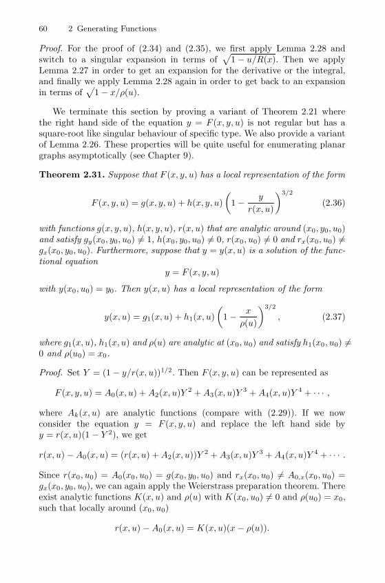
60 2 Generating Functions
Proof. For the proof of (2.34) and (2.35), we first apply Lemma 2.28 andswitch to a singular expansion in terms of
√1− u/R(x). Then we apply
Lemma 2.27 in order to get an expansion for the derivative or the integral,and finally we apply Lemma 2.28 again in order to get back to an expansionin terms of
√1− x/ρ(u).
We terminate this section by proving a variant of Theorem 2.21 wherethe right hand side of the equation y = F (x, y, u) is not regular but has asquare-root like singular behaviour of specific type. We also provide a variantof Lemma 2.26. These properties will be quite useful for enumerating planargraphs asymptotically (see Chapter 9).
Theorem 2.31. Suppose that F (x, y, u) has a local representation of the form
F (x, y, u) = g(x, y, u) + h(x, y, u)
(1− y
r(x, u)
)3/2
(2.36)
with functions g(x, y, u), h(x, y, u), r(x, u) that are analytic around (x0, y0, u0)and satisfy gy(x0, y0, u0) = 1, h(x0, y0, u0) = 0, r(x0, u0) = 0 and rx(x0, u0) =gx(x0, y0, u0). Furthermore, suppose that y = y(x, u) is a solution of the func-tional equation
y = F (x, y, u)
with y(x0, u0) = y0. Then y(x, u) has a local representation of the form
y(x, u) = g1(x, u) + h1(x, u)
(1− x
ρ(u)
)3/2
, (2.37)
where g1(x, u), h1(x, u) and ρ(u) are analytic at (x0, u0) and satisfy h1(x0, u0) =0 and ρ(u0) = x0.
Proof. Set Y = (1− y/r(x, u))1/2. Then F (x, y, u) can be represented as
F (x, y, u) = A0(x, u) +A2(x, u)Y 2 +A3(x, u)Y 3 +A4(x, u)Y 4 + · · · ,
where Ak(x, u) are analytic functions (compare with (2.29)). If we nowconsider the equation y = F (x, y, u) and replace the left hand side byy = r(x, u)(1 − Y 2), we get
r(x, u)−A0(x, u) = (r(x, u) +A2(x, u))Y 2 +A3(x, u)Y 3 +A4(x, u)Y 4 + · · · .
Since r(x0, u0) = A0(x0, u0) = g(x0, y0, u0) and rx(x0, u0) = A0,x(x0, u0) =gx(x0, y0, u0), we can again apply the Weierstrass preparation theorem. Thereexist analytic functions K(x, u) and ρ(u) with K(x0, u0) = 0 and ρ(u0) = x0,such that locally around (x0, u0)
r(x, u) −A0(x, u) = K(x, u)(x− ρ(u)).
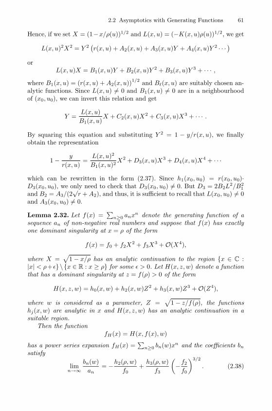
2.2 Asymptotics with Generating Functions 61
Hence, if we set X = (1−x/ρ(u))1/2 and L(x, u) = (−K(x, u)ρ(u))1/2, we get
L(x, u)2X2 = Y 2(r(x, u) +A2(x, u) +A3(x, u)Y +A4(x, u)Y 2 · · ·
)or
L(x, u)X = B1(x, u)Y +B2(x, u)Y 2 +B3(x, u)Y 3 + · · · ,
where B1(x, u) = (r(x, u) +A2(x, u))1/2 and B�(x, u) are suitably chosen an-alytic functions. Since L(x, u) = 0 and B1(x, u) = 0 are in a neighbourhoodof (x0, u0), we can invert this relation and get
Y =L(x, u)
B1(x, u)X + C2(x, u)X2 + C3(x, u)X3 + · · · .
By squaring this equation and substituting Y 2 = 1 − y/r(x, u), we finallyobtain the representation
1− y
r(x, u)=L(x, u)2
B1(x, u)2X2 +D3(x, u)X3 +D4(x, u)X4 + · · ·
which can be rewritten in the form (2.37). Since h1(x0, u0) = r(x0, u0)·D3(x0, u0), we only need to check that D3(x0, u0) = 0. But D3 = 2B2L
2/B21
and B2 = A3/(2√r +A2), and thus, it is sufficient to recall that L(x0, u0) = 0
and A3(x0, u0) = 0.
Lemma 2.32. Let f(x) =∑
n≥0 anxn denote the generating function of a
sequence an of non-negative real numbers and suppose that f(x) has exactlyone dominant singularity at x = ρ of the form
f(x) = f0 + f2X2 + f3X
3 +O(X4),
where X =√
1− x/ρ has an analytic continuation to the region {x ∈ C :|x| < ρ+ ε}\{x ∈ R : x ≥ ρ} for some ε > 0. Let H(x, z, w) denote a functionthat has a dominant singularity at z = f(ρ) > 0 of the form
H(x, z, w) = h0(x,w) + h2(x,w)Z2 + h3(x,w)Z3 +O(Z4),
where w is considered as a parameter, Z =√
1− z/f(ρ), the functionshj(x,w) are analytic in x and H(x, z, w) has an analytic continuation in asuitable region.
Then the functionfH(x) = H(x, f(x), w)
has a power series expansion fH(x) =∑
n≥0 bn(w)xn and the coefficients bnsatisfy
limn→∞
bn(w)
an= −h2(ρ, w)
f0+h3(ρ, w)
f3
(−f2f0
)3/2
. (2.38)
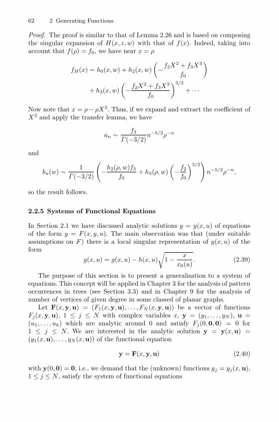
62 2 Generating Functions
Proof. The proof is similar to that of Lemma 2.26 and is based on composingthe singular expansion of H(x, z, w) with that of f(x). Indeed, taking intoaccount that f(ρ) = f0, we have near x = ρ
fH(x) = h0(x,w) + h2(x,w)
(−f2X
2 + f3X3
f0
)+ h3(x,w)
(−f2X
2 + f3X3
f0
)3/2
+ · · ·
Now note that x = ρ− ρX2. Thus, if we expand and extract the coefficient ofX3 and apply the transfer lemma, we have
an ∼f3
Γ (−3/2)n−5/2ρ−n
and
bn(w) ∼ 1
Γ (−3/2)
(−h2(ρ, w)f3
f0+ h3(ρ, w)
(−f2f0
)3/2)n−5/2ρ−n,
so the result follows.
2.2.5 Systems of Functional Equations
In Section 2.1 we have discussed analytic solutions y = y(x, u) of equationsof the form y = F (x, y, u). The main observation was that (under suitableassumptions on F ) there is a local singular representation of y(x, u) of theform
y(x, u) = g(x, u)− h(x, u)
√1− x
x0(u). (2.39)
The purpose of this section is to present a generalisation to a system ofequations. This concept will be applied in Chapter 3 for the analysis of patternoccurrences in trees (see Section 3.3) and in Chapter 9 for the analysis ofnumber of vertices of given degree in some classed of planar graphs.
Let F(x,y,u) = (F1(x,y,u), . . . , FN (x,y,u)) be a vector of functionsFj(x,y,u), 1 ≤ j ≤ N with complex variables x, y = (y1, . . . , yN), u =(u1, . . . , uk) which are analytic around 0 and satisfy Fj(0,0,0) = 0 for1 ≤ j ≤ N . We are interested in the analytic solution y = y(x,u) =(y1(x,u), . . . , yN(x,u)) of the functional equation
y = F(x,y,u) (2.40)
with y(0,0) = 0, i.e., we demand that the (unknown) functions yj = yj(x,u),1 ≤ j ≤ N , satisfy the system of functional equations
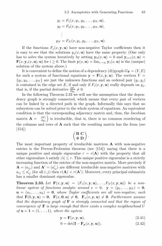
2.2 Asymptotics with Generating Functions 63
y1 = F1(x, y1, y2, . . . , yN ,u),
y2 = F2(x, y1, y2, . . . , yN ,u),
...
yN = FN (x, y1, y2, . . . , yN ,u).
If the functions Fj(x,y,u) have non-negative Taylor coefficients then itis easy to see that the solutions yj(x,u) have the same property. (One onlyhas to solve the system iteratively by setting y0(x,u) = 0 and yi+1(x,u) =F(x,yi(x,u),u) for i ≥ 0. The limit y(x,u) = limi→∞ yi(x,u) is the (unique)solution of the system above.)
It is convenient to define the notion of a dependency (di)graphGF = (V,E)for such a system of functional equations y = F(x,y,u). The vertices V ={y1, y2, . . . , yN} are just the unknown functions and an ordered pair (yi, yj)is contained in the edge set E, if and only if Fi(x,y,u) really depends on yj ,that is, if the partial derivative ∂Fi
∂yj = 0.
In the following Theorem 2.33 we will use the assumption that the depen-dency graph is strongly connected, which means that every pair of verticescan be linked by a directed path in the graph. Informally this says that nosubsystem can be solved prior to the whole system of equations. An equivalentcondition is that the corresponding adjacency matrix and, thus, the Jacobian
matrix A =(
∂Fi
∂yj
)is irreducible, that is, there is no common reordering of
the columns and rows of A such that the resulting matrix has the form (see[154]) (
B C
0 D
).
The most important property of irreducible matrices A with non-negativeentries is the Perron-Frobenius theorem (see [154]) saying that there is aunique positive and simple eigenvalue r = r(A) with the property that allother eigenvalues λ satisfy |λ| ≤ r. This unique positive eigenvalue is a strictlyincreasing function of the entries of the non-negative matrix. More precisely ifA = (aij) and A′ = (a′ij) are different irreducible non-negative matrices withaij ≤ a′ij (for all i, j) then r(A) < r(A′). Moreover, every principal submatrixhas a smaller dominant eigenvalue.
Theorem 2.33. Let F(x,y,u) = (F1(x,y,u), . . . , FN (x,y,u)) be a non-linear system of functions analytic around x = 0, y = (y1, . . . , yN ) = 0,u = (u1, . . . , uk) = 0, whose Taylor coefficients are all non-negative, suchthat F(0,y,u) = 0, F(x,0,u) = 0, Fx(x,y,u) = 0. Furthermore assumethat the dependency graph of F is strongly connected and that the region ofconvergence of F is large enough that there exists a complex neighbourhood Uof u = 1 = (1, . . . , 1), where the system
y = F(x,y,u), (2.41)
0 = det(I− Fy(x,y,u)), (2.42)
64 2 Generating Functions
has solutions x = x0(u) and y = y0(u) that are real, positive and minimalfor positive real u ∈ U .
Lety = y(x,u) = (y1(x,u), . . . , yN(x,u))
denote the analytic solutions of the system
y = F(x,y,u) (2.43)
with y(0,u) = 0.Then there exists ε > 0 such that yj(x,u) admit a representation of the
form
yj(x,u) = gj(x,u)− hj(x,u)
√1− x
x0(u)(2.44)
for u ∈ U , |x − x0(u)| < ε and | arg(x − x0(u)| = 0, where gj(x,u) = 0 andhj(x,u) = 0 are analytic functions with (gj(x0(u),u))j = (yj(x0(u),u))j =y0(u).
Furthermore, if [xn] yj(x,1) > 0 for 1 ≤ j ≤ N and for sufficiently largen ≥ n1, then there exists 0 < δ < ε such that yj(x,u) is analytic in (x,u) foru ∈ U and |x−x0(u)| ≥ ε but |x| ≤ |x0(u)|+ δ (this condition guarantees thaty(x,u) has a unique smallest singularity with |x| = |x0(u)|).
Proof. In order to simplify the proof we first assume that u is real, positiveand fixed, and we also suppress the dependency on u in the notation. Thus,we will work with x0 and y0 that satisfy y0 = F(x0,y0) and det(I−A) = 0,where A = Fy(x0,y0) abbreviates the Jacobian matrix of F with respect toy. Note that the condition det(I−A) = 0 says that 1 is eigenvalue of A. If theJacobian matrix A had no eigenvalue 1, then the implicit function theoremcould be applied and it would follow that the system of functional equationsy = F(x,y) has locally an analytic solution y = y(x) with y(x0) = y0.
Recall that the assumption that the dependency graph is strongly con-nected can be rephrased in A is a non-negative irreducible matrix. Hence,there is a unique (dominant) positive real simple eigenvalue. It is easy to ob-serve that this dominating eigenvalue is actually 1. Set A(x) = Fy(x,y(x)) for0 ≤ x ≤ x0. Then by assumption A(0) = 0 and A(x) is (again) an irreduciblepositive matrix for x > 0 with the property that all non-zero entries of A(x)are strictly increasing in x. Thus, by the properties of irreducible non-negativematrices the dominant positive eigenvalue of A(x) is an increasing function,too. Since (x0,y0) is the minimal solution of (2.41) and (2.42), the eigenvalue1 appears first for x = x0.
Next we divide the system into the first equation and into the system ofthe remaining equations:
y1 = F1(x, y1,y), (2.45)
y = F(x, y1,y), (2.46)
2.2 Asymptotics with Generating Functions 65
where y = (y2, . . . , yN) and F = (F2, . . . , FN ). Observe that the Jacobian ma-trix Fy(x0,y0) of F can be also obtained by deleting the first row and columnof A. Hence, all eigenvalues of B are strictly smaller than 1. Consequently, thematrix I−B is invertible and, thus, by the implicit function theorem, there isa local solution y = y(x, y1) of (2.46), where y1 is considered as an additionalvariable. As in the proof of Theorem 2.19 it follows that this solution is pre-cisely the unique solution of (2.46) that has a power series expansion in x andy1 at 0. Note, too, that due to the positivity assumptions on the coefficientsof F this solution has non-negative coefficients as a power series in x and y1.
We now insert this function into the first equation (2.45) and obtain asingle equation
y1 = F1(x, y1,y(x, y1)) (2.47)
for y1 = y1(x). Again, the coefficients of
G(x, y1) = F1(x, y1,y(x, y1))
as a power series in x and y1 are non-negative. At this point we can safelyapply the methods of Theorem 2.19 (and 2.21). Actually, equation (2.47) is anequation of the form y1 = G(x, y1) with the property that Gy1(x0, y1,0) = 1.Thus, it follows from Theorem 2.19 that y1(x) has a local representation of theform y1(x) = g(x) − h(x)
√1− x/x0. Consequently there are corresponding
local representations for (y1(x), . . . , yN (x)) = y2(x, y1(x)). Of course, x0 isthe common radius of convergence of y1(x), . . . , yN(x).
This proves (2.44) for fixed real and positive u. However, it is easy toadapt the above proof for u close to the real axis. In particular, by continuityit follows that 1 will stay a simple eigenvalue of the Jacobian matrix.
Furthermore, if [xn]y1(x,1) > 0 for sufficiently large n ≥ n1, then as in theproof of Theorem 2.19 it follows that x0 is the only singularity on the circle ofconvergence of y1(x), and there is an analytic continuation to |x| ≤ x0 +δ and|x− x0| ≥ ε. This also applies for yj for 2 ≤ j ≤ N , and finally by continuitythis is also true for u sufficiently close to the positive real axis.
With the help of a variation of Lemma 2.26 we derive the following
Corollary 2.34 Let y = y(x,u) = (y1(x,u), . . . , yN(x,u)) be the solutionof the system of equations (2.43) and assume that all assumptions of The-orem 2.33 are satisfied. Suppose that G(x,y,u) is a power series such thatthe point (x0(1),y0(x0(1),1),1) is contained in the interior of the region ofconvergence of G(x,y,u) and that Gy(x0(1),y0(1),1) = 0.
Then G(x,y(x,u),u) has a representation of the form
G(x,y(x,u),u) = g(x,u)− h(x,u)
√1− x
x0(u)(2.48)
for u ∈ U and |x − x0(u)| < ε, where g(x,u) = 0 and h(x,u) = 0 areanalytic functions. Moreover, G(x,y(x,u),u) is analytic in (x,u) for u ∈ Uand |x− x0(u)| ≥ ε, but |x| ≤ |x0(u)|+ δ.
66 2 Generating Functions
Let G(x,y,u) be also a power series with non-negative Taylor coefficientsat (0,0,0) such that (x0(1),y0(1),1) is an inner point of the region of con-vergence of G(x,y,u). Then (with y(x,u), the solution of (2.43) from Theo-rem 2.33)
G(x,y(x,u),u) =∑n,m
cn,mxnum
has non-negative coefficients cn,m, too. In fact, for sufficiently large n ≥ n0
there exists m with cn,m > 0. In particular it follows that
cn(u) =∑m
cn,mum
is non-zero for n ≥ n0.Let Xn = (X
(1)n , . . . , X
(N)n ), (n ≥ n0) denote an N -dimensional discrete
random vector withP{Xn = m} =
cn,m
cn. (2.49)
Then the expectation EuXn = EuX(1)
n1 · · ·uX(N)
n
N is given by
EuXn =cn(u)
cn(1).
Putting these preliminaries together we finally get a central limit theoremfor random variables that are related to systems of functional equations. Forconvenience we set
μ = −x0,u(1)
x0(1),
and define a matrix Σ by
Σ = −x0,uu(1)
x0(1)+ μμT + diag(μ), (2.50)
where x = x0(u) and y = y0(u) are the solutions of the system (2.41) and(2.42).
Theorem 2.35. Suppose that Xn is a sequence of N -dimensional randomvectors that are defined by (2.49), where
∑n,m cn,mx
num = G(x,y(x,u),u)and the generating functions y(x,u) = (yj(x,u))1≤j≤N satisfy a system offunctional equations of the form (2.43), in which F satisfies the assumptionsof Theorem 2.33.
Then Xn satisfies a central limit theorem of the form
1√n
(Xn − EXn)d−→ N (0,Σ) . (2.51)
Furthermore there exist positive constants c1, c2, c3 such that
P{‖Xn − EXn‖ ≥ ε
√n}≤ c1e−c2ε2 (2.52)
uniformly for ε ≤ c3√n.
2.2 Asymptotics with Generating Functions 67
Finally we comment the evaluation of μ and Σ. The problem is to extractthe derivatives of x0(u). The function x0(u) is the solution of the system(2.41)–(2.42) and is exactly the location of the singularity of the mappingx �→ y(x,u) when u is fixed (and close to 1).
Let x0(u) and y0(u) = y(x0(u),u) denote the solutions of (2.41–2.42).Then we have
y0(u) = F(x0(u),y0(u),u). (2.53)
Taking derivatives with respect to u we get
y0,u(u) = Fx(x0(u),y0(u),u)x0,u(u) + Fy(x0(u),y0(u),u)y0,u(u) (2.54)
+ Fu(x0(u),y0(u),u),
where the three terms in F denote evaluations at (x0(u),y0(u),u) of thepartial derivatives of F, and not the (total) derivative of the composite func-tion F(x0(u),y0(u),u), and where x0,u and y0,u denote the Jacobian matricesof x0 and y0 with respect to u. In particular, for u = 1 we have x0(1) = x0
and y0(1) = y0 anddet(I− Fy(x0,y0,1)) = 0.
Since Fy is a non-negative matrix and the dependency graph is strongly con-nected, there is a unique Perron-Frobenius eigenvalue of multiplicity 1. Herethis eigenvalue equals 1. Thus, I−Fy has rank N − 1 and (up to scaling) hasa unique positive left eigenvector b:
bT(I− Fy(x0,y0,1)) = 0.
From (2.54) we obtain
(I− Fy(x0,y0,1))yu(1) = Fx(x0,y0,1)xu(1) + Fu(x0,y0,1).
By multiplying b from the left we thus get
bTFx(x0,y0,1)xu + bTFu(x0,y0,1) = 0, (2.55)
and consequently
μ =1
x0
bTFu(x0,y0,1)
bTFx(x0,y0,1). (2.56)
The derivation of Σ is more involved. We first define b(x,y,u) as the(generalised) vector product6 of the N − 1 last columns of the matrix I −Fy(x,y,u). We define D(x,y,u) as
D(x,y,u) =(bT(x,y,u) (I− Fy(x,y,u))
)1
= det (I− Fy(x,y,u)) ,
where the subindex denotes the first coordinate. In particular we have
6 More precisely, this is the wedge product combined with the Hodge duality.
68 2 Generating Functions
D(x(u),y(u),u) = 0.
Then from
(I− Fy)yu = Fxxu + Fu,
−Dyyu = Dxxu +Du (2.57)
we can calculate yu (the first system has rank N − 1; this means that we canskip the first equation. This reduced system is then completed to a regularsystem by appending the second equation (2.57)).
We now set
d1(u) = d1(x(u),y(u),u) = b(x(u),y(u),u)Fx(x(u),y(u),u)
d2(u) = d2(x(u),y(u),u) = b(x(u),y(u),u)Fu(x(u),y(u),u).
By differentiating equation (2.55) we get
xuu(u) = − (d1xxu + d1yyu + d1u)xu + (d2xxu + d2yyu + d2u)
d1, (2.58)
where d1x, d1y, d1u,d2x,d2y,d2u denote the respective partial derivatives, andwhere we have omitted the dependence on u. With the knowledge of x0,y0
and yu(1) we can now evaluate xuu at u = 1 and compute Σ from (2.50).
3
Advanced Tree Counting
In this third chapter we will present methods for counting trees that are basedon the concept of generating functions. First we derive explicit formulas forbasic tree classes and asymptotic formulas for simply generated trees andPolya trees. However, the main goal is to show that certain tree parametersthat behave additively (in a proper sense) satisfy a central limit theorem in anatural probabilistic setting.
For instance, if we consider certain trees Tn of size n it is natural to assumethat every tree in Tn is equally likely. Every tree parameter then induces asequence of random variables Xn (depending on the size n). A prominentexample of tree parameters is the number of leaves or the number of nodesof degree k. We call a parameter additive if it is also obtained (up to somesmall correction term) by splitting the tree into subtrees and adding up. Thenumber of leaves is additive in this sense. Another additive parameter is thenumber of occurrences of a certain pattern that we will discuss in Section 3.3.
Intuitively we can expect a central limit theorem for additive tree parame-ters, since they can be seen as the approximate sum of random variables if wesplit the tree into small subtrees. Nevertheless, it seems not to be possible toapply a direct probabilistic approach. The dependence structure is not easy tocover and there is no direct evolution process that recovers the combinatorialprobability model.
Instead we use the method of generating functions that directly extends tothe counting problem of additive parameters. Depending on the complexity ofthe parameter the recursive structure of trees leads to a functional equation orto a system of functional equations for the corresponding generating functions,and the result of Chapter 2 can be applied.
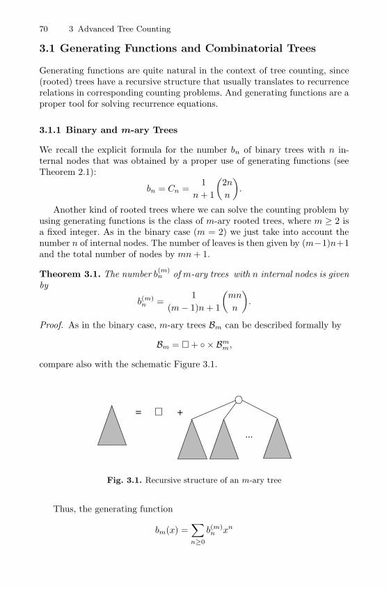
70 3 Advanced Tree Counting
3.1 Generating Functions and Combinatorial Trees
Generating functions are quite natural in the context of tree counting, since(rooted) trees have a recursive structure that usually translates to recurrencerelations in corresponding counting problems. And generating functions are aproper tool for solving recurrence equations.
3.1.1 Binary and m-ary Trees
We recall the explicit formula for the number bn of binary trees with n in-ternal nodes that was obtained by a proper use of generating functions (seeTheorem 2.1):
bn = Cn =1
n+ 1
(2n
n
).
Another kind of rooted trees where we can solve the counting problem byusing generating functions is the class of m-ary rooted trees, where m ≥ 2 isa fixed integer. As in the binary case (m = 2) we just take into account thenumber n of internal nodes. The number of leaves is then given by (m−1)n+1and the total number of nodes by mn+ 1.
Theorem 3.1. The number b(m)n of m-ary trees with n internal nodes is given
by
b(m)n =
1
(m− 1)n+ 1
(mn
n
).
Proof. As in the binary case, m-ary trees Bm can be described formally by
Bm = � + ◦ × Bmm,
compare also with the schematic Figure 3.1.
= +
...
Fig. 3.1. Recursive structure of an m-ary tree
Thus, the generating function
bm(x) =∑n≥0
b(m)n xn
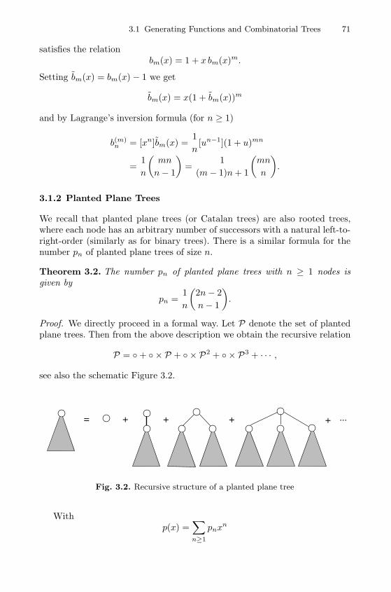
3.1 Generating Functions and Combinatorial Trees 71
satisfies the relationbm(x) = 1 + x bm(x)m.
Setting bm(x) = bm(x) − 1 we get
bm(x) = x(1 + bm(x))m
and by Lagrange’s inversion formula (for n ≥ 1)
b(m)n = [xn]bm(x) =
1
n[un−1](1 + u)mn
=1
n
(mn
n− 1
)=
1
(m− 1)n+ 1
(mn
n
).
3.1.2 Planted Plane Trees
We recall that planted plane trees (or Catalan trees) are also rooted trees,where each node has an arbitrary number of successors with a natural left-to-right-order (similarly as for binary trees). There is a similar formula for thenumber pn of planted plane trees of size n.
Theorem 3.2. The number pn of planted plane trees with n ≥ 1 nodes isgiven by
pn =1
n
(2n− 2
n− 1
).
Proof. We directly proceed in a formal way. Let P denote the set of plantedplane trees. Then from the above description we obtain the recursive relation
P = ◦+ ◦ × P + ◦ × P2 + ◦ × P3 + · · · ,
see also the schematic Figure 3.2.
= + + + ...+
Fig. 3.2. Recursive structure of a planted plane tree
Withp(x) =
∑n≥1
pnxn
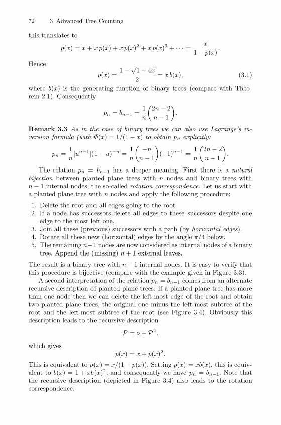
72 3 Advanced Tree Counting
this translates to
p(x) = x+ x p(x) + x p(x)2 + x p(x)3 + · · · =x
1− p(x).
Hence
p(x) =1−
√1− 4x
2= x b(x), (3.1)
where b(x) is the generating function of binary trees (compare with Theo-rem 2.1). Consequently
pn = bn−1 =1
n
(2n− 2
n− 1
).
Remark 3.3 As in the case of binary trees we can also use Lagrange’s in-version formula (with Φ(x) = 1/(1− x) to obtain pn explicitly:
pn =1
n[un−1](1− u)−n =
1
n
( −nn− 1
)(−1)n−1 =
1
n
(2n− 2
n− 1
).
The relation pn = bn−1 has a deeper meaning. First there is a naturalbijection between planted plane trees with n nodes and binary trees withn− 1 internal nodes, the so-called rotation correspondence. Let us start witha planted plane tree with n nodes and apply the following procedure:
1. Delete the root and all edges going to the root.2. If a node has successors delete all edges to these successors despite one
edge to the most left one.3. Join all these (previous) successors with a path (by horizontal edges).4. Rotate all these new (horizontal) edges by the angle π/4 below.5. The remaining n−1 nodes are now considered as internal nodes of a binary
tree. Append the (missing) n+ 1 external leaves.
The result is a binary tree with n− 1 internal nodes. It is easy to verify thatthis procedure is bijective (compare with the example given in Figure 3.3).
A second interpretation of the relation pn = bn−1 comes from an alternaterecursive description of planted plane trees. If a planted plane tree has morethan one node then we can delete the left-most edge of the root and obtaintwo planted plane trees, the original one minus the left-most subtree of theroot and the left-most subtree of the root (see Figure 3.4). Obviously thisdescription leads to the recursive description
P = ◦+ P2,
which givesp(x) = x+ p(x)2.
This is equivalent to p(x) = x/(1− p(x)). Setting p(x) = xb(x), this is equiv-alent to b(x) = 1 + xb(x)2, and consequently we have pn = bn−1. Note thatthe recursive description (depicted in Figure 3.4) also leads to the rotationcorrespondence.
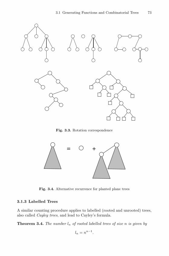
3.1 Generating Functions and Combinatorial Trees 73
Fig. 3.3. Rotation correspondence
= +
Fig. 3.4. Alternative recurrence for planted plane trees
3.1.3 Labelled Trees
A similar counting procedure applies to labelled (rooted and unrooted) trees,also called Cayley trees, and lead to Cayley’s formula.
Theorem 3.4. The number ln of rooted labelled trees of size n is given by
ln = nn−1.
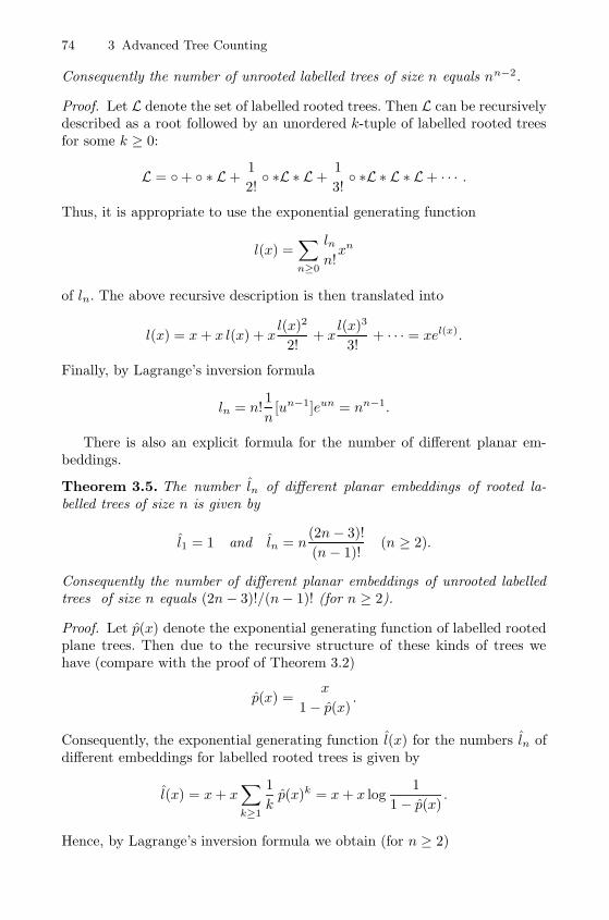
74 3 Advanced Tree Counting
Consequently the number of unrooted labelled trees of size n equals nn−2.
Proof. Let L denote the set of labelled rooted trees. Then L can be recursivelydescribed as a root followed by an unordered k-tuple of labelled rooted treesfor some k ≥ 0:
L = ◦+ ◦ ∗ L+1
2!◦ ∗L ∗ L+
1
3!◦ ∗L ∗ L ∗ L+ · · · .
Thus, it is appropriate to use the exponential generating function
l(x) =∑n≥0
lnn!xn
of ln. The above recursive description is then translated into
l(x) = x+ x l(x) + xl(x)2
2!+ x
l(x)3
3!+ · · · = xel(x).
Finally, by Lagrange’s inversion formula
ln = n!1
n[un−1]eun = nn−1.
There is also an explicit formula for the number of different planar em-beddings.
Theorem 3.5. The number ln of different planar embeddings of rooted la-belled trees of size n is given by
l1 = 1 and ln = n(2n− 3)!
(n− 1)!(n ≥ 2).
Consequently the number of different planar embeddings of unrooted labelledtrees of size n equals (2n− 3)!/(n− 1)! (for n ≥ 2).
Proof. Let p(x) denote the exponential generating function of labelled rootedplane trees. Then due to the recursive structure of these kinds of trees wehave (compare with the proof of Theorem 3.2)
p(x) =x
1− p(x).
Consequently, the exponential generating function l(x) for the numbers ln ofdifferent embeddings for labelled rooted trees is given by
l(x) = x+ x∑k≥1
1
kp(x)k = x+ x log
1
1− p(x).
Hence, by Lagrange’s inversion formula we obtain (for n ≥ 2)
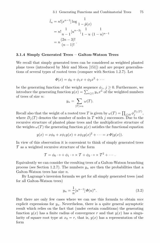
3.1 Generating Functions and Combinatorial Trees 75
ln = n![xn−1] log1
1− p(x)
= n!1
n− 1[un−2]
1
1− u1
(1 − u)n−1
= n(2n− 3)!
(n− 1)!.
3.1.4 Simply Generated Trees – Galton-Watson Trees
We recall that simply generated trees can be considered as weighted plantedplane trees (introduced by Meir and Moon [151]) and are proper generalisa-tions of several types of rooted trees (compare with Section 1.2.7). Let
Φ(x) = φ0 + φ1x+ φ2x2 + · · ·
be the generating function of the weight sequence φj , j ≥ 0. Furthermore, weintroduce the generating function y(x) =
∑n≥1 ynx
n of the weighted numbersof trees of size n:
yn =∑|T |=n
ω(T ).
Recall also that the weight of a rooted tree T is given by ω(T ) =∏
j≥0 φDj(T )j ,
where Dj(T ) denotes the number of nodes in T with j successors. Due to therecursive structure of planted plane trees and the multiplicative structure ofthe weights ω(T ) the generating function y(x) satisfies the functional equation
y(x) = xφ0 + xφ1y(x) + xφ2y(x)2 + · · · = xΦ(y(x)).
In view of this observation it is convenient to think of simply generated treesT as a weighted recursive structure of the form
T = φ0 · ◦+ φ1 · ◦ × T + φ2 · ◦ × T 2 + · · · .
Equivalently we can consider the resulting trees of a Galton-Watson branchingprocess (see Section 1.2.7). The numbers yn are then the probabilities that aGalton-Watson trees has size n.
By Lagrange’s inversion formula we get for all simply generated trees (andfor all Galton-Watson trees)
yn =1
n[un−1]Φ(u)n. (3.2)
But there are only few cases where we can use this formula to obtain niceexplicit expressions for yn. Nevertheless, there is a quite general asymptoticresult which relies on the fact that (under certain conditions) the generatingfunction y(x) has a finite radius of convergence r and that y(x) has a singu-larity of square root type at x0 = r, that is, y(x) has a representation of theform
76 3 Advanced Tree Counting
y(x) = g(x)− h(x)
√1− x
x0
= c0 + c1√x− x0 + c2(x− x0) +O
(|x− x0|3/2
),
where g(x) and h(x) are analytic at x0 (compare with Theorem 2.19). Forbinary and planted plane trees this has been made explicit, see (2.3) and(3.1). Such representations can be used to derive asymptotic expansions forthe coefficients yn.
Theorem 3.6. Let R denote the radius of convergence of Φ(x) and supposethat there exists τ with 0 < τ < R that satisfies τΦ′(τ) = Φ(τ). Set d =gcd{j > 0 : φj > 0}. Then
yn = d
√Φ(τ)
2πΦ′′(τ)
Φ′(τ)n
n3/2
(1 +O(n−1)
)(n ≡ 1 mod d) (3.3)
and yn = 0 if n ≡ 1 mod d.
Proof. We apply Theorem 2.19 for F (x, y) = xΦ(y) and assume first for sim-plicity that d = 1. Then all assumptions are satisfied. In particular we havex0 = 1/Φ′(τ) and y0 = τ .
If d > 1 then it is easy to see that yn = 0 if n ≡ 1 mod d. Consequently wehave y(x) = y(xd)/xd−1 and (of course) Φ(x) = Φ(xd) for analytic functionsy(x) and Φ(x). They satisfy y(x) = xΦ(y(x)) and the corresponding gcd d = 1.Thus, Theorem 2.19 can be applied to this equation and we obtain (3.3) ingeneral.
Note that for m-ary trees and for planted plane trees this asymptotic
formula also follows from the explicit formula for b(m)n and pn via Stirling’s
formula.
Remark 3.7 Theorem 3.6 remains true in a slightly more general situation.Suppose that τ > 0 is the radius of convergence of Φ(x) for which we haveτΦ′(τ) = Φ(τ) and Φ′′(τ) <∞. Then yn is asymptotically given by
yn ∼ d√
Φ(τ)
2πΦ′′(τ)
Φ′(τ)n
n3/2(n ≡ 1 mod d). (3.4)
The proof of (3.4) is in principle very similar to the proof of (3.3). One alsoobserves that the generating function y(x) analytically extends to a Δ-regionsuch that y(x) = c0 + c1
√x− x0 (1 + o(1)) as x → x0 (in Δ). Thus, the
Transfer Lemma 2.12, or its variant mentioned in Remark 2.13, leads to (3.4)(for detail see [114]).
3.1 Generating Functions and Combinatorial Trees 77
3.1.5 Unrooted Trees
Let T denote the set of unlabelled unrooted trees and T the set of unla-belled rooted trees (we do not distinguish between different embeddings inthe plane). Sometimes these kinds of trees are called Polya trees. The corre-sponding cardinalities of these trees (of size n) are denoted by tn and tn, andthe generating functions by
t(x) =∑n≥1
tnxn and t(x) =
∑n≥1
tnxn.
The structure of these trees is much more complex than that of rooted trees,where the successors have a left-to-right-order. We have to apply Polya’s the-ory of counting and an amazing observation (3.6) by Otter [168].
Theorem 3.8. The generating functions t(x) and t(x) satisfy the functionalequations
t(x) = x exp
(t(x) +
1
2t(x2) +
1
3t(x3) + · · ·
)(3.5)
and
t(x) = t(x) − 1
2t(x)2 +
1
2t(x2). (3.6)
They have a common radius of convergence ρ ≈ 0.338219 which is given byt(ρ) = 1, that is, t(x) is convergent at x = ρ. They have a local expansion ofthe form
t(x) = 1− b(ρ− x)1/2 + c(ρ− x) + d(ρ− x)3/2 +O((ρ− x)2)) (3.7)
and
t(x) =1 + t(ρ2)
2+b2 − ρt′(ρ2)
2(ρ− x) + bc(ρ− x)3/2 +O((ρ − x)2), (3.8)
where b ≈ 2.6811266 and c = b2/3 ≈ 2.3961466 and x = ρ is the only singular-ity on the circle of convergence |x| = ρ. Finally, tn and tn are asymptoticallygiven by
tn =b√ρ
2√πn−3/2ρ−n
(1 +O(n−1)
)(3.9)
and
tn =b3ρ3/2
4√πn−5/2ρ−n
(1 +O(n−1)
). (3.10)
Remark 3.9 In 1937, Polya [176] already discussed the generating functiont(x) and showed that the radius of convergence ρ satisfies 0 < ρ < 1 andthat x = ρ is the only singularity on the circle of convergence |x| = ρ. LaterOtter [168] showed that t(ρ) = 1 and used the representation (3.7) to deducethe asymptotics for tn. He also calculated ρ ≈ 0.338219 and b ≈ 2.6811266.However, his main contribution was to show (3.6). Consequently he derived(3.8) and (3.10).
78 3 Advanced Tree Counting
Proof. Firt we derive (3.5). As in the previous cases we can think of rootedtrees in a recursive way, that is, T is a root followed by an unordered sequenceof rooted trees:
T = ◦ ×Mfin(T ).
Thus, we obtain (3.5).The radius of convergence ρ of t(x) surely satisfies 1
4 ≤ ρ ≤ 1 (this followsfrom tn ≤ pn and tn → ∞). Next we show that t(ρ) is finite (althoughx = ρ is a singularity of t(x)) and that ρ < 1. From (3.5) it follows thatlog(t(x)/x) ≥ t(x) for 0 < x < ρ. Hence,
t(x)/x
log(t(x)/x)≤ 1
x
and consequently t(ρ) has to be finite. If ρ = 1 then t(ρk) = t(ρ) for all k ≥ 1and it would follow that
limx→ρ−
et(x)+ 12 t(x2)+ 1
3 t(x3)+··· = ∞,
which is impossible. Thus, ρ < 1 and consequently the functions t(x2), t(x3), . . .are regular at x = ρ. Moreover, they are analytic for |x| ≤ ρ + ε (for somesufficiently small ε > 0) and are also bounded by |t(xk)| ≤ C|xk| in thisrange. Hence, t(x) may be considered as the solution of the functional equa-tion y = F (x, y), where
F (x, y) = x exp
(y +
1
2t(x2) +
1
3t(x3) + · · ·
).
This function satisfies the assumptions of Theorem 2.19. In particular, thesingularity x = ρ and η = t(ρ) satisfy the system of equations
η = ρ exp
(η +
1
2t(ρ2) +
1
3t(ρ3) + · · ·
),
1 = ρ exp
(η +
1
2t(ρ2) +
1
3t(ρ3) + · · ·
)that directly gives η = t(ρ) = 1. Now, by using the expansion (3.7) and (3.5)we also get c = b2/3 by comparing coefficients. In this way we get (3.8) and(3.9). Note also that Theorem 2.19 implies that x = ρ is the only singularityon the circle of convergence of t(x).
Next, observe that (3.7) and (3.6) imply (3.8) and (with the help of theTransfer Lemma 2.12 or its corollary) (3.10). Therefore it remains to prove(3.6).
We consider three sets of trees, the set T of rooted trees, the set T ofunrooted trees and the set T (p) of (unordered) pairs {T1, T2} of rooted treesof T with T1 = T2. (It will be convenient to consider the pair {T1, T2} as a
3.1 Generating Functions and Combinatorial Trees 79
tree that is rooted by an additional edge joining the roots of T1 and T2.) Let
t(p)n denote the number of pairs of that kind with a total number of n nodes,
and let t(p)(x) denote the generating function of t(p)n . Then we have
t(p)(x) =1
2t(x)2 − 1
2t(x2). (3.11)
We will now show that there is a bijection between T and T ∪ T (p). In viewof (3.11) such a bijection implies (3.6).
Recall that an arbitrary (finite) tree has either a central node or a centraledge. The central edge e = (v, w) is called symmetry line, if the two subtreesrooted at the endpoints v and w are equal.
We first divide the set T into 6 subsets:
1. Let T1 denote those rooted trees that are rooted at the central node.2. Let T2 denote those rooted trees that have a central node that is different
from the root.3. Let T3 denote those rooted trees that have a central edge which is not a
symmetry line and where one of the two endpoints of the central edge isthe root.
4. Let T4 denote those rooted trees that have a central edge which is not asymmetry line and where the root is not one of the two endpoints of thecentral edge.
5. Let T5 denote those rooted trees that have a central edge which is asymmetry line and where one of the two endpoints of the central edge isthe root.
6. Let T6 denote those rooted trees that have a central edge which is asymmetry line and where the root is not one of the two endpoints of thecentral edge.
In a similar way we divide the unrooted trees T :
1. Let T1 denote those unrooted trees that have a central node.2. Let T2 denote those unrooted trees that have a central edge, that is not a
symmetry line.3. Let T3 denote those unrooted trees that have a symmetry line as a central
edge.
Finally we partition T (p) that we consider as trees rooted at an edge.
1. Let T (p)1 be the set of pairs {T1, T2} with T1 = T2 with the property that,
if we join the roots of T1 and T2 by an edge then the resulting tree has acentral node.
2. Let T (p)2 be the set of pairs {T1, T2} with T1 = T2, such that the tree that
results from T1 and T2 by joining the roots by an edge has a central edgethat is not a symmetry line and that is different from the edge joining T1
and T2.
80 3 Advanced Tree Counting
3. Let T (p)3 be the set of pairs {T1, T2} with T1 = T2, such that the tree that
results from T1 and T2 by joining the roots by an edge has this edge asthe central one, but it is not a symmetry line.
4. Let T (p)4 be the set of pairs {T1, T2} with T1 = T2, such that the tree that
results from T1 and T2 by joining the roots by an edge has a symmetryline as a central edge that is different from the edge joining T1 and T2.
There is a natural bijection between T1 and T1. We only have to take thecentral node as the root.
Next, there is a bijection between T2 and T (p)1 . We identify the first edge
from the path connecting the root and the central node with the edge joiningT1 and T2.
Next, there is a trivial bijection between the sets T2 and T (p)2 . By marking
one of the two endpoints of the central edge in the trees of T2 we obtain T3.
This can be rewritten as a bijection between T3 and T2 ∪ T (p)2 .
Next, there is a bijection between T4 and T (p)3 . We identify the first edge
from the path connecting the root and the central edge with the edge joining
T1 and T2. Similarly there is a bijection between T6 and T (p)4 . Finally, there
is a natural bijection between T5 and T3.Putting these parts together provides the proposed bijection between T
and T ∪ T (p).
In a similar way we can deal with unlabelled binary trees B, where we donot care about the embedding in the plane. In particular this means that withthe only exception of the root (that has degree 2) all nodes have either degree1 or 3. The corresponding unrooted version B is the set of unlabelled trees,where every node has either degree 1 or 3. Let the corresponding cardinalitiesof these trees (of size n) be denoted by bn and bn, and the generating functionsby
b(x) =∑n≥1
bnxn and b(x) =
∑n≥1
bnxn.
Then we have (similarly to the above, compare also with [28]):
Theorem 3.10. The generating functions b(x) and b(x) satisfy the functionalequations
b(x) = x+x
2
(b(x)2 + b(x2)
)(3.12)
and
b(x) =x
6
(b(x)3 + 3b(x)b(x2) + 2b(x3)
)− 1
2b(x)2 +
1
2b(x2). (3.13)
They have a common radius of convergence ρ2 ≈ 0.6345845127 which is givenby ρ2 b(ρ2) = 1 and singular expansions corresponding to (3.7) and (3.8).Furthermore, bn and bn are asymptotically given by
bn = c1n−3/2ρ−n
2
(1 +O(n−1)
)(n ≡ 1 mod 2) (3.14)
3.1 Generating Functions and Combinatorial Trees 81
andbn = c2n
−5/2ρ−n2
(1 +O(n−1)
)(3.15)
with certain positive constants c1, c2.
Proof. We just comment on the combinatorial part, that is, on (3.12) and(3.13). The first equation can be rewritten as
b(x) = x+ xPS2 (b(x), b(x2))
and is just a rewriting of the definition. Recall that the root vertex is theonly exceptional node that has degree 2. Nevertheless with the help of b(x)we obtain the generating function r(x) of rooted (unlabelled) trees, where allvertices (including the root) have either degree 1 or 3:
r(x) = xPS3 (b(x), b(x2), b(x3)).
Finally, we can adapt the above bijection between rooted trees and unrootedtrees plus pairs of rooted trees to the binary case which leads to
r(x) = b(x) +1
2b(x)2 − 1
2b(x2).
This completes the proof of (3.13).The proof of the analytic part runs along the same lines as in the proof of
Theorem 3.8. It is even easier.
3.1.6 Trees Embedded in the Plane
In a similar (but easier) way one can also consider all possible embeddingsP of trees in the plane. We already discussed planted plane trees P andtheir generating function p(x) which satisfies p(x) = x/(1 − p(x)). Let p(x)denote the generating function of the numbers pn of different embeddings of(unrooted) trees of size n. Then the following relations hold.
Theorem 3.11. The generating function p(x) is given by
p(x) = x∑k≥0
PCk(p(x), p(x2), . . . , p(xk))− 1
2p(x)2 +
1
2p(x2), (3.16)
where PCk(x1, x2, . . . , xk) = 1
k
∑d|k ϕ(d)x
k/dd denotes the cycle index of the
cyclic group Ck of k elements. The numbers pn of different embedding of (un-rooted) trees of size n are asymptotically given by
pn =1
8√π
4nn−5/2(1 +O(n−1)
). (3.17)
82 3 Advanced Tree Counting
Proof. First, the generating function r(x) of different embeddings of rootedtrees is given by
r(x) = x∑k≥0
PCk(p(x), p(x2), . . . , p(xk)).
This is due to the fact that the subtrees of the root in planted plane trees havea left-to-right-order, but rotations around the root are not allowed. Second,as in the proof of Theorem 3.8 one has
p(x) = r(x) − 1
2p(x)2 +
1
2p(x2).
Consequently p(x) has a local expansion of the form
p(x) =1
6(1− 4x)3/2 + · · ·
which gives (3.17) by applying Corollary 2.15 of the transfer lemma (Lemma 2.12).
3.2 Additive Parameters in Trees
In this section we will treat more involved enumeration problems. As an in-troductory example we consider the numbers pn,k of planted plane trees ofsize n with exactly k leaves. Again the concept of generating functions is avaluable tool for deriving explicit and asymptotic results.
Theorem 3.12. The numbers pn,k of planted plane trees of size n with exactlyk leaves are given by
pn,k =1
n
(n
k
)(n− 1
k
).
Proof. Let p(x, u) =∑
n,k pn,kxnuk denote the bivariate generating function
of the numbers pn,k. Then, following the recursive description of planted planetrees one gets
p(x, u) = xu + x∑k≥1
p(x, u)k = xu +x p(x, u)
1− p(x, u).
For an instance, let x be considered as a parameter. Then we have
p(x, u) =ux(
1− x1−p(x,u)
) , (3.18)
and consequently
[uk]p(x, u) =1
k[vk−1]
(x
1− x1−v
)k
.
3.2 Additive Parameters in Trees 83
Finally this implies
pn,k = [xnuk]p(x, u)
=1
k[xnvk−1]
(x
1− x1−v
)k
=1
k
(n− 1
k − 1
)[vk−1](1− v)−n+k
=1
k
(n− 1
k − 1
)(n− 1
k
)=
1
n
(n
k
)(n− 1
k
).
By using Stirling’s formula we directly obtain bivariate asymptotic expan-sions for pn,k of the form
pn,k =1
2πkn
(nk
)2k(
n
n− k
)2(n−k) (1 +O
(1
k
)+O
(1
n− k
))
=1
2πn2
n
k
(1− k
nkn
)2k (1
1− kn
)2n (1 +O
(1
k
)+O
(1
n− k
)).
(3.19)
In particular, if we fix n then pn,k is maximal if k ≈ n/2 and we locally get abehaviour of the kind
pn,k ∼4n
πn2exp
(− (n− 2k)2
n
). (3.20)
This approximation has several implications. First, it shows that it is mostlikely that a typical tree of size n has approximately n/2 leaves and the distri-bution of the number of leaves around n/2 looks like a Gaussian distribution.
We can make this observation more precise. Let n be given and assumethat each of the pn planted plane trees of size n is equally likely. Then thenumber of leaves is a random variable on this set of trees which we will denoteby Xn. More precisely, we have
P{Xn = k} =pn,k
pn.
Then EXn ∼ n/2 and VarXn ∼ n/8, and (3.20) can be restated as a weaklimit theorem:
Xn − EXn√VarXn
d−→ N(0, 1).
In view of Theorem 2.23 this result is not unexpected. The generating func-tion p(x, u) is the solution of the functional equation (3.18) that satisfies allassumptions of Theorem 2.23. Thus, we directly obtain a central limit theo-rem.
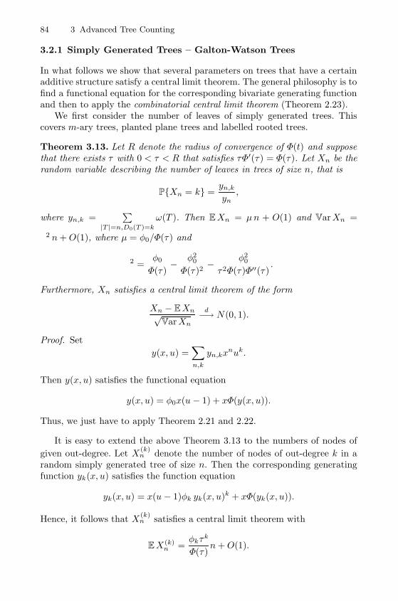
84 3 Advanced Tree Counting
3.2.1 Simply Generated Trees – Galton-Watson Trees
In what follows we show that several parameters on trees that have a certainadditive structure satisfy a central limit theorem. The general philosophy is tofind a functional equation for the corresponding bivariate generating functionand then to apply the combinatorial central limit theorem (Theorem 2.23).
We first consider the number of leaves of simply generated trees. Thiscovers m-ary trees, planted plane trees and labelled rooted trees.
Theorem 3.13. Let R denote the radius of convergence of Φ(t) and supposethat there exists τ with 0 < τ < R that satisfies τΦ′(τ) = Φ(τ). Let Xn be therandom variable describing the number of leaves in trees of size n, that is
P{Xn = k} =yn,k
yn,
where yn,k =∑
|T |=n,D0(T )=k
ω(T ). Then EXn = μn + O(1) and VarXn =
σ2 n+O(1), where μ = φ0/Φ(τ) and
σ2 =φ0
Φ(τ)− φ2
0
Φ(τ)2− φ2
0
τ2Φ(τ)Φ′′(τ).
Furthermore, Xn satisfies a central limit theorem of the form
Xn − EXn√VarXn
d−→ N(0, 1).
Proof. Set
y(x, u) =∑n,k
yn,kxnuk.
Then y(x, u) satisfies the functional equation
y(x, u) = φ0x(u − 1) + xΦ(y(x, u)).
Thus, we just have to apply Theorem 2.21 and 2.22.
It is easy to extend the above Theorem 3.13 to the numbers of nodes of
given out-degree. Let X(k)n denote the number of nodes of out-degree k in a
random simply generated tree of size n. Then the corresponding generatingfunction yk(x, u) satisfies the function equation
yk(x, u) = x(u − 1)φk yk(x, u)k + xΦ(yk(x, u)).
Hence, it follows that X(k)n satisfies a central limit theorem with
EX(k)n =
φkτk
Φ(τ)n+O(1).
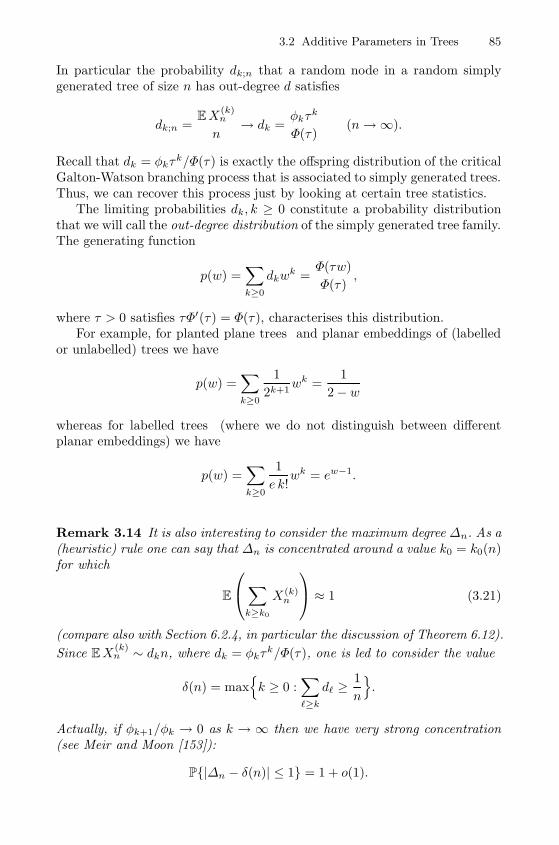
3.2 Additive Parameters in Trees 85
In particular the probability dk;n that a random node in a random simplygenerated tree of size n has out-degree d satisfies
dk;n =EX
(k)n
n→ dk =
φkτk
Φ(τ)(n→∞).
Recall that dk = φkτk/Φ(τ) is exactly the offspring distribution of the critical
Galton-Watson branching process that is associated to simply generated trees.Thus, we can recover this process just by looking at certain tree statistics.
The limiting probabilities dk, k ≥ 0 constitute a probability distributionthat we will call the out-degree distribution of the simply generated tree family.The generating function
p(w) =∑k≥0
dkwk =
Φ(τw)
Φ(τ),
where τ > 0 satisfies τΦ′(τ) = Φ(τ), characterises this distribution.For example, for planted plane trees and planar embeddings of (labelled
or unlabelled) trees we have
p(w) =∑k≥0
1
2k+1wk =
1
2− w
whereas for labelled trees (where we do not distinguish between differentplanar embeddings) we have
p(w) =∑k≥0
1
e k!wk = ew−1.
Remark 3.14 It is also interesting to consider the maximum degree Δn. As a(heuristic) rule one can say that Δn is concentrated around a value k0 = k0(n)for which
E
⎛⎝∑k≥k0
X(k)n
⎞⎠ ≈ 1 (3.21)
(compare also with Section 6.2.4, in particular the discussion of Theorem 6.12).
Since EX(k)n ∼ dkn, where dk = φkτ
k/Φ(τ), one is led to consider the value
δ(n) = max{k ≥ 0 :
∑�≥k
d� ≥1
n
}.
Actually, if φk+1/φk → 0 as k → ∞ then we have very strong concentration(see Meir and Moon [153]):
P{|Δn − δ(n)| ≤ 1} = 1 + o(1).
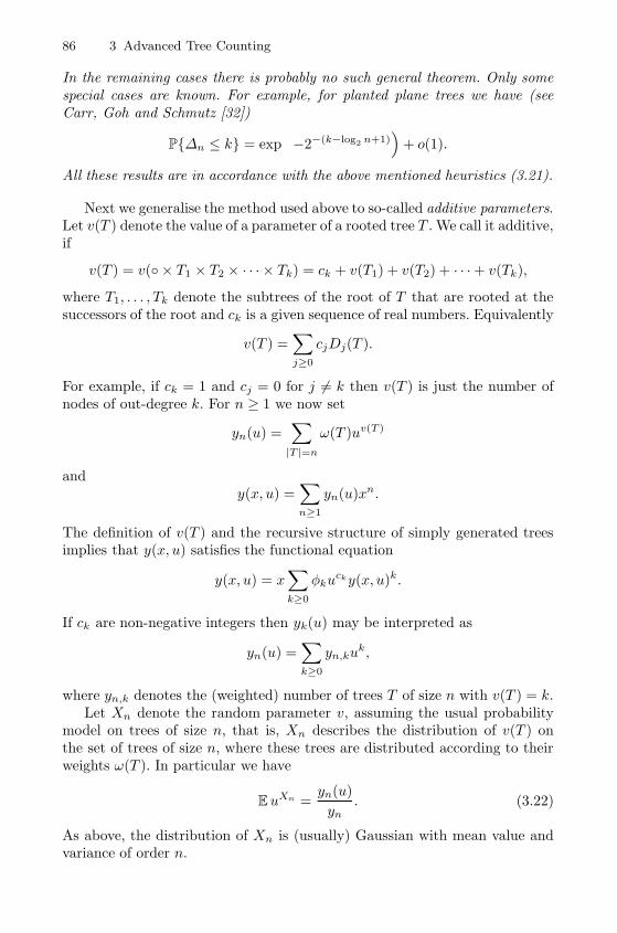
86 3 Advanced Tree Counting
In the remaining cases there is probably no such general theorem. Only somespecial cases are known. For example, for planted plane trees we have (seeCarr, Goh and Schmutz [32])
P{Δn ≤ k} = exp(−2−(k−log2 n+1)
)+ o(1).
All these results are in accordance with the above mentioned heuristics (3.21).
Next we generalise the method used above to so-called additive parameters.Let v(T ) denote the value of a parameter of a rooted tree T . We call it additive,if
v(T ) = v(◦ × T1 × T2 × · · · × Tk) = ck + v(T1) + v(T2) + · · ·+ v(Tk),
where T1, . . . , Tk denote the subtrees of the root of T that are rooted at thesuccessors of the root and ck is a given sequence of real numbers. Equivalently
v(T ) =∑j≥0
cjDj(T ).
For example, if ck = 1 and cj = 0 for j = k then v(T ) is just the number ofnodes of out-degree k. For n ≥ 1 we now set
yn(u) =∑|T |=n
ω(T )uv(T )
andy(x, u) =
∑n≥1
yn(u)xn.
The definition of v(T ) and the recursive structure of simply generated treesimplies that y(x, u) satisfies the functional equation
y(x, u) = x∑k≥0
φkucky(x, u)k.
If ck are non-negative integers then yk(u) may be interpreted as
yn(u) =∑k≥0
yn,kuk,
where yn,k denotes the (weighted) number of trees T of size n with v(T ) = k.Let Xn denote the random parameter v, assuming the usual probability
model on trees of size n, that is, Xn describes the distribution of v(T ) onthe set of trees of size n, where these trees are distributed according to theirweights ω(T ). In particular we have
EuXn =yn(u)
yn. (3.22)
As above, the distribution of Xn is (usually) Gaussian with mean value andvariance of order n.
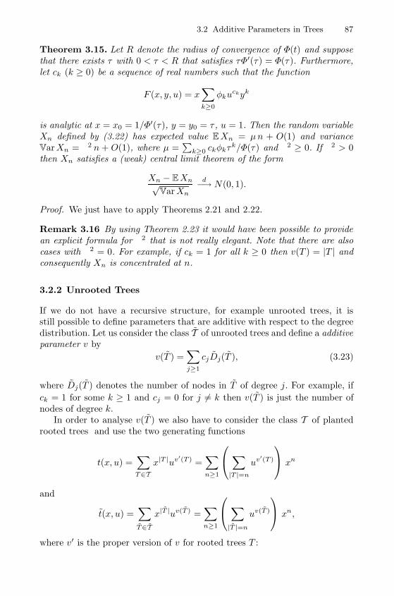
3.2 Additive Parameters in Trees 87
Theorem 3.15. Let R denote the radius of convergence of Φ(t) and supposethat there exists τ with 0 < τ < R that satisfies τΦ′(τ) = Φ(τ). Furthermore,let ck (k ≥ 0) be a sequence of real numbers such that the function
F (x, y, u) = x∑k≥0
φkuckyk
is analytic at x = x0 = 1/Φ′(τ), y = y0 = τ , u = 1. Then the random variableXn defined by (3.22) has expected value EXn = μn + O(1) and varianceVarXn = σ2 n+ O(1), where μ =
∑k≥0 ckφkτ
k/Φ(τ) and σ2 ≥ 0. If σ2 > 0then Xn satisfies a (weak) central limit theorem of the form
Xn − EXn√VarXn
d−→ N(0, 1).
Proof. We just have to apply Theorems 2.21 and 2.22.
Remark 3.16 By using Theorem 2.23 it would have been possible to providean explicit formula for σ2 that is not really elegant. Note that there are alsocases with σ2 = 0. For example, if ck = 1 for all k ≥ 0 then v(T ) = |T | andconsequently Xn is concentrated at n.
3.2.2 Unrooted Trees
If we do not have a recursive structure, for example unrooted trees, it isstill possible to define parameters that are additive with respect to the degreedistribution. Let us consider the class T of unrooted trees and define a additiveparameter v by
v(T ) =∑j≥1
cjDj(T ), (3.23)
where Dj(T ) denotes the number of nodes in T of degree j. For example, if
ck = 1 for some k ≥ 1 and cj = 0 for j = k then v(T ) is just the number ofnodes of degree k.
In order to analyse v(T ) we also have to consider the class T of plantedrooted trees and use the two generating functions
t(x, u) =∑T∈T
x|T |uv′(T ) =∑n≥1
⎛⎝ ∑|T |=n
uv′(T )
⎞⎠ xn
and
t(x, u) =∑T∈T
x|T |uv(T ) =∑n≥1
⎛⎝ ∑|T |=n
uv(T )
⎞⎠ xn,
where v′ is the proper version of v for rooted trees T :
88 3 Advanced Tree Counting
v′(T ) =∑j≥0
cj+1Dj(T ).
Note that both definitions are consistent since the degree of any node in aplanted rooted tree equals the out-degree plus 1 (see Section 1.2.2).
Following the combinatorial constructions of Section 3.1.5 we obtain thefollowing system of functional equations. In order to make the equations moretransparent we include, too, a function r(x, u) that corresponds to rootedtrees, where the degree of the root equals the out-degree.
t(x, u) = x∑k≥0
uck+1PSk(t(x, u), t(x2, u2), . . . , t(xk, uk)), (3.24)
r(x, u) = x+ x∑k≥1
uckPSk(t(x, u), t(x2, u2), . . . , t(xk, uk)), (3.25)
t(x, u) = r(x, u)− 1
2t(x, u)2 +
1
2t(x2, u2). (3.26)
Finally, we introduce the random variable Xn (describing the distribution ofv on trees of size n) in the usual way:
EuXn =1
tn
∑|T |=n
uv(T ). (3.27)
Theorem 3.17. Let (ck)k≥1 be a bounded sequence of real numbers, and letv(T ) and Xn be defined by (3.23) and (3.27). Then there exist μ and σ2 ≥ 0with EXn = μn+O(1) and VarXn = σ2 n+O(1). If σ2 > 0 then Xn satisfiesa (weak) central limit theorem of the form
Xn − EXn√VarXn
d−→ N(0, 1).
Proof. The proof runs as follows. First, we apply Theorem 2.21 to (3.24) whichimplies that t(x, u) has a square root singularity of the kind (2.21). Second,we use this representation and (3.26) to get an expansion for t(x, u) of theform
t(x, u) = g(x, u)− h(x, u)
(1− x
f(u)
)3/2
. (3.28)
Then we apply Theorem 2.25 to obtain a central limit theorem. The last stepis a direct application. So we just have to look at the first two steps.
In order to apply Theorem 2.21 we just have to ensure that the functionst(x2, u2), t(x3, u3), . . . are analytic if x is close to ρ and u is close to 1. Sincethe sequence ck is bounded we have |ck| ≤ M for some M > 0 and thus|v′(T )| ≤M |T |. Hence, if |u| > 1 and |xuM | < ρ then we have
|t(x, u)| ≤∑n≥1
tn|u|Mn|x|n = t(|xuM |, 1).
3.2 Additive Parameters in Trees 89
In particular if |x| ≤ ρ+ η and |u| ≤ (√ρ/(ρ + η))1/M (where η > 0 is small
enough that (√ρ/(ρ+ η))1/M > 1) we get for k ≥ 2
|t(xk, uk)| ≤ t(|xuM |k, 1) ≤ t(ρk/2, 1) ≤ Cρk/2.
Thus, we can apply Theorem 2.21 with
F (x, y, u) = x∑k≥0
uck+1PSk(y, t(x2, u2), . . . , t(xk, uk))
and obtain a representation of the form
t(x, u) = g(x, u)− h(x, u)
√1− x
f(u), (3.29)
where g1 = g(f(u), u) satisfies the relation
g1 = f(u)∑k≥0
uck+1PSk(g1, t(f(u)2, u2), . . . , t(f(u)k, uk)).
Consequently, from (3.26) and (3.29) we obtain a representation for t(x, u) ofthe form
t(x, u) = g2(x, u)− h2(x, u)
√1− x
f(u), (3.30)
where
h2(x, u) = h(x, u)
(x∑k≥1
uck∂
∂x1PSk
(g(x, u), t(x2, u2), . . . , t(xk, uk))
− g(x, u) + (x− f(u))H(x, u)
)in which H(x, u) denotes an analytic function in x and u. Note that
∂
∂x1PSk
(x1, . . . , xk) = PSk−1(x1, . . . , xk−1).
This implies that
h2(f(u), u) = h(f(u), u)f(u)
⎛⎝∑k≥1
uck∂
∂x1PSk
(g1, . . .)−∑k≥0
uck+1PSk(g1, . . .)
⎞⎠= 0.
Hence, h2(x, u) can be represented as
h2(x, u) = h(x, u)
(1− x
f(u)
).
This implies (3.28) and completes the proof of Theorem 3.17.
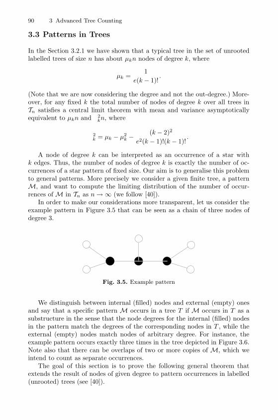
90 3 Advanced Tree Counting
3.3 Patterns in Trees
In the Section 3.2.1 we have shown that a typical tree in the set of unrootedlabelled trees of size n has about μkn nodes of degree k, where
μk =1
e(k − 1)!.
(Note that we are now considering the degree and not the out-degree.) More-over, for any fixed k the total number of nodes of degree k over all trees inTn satisfies a central limit theorem with mean and variance asymptoticallyequivalent to μkn and σ2
kn, where
σ2k = μk − μ2
k −(k − 2)2
e2(k − 1)!(k − 1)!.
A node of degree k can be interpreted as an occurrence of a star withk edges. Thus, the number of nodes of degree k is exactly the number of oc-currences of a star pattern of fixed size. Our aim is to generalise this problemto general patterns. More precisely we consider a given finite tree, a patternM, and want to compute the limiting distribution of the number of occur-rences of M in Tn as n→∞ (we follow [40]).
In order to make our considerations more transparent, let us consider theexample pattern in Figure 3.5 that can be seen as a chain of three nodes ofdegree 3.
Fig. 3.5. Example pattern
We distinguish between internal (filled) nodes and external (empty) onesand say that a specific pattern M occurs in a tree T if M occurs in T as asubstructure in the sense that the node degrees for the internal (filled) nodesin the pattern match the degrees of the corresponding nodes in T , while theexternal (empty) nodes match nodes of arbitrary degree. For instance, theexample pattern occurs exactly three times in the tree depicted in Figure 3.6.Note also that there can be overlaps of two or more copies of M, which weintend to count as separate occurrences.
The goal of this section is to prove the following general theorem thatextends the result of nodes of given degree to pattern occurrences in labelled(unrooted) trees (see [40]).
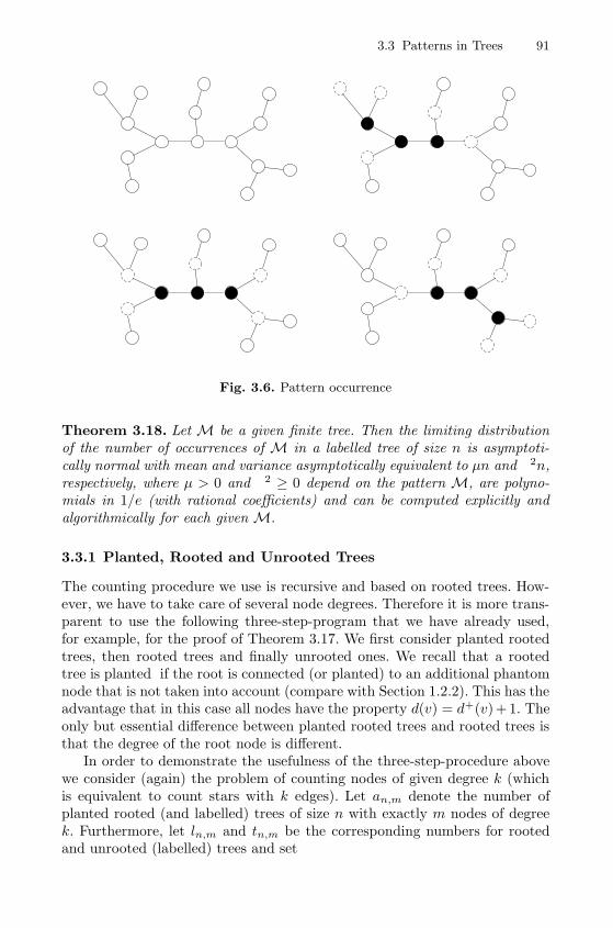
3.3 Patterns in Trees 91
Fig. 3.6. Pattern occurrence
Theorem 3.18. Let M be a given finite tree. Then the limiting distributionof the number of occurrences of M in a labelled tree of size n is asymptoti-cally normal with mean and variance asymptotically equivalent to μn and σ2n,respectively, where μ > 0 and σ2 ≥ 0 depend on the pattern M, are polyno-mials in 1/e (with rational coefficients) and can be computed explicitly andalgorithmically for each given M.
3.3.1 Planted, Rooted and Unrooted Trees
The counting procedure we use is recursive and based on rooted trees. How-ever, we have to take care of several node degrees. Therefore it is more trans-parent to use the following three-step-program that we have already used,for example, for the proof of Theorem 3.17. We first consider planted rootedtrees, then rooted trees and finally unrooted ones. We recall that a rootedtree is planted if the root is connected (or planted) to an additional phantomnode that is not taken into account (compare with Section 1.2.2). This has theadvantage that in this case all nodes have the property d(v) = d+(v) + 1. Theonly but essential difference between planted rooted trees and rooted trees isthat the degree of the root node is different.
In order to demonstrate the usefulness of the three-step-procedure abovewe consider (again) the problem of counting nodes of given degree k (whichis equivalent to count stars with k edges). Let an,m denote the number ofplanted rooted (and labelled) trees of size n with exactly m nodes of degreek. Furthermore, let ln,m and tn,m be the corresponding numbers for rootedand unrooted (labelled) trees and set
92 3 Advanced Tree Counting
a(x, u) =∞∑
n,m=0
an,mxnum
n!, l(x, u) =
∞∑n,m=0
ln,mxnum
n!, and
t(x, u) =
∞∑n,m=0
tn,mxnum
n!.
Then we have (compare also with (3.24)–(3.26)):
1. Planted Rooted Trees:
a(x, u) =
∞∑n=0
n�=k−1
xa(x, u)n
n!+xu a(x, u)k−1
(k − 1)!= xea(x,u)+
x(u− 1)a(x, u)k−1
(k − 1)!.
2. Rooted Trees:
l(x, u) =
∞∑n=0n�=k
xa(x, u)n
n!+xu a(x, u)k
k!= xea(x,u) +
x(u− 1)a(x, u)k
k!.
3. Unrooted Trees: Since we are considering labelled trees, we simply havetn,m = ln,m/n. Thus, the statistics on the number of nodes of degree kare precisely the same. However, it is also possible to express t(x, u) by
t(x, u) = l(x, u)− 1
2a(x, u)2.
This follows from a natural bijection between rooted trees on the one handand unrooted trees and pairs of planted rooted trees (that are joined byidentifying the additional edges at their planted roots and discarding thephantom nodes) on the other hand.1
We now generalise the counting procedure of Section 3.3.1 to more com-plicated patterns. For our purpose, a pattern is a given (finite unrooted unla-belled) tree M. For M we will use the example graph in Figure 3.5 in orderto make the arguments more transparent.
3.3.2 Generating Functions for Planted Rooted Trees
Let an,m denote the number of planted rooted (and labelled) trees withn nodes and exactly m occurrences of the pattern M, where the additional(phantom) node is taken into account in the matching procedure. Further-more, let
1 Consider the class of rooted (labelled) trees. If the root is labelled by 1 thenconsider the tree as an unrooted tree. If the root is not labelled by 1 then considerthe first edge of the path between the root and 1 and cut the tree into two plantedrooted trees at this edge.
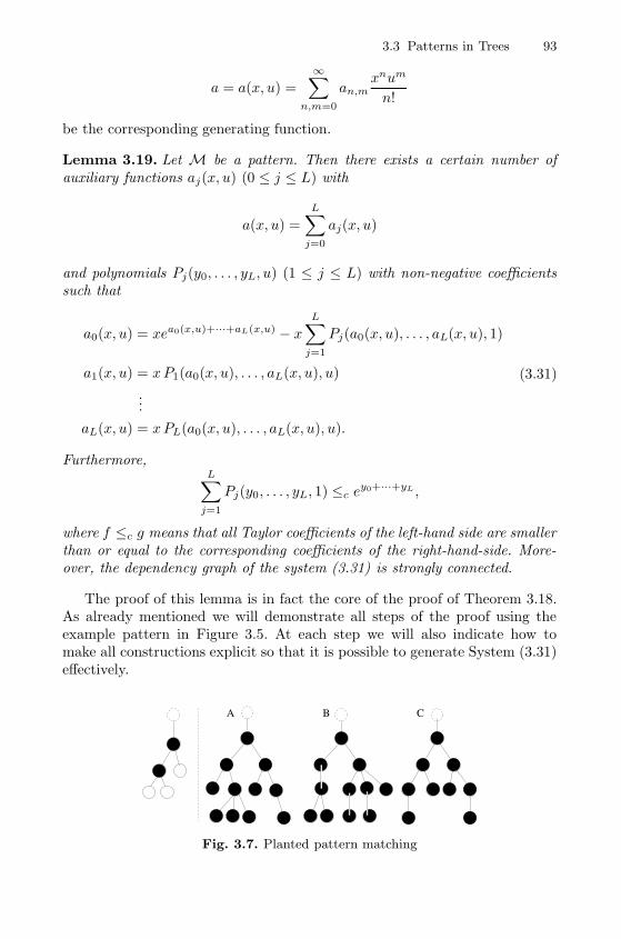
3.3 Patterns in Trees 93
a = a(x, u) =∞∑
n,m=0
an,mxnum
n!
be the corresponding generating function.
Lemma 3.19. Let M be a pattern. Then there exists a certain number ofauxiliary functions aj(x, u) (0 ≤ j ≤ L) with
a(x, u) =
L∑j=0
aj(x, u)
and polynomials Pj(y0, . . . , yL, u) (1 ≤ j ≤ L) with non-negative coefficientssuch that
a0(x, u) = xea0(x,u)+···+aL(x,u) − xL∑
j=1
Pj(a0(x, u), . . . , aL(x, u), 1)
a1(x, u) = xP1(a0(x, u), . . . , aL(x, u), u)
...
aL(x, u) = xPL(a0(x, u), . . . , aL(x, u), u).
(3.31)
Furthermore,L∑
j=1
Pj(y0, . . . , yL, 1) ≤c ey0+···+yL ,
where f ≤c g means that all Taylor coefficients of the left-hand side are smallerthan or equal to the corresponding coefficients of the right-hand-side. More-over, the dependency graph of the system (3.31) is strongly connected.
The proof of this lemma is in fact the core of the proof of Theorem 3.18.As already mentioned we will demonstrate all steps of the proof using theexample pattern in Figure 3.5. At each step we will also indicate how tomake all constructions explicit so that it is possible to generate System (3.31)effectively.
A B C
Fig. 3.7. Planted pattern matching
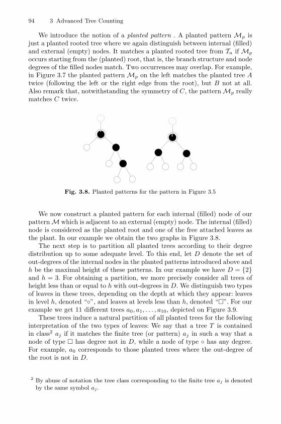
94 3 Advanced Tree Counting
We introduce the notion of a planted pattern . A planted pattern Mp isjust a planted rooted tree where we again distinguish between internal (filled)and external (empty) nodes. It matches a planted rooted tree from Tn if Mp
occurs starting from the (planted) root, that is, the branch structure and nodedegrees of the filled nodes match. Two occurrences may overlap. For example,in Figure 3.7 the planted pattern Mp on the left matches the planted tree Atwice (following the left or the right edge from the root), but B not at all.Also remark that, notwithstanding the symmetry of C, the pattern Mp reallymatches C twice.
Fig. 3.8. Planted patterns for the pattern in Figure 3.5
We now construct a planted pattern for each internal (filled) node of ourpatternM which is adjacent to an external (empty) node. The internal (filled)node is considered as the planted root and one of the free attached leaves asthe plant. In our example we obtain the two graphs in Figure 3.8.
The next step is to partition all planted trees according to their degreedistribution up to some adequate level. To this end, let D denote the set ofout-degrees of the internal nodes in the planted patterns introduced above andh be the maximal height of these patterns. In our example we have D = {2}and h = 3. For obtaining a partition, we more precisely consider all trees ofheight less than or equal to h with out-degrees in D. We distinguish two typesof leaves in these trees, depending on the depth at which they appear: leavesin level h, denoted “◦”, and leaves at levels less than h, denoted “�”. For ourexample we get 11 different trees a0, a1, . . . , a10, depicted on Figure 3.9.
These trees induce a natural partition of all planted trees for the followinginterpretation of the two types of leaves: We say that a tree T is containedin class2 aj if it matches the finite tree (or pattern) aj in such a way that anode of type � has degree not in D, while a node of type ◦ has any degree.For example, a0 corresponds to those planted trees where the out-degree ofthe root is not in D.
2 By abuse of notation the tree class corresponding to the finite tree aj is denotedby the same symbol aj .
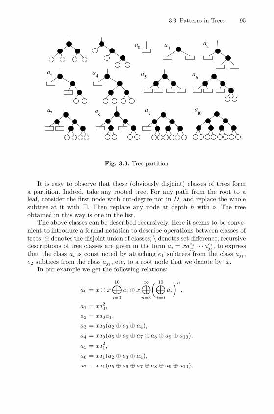
3.3 Patterns in Trees 95
a a
a
a
aa
a
a a a a7
65
0
43
21
98 10
Fig. 3.9. Tree partition
It is easy to observe that these (obviously disjoint) classes of trees forma partition. Indeed, take any rooted tree. For any path from the root to aleaf, consider the first node with out-degree not in D, and replace the wholesubtree at it with �. Then replace any node at depth h with ◦. The treeobtained in this way is one in the list.
The above classes can be described recursively. Here it seems to be conve-nient to introduce a formal notation to describe operations between classes oftrees: ⊕ denotes the disjoint union of classes; \ denotes set difference; recursivedescriptions of tree classes are given in the form ai = xae1
j1· · ·ae�
j�, to express
that the class ai is constructed by attaching e1 subtrees from the class aj1 ,e2 subtrees from the class aj2 , etc, to a root node that we denote by x.
In our example we get the following relations:
a0 = x⊕ x10⊕
i=0
ai ⊕ x∞⊕
n=3
( 10⊕i=0
ai
)n
,
a1 = xa20,
a2 = xa0a1,
a3 = xa0(a2 ⊕ a3 ⊕ a4),
a4 = xa0(a5 ⊕ a6 ⊕ a7 ⊕ a8 ⊕ a9 ⊕ a10),
a5 = xa21,
a6 = xa1(a2 ⊕ a3 ⊕ a4),
a7 = xa1(a5 ⊕ a6 ⊕ a7 ⊕ a8 ⊕ a9 ⊕ a10),
96 3 Advanced Tree Counting
a8 = x(a2 ⊕ a3 ⊕ a4)2,
a9 = x(a2 ⊕ a3 ⊕ a4)(a5 ⊕ a6 ⊕ a7 ⊕ a8 ⊕ a9 ⊕ a10),
a10 = x(a5 ⊕ a6 ⊕ a7 ⊕ a8 ⊕ a9 ⊕ a10)2.
This is to be interpreted as follows. First, trees in a0 consist of a (planted)root that is denoted by x and has out-degree j which is not contained inD = {2}. The successors of the root are arbitrary trees. Next, trees in a1
consist of a root that has out-degree 2, and two successors that are of out-degree distinct from 2, that is, in a0. Similarly, trees in a3 consist of a root xwith out-degree 2 and subject to the following additional constraints: onesubtree at the root is exactly of type a0; the other subtree, call it T , is ofout-degree 2, either with both subtrees of degree other than 2 (leading toT in a2), or with one subtree of degree 2 and the other of degree other than 2(leading to T in a3), or with both of its subtrees of degree 2 (leading to T inclass a4). Summarising: a3 = xa0(a2 ⊕ a3 ⊕ a4). Of course this can also beinterpreted as a3 = xa0a2 ⊕ xa0a3 ⊕ xa0a4. Another more involved examplecorresponds to a8; here both subtrees are of the form a2 ⊕ a3 ⊕ a4.
To show that the recursive description can be obtained in general, considera tree aj obtained from some planted pattern Mp. Let s1, . . . , sd denote itssubtrees at the root. Then, in each si, leaves of type ◦ can appear only atlevel h − 1. Substitute for all such ◦ either � or a node of out-degree chosenfrom D and having ◦ for all its subtrees. Do this substitution in all possibleways. The collection of trees obtained are some of the ak’s, say a
k(j)1
, ak(j)2
, etc.
Thus, we obtain the recursive relation aj = x(ak(1)1⊕ a
k(1)2⊕ · · · ) · · · (a
k(d)1⊕
ak(d)2⊕ · · · ) for aj .
In general, we obtain a partition of L + 1 classes a0, . . . , aL and corre-sponding recursive descriptions, where each tree type aj can be expressed asa disjoint union of tree classes of the kind
xaj1 · · ·ajr = xal00 · · ·alL
L , (3.32)
where r denotes the degree of the root of aj and the non-negative integer liis the number of repetitions of the tree type ai.
We proceed to show that this directly leads to a system of equations of theform (3.31), where each polynomial relation stems from a recursive equationbetween combinatorial classes.
Let Λj be the set of tuples (l0, . . . , lL) with the property that (l0, . . . , lL) ∈Λj , if and only if the term of type (3.32) is involved in the recursive descriptionof aj (in expanded form). Further, let k = K(l0, . . . , lL) denote the numberof additional occurrences of the pattern M in (3.32) in the following sense: ifb = xaj1 · · · ajr and T is a labelled tree of b with subtrees T1 ∈ aj1 , T2 ∈ aj2 ,etc, and M occurs m1 times in T1, m2 times in T2, etc, then T contains Mexactlym1+m2+· · ·+md+k times. The number k corresponds to the numberof occurrences of M in T in which the root of T occurs as internal node ofthe pattern. By construction of the classes ai this number only depends on
3.3 Patterns in Trees 97
b and not on the particular tree T ∈ b. Let us clarify the calculation of k =K(l0, . . . , lL) with an example. Consider the class a9 of the partition for theexample pattern. Now we have to match the planted patterns of Figure 3.8 atthe root of an arbitrary tree of class a9. The left planted pattern of Figure 3.8matches three times, the right one matches once. Thus we find that in this casek = 4. For the other classes we find the following values of k = K(l0, . . . , lL):
Terms of class a0 a1 a2 a3 a4 a5 a6 a7 a8 a9 a10Value of k 0 0 0 1 2 1 2 3 3 4 5
.
Now define series Pj by
Pj(y0, . . . , yL, u) =∑
(l0,...,lL)∈Λj
1
l0! · · · lL!yl00 · · · ylL
L uK(l0,...,lL).
These are in fact polynomials for 1 ≤ j ≤ L by the finiteness of the cor-responding Λj . All matches of the planted patterns are handled in the Pj ,1 ≤ j ≤ L, thus
P0(y0, . . . , yL, u) = ey0+···+yL −L∑
j=1
Pj(y0, . . . , yL, 1)
does not depend on u.In our pattern we get for example
P8(y0, . . . , y10, u) =1
2xy22u
3 + xy2y3u3 + xy2y4u
3 +1
2xy23u
3 + xy3y4u3 +
1
2xy24u
3
=1
2x(y2 + y3 + y4)2u3.
Finally, let aj;n,m denote the number of planted rooted trees of type aj withn nodes and m occurrences of the pattern M and set
aj(x, u) =
∞∑n,m=0
aj;n,mxnum
n!.
By this definition it is clear that
aj(x, u) = x · Pj
(a0(x, u), . . . , aL(x, u), u
),
because the number of labelled trees is counted by x (exponential generatingfunction) and the number of patterns is additive and counted by u. Hence, weexplicitly obtain the proposed structure of the system of functional equations(3.31).
Concerning the example pattern we reach the following system of equa-tions, where we denote the generating function of the class ai by the samesymbol ai:
98 3 Advanced Tree Counting
a0 = a0(x, u) = x+ x10∑
i=0
ai + x∞∑
n=3
1
n!
(10∑
i=0
ai
)n
,
a1 = a1(x, u) =1
2xa20,
a2 = a2(x, u) = xa0a1,
a3 = a3(x, u) = xa0(a2 + a3 + a4)u,
a4 = a4(x, u) = xa0(a5 + a6 + a7 + a8 + a9 + a10)u2,
a5 = a5(x, u) =1
2xa21u,
a6 = a6(x, u) = xa1(a2 + a3 + a4)u2,
a7 = a7(x, u) = xa1(a5 + a6 + a7 + a8 + a9 + a10)u3,
a8 = a8(x, u) =1
2x(a2 + a3 + a4)2u3,
a9 = a9(x, u) = x(a2 + a3 + a4)(a5 + a6 + a7 + a8 + a9 + a10)u4,
a10 = a10(x, u) =1
2x(a5 + a6 + a7 + a8 + a9 + a10)2u5.
In order to complete the proof of Lemma 3.19 we just have to show thatthe dependency graph is strongly connected. By construction, a0 = a0(x, u)depends on all functions ai = ai(x, u). Thus, it is sufficient to prove thatevery ai (1 ≤ i ≤ L) eventually depends on a0 in the sense that there existsa sequence of indices i1, i2, . . . , ir such that ai = xPi(a0, . . . , aK) directlydepends on ai1 , ai1 directly depends on ai2 etc, and finally air directly dependson a0. For this purpose consider the subtree of M that was labelled by ai
and consider a path from its root to an empty node. Each edge of this pathcorresponds to another subtree of M corresponding to ai1 , ai2 , . . . , air . Then,by construction of the system of functional equations above, ai depends onai1 , ai1 depends on ai2 , etc. Finally the root of air is adjacent to an emptynode and thus (the corresponding generating function) depends on a0. Thiscompletes the proof of Lemma 3.19.
Note that we obtain a relatively more compact form of this system byintroducing
b0 = b0(x, u) = a0(x, u)
b1 = b1(x, u) = a1(x, u) (3.33)
b2 = b2(x, u) = a2(x, u) + a3(x, u) + a4(x, u)
b3 = b3(x, u) = a5(x, u) + a6(x, u) + a7(x, u) + a8(x, u) + a9(x, u) + a10(x, u),
together with the recursive relations
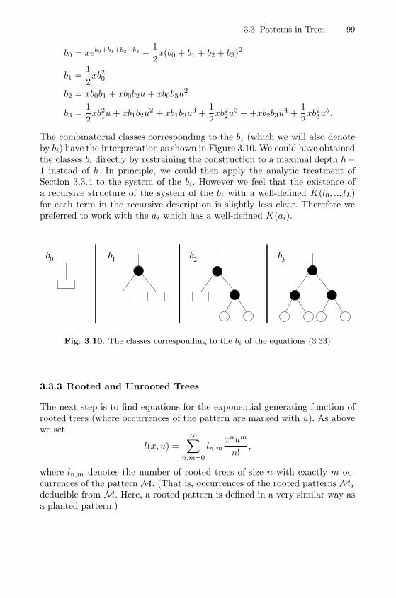
3.3 Patterns in Trees 99
b0 = xeb0+b1+b2+b3 − 1
2x(b0 + b1 + b2 + b3)2
b1 =1
2xb20
b2 = xb0b1 + xb0b2u+ xb0b3u2
b3 =1
2xb21u+ xb1b2u
2 + xb1b3u3 +
1
2xb22u
3 + +xb2b3u4 +
1
2xb23u
5.
The combinatorial classes corresponding to the bi (which we will also denoteby bi) have the interpretation as shown in Figure 3.10. We could have obtainedthe classes bi directly by restraining the construction to a maximal depth h−1 instead of h. In principle, we could then apply the analytic treatment ofSection 3.3.4 to the system of the bi. However we feel that the existence ofa recursive structure of the system of the bi with a well-defined K(l0, .., lL)for each term in the recursive description is slightly less clear. Therefore wepreferred to work with the ai which has a well-defined K(ai).
b b b b0 1 2 3
Fig. 3.10. The classes corresponding to the bi of the equations (3.33)
3.3.3 Rooted and Unrooted Trees
The next step is to find equations for the exponential generating function ofrooted trees (where occurrences of the pattern are marked with u). As abovewe set
l(x, u) =
∞∑n,m=0
ln,mxnum
n!,
where ln,m denotes the number of rooted trees of size n with exactly m oc-currences of the pattern M. (That is, occurrences of the rooted patterns Mr
deducible from M. Here, a rooted pattern is defined in a very similar way asa planted pattern.)
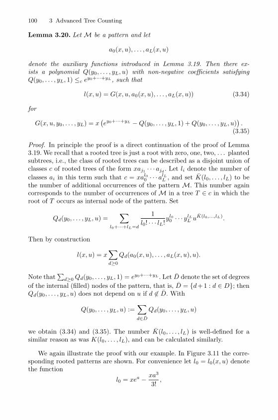
100 3 Advanced Tree Counting
Lemma 3.20. Let M be a pattern and let
a0(x, u), . . . , aL(x, u)
denote the auxiliary functions introduced in Lemma 3.19. Then there ex-ists a polynomial Q(y0, . . . , yL, u) with non-negative coefficients satisfyingQ(y0, . . . , yL, 1) ≤c e
y0+···+yL, such that
l(x, u) = G(x, u, a0(x, u), . . . , aL(x, u)) (3.34)
for
G(x, u, y0, . . . , yL) = x(ey0+···+yL −Q(y0, . . . , yL, 1) +Q(y0, . . . , yL, u)
).
(3.35)
Proof. In principle the proof is a direct continuation of the proof of Lemma3.19. We recall that a rooted tree is just a root with zero, one, two, . . . plantedsubtrees, i.e., the class of rooted trees can be described as a disjoint union ofclasses c of rooted trees of the form xaj1 · · · ajd
. Let li denote the number of
classes ai in this term such that c = xal00 · · · alL
L , and set K(l0, . . . , lL) to bethe number of additional occurrences of the pattern M. This number againcorresponds to the number of occurrences of M in a tree T ∈ c in which theroot of T occurs as internal node of the pattern. Set
Qd(y0, . . . , yL, u) =∑
l0+···+lL=d
1
l0! · · · lL!yl00 · · · ylL
L uK(l0,...,lL).
Then by construction
l(x, u) = x∑d≥0
Qd(a0(x, u), . . . , aL(x, u), u).
Note that∑
d≥0Qd(y0, . . . , yL, 1) = ey0+···+yL . Let D denote the set of degrees
of the internal (filled) nodes of the pattern, that is, D = {d+ 1 : d ∈ D}; thenQd(y0, . . . , yL, u) does not depend on u if d ∈ D. With
Q(y0, . . . , yL, u) :=∑d∈D
Qd(y0, . . . , yL, u)
we obtain (3.34) and (3.35). The number K(l0, . . . , lL) is well-defined for asimilar reason as was K(l0, . . . , lL), and can be calculated similarly.
We again illustrate the proof with our example. In Figure 3.11 the corre-sponding rooted patterns are shown. For convenience let l0 = l0(x, u) denotethe function
l0 = xea − xa3
3!,
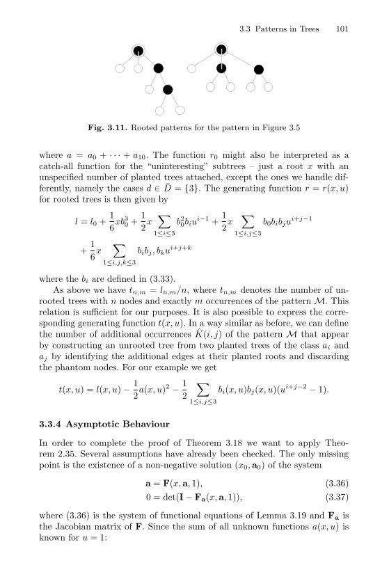
3.3 Patterns in Trees 101
Fig. 3.11. Rooted patterns for the pattern in Figure 3.5
where a = a0 + · · · + a10. The function r0 might also be interpreted as acatch-all function for the “uninteresting” subtrees – just a root x with anunspecified number of planted trees attached, except the ones we handle dif-ferently, namely the cases d ∈ D = {3}. The generating function r = r(x, u)for rooted trees is then given by
l = l0 +1
6xb30 +
1
2x∑
1≤i≤3
b20biui−1 +
1
2x∑
1≤i,j≤3
b0bibjui+j−1
+1
6x∑
1≤i,j,k≤3
bibj , bkui+j+k
where the bi are defined in (3.33).As above we have tn,m = ln,m/n, where tn,m denotes the number of un-
rooted trees with n nodes and exactly m occurrences of the pattern M. Thisrelation is sufficient for our purposes. It is also possible to express the corre-sponding generating function t(x, u). In a way similar as before, we can definethe number of additional occurrences K(i, j) of the pattern M that appearby constructing an unrooted tree from two planted trees of the class ai andaj by identifying the additional edges at their planted roots and discardingthe phantom nodes. For our example we get
t(x, u) = l(x, u)− 1
2a(x, u)2 − 1
2
∑1≤i,j≤3
bi(x, u)bj(x, u)(ui+j−2 − 1).
3.3.4 Asymptotic Behaviour
In order to complete the proof of Theorem 3.18 we want to apply Theo-rem 2.35. Several assumptions have already been checked. The only missingpoint is the existence of a non-negative solution (x0, a0) of the system
a = F(x,a, 1), (3.36)
0 = det(I− Fa(x,a, 1)), (3.37)
where (3.36) is the system of functional equations of Lemma 3.19 and Fa isthe Jacobian matrix of F. Since the sum of all unknown functions a(x, u) isknown for u = 1:
102 3 Advanced Tree Counting
a(x, 1) = a(x) =∑n≥1
nn−1xn
n!= 1−
√2√
1− ex+ · · · ,
it is not unexpected that x0 = 1/e.
Lemma 3.21. There exists a unique non-negative solution (x0, a0) of Sys-tem (3.36)–(3.37), x0 = 1/e and the components of a0 are polynomials (withrational coefficients) in 1/e.
Proof. For a proof, set u = 1 and consider the solution a(x, 1) = (a0(x, 1), . . . ,aL−1(x, 1)). Since the dependency graph is strongly connected, it follows thatall functions aj(x, 1) have the same radius of convergence which has to be x0 =1/e, and all functions are singular at x = x0. Since 0 ≤ aj(x, 1) ≤ p(x, 1) <∞for 0 ≤ x ≤ x0, it also follows that aj(x0, 1) is finite, and we have a(x0, 1) =F(x0, a(x0, 1), 1). If we had the inequality det(I − Fa(x0, a(x0, 1), 1)) = 0then the implicit function theorem would imply the existence of an analyticcontinuation for aj(x, 1) around x = x0, which is, of course, a contradiction.Thus, the system above has a unique solution.
To see that the components a0, . . . aL (with ai = ai(1/e, 1)) of a0 arepolynomials in 1/e we will construct the partition A = {a0, a1, . . . , aL} onwhich the system of equations (3.36)–(3.37) is based by refining the trivialpartition consisting of only one class p step by step. The recursive descriptionof this trivial partition is given by the formal equation p = x
∑i≥0 p
i andthe solution of the corresponding equation p = x exp(p) for the generatingfunction p (denoted by the same symbol p) is given by (x0, p) = (1/e, 1), withp clearly a (constant) polynomial in 1/e. Now let D = {d1, . . . , ds} (s ∈ N)again denote the set of out-degrees that occur in the planted patterns. Wewill refine p by introducing for each di ∈ D a class ai consisting of all treesof root out-degree di together with the class a0 of trees with root out-degreenot in D. The partition {a0, a1, . . . , as} has the recursive description
a0 = x∑
j∈N\D(a0 ⊕ a1 ⊕ · · · ⊕ as)j
ai = x(a0 ⊕ a1 ⊕ · · · ⊕ as)di (i = 1, . . . , s) (3.38)
and the solution of the corresponding system of equations is given by
x0 =1
e,
ai =1
di!e(i = 1, . . . , s), (3.39)
a0 = 1− (a1 + · · ·+ as),
thus again polynomials in 1/e. We continue by refining this last partition byintroducing classes c1, . . . , cu (u ∈ N) for each term at the right hand side of
(3.38) after expanding. Such a class cj is of the form cj = xal(j)00 a
l(j)11 · · ·al(j)s
s
3.3 Patterns in Trees 103
with natural numbers l(j)i , i = 0, . . . , s. We get a new partition {a0, c1, . . . , cu}
which has a recursive description by construction (because we can replace theai by disjoint unions of certain cj). The solution of the corresponding systemof equations for the generating functions is given by
x0 =1
e,
cj =1
e
1
l(j)0 !l
(j)1 ! · · · l(j)s !
al(j)00 a
l(j)11 · · · al(j)s
s (j = 1, . . . , u),
a0 = 1− (a1 + · · ·+ as)
with the ai of (3.39). Thus the cj are again polynomials in 1/e. By continuingthis procedure until level h (i.e. performing the refinement step h times) weend up with the partition A and we see that the solution for the correspondingsystem of equations consists of polynomials in 1/e, which ends the proof ofLemma 3.21.
Note that there is a close link to Galton-Watson branching processes. Letpk = 1
k!e denote the offspring distribution. Now we interpret a class ai as theclass of branching processes for which the (non-plane) branching structureat the start of the process is the same as the tree structure at the root ofthe trees in ai. By arguments of probabilistic independence it follows thatthe solution ai, i = 0, . . . , L from the system of equations (3.36) correspondsto the probabilities qi, i = 0, . . . , L that a branching process is in the classai, i = 0, . . . , L. To see this, let the equation of class ai be given by
ai = x1
l0! . . . lL!al00 · · ·alL
L =x
n!
n!
l0! . . . lL!al00 · · · alL
L , (n = l0 + · · ·+ lL).
Now the probability that a branching process is in class ai is the probabilityx0
n! = 1en! that the first node has degree n, and that li of the branching processes
starting at the children of this first node are in the class ai (0 ≤ i ≤ L). Thisyields a factor al0
0 · · ·alLL . Since the left-to-right-order of this child-processes is
not relevant, we also get a factor n!l0!...lL! to discount different embeddings into
the plane. However we can also calculate the qi by elementary probabilisticconsiderations. Therefore we consider the probabilities pd1, . . . , pds of the out-degrees d1, . . . , ds of the pattern nodes and r = 1−pd1−· · ·−pds for the otherout-degrees. Now we get the probabilities qi(= ai) by multiplication of the pdk
and r corresponding to the branching degrees of the processes in each class ai
and discounting different embeddings into the plane by some multiplicativefactors which follow from symmetry considerations. So again we see that a0
consists of polynomials in 1/e.
Consequently, it follows from Theorem 2.35 that the numbers ln,m have aGaussian limiting distribution with mean and variance which are proportionalto n. Since tn,m = ln,m/n, we get exactly the same rule for unrooted trees.
104 3 Advanced Tree Counting
We now solve the system of equations (3.36)–(3.37) for the example pat-tern, where we apply the relation to Galton-Watson processes as describedabove. Recall that x0 = 1/e. We only have to consider the probabilitiesp = 1/(2e) for nodes with out-degree 2 and q = 1 − 1/(2e) for the othernodes. For example we get a4 = a4(1/e, 1) = 2qp3 = 2e−1
16e5 . The factor 2 comesfrom the fact that the two subtrees of the root may be exchanged (see Figure3.9). The other classes can be treated similarly and we find:
a(1/e, 1) = 1, a5(1/e, 1) = (2e− 1)4/(128e7),
a0(1/e, 1) = (2e− 1)/(2e) a6(1/e, 1) = (2e− 1)3/(32e7),
a1(1/e, 1) = (2e− 1)2/(8e3) a7(1/e, 1) = (2e− 1)2/(64e7),
a2(1/e, 1) = (2e− 1)3/(16e5) a8(1/e, 1) = (2e− 1)2/(32e7),
a3(1/e, 1) = (2e− 1)2/(8e5) a9(1/e, 1) = (2e− 1)/(32e7),
a4(1/e, 1) = (2e− 1)/(16e5) a10(1/e, 1) = 1/(128e7).
(3.40)
We now give a formula for the mean value μ.
Lemma 3.22. Let x0 = 1/e and a0 be given by Lemma 3.21 and let Pj(y, u)(1 ≤ j ≤ L) be the polynomials of Lemma 3.19, with y = (y0, . . . , yL). Then μ(of Theorem 3.18) is a polynomial in 1/e with rational coefficients and givenby
μ =1
e
L∑j=1
∂Pj
∂u(a0, 1). (3.41)
Proof. Let a = F(x,a, u) be the system of functional equations of Lemma 3.19.We recall that (2.56) provides a formula for the mean constant:
μ =1
x0
bTFu(x0, a0, 1)
bTFx(x0, a0, 1). (3.42)
Here bT denotes a positive left eigenvector of I− Fa, which is unique up toscaling.
Since
F(x,a, u) =
⎛⎜⎜⎜⎜⎜⎜⎝x(ea0+···+aL −∑L
j=1 Pj(a, 1))
xP1(a, u)xP2(a, u)
...xPL(a, u)
⎞⎟⎟⎟⎟⎟⎟⎠ ,
we get, after denoting ∂Pi
∂ajwith Pi,aj ,
Fa = x
⎛⎜⎜⎜⎝ea0+···+aL −
∑Lj=1 Pj,a0 · · · ea0+···+aL −
∑Lj=1 Pj,aL
P1,a0 · · · P1,aL
......
PL,a0 · · · PL,aL
⎞⎟⎟⎟⎠ .
3.3 Patterns in Trees 105
Since a0(x0, 1)+· · ·+aL(x0, 1) = a(x0, 1) = 1, we have x0ea0(x0,1)+···aL(x0,1) =
1. Consequently the sum of all rows of Fa equals (1, 1, . . . , 1) for x = x0 = 1/e.Thus, denoting the transpose of a vector v by vT, the vector bT = (1, 1, . . . , 1)is the unique positive left eigenvector of I− Fa, up to scaling.
It is now easy to check that
x0bTFx(x0, a0, 1) =
1
eea0(x0,1)+···aL(x0,1) = 1
and that
bTFu(x0, a0, 1) =1
e
L∑j=1
Pj,u(a0, 1).
The fact that μ is a polynomial in 1/e is now a direct consequence fromthe observation that a0 consists of polynomials in 1/e, and the fact that thecoefficients are rational follows from the property that F(x,a, u) has rationalcoefficients.
This completes the proof of Theorem 3.18. We point out here that it is alsopossible to prove that the constant σ2 can be represented as a polynomial in1/e with rational coefficients. However, the proof is very involved (see [40]).

4
The Shape of Galton-Watson Trees and Polya
Trees
Galton-Watson trees or simply generated trees are random trees that areobtained by Galton-Watson branching processes conditioned on the totalprogeny.1 This is in fact a very natural and general concept of random treesthat includes several kinds of combinatorial tree models like binary trees,planted plane trees, labelled rooted trees, etc. (compare with Section 1.2.7).
One important point is that Galton-Watson trees have a continuous lim-iting object, the so-called continuum random tree, by scaling the distances tothe root by 1/
√n. This concept has been introduced by Aldous [2, 3, 4] and
further developed by Duquesne and Le Gall [72, 73, 74].First we present an introduction to these limiting objects (for more details
we refer to the recent surveys by Le Gall [135, 136]).The main focus of this chapter is to characterise the so-called profile of
Galton-Watson trees, that is, the number of nodes of given distance to theroot. It is a very natural measure of the shape of a tree. Interestingly, theprofile process can be approximated by the total local time of a Brownianexcursion of duration 1. Since the profile is not a continuous functional ofa random tree (more precisely of its depth-first search process), its limitingbehaviour cannot be deduced from the structure of the continuum randomtree.
The approach that we present here – that is based on combinatorics withthe help of generating functions – is probably not the most elegant one, sinceit is quite technical. However, it can be generalised to unlabelled rooted trees(Polya trees) that cannot be represented as conditioned Galton-Watson trees.
We also comment on the height of conditioned Galton-Watson trees andPolya trees that are of order
√n.
1 The notion Galton-Watson tree (or more precisely, conditioned Galton-Watsontree) has become standard in the literature. Therefore we restrict ourselves to thisnotion throughout this chapter and do not use the equivalent notion of simplygenerated trees.
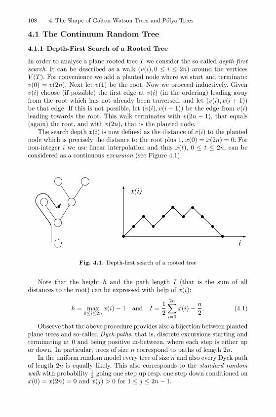
108 4 The Shape of Galton-Watson Trees and Polya Trees
4.1 The Continuum Random Tree
4.1.1 Depth-First Search of a Rooted Tree
In order to analyse a plane rooted tree T we consider the so-called depth-firstsearch. It can be described as a walk (v(i), 0 ≤ i ≤ 2n) around the verticesV (T ). For convenience we add a planted node where we start and terminate:v(0) = v(2n). Next let v(1) be the root. Now we proceed inductively. Givenv(i) choose (if possible) the first edge at v(i) (in the ordering) leading awayfrom the root which has not already been traversed, and let (v(i), v(i + 1))be that edge. If this is not possible, let (v(i), v(i + 1)) be the edge from v(i)leading towards the root. This walk terminates with v(2n − 1), that equals(again) the root, and with v(2n), that is the planted node.
The search depth x(i) is now defined as the distance of v(i) to the plantednode which is precisely the distance to the root plus 1, x(0) = x(2n) = 0. Fornon-integer i we use linear interpolation and thus x(t), 0 ≤ t ≤ 2n, can beconsidered as a continuous excursion (see Figure 4.1).
i
x(i)
Fig. 4.1. Depth-first search of a rooted tree
Note that the height h and the path length I (that is the sum of alldistances to the root) can be expressed with help of x(i):
h = max0≤i≤2n
x(i)− 1 and I =1
2
2n∑i=0
x(i)− n2. (4.1)
Observe that the above procedure provides also a bijection between plantedplane trees and so-called Dyck paths, that is, discrete excursions starting andterminating at 0 and being positive in-between, where each step is either upor down. In particular, trees of size n correspond to paths of length 2n.
In the uniform random model every tree of size n and also every Dyck pathof length 2n is equally likely. This also corresponds to the standard randomwalk with probability 1
2 going one step up resp. one step down conditioned onx(0) = x(2n) = 0 and x(j) > 0 for 1 ≤ j ≤ 2n− 1.
4.1 The Continuum Random Tree 109
4.1.2 Real Trees
Suppose that a (rooted or unrooted) tree T is embedded into the plane suchthat the edges are straight lines (or rectifiable curves) that only intersect attheir incident vertices. Let T ⊆ R2 denote the actually embedded set. ThenT can be considered as a (compact) metric space (T , d), where the distanced(x, y) between two points x, y ∈ T is defined as the shortest length of a curveγ ⊆ T that connects x and y. Actually, the range of every curve of lengthd(x, y) that connects x and y coincides with γ.
These properties motivate the definition of an (abstract) real tree.
Definition 4.1. A metric space (T , d) is a real tree if the following two prop-erties hold for every x, y ∈ T .
1. There is a unique isometric map hx,y : [0, d(x, y)] → T such that hx,y(0) =x and hx,y(d(x, y)) = y.
2. If q is a continuous injective map from [0, 1] into T with q(0) = x andq(1) = y then
q([0, 1]) = hx,y([0, d(x, y)]).
A rooted real tree (T , d) is a real tree with a distinguished vertex r = r(T )called the root.
Of course, the embedded tree from above is a real tree in this sense. Ifwe interpret combinatorial trees as real trees it is convenient to choose theembedding in a way that adjacent vertices are connected by lines of length 1so that the usual distance of nodes is preserved.
Next we deal with the problem of equivalent real trees resp. with theproblem of measuring the difference between real trees. For simplicity weassume now that all real trees that we consider are compact and rooted.
We say that two real trees (T1, d1), (T2, d2) are equivalent if there is aroot-preserving isometry that maps T1 onto T2. We denote by T the set of allequivalence classes of rooted compact real trees.
It is easy to measure the difference of two real trees (if they are bothcontained in the same metric space) by using the Hausdorff distance
δHaus(X,Y ) = max
{supx∈X
infy∈Y
d(x, y), supy∈Y
infx∈X
d(x, y)
}.
Thus, it is natural to define the so-called Gromov-Hausdorff distance dGH(T1, T2)of two real trees (T1, d1), (T2, d2) by
dGH(T1, T2) = inf(
max{δHaus(φ1(T1), φ2(T2)), δ(φ1(r(T1)), φ2(r(T2)))
}),
where the infimum is taken over all isometric embeddings φ1 : T1 → E andφ2 : T2 → E of T1 and T2 into a common metric space (E, δ). It is immediatelyclear that this distance only depends on the equivalence classes of T1 resp. T2.Moreover, dGH defines a metric on T and we have the following importantproperties (see [76]):
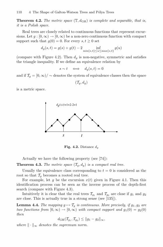
110 4 The Shape of Galton-Watson Trees and Polya Trees
Theorem 4.2. The metric space (T, dGH) is complete and separable, that is,it is a Polish space.
Real trees are closely related to continuous functions that represent excur-sions. Let g : [0,∞) → [0,∞) be a non-zero continuous function with compactsupport such that g(0) = 0. For every s, t ≥ 0 set
dg(s, t) = g(s) + g(t)− 2 infmin{s,t}≤u≤max{s,t}
g(u)
(compare with Figure 4.2). Then dg is non-negative, symmetric and satisfiesthe triangle inequality. If we define an equivalence relation by
s ∼ t ⇐⇒ dg(s, t) = 0
and if Tg = [0,∞)/ ∼ denotes the system of equivalence classes then the space
(Tg, dg)
is a metric space.
s t
d (s,t)=1+2-2=1g
Fig. 4.2. Distance dg
Actually we have the following property (see [74]):
Theorem 4.3. The metric space (Tg, dg) is a compact real tree.
Usually the equivalence class corresponding to t = 0 is considered as theroot so that Tg becomes a rooted real tree.
For example, let g be the excursion x(t) given in Figure 4.1. Then thisidentification process can be seen as the inverse process of the depth-firstsearch (compare with Figure 4.3).
Intuitively it is clear that the real trees Tg1 and Tg2 are close if g1 and g2are close. This is actually true in a strong sense (see [135]).
Lemma 4.4. The mapping g �→ Tg is continuous. More precisely, if g1, g2 aretwo functions from [0,∞) → [0,∞) with compact support and g1(0) = g2(0)then
dGH(Tg1 , Tg2) ≤ ‖g1 − g2‖∞,where ‖ · ‖∞ denotes the supremum norm.
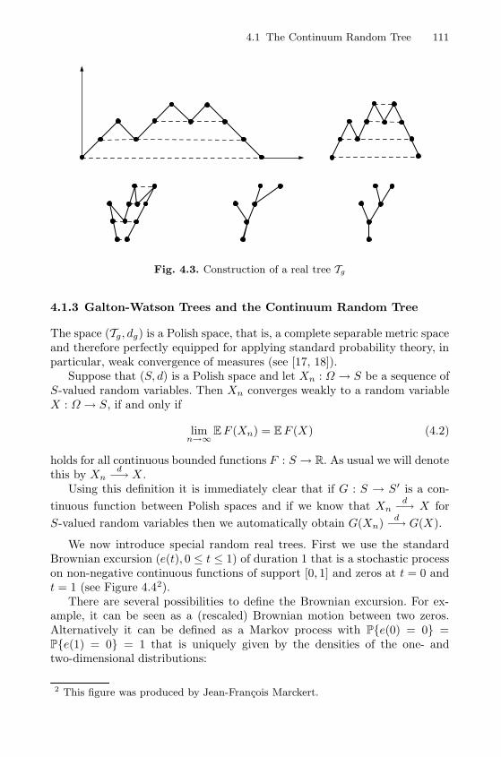
4.1 The Continuum Random Tree 111
Fig. 4.3. Construction of a real tree Tg
4.1.3 Galton-Watson Trees and the Continuum Random Tree
The space (Tg, dg) is a Polish space, that is, a complete separable metric spaceand therefore perfectly equipped for applying standard probability theory, inparticular, weak convergence of measures (see [17, 18]).
Suppose that (S, d) is a Polish space and let Xn : Ω → S be a sequence ofS-valued random variables. Then Xn converges weakly to a random variableX : Ω → S, if and only if
limn→∞
EF (Xn) = EF (X) (4.2)
holds for all continuous bounded functions F : S → R. As usual we will denotethis by Xn
d−→ X .Using this definition it is immediately clear that if G : S → S ′ is a con-
tinuous function between Polish spaces and if we know that Xnd−→ X for
S-valued random variables then we automatically obtain G(Xn)d−→ G(X).
We now introduce special random real trees. First we use the standardBrownian excursion (e(t), 0 ≤ t ≤ 1) of duration 1 that is a stochastic processon non-negative continuous functions of support [0, 1] and zeros at t = 0 andt = 1 (see Figure 4.42).
There are several possibilities to define the Brownian excursion. For ex-ample, it can be seen as a (rescaled) Brownian motion between two zeros.Alternatively it can be defined as a Markov process with P{e(0) = 0} =P{e(1) = 0} = 1 that is uniquely given by the densities of the one- andtwo-dimensional distributions:
2 This figure was produced by Jean-Francois Marckert.
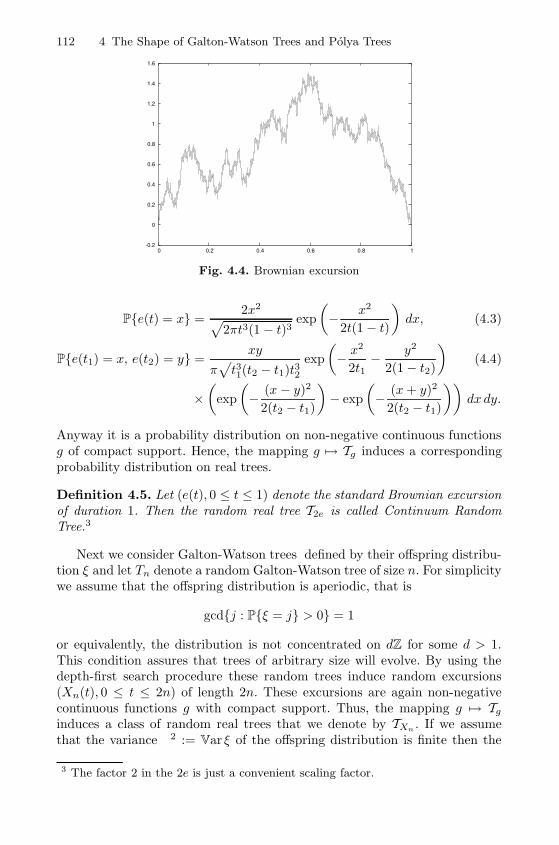
112 4 The Shape of Galton-Watson Trees and Polya Trees
-0.2
0
0.2
0.4
0.6
0.8
1
1.2
1.4
1.6
0 0.2 0.4 0.6 0.8 1
Fig. 4.4. Brownian excursion
P{e(t) = x} =2x2√
2πt3(1 − t)3exp
(− x2
2t(1− t)
)dx, (4.3)
P{e(t1) = x, e(t2) = y} =xy
π√t31(t2 − t1)t32
exp
(− x
2
2t1− y2
2(1− t2)
)(4.4)
×(
exp
(− (x − y)2
2(t2 − t1)
)− exp
(− (x+ y)2
2(t2 − t1)
))dx dy.
Anyway it is a probability distribution on non-negative continuous functionsg of compact support. Hence, the mapping g �→ Tg induces a correspondingprobability distribution on real trees.
Definition 4.5. Let (e(t), 0 ≤ t ≤ 1) denote the standard Brownian excursionof duration 1. Then the random real tree T2e is called Continuum RandomTree.3
Next we consider Galton-Watson trees defined by their offspring distribu-tion ξ and let Tn denote a random Galton-Watson tree of size n. For simplicitywe assume that the offspring distribution is aperiodic, that is
gcd{j : P{ξ = j} > 0} = 1
or equivalently, the distribution is not concentrated on dZ for some d > 1.This condition assures that trees of arbitrary size will evolve. By using thedepth-first search procedure these random trees induce random excursions(Xn(t), 0 ≤ t ≤ 2n) of length 2n. These excursions are again non-negativecontinuous functions g with compact support. Thus, the mapping g �→ Tg
induces a class of random real trees that we denote by TXn . If we assumethat the variance σ2 := Var ξ of the offspring distribution is finite then the
3 The factor 2 in the 2e is just a convenient scaling factor.
4.1 The Continuum Random Tree 113
expected height of a Galton-Watson tree is of order√n (see Section 4.4).
Hence it is natural to scale Xn(t) and consequently the corresponding realtrees by the factor 1/
√n so that the resulting trees are of comparable size.
The main result in this context is an invariance principle by Aldous [4].
Theorem 4.6. Suppose that the offspring distribution ξ of a Galton-Watsonbranching process is aperiodic and critical with finite variance σ2 = Var ξ.Then the scaled real trees
σ√nTXn
corresponding to Galton-Watson trees of size n converge weakly to the contin-uum random tree T2e.
There are also several extensions of Theorem 4.6, for example by Duquesneand Le Gall [72, 73, 74] if the variance Var ξ is infinite but ξ is in the domainof attraction of a stable law. However, for this purpose one has to introducerandom real trees based on a stable Levy process.
A natural way to prove Theorem 4.6 is to consider the depth-first searchprocess Xn(t) corresponding to Galton-Watson trees and to prove the follow-ing property that is also due to Aldous [4].
Theorem 4.7. Suppose that the offspring distribution ξ of a Galton-Watsonbranching process is aperiodic and critical with finite variance σ2 = Var ξ.Then the depth-first search process Xn(t) satisfies(
σ
2√nXn(2nt), 0 ≤ t ≤ 1
)d−→ (e(t), 0 ≤ t ≤ 1). (4.5)
In other words, the normalised depth-first search process is approximated bythe Brownian excursion Obviously, Theorem 4.7 implies Theorem 4.6, sincethe mapping g �→ Tg is continuous.
We do not supply the original proof of this theorem here. There are severalrecent surveys on this subject (see [135, 136]). Nevertheless, in Section 4.2.8we comment on an alternative approach that is based on generating functionsand analytic methods.
One important issue of Theorems 4.6 and 4.7 is that they can be used toderive the limiting distribution of several parameters of trees. For example,let us consider the height Hn, the maximal distance between a node and theroot.
Theorem 4.8. Suppose that the offspring distribution ξ of a Galton-Watsonbranching process satisfies the assumptions of Theorem 4.6 and let Hn denotethe height of the corresponding Galton-Watson trees. Then we have
1√nHn
d−→ 2
σmax0≤t≤1
e(t).
114 4 The Shape of Galton-Watson Trees and Polya Trees
This theorem was first proved by Flajolet and Odlyzko [82]. A local versionis due to Flajolet, Gao, Odlyzko, and Richmond [80].
It is well known that the distribution function of M = max0≤t≤1
e(t) is given
by
P{M ≤ x} = 1− 2
∞∑k=1
(4x2k2 − 1)e−2x2k2
and the moments by
E(M r) = 2−r/2r(r − 1)Γ (r/2)ζ(r),
where ζ(s) denotes the Riemann ζ-function (and where we make the conven-tion (r − 1)ζ(r) = 1 for r = 1).
Thus, one might expect that
E(Hrn) ∼(
2
σ
)r
E(M r)nr/2
for r ≥ 0. In fact this is true if we additionally assume that the exponentialmoment Eeηξ is finite for some η > 0. One possible way is to apply The-orem 4.15 (the assumptions can be verified by Proposition 4.41) or to useanalytic methods (see Theorem 4.29).
Another corollary concerns the path length In of Galton-Watson trees,that is the sum of all distances to the root. Here the limiting relation (4.5)and the second part of (4.1) provide the following result.
Theorem 4.9. Suppose that the offspring distribution ξ of a Galton-Watsonbranching process satisfies the assumptions of Theorem 4.6 and let In denotethe path length of the corresponding Galton-Watson trees. Then we have
1
n3/2In
d−→ 2
σ
∫ 1
0
e(t) dt.
The moments of I =∫ 10e(t) dt are determined by
E(Ir) = Kr4√πr!
Γ(
3r−12
)2r/2
,
where Kr is recursively given by
Kr =3r − 4
4Kr−1 +
r−1∑j=1
KjKr−j, (r ≥ 2),
with initial values K0 = − 12 and K1 = 1
8 . The convergence of moments wasfirst proved by Takacs [200]. Louchard [140] identified then the relation of thelimiting distribution to the Brownian excursion area.
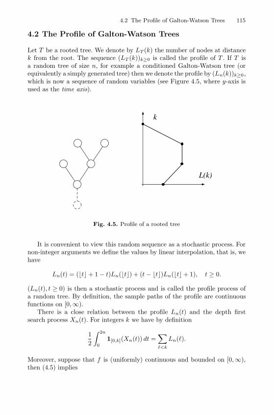
4.2 The Profile of Galton-Watson Trees 115
4.2 The Profile of Galton-Watson Trees
Let T be a rooted tree. We denote by LT (k) the number of nodes at distancek from the root. The sequence (LT (k))k≥0 is called the profile of T . If T isa random tree of size n, for example a conditioned Galton-Watson tree (orequivalently a simply generated tree) then we denote the profile by (Ln(k))k≥0,which is now a sequence of random variables (see Figure 4.5, where y-axis isused as the time axis).
k
L(k)
Fig. 4.5. Profile of a rooted tree
It is convenient to view this random sequence as a stochastic process. Fornon-integer arguments we define the values by linear interpolation, that is, wehave
Ln(t) = (�t�+ 1− t)Ln(�t�) + (t− �t�)Ln(�t�+ 1), t ≥ 0.
(Ln(t), t ≥ 0) is then a stochastic process and is called the profile process ofa random tree. By definition, the sample paths of the profile are continuousfunctions on [0,∞).
There is a close relation between the profile Ln(t) and the depth firstsearch process Xn(t). For integers k we have by definition
1
2
∫ 2n
0
1[0,k](Xn(t)) dt =∑�<k
Ln(�).
Moreover, suppose that f is (uniformly) continuous and bounded on [0,∞),then (4.5) implies
116 4 The Shape of Galton-Watson Trees and Polya Trees
1
n
∑�≥0
f
(σ�
2√n
)Ln(�) =
1
2n
∫ 2n
0
f
(σ
2√nXn(t)
)dt+ o(1)
=
∫ 1
0
f
(σ
2√nXn(2nt)
)dt+ o(1) (4.6)
d−→∫ 1
0
f(e(t)) dt.
In other words, the occupation measure of the scaled depth-first search con-verges to the occupation measure of e(t).
It is natural to ask whether the occupation measure of e(t) has a (random)density. Actually such a density
l(t) = limε→0
1
ε
1∫0
1[t,t+ε](e(s)) ds
exists (almost surely) and constitutes a continuous stochastic process (l(t), t ≥0) that is also called local time local time of a stochastic process of the Brow-nian excursion (of duration 1).
One also expects that the (normalised) profile process is approximatedby l(t). Since the mapping that assigns the local time l to an excursion e isnot continuous, we cannot apply (4.5) resp. Theorem 4.6 to obtain a weaklimit theorem for the profile process. Nevertheless, such a property still holds(compare also with the discussion following Theorem 4.17).
Theorem 4.10. Suppose that the offspring distribution ξ of a Galton-Watsonbranching process is aperiodic and critical with finite variance σ2 = Var ξ.Then we have (in C[0,∞))
(ln(t), t ≥ 0)d−→(σ
2l(σ
2t), t ≥ 0),
where
ln(t) =1√nLn(t
√n), t ≥ 0,
denotes the profile process scaled by√n.
Theorem 4.10 was conjectured by Aldous [3, Conjecture 4], and then provedby Drmota and Gittenberger [66], by Kersting [124] and Pitman [170]. Inwhat follows we present a detailed proof of Theorem 4.10 that is based on themethods of [66]. The proof is analytically very involved and not as elegantas, for example, Pitman’s approach that is based on stochastic differentialequations. However, it seems that this analytic approach is, at the moment,the only way to generalise to Polya trees that we discuss in Section 4.3.
By the way, originally Aldous [3] formulated his conjecture in terms of thestep function process 1√
nLn(�t√n�) (in the space D[0,∞)). However, it is not
4.2 The Profile of Galton-Watson Trees 117
difficult to show that both properties are equivalent. The setting in C[0,∞)is technically easier. Therefore we will only work with continuous processes.
Historically the first investigations of the profile of random trees seem togo back to [193], who derived explicit formulas for the distribution of thesize of one level. Further papers mainly deal with simply generated trees asdefined by [151]. Kolchin (see [131, 132]) related the level size distributions todistributions occurring in particle allocation schemes.
Another interesting tree parameter is the width
W = maxk≥0
L(k) = maxt≥0
L(t),
that is the maximal number of nodes in a level. Since the maximum is acontinuous functional, Theorem 4.10 provides a distributional result for thewidth Wn of Galton-Watson trees.
Theorem 4.11. Under the assumption of Theorem 4.10 we have
1√nWn
d−→ σ
2sup
0≤t≤1l(t).
A corresponding result for convergence of moments seems to be more difficultto obtain. Nevertheless first results on the expected width are due Odlyzkoand Wilf [166], later Chassaing and Marckert [34, 33] and Drmota and Git-tenberger [67] settled the general case.
Note that the distribution of supt≥0 l(t) is the same as that of 2 sup0≤t≤1 e(t)(see [15] or [3]).
There are several extensions of Theorem 4.10. We just state one that isrelated to the leaves of Galton-Watson trees. Let LT (k) denote the number ofleaves at distance k from the root and Ln(k) the random variable we get, if T isa random Galton-Watson tree. As above Ln(t) denotes the linear interpolatedfunction of the sequence Ln(k). Then we have in C[0,∞)
(ln(t), t ≥ 0)d−→(φ0
φ(τ)
σ
2l(σ
2t), t ≥ 0
),
where
ln(t) =1√nLn(
√n t).
Interestingly, a limiting result of the form given in Theorem 4.10 seemsto be quite universal. The property for Ln(t) is only a first indication in theframework of Galton-Watson trees. However, there are also other kinds of treesthat have such a limiting shape. In what follows we will in particular discussunlabelled rooted trees (Polya trees). The natural approach to unlabelledrooted trees is to use generating functions; and the proof that the profile ofunlabelled rooted trees is approximated by l(t) is based on the analysis of
118 4 The Shape of Galton-Watson Trees and Polya Trees
properly defined generating functions. Therefore we have decided to presentalso a generating function proof of Theorem 4.10, although it is not the mostgeneral one. In particular, we assume here that the offspring distribution hasfinite exponential moments (which makes the analysis easier, compare withRemark 3.7). Nevertheless, we need a proper probabilistic framework in orderto prove weak convergence of stochastic processes (see Theorem 4.14).
4.2.1 The Distribution of the Local Time
There are several interesting integral representations of densities and distri-bution functions of the local time l(t) that we collect here. Some of them willbe actually used in the proof of Theorem 4.10.
The one dimensional density of (l(t); t ≥ 0) at t = ρ is well studied. Thereare several representations available in the literature: Using the theory ofbranching processes Kennedy [123] and Kolchin [132, Theorem 2.5.6] obtained
fρ(x) =x
4
1∫0
(1− s)− 32 e−
x2ρ2
8(1−s) g2ρ
(x2, s)ds, (4.7)
where gr(z, s) is the density of a distribution given by its characteristic func-tion:
ψr(ϑ1, ϑ2) =
⎡⎣sinh(r√−2iϑ2)
r√−2iϑ2
− iϑ1
(sinh(r√−iϑ2/2)
r√−iϑ2/2
)2⎤⎦−1
.
Takacs [200] calculated this density by means of a generating function ap-proach
fρ(x) = 2∑j≥1
j∑k=1
(j
k
)e−(x+2ρj)2/2 (−x)k
(k − 1)!Hk+2(x + 2ρj). (4.8)
Hk(z) are the Hermite polynomials defined by
Hk(z) = (−1)kez2/2 d
k
dzke−z2/2.
Knight [127] worked with the Brownian excursion and obtained
fρ(x) = 2−1/2π5/2ρ−3
1∫0
f∗(π2(1− s)
2ρ2
)h(s, x) ds (4.9)
with
f∗(z) = 4√
2π3∑k≥1
k2 d
dz
(e−k2π2/z
√2πz3
)
4.2 The Profile of Galton-Watson Trees 119
and
h(s, x) = − 1
2ρ√
2πs
∑i≥0
1
i!
di−1
dxi−1
(xi d
2
dx2e−2ρ2(x+i)2/s
),
where d−1
dx−1 =(
ddx
)−1.
Getoor and Sharpe [90] also used a direct approach and derived a doubleLaplace transform of the density:
∞∫0
e−αt
t∫0
1√2πs
∞∫t−s
1√2πr3
E
(e−βl(ρ/
√r)√
r)dr ds dt = ϕρ(α, β) (4.10)
where
ϕρ(α, β) =1
α
√2α+ β(1 + e−2ρ
√2α)√
2α+ β(1 − e−2ρ√
2α)− β
√2
(1 + 2ρβ)α3/2.
This formula was also shown by Louchard [141] who found a considerablyshorter proof via Kac’s formula for Brownian functionals.
When studying M/M/1-queues Cohen and Hooghiemstra [42] got an in-tegral representation for the above density:
fρ(x) =1
i√
2π
∫γ
−se−s
sinh2(ρ√−2s)
exp
(− x√
2
√−seρ
√−2s
sinh(ρ√−2s)
)ds, (4.11)
where γ is the straight line {z ∈ C : �z = −1}. They also derived theLaplace transform of the two dimensional densities of local and occupationtime (compare also with the general result in Theorem 4.13).
Finally it should be mentioned that Hooghiemstra [103] found a directproof for the equivalence of (4.9) and (4.11).
Remark 4.12 Note that the expressions (4.7)–(4.11) are only representa-tions of the continuous part of the local density. Obviously the local time den-sity has a jump of magnitude P
{sup0≤t≤1 e(t) < ρ
}at 0. This quantity is
given by
P
{sup
0≤t≤1e(t) ≤ ρ
}= 1− 2
∑k≥1
(4ρ2k2 − 1)e−2ρ2k2
. (4.12)
The proof of Theorem 4.10 is based on a precise analysis of finite di-mensional projections (and on tightness estimates). For this purpose we needproper representations of the characteristic function of finite dimensional pro-jections of l(t) (compare with [66]).
Theorem 4.13. Suppose that 0 < κ1 < κ2 < · · · < κd are positive realnumber and let fκ1,...,κd
be defined by
fκ1,...,κd(s, t1, . . . , td) = (4.13)
Ψκ1(s, it1 + Ψκ2−κ1(. . . Ψκd−1−κd−2(s, itd−1 + Ψκd−κd−1
(s, itd)) · · · )
120 4 The Shape of Galton-Watson Trees and Polya Trees
with
Ψκ(s, t) =t√−2s e−κ
√−2s
√−2s eκ
√−2s − 2t sinh
(κ√−2s) . (4.14)
Then the characteristic function of the random vector (l(κ1), . . . , l(κd)) isgiven by
E et1 l(κ1)+···+td l(κd) = 1 +
√2
i√π
∫γ
fκ1,...,κd(s, t1, . . . , td) e−s ds, (4.15)
where γ is the straight line {s ∈ C : �s = −1}.
4.2.2 Weak Convergence of Continuous Stochastic Processes
Let S = C[0, 1] be the Polish space of continuous functions on [0, 1]. An S-valued random variable X (where the measure on S is defined on the Borelsets of S) is just a stochastic process (X(t), 0 ≤ t ≤ 1). It is well known thatthe distribution of (X(t), 0 ≤ t ≤ 1) is characterised by the finite dimensionaldistributions of the random vectors
(X(κ1), . . . , X(κd)),
where d ≥ 1 and 0 ≤ κ1 < κ2 < · · · < κd.
However, weak convergenceXnd−→ X of a sequence of stochastic processes
cannot be characterised just by finite dimensional convergence. In particular,if
(Xn(κ1), . . . , Xn(κd))d−→ (X(κ1), . . . , X(κd))
for all d ≥ 1 and 0 ≤ κ1 < κ2 < · · · < κd then this does not guarantee that
Xnd−→ X . One has to assume additionally that Xn is tight. Recall that a
sequence (Xn) of random variables in a metric space S is tight if for everyε > 0, there exists a compact subset K ⊆ S such that P{Xn ∈ K} > 1 − εfor every n. In a Polish space, a complete separable metric space, tightnessis equivalent to relative compactness (of the corresponding distributions) byProhorov’s theorem [18, Theorems 6.1 and 6.2], [119, Theorem 16.3].
In our special case of S = C[0, 1] (with the supremum norm) tightnessmeans that
lima→0
lim supn→∞
P{|Xn(0)| > a} = 0 (4.16)
and
limδ→0
lim supn→∞
P
{sup
|s−t|≤δ
|Xn(s)−Xn(t)| ≥ ε}
= 0 (4.17)
for all ε > 0. Informally, this says that, with high probability,Xn(s) and Xn(t)do not differ too much if s and t are close.
Property (4.17) cannot be checked easily in a direct way. However, thereare sufficient moment conditions (4.19) so that we have the following theorem(compare with [18]).
4.2 The Profile of Galton-Watson Trees 121
Theorem 4.14. Suppose that (Xn(t), 0 ≤ t ≤ 1) is a sequence of stochasticprocesses and (X(t), 0 ≤ t ≤ 1) a stochastic process on C[0, 1] that satisfiesthe following conditions.
1. For every d ≥ 1 and 0 ≤ κ1 < κ2 < · · · < κd we have
(Xn(κ1), . . . , Xn(κd))d−→ (X(κ1), . . . , X(κd)).
2. There exists a constant C > 0 and an exponent β > 0 such that
E(|Xn(0)|β
)≤ C (4.18)
for all n.3. There exists a constant C > 0 and exponents α > 1 and β > 0 such that
E(|Xn(t)−Xn(s)|β
)≤ C|t− s|α for all s, t ∈ [0, 1]. (4.19)
Then(Xn(t), 0 ≤ t ≤ 1)
d−→ (X(t), 0 ≤ t ≤ 1).
By Markov’s inequality it is clear that (4.18) implies (4.16). However, it isa non-trivial task to show that (4.19) is sufficient to prove (4.17). Actually,(4.19) implies
P
{sup
|t−s|≤δ
|Xn(t)−Xn(s)| ≥ ε}≤ Kδ
α−1
εβ(4.20)
for some constant K (see [18]). Note that the condition α > 1 is essential fordeducing (4.17).
Theorem 4.14 does not apply directly to processes in C[0,∞). However,weak convergence in C[0,∞) holds, if and only if we have weak convergence ofthe restrictions to the compact interval [0, T ] for all T <∞ (see [18]). Hence,we can work with Theorem 4.14 in both cases.
Finally we want to mention that a condition of the kind (4.19) is actuallyquite strong. It is sufficient (but not necessary) to prove tightness, and itcan also be used to prove convergence of moments. The problem is that the
function F (x) = xr is unbounded so that Xnd−→ X not necessarily implies
EXrn → EXr even if the expected values exist.
Theorem 4.15. Suppose that a sequence of stochastic processes Xn = Xn(t),defined on C[0, 1], converges weakly to X = X(t). Furthermore suppose thatthere exists s0 ∈ [0, 1] such that for all r ≥ 0
supn≥0
E (|Xn(s0)|r) <∞, (4.21)
and that for every α > 1 there are β > 0 and C > 0 with (4.19).
122 4 The Shape of Galton-Watson Trees and Polya Trees
Let F : C[0, 1] → R be a continuous functional of polynomial growth, thatis, there exists r ≥ 0 with
|F (y)| ≤ (1 + ‖y‖∞)r
for all y ∈ C[0, 1]. Then
limn→∞
EF (Xn) = EF (X). (4.22)
For example, Theorem 4.15 implies that all finite dimensional moments ofXn(t) converge to that of X(t), that is, for all fixed 0 ≤ κ1 < κ2 < · · · < κp
and r1, r2, . . . , rp ≥ 0
limn→∞
E (Xn(κ1)r1Xn(κ2)r2 · · ·Xn(κp)rp) = E (X(κ1)r1X(κ2)r2 · · ·X(κp)rp) .
Furthermore, we have
limn→∞
E
(max0≤t≤1
Xn(t)
)r
= E
(max0≤t≤1
X(t)
)r
and similarly for the integral∫ 10 Xn(t) dt.
We present a short proof of Theorem 4.15 since it also sheds some light onthe tightness condition (4.19).
The key of the proof of Theorem 4.15 is the following observation.
Lemma 4.16. Suppose that Xn(t) and X(t) are stochastic processes satisfyingthe assumptions of Theorem 4.15. Then for every α > 1 there exists a constantK > 0 such that for ε > 0 and 0 < δ < 1
P
{sup
|s−t|≤δ
|Xn(s)−Xn(t)| ≥ ε}≤ Kδ
α−1
εβ(4.23)
and consequently
E
(sup
|s−t|≤δ
|Xn(s)−Xn(t)|r)
= O(δr
α−1β
)(4.24)
for every fixed r < β.
Note that if (4.19) holds for all α > 1, then β = β(α) is unbounded as afunction in α. Thus, the restriction r < β is not that serious. Actually wenecessarily have β ≥ α, except in the trivial case Xn(t) = Xn(0) for all t andn.
Proof. We already mentioned that (4.20) follows from (4.19) by using themethods of Billingsley [18, pp. 95]. Finally, (4.24) is an easy consequence of(4.20).
4.2 The Profile of Galton-Watson Trees 123
Using these preliminaries it is easy to complete the proof of Theorem 4.15.
Proof. By combining (4.21) and (4.19) it follows that for every s0 ∈ [0, 1]
supn≥0
E (|Xn(s0)|r) <∞.
Next, by a direct combination of (4.21) with s0 = 12 and (4.24) with δ = 1
2 weobtain (for all r ≥ 0)
supn≥0
E
(max0≤t≤1
|Xn(t)|r)<∞
and consequently (for any ε > 0)
supn≥0
E(F (Xn)1+ε
)<∞.
By weak convergence we also have F (Xn)d−→ F (X). Thus, by [17, p. 348]
the expected value EF (X) exists and
limn→∞
EF (Xn) = EF (X).
Again this theorem does not apply to stochastic processes Xn in C[0,∞).However, it is easy to adapt the above theorem to cover this case, too.
For example, suppose that for any choice of fixed positive integers r andα there exist positive constants c0, c1, c2, c3 such that
supn≥0
E (|Xn(t)|r) ≤ f1(t) for all t ≥ 0, (4.25)
and
supn≥0
E(|Xn(t+ s)−Xn(t)|2α
)≤ f2(t)sα for all s, t ≥ 0, (4.26)
where f1(t) and f2(t) are bounded functions with f1(t) → 0 and f2(t) → 0as t → ∞. Then for all continuous functions F : C[0,∞) → R of polynomialgrowth (in C0([0,∞))) we have
limn→∞
EF (Xn) = EF (X),
(compare with [67]).For example, Theorem 4.15 (and its adaption to C[0,∞)) can be applied
to the height and width of Galton-Watson trees (compare with [67, 69]).
We finally give another useful application of tightness that could lead to ashortcut in the proof of Theorem 4.10 provided that Theorem 4.7 is alreadyknown. The basis is the following observation due to Bousquet-Melou andJanson [24].
124 4 The Shape of Galton-Watson Trees and Polya Trees
Theorem 4.17. Let S1 and S2 be two Polish spaces, and let ϕ : S1 → S2 bean injective continuous map. If (Wn) is a tight sequence of random elements
of S1 such that ϕ(Wn)d−→ Z in S2 for some random Z ∈ S2 then Wn
d−→W
in S1 for some W with ϕ(W )d= Z.
Proof. By Prohorov’s theorem, each subsequence of (Wn) has a subsequencethat converges in distribution to some limit. Let W ′ and W ′′ be limits indistribution of two such subsequences Wn′i and Wn′′i . Since ϕ is continuous,
ϕ(Wn′i )d−→ ϕ(W ′) and ϕ(Wn′′i )
d−→ ϕ(W ′′). Hence, ϕ(W ′)d= Z
d= ϕ(W ′′).
Let A be a (Borel) measurable subset of S1. By the Souslin–Lusin theorem[45, Theorem III.21, see also III.16–17], ϕ(A) ⊆ S2 is measurable. Thus, usingthe injectivity of ϕ,
P{W ′ ∈ A} = P{ϕ(W ′) ∈ ϕ(A)} = P{ϕ(W ′′) ∈ ϕ(A)} = P{W ′′ ∈ A}.
Consequently, W ′ d= W ′′.
In other words, there is a unique distribution of the subsequence limits.Thus, ifW is one such limit, then every subsequence of (Wn) has a subsequence
that converges in distribution to W ; this is equivalent to Wnd−→ W (recall
that by (4.2), weak convergence can be reduced to convergence of sequencesof real numbers).
This theorem applies in the following situation. Let S1 = {f ∈ C0(R) :f ≥ 0}, with the uniform topology inherited from C0(R); let S2 be the spaceof locally finite measures on R with the vague topology (see Kallenberg [119,Appendix A2]) and let ϕ map a function f to the corresponding measuref dx, that is, ϕ(f) is the measure with density f . Then S1 is a closed subsetof the separable Banach space C0(R), and is thus Polish, and so is S2 by [119,Theorem A2.3]. Further, ϕ is continuous and injective.
In particular, let
ln(t) =1√nLn(t
√n) ∈ S1
be the normalised profile of Galton-Watson trees. Then ϕ(ln) is precisely themeasure
1
n
∑j≥0
Ln(j)νjn−1/2,n−1/2 ,
where νy,h denotes the measure with (triangular) density function
f(x) =1
hmax
{1− |x− y|
h, 0
}that is centred at y and has support [y−h, y+h]. Note that νy,h approximatesthe delta distribution δy, if h → ∞. It also follows easily that the differenceof ϕ(ln) and the normalised occupation measure
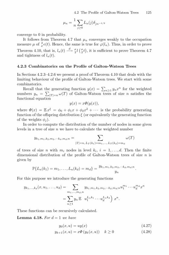
4.2 The Profile of Galton-Watson Trees 125
μn =1
n
∑j≥0
Ln(j)δjn−1/2
converge to 0 in probability.It follows from Theorem 4.7 that μn converges weakly to the occupation
measure μ of 2σ e(t). Hence, the same is true for ϕ(ln). Thus, in order to prove
Theorem 4.10, that is, ln(t)d−→ σ
2 l(
σ2 t), it is sufficient to prove Theorem 4.7
and tightness of ln(t).
4.2.3 Combinatorics on the Profile of Galton-Watson Trees
In Sections 4.2.3–4.2.6 we present a proof of Theorem 4.10 that deals with thelimiting behaviour of the profile of Galton-Watson trees. We start with somecombinatorics.
Recall that the generating function y(x) =∑
n≥1 ynxn for the weighted
numbers yn =∑|T |=n ω(T ) of Galton-Watson trees of size n satisfies the
functional equationy(x) = xΦ(y(x)),
where Φ(x) = Exξ = φ0 + φ1x + φ2x2 + · · · is the probability generating
function of the offspring distribution ξ (or equivalently the generating functionof the weights φj).
In order to compute the distribution of the number of nodes in some givenlevels in a tree of size n we have to calculate the weighted number
yk1,m1,k2,m2,···kd,md;n =∑
|T |=n, LT (k1)=m1,..., LT (kd)=md
ω(T )
of trees of size n with mi nodes in level ki, i = 1, . . . , d. Then the finitedimensional distribution of the profile of Galton-Watson trees of size n isgiven by
P{Ln(k1) = m1, . . . , Ln(kd) = md} =yk1,m1,k2,m2,···kd,md;n
yn.
For this purpose we introduce the generating functions
yk1,...,kd(x, u1, . . . , ud) =
∑m1,...,md,n
yk1,m1,k2,m2,···kd,md;num11 · · ·umd
d xn
=∑n≥1
yn E
(uLnk1
1 · · ·uLnkd
d
)xn.
These functions can be recursively calculated.
Lemma 4.18. For d = 1 we have
y0(x, u) = uy(x) (4.27)
yk+1(x, u) = xΦ (yk(x, u)) k ≥ 0 (4.28)
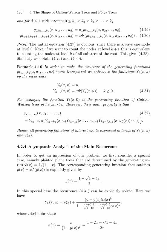
126 4 The Shape of Galton-Watson Trees and Polya Trees
and for d > 1 with integers 0 ≤ k1 < k2 < k3 < · · · < kd
y0,k2,...,kd(x, u1, . . . , ud) = u1yk2,...,kd
(x, u2, . . . , ud) (4.29)
yk1+1,k2+1,...,kd+1(x, u1, . . . , ud) = xΦ (yk1,k2,...,kd(x, u1, u2, . . . , ud)) . (4.30)
Proof. The initial equation (4.27) is obvious, since there is always one nodeat level 0. Next, if we want to count the nodes at level k+ 1 this is equivalentto counting the nodes at level k of all subtrees of the root. This gives (4.28).Similarly we obtain (4.29) and (4.30).
Remark 4.19 In order to make the structure of the generating functionsyk1,...,kd
(x, u1, . . . , ud) more transparent we introduce the functions Yk(x, u)by the recurrence
Y0(x, u) = u,
Yk+1(x, u) = xΦ(Yk(x, u)), k ≥ 0. (4.31)
For example, the function Yk(x, 0) is the generating function of Galton-Watson trees of height < k. However, their main property is that
yk1,...,kd(x, u1, . . . , ud) (4.32)
= Yk1
(x, u1Yk2−k1
(x, u2Yk3−k2(x, . . . , ud−1Ykd−kd−1
(x, uy(x)) · · · ))).
Hence, all generating functions of interest can be expressed in terms of Yk(x, u)and y(x).
4.2.4 Asymptotic Analysis of the Main Recurrence
In order to get an impression of our problem we first consider a specialcase, namely planted plane trees that are determined by the generating se-ries Φ(x) = 1/(1 − x). The corresponding generating function that satisfiesy(x) = xΦ(y(x)) is explicitly given by
y(x) =1−
√1− 4x
2.
In this special case the recurrence (4.31) can be explicitly solved. Here wehave
Yk(x, u) = y(x) +(u− y(x))α(x)k
1− u−y(x)√1−4x
+ u−y(x)√1−4x
α(x)k,
where α(x) abbreviates
α(x) =x
(1− y(x))2=
1− 2x−√
1− 4x
2x.
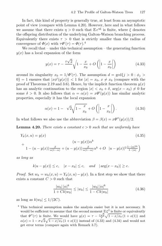
4.2 The Profile of Galton-Watson Trees 127
In fact, this kind of property is generally true, at least from an asymptoticpoint of view (compare with Lemma 4.20). However, here and in what followswe assume that there exists η > 0 such that E eηξ is finite, where ξ denotesthe offspring distribution of the underlying Galton-Watson branching process.Equivalently there exists τ > 0 that is strictly smaller than the radius ofconvergence of Φ(x) with τΦ′(τ) = Φ(τ).4
We recall that – under this technical assumption – the generating functiony(x) has a local expansion of the form
y(x) = τ − τ√
2
σ
√1− x
x0+O
(∣∣∣∣1− x
x0
∣∣∣∣) (4.33)
around its singularity x0 = 1/Φ′(τ). The assumption d = gcd{j > 0 : φj >0} = 1 ensures that |xφ′(y(x))| < 1 for |x| = x0, x = x0 (compare with theproof of Theorems 2.19 and 3.6). Hence, by the implicit function theorem y(x)has an analytic continuation to the region |x| < x0 + δ, arg(x − x0) = 0 forsome δ > 0. It also follows that α = α(x) = xΦ′(y(x)) has similar analyticproperties, especially it has the local expansion
α(x) = 1− σ√
2
√1− x
x0+O
(∣∣∣∣1− x
x0
∣∣∣∣) . (4.34)
In what follows we also use the abbreviation β = β(x) = xΦ′′(y(x))/2.
Lemma 4.20. There exists a constant c > 0 such that we uniformly have
Yk(x, u) = y(x) (4.35)
+(u− y(x))αk
1− (u− y(x)) βα(1−α) + (u− y(x)) β
α(1−α)αk +O(|u− y(x)|2 1−|α|2k
1−|α|
)as long as
k|u− y(x)| ≤ c, |x− x0| ≤ c, and | arg(x− x0)| ≥ c.
Proof. Set wk = wk(x, u) = Yk(x, u)− y(x). In a first step we show that thereexists a constant C > 0 such that
|w0| |α|k1 + Ck|w0|
≤ |wk| ≤|w0| |α|k
1− Ck|w0|(4.36)
as long as k|w0| ≤ 1/(2C).
4 This technical assumption makes the analysis easier but it is not necessary. Itwould be sufficient to assume that the second moment E ξ2 is finite or equivalently
that Φ′′(τ ) is finite. We would have y(x) = τ − τ√
2σ
p1 − x/x0 (1 + o(1)) and
α(x) = 1 − σ√
2p
1 − x/x0 (1 + o(1)) instead of (4.33) and (4.34) and would notget error terms (compare again with Remark 3.7).
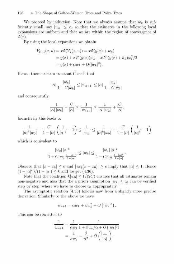
128 4 The Shape of Galton-Watson Trees and Polya Trees
We proceed by induction. Note that we always assume that wk is suf-ficiently small, say |wk| ≤ c0 so that the estimates in the following localexpansions are uniform and that we are within the region of convergence ofΦ(x).
By using the local expansions we obtain
Yk+1(x, u) = xΦ(Yk(x, u)) = xΦ(y(x) + wk)
= y(x) + xΦ′(y(x))wk + xΦ′′(y(x) + ϑk)w2k/2
= y(x) + αwk + O(|wk|2).
Hence, there exists a constant C such that
|α| |wk|1 + C|wk|
≤ |wk+1| ≤ |α||wk|
1− C|wk|
and consequently
1
|α| |wk|− C
|α| ≤1
|wk+1|≤ 1
|α| |wk|+C
|α| .
Inductively this leads to
1
|α|k|w0|− C
1− |α|
(1
|α|k − 1
)≤ 1
|wk|≤ 1
|α|k|w0|+
C
1− |α|
(1
|α|k − 1
)which is equivalent to
|w0| |α|k
1 + C|w0|1−|α|k
1−|α|≤ |wk| ≤
|w0| |α|k
1− C|w0| 1−|α|k
1−|α|.
Observe that |x − x0| ≤ c and | arg(x − x0)| ≥ c imply that |α| ≤ 1. Hence(1− |α|k)/(1− |α|) ≤ k and we get (4.36).
Note that the condition k|w0| ≤ 1/(2C) ensures that all estimates remainnon-negative and also that the a priori assumption |wk| ≤ c0 can be verifiedstep by step, where we have to choose c0 appropriately.
The asymptotic relation (4.35) follows now from a slightly more precisederivation. Similarly to the above we have
wk+1 = αwk + βw2k +O(|wk|3).
This can be rewritten to
1
wk+1=
1
αwk
1
1 + βwk/α+O (|wk|2)
=1
αwk− β
α2+O
( |wk||α|
).
4.2 The Profile of Galton-Watson Trees 129
If we set qk = αk/wk then
qk+1 = qk − βαk−1 +O(|wk||α|k
)which, with help of the a priori estimate, provides wk = O(w0α
k)
qk =1
w0− βα
1− αk
1− α +O
(|w0|∣∣∣∣1− α2k
1− α2
∣∣∣∣)and consequently (4.35).
4.2.5 Finite Dimensional Limiting Distributions
We will use the results of the previous section to prove finite dimensionalconvergence. For simplicity we only discuss the cases d = 1 and d = 2 indetail. It will then be clear how to deal with the general case.
Let us start with d = 1. Recall that the characteristic function of the localtime l at level κ is given by
E eit l(κ) = 1 +
√2√π
−1+i∞∫−1−i∞
t√−2s exp(−κ
√−2s )√
−2s exp(κ√−2s )− 2it sinh
(κ√−2s)e−s ds.
(4.37)
Proposition 4.21. Let κ ≥ 0 be given. Then we have for |t| ≤ c/(τκ)
limn→∞
Eeit 1√
nLn(κ
√n)
= E eitσ2 l( σ
2 κ). (4.38)
Consequently1√nLn(κ
√n)
d−→ σ
2l(σ
2κ).
Proof. Recall that the generating function yk(x, u) = Yk(x, uy(x)) can beinterpreted as
yk(x, u) =∑n≥1
yn EuLn(k) xn
and is, thus, related to the characteristic function of Ln(k). In particular, wehave
EeitLn(k)/√
n =1
yn[xn]yk
(x, eit/
√n).
In order to get asymptotics for this characteristic function we will use the localrepresentation of Yk(x, u) from Lemma 4.20 and a properly chosen contourintegration applied to Cauchy’s formula.
Let Γ = γ′ ∪ Γ ′ consist of a line
γ′ ={x = x0
(1 +
s
n
): �(s) = −1, |�(s)| ≤ C log2 n
}
130 4 The Shape of Galton-Watson Trees and Polya Trees
with an arbitrarily chosen fixed constant C > 0, and Γ ′ be a circular arccentred at the origin and making Γ a closed curve. Then
EeitLn(k)/√
n =1
yn
1
2πi
∫Γ
yk
(x, eit/
√n) dx
xn+1. (4.39)
The contribution of Γ ′ is exponentially small, since for x ∈ Γ ′ we have
|x−n−1| ∼ x−n0 e−C log2 n, whereas
∣∣∣yk
(x, eit/
√n)∣∣∣ is bounded.
If x ∈ γ′ then the local expansion (4.35) is valid for a proper range for k.In particular, we replace k by �κ√n�, u by eit/
√ny(x) and x by x0
(1 + s
n
).
If we assume that κ > 0 is given then the assumptions of Lemma 4.20 aresatisfied provided that |t| ≤ c/(κτ), where c is the constant from Lemma 4.20:
k|(u− 1)y(x)| ≤ κ√n∣∣∣eit/√n − 1
∣∣∣ |y(x)| ≤ κ|t|τ ≤ c.
Next we use the local expansions
y(x) = τ − τ√
2
σ
√− sn
+O(|s|/n),
α = 1− σ√
2
√− sn
+O(|s|/n),
β =σ2
2τ+O
(√− sn
)and
αk = exp(−σκ
√−2s) (
1 +O(κs/√n))
to get asymptotically for x ∈ γ ′
(u− 1)y(x)αk
1− (u− 1)y(x) βα(1−α) + (u− 1)y(x) β
α(1−α)αk +O(|u− 1|2 1−|α|2k
1−|α|
)=
1√n
itτe−σκ√−2s(1 +O(s/
√n))
1− itσ2√−2s
+ itσ2√−2s
exp(−σκ
√−2s)
+O(|s|3/2/√n)
=1√n
it√−2s τ exp
(−σκ
√−2s)
(1 +O(s/√n))
√−2s− itσ
2 + itσ2 exp(−σκ
√−2s)
+O(√|s|/n)
=1√n
it√−2s τ exp
(− 1
2σκ√−2s)
(1 +O(s/√n))√
−2s exp(
12σκ
√−2s)
(1 +O(1/√n))− itσ sinh
(12σκ
√−2s) .
Finally, by applying the substitution x = x0(1 + s/n) and the approximationx−n = x−n
0 e−s(1 +O(|s|2/n)) we notice that the integral
1
2πi
∫γ′
(u − 1)y(x)αk
1− (u− 1)y(x) βα(1−α) (1− αk) +O
(|u− 1|2 1−|α|2k
1−|α|
) dxxn+1
4.2 The Profile of Galton-Watson Trees 131
is approximated by
τx−n0
σ√
2π n3/2
√2√π
1+log2 n∫−1−log2 n
itσ2
√−2s exp(− 1
2κσ√−2s )√
−2s exp( 12κσ
√−2s )− 2it sinh
(12κσ
√−2s) e−s ds.
Since the integral is absolutely convergent, we can safely replace the integral∫ −1+log2 n
−1−log2 n by∫ −1+∞−1−∞ . We recall that yn ∼ (τ/(σ
√2π))x−n
0 n−3/2. Hence,
limn→∞
E eit 1√
nLn(�κ√n�)
= E eitσ2 l( σ
2 κ)
follows. However, in view of (4.41) (that we will prove independently of thepresent proposition)
E eit 1√
nLn(�κ√n�)
and E eit 1√
nLn(κ
√n)
have the same limit. This completes the proof of (4.38) for a small openinterval for t (that contains t = 0).
Since the characteristic function E eitσ2 l( σ
2 κ) represents an analytic function
in t, we thus get weak convergence of 1√nLn(κ
√n)
d−→ σ2 l(
σ2κ)
(compare with
[139, pp. 224–225]).
With the help of the same techniques it is also possible to obtain asymp-totics for moments (compare with [199, 93]). We just demonstrate this for theexpected profile ELn(k).
By definition the partial derivative
γk(x) =
[∂yk(x, u)
∂u
]u=1
=∑n≥1
ynELn(k) xn
encodes the first moment. By induction it follows that
γk(x) = y(x)α(x)k .
Thus if k = �κ√n� (with some κ > 0) we obtain (by using exactly the samekind of contour integration as above)
ynELn(k) ∼ τx−n0
n
1
2πi
∫ −1+i∞
−1−i∞exp(−σκ
√−2s)e−s ds.
In view of Lemma 4.22 we immediately derive
ELn(�κ√n�) ∼ σ2κe−
12 σ2κ2√
n.
Lemma 4.22. Let r > 0. Then the following formula holds:
1
2πi
∫ −1+i∞
−1−i∞exp(−r√−2s)e−s ds =
r√2πe−
12 r2
.
132 4 The Shape of Galton-Watson Trees and Polya Trees
Proof. We first show that the integral over the line from −1− i∞ to −1 + i∞can be replaced by the contour that surrounds the positive real axis as a so-called Hankel contour H (see Figure 2.5). For this purpose we have to showthat the integrals ∫
|s|=R, 0<| arg(s)|≤π/2
exp(−r√−2s)e−s ds
are negligible (as R→∞) which is actually true since∫ π/2
0
∣∣∣e−r√−2Reiϕ−Reiϕ
∣∣∣Rdϕ ≤ Rπ
2max{e−r
√R, e−R/
√2}.
After that we use the substitution s = 12 t
2, where t goes from i−∞ to i+∞,and the resulting integral can be finally calculated. Summing up we have
1
2πi
∫ −1+i∞
−1−i∞exp(−r√−2s)e−s ds =
1
2πi
∫H
exp(−r√−2s)e−s ds
=1
2πi
∫ i+∞
i−∞eirt− 1
2 t2t dt
=e−
12 r2
2πi
∫ i+∞
i−∞e−
12 (t−ir)2(t− ir + ir) dt
=re−
12 r2
2π
∫ ∞−∞
e−12 w2
dw
=r√2πe−
12 r2
.
Next consider the two dimensional case. The characteristic function of(l(κ1), l(κ2)) with 0 < κ1 < κ2 is given by
E eit1 l(κ1)+it2 l(κ2) = 1 +
√2
i√π
∫ −1+i∞
−1−i∞Ψκ1 (s, it1 + Ψκ2−κ1(s, it2)) e−s ds,
with
Ψκ1 (s, it1 + Ψκ2−κ1(s, it2)) =
√−2s e−κ1
√−2s
(it1+
it2√−2s e−(κ2−κ1)
√−2s
√−2se(κ2−κ1)
√−2s−2it2 sinh((κ2−κ1)√−2s )
)√−2s eκ1
√−2s −(it1+
it2√−2se−(κ2−κ1)
√−2s√−2s e(κ2−κ1)
√−2s−2it2 sinh((κ2−κ1)√−2s )
)sinh(κ1
√−2s) .
Proposition 4.23. Let 0 ≤ κ1 < κ2 be given. Then we have for real t1 andt2 with sufficiently small absolute value
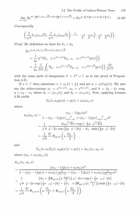
4.2 The Profile of Galton-Watson Trees 133
limn→∞
Eeit1
1√n
Ln(κ1√
n)+it21√n
Ln(κ2√
n)= E eit1
σ2 l( σ
2 κ1)+it2σ2 l( σ
2 κ2). (4.40)
Consequently(1√nLn(κ1
√n),
1√nLn(κ2
√n)
)d−→(σ
2l(σ
2κ1
),σ
2l(σ
2κ2
)).
Proof. By definition we have for k1 < k2
E eit1Ln(k1)/√
n+it2Ln(k2)/√
n
=1
yn[xn]Yk1
(x, eit1/
√nYk2−k1
(x, eit2/
√ny(x)))
=1
yn
1
2πi
∫Γ
Yk1
(x, eit1/
√nYk2−k1
(x, eit2/
√ny(x))) dx
xn+1
with the same path of integration Γ = Γ ′ ∪ γ′ as in the proof of Proposi-tion 4.21.
If x ∈ γ′ then substitute x = x0
(1 + s
n
)and set α = xφ′(y(x)). We also
use the abbreviations u1 = eit1/√
n, u2 = eit2/√
n, and h = k2 − k1 resp.η = κ2 − κ1 where k1 = �κ1
√n� and k2 = �κ1
√n�. Now, applying Lemma
4.20 yieldsYh(x, u2y(x)) = y(x) + wh(u2, x)
where
wh(u2, x) ∼ (u2 − 1)y(x)αh
1− (u2 − 1)y(x) βα(1−α) + (u2 − 1)y(x) β
α(1−α)αh
∼ 1√n
it2√−2s τ exp
(− 1
2ση√−2s)
√−2s exp
(12ση
√−2s)− it2σ sinh
(12ση
√−2s)
=1√n
2τ
σΨησ/2
(s,it2σ
2
)and
Yk1(x, u1Yh(x, u2y(x))) = y(x) + wk1(u1, u2, x)
where (wh = wh(u2, x))
wk1(u1, u2, x)
∼ ((u1 − 1)y(x) + u1wh)αk1
1− ((u1 − 1)y(x) + u1wh) βα(1−α) + ((u1 − 1)y(x) + u1wh) β
α(1−α)αk1
∼ 1√n
(it1 + 2
σΨησ/2
(s, it2σ
2
))√−2s τ exp
(− 1
2σκ1
√−2s)
√−2s exp
(12σκ1
√−2s)−(it1σ + 2Ψησ/2
(s, it2σ
2
))sinh(
12σκ1
√−2s)
=1√n
2τ
σΨκ1σ/2
(s,it1σ
2+ Ψησ/2
(s,it2σ
2
)).
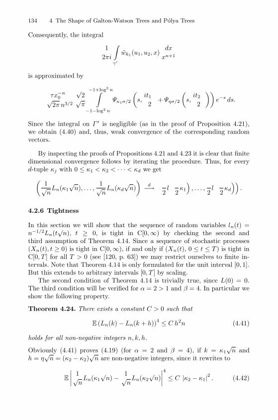
134 4 The Shape of Galton-Watson Trees and Polya Trees
Consequently, the integral
1
2πi
∫γ′
wk1(u1, u2, x)dx
xn+1
is approximated by
τx−n0
σ√
2π n3/2
√2√π
−1+log2 n∫−1−log2 n
Ψκ1σ/2
(s,it1σ
2+ Ψησ/2
(s,it2σ
2
))e−s ds.
Since the integral on Γ ′ is negligible (as in the proof of Proposition 4.21),we obtain (4.40) and, thus, weak convergence of the corresponding randomvectors.
By inspecting the proofs of Propositions 4.21 and 4.23 it is clear that finitedimensional convergence follows by iterating the procedure. Thus, for everyd-tuple κj with 0 ≤ κ1 < κ2 < · · · < κd we get(
1√nLn(κ1
√n), . . . ,
1√nLn(κd
√n)
)d−→(σ
2l(σ
2κ1
), . . . ,
σ
2l(σ
2κd
)).
4.2.6 Tightness
In this section we will show that the sequence of random variables ln(t) =n−1/2Ln(t
√n), t ≥ 0, is tight in C[0,∞) by checking the second and
third assumption of Theorem 4.14. Since a sequence of stochastic processes(Xn(t), t ≥ 0) is tight in C[0,∞), if and only if (Xn(t), 0 ≤ t ≤ T ) is tight inC[0, T ] for all T > 0 (see [120, p. 63]) we may restrict ourselves to finite in-tervals. Note that Theorem 4.14 is only formulated for the unit interval [0, 1].But this extends to arbitrary intervals [0, T ] by scaling.
The second condition of Theorem 4.14 is trivially true, since L(0) = 0.The third condition will be verified for α = 2 > 1 and β = 4. In particular weshow the following property.
Theorem 4.24. There exists a constant C > 0 such that
E (Ln(k)− Ln(k + h))4 ≤ C h2n (4.41)
holds for all non-negative integers n, k, h.
Obviously (4.41) proves (4.19) (for α = 2 and β = 4), if k = κ1√n and
h = η√n = (κ2 − κ2)
√n are non-negative integers, since it rewrites to
E
∣∣∣∣ 1√nLn(κ1
√n)− 1√
nLn(κ2
√n)
∣∣∣∣4 ≤ C |κ2 − κ1|2 . (4.42)
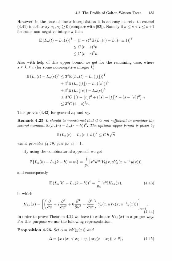
4.2 The Profile of Galton-Watson Trees 135
However, in the case of linear interpolation it is an easy exercise to extend(4.41) to arbitrary κ1, κ2 ≥ 0 (compare with [92]). Namely if k ≤ s < t ≤ k+1for some non-negative integer k then
E (Ln(t)− Ln(s))4
= (t− s)4 E (Ln(r)− Ln(r ± 1))4
≤ C (t− s)4n≤ C (t− s)2n.
Also with help of this upper bound we get for the remaining case, wheres ≤ k ≤ t (for some non-negative integer k)
E (Ln(t)− Ln(s))4 ≤ 34E (Ln(t)− Ln(�t�))4
+ 34E (Ln(�t�)− Ln(�s�))4
+ 34E (Ln(�s�)− Ln(s))4
≤ 34C((t− �t�)2 + (�s� − �t�)2 + (s− �s�)2
)n
≤ 34C (t− s)2n.
This proves (4.42) for general κ1 and κ2.
Remark 4.25 It should be mentioned that it is not sufficient to consider thesecond moment E (Ln(r) − Ln(r + h))
2. The optimal upper bound is given by
E (Ln(r) − Ln(r + h))2 ≤ C h√n
which provides (4.19) just for α = 1.
By using the combinatorial approach we get
P{Ln(k)− Ln(k + h) = m} =1
yn[xnum]Yk(x, uYh(x, u−1y(x)))
and consequently
E (Ln(k)− Ln(k + h))4 =1
yn[xn]Hkh(x), (4.43)
in which
Hkh(x) =
[(∂
∂u+ 7
∂2
∂u2+ 6
∂3
∂u3+∂4
∂u4
)Yk(x, uYh(x, u−1y(x)))
]u=1
.
(4.44)In order to prove Theorem 4.24 we have to estimate Hkh(x) in a proper way.For this purpose we use the following representation.
Proposition 4.26. Set α = xΦ′(y(x)) and
Δ = {x : |x| < x0 + η, | arg(x − x0)| > θ}, (4.45)
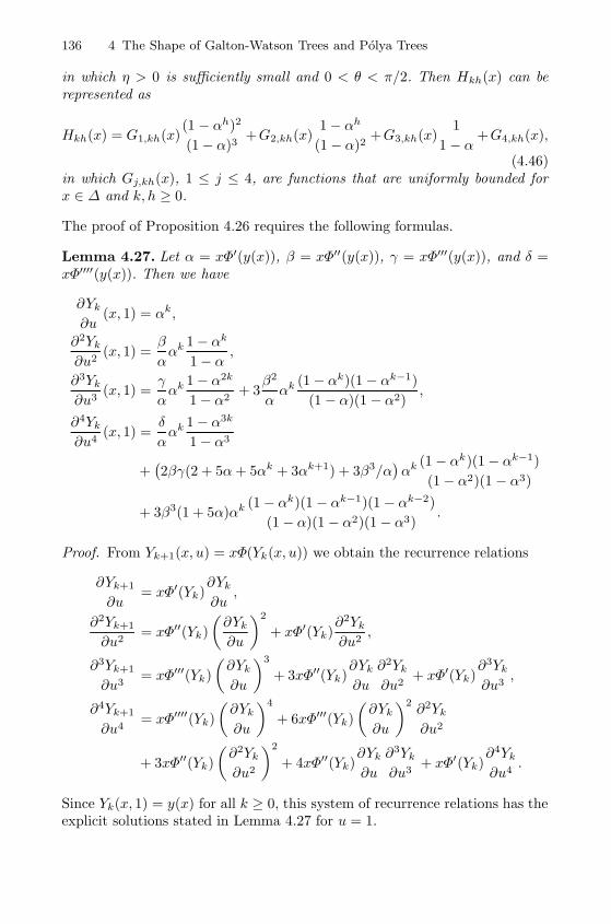
136 4 The Shape of Galton-Watson Trees and Polya Trees
in which η > 0 is sufficiently small and 0 < θ < π/2. Then Hkh(x) can berepresented as
Hkh(x) = G1,kh(x)(1 − αh)2
(1− α)3+G2,kh(x)
1− αh
(1− α)2+G3,kh(x)
1
1 − α +G4,kh(x),
(4.46)in which Gj,kh(x), 1 ≤ j ≤ 4, are functions that are uniformly bounded forx ∈ Δ and k, h ≥ 0.
The proof of Proposition 4.26 requires the following formulas.
Lemma 4.27. Let α = xΦ′(y(x)), β = xΦ′′(y(x)), γ = xΦ′′′(y(x)), and δ =xΦ′′′′(y(x)). Then we have
∂Yk
∂u(x, 1) = αk,
∂2Yk
∂u2(x, 1) =
β
ααk 1− αk
1− α ,
∂3Yk
∂u3(x, 1) =
γ
ααk 1− α2k
1− α2+ 3
β2
ααk (1− αk)(1 − αk−1)
(1 − α)(1 − α2),
∂4Yk
∂u4(x, 1) =
δ
ααk 1− α3k
1− α3
+(2βγ(2 + 5α+ 5αk + 3αk+1) + 3β3/α
)αk (1− αk)(1− αk−1)
(1− α2)(1 − α3)
+ 3β3(1 + 5α)αk (1− αk)(1 − αk−1)(1 − αk−2)
(1− α)(1 − α2)(1− α3).
Proof. From Yk+1(x, u) = xΦ(Yk(x, u)) we obtain the recurrence relations
∂Yk+1
∂u= xΦ′(Yk)
∂Yk
∂u,
∂2Yk+1
∂u2= xΦ′′(Yk)
(∂Yk
∂u
)2
+ xΦ′(Yk)∂2Yk
∂u2,
∂3Yk+1
∂u3= xΦ′′′(Yk)
(∂Yk
∂u
)3
+ 3xΦ′′(Yk)∂Yk
∂u
∂2Yk
∂u2+ xΦ′(Yk)
∂3Yk
∂u3,
∂4Yk+1
∂u4= xΦ′′′′(Yk)
(∂Yk
∂u
)4
+ 6xΦ′′′(Yk)
(∂Yk
∂u
)2∂2Yk
∂u2
+ 3xΦ′′(Yk)
(∂2Yk
∂u2
)2
+ 4xΦ′′(Yk)∂Yk
∂u
∂3Yk
∂u3+ xΦ′(Yk)
∂4Yk
∂u4.
Since Yk(x, 1) = y(x) for all k ≥ 0, this system of recurrence relations has theexplicit solutions stated in Lemma 4.27 for u = 1.
4.2 The Profile of Galton-Watson Trees 137
Proof. (Proposition 4.26) First we can use Lemma 4.27 to make (4.44) moreexplicit. Since
∂
∂uYk(x, uYh(x, u−1y(x))) =
∂Yk
∂u(x, uYh(x, u−1y(x)))
×(Yh(x, u−1y(x))− u−1y(x)
∂Yh
∂u(x, u−1y(x))
),
we obtain [∂
∂uYk(x, uYh(x, u−1y(x)))
]u=1
= y(x)αk(1 − αh).
Similarly[∂2
∂u2Yk(x, uYh(x, u−1y(x)))
]u=1
= y(x)2∂2Yk
∂u2(x, 1)(1 − αh)2 + y(x)2αk ∂
2Yh
∂u2(x, 1),[
∂3
∂u3Yk(x, uYh(x, u−1y(x)))
]u=1
= y(x)3∂3Yk
∂u3(x, 1)(1 − αh)3 + 3y(x)3
∂2Yk
∂u2(x, 1)
∂2Yh
∂u2(x, 1)(1 − αh),
− 3y(x)2αk ∂2Yh
∂u2(x, 1)− y(x)3αk ∂
3Yh
∂u3(x, 1),
and[∂4
∂u4Yk(x, uYh(x, u−1y(x)))
]u=1
= y(x)4∂4Yk
∂u4(x, 1)(1− αh)4 + 7y(x)4
∂3Yk
∂u3(x, 1)
∂2Yh
∂u2(x, 1)(1− αh)2
− 12y(x)4∂2Yk
∂u2(x, 1)
∂2Yh
∂u2(x, 1)(1 − αh)
+ 3y(x)4∂2Yk
∂u2(x, 1)
(∂2Yh
∂u2(x, 1)
)2
− 4y(x)4∂2Yk
∂u2(x, 1)
∂3Yh
∂u3(x, 1)(1− αh) + 12y(x)2αk ∂
2Yh
∂u2(x, 1)
+ 8y(x)3αk ∂3Yh
∂u3(x, 1) + y(x)4αk ∂
4Yh
∂u4(x, 1),
yielding an explicit expression of Hkh(x) in terms of y(x).Now notice that
supx∈Δ
|α| = 1, (4.47)
138 4 The Shape of Galton-Watson Trees and Polya Trees
since α = xΦ′(y(x)) has the local expansion (4.34). Hence, a representationof the form (4.46) follows immediately with functions Gj,kh(x), 1 ≤ j ≤ 4,which are uniformly bounded for x ∈ Δ.
The final step of the proof of Theorem 4.24 is to use (4.46) and the TransferLemma 2.12.
Proof. (Theorem 4.24) Since yn ∼ (τ/√
2πσ2)x−n0 n−3/2, Theorem 4.24 is
equivalent to
[xn]Hkh(x) = O
(x−n
0
h2
√n
)(4.48)
uniformly for all k, h ≥ 0. Note that Hk0(x) ≡ 0. So we may assume thath ≥ 1.
First, let us consider the first term ofHkh(x) (in the representation (4.46)):
G1,kh(x)(1 − αh)2
(1− α)3= G1,kh(x)
1
1 − α
h−1∑i=0
αih−1∑j=0
αj
=
h−1∑i,j=0
G1,kh(x)αi+j
1− α = O
(h2 1
|1− α|
).
Since1
1− α = O(
(1− x/x0)−1/2),
we can apply Lemma 2.12 (with β = 1/2) and obtain
G1,kh(x)(1 − αh)2
(1− α)3= O(x−n
0 h2n−1/2).
The coefficient of the second term is even smaller:
[xn]G2,kh(x)(1 − αh)
(1 − α)2= [xn]G2,kh(x)
1
1 − α
h−1∑i=0
αi
= O(x−n
0 hn−1/2)
= O(x−n
0 h2n−1/2).
Similarly we can handle the remaining terms:
[xn]G3,kh(x)1
1 − α = O(x−n
0 n−1/2)
= O(x−n
0 h2n−1/2)
and[xn]G4,kh(x) = O
(x−n
0 n−1)
= O(x−n
0 h2n−1/2).
Thus we have proved (4.48) which is equivalent to (4.41).
This also completes the proof of Theorem 4.10 in the case that the offspringdistribution ξ has finite exponential moments.
4.2 The Profile of Galton-Watson Trees 139
4.2.7 The Height of Galton-Watson Trees
We have already mentioned that the limiting distribution of the height Hn ofGalton-Watson trees is asymptotically given by
1√nHn
d−→ 2
σmax0≤t≤1
e(t),
where e(t) denotes the Brownian excursion of duration 1 (compare with The-orem 4.8).
In what follows we will shortly present a combinatorial proof of this lim-iting relation that goes back to Flajolet and Odlyko [82] who derived asymp-totics for all moments EHr
n in the binary case.The generating functions yk(x, u) that describe the profile of Galton-
Watson trees are closely related to the height distribution. Let yk(x) denotethe generating function of trees with height < k, that is,
yk(x) =∑n≥1
⎛⎝ ∑|T |=n, h(T )<k
ω(T )
⎞⎠ xn.
Then we haveyk(x) = yk(x, 0),
since LT (k) = 0, if and only if h(T ) < k. In particular we have
y0(x) = 0,
yk+1(x) = xΦ(yk(x)).
In the case of planted plane trees, that is Φ(x) = 1/(1−x), this recurrencecan be explicitly solved and is given by
yk(x) = y(x) − y(x)α(x)k
1 + y(x)√1−4x
(1− α(x)k),
where y(x) = (1 −√
1− 4x)/2 and α(x) = x/(1 − y(x))2. As we did in thecase of the profile we will show that such a relation holds asymptotically inthe general case. For convenience we set
ek(x) = y(x)− yk(x),
which is the generating function of the (weighted) numbers of trees of size nof height ≥ k.
We will also make use of a properly chosen Δ-region
Δ = Δ(x0, η, δ) = {x : |x| < x0 + η, | arg(x/x0 − 1)| > δ},
where η > 0 and 0 < δ < π2 . In particular we will choose η sufficiently small
and δ very close to π2 .
140 4 The Shape of Galton-Watson Trees and Polya Trees
Proposition 4.28. We have uniformly for x ∈ Δ and k ≥ 0
ek(x) =α(x)k
β(x)α(x)
1−α(x)k
1−α(x) +O(
min{log k, log 11−|α(x)|}
) ,where α(x) = xΦ′(y(x)) and β(x) = 1
2xΦ′′(y(x)).
With the help of these representations it is relatively easy to derive thecorresponding limiting result for the height.
Theorem 4.29. For every κ > 0 we have
P{Hn ≥ κ√n} =
σ
i√
2π
∫ −1+i∞
−1−i∞
√−2s e−s
exp(σκ√−2s)− 1
ds+ o(1). (4.49)
Furthermore, for all integers r ≥ 1
EHrn ∼(
2
σ
)r
2−r/2r(r − 1)Γ (r/2)ζ(r)nr/2, (4.50)
(where we make the convention (r − 1)ζ(r) = 1 for r = 1).
The integral representation (4.49) of the distribution of M = max0≤t≤1 e(t)is unusual; however, it perfectly fits into our asymptotic frame.
The proof of Proposition 4.28 relies on a precise analysis of the recurrence
ek+1(x) = y(x)− xΦ(y(x) − ek(x)). (4.51)
We start with some preliminary properties.
Lemma 4.30. Let h(x, v) be defined by
α(x)v
y(x)− xΦ(y(x) − v) = 1 +β(x)
α(x)v + v2h(x, v),
where α(x) = xΦ′(y(x)) and β(x) = 12xΦ
′′(y(x)). Then the functions ek(x)satisfy the recurrence
ek(x) =e0(x)α(x)k
1 + e0(x) β(x)α(x)
1−α(x)k
1−α(x) + e0(x)∑
�<k α(x)�e�(x)h(x, e�(x)). (4.52)
Note that h(x, v) is actually an analytic function in v, since the Taylor seriesexpansion of y(x)− xΦ(y(x) − v) is given by
y(x)− xΦ(y(x) − v) = α(x)v + β(x)v2 +O(v3) =α(x)v
1− β(x)α(x)v +O(v2)
.
4.2 The Profile of Galton-Watson Trees 141
Proof. By definition we have
ek+1 = y − xΦ(y − ek) =αek
1 + βαek + e2kh
or equivalently
α
ek+1=
1
ek
(1 +
β
αek + e2kh
)=
1
ek+β
α+ ekh.
By multiplying by αk we obtain
αk+1
ek+1=αk
ek+β
ααk + αkekh,
which givesαk
ek=
1
e0+β
α
1− αk
1− α +∑�<k
α�e�h(x, e�).
This proves the lemma.
Lemma 4.31. For |x| ≤ x0 we have
|ek(x)| ≤ ek(x0) ∼ 1
βk.
Proof. The inequality |ek(x)| ≤ ek(x0) is obvious, since the coefficients ofek are non-negative. Since y(x) is convergent at x = x0, it follows thatlimk→∞ ek(x0) = 0. This implies that∑
�<k
e�(x0)h(x0, e�(x0)) = o(k)
as k →∞. Hence, since α(x0) = 1, by (4.52) we obtain
ek(x0) =1
βk + o(k)∼ 1
βk.
Lemma 4.32. There exists a constant C with the property that if x ∈ Δ and
|ek(x)| < 1
C
(1
|α(x)| − 1
)(4.53)
then we have|ek+1(x)| < |ek(x)|.
In particular, if there exists some k with (4.53) then ek(x) = O(α(x)k) ask →∞.
142 4 The Shape of Galton-Watson Trees and Polya Trees
Proof. By Taylor’s expansion we have
y(x)− xΦ(y(x) − v) = α(x)v(1 +O(v))
and consequently
|y(x)− xΦ(y(x) − v)| < |α(x)| |v| (1 + C|v|)
for a properly chosen constant C > 0. Hence, if (4.53) is satisfied then
|ek+1(x)| = |y(x) − xΦ(y(x) − ek(x))|< |α(x)| |ek(x)| (1 + C|ek(x)|)≤ |ek(x)|.
Finally, if (4.53) is satisfied for some k = k0 then we can apply (4.53) recur-sively and consequently ek(x) stays bounded. We now use a shifted variant of(4.52), namely
ek(x) =α(x)k−k0
1ek0
+ βα
1−αk−k0
1−α +∑
�<k−k0α�ek0+�h(x, ek0+�)
, (4.54)
in order to prove that ek = O(αk). We only have to check that∣∣∣∣βα 1− αk
1− α
∣∣∣∣ ≤ 1
4
C|α|1− |α| , (4.55)
and that∣∣∣∣∣ ∑�<k−k0
α�ek0+�h(x, ek0+�)
∣∣∣∣∣ ≤ ‖h‖∞ 1− |α|C|α|
1− |αk|1− |α| ≤
1
4
C|α|1− |α| , (4.56)
so that (4.54) implies ek = O(αk). However, (4.55) and (4.56) are certainlysatisfied, if C is chosen sufficiently large, since x ∈ Δ implies |1−α| ≥ c(1−|α|)for some constant c > 0.
Remark 4.33 The value of the constant C can be made more precise, if weassume, for example, that we already know that ek(x) is sufficiently small. Inthis case we can assume that C is arbitrarily close to β(x0).
With the help of these preliminaries we obtain a first approximation forek(x), if x is far-off from the singularity.
Lemma 4.34. For every ε > 0 there exists δ > 0 such that
ek(x) = E(x)α(x)k +O(α(x)2k) (4.57)
uniformly for |x| ≤ x0+δ and |x−x0| ≥ ε, where E(x) = α(x)(1−α(x))/β(x).
4.2 The Profile of Galton-Watson Trees 143
Proof. If |x− x0| ≥ ε and |x| ≤ x0 + δ then we have uniformly |α(x)| ≤ 1− ηfor some η > 0. Now fix k0 such that
ek0(x0) <1
2C
η
1− η
where C is the constant given in Lemma 4.32. By continuity there exists δ > 0such that
|ek0(x)| < 1
C
η
1− ηuniformly for |x− x0| ≥ ε and |x| ≤ x0 + δ. Without loss of generality we canassume that δ ≤ ε. Hence, we also get
|ek0(x)| < 1
C
η
1− η ≤1
C
(1
|α| − 1
).
Thus, the assumptions of Lemma 4.32 are satisfied and we have ek(x) =O(α(x)k). Now with help of this a priori bound and (4.52) it follows thatek(x) can be represented in the form (4.57).
It is also quite easy to discuss the case |x− x0| ≤ ε but |x| ≤ x0.
Lemma 4.35. Suppose that |x−x0| ≤ ε but |x| ≤ x0. Then we have uniformlyin this range
ek(x) =α(x)k
β(x)α(x)
1−α(x)k
1−α(x) +O(
min{log k, log 11−|α(x)|}
) .Proof. Since we know a priori, that |ek(x)| ≤ ek(x0) ∼ α/(βk),∑
�<k
αle�h(x, e�) = O (min{log k, log 1/(1− |α|)}) ,
as k → ∞. Hence, a direct application of (4.52) completes the proof of thelemma.
It remains to discuss the asymptotic behaviour of ek(x), if x ∈ Δ but|x| ≥ x0. The problem is that it is not immediately clear that ek(x) → 0.Note, however, that ek(x0) ∼ 1/(βk). Thus, by continuity for every fixed k0
there is definitely ε > 0 such that |ek0(x)| ≤ (2α)/(βk0) for |x − x0| ≤ ε andx ∈ Δ. However, this does not guarantee that Lemma 4.32 can be applied.We have to use a different argument.
Lemma 4.36. There exists ε > 0 and a constant c1 > 0 such that for allx ∈ Δ with |x− x0| ≤ ε we have
|ek(x)| ≤ 1
C
(1
|α(x)| − 1
)
144 4 The Shape of Galton-Watson Trees and Polya Trees
for
k = K(x) =
⌊c1
| arg(α(x))|
⌋,
where C is the constant from Lemma 4.32.
Proof. The idea of the proof is to use formula (4.54), where k0 is chosen ina way that ek0(x) is sufficiently small and k is approximately c1/| arg(α(x))|,where c1 has to be chosen in a proper way. Suppose that we already knowthat
|ek0+�(x)| ≤ |ek0(x)| for � ≤ k − k0, (4.58)
then ∣∣∣∣∣ ∑�<k−k0
αlek0+�h(x, ek0+�)
∣∣∣∣∣ ≤ |ek0(x)| ‖h‖∞1− |α|k−k0
1− |α| .
Since |1 − α| ≤ c(1 − |α|) for x ∈ Δ (with a suitable constant c > 0) and|1 − αk−k0 | ≥ 1 − |α|k−k0 , it follows that this term can be made arbitrarilysmall compared to (β/α)(1−αk−k0 )/(1−α). Furthermore, if we assume thatarg(x0−x) = ϑ ∈
[−π
2 − ε′, π2 + ε′]
(for some ε′ > 0 that has to be sufficiently
small) and r = σ√
2|√
1− x/x0|, then
|α| = 1− r cosϑ
2+O(r2),
log |α| = −r cosϑ
2+O(r2),
arg(α) = −r sinϑ
2+O(r2).
Hence with k = K(x) = �c1/| arg(α)|� we have
|αk−k0 | ∼ e−c1 cot(ϑ/2)+O(r2) ≤ e−c1 cot( π4 + ε′
2 )+O(r2) ≤ e−c1(1−ε′′)
for some arbitrarily small ε′′ > 0 (depending on ε′). Consequently∣∣∣∣βα 1− αk−k0
1− α
∣∣∣∣ ≥ ∣∣∣∣βα∣∣∣∣ 1− e−c1(1−ε′′)
r.
Thus, if r is sufficiently small (that we can assume without loss of generality)then this term is actually much larger than 1/ek0.
In other words, if (4.58) holds then for k = K(x) = �c1/| arg(α)|� we have
|α|k−k0
|ek|≥∣∣∣∣βα 1− αk−k0
1− α
∣∣∣∣ (1− ε′′′),where ε′′′ > 0 can be chosen arbitrarily small, provided that k0 and ε areproperly chosen. Hence, if we want to conclude that |ek| ≤ (1/C)(1/|α| − 1),or equivalently, that
4.2 The Profile of Galton-Watson Trees 145
|α|k−k0
|ek|≥ C|α|k−k0+1
1− |α|then we just have to show that∣∣∣∣βα 1− αk−k0
1− α
∣∣∣∣ (1− ε′′′) ≥ C|α|k−k0+1
1− |α| (4.59)
for some ε′′′ > 0. Note that C is a constant that can be chosen arbitrarilyclose to β. Hence, if k = K(x) = �c1/| arg(α)|� then (4.59) is implied by therelation
e−c1 <1
1 + 1/√
2. (4.60)
Namely, if (4.60) is satisfied then there exists ε′ > 0, ε′′′ > 0 and some C > β/αsuch that ∣∣∣∣βα
∣∣∣∣ 1− e−c1 cot( π4 + ε′
2 )
r(1− ε′′′) ≥ C e
−c1 cot( π4 + ε′
2 )
r cos(π4 + ε′
2 )
which is asymptotically equivalent to (4.59).It remains to be shown that (4.58) is satisfied for k = K(x) = �c1/| arg(α)|�
with c1 > log(1 + 1/√
2) = 0.534799...For this purpose we show that the argument of ek(x) can be controlled.
In particular, we show that | arg(e�)| < π4 = 0.78539... for � ≤ k. If this
condition is satisfied, it is clear that for x ∈ Δ and |x− x0| ≤ ε we have (if e�is sufficiently small, too) ∣∣∣∣1− βαe� +O(e2� )
∣∣∣∣ ≤ 1,
and consequently
|e�+1| = |α| |e�|∣∣∣∣1− βαe� +O(e2� )
∣∣∣∣ ≤ |e�|.Moreover, the argument of e�+1 is given by
arg(e�+1) = arg(α) + arg(e�) + arg
(1− β
αe�(1 +O(e�))
)= arg(α) + arg(e�)
−∣∣∣∣βαe�∣∣∣∣ sin(c′′r sin
ϑ
2+O(r2) + arg(e�) +O(e�)
)for some real number c′′ and ϑ = arg(x0−x). Suppose that arg(e�) ≥ ε′′′′ > 0is large enough so that
c′′r sinϑ
2+O(r2) + arg(e�) +O(e�) > 0.
146 4 The Shape of Galton-Watson Trees and Polya Trees
Then it follows that
arg(e�+1) ≤ arg(α) + arg(e�).
In particular, it follows by induction
arg(e�) ≤ arg(ek0) + (�− k0) arg(α) + ε′′′′.
We can adapt ε such that | arg(ek0)| ≤ ε′′′′. Hence, if we apply this inequalityfor k − k0 = �c1/| arg(α)|� with c1 = π
4 − 2ε′′′′ then it follows that
| arg(e�)| ≤π
4
for k0 ≤ � ≤ k. Consequently we actually have |e�+1| ≤ |e�| and the inductionworks.
This also completes the proof of the lemma.
It is now easy to complete the proof of Proposition 4.28. Lemma 4.34 andLemma 4.35 cover the range |x| ≤ x0 + η and |x − x0| ≥ ε resp. the range|x| ≤ x0 and |x− x0| ≤ ε. In the remaining range x ∈ Δ, x ≥ x0, |x− x0| ≤ εwe use Lemma 4.36 and Lemma 4.32 to show that ek(x) → 0. From that itfollows that ∑
�<k
α�e�h(x, e�) = o
(1− |α|k1− |α|
)and consequently (by applying Lemma 4.30)
ek =αk
βα
1−αk
1−α (1 + o(1)).
This implies the upper bound
ek = O
(min
{1
k, (1− |α|)αk
}),
and consequently∑�<k
α�e�h(x, e�) = O
(min
{log k, log
1
1− |α|
}).
Hence a second application of Lemma 4.30 completes the proof of Proposi-tion 4.28.
The proof of Theorem 4.29 is based on the asymptotic formula for ek(x)that is given in Proposition 4.28. Recall that
P{Hn ≥ k} =1
yn[xn]ek(x) =
1
yn
1
2πi
∫Γ
ek(x)dx
xn+1,
4.2 The Profile of Galton-Watson Trees 147
where we use the same contour Γ = γ ′∪Γ ′ as in the proof of Proposition 4.21.Again it is sufficient to concentrate on the integral over
γ′ ={x = x0
(1 +
s
n
): �(s) = −1, |�(s)| ≤ C log2 n
}.
For x ∈ Γ ′ the functions ek(x) are uniformly bounded and hence the integral
over Γ ′ is bounded above by O(x−n0 e−C log2 n). On the other hand, if k =
�κ√n� the integral over γ ′ is asymptotically given by
1
2πi
∫γ′ek(x)
dx
xn+1∼ x−n
0 n−3/2 1
2πi
∫ −1+i∞
−1−i∞
exp(−σκ
√−2s)
β1−exp(−σκ
√−2s)
σ√−2s
e−s ds
= x−n0 n−3/2 τ
2πi
∫ −1+i∞
−1−i∞
√−2se−s
exp(σκ√−2s)− 1
ds.
Note that β(x0) = σ/τ . Since yn ∼ τ/(σ√
2π)x−n0 n−3/2, we obtain the pro-
posed asymptotic representation (4.49).In order to obtain the asymptotics for the moments (4.50) we observe that
the generating function of the r-th moment EHrn is given by∑
n≥1
EHrn ynx
n =∑k≥1
(kr − (k − 1)r) ek(x).
Since kr − (k − 1)r ∼ rkr−1 and ek ∼ (α/β)(1 − α)αk/(1 − αk), we have (asx→ x0 in Δ)
∑n≥1
EHrn ynx
n ∼ rαβ
(1 − α)∑k≥1
kr−1 αk
1− αk.
This kind of sum can be analysed with help of the following lemma.
Lemma 4.37. Let R ≥ 0 be a fixed real number. Then the function
DR(z) =∑k≥1
kR zk
1− zk
has radius of convergence 1 and we have, as z → 1 with | arg(1− z)| ≤ φ (forsome φ < π/2),
DR(z) ∼
⎧⎪⎪⎨⎪⎪⎩1
1− z log1
1− z for R = 0,
R!ζ(R + 1)
(1− z)R+1for R > 0.
Proof. We use the substitution z = e−x. Then the Mellin transform of thefunction
148 4 The Shape of Galton-Watson Trees and Polya Trees
FR(x) =∑k≥1
kR e−kx
1− e−kx
is given by
F ∗R(s) =
∫ ∞0
FR(x)xs−1 dx = Γ (s)ζ(s)ζ(s −R), (�(s) > R+ 1).
Hence, a standard inversion by using a shift of the line of integration in theinversion formula
FR(x) =1
2πi
∫ σ+i∞
σ−i∞F ∗R(s)xs ds
to σ < R + 1 and collecting the contributions of the polar singularity ats = R + 1 leads to the asymptotic leading term for the behaviour x → 0+.For R = 0 we have a double pole corresponding to (1/x) log(1/x), whereas forR > 0 there is a single pole with residue Γ (R + 1)ζ(R + 1)xR+1 (for detailssee [81]).
Note further that this procedure also works, if x→ 0 in the complex plane,provided that | arg(x)| ≤ φ with φ < π/2.
This implies that for r = 1 we obtain∑n≥1
EHn ynxn ∼ 1
2βlog
1
1− x/x0
and consequently
ynEHn ∼x−n
0
2β
1
n.
Since β = σ2/(2τ) and yn ∼ τ/(σ√
2π)x−n0 n−3/2, we get
EHn ∼√
2π
σ
√n
as proposed.Finally, for r > 1 we have
∑n≥1
EHrn ynx
n ∼ r!ζ(r)
β(σ√
2)r−1
(1− x
x0
) r−12
which leads to
EHrn ∼
2r!ζ(r)√
2π
σr2(r−1)/2Γ ( r−12 )
nr/2.
In view of the duplication formula for the Gamma function this is equivalentto (4.50).
Remark 4.38 With slightly more case it is also possible to derive a localversion of Theorem 4.29, that is, an asymptotic expansion for P{Hn = k} ifk is of order
√n (see [80]).
4.2 The Profile of Galton-Watson Trees 149
4.2.8 Depth-First Search
Aldous’ result on the normalised depth-first search process of Galton-Watsontrees (Theorem 4.7), saying that(
σ
2√nXn(2nt), 0 ≤ 1 ≤ t
)d−→ (e(t), 0 ≤ t ≤ 1)
is a fundamental observation in the framework of Galton-Watson trees. Itimplies convergence to the continuum random tree (Theorem 4.6) and alsoproves that the normalised occupation measure μn converges to the occupationmeasure of the Brownian excursion. Recall that Theorem 4.10 is a local versionof the latter observation.
Theorem 4.7 was first proved in the framework of the continuum randomtree [4]. One major step in Aldous’ method is to consider, for every fixedinteger k ≥ 1, random subtrees of Galton-Watson trees of size n that arespanned by k random vertices and the root and to show that there is a properlimiting object Rk.5 These limiting objects characterise then the limit of thedepth-first search process. Aldous shows that (up to a scaling factor 1/σ) allGalton-Watson trees have the same limiting object Rk. Since the normaliseddepth-first search process for planted plane trees (Φ(x) = 1/(2− x)) is knownto be the Brownian excursion, we obtain the same result for all Galton-Watsontrees. However, in order to check the existence of the limiting objects Rk onehas to invest several precise asymptotic properties of Galton-Watson trees,in particular of the height distribution (compare with [4] and [132]). Theadvantage of that approach is its universality, since it is not restricted toGalton-Watson trees.
In what follows we indicate an alternative proof with the help of combina-torial and analytic methods. As in the case of the profile we first prove finitedimensional convergence and then tightness (compare with [92]).
Lemma 4.39. Let x(·) denote the depth-first search process of a rooted treeand set
ak,m,n =∑
|T |=n, x(m)=k
ω(T ) = yn P{Xn(m) = k}.
Then the generating function Ak(x, u) =∑
m,n ak,m,nxnuk is given by
Ak(x, u) = A(x, u)Φ1(x, u, 1)k−1, (4.61)
where
A(x, u) = xuy(xu2)Φ(y(xu2))− y(x)Φ(y(x))
y(xu2)− y(x)
and
Φ1(x, u, v) = xuvΦ(y(xu2))− Φ(y(xv2))
y(xu2)− y(xv2).
5 We do not give a precise definition of these objects. For detail we refer to [4]).
150 4 The Shape of Galton-Watson Trees and Polya Trees
Proof. Suppose that k = 1, that is, the depth-first search process passes theroot. Recall that a Galton-Watson tree can be described as a root with i ≥ 0subtrees. Thus, there exists j with 0 ≤ j ≤ i such that the first j subtreeshave been already traversed but not the (j + 1)-st one. The correspondinggenerating function is then given by
A1(x, u) = xu∑i≥0
φi
i∑j=0
y(xu2)jy(x)i−j
= A(x, u).
If k > 1 then there exists a subtree of the root, in which the depth-first searchprocess passes a corresponding node at level k − 1. Hence, we get
Ak(x, u) = xu∑i≥0
φi
i−1∑j=0
y(xu2)jAk−1(x, u)y(x)i−j−1
= Ak−1(x, u)Φ1(x, u, 1).
By induction this completes the proof of the lemma.
The explicit representation of Ak(x, u) leads to an asymptotic expansionfor ak,m,n
Proposition 4.40. Suppose that κ > 0 and 0 < t < 1 are fixed real numbers.Then for k = �κ√n� and m = �2tn� we have, as n→∞,
ak,m,n
yn∼ 1
4√
2πn
σ3κ2
(t(1− t))3/2exp
(− σ2κ2
8t(1− t)
). (4.62)
Proof. By Cauchy’s formula
ak,m,n =1
(2πi)2
∫Γ
∫Γ
Ak(x, u)du
um+1
dx
xn+1,
where Γ and Γ a properly chosen contours around the origin. Here we use (asin the proof of Proposition 4.21) Γ = γ ′ ∪ Γ ′, where
γ′ ={x = x0
(1 +
s
n
): �(s) = −1, |�(s)| ≤ C log2 n
}with an arbitrarily chosen fixed constant C > 0 and Γ ′ is a circular arc centredat the origin and making Γ a closed curve. Similarly, Γ = γ′ ∪ Γ ′ with
γ′ ={u = 1 +
s1m
: �(s1) = −1, |�(s1)| ≤ C log2m}
with a properly chosen constant C and a circular arc Γ ′ making Γ a closedcurve.
4.2 The Profile of Galton-Watson Trees 151
We will only concentrate on γ ′ resp. on γ′. The remaining parts of theintegral are negligible (similarly to the proof of Proposition 4.21).
For x ∈ γ′ and u ∈ γ′ we use the approximations
y(x) = τ − τ√
2
σ
√− sn
+O
( |s|n
),
y(xu2) = τ − τ√
2
σ
√− sn− 2s1m
+O
( |s|n
+|s1|m
),
A(x, u) = 2τ +O
(√|s|n
+
√|s1|m
),
Φ1(x, u, 1) = 1− σ√2
(√− sn
+
√− sn− 2s1m
)+O
( |s|n
+|s1|m
).
We fix κ > 0 and 0 < t < 1 and set k = �κ√n� and m = �2tn�. Thus, weobtain the integral approximation
1
(2πi)2
∫γ′
∫γ′Ak(x, u)
dx
xn+1
du
um+1
∼ x−n0
mn
1
(2πi)2
∫ −1+iC log2 n
−1−iC log2 n
∫ −1+iC log2 m
−1−iC log2 m
2τ exp
(− σκ√
2
(√−s+
√−s− 2n
ms1
))e−s−s1 ds1 ds
∼ x−n0
mn
1
(2πi)2
∫ −1+i∞
−1−i∞
∫ −1+i∞
−1−i∞
2τ exp
(− σκ√
2
(√−s+
√−s− 1
ts1
))e−s−s1 ds1 ds.
By using the substitution s1 = w − ts, a proper shift of integration and byLemma 4.22 we can evaluate the double integral:
1
(2πi)2
∫ −1+i∞
−1−i∞
∫ −1+i∞
−1−i∞exp
(− σκ√
2
(√−s+
√−s− 1
ts1
))e−s−s1 ds1 ds
=1
(2πi)2
∫ −1+i∞
−1−i∞exp
(− σκ√
2
√−s)e−s(1−t)
×∫ −1+ts+i∞
−1+ts−i∞exp
(− σκ√
2t
√−w)e−w dw ds
=1
(2πi)2
∫ −1+i∞
−1−i∞exp
(− σκ√
2
√−s)e−s(1−t)
×∫ −1+i∞
−1−i∞exp
(− σκ√
2t
√−w)e−w dw ds
152 4 The Shape of Galton-Watson Trees and Polya Trees
=1
4π
σ2κ2
t1/2(1− t)3/2exp
(− σ2κ2
8(1− t) −σ2κ2
8t
).
Hence, (4.62) follows.
Note that (4.62) is in accordance with the density of the one dimensionaldensity of 2
σ e(t) (compare with (4.3)). By inspecting the above proof it isclear that all estimates are also uniform, if κ varies in a compact interval(contained in the positive real line). Hence, we also get weak convergence forevery 0 < t < 1:
σ
2√nXn(2nt)
d−→ e(t).
Similarly one can work out the finite dimensional case. For example, set
bk1,m1,k2,m2,n =∑
|T |=n, x(m1)=k1, x(m2)=k2
ω(T )
= ynP{Xn(m1) = k1, Xn(m2) = k2}.Then we have
Bk1,k2(x, u1, u2) =∑
m1,m2,n≥0
bk1,m1,k2,m2,nxnum1
1 um22
= A(x(u1u2)2, 1)A(x, u)Φ2(x, u1u2, u2)
×min{k1,k2}−1∑
r=0
Φ1(x, u1u2, u2)k1−1−rΦ1(x, u2, 1)k2−1−rΦ1(x, u1u2, 1)r,
where
Φ2(x, u, v) = x∑i≥2
φi
∑j1+j2+j3=i−2
y(xu2)j1y(xv2)j2y(x)j3 .
With the help of these explicit representations one obtains two dimensionalconvergence for 0 < t1 < t2 < 1:(
σ
2√nXn(2nt1),
σ
2√nXn(2nt2)
)d−→ (e(t1), e(t2)) .
The general case is even more involved (compare with [58, 92]).Finally, with the help of Bk1,k2(x, u1, u2) it is also possible to prove tight-
ness (see [92]).
Proposition 4.41. Set
en(t) :=σ
2√nXn(2nt).
Then there exist constants C,D > 0 such that for all s, t ∈ [0, 1] and ε > 0,
P{|en(s)− en(t)| ≥ ε} ≤ C√|s− t|
exp
(−D ε√
|s− t|
). (4.63)
4.2 The Profile of Galton-Watson Trees 153
Hence it follows that
P{|en(s)− en(t)| ≥ ε} ≤ C |s− t|α− 1
2
ε2α
for every α > 3/2. Thus, by [18, Theorem 12.3] the sequence of processes en(t)is tight.
Proof. The proof of Proposition 4.41 uses the explicit representation for
C�(x, u1, u2) =∑
|k1−k2|≥�
Bk1k2(x, u1, u2)
=A(x(u1u2)2, 1)A(x, u2)Φ2(x, u1u2, u2)
(1 − Φ1(x, u1u2, u2)Φ1(x, u2, 1))(1 − Φ1(x, u1u2, 1))
×(Φ1(x, u1u2, u2)�
1− Φ1(x, u1u2, u2)+
Φ1(x, u2, 1)�
1− Φ1(x, u2, 1)
).
Since um11 um2
2 = (u1u2)m1um2−m12 and we are interested in the dependence of
the difference d = m2−m1, it is appropriate to use the substitution u = u1u2
and to estimate the coefficient of xnum1ud2.
For this purpose one uses Cauchy’s formula for each variable, where weuse the same kind of integration as in the proof of Proposition 4.40, that isx ∈ Γ and u, u2 ∈ Γ ′. By using the local expansion of
Φ1(x, u, v) = 1− σ√2
⎛⎝√1− xu2
x0+
√1− xv
2
x0
⎞⎠+O
(∣∣∣∣1− xu2
x0
∣∣∣∣+ ∣∣∣∣1− xv2x0
∣∣∣∣)one obtains for x ∈ Γ and u, u2 ∈ Γ ′ the bounds
|(1− Φ1(x, u, u2)Φ1(x, u2, 1))(1− Φ1(x, u, 1))(1 − Φ1(x, u, u2))| ≥ C1
m1
√d,
|(1− Φ1(x, u, u2)Φ1(x, u2, 1))(1− Φ1(x, u, 1))(1 − Φ1(x, u2, 1))| ≥ C1
m1
√d,
andmax{|Φ1(x, u, u2)| , |Φ1(x, u2, 1)|} ≤ e−C2
√|u2|/d
for some constants C1, C2 > 0. Hence it follows that
[xnum1ud]C�(x, u/u2, u2) = O
(x−n
0
m1
√d
nm1de−C3�/
√d
)for some constant C3 > 0. Consequently
P{|Xn(m1)−Xn(m1 + d)| ≥ �} =[xnum1ud
2]C�(x, u/u2, u2)
yn
= O(√
n/de−C3�/√
d).
154 4 The Shape of Galton-Watson Trees and Polya Trees
This proves (4.63), if m1 = 2t1n and m2 = 2t2n are integers. However, it isan easy exercise to extend this estimate for the interpolated process for all0 < t1 < t2 < 1 (compare with the comments following Theorem 4.24). Thiscompletes the proof of Proposition 4.41.
4.3 The Profile of Polya Trees
We analyse next the profile of unlabelled rooted random trees, also calledPolya trees. In Section 3.1.5 we have already shown that the analysis of thiskind of trees is quite similar to that of Galton-Watson trees. Moreover, theshape of Polya trees has the same asymptotic behaviour as that of Galton-Watson trees. The height is of order
√n and – this is the main focus of this
section – the profile Ln(k) can be approximated by the local time of Brownianexcursion, too, although the uniform probability model cannot be realised onPolya trees as Galton-Watson trees. (We follow Drmota and Gittenberger[65].)
Theorem 4.42. Let Ln(k) denote the number of nodes at distance k to theroot in random Polya trees of size n and l(t) the local time of a Brownianexcursion of duration 1. Then(
1√nLn
(t√n), t ≥ 0
)d−→(b√ρ
2√
2· l(b√ρ
2√
2· t), t ≥ 0
)in C[0,∞), as n→∞, where b ≈ 2.6811266 is the constant and ρ ≈ 0.3383219the singularity appearing in equation (3.7).
The structure of the proof of Theorem 4.42 is very similar to that of Theo-rem 4.10. Following Theorem 4.14 we prove convergence of finite dimensionaldistributions and tightness. We start with the combinatorial setup that isbased on an involved recurrence; then we asymptotically solve this recurrencewhich leads to the proof of weak convergence of the finite dimensional dis-tributions. Finally, we check tightness according to the moment conditions ofTheorem 4.14.
We will also consider the height of Polya trees in Section 4.3.5.
4.3.1 Combinatorial Setup
First we recall some facts on unlabelled rooted trees T . Let tn denote thenumber of these trees of size n. Then the generating function
t(x) =∑n≥1
tnxn
satisfies the functional equation
4.3 The Profile of Polya Trees 155
t(x) = x exp
(t(x) +
1
2t(x2) +
1
3t(x3) + · · ·
). (4.64)
It has radius of convergence ρ ≈ 0.3383219 and a local singular expansion ofthe form t(x) = 1 − b(ρ − x)1/2 + c(ρ − x) + · · · , where b ≈ 2.6811266, andc = b2/3 ≈ 2.3961466. Recall, too, that this singular expansion can be usedto obtain an asymptotic formula for tn (compare with (3.9)).
In order to compute the distribution of the number of nodes in some givenlevels k1 < k2 < · · · < kd in a tree of size n we have to calculate the numbertk1,m1,k2,m2,···kd,md;n of trees of size n with mi nodes in level ki, i = 1, . . . , dand normalise by tn. As in the case of Galton-Watson trees we introduce thegenerating functions
tk1,k2,...,kd(x, u1, . . . , ud) =
∑m1,...,md,n
tk1,m1,k2,m2,···kd,md;n um11 um2
2 · · ·umd
d xn.
They can be recursively calculated. However, the procedure is more involvedthan that of Galton-Watson trees.
Lemma 4.43. For d = 1 we have
t0(x, u) = ut(x) (4.65)
tk+1(x, u) = x exp
⎛⎝∑i≥1
tk(xi, ui)
i
⎞⎠ , (k ≥ 0), (4.66)
and for d > 1 with integers 0 ≤ k1 < k2 < k3 < · · · < kd
t0,k2,...,kd(x, u1, . . . , ud) = u1tk2,...,kd
(x, u2, . . . , ud) (4.67)
tk1+1,k2+1,...,kd+1(x, u1, . . . , ud) = x exp
⎛⎝∑i≥1
tk1,k2,...,kd(xi, ui
1, ui2, . . . , u
id)
i
⎞⎠ .(4.68)
Proof. The proof is principally the same as that of Lemma 4.18. The onlydifference is that one has to apply the multiset construction for ordinarygenerating functions (compare with Section 2.1.1), now applied for severalvariables, if we proceed from one level to the next.
There is, however, a slight difference to the Galton-Watson case. There wecould define a function Yk(x, u) (see (4.31)) so that
yk1,...,kd(x, u1, . . . , ud)
= Yk1
(x, u1Yk2−k−1
(x, u2Yk3−k2(x, . . . , ud−1Ykd−kd−1
(x, uy(x)) · · · ))).
Such a representation is not present for Polya trees. Therefore we have to bemore precise in the asymptotic analysis. Even the case d = 1 requires muchmore care than in the Galton-Watson case.
156 4 The Shape of Galton-Watson Trees and Polya Trees
4.3.2 Asymptotic Analysis of the Main Recurrence
The asymptotic structure of tk(x, u) is very similar to that of yk(x, u) (in thecontext of Galton-Watson trees).
Proposition 4.44. Let x = ρ(1 + s
n
), where �(s) = −1, u = eiτ/
√n, and
k = �κ√n�. Moreover, assume that, as n → ∞, we have s = O(log2 n)
whereas τ and κ are fixed. Then we have, as n→∞,
tk(x, u)− t(x) ∼ b2ρ
2√n· iτ
√−s exp
(− 1
2κb√−ρs)
√−s exp
(12κb√−ρs)− iτb
√ρ
2 sinh(
12κb√−ρs)
=b√
2ρ√nΨκb
√ρ/(2
√2)
(s,iτb√ρ
2√
2
). (4.69)
As in the case of Galton-Watson trees we introduce the quantity
wk(x, u) = tk(x, u)− t(x). (4.70)
Obviously, wk(x, 1) = 0. Hence, we expect that wk(x, u) → 0 as k → ∞, if uis sufficiently close to 1 and x is in the analyticity range of t(x).
We start with a useful property of t(x).
Lemma 4.45. The generating function t(x) has the following properties:
1. For |x| ≤ ρ we have |t(x)| ≤ 1. Equality holds only for x = ρ.2. Let x = ρ
(1 + s
n
)with �(s) = −1 and |s| ≤ C log2 n for some fixed C > 0.
Then there is a c > 0 such that
|t(x)| ≤ 1− c√|s|n.
Proof. The first statement follows from the fact that t(x) has only positivecoefficients (except t0 = 0), t(ρ) = 1 and there are no periodicities. The secondstatement is an immediate consequence of the singular expansion (3.7) of t(x).
Next let us consider the derivative
γk(x, u) =∂
∂utk(x, u).
Lemma 4.46. For |x| < ρ+ η and arg(x− ρ) = 0 (where η > 0 is sufficientlysmall) the functions γk(x, 1) can be represented as
γk(x, 1) = Ck(x)t(x)k+1 , (4.71)
where Ck(x) are analytic and converge uniformly to an analytic limit functionC(x) (for |x| < ρ+ η and arg(x− ρ) = 0) with convergence rate
Ck(x) = C(x) +O(Lk),
4.3 The Profile of Polya Trees 157
for some L with 0 < L < 1. Furthermore we have C(ρ) = 12 b
2ρ.There also exist constants c1, c2, c3 > 0 with c3 <
π2 such that
|γk(x, u)| = O(|t(x)|k) (4.72)
uniformly for |u| ≤ 1, k|u− 1| ≤ c1, |x− ρ| < c2 and | arg(x− ρ)| ≥ c3.
Proof. A tree that has nodes at level k must have a size larger than k. Thus[xr]tk(x, u) does not depend on u for r ≤ k. Consequently, the lowest ordernon-vanishing term in the power series expansion of γk(x) = γk(x, 1) is oforder k+ 1. The power series expansion of t(x) starts with x. Hence Ck(x) =γk(x)t(x)−k−1 is analytic for |x| < ρ + η and arg(x − ρ) = 0. We will showthat the sequence (Ck(x))k≥0 has a uniform limit C(x) which has the requiredproperties.
Using the recurrence relation of tk(x, u) we get
γk+1(x, u) =∂
∂ux exp
⎛⎝∑i≥1
tk(xi, ui)
i
⎞⎠= x exp
⎛⎝∑i≥1
tk(xi, ui)
i
⎞⎠∑i≥1
∂
∂utk(xi, ui)ui−1
= tk+1(x, u)∑i≥1
γk(xi, ui)ui−1. (4.73)
Setting u = 1 this rewrites to
Ck+1(x)t(x)k+2 = Ck(x)t(x)k+2+t(x)(Ck(x2)t(x2)k+1 + Ck(x3)t(x3)k+1 + . . .
),
(4.74)resp. to
Ck+1(x) =∑i≥1
Ck(xi)t(xi)k+1
t(x)k+1. (4.75)
Set
Lk := sup|x|<ρ+η, arg(x−ρ) �=0
∑i≥2
|t(xi)|k+1
|t(x)|k+1.
If η > 0 is sufficiently small then
sup|x|<ρ+η, arg(x−ρ) �=0
|t(xi)||t(x)| < 1
for all i ≥ 2 and
sup|x|<ρ+η, arg(x−ρ) �=0
|t(xi)||t(x)| = O(L
i)
for some L with 0 < L < 1. Consequently we also get
158 4 The Shape of Galton-Watson Trees and Polya Trees
Lk = O(Lk)
for some L with 0 < L < 1. Thus, if we use the notation
‖f‖ = sup|x|<ρ+η, arg(x−ρ) �=0
|f(x)|
then (4.75) implies‖Ck+1‖ ≤ ‖Ck‖(1 + Lk) (4.76)
and also‖Ck+1 − Ck‖ ≤ ‖Ck‖Lk. (4.77)
Now (4.76) implies that the functions Ck(x) are uniformly bounded in Δ by
‖Ck‖ ≤ c0 :=∏�≥1
(1 + L�).
Furthermore, (4.77) implies that there exists a limit limk→∞ Ck(x) = C(x)that is analytic for |x| < ρ+η, arg(x−ρ) = 0; and we have uniform exponentialconvergence rate
‖Ck − C‖ ≤ c0∑�≥k
L� = O(Lk).
Hence, we get (4.71).Finally, note that (for |x| ≤ ρ)∑
k≥0
γk(x, 1) =∑n≥1
ntnxn.
However, if we use (4.71) we get uniformly for |x| < ρ+ η and arg(x− ρ) = 0∑k≥0
γk(x, 1) =∑k≥0
(C(x) + Lk)t(x)k+1
= C(x)t(x)
1 − t(x)+O(1)
which leads to an asymptotic expansion of the n-th coefficient of the form
ntn ∼C(ρ)
b√πρn−
12 ρ−n.
Note that here we have used the fact that C(x) is a continuous functionas the uniform limit of continuous functions Ck(x), where x = ρ is also apoint of continuity. By comparing this with the (known) expansion for tn ∼12b√ρ/πn−3/2ρ−n we obtain C(ρ) = 1
2b2ρ.
In order to obtain the upper bound (4.72) we set for � ≤ k
C� = sup |γ�(x, u)t(x)−�−1|,
4.3 The Profile of Polya Trees 159
where the supremum is over (x, u) with |u| ≤ 1, k|u − 1| ≤ c1, |x − ρ| < c2and | arg(x− ρ)| ≥ c3, where the constants c1, c2, c3 > 0 (with c3 <
π2 ) will be
chosen in the sequel. From (4.73) we get (as above) the inequality
C�+1 ≤ C� ec1C�/k (1 +O(L�)), (4.78)
where we have implicitly used the inequality
|t�+1| ≤ |t(x)| exp
⎛⎝∑i≥1
|w�(xi, ui)|i
⎞⎠≤ |t(x)|eC�|u−1|+O(L�).
Setc0 =∏j≥0
(1 +O(Lj))
and choose c1 > 0 such that e2c0c1 ≤ 2. We also choose c2 ≤ η and 0 < c3 <π2
such that |t(x)| ≤ 1 for |x − ρ| < c2 and | arg(x − ρ)| ≥ c3. Now if k > 0 isfixed, it follows by induction that if |u− 1| ≤ c1/k
C� ≤∏j<�
(1 +O(Lj)) · e2c0c1�/k ≤ 2c0 (� ≤ k).
This completes the proof of the lemma.
The representation (4.71) from Lemma 4.46 gives us a first indication ofthe behaviour of wk(x, u) for u close to 1. We expect that
wk(x, u) ≈ (u − 1)γk(x, 1) ∼ (u − 1)C(x)t(x)k . (4.79)
This actually holds (up to constants) in a proper range for u and x, althoughit is only partially true in the range of interest (see Proposition 4.44).
In order to make this more precise we derive estimates for the secondderivative
γ[2]k (x, u) =
∂2
∂u2tk(x, u).
Lemma 4.47. Suppose that |x| ≤ ρ − η for some η > 0 and |u| ≤ 1. Thenuniformly
γ[2]k (x, u) = O(t(|x|)k+1). (4.80)
There also exist constants c1, c2, c3 > 0 with c3 <π2 such that
γ[2]k (x, u) = O(k |t(x)|k+1) (4.81)
uniformly for |u| ≤ 1, k|u− 1| ≤ c1, |x− ρ| < c2 and | arg(x− ρ)| ≥ c3.
160 4 The Shape of Galton-Watson Trees and Polya Trees
Proof. By definition we have the recurrence
γ[2]k+1(x, u) = tk+1(x, u)
∑i≥1
iγ[2]k (xi, ui)u2i−2
+ tk+1(x, u)
⎛⎝∑i≥1
γk(xi, ui)ui−1
⎞⎠2
(4.82)
+ tk+1(x, u)∑i≥2
(i− 1)γk(xi, ui)ui−2
with initial condition γ[2]0 (x) = 0.
First suppose that |x| ≤ ρ− η for some η > 0 and |u| ≤ 1. Then we have
|γ[2]k (x, u)| ≤ γ
[2]k (|x|, 1). Thus, in this case it is sufficient to consider non-
negative real x ≤ ρ − η. We proceed by induction. Suppose that we already
know that γ[2]k (x) = γ
[2]k (x, 1) ≤ Dkt(x)k+1 (where D0 = 0). Then we get from
(4.82) and the already known bound γk(x, 1) ≤ Ct(x)k the upper bound
γ[2]k+1(x) ≤ Dkt(x)k+2 +Dkt(x)k+2
∑i≥2
it(xi)k+1
t(x)k+1
+ C2t(x)2k−1 + Ct(x)k+2∑i≥2
(i− 1)t(xi)k+1
t(x)k+1
≤ t(x)k+2(Dk(1 +O(Lk)) + C2t(ρ− η)k +O(Lk)
).
Consequently we can set
Dk+1 = Dk(1 +O(Lk)) + C2t(ρ− η)k +O(Lk)
and obtain that Dk = O (1) as k →∞ which proves (4.80).Next set (for � ≤ k)
D� = sup∣∣∣γ[2]
� (x, u)t(x)−�−1∣∣∣ ,
where the supremum is taken over |u| ≤ 1, k|u − 1| ≤ c1, |x − ρ| < c2 and| arg(x − ρ)| ≥ c3 and where c1, c2, c3 > 0 are chosen as in the proof ofLemma 4.46. By the same reasoning as in the proof of Lemma 4.46, where weuse the already proved bound |γ�(x, u) ≤ C|t(x)|�+1 we obtain
D�+1 ≤ D� ec1C/k(1 +O(L�)) + C2 ec1C/k +O(L�),
that is, we haveD�+1 ≤ α�D� + β�
with α� = ec1C/k(1 +O(L�)) and β� = C2 ec1C/k +O(L�). Hence we get
4.3 The Profile of Polya Trees 161
Dk ≤k−1∑j=0
βj
k−1∏i=j+1
αi
≤ k maxjβj e
c1C∏�≥0
(1 +O(L�))
= O(k).
This completes the proof of (4.81).
Using the estimates for γk(x, u) and γ[2]k (x, u) we derive the following rep-
resentations (4.83) for wk and Σk(x, u), where
Σk(x, u) =∑i≥2
wk(xi, ui)
i.
Lemma 4.48. There exist c1, c2, c3 > 0 with c3 <π2 such that
wk(x, u) = Ck(x)(u − 1)t(x)k+1 (1 +O(k|u− 1|)) (4.83)
uniformly for |u| ≤ 1, k|u− 1| ≤ c1, |x− ρ| < c2 and | arg(x− ρ)| ≥ c2, whereCk(x) = γk(x, 1)/t(x)k+1 is given in Lemma 4.46.
Furthermore we have for |x| ≤ ρ+ η (for some η > 0) and |u| ≤ 1
Σk(x, u) = Ck(x)(u − 1)t(x2)k+1 +O(|u− 1|2t(|x|2)k
), (4.84)
where the analytic functions Ck(x) are given by
Ck(x) =∑i≥2
Ck(xi)
(t(xi)
t(x2)
)k+1
. (4.85)
They have a uniform limit C(x) with convergence rate
Ck(x) = C(x) +O(Lk)
for some constant L with 0 < L < 1.
Proof. The first relation (4.83) follows from Lemma 4.46, Lemma 4.47 andTaylor’s theorem.
In order to prove (4.84) we first note that |xi| ≤ ρ − η for i ≥ 2 and|x| ≤ ρ+ η (if η > 0 is sufficiently small). Hence, by a second use of Taylor’stheorem we get uniformly
wk(xi, ui) = Ck(xi)(ui − 1)t(xi)k+1 +O(|ui − 1|2t(|xi|)k+1
)and consequently
162 4 The Shape of Galton-Watson Trees and Polya Trees
Σk(x, u) =∑i≥2
1
iCk(xi)(ui − 1)t(xi)k+1 +O
(|u− 1|2t(|x|2)k
)= (u− 1)Ck(x)t(x2)k+1 +O
(|u− 1|2t(|x|2)k
).
Here we have used the property that the sum
∑i≥2
Ck(xi)ui − 1
i(u − 1)
t(xi)k+1
t(x2)k+1
represents an analytic function in x and u. Finally, since Ck(x) = C(x) +O(Lk), it also follows that Ck(x) has a limit C(x) and the same order ofconvergence.
With these auxiliary results we are able to get a precise result for wk(x, u).
Lemma 4.49. There exists positive constants c1, c2, c3 with c3 <π2 such that
wk(x, u) =Ck(x)w0(x, u) t(x)k
1− 12Ck(x)w0(x, u)1−t(x)k
1−t(x) +O (|u− 1|)
as long as |u| ≤ 1, k|u− 1| ≤ c1, |x− ρ| ≤ c2, and | arg(x− ρ)| ≥ c3.
Proof. Since Σk(x, u) = O(wk(x, u)Lk) = O(wk(x, u)) (see Lemma 4.48), weobserve that wk(x, u) satisfies the recurrence relation (we omit the argumentsnow)
wk+1 = t(ewk+Σk − 1
)= t
(wk +
w2k
2+Σk +O(w3
k) +O(Σ2k)
)= twk
(1 +
wk
2+O(w2
k
)+O (Σk)
)(1 +
Σk
wk
).
Equivalently we have
t
wk+1+
tΣk
wkwk+1=
1
wk
(1− wk
2+O(w2
k
)+ O (Σk)
)=
1
wk− 1
2+O (wk) +O
(Σk
wk
),
and consequently
tk+1
wk+1=tk
wk− Σkt
k+1
wkwk+1− 1
2tk +O
(wkt
k)
+O
(Σkt
k
wk
).
Thus we get
4.3 The Profile of Polya Trees 163
tk
wk=
1
w0−
k−1∑�=0
Σ�
w�w�+1t�+1 − 1
2
1− tk1− t +O
(1− Lk
1− L
)+O
(w0
1− t2k
1− t2).
Now we use again Lemma 4.48 to obtain
w0
k−1∑�=0
Σ�
w�w�+1t�+1 =
k−1∑�=0
C�(x)t(x2)�+1 +O(|u− 1|t(|x|2)�
)C�(x)C�+1(x)t(x)�+1(1 +O(�|u − 1|))
=
k−1∑�=0
C�(x)
C�(x)C�+1(x)
t(x2)�+1
t(x)�+1+O(|u − 1|)
= ck(x) +O(u − 1)
with a proper function ck(x). Observe, too, that w01−t2k
1−t2 = O(1), if k|u−1| ≤c1. Hence we obtain the representation
wk =w0t
k
1− ck(x)− w0
21−tk
1−t +O (|u− 1|). (4.86)
Thus, it remains to verify that 1 − ck(x) = 1/Ck(x). By using (4.75) and(4.85) it follows that
Ck(x) =∑i≥2
Ck(xi)
(t(xi)
t(x2)
)k+1
= (Ck+1(x)− Ck(x))
(t(x)
t(x2)
)k+1
(4.87)
and consequently by telescoping
ck(x) =
k−1∑�=0
C�+1(x)− C�(x)
C�(x)C�+1(x)=
1
C0(x)− 1
Ck(x)= 1− 1
Ck(x).
Alternatively we can compare (4.86) with (4.83) for u → 1 which also shows1− ck(x) = 1/Ck(x). This completes the proof of the lemma.
The proof of Proposition 4.44 is now immediate. We substitute x =ρ(1 + s
n
)(where �(s) = −1), u = eiτ/
√n and set k = κ
√n. We also use
the local expansion t(x) = 1− b√ρ√
1− x/ρ+O(|x − ρ|). That leads to
t(x)k = exp(−κb√−ρs
)(1 +O
(κ√n
)).
Finally, since the functions Ck(x) are continuous and uniformly convergent toC(x), they are also uniformly continuous and, thus, Ck(x) ∼ C(ρ) = 1
2b2ρ.
Altogether this leads to
164 4 The Shape of Galton-Watson Trees and Polya Trees
w0(x, u) t(x)k
1Ck(x) −
w0(x,u)2
1−t(x)k
1−t(x) +O (|u− 1|)
=Ck(x)(u − 1)(1− t(x)) t(x)k+1
1− t(x) − Ck(x)w0(x,u)2 (1− t(x)k) +O (|u− 1| · |1− t(x)|)
∼ b2ρ
2√n· iτ
√−s exp
(− 1
2κb√−ρs)
√−s exp
(12κb√−ρs)− iτb
√ρ
2 sinh(
12κb√−ρs)
as proposed.
4.3.3 Finite Dimensional Limiting Distributions
We will use the results of the previous section to prove finite dimensionalconvergence. We only discuss the cases d = 1 and d = 2 in detail. As above,(l(t), t ≥ 0) denotes the local time of the Brownian excursion.
Proposition 4.50. Let κ > 0 and τ be given with |κτ | ≤ c. Then we have
limn→∞
Eeiτ 1√
nLn(κ
√n)
= E eiτ
b√
ρ
2√
2l(
b√
ρ
2√
2κ), (4.88)
and consequently
1√nLn(κ
√n)
d−→ b√ρ
2√
2· l(b√ρ
2√
2κ
).
Proof. By definition the generating function tk(x, u) can be interpreted as
tk(x, u) =∑n≥1
tn EuLn(k) xn
and consequently
EeiτLn(k)/√
n =1
tn[xn]tk
(x, eiτ/
√n).
In order to get asymptotics for this characteristic function we will use thelocal representation for tk(x, u) of Proposition 4.44 and the same contourintegration as in the proof of Proposition 4.21.
Let Γ = γ′ ∪ Γ ′ consist of a line
γ′ ={x = ρ(
1 +s
n
): �(s) = −1, |�(s)| ≤ C log2 n
}with an arbitrarily chosen fixed constant C > 0 and of Γ ′, a circular arccentred at the origin and making Γ a closed curve. Then
4.3 The Profile of Polya Trees 165
EeiτLn(k)/√
n =1
tn
1
2πi
∫Γ
tk
(x, eiτ/
√n) dx
xn+1(4.89)
= 1 +1
tn
1
2πi
∫Γ
wk
(x, eiτ/
√n) dx
xn+1. (4.90)
The contribution of Γ ′ is exponentially small, since for x ∈ Γ ′ we have
|x−n−1| ∼ ρ−ne−C log2 n, whereas∣∣∣yk
(x, eiτ/
√n)∣∣∣ is bounded.
If x ∈ γ′ then the local expansion (4.69) is valid for a proper range fork. In particular, we replace k by �κ√n�, u by eiτ/
√n and x by x0
(1 + s
n
). If
we assume that κ > 0 is given then the assumptions of Proposition 4.44 aresatisfied, if κτ ≤ c. Finally, by applying the approximation x−n = x−n
0 e−s(1+O(|s|2/n)) we observe that the integral
1
2πi
∫γ′wk
(x, eiτ/
√n) dx
xn+1
is approximated by
b√ρ ρ−n
2√π n3/2
√2√π
1+i∞∫−1−i∞
iτb2
√−ρs exp(− 12κb√−ρs )
√−2s exp( 1
2κb√−ρs )− iτb
√ρ√
2sinh(
12τb√−ρs) e−s ds.
Since tn ∼ 12b√ρ/πρ−nn−3/2 we thus obtain (4.88) for τ ≤ c/κ. But this
is sufficient to prove weak convergence (compare with the proof of Proposi-tion 4.21).
The corresponding property in the two dimensional case is the followingone.
Proposition 4.51. Let κ2 > κ1 > 0 and τ1, τ2 be given with |κ2τ1| ≤ c and|κ2τ2| ≤ c. Then we have
limn→∞
E eiτ1
1√n
Ln(κ1√
n)+iτ21√n
Ln(κ2√
n)= E e
iτ1b√
ρ
2√
2l(
b√
ρ
2√
2κ1)+iτ2
b√
ρ
2√
2l(
b√
ρ
2√
2κ2)
(4.91)and consequently(
1√nLn(κ1
√n),
1√nLn(κ2
√n)
)d−→(b√ρ
2√
2· l(b√ρ
2√
2κ1
),b√ρ
2√
2· l(b√ρ
2√
2κ1
)).
Proof. In order to prove two dimensional convergence we need precise asymp-totic properties of tk1,k2(x, u1, u2) for k1 = κ1
√n, k2 = κ2
√n, u1 = eiτ1/
√n
and u2 = eiτ2/√
n. Similarly to the above we define
wk1,k2(x, u1, u2) = tk1,k2(x, u1, u2)− t(x)
so that wk1,k2(x, 1, 1) = 0. We further have wk1,k2(x, u1, 1) = wk1(x, u1) andwk1,k2(x, 1, u2) = wk2(x, u2). Thus, the first derivatives are given by
166 4 The Shape of Galton-Watson Trees and Polya Trees[∂
∂u1wk1,k2(x, u1, u2)
]u1=u2=1
= γk1(x, 1),[∂
∂u2wk1,k2(x, u1, u2)
]u1=u2=1
= γk2(x, 1).
It is also possible to get bounds for the second derivatives of the formO(k2t(x)k1 ), if k1|u1− 1| ≤ c, k2|u2− 1| ≤ c, |x− ρ| < c, and | arg(x− ρ)| ≥ c. Hence, we can approximate wk1,k2(x, u1, u2) by
wk1,k2(x, u1, u2) = Ck1(x)(u1 − 1)t(x)k1+1 + Ck2(x)(u2 − 1)t(x)k2+1 (4.92)
+O(k2t(x)k1 (|u1 − 1|2 + |u2 − 1|2)
).
Similarly (and even more easily) we obtain a representation for
Σk1,k2(x, u1, u2) =∑i≥2
wk1,k2(xi, ui1, u
i2)
i
= Ck1 (x)(u1 − 1)t(x2)k1+1 + Ck2(x)(u2 − 1)t(x2)k2+1
+O(t(|x|2)k1 |u1 − 1|2 + t(|x|2)k2 |u2 − 1|2)
). (4.93)
Since k2−k1 ∼ (κ2−κ1)√n and t(x2) < 1 for |x| ≤ ρ+η, the term t(x2)k2+1 is
significantly smaller than t(x2)k1+1. Thus, in what follows it will be sufficientto consider just the first term Ck1(x)(u1 − 1)t(x2)k1+1.
We also assume that u1 = eiτ1/√
n and u2 = eiτ2/√
n, that is, u1 − 1 andu2 − 1 are (asymptotically) proportional. Since we have for x = ρ(1 + s/n)
t(x)k2−k1 ∼ exp(−(κ2 − κ1)b
√−ρs)
and since we can shift the line �(s) = −1 of integration to any parallel line�(s) = σ0 with σ0 < 0, we can always assure that the leading terms of wk1,k2 ,that is, Ck1 (x)(u1 − 1)t(x)k1+1 and Ck2 (x)(u2 − 1)t(x)k2+1, do not cancel tolower order terms.
By using the same reasoning as in the proof of Lemma 4.49 we get therepresentation
wk1,k2 =w0,k2−k1t
k1
1− fk1 −w0,k2−k1
21−tk1
1−t + O(|u1 − 1|+ |u2 − 1|),
where
fk1 = fk1(x, u1, u2)
= w0,k2−k1(x, u1, u2)
k1−1∑�=0
Σ�,k2−k1+�(x, u1, u2) t(x)�+1
w�,k2−k1+�(x, u1, u2)w�+1,k2−k1+�+1(x, u1, u2).
Note that
4.3 The Profile of Polya Trees 167
w0,k2−k1 = u1tk2−k1(x, u2)− t(x)
= (u1 − 1)t(x) + u1wk2−k1(x, u2)
= U +W,
where U and W abbreviate U = (u1 − 1)t(x) and W = u1wk2−k1(x, u2). Bythe above assumption we can assume that |W | < 1
2 |U | so that there is nocancellation.
Next by (4.92) and Lemma 4.49 it follows that w�,k2−k1+� can be repre-sented by
w�,k2−k1+� = (C�(x)U +W ) t(x)� (1 +O(�|u1 − 1|+ (�+ k2 − k1)|u2 − 1|)) .
Hence, fk can be approximated by (for simplicity we omit the error terms)
fk1 ∼ U(U +W )
k1−1∑�=0
C�(x) (t(x2)/t(x))�+1
(C�(x)U +W )(C�+1(x)U +W )
= (U +W )
k1−1∑�=0
(C�+1(x)U +W )− (C�(x)U +W )
(C�(x)U +W )(C�+1(x)U +W )
= (U +W )
(1
U +W− 1
CkU +W
)= 1− U +W
CkU +W,
where we have used the formula (4.87) and telescoping. Consequently, it fol-lows that
wk1,k2 ∼(U +W )tk1
U+WCkU+W − U+W
21−tk1
1−t
=(CkU +W )tk1
1− CkU+W2
1−tk1
1−t
.
Now if we use the approximations
Ck(x) ∼ b2ρ
2,
U = t(u1 − 1) ∼ iτ1√n,
W = u1wk2−k1(x, u2) ∼ b√
2ρ√nΨ (κ2−κ1)b
√ρ
2√
2
(s,iτ2b
√ρ
2√
2
),
tk1 ∼ exp
(−1
2κ1b√−ρs),
1− t ∼ b√ρ√s
n,
168 4 The Shape of Galton-Watson Trees and Polya Trees
we finally get
wk1,k2 ∼b√
2ρ√nΨκ1b
√ρ
2√
2
(s,iτ1b
√ρ
2√
2+ Ψ (κ2−κ1)b
√ρ
2√
2
(s,iτ2b
√ρ
2√
2
)).
(Recall, that Ψκ(s, t) is defined in (4.14).)Using this approximation it follows that the characteristic function of the
random vector(
1√nLn(k1), 1√
nLn(k2))
where k1 = �κ1√n� and k2 = �κ2
√n�
is asymptotically given by
E eit1Ln(k1)/√
n+it2Ln(k2)/√
n
=1
tn[xn]tk1,k2
(x, eit1/
√n, eit2/
√n)
= 1 +1
tn
1
2πi
∫Γ
wk1,k2
(x, eit1/
√n, eit2/
√n) dx
xn+1
= 1 +
√2
i√π
∫ σ0+i∞
σ0−i∞Ψκ1b
√ρ
2√
2
(s,iτ1b
√ρ
2√
2+ Ψ (κ2−κ1)b
√ρ
2√
2
(s,iτ2b
√ρ
2√
2
))e−s ds
+ o(1).
This completes the proof of the two dimensional case.
The general finite dimensional case now follows from an iterative use ofthe above techniques.
4.3.4 Tightness
In this section we will show that the sequence of random variables ln(t) =n−1/2Ln(t
√n), t ≥ 0 is tight in C[0,∞). As in the case of Galton-Watson trees
it is sufficient to prove the following property (compare with Theorem 4.24).
Theorem 4.52. There exists a constant C > 0 such that
E (Ln(k)− Ln(k + h))4 ≤ C h2n (4.94)
holds for all non-negative integers n, k, h.
The fourth moment in the above equation can be expressed as the coeffi-cient of a suitable generating function. We have
E (Ln(k)− Ln(k + h))4
=1
tn[xn]
[(∂
∂u+ 7
∂2
∂u2+ 6
∂3
∂u3+∂4
∂u4
)tk,k+h
(x, u,
1
u
)]u=1
where tk,k+h(x, u1, u2) is recursively given in Lemma 4.43. Thus, (4.94) isequivalent to
4.3 The Profile of Polya Trees 169
[xn]
[(∂
∂u+ 7
∂2
∂u2+ 6
∂3
∂u3+∂4
∂u4
)tk,k+h
(x, u,
1
u
)]u=1
≤ C h2
√nρ−n.
(4.95)Hence, it is sufficient to show that[(
∂
∂u+ 7
∂2
∂u2+ 6
∂3
∂u3+∂4
∂u4
)tk,k+h
(x, u,
1
u
)]u=1
= O
(h2
1− |t(x)|
)(4.96)
= O
(h2√
|1− x/ρ|
)
for x ∈ Δ and h ≥ 1. Recall that we have 1− |t(x)| ≥ c√|1− x/ρ| for x ∈ Δ
(for some constant c > 0).For convenience we use the notation6
γ[j]k (x) =
[∂jtk(x, u)
∂uj
]u=1
and γ[j]k,h(x) =
[∂jtk,k+h
(x, u, 1
u
)∂uj
]u=1
.
The main part of the proof of Theorem 4.52 is to provide upper bounds forthese derivatives. We have already derived upper bounds for γ [1](x) and γ[2](x)(compare with Lemma 4.46 and Lemma 4.47). However, we have to be moreprecise. On the other hand we use the convexity bound |t(x)| ≤ t(|x|) ≤ |x/ρ|for |x| ≤ ρ in order to simplify the calculations.
Lemma 4.53. We have
γ[1]k (x) =
{O (1) uniformly for x ∈ Δ,O(|x/ρ|k)
uniformly for |x| ≤ ρ, (4.97)
and
γ[1]k,h(x) =
{O(
hk+h
)uniformly for x ∈ Δ,
O(|x/ρ|k)
uniformly for |x| ≤ ρ,(4.98)
where L is constant with 0 < L < 1.
Proof. We already know that γ[1]k (x) = Ck(x)t(x)k , where Ck(x) = O (1) and
|t(x)| ≤ 1 for x ∈ Δ (see Lemma 4.46). By convexity we also have |t(x)| ≤ |x/ρ|for |x| ≤ ρ. Hence, we obtain γ
[1]k (x) = O
(|x/ρ|k)
for |x| ≤ ρ.The functions γ
[1]k,h(x) are given by the recurrence
γ[1]k+1,h(x) = t(x)
∑i≥1
γ[1]k,h(xi)
6 In Section 4.3.3 we already used the notation γ(x, u) for the first derivative andγ[2](x, u) for the second derivative. There will be no confusion, the only differenceis that we now always have u = 1.
170 4 The Shape of Galton-Watson Trees and Polya Trees
with initial value γ[1]0,h(x) = t(x)− γh(x). Hence, the representation γ
[1]k,h(x) =
γ[1]k (x) − γ[1]
h+k(x) follows by induction. Since γ[1]k (x) = (C(x) + O(Lk))t(x)k ,
we thus get that
γ[1]k,h(x) = O
(supx∈Δ
|t(x)k(1− t(x)h)|+ Lk
).
However, it is an easy exercise to show that
supx∈Δ
|t(x)k(1− t(x)h)| = O
(h
k + h
). (4.99)
For this purpose observe that if x ∈ Δ then we either have |t(x)− 1| ≤ 1 and|t(x)| ≤ 1, or |t(x)| ≤ 1− η for some η > 0. In the second case we surely have
|t(x)k(1 − t(x)h)| ≤ 2(1− η)k = O(Lk).
For the first case we set t = 1− ρeiφ and observe that∣∣1− (1 − ρeiφ)h∣∣ ≤ (1 + ρ)h − 1.
Hence, if k ≥ 3h we thus obtain that
|t(x)k(1− t(x)h)| ≤ max0≤ρ≤1
(1− ρ)k((1 + ρ)h − 1
)≤ h
k − h ≤2h
k + h.
If k < 3h,we obviously have
|t(x)k(1− t(x)h)| ≤ 2 ≤ 4h
k + h
which completes the proof of (4.99). Of course, we also have Lk = O(
hh+k
).
This completes the proof of the upper bound of γ[1]k,h(x) for x ∈ Δ.
Finally, the upper bound γ[1]k,h(x) = O
(|x/ρ|k)
follows from (4.97).
Lemma 4.54. We have
γ[2]k (x) =
{O(
min{k, 1
1−|t(x)|
})uniformly for x ∈ Δ,
O(|x/ρ|k)
uniformly for |x| ≤ ρ− η,(4.100)
and
γ[2]k,h(x) =
{O(
min{h, 1
1−|t(x)|
})uniformly for x ∈ Δ,
O(|x/ρ|k)
uniformly for |x| ≤ ρ− η,(4.101)
for every η > 0.
4.3 The Profile of Polya Trees 171
Proof. The bound γ[2]k (x) = O(|x/ρ|k) (for |x| ≤ ρ − η) and the bound
γ[2]k (x) = O(k) follow from Lemma 4.47. In order to complete the analysis
for γ[2]k (x) we recall the recurrence
γ[2]k+1(x) = t(x)
∑i≥1
iγ[2]k (xi) + t(x)
⎛⎝∑i≥1
γ[1]k (xi)
⎞⎠2
+ t(x)∑i≥2
(i− 1)γ[1]k (xi)
(4.102)that we rewrite to
γ[2]k+1(x) = t(x)γ
[2]k (x) + bk(x),
where
bk(x) = t(x)∑i≥2
iγ[2]k (xi) + t(x)
⎛⎝∑i≥1
γ[1]k (xi)
⎞⎠2
+ t(x)∑i≥2
(i− 1)γ[1]k (xi).
Since γ[2]0 (x) = 0, the solution of this recurrence can be written as
γ[2]k (x) = bk−1(x) + t(x)bk−2(x) + · · ·+ t(x)k−1b0(x).
Hence bk(x) = O (1) uniformly for x ∈ Δ and consequently
γ[2]k (x) = O
⎛⎝k−1∑j=0
|t(x)|j⎞⎠ = O
(1
1− |t(x)|
).
This completes the proof of (4.100).
The recurrence for γ[2]h,k(x) is similar to that of γ
[2]k (x):
γ[2]k+1,h(x) = t(x)
∑i≥1
iγ[2]k,h(xi) + t(x)
⎛⎝∑i≥1
γ[1]k,h(xi)
⎞⎠2
+ t(x)∑i≥2
(i− 1)γ[1]k,h(xi)
(4.103)
with initial value γ[2]0,h(x) = γ
[2]h (x). We again use induction. Assume that we
already know that |γ [2]k,h(x)| ≤ Dk,h|x/ρ|k for |x| ≤ ρ−η and for some constant
Dk,h. By (4.101) we can set D0,h = Dh which is bounded as h→∞. We also
assume that |γ[1]k,h(x)| ≤ C|x/ρ|k for |x| ≤ ρ− η. Then by (4.103) we get
|γ[2]k+1,h(x)| ≤ Dk,h|x/ρ|k+1 +Dk,h|x/ρ|
2|x|2k/ρk
(1− |x|k)2
+ C2|x/ρ|( |x/ρ|k
1− |x|k)2
+ C|x/ρ| 2|x|2k/ρk
(1− |x|k)2.
Thus, we can set
172 4 The Shape of Galton-Watson Trees and Polya Trees
Dk+1,h = Dk,h
(1 +
2(ρ− η)k
(1− ρk)2
)+ C2 (ρ− η)k
(1− ρk)2+ C
2(ρ− η)k
(1 − ρk)2
which shows that the constants Dk,h are uniformly bounded. Consequently
γ[1]k,h(x) = O
(|x/ρ|k)
for |x| ≤ ρ− η.Next we assume that |γ [2]
k,h(x)| ≤ Dk,h for x ∈ Δ. We already know that
|γ[1]k,h(x)| ≤ C h
h+k for x ∈ Δ. Hence,
|γ[2]k+1,h(x)| ≤ Dk,h +Dk,h
∑i≥2
i|xi/ρ|k
+ C2
⎛⎝ h
k + h+∑i≥2
|xi/ρ|k⎞⎠2
+ C∑i≥2
(i− 1)|xi/ρ|k
≤ Dk,h + 8Dk,h(ρ+ η)2k/ρk
+ C2
(h
k + h+ 2(ρ+ η)2k/ρk
)2
+ 4C(ρ+ η)2k/ρk.
Thus, we can set
Dk+1,h = Dk,h + 8Dk,h(ρ+ η)2k/ρk + C2
(h
k + h+ 2(ρ+ η)2k/ρk
)2
+ 4C(ρ+ η)2k/ρk
with initial value D0,h = Dh = O (h) and obtain a uniform upper bound ofthe form
Dk,h = O (h) .
Consequently γ[2]k,h(x) = O (h) for x ∈ Δ.
Thus, in order to complete the proof of (4.101) it remains to prove
γ[2]k,h(x) = O (1/(1− |t(x)|)) for x ∈ Δ. Similarly to the above we represent
γ[2]k,h(x) as
γ[2]k,h(x) = γ
[2]0,h(x) + ck−1,h(x) + t(x)ck−2,h(x) + · · ·+ t(x)k−1c0,h(x), (4.104)
where
cj,h(x) = t(x)∑i≥2
iγ[2]j,h(xi) + t(x)
⎛⎝∑i≥1
γ[1]j,h(xi)
⎞⎠2
+ t(x)∑i≥2
(i− 1)γ[1]j,h(xi).
Observe that there exists η > 0 such that |xi| ≤ ρ − η for i ≥ 2 and x ∈ Δ.
Hence it follows that cj,h(x) = O (1) for x ∈ Δ. Since γ[2]0,h(x) = γ
[2]h (x) =
O (1/(1− |t(x)|)), we consequently get
γ[2]k,h(x) = γ
[2]h (x) +O
(1
1− |t(x)|
)= O
(1
1− |t(x)|
).
4.3 The Profile of Polya Trees 173
Remark 4.55 Note that the estimates of Lemma 4.54 already prove that
E (Ln(k)− Ln(k + h))2 = O(h√n).
Unfortunately, this estimate is not sufficient to prove tightness. We have todeal with the 4-th moments.
Before we start with bounds for γ[3]k (x) and γ
[4]k (x) we need an auxiliary
bound.
Lemma 4.56. We have uniformly for x ∈ Δ∑k≥0
|γ[1]k,h(x)γ
[2]k,h(x)| = O
(h2). (4.105)
Proof. We use the representation (4.104), where we can approximate cj,h(x)by
cj,h(x) = t(x)γ[1]j,h(x)2 +O
(Lj)
= O
(h2
(k + h)2
)uniformly for x ∈ Δ with some constant L that satisfies 0 < L < 1. Further-more, we use the approximation
γ[1]k,h(x) = C(x)t(x)k(1− t(x)h) +O
(Lk)
that is uniform for x ∈ Δ. This shows∑k≥0
|γ[1]k,h(x)| = |C(x)| |1 − t(x)h|
1− |t(x)| +O (1) .
Now observe that for x ∈ Δ there exists a constant c > 0 with |1 − t(x)| ≥c(1− |t(x)|). Hence it follows that
|1− t(x)h|1− |t(x)| = O
(1− t(x)h
1− t(x)
)= O (h) ,
and consequently ∑k≥0
|γ[1]k,h(x)| = O (h) .
Similarly we get
∑k≥1
|γ[1]k,h(x)|
∣∣∣∣∣∣∑j<k
t(x)k−j−1cj,h(x)
∣∣∣∣∣∣ ≤∑j≥0
|cj,h(x)| |t(x)|−j−1∑k>j
|t(x)|k|γ[1]k,h(x)|
=∑j≥0
|cj,h(x)| |t(x)|−j−1
(|C(x)| |t(x)|2j+2 |1 − t(x)h|
1− |t(x)|2 +O(|t(x)|j+1Lj
))
= O
⎛⎝∑j≥0
h3
(j + h)2
⎞⎠= O(h2).
174 4 The Shape of Galton-Watson Trees and Polya Trees
Hence, we finally obtain
∑k≥0
|γ[1]k,h(x)γ
[2]k,h(x)| ≤
∑k≥0
|γ[1]k,h(x)| |γ[2]
k,h(x)|+∑k≥1
|γ[1]k,h(x)|
∣∣∣∣∣∣∑j<k
t(x)k−j−1cj,h(x)
∣∣∣∣∣∣= O(h2).
Lemma 4.57. We have
γ[3]k (x) =
{O(
min{k2, k1−|t(x)|}
)uniformly for x ∈ Δ,
O(|x/ρ|k)
uniformly for |x| ≤ ρ− η,(4.106)
and
γ[3]k,h(x) =
{O(
min{h2, h1−|t(x)|}
)uniformly for x ∈ Δ,
O(|x/ρ|k)
uniformly for |x| ≤ ρ− η,(4.107)
for every η > 0.
Proof. The recurrence for γ[3]k (x) is given by
γ[3]k+1(x) = t(x)
∑i≥1
i3γ[3]k (xi) + t(x)
⎛⎝∑i≥i
γ[1]k (xi)
⎞⎠3
+ 3t(x)
⎛⎝∑i≥1
γ[1]k (xi)
⎞⎠⎛⎝∑i≥1
iγ[2]k (xi)
⎞⎠ (4.108)
+ 3t(x)
⎛⎝∑i≥1
γ[1]k (xi)
⎞⎠⎛⎝∑i≥1
(i− 1)γ[i]k (xi)
⎞⎠+ 3t(x)
∑i≥1
i(i− 1)γ[2]k (xi) + t(x)
∑i≥1
(i− 1)(i− 2)γ[1]k (xi).
By inspecting the proof of Lemmas 4.53 and 4.54 one expects that the onlyimportant part of this recurrence is given by
γ[3]k+1(x) = t(x)γ
[3]k (x) + t(x)γ
[1]k (x)3 + 3t(x)γ
[1]k (x)γ
[2]k (x) +Rk (4.109)
and Rk collects the less important remainder terms that only contribute expo-nentially small terms. Thus, in order to shorten our presentation we will not
focus on Rk. In particular, it is easy to show the bound γ[3]k (x) = O
(|x/ρ|k)
for |x| ≤ ρ− η. (We omit the details.)
Next, since t(x)γ[1]k (x)3 + 3t(x)γ
[1]k (x)γ
[2]k (x) + Rk = O (k), it follows that
γ[3]k (x) = O
(k2).
4.3 The Profile of Polya Trees 175
Now we proceed by induction and observe that a bound of the form
|γ[3]k (x)| ≤ Ek/(1− |t(x)|) leads to
|γ[3]k+1(x)| ≤ Ek
1− |t(x)| +O
(1
1− |t(x)|
)+ |Rk|
and consequently to Ek+1 ≤ Ek + O (1). Hence, Ek = O (k) and γ[3]k (x) =
O (k/(1− |t(x)|)).Similarly, the leading part of the recurrence for γ
[3]k,h(x) is given by
γ[3]k+1,h(x) = t(x)γ
[3]k,h(x) + t(x)γ
[1]k,h(x)3 + 3t(x)γ
[1]k,h(x)γ
[2]k,h(x) + Rk,h (4.110)
= t(x)γ[3]k,h(x) + dk,h(x),
where
dk,h(x) = t(x)γ[1]k,h(x)3 + 3t(x)γ
[1]k,h(x)γ
[2]k,h(x) + Rk,h = O (h) ,
and the initial value is given by
γ[3]0,h(x) = −γ[3]
h (x)− 3γ[2]h (x) = O
(min
{h2,
h
1− |t(x)|
}).
Note that we also assume that γ[3]k,h(x) = O
(|x/ρ|k)
for |x| ≤ ρ − η (whichcan be proved easily). Consequently it follows that
γ[3]k,h(x) = γ
[3]0,h(x) + dk−1,h(x) + t(x)dk−1,h(x) + · · ·+ t(x)k−1d0,h(x)
= O
(h
1− |t(x)|
).
Next observe that Lemmas 4.53–4.56 ensure that∑j≥0
|dj,h(x)| = O(h2)
uniformly for x ∈ Δ. Hence, we finally get
γ[3]k,h(x) = O
(h2),
which completes the proof of Lemma 4.57.
Lemma 4.58. We have
γ[4]k (x) =
{O(
k2
1−|t(x)|
)uniformly for x ∈ Δ,
O(|x/ρ|k)
uniformly for |x| ≤ ρ− η,(4.111)
and
γ[4]k,h(x) =
{O(
h2
1−|t(x)|
)uniformly for x ∈ Δ,
O(|x/ρ|k)
uniformly for |x| ≤ ρ− η,(4.112)
for every η > 0.

176 4 The Shape of Galton-Watson Trees and Polya Trees
Proof. The proof is very similar to that of Lemma 4.57. First, the recurrence
for γ[4]k (x) is essentially of the form
γ[4]k+1(x) = t(x)γ
[4]k (x) + t(x)γ
[1]k (x)4 + 4t(x)γ
[1]k (x)γ
[3]k (x) (4.113)
+ 6t(x)γ[1]k (x)2γ
[2]k (x) + 3t(x)γ
[2]k (x)2 +Rk,
where Rk collects all exponentially small terms. We assume that we have al-
ready proved the upper bound γ[4]k (x) = O
(|x/ρ|k)
for |x| ≤ ρ − η. Now,
by assuming that |γ[4]k (x)| ≤ Fk/(1 − |t(x)|) and by using the known esti-
mates γ[1]k (x) = O (1), γ
[2]k (x) = O (min{k, 1/(1− |t(x)|)}), and γ
[3]k (x) =
O (k/(1− |t(x)|)), we get
|γ[4]k+1(x)| ≤ Fk
1− |t(x)|+O(|t(x)|k)+O
(k
1− |t(x)|
)+O
(1
1− |t(x)|
)+|Rk|
≤ Fk+1
1− |t(x)|with Fk+1 = Fk +O(k). Consequently Fk = O
(k2).
Finally, the essential part of the recurrence for γ[4]k,h(x) is given by
γ[4]k+1,h(x) = t(x)γ
[4]k,h(x) + t(x)γ
[1]k,h(x)4 + 4t(x)γ
[1]k,h(x)γ
[3]k,h(x) (4.114)
+ 6t(x)γ[1]k,h(x)2γ
[2]k,h(x) + 3t(x)γ
[2]k,h(x)2 + Rk,h
= t(x)γ[4]k,h(x) + ek,h(x),
where
ek,h(x) = t(x)γ[1]k,h(x)4 + 4t(x)γ
[1]k,h(x)γ
[3]k,h(x)
+ 6t(x)γ[1]k,h(x)2γ
[2]k,h(x) + 3t(x)γ
[2]k,h(x)2 + Rk,h.
As above, Rk,h collects all exponentially small terms. Thus,
γ[4]k,h(x) = γ
[4]0,h(x) + ek−1,h(x) + t(x)ek−1,h(x) + · · ·+ t(x)k−1e0,h(x).
By applying the known estimates γ[1]k,h(x) = O (1), γ
[2]k,h(x) = O (h) and
γ[3]k,h(x) = O
(h2)
we obtain ek,h = O(h2). By combining that with the initial
condition
γ[4]0,h(x) = 12γ
[2]h (x) + 8γ
[3]h (x) + γ
[4]h (x) = O
(h2
1− |t(x)|
),
we finally get
γ[4]k,h(x) = O
(h2
1− |t(x)|
)which completes the proof of Lemma 4.58.
The proof of (4.96) is now immediate. As already noted this implies (4.95)and proves Theorem 4.52.
4.3 The Profile of Polya Trees 177
4.3.5 The Height of Polya Trees
Since the profile of Polya trees behaves similarly to the profile of conditionedGalton-Watson trees, there is no doubt that there is a similar correspondencefor the height (compare with [65]).
Theorem 4.59. Let Hn denote the height of an unlabelled rooted random treewith n vertices. Then we have
1√nHn
d−→ 2√
2
b√ρ
max0≤t≤1
e(t)
and
EHrn ∼(b√ρ
4
)r
r(r − 1)Γ (r/2)ζ(r)nr/2
for every integer r ≥ 1.
A similar theorem was proved by Broutin and Flajolet [28] for binary unla-belled trees who also provide a local version, that is, asymptotic expansionfor P{Hn = k} (compare with [80]). For the sake of brevity we will not makethis explicit but a local version of Theorem 4.59 still holds.
Let tn,k denote the number of trees with n nodes and height at most k.Then the generating function tk(x) =
∑n≥1 tn,kx
n satisfies the recurrencerelation
t0(x) = 0
tk+1(x) = x exp
⎛⎝∑i≥1
tk(xi)
i
⎞⎠ , (k ≥ 0).
Obviously tk(x) = tk(x, 0) where the function on the right-hand-side is thegenerating function of (4.28) which we used to analyse the profile in theprevious sections.
Setek(x) = t(x) − tk(x),
that is ek(x) = −wk(x, 0). Then ek satisfies the recurrence
ek+1(x) = t(x)(
1− e−ek(x)−Ek(x)), (4.115)
where
Ek(x) =∑i≥1
ek(xi)
i= −Σk(x, 0).
The proof follows the same principles as the proof of the correspondingproperties of the height of Galton-Watson trees (see Section 4.2.7). However,
178 4 The Shape of Galton-Watson Trees and Polya Trees
the term Ek(x) needs some additional considerations. In particular we willalways have to verify that in the range of interest, that is x ∈ Δ and |x−ρ| < ε,we have an estimate of the kind
|Ek(x)||ek(x)|2 = O(Lk) (4.116)
for some L < 1. Suppose for a moment that (4.116) is satisfied and that wealso know that ek = O(1). Then (4.115) rewrites to
ek+1 = tek
(1− ek
2+O
(e2k +
Ek
ek
)),
resp. tot
ek+1=
1
ek+
1
2+O
(ek +
Ek
e2k
).
This leads to the representation
tk
ek=
1
e0+
1
2
1− tk1− t +O
(∑�<k
|e�t�|)
+O
(∑�<k
|E�||e2� |
|t�|). (4.117)
Now, if (4.116) is satisfied then it follows that
ek =tk
12
1−tk
1−t + +O(∑
�<k |e�t�|)
+O(1)
which can be handled as in Section 4.2.7 to obtain
ek(x) =t(x)k
12
1−t(x)k
1−t(x) +O(
min{
log k, log 11−|t(x)|
}) . (4.118)
If ek(x) has this kind of asymptotic representation Theorem 4.59 follows. Wejust have to repeat the corresponding steps from Section 4.2.7.
Note that (4.117) and (4.118) can be made more precise. Set
Sk =e2k(e−Ek − 1
)(eek − 1) (1− e−ek−Ek)
,
and define a function h(v) by
v
1− e−v= 1 +
v
2+ v2h(v).
Then the recurrence ek+1 = t(1− e−ek−Ek) rewrites to
t
ek+1=
1
ek+
1
2+ ekh(ek) +
Sk
e2k
4.3 The Profile of Polya Trees 179
and leads to the explicit representations
tk
ek=
1
e0+
1
2
1− tk1− t +
∑�<k
e�h(e�)t� +∑�<k
S�
e2�t� (4.119)
and
ek =tk
1e0
+ 12
1−tk
1−t +∑
�<k e�h(e�)t� +∑
�<kS�
e2�t�. (4.120)
Note also that if we just assume ek → 0 and Ek = o(ek) as k→∞ then
Sk ∼ −Ek.
We start our precise analysis with an a priori bound for ek(x).
Lemma 4.60. Let |x| ≤ ρ. Then there is a C > 0 such that
|ek(x)| ≤ C√k
∣∣∣∣xρ∣∣∣∣k .
Proof. Obviously, we have
|ek(x)| =∑n>k
(tn − tkn)|x|n ≤∑n>k
tn|x|n.
The assertion follows now from tn ∼ cρ−nn−3/2 for some constant c > 0.
Lemma 4.60 applies to Ek(x).
Corollary 4.61 Suppose that |x| < √ρ. Then there exists a constant C0 > 0with
|Ek(x)| ≤ C0√k
∣∣∣∣x2
ρ
∣∣∣∣k .The next lemma shows that ek(x) behaves as expected if x is on the positive
real axis.
Lemma 4.62. Suppose that 0 ≤ x ≤ ρ is real. Then (4.118) holds.
Proof. Let ek(x) be defined by e0(x) = t(x) and by ek+1(x) = t(x)(1−e−ek(x))(for k ≥ 0). Then it follows by the methods of Section 4.2.7 that ek(x) behaveslike (4.118), even in a proper Δ-domain.
However, if 0 ≤ x ≤ ρ then we obtain by induction that ek(x) ≥ ek(x).Hence, by combining (4.118) with the upper bound from Lemma 4.60 we have
Ek(x)
ek(x)2≤ Ek(x)
ek(x)2= O(Lk)
for some L with 0 < L < 1. Thus, (4.116) is satisfied and we are done.
180 4 The Shape of Galton-Watson Trees and Polya Trees
The analysis of ek(x) for complex x with |x| ≤ ρ is also not too difficult.The next two lemmas consider the case |x| ≤ ρ and |x − ρ| ≤ ε and the case|x| ≤ ρ− ε.
Lemma 4.63. There exists ε > 0 such that (4.118) holds for all x with |x| ≤ ρand |x− ρ| ≤ ε.
Proof. Recall that |ek(x)| ≤ C/√k. Suppose that we can show that |Ek/e
2k| ≤
1. Then it follows that
|ek+1| ≥ |t| |ek| exp
(−C1|ek|
(1 +
|Ek||ek|2))
≥ |t| |ek|e−C2k−1/2
. (4.121)
with C2 = 2C1C.We now choose k0 sufficiently large that
e−2C2
√k ≤ 1
kand C2ρ
k/2e4C0
√k ≤ 1
hold for all k ≥ k0. We already know that ek(ρ) ∼ 2/k. Hence, by continuitythere exists ε > 0 with |ek0(x)| ≥ 1
k0and |t(x)| ≥ ρ1/4 for |x| ≤ ρ and
|x− ρ| ≤ ε. These assumptions imply
|ek0(x)| ≥ 1
k0≥ e−2C2
√k0 ≥ |t(x)|k0e−2C2
√k0
and (by Corollary 4.61)
|Ek0 ||e2k0
| ≤ C0ρk|t|−2ke4C2
√k ≤ C0ρ
k/2e4C2
√k ≤ 1
The goal is to show by induction that for k ≥ k0 and for |x| ≤ ρ and|x− ρ| ≤ ε
|ek| ≥ |t|ke−2C2
√k and
∣∣∣∣Ek
e2k
∣∣∣∣ ≤ 1. (4.122)
By assumption (4.122) is satisfied for k = k0. Now suppose that (4.122) holdsfor some k ≥ k0. Then (4.121) implies
|ek+1| ≥ |t| |ek|e−C2k−1/2
≥ |t|k+1e−2C2
√ke−C2k−1/2
≥ |t|k+1e−2C2
√k+1.
Furthermore
|Ek+1||e2k+1|
≤ C0ρk|t|−2k−2e4C2
√k+1 ≤ C0ρ
(k+1)/2e4C2
√k+1 ≤ 1.
4.3 The Profile of Polya Trees 181
Hence, we have proved (4.122) for all k ≥ k0.In the last step of the induction proof we also obtained the upper bound
|Ek||e2k|
≤ C0ρk/2e4C2
√k
which is sufficient to obtain the asymptotic representation (4.118).
Lemma 4.64. Suppose that |x| ≤ ρ − ε for some ε > 0. Then we have uni-formly
ek(x) = Ck(x)t(x)k = (C(x) + o(1))t(x)k
for some analytic function C(x). Consequently we have uniformly for |x| ≤√ρ− ε
Ek(x) = Ck(x)t(x2)k = (C(x) + o(1))t(x2)k
with an analytic function C(x).
Proof. If |x| ≤ ρ − ε then we have |ek(x)| ≤ ek(ρ − ε) = O(t(ρ − ε)k). Thus,we can replace the upper bound |ek(x)| ≤ C/
√k in the proof of Lemma 4.63
by an exponential bound which leads to a lower bound for ek(x) of the form
|ek(x)| ≥ c0|t(x)|k.
Hence, by using (4.120) the result follows with straightforward calculations.
The disadvantage of the previous two lemmas is that they only work for|x| ≤ ρ. In order to obtain some progress for |x| > ρ we have to find a properanalogue to Lemma 4.32. We fix a constant C > 0 such that
∣∣∣e−Ek(x) − 1∣∣∣ ≤ C√
k
( |x|2ρ
)k
for all k ≥ 1 and for all |x| ≤ √ρ. Furthermore we choose a proper Δ-domainΔ(ρ, η, δ) with ρ+ η <
√ρ such that |t(x)| < 1 for all x ∈ Δ.
Lemma 4.65. Suppose that x ∈ Δ such that |t(x)| > |x2/ρ| and that thereexist real numbers D1 and D2 with 0 < D1, D2 < 1 and some integer K ≥ 1with
|eK(x)| < D1, |t(x)|eD1 − 1
D1< D2, D1D2 + eD1
C√K
( |x|2ρ
)K
< D1.
(4.123)Then we have |ek(x)| < D1 for all k ≥ K and
ek(x) = O(t(x)k)
as k →∞, where the implicit constant might depend on x.
182 4 The Shape of Galton-Watson Trees and Polya Trees
Proof. By definition we have eK+1 = t(1 − e−eK−EK ). Hence, if we writee−Ek = 1 +Rk we obtain
|eK+1| ≤ |eK | |t|e|eK | − 1
|eK |+ e|eK |RK .
If (4.123) is satisfied then it follows that
|eK+1| ≤ D1D2 + eD1C√K
( |x|2ρ
)K
< D1.
Now we can proceed by induction and obtain |ek| < D1 for all k ≥ K. Notethat D2 < 1 and
∑k Rk = O(1) also imply that
ek = O(Dk2 ).
If we set ak = t(1− e−ek)/ek and bk = −e−ekRk we obtain the recurrence
ek+1 = ekak + bk
with an explicit solution of the form
ek = eK∏
K≤i<k
ai +∑
K≤j<k
bj∏
j<i<k
ai.
Since ek = O(Dk2 ), we have ∏
j<i<k
ai = t(x)k−jeO(1)
and consequently
bj∏
j<i<k
ai = O(t(x)k−j |x2/ρ|j
)= O(t(x)kLj
)for some L with 0 < L < 1. Hence,
ek = eKt(x)k−KeO(1) +O(t(x)kLK
)= O(t(x)k). (4.124)
Recall that ek(x) → 0 for |x| ≤ ρ. Using Lemma 4.65 we deduce thatek → 0 in a certain region that extends the circle |x| ≤ ρ.Lemma 4.66. For every ε > 0 there exists δ > 0 such that ek(x) → 0,if|x| ≤ ρ+ δ and |x− ρ| ≥ ε.
Proof. The same arguments as in the proof of Lemma 4.34 show that we canapply Lemma 4.65.
For the most interesting range, namely for x ∈ Δ and |x− ρ| ≤ ε, we needa proper variant of Lemma 4.36.
4.3 The Profile of Polya Trees 183
Lemma 4.67. There exists ε > 0 and a constant c1 > 0 such that for allx ∈ Δ with x ≥ ρ and |x − ρ| ≤ ε and arg(x) = 0 the conditions (4.123) aresatisfied for
k = K(x) =
⌊c1
| arg(t(x))|
⌋and properly chosen real numbers D1, D2. Consequently, ek(x) → 0.
Proof. The arguments are about the same as in Lemma 4.36, but there aresome essential differences.
Suppose that arg(x) and arg(t(x)) are positive and that K(x) =�c1/| arg(t(x))|�, where c1 = arccos(1/4)− ε1 and ε1 > 0 is arbitrarily small.
The first step is to prove that |ek(x)| ≤ ε2 and arg(ek(x)) ≤ k arg(t(x))+ε3for k0 ≤ k ≤ K(x), where ε2 > 0 and ε3 > 0 can be chosen arbitrarilysmall and k0 is sufficiently large. Here we use the recurrence (4.115) andproceed inductively as in the proof of Lemma 4.36. Note that 0 < arg(ek(x)) <arccos(1/4) ensures that |ek+1| ≤ |ek|+|Ek| and consequently, by Lemma 4.64and the property ek0(ρ) ∼ c/k0 it follows that
|ek(x)| ≤ |ek0 |+∑
k0≤�<k
|E�| < ε2
provided that k0 is chosen sufficiently large. (We do not repeat the details.)The second step is to prove a lower bound for ek(x) for k0 ≤ k ≤ K(x) of
the form |ek(x)| ≥ c|t(x)|k/k for some c > 0. By Lemma 4.64 Ek(x) = (C(x)+o(1))t(x2)k behaves nicely, if |x−ρ| ≤ ε. Suppose that |x| ≥ ρ and x ∈ Δ. Sincearg(t(x2)) is of order arg(t(x))2 we deduce that arg(Ek(x)) = O(arg(t(x))) fork0 ≤ k ≤ K(x). In particular, it follows that (for k0 ≤ k ≤ K(x))
|ek+1(x)| =∣∣∣t(x)(1 − e−ek(x)−Ek(x))
∣∣∣ ≥ |t(x)|(1 − e−|ek(x)|).
Hence, by applying the methods of Section 4.2.7 it follows that |ek(x)| ≥c|t(x)|k/k for some c > 0.
Finally we have to check that the conditions (4.123) are satisfied for k =K(x). First we use the formula
ek =tk−k0
1ek0
+ 12
1−tk−k0
1−t +∑
k0≤�<k e�h(e�)t� +∑
k0≤�<kS�
e2�t�. (4.125)
to show (as in the proof of Lemma 4.36) that the term
1
2
1− tk−k0
1− tdominates the denominator on the right-hand-side of the equation. The firstand the third term can be handled as in Lemma 4.36. Finally, due to the
184 4 The Shape of Galton-Watson Trees and Polya Trees
already obtained bounds |ek(x)| ≥ c|t(x)|k/k, Ek(x) = O(t(x2)k) and theproperty S� ∼ −E� the last term∑
k0≤�<k
S�
e2�t� = O(1)
and does not contribute to the main term, either. Summing up we have
|ek| ≤|t|k−k0∣∣∣ 12 1−tk−k0
1−t
∣∣∣(1 + ε4)
for an arbitrarily small ε4 > 0.We set arg(ρ − x) = ϑ, where we assume that ϑ ∈
[−π
2 − ε5, π2 + ε5]
(for
some ε5 > 0 that has to be sufficiently small), and r = b|ρ − x|1/2, whereb ≈ 2.6811266 is the constant appearing in Theorem 3.8. Then we have (as inthe proof of Lemma 4.36)
|t| = 1− r cosϑ
2+O(r2),
log |t| = −r cosϑ
2+O(r2),
arg(t) = −r sinϑ
2+O(r2).
Hence with k = K(x) = �c1/| arg(t)|� we have
|tk−k0 | ∼ e−c1 cot(ϑ/2)+O(r2) ≤ e−c1 cot( π4 +
ε52 )+O(r2) ≤ e−c1(1− ε6)
for some arbitrarily small ε6 > 0 (depending on ε5). Consequently
|ek| < D1 := 2e− arccos(1/4)
1− e− arccos(1/4)r(1 + ε7) = c′r,
where ε7 > 0 can be chosen arbitrarily small. Moreover
|t| = 1− r cosϑ
2+O(r2) ≤ 1− r√
2(1− ε8)
for some (small) ε8 > 0 and consequently
|t|eD1 − 1
D1= 1−(
1√2− e− arccos(1/4)
1− e− arccos(1/4)
)r(1 − ε9) +O(r2).
Thus, we are led to set
D2 := 1− 1
2
(1√2− e− arccos(1/4)
1− e− arccos(1/4)
)r = 1− c′′r
4.3 The Profile of Polya Trees 185
and the first two conditions of (4.123) are satisfied if r is sufficiently small.Since D1 −D1D2 = c′c′′r2 we just have to check whether
eD1C√k
∣∣∣∣x2
ρ
∣∣∣∣k < c′c′′r2.However, since k = K(x) ≥ c1
√2 r−1 the left hand side of this inequality is
definitely smaller than c′c′′r2 if r is sufficiently small. Hence all conditions of(4.123) are satisfied for k = K(x).
Lemma 4.68. There exists ε > 0 such that (4.118) holds for all x with x ∈ Δwith |x| ≥ ρ and |x− ρ| ≤ ε.
Proof. We recall that the properties ek = O(1) and (4.116) imply (4.118).By Lemma 4.67 we already know that ek → 0. Furthermore, we have upperbounds for Ek (see Lemma 4.64). Hence, it remains to provide proper lowerbounds for ek.
Since we already know that ek → 0 and |Ek| = O(Lk) (for some L < 1),the recurrence (4.115) implies
|ek+1| ≥ (1 − δ) (|ek| − |Ek|)
for some δ > 0 provided that x ∈ Δ and |x−ρ| < ε. Without loss of generalitywe can assume that L < (1 − δ)2. Hence
|ek| ≥ (1− δ)k −∑�<k
|E�|(1 − δ)k−� ≥ c0(1 − δ)k
for some constant c0 > 0. Consequently∣∣∣∣Ek
e2k
∣∣∣∣ = O
((L
(1 − δ)2)k).
As noted above, this upper bound is sufficient to deduce (4.118).
As already mentioned the proof of Theorem 4.59 is now a direct copy ofthe corresponding parts of the proof of Theorem 4.29 (compare with Sec-tion 4.2.7).

5
The Vertical Profile of Trees
Chapter 4 was devoted to the horizontal profile of certain classes of trees andwe have observed that this kind of profile can be approximated by the localtime of the Brownian excursion.
However, it is also possible to introduce a vertical profile of trees. For abinary tree, for example, we can define the vertical position of a vertex by thedifference between the number of steps to the right and to the left on the pathfrom the root. Then the vertical profile counts the number of nodes of a givenvertical position. Interestingly, this new kind of profile can be approximatedin terms of the ISE, the Integrated Super-Brownian Excursion.
The study of the vertical profile of binary trees is not only interestingfrom a probabilistic point of view. The generating functions related to theseproblem are interesting by themselves, since they have an explicit form thatis not understood from a combinatorial point of view.
Similar phenomena appear for embedded trees and so-called well balancedtrees. The latter kind of trees is of specific interest, since there is a bijection toquadrangulations – due to Schaeffer [188] – that transfers the (usual) profileof a quadrangulation to the profile of the labels of well balanced trees.
After a description of the Schaeffer bijection we survey the relations be-tween general (vertical) profiles in random trees and the ISE that turns outto be a universal limiting object. However, the main part of this chapter isdevoted to some special cases of this limit relation which can be worked outexplicitly and lead to integral representations for distribution of certain func-tionals of the ISE. These results are due to Bousquet-Melou [23] who extendedprevious work of Bouttier, Di Francesco and Guitter [25] considerably. Thegeneral convergence theorem to the ISE is based on the work of Aldous [5],Janson and Marckert [117], Bousquet-Melou and Janson [24], and Devroyeand Janson [52].
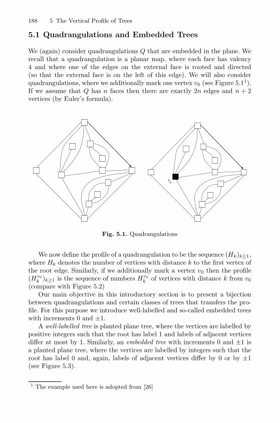
188 5 The Vertical Profile of Trees
5.1 Quadrangulations and Embedded Trees
We (again) consider quadrangulations Q that are embedded in the plane. Werecall that a quadrangulation is a planar map, where each face has valency4 and where one of the edges on the external face is rooted and directed(so that the external face is on the left of this edge). We will also considerquadrangulations, where we additionally mark one vertex v0 (see Figure 5.11).If we assume that Q has n faces then there are exactly 2n edges and n + 2vertices (by Euler’s formula).
v0
Fig. 5.1. Quadrangulations
We now define the profile of a quadrangulation to be the sequence (Hk)k≥1,where Hk denotes the number of vertices with distance k to the first vertex ofthe root edge. Similarly, if we additionally mark a vertex v0 then the profile(Hv0
k )k≥1 is the sequence of numbers Hv0
k of vertices with distance k from v0(compare with Figure 5.2)
Our main objective in this introductory section is to present a bijectionbetween quadrangulations and certain classes of trees that transfers the pro-file. For this purpose we introduce well-labelled and so-called embedded treeswith increments 0 and ±1.
A well-labelled tree is planted plane tree, where the vertices are labelled bypositive integers such that the root has label 1 and labels of adjacent verticesdiffer at most by 1. Similarly, an embedded tree with increments 0 and ±1 isa planted plane tree, where the vertices are labelled by integers such that theroot has label 0 and, again, labels of adjacent vertices differ by 0 or by ±1(see Figure 5.3).
1 The example used here is adopted from [26]
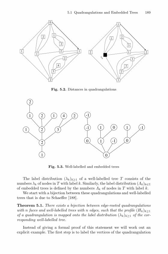
5.1 Quadrangulations and Embedded Trees 189
0
4
1
2
21
1 1
2
2
2
3
v0
2
1
1
1
12
2
2
3
3
3
Fig. 5.2. Distances in quadrangulations
1
1
1
2
2
2 3
41
2
2
1
1
0
-1
0
0 -1
1 0-1
-1
Fig. 5.3. Well-labelled and embedded trees
The label distribution (λk)k≥1 of a well-labelled tree T consists of thenumbers λk of nodes in T with label k. Similarly, the label distribution (Λk)k∈Z
of embedded trees is defined by the numbers Λk of nodes in T with label k.We start with a bijection between these quadrangulations and well-labelled
trees that is due to Schaeffer [188].
Theorem 5.1. There exists a bijection between edge-rooted quadrangulationswith n faces and well-labelled trees with n edges, such that the profile (Hk)k≥1
of a quadrangulation is mapped onto the label distribution (λk)k≥1 of the cor-responding well-labelled tree.
Instead of giving a formal proof of this statement we will work out anexplicit example. The first step is to label the vertices of the quadrangulation
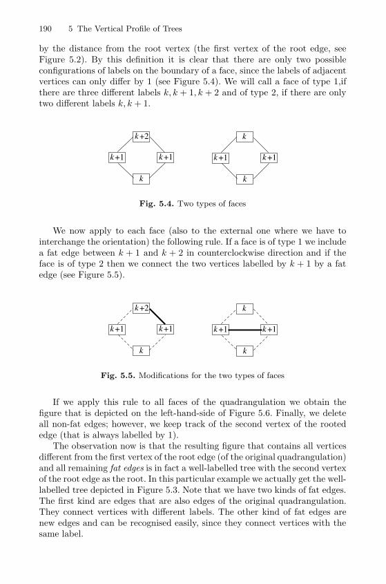
190 5 The Vertical Profile of Trees
by the distance from the root vertex (the first vertex of the root edge, seeFigure 5.2). By this definition it is clear that there are only two possibleconfigurations of labels on the boundary of a face, since the labels of adjacentvertices can only differ by 1 (see Figure 5.4). We will call a face of type 1,ifthere are three different labels k, k + 1, k + 2 and of type 2, if there are onlytwo different labels k, k + 1.
k
+1k +1k
+2k
k
+1k +1k
k
Fig. 5.4. Two types of faces
We now apply to each face (also to the external one where we have tointerchange the orientation) the following rule. If a face is of type 1 we includea fat edge between k + 1 and k + 2 in counterclockwise direction and if theface is of type 2 then we connect the two vertices labelled by k + 1 by a fatedge (see Figure 5.5).
k
+1k +1k
+2k
k
+1k +1k
k
Fig. 5.5. Modifications for the two types of faces
If we apply this rule to all faces of the quadrangulation we obtain thefigure that is depicted on the left-hand-side of Figure 5.6. Finally, we deleteall non-fat edges; however, we keep track of the second vertex of the rootededge (that is always labelled by 1).
The observation now is that the resulting figure that contains all verticesdifferent from the first vertex of the root edge (of the original quadrangulation)and all remaining fat edges is in fact a well-labelled tree with the second vertexof the root edge as the root. In this particular example we actually get the well-labelled tree depicted in Figure 5.3. Note that we have two kinds of fat edges.The first kind are edges that are also edges of the original quadrangulation.They connect vertices with different labels. The other kind of fat edges arenew edges and can be recognised easily, since they connect vertices with thesame label.
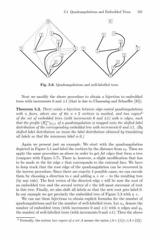
5.1 Quadrangulations and Embedded Trees 191
0
4
1
2
21
1 1
2
2
2
3
0
4
1
2
21
1 1
2
2
2
3
Fig. 5.6. Quadrangulations and well-labelled trees
Next we modify the above procedure to obtain a bijection to embeddedtrees with increments 0 and ±1 (that is due to Chassaing and Schaeffer [35]).
Theorem 5.2. There exists a bijection between edge-rooted quadrangulationswith n faces, where one of the n + 2 vertices is marked, and two copies2
of the set of embedded trees (with increments 0 and ±1) with n edges, suchthat the profile (Hv0
k )k≥1 of a quadrangulation is mapped onto the shifted labeldistribution of the corresponding embedded tree with increments 0 and ±1. (Byshifted label distribution we mean the label distribution obtained by translatingall labels so that the minimum label is 0.)
Again we present just an example. We start with the quadrangulationdepicted in Figure 5.1 and label the vertices by the distance from v0. Then weapply the same procedure as above in order to get fat edges that form a tree(compare with Figure 5.7). There is, however, a slight modification that hasto be made at the fat edge e that corresponds to the external face. We haveto keep track that the root edge of the quadrangulation can be recovered inthe inverse procedure. Since there are exactly 4 possible cases, we can encodethem by choosing a direction to e and adding a + or − to the resulting tree(by any rule). The first vertex of the directed edge e will be now the root ofan embedded tree and the second vertex of e the left-most successor of rootin this tree. Finally, we also shift all labels so that the new root gets label 0.In our example we get precisely the embedded tree of Figure 5.3 with a +.
We can use these bijections to obtain explicit formulas for the number ofquadrangulations and for the number of well-labelled trees. Let un denote thenumber of embedded trees (with increments 0 and ±1) with n edges and qnthe number of well-labelled trees (with increments 0 and ±1). Then the above
2 Formally, the notion two copies of a set A means the union (A×{1})∪ (A×{2}).
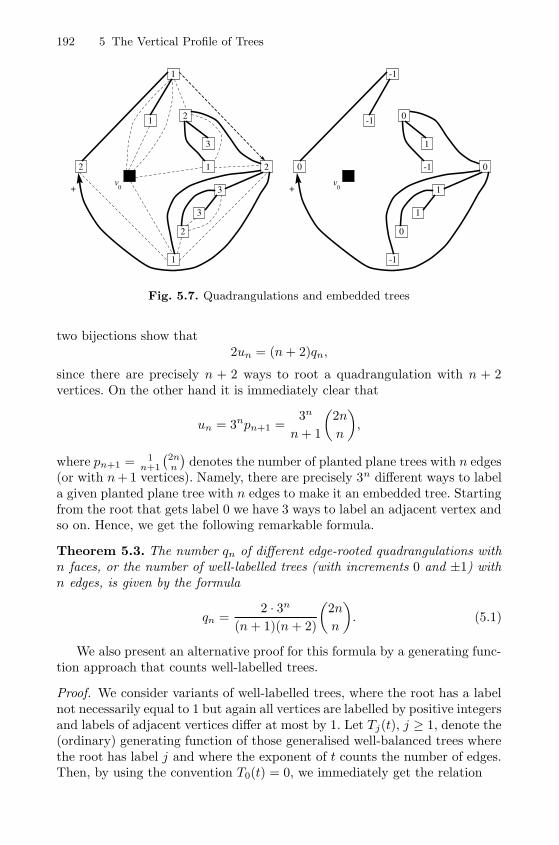
192 5 The Vertical Profile of Trees
v0
2
1
1
1
12
2
2
3
3
3
+v
0
0
-1
-1
-1
-10
0
0
1
1
1
+
Fig. 5.7. Quadrangulations and embedded trees
two bijections show that2un = (n+ 2)qn,
since there are precisely n + 2 ways to root a quadrangulation with n + 2vertices. On the other hand it is immediately clear that
un = 3npn+1 =3n
n+ 1
(2n
n
),
where pn+1 = 1n+1
(2nn
)denotes the number of planted plane trees with n edges
(or with n+ 1 vertices). Namely, there are precisely 3n different ways to labela given planted plane tree with n edges to make it an embedded tree. Startingfrom the root that gets label 0 we have 3 ways to label an adjacent vertex andso on. Hence, we get the following remarkable formula.
Theorem 5.3. The number qn of different edge-rooted quadrangulations withn faces, or the number of well-labelled trees (with increments 0 and ±1) withn edges, is given by the formula
qn =2 · 3n
(n+ 1)(n+ 2)
(2n
n
). (5.1)
We also present an alternative proof for this formula by a generating func-tion approach that counts well-labelled trees.
Proof. We consider variants of well-labelled trees, where the root has a labelnot necessarily equal to 1 but again all vertices are labelled by positive integersand labels of adjacent vertices differ at most by 1. Let Tj(t), j ≥ 1, denote the(ordinary) generating function of those generalised well-balanced trees wherethe root has label j and where the exponent of t counts the number of edges.Then, by using the convention T0(t) = 0, we immediately get the relation
5.1 Quadrangulations and Embedded Trees 193
Tj(t) =1
1− t(Tj−1(t) + Tj(t) + Tj+1(t)), (j ≥ 1). (5.2)
This relation comes from the usual decomposition of a planted plane tree intothe root and its subtrees. If the root has label j then the successors of the rootmust have a label in the set {j − 1, j, j + 1} and the subtrees are again well-balanced trees. This justifies (5.2). Note also that the infinite system (5.2)uniquely determines the functions Tj(t). In particular, the equations (5.2)provide a recurrence for the coefficients [tn]Tj(t) that can be solved by usingthe initial condition T0(t) = 0. For example we have indeed [t0]T0(t) = 0 and[t0]Tj(t) = 1 for j ≥ 1. Hence, it follows that [t1]T1(t) = 2 and [t1]Tj(t) = 3for j ≥ 2. In the same way we can proceed further. If we already know [tk]Tj(t)for all k ≤ n and all j ≥ 0 then [tn+1]Tj(t) can be computed for all j ≥ 1.Since [tn+1]T0(t) = 0 the induction works.
Let T (t) = (1−√
1− 12t)/(6t) be the solution of the equation
T (t) =1
1− 3tT (t), (5.3)
and let Z(t) be defined by
Z(t) +1
Z(t)+ 1 =
1
tT (t)2. (5.4)
Note that one of the two possible choices of Z(t) represents a power series in twith constant term 0 (and non-negative coefficients) which we will use in thesequel.
By using the ansatz
Tj(t) = T (t)ujuj+3
uj+1uj+2
with unknown functions uj , the recurrence (5.2) is equivalent to
ujuj+1uj+2uj+3 =1
T (t)u2
j+1u2j+2 (5.5)
+ tT (t)(uj−1u
2j+2uj+3 + u2
ju2j+3 + uju
2j+1uj+4
).
By using (5.3) and (5.4) it is easy to check that
uj = 1− Z(t)j
satisfies (5.5) which is kind of a mystery. Hence, the functions
Tj(t) = T (t)(1− Z(t)j)(1 − Z(t)j+3)
(1− Z(t)j+1)(1 − Z(t)j+2)(5.6)
satisfy the system of equations (5.2) and we also have T0(t) = 0. Since all thesefunctions Tj(t) are power series in t, we have found the solution of interest ofthe system (5.2).
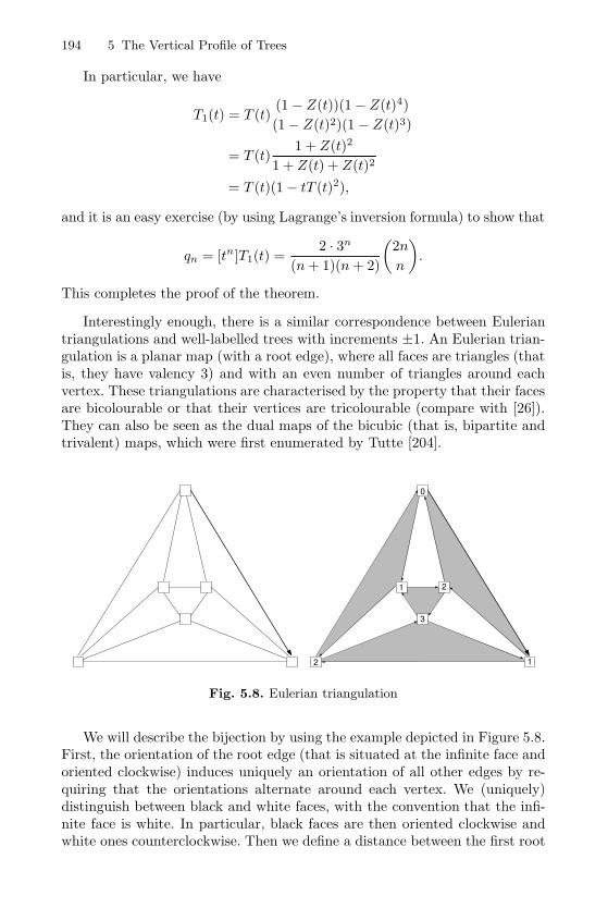
194 5 The Vertical Profile of Trees
In particular, we have
T1(t) = T (t)(1 − Z(t))(1− Z(t)4)
(1− Z(t)2)(1 − Z(t)3)
= T (t)1 + Z(t)2
1 + Z(t) + Z(t)2
= T (t)(1− tT (t)2),
and it is an easy exercise (by using Lagrange’s inversion formula) to show that
qn = [tn]T1(t) =2 · 3n
(n+ 1)(n+ 2)
(2n
n
).
This completes the proof of the theorem.
Interestingly enough, there is a similar correspondence between Euleriantriangulations and well-labelled trees with increments ±1. An Eulerian trian-gulation is a planar map (with a root edge), where all faces are triangles (thatis, they have valency 3) and with an even number of triangles around eachvertex. These triangulations are characterised by the property that their facesare bicolourable or that their vertices are tricolourable (compare with [26]).They can also be seen as the dual maps of the bicubic (that is, bipartite andtrivalent) maps, which were first enumerated by Tutte [204].
0
1
21
3
2
Fig. 5.8. Eulerian triangulation
We will describe the bijection by using the example depicted in Figure 5.8.First, the orientation of the root edge (that is situated at the infinite face andoriented clockwise) induces uniquely an orientation of all other edges by re-quiring that the orientations alternate around each vertex. We (uniquely)distinguish between black and white faces, with the convention that the infi-nite face is white. In particular, black faces are then oriented clockwise andwhite ones counterclockwise. Then we define a distance between the first root
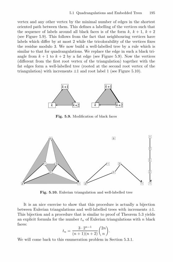
5.1 Quadrangulations and Embedded Trees 195
vertex and any other vertex by the minimal number of edges in the shortestoriented path between them. This defines a labelling of the vertices such thatthe sequence of labels around all black faces is of the form k, k + 1, k + 2(see Figure 5.9). This follows from the fact that neighbouring vertices havelabels which differ by at most 2 while the tricolorability of the vertices fixesthe residue modulo 3. We now build a well-labelled tree by a rule which issimilar to that for quadrangulations. We replace the edge in such a black tri-angle from k + 1 to k + 2 by a fat edge (see Figure 5.9). Now the vertices(different from the first root vertex of the triangulation) together with thefat edges form a well-labelled tree (rooted at the second root vertex of thetriangulation) with increments ±1 and root label 1 (see Figure 5.10).
+1
k+2k
k +1
k+2k
k
Fig. 5.9. Modification of black faces
0
1
21
3
2
0
1
21
3
2 1
2
1
3
2
Fig. 5.10. Eulerian triangulation and well-labelled tree
It is an nice exercise to show that this procedure is actually a bijectionbetween Eulerian triangulations and well-labelled trees with increments ±1.This bijection and a procedure that is similar to proof of Theorem 5.3 yieldsan explicit formula for the number tn of Eulerian triangulations with n blackfaces:
tn =3 · 2n−1
(n+ 1)(n+ 2)
(2n
n
).
We will come back to this enumeration problem in Section 5.3.1.
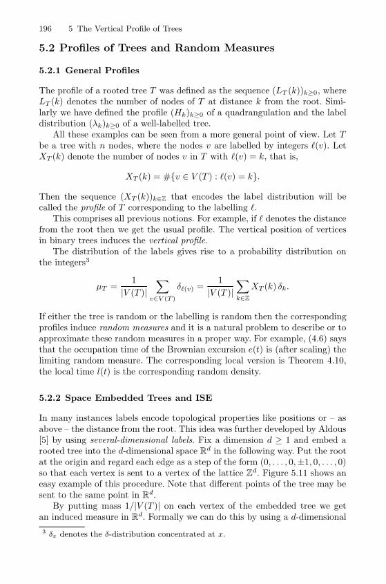
196 5 The Vertical Profile of Trees
5.2 Profiles of Trees and Random Measures
5.2.1 General Profiles
The profile of a rooted tree T was defined as the sequence (LT (k))k≥0, whereLT (k) denotes the number of nodes of T at distance k from the root. Simi-larly we have defined the profile (Hk)k≥0 of a quadrangulation and the labeldistribution (λk)k≥0 of a well-labelled tree.
All these examples can be seen from a more general point of view. Let Tbe a tree with n nodes, where the nodes v are labelled by integers �(v). LetXT (k) denote the number of nodes v in T with �(v) = k, that is,
XT (k) = #{v ∈ V (T ) : �(v) = k}.
Then the sequence (XT (k))k∈Z that encodes the label distribution will becalled the profile of T corresponding to the labelling �.
This comprises all previous notions. For example, if � denotes the distancefrom the root then we get the usual profile. The vertical position of verticesin binary trees induces the vertical profile.
The distribution of the labels gives rise to a probability distribution onthe integers3
μT =1
|V (T )|∑
v∈V (T )
δ�(v) =1
|V (T )|∑k∈Z
XT (k) δk.
If either the tree is random or the labelling is random then the correspondingprofiles induce random measures and it is a natural problem to describe or toapproximate these random measures in a proper way. For example, (4.6) saysthat the occupation time of the Brownian excursion e(t) is (after scaling) thelimiting random measure. The corresponding local version is Theorem 4.10,the local time l(t) is the corresponding random density.
5.2.2 Space Embedded Trees and ISE
In many instances labels encode topological properties like positions or – asabove – the distance from the root. This idea was further developed by Aldous[5] by using several-dimensional labels. Fix a dimension d ≥ 1 and embed arooted tree into the d-dimensional space Rd in the following way. Put the rootat the origin and regard each edge as a step of the form (0, . . . , 0,±1, 0, . . . , 0)so that each vertex is sent to a vertex of the lattice Zd. Figure 5.11 shows aneasy example of this procedure. Note that different points of the tree may besent to the same point in Rd.
By putting mass 1/|V (T )| on each vertex of the embedded tree we getan induced measure in Rd. Formally we can do this by using a d-dimensional
3 δx denotes the δ-distribution concentrated at x.
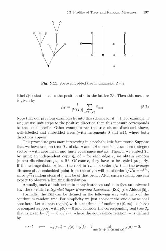
5.2 Profiles of Trees and Random Measures 197
Fig. 5.11. Space embedded tree in dimension d = 2
label �(v) that encodes the position of v in the lattice Zd. Then this measureis given by
μT =1
|V (T )|∑
v∈V (T )
δ�(v). (5.7)
Note that our previous examples fit into this scheme for d = 1. For example, ifwe just use unit steps to the positive direction then this measure correspondsto the usual profile. Other examples are the tree classes discussed above,well-labelled and embedded trees (with increments 0 and ±1), where bothdirections appear.
This procedure gets more interesting in a probabilistic framework. Supposethat we have random trees Tn of size n and a d-dimensional random (integer)vector η with zero mean and finite covariance matrix. Then, if we embed Tn
by using an independent copy ηe of η for each edge e, we obtain random(mass) distributions μn in Rd. Of course, they have to be scaled properly.If the average distance from the root in Tn is of order
√n then the average
distance of an embedded point from the origin will be of order√√
n = n1/4,since
√n random steps of η will be of that order. After such a scaling one can
expect to observe a limiting distribution.Actually, such a limit exists in many instances and is in fact an universal
law, the so-called Integrated Super-Brownian Excursion (ISE) (see Aldous [5]).Formally, the ISE can be defined in the following way with help of the
continuum random tree. For simplicity we just consider the one dimensionalcase here. Let us start (again) with a continuous function g : [0,∞) → [0,∞)of compact support with g(0) = 0 and consider the corresponding real tree Tg
that is given by Tg = [0,∞)/∼, where the equivalence relation ∼ is definedby
s ∼ t ⇐⇒ dg(s, t) = g(s) + g(t)− 2 infmin{s,t}≤u≤max{s,t}
g(u) = 0.
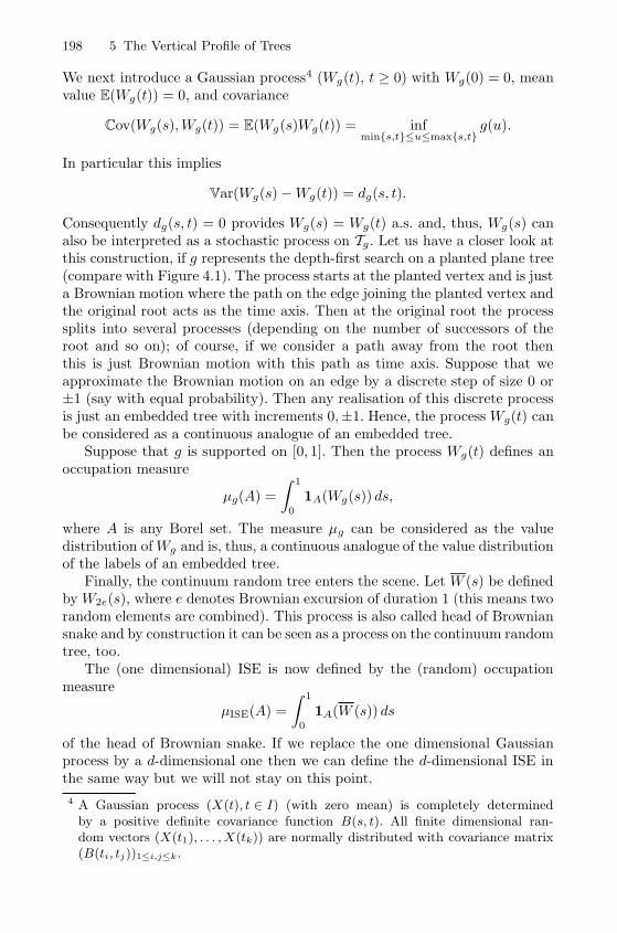
198 5 The Vertical Profile of Trees
We next introduce a Gaussian process4 (Wg(t), t ≥ 0) with Wg(0) = 0, meanvalue E(Wg(t)) = 0, and covariance
Cov(Wg(s),Wg(t)) = E(Wg(s)Wg(t)) = infmin{s,t}≤u≤max{s,t}
g(u).
In particular this implies
Var(Wg(s)−Wg(t)) = dg(s, t).
Consequently dg(s, t) = 0 provides Wg(s) = Wg(t) a.s. and, thus, Wg(s) canalso be interpreted as a stochastic process on Tg. Let us have a closer look atthis construction, if g represents the depth-first search on a planted plane tree(compare with Figure 4.1). The process starts at the planted vertex and is justa Brownian motion where the path on the edge joining the planted vertex andthe original root acts as the time axis. Then at the original root the processsplits into several processes (depending on the number of successors of theroot and so on); of course, if we consider a path away from the root thenthis is just Brownian motion with this path as time axis. Suppose that weapproximate the Brownian motion on an edge by a discrete step of size 0 or±1 (say with equal probability). Then any realisation of this discrete processis just an embedded tree with increments 0,±1. Hence, the process Wg(t) canbe considered as a continuous analogue of an embedded tree.
Suppose that g is supported on [0, 1]. Then the process Wg(t) defines anoccupation measure
μg(A) =
∫ 1
0
1A(Wg(s)) ds,
where A is any Borel set. The measure μg can be considered as the valuedistribution ofWg and is, thus, a continuous analogue of the value distributionof the labels of an embedded tree.
Finally, the continuum random tree enters the scene. Let W (s) be definedby W2e(s), where e denotes Brownian excursion of duration 1 (this means tworandom elements are combined). This process is also called head of Browniansnake and by construction it can be seen as a process on the continuum randomtree, too.
The (one dimensional) ISE is now defined by the (random) occupationmeasure
μISE(A) =
∫ 1
0
1A(W (s)) ds
of the head of Brownian snake. If we replace the one dimensional Gaussianprocess by a d-dimensional one then we can define the d-dimensional ISE inthe same way but we will not stay on this point.
4 A Gaussian process (X(t), t ∈ I) (with zero mean) is completely determinedby a positive definite covariance function B(s, t). All finite dimensional ran-dom vectors (X(t1), . . . , X(tk)) are normally distributed with covariance matrix(B(ti, tj))1≤i,j≤k.
5.2 Profiles of Trees and Random Measures 199
By Aldous’ result (Theorem 4.6) we know that properly scaled Galton-Watson trees converge to the continuum random tree (where we assume thatthe offspring distribution ξ satisfies E ξ = 1 and 0 < Var ξ = σ2
ξ < ∞). Let
η be a random variable with E η = 0 and variance 0 < Varη = σ2η < ∞
that embeds the tree into the line (as described above). The displacementsare now interpreted as labels: the root r has label �(r) = 0 and if v′ is asuccessor of v that is linked by an edge e, then set �(v′) = �(v) + ηe, whereηe is an independent copy of η. For example, if we consider planted planetrees (Exξ = 1/(2− x)) and η is the uniform distribution on {−1, 0, 1} thenthis construction leads to the embedded trees with increments 0 and ±1 (alsodiscussed above).
Then we have the following limit theorem (see Aldous [5] and Janson andMarckert [117]).
Theorem 5.4. Let the labels �(v) on Galton-Watson trees Tn be defined as
above. Then with γ = σ−1η σ
1/2ξ we have
1
n
∑v∈V (Tn)
δγn−1/4�(v)d−→ μISE, (5.8)
with convergence in the space of probability measures on R.5
The left hand side of (5.8) is just a scaled version of the (random) displace-ment distribution (5.7) of the (random) labels �(v). Thus, one dimensionalembedded Galton-Watson trees are actually approximated by the ISE (as itshould be).
This result is also an analogue to (4.6). We just have to replace the la-bels �(v) by the distances from the root and μISE by the occupation time ofBrownian excursion; of course, the scaling is different.
It is natural to ask whether there is a local version of Theorem 5.4, thatis, an analogue to Theorem 4.10. Here one has to verify first whether the(random) measures μISE has a proper (random) density. Actually, there is acorresponding local time of W ,
limε→0
1
ε
1∫0
1[t,t+ε](W (s)) ds,
and thus there exists a continuous stochastic process
(fISE(t), −∞ < t <∞)
with dμISE = fISE dt, the density of the ISE (see [24]). In fact, a local resulton these (vertical) profiles has been recently proved by Bousquet-Melou andJanson [24] and by Devroye and Janson [52].
5 The space of probability measures on R with the weak topology is a Polish space.
200 5 The Vertical Profile of Trees
Theorem 5.5. Additionally to the assumptions of Theorem 5.4 we assumethat η is integer valued and aperiodic, that is, it is not concentrated on dZ forsome d > 1. Let (Xn(j))j∈Z the corresponding profile, that is, Xn(j) is thenumber of vertices in Tn with �(v) = j, and (Xn(t),−∞ < t <∞) the linearlyinterpolated process. Then we have(
n−3/4Xn(n1/4t), −∞ < t <∞)
d−→ (γfISE(γt), −∞ < t <∞)
in the space C0(R), where γ = σ−1η σ
1/2ξ .
Interestingly, Theorems 5.4 and 5.5 appear in other settings, too. We justmention an example, namely the vertical profile of (incomplete) binary trees,where we have precisely the same result although the labels are not random.
We recall that a (complete) binary tree is a plane rooted tree where eachnode has either two or no successors. In particular we can distinguish betweeninternal nodes that have two successors and external ones. If we disregard theexternal nodes then the resulting object is a rooted tree, a so-called incompletebinary tree, where each node has either no successor, a right successor, a leftsuccessor or a left and a right successor.6 There is a natural labelling of thenodes, namely the number of right steps minus the number of left steps onthe path from the root to this node (see Figure 5.12). This labelling inducesa natural embedding of these binary trees and also explains why we call thesequence (Xn(j))j∈Z, where Xn(j) denotes the number of nodes of label j,vertical profile.
Theorem 5.6. Let Xn(j) denote the number of nodes of label j in naturallyembedded reduced binary trees with n nodes and (Xn(t),−∞ < t < ∞) thecorresponding linearly interpolated process. Then we have
1
n
∑v∈V (Tn)
δ(2n)−1/4�(v)d−→ μISE,
and(n−3/4Xn(n1/4t), −∞ < t <∞
)d−→(
2−1/4fISE(2−1/4t), −∞ < t <∞).
In view of the bijections between quadrangulations (together with theirprofile) and well-labelled and embedded trees (with increments 0 and ±1) thefollowing theorem on quadrangulations is not unexpected (see [35] for details).
For convenience let [L,N ] = [LISE, NISE] denote the (random) supportof μISE and μISE the shifted ISE that is supported by [0, N − L], that is,μISE((−∞, λ]) = μISE((−∞, λ+ L])
6 Reduced binary trees of this kind are easier to handle; for example, the countingproblem for binary trees is based on the number of internal nodes. Therefore wehave decided to formulate the following results in terms of this notion.
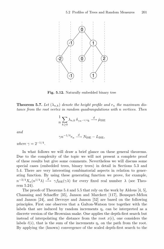
5.2 Profiles of Trees and Random Measures 201
0
-1
-2
-1
0
1
2
1
Fig. 5.12. Naturally embedded binary tree
Theorem 5.7. Let (λn,k) denote the height profile and rn the maximum dis-tance from the root vertex in random quadrangulations with n vertices. Then
1
n
∑k≥0
λn,k δγn−1/4kd−→ μISE
andγn−1/4rn
d−→ NISE − LISE,
where γ = 2−1/4.
In what follows we will draw a brief glance on these general theorems.Due to the complexity of the topic we will not present a complete proofof these results but give some comments. Nevertheless we will discuss somespecial cases (embedded trees, binary trees) in detail in Sections 5.3 and5.4. There are very interesting combinatorial aspects in relation to gener-ating function. By using these generating function we prove, for example,
n−3/4Xn(n1/4λ)d−→ γfISE(γλ) for every fixed real number λ (see Theo-
rem 5.24).The proofs of Theorems 5.4 and 5.5 that rely on the work by Aldous [4, 5],
Chassaing and Schaeffer [35], Janson and Marckert [117], Bousquet-Melouand Janson [24], and Devroye and Janson [52] are based on the followingprinciples. First one observes that a Galton-Watson tree together with thelabels that are induced by random increments ηe can be interpreted as adiscrete version of the Brownian snake. One applies the depth-first search butinstead of interpolating the distance from the root x(i), one considers thelabels �(i), that is the sum of the increments ηe on the path from the root.By applying the (known) convergence of the scaled depth-first search to the
202 5 The Vertical Profile of Trees
Brownian excursion, the central limit theorem and proper tightness estimatesit follows that the discrete snake process converges to the Brownian snake (see,for example [117]). Theorem 5.4 is a direct consequence of this convergenceresult (recall that the ISE is the occupation measure of the Brownian snake).
Theorem 5.7 is deduced by similar arguments, however, one has to use someadditional properties of the relation between quadrangulations and embeddedtrees (see [35]).
Now suppose that the distribution of the increments η is discrete (andaperiodic). Let Xn(j) denote the number of nodes with label j in a randomGalton-Watson tree of size n and let Xn(t) be the corresponding linear inter-polated process. Then the scaled process n−3/4Xn(n1/4t) can be seen as the(random) density of a measure
1
n
∑j≥0
Xn(j) νjn−1/4,n−1/4 ,
that is close to the (scaled) occupation measure
1
n
∑j≥0
Xn(j) δjn−1/4
of the label distribution (recall that νh,y is the measure with triangular densityf(x) = h−1 max{1− |x− y|/h, 0}, compare with Theorem 4.17 and its discus-sion). Thus, in order to prove Theorem 5.5 it is sufficient to prove tightnessof n−3/4Xn(n1/4t).
Bousquet-Melou and Janson [24] have formulated an interesting sufficientcondition for tightness (in this context).
Lemma 5.8. Suppose that there exists a constant C such that for all n ≥ 1and u ∈ [−π, π],
E
(|n−1Xn(u)|2
)≤ C
1 + nu4, (5.9)
whereXn(u) =
∑j
Xn(j)eiju
denotes the Fourier transform of the occupations measure∑
j Xn(j)δj andthat there exists a random variable W with
n−1/4 sup{|j| : Xn(j) = 0} d−→W. (5.10)
Then n−3/4Xn(n1/4t) is tight in C0(R).
We sketch the proof of Lemma 5.8. First, by basic Fourier analytic toolsit follows that (for 0 ≤ a < 3)
E
(∫ ∞−∞
|t|a∣∣∣n−3/4Xn(n1/4t)
∣∣∣2 dy)
5.2 Profiles of Trees and Random Measures 203
is finite so that with high probability∫ ∞−∞
|t|a∣∣∣n−3/4Xn(n1/4t)
∣∣∣2 < Afor some A > 0. The condition (5.10) ensures that again with high probability∣∣∣n−3/4Xn(n1/4t)
∣∣∣ = 0
for |t| > M , if M is chosen sufficiently large. Let KM,A denote the set of allfunctions in C0(R) with f(t) = 0 for |t| > M and∫ ∞
−∞|t|a |f(t)|2 < A.
Then KM,A is a relative compact subset of C([−M,M ]), and thus of C0(R),too (compare with [24]). Since n−3/4Xn(n1/4t) is contained inKM,A with highprobability, this proves tightness.
Note that (5.10) is related to Theorems 5.7 and 5.22 and can be deducedfrom the convergence of the (scaled) discrete snake process to the Browniansnake. Actually, W = γ−1 max{NISE,−LISE}.
It remains to verify (5.9). For this purpose we introduce the followingnotions. For each pair of vertices v, w in a random Galton-Watson tree Tn ofsize n, the path from v to w consists of two (possibly empty) parts, one goingfrom v towards the root, ending at the last common ancestor v ∧ w of v andw, and another part going from v ∧ w to w in the direction away from theroot. We will also prove a more general result, where we consider separatelythe lengths of these two parts. Define
hn(x1, x2) = E
⎛⎝ ∑v,w∈Tn
xd(v,v∧w)1 x
d(w,v∧w)2
⎞⎠ , (5.11)
where d(v, w) denotes the distance between v and w, and
H(z, x1, x2) =∑n≥1
ynhn(x1, x2)zn,
where yn =∑|T |=n ω(T ). It can be shown (see [52]) that H(z, x1, x2) can be
explicitly represented as
H(z, x1, x2) =
zx1x2Φ′′(y(z))G(z, x1)G(z, x2) + zΦ′(y(z)) (x1G(z, x1) + x2G(z, x2)) + y(z)
1− zΦ′(y(z)) ,
where
204 5 The Vertical Profile of Trees
G(z, x) =y(z)
1− zxΦ′(y(z)) .
On the other hand, there is a direct relation to Xn(u). Let �(v) denote therandom label of the vertex v, that is, the sum of the increments on the pathfrom the root to v and let ϕ(t) = E eitη the characteristic function of thedistribution of the increment η. Then from
E
(eiu(�(v)−�(w))|Tn
)= E
(eiu(�(v)−�(v∧w))|Tn
)E
(e−iu(�(w)−�(v∧w))|Tn
)= ϕ(u)d(v,v∧w)ϕ(u)
d(w,v∧w)
we obtain
E
(|n−1Xn(u)|2
)=
1
n2E
⎛⎝ ∑v,w∈Tn
(eiu(�(v)−�(w))
)⎞⎠=
1
n2E
⎛⎝ ∑v,w∈Tn
ϕ(u)d(v,v∧w)ϕ(u)d(w,v∧w)
⎞⎠=
1
n2hn(ϕ(u), ϕ(u)).
This means that we have almost direct access to E|n−1Xn(u)|2 with help ofanalytic tools. In particular, by singularity analysis it follows that
|hn(x1, x2)| ≤ C
n |1− x1| |1− x2|
uniformly for x1, x2 in a Δ-domain (compare with [52]). We also have |ϕ(u)−1| ≥ cu2 for u ∈ [−π, π] and consequently
(1 + nu4) E
(|n−1Xn(u)|2
)≤ 1 + nu4 C
n|1− ϕ(u)|2
≤ 1 +C
c2.
Thus, Lemma 5.8 can be applied and Theorem 5.5 follows.The proof of Theorem 5.6 can be worked out in a similar way.
5.2.3 The Distribution of the ISE
The definition of the ISE does not provide directly analytic expressions forthe distribution of the ISE. Nevertheless there are integral representations forseveral statistics of the ISE. In this section we list some of them, however, theyare derived an indirect way. More precisely, they will appear in the proofs of
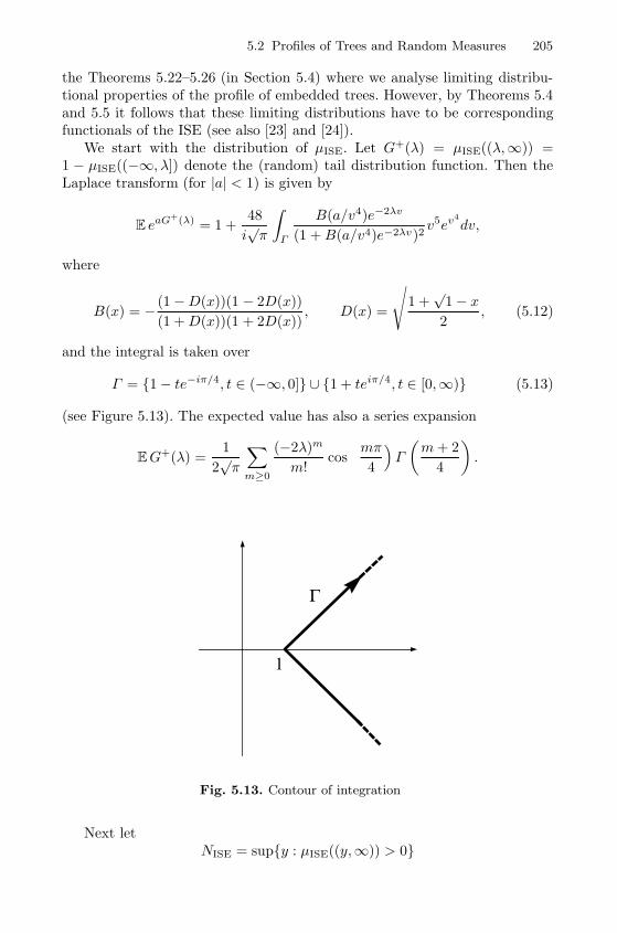
5.2 Profiles of Trees and Random Measures 205
the Theorems 5.22–5.26 (in Section 5.4) where we analyse limiting distribu-tional properties of the profile of embedded trees. However, by Theorems 5.4and 5.5 it follows that these limiting distributions have to be correspondingfunctionals of the ISE (see also [23] and [24]).
We start with the distribution of μISE. Let G+(λ) = μISE((λ,∞)) =1 − μISE((−∞, λ]) denote the (random) tail distribution function. Then theLaplace transform (for |a| < 1) is given by
E eaG+(λ) = 1 +48
i√π
∫Γ
B(a/v4)e−2λv
(1 +B(a/v4)e−2λv)2v5ev
4
dv,
where
B(x) = − (1−D(x))(1 − 2D(x))
(1 +D(x))(1 + 2D(x)), D(x) =
√1 +
√1− x
2, (5.12)
and the integral is taken over
Γ = {1− te−iπ/4, t ∈ (−∞, 0]} ∪ {1 + teiπ/4, t ∈ [0,∞)} (5.13)
(see Figure 5.13). The expected value has also a series expansion
EG+(λ) =1
2√π
∑m≥0
(−2λ)m
m!cos(mπ
4
)Γ
(m+ 2
4
).
Γ
1
Fig. 5.13. Contour of integration Γ
Next letNISE = sup{y : μISE((y,∞)) > 0}
206 5 The Vertical Profile of Trees
denote the supremum of the support of the ISE. Its tail distribution functioncan be expressed by
P{NISE > λ} =12
i√π
∫Γ
v5ev4
sinh2(λv)dv
Observe that the integration contour Γ can be replaced by its translatedversion
Γ0 = {−re−iπ/4, r ∈ (−∞, 0]} ∪ {reiπ/4, r ∈ [0,∞)}.This parametrisation of Γ0 by r splits the integral into two real integrals, andone finds
G(λ) = − 12√π
∫ ∞0
(1
sinh2(λreiπ/4)+
1
sinh2(λre−iπ/4)
)r5e−r4
dr
=48√π
∫ ∞0
1− cos(√
2λr) cosh(√
2λr)
(cosh(√
2λr) − cos(√
2λr))2r5e−r4
dr (5.14)
=6√πλ6
∫ ∞0
1− cosu coshu
(coshu− cosu)2u5e−u4/(4λ4)du.
The density is given by
f(λ) =24
i√π
∫Γ
cosh(λv)v6ev4
sinh3(λv)dv
=6√πλ11
∫ ∞0
1− cosu coshu
(coshu− cosu)2u5(6λ4 − u4)e−u4/(4λ4)du,
where the contour Γ is given by (5.13).The moments of Nise are explicit, for �(r) > −4 we have
E(N rise
) =24√π Γ (r + 1)ζ(r − 1)
2rΓ ((r − 2)/4),
with analytic continuation at the points −3,−2,−1, 2. For example
ENISE =3√π
2Γ (3/4), E(N2
ISE) = 3√π.
These moments were already obtained by Delmas [46] and rediscovered by[23].
Finally, we consider the density of the ISE fISE. The one dimensionaldistribution of fISE(λ) is characterised by the Laplace transform (for |a| <4/√
3)
E eafISE(λ) = 1 +48
i√π
∫Γ
A(a/v3)e−2λv
(1 +A(a/v3)e−2λv)2v5ev
4
dv,
where A(x) = A is the unique solution of
5.3 Combinatorics on Embedded Trees 207
A =x
24
(1 +A)3
1−A (5.15)
satisfying A(0) = 0, and the integral is taken over the contour Γ given by(5.13).
The expected value is given by
E fISE(λ) = (2π)−1/2
∫ ∞0
y1/2 exp
(−λ
2
2y− y
2
2
)dy
=2−1/4
√π
∑m≥0
(−23/4|λ|)m
m!cos
(m+ 1)π
4Γ
(m+ 3
4
).
In particular, fISE(0) has the same distribution as 21/43−1T−1, where T is
a positive 2/3-stable variable defined by its Laplace transform E e−tT = e−t2/3
.Hence fISE(0) has the moments
E fISE(0)r = 2r/43−rΓ (3r/4 + 1)
Γ (r/2 + 1), −4/3 < r <∞.
5.3 Combinatorics on Embedded Trees
The discussion in the previous section shows that there is considerable interestin labelled trees, where the labels of adjacent vertices are described by a fixedlaw (for example, that they differ at most by one).
We have also shown that well-labelled trees can be counted with help ofgenerating functions (5.6) that have a mysterious representation in terms ofZ(t).
We will next discuss three different kinds of trees: two versions of em-bedded trees and binary trees (where the labels are not randomly chosen butcorrespond to the vertical position). Interestingly, the counting procedures arealmost the same. We follow the work of Bousquet-Melou [23].
The subsequent asymptotic analysis (see Section 5.4) provides one dimen-sional versions of Theorems 5.4 and 5.5. As already indicated, a full proof ofthese theorems will not be given in this book.
5.3.1 Embedded Trees with Increments ±1
We start by considering a family of embedded planted plane trees, wherethe root is labelled 0, and the labels of two adjacent nodes differ by ±1 (seeFigure 5.14), where the counting procedure is slightly easier; the case of in-crements 0 and ±1 will be discussed in Section 5.3.2. Furthermore, trees withincrements ±1 appear as objects related to special triangulations as we havementioned in Section 5.1.
The total number of trees with n edges of that kind is given by
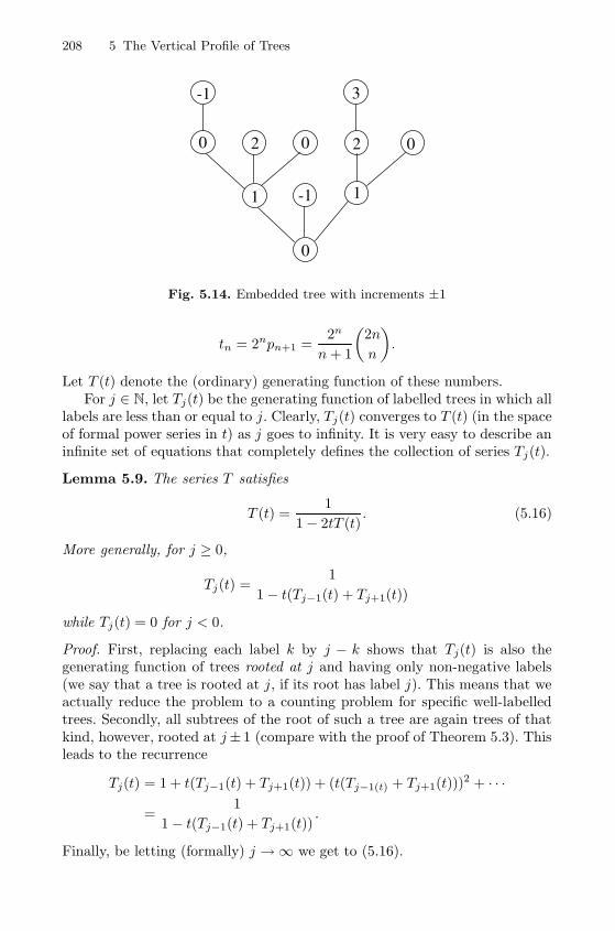
208 5 The Vertical Profile of Trees
1
2 0
0
2
-1
0
1
0
-1 3
Fig. 5.14. Embedded tree with increments ±1
tn = 2npn+1 =2n
n+ 1
(2n
n
).
Let T (t) denote the (ordinary) generating function of these numbers.For j ∈ N, let Tj(t) be the generating function of labelled trees in which all
labels are less than or equal to j. Clearly, Tj(t) converges to T (t) (in the spaceof formal power series in t) as j goes to infinity. It is very easy to describe aninfinite set of equations that completely defines the collection of series Tj(t).
Lemma 5.9. The series T satisfies
T (t) =1
1− 2tT (t). (5.16)
More generally, for j ≥ 0,
Tj(t) =1
1− t(Tj−1(t) + Tj+1(t))
while Tj(t) = 0 for j < 0.
Proof. First, replacing each label k by j − k shows that Tj(t) is also thegenerating function of trees rooted at j and having only non-negative labels(we say that a tree is rooted at j, if its root has label j). This means that weactually reduce the problem to a counting problem for specific well-labelledtrees. Secondly, all subtrees of the root of such a tree are again trees of thatkind, however, rooted at j± 1 (compare with the proof of Theorem 5.3). Thisleads to the recurrence
Tj(t) = 1 + t(Tj−1(t) + Tj+1(t)) + (t(Tj−1(t) + Tj+1(t)))2 + · · ·
=1
1− t(Tj−1(t) + Tj+1(t)).
Finally, be letting (formally) j →∞ we get to (5.16).
5.3 Combinatorics on Embedded Trees 209
The above lemma also shows that the series T (t), counting labelled treesby edges, is algebraic. What is far less clear – but nevertheless true – is thateach of the series Tj(t) is algebraic too, as stated in the proposition below.These series will be expressed in terms of the series T (t) and of the uniqueformal power series Z(t), with constant term 0, satisfying
Z(t) +1
Z(t)=
1
tT (t)2. (5.17)
Observe that Z(t) and t are related by
Z(t) = t(1 + Z(t))4
1 + Z(t)2(5.18)
and Z(t) and T (t) by
T (t) =(1 + Z(t))2
1 + Z(t)2. (5.19)
Proposition 5.10. Let Tj(t) be the generating function of embedded trees withincrements ±1 having no label greater than j. Then we have
Tj(t) = T (t)
(1− Z(t)j+1
) (1− Z(t)j+5
)(1− Z(t)j+2) (1− Z(t)j+4)
, (5.20)
with Z(t) given by (5.18). These functions are algebraic of degree 2 (at most).In particular, T0(t) satisfies the equation
T0(t) = 1− 11 t− t2 + 4 t (3 + 2 t)T0(t)− 16 t2T0(t)2.
Proof. It is very easy to check, using (5.18)–(5.19), that the above values ofTj(t) satisfy the recurrence relation of Lemma 5.9 and the initial conditionT−1(t) = 0 (compare also with the proof of Theorem 5.3).
The equation satisfied by T0(t) is obtained by eliminating T (t) and Z(t)from the case j = 0 of (5.20). Then an induction on j, based on Lemma 5.9,implies that each Tj(t) is quadratic (at most) over Q(t).
Remark 5.11 As we have mentioned in Section 5.1, trees counted by T0(t)(equivalently, the trees having only non-negative labels) are known to be inbijection with certain planar maps called Eulerian triangulations (see also[26]).
Let us now turn to a bivariate counting problem. Let Sj(t, u) be the gen-erating function of embedded trees (with increments ±1), counted by thenumber of edges (variable t) and the number of nodes labelled j (variable u).Clearly, Sj(t, 1) = T (t) for all j. Moreover, an obvious symmetry shows thatSj(t, u) = S−j(t, u).
210 5 The Vertical Profile of Trees
Lemma 5.12. For j = 0,
Sj(t, u) =1
1− t(Sj−1(t, u) + Sj+1(t, u)), (5.21)
while for j = 0,
S0(t, u) =u
1− t(S−1(t, u) + S1(t, u))=
u
1− 2tS1(t, u). (5.22)
Proof. Observe that Sj(t, u) is also the generating function of labelled treesrooted at j, counted by the number of edges and the number of nodes labelled0. The decomposition of planted plane trees provides the lemma. The onlydifference between the cases j = 0 and j = 0 lies in the generating functionof the tree reduced to a single node.
Again, the series Sj(t, u) has a remarkable explicit representation (thatshows that it is algebraic, too, for reasons that currently remain mysteriousfrom the combinatorial point of view). They can be expressed in terms of theseries T (t) and Z(t) given by (5.18)–(5.19). By symmetry we also Sj(t, u) =S−j(t, u). Thus, it is sufficient to consider the case j ≥ 0.
Proposition 5.13. For any j ≥ 0, the generating function Sj(t, u) thatcounts embedded trees (with increments ±1) by the number of edges and thenumber of nodes with label j is given by
Sj(t, u) = T (t)
(1 + μ(t, u)Z(t)j
) (1 + μ(t, u)Z(t)j+4
)(1 + μ(t, u)Z(t)j+1) (1 + μ(t, u)Z(t)j+3)
, (5.23)
where Z(t) is given by (5.18) and μ = μ(t, u) is the unique formal power seriesin t satisfying
μ = (u − 1)(1 + Z(t)2)(1 + μZ(t))(1 + μZ(t)2)(1 + μZ(t)3)
(1 + Z(t))(1 + Z(t) + Z(t)2)(1 − Z(t))3(1− μZ(t)2). (5.24)
The series μ(t, u) has polynomial coefficients in u and satisfies μ(t, 1) = 0. Inparticular, S0(t, u) satisfies the equation
(T (t)− S0(t, u))2
(u− 1)2= 1− 2(1− T (t)2)
2 + S0(t, u)− S0(t, u)T (t). (5.25)
Proof. First, observe that the family of series S0(t, u), S1(t, u), S2(t, u), . . .is completely determined by (5.21) (taken for j > 0) and the second partof (5.22). The fact that for any series μ(t, u) ∈ Q(u)[[t]] the expression (5.23)satisfies (5.21) for all j > 0 is a straightforward verification, once t and T (t)have been expressed in terms of Z(t) (see (5.18) and (5.19)). In order toprove that (5.23) is the correct expression of Sj(t, u), it remains to satisfythe second part of (5.22). This last condition provides a polynomial equation
5.3 Combinatorics on Embedded Trees 211
relating μ(t, u), T (t), Z(t), t and u. In this equation, replace t and T (t) bytheir expressions in terms of Z(t) (given by (5.18)–(5.19)). This exactly gives(5.24).
Equation (5.25) satisfied by S0 is obtained by eliminating μ(t, u) and Z(t)(using (5.24) and (5.19)) from the expression (5.23) of S0(t, u).
In the proof of Lemma 5.25 we will need a closed form expression for μ(t, u)in terms of Z(t). Write
v =(u− 1)Z(t)(1 + Z(t)2)
(1 + Z(t))(1 + Z(t) + Z(t)2)(1− Z(t))3.
Then μ(t, u) is given by
μ(t, u) =1
Z(t)2
(2
1 + v(1− Z(t))2/3 + 2/3√
3 + v2(1 − Z(t))4 cos(ϕ/3)− 1
)(5.26)
where
ϕ = arccos
(−9v(1 + 4Z(t) + Z(t)2) + v3(1− Z(t))6
(3 + v2(1 − Z(t))4)3/2
).
The reason for that is that equation (5.24) which defines μ(t, u) can be rewrit-ten to
μ(t, u) =v
Z(t)
(1 + μ(t, u)Z(t))(1 + μ(t, u)Z(t)2)(1 + μ(t, u)Z(t)3)
1− μ(t, u)Z(t)2.
Hence, μ(t, u) is the unique formal power series in v (with rational coefficientsin Z(t)) that satisfies the above equation and equals 0 when v is 0. And itis not hard to check that the expression given in (5.26) satisfies these twoconditions.
Let us finally study a third problem. LetRj(t, u) be the generating functionof embedded trees (with increments ±1), counted by the number of edges(variable t) and the number of nodes labelled at least j (variable u).
Lemma 5.14. The set of series R0(t, u), R1(t, u), R2(t, u), . . . is completelydetermined by the following equations: for j ≥ 1,
Rj(t, u) =1
1− t(Rj−1(t, u) +Rj+1(t, u))(5.27)
andR0(t, u) = uR1(tu, 1/u). (5.28)
More generally, for all j ∈ Z, one has:
R−j(t, u) = uRj+1(tu, 1/u). (5.29)
212 5 The Vertical Profile of Trees
Proof. For all j ∈ Z, the series Rj(t, u) is also the generating function of treesrooted at j, counted by their number of edges and the number of nodes havinga non-positive label. The equation satisfied by j, for j ≥ 0, follows once againfrom the recursive structure.
It remains to prove the symmetry relation (5.29). For any tree T , letn≤0(T ) denote the number of nodes of T having a non-positive label. Weuse similar notations for the number of nodes having label at most j, etc. LetTj,n denote the set of trees rooted at j and having n edges. As observed above,
R−j(t, u) =∑n≥0
tn∑
T∈T−j,n
un≤0(T ) =∑n≥0
tn∑
T∈T−j,n
un+1−n>0(T ),
because a tree with n edges has a total of n + 1 nodes. A translation of alllabels by −1 gives
R−j(t, u) = u∑n≥0
(tu)n∑
T∈T−j−1,n
u−n≥0(T ),
while replacing each label k by −k finally gives
R−j(t, u) = u∑n≥0
(tu)n∑
T∈Tj+1,n
u−n≤0(T ) = uRj+1(tu, 1/u).
Remarkably, the series Rj(t, u) admit a closed form expression in terms ofT (t) and Z(t), too. Due to the symmetry (5.29) it is sufficient to consider thecase j ≥ 0.
Proposition 5.15. Let j ≥ 0. The generating function Rj(t, u) that countsembedded trees (with increments ±1) by the number of edges and the numberof nodes with labels ≥ j is given by
Rj(t, u) = T (t)
(1 + ν(t, u)Z(t)j
) (1 + ν(t, u)Z(t)j+4
)(1 + ν(t, u)Z(t)j+1) (1 + ν(t, u)Z(t)j+3)
, (5.30)
where Z(t) is determined by (5.18) and ν(t, u) is expressed by
ν(t, u) =P (t, u)
Z(t)
1− P (t, u)(1 + Z(t))− P (t, u)2(1 + Z(t) + Z(t)2)
1 + Z(t) + Z(t)2 + P (t, u)Z(t)(1 + Z(t))− P (t, u)2Z(t)2,
with
P (t, u) = (1 + Z(t))1− V (t, u)−
√Δ(t, u)
2V (t, u)Z(t),
in which
V (t, u) =1−√
1−8tu1−8t
4,
and
Δ(t, u) = (1− V (t, u))2 − 4Z(t)V (t, u)2
(1 + Z(t))2.
5.3 Combinatorics on Embedded Trees 213
We note that the generating function ν(t, u) considered as a series in t haspolynomial coefficients in u and the first terms in its expansion are
ν(t, u) = (u−1)(
1+2 ut+(7 u+ 6 u2
)t2 +(32 u+ 36 u2 + 23 u3
)t3 +O(t4)
).
Proof. In the proof of Proposition 5.13 we have already checked, that for anyformal power series ν in t, the series defined by (5.30) for j ≥ 0 satisfy therecurrence relation (5.27) for j ≥ 1. It remains to prove that one can chooseν so as to satisfy (5.28). For any formal power series A in t having rationalcoefficients in u, we denote by A the series A(t, u) = A(tu, 1/u). In particular
T (t, u) = T (tu). Observe that ˜A = A. With this notation, if Rj(t, u) is of thegeneric form (5.30), the relation (5.28) holds, if and only if
1 + ν = uT
T
(1 + νZ)(1 + νZ3)(1 + νZ)(1 + νZ5)
(1 + νZ4)(1 + νZ2)(1 + νZ4), (5.31)
where we use the abbreviations T = T (t), T = T (t, u), Z = Z(t), Z =Z(t, u) = Z(tu), ν = ν(t, u), and ν = ν(t, u) = ν(tu, 1/u). Let Rm[u] denotethe space of polynomials in u, with real coefficients, of degree at most m. LetRn[u][[t]] denote the set of formal power series in t with polynomial coefficientsin u such that for all m ≤ n, the coefficient of tm has degree at most m.Observe that this set of series is stable under the usual operations on series:sum, product, and quasi-inverse. Write ν =
∑n≥0 νn(u)tn. We are going to
prove, by induction on n, that (5.31) determines uniquely each coefficientνn(u), and that this coefficient belongs to Rn+1[u].
First, observe that for any formal power series ν, the right-hand-sideof (5.31) is u + O(t). This implies ν0(u) = u − 1. Now assume that ourinduction hypothesis holds for all m < n. Recall that Z is a multiple oft: this implies that νZ belongs to Rn[u][[t]]. The induction hypothesis alsoimplies that the coefficient of tm in uν belongs to Rm+1[u], for all m < n.Note that Z = Z(tu) = tu + O(t2) is a multiple of t and u and also be-longs to Rn[u][[t]]. This implies that νZ belongs to Rn[u][[t]], too. The same istrue for all the other series occurring in the right-hand-side of (5.31), namelyT, T , Z, Z. Given the closure properties of the set Rn[u][[t]], we conclude thatthe right-hand-side of (5.31), divided by u, belongs to this set. Moreover, thefact that Z and Z are multiples of t guarantees that the coefficient of tn inthis series only involves the νi(u) for i < n. By extracting the coefficient oftn in (5.31), we conclude that νn(u) is uniquely determined and belongs touRn[u] ⊂ Rn+1[u].
This completes the proof of the existence and uniqueness of the series νsatisfying (5.31). Also, setting u = 1 (that is, T = T and Z = Z) in thisequation shows that ν(t, 1) = 0.
Let us now replace t by tu and u by 1/u in (5.31). This gives
1 + ν =1
u
T
T
(1 + νZ)(1 + νZ3)(1 + νZ)(1 + νZ5)
(1 + νZ4)(1 + νZ2)(1 + νZ4). (5.32)
214 5 The Vertical Profile of Trees
In the above two equations, replace T by its expression (5.19) in terms ofZ. Similarly, replace T by its expression in terms of Z. Finally, it followsfrom (5.18) and from the fact that Z = Z(tu) that
u =Z
Z
(1 + Z)4(1 + Z2)
(1 + Z)4(1 + Z2). (5.33)
Replace u by this expression in (5.31) and (5.32). Eliminate ν between theresulting two equations: this gives a polynomial equation of degree 2 in νthat relates ν, Z and Z. The elimination of Z between this quadratic equationand (5.33) provides an equation of degree 4 in ν that relates ν = ν(t, u) toZ = Z(t) and u.
We do not make this equation explicit but it follows from (5.31) and (5.32).In this equation, we replace u in terms of
δ = δ(t, u) = 1− 8(u− 1)Z(t)(1 + Z(t)2)
(1− Z(t))4=
1− 8tu
1− 8t,
and Z, that is, we set
u = 1− 1− δ8
(1− Z)4
Z(1 + Z2).
Then we replace δ in terms of
V =1−
√δ
4,
that is, we set δ = (1− 4V )2. Interestingly, the resulting equation factors intotwo terms. Each of them is quadratic in ν. In order to decide which of thesefactors cancels, one uses the fact that when u = 1 (that is, V = 0), the seriesν must be 0. It remains to solve a quadratic equation in ν. Its discriminant isfound to be Δ, and it is convenient to introduce the series P and satisfies theequation
P =V
1 + Z(1 + P )(1 + ZP ).
5.3.2 Embedded Trees with Increments 0, ±1
Next we consider the case of embedded trees with increments 0 and ±1. Aswe have discussed in Section 5.1 this class of trees is of interest because ofits relation to quadrangulations, but there are also relations to general planarmaps [26, 35].
As above, let Tj(t) be the generating function of labelled trees in which alllabels are at most j, counted by their number of edges.7 Let Sj(t, u) be the
7 We use the same notation as in Section 5.3.1 although they correspond to differenttrees. However, it will be always clear from the context which kind of trees isconsidered.
5.3 Combinatorics on Embedded Trees 215
generating function of labelled trees, counted by the number of edges (variablet) and the number of nodes labelled j (variable u). Finally, let Rj(t, u) be thegenerating function of labelled trees, counted by the number of edges and thenumber of nodes having label at least j. As above, it is easy to write an infinitesystem of equations defining any of the families Tj(t), Sj(t, u) or Rj(t, u).The only difference to our first family of trees is that a third case arises inthe decomposition of trees (compare also with the proof of Theorem 5.3). Inparticular, the generating function T = T (t) counting these embedded treesnow satisfies
T (t) =1
1− 3tT (t),
while for j ≥ 0,
Tj(t) =1
1− t(Tj−1(t) + Tj(t) + Tj+1(t)). (5.34)
The equations of Lemma 5.12 and Lemma 5.14 are modified in a similar way.The three infinite systems of equations obtained in that way can be solvedusing the same techniques as in Section 5.3.1. The solutions are expressed interms of the above series T (t) and the unique formal power series Z(t), withconstant term 0, satisfying
Z(t) +1
Z(t)+ 1 =
1
tT (t)2(5.35)
or equivalently
Z(t) = t(1 + 4Z(t) + Z(t)2)2
1 + Z(t) + Z(t)2, (5.36)
resp.
T (t) =1 + 4Z(t) + Z(t)2
1 + Z(t) + Z(t)2.
We state the counterparts of Propositions 5.10, 5.13 and 5.15 without proof.
Proposition 5.16. Let Tj(t) be the generating function of embedded trees(with increments 0 and ±1) having no label greater than j. Then we have(for j ≥ −1)
Tj(t) = T (t)(1− Z(t)j+1)(1− Z(t)j+4)
(1− Z(t)j+2)(1− Z(t)j+3),
where Z(t) is given by (5.36). These functions are algebraic of degree (at most)2. In particular, T0(t) satisfies the equation
T0(t) = 1− 16 t+ 18 tT0(t)− 27 t2T0(t)2.
Proposition 5.17. For any j ≥ 0, the generating function Sj(t, u) thatcounts embedded trees (with increments 0 and ±1) by the number of edgesand the number of nodes labelled j is given by
216 5 The Vertical Profile of Trees
Sj(t, u) = T (t)(1 + μ(t, u)Z(t)j)(1 + μ(t, u)Z(t)j+3)
(1 + μ(t, u)Z(t)j+1)(1 + μ(t, u)Z(t)j+2), (5.37)
where Z(t) is given by (5.36) and μ(t, u) is the unique formal power series int satisfying
μ(t, u) = (u− 1)(1 + Z(t) + Z(t)2)(1 + μ(t, u)Z(t))2(1 + μ(t, u)Z(t)2)2
(1 + Z(t))2(1− Z(t))3(1− μ(t, u)2Z(t)3).
The series μ(t, u) has polynomial coefficients in u and satisfies μ(t, 1) = 0. Inparticular, S0(t, u) satisfies the equation
9T (t)4(u − 1)2
(T (t)− S0(t, u))2
= 9T (t)2 − 2T (t)(T (t)− 1)(2T (t) + 1)S0(t, u) + (T (t)− 1)2S0(t, u)2.
Recall that by symmetry S−j(t, u) = Sj(t, u). Thus (5.37) provides an explicitrepresentation for all j ∈ Z.
The functions Rj(t, u) have a similar symmetry:R−j(t, u) = uRj+1(tu, 1/u).Hence, it is again sufficient to consider just the case j ≥ 0.
Proposition 5.18. Let j ≥ 0. The generating function Rj(t, u) that countsembedded trees (with increments 0 and ±1) by the number of edges and thenumber of nodes labelled j or more is given by
Rj(t, u) = T (t)(1 + ν(t, u)Z(t)j)(1 + ν(t, u)Z(t)j+3)
(1 + ν(t, u)Z(t)j+1)(1 + ν(t, u)Z(t)j+2),
where Z(t) is given by (5.36) and ν(t, u) is a formal power series in t, withpolynomial coefficients in u.8 This series satisfies ν(t, 1) = 0 and the firstterms in its expansion are
ν(t, u)=(u−1)(
1+3 ut+(15 u+ 14 u2
)t2+(104 u+ 117 u2 + 83 u3
)t3+O(t4)
).
5.3.3 Naturally Embedded Binary Trees
In this section we study incomplete binary trees. Such trees are either emptyor have a root to which a left and right subtree (both possibly empty) areattached. Equivalently, we could consider complete binary trees and only takeinternal nodes into account.
A (minor) difference to the two previous families of trees is that the mainenumeration parameter is now the number of nodes rather than the numberof edges. The number of trees with n nodes is now Cn = 1
n+1
(2nn
)(compare
8 The function ν(t, u) is also algebraic of degree 2 over Q(Z(t), Z(tu)), of degree 4over Q(u, Z), and of degree 16 over Q(t, u) (see [23]).
5.3 Combinatorics on Embedded Trees 217
with Section 3.1.1). For notational convenience we will again use the notationT (t) for the generating function T (t) =
(1−
√1− 4t)/(2t) of binary trees.
As explained in Section 5.2.2 we embed binary trees into the plane accord-ing to the position of the nodes (compare also with Figure 5.12). The positionor natural label of a node is the number of right steps minus the number ofleft steps on the path from the root to this node
Let Tj(t) be the generating function of (naturally labelled) binary treesin which all labels are at most j, counted by their number of nodes. LetSj(t, u) be the generating function of binary trees, counted by the number ofnodes (variable t) and the number of nodes labelled j (variable u). Finally,let Rj(t, u) be the generating function of binary trees, counted by the numberof nodes and the number of nodes having label j at least. Again it is easy towrite an infinite system of equations defining any of the families Tj(t), Sj(t, u)or Rj(t, u). The decomposition of trees that was crucial in Section 5.3.1 isnow replaced by the decomposition explained in Section 2.1. The generatingfunction T (t) counting naturally labelled binary trees satisfies
T (t) = 1 + tT (t)2,
while for j ≥ 0,Tj(t) = 1 + tTj−1(t)Tj+1(t). (5.38)
The initial condition is now T−1(t) = 1 (accounting for the empty tree).The equations of Lemmas 5.12 and 5.14 respectively become:
Sj(t, u) =
{1 + tSj−1(t, u)Sj+1(t, u) if j = 0,1 + tuS1(t, u)2 if j = 0,
(5.39)
whileRj(t, u) = 1 + tRj−1(t, u)Rj+1(t, u) for j ≥ 1, (5.40)
andR−j(t, u) = Rj+1(tu, 1/u) for all j ∈ Z. (5.41)
These three infinite systems of equations can be solved using the sametechniques as in Section 5.3.1. The solutions are expressed in terms of theabove series T (t) and of the unique formal power series Z(t), with constantterm 0, satisfying
Z(t) +1
Z(t)− 1 =
1
tT (t)2. (5.42)
Equivalently we have
Z(t) = t
(1 + Z(t)
2)2
1− Z(t) + Z(t)2 (5.43)
or
T (t) =1 + Z(t)2
1− Z(t) + Z(t)2.
218 5 The Vertical Profile of Trees
Again we state without proof the counterparts of Propositions 5.10, 5.13and 5.15.
Proposition 5.19. Let Tj(t) be the generating function of (naturally embed-ded) binary trees having no label greater than j. Then we have for all j ≥ −1,
Tj(t) = T (t)(1− Z(t)j+2)(1− Z(t)j+7)
(1− Z(t)j+4)(1− Z(t)j+5),
where Z(t) is given by (5.43). These functions are algebraic of degree (at most)2. In particular, T0(t) is given by
T0(t) =(1− 4t)3/2 − 1 + 8t− 2t2
2t(1 + t).
Recall that by symmetry we only have to discuss the case j ≥ 0 in thenext two propositions.
Proposition 5.20. For any j ≥ 0, the generating function Sj(t, u) thatcounts (naturally embedded) binary trees by the number of nodes and the num-ber of nodes labelled j is given by
Sj(t, u) = T (t)(1 + μ(t, u)Z(t)j)(1 + μ(t, u)Z(t)j+5)
(1 + μ(t, u)Z(t)j+2)(1 + μ(t, u)Z(t)j+3),
where Z(t) is given by (5.43) and μ(t, u) is the unique formal power series int satisfying
μ(t, u) = (u − 1)Z(t)(1 + μ(t, u)Z(t))2(1 + μ(t, u)Z(t)2)(1 + μ(t, u)Z(t)6)
(1 + Z(t))2(1 + Z(t) + Z(t)2)(1− Z(t))3(1− μ(t, u)2Z(t)5).
The series μ(t, u) has polynomial coefficients in u and satisfies μ(t, 1) = 0. Inparticular, S0 = S0(t, u) satisfies the equation
T (t)2(u− 1)2
u(T (t)− S0)2=
(T (t)− 1)4S0)2 − 2T (t)S0(T (t)− 1)2(3− 9T (t) + 7T (t)2)
(T (t)− 1)(S0 − 1)(T (t)2 + T (t)S0)− S0)2
+T (t)2(T (t)2 + T (t)− 1)2
(T (t)− 1)(S0 − 1)(T (t)2 + T (t)S0)− S0)2.
Proposition 5.21. Let j ≥ 0. The generating function Rj(t, u) that counts(naturally embedded) binary trees by the number of nodes and the number ofnodes labelled j or more is given by
Rj(t, u) = T (t)
(1 + ν(t, u)Z(t)j
) (1 + ν(t, u)Z(t)j+5
)(1 + ν(t, u)Z(t)j+2) (1 + ν(t, u)Z(t)j+3)
,
where Z(t) is given by (5.43) and ν(t, u) is a formal power series in t, withpolynomial coefficients in u. This series satisfies ν(t, 1) = 0 and the first termsin its expansion are
ν(t, u) = (u − 1)(t+ (u + 1)t2 + (2u2 + 3u+ 3)t3 +O(t4)
).
5.4 Asymptotics on Embedded Trees 219
5.4 Asymptotics on Embedded Trees
By Theorems 5.4–5.6 we already know the limiting behaviour of the verticalprofile of embedded trees and also of naturally embedded binary trees. Inwhat follows we show how the explicit formulas for the generating functionsgiven in Section 5.3 can be used to derive one dimensional versions9 of theseproperties. By this procedure we do not get the full result. On the otherhand we get error terms and convergence of moments, too. We again followBousquet-Melou [23].
Since the generating functions for the three classes of trees presented inSection 5.3 are principally very close to each other, we will only discuss em-bedded trees with increments ±1 in detail.
5.4.1 Trees with Small Labels
Let T0 denote the set of well-labelled trees with increments ±1, and let T0,n
denote the subset of T0 formed by trees having n edges. We endow T0,n withthe uniform distribution. In other words, any of its elements occurs withprobability
12n
n+1
(2nn
) .Let Mn denote the random variable equal to the largest label occurring in
a random tree of T0,n. By definition the distribution of Mn is related to theseries Tj(t) studied in Proposition 5.10:
P {Mn ≤ j} =[tn]Tj(t)2n
n+1
(2nn
) .Theorem 5.22. Let
NISE = sup{y : μISE((y,∞)) > 0}.
Then, as n→∞,Mn
n1/4
d−→ NISE.
Furthermore, the moments of Mn/n1/4 converge to the moments of NISE.
Set Nn = Mn/n1/4 and let λ ≥ 0 and j = �λn1/4�. We are interested in
the probability
P{Nn > λ} = P{Mn > λn1/4} = P{Mn > j} =
[tn]Uj(t)2n
n+1
(2nn
) , (5.44)
9 In this context one dimensional means a one dimensional projection Xn(t0)d−→
X(t0) of a functional limit theorem (Xn(t),−∞ < t < ∞)d−→ (X(t),−∞ <
t < ∞).
220 5 The Vertical Profile of Trees
where
Uj(t) = T (t)− Tj(t) (5.45)
=(1 + Z(t))2 Z(t)j+1
(1 + Z(t) + Z(t)2
)(1− Z(t))2(
1 + Z(t)2)(
1− Z(t)j+2)(
1− Z(t)j+4)
is the generating function of trees having at least one label greater than j.This algebraic series has a positive radius of convergence, and by Cauchy’sformula
[tn]Uj(t) =1
2iπ
∫γ
Uj(t)dt
tn+1
=1
2iπ
∫γ
(1 + Z)2Zj+1(1 + Z + Z2
)(1− Z)
2
(1 + Z2) (1− Zj+2) (1− Zj+4)
dt
tn+1(5.46)
for any contour γ included in the analyticity domain of Uj(t) and enclosingpositively the origin.
This leads us to study the singularities of Uj(t), and therefore those ofZ(t). The following lemma provides a complete picture of the (surprisinglysimple) singular structure of Z(t).
Lemma 5.23. Let Z(t) be the unique formal power series in t with constantterm 0 satisfying (5.18). This series has non-negative integer coefficients. Ithas radius of convergence 1/8, and can be continued analytically on the domainD = C \ [1/8,+∞). In the neighbourhood of t = 1/8, one has
Z(t) = 1− 2(1− 8t)1/4 +O(√
1− 8t). (5.47)
Moreover, |Z(t)| < 1 on the domain D. More precisely, the only roots of unitythat are accumulation points of the set Z(D) are 1 and −1, and they are onlyapproached by Z(t) when t tends to 1/8 and when |t| tends to ∞, respectively.
Proof. In order to establish the first statement, we observe that
Z(t) = W (t)(1 + Z(t))2
where W (t) is the only formal power series in t with constant term zerosatisfying
W (t) = t+ 2W (t)2. (5.48)
These equations imply that both W (t) and Z(t) have non-negative integercoefficients.
The polynomial equation defining Z(t) has the leading coefficient t andthe discriminant 4(1 − 8t)3, so that the only possible singularity of Z(t) is1/8. Alternatively, one can exploit the following closed form expression
5.4 Asymptotics on Embedded Trees 221
Z(t) =
√1− 4t+
√1− 8t(√
1− 4t+√
1− 8t−√
2(1− 8t)1/4)
4t, (5.49)
which can also be used to obtain (5.47).Next we prove that |Z(t)| never reaches 1 on the domainD. Assume Z(t) =
eiϑ, with ϑ ∈ [−π, π]. From (5.18), one has
t = tϑ where tϑ =cosϑ
8 cos4(ϑ/2)and ϑ ∈ (−π, π).
This shows that t is real and belongs to (−∞, 1/8). But the expression (5.49)of Z(t) shows that Z(t) is real, which contradicts the hypothesis Z(t) = eiϑ,unless ϑ = 0. But then t = 1/8 which does not belong to the domain D. Hencethe modulus of Z never reaches 1 on D.
Finally, if a sequence tn of D is such that Z(tn) → eiϑ as n → ∞, withϑ ∈ (−π, π], then either ϑ = π and, by (5.18), the sequence |tn| tends to ∞or ϑ ∈ (−π, π) and tn converges to tϑ. But then by continuity, Z(tn) actuallyconverges to Z(tϑ), which, as argued above, only coincides with eiϑ whenϑ = 0, that is, tϑ = 1/8. In this case, Z(tn) → 1.
Let us now go back to the evaluation of the tail distribution functionof Nn = Mn/n
1/4 via the integral (5.46). We use the Hankel like contourγ = γ1 ∪ γ2 ∪ γ3 ∪ γ4, where
γ1 =
{t =
1
8
(1 +
−i+ (log n)2 − wn
): 0 ≤ w ≤ (logn)2
},
γ2 =
{t =
1
8
(1− 1
ne−iϕ
): −π
2≤ ϕ ≤ π
2
},
γ3 =
{t =
1
8
(1 +
i+ w
n
): 0 ≤ w ≤ (log n)2
},
and γ4 is a circular arc centred at the origin and making γ a closed curve,that is, if we set t = 1
8
(1 + z
n
)then for t ∈ γ1 ∪ γ2 ∪ γ3 the (new) variable z
varies over a finite section Hn of a Hankel contour H (see Figure 2.5).First observe that for t ∈ γ
1− |Z(t)| ≥ 1
2n−1/4, (5.50)
and consequently for all j ≥ 1
|1− Z(t)j | ≥ 1− |Z(t)|j ≥ 1− |Z(t)| ≥ 1
2n−1/4.
By Lemma 5.23, the quantity
(1 + Z(t))2Z(t)
j+1(
1 + Z(t) + Z(t)2)
(1− Z(t))2
1 + Z(t)2
222 5 The Vertical Profile of Trees
is uniformly bounded on γ. Therefore the contribution of the integral over γ4
is bounded by ∫γ4
Uj(t)dt
tn+1= O(
8nn1/2e−(log n)2). (5.51)
The dominant part of the integral comes from the Hankel-like contour γ1 ∪γ2∪γ3. Recall that t = 1
8
(1 + z
n
)and that |z| ≤ log2 n. We have the following
approximations as n→∞ and j = �λn1/4�:
Z(t) = 1− 2(−z)1/4n−1/4 +O(n−1/2 logn
)1− Z(t) = 2(−z)1/4n−1/4
(1 +O(n−1/4
√logn))
Z(t)j = exp(−2λ(−z)1/4)(
1 +O(n−1/4logn))
t−n−1 = 8n+1e−z(1 +O((log n)4/n)
).
Observe that, for z ∈ Hn, the real part of (−z)1/4 is bounded from below bya positive constant c0. Hence,
| exp(−2λ(−z)1/4)| = exp(−2λ�(−z)1/4) ≤ exp(−2λc0),
so that exp(−2λ(−z)1/4) does not approach 1. This allows us to write
1
1− Zj+2=
1
1− exp(−2λ(−z)1/4)
(1 +O(n−1/4logn)
).
Hence, uniformly in t ∈ γ1 ∪ γ2 ∪ γ3, we have
Uj(t)t−n−1 =(1 + Z)
2Zj+1(1 + Z + Z2
)(1− Z)
2
(1 + Z2) (1− Zj+2) (1− Zj+4)t−n−1
=6 · 8n+1
n1/2
√−ze−z
sinh2(λ(−z)1/4)(1 +O(n−1/4 logn))
and consequently∫γ1∪γ2∪γ3
Uj(t)dt
tn+1=
6 · 8n
n3/2
∫Hn
√−ze−z(1 +O(n−1/4 logn))
sinh2(λ(−z)1/4)dz
=6 · 8n
n3/2
(∫H
√−ze−z
sinh2(λ(−z)1/4)dz + o(1)
).
Hence,
[tn]Uj(t) =6 · 8nn−3/2
2iπ
(∫H
√−ze−z
sinh2(λ(−z)1/4)dz + o(1)
)and by using the estimate 1
n+1
(2nn
)∼ 4nn−3/2/
√π, this gives
5.4 Asymptotics on Embedded Trees 223
P{Nn > λ} →3
i√π
∫H
√−ze−z
sinh2(λ(−z)1/4)dz = G(λ).
If we use the substitution v = (−z)1/4 in the above integral, the variable vruns to a contour that is close to the contour Γ that is defined by (5.13). Dueto analyticity we can shift the line of integration to Γ and also obtain
G(λ) =12
i√π
∫Γ
v5ev4
sinh2(λv)dv.
Thus we have proved weak convergence of Nn to some random variableN which has tail distribution function G(λ). By using the property that thediscrete Brownian snake process (which is precisely the process of traversingan embedded tree and looking at the labels) converges (after scaling) to theBrownian snake it also follows that the maximum label converges (after scal-
ing) to NISE. Hence, Nd= NISE. This completes the first part of the proof of
Theorem 5.22.Now recall that the series Uj(t), given by (5.45), counts the trees that
contain at least one label larger than j. Hence, Uj−1(t) − Uj(t) counts thetrees having maximal label j. Also, note that
Uj(t) = V (Z(t)j , t)− V (Z(t)j+2, t), (5.52)
where
V (x, t) =xZ(t)(1 + Z(t))(1− Z(t)3)
(1 + Z(t)2)(1− xZ(t)2).
Consequently, for k ≥ 1,
EMkn =
12n
n+1
(2nn
) ∑j≥1
jk[tn](Uj−1(t)− Uj(t)) (5.53)
=1
2n
n+1
(2nn
) [tn]∑j≥0
((j + 1)k − jk
)Uj(t).
For example, for k = 1 this gives
EMn =1
2n
n+1
(2nn
) [tn]∑j≥0
(V (Z(t)j , t)− V (Z(t)j+2, t)
)=
12n
n+1
(2nn
) [tn] (V (1, t) + V (Z(t), t))
=1
2n
n+1
(2nn
) [tn]Z(t)(1 + 2Z(t) + 2Z(t)2)
1 + Z(t)2.
Since
224 5 The Vertical Profile of Trees
Z(t)(1 + 2Z(t) + 2Z(t)2)
1 + Z(t)2=
5
6− 6(1− 8t)1/4 +O(
√1− 8t),
we have
[tn]Z(t)(1 + 2Z(t) + 2Z(t)2)
1 + Z(t)2∼ −6
8nn−5/4
Γ (−1/4)=
3
2
8nn−5/4
Γ (3/4)
and consequently
EMn ∼3√π
2Γ (3/4)n1/4
which corresponds to the first moment of NISE.Now, by combining the expression (5.52) of Uj(t) and (5.53), one obtains,
for k ≥ 2,∑j≥0
((j + 1)k − jk
)Uj(t) = V (1, t) + (2k − 1)V (Z(t), t) (5.54)
+∑j≥2
((j + 1)k − jk − (j − 1)k + (j − 2)k
)V (Z(t)j , t).
Observe that
(j + 1)k − jk − (j − 1)k + (j − 2)k ∼ 2k(k − 1)jk−2
∼ 2k(k − 1)(j + 2)k−2.
Hence, the dominating part of this sum will be of the form
Ak(z) = 2k(k − 1)∑
j≥−1
(j + 2)V (Z(t)j , t)
= 2k(k − 1)(1 + Z(t))(1 − Z(t)3)
Z(t)(1 + Z(t)2)
∑j≥−1
(j + 2)k−2 Z(t)j+2
1− Z(t)j+2
= 2k(k − 1)(1 + Z(t))(1 − Z(t)3)
Z(t)(1 + Z(t)2)Dk−2(Z(t)),
where DR(z) =∑
k≥1 kRzk/(1− zk) was discussed in Lemma 4.37. In partic-
ular it follows that
Dk−2(Z(t)) ∼
⎧⎪⎪⎨⎪⎪⎩1
8(1− 8t)1/4log
1
1− 8tfor k = 2,
(k − 2)!ζ(k − 1)
2k−1(1− 8t)k−12
for k > 2,
and consequently
Ak(t) ∼
⎧⎪⎪⎨⎪⎪⎩3 log
1
1− 8tfor k = 2,
24 k!ζ(k − 1)
2k−1(1− 8t)k−24
for k > 2.
5.4 Asymptotics on Embedded Trees 225
Hence, after applying Lemma 2.14 and normalising by 2n
n+1
(2nn
), this gives, as
expected:
EMkn ∼
⎧⎨⎩ 3√π n1/4 if k = 2,
24√πk!ζ(k − 1)
2kΓ ((k − 2)/4)nk/4 if k ≥ 3.
This completes the proof of Theorem 5.22.
5.4.2 The Number of Nodes of Given Label
Next let Xn(j) denote the (random) number of nodes having label j in arandom tree of T0,n. This quantity is related to the series Sj(t, u) studied inProposition 5.13. In particular,
E
(eaXn(j)
)=
[tn]Sj(t, ea)2n
n+1
(2nn
) .Let us denote the normalised version of Xn(j) by
Yn(j) =Xn(j)
n3/4.
The aim of this section is to prove a weak limit theorem for Yn(�λn1/4�), whereλ ∈ R is arbitrary but fixed. Actually this is the one dimensional version ofTheorem 5.5 applied to planted plane trees and η uniformly distributed on{−1, 1}.
Theorem 5.24. For every λ ∈ R and for all |a| < 4/√
3 we have
E eaYn(�λn1/4�) → E ea√
2fISE(√
2 λ).
Hence,
Yn(�λn1/4�) d−→√
2fISE(√
2λ).
and all moments of Yn converge to the corresponding moments of fISE.
An interesting special case of Theorem 5.24 is λ = 0. Here Xn(0) is thenumber of nodes labelled 0 in a tree rooted at 0 and we obtain
3Xn(0)√2n3/4
d−→ T−1/2,
where T follows a unilateral stable law of parameter 2/3 (that can be defined
by its Laplace transform E(e−aT ) = e−a2/3
for a ≥ 0).
In what follows we will show that (for |a| < 4/√
3)
E eaYn(�λn1/4�) → 1 +48
i√π
∫Γ
A(a/v3)e−2λv
(1 +A(a/v3)e−2λv)2v5ev
4
dv, (5.55)
226 5 The Vertical Profile of Trees
where A(x) is the unique solution of
A =x
24
(1 +A)3
1−A ,
satisfying A(0) = 0, and the integral is taken over the contour Γ given by
(5.13). By Theorem 5.5 we already know that Yn(�λn1/4�) d−→√
2fISE(√
2λ).Thus, the Laplace transform of
√2fISE(
√2λ) is given by right hand side
in (5.55). Moreover, convergence of Laplace transforms implies not onlyconvergence in distribution but also convergence of all moments (see [71,Thm. 9.8.2]). This proves Theorem 5.24. Thus, we just have to concentrateon the limit relation (5.55).
Note that the series A(x) admits the following closed form expression:
A(x) =2
1 + 2√3
cos( arccos(−x√
3/4)3 )
− 1. (5.56)
This can be checked by proving that this expression satisfies the definingrelations for A(x).
Let λ ≥ 0 and j = �λn1/4�. The Laplace transform of Yn(j) is related tothe generating functions Sj(t, u) of Proposition 5.13:
E
(eaYn(j))
= E
(ean−3/4Xn(j)
)=
[tn]Sj(t, ean−3/4
)2n
n+1
(2nn
) . (5.57)
We will evaluate this Laplace transform by contour integration over γ = γ1 ∪γ2∪γ3∪γ4, the same contour that we used in the proof of Theorem 5.22. Thisrequires to prove that Sj(t, u) is analytic in a neighbourhood of this contour
(for n large and u = ean−3/4
) which is guaranteed by the following lemma.For convenience we denote by In the part of the complex plane enclosed by γ(including γ itself; note that γ depends on n).
Lemma 5.25. Let a be a real number such that |a| < 4/√
3. Then there exists
ε > 0 such that for n large enough the series μ(t, un) with un = ean−3/4
isanalytic in the domain
En = {t : |t− 1/8| > 1/((8 + ε)n)} \ [1/8,+∞).
In particular, μ(t, un) is analytic in a neighbourhood of In. Its modulus in Inis smaller than α, for some α < 1 independent of a and n. The series Sj(t, un)is also analytic in a neighbourhood of In.
Proof. The lemma is clear, if a = 0; in this case un = 1, the series μ(t, un)vanishes, and the series Sj(t, u) reduces to the size generating function oflabelled trees, namely T (t), which is analytic in C \ [1/8,∞). We now assumethat a = 0 and |a| < 4/
√3. This guarantees that A(a) is well-defined.
5.4 Asymptotics on Embedded Trees 227
Let us first study the singularities of the series μ = μ(z, u) defined as theunique formal power series in z, satisfying
μ = (u− 1)(1 + z2)(1 + μz)(1 + μz2)(1 + μz3)
(1 + z)(1 + z + z2)(1 − z)3(1 − μz2).
Note that μ has polynomial coefficients in u, and vanishes when u = 1. As-sume that u is a fixed real number close to, but different from, 1. Recallthat, as all algebraic formal power series, μ(t, u) has a positive radius of con-vergence. We perform a classical analysis to detect its possible singularities.These singularities are found in the union of the sets S1 and S2:
1. S1 is the set of non-zero roots of the dominant coefficient of the equationdefining μ, that is, S1 = {±i}.
2. S2 is the set of the roots of the discriminant of the equation defining μ.For u = 1 + x and x small, these roots are found to be
z = ±1, z = −1 +O(x),
z = e±2iπ/3 +O(x), z = 1 + ω121/6x1/3 +O(|x|2/3),
where ω satisfies ω6 = 1. (The term ω allows us to write x1/3 withoutsaying which of the cubic root we take.)Observe that the moduli of all these “candidates for singularities” go to1 as x goes to 0.
Now the series μ = μ(t, u) involved in the expression (5.23) of Sj(t, u) satisfies
μ(t, u) = μ(Z(t), u)
where Z(t) is defined by (5.18). In other words, we could have defined theseries μ by
μ(z, u) = μ
(z(1 + z2)
(1 + z)4, u
).
Recall that Z(t) is analytic in the domain D = C \ [1/8,∞). Take u = un =
ean−3/4
= 1 + x, with x = an−3/4(1 + o(1)). By Lemma 5.23, for n large, theonly values of S1 ∪S2 that may be reached by Z(t), for t ∈ D, are of the form
z = 1 + ω121/6a1/3n−1/4 +O(n−1/2).
In view of (5.18), these values of Z(t) are reached for
t =1
8− ω
4(12)2/3
128
a4/3
n+O(n−5/4).
Since |a| < 4/√
3, these values of t are at distance less than 1/((8 + ε)n) of1/8, for some ε > 0, and hence outside the domain En. Consequently, μ(t, un)is analytic inside En.
228 5 The Vertical Profile of Trees
We now want to bound μ(t, un) inside In. Let tn ∈ In be such that
|μ(tn, un)| = maxt∈In
|μ(t, un)|.
In particular, |μ(tn, un)| ≥ |μ((1−1/n)/8, un)|. In order to evaluate the latterquantity, note that Z((1−1/n)/8) = 1−2n−1/4+O(n−1/2). Due to the closedform expression of μ given in (5.26), and to the expression (5.56) of the seriesA, we see that μ((1 − 1/n)/8, un) → A(a). Since a = 0, A(a) = 0, and for nlarge enough,
|μ(tn, un)| ≥ |μ((1− 1/n)/8, un)| = |A(a)|+ o(1) > 0. (5.58)
Recall that all the sets In are included in a ball of finite radius centred at theorigin. Let α be an accumulation point of the sequence tn. Then |α| ≤ 1/8.
Assume first that α = 1/8. Then there exists N0 such that α is in En
for all n ≥ N0, that is, in the analyticity domain of μ(·, un). Let tn1 , tn2 , . . .converge to α. By continuity of μ in t and u, we have
μ(tni , uni) → μ(α, 1) = 0.
This contradicts (5.58). Hence the only accumulation point of tn is 1/8, andtn converges to 1/8. Let us thus write
tn =1
8
(1− xn
n
).
We have xn = o(n), but also |xn| > 1, since tn belongs to In. We wish toestimate μ(tn, un). From the singular behaviour of Z(t) (Lemma 5.23), wederive
Z(tn) = 1− 2(xn
n
)1/4
+O
((xn
n
)1/2).
Moreover,
un − 1 = an−3/4(
1 +O(n−3/4)),
which givesun − 1
(1 − Z)3=
a
8x3/4n
(1 + O
((xn
n
)1/4))
.
If the sequence xn was unbounded, then there would exist a subsequence xni
converging to infinity. Then (uni − 1)/(1− Z(t))3 would tend to 0. The closedform expression of μ given in (5.26) implies that μ(tni , uni) would tend to 0,contradicting (5.58). Hence, the sequence xn is bounded, and one derives fromthe explicit expressions of μ and A that
μ(tn, un) = A(ax−3/4n ) + o(1).
Since A is bounded by 2 −√
3 inside its disk of convergence, |μ(tn, un)| iscertainly smaller than some α for α < 1 and n large enough. This concludesthe proof of the second statement of Lemma 5.25.
5.4 Asymptotics on Embedded Trees 229
By continuity of μ(t, un), this function in t is still bounded by 1 (in mod-ulus) in a neighbourhood of In. Recall also that the modulus |Z(t)| neverreaches 1 for t ∈ C \ [1/8,∞). The form (5.23) then implies that Sj(t, un) isan analytic function of t in a neighbourhood of In.
Let us now go back to the expression (5.57) of the Laplace transform ofYn(j). We use Cauchy’s formula to extract the coefficient of tn in Sj(t, un).From (5.23) we obtain the representation
Sj(t, u) = T (t) + T (t)(1− Z(t))2(1 + Z(t) + Z(t)2)μ(t, u)Z(t)j
(1 + μ(t, u)Z(t)j+1)(1 + μ(t, u)Z(t)j+3).
Thus
[tn]Sj(t, un) =2n
n+ 1
(2n
n
)+
1
2iπ
∫γ
T(1− Z)2(1 + Z + Z2)μZj
(1 + μZj+1)(1 + μZj+3)
dt
tn+1.
We split the contour γ into two parts γ1 ∪ γ2 ∪ γ3 and γ4. As in the proofof Theorem 5.22, the contribution of γ4 is easily seen to be o(8n/nm) for allm > 0, thanks to the results of Lemmas 5.23 and 5.25. On γ1 ∪ γ2 ∪ γ3, onehas
t =1
8
(1 +
z
n
)where z lies in the truncated Hankel contour Hn. Conversely, let z ∈ H . Thenz ∈ Hn for n large enough, and, in addition to the estimates already used inthe proof of Theorem 5.22, one finds
μ(t, un) = A(a(−z)−3/4)(1 + o(1)), (5.59)
where A(x) is the series defined by (5.15). After a few reductions, one finallyobtains
[tn]Sj(t, un) =2n
n+ 1
(2n
n
)+
12 · 8nn−3/2
iπ
∫H
A(a(−z)−3/4) exp(−2λ(−z)1/4)√−ze−z
(1 +A(a(−z)−3/4) exp(−2λ(−z)1/4))2dz + o(8nn−3/2).
It remains to normalise by 2n
n+1
(2nn
)∼ 8nn−3/2/
√π, and then to set v =
(−z)1/4 to obtain the expected expression for the limit of the Laplace trans-form of Yn(j), with j = �λn1/4�. This completes the proof of Theorem 5.24.
5.4.3 The Number of Nodes of Large Labels
Let X+n (j) denote the (random) number of nodes having label at least j in a
random tree of T0,n. We denote the normalised version of X+n (j) by
Y +n (j) =
X+n (j)
n.
230 5 The Vertical Profile of Trees
These quantities are related to the series Rj(t, u) studied in Proposition 5.15.In particular,
E
(eaY +
n (j))
= E
(ean−1X+
n (j))
=[tn]Rj(t, ea/n)
2n
n+1
(2nn
) .
In the present context it is convenient to extend the definition of X+n and Y +
n
to real values by setting X+n (t) = X+
n (�t�) and Y +n (t) = Y +
n (�t�). Our nextaim is to prove that Y +
n (λn1/4) (for some λ ≥ 0) converges weakly and interms of all moments to the (random) tail distribution function
G+(λ) = μISE((λ,∞))
of the ISE. This is the one dimensional version of Theorem 5.4 appliedto planted plane trees with increments η that are uniformly distributed on{−1, 1}.
Theorem 5.26. For every λ ∈ R and for all |a| < 1 we have
E eaY +n (�λn1/4�) → E eaG+(λ/
√2).
Hence,
Y +n (�λn1/4�) d−→ G+(λ/
√2).
and all moments of Y +n converge to the corresponding moments of G+.
One interesting consequence of Theorem 5.26 is the limit law for X+n (0),
the number of nodes having a non-negative label in a tree rooted at 0:
X+n (0)
n
d−→ U,
where U is uniformly distributed on [0, 1].
Similarly to the proof of Theorem 5.24 we just show that
E eaY +n (�λn1/4�) → 1 +
48
i√π
∫Γ
B(a/v4)e−2λv
(1 +B(a/v4)e−2λv)2v5ev
4
dv,
where
B(x) = − (1−D)(1 − 2D)
(1 +D)(1 + 2D), D =
√1 +
√1− x
2.
By Theorem 5.4 the limiting distribution of Y +n (�λn1/4�) coincides with G+.
For the proof of Theorem 5.26 let j = �λn1/4�. Since the product forms ofthe series Sj(t, u), and Rj(t, u) are very similar, it is not surprising that theanalysis is similar, too. We start from
5.4 Asymptotics on Embedded Trees 231
E(eaY +n (j)) = E(u
X+n (j)
n ) =[tn]Rj(t, un)
2n
n+1
(2nn
) ,
with un = ea/n. For technical reasons, we choose to modify slightly the inte-gration contour γ to γ = γ1 ∪ γ2 ∪ γ3 ∪ γ4 given by
γ1 =
{t =
1
8
(1 +
4
3
−i+ (log n)2 − wn
): 0 ≤ w ≤ (logn)2
},
γ2 =
{t =
1
8
(1− 4
3
1
ne−iϕ
): −π
2≤ ϕ ≤ π
2
},
γ3 =
{t =
1
8
(1 +
4
3
i+ w
n
): 0 ≤ w ≤ (log n)2
},
and γ4 is a circular arc centred at the origin and making γ a closed curve.Informally, we are now considering a Hankel contour centred around 1/8 atdistance 1/(6n) to the real axis.
We first need to prove that the series Rj(t, un) is analytic in a neighbour-hood of In, the region lying inside the integration contour γ. The followinglemma is the counterpart of Lemma 5.25.
Lemma 5.27. Let a be a real number such that |a| < 1. Then ν(t, un) isanalytic in a neighbourhood of In. Its modulus in In is smaller than α, forsome α < 1 independent of a and n. The series Rj(t, un) is also analytic in aneighbourhood of In.
Proof. The lemma is obvious if a = 0. We thus assume a = 0 and |a| < 1.Let us first study the singularities of the series ν = ν(z, u) defined by
ν(z, u) = ν
(z(1 + z2)
(1 + z)4, u
).
According to Proposition 5.15, ν is a formal power series in z with polynomialcoefficients in u, and by (5.18), one has:
ν(t, u) = ν(Z(t), u).
In the proof of Proposition 5.15, we have obtained a polynomial equationP (ν, Z, u) = 0 of degree 4 in ν, relating ν(t, u), Z(t) and the variable u whichcan be obtained by using the expression of ν given in Proposition 5.15. Bydefinition of ν, we have P (ν, z, u) = 0.
Assume that u is a fixed real number close to 1. That is, u = 1 + x, withx being small. In order to study the singularities of ν, we look again at thezeros of the leading coefficient of P , and at the zeros of its discriminant. Thisgives several candidates for singularities of ν(z, u), which we classify in threeseries according to their behaviour when x is small. First, some candidatestend to a limit that is different from 1,
232 5 The Vertical Profile of Trees
z = −1, z = ±i, z = e±2iπ/3, z = e±2iπ/3 +O(x), z = −1 +O(x).
Then, some candidates tend to 1 and lie at distance at most |x|1/4 of 1 (upto a multiplicative constant):
z = 1 + ω(cx)1/4 +O(√|x|),
where ω is a fourth root of unity and c is in the set {0, 16, 64/3,−16/3}.Finally, some candidates tend to 1 but lie further away from 1 (more precisely,at distance |x|1/6):
z = 1 + 2eiπ/6ω′x1/6 +O(|x|1/3),
where ω′ is a sixth root of unity.Let us now consider ν(t, u) = ν(Z(t), u) with u = un = ea/n = 1+x, where
x = a/n(1 + o(1)). Recall that Z is analytic in C \ [1/8,∞). By Lemma 5.23,the series Z(t) never approaches any root of unity different from 1. Hence forn being large enough, Z(t) never reaches any of the candidates z of the firstseries.
The candidates of the second series are of the form
z = 1 + ω(ac/n)1/4 +O(n−1/2)
for some constant c, with |c| ≤ 64/3 depending on the candidate. By (5.18),Z(t) may only reach these values for
t =1
8− ac
128n+O(n−5/4).
Since |a| < 1, there exists ε > 0 such that these values lie at distance lessthan 1/((6 + ε)n) of 1/8, that is, outside a neighbourhood of the domain In.
The candidates of the third series are more worrying: Z(t) may reach themfor
t =1
8− ω
′′
8
(an
)2/3
+O(n−5/6), (5.60)
where ω′′ is a cubic root of unity, and these values may lie inside In. If a > 0and ω′′ = e±2iπ/3, or if a < 0 and ω′′ = e2iπ/3, the modulus of the above valueof t is found to be 1/8(1+cn−2/3+o(n−2/3)), for some positive constant c: thisis larger than the radius of the contour γ, which implies that t lies outsidea neighbourhood of In. However, if a > 0 and ω′′ = 1, or if a < 0 andω′′ = 1 or e−2iπ/3, the above value of t definitely lies inside In. Its modulusis 1/8(1− cn−2/3 + o(n−2/3)), for some positive constant c.
In order to rule out the possibility that ν(t, un) has such a singularity,we are going to prove, by having a close look at the expression of ν given inProposition 5.15, that the radius of convergence of ν(t, un) is at least 1/8 −O(1/n). Below we use the notation of Proposition 5.15.
5.4 Asymptotics on Embedded Trees 233
Clearly, the series V (t, un) has radius of convergence min(1/8, 1/(8un)).In particular, this radius is at least ρn = 1/(8(1 + |x|)) with un = 1 + x.Moreover, the series V admits the following expansion
V (t, 1 + x) =1
4
(1−√
1− 8tx
1− 8t
)=
1
2
∑n≥1
Cn−1
(2tx
1− 8t
)n
,
where Cn = 1n+1
(2nn
)is the n-th Catalan number. This shows that V (t, 1+ |x|)
is a series in t with positive coefficients and that for all t such that |t| ≤ ρn,
|V (t, 1 + x)| ≤ V (|t|, 1 + |x|) ≤ V(
1
8(1 + |x|) , 1 + |x|)
=1
4.
The next step is to prove that Δ(t, un) never vanishes for |t| ≤ ρn. Indeed,
Δ = (1− V )2 − 4WV 2,
where W = W (t) is the formal power series in t defined by (5.48). Thisseries has radius 1/8, and non-negative coefficients. Hence, for all t such that|t| ≤ 1/8, one has |W (t)| ≤W (1/8) = 1/4. Consequently, for |t| ≤ ρn,
|Δ(t, 1+x)| ≥ (1−|V (t, 1+x)|)2−4|W (t)||V (t, 1+x)|2 ≥(
1− 1
4
)2
− 1
16=
1
2.
Hence, Δ(t, un) does not vanish in the centred disk of radius ρn. It followsthat the series P (t, un) is analytic inside this disk.
According to the expression of ν given in Proposition 5.15, the seriesν(t, un) is meromorphic for |t| ≤ ρn. The final question we have to answeris whether ν has poles in this disk, and where. Returning to the polynomialP such that P (ν, Z, u) = 0 shows that this can only happen, if the coefficientof ν4 in this polynomial vanishes. But this can only occur, if z = Z(t) has oneof the following forms:
z = ±i, z = e±2iπ/3+O(x), z = −1+O(x), z = 1+ω(64x/3)1/4+O(x1/2).
As argued above, only the last value of z is likely to be reached by Z(t), andthis may only occur, if
t =1
8− a
6n+O(n−5/4).
Consequently, the radius of ν(t, un) is at least 1/8−O(1/n), and this provesthat the values (5.60) that have been shown to lie in the centred disk of radius1/8, are not, after all, singularities of ν(t, un). This completes our proof thatν(t, un) is analytic in a neighbourhood of In.
We now want to bound ν(t, un) inside In. From now on, we can walk safelyalong the steps of the proof of Lemma 5.25. Let tn ∈ In be such that
234 5 The Vertical Profile of Trees
|ν(tn, un)| = maxt∈In
|ν(t, un)|.
We first give a lower bound for this quantity, by estimating ν(t, un) for t =1/8− 1/(6n). This is easily done by combining the closed form expressions ofν (Proposition 5.15) and B(x) (see (5.12)). One obtains:
|ν(tn, un)| ≥ |μ(1/8− 1/(6n), un)| = |B(3a/4)|+ o(1) > 0.
This lower bound is then used to rule out the possibility that the sequence tnhas an accumulation point different from 1/8. Thus tn converges to 1/8, andone can write
tn =1
8
(1− xn
n
).
We have xn = o(n), but also |xn| > 4/3, since tn belongs to In. We want toestimate ν(tn, un). Since
Z(tn) = 1− 2(xn
n
)1/4
+O
((xn
n
)1/2)
andun − 1 = a/n (1 +O(1/n)) ,
one hasu− 1
(1− Z(t))4=
a
16xn
(1 +O
((xn
n
)1/4))
.
The closed form expressions of ν and B imply that the sequence xn is boundedand
ν(tn, un) = B(a/xn) + o(1).
Since B is bounded by 0.12 inside its disk of convergence, |ν(tn, un)| is cer-tainly smaller than some α for α < 1 and n large enough. This concludes theproof of the second statement of Lemma 5.27.
By continuity of ν(t, un), this function in t is still bounded by 1 (in mod-ulus) in a neighbourhood of In. Recall also that the modulus of Z(t) neverreaches 1 for t ∈ C \ [1/8,∞). The form (5.30) then implies that Rj(t, un) isan analytic function of t in a neighbourhood of In.
The rest of the proof of Theorem 5.26 is precisely the same as the corre-sponding part of the proof of Theorem 5.24, with Sj , μ and A, respectively,replaced by Rj , ν and B. The counterpart of (5.59) is
ν(t, un) = B(−a/z)(1 + o(1)).
Recall that the Hankel part of the contour γ is now at distance 1/(6n) of thereal axis. Hence, when n goes to infinity, one finds
5.4 Asymptotics on Embedded Trees 235
[tn]Rj(t, un) =2n
n+ 1
(2n
n
)+
12 · 8nn−3/2
iπ
∫4/3H
B(−a/z) exp(−2λ(−z)1/4)√−ze−z
(1 +B(−a/z) exp(−2λ(−z)1/4))2dz + o(8nn−3/2).
After normalising by 2n
n+1
(2nn
)and setting v = (−z)1/4, this gives
E eaY +n (j) → 1 +
48
i√π
∫(4/3)1/4Γ
B(a/v4)e−2λv
(1 +B(a/v4)e−2λv)2v5ev
4
dv,
but the analyticity properties of the integrand allow us to replace the integra-tion contour by Γ .
Remark 5.28 It is probably possible to prove finite dimensional conver-gence and tightness by using the above combinatorial and analytic tools (seeLemma 5.8 and its application). This would provide an alternative proof ofTheorems 5.4 and 5.5 in these special cases. However, it is not clear whetherthe above methods will generalise to arbitrary Galton-Watson trees or evento Polya trees. It would be necessary to study analytic properties of infinitesystems of functional equations and so forth. This seems to be out of reach atthe moment.
5.4.4 Embedded Trees with Increments 0 and ±1
If we consider embedded trees with increments 0 and ±1 then we can obtainprecisely the same results as presented in Theorems 5.22, 5.24 and 5.26. Wejust comment the slight modifications that have to be made.
We consider the set of labelled trees having n edges with the uniformdistribution, and look at the same random variables as for our first family oftrees: Mn, the largest label, Xn(j), the number of nodes having label j, andfinally X+
n (j), the number of nodes having at least label j.
Again, we can prove thatMnn−1/4 d−→ NISE/
√3, where NISE is the supre-
mum of the support of the ISE, and that for all λ ∈ R, Xn(�λn1/4�)n−3/4 d−→√3fISE(
√3λ) and X+
n (λn1/4)/nd−→ G+(
√3λ). In all three cases, the conver-
gence of the moments holds as well.
5.4.5 Naturally Embedded Binary Trees
For binary trees with n nodes (that are considered to be equally likely) we usethe labels corresponding to the natural embedding and consider the same ran-dom variables as above:Mn, the largest label,Xn(j), the number of nodes hav-ing label j, andX+
n (j), the number of nodes having label at least j. Here we get
thatMnn−1/4 d−→ NISE and that for all λ ∈ R,Xn(�λn1/4�)n−3/4 d−→ fISE(λ)
and X+n (λn1/4)/n
d−→ G+(λ), that is, we just have to replace the constant√3 by 1.

6
Recursive Trees and Binary Search Trees
Recursive trees and binary search trees can be considered as the result ofa growth process and although they are of different structure (in particular,concerning their degree distribution) they have many properties in common.
First, one observes that both kinds of trees are closely related to permu-tations so that their generating functions are almost the same. But even thefiner structure is comparable. In particular we will discuss profile and height.Although the limiting behaviour is not as universal as it is for Galton-Watsontrees there are remarkable similarities. The limiting object of the normalisedprofile is now a stochastic process of random analytic functions and the heightdistribution is highly concentrated around its mean that is of order logn.
We also discuss d-ary recursive trees, generalised plane oriented trees and(fringe balanced) m-ary search trees, where we observe analogue properties.
The proof methods are leaning very much on the analytic side. Generatingfunctions are very well suited for the above mentioned classes of randomtrees. Nevertheless, we also make use of sophisticated probabilistic tools likeproper L2 settings for martingales or the contraction method for recursivelydefined random variables. We completely skip the use of Polya urn model,since there is a recent monograph [147] on that subject. For early literatureand complementary results we refer to the excellent survey by Smythe andMahmoud [192] and to the article by Bergeron, Flajolet and Salvy [12].
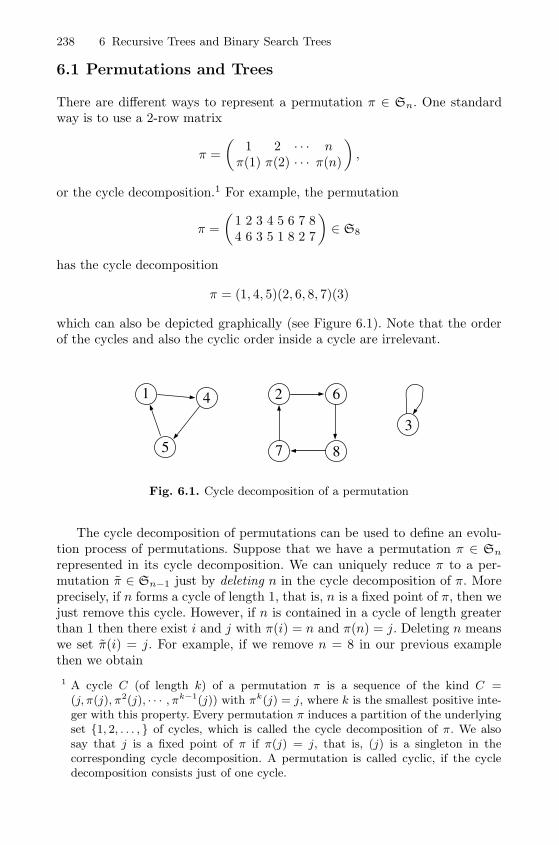
238 6 Recursive Trees and Binary Search Trees
6.1 Permutations and Trees
There are different ways to represent a permutation π ∈ Sn. One standardway is to use a 2-row matrix
π =
(1 2 · · · nπ(1) π(2) · · · π(n)
),
or the cycle decomposition.1 For example, the permutation
π =
(1 2 3 4 5 6 7 84 6 3 5 1 8 2 7
)∈ S8
has the cycle decomposition
π = (1, 4, 5)(2, 6, 8, 7)(3)
which can also be depicted graphically (see Figure 6.1). Note that the orderof the cycles and also the cyclic order inside a cycle are irrelevant.
3
1 4
5
2 6
7 8
Fig. 6.1. Cycle decomposition of a permutation
The cycle decomposition of permutations can be used to define an evolu-tion process of permutations. Suppose that we have a permutation π ∈ Sn
represented in its cycle decomposition. We can uniquely reduce π to a per-mutation π ∈ Sn−1 just by deleting n in the cycle decomposition of π. Moreprecisely, if n forms a cycle of length 1, that is, n is a fixed point of π, then wejust remove this cycle. However, if n is contained in a cycle of length greaterthan 1 then there exist i and j with π(i) = n and π(n) = j. Deleting n meanswe set π(i) = j. For example, if we remove n = 8 in our previous examplethen we obtain
1 A cycle C (of length k) of a permutation π is a sequence of the kind C =(j, π(j), π2(j), · · · , πk−1(j)) with πk(j) = j, where k is the smallest positive inte-ger with this property. Every permutation π induces a partition of the underlyingset {1, 2, . . . , } of cycles, which is called the cycle decomposition of π. We alsosay that j is a fixed point of π if π(j) = j, that is, (j) is a singleton in thecorresponding cycle decomposition. A permutation is called cyclic, if the cycledecomposition consists just of one cycle.
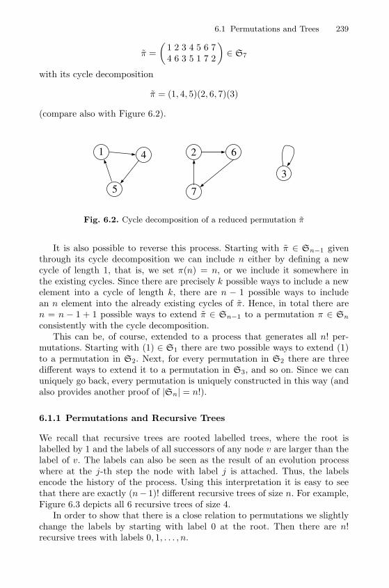
6.1 Permutations and Trees 239
π =
(1 2 3 4 5 6 74 6 3 5 1 7 2
)∈ S7
with its cycle decomposition
π = (1, 4, 5)(2, 6, 7)(3)
(compare also with Figure 6.2).
3
1 4
5
2 6
7
Fig. 6.2. Cycle decomposition of a reduced permutation π
It is also possible to reverse this process. Starting with π ∈ Sn−1 giventhrough its cycle decomposition we can include n either by defining a newcycle of length 1, that is, we set π(n) = n, or we include it somewhere inthe existing cycles. Since there are precisely k possible ways to include a newelement into a cycle of length k, there are n − 1 possible ways to includean n element into the already existing cycles of π. Hence, in total there aren = n − 1 + 1 possible ways to extend π ∈ Sn−1 to a permutation π ∈ Sn
consistently with the cycle decomposition.This can be, of course, extended to a process that generates all n! per-
mutations. Starting with (1) ∈ S1 there are two possible ways to extend (1)to a permutation in S2. Next, for every permutation in S2 there are threedifferent ways to extend it to a permutation in S3, and so on. Since we canuniquely go back, every permutation is uniquely constructed in this way (andalso provides another proof of |Sn| = n!).
6.1.1 Permutations and Recursive Trees
We recall that recursive trees are rooted labelled trees, where the root islabelled by 1 and the labels of all successors of any node v are larger than thelabel of v. The labels can also be seen as the result of an evolution processwhere at the j-th step the node with label j is attached. Thus, the labelsencode the history of the process. Using this interpretation it is easy to seethat there are exactly (n− 1)! different recursive trees of size n. For example,Figure 6.3 depicts all 6 recursive trees of size 4.
In order to show that there is a close relation to permutations we slightlychange the labels by starting with label 0 at the root. Then there are n!recursive trees with labels 0, 1, . . . , n.
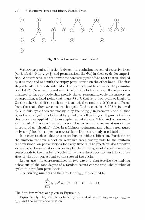
240 6 Recursive Trees and Binary Search Trees
1
4
111
2 2 2 2
3 3 3
3
4
4
4
1
2 3
4
1
2 3
4
Fig. 6.3. All recursive trees of size 4
We now present a bijection between the evolution process of recursive trees(with labels {0, 1, . . . , n}) and permutations (in Sn) in their cycle decomposi-tion. We start with the recursive tree consisting just of the root that is labelledby 0 at one hand and with the empty permutation on the other hand. The firststep is to attach a node with label 1 to the root and to consider the permuta-tion 1 ∈ S1. Now we proceed inductively in the following way. If the j-node isattached to the root node then modify the corresponding cycle decompositionby appending a fixed point that maps j to j, that is, a new cycle of length 1.On the other hand, if the j-th node is attached to node i > 0 (that is differentfrom the root) then we consider the cycle C that contains i. If i is followedby k in this cycle then we modify it by including j in-between i and k, thatis, in the new cycle i is followed by j and j is followed by k. Figure 6.4 showsthis procedure applied to the example permutation π. This kind of process isalso called Chinese restaurant process. The cycles in the permutations can beinterpreted as (circular) tables in a Chinese restaurant and when a new guestarrives he/she either opens a new table or joins an already used table.
It is easy to check that this procedure provides a bijection. Furthermorethe uniform random model on recursive trees corresponds to the uniformrandom model on permutations for every fixed n. The bijection also transferssome shape characteristics. For example, the root degree of the recursive treecorresponds to the number of cycles in the cycle decomposition and the subtreesizes of the root correspond to the sizes of the cycles.
Let us use this correspondence in two ways to characterise the limitingbehaviour of the root degree of a random recursive tree resp. the number ofcycles in a random permutation.
The Stirling numbers of the first kind sn,k are defined by
n∑k=0
sn,kuk = u(u− 1) · · · (u− n+ 1).
The first few values are given in Figure 6.5.Equivalently, they can be defined by the initial values s0,k = δ0,k, sn,0 =
δn,0 and the recurrence relation
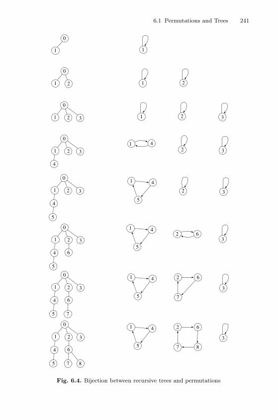
6.1 Permutations and Trees 241
3
1 4
5
2 6
7 8
3
1 4
5
2 6
7
3
1 4
5
2 6
3
1 4
5
2
31 4
2
31 2
1 2
1
0
1
0
1 2
0
1 2 3
0
1 2 3
4
0
1 2 3
4
5
0
1 2 3
4
5
6
0
1 2 3
4
5
6
7
0
1 2 3
4
5
6
7 8
Fig. 6.4. Bijection between recursive trees and permutations
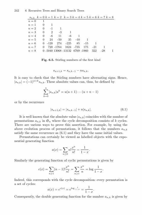
242 6 Recursive Trees and Binary Search Trees
sn,k k = 0 k = 1 k = 2 k = 3 k = 4 k = 5 k = 6 k = 7 k = 8
n = 0 1n = 1 0 1n = 2 0 -1 1n = 3 0 2 -3 1n = 4 0 -6 11 -6 1n = 5 0 24 -50 35 -10 1n = 6 0 -120 274 -225 85 -15 1n = 7 0 720 -1764 1624 -735 175 -21 1n = 8 0 -5040 13068 -13132 6769 -1960 322 -28 1
Fig. 6.5. Stirling numbers of the first kind
sn+1,k = sn,k−1 − nsn,k.
It is easy to check that the Stirling numbers have alternating signs. Hence,|sn,k| = (−1)n+ksn,k. These absolute values can, thus, be defined by
n∑k=0
|sn,k|uk = u(u+ 1) · · · (u + n− 1)
or by the recurrence
|sn+1,k| = |sn,k−1|+ n|sn,k|. (6.1)
It is well known that the absolute value |sn,k| coincides with the number ofpermutations an,k in Sn where the cycle decomposition consists of k cycles.There are various ways to prove this assertion. For example, by using theabove evolution process of permutations, it follows that the numbers an,k
satisfy the same recurrence as (6.1) and they have the same initial values.Permutations can certainly be viewed as labelled objects with the expo-
nential generating function
a(x) =∑n≥0
n!xn
n!=
1
1− x .
Similarly the generating function of cyclic permutations is given by
c(x) =∑n≥1
(n− 1)!xn
n!=∑n≥1
xn
n= log
1
1− x .
Indeed, this corresponds with the cycle decomposition: every permutation isa set of cycles:
a(x) = ec(x) = elog1
1−x =1
1− x.
Consequently, the double generating function for the number an,k is given by
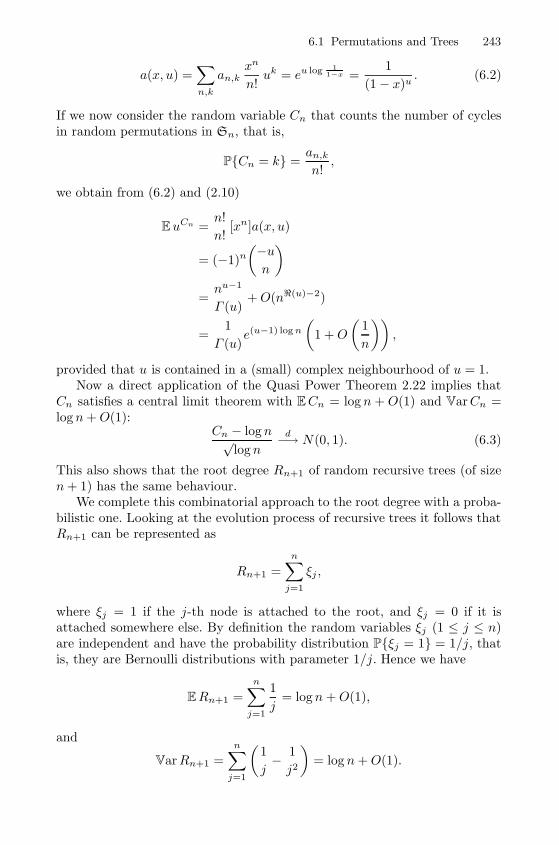
6.1 Permutations and Trees 243
a(x, u) =∑n,k
an,kxn
n!uk = eu log 1
1−x =1
(1− x)u. (6.2)
If we now consider the random variable Cn that counts the number of cyclesin random permutations in Sn, that is,
P{Cn = k} =an,k
n!,
we obtain from (6.2) and (2.10)
EuCn =n!
n![xn]a(x, u)
= (−1)n
(−un
)=nu−1
Γ (u)+O(n�(u)−2)
=1
Γ (u)e(u−1) log n
(1 +O
(1
n
)),
provided that u is contained in a (small) complex neighbourhood of u = 1.Now a direct application of the Quasi Power Theorem 2.22 implies that
Cn satisfies a central limit theorem with ECn = log n + O(1) and VarCn =logn+O(1):
Cn − logn√logn
d−→ N(0, 1). (6.3)
This also shows that the root degree Rn+1 of random recursive trees (of sizen+ 1) has the same behaviour.
We complete this combinatorial approach to the root degree with a proba-bilistic one. Looking at the evolution process of recursive trees it follows thatRn+1 can be represented as
Rn+1 =
n∑j=1
ξj ,
where ξj = 1 if the j-th node is attached to the root, and ξj = 0 if it isattached somewhere else. By definition the random variables ξj (1 ≤ j ≤ n)are independent and have the probability distribution P{ξj = 1} = 1/j, thatis, they are Bernoulli distributions with parameter 1/j. Hence we have
ERn+1 =
n∑j=1
1
j= logn+O(1),
and
VarRn+1 =n∑
j=1
(1
j− 1
j2
)= log n+O(1).
244 6 Recursive Trees and Binary Search Trees
Finally, the classical central limit theorem (for independent but not necessarilyidentically distributed random variables) can be applied and we recover (6.3).
We close this section by providing a bivariate asymptotic expansion forStirling numbers of the first kind that is valid for k = O(log n).
Lemma 6.1. We have uniformly for c logn ≤ k ≤ C logn
|sn,k| =(n− 1)!(logn)k
k!Γ(
klog n
) (1 +O
(1√
logn
)),
where c < C are arbitrary positive constants.
Proof. By definition we have∑k≥0
|sn,k|uk = (−1)n
(−un
)n!.
Hence, by Lemma 2.14 we have uniformly for c ≤ |u| ≤ C∑k≥0
|sn,k|uk = n!nu−1
Γ (u)
(1 +O
(1
n
))
= (n− 1)!eu log n
Γ (u)
(1 +O
(1
n
))and consequently by Cauchy’s formula
|sn,k| =(n− 1)!
2πi
∫γ
eu log n
Γ (u)
(1 +O
(1
n
))du
uk+1.
We will choose γ to be a circle |u| = r with radius r = k/ logn, since thedominating part of the integrand
eu log nu−k = eu log n−k log u
has a saddle point at u = k/ logn. In fact, a standard saddle point methodyields the result.
We use the substitution u = reit (−π < t ≤ π) with r = k/ logn. Then byusing the approximation eit = 1 + it− 1
2 t2 +O(t3) we get
eu log nu−k = ekr−ke−k2 t2+O(kt3).
We split up the integral into two parts:
γ1 = {u = reit : |t| ≤ k−1/3},γ2 = {u = reit : k−1/3 < |t| ≤ π}.
6.1 Permutations and Trees 245
For the integral over γ1 we have
(n− 1)!
2πi
∫γ1
eu log n
Γ (u)
(1 +O
(1
n
))du
uk+1
=(n− 1)!
2π
∫|t|≤k−1/3
ekr−k
Γ (r) +O(t)e−
k2 t2+O(kt3)
(1 +O
(1
n
))dt
=ekr−k
Γ (r)
(n− 1)!
2π
∫|t|≤k−1/3
e−k2 t2(
1 +O(t) +O(kt3) +O
(1
n
))
=ekr−k
Γ (r)
(n− 1)!
2π
(√2π
k+O(e−
12 k1/3)
+O
(1
k
)+O
(1
n
))
=(n− 1)!(logn)k
k!Γ (r)
(1 +O
(1√k
)).
The integral over γ2 is negligible. This can be checked by the following obser-vations. By continuity it follows that there exists a constant c′ > 0 such thatfor all |t| ≤ π and uniformly for c ≤ r ≤ C∣∣eu log nu−k
∣∣ ≤ ekr−ke−c′kt2 .
Furthermore we have ∫k−1/3≤|t|≤π
e−c′kt2 dt = O(e−c′k1/3
).
This completes the proof of the lemma.
Remark 6.2 Lemma 6.1 holds even uniformly for 1 ≤ k ≤ C logn. This canbe proved, for example, by using the series expansion
∑n≥0
|sn,k|xn
n!=
1
k!
(log
1
1− x
)k
and a Hankel like contour integration applied to Cauchy’s formula (similarlyto the proof of Lemma 2.14).
Using this asymptotic expansion we obtain even more precise informationon the local behaviour of the distribution of the number of cycles in permuta-tions (resp. of the root degree of recursive trees). Since P{Cn = k} = |sn,k|/n!,we have (uniformly for c logn ≤ k ≤ C log n)
P{Cn = k} =(logn)k
n k!Γ(
klog n
) (1 +O
(1√
logn
)).
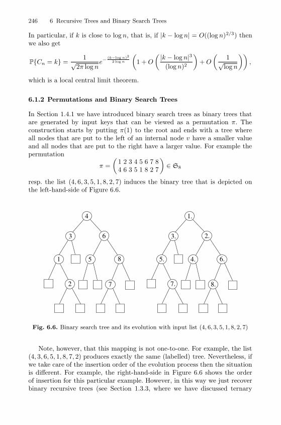
246 6 Recursive Trees and Binary Search Trees
In particular, if k is close to logn, that is, if |k − logn| = O((log n)2/3) thenwe also get
P{Cn = k} =1√
2π log ne−
(k−log n)2
2 log n
(1 +O
( |k − logn|3(logn)2
)+O
(1√
log n
)),
which is a local central limit theorem.
6.1.2 Permutations and Binary Search Trees
In Section 1.4.1 we have introduced binary search trees as binary trees thatare generated by input keys that can be viewed as a permutation π. Theconstruction starts by putting π(1) to the root and ends with a tree whereall nodes that are put to the left of an internal node v have a smaller valueand all nodes that are put to the right have a larger value. For example thepermutation
π =
(1 2 3 4 5 6 7 84 6 3 5 1 8 2 7
)∈ S8
resp. the list (4, 6, 3, 5, 1, 8, 2, 7) induces the binary tree that is depicted onthe left-hand-side of Figure 6.6.
1
2
3
4
5
6
7
8 5.
7.
3.
1.
4.
2.
8.
6.
Fig. 6.6. Binary search tree and its evolution with input list (4, 6, 3, 5, 1, 8, 2, 7)
Note, however, that this mapping is not one-to-one. For example, the list(4, 3, 6, 5, 1, 8, 7, 2) produces exactly the same (labelled) tree. Nevertheless, ifwe take care of the insertion order of the evolution process then the situationis different. For example, the right-hand-side in Figure 6.6 shows the orderof insertion for this particular example. However, in this way we just recoverbinary recursive trees (see Section 1.3.3, where we have discussed ternary
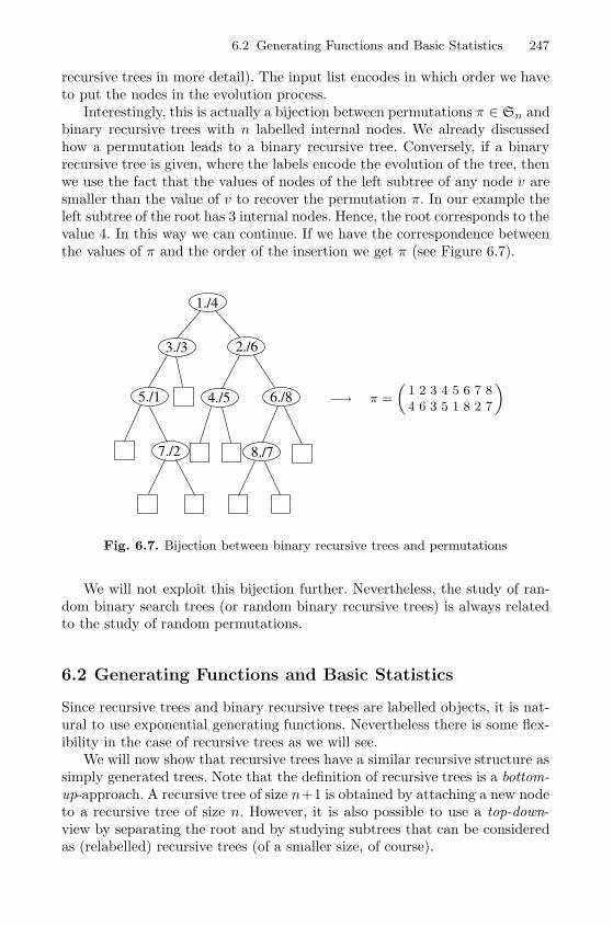
6.2 Generating Functions and Basic Statistics 247
recursive trees in more detail). The input list encodes in which order we haveto put the nodes in the evolution process.
Interestingly, this is actually a bijection between permutations π ∈ Sn andbinary recursive trees with n labelled internal nodes. We already discussedhow a permutation leads to a binary recursive tree. Conversely, if a binaryrecursive tree is given, where the labels encode the evolution of the tree, thenwe use the fact that the values of nodes of the left subtree of any node v aresmaller than the value of v to recover the permutation π. In our example theleft subtree of the root has 3 internal nodes. Hence, the root corresponds to thevalue 4. In this way we can continue. If we have the correspondence betweenthe values of π and the order of the insertion we get π (see Figure 6.7).
5./1
3./3
1./4
4./5
2./6
8./7
6./8
7./2
−→ π =
„1 2 3 4 5 6 7 84 6 3 5 1 8 2 7
«
Fig. 6.7. Bijection between binary recursive trees and permutations
We will not exploit this bijection further. Nevertheless, the study of ran-dom binary search trees (or random binary recursive trees) is always relatedto the study of random permutations.
6.2 Generating Functions and Basic Statistics
Since recursive trees and binary recursive trees are labelled objects, it is nat-ural to use exponential generating functions. Nevertheless there is some flex-ibility in the case of recursive trees as we will see.
We will now show that recursive trees have a similar recursive structure assimply generated trees. Note that the definition of recursive trees is a bottom-up-approach. A recursive tree of size n+1 is obtained by attaching a new nodeto a recursive tree of size n. However, it is also possible to use a top-down-view by separating the root and by studying subtrees that can be consideredas (relabelled) recursive trees (of a smaller size, of course).
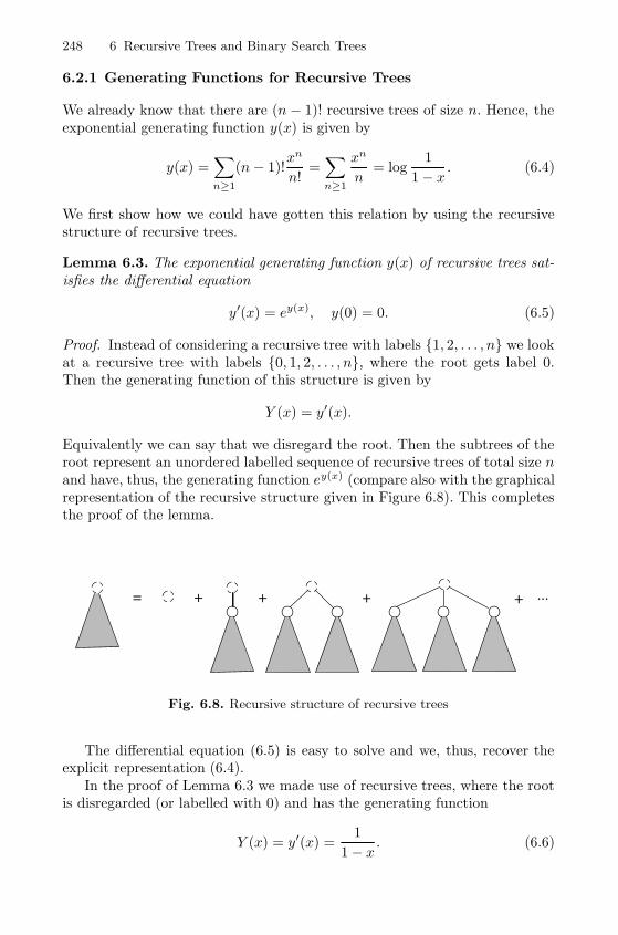
248 6 Recursive Trees and Binary Search Trees
6.2.1 Generating Functions for Recursive Trees
We already know that there are (n− 1)! recursive trees of size n. Hence, theexponential generating function y(x) is given by
y(x) =∑n≥1
(n− 1)!xn
n!=∑n≥1
xn
n= log
1
1− x . (6.4)
We first show how we could have gotten this relation by using the recursivestructure of recursive trees.
Lemma 6.3. The exponential generating function y(x) of recursive trees sat-isfies the differential equation
y′(x) = ey(x), y(0) = 0. (6.5)
Proof. Instead of considering a recursive tree with labels {1, 2, . . . , n} we lookat a recursive tree with labels {0, 1, 2, . . . , n}, where the root gets label 0.Then the generating function of this structure is given by
Y (x) = y′(x).
Equivalently we can say that we disregard the root. Then the subtrees of theroot represent an unordered labelled sequence of recursive trees of total size nand have, thus, the generating function ey(x) (compare also with the graphicalrepresentation of the recursive structure given in Figure 6.8). This completesthe proof of the lemma.
= + + + ...+
Fig. 6.8. Recursive structure of recursive trees
The differential equation (6.5) is easy to solve and we, thus, recover theexplicit representation (6.4).
In the proof of Lemma 6.3 we made use of recursive trees, where the rootis disregarded (or labelled with 0) and has the generating function
Y (x) = y′(x) =1
1− x. (6.6)
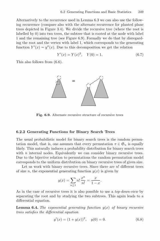
6.2 Generating Functions and Basic Statistics 249
Alternatively to the recurrence used in Lemma 6.3 we can also use the follow-ing recurrence (compare also with the alternate recurrence for planted planetrees depicted in Figure 3.4). We divide the recursive tree (where the root islabelled by 0) into two trees, the subtree that is rooted at the node with label1 and the remaining tree (see Figure 6.9). Formally we do that by disregard-ing the root and the vertex with label 1, which corresponds to the generatingfunction Y ′(x) = y′′(x). Due to this decomposition we get the relation
Y ′(x) = Y (x)2, Y (0) = 1. (6.7)
This also follows from (6.6).
=
Fig. 6.9. Alternate recursive structure of recursive trees
6.2.2 Generating Functions for Binary Search Trees
The usual probabilistic model for binary search trees is the random permu-tation model, that is, one assumes that every permutation π ∈ Sn is equallylikely. This naturally induces a probability distribution for binary search treeswith n internal nodes. Equivalently we can consider binary recursive trees.Due to the bijective relation to permutations the random permutation modelcorresponds to the uniform distribution on binary recursive trees of given size.
Let us work with binary recursive trees. Since there are n! different treesof size n, the exponential generating function y(x) is given by
y(x) =∑n≥1
n!xn
n!=
x
1− x .
As in the case of recursive trees it is also possible to use a top-down-view byseparating the root and by studying the two subtrees. This again leads to adifferential equation.
Lemma 6.4. The exponential generating function y(x) of binary recursivetrees satisfies the differential equation
y′(x) = (1 + y(x))2, y(0) = 0. (6.8)
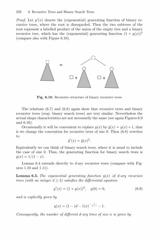
250 6 Recursive Trees and Binary Search Trees
Proof. Let y′(x) denote the (exponential) generating function of binary re-cursive trees, where the root is disregarded. Then the two subtrees of theroot represent a labelled product of the union of the empty tree and a binaryrecursive tree, which has the (exponential) generating function (1 + y(x))2
(compare also with Figure 6.10).
=
++
Fig. 6.10. Recursive structure of binary recursive trees
The relations (6.7) and (6.8) again show that recursive trees and binaryrecursive trees (resp. binary search trees) are very similar. Nevertheless theactual shape characteristics are not necessarily the same (see again Figures 6.9and 6.10).
Occasionally it will be convenient to replace y(x) by y(x) = y(x) + 1, thatis we change the convention for recursive trees of size 0. Then (6.8) rewritesto
y′(x) = y(x)2.
Equivalently we can think of binary search trees, where it is usual to includethe case of size 0. Thus, the generating function for binary search trees isy(x) = 1/(1− x).
Lemma 6.4 extends directly to d-ary recursive trees (compare with Fig-ures 1.10 and 1.11).
Lemma 6.5. The exponential generating function y(x) of d-ary recursivetrees (with an integer d ≥ 2) satisfies the differential equation
y′(x) = (1 + y(x))d, y(0) = 0, (6.9)
and is explicitly given by
y(x) = (1− (d− 1)x)− 1
d−1 − 1.
Consequently, the number of different d-ary trees of size n is given by
6.2 Generating Functions and Basic Statistics 251
yn =
n−1∏j=1
(jd− (j − 1))
= n!(−1)n(d− 1)n
(− 1d−1
n
)∼ n!(d− 1)n n
2−dd−1
Γ(
1d−1
) .Again it is also convenient to consider instead
y(x) = y(x) + 1 = (1− (d− 1)x)− 1
d−1
that satisfies the differential equation y′(x) = y(x)d.
6.2.3 Generating Functions for Plane Oriented Recursive Trees
Plane oriented recursive trees are similarly defined to recursive trees withthe only difference that the left-to-right-order of the successors is taken intoaccount. This means that we are considering plane trees. There are againdifferent points of view.
The corresponding evolution process works as follows. As usual we startwith the root that gets label 0. Now if a node already has out-degree k (wherethe descendants are ordered), then there are k + 1 possible ways to attacha new node. Hence, if a plane tree already has j − 1 nodes then there areprecisely 2j − 3 possibilities to attach the j-th node and to generate a planeoriented recursive tree of size j. We already observed in Section 1.3.2 that thisconsideration implies that there are
1 · 3 · . . . · (2n− 3) = (2n− 3)!! =1
2n−1
(2(n− 1))!
(n− 1)!
different plane oriented recursive trees.We can also use a generating function approach.
Lemma 6.6. The exponential generating function y(x) of plane oriented re-cursive trees satisfies the differential equation
y′(x) =1
1− y(x), y(0) = 0 (6.10)
and is explicitly given by
y(x) = 1−√
1− 2x =∑n≥1
(2n− 3)!!xn
n!.
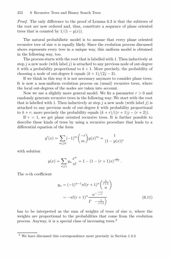
252 6 Recursive Trees and Binary Search Trees
Proof. The only difference to the proof of Lemma 6.3 is that the subtrees ofthe root are now ordered and, thus, constitute a sequence of plane orientedtrees that is counted by 1/(1− y(x)).
The natural probabilistic model is to assume that every plane orientedrecursive tree of size n is equally likely. Since the evolution process discussedabove represents every tree in a unique way, this uniform model is obtainedin the following way, too.
The process starts with the root that is labelled with 1. Then inductively atstep j a new node (with label j) is attached to any previous node of out-degreek with a probability proportional to k + 1. More precisely, the probability ofchoosing a node of out-degree k equals (k + 1)/(2j − 3).
If we think in this way it is not necessary anymore to consider plane trees.It is now a non-uniform evolution process on (usual) recursive trees, wherethe local out-degrees of the nodes are taken into account.
Now we use a slightly more general model. We fix a parameter r > 0 andrandomly generate recursive trees in the following way: We start with the rootthat is labelled with 1. Then inductively at step j a new node (with label j) isattached to any previous node of out-degree k with probability proportionalto k + r; more precisely the probability equals (k + r)/((r + 1)j − (r + 2)).
If r = 1, we get plane oriented recursive trees. It is further possible todescribe these kinds of trees by using a recursive procedure that leads to adifferential equation of the form
y′(x) =∑m≥0
(−1)m
(−rm
)y(x)m =
1
(1 − y(x))r
with solution
y(x) =∑n≥1
ynxn
n!= 1− (1− (r + 1)x)
1r+1 .
The n-th coefficient
yn = (−1)n−1n!(r + 1)n
( 1r+1
n
)∼ −n!(r + 1)n n−
r+2r+1
Γ(− 1
r+1
) (6.11)
has to be interpreted as the sum of weights of trees of size n, where theweights are proportional to the probabilities that come from the evolutionprocess. Anyway, it is a special class of increasing trees.2
2 We have discussed this correspondence more precisely in Section 1.3.3.
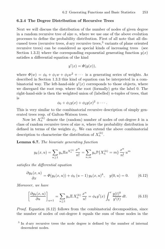
6.2 Generating Functions and Basic Statistics 253
6.2.4 The Degree Distribution of Recursive Trees
Next we will discuss the distribution of the number of nodes of given degreein a random recursive tree of size n, where we use one of the above evolutionprocesses to define the probability distribution. First of all note that all dis-cussed trees (recursive trees, d-ary recursive trees,3 variants of plane orientedrecursive trees) can be considered as special kinds of increasing trees (seeSection 1.3.3) where the corresponding exponential generating function y(x)satisfies a differential equation of the kind
y′(x) = Φ(y(x)),
where Φ(w) = φ0 + φ1w + φ2w2 + · · · is a generating series of weights. As
described in Section 1.3.3 this kind of equation can be interpreted in a com-binatorial way. The left-hand-side y′(x) corresponds to those objects, wherewe disregard the root resp. where the root (formally) gets the label 0. Theright-hand-side is then the weighted union of (labelled) n-tuples of trees, thatis
φ0 + φ1y(x) + φ2y(x)2 + · · · .This is very similar to the combinatorial recursive description of simply gen-erated trees resp. of Galton-Watson trees.
Now let X(k)n denote the (random) number of nodes of out-degree k in a
class of random recursive trees of size n, where the probability distribution isdefined in terms of the weights φj . We can extend the above combinatorial
description to characterise the distribution of X(k)n .
Lemma 6.7. The bivariate generating function
yk(x, u) =∑n≥1
ynEuX(k)nxn
n!=∑n,m
ynP{X(k)n = m} x
n
n!um
satisfies the differential equation
∂yk(x, u)
∂x= Φ(yk(x, u)) + φk (u− 1) yk(x, u)k, y(0, u) = 0. (6.12)
Moreover, we have[∂yk(x, u)
∂u
]u=1
=∑n≥1
ynEX(k)n
xn
n!= φky
′(x)
∫ x
0
y(t)k
y′(t)dt. (6.13)
Proof. Equation (6.12) follows from the combinatorial decomposition, sincethe number of nodes of out-degree k equals the sum of those nodes in the
3 In d-ary recursive trees the node degree is defined by the number of internaldescendent nodes.
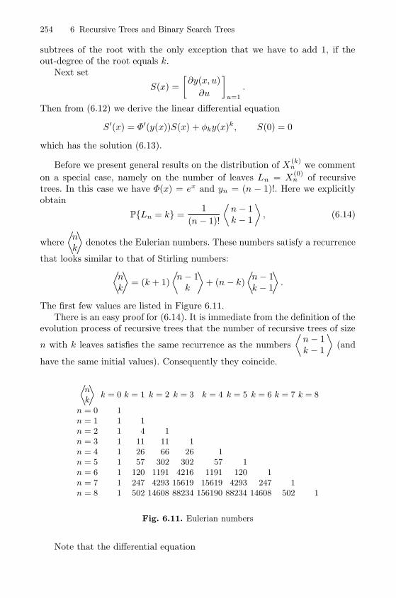
254 6 Recursive Trees and Binary Search Trees
subtrees of the root with the only exception that we have to add 1, if theout-degree of the root equals k.
Next set
S(x) =
[∂y(x, u)
∂u
]u=1
.
Then from (6.12) we derive the linear differential equation
S′(x) = Φ′(y(x))S(x) + φky(x)k, S(0) = 0
which has the solution (6.13).
Before we present general results on the distribution of X(k)n we comment
on a special case, namely on the number of leaves Ln = X(0)n of recursive
trees. In this case we have Φ(x) = ex and yn = (n − 1)!. Here we explicitlyobtain
P{Ln = k} =1
(n− 1)!
⟨n− 1k − 1
⟩, (6.14)
where
⟨nk
⟩denotes the Eulerian numbers. These numbers satisfy a recurrence
that looks similar to that of Stirling numbers:⟨nk
⟩= (k + 1)
⟨n− 1k
⟩+ (n− k)
⟨n− 1k − 1
⟩.
The first few values are listed in Figure 6.11.There is an easy proof for (6.14). It is immediate from the definition of the
evolution process of recursive trees that the number of recursive trees of size
n with k leaves satisfies the same recurrence as the numbers
⟨n− 1k − 1
⟩(and
have the same initial values). Consequently they coincide.
fink
flk = 0 k = 1 k = 2 k = 3 k = 4 k = 5 k = 6 k = 7 k = 8
n = 0 1n = 1 1 1n = 2 1 4 1n = 3 1 11 11 1n = 4 1 26 66 26 1n = 5 1 57 302 302 57 1n = 6 1 120 1191 4216 1191 120 1n = 7 1 247 4293 15619 15619 4293 247 1n = 8 1 502 14608 88234 156190 88234 14608 502 1
Fig. 6.11. Eulerian numbers
Note that the differential equation
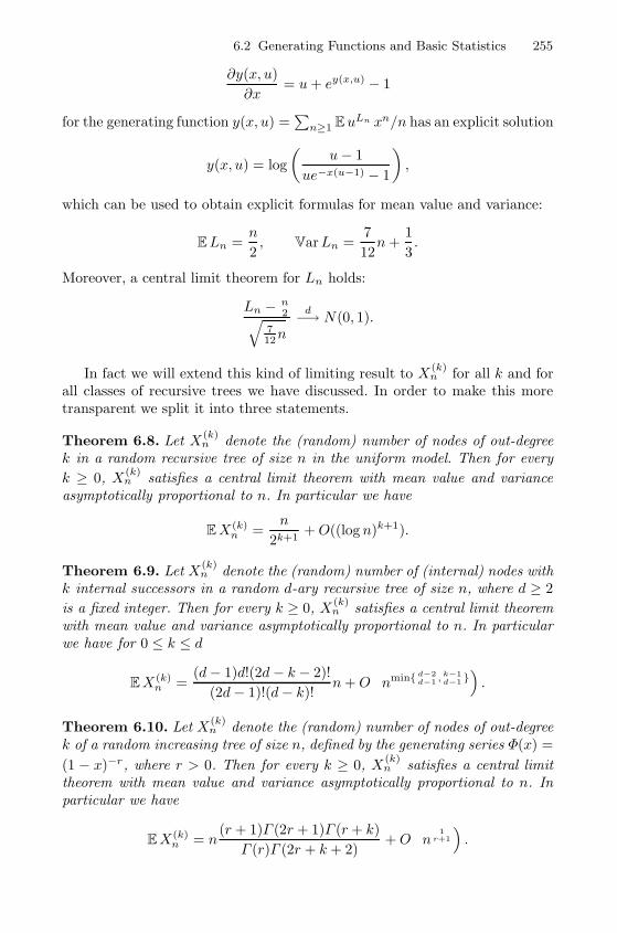
6.2 Generating Functions and Basic Statistics 255
∂y(x, u)
∂x= u+ ey(x,u) − 1
for the generating function y(x, u) =∑
n≥1 EuLn xn/n has an explicit solution
y(x, u) = log
(u− 1
ue−x(u−1) − 1
),
which can be used to obtain explicit formulas for mean value and variance:
ELn =n
2, VarLn =
7
12n+
1
3.
Moreover, a central limit theorem for Ln holds:
Ln − n2√
712n
d−→ N(0, 1).
In fact we will extend this kind of limiting result to X(k)n for all k and for
all classes of recursive trees we have discussed. In order to make this moretransparent we split it into three statements.
Theorem 6.8. Let X(k)n denote the (random) number of nodes of out-degree
k in a random recursive tree of size n in the uniform model. Then for every
k ≥ 0, X(k)n satisfies a central limit theorem with mean value and variance
asymptotically proportional to n. In particular we have
EX(k)n =
n
2k+1+O((log n)k+1).
Theorem 6.9. Let X(k)n denote the (random) number of (internal) nodes with
k internal successors in a random d-ary recursive tree of size n, where d ≥ 2
is a fixed integer. Then for every k ≥ 0, X(k)n satisfies a central limit theorem
with mean value and variance asymptotically proportional to n. In particularwe have for 0 ≤ k ≤ d
EX(k)n =
(d− 1)d!(2d− k − 2)!
(2d− 1)!(d− k)!n+O(nmin{ d−2
d−1 , k−1d−1 }).
Theorem 6.10. Let X(k)n denote the (random) number of nodes of out-degree
k of a random increasing tree of size n, defined by the generating series Φ(x) =
(1 − x)−r, where r > 0. Then for every k ≥ 0, X(k)n satisfies a central limit
theorem with mean value and variance asymptotically proportional to n. Inparticular we have
EX(k)n = n
(r + 1)Γ (2r + 1)Γ (r + k)
Γ (r)Γ (2r + k + 2)+O(n
1r+1
).
256 6 Recursive Trees and Binary Search Trees
Theorem 6.10 is of special interest, since the corresponding (asymptotic)degree distribution
dk =(r + 1)Γ (2r + 1)Γ (r + k)
Γ (r)Γ (2r + k + 2)
has a polynomial tail of the form
(r + 1)Γ (2r + 1)
Γ (r)k−2−r.
Such distributions are also called scale-free and appear in several real networkslike the internet or social networks that have an evolution in time. In particularthere is substantial interest in random graph models where vertices are addedto the graph successively and are connected to several already existing nodesaccording to some given law. The so-called Albert-Barabasi model (see [1])joins a new node to an existing one with probability proportional to the degree.Recall that the random recursive trees that are considered in Theorem 6.10are constructed exactly by this principle: a new node is attached to an alreadyexisting one (with out-degree k) with probability proportional to k+ r. Thus,these models confirm the observation that networks that follow the Albert-Barabasi principle have asymptotically a scale-free degree distribution.
The proofs of Theorems 6.8–6.10 are very similar. So we group them to-gether.
Proof. Let us start with recursive trees. The differential equation (y =yk(x, u))
∂y
∂x= ey +
yk
k!(u− 1) (6.15)
can be rewritten to ∫ y
0
1
ev + vk
k! (u − 1)dv = x. (6.16)
We split up the integral on the left-hand-side into two parts:∫ y
0
1
ev + vk
k! (u− 1)dv =
∫ ∞0
1
ev + vk
k! (u− 1)dv
−∫ ∞
y
1
ev + vk
k! (u− 1)dv
= C(u)−D(y, u).
Observe that D(y, u) is given asymptotically by
D(y, u) = e−y(1 +O(e−yyk|u− 1|
)).
Hence (6.16) translates to
6.2 Generating Functions and Basic Statistics 257
C(u)− x = e−y(1 +O(e−yyk|u− 1|
))which can be inverted to
yk(x, u) = log1
C(u)− x +O
(|u− 1| |C(u)− x|
(log
1
C(u)− x
)k+1).
Consequently it follows from Theorem 2.25 (combined with the Remark fol-
lowing Corollary 2.16) that X(k)n satisfies a central limit theorem with mean
value
EX(k)n = −C
′(1)
C(1)n+O((log n)k+1
)and variance
VarX(k)n =
(−C
′′(1)
C(1)− C
′(1)
C(1)+C′(1)2
C(1)2
)n+O((logn)k+1
).
It is now an easy exercise to compute
C(1) = 1, C ′(1) = − 1
2k+1, C′′(1) =
2
32k+1
(2k)!
(k!)2.
This completes the proof for recursive trees.In the d-ary case we can work in completely the same way. The solution of
the corresponding differential equation rewrites to x−C(u) = D(y, u), where(for k < d)
C(u) =
∫ ∞0
1
(1 + v)d +(
dk
)vk(u− 1)
dv
and
D(y, u) =
∫ ∞y
1
(1 + v)d +(
dk
)vk(u − 1)
dv
=1
d− 1
1
(1 + y)d−1
(1 +O
( |u− 1|yd−k
)).
This leads to
yk(x, u) = ((d− 1)(C(u)− x))− 1
d−1
(1 +O(|u − 1| |C(u)− x| d−k
d−1
))− 1
which again implies a central limit theorem with expected value and variancethat is asymptotically proportional to n. In particular we have
C(1) =1
d− 1, C′(1) = − d!(2d− k − 2)!
(2d− 1)!(d− k)!, and
C′′(1) = 2
(d
k
)2(2k)!(3d− 2k − 2)!
(3d− 1)!.
258 6 Recursive Trees and Binary Search Trees
Since X(d)n = n−∑k<dX
(k)n , the case k = d can be reduced (more or less) to
the previous cases by considering the differential equation
∂y
∂x= (y + 1)d + (u− 1)
((y + 1)d − yd
).
The proof in the final case, where Φ(w) = (1− w)−r , is slightly different,since y(x0) is finite at the radius of convergence. Here the solution y = yk(x, u)of the corresponding differential equation is determined by x−C(u) = D(y, u),where
C(u) =
∫ 1
0
1
(1− v)−r +(r+k−1
k
)vk(u − 1)
dv
and
D(y, u) =
∫ y
0
1
(1− v)−r +(r+k−1
k
)vk(u− 1)
dv
=1
r + 1(1− y)r+1 (1 +O (|u− 1| |1− y|r)) .
Hence, we get
yk(x, u) = 1− ((r + 1)(C(u)− x))1
r+1 +O (|u− 1| |C(u)− x|) .
Consequently it follows from Theorem 2.25 that X(k)n satisfies a central limit
theorem with mean and variance asymptotically proportional to n. It is aneasy exercise to compute
C(1) =1
r + 1, C′(1) = −k!Γ (r + k)Γ (2r + 1)
Γ (r)Γ (2r + k + 2)and
C′′(1) =(2k)!Γ (r + k)2Γ (3r + 1)
(k!)2Γ (r)2Γ (3r + 2k + 2)
which completes the proof of Theorems 6.8–6.10.
Note that in the previous discussion we have not distinguished nodes bytheir label. Obviously the out-degree of node n is always 0, whereas the rootdegree is usually much larger than the average degree. We will not go muchinto detail here (for a detailed analysis see Kuba and Panholzer [134]). Wewill only focus on the root degree Rn. By construction it follows that thederivative with respect to x of the function
y(x, u) =∑n≥1
ynEuRnxn
n!
is given by∂y(x, u)
∂x= Φ(uy(x)).
6.2 Generating Functions and Basic Statistics 259
Note that the analysis is relatively simple, since
∂y(x, u)
∂x=∑n≥1
ynEuRnxn−1
(n− 1)!.
We have already observed that the root degree of recursive trees is re-lated directly to Stirling numbers of the first kind and satisfies a central limittheorem with mean value and variance asymptotically proportional to logn.Thus, we just present a corresponding result for plane oriented recursive trees(and their variants defined by Φ(w) = 1/(1− w)r). For the d-ary case we getconcentration at d.
Theorem 6.11. Let Rn denote the root degree of a random increasing tree ofsize n, defined by the generating series Φ(w) = (1−w)−r, where r > 0. Thenfor every κ > 0 we have
P{Rn = �κn 1r+1 �} ∼
Γ(
rr+1
)Γ (r)
κr−1
n1
r+1
1
2πi
∫H
e−κ·(−z)1
r+1−z dz, (6.17)
where H denotes a Hankel contour, and
ERn ∼ rΓ(
r
r + 1
)n
1r+1 . (6.18)
In particular for r = 1 we have
P{Rn = k} =(2n− 3− k)!
2n−1−k(n− 1− k)!∼√
2
πne−k2/(4n)
and ERn =√πn+O(1).
Proof. Since ∂y(x,u)∂x = (1− uy(x))−r, it follows that
P{Rn = k} =(n− 1)!
yn
(r + k − 1
k
)[xn−1]y(x)k,
where y(x) =∑
n≥1 yn xn/n! = 1−(1−(r+1)x)
1r+1 . By using an approximate
Hankel contour and the substitution x = 1r+1
(1 + z
n
)one obtains (if k is
proportional to n1
r+1 )
[xn−1]y(x)k =1
2πi
∫γ
(1− (1 − (r + 1)x)
1r+1
)k dxxn
∼ (r + 1)n−1
n
1
2πi
∫H
e−kn− 1
r+1 ·(−z)1
r+1−z dz.
By using the asymptotic relations(r+k−1
k
)∼ kr−1/Γ (r) and (6.11), we obtain
(6.17).
260 6 Recursive Trees and Binary Search Trees
The generating function for the expected value is r y(x)(1−y(x))−2r. Thus,(6.18) follows easily.
For the case r = 1 we have y(x) = 1 −√
1− 2x, which is the solution ofthe equation
y =x
1− y2
.
Hence, by Lagrange’s inversion formula, we obtain explicit formulas for yn
and [xn−1]y(x)k, and consequently for P{Rn = k}.
Another interesting parameter is the maximum degree Δn. For recursivetrees the following precise result due to Goh and Schmutz [94] is known. (Itextends previous results by Szymanski [198] and Devroye and Jiang Lu [53].)
Theorem 6.12. The maximum degree Δn in random recursive trees of sizen satisfies
P{Δn ≤ d} = exp(−2−(d−log2 n+1)
)+ o(1).
This says that the distribution of Δn is highly concentrated around the valuelog2 n and the distribution’s behaviour is related to the extreme value dis-
tribution (or Gumbel distribution) with distribution function F (t) = e−e−t
.Note that the root degree is approximately logn which is considerably smallerthan the maximum degree.
The proof of Theorem 6.12 is an analytic tour de force which we do notpresent here. Nevertheless we want to give some indications why the maximumdegree is concentrated around log2 n. More precisely we derive an upper boundfor the expected maximum degree and indicate that a corresponding lowerbound can be obtained, too.
The method we use here relies on the so-called first moment method.
Lemma 6.13. Let X be a discrete random variable on non-negative integers.Then
P{X > 0} ≤ min{1,EX}.
Proof. We only have to observe that
EX =∑k≥0
k P{X = k} ≥∑k≥1
P{X = k} = P{X > 0}.
We apply this principle to the random variable X(>k)n that counts the
number of nodes in recursive trees with out-degree > k. Obviously we have
Δn > k ⇐⇒ X(>k)n > 0
and consequently
EΔn =∑k≥0
P{Δn > k}
6.2 Generating Functions and Basic Statistics 261
=∑k≥0
P{X(>k)n > 0}
≤∑k≥0
min{1,EX(>k)n }.
Thus, if we have some (uniform) information on the expected values
EX(>k)n =
∑j>k
EX(j)n
then we obtain an upper bound for EΔn.
Lemma 6.14. For random recursive trees of size n we have uniformly ink ≥ 0
EX(k)n =
n
2k+1+O
(1
n
(logn)k
k!
). (6.19)
Proof. By Lemma 6.7 we have
∑n≥1
EX(k)n
xn
n=
1
k!(1 − x)
∫ x
0
(1− t)(
log1
1− t
)k
dt
=1
2k+1
1
1− x + (x − 1)
k∑j=0
1
j!2k+1−j
(log
1
1− x
)j
.
It is now an easy exercise to use the methods of Lemma 2.12 to obtain theuniform estimate
[xn](x − 1)
(log
1
1− x
)k
≤ C
n2(logn)k
for some constant C > 0. Hence, (6.19) follows.
Suppose that k ≥ log2 n. Then∑j>k
(logn)j
j!= O
((log n)k+1
(k + 1)!
).
Consequently we get (for k ≥ log2 n)
EX(>k)n =
n
2k+1+O
(1
n
(logn)k+1
(k + 1)!
)and also ∑
k≥log2 n
EX(>k)n = O(1).
Summing up we, thus, obtain
262 6 Recursive Trees and Binary Search Trees
EΔn ≤∑k≥0
min{1,EX(>k)n }
≤∑
k<log2 n
1 +∑
k≥log2 n
EX(>k)n
= log2 n+O(1).
In order to obtain a corresponding lower bound one can use the so-calledsecond moment method.
Lemma 6.15. Suppose that X is a non-negative random variable which is notidentically zero and has finite second moment. Then
P{X > 0} ≥ (EX)2
E (X2).
Proof. This follows from an application of the Cauchy-Schwarz inequality:
EX = E(X · 1[X>0]
)≤√
E (X2)√
E (12[X>0]) =
√E(X2)√
P{X > 0}.
In order to apply the second moment method to obtain a lower bound for
EΔn one needs estimates for E (X(>k)n )2 which can be derived in a similar
way as above. In particular it follows that
EΔn ≥ log2 n+O(1)
and, hence, EΔn = log2 n+O(1). However, we do not work out the details.Nevertheless, remark that the threshold k ≈ log2 n is determined by the
equationEX(>k)
n ≈ 1 resp. by EX(k)n ≈ 1.
Thus, in order to get a first impression where the average maximum degree issituated one should look at this equation. A rigorous treatment can then berealised with the help of the first and second moment method.
6.2.5 The Insertion Depth
The insertion depth Dn of a recursive tree is the distance of the n-th nodeto the root. Note that the distribution of Dn depends on the whole evolutionprocess until step n− 1. Nevertheless, there is a very elegant way to describethe distribution ofDn in relation to the profiles of the occurring random trees.Let (T1, T2, . . .) denote the sequence of random recursive trees, where in eachstep a new node is attached to one of the existing ones. The profile Xn,k ofTn is the number of nodes at distance k to the root. Now the conditionalprobability P{Dn = k|Tn−1} is given by
P{Dn = k|Tn−1} =Xn−1,k−1
n− 1,
6.2 Generating Functions and Basic Statistics 263
because Dn = k if the n-th node is attached to a node at distance k − 1 inTn−1. Hence, by taking expectations we obtain
P{Dn = k} =EXn−1,k−1
n− 1.
Therefore, the distribution ofDn is determined by the expected profile that wewill calculate in the next lemma (that is due to Dondajewski and Szymanski[56], see also Meir and Moon [151]).
Lemma 6.16. The expected profile in random recursive trees is given by
EXn,k =|sn,k+1|(n− 1)!
,
where sn,k denotes the of the first kind.
Proof. We present two different proofs of this property. The first proof uses theevolution process (T1, T2, . . .) and conditional probabilities resp. expectations.The insertion of the n-th node has the following (conditional) effect on theprofile:
E(Xn,k|Tn−1) =
(1− Xn−1,k−1
n− 1
)Xn−1,k +
Xn−1,k−1
n− 1(Xn−1,k + 1)
= Xn−1,k +Xn−1,k−1
n− 1.
Taking the expectation this leads to the recurrence relation
EXn,k = EXn−1,k +EXn−1,k−1
n− 1. (6.20)
Hence, by using the series
en(u) =∑k≥0
EXn,k uk,
we derive the recurrence
en(u) = en−1(u)
(1 +
u
n− 1
).
Since e1(u) = 1, we this leads to an explicit representation
en(u) =
(1 +
u
n− 1
)(1 +
u
n− 2
)· · ·(
1 +u
1
)or to
(n− 1)! en(u) = (u+ 1) · · · (u + n− 1).
264 6 Recursive Trees and Binary Search Trees
Hence, by definition(n− 1)!EXn,k = |sn,k+1|.
The second proof uses the fact that a random recursive tree can be parti-tioned into two random recursive trees (compare with Figure 6.9). This showsthat the double sequence (Xn,k) satisfies
Xn,kd= XIn,k−1 +X∗n−In,k, (6.21)
whered= denotes equality in distribution and where (Xn,k), (X∗n,k), and
(In) are independent, Xn,kd= X∗n,k, and In is uniformly distributed over
{1, 2, . . . , n− 1}. Taking expectations this relation implies
EXn,k =1
n− 1
n−1∑j=1
(EXj,k−1 + EXj,k) . (6.22)
Setting
F (x, u) =∑n,k
EXn,k xn uk
the equation (6.22) rewrites to
x∂F
∂x− F = (1 + u)
xF
1− x
with initial condition F (0, u) = 0. Its unique solution is given by
F (x, u) = x(1 − x)−1−u =∑n≥1
(n+ u− 1
n− 1
)xn =∑n,k
|sn,k+1|(n− 1)!
xn uk
which again proves the formula EXn,k =|sn,k+1|(n−1)! .
We can now use the fact that Stirling numbers approximate a Gaussiandistribution (compare with (6.3)) or we apply the Quasi-Power Theorem toderive the following theorem for the insertion depth.
Theorem 6.17. The insertion depth Dn in random recursive trees satisfies acentral limit theorem of the form
Dn − logn√logn
d−→ N(0, 1)
and we have
EDn = logn+O(1) and VarDn = logn+O(1).
6.3 The Profile of Recursive Trees 265
This theorem has a natural probabilistic interpretation.4 Fix n and letξj = 1 if node j appears on the path from the root to node n, and ξj = 0 ifnot. Evidently
Dn =
n−1∑j=1
ξj .
It is a nice exercise to show that ξj , 1 ≤ j ≤ n− 1, are independent Bernoullirandom variables with P{ξj = 1} = 1/j (see [54]). This implies the centrallimit theorem and is also consistent with the explicit relation between theprobability distribution of Dn and the Stirling numbers sn,k.
6.3 The Profile of Recursive Trees
We already observed that the expected profile of random recursive trees is
given by EXn,k =|sn,k+1|(n−1)! . Due to the asymptotic properties of Stirling num-
bers (see Lemma 6.1) we have for k = α logn
EXn,k ∼(logn)k
k!Γ(
klog n + 1
) ∼ nα(1−log α)
Γ (α+ 1)√
2πα logn(6.23)
and if k is close to logn
EXn,k ∼n√
2π log ne−
(k−log n)2
2 log n .
These asymptotic expansions show that almost all nodes are concentratedaround the level logn. This concentration property is not present for condi-tioned Galton-Watson trees, where the profile was of order
√n in the whole
range. Therefore we cannot expect that the profile of recursive trees is approxi-mated by a process like the local time of the Brownian excursion. Neverthelessthere is a natural limiting structure if we consider the normalised profile
Xn,k
EXn,k.
Theorem 6.18. For 0 ≤ α ≤ e there exists a random variable X(α) thatsatisfies the equation
X(α)d= αUαX(α) + (1 − U)αX(α)∗
with EX(α) = 1, where X(α), X(α)∗, U are independent, X(α)d= X(α)∗,
and U is uniformly distributed on [0, 1], such that
4 This fact was communicated to the author by Svante Janson.
266 6 Recursive Trees and Binary Search Trees
Xn,�α log n�EXn,�α log n�
d−→ X(α). (6.24)
Furthermore, for 0 ≤ α ≤ m1/(m−1) we also have convergence up to the m-thmoment.
Remark 6.19 It is also possible to define (X(α), 0 ≤ α ≤ e) as a stochasticprocess, where the elements X(α) are not only continuous (a.s.) but evenanalytic and have, thus, an analytic continuation to a proper region of thecomplex plane. Theorem 6.18 then extends to a weak limit law of the form(
Xn,�α log n�EXn,�α log n�
0 ≤ α ≤ e)
d−→ (X(α), 0 ≤ α ≤ e)
(compare with [68]).
There are at least three different possible approaches to prove Theo-rem 6.18, namely a martingale approach, a moment approach, and a contrac-tion method approach. All these three methods have advantages and draw-backs. In what follows we will describe all these methods, however, we mainlyfocus on the martingale approach (although we do not give a full treatmentfor the whole range of Theorem 6.18) and comment on the underlying ideasof the other two methods.
6.3.1 The Martingale Method
The martingale method is in fact the strongest method (of the three men-tioned ones), since we also obtain almost sure convergence (instead of weakconvergence). In what follows we prove that
supk
log n∈K
∣∣∣∣ Xn,k
EXn,k−X(
k
logn
)∣∣∣∣→ 0 a.s. (6.25)
as n → ∞, for all compact sets K that are contained in the open interval((3 −
√2)/2, 1.58). The reason why we restrict to this interval is that we
apply L2 methods. Since the limit X(α) has finite second moments only forα ∈ (0, 2), we might extend the interval ((3 −
√2)/2, 1.58) to the interval
(0, 2) but we will not cover the whole interval (0, e). It is possible to extend(6.25) to all compact sets K ⊆ (0, e). For this purpose we would have tointroduce proper continuous embeddings of recursive trees (Yule processes)which is much beyond the scope of this book (for details we refer to [38, 39]and [189]).
The martingale method makes use of certain random polynomials, theso-called profile polynomials
Wn(u) =∑k≥0
Xn,k uk (u ∈ C).
6.3 The Profile of Recursive Trees 267
From the proof of Lemma 6.16 we already know that the expected values aregiven by
EWn(u) =(u+ 1) · · · (u+ n− 1)
(n− 1)!= (−1)n−1
(−u− 1
n− 1
). (6.26)
The main observation is the following martingale property. In the (similar)context of binary search trees this observation is due to Jabbour-Hattab [108].
Lemma 6.20. The normalised profile polynomial
Mn(u) =Wn(u)
EWn(u)
is a martingale (with respect to the natural filtration related to the tree evolu-tion process).
Proof. We use the identity
E(Xn,k|Tn−1) = Xn−1,k +Xn−1,k−1
n− 1
from the proof of Lemma 6.16 to deduce that
E (Wn(u)|Tn−1) = Wn−1(u)
(1 +
u
n− 1
).
Alternatively we can use the recurrence
Wn(u) = Wn−1(u) + uDn
and the observation
E(uDn |Tn−1
)=∑k≥1
Xn−1,k−1
n− 1uk =
uWn−1(u)
n− 1. (6.27)
Thus, normalising by the expected profile (6.26) leads to
E (Mn(u)|Tn−1) = Mn−1(u),
which proves the martingale property.
If u is real and non-negative, then Mn(u) is a non-negative martingale.Hence, there exits M(u) which is the a.s. limit:
Mn(u) →M(u) a.s.
The idea of the martingale method is to first show that this conver-gence also holds in a certain complex domain and then to use Cauchy’s for-mula to derive a limit relation for Xn,k from the limit relation Wn(u) =Mn(u) EWn(u) ∼M(u) EWn(u).
Accordingly our first goal is to extend the convergence property of themartingale Mn(u) to complex u.
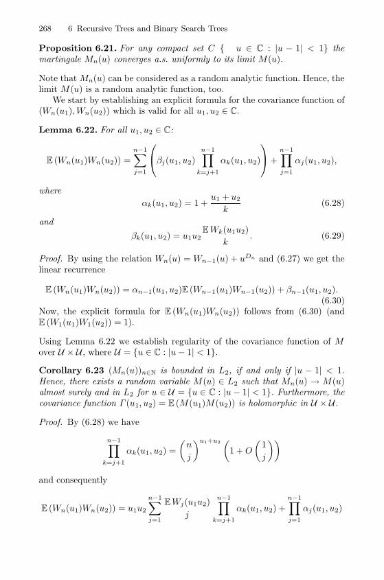
268 6 Recursive Trees and Binary Search Trees
Proposition 6.21. For any compact set C ⊆ {u ∈ C : |u − 1| < 1} themartingale Mn(u) converges a.s. uniformly to its limit M(u).
Note that Mn(u) can be considered as a random analytic function. Hence, thelimit M(u) is a random analytic function, too.
We start by establishing an explicit formula for the covariance function of(Wn(u1),Wn(u2)) which is valid for all u1, u2 ∈ C.
Lemma 6.22. For all u1, u2 ∈ C:
E (Wn(u1)Wn(u2)) =
n−1∑j=1
⎛⎝βj(u1, u2)
n−1∏k=j+1
αk(u1, u2)
⎞⎠+
n−1∏j=1
αj(u1, u2),
where
αk(u1, u2) = 1 +u1 + u2
k(6.28)
and
βk(u1, u2) = u1u2EWk(u1u2)
k. (6.29)
Proof. By using the relation Wn(u) = Wn−1(u) + uDn and (6.27) we get thelinear recurrence
E (Wn(u1)Wn(u2)) = αn−1(u1, u2)E (Wn−1(u1)Wn−1(u2)) + βn−1(u1, u2).(6.30)
Now, the explicit formula for E (Wn(u1)Wn(u2)) follows from (6.30) (andE (W1(u1)W1(u2)) = 1).
Using Lemma 6.22 we establish regularity of the covariance function of Mover U × U , where U = {u ∈ C : |u− 1| < 1}.
Corollary 6.23 (Mn(u))n∈N is bounded in L2, if and only if |u − 1| < 1.Hence, there exists a random variable M(u) ∈ L2 such that Mn(u) → M(u)almost surely and in L2 for u ∈ U = {u ∈ C : |u− 1| < 1}. Furthermore, thecovariance function Γ (u1, u2) = E (M(u1)M(u2)) is holomorphic in U × U .
Proof. By (6.28) we have
n−1∏k=j+1
αk(u1, u2) =
(n
j
)u1+u2(
1 +O
(1
j
))and consequently
E (Wn(u1)Wn(u2)) = u1u2
n−1∑j=1
EWj(u1u2)
j
n−1∏k=j+1
αk(u1, u2) +
n−1∏j=1
αj(u1, u2)
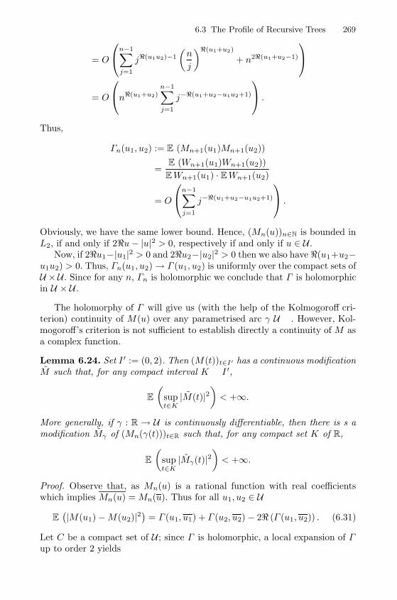
6.3 The Profile of Recursive Trees 269
= O
⎛⎝n−1∑j=1
j�(u1u2)−1
(n
j
)�(u1+u2)
+ n2�(u1+u2−1)
⎞⎠= O
⎛⎝n�(u1+u2)n−1∑j=1
j−�(u1+u2−u1u2+1)
⎞⎠ .Thus,
Γn(u1, u2) := E (Mn+1(u1)Mn+1(u2))
=E (Wn+1(u1)Wn+1(u2))
EWn+1(u1) · EWn+1(u2)
= O
⎛⎝n−1∑j=1
j−�(u1+u2−u1u2+1)
⎞⎠ .Obviously, we have the same lower bound. Hence, (Mn(u))n∈N is bounded inL2, if and only if 2�u− |u|2 > 0, respectively if and only if u ∈ U .
Now, if 2�u1−|u1|2 > 0 and 2�u2−|u2|2 > 0 then we also have �(u1+u2−u1u2) > 0. Thus, Γn(u1, u2) → Γ (u1, u2) is uniformly over the compact sets ofU ×U . Since for any n, Γn is holomorphic we conclude that Γ is holomorphicin U × U .
The holomorphy of Γ will give us (with the help of the Kolmogoroff cri-terion) continuity of M(u) over any parametrised arc γ ⊆ U . However, Kol-mogoroff’s criterion is not sufficient to establish directly a continuity of M asa complex function.
Lemma 6.24. Set I ′ := (0, 2). Then (M(t))t∈I′ has a continuous modificationM such that, for any compact interval K ⊆ I ′,
E
(supt∈K
|M(t)|2)< +∞.
More generally, if γ : R → U is continuously differentiable, then there is s amodification Mγ of (Mn(γ(t)))t∈R such that, for any compact set K of R,
E
(supt∈K
|Mγ(t)|2)< +∞.
Proof. Observe that, as Mn(u) is a rational function with real coefficientswhich implies Mn(u) = Mn(u). Thus for all u1, u2 ∈ U
E(|M(u1)−M(u2)|2
)= Γ (u1, u1) + Γ (u2, u2)− 2� (Γ (u1, u2)) . (6.31)
Let C be a compact set of U ; since Γ is holomorphic, a local expansion of Γup to order 2 yields
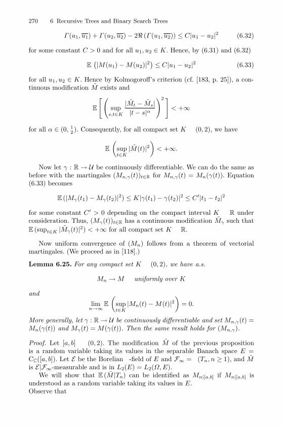
270 6 Recursive Trees and Binary Search Trees
Γ (u1, u1) + Γ (u2, u2)− 2� (Γ (u1, u2)) ≤ C|u1 − u2|2 (6.32)
for some constant C > 0 and for all u1, u2 ∈ K. Hence, by (6.31) and (6.32)
E(|M(u1)−M(u2)|2
)≤ C|u1 − u2|2 (6.33)
for all u1, u2 ∈ K. Hence by Kolmogoroff’s criterion (cf. [183, p. 25]), a con-tinuous modification M exists and
E
[(sup
s,t∈K
|Mt − Ms||t− s|α
)2 ]< +∞
for all α ∈ (0, 12 ). Consequently, for all compact set K ⊆ (0, 2), we have
E
(supt∈K
|M(t)|2)< +∞.
Now let γ : R → U be continuously differentiable. We can do the same asbefore with the martingales (Mn,γ(t))t∈R for Mn,γ(t) = Mn(γ(t)). Equation(6.33) becomes
E (|Mγ(t1)−Mγ(t2)|2) ≤ K|γ(t1)− γ(t2)|2 ≤ C′|t1 − t2|2
for some constant C ′ > 0 depending on the compact interval K ⊆ R underconsideration. Thus, (Mγ(t))t∈R has a continuous modification Mγ such that
E (supt∈K |Mγ(t)|2) < +∞ for all compact set K ⊆ R.
Now uniform convergence of (Mn) follows from a theorem of vectorialmartingales. (We proceed as in [118].)
Lemma 6.25. For any compact set K ⊆ (0, 2), we have a.s.
Mn →M uniformly over K
and
limn→∞
E
(supt∈K
|Mn(t)−M(t)|2)
= 0.
More generally, let γ : R → U be continuously differentiable and set Mn,γ(t) =Mn(γ(t)) and Mγ(t) = M(γ(t)). Then the same result holds for (Mn,γ).
Proof. Let [a, b] ⊆ (0, 2). The modification M of the previous propositionis a random variable taking its values in the separable Banach space E =CC([a, b]). Let E be the Borelian σ-field of E and F∞ = σ(Tn, n ≥ 1), and Mis E|F∞-measurable and is in L2(E) = L2(Ω,E).
We will show that E (M |Tn) can be identified as Mn|[a,b] if Mn|[a,b] isunderstood as a random variable taking its values in E.Observe that
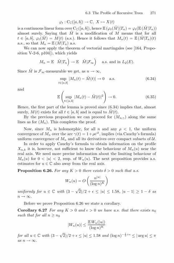
6.3 The Profile of Recursive Trees 271
ϕt : CC([a, b]) → C, X �→ X(t)
is a continuous linear form over CC([a, b]), hence E (ϕt(M)|Tn) = ϕt(E (M |Tn))almost surely. Saying that M is a modification of M means that for allt ∈ [a, b], ϕt(M) = M(t) (a.s.). Hence it follows that Mn(t) = E (M |Tn)(t)a.s., so that Mn = E (M |Tn) a.s.
We can now apply the theorem of vectorial martingales (see [164, Propo-sition V-2-6, p104]), which yields
Mn = E
(M |Tn
)→ E
(M |F∞)
a.s. and in L2(E).
Since M is F∞-measurable we get, as n→∞,
supt∈[a,b]
|Mn(t)− M(t)| → 0 a.s. (6.34)
and
E
(sup
t∈[a,b]
|Mn(t)− M(t)|2)→ 0. (6.35)
Hence, the first part of the lemma is proved since (6.34) implies that, almostsurely, M(t) exists for all t ∈ [a, b] and is equal to M(t).
By the previous proposition we can proceed for (Mn,γ) along the samelines as for (Mn). This completes the proof.
Now, since Mn is holomorphic, for all n and any ρ < 1, the uniformconvergence of Mn over the arc γ(t) = 1+ρeit, implies (via Cauchy’s formula)uniform convergence of Mn and all its derivatives over compact subsets of U .
In order to apply Cauchy’s formula to obtain information on the profileXn,k it is, however, not sufficient to know the behaviour of Mn(u) near thereal axis. We need more precise information about the limiting behaviour ofMn(u) for 0 < |u| < 2, resp. of Wn(u). The next proposition provides a.s.estimates for u ∈ C also away from the real axis.
Proposition 6.26. For any K > 0 there exists δ > 0 such that a.s.
Wn(u) = O
(n|u|
(logn)K
)uniformly for u ∈ C with (3 −
√2)/2 + ε ≤ |u| ≤ 1.58, |u − 1| ≥ 1 − δ as
n→∞.
Before we prove Proposition 6.26 we state a corollary.
Corollary 6.27 For any K > 0 and ε > 0 we have a.s. that there exists n0
such that for all n ≥ n0
|Wn(u)| ≤ EWn(|u|)(log n)K
for all u ∈ C with (3−√
2)/2 + ε ≤ |u| ≤ 1.58 and (log n)−12+ε ≤ | arg u| ≤ π
as n→∞.
272 6 Recursive Trees and Binary Search Trees
Proof. By Proposition 6.26 this estimate is true for u ∈ C with (3−√
2)/2+ε ≤|u| ≤ 1.58 and |u − 1| ≥ 1 − δ. Moreover, for u ∈ C with |u − 1| ≤ 1 − δ weknow that Mn(u) is a.s. bounded. Furthermore we have uniformly in n and tfor (logn)ε/
√logn ≤ |t| ≤ π
|EWn(u0eit)| ≤ EWn(u0)e−ct2 log n
for some constant c > 0 (depending continuously on u0). A combination ofthese two estimates proves the corollary.
For the proof of Proposition 6.26 we need an estimate for E |Wn(u)|2.
Lemma 6.28. For every δ > 0 we have uniformly for u with |u− 1| ≤ 1− δ
E |Wn(u)|2 = O(n2�u)
and for u with 1− δ ≤ |u− 1| ≤ 1
E |Wn(u)|2 = O(n2�u logn)
as n→∞. Let K be a compact set in the complex plane such that |u− 1| ≥ 1for all u ∈ C. Then
E |Wn(u)|2 = O(n|u|2
logn)
as n→∞, uniformly for u ∈ K.
Proof. We recall that
E |Mn(u)|2 = O
⎛⎝n2�un−1∑j=1
j−(2�u−|u|2+1)
⎞⎠ .We also have 2�u−|u|2 > 0 for |u−1| < 1 and 2�u−|u|2 < 0 for |u−1| > 1.Thus, for |u − 1| ≤ 1− δ, there exists δ′ > 0 such that
E |Wn(u)|2 = O
⎛⎝n2�un∑
j=1
j−1−δ′
⎞⎠ = O(n2�u),
and for 1− δ ≤ |u− 1| ≤ 1
E |Wn(u)|2 = O
⎛⎝n2�un∑
j=1
j−1
⎞⎠ = O(n2�u logn
),
which prove the first part of the lemma.Finally, for u with |u− 1| > 1 we obtain
E |Wn(u)|2 = O(n|u|
2
logn).
This completes the proof of the lemma.
6.3 The Profile of Recursive Trees 273
We will also use an a.s. estimate for the derivative of Wn(u).
Lemma 6.29. We have for all u with |u| < 2
|W ′n(u)| ≤W ′
n(|u|) = O(|u|−1n|u| log n
)a.s.
Proof. Obviously, we have |W ′n(u)| ≤ W ′
n(|u|). It is also known that Hn ∼e logn a.s. (compare with Section 6.4 and [175]). Hence, Xn,k = 0 a.s. ifk > (e+ 1) logn. This implies a.s.
W ′n(|u|) =
∑k≥0
kXn,k|u|k−1 ≤ (e+1) logn∑k≥0
Xn,k|u|k−1 = (c+1) lognWn(|u|)|u| .
Since Wn(|u|) ∼Mn(|u|)EWn(|u|) = O(n|u|), this proves the lemma.
We are now ready to work out the Proof of Proposition 6.26. By Lemma 6.28we have for (3−
√2)/2 < |u| ≤ 1.58 and |u− 1| ≥ 1− δ (for some sufficiently
small δ > 0)
P
{|Wn(u)| ≥ n|u|
(logn)K
}≤ E |Wn(u)|2
(n|u|/(logn)K)2= O
((logn)2K+1
n2|u|−|u|2
).
First, let us consider the range R1 := {u ∈ C : |u− 1| ≥ 1− δ, 1 ≤ |u| ≤ 1.58}.Set α = 1/(1.581(2− 1.581)). Then we have
α|u|(2− |u|) > 1 and α− 1 + αe log |u| < α|u|
for all u with 1 ≤ |u| ≤ 1.58.We now use O((log n)2K+2) points un,j covering R1 with maximal distance
(logn)−K−1. Observe that for u ∈ R1 the series∑n≥1
(log[nα])2K+1
[nα]2|u|−|u|2
converges uniformly. Hence, by the Borel-Cantelli-Lemma we have a.s.
supj|W[nα](u[nα],j)| ≤ [nα]|u|
(log[nα])K
for all but finitely many n. By using Lemma 6.29 we obtain a.s.
|W[nα](u)−W[nα](v)| = O(
[nα]max{|u|,|v|} logn)
which implies that we can interpolate between u[nα],j and obtain a.s.
supu∈R1
|W[nα](u)| ≤ [nα]|u|
(log[nα])K
274 6 Recursive Trees and Binary Search Trees
for all but finitely many n.Finally, we have to observe that a.s., uniformly for nα ≤ k ≤ (n+ 1)α
|Wk(u)−W[nα](u)| = O
([nα]2|u|−1
(log[nα])K
). (6.36)
Since
Wn+k(u)−Wn(u) =
n+k∑l=n+1
uDl ,
we have to estimate uDl . We know that a.s. Hn ≤ e logn (for sufficiently largen). Hence it follows that a.s.
maxnα≤l≤(n+1)α
Dl ≤ e · log(nα).
So we only have to check that
|u| ([(n+ 1)α]− [nα]) |u|e log(nα) = O
([nα]|u|
(log[nα])K
).
Alternatively, it suffices to show that there exists η > 0 such that
α− 1 + αe log |u| ≤ α|u| − η
for 1 ≤ |u| ≤ 1.58. However, this is true for the above choice of α. Hence,(6.36) follows, which completes the proof for u ∈ R1.
For u ∈ R2 := {u ∈ C : |u − 1| ≥ 1/ − δ, (3 −√
2)/2 + ε ≤ |u| ≤ 1} wehave to do almost the same. Again we use a subsequence [nβ ] to apply theBorel-Cantelli-Lemma. We set β = (1 +
√5)/2 and observe that
β|u|(2− |u|) > 1 and β − 1 < β|u|
for all u with (3 −√
2)/2 + ε ≤ |u| ≤ 1. This completes the proof of Proposi-tion 6.26.
The proof of (6.25) can now be completed in the following way. In partic-ular we show that the limit X(α) coincides with the limit M(α). For small twe use the a.s. expansion
Mn(u0eit) = Mn(u0)eitM
′n(u0)/Mn(u0)+O(t2)
and Wn(u0eit) = Mn(u0e
it)EWn(u0eit). For large t we use the estimate of
Proposition 6.26 (resp. of its Corollary 6.27).By Cauchy’s formula we have
Xn,k =u−k
0
2π
∫ π
−π
Wn(u0eit)e−kit dt,
6.3 The Profile of Recursive Trees 275
where we will use u0 = k/ logn. First, for any (sufficiently small) η > 0 wehave by Corollary 6.27
|Wn(u0eit)| ≤ EWn(u0)
logna.s.
for (3−√
2)/2 + ε ≤ u0 ≤ 1.58 and (log n)−1−η2 ≤ |t| ≤ π. Hence∣∣∣∣∣u−k
0
2π
∫(log n)−
1−η2 ≤|t|≤π
Wn(u0eit)e−kit dt
∣∣∣∣∣ = O
(EWn(u0)
uk0 log n
).
Conversely, for real t with |t| ≤ (logn)−1−η2 we have uniformly
Wn(u0eit)e−kit = Mn(u0e
it)EWn(u0eit)e−kit
= Mn(u0)EWn(u0)e2u0 log n(eit−1)−kit(1 +O(|t|) +O(n−1))
= Mn(u0)EWn(u0)e−u0 log n t2(1 +O((log n)−1−3η
2 )).
This implies that a.s.
Xn,k =u−k
0
2π
∫|t|≤(log n)−
1−η2
Wn(u0eit)e−kit dt+O
(u−k
0
EWn(u0)
logn
)= Mn(u0)u−k
0
√2πkEWn(u0)(1 +O((log n)−
1−3η2 )).
Since we uniformly have
u−k0
√2πkEWn(u0) ∼ EXn,k
and Mn(u0) ∼M(u0), the result follows.
6.3.2 The Moment Method
Suppose that 0 ≤ α ≤ 1. We indicate a proof of (6.24) in this range by showingthat for all integers k ≥ 1
limn→∞
E
(Xn,�α log n�
EXn,�α log n�
)k
= EX(α)k.
This moment method only works for 0 ≤ α ≤ 1, since X(α) does not havemoments of arbitrary order if α > 1 (compare with [87]).
Let Pn,k(u) = EuXn,k denote the probability generating function of Xn,k.Then the recurrence (6.21) implies that
Pn,k(u) =1
n− 1
n−1∑j=1
Pj,k−1(u)Pn−j,k(u), (n ≥ 2, k ≥ 1),
276 6 Recursive Trees and Binary Search Trees
with Pn,0(u) = u for n ≥ 1 and P0,k = 1. Taking derivatives and setting u = 1yields the recurrence
EXn,k =1
n− 1
n−1∑j=1
(EXj,k−1 + EXn−j,k)
with EXn,0 = 1 for n ≥ 1 and EX0,k = 0. This recurrence is different from(6.20) but can be extended to higher moments.
By taking m-th derivatives we are led to the recurrence
A(m)n,k =
1
n− 1
n−1∑j=1
(A
(m)j,k−1 +A
(m)n−j,k
)+B
(m)n,k
with A(1)n,0 = 1 for n ≥ 1 and An,0(m) = 0 for m ≥ 2 and n ≥ 1, where
A(m)n,k = E (Xn,k(Xn,k − 1) · · · (Xn,k −m+ 1)) = P
(m)n,k (1)
and where B(m)n,k abbreviates
B(m)n,k =
m−1∑h=1
(m
h
)1
n− 1
n−1∑j=1
A(h)j,k−1A
(m−h)n−j,k .
Hence, for every fixed m ≥ 1 the sequence (A(m)n,k ) satisfies a recurrence of the
form
an,k =
n−1∑j=1
(aj,k−1 + an−j,k) + bn,k, (n ≥ 2, k ≥ 1), (6.37)
with given initial values a1,k and a given sequence bn,k. For the interest ofconsistency we set b1,k = a1,k. Then (6.37) holds also for n = 1. Remarkablythe recurrence (6.37) has an explicit solution of the following form (see [87]).
Lemma 6.30. Suppose that the sequence an,k satisfies the recurrence (6.37).Then we have (for n ≥ 1 and k ≥ 0)
an,k = bn,k +
n−1∑j=1
k∑r=0
bj,k−r
j[ur] (u+ 1)
∏j<�<k
(1 +
u
�
).
Proof. Setting an(u) =∑
k an+1,kuk and bn(u) =
∑k bn+1,ku
k the recurrence(6.37) rewrites to
an(u) =1 + u
n
n−1∑j=0
aj(u) + bn(u) (n ≥ 1)
6.3 The Profile of Recursive Trees 277
with initial condition a0(u) =∑
k a1,kuk. By taking the difference nan(u) −
(n− 1)an−1(u) we thus obtain
an(u) =(
1 +u
n
)an−1(u) + bn−1(u)− n− 1
nbn−1(u), (n ≥ 2),
and consequently
an(u) = bn(u) + (1 + u)
n−1∑j=0
bj(u)
j + 1
∏j+1≤�≤n
(1 +
u
�
).
Taking the coefficient of uk on both sides provides the result.
For example, in the case m = 1 we have bn,k = δn,1δ0,k for n ≥ 1 andk ≥ 0. Thus, we recover the explicit (and also the asymptotic) formula for the
expected value A(1)n,k = EXn,k:
EXn,k = [uk]∏
1≤�<n
(1 +
u
j
)=|sn,k+1|(n− 1)!
∼ (log n)k
k!Γ(
1 + klog n
) .Starting from this solution one can iteratively apply Lemma 6.30 to obtain
asymptotic expansions for A(m)n,k for m ≥ 2.
Proposition 6.31. For 0 ≤ α ≤ m1/(m−1) set ν0(α) = ν1(α) = 1 and recur-sively (for m ≥ 2)
νm(α) =1
m− αm−1
m−1∑h=1
(m
h
)νh(α)νm−h(α)
Γ (hα + 1)Γ ((m− h)α+ 1)
Γ (mα+ 1)
Then for every fixed 0 ≤ α ≤ m1/(m−1) we have, as n→∞,
EXmn,�α log n� ∼ νm(α)
(EXn,�α log n�
)m(6.38)
It is easy to check that for every 0 ≤ α ≤ 1 the sequence νm(α) is the momentsequence of a random variableX(α). From the contraction method (see Chap-ter 8) it follows that (6.41) has a unique solution X(α) (with EX(α) = 1)and by definition the sequence νm(α) is the moment sequence of X(α). Byinduction it follows that νm(α)Γ (mα + 1)/m! = O(Km) (for some K > 0,see [107]). Hence, the sequence νm(α) determines uniquely the distribution ofX(α). Consequently, for 0 ≤ α ≤ 1, Proposition 6.31 implies the limit relation(6.24).
If α > 1 then only few moments exist. More precisely if α ≤ m1/(m−1 thenX(α) has moments up to order m (and we have convergence of moments upto this order) but the (m+ 1)-st moment is infinite.
The proof of Proposition 6.31 is very technical. Following [87] one startswith a uniform upper bound for the expected profile of the form
278 6 Recursive Trees and Binary Search Trees
A(1)n,k = O
((v logn)−1/2v−knv
), (0 ≤ k < n),
where 0 < v ≤ v0. If k is of logarithmic order then this bound is optimal,since we can set v = k/ logn. Then Lemma 6.30 implies inductively
A(m)n,k = O
(1
m− vm−1
((v logn)−1/2v−knv
)m),
uniformly for 0 ≤ k < n, where 0 < v < m1/(m−1).By using this a priori bound Proposition 6.31 follows by induction on m.
More precisely one shows that for every integer m ≥ 1
A(m)n,k ∼ νm(α)
((logn)k
k!Γ (α+ 1)
)m
, (6.39)
where k = �α logn�. We just observed that this is true form = 1. By assumingthat (6.39) holds all integers < m and by using the definition of νm(α) oneobtains
B(m)n,k ∼ νm(α)
mα − αm
mα+ 1
((logn)k
k!Γ (α+ 1)
)m
.
Furthermore, from
[ur]∏
j<�<n
(1 +
u
�
)=
(log(n/j))r
j
(1 +O(r2/j)
)(for εn ≤ j ≤ (1 − ε)n and 0 ≤ r ≤ k = o(
√j)) it follows that
n−1∑j=1
k∑r=0
B(m)j,k−r
j[ur](u + 1)
∏j<�<k
(1 +
u
�
)= μm(α)
mα − αm
mα+ 1(αm + 1)
((log n)k
k!Γ (α+ 1)
)m ∫ 1
0
xmα−αm−1 dx
= μm(α)αm + 1
mα + 1
((log n)k
k!Γ (α+ 1)
)m
Hence, (6.39) holds for m, too.Finally we have
EXmn,�α log n� ∼ A
(m)n,�α log n�
which implies (6.38) for all m ≥ 1.
6.3.3 The Contraction Method
The contraction method makes use of the fact that there is a fixed pointequation for the (expected) limiting distribution.
6.3 The Profile of Recursive Trees 279
Assume for a moment that we already know a limiting relation for the
profile Xn,k of the form Xn,�α log n�/EXn,�α log n�d−→ X(α). Motivated by
that we rewrite the recurrence (6.21) in the form:
Xn,k
EXn,k
d=
EXIn,k−1
EXn,k
XIn,k−1
EXIn,k−1+
EX∗n−In,k
EXn,k
X∗n−In,k
EX∗n−In,k
. (6.40)
Recall that X∗n,k is an independent copy of Xn,k and that (Xn,k), (X∗n,k), and(In) are independent. By (6.23) we have for k = �α logn�
EXIn,k−1
EXn,k∼ k
logn
(log Inlogn
)k−1
∼ α(Inn
)α
,
andEX∗n−In,k
EXn,k∼(
1− Inn
)α
.
Hence, by (formally) taking the limit n→∞ and by observing that In/nd−→ U ,
the (expected) limit relation for X(α) is
X(α)d= αUαX(α) + (1− U)αX(α)∗. (6.41)
Interestingly we can do a similar calculation for the profile polynomialWn(u). For simplicity we assume that u is a positive real number. Then we
already know that Mn(u) = Wn(u)/EWn(u)d−→ M(u), where M(u) is the
limiting martingale. Again from (6.21) we obtain
Wn(u)d= uWIn(u) +Wn−In (u)∗,
and consequently
Mn(u)d= u
EWIn(u)
EWn(u)MIn(u) +
EWn−In (u)∗
EWn(u)M∗
n−In(u)
∼ u(Inn
)u
MIn(u) +
(n− Inn
)u
Mn−In(u)∗.
By taking the limit n→∞ we get
M(u)d= uUuM(u) + (1− U)uM(u)∗. (6.42)
Thus, X(α) and M(u) satisfy the same distributional fixed point equation
(6.41), resp. (6.42) when we set α = u. Actually we have X(α)d= M(α). By
the martingale method we already know that Xn,�α log n�/EXn,�α log n� has alimit X(α) which equals M(α).
Nevertheless, one can proceed directly without using profile polynomials.We will make this more precise in Section 8.2.3, however, the underlying idea
280 6 Recursive Trees and Binary Search Trees
is the following. In order to solve a distributional fixed point equation of theform (6.41) one has to introduce a proper metric on a space of measures sothat the right-hand-side of the fixed point equation becomes a contraction. Inparticular, one gets a unique solution and since the normalised version (6.40)of the original underlying recurrence is close to the limit equation (6.41),one can expect that Xn,k/EXn,k (for k ∼ α logn) stabilises around the limitX(α).
This concept works quite well if the random variable of interest is notdouble indexed. For example, the so-called contraction method (introduced inChapter 8) applies to the profile polynomial Wn(u). In the case of the profileXn,k one has to take care of the second index k, too, which causes some extrawork (compare with [87]). In fact, it is possible to prove Theorem 6.18 in thefull range 0 < α < e. We will give more details in Section 8.2.3.
6.4 The Height of Recursive Trees
We encode the distribution of the height Hn of recursive trees by the gener-ating function
yk(x) =∑n≥1
P{Hn < k}xn
n.
This is consistent with the generating function y(x) = log(1/(1 − x)) of re-cursive trees. More precisely, let yn,k denote the number of recursive trees ofsize n and height < k. Then
P{Hn < k} =yn,k
(n− 1)!,
and yk(x) also is the exponential generating function of these numbers:
yk(x) =∑n≥1
yn,kxn
n!.
Thus, we can use the usual counting procedure and obtain recursively
y′k+1(x) = eyk(x), (yk+1(0) = 0),
with the initial condition y0(x) = 0. In parallel we will work with
Yk(x) = y′k(x) =∑n≥0
P{Hn+1 < k} xn.
Here we have Y1(x) = 1 and
Y ′k+1(x) = Yk+1(x)Yk(x), (Yk+1(0) = 1).
The analysis of these generating functions is the basis of the following result(that is due to Drmota [57]).
6.4 The Height of Recursive Trees 281
Theorem 6.32. The height Hn of random recursive trees has expected value
EHn ∼ e logn. (6.43)
Furthermore there are exponential tail estimates of the form
P{|Hn − EHn| ≥ η} = O(e−cη)
with some c > 0.
This result is in accordance with Pittel’s result [175] saying thatHn/ logn→ ea.s.
Note that the exponential tail estimate shows that the distribution ofthe height is heavily concentrated around its expected value. In particular itfollows that, as n→∞,
VarHn = O(1).
One can also be much more precise about the distribution of the heightHn. In particular the values Yk(1) play an essential role in the analysis. Forexample, we have
EHn = max{k : Yk(1) ≤ n}+O(1)
(compare with (6.48)), and
P{Hn < k} = F (n/Yk(1)) + o(1),
uniformly for all k ≥ 0 as n→∞, where F (y) satisfies the integral equation
y F (y/e1/e) =
∫ y
0
F (z/e1/e)F (y − z) dz. (6.44)
We will comment on this problem at the end of the section. Anyway, thisalready shows that although the results on the height are quite precise, thebehaviour of the distribution is in some sense implicit, since it uses y′k(1) =Yk(1) =
∑n≥1 P{Hn < k}, a value that is unknown. We will just prove
logYk(1) ∼ k/e which provides (6.43). It is conjectured that
logYk(1) =k
e+ c1 log k + c2(log k) + o(1)
for some constant c1 > 0 and a periodic function c2(x). Of course, if thisconjectural relation can be verified then we actually get an explicit asymptoticrepresentation for the height distribution.
The proof of Theorem 6.32 is divided into several steps. We start withsome technical lemmas.
Lemma 6.33. Suppose that Y1(x), Y2(x), Y 1(x), Y 2(x) are non-negative con-tinuous functions that are defined for x ≥ 0 such that Y1(0) < Y 1(0),
Y2(0) < Y 2(0), Y ′2(x) = Y2(x)Y1(x), Y′2(x) = Y 2(x)Y 1(x), and that the
difference Y 1(x) − Y1(x) has exactly one positive zero. Then the differenceY 2(x)− Y2(x) has at most one positive zero.
282 6 Recursive Trees and Binary Search Trees
Proof. For j = 1, 2 set
yj(x) =
∫ x
0
Yj(t) dt and yj(x) =
∫ x
0
Y j(t) dt.
Then we have y1(x) < y1(x), y2(x) < y2(x) (at least) for a small interval0 < x < ζ and also y′2(x) = ey1(x) and y′2(x) = ey1(x). Since Y 1(x) − Y1(x)is positive (for small positive x) and has at most one positive zero, the samefollows for
y1(x)− y1(x) =
∫ x
0
(Y 1(t)− Y1(t)
)dt.
Namely, if Y 1(t)− Y1(t) ≥ 0 for all t ≥ 0 then y1(x) − y1(x) is an increasingfunction with y1(0)− y1(0) = 0. If, however, Y 1(t) − Y1(t) ≥ 0 for 0 ≤ t ≤ t0and Y 1(t)−Y1(t) ≤ 0 for t ≥ t0 then y1(x)−y1(x) is increasing for 0 ≤ x ≤ t0and decreasing for x ≥ t0. In the first case the function y1(x) − y1(x) has nopositive zero and in the second case at most one.
Now observe that (ey − ez)/(y − z) > 0 for real y = z. Hence,
Y 2(x)−Y2(x) = y′2(x)−y′2(x) = ey1(x)−ey1(x) =ey1(x) − ey1(x)
y1(x)− y1(x)(y1(x) − y1(x))
has at most one positive zero, too.
Lemma 6.34. For all k ≥ 0 we have
Yk+2(1)
Yk+1(1)≤ Yk+1(1)
Yk(1).
Proof. For 0 ≤ γ < 1 set
Vk(x, γ) =
{1
1−x for 0 ≤ x ≤ 1− γ,
γ−1Yk
(x−(1−γ)
γ
)for 1− γ ≤ x ≤ 1.
These functions satisfy
V ′k+1(x, γ) = Vk+1(x, γ)Vk(x, γ),
Vk(0) = 1 and Vk(1, γ) = γ−1Yk(1). In particular, for γk = Yk+1(1)/Yk(1)we have Vk(1, γk) = Yk+1(1). Now the inductive application of Lemma 6.33shows that Yk+1(x)− Vk(x, 1) have (at most) one positive zero. Hence we get
Yk+1(x) ≤ Vk(x, γk) for 0 ≤ x ≤ 1,
and after integration
Yk+2(1) ≤ Vk+1(1, γk) = γ−1k Yk+1(1) =
Yk+1(1)2
Yk+1(1).
6.4 The Height of Recursive Trees 283
Corollary 6.35 There exists α0 > 1 with
α0 = limk→∞
Yk+1(1)
Yk(1). (6.45)
Proof. Lemma 6.34 implies that there exists α0 ≥ 1 with
α0 = limk→∞
Yk+1(1)
Yk(1).
We show that Yk(1) grows at least exponentially which implies α0 > 1.Set δk = y(x)− yk(x). Then it follows by induction that
δk(x) ≤ L(x)k+1
(k + 1)!(0 ≤ x ≤ 1), (6.46)
where L(x) abbreviates log(1/(1− x)). By definition (6.46) is true for k = 0.Now observe that yk(x) ≤ y(x) implies
δ′k+1(x) = ey(x) − eyk(x) ≤ ey(x)δk(x) ≤ 1
1− xL(x)k+1
(k + 1)!.
Since δk+1(0) = 0, integration gives
δk+1(x) ≤∫ x
0
1
1− tL(t)k+1
(k + 1)!dt =
L(x)k+2
(k + 2)!.
For xk = 1− e−(k+1)/e we have y(xk) = (k + 1)/e and
L(xk)k+1
(k + 1)!∼ 1√
2πk.
Hence it follows that (for sufficiently large k)
yk(1) ≥ yk(xk) ≥ y(xk)− L(xk)k+1
(k + 1)!=k + 1
e− 1√
2πk(1 + o(1)) ≥ k
e.
This completes the proof of the lemma since
Yk(1) = y′k(1) = eyk−1(1) ≥ e(k−1)/e.
Remark 6.36 If we replace xk in the proof of Corollary (6.35) by
xk = 1− e−(k+log√
k)/e
we get the slightly better lower bound
Yk(1) ≥ e(k+log√
k)/e+O(1).
However, it is conjectured that the correct order of magnitude is
Yk(1) = e(k+ 32 log k)/e+O(1),
which cannot be reached by the method mentioned above.
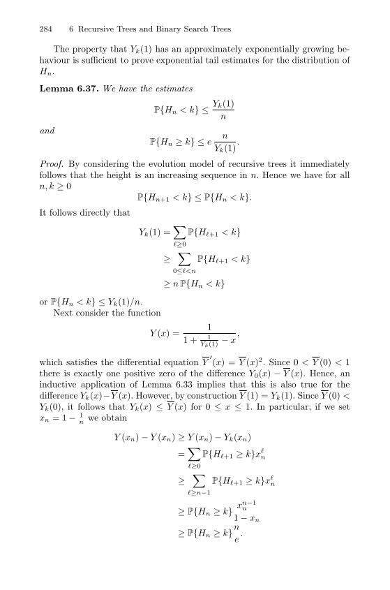
284 6 Recursive Trees and Binary Search Trees
The property that Yk(1) has an approximately exponentially growing be-haviour is sufficient to prove exponential tail estimates for the distribution ofHn.
Lemma 6.37. We have the estimates
P{Hn < k} ≤Yk(1)
n
andP{Hn ≥ k} ≤ e
n
Yk(1).
Proof. By considering the evolution model of recursive trees it immediatelyfollows that the height is an increasing sequence in n. Hence we have for alln, k ≥ 0
P{Hn+1 < k} ≤ P{Hn < k}.It follows directly that
Yk(1) =∑�≥0
P{H�+1 < k}
≥∑
0≤�<n
P{H�+1 < k}
≥ nP{Hn < k}
or P{Hn < k} ≤ Yk(1)/n.Next consider the function
Y (x) =1
1 + 1Yk(1) − x
,
which satisfies the differential equation Y′(x) = Y (x)2. Since 0 < Y (0) < 1
there is exactly one positive zero of the difference Y0(x) − Y (x). Hence, aninductive application of Lemma 6.33 implies that this is also true for thedifference Yk(x)−Y (x). However, by construction Y (1) = Yk(1). Since Y (0) <Yk(0), it follows that Yk(x) ≤ Y (x) for 0 ≤ x ≤ 1. In particular, if we setxn = 1− 1
n we obtain
Y (xn)− Y (xn) ≥ Y (xn)− Yk(xn)
=∑�≥0
P{H�+1 ≥ k}x�n
≥∑
�≥n−1
P{H�+1 ≥ k}x�n
≥ P{Hn ≥ k}xn−1
n
1− xn
≥ P{Hn ≥ k}n
e.
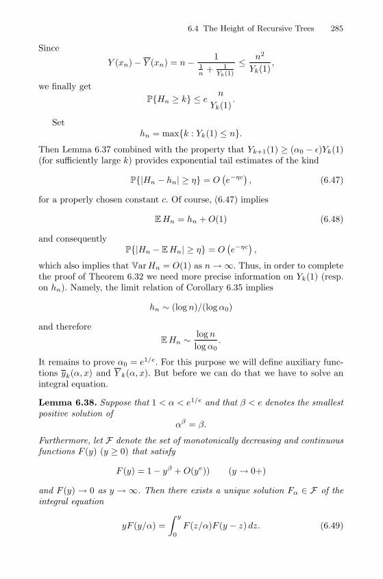
6.4 The Height of Recursive Trees 285
Since
Y (xn)− Y (xn) = n− 11n + 1
Yk(1)
≤ n2
Yk(1),
we finally get
P{Hn ≥ k} ≤ en
Yk(1).
Sethn = max{k : Yk(1) ≤ n}.
Then Lemma 6.37 combined with the property that Yk+1(1) ≥ (α0 − ε)Yk(1)(for sufficiently large k) provides exponential tail estimates of the kind
P{|Hn − hn| ≥ η} = O(e−ηc), (6.47)
for a properly chosen constant c. Of course, (6.47) implies
EHn = hn +O(1) (6.48)
and consequentlyP{|Hn − EHn| ≥ η} = O
(e−ηc),
which also implies that VarHn = O(1) as n→∞. Thus, in order to completethe proof of Theorem 6.32 we need more precise information on Yk(1) (resp.on hn). Namely, the limit relation of Corollary 6.35 implies
hn ∼ (log n)/(logα0)
and therefore
EHn ∼logn
logα0.
It remains to prove α0 = e1/e. For this purpose we will define auxiliary func-tions yk(α, x) and Y k(α, x). But before we can do that we have to solve anintegral equation.
Lemma 6.38. Suppose that 1 < α < e1/e and that β < e denotes the smallestpositive solution of
αβ = β.
Furthermore, let F denote the set of monotonically decreasing and continuousfunctions F (y) (y ≥ 0) that satisfy
F (y) = 1− yβ +O(ye)) (y → 0+)
and F (y) → 0 as y → ∞. Then there exists a unique solution Fα ∈ F of theintegral equation
yF (y/α) =
∫ y
0
F (z/α)F (y − z) dz. (6.49)
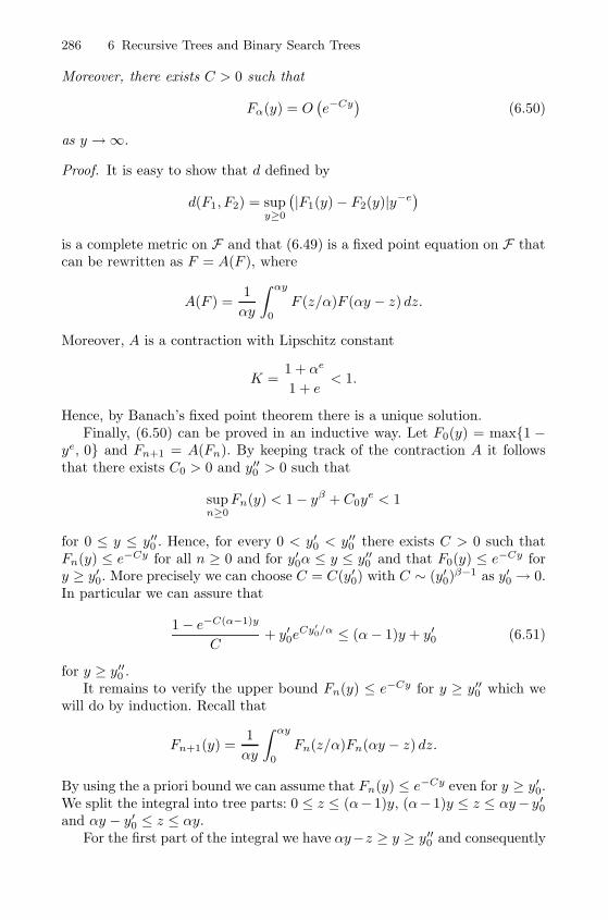
286 6 Recursive Trees and Binary Search Trees
Moreover, there exists C > 0 such that
Fα(y) = O(e−Cy)
(6.50)
as y →∞.
Proof. It is easy to show that d defined by
d(F1, F2) = supy≥0
(|F1(y)− F2(y)|y−e
)is a complete metric on F and that (6.49) is a fixed point equation on F thatcan be rewritten as F = A(F ), where
A(F ) =1
αy
∫ αy
0
F (z/α)F (αy − z) dz.
Moreover, A is a contraction with Lipschitz constant
K =1 + αe
1 + e< 1.
Hence, by Banach’s fixed point theorem there is a unique solution.Finally, (6.50) can be proved in an inductive way. Let F0(y) = max{1 −
ye, 0} and Fn+1 = A(Fn). By keeping track of the contraction A it followsthat there exists C0 > 0 and y′′0 > 0 such that
supn≥0
Fn(y) < 1− yβ + C0ye < 1
for 0 ≤ y ≤ y′′0 . Hence, for every 0 < y′0 < y′′0 there exists C > 0 such that
Fn(y) ≤ e−Cy for all n ≥ 0 and for y′0α ≤ y ≤ y′′0 and that F0(y) ≤ e−Cy fory ≥ y′0. More precisely we can choose C = C(y′0) with C ∼ (y′0)β−1 as y′0 → 0.In particular we can assure that
1− e−C(α−1)y
C+ y′0e
Cy′0/α ≤ (α− 1)y + y′0 (6.51)
for y ≥ y′′0 .It remains to verify the upper bound Fn(y) ≤ e−Cy for y ≥ y′′0 which we
will do by induction. Recall that
Fn+1(y) =1
αy
∫ αy
0
Fn(z/α)Fn(αy − z) dz.
By using the a priori bound we can assume that Fn(y) ≤ e−Cy even for y ≥ y′0.We split the integral into tree parts: 0 ≤ z ≤ (α−1)y, (α−1)y ≤ z ≤ αy− y ′0and αy − y′0 ≤ z ≤ αy.
For the first part of the integral we have αy−z ≥ y ≥ y′′0 and consequently
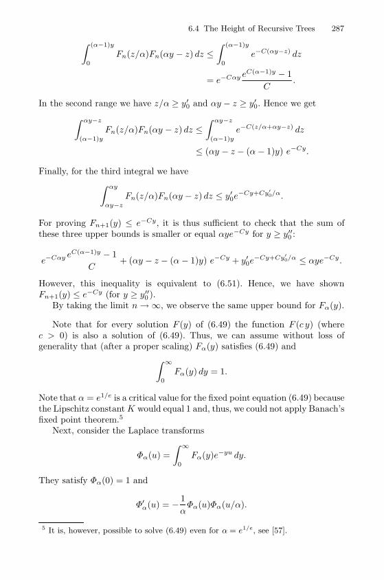
6.4 The Height of Recursive Trees 287∫ (α−1)y
0
Fn(z/α)Fn(αy − z) dz ≤∫ (α−1)y
0
e−C(αy−z) dz
= e−Cαy eC(α−1)y − 1
C.
In the second range we have z/α ≥ y′0 and αy − z ≥ y′0. Hence we get∫ αy−z
(α−1)y
Fn(z/α)Fn(αy − z) dz ≤∫ αy−z
(α−1)y
e−C(z/α+αy−z) dz
≤ (αy − z − (α− 1)y) e−Cy.
Finally, for the third integral we have∫ αy
αy−z
Fn(z/α)Fn(αy − z) dz ≤ y′0e−Cy+Cy′0/α.
For proving Fn+1(y) ≤ e−Cy, it is thus sufficient to check that the sum ofthese three upper bounds is smaller or equal αye−Cy for y ≥ y′′0 :
e−Cαy eC(α−1)y − 1
C+ (αy − z − (α − 1)y) e−Cy + y′0e
−Cy+Cy′0/α ≤ αye−Cy.
However, this inequality is equivalent to (6.51). Hence, we have shownFn+1(y) ≤ e−Cy (for y ≥ y′′0 ).
By taking the limit n→∞, we observe the same upper bound for Fα(y).
Note that for every solution F (y) of (6.49) the function F (c y) (wherec > 0) is also a solution of (6.49). Thus, we can assume without loss ofgenerality that (after a proper scaling) Fα(y) satisfies (6.49) and∫ ∞
0
Fα(y) dy = 1.
Note that α = e1/e is a critical value for the fixed point equation (6.49) becausethe Lipschitz constantK would equal 1 and, thus, we could not apply Banach’sfixed point theorem.5
Next, consider the Laplace transforms
Φα(u) =
∫ ∞0
Fα(y)e−yu dy.
They satisfy Φα(0) = 1 and
Φ′α(u) = − 1
αΦα(u)Φα(u/α).
5 It is, however, possible to solve (6.49) even for α = e1/e, see [57].
288 6 Recursive Trees and Binary Search Trees
The crucial step in this analysis it to introduce (for 1 < α < e1/e) thefollowing auxiliary functions
Y k(α, x) = αkΦα
(αk(1− x)
), (6.52)
where k can be considered a real (not necessarily integral) parameter and
yk(α, x) =
∫ x
0
Y k(α, t) dt = logY k+1(α, x).
The next lemma collects some useful facts on Y k(α, x) if α < e1/e. In fact,these auxiliary functions have almost the same properties as the functionYk(x). The proof is immediate by translating the corresponding properties ofFα and Φα respectively.
Lemma 6.39. Suppose that 1 < α < e1/e and let β < e be given by αβ = β.Let Y k(α, x) be defined by (6.52). Then the following assertions hold:
1. For all k > 0 the function Y k(α, x) is monotone for x ≥ 0. It satisfies0 < Y k(α, 0) < 1, more precisely, 1−Y k(α, 0) ∼ Cα−βk for some constantC depending on α. Furthermore we have Y k(α, 1) = αk.
2. They satisfy the recurrence relation
Y′k+1(x) = Y k+1(x)Y k(x).
3. For all integers � ≥ 0 and for all real numbers k > 0 the difference Y�(x)−Y k(α, x) has exactly one positive zero x�,k. In particular we have Y k(x) ≤Y�(x) for 0 ≤ x ≤ x�,k and Y k(x) ≥ Y�(x) for x ≥ x�,k.
Note that yk(x) = logYk+1(x) and yk(α, x) = logY k+1(α, x). Hence, theabove properties can be translated to yk(α, x) and yk(x).
The next lemma completes the proof of Theorem 6.32.
Lemma 6.40. We have limk→∞ Yk+1(1)/Yk(1) = e1/e and consequently
EHn ∼ e logn. (6.53)
Proof. Suppose that 1 < α < e1/e and set ek := yk(1)/(logα) − 1. Then thefunction yek
(α, x) satisfies yek(α, 0) < yk(0) and
yek(α, 1) = yk(1).
Hence, by Lemma 6.39 (reformulated for yk(α, x)) it follows that yek(α, x) ≤
yk(x) for 0 ≤ x ≤ 1. Hence, by integration it also follows that yek+1(α, x) ≤yk+1(x) for 0 ≤ x ≤ 1. In particular,
yek+1(α, 1) = yk(1) + logα ≤ yk+1(1).
Thus, we have yk+1(1) − yk(1) ≥ logα for all α < e1/e and consequentlyyk+1(1)− yk(1) ≥ 1/e. This also shows that Yk(1)/Yk−1(1) ≥ e1/e.
6.4 The Height of Recursive Trees 289
In a second step we will show that for every ε > 0
yk(1) ≤ k
e(1 + ε)
for sufficiently k ≥ k0(ε). This is sufficient to complete the proof of Lemma 6.40.We again fix α < e1/e and define t(α) > 0 by
(1 + t(α))αβ logα = 1.
Note that limα→e1/e t(α) = 0.Set δk(x) = yk(x) − yk+r(α, x), where r ≥ 0 is a parameter that will
be chosen appropriately. Note that yk(x) ≤ y(x) and yk+r(α, x) ≤ y(x) for0 ≤ x < 1. By induction it follows that
δk(x) ≤k∑
�=0
δ�(0)L(x)k−�
(k − �)! ,
where L = log 1/(1 − x). We now suppose that r = 2kt(α) − 1, set x′ =1− α−k(1+t(α)) and estimate yk(x′) = yk+2kt(α)−1(α, x′) + δk(x′) from above.We have
yk+2kt(α)−1(α, x′) = k(1 + t(α)) − C
αβkt(α)(1 + o(1)),
and
δk(x′) ≤k∑
�=0
C
αβ�+2βkt(α)
(k(1 + t(α)) logα)k−�
(k − �)!
=C
αβk(1+2t(α))
k∑�=0
(k(1 + t(α))αβ logα
)k−�
(k − �)!
=C
αβk(1+2t(α))
k∑�=0
kk−�
(k − �)!
∼ C
αβk(1+2t(α))
ek
2
=1
2
C
αβkt(α).
Consequently we obtain
yk(x′) ≤ k(1 + t(α)) log α− 1
2
C
αβkt(α)(1 + o(1)).
If we compare that with
yk+3kt(α)−1(α, x′) = k(1 + t(α)) logα− C
α2βkt(α)(1 + o(1))
290 6 Recursive Trees and Binary Search Trees
we observe that (for sufficiently large k)
yk(x′) ≤ yk+3kt(α)−1(α, x′).
Since yk(0) > yk+3kt(α)(α, 0), it follows from Lemma 6.39 (resp. from itsreformulation to yk(α, x)), that yk(x) ≤ yk+3kt(α)(α, x) even for all x ≥ x′. Inparticular we have (for sufficiently large k)
yk(1) ≤ yk+3kt(α)−1(α, 1) = k(1 + 3t(α)) logα ≤ k
e(1 + 3t(α)).
Since we can choose α such that t(α) is arbitrarily small this completes theproof of Lemma 6.40.
We close this section with some comments on the distribution of Hn. InLemma 6.38 we have observed that for every α < e1/e the integral equation(6.49) has a solution Fα, since it is a fixed point of a proper contraction. Forα0 = e1/e the method fails. Nevertheless it is possible to find a non-trivialcontinuous solution for α0 (see [57, 36]). As above we consider the Laplacetransform Φα0 and the auxiliary functions
Y k(x) = αk0Φα0(αk
0(1 − x))
= αk0
∫ ∞0
Fα0(y)e−yαk0(1−x) dy
=
∫ ∞0
Fα0(yα−k0 )e−yeyx dy
=∑n≥0
(1
n!
∫ ∞0
yne−yFα0(yα−k0 ) dy
)xn.
Observe that1
n!
∫ ∞0
yne−y dy = 1
and that the integrand yne−y = en log y−y is highly concentrated around y = n.Hence, by a simple application of the Laplace method and by continuity ofFα0 we obtain
[xn]Y k(x) = Fα0(nα−k0 ) + o(1)
uniformly for n and k with C1 ≤ nα−k ≤ C2, where 0 < C1 < C2 are arbitraryconstants.
Recall that Yk+1(1)/Yk(1) ∼ α0 = e1/e. By definition we also have therelation Y k+1(1)/Y k(1) = α0 = e1/c. Since Yk(x) and Y k(x) satisfy the same
recurrence Y ′k+1(x) = Yk+1(x)Yk(x) resp. Y′k+1(x) = Y k+1(x)Y k(x), one is
led to the conjecture that Yk(x) and Y k(x) are quite close. This is definitelytrue for small x but not for x close to 1. However, we can do the followingtrick. Define dk by the relation
6.5 Profile and Height of Binary Search Trees and Related Trees 291
αdk0 = Yk(1),
that is, we have Y dk(1) = Yk(1). Then
Y ′k(1) = Yk(1)Yk−1(1) ∼ Yk(1)2α−10 = α2dk−1
0 = Y k(1)Y k−1(1),= Y′dk
(1)
and similarly Y(j)k (1) ∼ Y
(j)
dk(1) for all j ≥ 1. Thus, Yk(x) can be properly
approximated by Y dk(x) in a complex neighbourhood of x = 1. Together with
some further (technical but easy) estimates (compare with [62]) it follows viaCauchy’s formula that
P{Hn+1 < k} =1
2πi
∫|x|=1
Yk(x)
xn+1dx
=1
2πi
∫|x|=1
Ydk(x)
xn+1dx + o(1)
= Fα0(nα−dk0 ) + o(1)
= Fα0(n/Yk(1)) + o(1),
which leads to the proposed asymptotic representation of the height distribu-tion.
6.5 Profile and Height of Binary Search Trees and
Related Trees
Recursive trees have several generalisations including binary search trees, m-ary increasing trees and (generalised) plane oriented recursive trees. A secondline of generalisations are m-ary search trees as introduced in Section 1.4.2.
All these classes of trees have similar asymptotic properties. In contrast toGalton-Watson trees their height is of order logn. The corresponding limitingprofile processes are similar to each other but not identical.
6.5.1 The Profile of Binary Search Trees and Related Trees
In the case of binary search trees we distinguish between internal and externalnodes. Accordingly we consider the internal profile In,k and the external profileBn,k, that is, the number of internal resp. external nodes at level k in treeswith a total number of n internal nodes. Both profiles are closely related toeach other. Due to the structure of a binary tree
Bn,k = 2In,k−1 − In,k and In,k =∑j>k
2k−jBn,j . (6.54)
Actually, the external profile is easier to study. It has almost the sameproperties as the profile or recursive trees. First, it is related to the insertiondepth Dn (of the internal nodes) by
292 6 Recursive Trees and Binary Search Trees
P{Dn = k} =EBn−1,k
n− 1.
Second, we have
Bn,kd= BIn,k−1 +B∗n−1−In,k−1,
where In is uniformly distributed over {0, 1, . . . , n− 1}, Bn,kd= B∗n,k, and In,
(Bn,k) and (B∗n,k) are independent. We also have
E(Bn,k|Tn−1) = (Bn−1,k + 2)Bn−1,k−1
n+ (Bn−1,k − 1)
Bn−1,k
n
+Bn−1,k
(1− Bn−1,k−1 +Bn−1,k
n
)=
2Bn−1,k−1
n+
(n− 1)Bn−1,k
n.
For example, by using the last property it follows that
EWn(z) = E∑k≥0
Bn,kxk = (−1)n
(−2x
n
),
and consequently
E Bn,k =2k
n!|sn,k|. (6.55)
(It seems that this explicit formula was first observed by Lynch [145], comparealso with [146]).
There are several other ways to derive (6.55). If we introduce the generatingfunctions
Yk(x, u) =∑n≥0
E uBn,k , xn.
Then we have Y0(x, u) = u+ x/(1− x) and recursively
∂Yk+1(x, u)
∂x= Yk(x, u)2 (6.56)
with Yk+1(0, u) = 1 (for k ≥ 0). By taking derivatives with respect to u weobtain
Zk(x) =
[∂Yk(x, u)
∂u
]u=1
=∑n≥0
E Bn,k xn
which satisfies Z0(x) = 1 and by (6.56)
Z ′k+1(x) = 2Yk(x, 1)Zk(x) =2
1− xZk(x),
with Zk+1(0) = 0 (for k ≥ 0). Hence,
6.5 Profile and Height of Binary Search Trees and Related Trees 293
Zk(x) =2k
k!
(1
1− x
)k
,
which translates to (6.55).By using the asymptotic expansion for Stirling numbers (from Lemma 6.1)
the representation (6.55) implies
EBn,k =2k(log n)k
k!nΓ(
klog n
) ∼ nα(1−log(α/2))−1
√2πk
(1 +O
(1
n
)), (6.57)
where α = klog n . In particular, if we just consider a local expansion for k close
to 2 logn we obtain
EBn,k =n√
4π logn
(e−
(k−2 log n)2
4 log n +O
(1√
logn
)). (6.58)
By (6.54) we get the same for In,k:
E In,k =n√
4π logn
(e−
(k−2 log n)2
4 log n +O
(1√
logn
)).
This indicates that the majority of the nodes of a binary search tree Tn isconcentrated around level 2 logn. In particular, a central limit theorem forthe insertion depth Dn follows.
From (6.58) it also follows that EBn,k →∞ (for k ∼ α logn), if and onlyif α ∈ (α−, α+), where 0 < α− < 2 < α+ are the solutions of the equation
α log
(2e
α
)= 1, α− = 0.373 . . . , α+ = 4.311 . . .
This implies that the natural range of the external profile is α− logn ≤ k ≤α+ logn. The corresponding limit theorem is the following one (see [37, 87]).
Theorem 6.41. For α− < α < α+ there exists a random variable X(α) thatsatisfies the equation
X(α)d=α
2Uα−1X(α) +
α
2(1− U)α−1X(α)∗
with EX(α) = 1, where X(α), X(α)∗, U are independent, X(α)d= X(α)∗,
and U is uniformly distributed on [0, 1], such that
Bn,�α log n�EXn,�α log n�
d−→ X(α).
The internal profile behaves different. Here we have (see [87])
294 6 Recursive Trees and Binary Search Trees
E In,k ∼
⎧⎪⎪⎪⎨⎪⎪⎪⎩2k − (2 log n)k
nk!(1− klog n )Γ( k
log n )for k ≤ logn−O(
√logn),
2kΦ(−k−log n√
log n
)for k = logn+ o((log n)2/3),
(2 log n)k
nk!(1− klog n )Γ( k
log n )for logn+O(
√logn) ≤ k ≤ O(log n),
where Φ(x) denotes the normal distribution function. This means that thebinary search tree is almost full up to level k = logn, that is, the expectednumber of internal nodes is approximately 2k. For higher level the situationis different. There the number of internals and externals are (asymptotically)proportional. According to these two regimes we have
2k − In,�α log n�2k − EXn,�α log n�
d−→ X(α)
for α− < α < 1 andIn,�α log n�
EXn,�α log n�
d−→ X(α)
for 1 < α < α+, where X(α) is the same limiting random variable as inTheorem 6.41.
There are again at least three different proofs for these properties: themartingale method (see [37, 38, 39]), the moment method and the contractionmethod (see [87]) which work exactly as in the case of recursive trees.
Binary search trees can be considered as special cases of d-ary recursivetrees (see Section 1.3.3), that are determined by the generating series Φ(x) =(1 +x)d. This implies that the differential equation of the generating functiony(x) =
∑n≥1 ynx
n/n! of d-ary recursive trees is given by y′(x) = (1 + y(x))d.We have (see Section 6.2.2)
y(x) = (1− (d− 1)x)−1
d−1 − 1
and
yn = n!(−(d− 1))n
(− 1d−1
n
)∼ n!(d− 1)n n
2−dd−1
Γ(
1d−1
) .We slightly change the generating function to Y (x) = 1 + y(x). Here we havethe differential equation Y ′(x) = Y (x)d with initial condition Y (0) = 1.
In order to study the external profile we introduce the generating functions
Yk(x, u) =∑n≥0
E uBn,k ynxn
n!. (6.59)
As in the binary case we have Y0(x, u) = u+ y(x) and recursively
∂Yk+1(x, u)
∂x= Yk(x, u)d
6.5 Profile and Height of Binary Search Trees and Related Trees 295
with Yk(0, u) = 1. The corresponding generating function
Zk(x) =
[∂Yk(x, u)
∂u
]u=1
=∑n≥0
EBn,k ynxn
n!
of the expected profile satisfies
Z ′k+1(x) =d
1− (1− d)xZk(x)
(with Zk+1(0) = 0 for k ≥ 0). The solution
Zk(x) =dk
k!
(log
(1
1− (1 − d)x
))k
rewrites to
EBn,k =dk|sn,k|
k!(−1)n(− 1
d−1n
)∼
(d log n)kΓ(
1d−1
)n
1d−1 k!Γ
(k
log n
)∼nα(1−log(α/d))− 1
d−1Γ(
1d−1
)√
2πkΓ (α),
where α = k/ logn = O(1). The profile is thus concentrated around the levelk = d logn and by P[Dn = k] = EBn−1,k/((d− 1)(n− 1) + 1) we again get acentral limit theorem for the insertion depth Dn with EDn = d log n+ O(1)and VarDn = d logn+O(1).
Furthermore it follows that EBn,k → ∞ (for k ∼ α logn), if and only ifα ∈ (αd,−, αd,+), where 0 < αd,− < d < αd,+ are the solutions of the equation
α log
(de
(d− 1)α
)=
1
d− 1.
Hence, the natural range for the external profile is αd,− logn ≤ k ≤ αd,+ lognfor which we have the following property (which is a direct extension of The-orem 6.41).
Theorem 6.42. Let Bn,k denote the external profile of d-ary recursive trees.Then for αd,− < α < αd,+ there exists a random variable X(α) that
satisfies the equation
X(α)d=α
dV
α− 1d−1
1 X(α)(1) + · · · αdV
α− 1d−1
d X(α)(d)
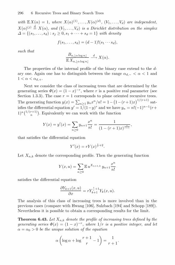
296 6 Recursive Trees and Binary Search Trees
with EX(α) = 1, where X(α)(1), . . . , X(α)(d), (V1, . . . , Vd) are independent,
X(α)(j)d= X(α), and (V1, . . . , Vd) is a Dirichlet distribution on the simplex
Δ = {(s1, . . . , sd) : sj ≥ 0, s1 + · · ·+ sd = 1} with density
f(s1, . . . , sd) = (d− 1)!(s1 · · · sd),
such thatBn,�α log n�
EXn,�α log n�
d−→ X(α).
The properties of the internal profile of the binary case extend to the d-ary one. Again one has to distinguish between the range αd,− < α < 1 and1 < α < αd,+.
Next we consider the class of increasing trees that are determined by thegenerating series Φ(x) = (1 − x)−r, where r is a positive real parameter (seeSection 1.3.3). The case r = 1 corresponds to plane oriented recursive trees.
The generating function y(x) =∑
n≥1 ynxn/n! = 1−
(1−(r+1)x
)1/(r+1)sat-
isfies the differential equation y′ = 1/(1−y)r and we have yn = n!(−1)n−1(r+
1)n(1/(r+1)
n
). Equivalently we can work with the function
Y (x) = y′(x) =∑n≥0
yn+1xn
n!=
1
(1− (r + 1)x)r
r+1,
that satisfies the differential equation
Y ′(x) = rY (x)1r +2.
Let Xn,k denote the corresponding profile. Then the generating function
Y (x, u) =∑n≥0
EuXn+1,k yn+1xn
n!
satisfies the differential equation
∂Yk+1(x, u)
∂x= rY
1r +1
k+1 Yk(x, u).
The analysis of this class of increasing trees is more involved than in theprevious cases (compare with Hwang [106], Sulzbach [194] and Schopp [189]).Nevertheless it is possible to obtain a corresponding results for the limit.
Theorem 6.43. Let Xn,k denote the profile of increasing trees defined by thegenerating series Φ(x) = (1 − x)−r, where 1/r is a positive integer, and letα = α0 > 0 be the unique solution of the equation
α
(logα+ log
r + 1
r− 1
)=
1
r + 1.
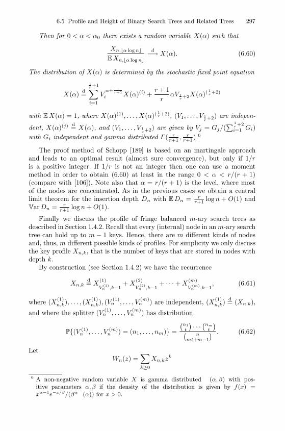
6.5 Profile and Height of Binary Search Trees and Related Trees 297
Then for 0 < α < α0 there exists a random variable X(α) such that
Xn,�α log n�EXn,�α log n�
d−→ X(α). (6.60)
The distribution of X(α) is determined by the stochastic fixed point equation
X(α)d=
1r +1∑i=1
Vα+ 1
r+1
i X(α)(i) +r + 1
rαV 1
r +2X(α)(1r +2)
with EX(α) = 1, where X(α)(1), . . . , X(α)(1r +2), (V1, . . . , V 1
r +2) are indepen-
dent, X(α)(j)d= X(α), and (V1, . . . , V 1
r +2) are given by Vj = Gj/(∑ 1
r +2i=1 Gi)
with Gi independent and gamma distributed Γ ( rr+1 ,
rr+1).6
The proof method of Schopp [189] is based on an martingale approachand leads to an optimal result (almost sure convergence), but only if 1/ris a positive integer. If 1/r is not an integer then one can use a momentmethod in order to obtain (6.60) at least in the range 0 < α < r/(r + 1)(compare with [106]). Note also that α = r/(r + 1) is the level, where mostof the nodes are concentrated. As in the previous cases we obtain a centrallimit theorem for the insertion depth Dn with EDn = r
r+1 logn + O(1) andVarDn = r
r+1 logn+O(1).
Finally we discuss the profile of fringe balanced m-ary search trees asdescribed in Section 1.4.2. Recall that every (internal) node in anm-ary searchtree can hold up to m − 1 keys. Hence, there are m different kinds of nodesand, thus, m different possible kinds of profiles. For simplicity we only discussthe key profile Xn,k, that is the number of keys that are stored in nodes withdepth k.
By construction (see Section 1.4.2) we have the recurrence
Xn,kd= X
(1)
V(1)
n ,k−1+X
(2)
V(2)
n ,k−1+ · · ·+X(m)
V(m)
n ,k−1, (6.61)
where (X(1)n,k), . . . , (X
(1)n,k), (V
(1)n , . . . , V
(m)n ) are independent, (X
(1)n,k)
d= (Xn,k),
and where the splitter (V(1)n , . . . , V
(m)n ) has distribution
P{(V (1)n , . . . , V (m)
n ) = (n1, . . . , nm)} =
(n1
t
)· · ·(nm
t
)(n
mt+m−1
) . (6.62)
LetWn(z) =
∑k≥0
Xn,kzk
6 A non-negative random variable X is gamma distributed Γ (α,β) with pos-itive parameters α, β if the density of the distribution is given by f(x) =xα−1e−x/β/(βαΓ (α)) for x > 0.
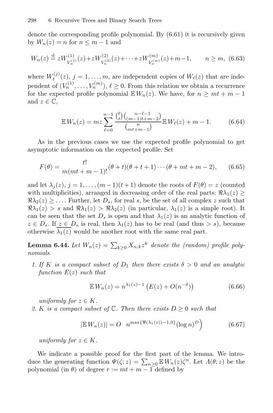
298 6 Recursive Trees and Binary Search Trees
denote the corresponding profile polynomial. By (6.61) it is recursively givenby Wn(z) = n for n ≤ m− 1 and
Wn(z)d= zW
(1)
V(1)
n
(z)+zW(2)
V(2)
n
(z)+· · ·+zW (m)
V(m)
n
(z)+m−1, n ≥ m, (6.63)
where W(j)� (z), j = 1, . . . ,m, are independent copies of W�(z) that are inde-
pendent of (V(1)
n , . . . , V(m)n ), � ≥ 0. From this relation we obtain a recurrence
for the expected profile polynomial EWn(z). We have, for n ≥ mt +m − 1and z ∈ C,
EWn(z) = mz
n−1∑�=0
(�t
)(n−�−1
(m−1)t+m−2
)(n
mt+m−1
) EW�(z) +m− 1. (6.64)
As in the previous cases we use the expected profile polynomial to getasymptotic information on the expected profile. Set
F (θ) =t!
m(mt+m− 1)!(θ + t)(θ + t+ 1) · · · (θ +mt+m− 2), (6.65)
and let λj(z), j = 1, . . . , (m− 1)(t+ 1) denote the roots of F (θ) = z (countedwith multiplicities), arranged in decreasing order of the real parts: �λ1(z) ≥�λ2(z) ≥ . . . . Further, let Ds, for real s, be the set of all complex z such that�λ1(z) > s and �λ1(z) > �λ2(z) (in particular, λ1(z) is a simple root). Itcan be seen that the set Ds is open and that λ1(z) is an analytic function ofz ∈ Ds. If z ∈ Ds is real, then λ1(z) has to be real (and thus > s), becauseotherwise λ1(z) would be another root with the same real part.
Lemma 6.44. Let Wn(z) =∑
k≥0Xn,kzk denote the (random) profile poly-
nomials.
1. If K is a compact subset of D1 then there exists δ > 0 and an analyticfunction E(z) such that
EWn(z) = nλ1(z)−1(E(z) +O(n−δ)
)(6.66)
uniformly for z ∈ K.2. K is a compact subset of C. Then there exists D ≥ 0 such that
|EWn(z)| = O(nmax{�(λ1(z))−1,0}(logn)D
)(6.67)
uniformly for z ∈ K.
We indicate a possible proof for the first part of the lemma. We intro-duce the generating function Ψ(ζ; z) =
∑n≥0 EWn(z)ζn. Let Λ(θ; z) be the
polynomial (in θ) of degree r := mt+m− 1 defined by
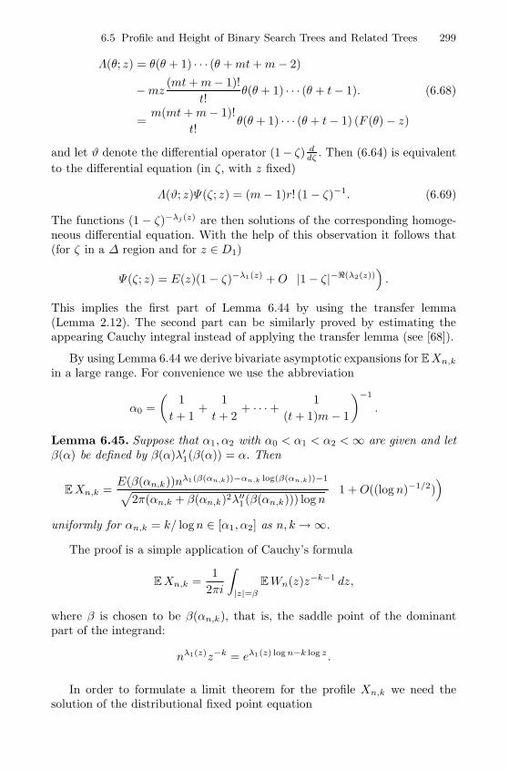
6.5 Profile and Height of Binary Search Trees and Related Trees 299
Λ(θ; z) = θ(θ + 1) · · · (θ +mt+m− 2)
−mz (mt+m− 1)!
t!θ(θ + 1) · · · (θ + t− 1). (6.68)
=m(mt+m− 1)!
t!θ(θ + 1) · · · (θ + t− 1) (F (θ)− z)
and let ϑ denote the differential operator (1− ζ) ddζ . Then (6.64) is equivalent
to the differential equation (in ζ, with z fixed)
Λ(ϑ; z)Ψ(ζ; z) = (m− 1)r! (1− ζ)−1. (6.69)
The functions (1 − ζ)−λj(z) are then solutions of the corresponding homoge-neous differential equation. With the help of this observation it follows that(for ζ in a Δ region and for z ∈ D1)
Ψ(ζ; z) = E(z)(1− ζ)−λ1(z) +O(|1− ζ|−�(λ2(z))
).
This implies the first part of Lemma 6.44 by using the transfer lemma(Lemma 2.12). The second part can be similarly proved by estimating theappearing Cauchy integral instead of applying the transfer lemma (see [68]).
By using Lemma 6.44 we derive bivariate asymptotic expansions for EXn,k
in a large range. For convenience we use the abbreviation
α0 =
(1
t+ 1+
1
t+ 2+ · · ·+ 1
(t+ 1)m− 1
)−1
.
Lemma 6.45. Suppose that α1, α2 with α0 < α1 < α2 <∞ are given and letβ(α) be defined by β(α)λ′1(β(α)) = α. Then
EXn,k =E(β(αn,k))nλ1(β(αn,k))−αn,k log(β(αn,k))−1√
2π(αn,k + β(αn,k)2λ′′1 (β(αn,k))) logn
(1 +O((log n)−1/2)
)uniformly for αn,k = k/ logn ∈ [α1, α2] as n, k→∞.
The proof is a simple application of Cauchy’s formula
EXn,k =1
2πi
∫|z|=β
EWn(z)z−k−1 dz,
where β is chosen to be β(αn,k), that is, the saddle point of the dominantpart of the integrand:
nλ1(z)z−k = eλ1(z) log n−k log z .
In order to formulate a limit theorem for the profile Xn,k we need thesolution of the distributional fixed point equation
300 6 Recursive Trees and Binary Search Trees
Y (z)d= zV
λ1(z)−11 Y (1)(z)+zV
λ1(z)−12 Y (2)(z)+· · ·+zV λ1(z)−1
m Y (m)(z), (6.70)
where Y (1)(z), . . . , Y (m)(z), (V1, . . . , Vm) are independent, Y (j)(z)d= Y (z),
and where (V1, . . . , Vm) is supported on the simplex Δ = {(s1, . . . , sm) : sj ≥0, s1 + · · ·+ sm = 1} with density
f(s1, . . . , sm) =((t+ 1)m− 1)!
(t!)m(s1 · · · sm)t.
In particular one first shows that for suitable z ∈ C
Wn(z)
EWn(z)
d−→ Y (z)
(compare with [68]). Finally, by applying Cauchy’s formula one then derivesa limit theorem for Xn,k.
Theorem 6.46. Let m ≥ 2 and t ≥ 0 be given integers and let (Xn,k)k≥0 bethe profile of the corresponding random search tree with n keys.
Set I = {β > 0 : 1 < λ1(β2) < 2λ1(β)− 1}, I ′ = {βλ′1(β) : β ∈ I}, and letβ(α) > 0 be defined by β(α)λ′1(β(α)) = α. Then for every α ∈ I ′
Xn,�α log n�EXn,�α log n�
d−→ Y (β(α)). (6.71)
A corresponding result holds for several different kinds of profiles accordingto the m different kinds of nodes that appear in m-ary search trees. Theo-rem 6.46 generalises to a functional limit theorem, too (see [68]).
6.5.2 The Height of Binary Search Trees and Related Trees
In the previous section we have discussed the profile of d-ary recursive trees,generalised plane oriented recursive trees and m-ary search trees. For all theseclasses of random trees we have observed a structure that is similar to thatof recursive trees. Since the height is closely related to the profile we expecta similar phenomenon for the height. All these trees are so-called logn-trees,that is, the height is of order logn. The second observation is that the heightis highly concentrated around its mean.
We start with d-ary recursive trees that include the class of binary searchtrees. Besides the height Hn there is a second level of interest. The saturationlevel Hn is the maximum level with In,k = dk, that is, up to this level thetree is a complete d-ary tree.
Theorem 6.47. The height Hn and the saturation level Hn of random d-aryrecursive trees have expected value
EHn ∼ αd,+ logn and EHn ∼ αd,− logn, (6.72)
6.5 Profile and Height of Binary Search Trees and Related Trees 301
where 0 < αd,− < d < αd,+ are the solutions of the equation
α log
(de
(d− 1)α
)=
1
d− 1.
Furthermore there are exponential tail estimates of the form
P{|Hn − EHn| ≥ η} = O(e−cη)
and P{|Hn − EHn| ≥ η} = O(e−cη)
with some c > 0.
Remark 6.48 We want to note that in the binary case Φ(x) = (1 +x)2 (thatis equivalent to binary search trees) various results of that kind (and evenmuch more precise ones) are well known (see [49, 61, 181]). For example, itis known that
EHn = α2,+ logn− 3α2,+
2(α2,+ − 1)log logn+O(1).
Of course, we expect similar relations for general d-ary recursive trees.The first breakthrough was due to Devroye [49] who related the height of bi-
nary search trees to branching random walks and could prove that Hn/ logn→α2,+ = 4.331... a.s. Previously Pittel [172] had shown that Hn/ logn→ γ forsome γ ≤ α2,+. Based on numerical data Robson conjectured that the varianceVarHn is bounded. In fact, he could prove (see [185]) that there is an infi-nite subsequence for which E|Hn − EHn| stays bounded. Eventually Robson’sconjecture was independently solved by Reed [181] and (few month later) byDrmota [62].
Nowadays the height constant is known in very general setting, for exam-ple, in [27] it is shown that Hn/ logn → αd,+ for all polynomial classed ofincreasing trees of degree d.
The analysis of the height Hn of d-ary recursive trees is very similar tothat of recursive trees. The generating functions
yk(x) =∑n≥1
P{Hn ≤ k}ynxn
n!
with yn = (−1)nn!(d− 1)n(−1/(d−1)
n
)satisfy y0(x) = 0 and
y′k+1(x) = (1 + yk(x))d, yk+1(x) = 0
(compare also with Section 6.2.2). For convenience we will work with Yk(x) =1 + yk(x) that satisfy Y ′k+1(x) = Yk(x)d and Yk+1(0) = 1. Note that bydefinition
limk→∞
Yk(x) = Y (x) =1
(1 − (d− 1)x)1
d−1
.
302 6 Recursive Trees and Binary Search Trees
Thus, one might expect that the behaviour of the sequence Yk(1/(d− 1)) willplay an essential role in the analysis as it was with Yk(1) in the case of recursivetrees. This is actually true. In particular Lemma 6.33 and Lemma 6.34 havedirect counterparts. Hence the limit
α0 = limk→∞
Yk+1(1/(d− 1))
Yk(1/(d− 1))(6.73)
exists. Furthermore, Lemma 6.37 generalises to
P{Hn ≤ k} = O
(Yk( 1
d−1 )
n1/(d−1)
)and P{Hn > k} = O
(n
Yk( 1d−1)d−1
).
(6.74)The essential part of the proof is to show that α0 > 1. Here we use the
estimate
δk(x) = Y (x)− Yk(x) ≤ dk∑�>k
1
�!
(1
d− 1log
1
1− (d− 1)x
)�
,
which follows by induction with the help of the inequality δ′k+1(x) ≤ dY (x)d−1δk(x).
If we set xk = 1d−1
(1−A−k
)with A = e1/αd,+ then this inequality implies
Yk(1/(d− 1)) ≥ Yk(xk) ≥ Ak/(d−1)(
1−O(k−1/2),)
and consequently α0 ≥ A1/(d−1) > 1.By combining (6.73) and (6.74) it follows (as in the case of recursive trees)
that
EHn = max{k : Yk(1/(d− 1)) ≤ n1/(d−1)
}+O(1) ∼ logn
(d− 1) logα0
and that we have exponential tail estimates of the form
P{|Hn − EHn| ≥ η} = O(e−cη).
It remains to show that α0 = A1/(d−1). Since αd,+ = ((d − 1) logA)−1,this will imply EHn ∼ αd,+ logn. For this purpose we consider solutions ofthe integral equation
y1
d−1F (y/A) =Γ(
dd−1
)Γ(
1d−1
)d ∫y1+···+yd=y,yj≥0
d∏j=1
(F (yj)y
1d−1−1
j
)dy, (6.75)
for 1 < A < e1/αd,+ and auxiliary functions
Y k(x) = Ak/(d−1)Φ
(Ak
(x− 1
d− 1
)),
6.5 Profile and Height of Binary Search Trees and Related Trees 303
where
Φ(u) =1
(d− 1)1
d−1Γ(
1d−1
) ∫ ∞0
F (y) y1
d−1−1e−uy dy.
These functions satisfy the recurrence Y′k+1(x) = Y
d
k(x) and can be used toprovide upper bounds for Yk(1/(d−1)) (compare with Lemmas 6.38–6.40, seealso [57]).
Remark 6.49 An even more refined analysis (see [57]) shows that
P{Hn ≤ k} = F((d− 1)n/Yk(1/(d− 1))d−1
)+ o(1)
uniformly for all k ≥ 0 as n → ∞, where F (y) satisfies the integral equation(6.75) for A = e1/αd,+ .
The analysis of the saturation level Hn of d-ary recursive trees runs alongsimilar lines. Here one has to study the generating functions
yk(x) =∑n≥1
P{Hn ≥ k} ynxn
n!
that satisfy the recurrence
y′k+1(x) = yk(x)d, yk+1(0) = 0
with initial condition y0(x) = y(x). The major difference between the analysisof the height and the saturation level is that one cannot consider yk(1/(d−1)),since the function yk(x) is singular at x = 1/(d− 1). Instead, one can studythe behaviour of the sequence yk(xk) that is determined by the equation
yk(xk) =y(xk)
2.
For details see [60] and [36].
Next we turn to generalised plane oriented recursive trees.
Theorem 6.50. The height Hn of random increasing trees defined by the gen-erating series Φ(x) = (1− x)−r (for some real r > 0) has expected value
EHn ∼ αr logn, (6.76)
where αr > 0 is the solution of the equation
αr
(logαr + log
r + 1
r− 1
)=
1
r + 1.
Furthermore there are exponential tail estimates of the form
P{|Hn − EHn| ≥ η} = O(e−cη)
with some c > 0.
304 6 Recursive Trees and Binary Search Trees
Here the generating function y(z) =∑
n≥1 ynzn/n! satisfies y′(z) =
(1 − y(z))−r and is explicitly given by y(z) = 1 −(1 − (r + 1)z
)1/(r+1)with
coefficients yn = n!(−1)n−1(r + 1)n(1/(r+1)
n
). The height distribution is then
encoded in the generating functions
yk(x) =∑n≥0
ynP{Hn ≤ k}xn
n!,
which are given by y0(z) = 0 and recursively by
y′k+1(z) =1
(1− yk(z))r, yk+1(0) = 0.
By taking derivatives it follows that
y′′k+1(z) = r(y′k+1(z)
)1+ 1r y′k(z).
If we set
Yk(z) = y′k(z) =∑n≥0
yn+1P{Hn+1 ≤ k}zn
n!
then we have Y1(z) = 1 and the recurrence relation
Y ′k+1(z) = r Yk+1(z)1+1r Yk(z), Yk+1(0) = 1. (6.77)
This equation looks like a mixture of the corresponding generating functionsfor recursive trees and d-ary recursive trees. Therefore a similar analysis ap-plies (see also [60, 57]) and we obtain the result.
Remark 6.51 If r = AB > 0 is a rational number (with positive coprime
integers A,B) then we have (uniformly for all k ≥ 0 as n→∞)
P{Hn ≤ k} = G((r + 1)n/(y′k(r/(r + 1)))1+
1r
)+ o(1)
with
G(y) =Γ(
AA+B
)Γ(
1A+B
)A ∫z1+···+zd=1,zj≥0
d∏j=1
(F (yzj)z
1A+B−1
j
)dz
and where F (y) satisfies the integral equation
y1
d−1F (ye−1/αr) =Γ(
1 + 1A+B
)Γ(
1A+B
)A+B+1
×∫
y1+···+yA+B+1=y,yj≥0
B+1∏j=1
(F (yje
−1/αr )y1
A+B−1
j
)
×A+B+1∏�=B+2
(F (y�)y
1A+B−1
�
)dy.
6.5 Profile and Height of Binary Search Trees and Related Trees 305
Finally we consider fringe balanced m-ary search trees.
Theorem 6.52. The height Hn and the saturation level Hn of random fringebalanced m-ary search trees (with parameter t) have expected value
EHn ∼ αm,t,+ logn and EHn ∼ αm,t,− logn, (6.78)
where 0 < αm,t,− < αm,t,+ are given by
αm,t,− =
(m−1)(t+1)−1∑j=0
1
β1 + t+ 1 + j,
αm,t,+ =
(m−1)(t+1)−1∑j=0
1
β2 + t+ 1 + j,
where β1 > 0 and β2 < 0 are the solutions of the equation
(m−1)(t+1)−1∑j=0
log(β+t+1+j)−log
((m(t+ 1))!
(t+ 1)!
)=
(m−1)(t+1)−1∑j=0
β
β + t+ 1 + j.
(6.79)Furthermore there are exponential tail estimates of the form
P{|Hn − EHn| ≥ η} = O(e−cη)
and P{|Hn − EHn| ≥ η} = O(e−cη)
with some c > 0.
In this case the generating functions
yk(x) =∑n≥0
P{H(m,t)n ≤ k} xn and yk(x) =
∑n≥0
P{H(m,t)
n ≥ k} xn
satisfy the recurrence relation
y(m(t+1)−1)k+1 (x) =
(m(t+ 1)− 1)!
(t!)m
(y(t)k (x))m, (6.80)
y(m(t+1)−1)k+1 (x) =
(m(t+ 1)− 1)!
(t!)m
(y(t)k (x))m, (6.81)
with initial conditions
y0(x) = 1, yk(0) = y′k(0) = · · · = y(m−1)k (0) = 1,
resp.
y0(x) =x
1− x, yk(0) = y′k(0) = · · · = y(m−1)k (0) = 0.
Thus, we are again in a similar situation as in the above cases (for details werefer to [36]).

7
Tries and Digital Search Trees
Digital trees like tries or digital search trees are important in many computerscience applications like data compression, pattern matching or hashing. Forexample, the popular Lempel-Ziv compression scheme [208] is strongly relatedto digital search trees.
The basic idea of the Lempel-Ziv algorithm is to partition a sequence overa finite alphabet into phrases (blocks) of variable sizes such that a new block isthe shortest substring not seen in the past as a phrase. For example, the string110010100010001000 is parsed into (1)(10)(0)(101)(00)(01)(000)(100). Thisalgorithm can be implemented efficiently by using the digital tree structure(compare with Figure 1.13). Assume that the first phrase of the Lempel-Zivscheme is an empty phrase that is stored in the root. When a new phrase iscreated, the search starts at the root and proceeds down the tree as directedby the input symbols exactly in the same manner as in the digital search treeconstruction. The search is completed when a branch is taken from an existingtree node to a new node that has not been visited before. Then, an edge anda new node are added to the tree. Phrases created in such a way are storeddirectly in the nodes of the tree. The example string produces exactly thedigital search tree depicted in Figure 1.13.
Digital trees have been widely studied in the literature (see [146, 197] andthe references therein). Here we will concentrate on the profile and commentshortly on the height. The motivation of studying the profiles of such treesis multifold. Of course, digital trees are used in various applications (for ex-ample, the profile Xn,k represents the number of phrases of length k in theLempel-Ziv’78 built over n phrases). Second, the profile is a fine shape mea-sure closely connected to many other cost measures (height, saturation level,depth, path length, etc.). And finally, the analytic problems are mathemati-cally challenging and lead to interesting distributional results. It is remarkablethat the profile process is almost deterministic. In contrast to the previouslystudied classes of trees (Galton-Watson trees in Chapter 4 and recursive treesin Chapter 6) the normalised profile Bn,k/EBn,k converges to 1 and there isa central limit theorem.
308 7 Tries and Digital Search Trees
The following treatment on tries is based on the work by Park, Hwang,Nicodeme, and Szpankowski [169]. The corresponding result for digital searchtrees follows some recent work by Drmota and Szpankowski [70].
7.1 The Profile of Tries
Tries are prototype data structures useful for many indexing and retrievalpurposes. They were first proposed by de la Briandais [44] in the late 1950sfor information processing; Fredkin [86] suggested the current name is part ofretrieval. Due to their simplicity and efficiency, tries found widespread use indiverse applications (see [87, 130, 146, 197]).
Tries are a natural choices of data structures when the input records in-volve a notion of alphabets or digits. They are often used to store such dataso that future retrieval can be made efficient. Recall that (m-ary) tries can beconstructed in the following way. Suppose that a sequence of n strings over anm-ary alphabet, m ≥ 2, is given. If n = 0, then the trie is empty. If n = 1 thena single (external) node holding this string is allocated. If n ≥ 1 then the trieconsists of a (internal) root node directing strings to the m subtrees accordingto the first letter of each string, and strings directed to the same subtree arethemselves tries (see [130, 146, 197] for more details). For simplicity, we onlydeal with binary tries here. Unlike other search trees, such as digital searchtrees and binary search trees, where records or keys are stored in the internalnodes, the internal nodes in tries are branching nodes used merely to directrecords to each sub trie. The keys are all stored in external nodes that areleaves of such tries. A trie has more internal nodes than external nodes (fixedto be n), differing from almost all other search trees.
7.1.1 Generating Functions for the Profile
Our first and main goal is to study the profile of tries, where we have todistinguish, as in the case of binary search trees, between the internal andthe external profile. We write Bn,k to denote the number of external nodes(leaves) at distance k from the root (external profile) and the number ofinternal nodes at distance k from the root is denoted by In,k (internal profile).
In the example (depicted in Figure 1.14) we have B8,0 = B8,1 = 0, B8,2 =B8,3 = 1, B8,4 = 2, B8,5 = 6 and I8,0 = 1, I8,1 = 2, I8,2 = I8,3 = 3, I8,4 = 2.
We also assume the simplest probabilistic model, namely the standardBernoulli model. More precisely, we assume that the input is a sequence ofn independent and identically distributed random variables, each being com-posed of an infinite sequence of Bernoulli random variables with mean p, where0 < p < 1 is the probability of a 1 and q = 1 − p is the probability of a 0.The corresponding trie constructed from these n bit-strings is called a randomtrie. This simple model may seem to be too idealised for practical purposes,however, the typical behaviours of such a model often hold for more general
7.1 The Profile of Tries 309
models such as Markovian or dynamical sources, although the technicalitiesare usually more involved (see for example [41, 50, 51, 111]).
We start with the external profile Bn,k. Let
Pn,k(u) = EuBn,k
be the corresponding probability generating function. Then by using the re-cursive definition of tries we have
Pn,k(u) =
n∑j=0
(n
j
)pjqn−jPj,k−1(u)Pn−j,k−1(u), (n ≥ 2, k ≥ 1) (7.1)
with initial conditions P0,k(u) = 1 for k ≥ 0, P1,0(u) = u, P1,k(u) = 1 fork ≥ 1, and Pn,0(u) = 1 for n ≥ 1. Recall that the first digit determineswhether the corresponding string is put to the left or to the right subtree.Due to the independence assumption the number of strings where the firstdigit is 0 follows a binomial distribution. The splitting probabilities are thusgiven by
(nj
)pjqn−j .
From (7.1) one gets directly a recurrence relation for the exponential gen-erating functions
Gk(x, u) =∑n≥0
Pn,k(u)xn
n!
of the form
Gk(x, u) = Gk−1(px, u)Gk−1(qx, u) + (P1,k(u)− P1,k−1(u))x, (k ≥ 1),(7.2)
with initial condition G0(x, u) = ex + x(u − 1). With the help of the initialconditions of P1,k(u) it follows that
G1(x, u) = ex + (epxqx+ eqxpx− 1) (u− 1) + pqx2(u− 1)2
andGk(x, u) = Gk−1(px, u)Gk−1(qx, u), (k ≥ 2). (7.3)
The corresponding probability generating functions for the internal profile,
P[I]n,k(u) = EuIn,k ,
satisfy the same recurrence
P[I]n,k(u) =
n∑j=0
(n
j
)pjqn−jP
[I]j,k−1(u)P
[I]n−j,k−1(u), (n ≥ 2, k ≥ 1),
but with initial conditions P[I]n,0(u) = u for n ≥ 2 and P
[I]n,k(u) = 1 for n ≤ 1
and k ≥ 0. Similarly to the external profile we introduce the exponentialgenerating functions
310 7 Tries and Digital Search Trees
G[I]k (x, u) =
∑n≥0
P[I]n,k(u)
xn
n!,
that satisfy
G[I]k (x, u) = G
[I]k−1(px, u)G
[I]k−1(qx, u), (k ≥ 1), (7.4)
with initial condition G[I]0 (x, u) = uex − (1 + x)(u − 1).
We will come back to the relations (7.3) and (7.4) in Section 7.1.3. In orderto get a first impression of the behaviour of such profiles we will study theexpected profile (see Section 7.1.2). Set
Ek(x) =∑n≥0
EBn,kxn
n!=
[∂Gk(x, u)
∂u
]u=1
.
Then (7.3) implies
Ek(x) = eqxEk−1(px) + epxEk−1(qx) (k ≥ 2).
Setting
Δk(x) = e−xEk(x) =∑n≥0
EBn,kxn
n!e−x
this rewrites to
Δk(x) = Δk−1(px) +Δk−1(qx) (k ≥ 2) (7.5)
with initial conditions Δ0(x) = xe−x and Δ1(x) = pxe−px + qxe−qx − xe−x.Note that if x is a positive real number then Δk(x) can be considered as
the expected value of the external profile (at level k) if the number n of inputstrings is Poisson distributed with parameter x. The mapping
(an)n≥0 �→ A(x) =∑n≥0
anxn
n!e−x
is also called Poisson transform. In the context of tries the Poisson transformhas turned out to be natural; the relation (7.5) is remarkably easy. With thehelp of the Mellin transform we will be able to provide an asymptotic solutionof Δk(x) (see Section 7.1.2). The final step is then to derive asymptotics forEBn,k from that of Δk(x), that is, we have to invert the Poisson transform.This is of independent interest (compare also with Jacquet and Szpankowski[113]). For example, the Poisson transform of the sequence an = n equalsA(x) = x, and the the Poisson transform of the sequence bn = n2 is B(x) =x + x2. In these two examples we have A(n) = an and B(n) ∼ bn. Such aproperty is surely not generally true (for example, for an = 2n) but the crucialobservation is that (under suitable assumptions) A(n) and an are very close
7.1 The Profile of Tries 311
(see [113]). Thus, inversion of the Poisson transform is mostly relatively easy.We can expect that EBn,k is approximated by Δk(n), but one has to keeptrack of the second parameter k.
From a computational point of view depoissonisation is done with Cauchyintegration
an =1
2πi
∫|x|=r
exA(x)dx
xn+1,
where the radius r is usually chosen to be n, since x = n is the saddle pointof the function exx−n. Thus, if A(x) has a regular behaviour, for examplepolynomial growth, then the integral is concentrated at x = n and we (usually)get
an ∼1
2πi
∫|x|=n, | arg(x)|≤ε
exA(x)dx
xn+1
∼ A(n) · 1
2πi
∫|x|=n, | arg(x)|≤ε
exdx
xn+1
∼ A(n),
as expected.
7.1.2 The Expected Profile of Tries
In order to state our main result we need the following notations. For a realnumber α with (log 1
p )−1 < α < (log 1q )−1, let
ρ = ρ(α) =1
log(p/q)log
1− α log(1/p)
α log(1/q)− 1. (7.6)
Equivalently, α and ρ satisfy the equation
α =p−ρ + q−ρ
p−ρ log 1p + q−ρ log 1
q
.
Furthermore, we set
β(ρ) =p−ρq−ρ log(p/q)2
(p−ρ + q−ρ)2, (7.7)
and
α1 =1
log(1/p), α0 =
2
log 1p + log 1
q
,
α2 =p2 + q2
p2 log 1p + q2 log 1
q
, α3 =2
log(1/(p2 + q2)).
Then we have the following relations.
312 7 Tries and Digital Search Trees
Theorem 7.1. Let EBn,k denote the expected external profile in binary ran-dom tries with underlying (non-zero) probabilities p > q = 1− p. Then:
1. If α1 + ε ≤ klog n ≤ α2 − ε (for some ε > 0) then we have uniformly
EBn,k = G(ρn,k, logp/q p
kn) (p−ρn,k + q−ρn,k )kn−ρn,k√
2πβ(ρn,k)k
(1 +O(k−1/2)),
where G(ρ, x) is a non-zero periodic function with period 1 and ρn,k =ρ(k/ logn).
2. If k = α2
(logn+ ξ
√α2β(−2) logn
), where ξ = o((log n)
16 ) then
EBn,k = 2pqn2(p2 + q2)k−1Φ(ξ)
(1 +O
(1 + |ξ|3√
logn
)),
where Φ(x) denotes the normal distribution function.3. If k
log n ≥ α2 + ε (for some ε > 0) then uniformly
EBn,k = 2pqn2(p2 + q2)k−1(1 +O(n−η)
)for some η > 0.
Theorem 7.2. Let E In,k denote the expected internal profile in binary ran-dom tries with underlying (non-zero) probabilities p > q = 1− p. Then:
1. If α1 + ε ≤ klog n ≤ α0 − ε (for some ε > 0) then we have uniformly
E In,k = 2k−G(ρn,k, logp/q p
kn) (p−ρn,k + q−ρn,k)kn−ρn,k√
2πβ(ρn,k)k
(1 +O(k−1/2)),
where G(ρ, x) is a non-zero periodic function with period 1 and ρn,k =ρ(k/ logn).
2. If k = α0
(logn+ ξ
√α0β(0) logn
), where ξ = o((log n)
16 ) then
E In,k = 2kΦ(−ξ)(
1 +O
(1 + |ξ|3√
logn
)).
3. If α0 + ε ≤ klog n ≤ α2 − ε (for some ε > 0) then uniformly
E In,k = G(ρn,k, logp/q p
kn) (p−ρn,k + q−ρn,k)kn−ρn,k√
2πβ(ρn,k)k
(1 +O(k−1/2)).
4. If k = α2
(logn+ ξ
√α2β(−2) logn
), where ξ = o((log n)
16 ) then
E In,k =1
2Φ(ξ)n2(p2 + q2)k
(1 +O
(1 + |ξ|3√
logn
)).
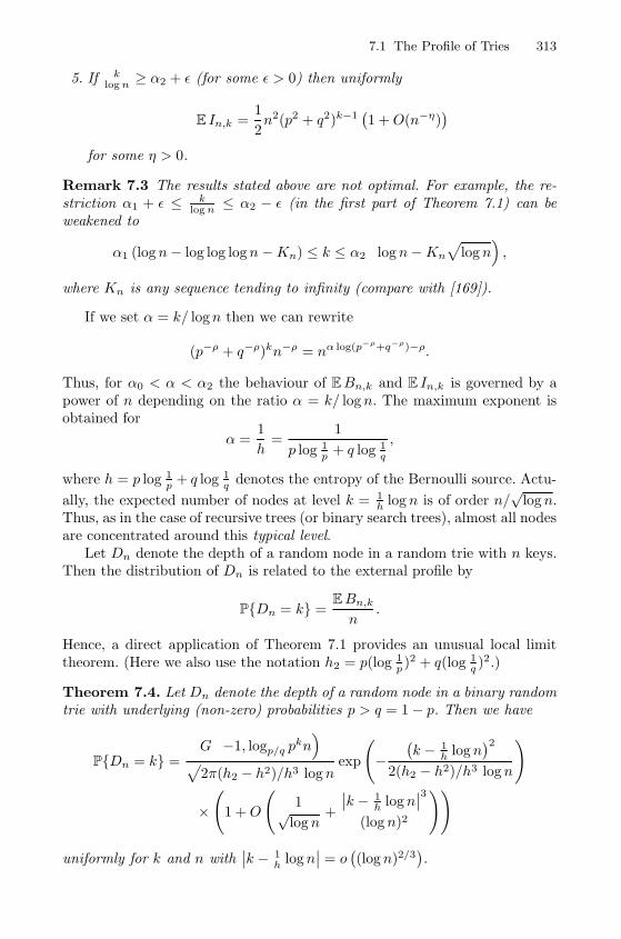
7.1 The Profile of Tries 313
5. If klog n ≥ α2 + ε (for some ε > 0) then uniformly
E In,k =1
2n2(p2 + q2)k−1
(1 +O(n−η)
)for some η > 0.
Remark 7.3 The results stated above are not optimal. For example, the re-striction α1 + ε ≤ k
log n ≤ α2 − ε (in the first part of Theorem 7.1) can beweakened to
α1 (logn− log log logn−Kn) ≤ k ≤ α2
(logn−Kn
√logn),
where Kn is any sequence tending to infinity (compare with [169]).
If we set α = k/ logn then we can rewrite
(p−ρ + q−ρ)kn−ρ = nα log(p−ρ+q−ρ)−ρ.
Thus, for α0 < α < α2 the behaviour of EBn,k and E In,k is governed by apower of n depending on the ratio α = k/ logn. The maximum exponent isobtained for
α =1
h=
1
p log 1p + q log 1
q
,
where h = p log 1p + q log 1
q denotes the entropy of the Bernoulli source. Actu-
ally, the expected number of nodes at level k = 1h logn is of order n/
√logn.
Thus, as in the case of recursive trees (or binary search trees), almost all nodesare concentrated around this typical level.
Let Dn denote the depth of a random node in a random trie with n keys.Then the distribution of Dn is related to the external profile by
P{Dn = k} =EBn,k
n.
Hence, a direct application of Theorem 7.1 provides an unusual local limittheorem. (Here we also use the notation h2 = p(log 1
p )2 + q(log 1q )2.)
Theorem 7.4. Let Dn denote the depth of a random node in a binary randomtrie with underlying (non-zero) probabilities p > q = 1− p. Then we have
P{Dn = k} =G(−1, logp/q p
kn)
√2π(h2 − h2)/h3 logn
exp
(−(k − 1
h logn)2
2(h2 − h2)/h3 logn
)
×(
1 +O
(1√
logn+
∣∣k − 1h logn∣∣3
(logn)2
))
uniformly for k and n with∣∣k − 1
h logn∣∣ = o((logn)2/3
).
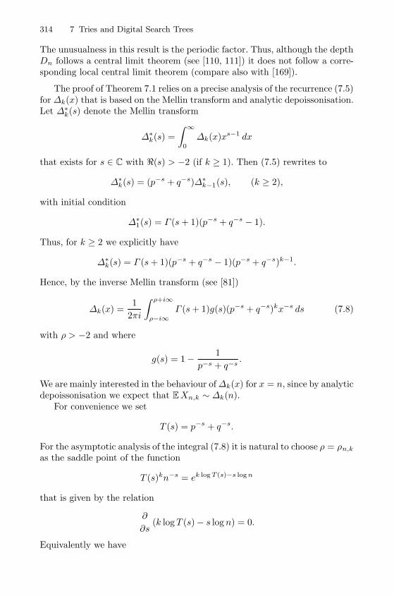
314 7 Tries and Digital Search Trees
The unusualness in this result is the periodic factor. Thus, although the depthDn follows a central limit theorem (see [110, 111]) it does not follow a corre-sponding local central limit theorem (compare also with [169]).
The proof of Theorem 7.1 relies on a precise analysis of the recurrence (7.5)for Δk(x) that is based on the Mellin transform and analytic depoissonisation.Let Δ∗k(s) denote the Mellin transform
Δ∗k(s) =
∫ ∞0
Δk(x)xs−1 dx
that exists for s ∈ C with �(s) > −2 (if k ≥ 1). Then (7.5) rewrites to
Δ∗k(s) = (p−s + q−s)Δ∗k−1(s), (k ≥ 2),
with initial condition
Δ∗1(s) = Γ (s+ 1)(p−s + q−s − 1).
Thus, for k ≥ 2 we explicitly have
Δ∗k(s) = Γ (s+ 1)(p−s + q−s − 1)(p−s + q−s)k−1.
Hence, by the inverse Mellin transform (see [81])
Δk(x) =1
2πi
∫ ρ+i∞
ρ−i∞Γ (s+ 1)g(s)(p−s + q−s)kx−s ds (7.8)
with ρ > −2 and where
g(s) = 1− 1
p−s + q−s.
We are mainly interested in the behaviour ofΔk(x) for x = n, since by analyticdepoissonisation we expect that EXn,k ∼ Δk(n).
For convenience we set
T (s) = p−s + q−s.
For the asymptotic analysis of the integral (7.8) it is natural to choose ρ = ρn,k
as the saddle point of the function
T (s)kn−s = ek log T (s)−s log n
that is given by the relation
∂
∂s(k logT (s)− s logn) = 0.
Equivalently we have

7.1 The Profile of Tries 315
k
logn=
p−ρ + q−ρ
p−ρ log 1p + q−ρ log 1
q
,
that is, ρ = ρn,k = ρ(k/ logn).However, we have to distinguish between several cases. We start with the
range α1 < k/ logn < α2. Here we have −2 < ρn,k < ∞ and we can chooseρ = ρn,k. Another observation is that on the line �(s) = ρ there will beinfinitely many saddle points
sj = ρ+2πij
log pq
.
This is due to the fact that T (sj) = e−2πij(log p)/(log p/q)T (ρ) and consequentlythe behaviour of T (s)kz−s around s = sj is almost the same as that ofT (s)kz−s around s = ρ. This phenomenon gives a periodic leading factorin the asymptotics of Δk(n) and also of μn,k = EBn,k.
Lemma 7.5. Suppose that α1 + ε ≤ klog n ≤ α2− ε (for some ε > 0). Then we
have
Δk(n) = G(ρn,k, logp/q p
kn) (p−ρn,k + q−ρn,k )kn−ρn,k√
2πβ(ρn,k)k
(1 +O
(1√k
)),
whereG(ρ, x) =
∑j∈Z
g(ρ+ itj)Γ (ρ+ itj + 1)e−2jπix
is a non-zero periodic function with period 1 and tj = 2jπ/ log(p/q).
Proof. For convenience we set Jk(n, s) = n−sΓ (s+ 1)g(s)T (s)k. We split theintegral (7.8) into two parts where we use the substitution s = ρ + it. Letus start with the range |t| ≥ √
logn and recall that by Stirling’s formulaΓ (ρ+ 1 + it) = O
(|t|ρ+1/2e−π|t|/2
):
1
2π
∫|t|≥
√log n
Jk(n, ρ+ it) dt = O
(n−ρT (ρ)k
∫ ∞√
log n
|Γ (ρ+ it) dt
)
= O
(n−ρT (ρ)k
∫ ∞√
log n
tρ+1/2e−πt/2
)= O(n−ρT (ρ)k(logn)ρ/2+1/4e−π
√log n/2)
= O(n−ρT (ρ)ke−
√log n).
Next set
Tj =1
2π
∫|t−tj|≤π/ log(p/q)
Jk(n, ρ+ it) dt,
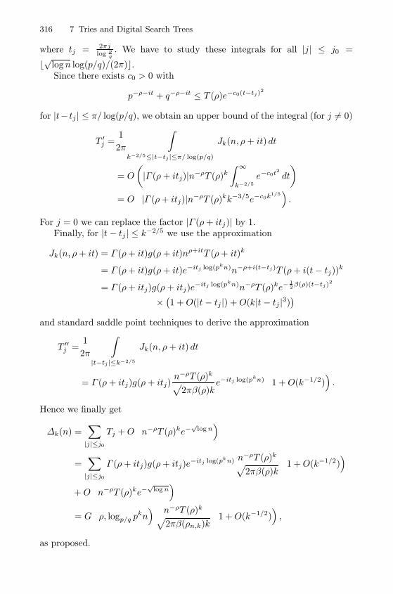
316 7 Tries and Digital Search Trees
where tj = 2πjlog p
q. We have to study these integrals for all |j| ≤ j0 =
�√
logn log(p/q)/(2π)�.Since there exists c0 > 0 with
p−ρ−it + q−ρ−it ≤ T (ρ)e−c0(t−tj)2
for |t− tj | ≤ π/ log(p/q), we obtain an upper bound of the integral (for j = 0)
T ′j =1
2π
∫k−2/5≤|t−tj |≤π/ log(p/q)
Jk(n, ρ+ it) dt
= O
(|Γ (ρ+ itj)|n−ρT (ρ)k
∫ ∞k−2/5
e−c0t2 dt
)= O(|Γ (ρ+ itj)|n−ρT (ρ)kk−3/5e−c0k1/5
).
For j = 0 we can replace the factor |Γ (ρ+ itj)| by 1.Finally, for |t− tj | ≤ k−2/5 we use the approximation
Jk(n, ρ+ it) = Γ (ρ+ it)g(ρ+ it)nρ+itT (ρ+ it)k
= Γ (ρ+ it)g(ρ+ it)e−itj log(pkn)n−ρ+i(t−tj)T (ρ+ i(t− tj))k
= Γ (ρ+ itj)g(ρ+ itj)e−itj log(pkn)n−ρT (ρ)ke−12 β(ρ)(t−tj)
2
×(1 +O(|t − tj |) +O(k|t− tj |3)
)and standard saddle point techniques to derive the approximation
T ′′j =1
2π
∫|t−tj |≤k−2/5
Jk(n, ρ+ it) dt
= Γ (ρ+ itj)g(ρ+ itj)n−ρT (ρ)k√
2πβ(ρ)ke−itj log(pkn)
(1 +O(k−1/2)
).
Hence we finally get
Δk(n) =∑|j|≤j0
Tj +O(n−ρT (ρ)ke−
√log n)
=∑|j|≤j0
Γ (ρ+ itj)g(ρ+ itj)e−itj log(pkn) n−ρT (ρ)k√2πβ(ρ)k
(1 +O(k−1/2)
)+O(n−ρT (ρ)ke−
√log n)
= G(ρ, logp/q p
kn) n−ρT (ρ)k√
2πβ(ρn,k)k
(1 +O(k−1/2)
),
as proposed.
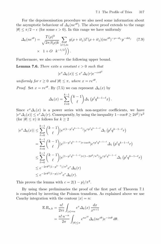
7.1 The Profile of Tries 317
For the depoissonisation procedure we also need some information aboutthe asymptotic behaviour of Δk(neiθ). The above proof extends to the range|θ| ≤ π/2− ε (for some ε > 0). In this range we have uniformly
Δk(neiθ) =T (ρ)k√2πβ(ρ)k
∑|j|≤j0
g(ρ+ itj)Γ (ρ+ itj)(neiθ)−ρ−itj p−iktj (7.9)
×(
1 +O(k−1/2)).
Furthermore, we also ovserve the following upper bound.
Lemma 7.6. There exits a constant c > 0 such that
|exΔk(x)| ≤ erΔk(r)e−crθ2
uniformly for r ≥ 0 and |θ| ≤ π, where x = reiθ.
Proof. Set x = reiθ . By (7.5) we can represent Δk(x) by
Δk(x) =
k−1∑�=0
(k − 1
�
)Δ1
(p�qk−1−�x
).
Since exΔ1(x) is a power series with non-negative coefficients, we have|exΔ1(x)| ≤ erΔ1(r). Consequently, by using the inequality 1−cos θ ≥ 2ϑ2/π2
(for |θ| ≤ π) it follows for k ≥ 2
|exΔk(x)| ≤k−1∑�=0
(k − 1
�
)|ex(1−p�qk−1−�)|erp�qk−1−�
Δ1
(p�qk−1−�r
)=
k−1∑�=0
(k − 1
�
)|e(1−p�qk−1−�)r cos θ|erp�qk−1−�
Δ1
(p�qk−1−�r
)≤
k−1∑�=0
(k − 1
�
)|e(1−p�qk−1−�)r(1−2ϑ2/π2)|erp�qk−1−�
Δ1
(p�qk−1−�r
)≤ e−2rθ2(1−pk−1)/π2
erΔk(r)
≤ e−2rθ2(1−p)/π2
erΔk(r).
This proves the lemma with c = 2(1− p)/π2.
By using these preliminaries the proof of the first part of Theorem 7.1is completed by inverting the Poisson transform. As explained above we useCauchy integration with the contour |x| = n:
EBn,k =n!
2πi
∫|x|=n
exΔk(x)dx
xn+1
=n!n−n
2π
∫|θ|≤π
eneiθ
Δk(neiθ)e−inθ dθ.
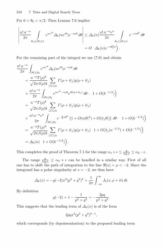
318 7 Tries and Digital Search Trees
Fix 0 < θ0 < π/2. Then Lemma 7.6 implies∣∣∣∣∣∣∣n!n−n
2π
∫θ0≤|θ|≤π
eneiθ
Δk(neiθ)e−inθ dθ
∣∣∣∣∣∣∣ ≤ Δk(n)n!n−nen
2π
∫θ0≤|θ|≤π
e−cnθ2
dθ
= O(Δk(n)e−cθ2
0n).
For the remaining part of the integral we use (7.9) and obtain
n!n−n
2π
∫|θ|≤θ0
eneiθ
Δk(neiθ)e−inθ dθ
=n−ρT (ρ)k√
2πβ(ρ)k
∑|j|≤j0
Γ (ρ+ itj)g(ρ+ itj)
× n!n−n
2π
∫|θ|≤θ0
eneiθ−inθeiθ(ρ+itj) dθ ·(
1 +O(k−1/2))
=n−ρT (ρ)k√
2πβ(ρ)k
∑|j|≤j0
Γ (ρ+ itj)g(ρ+ itj)
× n!n−nen
2π
∫|θ|≤θ0
e−12 nθ2 (
1 +O(n|θ|3) +O(|tjθ|))dθ ·(
1 +O(k−1/2))
=n−ρT (ρ)k√
2πβ(ρ)k
∑|j|≤j0
Γ (ρ+ itj)g(ρ+ itj)(
1 +O(|tj |n−1/2) +O(k−1/2))
= Δk(n)(
1 +O(k−1/2)).
This completes the proof of Theorem 7.1 for the range α1 + ε ≤ klog n ≤ α2− ε.
The range klog n ≥ α2 + ε can be handled in a similar way. First of all
one has to shift the path of integration to the line �(s) = ρ < −2. Since theintegrand has a polar singularity at s = −2, we thus have
Δk(x) = −g(−2)x2(p2 + q2)k +1
2π
∫ ∞−∞
Jk(x, ρ+ it) dt.
By definition
g(−2) = 1− 1
p2 + q2= − 2pq
p2 + q2.
This suggests that the leading term of Δk(x) is of the form
2pqx2(p2 + q2)k−1,
which corresponds (by depoissonisation) to the proposed leading term
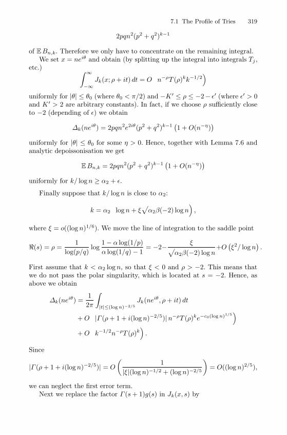
7.1 The Profile of Tries 319
2pqn2(p2 + q2)k−1
of EBn,k. Therefore we only have to concentrate on the remaining integral.We set x = neiθ and obtain (by splitting up the integral into integrals Tj ,
etc.) ∫ ∞−∞
Jk(x; ρ+ it) dt = O(n−ρT (ρ)kk−1/2
)uniformly for |θ| ≤ θ0 (where θ0 < π/2) and −K ′ ≤ ρ ≤ −2− ε′ (where ε′ > 0and K ′ > 2 are arbitrary constants). In fact, if we choose ρ sufficiently closeto −2 (depending of ε) we obtain
Δk(neiθ) = 2pqn2e2iθ(p2 + q2)k−1(1 +O(n−η)
)uniformly for |θ| ≤ θ0 for some η > 0. Hence, together with Lemma 7.6 andanalytic depoissonisation we get
EBn,k = 2pqn2(p2 + q2)k−1(1 +O(n−η)
)uniformly for k/ logn ≥ α2 + ε.
Finally suppose that k/ logn is close to α2:
k = α2
(logn+ ξ
√α2β(−2) logn
),
where ξ = o((log n)1/6). We move the line of integration to the saddle point
�(s) = ρ =1
log(p/q)log
1− α log(1/p)
α log(1/q)− 1= −2− ξ√
α2β(−2) logn+O(ξ2/ logn
).
First assume that k < α2 logn, so that ξ < 0 and ρ > −2. This means thatwe do not pass the polar singularity, which is located at s = −2. Hence, asabove we obtain
Δk(neiθ) =1
2π
∫|t|≤(log n)−2/5
Jk(neiθ, ρ+ it) dt
+O(|Γ (ρ+ 1 + i(logn)−2/5)|n−ρT (ρ)ke−c0(log n)1/5
)+O(k−1/2n−ρT (ρ)k
).
Since
|Γ (ρ+ 1 + i(logn)−2/5)| = O
(1
|ξ|(log n)−1/2 + (log n)−2/5
)= O((log n)2/5),
we can neglect the first error term.Next we replace the factor Γ (s+ 1)g(s) in Jk(x, s) by
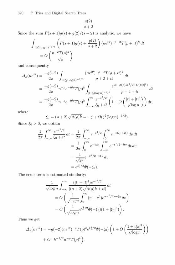
320 7 Tries and Digital Search Trees
− g(2)
s+ 2.
Since the sum Γ (s+ 1)g(s) + g(2)/(s+ 2) is analytic, we have∫|t|≤(log n)−2/5
(Γ (s+ 1)g(s) +
g(2)
s+ 2
)(neiθ)−ρ−itT (ρ+ it)k dt
= O
(n−ρT (ρ)k
√k
)and consequently
Δk(neiθ) =−g(−2)
2π
∫|t|≤(log n)−2/5
(neiθ)−ρ−itT (ρ+ it)k
ρ+ 2 + itdt
=−g(−2)
2πn−ρe−iθρT (ρ)k
∫|t|≤(log n)−2/5
eθt−β(ρ)kt2/2+O(k|t|3)
ρ+ 2 + itdt
=−g(−2)
2πn−ρe−iθρT (ρ)k
∫ ∞−∞
e−t2/2
ξ0 + it
(1 +O
( |t|+ |t|3√logn
))dt,
whereξ0 = (ρ+ 2)
√β(ρ)k = −ξ +O(ξ2(logn)−1/2).
Since ξ0 > 0, we obtain
1
2π
∫ ∞−∞
e−t2/2
ξ0 + itdt =
1
2π
∫ ∞−∞
e−t2/2
∫ ∞0
e−v(ξ0+it) dv dt
=1
2π
∫ ∞0
e−vξ0
∫ ∞−∞
e−t2/2−itv dt dv
=1√2πe−v2/2−vξ0 dv
= eξ20/2Φ(−ξ0).
The error term is estimated similarly:
1√log n
∫ ∞−∞
(|t|+ |t|3)e−t2/2
|(ρ+ 2)√β(ρ)k + it|
dt
= O
(1√
logn
∫ ∞0
(v + v3)e−v2/2−vξ0 dv
)= O
(1√
logneξ
20/2Φ(−ξ0)(1 + |ξ0|3)
).
Thus we get
Δk(neiθ) = −g(−2)(neiθ)−ρT (ρ)keξ20/2Φ(−ξ0)
(1 +O
(1 + |ξ0|3√
logn
))+O(k−1/2n−ρT (ρ)k
).
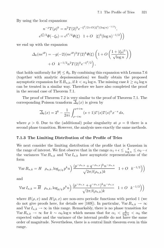
7.1 The Profile of Tries 321
By using the local expansions
n−ρT (ρ)k = n2T (2)ke−ξ2/2+O(|ξ3|(log n)−1/2),
eξ20/2Φ(−ξ0) = eξ
2/2Φ(ξ)(
1 +O(|ξ|3(logn)−1/2
))we end up with the expansion
Δk(neiθ) = −g(−2)(neiθ)2T (2)kΦ(ξ)
(1 +O
(1 + |ξ0|3√
logn
))+O(k−1/2n2T (2)ke−ξ2/2
),
that holds uniformly for |θ| ≤ θ0. By combining this expansion with Lemma 7.6(together with analytic depoissonisation) we finally obtain the proposedasymptotic expansion for EBn,k, if k < α2 logn. The missing case k ≥ α2 logncan be treated in a similar way. Therefore we have also completed the proofin the second case of Theorem 7.1.
The proof of Theorem 7.2 is very similar to the proof of Theorem 7.1. Thecorresponding Poisson transform Δk(x) is given by
Δk(x) = 2k − 1
2πi
∫ ρ+i∞
ρ−i∞(s+ 1)Γ (s)T (s)kx−s ds,
where ρ > 0. Due to the (additional) polar singularity at ρ = 0 there is asecond phase transition. However, the analysis uses exactly the same methods.
7.1.3 The Limiting Distribution of the Profile of Tries
We next consider the limiting distribution of the profile that is Gaussian inthe range of interest. We first observe that in the range α1 + ε ≤ k
log n ≤ α2− εthe variances VarBn,k and Var In,k have asymptotic representations of theform
VarBn,k = H(ρn,k, logp/q p
kn) (p−ρn,k + q−ρn,k )kn−ρn,k√
2πβ(ρn,k)k
(1 +O(k−1/2))
and
Var In,k = H(ρn,k, logp/q p
kn) (p−ρn,k + q−ρn,k)kn−ρn,k√
2πβ(ρn,k)k
(1 +O(k−1/2))
where H(ρ, x) and H(ρ, x) are non-zero periodic functions with period 1 (wedo not give proofs here, for details see [169]). In particular, VarBn,k → ∞and Var In,k →∞ in this range. Remarkably, there is no phase transition forVarBn,k → ∞ for k ∼ α0 logn which means that for α1 <
klog n < α0 the
expected value and the variance of the internal profile do not have the sameorder of magnitude. Nevertheless, there is a central limit theorem even in thisrange.
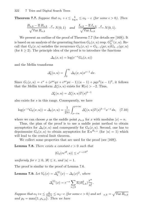
322 7 Tries and Digital Search Trees
Theorem 7.7. Suppose that α1 + ε ≤ klog n ≤ α2 − ε (for some ε > 0). Then
Bn,k − EBn,k√VarBn,k
d−→ N(0, 1) andIn,k − E In,k√
Var In,k
d−→ N(0, 1).
We present an outline of the proof of Theorem 7.7 (for details see [169]). It
is based on an analysis of the generating function Gk(x, u) resp. G[I]k (x, u). Re-
call that Gk(x, u) satisfies the recurrence Gk(x, u) = Gk−1(px, u)Gk−1(qx, u)(for k ≥ 2). The principle idea of the proof is to introduce the functions
Δk(x, u) = log(e−xGk(x, u))
and the Mellin transforms
Δ∗k(s, u) =
∫ ∞0
Δk(x, u)xs−1 dx.
Since G1(x, u) = ex + (epxqx+ eqxpx− 1) (u − 1) + pqx2(u − 1)2, it followsthat the Mellin transform Δ∗1(s, u) exists for �(s) > −2. Thus,
Δ∗k(s, u) = Δ∗1(s, u)T (s)k−1
also exists for s in this range. Consequently, we have
log(e−xGk(x, u)) = Δk(x, u) =1
2πi
∫ ρ+i∞
ρ−i∞Δ∗1(s, u)T (s)k−1x−s ds, (7.10)
where we can choose ρ as the saddle point ρn,k for x with modulus |x| = n.Thus, the plan of the proof is to use a saddle point method to obtain
asymptotics for Δk(x, u) and consequently for Gk(x, u). Second, one has todepoissonise Gk(x, u) to obtain asymptotics for EuBn,k (for |u| = 1) whichwill lead to the central limit theorem.
We collect some properties that are used for the proof (see [169]).
Lemma 7.8. There exists a constant c > 0 such that
|Gk(reiθ, u)| ≤ er−crθ2
uniformly for r ≥ 0, |θ| ≤ π, and |u| = 1.
The proof is similar to the proof of Lemma 7.6.
Lemma 7.9. Let Vk(x) = Δ(2)k (x)−Δk(x)2, where
Δ(2)k (x) = e−x
∑n≥0
E(B2n,k)
xn
n!.
Suppose that α1+ε ≤ klog n ≤ α2−ε (for some ε > 0) and set σn,k =
√VarBn,k
and ρ0 = max{1, ρn,k}. Then we have
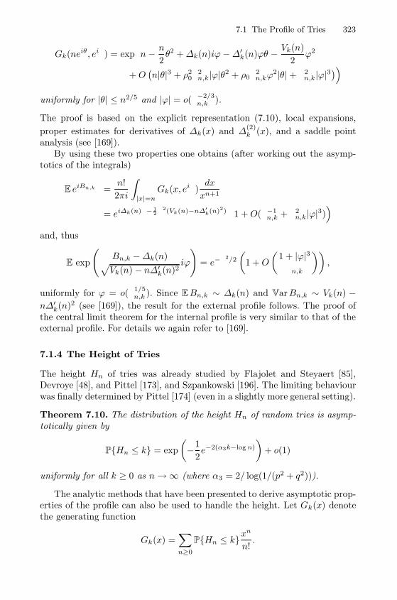
7.1 The Profile of Tries 323
Gk(neiθ, eiϕ) = exp(n− n
2θ2 +Δk(n)iϕ−Δ′k(n)ϕθ − Vk(n)
2ϕ2
+O(n|θ|3 + ρ20σ
2n,k|ϕ|θ2 + ρ0σ
2n,kϕ
2|θ|+ σ2n,k|ϕ|3))
uniformly for |θ| ≤ n2/5 and |ϕ| = o(σ−2/3n,k ).
The proof is based on the explicit representation (7.10), local expansions,
proper estimates for derivatives of Δk(x) and Δ(2)k (x), and a saddle point
analysis (see [169]).By using these two properties one obtains (after working out the asymp-
totics of the integrals)
E eiBn,kϕ =n!
2πi
∫|x|=n
Gk(x, eiϕ)dx
xn+1
= eiΔk(n)ϕ− 12 ϕ2(Vk(n)−nΔ′k(n)2)
(1 +O(σ−1
n,k + σ2n,k|ϕ|3)
)and, thus
E exp
(Bn,k −Δk(n)√Vk(n)− nΔ′k(n)2
iϕ
)= e−ϕ2/2
(1 +O
(1 + |ϕ|3σn,k
)),
uniformly for ϕ = o(σ1/5n,k ). Since EBn,k ∼ Δk(n) and VarBn,k ∼ Vk(n) −
nΔ′k(n)2 (see [169]), the result for the external profile follows. The proof ofthe central limit theorem for the internal profile is very similar to that of theexternal profile. For details we again refer to [169].
7.1.4 The Height of Tries
The height Hn of tries was already studied by Flajolet and Steyaert [85],Devroye [48], and Pittel [173], and Szpankowski [196]. The limiting behaviourwas finally determined by Pittel [174] (even in a slightly more general setting).
Theorem 7.10. The distribution of the height Hn of random tries is asymp-totically given by
P{Hn ≤ k} = exp
(−1
2e−2(α3k−log n)
)+ o(1)
uniformly for all k ≥ 0 as n→∞ (where α3 = 2/ log(1/(p2 + q2))).
The analytic methods that have been presented to derive asymptotic prop-erties of the profile can also be used to handle the height. Let Gk(x) denotethe generating function
Gk(x) =∑n≥0
P{Hn ≤ k}xn
n!.
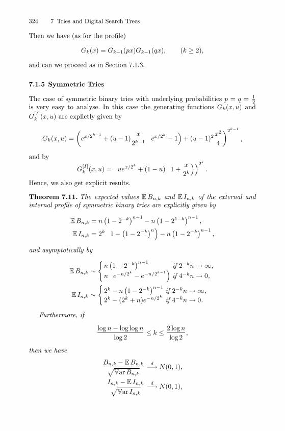
324 7 Tries and Digital Search Trees
Then we have (as for the profile)
Gk(x) = Gk−1(px)Gk−1(qx), (k ≥ 2),
and can we proceed as in Section 7.1.3.
7.1.5 Symmetric Tries
The case of symmetric binary tries with underlying probabilities p = q = 12
is very easy to analyse. In this case the generating functions Gk(x, u) and
G[I]k (x, u) are explictly given by
Gk(x, u) =
(ex/2k−1
+ (u− 1)x
2k−1
(ex/2k − 1
)+ (u − 1)2
x2
4
)2k−1
,
and by
G[I]k (x, u) =
(uex/2k
+ (1 − u)(
1 +x
2k
))2k
.
Hence, we also get explicit results.
Theorem 7.11. The expected values EBn,k and E In,k of the external andinternal profile of symmetric binary tries are explicitly given by
EBn,k = n(1− 2−k
)n−1 − n(1− 21−k
)n−1,
E In,k = 2k(
1−(1− 2−k
)n)− n (1− 2−k)n−1
,
and asymptotically by
EBn,k ∼{n(1− 2−k
)n−1if 2−kn→∞,
n(e−n/2k − e−n/2k−1
)if 4−kn→ 0,
E In,k ∼{
2k − n(1− 2−k
)n−1if 2−kn→∞,
2k − (2k + n)e−n/2k
if 4−kn→ 0.
Furthermore, if
logn− log logn
log 2≤ k ≤ 2 logn
log 2,
then we have
Bn,k − EBn,k√VarBn,k
d−→ N(0, 1),
In,k − E In,k√Var In,k
d−→ N(0, 1),
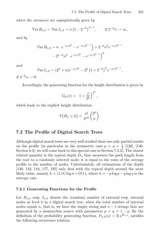
7.2 The Profile of Digital Search Trees 325
where the variances are asymptotically given by
VarBn,k ∼ Var In,k ∼ n(1− 2−k
)n−1, if 2−kn→∞,
and by
VarBn,k ∼ n(e−n/2k − e−n/2k−1
)+ 2−kn2e−n/2k−1
− 21−kn2(e−n/2k − e−n/2k−1
)2and
Var In,k ∼ (2k + n)e−n/2k − 2k(1 + 2−k
)2e−n/2k−1
,
if 4−kn→ 0.
Accordingly, the generating function for the height distribution is given by
Gk(x) =(
1 +x
2k
)2k
,
which leads to the explicit height distribution
P{Hn ≤ k} =n!
2nk
(2k
n
).
7.2 The Profile of Digital Search Trees
Although digital search trees are very well studied there are only partial resultson the profile (in particular in the symmetric case p = q = 1
2 [126], [130,Section 6.3]; we will come back to this special case in Section 7.2.3). The closestrelated quantity is the typical depth Dn that measures the path length fromthe root to a randomly selected node; it is equal to the ratio of the averageprofile to the number of nodes. Unfortunately, all estimations of the depth[130, 142, 144, 177, 195] only deal with the typical depth around the mostlikely value, namely k = (1/h) logn+O(1), where h = −p log p− q log q is theentropy rate.
7.2.1 Generating Functions for the Profile
Let Bn,k resp. In,k denote the (random) number of external resp. internalnodes at level k in a digital search tree, when the total number of internalnodes equals n, that is, we have the empty string and n − 1 strings that aregenerated by a memoryless source with parameters p > q = 1 − p. By thedefinition of the probability generating function, Pn,k(u) = EuBn,k , satisfiesthe following recurrence relation
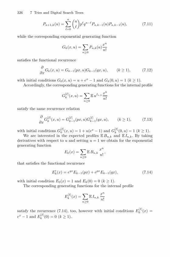
326 7 Tries and Digital Search Trees
Pn+1,k(u) =n∑
�=0
(n
�
)p�qn−�Pn,k−1(u)Pn,k−1(u), (7.11)
while the corresponding exponential generating function
Gk(x, u) =∑n≥0
Pn,k(u)xn
n!
satisfies the functional recurrence
∂
∂xGk(x, u) = Gk−1(px, u)Gk−1(qx, u), (k ≥ 1), (7.12)
with initial conditions G0(x, u) = u+ ex − 1 and Gk(0, u) = 1 (k ≥ 1).Accordingly, the corresponding generating functions for the internal profile
G[I]k (x, u) =
∑n≥0
EuIn,kxn
n!
satisfy the same recurrence relation
∂
∂xG
[I]k (x, u) = G
[I]k−1(px, u)G
[I]k−1(qx, u), (k ≥ 1), (7.13)
with initial conditions G[I]0 (x, u) = 1 + u(ex − 1) and G
[I]k (0, u) = 1 (k ≥ 1).
We are interested in the expected profiles EBn,k and E In,k. By takingderivatives with respect to u and setting u = 1 we obtain for the exponentialgenerating function
Ek(x) =∑n≥0
EBn,kxn
n!,
that satisfies the functional recurrence
E′k(x) = eqxEk−1(px) + epxEk−1(qx), (7.14)
with initial condition E0(x) = 1 and Ek(0) = 0 (k ≥ 1).The corresponding generating functions for the internal profile
E[I]k (x) =
∑n≥0
E In,kxn
n!
satisfy the recurrence (7.14), too, however with initial conditions E[I]0 (x) =
ex − 1 and E[I]k (0) = 0 (k ≥ 1).
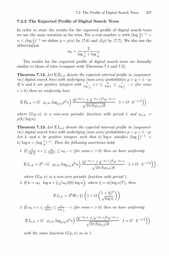
7.2 The Profile of Digital Search Trees 327
7.2.2 The Expected Profile of Digital Search Trees
In order to state the results for the expected profile of digital search treeswe use the same notation as for tries. For a real number α with (log 1
p )−1 <
α < (log 1q )−1 we define ρ = ρ(α) by (7.6) and β(ρ) by (7.7). We also use the
abbreviation
α0 =2
log 1p + log 1
q
.
The results for the expected profile of digital search trees are formallysimilar to those of tries (compare with Theorems 7.1 and 7.2).
Theorem 7.12. Let EBn,k denote the expected external profile in (asymmet-ric) digital search trees with underlying (non-zero) probabilities p > q = 1−p.If n and k are positive integers with 1
log 1p
+ ε ≤ klog n ≤ 1
log 1q
− ε (for some
ε > 0) then we uniformly have
EBn,k = G(ρn,k, logp/q p
kn) (p−ρn,k + q−ρn,k )kn−ρn,k√
2πβ(ρn,k)k
(1 +O(k−1/2)),
where G(ρ, x) is a non-zero periodic function with period 1 and ρn,k =ρ(k/ logn).
Theorem 7.13. Let E In,k denote the expected internal profile in (asymmet-ric) digital search trees with underlying (non-zero) probabilities p > q = 1−p.Let k and n be positive integers such that k/ logn satisfies (log 1
p )−1 <
k/ logn < (log 1q )−1. Then the following assertions hold:
1. If 1log 1
p
+ ε ≤ klog n ≤ α0 − ε (for some ε > 0) then we have uniformly
E In,k = 2k−G(ρn,k, logp/q p
kn) (p−ρn,k + q−ρn,k)kn−ρn,k√
2πβ(ρn,k)k
(1 +O(k−1/2)),
where G(ρ, x) is a non-zero periodic function with period 1.
2. If k = α0
(logn+ ξ
√α0β(0) logn
), where ξ = o((log n)
16 ), then
E In,k = 2kΦ(−ξ)(
1 +O
(1 + |ξ|3√
logn
)).
3. If α0 + ε ≤ klog n ≤ 1
log 1q
− ε (for some ε > 0) then we have uniformly
E In,k = G(ρn,k, logp/q p
kn) (p−ρn,k + q−ρn,k)kn−ρn,k√
2πβ(ρn,k)k
(1 +O(k−1/2))
with the same function G(ρ, x) as in 1.
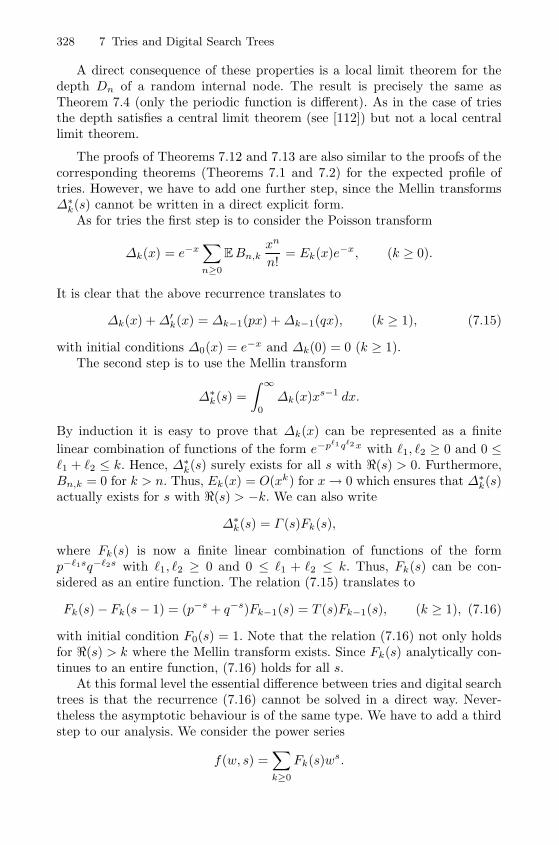
328 7 Tries and Digital Search Trees
A direct consequence of these properties is a local limit theorem for thedepth Dn of a random internal node. The result is precisely the same asTheorem 7.4 (only the periodic function is different). As in the case of triesthe depth satisfies a central limit theorem (see [112]) but not a local centrallimit theorem.
The proofs of Theorems 7.12 and 7.13 are also similar to the proofs of thecorresponding theorems (Theorems 7.1 and 7.2) for the expected profile oftries. However, we have to add one further step, since the Mellin transformsΔ∗k(s) cannot be written in a direct explicit form.
As for tries the first step is to consider the Poisson transform
Δk(x) = e−x∑n≥0
EBn,kxn
n!= Ek(x)e−x, (k ≥ 0).
It is clear that the above recurrence translates to
Δk(x) +Δ′k(x) = Δk−1(px) +Δk−1(qx), (k ≥ 1), (7.15)
with initial conditions Δ0(x) = e−x and Δk(0) = 0 (k ≥ 1).The second step is to use the Mellin transform
Δ∗k(s) =
∫ ∞0
Δk(x)xs−1 dx.
By induction it is easy to prove that Δk(x) can be represented as a finite
linear combination of functions of the form e−p�1q�2x with �1, �2 ≥ 0 and 0 ≤�1 + �2 ≤ k. Hence, Δ∗k(s) surely exists for all s with �(s) > 0. Furthermore,Bn,k = 0 for k > n. Thus, Ek(x) = O(xk) for x→ 0 which ensures that Δ∗k(s)actually exists for s with �(s) > −k. We can also write
Δ∗k(s) = Γ (s)Fk(s),
where Fk(s) is now a finite linear combination of functions of the formp−�1sq−�2s with �1, �2 ≥ 0 and 0 ≤ �1 + �2 ≤ k. Thus, Fk(s) can be con-sidered as an entire function. The relation (7.15) translates to
Fk(s)− Fk(s− 1) = (p−s + q−s)Fk−1(s) = T (s)Fk−1(s), (k ≥ 1), (7.16)
with initial condition F0(s) = 1. Note that the relation (7.16) not only holdsfor �(s) > k where the Mellin transform exists. Since Fk(s) analytically con-tinues to an entire function, (7.16) holds for all s.
At this formal level the essential difference between tries and digital searchtrees is that the recurrence (7.16) cannot be solved in a direct way. Never-theless the asymptotic behaviour is of the same type. We have to add a thirdstep to our analysis. We consider the power series
f(w, s) =∑k≥0
Fk(s)ws.
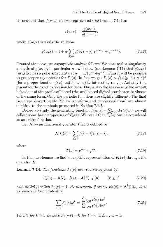
7.2 The Profile of Digital Search Trees 329
It turns out that f(w, s) can we represented (see Lemma 7.14) as
f(w, s) =g(w, s)
g(w,−1),
where g(w, s) satisfies the relation
g(w, s) = 1 + w∑j≥0
g(w, s− j)(p−s+j + q−s+j). (7.17)
Granted the above, an asymptotic analysis follows. We start with a singularityanalysis of g(w, s), in particular we will show (see Lemma 7.17) that g(w, s)(usually) has a polar singularity at w = 1/(p−s +q−s). Thus it will be possibleto get proper asymptotics for Fk(s). In fact we get Fk(s) ∼ f(s)(p−s + q−s)k
(for a proper function f(x) and for s in the interesting range). Actually thisresembles the exact expression for tries. This is also the reason why the overallbehaviour of the profile of biased tries and biased digital search trees is almostof the same form. Only the periodic functions are slightly different. The finaltwo steps (inverting the Mellin transform and depoissonisation) are almostidentical to the methods presented in Section 7.1.2.
Before we study the generating function f(w, s) =∑
k≥0 Fk(s)wk, we willcollect some basic properties of Fk(s). We recall that Fk(s) can be consideredas an entire function.
Let A be an functional operator that is defined by
A[f ](s) =∑j≥0
f(s− j)T (s− j), (7.18)
whereT (s) = p−s + q−s. (7.19)
In the next lemma we find an explicit representation of Fk(x) through theoperator A.
Lemma 7.14. The functions Fk(s) are recursively given by
Fk(s) = A[Fk−1](s)−A[Fk−1](0) (k ≥ 1) (7.20)
with initial function F0(s) = 1. Furthermore, if we set Rk(s) = Ak[1](s) thenwe have the formal identity
∑k≥0
Fk(s)wk =
∑�≥0R�(s)w
�∑�≥0R�(0)w�
. (7.21)
Finally for k ≥ 1 we have Fk(−�) = 0 for � = 0, 1, 2, . . . , k − 1.
330 7 Tries and Digital Search Trees
Proof. Set Fk(s) = 1 and recursively
Fk(s) = A[Fk−1](s)−A[Fk−1](0) (k ≥ 1).
It is easy to see that Fk(s) is a well defined entire function. In particular itfollows that Fk(s) is (as it is for Fk(s)) a finite linear combination of a functionof the form p−�1sq−�2s with �1, �2 ≥ 0 and �1 + �2 ≤ k. Further (by definition)these functions satisfy Fk(0) = 0 (for k ≥ 1) and fulfil the relation
Fk(s)− Fk(s− 1) = T (s)Fk−1(s)
for k ≥ 0 and all s.Now we can proceed by induction to show that Fk(s) = Fk(s). By def-
inition we have F0(s) = F0(s). Now suppose that Fk(s) = Fk(s) holds forsome k ≥ 0. Then with the help of the above considerations it follows thatFk+1(s) = Fk+1(s) +G(s), where G(s) satisfies
G(0) = 0 and G(s)−G(s− 1) = 0, (�(s) > −k). (7.22)
By the above observations G(s) has to be a finite linear combination of func-tions of the form p−�1sq−�2s. However, the only periodic function of this formthat meets conditions (7.22) is the zero function. Hence, Fk+1(s) = Fk+1(s).
Now we prove (7.21). First, (7.21) is equivalent to
k∑�=0
F�(s)Rk−�(0) = Rk(s), (k ≥ 0),
or to
Fk(s) = Rk(s)−k−1∑�=0
F�(s)Rk−�(0), (k ≥ 0).
We will prove this relation by induction. Of course, it is satisfied for k = 0.Now suppose that is holds for some k ≥ 0. Then from (7.20) we find
Fk+1(s) = A[Fk](s)−A[Fk](0)
= A[Rk](s)−A[Rk](0)
−k−1∑�=0
(A[F�](s)−A[F�](0))Rk−�(0)
= Rk+1(s)−Rk+1(0)−k−1∑�=0
F�+1(s)Rk−�(0)
= Rk+1(s)−k∑
�=0
F�(s)Rk+1−�(0).
This completes the induction proof.Finally, since Fk(s) = −Δ∗k(s)/Γ (s) is analytic for s with �(s) > −k and
1/Γ (−�) = 0, it also follows that Fk(−�) = 0 for � = 0, 1, . . . , k − 1.
7.2 The Profile of Digital Search Trees 331
Remark 7.15 The proof of (7.20) (and consequently that of (7.21)) makesuse of the fact that Fk(0) = 0 for k ≥ 1. However, we also have Fk(−r) = 0for k > r. In particular, if we set s = −r in (7.21) we get
r∑k=0
Fk(−r)wk =
∑�≥0Rk(−r)wk∑�≥0Rk(0)wk
,
and consequently
∑k≥0
Fk(s)wk =
∑�≥0Rk(s)wk∑
�≥0Rk(−r)wk
r∑k=0
Fk(−r)wr . (7.23)
Our next goal is to study the function g(w, s) =∑
�≥0R�(s)w�, where we
now consider w as a complex variable, too. Note that g(w, s) satisfies the (atthe moment formal) identity
g(w, s) = 1 + wA[g(w, ·)](s) = 1 +∑j≥0
g(w, s− j)T (s− j). (7.24)
In the next lemma we establish a crucial property of g(w, s).
Lemma 7.16. There exists a function h(w, s) that is analytic for all w ands with
wT (s−m) = 1 for all m ≥ 1
such that
g(w, s) =h(w, s)
1− wT (s). (7.25)
Thus, g(w, s) has a meromorphic continuation where w0 = 1/T (s) is a polarsingularity.
Proof. We recall that Rk(s) = Ak[1](s). In particular, the first few functionsRk(s) are given by
R0(s) = 1,
R1(s) =p−s
1− p +q−s
1− q ,
R2(s) =p−2s
(1− p)(1− p2)+
p−sq−s
(1− p)(1 − pq)
+p−sq−s
(1− q)(1− pq) +q−2s
(1− q)(1 − q2).
With the help of (7.18) we can derive corresponding representations for generalk. Hence, by using the assumption p > q it follows that
|Rk(s)| ≤ 1∏j≥1(1 − pj)
(p−�(s) + q−�(s))k.
332 7 Tries and Digital Search Trees
Thus, if |w| < T (�(s))−1 then the series
g(w, s) =∑�≥0
R�(s)w� =
⎛⎝∑�≥0
w�A�
⎞⎠ [1](s) (7.26)
converges absolutely and represents an analytic function. We can rewrite(7.26) to
g(w, s) = (I− wA)−1[1](s),
or to
(I− wA)[g(w, ·)](s) = g(w, s)− w∑j≥0
g(w, s− j)T (s− j) = 1, (7.27)
which is the same as (7.24).If we substitute g(w, s) in (7.27) by
g(w, s) =h(w, s)
1− wT (s),
we get a relation for h(w, s) of the form
h(w, s) = 1 +∑j≥1
h(w, s− j) wT (s− j)1− wT (s− j) . (7.28)
Recall that we already know that h(w, s) exists for |w| < T (�(s))−1. Wewill now use (7.28) to show that h(w, s) can be analytically continued to therange |w| < T (�(s)− 1)−1 (and even to the range where wT (s−m) = 1) sothat we also get a meromorphic continuation as proposed.
For this purpose we introduce another operator B by
B[f ](s) =∑j≥1
f(w, s− j) wT (s− j)1− wT (s− j) . (7.29)
For convenience set U(w, s) = wT (s)/(1 − wT (s)). By induction it followsthat
Bk[1](s) =∑i1≥1
∑i2≥1
· · ·∑ik≥1
U(w, s− i1)U(w, s− i1 − i2)
· · ·U(w, s− i1 − i2 − · · · − ik)
=∑
mk≥k
mk−1∑mk−1=k−1
mk−1−1∑mk−2=k−2
· · ·m2−1∑m1=1
U(w, s−m1)U(w, s−m2) · · ·U(w, s−mk).
7.2 The Profile of Digital Search Trees 333
Hence, we get the upper bound
|Bk[1](s)| ≤∑
mk≥k
∑mk−1≥k−1
· · ·
∑m1≥1
|U(w, s−m1)U(w, s−m2) · · ·U(w, s−mk)|
=∑
m1≥1
|U(w, s−m1)| ·∑
m2≥2
|U(w, s−m2)|
· · ·∑
mk≥k
|U(w, s−mk)|.
By using the fact that T (s−m) = O(qm) it follows directly that the series
S :=∑m≥1
|U(w, s−m)| =∑m≥1
|wT (s−m)||1− wT (s−m)|
converges if wT (s −m) = 1 for all m ≥ 1. Thus for any choice of w and sthere are only finitely many exceptional points where wT (s−m) = 1. Let k0
be any value with ∑m≥k0
|U(w, s−m)| ≤ 1
2.
Then we have for all k ≥ k0
|Bk[1](s)| ≤ Sk02−(k−k0) = (2S)k02−k.
Hence, we can set
h(w, s) =∑k≥0
Bk[1](s), (7.30)
which obviously satisfies (7.28). Furthermore, we have the upper bound|h(w, s)| ≤ 2(2S)k0 .
Finally, we are in the position to derive an asymptotic representation forFk(s).
Lemma 7.17. For every real interval [a, b] there exist k0, η > 0 and ε > 0such that
Fk(s) = f(s)T (s)k(1 +O(e−ηk)))
(7.31)
uniformly for all s with �(s) ∈ [a, b], |�(s)−2�π log(q/p)| ≤ ε for some integer� and k ≥ k0, where f(s) is an analytic function that satisfies f(−r) = 0 forr = 0, 1, 2, . . ..
Furthermore, if |�(s)−2�π log(q/p)| > ε for for all integers � then we have
Fk(s) = O(T (σ)k e−ηk)
)(7.32)
uniformly for �(s) ∈ [a, b].
334 7 Tries and Digital Search Trees
Proof. Suppose first that s is a real number with −r − 1 < s < −r for someinteger r ≥ 0. Here we use the representation
f(w, s) =
r+1∑k=0
Fk(−r − 1)wk g(w, s)
g(−r − 1, w)
=
r+1∑k=0
Fk(−r − 1)wk h(w, s)
h(−r − 1, w)
1− wT (−r − 1)
1− wT (s).
By Lemma 7.16 there exists η > 0 such that h(w, s) is analytic for |w| ≤eη/T (s). Since T (−r− 1) < T (s), it also follows that h(w,−r − 1) is analyticin that region. Furthermore, since h(w,−r−1) is non-zero for positive realw <1/T (−r− 2) (compare with (7.30)), we obtain that the radius of convergenceof the series
∑k≥0 Fk(s)wk equals w0 = 1/T (s).
With the help of this observation we can also deduce that the functionf(w, s) has no other singularities on the circle |w| = 1/T (s). Suppose that
h(w,−r − 1) has a zero w1 with |w1| < 1/T (s). If∑r+1
k=0 Fk(−r − 1)wk1 =
0 then w1 has to be a zero of h(w, s), too: h(w1, s) = 0. However, if weslightly decrease s then certainly h(w1, s − η) = 0. In this case the functionf(w, s) would be singular for w = w1 although its radius of convergence is1/T (s − η) > 1/T (s) > |w1|. This is, of course, a contradiction and, thus,∑r+1
k=0 Fk(−r − 1)wk1 = 0 too. Actually, it also follows that the order of the
zeros are the same. Furthermore, by a slight variation of the above argument,we also deduce that f(w, s) has no singularities on the circle |w| = 1/T (s)other than w0 = 1/T (s), as proposed.
Hence, by using a contour integration on the circle |w| = eη/T (s) and theresidue theorem it follows that
Fk(s) = f(s)T (s)k +O(|T (s)e−η|k
),
where
f(s) =r+1∑k=0
Fk(−r − 1)T (s)−k h(1/T (s)), s
h(1/T (s),−r− 1)
(1− T (−r − 1)
T (s)
).
These estimates are uniform for s ∈ [a, b], where −r − 1 < a < b < r.Furthermore, we get the same result if s is sufficiently close to the real axis.Thus, if a ≤ �(s) ≤ b and |�(s)| ≤ ε for some sufficiently small ε > 0 then weobtain (7.31), too.
Next, suppose that s is real (or sufficiently close to the real axis) and closeto an integer −r ≤ 0, say −r− η ≤ s ≤ −r+ η (for some η > 0). Here we usethe representation
∑k≥0
Fk(s)wk =
r∑k=0
Fk(−r)wk g(w, s)
g(w,−r)
7.2 The Profile of Digital Search Trees 335
=r∑
k=0
Fk(−r)wk h(w, s)
h(w,−r)1− wT (−r)1− wT (s)
=
r∑k=0
Fk(−r)wk h(w, s) − h(w,−r)h(w,−r)
1− wT (−r)1− wT (s)
+
r∑k=0
Fk(−r)wk +
r−1∑k=0
Fk(−r)wk+1 T (s)− T (−r)1− wT (s)
.
Now if we subtract the finite sum∑r
k=0 Fk(−r) then we can safely multiplyby Γ (s) (that is singular at s = −r) and obtain a function of the form
r∑k=0
Fk(−r)wk Γ (s)(h(w, s) − h(w,−r))h(w,−r)
1− wT (−r)1− wT (s)
+r−1∑k=0
Fk(−r)wk+1 Γ (s)(T (s)− T (−r))1− wT (s)
,
which we can handle in the same way as above. Actually, we proved (7.31) fork ≥ r with f(−r) = 0.
Finally, if �(s) is positive (and �(s) sufficiently close to 2�π/ log(q/p) forsome integer �) then we can also use∑
k≥0
Fk(s)wk =h(w, s)
h(0, w)
1− wT (0)
1− wT (s)
and obtain the proposed result. (Note that h(w, 0) is analytic for |w| <1/T (0).)
Next suppose that s = σ + it, where t is not necessarily small. Then
T (s) = eit log p(p−σ + q−σeit log(q/p)
).
Consequently |T (s)| = T (ρ), if and only if t = 2jπ/ log(q/p) = tj for someinteger j. Hence, if |t − 2jπ/ log(q/p)| ≤ ε for some integer j we can do thesame contour integration as above and again get (7.31).
Finally, if |t−2jπ/ log(q/p)| > ε for all integers j then we trivially estimateFk(s) by
|Fk(s)| ≤ ρ−k · max|w|=ρ
|g(w, s)|,
where ρ is chosen in a way that g(w, s) is analytic for |w| ≤ ρ. Since there isη > 0 with
|T (s−m)| = |p−σ+m + eit log(q/p)q−σ+m| ≤ e−2ηT (σ −m),
it follows that h(w, s) exists for |w| ≤ eη/T (σ). Hence, we can actually setρ = eη/T (σ) and obtain (7.32). In order to complete the proof, note thatΔ∗k(s) = −Γ (s)Fk(s) exists for �(s) > −k and that Fk(−r) = 0 for r =0, 1, 2, . . . and k ≥ r. Thus, f(−r) = 0, too.
336 7 Tries and Digital Search Trees
Putting these observations together it follows that we can represent Δ∗k(s)as
Δ∗k(s) = Γ (s)f(s)T (s)k(1 +O(e−ηk)
)if |�(s) − tj | ≤ ε for some integer j, where Γ (s)f(s) is an entire function.Furthermore, we have proper upper bounds in the remaining range. Thus, weare precisely in the same situation as in the proof of Theorem 7.1. With thehelp of the Mellin inversion formula (with the line of integration �(s) = ρn,k)and by approximating the integral by infinitely many saddle point integralsaround tj we obtain
Δk(neiθ) =T (ρ)k√2πβ(ρ)k
∑|j|≤j0
f(ρ+ itj)Γ (ρ+ itj)(neiθ)−ρ−itjp−iktj
×(
1 +O(k−1/2))
(7.33)
uniformly for |θ| ≤ θ0 (for some 0 < θ0 < π/2).It remains to have an a priori upper bound for Δk(neiθ) that is valid for
all |θ| ≤ π. Here we cannot use Lemma 7.6, since the recurrence relation isdifferent. However, it can be shown that for every real ρ there exists a constantC = C(ρ) and an integer k0 = k0(ρ) such that
|exΔk(x)| ≤ C(1− cθ2)−krmax{−ρ,0}T (ρ)ker(1−cθ2) (7.34)
for k ≥ k0 and uniformly for all r ≥ 0 and |θ| ≤ π, where x = reiθ. Weindicate a proof for ρ ≤ 0. Obviously there exists k0 and C such that (7.34)holds for k = k0. Then by definition we have recursively (for k ≥ k0)
|exΔk+1(x)| =
∣∣∣∣∫ x
0
eξ (Δk(pξ) +Δk(qξ)) dξ
∣∣∣∣=
∣∣∣∣∫ r
0
eteiθ (Δk(pteiθ) +Δk(qteiθ)
)dt
∣∣∣∣≤ C(1− cθ2)−k T (ρ)k
×∫ r
0
(eqt cos θ(pt)−ρept(1−cθ2) + ept cos θ(qt)−ρeqt(1−cθ2)
)dt
≤ C(1− cθ2)−kT (ρ)k+1
∫ r
0
t−ρet(1−cθ2) dt
≤ C(1− cθ2)−k−1T (ρ)k+1 r−ρer(1−cθ2).
A similar proof works for ρ ≥ 0.Finally by combining (7.33) and (7.34) with another Cauchy integration
one obtains
EBn,k =n!
2πi
∫|x|=n
exΔk(x)dx
xn+1∼ Δk(n)
in the range of interest which also completes the proof of Theorem 7.12.
7.2 The Profile of Digital Search Trees 337
For the internal profile In,k we use the Poisson transform
Δk(x) = e−x∑n≥0
E In,kxn
n!
that satisfies
Δk(x) +Δ′k(x) = Δk−1(px) +Δk−1(qx), (k ≥ 1), (7.35)
with initial conditions Δ0(x) = 1 − e−x. The Mellin transforms Δ∗k(s) exist
for −k − 1 < �(s) < 0 and can be represented as
Δ∗k(s) = −Γ (s)F k(s),
where F 0(s) = 1 and
F k(s)− F k(s− 1) = T (s)F k−1(s), (k ≥ 1).
The corresponding explicit recurrence is
F k(s) = A[F k−1](s)−A[F k−1](−1), (k ≥ 1),
and we have ∑k≥0
F k(s)wk =
∑�≥0R�(s)w
�∑�≥0R�(−1)w�
and F k(−�) = 0 for � = 1, 2, . . . , k. As above it follows that (for |�(s)− tj| ≤ εfor some integer j)
F k(s) = f(s)T (s)k(1 +O(e−ηk)
),
where f(−r) = 0 for r = 1, 2, . . .. Thus,
Δ∗k(s) = −Γ (s)f(s)T (s)k
(1 +O(e−ηk)
)has a polar singularity at s = 0 which induces the phase transition at thelevel k = α0 logn. More precisely, if k < α0 logn one has to shift the line ofintegration �(s) = ρ (−k − 1 < ρ < 0), where the Mellin transform exists,to �(s) = ρn,k > 0 so that the residue 2k (at ρ = 0) has to be taken intoaccount. In principle one can proceed as in the case of tries.
7.2.3 Symmetric Digital Search Trees
The symmetric case p = q = 12 is different, since log 1
p and log 1q coincide. Of
course, the corresponding generating functions have as simpler structure. Wehave
∂
∂xGk(x, u) = Gk−1
(x2, u)2, (k ≥ 1),
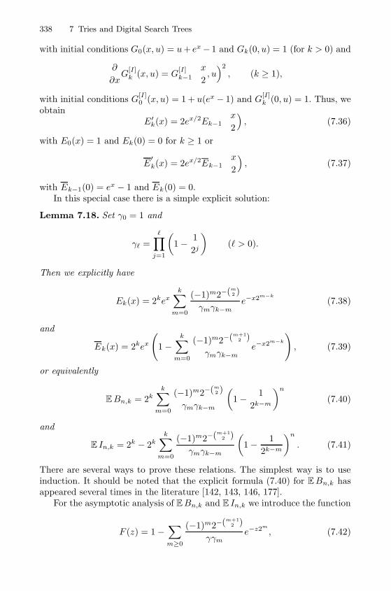
338 7 Tries and Digital Search Trees
with initial conditions G0(x, u) = u+ ex− 1 and Gk(0, u) = 1 (for k > 0) and
∂
∂xG
[I]k (x, u) = G
[I]k−1
(x2, u)2, (k ≥ 1),
with initial conditions G[I]0 (x, u) = 1 + u(ex − 1) and G
[I]k (0, u) = 1. Thus, we
obtainE′k(x) = 2ex/2Ek−1
(x2
), (7.36)
with E0(x) = 1 and Ek(0) = 0 for k ≥ 1 or
E′k(x) = 2ex/2Ek−1
(x2
), (7.37)
with Ek−1(0) = ex − 1 and Ek(0) = 0.In this special case there is a simple explicit solution:
Lemma 7.18. Set γ0 = 1 and
γ� =
�∏j=1
(1− 1
2j
)(� > 0).
Then we explicitly have
Ek(x) = 2kexk∑
m=0
(−1)m2−(m2 )
γmγk−me−x2m−k
(7.38)
and
Ek(x) = 2kex
(1−
k∑m=0
(−1)m2−(m+12 )
γmγk−me−x2m−k
), (7.39)
or equivalently
EBn,k = 2kk∑
m=0
(−1)m2−(m2 )
γmγk−m
(1− 1
2k−m
)n
(7.40)
and
E In,k = 2k − 2kk∑
m=0
(−1)m2−(m+12 )
γmγk−m
(1− 1
2k−m
)n
. (7.41)
There are several ways to prove these relations. The simplest way is to useinduction. It should be noted that the explicit formula (7.40) for EBn,k hasappeared several times in the literature [142, 143, 146, 177].
For the asymptotic analysis of EBn,k and E In,k we introduce the function
F (z) = 1−∑m≥0
(−1)m2−(m+12 )
γγme−z2m
, (7.42)
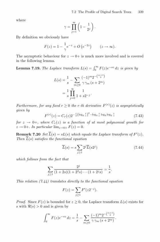
7.2 The Profile of Digital Search Trees 339
where
γ =
∞∏j=1
(1− 1
2j
).
By definition we obviously have
F (z) = 1− 1
γe−z +O
(e−2z)
(z →∞).
The asymptotic behaviour for z → 0+ is much more involved and is coveredin the following lemma.
Lemma 7.19. The Laplace transform L(s) =∫∞0F (z)e−sz dz is given by
L(s) =1
s−∑m≥0
(−1)m2−(m+12 )
γ γm (s+ 2m)
=1
s
∞∏j=0
1
1 + s2−j.
Furthermore, for any fixed r ≥ 0 the r-th derivative F (r)(z) is asymptoticallygiven by
F (r)(z) = Cr(z)2−12 (log2
1z )
2−log21z log2 log2
1z (7.43)
for z → 0+, where Cr(z) is a function of at most polynomial growth forz → 0+. In particular limz→0+ F (z) = 0.
Remark 7.20 Set L(s) = sL(s) which equals the Laplace transform of F ′(z).Then L(s) satisfies the functional equation
L(s) = s∑j≥1
2jL(s2j) (7.44)
which follows from the fact that∑j≥1
2j
(1 + 2s)(1 + 22s) · · · (1 + 2js)=
1
s.
This relation (7.44) translates directly to the functional equation
F (z) =∑j≥1
F ′(z2−j).
Proof. Since F (z) is bounded for z ≥ 0, the Laplace transform L(s) exists fors with �(s) > 0 and is given by∫ ∞
0
F (z)e−sz dz =1
s−∑m≥0
(−1)m2−(m+12 )
γ γm (s+ 2m).
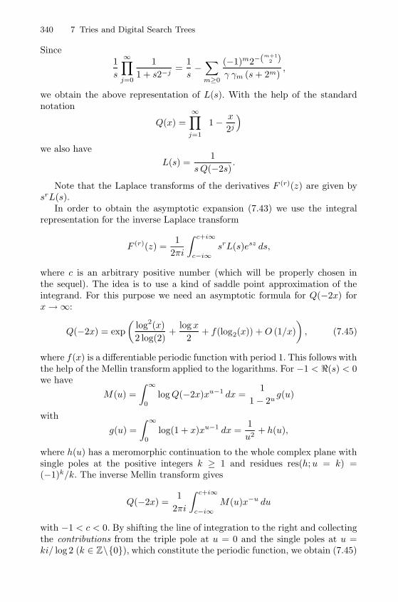
340 7 Tries and Digital Search Trees
Since1
s
∞∏j=0
1
1 + s2−j=
1
s−∑m≥0
(−1)m2−(m+12 )
γ γm (s+ 2m),
we obtain the above representation of L(s). With the help of the standardnotation
Q(x) =
∞∏j=1
(1− x
2j
)we also have
L(s) =1
sQ(−2s).
Note that the Laplace transforms of the derivatives F (r)(z) are given bysrL(s).
In order to obtain the asymptotic expansion (7.43) we use the integralrepresentation for the inverse Laplace transform
F (r)(z) =1
2πi
∫ c+i∞
c−i∞srL(s)esz ds,
where c is an arbitrary positive number (which will be properly chosen inthe sequel). The idea is to use a kind of saddle point approximation of theintegrand. For this purpose we need an asymptotic formula for Q(−2x) forx→∞:
Q(−2x) = exp
(log2(x)
2 log(2)+
log x
2+ f(log2(x)) +O (1/x)
), (7.45)
where f(x) is a differentiable periodic function with period 1. This follows withthe help of the Mellin transform applied to the logarithms. For −1 < �(s) < 0we have
M(u) =
∫ ∞0
logQ(−2x)xu−1 dx =1
1− 2ug(u)
with
g(u) =
∫ ∞0
log(1 + x)xu−1 dx =1
u2+ h(u),
where h(u) has a meromorphic continuation to the whole complex plane withsingle poles at the positive integers k ≥ 1 and residues res(h;u = k) =(−1)k/k. The inverse Mellin transform gives
Q(−2x) =1
2πi
∫ c+i∞
c−i∞M(u)x−u du
with −1 < c < 0. By shifting the line of integration to the right and collectingthe contributions from the triple pole at u = 0 and the single poles at u =ki/ log 2 (k ∈ Z\{0}), which constitute the periodic function, we obtain (7.45)
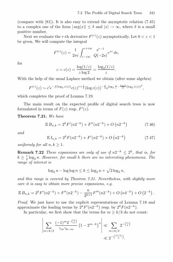
7.2 The Profile of Digital Search Trees 341
(compare with [81]). It is also easy to extend the asymptotic relation (7.45)to a complex one of the form | arg(x)| ≤ δ and |x| → ∞, where δ is a smallpositive number.
Next we evaluate the r-th derivative F (r)(z) asymptotically. Let 0 < z < 1be given. We will compute the integral
F (r)(z) =1
2πi
∫ c+i∞
c−i∞
sr−1
Q(−2s)esz ds,
for
c = c(z) =log(1/z)
z log 2=
log2(1/z)
z.
With the help of the usual Laplace method we obtain (after some algebra)
F (r)(z) ∼ c′e−f(log2 c(z))c(z)r+ 12 (log c(z))−
32 elog2
1z−
log 22 (log2 c(z))2 ,
which completes the proof of Lemma 7.19.
The main result on the expected profile of digital search trees is nowformulated in terms of F (z) resp. F ′(z).
Theorem 7.21. We have
EBn,k = 2kF ′(n2−k) + F ′′(n2−k) +O(n2−k)
(7.46)
andE In,k = 2kF (n2−k) + F ′(n2−k) +O
(n2−k)
(7.47)
uniformly for all n, k ≥ 1.
Remark 7.22 These expansions are only of use if n2−k ≤ 2k, that is, fork ≥ 1
2 log2 n. However, for small k there are no interesting phenomena. Therange of interest is
log2 n− log log n ≤ k ≤ log2 n+√
2 log2 n,
and this range is covered by Theorem 7.21. Nevertheless, with slightly morecare it is easy to obtain more precise expansions, e.g.
EBn,k = 2kF ′(n2−k) + F ′′(n2−k)− n
2k+1F ′′′(n2−k) +O
(n4−k)
+O(2−k).
Proof. We just have to use the explicit representations of Lemma 7.18 andapproximate the leading terms by 2kF ′(n2−k) resp. by 2kF (n2−k).
In particular, we first show that the terms for m ≥ k/3 do not count:∣∣∣∣∣∣∑
m>k/3
(−1)m2−(m2 )
γmγk−m
(1− 2m−k
)n∣∣∣∣∣∣�∑
m>k/3
2−(m2 )
� 2−(�k/3�2 ).
342 7 Tries and Digital Search Trees
In a next step we use the approximation (for m ≤ k/3)(1− 2m−k
)n= e−n2m−k
(1 +O( n
4k−m
))= e−n2m−k
+O( n
4k−m
),
and obtain an error term of the form
∑m≤k/3
(−1)m2−(m2 )
γmγk−m·O( n
4k−m
)= O( n
4k
).
Finally, we approximate the ratio
γ
γm= 1− 1
2k−m+ O
(1
4k−m
)and get an even smaller error of order O
(4−k).
Summing up we get
EBn,k = 2kk∑
m=0
(−1)m2−(m2 )
γmγk−m
(1− 2m−k
)n= 2k∑
m≤k/3
(−1)m2−(m2 )
γγm
(1− 1
2k−m
)e−n2m−k
+O(
2k n
4k
)+O(
2k2−(�k/3�2 ))
2k∞∑
m=0
(−1)m2−(m2 )
γγm
(1− 2m
2k
)e−n2m−k
+O( n
2k
)= 2kF ′(n2−k) + F ′′(n2−k) +O
(n2−k).
This completes the proof of (7.46). The proof of (7.47) is exactly the same.
8
Recursive Algorithms and the Contraction
Method
Recursive Algorithms follow the Divide-and-Conquer-Principle. The idea be-hind this principle is to break a problem into two or several subproblemswhich are easier to solve (heuristically because they are just smaller prob-lems) and then to construct the solution of the original problem by combiningthe solutions of the subproblems appropriately. If this idea is iteratively (orrecursively) applied then one speaks of a recursive algorithm and, moreover,these kinds of algorithms give rise to a (hidden) tree structure.
The most prominent example in this context is the widely used sortingalgorithm Quicksort which was invented by C. A. R. Hoare [100, 101]. It isthe standard sorting procedure in Unix systems, and the basic idea can bedescribed easily:
A list of n real numbers A = (x1, x2, . . . , xn) is given. Select a pivotelement xj from this list. Divide the remaining numbers into setsA≤, A> of numbers smaller (or equal) and larger than xj . Next applythe same procedure to each of these two sets if they contain morethan one element. Finally, we end up with a sorted list of the originalnumbers.
This sorting procedure can be encoded with a binary tree with n (internal)nodes. The first selected element xj is put to the root, whereas recursivelyA≤ produces a left subtree of xj and A> the right subtree of xj . (An emptystring produces an empty tree which is usually encoded as an external node.)
For example, if one always uses the first element of the list as the pivotelement then the tree structure behind Quicksort is precisely the binary searchtree associated to the same input data (see Figure 8.1 and compare withSection 6.1.2). In particular, the number of comparisons needed for Quicksortequals the internal path length of the corresponding binary search tree, andthe maximum number of recursive calls equals the height of the tree. Theanalysis of Quicksort is therefore – despite of a reformulation – the same asthe analysis of binary search trees.
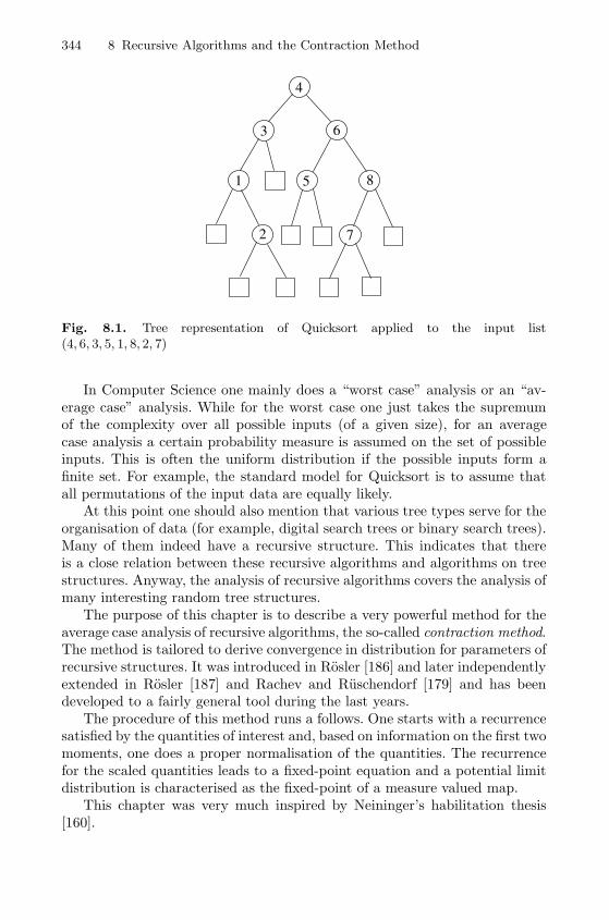
344 8 Recursive Algorithms and the Contraction Method
1
2
3
4
5
6
7
8
Fig. 8.1. Tree representation of Quicksort applied to the input list(4, 6, 3, 5, 1, 8, 2, 7)
In Computer Science one mainly does a “worst case” analysis or an “av-erage case” analysis. While for the worst case one just takes the supremumof the complexity over all possible inputs (of a given size), for an averagecase analysis a certain probability measure is assumed on the set of possibleinputs. This is often the uniform distribution if the possible inputs form afinite set. For example, the standard model for Quicksort is to assume thatall permutations of the input data are equally likely.
At this point one should also mention that various tree types serve for theorganisation of data (for example, digital search trees or binary search trees).Many of them indeed have a recursive structure. This indicates that thereis a close relation between these recursive algorithms and algorithms on treestructures. Anyway, the analysis of recursive algorithms covers the analysis ofmany interesting random tree structures.
The purpose of this chapter is to describe a very powerful method for theaverage case analysis of recursive algorithms, the so-called contraction method.The method is tailored to derive convergence in distribution for parameters ofrecursive structures. It was introduced in Rosler [186] and later independentlyextended in Rosler [187] and Rachev and Ruschendorf [179] and has beendeveloped to a fairly general tool during the last years.
The procedure of this method runs a follows. One starts with a recurrencesatisfied by the quantities of interest and, based on information on the first twomoments, one does a proper normalisation of the quantities. The recurrencefor the scaled quantities leads to a fixed-point equation and a potential limitdistribution is characterised as the fixed-point of a measure valued map.
This chapter was very much inspired by Neininger’s habilitation thesis[160].
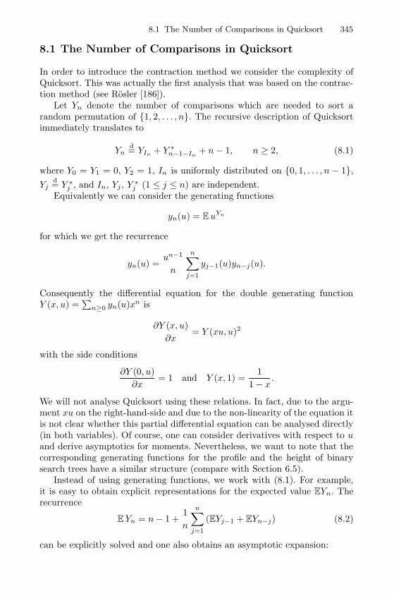
8.1 The Number of Comparisons in Quicksort 345
8.1 The Number of Comparisons in Quicksort
In order to introduce the contraction method we consider the complexity ofQuicksort. This was actually the first analysis that was based on the contrac-tion method (see Rosler [186]).
Let Yn denote the number of comparisons which are needed to sort arandom permutation of {1, 2, . . . , n}. The recursive description of Quicksortimmediately translates to
Ynd= YIn + Y ∗n−1−In
+ n− 1, n ≥ 2, (8.1)
where Y0 = Y1 = 0, Y2 = 1, In is uniformly distributed on {0, 1, . . . , n − 1},Yj
d= Y ∗j , and In, Yj , Y ∗j (1 ≤ j ≤ n) are independent.Equivalently we can consider the generating functions
yn(u) = EuYn
for which we get the recurrence
yn(u) =un−1
n
n∑j=1
yj−1(u)yn−j(u).
Consequently the differential equation for the double generating functionY (x, u) =
∑n≥0 yn(u)xn is
∂Y (x, u)
∂x= Y (xu, u)2
with the side conditions
∂Y (0, u)
∂x= 1 and Y (x, 1) =
1
1− x.
We will not analyse Quicksort using these relations. In fact, due to the argu-ment xu on the right-hand-side and due to the non-linearity of the equation itis not clear whether this partial differential equation can be analysed directly(in both variables). Of course, one can consider derivatives with respect to uand derive asymptotics for moments. Nevertheless, we want to note that thecorresponding generating functions for the profile and the height of binarysearch trees have a similar structure (compare with Section 6.5).
Instead of using generating functions, we work with (8.1). For example,it is easy to obtain explicit representations for the expected value EYn. Therecurrence
EYn = n− 1 +1
n
n∑j=1
(EYj−1 + EYn−j) (8.2)
can be explicitly solved and one also obtains an asymptotic expansion:
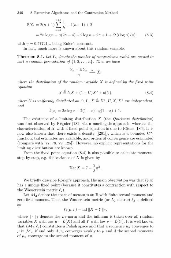
346 8 Recursive Algorithms and the Contraction Method
EYn = 2(n+ 1)
n+1∑h=1
1
h− 4(n+ 1) + 2
= 2n logn+ n(2γ − 4) + 2 logn+ 2γ + 1 +O ((logn)/n) (8.3)
with γ = 0.57721... being Euler’s constant.In fact, much more is known about this random variable.
Theorem 8.1. Let Yn denote the number of comparisons which are needed tosort a random permutation of {1, 2, . . . , n}. Then we have
Yn − EYn
n
d−→ X,
where the distribution of the random variable X is defined by the fixed pointequation
Xd= UX + (1 − U)X∗ + b(U), (8.4)
where U is uniformly distributed on [0, 1], Xd= X∗, U,X,X∗ are independent,
andb(x) = 2x log x+ 2(1− x) log(1− x) + 1.
The existence of a limiting distribution X (the Quicksort distribution)was first observed by Regnier [182] via a martingale approach, whereas thecharacterisation of X with a fixed point equation is due to Rosler [186]. It isnow also known that there exists a density ([201]), which is a bounded C∞
function; tail estimates are available, and orders of convergence are estimated(compare with [77, 78, 79, 125]). However, no explicit representations for thelimiting distribution are known.
From the fixed point equation (8.4) it also possible to calculate momentsstep by step, e.g. the variance of X is given by
VarX = 7− 2
3π2.
We briefly describe Rosler’s approach. His main observation was that (8.4)has a unique fixed point (because it constitutes a contraction with respect tothe Wasserstein metric �2).
Let M2 denote the space of measures on R with finite second moment andzero first moment. Then the Wasserstein metric (or L2 metric) �2 is definedas
�2(μ, ν) = inf ‖X − Y ‖2,where ‖ · ‖2 denotes the L2-norm and the infimum is taken over all randomvariables X with law μ = L(X) and all Y with law ν = L(Y ). It is well knownthat (M2, �2) constitutes a Polish space and that a sequence μn converges toμ in M2, if and only if μn converges weakly to μ and if the second momentsof μn converge to the second moment of μ.
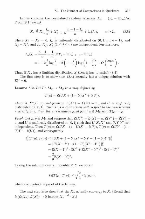
8.1 The Number of Comparisons in Quicksort 347
Let us consider the normalised random variables Xn = (Yn − EYn)/n.From (8.1) we get
Xnd= XIn
Inn
+X∗n−1−In
n− 1− Inn
+ bn(In), n ≥ 2, (8.5)
where X0 = X1 = 0, In is uniformly distributed on {0, 1, . . . , n − 1}, andXj = X∗j , and In, Xj, X∗j (1 ≤ j ≤ n) are independent. Furthermore,
bn(j) =n− 1
n+
1
n(EYj + EYn−1−j − EYn)
= 1 + 2j
nlog
j
n+ 2
(1− j
n
)log
(1− j
n
)+O
(logn
n
).
Thus, if Xn has a limiting distribution X then it has to satisfy (8.4).The first step is to show that (8.4) actually has a unique solution with
EY = 0.
Lemma 8.2. Let T : M2 →M2 be a map defined by
T (μ) = L(UX + (1− U)X∗ + b(U)),
where X,X∗, U are independent, L(X∗) = L(X) = μ, and U is uniformlydistributed on [0, 1]. Then T is a contraction with respect to the Wassersteinmetric �2 and, thus, there is a unique fixed point μ ∈M2 with T (μ) = μ.
Proof. Let μ, ν ∈ M2 and suppose that L(X∗) = L(X) = μ, L(Y ∗) = L(Y ) =ν, and U is uniformly distributed on [0, 1] such that U,X,X∗ and U, Y, Y ∗ areindependent. Then T (μ) = L(UX + (1−U)X∗ + b(U)), T (ν) = L(UY + (1−U)Y ∗ + b(U)), and consequently
�22(T (μ), T (ν)) ≤ ‖UX + (1− U)X∗ − UY − (1− U)Y ∗‖22= ‖U(X − Y ) + (1− U)(X∗ − Y ∗)‖22= E(X − Y )2 · EU2 + E(X∗ − Y ∗)2 · E(1 − U)2
=2
3E(X − Y )2.
Taking the infimum over all possible X,Y we obtain
�2(T (μ), T (ν)) ≤√
2
3· �2(μ, ν),
which completes the proof of the lemma.
The next step is to show that the Xn actually converge to X . (Recall that
�2(L(Xn),L(X)) → 0 implies Xnd−→ X .)
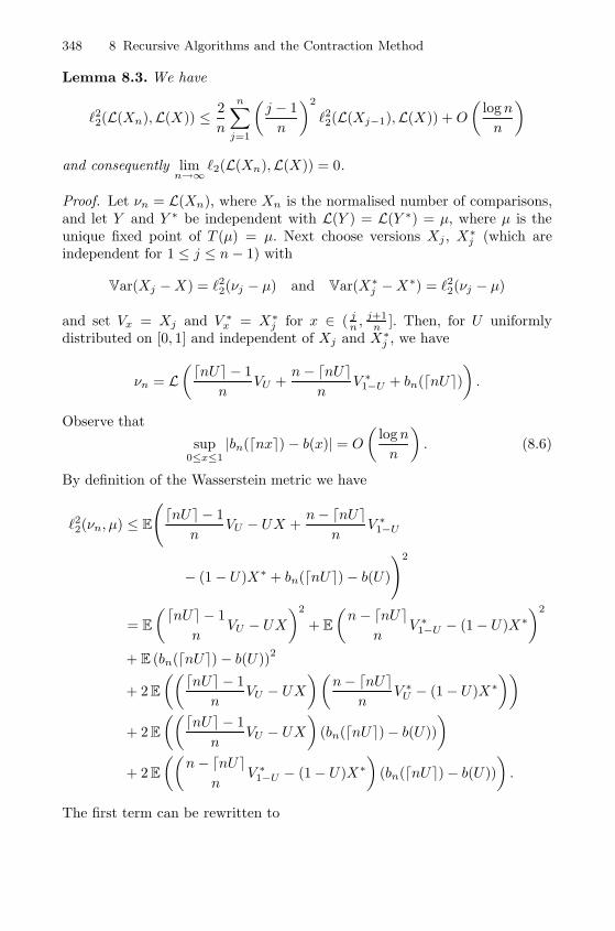
348 8 Recursive Algorithms and the Contraction Method
Lemma 8.3. We have
�22(L(Xn),L(X)) ≤ 2
n
n∑j=1
(j − 1
n
)2
�22(L(Xj−1),L(X)) + O
(logn
n
)
and consequently limn→∞
�2(L(Xn),L(X)) = 0.
Proof. Let νn = L(Xn), where Xn is the normalised number of comparisons,and let Y and Y ∗ be independent with L(Y ) = L(Y ∗) = μ, where μ is theunique fixed point of T (μ) = μ. Next choose versions Xj , X∗j (which areindependent for 1 ≤ j ≤ n− 1) with
Var(Xj −X) = �22(νj − μ) and Var(X∗j −X∗) = �22(νj − μ)
and set Vx = Xj and V ∗x = X∗j for x ∈ ( jn ,
j+1n ]. Then, for U uniformly
distributed on [0, 1] and independent of Xj and X∗j , we have
νn = L(�nU� − 1
nVU +
n− �nU�n
V ∗1−U + bn(�nU�)).
Observe that
sup0≤x≤1
|bn(�nx�) − b(x)| = O
(logn
n
). (8.6)
By definition of the Wasserstein metric we have
�22(νn, μ) ≤ E
(�nU� − 1
nVU − UX +
n− �nU�n
V ∗1−U
− (1− U)X∗ + bn(�nU�)− b(U)
)2
= E
(�nU� − 1
nVU − UX
)2
+ E
(n− �nU�
nV ∗1−U − (1− U)X∗
)2
+ E (bn(�nU�)− b(U))2
+ 2 E
((�nU� − 1
nVU − UX
)(n− �nU�
nV ∗U − (1− U)X∗
))+ 2 E
((�nU� − 1
nVU − UX
)(bn(�nU�)− b(U))
)+ 2 E
((n− �nU�
nV ∗1−U − (1− U)X∗
)(bn(�nU�)− b(U))
).
The first term can be rewritten to
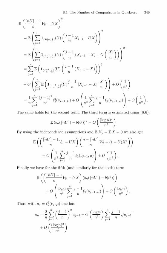
8.1 The Number of Comparisons in Quicksort 349
E
(�nU� − 1
nVU − UX
)2
= E
⎛⎝ n∑j=1
1( j−1n , j
n ](U)
(j − 1
nXj−1 − UX
)⎞⎠2
= E
⎛⎝ n∑j=1
1( j−1n , j
n ](U)
(j − 1
n(Xj−1 −X) +O
( |X |n
))⎞⎠2
=
n∑j=1
E
(1( j−1
n , jn ](U)
(j − 1
n(Xj−1 −X)
))2
+O
⎛⎝ n∑j=1
E
(1( j−1
n , jn ](U)
j − 1
n|Xj−1 −X |
|X |n
)⎞⎠+O
(1
n2
)
=1
n
n∑j=1
(j − 1)2
n2�22(νj−1, μ) +O
⎛⎝ 1
n2
n∑j=1
j − 1
n�2(νj−1, μ)
⎞⎠+O
(1
n2
).
The same holds for the second term. The third term is estimated using (8.6):
E (bn(�nU�)− b(U))2
= O
((logn)2
n2
)By using the independence assumptions and EXj = EX = 0 we also get
E
((�nU� − 1
nVU − UX
)(n− �nU�
nV ∗U − (1− U)X∗
))
= O
⎛⎝ 1
n2
n∑j=1
j − 1
n�2(νj−1, μ)
⎞⎠+O
(1
n2
).
Finally we have for the fifth (and similarly for the sixth) term
E
((�nU� − 1
nVU − UX
)(bn(�nU�)− b(U))
)
= O
⎛⎝ logn
n2
n∑j=1
j − 1
n�2(νj−1, μ)
⎞⎠+O
(logn
n2
).
Thus, with aj = �22(νj , μ) one has
an =2
n
n∑j=1
(j − 1
n
)2
aj−1 +O
(logn
n2
) n∑j=1
j − 1
n
√aj−1
+O
((logn)2
n2
)
350 8 Recursive Algorithms and the Contraction Method
and thus
an ≤2
3max
0≤j≤n−1aj + C1
logn
nmax
0≤j≤n−1
√aj + C2
log2 n
n2.
for some positive constants C1, C2. It is now easy to show that an → 0. Firstit follows that an ≤ A, where A satisfies a1 ≤ A and the inequality
A ≤ 2
3A+ C1
logn
n
√A+ C2
log2 n
n2
for all n ≥ 2. Consequently we also have
an ≤2
3max
0≤j≤n−1aj + C3
logn
n
for a proper constant C3 which shows that an → 0, as proposed.
8.2 The L2 Setting of the Contraction Method
The method that has been discussed in Section 8.1 can be generalised inseveral ways. For this purpose we specify a class of recursive sequences ofdistributions that can be analysed by using L2 techniques. In order to be abit more general we develop the theory for random vectors in Rd.
8.2.1 A General Type of Recurrence
We consider a sequence of random, d-dimensional vectors (Yn)n≥0 which sat-isfy the recurrence
Ynd=
K∑r=1
Ar(n)Y(r)
I(n)r
+ bn, (n ≥ n0), (8.7)
where (A1(n), . . . , AK(n), bn, I(n)), (Y
(1)n ), . . . , (Y
(K)n ) are independent, A1(n),
. . . , AK(n) are random d × d matrices, bn is a random d-dimensional vector,
I(n) is a vector of random integers I(n)r ∈ {0, . . . , n}, and (Y
(1)n ), . . . , (Y
(K)n )
are identical distributed as (Yn). We have n0 ≥ 1 and Y0, . . . , Yn0−1 are giveninitialising random vectors. The number K ≥ 1 is deterministic.
We rescale the random vector Yn in (8.7) by
Xn = C−1/2n (Yn −Mn) (n ≥ 0), (8.8)
where Mn ∈ Rd and Cn is a symmetric, positive-definite d× d matrix. If thefirst two moments of Yn are finite thenMn and Cn are typically of the order ofthe expectation and the covariance matrix of Yn respectively. From recurrence(8.7) we obtain for Xn the modified recurrence
8.2 The L2 Setting of the Contraction Method 351
Xnd=
K∑r=1
A(n)r X
(r)
I(n)r
+ b(n), n ≥ n0, (8.9)
with
A(n)r = C−1/2
n Ar(n)C1/2
I(n)r
, (8.10)
b(n) = C−1/2n
(bn −Mn +
K∑r=1
Ar(n)MI(n)r
), (8.11)
and independence properties as in (8.7).
The contraction method aims to provide assertions of the following type:
Suppose that we (Xn) is characterised by (8.9). Then appropriateconvergence of the coefficients
A(n)r
d−→ A∗r , b(n) d−→ b∗, (n→∞) (8.12)
implies convergence in distribution of the quantities (Xn) to a limit X .The limit distribution L(X) is characterised by a fixed-point equation,which is obtained from the modified recurrence by formally lettingn→∞:
Xd=
K∑r=1
A∗rX(r) + b∗. (8.13)
Here, (A∗1, . . . , A∗K , b
∗), X(1), . . . , X(K) are independent and X(r) d= X
for r = 1, . . . ,K.
To reformulate the fixed-point property, we denote by Md the space of allprobability measures on Rd and by T the measure valued map
T : Md →Md, μ �→ L(
K∑r=1
A∗rZ(r) + b∗
), (8.14)
where (A∗1, . . . , A∗K , b
∗), Z(1), . . . , Z(K) are independent and L(Z(r)) = μ forr = 1, . . . ,K. Then, X is a solution of the fixed-point equation (8.13), if andonly if its distribution L(X) is a fixed-point of the map T .
Remark 8.4 Maps of type (8.14) do not often have unique fixed-points in thespace of all probability distributions, and the characterisation of the set of allfixed-points is – up to a few special cases – an open and important problem(see Section 8.3).
In order to have a more precise study we define the following subsets ofMd:
352 8 Recursive Algorithms and the Contraction Method
Mds = {μ ∈Md : ‖μ‖s <∞}, s > 0, (8.15)
Mds(M) = {μ ∈Md
s : Eμ = M}, s ≥ 1, (8.16)
Mds(M,C) = {μ ∈Md
s(M) : Cov(μ) = C}, s ≥ 2, (8.17)
where M ∈ Rd and C is a symmetric, positive-definite d × d matrix, andwhere ‖μ‖s, Eμ and Cov(μ) denote the s-th absolute moment, expectationand covariance matrix, respectively, of a random variable with distribution μ.
The core of the method is to endow an appropriate subset M∗ ⊂Md, e.g.,on one of the sets in (8.15)–(8.17), with a complete metric δ such that therestriction of T toM∗ is a contraction on the metric space (M∗, δ) in the senseof Banach’s fixed-point theorem. This implies the existence of a fixed-pointL(X) of T , being unique inM∗. In a second step one shows convergence of therescaled quantities L(Xn) to L(X) in the metric δ, δ(L(Xn),L(X)) → 0 forn → ∞, based on an appropriate convergence of the coefficients as in (8.12).If δ is chosen such that convergence in δ implies weak convergence then thedesired convergence in distribution follows.
8.2.2 A General L2 Convergence Theorem
One crucial point is to choose a proper metric for which one can show thatthe mapping T is a contraction. A natural choice is the minimal Lp metric �p(for some p > 0) that is defined by
�p(μ, ν) := inf {‖X − Y ‖p : L(X) = μ, L(Y ) = ν} , μ, ν ∈ Mdp,
where ‖X‖p := (E ‖X‖p)min{(1/p),1} denotes the Lp norm of a random vectorX and ‖X‖ denotes its Euclidean norm. The Wasserstein metric �2 is a specialbut important case.
Furthermore, the spaces (Mdp, �p) for p > 0 as well as (Md
p(M), �p) for
M ∈ Rd, p ≥ 1 are complete metric spaces and convergence in �p is equiva-lent to weak convergence plus convergence of the p-th absolute moment. Forμ, ν ∈ Md
p there always exist vectors X , Y on a joint probability space withL(X) = μ, L(Y ) = ν and �p(μ, ν) = ‖X − Y ‖p. Such vectors are called opti-mal couplings of μ and ν. For these and further properties of the minimal Lp
metric �p see Dall’Aglio [43], Major [148], Bickel and Freedman [16], Rachev[178], and Rachev and Ruschendorf [180].
In order to obtain contraction properties of the map (8.14) we denote by
‖A‖op = sup‖x‖=1
‖Ax‖
the operator norm of a square matrix A, by AT the transpose of the matrixA, and by
lip(T ) = infμ,ν∈M∗, μ�=ν
�p(T (μ), T (ν))
�p(μ, ν)
the Lipschitz constant of T if it is finite. Actually, in the case p = 2 theLipschitz constant can be estimated easily.
8.2 The L2 Setting of the Contraction Method 353
Lemma 8.5. Let (A∗1, . . . , A∗K , b
∗) be an L2-integrable vector of random d× dmatrices A∗1 . . . , A
∗K and a random d-dimensional vector b∗ with Eb∗ = 0 and
assume that T is as in (8.14). Then the restriction of T to Md2(0) is Lipschitz
continuous in �2, and for the Lipschitz constant lip(T ) we have
lip(T ) ≤∥∥∥∥∥E(
K∑r=1
(A∗r)TA∗r
)∥∥∥∥∥1/2
op
. (8.18)
Proof. Clearly, if μ ∈ Md2(0), then T (μ) has a finite second moment and
ET (μ) = 0. We just have to apply the independence conditions and the as-sumption E b = 0. Thus, T : Md
2(0) →Md2(0) is a well-defined map. Let μ, ν ∈
Md2(0) be given and (W (1), Z(1)), . . . , (W (K), Z(K)) be optimal couplings of
(μ, ν) for r = 1, . . . ,K so that (A1, . . . , Ak, b), (W (1), Z(1)), . . . , (W (K), Z(K))are independent. Then
�22(T (μ), T (ν)) ≤ E
⎛⎝∥∥∥∥∥K∑
r=1
Ar(W (r) − Z(r))
∥∥∥∥∥2⎞⎠
= E
(K∑
r=1
(Ar(W (r) − Z(r))
)T·(Ar(W (r) − Z(r))
))
+ E
⎛⎝ ∑1≤r �=s≤K
(Ar(W (r) − Z(r))
)T·(As(W (r) − Z(r))
)⎞⎠= E
(K∑
r=1
(W (r) − Z(r)
)T·(AT
r Ar(W (r) − Z(r))))
= E
(K∑
r=1
(W (r) − Z(r)
)T·(
E(ATr Ar)(W (r) − Z(r))
))
= E
((W (1) − Z(1)
)T·((
K∑r=1
E(ATr Ar)
)(W (1) − Z(1))
))
≤∥∥∥∥∥
K∑r=1
E(ATr Ar)
∥∥∥∥∥op
E
(∥∥∥W (1) − Z(1)∥∥∥2)
=
∥∥∥∥∥K∑
r=1
E(ATr Ar)
∥∥∥∥∥op
�22(μ, ν).
Note that we have used the independence of W (r) − Z(r) and W (s) − Z(s)
for r = s together with the fact that E(W (r) − Z(r)) = 0. The additionalexpectation E(AT
r Ar) is also justified by independence.
354 8 Recursive Algorithms and the Contraction Method
The second step of the contraction method is to show convergence in �2for sequences (L(Xn)) of the form (8.9). The following Theorem providessufficient conditions (see [187, Theorem 3.1] and [158, Theorem 4.1]).
Theorem 8.6. Assume (Xn) is a sequence of centred d-dimensional, L2-integrable random vectors, satisfying the recurrence (8.9) with L2-integrable
random d× d matrices A(n)r , 1 ≤ r ≤ K, a random L2-integrable centred vec-
tor b(n), and a vector of random integers I(n) = (I(n)1 , . . . , I
(n)K ) with values in
I(n)r ∈ {0, 1, . . . , n}. Assume that we have(
A(n)1 , . . . , A
(n)K , b(n)
)L2−→ (A∗1, . . . , A
∗K , b
∗) (n→∞), (8.19)
E
(K∑
r=1
∥∥(A∗r)TA∗r∥∥
op
)< 1, (8.20)
E
(1{I(n)
r ≤�}
∥∥∥(A(n)r )TA(n)
r
∥∥∥op
)→ 0, (n→∞), (8.21)
for all integers � ≥ 0 and r = 1, . . . ,K. Then we have
�2(L(Xn),L(X)) → 0 (n→∞),
where L(X) is the fixed-point of map T defined in (8.14), which is unique inMd
2(0) .
Before giving the proof we comment on the conditions of Theorem 8.6 andtheir applicability.
Condition (8.19) means that the convergence of the coefficients in (8.12)has to hold in L2. For this reason we are allowed to construct (A∗1, . . . , A
∗K , b
∗)
according to (A(n)1 , . . . , A
(n)K , b(n)) on a joint probability space, i.e., (8.19)
means
�2(L(A(n)1 , . . . , A
(n)K , b(n)),L(A∗1, . . . , A
∗K , b
∗)) → 0. (8.22)
Condition (8.20), by Jensen’s inequality, is stronger than the contractioncondition ∥∥∥∥∥E
(K∑
r=1
(A∗r)TA∗r
)∥∥∥∥∥op
< 1 (8.23)
from Lemma 8.5. Whether condition (8.20) in Theorem 8.6 can be replacedby the weaker condition (8.23) is unknown (compare with the discussion in[163]).
Condition (8.21) is a technical condition, which is usually easy to verifyin application. In Section 8.1 we have not made explicit use of this condition
but have checked the convergence Xnd−→ X directly (see Lemma 8.3).
8.2 The L2 Setting of the Contraction Method 355
For the application of Theorem 8.6 to recursive sequences (Yn) as in (8.7)one has to note, that for the scaling in (8.8) we have to choose Mn = EYn
in order to guarantee the conditions EXn = 0 and Eb(n) = 0. Since, on theother hand b(n) in (8.11) contains the quantities Mn and in (8.19) we needto derive a limit for b(n), this implies that for the application of Theorem8.6 an asymptotic expansion of the mean EYn has to be known. In contrast,the covariance matrix Cov(Yn) can be guessed in its first order asymptoticexpansion such that Theorem 8.6 applies. Since convergence in �2 impliesconvergence of the second moment, Theorem 8.6 then automatically impliesan asymptotic expansion of the covariance matrix Cov(Yn).
Proof. We already observed that Jensen’s inequality (8.20) implies (8.23), thatis, we have a contraction. Namely, by the definition of b(n) we have E b(n) = 0.Thus, the L2-convergence of (b(n)) implies E b∗ = 0. Therefore we can applyLemma 8.5 so that there is a unique distributional fixed-point X of map T in
(8.14). Let X(r)n
d= Xn, X(r) d
= X so that (X(r)n , X(r)) are optimal couplings
of (Xn, X) for all n ∈ N and r = 1, . . . ,K and that (A1, . . . , AK , bn, I(n)),
(X(1)n , X(1)), . . . , (X
(K)n , X(K)) are independent.
In a first step we derive an estimate of �22(Xn, X) in terms of �22(X0, X), . . . ,�22(Xn−1, X). This inequality will be sufficient to deduce that �2(Xn, X) → 0.From (8.9) and (8.14) and from the independence conditions it follows that(for n ≥ n0)
�22(Xn, X) ≤∥∥∥∥∥
K∑r=1
(A(n)
r X(r)
I(n)r
−A∗rX(r))
+ b(n) − b∗∥∥∥∥∥
2
=
K∑r=1
∥∥∥A(n)r X
(r)
I(n)r
−A∗rX(r)∥∥∥2 +∥∥∥b(n) − b∗
∥∥∥2 .By assumption we have
∥∥b(n) − b∗∥∥ d−→ 0, so we only have to take care of the
first term:
K∑r=1
∥∥∥A(n)r X
(r)
I(n)r
−A∗rX(r)∥∥∥2
=K∑
r=1
∥∥∥A(n)r
(X
(r)
I(n)r
−X(r))
+(A(n)
r −A∗r)X(r)∥∥∥2
=
K∑r=1
∥∥∥A(n)r
(X
(r)
I(n)r
−X(r))∥∥∥2 +
K∑r=1
∥∥∥(A(n)r −A∗r
)X(r)∥∥∥2 (8.24)
+ 2
K∑r=1
(A(n)
r
(X
(r)
I(n)r
−X(r)))T
·((A(n)
r −A∗r)X(r)).
By (8.19), independence, and ‖X‖2 < ∞ it follows that, as n → ∞, and forr = 1, . . . ,K,
356 8 Recursive Algorithms and the Contraction Method∥∥∥(A(n)r −A∗r
)X(r)∥∥∥2 d−→ 0.
For the first term in (8.24) we have the estimate∥∥∥A(n)r
(X
(r)
I(n)r
−X(r))∥∥∥2
= E
(X
(r)
I(n)r
−X(r))T·(
(A(n)r )TA(n)
r
(X
(r)
I(n)r
−X(r)))
≤ E
(∥∥∥(A(n)r )TA(n)
r
∥∥∥2op·∥∥∥X(r)
I(n)r
−X(r)∥∥∥) .
Since the operator norm is a Lipschitz continuous map and by the L2 conver-
gence of (A(n)r ), we have E
∥∥∥A(n)r −A∗r
∥∥∥2op→ 0 and consequently
limn→∞
E
∥∥∥(A(n)r )TA(n)
r
∥∥∥2op
= E∥∥(A∗r)TA∗r
∥∥2op
for r = 1, . . . ,K.For the third term in (8.24) we use the estimate
E
(A(n)
r
(X
(r)
I(n)r
−X(r)))T
·((A(n)
r −A∗r)X(r))
≤ E
(∥∥∥A(n)r
(X
(r)
I(n)r
−X(r))∥∥∥ · ∥∥∥(A(n)
r −A∗r)X(r)∥∥∥)
≤∥∥∥A(n)
r
(X
(r)
I(n)r
−X(r))∥∥∥
2·∥∥∥(A(n)
r −A∗r)X(r)∥∥∥
2
= o(∥∥∥A(n)
r
(X
(r)
I(n)r
−X(r))∥∥∥
2
)= o
(∥∥∥A(n)r
(X
(r)
I(n)r
−X(r))∥∥∥2
2
)+ o(1)
= ηr,n
∥∥∥A(n)r
(X
(r)
I(n)r
−X(r))∥∥∥2
2+ o(1),
where ηr,n → 0 as n→∞. Putting things together and by using the notation
Mr,n =∥∥(A∗r)TA∗r
∥∥2op
+ ηr,n
we get
�22(Xn, X) ≤K∑
r=1
E
(Mr,n
∥∥∥X(r)
I(n)r
−X(r)∥∥∥2)+ o(1)
=
K∑r=1
E
(n∑
i=0
1{I(n)r =i}Mr,n
∥∥∥X(r)i −X(r)
∥∥∥2)+ o(1)
=
n∑i=0
(K∑
r=1
E
(1{I(n)
r =i}Mr,n
))�22(Xi, X) + o(1).
8.2 The L2 Setting of the Contraction Method 357
By assumption there exist n0 and ξ < 1 such that
K∑r=1
EMr,n =
K∑r=1
E∥∥(A∗r)TA∗r
∥∥2op
+
K∑r=1
ηr,n ≤ ξ
for n ≥ n0. Thus, with an = �22(Xn, X) and An = maxn0≤j≤n aj we obtainfor n ≥ n0 and some constant R > 0
an ≤ ξAn +R.
Since An is monotone, this also implies An ≤ ξAn +R and consequently
An ≤R
1− ξ = O(1).
Hence, the sequence an is bounded. Set A = supn≥0 an < ∞ and L =lim supn→∞ an. Then for every ε > 0 there exists n1 ≥ n0 with an ≤ L+ ε forn ≥ n1. Now for n ≥ n1 we obtain (as above and by using (8.21))
an ≤K∑
r=1
E
(1{I(n)
r ≤�}
∥∥∥(A(n)r )TA(n)
r
∥∥∥op
+ ηr,n
)A+ ξ(L + ε) + o(1)
and consequentlyL ≤ ξ(L+ ε).
If L > 0, this is a contradiction for 0 < ε < L(1 − ξ)/ξ. Hence, L = 0. Thiscompletes the proof of the theorem.
8.2.3 Applications of the L2 Setting
We apply Theorem 8.6 to some examples from computer science and relatedareas in detail.
Quicksort
We already discussed the number Yn of key comparisons needed by the sortingalgorithm Quicksort when applied to a uniform random permutation of lengthn. The recurrence (8.7) applies here with d = 1, K = 2, A1(n) = A2(n) = 1,
I(n)1 uniformly distributed on {0, . . . , n−1}, I(n)
2 = n−1−I(n)1 and bn = n−1.
Recall that we have to work in the space M2(0), that is, we have to knowsomething of the first moment in order to reduce (8.7) to (8.9). This is providedby (8.3). It then is natural to normalise by the 1/n:
Xn =Yn − EYn
n.
358 8 Recursive Algorithms and the Contraction Method
As we have observed in Section 8.1 this leads to the recurrence (8.5) that isof the form (8.9). The limit equation for X is given by (8.4). Thus, A∗1 = U ,A∗2 = 1 − U and b∗ = 1 + 2U logU + 2(1 − U) log(1 − U). The conditions ofTheorem 8.6 can be checked directly. For example, the Lipschitz constant canbe estimated by
(E‖(A∗1)2‖op + E‖(A∗2)2‖op
)1/2=
(2
∫ 1
0
u2 du
)1/2
=
√2
3.
Thus, everything works precisely as in Section 8.1.We apply the general concept to a slightly different parameter, the number
of key exchanges Kn. Of course, key exchanges are only necessary if the keysare not in the right order. We again get a recurrence of the form (8.7), wherethe parameters d, K, A1(n), A2(n), I(n) are given as for the key comparisons,however bn now depends on I(n) as
P(bn = j | I(n)1 = k) =
(kj
)(n−1−k
j
)(n−1
k
) , 0 ≤ j ≤ k < n,
that is, the probability that there are exactly j exchanges when the rank of thepivot element is k + 1 (compare also with Sedgewick [190, p. 55] and Hwangand Neininger [107, section 6]). We have
EKn =n+ 1
3Hn −
7
9n+
1
18, (n ≥ 2).
The limiting fixed point equation for the normalised random variable (Kn −EKn)/n equals
Xd= UX(1) + (1− U)X(2) + U(1− U) +
1
3U logU +
1
3(1 − U) log(1− U).
Again all conditions are satisfied, the only difference is in the term b∗.
Wiener Index of Random Binary Search Trees
The Wiener index of a connected graph is the sum of the distances betweenall pairs of nodes in the graph, where the distance is the minimal numberof edges connecting the nodes in the graph. The Wiener index has its originin mathematical chemistry but has independently been investigated in graphtheory (see [97, 55]). The Wiener index Wn of a random binary search treedoes not satisfy the recurrence (8.7) with dimension d = 1. However, it canbe covered by (8.7) in dimension d = 2 as follows (see [159]). Suppose thatYn denotes the internal path length (which is precisely the number of keycomparisons in Quicksort). Then we have
8.2 The L2 Setting of the Contraction Method 359
Wnd= W
(1)In
+ (n− In)YIn +W(2)n−1−In
+ (In + 1)Yn−In−1
+ 2I(n)(n− 1− I(n)) + n− 1,
Ynd= Y
(1)In
+ Y(2)n−1−In
+ n− 1.
This means, that we choose d = 2, K = 2, I(n)1 uniformly distributed on
{0, . . . , n− 1}, I(n)2 = n− 1− I(n)
1 as well as
A1(n) =
(1 n− I(n)
1
0 1
), A2(n) =
(1 n− I(n)
2
0 1
),
bn =
(2I
(n)1 I
(n)2 + n− 1n− 1
).
The expectation can be computed by
EWn = 2n2Hn − 6n2 + 8nHn − 10n+ 6Hn
= 2n2 logn+ (2γ − 6)n2 + o(n2). (8.25)
This leads, together with the expansion of the mean of Yn in (8.3), to theapplicability of Theorem 8.6. In particular we use the normalised randomvector
Xn =
(Wn − EWn
n2,Yn − EYn
n
).
The corresponding limit equation (8.13) and (8.14), respectively, are given by
A∗1 =
((1 − U)2 U(1− U)
0 1− U
), A∗2 =
((1− U)2 U(1− U)
0 1− U
),
b∗ =
(6U(1− U) + 2U logU + 2(1− U) log(1− U)
1 + 2U logU + 2(1− U) log(1− U)
),
where U is uniformly distributed in [0, 1].Interestingly, the contraction method can only be applied in this case,
since we have the relation 2γ− 6 = (2γ− 4)− 2 for the constants in the linearresp. in the quadratic terms of (8.3) and (8.25).
Profile of Random Recursive Trees and Binary Search Trees
In Sections 6.3 and 6.5 we have discussed the profiles of recursive trees andbinary search trees and indicated that the contraction method is a proper toolto obtain limiting relations.
Let Xn,k denote the number of nodes of distance k to the root in randomrecursive trees of size n. Then Xn,0 = 1− δn,0 (with Kronecker’s δ) and
360 8 Recursive Algorithms and the Contraction Method
Xn,kd= X
(1)
I(n)1 ,k−1
+X(2)
I(n)2 ,k
, n ≥ 1, 1 ≤ k ≤ n, (8.26)
where I(n)1 is uniformly distributed on {0, . . . , n− 1}, I(n)
2 = n− 1− I(n)1 and
independence properties as in (8.7).Similarly the external profile of random binary search trees satisfies Bn,0 =
δn,0 and
Bn,kd= B
(1)
I(n)1 ,k−1
+B(2)
I(n)2 ,k−1
, n ≥ 1, 1 ≤ k ≤ n, (8.27)
where I(n)1 and I
(n)2 = n− 1− I(n)
1 are as above.The expectations are given by
EXn,k =|sn,k+1|(n− 1)!
∼ (log n)k
k!Γ(
klog n + 1
) (8.28)
and by
EBn,k =2k
n!|sn,k| ∼
(2 logn)k
n k!Γ(
klog n
) (8.29)
where |sn,k| are the (sign-less) Stirling numbers of first kind (see Section 6.1.1).By considering the normalised profiles
Xn,k
EXn,kand
Bn,k
EBn,k(8.30)
and setting k ∼ α logn one observes that the recurrences (8.26) and (8.27),rewritten to the normalised profiles, stabilise to stochastic fixed point equa-tions
X(α)d= αUαX(α)(1) + (1 − U)αX(α)(2)
for recursive trees, respectively to
Y (α)d=α
2Uα−1Y (α)(1) +
α
2(1− U)α−1Y (α)(2)
for binary search trees (see Theorems 6.18 and 6.41 and Section 6.3.3).The first problem is to check whether these fixed point equations have
unique solutions. By using the L2 setting the Lipschitz constant in the recur-sive tree case is given by
lip(T1) ≤ α2 + 1
2α+ 1
and for the binary search tree case by
lip(T2) ≤ α2
4α− 2.
8.3 Limitations of the L2 Setting and Extensions 361
This means that we have contraction for 0 < α < 2 in the recursive tree caseand for 2−
√2 < α < 2 +
√2 in the binary search tree case.
Actually it can be shown that the normalised profiles (8.30) converge toX(α) resp. to Y (α) in these ranges in the L2 sense (compare with [87]). In thissetting it is impossible to do it better. There are, however, solution X(α) for0 < α < e and Y (α) for α− < α < α+ (where α− = 0.373... and α+ = 4.311...are the solution of the equation α log
(2eα
)= 1) but X(α) and Y (α) have finite
second moments only for 0 < α < 2 resp. for 2−√
2 < α < 2 +√
2 (for detailssee [87]).
In order to extend these limit theorems to the maximum ranges 0 < α < eresp. α− < α < α+ one has to use a different setting. For example, by usingthe Zolotarev metric ζs for a suitable s > 1 (see Section 8.3.1) it is possibleto prove convergence of the normalised profiles in the ranges of interest (fordetails see again [87]).
8.3 Limitations of the L2 Setting and Extensions
The L2 setting is relatively easy but has several limitations. For example, itdoes not apply if (for simplicity we just consider the case d = 1)
E
(K∑
r=1
(A∗r)2
)= 1, (8.31)
that is, the contraction condition (8.23) resp. (8.20) is not satisfied. In partic-ular, there are many applications that lead to the limit equation
Xd=
K∑r=1
A∗rX(r), (8.32)
with
K∑r=1
(A∗r)2 = 1. (8.33)
From the convolution property of the normal distribution it follows that nor-mally distributed random variables with lawN(0, σ2) are solutions of the limitequation (8.32) under (8.33). Thus, it seems, that one cannot prove a centrallimit theorem even if there is one. Since the limit equation has no unique fixedpoint, there is definitely no metric for which T is a contraction.
Another principal problem of the contraction method is the occurrence ofdegenerate limit equations. For example, if we rescale a recurrence of the form
Ynd= YIn + bn, (n ≥ n0), (8.34)
362 8 Recursive Algorithms and the Contraction Method
we might end up with the degenerate limit equation
Xd= X. (8.35)
This limit equation does not give any information about a potential limit dis-tribution and the concept of the contraction method needs to be significantlyextended to deal with such cases.
8.3.1 The Zolotarev Metric
In order to overcome the problem of limit equations with no unique solutionone has to choose a proper subspace. For example, if we work with Md
s(M,C)instead of Md
s(M) then the (co-)variance is fixed, and equation (8.32) under(8.33) will have a unique limit. Furthermore one has to use another metricthat makes T a contraction on that subspace.
Actually, this program was realised by Neininger and Ruschendorf [161].They used the Zolotarev metric ζs (introduced by Zolotarev [209]) which isdefined for random vectors X , Y in Rd by
ζs(X,Y ) = supf∈Fs
|E[f(X)− f(Y )]| (8.36)
where s = m+ α with 0 < α ≤ 1, m ∈ N0, and
Fs := {f ∈ Cm(Rd,R) : ‖f (m)(x)− f (m)(y)‖ ≤ ‖x− y‖α},
denotes the space of m times continuously differentiable functions from Rd
to R such that the m-th derivative is Holder continuous of order α. We usethe short notation ζs(L(X),L(Y )) = ζs(X,Y ). We have ζs(X,Y ) < ∞, ifall mixed moments of orders 1, . . . ,m of X and Y are equal and if the s-th absolute moments of X and Y are finite. Furthermore, (Md
s , ζs) for 0 <s ≤ 1, (Md
s(M), ζs) for 1 < s ≤ 2 and (Mds(M,C), ζs) for 2 < s ≤ 3 are
complete metric spaces with M ∈ Rd, and C being a symmetric, positivedefinite d× d matrix. Furthermore, the Lipschitz constant of the mapping Tcan be estimated by
lip(T ) ≤ E
(K∑
r=1
‖A∗r‖sop
).
For example, if (8.33) is satisfied then T : M1s(0, 1) →M1
s(0, 1) is a contrac-tion for all 2 < s ≤ 3.
There is a direct extension of Theorem 8.6 to the Zolotarev setting withmany applications to statistics of recursive algorithms and related subjects(see [161, 162]) also leading to central limit theorems under very general con-ditions. It is even possible to work in a suitable Banach space setting (see[68]).
8.3 Limitations of the L2 Setting and Extensions 363
8.3.2 Degenerate Limit Equations
Degenerate limit equations Xd= X do not give any information on the nature
of the potential limiting distribution. Nevertheless, in a quite general class ofproblems (see [162]) it is possible to prove a central limit theorem. The idea isto keep track of the recurrence and to show that an accompanying sequence ofnormal distributions is close to Xn. It applies to equations of the form (8.34)under some regularity conditions on In and under the assumption that thevariance of Yn is of logarithmic order.

9
Planar Graphs
At first sight planar graphs and trees have nothing in common despite thetrivial fact that trees are planar. Nevertheless there are strong similarities inthe combinatorial and asymptotic analysis of trees and planar graphs. Pla-nar graphs contain several (hidden) tree or tree-like structures. The tree-decomposition into cut-vertices and blocks (2-connected components) is themost prominent one. The reduction to 3-connected components is more in-volved but uses so-called series-parallel networks that are obtained from series-parallel extensions of trees. Thus, it is natural that properly extended treecounting techniques and analytic techniques that have been developed fortrees apply. However, these extensions are not straight forward. Several graphtheoretical and and also topological concepts have to be combined with com-binatorics on trees. There are also different levels of complexity in the asymp-totics analysis. From this point of view outerplanar graphs and series-parallelgraphs – these are two subclasses of planar graphs that we will study first– are more tree-like than the class of all planar graphs, since the singular-ity structure of the corresponding generating functions is of square root type√R− x, whereas the class of all planar graphs has a dominant singularity of
the form (R−x)3/2. Geometrically this indicates that outerplanar graphs andseries-parallel graphs are more or less governed by a one-dimensional topology(as trees) but the class of all planar graphs by a two-dimensional one.
In this chapter we focus on labelled planar graphs R and use a generatingfunction approach. As in the case of trees we then consider the uniform ran-dom model on the subclasses Rn with n vertices. We will shortly call themrandom planar graphs. There are of course different models that could be usedfor a random model for planar graphs. For example, there are many results onrandom planar maps that we will not discuss in detail (this goes back to Tutte[30, 203, 204, 205], see also [137] and the references therein). The differencebetween planar maps and planar graphs is that a planar map is an alreadyembedded planar graph. If a planar graph has several non-equivalent embed-dings on the 2-sphere then each of them corresponds to different planar mapsalthough the underlying planar graph is the same. Of course, it is also inter-
366 9 Planar Graphs
esting to consider unlabelled planar graphs. However, this model is actuallymuch more involved than the labelled one – at least from the combinatorialpoint of view. At the moment there are only some results on outerplanarunlabelled graphs (see [19]).
The counting problem of several classes of planar graphs and planar mapsgoes back to Tutte [30, 203, 204, 205]. Interestingly the study of randomplanar graphs is a recent one. Random planar graphs were introduced byDenise et al [47], and since then they have been widely studied. Several naturalparameters defined on Rn have been studied, starting with the number ofedges, which is probably the most basic one. Partial results where obtained in[22, 47, 89, 167], until it was shown by Gimenez and Noy [91] that the numberof edges in random planar graphs asymptotically obeys a normal limit law withlinear expectation and variance. The expectation is asymptotically κn, whereκ ≈ 2.21326 is a well-defined analytic constant. This implies that the averagedegree of the vertices is 2κ ≈ 4.42652. McDiarmid et al showed that withhigh probability a planar graph has a linear number of vertices of degree k,for each k ≥ 1.
In this chapter we present a systematic combinatorial and asymptoticstudy of labelled random planar graphs. As already indicated the (asymp-totic) counting problem is solved by using generating functions and singularityanalysis. We also focus on the degree distribution. More precisely, for everyk we will determine the limiting probability dk that a random vertex in arandom planar graph has degree k. This is based on recent work by Drmota,Gimenez and Noy [63, 64] and extends the results of [150]. Related resultshave also been obtained by Bernasconi, Panagiotou and Steger [13, 14]. In-terestingly the degree distribution of labelled planar graphs is different fromthe degree distribution of labelled trees, where we have observed a Poissonlaw (see Section 3.2.1). For planar graphs the degree distribution behaves asdk ∼ ck−1/2qk as k →∞ (for some constant q < 1; see Theorem 9.46).
9.1 Basic Notions
There are several ways to introduce planar graphs. Historically they are con-sidered as graphs that can be embedded into the plane (or into the 2-sphere)without edge crossings. For example, Kuratowski’s theorem says that planargraphs are characterised by the property that no minor1 is isomorphic to K5
or to K3,3.2
1 H is a minor of G if it can be obtained from G by contracting edges, removingedges, and removing isolated nodes.
2 A complete graph Kn is an undirected graph with n vertices where each vertexis connected to all other vertices by an edge. A complete bipartite graph Km,n
consists of 2 vertex sets of m and n vertices, where each vertex of the first vertexset is connected to all vertices of the second vertex set by an undirected edge.
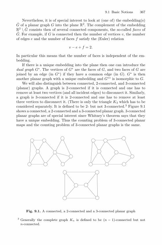
9.1 Basic Notions 367
Nevertheless, it is of special interest to look at (one of) the embedding(s)G of a planar graph G into the plane R2. The complement of the embeddingR2 \ G consists then of several connected components, the so-called faces ofG. For example, if G is connected then the number of vertices v, the numberof edges e and the number of faces f satisfy the (Euler) relation
v − e+ f = 2.
In particular this means that the number of faces is independent of the em-bedding.
If there is a unique embedding into the plane then one can introduce thedual graph G∗. The vertices of G∗ are the faces of G, and two faces of G arejoined by an edge (in G∗) if they have a common edge (in G). G∗ is thenanother planar graph with a unique embedding and G∗∗ is isomorphic to G.
We will also distinguish between connected, 2-connected, and 3-connected(planar) graphs. A graph is 2-connected if it is connected and one has toremove at least two vertices (and all incident edges) to disconnect it. Similarly,a graph is 3-connected if it is 2-connected and one has to remove at leastthree vertices to disconnect it. (There is only the triangle K3 which has to beconsidered separately. It is defined to be 2- but not 3-connected.3 Figure 9.1shows a connected, a 2-connected and a 3-connected planar graph. 3-connectedplanar graphs are of special interest since Whitney’s theorem says that theyhave a unique embedding. Thus the counting problem of 3-connected planarmaps and the counting problem of 3-connected planar graphs is the same.
Fig. 9.1. A connected, a 2-connected and a 3-connected planar graph
3 Generally the complete graph Kn is defined to be (n − 1)-connected but notn-connected.
368 9 Planar Graphs
There is an intimate relation between connected, 2-connected and3-connected planar graphs as we will see in the sequel. In fact, if one is inter-ested in the number of (labelled) planar graphs then one should first study3-connected graphs (or equivalently 3-connected maps), knowing that there isa general procedure to generate 2-connected ones and finally connected planargraphs.
We will also consider two subclasses of planar graphs, namely so-calledouterplanar graphs and series-parallel graphs.
An outerplanar graph is a planar graph that can be embedded into theplane so that all vertices are incident to the external face. Equivalently theyare characterised as those graphs not containing a minor isomorphic to K4 orK2,3.
A graph is series-parallel if it does not contain the complete graph K4
as a minor. Since both K5 and K3,3 have a minor isomorphic to K4, byKuratowski’s theorem a series-parallel graph is planar. Furthermore, everyouterplanar graph is series-parallel. The notation series-parallel comes fromthe fact that this kind of graphs can be seen as the result of consecutiveseries-parallel edge extensions applied to a tree. In a series extension an edgeis replaced by a chain of arbitrary finite length, whereas in a parallel extensionan edge is replaced by a multiple edge. Since we are only interested in simplegraphs we restrict ourselves to those graphs where the final result of thisprocedure has no multiple edges.
In what follows we will first solve the counting problem for labelled out-erplanar, series-parallel and planar graphs. The complexity of the countingproblem of these three classes increases. In particular series-parallel networksplay an important role in describing the relation between 2-connected and3-connected planar graphs.
However, the main goal of this chapter is to characterise the degree distri-bution of these three classes of planar graphs.
For all these problems we use (again) the concept of generating functionsand singularity analysis.
9.2 Counting Planar Graphs
In this section we present the solution of the counting problem for labelledplanar graphs. On the level of generating functions this is classical. However,the corresponding asymptotics are not obvious at all. In particular the casesof 2-connected and connected planar graphs have been resolved quite recentlyby Bender, Gao and Wormald [9] and Gimenez and Noy [91].
9.2.1 Outerplanar Graphs
As explained above an outerplanar graph is a planar graph that can be em-bedded into the plane so that all vertices are incident to the external face.
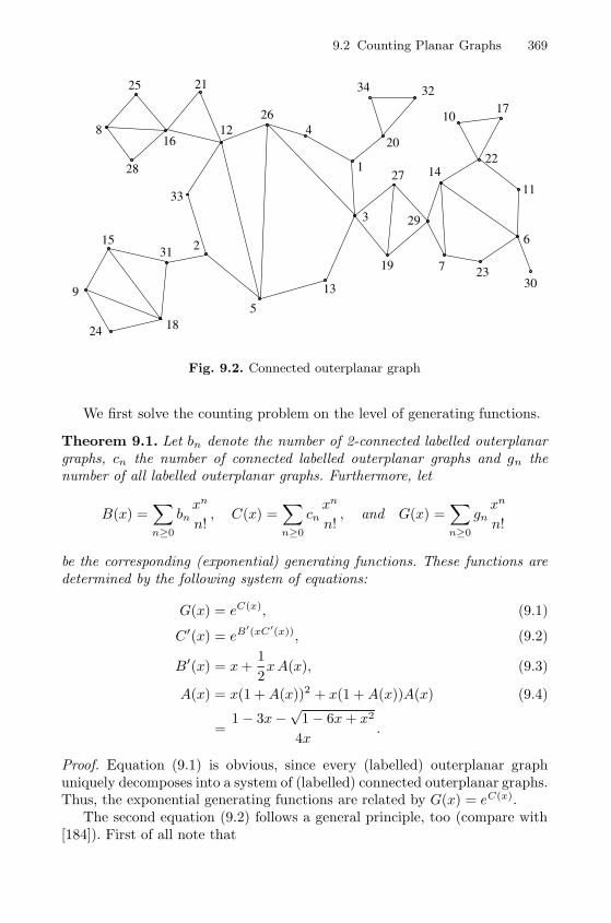
9.2 Counting Planar Graphs 369
4
1
3
7
8
62
59
27
16
19
26
15
33
18
22
24
28
25 21
13
1210
17
14
29
23
11
31
34
30
32
20
Fig. 9.2. Connected outerplanar graph
We first solve the counting problem on the level of generating functions.
Theorem 9.1. Let bn denote the number of 2-connected labelled outerplanargraphs, cn the number of connected labelled outerplanar graphs and gn thenumber of all labelled outerplanar graphs. Furthermore, let
B(x) =∑n≥0
bnxn
n!, C(x) =
∑n≥0
cnxn
n!, and G(x) =
∑n≥0
gnxn
n!
be the corresponding (exponential) generating functions. These functions aredetermined by the following system of equations:
G(x) = eC(x), (9.1)
C′(x) = eB′(xC′(x)), (9.2)
B′(x) = x+1
2xA(x), (9.3)
A(x) = x(1 +A(x))2 + x(1 +A(x))A(x) (9.4)
=1− 3x−
√1− 6x+ x2
4x.
Proof. Equation (9.1) is obvious, since every (labelled) outerplanar graphuniquely decomposes into a system of (labelled) connected outerplanar graphs.Thus, the exponential generating functions are related by G(x) = eC(x).
The second equation (9.2) follows a general principle, too (compare with[184]). First of all note that
370 9 Planar Graphs
B′(x) =∑n≥1
bn+1xn
n!
can be considered as the generating function of the 2-connected outerplanargraphs with n+ 1 vertices, where one vertex (without label) is distinguishedas a root. Similarly we interprete C ′(x).
The right hand side
eB′(xC′(x)) =
∞∑k=0
1
k!B′(xC′(x))k
can be interpreted as the exponential generating function of a finite set ofrooted 2-connected outerplanar graphs, where the root vertices are identifiedto form a new connected rooted outerplanar graph, and every vertex differ-ent from the root is replaced by a rooted connected outerplanar graph (seeFigure 9.3). It is clear that every graph of that kind constitutes a rooted con-nected outerplanar graph. Furthermore every rooted connected outerplanargraph G can be decomposed uniquely in the above way, as we indicate next.
Recall that a cut-vertex v of a graph G is defined by the property that thenumber of components of G\{v} is larger than that of G (G\{v} means thatwe remove v and all incident edges). Of course, a graph is 2-connected, if andonly if it is connected and contains no cut-vertices. In what follows we willmake use of the following reduction procedure. Let G be a connected graphand v a vertex of G and let G1, . . . , GJ denote the connected components ofG \ {v}. Then the subgraphs
G′j = G \ ((G1 ∪ · · · ∪Gj−1 ∪Gj ∪ · · · ∪GJ) \ {v}) (1 ≤ j ≤ J)
can be considered as subgraphs of G that can be glued together at the(cut-)point v to recover G. Furthermore, set G′′j = G \ Gj which is againa connected graph. Then we can also recover G by gluing G′j and G′′j at v.Of course, if v is not a cut-point then J = 1, G1 = G \ {v}, G′1 = G, andG′′1 = {v}.
Let vroot denote the root vertex of a connected outerplanar graph. If wedelete an arbitrary vertex v = vroot (in the above sense) then the graphdecomposes into k ≥ 1 components G1, G2, . . . GJ , where we assume that theroot vroot is contained in G1. Without loss of generality we can assume that vis not a cut-vertex. We reduce G to G′1 and have in mind that we can recoverG by gluing G′1 and G′′1 at v. We can also think of cutting off G2, . . . , GJ .Note that G′′1 is a connected graph that can be considered as rooted at v. Byrepeating this reduction procedure we end up with a graph G that containsthe root vroot and has no cut-vertex different from vroot. Finally we delete theroot vroot and obtain k ≥ 1 connected (outerplanar) graphs G1, . . . , Gk. SetBj = G′j , 1 ≤ j ≤ k. Then Bj , 1 ≤ j ≤ k, is a 2-connected planar graph that
is rooted at vroot, and G is obtained by identifying all Bj at the root vertices.
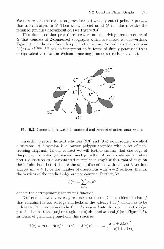
9.2 Counting Planar Graphs 371
We now restart the reduction procedure but we only cut at points v = vroot
that are contained in G. Then we again end up at G and this provides therequired (unique) decomposition (see Figure 9.3).
This decomposition procedure recovers an underlying tree structure ofG that consists of 2-connected subgraphs which are linked at cut-vertices.Figure 9.3 can be seen from this point of view, too. Accordingly the equationC′(x) = eB
′(xC′(x)) has an interpretation in terms of simply generated treesor equivalently of Galton-Watson branching processes (see Remark 9.2).
B' B'
B'
xC'
xC'xC'
xC'
xC' xC'
xC'
C'
Fig. 9.3. Connection between 2-connected and connected outerplanar graphs
In order to prove the next relations (9.3) and (9.4) we introduce so-calleddissections. A dissection is a convex polygon together with a set of non-crossing diagonals. In our context we will further assume that one edge ofthe polygon is rooted (or marked, see Figure 9.4). Alternatively we can inter-pret a dissection as a 2-connected outerplanar graph with a rooted edge onthe infinite face. Let A denote the set of dissections with at least 3 verticesand let an, n ≥ 1, be the number of dissections with n + 2 vertices, that is,the vertices of the marked edge are not counted. Further, let
A(x) =∑n≥1
anxn
denote the corresponding generating function.Dissections have a very easy recursive structure. One considers the face f
that contains the rooted edge and looks at the valency � of f which has to beat least 3. The dissection can be then decomposed into the original rooted edgeplus �−1 dissections (or just single edges) situated around f (see Figure 9.5).In terms of generating functions this reads as
A(x) = x(1 +A(x))2 + x2(1 +A(x))3 + · · · =x(1 +A(x))2
1− x(1 +A(x)).
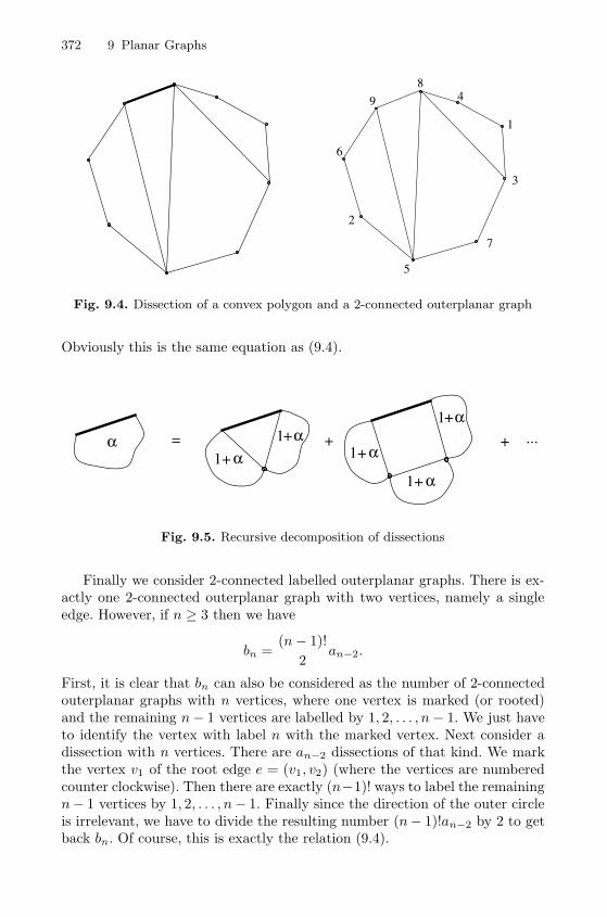
372 9 Planar Graphs
4
1
3
7
8
6
2
5
9
Fig. 9.4. Dissection of a convex polygon and a 2-connected outerplanar graph
Obviously this is the same equation as (9.4).
+
+= +1
1αα
α
+
+
1
1
α
α
+1 α+ ...
Fig. 9.5. Recursive decomposition of dissections
Finally we consider 2-connected labelled outerplanar graphs. There is ex-actly one 2-connected outerplanar graph with two vertices, namely a singleedge. However, if n ≥ 3 then we have
bn =(n− 1)!
2an−2.
First, it is clear that bn can also be considered as the number of 2-connectedouterplanar graphs with n vertices, where one vertex is marked (or rooted)and the remaining n− 1 vertices are labelled by 1, 2, . . . , n− 1. We just haveto identify the vertex with label n with the marked vertex. Next consider adissection with n vertices. There are an−2 dissections of that kind. We markthe vertex v1 of the root edge e = (v1, v2) (where the vertices are numberedcounter clockwise). Then there are exactly (n−1)! ways to label the remainingn− 1 vertices by 1, 2, . . . , n− 1. Finally since the direction of the outer circleis irrelevant, we have to divide the resulting number (n− 1)!an−2 by 2 to getback bn. Of course, this is exactly the relation (9.4).
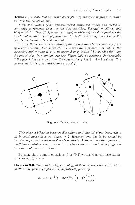
9.2 Counting Planar Graphs 373
Remark 9.2 Note that the above description of outerplanar graphs containstwo tree-like constructions.
First, the relation (9.2) between rooted connected graphs and rooted 2-connected corresponds to a tree-like decomposition. Set y(x) = xC ′(x) andΦ(x) = eB
′(x). Then (9.2) rewrites to y(x) = xΦ(y(x)) which is precisely thefunctional equation of simply generated (or Galton-Watson) trees. Figure 9.3depicts the tree-structure at the root.
Second, the recursive description of dissections could be alternatively givenby a corresponding tree approach. We start with a planted root outside thedissection and connect it with an internal node inside f by an edge that cutsthe rooted edge. In a similar way (see Figure 9.6) we continue. For example,if the face f has valency 4 then the node inside f has 3 = 4− 1 subtrees thatcorrespond to the 3 sub-dissections around f .
Fig. 9.6. Dissections and trees
This gives a bijection between dissections and planted plane trees, whereall internal nodes have out-degree ≥ 2. However, one has to be careful bytransferring statistics between these two objects. A dissection with r faces andn+ 2 (non-rooted) edges corresponds to a tree with r internal nodes (differentfrom the root) and n+ 1 leaves.
By using the system of equations (9.1)–(9.4) we derive asymptotic expan-sions for bn, cn, and gn.
Theorem 9.3. The numbers bn, cn and gn of 2-connected, connected and alllabelled outerplanar graphs are asymptotically given by
bn = b · n− 52 (3 + 2
√2)nn!
(1 +O
(1
n
)),
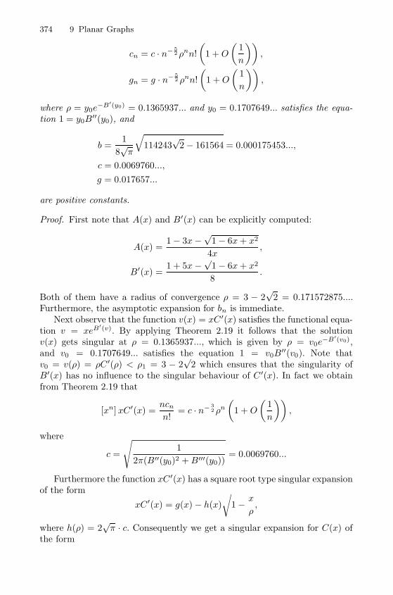
374 9 Planar Graphs
cn = c · n− 52 ρnn!
(1 +O
(1
n
)),
gn = g · n− 52 ρnn!
(1 +O
(1
n
)),
where ρ = y0e−B′(y0) = 0.1365937... and y0 = 0.1707649... satisfies the equa-
tion 1 = y0B′′(y0), and
b =1
8√π
√114243
√2− 161564 = 0.000175453...,
c = 0.0069760...,
g = 0.017657...
are positive constants.
Proof. First note that A(x) and B′(x) can be explicitly computed:
A(x) =1− 3x−
√1− 6x+ x2
4x,
B′(x) =1 + 5x−
√1− 6x+ x2
8.
Both of them have a radius of convergence ρ = 3 − 2√
2 = 0.171572875....Furthermore, the asymptotic expansion for bn is immediate.
Next observe that the function v(x) = xC ′(x) satisfies the functional equa-tion v = xeB
′(v). By applying Theorem 2.19 it follows that the solutionv(x) gets singular at ρ = 0.1365937..., which is given by ρ = v0e
−B′(v0),and v0 = 0.1707649... satisfies the equation 1 = v0B
′′(v0). Note thatv0 = v(ρ) = ρC ′(ρ) < ρ1 = 3 − 2
√2 which ensures that the singularity of
B′(x) has no influence to the singular behaviour of C ′(x). In fact we obtainfrom Theorem 2.19 that
[xn]xC′(x) =ncnn!
= c · n− 32 ρn
(1 + O
(1
n
)),
where
c =
√1
2π(B′′(y0)2 +B′′′(y0))= 0.0069760...
Furthermore the function xC ′(x) has a square root type singular expansionof the form
xC′(x) = g(x)− h(x)
√1− x
ρ,
where h(ρ) = 2√π · c. Consequently we get a singular expansion for C(x) of
the form
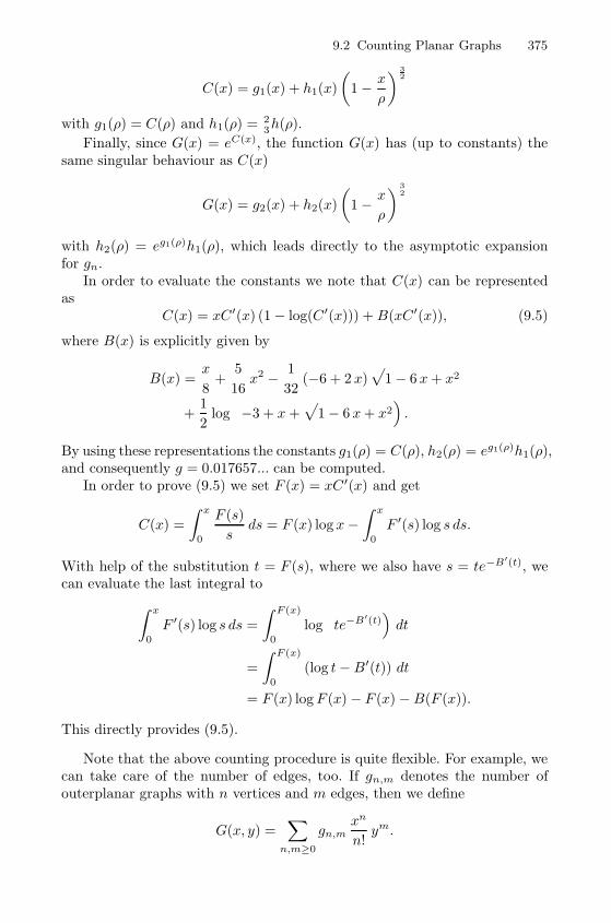
9.2 Counting Planar Graphs 375
C(x) = g1(x) + h1(x)
(1− x
ρ
) 32
with g1(ρ) = C(ρ) and h1(ρ) = 23h(ρ).
Finally, since G(x) = eC(x), the function G(x) has (up to constants) thesame singular behaviour as C(x)
G(x) = g2(x) + h2(x)
(1− x
ρ
) 32
with h2(ρ) = eg1(ρ)h1(ρ), which leads directly to the asymptotic expansionfor gn.
In order to evaluate the constants we note that C(x) can be representedas
C(x) = xC ′(x) (1− log(C ′(x))) +B(xC ′(x)), (9.5)
where B(x) is explicitly given by
B(x) =x
8+
5
16x2 − 1
32(−6 + 2 x)
√1− 6 x+ x2
+1
2log(−3 + x+
√1− 6 x+ x2
).
By using these representations the constants g1(ρ) = C(ρ), h2(ρ) = eg1(ρ)h1(ρ),and consequently g = 0.017657... can be computed.
In order to prove (9.5) we set F (x) = xC ′(x) and get
C(x) =
∫ x
0
F (s)
sds = F (x) log x−
∫ x
0
F ′(s) log s ds.
With help of the substitution t = F (s), where we also have s = te−B′(t), wecan evaluate the last integral to∫ x
0
F ′(s) log s ds =
∫ F (x)
0
log(te−B′(t)
)dt
=
∫ F (x)
0
(log t−B′(t)) dt
= F (x) logF (x)− F (x) −B(F (x)).
This directly provides (9.5).
Note that the above counting procedure is quite flexible. For example, wecan take care of the number of edges, too. If gn,m denotes the number ofouterplanar graphs with n vertices and m edges, then we define
G(x, y) =∑
n,m≥0
gn,mxn
n!ym.
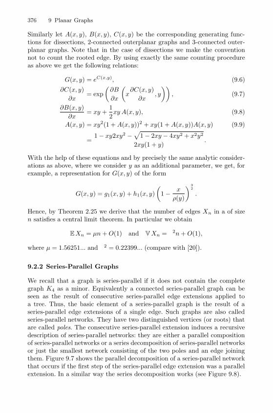
376 9 Planar Graphs
Similarly let A(x, y), B(x, y), C(x, y) be the corresponding generating func-tions for dissections, 2-connected outerplanar graphs and 3-connected outer-planar graphs. Note that in the case of dissections we make the conventionnot to count the rooted edge. By using exactly the same counting procedureas above we get the following relations:
G(x, y) = eC(x,y), (9.6)
∂C(x, y)
∂x= exp
(∂B
∂x
(x∂C(x, y)
∂x, y
)), (9.7)
∂B(x, y)
∂x= xy +
1
2xy A(x, y), (9.8)
A(x, y) = xy2(1 +A(x, y))2 + xy(1 +A(x, y))A(x, y) (9.9)
=1− xy2xy2 −
√1− 2xy − 4xy2 + x2y2
2xy(1 + y).
With the help of these equations and by precisely the same analytic consider-ations as above, where we consider y as an additional parameter, we get, forexample, a representation for G(x, y) of the form
G(x, y) = g1(x, y) + h1(x, y)
(1− x
ρ(y)
) 32
.
Hence, by Theorem 2.25 we derive that the number of edges Xn in a of sizen satisfies a central limit theorem. In particular we obtain
EXn = μn+O(1) and VXn = σ2n+O(1),
where μ = 1.56251... and σ2 = 0.22399... (compare with [20]).
9.2.2 Series-Parallel Graphs
We recall that a graph is series-parallel if it does not contain the completegraph K4 as a minor. Equivalently a connected series-parallel graph can beseen as the result of consecutive series-parallel edge extensions applied toa tree. Thus, the basic element of a series-parallel graph is the result of aseries-parallel edge extensions of a single edge. Such graphs are also calledseries-parallel networks. They have two distinguished vertices (or roots) thatare called poles. The consecutive series-parallel extension induces a recursivedescription of series-parallel networks: they are either a parallel compositionof series-parallel networks or a series decomposition of series-parallel networksor just the smallest network consisting of the two poles and an edge joiningthem. Figure 9.7 shows the parallel decomposition of a series-parallel networkthat occurs if the first step of the series-parallel edge extension was a parallelextension. In a similar way the series decomposition works (see Figure 9.8).
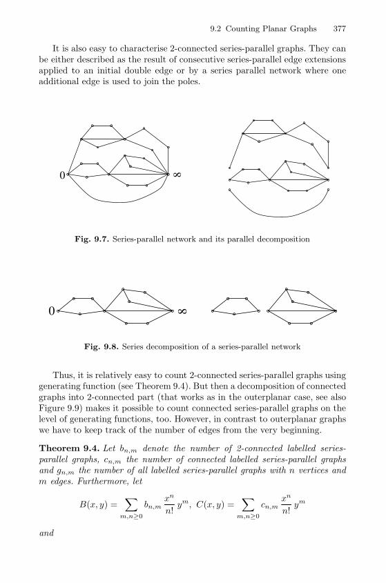
9.2 Counting Planar Graphs 377
It is also easy to characterise 2-connected series-parallel graphs. They canbe either described as the result of consecutive series-parallel edge extensionsapplied to an initial double edge or by a series parallel network where oneadditional edge is used to join the poles.
0 8
Fig. 9.7. Series-parallel network and its parallel decomposition
0 8
Fig. 9.8. Series decomposition of a series-parallel network
Thus, it is relatively easy to count 2-connected series-parallel graphs usinggenerating function (see Theorem 9.4). But then a decomposition of connectedgraphs into 2-connected part (that works as in the outerplanar case, see alsoFigure 9.9) makes it possible to count connected series-parallel graphs on thelevel of generating functions, too. However, in contrast to outerplanar graphswe have to keep track of the number of edges from the very beginning.
Theorem 9.4. Let bn,m denote the number of 2-connected labelled series-parallel graphs, cn,m the number of connected labelled series-parallel graphsand gn,m the number of all labelled series-parallel graphs with n vertices andm edges. Furthermore, let
B(x, y) =∑
m,n≥0
bn,mxn
n!ym, C(x, y) =
∑m,n≥0
cn,mxn
n!ym
and
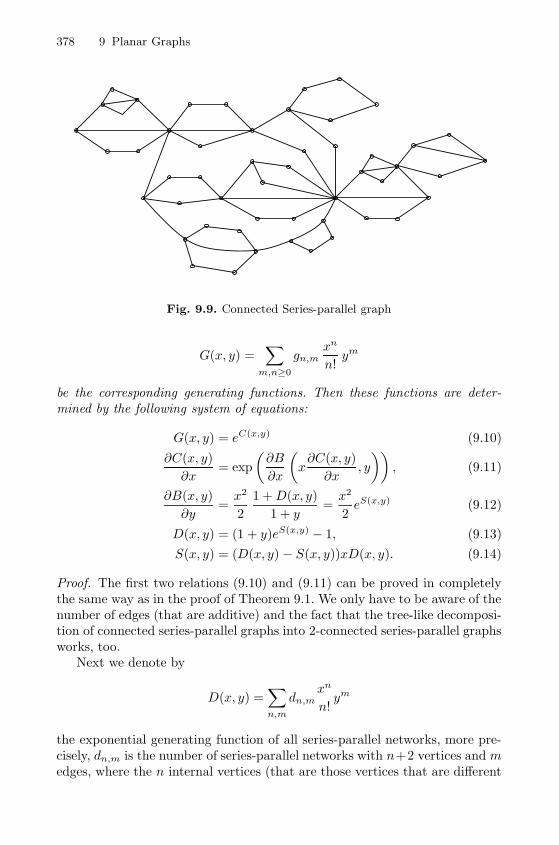
378 9 Planar Graphs
Fig. 9.9. Connected Series-parallel graph
G(x, y) =∑
m,n≥0
gn,mxn
n!ym
be the corresponding generating functions. Then these functions are deter-mined by the following system of equations:
G(x, y) = eC(x,y) (9.10)
∂C(x, y)
∂x= exp
(∂B
∂x
(x∂C(x, y)
∂x, y
)), (9.11)
∂B(x, y)
∂y=x2
2
1 +D(x, y)
1 + y=x2
2eS(x,y) (9.12)
D(x, y) = (1 + y)eS(x,y) − 1, (9.13)
S(x, y) = (D(x, y) − S(x, y))xD(x, y). (9.14)
Proof. The first two relations (9.10) and (9.11) can be proved in completelythe same way as in the proof of Theorem 9.1. We only have to be aware of thenumber of edges (that are additive) and the fact that the tree-like decomposi-tion of connected series-parallel graphs into 2-connected series-parallel graphsworks, too.
Next we denote by
D(x, y) =∑n,m
dn,mxn
n!ym
the exponential generating function of all series-parallel networks, more pre-cisely, dn,m is the number of series-parallel networks with n+2 vertices and medges, where the n internal vertices (that are those vertices that are different
9.2 Counting Planar Graphs 379
from the poles) are labelled by {1, 2, . . . , n}. In the same way we define S(x, y)for series-parallel networks that have a series decomposition into at least twoseries-parallel networks and P (x, y) for series-parallel networks that have aparallel decomposition into at least two series-parallel networks. For short, wecall these networks s- and p-networks. By definition we have
D(x, y) = S(x, y) + P (x, y) + y.
Furthermore, observe that the series decomposition of a s-network (and theparallel decomposition of a p-network) is unique if we require that the com-ponents are either edges or p-networks (or at most one edge and s-networks).This unique decomposition translates directly into the system of equations
S(x, y) = x(P (x, y) + y)2 + x2(P (x, y) + y)3 + · · · (9.15)
=x(P (x, y) + y)2
1− x(P (x, y) + y),
P (x, y) = (eS(x,y) − 1− S(x, y)) + y(eS(x,y) − 1). (9.16)
Of course, these two equations can be rewritten to the system (9.13) and(9.14) if we use D − S instead of P + y.
Alternatively we can interprete the equations (9.13) and (9.14). The firstequation (9.13) expresses the fact that a series-parallel network is a parallelcomposition of series networks (this is the exponential term), to which wemay add or not the edge connecting the two poles. The second equation (9.14)means that a series network is formed by taking at first a non-series network(this is the term D − S), and concatenating to it an arbitrary network.
Finally we have (9.12), since a series-parallel network with non-adjacentpoles (which is counted by eS(x,y)) can be obtained by distinguishing, orientingand then deleting any edge of an arbitrary 2-connected series-parallel graph.The factor x2 takes into account the two poles, the factor 1/2 the two possibleorientations and the derivative with respect to y the choice and deletion of anarbitrary edge.
Remark 9.5 Note that the system (9.15) and (9.16) can be interpreted asa tree-like composition with two kinds of nodes (S and P ) and two differentreproductions rules.
Furthermore, we want to note that D(x, y) solves a single equation
log
(1 +D(x, y)
1 + y
)=
xD(x, y)2
1 + xD(x, y), (9.17)
which will make the singularity analysis slightly easier.
Theorem 9.6. The numbers bn, cn and gn of 2-connected, connected and allseries-parallel graphs are asymptotically given by
380 9 Planar Graphs
bn = b · n− 52 ρn
1n!
(1 +O
(1
n
)),
cn = c · n− 52 ρn
2n!
(1 +O
(1
n
)),
gn = g · n− 52 ρn
2n!
(1 +O
(1
n
)),
where ρ1 = 0.1280038..., ρ2 = 0.11021... and
b = 0.0010131...,
c = 0.0067912...,
g = 0.0076388...
are positive constants.
Proof. Since D(x, y) satisfies a single equation (9.17), it follows that there isa singular expansion of the form
D(x, y) = g(x, y)− h(x, y)
√1− x
ρ(y),
where ρ(1) = ρ1 = 0.12800.... Since eS(x,y) = (D(x, y) + 1)/(1 + y), we get acorresponding expansion for
∂B(x, y)
∂y= g1(x, y)− h1(x, y)
√1− x
ρ(y).
By Theorem 2.30 this implies that B(x, y) has a representation of the form
B(x, y) = g2(x, y) + h2(x, y)
(1− x
ρ(y)
) 32
. (9.18)
Of course, by setting y = 1 this leads to the asymptotic expansion for bn withρ1 = ρ(1).
From (9.18) we also obtain a representation for
∂B(x, y)
∂x= g3(x, y)− h3(x, y)
√1− x
ρ(y),
where we can safely set y = 1. For notational simplicity we set B ′(x) = ∂B(x,1)∂x
and C′(x) = ∂C(x,1)∂x . Then the function v(x) = xC ′(x) satisfies the functional
equation v(x) = xeB′(v(x)), that is, we are in a similar situation as in the proof
of Theorem 9.3. Again we observe that there exists v0 = 0.1279695... < ρ1with v0B
′′(v0) = 1 (compare with [20]). Thus, by Theorem 2.19, the functionv(x) = xC ′(x) has a local representation of the form
9.2 Counting Planar Graphs 381
xC′(x) = g4(x)− h4(x)
√1− x
ρ2,
where ρ2 = v0e−B′(v0) = 0.11021.... Consequently we obtain corresponding
representations for
C(x) = g5(x) + h5(x)
(1− x
ρ2
) 32
,
and for
G(x) = eC(x) = g6(x) + h6(x)
(1− x
ρ2
) 32
,
that induce corresponding asymptotic representations for cn and gn.
Remark 9.7 We want to remark that one has to be careful with the evaluationof constants since we have been working with derivatives with respect to x andy. Nevertheless it is not difficult to solve the above system of (differential)equations numerically and check all necessary conditions, for example, thatthere exists v0 < ρ1 with v0B
′′(v0) = 1.However, due to the simplicity of the above equations, one can solve some
of the integrals explicitly. For example, in [20] it is shown that B(x, y) can berepresented in terms of D = D(x, y):
B(x, y) =1
2log(1 + xD)− xD(x2D2 + xD + 2− 2x)
4(1 + xD),
and C(x, y) can be represented in terms of ∂C(x,1)∂x and B(x, y):
C(x, y) = x∂C(x, 1)
∂x
(1− log
∂C(x, 1)
∂x
)−B(x∂C(x, 1)
∂x, y
).
Remark 9.8 As in the case of outerplanar graphs we also get a central limittheorem for the number Xn of edges in a random series-parallel graph of sizen, with
EXn = μn+O(1) and VXn = σ2n+O(1),
where μ = 1.61673... and σ2 = 0.55347... (compare with [20]). By a slight vari-ation of the proof of Theorem 9.6 we obtain a local representation of G(x, y)of the form
G(x, y) = g6(x, y) + h6(x, y)
(1− x
ρ2(y)
) 32
.
Thus, a direct application of Theorem 2.25 gives the result.

382 9 Planar Graphs
9.2.3 Quadrangulations and Planar Maps
Before we can count planar graphs we have to know something on the relationbetween quadrangulations and planar maps. A planar map is – informallyspoken – an embedded planar graph, and a quadrangulation is a planar mapwhere every face has valency 4 (also the external face).
Interestingly, there is a bijective relation between quadrangulations and2-connected maps. Suppose a 2-connected mapM is given. LetM ∗ denote thedual map, that is, the vertices ofM ∗ are the faces ofM and two vertices ofM ∗
are linked by an edge (of M ∗) if the corresponding faces of M have an edge incommon. For simplicity the vertices ofM ∗ are represented by points containedin the corresponding faces of M . Now we construct a quadrangulation Q inthe following way. The vertices of Q are the vertices of M together with thevertices ofM∗ (represented as points in the plane). Finally we connect a vertexv of M with a vertex v∗ of M∗ by an edge (in Q) if v is contained on theboundary of the face of M corresponding to v∗. Figure 9.10 shows an exampleof this procedure.
Fig. 9.10. Quadrangulations and maps
A diagonal in a quadrangulation is an internal path of length 2 joining twoopposite vertices of the external face. A quadrangulation is simple if it has nodiagonal, if every cycle of length 4 (other than the external cycle that encirclesthe whole graph) defines a face, and if it is not the trivial map reduced to asingle quadrangle. For example, the quadrangulation depicted in Figure 9.10
9.2 Counting Planar Graphs 383
is a simple one. It is a well known fact and an easy exercise (see [29, 156])that the above described procedure leads to a simple quadrangulation, if andonly if the corresponding map is 3-connected.
Furthermore, it is easy to see that edge-rooted maps correspond to edgerooted quadrangulations, where the rooted edge is directed and always onthe external face. These kinds of objects can now be counted with the help ofgenerating functions. Note further, that quadrangulations are bipartite graphsso that we can distinguish between black and white vertices. This is uniquelydefined by assuming that the rooted (directed) edge starts from a black vertex.With this convention the above bijection transfers vertices of the 2-connectedmap to black vertices of the quadrangulation, edges to faces, faces to whitevertices, and the root degree (of the first vertex of the root edge) stays thesame.
Let fi,j,k be the number of edge-rooted 2-connected maps with i+1 verticesand j + 1 faces where the (first) vertex of the rooted edge has degree k + 1.Then fi,j,k is also the number of edge-rooted quadrangulations with i+1 blackvertices, and j + 1 white vertices where the (first) vertex of the rooted edgehas degree k + 1. The following lemma provides an explicit representation ofthe trivariate generating function of these numbers.
Lemma 9.9. The generating function
F (x, y, w) =∑i,j,k
fi,j,kxiyjwk
is given by
F (x, y, w) = − 1
2w(1− (1 + v − u+ uv − 2v2u)w + v(1 − u)2w2)
+1
2w(1 − (1− u)w)
√1− 2v(1 + u+ 2uv)w + v2(1− u)2w2,
where u = u(x, y) and v = v(x, y) are determined by the system
x = u(1− v)2, (9.19)
y = v(1− u)2. (9.20)
Remark 9.10 Note that the function F (x, y, 1) is given by
F (x, y, 1) = uv(1− u− v). (9.21)
This representation is due to Brown and Tutte [30]. In particular, it can beused to prove an explicit formula for
fi,j =∑k≥0
fi,j,k =(2i+ j − 2)!(2j + i− 2)!
i!j!(2i− 1)!(2j − 1)!.
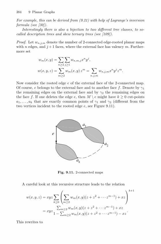
384 9 Planar Graphs
For example, this can be derived from (9.21) with help of Lagrange’s inversionformula (see [30]).
Interestingly there is also a bijection to two different tree classes, to so-called description trees and skew ternary trees (see [109]).
Proof. Let wn,j,m denote the number of 2-connected edge-rooted planar mapswith n edges, and j+ 1 faces, where the external face has valency m. Further-more set
wm(x, y) =∑n≥2
∑j≥1
wn,m,jxnyj ,
w(x, y, z) =∑m≥2
wm(x, y) zm =∑
n,j,m
wn,j,mxnyjzm.
Now consider the rooted edge e of the external face of the 2-connected map.Of course, e belongs to the external face and to another face f . Denote by γ1
the remaining edges on the external face and by γ2 the remaining edges onthe face f . If one deletes the edge e, then M \ e might have k ≥ 0 cut-pointsa1, . . . , ak that are exactly common points of γ1 and γ2 (different from thetwo vertices incident to the rooted edge e, see Figure 9.11).
a
a
a
e
1
2
k
Fig. 9.11. 2-connected maps
A careful look at this recursive structure leads to the relation
w(x, y, z) = xyz∑k≥0
⎛⎝∑m≥2
wm(x, y)(z + z2 + · · · zm−1) + xz
⎞⎠k+1
= xyz
∑m≥2 wm(x, y)(z + z2 + · · · zm−1) + xz
1−∑
m≥2 wm(x, y)(z + z2 + · · · zm−1)− xz .
This rewrites to
9.2 Counting Planar Graphs 385
w(x, y, z)2 + ((1 − z)(1− xz) + xyz − zw(x, y, 1))w(x, y, z)
−xz2y(x(1− z) + w(x, y, 1)) = 0.
Now let hi,j,m be the number of edge-rooted 2-connected planar maps withi + 1 vertices, and j + 1 faces with an external face of valency m (where weexclude the map that consists just of one edge). Then by Euler’s relation wehave
hi,j,m = wi+j,j,m
and consequently the corresponding generating function h(x, y, z) is given by
h(x, y, z) =∑i,j,m
hi,j,mxiyjzm = w(x, y/x, z)
and satisfies the relation
h(x, y, z)2 + ((1− z)(1− xz) + yz − zh(x, y, 1))h(x, y, z) (9.22)
−yz2(x(1 − z) + h(x, y, 1)) = 0.
It is easy to check that (9.22) has a unique analytic solution if one assumesthat h(x, 0, z) = 0. Namely, if we set
h(x, y, z) =∑j≥0
hj(x, z)yj
(with h0(x, z) = h(x, 0, z) = 0) then (9.22) rewrites to a recurrence forhj(x, z). Now observe that
h(x, y, z) = −1
2(1− (1 + u− v + uv − 2u2v)z + u(1− v)2z2)
+1
2(1 − (1− v)z)
√1− 2u(1 + v + 2uv)z + u2(1− v)2z2,
where u = u(x, y) and v = v(x, y) are defined by (9.19) and (9.20) is actuallyan analytic solution of (9.22) that meets these conditions.
Finally we apply the above enumeration result to the dual maps. Herevertices are transferred to faces, faces to vertices, and the valency of the outerface to the degree of the degree of the root vertex. As a consequence we havethat h(x, y, w) = wF (x, y, w), where the extra factor w appears, because inF we are counting the degree of the root vertex minus one. Of course, thiscompletes the proof of the lemma.
We now turn to simple triangulations or equivalently to 3-connected edge-rooted maps. Let qi,j,k denote the number of 3-connected edge-rooted mapswith i + 1 vertices and j + 1 faces, where the (first) vertex of the root edgehas degree k + 1. Equivalently this is the number of simple quadrangulationswith i+ 1 black vertices and j + 1 white vertices, where the (first) vertex ofthe root edge has degree k + 1.
386 9 Planar Graphs
Lemma 9.11. The generating function
Q(x, y, w) =∑
i,j,k≥1
qi,j,kxiyjwk (9.23)
is given by
Q(x, y, w) = xyw
(1
1 + x+
1
1 + wy− 1
)− rs
(1 + r + s)3−w1(r, s, w) + (r − w + 1)
√w2(r, s, w)
2(s+ 1)2(sw + r2 + 2r + 1),
where w1(r, s, w) and w2(r, s, w) are polynomials given by
w1(x, r, s) =− rsw2 + w(1 + 4s+ 3rs2 + 5s2 + r2 + 2r + 2s3 + 3r2s+ 7rs)(9.24)
+ (r + 1)2(r + 2s+ 1 + s2),
w2(x, r, s) =r2s2w2 − 2wrs(2r2s+ 6rs+ 2s3 + 3rs2 + 5s2 + r2 + 2r + 4s+ 1)(9.25)
+ (r + 1)2(r + 2s+ 1 + s2)2
and r = r(x, y), and s = s(x, y) are determined by the system
r = x(s+ 1)2, (9.26)
s = y(r + 1)2. (9.27)
Observe, too, that the function Q(x, y, 1) is given by
Q(x, y, 1) = xy
(1
1 + x+
1
1 + y− 1
)− rs
(r + s+ 1)3.
This formula is due to Mullin and Schellenberg [156]. In passing we also ob-tain a representation of the function M(x, y) that counts the number of 3-connected edge-rooted planar maps according to the (total) number of verticesand edges:
M(x, y) = x2y2(
1
1 + xy+
1
1 + y− 1− (1 + U)2(1 + V )2
(1 + U + V )3
), (9.28)
where U = U(x, y) and V = V (x, y) are defined by U = xy(1 + V )2 andV = y(1 + U)2.
Proof. Let F (x, y, w) be the generating function used in Lemma 9.9. However,we now use it as the generating function of rooted quadrangulations, wherethe variables x, y and w mark, respectively, the number of black vertices minusone, the number of white vertices minus one, and the degree of the first vertex
9.2 Counting Planar Graphs 387
of the rooted edge minus one. We recall that a diagonal is an internal pathof length 2 joining two opposite vertices of the external face. We will call adiagonal black or white, according to the colour of the external vertices theyjoin.
We associate generating functions FN , FB and FW , respectively, to quad-rangulations with no diagonal, to those with at least one black diagonal (atthe root vertex), and to those with at least one white diagonal (not at theroot vertex). By planarity only one of the two kinds of diagonals can appearin a quadrangulation; it follows that
F (x, y, w) = FN (x, y, w) + FB(x, y, w) + FW (x, y, w).
A quadrangulation with a diagonal can be decomposed into two quadrangu-lations, by considering the maps to the left and to the right of this diagonal.In order to make this decomposition unique we assume that we decompose atthe leftmost diagonal when there are several of them. This gives raise to theequations
FB(x, y, w) = (FN (x, y, w) + FW (x, y, w))F (x, y, w)
x,
FW (x, y, w) = (FN (x, y, w) + FB(x, y, w))F (x, y, 1)
y.
In the second case, only one of the two quadrangulations contributes to thedegree of the root vertex; this is the reason why the term F (x, y, 1) appears.The x and the y in the denominators appear because the three vertices of thediagonal are common to the two quadrangulations. Since we are consideringvertices minus one, we only need to correct the colour that appears twice atthe diagonal. Incidentally, no term w appears in the equations for the samereason.
Let us write F = F (x, y, w) and F (1) = F (x, y, 1). From the previousequations we deduce that
F = FN + FB + FW = (FN + FB)(1 +F
x),
F = FN + FB + FW = (FN + FW )(1 +F (1)
y),
so that
F + FN = (FN + FB) + (FN + FW ) = F
(1
1 + Fx
+1
1 + F (1)y
),
and finally
FN = F
(1
1 + Fx
+1
1 + F (1)y
− 1
). (9.29)
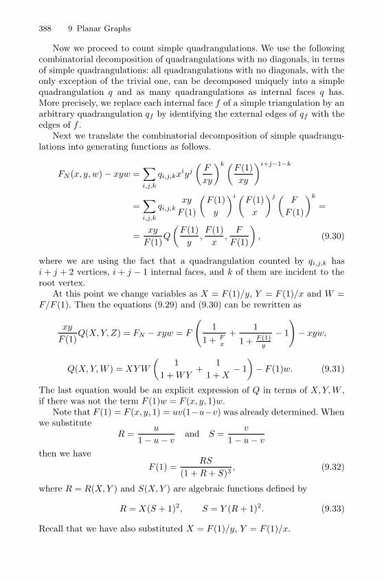
388 9 Planar Graphs
Now we proceed to count simple quadrangulations. We use the followingcombinatorial decomposition of quadrangulations with no diagonals, in termsof simple quadrangulations: all quadrangulations with no diagonals, with theonly exception of the trivial one, can be decomposed uniquely into a simplequadrangulation q and as many quadrangulations as internal faces q has.More precisely, we replace each internal face f of a simple triangulation by anarbitrary quadrangulation qf by identifying the external edges of qf with theedges of f .
Next we translate the combinatorial decomposition of simple quadrangu-lations into generating functions as follows.
FN (x, y, w) − xyw =∑i,j,k
qi,j,kxiyj
(F
xy
)k (F (1)
xy
)i+j−1−k
=∑i,j,k
qi,j,kxy
F (1)
(F (1)
y
)i(F (1)
x
)j (F
F (1)
)k
=
=xy
F (1)Q
(F (1)
y,F (1)
x,F
F (1)
), (9.30)
where we are using the fact that a quadrangulation counted by qi,j,k hasi + j + 2 vertices, i+ j − 1 internal faces, and k of them are incident to theroot vertex.
At this point we change variables as X = F (1)/y, Y = F (1)/x and W =F/F (1). Then the equations (9.29) and (9.30) can be rewritten as
xy
F (1)Q(X,Y, Z) = FN − xyw = F
(1
1 + Fx
+1
1 + F (1)y
− 1
)− xyw,
Q(X,Y,W ) = XYW
(1
1 +WY+
1
1 +X− 1
)− F (1)w. (9.31)
The last equation would be an explicit expression of Q in terms of X,Y,W ,if there was not the term F (1)w = F (x, y, 1)w.
Note that F (1) = F (x, y, 1) = uv(1−u−v) was already determined. Whenwe substitute
R =u
1− u− v and S =v
1− u− vthen we have
F (1) =RS
(1 +R+ S)3, (9.32)
where R = R(X,Y ) and S(X,Y ) are algebraic functions defined by
R = X(S + 1)2, S = Y (R + 1)2. (9.33)
Recall that we have also substituted X = F (1)/y, Y = F (1)/x.
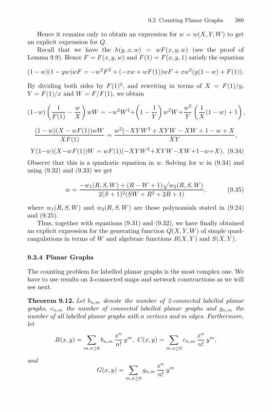
9.2 Counting Planar Graphs 389
Hence it remains only to obtain an expression for w = w(X,Y,W ) to getan explicit expression for Q.
Recall that we have the h(y, x, w) = wF (x, y, w) (see the proof ofLemma 9.9). Hence F = F (x, y, w) and F (1) = F (x, y, 1) satisfy the equation
(1−w)(1− yw)wF = −w2F 2 + (−xw +wF (1))wF + xw2(y(1−w) + F (1)).
By dividing both sides by F (1)2, and rewriting in terms of X = F (1)/y,Y = F (1)/x and W = F/F (1), we obtain
(1−w)
(1
F (1)− w
X
)wW = −w2W 2+
(1− 1
Y
)w2W+
w2
Y
(1
X(1− w) + 1
),
(1− w)(X − wF (1))wW
XF (1)=w2(−XYW 2 +XYW −XW + 1− w +X
XY,
Y (1−w)(X−wF (1))W = wF (1)(−XYW 2+XYW−XW+1−w+X). (9.34)
Observe that this is a quadratic equation in w. Solving for w in (9.34) andusing (9.32) and (9.33) we get
w =−w1(R,S,W ) + (R−W + 1)
√w2(R,S,W )
2(S + 1)2(SW +R2 + 2R+ 1), (9.35)
where w1(R,S,W ) and w2(R,S,W ) are those polynomials stated in (9.24)and (9.25).
Thus, together with equations (9.31) and (9.32), we have finally obtainedan explicit expression for the generating function Q(X,Y,W ) of simple quad-rangulations in terms of W and algebraic functions R(X,Y ) and S(X,Y ).
9.2.4 Planar Graphs
The counting problem for labelled planar graphs is the most complex one. Wehave to use results on 3-connected maps and network constructions as we willsee next.
Theorem 9.12. Let bn,m denote the number of 2-connected labelled planargraphs, cn,m the number of connected labelled planar graphs and gn,m thenumber of all labelled planar graphs with n vertices and m edges. Furthermore,let
B(x, y) =∑
m,n≥0
bn,mxn
n!ym, C(x, y) =
∑m,n≥0
cn,mxn
n!ym,
and
G(x, y) =∑
m,n≥0
gn,mxn
n!ym
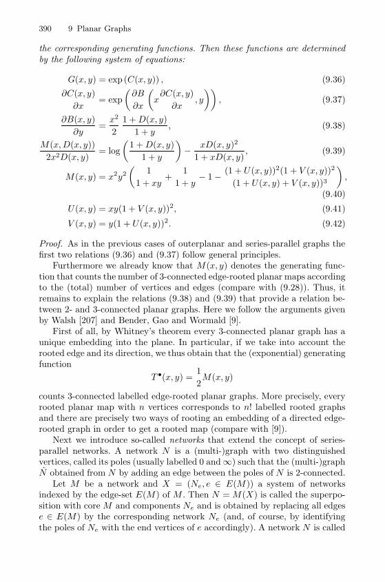
390 9 Planar Graphs
the corresponding generating functions. Then these functions are determinedby the following system of equations:
G(x, y) = exp (C(x, y)) , (9.36)
∂C(x, y)
∂x= exp
(∂B
∂x
(x∂C(x, y)
∂x, y
)), (9.37)
∂B(x, y)
∂y=x2
2
1 +D(x, y)
1 + y, (9.38)
M(x,D(x, y))
2x2D(x, y)= log
(1 +D(x, y)
1 + y
)− xD(x, y)2
1 + xD(x, y), (9.39)
M(x, y) = x2y2(
1
1 + xy+
1
1 + y− 1− (1 + U(x, y))2(1 + V (x, y))2
(1 + U(x, y) + V (x, y))3
),
(9.40)
U(x, y) = xy(1 + V (x, y))2, (9.41)
V (x, y) = y(1 + U(x, y))2. (9.42)
Proof. As in the previous cases of outerplanar and series-parallel graphs thefirst two relations (9.36) and (9.37) follow general principles.
Furthermore we already know that M(x, y) denotes the generating func-tion that counts the number of 3-connected edge-rooted planar maps accordingto the (total) number of vertices and edges (compare with (9.28)). Thus, itremains to explain the relations (9.38) and (9.39) that provide a relation be-tween 2- and 3-connected planar graphs. Here we follow the arguments givenby Walsh [207] and Bender, Gao and Wormald [9].
First of all, by Whitney’s theorem every 3-connected planar graph has aunique embedding into the plane. In particular, if we take into account therooted edge and its direction, we thus obtain that the (exponential) generatingfunction
T •(x, y) =1
2M(x, y)
counts 3-connected labelled edge-rooted planar graphs. More precisely, everyrooted planar map with n vertices corresponds to n! labelled rooted graphsand there are precisely two ways of rooting an embedding of a directed edge-rooted graph in order to get a rooted map (compare with [9]).
Next we introduce so-called networks that extend the concept of series-parallel networks. A network N is a (multi-)graph with two distinguishedvertices, called its poles (usually labelled 0 and∞) such that the (multi-)graphN obtained from N by adding an edge between the poles of N is 2-connected.
Let M be a network and X = (Ne, e ∈ E(M)) a system of networksindexed by the edge-set E(M) of M . Then N = M(X) is called the superpo-sition with core M and components Ne and is obtained by replacing all edgese ∈ E(M) by the corresponding network Ne (and, of course, by identifyingthe poles of Ne with the end vertices of e accordingly). A network N is called
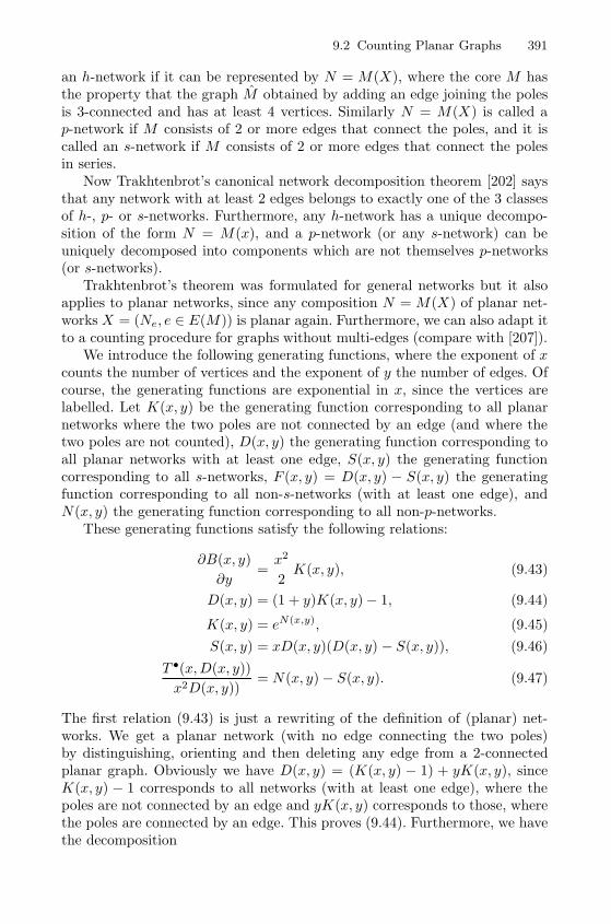
9.2 Counting Planar Graphs 391
an h-network if it can be represented by N = M(X), where the core M hasthe property that the graph M obtained by adding an edge joining the polesis 3-connected and has at least 4 vertices. Similarly N = M(X) is called ap-network if M consists of 2 or more edges that connect the poles, and it iscalled an s-network if M consists of 2 or more edges that connect the polesin series.
Now Trakhtenbrot’s canonical network decomposition theorem [202] saysthat any network with at least 2 edges belongs to exactly one of the 3 classesof h-, p- or s-networks. Furthermore, any h-network has a unique decompo-sition of the form N = M(x), and a p-network (or any s-network) can beuniquely decomposed into components which are not themselves p-networks(or s-networks).
Trakhtenbrot’s theorem was formulated for general networks but it alsoapplies to planar networks, since any composition N = M(X) of planar net-works X = (Ne, e ∈ E(M)) is planar again. Furthermore, we can also adapt itto a counting procedure for graphs without multi-edges (compare with [207]).
We introduce the following generating functions, where the exponent of xcounts the number of vertices and the exponent of y the number of edges. Ofcourse, the generating functions are exponential in x, since the vertices arelabelled. Let K(x, y) be the generating function corresponding to all planarnetworks where the two poles are not connected by an edge (and where thetwo poles are not counted), D(x, y) the generating function corresponding toall planar networks with at least one edge, S(x, y) the generating functioncorresponding to all s-networks, F (x, y) = D(x, y) − S(x, y) the generatingfunction corresponding to all non-s-networks (with at least one edge), andN(x, y) the generating function corresponding to all non-p-networks.
These generating functions satisfy the following relations:
∂B(x, y)
∂y=x2
2K(x, y), (9.43)
D(x, y) = (1 + y)K(x, y)− 1, (9.44)
K(x, y) = eN(x,y), (9.45)
S(x, y) = xD(x, y)(D(x, y) − S(x, y)), (9.46)
T •(x,D(x, y))
x2D(x, y))= N(x, y)− S(x, y). (9.47)
The first relation (9.43) is just a rewriting of the definition of (planar) net-works. We get a planar network (with no edge connecting the two poles)by distinguishing, orienting and then deleting any edge from a 2-connectedplanar graph. Obviously we have D(x, y) = (K(x, y) − 1) + yK(x, y), sinceK(x, y) − 1 corresponds to all networks (with at least one edge), where thepoles are not connected by an edge and yK(x, y) corresponds to those, wherethe poles are connected by an edge. This proves (9.44). Furthermore, we havethe decomposition
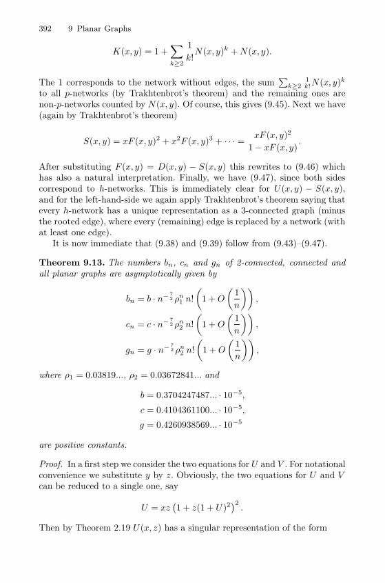
392 9 Planar Graphs
K(x, y) = 1 +∑k≥2
1
k!N(x, y)k +N(x, y).
The 1 corresponds to the network without edges, the sum∑
k≥21k!N(x, y)k
to all p-networks (by Trakhtenbrot’s theorem) and the remaining ones arenon-p-networks counted by N(x, y). Of course, this gives (9.45). Next we have(again by Trakhtenbrot’s theorem)
S(x, y) = xF (x, y)2 + x2F (x, y)3 + · · · =xF (x, y)2
1− xF (x, y).
After substituting F (x, y) = D(x, y) − S(x, y) this rewrites to (9.46) whichhas also a natural interpretation. Finally, we have (9.47), since both sidescorrespond to h-networks. This is immediately clear for U(x, y) − S(x, y),and for the left-hand-side we again apply Trakhtenbrot’s theorem saying thatevery h-network has a unique representation as a 3-connected graph (minusthe rooted edge), where every (remaining) edge is replaced by a network (withat least one edge).
It is now immediate that (9.38) and (9.39) follow from (9.43)–(9.47).
Theorem 9.13. The numbers bn, cn and gn of 2-connected, connected andall planar graphs are asymptotically given by
bn = b · n− 72 ρn
1 n!
(1 +O
(1
n
)),
cn = c · n− 72 ρn
2 n!
(1 +O
(1
n
)),
gn = g · n− 72 ρn
2 n!
(1 +O
(1
n
)),
where ρ1 = 0.03819..., ρ2 = 0.03672841... and
b = 0.3704247487... · 10−5,
c = 0.4104361100... · 10−5,
g = 0.4260938569... · 10−5
are positive constants.
Proof. In a first step we consider the two equations for U and V . For notationalconvenience we substitute y by z. Obviously, the two equations for U and Vcan be reduced to a single one, say
U = xz(1 + z(1 + U)2
)2.
Then by Theorem 2.19 U(x, z) has a singular representation of the form
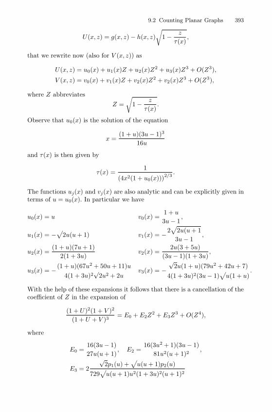
9.2 Counting Planar Graphs 393
U(x, z) = g(x, z)− h(x, z)
√1− z
τ(x),
that we rewrite now (also for V (x, z)) as
U(x, z) = u0(x) + u1(x)Z + u2(x)Z2 + u3(x)Z3 +O(Z3),
V (x, z) = v0(x) + v1(x)Z + v2(x)Z2 + v2(x)Z3 +O(Z3),
where Z abbreviates
Z =
√1− z
τ(x).
Observe that u0(x) is the solution of the equation
x =(1 + u)(3u− 1)3
16u
and τ(x) is then given by
τ(x) =1
(4x2(1 + u0(x)))2/3.
The functions uj(x) and vj(x) are also analytic and can be explicitly given interms of u = u0(x). In particular we have
u0(x) = u v0(x) =1 + u
3u− 1,
u1(x) = −√
2u(u+ 1) v1(x) = −2√
2u(u+ 1
3u− 1,
u2(x) =(1 + u)(7u+ 1)
2(1 + 3u)v2(x) =
2u(3 + 5u)
(3u− 1)(1 + 3u),
u3(x) = − (1 + u)(67u2 + 50u+ 11)u
4(1 + 3u)2√
2u2 + 2uv3(x) = −
√2u(1 + u)(79u2 + 42u+ 7)
4(1 + 3u)2(3u− 1)√u(1 + u)
.
With the help of these expansions it follows that there is a cancellation of thecoefficient of Z in the expansion of
(1 + U)2(1 + V )2
(1 + U + V )3= E0 +E2Z
2 +E3Z3 +O(Z4),
where
E0 =16(3u− 1)
27u(u+ 1), E2 =
16(3u2 + 1)(3u− 1)
81u2(u+ 1)2,
E3 = 2
√2p1(u) +
√u(u+ 1)p2(u)
729√u(u+ 1)u2(1 + 3u)2(u+ 1)2
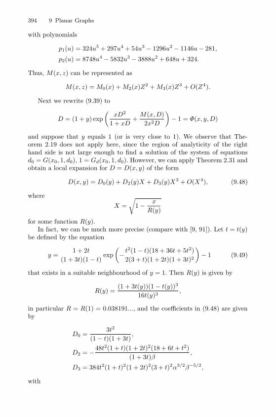
394 9 Planar Graphs
with polynomials
p1(u) = 324u5 + 297u4 + 54u3 − 1296u2 − 1146u− 281,
p2(u) = 8748u4 − 5832u3 − 3888u2 + 648u+ 324.
Thus, M(x, z) can be represented as
M(x, z) = M0(x) +M2(x)Z2 +M3(x)Z3 +O(Z4).
Next we rewrite (9.39) to
D = (1 + y) exp
(xD2
1 + xD+M(x,D)
2x2D
)− 1 = Φ(x, y,D)
and suppose that y equals 1 (or is very close to 1). We observe that The-orem 2.19 does not apply here, since the region of analyticity of the righthand side is not large enough to find a solution of the system of equationsd0 = G(x0, 1, d0), 1 = Gd(x0, 1, d0). However, we can apply Theorem 2.31 andobtain a local expansion for D = D(x, y) of the form
D(x, y) = D0(y) +D2(y)X +D3(y)X3 +O(X4), (9.48)
where
X =
√1− x
R(y)
for some function R(y).In fact, we can be much more precise (compare with [9, 91]). Let t = t(y)
be defined by the equation
y =1 + 2t
(1 + 3t)(1− t) exp
(− t
2(1− t)(18 + 36t+ 5t2)
2(3 + t)(1 + 2t)(1 + 3t)2
)− 1 (9.49)
that exists in a suitable neighbourhood of y = 1. Then R(y) is given by
R(y) =(1 + 3t(y))(1− t(y))3
16t(y)3,
in particular R = R(1) = 0.038191..., and the coefficients in (9.48) are givenby
D0 =3t2
(1− t)(1 + 3t),
D2 = −48t2(1 + t)(1 + 2t)2(18 + 6t+ t2)
(1 + 3t)β,
D3 = 384t2(1 + t)2(1 + 2t)2(3 + t)2α3/2β−5/2,
with
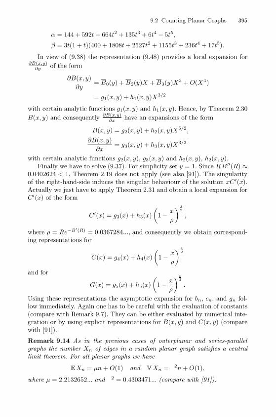
9.2 Counting Planar Graphs 395
α = 144 + 592t+ 664t2 + 135t3 + 6t4 − 5t5,
β = 3t(1 + t)(400 + 1808t+ 2527t2 + 1155t3 + 236t4 + 17t5).
In view of (9.38) the representation (9.48) provides a local expansion for∂B(x,y)
∂y of the form
∂B(x, y)
∂y= B0(y) +B2(y)X +B3(y)X3 +O(X4)
= g1(x, y) + h1(x, y)X3/2
with certain analytic functions g1(x, y) and h1(x, y). Hence, by Theorem 2.30
B(x, y) and consequently ∂B(x,y)∂x have an expansions of the form
B(x, y) = g2(x, y) + h2(x, y)X5/2,
∂B(x, y)
∂x= g3(x, y) + h3(x, y)X3/2
with certain analytic functions g2(x, y), g3(x, y) and h2(x, y), h2(x, y).Finally we have to solve (9.37). For simplicity set y = 1. Since RB ′′(R) ≈
0.0402624 < 1, Theorem 2.19 does not apply (see also [91]). The singularityof the right-hand-side induces the singular behaviour of the solution xC ′(x).Actually we just have to apply Theorem 2.31 and obtain a local expansion forC′(x) of the form
C′(x) = g3(x) + h3(x)
(1− x
ρ
) 32
,
where ρ = Re−B′(R) = 0.0367284..., and consequently we obtain correspond-ing representations for
C(x) = g4(x) + h4(x)
(1− x
ρ
) 52
and for
G(x) = g5(x) + h5(x)
(1− x
ρ
) 52
.
Using these representations the asymptotic expansion for bn, cn, and gn fol-low immediately. Again one has to be careful with the evaluation of constants(compare with Remark 9.7). They can be either evaluated by numerical inte-gration or by using explicit representations for B(x, y) and C(x, y) (comparewith [91]).
Remark 9.14 As in the previous cases of outerplanar and series-parallelgraphs the number Xn of edges in a random planar graph satisfies a centrallimit theorem. For all planar graphs we have
EXn = μn+O(1) and VXn = σ2n+O(1),
where μ = 2.2132652... and σ2 = 0.4303471... (compare with [91]).
396 9 Planar Graphs
9.3 Outerplanar Graphs
9.3.1 The Degree Distribution of Outerplanar Graphs
We already determined the degree distribution of several classes of randomtrees. We next show that such distributions exist for planar graphs, too. Recall,that we are interested in the limits
dk = limn→∞
dk;n,
where dk;n denotes the probability that a randomly chosen node in a randomplanar graph has degree k.
In fact there are two different points of view to this problem. First, if X(k)n
denotes the (random) number of vertices of degree k in a random planar graphof size n then
dk;n =EX
(k)n
n.
Second, we can change the model. Recall that we are considering unrootedlabelled combinatorial objects. Suppose that gn is the number of objects ofsize n. Then for each of these objects there are precisely n possible ways toroot these objects and we, thus, obtain ngn corresponding rooted objects. Nowthe probability that a random vertex (in the unrooted model) has degree kis precisely the same as the probability that the root vertex (in the rootedmodel) has degree k. Thus, if we are only interested in the degree distributionit is sufficient to look at the degree of the root. In what follows we will makeuse of both points of view. We will start by looking at the degree of the root(which is actually easier) and then we will have a closer look at the random
variable X(k)n . As a matter of fact these random variables (usually) obey a
central limit theorem with mean and variance asymptotically proportional ton. Of course, this is a much more precise statement than just the existence ofa degree distribution.
Before we start with the calculations we make some general remarks on themethods we use. Again, they are based on generating functions. Let Ck(x) bethe exponential generating function of a certain class4 of rooted vertex labelledconnected graphs, where the root bears no label and has degree k; that is, thecoefficient [xn/n!]Ck(x) equals the number of rooted connected graphs withn+ 1 vertices, in which the root has no label and has degree k. Analogouslywe define Bk(x) for 2-connected graphs. Also, let
B•(x,w) =∑
Bk(x)wk , C•(x,w) =∑
Ck(x)wk .
Suppose that we have the relation
4 In this context we can confine ourselves to outerplanar graphs, series-parallelgraphs or planar graphs.
9.3 Outerplanar Graphs 397
C′(x) = eB′(xC′(x))
between the generating function for 2-connected and connected graphs (whichis certainly true for outerplanar graphs, series-parallel graphs or planargraphs). If we introduce the degree of the root, then the equation becomes
C•(x,w) = eB•(xC′(x),w). (9.50)
The reason is that only the 2-connected components containing the root vertexcontribute to its degree.
Our goal in each case is to estimate [xn]Ck(x), since the limit probabilitythat a given fixed vertex has degree k is equal to
dk = limn→∞
[xn]Ck(x)
[xn]C′(x). (9.51)
Another observation is that the asymptotic degree distribution is the samefor connected members of a class than for all members in the class. Let G(x)be the generating function for all members of the class, and let Gk(x) be thegenerating function of all rooted graphs of the class, where the root has degreek. Then we have
G(x) = eC(x), Gk(x) = Ck(x)eC(x).
The first equation is standard, and in the second equation the factor Ck(x)corresponds to the connected component containing the root, and the secondfactor to the remaining components. The functions G(x) and C(x) have thesame dominant singularity. Given the singular expansions of G(x) and C(x)at the dominant singularity in each of the considered cases, it follows that
limn→∞
[xn]Gk(x)
[xn]G′(x)= lim
n→∞[xn]Ck(x)
[xn]C′(x).
Hence, in each case we only need to determine the degree distribution forconnected graphs. A more intuitive explanation is that the largest componentin random planar graphs eats up almost everything. It is a fact that theexpected number of vertices not in the largest component is constant [149].
As in the counting procedure of outerplanar graphs we discuss first dissec-tions and can then derive the results for 2-connected outerplanar graphs andfinally for connected graphs.
Recall that the generating function for dissections is given by
A(x) =1− 3x−
√1− 6x+ x2
4x, (9.52)
and let Ak(x) denote the generating function, where the root vertex (thefirst vertex of the rooted edge) has degree k and where the root vertices are
398 9 Planar Graphs
not counted by x. Then by using the recursive structure of dissections weimmediately get
A2(x) = x(A(x) + 1) + (x(A(x) + 1))2 + (x(A(x) + 1))3 + · · ·
=x(A(x) + 1)
1− x(A(x) + 1)
= x(2A(x) + 1).
Furthermore, we have inductively
Ak+1(x) = Ak(x)x(A(x) + 1) +Ak(x)(x(A(x) + 1))2 +Ak(x)(x(A(x) + 1))3 + · · ·= Ak(x)x(2A(x) + 1).
Consequently we obtain for k ≥ 2
Ak(x) = (x(2A(x) + 1))k−1.
Due to the general relation between dissections and 2-connected outerplanargraphs we have
Bk(x) =x
2Ak(x), k ≥ 2, B1 = x.
By summing a geometric series we have an explicit expression for B•, namely
B•(x,w) = xw +∞∑
k=2
xk
2(2A(x) + 1)k−1wk
= xw +xw2
2
x(2A(x) + 1)
1− x(2A(x) + 1)w. (9.53)
Theorem 9.15. For every k ≥ 2 the limiting probability dk that a vertex of atwo-connected outerplanar graph has degree k exists and we have
p(w) =∑k≥2
dkwk =
2(3− 2√
2)w2
(1 − (√
2− 1)w)2=∑k≥2
2(k − 1)(√
2− 1)kwk.
Moreover p(1) = 1, so that the dk are indeed a probability distribution.
Remark 9.16 The degree distribution of dissections is precisely the same asof outerplanar graphs (compare also with [13]).
Proof. Since B•(x, 1) = B′(x) and A(x) = 2(B′(x) − x)/x, we can representB•(x,w) as
B•(x,w) = xw +xw2
2
4B′(x)− 3x
1− (4B′(x) − 3x)w.
Hence, by applying Lemma 2.26 with f(x) = B′(x) and
9.3 Outerplanar Graphs 399
H(x, z) = xw +xw2
2
4z − 3x
1− (4z − 3x)w
we obtain
p(w) = limn→∞
[xn]B•(x,w)
[xn]B′(x)=
2(3− 2√
2)w2
(1− (√
2− 1)w)2.
Note that ρ = 3 − 2√
2 and that w is considered as an additional (complex)parameter.
Theorem 9.17. Let dk be the limit probability that a vertex of a connectedouterplanar graph has degree k. Then
p(w) =∑k≥1
dkwk = ρ · ∂
∂xeB
•(x,w)∣∣x=ρC′(ρ) ,
where B• is given by equations (9.52) and (9.53).Moreover p(1) = 1, so that the dk are indeed a probability distribution and
we have asymptotically, as k →∞
dk ∼ c1k1/4ec2
√kqk,
where c1 = 0.667187..., c2 = 0.947130..., and q = 0.3808138....
Proof. We have ∑k
Ck(x)wk = C•(x,w) = eB•(xC′(x),w).
The radius of convergence 3−2√
2 ofB(x) is larger than ρC ′(ρ) = τ ≈ 0.17076.Hence we can apply Lemma 2.26 f(x) = xC ′(x) and H(x,w, z) = xeB
•(z,w),where w is considered as a parameter. Then we have[
∂
∂xeB
•(x,w)
]x=ρC′(ρ)
= limn→∞
[xn]C•(x,w)
[xn]xC′(x)
= limn→∞
∑k≥1
ρ−1 [xn]Ck(x)
[xn]C′(x)wk
= ρ−1∑k≥1
dkwk,
and the result follows.For the second assertion let us note that B•(x, 1) = B′(x). If we recall
that ρC ′(ρ) = v0 and v0B′′(v0) = 1, then
p(1) = ρ eB′(v0)B′′(v0) = ρC ′(ρ)v−1
0 = 1.
In order to get an asymptotic expansion for dk we have to compute p(w)explicitly:
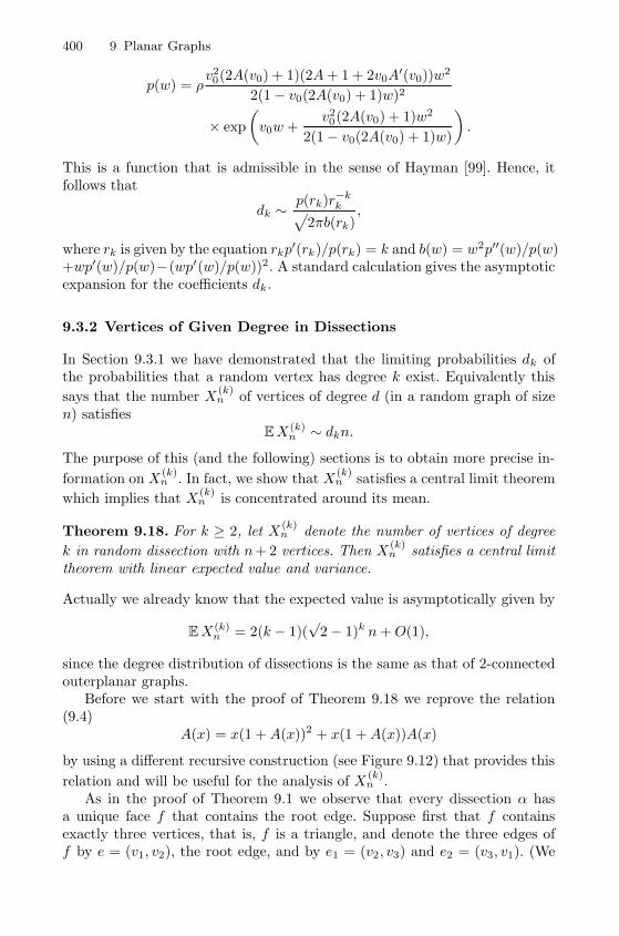
400 9 Planar Graphs
p(w) = ρv20(2A(v0) + 1)(2A+ 1 + 2v0A
′(v0))w2
2(1− v0(2A(v0) + 1)w)2
× exp
(v0w +
v20(2A(v0) + 1)w2
2(1− v0(2A(v0) + 1)w)
).
This is a function that is admissible in the sense of Hayman [99]. Hence, itfollows that
dk ∼p(rk)r−k
k√2πb(rk)
,
where rk is given by the equation rkp′(rk)/p(rk) = k and b(w) = w2p′′(w)/p(w)
+wp′(w)/p(w)−(wp′(w)/p(w))2. A standard calculation gives the asymptoticexpansion for the coefficients dk.
9.3.2 Vertices of Given Degree in Dissections
In Section 9.3.1 we have demonstrated that the limiting probabilities dk ofthe probabilities that a random vertex has degree k exist. Equivalently this
says that the number X(k)n of vertices of degree d (in a random graph of size
n) satisfiesEX(k)
n ∼ dkn.
The purpose of this (and the following) sections is to obtain more precise in-
formation on X(k)n . In fact, we show that X
(k)n satisfies a central limit theorem
which implies that X(k)n is concentrated around its mean.
Theorem 9.18. For k ≥ 2, let X(k)n denote the number of vertices of degree
k in random dissection with n+ 2 vertices. Then X(k)n satisfies a central limit
theorem with linear expected value and variance.
Actually we already know that the expected value is asymptotically given by
EX(k)n = 2(k − 1)(
√2− 1)k n+O(1),
since the degree distribution of dissections is the same as that of 2-connectedouterplanar graphs.
Before we start with the proof of Theorem 9.18 we reprove the relation(9.4)
A(x) = x(1 +A(x))2 + x(1 +A(x))A(x)
by using a different recursive construction (see Figure 9.12) that provides this
relation and will be useful for the analysis of X(k)n .
As in the proof of Theorem 9.1 we observe that every dissection α hasa unique face f that contains the root edge. Suppose first that f containsexactly three vertices, that is, f is a triangle, and denote the three edges off by e = (v1, v2), the root edge, and by e1 = (v2, v3) and e2 = (v3, v1). (We
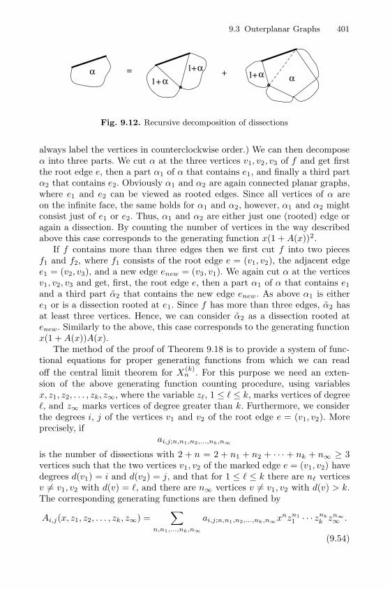
9.3 Outerplanar Graphs 401
+
++ α
= +1
11α
αα
α
Fig. 9.12. Recursive decomposition of dissections
always label the vertices in counterclockwise order.) We can then decomposeα into three parts. We cut α at the three vertices v1, v2, v3 of f and get firstthe root edge e, then a part α1 of α that contains e1, and finally a third partα2 that contains e2. Obviously α1 and α2 are again connected planar graphs,where e1 and e2 can be viewed as rooted edges. Since all vertices of α areon the infinite face, the same holds for α1 and α2, however, α1 and α2 mightconsist just of e1 or e2. Thus, α1 and α2 are either just one (rooted) edge oragain a dissection. By counting the number of vertices in the way describedabove this case corresponds to the generating function x(1 +A(x))2.
If f contains more than three edges then we first cut f into two piecesf1 and f2, where f1 consists of the root edge e = (v1, v2), the adjacent edgee1 = (v2, v3), and a new edge enew = (v3, v1). We again cut α at the verticesv1, v2, v3 and get, first, the root edge e, then a part α1 of α that contains e1and a third part α2 that contains the new edge enew. As above α1 is eithere1 or is a dissection rooted at e1. Since f has more than three edges, α2 hasat least three vertices. Hence, we can consider α2 as a dissection rooted atenew. Similarly to the above, this case corresponds to the generating functionx(1 +A(x))A(x).
The method of the proof of Theorem 9.18 is to provide a system of func-tional equations for proper generating functions from which we can read
off the central limit theorem for X(k)n . For this purpose we need an exten-
sion of the above generating function counting procedure, using variablesx, z1, z2, . . . , zk, z∞, where the variable z�, 1 ≤ � ≤ k, marks vertices of degree�, and z∞ marks vertices of degree greater than k. Furthermore, we considerthe degrees i, j of the vertices v1 and v2 of the root edge e = (v1, v2). Moreprecisely, if
ai,j;n,n1,n2,...,nk,n∞
is the number of dissections with 2 + n = 2 + n1 + n2 + · · · + nk + n∞ ≥ 3vertices such that the two vertices v1, v2 of the marked edge e = (v1, v2) havedegrees d(v1) = i and d(v2) = j, and that for 1 ≤ � ≤ k there are n� verticesv = v1, v2 with d(v) = �, and there are n∞ vertices v = v1, v2 with d(v) > k.The corresponding generating functions are then defined by
Ai,j(x, z1, z2, . . . , zk, z∞) =∑
n,n1,...,nk,n∞
ai,j;n,n1,n2,...,nk,n∞xnzn1
1 · · · znk
k zn∞∞ .
(9.54)
402 9 Planar Graphs
Similarly we define Ai,∞, A∞,j and A∞,∞, if one (or both) of the vertices ofthe root edge have degree(s) greater than k.
Note that z1 is not necessary, since there are no vertices of degree onein dissections. However, we use z1 for later purposes. Further observe thatAij(z1, z2, . . . , zk, z∞) = Aji(z1, z2, . . . , zk, z∞). Thus, it is sufficient to con-sider Aij for i ≤ j.
In order to state the following lemma in a more compact form we use theconvention that ∞ means > k, and ∞− 1 means > k − 1. In particular weset �+∞ = ∞ for all positive integers �.
Lemma 9.19. The generating functions Aij = Aji = Aij(x, z1, z2, . . . , zk, z∞),i, j ∈ {2, 3, . . . , k,∞} satisfy the following strongly connected positive systemof equations:
Aij = x∑
�1+�2≤k
z�1+�2Ai−1,�1Aj−1,�2 + xz∞
( ∑�1+�2>k
Ai−1,�1Aj−1,�2
)
+ x∑
�1+�2≤k+1
z�1+�2−1Ai−1,�1Aj,�2 + xz∞
( ∑�1+�2>k+1
Ai−1,�1Aj,�2
).
One has to be cautious in writing down the equations explicitly. For ex-ample we have
Ai,∞ = x∑
�1+�2≤k
z�1+�2Ai−1,�1(Ak,�2 + A∞,�2)
+ xz∞
( ∑�1+�2>k
Ai−1,�1(Ak,�2 +A∞,�2)
)+ x
∑�1+�2≤k+1
z�1+�2−1Ai−1,�1A∞,�2
+ xz∞
( ∑�1+�2>k+1
Ai−1,�1A∞,�2
).
As an illustration, for k = 3 we have the following system:
A22 = xz2
+ xz2A22 + xz3A23 + xz∞A2∞,
A23 = xz3A22 + xz∞(A23 +A2∞)
= xz2A23 + xz3A33 + xz∞A3∞,
A2∞ = xz3A23 + xz∞(A33 +A3∞) + xz∞(A2∞ +A3∞ +A∞,∞)
+ xz2A2∞ + xz3A3∞ + xz∞A∞,∞,
9.3 Outerplanar Graphs 403
A33 = xz∞(A22 +A23 +A2∞)2
+ xz∞(A22 +A23 +A2∞)(A23 +A33 +A3∞),
A3∞ = xz∞(A23 +A33 +A3∞)(A2∞ +A3∞ +A∞,∞)
+ xz∞(A22 +A23 +A2∞)(A2∞ +A3∞ +A∞,∞),
A∞,∞ = xz∞(A23 +A33 +A3∞ +A2∞ +A3∞ +A∞,∞)2
+ xz∞(A23 +A33 +A3∞ +A2∞ +A3∞ +A∞,∞)
× (A2∞ +A3∞ +A∞,∞).
Proof. The idea is to have a more detailed look at the (second version of the)recursive structure of A as described above (see Figure 9.12).
We only discuss the recurrence for Aij for finite i, j. If i = ∞ or j = ∞similar considerations apply. The root edge will be denoted by e = (v1, v2). Weassume that v1 has degree j and v2 has degree i. Again we have to distinguishbetween the case where the face f containing the root edge e has exactly threeedges, and the case where it has more than three edges.
In the first case we cut a dissection α at the three vertices v1, v2, v3 of fand get the root edge e, and two dissections α1 and α2 that are rooted ate1 = (v2, v3) and e2 = (v3, v1). After the cut, α1 has degree i−1 at v2, and α2
has degree j−1 at v1. Furthermore, the total degree of the common vertex v3is just the sum of the degrees coming from α1 and α2. Hence, if the degree ofv3 is smaller or equal than k, then this situation corresponds to the generatingfunction
x∑
�1+�2≤k
z�1+�2Ai−1,�1Aj−1,�2 .
Since all possible cases for α1 are encoded in Ai−1 = Ai−1,2 + · · ·+Ai−1,k +Ai−1,∞, and all cases for α2 are encoded in Aj−1, it follows that all situationswhere the total degree of v3 is greater than k are given by the generatingfunction
xz∞
( ∑�1+�2>k
Ai−1,�1Aj−1,�2
).
Similarly we argue in the case where f contains more than three edges.After cutting f into two pieces f1 and f2 with a new edge enew = (v3, v1),and cutting α at the vertices v1, v2, v3, we get again the root edge e and twodissections α1 and α2 that are rooted at e1 = (v2, v3), and at the new edgeenew = (v3, v1). After the cut, α1 has degree i− 1 at v2 and α2 has degree jat v1, since the new edge enew has to be taken into account. The total degreeof the common vertex v3 is the sum of the degrees coming from α1 and α2
minus 1, since the new edge enew is used in the construction of α2. As abovethese observations translate into the generating functions
x∑
�1+�2≤k+1
z�1+�2−1Ai−1,�1Aj,�2
404 9 Planar Graphs
and
xz∞
( ∑�1+�2>k+1
Ai−1,�1Aj,�2
).
Finally, by using the definition of Ai,j and A∞, it follows that the abovesystem of equations is a positive one, that is, all coefficients on the right handside are non-negative. Further, it is easy to check that the correspondingdependency graph is strongly connected (which means that no subsystem canbe solved before the whole system is solved).
The proof of Theorem 9.18 is now a direct application of the analyticcentral limit theorem related to systems of generating functions formulatedin Theorem 2.35. For this purpose we have to check that the assumptions aresatisfied. Note, that if we set all variables z1 = · · · = zk = z∞ = 1 and sum allfunction Ai,j then they sum up to A(x) which has a square root singularity atρ = 3− 2
√2. Thus, we can proceed as in the proof of Theorem 3.18 to show
that the assumptions of Theorem 2.35 are satisfied.In particular the function
Ad=k(x, u) =∑
2≤i≤∞Ai,i(x, 1, . . . , 1, u, 1) + 2
∑2≤i<j≤∞
Ai,j(x, 1, . . . , 1, u, 1)
is the bivariate generating function for dissections with n+ 2 vertices, wherethe exponent of u counts the number of vertices different from the root vertexthat has degree k. Of course, it is also possible to take the root vertex intoaccount by considering the function
Ad=k(x, u) = x2∑
2≤i≤∞,i�=k
Ai,i(x, 1, . . . , 1, u, 1) + x2u2Ak,k(x, 1, . . . , 1, u, 1)
+ 2x2∑
2≤i<j≤∞,i�=k,j �=k
Ai,i(x, 1, . . . , 1, u, 1)
+ 2x2u∑
2≤i≤∞,i�=k
Ai,k(x, 1, . . . , 1, u, 1).
For both versions we can apply Theorem 2.35 and obtain a central limit the-orem for the number of vertices of degree k.
9.3.3 Vertices of Given Degree in 2-Connected Outerplanar
Graphs
We consider now vertex labelled 2-connected outerplanar graphs. The resultwe obtain is exactly the same as for dissections.
Theorem 9.20. For k ≥ 2, let X(k)n denote the number of vertices of degree k
in a random 2-connected outerplanar graph with n vertices. Then X(k)n satisfies
a central limit theorem with linear expected value and variance.
9.3 Outerplanar Graphs 405
Recall that we already know that the expected value is asymptotically givenby
EX(k)n = 2(k − 1)(
√2− 1)k n+O(1).
For the proof we have to adapt the corresponding generating functions.Note that the generating function
B′(x) =∑n≥2
bnxn−1
(n− 1)!=∑n≥1
bn+1xn
n!
can also be interpreted as the exponential generating function B•(x) of 2-connected outerplanar graphs, where one vertex is marked and is not counted.
Next we set
B•j (x, z1, z2, . . . , zk, z∞) =∑
n,n1,...,nk,n∞
b•j;n,n1,...,nk,n∞xnzn1
1 · · · znk
k zn∞∞
n!,
where b•j;n,n1,...,nk,n∞ is the number of 2-connected outerplanar graphs with1+n = 1+n1 + · · ·+nk +n∞ vertices, where one vertex of degree j is markedand the remaining n vertices are labelled by 1, 2, . . . , n and where n� verticeshave degree �, 1 ≤ � ≤ k, and n∞ vertices have degree greater than k.
Lemma 9.21. Let Aij = Aji = Aij(x, z1, z2, . . . , zk, z∞), i, j ∈ {1, 2, . . . , k,∞}be defined by (9.54). Then the functions Bj = B•j (x, z1, z2, . . . , zk, z∞),j ∈ {1, 2, . . . , k,∞}, are given by
B•1 = xz1,
B•j =1
2
k∑i=1
xziAij +1
2xz∞Aj∞,
B•∞ =1
2
k∑i=1
xziAj∞ +1
2xz∞A∞,∞.
Proof. The proof is immediate by using the relation between dissections andouterplanar graphs. However, we have to take care of the vertex degrees.
Now let
Bd=k(x, u) =∑n,ν
b(k)n,ν
xn
n!uν
denote the exponential generating function of the numbers b(k)n,ν of 2-connected
outerplanar labelled graphs with n vertices, where ν vertices have degree k.Then we have
∂Bd=k(x, u)
∂x=
k−1∑j=1
B•j (x, 1, . . . , 1, u, 1) + uB•k(x, 1, . . . , 1, u, 1) (9.55)
+B•∞(x, 1, . . . , 1, u, 1).
406 9 Planar Graphs
Since B(0, u) = 0, this equation completely determines Bd=k(x, u).As in the case of dissections all assumptions of Theorem 2.35 are satisfied.
In particular we get a singular representation of the form
∂Bd=k(x, u)
∂x= g(x, u)− h(x, u)
√1− x
ρ(u)
and consequently a corresponding singular representation for Bd=k(x, u):
Bd=k(x, u) = g(x, u) + h(x, u)
(1− x
ρ(u)
) 32
.
Of course, this also implies a central limit theorem for X(k)n .
9.3.4 Vertices of Given Degree in Connected Outerplanar Graphs
The next theorem concerns connected outerplanar graphs. Since the result(even at the level of expectation and variance) is the same for all outerplanargraphs, we include this case, too.
Theorem 9.22. For k ≥ 2, let X(k)n denote the number of vertices of degree
k in random connected (or a general) outerplanar graph with n vertices. Then
X(k)n satisfies a central limit theorem with linear expected value and variance.
The proof uses a refined version of the general relation between rooted2-connected graphs and rooted connected graphs which states in terms ofgenerating functions as
C•(x) = eB•(xC•(x)). (9.56)
For this purpose we introduce the generating functions
C•j (x, z1, z2, . . . , zk, z∞) =∑
n,n1,...,nk,n∞
c•j;n;n1,...,nk,n∞zn11 · · · znk
k zn∞∞xn
n!,
j ∈ {1, 2, . . . , k,∞}, where c•j;n;n1,...,nk,n∞ is the number of connected outer-planar graphs with 1 + n = 1 + n1 + · · ·+ nk + n∞ vertices, where one vertexof degree j is marked5 and the remaining n vertices are labelled by 1, 2, . . . , nand where n� of these n vertices have degree �, 1 ≤ � ≤ k, and n∞ of thesevertices have degree greater than k. For convenience, we also define
C•0 (x, z1, z2, . . . , zk, z∞) = 1,
which corresponds to the case of a graph with a single rooted vertex.The main observation is that these functions satisfy a system of functional
equations, a refined version of (9.56).
5 If j = ∞ this has to be interpreted as a vertex of degree > k.
9.3 Outerplanar Graphs 407
Lemma 9.23. Let Wj = Wj(z1, . . . , zk, z∞, C•1 , . . . , C•k , C
•∞), j ∈ {1, 2, . . . , k,
∞} be defined by
Wj =
k−j∑i=0
zi+jC•i (x, z1, . . . , zk, z∞)
+ z∞
⎛⎝ k∑i=k−j+1
C•i (x, z1, . . . , zk, z∞) + C•∞(x, z1, . . . , zk, z∞)
⎞⎠ ,(1 ≤ j ≤ k),
W∞ = z∞
(k∑
i=0
C•i (x, z1, . . . , zk, z∞) + C•∞(x, z1, . . . , zk, z∞)
).
Then the functions C•1 , . . . , C•k , C
•∞ satisfy the system of equations
C•j (x, z1, . . . , zk, z∞) =∑
�1+2�2+3�3+···j�j=j
j∏r=1
B•r (x,W1, . . . ,Wk,W∞)�r
�r!
(1 ≤ j ≤ k),
C•∞(x, z1, . . . , zk, z∞) = exp
(k∑
j=1
B•j (x,W1, . . . ,Wk,W∞)
+B•∞(x,W1, . . . ,Wk,W∞)
)− 1
−∑
1≤�1+2�2+3�3+···k�k≤k
k∏r=1
B•r (x,W1, . . . ,Wk,W∞)�r
�r!.
Proof. As already indicated, the proof is a refined version of the proof of(9.56), which reflects the decomposition of a rooted connected graph into afinite set of rooted 2-connected graphs, where every vertex (different from theroot) is substituted by a rooted connected graph. The functions Wj serve thepurpose of marking (recursively) the degree of the vertices in the 2-connectedblocks which are substituted by other graphs. If we look at the definition ofWj , the summation means that we are substituting a vertex of degree i, butsince originally the vertex had degree j, we are creating a new vertex of degreei+ j, which is marked accordingly by zi+j . The same remark applies to W∞.
Finally let
Cd=k(x, u) =∑n,ν
c(k)n,ν
xn
n!uν
denote the exponential generating function for the numbers c(k)n,� of connected
outerplanar vertex labelled graphs with n vertices, where ν vertices have de-gree k. Then we have
408 9 Planar Graphs
∂Cd=k(x, u)
∂x=
k−1∑j=1
C•j (x, 1, . . . , 1, u, 1) + uC•k(x, 1, . . . , 1, u, 1) (9.57)
+ C•∞(x, 1, . . . , 1, u, 1).
Since C(0, u) = 0, this equation completely determines Cd=k(x, u).
Thus, the derivative ∂Cd=k(x,u)∂x is a linear combination of functions C•j (x, z1,
. . . , zk, z∞) that satisfy a positive and strongly connected system of equations.Note that the system of equations given in Lemma 9.23 uses the functionsB•j (x, z1, . . . , zk, z∞), that have a square-root singularity if the zj are suffi-ciently close to 1; recall that B′(x) and B•j (x, 1, . . . , 1) have a square-root
singularity at ρ1 = 3 − 2√
2. In order to apply Theorem 2.35 we have tocheck that the critical point of the system (9.57) does not interfere with thesquare-root singularity of B•j .
We already know that the radius of convergence of C ′(x) is given by ρ2 =0.1366 · · · which satisfies ρ2C
′(ρ2) < ρ1 so that the singularity of B′(x) doesnot interfere with the singularity of C ′(x); recall that xC ′(x) = xeB
′(xC′(x)).We are again in a situation, where we can apply Theorem 2.35 (we can
argue in the same way as in the proof of Theorem 3.18 or Theorem 9.18). Inparticular we get a singular representation of the form
∂Cd=k(x, u)
∂x= g(x, u)− h(x, u)
√1− x
ρ2(u)
and consequently a corresponding singular representation for Cd=k(x, u):
Cd=k(x, u) = g(x, u) + h(x, u)
(1− x
ρ2(u)
) 32
(9.58)
which implies a central limit theorem for X(k)n .
Finally, we obtain a corresponding representation for the generating func-tion of Gd=k(x, u) for all outerplanar graphs of the form
Gd=k(x, u) = eCd=k(x,u) = g(x, u) + h(x, u)
(1− x
ρ2(u)
)3/2
(9.59)
and a central limit theorem in this case, too.
9.4 Series-Parallel Graphs
9.4.1 The Degree Distribution of Series-Parallel Graphs
In this section C(x) and B(x) denote the generating functions of connectedand 2-connected, respectively, series-parallel graphs.
9.4 Series-Parallel Graphs 409
In order to study 2-connected series-parallel graphs, we need to considerseries-parallel networks. We recall that a network is a graph with two distin-guished vertices, called poles, such that the multi-graph obtained by adding anedge between the two poles is 2-connected. Let D(x, y, w) be the exponentialgenerating function of series-parallel networks, where x, y, w mark, respec-tively, vertices, edges, and the degree of the first pole. We define S(x, y, w)analogously for series networks. Then we have
D(x, y, w) = (1 + yw)eS(x,y,w) − 1, (9.60)
S(x, y, w) = (D(x, y, w)− S(x, y, w)) xD(x, y, 1). (9.61)
The first equation reflects the fact that a network is a parallel compositionof series networks, and the second one the fact that a series network is ob-tained by connecting a non-series network with an arbitrary network; thefactor D(x, y, 1) appears because we only keep track of the degree of the firstpole.
Remark 9.24 It would not be necessary to take into account the number ofedges and we could set y = 1 everywhere. However, in the case of planargraphs we do need generating functions according to all three variables and itis appropriate to present the full development already here. In the proof of themain result of this section, Theorem 9.29, we just set y = 1.
We also set E(x, y) = D(x, y, 1) that is the generating function for series-parallel networks without marking the degree of the root. Then from (9.60)–(9.61) we obtain the equations
log
(1 +E(x, y)
1 + y
)=
xE(x, y)2
1 + xE(x, y)(9.62)
and
log
(1 +D(x, y, w)
1 + yw
)=xE(x, y)D(x, y, w)
1 + xE(x, y). (9.63)
Let now B•k(x, y) be the generating function for 2-connected series-parallelgraphs, where the root bears no label and has degree k, and where y marksedges. Then we have the following relation.
Lemma 9.25.
w∂B•(x, y, w)
∂w=∑k≥1
kB•k(x, y)wk = xyweS(x,y,w).
Proof. The sum counts rooted 2-connected graphs with a distinguished edgeincident to the root. By definition this is precisely the set of networks contain-ing an edge between the poles. The degree of the root in a 2-connected graphcorresponds to the degree of the first pole in the corresponding network, hencethe equation follows.
410 9 Planar Graphs
From the previous equation it follows that
B•(x, y, w) = xy
∫ w
0
eS(x,y,s)ds. (9.64)
From an analytic point of view it would be sufficient to work with this equa-tion. However, if we are interested in more or less explicit formulas for thedegree distribution we have to remove the integral and to express B• in termsof D. Recall that E(x, y) = D(x, y, 1).
Lemma 9.26. The generating function of rooted 2-connected series-parallelgraphs is equal to
B•(x, y, w) = x
(D(x, y, w)− xE(x, y)
1 + xE(x, y)D(x, y, w)
(1 +
D(x, y, w)
2
)).
Proof. We start by using (9.60) to obtain∫eSdw =
∫1 +D
1 + ywdw = y−1 log(1 + yw) +
∫D
1 + ywdw.
Now we integrate by parts and derive at∫D
1 + ywdw = y−1 log(1 + yw)D −
∫y−1 log(1 + yw)
∂D
∂wdw.
For the last integral we change variables t = D(x, y, w) and use the fact thatlog(1 + yw) = log(1 + t)− xEt/(1 + xE). Consequently we obtain∫
log(1 + yw)∂D
∂wdw =
∫ D
0
log(1 + t) dt− xE
1 + xE
∫ D
0
t dt.
Now everything can be integrated in closed form and, after a simple manipu-lation, we obtain the result as claimed.
Next we analyse the singular structure of the above generating functions.We start with E(x, y) = D(x, y, 1) and D(x, y, w).
Lemma 9.27. For |w| ≤ 1 and for fixed y (sufficiently close to 1) the dom-inant singularity of the functions E(x, y), D(x, y, w), and B•(x, y, w) (con-sidered as functions in x) is given by x = R(y), where R(y) is an analyticfunction in y with R = R(1) ≈ 0.1280038. Furthermore, we have the followinglocal expansion:
E(x, y) = E0(y) +E1(y)X +E2(y)X2 + · · · ,D(x, y, w) = D0(y, w) +D1(y, w)X +D2(y, w)X2 + · · · ,B•(x, y, w) = B0(y, w) +B1(y, w)X +B2(y, w)X2 + · · · ,
9.4 Series-Parallel Graphs 411
where X =√
1− x/R(y).The functions R(y), Ej(y), Dj(y, w), and Bj(y, w) are analytic in y and
w and satisfy the relations
E0(y)3
E0(y)− 1=
(log
1 +E0(y)
1 +R(y)−E0(y)
)2
,
R(y) =
√1− 1/E0(y)− 1
E0(y),
E1(y) = −(
2R(y)E0(y)2(1 +R(y)E0(y))2
(2R(y)E0(y) +R(y)2E0(y)2)2 + 2R(y)(1 +R(y)E0(y))
)1/2
,
D0(y, w) = (1 + yw) exp
(R(y)E0(y)
1 +R(y)E0(y)D0(y, w)
)− 1,
D1(y, w) = − D0(y, w)E1(y)R(y)(D0(y, w) + 1)
(R(y)E0(y)D0(y, w)− 1)(1 +R(y)E0(y)),
B0(y, w) = −R(y)D0(y, w)(R(y)E0(y)D0(y, w)− 2)
2(1 +R(y)E0(y)),
B1(y, w) =E1(y)R(y)2D0(y, w)2
2(1 +R(y)E0(y))2.
Proof. Since E(x, y) satisfies Equation (9.62), it follows that the dominantsingularity of the mapping x �→ E(x, y) is of square-root type and there isan expansion of the form E(x, y) = E0(y) + E1(y)X + E2(y)X2 + · · · (withX =√
1− x/R(y)), where R(y) and Ej(y) are analytic in y. Furthermore, ifwe set
Φ(x, y, z) = (1 + y) exp
(xz2
1 + xz
)− 1
then R(y) and E0(y) satisfy the two equations
Φ(R(y), y, E0(y)) = E0(y) and Φz(R(y), y, E0(y)) = 0
and E1(y) is then given by
E1(y) = −(
2R(y)Φx(R(y), y, E0(y))
Φzz(R(y), y, E0(y))
)1/2
(compare with Theorem 2.19).Next notice that for |w| ≤ 1 the radius of convergence of the function
x �→ D(x, y, w) is surely ≥ |R(y)|. However, D(x, y, w) satisfies Equation(9.63), which implies that the dominant singularity of E(x, y) leads to thatof D(x, y, w). Thus, the mapping x �→ D(x, y, w) has dominant singularityR(y) and it also follows that D(x, y, w) has a singular expansion of the formD(x, y, w) = D0(y, w)+D1(y, w)X+D2(y, w)X2+· · · . Hence, by Lemma 9.25we also get an expansion for B•(x, y, w) of that form.
Finally the relations forD0, D1 andB0, B1 follow by comparing coefficientsin the corresponding expansions.
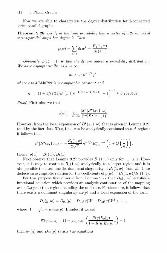
412 9 Planar Graphs
Now we are able to characterise the degree distribution for 2-connectedseries parallel graphs.
Theorem 9.28. Let dk be the limit probability that a vertex of a 2-connectedseries-parallel graph has degree k. Then
p(w) =∑k≥1
dkwk =
B1(1, w)
B1(1, 1).
Obviously, p(1) = 1, so that the dk are indeed a probability distribution.We have asymptotically, as k →∞,
dk ∼ c · k−3/2qk,
where c ≈ 3.7340799 is a computable constant and
q =(
(1 + 1/(R(1)E0(1))) e−1/(1+R(1)E0(1)) − 1)−1
≈ 0.7620402.
Proof. First observe that
p(w) = limn→∞
[xn]B•(x, 1, w)
[xn]B•(x, 1, 1).
However, from the local expansion of B•(x, 1, w) that is given in Lemma 9.27(and by the fact that B•(x, 1, w) can be analytically continued to a Δ-region)it follows that
[xn]B•(x, 1, w) = −B1(1, w)
2√π
n−3/2R(1)−n
(1 +O
(1
n
)).
Hence, p(w) = B1(w)/B1(1).Next observe that Lemma 9.27 provides B1(1, w) only for |w| ≤ 1. How-
ever, it is easy to continue B1(1, w) analytically to a larger region and it isalso possible to determine the dominant singularity of B1(1, w), from which wededuce an asymptotic relation for the coefficients of p(w) = B1(1, w)/B1(1, 1).
For this purpose first observe from Lemma 9.27 that D0(y, w) satisfies afunctional equation which provides an analytic continuation of the mappingw �→ D0(y, w) to a region including the unit disc. Furthermore, it follows thatthere exists a dominant singularity w0(y) and a local expansion of the form
D0(y, w) = D00(y) +D01(y)W +D02(y)W 2 + · · · ,
where W =√
1− w/w0(y). Besides, if we set
Ψ(y, w, z) = (1 + yw) exp
(R(y)E0(y)
1 +R(y)E0(y)z
)− 1
then w0(y) and D00(y) satisfy the equations
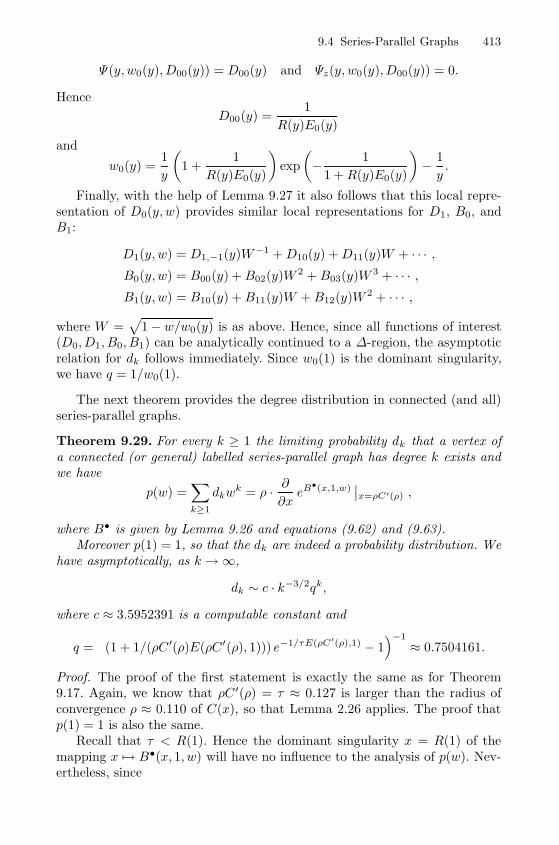
9.4 Series-Parallel Graphs 413
Ψ(y, w0(y), D00(y)) = D00(y) and Ψz(y, w0(y), D00(y)) = 0.
Hence
D00(y) =1
R(y)E0(y)
and
w0(y) =1
y
(1 +
1
R(y)E0(y)
)exp
(− 1
1 +R(y)E0(y)
)− 1
y.
Finally, with the help of Lemma 9.27 it also follows that this local repre-sentation of D0(y, w) provides similar local representations for D1, B0, andB1:
D1(y, w) = D1,−1(y)W−1 +D10(y) +D11(y)W + · · · ,B0(y, w) = B00(y) +B02(y)W 2 + B03(y)W 3 + · · · ,B1(y, w) = B10(y) +B11(y)W +B12(y)W 2 + · · · ,
where W =√
1− w/w0(y) is as above. Hence, since all functions of interest(D0, D1, B0, B1) can be analytically continued to a Δ-region, the asymptoticrelation for dk follows immediately. Since w0(1) is the dominant singularity,we have q = 1/w0(1).
The next theorem provides the degree distribution in connected (and all)series-parallel graphs.
Theorem 9.29. For every k ≥ 1 the limiting probability dk that a vertex ofa connected (or general) labelled series-parallel graph has degree k exists andwe have
p(w) =∑k≥1
dkwk = ρ · ∂
∂xeB
•(x,1,w)∣∣x=ρC′(ρ) ,
where B• is given by Lemma 9.26 and equations (9.62) and (9.63).Moreover p(1) = 1, so that the dk are indeed a probability distribution. We
have asymptotically, as k →∞,
dk ∼ c · k−3/2qk,
where c ≈ 3.5952391 is a computable constant and
q =(
(1 + 1/(ρC ′(ρ)E(ρC ′(ρ), 1))) e−1/τE(ρC′(ρ),1) − 1)−1
≈ 0.7504161.
Proof. The proof of the first statement is exactly the same as for Theorem9.17. Again, we know that ρC ′(ρ) = τ ≈ 0.127 is larger than the radius ofconvergence ρ ≈ 0.110 of C(x), so that Lemma 2.26 applies. The proof thatp(1) = 1 is also the same.
Recall that τ < R(1). Hence the dominant singularity x = R(1) of themapping x �→ B•(x, 1, w) will have no influence to the analysis of p(w). Nev-ertheless, since
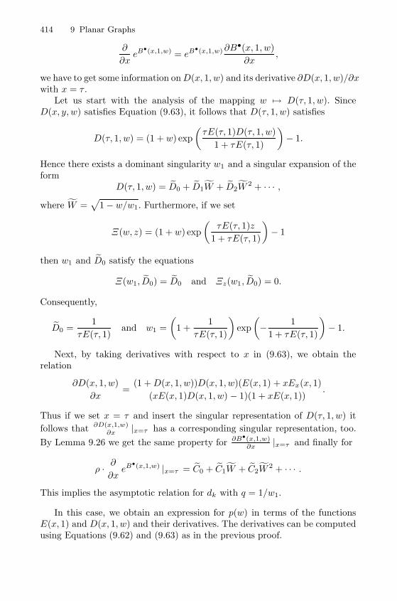
414 9 Planar Graphs
∂
∂xeB
•(x,1,w) = eB•(x,1,w) ∂B
•(x, 1, w)
∂x,
we have to get some information onD(x, 1, w) and its derivative ∂D(x, 1, w)/∂xwith x = τ .
Let us start with the analysis of the mapping w �→ D(τ, 1, w). SinceD(x, y, w) satisfies Equation (9.63), it follows that D(τ, 1, w) satisfies
D(τ, 1, w) = (1 + w) exp
(τE(τ, 1)D(τ, 1, w)
1 + τE(τ, 1)
)− 1.
Hence there exists a dominant singularity w1 and a singular expansion of theform
D(τ, 1, w) = D0 + D1W + D2W2 + · · · ,
where W =√
1− w/w1. Furthermore, if we set
Ξ(w, z) = (1 + w) exp
(τE(τ, 1)z
1 + τE(τ, 1)
)− 1
then w1 and D0 satisfy the equations
Ξ(w1, D0) = D0 and Ξz(w1, D0) = 0.
Consequently,
D0 =1
τE(τ, 1)and w1 =
(1 +
1
τE(τ, 1)
)exp
(− 1
1 + τE(τ, 1)
)− 1.
Next, by taking derivatives with respect to x in (9.63), we obtain therelation
∂D(x, 1, w)
∂x=
(1 +D(x, 1, w))D(x, 1, w)(E(x, 1) + xEx(x, 1)
(xE(x, 1)D(x, 1, w) − 1)(1 + xE(x, 1)).
Thus if we set x = τ and insert the singular representation of D(τ, 1, w) it
follows that ∂D(x,1,w)∂x |x=τ has a corresponding singular representation, too.
By Lemma 9.26 we get the same property for ∂B•(x,1,w)∂x |x=τ and finally for
ρ · ∂∂xeB
•(x,1,w) |x=τ = C0 + C1W + C2W2 + · · · .
This implies the asymptotic relation for dk with q = 1/w1.
In this case, we obtain an expression for p(w) in terms of the functionsE(x, 1) and D(x, 1, w) and their derivatives. The derivatives can be computedusing Equations (9.62) and (9.63) as in the previous proof.
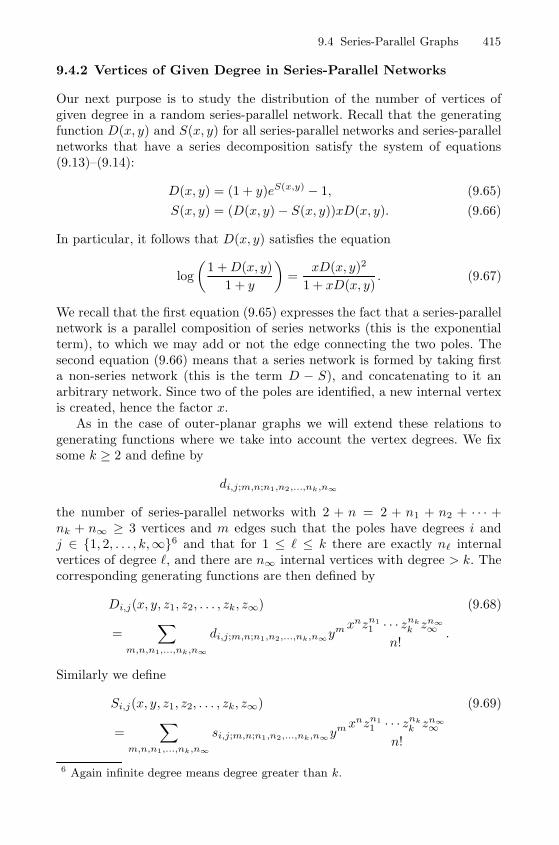
9.4 Series-Parallel Graphs 415
9.4.2 Vertices of Given Degree in Series-Parallel Networks
Our next purpose is to study the distribution of the number of vertices ofgiven degree in a random series-parallel network. Recall that the generatingfunction D(x, y) and S(x, y) for all series-parallel networks and series-parallelnetworks that have a series decomposition satisfy the system of equations(9.13)–(9.14):
D(x, y) = (1 + y)eS(x,y) − 1, (9.65)
S(x, y) = (D(x, y)− S(x, y))xD(x, y). (9.66)
In particular, it follows that D(x, y) satisfies the equation
log
(1 +D(x, y)
1 + y
)=
xD(x, y)2
1 + xD(x, y). (9.67)
We recall that the first equation (9.65) expresses the fact that a series-parallelnetwork is a parallel composition of series networks (this is the exponentialterm), to which we may add or not the edge connecting the two poles. Thesecond equation (9.66) means that a series network is formed by taking firsta non-series network (this is the term D − S), and concatenating to it anarbitrary network. Since two of the poles are identified, a new internal vertexis created, hence the factor x.
As in the case of outer-planar graphs we will extend these relations togenerating functions where we take into account the vertex degrees. We fixsome k ≥ 2 and define by
di,j;m,n;n1,n2,...,nk,n∞
the number of series-parallel networks with 2 + n = 2 + n1 + n2 + · · · +nk + n∞ ≥ 3 vertices and m edges such that the poles have degrees i andj ∈ {1, 2, . . . , k,∞}6 and that for 1 ≤ � ≤ k there are exactly n� internalvertices of degree �, and there are n∞ internal vertices with degree > k. Thecorresponding generating functions are then defined by
Di,j(x, y, z1, z2, . . . , zk, z∞) (9.68)
=∑
m,n,n1,...,nk,n∞
di,j;m,n;n1,n2,...,nk,n∞ymx
nzn11 · · · znk
k zn∞∞
n!.
Similarly we define
Si,j(x, y, z1, z2, . . . , zk, z∞) (9.69)
=∑
m,n,n1,...,nk,n∞
si,j;m,n;n1,n2,...,nk,n∞ymx
nzn11 · · · znk
k zn∞∞
n!
6 Again infinite degree means degree greater than k.
416 9 Planar Graphs
where we count series-parallel networks that have a series decomposition intoat least two series-parallel networks.
The next lemma provides a system of equations for Di,j and Si,j . Again,in order to state the results in a more compact form we use the conventionthat ∞ means > k and ∞− 1 means > k− 1, in particular we set �+∞ = ∞for all positive integers �.
Lemma 9.30. The generating functions Dij = Di,j(x, y, z1, z2, . . . , zk, z∞)and Sij = Si,j(x, y, z1, z2, . . . , zk, z∞), i, j ∈ {1, . . . , k,∞}, satisfy the fol-lowing system of equations:
Di,j =∑r≥1
∑i1+···+ir=i
∑j1+···+jr=j
1
r!
r∏�=1
Si�,j�(9.70)
+ y∑r≥1
∑i1+···+ir=i−1
∑j1+···+jr=j−1
1
r!
r∏�=1
Si�,j�
Si,j = x∑
�1+�2≤k
(Di,�1 − Si,�1)z�1+�2D�2,j + xz∞∑
�1+�2>k
(Di,�1 − Si,�1)D�2,j .
(9.71)
Proof. This is a refinement of the counting procedure that leads to the sys-tem (9.65) and (9.66). The first equation means that a series-parallel networkwith degrees i and j at the poles is obtained by parallel composition of seriesnetworks whose degrees at the left and right pole sum up to i and j, respec-tively; one has to distinguish according to whether the edge between the polesis added or not.
The second equation reflects the series composition. In this case only thedegrees of the right pole in the first network and of the left pole in the secondnetwork have to be added.
Remark 9.31 The system provided in Lemma 9.30 is not a positive systemsince the equation for Si,j contains negative terms. However, we can replacethe term Di,�1 by the right hand side of (9.70). Further, note that Si,�1 appearsin this sum so that we really achieve a positive system.
Finally, it is easy to see that this (new) system is strongly connected.
9.4.3 Vertices of Given Degree in 2-Connected Series-Parallel
Graphs
The next theorem concerns 2-connected series-parallel graphs.
Theorem 9.32. For k ≥ 2, let X(k)n denote the number of vertices of degree
k in a random 2-connected labelled series-parallel graph with n vertices. Then
X(k)n satisfies a central limit theorem with linear expected value and variance.
9.4 Series-Parallel Graphs 417
Let bn,m be the number of 2-connected vertex labelled series-parallelgraphs with n vertices and m edges and let
B(x, y) =∑n,m
bn,mxn
n!ym
be the corresponding exponential generating function. By the definition ofseries-parallel networks we have
∂B(x, y)
∂y=x2
2eS(x,y). (9.72)
Note that 2 ∂B(x,y)∂y can be interpreted as the generating function of 2-
connected series-parallel graphs with a rooted and directed edge. We nowalso take into account the degrees of the vertices. In particular let Bi,j =Bi,j(x, y, z1, . . . , zk, z∞), i, j ∈ {2, . . . , k,∞}, denote the exponential generat-ing function of 2-connected series-parallel graphs with a directed rooted edge,where the two root vertices have degrees i and j.7 The directed root edgeconnects the root vertex of degree i with the other root vertex of degree j.
Furthermore, let Bi = Bi(x, y, z1, . . . , zk, z∞), i ∈ {2, . . . , k,∞}, be thegenerating function of 2-connected series-parallel graphs where we just rootat one vertex that has degree i (and where no edge is rooted). Finally, let B =B(x, y, z1, . . . , zk, z∞) be the generating function of all 2-connected series-parallel graphs.
The next lemma quantifies the relation between series-parallel networksand 2-connected series-parallel graphs. As above we use the convention that∞ means > k and ∞− 1 means ≥ k − 1, in particular we set �+∞ = ∞ forall positive integers �.
Lemma 9.33. We have
Bi,j = x2zizjy∑r≥1
∑i1+···+ir=i−1
∑j1+···+jr=j−1
1
r!
r∏�=1
Si�,j�,
Bi =1
i
k∑j=2
Bi,j +1
iBi,∞ (i ∈ {2, . . . , k})
B∞ = x∂B
∂x−
k∑i=2
Bi
2y∂B
∂y=∑
i,j∈{2,...,k,∞}Bi,j ,
x∂B
∂x=∑
i∈{2,...,k,∞}Bi.
7 As above we interpret ∞ as > k.
418 9 Planar Graphs
Proof. The first equation is essentially a refinement of the relation (9.72).It means that 2-connected series-parallel graphs are formed by taking paral-lel compositions of series-parallel networks and adding the edge between thepoles. The sum of the degrees of the poles in the networks must be one lessthan the degree of the resulting vertex in the series-parallel graph.
The second equation reflects the fact that a series-parallel graph rooted ata vertex of degree i comes from a series-parallel graph rooted at an edge whosefirst vertex has degree i, but then each of them has been counted i times. Theremaining equations are clear if we recall that x∂B/∂x corresponds to graphsrooted at a vertex and y∂B/∂y corresponds to graphs rooted at an edge (inthis last case the factor 2 appears because in the definition of Bi,j the rootedge is directed).
Let
Bd=k(x, u) =∑n,ν
b(k)n,ν
xn
n!uν
denote the exponential generating function for the numbers b(k)n,ν that count the
number of 2-connected vertex labelled series-parallel graphs with n vertices,where ν vertices have degree k. Then we have
Bd=k(x, u) = B(x, 1, 1, . . . , 1, u, 1).
We are now ready to prove Theorem 9.32. We first observe that the func-tion Dij and Sij satisfy a positive and strongly connected system of equations(Lemma 9.30), so that by Theorem 2.19 all these functions have a commonsquare-root singularity of the kind
g(x, y, z1, . . . , zk, z∞)− h(x, y, z1, . . . , zk, z∞)
√1− x
ρ(y, z1, . . . , zk, z∞).
(9.73)Hence, by Lemma 2.26 the same is true for all functions Bij and conse-
quently for
2y∂B
∂y=∑
i,j∈{2,...,k,∞}Bij .
From Theorem 2.30 it follows that B has a singularity of the kind
g(x, y, z1, . . . , zk, z∞) + h(x, y, z1, . . . , zk, z∞)
(1− x
ρ(z1, . . . , zk, z∞)
)3/2
.
(9.74)As a consequence, by applying Theorem 2.25 we derive Theorem 9.32 for the2-connected case.
Note that B1, . . . Bk also have a square-root singularity of the kind (9.73),since they can be expressed with the help of the function Bij . Interestingly,B∞ has the same kind of singularity. This follows from the formula
9.4 Series-Parallel Graphs 419
B∞ = x∂B
∂x−
k∑i=1
Bi,
since ∂B∂x also has a square-root singularity of the kind (9.73).
9.4.4 Vertices of Given Degree in Connected Series-Parallel
Graphs
Finally we also have a central limit theorem for the number of vertices of givendegree in connected (and all) series-parallel graphs.
Theorem 9.34. For k ≥ 2, let X(k)n denote the number of vertices of degree
k in a random connected (or general) labelled series-parallel graph with n
vertices. Then X(k)n satisfies a central limit theorem with linear expected value
and variance.
For the proof we introduce the generating function
Cj(x, y, z1, z2, . . . , zk, z∞)
=∑
m,n,n1,...,nk,n∞
cj;m,n;n1,...,nk,n∞ ym xnzn1
1 · · · znk
k zn∞∞
n!,
j ∈ {1, 2, . . . , k,∞}, where cj;m,n,n1,...,nk,n∞ is the number of labelled seriesparallel graphs with n = n1 + · · ·+ nk + n∞ vertices and m edges, where onevertex of degree j is marked and where n� of these n vertices have degree �,1 ≤ � ≤ k, and n∞ of these vertices have degree greater than k. Further set
B•j (x, y, z1, z2, . . . , zk, z∞) =1
xzjBj(x, y, z1, z2, . . . , zk, z∞)
and
C•j (x, y, z1, z2, . . . , zk, z∞) =1
xzjCj(x, y, z1, z2, . . . , zk, z∞).
Then B•j and C•j have the same interpretation as in the case of outerplanargraphs. Hence we get the same relations as stated in Lemma 9.23. The onlydifference is that we also take the number of edges into account, that is, wehave an additional variable y.
Lemma 9.35. Let Wj = Wj(z1, . . . , zk, z∞, C•1 , . . . , C•k , C
•∞), j ∈ {1, 2, . . . , k,
∞}, be defined by
Wj =
k−j∑i=0
zi+jC•i (x, y, z1, . . . , zk, z∞)
+ z∞
⎛⎝ k∑i=k−j+1
C•i (x, y, z1, . . . , zk, z∞) + C•∞(x, y, z1, . . . , zk, z∞)
⎞⎠ ,(1 ≤ j ≤ k),
420 9 Planar Graphs
W∞ = z∞
(k∑
i=0
C•i (x, y, z1, . . . , zk, z∞) + C•∞(x, y, z1, . . . , zk, z∞)
).
Then the functions C•1 , . . . , C•k , C
•∞ satisfy the system of equations
C•j (x, y, z1, . . . ,zk, z∞)
=∑
�1+2�2+3�3+···+j�j=j
j∏r=1
B•r (x, y,W1, . . . ,Wk,W∞)�r
�r!
(1 ≤ j ≤ k),
C•∞(x, y, z1, . . . ,zk, z∞) = exp
(k∑
j=1
B•j (x, y,W1, . . . ,Wk,W∞)
+B•∞(x, y,W1, . . . ,Wk,W∞)
)− 1
−∑
1≤�1+2�2+3�3+···+k�k≤k
k∏r=1
B•r (x, y,W1, . . . ,Wk,W∞)�r
�r!.
Consequently the generating function Cd=k(x, u) (of the numbers c(k)n,ν that
count the number of connected vertex labelled series-parallel graphs with nvertices, where ν vertices have degree k) is given by
∂Cd=k(x, u)
∂x=
k−1∑j=1
C•j (x, 1, 1, . . . , 1, u, 1) + uC•k(x, 1, 1, . . . , 1, u, 1)
+ C•∞(x, 1, 1, . . . , 1, u, 1)
and the generation function Gd=k(x, u) for all series-parallel graphs by
Gd=k(x, u) = eCd=k(x,u).
The proof of Theorem 9.34 is exactly the same as in the outerplanar case.The essential point is to observe that the singularity of B•i does not interferewith the singularity of C•j . Thus, we can safely apply Theorem 2.35.
As in the outerplanar case it follows that Cd=k(x, u) has a singularity ofthe kind (9.58). Hence, the same follows for Gd=k(x, u) and, thus, we canapply Theorem 2.25.
9.5 All Planar Graphs
The goal of this section is to characterise the degree distribution of labelledplanar graphs. For this purpose we have to find the generating function of
9.5 All Planar Graphs 421
3-connected planar graphs according to the degree of the root. We will alsodiscuss the distribution of the number of vertices of degree k = 1 and k = 2.The case k ≥ 3 cannot be covered with the present methodology since thecounting procedure for 3-connected planar graphs that is used here cannot beextended in order to take care of all vertices of given degree.
From now on (and for the rest of Chapter 9) all generating functions areassociated to planar graphs.
9.5.1 The Degree of a Rooted Vertex
We will now repeat (more or less) the counting procedure for labelled planargraphs, where we also take care of the degree of a rooted vertex.
Theorem 9.36. Let b•n,m,k denote the number of vertex-rooted 2-connected la-belled planar graphs with n vertices, m edges and root-degree k, and c•n,m,k andg•n,m,k the corresponding numbers for connected and all vertex-rooted planargraphs. Then the corresponding generating functions
B•(x, y, w) =∑
n,m,k
b•n,m,k
xn
n!ym zk,
C•(x, y, w) =∑
n,m,k
c•n,m,k
xn
n!ym zk,
G•(x, y, w) =∑
n,m,k
g•n,m,k
xn
n!ym zk
are determined by the following system of equations:
G•(x, y, w) = exp (C(x, y, 1))C•(x, y, w), (9.75)
C•(x, y, w) = exp (B• (xC•(x, y, 1), y, w)) , (9.76)
∂B•(x, y, w)
∂w= xy
1 +D(x, y, w)
1 + yw(9.77)
1
x2D(x, y, w)T •(x,D(x, y, 1),
D(x, y, w)
D(x, y, 1)
)= log
(1 +D(x, y, w)
1 + yw
)− xD(x, y, w)D(x, y, 1)
1 + xD(x, y, 1), (9.78)
T •(x, y, w) =x2y2w2
2
(1
1 + wy+
1
1 + xy− 1− (9.79)
−(U + 1)2
(−w1(U, V, w) + (U − w + 1)
√w2(U, V, w)
)2w(V w + U2 + 2U + 1)(1 + U + V )3
⎞⎠ ,U(x, y) = xy(1 + V (x, y))2, V (x, y) = y(1 + U(x, y))2 (9.80)
with polynomials w1 = w1(U, V, w) and w2 = w2(U, V, w) given by
422 9 Planar Graphs
w1 = −UV w2 + w(1 + 4V + 3UV 2 + 5V 2 + U2 + 2U + 2V 3 + 3U2V + 7UV )
+ (U + 1)2(U + 2V + 1 + V 2),
w2 = U2V 2w2 − 2wUV (2U2V + 6UV + 2V 3 + 3UV 2 + 5V 2 + U2 + 2U
+ 4V + 1) + (U + 1)2(U + 2V + 1 + V 2)2.
Remark 9.37 Observe that the above system looks very similar to the sys-tem of Theorem 9.12. However, the third equation (9.77) contains a partialderivative with respect to w instead of a partial derivative with respect y.
Proof. The first two equations (9.75) and (9.76) follow the general principlesbetween 2-connected, connected and all graphs. The remaining equations con-cern 3-connected planar graphs and the relation between 2- and 3-connectedones.
Let T •(x, z, w) denote the generating function of edge rooted 3-connectedplanar graphs, where the rooted edge is directed, and where (the exponent of)x counts vertices, z counts edges, and w counts the degree of the tail of theroot edge. Now we relate T • to the generating function Q(X,Y,W ) of simplequadrangulations that were defined in (9.23). By the bijection between simplequadrangulations and 3-connected planar maps, and using Euler’s relation,the generating function xwQ(xz, z, w) counts rooted 3-connected planar maps,where z marks edges (we have added an extra term w to correct the ‘minusone’ in the definition of Q).
By Whitney’s theorem 3-connected planar graphs have a unique embed-ding on the sphere. There are two ways of rooting an embedding of a directededge-rooted graph in order to get a rooted map, since there are two ways ofchoosing the root face adjacent to the root edge. Thus, we have
T •(x, z, w) =xw
2Q(xz, z, w) (9.81)
and consequently
T •(x, y, w) =x2y2w2
2
(1
1 + wy+
1
1 + xy− 1− (9.82)
−(U + 1)2
(−w1(U, V, w) + (U − w + 1)
√w2(U, V, w)
)2w(V w + U2 + 2U + 1)(1 + U + V )3
⎞⎠ .We only have to combine equation (9.81), together with (9.31), (9.32), and(9.35).
Next we denote by D(x, y, w) and S(x, y, w), respectively, the generatingfunctions of (planar) networks and series networks, with the same meaningfor the variables x, y and w (as in Section 9.4.1). Here we obtain
1
x2D(x, y, w)T •(x,E(x, y),
D(x, y, w)
E(x, y)
)= log
(1 +D(x, y, w)
1 + yw
)− S(x, y, w)
(9.83)
9.5 All Planar Graphs 423
andS(x, y, w) = xE(x, y) (D(x, y, w) − S(x, y, w)) , (9.84)
where E(x, y) = D(x, y, 1) is the generating function for planar networks(without marking the degree of the root). Of course, these two equationssimplify to (9.78). The relations (9.83)–(9.84) follow from a slight extensionof the proof of the equations (9.43)–(9.47), taking into account the degree ofthe first pole in a network. The main point is the substitution of variablesin T •: An edge is substituted by an ordinary planar network (this accountsfor the term E(x, y)), except if it is incident with the first pole, in whichcase it is substituted by a planar network marking the degree, hence the termD(x, y, w) (it is divided by E(x, y) in order to avoid over-counting of ordinaryedges).
As in Lemma 9.25, and for the same reason, we have
w∂B•(x, y, w)
∂w=∑k≥1
kB•k(x, y)wk
= xyw exp
(S(x, y, w)
+1
x2D(x, y, w)T •(x,E(x, y),
D(x, y, w)
E(x, y)
))
= xyw1 +D(x, y, w)
1 + yw.
This proves (9.77) and completes the proof of Theorem 9.36.
In principal, the above relations are sufficient for the proof of the existenceof a degree distribution. However, if we want to obtain it explicitly we haveto get rid of some partial derivatives.
Lemma 9.38. The generating function of rooted 2-connected planar graphs isequal to
B•(x, y, w) = x
(D − xED
1 + xE
(1 +
D
2
))− 1 +D
xDT •(x,E,D/E) (9.85)
+1
x
∫ D
0
T •(x,E, t/E)
tdt,
where D = D(x, y, w) and E = E(x, y) and∫ w
0
T •(x, z, t)
tdt = −x
2(z3xw2 − 2wz − 2xz2w + (2 + 2xz) log(1 + wz))
4(1 + xz)
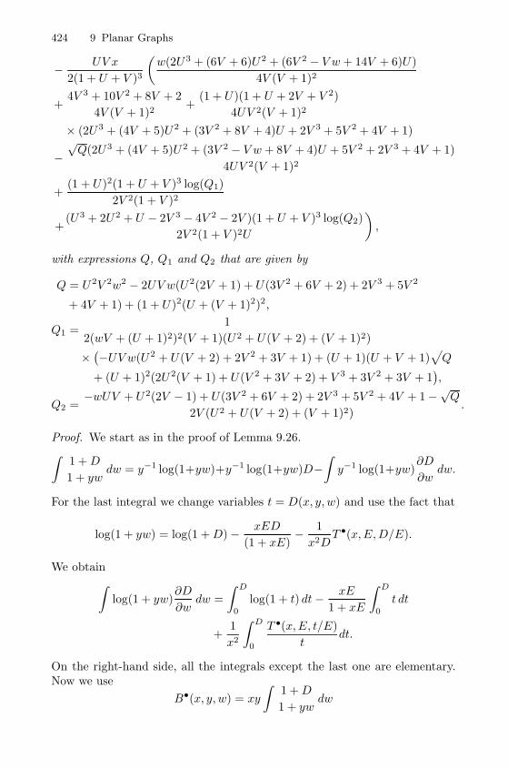
424 9 Planar Graphs
− UV x
2(1 + U + V )3
(w(2U3 + (6V + 6)U2 + (6V 2 − V w + 14V + 6)U)
4V (V + 1)2
+4V 3 + 10V 2 + 8V + 2
4V (V + 1)2+
(1 + U)(1 + U + 2V + V 2)
4UV 2(V + 1)2
× (2U3 + (4V + 5)U2 + (3V 2 + 8V + 4)U + 2V 3 + 5V 2 + 4V + 1)
−√Q(2U3 + (4V + 5)U2 + (3V 2 − V w + 8V + 4)U + 5V 2 + 2V 3 + 4V + 1)
4UV 2(V + 1)2
+(1 + U)2(1 + U + V )3 log(Q1)
2V 2(1 + V )2
+(U3 + 2U2 + U − 2V 3 − 4V 2 − 2V )(1 + U + V )3 log(Q2)
2V 2(1 + V )2U
),
with expressions Q, Q1 and Q2 that are given by
Q = U2V 2w2 − 2UV w(U2(2V + 1) + U(3V 2 + 6V + 2) + 2V 3 + 5V 2
+ 4V + 1) + (1 + U)2(U + (V + 1)2)2,
Q1 =1
2(wV + (U + 1)2)2(V + 1)(U2 + U(V + 2) + (V + 1)2)
×(−UV w(U2 + U(V + 2) + 2V 2 + 3V + 1) + (U + 1)(U + V + 1)
√Q
+ (U + 1)2(2U2(V + 1) + U(V 2 + 3V + 2) + V 3 + 3V 2 + 3V + 1),
Q2 =−wUV + U2(2V − 1) + U(3V 2 + 6V + 2) + 2V 3 + 5V 2 + 4V + 1−√Q
2V (U2 + U(V + 2) + (V + 1)2).
Proof. We start as in the proof of Lemma 9.26.∫1 +D
1 + ywdw = y−1 log(1+yw)+y−1 log(1+yw)D−
∫y−1 log(1+yw)
∂D
∂wdw.
For the last integral we change variables t = D(x, y, w) and use the fact that
log(1 + yw) = log(1 +D)− xED
(1 + xE)− 1
x2DT •(x,E,D/E).
We obtain∫log(1 + yw)
∂D
∂wdw =
∫ D
0
log(1 + t) dt− xE
1 + xE
∫ D
0
t dt
+1
x2
∫ D
0
T •(x,E, t/E)
tdt.
On the right-hand side, all the integrals except the last one are elementary.Now we use
B•(x, y, w) = xy
∫1 +D
1 + ywdw
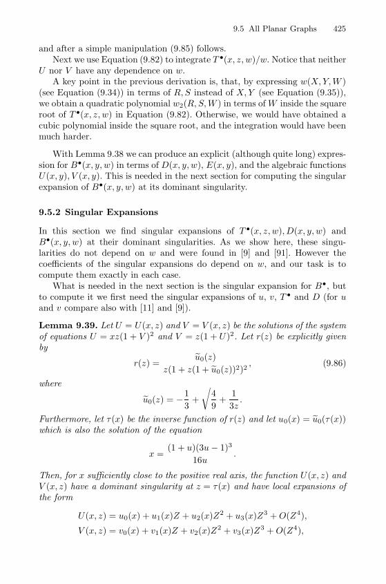
9.5 All Planar Graphs 425
and after a simple manipulation (9.85) follows.Next we use Equation (9.82) to integrate T •(x, z, w)/w. Notice that neither
U nor V have any dependence on w.A key point in the previous derivation is, that, by expressing w(X,Y,W )
(see Equation (9.34)) in terms of R,S instead of X,Y (see Equation (9.35)),we obtain a quadratic polynomial w2(R,S,W ) in terms ofW inside the squareroot of T •(x, z, w) in Equation (9.82). Otherwise, we would have obtained acubic polynomial inside the square root, and the integration would have beenmuch harder.
With Lemma 9.38 we can produce an explicit (although quite long) expres-sion for B•(x, y, w) in terms of D(x, y, w), E(x, y), and the algebraic functionsU(x, y), V (x, y). This is needed in the next section for computing the singularexpansion of B•(x, y, w) at its dominant singularity.
9.5.2 Singular Expansions
In this section we find singular expansions of T •(x, z, w), D(x, y, w) andB•(x, y, w) at their dominant singularities. As we show here, these singu-larities do not depend on w and were found in [9] and [91]. However thecoefficients of the singular expansions do depend on w, and our task is tocompute them exactly in each case.
What is needed in the next section is the singular expansion for B•, butto compute it we first need the singular expansions of u, v, T • and D (for uand v compare also with [11] and [9]).
Lemma 9.39. Let U = U(x, z) and V = V (x, z) be the solutions of the systemof equations U = xz(1 + V )2 and V = z(1 + U)2. Let r(z) be explicitly givenby
r(z) =u0(z)
z(1 + z(1 + u0(z))2)2, (9.86)
where
u0(z) = −1
3+
√4
9+
1
3z.
Furthermore, let τ(x) be the inverse function of r(z) and let u0(x) = u0(τ(x))which is also the solution of the equation
x =(1 + u)(3u− 1)3
16u.
Then, for x sufficiently close to the positive real axis, the function U(x, z) andV (x, z) have a dominant singularity at z = τ(x) and have local expansions ofthe form
U(x, z) = u0(x) + u1(x)Z + u2(x)Z2 + u3(x)Z3 +O(Z4),
V (x, z) = v0(x) + v1(x)Z + v2(x)Z2 + v3(x)Z3 +O(Z4),
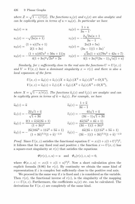
426 9 Planar Graphs
where Z =√
1− z/τ(x). The functions uj(x) and vj(x) are also analytic andcan be explicitly given in terms of u = u0(x). In particular we have
u0(x) = u v0(x) =1 + u
3u− 1,
u1(x) = −√
2u(u+ 1) v1(x) = −2√
2u(u+ 1
3u− 1,
u2(x) =(1 + u)(7u+ 1)
2(1 + 3u)v2(x) =
2u(3 + 5u)
(3u− 1)(1 + 3u),
u3(x) = − (1 + u)(67u2 + 50u+ 11)u
4(1 + 3u)2√
2u2 + 2uv3(x) = −
√2u(1 + u)(79u2 + 42u+ 7)
4(1 + 3u)2(3u− 1)√u(1 + u)
.
Similarly, for z sufficiently close to the real axis the functions U = U(x, z)and V = V (x, z) have a dominant singularity x = r(z) and there is also alocal expansion of the form
U(x, z) = u0(z) + u1(z)X + u2(z)X2 + u3(z)X3 +O(X4),
V (x, z) = v0(z) + v1(z)X + v2(z)X2 + v3(z)X3 +O(X4),
where X =√
1− x/r(z). The functions uj(z) and vj(z) are analytic and canbe explicitly given in terms of u = u0(z). For example, we have
u0(z) = u v0(z) =1 + u
3u− 1
u1(z) = −2u√
1 + u√1 + 3u
v1(z) = − 4u√
1 + u
(3u− 1)√
1 + 3u
u2(z) =2(1 + u)u(2u+ 1)
(1 + 3u)2v2(z) =
4u(5u2 + 4u+ 1)
(3u− 1)(1 + 3u)2
u3(z) = −2u(10u3 + 11u2 + 5u+ 1)
(1 + 3u)7/2(1 + u)−1/2v3(z)− 4u(2u+ 1)(11u2 + 5u+ 1)
(3u− 1)(1 + 3u)7/2(1 + u)−1/2
Proof. Since U(x, z) satisfies the functional equation U = xz(1 + z(1 +U)2)2,it follows that for any fixed real and positive z the function x �→ U(x, z) hasa square-root singularity at r(z) that satisfies the equations
Φ(r(z), z, u) = u and Φu(r(z), z, u) = 0,
where Φ(x, z, u) = xz(1 + z(1 + u)2)2. Now a short calculation gives theexplicit formula (9.86) for r(z). By continuity we obtain the same kind ofrepresentation if z is complex but sufficiently close to the positive real axis.
We proceed in the same way if x is fixed and z is considered as the variable.Then τ(x), the functional inverse of r(z), is the singularity of the mappingz �→ U(x, z). Furthermore, the coefficients u1(x) etc. can be calculated. Thederivations for V (x, z) are completely of the same kind.
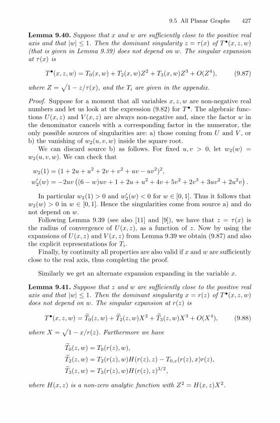
9.5 All Planar Graphs 427
Lemma 9.40. Suppose that x and w are sufficiently close to the positive realaxis and that |w| ≤ 1. Then the dominant singularity z = τ(x) of T •(x, z, w)(that is given in Lemma 9.39) does not depend on w. The singular expansionat τ(x) is
T •(x, z, w) = T0(x,w) + T2(x,w)Z2 + T3(x,w)Z3 +O(Z4), (9.87)
where Z =√
1− z/τ(x), and the Ti are given in the appendix.
Proof. Suppose for a moment that all variables x, z, w are non-negative realnumbers and let us look at the expression (9.82) for T •. The algebraic func-tions U(x, z) and V (x, z) are always non-negative and, since the factor w inthe denominator cancels with a corresponding factor in the numerator, theonly possible sources of singularities are: a) those coming from U and V , orb) the vanishing of w2(u, v, w) inside the square root.
We can discard source b) as follows. For fixed u, v > 0, let w2(w) =w2(u, v, w). We can check that
w2(1) = (1 + 2u+ u2 + 2v + v2 + uv − uv2)2,
w′2(w) = −2uv((6− w)uv + 1 + 2u+ u2 + 4v + 5v2 + 2v3 + 3uv2 + 2u2v
).
In particular w2(1) > 0 and w′2(w) < 0 for w ∈ [0, 1]. Thus it follows thatw2(w) > 0 in w ∈ [0, 1]. Hence the singularities come from source a) and donot depend on w.
Following Lemma 9.39 (see also [11] and [9]), we have that z = τ(x) isthe radius of convergence of U(x, z), as a function of z. Now by using theexpansions of U(x, z) and V (x, z) from Lemma 9.39 we obtain (9.87) and alsothe explicit representations for Ti.
Finally, by continuity all properties are also valid if x and w are sufficientlyclose to the real axis, thus completing the proof.
Similarly we get an alternate expansion expanding in the variable x.
Lemma 9.41. Suppose that z and w are sufficiently close to the positive realaxis and that |w| ≤ 1. Then the dominant singularity x = r(z) of T •(x, z, w)does not depend on w. The singular expansion at r(z) is
T •(x, z, w) = T0(z, w) + T2(z, w)X2 + T3(z, w)X3 +O(X4), (9.88)
where X =√
1− x/r(z). Furthermore we have
T0(z, w) = T0(r(z), w),
T2(z, w) = T2(r(z), w)H(r(z), z) − T0,x(r(z), x)r(z),
T3(z, w) = T3(r(z), w)H(r(z), z)3/2,
where H(x, z) is a non-zero analytic function with Z2 = H(x, z)X2.
428 9 Planar Graphs
Proof. We could repeat the proof of Lemma 9.40. However, we present an al-ternate approach that uses the results of Lemma 9.40 and a kind of singularitytransfer.
By applying the Weierstrass preparation theorem it follows that there is anon-zero analytic function with Z2 = H(x, z)X2. Furthermore, by using therepresentation x = r(z)(1 −X2) and Taylor expansion we have
H(x, z) = H(r(z), z)−Hx(r(z), z)r(z)X2 +O(X4),
Tj(x,w) = Tj(r(z), w) − Tj,x(r(z), w)r(z)X2 +O(X4).
Hence, Lemma (9.40) proves the result. In fact, H can be computed explicitlyand is equal to H(x, τ(x)) = (1 + 3u)/2u.
Lemma 9.42. Suppose that y and w are sufficiently close to the positive realaxis and that |w| ≤ 1. Then the dominant singularity x = R(y) of D(x, y, w)does not depend on w. The singular expansion at R(y) is
D(x, y, w) = D0(y, w) +D2(y, w)X2 +D3(y, w)X3 +O(X4), (9.89)
where X =√
1− x/R(y), and the Di are given by in the Appendix.
Proof. By (9.48) we already know that E(x, y) = D(x, y, 1) has a singularexpansion of the form
E(x, y) = E0(y) +E2(y)X2 +E3(y)X3 + O(X4). (9.90)
Next we rewrite (9.78) to
D(x, y, w) = (1 + yw) exp
(xE(x, y)D(x, y, w)
1 + xE(x, y)(9.91)
+1
x2D(x, y, w)T •(x,E(x, y),
D(x, y, w)
E(x, y)
))− 1.
Now an application of Lemma 9.41 and Theorem 2.31 yields the result. Notethat the singularity does not depend on w.
Lemma 9.43. Suppose that y and w are sufficiently close to the positive realaxis and that |w| ≤ 1. Then the dominant singularity x = R(y) of B•(x, y, w)does not depend on w, and is the same as for D(x, y, w). The singular expan-sion at R(y) is
B•(x, y, w) = B0(y, w) +B2(y, w)X2 +B3(y, w)X3 +O(X4), (9.92)
where X =√
1− x/R(y), and the Bi are given in the Appendix.
Proof. We just have to use the representation of B•(x, y, w) that is given inLemma 9.38 and the singular expansion of D(x, y, w) from Lemma 9.42.
9.5 All Planar Graphs 429
9.5.3 Degree Distribution for Planar Graphs
We start with the degree distribution in 3-connected graphs, both for edge-rooted and vertex-rooted graphs.
Theorem 9.44. For every k ≥ 3 the limiting probability dk that a vertex ofa three-connected planar graph has degree k and the limiting probability ek
that the tail root vertex of an edge-rooted (where the edge is oriented) three-connected planar graph has degree k exist. We have∑
k≥3
ekwk =
T3(r, w)
T3(r, 1),
with T3(x,w) from above and r = r(1) = (7√
7 − 17)/32 is explicitly givenby (9.86). Obviously the ek are indeed a probability distribution. We haveasymptotically, as k →∞,
ek ∼ c · k1/2qk,
where c ≈ 0.9313492 is a computable constant and q = 1/(u0 + 1) =√
7 − 2,and where u0 = u(r) = (
√7− 1)/3.
Moreover, we have
dk = αekk∼ cα · k−1/2qk,
where
α =(3u0 − 1)(3u0 + 1)(u0 + 1)
u0=
√7 + 7
2
is the asymptotic value of the expected average degree in 3-connected planargraphs.
We remark that the degree distribution in 3-connected planar mapscounted according to the number of edges was obtained in [8]. The asymptoticestimates have the same shape as our dk, but the corresponding value of q isequal to 1/2.
Proof. First the proof uses the singular expansion (9.88). The representation∑k≥3
ekwk = T3(r, w)/T3(r, 1)
follows in completely the same way as the proof of Theorem 9.28, using nowLemma 9.40, with the difference that now the dominant term is the coefficientof Z3.
In order to characterise the dominant singularity of T3(1, w) and to de-termine the singular behaviour we observe that the explicit representationof T3 contains in the denominator a (dominating) singular term of the form
430 9 Planar Graphs
(−w+U + 1)3/2. Hence, it follows that u0 + 1 is the dominant singularity andwe also get the proposed asymptotic relation for ek.
For the proof of the second part of the statement, let tn,k be the numberof vertex-rooted graphs with n vertices and with degree of the root equal tok, and let sn,k be the analogous quantity for edge-rooted graphs. Let alsotn =∑
k tn,k and sn =∑
k sn,k. Since a vertex-rooted graph with a rootof degree k is counted k times as an oriented-edge-rooted graph, we havesn,k = ktn,k (a similar argument is used in [137]). Notice that ek = lim sn,k/snand dk = lim tn,k/tn.
Using Theorem 2.22 it follows that the expected number of edges μn in3-connected planar graphs is asymptotically μn ∼ κn, where κ = −τ ′(1)/τ(1),and τ(x) is as in Lemma 9.39. Clearly sn = 2μntn/n.
Finally 2μn/n is asymptotic to the expected average degree α = 2κ. Sum-ming up, we obtain
kdk = α ek.
A simple calculation gives the value of α as claimed.
Theorem 9.45. For every k ≥ 2 the limiting probability dk that a vertex of atwo-connected planar graph has degree k exists and we have
p(w) =∑k≥2
dkwk =
B3(1, w)
B3(1, 1),
with B3(y, w) given in Lemma 9.43.Obviously, p(1) = 1, so that the dk are indeed a probability distribution
and we have asymptotically, as k →∞,
dk ∼ ck−1/2qk,
where c ≈ 3.0826285 is a computable constant and
q =
(1
1− t0exp
((t0 − 1)(t0 + 6)
6t20 + 20t0 + 6
)− 1
)−1
≈ 0.6734506,
and t0 = t(1) ≈ 0.6263717 is a computable constant given by the equation(9.99).
Proof. The representation of p(w) follows from (9.92).Now, in order to characterise the dominant singularity of B3(1, w) and to
determine the singular behaviour we first observe that the right hand side ofthe equation for D0 contains a singular term of the form (D0(t−1)+t)3/2 thatdominates the right hand side. Hence, by applying Theorem 2.31 it followsthat D0(1, w) has the dominant singularity w3, where D0(1, w3) = t/(1 − t)and we have a local singular representation of the form
D0(1, w) = D00 + D02W2 + D03W
3 + · · · ,
9.5 All Planar Graphs 431
where W =√
1− w/w3 and D00 = t/(1− t). The fact that the coefficient of
W vanishes is due to the shape of the equation (9.98) satisfied by D0(1, w).We now insert this expansion into the representation for D2. Observe that
S has an expansion of the form
S = S2W2 + S3W
3 + · · ·
with S2 = 0. Thus we have√S =
√S2W+O(W 2). Furthermore, we get expan-
sions for S2,1, S2,2, S2,3, and S2,4. However, we observe that S2,3(1, w3) = 0,whereas S2,1(1, w3) = 0, S2,2(1, w3) = 0, and S2,4(1, w3) = 0. Consequentlywe can represent D2(1, w) as
D2(1, w) = D2,−11
W+ D2,0 + D2,1W + +D22W
2 + · · · ,
where D1,−1 = 0.In completely the same way it follows that D3(1, w) has a local expansion
of the form
D3(1, w) = D3,−31
W 3+ +D3,−1
1
W+ D3,0 + D3,1W + · · · ,
where D3,−3 = 0 and the coefficient of W−2 vanish identically.These types of singular expansions lead to B3(1, w), and we get
B3(1, w) = B3,−11
W+ B3,0 + B3,1W + · · · , (9.93)
where B3,−1 = 0. The fact that the coefficients of W−3 and W−2 vanishis a consequence of non trivial cancellations. Hence, we obtain the proposedasymptotic relation for dk.
Theorem 9.46. For every k ≥ 1 the limiting probability dk that a vertex of aconnected planar graph has degree k exists and we have
p(w) =∑k≥1
dkwk = −eB0(1,w)−B0(1,1)B2(1, w)
+ eB0(1,w)−B0(1,1) 1 +B2(1, 1)
B3(1, 1)B3(1, w),
where Bj(y, w), j = 0, 2, 3 are given above.Moreover, p(1) = 1, so that the dk is indeed a probability distribution and
we have asymptotically, as k →∞,
dk ∼ ck−1/2qk,
where c ≈ 3.0175067 is a computable constant and q is as in Theorem 9.45.
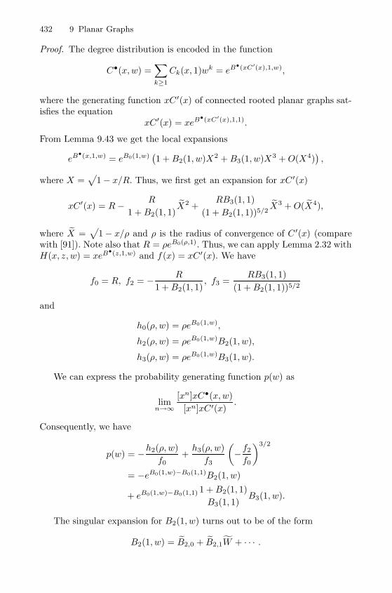
432 9 Planar Graphs
Proof. The degree distribution is encoded in the function
C•(x,w) =∑k≥1
Ck(x, 1)wk = eB•(xC′(x),1,w),
where the generating function xC ′(x) of connected rooted planar graphs sat-isfies the equation
xC′(x) = xeB•(xC′(x),1,1).
From Lemma 9.43 we get the local expansions
eB•(x,1,w) = eB0(1,w)
(1 +B2(1, w)X2 +B3(1, w)X3 +O(X4)
),
where X =√
1− x/R. Thus, we first get an expansion for xC ′(x)
xC′(x) = R− R
1 +B2(1, 1)X2 +
RB3(1, 1)
(1 +B2(1, 1))5/2X3 +O(X4),
where X =√
1− x/ρ and ρ is the radius of convergence of C ′(x) (comparewith [91]). Note also that R = ρeB0(ρ,1). Thus, we can apply Lemma 2.32 withH(x, z, w) = xeB
•(z,1,w) and f(x) = xC ′(x). We have
f0 = R, f2 = − R
1 +B2(1, 1), f3 =
RB3(1, 1)
(1 +B2(1, 1))5/2
and
h0(ρ, w) = ρeB0(1,w),
h2(ρ, w) = ρeB0(1,w)B2(1, w),
h3(ρ, w) = ρeB0(1,w)B3(1, w).
We can express the probability generating function p(w) as
limn→∞
[xn]xC•(x,w)
[xn]xC′(x).
Consequently, we have
p(w) = −h2(ρ, w)
f0+h3(ρ, w)
f3
(−f2f0
)3/2
= −eB0(1,w)−B0(1,1)B2(1, w)
+ eB0(1,w)−B0(1,1) 1 +B2(1, 1)
B3(1, 1)B3(1, w).
The singular expansion for B2(1, w) turns out to be of the form
B2(1, w) = B2,0 + B2,1W + · · · .
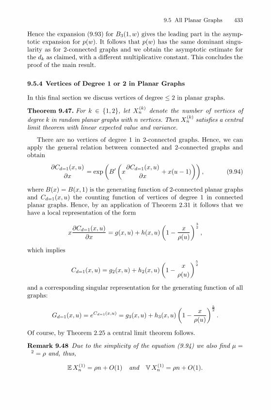
9.5 All Planar Graphs 433
Hence the expansion (9.93) for B3(1, w) gives the leading part in the asymp-totic expansion for p(w). It follows that p(w) has the same dominant singu-larity as for 2-connected graphs and we obtain the asymptotic estimate forthe dk as claimed, with a different multiplicative constant. This concludes theproof of the main result.
9.5.4 Vertices of Degree 1 or 2 in Planar Graphs
In this final section we discuss vertices of degree ≤ 2 in planar graphs.
Theorem 9.47. For k ∈ {1, 2}, let X(k)n denote the number of vertices of
degree k in random planar graphs with n vertices. Then X(k)n satisfies a central
limit theorem with linear expected value and variance.
There are no vertices of degree 1 in 2-connected graphs. Hence, we canapply the general relation between connected and 2-connected graphs andobtain
∂Cd=1(x, u)
∂x= exp
(B′(x∂Cd=1(x, u)
∂x+ x(u − 1)
)), (9.94)
where B(x) = B(x, 1) is the generating function of 2-connected planar graphsand Cd=1(x, u) the counting function of vertices of degree 1 in connectedplanar graphs. Hence, by an application of Theorem 2.31 it follows that wehave a local representation of the form
x∂Cd=1(x, u)
∂x= g(x, u) + h(x, u)
(1− x
ρ(u)
) 32
,
which implies
Cd=1(x, u) = g2(x, u) + h2(x, u)
(1− x
ρ(u)
) 52
and a corresponding singular representation for the generating function of allgraphs:
Gd=1(x, u) = eCd=1(x,u) = g3(x, u) + h3(x, u)
(1− x
ρ(u)
) 52
.
Of course, by Theorem 2.25 a central limit theorem follows.
Remark 9.48 Due to the simplicity of the equation (9.94) we also find μ =σ2 = ρ and, thus,
EX(1)n = ρn+O(1) and VX (1)
n = ρn+O(1).
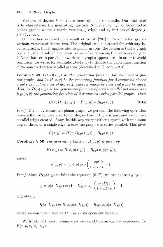
434 9 Planar Graphs
Vertices of degree k = 2 are more difficult to handle. Our first goalis to characterise the generating function B(x, y, z1, z2, z∞) of 2-connectedplanar graphs where x marks vertices, y edges and zj vertices of degree j,j ∈ {1, 2,∞}.
Our method is based on a result of Walsh [207] on 2-connected graphswithout vertices of degree two. The original result is stated for arbitrary la-belled graphs, but it applies also to planar graphs; the reason is that a graphis planar, if and only if it remains planar after removing the vertices of degree2. Note that series-parallel networks and graphs appear here. In order to avoidconfusion, we write, for example, BSP(x, y) to denote the generating functionof 2-connected series-parallel graphs (described in Theorem 9.4).
Lemma 9.49. Let B(x, y) be the generating function for 2-connected pla-nar graphs, and let H(x, y) be the generating function for 2-connected planargraphs without vertices of degree 2, where x marks vertices and y marks edges.Also, let DSP(x, y) be the generating function of series-parallel networks, andBSP(x, y) the generating function of 2-connected series-parallel graphs. Then
H(x,DSP(x, y)) = B(x, y)−BSP(x, y). (9.95)
Proof. Given a 2-connected planar graph, we perform the following operationrepeatedly: we remove a vertex of degree two, if there is any, and we removeparallel edges created, if any. In this way we get either a graph with minimumdegree three, or a single edge in case the graph was series-parallel. This gives
B(x, y) = H(x,DSP(x, y)) +BSP(x, y).
Corollary 9.50 The generating function H(x, y) is given by
H(x, y) = B(x, φ(x, y)) −BSP(x, φ(x, y)),
where
φ(x, y) = (1 + y) exp
( −xy21 + xy
)− 1.
Proof. Since DSP(x, y) satisfies the equation (9.17), we can express y by
y = φ(x,DSP) = (1 +DSP) exp
( −xD2SP
1 + xDSP
)− 1
and obtain
H(x,DSP) = B(x, φ(x,DSP))−BSP(x, φ(x,DSP))
where we can now interpret DSP as an independent variable.
With help of theses preliminaries we can obtain an explicit expression forB(x, y, z1, z2, z∞).
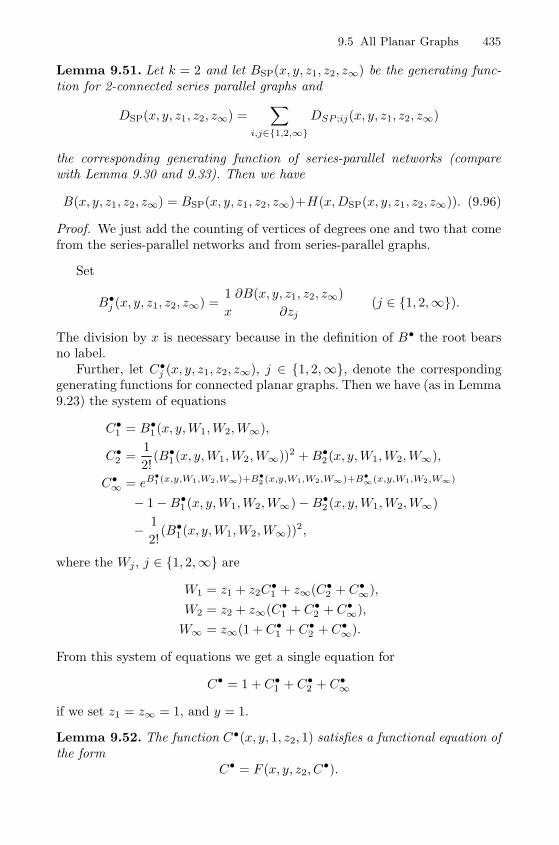
9.5 All Planar Graphs 435
Lemma 9.51. Let k = 2 and let BSP(x, y, z1, z2, z∞) be the generating func-tion for 2-connected series parallel graphs and
DSP(x, y, z1, z2, z∞) =∑
i,j∈{1,2,∞}DSP ;ij(x, y, z1, z2, z∞)
the corresponding generating function of series-parallel networks (comparewith Lemma 9.30 and 9.33). Then we have
B(x, y, z1, z2, z∞) = BSP(x, y, z1, z2, z∞)+H(x,DSP(x, y, z1, z2, z∞)). (9.96)
Proof. We just add the counting of vertices of degrees one and two that comefrom the series-parallel networks and from series-parallel graphs.
Set
B•j (x, y, z1, z2, z∞) =1
x
∂B(x, y, z1, z2, z∞)
∂zj(j ∈ {1, 2,∞}).
The division by x is necessary because in the definition of B• the root bearsno label.
Further, let C•j (x, y, z1, z2, z∞), j ∈ {1, 2,∞}, denote the correspondinggenerating functions for connected planar graphs. Then we have (as in Lemma9.23) the system of equations
C•1 = B•1(x, y,W1,W2,W∞),
C•2 =1
2!(B•1(x, y,W1,W2,W∞))2 +B•2(x, y,W1,W2,W∞),
C•∞ = eB•1 (x,y,W1,W2,W∞)+B•2 (x,y,W1,W2,W∞)+B•∞(x,y,W1,W2,W∞)
− 1−B•1 (x, y,W1,W2,W∞)−B•2 (x, y,W1,W2,W∞)
− 1
2!(B•1(x, y,W1,W2,W∞))2,
where the Wj , j ∈ {1, 2,∞} are
W1 = z1 + z2C•1 + z∞(C•2 + C•∞),
W2 = z2 + z∞(C•1 + C•2 + C•∞),
W∞ = z∞(1 + C•1 + C•2 + C•∞).
From this system of equations we get a single equation for
C• = 1 + C•1 + C•2 + C•∞
if we set z1 = z∞ = 1, and y = 1.
Lemma 9.52. The function C•(x, y, 1, z2, 1) satisfies a functional equation ofthe form
C• = F (x, y, z2, C•).
436 9 Planar Graphs
Proof. Since B•1 = xz1, the equation for C•1 is
C•1 = xW1 = x (1 + z2C•1 + C•2 + C•∞) = xC• + x(z2 − 1)C•1 ,
which gives
C•1 =xC•
1− x(z2 − 1).
Consequently, we have
W1 = C• + (z2 − 1)C•1 =C•
1− x(z2 − 1).
Since W2 = z2 − 1 + C• and W∞ = C•, we can sum the three equations forC•1 , C
•2 , C
•∞ and obtain
C• = eB•1 (x,y,W1,W2,W∞)+B•2 (x,y,W1,W2,W∞)+B•∞(x,y,W1,W2,W∞)
which is now a single equation for C•.
Finally the generating function Cd=2(x, u) for connected planar graphs isdetermined by
∂Cd=2(x, u)
∂x= C•1 (x, 1, 1, u, 1) + uC•2 (x, 1, 1, u, 1) + C•∞(x, 1, 1, u, 1).
We recall that
B(x, y, z1, z2, z∞) = BSP(x, y, z1, z2, z∞) +H(x,DSP(x, y, z1, z2, z∞))
= B(x, φ(x,DSP(x, y, z1, z2, z∞)))
+BSP(x, y, z1, z2, z∞)−BSP(x, φ(x,DSP(x, y, z1, z2, z∞))).
We already know that B(x, y) has a singular expansion of the form
B(x, y) = B0(y) +B2(y)X2 +B4(y)X4 +B5(y)X5 +B6(y)X6 + · · · ,
where X =√
1− x/R(y) and R(1) = 0.03819 . . . Alternatively this can berewritten as
B(x, y) = g(x, y) + h(x, y)
(1− x
R(y)
) 52
.
Further note that BSP(x, y, z1, z2, z∞), BSP(x, y) = BSP(x, y, 1, . . . , 1), andφ(x,DSP(x, y, z1, z2, z∞)) are analytic around x = R(1), y = 1 and zj = 1,j ∈ {1, . . . , k,∞}. Hence, B(x, y, z1, z2, z∞) can be represented as
B(x, y, z1, z2, z∞) = g2(x, y, z1, z2, z∞) + (9.97)
h2(x, y, z1, z2, z∞)
(1− x
R(y, z1, z2, z∞)
)5/2
,
9.5 All Planar Graphs 437
where g2, h2, and R are analytic functions with
g2(x, y, 1, 1, 1) = g(x, y),
h2(x, y, 1, 1, 1) = h(x, y),
R(y, 1, 1, 1) = R(y).
We can apply Theorem 2.25 with α = 52 and obtain the central limit theorem
in the 2-connected case.From (9.97) it follows that B•j (x, y, z1, z2, z∞) has a singularity of the kind
(9.74). Hence, the function F (x, y, u) from Lemma 9.52 has also a singularityof that kind. Note that F (x, y, 1) = eB
•(x,xy). Furthermore, for u = 1 it isknown that the singularity of C• interferes with the singularity of B•.
Hence all assumptions of Proposition 2.31 are satisfied and it follows thatC•(x, 1, 1, u, 1) has a singular expansion of the form (9.74). Of course, withhelp of Theorem 2.25 we get a central limit theorem in the connected case.Finally, since Gd=2(x, u) = eCd=2(x,u) the result follows for general planargraphs, too.

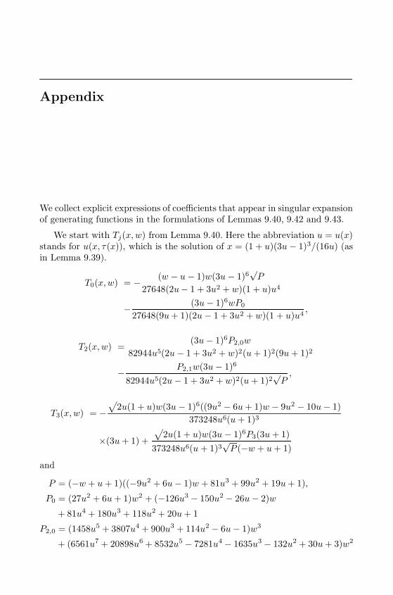
Appendix
We collect explicit expressions of coefficients that appear in singular expansionof generating functions in the formulations of Lemmas 9.40, 9.42 and 9.43.
We start with Tj(x,w) from Lemma 9.40. Here the abbreviation u = u(x)stands for u(x, τ(x)), which is the solution of x = (1 + u)(3u− 1)3/(16u) (asin Lemma 9.39).
T0(x,w) = − (w − u− 1)w(3u− 1)6√P
27648(2u− 1 + 3u2 + w)(1 + u)u4
− (3u− 1)6wP0
27648(9u+ 1)(2u− 1 + 3u2 + w)(1 + u)u4,
T2(x,w) =(3u− 1)6P2,0w
82944u5(2u− 1 + 3u2 + w)2(u+ 1)2(9u+ 1)2
− P2,1w(3u− 1)6
82944u5(2u− 1 + 3u2 + w)2(u+ 1)2√P,
T3(x,w) = −√
2u(1 + u)w(3u − 1)6((9u2 − 6u+ 1)w − 9u2 − 10u− 1)
373248u6(u+ 1)3
×(3u+ 1) +
√2u(1 + u)w(3u − 1)6P3(3u+ 1)
373248u6(u + 1)3√P (−w + u+ 1)
and
P = (−w + u+ 1)((−9u2 + 6u− 1)w + 81u3 + 99u2 + 19u+ 1),
P0 = (27u2 + 6u+ 1)w2 + (−126u3 − 150u2 − 26u− 2)w
+ 81u4 + 180u3 + 118u2 + 20u+ 1
P2,0 = (1458u5 + 3807u4 + 900u3 + 114u2 − 6u− 1)w3
+ (6561u7 + 20898u6 + 8532u5 − 7281u4 − 1635u3 − 132u2 + 30u+ 3)w2
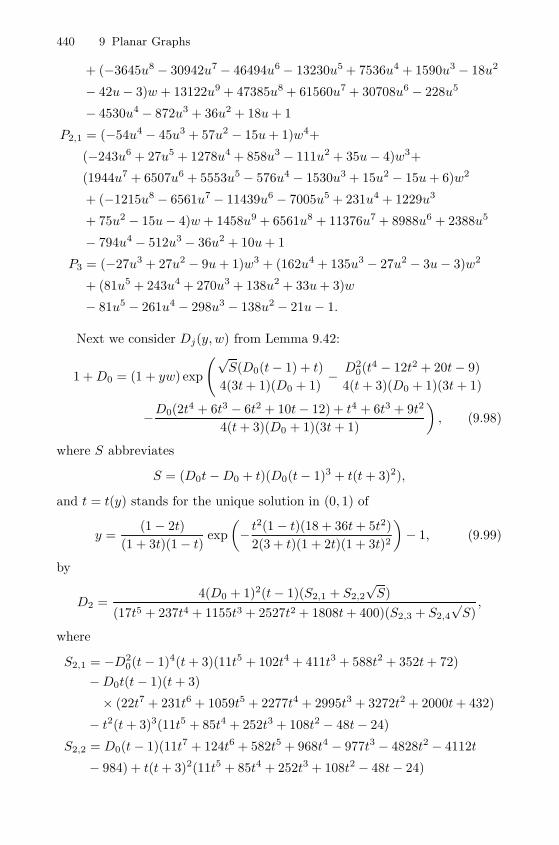
440 9 Planar Graphs
+ (−3645u8 − 30942u7 − 46494u6− 13230u5 + 7536u4 + 1590u3 − 18u2
− 42u− 3)w + 13122u9 + 47385u8 + 61560u7 + 30708u6 − 228u5
− 4530u4 − 872u3 + 36u2 + 18u+ 1
P2,1 = (−54u4 − 45u3 + 57u2 − 15u+ 1)w4+
(−243u6 + 27u5 + 1278u4 + 858u3 − 111u2 + 35u− 4)w3+
(1944u7 + 6507u6 + 5553u5 − 576u4 − 1530u3 + 15u2 − 15u+ 6)w2
+ (−1215u8 − 6561u7 − 11439u6 − 7005u5 + 231u4 + 1229u3
+ 75u2 − 15u− 4)w + 1458u9 + 6561u8 + 11376u7 + 8988u6 + 2388u5
− 794u4 − 512u3 − 36u2 + 10u+ 1
P3 = (−27u3 + 27u2 − 9u+ 1)w3 + (162u4 + 135u3 − 27u2 − 3u− 3)w2
+ (81u5 + 243u4 + 270u3 + 138u2 + 33u+ 3)w
− 81u5 − 261u4 − 298u3 − 138u2 − 21u− 1.
Next we consider Dj(y, w) from Lemma 9.42:
1 +D0 = (1 + yw) exp
(√S(D0(t− 1) + t)
4(3t+ 1)(D0 + 1)− D2
0(t4 − 12t2 + 20t− 9)
4(t+ 3)(D0 + 1)(3t+ 1)
−D0(2t4 + 6t3 − 6t2 + 10t− 12) + t4 + 6t3 + 9t2
4(t+ 3)(D0 + 1)(3t+ 1)
), (9.98)
where S abbreviates
S = (D0t−D0 + t)(D0(t− 1)3 + t(t+ 3)2),
and t = t(y) stands for the unique solution in (0, 1) of
y =(1− 2t)
(1 + 3t)(1− t) exp
(− t
2(1 − t)(18 + 36t+ 5t2)
2(3 + t)(1 + 2t)(1 + 3t)2
)− 1, (9.99)
by
D2 =4(D0 + 1)2(t− 1)(S2,1 + S2,2
√S)
(17t5 + 237t4 + 1155t3 + 2527t2 + 1808t+ 400)(S2,3 + S2,4
√S),
where
S2,1 = −D20(t− 1)4(t+ 3)(11t5 + 102t4 + 411t3 + 588t2 + 352t+ 72)
−D0t(t− 1)(t+ 3)
× (22t7 + 231t6 + 1059t5 + 2277t4 + 2995t3 + 3272t2 + 2000t+ 432)
− t2(t+ 3)3(11t5 + 85t4 + 252t3 + 108t2 − 48t− 24)
S2,2 = D0(t− 1)(11t7 + 124t6 + 582t5 + 968t4 − 977t3 − 4828t2 − 4112t
− 984) + t(t+ 3)2(11t5 + 85t4 + 252t3 + 108t2 − 48t− 24)
9.5 All Planar Graphs 441
S2,3 = −(t+ 3)(D0t−D0 + t)(D20(t− 1)4 + 2D0(t− 1)(t3 − t2 + 5t− 1)
+ t(t3 − 3t− 14)
S2,4 = D20(t2 + 2t− 9)(t− 1)2 +D0(2t4 − 12t2 + 80t− 6) + t(t3 − 3t+ 50),
and by
D3 =24(t+ 3)(D0 + 1)2(t− 1)t2(t+ 1)2S
3/23,1
(S3,2 − S3,3(D0t−D0 + t)
√S)
(β)5/2(D0t−D0 + t)(S3,4
√S − (t+ 3)(D0t−D0 + t)S3,5
) ,
where
β = 3t(1 + t)(17t5 + 237t4 + 1155t3 + 2527t2 + 1808t+ 400),
S3,1 = −5t5 + 6t4 + 135t3 + 664t2 + 592t+ 144,
S3,2 = D30(81t11 + 135t10 − 828t9 − 180t8 + 1982t7 + 1090t6 − 5196t5
+ 2108t4 + 2425t3 − 1617t2 − 256t+ 256),
+D20(243t11 + 1313t10 + 1681t9 − 51t8 − 5269t7 − 7325t6 + 2571t5
+ 10271t4 + 1846t3 − 3888t2 − 1392t)
+D0(243t11 + 2221t10 + 8135t9 + 15609t8 + 12953t7 − 3929t6 − 12627t5
− 13293t4 − 7680t3 − 1632t2)
+ 81t11 + 1043t10 + 5626t9 + 16806t8 + 30165t7 + 30663t6 + 13344t5
+ 1008t4 − 432t3,
S3,3 = D0(81t8 + 378t7 + 63t6−1044t5 + 1087t4−646t3−687t2 + 512t+ 256)
+ 81t8 + 800t7 + 3226t6 + 7128t5 + 8781t4 + 4320t3 + 384t2 − 144t,
S3,4 = D20(t4 − 12t2 + 20t− 9) +D0(2t4 − 12t2 + 80t− 6) + t4 − 3t2 + 50t
S3,5 = D20(t4 − 4t3 + 6t2 − 4t+ 1) +D0(2t4 − 4t3 + 12t2 − 12t+ 2)
+ t4 − 3t2 − 14t.
Finally the coefficients Bj(y, w) from Lemma 9.43 are given by the follow-ing formulas:
B0 =1
128t3
(−8 log(2)(3t4 + 6t2 − 1)− 8 log(t+ 1)(3t− 1)(t+ 1)3
− 4 log(t)(3t− 1)(t+ 1)3 + 2 log(A)(t− 1)3(3t+ 1)
+ 2 log(B)(3t4 + 24t3 + 6t2 − 1)
+√S(t− 1)(D0(t3 − 3t2 + 3t− 1) + t3 − 8t2 + t− 2)
− D0
t+ 3
(D0(t− 1)5(t2 + 2t− 9) + 2(t− 1)3)(t4 + 60t+ 3)
+ (t+ 3)2(t− 1)(t3 − 8t2 + t− 2)t)),
442 9 Planar Graphs
B2 =RD0(D0(R2E2
0 +RE2)− 2(1 +RE0))
2(1 +RE0)2+
1
R(I0,0 + I0,2 + I2,2)
+
(log(1 +D0)− log(1 + yw) − R
2E0D0
1 +RE0
)(1 +D0 −D2)R,
B3 =R2D0
(2D3E
20R + 2D3E0 +E3D0
)2(E0R+ 1)2
+RD3(log(1 + yw)− log(D0 + 1))
+1
R(I0,3 + I2,3 + I3,3),
with
I0,0 =(3t+ 1)(t− 1)3
2048t6
(4(3t− 1)(t+ 1)3 log(t) + 8(3t− 1)(t+ 1)3 log(t+ 1)
+ 8(3t4 + 6t2 − 1) log(2) − 2(t− 1)3(3t+ 1) log(A)
− 2(3t4 + 6t2 − 1) log(B)
+ (t− 1)(D0(t3 − 3t2 + 3t− 1) + t3 + 4t2 + t+ 2)√S
− t− 1
t+ 3
(D2
0(t6 − 2t5 + t4 − 4t3 + 11t2 − 10t+ 3)
+D0(2t6 + 8t5 − 10t4 − 32t3 + 46t2 − 8t− 6)
+ t6 + 10t5 + 34t4 + 44t3 + 21t2 + 18t)),
I0,2 =−(3t+ 1)(t− 1)3
512t6
(4(3t4 − 4t3 + 6t2 − 1) log(2) + 2(3t4 + 6t2 − 1) log(t)
+ 4(3t4 + 6t2 − 1) log(t+ 1) + (−3t4 + 8t3 − 6t2 + 1) log(3A)
+ (−3t4 − 8t3 − 6t2 + 1) log(B)
+D2(t− 1)5(R0,0
√S +R0,1)− (t−1)2
β(t+3) (R0,4
√S +R0,5)
(t+ 3)(R0,6
√S +R0,7
) ),
I0,3 = − (3t+ 1)t2(t− 1)8(R0,0
√S +R0,1)(D3β
5/2 +D0α3/2R0,2)
512(t+ 3)t8β5/2((D0(t2 − 2t+ 1) + t2 + t+ 2)
√S +R0,3
) ,I2,2 =
(t− 1)6R2,0
(R2,1
√S +R2,2
)3072βt6(t+ 1)(D0 + 1)
,
I2,3 =(t+ 1)2(1 + 2t)2α3/2(3t+ 1)(t− 1)7
((t+ 3)2R2,3
√S −R2,4
)16t5β5/2(1 +D0)
,
I3,3 =
√3(t− 1)6R
3/22,0
(R3,0
√S −R3,1(D0t−D0 + t)
)2304
√3t+ 1t5β3/2(t+ 1)3/2(D0t−D0 + t)
,
where the expressions A, B, and polynomials Ri,j are given by
9.5 All Planar Graphs 443
A = D0(5t3 − 3t2 − t− 1) + 5t3 + 6t2 + 5t+ (3t+ 1)√S,
B = D0(t3 − 3t2 + 3t− 1) + t3 + 2t2 + 5t+ (t− 1)√S,
R0,0 = 3D20(t− 1)2 −D0(7t− 3)− t(t+ 3),
R0,1 = 3D30(t− 1)4 −D2
0(t− 1)(3t3 − t2 + 25t− 3)
+D0t(t3 + 8t2 + 21t− 14) + (t+ 3)2t2,
R0,2 = 128t(3t+ 1)(t− 1)(1 + 2t)2(t+ 3)2(t+ 1)2,
R0,3 = D20(t4 − 4t3 + 6t2 − 4t+ 1) +D0(2t4 + 4t2 − 8t+ 2)
+ t4 + 4t3 + 7t2 + 2t+ 2,
R0,4 = 3D30(t− 1)5(51t8 + 1081t7 + 8422t6 + 31914t5 + 59639t4 + 42461t3
+ 7584t2 − 2832t− 864)
−D20(t− 1)3(153t10 + 3204t9 + 29055t8 + 146710t7 + 432951t6
+ 717528t5 + 561457t4 + 208750t3 + 47040t2 + 13248t+ 2592)
−D0(t+ 3)2t(408t10 + 6177t9 + 34003t8 + 92097t7 + 122523t6
+ 126075t5 + 145777t4 + 82707t3 − 1543t2 − 15088t− 3312)
+ 3t(t− 1)(t+ 3)2(2t4 + 3t3 − 2t2 + 3t+ 2)
× (400 + 1808t+ 2527t2 + 1155t3 + 237t4 + 17t5),
R0,5 = 3D40(t− 1)7(51t8 + 1081t7 + 8422t6 + 31914t5 + 59639t4 + 42461t3
+ 7584t2 − 2832t− 864)
+ 2D30(t− 1)4(249t10 + 3333t9 + 22417t8 + 105245t7 + 339675t6+
664087t5 + 513315t4 + 127943t3− 6936t2 − 1152t+ 1296)
−D20t(t− 1)2(357t12 + 7089t11 + 58637t10 + 273500t9 + 828314t8
+ 1886278t7 + 3638786t6 + 5441836t5 + 4731121t4 + 1945329t3
+ 179665t2− 96240t− 20304)
− 2D0t(t+ 3)2(51t12 + 849t11 + 6580t10 + 33465t9 + 115887t8
+ 253743t7 + 285517t6 + 148083t5 + 130634t4 + 141380t3
+ 59715t2 + 4944t− 1200)
+ 3t2(t− 1)(t+ 3)3(2t4 + 3t3 − 2t2 + 3t+ 2)
× (400 + 1808t+ 2527t2 + 1155t3 + 237t4 + 17t5),
R0,6 = D0(t− 1)2 + t2 + t+ 2,
R0,7 = D20(t− 1)4 +D02(t− 1)(t3 + t2 + 3t− 1) + t4 + 4t3 + 7t2 + 2t+ 2,
R2,0 = 3(3t+ 1)(t+ 1)(−5t5 + 6t4 + 135t3 + 664t2 + 592t+ 144),
R2,1 = D20(3t3 − 12t2 + 7t+ 2) +D0(6t3 − 3t2 + t) + 3t3 + 9t2,
444 9 Planar Graphs
R2,2 = D30(3t7 − 47t5 − 18t4 + 21t3 + 164t2 − 105t− 18)
+D20(9t7 + 36t6 − 19t5 − 168t4 − 165t3 + 292t2 + 15t)
+D0(9t7 + 72t6 + 190t5 + 156t4 − 63t3 − 108t2)
+ 3t7 + 36t6 + 162t5 + 324t4 + 243t3,
R2,3 = D20(3t3 − 12t2 + 7t+ 2) +D0(6t3 − 3t2 + t) + 3t3 + 9t2,
R2,4 = D30(3t7 − 47t5 − 18t4 + 21t3 + 164t2 − 105t− 18)
+D20(9t7 + 36t6 − 19t5 − 168t4 − 165t3 + 292t2 + 15t)
+D0(9t7 + 72t6 + 190t5 + 156t4 − 63t3 − 108t2)
+ 3t7 + 36t6 + 162t5 + 324t4 + 243t3,
R3,0 = D20(t4 − 2t3 + 2t− 1) +D0(2t4 + 4t3 − 2t2 − 4t) + t4 + 6t3 + 9t2,
R3,1 = D20(t5 − 3t4 + 2t3 + 2t2 − 3t+ 1) +D0(2t5 + 6t4 − 2t3 − 6t2)
+ t5 + 9t4 + 27t3 + 27t2.
References
1. R. Albert and A.-L. Barabasi. Statistical mechanics of complex networks. Rev.Mod. Phys., 74:47–97, 2002.
2. D. Aldous. The continuum random tree. I. Ann. Probab., 19(1):1–28, 1991.3. D. Aldous. The continuum random tree. II: An overview. Stochastic analysis,
Proc. Symp., Durham/UK 1990, Lond. Math. Soc. Lect. Note Ser. 167, 23-70(1991)., 1991.
4. D. Aldous. The continuum random tree. III. Ann. Probab., 21(1):248–289,1993.
5. D. Aldous. Tree-based models for random distribution of mass. J. Stat. Phys.,73(3-4):625–641, 1993.
6. E. A. Bender. Central and local limit theorems applied to asymptotic enumer-ation. J. Combin. Theory Ser. A, 15:91–111, 1973.
7. E. A. Bender. Asymptotic methods in enumeration. SIAM Review, 16(4):485–515, 1974.
8. E. A. Bender and E. R. Canfield. Face sizes of 3-polytopes. J. Combin. TheorySer. B, 46(1):58–65, 1989.
9. E. A. Bender, Z. Gao, and N. C. Wormald. 2-connected labelled planar graphs.Elec. J. Combinatorics, 9(#43), 2002.
10. E. A. Bender and L. B. Richmond. Central and local limit theorems appliedto asymptotic enumeration. II. Multivariate generating functions. J. Combin.Theory Ser. A, 34(3):255–265, 1983.
11. E. A. Bender and L. B. Richmond. The asymptotic enumeration of rootedconvex polyhedra. J. Combin. Theory Ser. B, 36(3):276–283, 1984.
12. F. Bergeron, P. Flajolet, and B. Salvy. Varieties of increasing trees. In CAAP’92 (Rennes, 1992), volume 581 of Lecture Notes in Comput. Sci., pages 24–48.Springer, Berlin, 1992.
13. N. Bernasconi, K. Panagiotou, and A. Steger. On properties of random dis-sections and triangulations. In Proceedings of the 19th Annual ACM-SIAMSymposium on Discrete Algorithms (SODA ’08), pages 132–141.
14. N. Bernasconi, K. Panagiotou, and A. Steger. On the degree sequences ofrandom outerplanar and series-parallel graph. In Proceedings of the 12th In-ternational Workshop on Randomized Techniques in Computation (RANDOM’08), LNCS 5171, Springer Verlag, pages 303–316, 2008.
446 References
15. P. Biane and M. Yor. Valeurs principales associees aux temps locaux browniens.Bull. Sci. Math. (2), 111(1):23–101, 1987.
16. P. J. Bickel and D. A. Freedman. Some asymptotic theory for the bootstrap.Ann. Statist., 9(6):1196–1217, 1981.
17. P. Billingsley. Probability and measure. John Wiley & Sons Inc., New York,second edition, 1986.
18. P. Billingsley. Convergence of probability measures. John Wiley & Sons Inc.,New York, second edition, 1999.
19. M. Bodirsky, E. Fusy, M. Kang, and S. Vigerske. Enumeration and asymptoticproperties of unlabeled outerplanar graphs. Electronic J. Combinat., 14:R66.
20. M. Bodirsky, O. Gimenez, M. Kang., and M. Noy. Enumeration and limit lawsfor series-parallel graphs. European J. Combin., 28(8):2091–2105, 2007.
21. B. Bollobas. Random graphs. Cambridge University Press, Cambridge, secondedition, 2001.
22. N. Bonichon, C. Gavoille, N. Hanusse, D. Poulalhon, and G. Schaeffer. Planargraphs, via well-orderly maps and trees. Graphs and Combinatorics, 22:185–202, 2006.
23. M. Bousquet-Melou. Limit laws for embedded trees: applications to the inte-grated super-Brownian excursion. Random Structures Algorithms, 29(4):475–523, 2006.
24. M. Bousquet-Melou and S. Janson. The density of the ISE and local limit lawsfor embedded trees. Ann. Appl. Probab., 16(3):1597–1632, 2006.
25. J. Bouttier, P. Di Francesco, and E. Guitter. Geodesic distance in planargraphs. Nucl. Phys., B, 663(3):535–567, 2003.
26. J. Bouttier, P. Di Francesco, and E. Guitter. Statistics of planar graphs viewedfrom a vertex: A study via labeled trees. Nucl. Phys., B, 675(3):631–660, 2003.
27. N. Broutin, L. Devroye, E. McLeish, and M. de la Salle. The height of increasingtrees. Random Structures Algorithms, 32:494–518, 2008.
28. N. Broutin and P. Flajolet. The height of random binary unlabelled trees.In Fifth Colloquium on Mathematics and Computer Science (2008), DiscreteMath. Theor. Comput. Sci. Proc., AC.
29. W. G. Brown. Enumeration of quadrangular dissections on the disk. Can. J.Math., 17:302–317, 1965.
30. W. G. Brown and W. T. Tutte. On the enumeration of rooted non-separableplanar maps. Can. J. Math., 16:572–577, 1964.
31. E. R. Canfield. Remarks on an asymptotic method in combinatorics. J. Com-bin. Theory Ser. A, 37:348–352, 1984.
32. R. Carr, W. M. Y. Goh, and E. Schmutz. The maximum degree in a randomtree an related problems. Random Structures Algorithms, 5:13–24, 1994.
33. P. Chassaing and J.-F. Marckert. Parking functions, empirical processes, andthe width of rooted labeled trees. Electron. J. Combin., 8(1):Research Paper14, 19 pp., 2001.
34. P. Chassaing, J. F. Marckert, and M. Yor. The height and width of simpletrees. In Mathematics and computer science (Versailles, 2000), Trends Math.,pages 17–30. Birkhauser, Basel, 2000.
35. P. Chassaing and G. Schaeffer. Random planar lattices and integrated super-Brownian excursion. Probab. Theory Relat. Fields, 128(2):161–212, 2004.
36. B. Chauvin and M. Drmota. The random multisection problem, travellingwaves and the distribution of the height of m-ary search trees. Algorithmica,46(3-4):299–327, 2006.
References 447
37. B. Chauvin, M. Drmota, and J. Jabbour-Hattab. The profile of binary searchtrees. Ann. Appl. Probab., 11(4):1042–1062, 2001.
38. B. Chauvin, T. Klein, J.-F. Marckert, and A. Rouault. Martingales and profileof binary search trees. Electron. J. Probab., 10:no. 12, 420–435, 2005.
39. B. Chauvin and A. Rouault. Connecting yule process, bisection and binarysearch trees via martingales. J. Iranian Statist. Soc., 3(2):89–116, 2004.
40. F. Chyzak, M. Drmota, T. Klausner, and G. Kok. The distribution of patternsin random trees. Combin. Probab. Comput., 17:21–59, 2008.
41. J. Clement, P. Flajolet, and B. Vallee. Dynamical sources in information the-ory: A general analysis of trie structures. Algorithmica, 29(1–2):307–369, 2001.
42. J. W. Cohen and G. Hooghiemstra. Brownian excursion, the M/M/1 queueand their occupation times. Math. Oper. Res., 6(4):608–629, 1981.
43. G. Dall’Aglio. Sugli estremi dei momenti delle funzioni di ripartizione doppia.Ann. Scuoloa Norm. Sup. Pisa (3), 10:35–74, 1956.
44. R. de la Briandais. File searching using variable length keys. In Proceedings ofthe AFIPS Spring Joint Computer Conference, pages 295–298. AFIPS Press,Reston, Va., 1959.
45. C. Dellacherie and P.-A. Meyer. Probabilites et potentiel. Hermann, Paris,1975.
46. J.-F. Delmas. Computation of moments for the length of the one dimensionalISE support. Electron. J. Probab., 8(Paper No. 17):15 p., 2003.
47. A. Denise, M. Vasconcellos, and D. J. A. Welsh. The random planar graph.Congr. Numer., 113:61–79, 1996.
48. L. Devroye. A probabilistic analysis of the height of tries and of the complexityof triesort. Acta Inform., 21(3):229–237, 1984.
49. L. Devroye. A note on the height of binary search trees. J. Assoc. Comput.Mach., 33(3):489–498, 1986.
50. L. Devroye. A study of trie-like structures under the density model. Ann.Appl. Probab., 2(2):402–434, 1992.
51. L. Devroye. Universal asymptotics for random tries and PATRICIA trees.Algorithmica, 42(1):11–29, 2005.
52. L. Devroye and S. Janson. Distances between pairs of vertices and verticalprofile in conditioned Galton–Watson trees. manuscript.
53. L. Devroye and J. Lu. The strong convergence of maximal degrees in uniformrandom recursive trees and dags. Random Structures Algorithms, 7(1):1–14,1995.
54. R. P. Dobrow and R. T. Smythe. Poisson approximations for functionals orrandom trees. Random Structures Algorithms, 9(1–2):79–92, 1996.
55. A. A. Dobrynin, R. Entringer, and I. Gutman. Wiener index of trees: theoryand applications. Acta Appl. Math., 66(3):211–249, 2001.
56. M. Dondajewski and J. Szymanski. On the distribution of vertex-degrees ina strata of a random recursive tree. Bull. Acad. Polon. Sci. Ser. Sci. Math.,30(5-6):205–209, 1982.
57. M. Drmota. The height of increasing trees. Ann. Combinat. to appear.58. M. Drmota. Distribution of the height of leaves of rooted trees. Diskret. Mat.,
6(1):67–82, 1994.59. M. Drmota. Systems of functional equations. Random Structures Algorithms,
10(1-2):103–124, 1997.
448 References
60. M. Drmota. The saturation level in binary search tree. In Mathematics andcomputer science (Versailles, 2000), Trends Math., pages 41–51. Birkhauser,Basel, 2000.
61. M. Drmota. The variance of the height of binary search trees. Theoret. Comput.Sci., 270(1-2):913–919, 2002.
62. M. Drmota. An analytic approach to the height of binary search trees. II. J.ACM, 50(3):333–374), 2003.
63. M. Drmota, O. Gimenez, and M. Noy. Degree distribution in random planargraph. manuscript.
64. M. Drmota, O. Gimenez, and M. Noy. Vertices of given degree in series-parallesgraphs. Random Structures Algorithms, 2009. to appear.
65. M. Drmota and B. Gittenberger. The shape of unlabeled rooted random trees.manuscript.
66. M. Drmota and B. Gittenberger. On the profile of random trees. RandomStructures Algorithms, 10(4):421–451, 1997.
67. M. Drmota and B. Gittenberger. The width of Galton-Watson trees condi-tioned by the size. Discrete Math. Theor. Comput. Sci., 6(2):387–400, 2004.
68. M. Drmota, S. Janson, and R. Neininger. A functional limit theorem for theprofile of search trees. Ann. Appl. Probab., 18(1):288–333, 2008.
69. M. Drmota and J.-F. Marckert. Reinforced weak convergence of stochasticprocesses. Statist. Probab. Lett., 71(3):283–294, 2005.
70. M. Drmota and W. Szpankowsi. (Un)expected behavior of digital search treeprofile. In Proceedings of the 19th Annual ACM-SIAM Symposium on DiscreteAlgorithms (SODA ’09).
71. R. M. Dudley. Real analysis and probability. Wadsworth & Brooks/Cole Ad-vanced Books & Software, Pacific Grove, CA, 1989.
72. T. Duquesne. A limit theorem for the contour process of conditioned Galton-Watson trees. Ann. Probab., 31(2):996–1027, 2003.
73. T. Duquesne and J.-F. Le Gall. Random trees, Levy processes and spatialbranching processes. Asterisque, (281):vi+147 pages, 2002.
74. T. Duquesne and J.-F. Le Gall. Probabilistic and fractal aspects of Levy trees.Probab. Theory Related Fields, 131(4):553–603, 2005.
75. S. N. Evans. Probability and real trees, volume 1920 of Lecture Notes in Math-ematics. Springer, Berlin, 2008.
76. S. N. Evans, J. Pitman, and A. Winter. Rayleigh processes, real trees, and rootgrowth with re-grafting. Probab. Theory Related Fields, 134(1):81–126, 2006.
77. J. A. Fill and S. Janson. Smoothness and decay properties of the limitingQuicksort density function. In Mathematics and Computer Science (Versailles,2000), Trends Math., pages 53–64. Birkhauser, Basel, 2000.
78. J. A. Fill and S. Janson. Approximating the limiting Quicksort distribution.Random Structures Algorithms, 19(3-4):376–406, 2001.
79. J. A. Fill and S. Janson. Quicksort asymptotics. J. Algorithms, 44(1):4–28,2002.
80. P. Flajolet, Z. Gao, A. Odlyzko, and B. Richmond. The distribution of heightsof binary trees and other simple trees. Combin. Probab. Comput., 2(2):145–156,1993.
81. P. Flajolet, X. Gourdon, and P. Dumas. Mellin transforms and asymptotics:harmonic sums. Theoret. Comput. Sci., 144(1-2):3–58, 1995.
82. P. Flajolet and A. Odlyzko. The average height of binary trees and othersimple trees. J. Comput. System Sci., 25(2):171–213, 1982.
References 449
83. P. Flajolet and A. Odlyzko. Singularity analysis of generating functions. SIAMJ. Discrete Math., 3(2):216–240, 1990.
84. P. Flajolet and R. Sedgewick. Analytic Combinatorics. Cambridge UniversityPress, Cambridge, 2008.
85. P. Flajolet and J.-M Steyaert. A branching process arising in dynamic hash-ing, trie searching and polynomial factorization. In Automata, languages andprogramming (Aarhus, 1982), volume 140 of Lecture Notes in Comput. Sci.,pages 239–251. Springer, Berlin, 1982.
86. E. Fredkin. Trie memory. Communications of the ACM, 3:490–499, 1960.87. M. Fuchs, H.-K. Hwang, and R. Neininger. Profiles of random trees: limit
theorems for random recursive trees and binary search trees. Algorithmica,46(3-4):367–407, 2006.
88. J. Gastwirth and P. Bhattacharya. Two probability models of pyramids orchain letter schemes demo strating that their promotional claims are unreliable.Operations Research, 32:527–536, 1984.
89. S. Gerke and C. McDiarmid. On the number of edges in random planar graphs.Combin. Probab. Comput., 13(2):165–183, 2004.
90. R. K. Getoor and M. J. Sharpe. Excursions of Brownian motion and Besselprocesses. Z. Wahrsch. Verw. Gebiete, 47(1):83–106, 1979.
91. O. Gimenez and M. Noy. Asymptotic enumeration and limit laws of planargraphs. J. Amer. Math. Soc. to appear, arXiv:math/0501269.
92. B. Gittenberger. On the contour of random trees. SIAM J. Discrete Math.,12(4):434–458, 1999.
93. B. Gittenberger and G. Louchard. The Brownian excursion multi-dimensionallocal time density. J. Appl. Probab., 36(2):350–373, 1999.
94. W. Goh and E. Schmutz. Limit distribution for the maximum degree of arandom recursive tree. J. Comput. Appl. Math., 142(1):61–82, 2002.
95. R. L. Graham, D. E. Knuth, and O. Patashnik. Concrete mathematics.Addison-Wesley, Reading, MA, 1989.
96. D. H. Greene and D. E. Knuth. Mathematics for the analysis of algorithms.Birkhauser Boston Inc., Boston, MA, third edition, 1990.
97. I. Gutman and O. E. Polanski. Mathematical Concepts in Organic Chemistry.Springer, Berlin, 1986.
98. F. Harary and E. M. Palmer. Graphical enumeration. Academic Press, NewYork, 1973.
99. W. K. Hayman. A generalisation of Stirling’s formula. J. Reine Angew. Math.,196:67–95, 1956.
100. C. A. R. Hoare. Algorithm 64: Quicksort. Communic. Assoc. Comput. Masch.,4:321, 1961.
101. C. A. R. Hoare. Quicksort. Computer Journal, 5:10–15, 1962.102. M. Hofri. Analysis of algorithms. The Clarendon Press Oxford University
Press, New York, 1995.103. G. Hooghiemstra. On the explicit form of the density of Brownian excursion
local time. Proc. Amer. Math. Soc., 84(1):127–130, 1982.104. H.-K. Hwang. Theoremes limites pour les structures combinatoires et les fonc-
tions arithmetiques. PhD Thesis, Ecole Polytechnique, New York, 1994.105. H.-K. Hwang. Large deviations for combinatorial distributions. I. central limit
theorems. Ann. Appl. Probab., 6:297–319, 1996.106. H.-K. Hwang. Profiles of random trees: plane-oriented recursive trees. Random
Structures Algorithms, 30(3):380–413, 2007.
450 References
107. H.-K. Hwang and R. Neininger. Phase change of limit laws in the quicksortrecurrence under varying toll functions. SIAM J. Comput., 31(6):1687–1722,2002.
108. J. Jabbour-Hattab. Martingales and large deviations for binary search trees.Random Structures Algorithms, 19(2):112–127, 2001.
109. B. Jacquard and G. Schaeffer. A bijective census of nonseparable planar maps.J. Combin. Theory Ser. A, 83(1):1–20, 1998.
110. P. Jacquet and M. Regnier. Trie partitioning process: limiting distributions. InCAAP ’86 (Nice, 1986), volume 214 of Lecture Notes in Comput. Sci., pages196–210. Springer, Berlin, 1986.
111. P. Jacquet and W. Szpankowski. Analysis of digital tries with Markoviandependency. IEEE Trans. Information Theory, 37:1470–1475, 1991.
112. P. Jacquet and W. Szpankowski. Asymptotic behavior of the Lempel-Ziv pars-ing scheme and [in] digital search trees. Theoret. Comput. Sci., 144(1-2):161–197, 1995.
113. P. Jacquet and W. Szpankowski. Analytical de-Poissonization and its applica-tions. Theoret. Comput. Sci., 201(1-2):1–62, 1998.
114. S. Janson. Random cutting and records in deterministic and random trees.Random Structures Algorithms, 29(2):139–179, 2006.
115. S. Janson, D. E. Knuth, T. �Luczak, and B. Pittel. The birth of the giantcomponent. Random Structures Algorithms, 4(3):231–358, 1993.
116. S. Janson, T. �Luczak, and A. Rucinski. Random graphs. Wiley-Interscience,New York, 2000.
117. S. Janson and J.-F. Marckert. Convergence of discrete snakes. J. Theor.Probab., 18(3):615–645, 2005.
118. A. Joffe, L. Le Cam, and J. Neveu. Sur la loi des grands nombres pour desvariables aleatoires de Bernoulli attachees a un arbre dyadique. C. R. Acad.Sci. Paris Ser. A-B, 277:A963–A964, 1973.
119. O. Kallenberg. Foundations of modern probability. Springer-Verlag, New York,second edition, 2002.
120. I. Karatzas and S. E. Shreve. Brownian motion and stochastic calculus.Springer-Verlag, New York, 1988.
121. L. Kaup and B. Kaup. Holomorphic functions of several variables. Walter deGruyter & Co., Berlin, 1983.
122. R. Kemp. Fundamentals of the average case analysis of particular algorithms.John Wiley & Sons Ltd., Chichester, 1984.
123. D. P. Kennedy. The distribution of the maximum Brownian excursion. J. Appl.Probab., 13:371–376, 1976.
124. G. Kersting. On the height profile of a conditioned Galton-Watson tree.manuscript, 1998.
125. C. Knessl and W. Szpankowski. Quicksort algorithm again revisited. DiscreteMath. Theor. Comput. Sci., 3(2):43–64, 1999.
126. C. Knessl and W. Szpankowski. On the average profile of symmetric digitalsearch trees. manuscript, 2008.
127. F. B. Knight. On the excursion process of Brownian motion. Trans. Am. Math.Soc., 258:77–86, 1980.
128. D. E. Knuth. The art of computer programming. Vol. 1. Addison-WesleyPublishing Co., Reading, Mass.-London-Amsterdam, second edition, 1975.
129. D. E. Knuth. The art of computer programming. Vol. 2. Addison-WesleyPublishing Co., Reading, Mass., second edition, 1981.
References 451
130. D. E. Knuth. The art of computer programming. Vol. 3. Addison-WesleyPublishing Co., Reading, Mass., second edition, 1998.
131. V. F. Kolchin. Branching processes, random trees, and a generalized schemeof arrangements of particles. Math. Notes, 21:386–394, 1977.
132. V. F. Kolchin. Random mappings. Optimization Software Inc. PublicationsDivision, New York, 1986.
133. V. F. Kolchin. Random graphs. Cambridge University Press, Cambridge, 1999.134. M. Kuba and A. Panholzer. On the degree distribution of the nodes in increas-
ing trees. J. Combin. Theory Ser. A, 114:597–618, 2007.135. J.-F. Le Gall. Random trees and applications. Probab. Surv., 2:245–311, 2005.136. J.-F. Le Gall. Random real trees. Ann. Fac. Sci. Toulouse Serie 6, 15:35–62,
2006.137. V. A. Liskovets. A pattern of asymptotic vertex valency distributions in planar
maps. J. Combin. Theory Ser. B, 75(1):116–133, 1999.138. C. L. Liu. Introduction to combinatorial mathematics. McGraw-Hill Book Co.,
New York, 1968.139. M. Loeve. Probability theory. I. Springer-Verlag, New York, fourth edition,
1977.140. G. Louchard. The Brownian excursion area: a numerical analysis. Comput.
Math. Appl., 10(6):413–417 (1985), 1984.141. G. Louchard. Kac’s formula, Levy’s local time and Brownian excursion. J.
Appl. Probab., 21(3):479–499, 1984.142. G. Louchard. Exact and asymptotic distributions in digital and binary search
trees. RAIRO Inform. Theor. Appl., 21(4):479–495, 1987.143. G. Louchard and W. Szpankowski. Average profile and limiting distribution
for a phrase size in the Lempel-Ziv parsing algorithm. IEEE Trans. Inf. Th.,41:478–488, 1995.
144. G. Louchard and W. Szpankowski. A probabilistic analysis of a string editingproblem and its variations. Combin. Probab. Comput., 4(2):143–166, 1995.
145. W. C. Lynch. More combinatorial properties of certain trees. The ComputerJournal, 7(4):299–302, 1965.
146. H. M. Mahmoud. Evolution of random search trees. John Wiley & Sons Inc.,New York, 1992.
147. H. M. Mahmoud. Polya urn modles. Text in Statistical Science. Boca Raton,FL: CRC Press., 2009.
148. P. Major. On the invariance principle for sums of independent identicallydistributed random variables. J. Multivariate Anal., 8(4):487–517, 1978.
149. C. McDiarmid and B. Reed. On the maximum degree of a random planargraph. Combin. Probab. Comput., 17(4):591–601, 2008.
150. C. McDiarmid, A. Steger, and D. J. A. Welsh. Random planar graphs. J.Combin. Theory Ser. B, 93:187–205, 2005.
151. A. Meir and J. W. Moon. On the altitude of nodes in random trees. Canad.J. Math., 30(5):997–1015, 1978.
152. A. Meir and J. W. Moon. On an asymptotic method in enumeration. J.Combin. Theory Ser. A, 51(1):77–89, 1989.
153. A. Meir and J. W. Moon. On nodes of large out-degree in random trees. InProceedings of the Twenty-second Southeastern Conference on Combinatorics,Graph Theory and Computing (Baton Rouge, LA, 1991), Congr. Numer., 82:3–13, 1991.
452 References
154. H. Minc. Nonnegative matrices. John Wiley & Sons Inc., New York, 1988.155. J. Moon. The distance between nodes in recursive trees. London Math . Soc .
Lecture Notes, Cambridge Univ. Press, London, 13:125–132, 1974.156. R. C. Mullin and P. J. Schellenberg. The enumeration of c-nets via quadran-
gulations. J. Combin. Theory, 4:259–276, 1968.157. D. Najock and C. Heyde. On the number of terminal vertices in certain random
trees with an application to stemma construction in Philology. J. AppliedProbab., 19:675–680, 1982.
158. R. Neininger. On a multivariate contraction method for random recursivestructures with applications to Quicksort. Random Structures Algorithms,19(3-4):498–524, 2001.
159. R. Neininger. The Wiener index of random trees. Combin. Probab. Comput.,11(6):587–597, 2002.
160. R. Neininger. Stochastische Analyse von Algorithmen, Fixpunktgleichungenund ideale Metriken. Habilitation Thesis, Universitat Frankfurt a.M., 2004.
161. R. Neininger and L. Ruschendorf. A general limit theorem for recursive al-gorithms and combinatorial structures. Ann. Appl. Probab., 14(1):378–418,2004.
162. R. Neininger and L. Ruschendorf. On the contraction method with degeneratelimit equation. Ann. Probab., 32(3B):2838–2856, 2004.
163. R. Neininger and L. Ruschendorf. A survey of multivariate aspects of thecontraction method. Discrete Math. Theor. Comput. Sci., 8(1):31–56, 2006.
164. J. Neveu. Martingales a temps discret. Masson et Cie, editeurs, Paris, 1972.165. A. M. Odlyzko. Asymptotic enumeration methods. In Handbook of combina-
torics, Vol. 1, 2, pages 1063–1229. Elsevier, Amsterdam, 1995.166. A. M. Odlyzko and H. S. Wilf. Bandwidths and profiles of trees. J. Combin.
Theory Ser. B, 42(3):348–370, 1987.167. D. Osthus, H. J. Promel, and A. Taraz. On random planar graphs, the number
of planar graphs and their triangulations,. J. Combin. Theory Ser. B, 88:119–134, 2003.
168. R. Otter. The number of trees. Ann. of Math. (2), 49:583–599, 1948.169. G. Park, H.-K. Hwang, P. Nicodeme, and W. Szpankowski. Profiles of tries.
SIAM J. Computing, page to appear.170. J. Pitman. The SDE solved by local times of a brownian excursion or bridge
derived from the height profile of a random tree or forest. Ann. Probab.,27:261–283, 1999.
171. J. Pitman. Combinatorial stochastic processes, volume 1875 of Lecture Notesin Mathematics. Springer-Verlag, Berlin, 2006.
172. B. Pittel. On growing random binary trees. J. Math. Anal. Appl., 103(2):461–480, 1984.
173. B. Pittel. Asymptotical growth of a class of random trees. Ann. Probab.,13(2):414–427, 1985.
174. B. Pittel. Paths in a random digital tree: limiting distributions. Adv. in Appl.Probab., 18(1):139–155, 1986.
175. B. Pittel. Note on the heights of random recursive trees and random m-arysearch trees. Random Structures Algorithms, 5(2):337–347, 1994.
176. G. Polya. Kombinatorische Anzahlbestimmungen fur Gruppen, Graphen undchemische Verbindungen. Acta Math., 68:145–254, 1937.
177. H. Prodinger. Digital search trees and basic hypergeometric functions. Bulletinof the EATCS, 56, 1995.
References 453
178. S. T. Rachev. Probability metrics and the stability of stochastic models. JohnWiley & Sons Ltd., Chichester, 1991.
179. S. T. Rachev and L. Ruschendorf. Probability metrics and recursive algorithms.Adv. in Appl. Probab., 27(3):770–799, 1995.
180. S. T. Rachev and L. Ruschendorf. Mass transportation problems. Vol. I.Springer-Verlag, New York, 1998.
181. B. Reed. The height of a random binary search tree. J. Assoc. Comput. Mach.,50(3):306–332, 2003.
182. M. Regnier. A limiting distribution for quicksort. RAIRO Inform. Theor.Appl., 23(3):335–343, 1989.
183. D. Revuz and M. Yor. Continuous martingales and Brownian motion. Springer-Verlag, Berlin, third edition, 1999.
184. R. J. Riddell. Contribution to the theory of condensation. PhD Thesis, Univ.Michigan, Ann Arbor, 1951.
185. J. M. Robson. On the concentration of the height of binary search trees. ICALP97 Proceedings, LNCS 1256, pages 441–448, 1997.
186. U. Rosler. A limit theorem for “Quicksort”. RAIRO Inform. Theor. Appl.,25(1):85–100, 1991.
187. U. Rosler. On the analysis of stochastic divide and conquer algorithms. Algo-rithmica, 29(1-2):238–261, 2001.
188. G. Schaeffer. Conjugaison darbres et cartes combinatoires aleatoires. PhDThesis, Universite Bordeaux I, 1998.
189. E.-M. Schopp. Tail Behaviour and Martingale Convergence of Random Re-cursive Structures and Algorithms. PhD Thesis, Univ. Freiburg (Germany),2008.
190. R. Sedgewick. Quicksort. Gurland Publishing, New York, 1980.191. R. Sedgewick and P. Flajolet. An Introduction to the Analysis of Algorithms.
Addison Wesley, Reading, MA, 1996.192. R. T. Smythe and H. M. Mahmoud. A survey of recursive trees. Theory Probab.
Math. Stat., 51:1–27, 1994.193. V. E. Stepanov. The distribution of the number of vertices in the layers of a
random tree. Teor. Verojatnost. i Primenen., 14:64–77, 1969.194. H. Sulzbach. A functional limit law for the profile of plane-oriented recursive
trees. In Fifth Colloquium on Mathematics and Computer Science (2008),Discrete Math. Theor. Comput. Sci. Proc., AC.
195. W. Szpankowski. A characterization of digital search trees from the successfulsearch viewpoint. Theoret. Comput. Sci., 85(1):117–134, 1991.
196. W. Szpankowski. On the height of digital trees and related problems. Algo-rithmica, 6(2):256–277, 1991.
197. W. Szpankowski. Average case analysis of algorithms on sequences. Wiley-Interscience, New York, 2001.
198. J. Szymanski. On the maximum degree and the height of a random recursivetree. In Random graphs ’87 (Poznan, 1987), pages 313–324. Wiley, Chichester,1990.
199. L. Takacs. Conditional limit theorems for branching processes. J. Appl. Math.Stochastic Anal., 4(4):263–292, 1991.
200. L. Takacs. The asymptotic distribution of the total heights of random rootedtrees. Acta Sci. Math., 57:613–625, 1993.
201. K. H. Tan and P. Hadjicostas. Some properties of a limiting distribution ofQuicksort. Statistics Probab. Letter, 25:87–94, 1995.
454 References
202. B. A. Trakhtenbrot. Towards a theory of non-repeating contract schemes.Trudi Mat. Inst. Akad. Nauk SSSR, 51:226–269, 1958.
203. W. T. Tutte. A census of planar triangulations. Canad. J. Math., 14:21–38,1962.
204. W. T. Tutte. A census of planar maps. Canad. J. Math., 15:249–271, 1963.205. W. T. Tutte. On the enumeration of planar maps. Bull. Amer. Math. Soc.,
74:64–74, 1968.206. B. Vallee. Dynamical sources in information theory: fundamental intervals and
word prefixes. Algorithmica, 29(1–2):262–306, 2001.207. T. R. S. Walsh. Counting unlabelled three-connected and homeomorphically
irreducible two-connected graphs. J. Combin. Theory Ser. B, 32(1):12–32,1982.
208. J. Ziv and A. Lempel. Compression of individual sequences via variable-ratecoding. IEEE Trans. Inform. Theory, 24(5):530–536, 1978.
209. V. M. Zolotarev. Approximation of the distributions of sums of independentrandom variables with values in infinite-dimensional spaces. Teor. Verojatnost.i Primenen., 21(4):741–758, 1976.
Index
2-connected graph, 3673-connected graph, 3673-connected planar maps, 389
additive tree parameter, 86Albert-Barabasi model, 256asymptotic expansion, 43
Bernoulli model, 21, 308binary recursive tree, 249binary search tree, 18, 237, 246, 291,
300, 343, 359binary tree, 5, 10, 12, 26, 29, 200, 216,
235binomial coefficient, 39Borel-Cantelli lemma, 273Brownian excursion, 111, 113, 118, 139Brownian snake, 198, 201
Catalan number, 6, 26Catalan tree, 6, 71Cauchy’s formula, 28, 37, 38, 150, 244Cayley tree, 8, 73Cayley’s formula, 8, 73central limit theorem, 48
additive parameters, 83, 87, 88contraction method, 362functional equations, 51, 66generating functions, 49, 51, 53insertion depth, 264Stirling numbers, 244vertices of given degree, 400, 404,
419, 433characteristic function, 47, 129, 132, 164
coefficient of a generating function, 28combinatorial construction, 30, 31, 34combinatorial object, 29combinatorial tree, 4, 70continuum random tree, 107, 108, 111,
112, 149, 198contraction method, 278, 344, 354covariance matrix, 48, 51cut-vertex, 370cycle decomposition, 238cycle index, 33, 81
d-ary recursive tree, 294, 295, 300degree distribution, 253, 255
dissections, 398labelled trees, 85outerplanar graphs, 396, 398, 399planar graphs, 429–431planted plane trees, 85series-parallel graphs, 412, 413simply generated trees, 85
degree of a vertex, 6Delta-domain, 38, 39dependency graph, 63, 93depth in a trie, 313depth-first search, 108, 110, 113, 149,
201diagonal in a quadrangulation, 382digital search tree, 21, 307, 325, 327,
337Dirichlet distribution, 296dissection, 371, 400dominant eigenvalue, 63dual graph, 367, 385
456 Index
Dyck path, 108
embedded tree, 188, 191, 198, 207, 209,214, 219, 235
entropy, 313Euler relation, 367, 385, 422Euler’s constant, 346Eulerian triangulation, 194, 195, 209external node, 2, 5external profile, 291, 308, 312, 324, 327,
341extreme value distribution, 260
finite dimensional convergence, 129, 164finite dimensional distribution, 120,
125, 154first moment method, 260functional equation, 43, 47, 62
Galton-Watson branching process, 10,103
critical, 12sub-critical, 12supercritical, 12
Galton-Watson tree, 9, 11, 84, 107, 112,124, 125, 139, 149, 199, 201, 202
Gamma function, 148Gaussian process, 198generating function, 5, 9, 26, 27, 29, 34,
70, 74, 75, 82, 125, 192, 209exponential, 28ordinary, 28
generating series, 9, 15, 253Gumbel distribution, 260
h-network, 391Hankel contour, 40, 132, 234, 259height, 108
m-ary search trees, 305binary search trees, 300Galton-Watson trees, 113, 123, 139,
140Polya trees, 177plane oriented recursive trees, 303recursive trees, 280tries, 323
Hermite polynomial, 118
implicit function theorem, 45
increasing tree, 15, 253insertion depth, 262, 264internal node, 2, 5internal profile, 291, 308, 312, 322, 324,
327, 341ISE, 196, 197, 200, 204
Kolmogoroff criterion, 269Kuratowski’s theorem, 366
Lp metric, 352Levy process, 113Levy’s criterion, 48labelled plane tree, 8, 74labelled rooted plane tree, 74labelled tree, 3, 7, 73, 85Lagrange inversion formula, 36, 71, 72,
74, 75, 260Laplace transform, 119, 205, 207, 226,
287, 339leaf, 82, 84, 117leaf of a tree, 2Lempel-Ziv algorithm, 307Lipschitz constant, 353local time of a stochastic process, 118
m-ary search tree, 19, 297, 305m-ary tree, 5, 10, 12, 70Markov’s inequality, 121martingale, 266, 267, 270maximum degree, 85, 260Mellin transform, 147, 328method of moments, 275metric space, 109minor of a graph, 366Motzkin tree, 10, 12
network, 390non-negative matrix, 63normal distribution, 47, 51
occupation measure, 116, 124, 149, 198occupations measure, 202offspring distribution, 10, 112operator norm, 352ordered tree, 3Otter’s bijection, 79out-degree of a node, 2outerplanar graph, 368, 396
Index 457
p-network, 379, 391Polya tree, 8, 77, 107, 154, 177Polya’s theorem, 33, 34path length, 108, 114Patricia trie, 22pattern in trees, 90permutation, 30, 238, 240, 246Perron-Frobenius theorem, 63planar graph, 366, 420planar map, 365, 382planar network, 423plane oriented recursive tree, 14, 251,
296, 303plane tree, 3, 81planted pattern, 94planted plane tree, 6, 10, 12, 71, 85,
108, 126, 139, 373planted rooted tree, 87, 92planted tree, 91Poisson transform, 310, 328poles of series-parallel networks, 376Polish space, 110, 111, 120, 124, 346PORT, 14profile, 196, 308, 312
d-ary recursive trees, 295m-ary search trees, 300binary search trees, 291, 359external, 312, 324, 327, 341Galton-Watson trees, 107, 116, 124,
125internal, 308, 312, 322, 324, 327, 341Polya trees, 154plane oriented recursive trees, 296quadrangulations, 188recursive trees, 263, 265, 359trie, 322
profile external, 308profile polynomial, 266, 279Prohorov’s theorem, 120, 124
quadrangulation, 188, 191, 200, 382quasi power theorem, 48, 243Quicksort, 19, 343, 357Quicksort distribution, 346
radius of convergence, 28random permutation model, 19, 249random vector, 51real tree, 109
recursive algorithm, 343recursive tree, 13, 237, 239, 240, 253,
265, 280, 3593-ary, 17d-ary, 17binary, 16plane oriented, 14, 251, 296, 303
Riemann ζ-function, 114root degree, 243, 259rooted real tree, 110rooted tree, 2rotation correspondence, 72, 73
s-network, 379, 391saddle point method, 244scale-free distribution, 256search tree, 17second moment method, 262series-parallel graph, 368, 376series-parallel network, 376simple quadrangulation, 382, 388simply generated tree, 9, 75, 84, 107,
117singularity, 54singularity analysis, 38skew ternary tree, 384space embedded tree, 196spanning tree, 7square root singularity, 43, 54, 75, 374Stirling numbers, 240, 244, 263Stirling’s formula, 83stochastic process, 111, 120, 121symmetric digital search tree, 337symmetric group, 35symmetric trie, 324system of functional equations, 62, 63,
93, 401
tail estimate, 49, 281tightness, 120, 124, 134, 154, 168, 202total progeny, 11Trakhtenbrot’s theorem, 391transfer lemma, 38tree
d-ary recursive, 294, 295, 300m-ary, 5, 10, 12, 70m-ary search, 19, 297, 305binary, 5, 10, 12, 200, 216, 235binary recursive, 249
458 Index
binary search, 18, 237, 246, 291, 300,343, 359
combinatorial, 4, 70continuum random, 107, 108, 111,
112, 149, 198digital search, 21, 307, 325, 327, 337embedded, 188, 191, 198, 207, 209,
214, 219, 235Galton-Watson, 9, 11, 84, 107, 112,
124, 125, 139, 149, 199, 201, 202increasing, 15, 253labelled, 3, 7, 8, 73, 74, 85ordered, 3Polya, 77, 107, 154, 177plane, 3, 8, 9, 74, 81plane oriented recursive, 14, 251, 296,
303planted, 87, 91, 92planted plane, 6, 10, 12, 71, 85, 108,
126, 139, 373real, 109recursive, 13, 237, 239, 240, 253, 265,
280, 359rooted, 2, 74, 87, 92
simply generated, 9, 75, 84, 107, 117skew ternary, 384space embedded, 196unlabelled, 3, 8, 9unrooted, 2, 77, 87, 99well-labelled, 188, 192
trie, 22, 307, 312, 322
unlabelled plane tree, 9unlabelled rooted tree, 154, 177unlabelled tree, 3, 8unrooted tree, 2, 77, 87, 99
Wasserstein metric, 346weak convergence, 48, 111, 120, 121,
154, 352Weierstrass preparation theorem, 45,
58, 428well-labelled tree, 188, 192Whitney’s theorem, 367, 390, 422width, 117, 123Wiener index, 358
Zolotarev metric, 362