delayed random walks: investigating the interplay between

Delayed random walks: Investigating theinterplay between delay and noise

Toru Ohira1 and John Milton2

1 Sony Computer Science Laboratories, Inc., Tokyo, [email protected]

2 Joint Science Department, The Claremont Colleges, Claremont, [email protected]

Summary. A model for a 1–dimensional delayed random walk is developed by gen-eralizing the Ehrenfest model of a discrete random walk evolving on a quadratic,or harmonic, potential to the case of non–zero delay. The Fokker–Planck equationderived from this delayed random walk (DRW) is identical to that obtained startingfrom the delayed Langevin equation, i.e. a first–order stochastic delay differentialequation (SDDE). Thus this DRW and SDDE provide alternate, but complimen-tary ways for describing the interplay between noise and delay in the vicinity ofa fixed point. The DRW representation lends itself to determinations of the jointprobability function and, in particular, to the auto–correlation function for both thestationary and transient states. Thus the effects of delay are manisfested throughexperimentally measurable quantities such as the variance, correlation time, and thepower spectrum. Our findings are illustrated through applications to the analysis ofthe fluctuations in the center of pressure that occur during quiet standing.

Key words: delay, random walk, stochastic delay differential equation,Fokker-Planck equation, auto–correlation function, postural sway

Feedback control mechanisms are ubiquitous in physiology [2, 8, 17, 22,34, 41, 47, 48, 60, 63, 65, 66, 67]. There are two important intrinsic fea-tures of these control mechanisms: 1) all of them contain time delays; and 2)all of them are continually subjected to the effects of random, uncontrolledfluctuations (herein referred to as “noise”). The presence of time delays is aconsequence of the simple fact that the different sensors that detect changesin the controlled variable and the effectors that act on this variable are spa-tially distributed. Since transmission and conduction times are finite, timedelays are unavoidable. As a consequence, mathematical models for feedbackcontrol take the form of stochastic delay differential equations (SDDE); anexample is the delayed Langevin equation or first–order SDDE with additivenoise [20, 25, 33, 36, 37, 42, 43, 53, 59]

dx(t) = −kx(t− τ)dt + dW (1)

2 Toru Ohira and John Milton

where x(t), x(t− τ) are, respectively, the values of the state variable at timest, and t− τ , τ is the time delay, k is a constant, and W describes the Wienerprocess. In order to obtain a solution of (1) it is necessary to define an initialfunction, x(t) = Φ(t), t ∈ [−τ, 0], denoted herein as Φ0(t).

Understanding the properties of SDDEs is an important first step for in-terpreting the nature of the fluctuations in physiological variables measuredexperimentally [11, 37, 53]. However, an increasingly popular way to analyzethese fluctuations has been to replace the SDDE by a delayed random walk,i.e. a discrete random walk for which the transition probabilities at the n–thstep depend on the position of the walker τ steps before [55, 56, 57, 58, 59].Examples include human postural sway [49, 56], eye movements [46], neolithictransitions [18], econophysics [23, 58], and stochastic resonance–like phenom-ena [57]. What is the proper way to formulate the delayed random walk sothat its properties are equivalent to those predicted by (1)?

An extensive mathematical literature has been devoted to addressing issuesrelated to the existence and uniqueness of solutions of (1) and their stability[51, 52]. These fundamental mathematical studies have formed the basis for en-gineering control theoretic studies of the effects of the interplay between noiseand delay on the stability of man–made feedback control mechanisms [6, 54].Lost in these mathematical discussions of SDDEs is the nearly 100 years ofcareful experimental observation and physical insight that established the cor-respondence between (1) and an appropriately formulated random walk whenτ = 0 [15, 16, 21, 31, 40, 45, 61] that does not have its counterpart for the casewhen τ 6= 0. Briefly the current state of affairs is as follows. The continuoustime model described by (1), referred to as the delayed Langevin equation,and the delayed random walk must be linked by a Fokker–Planck equation,i.e. a partial differential equation which describes the time evolution of theprobability density function. This is because all of these models describe thesame phenomenon and hence they must be equivalent in some sense. Whenτ = 0 it has been well demonstrated that the Langevin equation and the ran-dom walk leds to the same Fokker–Planck equation provided that the randomwalk occurs in a harmonic, or quadratic, potential (the Ehrenfest model) [31].Although it has been possible to derive the Fokker–Planck equation from (1)when τ 6= 0 [19, 59], the form of the Fokker–Planck equation obtained fromthe delayed random walk has not yet been obtained. One of the objectives ofthis chapter is to show that the Fokker–Planck equation for the random walkcan be readily obtained by generalizing the Ehrenfest model on a quadraticpotential to non–zero delay. The importance of this demonstration is thatit establishes that (1) and this delayed random walk give two different, butcomplimentary views of the same process.

Since (1) indicates that the dynamics observed at time t depend on whathappened at time t− τ , it is obvious that the joint probability function mustplay a fundamental role in understanding the interplay between noise and de-lay. Moreover, the auto–correlation function, c(∆) ≡ 〈x(t)x(t+∆)〉, is essentialfor the experimental descriptions of real dynamical systems [4, 14, 30]. This

Delayed random walks 3

follows from the fact that three measurements are required to fully describe anoisy signal: 1) its probability density function (e.g. uniform, Gaussian); 2) itsintensity; and 3) its correlation time (e.g. white, colored). From a knowledge ofc(∆) we can obtain an estimate of the variance (∆ = 0) which provides a mea-sure of signal intensity, the correlation time, and the power spectrum. Armedwith these quantities the experimentalist can directly compare experimentalobservation with prediction. Surprinsingly little attention has been devotedto the subject of the joint probability functions in the SDDE literature.

The organization of this chapter is as follows. First, we review the simplerandom walk that appears in standard introductory textbooks [1, 5, 40, 45, 62].We use this simple random walk to introduce a variety of techniques that areused in the subsequent discussion including the concepts of the generatingand characteristic functions, joint probability and the inter–relationship be-tween the auto–correlation function and the power spectral density (Wiener–Khintchine theorem). The Fokker–Planck equation for the simple random walkis the familiar diffusion equation [45]. Second, we discuss the Ehrenfest modelfor a discrete random walk in a quadratic, or harmonic, potential in order tointroduce the concept of stability into a random walk. Third, we introduce adiscrete delay into the Ehrenfest model. The Fokker–Planck equation is ob-tained and is shown to be identical to that obtained starting from (1). In allcases particular attention is given to obtaining an estimate of c(∆) and todemonstrating how the presence of τ influence the correlation time and thepower spectrum. In the final section we review the application of delayed ran-dom walk models to the analysis of the fluctuations recorded during humanpostural sway.

1 Simple random walk

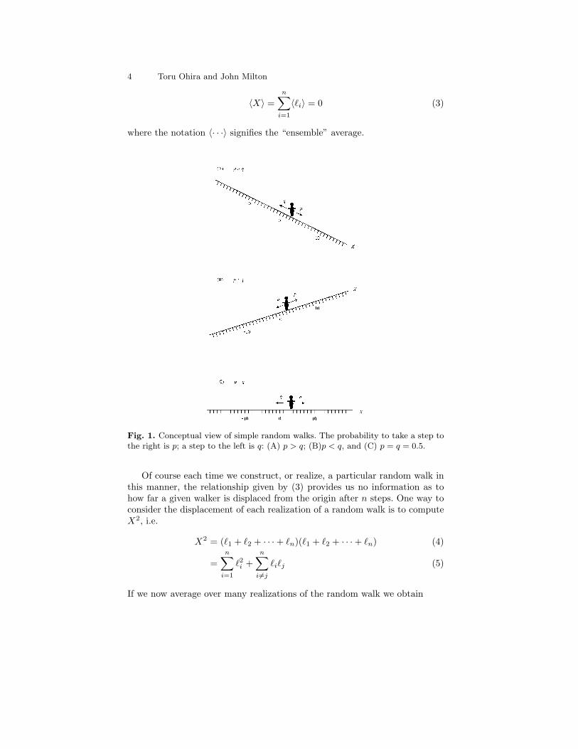
Analyses of random walks in its various forms lie at the core of statisticalphysics [16, 40, 45, 61, 64] and its applications ranging from biology [5] toeconomics [44]. The simplest case describes a walker which is confined tomove along a line by taking identical discrete steps at identical discrete timeintervals (Figure 1). Let X(n) be the position of the walker after the n–thstep. Assume that at zero time all walkers start at the origin, i.e. the initialcondition is X(0) = 0, and that the probability, p, that the walker takesa step of unit length, `, to the right (i.e. X(n + 1) − X(n) = +`) is thesame as the probability, q, that it takes a step of unit length to the left (i.e.X(n + 1)−X(n) = −`), i.e. p = q = 0.5.

The total displacement, X, after n steps is

X =n∑

i=1

`i (2)

where ` = ±1. Since steps to the right and to the left are equally probable,then after a large number of steps, we have


〈X〉 =n∑

i=1

〈`i〉 = 0 (3)

where the notation 〈· · ·〉 signifies the “ensemble” average.

Fig. 1. Conceptual view of simple random walks. The probability to take a step tothe right is p; a step to the left is q: (A) p > q; (B)p < q, and (C) p = q = 0.5.

Of course each time we construct, or realize, a particular random walk inthis manner, the relationship given by (3) provides us no information as tohow far a given walker is displaced from the origin after n steps. One way toconsider the displacement of each realization of a random walk is to computeX2, i.e.

X2 = (`1 + `2 + · · ·+ `n)(`1 + `2 + · · ·+ `n) (4)

=n∑

i=1

`2i +n∑

i 6=j

`i`j (5)

If we now average over many realizations of the random walk we obtain


〈X2〉 =n∑

i=1

〈`2i 〉+n∑

i 6=j

〈`i`j〉 (6)

The first term is obviously n`2. The second term vanishes since the directionof the step that a walker takes at a given instance does not depend on thedirection of previous steps. In other words the direction of steps taken by thewalker are uncorrelated and `i and `j are independent for i 6= j. Hence wehave

〈X2〉 = n`2 (7)

The problem with this method of analysis of the random walk is that it isnot readily transferable to more complex types of random walks. In particular,in order to use the notion of a random walk to investigate the properties of astochastic delay differential equations, such as (1), it is necessary to introducemore powerful tools such as the characteristic, generating and auto–correlationfunctions. Without loss of generality we assume that the walker takes a stepof unit length, i.e. |`| = 1.

1.1 Probability distribution function

The probability that after n steps the walker attains a position r (X(n) = r) isP (X = r, n) = P (r, n), where P (r, n) is the probability distribution functionand satisfies

∞∑r=−∞

P (r, n) = 1

By analogy with the use of the characteristic function in continuous dynamicalsystems [7, 14], the discrete characteristic function,

R(θ, n) =+∞∑

r=−∞P (r, n)ejθr (8)

where θ is the continuous ”frequency” parameter, can be used to calculateP (r, n). Since R(θ, n) is defined in terms of a Fourier series whose coefficientsare the P (r, n), the probability distribution after n steps can be representedin integral form as

P (r, n) =12π

∫ π

−π

R(θ, n)e−jθrdθ. (9)

In order to use R(θ, n) to calculate P (r, n) we first write down an equationthat describes the dynamics of the changes in P (r, n) as a function of thenumber of steps, i.e.

P (r, 0) = δr,0 (10)P (r, n) = pP (r − 1, n− 1) + qP (r + 1, n− 1).


where δr,0 is the Kronecker delta function defined by

δr,0 = 1, (r = 0)δr,0 = 0, (r 6= 0).

Second, we multiply both sides of (10) by ejθr, and sum over r to obtain

R(θ, 0) = 1R(θ, n) = (pejθ + qe−jθ)R(θ, n− 1).

The solution of these equations is

R(θ, n) = (pejθ + qe−jθ)n (11)

Taking the inverse Fourier transform of (11) we eventually obtain

P (r, n) =(

nr+n

2

)p

r+n2 q

n−r2 , (r + n = 2m) (12)

= 0, (r + n 6= 2m),

where m is a non-negative integer. For the special case that p = q = 0.5 thisexpression for P (r, n) simplifies to

P (r, n) =(

nr+n

2

) (12

)n

, (r + n = 2m) (13)

= 0, (r + n 6= 2m),

and we obtain

〈X(n)〉 = 0 (14)σ2(n) = n. (15)

When p > q the walker drifts towards the right (Figure 1a) and when p < qtowards the left (Figure 1b). The evolution of P (r, n) as a function of timewhen p = 0.6 is shown in Figure 2 (for the special case of Brownian motion,i.e. p = q = 0.5, see Figure 3).

1.2 Variance

The importance of P (r, n) is that averaged quantities of interest, or expecta-tions, such as the mean and variance can be readily determined from it. For adiscrete variable, X, the moments can be determined by using the generatingfunction, Q(s, n), i.e.

Q(s, n) =+∞∑

r=−∞srP (r, n) (16)


Fig. 2. The probability density function, P (r, n), as a function of time for a simplerandom walk that starts at the origin with p = 0.6:(•) n = 10, (◦) n = 30, (2)n = 100. We have plotted P (r, n) for even r only: for these values of n, P (r, n) = 0when r is odd.

Fig. 3. The probability density function, P (r, n), as a function of time for Brownianmotion, i.e. a simple random walk that starts at the origin with p = 0.5: (•) n = 10,(◦) n = 30, (2) n = 100. We have plotted P (r, n) for even n only: for these valuesof n, P (r, n) = 0 when n is odd.

The averaged quantities of interest are calculated by differentiating Q(s, n)with respect to s.

By repeating arguments analogous to those we used to obtain P (r, n) fromthe characteristic function, we obtain

Q(s, n) =[ps +

q

s

]n

(17)

The mean is obtained by differentiating Q(s, n) with respect to s


∂

∂sQ(s, n) |s=1≡ 〈X(n)〉 = n(p− q) (18)

The second differentiation leads to

∂2

∂s2Q(s, n) |s=1= 〈X(n)2〉 − 〈X(n)〉 (19)

The variance can be calculated from these two equations as σ2(n) = 4npq.The variance gives the intensity of the varying component of the randomprocess, i.e. the AC component or the variance. The positive square root ofthe variance is the standard deviation which is typically referred to as theroot-mean-square (rms) value of the AC component of the random process.When 〈X(n)〉 = 0, the variance equals the mean square displacement.

1.3 Fokker-Planck equation

We note here briefly that the random walks presented here has a correspon-dence with the continuous time stochastic partial differential equation

dx

dt= µ + ξ(t) (20)

where ξ(t) is a gaussian white noise, and µ is a ‘drift constant’. Both fromthe random walk presented above and from this differential equation, we canobtain the Fokker-Planck equation [21, 45]

∂

∂tP (x, t) = −v

∂

∂xP (x, t) + D

∂2

∂x2P (x, t). (21)

where v and D are constants. When there is no bias, µ = 0, p = q = 12 and we

have v = 0, leading to the diffusion equation. This establishes a link betweenthe Wiener process and simple symmetric random walk.

1.4 Auto–correlation function: Special case

The stationary discrete auto-correlation function, C(∆), provides a measure ofhow much average influence random variables separated ∆ steps apart haveon each other. Typically little attention is given to determining the auto–correlation function for a simple random walk. However, it is useful to have abaseline knowledge of what the auto–correlation looks like for a simple randomprocess.

Suppose we measure the direction that the simple random walker moveseach step. Designate a step to the right as R, a step to the left as L, and a‘flip’ as an abrupt change in the direction that the walker moves. Then thetime series for a simple random walker takes the form


R · · ·flip︷︸︸︷RL · · · LR︸︷︷︸

flip

· · ·flip︷︸︸︷RL · · · (22)

Assume that the step interval, δn, is so small that the probability that twoflips occur within the same step is approximately zero. The auto-correlationfunction, C(∆), where |∆| ≥ |δn|, for this process will be

C(∆) ≡ 〈X(n)X(n + |∆|)〉 = A2(p0(∆)− p1(∆) + p2(∆)− p3(∆) + · · ·) (23)

where pκ(∆) is the probability that in a time interval ∆ that exactly κ flipsoccur and A is the length of each step.

In order to calculate the pκ we proceed as follows. The probability that aflip occurs in δn is λδn, where λ is some suitably defined parameter. Hencethe probability that no flip occurs is 1−λδn. If n > 0 then the state involvingprecisely κ flips in the interval (n, n + δn) arises from either κ − 1 events inthe interval (0, n) with one flip in time δn, or from κ events in the interval(0, n) and no new flips in δn. Thus

pκ(n + δn) = pκ−1(n)λδn + pκ(n)(1− λδn) (24)

and hence we have

limδn→0

pκ(n + δn)− pκ(n)δn

≡ dpκ(n)dn

= λ [pκ−1(n)− pκ(n)] (25)

for κ > 0. When κ = 0 we have

dp0(n)dn

= −λp0(n) (26)

and at n = 0p0(0) = 1. (27)

Equations (25)-(27) describe an iterative procedure to determine pκ. In par-ticular we have

pκ(∆) =(λ|∆|)κe−λ|∆|

κ!(28)

The required auto-correlation function C(∆) is obtained by combining (23)and (28) as

C(∆) = A2e−2λ|∆| (29)

The auto-correlation function, C(∆), and the power spectrum, W (f), areintimately connected. In particular, they form a Fourier transform pair

W (f) = ∆n−1∑

m=−(n−1)

C(∆)e−j2πfm∆, − 12∆

≤ f <1

2∆(30)

and


C(∆) =∫ 1/2∆

−1/2∆

W (f)ej2πf∆df, −n∆ ≤ ∆ ≤ n∆ (31)

Our interest is to compare C(∆) and W (f) calculated for a discrete randomwalk to those that would be observed for a continuous random walk, respec-tively, c(∆) and w(f). Thus we assume in the discussion that follows that thelength of the step taken by the random walker can be small enough so thatwe can replace (30) and (31) by, respectively,

w(f) =∫ ∞

−∞c(∆)e−j2πf∆d∆ (32)

andc(∆) =

∫ ∞

−∞w(f)ej2πf∆df (33)

Together (32) and (33) (or (30) and (31) are referred to as the Wiener–Khintchine theorem.

The power spectrum, w(f), describes how the energy (or variance) of signalis distributed with respect to frequency. Since the energy must be the samewhether we are in the time or frequency domian, it must necessarily be truethat ∫ ∞

−∞|X(t)|2dt =

∫ ∞

−∞|w(f)|2df (34)

This result is sometimes referred to as Parseval’s formula. If g(t) is a continu-ous signal, w(f) of the signal is the square of the magnitude of the continuousFourier transform of the signal, i.e.

w(f) =∣∣∣∣∫ ∞

−∞g(t)e−j2πftdt

∣∣∣∣2 = |G(f)|2 = G(f)G∗(f) (35)

where G(f) is the continuous Fourier transform of g(t) and G∗(f) is its com-plex conjugate.

Thus we can determine w(f) for this random process as

w(f) =2A2

λ

[1

1 + (πf/λ)2

](36)

Figure 4 shows c(∆) and w(f) for this random process, where f is ∆−1. Wecan see that the noise spectrum for this random process is essentially “flat”for f � λ and thereafter decays rapidly to zero with a power law 1/f2.

1.5 Auto-correlation function: General case

The important point is that the Fourier transform pairs given by (32)–(33)are valid whether X(t) represents a deterministic time series or a realiza-tion of a stochastic process [30]. Unfortunately, it is not possible to reliably


Fig. 4. (a) Auto–correlation function, c(∆) and (b) power spectrum, w(f), for therandom process described by (22). Parameters: A = 1, λ = 0.5.

estimate w(f) from a finitely long time series (see pp. 211-213 in [30]). Theproblem is that w(f) measured for a finite length stochastic processes does notconverge in any statistical sense to a limiting value as the sample length be-comes infinitely long. This observation should not be particularly surprising.Fourier analysis is based on the assumption of fixed amplitudes, frequencies,and phases, but time series of stochastic processes are characterized by ran-dom changes of amplitudes, frequencies, and phases. Unlike w(f) a reliableestimate of c(∆) can be obtained from a long time series. These observationsemphasize the critical importance of the Wiener–Khintchine theorem for de-scribing the properties of a stochastic dynamical system in the frequencydomain.

In order to define C(∆) for a random walk it is necessary to introducethe concept of a joint probability, P (r, n1;m,n2). The joint probability isa probability density function that describes the occurence X(n1) = r andX(n2) = m, i.e. the probability that X(n1) is at r at n1 when X(n2) is at sitem at n2. The importance of P (r, n1;m,n2) is that we can use it to determinethe probability that each of these events occurs separately. In particular, theprobability, P (r, n1), that X(n1) is at site r irrespective of the location ofX(n2) is

P (r, n1) =+∞∑

m=−∞P (r, n1;m,n2)

Similarly, the probability, P (m,n2), that X(n2) is at site m irrespective ofthe location of X(n1) is


P (m,n2) =+∞∑

r=−∞P (r, n1;m,n2)

Using these definitions and the fact that P (r, n1;m,n2) is a joint probabilitydistribution function, we can determine C(∆, n) to be

C(∆, n) ≡ 〈X(n)X(n−∆)〉 (37)

=+∞∑

r=−∞

+∞∑m=−∞

rmP (r, n;m,n−∆)

The stationary auto-correlation function can be defined by taking the longtime limit as follows

C(∆) ≡ 〈X(n)X(n−∆)〉s ≡ limn→∞

C(∆, n) (38)

= limn→∞

+∞∑r=−∞

+∞∑m=−∞

rmP (r, n;m,n−∆))

2 Random walks on a quadratic potential

The major limitation for applying simple random walk models to questionsrelated to feedback is that they lack the notion of stability, i.e. the resistanceof dynamical systems to the effects of perturbations. In order to understandhow stability can be incorporated into a random walk it is useful to review theconcept of a potential function, φ(x), in continuous time dynamical systems.For τ = 0 the deterministic version of (1) can be written as [26]

x(t) = −kx(t) = −dφ

dx(39)

and hence

φ(x) =∫ x

0

g(s)ds =kx2

2

describes a quadratic, or harmonic, function. The bottom of this well corre-sponds to the fixed–point attractor x = 0; the well to its basin of attraction.If x(t) is a solution of (39) then

d

dtφ(x(t)) =

d

dxφ(x(t)) · d

dtx(t)

= −[g(x(t))]2 ≤ 0

In other words φ is always decreasing along the solution curves and in thissense is analogous to the “potential functions” in physical systems.

The urn model developed by Paul and Tatyana Ehrenfest showed how aquadratic potential could be incorporated into a discrete random walk [15,


31, 32]. The demonstration that the Fokker–Planck equation obtained for theEhrenfest random walk is the same as that for Langevin’s equation, i.e. (1), isdue to M. Kac [31]. Here we derive the auto–correlation function, C(∆), forthe Ehrenfest random walk and the Langevin equation. The derivation of theFokker-Planck equation for τ = 0 and τ 6= 0 is identical. Therefore we presentthe Fokker–Planck equation for the Ehrenfest random walk as a special caseof that for a delayed random walk in section 3.1.

By analogy with the above observations, we can incorporate the influenceof a quadratic–shaped potential on a random walker by assuming that thetransition probability towards the origin increases linearly with distance fromthe origin (of course up to a point). In particular the transition probabilityfor the walker to move toward the origin increases linearly at a rate of β asthe distance increases from the origin up to the position ±a beyond whichit is constant (since the transition probability is between 0 and 1). Equation(10) becomes

P (r, 0) = δr,0 (40)P (r, n) = g(r − 1)P (r − 1, n− 1)

+ f(r + 1)P (r + 1, n− 1)

where a and d are positive parameters, β = 2d/a, and

f(x) =

1+2d

2 x > a1+βn

2 −a ≤ x ≤ a1−2d

2 x < −a

g(x) =

1−2d

2 x > a1−βn

2 −a ≤ x ≤ a1+2d

2 x < −a

where f(x), g(x) are, respectively, the transition probabilities to take a stepin the negative and positive directions at position x such that

f(x) + g(x) = 1 (41)

The random walk is symmetric with respect to the origin provided that

f(−x) = g(x) (∀x). (42)

We classify random walks by their tendency toward move towards the origin.The random walk is said to be attractive when

f(x) > g(x) (x > 0). (43)

and repulsive whenf(x) < g(x) (x > 0). (44)

We note that when


f(x) = g(x) =12

(∀x), (45)

the general random walk given by (41) reduces to the simple random walkdiscussed Section 2. In this section we consider only the attractive case.

2.1 Auto–Correlation function: Ehrenfest random walk

Assume that with sufficiently large a, we can ignore the probability that thewalker is outside of the range (-a, a). In this case, the probability distributionfunction P (r, n) approximately satisfies the equation

P (r, n) =12(1− β(r − 1))P (r − 1, n− 1) (46)

+12(1 + β(r + 1))P (r + 1, n− 1).

By symmetry, we have

P (r, n) = P (−r, n)〈X(t)〉 = 0

The variance, obtained by multiplying (46) by r2 and summing over all r, is

σ2(n) = 〈X2(n)〉 =12β

(1− (1− 2β)n) (47)

Thus the variance in the stationary state is

σ2s = 〈X2〉s =

12β

. (48)

The auto-correlation function for this random walk can be obtained byrewriting (46) in terms of joint probabilities to obtain

P (r, n;m,n−∆) =12(1− β(r − 1))P (r − 1, n− 1;m,n−∆) (49)

+12(1 + β(r + 1))P (r + 1, n− 1;m,n−∆).

By definingPs(r;m,∆) ≡ lim

n→∞P (r, n;m,n−∆)

the joint probability obtained in the stationary state, i.e. the long time limit,becomes

Ps(r;m,∆) =12(1− β(r − 1))Ps(r − 1;m,∆− 1) (50)

+12(1 + β(r + 1))Ps(r + 1;m,∆− 1).


Multiplying by rm and summing over all r and m yields

C(∆) = (1− β)C(∆− 1) (51)

which we can rewrite as

C(∆) = (1− β)∆C(0) =12β

(1− β)∆ (52)

where C(0) is equal to the mean-square displacement, 〈X2〉s. When β << 1,we can approximate,

C(∆) ≈ 12β

e−β|∆|. (53)

Then, from the Wiener–Khintchine theorem we have

w(f) ≈ 2β2

[1

1 + (2πf/β)2

](54)

These expressions for C(∆) and w(f) are in the same form as those ob-tained for a random process, i.e. (28) and (36). Hence C(∆) and w(f) arequalitatively the same as those shown in Figure 4.

2.2 Auto–correlation function: Langevin equation

When τ = 0, (1) describes the effects of random perturbations on a dynamicalsystem confined to move within a quadratic potential. It is well known thatthe variance, c(0), is

c(0) =12k

(55)

which is identical to (53) if we identify k with β and take ∆ = 0 [21, 35].In order to determine c(∆) and w(f) we note that when τ = 0, (1) describes

the effects of a low–pass filter on δ–correlated (white) noise. Thus we can writethe Fourier transform of (1) when τ = 0 as

X(f) = H(f)I(f) (56)

where the frequency response, H(f), is given by

H(f) =1

j2πf + k(57)

andI(f) = σ2 (58)

where σ is a constant. Hence we obtain

w(f) =σ2

(2πf)2 + k2(59)

and, applying the Weiner-Khintchine theorem,

c(∆) =σ2

2ke−k∆ (60)

Equation (54) is the same as (59) and (53) is the same as (60).


3 Delayed random walks

For a delayed random walk, the transition probability depends on its paststate. If we generalize the random walk in a quadratic potential developed inSection 2 to non–zero delay we obtain the following definition for the transitionprobability

P (r, n + 1) =∑m

g(m)P (r − 1, n;m,n− τ)

+∑m

f(m)P (r + 1, n;m,n− τ), (61)

where the position of the walker at time n is X(n), P (r, n) is the joint prob-ability for the walker to be at X(n) = r and P (r, n;m,n − τ) is the jointprobability such that X(n) = r and X(n− τ) = m takes place. f(x) and g(x)are transition probabilities for the walker to take the step to the negative (−1)and positive (+1) directions respectively, and are the same as those used forthe random walk in a quadratic potential described in the previous section.

3.1 Delayed Fokker–Planck equation

Here we derive the Fokker–Planck equation for the delayed random walk in aquadratic potential. This method is a direct use of the procedure used by M.Kac to obtain the Fokker–Planck equation for the case that τ = 0. For f andg as defined in the previous section, (61) becomes

P (r, n + 1) =∑m

12(1− βm)P (r − 1, n;m,n− τd)

+∑m

12(1 + βm)P (r + 1, n;m,n− τd), (62)

To make a connection, we assume that the random walk takes a step witha size of ∆x at a time interval of ∆t, both of which are very small comparedto the scale of space and time we are interested in. We take x = r∆x andy = m∆x, t = n∆t and τ = τd∆t. With this stipulation, we can re-write (62)as follows

P (x, t + ∆t)− P (x, t)∆t

=

12

(P (x−∆x, t) + P (x + ∆x, t)− 2P (x, t)

(∆x)2

) ((∆x)2

∆t

)+

12

∑y

∆x

y

∆x(P (x, t; y, t− τ)− P (x−∆x, t; y, t− τ))

β

∆t

+12

∑y

∆x

y

∆x(P (x + ∆x, t; y, t− τ)− P (x, t; y, t− τ))

β

∆t(63)


In the limits

∆x → 0, ∆t → 0, β → 0(∆x)2

2∆t→ D,

β

∆t→ γ, n∆t → t, τd∆t → τ

n∆x → x, m∆x → y, (64)

the difference equation (63) goes over to the following integro–partial differ-ential equation

∂

∂t

∫ ∞

−∞P (x, t; y, t− τ)dy =∫ ∞

−∞γ

∂

∂x(yP (x, t; y, t− τ))dy + D

∫ ∞

−∞

∂2

∂x2P (x, t; y, t− τ)dy. (65)

This is the same Fokker-Planck equation that is obtained from the delayedLangevin equation, (1) [19]. When τ = 0 we have

P (x, t; y, t− τ) → P (x, t)δ(x− y), (66)

and the above Fokker-Planck equation reduces to the following familiar form.

∂

∂tP (x, t) = γ

∂

∂x(xP (x, t)) + D

∂2

∂x2P (x, t). (67)

Thus, the correspondence between Ehrenfest’s model and Langevin equationcarries over to that between the delayed random walk model and the delayedLangevin equation.

We can re-write (65) by making the definition

Pτ (x, t) ≡∫ ∞

−∞P (x, t; y, t− τ)dy

to obatin

∂

∂tPτ (x, t) =

∫ ∞

−∞γ

∂

∂x[yP (x, t; y, t− τ)] dy + D

∂2

∂x2Pτ (x, t) (68)

In this form we can more clearly see the effect of the delay on the drift of therandom walker.

3.2 Auto–correlation function: delayed random walk

Three properties delayed random walks are particularly important for thediscussion that follows. First, by the symmetry with respect to the origin,we have that the average position of the walker is 0. In particular, for anattractive delayed random walk, the stationary state (i.e. when n →∞)


P (r, n + 1; r + 1, n) = P (r + 1, n + 1; r, n). (69)

We can show the above as follows. By the definition of the stationarity, wehave

P (r, n + 1; r + 1, n) + P (r, n + 1; r − 1, n) = (70)P (r + 1, n + 1; r, n) + P (r − 1, n + 1; r, n). (71)

For r = 0, we note that due to the symmetry, we have

P (0, n + 1; 1, n) = P (1, n + 1; 0, n). (72)

Using these two equations inductively leads us to the desired relation (69).Second, the generating function

〈cos(αX(n))〉 = (73)cos(α)〈cos(αX(n))〉+ sin(α)〈sin(αX(n)){f(X(n− τ))− g(X(n− τ))}〉

can be obtained by multiplying Eq. (61) for the stationary state by cos(αr)and then summing over r and m.

Finally we have the following invariant relationship with respect to thedelay

12

= 〈X(n){f(X(n− τ))− g(X(n− τ))}〉 (74)

When we choose f, g as before, this invariant relation in Eq. (74) becomesthe following with this model:

〈X(n + τ)X(n)〉 = C(τ) =12β

. (75)

This invariance with respect to τ of the correlation function with τ stepsapart is a simple characteristic of this quadratic potential delayed randomwalk model. This property is a key to obtaining the analytical expressionfor the correlation function. Below we discuss C(∆) for the stationary state.Observations pertaining to C(∆) in the transient state are presented in Sec-tion 4.1.

For the stationary state and 0 ≤ ∆ ≤ τ , the following is obtained fromthe definition (61):

Ps(r, n + ∆;m,n) =∑

`

g(`)Ps(r − 1, n + ∆;m,n + 1; `, n + ∆− τ)

+∑

`

f(`)Ps(r + 1, n + ∆;m,n + 1; `, n + ∆− τ)

(76)

We can derive the following equation for the correlation function by mul-tiplication of this equation by rm and summing over.


C(∆) = C(∆− 1)− βC(τ + 1−∆), (0 ≤ ∆ ≤ τ). (77)

A similar argument can be given for τ < ∆,

C(∆) = C(∆− 1)− βC(∆− 1− τ), (τ < ∆). (78)

Equations (77) and (78) can be solved explicitly using (75). In particular, for0 ≤ ∆ ≤ τ we obtain

C(∆) = C(0)(z∆

+ − z∆−1+ )− (z∆

− − z∆−1− )

z+ − z−− 1

2(z∆

+ − z∆− )

z+ − z−

C(0) =12β

(z+ − z−) + β(zτ+ − zτ

−)(zτ

+ − zτ−1+ )− (zτ

− − zτ−1− )

(79)

where

z± = (1− β2

2)± β

2

√β2 − 4

For τ < ∆, it is possible to write C(∆) in a multiple summation form,though the expression becomes rather complex. For example, with τ < ∆ ≤2τ ,

C(∆) =12β

− β∆−τ∑i=1

C(i) (80)

where the C(i) are given by (79).

Fig. 5. Stationary auto–correlation function, C(∆) (left–hand column) and powerspectra, W (f) (right–hand column) for an attractive delayed random walk on aquadratic potential for different time delays, τ . Stationary correlation function C(u)calculated using (80) and W (f) calculated from this using the Weiner–Klintchinetheorem. The parameters were a = 50, d = 0.4 and τ was 0 for (a) and (b), 40 for(c) and (d) and 80 for (e) and (f).


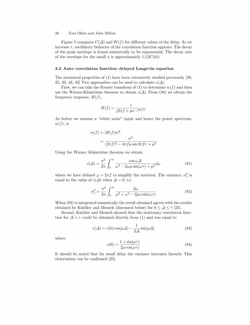
Figure 5 compares C(∆) and W (f) for different values of the delay. As weincrease τ , oscillatory behavior of the correlation function appears. The decayof the peak envelope is found numerically to be exponential. The decay rateof the envelope for the small u is approximately 1/(2C(0)).

3.3 Auto–correlation function: delayed Langevin equation

The statistical properties of (1) have been extensively studied previously [20,25, 33, 42, 43] Two approaches can be used to calculate c(∆).

First, we can take the Fourier transform of (1) to determine w(f) and thenuse the Wiener-Khintchine theorem to obtain c(∆). From (56) we obtain thefrequency response, H(f),

H(f) =1

j2πf + µe−j2πfτ

As before we assume a “white noise” input and hence the power spectrum,w(f), is

w(f) = |H(f)σ|2

=σ2

(2πf)2 − 4πfµ sin 2πfτ + µ2

Using the Wiener–Khintchine theorem we obtain

c(∆) =σ2

2π

∫ ∞

0

cos ω∆

ω2 − 2ωµ sin(ωτ) + µ2dω (81)

where we have defined ω = 2πf to simplify the notation. The variance, σ2x is

equal to the value of c(∆) when ∆ = 0, i.e.

σ2x =

σ2

2π

∫ ∞

0

dω

µ2 + ω2 − 2µω sin(ωτ)(82)

When (82) is integrated numerically the result obtained agrees with the resultsobtained by Kuchler and Mensch (discussed below) for 0 ≤ ∆ ≤ τ [25].

Second, Kuchler and Mensch showed that the stationary correlation func-tion for ∆ < τ could be obtained directly from (1) and was equal to

c(∆) = c(0) cos(µ∆)− 12∆

sin(µ∆) (83)

where

c(0) =1 + sin(µτ)2µ cos(µτ)

(84)

It should be noted that for small delay the variance increases linearly. Thisobservation can be confirmed [25].


We now show that the expressions for C(∆) obtained from the delayedrandom walk (80) is equivalent to those given by (83) for 0 ≤ ∆ ≤ τ . Inparticular, for small β, we have

(z∆+ − z∆−1

+ )− (z∆− − z∆−1

− )z+ − z−

∼ cos(β∆)

β(z∆+ − z∆

− )z+ − z−

∼ sin(β∆)

ThusC(∆) ∼ C(0) cos(β∆)− 1

2∆sin(β∆) (85)

with

C(0) ∼ 1 + sin(βτ)2β cos(βτ)

(86)

4 Postural sway

Postural sway refers to the fluctuations in the center of pressure (COP) thatoccur as a subject stands quietly with eyes closed on a force platform [13, 53].Mathematical models for balance control identify three essential components[17, 49, 50, 56]: 1) feedback, 2) time delays, and 3) the effects of random,uncontrolled perturbations (“noise”). Thus it is not surprising that the firstapplication of a delayed random walk was to investigate the fluctuations inCOP [56]. In this study it was assumed that the probability p+(n) for thewalker to take a step at time n to the right (positive direction) was given by

p+(n) =

p X(n− τ) > 00.5 X(n− τ) = 01− p X(n− τ) < 0

(87)

where 0 < p < 1. The origin is attractive when p < 0.5. By symmetry withrespect to the origin we have 〈X(n)〉 = 0. As shown in Figure 6 this simplemodel was remarkably capable of reproducing some of the features observedfor the fluctuations in the center–of–pressure observed for certain human sub-jects.

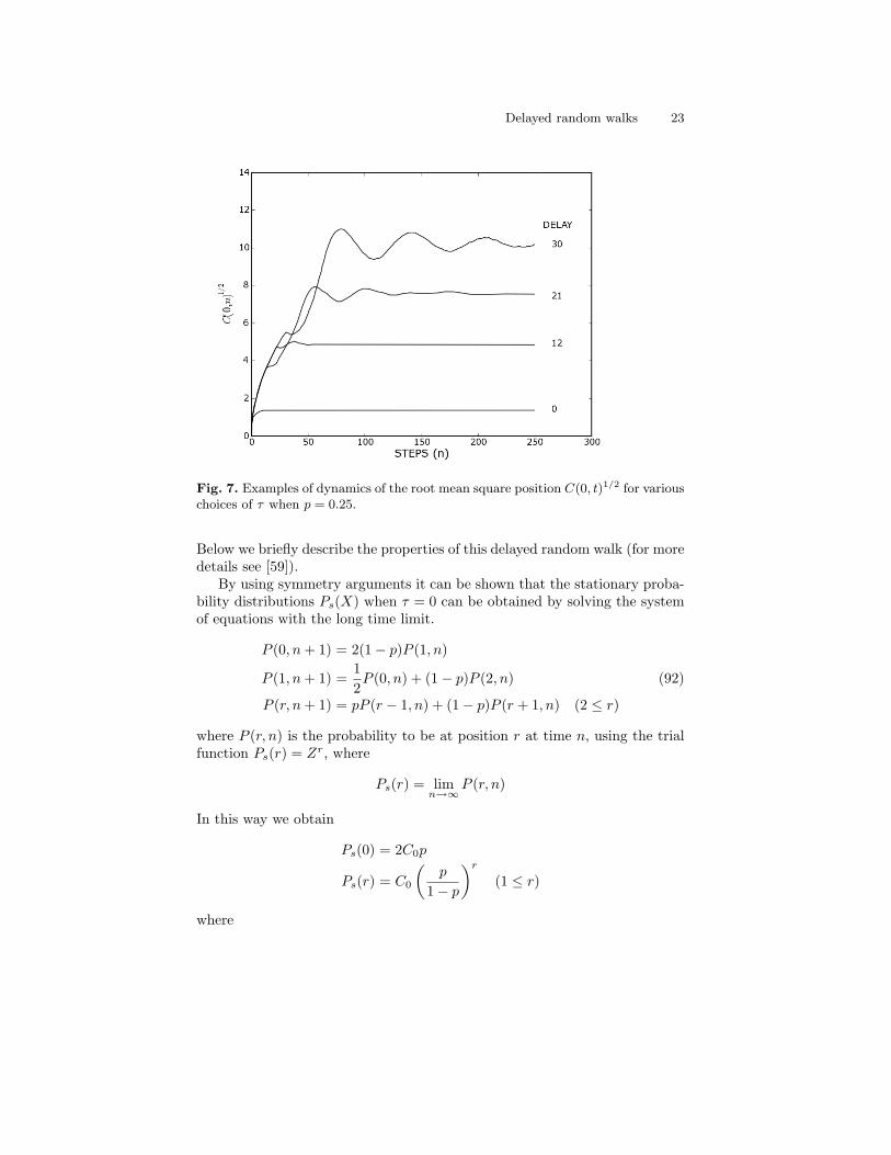
There are a number of interesting properties of this random walk (Fig-ure 7). First, for all choices of τ ≥ 0,

√〈X2(n)〉 approaches a limiting value,

Ψ . Second, the qualitative nature of the approach of√〈X2(n)〉 to Ψ depends

on the value of τ . In particular, for short τ there is a non–oscillatory approachto Ψ , whereas for longer τ damped oscillations occur (Figure 7) whose periodis approximately twice the delay. Numerical simulations of this random walkled to the approximation

Ψ(τ) ∼ (0.59− 1.18p)τ +1√

2(1− 2p)(88)


Fig. 6. Comparison of the two–point correlation function, K(s) = 〈(X(n)−X(n−s))2〉, for the fluctuations in the center–of–pressure observed for two healthy subjects(solid line) with that predicted using a delayed random walk model (◦). In a) theparameters for the delayed random walk were p = 0.35 and τ = 1 with an estimatedunit step length of 1.2 mm and a unit time of 320 ms. In b) the parameters werep = 0.40 and τ = 10 with an estimated step length and unit time step of, respectively,1.4 mm and 40 ms. For more details see [56].

This approximation was used to fit the delayed random walk model to theexperimentally measured fluctuations in postural sway shown in Figure 6.

In the context of a generalized delayed random walk (61) introduced inSection 4, (87) corresponds to choosing f(x) and g(x) to be

f(x) =12[1 + ηθ(x)] (89)

g(x) =12[1− ηθ(x)] (90)

whereη = 1− 2p.

and θ is a step-function defined by

θ(x) =

1 if x > 00 if x = 0−1 if x < 0

(91)

In other words the delayed random walk occurs on a V–shaped potential(which, of course is simply a linear approximation to a quadratic potential).


Fig. 7. Examples of dynamics of the root mean square position C(0, t)1/2 for variouschoices of τ when p = 0.25.

Below we briefly describe the properties of this delayed random walk (for moredetails see [59]).

By using symmetry arguments it can be shown that the stationary proba-bility distributions Ps(X) when τ = 0 can be obtained by solving the systemof equations with the long time limit.

P (0, n + 1) = 2(1− p)P (1, n)

P (1, n + 1) =12P (0, n) + (1− p)P (2, n) (92)

P (r, n + 1) = pP (r − 1, n) + (1− p)P (r + 1, n) (2 ≤ r)

where P (r, n) is the probability to be at position r at time n, using the trialfunction Ps(r) = Zr, where

Ps(r) = limn→∞

P (r, n)

In this way we obtain

Ps(0) = 2C0p

Ps(r) = C0

(p

1− p

)r

(1 ≤ r)

where


C0 =(1− 2p)4p(1− p)

Since we know the p.d.f. we can easily calculate the variance when τ = 0,σ2(0), as

σ2(0) =1

2(1− 2p)2(93)

The stationary probability distributions when τ > 0 can be obtained bysolving the set of equations with the long time limit.

for (0 ≤ r < τ + 2)

P (r, n + 1) = pP (r − 1, n; r > 0, n− τ) +12P (r − 1, n; r = 0, n− τ)

+ (1− p)P (r − 1, n; r < 0, n− τ) + pP (r + 1, n; r < 0, n− τ)

+12P (r + 1, n; r = 0, n− τ) + (1− p)P (r + 1, n; r > 0, n− τ)

for (τ + 2 ≤ r)

P (r, n + 1) = pP (r − 1, n) + (1− p)P (r + 1, n)

These equations are very tedious to solve and not very illuminating. Indeedwe have only been able to obtain the following results for τ = 1

〈X2〉 =1

2(1− 2p)2

(7− 24p + 32p2 − 16p3

3− 4p

)and for τ = 2

〈X2〉 =1

2(1− 2p)2

(25− 94p + 96p2 + 64p3 − 160p4 + 64p5

5 + 2p− 24p2 + 16p3

)

4.1 Transient auto–correlation function

In Section 4 we assumed that the fluctuations in COP were realizations ofa stationary stochastic dynamical system. However, this assumption is byno means clear. An advantage of a delayed random walk model is that it ispossible to gain some insight into the nature of the auto–correlation functionfor the transient state, Ct(∆). In particular, for the transient state we cancalculate in the similar manner to (77)–(78), the set of coupled dynamicalequations

Ct(0, n + 1) = Ct(0, n) + 1− 2βCt(τ, n− τ) (94)Ct(∆, n + 1) = Ct(∆− 1, n + 1)− βCt(τ − (∆− 1), n + ∆− τ), (1 ≤ ∆ ≤ τ)Ct(∆, n + 1) = Ct(∆− 1, n + 1)− βCt((∆− 1)− τ, n + 1), (∆ > τ)


For the initial condition, we need to specify the correlation function for theinterval of initial τ steps. When the random walker begins at the origin wehave a simple symmetric random walk for n ∈ (1, τ). This translates to theinitial condition for the correlation function as

Ct(0, n) = n (0 ≤ ∆ ≤ τ) Ct(u, 0) = 0 (∀u). (95)

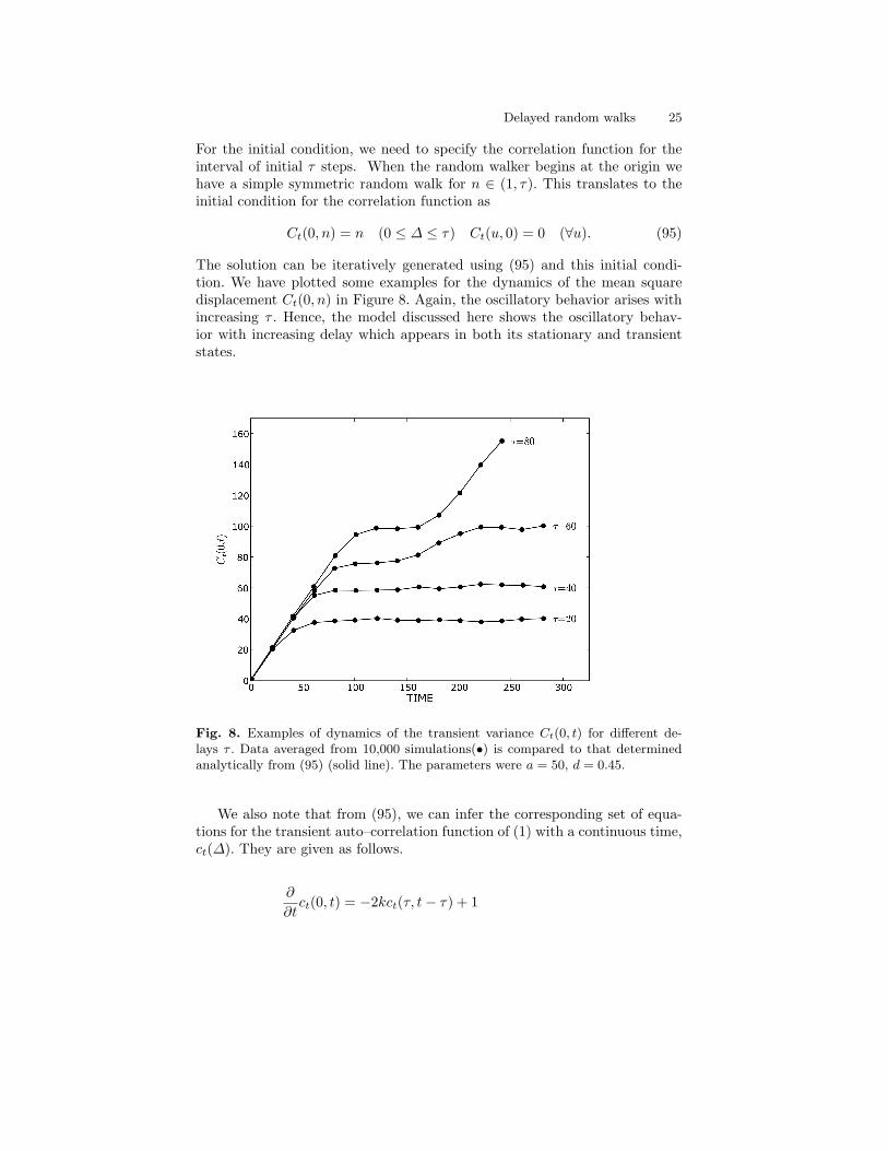
The solution can be iteratively generated using (95) and this initial condi-tion. We have plotted some examples for the dynamics of the mean squaredisplacement Ct(0, n) in Figure 8. Again, the oscillatory behavior arises withincreasing τ . Hence, the model discussed here shows the oscillatory behav-ior with increasing delay which appears in both its stationary and transientstates.

Fig. 8. Examples of dynamics of the transient variance Ct(0, t) for different de-lays τ . Data averaged from 10,000 simulations(•) is compared to that determinedanalytically from (95) (solid line). The parameters were a = 50, d = 0.45.

We also note that from (95), we can infer the corresponding set of equa-tions for the transient auto–correlation function of (1) with a continuous time,ct(∆). They are given as follows.

∂

∂tct(0, t) = −2kct(τ, t− τ) + 1


∂

∂∆ct(∆, t) = −kct(τ −∆, t + ∆− τ) (0 < ∆ ≤ τ) (96)

∂

∂∆ct(∆, t) = −kct(∆− τ, t) (τ < ∆)

Studies on these coupled partial differential equations with delay are yet tobe done.

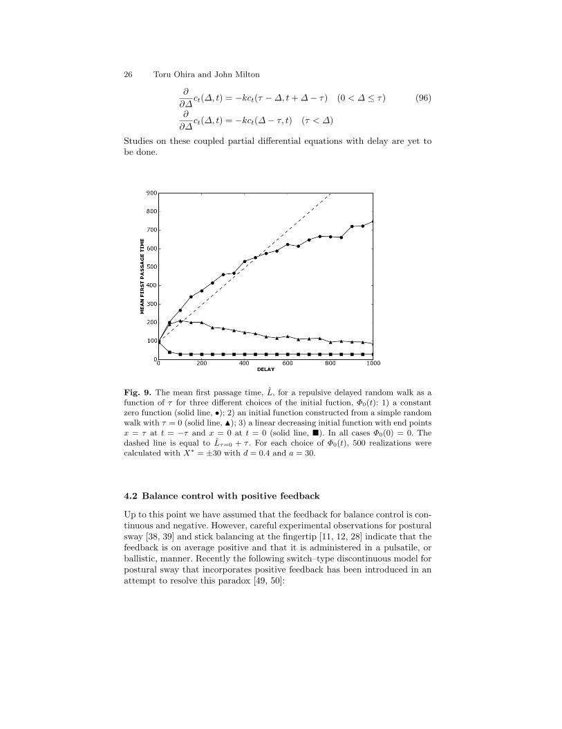
Fig. 9. The mean first passage time, L, for a repulsive delayed random walk as afunction of τ for three different choices of the initial fuction, Φ0(t): 1) a constantzero function (solid line, •); 2) an initial function constructed from a simple randomwalk with τ = 0 (solid line, N); 3) a linear decreasing initial function with end pointsx = τ at t = −τ and x = 0 at t = 0 (solid line, �). In all cases Φ0(0) = 0. Thedashed line is equal to Lτ=0 + τ . For each choice of Φ0(t), 500 realizations werecalculated with X∗ = ±30 with d = 0.4 and a = 30.

4.2 Balance control with positive feedback

Up to this point we have assumed that the feedback for balance control is con-tinuous and negative. However, careful experimental observations for posturalsway [38, 39] and stick balancing at the fingertip [11, 12, 28] indicate that thefeedback is on average positive and that it is administered in a pulsatile, orballistic, manner. Recently the following switch–type discontinuous model forpostural sway that incorporates positive feedback has been introduced in anattempt to resolve this paradox [49, 50]:


dx

dt=

αx(t− τ) + η2ξ(t) + K if x(t− τ) < −Παx(t− τ) + η2ξ(t) if −Π ≤ x(t− τ) ≤ Παx(t− τ) + η2ξ(t)−K if x(t− τ) > Π

(97)

where α, K, and Π are positive constants. This model is a simple extensionof a model proposed by Eurich and Milton [17] and states that the nervoussystem allows the controlled variable to drift under the effects of noise (ξ(t))and positive feedback (α > 0) with corrective actions (‘negative feedback’)taken only when x(t − τ) exceeds a certain threshold, Π. It is assumed thatα is small and that τ < 3π/2α. This means that there is one real positiveeigenvalue and an infinite number of complex eigenvalue pairs whose realpart is negative. The magnitude of the real positive eigenvalue decreases as τincreases for 0 < τ < 3π/2α. “Safety net” type controllers also arise in thedesign of strategies to control attractors that have shallow basins of attraction[24].

The cost to operate this discontinuous balance controller is directly propor-tional to the number of times it is activated. Thus the mathematical problembecomes that of determining the first passage times for a repulsive delayedrandom walk, i.e. the times it takes a walker starting at the origin to cross thethreshold, ±|Π|. Numerical simulations of a repulsive delayed random walkindicate that the mean first passage time depends on the choice of Φ0(t) (seeFigure 9).

In principle, the most probable, or mean, first passage time can be calcu-lated from the backward Kolmogorov equation for (1). We have been unableto complete this calculation. However, simulations of (97) indicate that thisdicontinuous balance controller takes advantage of two intrinsic properties ofa repulsive delayed random walk: 1) the time delay which slows scape, and2) the fact that the distribution of first passage times is bomodal. Since thedistribution of first passage times is biomodal it is possible that a reset dueto the activation of the negative feedback controller can lead to a trasientconfinement of the walker near the origin thus further slowing escape.

5 Concluding remarks

In this chapter we have shown that a properly formulated delayed randomwalk can provide an alternate and complimentary approach for the analysisfor stochastic delay differential equations such as (1). By placing the studyof a stochastic differential equation into the context of a random walk it ispossible to draw upon the large arsenal of analytical tools previously devel-oped for the study of random walks and apply them to the study of thesecomplex dynamical systems. The advantages of this approach to the analysisof SDDEs include 1) it avoids issues inherent in the Ito versus Stratonovichstochastic calculus, 2) it provides insight into transient dynamics, and 3) itis, in principle, applicable to the study of delayed stochastic dynamical sys-tems in the setting of complex potential surfaces such as those that arise in


the setting of multistability. In general the use of the delayed random walkinvolves solutions in the form of equations which must be solved iteratively.However, this procedure causes no practical problem given the ready availabil-ity of symbolic manipulation computer software programs such as Maple c©and Mathematica c©. The use of these computer programs compliment thevariety of numerical methods [3, 27, 29] that have been developed to investi-gate SDDEs, such as (1). However, much remains to be done, particularly theimportant cases in which the noise enters the dynamics in a multiplicative, orparametric, fashion [9, 10, 52]. Thus we anticipate that the subject of delayedrandom walks will continue to gain in importance.

Acknowledgements

We thank Sue Ann Campbell for useful discussions. We acknowledge supportfrom the William R. Kenan, Jr. Foundation (JM) and the National ScienceFoundation (Grant 0617072)(JM,TO).

References

1. Bailey, N. T., The Elements of Stochastic Processes, J. Wiley & Sons, NewYork, 1990.

2. Bechhoefer, J., ‘Feedback for physicists: A tutorial essay on control’, Rev. Mod.Phys. 77, 2005, 783–836.

3. Bellen, A. and Zennaro, M., Numerical Methods for Delay Differential Equa-tions, Oxford University Press, New York, 2003.

4. Bendat, J. S. and Piersol, A. G., Random Data: Analysis and MeasurementProcedures, 2nd Edition, J. Wiley & Sons, New York, 1986.

5. Berg, H. C., Random Walks in Biology, expanded edition, Princeton UniversityPress, Princeton, New Jersey, 1993.

6. Boukas, E–K. and Liu Z–K., Deterministic and Stochastic Time Delay Systems,Birkhauser, Boston, 2002.

7. Bracewell, R. N., The Fourier Transform and Its Applications, 2nd edition,McGraw–Hill, New York, 1986.

8. Bratsun, D., Volfson, D., Tsimring, L. S. and Hasty, J., ‘Delay–induced sto-chastic oscillations in gene regulation’, Proc. Natl. Acad. Sci. USA 102, 2005,14593–14598.

9. Cabrera, J. L. and Milton, J. G., ‘On–off intermittency in a human balancingtask’, Phys. Lett. Rev. 89, 2002, 158702.

10. Cabrera, J. L. and Milton, J. G., ‘Human stick balancing: Tuning Levy flightsto improve balance control’, Chaos 14, 2004, 691–698.

11. Cabrera, J. L., Bormann, R., Eurich, C. W., Ohira, T. and Milton, J., ‘State–dependent noise and human balance control’, Fluctuation Noise Letters 4, 2004,L107–L117.

12. Cabrera, J. L., Luciani, C., and Milton, J., ‘Neural control on multiple timescales: Insights from human stick balancing’, Condensed Matter Physics 2, 2006,373–383.


13. Collins, J. J. and De Luca, C. J., ‘Random walking during quiet standing’,Phys. Rev. Lett. 73, 1994, 907–912.

14. Davenport, W. B. and Root, W. L., An Introduction to the Theory of RandomSignals and Noise, IEEE Press, New York, 1987.

15. Ehrenfest, P. and Ehrenfest, T., ‘Uber zwei bekannte Einwande gegan das Boltz-mannsche H–Theorem’, Phys. Zeit. 8, 1907, 311–314.

16. Einstein, A., ‘Zur Theorie der Brownschen Bewegung’, Annalen der Physik 19,1905, 371–381.

17. Eurich, C. W. and Milton, J. G., ‘Noise–induced transitions in human posturalsway’, Phys. Rev. E 54, 1996, 6681–6684.

18. Fort, J., Jana, D. and Humet, J., ‘Multidelayed random walk: Theory and ap-plication to the neolithic transition in Europe’, Phys. Rev. E. 70, 2004, 031913.

19. Frank, T. D., ‘Delay Fokker–Planck equations, Novikov’s theorem, and Boltz-mann distributions as small delay approximations’, Phys. Rev. E 72, 2005,011112.

20. Frank, T. D. and Beek, P. J., ‘Stationary solutions of linear stochastic delaydifferential equations: Applications to biological systems’, Phys. Rev. E 64,2001, 021917.

21. Gardiner, C. W., Handbook of Stochastic Methods for Physics, Chemistry andthe Natural Sciences, Springer–Verlag, New York, 1994.

22. Glass, L. and Mackey, M. C., From Clocks to Chaos: The Rhythms of Life,Princeton University Press, Princeton, New Jersey, 1988.

23. Grassia, P. S., ‘Delay, feedback and quenching in financial markets’, Eur. Phys.J. B 17, 2000, 347–362.

24. Guckhenheimer, J., ‘A robust hybrid stabilization strategy for equilibria’, IEEETrans. Automatic Control 40, 1995, 321-326.

25. Guillouzic, S., L’Heureux, I. and Longtin, A., ‘Small delay approximation ofstochastic delay differential equation’, Phys. Rev. E 59, 1999, 3970–3982.

26. Hale, J. and Kocak, H., Dynamics and Bifurcations, Springer–Verlag, New York,1991.

27. Hofmann, N. and Muller–Gronbach, T., ‘A modified Milstein scheme for ap-proximation of stochastic delay differential equation with constant time lag’, J.Comput. Appl. Math. 197, 2006, 89–121.

28. Hosaka, T., Ohira, T., Luciani, C., Cabrera, J. L. and Milton, J. G., ‘Balancingwith noise and delay’, Prog. Theoret. Physics Supple. 161, 2006, 314–319.

29. Hu, Y., Mohammed, S.–E. A. and Yan,F., ‘Discrete time approximations ofstochastic delay equations: the Milstein scheme’, Ann. Probab. 32, 2004, 265–314.

30. Jenkins, G. M. and Watts, D. G., Spectral Analysis and its Applications,Holden–Day, San Francisco, 1968.

31. Kac, M., ‘Random walk and the theory of Brownian motion’, Amer. Math.Monthly 54, 1947, 369–391.

32. Karlin, S. and McGregor, J., ‘Ehrenfest urn models’, J. Appl. Prob. 2, 1965,352–376.

33. Kuchler, U. and Mensch, B., ‘Langevins stochastic differential equation ex-tended by a time–delayed term’, Stochastic Stochastic Rep. 40, 1992, 23–42.

34. Landry, M., Campbell, S. A., Morris, K. and Aguilar, C. O., ‘Dynamics of aninverted pendulum with delayed feedback control’, SIAM J. Dynam. Sys. 4,2005, 333–351.


35. Lasota, A. and Mackey, M. C., Chaos, Fractals and Noise: Stochastic Aspectsof Dynamics, Springer–Verlag, New York, 1994.

36. Longtin, A., ‘Noise–induced transitions at a Hopf bifurcation in a first–orderdelay–differential equation’, Phys. Rev. A 44, 1991, 4801–4813.

37. Longtin, A., Milton, J. G., Bos, J. E., and Mackey, M. C., ‘Noise and criticalbehavior of the pupil light reflex at oscillation onset’, Phys. Rev. A 41, 1990,6992–7005.

38. Loram, I. D. and Lakie, M., ‘Human balancing of an inverted pendulum: po-sition control by small, ballistic–like, throw and catch movements’, J. Physiol.540, 2002, 1111–1124.

39. Loram, I. D., Maganaris,C. N. and Lakie, M., ‘Active, non–spring–like musclemovements in human postural sway: how might paradoxical changes in musclelength be produced?’ J. Physiol. 564.1, 2005, 281–293.

40. MacDonald, D. K. C., Noise and Fluctuations: An Introduction, John Wileyand Sons, New York, 1962.

41. MacDonald, N., Biological Delay Systems: Linear Stability Theory, CambridgeUniversity Press, New York, 1989.

42. Mackey, M. C. and Nechaeva, I. G., ‘Noise and stability in differential delayequations’, J. Dynam. Diff. Eqns. 6, 1994, 395–426.

43. Mackey, M. C. and Nechaeva, I. G., ‘Solution moment stability in stochasticdifferential delay equations’, Phys. Rev. E 52, 1995, 3366–3376.

44. Malkiel, B. G., A Random Walk Down Wall Street, W. W. Norton & Company,New York, 1993

45. Mazo, R. M., Brownian Motion: Fluctuation, Dynamics and Applications,Clarendon Press, Oxford, 2002.

46. Mergenthaler, K. and Enghert, R., ‘Modeling the control of fixational eye move-ments with neurophysiological delays’, Phys. Rev. Lett. 98, 2007, 138104.

47. Milton, J. and Foss, J., ‘Oscillations and multistability in delayed feedbackcontrol’. In: Case Studies in Mathematical Modeling: Ecology, Physiology, andCell Biology (H G Othmer, F R Adler, M A Lewis and J C Dallon, eds). PrenticeHall, Upper Saddle River, NJ, pp. 179–198, 1997.

48. Milton, J. G., Longtin, A., Beuter, A., Mackey, M. C. and Glass, L., ‘Complexdynamics and bifurcations in neurology’, J. Theoret. Biol. 138, 1989, 129–147.

49. Milton, J., Cabrera, J. L. and Ohira, T., ‘Unstable dynamical systems: Delays,noise and control’, Europhysics Letters, 83, 2008, 48001.

50. Milton, J., Townsend, J. L., King, M. A. and Ohita, T., ‘Balancing with positivefeedback: The case for discontinuous control’, Phil. Trans. Royal Soc. (in press).

51. Mohammed, S.-E. A., Stochastic Functional Differential Equations, Pitman,Boston, 1984.

52. Mohammed, S.-E. A. and Scheutzow, M. K. R., ‘Lyapunov exponents of linearstochastic functional differential equations. Part II. Examples and case studies’,Ann. Probab. 25, 1997, 1210–1240.

53. Newell, K. M., Slobounov, S. M., Slobounova, E. S. and Molenaar, P. C. M.,‘Stochastic processes in postural center–of–pressure profiles’, Exp. Brain Res.113, 1997, 158–164.

54. Niculescu, S.–I. and Gu, K., Advances in Time–Delay Systems, Springer, NewYork, 2004.

55. Ohira, T., ‘Oscillatory correlation of delayed random walks’, Phys. Rev. E 55,1997, R1255–R1258.


56. Ohira, T. and Milton, J., ‘Delayed random walks’, Phys. Rev. E 52, 1995,3277–3280.

57. Ohira, T. and Sato, Y., ‘Resonance with noise and delay’, Phys. Rev. Lett. 82,1999, 2811–2815.

58. Ohira, T., Sazuka, N., Marumo, K., Shimizu, T., Takayasu, M. and Takayasu,H., ‘Predictability of currency market exchange’, Physica A 308, 2002, 368–374.

59. Ohira, T. and Yamane, T., ‘Delayed stochastic systems’, Phys. Rev. E 61, 2000,1247–1257.

60. Patanarapeelert, K., Frank, T. D., Friedrich, R., Beek, P. J. and Tang, I. M.,‘Theoretical analysis of destablization resonances in time–delayed stochasticsecond–order dynamical systems and some implications for human motor con-trol’, Phys. Rev. E 73, 2006, 021901.

61. Perrin, J, Brownian Movement and Molecular Reality, Taylor & Francis, Lon-don, 1910.

62. Rudnick, J. and Gaspari, G., Elements of the Random Walk, Cambridge Uni-versity Press, New York, 2004.

63. Santillan, M. and Mackey, M. C., ‘Dynamic regulation of the tryptophanoperon: A modeling study and comparison with experimental data’, Proc. Natl.Acad. Sci. 98, 2001, 1364–1369.

64. Weiss, G. H., Aspects and Applications of the Random Walk, North–Holland,New York, 1994.

65. Wu, D. and Zhu, S., ‘Brownian motor with time–delayed feedback’, Phys. Rev.E 73, 2006, 051107.

66. Yao, W., Yu, P. and Essex, C., ‘Delayed stochastic differential equation modelfor quiet standing’, Phys. Rev. E 63, 2001, 021902.

67. Yildirim, N., Santillan, M., Horik, D. and Mackey, M. C., ‘Dynamics and sta-bility in a reduced model of the lac operon’, Chaos 14, 2004, 279–292.

delayed random walks: investigating the interplay between

Documents