random perfect lattices and the sphere packing problem...

PHYSICAL REVIEW E 86, 041117 (2012)

Random perfect lattices and the sphere packing problem

A. Andreanov1 and A. Scardicchio1,2

1Abdus Salam ICTP, Strada Costiera 11, 34151, Trieste, Italy2INFN, Sezione di Trieste, via Valerio 2, 34127 Trieste, Italy

(Received 31 July 2012; published 11 October 2012)

Motivated by the search for best lattice sphere packings in Euclidean spaces of large dimensions we studyrandomly generated perfect lattices in moderately large dimensions (up to d = 19 included). Perfect lattices arerelevant in the solution of the problem of lattice sphere packing, because the best lattice packing is a perfect latticeand because they can be generated easily. Their number, however, grows superexponentially with the dimension,so to get an idea of their properties we propose to study a randomized version of the generating algorithm and todefine a random ensemble with an effective temperature in a way reminiscent of a Monte Carlo simulation. Wetherefore study the distribution of packing fractions and kissing numbers of these ensembles and show how as thetemperature is decreased the best known packers are easily recovered. We find that, even at infinite temperature,the typical perfect lattices are considerably denser than known families (like Ad and Dd ), and we propose twohypotheses between which we cannot distinguish in this paper: one in which they improve the Minkowskybound φ ∼ 2−(0.84±0.06)d , and a competitor in which their packing fraction decreases superexponentially, namely,φ ∼ d−ad but with a very small coefficient a = 0.06 ± 0.04. We also find properties of the random walk whichare suggestive of a glassy system already for moderately small dimensions. We also analyze local structure ofnetwork of perfect lattices conjecturing that this is a scale-free network in all dimensions with constant scalingexponent 2.6 ± 0.1.

DOI: 10.1103/PhysRevE.86.041117 PACS number(s): 05.20.−y, 61.50.Ah

I. INTRODUCTION

Sphere packing is a classic problem with many connectionsto pure and applied mathematics (number theory and geometry[1]), communication theory [2], and physics [3]. The statementof the problem is very simple: Given an Euclidean spaceof dimension d what is the densest spatial arrangement ofimpenetrable spheres? In a more formal way one seeks to finda maximum over all packings:

φbest(d) = maxP∈S

φ(P).

Here P is a packing of spheres (an allowed configuration ofthe impenetrable spheres), S is the set of all packings, andφ(P) is the fraction of space covered by the packing P .

As is often the case with problems related to numbertheory, the simplest questions do not have simple answers.Despite over 200 years of research the problem has beensolved only for d = 2 [4] and d = 3 [5] (the famous Keplerconjecture). The latter case has been proved only about 15years ago and required a substantial amount of computer work.Although good and very good candidates for the best packingshave been identified in higher dimensions (namely, � 30) ourknowledge deteriorates quickly as dimensions become reallyhigh, say, of order 103, where the problem becomes of interestto communication theory.

One the greatest challenges in the sphere packing problemis that no universal behavior is identifiable. Every dimensionseems to be peculiar, with some dimensions being very special,like 8,12,24. In the generic case there is no restriction onpackings: They can be of any nature, ordered (crystallinebreaking of translational symmetry), or even disordered. Forrelatively low dimensions, d � 9, the best (known) packingsare all lattice packings, that is, packings where spheres areplaced at the vertices of a certain Bravais lattice (one particle

per unit cell of the lattice). In d = 10 for the first time, the bestknown packing is generated by a non-Bravais lattice [1]. Somerecent works [6,7] conjecture that in high enough dimensionscompletely disordered packings might win over regular ones.

To understand the degree of difficulty of the problem itis sufficient to mention that even finding good upper boundson best packing fractions uniformly valid for all dimensionshave resisted all attacks so far. The 100-year-old lower boundby Minkowsky received only linear improvements until today,and an exponential improvement [6,8] only exists subject toan interesting but very strong conjecture.1 Even worse, theMinkowsky bound is nonconstructive, and no methods areknown which would allow one to construct a lattice whichsatisfies at least that bound in very high dimensions. Arguablythe most important recent contribution in this respect has beengiven by Refs. [14,15] in which the problem is reduced, for anygiven dimension, to an infinite linear programming problem.The technique is powerful (in 8 and 24 dimensions the boundsare saturated by the best known packing, proving hence theirglobal optimality) but has not yielded an understanding of theproblem for generic d.

Given the complexity of the generic case it might proveuseful to consider a simpler version of the problem. One ofthem is the so-called lattice packing problem, which restrictsallowed packings to Bravais lattice packing only.2 Althoughthe set of possible packings is severely reduced, exact results

1For recent considerations of the applications of statistical mechan-ics to the Roger bound [9] see the work of Parisi [10]; see alsoRefs. [11–13].

2Two slightly different terminologies are being used in mathematicsand physics with respect to lattices: mathematicians differentiatebetween lattices and periodic sets, while physicists talk about Bravaisand non-Bravais lattices.

041117-11539-3755/2012/86(4)/041117(19) ©2012 American Physical Society

http://dx.doi.org/10.1103/PhysRevE.86.041117

A. ANDREANOV AND A. SCARDICCHIO PHYSICAL REVIEW E 86, 041117 (2012)

are established only up to d � 8, with the d = 9 case unlikelyto be closed in the near future.

In theory the lattice sphere packing problem is simpler,because it admits an explicit algorithmic solution [16] whereone has to check a finite number of special lattices to find thebest one. The best packing, in fact, is both a perfect and eutacticlattice (we give the characterization of these lattices later), andboth the number of perfect [16,17] and that of eutactic latticesare finite [18] (hence the intersection is). This algorithm hasbeen applied to dimensions d � 8 to systematically find allsuch lattices [19–25]. In this paper we will run a randomizedversion of the algorithm in dimensions 8 to 19 to generatelarge (up to several millions) sets of perfect lattices in eachdimension and then study the statistical properties thereof. Wewill introduce a fictitious temperature to explore nontypicalregions of the space of perfect lattices and get the best knownpackings.

II. LATTICES, PERFECT LATTICES, ANDEUTACTIC LATTICES

A. Notation

In this paper we will consider only lattices or in Physicsterminology Bravais lattices, namely lattices which have onlyone particle per unit cell (see Fig. 1). A generalization of ourresults to an arbitrary but finite number of particles per unitcell will be discussed at the end of the paper. In our definitionsand logic of discussion we will follow closely Schurmann [17],although we will not pretend to achieve the same level of rigor.

We will define a lattice A, one particle per unit cell, in Rd

by means of the square matrix of the components of the d,d-dimensional linearly independent (basis) real vectors ei :

A =

⎛⎜⎜⎜⎜⎜⎜⎝

e11 e1

2 ... e1d

e21 e2

2 ... e1d

......

. . ....

ed1 ed

2 ... edd

⎞⎟⎟⎟⎟⎟⎟⎠

. (1)

The points in the lattice are elements of the set

� = {x : x = Az, z ∈ Zd/{0}}. (2)

The associated symmetric, positive definite d-by-d quadraticform Q is defined by matrix multiplication as

Q = AT A. (3)

a b

FIG. 1. (a) Square lattice. (b) Hexagonal lattice (also known astriangular lattice).

We will refer without a difference to the quadratic form Q orto the basis matrix A when we talk about a lattice. The distanceof a point Az in the lattice is (here T stands for transpose, bothof a vector and of a matrix)

l = ||x|| =√

zT AT A z =√

zT Qz, (4)

where zT Qz = ∑di,j=1 ziQij zj .

The notion of shortest vector of a lattice is fundamental inthe theory of lattices and allows one to connect to the theoryof sphere packing. Namely, we define the arithmetic minimumof a lattice Q as the square of the minimum length of a vectorin the lattice

λ(Q) = minz∈Zd /{0}

zT Qz (5)

and the set

Min(Q) = {z ∈ Zd : zT Qz = λ(Q)}. (6)

Let us point out that the set Min(Q) should contain at leasttwo vectors (as x and −x have the same length) but forthe “interesting” lattices the cardinality of the set (known asthe kissing number) is usually much larger, sometimes evenexponential in d. The maximum cardinality of Min(Q) overthe set of d-dimensional lattices is an open problem in most d

and has been dubbed the kissing number problem [1].The connection with the sphere packing problem is easily

made. The largest nonoverlapping spheres we can fit in a latticemust have as radius half the length of the shortest vectors of Q.Considering that the volume of a unit cell is det A = √

det Q,we have that the maximum fraction of space covered by asphere packing Q is the ratio of the volume of this spheredivided by the volume of the unit cell:

φ(Q) = Bd

[√

λ(Q)/2]d

det(Q)1/2, (7)

where Bd is the volume of a d-dimensional unit sphere:

Bd = 2πd/2

d �(d/2). (8)

A strictly related quantity is the Hermite constant of Q (interms of which the packing fraction can be expressed):

H (Q) = λ(Q)

det1/d (Q). (9)

In the following we will also use another indicator that wewill call “energy” as a target function to minimize with theintroduction of a temperature:

e(Q) = − 1

dln[φ(Q)]. (10)

The Minkowksy bound ensures that this quantity is boundedfrom below by the best lattices even in the limit d → ∞.

The lattice sphere packing problem (henceforth LSP prob-lem) in d dimensions is the problem of finding the maximumof φ(Q) [or H (Q)] among all the d-dimensional lattices. Theproblem is solved for d = 1,...,8 [19–25] and d = 24 [14,15]only.

041117-2

RANDOM PERFECT LATTICES AND THE SPHERE . . . PHYSICAL REVIEW E 86, 041117 (2012)

B. Perfect lattices

We will now concentrate on a subset of lattices which turnsout to be fundamental in the solution of the lattice spherepacking problem: the perfect lattices.

A lattice is named perfect iff the projectors built with itsshortest vectors span the space of symmetric d-by-d matrices.So for a perfect lattice Q let Z be the cardinality of Min(Q)and let va ∈ Min(Q), a = 1, . . . ,Z (Z is also called the kissingnumber of a lattice). Let M be any symmetric d-by-d matrix;there exists a set of real numbers μa such that

M =Z∑

a=1

μavavTa . (11)

For example, take the square lattice in d = 2:

Qsq =(

1 0

0 1

); (12)

the shortest vectors are

Min(Qsq) = {(1,0),(0,1)}, (13)

and the projectors are

P1 =(

1 0

0 0

), P2 =

(0 0

0 1

), (14)

which do not span the space of symmetric matrices. Thereforethe square lattice is not a perfect lattice.

Instead, consider the hexagonal lattice

Qhex =(

2 1

1 2

). (15)

It has three shortest vectors (of length√

2)3

Min(Qhex) = {(1,0),(0,1),(1, − 1)}, (16)

and the corresponding projectors are

P1 =(

1 0

0 0

), P2 =

(0 0

0 1

), P3 =

(1 −1

−1 1

),

(17)

and the reader can verify that they form a basis for symmetric2-by-2 matrices (one can easily form linear combinations of theP to obtain the identity and two of the three Pauli matrices).Note that the number of shortest vectors of a perfect latticeis bounded from below by (d + 1)d since this is twice thesmallest possible number of projectors that can span the spaceof symmetric matrices (the dimension of space of symmetricmatrices). So in the previous example we could have saidbeforehand that the square lattice is not perfect, but we shouldhave checked anyway that the hexagonal lattice was indeedperfect.4

3We remind the reader that the length of a vector is (xT Qx)1/2.4In d = 2 it turns out that 6 (3 shortest vectors and their opposite

−x) is also the maximum kissing number achievable among lattices(and among general point patterns too).

Voronoi proved [16,17] that perfect forms are vertices ofthe Ryshkov polyhedron5 defined as a set of forms Q whoseshortest vector is larger than a given value:

Pλ = {Q : λ(Q) � λ}, (18)

where the actual value of λ (as far as λ > 0) is immaterial asthe axes can be rescaled freely. Therefore we can reduce thesphere packing problem on Pλ, hence constraining to formswith λ(Q) = λ without any loss by finding

H = λ

infQ∈Pλdet1/d (Q)

. (19)

The number of vertices of the Ryshkov polyhedron and henceof perfect forms is (up to isometries that we define below)finite (a small subset of all the lattices in any given dimensiond).

The main result which gives importance to perfect lattices inthe context of the LSP problem is the classic Voronoi theorem,which can be stated as follows:

Theorem: The best lattice sphere packing is a perfect lattice.The proof (which we do not give here; see Ref. [17]) follows

if one shows that det1/d (Q) does not have stationary pointsinside the Ryshkov polyhedron. This in fact implies that theminimum of det(Q) and the maximum of φ (or H ) occur onthe vertices of the polyhedron, hence on perfect lattices.

Therefore the problem of LSP is reduced to finding allthe perfect lattices and comparing their packing fractions: Itbecomes a problem for a computer to solve.6 Unfortunately (ormaybe, fortunately) things are not so easy as they might seem.Indeed, the number of perfect lattices grows very fast with thedimension (probably faster than exponential, as we will arguelater) and the task of finding them all has been completed upto d = 8 (where they are 10 916). For d = 9 one has found5 × 105 forms [26], but the conjectured total number shouldbe about 2 × 106.

C. Isometry of lattices

A lattice admits many equivalent representations in termsof quadratic forms Q: One can rotate the lattice or replace itsbasis vectors with their independent linear combinations. Thisequivalence is captured by notion of isometry:

Definition: Lattices Q and Q′ are isometric if there exists amatrix U ∈ GLd (Z) and c ∈ R such that

Q′ = c Ut QU.

Another name in use is arithmetical equivalence. Forexample, the hexagonal lattice Qhex given by Eq. (15) has

5The Ryshkov polyhedron is not a finite polyhedron but is a locallyfinite polyhedron. This difference turns out to be immaterial here.

6In principle LSP is an algorithmically solvable problem evenwithout restricting to perfect lattices, since the number of Bravaislattices is finite in any dimension (for example, there are 14 suchlattices in three dimensions, 64 in four dimensions, and the numbershould rapidly increase with d). However, the mere enumerationof Bravais lattices is an unaccomplished task in d � 7, and to ourknowledge no algorithm for generating them sequentially exists.Restricting the problem to perfect lattices simplifies it considerably.

041117-3


an equivalent representation

Q′hex =

(2 −1

−1 2

),

which is isometric to Qhex with isometry matrix

U =(

1 −1

−1 0

).

A practical way of checking if a given pair of forms areisometric was developed in Ref. [27] where one uses backtracksearch to construct an isometry matrix (if this exists). However,most of the times it is sufficient to check if some criteria (likethe number of shortest vectors) are satisfied before running thegeneric code, which can be quite slow in high dimensions.

D. Eutaxy

The last concept that we need for our investigation is that ofeutactic lattice. This is not strictly necessary for understandingour results in this paper, but it gives a suggestive connectionwith the theory of spin glasses, which we plan to investigate as acontinuation of this work. Eutactic lattices cannot be improved(as we will prove below) by an infinitesimal transformation ofthe matrix base and therefore are local maxima of the packingfraction. Their number also grows with the dimension d, andone is then led to think that in high enough dimensions thisphenomenon is reminiscent of the landscape of a mean-fieldspin glass free energy [28].

Given a perfect form Q we can always write (since it is asymmetric, nonsingular matrix) its inverse Q−1 in terms of theprojectors built on its shortest vectors

Q−1 =∑

x∈Min(Q)

αx xxT (20)

(here xxT is the matrix with elements xixj ).Definition: Eutactic form is one for which one can choose

all the above αx > 0. An equivalent definition is that Q−1 isin the interior of the Voronoi domain of the perfect form Q,defined as

V(Q) = cone{xxT : x ∈ Min(Q)}, (21)

the cone in the space of forms generated by the projectors builtwith the shortest vectors of Q.

The Hermite constant (or packing fraction) of an eutacticform can be decreased by any infinitesimal change of the form.In fact, by using the identity

Tr [(∇ det Q)A] = det(Q)Tr Q−1A, (22)

we obtain, to first order in δQ = Q′ − Q where Q′ ∈ Pλ(Q)

(so the length of the minimal vectors is unchanged)

H (Q + δQ) = H (Q) − λ/d

det1/d (Q)Tr(Q−1δQ) < H (Q),

(23)

where the inequality follows from

Tr(Q−1,Q′ − Q) =∑

x∈Min(Q)

αx(xT Q′x − xT Qx) > 0, (24)

as Q′ ∈ Pλ(Q) and αx > 0.

It follows then that a perfect and eutactic lattice is a localmaximum of H from which we obtain the following theorem:

Theorem: Perfect and eutactic (PE) lattices are localmaxima of the Hermite constant and hence of the packingfraction

and thereforeCorollary: The best packing lattice is both perfect and

eutactic.The concept of eutaxy is extended to arbitrary lattices with

introduction of weakly eutactic, semi-eutactic, and stronglyeutactic lattices. Weakly eutactic lattices satisfy Eq. (20) withreal coefficients αx , semieutactic lattices have αx � 0 [i.e.,some of the coefficients in Eq. (20) are zero], and finallystrongly eutactic lattices are eutactic lattices with all αx

equal. Recall that by definition a perfect lattice is (at least)weakly eutactic since xxT span the space. The interest instrongly eutactic lattices comes from the fact they are alsothe best packers locally among lattices with arbitrary numberof particles per unit cell [29].

The problem of determining eutaxy class of a form admitsan efficient solution: Given a form, its eutaxy class, either non-eutactic, weakly eutactic, semi-eutactic, or strongly eutactic,can be decided by solving a sequence of linear programs [25]and therefore is of polynomial complexity with respect to thenumber of shortest vectors (which, however, can grow as fastas an exponential of d).

Summarizing, the take-home messages of this section arethat the maximum of the packing fraction over lattices in anygiven dimension is attained by one of the PE lattices, of whichthere is a finite number (in any given d) and that each of the PElattices is a local maximum. This characterization is extremelypowerful but still does not prevent us from having to find allperfect lattices and checking which ones are eutactic and whichare not. There is a simple and efficient way to generate perfectlattices, but there is not (as far as we know) a similarly efficientway to generate eutactic [30,31] or PE lattices. One should firstgenerate perfect lattices and then check them for eutaxy. Thesimple and efficient way to generate perfect lattices is givenby the Voronoi algorithm, which we review in the followingsection.

III. THE VORONOI ALGORITHM ANDITS RANDOMIZATION

We have now reduced the problem of finding the best latticepacking to that of finding the best lattice packing among perfectand eutactic lattices. We need a way to generate all the perfectlattices, select the eutactic ones, and look at the most denseamong them. The first task is accomplished by the Voronoialgorithm [16,17,32], which we now describe.

Start with a perfect form Q.(1) Find all the shortest vectors x ∈ Min(Q), and the

inequalities describing the cone V(Q):

V(Q) = {Q′| ∀x ∈ Min(Q) : xT Q′x � 0}. (25)

(2) Find all the extreme rays of the polyhedral cone V(Q).Call them R1, . . . ,Rk .

(3) Create the forms Qi = Q + αiRi , choosing rationalnumbers αi such that the new form Qi is again perfect.

041117-4


(4) Check for isometries and repeat from Start with each ofthe genuinely new Qi .

In this way we are guaranteed to find all the perfectforms. If we check for isometry with previously found formsthe algorithm will at a certain point terminate, its outputbeing the list of all perfect forms in a given dimension. Theextreme rays of an n-dimensional polyhedral cone are thehalf-lines at which at least n − 1 inequalities are binding[n = d(d + 1)/2 here]. The bottleneck of the algorithm isfinding all the extreme rays Ri of a given lattice Q [33] [ormore rigorously of the Voronoi domain V(Q)], which, sincethe number of minimal vectors can be quite large (as much asexponential in d), can be a complicated linear programmingproblem. The generic version of this problem is known as apolyhedral representation conversion problem in polyhedralgeometry computation community, and its complexity iscurrently unknown [33,34]. All the forms generated froma given form Q are called neighbors of Q, and the graphconsisting of perfect forms linked to their neighbors is calledthe Voronoi graph of perfect forms in a given dimension d.Importantly, the graph is connected and starting from anyvertex one can at least in principle reach any other vertexof the graph [16,17,32].

Thus generated lattices might (and often do) have gen-erating forms with rather large norms of basis vectors. Forexample, we know there is just a single perfect form ind = 2. A plain random walk would generate forms with entriesgrowing as a function of the step number. To remedy thisproblem we use the fact that for a given lattice its basis canbe transformed to an equivalent basis but with reduced basisvector norms. Figure 2 illustrates this idea for a square lattice.The exact transformation which reduces the norms to thesmallest possible value is expensive, and we use a inexact oneknown as the LLL reduction after the names of the authors [35]to produce equivalent representations of lattices with rathershort basis vectors. Technically we apply the LLL reductionon every newly generated form: This extra step allows us togenerate forms with relatively small entries. Coming back tod = 2 case we find just three distinct forms (all of whichare isometric). It is worth pointing out that the probabilityof generating isometric forms becomes much less relevantfor higher dimensions and completely irrelevant for d � 13.The LLL reduction is also a subset of isometry testing andactually removes the most trivial isometries. In order to focuson higher dimensions we propose to randomize the Voronoialgorithm, namely, to introduce a randomized subroutine to

a b

FIG. 2. Example of lattice reduction for a square lattice: randominitial basis (a) where basis vectors have large norms. After latticereduction (b) one gets “short” basis vectors.

find an extreme ray Ri . In this way we do not have to find allthe extreme rays but just pick one and move in that direction.

We do the following: We slice the cone V(Q) with a plane;in this way the extreme rays become vertices of a polytope.We then define a random linear cost function

f (Q′) =d∑

i,j=1

AijQ′ij , (26)

where the Aij are Gaussian random variables, and wesolve the corresponding linear programming problemmaxQ′∈V(Q) f (Q′). Linear functions are necessarily maxi-mized at the vertices of the polytope, and therefore in this waywe select randomly an extreme ray, which gives a neighbor ofQ. The Gaussian distribution of the Aij induces a distributionon the frequency each neighbor is visited with which is far fromuniform (a vertex is visited more often if in the polyhedronit is surrounded by facets with relatively large surface). Wewill discuss later our attempts to make more uniform thisdistribution.

We have now defined the random generation of a newneighbor of Q, so in order to define a random walk we needto define the rules for accepting or rejecting said moves.

IV. MONTE CARLO PROCEDURE ANDTHE VORONOI GRAPH

It is clear that if we are only interested in the structure of theVoronoi graph we should run a random walk as unbiased as wecan. Of course, the most naturally unbiased algorithm wouldideally generate any neighbor with equal probability. However,this would be equivalent to finding all the neighbors for everyperfect lattice; this problem can be incredibly difficult, andit has been solved only for d � 8 [24], with a large use ofcomputer resources, so we do not attempt to solve it here.

A. A warm-up: Simple cases d � 7

As a warm-up we study very low dimensions: For d � 7 theproblem of enumeration of perfect lattices is relatively simpledue to small number of nonisometric perfect forms N :

Dimension 1 2 3 4 5 6 7N 1 1 1 2 3 7 33

The problem is completely trivial for d � 3 since thereis a single perfect lattice (up to isometries). For d = 4,5enumeration is trivial: Our code finds the other forms on thefirst steps. Less trivial cases are d = 6 and d = 7 with 7 and33 perfect forms, respectively (the Voronoi graphs are shownin Fig. 3). It takes about 1000 steps to find all 7 forms in d = 6.In d = 7 we recover 32 forms after 106 steps.

B. Properties of the d = 8 and d = 9 Voronoi graphs

We compare the random walk on the exact Voronoi graph asfound in Ref. [24] with the numerical results of the previouslydescribed randomized Voronoi algorithm.

The Voronoi graph for d = 8 is quite an interesting objectif seen through the lens of statistical mechanics of random

041117-5


(a)

E6

D6

A6(b)

FIG. 3. (Color online) (a) The Voronoi graph in d = 6; vertex 1is E6, vertex 3 is D6, vertex 7 is A6. (b) The Voronoi graph in d = 7;there are just 33 perfect forms. The central point is E7; it is connectedto all the other vertices but A7, which is the rightmost vertex of thegraph.

graphs. We unveil here only a small set of observations. Thenumber of vertices is the number of perfect forms, namely,10 916, and we put an edge whenever two forms are the Voronoineighbors. The most connected form is the densest packing E8,which has 10 913 neighbors, and it is interesting to notice thatthe distribution of the connectivity of the graph follows quiteclosely a power law decay (a so-called scale-free network) forc � 150 as we see in Fig. 4. Over this two orders of magnituderange we can fit the connectivity distribution by the law

p(c) ∝ c−(2.5±0.1), (27)

which defines a critical exponent. We will see that this is alsothe case in d = 9.

It follows from the large connectivity of E8 that an unbiasedrandom walk on this graph would visit E8 a large number oftimes. By running a completely unbiased random walk on theexact Voronoi graph in eight dimensions we find that E8 shouldbe visited about 1.6% of the times (this has to be comparedwith an average of 1/10 916 � 0.01%). In our algorithm wesee, however, that this number is much larger: E8 is visitedabout 80% of the time. This means that our algorithm is biasedtowards lattices with higher connectivity even more than anunbiased random walk is. This has to do with the large surfaceoccupied by facets of the Ryshkov polyhedron enclosed byrays generating E8.

This is a common feature in any dimension: The densestlattices are reached quite fast by our randomized algorithmeven in the absence of any a priori bias towards them. Thebalance between the increase in the attractivity of the bestpackers and the increase in the size of the graph allows oneto stumble upon the densest lattice up to d = 12 with a fewhundred trials without having to bias the random walk towardsthe densest lattices. Moreover, as a typical scale-free network,the diameter of the Voronoi graphs will be quite small, scalingas the logarithm of the number of vertices divided by averageof the logarithm of the connectivity.

We now discuss the results of our randomized algorithmin d = 8. We find, as said, that 80% of the times is spenton E8. The remaining 20% of the time is divided among theremaining lattices. Every time a lattice is visited, an isometrytest is run against the previously visited lattices. If it is new,it is added to the list; in any case a link between the two

3.5 4.0 4.5 5.0 5.5 6.0 6.5 7.00

1

2

3

4

5

6

7

ln c

lnN

(a)

1.5 2.0 2.5 3.0 3.5 4.0 4.5 5.00

1

2

3

4

5

6

ln c

lnN

(b)

FIG. 4. (Color online) (a) The distribution of the connectivity ofthe d = 8 Voronoi graph, exact results. (b) The same distributionsampled with the randomized Voronoi algorithm. N is the numberof perfect lattices with connectivities between c and c + δc, whereδc = 10,1 for the exact and sampled cases. The power-law fit isdescribed in Eq. (27). In general, an underestimation by the randomwalk of the connectivity of the nodes is observed, but a power lawfit still works well, and the power law is compatible with the exactresult (see text).

lattices is added to the list of edges in the graph. In this way,in 106 runs we generate about 3 × 103 nonisometric perfectlattices (out of 10 916). This might be taken as a measure ofthe importance of isometry as well as of the dominance of E8

in eight dimensions.In d = 9 we run the randomized Voronoi algorithm for 5 ×

106 steps, and we generate about 3 × 105 nonisometric perfectforms. We recall that in d = 9 the Voronoi graph is conjecturedto be made of about 2 × 106 inequivalent perfect forms. Wehence find in this case that the importance of isometry is muchreduced. We will see that in higher dimensions the isometrytest becomes irrelevant as randomly generated forms turn outto be almost always nonisometric.

By looking at the distribution of the local connectivity inFig. 5(a) we see that also in this case a power-law distributionis the best fit over three orders of magnitude:

p(c) ∝ c−2.5±0.1. (28)

We also observe the same slight overestimate of the fractionof low-connectivity graphs we saw in d = 8. This is due (as in

041117-6


2 3 4 5 6 7 80

1

2

3

4

5

6

7

ln c

lnN

(a)

2 3 4 5 60

1

2

3

4

5

6

7

ln c

lnN

(b)

2 3 4 5 60

1

2

3

4

5

6

7

ln c

lnN

(c)

FIG. 5. (Color online) The distribution of the connectivity of thed = 9 (a), d = 10 (b), and d = 11 (c) Voronoi graphs estimated by therandom walk. N (c) is the number of perfect lattices with connectivityc. The power-law fit is described in Eq. (28).

other dimensions) to the fact that in order to assign a connectiv-ity c to a graph the random walk has to visit said graph at leastc times. There is no proved estimate of the number of perfectlattices (size of the Voronoi graph) as a function of dimension.The sequence looks like 1,1,1,3,7,33,10 916, ∼ 2 × 106, . . .

and suggests a superexponential growth, for example, likeeA d2

. Consequently the number of steps required for anaccurate estimation of connectivity grows rapidly. This means

0.18 0.20 0.22 0.24 0.26 0.28 0.30

100

150

200

e

Z

0.22 0.24 0.26 0.28 0.3060708090100110

(a)

0.18 0.20 0.22 0.24 0.26 0.28 0.30

100

150

200

e

Z0.22 0.24 0.26 0.28 0.3070

80

90

100

(b)

FIG. 6. (Color online) (a) Kissing number vs energy (d = 8),generated set. (b) Kissing number vs energy (d = 8), exact data.The insets show same plots with kissing numbers Z � 110. In bothcases the best packer and kisser is alone in the upper left of thefigures.

that for dimensions higher than nine a different strategy has tobe used.

However, after observing the similarity between the twoexponents for the connectivity distribution and checking ourrandom walk results against the exact results in d = 8, it isnothing but tempting to conjecture that the Voronoi graphis a scale-free random network in any dimension and thatthe exponent of the distribution of the connectivity is about2.4–2.5. With the above proviso we also checked d = 10,11and found p(c) ∼ c−2.4 as shown in Fig. 5(b) and 5(c).

One can also plot (see Figs. 6 and 7) the joint distributionof kissing number and energy observing how the best packershave largest kissing number, and they are both rare eventswith respect to the typical distribution. This phenomenon isconstant across all dimensions.

V. BIASING THE RANDOM WALKWITH A TEMPERATURE

Following a common trick in statistical mechanics weintroduce a temperature β as a Lagrange multiplier for thepacking fraction. We therefore would like to define a statistical

041117-7


0.22 0.24 0.26 0.28 0.30 0.32 0.34

100

150

200

250

e

Z 0.24 0.25 0.26 0.27 0.28 0.29 0.8090100110120130140

FIG. 7. (Color online) Kissing number vs energy (d = 9). Theinset shows detailed plot for kissing numbers Z � 140.

ensemble described by the partition function:

Z =∑Q

μ(Q) e−β d2 e(Q),

(29)

e(Q) = − 1

dln φ(Q),

where Q is a perfect lattice in d dimensions and μ(Q) isthe measure induced on the space of perfect lattices by thesolution of the linear program (26);7 namely, μ(Q) is thefraction of times the lattice Q is visited when the randomwalk described in the previous section is run. We also definedenergy of a packing e(Q) thus in (10) that it is a quantity oforder 1 for the best packings which have a packing fractiondecreasing exponentially in dimension. Quite convenientlythe best packings translate into packings with lowest energy,i.e., “ground states.” The normalization for the temperature isdue to the expectation that for the densest lattices ln(φ) ∼ d

(as both upper and lower bounds predict), and we need theexponent to be the order of the number of degrees of freedom,namely, ∼ d2.

By lowering the temperature we expect to explore theregions of the Voronoi graph in which lattices are denser.

VI. RESULTS

Below we present the numerical results generated byrandom walks described above and their interpretation.

A. Aims

The generation procedure is inherently stochastic, and wedo not aim at generating complete sets of perfect lattices in agiven dimension. As we already mentioned we have discovered32 and approximately 3 × 103 forms after 1000 and ∼106

runs in d = 7 and 8, respectively. The number of discovered

7In practice we introduce the temperature on the random walk viaMonte Carlo sampling, but since we cannot ensure that the detailedbalance holds for our randomized Voronoi algorithm, we cannotensure that we are quantitatively sampling the partition functionabove. For the purpose of this paper this is a minor point.

forms in d = 8 increases with extra runs, although a completeenumeration would require a huge number of runs.

Such a huge number of perfect lattices suggests a statisticalapproach so that properties of typical or even dense latticescan be extracted from a subset of the complete set. Thus ourgoal is rather to generate sufficiently large, representative setsof perfect forms in a given dimension which would allow us tounderstand typical properties of perfect lattices and spot anyuniversal pattern behind.

The fact that we are dealing with relatively large sets offorms together with the stochastic nature of the generatingprocedure allows to introduce empirical distributions of vari-ous characteristics of lattices. We are going to focus mainly ontwo quantities: energy, which was defined above, and kissingnumber. Both quantities are of interest with respect to thebest packings. We will analyze their statistical properties, inparticular, their distributions and moments on the ensemblegenerated by the random walk.

We have generated random walks (both simple and biased)in dimensions from 8 to 19. Complexity of computationgradually increases with dimension as does typical runningtime to generate sufficiently representative set of lattices.Running times vary from about an hour in d = 8,9 to 5–7 daysin d = 19 to generate 5 × 104 lattices. Higher dimensions, i.e.,d � 20 are accessible, the difficulties encountered being ratherof a technical than a conceptual nature.

B. Random walk at infinite temperature

We have first performed runs in different dimensions atinfinite temperature which correspond to plain random walks:Departing from an initial lattice one computes a randomneighbor and hops there. It is natural to think that in this wayone generates typical perfect lattices.8 The walk terminatesafter a finite number of steps N have been made. The averages〈. . . 〉 are simple summations normalized by N .

Typically Ad was used as a starting point of a random walkfor d � 12 and Dd was used for d � 16 since here the energyof Ad becomes too high. In even higher dimensions (d > 16)the energy of Dd itself becomes too high for Dd to be a goodstarting point, and we used different initial lattices with betterpacking fractions which we generated by chain runs, that is,first running a random walk starting at Dd and then pickinga suitably dense lattice as a starting point for a new randomwalk.

As already mentioned our randomized code is biasedtowards denser lattices, and it does not sample all latticesuniformly like a complete enumeration would do (this effect ison top of the bias given by the larger connectivity of the densestlattices). It is instructive to compare our results to exact data.Unfortunately the latter are known only for d < 9,9 and thereare too few perfect lattices for our approach to be beneficial ford < 8. So we start by comparing energy and kissing number

8Remember that there is already a bias built in into generation ofneighbors.

9Enumeration in d = 9 is in progress; see Ref. [26]. Partial resultsare available, but due to nature of the enumeration procedure they arebiased and cannot be directly compared to our data.

041117-8


0.18 0.20 0.22 0.24 0.26 0.28 0.300

20

40

60

80

100

120

e

P 8e

(a)

50 60 70 80 90 1000.0

0.2

0.4

0.6

0.8

1.0

z

P 8z

(b)

FIG. 8. (Color online) Comparison of exact and empirical dis-tributions generated by the randomized Voronoi algorithm. (a)Distribution of energies e from the randomized Voronoi algorithmwith isometry testing (blue/dashed) and exact distribution (red/solid)for d = 8. (b) Same comparison of distributions of kissing numbersfrom the randomized Voronoi algorithm with isometry testing (blue)and exact distribution (red) for d = 8.

distributions as sampled by our code and their exact values ind = 8 shown in Fig. 8. We see a reasonable agreement betweenthe exact data and the ones generated by the randomizedalgorithm. This allows us to assume that data generated bythe randomized Voronoi algorithm are representative andunbiased, and we use data generated in higher dimensionswhere no exact data are available. The discrepancies presentcan be attributed to fluctuations associated to stochastic natureof our algorithm. This is especially clear for the kissing numberwhich is integer by definition.

A rough measure of representativity of a sample generatedby a random walk is whether it visits “dense” lattices with highkissing numbers, or even better, the densest (known) lattice inthat dimension. For low dimensions, d < 13, just Nd = 104

runs were enough to satisfy this requirement. Starting withd = 13 one has to make more runs (although in d = 13 arandom walk of 104 steps comes quite close to the best packing:e = 0.28 and ebest = 0.27). The required number of steps Nd

is growing fast: N13 ∼ 105, while N14 > 105. The situationquickly deteriorates in higher dimensions: While in d = 8 therandom walk is hitting E8 about 80% of the time, the numberdrops down to < 1% of hits for �10 (the best known latticepacking in d = 10) and goes further down for higher d. Table I

TABLE I. Frequencies with which a best known packing is visitedby a random walk as a function of dimension.

Dimension 8 9 10 11 12Frequency 0.835 0.341 0.096 0.0156 0.00191

gives frequencies for a random walk to visit the best packers ind = 8 − 12. The data seem to suggest a faster than exponentialdecay, a simple fit giving ∼e−7.0 x1.92

.Table II gives a summary on average energies, their standard

deviations σe, best found, worst found, and best known latticefor d = 8–19 (N is number of steps in random walk): Thestandard deviation clearly decreases with dimensions; theincrease for d = 17–19 indicates that more runs are requiredto get a representative set of lattices. Indeed, comparing thebehavior of the deviation with number of runs for d = 17 (SeeTable III), one sees the decrease as the number of runs increases(the same behavior is present in d = 18,19): The decrease ofstandard deviation suggests that distribution of energies Pd (e)is concentrating around the mean value and becomes peakedaround its mean value for large d:

Pd→∞(e) ∼ δ(e − 〈 e〉d→∞). (30)

Figure 10 shows behavior of average energy (no checks forisometry) with dimension. Large deviations in low dimensionsup to d < 12, represented by error bars on the figure, are relatedto the fact that the distribution of energies in these dimensionsis highly irregular if no check for isometry is performed duringthe random walk (see Fig. 9, case of d = 8 for an illustration).

An important issue is equivalence or isometry of generatedlattices. As we have discussed above a single lattice admitsmany equivalent representations in terms of quadratic forms.One might worry if random walk is generating many orfew equivalent lattices. The above results were generatedneglecting isometry partially: Only the LLL reduction wasperformed on newly generated forms. Based on d = 7,8results we know that isometry is definitely important in lowdimensions. However, it is relevant only for low dimensions,

TABLE II. Average energies of perfect lattices for d = 8, . . . ,19.Sample sizes N are 106 for d = 8–12, 105 for d = 13–16, 2 × 105

for d = 17,18, and 1.5 × 105 for d = 19. The observed increase ofstandard deviation σe for d > 17 indicates that sample size was notbig enough. Increasing the sample size decreases the deviation.

Best Worst BestDim. 〈e〉 σe found found known

8 0.180572 0.021502 0.171465 0.308792 0.1714659 0.23352 0.01823 0.21396 0.34188 0.2139610 0.26828 0.01422 0.23857 0.37285 0.2385711 0.29347 0.01228 0.25511 0.40193 0.2551112 0.31505 0.00796 0.25055 0.38024 0.2504113 0.33106 0.00328 0.27179 0.40709 0.2717814 0.34277 0.00236 0.31862 0.43265 0.2738615 0.35405 0.00273 0.33522 0.45703 0.2721816 0.36507 0.00197 0.34235 0.48031 0.2637017 0.37205 0.00280 0.33949 0.50258 0.2783318 0.38322 0.00235 0.37805 0.39238 0.2848919 0.39000 0.00391 0.37909 0.40146 0.28903

041117-9


TABLE III. Standard deviation of energy in d = 17 as a functionof number of runs N .

N 104 105 2 × 105

Deviation 0.0064997 0.0030565 0.0028058

our data suggest d < 13, where the number of perfect latticesis relatively small and random walks of moderate sizecontain many isometric copies of the same lattice. For higherdimensions, d � 13, where the number of perfect lattices ishuge, the chance of hitting an isometric lattice is vanishinglysmall except for the densest lattices, which have a largerisometry family. This is illustrated by Fig. 9, which comparesprobability distributions of energies for d = 8 and 12. It isworth stressing that this statement holds true only if onesamples a relatively small subset of all perfect lattices. Oncesample size is comparable to the size of the full set of perfectforms, isometry becomes important in any dimension. This factcan in principle be used to define a formal criterion whetherone has generated a representative sample. Including isometrytest in generation procedure is easy: Every newly generated

0.20 0.25 0.300

50

100

150

e

P 8e

(a)

0.25 0.30 0.35 0.400

20

40

60

80

100

e

P 12e

(b)

FIG. 9. (Color online) (a) Distribution of energies e with isometrytest (blue/dashed) and without (red/solid) the test in d = 8. Isometryis very important and the two distributions are completely different:Without isometry check distribution concentrates around the energyof E8. (b) Distribution of energies e with (blue/dashed) and without(red/solid) isometry test in d = 12. Isometry is no longer important,and the distributions are almost the same, except the low energy tail,where one still sees small spikes.

8 10 12 14 16 18

0.20

0.25

0.30

0.35

0.40

d

e

FIG. 10. (Color online) Average energy 〈e〉 = − 1d〈ln ϕ〉 of a

random walk as a function of dimension (d = 8 − 19) (black dots).Error bars correspond to standard deviation of energy. The smoothcurve (blue/top) is a guide to the eye. The red curve (bottom) is theenergy of the best known lattice packings.

form is checked for isometry against all previously generatedforms.10

The effect of isometry on energy average 〈 e〉 is toincrease values for low dimensions, which are dominatedby dense lattices if no isometry checks are performed. Thehigher-dimensional data, d > 12, are left intact since isometrybecomes completely irrelevant. We reproduce in Table IVthe 〈 e〉 curves for data with isometry checks. We see thesame trend of decreasing standard deviation with increase ofdimension as in the case of no isometry testing.

In what follows we use a mixed set of data: Samples withisometry checks for d < 13 and samples with no isometrytesting applied for d > 11. We do so to remove featuresspecific to low dimensions d < 13 and reveal the genericfeatures common with dimensions d > 11.

Let us concentrate on two possible scenarios, the simplestcases where to locate our typical lattices. On one hand wecan for example look at the energies of Ad , Dd families oflattices [7]:

e(Ad ) = 1

2ln

2

π+ ln(1 + d)

2d+ 1

dln �

(1 + d

2

)(31)

� ln(d)/2 + O(1), (32)

e(Dd ) = −1

2ln π +

(1

2+ 1

d

)ln 2 + 1

dln �

(1 + d

2

)� ln(d)/2 + O(1). (33)

Both Ad and Dd have asymptotically equal energies ford → ∞: ∼ ln d/2, which means the subexponential packingfraction.

The Minkosky and the Kabatiansky-Levenstein bounds tellus that there are lattices with only exponentially small packingfraction. Asymptotically in large dimensions, upper and lower

10See Appendix B for more details.

041117-10


TABLE IV. Comparison of energy averages 〈 e〉 without and with isometry test. Additionally exact values of average and standard deviationare given for d = 8.

d 〈e〉 Std(e) 〈e〉i Stdi(e) 〈e〉ex Stdex(e)

8 0.180571 0.021502 0.258296 0.0050364 0.258845 0.0035939 0.233521 0.018231 0.266341 0.005073 0.259662a 0.006006a

10 0.268281 0.014227 0.281615 0.005484 – –11 0.293471 0.012288 0.299142 0.005262 – –12 0.31506 0.007967 – – – –

aValues for d = 9 are extracted from partial enumeration [26].

bounds give

eM = ln(2) + O[ln(d)/d], (34)

eKL = 0.413 . . . , (35)

and it is worth remembering the Torquato-Stillinger conjec-tured bound which should replace Minkoswky’s under anappropriate hypothesis on high-dimensional lattices [6,8]:

eTS = 0.539 + O[ln(d)/d]. (36)

Random walks in high dimensions are sampling latticeswith energy close to its mean value 〈e〉. We try two fits forthis function of d, one with the leading order term constant,hypothesizing a “best packer” behavior for typical lattices inhigh dimensions and the other with leading ln(d).11 For thefirst we obtain

〈e〉 = (0.58 ± 0.04) − ln(d)

d(0.9 ± 1.0) − (0.8 ± 0.6)d−1.

(37)

The constant term is suggestively close to the Torquato-Stillinger bound, and, within the associated error, it is below theMinkowsky bound ln(2) = 0.69. However, an equally good fitcan be obtained by assuming that the leading term is growinglogarithmically:

〈e〉= (0.066 ± 0.04) ln(d) + (0.27 ± 0.04) − (1.4 ± 0.2)d−1,

(38)

although the coefficient of the logarithm is well below thevalue 0.5 of the Ad and Dd families (typical lattices are muchdenser than these examples). Both fits are equally good; as canbe seen from Fig. 11, the resolution of the two can occur onlyfor d � 40.

The main effect of isometry on distribution of energiesP(e) is to suppress low energy spikes (see Fig. 9) associatedwith dense lattices which are relatively often visited in thesedimensions by a random walk, and shift the weight to theuniversal bell-like feature which dominates the distributionPd (e) in high dimensions as presented in Fig. 12. As for thedistribution of kissing numbers Z switching on the isometrytesting kills the large-Z tail of the distribution and concentratesthe weight around small values of Z of order d(d + 1) (recallthat this is the lower bound on kissing number for perfect

11We use eight points between d = 12 and 19; no sensible differencesare obtained including less points in this range.

lattices). These facts indicate that in high dimensions typicalperfect lattices have relatively high energy (but still lower thanAd and Dd ) and small kissing numbers, of order d(d + 1).If we define rescaled variable x = (e − 〈 e〉d )/σe we expectthe probability distribution functions of x to collapse on somemaster curve with mild dependence on d:

Pd (x) ∝ Pd

(e − 〈 e〉

σe

).

Indeed, after rescaling a master curve is emerging as shownin Fig. 13 though the collapse is not perfect: The case d = 12is special with a quite different shape as compared to otherdimensions as highlighted in Fig. 13. All the distributions areskewed to the left, i.e., towards denser lattices, although thisis hard to spot in Fig. 13 while this is clearly so for d =12. These features become more pronounced if one studiesgd (x) = − ln Pd (x), shown in Fig. 14: The generic skewnessto the left (towards the denser lattices) becomes clear. For alldimensions studied except d = 12 the central part of gd (x) canbe well fitted with a Gaussian

− lnPd (x ∼ 0) ∼ 0.85 + x2

1.8;

10 15 20 25 30 35 40

0.2

0.3

0.4

0.5

0.6

0.7

d

e

M

TS

KL

FIG. 11. (Color online) Average energy 〈e〉 = − 1d〈ln φ〉 of a

random walk as a function of dimension (d = 8 − 19) (red dots)compared to energy of Ad and Dd lattices [yellow/top solid andblue/next to the top solid continuous lines; see Eq. (31)]. Thedashed curves are the leading asymptotics of the Minkowksy (M,top), Torquato-Stillinger (TS, middle) and Kabatiansky-Levenstein(KL, bottom) bounds. The Minkowksy and Torquato-Stillinger areupper bounds, while the Kabatiansky-Levenstein bound is a lowerbound on the energy of the best packing. The green/lowest solid andpurple/dot-dashed lines are the two fits (37) and (38).

041117-11


0.25 0.30 0.35 0.400

50

100

150

200

P de

e

FIG. 12. (Color online) Probability distributions Pd of energye for d = 8–10,12–19; color/peak goes from red/left (d = 8) toviolet/right (d = 19). As dimension increases averages increase andpeaks shift to the right.

the value of the coefficient of x2 being slightly larger than(but still consistent with) 1/2 reflects the skewness of thedistribution. The skewness appears only for larger values of x

which are noisy because we do not have enough statistics toprobe them accurately.

We now study the statistics of kissing number. For a typicalperfect lattice the kissing number is of order d2, i.e., like for Ad

or Dd , and of the same order of magnitude as the lower boundd(d + 1). To highlight this point we normalized 〈z〉 by d(d +1), the minimal possible kissing number which gave a curveshown in Fig. 16. Thus a typical perfect lattice is similar to Ad

or Dd in kissing numbers but has a lower energy or higher pack-ing fraction. As we see from Figs. 15 and 16 the kissing numberfluctuates much stronger than energy, and the only conclusionwe can make from the plots is that the distributions concentratearound their means just like it happens with energy. Combiningthis observation together with behavior of average energy wesee that in high dimensions the Voronoi graph is dominated bylattices which have properties similar to Ad and Dd .

C. Random walk with β > 0

As the dimension of space is increased beyond d = 13 weare no longer able to recover the densest known lattice packingwith a plain random walk, at least for the number of steps wehave tried (from a few hundred thousands to a few millions,depending on dimension). Given a fast growth of the number

FIG. 13. (Color online) (a) Probability distributions P(x) vs x

for d = 8–10,13–17; color goes from red for d = 8 to magenta ford = 19. We have used exact distribution for d = 8 for convenienceand skipped d = 12. (b) Comparison of distributions Pd (x) for d =10,12,13. The case d = 12 (red, the highest peaked curve) is verydistinct from neighboring dimensions shown here for comparison.

4 2 0 2 40

2

4

6

8

10

12

x

LogP d

x

FIG. 14. (Color online) Gaussian fit (red dashed curve) to the cen-tral part of the probability distributions Pd (x) for d = 8–11,13–19.

of perfect forms with dimension, one would likely have tosample random walks of size comparable to the number ofperfect forms to see the densest lattices, something that is outof reach already for moderate dimensions d ∼ 13–14.

We therefore introduced a procedure which biases the walktowards denser lattices. We employed the standard Metropolis-like rule with fictitious temperature β described in Sec. Vwhich favors denser lattices. Namely, we generate a neighborQ′ of the lattice Q and compute its packing fraction φ(Q′)and from this its energy e(Q′). If e(Q′) � e(Q), we acceptthe move, and if e(Q′) > e(Q), we accept the move only withprobability exp[−β(e(Q′) − e(Q)]).

This allowed us to recover consistently the densest (known)lattice packings up to d = 17 and to get very close to thebest known lattices in d = 18,19, where we start seeing somecomplex landscape behavior. We managed to get the bestknown packing in these dimensions too but in a much lessconsistent fashion.

Again we are looking at distributions and moments, aver-age, and standard deviation of energy and kissing number. Wesaw for a plain random walk which corresponds to β = 0 thatE(d) = 〈 e〉 is a smooth curve as a function of dimension. Asthe temperature is lowered Eβ (d) curves become more singular

8 10 12 14 16 180

200

400

600

800

d

Z

FIG. 15. (Color online) Average kissing number for d =8–10,12–19 (black dots). The red (top) curve is the best known kissingnumbers in corresponding dimensions.

041117-12


8 10 12 14 16 181.0

1.1

1.2

1.3

1.4

1.5

d

zdd

1

FIG. 16. (Color online) Average kissing number normalized byd(d + 1) for d = 8–19. Error bars correspond to first and thirdquartiles (these are zero for d = 18,19). Despite strong fluctuationsthe value of normalized kissing numbers is of order 1.

reflecting the peculiarities of any given dimension (Fig. 17): Itis well known that the nature of dense sphere packings variesgreatly as a function of dimension, one of the factors that makesthe problem of sphere packing so complicated. Up to d = 11changing the temperature immediately affects the range ofenergies probed by the random walk: The lower the temper-ature the lower the energy and E(β) = 〈 e〉β is essentially anexponentially decaying function of β (Fig. 18). Starting fromd = 12 and up the pattern of E(β) changes qualitatively: Aplateau emerges at small β where the probed energy is almostinsensitive to variations of temperature and is roughly equal tothe energy of β = 0 random walk (see Fig. 19). As the inversetemperature β is increased there is a crossover to a lower valueof energy. The value E(β) for large β is approximately equal tothe ground state energy, again almost insensitive to variation ofβ. Furthermore, sufficiently close to the crossover we observe astrong run to run fluctuations of values of 〈 e〉β , a phenomenonwhich is reminiscent of a glassy free energy landscape [28].Such behavior suggests a phase transition as a function of β, as

8 10 12 14 16

0.20

0.25

0.30

0.35

d

e

FIG. 17. (Color online) (Top) Average energy 〈e〉 = − 1d〈ln φ〉 of

a biased random walk as a function of dimension d = 8–17: inversetemperature β goes from 0 (red/higher curves) to 5 (violet/lowercurves); (red) asterisks mark the best known lattice packings. As thetemperature is decreased, details of the scenarios in finite dimensionsbecome relevant.

0 1 2 3 4 5

0.18

0.20

0.22

0.24

0.26

0.28

e

FIG. 18. (Color online) Average energy 〈e〉 = − 1d〈ln φ〉 of a

biased random walk as a function of temperature for dimensionsd = 8–11 (colors go from red to green, bottom curve is d = 8,top curve is d = 11); dashed lines are the best known energies incorresponding dimensions.

d → ∞: As the temperature is lowered one leaves a universalphase dominated by typical perfect lattices and enters a phasewhere lattices with low energies dominate the biased randomwalks. To test this assumption we define βc(d) as a solutionto Ed (βc) = Ec(d) = [Ed (0) + Ed (∞)]/2. As usual Ed (∞)should read as Ed (β1) for some sufficiently large β1. Thecrossover width is defined as β<(d) − β>(d) where

�d = Ed (0) − Ed (∞)

2,

E<(d) = Ed (β<) = Ed (∞) + 3

4�d = 3

4Ed (0) − 1

4Ed (∞),

E>(d) = Ed (β>) = Ed (∞) + 1

4�d = 1

4Ed (0) − 3

4Ed (∞).

The choice of factors 1/4 and 3/4 is not important, andthey can be replaced by other number. If there is indeed aphase transition, then W = (β> − β<)/βc should converge toa constant value as d → ∞. Figure 20 shows dependenceof W on dimension. One observes, indeed, a tendency to

0 1 2 3 4 5

0.26

0.28

0.30

0.32

0.34

0.36

0.38

e

FIG. 19. (Color online) Average energy 〈e〉 = − 1d〈ln ϕ〉 of a

biased random walk as a function of temperature for dimensionsd = 12–17 (colors go from yellow to red, bottom curve is d = 12,top curve is d = 17).

041117-13


11 12 13 14 15 16 170.2

0.3

0.4

0.5

0.6

0.7

0.8

d

W

FIG. 20. (Color online) W = (E> − E<)/Ec as function of di-mension d = 8–18.

convergence to a constant value of O(1) (although with notice-able oscillations around it). We attribute the increase for d >

17 to the glassy nature of the energy landscape of perfect lat-tices: These are exactly the dimension where the simple MonteCarlo approach starts experiencing problems finding the bestpacker. The d = 18 is intermediate between d < 18 and 19.

The situation seems to change qualitatively in d = 18 and19: For mildly low temperature one has to increase drasticallyrunning time (as compared to d < 18) in order to reach thebest known packings. For very low temperatures, β ∼ 3–5 ford = 18,19, the Monte Carlo routine gets stuck around somerelatively dense lattices and is never able to recover the densestlattice, or even approach it within the accuracy achieved insmaller dimensions. Typical energies reached by Monte Carloare of order e ∼ 0.35–0.36 for β � 5. This is to be comparedto the ground state e = 0.29 corresponding to lattice �19. It isthen crucial to study higher dimensions in order to understandwhether this behavior is a peculiarity of d = 18,19 or if it isa generic trend establishing in high dimensions. However, weare unfortunately currently unable to investigate dimensionshigher than 19, but we hope to be able to do so in the future.

VII. DIAMETER OF THE VORONOI GRAPH

An interesting question is the number of perfect forms asa function of dimension d. The exact numbers for d < 9and the estimate in d = 9 suggest a very steep, perhapssuperexponential law which would make the full enumerationimpossible beyond d ∼ 11. We conjecture that the numberof perfect lattices should grow as Nd ∼ exp(Ad2) for anappropriate constant A for large d. This conjecture is naturalin the framework of statistical mechanics as the number ofdegrees of freedom is O(d2), and so should be the “entropy”of the system.

Looking at the distribution of the connectivities we canmoreover conjecture that the Voronoi graph is a scale-freerandom graph, at least for a range of connectivities and forlarge d. For scale-free networks an estimate of number ofvertices as a function of connectivities c of the vertices of thegraph is [36]

lnNd

〈ln c〉 � Diam(Gd ). (39)

Here Diam(Gd ) is diameter of the graph: the longest amongthe shortest paths between any pair of vertices.

We have estimated the diameter of the Voronoi graph Gd

using the information on the graph provided by the randomwalk. This contains partial information and serves just asan order of magnitude consideration, so we must considerthe dependence on the size of the sample. This computationbecomes increasingly harder with growing d and, we haverestricted this study to d � 11.

If the distribution of the connectivity is indeed scale freewith fixed exponent 2.6, we find that

〈ln c〉 = 1

2.6 − 1= 0.62. (40)

We find a reasonable agreement with numerical estimatesof 〈ln c〉: 1.274, 0.954, 0.771, 0.7 for d = 8,9,10,11, re-spectively. The excess of values of 〈ln c〉d with respect toconjectured value 0.62 is due to the fact that we sample manywell-connected, dense lattices while not visiting many latticeswith low connectivity. Therefore the logarithm of the size ofthe graph and the diameter should be proportional as

lnNd � 0.62 Diam(Gd ). (41)

We can then test if our hypotheses on the connectivity, thenumber of forms, and size of the graph fit well together. Wefind graph diameters 3, 6, 13, 32, and 131 for d = 7,8,9,10,11,respectively. Remark that the exact diameter is 3 and 4 in d = 7and 8, respectively. The growth is clearly faster than linearas shown in Fig. 21 and is consistent with the hypothesis ofscale-free Voronoi graph. The quadratic fit for Diam(Gd ) basedon data for d = 7 − 10 reads as

Diam(Gd ) = 217.6 − 58.6 d + 4 d2.

However, with the actual data we cannot find the precisescaling. Although the exponential fit looks more accuratethan the quadratic in Fig. 21, we know that there are manyforms in d = 11 which were not visited by a random walk.Their addition to the graph would reduce the diameter andperhaps smear the seemingly exponential growth. More data

7 8 9 10 110

20

40

60

80

100

120

d

Diam

d

FIG. 21. (Color online) (Red) asterisks: estimate of diameterof the Voronoi graph as function of dimension. Blue/dashed andbrown/solid curves are quadratic and exponential fits, respectively,provided here as guides for the eye.

041117-14


Input: Voronoi domain V(Q)Pick an inequality at randomSaturate the inequality, i.e. replace it with equalityMake a random Gaussian cost function f as beforeSolve linear program to get an extreme ray

Output: Random extreme ray R

FIG. 22. Algorithm for uniformized random extreme raygeneration.

are required to resolve this issue, and we leave the resolutionof this problem for future work.

VIII. TRYING TO UNIFORMIZE THE CHOICEOF A NEIGHBOR

As we have already mentioned above, the randomization ofthe Voronoi algorithm is not unique: Different cost functions(26) produce slightly different results. We have considereda number of functions, targeting uniformization, i.e., tryingto make sampling of rays or neighbors more uniform, morelike it is for full enumeration. In all cases we observed a biastowards denser forms with higher kissing numbers, which wetry to reduce. In particular we constructed a “uniformized”cost function as shown in Fig. 22 [recall that we have a n-dimensional polyhedron, n = d(d + 1)/2 here, defined by aset of inequalities, the number of inequalities N � n]. Thisconstruction is inspired by the remark that a purely randomcost function generates rays weighted with areas of facetsadjacent to that ray, and it also favors forms that have higherconnectivity, i.e., number of neighbors. This is an advantage ifone is interested in denser forms. However, if one is studyingproperties of the Voronoi graph it might be preferable to makethe outcome of neighbor generation more uniform.

The above construction tries to give facets a more uniformweights. Comparison of numerical results for random anduniform cost functions is presented in Fig. 23, which showsdistributions of the kissing number and energy in d = 8. Thereis no significant difference of distributions between the randomand uniformized cost function. However, the uniformized costfunction is advantageous over the random function if one isinterested in the properties of the Voronoi graph: Typically ityields more nonisometric forms than the pure random functionfor equal number of runs. We have performed this comparisonfor d = 8–12, and results are summarized in the table below(where the Fraction column is a ratio Nu/Nr of number offorms found Nr and Nu with random and uniformized costfunctions, respectively):

Dim. Steps Random Uniformized Fraction

8 2 × 106 1793 2955 1.6488 4 × 106 2529 3963 1.56710 106 331 065 434 317 1.31211 106 744 282 825 695 1.109

The difference between the two cost functions is decreasingrapidly as dimensionality is increased. We believe that thesestrategies are better suited for lower dimensions d � 12 whereisometry is important.

0.22 0.24 0.26 0.28 0.300

20

40

60

80

100

120

e

P 8e

(a)

60 70 80 90 1000.00

0.05

0.10

0.15

0.20

0.25

0.30

Z

P 8Z

(b)

FIG. 23. (a) Distribution of energies. (b) Distributions of kissingnumbers. Blue(dashed) and red(solid) curves are generated by randomwalks in d = 8 with random and uniformized cost functions.

IX. EXTENSION TO PERIODIC SETS

Before concluding let us describe a possible extension ofour approach to lattices with many particles per unit cell,which we refer to as periodic sets throughout this section.Such an extension is possible but has a number of limitationswhich make the problem more difficult than the Bravais latticeversion.

The generalization of the Voronoi algorithm to periodicsets was introduced by Schurmann [17]. An m-periodic set isdefined by a quadratic form which describes how a unit cell istranslated in space and a set of m real vectors (translationalpart) that defines the positions of m particles inside the cell. It isthen possible to extend the Voronoi theory presented in Sec. IIand introduce m-perfect and m-eutactic lattices; m-extremelattices are defined as local maxima of a packing fraction ofm-periodic sets, just like in the Bravais case. There is as wellan analog of the Ryshkov polyhedron.

It is at this point that a crucial difference appears whichmakes the problem more complicated than the lattice one. Ingeneral not all extreme lattices are m-perfect and m-eutactic:There exist lattices which are extreme, but not perfect. Anexample is provided by fluid diamond packings [1] wherea fraction of spheres can be moved around freely withoutchanging the packing fraction. Furthermore the Voronoi graphno longer exists: The method provides only a local direction inwhich packing fraction is increasing. Potentially this allows

041117-15


one to design an algorithm that starts with a periodic setand ends up at an m-perfect lattice [17]. On the other hand,the extension to many particles in a unit cell highlights theimportance of perfect, strongly eutactic lattices since one canprove that they are extreme [29], that is, they are extremeamong lattices with any number of particles per unit cell.

These limitations are lifted if one fixes translational partand replaces real vectors in the definition of a periodic setby their rational approximations [17]. Under this assumption,all the features of the Voronoi theory are recovered. Yet thecomplexity is increasing too: The computation of the shortestvectors of such periodic set is more involved.

X. COMPARISON WITH OTHER ALGORITHMS FORGENERATION OF DENSE PACKINGS

It is instructive to compare the performance and the rangeof applicability of our method to other algorithms devised togenerate dense packings [37–40]. The main difference withrespect to these other approaches is that they perform searchesand construct dense packings in an iterative manner fromsome initial guess imposing the no overlap constraints. Wesample lattices from a large but finite set of perfect latticeswhich contains the densest lattice by construction and optimizethe sampling procedure, while consequtive lattices are notnecessarily close or similar or denser a priori. The advantageof the algorithms [39,40] is their universality, as they can beadapted to problems of packing other convex nonsphericalbodies, like tetrahedra, while the Voronoi theory is hardly if atall extendable to cover these cases. On the other hand we expectto be able to study higher dimensions than other methods couldprobably handle.12

XI. CONCLUSIONS AND FURTHER DIRECTIONS

We have suggested a new approach to the lattice spherepacking problem based on randomization of the exact Voronoialgorithm. Previous works used complete enumeration thatbecomes computationally unfeasible beyond d ∼ 10–11 (see,however, Refs. [33,41–43]). We have developed an implemen-tation of our algorithm that allowed us to study dimensionsfrom 8 to 19 and we foresee its application for studying perfectlattices up to d = 40 at least (beyond that, technical problemswith the implementation of the algorithm become conceptualproblems).

We have studied statistical properties of the sets of perfectlattices generated by our algorithm, both typical and extremevalues focusing on two quantities: energy, which we define asproportional to the logarithm of the packing fraction, and thekissing number. For all dimensions except d = 19 we wereable to retrieve the best known packings starting from Ad orDd lattices either using a simple random walk for d � 12 orbiasing the random walk with temperature for d > 12. In d =19 we had to restart the walk many times in order to hit the bestpacker: The random walk was always getting stuck in some

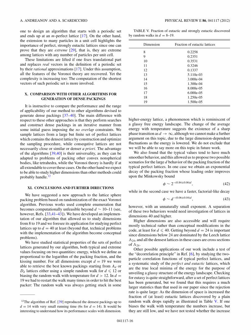
12The algorithm of Ref. [39] reproduced the densest packings up tod = 14 with very small running time (6s for d = 14). It would beinteresting to understand how its performance scales with dimension.

TABLE V. Fraction of eutactic and strongly eutactic discoveredby random walks in d = 8–19.

Dimension Fraction of eutactic lattices

8 0.22589 0.235110 0.353111 0.324612 0.133713 5.110e-0314 3.000e-0415 1.300e-0416 8.000e-0517 6.000e-0518 1.250e-0519 1.500e-05

higher-energy lattice, a phenomenon which is reminiscent ofa glassy free energy landscape. The change of the averageenergy with temperature suggests the existence of a sharpphase transition as d → ∞, although we cannot make a furtherargument on this topic, due to the large dimension-dependentfluctuations as the energy is lowered. We do not exclude thatwe will be able to say more on this topic in future work.

We also found that the typical values tend to have muchsmoother behavior, and this allowed us to propose two possiblescenarios for the large d behavior of the packing fraction of thetypical perfect lattices. In one case we obtain an exponentialdecay of the packing fraction whose leading order improvesupon the Minkowsky bound

φ ∼ 2−(0.84±0.06)d , (42)

while in the second case we have a faster, factorial-like decay

φ ∼ d−(0.06±0.04)d , (43)

however, with an unnaturally small exponent. A separationof these two behaviors would need investigation of lattices indimensions 40 and higher.

Higher dimensions are also accessible and will requiremostly technical rather than conceptual modifications in thecode, at least for d � 40. Getting beyond d = 24 is importantsince dimensions below 24 are dominated by the Leech lattice�24, and all the densest lattices in these cases are cross sectionsof �24.

Other possible applications of our work include a test ofthe “decorrelation principle” in Ref. [6], by studying the two-particle correlation functions of typical perfect lattices, anda systematic study of the perfect and eutactic lattices, whichare the true local minima of the energy for the purpose ofunveiling a glassy structure of the energy landscape. Checkingfor eutaxy is quite straightforward, after a set of perfect latticeshas been generated, but we found that this requires a muchlarger statistics than that used in our paper since the rejectionrate is quite large: As the dimension of space is increased thefraction of (at least) eutactic lattices discovered by a plainrandom walk drops rapidly as illustrated in Table V. If onebiases the walk with temperature the numbers increase, butthey are still low, and we have not tested whether the increase

041117-16


is due to different lattices or isometric copies of few lattices.Therefore we leave this for future work.

Finally, the randomization procedure we have introducedcould also be applied to other optimization problems like thelattice covering problem [17], where one searches for the mosteconomical way of covering a space with spheres of equal size.Another possible activity along the same direction is to adaptour randomization procedure to the algorithm generating alleutactic lattices in a given dimension [30].

As we have indicated, finding extreme rays of the Voronoidomain V is a particular case of a general polyhedral represen-tation conversion problem [34]. This is an important problemin combinatorial optimization and computational geometry.Although efficient algorithms exist for certain classes of poly-hedra, its complexity in general is unknown [33,34], but all ex-isting full conversion algorithms are exponential in the numberof constraints that define a polyhedron [34]. In this wider con-text our randomization approach offers a possible work-aroundfor optimization problems which require a solution of therepresentation conversion problem in order to find an optimum.

ACKNOWLEDGMENTS

We wish to thank A.Schurmann and G.Nebe for providingcode for isometry testing. We are also indebted to S.Torquato,A. Kumar, and H. Cohn for many stimulating discussions.We would like to thank the developers of the PARI/GP [44]libraries for their quick response in fixing bugs. A.S. wouldlike to thank the Center for Theoretical Physics at MIT wherepart of this work was completed.

APPENDIX A: SOME TECHNICAL DETAILS

The two main technical ingredients of the Voronoi algo-rithm are generation of a random extreme ray R of the Voronoidomain V(Q) and finding a neighbor Q′ of a given lattice Q

provided an extreme ray R.Computing a random extreme ray has the same complexity

as generating the Voronoi domain V(Q) and solving a linearprogram. We need to know shortest vectors of Q in order tobuild V(Q). Computing the shortest vectors of a lattice is anexponentially hard problem in d. However, good algorithmsexist allowing computation to be carried out in reasonabletime at least up to d ∼ 40 [45,46]. The other source ofcomplexity is the size of linear program, which is defined by akissing number of Q (and hence scales exponentially in d fordense packings) and is limited by the ability of linear program(LP) solvers to cope with huge linear programs: Size of the LPbecomes of order 1010 for the densest known lattices in d � 40.Based on this observation we expect our method to work upto d ∼ 40, at least in theory. It is also worth pointing out thatit is straightforward to check if a given ray R is extreme [34].

Finding a neighbor Q′ = Q + α R with α ∈ Q proved tobe a harder problem computationally, and it is this part ofthe problem that limited our data to d < 20. The value of α isrational [17,32], so that we can always choose Q′ to be integral,and all perfect lattices then have integral representation. We usea modified binary search algorithm as defined by Schurmann[17] to compute neighbors of a lattice (Sd

>0 is set of all lattices)presented in Fig. 24. The idea behind this construction is

Input: perfect form Q, extreme ray RwhileQ + u R Sd

>0 and λ(Q + u R) = λ(Q) doifQ + u R Sd

>0 and λ(Q + u R) = λ(Q) thenu ← (l + u)/2

else(l, u) ← (u, 2 u)

end ifend whilewhileMin(Q + l R) ⊂ Min(Q) do

g ← (u + l)/2if λ(Q + g R) ≥ λ(Q) then

l ← gelse

u ← min{(λ(Q) − Q[v])/R[v]|v ∈ Min(Q +g R),R[v] < 0} ∪ {g}end if

end whileOutput: α ← l

FIG. 24. Modified binary search for neighbor Q′ of a lattice Q

given an extreme ray R.

very simple: The neighbor of Q is Q′ = Q + α R with thesmallest positive rational α such that λ(Q) = λ(Q + α R) andMin(Q + α R) �⊆ Min(Q).13 In the first part of the algorithmpresented in Fig. 24 upper and lower boundaries for α aredefined. The second part of the algorithm is a modified binarysearch for value of α. The modification, an extra conditional inthe assignment of u, is necessary to make the algorithm con-verge in a finite number of steps to an exact rational value of α.

APPENDIX B: RANDOM WALKS AND ISOMETRY CHECK

We have used two different approaches to perform checksfor isometry of lattices. In the first approach we split thedata generation into two steps: (1) Generate a random walkin space of lattices with no check for isometry and (2) runan isometry test on the trajectory of the random walk andgenerate an approximate Voronoi graph. After the first stepone obtains a full trajectory of a random walk as list of lattices.The second step generates the graph by eliminating isometriccopies of lattices by gluing together isometric elements of thelist. This induces a relation of the neighborhood in the list andtransforms the list into a graph.

The second possibility is to perform an isometry checkand graph construction on the fly (P ∼ Q denotes isometricequivalence, and V and E are sets of vertices and edges of thegraph G, respectively) as shown in Fig. 25.

Both algorithms terminate after a predefined number ofsteps has been done.

An algorithm to check whether two lattices are isometricwas developed by W. Plesken and B. Souvignier in Ref. [27].We adapted the original code of B. Souvignier to performisometry testing.

13Note that self-loops are allowed, i.e. α �= 0 and Min(Q + α R) =Min(Q).

041117-17


Input: perfect Q, graph G = (V = ∅, E = ∅)loopRandom extreme ray R ← QNeighbor Q ← Q + α Rfor P ∈ G doif P ∼ Q then

E ← E ∪ (Q, P )else

V ← V ∪ QE ← E ∪ (Q , Q)

end ifend for

end loopOutput: Voronoi graph G

FIG. 25. Algorithm that constructs an approximation to theVoronoi graph.

APPENDIX C: NAIVE RANDOM WALK

It is worth discussing performance of a straightforwardapproach that one might be tempted to follow. The Voronoiconstruction is elaborate and requires computational effort. Apriori one might wonder if a simple lattice random walk orMonte Carlo approach [10] is preferable (maybe in higherdimensions?). The algorithm shown in Fig. 26 is extremelysimple: One hopes to approach the best packer by small steps ifthe random walk is sufficiently biased towards denser lattices.When generating a move one has the option of either producinga new lattice A′ which might or might not be an isometric copyof A. Acceptance probability p could be 1 (random walk) or,for example, the Metropolis rule (a la Monte Carlo).

An unbiased random walk (infinite temperature in ourlanguage) with moves that generate nonisometric lattices A′

Input: Lattice Aloop

(∗) A ← AAccept A with some probability pGoto (∗)

end loopOutput: Dense lattice A

FIG. 26. Naive random walk.

gives an average packing fraction which is equal to theMinkovsky bound [9,10,47–49]. This is a rather strongresult since the Minkovsky bound is nonconstructive andconstructing a lattice in a given dimension satisfying the boundis yet an open problem. However, it is very hard to implementthat type of updates in practice [9,10,47–50], and one has torely on various approximations. In the case when one allowsfor any A′ the performance of the algorithm is extremelypoor: With the simple Gaussian measure for lattices [10]P(A) ∼ exp(−γ Tr AAt ) we were able to recover the bestpackers in d = 2,3, although already in three dimensions wehad to go to very low temperatures. The performance of thealgorithm quickly deteriorates with dimension, and by d = 10it is completely useless. The above mentioned variant of thealgorithm where one samples only among the nonisometriclattices has similar performance when approximations areused. Finally it is worth mentioning that the lattices generatedby such Markov chains are never perfect and are typically farfrom being such.

These negative results provide an extra motivation forstudying perfect lattices and the Voronoi construction wheremuch better performance is achieved.

[1] J. H. Conway and N. J. A. Sloane, Sphere Packings, Lattices andGroups, Vol. 290 (Springer, New York, 1999).

[2] C. Shannon, Bell Syst. Tech. J. 27, 379 (1948).[3] S. Torquato, Random Heterogeneous Materials (Springer, New

York, 2005).[4] L. Fejes Toth, Math. Z. 46, 83 (1940).[5] T. Hales, Ann. Math. 162, 1065 (2005).[6] S. Torquato and F. H. Stillinger, Exp. Math. 15, 307 (2006).[7] C. Zachary and S. Torquato, J. Stat. Mech. (2011) P10017.[8] A. Scardicchio, F. H. Stillinger, and S. Torquato, J. Math. Phys.

49, 043301 (2008).[9] C. Rogers, Proc. Lond. Math. Soc. 3, 609 (1958).

[10] G. Parisi, J. Stat. Phys. 132, 207 (2008).[11] Y. Jin, P. Charbonneau, S. Meyer, C. Song, and F. Zamponi,

Phys. Rev. E 82, 051126 (2010).[12] G. Parisi and F. Zamponi, J. Stat. Mech. (2006) P03017.[13] G. Parisi and F. Zamponi, Rev. Mod. Phys. 82, 789 (2010).[14] H. Cohn and N. Elkies, Ann. Math. 157, 689 (2003).[15] H. Cohn and A. Kumar, Ann. Math. 170, 1003 (2009).[16] G. Voronoi, J. Reine. Angew. Math. 133, 97 (1908).[17] A. Schurmann, Computational Geometry of Positive Definite

Quadratic Forms: Polyhedral Reduction Theories, Algorithms,and Applications, Vol. 48 (American Mathematical Society,Providence, RI, 2009).

[18] A. Ash, Can. J. Math 29, 1040 (1977).[19] J. Lagrange, Nouv. Mem. Acad. Berlin 265 (1773).[20] C. Gauss, J. Reine. Angew. Math. 20, 312 (1840).[21] A. Korkin and E. Zolotarev, Math. Ann. 11, 242 (1877).[22] E. Barnes, Philos. Trans. R. Soc. Lond. A 249, 461 (1957).[23] D. Jaquet-Chiffelle, Ann. Inst. Fourier (Grenoble) 43, 21 (1993).[24] M. D. Sikiric, A. Schurmann, and F. Vallentin, Electron. Res.

Announc. Am. Math. Soc 13, 21 (2007).[25] C. Riener, J. Theorie Nombres Bordeaux 18, 677 (2006).[26] A. Schurmann et al., fma2.math.uni-magdeburg.de/∼latgeo/ and

http://www.geometrie.uni-rostock.de/.[27] W. Plesken and B. Souvignier, J. Symb. Comput. 24, 327 (1997).[28] M. Mezard, G. Parisi, and M. Virasoro, Spin Glass Theory and

Beyond, Vol. 9 (World Scientific, Singapore, 1987).[29] A. Schurmann, Advances in Mathematics 225, 2546 (2010).[30] C. Batut, Math. Comput. 70, 395 (2001).[31] A. Berge and J. Martinet, J. Lond. Math. Soc. 53, 417 (1996).[32] J. Martinet, Perfect Lattices in Euclidean Spaces, Vol. 327

(Springer, New York, 2003).[33] D. Bremner, M. D. Sikiric, and A. Schurmann, CRM Proceed-

ings & Lecture Notes, 45 (American Mathematical Society,Providence, RI, 2009).

[34] D. Avis, D. Bremner, and A. Deza, Polyhedral Computation, Vol.48 (American Mathematical Society, Providence, RI, 2009).

041117-18

http://dx.doi.org/10.1007/BF01181430

http://dx.doi.org/10.4007/annals.2005.162.1065

http://dx.doi.org/10.1080/10586458.2006.10128964

http://dx.doi.org/10.1088/1742-5468/2011/10/P10017

http://dx.doi.org/10.1063/1.2897027

http://dx.doi.org/10.1063/1.2897027

http://dx.doi.org/10.1112/plms/s3-8.4.609

http://dx.doi.org/10.1007/s10955-008-9539-6


http://dx.doi.org/10.1088/1742-5468/2006/03/P03017

http://dx.doi.org/10.1103/RevModPhys.82.789



http://dx.doi.org/10.4153/CJM-1977-101-2

http://dx.doi.org/10.1007/BF01442667

http://dx.doi.org/10.1098/rsta.1957.0005

http://dx.doi.org/10.5802/aif.1320

http://dx.doi.org/10.1090/S1079-6762-07-00171-0

http://dx.doi.org/10.1090/S1079-6762-07-00171-0

http://dx.doi.org/10.5802/jtnb.565

http://fma2.math.uni-magdeburg.de/%7Elatgeo/

http://www.geometrie.uni-rostock.de/

http://dx.doi.org/10.1006/jsco.1996.0130

http://dx.doi.org/10.1016/j.aim.2010.05.002

http://dx.doi.org/10.1112/jlms/53.3.417


[35] A. Lenstra, H. Lenstra, and L. Lovasz, Math. Ann. 261, 515(1982).

[36] B. Bollobas and O. Riordan, Combinatorica 24, 5 (2004).[37] B. D. Lubachevsky and F. H. Stillinger, J. Stat. Phys. 60, 561

(1990); B. D. Lubachevsky, F. H. Stillinger, and E. N. Pinson,ibid. 64, 501 (1991).

[38] H. Cohn, A. Kumar, and A. Schurmann, Phys. Rev. E 80, 061116(2009).

[39] Y. Kallus, V. Elser, and S. Gravel, Phys. Rev. E 82, 056707(2010).

[40] S. Torquato and Y. Jiao, Phys. Rev. E 82, 061302 (2010).[41] M. D. Sikiric, A. Schurmann, and F. Vallentin, Math. Comput.

78, 1713 (2009).[42] M. D. Sikiric, A. Schurmann, and F. Vallentin, Discrete Comput.

Geom. 44, 904 (2010).

[43] T. Rehn and A. Schurmann, Mathematical Sofware ICMS 2010,Lecture Notes in Comput. Sci., Vol. 6327 (Springer, Berlin,2010), pp. 295–298.

[44] The PARI Group, Bordeaux, PARI/GP, version 2.5.2 (2012),http://pari.math.u-bordeaux.fr/.

[45] U. Fincke and M. Pohst, Math. Comput. 44, 463 (1985).[46] H. Cohen, A Course in Computational Algebraic

Number Theory, Vol. 138 (Springer, New York,1993).

[47] C. A. Rogers, Acta Mathematica 94, 249 (1955).[48] C. A. Rogers, Proc. Lond. Math. Soc. 3, 305 (1956).[49] C. A. Rogers, Packing and Covering, Cambridge Mathemat-

ical Tracts, No. 54 (Cambridge University Press, Cambridge,1964).

[50] C. Siegel, Ann. Math. 46, 340 (1945).

041117-19

http://dx.doi.org/10.1007/BF01457454

http://dx.doi.org/10.1007/BF01457454

http://dx.doi.org/10.1007/s00493-004-0002-2

http://dx.doi.org/10.1007/BF01025983

http://dx.doi.org/10.1007/BF01025983

http://dx.doi.org/10.1007/BF01048304






http://dx.doi.org/10.1090/S0025-5718-09-02224-8

http://dx.doi.org/10.1090/S0025-5718-09-02224-8

http://dx.doi.org/10.1007/s00454-010-9266-z

http://dx.doi.org/10.1007/s00454-010-9266-z

http://pari.math.u-bordeaux.fr/

http://dx.doi.org/10.1090/S0025-5718-1985-0777278-8

http://dx.doi.org/10.1007/BF02392493

http://dx.doi.org/10.1112/plms/s3-6.2.305

http://dx.doi.org/10.2307/1969027

random perfect lattices and the sphere packing problem...

Documents