ralph gregor andrzejak

125

9 Nonlinear Time Series Analysis in a Nutshell

Ralph Gregor Andrzejak

9.1 IntroductIon

Nonlinear time series analysis is a practical spinoff from complex dynamical systems theory and chaos theory. It allows one to characterize dynamical systems in which nonlinearities give rise to a complex temporal evolution. Importantly, this concept allows extracting information that cannot be resolved using classical linear techniques such as the power spectrum or spectral coherence. Applications of nonlinear time series analysis to signals measured from the brain contribute to our understanding of brain functions and malfunctions and thereby help to advance cognitive neurosci-ence and neurology. In this chapter, we show how a combination of a nonlinear prediction error and the Monte Carlo concept of surrogate time series can be used to attempt to distinguish between purely stochastic, purely deterministic, and deterministic dynamics superimposed with noise.

The framework of nonlinear time series analysis comprises a wide variety of measures that allow one to extract different characteristic features of a dynamical system underlying some mea-sured signal (Kantz and Schreiber 1997). These include the correlation dimension as an estimate of the number of independent degrees of freedom, the Lyapunov exponent as a measure for the divergence of similar system states in time, prediction errors as detectors for characteristic traits of deterministic dynamics, or different information theory measures. The aforementioned nonlinear time series measures are univariate, i.e., they are applied to single signals measured from individual dynamics. In contrast, bivariate measures are used to analyze pairs of signals measured simultane-ously from two dynamics. Such bivariate time series analysis measures aim to distinguish whether the two dynamics are independent or interacting through some coupling. Some of these bivariate measures aim to extract not only the strength, but also the direction of these couplings. The Monte Carlo concept of surrogates allows one to test the results of the different nonlinear measures against well-specified null hypotheses.

contents

9.1 Introduction .......................................................................................................................... 1259.2 Dynamics and Time Series ................................................................................................... 127

9.2.1 Nonlinear Deterministic Dynamics—Lorenz Dynamics ........................................ 1279.2.2 Noisy Deterministic Dynamics—Noisy Lorenz Dynamics ..................................... 1279.2.3 Stochastic Processes—Linear Autoregressive Models ............................................. 129

9.3 Deterministic versus Stochastic Dynamics .......................................................................... 1299.4 Delay Coordinates ................................................................................................................ 1299.5 Nonlinear Prediction Error ................................................................................................... 1329.6 The Concept of Surrogate Time Series ................................................................................ 1349.7 Influencing Parameters ......................................................................................................... 1359.8 What Can and Cannot be Concluded? .................................................................................. 137References ...................................................................................................................................... 138

K11766_C009.indd 125 11/24/2010 1:35:58 PM

126 Epilepsy: The Intersection of Neurosciences, Biology, Mathematics, Engineering and Physics

We should briefly define the different types of dynamics. Let x(t) denote a q-dimensional vector that fully defines the state of the dynamics at time t. For purely deterministic dynamics, the future temporal evolution of the state is unambiguously defined as a function f of the present state:

x f x( ) ( ( ))t t= . (9.1)

Here x(t) denotes the time derivative of the state x(t). We further suppose that a univariate time series si is measured at integer multiples of a sampling time Δt from the dynamics using some mea-surement function h:

si = h(x(iΔt)). (9.2)

The combination of Equation 9.1 and Equation 9.2 results in the purely deterministic case. When some noise ψ(t) enters the measurement:

si = h(x(iΔt),ψ(iΔt)), (9.3)

we obtain the case of deterministic dynamics superimposed with noise. Here it is important to note that the noise only enters at the measurement. The deterministic evolution of the system state x(t) via Equation 9.1 is not distorted. In contrast to such measurement noise stands dynamical noise ξ(t) for which we have:

x f x( ) ( ( ), ( ))t t t= ξ . (9.4)

Due to the noise term, the future temporal evolution of x(t) is not unambiguously determined by the present state. Accordingly, Equation 9.4 represents stochastic dynamics. We again suppose that a measurement function, with or without measurement noise (Equations 9.3 and 9.2, respectively), is used to derive a univariate time series si from this stochastic dynamics.

As stated above, we aim to distinguish between purely stochastic, purely deterministic, and deterministic dynamics superimposed with noise. Accordingly, we want to design an algorithm A to be applied to a time series si that fulfills the following criteria:

i. A(si) should attain its highest values for time series si measured from any purely stochastic process.

ii. A(si) should attain its lowest values for time series si measured from a noise-free determin-istic dynamics.*,†

iii. A(si) should attain some value in the middle of its scale for time series si measured from noisy deterministic dynamics.

In particular, the ranges obtained for ii. and iii. should not overlap with the one of i. For iii., A(si) should ideally vary with the relative noise amplitude.

In order to study our problem under controlled conditions, we use a time series of mathematical model systems that represent these different types of dynamics. While this chapter is restricted to these model systems, the underlying lecture included results for exemplary intracranial electroen-cephalographic (EEG) recordings of epilepsy patients (Andrzejak et al. 2001). These EEG times

* The following text contains a number of footnotes. These are meant to provide background information. The reader might safely ignore them without risk of losing the essentials of the main text.

† The polarity of A does not matter. It could likewise attain lowest values for i. and highest values for ii.

K11766_C009.indd 126 11/24/2010 1:35:58 PM

Nonlinear Time Series Analysis in a Nutshell 127

series as well as the source codes to generate the different time series studied here, the generation of surrogates, and the nonlinear prediction error are freely available.*

9.2 dynamIcs and tIme serIes

9.2.1 NoNliNear DetermiNistic DyNamics—loreNz DyNamics

As nonlinear deterministic dynamics we use the following Lorenz dynamics.†

x t y t x t( ) ( ( ) ( ))= −10 (9.5)

y t x t y t x t z t( ) ( ) ( ) ( ) ( )= − −39 (9.6)

z t x t y t z t( ) ( ) ( ) ( ) ( )= − 8 3/ . (9.7)

This set of first-order differential equations can be integrated using, for example, a fourth order Runge–Kutta algorithm.‡ To obtain time series xi, yi, zi for i = 1,…,N = 2048, we sample the output of the numerical integration at an interval of Δt = 0.03 time units.§ We denote the resulting temporal sequence of three-dimensional vectors as Li = (xi, yi, zi). In our analysis, we restrict ourselves to the first component xi (see Table 9.1 and Figure 9.1). Hence, we have an example of purely deterministic dynamics (Equation 9.1). The discretization in time is obtained from the numerical integration of the dynamics. This integration can be considered as part of the measurement function (Equation 9.2), which furthermore consists of the projection to the first component.

9.2.2 Noisy DetermiNistic DyNamics—Noisy loreNz DyNamics

By adding white noise to the first component of our Lorenz time series xi, we obtain noisy deter-ministic dynamics:

ni = xi + 18ψi, (9.8)

where ψi denotes uncorrelated noise with uniform amplitude distribution between 0 and 1 (see Table 9.1 and Figure 9.1). Our time series ni is an example of a signal generated by deterministic dynamics (Equation 9.1) where noise is superimposed on the measurement function Equation 9.3. To roughly assess the strength of the noise, we have to know that the standard deviation of the noise term ψi and the Lorenz time series xi is approximately 0.29 and 9.6, respectively. With the prefactor of 18, the standard deviation of the noise¶ amounts to approximately 5.2.

* www.meb.uni-bonn.de/epileptologie/science/physik/eegdata.html; www.cns.upf.edu/ralph.† Equations 9.5 through 9.7 result in chaotic dynamics. However, this is not of our concern here. Rather, we use the Lorenz

dynamics as a representative of some aperiodic deterministic dynamics.‡ Here we use an algorithm with fixed step size of 0.005 time units. Starting at random initial condition we use some arbi-

trary but high number (e.g., 106) of preiterations to diminish transients.§ In the signal analysis literature, one often finds 1024, 2048, 4096, etc. for the number of samples. The reason is that these

numbers are integer powers of two: N* = 2n with n being an integer. For these numbers of samples, one can use the very efficient fast Fourier transform algorithm. For other numbers of samples, one has to use algorithms that divide the number of samples in prime factors and that are slower.

¶ In assessing the relative strength of noise superimposed to the Lorenz dynamics, it is important to note that a major contribution to the overall standard deviation originates from the switching behavior of this dynamics. The standard deviation of the actual aperiodic oscillations in the two wings is smaller (see Figures 9.1–9.2).

K11766_C009.indd 127 11/24/2010 1:35:58 PM


table 9.1overview of different time series studied

type origin and Parameter

ai Stochastic AR process, Equation 9.9 with r = 0

bi Stochastic AR process, Equation 9.9 with r = 0.95

ci Stochastic AR process, Equation 9.9 with r = 0.98

xi Deterministic x-component of Lorenz dynamics

ni Noisy deterministic xi superimposed with white noise

0 500 1000 1500 2000−5

0

5

i

0 500 1000 1500 2000−10

0

10

i

0 500 1000 1500 2000−10

0

10

i

0 500 1000 1500 2000−20

0

20

i

x in i

c ib i

a i

0 500 1000 1500 2000−20

0

20

40

i

FIgure 9.1 Plots of the different time series studied here.

K11766_C009.indd 128 11/24/2010 1:35:59 PM


9.2.3 stochastic Processes—liNear autoregressive moDels

As a stochastic process, we use a simple but still very instructive example—a first-order linear autoregressive process with varying degrees of autocorrelation:

ζi+1 = r ζi + ξi , (9.9)

for i = 1, . . . ,N = 2048, where ξi denotes uncorrelated Gaussian noise with 0 mean and unit vari-ance.* We can readily see that for r = 0, Equation 9.9 results in white, i.e., uncorrelated noise. Upon the increase of r, within the interval 0 < r < 1, the strength of the autocorrelation increases. For this chapter, we study three different time series derived from Equation 9.9 using different values of r (see Table 9.1 and Figure 9.1).

In contrast to the time-continuous stochastic dynamics expressed in Equation 9.4, the autore-gressive process of Equation 9.9 is defined for discrete time. What is common to both formulations, and what is the important point here, is that the noise is intrinsic to the dynamics; no additional noise enters through the measurement. We should note that the fact that we can write down a rule to generate an autoregressive process (as in Equation 9.9) does not conflict with its stochastic nature in any way. The point is that due to the noise term, ξi, an initial condition does not unambiguously determine the future temporal evolution of the dynamics. Furthermore, without this noise term, the autoregressive process would not result in sustained dynamics but rather decay to 0.

9.3 determInIstIc versus stochastIc dynamIcs

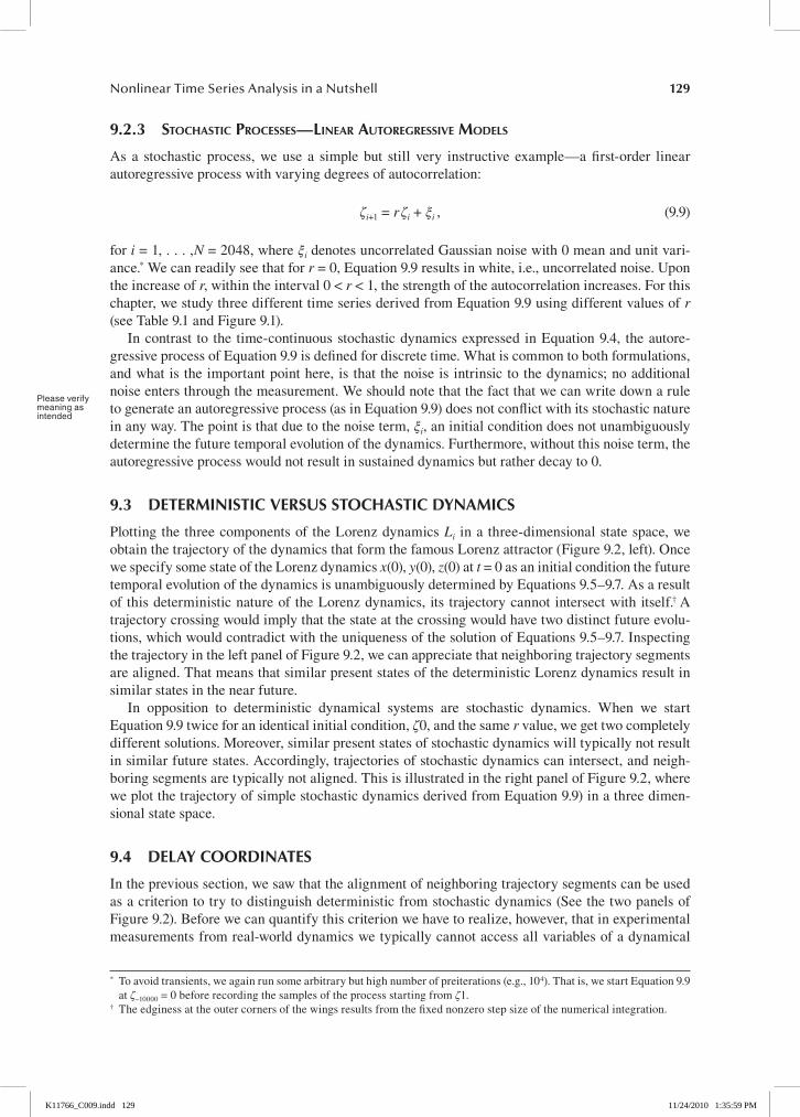
Plotting the three components of the Lorenz dynamics Li in a three-dimensional state space, we obtain the trajectory of the dynamics that form the famous Lorenz attractor (Figure 9.2, left). Once we specify some state of the Lorenz dynamics x(0), y(0), z(0) at t = 0 as an initial condition the future temporal evolution of the dynamics is unambiguously determined by Equations 9.5–9.7. As a result of this deterministic nature of the Lorenz dynamics, its trajectory cannot intersect with itself.† A trajectory crossing would imply that the state at the crossing would have two distinct future evolu-tions, which would contradict with the uniqueness of the solution of Equations 9.5–9.7. Inspecting the trajectory in the left panel of Figure 9.2, we can appreciate that neighboring trajectory segments are aligned. That means that similar present states of the deterministic Lorenz dynamics result in similar states in the near future.

In opposition to deterministic dynamical systems are stochastic dynamics. When we start Equation 9.9 twice for an identical initial condition, ζ0, and the same r value, we get two completely different solutions. Moreover, similar present states of stochastic dynamics will typically not result in similar future states. Accordingly, trajectories of stochastic dynamics can intersect, and neigh-boring segments are typically not aligned. This is illustrated in the right panel of Figure 9.2, where we plot the trajectory of simple stochastic dynamics derived from Equation 9.9) in a three dimen-sional state space.

9.4 delay coordInates

In the previous section, we saw that the alignment of neighboring trajectory segments can be used as a criterion to try to distinguish deterministic from stochastic dynamics (See the two panels of Figure 9.2). Before we can quantify this criterion we have to realize, however, that in experimental measurements from real-world dynamics we typically cannot access all variables of a dynamical

* To avoid transients, we again run some arbitrary but high number of preiterations (e.g., 104). That is, we start Equation 9.9 at ζ–10000 = 0 before recording the samples of the process starting from ζ1.

† The edginess at the outer corners of the wings results from the fixed nonzero step size of the numerical integration.

Please verify meaning as intended

K11766_C009.indd 129 11/24/2010 1:35:59 PM


system. Suppose for example that we study a real-world dynamical system that is fully described by the Lorenz differential Equations 9.5–9.7. Suppose, however, that we cannot measure all three components of Li, but rather only si = xi is assessed by our measurement function. In this case, we can use the method of delay coordinates to obtain an estimate of the underlying dynamics (Takens 1981):

vi = (si,…,si–(m–1)τ ), (9.10)

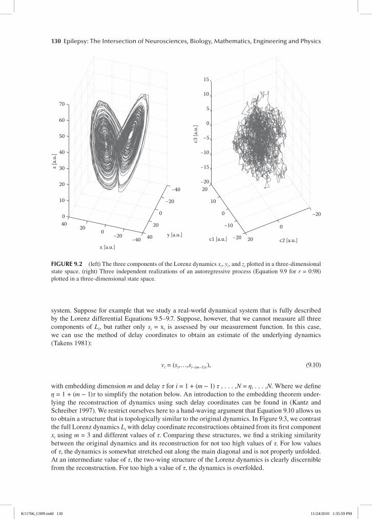
with embedding dimension m and delay τ for i = 1 + (m − 1) τ , . . . ,N = η, . . . ,N. Where we define η = 1 + (m − 1)τ to simplify the notation below. An introduction to the embedding theorem under-lying the reconstruction of dynamics using such delay coordinates can be found in (Kantz and Schreiber 1997). We restrict ourselves here to a hand-waving argument that Equation 9.10 allows us to obtain a structure that is topologically similar to the original dynamics. In Figure 9.3, we contrast the full Lorenz dynamics Li with delay coordinate reconstructions obtained from its first component xi using m = 3 and different values of τ. Comparing these structures, we find a striking similarity between the original dynamics and its reconstruction for not too high values of τ. For low values of τ, the dynamics is somewhat stretched out along the main diagonal and is not properly unfolded. At an intermediate value of τ, the two-wing structure of the Lorenz dynamics is clearly discernible from the reconstruction. For too high a value of τ, the dynamics is overfolded.

−40−20

020

40

−40

−20

0

20

40

0

10

20

30

40

50

60

70

y [a.u.]

x [a.u.]

z [a.u

.]

−20

−10

0

10

20

−20

0

20

−20

−15

−10

−5

0

5

10

15

c2 [a.u.]c1 [a.u.]

c3 [a

.u.]

FIgure 9.2 (left) The three components of the Lorenz dynamics xi, yi, and zi plotted in a three-dimensional state space. (right) Three independent realizations of an autoregressive process (Equation 9.9 for r = 0:98) plotted in a three-dimensional state space.

K11766_C009.indd 130 11/24/2010 1:35:59 PM


−200

20−20

020

20

40

60

xiyi

z i

i

j

500 1000 1500 2000

500

1000

1500

2000

−200

20

−200

20−20

0

20

xixi−1

x i−2

i

j500 1000 1500 2000

500

1000

1500

2000

−200

20

−200

20−20

0

20

xixi−3

x i−6

i

j

500 1000 1500 2000

500

1000

1500

2000

−200

20

−200

20−20

0

20

xixi−30

x i−60

i

j

500 1000 1500

500

1000

1500

FIgure 9.3 (first row, left) The three components of the Lorenz dynamics Li = (xi, yi, zi) plotted in a three-dimensional state space. Hence, this panel is the same as the left panel of Figure 9.2, but viewed from a dif-ferent angle. (first row, right) Euclidean distance matrix calculated for the Lorenz dynamics Li. (second row, left) Delay reconstruction of the Lorenz dynamics based on the first component, xi. Here we use a time delay of τ = 1. For obvious reasons, the maximal embedding dimension that we can use for this illustration is m = 3. (second row, right) Euclidean distance matrix calculated from such an embedding, but for m = 6. (third and fourth rows) Same as second row, but for τ = 6 and τ = 30, respectively.

K11766_C009.indd 131 11/24/2010 1:36:00 PM


We can appreciate this similarity further by inspecting Euclidean distance matrices derived from the full Lorenz dynamics and its delay coordinate reconstruction.* For a set of q-component vectors wi for i = η, . . . ,N, such a matrix contains in its element Dij the Euclidean distance between the vec-tors wi and wj. The Euclidean distance between two q-component vectors w1 and w2 is defined as

d w w w wl l

l

q

( , ) ( ), ,1 2 1 22

1

= −=

∑ . (9.11)

Figure 9.3 shows the distance matrix for the full Lorenz dynamics Li, which can also be seen as a set of N vectors with q = 3 components. This is contrasted to the distance matrix derived from delay coordinate reconstructions vi, which is a set of N vectors with q = m components. While the overall scales of the different matrices are different, we can observe an evident similarity between the structures found in these matrices for the original and its delay coordinate reconstruction for not too high values of τ. Importantly, this similarity implies that close and distant states in the full Lorenz dynamics are mapped to close and distant states in the reconstructed dynamics, respectively. This topological similarity implies that our criterion of distinction between deterministic and stochastic dynamics, namely the alignment of neighboring trajectory segments, carries over from the original dynamics to the reconstructed dynamics obtained by means of delay coordinates. The different distance matrices derived from the delay reconstructions are, however, not identical to the original distance matrix and the degree of their similarity depends on the embedding parameters m and τ. These aspects will be discussed in more detail below. To get a thorough understanding of the quality of the embedding requires playing with different parameters and viewing the result from different angles. This can be done using the source code referred to in the introduction.

9.5 nonlInear PredIctIon error

Above we have identified the alignment of neighboring trajectory segments as a signature of deter-ministic dynamics. We will now introduce the nonlinear prediction error as a straightforward way to quantify the degree of this alignment (see Kantz and Schreiber (1997) and references therein).

Before we begin, we first normalize our time series si to have zero mean and unit standard deviation and variance.† Subsequently, we form a delay reconstruction vi from our time series for i = η, . . . ,N. To calculate the nonlinear prediction error with horizon h we carry out the following steps for i0 = η, . . . ,N − h. We take vi as reference point and look up the time indices of the k nearest neighbors of the reference point: {ig}(g = 1, . . . ,k). These k nearest neighbors are simply those points that have the k smallest distances to our reference point in the reconstructed state space. In other words, {ig}(g = 1, . . . ,k) are the indices of the k smallest entries in row i0 of the distance matrix derived from vi.‡ Now we use the future states of these nearest neighbors to predict the future states of our reference point and quantify the error that we make in doing so by

εi i i

g

k

s hk

s hg0 0

1

1

= + − +=

∑ . (9.12)

* The choice of the Euclidean distance is arbitrary. The same arguments hold when other definitions of distances are used.

† In this way we do not have to normalize the prediction error itself and the subsequent notations become simpler.‡ Since distance matrices are symmetric, these indices coincide with the k smallest entries in the column i0 of the matrix.

Note however that if vi1 is among the k nearest neighbors of vi2, this does not imply that vi2 is among the k nearest neigh-bors of vi1.

K11766_C009.indd 132 11/24/2010 1:36:00 PM


Finally, we take the root-mean-square over all reference points:

EN h i

i

i N h

=− − +

=

= −

∑11 0

0

0

2

ηε

η

. (9.13)

Note that while the nearest neighbors are determined according to their distance in the reconstructed state space, the actual prediction in Equation 9.12 is made using the scalar time series values. Regarding Equation 9.12, it also becomes clear that we must exclude nearest neighbors with indices ir > N − h. Furthermore, we should aim to base our prediction on neighboring trajectory segments rather than on the preceding and subsequent piece of the trajectory on which our reference point vi0 is located on. For this purpose we apply the so-called Theiler correction with window length W (Theiler 1986), by including only points to the set of k nearest neighbors that fulfill |ig − i0| > W.

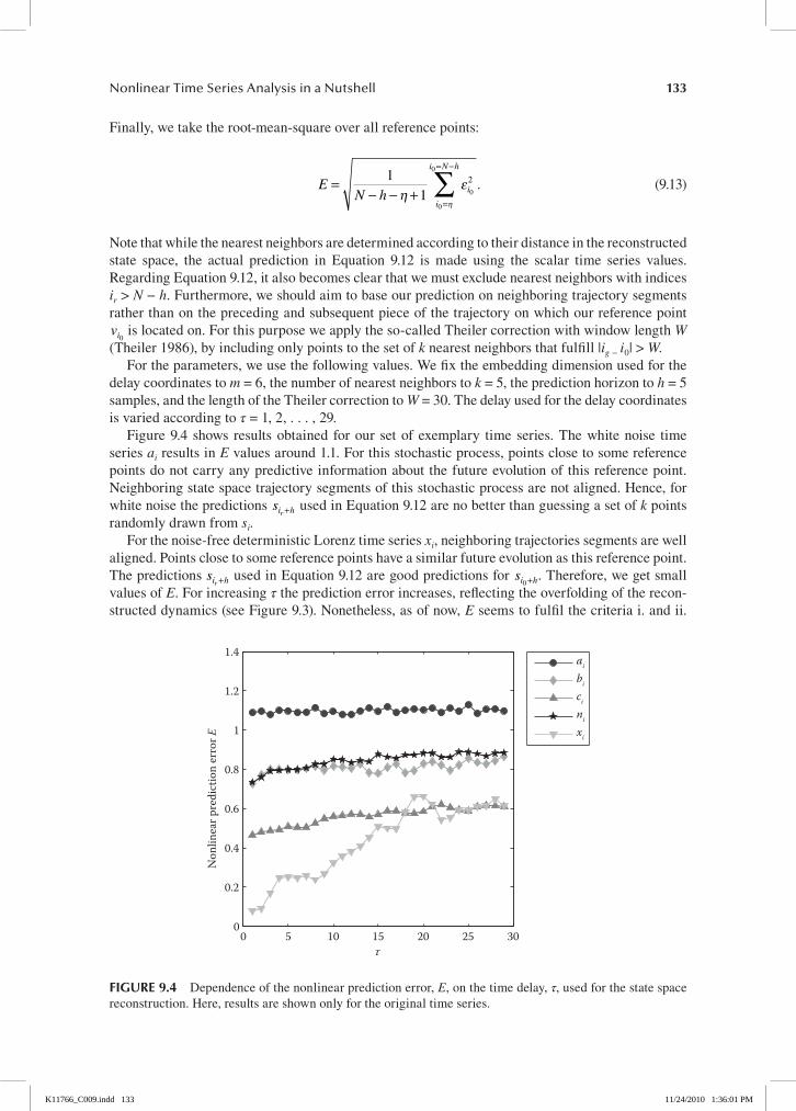
For the parameters, we use the following values. We fix the embedding dimension used for the delay coordinates to m = 6, the number of nearest neighbors to k = 5, the prediction horizon to h = 5 samples, and the length of the Theiler correction to W = 30. The delay used for the delay coordinates is varied according to τ = 1, 2, . . . , 29.

Figure 9.4 shows results obtained for our set of exemplary time series. The white noise time series ai results in E values around 1.1. For this stochastic process, points close to some reference points do not carry any predictive information about the future evolution of this reference point. Neighboring state space trajectory segments of this stochastic process are not aligned. Hence, for white noise the predictions si hr+ used in Equation 9.12 are no better than guessing a set of k points randomly drawn from si.

For the noise-free deterministic Lorenz time series xi, neighboring trajectories segments are well aligned. Points close to some reference points have a similar future evolution as this reference point. The predictions si hr+ used in Equation 9.12 are good predictions for si h0+ . Therefore, we get small values of E. For increasing τ the prediction error increases, reflecting the overfolding of the recon-structed dynamics (see Figure 9.3). Nonetheless, as of now, E seems to fulfil the criteria i. and ii.

0 5 10 15 20 25 300

0.2

0.4

0.6

0.8

1

1.2

1.4

Non

linea

r pre

dict

ion

erro

r E

ai

bi

cini

xi

τ

FIgure 9.4 Dependence of the nonlinear prediction error, E, on the time delay, τ, used for the state space reconstruction. Here, results are shown only for the original time series.

K11766_C009.indd 133 11/24/2010 1:36:01 PM


formulated in the Introduction. It allows us to clearly tell apart our deterministic Lorenz time series from white noise. It can be objected that this distinction is not terribly difficult, and could readily be achieved by visual inspection of our data.

We should therefore proceed to our noisy deterministic time series ni and time series of autore-gressive processes with stronger autocorrelation (bi, ci). When we look at their results in Figure 9.4, we must realize that E is in fact not a good candidate for Figure 9.4A. For the time series ni it is clear that the noise must degrade the quality of the predictions of Equation 9.12 as compared to the noise-free case of xi. This increase in E by itself would not disqualify E, as it is compatible with criterion iii. The problem is that E values for bi overlap with those for ni. Results for ci are even lower than those for ni and for higher τ, even similar to those of xi. The reason why these autocorrelated time series exhibit a higher predictability as opposed to white noise is the following: vi1 being a close neighbor of vi2 implies that the scalar si1 is typically similar to the scalar si2 . Furthermore, si1 being similar to si2 implies, to a certain degree, that si h1+ is similar to si h2+ . It is instructive to convince one-self that it is just the strength of the autocorrelation that determines the strength of the “to a certain degree” in the previous statement.

As a consequence, stochastic time series with stronger autocorrelation and noisy deterministic dynamics cannot be told apart by our nonlinear time series algorithm E. We are still missing one very substantial ingredient to reach our aim, which will we introduce in Section 9.6.

9.6 the concePt oF surrogate tIme serIes

Nonlinear time series analysis was initially developed studying complex low-dimensional deter-ministic model systems such as the Lorenz dynamics. The brain is certainly not a low-dimensional deterministic dynamics and will typically not behave as one. Rather, it might be regarded as a partic-ularly challenging high-dimensional and complicated dynamical system that might have both deter-ministic and stochastic features. Problems that arise in applications to signals measured from the nervous system continue to trigger the refinement of existing algorithms and development of novel approaches and, thereby, help to advance nonlinear time series analysis. One important concept in nonlinear time series analysis, which has some of its roots in EEG analysis (Pijn et al. 1991), is the Monte Carlo framework of surrogate time series (Theiler et al. 1992; Schreiber and Schmitz 2000).

Suppose that we have calculated the nonlinear prediction error for some experimental times series and consider the following scenarios. First, we obtain a relatively low E value but have doubts that this is due to some deterministic structure in our time series. Second, we obtain a relatively high E value but we suspect that our time series should have some deterministic structure that is possibly distorted by some measurement noise. In any case, we want to know what a relatively high or a relatively low value of the nonlinear prediction error means. A way to address this problem is to scrutinize our time series further by testing different null hypotheses about it by means of sur-rogate time series. Such surrogate time series are generated from a constrained randomization of an original time series.* The surrogates are designed to share specific properties with the original time series, but are otherwise random. In particular, the properties that the surrogates share with the original time series are selected such that the surrogates represent signals that are consistent with a well-specified null hypothesis.

Here, we use the simple but illustrative example of phase-randomized surrogates (Theiler et al. 1992). To construct these surrogates, first calculate the complex-valued Fourier transform of the original time series. In the next step, randomize all phases of the complex-valued Fourier coefficients between 0 and 2π.† Finally, the inverse Fourier transform of these modified Fourier

* See Schreiber and Schmitz (2000) for the alternative to using a typical randomization to generate surrogates.† In this randomization it is very important to preserve the antisymmetry between Fourier coefficients representing posi-

tive and negative frequencies. This antisymmetry holds for real-valued signals. If it is not preserved the inverse Fourier transform will not result in a real-valued time series.

K11766_C009.indd 134 11/24/2010 1:36:01 PM


coefficients results in a surrogate time series. An ensemble of surrogates is generated using differ-ent randomization of the phases. Randomizing the phase of a complex number does not affect its absolute value, that is, the length of the corresponding vector in the complex plane is preserved. Therefore, the power of the resulting signal and its distribution over all frequencies, as measured via the periodogram, is identical to the one of the original time series. Consequently, the surrogates also have the same autocorrelation function as the original time series. However, regardless of the nature of the original time series, the surrogate time series is a stationary linear stochastic Gaussian process. Whether the original was deterministic or stochastic, stationary or nonstationary, Gaussian or nonGaussian, the surrogate is stochastic, stationary, and Gaussian. In that sense, the surrogate algorithm projects from the space of all possible time series with a certain periodogram to the space of all stationary linear stochastic time Gaussian time series with this same periodogram. To see this point, it is instructive to convince oneself that a phase-randomized surrogate of a phase-randomized surrogate cannot be distinguished from a phase-randomized surrogate of the original time series.

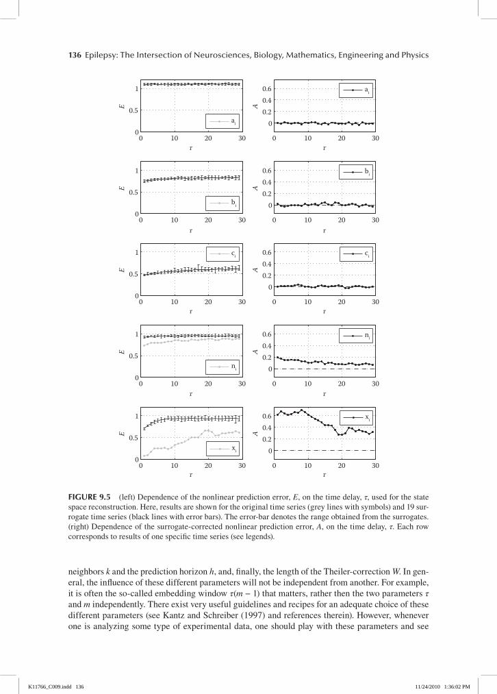
In Figure 9.5, we again show values of the nonlinear prediction error for our exemplary time series (see again Figure 9.4). Here, however, we not only show results for the original time series but also contrast these to results obtained for an ensemble of 19 phase-randomized surrogate time series generated for each original time series. For all time series from autoregressive processes ai, bi, and ci, the results for the surrogates match those of the original time series. The autoregressive processes generated by Equation 9.9 are stationary linear stochastic Gaussian processes. The r value deter-mines the strength of the autocorrelation of this process and thereby the shape of the periodogram. A phase-randomized surrogate of a stationary linear stochastic Gaussian process with any periodo-gram is a stationary linear stochastic Gaussian process with this very periodogram. Accordingly, phase-randomized surrogates constructed from ai, bi, and ci cannot be distinguished from their cor-responding original time series. The null hypothesis is correctly accepted for all three cases.*

For both the noise-free Lorenz time series xi and the noisy Lorenz time series ni, we find that the original time series results in lower E values as compared to their corresponding ensemble of sur-rogates. Here, we deal with a purely deterministic time series and a noisy deterministic one. When we construct surrogates from them, their deterministic structures are destroyed. In particular, the randomization destroys the local alignment of neighboring trajectory segments. Regarding the sig-nificant difference between the E values for the original time series and the mean values obtained for the surrogates, we can conclude that the null hypothesis is correctly rejected for both xi and ni.

From these results, it is only a small step for us to arrive at our aim by defining

A = ⟨E⟩surr – Eorig, (9.14)

where the brackets denote the average taken across the ensemble of 19 surrogates. The resulting surrogate-corrected nonlinear prediction error values A are shown in Figure 9.5, and we can see that the definition of Equation 9.14 fulfills criteria i., ii., and iii. that we defined as the aim of this chapter.

9.7 InFluencIng Parameters

In this chapter, we have plotted the nonlinear prediction error only in dependence on the time delay τ used for the delay coordinates. To fully understand how nonlinear techniques and surrogates work, it is always important to study the influence of all parameters in detail. In our case, these parameters are the delay τ and embedding dimension m used for the delay coordinates, the number of nearest

* A good check of whether one is still on track in understanding this chapter is to find an explanation of why our differ-ent autoregressive processes result in different E values, and why the surrogates match closely with their corresponding original time series in these E values, rather than just undiscriminatingly covering the entire range of E values obtained for ai, bi, and ci.

K11766_C009.indd 135 11/24/2010 1:36:01 PM


neighbors k and the prediction horizon h, and, finally, the length of the Theiler-correction W. In gen-eral, the influence of these different parameters will not be independent from another. For example, it is often the so-called embedding window τ(m − 1) that matters, rather then the two parameters τ and m independently. There exist very useful guidelines and recipes for an adequate choice of these different parameters (see Kantz and Schreiber (1997) and references therein). However, whenever one is analyzing some type of experimental data, one should play with these parameters and see

0 10 20 300

0.5

1

E

ai

0 10 20 30

00.20.40.6

A

ai

0 10 20 300

0.5

1

E

bi

0 10 20 30

00.20.40.6

A

bi

0 10 20 300

0.5

1

E

ci

0 10 20 30

00.20.40.6

A

ci

0 10 20 300

0.5

1

E

ni

0 10 20 30

00.20.40.6

A

ni

0 10 20 300

0.5

1

E

xi

0 10 20 30

00.20.40.6

A

xi

τ τ

τ τ

τ τ

τ τ

τ τ

FIgure 9.5 (left) Dependence of the nonlinear prediction error, E, on the time delay, τ, used for the state space reconstruction. Here, results are shown for the original time series (grey lines with symbols) and 19 sur-rogate time series (black lines with error bars). The error-bar denotes the range obtained from the surrogates. (right) Dependence of the surrogate-corrected nonlinear prediction error, A, on the time delay, τ. Each row corresponds to results of one specific time series (see legends).

K11766_C009.indd 136 11/24/2010 1:36:02 PM


how they influence results. Certainly, if one finds some effect in experimental data using nonlinear time series analysis techniques, the significance of this effect should not critically depend on the choice of the different parameters.

We have studied our problem based on only single realizations of our time series. However, whenever we have controlled conditions, we should make use of them and generate many indepen-dent realizations of our time series. In this way, we can get more reliable results and also learn more about our measures by regarding their variability across realizations. Another important issue that we have neglected here is that it can be very informative to study the influence of noise for a whole range of noise amplitudes and for different types of noise.

9.8 What can and cannot be concluded?

First, we can draw a very positive conclusion: We reached the aim that we stated in the Introduction. Using a combination of a nonlinear prediction error and surrogates, we were able to distinguish between purely stochastic, purely deterministic, and deterministic dynamics superimposed with noise. We demonstrated this distinction under controlled conditions using mathematical model sys-tems with well-defined properties. However, how do these results carry over once we leave the secure environment of controlled conditions? Under controlled conditions, we know what dynam-ics underlie our time series. Here, we can draw conclusions such as the null hypothesis is correctly accepted or rejected, but what conclusions can be drawn when facing real-world experimental time series from some unknown dynamical system?

Let us suppose we want to test the following working hypothesis consisting of two parts. First, the dynamics exhibited by an epileptic focus is nonlinear deterministic. Second, the dynamics exhibited by healthy brain tissue is linear stochastic. Suppose that to test this hypothesis we com-pare EEG time series measured from within an epileptic focus against EEG time series measured outside the focal area. We calculate the nonlinear prediction error for these EEG time series and phase-randomized surrogates constructed from them. Suppose further that for the focal EEG time series we find significant differences between the results for original EEG time series and those of the surrogates, whereas for the nonfocal EEG we find that the results for the original are not sig-nificantly different from the surrogates. (In the lecture underlying this chapter we looked at such results for real EEG time series.) Have we proven our working hypothesis? The answer is no, we have not—neither its first nor its second part.

First, we need to recall that the rejection of a null hypothesis at say p < 0.05 in no way proves that the null hypothesis is wrong. It only implies that if the null hypothesis was true, the probability to get our result (or a more extreme result) is less than 5%. Putting that aside, let us assume that the difference between the focal EEG and surrogates is so pronounced that we deem the underlying null hypothesis as indeed very implausible. Still, this does not prove that the dynamics are nonlinear deterministic. Recall that we used phase-randomized surrogates representing the null hypothesis of a linear stochastic Gaussian stationary process. We have to keep in mind that the complement to our null hypothesis is the world of all dynamics that do not comprise all the properties: linear, sto-chastic, Gaussian, and stationary. Hence, if we deal, for example, with a stationary linear stochastic nonGaussian dynamics, our null hypothesis is wrong. Our test should reject it. Likewise, we might have nonstationary linear stochastic Gaussian dynamics or nonlinear deterministic process. We might also deal with stationary linear stochastic Gaussian dynamics measured by some nonlinear measurement function. We have to realize that the dynamics exhibited by an epileptic focus is non-linear deterministic and is among these alternatives. However, it is only one of many explanations of our findings. Given only the results of our test, our working hypothesis is not more likely than any of the other explanations of the rejection of our null hypothesis.

We should furthermore note that our test cannot prove the second part of our null hypothesis either. The fact that we could not reject the null hypothesis for our nonfocal EEG does not prove the correctness of this null hypothesis. We cannot rule out that our nonfocal EEG originates from some

K11766_C009.indd 137 11/24/2010 1:36:02 PM


nonlinear deterministic dynamics, but our test is not sufficiently sensitive to detect this feature. Our time series might be too short or too noisy for the prediction error to detect the alignment of neigh-boring trajectories, or we might have used inadequate values of our parameters m, τ, and k.

It is important to keep these limitations in mind when interpreting results derived from nonlinear measures in combination with surrogates.* Nonetheless, nonlinear measures in combination with surrogates can still be very useful in characterizing signals measured from the brain. Andrzejak et al. studied the discriminative power of different time series analysis measures to lateralize the seizure-generating hemisphere in patients with medically intractable mesial temporal lobe epi-lepsy (Andrzejak et al. 2006). The measures that were tested comprised different linear time series analysis measures, different nonlinear time series analysis measures, and a combination of these nonlinear time series analysis measures with surrogates. Subject to the analysis were intracranial electroencephalographic recordings from the seizure-free interval of 29 patients. The performance of both linear and nonlinear measures was weak, if not insignificant. A very high performance in correctly lateralizing the seizure-generating hemisphere was, however, obtained by the combina-tion of nonlinear measures with surrogates. Hence, the very strategy that brought us closest to the aim formulated in the introduction of this chapter—to reliably distinguish between stochastic and deterministic dynamics in mathematical model systems—also seems key to a successful character-ization of the spatial distribution of the epileptic process. The degree to which such findings carry over to the study of the predictability of seizures was among the topics discussed at the meeting in Kansas.

reFerences

Andrzejak, R. G., K. Lehnertz, F. Mormann, C. Rieke, P. David, and C. E. Elger. 2001. Indications of nonlinear deterministic and finite-dimensional structures in time series of brain electrical activity: Dependence on recording region and brain state. Phys. Rev. E 64:061907.

Andrzejak, R. G., G. Widman, F. Mormann, T. Kreuz, C. E. Elger, and K. Lehnertz. 2006. Improved spatial characterization of the epileptic brain by focusing on nonlinearity. Epilepsy Res. 69:30–44.

Kantz, H., and T. Schreiber. 1997. Nonlinear time series analysis. Cambridge: Cambridge Univ. Press.Pijn, J. P., J. van Neerven, A. Noes, and F. Lopes da Silva. 1991. Chaos or noise in EEG signals; dependence

on state and brain site. Clin. Neurophysiol. 79:371–381.Schreiber, T., and A. Schmitz. 2000. Surrogate time series. Physica D 142:346–382.Takens, F. 1981. Detecting strange attractors in turbulence. In Dynamical systems and turbulence, Vol. 898 of

Lecture notes in mathematics, eds. D. A. Rand and L.-S. Young, 366–381. Berlin: Springer-Verlag.Theiler, J. 1986. Spurious dimensions from correlation algorithms applied to limited time-series data. Phys.

Rev. A 34:2427–2432.Theiler, J., S. Eubank, A. Longtin, B. Galdrikian, and J. D. Farmer. 1992. Testing for nonlinearity in time series:

The method of surrogate data. Physica D 58:77–94.

* Consider as a further principle limitation, a periodic process with a very long period that exhibits no regularities within each period. We would need to observe at least two periods to appreciate the periodicity of the process. In principle, we need an infinite amount of data to rule out that we misinterpret periodic, and hence deterministic, processes as stochastic processes.

K11766_C009.indd 138 11/24/2010 1:36:02 PM

ralph gregor andrzejak

Documents