raffaello sanzio, lo sposalizio della vergine, 1504, milano, pinacoteca...
TRANSCRIPT

The photometric track
Raffaello Sanzio, Lo sposalizio della Vergine, 1504, Milano, Pinacoteca di Brera
Michelangelo, 1528
Lo sposalizio della Vergine Raffaello Sanzio – Pinacoteca di Brera

Standard nearby point source model• N is the surface normal, is diffuse albedo, S is source vector - a
vector from x to the source, whose length is the intensity term
• Assume that all points in the model are close to each other with respect to the distance to the source. Then the source vector doesn’t vary much, and the distance doesn’t vary much either, the computation are simplified.
2xr
xSxNxd
N S
nearby point source model distant point source model
xSxNx dd
NS

A photon’s life choices
• Absorption
• Diffusion
• Reflection
• Transparency
• Refraction
• Fluorescence
• Subsurface scattering
• Phosphorescence
• Inter-reflection
λ
light source
?

A photon’s life choices
• Absorption
• Diffusion
• Reflection
• Transparency
• Refraction
• Fluorescence
• Subsurface scattering
• Phosphorescence
• Inter-reflection
λ
light source

A photon’s life choices
• Absorption
• Diffuse Reflection
• Reflection
• Transparency
• Refraction
• Fluorescence
• Subsurface scattering
• Phosphorescence
• Interreflection
λ
light source

A photon’s life choices
• Absorption
• Diffusion
• Specular Reflection
• Transparency
• Refraction
• Fluorescence
• Subsurface scattering
• Phosphorescence
• Interreflection
λ
light source

A photon’s life choices
• Absorption
• Diffusion
• Reflection
• Transparency
• Refraction
• Fluorescence
• Subsurface scattering
• Phosphorescence
• Interreflection
λ
light source

A photon’s life choices
• Absorption
• Diffusion
• Reflection
• Transparency
• Refraction
• Fluorescence
• Subsurface scattering
• Phosphorescence
• Interreflection
λ
lightsource
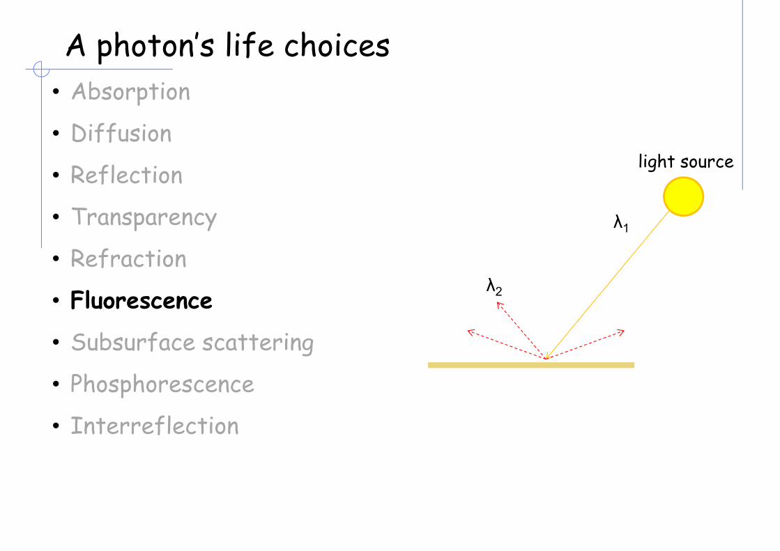
A photon’s life choices• Absorption
• Diffusion
• Reflection
• Transparency
• Refraction
• Fluorescence
• Subsurface scattering
• Phosphorescence
• Interreflection
λ1
light source
λ2
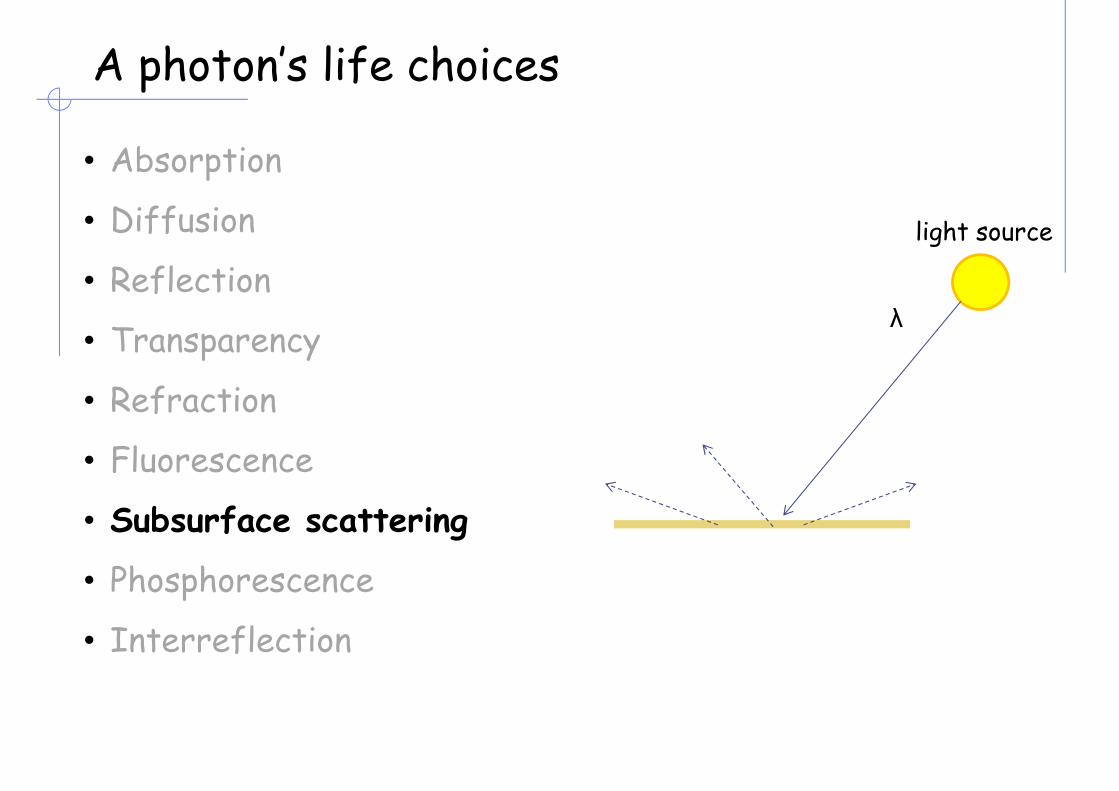
A photon’s life choices
• Absorption
• Diffusion
• Reflection
• Transparency
• Refraction
• Fluorescence
• Subsurface scattering
• Phosphorescence
• Interreflection
λ
light source

A photon’s life choices
• Absorption
• Diffusion
• Reflection
• Transparency
• Refraction
• Fluorescence
• Subsurface scattering
• Phosphorescence
• Interreflection
t=1
light source
t=n
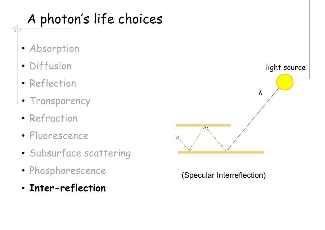
A photon’s life choices
• Absorption
• Diffusion
• Reflection
• Transparency
• Refraction
• Fluorescence
• Subsurface scattering
• Phosphorescence
• Inter-reflection
λ
light source
(Specular Interreflection)

Local rendering• Optical geometry of the light-source/eye-receiver system
• Notation: • n is the normal to the surface at the incidence point• î corresponds to the incidence angle• â = î is the reflectance angle• ô is the mirrored emergence angle• û is the phase angle • ê is the emergence angle.
13
n
ôû
â î
ê

The Lambertian model
14
2 20
ˆˆcos
elsewhere
n
î

The specular model
15
2 20
ˆˆcosm o
elsewhere
o
n
â îô
100 80 60 40 20 0 20 40 60 80 1000
0.1
0.2
0.3
0.4
0.5
0.6
0.7
0.8
0.9
1
cosns φ
φ
ns = 1
ns = 128

The mirrored emergence angle
cos (o) = 2 cos (i) cos (e) - cos (u)
r
o
eu
cos(e)=no cos(u)=oi
p

The Phong model• a is the amount of incident light diffused according to a Lambertian model
(isotropic) independent from the receiver’s position
• b is the amount of incident light specularly reflected by the object, which depends on the phase angle, and m being the exponential specular reflection coefficient
• c accounts for the background illumination
Bùi Tường Phong, Illumination for computer generated images, Commun. ACM 18 (6) (1975) 311317.17
ˆˆcos cosma b o c

Wire frame

Computing the light source direction
• Can compute N by studying this figure Hints:- use this equation:- can measure c, h, and r in the image
N
rNC
H
c
h
Chrome sphere that has a highlight at position h in the image
image plane
sphere in 3D

Local rendering
http://www.danielrobichaud.com/animation/#/marlene/

Sphere (m=10, c=0)
a=1.0
1.00.0
b=0.0 0.8 0.2 0.6 0.4
0.2 0.8 0.4 0.6

Specular sphere (b=0.9, c=0.1)
m=1
m=1000 m=100 m=10
m=3 m=6

Computing light source directions• Trick: place a chrome sphere in the scene
the location of the highlight tells you where the light source is

Depth from normals
• Get a similar equation for V2 Each normal gives us two linear constraints on z compute z values by solving a matrix equation
V1
V2
N

Surface Normal
N
surface normal
y
z
x
0 DCzByAx
0CDzy
CBx
CAor
Letp
CA
xz
qCB
yz
1,,1,, qpCB
CA
N
Surface normal
Equation of plane
)1,,(1
1ˆ22
qpqp
n

Gradient space
xfp
yfq
)1,,(1
1ˆ
)1,,(
22qp
qp
qp
n
n(p,q,1)
)),(,,(),( yxfyxyxs T
xf
xs
,0,1
T
yf
ys
,1,0
T
yf
xf
ys
xs
1,,n
Gradient Space
y
z
x
1zq
p
1
s n
N
1
1,,22
qpqp
NNn
1
1,,22
SS
SS
qpqp
SSs
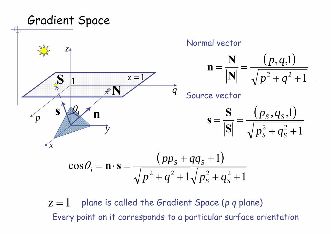
Normal vector
Source vector
i
11
1cos2222
SS
SSi
qpqpqqppsn
1z plane is called the Gradient Space (p q plane)Every point on it corresponds to a particular surface orientation
S
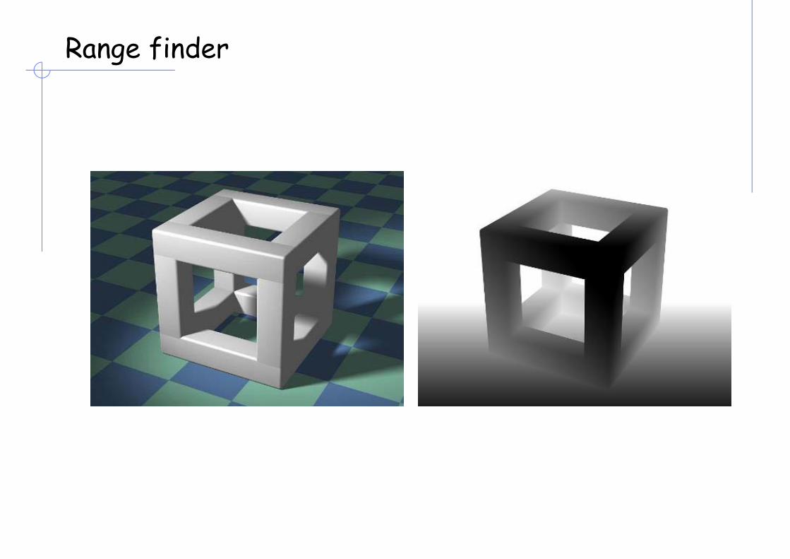
Range finder

Reflectance maps• Let us take a reference system where the optical axis of
the acquisition system (the receiver) coincides with the z axis.
• The surface described by the function z = f(x, y) has the normal vector: (∂z/∂x, ∂z/∂y, -1)t.
• Calling p=∂z/∂x and q=∂z/∂y there is a one-to-one correspondence between the plane p, q (called gradient plane) and the normal directions to the surface.
• The three angles î, û and ê may be computed with the following formulas:
29
2 2 2 2
1
1 1ˆcos s s
s s
pp qq
p q p q
2 2
1
1ˆcos e
p q
2 2
1
1ˆcos
s s
up q

Reflectance Map• Lambertian case
qpRqpqp
qqppISS
ssi ,
111cos
2222
sn
Reflectance Map(Lambertian)
cone of constant i
Iso-brightness contour

• Glossy surfaces
p
q
5.0, qpR
SS qp ,
Diffuse peak
Specular peak
Reflectance Map

Reflectance maps• reflectivity map for a Lambertian case having both camera
and light source coincident with the z-axis (0, 0, -1);
• the specular case having the specularity index m=3;
• an intermediate case with a = b = 0.5, m=3 and c = 0
32

Reflectance Map• Lambertian case
0.1
3.0
0.0
9.08.0
7.0, qpR
p
q
90i 01 SS qqpp
SS qp ,
iso-brightness contour
Note: is maximum when qpR , SS qpqp ,,
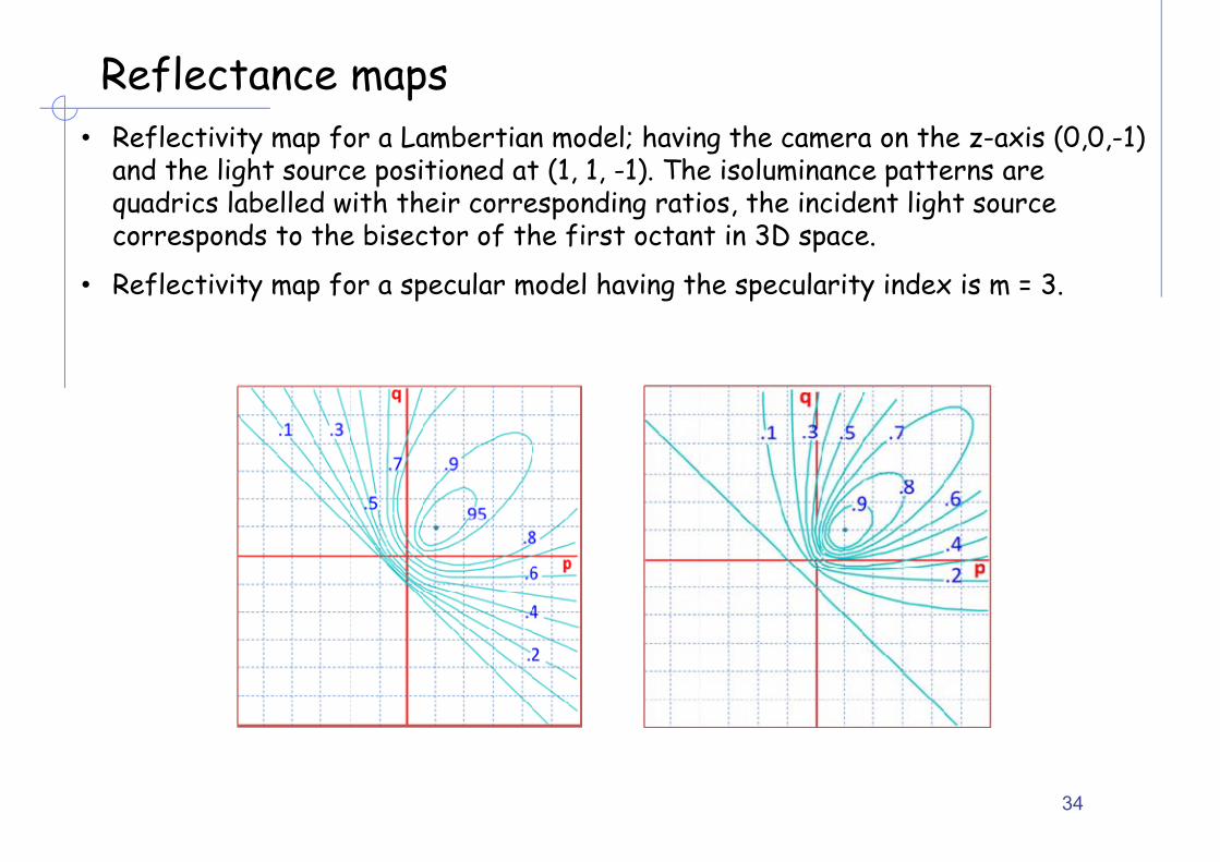
Reflectance maps• Reflectivity map for a Lambertian model; having the camera on the z-axis (0,0,-1)
and the light source positioned at (1, 1, -1). The isoluminance patterns are quadrics labelled with their corresponding ratios, the incident light source corresponds to the bisector of the first octant in 3D space.
• Reflectivity map for a specular model having the specularity index is m = 3.
34

Shape from a Single Image?
• Given a single image of an object with known surface reflectance taken under a known light source, can we recover the shape of the object?
• Two reflectance maps?
p
q
bqpR ),(1
aqpR ),(2Intersections:2 solutions for
p and q.

Photometric Stereo
p
q
11 ,SS
qp
22 ,SS
qp 33 ,
SSqp
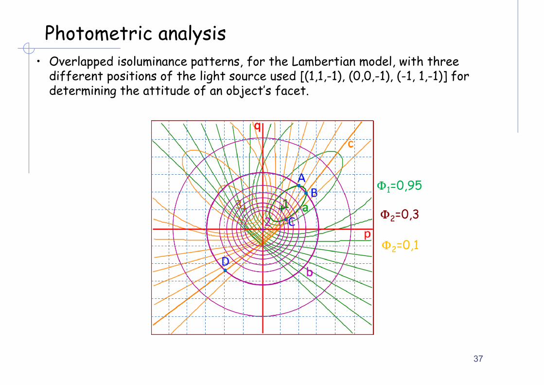
Photometric analysis• Overlapped isoluminance patterns, for the Lambertian model, with three
different positions of the light source used [(1,1,-1), (0,0,-1), (-1, 1,-1)] for determining the attitude of an object’s facet.
37
1=0,95
2=0,3
2=0,1

Radiometric Camera Calibration
• Pixel intensities are usually not proportional to the energy that hit the CCD
RAW image Published image
Austin Abrams
f
RAW
Published
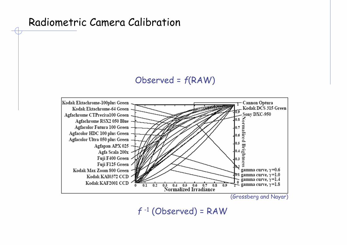
Radiometric Camera Calibration
Observed = f(RAW)
(Grossberg and Nayar)
f -1 (Observed) = RAW

Vision is Inferential: Prior Knowledge
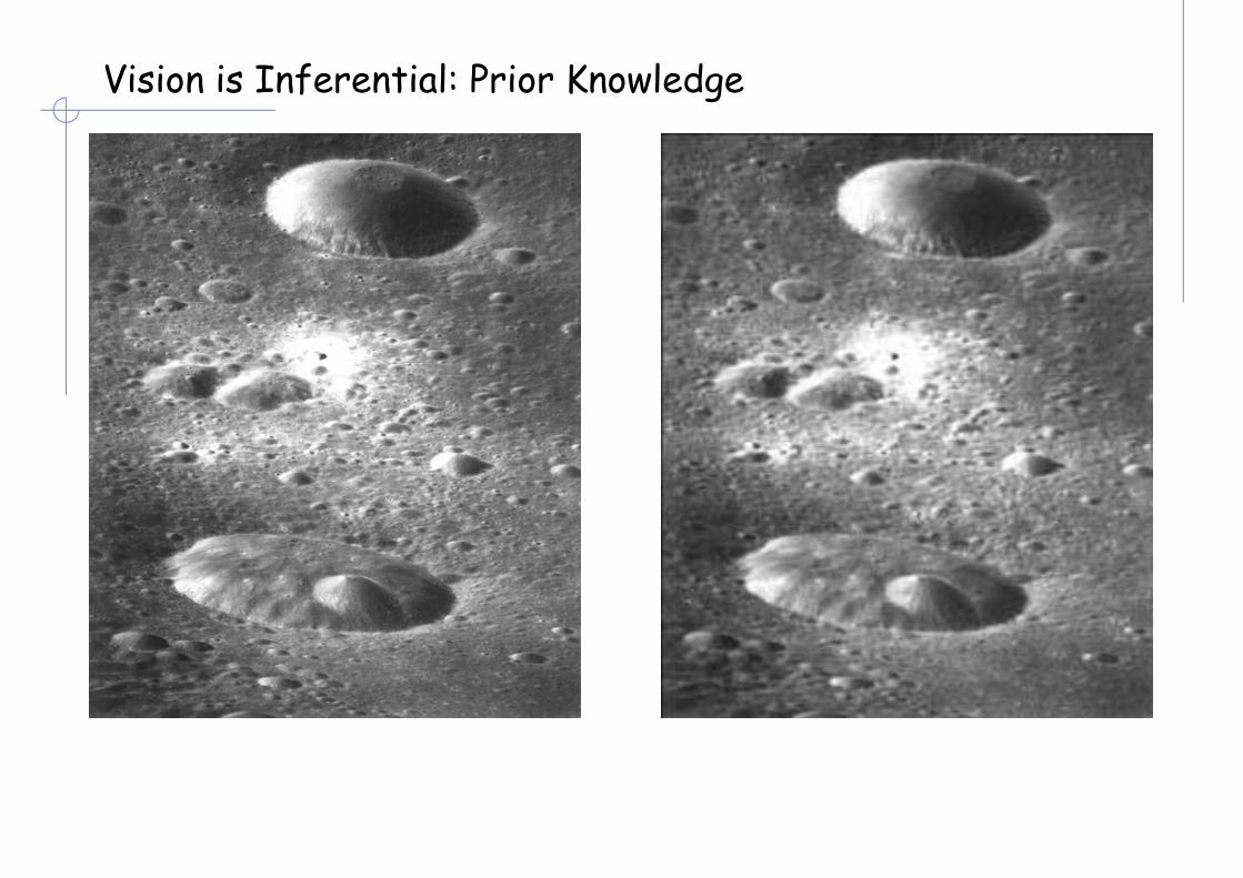
Vision is Inferential: Prior Knowledge

The life of a photon

Global rendering: ray tracing• The two basic schemes of forward and backward ray tracing, this is
last is computationally efficient but and cannot properly model diffuse reflections and all other changes in light intensity due to non-specular reflections
43Image Plane
Light
Image Plane
Light

Global rendering: ray tracing• A ray sent from the eye to the scene
through the image plane may intersect an object; in this case secondary rays are sent out and three different lighting models can be considered: • transmission. The secondary ray is sent
in the direction of refraction, following the Descartes’law;
• reflection. The secondary ray is sent in the direction of reflection, and the Phong model is applied;
• shadowing. The secondary ray is sent toward a light source, if intercepted by an object the point is shadowed.
Figure. A background pixel corresponding to the ray P1 and a pixel representing an object (ray P2). The secondary rays triggered by the primary ray P2 according to the three models: transmission (T1 and T2), reflection (R1, R2and R3), and tentative shadowing (S1, S2: true shadows, and S3).
44
Image plane
Light
Opaqueobject
Opaqueobject
Opaqueobject
Transparentobject
P1P2
R1
R2
R3
S1
S3
S2
T1
T2

Reflections and transparencies
Created by David Derman – CISC 440

Example

Global rendering: radiosity• The radiosity method has been developed to model the
diffuse-diffuse interactions so gaining a more realistic visualization of surfaces.
• The diffused surfaces scatter light in all directions (i.e. in Lambertian way). Thus a scene is divided into patches -small flat polygons. For each patch the goal is to measure energies emitted from and reflected to respectively. The radiosity of the patch i is given by:
• Where represents the energy emitted by patch i, the reflectivity parameter of patch i, and
the energy reflected to patch i from the n patches jaround it, depending on the form factors .
• The form factor represents the fraction of light thatreaches patch i from patch j. It depends on the distanceand orientation of the two patches.
• A scene with n patches, follows a system of n equations for which the solution yields the radiosity of each patch.
47
Ai
Aj
Ni
Nj
r
j
i
dAi
dAj
1
n
i i i j ijj
B E B F

Example

Global illumination photon mapping• Photon mapping is a two-pass algorithm developed by Henrik Wann Jensen that approximately solves
the rendering equation.
• Rays from the light source and rays from the camera are traced independently until some termination criterion is met, then they are connected in a second step to produce a radiance value.
• It is used to realistically simulate the interaction of light with different objects. Specifically, it is capable of simulating the refraction of light through a transparent substance such as glass or water, diffuse interreflection between illuminated objects, the subsurface scattering of light in translucent materials, and some of the effects caused by particulate matter such as smoke or water vapor.

Example

A comparison by Ledah Casburn

…. Phong model
• No shadows
• No objects interactions
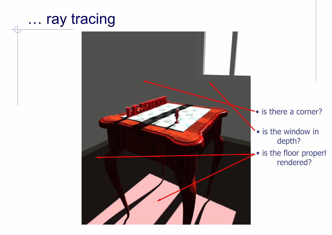
… ray tracing
• is there a corner?
• is the floor properlyrendered?
• is the window in depth?

.. radiosity
• floor and walls are clearer and pink
• the window is in depth
• there is a corner
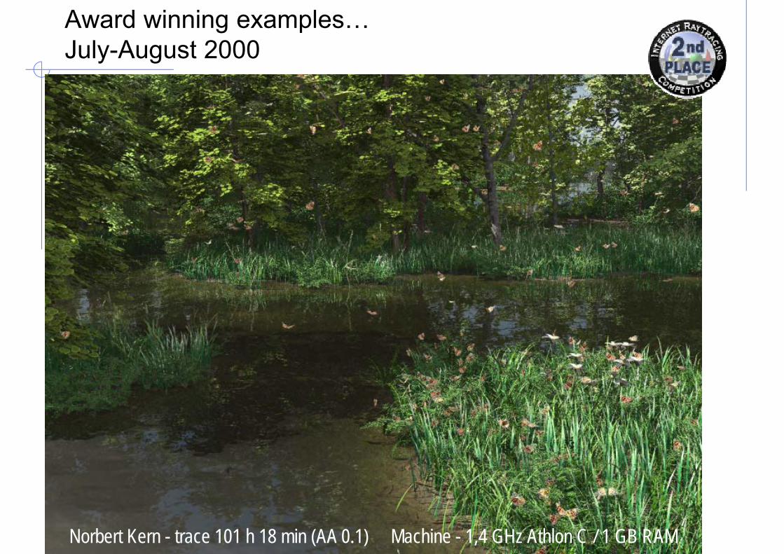
Award winning examples…July-August 2000
Norbert Kern - trace 101 h 18 min (AA 0.1) Machine - 1,4 GHz Athlon C / 1 GB RAM

Example: Render of the year 2014

The betrothal of the Arnolfini Jan Van Eyck 1434, National Gallery, London

Examples
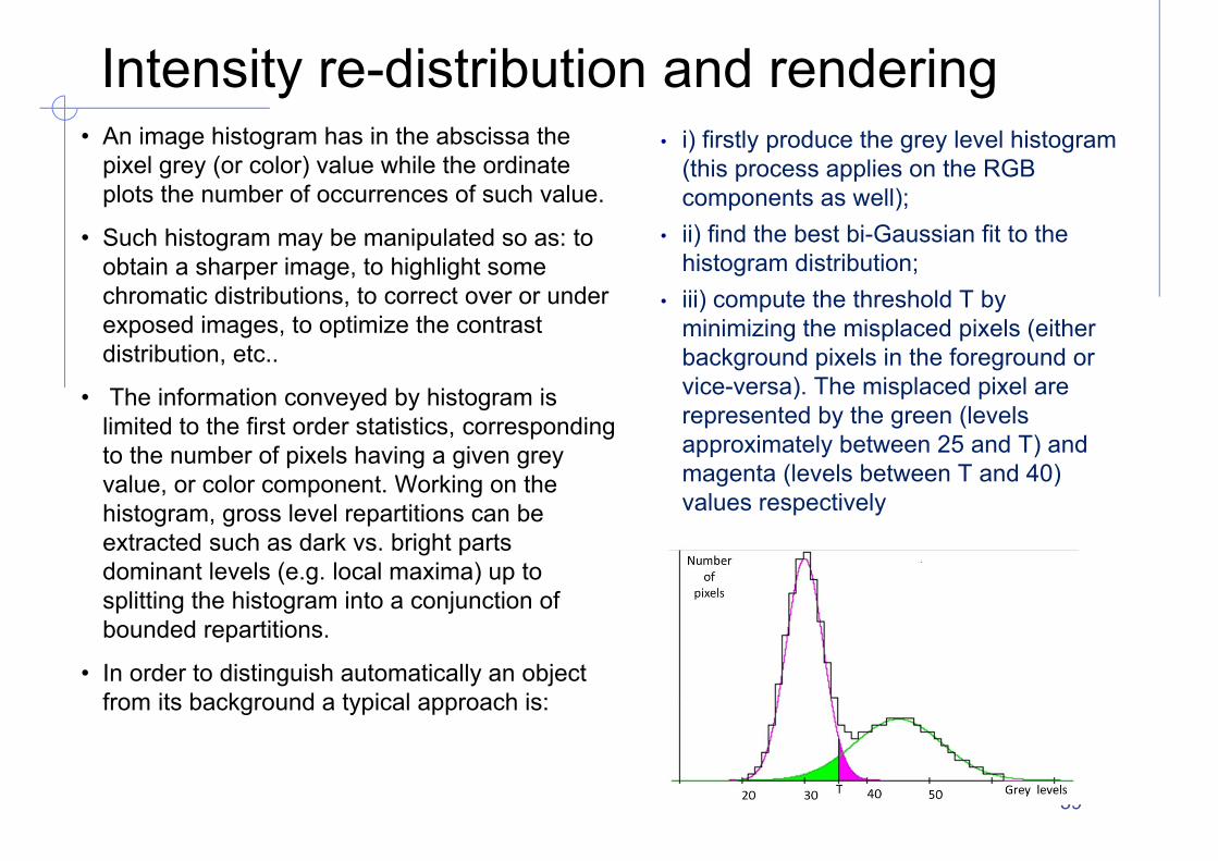
Intensity re-distribution and rendering• An image histogram has in the abscissa the
pixel grey (or color) value while the ordinate plots the number of occurrences of such value.
• Such histogram may be manipulated so as: to obtain a sharper image, to highlight some chromatic distributions, to correct over or under exposed images, to optimize the contrast distribution, etc..
• The information conveyed by histogram is limited to the first order statistics, corresponding to the number of pixels having a given grey value, or color component. Working on the histogram, gross level repartitions can be extracted such as dark vs. bright parts dominant levels (e.g. local maxima) up to splitting the histogram into a conjunction of bounded repartitions.
• In order to distinguish automatically an object from its background a typical approach is:
59
• i) firstly produce the grey level histogram (this process applies on the RGB components as well);
• ii) find the best bi-Gaussian fit to the histogram distribution;
• iii) compute the threshold T by minimizing the misplaced pixels (either background pixels in the foreground or vice-versa). The misplaced pixel are represented by the green (levels approximately between 25 and T) and magenta (levels between T and 40) values respectively

Original image• Image: History of Saint Peter by Masaccio, around 1427, Church of the Holy
Spirit, Florence
• Histogram
60
0 255

Extended dynamics• To profit from the full grey level
scale, note that very clear and dark pixels are absent, the pixel distribution may extended by stretching with the following formula:
where gmax, and gmin correspond to the maximum and minimum grey levels respectively, and 255-0 is the whole available grey level scale.
61
a b0 255

Stretching of a range in grey scale• To enhance significant details in the image
the whole dynamics can be concentrated on a given interval [a, b] of the grey scale; thena linear transformation inside the intervalcan be computed by:
• This process produces the maximal contraston the interval [a,b] of the grey scale. Considering this chosen interval no specificinformation is particularly enhanced.
62
255
b0 a 2550 255

Under-exposure• To compensate or even create lighting
effects as, for instance, under-exposure, a non linear transformation of the greylevels can be performed by:
63
0 255
255, ,g i j g i j

Over-exposure• To compensate or even create
lighting effects as, for instance, over-exposure, a non linear transformation of the grey levelscan be performed by:
640 255
2
255,
,g i j
g i j

Uniform distribution• To obtain a uniform distribution of image
contrast a technique known as equalization is employed. This technique consists in making the empiric grey level distribution as close as possible to a uniform distribution, in an adaptive way. The more uniform is a grey level distribution, the better contrasted is the associated image – i.e. maximal entropy.
650 255
g(i,j) h(s)
s=0g’(i,j) = 255255
h(s)s=0
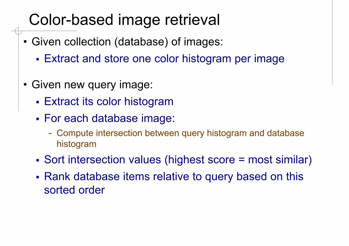
Color-based image retrieval• Given collection (database) of images: Extract and store one color histogram per image
• Given new query image: Extract its color histogram For each database image:- Compute intersection between query histogram and database
histogram
Sort intersection values (highest score = most similar) Rank database items relative to query based on this
sorted order
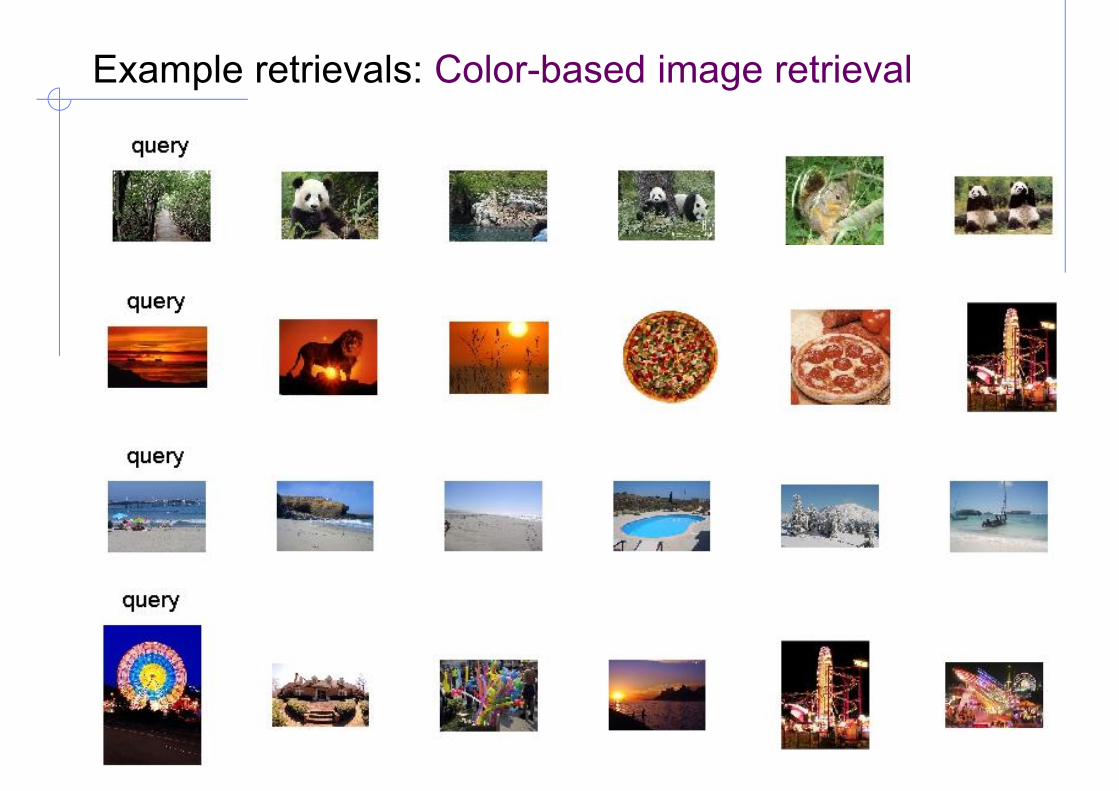
Example retrievals: Color-based image retrieval

Example retrievals: Color-based image retrieval