LABORATOIRE DE PHYSIQUE DES LASERS

UNIVERSITÉ PARIS-NORDINSTITUT GALILÉE

DOCTORAL THESIS OF THE UNIVERSITÉ PARIS-NORDpresented by

Radu CHICIREANUfor the degree of: Doctor of Philosophy

specialty : physics

STUDIES OF COLD CHROMIUM ATOMS INMAGNETIC AND OPTICAL TRAPS:

steps towards Bose-Einstein Condensation–

ATOMES FROIDS DE CHROME PIEGÉSMAGNÉTIQUEMENT ET OPTIQUEMENT:

premières étapes vers la condensation

Defended the 25th October 2007, in front of the commission consisting of:

M. Tilman PFAU Président

M. Jean DALIBARD Rapporteur

M. Christoph WESTBROOK Rapporteur

M. Christian CHARDONNET Examinateur

M. Bruno LABURTHE-TOLRA Examinateur

M. Olivier GORCEIX Directeur de thèse

Contents

Acknowledgements i

Introduction iii

1 Chromium 1

2 Experimental setup 52.1 The atomic source . . . . . . . . . . . . . . . . . . . . . . . . . . . . . 52.2 The vacuum system . . . . . . . . . . . . . . . . . . . . . . . . . . . . . 92.3 The laser sources . . . . . . . . . . . . . . . . . . . . . . . . . . . . . . 11

2.3.1 The cooling lasers . . . . . . . . . . . . . . . . . . . . . . . . . . 122.3.2 The ’red’ diodes . . . . . . . . . . . . . . . . . . . . . . . . . . . 172.3.3 The optical pumping system . . . . . . . . . . . . . . . . . . . . 19

2.4 The magnetic fields . . . . . . . . . . . . . . . . . . . . . . . . . . . . . 202.4.1 The Zeeman slower . . . . . . . . . . . . . . . . . . . . . . . . . 202.4.2 The MOT coils . . . . . . . . . . . . . . . . . . . . . . . . . . . 25

2.5 The imaging system . . . . . . . . . . . . . . . . . . . . . . . . . . . . 252.6 The control system . . . . . . . . . . . . . . . . . . . . . . . . . . . . . 282.7 Image acquisition and analysis . . . . . . . . . . . . . . . . . . . . . . . 29

3 Magneto-optical trapping of fermionic and bosonic chromium iso-topes 313.1 Fluorescence imaging system . . . . . . . . . . . . . . . . . . . . . . . . 313.2 Magneto-optical trapping of 52Cr atoms . . . . . . . . . . . . . . . . . . 32

3.2.1 Study of a 52Cr MOT . . . . . . . . . . . . . . . . . . . . . . . . 323.2.2 Loading dynamics of a Cr MOT . . . . . . . . . . . . . . . . . . 353.2.3 Density saturation . . . . . . . . . . . . . . . . . . . . . . . . . 403.2.4 52Cr Zeeman slower . . . . . . . . . . . . . . . . . . . . . . . . . 43

5

3.3 Magneto-optical trapping of 53Cr atoms . . . . . . . . . . . . . . . . . . 463.3.1 53Cr Zeeman slower . . . . . . . . . . . . . . . . . . . . . . . . . 463.3.2 The 53Cr MOT . . . . . . . . . . . . . . . . . . . . . . . . . . . 513.3.3 Oven temperature-dependence of the MOT loading rates . . . . 53

3.4 Accumulation of metastable Cr atoms in a magnetic trap . . . . . . . . 553.4.1 Magnetic trapping of 52Cr . . . . . . . . . . . . . . . . . . . . . 553.4.2 Magnetic trapping of 53Cr . . . . . . . . . . . . . . . . . . . . . 56

3.5 Resonance frequency measurements and isotopic shift determination . . 563.6 Magneto-optical trapping of a cold mixture of 52Cr and 53Cr atoms . . 58

4 Light-assisted inelastic collisions in Chromium MOTs 634.1 Measurement of inelastic collision parameters of Cr . . . . . . . . . . . 64

4.1.1 Inelastic collision parameters in a single-species Cr MOT . . . . 644.1.2 Inelastic collision parameters in a double-species MOT . . . . . 68

4.2 General considerations . . . . . . . . . . . . . . . . . . . . . . . . . . . 704.2.1 Loss mechanisms in light assisted collisions . . . . . . . . . . . . 704.2.2 Temperature dependence . . . . . . . . . . . . . . . . . . . . . . 73

4.3 Considerations about Chromium . . . . . . . . . . . . . . . . . . . . . . 744.3.1 The case of Chromium . . . . . . . . . . . . . . . . . . . . . . . 744.3.2 Qualitative comparison with other atoms . . . . . . . . . . . . . 75

4.4 Chromium temperature dependence . . . . . . . . . . . . . . . . . . . . 764.4.1 Julienne – Vigué model . . . . . . . . . . . . . . . . . . . . . . . 774.4.2 Results for Cr . . . . . . . . . . . . . . . . . . . . . . . . . . . . 79

5 Continuous loading of a finite-depth magnetic trap with 52Cr metastableatoms 855.1 Magnetic trapping . . . . . . . . . . . . . . . . . . . . . . . . . . . . . 865.2 Collisional properties of metastable 52Cr atoms . . . . . . . . . . . . . . 91

5.2.1 Inelastic D-D collisions . . . . . . . . . . . . . . . . . . . . . . . 915.2.2 Elastic collision cross-section of the 5D4 state . . . . . . . . . . 93

5.3 Continuous accumulation in a RF-truncated magnetic trap . . . . . . . 955.4 Theoretical model . . . . . . . . . . . . . . . . . . . . . . . . . . . . . . 98

5.4.1 Theoretical model for Cr . . . . . . . . . . . . . . . . . . . . . . 1005.4.2 Numerical results . . . . . . . . . . . . . . . . . . . . . . . . . . 106

5.5 Boltzmann equation and the issue of thermal equilibrium . . . . . . . . 1095.6 RF-dressed magnetic potentials . . . . . . . . . . . . . . . . . . . . . . 115

5.6.1 Accumulation at low RF frequencies . . . . . . . . . . . . . . . 1155.6.2 Magnetic+RF adiabatic potentials . . . . . . . . . . . . . . . . 1175.6.3 Landau-Zener crossings and lifetime . . . . . . . . . . . . . . . . 1195.6.4 Experiments . . . . . . . . . . . . . . . . . . . . . . . . . . . . . 122

6 Accumulation of 52Cr metastable atoms into an optical trap 1256.1 Optical trapping . . . . . . . . . . . . . . . . . . . . . . . . . . . . . . 126

6.1.1 Classical model . . . . . . . . . . . . . . . . . . . . . . . . . . . 1266.1.2 Theoretical evaluation of the light shifts . . . . . . . . . . . . . 129

6.2 Experimental setup . . . . . . . . . . . . . . . . . . . . . . . . . . . . . 1326.3 Accumulation of metastable 52Cr in a mixed optical+magnetic trap . . 137

6.3.1 Optical trap and mixed trap geometries . . . . . . . . . . . . . . 1386.3.2 Experimental results . . . . . . . . . . . . . . . . . . . . . . . . 1416.3.3 Diagnostic techniques . . . . . . . . . . . . . . . . . . . . . . . . 1436.3.4 Experimental issues . . . . . . . . . . . . . . . . . . . . . . . . . 146

6.4 Measurement of the trap properties . . . . . . . . . . . . . . . . . . . . 1486.4.1 Parametric excitation spectra . . . . . . . . . . . . . . . . . . . 1486.4.2 Simulation of the parametric excitation spectra . . . . . . . . . 150

6.5 ODT loading dynamics . . . . . . . . . . . . . . . . . . . . . . . . . . . 1536.5.1 Experimental results . . . . . . . . . . . . . . . . . . . . . . . . 1536.5.2 Majorana and two-body inelastic collision loss rates . . . . . . . 1546.5.3 RF-deformation of the mixed trap . . . . . . . . . . . . . . . . . 1576.5.4 Trap characteristics dependence on IR laser power . . . . . . . . 161

6.6 Other experiments and perspectives . . . . . . . . . . . . . . . . . . . . 1636.6.1 Accumulation in two separate horizontal ODT beams . . . . . . 1636.6.2 Other experiments for loading a single beam ODT . . . . . . . . 1646.6.3 Direct loading of metastable atoms in a crossed ODT . . . . . . 166

7 Evaporation experiments in the ODT 1697.1 Optical pumping . . . . . . . . . . . . . . . . . . . . . . . . . . . . . . 169

7.1.1 Introduction . . . . . . . . . . . . . . . . . . . . . . . . . . . . . 1697.1.2 Optical pumping in presence of a magnetic field . . . . . . . . . 1707.1.3 Polarization experiments . . . . . . . . . . . . . . . . . . . . . . 1717.1.4 Transfer to the lowest energy state . . . . . . . . . . . . . . . . 174

7.2 Single-beam lifetime experiments . . . . . . . . . . . . . . . . . . . . . 1757.2.1 Compensation of the residual magnetic field gradient . . . . . . 175

7.2.2 Compensation of the longitudinal magnetic field curvature . . . 1787.2.3 Plain evaporation and lifetime . . . . . . . . . . . . . . . . . . . 1817.2.4 Adiabatic recompression of the ODT . . . . . . . . . . . . . . . 183

7.3 Preliminary optimization procedures for evaporative cooling . . . . . . 184

A Hyperfine splitting and nonlinear Zeeman effect 195A.1 Hyperfine splitting . . . . . . . . . . . . . . . . . . . . . . . . . . . . . 195A.2 Non-linear Zeeman effect . . . . . . . . . . . . . . . . . . . . . . . . . . 196

B Chromium light assisted collisions 197B.1 Survival probability . . . . . . . . . . . . . . . . . . . . . . . . . . . . . 197B.2 Excitation rate . . . . . . . . . . . . . . . . . . . . . . . . . . . . . . . 198B.3 Partial waves . . . . . . . . . . . . . . . . . . . . . . . . . . . . . . . . 199

Acknowledgements

The experimental work described in this thesis is the product of a collaboration ofmany people to whom I am deeply grateful. I want to thank them for all their supportand encouragement through out my Ph.D. years.

I thank my supervisor, Olivier Gorceix, who made possible the realization of thisproject by creating this new experiment and finding resources to sustain its develop-ment. He managed to create a wonderful environment to work in, and I can say I havelearned a lot during the three years I spent in his group.

By joining the Chromium project from its very beginning and helping to build theexperiment piece by piece I have discovered also the importance of working as part ofa team. I thus learned that building a team is not only putting together a bunch ofpeople with different backgrounds – it takes time and a lot of work together to createsynergies among them. For showing me the delights of experimental physics, I amdeeply grateful to all the members of this team: Bruno, especially for his availabilityand for his ideas that always made us advance in times of despair; Laurent, especiallyfor insisting in his determination that every odd experimental observation must havea logical answer; Etienne, specially for his optimism and patient explanations, andlast, but not least, Arnaud, my co-Ph.D. student, for his continuous hard work andcommitment. Of course, I want to thank the two older members of the group, Rene andJean-Claude, whom I have had the pleasure to know and cherish, who have inspiredme and from whom I have learned a great deal.

However, our experiment would not have been possible without the support of thetechnical and administrative services. Thus, I would like to thank the technical staff ofthe laboratory (Julien, Fabrice, Olivier, Michel, Gerard, Albert, Thierry) who provideda great deal of help, with tons of electronic, mechanical or optical components, and theadministration center (Sabine, Nathalie and Martine) for their efficiency and diligencein solving all the tedious administrative problems.

Finally, I want to express my deepest gratitude to my family: my parents, Rodicaand Radu, for their love and encouragement throughout my whole life, and my wife,Ramona, for standing by my side during my graduate career, for her love and constantsupport.

i

Introduction

Seventy years passed from Einstein’s predictions, in 1925, (based on the photonstatistics invented by Bose) to the outstanding first experimental realization, in 1995,of a ’pure’ Bose-Einstein condensate (BEC) [1, 2], in a dilute atomic gas.

This collective behavior of a many-particle bosonic ensemble has a purely quantum-statistical nature. At sufficient low temperatures, the ’size’ of a particle, given by thedeBroglie wavelength ΛdB, begins to be comparable, or even larger, than the interpar-ticle separation (distance) and the particles, indistinguishable from one another, canno longer be treated as independent objects. They all sit then in the same quantumstate, forming a single macroscopic ’super-particle’, with exciting properties such assuperfluidity (like that of 4He) or long-range coherence (similar to that of a laser, butthis time between massive particles).

More recently, effects of a different quantum statistics were investigated at ultra-lowtemperatures, using fermions. Unlike the bosons, they cannot be in the same quantumstate, and pile up on top of each other to form a non-interacting Fermi sea [3].

Interesting features of BECs emerged from the interplay of the quantum-statisticaleffects and the interactions between particles. From a practical point of view, it wasshown for example that, when the interactions are attractive, the condensate becomesless stable, and can collapse when a critical number of atoms is exceeded [4]. Wheninteractions are repulsive, BEC is possible with large number of atoms; in this case, adeviation from the critical temperature Tc was observed [5], and the size of the BECis greatly increased due to interactions [6, 7].

In most cases, interactions in a BEC are dominated by Van-der Waals interaction,which is short-ranged and isotropic, and can be modeled by a contact-interaction po-tential. At sufficiently low temperatures, it leads to an s-wave scattering, characterizedby a single parameter which is the scattering length a.

iii

In the first years of BECs, the experiments were conducted in the regime where theinteraction energy (U = 4πh2a

mn) was small compared to the quantum kinetic energy

(J = h2

2md2 ) of the particles (U/J ∝ n1/3a � 1). In this regime, the coherence propertiesof BECs are not modified by interactions, and the mean-field theories are sufficient fordescribing their effects. The interference between two condensates [8], the realizationof atom-lasers [9, 10] and the formation of vortices [11, 12] were thus achieved.

More recently-developed experimental tools – such as Feshbach resonances (whichallow to tune the contact interaction, and thus increase the scattering length), andoptical lattices (periodic arrays created by the AC Stark shift of a standing light wave,which tightly-confine the atoms and reduce their mobility) – allowed reaching the’strongly-correlated regimes’, by either increasing U or decreasing J . Due to this, newphenomena arose, such as the Mott transition between a superfluid and an insulatingphase [13, 14], or the ’fermionization’ of a 1D Bose gas [15]. For fermions, reaching thestrong-interaction regime led to the creation of a BEC of molecules, formed by pairingbetween two fermionic atoms [16, 17, 18], and the study of the BEC-BCS crossover[19, 20, 21].

We see that interactions greatly enrich the physics of BECs, by opening a bondwith other domains of physics, such as the condensed matter physics, or quantum in-formation. From this point of view, degenerate systems with other types of interactionmay increase even more the perspectives for the study of interactions in the quantumregimes. This is why several theoretical and experimental teams turned towards thedipole-dipole interaction, which is long-ranged (∝ 1/r3) and anisotropic (attractive inone direction and repulsive in the other two).

The long-range character makes the dipole-dipole interaction quite different fromthe contact interaction: even at low temperatures, many partial waves contribute tocollisions between atoms. Another consequence is that, if a dipolar BEC is loaded inan optical lattice, the sites cannot be treated as independent and will interact witheach other.

The anisotropic character on the other hand greatly influences the stability dia-gram of a dipolar BEC [22, 23], and also can lead to new quantum phases, such asthe supersolid phase or the insulating checkerboard phase [24]. In a 2D geometry ofpancake-shaped traps the occurrence of a roton-maxon excitation spectrum [25] is ex-pected.

Although there are several candidates for studying the quantum-degenerate regimeswith dipole-dipole interactions (such as heteronuclear molecules or Rydberg atoms,with large electric dipoles), chromium is the only system which has been already con-densed [26], in the group of T. Pfau in Stuttgart. It has a large magnetic dipole momentμ = 6μB; the dipole-dipole interaction energy Udd (scaling with the square of μ) is thus36 times stronger than for an alkali atom. Soon after condensation of Cr, the same

iv

group showed that dipolar effects affect the expansion of a BEC when released fromits trap [27].

To characterize how important dipole-dipole interactions are compared to contactinteraction, it is useful to introduce the parameter εdd = μ0μ2m

12πh2a∝ Udd

U. Although

strongly enhanced by the large magnetic dipole moment, the dipole-dipole interactionsin Cr are however dominated by the contact interaction: for 52Cr, εdd = 0.159. Re-ducing the scattering length using a Feshbach resonance allowed to reach the regimeof a quantum ferrofluid [28], where the dipole-dipole interaction is comparable to thecontact interaction (εdd ∼ 1). In this case, the stability diagram of a BEC is completelymodified. One enters a fascinating regime where dipole-dipole interactions dominate...

Another interest of Chromium is the existence of a fermionic isotope (53Cr) with arelatively high natural abundance; it is a good candidate for experimentally studying,for the first time, dipole-dipole interaction in a Fermi Sea. We note that, usually anon-interacting at low temperatures, a gas of spin-polarized dipolar fermions can stillinteract through dipole-dipole interaction (which does not vanish when T → 0).

This thesis

I began my Ph.D. just as a new experiment, concerning the study of dipolar inter-actions in ultracold, degenerate Bose and Fermi gases of Cr started, in the group ofO. Gorceix. My work has been performed in Laboratoire de Physique des Lasers, atUniversité Paris Nord in Villetaneuse, France.

This thesis consists of seven chapters. The first chapter is an introduction whichsummarizes some of the important properties of Cr (such as the atomic levels of inter-est for laser cooling, etc.).

Before our experiment, there were only two groups in the world which had obtainedmagneto-optical traps with the 52Cr isotope [29, 30]. To obtain a MOT with Cr atomsis a technical challenge, due to the necessity of a high-temperature oven, and to theneed to generate a high power of 425 nm laser light. Our solutions to these problems aredescribed in Chapter 2, as well as the rest of the experimental apparatus. As in manycold atom experiments, it consists of ultra-high vacuum chambers, a Zeeman slowerwhich is used to load atoms in a magneto-optical trap, repumper and optical pumpinglaser systems, an absorption imaging system and computer-control and data-analysissystems.

Cr magneto-optical traps are different from alkali atom MOTs: they are dominatedby unusually-large inelastic collision rates, which limit the number of atoms that canbe accumulated, to a few 106 (in the case of 52Cr). Chapters 3 and 4 of this manuscriptare dedicated to the experimental realization and characterization of Cr MOTs, as wellas that of the main limiting factors.

v

In Chapter 3 I describe our main results on magneto-optical trapping of 52Cr (∼ 4×106 atoms at a temperature T = 120 μK), 53Cr (∼ 5×105 atoms) and on simultaneousmagneto-optical trapping of both isotopes. We found that the atom numbers arelimited even more in the case of the fermion – besides the inelastic collisions – by itssmaller natural abundance, and by its hyperfine structure, which significantly reducethe flux of Zeeman-slowed atoms.

Chapter 4 is dedicated to the study of light-assisted inelastic collisions in Cr MOTs.For the fermionic isotope, we measured an inelastic collision parameter β ∼ 8 × 10−9

cm3/s, almost one order of magnitude larger than for the boson. We also develop, inthe same chapter, a theoretical model to interpret the differences with the alkalis, forwhich the β−parameters are about two orders of magnitude lower than for Cr.

Because of the presence of long-lived metastable states, and of the leaks towardsthem from the excited MOT atoms via intercombination lines, Cr offers an interestingway of decoupling cooling and trapping. We were able to accumulate large number ofatoms (up to 4×107 for 52Cr) in these states, as they are shielded from the light-assistedcollisions of the MOT.

In Chapter 5 we study the possibility of combining the continuous accumulation ofatoms in the metastable states with evaporative cooling. For that, we added an RFmagnetic field which truncates the magnetic trap at different depths, depending on theRF frequency. At low frequencies, we observe an increase of the phase-space density,reaching values up to 6×10−6, about six times larger that in the MOT, in less than 300ms. In the same chapter I present a theoretical model, based on simple rate equations,which reproduces the experimental observations, and allowed to infer the inelastic lossparameter with the excited MOT atoms βPD = 5 × 10−10 cm3/s, which is the mainlimitation factor for the phase-space density in this experiment.

In order to diminish the effect of the collisional limitation factors, and increasethus the number of atoms accumulated in the metastable states, we investigated thepossibility of creating large, W-shaped magnetic traps; a limitation in this case wasfound to be the presence of RF second harmonics.

In Chapter 5, I also describe two experiments to measure the inelastic and elasticcollisional properties of the metastable 5D4 state (i.e. the elastic collision cross sectionσel. = 7 × 10−10 cm2 and the inelastic collision parameter between metastable atomsβDD = 3.3 × 10−11 cm3/s).

The high inelastic collision loss parameter βDD shows that evaporative cooling inthe metastable states cannot lead to condensation. On the other hand, condensationof ground-state Cr atoms in a magnetic trap is not likely, because of strong dipolarrelaxation processes. A solution (which successfully led to condensation in T.Pfau’sgroup) is to transfer the atoms in the lowest energy state, which is not magneticallytrappable; they can however be trapped in optical dipole traps (ODT).

vi

In our quadrupole magnetic trap, spin-changing collisions and Majorana losses limitthe evaporative cooling stage before transferring the atoms in an ODT. In Chapter6 we demonstrate a way of directly loading a mixed, magnetic+single-beam opticaldipole trap with metastable atoms; after switching off the magnetic trap, up to 1.2×106

atoms, at 100 μK, remain trapped in the ODT. This very efficient accumulation processis nevertheless equally limited by inelastic collisions between metastable atoms, and byMajorana spin-flips.

I also describe in Chapter 6 two procedures to limit these effects: one is to shift theposition of the ODT beam away from the zero magnetic field position; the other is touse RF magnetic fields, which allow to trap both high- and low-field seeking atoms.Finally, I describe the parametric excitation spectroscopy in the ODT, which allowsto characterize our trapping potential, and to measure for the first time the AC Starkshift of the 5D4 metastable state.

In the last chapter of this thesis I present recent works that were performed towardsthe condensation of Cr. I tested in particular the effect of optical pumping to the lowestenergy states, by demonstrating a strong reduction of inelastic losses, in a crossed ODTconfiguration. The modification of the shape of the ODT, from a single-beam to atwo-crossed-beam configuration led to a 20-fold increase of the phase-space density.Finally, I present some preliminary optimization procedures of evaporative cooling inthe crossed optical trap.

vii

Chapter 1

Chromium

In this chapter I summarize some of the general physical properties of Chromium,which are relevant for the experiments presented in this dissertation.

Chromium (Cr) is a transition element with an atomic number Z = 24, belonging tothe 6th group of the periodic table of the elements. It is a steel-gray, lustrous, hard metalwhich has high melting (1850◦C) and boiling (2690◦C) points, at atmospheric pressure.

Naturally-occurring chromium is composed of four stable isotopes: 50Cr, 52Cr and54Cr, which are bosons, and 53Cr, which is a fermion. Some properties of these isotopesare summarized in Table(1.1).

Isotope 50Cr 52Cr 53Cr 54CrAbundance 4.35% 83.79% 9.50% 2.37%Nuclear spin I = 0 I = 0 I = 3/2 I = 0

Statistics boson boson fermion boson

Table 1.1: Properties of the Cr natural isotopes.

The work presented in this dissertation uses the two most abundant isotopes, 52Crand 53Cr, which are interesting from an experimental point of view because they obeyto different quantum-mechanical statistics. They are good candidates for creating andstudying degenerate mixtures of bosons and fermions.

1

Spectroscopic properties of 52Cr

All the bosonic isotopes of Cr have a zero nuclear spin, resulting in the absence ofany hyperfine structure. The relevant part of the 52Cr atomic level structure is shown infig.(1.1). This isotope has an (’almost closed’) strong electronic transition, between theground 7S3 state and the excited 7P4 state, which is used in our experiment for Zeeman-slowing and magneto-optical trapping the 52Cr atoms. Some important properties ofthis transition are summarized in Table(1.2).

Besides the cooling transition, Cr also has a non-cycling transition 7S3 →7P3, at awavelength of 427.60 nm, which is appropriate for optically pumping the atoms to thelowest-in-energy stretched state (see Chapter(7)).

Figure 1.1: Simplified level structure of 52Cr and 53Cr; only transitions relevant to our laser cooling experimentsare shown.

The Table (1.3) shows some properties of the levels of Cr which are importantfor our experiment. Another interesting property of Cr is thus the value of 6μB of

2

magnetic moment in the ground state 7S3. The reason for this is the presence of sixvalence electrons ([Ar]3d54s1 configuration), which leads to a total spin S=3. This highvalue makes the dipole-dipole interaction between two Cr atoms (which scales with thesquare of the magnetic moment) to be 36 times higher than of the alkali atoms. Cr isthus a good candidate for studying effects of the magnetic dipole-dipole interaction inquantum gases.

Vacuum wavelength λ = 2πk

= 425.553 nmTransition energy hc

λ= 2,62 eV

Linewidth Γ = 1τ

= 31.8 × 106 s−1

Saturation intensity Isat = πhcΓ3λ

= 8.52 mW/cm−2

Doppler temperature TD = hΓ2kB

= 124 μKRecoil temperature Trec = (hk)2

mkB= 1.02 μK

Recoil velocity vrec = hkm

= 1.8 cm/s

Table 1.2: Properties of the 7S3 →7P4 transition of 52Cr.

The 52Cr atoms in the excited 7P4 state can radiatively decay, via intercombinationlines, towards two metastable states (5D4 and 5D3), which have a long lifetime, of morethan 50 s [32]. The corresponding decay rates (γ5D4

= 127 s−1 and γ5D3= 42 s−1 [31])

are considerably smaller than the cycling rate of the cooling transition, and do notprevent laser cooling in a MOT.

The metastable 5D3,4 states have also large magnetic moments – respectively 4.5μB

and 6μB –, which makes possible the accumulation of the atoms (decaying to thesestates from the MOT), even in the magnetic trap formed by the relatively-low gradientsof the MOT (∼ 9 G/cm). These atoms can be repumped back in the ground state viathe 7P3 state (transitions at respectively 653.973 nm and 663.185 nm).

Level J Energy [cm−1] gJ |−→μ |7S 3 0 2.00 6μB

z 7P 4 23498.84 1.75 7μB

z 7P 3 23386.35 1.92 5.8μB

a 5D 4 8307.57 1.50 6μB

a 5D 3 8095.21 1.50 4.5μB

Table 1.3: Properties of the relevant levels of the 52Cr isotope: Energy, Landé g-factor, magnetic moment.

3

Properties of the fermionic 53Cr isotope

Unlike the bosonic isotopes, the fermionic 53Cr has a nuclear spin I = 3/2. Thecoupling between the nuclear spin I with the electronic total momentum J (see Ap-pendix(A)) leads to the splitting of each atomic level into four hyperfine sublevels, asit can be seen in fig.(1.1). The values of the hyperfine coupling constants A and Bare given in Table(1.4); we note that these values are negative, leading to a so-called’inverted’ hyperfine structure.

The relatively small values of the hyperfine constants leads to a hyperfine splittingof less than 1 GHz in the ground state, and less than 200 MHz in the excited state.Experimentally this is very convenient, because the laser cooling frequencies of thefermion are sufficiently close to the ones of the boson to be obtained by means ofacousto-optical modulators (AOMs).

Level A [MHz] B [MHz]7S3 −83.599 ± 0.002 07P4 −11.8 ± 0.4 −0.6 ± 0.67P3 −1.5 ± 2.0 -2.05D4 −48.755 ± 0.005 63.021 ± 0.0105D3 −35.683 ± 0.005 15.565 ± 0.005

Table 1.4: The dipolar (A) and quadrupolar (B) hyperfine constants of 53Cr.

4

Chapter 2

Experimental setup

In this Chapter I present the experimental setup which was built during my thesis.

2.1 The atomic source

The saturated vapor pressure of Cr is expected to be very low at room temperature,because of the high melting point, of 1857◦C (at atmospheric pressure). To create aCr vapor source, required for laser cooling experiments, one needs to heat up Cr, asclose as possible to its melting point. In our experiment, this is done using a high-temperature Cr oven.

The choice of the oven temperature is very important as it sets the atomic flux. Theavailable data on the saturated vapor pressure temperature dependence, as well as priorexperiments in other groups, show that Cr atomic fluxes suitable for our applicationscan be obtained using ovens operated at about 1500◦C.

The temperature dependence of the saturated vapor pressure for Cr, in the 300 Kto 2000 K range, can be estimated using [33]:

Psat(T ) = exp

(a − b

T+ c ln(T ) − d

T 3

)(2.1)

where Psat is in Pa, T is in K and a = 27.2, b = 47740 K, c = 0.44, d = 0.94 K3 areconstants. This formula can be used to obtain a rough estimate of the dependence ofthe atom flux as a function of the oven temperature. In the effusive regime (i.e. whenthe diameter φem. of the emission hole is much smaller than the mean free path ofatoms inside the oven) the longitudinal velocity distribution of atoms emitted inside a

5

small solid angle of azimuth θem., is given by:

fem.(v, T ) =

(πφem.

2

)2Psat(T )

kBT

(m

2πkBT

)3/2

v3 exp

(− mv2

2kBT

)sin2(θem.), (2.2)

where v is the longitudinal velocity of the beam, kB is the Boltzmann constant and mis the Cr mass. fem.(v, t) is plotted in fig.(2.1.A) for three different temperatures.

Figure 2.1: A) Velocity distribution f(v, T ) for 3 different temperatures: T=1400◦C (dotted line), T=1500◦C(dashed line) and T=1600◦C (full line). The vertical dashed line indicates the Zeeman slower capture velocity. B) Thetotal flux temperature dependence (integration up to vc ∼ 460 m/s), shown in a semi-log scale.

At a temperature ∼ 1500◦C, fem.(v, T ) has a maximum at vmax =√

3kBTm

∼ 900 m/s.The fraction of atoms having a velocity smaller than 40 m/s (typical MOT capturevelocity) is very small (∼ 10−5) and the use of a Zeeman slower is mandatory. Inthis case, the ’useful’ flux of atoms Φ(T ) can be estimated by integration of eq.(2.2)up to the Zeeman slower capture velocity vc (∼ 460 m/s, as shown later): Φ(T ) =vc∫0

fem.(v, T )dv ∝ Psat(T )√T

.

An indication on the temperature dependence of Φ(T ) is shown in fig.(2.1.B).

Oven design

To build a chromium source is a technical challenge. The main reason is that Crtends to react with most of the materials used for making high-temperature ovens.For example, direct contact between tantalum (Ta) or tungsten (W) must be avoided,because they form alloys with Cr, with melting point temperature lower than that ofeach individual component (eutectic).

Fairly long ’lifetimes’ (set by the evaporation of the Cr bar), of at least severalmonths, are required, because of ultra-high vacuum constraints. Because of the need

6

of a Zeeman slower, the Cr source has to be placed fairly far from the experimentalchamber. Another difficulty comes from the fact that a beam with relatively smallangular apertures, aiming to the MOT, is required.

Our chromium oven is a commercial high-temperature effusion cell fabricated byAddon. A schematic description of the oven is given in fig.(2.2). Two different combi-nations of materials were used in different stages of the experiment, as explained below.For practical (and security) reasons – such as having the experimental chamber andthe laser beams well below the height of the eyes – we chose to operate the oven in thehorizontal plane1.

Figure 2.2: The Cr oven. Different choices for the crucibles are given, as explained in the text.

The oven consists of a main crucible initially made of Ta2 which is heated by theradiation emitted by two current-carrying, self-sustained W filaments. The main cru-cible and the filaments are enclosed inside an oven cell also made of W. A water-cooledthermal shield, surrounding the oven cell, maintains the oven vacuum chamber at amoderate temperature (below ∼70◦C everywhere).

Due to the low temperature eutectic formed by Cr and Ta, Cr cannot be directly

1 This was not an obvious choice, because of the possibility of deformation of the heating filaments(under gravity and at high temperatures), which may have led to short-circuits.

2 This was a first choice, because Addon did not provide W crucibles and no other supplier couldinitially be found.

7

inserted inside the main crucible; it must be isolated using an internal crucible, with alow high-temperature reactivity with both Ta and Cr. A Cr bar (20 g, 6.5 cm long, 8mm of diameter) of purity 99.7% is enclosed inside the internal crucible by a piercedcap, having a diameter φem. = 2 mm, which is thus the ’emission source’. A second,4-mm-diameter aperture (not shown in fig.(2.2)), set at a distance of 5 cm from theemission source, defines the direction of the effusion beam.

The oven is connected to the vacuum chamber through a CF40 directional flange.This provides the necessary fine tuning for the orientation of the atomic beam alongthe 1-meter-long Zeeman slower tube. The beam can be switched on and off within 200ms with a computer-controlled mechanical shutter, placed at 1 cm after the ’emissionsource’.

The temperature of the oven is measured with a W/Re thermocouple. The DCsource which feeds the heating wires is controlled by a programable controller througha PID loop. The oven temperature is always lowered to 1000◦C during nighttime,to increase the lifetime of the Cr bar. We always use relatively long temperature-ramps, in order to avoid possible damages caused by fast temperature variations ; forinstance, heating or cooling the oven between 1000◦C and 1500◦C is usually done using2.5 to 3 hour ramps. A security system, using rechargeable batteries, was preparedfor automatically lowering the oven temperature down to room temperature in case ofpower outages.

Choice of the crucible materials

For the internal crucible we tested two different materials: ZrO2 (zirconia – a orange-colored ceramic) and Al2O3 (alumina – a white ceramic).

We first performed preliminary tests, without Cr, in order to test the compatibil-ity between the materials of the two crucibles. We observed that the combinationZrO2−Ta was not suitable, because, after heating up to 1600◦C, the ZrO2 cruciblechanged its color to black and became extremely fragile (it had even broken inside theoven). On the other hand the test with a second crucible, made of Al2O3, gave goodresults, both to the empty crucible test (heating up to 1600◦C) and to the Cr-filledcrucible test (heating up to 1500◦C). The cap which seals the Cr bar was made of Ta.

This first combination of materials allowed us to obtain our first Cr MOTs andworked fine for about one year of operation at 1500◦C. After this period, a suddenchange of the value of the heating wires resistance was noticed. Analyzing the ovenshowed that the alumina crucible had significantly shrunk, while the Ta main cruciblewas severely flexed downwards, under the action of gravity, probably as it softenedduring the high-temperature operation. The Cr bar was consumed to about 2g whilethe alumina crucible was filled with a very light, pink powder (probably ruby). Thechange of the filament resistance was probably due to a short-circuit. We however could

8

not check what was the exact cause of this short-circuit (bent Ta crucible touching thefilaments, or bent filaments touching the oven cell), as it was impossible to extract thedeformed Ta crucible out of the oven cell without breaking it.

A second choice of materials was then tested (along with a new oven cell). We useda main oven crucible made of W along with an internal crucible made of ZrO2. Due tothe bad reaction observed between Ta and ZrO2, the Ta cap was replaced by another,made of ZrO2 and glued to the crucible (with high-temperature – up to 2200◦C –resistant glue). The second oven has been operated for more than 12 month (and isstill working), at temperatures up to 1550◦C.

2.2 The vacuum system

Our ultra-high vacuum (UHV) system consists of two horizontally-arranged vacuumchambers. The first one (the oven chamber) is used for isolating the hot Cr sourcefrom the second one (the experimental chamber), where the vacuum requirements aremore severe. The two are connected by the Zeeman slower (ZS) tube.

Figure 2.3: Vacuum system.

The oven is placed inside a cylindrical (0.5m long and 30cm diameter) vacuumchamber, which is pumped by a Turbo pump (with a pumping speed of 250 L/s),pre-pumped by a dry scroll pump (110 L/min) through a 1 m long flexible hose. Thescroll pump is kept in a ventilated, acoustically-isolated box. Pressure inside the ovenchamber is measured by a thermocouple gauge and a Bayard-Alpert ionization gauge.The pressure is typically equal to 6 × 10−11 mbar when the oven is at T = 1000◦Cand raises to 2 × 10−10 mbar when the oven is heated to T = 1500◦C. The pressure inthe oven chamber is significantly improved by the getter properties of Cr. Indeed we

9

observe that, after opening this chamber, the vacuum gradually improves, throughouta few days, when operating the oven.

A pneumatic valve is used to isolate the oven chamber from the Turbo pump. Asecurity circuit automatically closes this valve if the pressure becomes to high.

The oven chamber has eight 425 nm-AR-coated CF40 viewports (four in the hori-zontal and four in the vertical plane), which are used to diagnose the Cr beam and toperform a 2D atomic beam collimation, as explained in the next chapter.

Figure 2.4: Experimental chamber, seen along the direction of the Zeeman Slower tube (left) and from above(right).

The experimental chamber (fig.(2.4)) is a compact octagonal chamber with eightCF40 viewports in the horizontal plane and two CF100 viewports for the couplingof vertical laser beams. A 150 L/s ion pump and a Ti-sublimation pump maintainthe pressure at about 5 × 10−11 mbar. This value is measured with a Bayard-Alpertionization gauge; the pressure might be lower at the position of the MOT, which iscloser to the ion pump than the gauge. Magnetic trap lifetime measurements (describedlater) show, in the low atomic density regime, a 1/e time constant of 30 s. An additionalpneumatic valve separates the two ultra-vacuum chambers. It is controlled by a securitycircuit, and closes if the pressure in the oven chamber passes above a certain threshold(a few 10−9 mbar).

Four of the CF40 viewports are wide range AR-coated, between 400 nm and 700 nmand used for coupling the horizontal MOT beams and the ’red’ repumpers. The otherviewports of the chamber (two CF40 and two CF100, coated for 425 nm, 530 nm and1075 nm) are used also for coupling the optical dipole trap laser and possible opticallattice lasers (not used in this thesis).

A direct coupling of the ZS beam through a viewport must be avoided in our exper-

10

iment because the atomic Cr beam would rapidly coat it3. We use an undervacuummetallic Al mirror – made at our lab’s optics shop – to reflect the ZS beam and directit along the ZS axis (although this mirror also becomes coated with Cr, the changesof its reflectivity properties are moderate, compared to those of a Cr-coated viewport,whose transmissivity would rapidly fall).

Figure 2.5: Zeeman shower tube and the differential tube.

The 90 cm-long, 14 mm inner diameter Zeeman Slower tube connects the two vacuumchambers. During the baking of the vacuum system, we observed the apparition ofleaks at the connection with the experiment chamber, induced probably by the thermaldilatation of the ZS tube; we therefore added a 10 cm-long flexible hose at the entranceof the ZS tube, shown in fig.(2.5), which finally prevents the thermal dilatation effectson the ZS connections.

An additional differential tube (25 cm long and 9 mm of diameter) is placed at theentrance of the ZS. It can ensure a pressure reduction factor of ∼ 400, in order notto alter the pressure in the experimental chamber, in the case where the pressure inthe oven chamber accidentally increases to the 10−8 mbar range. We note that usuallythis high reduction factor is not required, as the oven chamber pressure is much lowerthan 10−8 mBar; it is however useful, after the oven chamber chamber is opened, forexample after the replacement of the oven cell.

2.3 The laser sources

Several laser sources are necessary to cool and manipulate Cr atoms. These sourcescan be grouped in four components: the optical cooling laser-chain, the ’red’ repumpers,the optical pumping system and the optical dipole trapping laser.

The magneto-optical cooling light is obtained by frequency-doubling a Ti:saphirelaser. The Ti:saphire is frequency-locked to an external reference Fabry-Perot cavity,itself locked to a Cr atomic transition. The ’red’ repumpers are provided by extended-cavity laser diodes, frequency-stabilized on the same Fabry-Perot cavity. The optical

3 J.J. McClelland and T. Pfau, private communications.

11

pumping system is a frequency-doubled laser diode, stabilized independently on anatomic reference. Each of these components will be described in the following pages.The laser system used for optical trapping will be presented later, in Chapter(6).

2.3.1 The cooling lasers

Chromium has a strong ’blue’ optical transition at 425.553 nm. No commercial laserdiode system, providing both the required wavelength and a reasonable power (a few100 mW for a cold atom experiment), is currently available. The solution we use in theexperiment is based on the external cavity frequency doubling of a Ti:saphire laser.

The Ti:saphire laser

The Ti:saphire is a commercial Tekhnoscan laser, model TIS–SF–07. At the be-ginning of the experiment it was pumped by a Coherent Ar+ laser, already availablein our lab. After about 1.5 years, the pump laser was replaced by a Coherent Verdilaser, providing 18 W of single mode green light, at a wavelength of 532 nm. Froma practical point of view, the better pointing stability and mode quality of the Verdilaser improved the stability our Ti:saphire laser (and, consequently, of the whole lasercooling system).

About 10.5 W of the Verdi laser are used for pumping the Ti:saphire; the extra 7.5W available, single mode, laser power will be used in future optical lattice experimentswith degenerate Cr gases. The Ti:saphire efficiency also improved with the new pumplaser. In normal operating conditions we get 1.45 W, single mode laser at 851.105nm from 10.5 W of pump laser. This yields an efficiency of almost 14% (compared to∼ 11% obtained with the Ar+ laser). The frequency jitter of the Ti:saphire, specifiedby the manufacturer, is < 5 MHz rms at a one second scale.

Our Ti:saphire has a typical warming-up time of about two hours (after turning onthe pump laser), during which the power reaches the maximum value and the frequencymode-hops stop. We observed that, for optimal operating conditions, a good thermalstability of the experiment room is required (typically of ±1◦C), as well as the use of aflow box. Some occasional problems occur (typically two to three times a year) whenthe thin etalon of the laser gets misaligned; this requires a realignment of the etalon,as well as of the laser cavity.

We also observed that the performances of our Ti:saphire become poorer (powerdecreasing of ∼ 10%) during summertime, when the cooling water is warmer. To solvethis problem, we adapted the cooling circuit to a water chiller, which keeps the crystaltemperature constant to 12.5◦C.

12

The doubling cavity

The Ti:saphire laser light is frequency-doubled in an external four-mirror ring com-mercial cavity (model FD–SF–07), also produced by Tekhnoscan. The second harmonicis generated in a 15-mm-long lithium triborate (LBO) crystal. The doubling cavity canbe continuously scanned, with a 3 GHz span, using the piezos supporting two of thecavity mirrors.

A Hänsch-Couillaud [35] scheme locks the doubling cavity length to the Ti:saphirelaser frequency. The Ti:saphire beam needs to be injected in the doubling cavitythrough an optical isolator, which has a 93% transmission. Indeed, in absence of theoptical isolator, we observed back-reflection effects on the lock of the Ti:saphire whenthe doubling cavity is locked on resonance with the IR light; this is attributed to thefact that the front of the LBO crystal is cut perpendicularly to the IR beam direction.

We also observed thermal effects in the doubling crystal: after the cavity was lockedon resonance with the Ti:Saphire laser, the output power progressively dropped down(because of thermal dilatation of the crystal, the optical length of the cavity is modifiedand the resonance condition is no longer fulfilled). In order to reduce these effects, weset up a temperature stabilization device, which heats up the crystal, at a temperatureof about 30◦C, and the heating from the IR laser becomes negligible.

We finally obtain an output power of ∼ 340 mW of 425.553 nm blue laser light,with a doubling efficiency of 20%. We note however that the intensity noise is rela-tively high (about 10% of amplitude), and the cavity is quite sensitive to acoustic noise.

The output beam of the doubling cavity presents a strong astigmatism, which ismainly due to the crystal4, and needs to be corrected for. We measured with a beamanalyzer the position and size of the beam waists along the horizontal (OX) and vertical(OY) axis. In the horizontal direction we found a waist of wx,0 = 26 μm situated atX0 = −189 mm (with respect to the output mirror of the cavity), while in the verticaldirection the waist is wy,0 = 99.3 μm situated at Y0 = −215 mm. We correct for theastigmatism using two lenses: a first f = 150 mm spherical lens followed by a second,cylindrical, f = 150 mm lens [34].

The reference cavity

The frequency of the Ti:saphire is stabilized using a high-stability Fabry-Perot (FP)reference cavity. Its mirrors are mounted on a tube made of Invar (which has a verylow thermal dilatation coefficient ∼ 10−6 K−1), which ensures a good mechanical andthermal stability. The cavity is placed in a vacuum chamber (∼ 10 mbar) in order toprotect it from air-pressure variations and to lower acoustic perturbations.

We use a L = 0.5 m long confocal cavity, for which all the modes of the same4 Ordinary-ordinary-extraordinary (OOE) type.

13

parity are degenerate. The free spectral range is Δcav. = c/2L = 300 MHz and thereflectivity of the cavity mirrors is R = 98.5%, yielding a theoretical finesse �th. = 107.We measured a width of the transmission peaks of the cavity Δf0 = 5 MHz, whichcorresponds to an experimental finesse value �exp. = 60 5.

The laser frequency is stabilized on the side of a Fabry-Perot reference cavity trans-mission peak. The error signal is generated by a differential photodiode, which recordsthe difference between the transmitted FP signal intensity and the intensity of an addi-tional (offset) optical signal6; a feedback is sent to the piezos of the laser-cavity mirrors(a fast and a slow loop – according to the band-width of the corresponding piezos –are required for correcting both the high and low frequency drifts). We are able tostabilize the frequency jitter of the Ti:saphire down to a few 10 kHz, with respect tothe length of the FP cavity.

Figure 2.6: Scheme of the laser system for magneto-optically trapping and cooling Cr atoms.

5 This is consistent with the measured cavity transmission T = 15 %, yielding additional intracavitylosses of 3.5%. These losses are probably due to a misalignment of the two mirrors of the FP cavity,which makes the output beam slightly ’clipped’ by the final cavity mirror.

6 This differential scheme minimizes the sensitivity to laser intensity fluctuations.

14

The reference cavity stabilization

Once locked, the wavelength λIR of the Ti:saphire (and of the blue light) is set bythe length L0 of the FP reference cavity:

L0 = NλIR

2= N

c

2fIR

(2.3)

where N is an integer (we will call it ’the FP order’) and fIR is the Ti:saphire frequency.We can tune λIR by changing the length of the cavity, using the piezo supporting oneof its mirrors.

An atomic reference is used to set the frequency of the blue light at a precise value,close to the Cr transition frequency. To do that we use the saturated absorption tech-nique. A Cr vapor is obtained (by a krypton discharge) inside a commercial hollowcathode lamp.

Figure 2.7: A) Saturated absorption signal, shifted by −150 MHz from the 52Cr atomic resonance (center of theDoppler distribution). B) Lock-in amplifier signal. We observe additional atomic signals, that can be identified withtransitions of other Cr isotopes.

A sinusoidal modulation at 100 kHz is applied to the frequency of a saturating pumpbeam passing through the hollow cathode via a double-pass acousto-optical modulator(AOM). The pump frequency is thus shifted by 300 MHz with respect to a counter-propagating low intensity probe beam. Both the pump and the probe beams areobtained from the residual transmission of one of the doubling cavity mirrors (seefig.(2.6)).

The two beams can be simultaneously resonant with the same velocity-class atomsonly when the probe beam frequency is shifted by 150 MHz below atomic resonance.This can be observed in the saturated absorption signal shown in fig.(2.7.A). We alsomeasured, using a calibrated sweep of the length of the cavity, a width (FWHM) of 30

15

MHz of the saturated absorption signal. This is about six times the natural width ofthe 52Cr 7S3 →7P4 transition, and we explain this difference by collisional effects in thehollow cathode lamp. Demodulation at 100 kHz of the probe, using a lock-in amplifier,provides the dispersive error signal shown in fig.(2.7.A). This signal is used to lock thelength of the FP cavity, via a PID loop, whose output is sent to the piezo-mount ofone of the FP cavity mirrors.

The output of the doubling cavity, which has the same frequency as the probe, istherefore frequency-locked 150 MHz below the resonance of the 52Cr 7S3 →7P4 transi-tion. Finally, we estimate that the frequency of the cooling laser is stabilized to ∼ 2.5MHz7. This value is probably limited by the bandwidth of the piezo used to lock thereference cavity.

The 52Cr and 53Cr trapping frequencies

Five different laser frequencies are needed for the simultaneous magneto-opticaltrapping of 52Cr and 53Cr, as explained in the next chapter. One of them coincidesdirectly with the output of the doubling cavity, while the other four are obtained usingacousto-optical modulators (AOM).

Figure 2.8: Frequency diagram for magneto-optical trapping of 52Cr and 53Cr isotopes. All frequencies are givenwith respect to the 52Cr MOT transition. The output of the doubling cavity, detuned by -150 MHz, gives directly the53Cr Zeeman slower frequency.

These different frequencies are schematically shown in fig.(2.8). The AOMs we

7 This value is deduced by comparing the amplitude of the error signal when the laser is locked tothe widths of the saturated absorption signal – see fig.(2.7)

16

use have limited overall efficiencies, which is mainly due to a very high absorption, ofabout 10% at 425nm. The AOM overall efficiencies, after double-pass, are between 26%and 45%. This is an additional limitation for the power available for magneto-opticalcooling in our experiment.

2.3.2 The ’red’ diodes

The cooling transition of Cr is not perfectly closed, due to leaks to the metastable5D states (see the level scheme in fig.(1.1)). In our experiment, we use two extended-cavity laser diodes, operating at 663 and 654 nm in order to repump the 5D4 and 5D3

states back into the cooling cycle via the 7P3 state. These laser diodes, fabricated byToptica (model DL100), provide a power of typically 10-20 mW and have a spectralwidth of ∼ 1 MHz.

Figure 2.9: Modulation circuit for the laser diodes. The modulation is applied through the ’Bias-T’ circuit beforepassing through a security switch.

The diodes are frequency-stabilized, using a Pound-Drever-Hall (PDH) scheme [36],on the same external Fabry-Perot cavity used to stabilize the Ti:saphire laser.

A modulation is applied directly to the current of each diode via the ’bias-T’ circuitshown in fig.(2.9). We added extra security circuits, which stop the AC modulation ifthe DC current applied to the diode is accidentally stopped (which may damage thediode, if the AC modulation is still present).

The optical setup is shown in fig.(2.10). We use optical isolators (90% transmission)to protect the diodes from back-reflections, and their beams transverse modes arecircularized with anamorphic prisms pairs (not shown in fig.(2.10)).

Small fractions (∼ 1 mW) of the light emitted by each diode are combined on anon-polarizing plate before being injected into the reference cavity. The light reflectedby the cavity is detected on a photodiode. We use different modulation frequencies(fRF1 and fRF2) for each diode, which allows for the electric signal to be demodulated

17

Figure 2.10: Optical setup for locking the two ’red’ repumper diodes. Small fractions of the laser light are combinedbefore injection into the FP cavity. The dichroic mirror both allows simultaneous injection of the Ti:saphire light andfiltering of the IR from the red light reflected by the FP cavity.

separately. This allows to independently obtain the dispersive error signals requiredfor locking each diode. We use the values fRF1 = 6.5 MHz and fRF2 = 11 MHz, whichwere experimentally chosen such that each one of the locks does not affect the other.

Finally, the error signal is sent to a PID correction loop. The correction signal ob-tained is sent to the laser diode via two channels: fast corrections are applied directlyto the current of the diode, whereas slow corrections are sent both to the diode currentand diffraction grating (via the ’Scan-Control’ module provided by the constructor),in order to prevent mode-hops.

Once stabilized on the FP cavity, it is possible to simultaneously tune the frequenciesof both diodes on resonance with the 5Di → 7P3 (i = 3, 4) atomic transitions, usingtwo double-passed AOMs. Indeed, the required AOM frequency fAOM,i for each diodeis set by the condition:

N

fIR

=N ′

fred,i − 2fAOM,i

, (2.4)

where fIR is the Ti:saphire laser frequency when the FP cavity is locked on the Cratomic signal, and fred,i is the 5Di → 7P3 transition frequency; N is the FP cavityorder, set by eq.(2.3). The AOM frequency fAOM,i must thus be set to a value whichyields an integer value for N ′, and which ’falls’ inside the AOM band-width. In ourcase, this represents 2 × 70 MHz (for a double passed AOM), which is close to abouthalf the free spectral range of the cavity.

18

Temperature lock of the FP cavity

The choice of locking three lasers on the same reference cavity is very convenient forthe simplicity of implementation. On the other hand it may also raise complications,linked to the thermal drifts of the FP cavity length L0. Indeed, a small variation, onthe order of 450 nm, cannot be recovered with the cavity piezo and leads to a changeof one for the cavity order. This will consequently change the two AOM frequencieswhich fulfill the resonance condition for both ’red’ transition.

These considerations translate into a temperature stability criterion, since we requirea thermal variation of the cavity order N of less than ±1/4 (meaning L0 variations≤ λIR/8):

|ΔT | ≤ 1

4

λIR

2αL0

(2.5)

where α is the Invar thermal dilatation coefficient. It corresponds to a temperaturevariation ΔT ≤ 0.18◦C.

We measured temperature variations of the experiment room of ±0.5◦C throughoutone day, which is far from satisfactory considering our criterion. A temperature stabi-lization system was constructed by Arnaud Pouderous [34]. It consists of an isolatingbox (which reduces the room temperature variations by a factor of 3) and of an activetemperature regulator.

Temperature is measured inside the isolating box, using a thermistor in a Wheat-stone bridge. A correction, obtained with a common PID controller, is applied througha heating wire uniformly wrapped around the vacuum chamber of the FP cavity. Toensure a better uniformity of the heating, the cavity was additionally wrapped inaluminum foils. Results are remarkably good, since the temperature variations werelowered down to less than 0.05◦C (which corresponds thus to an improvement of morethan a factor 10).

2.3.3 The optical pumping system

An additional laser system was set up for optically-pumping the atoms to the lowestenergy Zeeman state. It uses an extended-cavity laser diode (model SYS DLL100Lfrom Toptica), providing a power of 140 mW at a 855.2 nm wavelength. The output ofthe diode is frequency-doubled by an LBO crystal, inside a commercial external cavity(Wavetrain from Spectra Physics). The cavity is frequency-locked on the laser diodewith a Pound-Drever-Hall technique (using an electro-optic modulation of the IR lightfrequency). We obtain 5 mW of 427 nm light, representing a 3.6% conversion efficiency.

A small fraction (∼ 1 mW) of the blue light is used to obtain a Cr saturatedabsorption signal, in a second hollow-cathode lamp. The scheme is similar to theone used to get the saturated absorption signal of the 425 nm transition; the frequency

19

of the pump is shifted by 400 MHz (with a double-passed, 200 MHz AOM) below theatomic transition. A dispersive signal, obtained with a lock-in amplifier, is used as anerror signal for locking the frequency of the diode. The output of the doubling cavityis, in these conditions, 200 MHz below the atomic transition frequency, and can beshifted on-resonance with a single-passed AOM.

The optical setup presented here was installed on a separate optical table; the 427nm light is transported to the experiment with a polarization-maintaining optical fiber,with a ∼ 50% total efficiency. The output beam of the fiber is ’collimated’ to a 1.6mm 1/e2 radius and sent to the atoms. Finally, a 2 mW blue laser beam is available,which corresponds to an intensity of 50 mW/cm2 (∼ 6Isat).

2.4 The magnetic fields

This section presents the design and realization of the coils which produce the ’main’magnetic fields used in our experiment, for Zeeman-slowing and magneto-optical trap-ping Cr atoms.

2.4.1 The Zeeman slower

As we showed earlier, in Section(2.1), the atoms emitted by the 1500◦C oven havea mean longitudinal velocity of 900 m/s, and only a negligible fraction have a velocitysmaller than the typical capture velocity of a magneto-optical trap. The flux of slowatoms must be enhanced with the use of a Zeeman slower (ZS). In our experiment, theZeeman slower works on the Cr |7S3, mJ = +3〉 → |7P4, m

′J = +4〉 cycling transition

(see fig.(1.1)).

Principle of a Zeeman slower

The atoms of an effusive beam can be slowed down using a resonant, counter-propagating laser beam. After each absorption of a photon from the beam, an atomreceives a momentum kick hk in the direction opposite to its velocity (k being the lightwavenumber). On the other hand, the spontaneous decay which follows is isotropic,and the corresponding momentum kicks average down to zero after several fluorescencecycles.

Because of the Doppler effect, the atoms having a velocity v feel a laser frequencyf(v) = fL,0 +kv, where fL,0 is the laser frequency. In order for the light to be resonantuntil the atoms are decelerated down to almost zero velocity, the Doppler effect varia-tion needs to be compensated, in the case of a ZS [38] by a space-varying magnetic fieldB(z), which modifies the energy of the atomic levels by Zeeman effect. The position-dependent atomic transition frequency reads: fat(z) = fat,0 + (μB/h)B(z), fat,0 being

20

the atomic transition frequency in zero magnetic field. The effective detuning is:

δ(z, v) = f(v) − fat(z) = δ0 +v

λ− μB

hB(z) (2.6)

where δ0 = fL,0 − fat,0.The deceleration that can be achieved by laser means is limited by the maximum

photon scattering rate of an atom to a value called Doppler deceleration, given by:aD = vrec · Γ

2= 5.6× 106 m/s2, where vrec = hk

m= 1.8 cm/s is the recoil velocity for Cr

atoms.

Design

In practice, we choose a constant value aZS

of the deceleration (smaller than aD) asa starting point in the ZS conception. This sets the velocity dependence to: v2(z) =v2

c − 2aZS

z, where the ’capture velocity’ vc is the maximum velocity of atoms that canbe slowed by the ZS. Atoms are typically slowed down to a small, positive ’extractionvelocity’ ve =

√v2

c − 2aZS

L � vc. The velocity dependence fixes the ZS magnetic fieldprofile, by imposing δ(z, v) = 0 in eq.(2.6):

B(z) =h

μB

(δ0 +

1

λ

√v2

c − 2aZS

z)

(2.7)

This is a ’square-root’ profile and the magnetic field intensity varies between an initialvalue Bi = h

μB

(δ0 + vc

λ

)and a final value Bf = h

μB

(δ0 + ve

λ

).

The parameters to be chosen for a Zeeman slower design are: the capture velocityvc, the ZS beam detuning δ0 and the so-called ’security parameter’ η = aZS

aD(which

accounts for the irregularities of the ’real’ magnetic field profile, as explained in thenext paragraphs). vc has to be as high as possible, in order to increase the flux ofatoms that can be slowed. On the other hand, since the deceleration is limited to aD,the length of the deceleration zone L (and of the ZS) increases proportionally to v2

c andthere is a constraint about the compactness of the experiment. A proper extractionof atoms (i.e. the atoms slowed to ve need to get rapidly out of resonance with theZS beam once they exit the ZS, in order to travel ’safely’ to the MOT region) imposes|δ0+ve/λ| Γ (or |μB

hBf | Γ). There are also constrains for δ0, some of them related

to the overall design of the experiment8, but also to the fact that the ZS beam has tobe off-resonance with the MOT atoms.

Finally we chose a value of vc 550 m/s, which gives both a sufficient ZS atom fluxand a reasonable ZS length L 0.9 m. A detuning δ0 = −450 MHz was chosen fortwo reasons: first it allows a flexible frequency scheme both for the boson and fermion

8 In our case to have a suitable laser frequency scheme, allowing simultaneous magneto-opticaltrapping of two Cr isotopes.

21

magneto-optical trapping9. Second, the corresponding magnetic field profile variesbetween a positive initial value to a negative final value, which reduces considerablythe power dissipated by the ZS coils, and allows a better definition for the extractionvelocity ve [39].

ZS coils design and slowing simulation

Once the ideal B-field profile is known, one needs to approximate it using severallayers of coils, all having different lengths. The transition between layers inducesirregularities of the magnetic field compared to the ideal profile. If the irregularitiesare too steep, atoms may drop out of resonance before they could be sufficiently slowedin order to follow the ideal deceleration profile.

Figure 2.11: Comparison between two different ZS coil designs. The first corresponds to 15 layers and the secondto 21. The magnetic field (full line) – plotted in ’velocity units’, i.e. λ

(−δ0 + μB

h· B(z)

)– corresponds to the desired

velocity z-dependence. The dotted line is the result of the velocity evolution found by solving the equation of motion,for an initial velocity of 500 m/s. The difference between the two field profiles is hardly distinguishable (see insert:zoom of the magnetic field profile); it is sufficient nevertheless, in the first case, to make atoms leave the ZS slowingregion well before reaching the extraction velocity ve.

As the real profile will always be slightly different from the ideal one, one should takea certain margin in the ZS deceleration compared to the maximal value. For that wechose a value η = 0.85 for the security parameter. With a beam saturation parameters0 ≡ I/Isat = 2.5, we have a

ZS= η s0

1+s0a

D∼ 0.61 a

D.

In fig.(2.11) (full lines) we show two different designs for the ZS magnetic field profileBtest(z). They have a different number of layers, meaning different B-field modulations.We can then solve the equation of motion of an atom in the ’real’ magnetic field profile.For this we use δ(z, v) given in eq.(2.6) to determine the exact acceleration:

a(z, v) =Γ

2· I/Isat

1 + I/Isat + (2δ(z, v)/Γ)2vrec . (2.8)

9 As mentioned earlier, the 53Cr Zeeman slower frequency is directly obtained from the output ofthe doubling cavity, without any additional AOM.

22

Using the fact that a(z, v) = dv/dt = v dv/dz we obtain a first order differential equa-tion which can be solved numerically. Fig.(2.11) shows the result of such a calculationfor the two different Btest(z) profiles. In one case, because of the irregularities of themagnetic field, the atoms leave the resonance before the end of the ZS; in the othercase, with a more regular profile, they are slowed up to the final ZS velocity.

Final characteristics

In order to achieve the desired field profile we chose to separate the ZS into 3independent coils. The first, containing 21 layers, is producing the positive part of thefield (between z = 0 and z = 80 cm). The negative part of the B-field is produced bytwo different coils. One is between z = 80 cm and z = 95 cm and contains 10 layers.The final coil is very narrow (1cm only) and has a small diameter which assures a steepvariation of B and a proper ’extraction’ of atoms, once they leave the Zeeman slowingregion. It also allows us to produce the MOTs close to the exit of the tube (10 cm),which reduces losses due to transverse expansion of the slowed atomic beam at the exitof the ZS.

Figure 2.12: On the left: the ’final’ (measured) profile of the Zeeman slower magnetic field. We highlighted thethree main zones: I) the ’branching zone’, II) the ’slowing zone’ and III) the ’extraction zone’. On the right hand sidewe show each of the three magnetic fields, given by the three independent set of coils used to produce the ’final’ profile.

The coils were wrapped directly onto the Zeeman slower tube, which contains awater-cooling circuit – see fig.(2.5) – in order to dissipate the heat generated by theZS coils (respectively 100W, 6W and 22W).

The magnetic field profile was measured using a Hall-effect Gauss-meter and isshown in fig.(2.12). The final values of current for each coil was fixed experimentally,when optimizing our MOT (see chapter(3)) and are slightly different from the valuespredicted during the design phase. For a ZS detuning δ0 = −450 MHz we found

23

Bmax = 470 G and Bmin = −260 G, which correspond to a capture velocity vc = 460m/s and to an extraction velocity ve = 40 m/s. This value is smaller than the onefound for the design of the ZS (550 m/s): this could be explained by irregularities inthe ’real’ ZS B-field profile, or by the transverse broadening of the slowed atomic beam,which increases with the ZS capture velocity, as explained in the next paragraph.

Transverse broadening of the atomic beam

The number of photons that are absorbed, during the whole deceleration timeτ

ZS vc/aZS

∼ 2.7 ms from vc to ve, is: Nphot = (vc − ve)/vrec ∼ 24000. As thephotons are scattered in random directions, the atoms will experience a transverseheating of ΔT = Nphot

mv2rec

kB∼ 50 mK. This is much smaller than the temperature

T∼ 10 K corresponding to the typical MOT capture velocity, and will not affect thepossibility of atoms to be captured by the MOT beams.

Photon scattering leads also to a transverse broadening of the atomic beam, whosediameter increases throughout the Zeeman deceleration. To evaluate this effect, let usconsider a packet of atoms, with an initial transverse velocity v⊥ and initial transverseextension Δr0, at a time t during the propagation through the ZS. Each atom hasscattered N(t) = a

ZSt/vrec photons, and the velocity of the packet is broadened by

Δv⊥(t) = vrec

√N(t) ∼ 2.8 m/s. The radius of the packet is:

Δr⊥(t) = Δr0 +

t∫0

Δv⊥(t′)dt′ = Δr0 +2

3t3/2 · √a

ZSvrec . (2.9)

At the end of the ZS, after the deceleration time τZS

, the final size of the packet is:

Δr⊥(τZS

) = Δr0 +2

3

v3/2c v1/2

rec

aZS

. (2.10)

With our ZS parameters, this gives an increase of the atom packet radius of 5.3 mm.This means that the MOT capture radius (mainly fixed by the size of the MOT beams)should be larger than this value10. On the other hand, because of the v3/2

c dependencein eq.(2.10), we notice that an increase of the ZS capture velocity leads to a fast in-crease in the beam broadening. This represents a limitation of the value of the capturevelocity (and of the length) of a Zeeman Slower.

Finally, we mention that other effects come into play: for example, there is anadditional transverse expansion (due to Δv⊥) of the slowed atomic beam while traveling

10 A substantial increase of the MOT beam diameter is difficult in our case, because of powerlimitations.

24

the distance between the end of the ZS and the MOT (∼ 12 cm in our case). Thisexpansion increases further the radius of the beam to about 10 mm: this value definesthe ’ideal’ capture volume of a MOT. In our case however, because of power limitations,the MOT beams have smaller radii (as explained in the following chapter).

2.4.2 The MOT coils

The MOT magnetic field gradient is produced by a pair of coils, in the anti-Helmtoltzconfiguration, symmetrically positioned on each side of the octagonal experimental cell,as shown in fig.(2.13.A). The coils are separated by ∼ 10 cm, and each one is made of130 turns of φ = 1.5 mm diameter copper wire, with a mean radius of ∼ 18 cm.

The MOT coils typically produce, in the center of the cell, a magnetic field gradientof 20 G/cm along the vertical z axis and two times smaller on the x and y axis. Inthese conditions, they dissipate about 200 W and a water-cooling circuit is needed.The coils were thus wrapped on a solid copper structure (made in our labs’ mechani-cal shop) on which we attached the cooling water-pipes, also made of copper, using athermoconducting glue.

A fast switch, shown in fig.(2.13) is used to rapidly turn off the current in the coils.We use a MOS-FET transistor which switches off the current of the supply, while thecurrent in the coils dissipates into a resistance R = 18 Ω which fixes the time constantto τ L/R. The measured switch-off 1/e time constant is 500 μs, while the turning-ontime is about 6ms, limited by the power supply. We also measured, using a small coilplaced on the upper viewport of the cell, an effective switch-off time of 20ms for themagnetic fields. This time scale is fixed by the extinction of the eddy currents inducedin our metal cell.

A security circuit was built for turning off the MOT coils current supply if thetemperature exceeds 50◦C, or in case there is no water running in the cooling circuit.Three additional pairs of coils were built for compensating the residual magnetic fieldsnear the cell center, in all three directions. Two of these pairs, have a large diameter(0.8 m) and are placed far from the experimental chamber (for securing the beampassages); the third is wrapped together with the MOT coils and compensates alongthe vertical direction.

2.5 The imaging system

The imaging system allows for the acquisition of images of the atomic cloud andprovides information about the shape and size of the trapped cloud and also allows ameasurement of the number of atoms. In our experiment we use an imaging system

25

Figure 2.13: A) picture of the MOT coils B) MOT coils switch circuit C) the corresponding ’switch-off’ and’switch-on’ time-sequences.

which is adapted both for fluorescence and absorption imaging11. It was conceived andbuilt by Arnaud Pouderous; more details are available in [34].

Additionally, the time-resolved evolution of the fluorescence of the atomic cloudscan be recorded using a photomultiplier.

We use a 12bit CCD camera, model QE from PixelFly, with a 1392×1024 resolution.It has square-shaped pixels (6.45 × 6.45 μm) with a quantum efficiency of 50% at 425nm. The imaging axis is in the horizontal plane, perpendicular to the ZS axis. Thisprovides both a good accessibility and a fairly good numerical aperture, the drawbackbeing a fairly important (15 cm minimum) distance to the center of the experimentchamber.

The solution we adopted consists of a symmetrical, 1 ÷ 1 telescope made of twoidentical f=20 cm achromatic doublets (model AC508 − 200A1 from Thorlabs). Theon-axis imaging performance is limited by the pixel size. Problems due to off-axisabberations may appear when taking time-of-flight (TOF) images, as the expanding

11 The imaging system presented here was available only for the experiments presented in theChapters(5) to (7).

26

Figure 2.14: Absorption imaging system.

cloud is falling under gravity (for a 20 ms TOF for instance the cloud falls by 2 mm).In order to bypass the off-axis abberations, the whole absorption imaging system ismounted on a rigid L-shaped aluminium platform which can be translated verticallyby a computer-controlled translation stage (not used in this thesis).

An additional ×4 magnification system was conceived for in-situ imaging of small(∼ few 10 μm) atomic clouds, such as a BEC. It is made of a commercial microscopeobjective – model XSZ − H − OP4 from Nachet, with a 0.1 numerical aperture. Inthis configuration the main limitation comes from the abberations introduced by theintermediate doublets of the telescope, but we estimate that they are only slightlyabove the diffraction limit.

The photomultiplier is placed above the experimental chamber, at 30 cm from theposition of the MOT. The fluorescence of the atoms is collected with a 1 ÷ 1 imaginglens (2.4 cm diameter and 7.5 cm focal length). We performed a calibration of theconversion factor of the PM (33 mV/nW in our case), which allows a quantitativeevaluation of the number of trapped atoms. The PM was mostly used in the first stageof our experiment, when the absorption imaging system was not yet available – seeChapter(3-4).

27

2.6 The control system

The time-sequences of our experiment are computer-controlled. We use a 64-outputdigital card (Viewpoint Systems DIO-64) and an 8-output analogical card (NationalInstruments PCI 6713), both controlled by a specially-dedicated computer.

Figure 2.15: Labview control sequence.

In most cold atom and BEC experiments the cycling time is rather long (up to afew minutes), and the number of different ’events’ is relatively low; on the other handa good timing accuracy is necessary. The DIO-64 card we use is well adapted forcontrolling such experiments, because it requires for the user to indicate only the timeinstants when changes of the outputs are intended (a different and more common wayof addressing would be to continuously send the data, at a constant rate, to the card,even if no change of the outputs is intended). In this way the amount of data sent tothe card is significantly reduced, and can be first loaded into the buffer of the DIO-64 card before an external trigger marks the beginning of the sequence. The DIO-64digital card can thus have a time resolution of 100 ns.

Besides providing different trigger signals for the experiment, the digital card also

28

serves as master for the analogical card, assuring the synchronization between theanalogical and digital control data. A Labview sequence drives the two cards andprovides a user-friendly interface which is shown in fig.(2.15).

For protecting the card, most of its outputs are sent to the experiment through op-tocouplor circuits. Their use increases the output switching time up to 1 μs; howeverthis time still remains short enough for our applications.

2.7 Image acquisition and analysis

The control of our CCD camera, as well as the image acquisition are performed by asecond Labview program, running on a separate computer; this choice was made so thatthe image acquisition and treatment does not affect the performances of the computercontrolling the experimental time-sequences. The image treatment is performed usingthe IGOR-pro (v.5) analysis software.

As it is usually done in absorption-imaging technique, three pictures of the imagingbeam are taken (’A’ – in presence of the cloud, for having the absorption of the atoms,’B’ – without the cloud, giving the laser beam ’reference’ profile, and ’C’ for having animage of the ’background’ light). Labview performs the A−C

B−Coperation and the result

– a 1392 × 1024 matrix – is automatically transferred to a IGOR analysis routine.The data transfer is possible using ActiveX controls (’Automation’) of communicationbetween two Windows programs (Labview and IGOR in our case).

IGOR Pro is a well-adapted software for image analysis and for implementing data-fitting procedures, all using a programmable interface. The procedure I wrote for ourexperiment, shown in fig.(2.16), allows to perform a real-time analysis of the absorptionimages.

Each image of the cloud is automatically sent to the Igor routine (as explainedabove), which displays it on the main window. Different types of analysis were pro-grammed, according to the nature of the imaged cloud (i.e. magnetically- or optically-trapped). With a click of a button, one can for example make slices through the imageand fit them, using different user-defined functions (for having the size and the peakdensity of the cloud) or integrate the image (for having the total absorption of thecloud and the number of atoms).

29

Figure 2.16: Igor interface for the real-time analysis of the images of the cloud.

30

Chapter 3

Magneto-optical trapping of fermionicand bosonic chromium isotopes

This chapter presents the realization and study of magneto-optical traps for the twomain isotopes of chromium. We first present the results for bosonic isotope 52Cr andthen concentrate on the fermionic isotope 53Cr. We also demonstrate the possibility ofcreating a double-isotope MOT.

3.1 Fluorescence imaging system

For the experiments presented in this chapter, we used two different tools to eval-uate the properties of the trapped clouds, both presented in fig.(3.1). A f = 12.5 cmplano-convex lens is used to capture the fluorescence of the atoms and make a 2f − 2f(magnification −1) image of the cloud, at 50 cm. A 50/50 (experimentally 40/60)non-polarizing beam-splitter separates the fluorescence into two: one part is sent to aCCD camera, to evaluate the size of the atomic cloud, the other part is collected by acalibrated photomultiplier (PM) which records the power of the light scattered by theatoms.

The number of atoms N can be derived considering the scattering rate of one atom:

Rscatt(Ω, δ) =Γ

2

〈C2〉 Ω2

2

〈C2〉 Ω2

2+ Γ2

4+ δ2

. (3.1)

where Γ is the width of the excited state, δ is the detuning of the MOT laser beamsand Ω = Γ

√I/2Isat is the Rabi frequency, which depends on the total intensity of the

MOT beams. The 〈C2〉 coefficient is taken equal to the averaged squared Clebsch-Gordan coefficient over all the Zeeman sublevels of the ground state, for a given light

31

Figure 3.1: MOT fluorescence imaging system.

polarization1. For the boson (J = 3) → (J = 4) transition we have 〈C2〉 = 3/7, whilefor the fermion (F = 9/2) → (F = 11/2) transition 〈C2〉 = 2/5. Determining theRabi frequency Ω requires a precise measurement of the laser intensity of all the MOTbeams.

Using the measured scattering rate, the following equation relates the number ofatoms in the MOT N to the light power recorded by the PM:

PPM = T · N Φ

4πRscatt(Ω, δ) hω, (3.2)

where ω is the photon frequency, Φ is the solid angle defined by the MOT and theaperture of the imaging lens and T is the transmission coefficient of the differentoptical elements (beam splitter, viewports, lens, etc.).

3.2 Magneto-optical trapping of 52Cr atoms

3.2.1 Study of a 52Cr MOT

A first achievement of this thesis was the magneto-optical trapping of bosonic 52Cratoms. Because 52Cr has no hyperfine structure, a single frequency is sufficient to slowthe atoms in the ZS and another to cool and trap atoms in the MOT.

1 This formula assumes that the MOT atoms are evenly distributed in all the Zeeman sublevels;the 〈C2〉 values are the same for any light polarization (σ± or π).

32

Figure 3.2: Left: Fluorescence image of the 52Cr MOT. Right: ballistic expansion of the cloud, when released fromthe MOT: 1/e radius wMOT as a function of the expansion time. The fit to the data, using the function wMOT (t) =√

w2MOT

(0) + kBTMOTm

, corresponds to a MOT temperature TMOT = 120 μK.

MOT and ZS beam coupling

After the double-passed AOM (see fig.(2.6)), the horizontal and vertical MOT beamsare separated, using a non-polarizing beam splitter. In order to increase the total’useful’ laser power, the four horizontal arms of the MOT are obtained using the sameretro-reflected beam, as shown in fig.(3.1); the vertical beam is also retro-reflected.This procedure can be applied in our case, because of the small absorption of the lightby the trapped cloud (due to the fairly small atom number possible in the Cr MOTs),which does not unbalance significantly the power in the horizontal MOT beams.

The size of the MOT beams is finally set using a pair of telescopes (one for thehorizontal and the other for the vertical beams). Because of the beam trajectories,passing through a large number of optical elements (viewports, λ/4 plates, etc.), whichresults in non-negligible absorption, the MOT beams are made slightly convergent,such that the intensity after each passage is almost constant.

The size of the ZS beam is increased, after the double-pass through the correspond-ing AOM, using a ’telescope’, which also focalizes it on the oven emission hole. In thecase of the Zeeman slower beam we found that a convenient way to vary the beamsize at the entrance of the ZS was to translate the retro-reflecting mirror of the ZSdouble-passed AOM.

Optimization

The optimization of the atom number in a MOT is usually a slow-converging process,because of the large number of the adjusting experimental parameters; we changed al-ternatively several parameters, such as the size and power of the MOT and ZS beams,the value of the magnetic field gradient, the ZS extraction velocity. Several optimiza-tion procedures were performed.

33

By varying the relative power of the MOT and ZS beams, as well as their sizes, wefound that the optimal values correspond to ∼ 30 mW for the MOT beams and ∼ 22mW for the ZS. The optimal mean 1/e2 radius of the MOT beams was about 7 mm,which corresponds to an intensity of ∼ 19 mW/cm2 per MOT beam. The 1/e2 radiusof the converging ZS beam, when entering the ZS tube, is about 3 mm.

Figure 3.3: A): 52Cr MOT atom number as a function of the magnetic field gradient. The optimal gradient valueis 18 G/cm. B): Value of the current of the ZS extraction coil, obtained by optimizing the MOT atom number, as afunction of the MOT gradient.

Additionally, we varied the final velocity of the Zeeman-slowed atoms, by changingthe current in the extraction coil of the ZS. For each value of the current, we optimizedthe MOT number of atoms, by changing the MOT magnetic field gradient; the resultsare shown in fig.(3.3.A). We found that the optimum is obtained for a magnetic fieldgradient of 18 G/cm (along the axis of the coils), as shown in fig.(3.3), and an extractionvelocity of ∼ 40 m/s (corresponding to a 5.5 A current in the ZS extraction coil).

The optimal value of the MOT gradient and ZS final velocity appear almost constant,over the detuning ranges of the MOT beams that we studied2. We note that it isexpected that the best loading rate of the MOT corresponds to a matching betweenthe ZS final velocity and the capture velocity fixed by the size of our MOT beams.

Characteristics of the 52Cr MOT

We studied the dependence of the number of atoms and of the MOT density byvarying the MOT laser beams detuning. The results are shown in fig.(3.4).

We obtain a maximum number of 4 × 106 atoms for a detuning of −22 MHz anda total laser intensity of 116 mW/cm2. The maximum central density of the cloud is8 × 1010 atoms/cm−3, and is reached for a detuning equal to −12 MHz. The loading

2 Having larger laser powers available would permit to explore larger detunings. In this case, forkeeping a constant MOT capture volume one would probably find that an increase in the gradientwould be needed - see [37]

34

rate (measured in the experiments presented in the next sections) is Γload = 3.7 ×108 atoms/s. Although we did not experimentally investigate what determines thedependance of the MOT atoms number on the detuning, we believe that the suddendecrease below −25 MHz may be explained by the decrease of the MOT capture velocitybelow the ZS extraction velocity.

Figure 3.4: 52Cr MOT atom number (circles) and peak atom density (triangles) as a function of the detuning ofthe MOT laser beams. The lines are guidelines for the eye.

The temperature of the MOT was measured by analyzing the free expansion ofthe atomic cloud released from the MOT. An evolution of the cloud radius is shownin fig.(3.2), and the results are typically around 120 ± 20 μK, close to the Dopplertemperature (124 μK). The maximum phase space density obtained in the 52Cr MOTis around 10−6.

We mention that our results roughly reproduce those previously obtained in thegroups of J.J.McClelland [30] and T.Pfau [29].

We also measured the MOT loading times, for different laser detunings, and foundthat they typically scale between 10 and 100ms. These are short timescales, comparedfor example to the alkali atoms; this point will be discussed in detail in the followingsection.

3.2.2 Loading dynamics of a Cr MOT

The 52Cr MOT characteristics, presented in the previous section, are quite differentfrom those of the alkali MOTs. Much smaller loading time scales are observed, andconsequently the atom number which are obtained are also considerably reduced. Inthis subsection we will study the loading dynamics of the 52Cr MOTs, in order to un-derstand what are the main limitations.

35

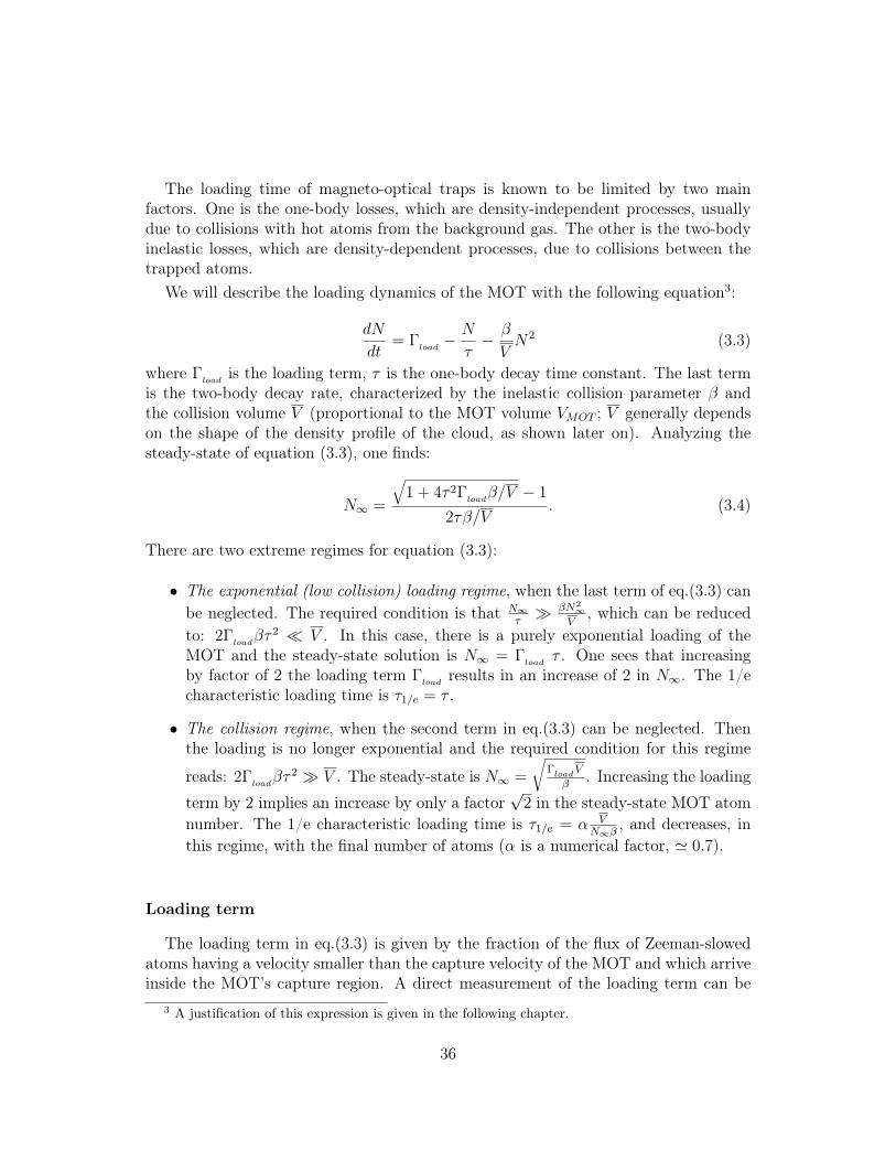
The loading time of magneto-optical traps is known to be limited by two mainfactors. One is the one-body losses, which are density-independent processes, usuallydue to collisions with hot atoms from the background gas. The other is the two-bodyinelastic losses, which are density-dependent processes, due to collisions between thetrapped atoms.

We will describe the loading dynamics of the MOT with the following equation3:

dN

dt= Γ

load− N

τ− β

VN2 (3.3)

where Γload

is the loading term, τ is the one-body decay time constant. The last termis the two-body decay rate, characterized by the inelastic collision parameter β andthe collision volume V (proportional to the MOT volume VMOT ; V generally dependson the shape of the density profile of the cloud, as shown later on). Analyzing thesteady-state of equation (3.3), one finds:

N∞ =

√1 + 4τ 2Γ

loadβ/V − 1

2τβ/V. (3.4)

There are two extreme regimes for equation (3.3):

• The exponential (low collision) loading regime, when the last term of eq.(3.3) canbe neglected. The required condition is that N∞

τ βN2∞

V, which can be reduced

to: 2Γload

βτ 2 � V . In this case, there is a purely exponential loading of theMOT and the steady-state solution is N∞ = Γ

loadτ . One sees that increasing

by factor of 2 the loading term Γload

results in an increase of 2 in N∞. The 1/echaracteristic loading time is τ1/e = τ .

• The collision regime, when the second term in eq.(3.3) can be neglected. Thenthe loading is no longer exponential and the required condition for this regime

reads: 2Γload

βτ 2 V . The steady-state is N∞ =

√Γ

loadV

β. Increasing the loading

term by 2 implies an increase by only a factor√

2 in the steady-state MOT atomnumber. The 1/e characteristic loading time is τ1/e = α V

N∞β, and decreases, in

this regime, with the final number of atoms (α is a numerical factor, 0.7).

Loading term

The loading term in eq.(3.3) is given by the fraction of the flux of Zeeman-slowedatoms having a velocity smaller than the capture velocity of the MOT and which arriveinside the MOT’s capture region. A direct measurement of the loading term can be

3 A justification of this expression is given in the following chapter.

36

Figure 3.5: Loading of the 52Cr MOT. The cloud fluorescence, as recorded on the PM, is plotted as a functionof time. A linear fit at short time, represented by the straight dashed line, gives the loading term Γload = 3.7 × 108

atoms/s. The time-evolution can be well fitted (full line) by an exponential function (although we are in a regime whereinelastic collisions cannot be neglected – see text), which gives the 1/e loading time τ1/e = 15ms

performed, whatever the collisional regime. It is simply given by the slope at theorigin of the MOT loading curve. For the 52Cr MOT we measured, under optimalconditions4, a loading rate Γ

load= 3.7× 108 atoms/s at an oven temperature of 1500◦C

(see fig.(3.5)).A detailed study on the oven temperature dependence of the MOT loading rate, as

well as a comparison with the fermion case will be presented below.

One body losses

The Cr MOTs are characterized by very fast loading times, scaling from a few 10 msto ∼ 100 ms. The presence of leaks towards the metastable states can partly explainthese short time scales. It has been previously measured [31] that the total decay rateof atoms in 7P4 state towards the 5D states is γ5D

= (γ5D4+ γ5D3

) = 170 s−1 (whereγ5D3(4)

are the decay rates towards the 5D3(4) state). The corresponding loss term isproportional to the number of atoms which are in the excited state.

The one body decay rate in eq.(3.3) can then be expressed as:

1

τ= Π7P4

γ5D+ γres , (3.5)

where Π7P4is the excited state fraction and γres is the residual loss rate, related to

background gas collisions (in our case, especially with hot atoms from the Cr beam).Π7P4

depends on the MOT laser intensity and detuning. Since the decay rate to themetastable states is much smaller than the one towards the ground state (3.107 s−1)

4 Including a 2D transverse cooling in the oven chamber, presented in detail in the next section.

37

the excited fraction is5:

Π7P4=

〈C2〉 Ω2

4

〈C2〉 Ω2

2+ Γ2

4+ δ2

. (3.6)

Two body losses

Our experimental observations show that the loading dynamics of our 52Cr MOTcannot be interpreted using only the one body decay term in eq.(3.3). The MOTcharacteristic 1/e loading times (given by exponential fits – see fig.(3.5)) for differentloading curves, corresponding to different detunings and intensities, are always shorterthan the ones predicted by the time constant given by eq.(3.5). Moreover, the residualcollision time constant γ−1

res = 8 s (independently measured – see Chapter(5)) is muchlarger than the observed loading times.

On the other hand one can almost entirely block the one body loss channels towardsthe metastables by using two ’red’ repumpers at 654 and 663 mn. They practically closethe cooling transitions, by repumping the atoms ’lost’ to the metastable states backinto the MOT cycle. In absence of other limiting factors, this is expected to increasethe MOT steady state number by a factor 1+(γ5D

/γres), which in our case correspondsto a gain of more than 103. In practice we observe that adding the repumpers increasesN∞ only by a factor of about two.

This indicates that inelastic processes are a second limiting factor. At our MOTdensities, they appear to be on the same order of magnitude as the one body losses.We can make a rough estimate of the loss parameter β, by comparing the stationarysolutions of eq.(3.3), in presence (when two-body losses totaly dominate) and in absence(when both types of losses are present) of the ’red’ repumpers. For a peak density of1011 at./cm3 and for an excited state fraction of ∼ 1/2 we find that β ∼ 8.10−10 cm3

s−1.A precise measurement of inelastic collision parameters, presented in the next chap-

ter, confirms this rough estimate. This value represents an extremely high inelasticcollision parameter in a MOT and is about 2 orders of magnitude larger than for thealkali MOTs.

We finally present in fig.(3.6) a numerical comparison of the results of eq.(3.3), whichshows the role of inelastic collision in limiting the number of atoms in a Cr MOT. Thefull and dashed curves reproduce the loading of a Cr MOT, using the typical measuredloading and loss rates. For the full curve, we take into account both the leaks towardsthe metastable states and the inelastic collisions while for the dashed one we neglectthe losses to the metastable states. For the dotted curve, the inelastic loss parameter isreduced by a factor of 50, which roughly reproduces the loss parameters of the alkalis.

5 Π7P4is related to the mean scattering rate of the MOT atoms Rscatt, given in eq.(3.1), by:

Rscatt = Γ · Π7P4.

38

Figure 3.6: A) MOT loading in different regimes. The full-line curve is a simulation of the ’real’ Cr MOT loadingcurve, where both the leaks to the metastable states and inelastic collisions are present. The dashed curve is the’collision regime’ for Cr, where leaks towards the metastable states are removed. The dotted curve is a hypotheticalsituation, where leaks towards the metastable are suppressed and the inelastic collision parameter was reduced by afactor of fifty (which is analogous to the one measured in alkalis). B) MOT steady-state number of atoms, given byeq.(3.4), as a function of the β parameter (log-log scale), when γ5D = 0. The dotted lines correspond respectively tothe dashed and dotted curve in A).

These curves show that inelastic collisions not only reduce the loading time constantof a Cr MOT, but also dramatically limit the steady-state number of atoms that canbe trapped.

Conclusions

The previous considerations show that, despite the necessity of using a high-temperatureeffusion cell, we are able to obtain reasonably good slowed atom fluxes; however thefairly small atom numbers obtained in the 52Cr MOTs are severely limited by the highlight-assisted inelastic collision rates.

Finally, in order to emphasize the originality of a Cr magneto-optical trap, let uscompare some of the relevant characteristic timescales. One is the loading time, fixedby the one body losses to the metastable states and the inelastic collisions, and is aslow as a few 10 ms. We independently measured, in experiments presented in the nextchapter (fig.(4.2)) a second timescale: it is the ’trapping time’ (i.e. the time neededto form a MOT from a large magnetically trapped sample) of our Cr MOTs, which ison the time scale of 2 to 20 ms. We see that these timescales are not very different,which means there is an interesting question one can raise, about how one can correctlydescribe the ’equilibrium’ of a Cr MOT.

We finally note that the MOT cooling time, which is required for decelerating anatom from ∼ 40 m/s down to the Doppler temperature, is on the order of 0.2 ms (ataD,max). This is shorter than the two previous timescales, which means that temper-atures as low as the Doppler temperature can indeed be reached, which we observeexperimentally.

39

3.2.3 Density saturation

Our experimental observations show a saturation of the peak density of the cloudwhen increasing the number of atoms in the MOT.

For better understanding this phenomenon, we performed a systematic study andthe results are shown in fig.(3.7). We notice a fast initial increase of the density, whichbegins to slow down when the atom number becomes larger than ∼ 106; a full saturationis not observed and relatively high value of 1.1 × 1011 atomes/cm3 is reached.

Figure 3.7: MOT radius and peak density versus the number of magneto-optically trapped atoms.

Changing the number of atoms in the MOT was achieved by varying the power ofthe Zeeman slower beam. Fluorescence pictures provided information about the sizeand number of atoms in the MOT. The cloud shape appears gaussian in both directionsof the imaging plane, with an aspect ratio of ∼ 2 (presumably due to a tighter confine-ment on the MOT coil axis). The experiment was performed for a fixed MOT beamstotal intensity of ∼ 200 mW/cm2 and for a detuning of −12 MHz. In order to extendthe study to higher MOT atom numbers, both ’red’ repumpers were permanently kepton.

We may consider two possible explanations for the MOT density saturation. Oneis due to multiple scattering of the light by an optically dense trapped cloud andhas already been demonstrated for other atomic species (see for example [64]). Theradiation spontaneously emitted by the excited trapped atoms may be reabsorbed bythe neighboring atoms. This creates an overall repulsive force and consequently limitsthe peak density.

Another possibility we take into account, which is more specific to chromium, comesfrom the very high inelastic collision rate presented earlier. Indeed, the atoms whichare close to the trap center, where the density is higher, have a higher probability ofundergoing inelastic collisions compared to the atoms closer to the edge of the cloud.

40

The space-dependent density of the cloud produces a space-dependent loss rate whichmay change the size of the cloud and limit the density.

We will try in the following lines to evaluate the influence of inelastic collisions onthe size and density of a Cr MOT. Our model uses the Fokker-Plank equation [40, 41]with two additional terms:

∂n(r, t)

∂t= ∇ ·

[1

mγv

n(r, t)∇U(r) + Dr∇n(r, t)

]+ Γ

load(r) − βn2(r, t). (3.7)

The additional terms are a loading term Γload

(r), and an inelastic collision term6

−βn2(r, t), depending quadratically on the density. The first term in the right-handside is the divergence of the total current of particles. It is the sum of the drift current– (1/mγp)n(r, t)∇U(r), due to the MOT confining potential U(r) – and of the diffusioncurrent – Dr∇n(r, t). In eq.(3.7) γv is the velocity-damping coefficient of the MOTand Dr = kBT/mγv is the spatial diffusion constant.

In our simulations we consider the maximum value of the damping coefficient γv hk2/2m = Erec/h [63], which is about 2π× 20 kHz. The confining potential isU(r) = −κr2/2, where κ is the MOT spring constant. We determined κ from themeasured MOT temperature T = 120 μK and from the mean 1/e radius w = 60 μmof the MOT at small atom number: κ = 2kBT/w2. For simplicity of the numericalsimulations, we consider a uniform spatial distribution, with a finite extent, of theloading term Γ

load(r); integrating Γ

load(r) over the whole space gives the total MOT

loading rate, which is the experimental parameter we varied for obtaining fig.(3.7). Inorder to give an upper boundary for the effect of inelastic collisions, we consider a valueβ = 10−9 cm3/s.

Our simulations typically show an almost gaussian-shaped cloud, with a radius de-pending on the Γ

loadparameter. Results are shown in fig.(3.8), where we compare the

simulated cloud 1/e radius to the one determined experimentally. At small atom num-ber, the initial size of the MOT is not affected by the inelastic collisions, and coincides(as expected) with the experimental value. When the atom number increases, the weobserve that cloud radius increases; we checked that, for a β parameter one order ofmagnitude smaller, the cloud radius remains constant (in the values shown in fig.(3.8)).Finally, we notice that, when the atom number reaches 4.5×106, the inelastic collisionslead to an increase up to 40% of the cloud radius .

This value does not entirely explained the measured increase (of about 120%). Wetherefore think that multiple scattering is responsible for the major part of the densitysaturation. A simple model could take into account their role, adding a repulsive po-

6 Integrating this term over r provides the last term in eq.(3.3) – as shown in the following chapter.

41

Figure 3.8: Effect of the inelastic collisions on the size of the MOT: the results of our simulations (diamonds) mayexplain up to 40% of the observed (circles) increase of the MOT radius.

tential (see below) to the MOT confining potential.

Very simple considerations can qualitatively give the space-dependance of the mul-tiple scattering repulsive potential Um.sc.(r). Because of the presence of the trappinglasers, the atoms scatter photons, which can be subsequently reabsorbed by their neigh-bors. The repulsion force between two atoms, separated by a distance r, is proportionalto the intensity of the scattered light, which is proportional to r−2. Multiple scatteringgives thus rise to a Coulomb-like, 1/r potential.

In the (very simplified) case of a spherical MOT, with uniform density distribution,we can thus apply the Gauss theorem7 and find that the multiple scattering potentialis proportional can be written as: Um.sc.(r) = αsc.r

2 within the MOT volume. Wesee that Um.sc.(r) has the same space-dependence, but an opposite sign as the MOTconfining (harmonic) potential: it leads to a reduction of the MOT spring constant, toan ’effective value’: κeff = κ − αsc..

The αsc. coefficient is expected to depend on the density of the cloud. This meansthat, in reality, things are more complicated than in our simple model, for examplein case of a non-uniform density distribution of a MOT. However, multiple scatteringmay cancel the confinement in the center of a MOT, which led to the observation, forother atoms, of ’uniform density’ profiles [64, 65].

Finally, let us notice that the coefficient αsc. is proportional to the probability ofreabsorption of the scattered photons, i.e. to the absorption cross section σabs. Itscales thus with the square of the wavelength: αsc. ∝ λ2. This scaling law qualitativelyexplains why, at densities comparable to those obtained for other atoms, with IRtransitions (below 1011 atoms/cm3 for Cs, with λ = 852 nm [65]), in our Cr MOTs

7 Exactly as in the case of a uniform charge distribution

42

(λ = 425 nm) uniform density distributions are not observed and saturation is notfully reached (see fig.(3.7)).

3.2.4 52Cr Zeeman slower

In this subsection I will address two issues: one is the possibility of having effi-cient optical pumping in the increasing B-field region, at the entrance of the ZS (ZS’branching zone’), and the other is a method to enhance the flux of slowed atoms, bytransverse-cooling the atomic beam.

Optical pumping in the 52Cr ZS ’branching zone’

The hot 52Cr atoms which leave the oven are evenly distributed in the differentZeeman sublevels of the 7S3 ground state.

The Zeeman slower can only slow down the 52Cr atoms which are in the |mJ = +3〉state. This is explained in fig.(3.9), where we plotted (horizontal dotted lines) themagnetic field corresponding to the ZS resonance for the |mJ = +3〉 and the |mJ = +2〉atoms, traveling at a given velocity – here, 300 m/s – , smaller than the ZS capturevelocity.

In the ’slowing region’ (II), the mJ = +3 atoms are resonant in the (b)-point; theystart scattering photons from the ZS beam, and remain in the |mJ = +3〉 state allalong the ZS profile. On the other hand, the mJ = +2 atoms, resonant in (b’), areoptically pumped to |mJ = +3〉 state by the ZS σ+ beam. They are however lost,despite arriving in this state, because they are not resonant any more with the ZSbeam (because of the Doppler effect).

Figure 3.9: Resonances corresponding to the mJ = +2 and mJ = +3 atoms of the Cr beam, traveling at 460 m/s,in the ZS B-field profile.

In fig.(3.9) we see that there is however a first resonance for the |mJ = +2〉 atoms,in the ZS ’branching region’(I); in (a’), these atoms may be optically pumped to |mJ =

43

+3〉 by the ZS beam, and enter the ’slowing region’ in the ’good’ Zeeman state. Weanalyzed this possibility, by performing optical pumping simulations, which show that,for an estimated interaction time of ∼ 4 μs (which is realistic for our ZS B-field profileand capture velocity) all the atoms are expected to be efficiently pumped to the |mJ =+3〉 state in the ZS ’branching zone’.

We will come back to this point later, when we will address the question of opticalpumping of the 53Cr isotope in the ’branching zone’.

Transverse cooling of the 52Cr atomic beam

To increase the flux of atoms that can be slowed down by the ZS and reach theMOT capture region, we implemented a transverse cooling scheme. The principle isschematically shown in fig.(3.10.A). One can see that the atoms that may be capturedby the MOT are those traveling inside the solid angle defined by the oven apertureand the surface corresponding to the MOT capture volume. One might increase thecorresponding atom flux, by cooling down the transverse velocity distribution after theoven collimation aperture. We note however that the real situation is more complicatedthan the one shown in fig.(3.10.A), because of the additional transverse heating duringthe Zeeman slowing process (discussed in Section(2.4)).

Figure 3.10: A) Principle of the beam transverse cooling. B) Experimental setup for the transverse cooling scheme.

For the transverse cooling we use a small fraction of the MOT laser light (∼ 10

44

mW), directed towards the oven and sent perpendicularly to the atomic beam; thelight is than retro-reflected, as shown in fig.(3.10). The aspect ratio of the beam waschanged using a ×5 cylindrical telescope, in order to better match the shape of theatomic beam, and increase thus the interaction length up to 2 cm, which correspondsto ∼ 40μs interaction time for atoms traveling at the ZS capture velocity (∼ 460 m/s).

We also superimposed, in the interaction zone, a magnetic field to tune the atomiclevels and change the detuning of the transverse cooling light, independently of theMOT detuning. A pair of ’compensation coils’ (with a diameter of 5 cm, separated by26 cm and each having 800 turns, made of 0.5 mm diameter copper wire) can producean adjustable magnetic field at the atomic beam location, roughly between 0 and 6G.An additional water-cooling circuit had to be used in order to limit the heating due tothese coils (∼ 15 W).

We performed two optimization experiments of the 1D transverse cooling and theresults are shown in fig.(3.11). First we studied the influence of the transverse magneticfield. We found that the value of 5G optimizes the transverse cooling, for a MOTdetuning of −2.5 Γ 8. We also studied the evolution of the MOT fluorescence as afunction of the laser power in the transverse beam, at fixed MOT intensity (which wasintentionally lowered to 17mW, in order to have about 20 mW of transverse poweravailable to perform this experiment). We observe that saturation occurs at about 10mW, corresponding to ∼ 16 mW/cm2.

In a later stage of the experiment (April 2007) we implemented the transverse cool-ing in the vertical direction. The light used for the first – horizontal – cooling stage wasrecycled and sent through the other set of view-ports shown in fig.(3.10). An additionalset of ’compensation coils’ was constructed.

Figure 3.11: A) Number of atoms in the MOT (arbitrary units) as a function of the magnetic field used forcompensating for the MOT beams detuning. The optimum is obtained for value of 5G. B) Saturation of the atomnumber in the MOT with the power of the transverse cooling beam.

8 This value corresponds to an ’effective’ detuning of the transverse cooling beams of ∼ −Γ, withrespect to the |7S3, mJ = 3〉 → |7P4, mJ = 3〉.

45

To evaluate the gain on the slowed atomic flux at the end of the ZS, we compared theMOT signal, with and without the transverse cooling, keeping the two red repumperson. We thus substantially decrease the influence of one body losses (by blocking theleaks towards the metastable states) compared to the two body losses and forcing thesystem into the ’collision regime’ (defined earlier). The steady state atom number is:

N∞ =

√ΓVβ

, and the slowed atom flux Γ is:

Γ ∝ βN∞n0,∞ (3.8)

where n0,∞ is the steady-state MOT peak density. Using only the horizontal coolingstage gives a 2.7 gain in N∞, while adding the second gives an overall 4.9 gain. Bymeasuring the volume of the MOT, we also observed that n0,∞ increases less rapidlythan N∞ (by a factor 1.3, respectively 1.5, for the 1D/2D stage), which is explainedby the saturation of the peak density mentioned earlier.

We finally conclude from eq.(3.8) that the 2D (1D – horizontal) transverse coolingincreases the slowed atomic flux by a factor 7.4 (3.2). We then indirectly deduce again of 2.3 for the vertical cooling, which appears less effective than the horizontal one.This may be attributed to the fact that ∼ 65% less power is available for the second(vertical) stage – due to light absorption of the atoms and of the optical elements– and to the fact that the beam shape is appreciably different, because of imperfectcollimation.

In conclusion, using the two transverse cooling stages, we obtain a flux ∼ 3.7 × 108

(slowed) atoms/s which are captured in the MOT.

3.3 Magneto-optical trapping of 53Cr atoms

Magneto-optical trapping of fermionic 53Cr is not a straightforward extension of thework concerning 52Cr. The main difference between the two isotopes is the additional,complex hyperfine structure of 53Cr (see Chapter(1)), whose electronic ground andexcited states have four hyperfine components. As a consequence, several repumpersare needed in a 53Cr MOTs.

The fermionic 53Cr isotope has already been cooled by collisions with a cold buffergas in the group of Doyle [42]. Preliminary observations of a 53Cr MOT were also madein the group of T. Pfau [31].

3.3.1 53Cr Zeeman slower

The 53Cr atom flux is expected to be significantly smaller than the 52Cr flux for twomain reasons. First, the natural abundance is ∼ 9 times smaller. Second, the hyperfinesplitting of the ground state (∼ 42 mK) is much smaller than the oven temperature

46

(1773 K). This means that the 53Cr atoms in the oven are evenly distributed in allthe 28 Zeeman sublevels of the ground state. In absence of optical pumping, only 1/28of them are expected to be slowed down by the Zeeman slower, and the fermionicZeeman-slowed flux will be a factor of ∼ 250 smaller than the bosonic one.

In the following part we will address two issues concerning the fermionic ZS: theneed of a repumper inside the ZS, and the possibility to have efficient optical pumpingin the ’branching zone’ of the Zeeman slower, as it was the case for the boson.

Need of a Zeeman slower repumper for 53Cr

We carefully analyzed the fermionic transitions inside the Zeeman slower, looking foreffects of slight polarization imperfections of the ZS beam. We found a ’bad crossing’taking place at a magnetic field B= 25.4 G. At this magnetic field value, two excitedeigenstates, which are adiabatically connected to |F ′ = 11/2, mF ′ = +11/2〉 and to|F ′ = 9/2, mF ′ = +7/2〉 at B=0, become degenerate (see fig.(3.12).). This means thatany σ−-polarized component in the ZS laser beam depumps the atoms towards theF= 7/2 ground state9.

In our experiment we think that the ZS laser beam may not be perfectly σ+ polarized,because the undervacuum aluminium mirror which reflects the ZS beam gets coatedwith chromium, and does no longer act as a perfect metallic mirror for the 425 nmlight.

Figure 3.12: 53Cr Zeeman slower repumping mechanism. The diagram corresponds to a value of 25 G of themagnetic field, where the |F ′ = 11/2, mF ′ = +11/2〉 and |F ′ = 9/2, mF ′ = +7/2〉 states are degenerate. A small σ−component of the ZS (dashed arrow) can thus depump the atoms in |F = 9/2, mF = 9/2〉 to the |F = 7/2, mF = 5/2〉and |F = 7/2, mF = 7/2〉 states. The lost atoms can be repumped into the |F = 9/2, mF = 9/2〉 state using a repumperbeam (grey arrow).

9 We remind the reader that only the 53Cr atoms in the |F = 9/2, mF = +9/2〉 can be sloweddown by the ZS, as seen for the 52Cr, in Section(3.2).

47

Atoms travel relatively slowly throughout the ’bad crossing’ region, as B=25 G cor-responds to a velocity of about 200 m/s (see eq.(2.7)). At this point the gradient of theZS magnetic field is 11G/cm and we estimate the interaction time with the depumpinglight to 20 μs. Optical pumping calculations showed that about 50% of the atoms canbe lost if 10% of the ZS power is σ− polarized. This means that an additional laser,resonant at B=25 G with the transition between the states adiabatically connected to|F = 7/2, mF = 7/2〉 – |F ′ = 9/2, mF ′ = 9/2〉, needs to be used in order to pump backthe atoms to |F = 9/2, mF = 9/2〉. The frequency of the repumper needs to be about300 MHz above the 53Cr ZS frequency. In fact, this frequency nearly coincides withthe 52Cr ZS beam frequency, and no additional laser frequency has to be generated.

Optical pumping in the ZS ’branching zone’

In Section(3.2) we presented the bosonic Zeeman slower. We showed that onlythe atoms arriving in the ’slowing region’ (II in fig.(2.12)) being in the right internalstate |J = 3, mJ = +3〉 will eventually be slowed. Fortunately, optical pumping inthe ’branching zone’ is expected to efficiently bring all the 52Cr beam atoms (hav-ing a velocity ∼ 460 m/s or less) to the |J = 3, mJ = +3〉 state. Let us focus nowon the possibility of optical pumping in the ’branching zone’, in the case of the fermion.

The approach is the following: we start from an initial population evenly distributedin the 28 Zeeman sublevels of the ground state. For a given velocity class (we chosehere 460 m/s, which is the ZS capture velocity), we consider a series of resonances ofthe (σ+−polarized) ZS beam, with the transitions connecting these levels to the 38Zeeman sublevels of the 7P4 excited state. These resonances occur in a certain order,in the increasing B-field profile of the ZS ’branching zone’. Using optical pumpingcalculations (based on rate equations), we estimate the populations of each of the Zee-man sublevels of the ground state, after each resonance, until reaching the maximumB-field value, which corresponds to the beginning of the ZS ’slowing zone’. Finally, weare interested by the number of atoms which are found in the |F = 9/2, mF = +9/2〉state, which may be slowed down by the ZS.

The situation is quite complicated, because of the non-linear Zeeman effect. Dueto the small values of the hyperfine constant A and to the large gF -factors (see Chap-ter(1)), the transition between the low-field and high-field-limit eigenstates takes placeat relatively low values for the magnetic fields, for the 7S3 state, and at even lower val-ues for the 7P4 state; the exact order of the ZS resonances is thus not straightforwardto predict.

In fig.(3.13) we (try to) show the complexity of the problem, by first consideringthe transitions from the 7S3 – F=9/2 manifold to the 7P4 – F’=11/2 manifold, which

48

Figure 3.13: 53Cr Zeeman transition diagram, for the 460 m/s velocity class: detuning vs. magnetic field in theZS ’branching’ zone. We represented the following ZS beam transitions: |F = 7/2〉 → |F ′ = 9/2〉 (A), |F = 9/2〉 →|F ′ = 11/2〉 (B), |F = 9/2〉 → |F ′ = 9/2〉 (C), |F = 9/2〉 → |F ′ = 7/2〉 (D). Intersections with the x-axis representthe magnetic field values for which different transition come in resonance. The thick line represents the ZS transition(|F = 9/2, mF = 9/2〉 → |F ′ = 11/2, mF ′ = 11/2〉)

may eventually increase the population of the |F = 9/2, mF = +9/2〉 state (as theyarrive in the ’good’ order, i.e. for increasing mF s). However, there are other σ+

transitions possible, for example from the 7S3 – F=9/2 manifold to the 7P5 – F’=9/2manifold. Atoms in the 7P5 – F’=9/2 manifold decay essentially to the 7S3 – F=7/2manifold (because of the stronger Clebsch-Gordan coefficients); these are rather ’bad’transitions, which empty the 7S3 – F=9/2 manifold; we see that they occur for smallerB-field values, i.e. before the 7S3 – F=9/2 to 7P4 – F’=11/2 transitions.

One should also consider a small σ−− polarization component of the ZS beam, andadditional transitions due to the ZS repumper (we recall that it has a σ+ polarization,as the ZS beam, and it is detuned by 300 MHz).

One can see now that the problem of performing optical pumping calculations, tak-ing into account 28 ground-state sublevels (evenly populated with 1/28 = 3.57% ofthe total population at t = 0) connected to 38 excited-state levels is quite complex.The calculations are based on several assumptions, like the exact amount of σ− com-ponent in the ZS beam and the interaction time for a certain longitudinal velocityclass considered. Moreover, the use of rate equations is not valid in our case, where anarrow-frequency laser is used, and the adiabatic elimination of coherences is not justi-

49

fied. For all these reasons, we think that the results are rather qualitative; we howeverestimate that they give at least some hints about the optical pumping dynamics in theZS ’branching zone’.

Figure 3.14: Population enhancement of the |F = 9/2, mF = 9/2〉 level at the end of the ’branching’ zone: onlythe small fraction in |F = 9/2, mF = 7/2〉 is efficiently transferred by the laser beam to the desired state. The colorcode is the same as in fig.(3.13): violet is the ZS (σ+) beam on the F = 7/2 → F ′ = 9/2 transition and orange is alsothe ZS beam on the F = 9/2 → F ′ = 11/2 transition.

We counted a total of 25 successive resonances10 (some of them taking place at aboutthe same value of the magnetic field). Most of these resonances do not affect the popu-lation of atoms in the |F = 9/2, mF = 9/2〉 state. Only the last ones, occurring aroundB = 445 G, are likely to increase significantly its population. The situation beforethis resonance is shown in fig.(3.14). We observe that a relatively significant amountof atoms (about 12%) has been accumulated in the |F = 7/2, mF = 7/2〉 state. Unfor-tunately, because of the small Clebsch-Gordan coefficients involved (see fig.(3.14.B)),these atoms are not efficient transferred into the desired state; we efficiently ’recuper-ate’ only the atoms in the |F = 9/2, mF = 7/2〉 state (which unfortunately are veryfew).

Our estimations show a final enhancement of only 25% of the |F = 9/2, mF = 9/2〉state (from 3.6% to 4.5%). This means that, unfortunately, the optical pumping inthe 53Cr ZS ’branching zone’ is not expected to increase significantly the initial flux ofatoms exiting the oven in the ’good’ Zeeman state.

10 For simplicity, we considered only transitions which affect the atoms in F=7/2 and F=9/2hyperfine levels; it is less likely for the F=3/2 and F=5/2 to be pumped to the |F = 9/2, mF = 9/2〉state.

50

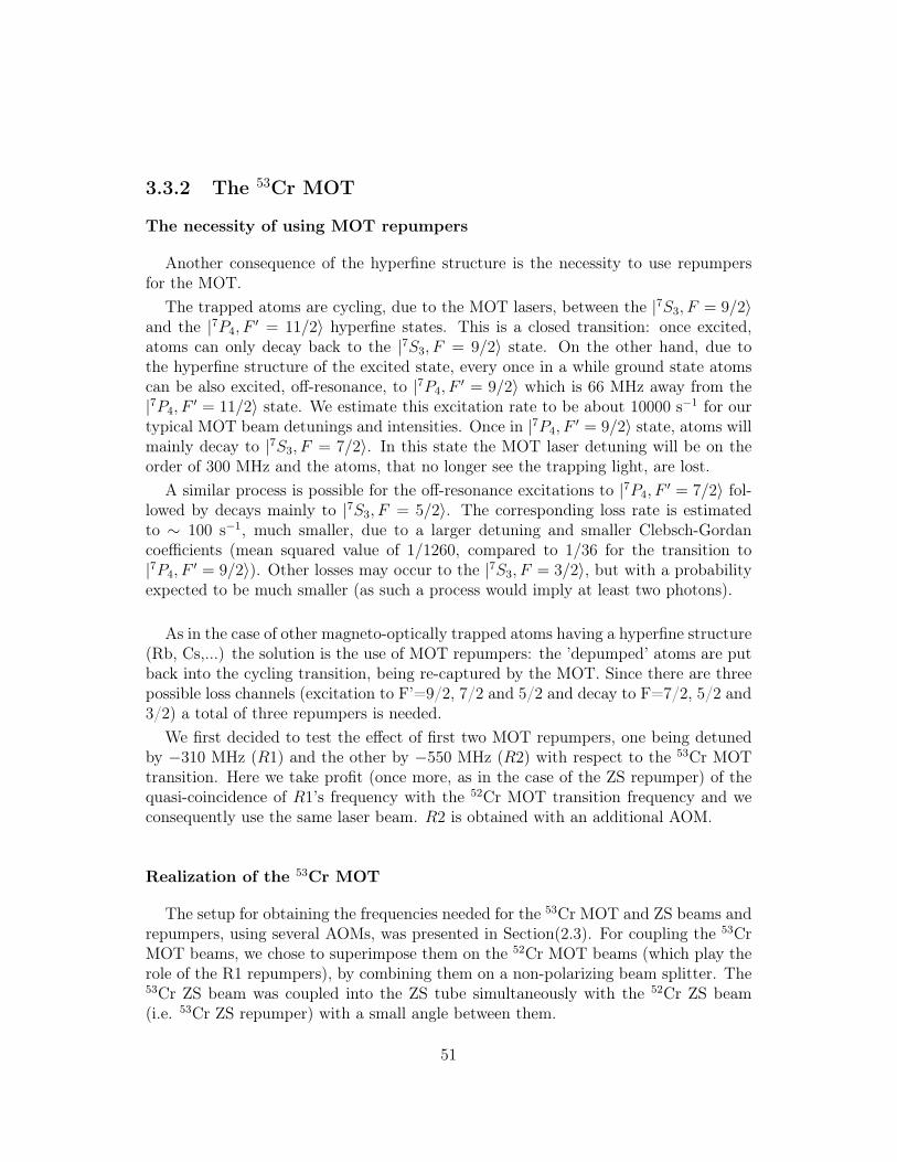
3.3.2 The 53Cr MOT

The necessity of using MOT repumpers

Another consequence of the hyperfine structure is the necessity to use repumpersfor the MOT.

The trapped atoms are cycling, due to the MOT lasers, between the |7S3, F = 9/2〉and the |7P4, F

′ = 11/2〉 hyperfine states. This is a closed transition: once excited,atoms can only decay back to the |7S3, F = 9/2〉 state. On the other hand, due tothe hyperfine structure of the excited state, every once in a while ground state atomscan be also excited, off-resonance, to |7P4, F

′ = 9/2〉 which is 66 MHz away from the|7P4, F

′ = 11/2〉 state. We estimate this excitation rate to be about 10000 s−1 for ourtypical MOT beam detunings and intensities. Once in |7P4, F

′ = 9/2〉 state, atoms willmainly decay to |7S3, F = 7/2〉. In this state the MOT laser detuning will be on theorder of 300 MHz and the atoms, that no longer see the trapping light, are lost.

A similar process is possible for the off-resonance excitations to |7P4, F′ = 7/2〉 fol-

lowed by decays mainly to |7S3, F = 5/2〉. The corresponding loss rate is estimatedto ∼ 100 s−1, much smaller, due to a larger detuning and smaller Clebsch-Gordancoefficients (mean squared value of 1/1260, compared to 1/36 for the transition to|7P4, F

′ = 9/2〉). Other losses may occur to the |7S3, F = 3/2〉, but with a probabilityexpected to be much smaller (as such a process would imply at least two photons).

As in the case of other magneto-optically trapped atoms having a hyperfine structure(Rb, Cs,...) the solution is the use of MOT repumpers: the ’depumped’ atoms are putback into the cycling transition, being re-captured by the MOT. Since there are threepossible loss channels (excitation to F’=9/2, 7/2 and 5/2 and decay to F=7/2, 5/2 and3/2) a total of three repumpers is needed.

We first decided to test the effect of first two MOT repumpers, one being detunedby −310 MHz (R1) and the other by −550 MHz (R2) with respect to the 53Cr MOTtransition. Here we take profit (once more, as in the case of the ZS repumper) of thequasi-coincidence of R1’s frequency with the 52Cr MOT transition frequency and weconsequently use the same laser beam. R2 is obtained with an additional AOM.

Realization of the 53Cr MOT

The setup for obtaining the frequencies needed for the 53Cr MOT and ZS beams andrepumpers, using several AOMs, was presented in Section(2.3). For coupling the 53CrMOT beams, we chose to superimpose them on the 52Cr MOT beams (which play therole of the R1 repumpers), by combining them on a non-polarizing beam splitter. The53Cr ZS beam was coupled into the ZS tube simultaneously with the 52Cr ZS beam(i.e. 53Cr ZS repumper) with a small angle between them.

51

Figure 3.15: Coupling of the 53Cr MOT and repumper (i.e. 52Cr MOT) beams.

Experimentally we found that detection of a first 53Cr MOT signal was somewhatcomplicated by the fact that the repumpers could still form by themselves a (small) 52CrMOT. The solution for isolating the 53Cr MOT signal was to change the polarizationof the 52Cr MOT beams, using a λ/2 wave plate placed before the non-polarizing beamsplitter which combined the MOT beams for the two species (see fig.(3.15)). Thischanges the 52Cr MOT beam polarization to a ’anti-trapping’ configuration, where the52Cr are expelled from the trap.

This procedure allowed us to isolate the 53Cr MOT, and clearly demonstrate itsrealization.

Characteristics of the 53Cr MOT

The optimization procedure of the 53Cr MOT atom number, although slightly com-plicated by the need for using several repumpers, was similar to the one used for the52Cr MOT, presented in Section(2.3). We found roughly the same optimal values forthe ZS final velocity and MOT gradient.

We performed systematic studies to measure the total number of atoms in the MOT,as a function of the cooling laser intensity and detuning, and the results are shown infig.(3.16). The information about the number of atoms and the cloud size was obtainedby fluorescence-imaging, using the analysis technique presented in Section(3.1).

The data were obtained for an average 1/e2 size of the MOT beams of 4.5 mm andfor a total power of 24 mW; this corresponds to a total (six-beam) MOT intensity of225 mW/cm2. The ZS beam has a total power of 30 mW; it has a 1/e2 radius of 3.6mm, when entering the ZS tube, and is focalized on the oven aperture.

The maximum number of atoms we obtained in a 53Cr MOT was (5±0.25±1)×105,for a detuning of −22 MHz (see fig.(3.16.A)). In fig.(3.16.B) we see that that the numberof atoms saturates with the intensity, while the peak density does not saturate for the

52

Figure 3.16: A) 53Cr MOTatom number (dots) and peak atom density (triangles) as a function of the normalizeddetuning of the MOT beams, for a total laser intensity of 200 mW/cm2 B)Atom number (dots) and peak atom density(triangles) as a function of the total power in the MOT cooling beams, for a detuning of −21.5 MHz.

laser power available. The highest peak atomic density obtained was up to 2.5 × 1010

atoms/cm−3 (with a systematic uncertainty of 30%, mostly due to the MOT beamsintensity measurement).

Influence of the different repumpers

We studied the influence of the first two MOT repumpers on the trapped 53Cr atomnumber. We found that the effect of the first repumper is crucial: no MOT could beobtained without R1. When the second repumper is removed the number of atoms inthe MOT is only reduced by 30%. We inferred from this observation that repumpingon the transition |7S3, F = 3/2〉 to |7P4, F

′ = 5/2〉 would not significantly increase thenumber of atoms in the MOT.

We also checked that the repumping effect of R1 and R2 saturates, at an intensityrespectively of 13 mW/cm2 and 7 mW/cm2. This corresponds to a total power respec-tively of 10 mW (1/e2 beam radius of 7 mm) for R1 and 3 mW (1/e2 radius of 5.2 mm)for R2.

3.3.3 Oven temperature-dependence of the MOT loading rates

One of the questions which rose at the beginning of our experiment was relatedto the possibility of obtaining a sufficiently high flux of laser-slowed 53Cr atoms. Asshown previously, due to the smaller natural abundance and to the presence of hyper-fine structure, the initial (i.e. at the beginning of the Zeeman slowing region) flux offermions is expected to be about two orders of magnitude smaller than the bosonicone. The experimental realization of magneto-optical traps, for the bosons and for thefermions, allowed us to measure the corresponding MOT loading constants, as well as

53

their dependence on the oven temperature (Toven).

Figure 3.17: Dependence of 52Cr and 53Cr MOT loading constants on the oven temperature, deduced from theinitial slopes of the MOT loading curves. The experiment series was performed in absence of any transverse cooling, inorder to have a more appropriate comparison with the theoretical fluxes. The full line represents the theoretical flux,considering a ’real’ temperature which is 150 K lower then the one indicated by the ovens’ thermocouple.

For that, we recorded with a photomultiplier several MOT loading sequences, fordifferent values of temperature measured by the oven’s thermocouple Tth.. Fitting theirinitial slopes provides a direct measurement of the loading constant Γload. Fig.(3.17)shows the experimental results; we find a ratio of 45 between the boson and fermionloading constants (we remind that the initial theoretical ratio between the ’useful’ ovenfluxes was ∼ 250, as explained above).

Even though the measurements were performed in absence of any transverse cool-ing, it is still difficult to interpret this difference. The MOT and Zeeman Slower beamshave different sizes and the total laser power available in each case is different11. Thisis expected to change both the MOT capture velocities and the Zeeman Slowing per-formances. On the other hand the theoretical ratio is obtained using optical pumpingcalculations in the branching zone of the Zeeman Slower, which are particularly com-plicated in the case of the fermion.

Finally, we compared our experimental data with the ’theoretical’ prediction of theoven flux Φ(T ), obtained using the saturated vapor pressure given by the formula (2.1)– see Section(2.1). We observe that a reasonable agreement is obtained by consideringa difference ΔT ∼ 150±50 K between the temperature measured by the thermocoupleand the temperature Toven of the ’emission source’.

11 For 53Cr we have more laser power available, because no AOM is needed for obtaining the beamfrequency.

54

A possible explanation may come from the fact that the temperature at the positionof the thermocouple (i.e. at the bottom end of the W ’main crucible’ – see fig.(2.2)) issomewhat higher than the temperature of the ’emission source’ of the oven12.

3.4 Accumulation of metastable Cr atoms in a mag-netic trap

In the previous sections we showed that relatively small atom numbers can be ob-tained in Cr MOTs. Chromium nevertheless offers a nice way to decouple cooling antrapping. Indeed, atoms in Cr MOTs are slowly optically pumped into the long-livedmetastable 5D states, decoupled from the MOT light, and hence from light assistedcollisions. Furthermore, the magnetic moment in the metastable states is large enough(up to 6μB) for the atoms to be trapped in the MOT magnetic field gradient, providedthey are produced in a low-field-seeking state. This procedure was already demon-strated for 52Cr [43] and allowed to raise the number of cold atoms by one order ofmagnitude, compared to the number of atoms in magneto-optical traps.

After giving some experimental results obtained for 53Cr, we will demonstrate thepossibility of extending the same continuous accumulation method to the case of thefermionic 53Cr isotope.

3.4.1 Magnetic trapping of 52Cr

The experimental procedure is the following: we start by forming a MOT during afew seconds, in absence of any repumping light, which leads to accumulation of atoms inthe metastable states. At the end of the accumulation, the MOT beams are switchedoff. In order to be observed, the atoms accumulated in the 5D states must first berepumped in the ground state, where their fluorescence can be recorded, either on theCCD camera or the PM, by briefly shining the MOT beams, tuned on resonance. Theduration of this ’imaging’ pulse is typically a few 100 μs (much smaller than the MOTformation time, of a few ms), in order to affect as little as possible the atoms and toobtain accurate information about the cloud size13.

We observe that in the case of 52Cr, the number of accumulated metastable atomssaturates in a time scale which is fixed mostly by the inelastic collisions, between themetastable atoms and with the MOT atoms in the excited state 7P4 (as described indetail in Chapter(5). The typical time scale for this accumulation varies between 1.5 sand 8 s, depending on the MOT parameters. The upper time scale boundary (reachedat large MOT detunings, when both the MT and MOT are not optimal) is fixed by

12 However, we mention that the formula (2.1) could not be confirmed from several sources, othersources than [33].

13 Since these first results, we implemented an absorption imaging system, described in Section(2.5).

55

collisions with hot atoms from the Cr oven beam (as discussed in the next section). Asmany as 4 × 107 52Cr atoms could be accumulated, at a temperature of roughly 100μK.

3.4.2 Magnetic trapping of 53Cr

The techniques we applied for 52Cr were found to be also suitable in the case of53Cr.

The loading times we measured for the continuous accumulation of fermions in themetastable states are about 8 s when the oven is operated at 1500◦C. This is longerthan what was measured (in best operating conditions) in the case of 52Cr. On theother hand, this timescale is equal to the measured lifetime of the metastable fermionsin the magnetic trap when the atom shutter is not closed (when it is closed, the lifetimeincreases to 30 s). We conclude that in the case of 53Cr the number of accumulatedatoms is mainly limited by the collisions with fast atoms coming from the oven.

After the accumulation in the 5D4 metastable state and a 10 ms repumping sequence,we measured up to 8.5 105 atoms remaining magnetically trapped in the 7S3 state. Thisnumber was obtained for a detuning of the MOT beams equal to 12.5 MHz and a totalintensity in the MOT beams equal to 200 mW/cm2. This corresponds to an increaseof almost a factor of 6.5 compared to the steady-state MOT atom number for theseparameters.

This measurement was achieved close to resonance, and should probably not cor-respond to the optimal 53Cr atom number accumulated in the metastable state. Fortechnical reasons (related to the oven), we could not perform an elaborate optimiza-tion of the accumulation. In addition, such a number was measured using only one redrepumper (5D4 → 7P3), and the use of another red repumper for the 5D3 state shouldgive us a reasonable starting point for further experiments.

3.5 Resonance frequency measurements and isotopicshift determination

The magnetic trapping of both Cr isotopes in the same apparatus made possible tomake an accurate experimental determination of the resonance frequency of 52Cr and53Cr MOT transitions, and of the isotopic shift.

Collisional shift in the hollow cathode

We first performed the spectroscopy of a magnetically trapped 52Cr atom cloud. Af-ter accumulating the atoms in the metastable states and repumping them in the groundstate, we briefly turned on the MOT lasers and recorded the atomic fluorescence, for

56

different values of the MOT AOM frequencies. A lorentzian fit of this spectrum permit-ted the precise determination of the resonance frequency of the 52Cr MOT transition,which was found 146.5 MHz above the laser frequency.

The frequency of the laser is locked 150 MHz below the atomic resonance in thehollow cathode (see Section(2.3)). We observe thus that there is a 4.5 MHz differencebetween the two frequencies, which may be attributed to a collisional shift of the atomicresonance in the hollow cathode lamp.

’Isotopic shift’

A similar technique was used for finding the 53Cr transition resonance frequency, andthe results are shown in fig.(3.18). The slight dissymmetry of the lineshape comes fromthe fact that the Bragg angle of the 53Cr MOT beam AOM depends on the RF frequency(it was optimized for a MOT detuning of −3Γ and the diffraction efficiency drops downas we approach the resonance). The fit shown in fig.(3.18) takes into account thisfrequency-dependence of the beam intensity. The zero value of the frequency axis (notshown) represents the 52Cr MOT transition frequency.

Figure 3.18: Measurement of the resonance of the 53Cr MOT transition. The origin of the frequency axis corre-sponds to the 52Cr MOT transition resonance. The solid line is a modified Lorenzian fit, which takes into account thedependence of the beam intensity on the AOM frequency.

From these measurements we can infer the value of the ’isotopic shift’ – defined hereas the frequency difference between the bosonic (J = 3) → (J = 4) and the fermionic(F = 9/2) → (F = 11/2) transitions; we obtain 316.5 ± 1 MHz.

The same (modified) Lorenzian fit indicates a FWHM of 15 MHz of the spectra. Inorder to interpret this value, we consider three broadening factors for the fluorescencespectrum. One is the power-broadening, on the scale of 8 MHz for a 200 mW/cm2 totalMOT beam intensity. The second comes from the linewidth of our 425 nm laser, of 2.5MHz. The last one comes from the fact that the fluorescence of the cloud was recorded

57

in presence of the trapping magnetic field gradient. This leads to an additional Zeemanbroadening of the transition, which we estimate on the order of 7 MHz (this value wasobtained using the experimentally-determined shape of the cloud and the magneticfield profile).

These three factors are thus expected to lead to a symmetrical broadening of thefluorescence spectrum to a FWHM of 12 MHz, which seems in reasonable agreementto the observed 15 MHz widths, and should not affect significantly the results of ourdetermination of the isotopic shift.

3.6 Magneto-optical trapping of a cold mixture of52Cr and 53Cr atoms

In many experiments which study degenerate mixtures of two different atomicspecies [66, 67], or of two different isotopes [68, 69], the starting point is to createa MOT which traps simultaneously both species.

Because of the considerably smaller atom numbers available in the 53Cr MOTs andmagnetic traps, compared to 52Cr, creating a cold mixture of the two isotopes seemsan important point in reaching the degenerate regime for the fermion. Our experimentwas indeed designed for cooling and trapping the two most abundant isotopes of Cr.

Double-isotope MOT for 52Cr and 53Cr atoms

We also realized the simultaneous magneto-optical trapping of 52Cr and 53Cr atoms.This experiment requires to generate many different frequencies simultaneously. How-ever it is made simple by the fortuitous quasi-coincidence between two transitions:the cooling transition for 52Cr and the ’R1’ transition for 53Cr (see Section(2.3)). Asa consequence, the cooling beam for 52Cr is used in the 53Cr MOT as R1. Anotherconsequence is that the 52Cr ZS beam also plays the role of a repumper for the 53CrZS.

Fig.(3.19) demonstrates the successive loading of a magneto-optical trap, first with52Cr atoms and then with 53Cr atoms. The experiment consists in turning on first the52Cr MOT beams and, once the steady-state atom number for 52Cr is reached, the 53CrMOT beams.

Despite our efforts of optimization, the atom numbers we are able to obtain in atwo-isotope trap is severely reduced (up to a few 105), compared to the case of single-species MOTs. In fig.(3.19) we can also see that the number of 52Cr atoms is the same,before and after the creation of the 53Cr MOT; this proves that the reduction is notrelated to any bad influence of the 53Cr MOT beams on the 52Cr cloud. This point isdiscussed in the following paragraph.

58

Figure 3.19: Loading of a double-isotope magneto-optical trap for 52Cr and 53Cr atoms; the steady-state atomnumbers are ∼ 105. The full line represents an exponential fit of the loading of the 52Cr MOT; it shows that thesteady-state number of 52Cr atoms is not influenced by the presence of the 53Cr MOT beams.

Influence of 53Cr Zeeman slower beam on 52Cr slowed atoms

There are several limitations to producing a magneto-optically trapped mixture ofthe two Cr isotopes with large number of atoms. One is related to the limited laserpower available, which must be split between the two MOT and ZS beams. Havingless power for the ZS means that saturation of the atomic transition throughout theslowing region will be less efficiently accomplished than in the single species case, whichdiminishes the slowed atom flux. On the other hand, lowering the power for the MOTresults in a decrease of its capture velocity.

We encountered a second, more subtle problem. We observed that the simple pres-ence of the 53Cr Zeeman slower beam was sufficient to diminish the number of atomsin the 52Cr MOT. This can be understood considering the resonance condition of the53Cr ZS beam, in the ’extraction region’ of the ZS (see fig.(2.12)), with respect to the52Cr transition:

δZS,53 =μBB(z)

h+

vf

λ, (3.9)

where δZS,53 is the detuning of the 53Cr ZS beam with respect to the 52Cr atomicresonance (δZS,53 = −150 MHz).

The magnetic field B(z) varies between Bf = −260 G and 0 G throughout theZS ’extraction region’, and vf is the final velocity of the 52Cr ZS, given by δZS,52 =μBBf

h+

vf

λ. We observe that the ZS resonance condition (given by eq.(2.6)) is fulfilled

59

in z0, where the magnetic field is:

B(z0) = Bf +h

μB

(δZS,53 − δZS,52) = −45.7 G. (3.10)

This means that the slowed 52Cr atoms will pass, with a small velocity (i.e. ZS finalvelocity vf ) of 40 m/s, on resonance with the 53Cr ZS beam in the final part of the ZSand will partly be pushed back towards the oven before reaching the MOT trappingregion.

Perspectives

This unwanted resonance limits the number of 52Cr atoms in the double-speciesMOT, as well as the one in the metastable states (as they are loaded due to thespontaneous decay of the excited MOT atoms).

A perspective for increasing the 52Cr number of atoms in the double-species MOTwould be to bypass the influence of the 53Cr ZS on the slowed 52Cr atoms. This couldbe achieved by using an RF magnetic field, to flip the spin of the slowed 52Cr atomsfrom mJ = +3 to mJ = −3 (for details, see Section(5.6)). This changes the sign of thefirst term in the right-hand-side of eq.(3.9), and the resonance condition is fulfilled fora positive value of the magnetic field (+45.7 G). This resonance would in fact neveroccur, considering the ZS profile shown in fig.(2.12).

A second possibility for avoiding the unwanted ZS resonance is to operate separatelythe two magneto-optical traps. This allows to sequentially accumulate large numberof atoms, form both isotopes, in the metastable states. Preliminary observations ofthis method were made, and led to the measurement of the inter-isotope light-assistedcollision parameter; the procedure is explained in the following chapter.

Conclusions and perspectives

In this chapter I presented the realization of magneto-optical traps conceived fortrapping independently, or simultaneously, the two most abundant isotopes of Cr.

The results for 52Cr – 4 × 106 ground-state atoms at ∼ 100 μK in the MOT, and4 × 107 atoms at roughly the same temperature, in metastable states, are the startingpoint for most experiments presented in the rest of this dissertation (Chapters(5-7)).

In the case of fermionic 53Cr we found that the atom numbers are reduced (5× 105

at ∼ 100 μK) with respect to 52Cr, mostly due to the smaller natural abundance andexistence of a hyperfine structure.

We demonstrated the accumulation of 53Cr in the metastable 5D4 as a possibility toincrease the number of trapped atoms. This allowed to develop a method for studying

60

light-assisted inelastic collisions of 53Cr, which will make the subject of the followingchapter.

The achievement of a double-isotope MOT opens the way to many future stud-ies: determination of the two-isotope collisional properties, both in the ground andmetastable states, the search for inter-isotope Feshbach resonances and obtaining sym-pathetic cooling are some of the perspectives. Most importantly, it also opens the wayto the potential realization of a quantum degenerate Bose-Fermi mixture involvingdipolar species.

61

Chapter 4

Light-assisted inelastic collisions inChromium MOTs

As mentioned in the previous chapter, the main factors limiting the number of atomsthat can be obtained in Cr MOTs are the one body losses, related mainly to the leaktowards the metastable states (which can be prevented by ’closing’ the cooling transitionwith ’red’ repumpers), and the two body losses. Usually, the two body losses in MOTscome from the light-assisted inelastic collisions, which involve one atom in the ground-and the other in the excited-state

The light-assisted collision parameters in Chromium are unusually large compared tothose measured for other atomic species. They are also about two orders of magnitudelarger than the corresponding inelastic collision parameters between two ground-stateCr atoms [59, 60, 61, 62, 58].

In this chapter I will first present in detail the experimental methods we used tomeasure the two body loss rate parameter in the fermionic 53Cr MOTs. I will tryto interpret the very large values we measured by making a qualitative comparisonwith other atomic species, for which the collision mechanisms are well understood.Finally I will present some theoretical considerations concerning our results, based onthe ’Julienne-Vigué’ model for light-assisted collisions in magneto-optical traps.

My hope is that these considerations will trigger further, more elaborate theoreticaland experimental investigations of Cr MOT loss mechanisms.

63

4.1 Measurement of inelastic collision parameters ofCr

4.1.1 Inelastic collision parameters in a single-species Cr MOT

In the case of bosonic 52Cr, the inelastic collision parameter β has already been mea-sured, first in the NIST group [30] and then in Konstanz [31]. Their method consistsin analyzing the non-exponential decay of the number of atoms from the MOT whenthe source (Zeeman slower) is suddenly switched off.

In our experiment we have a different and slightly more complicated approach inmeasuring the β coefficient. Our motivation stands from the fact that we are inter-ested especially in investigating the characteristics of the fermionic 53Cr isotope. Thisappears as a more difficult task because, as shown in the previous chapter, the numberof MOT atoms and their density are smaller than those of 52Cr. The idea is to benefitfrom the fact that higher atom numbers are available in the metastable states. Byrepumping them into the ground state (in absence of any blue light) and then turningback on the MOT lasers one can enhance the effect of light-assisted collisions on theatom number evolution.

The time evolution of the MOT fluorescence is recorded with a calibrated photomul-tiplier (PM) on an oscilloscope. In parallel, we also take fluorescence pictures on a CCDcamera, via a f = 12.5cm lens, in order to obtain the time evolution of atomic cloudradius wx(t) and wz(t). The procedure is repeated for different MOT laser detunings,at an almost constant total intensity of 160 mW cm−2. Fig.(4.1) shows a typical de-cay of the MOT fluorescence and fig.(4.2) presents time evolutions of the cloud volume.

The standard definition of the inelastic collision parameter β is via the equation:

dN(t)

dt= −N(t)

τ− β

∫n2(−→r , t)d3r (4.1)

where N(t) is the number of atoms in the MOT, τ is the one body decay time constant(related to the decay towards metastable states, collisions with the hot atoms comingfrom the oven or from the background gas, etc.) and n(−→r , t) is the time-dependentMOT spatial density:

n(−→r , t) = n0(t) exp

[−2(x2 + y2)

w2x(t)

− 2z2

w2z(t)

](4.2)

Here we assume that the cloud has a 3D gaussian shape with rotational symmetryalong the axis of the two MOT coils. Integrating n(−→r , t) in eq.(4.2) over −→r gives N(t):

N(t) ≡ n0(t) VMOT (t) = n0(t)(

π

2

)3/2

w2x(t) wz(t) (4.3)

64

Figure 4.1: 53Cr atom number decay in the experiment permitting to measure the light-assisted collision parameterβ. The non-exponential character of the decay is easily seen in a semi-logarithmic scale. The continuous line is a fit ofthe data while the dotted line is a exponential fit of the final part of the curve, containing less than 3.104 atoms. Theexperimental curve is taken at a detuning of −6.5 MHz and at a total laser intensity of 160 mW cm−3. Insert : normallinear scale, as seen on the screen of the oscilloscope.

From equation (4.2) we calculate the collision integral∫

n2(−→r , t)d3r:

∫n2(−→r , t)d3r = n2

0(t)(

π

4

)3/2

w2x(t) wz(t) =

N2(t)

23/2VMOT (t)(4.4)

and equation (4.1) becomes:

dN(t)

dt= −N(t)

τ− β

N2(t)

Vcoll(t)(4.5)

where Vcoll ≡ 23/2 VMOT . The solution of eq.(4.5) can be written as:

N(t) =N0 · exp(−t/τ)

1 + N0βt∫0

exp(−t′/τ)Vcoll(t′)

dt′(4.6)

In the NIST experiment [30], the authors verify the fact that the volume of the MOTremains almost constant and the time dependence of n(−→r ,t) comes only from N(t)1.In our experiment, the initial size of the cloud – that of the MT – is larger than thetypical size of a MOT (the MOT confinement being stronger than that of the magneticpotential). We observe a relatively fast reduction in size, in a timescale between ∼ 10ms and up to 100 ms for larger laser detunings.

1In this case the integration of (4.6) becomes straightforward and one obtains:N(t) = N0e−t/τ

1+βτN0

Vcoll(1−e−t/τ )

65

Figure 4.2: A) Evolution of the volume of the atomic sample during the compression of the magnetic trap into aMOT, at two different laser detunings. The solid lines are fits using V0 (1 + a exp(−γt)); the time constants τ are 20ms for δ = −20 MHz and 3ms for δ = −6.5MHz B) MOT final volume as a function of the detuning.

The integral in (4.6) depends on the exact time evolution found for Vcoll(t). Eventhough an interpolation of Vcoll(t) followed by numerical integration is always possible,this is quite complicated for fitting N(t). In practice, we can fit Vcoll(t) by the empiricalfunction V0 (1 + a exp(−γt)) which agrees reasonably well with the data in Fig (4.2).Under these conditions the result of (4.6) is analytical and can be further used to fitthe experimental data.

To study the inelastic losses, we fit the observed decay of N(t) using τ and β as freeparameters. We start either only at a time long enough for the cloud to have reachedits final size or include the complete recorded time evolution of the volume. The secondapproach gives more significant corrections on the fitting parameter β at large laserdetunings, for which the volume evolution is slower.

Figure 4.3: One-body decay rate γ = 1/τ as a function of the fraction of atoms in the excited state.

66

Figure (4.3) shows the inverse of the first fit parameter – the one body decay rate(τ)−1 – as a function of the fraction of atoms which are in the excited state Πee, deducedfrom eq.(3.5). Between the possible one body loss mechanisms mentioned earlier, onlythe spontaneous decay towards the metastable states depends on the excited fractionof MOT atoms: γ = σee · γPD. The linear fit in fig.(4.3) shows that this indeed thedominant mechanism and allows us to infer the value γPD = 280 s−1, which is, to ourknowledge, the first determination of the total loss rate of the 53Cr towards the metas-tastable states. We estimate that this value has a 30% relative uncertainty, mainly ofstatistical origin.

The dependence of the other fit parameter β as a function of the MOT laser detun-ing is shown in fig.(4.4). This study shows that, in the case of fermionic 53Cr the twobody loss rate coefficient is, as in the case of 52Cr, unusually large, and scales typicallyin the (2 ± 0.2 ± 0.3) × 10−9 to (7 ± 0.8 ± 2.5) × 10−9 cm3 s−1 range.

Figure 4.4: Two body loss rate coefficient β (A) and rate coefficient K (B) as a function of the laser detuning(normalized to the transition natural linewidth Γ).

As a validation of our method, we also measured the inelastic loss parameter of 52Cr.We find a value of (6.25 ± 0.9 ± 1.9) × 10−10 cm3 s−1 at a detuning of −10 MHz anda total laser intensity of 116 mW cm−2, in good agreement with the values found inprevious 52Cr experiments [30, 31]. Our results thus indicate that the inelastic lossesin 53Cr MOTs are typically 10 times larger than in 52Cr MOTs.

We also plot in fig.(4.4-B) the rate coefficient K = β/(ΠeeΠgg). To a good approx-imation, K is constant over the range of detunings we studied. This indicates thatthe loss mechanism involves indeed one atom in the excited state and one atom in theground state: in Cr MOTs, as in other atom MOTs, the two body loss term comesfrom light-assisted collisions.

67

4.1.2 Inelastic collision parameters in a double-species MOT

As we have shown previously, our experiment enables us to simultaneously magneto-optically trap the two main isotopes of Cr. This gives also the opportunity to investigatethe interspecies light-assisted collisions. The experimental problem is, here again, thelimited number of atoms and the low densities – both for 52Cr and 53Cr – available inthe steady-state mixed MOT.

The strategy we chose is again to accumulate (in ∼ 10 s) a large number of metastable53Cr atoms in the quadrupole magnetic trap formed by the MOT coils. We then forma MOT of 52Cr and, once the steady-state with 4× 104 atoms is reached, we suddenlyrepump all the 5D4

53Cr atoms in the ground state while turning on the 53Cr MOTlasers for 20 ms. We thus superimpose a fairly large MOT of 7 × 105 atoms on thebosonic MOT. The estimated peak density upon the fermionic cloud is about 4× 1010

cm−3.The evolution of the fluorescence is recorded by a photomultiplier on an oscilloscope,

the result being shown in fig.(4.5). We observe a substantial loss of 52Cr atoms afterthe 53Cr MOT is superimposed, at time t1 on the bosonic MOT. This, along withthe fact that the 53Cr MOT light does not influence the 52Cr MOT (as demonstratedearlier, in fig.(3.19)), is a proof that fermionic atoms provide a new loss channel for thebosonic MOT. After turning off the 53Cr MOT lasers (at the time t2) we observe thatthe number of 52Cr MOT atoms increases back to the same steady-state value.

Additional information concerning the clouds sizes and positions, for quantitativelycharacterizing the collision parameter, is obtained through imaging the MOTs on aCCD camera (as discussed in the Section(2.2)).

In analogy with the eq.(4.1), we define the interisotope loss coefficient βBF throughthe following rate equation:

dN52

dt= Γ − N52

τ− βBF

∫n52(−→r )n53(−→r )d3r, (4.7)

where Γ is the loading rate of the 52Cr MOT, τ is the depumping time constant towardsthe metastable states, and n52(−→r ) and n53(−→r ) are the densities of the two clouds. Ineq.(4.7) we neglected any light-assisted collisions of the bosons amongst them, becauseof their reduced density.

We can rewrite these densities as ni(−→r ) = ni,0 fi(−→r ), where i is either 52 or 53, ni,0

are the peak densities and fi(−→r ) are Gaussians describing the measured cloud shapes.In these case, the overlap integral in eq.(4.7) can be expressed in function of N52 and acertain average fermionic density at the bosonic MOT position n53 = N53/V 52−53. This

68

Figure 4.5: Evolution of the fluorescence recorded by the PM. For times t < 0 (not shown): a large number of53Cr atoms were loaded in the metastable states. At t = 0 the 53Cr MOT lasers are turned off, while turning on the52Cr MOT. At t = t1 the 53Cr atoms are repumped in the ground state and the 53Cr MOT lasers are turned back on,until t = t2. We observe then a loss of 52Cr atoms with respect to the steady-state, which we interpret as light-assistedcollisions between atoms of the two isotopes. Since the Zeeman slower for 52Cr has been kept on all along, startingfrom t2 we observe a second loading of the 52Cr MOT to the same steady-state as for t < t1. The black line representsthe corresponding fit of the 52Cr fluorescence evolution (see text).

average density is obtained dividing N53 by the interisotopic collision volume definedas: V 52−53 =

∫f52(r)d3r

∫f53(r)d3r∫

f52(r)f53(r)d3r.

With the previous notations, eq.(4.7) can be presented in the form:

dN52

dt= Γ −

(1

τ+ βBF n53

)N52. (4.8)

which clearly shows that, from the bosonic atoms perspective, the presence of fermionscorresponds to an additional linear loss rate, equal to βBF n53.

Experimentally we found that the MOT density distributions fi(−→r ) are well fittedby Gaussians. We measured the 1/e horizontal and vertical radii of the two MOTs(wH52 = 110 μm, wH53 = 150 μm, wV 52 = 110 μm, wV 53 = 150 μm) and a small cloudcenter separation (Δz = 60 μm, along the vertical axis), which allows us to evaluateV 52−53. We also checked that the Δt = t2 − t1 = 20 ms time is sufficient for the 53CrMOT to reach its steady-state volume (which takes ∼ 6 ms).

For analyzing the evolution of the 52Cr atom number, shown in fig.(4.5), we proceedas follows. We first fit the time evolution for t < t1, where there is no influence of thelight-assisted collisions with the fermions and, deduce the parameters Γ and τ . Wethen adjusted βBF to reproduce the reduction of 52Cr atoms when the 53Cr MOT isremoved at t = t2. From this analysis (similar to the one performed for a K-Rb MOTin [53]), we estimated the light assisted inelastic loss coefficient between 52Cr and 53Cr

69

to be βBF = (1.8±0.45±0.65)×10−9 cm3 s−1. For this determination, the 52Cr (53Cr)MOT beams had a total intensity of 70(200) mW cm−2 and were red-detuned fromresonance by 10(12.5) MHz respectively.

4.2 General considerations

4.2.1 Loss mechanisms in light assisted collisions

As mentioned before, the two body losses in MOTs are usually dominated by lightassisted collisions. This is the case of our Cr MOTs, and I will give here some physicalinsight about the mechanism of these kind of collisions.

Molecular potentials of two colliding atoms The physics of the light-assistedcollisions between two neutral atoms is governed by the molecular potentials whichadiabatically connect to the dissociation limit of the two separated atoms, one beingin the ground and the other in an excited state. At large internuclear separations, theinteraction between the two neutral atoms is dominated by the electrostatic dipole-dipole interaction:

V (−→RA,

−→RB) =

e2

4πε0

·(−→RA · −→RB − 3(

−→RA · −→n )(

−→RB · −→n )

)∣∣∣−→RA −−→

RB

∣∣∣3 , (4.9)

−→RA and −→

RA being the center of mass positions of the two atoms and −→n – the unitaryvector along the direction defined by the two atoms. This interaction potential canbe treated as a perturbation of the two-separated atom hamiltonian and I will onlyconsider the leading term Cn/R

n of its development in R.

• Two atoms of the same species in the ground state: |A : 7S3; B : 7S3〉In this case both atoms have no dipole moment and the interaction diagonalmatrix element equals zero at first order in perturbation theory. At second order,there is interaction between the fluctuations of the dipole of the atom A (or B)and the dipole it induces in B (or A). This gives rise to a Van der Waals potentialwhich varies as C6/R

6 (dipole- induced dipole interaction). Furthermore, sincethe two atoms are both in their ground state, the C6 coefficient is negative andthe interaction is always attractive.

• One atom in the ground–, the other in an excited state: |A : 7S3; B : 7P4〉The un-perturbed state |A : 7S3; B : 7P4〉 is degenerated with the |A : 7P4; B : 7S3〉state, while a P-state atom possesses a non-zero dipole moment. The dipolar en-ergy is non-zero at first order perturbation theory and the interaction energy

70

varies as C3/R3 (resonant dipole-induced dipole interaction). The value of the

C3 coefficient is state-dependent and proportional to the square of the atomicdipole [54, 55, 56, 57]: C3 ∝ |d|2

4πε0= 3

4hΓ( λ

2π)3. The maximum absolute value is

|C3,max| = 2 · |d|24πε0

.

• Two atoms of different species (52Cr and 53Cr)

Let’s consider one atom in the ground- and the other in the excited state. Inthis case the interaction is non-resonant, because the |52Cr, 7S3;

53Cr, 7P4〉 and|52Cr, 7P4; 53Cr, 7S3〉 non-perturbed states are not degenerate. The second orderperturbation theory indicates that the interaction varies once more as C6/R

6. Thesign of the C6 coefficient depends on the energy difference between the consideredfree-atom asymptotes2. This proves that the |52Cr 7S3;

53Cr 7P4〉 state givesrise to a repulsive potential (positive C6), while the |52Cr 7P4;

53Cr 7S3〉 statecorresponds to a attractive potential (negative C6).

In the following sections I will only focus on the case of light assisted collisions of asingle-species MOT.

Scenario

The reference [58] – ’Julienne et Vigué (JV) model’ – presents the suitable way todescribe the cold collisions between ground- and excited-state atoms in a MOT. Theauthors present the mechanism of such collisions by considering three characteristiczones with different physical implications: the outer, intermediate and inner zones.

An atom pair is excited to an attractive excited molecular potential at large inter-atomic distances, in the outer zone. The atoms are thus ’prepared’ for the collision byoptical pumping due to the MOT laser light. The excitation is more or less localized, de-pending on the MOT detuning (see fig.(4.6)-B)), because of the 1/R3 space-dependenceof the excited state energy.

The intermediate zone corresponds to the acceleration of the two atoms towardseach other, due to the attractive character of the excited potential. This zone extendstypically from a characteristic distance Rν ∼ λ/2π of separation with the first zone3 tothe short-range distances (a few Bohr radii a0). Finally, the arrival of the excited pairto the third zone may lead to the loss of the pair, through various molecular mecha-nisms.

2 I am assuming that the sign is fixed by the leading term of the sum over all molecular states -i.e. the coupling to the state the closest in energy. In our case the large-distance energy differencebetween

∣∣52Cr, 7S3; 53Cr, 7P4

⟩and∣∣52Cr, 7P4; 52Cr, 7S3

⟩is only 300MHz.

3 The authors note that the boundary between the first two zones is by no means a sharp one,because of the relatively slow variation of the potential at large interatomic separations.

71

Figure 4.6: A) Light assisted collision mechanism. The long-distance excitation of the S+P attractive potential(outer zone I) is followed by the acceleration (intermediate zone II) and the short-range loss (inner zone III). B)Localization of the excitation for three different laser detunings: −1Γ (red), −4Γ (green), −15Γ (blue). The excitation

probabilities are peaked at the Condon point RC =(

C3hδ

)1/3.

The approach introduced by Julienne and Vigué consists in taking into accountthe probability Pexc for a pair to be excited at long distance R by the MOT lasers,convoluted to the survival probability of the pair, in the excited state, up to a certain(small) distance R0 and to the probability Ploss(R0) for the inelastic process to actuallyoccur at R0.

Different possible loss mechanisms

The previously-described model was initially applied to the alkalis, in the case of twopossible loss mechanisms: fine structure changing collisions (FS) and radiative escape(RE), but it can be extended basically to any other loss process, like for example thePenning ionization in the case of metastable He [72].

In the case of FS, the two atoms are accelerated towards each-other until theyreach the crossing region with a repulsive molecular potential of another fine-structuremanifold. A non-adiabatic crossing can occur, resulting, at the end of the collision, inan extra kinetic energy, equal to the fine structure energy splitting. This kinetic energyis large enough (∼ a few 100 K, for Cr) to expel both atoms from the MOT. The crossingusually occurs at very small interatomic distances RFS ∼ (2C3/ΔEFS)1/3(a few a0).

In the case of RE the atoms are accelerated on the attractive C3/R3 excited po-

tential and may gain a velocity larger than the MOT escape velocity vE (beforespontaneous decaying to the ground state)4. Losses occur at interatomic distancesRRE ∼ (2C3/mv2

E)1/3 (few a0).

4 The escape velocity of a MOT is expected to be somewhat smaller than the capture velocity,since the escaping atoms have to travel only half the diameter of the beams.

72

The mechanism of the Penning ionization is the following: an electron, occupyingthe metastable state of one atom, ’jumps’ and fills the hole in the core of the collisionpartner. The metastable electron of the latter becomes then unbound, while the firstatom is ionized. This exchange process is a very efficient loss mechanism, as it occurswith a probability almost equal to 1, once the colliding atoms have reached a distanceR0 of 7a0 or less [72, 73].

Non-polarized collisions in a MOT

In the case of a MOT there are many excited molecular potentials populated by thelaser beams. Optical pumping is generally very hard to be taken into account and theusual answer to the problem is to consider that the collisions are entirely non-polarized.This means that, in the case where a fairly large number of molecular potentials areinvolved, one considers that they all have the same excitation probability5.

In order to interpret the experimental results of inelastic collision parameter mea-surements one considers then a statistical average over all the possible collision chan-nels. For example, Julienne et Vigué showed that for alkalis there is only a smallnumber of channels that actually lead to trap losses. The loss rate for these chan-nels must then be weighted by the degeneracy factor (number of collision channels) ofthe excited state molecular potential. The ’effective’ trap losses, which are measuredexperimentally, will thus be considerably reduced.

4.2.2 Temperature dependence

A) High-temperature limit

At high temperature a semiclassical treatment is used for finding the loss rate [58].The thermal (kinetic) energies of the colliding atoms are large enough in this case sothat spontaneous emission does not play an important role in the survival probabilityto small distances. The calculation takes into account a cutoff of the classical impactparameter due to the centrifugal repulsion in the excited state.

Finally the loss rate parameter is proportional to the Langevin capture rate coeffi-cient:

βL = 3πC

2/33

μ1/2(2E)1/6. (4.10)

times the probability Ploss for the loss to actually take place at short internuclear dis-tances. In (4.10), μ = m/2 is the reduced mass and E = h2k2/2μ is the kinetic collisionenergy (k is the de Broglie wavenumber). In a thermal average, the loss rate is obtained

5 except when symmetry selection rules need to be taken into account, since they can null thisexcitation channel.

73

by replacing E by the thermal energy kBT .

If we simply apply this formula in the case of a MOT, the temperature, in the lowsaturation limit and at large detunings (δ Γ), is mainly fixed by the laser detuning:E ∼ kBT ∼ hδ 6. Under these circumstances, the Langevin capture rate becomesequal to the flux of particles through a sphere of radius equal to the Condon radiusRC = (C3/hδ)1/3 (i.e. the typical distance where resonance with the MOT lasersoccurs7).

B) Low-temperature limit

The previous expressions are not expected to give the correct description of the light-assisted losses in the cold collision regime, i.e. for the low temperatures of a MOT. Thedifference comes from the fact that spontaneous emission starts to play an importantrole and may lead to a severe reduction of the inelastic collision rates with respect tothe high temperature behavior (Langevin rate).

Indeed in this regime the thermal velocities are as low as 0.1 m/s= 1 Å/ns, (typicalDoppler velocity) and the colliding atoms should only approach each other by a fewÅ within one atomic excited state lifetime. Spontaneous emission then reduces signif-icantly the probability for the excited pair to reach short interatomic distances wherelosses are expected to take place.

4.3 Considerations about Chromium

4.3.1 The case of Chromium

At this point I would like to stress out two striking differences between light-assistedcollisions in Cr and in other atomic species.

• The first is the fact that in the case of the magneto-optically trapped alkali atomsthe measured inelastic loss parameters are two to three orders of magnitudesmaller than in the case of Cr.

• The second is the fact that the inelastic loss parameters that we measured (seefig.(4.4) are only slightly different from the high-temperature (Langevin) capture

6 T = TD(1 + 2I/Isat + (2δ/Γ)2)(Γ/2δ), where TD is the Doppler temperature: see, for example[63]

7 The meaning of the RC distance is rather qualitative for the small detunings of a MOT; becauseof the smooth variation of the C3/R3 potential, the excitation is (de)localized over a fairly large zone.

74

rate, which corresponds to the maximal theoretical light-assisted loss rate. In-deed, applying equation (4.10) in the case of chromium at ∼ 100 μK (as in ourMOTs), we obtain8 the value βL = 1.57×10−8 cm3 s−1. This value is remarkablyclose to the values of the inelastic loss parameter β and rate coefficient K wemeasured for Cr (see fig.(4.4)).

We note that, in the case of the alkalis, this is not the case: JV showed thatthe low-temperature loss rates are expected to be about two orders of magnitudesmaller than the corresponding high-temperature (Langevin) rate.

4.3.2 Qualitative comparison with other atoms

In the case of the alkalis, for which the main inelastic loss parameters are related toFS and RE, the measured loss parameters are about two orders of magnitude smallerthan those of chromium. This is explained mainly by their simple electronic structure.JV shows that the FS mechanism is dominant (except for Li, where it is forbidden)and can only occur through one channel: either the 0+

u or 2u (and both in the case ofRb). Finally the strong reduction comes from the relatively low excitation probabilityof these channels.

A special case where a high inelastic loss parameter β ∼ 4.5 × 10−10 cm3 s−1 hasbeen measured [71] is strontium. The explanation is the following: there are only fourexcited molecular potentials for Sr that connect to the |1S0,

1 P1〉 dissociation limit.Only two of them are attractive at long range, and one of them becomes metastable(for symmetry reasons) at short distance. This enhances the survival probability toshort distances, where efficient losses occur due to state-changing collisions.

The situation is rather different in chromium, where there is a total of 294 molecularpotentials which are connected to the |7S3,

7 P4〉 asymptote. Only one of them beingmetastable9, the probability of exciting it in our MOT is expected to be much smallercompared to the case of Sr.

Another interesting example is that of metastable He MOTs. Several experimentalgroups [44, 45, 46, 47] have reported large inelastic losses, on the order of 10−8 cm3

s−1. He∗ is a very light atom and the MOT cooling transition width (Γ4He∗ = 1.4MHz) is about three times smaller than in Cr. This means that the typical distancetraveled, at a MOT thermal velocity of ∼ 2m/s, within an atomic excited state life-time τat 100 ns is on the order of 2.10−7m, almost two order of magnitude biggerthan for other atoms. The probability of reaching small interatomic distances becomes

8 The given value takes into account the maximum possible value 32 hΓ( λ

2π )3 2.4 a.u. for the C3

coefficient. More rigourously, one should consider the average over all the possible collisions channels.9 We have investigated different possibilities during stimulating discussions with O. Dulieu at

Laboratoire Aimé Cotton (Orsay).

75

significant. Furthermore, as mentioned earlier, He∗ has a very efficient short-range lossmechanism. The Penning collisions, which take place at distances around 7a0, lead toloss with probability close to 1 for every attractive collision channel.

I want to point out that for He∗ it has been shown [47] that a way to circumvent lightassisted inelastic losses was to detune the MOT lasers very far away from resonance(up to 40 natural linewidths). This decreases considerably the fraction of excited stateatoms and the density. Up to 109 atoms were loaded in He∗ MOTs, despite the hugevalue of the β parameter. Even though a high detuning is expected to dramaticallylower the capture velocity of a MOT, the available laser power was sufficient to increaseit back (4He∗ saturation intensity being of only 0.17 mW/cm2 for the 1083 nm transitionused). This could not be achieved in our case, mainly because of the limited amountof laser power available (Cr having a much higher saturation intensity, of 8.5 mW/cm2).

From this comparison to alkalis, Sr and He∗ we can deduce that there are probablytwo important factors that together lead to a high light assisted collision parameter inthe case of Cr MOTs:

1. Once a molecular excited state is excited in the outer zone, the survival probabilityto short distances must be ∼ 1 in the case of Cr

2. Most of the attractive excited potentials in Cr must lead to losses.

4.4 Chromium temperature dependence

The purpose of the following part is to see if the relevant Cr physical parametersof the light-assisted collision problem could qualitatively explain the fact that themeasured loss parameters are so close to the high-temperature Langevin limit, even inthe 100 μK temperature range.

I want to point out that a complete treatment, giving quantitative results to com-pare to our experimental results, must be performed using the exact molecular excitedpotentials, which are unfortunately unknown for Cr (for the moment). I expect thatthe calculation presented here should nevertheless give some correct qualitative ideaon collisions in Cr MOTs.

My approach is the following: based on the JV model and on their results concerningthe Cs 0+

u potential10 I will consider a ’model potential’ for Cr, by rescaling the C3

coefficient with the Cr atomic dipole moment in the 7P4 state. The ’model potential’has then a C3 coefficient 8 times smaller than the Cs potential. The calculations willalso take into account the Cr mass, which is about 2.5 smaller than the Cs mass.

10 The attractive Cs 0+u potential which correlates to the 2P3/2+2S1/2 separated atom asymptote

has a coefficient C3 = 53

d2

4πε0and a lifetime τ0+

u= 3

4τ

76

4.4.1 Julienne – Vigué model

• The effective potential

We will consider the center-of-mass frame of the two colliding atoms and write theeffective molecular interaction potential for a given partial wave l:

V (R) = −C3

R3+

h2l(l + 1)

2μR2. (4.11)

where μ is the reduced mass. The first term is the attractive molecular interactionpotential (C3 > 0) and the second is the rotational (centrifugal) barrier for a given l.This effective potential presents a maximum at the distance:

R0 =3μC3

h2l(l + 1)(4.12)

and the height of the barrier is V (R0) = C3/2R30. The existence of such a barrier

introduces a natural cutoff in the number of partial waves that can play a role in thelight-assisted collisions:

lmax =

√3μ

hC

1/33 (2E)1/6 (4.13)

This cutoff is fixed thus by the competition of the attractive interaction potential andthe rotation barrier: for any partial wave with l > lmax the energy E is less than theheight V (R0) of the barrier and the atoms will be reflected before they can reach the’inner zone’, where losses occur.

This feature marks a difference with the collisions between two ground-state atoms,which at our MOT temperatures essentially are only s-wave (l = 0) collisions. For thelight-assisted collisions, there is a significant number of partial waves involved. For Crwe obtain lmax 15 at T

MOT∼ 120 μK.

• The atom-pair distribution

For a given partial wave l, one has to consider the distribution of ground-state atompairs, i.e. the number of atoms pairs, having a relative separation between R and R+dRand an energy between E and E + dE. At thermal equilibrium, this distribution reads[58]:

dN =N2

2

(2l + 1) exp(−E/kBT )

hv(R, E, l)(2πμkBT/h2)3/2dRdE. (4.14)

77

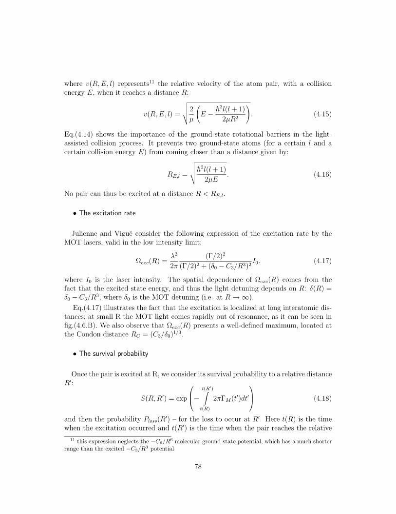
where v(R, E, l) represents11 the relative velocity of the atom pair, with a collisionenergy E, when it reaches a distance R:

v(R, E, l) =

√√√√ 2

μ

(E − h2l(l + 1)

2μR2

). (4.15)

Eq.(4.14) shows the importance of the ground-state rotational barriers in the light-assisted collision process. It prevents two ground-state atoms (for a certain l and acertain collision energy E) from coming closer than a distance given by:

RE,l =

√√√√ h2l(l + 1)

2μE. (4.16)

No pair can thus be excited at a distance R < RE,l.

• The excitation rate

Julienne and Vigué consider the following expression of the excitation rate by theMOT lasers, valid in the low intensity limit:

Ωexc(R) =λ2

2π

(Γ/2)2

(Γ/2)2 + (δ0 − C3/R3)2I0. (4.17)

where I0 is the laser intensity. The spatial dependence of Ωexc(R) comes from thefact that the excited state energy, and thus the light detuning depends on R: δ(R) =δ0 − C3/R

3, where δ0 is the MOT detuning (i.e. at R → ∞).Eq.(4.17) illustrates the fact that the excitation is localized at long interatomic dis-

tances; at small R the MOT light comes rapidly out of resonance, as it can be seen infig.(4.6.B). We also observe that Ωexc(R) presents a well-defined maximum, located atthe Condon distance RC = (C3/δ0)

1/3.

• The survival probability

Once the pair is excited at R, we consider its survival probability to a relative distanceR′:

S(R, R′) = exp

⎛⎜⎝− t(R′)∫t(R)

2πΓM(t′)dt′

⎞⎟⎠ (4.18)

and then the probability Ploss(R′) – for the loss to occur at R′. Here t(R) is the time

when the excitation occurred and t(R′) is the time when the pair reaches the relative11 this expression neglects the −C6/R6 molecular ground-state potential, which has a much shorter

range than the excited −C3/R3 potential

78

separation R′; ΓM is the decay rate of the pair.

• The loss probability

The final ingredient is the probability Ploss(R′) for a loss to occur, once the pair has

reached the relative distance R′.We note that in some cases (FS collisions and Penning ionization) the loss mecha-

nism is relatively well localized, at a distance R0, and the probability can be replacedwith the constant Ploss(R0). This is not true for RE collisions (this case is not consid-ered here).

• The one-channel loss rate

Under these conditions the loss rate Kloss for a given collision channel α is obtainedby taking the product of all these different probabilities, integrate it over R and E andsum over all the partial waves:

Kloss =lmax∑l=0

∞∫R=RE,l

∞∫E=0

Ploss(R0) × S(R, R0) × Ω(R) × dN. (4.19)

We note that in this expression the sum over l was limited to l ≤ lmax, because ofthe partial wave cutoff. The integral over R is also taken only between RE,l and ∞,because of the rotational barrier in the ground state, discussed earlier.

4.4.2 Results for Cr

I first performed the calculation for the J-V model in the case of the 0+u Cs molecular

potential, for different temperatures, and the results are shown in fig.(4.7). The cal-culation was performed using a saturation parameter s0 = I/Isat = 10 and a detuningδ = −10 MHz, which corresponds to two atomic linewidths. These results reproducethe temperature-dependance reported in [58].

Temperature dependence

In the case of Cr, using the ’model potential’ (i.e. using the rescaled C3 coefficient),we observe a different behavior. At high temperature we find the expected T−1/6

dependence, and the loss parameters connects to the corresponding Langevin limitseq.(4.10).

For Cs the loss rate starts deviating from the Langevin rate at about 100 mK andat T = 100 μK there is a 12.5 reduction factor. In Cr the decrease occurs considerably

79

Figure 4.7: Comparison of the temperature dependence of the inelastic loss parameter associated to a single losschannel: for Cs (triangles) we used the 0+

u potential, while for Cr (dots) we used a rescaled potential. We also show(squares) the case of non-polarized collisions in a Cs MOT, where the rates are significantly reduced (as losses areimportant for only one channel (0+

u ) out of 16 and happen with a probability of 0.28 [58]). The curves correspond to adetuning of 10 MHz and an intensity of 10Isat. The straight lines are the corresponding Langevin rates, for Cr and Cs.

later, at a few mK. At T = 100 μK the inelastic loss parameter is only a factor 2.5smaller than the high-temperature asymptote.

This different temperature-dependence can be attributed to the fact that the partialwave cutoff lmax, given by eq.(4.13), is different for the two atoms. Indeed, as Cr has asa smaller mass and C3 coefficient, there are about 3 times less partial waves contributingto the collision process than in the case of Cs.

Saturation effects

JV model applies in the low laser intensity limit, where the excitation probability,and thus the inelastic collision parameter depend linearly on the laser power.

In my simulations I tried to take into account saturation effects (see Appendix(B)),by considering a different expression for the excitation probability of a pair. The resultsfor this simulation, for Cr (at 100 μK and a detuning of δ = 2Γ), are shown in fig.(4.8).We observe that the inelastic collision parameter increases with the laser power, and

80

the beginning of the saturation is observed. At very high laser powers, we expect for βto approach the high-temperature asymptote βL (∼ 1.3 cm3/s). This should howeverhappen for intensities much larger than what is experimentally achievable.

Figure 4.8: Simulation results, showing the dependence of the light-assisted collision parameter on the intensity.

Finally I would like to note that there are other possible physical mechanisms, oc-curring at high laser intensities, which may increase the value of the inelastic lossparameter; it can thus come even closer to the high-temperature asymptote (or evenexceed it!!!). For example there are ’population recycling’ [48] effects, which meansthat at high laser intensities the atoms decaying from the excited molecular potentialfurther than the Condon point RC may be re-excited by the MOT lasers and continuetheir evolution to short interatomic distances. Usually this scenario is theoreticallyexplored by performing quantum Monte-Carlo simulations [49, 50].

Detuning dependence

Another comparison between Cs and Cr is shown in fig.(4.9), where I present thedependence of the loss parameter β on the MOT laser detuning. The behavior seemsagain qualitatively different, as for Cr we observe a decrease occurring quite rapidlyfor detunings larger than 2Γ.

The detuning-dependence of β, for Cr, does not reproduce exactly the experimentaldata shown in fig.(4.4.A). Although in our measurements we observe that the inelasticcollision parameter decreases with the detuning, we however do not observe any in-crease at small detunings (see fig.(4.9), for δ < 2Γ).

81

Figure 4.9: Simulation results, showing the dependence of the light-assisted collision parameter on the detuning.

This difference between simulation and experiments may come from the difficultyto have a precise treatment of the saturation effects, which are expected to be moreimportant at small detunings. Indeed, ’population recycling’ tends to increase thecollision parameters when the excitation takes place at large distances (i.e. at smalldetunings).

Conclusions

Our simple model proves qualitatively that for Cr the low-temperature collisionbehavior is expected to be different than the one described by [58] for Cs. At a tem-perature of 100 μK, the expected deviation from the high-temperature limit is reducedfor Cr by about one order of magnitude.

On the other hand, for alkalis the measured loss parameter in a MOT is much smallerthan the one-channel maximum rate, due to the fact that there is only a small number(one or two) of excited potentials which lead to trap losses. For non-polarized collisionsin a MOT, the probability of excitation to that particular channel is reduced by a factoron the order of the degeneracy of the excited molecular state, due to selection rules inthe excitation process.

In chromium we have both a high degeneracy and a high measured loss parameter.This may be explained by the existence of a large number among the excited potentialswhich have high short-range loss probabilities, and which actually contribute to thelight assisted losses in a Cr magneto-optical trap.

These considerations still need a rigorous confirmation. A major difficulty is thatcalculations for Cr2 molecular potentials are known to be extremely complicated, due

82

to the large number of electrons involved. Such molecular physics considerations arefar beyond the goal of this thesis.

Finally, our measurements also show that the loss parameters for the 53Cr are higherthan in the case of 52Cr. We measured a difference of almost one order of magnitude(for a detuning of −2Γ and with a laser intensity of 13Isat for 52Cr and 20Isat for 53Cr).This indicates that the hyperfine structure of 53Cr, even though relatively small in theexcited state (160 MHz), enhances the loss mechanism.

The very large light assisted collision parameters of Cr limits the maximum numberof atoms in our MOTs. This sets a strategy towards reaching Bose-Einstein with Cr,which will be described in the rest of the manuscript.

In perspective, optical shielding [74] – involving the use of a blue-detuned laser toprevent pairs form approaching one another – may be a way to increase the number ofatoms in Cr MOTs. Because of the lack of the suitable laser (until recently) we werenot able to test this possibility.

83

Chapter 5

Continuous loading of a finite-depthmagnetic trap with 52Cr metastableatoms

The road to Bose-Einstein condensation in magnetic traps usually consists in (atleast) three steps, separated in time: first comes the accumulation of large (up to 1010)atom numbers in magneto-optical traps, followed by a second step, which is the transferin a magnetic trap. The third step consists in applying RF-evaporative cooling tech-niques, i.e. continuously removing the hottest atoms, and reducing thus the mean energyper trapped atom. In presence of ’enough’ elastic collisions, the energy of the remain-ing atoms is redistributed, and one tends towards a new (quasi-)equilibrium situation,where the temperature is reduced.

In the case of Cr, the first two steps can be favorably performed together [81, 43].In the previous chapters I presented a study of the light-assisted collisions in Cr MOTs.The large values of the corresponding inelastic loss parameters β show that, in presenceof the quasi-resonant cooling light, the atom numbers in MOTs are severely reduced,compared to the alkali atoms. On the other hand, the electronic structure and the highmagnetic moment of chromium provide an interesting way of loading large ’reservoirs’– represented by the metastable 5D states – which are shielded from the MOT light.This increases by more than one order of magnitude the number of atoms available inthe MOT.

This chapter is dedicated to the study of the magnetically trapped metastable 52Cratoms. After presenting some measurements of the collisional (elastic and inelastic)properties of the metastable states, I will present a new trapping scheme, which com-bines together all three steps: continuous loading and evaporation in a RF-truncatedmagnetic trap. This scheme allowed in our case to obtain, in less than 1 s, phase-spacedensities up to 7× 10−6. I will also present a simple theoretical model which describesthe physics of continuous loading and evaporation, and provides a better understanding

85

of the limiting factors. In the final part of the chapter I will discuss some prelimi-nary results in the attempt of reducing the limiting factors, by accumulating atoms ina large-volume, RF-dressed magnetic trap.

5.1 Magnetic trapping

In this section I present some issues related to magnetic trapping inside a quadrupoletrap and to the measuring procedures which we use for analyzing absorption images,in order to estimate the number of atoms and the density of the cloud.

Magnetic trapping potential

The classical interaction potential between an atom, having a magnetic dipole mo-ment −→μ , and an external magnetic field −→

B reads: V (−→r ) = −−→μ ·−→B (−→r ). If the magneticfield is ’strong enough’, the direction of −→μ adiabatically follows that of the magneticfield and the potential simply becomes: V (−→r ) = −|−→μ ||−→B (−→r )|.

In the quantum picture, the projection of the magnetic moment on a given axis (inour case the axis defined by the local direction of −→B ) is quantized, and the magnetictrapping potential reads:

V (x, y, z) = mJgJμB|−→B (x, y, z)| (5.1)

where mJ is the magnetic quantum number (going from −J to +J), gJ is the Landéfactor, and μB is the Bohr magneton. This expression can be used for any magneticfield profile; in our case, the atoms are trapped in the quadrupole magnetic field createdby the MOT coils, given by:

−→B (x, y, z) = b′(xx + yy − 2zz) (5.2)

where b′ is the field gradient along the x and y axis and half the one along z (because ofGauss theorem and for symmetry reasons). The expression of the magnetic potentialbecomes thus:

VMT (x, y, z) = mJgJμBb′√

x2 + y2 + 4z2. (5.3)

Typically, we have b′ = 9 G/cm.

Depending on the sign of mJ , the atoms can have three different behaviors. IfmJ > 0 (low field seeker state) the atoms are trapped, as they are attracted towardsthe |−→B | minima (|−→B | = 0 in our case); on the contrary, atoms with mJ < 0 (high fieldseekers) are expelled from |−→B | minima, while mJ = 0 atoms do not interact with thefield and eventually fall under gravity.

86

The experiments described in the present chapter will only concern the 52Cr atoms,magnetically trapped in the 5D4 state. For this state the Landé factor is gJ = 3/2, andmJ can take integer values between from -4 to +4. We mention that for the 52Cr 5D3

state (not studied here) mJ is between -3 to +3 and gJ = 3/2. An expression similarto eq.(5.3) can be also applied for 53Cr magnetic potential, by replacing mJ and gJ bymF and gF .

Density profile at thermal equilibrium

In our experiment we deal with magnetically-trapped atom clouds that are notspin-polarized in a single mJ state. The reason is that they are initially accumulatedinto the metastable 5D states through spontaneous emission from magneto-opticallytrapped excited atoms, whose mJ−distribution is random. Furthermore, polarizationby optical pumping means inside our magnetic trap is not possible (not even afterrepumping in the 7S3 state), because the quantization axis given by the local directionof the quadrupole magnetic field varies in space throughout the atomic sample.

Eq.(5.3) shows that atoms in different mJ−states feel different trapping potentials.The density profile of the entire cloud is thus a sum over all mJ > 0 density distributions(3 for 7S3 and 5D3, 4 for 5D4), each of them being given, at thermal equilibrium, bythe Boltzmann distribution:

n(x, y, z) =∑

mJ>0

n0,mJexp

(−mJgJμBb′

√x2 + y2 + 4z2

kBT

), (5.4)

where n0,mJis the peak density for each mJ−component and T is the temperature.

In principle, eq.(5.4) could be used for determining the temperature of the trappedcloud, provided that one has a precise knowledge of the relative populations of differ-ent mJ states, using for example a Stern-Gerlach-like experiment. This is however notpossible, in our current experiment, because we cannot produce high-enough magneticfield gradients in order to spatially separate the different mJ components, for the typ-ical temperatures (∼ 100 μK) of our trapped clouds.

Since the atom cloud is not polarized, the exact analysis of the absorption imagesis complicated. We find it useful, for sake of simplicity, to assume that all atomsexperience an average magnetic potential given by:

V (x, y, z) = V0

√x2 + y2 + 4z2 (5.5)

where V0 = mJgJμBb′ and mJ is an ’average’ magnetic quantum number. The densityprofile at thermal equilibrium is then approximately given by the simplified expression:

nMT (x, y, z) = n0 exp

(− V0

kBT

√x2 + y2 + 4z2

). (5.6)

87

Using this expression we can define the 1/e size a of the atomic cloud in the x and ydirections:

a =kBT

V0

. (5.7)

Integrating eq.(5.6), we can relate the peak atomic density n0 and a to the total numberof atoms in the MT: NMT = 4πn0a

3. We also define the volume of the magnetic trapby: VMT ≡ NMT /n0 = 4πa3

Analysis of the absorption images

The absorption imaging technique has been used for the experiments presented in theremaining part of this manuscript. Like the fluorescence imaging technique, it providesinformation on the properties of an atomic sample (number of atoms, density and cloudsize). The main advantage of absorption imaging is that it does not require a precisemeasurement of the laser beam power, which is a main error source in fluorescenceimaging.

The absorption of the laser imaging beam passing through the atomic sample canbe expressed, in the low-saturation limit, using the Beer-Lambert law:

dI(x, y, z)

I(x, y, z)= −o.d.(x, y, z)dy. (5.8)

where o.d.(x, y, z) is the optical density of the cloud and I(x, y, z) is the intensity profileof the laser which propagates along the y (CCD camera) axis.

The optical depth O.D.(x, z) of the cloud, measured in the plane of the camera –see fig.(5.1), can be obtained by integration of eq.(5.8) along the y axis:

O.D.(x, z) ≡ − ln

[I∞(x, z)

I−∞(x, z)

]= +

+∞∫−∞

o.d.(x, y, z)dy. (5.9)

where I−∞(x, z) ≡ I(x, y = −∞, z) and I∞(x, z) ≡ I(x, y = +∞, z) are the beamintensity profiles before and after passing through the atomic cloud.

The optical density can be related to the atomic density via the absorption crosssection σabs: o.d.(x, y, z) = σabs · n(x, y, z). Replacing this expression in (5.9) gives:

O.D.(x, z) = σabs

+∞∫−∞

n(x, y, z)dy (5.10)

Eq.(5.10) relates thus the optical depth of the cloud to the ’column density’ of the

atomic cloud, defined as: n(x, z) ≡+∞∫−∞

n(x, y, z)dy.

88

Analysis of the in-situ magnetic trap profile

The number of atoms in the cloud can be found by integration of eq.(5.10):

N =1

σabs

+∞∫−∞

O.D.(x, z) dxdz (5.11)

Since the atomic sample is not spin-polarized and the magnetic field is inhomogeneous,we assume (as we also did in the case of the fluorescence imaging of the MOT) anaverage Clebsch-Gordan coefficient of 3/7. This yields a mean value for the resonant

photon absorption cross section σabs =3

7σ0, where σ0 =

3λ2

2πis the resonant photon

scattering cross section in the low-intensity regime (our imaging beam has a peak in-tensity of ∼ 0.2 mW/cm2, well below Isat = 8.5 mW/cm2).

Figure 5.1: In-situ absorption image of a magnetically trapped cloud of 52Cr. To the right: two slices of the image,passing through the center of the cloud, in the horizontal (above) and vertical (below) plane. The fit of the horizontalcut is done using the function nMT (x, 0) given by eq.(5.12). For the vertical slice, the fitting function nMT (0, z) wasmodified for taking into account the slight dissymmetry due to the gravity (not mentioned in the text). In principle, thisdissymmetry could provide an independent measure of mJ [31], but in our case this is not possible, as the vertical z axisis the strong-confining axis of the trap and the dissymmetry is too small, yielding large systematic fitting uncertainties.

The column density profile of a magnetically trapped cloud is obtained by integrationof eq.(5.6) along the imaging direction y:

nMT (x, z) = 2n0

√x2 + 4z2 BesselK

(1,

√x2 + 4z2

a

), (5.12)

where BesselK is the modified Bessel function of the second kind. Fig.(5.1) shows thatthis expression provides a good approximation for the observed shape of the atomiccloud.

89

Fitting a cut of the absorption image which passes through the center of the cloudprovides the 1/e radius a and the peak optical depth O.D.max, from which we cancalculate the value of the peak density n0. The peak atom density is then simply given

by: n0 =O.D.max

2a σabs

.

Absorption imaging can be used for the atoms in the ground state, via the 7S3 →7P4

strong transition. This technique is not applicable directly to the metastable 5Dtrapped cloud; it is nevertheless possible to ’map’ its density distribution onto the7S3 state, by repumping the atoms with the ’red’ diodes and immediately absorption-imaging them. The information about the shape of the cloud is correct, provided thatthe repumping time is short enough compared to the typical oscillation period in theMT.

In the case of an anharmonic trap, the oscillation period depends on the energy; wecan however define a typical (mean) oscillation period 〈Tosc〉, by taking the thermalaverage of the oscillation frequencies of all atoms:

〈Tosc〉 =4mvth

mJgJμBb′(5.13)

where vth is the mean thermal velocity. For mJ = 4 and a MT temperature T = 100 μK,we see that the typical oscillation period is ∼ 12 ms.

We found that pulsing the repumping light for 1 ms is sufficient to repump mostof the metastable atoms in the ground state, for a ’red’ repumper intensity of about15 mW/cm2. Since this time is about 1/10 of the typical oscillation period of theatoms at the MT temperature (100 μK), we can rely on our method of ’mapping’ themetastable atoms density distribution.

Temperature and mean magnetic moment

In addition to the density measurements, we perform direct temperature measure-ments by analyzing the free-fall expansion of the atoms after suddenly switching offthe magnetic trap. As we mentioned in Chapter(2), the eddy currents generate a non-negligible residual magnetic field at the atom location, which dies away in about 20 ms.We estimate however that this field does not affect the ballistic expansion of the atomsand consequently does not alter the results of the temperature measurements. Indeed,we checked that the center of mass of the cloud falls vertically, and is acceleratedonly by gravity. The residual field introduces however some additional Zeeman shiftand broadening of the imaging-laser resonance, but does not influence the temperaturedetermination.

On the other hand the MOT coils current, and thus the trapping magnetic fieldgradient, are switched off in 500 μs (1/e time), and we therefore include in our analysis

90

only the time of flights longer than 500 μs.

Finally, the value of the mean magnetic quantum number mJ can be deduced usingthe temperature and the measured in-situ 1/e radius of the cloud a:

mJ =kBT

agJμBb′. (5.14)

5.2 Collisional properties of metastable 52Cr atoms

After introducing, in the previous section, some general aspects of magnetic trapsand the related measuring procedures, we will now turn to an investigation of someof the properties of metastable 52Cr. In this section, we will measure the elastic andinelastic collision parameters, which are very important for all experiments presentedin the rest of this dissertation, because our strategy towards condensation consists infirst accumulating atoms in these states.

5.2.1 Inelastic D-D collisions

To investigate the inelastic collisions between metastable Cr atoms, we performeda lifetime measurement of the magnetic trap in the 5D4 state. For this experiment,the atoms are first accumulated for 5 s in the magnetic trap. The MOT beams arethen switched off and, after an adjustable delay t, the atoms are repumped into theground state. The number of atoms is measured and plotted as a function of t, as it isshown in fig.(5.2) in a semi-log scale. We observe a clear non-exponential initial decay,which indicates the influence of the two-body inelastic collisions on the lifetime of thetrapped cloud.

We fitted the data, assuming that the decay is characterized by the following equa-tion:

dN

dt= −Γ0N − βDD

Vcoll(t)N2, (5.15)

where, in addition to a one-body loss rate Γ0, we consider a temperature-independenttwo-body loss parameter βDD. This equation and the corresponding fitting procedureare very similar to the ones used for the light-assisted collisions (see eq.(4.5-4.6) inChapter(4)). From the MT density distribution (5.6) we calculate1 the collisionalvolume Vcoll = 32πa3 = 8VMT . During the decay, the cloud volume VMT increasesapproximately linearly, and we include this dependence in the equation describing thedecay.

1 The collisional volume is defined, in a similar way as for the light-assisted collisions (see Sec-

tion(4.1)), by: Vcoll =(∫

nMT (−→r )d3r)2∫

(nMT (−→r ))2d3r

91

Figure 5.2: Decay of the magnetically-trapped metastable atoms. Solid line: result of the fit (see text) which givesthe inelastic collision parameter βDD. The dotted line is a result of a purely exponential fit for t>5 s, providing thelifetime due to background gas collisions (mostly with hot atoms from the Cr beam). The dashed line is a result of anexponential fit for t<1 s.

We find the inelastic loss parameter to be βDD = (3.3± 0.5± 0.5)× 10−11 cm3/s (inreasonable agreement with [43]). The respective error bars are the statistic error bar ofthe fit, and the systematic error bar, mostly coming from the uncertainty on the totalnumber of atoms.

We note that this inelastic loss parameter is much larger than the expected dipolarrelaxation inelastic parameter βd.r. 3×10−12, for low magnetic fields (see [76]), whichrules out dipolar relaxation as the main inelastic loss channel. In our quadrupole mag-netic trap there are however other collisional mechanisms which may explain the highvalue of βDD: for example spin-exchange collisions, which were observed to have largerβ−parameters [76].

From the same fit we also deduce the one-body decay time constant T0 = 1/Γ0 = 9s. We repeated the same experiment without the Cr beam (by blocking it immediatelyafter the accumulation, together with the MOT beams) and found a longer one-bodyloss time constant, of 30 s, which we interpret as being fixed by the collisions with thevacuum background gas. We interpret this difference as the influence of the collisionswith the hot Cr atoms of the beam.

We additionally analyzed the temperature evolution during the decay. We observea strong heating at short times, which is shown in fig.(5.3) (squares). We interpret thisheating as the effect of inelastic collisions, which mostly expel the low-energy atoms(as explained later, in Section(5.4)).

92

5.2.2 Elastic collision cross-section of the 5D4 state

Evaporative cooling is based on preferential removal of atoms with an energy higherthan the average. Knowing the elastic collision properties is important, because theyare responsible for the energy redistribution among the remaining atoms and for reach-ing a new quasi-thermal equilibrium, at a lower temperature. In this section I presentexperiments which led to a measurement of the elastic cross-section of atoms in themetastable 5D4 state. This is, to our knowledge, the first measurement of an elasticcross section for a transition element in a metastable state.

In order to study the evaporation in the magnetic trap, we use a RF magneticfield, which truncates the MT trap to a finite depth. The RF magnetic field, with afrequency ω, induces spin-flip transitions of the atoms to non-trapped (mJ < 0) states,which are expelled from the trap. These transitions take place at the position of theRF resonance, where the energy difference between two adjacent mJ states is equal tothe energy of a RF photon: gJμBB(−→r ) = hω. In the case of our quadrupole magneticfield, this resonance condition is fulfilled on a ’iso-B’ ellipsoid, defined by the equation:

x2 + y2 + 4z2 =

(hω

gJμBb′

)2

. (5.16)

We assume that all the atoms that reach this surface are efficiently removed from thetrap.

RF ’shock-cooling’

We repeated the lifetime experiments presented in the previous subsection, by sud-denly applying a ω = 2π × 3 MHz RF field (’shock cooling’ [75]), at t = 0, just afterthe 5 s accumulation time in the 5D4 state. We observe that the decay of the cloudis modified by evaporation, which changes both the total loss rate, and the evolutionof the temperature, as shown in fig.(5.3) (triangles). We will use these observations toestimate the evaporation rate and infer the elastic collision rate.

For that, one must first evaluate the modification of the lifetime of the cloud linkedto spilling of atoms out of the trapping volume set by the RF frequency: the experi-mentally observed heating ’produces’ atoms whose energy is larger than the trap depth.They then leave the trap, without undergoing any elastic collision, assuming that themean free path of the atoms is larger than the size of the sample. Heating withoutRF translates into spilling when RF is applied, and the rate at which spilling occurs istherefore linked to the heating rate without RF. We measure the time evolution of the1/e radius of the cloud a, without RF, to estimate Γspill ≈ 0.1 s−1. Γspill corresponds

93

Figure 5.3: Time-dependence of the temperature of the atoms magnetically-trapped in the 5D4 state. In absenceof the RF (squares) we observe a strong heating of the cloud at short times, which we interpret as an effect of inelasticcollisions. In presence of a 3 MHz RF field (triangles), evaporation and ’spilling’ of hot atoms compensate for theheating (see Section(5.2.2)). The full lines are guides for the eyes.

to the rate of atoms leaving the trapping volume set by the RF frequency, i.e. the rateof atoms spilled out of the trap volume.

From the atom number decay at short times, we deduce the experimental valuesof the atom loss rates without RF (see fig.(5.2)), Γloss = 1/Tloss = 1/2.4 s−1, andwith RF, Γloss,RF = 1/1.35 s−1. We can therefore estimate the value of Γev + Γspill =Γloss,RF − Γloss = 0.32 s−1. We therefore obtain an estimate for the evaporation ratefrom the modification in the lifetime of the cloud in presence of the RF: Γev ≈ 0.22 s−1.In general, Γev is temperature dependent, but, in presence of RF, we performed thismeasurement in a situation where the temperature is almost constant (see fig.(5.3)).

The determination of the evaporation rate Γev allows us to infer the value of the elas-tic collision rate. For a given RF frequency, Γev can be directly related to the elastic col-lision rate, defined as Γel = n0σelv, where σel is the elastic cross section and v =

√8kBTπm

is the mean thermal velocity. Using eq.(5.36) – which will be explained in the theoreticalmodel presented in Section(5.4) – we find Γel = (20± 4± 11) s−1. The experimentallymeasured temperature, at t=0, is 100 μK, and the peak density is 1011 cm−3. Wetherefore infer an average elastic cross section of σel = (7.0 ± 1.4 ± 3.5) × 10−16 m2.

94

5.3 Continuous accumulation in a RF-truncated mag-netic trap

After determining the collisional properties of 52Cr atoms in the 5D4 state, I willpresent now the main result of this chapter, which is the study of the continuous load-ing of metastable Cr atoms in a RF-truncated quadrupole magnetic trap.

From the experimental point of view, the accumulation procedure, presented infig.(5.4), is the same as in the absence of the RF: atoms are continuously loaded inthe MT from the MOT, using the ’leaks’ due to spontaneous decay of the atoms inthe 7P4 state towards the 5D4 state. Interesting features arise from the presence of theRF field: not only the loading, but also the evaporation are continuous, and they bothtake place simultaneously. In the next paragraphs I will analyze the dependance of thecharacteristics of the could on the value of the RF frequency.

Figure 5.4: Right: scheme of accumulation of 5D4 metastable 52Cr atoms in RF-truncated quadrupole magnetictrap formed by the MOT gradient. Left: zoom of the truncated magnetic potentials, for different mJ Zeeman substates.

Atom number and density measurements

We analyzed the in-situ absorption images of the cloud, after a 5 s accumulationtime in the metastable states, for different values of the frequency of the RF field.

An interesting feature of the experimental data is the RF frequency dependenceof the cloud peak density in the steady state, also shown in fig.(5.5): although theatom number decreases dramatically when lowering ν, we observe that the peak den-sity remains almost at the constant value of ∼ 0.8 × 1011 atoms/cm3 for a large rangeof RF frequencies; it only starts decreasing when ν is set to values smaller than 1.5 MHz.

Additionally, we measure the number of atoms accumulated in the truncated MT, asa function of time τ , for different RF frequencies ν. At any frequency, we observe thatthe loading of the trap can be well fitted by an exponential, and we plot in fig.(5.6) the

95

Figure 5.5: Metastable atom number (left) and peak atom density (right), after 5 s of accumulation in the MT,as a function of the RF frequency. The error bars correspond to the uncertainty in determining the total number ofatoms by absorption imaging. The solid lines represent the results of the rate-equation theoretical model, presented inSection(5.4).

corresponding 1/e accumulation time, Tload, as a function of the RF frequency. Theaccumulation time increases approximately linearly from 0.3 s for ν = 1 MHz to 1.4 sfor ν ≥ 6 MHz. For higher frequencies the accumulation time saturates to an almostconstant value, which is equal to the accumulation time without RF. This proves that,after 5 s of accumulation the steady-state atom number in fig.(5.5) was indeed fullyreached.

Figure 5.6: Accumulation time Tload in the truncated MT, as a function of the RF frequency. The error bar is thetypical statistical error in an exponential fit of the number of accumulated atoms as a function of τ .

Temperature measurements

The ballistic expansion of the cloud is used for measuring the temperature of thecloud, for different values of the RF frequency. The results are shown in fig.(5.7.A)

96

The cloud analysis is made by gaussian fits, which is a good approximation in the limitwhere the cloud size after expansion becomes large compared to the initial size. Somesystematic errors are nevertheless expected at short times, because of the non-gaussianinitial shape of the cloud (see fig.(5.1)). We checked that the systematic error bar ofthis procedure is less than 10%, when fitting the vertical direction, along which theinitial extension of the cloud is the smallest.

Figure 5.7: A) Temperature of the atoms after 5 s of accumulation, as a function of the RF frequency. The errorbar corresponds to the estimated 10% systematic error in temperature determination. Dotted line: results, using therate-equation theoretical model (see Section(5.4)). B) Mean magnetic quantum number mJ as a function of the RFfrequency.

Using this temperature and the measured 1/e in-situ radius of the cloud a, we candeduce the mean magnetic quantum number mJ , using eq.(5.14). The results areshown in fig.(5.7.B), and we interestingly observe that mJ does not change much withthe RF frequency, staying close to 2. This indicates that the presence of the RF doesnot change much the mJ−distribution of the cloud, which may seem surprising, as thetrap depth depends on the value of mJ , as illustrated in fig.(5.4) (the atoms with lowermJ may evaporate faster than those with higher mJ).

Phase space density

From the previous measurements of the peak atom density and temperature we caninfer the values of the peak phase space density Dph.:

Dph. = n0Λ3dB = n0

(h2

2πmkBT

)3/2

. (5.17)

In fig.(5.8) we show the steady-state phase space density (i.e. after τ = 5 s ofaccumulation) in the magnetic trap as a function of the RF frequency. Because the

97

Figure 5.8: Phase-space density as a function of the RF frequency. The solid line represents the result of thetheoretical rate-equation model, presented in the Section(5.4).

measured temperature of the atoms decreases with decreasing RF frequency (as shownin the same figure), and because the measured peak atom density remains almostconstant (fig.(5.5)), we observe that the phase space density increases at lower RFfrequencies, to reach a maximum value of (7±1.5)×10−6 at ν=1.5 MHz. The error bar isdue to the systematic errors on the density and on the temperature measurements. Wenotice that this maximum phase-space density value is significantly higher than typicalphase-space densities achieved in a standard MOT, involving a strong resonance line.

At frequencies smaller than 1.5 MHz, the trend inverts: when lowering the RFfrequency, the density of the atoms decreases (see fig.(5.5)), which yields a decreaseof the phase-space density. For such low frequencies, the depth of the magnetic trapbecomes lower than the MOT temperature, and most of the atoms arriving in the 5D4

state are immediately spilled out of the trap.

5.4 Theoretical model

In this section I present a theoretical model which is used to interpret our experimen-tal results, concerning the accumulation of the atoms in the RF-truncated magnetictrap. The model is based on refs. [77] and [78] and consists of two rate equations, for

98

the total number of atoms N and the total energy E of the system:

dN

dt= Γ −

(∑i

Γi

)N (5.18)

dE

dt= ΓE ′ −

(∑i

fiΓi

)NkBT. (5.19)

Eq.(5.18) includes a loading term Γ and a loss rate, having several contributions, eachdescribing a different loss process (labeled i) with a rate Γi. The fi coefficients in (5.19)account for the average energy lost per particle, in units of kBT, for each of the lossmechanism considered and E ′ is the mean energy per loaded atom.

In the following pages I will first detail the model in the case of continuous accu-mulation of Cr metastable atoms in a finite-depth quadrupole magnetic trap, and thenI will present some numerical results, which are compared to the previously-presentedexperimental observations.

I also point out that the model described by the rate equations (5.18)-(5.19) canhave a fairly large degree of generality, as one may include, besides different loadingterms, many various physical loss mechanisms, such as one-, two- and three-body losses,Majorana losses, evaporation, etc. It can also, in principle, be applied to any arbitrarytrapping potentials U(−→r ).

Trap depth

A complete description of the accumulation process, taking into account all fourlow-field-seeking magnetic sublevels of the 5D4 state is quite complicated and hardto interpret in our experimental case (as the exact mJ−distribution is unknown). Inorder to describe the accumulation in the metastable finite-depth magnetic traps, wewill again consider the simplified model of a cloud with an average (measured) magneticquantum number mJ .

In the case of our quadrupole magnetic trap, the RF resonances shown in fig.(5.4)lead to mJ−dependent trap depths; we will nevertheless define an average depth, cor-responding to mJ :

U0 = mJhνRF

, (5.20)

and the situation we consider is schematically shown in fig.(5.9). As usually done inevaporative cooling description, we also define the dimensionless evaporation parameterη, which is the ratio between the trap depth to the temperature: η ≡ U0/kBT . It isinteresting to notice that the measurement of the 1/e radius of the cloud a allows oneto have an experimental estimate of η. Indeed, using (5.7) and (5.20), we find:

η =hν

RF

gJμBb′a(5.21)

99

Figure 5.9: The simplified situation we consider for describing the continuous accumulation of metastable atomsin a finite depth quadrupole magnetic trap: we characterize the cloud by its mean magnetic quantum number mJ , andthe trapping potential is given by eq.(5.3). The trap is truncated at RRF (position of the RF resonance) and has adepth U0 = mJhνRF .

which does not depend on mJ .

5.4.1 Theoretical model for Cr

I will now detail the model in the case which was presented in the previous section.Throughout this section I will assume that the phase-space distribution of metastableatoms in the magnetic trap is that of an ideal classical gas at thermal equilibrium.This is equivalent to saying that: a) the elastic collisions are sufficiently fast to define atemperature T , b) the ratio η of the total trap depth U0 to the temperature is sufficientlylarge that we can ignore the truncations of the Boltzmann distribution [79] and c) theatoms are non-interacting, so the single particle statistics are sufficient to calculatethermal averages of the relevant parameters. The validity of these assumptions will beinvestigated in detail in the next sections.

The RF frequency-dependence that we want to interpret will be taken into accountby two terms in eq(5.18). One is the evaporation term, which depends on the trapdepth, fixed by the RF frequency. The other ones are the loading rate Γ and theaverage energy per atom loaded in the MT, E ′, and we will show that both depend onthe RF frequency.

The loss terms relevant to our problem (which we include in the model) are thecollisions with the background gas, the collisions between the metastable and the MOTatoms, and the two-body losses. Other loss mechanisms, such as Majorana spin-flipsand three-body recombination are negligible under the conditions (temperature anddensity) of our experiments.

100

Average energy per magnetically-trapped atom

In the case of a linear magnetic trap, the magnetic potential energy of a trappedatom, VMT (x, y, z), is given by eq.(5.3). At thermal equilibrium in the trap, the localmean energy of atoms in the MT is 〈EMT 〉(−→r ) = 3

2kBT + VMT (−→r ); this expression

assumes that the average kinetic energy per trapped atom is 32kBT , whatever the

position of the atoms (which implies no correlation between position and velocity).The average total energy per trapped atom is then:

〈EMT 〉 =

∫nMT (x, y, z)

(32kBT + VMT (x, y, z)

)d3r∫

nMT (x, y, z)d3r=

9

2kBT. (5.22)

The integral was evaluated using (5.5) and (5.6) for the MT potential VMT (x, y, z) anddensity distribution nMT (x, y, z).

An important remark can now be made, concerning the fi coefficients defined in theenergy rate equation (5.19). A given loss mechanism i leads to the heating of the cloudif the mean energy per lost particle is smaller than the mean trap energy; in our case,according to eq.(5.22), this condition reads: fi < 9/2. If, on the contrary, fi > 9/2, themean energy per lost particle is larger than the mean trap energy, and the mechanismleads to the cooling of the cloud2.

The loading terms

As mentioned in the previous chapter, the loading of the MT is due to the radiativeleaks of the excited MOT atoms into the metastable 5D4 state. We experimentallychecked that the MOT atom number is not modified by the presence of the RF field(which indicates that the optical pumping rate due to the MOT lasers is much fasterthan spin-redistributions induced by the RF field). As a consequence we can assumein our model that the total production rate of atoms in the metastable states, Γ, doesnot depend on the RF frequency ν, and that the phase-space distribution of atomsarriving in the MT is identical to the MOT phase-space distribution:

nph,MOT (−→p ,−→r ) = n0,MOT1

2(π3/2)exp

(− p2/2m

kBTMOT

− x2 + y2 + 4z2

2w2MOT

). (5.23)

Here, TMOT , n0,MOT and wMOT are respectively the ’temperature’, peak density and’size’ (e−1/2 radius) of the MOT. The spatial dependence of nph,MOT , with an aspectratio of 2 between the vertical and horizontal directions, mostly reproduces the exper-imental one and allows great mathematical simplifications3.

2 This kind of arguments can be extended to any trapping potential, by recalculating the meanenergy per trapped atom (in the case of an harmonic potential, for example, the 9/2 factor should bereplaced by 3).

3 We checked that the exact aspect ratio of the MOT, which typically ranges between 1.5 and2 (depending on the day-to-day alignment of the MOT beams), does not modify much the physicalparameters that we deduce from this theoretical model.

101

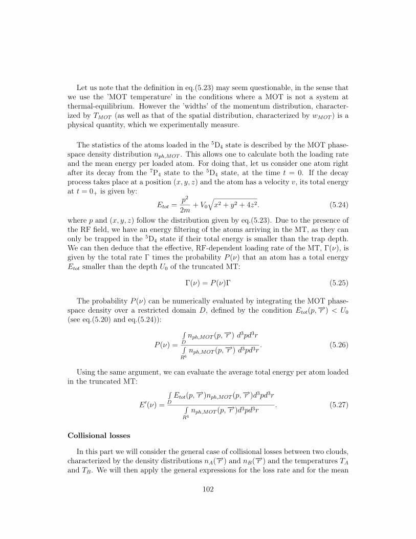
Let us note that the definition in eq.(5.23) may seem questionable, in the sense thatwe use the ’MOT temperature’ in the conditions where a MOT is not a system atthermal-equilibrium. However the ’widths’ of the momentum distribution, character-ized by TMOT (as well as that of the spatial distribution, characterized by wMOT ) is aphysical quantity, which we experimentally measure.

The statistics of the atoms loaded in the 5D4 state is described by the MOT phase-space density distribution nph,MOT . This allows one to calculate both the loading rateand the mean energy per loaded atom. For doing that, let us consider one atom rightafter its decay from the 7P4 state to the 5D4 state, at the time t = 0. If the decayprocess takes place at a position (x, y, z) and the atom has a velocity v, its total energyat t = 0+ is given by:

Etot =p2

2m+ V0

√x2 + y2 + 4z2. (5.24)

where p and (x, y, z) follow the distribution given by eq.(5.23). Due to the presence ofthe RF field, we have an energy filtering of the atoms arriving in the MT, as they canonly be trapped in the 5D4 state if their total energy is smaller than the trap depth.We can then deduce that the effective, RF-dependent loading rate of the MT, Γ(ν), isgiven by the total rate Γ times the probability P (ν) that an atom has a total energyEtot smaller than the depth U0 of the truncated MT:

Γ(ν) = P (ν)Γ (5.25)

The probability P (ν) can be numerically evaluated by integrating the MOT phase-space density over a restricted domain D, defined by the condition Etot(p,−→r ) < U0

(see eq.(5.20) and eq.(5.24)):

P (ν) =

∫D

nph,MOT (p,−→r ) d3pd3r∫R6

nph,MOT (p,−→r ) d3pd3r. (5.26)

Using the same argument, we can evaluate the average total energy per atom loadedin the truncated MT:

E ′(ν) =

∫D

Etot(p,−→r )nph,MOT (p,−→r )d3pd3r∫R4

nph,MOT (p,−→r )d3pd3r. (5.27)

Collisional losses

In this part we will consider the general case of collisional losses between two clouds,characterized by the density distributions nA(−→r ) and nB(−→r ) and the temperatures TA

and TB. We will then apply the general expressions for the loss rate and for the mean

102

energy per lost particle to our magnetically trapped cloud, in the case of collisionswith the background, of collisions with the MOT atoms, and in the case of collisionsbetween metastable atoms.

The main assumption we make4 for describing the mechanism of collisional lossesis that the corresponding rates depend only on the local product of the two densities,with a constant coefficient of proportionality β, independent of −→r . The loss rate ofcloud A then reads:

ΓA =β

NA

∫nA(−→r )nB(−→r )d3r (5.28)

and the average energy per lost particle is:

fAkBTA =β

NAΓA

∫EA(−→r )nA(−→r )nB(−→r )d3r (5.29)

where EA(−→r ) is the total (kinetic plus potential) energy of a particle of the cloud Aat the position −→r . Using the two previous equations, and assuming that the meanaverage kinetic energy per lost particle is 3kBTA/2, independent of the position −→r , weobtain the following expression for the fA coefficient:

fA =3

2+

1

kBTA

∫EP,A(−→r )nA(−→r )nB(−→r )d3r∫

nA(−→r )nB(−→r )d3r(5.30)

where EP,A(−→r ) is the trapping potential of the cloud A.

In the following paragraphs I will apply eq.(5.28) and (5.30) to the magneticallytrapped atoms (cloud A) – using the expressions (5.6) and (5.5) for the density nA(−→r )and trapping potential EP,A(−→r ) – in three cases:

• background gas collisionsThe one body loss rate due to collisions with the background gas can be modeledconsidering a uniform density distribution for the cloud B. This yields a constantvalue for the rate coefficient Γ0, independent of the trap properties, such asnumber of atoms N and temperature T . This also implies that the averageenergy per lost atom will be equal to the average energy of atoms in the MT(i.e. f0 = 9/2), and the background gas collisions will not lead to a change intemperature of the trapped cloud.

• collisions with the MOT atomsThe loss rate corresponding to inelastic collisions with the MOT atoms is as-sumed to be proportional to the product of the MOT and MT local density,with a proportionality coefficient βPD (inelastic loss parameter). This loss rate

4 The same assumption was also made in the case of light-assisted collision in a MOT – seeChapter(4)

103

can be calculated from (5.28), considering that the density distribution nB(−→r )corresponds to the MOT density:

nMOT (−→r ) =∫

nph,MOT (−→r , u)√

udu = n0,MOT exp

(−x2 + y2 + 4z2

2w2MOT

). (5.31)

Using eq.(5.28) we find then:

Γ1 = n0,MOT βPDF1

(wMOT

a

)(5.32)

where F1(x) ≡ x5

2

[− 1

x+√

π2

(1 + 1

x2

) (1 − Erf

(x√2

))exp(

x2

2

)]and Erf(x) is the

error function. The F1(x) function is plotted in fig.(5.10.A). We see that F1(x) in-creases with x = wMOT

a, which can be intuitively understood considering that the

overlap between the MT and the MOT increases when the MT size a decreases.

Figure 5.10: F1 and f1 as a function of the x parameter (ratio between MOT and MT sizes).

The corresponding f1 factor is obtained from eq.(5.30):

f1 =3

2+

F2

(wMOT

a

)F1

(wMOT

a

) , (5.33)

where F2(x) ≡ x7

4

[4x3 + 2

x−√

2π(1 + 3

x2

) (1 − Erf

(x√2

))exp(

x2

2

)].

Fig.(5.10) shows the dependence of the f1 factor on the ratio wMOT /a. We observethat collisions with the MOT atoms always result in the heating of the MT, asf1 < 9/2; the heating becomes smaller when we decrease the RF frequency (as adecreases too, and the ratio x increases).

• collisions between metastable atomsThe loss rate due to collisions between metastable atoms can be calculated makingnA(−→r ) = nB(−→r ) = nMT (−→r ) in eq.(5.28), which gives:

Γ2 = βDDn0

8. (5.34)

104

where βDD is the inelastic collision parameter between two metastable atoms.For the corresponding mean-energy loss factor f2 we find:

f2 = 3. (5.35)

This means that this process also leads to heating. This result (general, in fact,for any kind of trap) can be explained by the fact that the two-body inelasticlosses are mostly localized close to the bottom of the trap, where the density isthe highest and the potential energy of atoms is the smallest.

Evaporation

Due to the finite depth of the trap, all atoms having a total energy higher thanthe trap depth rapidly escape from the trap (in a time on the order of the averageoscillation frequency of the trap – ∼ 10 ms).

The evaporation process is triggered by an elastic collision between two atoms, whichmay promote one of them to an energy larger than the trap depth. The more energeticatom can then escape from the trap, leaving the other one with a lower energy thanbefore the collision. The evaporation rate is given by:

Γev =

√2

8Γel × f(η) (5.36)

where Γel = n0 σel v is the elastic collision rate, with σel the elastic cross sectionand v =

√8kBTπm

the mean thermal velocity. The parameter f(η), called the averageevaporation fraction is given by (see [77]):

f(η) =2√

2 [e−η(2η − 6) + e−2η(η2 + 4η + 6)]

1 − (2η2 + 2η + 1)e−2η(5.37)

which is valid for η ≥ 4, for which the density distribution in the trap is close to the onein an infinite-depth trap. The same reference [77] gives an expression for the averageenergy per evaporated atom:

fevkBT =

(61/3 +

η′2 + 2η′ + 2

η′ + 1

)kBT (5.38)

where η′ ≡ 1.035(η − 61/3). In the limit of large η, the parameter fev tends to (η + 1).Evaporation leads to cooling of the sample if fev > 9/2, i.e. if η > 3.01.

Majorana spin-flips

An important loss factor for magnetic traps with a field minimum close to zero (suchas a quadrupole magnetic trap), in the case of cold (or, equivalently, small) clouds, is

105

the nonadiabatic (Majorana) spin-flip transitions. For cold atoms, this mechanism wasdemonstrated experimentally in [80], where the authors also provide a simple modelfor calculating the corresponding loss rates.

We use this model to estimate an order of magnitude for the Majorana loss rateΓmaj. We find that the characteristic time scale Γ−1

maj is much longer than the typicaltrap accumulation times, at any value of the RF frequency (shown in fig.(5.6)). Forinstance, for a temperature of 40 μK (RF frequency of 3 MHz) we find Γ−1

maj ∼ 4 s,whereas the corresponding loading time is only ∼ 0.8 s.

5.4.2 Numerical results

Finally, the equations describing the accumulation and evaporation in the truncatedMT are:

dN

dt= Γ(ν) − (Γ0 + Γ1 + Γ2 + Γev)N (5.39)

d(9NkBT/2)

dt= E(ν)Γ(ν) − (f0Γ0 + f1Γ1 + f2Γ2 + fevΓev) NkBT (5.40)

and Table(5.1) summarizes the different Γi and fi coefficients.

i Vacuum coll. MOT coll. D-D coll evaporationΓi Γ0 Γ1

βDDn0

8Γev(ν)

fi 9/2 f1 3 fev(ν)heating/cooling – heating heating cooling

Table 5.1: List of parameters for the rate equations describing the accumulation of the metastable Cr atoms in theRF-truncated magnetic trap.

We will now turn to the interpretation of the experimental results presented in Sec-tion(5.3). The experimental parameters of the MOT (peak density n0,MOT = 7.5×1010

cm−3, temperature TMOT = 120 μK and size wMOT = 100 μm) are independently mea-sured and are not affected by the value of the RF frequency. In addition, the inelasticloss parameter βDD (and therefore Γ2) and Γ0 were already measured independently,in the experiments discussed in Subsection(5.2.1).

We have therefore only three free parameters (Γ, σev and βPD) which we used to fitthe numerical results to all experimental results concerning the RF-dependence of theMT density, steady-state total number of atoms and temperature, shown in fig.(5.5)and fig.(5.8).

The approach is the following: we numerically solve eq.(5.39) and (5.40) for differ-ent RF frequencies, and we compare the steady-state number of atoms, density and

106

temperature to the experimental results (see fig.(5.5) and fig.(5.8)). First we considerthe regime of large RF frequencies (ν > 4 MHz), for which the trap depth is muchlarger than the temperature of the atoms (for example for 8 MHz we have η > 10). Inthis case, the evaporation time Γ−1

ev becomes much smaller than the accumulation timein the truncated MT. We can therefore set Γev = 0, which reduces the number of freeparameters to two.

By comparing the simulation results to the data, we then deduce the values ofthe loading rate Γ = 3.3 × 107 s−1 and the inelastic loss parameter with the MOTβPD = (4.9 ± 0.3 ± 0.5) × 10−10 cm3/s (this value being in fairly good agreement withthe one measured in reference [43]). The error bars are respectively, the statistic error ofthe fit, and the systematic error, due mainly to the uncertainty on the number of atoms.

Once the parameters Γ and βPD determined, we tried to interpret the results forRF frequencies lower than 4 MHz, for which the role of evaporation is expected to benon-negligible. However, we find that varying the elastic cross section σel does notlead to large modifications of the numerical results. We interpret this by the fact thatthe RF frequency dependence of the loading parameters (eq.(5.24 -5.27)) and of theinelastic loss rates (fig.(5.11)) largely dominate the dynamics of the system, comparedto the evaporation terms. This makes it impossible to deduce an experimental valueof σel from the RF-accumulation results.

Conclusions

The main result of this analysis at high RF frequencies is the determination of theinelastic loss parameter between MOT atoms and the metastable atoms βPD.

The analysis also shows what are the dominant inelastic collision processes, whichlimit the accumulation. For the accumulation without RF (or for large values of the RFfrequency, > 8 MHz) we find that Γ1 0.49 s−1 and Γ2 0.33 s−1. These two valuesare relatively close, which indicates that both the collisions with the MOT atoms andthe D-D collisions limit the accumulation process.

The inelastic collisions with the MOT atoms, as well as the D-D inelastic collisionslimit the total number of atoms that can be accumulated in the MT, and produce astrong heating. In absence of inelastic collisions, this temperature could be as low asTMOT /3 40 μK [81], while we experimentally observe temperatures up to 100 μK forlarge RF frequencies.

When lowering the RF frequency, we find that the evolutions of Γ1 and Γ2 are dif-ferent. Indeed, as shown in fig.(5.11), the value of Γ2 is almost independent of theRF frequency. This can be understood from the fact that it is proportional to theMT density (see eq.(5.34)), which remains constant (fig.(5.5)) for a large range of RF

107

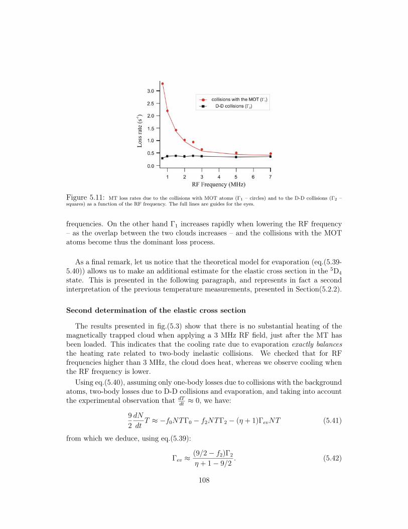
Figure 5.11: MT loss rates due to the collisions with MOT atoms (Γ1 – circles) and to the D-D collisions (Γ2 –squares) as a function of the RF frequency. The full lines are guides for the eyes.

frequencies. On the other hand Γ1 increases rapidly when lowering the RF frequency– as the overlap between the two clouds increases – and the collisions with the MOTatoms become thus the dominant loss process.

As a final remark, let us notice that the theoretical model for evaporation (eq.(5.39-5.40)) allows us to make an additional estimate for the elastic cross section in the 5D4

state. This is presented in the following paragraph, and represents in fact a secondinterpretation of the previous temperature measurements, presented in Section(5.2.2).

Second determination of the elastic cross section

The results presented in fig.(5.3) show that there is no substantial heating of themagnetically trapped cloud when applying a 3 MHz RF field, just after the MT hasbeen loaded. This indicates that the cooling rate due to evaporation exactly balancesthe heating rate related to two-body inelastic collisions. We checked that for RFfrequencies higher than 3 MHz, the cloud does heat, whereas we observe cooling whenthe RF frequency is lower.

Using eq.(5.40), assuming only one-body losses due to collisions with the backgroundatoms, two-body losses due to D-D collisions and evaporation, and taking into accountthe experimental observation that dT

dt≈ 0, we have:

9

2

dN

dtT ≈ −f0NTΓ0 − f2NTΓ2 − (η + 1)ΓevNT (5.41)

from which we deduce, using eq.(5.39):

Γev ≈ (9/2 − f2)Γ2

η + 1 − 9/2. (5.42)

108

Using the experimentally-measured density n0 (which, along with βDD gives Γ2 =0.27 s−1) and the evaporation parameter η = 5.5 ± 1 (using eq.(5.14)), we deduce theevaporation rate: Γev = 0.20 ± 0.04 s−1. This value is in reasonable agreement withour first estimate in Section(5.2.2), and confirms thus the first estimate of the elasticcross section σel. of the Cr atoms in the metastable 5D4 state.

5.5 Boltzmann equation and the issue of thermal equi-librium

In this section I present a complementary theoretical approach, based on the Boltz-mann equation. The main purpose is to have a second model, which describes theloading dynamics of our finite-depth magnetic trap, and which does not assume thatthe thermal equilibrium of the magnetically trapped cloud is reached. For this reason,the results shown in this section – which are quite time-demanding – do not repre-sent a fit of the experimental data, which were presented in Section(5.3). They aremore a verification of the results obtained with the previous model, as we are using noadjustable parameters.

Thermal equilibrium in our experiments

The theoretical model presented in Section(5.4) showed that the continuous accumu-lation in our trap takes place in a time scale which is mostly fixed by inelastic collisionswith the MOT atoms. For low RF frequencies ν, for which the spatial overlap betweenthe MT and the MOT is optimal, the loading time Tload is short, between 300 ms and1 s (see fig.(5.6)).

We now can raise the question of whether thermal equilibrium is indeed reached inthe case of the continuous accumulation in the RF-truncated magnetic trap. For that,it would be necessary that there is a ’sufficient’ number of elastic collisions taking placeduring the typical evolution time of the cloud, which is the loading time.

Using the previously-measured elastic cross section σel, we can have an estimate ofthe average number of elastic collisions undergone by the atoms before the steady-stateis reached in our trap. This quantity is approximatively given by n0σelvTload/2, and weplot it in fig.(5.12). We used the peak density, loading time and mean thermal velocitythat have been experimentally determined earlier.

One can see that the number of elastic collisions during the loading time decreaseslinearly when lowering ν; one can thus expect that thermal equilibrium of the trappedsample is not reached for low values of the RF frequencies. In order to better analyzethis issue, we will develop a model based on the Boltzmann equation [82].

109

Figure 5.12: Number of elastic collisions within the loading 1/e time Tload of our trap, as a function of the RFfrequency. The dashed line represents the frequency below which there are less than four elastic collisions during Tload.

Boltzmann and kinetic equation

The evolution of the phase-space distribution function f(−→r ,−→p ) of a classical gas inan external potential U(−→r ) is described by the Boltzmann equation:(−→p

m· −→∇−→r −−→∇−→r U · −→∇−→p +

∂

∂t

)f(−→r ,−→p ) = �coll(−→r ,−→p ) (5.43)

The normalization of f(−→r ,−→p ) gives: N = (2πh)−3∫

d3rd3pf(−→r ,−→p ). The left-handside of eq.(5.43) describes the time-evolution of f(−→r ,−→p ) in the potential U(−→r ), inabsence of collisions between particles. The collisional integral �coll(−→r ,−→p ) in theright-hand side accounts for the elastic collisions between the particles, which modi-fies f(−→r ,−→p ). It depends on the microscopical detail of these collisions and is usuallyquite difficult to estimate, even in the simple case (which we will consider here) oflow-temperature s-wave collisions, where the elastic cross section σ is temperature-independent.

Luiten et al. [79] showed however that this expression is greatly simplified whenmaking the "sufficient ergodicity" assumption, i.e. that the phase-space distributionf(−→r ,−→p ) is a function only of the single-particle energy ε. This allows one to write:

f(−→r ,−→p ) =∫

dεδ

(U(−→r ) +

p2

2m− ε

)f(ε) (5.44)

where the function f(ε) can be interpreted quantum-mechanically as the ’occupationnumber’ for the trap eigenstates with energy ε.

Although we will not detail here the demonstration of the kinetic equation, we men-tion that it is obtained by applying the operation h−3

∫d3rd3pδ(U(−→r ) + p2/2m − ε)

to both sides of eq.(5.43); on the left-hand side the gradient terms (which represent

110

simple fluxes of particles) sum to zero, leaving ρ(ε)f(ε), where:

ρ(ε) =2π(2m)3/2

(2πh)3

∫U(−→r )≤ε

d3r√

ε − U(−→r ) (5.45)

is called the trap density of states. As a consequence of the "sufficient ergodicity"assumption, ρ(ε) contains all the characteristics of the trapping potential; ρ(ε)dε givesthe number of single-particle eigenstates in the trapping potential, having energies be-tween ε and ε+ dε. In the case of a quadrupole magnetic trapping potential – given by

eq.(5.5) – we find ρMT (ε) =8(2m)3/2

105πV 30 h3 .

Finally, in the case of sufficiently low temperatures (where the interaction betweenparticles reduces only to the s-wave elastic collisions) the authors derive the following’kinetic equation’:

ρ(ε4)f(ε4) =mσ

π2h3

∫dε1dε2dε3δ(ε1+ε2−ε3−ε4)ρ(min[ε1, ε2, ε3, ε4])[f(ε1)f(ε2)−f(ε3)f(ε4)]

(5.46)where ε3 and ε4 (resp. ε1 and ε2) are the energies of the two colliding atoms before(after) the collision.

Thermal equilibrium

The kinetic equation can be used, for example, to study thermalization, i.e. the evo-lution of a system from an initial, non-equilibrium state towards a thermal equilibriumsituation. We can thus find the result of [107], which shows that, in an infinite trap,it takes typically about four elastic collisions to reach a situation close, within a few%, to thermal equilibrium. Using this criterion in our case – see fig.(5.12), we see thatindeed a lack of thermalization is expected at RF frequencies below ∼ 3 MHz.

The authors of [79] apply the kinetic equation for describing the time-evolution ofa non-equilibrium initial phase-space distribution of a gas in a finite-depth potential.Evaporation in such a case is easy to take into account by introducing an energy cut-off at the trap depth and simply removing, after each collision, the atoms with a totalenergy higher than the trap depth.

The important conclusion of [79], obtained by using the kinetic equation for a finite-depth trap, is the fact that one can use a distribution (the so-called ’truncated Boltz-mann distributions’) which is very close to the ’usual’, thermal equilibrium Boltzmanndistribution, in order to study the evaporative cooling in finite-depth traps.

Continuous loading and thermalization

I will now describe how we take into account the relevant physical mechanismswhich influence the continuous loading of the finite-depth magnetic trap. For that,

111

I will include in the left-hand side of the the Boltzmann equation (5.43) a series oflocal terms, which take into account the physical mechanisms considered in the modeldescribed in the previous section (such as the loading and the different loss terms):

+ ΓfMOT (−→r ,−→p ) − [Γ0 + βDDnMT (−→r ) + βPDnM0T (−→r )] f(−→r ,−→p ). (5.47)

When applying the operation h−3∫

d3rd3pδ(U(−→r ) + p2/2m − ε) to each of theseterms, we will obtain a series of terms which depend only on the energy ε and whichwill be added to the kinetic equation:

• Loading from the MOTFor the loading from the MOT we obtain5:

ρ(ε)f(ε) |load

= ΓfMOT (ε)ρMOT (ε), (5.48)

where fMOT (ε) and ρMOT (ε) are the phase space distribution and density of statesin the MOT and Γ is the loading rate. In order to calculate fMOT (ε) and ρMOT (ε):(i) we assume that the kinetic energy distribution of the MOT atoms is thatof thermal equilibrium at the temperature TMOT and (ii) we neglect the initialpotential energy of MOT atoms (which is equivalent to considering a small size ofthe MOT compared to the MT size), so that the MOT energy density of states isthe one in free space. With these two assumptions we find: ρMOT (ε) = 4π

√2m3/2

h3

√ε

and fMOT (ε) = exp(−ε/kBTMOT ).

• Background gas collisionsThe background gas collision term gives:

ρ(ε)f(ε) |bg

= −Γ0ρ(ε)f(ε), (5.49)

where Γ0 is a constant (energy-independent) rate.

• Inelastic D-D collisionsThe density-dependent inelastic collisions (such as the D-D collisions) are tech-nically more difficult to take into account, because the kinetic equation does notdirectly provide the time-evolution of density distribution nMT (−→r ). One can cir-cumvent this problem in the "sufficient ergodicity" approximation. Indeed, byintegrating eq.(5.44) over −→p we obtain:

nMT (−→r ) =2π(2m)3/2

h3

∫ε>U(

−→r )

dε√

ε − U(−→r )f(ε). (5.50)

5 For simplicity we will use the notation ε instead of ε4 – see eq.(5.46)

112

We account for the inelastic D-D collisions by adding an additional loss term:

∂f(−→r ,−→p )

∂t|DD

= βDDnMT (−→r )f(−→r ,−→p ) (5.51)

in the right-hand side of eq.(5.43). Applying the operation h−3∫

d3rd3pδ(U(−→−→r )−

p2/2m − ε) to this equation gives:

ρ(ε)f(ε) |DD

= −∫

d3rd3p βDDnMT (−→r )f(−→r ,−→p )δ

(U(−→r ) +

p2

2m− ε

)(5.52)

The momentum integral in the right-hand side can be easily evaluated6 and wefinally obtain a simplified expression for the inelastic D-D collision loss term:

ρ(ε)f(ε) |DD

= −

⎛⎜⎜⎝2π(

2m

h2

)3/2 ∫U(−→r )≤ε

d3rβDDnMT (−→r )√

ε − U(−→r )

⎞⎟⎟⎠ f(ε) (5.53)

• Collisions with the MOTThe collisions with the MOT lead to the additional term:

∂f(−→r ,−→p )

∂t|PD

= −βPDnMOT (−→r )f(−→r ,−→p ). (5.54)

Following a similar approach as in the case of the D-D collisions, we obtain:

ρ(ε)f(ε) |PD

= −

⎛⎜⎜⎝2π(

2m

h2

)3/2 ∫U(−→r )≤ε

d3rβPDnMOT (−→r )√

ε − U(−→r )

⎞⎟⎟⎠ f(ε)

(5.55)

Numerical simulation and results

We now have a model based on the kinetic equation which can describe the dynam-ics of our system. The numerical method we use for solving the kinetic equation (withadditional terms), is similar to the one presented in [79] (see SectionV therein): wediscretize both the time and energy scales. In this case evaporation becomes rathersimple to take into account numerically, by fixing a RF-dependent energy cut-off at thetrap depth U0 (see eq.(5.43)): after each time-step ti we ’remove’ (by putting f(ε) = 0)those particles which acquire an energy ε > U0.

6 Using once more the ’sufficient ergodicity’ assumption we get:∫d3pf(−→r ,−→p )δ

(U(−→r ) + p2

2m − ε)

= 4πm√

2m√

ε − U(−→r )f(ε).

113

The calculations are rather time-demanding (the main reason is that the inelasticcollision term ρ(ε)f(ε) |

DDrequires the knowledge of the density-distribution nMT (−→r )

at each moment of time – see eq.(5.50)). As mentioned in the beginning of this section,we did not use the simulations for better fitting the experimental data, but for a con-firmation of the results of our previous simple rate-equation model. We thus includedthe experimental parameters (Γ0, Γ, βPD, βDD and σel) deduced in Section(5.3).

Figure 5.13: A) 1/e loading time of the RF-truncated MT, as a function of the value of the RF frequency:comparison between the experimental data (squares) and results of the simulations, using the modified Boltzmannequation (triangles). The circle in the upper-right corner represents the measured loading time, without RF. B) atomicpeak density as a function of the value of the RF frequency: experimental data (squares) and simulations (triangles).

Figure 5.14: ’Effective temperature’ of the RF-truncated MT, as a function of the value of the RF frequency:comparison between the experimental data (squares) and results of the simulations, using the modified Boltzmannequation (triangles).

The time-evolution of the number of atoms is found to be approximately exponential,even though the limiting factor comes from the inelastic collisions. A comparison withthe experimental 1/e loading time is shown in fig.(5.13.A). The steady-state density dis-tribution, calculated using eq.(5.53)), also reproduces roughly the thermal-equilibrium

114

distribution given by eq.(5.6). We use the latter to fit the simulated cloud shape anddeduce the peak density, which is shown in fig.(5.13.B), together with the experimentaldata. Both for the loading time and for the peak density we find a reasonably goodagreement with the experiment.

The final energy distribution f(ε) is not exponential (as it would be expected atthermal equilibrium), even for long loading times. This is an effect due to inelasticcollisions, which prevent reaching thermal equilibrium. However, for comparing ourresults to the experimental data, we can always define, for example, the average kineticenergy of the sample; dividing it by 3kB/2, we obtain an ’effective temperature’ Teff .In fig.(5.14) we make a comparison between Teff and the experimental ’temperature’,and we again see a qualitative agreement between the simulation and the experiment.

Finally, we mention that in both cases (kinetic energy and density distribution), weestimate that the resolution and signal-to-noise ratio of our imaging system are notsufficiently good to detect any deviation from the thermal equilibrium distributions.

Conclusions

As mentioned above, the simulations using the Boltzmann equation show that ther-mal equilibrium is not fully reached. Because of inelastic collisions, this is observedeven for the large values of the RF frequency (or without any RF).

Nevertheless, the results presented in the last paragraphs show that we have a goodagreement with the experimental data, for the values of the different parameters thatwe used. Under these circumstances, the fact that the simple rate-equation model,presented in the previous section, provides good agreement with the experiments mayseem fortuitous. We however think that this is explained by the fact that, even thoughthermal equilibrium is not reached, the physical quantities relevant to this model (den-sity profile and ’effective temperature’ – i.e. widths of the velocity distribution) aredirectly measurable in experiments, and may be used in the model.

5.6 RF-dressed magnetic potentials

5.6.1 Accumulation at low RF frequencies

In the previous sections of this chapter I presented the continuous accumulation ofmetastable atoms in a finite depth magnetic trap. We found that, at high trap depths,the main limitations for the loading process come from two factors: the inelastic col-lisions with the MOT (P-D collisions) and the inelastic collisions between metastableatoms (D-D collisions). On the contrary, at trap depths lower than the MOT temper-ature (which correspond to RF frequencies smaller than ∼ 1 MHz) most of the atomsare not trapped. This explains the sudden decrease of the atomic density, which also

115

dramatically reduces the observed phase-space density.However for RF frequencies on the order of 800 kHz or below, new interesting fea-

tures appear in the absorption images. The 1/e size of the imaged cloud becomes muchlarger (see fig.(5.15)), and the atom lifetime is longer than the lifetime measured at 1MHz.

Figure 5.15: A) 1/e radius of the magnetically-trapped cloud (obtained by a Gaussian fit) as a function of theRF frequency. B) zoom for the RF frequencies smaller than 300 kHz, for which most of the atoms are trapped in theW-shaped potential and the cloud presents the shapes shown in fig.(5.19). We see that, for these frequencies the sizeincreases linearly with the RF frequency.

We interpret these observations as the result of accumulation of atoms in the W-shaped, ’RF-dressed’ magnetic potential minima, which are presented in fig.(5.16); thistrapping technique has been proposed in [83] and experimentally demonstrated in [84].Let us give an intuitive description of the accumulation mechanism, by consideringthe high-field seeking atoms, arriving in the 5D4 state after decaying from the MOT.In absence of RF, these atoms are initially expelled form the trap center. When asufficiently high RF power is applied, the atoms have their spin ’flipped’ when passingover the RF-resonance position; they are thus projected into a low-field seeking state,and are then attracted back to the magnetic field minima (B = 0 point).

The correct quantum picture – detailed below – can be obtained by considering theinteraction hamiltonian between the atoms and the total (static + RF) magnetic field.Diagonalizing this hamiltonian leads to the so-called ’RF-dressed’ states schematicallyshown in fig.(5.16).

Our experimental observations show an interesting possibility of increasing the num-ber of atoms accumulated in the metastable D states, by simultaneously reducing thetwo main limiting factors presented earlier (’P-D’ and ’D-D’ collisions). The ’usual’magnetic trap (i.e. without RF) and the MOT are both centered around the B = 0point. From the P-D collision point of view, this configuration is most unfavorable,because it maximizes the overlap integral of the MT with the MOT. The density pro-file shown in fig.(5.16) is, from this point of view, much more favorable, because themetastable cloud presents a local density minimum at the MOT position (i.e. B = 0),

116

Figure 5.16: Continuous loading in a W-shaped magnetic trap.

thus potentially decreasing the overlap and the inelastic collision term. Additionally,the D-D inelastic collision rate (proportional to the inverse of the trap volume) alsodecreases, proportionally to the RF frequency.

Another potential advantage of the W-shaped potentials is that their minima are lo-cated away from the B = 0 region; this could prevent the Majorana spin-flip transitionsand increase the lifetime of the trapped clouds, in the ’sufficiently cold’ regime wherethey could be the limitative factor (which is however not the case in our quadrupolemagnetic trap). This point will be revisited in Chapter(6).

In the rest of this chapter I study the possibility of efficiently accumulating atomsin such RF-dressed, W-shaped magnetic traps. The ideal scenario would be for theatoms, initially ’created’ at the MOT (B = 0) position, to accumulate in large numbersand eventually tend towards a thermal equilibrium situation, with density distributionspeaked around the avoided crossing positions.

5.6.2 Magnetic+RF adiabatic potentials

Let us now give a brief description of the ’RF-dressed adiabatic potentials’. For thedetails of these calculations, one can refer, for example, to [85].

The interaction (Zeeman) hamiltonian between the atom and the total magneticfield is: H(−→r , t) = gJμB

−→J · [

−−→B(r) +

−−→BRF cos(ωt)], where

−−→B(r) is the static magnetic

field of trap, −−→BRF is the amplitude of the RF field and −→J is the total kinetic moment

of the atom.A convenient way to treat this hamiltonian is to consider the rotating frame, at the

RF frequency; in this frame a time-independent hamiltonian can be obtained by making

117

the rotating wave approximation RWA (see for example [85]). By then diagonalizingthe hamiltonian7, one obtains the following eigenenergies (’dressed potentials’):

Um′RF

= m′RF h

√δ2RF (−→r ) + Ω2

RF (θ) , (5.56)

where m′RF is an integer (going from −J to +J), δRF (−→r ) = ω − gJμBB(

−→r )h

is the RF-detuning with respect to the |mJ〉 → |mJ ± 1〉 transition between adjacent Zeemansublevels, and θ is the angle between the direction of the RF and static magnetic fields.

In eq.(5.56), ΩRF (θ) = gJμBBRF

2hsin(θ) is the RF coupling constant (’Rabi fre-

quency’), and is proportional to the amplitude of the component of the RF magneticfield −−→

BRF perpendicular to the direction of the static field −→B (−→r ). We see that the

maximum coupling (ΩRF,max. ≡ gJμBBRF

2h) occurs for an RF field which is perpendicular

to the static field, whereas no coupling is possible if the two fields are parallel.

Figure 5.17: Zeeman levels without RF (left) and RF-dressed Zeeman potentials (right), for a RF frequency of 2MHz.

The corresponding eigenstates (’dressed states’), labeled |m′RF 〉 are space-dependent

linear superpositions of the Zeeman magnetic states |m〉 in absence of the RF field.When δRF → −∞ a |m′

RF 〉 state tends towards a given |mJ〉 Zeeman state, while whenδRF → ∞, |m′

RF 〉 tends towards the opposite, i.e. | − mJ〉 state.

In the case of a quadrupolar magnetic field, like the one in our experiment, the RF-dressed magnetic potentials are shown in fig.(5.17). We see that in the case of 52Cr,because of the absence of the hyperfine structure (and thus of the quadratic Zeemaneffect) all the RF resonances take place at the same position.

If ω = δRF (0) ΩRF , the atoms ’produced’ in the D-states in a given |mJ〉, at theposition R 0 (far from the RF resonance point), will be virtually in an eigenstate|m′

RF 〉 of the ’dressed’ hamiltonian. In addition, if the RF-coupling is strong enough7 We note that the expression (5.56) is valid for 52Cr, in absence of the non-linear Zeeman effect

(because of the absence of the hyperfine structure) and all RF resonances between adjacent |mJ〉 levelsare taking place at the same position RRF .

118

(in the sense discussed in the following paragraph), it will adiabatically follow thecorresponding RF-dressed potential.

Depending on their ’initial’ mJ state when decaying to the metastable states (closeto R = 0), atoms can feel two different types of potentials. If mJ > 0, which is a low-field seeking state in the ’undressed’ picture, we recognize RF-truncated, finite depthpotentials we studied in the first part of this chapter. On the other hand if mJ < 0,which is an untrapped, high-field seeking state in the ’undressed’ case, the atoms willfollow the W-shaped potential, which has two minima, as shown in fig.(5.17). In a 3Dcase the minima are located on the ’evaporation ellipsoid’ (defined in Section(5.2.2)).The atoms will then oscillate around the equilibrium position (RRF ).

5.6.3 Landau-Zener crossings and lifetime

I will now consider the possibility of accumulating atoms in the W-shaped poten-tials, by analyzing the probability of an atom to adiabatically follow the ’RF-dressed’potentials.

The magnetic potentials coupled by the RF field can be regarded as several avoidedcrossings (see fig.(5.17)), all taking place at RRF = hω

gJb′ , given by the RF resonancecondition δRF (−→r ) = 0. An atom can remain trapped in the W-shaped potentials, aslong as it adiabatically follows the initial dressed state at each passage at resonance; ifa non-adiabatic transition, which projects the atom to an untrapped state (i.e. adia-batically connected to a mJ < 0 state at R → ∞), occurs, then the atom will be lostfrom the trap.

For the simplicity of the discussion, let us consider for the moment only the case ofa maximum coupling strength ΩRF,max..

The situation is similar to the quantum-mechanical Landau-Zener problem for anavoided crossing between two intersecting levels. The non-adiabatic transition proba-bility, in this simple case, is given by [86, 87]: PLZ,2 = exp

(−π

2

Ω2RF,max.

δRF

), where δRF

is the time derivative of the RF detuning δRF (−→r (t)) at RRF .In our case, the situation is more complicated, as we have not two, but N = 9

potentials which are crossing in the same point. Rather then giving an exact calculationof the diabatic crossing probability (by solving the Schrodinger equation, using theexact hamiltonian [88]) we will give an intuitive solution. For N − 1 avoided crossings(between N intersecting levels), the ’survival probability’ of remaining in the sameinitial state is given by (1 − PLZ,2)

N−1.Finally, the probability of undergoing a diabatic Landau-Zener transition, for one

119

passage at r = RRF , is then given (replacing the value N − 1 = 8) by:

PLZ,9 = 1 −[1 − exp

(−π

2

Ω2RF,max.

δRF

)]8. (5.57)

This expression is in agreement8 with [88], and allows to estimate the rate γLZ

of suchdiabatic passages, which fixes the cloud lifetime τ

LZ: γ

LZ= 1/τ

LZ= PLZ,9/T , where

T is the time interval between two successive passages through the avoided crossingregion.

In our case, the atoms are ’created’ at the center of the W potential with a certaininitial velocity v0 obeying the thermal distribution at the MOT temperature TMOT .Both the Landau-Zener probability (through the δRF term) and the oscillation periodT0 depend on v0. Atoms arriving at the resonance point have a velocity v(RRF ) =√

v20 + 2mJ hω

mand the derivative of the detuning reads:

δRF (RRF ) = v(RRF )dδRF

dr|RRF

=gJμBb′

h

√v2

0 +2mJ hω

m(5.58)

whereas for the oscillation period we find (neglecting the curvature of the potentials atthe crossing point):

T0(v0) = 4m

mJgJμBB′

⎛⎝2

√v2

0 +2mJ hω

m− v0

⎞⎠ (5.59)

Using these two expressions and eq.(5.57) we can finally calculate the loss rate γ, bytaking the thermal average over v0:

γ =1

τ= 4

√m

2πkBTMOT

∞∫−∞

1

T0(v0)PLZ(v0) exp

(− mv2

0

2kBTMOT

)dv0. (5.60)

The loss rate depends on the RF frequency ω and on the RF coupling ΩRF . In theexperiments we want this loss rate to be smaller than all other inelastic collision lossrates, in order to never be limited by the non-adiabatic Landau-Zener transitions.

In fig.(5.18) we plot the dependence of the RF Rabi frequency Ωτ which is requiredfor obtaining a given Landau-Zener lifetime τ (1 s and 10 s) as a function of the RFfrequency ω. We observe that Ωτ increases with ω, as the atoms arrive at the avoided-crossing position with larger velocities v(RRF ).

This simple 1D calculation gives an order of magnitude for the RF field, consideringan optimal RF coupling, i.e. an RF field orthogonal to the static field direction. In

8 in the case (which applies here) where the adiabatic potentials at the crossing are equidistant.

120

Figure 5.18: Solid, thick curve: RF coupling strength vs. RF frequency for obtaining a trap lifetime of 1s,considering an initial temperature of the atoms of 100 μK. The upper, dashed curve shows the Rabi coupling neededfor a 10 s lifetime (for the same initial temperature of 100 μK). The dotted, lower curve shows, for illustration, Rabicoupling for a 1 s lifetime, in the case of lower initial temperature, of 10 μK (we observe, as expected, that at lowRF frequency the required RF field is lower than for the T = 100 μK case, while at high RF frequency the initialtemperature plays no role, and the two curves join together.)

our experiment, we use a 10 W RF amplifier. For an RF coil of 4 turns, having a 7 cmdiameter and placed at 5 cm away from the atoms, we estimate that the coupling is∼ 200 kHz, well above the limit shown in fig.(5.18).

Leaks

In our experiment, the RF field (created by a single coil, placed above the upperviewport of the cell) is oriented along the vertical (z) axis; on the other hand, thedirection of the static magnetic field (created by the MOT coils) is not spatially uniform.

We mentioned earlier (see eq.(5.56)) that only the projection of the RF field onthe local static B-field direction can couple different mJ states; this means that, inour case, the ’effective’ Rabi frequency will be space-dependent, given by ΩRF (−→r ) =sin(θ)ΩRF,max, where θ is the azimuthal angle, between the −→r direction and the z axis.The Landau-Zener transition lifetime will be position-dependent.

In practice, there will always be a region in space, corresponding to small azimuthalangles (i.e. for θ between 0 and a certain θmax), for which the Landau-Zener conditionwill not be satisfied. The value of θmax will be given by the maximum available RFpower.

We estimate that, for ΩRF,max ∼ 200 kHz, we have θmax 2.2◦ � 180◦, whichshould lead to negligible leaks.

We however note that it is possible to completely avoid the ’leaks’ problem, bycreating a ’fast-rotating’ RF field, who ’on average’ couples all the direction of thespace. Such a field can be easily created, using two RF coils with perpendicular axes,

121

whose currents are 90◦ out-of-phase: under these conditions the RF field directionrotates at the frequency of the RF field. We experimentally tested this possibility, andobserved that the results (exposed in the following paragraphs) are not modified. Forthis reason we conclude that indeed the RF power is not a limitation in our case.

5.6.4 Experiments

Let us now come back to the experimental realization of the W-shaped potentials.As mentioned earlier (see fig.(5.15.A)), we observe an increase in the size of the mag-netically trapped cloud for RF frequencies lower than 800 kHz. For even lower RFfrequencies (∼ 200 kHz) the slices through the absorption images clearly present adouble-peak structure, shown in fig.(5.19), which is due to the atoms trapped in theW-shaped, RF-dressed adiabatic potential.

Figure 5.19: Left: image of the atomic cloud in the W-shaped magnetic trap. Right: horizontal slices through theimage, passing through the B = 0 point, for two different RF frequencies.

We also observe that, because of the gravity, atoms are accumulated towards thebottom of the ’iso-B’ ellipsoid. We experimentally checked (see fig.(5.15.B)) that thecloud size increases linearly with the RF frequency, while its vertical position is alsolinearly shifted downwards.

Another interesting feature is related to the dependence of the number of trappedatoms on the RF power – shown in fig.(5.20), for a value of the RF frequency of 300kHz. Staring from zero, at low RF powers, we observe a drastic decrease of the numberof trapped atoms, which is due to the plain evaporation of the atoms (’low-field-seekers’which were trapped in the absence of the RF).

When increasing progressively the RF power, we observe a change in the shape of

122

Figure 5.20: Above: horizontal slice through the center of the trapped cloud, for a RF frequency of 300 kHz. Atlow RF powers we observe a double structure, which is due to the superposition of the clouds trapped in the M-shapedand W-shaped RF-dressed potentials. The line represents a double-gaussian fit, from which we deduce the number ofatoms respectively in the M- and W-shaped potentials. Below: Atom number in the W-shaped (full diamonds) and inthe M-shaped potential (open diamonds), as well as the total number of atoms(dots) as a function od the RF power(for a constant RF frequency of 300 kHz). The lines are guides for the eyes.

the cloud. In fig.(5.20) we observe a double structure, which is the superposition of acentral peak (due to the atoms in the M-shaped potential) and a larger structure thatis due to the atoms trapped the W-shaped potential. We also plotted the number ofatoms in each of the structures, as a function of the RF power, by performing a double-gaussian fit. We see that the atom number in the W-shaped potential (full diamondsin fig.(5.20)) increases with the RF power. This is due to the increase of the Landau-Zener adiabatic transition probability, accompanied with a progressive decrease of thesolid angle through which atoms, uncoupled by the RF, escape from the trap.

When increasing further the RF power we unfortunately observe that the atom num-ber in the W-shaped potential decreases back. We attribute this effect to the presenceof RF harmonics, at twice the RF frequency, which are resonant with the transitionbetween adjacent mJ -states at 2RRF . These second harmonics are responsible for un-wanted spin-flips, which lead to the evaporation of the atoms which have enough energyto reach 2RRF . The number of these atoms is relatively high, since they are initially’produced’ at the position where B = 0, where they have the same potential energy as

123

when they reach 2RRF .

Perspectives

The experiments presented in this section demonstrate the possibility of creatinglarge-volume (’W-shaped’) traps in which high-field seekers can be trapped. Unfortu-nately, there are technical limitations, related to the presence of RF second harmonics(with a frequency 2ν), for efficiently loading metastable 52Cr atoms in the W-shapedpotentials.

Filtering these harmonics good enough is somewhat difficult to do. As a perspective,one could however think about the possibility of minimizing the influence of theseharmonics, using a second RF field, with a frequency ν ′ > 2ν: in this case, the atomsundergoing a spin-flip at the position of the 2ν harmonics could be ’recuperated’, by asecond spin-flip at the position of the ν ′−resonance.

Another possibility is to find a way to prevent the atoms from reaching the secondRF-resonance. In this respect, some interesting experiments, using an additional opti-cal confinement, will be presented in the next chapter.

Conclusions

In this chapter I presented a new trapping scheme, which consists of the continuousloading of metastable 52Cr atoms in a RF-truncated quadrupole magnetic trap. Wewere able to reach phase space densities up to 7×10−6, in less than 1 s, which representsan increase of ∼ 7 with respect to the typical value in Cr MOTs.

The theoretical rate-equation model presented in this chapter, provides a convenienttool to describe the loading dynamics of the finite-depth trap. This model shows inparticular that heating due to inelastic collisions with the excited MOT atoms greatlylimits the phase-space densities which can be reached.

Another important result of the experiments presented here is the measurement ofthe elastic and inelastic collisional properties of metastable 52Cr atoms.

Finally, we investigated the possibility of accumulating atoms reaching the metastablestates in a high-field seeking state, by the use of RF magnetic fields. Although techni-cal problems, related to RF second harmonics, limit the number of atoms accumulatedusing this method, it opens the way to further experiments presented in the followingchapter.

124

Chapter 6

Accumulation of 52Cr metastableatoms into an optical trap

Why is Bose-Einstein condensation in our magnetic trap not possible forCr?

Although it provides the means for exploring new interactions in degenerate quan-tum gases, the large magnetic moment of Chromium (6μB in the stretched state) isalso a major experimental obstacle in achieving Bose-Einstein condensation in magnetictraps.

The measurement of a large inelastic collision parameter βDD between metastableCr atoms shows that it is not possible to use these states for achieving the BEC. Evenin the ground state, in our quadrupole magnetic trap configuration, Majorana losseswould become a limitation at temperatures close to the condensation threshhold.

Moreover, the works performed in T.Pfau’s group in Stuttgart [76, 90] showed that,even in a Ioffee-Pritchard-type trap, with a non-zero magnetic field minimum, thereare spin-changing collisional processes – dipolar relaxation and spin-exchange collisions– which are particularly important in Cr, and finally limit the achievable phase-spacedensity. These processes lead to magnetic trap losses, as they can promote atoms innon-trapping, mJ ≤ 0 states.

For instance, they measured a particularly high spin-exchange collision loss param-eter βs.e. ∼ 1 × 10−10 cm3/s. Spin-exchange collisions, which are processes where thetotal spin is conserved, can be suppressed by spin-polarizing the magnetically trappedsample in the mJ = +3 stretched state. However dipolar relaxation, which does notconserve the total spin, is still possible in these states (βd.r. ∼ 3 × 10−12 cm3/s), andeventually leads to the de-polarization of the sample to lower mJ states; it limited theachievable phase-space density, in their experiment, to values ∼ 10−2.

Under these conditions, Bose-Einstein condensation in a magnetic trap seems aparticularly difficult task in the case of Cr. The solution is the transfer of atoms from

125

the magnetic trap into an optical dipole trap (ODT). Although they are more difficultto use (mainly because of their limited depth), these traps have a major advantage,which is the fact that they also can be used to trap the high-field seekers. The atoms inthese traps can be spin-polarized in the lowest-energy Zeeman state (mJ = −3, whichis a high-field seeker). In this state, a spin-changing collision becomes energeticallyunfavorable, as it requires an increase of the Zeeman energy (of ΔEZeeman = gJμBB).If ΔEZeeman is high enough compared to the temperature of the sample, there is notenough kinetic energy in the system to provide this extra energy, and the spin-relaxationprocesses are suppressed.

We consequently chose for our experiment, as a strategy to achieve Bose-Einsteincondensation, to load atoms and perform evaporative cooling inside an optical dipoletrap.

6.1 Optical trapping

In this section I will first present a simple classical model for the optical trappingpotentials for neutral atoms, which mainly reproduces the description presented in areview paper by Grimm et al. [91], and which has the advantage of well explaining thephysics of the problem.

In the last part I will present a theoretical model for multilevel atoms, and use it toevaluate the lightshifts in the case of 7S3 and 5D4 states of 52Cr.

6.1.1 Classical model

Classical light – induced-dipole interaction

Let us consider the classical expression for the oscillating electric field of a laser lightbeam: −→

E (r, t) = −→ε [E0(−→r ) exp(−iωt) + E∗0(−→r ) exp(+iωt)] (6.1)

where −→ε is the unitary vector of polarization and E0(−→r ) is the fields’ (space-dependant)amplitude. E0(−→r ) is related to the local light field intensity by: I(−→r ) = 2ε0c|E0(−→r )|2,where ε0 is the vacuum permittivity and c is the vacuum light velocity.

If an atom is placed into the laser light, the oscillating electric field (6.1) inducesan atomic dipole moment −→p (−→r , t). It oscillates at the field frequency ω and has anamplitude p0(−→r ) proportional to the field amplitude:

p0(−→r ) = α · E0(−→r ) (6.2)

where α is the polarizability of the atom . Usually −→p (−→r ,t) and −→E (−→r ,t) oscillate

out-of-phase, which can be taken into account by allowing complex values for α.

126

The interaction potential between the light field and the induced dipole is −12−→p (r, t) · −→E (r, t).

In the limit where the timescale for atomic motion is much larger than the oscillationperiod 1

2πω, the atoms will only ’feel’ the time-average of this interaction potential,

which is called the dipole potential :

Udip = −1

2〈−→p (r, t) · −→E (r, t)〉 =

1

2ε0cRe(α)I(−→r ). (6.3)

One can thus see that the dipole potential is proportional to the local laser field inten-sity I(−→r ) and to the real part of the atomic polarizability α (i.e. to the part of theatomic induced-dipole which oscillates in-phase with the light electric field).

The out-of-phase part of the atomic dipole, on the other hand, allows us to calculatethe mean power which is absorbed by the atom Pabs = 〈−→p −→

E 〉. This power can beexpressed in terms of photon scattering rate and finally one finds:

Γsc =Pabs

hω=

1

hε0cIm(α)I(−→r ). (6.4)

Lorentz classical model

A very convenient way to derive the expression of the atomic polarizability α is theLorentz (elastically-bound electron) model.

The electron, having a mass me, is assimilated to a classical, damped harmonicoscillator, characterized by the oscillation eigenfrequency ω0 and the damping rate Γ.The oscillator is excited at the frequency ω by the Coulomb force of interaction with theexternal electric field. The time-evolution of the induced dipole p = e x can be foundby solving the classical equation of motion x + Γωx + ω2

0x = −eE(t)/me. The systemis in equilibrium provided that the absorbed energy balances exactly the energy lossdue to damping, which gives the expression of the damping coefficient: Γω = e2ω2

6πε0mec3.

This corresponds to the Larmor formula for an oscillating particle [93].After some algebra, one finally finds the following expression of the atomic polariz-

ability:

α = 6πε0c3 Γ/ω2

0

ω20 − ω2 − i(ω3/ω2

0)Γ(6.5)

Dipole potential

Finally, using eq.(6.5) for the polarizability of a two-level atom in the general ex-pression of the dipole potential (6.3), we find:

Udip(−→r ) = −3πc2

2ω30

(Γ

ω0 − ω+

Γ

ω0 + ω

)I(−→r ). (6.6)

127

The scattering rate, useful for estimating the heating due to photon scattering, is givenby:

Γsc(−→r ) =3πc2

2hω30

(ω

ω0

)3 ( Γ

ω0 − ω+

Γ

ω0 + ω

)2

I(−→r ). (6.7)

These expressions are valid in the case of large detunings and negligible saturation;they are not valid near resonance (where they both diverge).

In the case of a red detuning (ω < ω0) atoms can be trapped at the local lightintensity maxima, such as the focusing point of a laser beam; this is the case weconsider in this thesis. For a blue detuning (ω > ω0), the atoms are expelled form theintensity maxima (one can nevertheless trap them, for example in more exotic lasermodes, like the ’donut modes’).

In both cases the scattering rate decreases with the absolute value of the detuning|δ|. This means that Γsc can be reduced, by detuning further the trapping lasers; theprice to pay is, of course, a reduction of the dipole potential depth. An interesting andimportant feature of the optical traps is the fact that the ratio Udip/Γsc increases with|δ|, so one can, in principle, make Γsc arbitrarily small for a given dipole potential, bychoosing a laser detuning sufficiently large and increasing accordingly the light power.

There are two types of optical traps, according to the value of ω with respect toω0. In most experiments the value of the detuning is much smaller than the opticalfrequency, so one has: Γ � δ � ω0. In this case 1/|ω + ω0| � 1/|ω − ω0| and onecan neglect the ’counter-rotating’ term in eq.(6.6), which is the so-called ’rotating waveapproximation’. The dipole potential simply becomes Udip = 3πc2Γ

2ω20

Iδ, and this type of

trap is usually called a far-off-resonance trap (FORT).Another type of traps are those for which the optical frequency is much smaller

than the atomic transition frequency: ω � ω0 and the two resonance terms in eq.(6.6)are almost equal. The dipole potential becomes: Udip = −3πc2Γ

ω40

I, which does notdepend any more on ω; this gives the name of these traps: quasi-electrostatic traps(QUEST). Because of the extremely large detuning from resonance, QUESTs are quasi-non-dissipative traps, with optical scattering rates on the order of one photon per hour.

In the case of our experiment we use a 1075 nm laser, and we estimate that we arein an intermediate situation (as ω0−ω

ω0+ωranges roughly between 0.3 and 0.7 – see the

transitions listed in Table(6.1-6.2)) where one should consider both terms in eq.(6.6).

Semi-classical polarizability for a two-level atom

A semi-classical expression of the polarizability can be obtained, by consideringthe interaction between a two-level atom (ground state |g〉 and excited state |e〉) and aclassical laser field in the low-saturation regime. The result, in that case, is obtained [91]

128

from eq.(6.5), by simply replacing the oscillation frequency ω0 by the atomic transitionfrequency and the damping rate Γω0 by the damping rate corresponding to spontaneousemission:

Γ =ω3

0

3πε0hc3|〈e|d|g〉|2 (6.8)

where |〈e|d|g〉| is the dipole matrix element between the ground and the excited state.

Light shifts

A similar result can be obtained in the case of a two level atom, in the ’dressed states’picture [92]. This result is obtained by applying the second order time-independentperturbation theory to the combined system ’atom plus light field’ with the electricdipole interaction hamiltonian.

This perturbative treatment shows the interesting fact that the energy of the groundstate is shifted by an amount (called ’light shift’ or ’AC Stark shift’) correspondingexactly to the dipole potential in the classical picture. Moreover, the excited statepresents exactly the opposite energy shift.

6.1.2 Theoretical evaluation of the light shifts

We will now discuss the case of real atoms (Cr), where the simple two-level approx-imation does not apply because of the complex electronic structure, with many atomiclevels coupled to each-other by the laser light. In this case one has to consider (thesum of) all the allowed couplings with other levels.

We will make here a theoretical estimate for the Cr light shifts, based on the spectro-scopical data from NIST [106]. An interesting conclusion of these calculations is thatthe light shifts can in fact depend on the magnetic quantum number mJ and on thepolarization of the light (as opposed to the case of alkali atoms where the light shiftsare almost mJ−independent). In fact complications arise when a given level, or thelevels it is coupled to, are not purely spectroscopic terms (i.e. the angular momentumL and the spin S are not good quantum numbers).

As in the case of a two-level atom, when a given atomic level i, of energy hωi, iscoupled by a laser through dipolar electric transitions to other states n having energieshωn, its energy is shifted due to the presence of the AC laser electric field. This lightshift depends on I(−→r ), the local laser intensity, on ωni = ωn−ωi and on Γni (respectivelythe transition frequency and the cycling rate of the transition between the levels i andn) and on the laser frequency ω. The different Zeeman sublevels, corresponding to themagnetic quantum number mJi

, are coupled differently to the excited states, and the

129

light shift not only depends on the total angular momentum Ji, but as well on mJiand

on the laser polarization.In the case where there is no hyperfine splitting of levels (as in the bosonic 52Cr),

the coupling rate ΓmJi,n between a sublevel (i, Ji, mJi

) and another level (n, Jn, mJn) isgiven by:

ΓmJi,n = Γni(2Jn + 1) × C2

Ji,mJi,Jn,sign(ωni)×q. (6.9)

Here q gives the polarization of the laser (q = −1, 0, +1 for σ−, π or σ+ light) and

the 3J coefficient is CJi,mJi,Jn,q =

(Ji 1 Jn

−MJi −q MJi + q

). We also remind that the

selection rules impose that Ji and Jn may only differ by -1,0 or +1.The light shift can therefore be written [91, 94] as:

Ui,mJi(−→r ) = −3πc2I(−→r )

∑n

sign(ωni)ΓmJi,n

ω2ni(ω

2ni − ω2)

(6.10)

which is the generalization of (6.6) in the case of multilevel atoms.

An interesting simplification occurs if the state i is a S ground state and if all thestates it is coupled to (P states) belong to true spectroscopic terms, which means thatthey are fully characterized by their total orbital momentum L and spin S, in additionto the total momentum J (which is always a good quantum number). Then the cyclingrate Γni does not depend on the fine structure. Moreover, if the laser frequency is chosensuch that all the detunings are large compared to the fine structure splitting, we canuse the following sum rule over the 3J coefficients to get a great simplification:∑

Jn=Ji−1,Ji,Ji+1

(2 × Jn + 1)C2Ji,mJi

,Jn,q = 1, (∀q) (6.11)

From (6.10) we then see that the light shift is mJi− independent and can be calculated

by completely ignoring the fine structure splitting and the polarization of the light. Ageneralization of this discussion can be extended, with the same results, in the caseof a hyperfine splitting. This conclusion applies, for example, in the case of the alkalispecies [91].

However this simplification is not valid anymore if either the state i or the levelsit is coupled to are not pure spectroscopic terms, or if i is neither a ground state nora S state; in this case Γni depend on Jn. This is indeed the case of the ground state7S3 of Cr, where the coupling to the excited P states depends on the fine structure ofthese states (see Table.(6.1)). The effect is even larger for the 5D metastable states(Table.(6.2)), which are themselves not pure spectroscopic terms (as clearly shown bytheir non zero coupling to the 7P states).

130

Level Jn λni (nm) Γni (×107 s−1)

z 7P234

428.972427.480425.435

3.163.073.15

y 7P234

360.533359.349357.869

16.215.014.8

x 7P234

236.681236.591236.471

0.690.550.53

w 7P234

209.588209.539209.483

0.110.110.12

Table 6.1: Main atomic transitions contributing to the lightshift of the 7S3 level of Cr.

Level Jn λni(nm) Γni(×107s−1)z 5P 3 540.979 0.62w 5P 3 278.07 14y 5P 3 464.617 0.87

z 5F45

438.498435.177

0.271.2

z 5D34

394.149391.916

0.280.92

x 5P 3 305.388 7.97

y 5F45

303.704302.156

5.429.1

y 5D 3 300.506 9.2z 3G 3 258.466 0.61v 5P 3 271.618 1.1

Level Jn λni(nm) Γni(×107s−1)

x 5D34

291.114288.929

2.66.6

u 5P 3 259.185 6.5v 5D 4 252.712 5.3

x 5F45

270.348270.199

0.632.1

w 5D34

262.660262.286

0.931.3

w 5F 5 260.357 0.62z 5P 3 240.862 6.7

s 5F45

238.572238.333

1.74.1

r 5D 4 199.995 14

Table 6.2: Main atomic transitions participating to the lightshift of the 5D4 level of Cr.

131

Results

Using eq.(6.10), we can now turn to the estimation of the light shifts of the levels ofinterest . The laser that we use for optical trapping has a wavelength λIR = 1075 nmand its polarization is linear.

In the experiments presented in this chapter, we accumulate atoms in a mixed op-tical + magnetic quadrupole trap (this configuration will be described in detail inSection(6.3)). This means that the magnetic field direction (which defines the localquatization direction) is changing with −→r , and there is no good choice for q. The po-larization seen by the atoms can change between a π polarization (q = 0) and an equalmixture – qinc polarization – of σ+(q = 1) and σ−(q = −1) polarizations, correspondingto a local B-field respectively orthogonal and parallel to the laser propagation axis.

The results for these two polarizations, for the 7S3 and 5D4 states, are (in K):

U7S3,mJi=σinc

I0 × (−198.6 − 0.3 × m2Ji

) × 10−16

=π I0 × (−202.4 + 0.6 × m2Ji

) × 10−16 (6.12)U5D4,mJi

=σincI0 × (−151.4 − 1.2 × m2

Ji) × 10−16

=π I0 × (−174.6 − 2.4 × m2Ji

) × 10−16

where I0 is the laser intensity, measured in W/m2.We observe a quadratic dependance in m, which is due to the fact that, for q = 0

and qinc, there are no linear terms in m left1 in the sum (6.10).

In conclusion, we observe that for the 7S3 level there are only small differences, upto ∼ 3%, between the optical trap depths for different values of mJ . The situation isquite different for the 5D4 level: up to 21% differences may be expected between theshifts of the mJ = 0 and mJ = 4 sublevels for a π−polarization.

6.2 Experimental setup

Optical setup

The optical dipole trap is created, in our experiment, by a CW Ytterbium fiber laser,model YLR-50-LP (IPG). This laser delivers a power of 50 W, at a central wavelengthλ0 = 1075 nm. The beam is monomode transversally, with a 1/e2 diameter of 2.2 mm.

A first optical stage, shown in fig.(6.1), is used for preliminary shaping the beam.The output of the fiber laser is protected against back-reflections by an optical isolator

1 C2Ji,mJi

,Jn,0 and C2Ji,mJi

,Jn,+1 +C2Ji,mJi

,Jn,−1 do not include terms in m for Jn = Ji −1, Ji, Ji +1

132

(transmission 93%). A single-passed AOM is used both as a fast switch for the beamand for controlling the laser power during forced evaporation ramps (the utility and thechoice of this AOM will be explained in the following paragraphs). The beam diameteris reduced to 1.1 mm, with a 2 : 1 telescope placed before the AOM, in order to adaptits size to the aperture of the AOM and maximize the diffraction efficiency. Finallythe diameter is increased back about to its initial size, with a second, 1 : 2 telescope.

Figure 6.1: Setup for preliminary shaping of the optical dipole trapping beam.

After that, the beam is raised at the height of the experimental chamber (30 cm)with a periscope. A λ/2 plate and a polarizing beam-splitter (PBS) are used forseparating the beam into the two arms of the crossed ODT. The power ratio betweenthe arms can be changed with a motorized, computer-controlled rotation stage for theλ/2 plate. An alternate solution would be the use of two independent AOMs, one foreach arm. Although less flexible, our method has the advantage of allowing the use ofthe entire available laser power during the single-beam ODT accumulation procedure(see below). A possible limitation comes from the maximum speed (20◦/s) of the λ/2plate rotation stage.

The two beams are finally focused inside the experimental chamber with plano-convex lenses, mounted on translation stages. In order to double the useful laserpower, each arm is retro-reflected and focused back on the atoms. The direction ofeach IR beam can be finely adjusted using differential screws, which are used for themirror mounts (M1 and M2 for the horizontal beam and M3 and M4 for the verticalbeam – see fig.(6.2)). Finally, the light is sent to a water-cooled beam blocker.

Beam characterization

A weak fraction of the vertical IR laser beam, transmitted through a non-back-side-polished dielectric mirror (M0), is used to measure the transverse profile of thefocused beam which is sent to the atoms. A lens, identical to the one producing theODT, is used for focusing the weak transmitted beam onto a CCD camera, mountedon a micro-controlled translation stage. We can thus measure the size of the beam atdifferent position and deduce the position and the size of the waist of this weak beam.

133

Figure 6.2: Optical setup for the coupling of the horizontal (A) and vertical (B) optical dipole trapping beams.The (x′, y′, z′) reference frame, used throughout this chapter, is adapted for the description of the horizontal trappingbeam configuration: z′ is the beam propagation axis, while x′ (horizontal) and y′ (vertical) are orthogonal to the beamdirection.

We should note however that this technique does not take into account thermal lenseffects, related to the viewports of the vacuum chamber, which can modify the waistof the laser at the position of the atoms.

Beam profile dependence on the fiber laser power

The crossed ODT configuration requires a great deal of pointing stability of thetwo trapping beams. We tested the possibility of performing evaporative cooling bydecreasing the power of the IR beam, by reducing the current of the fiber laser. Asshown in fig.(6.3), we observed that the transverse position of the beam changes byup to 10 μm; moreover, the waist of the focused beam increases by almost 40% when

134

Figure 6.3: Left: size of the focused beam waist (using a 200 mm focal length lens) as a function of the fiber laserpower. Right: position of the beam center (along x and y directions) as a function of the fiber laser output power. Themeasurements were performed with the transmitted beam shown in fig.(6.2).

increasing the power from 0 to 50W. Additional tests also showed that a significantintensity noise (with an amplitude up to 50% at 1 W) appears when the laser power isreduced below 10 W.

Choice of the AOM

The previous observations indicate that it is not possible to perform evaporativecooling in satisfactory conditions, by reducing the current of the fiber laser. An alter-nate possibility of controlling the ODT beam power is using an AOM (the price to paybeing a loss of power, due to the limited diffraction efficiency).

We initially tested a first AOM (Gooch and Housego, model QS080-2G-5N3) workingat 80 MHz and dissipating ∼ 1 W of RF power for a maximum diffraction efficiency.After suddenly applying the RF modulation at t = 0, we observed that the transverseposition of the focused beam varies by ∼ 25 μm, and reaches a steady position onlyafter a few seconds timescale. We attribute this evolution to slow thermal effects,related to the RF power dissipated in the crystal; this would cause problems duringevaporative cooling experiments.

Figure 6.4: Position of the waist in the x (left) and y (right) directions, measured with the CCD ’test’ camera, asa function of the application time of the AOM RF modulation.

135

We tested a second AOM (A&A, model MTS 80−A3−1064), which uses a differentRF coupling technology, allowing a maximum diffraction efficiency for lower values ofthe RF powers (∼ 0.2 W), minimizing thus RF-related thermal effects. The results ofthe analysis are shown in fig.(6.4) and we indeed observe much smaller displacementsof the beam when applying the RF.

The maximum diffraction efficiency achieved with the A&A AOM is ∼ 77% and thetotal maximum power available, after the optical setup shown in fig.(6.1), is ∼ 35W .

Final focused beam characteristics

Figure 6.5: Transverse profile of the IR beam, after focusing with a fIR = 150 mm lens, as a function of thelongitudinal position (i.e. along the beam propagation direction). The measurement was performed at 50W and weobserve the difference between the position of the waist in the two directions, due to the astigmatism of the beam.

In our experiments we tested three different values for the focused waists: w0 =42 μm, 55 μm and 80 μm (corresponding to a focal length of the focusing lens ofrespectively fIR = 150 mm, 200 mm and 300 mm).

In fig.(6.5) we show the focused beam transverse profile (at 50 W laser power,fIR = 150 mm and maximum AOM diffraction efficiency), in two transverse orthogonaldirections, as a function of the longitudinal position (z’). At maximum diffractionefficiency we observe an astigmatism of the beam of ∼ 1 mm, which is reduced at lowAOM RF powers. We also observe very small variations of the center of the beamwhen lowering the RF power ( ±1.5 μm) which is less than the pixel size of our beamanalysis CCD camera.

The observation of the good beam pointing stability is a promising result for achiev-ing evaporative cooling in the crossed ODT configuration.

Preliminary alignment procedure

The geometrical alignment of the horizontal and vertical IR beams onto the centerof the experimental cell turned out to be a fairly difficult procedure, because of the factthat the center of the MT does not exactly coincide with the center of the experimentalchamber. The method that we use in practice consists in superimposing an additional,

136

low-intensity 425 nm beam on the IR trajectory. This beam, resonant on the 7S3 →7P4 transition, can be easily aligned onto the center of our magnetic trap.

The experimental procedure is the following: we first form a magnetically trappedcloud in the ground state and then pulse, for a few ms, the additional 425 nm beam. Be-cause of spontaneous emission, the sample can be depolarized, within a few fluorescencecycles, to mJ < 0 states, which are expelled from the MT. Using the micro-controlledmirrors we can minimize the fluorescence of the remaining trapped atoms, and thusalign the beam precisely on the center of the MT.

6.3 Accumulation of metastable 52Cr in a mixed op-tical+magnetic trap

Loading an optical dipole trap with Cr atoms is not a straightforward generalizationof the methods used for other atomic species. The most common technique is loadingan ODT directly from a MOT: this is largely used in the case of the alkalis, wherelarge number of atoms (up to ∼ 1010) are usually available in the MOTs. But even foralkalis there is no ’standard’ technique for yielding the loading process ’efficient’ (i.e.transferring up to a few million atoms left in the ODT).

One possibility [95] is to simultaneously operate the MOT and the ODT (this ispossible if the cooling transition is only slightly shifted – due to the AC Stark shift–, such that the presence of the ODT beam does not affect much the functioning ofthe MOT). The MOT atoms traveling inside the ODT beam are accelerated by theoptical potential; they can only remain trapped if they are efficiently cooled by theMOT friction force [96].

In other experiments, after fully loading the MOT, atoms are transferred in the ODTby applying additional cooling techniques: one may use optical molasses [97], Ramansideband cooling [98] or change the MOT configuration and forming an effective ’darkSPOT’ [99].

These techniques are clearly not relevant in the case of Cr, because of the smallnumber of atoms available in magneto-optical traps and of the large light-assisted col-lisions parameters, which greatly limit the atom number densities that can be reachedin the optical trap, in presence of the MOT beams.

More recent techniques consist in transferring atoms from a previously-loaded reser-voir (magnetic or optical trap) into an ODT [78]. This technique has been used, forexample, for Cs [100] and Rb atoms [101], but also for 52Cr [26]. In this reference,the authors start from a Ioffe-Pritchard type elongated MT, compress the trap andperform Doppler cooling in it and finally load a single axis ODT from this MT aftersome RF-evaporative cooling. The advantage of this configuration comes from thegood matching between the MT and the elongated geometry of the ODT beam, which

137

is aligned along the weak axis of the MT.

Our experimental setup provides the possibility (presented earlier) of loading largeatom numbers in a quadrupole MT. The trap geometry is however rather poorlyadapted for obtaining a good matching between the MT and the ODT beam. Weperformed preliminary tests of forced RF evaporation in the MT, in presence of theODT horizontal beam, which showed that this technique does not lead to an efficientloading of the optical trap. The reason for this stands in the large inelastic collisionrates – (dipolar relaxation and spin-exchange collisions) which are favored by the tightconfinement of the ODT – and in the Majorana spin-flips – which become an importantlimitation at low temperatures.

6.3.1 Optical trap and mixed trap geometries

Our idea was to test the accumulation of atoms in the optical dipole trap in themetastable states. As mentioned in the previous chapter, the metastable states areshielded from the light-assisted collisions due to the MOT lasers. However, the possi-bility of optical trapping for metastable Cr atoms has never been previously demon-strated; it was not obvious from the beginning that this strategy would be suitable,because of the high values of the inelastic collision parameters, both with the MOTatoms and amongst the metastable atoms, and of the higher densities which are ex-pected in the ODT, as compared to the typical MT densities.

Optical trapping geometry

The spatial profile of the dipole potential is given by the intensity profile of the laserbeam I(−→r ). In most of the experiments presented in this chapter we trap Cr atomsat the focus of a single (sometimes retro-reflected) laser beam. We will describe itsintensity profile as a gaussian one, given by:

I(x′, y′, z′) =I0

1 + (z′/zR)2exp

(−2(x′2 + y′2)

w2(z′)

)(6.13)

where I0 is the laser peak intensity at the focus point. The longitudinal variation of thebeam 1/e2 radius is given by: w(z′) = w0√

1+(z′/zR)2, where w0 is the waist of the beam

and zR is the Rayleigh length2, i.e. the characteristic length-scale along the directionof propagation of the beam (z’). I0 is related to w0 and to the total laser power P0 by:

I0 =2P0

πw20

. (6.14)

2 For a Gaussian beam zR = πw20

λ .

138

Reminding that the optical potential Udip(x′, y′, z′) is proportional to the laser in-

tensity we obtain the following expression:

Udip(x′, y′, z′) = U0

[1 − 1

1 + (z′/zR)2exp

(−2(x′2 + y′2)

w2(z′)

)], (6.15)

where we have chosen an offset of the potential such that Udip(−→r = 0) = 0. The depthof the optical trap3 U0 is proportional to the laser peak intensity I0; using eq.(6.14) wefind thus that U0 is proportional to the laser power P0 and inversely-proportional tothe waist w0:

U0 ∝ P0

w20

. (6.16)

Oscillation frequencies

The atoms trapped in the optical dipole trap are oscillating around the bottom ofthe trap. Provided that their energy is small enough compared to the trap depth,they only explore a small region around the trap bottom in which the potential can beapproximated to a harmonic potential.

One can in this case use the power series approximation of eq.(6.15) around −→r = 0and find:

Udip(x′, y′, z′) U0

(2(x′2 + y′2)

w20

+z′2

z2R

)≡ m(ω2

xx′2 + ω2

yy′2 + ω2

zz′2)

2(6.17)

which defines the transverse (ω⊥ ≡ ωx,y) and longitudinal (ω‖ ≡ ωz) oscillation fre-quencies:

ω⊥ =2

w0

√U0

m, ω‖ =

1

zR

√2U0

m. (6.18)

Using eq.(6.16) we find the following dependence of the oscillation frequencies on thelaser parameters:

ω⊥ ∝√

P0

w20

, ω‖ ∝√

P0

w0zR

. (6.19)

Mixed, magnetic and optical dipole trapping potential

The magnetic potential in the metastable states, presented in the previous chapter,is modified by the presence of an optical dipole trap. They form together a ’mixed’,

3 For sake of simplicity of the notations, we will call U0,X , or simply U0, the trap depth of theatomic level X (which is always positive), defined as the absolute value of the lightshift at the centerof the beam UX (which is a negative quantity for the levels 7S3 and 5D4, which are considered in thischapter): U0,X ≡ |UX |.

139

magnetic+optical potential which is schematically shown in fig.(6.6). Since the mag-netic interaction potential depends on the mJ state of the atoms, there are five possiblevalues with mJ ≥ 0 for the atoms in the 5D4 state. The optical potential also dependson mJ (as discussed above), but in a less important way – and, for sake of simplicity,we neglect this dependence.

Figure 6.6: Mixed, magnetic+optical dipole potential for the 52Cr atoms in the 5D4 metastable state: in the x′direction (left) and in the z′ direction (right). The dashed lines represents the purely magnetic potential. The opticaltrap parameters considered here are: U0 = 400 μK, w0 = 42 μm and zR = 2.5 mm, and the magnetic potentialcorresponds to a mJ = 4 atom.

The expression of the mixed magnetic + single-beam optical dipole potential reads:

U(−→r ) = U0

⎡⎢⎣1 − 1

1 +(

z′zR

)2 exp

(−2(x′2 + y′2)

w2(z′)

)⎤⎥⎦+mJgJμBb′√

x′2 + 4y′2 + z′2 (6.20)

where mJ takes integer values, between 0 and 4. As it can be seen in fig.(6.6), formJ > 0, the optical dipole potential is dominant, in the radial directions (x′ and y′),near the trap center (i.e. for distances on the order of w0), while at longer distances itis the magnetic potential which takes over. In the longitudinal beam direction (z′) itis always the magnetic potential which dominates, for the typical experimental valuesof the Rayleigh length (a few mm) and of the magnetic gradient (∼ 9 G/cm).

The mJ = 0 atoms, on the other hand, do not ’feel’ the magnetic potential. Theyexperience only the optical dipole potential of the horizontal beam, which overcomesthe gravity and keeps them trapped in all three directions of the space (contrary to thecase of a pure MT). Their longitudinal confinement is however much smoother thanthe one of the mJ > 0 states, and, for the same temperature, these atoms will expandover a larger space region in the z′ direction, on the order of zR.

Finally, the mJ < 0 atoms cannot be trapped in the mixed trap, as they are expelledfrom the |B| = 0 point along the z’ direction by the magnetic force.

140

6.3.2 Experimental results

Experimental observations about the loading mechanism

During the optimization process of the optically trapped atom number, we foundthat is is crucial to keep the IR laser on during the whole MOT loading process. Weobserve that virtually no atoms are loaded into the ODT directly from the MOT (in the7S3 state), after switching off the MOT lasers. We additionally tested the possibility ofloading the ODT with ground-state atoms from a (previously loaded) magnetic trap:we observe only little trapping if the ODT beam is turned on after the MOT beamswere turned off, and magnetically trapped atoms from the D states were repumpedinto the 7S3 state.

This indicates that the optical trap loading does not involve a loading mechanism ofatoms from the metastable-state magnetic trap. The atoms are in fact directly injectedfrom the MOT into the ODT, by spontaneous decay to the metastable sates. An atomfrom the MOT, traveling through the ODT experiences both the acceleration due tothe optical potential and the friction force of the MOT [96]. If friction is large enough,and if it gets optically pumped in the metastable states while it is in the ODT beamlocation, an atom will remain trapped in the ODT.

We observed that the functioning of the MOT is not much affected by the presenceof the ODT. We however noticed that, when the IR beam is well aligned with respectto the MOT, the central fluorescence of the magneto-optically trapped atoms is slightlydecreased – due to the AC Stark shift of the cooling transition. By shifting the fre-quency of the MOT beams by roughly 3 MHz further to the red of the resonance, thepeak fluorescence increases back, to a value ∼ 10% higher than the one in absence ofthe ODT beam; this proves that the lightshift of the 7P4 state is also negative (as itcan be predicted by calculations), and larger than the one of the 7S3 state.

Time sequence

The time-sequence used for accumulation of metastable atoms is the following. Att=0 we simultaneously turn on the MOT beams and the IR laser. After an accumula-tion time of ∼ 1s, we switch off the ZS beams, MOT beams and magnetic field gradient.As already mentioned, it takes 20 ms for the eddy currents (and the corresponding in-duced magnetic fields) to die away and thus a 20 ms waiting time is necessary beforetaking the image of the atoms in the ODT. Moreover this time is also sufficient for theoptically untrapped atoms to fall down under the gravity.

For imaging the remaining atoms we repump them in the ground state, by shiningthe 663 nm light during the 20 ms waiting time. The atoms are then polarized in the|mJ = −3〉 magnetic stretched state, in presence of a ∼ 2 G quantization magneticfield, using the 427 nm light (according to the procedure described in the next chapter).The absorption image is taken on the |7S3, mJ = −3〉 → |7P4, m

′J = −4〉 transition.

141

The cloud number of atoms, size and density are extracted according to the proceduredescribed thereafter.

The temperature of the atoms can also be measured using the ballistic expansiontechnique. For that the ODT beam is additionally switched off after a time τ (typicallybetween 0.5 to 3 ms) before an absorption image is taken. The time-evolution of thetransverse size is used for determining the ’transverse temperature’ of the cloud. Thistechnique cannot be applied to determine the ’longitudinal temperature’, because ofthe much larger initial size of the cloud, which increases insignificantly after τ = 3 ms(for longer expansion times the signal-to-noise ratio becomes too small for a reliableimage analysis).

Accumulation results

The experiments presented here were performed using a fIR = 150 mm focusing lens(IR beam waist w0 = 42 μm). The IR laser beam is retro-reflected (unless specifiedotherwise) and a total of ∼ 70 W IR laser power is sent to the atoms. Under theseconditions the corresponding calculated trap depth, for the 5D4 state, is U0 420 μK.

In fig.(6.7) we show the evolution of the trapped atom number as a function of theaccumulation time. We observe a very fast loading process of the ODT trap, and thecurve is well fitted by an exponential, with a 1/e characteristic time of 150 ms. Theinitial slope yields a loading rate of ∼ 1.1 × 107 atoms/s. At t = 500 ms the cloudhas reached the steady-state and we can estimate the asymptotic number of atomsN∞ = 1.2 × 106, and the peak atomic density (20 ms after they are released fromthe MT) n0 = 1.2 × 1011 cm−3. The temperature of the cloud is T = 120 μK, whichcorresponds to a value of the evaporation parameter η ≡ U0/kBT of ∼ 3.5.

Figure 6.7: Loading curve of the ODT at a maximum laser power and in presence of the retro-reflected beam. Theline represents an exponential fit of the data, with a characteristic 1/e loading time τ = 150 ms

142

6.3.3 Diagnostic techniques

A closer look of the imaging system orientation, with respect to the optical trappingbeam, is shown in fig.(6.8). We find it useful to use two different orthogonal basis:(x,y,z) is used to describe the images and (x’,y’,z’) are the natural coordinates for theODT. The angle between z (the imaging axis) and z′ (the weak axis of the ODT), orbetween x and x′ (one of the strong trapping axis of the ODT) is α = 7◦; y ≡ y′ is thevertical axis.

Figure 6.8: Top: image of an optically trapped Cr cloud, taken at t = 20 ms (after the extinction of the MOTbeams and magnetic gradient at t = 0). Bottom: Orientation of the imaging system with respect to the ODT beam.

Single-beam ODT analysis

The optical depth (OD) measured in the plane of the CCD camera is given by:

OD(x, y) =

+∞∫−∞

σabsn(x, y, z)dz (6.21)

In this expression, n(x, y, z) is the atomic density of the optically trapped cloud andσabs is the light absorption cross section. The total number of atoms Nat in the trap is

proportional to the total integral of OD(x, y): Nat = 1σabs

+∞∫−∞

+∞∫−∞

OD(x, y)dxdy.

In practice, to evaluate this integral, we first perform a numerical integration alongx of OD(x, y). The function obtained can be well fitted by a Gaussian, and from thefit parameters we deduce the value of the integral.

To obtain the peak density n0 from the OD measurements, one needs informationon the atomic density distribution. The ODT has a cylindrical revolution symmetry

143

around its weak axis, and the density dependence in y is decoupled from the oneson x and z: n(x, y, z) = n(y)f(x, z) A cut of the OD(x, y) along y gives thereforethe shape of n(y) (≡ n(y′)): this shape is roughly Gaussian, with a 1/e2 radius Wt

(equal, for example, to 36 μm for fIR = 150 mm and to 50 μm for fIR = 200 mm).In addition, if the width of the density along the weak axis z′, σz′ , is much largerthan Wt, we have around the trap center: n(x′, y′, z′) = n0 exp

(−2(x′2+y′2)W 2

t

). Using

x′ = x cos(α) − z sin(α), we thus obtain:

n(0, 0, z) = n0 exp

(−2(sin(α)2z2)

W 2t

). (6.22)

By integrating this equation we can therefore link the maximal value of the OD, ODmax,to the peak density:

n0 =ODmax sin(α)√

π2σabsWt

(6.23)

This equation is valid as long as the imaging beam path through the atomic cloud(along z′) is short compared to σz′ , which gives: Wt

tan(α)� σz′ . Introducing the width

of OD(x, y) along the x axis, σx = σz′ sin(α), we finally get the condition σx Wt.Experimentally we measure σz′ ∼ 700 μm for Wt ∼ 50 μm, which proves that thecondition is well satisfied, and we can reliably use eq.(6.23) to deduce n0.

In-situ images of the mixed trap

In experiments we are mostly interested in the loading optimization and character-ization of the optically trapped clouds. It is nevertheless useful to have informationon the atomic densities reached during the loading process, i.e. in the mixed mag-netic+optical trap.

The analysis of in-situ images of the mixed trap is less straightforward, because ofthe more complex trapping geometry and because of the angle between the imagingaxis and the ODT beam direction. An important part of the absorption signal of thecloud is due to the magnetically trapped atoms which are outside the optical trappingbeam. In order to correctly estimate the peak atomic density, in the center of themixed trap, one needs to distinguish between the signal which is due to the atoms inthe ODT region and that of the atoms in the MT (located outside the optical trappingbeam).

A useful technique for making this distinction is to consider two different horizontalslices through an absorption image, as shown in fig.(6.9). One of the slices passesthrough the center of the mixed trap, while the other is slightly off the ODT region. Wemake the assumption that the density of the large magnetically trapped cloud, whichsurrounds the ODT beam, varies on length-scales larger than the distance between thetwo sliced (typically 60 μm). In this case we may consider that the difference between

144

Figure 6.9: In-situ image of the mixed magnetic+optical trap. The image analysis, including two slices (the pixelsize is 6.5 μm) of the image and their difference, is described in the text. The MT slice is fitted with the proceduredescribed in Chapter(5), which gives a 1/e size a 300 μm.

the two slices gives, to a good approximation, the optical depth profile OD(x, y = 0)due only to the atoms located inside the ODT beam.

Analyzing this profile allows us to make estimations of the peak atomic densitiesreached during the loading process. Typical values, obtained under optimal experi-mental conditions, are up to 1012 atoms/cm3. It is important to notice that the atomicdensity for the ’in-situ’ mixed magnetic+optical trap (i.e. before the release of the mag-netic field gradient and the 20 ms waiting time) is much higher than the value foundearlier, for the pure ODT (n0 = 1.2 × 1011 cm−3). The drop in density we observeafter 20 ms is mainly due to the longitudinal expansion of the atoms, in the shallowoptical potential (along the z′ direction), after being released from the tightly-confiningmagnetic trap.

We also notice that the profile in fig.(6.9.D) presents a double-structure, consistingof a narrow central peak and a larger profile (which is however narrower than the MTprofile shown in fig.(6.9.C)). We interpret the narrow peak as coming from the atoms inmJ > 0 states, which are confined in the longitudinal direction mostly by the magneticpotential. The larger profile is a signature of the mJ = 0 atoms, which are insensitiveto the magnetic potential, but can still be trapped by the optical dipole trap. We willcome back to this point later, in Section(6.5).

145

6.3.4 Experimental issues

Waist position alignment

The preliminary alignment procedure, using a resonant beam (discussed earlier) isaccurate enough for obtaining an initial starting signal of optically trapped atoms. Amore precise alignment is however needed for matching the MOT and the beam waistposition.

The transverse alignment of the beam, using the mirror mounts with differentialscrews, for maximizing the number of trapped atoms is quite straightforward. Thelongitudinal alignment of the waist, on the other hand, is more difficult, because of thelack of precision in pointing accurately the center of the elongated cloud (which is evenmore difficult because of the imaging geometry).

A more suitable alignment technique, that we use in practice, involves the parametricexcitation of the atoms in the optical region of the mixed trap. This technique, whichwill be detailed later, provides a measurement of the parametric resonance frequency,which is proportional to the transverse oscillation frequency ω⊥ of the ODT.

The longitudinal position of the cloud center (for the mJ > 0 atoms) is fixed at thesame position as the MT center (B=0), because the MT confinement along z′ largelydominates the ODT confinement. Moving the beam focus with respect to the MTcenter will then change the beam 1/e2 diameter w(z′) at the position of the atoms.The local transverse oscillation frequency ω⊥(z′), proportional to w(z′)−2, will thenchange consequently, and will have a maximum value when w(z′) is at its minimum(i.e. when w(z′) ≡ w0).

We performed a series of experiments, varying each time the position of the beamfocus (using the micrometric translation stage of the IR focusing lens) and measuringthe parametric excitation resonance frequency. The results are shown in fig.(6.10.A),and the observed maximum corresponds to the position where the beam focus matchesprecisely the position of the MT center.

Figure 6.10: A): experimental dependence of the parametric excitation resonance frequency on the position of thefocusing lens. The solid line is a lorenzian fit indicating the optimal position. B): Temperature of the cloud as a functionof the transverse position (x’) of the retro-reflected beam.

146

This procedure cannot be performed separately for the retro-reflected beam. A dif-ferent method was used for adjusting the focus of this beam, by slightly missaligningit with respect to the ’main’ beam; in this way, an atomic cloud could be trapped ineach of the two beams. We then superposed the center of the two atomic clouds in thez′ direction, by varying the focusing lens position.

Finally, a precise alignment of the retro-reflection of the trapping beam is possibleby maximizing the trap depth. This was done by maximizing the temperature of thetrapped cloud. The results of this technique are shown in fig.(6.10.B), where we plotthe cloud temperature as a function of the transverse displacement between the twolaser beams.

Choice of the optimal waist

We performed additional experiments, in search of the optimal waist of the opticaltrapping beam. For that, we changed the focal length of the lens used for focusingthe IR beam onto the MOT. We repeated the alignment procedures described earlier(parametric excitation for different lens position, and temperature maximization forthe retro-reflection of the beam).

We found that for w0 = 55 μm (corresponding to fIR = 200 mm) we obtain roughlythe same number of trapped atoms as for w0 = 42 μm (fIR = 150 mm), whereas forw0 = 82 μm (fIR = 300 mm) the atom number is reduced by a factor ∼ 0.8. Thetransverse temperature we measure (T = 70 μK for fIR = 200 mm and T = 32 μK forfIR = 300 mm) is in each case consistent with a value of the evaporation parameterη of 3.5. Since the fIR = 300 mm value seems clearly less favorable than the othertwo, let us make a simple comparison between the two other cases (fIR = 150 mm andfIR = 200 mm).

For that, let us write the scaling of the peak density n0 and the phase-space den-sity Dph. with the laser geometric parameters w0 and zR. Assuming initial thermalequilibrium of the cloud in a 3D harmonic potential (with oscillation frequencies ω⊥in two directions and ω‖ in the other), one can show that the peak density scales like:n0 ∝ Nω2

⊥ω‖T 3/2 . Using eq.(6.18 - 6.19), as well as the experimental observation that η = 3.5

remains constant (which sets the temperature scaling: T = U0

ηkB∝ U0), we find that:

n0 ∝ 1w4

0. Finally, the phase-space density Dph. = n0Λ

3dB ∝ n0

T 3/2 scales as: Dph. ∝ 1w0

.

We observe that both n0 and Dph. increase when decreasing the waist w0 of the laser.We thus conclude that the fIR = 150 mm lens is the optimal choice: it provides thehighest phase-space density, but also the highest density, i.e. the highest initial elasticcollision rate, favorable for future evaporative cooling experiments.

147

As the best starting point (both in terms of phase space density and elastic collisionrate) seems to correspond to the smallest experimentally-tested value of the waist, itwould be interesting to extend our study to even smaller waist sizes. However we arelimited, in the current setup, by the radius of the experimental chamber (12 cm) whichprevents us from using lenses with shorter focal lengths.

Another possibility would be to increase the initial size of the IR beam, whichwould also reduce the waist after the focusing lens. This can however not be done inout current setup, because of limitations in the size of the optics used.

6.4 Measurement of the trap properties

In this section I present an experimental determination of the properties (depth andtransverse frequency) of the optical dipole trap. This provides a direct measurementof the light-shift and polarizability of the 5D4 metastable state.

6.4.1 Parametric excitation spectra

The parametric excitation is a commonly-used method for measuring the oscillationfrequencies of optical dipole traps [105]. The method can be understood by consideringan atom in a harmonic potential whose frequency ω0 is modulated at a frequencyωm. The equation of motion of the atom reads then: x + ω2

0(1 + ε sin(ωmt))x = 0.Considering the modulation as a small perturbation one can solve this equation (see[102]) and show that the energy of the atom increases exponentially at the so-calledparametric excitation resonance, when ωm = 2ω0.

Experimentally, the modulation of ω0 can easily be performed with the AOM whichadjusts the power of the trapping beam; one can see that this also translates intoa modulation of the trap frequency. The measurement of a parametric resonance fre-quency can be done by either monitoring the heating of the cloud [103] or the reductionin the trapped atom number [104]. The first technique is well adapted for high valuesof η, where the cooling due to evaporation is negligible and the cloud heats withoutmajor losses in atom number. The measurements are quite straightforward, by mon-itoring the temperature increase using the time-of-flight technique. The advantage ofthis method is to keep the atoms at a sufficiently low temperature (i.e. close to thetrap bottom) so that they experience an almost purely harmonic potential. In thesecond technique one takes advantage of the fact that, in a finite-depth ODT, heatingtranslates into an increase of the evaporation rate, and thus of the number of atomslost from the trap. In this case, effects related to the anharmonicity of the trap needto be taken into account (as discussed in the following paragraphs).

148

The parametric excitation spectra in the case of a single-beam optical dipole trapcan be affected by systematic effects, because of the shallow confinement of the atomsin the longitudinal direction. In this case the beam waist, and hence the transverseoscillation frequency vary throughout the atomic sample, leading both to a broadeningand a shift of the resonance. A solution to circumvent this problem is to form acrossed optical dipole trap, where the atoms are tightly confined in all three directionsand explore a much smaller region of space.

In the case of our experiment, because of the high inelastic D-D collisional losses,it is impossible to obtain a sufficiently long-lived sample of metastable atoms in thecrossed ODT and perform parametric excitation experiments. We chose to reducethe beam inhomogeneity effects by performing parametric excitation directly in themixed magnetic+optical trap; in this configuration the longitudinal size of the cloudis greatly reduced (for the mJ > 0 states), by the magnetic confinement. As the cloudhas a rather small initial value of η ( 3.5), we use the second technique describedabove: we monitor the atom losses as a function of the modulation frequency.

Figure 6.11: Experimental parametric excitation spectra for the 5D4 state (open diamonds) and for the 7S3 state(full diamonds). We plot the number of atoms left in the ODT (in %) versus the trap modulation frequency, after anexcitation duration of 40 ms.

For modulating the power of the trapping beam we apply a sinusoidal modulationto the voltage controlling the amount of RF power sent to the AOM. We modulate thisvoltage around a value corresponding to 29 W of power in the diffracted beam (∼ 80%of the maximal value), in order to obtain an almost linear intensity modulation. Thelaser power is modulated with a 20% peak-to-peak amplitude. These experimentswere performed for a IR beam waist w0 = 55 μm (fIR = 200 mm), for which the cloudtemperature is 60 μK. To reduce additional errors related to the retro-reflected beamwaist position and size, the excitation spectra was acquired using only the incident

149

trapping beam.The time-sequence we use is the following: we first load the mixed trap for 1 s. After

switching-off the MOT and ZS beams we apply the modulation of the optical trappower for 40 ms. Finally we monitor the losses in the optical trap by switching-off themagnetic field and imaging, 20 ms later, the remaining cloud. We repeat the sequence,for different values of ωm, and the results are shown in fig.(6.11). For comparison, wealso measured the excitation spectra in the 7S3 state, by first repumping the atoms,before applying the 40 ms trap depth modulation.

We observe that the lineshapes obtained are rather broad, with relatively well-defined minima, the one corresponding to the 5D4 state being slightly shifted to lowerfrequencies. A detailed interpretation of these spectra, yielding an estimate of theinduced lightshifts, is presented in the following section.

6.4.2 Simulation of the parametric excitation spectra

Eq.(6.17) shows that a gaussian optical dipole potential can be approximated to aharmonic potential near the trap bottom, where the quantized energy levels are almostequidistant. This is no longer true for higher energies, as it may be seen in fig.(6.12).We plotted the oscillation frequency (difference between two adjacent energy levels) asa function of the energy, and we observe indeed that this frequency decreases with theenergy.

As the oscillation amplitude of an atom depends on its energy, only the least ener-getic atoms, oscillating near the trap bottom, feel a ’purely’ harmonic potential. Wenote that, for an initial temperature of the cloud of 120 μK (which is only ∼ 3.5smaller than the trap depth) there are already many atoms oscillating at ∼ 85% of thetrap bottom oscillation frequency (see fig.(6.12)). The atoms are heated further duringthe parametric excitation, and they eventually explore the anharmonic regions of theoptical potential before leaving the trap.

Figure 6.12: Oscillation frequency (i.e. the energy difference between two adjacent levels) as a function of thequantum number in a 1D gaussian-shaped potential.

As a consequence, the parametric excitation spectra that we measured are expectedto be both broadened and shifted compared to the ones which would be obtained in a

150

purely harmonic trap, as noticed previously, for example, in [104]. Calculations pro-viding analytical expressions for describing the spectra are rather complicated; insteadwe chose to perform classical Monte Carlo simulations, which also permit to take intoaccount the 3D profile (6.20) of the mixed trap. The effect of both elastic and inelasticcollisions are not taken into account in this analysis.

To perform the Monte Carlo simulation we start by making an initial draw of theradial coordinate r =

√x′2 + y′2, the longitudinal coordinate z′ and the velocity vi.

We assume that all three quantities have gaussian distributions, characterized by the(experimentally-determined) respective 1/e2 widths: Wt = 50 μm, Δz′ = 280 μm (de-duced with the in-situ measurement technique – see Section(6.3) and fig.(6.9) therein)and 2

√kBT/m (where T = 120 μK is the cloud temperature). We then solve the

equation of motion in the mixed potential given by eq.(6.20), where we replace theconstant depth U0 of the ODT by the time-depending expression: U0(1 + f(t)), wheref(t) is a function which accounts for the experimental time-dependence of the IR laserpower during the modulation.

The final (after 40 ms of application of the modulation) total energy of atoms in

the ODT is given by Ef = 12mv2

f + U0

[1 − exp

(−2r2f

w20

)], where vf and rf are the final

velocity and radial position of the atoms. The proportion of atoms remaining in theODT, which correspond to the condition Ef < U0, gives the trap losses.

Numerical results

We computed various spectra, for different values of our only adjustable parameter,which is the optical trap depth U0. An example of a simulated spectra is shown infig.(6.13), along with the corresponding experimental one. The simulated spectra arealways narrower and we chose the one which reproduces the best the position of theminimum of the experimental spectra; this sets the value of U0.

Using this value and eq.(6.18) we can deduce the trap bottom radial oscillationfrequency. We then observe that the minimum of the experimental spectra is indeedconsiderably shifted, by about 25%, with respect to twice the trap bottom oscillationfrequency, represented by the vertical solid line in fig.(6.13). This confirms the impor-tance of trap anharmonicity effects in the excitation spectra.

The results for the optical trap depth in the 5D4 state is: U0,5D4= (3.2 ± 0.6 ± 0.6)

MHz. The first uncertainty of 20% is a result of the estimated 10% accuracy onthe waist measurement; the second is an estimate of the fit uncertainty. The sameprocedure, in the case of the optical potential depth in the 7S3 state gives: U0,7S3

=(3.8 ± 0.7 ± 0.7) MHz.

151

Figure 6.13: Comparison between the experimental excitation spectra (full diamonds) and the best adjustedsimulated excitation spectra for the 5D4 state. The full line corresponds to twice the optical trap-bottom frequency (for5D4), which would be the position of the resonance for the harmonic approximation of the optical potential.

Comparison with the theoretical values

In Section(6.1) we theoretically derived the expressions (6.13) of the lightshifts U7S3

and U7D4of the 7S3 and 5D4 levels, as a function of the laser intensity I0. We also

showed that these lightshifts are expected to depend on the Zeeman sublevel mJ .Because the parametric excitation is performed in the ’mixed’ trap, where the mag-

netic field direction is changing with −→r , we remind that there is no good choice for thelight polarization q which is seen by the atoms. However, for a majority of atoms, thelocal B-field is almost orthogonal to linear polarization axis of the IR trapping laser(except for a small region, near the B = 0 point). Therefore, we can chose the σinc

polarization to evaluate the lightshifts.Moreover, the atomic sample in the ’mixed’ trap is not spin-polarized, and the

exact mJ distribution is unknown. For all these reasons, giving an exact value of thelightshift is not obvious. However, for having a comparison with the experimentalvalues determined earlier, let us give the ’average’ values of the lightshifts, consideringthat the atomic sample is equally-distributed in all the mJ > 0 substates:

U7S3,mJi=σinc

−2.54 −2.53−2.56 MHz

U5D4,mJi=σinc

−2.02 −1.93−2.17 MHz (6.24)

We additionally gave the minimum (i.e. for mJ = 0) and maximum (i.e. for mJ = +3and mJ = +4, respectively for the 7S3 and 5D4 levels) values of the lightshifts. Thesevalues correspond to the experimental laser parameters (P = 29 W and w0 = 55 μm)used for obtaining the parametric excitation spectra.

152

When comparing the theoretical results to our experimental measurements, we ob-serve differences which are slightly off the experimental error bars. One possibility toexplain them is that the laser mode is modified by the passage through the viewport ofthe experimental chamber (we remind that the measurement of the experimental waistis done with a beam which does not cross the viewport). This hypothesis is confirmedby the fairly good agreement between the theoretical (1.25) and experimental (1.19)ratios between the lightshifts of the 7S3 and 5D4 levels.

Finally, let us mention that one could consider, for future experiments, more precisemeasurements of the trap oscillation frequencies, for example by using colder atomicsamples in a crossed optical trap. These measurements could be done directly in the7S3 state (in which evaporative cooling is possible), but also in the 5D4 state. For that,one could think of an experimental procedure which consists in optically pumping, inthe 5D4 state (using for example a Raman transition), a sample previously cooled inthe ground state crossed ODT.

6.5 ODT loading dynamics

In Section(6.2) we qualitatively presented the loading mechanism of the ’mixed’magnetic+optical trap with metastable atoms. We will now study in detail the loadingdynamics of this trap, in order to find (and eventually reduce) the main limiting factors.

6.5.1 Experimental results

We obtained interesting experimental information about the loading dynamics ofthe ODT by studying the influence of the horizontal IR beams’ pointing (transverseposition) on the stationary number of atoms in the trap, N∞. For this experiment wechanged the direction of the beam using the horizontal adjusting screw of the M1 mirrorin fig.(6.2), while the retro-reflection was blocked (in order to simplify the analysis).The results are shown in fig.(6.14.A) and we observe that there are two positions whichmaximize N∞, as well as a local minima, located between them.

We additionally recorded the ODT loading curves, corresponding to the positions ofthe two maxima and to that of the local minima; the results are shown in fig.(6.14.B).The characteristic 1/e time, obtained by exponential fitting, is τopt = 240 ms for theoptimal position (x′ = ±50μm), whereas for x′ = 0 we measure τ0 = 110 ms.

As the loading time is set by the dominant loss rate(s), and as the inelastic lossrate between metastable states should be higher for a larger number of atoms (andconsequently a larger density), this rules out the inelastic collision between metastablestates as the single dominant limiting factor.

In addition we verified that the 1/e lifetime of the mixed trap (when the MOT beams

153

Figure 6.14: A) Dependence of the steady-state number of atoms N∞ with the IR laser focus position on thehorizontal plane, in absence of the retro-reflected beam. If the IR beam crosses the MOT center (x′ = 0), the atomnumber reaches a local minimum. We fitted the data by the sum of two gaussians and the result is shown in the blackline. The centers of the two peaks are separated by 100μm. B) Loading curves, for x′ = 0 – triangles – and x′ = ±50μm– dots. The solid lines represent exponential fits of the data.

are turned off after the accumulation), in each position (x′ = 0 and x′ = ±50μm), isequal to the corresponding loading times. This rules out the inelastic collisions withthe MOT atoms as the limiting factor.

Finally, the slopes at t = 0 of the two loading curves shown in fig.(6.14B) are almostidentical, indicating an unchanged ODT loading rate which corresponds to the localminima and maxima in fig.(6.14B).

In conclusion, we interpret the dependence in fig.(6.14A) as a consequence of theinfluence of one-body losses on the loading dynamics. As the collisions with the MOTor with the background gas (which corresponds to much longer time-scale, of 9 s) areruled out, we conclude that the Majorana losses are in fact an important limiting factorof the loading. This possibility is analyzed in the following section.

6.5.2 Majorana and two-body inelastic collision loss rates

Non-adiabatic spin-flips may be an important loss factor for magnetic traps with azero magnetic field position near the potential minima. This can indeed be the case inour trapping configuration if the optical dipole trapping beam is well aligned with thecenter of the magnetic trap.

If the atoms initially in a mJ ≥ 0 state endure a spin-flip towards a mJ < 0 state,they are expelled from the mixed trap along the longitudinal (z′) axis, as the weakconfinement of the optical potential is dominated by the repulsive magnetic potential.When the IR beam is slightly off-centered from the B = 0 point, the Majorana lossesdecrease, as their source is cast out of the ODT volume. This also accounts for the largerloading time observed. On the other hand we note that for IR beam displacements

154

larger than 50 μm the loading rate Γload, proportional to the overlap with the MOT,decreases too, which leads to the experimental trade-off observed in fig.(6.14).

Majorana loss rate

In Section(5.1) we mentioned that, if the modulus of the magnetic field is ’strongenough’, the magnetic moment μ of a moving atom adiabatically follows the directionof the magnetic field. In a quantum picture, an atom initially in a |mJ〉 state (withrespect to the quantization axis defined by the direction of an initial field −→

Bi) willremain in the same |mJ〉 state, with respect to the direction of the local field at anytime later.

The condition for the adiabatic passage to happen is that the rate of change of themagnetic field direction is slow compared to the Larmor frequency ωL = μB/h. Onthe contrary, if this condition is not satisfied, the atom will remain in the same initialstate with respect to −→

Bi, which is a superposition of many states |m′J〉 with respect to

the magnetic field at a later time.

In order to estimate the Majorana loss rate Γmaj, we adapted the model presentedin [80] in the case of our mixed trap. Let us consider one atom traveling with a velocityv at a distance x from the B = 0 point. The direction of the magnetic field changesat a rate ΓB = 1/B(dB/dt) = v/b′, where b′ is the magnetic field gradient. Spin-flipswill occur inside a ’death-sphere’ of radius d, defined by the condition ωL ΓB whichgives: d =

√hvμb′ .

Compared to the case of a quadrupole magnetic trap [80], the Majorana loss rateis strongly modified by the geometry of the mixed trap. Indeed, the motion of theatoms is constrained in two directions by the strong confinement of the ODT. If theB = 0 point is well aligned with the IR beam, the loss rate will be given by twicethe oscillation frequency of the MT along the z′ axis4 times the probability of passingthrough the ’death sphere’, which is roughly given by the ratio between the transversesurface of the ’death sphere’ and the transverse surface of the cloud trapped inside theODT beam. We find thus:

Γmaj = a2

τMT

(d

Wt

)2

(6.25)

where a is a numerical factor on the order of one (for example, a was measured 3 in[80]).

Using the value b′ = 10 G/cm and the experimentally measured Wt 35 μm andT 100 μK, we obtain a radius of the ’death sphere’ d = 4 μm and an oscillationperiod τMT 20 ms. Finally the Majorana loss characteristic time is Γ−1

maj = 800a

ms.

4 as there are two passages through the MT center per oscillation period

155

The difference between the loading times (τopt = 240 ms and τ0 = 110 ms) observedin fig.(6.14.B) corresponds to an additional loss process with a time scale ∼ 200 ms. Wethus see that Γ−1

maj gives the correct order of magnitude for explaining this additionalloss process (for example, for a = 3, as in [80], we obtain Γ−1

maj = 266 ms).This estimate shows indeed the important difference – at comparable temperatures

– between the Majorana loss rates in a purely 3D magnetic trap ( ∼ 0.25 s−1), asmentioned in Section(5.4) and in our mixed, optical+magnetic trap.

Second limiting factor

The Majorana losses decrease rapidly with the distance to the B = 0 position. Weestimate thus that the Majorana losses should be almost completely suppressed whenthe IR beam waist is shifted by 50μm from the central position. On the other hand,we mentioned before that the lifetime τopt at the optimal position in fig.(6.14) becomesonly a factor of two larger than τ0, which means that other loss processes must comeinto play.

Let us now estimate the influence of two body collisions. The characteristic life-time in this case5 is given by Γ−1

inel, where Γinel = βDDn0/4 is the initial loss rateof the trap. The geometrical factor 4 comes from the shape of our mixed trap,which is roughly harmonic in two directions and linear in the third6. With the valueβDD 3 × 10−11 cm3/s, measured previously, and with n0 = 1012 cm−3 (as discussedabove), we obtain Γ−1

inel 280 ms, which is close to τopt.

Conclusion

In conclusion, we demonstrated that there are two limiting factors playing a role inthe accumulation of metastable Cr atoms in the ODT. These factors are the Majoranaspin-flips and the inelastic D-D collisions, and both have about the same loss rates(∼ 1/200 s−1).

The Majorana loss rate can be dramatically reduced, by shifting the position of theODT beam with respect to the MT center; this leads to an increase of ∼ 2 of thenumber of optically trapped atoms.

For this alignment (which was chosen for further experiments) the main limitationcomes from the inelastic D-D collisions. Decreasing the inelastic collision rate in themetastable states can only be achieved by decreasing the atomic densities, which implies

5 We remind that, for a system dominated by the inelastic collisions, the characteristic 1/e loading

time and lifetime are roughly equal – within a numerical factor close to 1 – and given by 0.7√

VβΓ (see

Section(3.2) and the notations therein).6 In this case the ’collisional volume’ Vcoll, defined in Section(4.1), is equal to 4Vtrap, where the

trap volume is defined by n0 = N/Vtrap.

156

a modification of the trapping geometry. Some ideas will be analyzed in the last sectionof this chapter.

6.5.3 RF-deformation of the mixed trap

In the previous chapter we presented an idea for increasing the number of atomsmagnetically-trapped in the metastable states with the use of RF magnetic fields. Theadvantage was the possibility of accumulating atoms in a W-shaped magnetic trap,having a large volume, which is favorable for reducing the role of the limiting inelas-tic (both D-P and D-D) collisions. However we found that the accumulation in theRF-dressed potentials was limited by the unwanted evaporation produced by secondharmonics of the RF.

The experimental observations presented previously showed that in the ’mixed’ op-tical+magnetic trap, Majorana losses are an important limitation of the accumulation,when the ODT beam is centered on the B = 0 point; shifting the position of the beamcan significantly reduce these losses.

Another possibility for reducing Majorana losses, that we will study here, is theuse of the RF-dressed magnetic potentials, presented in Chapter(5). In fig.(6.15.A) weexplain this idea: the atoms in the low-field seeking states are trapped near the B = 0point. They can thus undergo Majorana transitions to high-field seeking states and, inabsence of the RF field, be expelled from the trapping region. In presence of the RFfield, in the RF-dressed picture, they can however be ’recuperated’ and remain trappedin the W-shaped potential; the Majorana transitions would thus no longer lead to traplosses.

The RF field can, in fact, provide a means to accumulate not only atoms in mJ < 0states (which see a W-shaped potential, discussed up to now), but also atoms initiallyin mJ > 0 states. These atoms can be trapped in the z′ direction by the M-shaped(RF-truncated) magnetic potential, provided that this potential is deep enough (i.e.the RF frequency is high enough with respect to the MOT temperature).

In the previous chapter, we found that the accumulation in the magnetic quadrupoleRF-dressed potentials was limited by the unwanted evaporation produced by secondharmonics of the RF. The situation is slightly different and more favorable in the caseof the mixed magnetic+optical trap. In fig.(6.15.B) we compare the profile of a ’simple’W-shaped magnetic+RF trap (dashed line) and the same trap, modified by the opticaltrapping potential in the z′ direction (full line). In this case the ODT confinement,even though shallower than the magnetic potential, can nevertheless partially preventthe atoms from reaching the second harmonic resonance point. Indeed, for reaching the2RRF point, the atoms oscillating along the z′ axis need to overcome an extra (optical)potential energy given by ΔU = Udip(2RRF ).

157

Figure 6.15: A) Schematic demonstration of the reduction of Majorana losses using an RF field: a mJ > 0 atomundergoing a spin-flip is ’saved’ and remains trapped in the W-shaped magnetic potential. B) Solid line: profile of themixed, magnetic+RF+OD trap in the longitudinal direction of the ODT beam; dashed line: magnetic+RF trap; dottedline: optical dipole potential. We observe that the MT+RF trap is modified by the presence of the ODT beam, whichintroduces an additional confinement. Even though it is relatively shallow, the ODT can nevertheless prevent the atomsfrom reaching the second, unwanted RF resonance, as they have to beat the extra optical potential energy ΔU .

We finally note that the geometry of our mixed magnetic+optical trap gives the pos-sibility to benefit of the maximum RF coupling strength Ω0,max. Indeed, as mentionedbefore, only the RF field component which is perpendicular to the local static B fieldcan couple the different mJ−states; even if we thought that this was not a limitationin the case of a pure magnetic trap, the situation is even more favorable for the atomsin the ODT; by placing RF coils on top of the experimental chamber, the RF field willthen always be almost perpendicular to the ODT beam direction.

We performed experiments for studying the accumulation of metastable atoms in amixed, magnetic+RF+optical trap and the results are shown in fig.(6.16). We observethat the number of atoms trapped in the ODT (after switching off the MT gradient)increases with the RF frequency and reaches a maximal value for fRF 3 MHz. We also

158

observe in the absorption images a different, more elongated structure of the opticallytrapped cloud, with two lobes corresponding to the two potential minima shown infig.(6.15); the distance between the two lobes increases linearly with the RF frequency.At fRF > 3 MHz the signal starts to decrease and reaches the initial value (i.e. theone without RF) for frequencies above ∼ 10 MHz.

Figure 6.16: Left: experimental data of the dependence of the atom number on the RF frequency, in the mag-netic+RF+OD trap. Right: results of our simple theoretical model (see text).

Simple theoretical model

The shape of the number of atoms dependence on the RF frequency can be repro-duced with a simple model which takes into account two opposite effects. One is thebenefic effect of the ODT, which prevents atoms from reaching the RF second harmonicresonance; this effect increases with the RF frequency, because RRF (and thus ΔU)increases with fRF . The second effect, which tends to decrease the number of trappedatoms, comes form the fact that the trap depth at the equilibrium point RRF , givenby U0 − Udip(RRF ), decreases with fRF .

A very simple calculation can be performed, by considering that the atoms are’created’ in the 5D4 state at the position of the MOT (R = 0), with a thermal velocitydistribution at TMOT 100 μK. The atoms which are not evaporated by the RFsecond harmonic are those having a longitudinal kinetic energy Ec,‖ = mv2

‖/2 (wherev‖ is the initial longitudinal velocity) smaller than ΔU (as they cannot reach 2RRF ).The same atoms will remain trapped in the mixed, magnetic+RF+ODT only if theyhave a transverse kinetic energy Ec,⊥ = mv2

⊥/2 (where v⊥ is the initial longitudinalvelocity) smaller than the ODT depth at RRF (as only they can remain trapped inthe ODT). Finally we perform a thermal average over the transverse and longitudinalinitial (MOT) velocity distributions and obtain the dependence of the trapped numberof atoms on the RF frequency, which is shown in fig.(6.16.B). We observe that ourmodel is in qualitatively good agreement with the experimental data.

159

Conclusions

In conclusion, we interpret our results as a demonstration of the possibility of simul-taneously accumulating low- and high-field seeking atoms in the ’mixed’, trap wherethe magnetic potential is modified using RF fields. In such a configuration, we thinkthat Majorana no longer leads to trap losses.

This experiment is another demonstration of trapping of atoms in a RF-dressedmagnetic (plus optical) trap.

The results presented in fig.(6.16), which show an enhancement of ∼ 2 of the trappedatom number, were obtained in the configuration where the ODT beam was perfectlyaligned on the center of the MT. When the beam is off-centered (i.e. is in the optimalposition shown in fig.(6.14).A) we observe almost no enhancement of the ODT signalwith the RF.

Figure 6.17: Comparison between two ODT loading curves: one (dots) in presence of the RF field, when the beamis centered on the B = 0 point and the other (diamonds) where the beam was shifted to the optimal position, shown infig.(6.14), in absence of the RF.

We also compared the loading of the ODT, in presence of the RF, when the beam iscentered onto the B = 0 position to the loading in absence of the RF, when the optimalsituation, in absence of the RF and when the beam is shifted to the optimal position(see fig.(6.14)). The results are shown in fig.(6.17): we observe that the loading rates(given by the slopes at t = 0) are identical, which may be surprising, as the RF shouldmake possible the accumulation of all mJ states. The observation could be explainedby the fact that, although the RF allows the trapping of high-field seeking states, it alsoreduces the depth of the M-shaped potential (experienced by the high-field seekers).

Unfortunately, we observe that the maximum number of atoms, obtained in thepresence of the 3 MHz RF field, is very close to the one in the case when the ODTbeam (without RF) is only shifted from the MT center.

A possibility of increasing the number of atoms would be to increase the value of the

160

optimal RF frequency, and thus increase the depth of the M-shaped potential. Thiswould however require higher ODT laser powers.

6.5.4 Trap characteristics dependence on IR laser power

We studied the dependence of the steady-state number of optically trapped atomsN∞, and of their temperature TOT , as a function of the trapping laser power P0.

Figure 6.18: A) dependence of the number of optically trapped atoms on the total IR laser power (in presenceof the retro-reflected beam). B) same dependence of the temperature (rectangles) and of the evaporation parameter η(diamonds). On both graphs, the solid line represents a guide for the eyes.

In fig.(6.18.B) we observe that the temperature of the cloud (rectangles) increasesalmost linearly with P0. At full power (P0 = 70 W) we obtain TOT = 120 ± 10μK.We additionally plot, in the same figure, the dependance of the evaporation parameterη = U0(P0)

kBT, estimated using the theoretical value of the trap depth U0(P0), on the

total power P0. Interestingly, we observe that the value of the evaporation parameterremains almost constant (η 3.5) for large IR power.

The number of atoms trapped in the ODT, as a function of the trapping laser power,is shown in fig.(6.18.A). Although the slope of this dependence decreases with the IRpower, it still remains positive and we do not observe a complete saturation, even atfull power.

To interpret this lack of saturation we analyzed in-situ images of the hybrid mag-netic+optical trap, taken just after the accumulation and repumping in the groundstate, for different laser powers. Using the technique described earlier, we are able toextract from these images the density profile which corresponds only to the atoms in-side the optical trapping beam. In fig.(6.19) we compare these profiles, correspondingto different IR laser powers.

161

Figure 6.19: Above: In-situ images (left hand side) of the optically trapped cloud. On the right hand side thereis a comparison of four longitudinal profiles of the atoms in the ODT region, for four different IR laser powers. Below:Optical depth, averaged over 20 pixels, around the x = 0 position (right) and x = 40 pixels position (left) as a functionof the IR laser power.

For this experiment, the imaging laser was deliberately detuned by +2.5 MHz to theblue of the atomic resonance in zero magnetic field. This translates into a dissymmetryin the profiles shown in fig.(6.19): because of the Zeeman effect, the atoms to the rightare more resonant than those in the center, themselves ’more resonant’ with the imagingbeam than the atoms to the right. We checked that the dissymmetry is inverted whenchanging the sign of the laser detuning (to −2.5 MHz).

An interesting feature appears in the observed profiles as a function of the trappinglaser power. While the amplitude of the signal (proportional to the local atomic den-sity) in the center of the trap (where B=0) saturates for IR powers ∼ 25 W, the signalto the right does not show the same saturation, as it continues to increase even whenapproaching the maximum laser power.

We interpret the signal observed to the right as a signature of the presence of theatoms in the mJ = 0 state. As already mentioned, these atoms do not feel the mag-netic confinement in the IR beam longitudinal direction, and are thus trapped in thisdirection only by the optical dipole potential. They can thus expand over a largerspace region (fixed by the Rayleigh length, of ∼ 2.5 mm, of the beam) than the atomsin the mJ > 0 states, which are confined closer to the magnetic trap center.

162

The density saturation near the B = 0 region is interpreted as a consequence of theinelastic collisions and comes as a confirmation of our previous conclusions. The signaldue to mJ = 0 atoms on the other hand is expected to saturate less rapidly with thelaser power. These atoms oscillate along the z′ direction with a smaller longitudinalfrequency; they are thus spending less time in the high-density region (around B=0)and are less exposed to inelastic collisions.

6.6 Other experiments and perspectives

The experiments presented in the previous section demonstrated that the accumu-lation of atoms in the metastable states is ultimately limited by the inelastic D-Dcollisions. The mixed magnetic+optical trap configuration is not optimal from thispoint of view, because of the strong and unnecessary magnetic confinement of atomswith mJ > 0 along the longitudinal direction of the ODT beam.

Under these conditions one could increase the number of metastable atoms that aretrapped in the ODT by decreasing the atomic density or, equivalently, by increasingthe trap volume in the ODT longitudinal direction. For example, one can imaginethat an elongated Ioffe-Pritchard trap would provide a better matching between theMT and ODT shapes. Of course this would imply major changes in the design of outexperimental setup.

Another solution would be to try deform the quadrupole magnetic trap, at leastin the z′ direction, of course without altering significantly the performances of theMOT. The experiments I will shortly present in this section did not lead to betteraccumulation results; they nevertheless opened some promising perspectives for futureimprovements.

6.6.1 Accumulation in two separate horizontal ODT beams

The alignment procedure of the retro-reflected ODT beam, presented earlier, con-sisted in maximizing the temperature of the optically trapped cloud by maximizingthe trap depth. On the other hand, having two misaligned trapping beams can be re-garded as an increase in the optical trapping volume, which could eventually increasethe overlap with the MOT and decrease the inelastic collision rate during loading time(by decreasing the density of the optically-confined atoms).

In practice we can easily misalign (and subsequently recombine) the incident andretro-reflected ODT beams using the AOM shown in fig.(6.1), by taking advantage ofthe fact that the Bragg angle depends on the modulation frequency of the AOM7. Wedemonstrated this technique by accumulating atoms at different values of the AOM

7 Using simple geometrical optics arguments one can see that the incident and retro-reflected beamsare actually shifted in opposite directions along the z′ axis.

163

Figure 6.20: Cloud temperature (crosses) and number of atoms (lozenges) as a function of the AOM RF modulationfrequency. The full line is a gaussian fit and the dashed line is a guide for the eye. When the two beams are perfectlyaligned (for a AOM frequency 80.2 MHz) the temperature has a maximum value of 120 μK, which drops down toabout 60 μK when the beams are completely separated and the trap depth is reduced by a factor of two.

RF frequency and monitoring the temperature of the cloud. The experimental resultsare shown in fig.(6.20). The maximum value of the temperature (∼ 120 μK) is reachedwhen the two beams are perfectly aligned; the temperature drops down to about 60 μKwhen the beams are completely separated and the trap depth is reduced by a factor oftwo. The atom number remains almost constant over the entire RF frequency range.

After reaching the steady-state number of atoms we recombine back the two beams,by applying a linear RF frequency ramp back to 80.2 MHz. For ramping times shorterthan the optical trap oscillation period (< 1 ms) an important number of atoms wasspilled out of the trapping volume. For longer ramps, the two beams adiabaticallyrecombined and we were able in the end to keep the initial number of atoms. Un-fortunately the final temperature of the cloud, after recombination, always returnedto 120 μK. We attribute this effect to the adiabatic heating of the cloud during therecombination.

6.6.2 Other experiments for loading a single beam ODT

Time-averaged optical trap

An idea that we tested is to modulate the transverse position of ODT beam. Thisexperiment does not modify the longitudinal magnetic confinement; it nevertheless canbe useful by allowing to accumulate colder atoms.

The modulation, along x′, of the beam waist position can easily be performed, usingthe same idea as in the previous paragraphs, by applying a modulation to the AOM RFfrequency. If this modulation is fast enough, the atoms will feel a time-averaged opticpotential, shown in fig.(6.21.A). One can see that this technique effectively changes thesize of the waist – and thus the confinement – in one direction.

164

We performed some preliminary experiments; we found that, after accumulation inthe modulated trap – at frequencies up to 40 kHz – and recombination (in ∼ 50 ms) thetemperature of the trap was slightly reduced by about 15%; unfortunately the numberof atoms was also reduced, by more than 30%.

Figure 6.21: A) Effective optical dipole potential in the case of modulation of the beam direction: dashed linecorresponds to a linear modulation, while the dotted line to a sinusoidal modulation. The solid curve is the transverseprofile of the non-modulated optical dipole potential. B) Modulation of the MT trap along the center (1) – mixedmagnetic+optical trap; (2) – mixed trap in presence of a sinusoidal modulation of 0.5zR; (3) pure ODT.

We do not fully understand this reduction of the number of atoms. A possiblelimitation would come from the bandwidth of the AOM; we measured the ’responsetime’, when applying a 1 μs linear ramp: in this case, the beam moves in ∼ 8 μs in onedirection, and in ∼ 40 μs in the other. This important dissymmetry limits our abilityto modulate the optical trap at frequencies on the order of the kHz.

Time-averaged magnetic trap

Another idea that we tested was to decrease the longitudinal confinement of themagnetic trap by introducing a fast modulation of the MT center along the directionof the ODT beam. This idea uses similar arguments to the ones demonstrated in [80]by Cornell et al. for creating a time-orbiting potential (TOP) which prevents Majoranalosses in a in a quadrupole magnetic trap.

To illustrate this ides, let us consider a constant, uniform bias magnetic field B0

applied along the z′ axis, in addition to the MT quadrupole magnetic field. The biasfield shifts the position of the MT center (B = 0 point) by B0/b

′, where b′ is themagnetic gradient along z′.

If the bias field is rapidly modulated in time with a periodic function (for examplea sinus function, with a frequency ωmod and an amplitude B0) the magnetic potentialalong the z′ axis will be given by:

UMT (z, t) = mJgJμBb′∣∣∣∣z +

B0

b′sin(ωmodt)

∣∣∣∣ (6.26)

165

Provided that the modulation frequency ωmod is sufficiently high with respect to theMT oscillation frequency ωMT , the atoms will not be able to respond to the fast changesof the magnetic potential and will only feel an effective, time-averaged potential givenby:

Uav(z) = Udip(z) +ωmod

2π

2π/ωmod∫t=0

UMT (z, t)dt (6.27)

The corresponding time-averaged potential is shown in fig.(6.21.B), in the case of amodulation amplitude ∼ zR. We observe that the shape of the mixed trap is stronglymodified near the position of the ODT beam waist and the magnetic confinement isstrongly reduced.

We performed such experiments by using a modulated bias magnetic field, createdby an additional magnetic coil whose axis is aligned with the ODT beam. We observedthat at low modulation amplitudes there was no effect on the ODT signal, but whenincreasing the amplitude (up to a few mm) there was a negative effect of the modulation.For the same large amplitudes we also observed a decrease of the MOT fluorescence,which may explain the negative effect on the ODT signal. The effect on the MOT isdue to the fact that the zero B field is no longer correctly aligned with respect to theMOT beams.

6.6.3 Direct loading of metastable atoms in a crossed ODT

Our strategy for Bose-Einstein condensation implies using a crossed optical dipoletrap. After having demonstrated the possibility of loading 5D4 Cr atoms in the single-beam ODT, we experimentally investigated the perspective of loading of metastableatoms directly in the crossed ODT.

The alignment procedure, used in this experiment for the vertical ODT beam withthe MOT was similar to the one for the horizontal beam (i.e. by superposing a resonantblue laser beam and aligning it onto the MT center). The longitudinal confinementof the vertical ODT beam is not sufficient to overcome gravity, and atoms cannotaccumulate all along this beam (except for the small crossing region). For this reasonparametric oscillation procedure could not be applied for positioning the waist withthe MT center, as in the case of the horizontal beam. We performed only a geometricalalignment of the focusing lens.

Results of this accumulation technique are shown in fig.(6.22); the corresponding IRpowers were 30 W for the horizontal and 40 W for the vertical beam. The interestingfeature of these loading curves are the different 1/e loading times. We measure aloading time τ1 = 90 ms for the wings and a much shorter time τ2 = 20 ms for thecrossing region.

166

Figure 6.22: Loading curves of the crossed optical dipole trap with metastable atoms: atoms in the crossing region(diamonds) and in the wings (dots). The solid lines are exponential fits of the data.

We think that both time scales are fixed by the inelastic D-D collisions, and thedifference comes from the fact that much higher densities are reached inside the crossingregion. On the other hand we observe that the time scale τ2, although longer than τ1,is shorter than in the case of the loading of a single-beam ODT. This indicates thatthe presence of the vertical beam induces additional inelastic collisional losses for thehorizontal trap.

Finally, we observe that the steady-state number of atoms is 5 × 105 (about 12%being in the crossing region). This atom number represent a reduction by ∼ 2.4, com-pared to 1.2×106 at 70 W, and by ∼ 1.3, compared to 6×106 at 30 W (see fig.(6.18)).These reductions are due to the following facts: (i) the power in the horizontal beamis smaller (only 30 W compared to 70 W), while no atoms are trapped solely in thevertical beam, because of gravity, and (ii) the presence of the vertical beam increasesthe inelastic losses for the atoms in the horizontal wings.

In conclusion, because the overall number of atoms is significantly reduced, weestimate that the situation is less favorable then when loading a single-beam ODT.

However, there is a possibility for increasing, in future experiments, the number ofatoms accumulated in the crossed ODT. The idea is to build a configuration where bothof the arms would be horizontal ; in this way, losses due to gravity would be preventedand atoms could be trapped in both arms.

167

Conclusion and perspectives

In this chapter we demonstrated a new loading scheme for metastable Cr atoms,using a ’mixed’ trap created by the superposition of a quadrupole magnetic trap anda single-beam ODT. When releasing the magnetic field gradient, we observe up to1.2 × 106 atoms at a temperature T ∼ 120 μK. Parametric excitation of the ODTallowed to measure the trap characteristics and deduce the polarizability of the 5D4

metastable state.Studying the loading dynamics of the ODT we found that Majorana losses and in-

elastic collisions are the two main limitations, which set the loading time-scale (∼ 200ms) and limit the number of atoms. Increasing the number of atoms can be done byreducing the loss processes. We demonstrated that Majorana losses may be reducedusing two different methods: one is to shift the position of the ODT beam away fromthe B = 0 field. The other involves using an RF magnetic field; in its presence theatoms undergoing a spin-flip to a mJ < 0 state are recuperated in the W-shaped ’RF-dressed’ potential.

Inelastic collisions on the other hand can be reduced by decreasing the density (al-most 1012 atoms/cm3) during the accumulation procedure. This might be achieved bychanging the shape of the confining potential. A recent and most promising improve-ment in this direction was investigated during the writing of this manuscript. Theidea consists in ’erasing’ the magnetic potential felt by the metastable atoms, by usingrapid RF sweeps. Indeed, if the sweeps are fast enough with respect to the longitudi-nal oscillation frequency in the magnetic trap, the atoms will spend in average half ofthe time in a given mJ state and the rest in the opposite, −mJ state. Under certainconditions applying the sweeps will not lead to heating of the atoms and the result isa magnetic potential which averages to 0.

Preliminary results demonstrate a substantial increase in the number of opticallytrapped atoms by a factor of ∼ 2.

168

Chapter 7

Evaporation experiments in the ODT

7.1 Optical pumping

7.1.1 Introduction

Dipolar relaxation is ultimately the limiting factor in reaching the Bose-Einsteincondensation of Cr in a magnetic trap. In this section, I will present some experimen-tal results which show the influence of the polarization of atoms in the stretched spinstates (mJ = ±3) on the lifetime of the optically trapped cloud.

As shown in the previous chapter, optical dipole traps provide the possibility oftrapping all Zeeman sub-states; transitions to low-field seeking states, due to spin-changing collisions do not ’directly’ expel the atoms out of the trap, as it is the casefor a magnetic trap. However, because of the Zeeman energy released during a spin-changing collision, the cloud heats up; this heating translates into atom losses, due tothe evaporation in the finite-depth ODT.

Dipolar relaxation does not raise a problem in the B = 0 limit; in this case, theZeeman energy released by a spin-changing collision can be arbitrarily small, so thatno heating occurs. In this case, at thermal equilibrium, the sample is an evenly-distributed spin-mixture, where different spin components are discernable and Bose-Einstein condensation is harder to achieve, since it would necessitate1 an increasednumber of trapped atoms. Furthermore, this requires controlling the magnetic fieldsextremely well, which may be an important experimental challenge.

Another possibility to avoid problems due to dipolar-relaxation is to simply cancelit, using the idea (proposed in [109] and successfully used in the case of Cs [100], andalso for Cr [26]) which consists in transferring all the atoms in the lowest Zeemansubstate. In this case, spin-flip collisions become energetically unfavorable, since they

1 The saturation of the excited state populations would be required for each spin component.

169

would imply an increase in the Zeeman energy. If the Zeeman energy difference betweenadjacent levels is much larger than the temperature of the sample, the kinetic energyof the two colliding atoms is not large enough to provide the extra magnetic energyrequired for a spin-flip. This situation can be realized by applying a sufficiently-strongmagnetic field, i.e. having a value B0 which fulfils the condition: gJμBB0 kBT .

7.1.2 Optical pumping in presence of a magnetic field

Spin-polarization of the optically-trapped ground state Cr atoms in the lowestZeeman-energy state, i.e. |mJ = −3〉, can be realized by optical pumping. For that,we use a σ−−polarized laser beam2, resonant with the 7S3 →7P3 transition, at 427 nm.It drives ΔmJ = −1 transitions between |7S3, mJ〉 and |7P3, mJ − 1〉 states. Atoms in|7P3, mJ −1〉 can decay, through spontaneous emission, towards |7S3, mJ〉, |7S3, mJ −1〉and |7S3, mJ −2〉 states. An absorption+spontaneous emission cycle can thus decreasethe value of mJ . After several cycles, the atoms are eventually driven to the mJ = −3stretched state.

The advantage of using the 7S3 →7P3 transition for optical pumping (rather thanthe 7S3 →7P4 cycling transition) consists in the fact that the |7S3, mJ = −3〉 state isa ’dark state’ (with respect to the optical pumping transition). This means that anatom in |7S3, mJ = −3〉 no longer absorbs any resonant σ− light, and the heating dueto photon scattering (Trec. = 1.02 μK for Cr) stops as soon as the atom reaches thisstate.

Figure 7.1: Optical pumping scheme, using the 7S3 →7P3 transition.

In presence of a uniform magnetic field B, aligned along the axis of the opticalpumping beam, the detuning to resonance for different σ+ transition (|mJ〉 → |mJ +1〉)reads: δmJ

= δ0 −[mJg7S3

− (mJ − 1)g7P3

]μBB, where δ0 is the laser detuning to the

B = 0 resonance. For a non-zero magnetic field, δmJdepends on the value of mJ ;

2 The corresponding experimental setup was previously described, in Section(2.3), and in fig.(6.2).

170

however, because of the fact that the Landé g-factors of the 7S3 and 7P3 levels arerelatively close (g7S3

= 2.01 and g7P3= 1.92), these differences are small. For ex-

ample, for a typical magnetic field of B = 3 G (as mentioned below) there is only a∼ 2 MHz difference between the extreme values of the δm detunings (i.e. δ3 for the|mJ = 3〉 → |m′

J = 2〉 and δ−2 for the |mJ = −2〉 → |m′J = −3〉 transitions). This

is why the presence of a magnetic field does not affect the efficiency of optical pumping.

Using a non-zero magnetic field has however the advantage of yielding the stretchedstate |mJ = 3〉 more robust with respect to the heating due to additional photonscattering, in the eventuality of the presence of some unwanted σ+-component of thepumping light. The magnetic field shifts in opposite directions the resonances forσ− and σ+ polarizations. For a B = 3 G magnetic field, the frequency differencebetween the |mJ = −2〉 → |m′

J = −3〉 (σ−) and |mJ = −3〉 → |m′J = −2〉 (σ+)

transition resonances equals ∼ 16 MHz, about three times the natural line-width. Forsuch a difference, the unwanted σ+ component induces a negligible heating during theoptical pumping light pulse (duration ∼ 10 μs, corresponding to a saturation parameters0 = I/Isat 6 – see below).

7.1.3 Polarization experiments

Polarization of atoms in the magnetic stretched states

The precise alignment of the optical pumping beam can be done by shining it ontothe MOT. The presence of this beam translates in a decrease of the MOT number ofatoms, because the atoms excited in the 7P3 state can decay to the 5S2 state with arate of 2.9 × 104 s−1 [106].

A first adjustment of the frequency of the pumping beam on resonance with theatomic transition was performed, via a spectroscopy experiment. We used the 427nm light for absorption-imaging an optically-trapped atomic cloud, in the 7S3 state,in presence of a 3 G magnetic field. The spectrum shown in fig.(7.2.A) represents theatomic signal (cloud absorption) as a function of the AOM frequency; a lorenzian fitprovides the exact position of the resonance.

A measurement of the timescale for optical pumping is shown in fig.(7.2.B); we useda short σ+, 427 nm laser pulse, with a variable duration τ , shone to the atoms justbefore the absorption image was taken. For this image we used the usual σ+, 425 nmlight, attenuated to an intensity of ∼ 0.2 mW/cm2 (saturation parameter s0 ∼ 0.02).Under these circumstances, one can neglect the optical pumping due to the 425 nmlight during the imaging pulse (50 μs), and it is mostly the 427 nm pulse which opticallypumps the atoms in the stretched mJ = +3 state.

The increase in the absorption signal with the polarization pulse duration, observed

171

Figure 7.2: A): spectroscopy of the 7S3 →7P3, 427 nm transition, performed using a magnetically-trapped 52Crcloud. The solid line represents a lorenzian fit of the spectra, providing the position of the resonance. B): Determinationof the optical pumping time scale: we plot the absorption signal as a function of the duration of the polarization pulse.The line represents an exponential fit, with a 1/e time constant of 2.5 μs.

in fig.(7.2.B), is due to the fact that atoms which have reached the mJ = +3 state,due to the polarization pulse, absorb more 425 nm photons than the mJ < 3 atoms (asthey have the largest Clebsch-Gordan coefficient). The saturation corresponds to thesituation where a maximum of atoms have been polarized in the mJ = +3 state. Thecharacteristic polarization time-scale, given by the 1/e time of an exponential fit, is of∼ 2.5 μs, at an intensity of ∼ 50 mW/cm2 (saturation parameter s0 = 6). In practicewe chose a 10 μs duration for the optical pumping pulse.

A similar experiment was performed using the σ− polarization, both for the po-larization and imaging light. We measured a slightly longer time-scale, of ∼ 5 μs,indicating that the atoms accumulated in the horizontal ODT are initially mostly inmJ ≥ 0 states, and the optical pumping time to mJ = −3 is thus longer that the oneto mJ = +3. We finally chose for further experiments a τ = 20 μs optical pumpingpulse duration.

RF sweep spin-inversion

When polarizing the atoms in the mJ = −3 state, we observed the occurrence ofoscillations of the center of the cloud, trapped in the horizontal beam ODT, along thelongitudinal direction (see fig.(7.3)). These oscillations have a smaller amplitude whenthe atoms are polarized to the mJ = +3 state (not shown), and disappear when nopolarization pulse is applied.

We attribute these oscillations to the ’kicks’ received by the atoms during the po-larization in the mJ = −3 state. Indeed, each photon-absorption event results in arecoil of the atom, in the direction of the polarization beam, corresponding to therecoil velocity vrec = 1.8 cm/s. An atom initially with mJ = +3 absorbs about sixphotons, and thus a momentum corresponding to 6 vrec in the longitudinal direction,before reaching the mJ = −3 dark state. This kick produces the observed oscillationsin the ODT beam longitudinal direction; the oscillations are damped within a few 100

172

ms, because of the anharmonicity of the optical trap.

Figure 7.3: Cloud oscillations due to optical pumping to the mJ = −3 state: without polarization (diamonds),with polarization beam only (triangles) and with an RF sweep applied just before the polarization pulse.

A solution to reduce the amplitude of these oscillations is to apply an RF sweep,which inverts the sign of the initial mJ−distribution, bringing the atoms in the mJ ≤ 0states. The atoms are not yet fully polarized to the mJ = −3, and the 427 nm pulse isstill needed; however the atoms will absorb less photons before reaching the mJ = −3stretched state and the momentum kick is reduced.

The corresponding experiment is shown in fig.(7.3) (crosses), where a 20 ms linearsweep, from 5 to 9 MHz was applied before the optical pumping pulse, in the presenceof the 3 G polarization magnetic field. We observe that the oscillation amplitude isreduced by a factor of ∼ 2.

Heating due to optical pumping

Although reduced, the oscillations are not completely eliminated when using theRF mJ−inversion before the polarization pulse. To completely eliminate the unidirec-tional momentum kick, we then retro-reflected the optical pumping beam. In this case,the atoms absorb photons with equal probabilities from each beam, and the averagemomentum kick is zero.

A weak heating is however expected, coming from the momentum diffusion, asso-ciated with spontaneous emission on the one hand (3D heating), and to the randomabsorption on the other hand (1D heating, along the beam direction). Both heatingsare expected to be small compared to the atoms’ temperature, and we were not ableto measure it.

173

7.1.4 Transfer to the lowest energy state

Density-dependent losses in the ODT

In this subsection I study the influence of the polarization of the atomic sample onthe inelastic collision losses in the optical trap.

Because of the limited lifetime due to background gas collisions (30 s), we found ex-perimentally that the influence of the atomic spin-polarization on the inelastic collisions(dipolar relaxation) is rather hard to demonstrate in a single-beam ODT configuration,with typical densities limited to about 1011 atoms/cm3.

The experiments presented here were performed in a crossed optical dipole trap con-figuration. This configuration is used as a way of locally increasing the atomic density,and thus the inelastic collision rates, for better experimentally highlighting the pres-ence and the consequences of spin-changing collisions (such as dipolar relaxation).

In order to demonstrate the presence of such losses, we performed the followingexperiment. We first loaded the single-beam (horizontal) ODT, following the proceduredescribed in the previous chapter. After a 2 s loading time, the MOT beams andmagnetic gradient are switched off and the quantization magnetic field is turned on.The atoms are then optically pumped to the |mJ = +3〉 state.

About 3 s after the loading of the single-beam ODT, we start rotating the λ/2plate by ∼ 25◦ in 2.5 s. During this rotation the vertical beam was blocked, using amechanical shutter.

Figure 7.4: Demonstration of the influence of the vertical beam on the lifetime of the ODT: A) when the verticalbeam is turned on, we observe the fast accumulation (within a few 100 ms) of atoms in the crossing region. B) comparisonbetween the lifetime of the ODT, in presence and in absence of the vertical beam.

When the rotation is complete (time t = 0), the 45 W vertical beam is suddenlyunblocked and sent to the atoms. We observe (see fig.(7.4.A)) the formation of a dimple,

174

within about 500 ms, containing up to 10% of the atoms (5× 104) at a maximum peakdensity of ∼ 1012 atoms/cm3, which is a factor of about 10 higher than in the horizontalODT.

In fig.(7.4.B) (crosses) we show the total number of atoms in the ODT as a functionof time. For comparison, we also plotted (diamonds) the time-evolution of the numberof atoms, obtained with the same experimental sequence, except that we keep the ver-tical beam blocked all along the experiment.

We observe that the presence of the vertical beam creates important losses of atoms.As spin-changing collisions are not suppressed in the |mJ = +3〉 state, this observationcan be explained by the fact that the atoms in the horizontal ODT pass through aregion of high density, during their oscillations in the beam longitudinal direction,which increases the inelastic loss rates.

Polarization to the |mJ = −3〉 state

Finally, we checked the effect of polarization of atoms in the lowest-energy state,|mJ = −3〉, where dipolar relaxation can be suppressed, as discussed earlier. Theexperimental time-sequence is similar to the one previously presented, for the polar-ization in the |mJ = +3〉 state: after accumulating the atoms in the horizontal ODT– at only half the power, the rest being in the vertical beam, blocked with a shutterduring the loading sequence – we polarize the atoms in the lowest energy state and,after some 1 s of additional waiting time, we suddenly unblock the vertical beam andform a crossed ODT. The results, representing the number of atoms as a function oftime, are shown in fig.(7.5) (full diamonds), together with the case where the verticalbeam was kept off all the time (crosses).

We observe that the situation is different than in the previous case (polarization tothe |mJ = +3〉 state). For the same local increase of the density (1012 atoms/cm3 inthe dimple), this time there is no longer any influence of the presence of the verticalbeam on the lifetime of the ODT. We conclude that, indeed, the polarization of atomsin the lowest energy state dramatically reduces the collisional loss of our trap, andprovides the best starting point for future evaporative cooling experiments.

7.2 Single-beam lifetime experiments

7.2.1 Compensation of the residual magnetic field gradient

The elongated geometry of the single-beam (horizontal) ODT is very sensitive toany residual magnetic field gradients along the z’ direction. In fig.(7.6) we show,

175

Figure 7.5: Effect of polarization in the |mJ = −3〉 state: the presence of the vertical beam (applied at t = 1 s forthe full diamonds) is no longer a source for atom losses in the ODT.

for illustration, the longitudinal confinement of the ODT in presence of a 0.6 G/cmgradient. The trap depth is significantly lowered, from 500 μK (without the gradient)down to ∼ 250 μK.

Figure 7.6: Solid line: sum of the optical potential + magnetic potential, due to the residual uniform gradient (0.6G/cm). Dashed line: optical dipole potential.

Experimental measurement of the ’residual’ magnetic gradient

While performing the RF-sweep experiments – described in Section(7.1.3) – we ob-served that, if the RF is kept on after the 427 nm laser pulse, at the final value of theRF sweep, the shape of the cloud changes. We observe two components of the cloud,one being centered on the ODT beam and the other being shifted by a distance whichlinearly depends on the value of the RF frequency, as shown in fig.(7.7).

This observation can be explained by the presence of a residual magnetic field gra-dient, which, together with the RF, deforms the trapping potential along its weak

176

Figure 7.7: A) Full line: total potential, sum of the optical (dashed line) and magnetic potential modified by theRF (dotted line). B) Absorption images of the trapped cloud, for three different values of the RF frequency. C) positionof the cloud component which depends on the RF frequency.

(longitudinal) direction. The situation is illustrated in fig.(7.7), where we plot thetotal potential, sum of the optical dipole potential and the magnetic+RF potential,in the z direction. The position of the RF resonance, RRF , corresponds to a secondpotential minima in which atoms can accumulate, which explains the shapes observedexperimentally.

From the slope of the plot shown in fig.(7.7.C) we can deduce a value of the residualmagnetic field gradient of 0.5 G/cm. The origin of this gradient can be explained ascoming from two sources. The most important is the last coil of the Zeeman slower,which produces a magnetic field gradient of ∼ 0.45 G/cm at the position of the MOT.The second source is the ion pump, which produces a gradient of 0.1 G/cm at theposition of the MOT (this value has been measured, with a Hall effect gaussmeter,before the installation of the vacuum system).

177

Compensation of the magnetic field gradient

We decided to compensate for the residual field gradient by replacing the symmetricpair of coils, previously used for the optical pumping, by a single coil, which has theroles of both creating the polarization magnetic field and compensating for the residualgradient. This rather handy solution cannot offer the possibility of changing at willthe magnetic field; for an optimal gradient compensation it provides a B-field value of∼ 3 G at the position of the atoms, which is still high enough to ensure the robustnessof the polarization and also prevent dipolar relaxation in the lowest energy state (as itgives a 400 μK Zeeman level separation, which is almost by a factor 4 larger then theinitial temperature of the atoms accumulated in ODT)3.

7.2.2 Compensation of the longitudinal magnetic field curva-ture

After compensating the residual magnetic field gradient, we performed a lifetimeexperiment of the atoms in the horizontal optical trap, using different atomic polariza-tions. The results are shown in fig.(7.8), where we plot the time-evolution of the numberof atoms as a function of time, after having polarized the atoms in the |mJ = −3〉 state(circles) and |mJ = +3〉 state (triangles). For comparison, we also plot the evolutionof a non-polarized sample. The 3G magnetic field, used for optical pumping, was kepton all along these experiments.

In a previous subsection we showed that inelastic collisions can be suppressed inthe |mJ = −3〉 state, whereas they are still present in the |mJ = +3〉 state. However,fig.(7.8) shows the intriguing feature that the lifetime of the atoms in the |mJ = −3〉state, in the horizontal ODT, is shorter then the lifetime of the non-polarized sample,which is itself shorter than that of |mJ = +3〉 atoms.

This effect can be attributed to the fact that the polarization coil does not producea constant magnetic field gradient, on the longitudinal length-scale of the optical trap(i.e. the Rayleigh length). The situation is explained in fig.(7.9.A), where we plotthe total potential (optical and magnetic, due to the polarization coil) along the ODTbeam axis. The atoms in the |mJ = +3〉 state see, in this direction, a trap depthwhich is higher than the ODT depth, and their evaporation is somewhat slower thanfor the atoms in lower mJ−states (such as the atoms of a non-polarized sample; seefor example the case of |mJ = 0〉 atoms, which only feel the optical potential).

The situation is inverted for |mJ = −3〉 atoms: the trap depth in the longitudi-nal direction is lowered by the presence of the magnetic field curvature (typically of

3 Another solution would be to switch off the last ZS coil after the loading of the ODT and tomagnetically shield the ion pump.

178

Figure 7.8: Lifetime experiment for atoms in different spin states. We plot the time-evolution of the numberof atoms in the horizontal ODT, for the |mJ = −3〉 state (circles), for the |mJ = +3〉 state (triangles) and for anon-polarized sample. The solid lines are guidelines for the eye.

Figure 7.9: A) Optical + magnetic potential, for three different atomic spin states, in the ODT beam longitudinaldirection. B) Optical + magnetic potential, for the atoms in the |mJ = −3〉 state, with and without the curvature-compensating coil. The dashed line is the magnetic potential due to the curvature-compensation coil.

∼ 60 μK, in our experimental conditions). Evaporation removes more atoms in thiscase, which explains the curves in fig.(7.8).

In order to compensate for the magnetic field curvature, we used a ’transverse’magnetic coil, having a radius of ∼ 4.5 cm and placed at 9 cm above the upper viewportof the experimental chamber. Its axis is thus perpendicular to the horizontal ODT beamdirection. This coil produces a magnetic field maximum in the ODT weak-confiningdirection, and the corresponding Zeeman potential for mJ = −3 atoms (high fieldseekers) is illustrated in fig.(7.9.B) – dashed line4.

4 A well-known result says that the 3D magnetic trapping of high-field seekers is not possible; themagnetic field of this coil has however a maxima along two directions of space. An interesting ideawould be to use a ’transverse’ coil for increasing the longitudinal confinement of the ODT. However,calculations showed that relatively small distances to the atoms are required (a few cm), and this

179

On the other hand, the ’transverse’ coil also creates a magnetic field gradient in theODT beam direction (which changes thus the ’optimal’ value of the current for the’polarization coil’). However, one can show that the combination of these two coils canbe used for compensating the residual magnetic field gradient along z′, while providinga ’good’ magnetic field curvature (i.e. confining for the mJ = −3 atoms along the ODTbeam direction – see fig.(7.9.B)).

Figure 7.10: A) Time-sequence for polarization of atoms (mJ = +3), and for the subsequent compensation ofthe magnetic field curvature. B) Horizontal ODT lifetime, in presence (diamonds) and in absence (triangles) of the’curvature compensation’ coil (3 A current). C) Atomic signal, at t = 5 s during the ’lifetime experiment’, as a functionof the current applied to the coil.

To test the influence of the magnetic field curvature compensation, we performedthe following experiment: after loading the horizontal ODT, we optically pumped theatoms in the |mJ = −3〉 state, in presence of the ’usual’ 3 G polarization magnetic field,created by the ’polarization coil’. After atomic polarization, we switched on the currentin the ’transverse’ coil, and also changed the value of the ’polarization coil’ current.The switch-on time of both coils are relatively long – about 2.5 ms –, and we expectthat the atoms adiabatically follow the direction of the magnetic field, remaining thusin the |mJ = −3〉 state.

From this point, we repeated the lifetime experiment, by recording the time-evolutionof the atom number. The results are shown in fig.(7.10.B), and we observe that the

cannot be implemented in the current configuration of our experiment.

180

atom number, at ’long times’, is improved by a factor of ∼ 2. For optimization, we alsoplotted the dependence of the atom number, at t = 5 s, as a function of the current inthe ’transverse’ coil, as shown in fig.(7.10.C).

7.2.3 Plain evaporation and lifetime

We studied the time evolution of the atomic cloud trapped in the single beam (hor-izontal) ODT, after the beams and magnetic field gradient of the MOT are switchedoff, and after polarization in the lowest energy state. Fig.(7.11.A) shows the decay ofthe number of atoms, with a fast non-exponential evolution in the first few seconds.

We attribute this evolution to the plain evaporation, which occurs after the suddenrelease of the magnetic field gradient, when the depth of the trap is lowered, from an’almost infinite’ value (a few K) – mixed magnetic+ODT trap – to a finite value of∼ 400 μK in the pure ODT. We checked this hypothesis by analyzing the evolution ofthe temperature. We observe, in the plot shown in fig.(7.11.B), that indeed the lossof atoms is accompanied by a ∼ 40% temperature decrease, from the initial value of120 μK to about 80 μK.

The temperature evolution stops almost completely after about 5 seconds; this canbe also seen in fig.(7.11.A), as the atom loss also decreases and the atom numbertime-dependence becomes (almost) exponential, with a time constant of 25 s. At lowtime-scales, when the evaporation is expected to be almost completely reduced (as thedensity has dropped down to about a few 109 atoms/cm3) we could not detect anyincrease of the temperature.

Finally, in fig.(7.11.C) we plot the evolution of the phase-space density as a functionof time. We observe a fast increase of a factor of 2, in about 500 ms, before reaching aplateau at a value of ∼ 4 × 10−6. After 5 s, we observe a decrease, which is explainedby the fact that the cooling has almost completely stopped, whereas there is still a lossin the number of atoms.

The situation in our experiment is rather different that what has been observedin the group in Stuttgart [110, 103]: in their experiment, they observe an importantincrease, of more than one order of magnitude in the phase-space density in the first 5seconds of plain evaporation, while losing only a factor of two in the number of atoms.Although we do not have yet a final explanation for this difference, we think that theinitial conditions in the ODT, after releasing the magnetic trap, are rather differentin the two experiments. In their case, we think that the initial situation is closer tothermal equilibrium, as the optical trap has been loaded in a relatively long time –i.e. several seconds of RF evaporation in the MT, in presence of a horizontal ODTbeam –, sufficient to ensure thermal equilibrium. In our case, after releasing the MT,thermal equilibrium in the ODT is probably not reached, because of the strong inelastic

181

Figure 7.11: Plain evaporation in the horizontal optical dipole trap. A) time-evolution of the atom number (semi-log scale), showing a non-exponential decay at short times. B) temperature evolution during the first 7 seconds of thedecay. C) phase-space density evolution.

collision rates in the metastable states5.Simulations using the Boltzmann equation (not detailed here) confirmed that the ini-

tial conditions play indeed a crucial role and may lead to very different time-evolutionsfor the atom number and temperature. An exact simulation of our system is howevernot possible, because the exact phase-space distribution cannot be measured precisely.For example, deviations from the equilibrium velocity distribution could not be ob-served using the ballistic expansion of the cloud (it provides only the widths of thevelocity distribution).

5 We remind that this was already the case in the magnetic trap – see Chapter(5). During theloading of the ’mixed’ magnetic + horizontal-beam ODT, the peak densities are even higher; thisincreases the inelastic collision rates, which prevents thermal equilibrium to be reached.

182

7.2.4 Adiabatic recompression of the ODT

We performed additional experiments, by changing the initial conditions and testingtheir influence on the ’plain evaporation’ in the horizontal ODT. For that, we accu-mulated atoms using smaller laser powers (and thus at lower temperatures) beforeadiabatically ramping up the laser power to the maximum value and performing a’usual’ lifetime experiment.

The situation is rather complicated, in our experimental conditions: first, thermalequilibrium is not fulfilled at t = 0; second, the initial density and ’temperature’, beforecompression, both depend on the laser power used during the loading of the trap. Letus however give an intuitive idea of how the evaporation rates can be modified, byadiabatically compressing an optical trap, in the case of a thermalized sample.

Increasing the laser power, by a factor α, leads to an increase of α of the ODTdepth and of

√α of the trap bottom oscillation frequency (see eq.(6.19)). If the power

ramp is adiabatic (i.e. slow compared to the trap oscillation frequency), it leads to anincrease of the temperature by a factor

√α; the evaporation parameter η = U0/kBT

is thus also increased, by a factor√

α. On the other hand, the peak density increases6

by a factor α3/4.We can see that the initial evaporation rate, given by Γev,i ∝ n0σelvthf(η) (see

eq.(5.36)) will be thus decreased, to a final value Γev,f = Γev,iαf(

√αη)

f(η). In fig.(7.12) we

plot Γev,i and Γev,f , before and after a recompression by a factor two (α = 2) as afunction of the η parameter before the recompression.

Figure 7.12: Evaporation rate before (dashed line) and after (dotted line) recompression by a factor of two of theODT (α = 2).

We performed the following experiment: we loaded the horizontal ODT at a fractionα of the maximum power (using the AOM of the fiber laser). After a 2 s accumulation,we ramped up the laser power to the maximum value, in ∼ 40 ms, and performed theusual lifetime experiment, after polarization in the |mJ = −3〉 state. The results are

6 One sees that the compression does not lead to an increase of the phase space density.

183

shown in fig.(7.13.A), where we plot the number of atoms at t = 5 s (when plain evap-oration has stopped) as a function of the ODT laser power during the accumulation.

Figure 7.13: A) Number of atoms at 5 s after the recompression of the ODT, as a function of the IR laser powerduring the accumulation. B) Atom number as a function of the compression ramp duration, for an optimal accumulation,at ∼ 20 W.

Although the initial atom number is lower when we accumulate using a smaller laserpower (see fig.(6.18)), we observe that the number of atoms which remain in the ODT,at t = 5 s after the recompression, can be increased up to ∼ 35%, with respect tothe accumulation at full power. The final temperature is observed to be constant afterrecompression, independently of the ODT beam power during the accumulation. Theoptimum is rather smooth, and is reached when accumulating between 20 to 40 W.

We additionally checked (see fig.(7.13.B)) that the adiabaticity of the compressionis satisfied, by varying the time used to ramp up the power: for low compression timesatoms are lost in the process, whereas for times longer than 25 ms the signal reaches aplateau. This timescale is set by the oscillation time along the axis of the laser beam,which, in our experimental conditions, is ∼ 10 ms.

As reaching a BEC usually requires at least a few 10 s, and as the number of atoms att = 5 s is higher (than when accumulating at full power), we included the recompressionsequence in our ODT loading procedure.

7.3 Preliminary optimization procedures for evapora-tive cooling

The previous experiments showed that we are able to polarize the optically-trappedatoms in the lowest energy state, and thus suppress the inelastic collisions due to dipolarrelaxation. In the current stage of our experiment, we are trying to find a route toBose-Einstein condensation. For that, we need to optimize the transfer of the atomsfrom a single-beam ODT into a crossed ODT and then perform evaporative cooling,

184

by decreasing the trapping laser power.Experiments are currently in progress, and the results reported in this section are

preliminary. They may however provide some useful guidelines for the optimizationprocedure of the evaporative cooling in a crossed ODT.

Dynamic formation of a crossed ODT

In the previous chapter we presented the loading procedure of a single-beam ODT;as shown in fig.(6.18), the number of atoms which are accumulated does not saturatewith the trapping laser power. This means that the maximum is obtained when usingall the available power during the ODT loading sequence.

From this point, the following step in our experiment would be to dynamicallycreate a crossed ODT, i.e. by rotating the λ/2−wave plate which controls the powerratio between the horizontal and vertical ODT beams. In fact, this step combinestwo sequences: the formation and loading of the crossed ODT, and the first stage ofevaporative cooling, due to the decrease of the power in the horizontal beam.

We mention that the optimization procedure is not obvious, as there are severalimportant parameters: the final temperature (after the λ/2−wave plate rotation), thenumber of atoms in the dimple (which is important, as it increases the elastic collisionrate, and the evaporation speed), the number of atoms left in the ’wings’ (as theyrepresent a ’reservoir’ of atoms to join the ’dimple’ in future stage of the evaporation)or the final phase-space density.

Our experimental procedure consists in first loading (using the ’usual procedure’described in the previous chapter) the horizontal ODT with metastable atoms, followedby turning-off the MOT and the MT gradient, repumping the atoms in the groundstate. Additionally, we included in the sequence the ’ODT recompression’ technique,described in the previous section, and the polarization to the lowest-energetic Zeemanstate. After that, we start the λ/2−wave plate rotation sequence. Experimentally,there are two parameters that can be tuned: the final rotation angle θf and the durationof the rotation (or, equivalently, the rotation velocity, which is limited to 20 degrees/s).

For a given final angle θf of the λ/2−wave plate, we analyze the number of atomswhich are loaded inside the dimple, as a function of the time used for turning theplate. In fig.(7.14) we show the results, for three different values of θf : 25◦, 27◦ and30◦. In each case, we additionally measure the total number of atoms left in the trap(dimple+wings) and the final temperature.

For each value of θf , we observe different optima for the number of atoms in thedimple region; the best optimum from this point of view corresponds to θf = 27◦. Forθf = 25◦, the total number of atom is equivalent, but there are less atoms in the dimpleand the temperature is higher. For θf = 30◦, although the temperature is lower, bothNdimple and Ntotal are reduced by a factor of ∼ 2, which is probably not promising for

185

Figure 7.14: Optimization of the λ/2−wave plate rotation: for three different values of θf , we plot the final numberof atoms in the dimple region Ndimple (triangles) and the total number of atoms left Ntotal (crosses), as a function ofthe duration of the rotation.

future evaporation.

We conclude that the best rotation sequence is to turn the λ/2−wave plate by 27◦ in8 seconds. This sequence correspond to a final total number of atoms Ntotal = 1.5×105

and to a temperature of 18 μK. The dimple contains ∼ 3 × 104 atoms at a density of1.1×1011 atoms/cm3. We note that these values correspond to a phase-space density of2×10−5, which represents a 20-fold increase of the initial phase space density (obtainedat t = 0 after the loading of the single-beam ODT).

Of course, more complicated sequences, such as turning the λ/2−wave plate in sev-eral steps (with different durations and θf values) can be considered, and will make theobject of future optimization procedures. Such a possibility may include a different op-timization criterion; for example, after each rotation step, one may search to maximizethe ’evaporation efficiency’ (defined in the next paragraph).

Evaporative cooling optimization procedure

The following step, after the λ/2−wave plate rotation, consists of performing evap-orative cooling in the crossed ODT, by progressively lowering the power of the laser(using the RF power-control of the fiber laser’s AOM). The optimization criterion wechose is to maximize the quantity defined by:

ξev. = − log(Dph,f/Dph,i)

log(Nf/Ni)(7.1)

where Dph,f (Dph,i) and Nf (Ni) are respectively the final (initial) phase-space densityand number of atoms. ξev. is usually named ’evaporation efficiency’, and represents

186

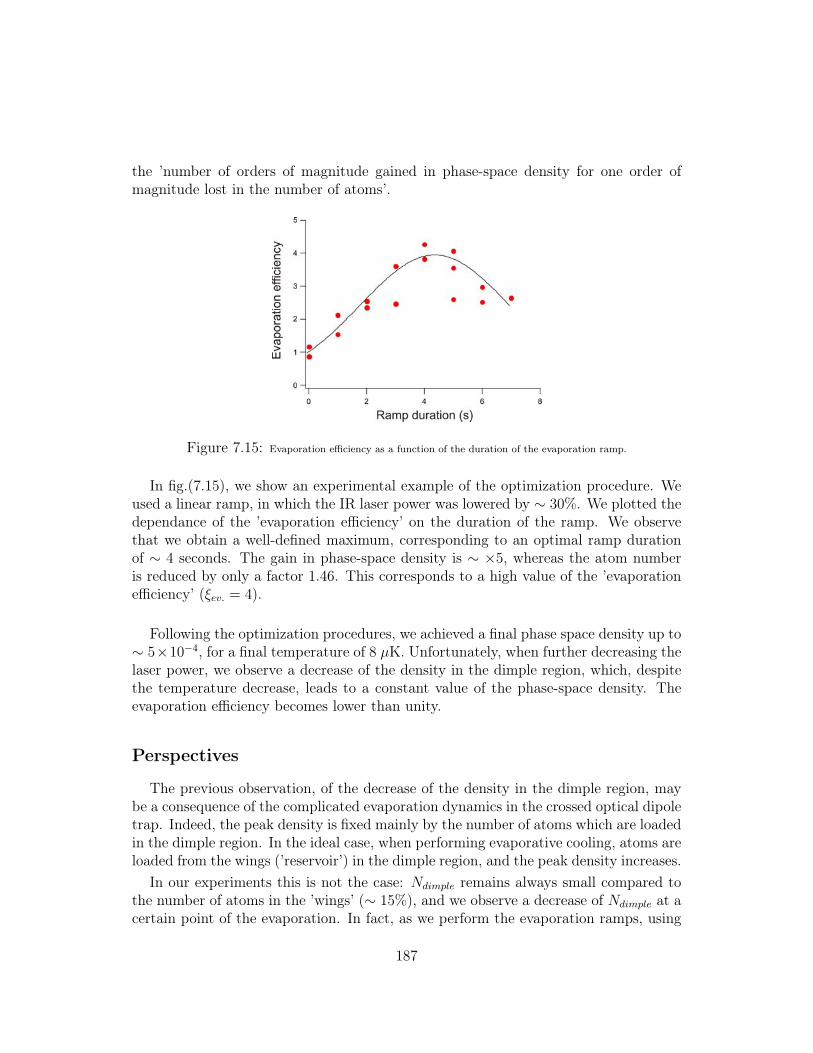
the ’number of orders of magnitude gained in phase-space density for one order ofmagnitude lost in the number of atoms’.

Figure 7.15: Evaporation efficiency as a function of the duration of the evaporation ramp.

In fig.(7.15), we show an experimental example of the optimization procedure. Weused a linear ramp, in which the IR laser power was lowered by ∼ 30%. We plotted thedependance of the ’evaporation efficiency’ on the duration of the ramp. We observethat we obtain a well-defined maximum, corresponding to an optimal ramp durationof ∼ 4 seconds. The gain in phase-space density is ∼ ×5, whereas the atom numberis reduced by only a factor 1.46. This corresponds to a high value of the ’evaporationefficiency’ (ξev. = 4).

Following the optimization procedures, we achieved a final phase space density up to∼ 5×10−4, for a final temperature of 8 μK. Unfortunately, when further decreasing thelaser power, we observe a decrease of the density in the dimple region, which, despitethe temperature decrease, leads to a constant value of the phase-space density. Theevaporation efficiency becomes lower than unity.

Perspectives

The previous observation, of the decrease of the density in the dimple region, maybe a consequence of the complicated evaporation dynamics in the crossed optical dipoletrap. Indeed, the peak density is fixed mainly by the number of atoms which are loadedin the dimple region. In the ideal case, when performing evaporative cooling, atoms areloaded from the wings (’reservoir’) in the dimple region, and the peak density increases.

In our experiments this is not the case: Ndimple remains always small compared tothe number of atoms in the ’wings’ (∼ 15%), and we observe a decrease of Ndimple at acertain point of the evaporation. In fact, as we perform the evaporation ramps, using

187

the AOM, the power decreases both in the horizontal and in the vertical beam (theratio of the two being constant, fixed by the angle of the λ/2−wave plate). This maylead to a situation where the atoms actually leave the dimple region into the wings (i.e.the dimple evaporation rate exceeds the loading rate, due to the atoms in the wings).

A possibility for canceling this effect is, for example, to maintain a constant powerin the vertical beam while decreasing the power of the horizontal trap. Although moredifficult in our current setup, this is possible by compensating the power decrease(due to the forced evaporation of the wings) by a rotation of the λ/2 plate. Somepreliminary tests showed that this allows, for the same final temperature and totalnumber of atoms, to obtain more atoms in the dimple region. Similar techniques,consisting in evaporating the atom reservoir in the ’wings’ for lowering the temperatureof the dimple, is currently used in other BEC experiments [100, 26].

Another perspective, which would allow to use longer evaporation ramps, is to in-crease the lifetime related to background gas collisions (currently limited to 30 s).There are several possibilities: either baking the cell or cooling it, with an externalchiller.

Other perspectives, currently under development in our group, consist in increasingthe initial number of atoms in the single-beam ODT. Increasing the initial number ofatoms (and density) could mean higher elastic collision rates, which would increase theevaporation speed; under these circumstances the limitation related to background gascollisions would be less important.

Yet another perspective would be to implement a cooling scheme, which is efficientfor Cr: demagnetization cooling. This scheme, proposed and demonstrated in the groupof T.Pfau [111], is particularly appealing as is permits to decrease the temperaturewithout loosing atoms. The authors found a very high evaporation efficiency, of about15, and the final limitation (when the temperature approaches 10 μK) was due to thedifficulty to control the magnetic fields ’accurately enough’.

In our case, the possibility is particularly appealing, as the initial number of atomsin the ODT is equivalent, but the temperature is considerably higher.

188

Conclusions

During my thesis, a new cold atom experiment for Cr atoms was designed andbuilt. The technical solutions, which have been detailed in this dissertation, are quitedifferent from the ones used in other similar experiments, mostly performed with alka-lis. The realization of a hot Cr oven, functioning around 1500◦C, as well as differenttests of materials were presented; the lasers system – providing ∼ 300 mW of 425 nmlaser light (a wavelength which is not available with diode lasers) was built and stabi-lized on an atomic transition. The experiment which was built during my thesis is aZeeman-slower-fed MOT. Both 52Cr and 53Cr MOTs were obtained and studied, eitherseparately or simultaneously.

The experiments presented in this dissertation improved the knowledge about theproperties of Cr atoms. Some of them have already been studied elsewhere: for exam-ple, our experiments confirmed a large inelastic collision parameter βMOT ∼ 6.3×10−10

cm3/s in a 52Cr MOT, but they also allowed us to measure it in the case of the fermionicMOT, which has values almost one order of magnitude higher. A large inter-isotopeinelastic collision parameter βMOT ∼ 2× 10−9 cm3/s was also measured. A theoreticalmodel was developed to understand better these results, and to account for the dif-ference with the alkali atoms – for which light-assisted collision parameters are muchsmaller, and the loss mechanisms are well understood. This model indicates that, inthe case of Cr, (almost) all pair of atoms, excited by the MOT beams and reaching atypical interparticle distance ∼ λ/2π, are mysteriously expelled from the trap.

Due to the high inelastic collision parameters, the number of atoms in Cr steady-state MOTs are limited to a few 106. To reach BEC, our strategy is to first accumulateatoms in the metastable 5D states, which are shielded from the MOT light-assistedcollisions. For this reason, the measurement of the elastic and inelastic collisionalproperties of the metastable Cr atoms had a major importance for us, and led to abetter understanding of the accumulation results.

Experiments performed in a quadrupole magnetic trap led to the measurement ofthe inelastic collision parameter βDD = 3.3 × 10−11 cm3/s between metastable atoms.Further experiments, involving RF magnetic field which truncate the magnetic trap,provided a measurement of the elastic collision cross section between metastable atoms

189

Cr isotope Value Error bar Unit53Cr βMOT = 4 × 10−9 ±40 % cm3/s53Cr γPD= 250 ±30 % s−1

52Cr – 53Cr βMOT = 1.8 × 10−9 ±40 % cm3/s52Cr βMOT = 6.3 × 10−10 ±35 % cm3/s52Cr βDD = 3.3 × 10−11 ±20 % cm3/s52Cr σel,DD= 7 × 10−12 ±50 % cm2

52Cr βPD = 4.9 × 10−10 ±15 % cm3/s

Table 7.1: Properties of the Cr which have been measured in this work.

σel = 7×10−12 cm2, close to the unitary limit, as well as the inelastic collision parame-ter with the excited atoms from the MOT βPD = 4.9×10−10 cm3/s. Finally, parametricexcitation experiments in an optical dipole trap (ODT) loaded with metastable atomsyielded a measurement of the AC Stark shift of these states.

The work presented here explored new trapping methods for metastable Cr atoms.For example, I demonstrated the continuous loading of metastable 52Cr atoms in a RF-truncated magnetic: in this scheme, accumulation and evaporation are simultaneous.This leads to the fast production, within less than 1 s, of a cold, magnetically trappedsample, having a phase-space density as high as 7 × 10−6 (see fig.(7.16)), which repre-sents an increase by almost one order of magnitude compared to the MOT phase-spacedensity. A theoretical model, using rate equation for the mean energy and number ofatoms, showed that this value is limited by inelastic collisions, mostly with the excitedMOT atoms.

Figure 7.16: Increase of the phase-space density of the cloud of 52Cr metastable atoms, accumulated in a RF-truncated magnetic state.

Even though the inelastic collision properties of Cr do not allow to reach condensa-tion in the metastable states, our experiments may be interesting in the perspective ofcontinuously loading a magnetic waveguide – for BEC or atom optics experiments.

190

Because dipolar relaxation is ultimately the major obstacle for condensing Cr in amagnetic trap, our experiments aiming towards condensation will be performed in anoptical trap. The very same inelastic collisional processes, as well as Majorana losses,make difficult the transfer of a Cr cloud from a quadrupole magnetic trap to an ODT.We developed a new accumulation technique to trap metastable atoms into a mixedmagnetic+optical trap. This is an original method, which allows us to load up to1.2 × 106 atoms (see fig.(7.17)) at 100 μK in a very short time (∼ 200 ms). Studiesof the loading dynamics of the mixed trap showed that the accumulation is limited byMajorana spin-flips and inelastic collisions between metastable atoms.

Figure 7.17: Loading of a single-beam optical dipole trap with metastable 52Cr atoms.

Using RF fields to modify magnetic potentials is a very interesting idea, openingnew ways for original trapping mechanisms. In this respect, we demonstrated thata magnetic quadrupole potential, modified by the RF, is able to capture not onlythe low-field seekers, but also the high-field seeking MOT atoms which decay to themetastable states. Low-field seekers are trapped close to the B = 0 point, whilehigh-field seekers are first expelled from the center of the quadrupole trap. However,once they reach the point where the RF field is resonant, their spin is flipped, andmagnetic forces bring them back to the center of the trap. An interesting applicationin the context of Cr would be to create large-volume, magnetically trapped metastablesamples, with lower densities, which presumably would allow to trap a higher numberof atoms. Furthermore, as atoms are trapped in the minima which are away from theB = 0 point, Majorana spin-flips are expected to induce negligible losses in such aconfiguration.

There is a technical difficulty for this method, residing in the existence of RF sec-ond harmonics, and which turned out difficult to overcome. In the case of a purelyquadrupole trap, high-field seekers, produced around B = 0, always reach the positionof the second RF harmonics resonance. There, their spin may be flipped again, whichprojects them back into a state which is expelled. We proved that, in presence of anadditional optical dipole confinement, the atoms are prevented from reaching 2RRF ,and are no longer expelled.

The use of the RF fields allows one to remove the influence of Majorana spin-flips(which is otherwise one of the limiting factors in the ODT) and to increase the number

191

Figure 7.18: Reduction of the Majorana losses in a mixed, optical+quadrupole magnetic trap, which leads to anincrease of the number of atoms accumulated in the ODT.

of atoms trapped in the optical dipole trap, as it is shown in fig.(7.18). Finally, currentstudies which are under development in our group, demonstrated the possibility of us-ing RF sweeps for periodically reversing the spins of atoms at a fast rate, for ’erasing’(i.e. averaging to zero) the strongly-confining magnetic potential of the mixed trap.These experiments (not presented in this manuscript) allowed us to further increase,by a factor of two, the number of atoms in the ODT.

The work performed during my Ph.D. opens perspectives for finding an originalroute towards Bose-Einstein condensation of Cr. Future experiments will study theoptimization of evaporative cooling in a crossed optical dipole trap; preliminary exper-imental procedures in this direction were presented here.

The results obtained for magneto-optical trapping of the fermionic isotope show thatsympathetic cooling by the boson will probably be the way towards obtaining the firstFermi sea, as well as the first degenerate Bose-Fermi mixture with strong dipole-dipoleinteractions. The path is still long, and experiments will be very exciting...

With Cr, the perspectives for fundamental studies in the quantum regimes arenumerous. From the experimental point of view, our setup gives the possibility oftransferring the atoms into optical lattices. There, the anisotropic character of thedipole-dipole interactions is expected to lead to many interesting effects, related to thereduced geometries. In a 2D geometry of pancake-shaped planes, repulsions due tothe dipole-dipole interactions – when the spins are perpendicular to the planes – maylead to a strong reduction of the three-body recombination rate; in a 1D geometry,in presence of attractive interactions, one may observe the formation of solitons. Ina spin-polarized sample of dipolar fermionic atoms, where contact interaction is sup-pressed at low temperature, dipole-dipole interactions may lead to the observation ofthermalization.

These are only three ideas developed by our group, which, I hope, give a flavor aboutthe richness of the physics of dipole-dipole interactions in the degenerate regime, whichcan be performed with Cr.

192

Appendix

193

Appendix A

Hyperfine splitting and nonlinearZeeman effect

In this appendix we briefly summarize the physics of the hyperfine coupling, whichis responsible for the hyperfine splitting of the atomic levels, but also for the non-linearZeeman effect.

A.1 Hyperfine splitting

The hyperfine coupling interaction hamiltonian HHyp is given by:

HHyp = AI · J (A.1)

where A is the coupling constant. HHyp couples the nuclear spin I to the electronicmomentum J. This means that, in presence of the hyperfine interaction, the so-called’decoupled basis’ |I, J, mI , mJ〉 (or simply |mI , mJ〉 – defined by a set of commoneigenvectors of I, J, Iz, Jz), does no longer diagonalize the total atomic hamiltonian.HHyp can however be written as:

HHyp =A

2

[F2 − J2 − I2

](A.2)

where F = I+J. The hyperfine interaction hamiltonian (and the total atomic hamilto-nian) are thus diagonal in the so-called ’coupled basis’ |I, J, F, mF 〉 (or simply |F, mF 〉– defined by a set of common eigenvectors of I, J, F, Fz).

Using this basis, we calculate the eigenenergies of the hyperfine hamiltonian, whichare given by:

HHyp =A

2h2 [F (F + 1) − I(I + 1) − J(J + 1)] (A.3)

This formula is used for finding the hyperfine structure of the atomic levels (seeChapter(1)).

195

A.2 Non-linear Zeeman effect

In presence of a magnetic field, we add the Zeeman interaction hamiltonian:

HZ = BgJμB

hJz . (A.4)

where Jz is the projection of J on the quantization axis given by the direction of themagnetic field1 (with the corresponding eigenvalues hmJ).

In order to diagonalize the hamiltonian HHyp + HZ , and find the eigenenergies as afunction of the external magnetic field, we may write it in the |F, mF 〉 basis:

〈F ′, m′F |H|F, mF 〉 = B · gJμB

∑mI ,mJ

mJ〈F ′, m′F |mI , mJ〉〈mJ , mI |F, mF 〉

+A

2h2 [F (F + 1) − I(I + 1) − J(J + 1)] (A.5)

In practice, for example to calculate the Zeeman effect for the 53Cr transitions inthe ZS, we use a mathematica program Mathematica to numerically diagonalize thehamiltonian given by eq.(A.5). For the ground-state of 53Cr, it is a 28 × 28 matrix,and a 36 × 36 for the 7P4 excited state.

The scalar products in the sum are nothing else than the ’common’ Clebsch-Gordancoefficients, which can be found using the ’ClebschGordan’ Mathematica function:〈mJ , mI |F, mF 〉 ≡ ClebschGordan[{J,mJ}, {I,mI}, {F, mF}].

1 Due to the fact that the nuclear magneton much smaller then the Bohr magneton (μN � μB)we neglected the nuclear magnetic moment, which is much smaller than the electronic one

196

Appendix B

Chromium light assisted collisions

B.1 Survival probability

I detail here the calculation of the survival probability which implies some subtleties.I consider the case where the lifetime of the excited molecular state, Γ−1

M , does notdepend on the interatomic distance. Since losses are expected to take place mostlyat distances R′ � R, I will also consider that S(R, R′) S(R, 0). In this case theeq.(4.18) becomes:

S(R, R′) exp

⎛⎜⎝−ΓM

t(0)∫t(R)

dt′

⎞⎟⎠ = exp

⎛⎝−ΓM

R∫0

dr

v(r)

⎞⎠ , (B.1)

where v(r) is the velocity acquired by the atom (which is traveling on the excited statepotential) when arriving at a distance r. To evaluate v(r), we can use the energyconservation for the evolution from the excitation point R and r:

μv(r)2

2+

h2l(l + 1)

2μr2− C3

r3=

μv(R, E, l)2

2+

h2l(l + 1)

2μR2− C3

R3. (B.2)

Using the previous expression (4.15) for v(R, E, l) we find:

v(r) =

√√√√ 2

μ

(E − C3

R3+

C3

r3− h2l(l + 1)

2μr2

)(B.3)

and the survival probability becomes:

S(R, 0) = exp

⎛⎜⎜⎝−ΓM

R∫0

dr√2μ

(E − C3

R3 + C3

r3 − h2l(l+1)2μr2

)⎞⎟⎟⎠ . (B.4)

197

Figure B.1: Evolution on the excited effective potential.

It is important to notice that there are certain values for the (RE,l parameters thatmight give negative values for v(r) in eq.(B.3). The situation is explained in fig.(B.1),considering the case where the classical turning point in the ground state, RE,l, is onthe left-hand-side of the excited state barrier R0(l).

If the atom-pair is excited in Rexc between R0(l) and RE,l, it may always reachR = 0, as it is created on the attractive part of the effective potential.

On the other hand, if the excitation occurs at Rexc > R0(l), the situation becomesslightly more complicated, as the pair is ’created’ on the repulsive part of the effectiveexcited potential. It can thus be ’reflected’, if its energy at the excitation point is lowerthan the excited state barrier, i.e. if:

E − C3

R3exc

< V (R0) (B.5)

When calculating the survival probability we impose thus an additional restriction onthe R−integration domain in eq.(4.19), which eliminates the excitation radius betweenR0 and Rrefl. =

(C3

E−V (R0)

)1/3.

B.2 Excitation rate

Julienne and Vigué use the following expression for the excitation rate:

Ωexc(R) =λ2

2π

(Γ/2)2

Γ2/4 + (δ0 − C3/R3)2I0. (B.6)

This expression, valid in the low excitation regime (I0 � Isat), shows a linear depen-dence of the excitation rate on the laser intensity.

198

The JV model often considered as a ’quasi-static’ model, because the excitation ratein eq.B.6 supposes that the optical pumping is very fast and the stationary populationof the excited state is reached for every R. The low excitation also implies that theexcited stationary population always remains very small compared to the ground statepopulation.

In the experimental conditions that we used when measuring the light assisted col-lision parameters, the low intensity condition was not fulfilled (we typically used totalMOT laser intensities of 10 to 20 Isat). We must thus take into account the saturationeffects which come to play. For that, we replaced the JV excitation rate by an expres-sion which is proportional to the product of the stationary populations in the ground-and excited-state:

Ωexc(R) = Γ

(Ω2/4

Ω2/2 + Γ2/4 + (δ0 − C3/hR3)2

)(1 − Ω2/4

Ω2/2 + Γ2/4 + (δ0 − C3/hR3)2

),

(B.7)where Ω = Γ

√I0/2Isat is the Rabi frequency. (B.7) expresses thus the fact that the

collision parameter β is proportional to the probability of exciting a pair. We consideredin our model that this probability is equal to the probability of having an atom in theground state, times the probability of having a second atom in the excited state.

We can easily see that (B.7) becomes identical to the JV rate (B.6) in the lowintensity regime, while for high intensity it saturates to Γ/4 (equal populations of 1/2in the ground and excited state).

B.3 Partial waves

An interesting result can be seen by plotting – see fig.(B.2) – the dependance of theterms in the sum given by eq.(4.19) as a function of the partial wave l. We observethat at high temperature, the cutoff is given qualitatively by lmax (see eq.(4.13)), i.e.the rotational barriers in the excited state.

At low temperature, the cutoff naturally occurs at l−values considerably smallerthan at high temperatures. This fact is explained as the effect of the centrifugalbarriers in the ground state, which gives another cutoff lmax,g < lmax [58], smaller thanthe one in the excited state (as the ground-state potential −C6/r

6 is flatter than the−C3/r

3 potential).

199

Figure B.2: Dependance of the terms in the sum (4.19) on the partial wave number l: at T = 100 μK (left) andT = 1 K (right). The corresponding cutoffs, due to excited potential rotation barriers, are lmax = 14 and respectivelylmax = 65.

200

Bibliography

[1] M. Anderson, J. Ensher, M. Matthews, C. Wieman, and E. Cornell, Observation ofBose-Einstein Condensation in a Dilute Atomic Vapor – Science, 269, 198 (1995)

[2] K. Davis, M.-O. Mewes, M. Andrews, N. van Druten, D. Durfee, D. Kurn,and W. Ketterle, Bose-Einstein Condensation in a Gas of Sodium Atoms –Phys. Rev. Lett., 75, 3969 (1995)

[3] B. DeMarco and D.S. Jin, Onset of Fermi degeneracy in a trapped atomic gas –Science., 285, 1703 (1999)

[4] J. M. Gerton, D. Strekalov, I. Prodan, and R. G. Hulet, BDirect observation ofgrowth and collapse of a Bose-Einstein condensate with attractive interactions –Nature, 408, 692 (2000)

[5] J. R. Ensher, D. S. Jin, M. R. Matthews, C. E. Wieman, and E. A. Cornell, Bose-Einstein Condensation in a Dilute Gas: Measurement of Energy and Ground-StateOccupation – Phys. Rev. Lett., 77, 4984 (1996) L. V. Hau, B. D. Busch, C.

[6] Liu, Z. Dutton, M. M. Burns, and J. A. Golovchenko Near-resonant spa-tial images of confined Bose-Einstein condensates in a 4-Dee magnetic bottle –Phys. Rev. A, 58, R54 (1998)

[7] F. Dalfovo, S. Giorgini, L. P. Pitaevskii, and S. Stringari Theory of Bose-Einsteincondensation in trapped gases – Rev. Mod. Phys., 71, 463 (1999)

[8] M. R. Andrews, C. G. Townsend, H.-J. Miesner, D. S. Durfee, D. M. Kurn,and W. Ketterle, Observation of interference between two Bose condensates –Science, 275, 637 (1997)

[9] M.-O. Mewes, M. R. Andrews, D. M. Kurn, D. S. Durfee, C. G. Townsend,and W. Ketterle, Output Coupler for Bose-Einstein Condensed Atoms –Phys. Rev. Lett., 78, 582 (1997)

[10] Immanuel Bloch, Theodor W. Hänsch, and Tilman Esslinger, Atom Laser with acw Output Coupler – Phys. Rev. Lett., 82, 3008 (1999)

201

[11] K. W. Madison, F. Chevy, W. Wohlleben, and J. Dalibard, Vortex Formation ina Stirred Bose-Einstein Condensate – Phys. Rev. Lett., 84, 806-809 (2000)

[12] M. R. Matthews, B. P. Anderson, P. C. Haljan, D. S. Hall, C. E.Wieman, and E. A. Cornell, Vortices in a Bose-Einstein Condensate –Phys. Rev. Lett., 83, 2498 (1999)

[13] M. Greiner, O. Mandel, T. Esslinger, T. H¨ansch, and I. Bloch, Quantum PhaseTransition from a Superfluid to a Mott Insulator in a Gas of Ultracold Atoms –Nature, 415, 39 (2002)

[14] T. Stoferle, H. Moritz, C. Schori, M. Kohl, and T. Esslinger, Tran-sition from a Strongly Interacting 1D Superfluid to a Mott Insulator –Phys. Rev. Lett., 92, 130403 (2004)

[15] B. Paredes, A. Widera, V. Murg, O. Mandel, S. Fölling, I. Cirac, G. V. Shlyap-nikov, T. W. Hänsch, and I. Bloch, Tonks-Girardeau gas of ultracold atoms in anoptical lattice – Nature, 429, 277 (2004)

[16] S. Jochim, M. Bartenstein, A. Altmeyer, G. Hendl, S. Riedl, C. Chin, J.Hecker Denschlag, and R. Grimm, Bose-Einstein Condensation of Molecules –Science, 302, 2101 (2003)

[17] M. W. Zwierlein, C. A. Stan, C. H. Schunck, S. M. F. Raupach, S. Gupta, Z. Hadz-ibabic, and W. Ketterle, Observation of Bose-Einstein Condensation of Molecules– Phys. Rev. Lett., 91, 250401 (2003)

[18] C. A. Regal, M. Greiner, and D. S. Jin, Observation of Resonance Condensationof Fermionic Atom Pairs – Phys. Rev. Lett., 92, 040403 (2004)

[19] T. Bourdel, L. Khaykovich, J. Cubizolles, J. Zhang, F. Chevy, M. Teichmann, L.Tarruell, S. J. J. M. F. Kokkelmans, and C. Salomon, Experimental Study of theBEC-BCS Crossover Region in Lithium 6 – Phys. Rev. Lett., 93, 050401 (2004)

[20] C. Chin, M. Bartenstein, A. Altmeyer, S. Riedl, S. Jochim, J. H. Denschlag, andR. Grimm, Observation of the Pairing Gap in a Strongly Interacting Fermi Gas –Science, 305, 1128 (2004)

[21] M. W. Zwierlein, C. A. Stan, C. H. Schunck, S. M. F. Raupach, A. J. Kerman, andW. Ketterle, Condensation of Pairs of Fermionic Atoms near a Feshbach Resonance– Phys. Rev. Lett., 92, 120403 (2004)

[22] L. Santos, G. V. Shlyapnikov, P. Zoller, and M. Lewenstein, Bose-Einstein Con-densation in Trapped Dipolar Gases – Phys. Rev. Lett., 85, 1791 (2000)

202

[23] K. Goral, K. Rzazewski, and T. Pfau, Bose-Einstein condensation with magneticdipole-dipole forces – Phys. Rev. A, 61, 051601 (2000)

[24] K. Goral, L. Santos, and M. Lewenstein, Quantum Phases of Dipolar Bosons inOptical Lattices – Phys. Rev. Lett., 88, 170406 (2002)

[25] L. Santos, G. V. Shlyapnikov, and M. Lewenstein, Roton-Maxon Spec-trum and Stability of Trapped Dipolar Bose-Einstein Condensates –Phys. Rev. Lett., 90, 250403 (2003)

[26] A. Griesmaier, J. Werner, S. Hensler, J. Stuhler and T. Pfau, Bose-Einstein con-densation of chromium – Phys. Rev. Lett, 94, 160401 (2005)

[27] J. Stuhler, A. Griesmaier, T. Koch, M. Fattori, S. Giovanazzi, P. Pedri, L. Santosand T. Pfau, Observation of Dipole-Dipole Interaction in a Degenerate QuantumGas – Phys. Rev. Lett., 95, 150406 (2005)

[28] Th. Lahaye, T. Koch, B. Fröhlich, M. Fattori, J. Metz, A. Griesmaier,S. Giovanazzi, T. Pfau, Strong dipolar effects in a quantum ferrofluid –Nature, 448, 672 (2007)

[29] A.S. Bell, J. Stuhler, S. Locher, S. Hensler, J. Mlynek and T. Pfau – A magneto-optical trap for chromium with population repumping via intercombination lines –Europhys. Lett., 45, 156 (1999)

[30] C. C. Bradley, J. J. McClelland, W. R. Anderson and R. J. Celotta, Magneto-optical trapping of chromium atoms – Phys. Rev. A, 61, 053407 (2000)

[31] Jürgen Stuhler, Ph.D. thesis, Kontinuierliches Laden einer Magnetfalle mitlasergekühlten Chromatomen – Universität Konstanz –(2001)

[32] Jonathan David Weinstein, Ph.D. thesis, Magnetic Trapping of Atomic Chromiumand Molecular Calcium Monohydride – Harvard University – (2001)

[33] Handbook of Physics and Chemistry (2000)

[34] Arnaud Pouderous, Ph.D. thesis, Refroidissement et piegeage d’atomes de Chrome– Université Paris Nord – (2007)

[35] T.W. Hänsch and B. Couillaud Laser frequency stabilization by polarization spec-troscopy of a reflecting reference cavity – Optics. Comm., 35, 441 (1980)

[36] R.W.P. Drever, J.L. Hall, F.V. Kowalski, J. Hough, G.M. Ford, A.J. Munley, andH. Ward, Laser phase and frequency stabilization using an optical resonator –Appl. Phys. B., 31, 97 (1983)

203

[37] Antoine Browaeys, Ph.D. thesis, Piegeage magnetique d’un gaz d’heliummetastable : vers la condensation de Bose-Einstein – Université Paris Sud –(2000)

[38] W. D. Phillips and H. Metcalf – Laser Deceleration of an Atomic Beam –Phys. Rev. Lett., 48, 596 (1982)

[39] P. A. Molenaar, P. van der Straten, H. G. M. Heideman, and H. Metcalf – Di-agnostic technique for Zeeman-compensated atomic beam slowing: Technique andresults – Phys. Rev. A, 55, 605 (1997)

[40] F. Reif, Fundamentals of Statistical and Thermal Physics (McGraw-Hill, NewYork, 1965)

[41] K. M. O’Hara, S. R. Granade, M. E. Gehm, and J. E. Thomas – Loading dynamicsof CO2 laser traps – Phys. Rev. A, 63, 043403 (2001)

[42] J. D. Weinstein, R. deCarvalho, C. I. Hancox, and J. M. Doyle – Evaporativecooling of atomic chromium – Phys. Rev. A, 65, 021604 (2002)

[43] P. O. Schmidt, S. Hensler, J. Werner, T. Binhammer, A. Gorlitz and T. Pfau– Continuous loading of cold atoms into a Ioffe-Pritchard magnetic trap –J. Opt.B.:Quantum Semiclass. Opt., 5, S170-S177 (2003)

[44] H. C. Mastwijk, J. W. Thomsen, P. van der Straten, and A. Niehaus – OpticalCollisions of Cold, Metastable Helium Atoms – Phys. Rev. Lett., 80, 5516 (1998)

[45] Paul J. J. Tol, Norbert Herschbach, Eric A. Hessels, Wim Hogervorst, and WimVassen – Large numbers of cold metastable helium atoms in a magneto-optical trap– Phys. Rev. A., 60, 5516 (1998)

[46] F. Bardou, O. Emile, J.M. Courty, C.I. Westbrook and A. Aspect, – Magneto-optical Trapping of Metastable Helium: Collisions in the Presence of ResonantLight. – Europhys. Lett., 20, 681 (1992)

[47] F. Pereira Dos Santos, F. Perales, J. Léonard, A. Sinatra, J. Wang, F. S. Pavone,E.Rasel, C. S. Unnikrishnan, and M. Leduc, – Efficient magneto-optical trapping ofa metastable helium gas. – Eur. Phys. J. AP, 14, 68-76 (2001)

[48] Kalle-Antti Suominen, – Theories for cold atomic collisions in light fields. –J. Phys. B.: At. Mol. Opt. Phys., 29, 5981-6007 (1996)

[49] M. J. Holland, K.-A. Suominen, and K. Burnett, – Cold collisions ina laser field: Quantum Monte Carlo treatment of radiative heating. –Phys. Rev. A., 50, 1513 (1994)

[50] Band Y. B., Tuvi I., Suominen K.-A., Burnett K. and Julienne P. S., – Loss frommagneto-optical traps in strong laser fields. – Phys. Rev. A., 50, R2826 (1994)

204

[51] R. Chicireanu, A. Pouderous, R. Barbé, B. Laburthe-Tolra, E. Maréchal, L.Vernac, J.-C. Keller and O. Gorceix, – Simultaneous magneto-optical trapping ofbosonic and fermionic chromium atoms – Phys. Rev. A, 73, 053406 (2006)

[52] F. Pereira Dos Santos, F. Perales, J. Léonard, A. Sinatra, Junmin Wang, F.S.Savone, E. Rasel, C.S. Unnikrishnan, M. Leduc, – Penning collisions of laser-cooledmetastable helium atoms – Eur. Phys. J. D, 14, 15-27 (2001)

[53] L. G. Marcassa, G. D. Telles, S. R. Muniz, and V. S. Bagnato, – Collisional lossesin a K-Rb cold mixture – Phys. Rev. A., 63, 013413 (2000)

[54] M. Marinescu, and A. Dalgarno, – Dispersion forces and long-rangeelectronic transition dipole moments of alkali-metal dimer excited states –Phys. Rev. A, 52, 331 (1995)

[55] E. I. Dashevskaya, A. I. Voronin, and E. E. Nikitin, – Theory of ex-citation transfer in collisions between alkali atoms. I. Identical partners –Can. J. Phys., 47, 1237 (1969)

[56] W. J. Meath, – Retarded Interaction Energies between Like Atoms in DifferentEnergy States – J. Chem. Phys., 48, 227 (1968)

[57] J. Léonard, A. P. Mosk, M. Walhout, P. van der Straten, M. Leduc, and C.Cohen-Tannoudji, – Analysis of photoassociation spectra for giant helium dimers– Phys. Rev. A, 69, 032702 (2004)

[58] P. S. Julienne, J. Vigué, Cold collisions of ground- and excited-state alkali-metalatoms – Phys. Rev. A., 44, 4464 (1991)

[59] P. L. Gould, P. D. Lett, P. S. Julienne, W. D. Phillips, H. R. Thorsheim and J.Weiner – Observation of associative ionization of ultracold laser-trapped sodiumatoms – Opt. Lett., 60, 788 (1988)

[60] M. G. Prentiss, A. Cable, J. E. Bjorkholm, S. Chu, E. L. Raab, andD. E. Pritchard – Atomic-density-dependent losses in an optical trap –Phys. Rev. A., 13, 452 (1988)

[61] A. Gallager, D. E. Pritchard– Exoergic Collisions of Cold Na∗-Na –Phys. Rev. Lett., 63, 957 (1989)

[62] D. Sesko, T. Walker, C. Monroe, A. Gallagher, and C. Wieman – Collisionallosses from a light-force atom trap – Phys. Rev. A., 63, 961 (1989)

[63] P. D. Lett, W. D. Phillips, S. L. Rolston, C. E. Tanner, R. N. Watts and C. I.Westbrook, – Optical Molasses – J. Opt. Soc. Am. B., 6, 2084 (1989)

205

[64] Thad Walker, David Sesko, and Carl Wieman, – Collective Behavior of OpticallyTrapped Neutral Atoms – Phys. Rev. lett., 64, 408 (1990)

[65] David Sesko, Thad Walker, and Carl Wieman, – Behavior of neutral atoms in aspontaneous force trap – J. Opt.Soc. Am. B., 8, 946 (1991)

[66] G. Modugno, G. Ferrari, G. Roati, R. J. Brecha, A. Simoni, M. Inguscio ,– Bose-Einstein Condensation of Potassium Atoms by Sympathetic Cooling –Science, 294, 1320 (2001)

[67] C. Silber, S. Günther, C. Marzok, B. Deh, Ph. W. Courteille, and C. Zimmer-mann, – Quantum-Degenerate Mixture of Fermionic Lithium and Bosonic Rubid-ium Gases – Phys. Rev. Lett, 95, 170408 (2005)

[68] F. Schreck, L. Khaykovich, K. L. Corwin, G. Ferrari, T. Bourdel, J. Cubizolles,and C. Salomon, – Quasipure Bose-Einstein Condensate Immersed in a Fermi Sea– Phys. Rev. Lett, 87, 080403 (2001)

[69] J. M. McNamara, T. Jeltes, A. S. Tychkov, W. Hogervorst, andW. Vassen, – Degenerate Bose-Fermi Mixture of Metastable Atoms –Phys. Rev. Lett, 97, 080404 (2006)

[70] H. C. Mastwijk, J. W. Thomsen, P. van der Straten, and A. Niehaus, –Optical Collisions of Cold, Metastable Helium Atoms –Phys. Rev. Lett., 80, 5516 (1998)

[71] T. P. Dinneen, K. R. Vogel, E. Arimondo, J. L. Hall, A. Gallager, – Cold collisonsof Sr∗-Sr in a mgneto-optical trap – Phys. Rev. A., 59, 1216 (1999)

[72] M.W. Müller, A. Merz, M.-W. Ruf, H. Hotop, W. Meyer, and M Movre,– Experimental and theoretical studies of He Bi-excited collision systemsHe*(2 3S)+He*(2 3S, 2 1S) at thermal and subthermal kinetic energies –Z. Phys. D., Atoms, Molecules and Clusters 21, 89 (1991)

[73] P. O. Fedichev, M. W. Reynolds, U. M. Rahmanov, and G. V. Shlyap-nikov – Inelastic decay processes in a gas of spin-polarized triplet helium –Phys. Rev. A. 53, 1447 (1996)

[74] M. Walhout, U. Sterr, C. Orzel , M. Hoogerland, and S. L. Rolston, – Optical Con-trol of Ultracold Collisions in Metastable Xenon – Phys. Rev. Lett., 74, 506 (1995)

[75] Stephan Ritter, Anton Öttl, Tobias Donner, Thomas Bourdel, Michael Köhl, andTilman Esslinger, – Observing the Formation of Long-Range Order during Bose-Einstein Condensation – Phys. Rev. Lett., 98, 090402 (2007)

206

[76] S. Hensler, J. Werner, A. Griesmaier, P.O. Schmidt, A. Görlitz, T. Pfau, S. Gio-vanazzi and K. Rzazewski, – Dipolar Relaxation in an ultra-cold Gas of magneticallytrapped chromium atoms – Appl. Phys. B., 77, 765 (2003)

[77] Robert deCarvalho and John Doyle, – Evaporative cooling at low trap depth –Phys. Rev. A., 70, 053709 (2004)

[78] D. Comparat, A. Fioretti, G. Stern, E. Dimova, B. Laburthe Tolra, andP. Pillet, – Optimized production of large Bose-Einstein condensates –Phys. Rev. A., 73, 043410 (2006)

[79] O. J. Luiten, M. W. Reynolds, and J. T. M. Walraven, – Kinetic theory of theevaporative cooling of a trapped gas – Phys. Rev. A., 53, 381 (1996)

[80] Wolfgang Petrich, Michael H. Anderson, Jason R. Ensher, and Eric A. Cornell, –Stable, Tightly Confining Magnetic Trap for Evaporative Cooling of Neutral Atoms– Phys. Rev. A., 74, 3352 (1995)

[81] J. Stuhler, P. O. Schmidt, S. Hensler, J. Werner, J. Mlynek, and T. Pfau, –Continuous loading of a magnetic trap – Phys. Rev. A., 64, 031405(R) (2001)

[82] K. Huang, – Statistical Mechanics – Wiley, New York (1987)

[83] O. Zobay et B.M. Garraway, – Two-dimensional atom trapping in field-inducedadiabatic potentials – Phys. Rev. Lett., 86, 1195 (2001)

[84] Y. Colombe, E. Knyazchyan, O. Morizot, B. Mercier, V. Lorent and H. Perrin,– Ultracold atoms confined in rf-induced two-dimensional trapping potentials –Europhys. Lett., 67, 593 (2004)

[85] Yves Colombe, Ph.D. thesis, Condensat de Bose-Einstein, champs evanescents etpiegeage bidimensionel – Université Paris Nord – (2004)

[86] L. Landau, – Zur Theorie der Energieübertragung - II – Phys. Z. Sowjetunion,2, 46 (1932)

[87] C. Zener, – Non-adiabatic crossing of energy levels – Proc. R. Soc. London Ser.A, 137, 696 (1932)

[88] N. V. Vitanov and K.-A. Suominen, – Time-dependent control of ultracold atomsin magnetic traps – Phys. Rev. A, 56, R4377 (1997)

[89] J.R. Rubbmark, M.M. Kash, M.G. Littman et D. Kleppner, – Dynamical effectsat avoided level crossings: a study of the Landau-Zener effect using Rydberd atoms– Phys. Rev. A, 23, 3107 (1981)

207

[90] Piet O. Schmidt, Ph.D. thesis, Scattering properties of ultra-cold chromium atoms– Universität Stuttgart – (2003)

[91] R. Grimm, M. Weidemüller, and Y. B. Ovchinnikov, – Optical dipole traps for neu-tral atoms – Advances in Atomic, Molecular, and Optical Physics, 42, 95 (2000)

[92] C. Cohen-Tannoudji, J. Dupont-Roc, and G. Grynberg, – Processus d’interactionentre photons et atomes – EDP Sciences (1996)

[93] J. D. Jackson, – Classical electrodynamics – Wiley, New York (1962)

[94] Claude Cohen-Tannoudji, Bernard Diu, Franck Laloë, – Mécanique quantique –Hermann (1997)

[95] K. M. O’Hara, S. R. Granade, M. E. Gehm, T. A. Savard, S. Bali, andJ. E. Thomas, – Ultrastable CO2 Laser Trapping of Lithium Fermions –Phys. Rev. Lett., 82, 4204 (1999)

[96] K. M. O’Hara, S. R. Granade, M. E. Gehm, and J. E. Thomas, – Loading dynamicsof CO2 laser traps – Phys. Rev. A, 63, 043403 (2001)

[97] D. L. Haycock, S. E. Hamman, G. Klose, and P. S. Jessen, – Atomtrapping in deeply bound states of a far-off-resonance optical lattice –Phys. Rev. A, 55, R3991 (1997)

[98] T. Weber, Bose-Einstein Condensation of Optically Trapped Cesium – UniversitätStuttgart – (2003)

[99] M. D. Barrett, J. A. Sauer, and M. S. Chapman, – All-Optical Formation of anAtomic Bose-Einstein Condensate – Phys. Rev. Lett., 87, 010404 (2001)

[100] T. Weber, J. Herbig, M. Mark, H.-C. Nägerl, and R. Grimm, – Bose-EinsteinCondensation of Cesium – Science, 299, 232 (2003)

[101] J. V. Porto, – Private communications

[102] L. D. Landau and E. Lifshitz, – Mecanique – Moscou (1960)

[103] Axel Griesmaier, Ph.D. thesis, Dipole-dipole interaction in a degenerate quantumgas – Universität Stuttgart – (2006)

[104] Kenneth O’Hara, Ph.D. thesis, Optical Trapping and Evaporative Cooling ofFermionic Atoms – Duke University – (2000)

[105] S. Friebel, C. D’Andrea, J. Walz, M. Weitz, and T. W. Hänsch, – CO2-laseroptical lattice with cold rubidium atoms – Phys. Rev. A, 57, R20 (1998)

208

[106] NIST Atomic Spectra Database – http://physics.nist.gov/PhysRefData/ASD

[107] D. W. Snoke, and J. P. Wolfe, – Population dynamics of a Bose gas near satu-ration – Phys. Rev. B, 39, 4030 (1989)

[108] A. Robert, O. Sirjean, A. Browaeys, J. Poupard,dagger S. Nowak,ddagger D. Bo-iron, C. I. Westbrook, and A. Aspect, – A Bose-Einstein Condensate of MetastableAtoms – Science, 292, 461 (2001)

[109] D. Guéry-Odelin, J. Söding, P. Desbiolles, and J. Dalibard, – Is Bose-Einsteincondensation of atomic Cesium possible? – Europhys. Lett., 44, 25 (1998)

[110] A. Griesmaier, J. Stuhler, and T. Pfau, – Production of a chromium Bose-Einstein condensate – Appl. Phys. B., 82, 190404 (2006)

[111] M. Fattori, T. Koch, S. Goetz, A. Griesmaier, S. Hensler, J. Stuhler, and T. Pfau,– Demagnetization cooling of a gas – Nature Physics, 2, 765 (2006)

209

STUDIES OF COLD CHROMIUM ATOMS IN MAGNETIC ANDOPTICAL TRAPS: steps towards Bose-Einstein Condensation

Abstract: In the perspective of studying dipole-dipole interactions in quantum degenerate Bose andFermi gases, we have built an experimental setup for cooling and trapping Chromium (Cr) atoms.In this respect, one needs to use appropriate technological solution, such as a high-temperature oven(∼ 1500◦C) and a laser system providing high laser power at 425nm. Our experiments allow us toobtain magneto-optical traps for the two main isotopes of Cr (i.e. the bosonic 52Cr and the fermionic53Cr). These traps are characterized by large light-assisted collisional loss rates, which have beenstudied both experimentally and theoretically. The existence of radiative decay channels towardstwo long-lived metastable states allows the magnetic trapping and accumulation of fairly large atomnumbers of cold Cr atoms. We have studied the possibility of modifying the shape of these traps withthe use of RF magnetic fields, which allowed the study of collisional properties of Cr atoms in themetastable states. Finally, we have demonstrated a new continuous loading technique of an opticaldipole trap with more than one million metastable 52Cr atoms, at 100μK. The transfer into the groundstate and the polarization in the lowest-energy Zeeman sublevel opens the perspective for reachingthe Bose-Einstein condensation of Cr through evaporative cooling.Keywords: chromium, magneto-optical trapping, cold collisions, magnetic trapping, optical trap-ping, evaporative cooling

ATOMES FROIDS DE CHROME PIEGES MAGNETIQUEMENT ETOPTIQUEMENT: premières étapes vers la condensation

Résumé: Dans la perspective d’étudier les interactions dipolaires dans des gaz de bosons et defermions dégénérés, nous avons mis en place un dispositif expérimental pour refroidir et piéger lesatomes de chrome (Cr). Il faut pour cela recourir à des solutions technologiques particulières, commel’utilisation d’un four à haute température (∼ 1500◦C) et d’un dispositif laser délivrant une puis-sance lumineuse élevée à 425nm. Nos expériences permettent d’obtenir des pièges magnéto-optiquespour les deux isotopes majoritaires du Cr (le 52Cr bosonique et le 53Cr fermionique). Ces piègessont caractérisés par des forts taux de collisions inélastiques assistées par la lumière, que nous avonsétudié expérimentalement et théoriquement. La présence de fuites vers des états métastables permetl’accumulation dans des pièges magnétiques d’un nombre conséquent d’atomes. Nous avons aussiétudié la possibilité de modifier la forme de ces pièges, à l’aide de champs RF. Les propriétés col-lisionelles des états métastables sont étudiées en détail. Finalement, nous avons mis en œuvre unenouvelle méthode de chargement en continu d’un piège optique avec plus d’un million d’atomes mé-tastables de 52Cr, à 100μK. La polarisation des atomes de Cr dans l’état minimal en énergie du niveaufondamental ouvre des perspectives pour atteindre la condensation de Bose-Einstein du chrome parrefroidissement évaporatif.Mots clés: chrome, piégeage magnéto-optique, collisions froides, piégeage magnétique, piégeage op-tique, refroidissement évaporatif