r2mlwin: a package to run mlwin from within r

Zhang, Z., Parker, R., Charlton, C., Leckie, G., & Browne, W. (2016).R2MLwiN: A program to run the MLwiN multilevel modelling softwarefrom within R. Journal of Statistical Software, 72(10).https://doi.org/10.18637/jss.v072.i10

Publisher's PDF, also known as Version of recordLicense (if available):CC BYLink to published version (if available):10.18637/jss.v072.i10

Link to publication record in Explore Bristol ResearchPDF-document

This is the final published version of the article (version of record). It first appeared online via University ofCalifornia at https://www.jstatsoft.org/article/view/v072i10. Please refer to any applicable terms of use of thepublisher.

University of Bristol - Explore Bristol ResearchGeneral rights

This document is made available in accordance with publisher policies. Please cite only thepublished version using the reference above. Full terms of use are available:http://www.bristol.ac.uk/red/research-policy/pure/user-guides/ebr-terms/

https://doi.org/10.18637/jss.v072.i10

https://doi.org/10.18637/jss.v072.i10

https://research-information.bris.ac.uk/en/publications/242f8a51-9034-4ca7-ab5c-4bda28f86a0b

https://research-information.bris.ac.uk/en/publications/242f8a51-9034-4ca7-ab5c-4bda28f86a0b

JSS Journal of Statistical SoftwareSeptember 2016, Volume 72, Issue 10. doi: 10.18637/jss.v072.i10

R2MLwiN: A Package to Run MLwiN from within R

Zhengzheng ZhangUniversity of Bristol

Richard M. A. ParkerUniversity of Bristol

Christopher M. J. CharltonUniversity of Bristol

George LeckieUniversity of Bristol

William J. BrowneUniversity of Bristol

Abstract

R2MLwiN is a new package designed to run the multilevel modeling software programMLwiN from within the R environment. It allows for a large range of models to be specifiedwhich take account of a multilevel structure, including continuous, binary, proportion,count, ordinal and nominal responses for data structures which are nested, cross-classifiedand/or exhibit multiple membership. Estimation is available via iterative generalizedleast squares (IGLS), which yields maximum likelihood estimates, and also via Markovchain Monte Carlo (MCMC) estimation for Bayesian inference. As well as employingMLwiN’s own MCMC engine, users can request that MLwiN write BUGS model, dataand initial values statements for use with WinBUGS or OpenBUGS (which R2MLwiNautomatically calls via rbugs), employing IGLS starting values from MLwiN. Users canalso take advantage of MLwiN’s graphical user interface: for example to specify models andinspect plots via its interactive equations and graphics windows. R2MLwiN is supportedby a large number of examples, reproducing all the analyses conducted in MLwiN’s IGLSand MCMC manuals.

Keywords: R2MLwiN, MLwiN, R, WinBUGS, OpenBUGS, multilevel model, random effectsmodel, mixed model, hierarchical linear model, clustered data, maximum likelihood estima-tion, Markov chain Monte Carlo estimation.

1. IntroductionIn research fields as diverse as education, economics, medicine, psychology, and biology, it iscommonplace to encounter data which are clustered: for example, exam results from manystudents across a smaller number of schools in a cross-sectional study, or clinical measurementstaken repeatedly from the same individuals in a longitudinal study. Multilevel modeling isan efficient way to model such data; it accounts for the lack of independence in clustered

http://dx.doi.org/10.18637/jss.v072.i10

2 R2MLwiN: A Package to Run MLwiN from within R

data, and adjusts the standard errors accordingly, whilst also opening avenues of enquiryto which more traditional multiple regression techniques are ill-suited, such as investigatinggroup effects (e.g., Goldstein 2010; Pinheiro and Bates 2000; Raudenbush and Bryk 2002).Multilevel models (also known as mixed models, random effects models, hierarchical models,etc.) achieve this by treating the units at each level (in the above examples: students andschools, measurement occasion and individuals, respectively), as a random sample from alarger population with an assumed distribution, partitioning the residual variance betweenlevels.

1.1. MLwiN software

The statistical software package MLwiN (Rasbash et al. 2009) is designed to allow researchersto specify, estimate and interpret multilevel models. It was first released, as a Windows-based program, in 1998, and is still actively-developed by the Centre for Multilevel Modelling(now at the University of Bristol). With an estimated 18,000 users worldwide, the currentversion (v2.36, at time of writing) was released in April 2016, and native versions of theMLwiN engine for Mac OS X and Linux have been recently made available. MLwiN allows fora variety of response types to be modeled, including continuous, binary, proportion, count,ordinal, nominal, and multivariate combinations (i.e., simultaneous equations); estimation isavailable via iterative generalized least squares (IGLS, Goldstein 1986), which yields maximumlikelihood estimates, and also via Markov chain Monte Carlo (MCMC) estimation for Bayesianinference (Browne 2012). It supports a range of data structures, including nested, cross-classified (i.e., crossed random effects) and/or multiple membership structures (Browne et al.2001). Other features include the fitting of complex level 1 variance (heteroskedastic) models,multilevel factor analysis (MCMC only; with multiple – correlated or uncorrelated – factorsat each level), adjustments for measurement errors in predictors, spatial conditional autoregressive (CAR) models, autoregressive residual structures at level 1, and a selection ofMCMC algorithms to increase efficiency.Although MLwiN can be run via a macro language and the command line, this can proveunwieldy, reflecting its origins building on the earlier statistical package NANOStat (Healy1989). Indeed, it is likely that many users operate MLwiN via its graphical user interface(GUI); this has a number of innovative features, such as an interactive equations window,in which users can point-and-click on elements of the fully-formatted mathematical formu-lae representing their model to change its specification, and interactive graphical displays,allowing users to ascertain the identity of plotted points by simply clicking on them.Funding from the UK’s Economic and Social Research Council (ESRC) has allowed MLwiNto be offered free to UK-based academics, and it is otherwise available for purchase, and asan unrestricted 30-day trial version. The Centre for Multilevel Modelling’s website (http://www.bristol.ac.uk/cmm/) provides details on how to obtain the software, as well as manualsand other resources offering guidance to MLwiN, and indeed to multilevel modeling in general.

1.2. RR (R Core Team 2016) is a freely-available, open source “language and environment for statis-tical computing and graphics” (https://www.R-project.org/). It is designed to be highlyextensible, as evidenced by the large number of user-authored add-on packages available onthe Comprehensive R Archive Network (CRAN; https://CRAN.R-project.org/). In con-

http://www.bristol.ac.uk/cmm/

http://www.bristol.ac.uk/cmm/

https://www.R-project.org/

https://CRAN.R-project.org/

Journal of Statistical Software 3

trast to MLwiN, R is chiefly designed to be operated via a command line interface (CLI),although alternative user interfaces are available. Considerable support and advice is avail-able to R users via https://www.R-project.org/, together with a vibrant online communityof other forums and resources, as well as a range of books and manuals.

1.3. The R2MLwiN package

R2MLwiN has been designed to run MLwiN from within the R environment, combining themultilevel modeling functionality of the former with the benefits of working within the envi-ronment of the latter. For example, one can parsimoniously specify, in R, the estimation of aseries of models in MLwiN, and take advantage of R’s scripting language, and powerful andflexible graphing functionality, to efficiently post-process the results returned. In addition,whilst a number of sophisticated data manipulation and handling functions are available inMLwiN, R offers further flexibility, including the import of data saved in a wide range of for-mats. Furthermore, since the recently-released native versions of the MLwiN engine for MacOS X and Linux only offer an MLwiN macro interface, R2MLwiN offers a convenient meansof interacting with them. More generally, performing analyses via the use of command linescripts can facilitate faithful documentation and thus aid reproducibility.As with all packages available on CRAN, R2MLwiN has supporting help files, and also has asupporting website maintained by R2MLwiN’s authors (http://www.bristol.ac.uk/cmm/software/r2mlwin/). In addition, R2MLwiN comes with a large number of demos: R scriptsreplicating all the analyses conducted in the user’s guide to MLwiN (Rasbash et al. 2012),which describes model-fitting via iterative generalized least squares (IGLS) estimation (whichyields maximum likelihood estimates), and the guide to MCMC estimation in MLwiN (Browne2012). The following will return a list of all available demos (note: in all the example scriptwhich follows, R> denotes the R prompt, whilst +, if appearing at the start of a line, indicatesit is a continuation of the line above):

R> library("R2MLwiN")R> demo(package = "R2MLwiN")

Note that on loading R2MLwiN, the default path to MLwiN will be stated in the text returned.This can be changed away from the default via options(MLwiN_path = "path/to/MLwiNvX.XX/"). A specific demo can be run via:

R> demo("MCMCGuide03")

In the following sections we work through a variety of examples chosen firstly to illustrate thefundamentals of working with R2MLwiN, including for those relatively inexperienced in R,MLwiN and/or multilevel modelling in general, and secondly to highlight features which maybe of particular interest to R users wishing to fit multilevel models, such as functionality notcommonly-supported by other R packages. We begin with an example using IGLS, and thenmove on to consider MCMC. The models start fairly simple so that we can familiarize the userwith the syntax used in R2MLwiN while in later sections we describe more complex models.


http://www.bristol.ac.uk/cmm/software/r2mlwin/



2. Fitting a 2-level continuous response model via IGLSFor our first example, we will fit a 2-level continuous response model using IGLS, employing aneducational dataset available as the sample dataset tutorial in both MLwiN and R2MLwiN.This is a subset of data from a much larger dataset of examination results from six inner-London Education Authorities (school boards). The original analysis (Goldstein et al. 1993)sought to establish whether some secondary schools had better student exam performanceat 16 than others, after taking account of variations in the characteristics of students whenthey started secondary school; i.e., the analysis investigated the extent to which schools‘added value’ (with regard to exam performance), and then examined what factors might beassociated with any such differences.

R> data("tutorial")

The variables we will analyze in the following examples are summarized in Table 1 (althoughyou can view descriptions of all the variables in the original dataset by typing ?tutorial).We will start with an example of the simplest multilevel model one can fit: a 2-level variancecomponents model with a continuous response. Such models partition the variance in theresponse variable between the levels specified in the model. We will choose normexam as ourresponse variable for student i in school j; see Equation 1.

normexamij = β0 + uj + eij

uj ∼ N(0, σ2

u

)eij ∼ N

(0, σ2

e

) (1)

Here, uj corresponds to the school-level random effect whilst eij is the student-level residualerror; uj and eij are assumed to be independent of one another and normally-distributedwith zero means and constant variances σ2

u and σ2e . The model thus partitions the variance

in normexam between that attributable to schools (σ2u), corresponding to departures of the

school means from the overall mean (β0), and that attributable to students within schools(σ2

e), corresponding to departures of students’ normexam scores from the mean of the schoolthey attend.We can fit this model as follows:

R> F1 <- normexam ~ 1 + (1 | school) + (1 | student)R> (VarCompModel <- runMLwiN(Formula = F1, data = tutorial))

Variable Descriptionschool Numeric school identifier.student Numeric student identifier.normexam Students’ exam score at age 16, normalized to have approxi-

mately a standard normal distribution.standlrt Student’s score at age 11 on the London reading test (LRT),

standardized using Z-scores.

Table 1: Variables in the tutorial dataset, as modeled in the worked example.


Here we have created an object, VarCompModel, to which we have assigned a call (withappropriate arguments) to R2MLwiN’s runMLwiN function. In this example the Formula anddata arguments are the only ones explicitly declared. In the case of the Formula, normexamhas been specified as the response variable, since it is to the left of the tilde (~), and only anintercept is included in the fixed part of the model. Note that the intercept is not includedby default (this is keeping with the manner in which models are specified in MLwiN), and sois explicitly added by including 1 to the right of the tilde. The random part of the model isspecified in sets of parentheses arranged in descending order with respect to their hierarchy.So here we have specified that the coefficient of the intercept is allowed to randomly-varyat level 2 (1 | school) and level 1 (1 | student). Note that the variable containing thelevel 1 ID needs to be explicitly specified unless the model is a discrete response model (inwhich case it should not be specified). See Table 2 (plus later examples) for details of how tospecify the Formula argument when modeling other distributions, and also Section 10 for anexample using categorical explanatory variables.Other than nominating the data.frame containing the variables to be modeled in the dataargument, we accept the defaults for runMLwiN’s other arguments (see ?runMLwiN). Theseinclude the distribution to be modeled (defaulting to D = "Normal"; see Table 2 for otherdistributions, many of which are explored in later examples) and also an argument pertainingto estimation options; this defaults to IGLS estimation, which is denoted by estoptions= list(EstM = 0). The argument estoptions is a list with a large number of possibleterms – some are covered in later examples, but a more comprehensive account is provided inthe relevant R2MLwiN help files. We also accept the default workdir = tempdir(), whichindicates the output files are to be saved in the temporary directory.Once this command has been entered, functions within the R2MLwiN package will then takethis input and create an MLwiN macro file; MLwiN is then called and executes the macroscript, and the output is returned to R for post-processing, such as producing the followingoutput table (which can be reproduced via e.g., summary(VarCompModel)):

-*-*-*-*-*-*-*-*-*-*-*-*-*-*-*-*-*-*-*-*-*-*-*-*-*-*-*-*-*-*-*-*-*-*-*-*-*-*-MLwiN (version: 2.36) multilevel model (Normal)

N min mean max N_complete min_complete mean_complete max_completeschool 65 2 62.44615 198 65 2 62.44615 198Estimation algorithm: IGLS Elapsed time : 0.12sNumber of obs: 4059 (from total 4059) The model converged after 3 iterations.Log likelihood: -5505.3Deviance statistic: 11010.6-----------------------------------------------------------------------------The model formula:normexam ~ 1 + (1 | school) + (1 | student)Level 2: school Level 1: student-----------------------------------------------------------------------------The fixed part estimates:

Coef. Std. Err. z Pr(>|z|) [95% Conf. Interval]Intercept -0.01317 0.05363 -0.25 0.806 -0.11827 0.09194Signif. codes: 0 '***' 0.001 '**' 0.01 '*' 0.05 '.' 0.1 ' ' 1-----------------------------------------------------------------------------The random part estimates at the school level:


D Formula Where <link>can equal . . .

"Normal" <y1> ~ 1 + <x1> + ... + (1|<L2>) +(1|<L1>)

(identity linkassumed)

"Poisson" <link>(<y1>) ~ 1 + offset(<offs>) + <x1> +... + (1|<L2>)

log

"Negbinom" <link>(<y1>) ~ 1 + offset(<offs>) + <x1> +... + (1|<L2>)

log

"Binomial" <link>(<y1>, <denom>) ~ 1 + <x1> + ... +(1|<L2>)

logit, probit,cloglog

"UnorderedMultinomial"

<link>(<y1>, <denom>, <ref_cat>) ~ 1 +<x1> + ... + (1|<L2>)

logit

"OrderedMultinomial"

<link>(<y1>, <denom>, <ref_cat>) ~1 + <x1> + <x2>[<common>] + ... +(1[<common>]|<L3>) + (1|<L2>)

logit, probit,cloglog

"MultivariateNormal"

c(<y1>, <y2>, ...) ~ 1 + <x1> +<x2>[<common>] + ... + (1[<common>]|<L3>)+ (1|<L2>) + (1|<L1>)

(identity linkassumed)

c("Mixed","Binomial","Normal")

c(<link>(<y2>, <denom>), <y1>, ...)~ 1 + <x1> + <x2>[<common>] + ...+ (1[<common>]|<L3>) + (1|<L2>) +(1[<Normal_resp>]|<L1>)

logit‡,probit,cloglog‡

c("Mixed","Poisson","Normal")‡

c(<link>(<y2>), <y1>, ...) ~ 1 +offset(<offs>) + <x1> + <x2>[<common>]+ ... + (1[<common>]|<L3>) + (1|<L2>) +(1[<Normal_resp>]|<L1>)

log

Table 2: A summary of options for the Formula argument in R2MLwiN. They assume anintercept is added (which needs to be explicitly specified, here via the addition of 1). <link>denotes the link function, <y1>, <y2>, etc. represent response variables, <denom> denotes thedenominator (optional; if not specified, a constant of ones is used as denominator), <offs>the offset (optional), <L2>, <L1>, etc. the variables containing the level 2 and level 1 identify-ing codes, and <ref_cat> represents the reference category of a categorical response variable(optional: if unspecified the lowest level of the factor is used as the reference category).Explanatory variables are specified as e.g., <x1> + <x2>. For "Ordered Multinomial","Multivariate Normal" and "Mixed" responses, [<common>] indicates a common coeffi-cient (i.e., the same for each category) is to be fitted; here <common> takes the form of anumeric identifier indicating the responses for which a common coefficient is to be added(e.g., [1:5] to fit a common coefficient for categories 1 to 5 of a 6-point ordered variable,[1] to fit a common coefficient for the response variable specified first in the Formula objectfor a "Mixed" response model, etc.). Otherwise a separate coefficient (i.e., one for each cate-gory) is added. <Normal_resp> indicates the position (as an integer) the Normal response(s)appears in the formula (2 in the examples in the table). For "Mixed" response models, theFormula arguments need to be grouped in the order the distributions are listed in D. Notethat, when using IGLS, quasi-likelihood methods are used for discrete response models (andnot, for example, adaptive quadrature). ‡ denotes IGLS only.


Coef. Std. Err.var_Intercept 0.16863 0.03245-----------------------------------------------------------------------------The random part estimates at the student level:

Coef. Std. Err.var_Intercept 0.84776 0.01897-*-*-*-*-*-*-*-*-*-*-*-*-*-*-*-*-*-*-*-*-*-*-*-*-*-*-*-*-*-*-*-*-*-*-*-*-*-*-

The first few lines returned, not reproduced here (and omitted from the output below too),provide information on how estimation is progressing during the model fit (such as the it-eration number), as well as a few miscellaneous MLwiN commands. Once convergence hasbeen achieved then the summary is returned as above, confirming first the version of ML-wiN used, the distribution chosen, and then some summary statistics concerning the level 2units: namely that there were 65 schools containing a mean of 62.4 students, ranging froma minimum of 2 to a maximum of 198 students (separate summary statistics, with the suffix_complete, are displayed alongside pertaining to complete cases only; unless a level 2 unithas data missing for every level 1 unit, N will equal N_complete). Otherwise, the estimationmethod is confirmed, the time elapsed between R exporting the data/macros and the resultsbeing returned, the number of (complete) observations from the total in the dataset (thisdataset has 4059 students, with no missing data for any of the modeled variables), confirma-tion that the model converged after 3 iterations, the log likelihood, and finally the deviancestatistic (−2 × log likelihood) which can be used to compare the fit of ‘nested’ models vialikelihood ratio tests (see below).Beneath that, there is a reiteration of the model formula/levels we specified earlier, followedby the model estimates. First we see the coefficient estimates for the fixed part of the model,which in this case consists only of the intercept, indicating that the overall mean of normexamis −0.013 (which is close to zero since it has been standardized), with a standard error of0.054, together with the corresponding z score, its p value, and confidence intervals (althoughthese latter statistics are of little substantive interest in this particular instance).Next we have the estimates (with standard errors) for the random part of the model, indicatingthat the school means are distributed around the overall mean with an estimated varianceof 0.169 (σ̂2

u), with the (within-school) student scores distributed around their school meanwith an estimated variance of 0.848 (σ̂2

e).

2.1. Conducting a likelihood ratio testIf we wish to investigate whether there are significant school differences in normexam (i.e.,whether it is necessary to take account of clustering at the school-level or not), we canconduct a likelihood ratio test: subtracting the deviance statistic from the current 2-levelmodel from the corresponding value from the simpler single-level model (Equation 2) andcomparing this against a χ2 distribution with the appropriate degrees of freedom (in this case1, since the addition of only one parameter distinguishes the two models).

normexami = β0 + ei

ei ∼ N(0, σ2

e

) (2)

We do so here using the generic S4 method logLik included in the mlwinfitIGLS-class


(IGLS model fit) object; this allows us to conduct a likelihood ratio test using the lrtestfunction, which is part of the lmtest package (Zeileis and Hothorn 2002):

R> F2 <- normexam ~ 1 + (1 | student)R> OneLevelModel <- runMLwiN(Formula = F2, data = tutorial)R> if (!require(lmtest)) install.packages("lmtest")R> lrtest(OneLevelModel, VarCompModel)

Likelihood ratio test

Model 1: OneLevelModelModel 2: VarCompModel

#Df LogLik Df Chisq Pr(>Chisq)1 2 -5754.72 3 -5505.3 1 498.72 < 2.2e-16 ***---Signif. codes: 0 '***' 0.001 '**' 0.01 '*' 0.05 '.' 0.1 ' ' 1

As such, we can see there are highly-significant effects of school on pupils’ normexam scores.

2.2. Calculating the variance partition coefficient (VPC)

If we wanted to find out how much of the variance in normexam is due to differences betweenschools, and how much is due to differences between students within schools, then we couldcalculate the variance partition coefficient using the relevant slots for this S4 class object topull out the estimates we need for the calculation; in this instance we use the slot "RP", whichstands for “random part” (typing slotNames(VarCompModel) will list all available slots):

R> print(VPC <- VarCompModel["RP"][["RP2_var_Intercept"]] /+ (VarCompModel["RP"][["RP1_var_Intercept"]] ++ VarCompModel["RP"][["RP2_var_Intercept"]]))

[1] 0.1659064

i.e., approximately 17% of the total variance in normexam is attributable to differences betweenschools. (Note that calculating the VPC is less straightforward for random coefficients anddiscrete response models; see, e.g., Goldstein et al. 2002.)

3. Storing residualsBy default, R2MLwiN does not store residuals (at any level), but it is straightforward torequest it to do so by simply toggling the value of resi.store, in the list of estoptions,as follows (see Section 8, as well as ?runMLwiN, for more advanced options regarding savingresiduals):

R> VarCompResid <- runMLwiN(Formula = F1, data = tutorial,+ estoptions = list(resi.store = TRUE))


0 10 20 30 40 50 60

−1.

0−

0.5

0.0

0.5

1.0

Rank

Inte

rcep

t

Figure 1: Caterpillar plot of level 2 residuals produced by R2MLwiN’s caterpillar function.

We can then, for instance, plot the residuals using R2MLwiN’s caterpillar function, awrapper for the plot function with the addition of error bars, yielding the plot displayed inFigure 1; see the R2MLwiN demo MCMCGuide04 for an alternative choice of caterpillar plot:

R> residuals <- VarCompResid@residual$lev_2_resi_est_InterceptR> residualsCI <- 1.96 * sqrt(VarCompResid@residual$lev_2_resi_var_Intercept)R> residualsRank <- rank(residuals)R> rankno <- order(residualsRank)R> caterpillar(y = residuals[rankno], x = 1:65,+ qtlow = (residuals - residualsCI)[rankno],+ qtup = (residuals + residualsCI)[rankno],+ xlab = 'Rank', ylab = 'Intercept')

4. A note on debugmode and show.file

If we had included debugmode = TRUE within the list of estoptions when fitting our variancecomponents model, above, this would have left the MLwiN application open if running viaWindows or in Wine (Wine Development Team 2015) on other platforms, with our variablesuploaded, the equation window displayed, and the starting values (in blue) of our specified


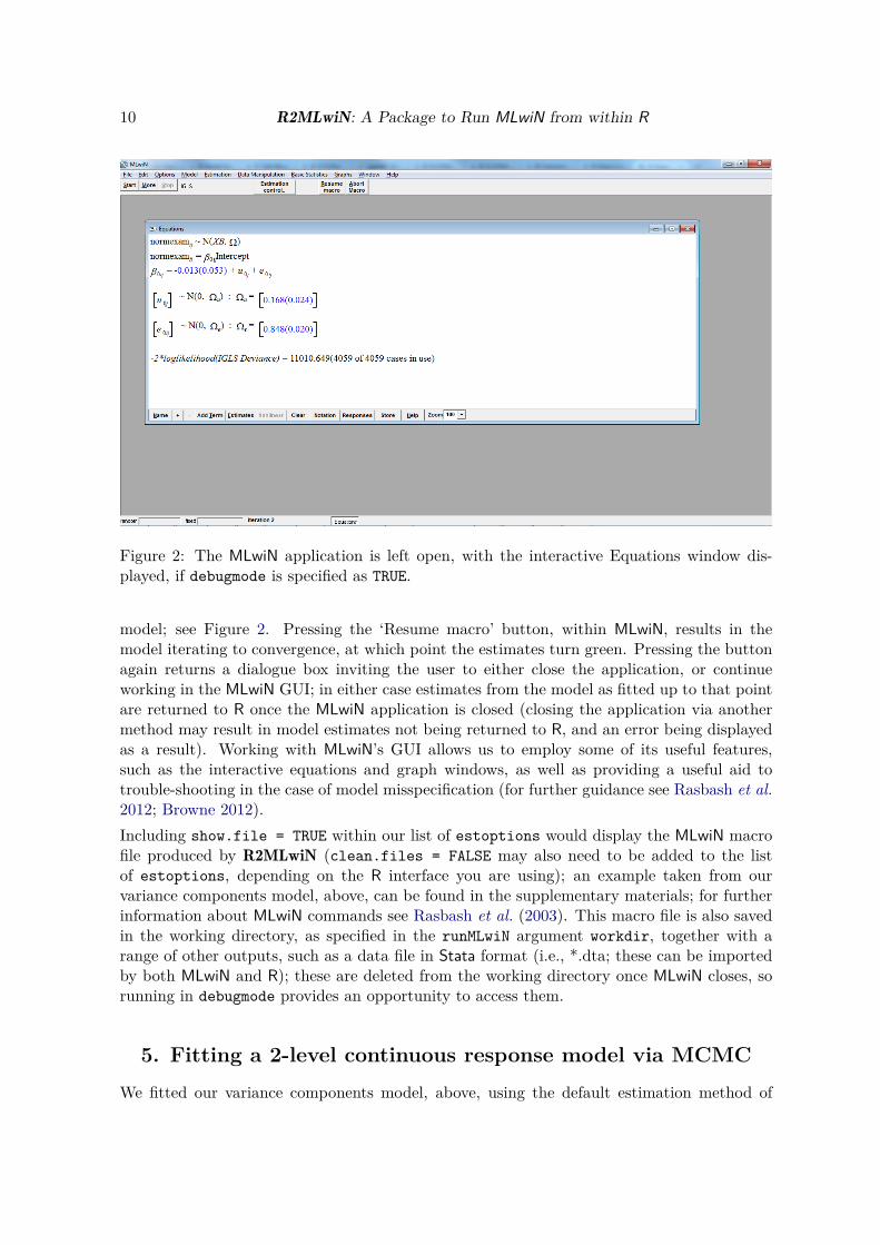
Figure 2: The MLwiN application is left open, with the interactive Equations window dis-played, if debugmode is specified as TRUE.

model; see Figure 2. Pressing the ‘Resume macro’ button, within MLwiN, results in themodel iterating to convergence, at which point the estimates turn green. Pressing the buttonagain returns a dialogue box inviting the user to either close the application, or continueworking in the MLwiN GUI; in either case estimates from the model as fitted up to that pointare returned to R once the MLwiN application is closed (closing the application via anothermethod may result in model estimates not being returned to R, and an error being displayedas a result). Working with MLwiN’s GUI allows us to employ some of its useful features,such as the interactive equations and graph windows, as well as providing a useful aid totrouble-shooting in the case of model misspecification (for further guidance see Rasbash et al.2012; Browne 2012).Including show.file = TRUE within our list of estoptions would display the MLwiN macrofile produced by R2MLwiN (clean.files = FALSE may also need to be added to the listof estoptions, depending on the R interface you are using); an example taken from ourvariance components model, above, can be found in the supplementary materials; for furtherinformation about MLwiN commands see Rasbash et al. (2003). This macro file is also savedin the working directory, as specified in the runMLwiN argument workdir, together with arange of other outputs, such as a data file in Stata format (i.e., *.dta; these can be importedby both MLwiN and R); these are deleted from the working directory once MLwiN closes, sorunning in debugmode provides an opportunity to access them.

5. Fitting a 2-level continuous response model via MCMCWe fitted our variance components model, above, using the default estimation method of


IGLS, but we can fit the same model using MCMC methods by simply toggling the value ofEstM (away from the default) as demonstrated below. MLwiN’s MCMC engine uses Gibbssampling for steps in the algorithm where the conditional posterior distribution has a standardform (as is the case for all parameters in the current model), and, if not, uses single siterandom walk Metropolis sampling with a normal proposal distribution and adaptive procedure(Browne and Draper 2000).R has, of course, a variety of other packages which fit models using MCMC methods (e.g.,Park et al. 2016), for example the MCMCglmm package written by Jarrod Hadfield (Hadfield2010) covers many of the same models as MLwiN and also has an impressively efficient MCMCimplementation, particularly for normal response models. However, for non-normal modelsit does require that they contain over-dispersion terms for each observation, in part so thatit can efficiently estimate the model. This is less of an issue for count data, but for binaryresponses can be problematic as it is not clear in such models that over-dispersion at theobservation level makes sense (Skrondal and Rabe-Hesketh 2007). Gelman and Hill (2007)cover many aspects of multilevel modelling within R, including, from an MCMC perspective,how to write an MCMC algorithm directly in the R language, and to call WinBUGS fromR via R2WinBUGS (Sturtz et al. 2005), which requires the user to write their own modelcode to send to WinBUGS, whilst R2MLwiN generates these files, using (by default) IGLSstarting values, on behalf of the user; see Section 12.Here we fit the model using the default MCMC estimation settings, but we would ultimatelyneed to investigate whether these were appropriate or not:

R> (VarCompMCMC <- runMLwiN(Formula = F1, data = tutorial,+ estoptions = list(EstM = 1)))


N min mean max N_complete min_complete mean_complete max_completeschool 65 2 62.44615 198 65 2 62.44615 198Estimation algorithm: MCMC Elapsed time : 1.15sNumber of obs:4059 (from total 4059) Number of iter:5000 Chains:1 Burn-in:500Bayesian Deviance Information Criterion (DIC)Dbar D(thetabar) pD DIC10850.046 10790.013 60.034 10910.080-----------------------------------------------------------------------------The model formula:normexam ~ 1 + (1 | school) + (1 | student)Level 2: school Level 1: student-----------------------------------------------------------------------------The fixed part estimates:

Coef. Std. Err. z Pr(>|z|) [95% Cred. Interval] ESSIntercept -0.01212 0.05410 -0.22 0.8227 -0.11977 0.08958 189Signif. codes: 0 '***' 0.001 '**' 0.01 '*' 0.05 '.' 0.1 ' ' 1-----------------------------------------------------------------------------The random part estimates at the school level:

Coef. Std. Err. [95% Cred. Interval] ESSvar_Intercept 0.17629 0.03606 0.11876 0.26114 3212


-----------------------------------------------------------------------------The random part estimates at the student level:

Coef. Std. Err. [95% Cred. Interval] ESSvar_Intercept 0.84862 0.01887 0.81254 0.88678 5016-*-*-*-*-*-*-*-*-*-*-*-*-*-*-*-*-*-*-*-*-*-*-*-*-*-*-*-*-*-*-*-*-*-*-*-*-*-*-

Here we see, towards the top of the output, that the chain has run for 5000 main iterations;this is the default in MLwiN, along with a burn-in of 500, a thinning factor of 1, and a randomnumber seed of 1. We have also run just one chain (the default); indeed, whilst it is not possi-ble to run more than one chain via the MLwiN GUI, it is via R2MLwiN, which can run multiplechains in parallel. If we wished not to use MLwiN’s defaults, then such parameters can be spec-ified in the mcmcMeth list within the estoptions argument, e.g., estoptions = list(EstM =1, mcmcMeth = list(burnin = 1000, nchains = 3, iterations = 10000, thinning =10, seed = 1:3)).Below that we have the deviance information criterion (DIC) model-fit statistic (Spiegelhalteret al. 2002), and the quantities from which it is derived:

• D̄ (Dbar): Average deviance across all (post-burnin) iterations.

• D(θ̄) (D(thetabar)): Deviance evaluated at the estimated means of the unknown pa-rameters θ.

• pD: The effective number of parameters, computed as D̄ −D(θ̄).

• DIC: Computed as D(θ̄) + 2pD: i.e., it is a measure of goodness of model fit which ad-justs for model complexity, thus allowing models to be compared: models with smallerDIC values are preferred to those with large values, with differences of 5 or more con-sidered substantial (e.g., Lunn et al. 2012).

Finally, following the model formula, we have the model estimates, which are largely similarto those from IGLS, and include 95% credible intervals (i.e., the 2.5th and 97.5th quantilesof each chain) for both the fixed and random part of the model. Note that, for the fixed partof the model, users can toggle between displaying the z score and its associated (two-tailed)p value (i.e., assuming normality), and a one-sided Bayesian p value (see Section 6 for anexample).The accompanying statistics include the ESS, or effective sample size (Kass et al. 1998), i.e.,the number of iterations necessary to obtain these estimates if the sample were independentand identically-distributed. As such, a low ESS (compared to the number of iterations thechain has actually run for) would indicate a strongly positively autocorrelated chain, suggest-ing it may need to be run longer and/or sampled in a different manner, or other alternativeMCMC methodologies could be employed to aid efficiency (see Section 11).As well as the ESS, other MCMC diagnostic aids available in the R2MLwiN package includetrajectory plots, as well as a larger suite of diagnostics available via the sixway function.We will demonstrate the latter when plotting the chain for the variance partition coefficient(VPC) in the following section; with regard to the former, however, entering

R> trajectories(VarCompMCMC)


0 1000 2000 3000 4000 5000

1082

010

840

1086

010

880

iteration

devi

ance

0 1000 2000 3000 4000 5000

−0.

15−

0.05

0.05

0.15

iteration

FP

_Int

erce

pt

0 1000 2000 3000 4000 5000

0.10

0.15

0.20

0.25

0.30

0.35

iteration

RP

2_va

r_In

terc

ept

0 1000 2000 3000 4000 5000

0.78

0.82

0.86

0.90

iteration

RP

1_va

r_In

terc

ept

Figure 3: Plots of MCMC chain trajectories produced by R2MLwiN’s trajectories function.

yields the plots presented in Figure 3, namely the trajectories for the deviance, the intercept inthe fixed part of the model (FP_Intercept), and the variances at level 2 (RP2_var_Intercept),and level 1 (RP1_var_Intercept) associated with the random part of the model.

5.1. Calculating the variance partition coefficient (VPC)

For our IGLS model fitted earlier, we calculated the VPC based on a single set of pointestimates; in the case of MCMC, however, we have chains for σ2

u and σ2e , and so can derive a

chain for the VPC, as follows:

R> VPC_MCMC <- VarCompMCMC["chains"][,"RP2_var_Intercept"] /+ (VarCompMCMC["chains"][,"RP1_var_Intercept"] ++ VarCompMCMC["chains"][,"RP2_var_Intercept"])R> sixway(VPC_MCMC, name = "VPC")

As you can see (Figure 4), using R2MLwiN’s sixway function we obtain a range of usefulstatistics we can use to describe this function, including mean, mode, and interval estimates(e.g., the 95% Bayesian credible interval runs from 0.123 to 0.235), as well as a range of other


0 1000 2000 3000 4000 5000

0.10

0.20

0.30

Iterations

para

met

er

0.10 0.15 0.20 0.25 0.30

05

1015

parameter value

kern

el d

ensi

ty

0 20 40 60 80 100

0.0

0.4

0.8

Lag

AC

F

2 4 6 8 10

0.0

0.4

0.8

Lag

Par

tial A

CF

0e+00 2e+04 4e+04 6e+04 8e+04 1e+051e−

044e

−04

7e−

04

updates

MC

SE

Accuracy DiagnosticsRaftery−Lewis (quantile) : Nhat =(4267,3803)

when q=(0.025,0.975), r=0.005 and s=0.95

Brooks−Draper (mean) : Nhat = 182

when k=2 sigfigs and alpha=0.05

Summary Statistics

param name : VPC posterior mean = 0.171 SD = 0.029 mode = 0.163

quantiles : 2.5% = 0.123 5% = 0.129 50% = 0.169 95% = 0.223 97.5% = 0.235

5000 actual iterations storing every 1th iteration. Effective Sample Size (ESS) = 3181

Figure 4: An example of diagnostic plots for MCMC chains produced by R2MLwiN’s sixwayfunction.

charts and diagnostics: in addition to the trajectory plot (top-left), we also have a kerneldensity plot of the posterior distribution (top-right), the Raftery-Lewis diagnostic (Rafteryand Lewis 1992) – indicating how long the chain should run to estimate the 0.025 and 0.975quantiles (respectively) to a given accuracy (see defaults for the raftery.diag function in thecoda package), and also the Brooks-Draper diagnostic – indicating the number of iterationsthe chain needs to run to estimate the mean to two significant places; Chapter 3 of Browne(2012) describes these, and the other diagnostics returned, in more detail.The chains returned by R2MLwiN, as mcmc objects, are also, of course, available for analysisby a range of other packages and functions in R, including the many useful functions availablein the coda package (Plummer et al. 2006).

6. Adding a predictor to the fixed part of a model

If we wish to see if a predictor, e.g., students’ exam performance at age 11, appreciably


improves the fit of the model, we can add it to the fixed part, as in Equation 3.

normexamij = β0 + β1standlrtij + uj + eij

uj ∼ N(0, σ2

u

)eij ∼ N

(0, σ2

e

) (3)

R> F3 <- normexam ~ 1 + standlrt + (1 | school) + (1 | student)R> (standlrtMCMC <- runMLwiN(Formula = F3, data = tutorial,+ estoptions = list(EstM = 1)))

In the resulting output (truncated below) we see its coefficient estimate is positive and muchgreater than its standard error, indicating that it is a highly significant predictor, as reflectedin its 95% credible interval, which excludes zero:

The fixed part estimates:Coef. Std. Err. z Pr(>|z|) [95% Cred. Interval] ESS

Intercept 0.00514 0.04246 0.12 0.9036 -0.07933 0.08896 211standlrt 0.56321 0.01250 45.05 0 *** 0.53862 0.58791 4060Signif. codes: 0 '***' 0.001 '**' 0.01 '*' 0.05 '.' 0.1 ' ' 1

Note that if we wish to instead view one-sided Bayesian p values – i.e., the proportion of chainiterations which are of the opposite sign to the chain mean (the coefficient estimate in ouroutput) – then we can request this as follows; here the output (again, truncated) indicatesthat the proportion of chain iterations which were below zero for the Intercept was 0.444,whilst none of the 5000 iterations were below zero for standlrt:

R> print(standlrtMCMC, z.ratio = FALSE)

The fixed part estimates:Coef. Std. Err. pMCMC(1-sided) [95% Cred. Interval] ESS

Intercept 0.00514 0.04246 0.444 -0.07933 0.08896 211standlrt 0.56321 0.01250 0 0.53862 0.58791 4060

We also see a large reduction in the DIC in this model):

R> VarCompMCMC["BDIC"][["DIC"]] - standlrtMCMC["BDIC"][["DIC"]]

[1] 1640.952

7. Priors, starting values, and random seedsBrowne (2012) describes in detail the priors, starting values, and random seeds used by defaultby MLwiN’s MCMC engine, and how to modify them to suit users’ own needs, so we will notfully reiterate those details here, other than providing the following few examples by meansof illustration of how to do so via R2MLwiN.


Den

sity

0

10

20

30

40

50

0.80 0.85 0.90 0.95 1.00 1.05

PosteriorPrior

Figure 5: A densityplot of the prior and posterior distributions for standlrt.

For fixed parameters MLwiN employs, by default, an improper uniform prior p(β) ∝ 1, butconjugate informative priors can readily be specified as a normal distribution with a meanand standard deviation as determined by the user. Let us assume we have gleaned, fromprior work, some knowledge leading us to propose a prior for standlrt with a mean of 1and standard deviation of 0.01; we can pass this information onto priorParam, listed withinmcmcMeth, itself listed within estoptions, by specifying (via fixe) that we wish to construct aproper normal prior for the term in the fixed part of the model called standlrt, with c(mean,sd). See Figure 5 for a plot produced using the lattice package (Sarkar 2008), automaticallyloaded with R2MLwiN, indicating a strong prior which disagrees with the data.

R> informpriorMCMC <- runMLwiN(Formula = F3, data = tutorial,+ estoptions = list(EstM = 1,+ mcmcMeth = list(priorParam = list(fixe = list(standlrt = c(1, 0.01))))))R> PlotDensities <- data.frame(+ PostAndPrior = c(informpriorMCMC["chains"][, "FP_standlrt"],+ qnorm(seq(1 / 5000, 1, by = 1 / 5000), mean = 1, sd = 0.01)),+ id = c(rep("Posterior", 5000), rep("Prior", 5000)))R> densityplot(~ PostAndPrior, data = PlotDensities, groups = id, ref = TRUE,+ plot.points = FALSE, auto.key = list(space = "bottom"), xlab = NULL)

Here, by means of illustration, we have described changing the prior for a parameter inthe fixed part of the model, but R2MLwiN allows conjugate priors for other parameters to


0 100 200 300 400 500

1000

014

000

1800

0

iteration

devi

ance

0 100 200 300 400 500

−2.

0−

1.5

−1.

0−

0.5

0.0

iteration

FP

_Int

erce

pt

0 100 200 300 400 500

0.6

0.7

0.8

0.9

1.0

iteration

FP

_sta

ndlr

t

0 100 200 300 400 500

01

23

45

67

iteration

RP

2_va

r_In

terc

ept

0 100 200 300 400 500

05

1015

iteration

RP

1_va

r_In

terc

ept

Figure 6: Chain trajectories from a model fit with custom (non-IGLS) starting values.

be modified as well, including Wishart or gamma priors for the covariance matrix, or scalarvariance, in the random part of the model; see ?runMLwiN or ?prior2macro for further details.By default, MLwiN’s MCMC engine uses IGLS estimates as starting values for each parameter;this is one of the reasons its MCMC engine converges comparatively quickly which is anadvantage over for example WinBUGS. However, if we wished to change the starting values,we can easily do so via the estoptions argument: specifically the startval list. Here wehave specified starting values of -2 and 5 for the coefficient estimates of the Intercept andstandlrt, respectively, in the fixed part of the model, and starting values of 2 and 4 forσ2

u and σ2e , respectively, in the random part of the model. For illustrative purposes, we also

dispense with the burnin, allowing us to subsequently view the first 500 iterations, as thesewill be most influenced by the starting values:

R> OurStartingValues <- list(FP.b = c(-2, 5), RP.b = c(2, 4))R> startvalMCMC <- runMLwiN(F3, data = tutorial,+ estoptions = list(EstM = 1, startval = OurStartingValues,+ mcmcMeth = list(burnin = 0, iterations = 500)))


R> trajectories(startvalMCMC["chains"], Range = c(1, 500))

Here we can see, in Figure 6, the chains quickly moving from the starting values we havegiven them to values closer to those we would have received from an initial IGLS fit.Finally, it is also a simple matter to change the random number seed from the default of 1(e.g., estoptions = list(EstM = 1, mcmcMeth = list(seed = 2)).

8. Adding a random slope/coefficientIn the modelling so far we have assumed that only the intercept term in our models variesacross clusters. We have already included standlrt in the fixed part of the model to allowfor a fixed slope effect; if we also include it to the left of | school in the random part ofthe model, we will additionally allow the coefficient of our predictor to randomly vary acrosslevel 2 units, thus specifying Equation 4.

normexamij = β0 + β1standlrtij + u0j + u1jstandlrtij + eij(u0j

u1j

)∼ N

{(00

),

(σ2

u0σu01 σ2

u1

)}eij ∼ N

(0, σ2

e

) (4)

R> F4 <- normexam ~ 1 + standlrt + (1 + standlrt | school) + (1 | student)R> (standlrtRS_MCMC <- runMLwiN(+ Formula = F4, data = tutorial,+ estoptions = list(EstM = 1, resi.store.levs = 2)))


N min mean max N_complete min_complete mean_complete max_completeschool 65 2 62.44615 198 65 2 62.44615 198Estimation algorithm: MCMC Elapsed time : 2.12sNumber of obs:4059 (from total 4059) Number of iter:5000 Chains:1 Burn-in:500Bayesian Deviance Information Criterion (DIC)Dbar D(thetabar) pD DIC9122.986 9031.321 91.666 9214.652-----------------------------------------------------------------------------The model formula:normexam ~ 1 + standlrt + (1 + standlrt | school) + (1 | student)Level 2: school Level 1: student-----------------------------------------------------------------------------The fixed part estimates:

Coef. Std. Err. z Pr(>|z|) [95% Cred. Interval] ESSIntercept -0.00569 0.03923 -0.15 0.8847 -0.08045 0.07369 233standlrt 0.55827 0.02047 27.27 9.883e-164 *** 0.51762 0.59858 769Signif. codes: 0 '***' 0.001 '**' 0.01 '*' 0.05 '.' 0.1 ' ' 1-----------------------------------------------------------------------------


The random part estimates at the school level:Coef. Std. Err. [95% Cred. Interval] ESS

var_Intercept 0.09600 0.01985 0.06396 0.13998 3117cov_Intercept_standlrt 0.01941 0.00723 0.00681 0.03476 1809var_standlrt 0.01547 0.00450 0.00810 0.02561 1063-----------------------------------------------------------------------------The random part estimates at the student level:


Here we see that including such a random slope increases the effective number of parameters(pD), but the reduction in DIC indicates that, despite this increase in complexity, it is abetter model:

R> ComparingModels <- rbind(standlrtMCMC["BDIC"], standlrtRS_MCMC["BDIC"])R> rownames(ComparingModels) <- c("Random intercept", "Random slope")R> ComparingModels

Dbar D(thetabar) pD DICRandom intercept 9209.146 9149.164 59.98223 9269.128Random slope 9122.986 9031.321 91.66588 9214.652

We included resi.store.levs = 2 in our list of estoptions, above, to illustrate R2MLwiN’spredLines function; this draws predicted lines against an explanatory variable for each groupat a higher level, calculating the median and quantiles in doing so (note that predLines usesa lot of contiguous memory, so we recommend using the 64-bit version of R to mitigate againstany problems this may cause). For example, the script below produces a plot of all 65 schoollines, plus their intervals (see Figure 7). As well as specifying the model object, we alsoprovide the name of the predictor (xname), the level (lev), and the probabilities (probs) usedto calculate the lower and upper quantiles from which the error bars are plotted:

R> predLines(standlrtRS_MCMC, xname = "standlrt", lev = 2,+ probs = c(0.025, 0.975), legend = FALSE)

By not declaring otherwise, we have accepted the default of selected = NULL and have thusproduced quite a busy plot, although a general fanning-out pattern is apparent, reflectingthe positive intercept/slope covariance at the school level (cov_Intercept_standlrt, inthe model output above). To better distinguish individual schools, however, we can insteadchoose to select just a few (requesting a legend whilst doing so; see Figure 8):

R> predLines(standlrtRS_MCMC, xname = "standlrt", lev = 2,+ selected = c(30, 44, 53, 59), probs = c(0.025, 0.975), legend = TRUE)


standlrt

ypre

d

−2

−1

0

1

2

3

−3 −2 −1 0 1 2 3

Figure 7: Predicted lines (with 95% credible intervals) for each of the 65 schools in thetutorial dataset.

standlrt

ypre

d

−2

−1

0

1

2

3

−3 −2 −1 0 1 2 3

30 44 53 59

Figure 8: Predicted lines (with 95% credible intervals) for four schools in the tutorialdataset.


9. Modeling complex level 1 varianceAnother important aspect of multilevel models is their ability to model complex level 1 vari-ance – i.e., residual heteroscedasticity. Whilst it is not currently possible to fit complex level 1variance models in R packages such as lme4 (Bates et al. 2015), it is possible to do so viaMLwiN (using both IGLS and MCMC, although here we focus on the latter). For example,taking the model we have just fitted above, we can allow for the possibility that variabilityin normexam within-schools (i.e., around their fitted regression lines) may also depend onstandlrt (see Browne et al. 2002, for an algorithm to fit this extension).When fitting this model below, note that we have chosen to include mcmcMeth = list(lclo= 1) in our list of estoptions so that MLwiN will fit the log of the precision (1/variance) atlevel 1 as a function of the predictors; since this can take any value on the real line, we arefree of the restrictions on prior distributions which result from fitting the variance as a linearfunction of the predictors (see Spiegelhalter et al. 2000):

R> F5 <- normexam ~ 1 + standlrt + (1 + standlrt | school) ++ (1 + standlrt | student)R> standlrtC1V_MCMC <- runMLwiN(+ Formula = F5, data = tutorial,+ estoptions = (list(EstM = 1, mcmcMeth = list(lclo = 1))))

Having fitted this model, we can then explore how the variance changes both within andbetween schools for different values of the intake score, standlrt, for example in a plot(Figure 9):

R> l2varfn <- standlrtC1V_MCMC["RP"][["RP2_var_Intercept"]] ++ 2 * standlrtC1V_MCMC["RP"][["RP2_cov_Intercept_standlrt"]] *+ tutorial[["standlrt"]] + standlrtC1V_MCMC["RP"][["RP2_var_standlrt"]] *+ tutorial[["standlrt"]]^2R> l1varfn <- 1 / exp(standlrtC1V_MCMC["RP"][["RP1_var_Intercept"]] ++ 2 * standlrtC1V_MCMC["RP"][["RP1_cov_Intercept_standlrt"]] *+ tutorial[["standlrt"]] + standlrtC1V_MCMC["RP"][["RP1_var_standlrt"]] *+ tutorial[["standlrt"]]^2)R> plot(sort(tutorial[["standlrt"]]),+ l2varfn[order (tutorial[["standlrt"]])], xlab = "standlrt",+ ylab = "variance", ylim = c(0,.7), type = "l")R> lines(sort(tutorial[["standlrt"]]),+ l1varfn[order (tutorial[["standlrt"]])], lty = "longdash")R> abline(v = 0, lty = "dotted")R> legend("bottomright", legend = c("between-student", "between-school"),+ lty = c("longdash", "solid"))

Figure 9 indicates that the between-school variation generally increases as standlrt in-creases, whereas the opposite is true for the between-student (within-school) variation.Finally, the following sample of three trajectory plots, plotting only the last 500 iterations(see Figure 10), illustrate that MLwiN has recognized that a different sampling method –Metropolis Hastings (MH), with its characteristic block-like appearance – is necessary toupdate the level 1 variance parameters, with Gibbs sampling updating the other parameters.


−3 −2 −1 0 1 2 3

0.0

0.1

0.2

0.3

0.4

0.5

0.6

0.7

standlrt

varia

nce

between−studentbetween−school

Figure 9: A plot of the variance function from a random slopes model allowing for hetero-geneity at level 1.

R> trajectories(standlrtC1V_MCMC["chains"][, "FP_Intercept",+ drop = FALSE], Range = c(4501, 5000))R> trajectories(standlrtC1V_MCMC["chains"][, "RP2_var_Intercept",+ drop = FALSE], Range = c(4501, 5000))R> trajectories(standlrtC1V_MCMC["chains"][, "RP1_var_Intercept",+ drop = FALSE], Range = c(4501, 5000))

10. Fitting a 2-level binary response model via MCMCWe will now move on from continuous response models to consider some of the other responsedistribution types supported by R2MLwiN. As Table 2 illustrates, many of these, includingthe "Binomial" distribution we explore in the next example, can be fitted using IGLS orMCMC estimation; here, though, we will stay with MCMC in order to illustrate alternativeMCMC methodology implemented in MLwiN, and also interoperability with BUGS, in thefollowing sections.Our example dataset is a sub-sample of the 1989 Bangladesh Fertility Survey (Huq andCleland 1990), provided as bang1 in both MLwiN and R2MLwiN (see Table 3 for a list of thevariables to be modeled).Below we construct a logit model to investigate whether the use of contraceptives at the time


4500 4600 4700 4800 4900 5000

−0.

100.

00

iteration

FP

_Int

erce

pt

4500 4600 4700 4800 4900 5000

0.06

0.10

0.14

iteration

RP

2_va

r_In

terc

ept

4500 4600 4700 4800 4900 5000

0.55

0.60

0.65

iteration

RP

1_va

r_In

terc

ept

Figure 10: Modeling complex level 1 variance: chain trajectories of (from top) β0, σ2u0, and

σ2e0.

Variable Descriptionwoman Identifying code for each woman.district Identifying code for each district.use Contraceptive use status at time of survey; levels are Not_using

and Using.lc Number of living children at time of survey; levels correspond to

none (None), one (One_child), two (Two_children), or threeor more children (Three_plus).

age Age of woman at time of survey (in years), centered on thesample mean of 30 years.

urban Type of region of residence; levels are Rural and Urban.

Table 3: Variables in the bang1 dataset, as modeled in the worked example.

of the survey is predicted by the age of the respondent, their number of children living at thetime of the survey (lc), and the type of region in which they reside (urban); furthermore,we will allow the coefficient of the latter predictor to randomly-vary at the district-levelto explore whether variability between Urban areas within districts differs from that between


Rural areas within districts, producing the random coefficient model in Equation 5.useij ∼ Bernouilli(πij)

logit(πij) = β0 + β1ageij + β2lcOne_childij + β3lcTwo_childrenij + β4lcThree_plusij

+ β5urbanij + u0j + u5jurbanij(u0j

u5j

)∼ N

{(00

),

(σ2

u0σu05 σ2

u5

)}(5)

We can fit this, via R2MLwiN, as follows:

R> data("bang1")R> F6 = logit(use) ~ 1 + age + lc + urban + (1 + urban | district)R> binomialMCMC <- runMLwiN(Formula = F6, D = "Binomial", data = bang1,+ estoptions = list(EstM = 1))R> trajectories(binomialMCMC["chains"][,"FP_Intercept", drop = FALSE])

As discussed in Table 2, the terms in the parentheses immediately following logit are of theform response variable, denominator; specifying the demoninator is actually optional,and if not specified will take the form of a constant of ones, which is appropriate here. SinceMLwiN requires binary response variables to be of the form 0/1, R2MLwiN transforms itinto that format having detected it is indeed binary, and thus we are modeling a Bernoullidistribution. lc is a factor variable and so dummy variables will be added as predictors withNone (see min(levels(bang1$lc))) as the reference category (the relevel function, part ofthe stats package, can be used to assign an alternative reference category, by re-ordering thelevels of a factor prior to an runMLwiN call).We have requested, on the last line, a plot of the chain trajectory for the intercept in thefixed part of the model. As the resulting plot (Figure 11) indicates, mixing here looks rela-tively poor, and so it may be worthwhile examining some of the alternative MCMC methodsimplemented in MLwiN; we review these, and apply one to the current example, in the nextsection.

11. Alternative MCMC methods implemented in MLwiNMLwiN’s MCMC engine features a number of methods which can improve the efficiency ofMCMC estimation (see Browne 2012, chapters 21-25). Table 4 provides a summary of avail-able methods, one of which – orthogonal parameterization – we explore in the example below,before moving on to discuss further options via MLwiN’s interoperability with BUGS.

11.1. An example using orthogonal parameterization to improve mixingGiven that we encountered poor mixing in our last model fit, above, we will examine whetherorthogonal parameterization may help; this replaces a set of fixed effect predictors with analternative group of predictors that span the same parameter space, but are orthogonal, and isparticularly useful for instances such as this, where we are modeling a non-normal distribution(since fixed effects in normal models are generally updated in a block).Here, then, we redefine estoptions, toggling orth to 1 in the list of mcmcOptions, and runthe model again:


0 1000 2000 3000 4000 5000

−2.

4−

2.0

−1.

6−

1.2

iteration

FP

_Int

erce

pt

Figure 11: Chain trajectory of β0 from a binomial response model, without orthogonal param-etization.

0 1000 2000 3000 4000 5000

−2.

2−

1.8

−1.

4

iteration

FP

_Int

erce

pt

Figure 12: Chain trajectory of β0 from a binomial response model, with orthogonal parame-tization.

R> (OrthogbinomialMCMC <- runMLwiN(Formula = F6, D = "Binomial",+ data = bang1, estoptions = list(EstM = 1, mcmcOptions = list(orth = 1))))

-*-*-*-*-*-*-*-*-*-*-*-*-*-*-*-*-*-*-*-*-*-*-*-*-*-*-*-*-*-*-*-*-*-*-*-*-*-*-MLwiN (version: 2.36) multilevel model (Binomial)

N min mean max N_complete min_complete mean_complete max_completedistrict 60 2 32.23333 118 60 2 32.23333 118Estimation algorithm: MCMC Elapsed time : 15.06sNumber of obs:1934 (from total 1934) Number of iter:5000 Chains:1 Burn-in:500Bayesian Deviance Information Criterion (DIC)Dbar D(thetabar) pD DIC2329.877 2273.176 56.702 2386.579-----------------------------------------------------------------------------The model formula:logit(use) ~ 1 + age + lc + urban + (1 + urban | district)Level 2: district Level 1: l1id-----------------------------------------------------------------------------The fixed part estimates:


Method As currently implemented in ML-wiN

As specified inmcmcOptions

Structured MCMC(e.g., Sargent et al. 2009)

2-level nested normal responsemodels, with no complex level 1variation, only

smcm = 1

Structured MVN framework(e.g., Browne et al. 2009a)

2-level variance componentsmodels only

smvn = 1

Othogonal fixed effect vectors(e.g., Browne et al. 2009b)

All models orth = 1

Parameter expansion(e.g., Liu and Wu 1999)

All models paex = c(<L>, 1)

Hierarchical centring(e.g., Gelfand et al. 1995)

All models hcen = <L>

Table 4: A summary of some alternative methods for MCMC estimation available via theR2MLwiN package. <L> is an integer specifying the level at which parameter expansion /hierarchical centering (respectively) is to occur. Taking Structured MCMC as an example,these methods are implemented as follows: estoptions = list(EstM = 1, mcmcOptions =list(smcm = 1), ...).

Coef. Std. Err. z Pr(>|z|) [95% Cred. Interval] ESSIntercept -1.70164 0.16702 -10.19 2.237e-24 *** -2.03503 -1.38148 246age -0.02645 0.00798 -3.31 0.0009172 *** -0.04191 -0.01117 1063lcOne_child 1.12627 0.16211 6.95 3.716e-12 *** 0.80576 1.45134 923lcTwo_children 1.34947 0.17658 7.64 2.133e-14 *** 1.00799 1.69571 921lcThree_plus 1.34643 0.18528 7.27 3.676e-13 *** 0.97975 1.70612 872urbanUrban 0.81100 0.19211 4.22 2.426e-05 *** 0.45403 1.22458 151Signif. codes: 0 '***' 0.001 '**' 0.01 '*' 0.05 '.' 0.1 ' ' 1-----------------------------------------------------------------------------The random part estimates at the district level:

Coef. Std. Err. [95% Cred. Interval] ESSvar_Intercept 0.41681 0.13544 0.21169 0.73256 223cov_Intercept_urbanUrban -0.41923 0.17235 -0.83135 -0.16282 139var_urbanUrban 0.70042 0.29966 0.28379 1.43387 102-----------------------------------------------------------------------------The random part estimates at the l1id level:

Coef. Std. Err. [95% Cred. Interval] ESSvar_bcons_1 1.00000 1e-05 1.00000 1.00000 5000-*-*-*-*-*-*-*-*-*-*-*-*-*-*-*-*-*-*-*-*-*-*-*-*-*-*-*-*-*-*-*-*-*-*-*-*-*-*-

R> trajectories(OrthogbinomialMCMC["chains"][,"FP_Intercept", drop = FALSE])

As such, we see that the mixing is considerably better (Figure 12), with the ESS considerably-improved for the fixed effects (see comparison table in the following section). The modelindicates that the probability of contraceptive use decreases with age, but increases with thenumber of living children, and is greater in Urban areas; furthermore, the variance in contra-


ceptive use differs between Rural areas (estimated as 0.417), and Urban areas (estimated as0.417− 2× 0.419 + 0.7 = 0.28).

12. Using R2MLwiN to write BUGS codeAs well as using its own MCMC estimation engine, MLwiN can write code to fit models inWinBUGS (Lunn et al. 2000) and OpenBUGS (Lunn et al. 2009), with the inclusion of itsown IGLS estimates as starting values. With the aid of the rbugs package (Yan and Prates2013), the user can employ a single runMLwiN function call to obtain starting values from anIGLS run in MLwiN, automatically generate the necessary BUGS model code, initial values,data files, and script, and then fit the model in BUGS.As demonstrated in the script below, WinBUGS and OpenBUGS are called via the runMLwiNargument BUGO; this is a vector where n.chains corresponds to the number of chains, debugdetermines whether BUGS stays open following completion of the model run, seed sets therandom number seed, bugs specifies the path, and OpenBUGS can toggle between FALSE forWinBUGS, and TRUE for OpenBUGS. Here we fit the same model as in the example above(the burnin, iterations and thinning we specify are the defaults, we simply make themexplicit here for the purposes of this example); by specifying show.file = TRUE in the listof estoptions, the BUGS model is returned (see supplementary materials):

R> WinBUGS <- "C:/WinBUGS14/WinBUGS14.exe"R> BUGSmodel = runMLwiN(Formula = F6, D = "Binomial",+ data = bang1, estoptions = list(EstM = 1,+ mcmcMeth = list(burnin = 500, iterations = 5000, thinning = 1)),+ BUGO = c(n.chains = 1, debug = FALSE, seed = 1,+ bugs = WinBUGS, OpenBugs = FALSE))R> summary(BUGSmodel)

Iterations = 1:5000Thinning interval = 1Number of chains = 1Sample size per chain = 5000

1. Empirical mean and standard deviation for each variable,plus standard error of the mean:

Mean SD Naive SE Time-series SEbeta[1] -1.721e+00 0.161037 0.0022774 0.0097350beta[2] -2.675e-02 0.007946 0.0001124 0.0002641beta[3] 1.140e+00 0.158146 0.0022365 0.0053347beta[4] 1.366e+00 0.179230 0.0025347 0.0068177beta[5] 1.365e+00 0.181054 0.0025605 0.0087925beta[6] 8.136e-01 0.171615 0.0024270 0.0081912deviance 2.329e+03 14.099908 0.1994028 0.5284579sigma2.u2[1,1] 4.216e-01 0.138640 0.0019607 0.0063190sigma2.u2[1,2] -4.350e-01 0.187684 0.0026542 0.0098587


sigma2.u2[2,1] -4.350e-01 0.187684 0.0026542 0.0098587sigma2.u2[2,2] 7.283e-01 0.341042 0.0048231 0.0199511u2[1,1] -9.429e-01 0.334778 0.0047345 0.0118369u2[1,2] 3.969e-01 0.417123 0.0058990 0.0149241...

On finishing the model run, the model estimates are returned (including the quantiles, notdisplayed in the truncated output above), but this time as a summary of an mcmc.list (seecoda (Plummer et al. 2006)).Running this on our machine took 140 seconds in WinBUGS, which uses (by default) amultivariate Metropolis update of the fixed effects (Gamerman 1997), whilst it took 16 secondsto run the model for the same length of chain in MLwiN (both via R2MLwiN), which usesa single site Metropolis sampler. As the table below indicates, however, the effective samplesizes (ESSs) from the run in BUGS are considerably larger than those from the run (withoutorthogonal parameterization) in MLwiN (although there is considerable improvement whenwe opt for orthogonal parameteristion in MLwiN, at least for the fixed effects; this took 15seconds to run on our machine).

R> cc = cbind(binomialMCMC["FP"], OrthogbinomialMCMC["FP"])R> dd = cbind(head(binomialMCMC["RP"], -1),+ head(OrthogbinomialMCMC["RP"], -1))R> ESS.binMCMC = effectiveSize(binomialMCMC["chains"][,2:10])R> ESS.orthogMCMC = effectiveSize(OrthogbinomialMCMC["chains"][,2:10])R> ESStable = round(rbind(cc, dd), 3)R> BUGSlist <- c(1:6, 8, 9, 11)R> BUGS.Coeff <- round(summary(BUGSmodel)$statistics[BUGSlist, 1], 3)R> BUGS.ESS <- as.data.frame(effectiveSize(BUGSmodel))R> ESStable = cbind(ESStable[, 1], round(ESS.binMCMC), ESStable[, 2],+ round(ESS.orthogMCMC), BUGS.Coeff, round(BUGS.ESS[BUGSlist, ]))R> colnames(ESStable) = c("A)Coeff.", "A)ESS", "B)Coeff.",+ "B)ESS", "C)Coeff.", "C)ESS")R> cat("NB: A = MLwiN(non-orthog.), B = MLwiN(orthog.), C = WinBUGS\n");+ ESStable

NB: A = MLwiN(non-orthog.), B = MLwiN(orthog.), C = WinBUGSA)Coeff. A)ESS B)Coeff. B)ESS C)Coeff. C)ESS

FP_Intercept -1.724 61 -1.702 246 -1.721 274FP_age -0.027 203 -0.026 1063 -0.027 905FP_lcOne_child 1.157 229 1.126 923 1.140 879FP_lcTwo_children 1.376 186 1.349 921 1.366 691FP_lcThree_plus 1.384 102 1.346 872 1.365 424FP_urbanUrban 0.805 110 0.811 151 0.814 439RP2_var_Intercept 0.418 206 0.417 223 0.422 481RP2_cov_Intercept_urbanUrban -0.432 127 -0.419 139 -0.435 362RP2_var_urbanUrban 0.738 142 0.700 102 0.728 292


13. Modeling a cross-classified data structureSo far the multilevel models we have examined have been strictly hierarchical, but researchersmay well encounter data structures which are cross-classified (i.e., crossed random effects),exhibit multiple membership, or indeed a combination of these; R2MLwiN allows users to fitsuch models via MCMC estimation.In the following example we use an educational dataset from Fife in Scotland (available as thesample dataset xc in MLwiN and R2MLwiN); see Table 5 for a description of the variableswe will model.We wish to model students’ examination attainment, whilst controlling for clustering dueto their current (secondary) school (sid), but also controlling for clustering due to their(earlier) primary school too (pid); since not all students who attended a given primary schoolall subsequently attended the same secondary school, the former are not nested within thelatter, and so we have a cross-classified structure; see Equation 6, which uses the classificationnotation as per Browne et al. (2001).

attaini = β0 + u(2)sid(i) + u

(3)pid(i) + ei

u(2)sid(i) ∼ N(0, σ2

u(2))

u(3)pid(i) ∼ N(0, σ2

u(3))

ei ∼ N(0, σ2e)

(6)

As indicated below, we need to specify that the data structure is cross-classified by declaringxc = TRUE within the list of estoptions:

R> data("xc")R> F7 = attain ~ 1 + (1 | sid) + (1 | pid) + (1 | pupil)R> (XCModel <- runMLwiN(Formula = F7, data = xc,+ estoptions = list(xc = TRUE, EstM = 1)))


N min mean max N_complete min_complete mean_complete max_completesid 19 92 180.78947 290 19 92 180.78947 290pid 148 1 23.20946 72 148 1 23.20946 72Estimation algorithm: MCMC Cross-classified Elapsed time : 2.12sNumber of obs:3435 (from total 3435) Number of iter:5000 Chains:1 Burn-in:500

Variable Descriptionattain Attainment score of pupils at age 16.pid Primary school identifying code.sid Secondary school identifying code.pupil Pupil identifying code.

Table 5: Variables in the xc dataset, as modeled in the worked example.


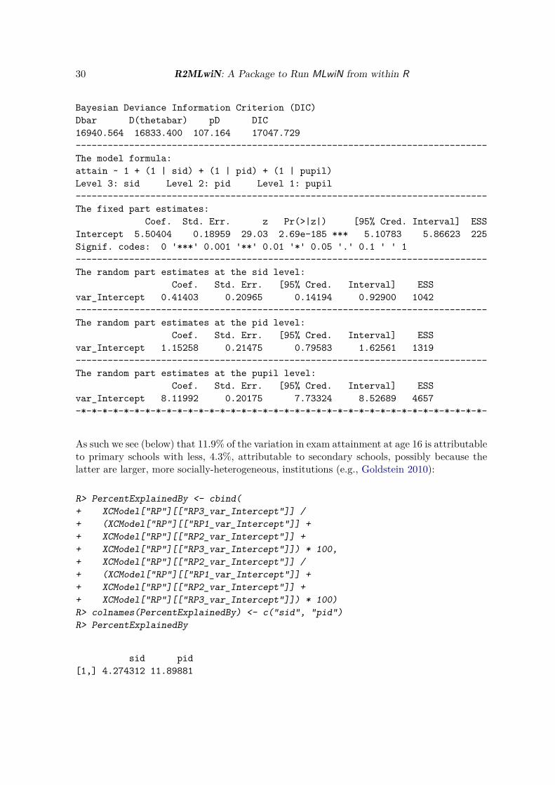
Bayesian Deviance Information Criterion (DIC)Dbar D(thetabar) pD DIC16940.564 16833.400 107.164 17047.729-----------------------------------------------------------------------------The model formula:attain ~ 1 + (1 | sid) + (1 | pid) + (1 | pupil)Level 3: sid Level 2: pid Level 1: pupil-----------------------------------------------------------------------------The fixed part estimates:

Coef. Std. Err. z Pr(>|z|) [95% Cred. Interval] ESSIntercept 5.50404 0.18959 29.03 2.69e-185 *** 5.10783 5.86623 225Signif. codes: 0 '***' 0.001 '**' 0.01 '*' 0.05 '.' 0.1 ' ' 1-----------------------------------------------------------------------------The random part estimates at the sid level:

Coef. Std. Err. [95% Cred. Interval] ESSvar_Intercept 0.41403 0.20965 0.14194 0.92900 1042-----------------------------------------------------------------------------The random part estimates at the pid level:

Coef. Std. Err. [95% Cred. Interval] ESSvar_Intercept 1.15258 0.21475 0.79583 1.62561 1319-----------------------------------------------------------------------------The random part estimates at the pupil level:


As such we see (below) that 11.9% of the variation in exam attainment at age 16 is attributableto primary schools with less, 4.3%, attributable to secondary schools, possibly because thelatter are larger, more socially-heterogeneous, institutions (e.g., Goldstein 2010):

R> PercentExplainedBy <- cbind(+ XCModel["RP"][["RP3_var_Intercept"]] /+ (XCModel["RP"][["RP1_var_Intercept"]] ++ XCModel["RP"][["RP2_var_Intercept"]] ++ XCModel["RP"][["RP3_var_Intercept"]]) * 100,+ XCModel["RP"][["RP2_var_Intercept"]] /+ (XCModel["RP"][["RP1_var_Intercept"]] ++ XCModel["RP"][["RP2_var_Intercept"]] ++ XCModel["RP"][["RP3_var_Intercept"]]) * 100)R> colnames(PercentExplainedBy) <- c("sid", "pid")R> PercentExplainedBy

sid pid[1,] 4.274312 11.89881


14. Modeling a multiple membership data structureMultiple membership models arise when we wish to control for clustering at a given ‘level’ orclassification, but have lower-level units which belong to more than one group at that higherlevel. For example, if we wished to model employees’ earnings over the past financial year,we might want to control for non-independence due to the companies which employed themduring this time. If the employees were employed by more than one company, however (i.e.,they were a ‘member’ of more than one group at this higher level), it would be judicious tocontrol for the effects of all of them.Below we fit such a model, using the wage1 sample dataset (available in both MLwiN andR2MLwiN); see Table 6 for a description of the variables we will model, and Equation 7 forthe model itself.

logearni = β0 + β1age_40i + β2numjobsi +∑

j∈company(i)w

(2)i,j u

(2)j + ei

i = 1, ..., Ncompany(i) ⊂ (1, ..., J)

u(2)j ∼ N(0, σ2

u(2))ei ∼ N(0, σ2

e)

(7)

You can see, below, that the argument mm, specifying the structure of the multiple membershipmodel, has been included in the list of estoptions (NB since mm is non-NULL, xc defaultsto TRUE). The argument mm can be a list of variable names, a list of vectors, or a matrix(e.g., see ?df2matrix). Here we employ variable names, which need to be assigned as liststo mmvar, specifying the classification units, and weights, specifying the weights. In the

Variable Descriptionid Identifying code for each office worker.company Identifying code for first company worked for over the last 12

months.company2 If worked for > 1 company over the last 12 months, identifying

code for second company.company3 If worked for > 2 company over the last 12 months, identifying

code for third company.company4 If worked for > 3 company over the last 12 months, identifying

code for fourth company.logearn Workers’ (natural) log-transformed earnings over the last finan-

cial year.numjobs The number of companies worked for over the last 12 months.weight1 Proportion of time worked for employer listed in company.weight2 Proportion of time worked for employer listed in company2.weight3 Proportion of time worked for employer listed in company3.weight4 Proportion of time worked for employer listed in company4.age_40 Age of workers, centered on 40 years.

Table 6: Variables in the wage1 dataset, as modeled in the worked example.


variables comprising the mmvar list, the same company, e.g., ACME Ltd, has the same value,e.g., 8, throughout. The weights specify the employee-level weighting given to each companythey worked for; here we have chosen the proportion of time an employee has spent witha particular company. Each element of the list corresponds to a level (classification) of themodel, in descending order, so the final NA indicates that there is not a multiple membershipclassification at level 1.

R> data("wage1")R> F8 = logearn ~ 1 + age_40 + numjobs + (1 | company) + (1 | id)R> OurMultiMemb <- list(list(+ mmvar = list("company", "company2", "company3","company4"),+ weights = list("weight1", "weight2", "weight3", "weight4")), NA)R> (MMembModel <- runMLwiN(Formula = F8, data = wage1,+ estoptions = list(EstM = 1, drop.data = FALSE, mm = OurMultiMemb)))


N min mean max N_complete min_complete mean_complete max_completecompany 141 2 21.43262 49 141 2 21.43262 49Estimation algorithm: MCMC Cross-classified Elapsed time : 1.46sNumber of obs:3022 (from total 3022) Number of iter:5000 Chains:1 Burn-in:500Bayesian Deviance Information Criterion (DIC)Dbar D(thetabar) pD DIC4625.279 4514.715 110.564 4735.843-----------------------------------------------------------------------------The model formula:logearn ~ 1 + age_40 + numjobs + (1 | company) + (1 | id)Level 2: company Level 1: id-----------------------------------------------------------------------------The fixed part estimates:

Coef. Std. Err. z Pr(>|z|) [95% Cred. Interval] ESSIntercept 3.04872 0.03534 86.26 0 *** 2.98024 3.11807 851age_40 0.01273 0.00098 13.06 5.924e-39 *** 0.01084 0.01460 4273numjobs -0.11190 0.02223 -5.03 4.803e-07 *** -0.15446 -0.06892 4594Signif. codes: 0 '***' 0.001 '**' 0.01 '*' 0.05 '.' 0.1 ' ' 1-----------------------------------------------------------------------------The random part estimates at the company level:

Coef. Std. Err. [95% Cred. Interval] ESSvar_Intercept 0.05793 0.00916 0.04225 0.07808 2196-----------------------------------------------------------------------------The random part estimates at the id level:


R> MMembModel["RP"][["RP2_var_Intercept"]] /+ (MMembModel["RP"][["RP2_var_Intercept"]] ++ MMembModel["RP"][["RP1_var_Intercept"]]) * 100


[1] 17.63173

The model indicates (as calculated at the bottom) that company accounted for 17.6% of thevariance in (log-transformed) earnings, having controlled for age and number of jobs. Lookingat the fixed effects, earnings on average increase with age, but those employees working formore companies over the past 12 months earn on average less; it would be interesting toinvestigate whether these effects persist once other variables available in the dataset aretaken into account, such as sex of the employee, and whether they work part-time or not, butwe will leave this model as it is, and move on to our next example.

15. Multivariate response modelsHere we illustrate fitting a multivariate response model. In this example dataset (see Browne2012), taken from the larger junior school project (JSP) dataset (Mortimore et al. 1988),we have two responses (see Table 7): english – an English test score marked out of 100,and behaviour – a binary behaviour score taken in the same year. We’re interested in thecorrelation between English test performance and behaviour, and the effect of predictors –such as sex, and an earlier test score (ravens) – on both of them, and also the effect of anearlier English fluency indicator (fluent) on the english test (i.e., not behaviour, sincepreliminary investigation revealed no correlation between the two); see Equation 8.Note that the MCMC engine in MLwiN can fit mixed response multivariate models, as well asnormal response models, but only if they consist of a mixture of normal responses and binaryresponses (with a probit, rather than logit, link), as in this case. In practice latent normalvariables are constructed for each binary response with the value of the binary responsegoverning the sign of the latent variable as illustrated below:

englishij = β0 + β1sexij + β2ravensij + β3fluentij + u0j + e0ij

behaviour∗ij = β4 + β5sexij + β6ravensij + u4j + e4ij

where behaviour∗ij ≥ 0 if behaviourij = 1and behaviour∗ij < 0 if behaviourij = 0(

u0j

u4j

)∼ N

{(00

),

(σ2

u0σu04 σ2

u4

)}(e0ij

e4ij

)∼ N

{(00

),

(σ2

e0σe04 1

)}(8)

R> data("jspmix1")R> F9 = c(english, probit(behaviour)) ~ 1 + sex + ravens + fluent[1] ++ (1 | school) + (1[1] | id)R> (MixedRespMCMC <- runMLwiN(Formula = F9, D = c("Mixed", "Normal",+ "Binomial"), data = jspmix1, estoptions = list(EstM = 1,+ mcmcMeth = list(fixM = 1, residM = 1, Lev1VarM = 2))))

Here then we have two terms to the left of the tilde (~) in the model formula, corresponding tothe two responses (their order matters, insofar as we use it to distinguish them when referringto the response variables in other parts of our model specification). Firstly we have english,


Variable Descriptionschool Identifying code for school.id Identifying code for pupil.sex Sex of pupil, with levels female and male.fluent Fluency at English measure taken in Year 1, where 0 = begin-

ner, 1 = intermediate, 2 = fully fluent.ravens Test score in Year 1, marked out of 40.english English test score taken in Year 3, marked out of 100.behaviour Behaviour rating taken in Year 3, coded lowerquarter if pupil

rated in bottom 25%, and upper otherwise.

Table 7: Variables in the jspmix1 dataset, as modeled in the worked example.

and then our binary variable behaviour: this is modeled via a probit link and, since we havenot specified otherwise, a constant of ones as the denominator. The default is for predictorsadded to the right of the tilde to have separate coefficients (i.e., one for each category) unlesstheir name is suffixed by square brackets. In the case of the latter, a common coefficient isadded to the model for the response(s) indicated in the numeric identifier within the squarebrackets. In this example, then, the model formula specifies separate coefficients for sex andravens, and a common coefficient for fluent to be added to the response we earlier listedfirst (english). Finally, separate coefficients for the intercept are allowed to vary at level 2(school) and also at level 1 (id), but the latter is only applicable in the case of the normalresponse variable (english; hence 1[1]).Next, after requesting MCMC estimation, and Gibbs sampling (denoted by 1) as the methodused to update both the fixed (fixM) and the random effects (residM), and univariate MH(denoted by 2; 3 corresponds to multivariate MH – see ?write.MCMC for further details) toupdate the level 1 variance (Lev1VarM), we specify our runMLwiN function call. The argumentshere will be familiar to you now, although we encounter a slightly different format for thevalue we assign to the distribution: if our multivariate response model consisted only ofnormal responses, we would simply specify "Multivariate Normal"; since we have mixedresponse types, however, we must identify the distribution of each (in an order correspondingto their position in the preceding model formula), hence the character string: D = c("Mixed","Normal", "Binomial").

-*-*-*-*-*-*-*-*-*-*-*-*-*-*-*-*-*-*-*-*-*-*-*-*-*-*-*-*-*-*-*-*-*-*-*-*-*-*-MLwiN (version: 2.36) multilevel model (Mixed)

N min mean max N_complete min_complete mean_complete max_completeschool 47 7 23.80851 76 47 7 23.80851 76Estimation algorithm: MCMC Elapsed time : 3.95sNumber of obs:1119 (from total 1119) Number of iter:5000 Chains:1 Burn-in:500Deviance statistic: NA-----------------------------------------------------------------------------The model formula:c(english, probit(behaviour)) ~ 1 + sex + ravens + fluent[1] +

(1 | school) + (1[1] | id)Level 2: school Level 1: id-----------------------------------------------------------------------------


The fixed part estimates:Coef.Std. Err. z Pr(>|z|) [95% Cred. Interval] ESS

sexmale_english -6.23710 1.03073 -6.05 1.438e-09 *** -8.25154 -4.23264 4371sexmale_behaviour -0.41890 0.08912 -4.70 2.595e-06 *** -0.59441 -0.24209 1411ravens_english 1.65807 0.09131 18.16 1.092e-73 *** 1.47805 1.83770 3974ravens_behaviour 0.05722 0.00774 7.39 1.456e-13 *** 0.04204 0.07242 1045fluent_1 6.36146 1.28814 4.94 7.873e-07 *** 3.86164 8.85984 3720Intercept_1 -9.19443 3.23664 -2.84 0.004501 ** -15.64483 -2.93315 3021Intercept_2 -0.36147 0.19366 -1.87 0.06197 . -0.74739 0.01087 1219Signif. codes: 0 '***' 0.001 '**' 0.01 '*' 0.05 '.' 0.1 ' ' 1-----------------------------------------------------------------------------The random part estimates at the school level:

Coef. Std. Err. [95% Cred. Interval] ESSvar_Intercept_1 41.50795 12.01852 23.29346 69.47876 1734cov_Intercept_1_Intercept_2 0.05258 0.42969 -0.77081 0.92794 628var_Intercept_2 0.06297 0.02899 0.02167 0.13411 437-----------------------------------------------------------------------------The random part estimates at the id level:

Coef. Std. Err. [95% Cred. Interval] ESSvar_bcons_2 1.00000 0.00001 1.00000 1.00000 5000cov_bcons_2_Intercept_1 6.22663 0.70827 4.77651 7.53054 347var_Intercept_1 291.91324 12.51061 267.92679 316.88733 740-*-*-*-*-*-*-*-*-*-*-*-*-*-*-*-*-*-*-*-*-*-*-*-*-*-*-*-*-*-*-*-*-*-*-*-*-*-*-

The model indicates that the Year 1 ravens test score has a positive effect on both of theYear 3 response variables we have fitted, whilst the Year 1 measure of fluency in Englishhas a positive effect on the Year 3 English test score. Girls are found to both have a higherbehaviour rating, and a better Year 3 English test score, than boys. There is a positive cor-relation between the two response variables at the pupil-level, but the correlation is negligibleat the school-level:

R> CompareCorrelation <- cbind(+ MixedRespMCMC["RP"][["RP2_cov_Intercept_1_Intercept_2"]] /+ sqrt(MixedRespMCMC["RP"][["RP2_var_Intercept_1"]] *+ MixedRespMCMC["RP"][["RP2_var_Intercept_2"]]),+ MixedRespMCMC["RP"][["RP1_cov_bcons_2_Intercept_1"]] /+ sqrt(MixedRespMCMC["RP"][["RP1_var_Intercept_1"]] *+ MixedRespMCMC["RP"][["RP1_var_bcons_2"]]))R> colnames(CompareCorrelation) <- c("school-level", "pupil-level")R> CompareCorrelation

school-level pupil-level[1,] 0.03252201 0.3644402

Furthermore, the model indicates that school effects explain 12.2% of the residual variationin the Year 3 English test scores, and less, 6.1%, of the residual variation in the behaviourtest scores (on the latent response scale):


R> ExplainedBySchool <- cbind(+ MixedRespMCMC["RP"][["RP2_var_Intercept_1"]] /+ (MixedRespMCMC["RP"][["RP1_var_Intercept_1"]] ++ MixedRespMCMC["RP"][["RP2_var_Intercept_1"]]) * 100,+ MixedRespMCMC["RP"][["RP2_var_Intercept_2"]] /+ (MixedRespMCMC["RP"][["RP1_var_bcons_2"]] ++ MixedRespMCMC["RP"][["RP2_var_Intercept_2"]]) * 100)R> colnames(ExplainedBySchool) <- c("english", "behaviour")R> ExplainedBySchool

english behaviour[1,] 12.4491 5.923972

Note, as reflected in the output returned, that the DIC is currently not available for mixedresponse models fitted in MLwiN.

16. Running simulations/fitting multiple modelsWhilst MLwiN can be run via a macro language and the command line, the R environmentis particularly well-suited to requesting the estimation of a series of models, and the efficientpost-processing of their results.For example, simulation studies can be a useful tool for researchers wishing to investigate hy-potheses such as how sensitive, or biased, their model estimates are to the different estimationmethods which could be used to derive them. We will illustrate this with an example based onBrowne and Draper (2000, 2006), and also Chapter 8 of Browne (2012), comparing Bayesianand likelihood-based methods of estimating multilevel models with very few level 2 units.Here we simulate a series of datasets from ‘true’ parameter values, and then fit each datasetto a model via the estimation methods of interest, before investigating how sensitive the modelestimates are with regard to the methods used to derive them (see demo(MCMCGuide08) foran example of conducting such a study using parallel processing).First we generate a dataset of 108 pupils, evenly-distributed across 6 schools; we will fit avariance components model, and so will also generate a constant (cons) for the intercept, andwe also specify the structure of our model (the variable resp will be generated later):

R> set.seed(1)R> pupil <- 1:108R> school <- rep(1:6, each = 18)R> F10 <- resp ~ 1 + (1 | school) + (1 | pupil)

Next we will fit two models – one via Bayesian MCMC methods and one via IGLS (acceptingR2MLwiN’s default settings) – to each of 100 simulated datasets in which the responsevariable (resp) is generated anew from the pupil- and school-level variances (40 and 10,respectively) and fixed effects (β0 = 30) for each dataset; the estimates from each model arethen compiled (in IGLS_array and MCMC_array, with some additional information collectedfrom the MCMC chains, namely the median estimate of the level 1 and levels 2 variances, andalso whether the ‘true’ parameter values fall within the 95% credible (i.e., coverage) intervals):


R> ns <- 100R> IGLS_array <- MCMC_array = array(, c(3, 2, ns))R> MCMC_median <- data.frame(RP2_var_Intercept = rep(0, ns),+ RP1_var_Intercept = rep(0, ns))R> CounterMCMC <- rep(0, 3)R> Actual <- c(30, 10, 40)R> for(i in 1:ns) {+ u_short <- rnorm(6, 0, sqrt(Actual[2]))+ u <- rep(u_short, each = 18, len = 108)+ e <- rnorm(108, 0, sqrt(Actual[3]))+ resp <- Actual[1] * 1 + u + e+ simData <- data.frame(cbind(pupil, school, resp))+ simModelIGLS <- runMLwiN(Formula = F10, data = simData)+ IGLS_array[,,i] <- cbind(coef(simModelIGLS), diag(vcov(simModelIGLS)))+ simModelMCMC <- runMLwiN(+ Formula = F10, estoptions = list(EstM = 1), data = simData)+ MCMC_array[,,i] <- cbind(coef(simModelMCMC), diag(vcov(simModelMCMC)))+ MCMC_median[i, ] <-+ c(median(simModelMCMC["chains"][,"RP2_var_Intercept"]),+ median(simModelMCMC["chains"][,"RP1_var_Intercept"]))+ if (Actual[1] >+ quantile(simModelMCMC["chains"][,"FP_Intercept"], 0.025) &+ Actual[1] <+ quantile(simModelMCMC["chains"][,"FP_Intercept"], 0.975)) {+ CounterMCMC[1] <- CounterMCMC[1] + 1+ }+ if (Actual[2] >+ quantile(simModelMCMC["chains"][,"RP2_var_Intercept"], 0.025) &+ Actual[2] <+ quantile(simModelMCMC["chains"][,"RP2_var_Intercept"], 0.975)) {+ CounterMCMC[2] <- CounterMCMC[2] + 1+ }+ if (Actual[3] >+ quantile(simModelMCMC["chains"][,"RP1_var_Intercept"], 0.025) &+ Actual[3] <+ quantile(simModelMCMC["chains"][,"RP1_var_Intercept"], 0.975)) {+ CounterMCMC[3] <- CounterMCMC[3] + 1+ }+ }

Having now obtained the information we need from each estimation method, for each ofthe 100 simulated datasets, we now need to summarize our results; here we calculate thepercentage bias of the average estimate away from the ‘true’ parameter value, together withthe percentage interval coverage. For IGLS we use central Gaussian (mean ± 1.96 × sd)intervals, but for alternative intervals see Browne and Draper (2006):

R> aa <- sapply(1:ns, function(x) na.omit(


+ stack(as.data.frame(IGLS_array[, , x])))$values)R> counterIGLS <- rep(0,3)R> for (i in 1:ns) {+ if (Actual[1] > aa[1,i] - 1.96 * sqrt(aa[4,i]) &+ Actual[1] < aa[1,i] + 1.96 * sqrt(aa[4,i])) {+ counterIGLS[1] <- counterIGLS[1] + 1+ }+ if (Actual[2] > aa[2,i] - 1.96 * sqrt(aa[5,i]) &+ Actual[2] < aa[2,i] + 1.96 * sqrt(aa[5,i])) {+ counterIGLS[2] <- counterIGLS[2] + 1+ }+ if (Actual[3] > aa[3,i] - 1.96 * sqrt(aa[6,i]) &+ Actual[3] < aa[3,i] + 1.96 * sqrt(aa[6,i])) {+ counterIGLS[3] <- counterIGLS[3] + 1+ }+ }R> Percent_interval_coverage <- (counterIGLS / ns) * 100R> Mean_across_simus <- round(c(mean(aa[1,]), mean(aa[2,]), mean(aa[3,])), 2)R> Percent_bias <- round(-100 * (1 - Mean_across_simus / Actual), 2)R> IGLS_results <- cbind(Mean_across_simus, Actual, Percent_bias,+ Percent_interval_coverage)R> rownames(IGLS_results) <- c("beta0", "sigma2_u", "sigma2_e")R> Percent_interval_coverage <- (CounterMCMC / ns) * 100R> bb <- sapply(1:ns, function(x) na.omit+ (stack(as.data.frame(MCMC_array[,,x])))$values)R> Mean_across_simus <- round(c(mean(bb[1,]), mean(bb[2,]), mean(bb[3,])), 2)R> Percent_bias <- round(-100 * (1 - Mean_across_simus / Actual), 2)R> MCMC_results <- cbind(Mean_across_simus, Actual, Percent_bias,+ Percent_interval_coverage)R> rownames(MCMC_results) <- c("beta0", "sigma2_u", "sigma2_e")R> cat("Simulation results using IGLS\n"); IGLS_results

Simulation results using IGLSMean_across_simus Actual Percent_bias Percent_interval_coverage

beta0 29.78 30 -0.73 87sigma2_u 8.12 10 -18.80 77sigma2_e 40.70 40 1.75 93

R> cat("Simulation results using MCMC\n"); MCMC_results

Simulation results using MCMCMean_across_simus Actual Percent_bias Percent_interval_coverage

beta0 29.57 30 -1.43 94sigma2_u 16.20 10 62.00 91sigma2_e 42.14 40 5.35 96

Whilst conducting fewer simulations (with fewer chain iterations too) than Browne and Draper(2006), the results are still largely in keeping with theirs, indicating little bias for the intercept,


slight bias (particularly via MCMC) for the level 1 variance, and considerable bias for thelevel 2 variance. Furthermore, the interval coverages tend to be better for MCMC, and thisis especially so for the level 2 variance. Incidentally, Browne and Draper (2006) found thatthe median estimate when specifying Γ(ε, ε) priors has considerably less bias, as we find here:

R> Mean_across_simus <- round(c(mean(MCMC_median$RP2_var_Intercept),+ mean(MCMC_median$RP1_var_Intercept)), 2)R> Actual <- tail(Actual, -1)R> Percent_bias <- round(-100 * (1 - Mean_across_simus / Actual), 2)R> Percent_interval_coverage <- tail(Percent_interval_coverage, -1)R> MCMC_results2 <- cbind(Mean_across_simus, Actual, Percent_bias,+ Percent_interval_coverage)R> rownames(MCMC_results2) <- c("sigma2_u", "sigma2_e")R> cat("Simulation results based on median MCMC estimates\n"); MCMC_results2

Simulation results based on median MCMC estimatesMean_across_simus Actual Percent_bias Percent_interval_coverage

sigma2_u 10.21 10 2.10 91sigma2_e 41.53 40 3.83 96

17. Other models and featuresIn addition to the models covered in the examples above, MLwiN, via R2MLwiN, has anumber of other useful features; examples of many of these can be found in R2MLwiN’sdemos (see Section 1.3), e.g., (with relevant demo in parentheses): adjusting for measure-ment errors in predictors (MCMCGuide14), fitting multiple membership multiple classification(MMMC) models (MCMCGuide16), fitting spatial data models (MCMCGuide17), creating impu-tations for multilevel datasets with missing values (MCMCGuide18), modeling autoregressiveresidual structures at level 1 (MCMCGuide19), and multilevel factor analysis (MCMCGuide20).

18. ConclusionsThis paper has introduced R2MLwiN, a new package which calls the multilevel modelingsoftware MLwiN from within the R environment. As such, it offers a route other than the GUI,or direct authoring of macros, to run MLwiN, enabling users to benefit from working withinthe R environment (e.g., to parsimoniously fit multiple models, and compile and analyzethe results returned using the many statistical and graphical functions available in R). Inaddition, R2MLwiN offers functionality not commonly-supported by existing R packages,such as modeling complex level 1 variance, multiple membership models, multivariate responsemodels, writing (and running) BUGS models with automatically-generated model code andIGLS starting values, and MLwiN’s interactive equation and graphics windows available viaits GUI, which can be opened from R (if running via Windows or in Wine (Wine DevelopmentTeam 2015) on other platforms). As a means to call MLwiN externally R2MLwiN joinsthe recently-developed programme Stat-JR (Charlton et al. 2013) (which interoperates witha large range of statistical software programmes) and the Stata package (StataCorp. 2015)


runmlwin (Leckie and Charlton 2013). This work therefore has the potential to be of benefitto a range of research communities, offering an accessible means of addressing a commonresearch problem: namely modeling datasets with multilevel structures.

AcknowledgmentsThis research was funded mainly under the e-Stat project, a quantitative node of the UKEconomic and Social Research Council (ESRC)’s National Centre for E-Social Science andDigital Social Research programmes (grant number RES-149-25-1084), and latterly underthe ESRC-funded research grants LEMMA 3 (RES-576-25-0032) and ‘The use of interactiveelectronic books in the teaching and application of modern quantitative methods in the socialsciences’ (ES/K007246/1).We thank two anonymous referees for their constructive comments on the manuscript and theR2MLwiN package, and also Dr. Rebecca Pillinger for her helpful remarks on the package,all of which have helped improve both.

References

Bates D, Mächler M, Bolker B, Walker S (2015). “Fitting Linear Mixed-Effects Models Usinglme4.” Journal of Statistical Software, 67(1), 1–48. doi:10.18637/jss.v067.i01.

Browne WJ (2012). MCMC Estimation in MLwiN Version 2.26. Centre for Multilevel Mod-elling, University of Bristol.

Browne WJ, Akkol S, Goldstein H (2009a). “MCMC Algorithms for Structured MultivariateNormal Models.” Unpublished manuscript, URL http://seis.bris.ac.uk/~frwjb/esrc/smvn-2.pdf.

Browne WJ, Draper D (2000). “Implementation and Performance Issues in the Bayesianand Likelihood Fitting of Multilevel Models.” Computational Statistics, 15, 391–420. doi:10.1007/s001800000041.

Browne WJ, Draper D (2006). “A Comparison of Bayesian and Likelihood-Based Methodsfor Fitting Multilevel Models.” Bayesian Analysis, 1, 473–550. doi:10.1214/06-ba117.

Browne WJ, Draper D, Goldstein H, Rasbash J (2002). “Bayesian and Likelihood Methodsfor Fitting Multilevel Models With Complex Level-1 Variation.” Computational Statistics& Data Analysis, 39(2), 203–225. doi:10.1016/s0167-9473(01)00058-5.

Browne WJ, Goldstein H, Rasbash J (2001). “Multiple Membership Multiple Classification(MMMC) Models.” Statistical Modelling, 1, 103–124. doi:10.1191/147108201128113.

Browne WJ, Steele F, Golalizadeh M, Green M (2009b). “The Use of Simple Reparame-terisations to Improve the Efficiency of MCMC Estimation for Multilevel Models WithApplications to Discrete-Time Survival Models.” Journal of the Royal Statistical SocietyA, 172, 579–598. doi:10.1111/j.1467-985x.2009.00586.x.


http://seis.bris.ac.uk/~frwjb/esrc/smvn-2.pdf

http://seis.bris.ac.uk/~frwjb/esrc/smvn-2.pdf

http://dx.doi.org/10.1007/s001800000041

http://dx.doi.org/10.1007/s001800000041

http://dx.doi.org/10.1214/06-ba117

http://dx.doi.org/10.1016/s0167-9473(01)00058-5

http://dx.doi.org/10.1191/147108201128113

http://dx.doi.org/10.1111/j.1467-985x.2009.00586.x


Charlton CMJ, Michaelides DT, Parker, A RM, Cameron B, Szmaragd C, Yang H, ZhangZ, Frazer AJ, Goldstein H, Jones K, Leckie G, Moreau L, Browne WJ (2013). “Stat-JRVersion 1.0.” URL http://www.bristol.ac.uk/cmm/software/statjr/.

Gamerman D (1997). “Sampling from the Posterior Distribution in Generalized Linear MixedModels.” Statistics and Computing, 7, 57–68. doi:10.1023/a:1018509429360.

Gelfand AE, Sahu SK, Carlin BP (1995). “Efficient Parameterisations for Normal LinearMixed Models.” Biometrika, 82, 479–488. doi:10.1093/biomet/82.3.479.

Gelman A, Hill J (2007). Data Analysis Using Regression and Multilevel/Hierarchical Models.Cambridge University Press, Cambridge. doi:10.1017/CBO9780511790942.

Goldstein H (1986). “Multilevel Mixed Linear Model Analysis Using Iterative GeneralisedLeast Squares.” Biometrika, 73, 43–56. doi:10.1093/biomet/73.1.43.

Goldstein H (2010). Multilevel Statistical Models. 4th edition. John Wiley & Sons, London.doi:10.1002/9780470973394.

Goldstein H, Browne WJ, Rasbash J (2002). “Partitioning Variance in Multilevel Models.”Understanding Statistics, 1, 223–231. doi:10.1207/s15328031us0104_02.

Goldstein H, Rasbash J, Yang M, Woodhouse G, Pan H, Nuttall D, Thomas S (1993). “AMultilevel Analysis of School Examination Results.” Oxford Review of Education, 19, 425–433. doi:10.1080/0305498930190401.

Hadfield JD (2010). “MCMC Methods for Multi-Response Generalized Linear Mixed Models:The MCMCglmm R Package.” Journal of Statistical Software, 33(2), 1–22. doi:10.18637/jss.v033.i02.

Healy MJR (1989). NANOSTAT: The Easy-to-Use Statistical Package. Alpha Bridge, London.

Huq NM, Cleland J (1990). Bangladesh Fertility Survey, 1989. National Institute of Popula-tion Research and Training (NIPORT), Dhaka.

Kass RE, Carlin BP, Gelman A, Neal R (1998). “Markov Chain Monte Carlo in Practice: ARoundtable Discussion.” The American Statistican, 52, 93–100. doi:10.1080/00031305.1998.10480547.

Leckie G, Charlton C (2013). “runmlwin: A Program to Run the MLwiN Multilevel ModelingSofware From Within Stata.” Journal of Statistical Software, 52(11), 1–40. doi:10.18637/jss.v052.i11.

Liu JS, Wu YN (1999). “Parameter Expansion for Data Augmentation.” Journal of theAmerican Statistical Association, 94, 1264–1274. doi:10.1080/01621459.1999.10473879.

Lunn DJ, Jackson C, Best N, Thomas A, Spiegelhalter D (2012). The BUGS Book: A PracticalIntroduction to Bayesian Analysis. Chapman & Hall/CRC, Boca Raton.

Lunn DJ, Spiegelhalter D, Thomas A, Best N (2009). “The BUGS Project: Evolu-tion, Critique, and Future Directions.” Statistics in Medicine, 28, 3049–3067. doi:10.1002/sim.3680.

http://www.bristol.ac.uk/cmm/software/statjr/

http://dx.doi.org/10.1023/a:1018509429360

http://dx.doi.org/10.1093/biomet/82.3.479

http://dx.doi.org/10.1017/CBO9780511790942

http://dx.doi.org/10.1093/biomet/73.1.43

http://dx.doi.org/10.1002/9780470973394

http://dx.doi.org/10.1207/s15328031us0104_02

http://dx.doi.org/10.1080/0305498930190401



http://dx.doi.org/10.1080/00031305.1998.10480547

http://dx.doi.org/10.1080/00031305.1998.10480547



http://dx.doi.org/10.1080/01621459.1999.10473879

http://dx.doi.org/10.1002/sim.3680

http://dx.doi.org/10.1002/sim.3680


Lunn DJ, Thomas A, Best N, Spiegelhalter D (2000). “WinBUGS – A Bayesian ModellingFramework: Concepts, Structure, and Extensibility.” Statistics and Computing, 10, 325–337. doi:10.1023/a:1008929526011.

Mortimore P, Sammons P, Stoll L, Lewis D, Ecob R (1988). School Matters. Open Books,Wells.

Park JH, Martin AD, Quinn KM (2016). “CRAN Task View: Bayesian Inference.” Ver-sion 2016-08-18, URL https://CRAN.R-project.org/view=Bayesian.

Pinheiro JC, Bates DM (2000). Mixed-Effects Models in S and S-PLUS. Springer-Verlag, NewYork.

Plummer M, Best N, Cowles K, Vines K (2006). “coda: Convergence Diagnosis and OutputAnalysis for MCMC.” R News, 6(1), 7–11. URL https://CRAN.R-project.org/doc/Rnews/.

Raftery AE, Lewis SM (1992). “How Many Iterations in the Gibbs Sampler?” In JM Bernado,JO Berfer, AP Dawid, AFM Smith (eds.), Bayesian Statistics 4, pp. 765–776. OxfordUniversity Press, Oxford.

Rasbash J, Browne WJ, Goldstein H (2003). MLwiN 2.0 Command Manual. Centre forMultilevel Modelling, University of Bristol.

Rasbash J, Charlton CMJ, Browne WJ, Healy M, Cameron B (2009). MLwiN, V2.1. Centrefor Multilevel Modelling, University of Bristol, URL http://www.bristol.ac.uk/cmm/software/mlwin/.

Rasbash J, Steele F, Browne WJ, Goldstein H (2012). A User’s Guide to MLwiN, V2.26.Centre for Multilevel Modelling, University of Bristol.

Raudenbush SW, Bryk AS (2002). Hierarchical Linear Models. 2nd edition. Sage Publications,Thousand Oaks.

R Core Team (2016). R: A Language and Environment for Statistical Computing. R Founda-tion for Statistical Computing, Vienna, Austria. URL https://www.R-project.org/.

Sargent DJ, Hodges JS, Carlin BP (2009). “Structured Markov Chain Monte Carlo.” Journalof Computational and Graphical Statistics, 9, 217–234. doi:10.1080/10618600.2000.10474877.

Sarkar D (2008). lattice: Multivariate Data Visualization with R. Springer-Verlag, New York.URL http://lmdvr.R-Forge.R-project.org/.

Skrondal A, Rabe-Hesketh S (2007). “Redundant Overdispersion Parameters in MultilevelModels for Categorical Responses.” Journal of Educational and Behavioral Statistics, 32(4),419–430. doi:10.3102/1076998607302629.

Spiegelhalter DJ, Best NG, Carlin BP, Van der Linde A (2002). “Bayesian Measures ofModel Complexity and Fit.” Journal of the Royal Statistical Society B, 64, 191–232. doi:10.1111/1467-9868.00353.

http://dx.doi.org/10.1023/a:1008929526011

https://CRAN.R-project.org/view=Bayesian

https://CRAN.R-project.org/doc/Rnews/

https://CRAN.R-project.org/doc/Rnews/

http://www.bristol.ac.uk/cmm/software/mlwin/

http://www.bristol.ac.uk/cmm/software/mlwin/


http://dx.doi.org/10.1080/10618600.2000.10474877

http://dx.doi.org/10.1080/10618600.2000.10474877

http://lmdvr.R-Forge.R-project.org/

http://dx.doi.org/10.3102/1076998607302629

http://dx.doi.org/10.1111/1467-9868.00353

http://dx.doi.org/10.1111/1467-9868.00353


Spiegelhalter DJ, Thomas A, Best NG (2000). WinBUGS Version 1.3: Examples Volume II.Medical Research Council Biostatistics Unit, Cambridge.

StataCorp (2015). Stata Statistical Software: Release 14. StataCorp LP, College Station.URL http://www.stata.com/.

Sturtz S, Ligges U, Gelman A (2005). “R2WinBUGS: A Package for Running WinBUGSfrom R.” Journal of Statistical Software, 12(3), 1–16. doi:10.18637/jss.v012.i03.

Wine Development Team (2015). Wine. URL https://www.winehq.org/.

Yan J, Prates M (2013). rbugs: Fusing R and OpenBugs and Beyond. R package version0.5-9, URL https://CRAN.R-project.org/package=rbugs.

Zeileis A, Hothorn T (2002). “Diagnostic Checking in Regression Relationships.” R News,2(3), 7–10. URL http://CRAN.R-project.org/doc/Rnews/.

Affiliation:Zhengzheng Zhangc/o Centre for Multilevel ModellingGraduate School of EducationUniversity of Bristol35 Berkeley SquareBristol, BS8 1JA, United KingdomE-mail: [email protected]: http://www.bristol.ac.uk/cmm/software/r2mlwin/

Journal of Statistical Software http://www.jstatsoft.org/published by the Foundation for Open Access Statistics http://www.foastat.org/September 2016, Volume 72, Issue 10 Submitted: 2013-09-18doi:10.18637/jss.v072.i10 Accepted: 2015-07-03

http://www.stata.com/


https://www.winehq.org/

https://CRAN.R-project.org/package=rbugs

http://CRAN.R-project.org/doc/Rnews/

mailto:[email protected]


http://www.jstatsoft.org/

http://www.foastat.org/


r2mlwin: a package to run mlwin from within r

Documents