mcmc estimation in mlwin - bristol.ac.uk
TRANSCRIPT

MCMC estimation in MLwiNVersion 2.36
by
William J. Browne
Programming byWilliam J. Browne, Chris Charlton and Jon Rasbash
Updates for later versions byWilliam J. Browne, Chris Charlton, Mike Kelly and Rebecca Pillinger
Printed 2016
Centre for Multilevel ModellingUniversity of Bristol

ii
MCMC Estimation in MLwiN version 2.36
© 2016. William J. Browne.
No part of this document may be reproduced or transmitted in any form or byany means, electronic or mechanical, including photocopying, for any purposeother than the owner’s personal use, without the prior written permission ofone of the copyright holders.
ISBN: 978-0-903024-99-0
Printed in the United Kingdom
First printing November 2004
Updated for University of Bristol, October 2005, January 2009, July 2009,August 2011, January 2012, September 2012, August 2014 January 2015 andMarch 2016.

Contents
Table of Contents viii
Acknowledgements ix
Preface to the 2009, 2011, 2012 and 2014 Editions xi
1 Introduction to MCMC Estimation and Bayesian Modelling 11.1 Bayesian modelling using Markov Chain Monte Carlo methods 11.2 MCMC methods and Bayesian modelling . . . . . . . . . . . . 21.3 Default prior distributions . . . . . . . . . . . . . . . . . . . . 41.4 MCMC estimation . . . . . . . . . . . . . . . . . . . . . . . . 51.5 Gibbs sampling . . . . . . . . . . . . . . . . . . . . . . . . . . 51.6 Metropolis Hastings sampling . . . . . . . . . . . . . . . . . . 81.7 Running macros to perform Gibbs sampling and Metropolis
Hastings sampling on the simple linear regression model . . . 101.8 Dynamic traces for MCMC . . . . . . . . . . . . . . . . . . . . 121.9 Macro to run a hybrid Metropolis and Gibbs sampling method
for a linear regression example . . . . . . . . . . . . . . . . . . 151.10 MCMC estimation of multilevel models in MLwiN . . . . . . . 18Chapter learning outcomes . . . . . . . . . . . . . . . . . . . . . . . 19
2 Single Level Normal Response Modelling 212.1 Running the Gibbs Sampler . . . . . . . . . . . . . . . . . . . 262.2 Deviance statistic and the DIC diagnostic . . . . . . . . . . . 282.3 Adding more predictors . . . . . . . . . . . . . . . . . . . . . . 292.4 Fitting school effects as fixed parameters . . . . . . . . . . . . 32Chapter learning outcomes . . . . . . . . . . . . . . . . . . . . . . . 33
3 Variance Components Models 353.1 A 2 level variance components model for the Tutorial dataset . 363.2 DIC and multilevel models . . . . . . . . . . . . . . . . . . . . 413.3 Comparison between fixed and random school effects . . . . . 41Chapter learning outcomes . . . . . . . . . . . . . . . . . . . . . . . 43
4 Other Features of Variance Components Models 454.1 Metropolis Hastings (MH) sampling for the variance compo-
nents model . . . . . . . . . . . . . . . . . . . . . . . . . . . . 464.2 Metropolis-Hastings settings . . . . . . . . . . . . . . . . . . . 474.3 Running the variance components with Metropolis Hastings . 48
iii

iv CONTENTS
4.4 MH cycles per Gibbs iteration . . . . . . . . . . . . . . . . . . 494.5 Block updating MH sampling . . . . . . . . . . . . . . . . . . 494.6 Residuals in MCMC . . . . . . . . . . . . . . . . . . . . . . . 514.7 Comparing two schools . . . . . . . . . . . . . . . . . . . . . . 544.8 Calculating ranks of schools . . . . . . . . . . . . . . . . . . . 554.9 Estimating a function of parameters . . . . . . . . . . . . . . . 59Chapter learning outcomes . . . . . . . . . . . . . . . . . . . . . . . 61
5 Prior Distributions, Starting Values and Random NumberSeeds 635.1 Prior distributions . . . . . . . . . . . . . . . . . . . . . . . . 635.2 Uniform on variance scale priors . . . . . . . . . . . . . . . . . 635.3 Using informative priors . . . . . . . . . . . . . . . . . . . . . 645.4 Specifying an informative prior for a random parameter . . . . 675.5 Changing the random number seed and the parameter starting
values . . . . . . . . . . . . . . . . . . . . . . . . . . . . . . . 685.6 Improving the speed of MCMC Estimation . . . . . . . . . . . 71Chapter learning outcomes . . . . . . . . . . . . . . . . . . . . . . . 72
6 Random Slopes Regression Models 736.1 Prediction intervals for a random slopes regression model . . . 776.2 Alternative priors for variance matrices . . . . . . . . . . . . . 806.3 WinBUGS priors (Prior 2) . . . . . . . . . . . . . . . . . . . . 806.4 Uniform prior . . . . . . . . . . . . . . . . . . . . . . . . . . . 816.5 Informative prior . . . . . . . . . . . . . . . . . . . . . . . . . 826.6 Results . . . . . . . . . . . . . . . . . . . . . . . . . . . . . . . 83Chapter learning outcomes . . . . . . . . . . . . . . . . . . . . . . . 83
7 Using the WinBUGS Interface in MLwiN 857.1 Variance components models in WinBUGS . . . . . . . . . . . 867.2 So why have a WinBUGS interface ? . . . . . . . . . . . . . . 947.3 t distributed school residuals . . . . . . . . . . . . . . . . . . . 94Chapter learning outcomes . . . . . . . . . . . . . . . . . . . . . . . 98
8 Running a Simulation Study in MLwiN 998.1 JSP dataset simulation study . . . . . . . . . . . . . . . . . . 998.2 Setting up the structure of the dataset . . . . . . . . . . . . . 1008.3 Generating simulated datasets based on true values . . . . . . 1048.4 Fitting the model to the simulated datasets . . . . . . . . . . 1098.5 Analysing the simulation results . . . . . . . . . . . . . . . . . 112Chapter learning outcomes . . . . . . . . . . . . . . . . . . . . . . . 113
9 Modelling Complex Variance at Level 1 / Heteroscedasticity1159.1 MCMC algorithm for a 1 level Normal model with complex
variation . . . . . . . . . . . . . . . . . . . . . . . . . . . . . . 1179.2 Setting up the model in MLwiN . . . . . . . . . . . . . . . . . 1199.3 Complex variance functions in multilevel models . . . . . . . . 1239.4 Relationship with gender . . . . . . . . . . . . . . . . . . . . . 1279.5 Alternative log precision formulation . . . . . . . . . . . . . . 130

CONTENTS v
Chapter learning outcomes . . . . . . . . . . . . . . . . . . . . . . . 132
10 Modelling Binary Responses 13310.1 Simple logistic regression model . . . . . . . . . . . . . . . . . 13410.2 Random effects logistic regression model . . . . . . . . . . . . 14010.3 Random coefficients for area type . . . . . . . . . . . . . . . . 14210.4 Probit regression . . . . . . . . . . . . . . . . . . . . . . . . . 14410.5 Running a probit regression in MLwiN . . . . . . . . . . . . . 14610.6 Comparison with WinBUGS . . . . . . . . . . . . . . . . . . . 147Chapter learning outcomes . . . . . . . . . . . . . . . . . . . . . . . 155
11 Poisson Response Modelling 15711.1 Simple Poisson regression model . . . . . . . . . . . . . . . . . 15911.2 Adding in region level random effects . . . . . . . . . . . . . . 16111.3 Including nation effects in the model . . . . . . . . . . . . . . 16311.4 Interaction with UV exposure . . . . . . . . . . . . . . . . . . 16511.5 Problems with univariate updating Metropolis procedures . . . 167Chapter learning outcomes . . . . . . . . . . . . . . . . . . . . . . . 169
12 Unordered Categorical Responses 17112.1 Fitting a first single-level multinomial model . . . . . . . . . . 17312.2 Adding predictor variables . . . . . . . . . . . . . . . . . . . . 17712.3 Interval estimates for conditional probabilities . . . . . . . . . 17912.4 Adding district level random effects . . . . . . . . . . . . . . . 181Chapter learning outcomes . . . . . . . . . . . . . . . . . . . . . . . 184
13 Ordered Categorical Responses 18513.1 A level chemistry dataset . . . . . . . . . . . . . . . . . . . . . 18513.2 Normal response models . . . . . . . . . . . . . . . . . . . . . 18713.3 Ordered multinomial modelling . . . . . . . . . . . . . . . . . 19013.4 Adding predictor variables . . . . . . . . . . . . . . . . . . . . 19513.5 Multilevel ordered response modelling . . . . . . . . . . . . . . 196Chapter learning outcomes . . . . . . . . . . . . . . . . . . . . . . . 200
14 Adjusting for Measurement Errors in Predictor Variables 20114.1 Effects of measurement error on predictors . . . . . . . . . . . 20214.2 Measurement error modelling in multilevel models . . . . . . . 20714.3 Measurement errors in binomial models . . . . . . . . . . . . . 21014.4 Measurement errors in more than one variable and misclassi-
fications . . . . . . . . . . . . . . . . . . . . . . . . . . . . . . 214Chapter learning outcomes . . . . . . . . . . . . . . . . . . . . . . . 215
15 Cross Classified Models 21715.1 Classifications and levels . . . . . . . . . . . . . . . . . . . . . 21815.2 Notation . . . . . . . . . . . . . . . . . . . . . . . . . . . . . . 21915.3 The Fife educational dataset . . . . . . . . . . . . . . . . . . . 21915.4 A Cross-classified model . . . . . . . . . . . . . . . . . . . . . 22215.5 Residuals . . . . . . . . . . . . . . . . . . . . . . . . . . . . . 22515.6 Adding predictors to the model . . . . . . . . . . . . . . . . . 227

vi CONTENTS
15.7 Current restrictions for cross-classified models . . . . . . . . . 231Chapter learning outcomes . . . . . . . . . . . . . . . . . . . . . . . 232
16 Multiple Membership Models 23316.1 Notation and weightings . . . . . . . . . . . . . . . . . . . . . 23416.2 Office workers salary dataset . . . . . . . . . . . . . . . . . . . 23416.3 Models for the earnings data . . . . . . . . . . . . . . . . . . . 23716.4 Fitting multiple membership models to the dataset . . . . . . 23916.5 Residuals in multiple membership models . . . . . . . . . . . . 24216.6 Alternative weights for multiple membership models . . . . . . 24516.7 Multiple membership multiple classification (MMMC) models 246Chapter learning outcomes . . . . . . . . . . . . . . . . . . . . . . . 247
17 Modelling Spatial Data 24917.1 Scottish lip cancer dataset . . . . . . . . . . . . . . . . . . . . 24917.2 Fixed effects models . . . . . . . . . . . . . . . . . . . . . . . 25017.3 Random effects models . . . . . . . . . . . . . . . . . . . . . . 25317.4 A spatial multiple-membership (MM) model . . . . . . . . . . 25417.5 Other spatial models . . . . . . . . . . . . . . . . . . . . . . . 25717.6 Fitting a CAR model in MLwiN . . . . . . . . . . . . . . . . . 25717.7 Including exchangeable random effects . . . . . . . . . . . . . 26117.8 Further reading on spatial modelling . . . . . . . . . . . . . . 262Chapter learning outcomes . . . . . . . . . . . . . . . . . . . . . . . 263
18 Multivariate Normal Response Models and Missing Data 26518.1 GCSE science data with complete records only . . . . . . . . . 26618.2 Fitting single level multivariate models . . . . . . . . . . . . . 26718.3 Adding predictor variables . . . . . . . . . . . . . . . . . . . . 27218.4 A multilevel multivariate model . . . . . . . . . . . . . . . . . 27318.5 GCSE science data with missing records . . . . . . . . . . . . 27718.6 Imputation methods for missing data . . . . . . . . . . . . . . 28218.7 Hungarian science exam dataset . . . . . . . . . . . . . . . . . 284Chapter learning outcomes . . . . . . . . . . . . . . . . . . . . . . . 288
19 Mixed Response Models and Correlated Residuals 28919.1 Mixed response models . . . . . . . . . . . . . . . . . . . . . . 28919.2 The JSP mixed response example . . . . . . . . . . . . . . . . 29119.3 Setting up a single level mixed response model . . . . . . . . . 29319.4 Multilevel mixed response model . . . . . . . . . . . . . . . . 29619.5 Rats dataset . . . . . . . . . . . . . . . . . . . . . . . . . . . . 29719.6 Fitting an autoregressive structure to the variance matrix . . . 300Chapter learning outcomes . . . . . . . . . . . . . . . . . . . . . . . 303
20 Multilevel Factor Analysis Modelling 30520.1 Factor analysis modelling . . . . . . . . . . . . . . . . . . . . . 30520.2 MCMC algorithm . . . . . . . . . . . . . . . . . . . . . . . . . 30620.3 Hungarian science exam dataset . . . . . . . . . . . . . . . . . 30620.4 A single factor Bayesian model . . . . . . . . . . . . . . . . . 31020.5 Adding a second factor to the model . . . . . . . . . . . . . . 315

CONTENTS vii
20.6 Examining the chains of the loading estimates . . . . . . . . . 31920.7 Correlated factors . . . . . . . . . . . . . . . . . . . . . . . . . 32120.8 Multilevel factor analysis . . . . . . . . . . . . . . . . . . . . . 32220.9 Two level factor model . . . . . . . . . . . . . . . . . . . . . . 32320.10Extensions and some warnings . . . . . . . . . . . . . . . . . . 326Chapter learning outcomes . . . . . . . . . . . . . . . . . . . . . . . 327
21 Using Structured MCMC 32921.1 SMCMC Theory . . . . . . . . . . . . . . . . . . . . . . . . . 32921.2 Fitting the model using MLwiN . . . . . . . . . . . . . . . . . 33221.3 A random intercepts model . . . . . . . . . . . . . . . . . . . 33621.4 Examining the residual chains . . . . . . . . . . . . . . . . . . 33721.5 Random slopes model theory . . . . . . . . . . . . . . . . . . . 33821.6 Random Slopes model practice . . . . . . . . . . . . . . . . . . 340Chapter learning outcomes . . . . . . . . . . . . . . . . . . . . . . . 342
22 Using the Structured MVN framework for models 34322.1 MCMC theory for Structured MVN models . . . . . . . . . . . 34322.2 Using the SMVN framework in practice . . . . . . . . . . . . . 34622.3 Model Comparison and structured MVN models . . . . . . . . 35122.4 Assessing the need for the level 2 variance . . . . . . . . . . . 352Chapter learning outcomes . . . . . . . . . . . . . . . . . . . . . . . 357
23 Using Orthogonal fixed effect vectors 35923.1 A simple example . . . . . . . . . . . . . . . . . . . . . . . . . 36023.2 Constructing orthogonal vectors . . . . . . . . . . . . . . . . . 36123.3 A Binomial response example . . . . . . . . . . . . . . . . . . 36223.4 A Poisson example . . . . . . . . . . . . . . . . . . . . . . . . 36623.5 An Ordered multinomial example . . . . . . . . . . . . . . . . 37023.6 The WinBUGS interface . . . . . . . . . . . . . . . . . . . . . 374Chapter learning outcomes . . . . . . . . . . . . . . . . . . . . . . . 381
24 Parameter expansion 38324.1 What is Parameter Expansion? . . . . . . . . . . . . . . . . . 38324.2 The tutorial example . . . . . . . . . . . . . . . . . . . . . . . 38524.3 Binary responses - Voting example . . . . . . . . . . . . . . . 38824.4 The choice of prior distribution . . . . . . . . . . . . . . . . . 39224.5 Parameter expansion and WinBUGS . . . . . . . . . . . . . . 39324.6 Parameter expansion and random slopes . . . . . . . . . . . . 398Chapter learning outcomes . . . . . . . . . . . . . . . . . . . . . . . 401
25 Hierarchical Centring 40325.1 What is hierarchical centering? . . . . . . . . . . . . . . . . . 40325.2 Centring Normal models using WinBUGS . . . . . . . . . . . 40525.3 Binomial hierarchical centering algorithm . . . . . . . . . . . . 41025.4 Binomial example in practice . . . . . . . . . . . . . . . . . . 41225.5 The Melanoma example . . . . . . . . . . . . . . . . . . . . . 41625.6 Normal response models in MLwiN . . . . . . . . . . . . . . . 421Chapter learning outcomes . . . . . . . . . . . . . . . . . . . . . . . 424

viii CONTENTS
Bibliography 425

Acknowledgements
This book would not have been written without the help of many people.
Firstly thanks to Jon Rasbash who has been responsible for the majorityof the programming effort in the MLwiN software package over the past 20years or so, and is also responsible for much of the interface work betweenmy MCMC estimation engine and the rest of the MLwiN package.
Thanks to all my colleagues at the Centre for Multilevel Modelling both nowand in the past. In particular thanks to Harvey Goldstein, Jon Rasbash,Fiona Steele, Min Yang and Philippe Mourouga for their comments andadvice on the material in the original version of this book.
Thanks to Chris Charlton for his programming effort in the more recentversions of MLwiN. Thanks to Edmond Ng for assistance in updating ealierversions of the book when MLwiN changed and thanks to Michael Kelly andRebecca Pillinger for LATEXing and updating the previous version. Thanksto Hilary Browne for her work on the multilevel modelling website that hoststhe manuals and software.
The Economic and Social Research Council (ESRC) has provided me person-ally with funding off and on since 1998 when I started my first post-doctoralposition and has provided members of the project team with continuous fund-ing since 1986 and without their support MLwiN and hence this book wouldnot have been possible.
In particular the grant RES-000-23-1190-A entitled “Sample Size, Identifia-bility and MCMC Efficiency in Complex Random Effect Models” has allowedme to extend the MCMC features in MLwiN and add the final five chaptersto this version of the book.
Thanks to my colleagues at Langford and in particular Richard Parker andSue Hughes for reading through this extended version and pointing out incor-rect screen shots and typographic errors. Thanks also to Mousa Golalizadehfor his work on the ESRC grant and to Camille Szmagard for completing mycurrent postdoc team at Langford.
Thanks to David Draper for his support to me as PhD supervisor at the
ix

x ACKNOWLEDGEMENTS
University of Bath. Thanks for sparking my interest in multilevel modellingand your assistance on the first release of MLwiN.
Thanks to the past attendees of the MLwiN fellows group for their commentsand advice. Thanks in no particular order to Michael Healy, Toby Lewis,Alastair Leyland, Alice McLeod, Vanessa Simonite, Andy Jones, Nigel Rice,Ian Plewis, Tony Fielding, Ian Langford, Dougal Hutchison, James Carpenterand Paul Bassett.
Thanks to the WinBUGS project team (of the time of writing the originalbook) for assistance and advice on the MLwiN to WinBUGS interface andthe DIC diagnostic. Thanks to David Spiegelhalter, Nicky Best, Dave Lunn,Andrew Thomas and Clare Marshall.
Finally thanks to Mary, my lovely daughters, Sarah and Helena, my Mum andDad and my many friends, relatives and colleagues for their love, friendshipand support over the years.
To health, happiness and honesty and many more years multilevel modelling!
William Browne, 7th July 2009.

Preface to the 2009, 2011, 2012and 2014 Editions
I first wrote a book entitled “MCMC estimation in MLwiN” towards the endof my time at the Centre for Multilevel Modelling at the Institute of Educa-tion (in 2002). This original work greatly expanded the couple of chaptersthat appeared in the MLwiN User’s Guide and mirrored the material in theUser’s Guide whilst including additional chapters that contained extensionsand features only available via MCMC estimation.
I then spent four and a half years away from the centre whilst working in themathematics department at the University of Nottingham. For the first fewyears at Nottingham, aside from minor bug fixing, the MCMC functionalityin MLwiN was fairly static. In 2006 I started an ESRC project RES-000-23-1190-A which allowed me to incorporate some additional MCMC function-ality into MLwiN. This new functionality does not increase the number ofmodels that can be fitted via MCMC in MLwiN but offers some alternativeMCMC methods for existing models.
I needed to document these new features and so rather than creating anadditional manual I have added 5 chapters to the end of the existing bookwhich in the interim has been converted to LATEX by Mike Kelly for which Iam very grateful. I also took the opportunity to update the existing chaptersa little. The existing chapters were presented in the order written and so Ihave also taken the opportunity to slightly reorder the material.
The book now essentially consists of 5 parts. Chapters 1-9 cover single leveland nested multilevel Normal response models. Chapters 10-13 cover otherresponse types. Chapters 14-17 cover other non-nested structures and mea-surement errors. Chapters 18-20 cover multivariate response models includ-ing multilevel factor analysis models and finally chapters 21-25 cover ad-ditional MCMC estimation techniques developed specifically for the latestrelease of MLwiN.
The book as written can be used with versions of MLwiN from 2.13 onward- earlier versions should work with chapters 1-20 but the new options willnot be available. This version also describes the WinBUGS package and theMLwiN to WinBUGS interface in more detail. I used WinBUGS version 1.4.2
xi

xii PREFACE TO THE 2009, 2011, 2012 AND 2014 EDITIONS
when writing this version of the book and so if you use a different versionyou may encounter different estimates, such is the nature of Monte Carloestimation and evolving estimation.
Please report any problems you have replicating the analyses in this bookand indeed any bugs you find in the MCMC functionality within MLwiN.Happy multilevel modelling!
William J. Browne, 7th July 2009.
This book has been slightly updated for versions of MLwiN from 2.24 on-wards. Historically the residuals produced by the IGLS algorithm in MLwiNhave been used as starting values when using MCMC. This doesn’t reallymake much sense for models like cross-classified and multiple-membershipmodels where the IGLS estimates are not from the same model. We havetherefore made some changes to the way starting values are given to MCMC.As MCMC methods are stochastic the change results in some changes toscreen shots in a few chapters. We have also taken this opportunity to cor-rect a few typographical mistakes including a typo in the Metropolis macroin chapter 1 and in the quantiles for the rank2 macro in chapter 4.
William J. Browne, 10th August 2011.
This book has had one further change for version 2.25 onwards with re-gard residual starting values for models like cross-classified and multiple-membership models. We initially made these all zero but this didn’t havethe desired effect and so they are now chosen at random from Normal distri-butions.
William J. Browne, 31st January 2012.
Dedicated to the memory of Jon Rasbash. A great mentor and friend whowill be sorely missed.

Chapter 1
Introduction to MCMCEstimation and BayesianModelling
In this chapter we will introduce the basic MCMC methods used in MLwiNand then illustrate how the methods work on a simple linear regression modelvia the MLwiN macro language. Although MCMC methods can be used forboth frequentist and Bayesian inference, it is more common and easier to usethem for Bayesian modelling and this is what we will do in MLwiN.
1.1 Bayesian modelling using Markov Chain
Monte Carlo methods
For Bayesian modelling MLwiN uses a combination of two Markov ChainMonte Carlo (MCMC) procedures: Gibbs sampling and Metropolis-Hastingssampling. In previous releases of MLwiN, MCMC estimation has been re-stricted to a subset of the potential models that can be fitted in MLwiN. Thisrelease of MLwiN allows the fitting of many more models using MCMC, in-cluding many models that can only be fitted using MCMC but there are stillsome models where only the maximum likelihood methods can be used andthe software will warn you when this is the case.
We will start this chapter with some of the background and theory behindMCMC methods and Bayesian statistics before going on to consider develop-ing the steps of the algorithms to fit a linear regression model. This we willdo using the MLwiN macro language. We will be using the same examinationdataset that is used in the User’s Guide to MLwiN (Rasbash et al., 2008)and in the next chapter we demonstrate how simple linear regression modelsmay be fitted to these data using the MCMC options in MLwiN.
1

2 CHAPTER 1.
Users of earlier MLwiN releases will find that the MCMC options and screenlayouts have been modified slightly and may find this manual useful to famil-iarise themselves with the new structure. The MCMC interface modificationsare due to the addition of new features and enhancements, and the new in-terface is designed to be more intuitive.
1.2 MCMC methods and Bayesian modelling
We will be using MCMC methods in a Bayesian framework. Bayesian statis-tics is a huge subject that we cannot hope to cover in the few lines here.Historically Bayesian statistics has been quite theoretical, as until abouttwenty years or so ago it had not been possible to solve practical problemsthrough the Bayesian approach due to the intractability of the integrationsinvolved. The increase in computer storage and processor speed and the riseto prominence of MCMC methods has however meant that now practicalBayesian statistical problems can be solved.
The Bayesian approach to statistics can be thought of as a sequential learningapproach. Let us assume we have a problem we wish to solve, or a questionwe wish to answer: then before collecting any data we have some (prior)beliefs/ideas about the problem. We then collect some data with the aim ofsolving our problem. In the frequentist approach we would then take thesedata and with a suitable distributional assumption (likelihood) we couldmake population-based inferences from the sample data. In the Bayesianapproach we wish to combine our prior beliefs/ideas with the data collectedto produce new posterior beliefs/ideas about the problem. Often we will haveno prior knowledge about the problem and so our posterior beliefs/ideas willcombine this lack of knowledge with the data and will tend to give similaranswers to the frequentist approach. The Bayesian approach is sequentialin nature as we can now use our posterior beliefs/ideas as prior knowledgeand collect more data. Incorporating this new data will give a new posteriorbelief.
The above paragraph explains the Bayesian approach in terms of ideas, inreality we must deal with statistical distributions. For our problem, we willhave some unknown parameters, θ, and we then condense our prior beliefsinto a prior distribution, p(θ). Then we collect our data, y, which (with adistributional assumption) will produce a likelihood function, L(y|θ), which isthe function that maximum likelihood methods maximize. We then combinethese two distributions to produce a posterior distribution for θ, p(θ|y) ∝p(θ)L(y|θ). This posterior is the distribution from which inferences aboutθ are then reached. To find the implicit form of the posterior distributionwe would need to calculate the proportionality constant. In all but thesimplest problems this involves performing a many dimensional integration,the historical stumbling block of the Bayesian approach. MCMC methods

1.2. MCMC METHODS AND BAYESIAN MODELLING 3
however circumvent this problem as they do not calculate the exact form ofthe posterior distribution but instead produce simulated draws from it.
Historically, the methods used in MLwiN were IGLS and RIGLS, which arelikelihood-based frequentist methods. These methods find maximum like-lihood (restricted maximum likelihood) point estimates for the unknownparameters of interest in the model. These methods are based on itera-tive procedures and the process involves iterating between two deterministicsteps until two consecutive estimates for each parameter are sufficiently closetogether, and hence convergence has been achieved. These methods are de-signed specifically for hierarchical models although they can be adapted tofit other models. They give point estimates for all parameters, estimatesof the parameter standard deviations and large sample hypothesis tests andconfidence intervals (see the User’s Guide to MLwiN for details).
MCMC methods are more general in that they can be used to fit manymore statistical models. They generally consist of several distinct steps mak-ing it easy to extend the algorithms to more complex structures. They aresimulation-based procedures so that rather than simply producing point es-timates the methods are run for many iterations and at each iteration anestimate for each unknown parameter is produced. These estimates will notbe independent as, at each iteration, the estimates from the last iteration areused to produce new estimates. The aim of the approach is then to generate asample of values from the posterior distribution of the unknown parameters.This means the methods are useful for producing accurate interval estimates(Note that bootstrapping methods, which are also available in MLwiN canalso be used in a similar way).
Let us consider a simple linear regression model
yi = β0 + β1x1i + ei
ei ∼ N(0, σ2e)
In a Bayesian formulation of this model we have the opportunity to combineprior information about the fixed and random parameters, β0, β1, and σ2
e ,with the data. As mentioned above these parameters are regarded as randomvariables described by probability distributions, and the prior information fora parameter is incorporated into the model via a prior distribution. Afterfitting the model, a distribution is produced for the above parameters thatcombines the prior information with the data and this is known as the pos-terior.
When using MCMC methods we are now no longer aiming to find simplepoint estimates for the parameters of interest. Instead MCMC methodsmake a large number of simulated random draws from the joint posteriordistribution of all the parameters, and use these random draws to form asummary of the underlying distributions. These summaries are currentlyunivariate. From the random draws of a parameter of interest, it is thenpossible to calculate the posterior mean and standard deviation (SD), as

4 CHAPTER 1.
well as density plots of the complete posterior distribution and quantiles ofthis distribution.
In the rest of this chapter, the aim is to give users sufficient backgroundmaterial to have enough understanding of the concepts behind both Bayesianstatistics and MCMC methods to allow them to use the MCMC optionsin the package. For the interested user, the book by Gilks, Richardson &Spiegelhalter (1996) gives more in-depth material on these topics than iscovered here.
1.3 Default prior distributions
In Bayesian statistics, every unknown parameter must have a prior distri-bution. This distribution should describe all information known about theparameter prior to data collection. Often little is known about the parame-ters a priori, and so default prior distributions are required that express thislack of knowledge. The default priors applied in MLwiN when MCMC esti-mation is used are ‘flat’ or ‘diffuse’ for all the parameters. In this release thefollowing diffuse prior distributions are used (note these are slightly differentfrom the default priors used in release 1.0 and we have modified the defaultprior for variance matrices since release 1.1):
• For fixed parameters p(β) ∝ 1. This improper uniform prior is func-tionally equivalent to a proper Normal prior with variance c2, wherec is extremely large with respect to the scale of the parameter. Animproper prior distribution is a function that is not a true probabilitydistribution in that it does not integrate to 1. For our purposes we onlyrequire the posterior distribution to be a true or proper distribution.
• For scalar variances, p( 1σ2 ) ∼ Γ(ε, ε), where ε is very small. This
(proper) prior is more or less equivalent to a Uniform prior for log(σ2).
• For variance matrices p(Ω−1) ∼Wishartp(p, p, Ω) where p is the number
of rows in the variance matrix and Ω is an estimate for the true valueof Ω. The estimate Ω will be the starting value of Ω (usually fromthe IGLS/RIGLS estimation routine) and so this prior is essentially aninformative prior. However the first parameter, which represents thesample size on which our prior belief is based, is set to the smallestpossible value (n the dimension of the variance matrix) so that thisprior is only weakly informative.
These variance priors have been compared in Browne (1998), and some followup work has been done on several different simulated datasets with the defaultpriors used in release 1.0. These simulations compared the biases of theestimates produced when the true values of the parameters were known.

1.4. MCMC ESTIMATION 5
It was shown that these priors tend to generally give less biased estimates(when using the mean as the estimate) than the previous default priors usedin release 1.0 although both methods give estimates with similar coverageproperties. We will show you in a later chapter how to write a simple macroto carry out a simple simulation in MLwiN. The priors used in release 1.0and informative priors can also be specified and these will be discussed inlater chapters. Note that in this development release the actual priors usedare displayed in the Equations window.
1.4 MCMC estimation
The models fitted in MLwiN contain many unknown parameters of interest,and the objective of using MCMC estimation for these models is to gener-ate a sample of points in the space defined by the joint posterior of theseparameters. In the simple linear regression model defined earlier we havethree unknowns, and our aim is to generate samples from the distributionp(β0, β1, σ
2e |y). Generally to calculate the joint posterior distribution directly
will involve integrating over many parameters, which in all but the simplestexamples proves intractable. Fortunately, however, an alternative approachis available. This is due to the fact that although the joint posterior distri-bution is difficult to simulate from, the conditional posterior distributions forthe unknown parameters often have forms that can be simulated from easily.It can be shown that sampling from these conditional posterior distributionsin turn is equivalent to sampling from the joint posterior distribution.
1.5 Gibbs sampling
The first MCMC method we will consider is Gibbs Sampling. Gibbs samplingworks by simulating a new value for each parameter (or block of parameters)in turn from its conditional distribution assuming that the current values forthe other parameters are the true values. For example, consider again thelinear regression model.
We have here three unknown variables β0, β1 and σ2e and we will here consider
updating each parameter in turn. Note that there is lots of research in MCMCmethodology involved in finding different blocking strategies to produce lessdependent samples for our unknown parameters (Chib & Carlin, 1999; Rue,2001; Sargent et al., 2000) and we will discuss some such methods in laterchapters.
Ideally if we could sample all the parameters together in one block we wouldhave independent sampling. Sampling parameters individually (often calledsingle site updating) as we will describe here will induce dependence in the

6 CHAPTER 1.
chains of parameters produced due to correlations between the parameters.Note that in the dataset we use in the example, because we have centredboth the response and predictor variables, there is no correlation betweenthe intercept and slope and so sampling individually still gives independentchains. In MLwiN as illustrated in the next chapter we actually update allthe fixed effects in one block, which reduces the correlation.
Note that, given the values of the fixed parameters, the residuals ei can becalculated by subtraction and so are not included in the algorithms thatfollow.
First we need to choose starting values for each parameter, β0(0), β1(0) andσ2e(0), and in MLwiN these are taken from the current values stored before
MCMC estimation is started. For this reason it is important to run IGLS orRIGLS before running MCMC estimation to give the method good startingvalues. The method then works by sampling from the following conditionalposterior distributions, firstly
1. p(β0|y, β1(0), σ2e(0)) to generate β0(1), and then from
2. p(β1|y, β0(1), σ2e(0)) to generate β1(1), and then from
3. p(σ2e |y, β0(1), β1(0) to generate σ2
e(1).
Having performed all three steps we have now updated all of the unknownquantities in the model. This process is then simply repeated many timesusing the previously generated set of parameter values to generate the nextset. The chain of values generated by this sampling procedure is known asa Markov chain, as every new value generated for a parameter only dependson its previous values through the last value generated.
To calculate point and interval estimates from a Markov chain we assumethat its values are a sample from the posterior distribution for the parameterit represents. We can then construct any summaries for that parameter thatwe want, for example the sample mean can easily be found from the chainand we can also find quantiles, e.g. the median of the distribution by sortingthe data and picking out the required values.
As we have started our chains off at particular starting values it will gener-ally take a while for the chains to settle down (converge) and sample fromthe actual posterior distribution. The period when the chains are settlingdown is normally called the burn-in period and these iterations are omittedfrom the sample from which summaries are constructed. The field of MCMCconvergence diagnostics is concerned with calculating when a chain has con-verged to its equilibrium distribution (here the joint posterior distribution)and there are many diagnostics available (see later chapters). In MLwiN bydefault we run for a burn-in period of 500 iterations. As we generally start

1.5. GIBBS SAMPLING 7
from good starting values (ML estimates) this is a conservative length andwe could probably reduce it.
The Gibbs sampling method works well if the conditional posterior distribu-tions are easy to simulate from (which for Normal models they are) but this isnot always the case. In our example we have three conditional distributionsto calculate.
To calculate the form of the conditional distribution for one parameter wewrite down the equation for the conditional posterior distribution (up to pro-portionality) and assume that the other parameters are known. The trick isthen that standard distributions have particular forms that can be matchedto the conditional distribution, for example if x has a Normal(µ, σ2) distri-bution then we can write: p(x) ∝ exp(ax2 + bx + const), where a = − 1
2σ2
and b = µσ2 , so we are left to match parameters as we will demonstrate in the
example that follows.
Similarly if x has a Γ(α, β) distribution then we can write: p(x) ∝ xa exp(bx),where a = α− 1 and b = −β.
We will assume here the MLwiN default priors, p(β0) ∝ 1, p(β1) ∝ 1,p(1/σ2
e) ∼ Γ(ε, ε), where ε = 10−3. Note that in the algorithm that fol-lows we work with the precision parameter, 1/σ2
e , rather than the variance,σ2e , as it has a distribution that is easier to simulate from. Then our posterior
distributions can be calculated as follows
Step 1: β0
p(β0|y, β1, σ2e) ∝
∏i
(1
σ2e
)1/2
exp
[− 1
2σ2e
(yi − β0 − xiβ1)2
]
∝ exp
[− N
2σ2e
β20 +
1
σ2e
∑i
(yi − xiβ1)β0 + const
]= exp
[aβ2
0 + bβ0 + const]
Matching powers gives:
σ2β0
= − 1
2a=σ2e
Nand µβ0 = bσ2
β0=
1
N
∑i
(yi − xiβ0),
and so p(β0|y, β1, σ2e) ∼ N
(1
N
∑i
(yi − xiβ1),σ2e
N
)

8 CHAPTER 1.
Step 2: β1
p(β1|y, β0, σ2e) ∝
∏i
(1
σ2e
)1/2
exp
[− 1
2σ2e
(yi − β0 − xiβ1)2
]
∝ exp
[− 1
2σ2e
∑i
x2iβ
21 +
1
σ2e
∑i
(yi − β0)xiβ1 + const
]
Matching powers gives:
σ2β1
= − 1
2a=
σ2e∑
i
x2i
and µβ1 = bσ2β1
=
∑i
(yi − β0)xi∑i
x2i
,
and so p(β1|y, β0, σ2e) ∼ N
∑i
yixi − β0
∑i
xi∑i
x2i
,σ2e∑
i
x2i
Step 3: 1/σ2e
p
(1
σ2e
|y, β0, β1
)∝(
1
σ2e
)ε−1
exp
[− ε
σ2e
]∏i
(1
σ2e
)1/2
exp
[− 1
2σ2e
(yi − β0 − xiβ1)2
]
∝(
1
σ2e
)N2
+ε−1
exp
[− 1
σ2e
(ε+
1
2
∑i
(yi − β0 − xiβ1)2
)]
and so p
(1
σ2e
|y, β0, β1
)∼ Γ
(ε+
N
2, ε+
1
2
∑i
e2i
)
So in this example we see that we can perform one iteration of our Gibbssampling algorithm by taking three random draws, two from Normal distri-butions and one from a Gamma distribution. It is worth noting that thefirst two conditional distributions contain summary statistics, such as
∑i
x2i ,
which are constant throughout the sampling and used at every iteration. Tosimplify the code and speed up estimation it is therefore worth storing thesesummary statistics rather than calculating them at each iteration. Later inthis chapter we will give code so that you can try running this model yourself.
1.6 Metropolis Hastings sampling
When the conditional posterior distributions do not have simple forms wewill consider a second MCMC method, called Metropolis Hastings sampling.

1.6. METROPOLIS HASTINGS SAMPLING 9
In general MCMC estimation methods generate new values from a proposaldistribution that determines how to choose a new parameter value giventhe current parameter value. As the name suggests a proposal distributionsuggests a new value for the parameter of interest. This new value is theneither accepted as the new estimate for the next iteration or rejected and thecurrent value is used as the new estimate for the next iteration. The Gibbssampler has as its proposal distribution the conditional posterior distribution,and is a special case of the Metropolis Hastings sampler where every proposedvalue is accepted.
In general almost any distribution can be used as a proposal distribution. InMLwiN, the Metropolis Hastings sampler uses Normal proposal distributionscentred at the current parameter value. This is known as a random-walkproposal. This proposal distribution, for parameter θ at time step t say, hasthe property that it is symmetric in θ(t− 1) and θ(t), that is:
p(θ(t) = a|θ(t− 1) = b) = p(θ(t) = b|θ(t− 1) = a)
and MCMC sampling with a symmetric proposal distribution is known aspure Metropolis sampling. The proposals are accepted or rejected in sucha way that the chain values are indeed sampled from the joint posteriordistribution. As an example of how the method works the updating procedurefor the parameter β0 at time step t in the Normal variance components modelis as follows:
1. Draw β∗0 from the proposal distribution β0(t) ∼ N(β0(t− 1), σ2p) where
σ2p is the proposal distribution variance.
2. Define rt = p(β∗0 , β1(t − 1), σ2e(t − 1)|y)/p(β0(t − 1), β1(t − 1), σ2
e(t −1)|y) as the posterior ratio and let at = min(1, rt) be the acceptanceprobability.
3. Accept the proposal β0(t) = β∗0 with probability at, otherwise letβ0(t) = β0(t− 1)
So from this algorithm you can see that the method either accepts the newvalue or rejects the new value and the chain stays where it is. The difficultywith Metropolis Hastings sampling is finding a ‘good’ proposal distributionthat induces a chain with low autocorrelation. The problem is that, sincethe output of an MCMC algorithm is a realisation of a Markov chain, we aremaking (auto)correlated (rather than independent) draws from the posteriordistribution. This autocorrelation tends to be positive, which can mean thatthe chain must be run for many thousands of iterations to produce accurateposterior summaries. When using the Normal proposals as above, reducingthe autocorrelation to decrease the required number of iterations equates tofinding a ‘good’ value for σ2
p, the proposal distribution variance. We will seelater in the examples the methods MLwiN uses to find a good value for σ2
p.

10 CHAPTER 1.
As the Gibbs sampler is a special case of the Metropolis Hastings sampler,it is possible to combine the two algorithms so that some parameters areupdated by Gibbs sampling and other parameters by Metropolis Hastingssampling as will be shown later. It is also possible to update parametersin groups by using a multivariate proposal distribution and this will also bedemonstrated in the later chapters.
1.7 Running macros to perform Gibbs sam-
pling and Metropolis Hastings sampling
on the simple linear regression model
MLwiN is descended from the DOS based multilevel modelling package MLnwhich itself was built on the general statistics package Nanostat written byProfessor Michael Healy. The legacy of both MLn and Nanostat lives on inMLwiN within its macro language. Most functions that are performed viaselections on the menus and windows in MLwiN will have a correspondingcommand in the macro language. These commands can be input directlyinto MLwiN via the Command interface window available from the DataManipulation menu. The list of commands and their parameters are cov-ered in the Command manual (Rasbash et al., 2000) and in the interactivehelp available from the Help menu.
The user can also create files of commands for example to set up a modelor run a simulation as we will talk about in Chapter 8. These files can becreated and executed via the macros options available from the File menu.Here we will look at a file that will run our linear regression model on thetutorial dataset described in the next chapter.
We will firstly have to load up the tutorial dataset:
• Select Open Sample Worksheet from the File menu.
• Select tutorial.ws from the list of possible worksheets.
When the worksheet is loaded its name (plus filepath) will appear at the topof the screen and the Names window will appear giving the variable namesin the worksheet. We now need to load up the macro file:
• Select Open Macro from the File menu.
• Select gibbslr.txt from the list of possible macros.
When the macro has been loaded a macro window showing the first twentyor so lines of the macro will appear on the screen:

1.7. MACROS TO PERFORM GIBBS AND MH SAMPLING 11
You will notice that the macro contains a lot of lines in green beginning withthe word note and this command is special in that it is simply a commentused to explain the macro code and does nothing when executed. The macrosets up starting values and then loops around the 3 steps of the Gibbs sam-pling algorithm as detailed earlier for the number of stored iterations (b17)plus the length of the burn-in (b16).
To run the macro we simply press the Execute button on the macro window.The mouse pointer will turn into an egg timer while the macro runs and thenback to a pointer when the macro has finished. The chains of values for thethree parameters have been stored in columns c14–c16 and we can look atsome summary statistics via the Averages and Correlations window
• Select Averages and Correlations from the Basic Statisticsmenu
If we now scroll down the list of columns we can select the three outputcolumns that contain the chains, these have been named beta0, beta1 andsigma2e. Note to select more than one column in this and any other windowpress the ‘Ctrl’ key when you click on the selection with the mouse. Whenthe three are selected the window should look as follows:
Now to display the estimates:

12 CHAPTER 1.
• Click the Calculate button
and the output window will appear with the following estimates:
These estimates are almost identical to those produced by the MLwiN MCMCengine. Any slight differences will be due to the stochastic nature of MCMCalgorithms and will reduce as the number of updates is increased.
1.8 Dynamic traces for MCMC
One feature that is offered in MLwiN and some other MCMC based packagessuch as WinBUGS (Spiegelhalter et al., 2000a) is the ability to view estimatetraces that update as the estimation proceeds. We can perform a crudeversion of this with our macro code that we have written to fit this model. Ifyou scan through the code you will notice that we define a box b18 to havevalue 50 and describe this in the comments as the refresh rate. Near thebottom of the code we have the following switch statement:
calc b60 = b1 mod b18
switch b60
case 0:
pause 1
leave
ends
The box b1 stores the current iteration and all this switch statement is reallysaying is if the iteration is a multiple of 50 (b18) perform the pause 1command. The pause 1 command simply releases control of MLwiN fromthe macro for a split second so that all the windows can be updated. Thiswill be how we set up dynamic traces and we will use this command againin the simulation chapter later.
We now have to set up the graphs for the traces. The Customised graphwindow is covered in reasonable detail in Chapter 5 of the User’s Guide toMLwiN and so we will abbreviate our commands here for brevity. Firstly:

1.8. DYNAMIC TRACES FOR MCMC 13
• Select the Customised Graph(s) option from the Graph menu
This will bring up the blank Customised graph window:
We will now select three graphs (one for each variable).
• Select beta0 from the y list
• Select itno from the x list
• Select line from the plot type list
This will set up the first graph (although not show it yet). We now need toadd the other two graphs:
• Select ds#2 (click in Y box next to 2) on the left of the screen.
• If this is done correctly the settings for all the plot what? tabs willreset.
• Select beta1 from the y list.
• Select itno from the x list.
• Select line from the plot type list.
• Now select the position tab.
• Click in the second box in the first column of the grid.
• If this is done correctly the initial X will vanish and appear in thisnew position.
Finally for parameter 3:
• Select ds#3 (click in Y box next to 3) on the left of the screen.
• Select sigma2e from the y list.

14 CHAPTER 1.
• Select itno from the x list.
• Select line from the plot type list.
• Now select the position tab.
• Click in the third box in the first column of the grid.
• Click on Apply and the 3 graphs will be drawn.
As we have already run the Gibbs sampler we should get three graphs of the5000 iterations for these runs as follows:
These chains show that the Gibbs sampler is mixing well as the whole of theposterior distribution is being visited in a short period of time. We can tellthis by the fact that there are no white large white patches on the traces.Convergence and mixing of Markov chains will be discussed in later chapters.
If we wish to now have dynamic traces instead we can simply restart themacro by pressing the Execute button on the macro window. Note that asthe iterations increase estimation will now slow down as the graphs redrawall points every refresh! Note also that after the chains finish you will get thesame estimates as you had for the first run. This is because the macro has aSeed command at the top. This command sets the MLwiN random numberseed used and although the MCMC estimation is stochastic, given the sameparameter starting values and random numbers it is obviously deterministic.It is also possible to have dynamic histogram plots for the three variablesbut this is left as an exercise for the reader.
We will now look at the second MCMC estimation method: Metropolis Hast-ings sampling.

1.9. MACRO TO RUN A HYBRID SAMPLING METHOD 15
1.9 Macro to run a hybrid Metropolis and
Gibbs sampling method for a linear re-
gression example
Our linear regression model has three unknown parameters and we havein the above macro updated all three using Gibbs sampling from the fullconditional posterior distributions. We will now look at how we can replacethe updating steps for the two fixed parameters, β0 and β1 with Metropolissteps.
We first need to load up the Metropolis macro file:
• Select Open Macro from the File Menu.
• Select mhlr.txt from the list of possible macros.
We will here discuss the step to update β0 as the step for β1 is similar. Ateach iteration, t, we firstly need to generate a new proposed value for β0, β∗0 ,and this is done in the macro by the following command:
calc b30 = b6+b32*b21
Here b30 stores the new value (β∗0), b6 is the current value (β0(t − 1)),b32 is the proposal distribution standard deviation and b21 is a randomNormal(0,1) draw.
Next we need to evaluate the posterior ratio. It is generally easier to workwith log-posteriors than posteriors so in reality we work with the log-posteriordifference, which at step t is:
rt = p(β∗0 , β1(t− 1), σ2e(t− 1)|y)/p(β0(t− 1), β1(t− 1), σ2
e(t− 1)|y)
= exp(log(p(β∗0 , β1(t− 1), σ2e(t− 1)|y))
− log(p(β0(t− 1), β1(t− 1), σ2e(t− 1)|y)))
= exp(dt)
We then have
dt = − 1
2σ2e(t− 1)
·
(∑i
(yi − β∗0 − xiβ1(t− 1))2
−∑i
(yi − β0(t− 1)− xiβ1(t− 1))2
)

16 CHAPTER 1.
which with expansion and cancellation of terms can be written as
dt = − 1
2σ2e(t− 1)
·
(2
(∑i
yi − β1(t− 1)∑i
xi
)
·(β0(t− 1)− β∗0 +N((β∗0)2 − β2
0(t− 1))))
We evaluate this in the macro with the command
calc b34 = -1*(2*(b7-b31)*(b15-b6*b12) + b13*(b31*b31 -
b7*b7))/(2*b8)
Then to decide whether to accept or not, we need to compare a randomuniform with the minimum of (1, exp(dt)). Note that if dt > 0 then exp(dt) >1 and so we always accept such proposals and in the macro we then onlyevaluate exp(dt) if dt > 0. This is important because as dt becomes larger,exp(dt) → ∞ and so if we try and evaluate it we will get an error. Theaccept/reject decision is performed via a SWITch command as follows inthe macro:
calc b35 = (b34 > 0)
switch b35
case 1 :
note definitely accept as higher likelihood
calc b6 = b30
calc b40 = b40+1
leave
case 0 :
note only sometimes accept and add 1 to b40 if accept
pick b1 c30 b36
calc b6 = b6 + (b30-b6)*(b36 < expo(b34))
calc b40 = b40 + 1*(b36 < expo(b34))
leave
ends
Here b40 is storing the number of accepted proposals. As the macro lan-guage does not have an if statement the calc b6 = b6 + (b30-b6)*(b36 <
expo(b34)) statement is equivalent to an if that keeps b6 (β0) at its currentvalue if the proposal is rejected and sets it to the proposed value (b30) if itis accepted.
The step for β1 has been modified in a similar manner. Here the log posterior

1.9. MACRO TO RUN A HYBRID SAMPLING METHOD 17
ratio at iteration t after expansion and cancellation of terms becomes
dt = − 1
2σ2e(t− 1)
·
(2
(∑i
xiyi − β0(t)∑i
xi
)
·(β1(t− 1)− β∗1) + ((β∗1)2 − β2
1(t− 1)
)·∑i
x2i
)To run this second macro we simply press the Execute button on the macrowindow. Again after some time the pointer will have changed back from theegg timer and the model will have run. As with the Gibbs sampling macroearlier we can now look at the estimates that are stored in c14–c16 via theAverages and Correlations window. This time we get the following:
The difference in the estimates between the two macros is small and is dueto the stochastic nature of the MCMC methods. The number of acceptedproposals for both β0 and β1 is stored in boxes b40 and b41 respectivelyand so to work out the acceptance rates we can use the command interfacewindow:
• Select Command Interface from the Data Manipulation menu.
• Type the following commands:
Calc b40=b40/5500
Calc b41=b41/5500
These commands will give the following acceptance rates:
->calc b40=b40/5500
0.75655
->calc b41=b41/5500
0.74291
So we can see that both parameters are being accepted about 75% of thetime. The acceptance rate is inversely related to the proposal distributionvariance and one of the difficulties in using Metropolis Hastings algorithmsis choosing a suitable value for the proposal variance. There are situationsto avoid at both ends of the proposal distribution scale. Firstly choosing

18 CHAPTER 1.
too large a proposal variance will mean that proposals are rarely acceptedand this will induce a highly autocorrelated chain. Secondly choosing toosmall a proposal variance will mean that although we have a high acceptancerate the moves proposed are small and so it takes many iterations to explorethe whole parameter space again inducing a highly autocorrelated chain. Inthe example here, due to the centering of the predictor we have very littlecorrelation between our parameters and so the high (75%) acceptance rateis OK. Generally however we will aim for lower acceptance rates.
To investigate this further the interested reader might try altering the pro-posal distribution standard deviations (the lines calc b32 = 0.01 and calc
b33 = 0.01 in the macro) and seeing the effect on the acceptance rate. It isalso interesting to look at the effect of using MH sampling via the parametertraces described earlier.
1.10 MCMC estimation of multilevel models
in MLwiN
The linear regression model we have considered in the above example canbe fitted easily using least squares in any standard statistics package. TheMLwiN macro language that we have used to fit the above model is a com-piled language and is therefore computationally fairly slow. In fact the speeddifference will become evident when we fit the same model with the MLwiNMCMC engine in the next chapter. If users wish, to improve their under-standing of MCMC, they can write their own macro code for fitting morecomplex models in MCMC and the algorithms for many basic multilevelmodels are given in Browne (1998). Their results could then be comparedwith those obtained using the MCMC engine.
The MCMC engine can be used to fit many multilevel models and manyextensions. As was described earlier, MCMC algorithms involve splittingthe unknown parameters into blocks and updating each block in a separatestep. This means that extensions to the standard multilevel models generallyinvolve simply adding extra steps to the algorithm. These extra steps willbe described when these models are introduced.
In the standard normal models that are the focus of the next few chapters weuse Gibbs sampling for all steps although the software allows the option tochange to univariate Metropolis sampling for the fixed effects and residuals.The parameters are blocked in a two level model into the fixed effects, thelevel 2 random effects (residuals), the level 2 variance matrix and the level1 variance. We then update the fixed effects as a block using a multivariatenormal draw from the full conditional, the level 2 random effects are updatedin blocks, 1 for each level 2 unit again by multivariate normal draws. Thelevel 2 variance matrix is updated by drawing from its inverse-Wishart full

1.10. MCMC ESTIMATION OF MULTILEVEL MODELS IN MLWIN 19
conditional and the level 1 variance from its inverse Gamma full conditional.For models with extra levels we have additional steps for the extra randomeffects and variance matrix.
Chapter learning outcomes
? Some theory behind the MCMC methods
? How to calculate full conditional distributions
? How to write MLwiN macros to run the MCMC methods
? How MLwiN performs MCMC estimation.

20 CHAPTER 1.

Chapter 2
Single Level Normal ResponseModelling
In this chapter we will consider fitting simple linear regression models andnormal general linear models. This will have three main aims: to start thenew user off with models they are familiar with before extending our mod-elling to multiple levels; to show how such models can be fitted in MLwiN,and finally to show how these models can be fit in a Bayesian framework andto introduce a model comparison diagnostic DIC (Spiegelhalter et al., 2002)that we will also be using in the models in later chapters.
We will consider here an examination dataset stored in the worksheet tuto-rial.ws. This dataset will be used in many of the chapters in this manualand is also the main example dataset in the MLwiN user’s guide (Rasbashet al., 2008). To view the variables in the dataset you need to load up theworksheet as follows:
• Select Open Sample Worksheet from the File menu.
• Select tutorial.ws.
This will open the following Names window:
Our response of interest is named normexam and is a (normalised) totalexam score at age 16 for each of the 4059 students in the dataset. Our
21

22 CHAPTER 2.
main predictor of interest is named standlrt and is the (standardised) marksachieved in the London reading test (LRT) taken by each student at age11. We are interested in the predictive strength of this variable and we canmeasure this by looking at how much of the variability in the exam score isexplained by a simple linear regression on LRT. Note that this is the modelwe fitted using macros in the last chapter.
We will set up the linear regression via MLwiN’s Equations window that canbe accessed as follows:
• Select Equations from the Model menu.
The Equations window will then appear:
How to set up models in MLwiN is explained in detail in the User’s Guideto MLwiN and so we will simply reiterate the procedure here but generallyless detail is given in this manual.
We now have to tell the program the structure of our model and whichcolumns hold the data for our response and predictor variables. We willfirstly define our response (y) variable to do this:
• Click on y (either of the y symbols shown will do).
• In the y list, select normexam.
We will next set up the structure of the model. We will be extending themodel to 2 levels later, so for now we will specify two levels although themodel itself will be 1 level. The model is set up as follows:
• In the N levels list, select 2-ij.
• In the level 2(j): list, select school.
• In the level 1(i): list, select student.
• Click on the done button.
In the Equations window the red y has changed to a black yij to indicatethat the response and the first and second level indicators have been defined.We now need to set up the predictors for the linear regression model:

23
• Click on the red x0.
• In the drop-down list, select cons.
Note that cons is a column containing the value 1 for every student andwill hence be used for the intercept term. The fixed parameter tick boxis checked by default and so we have added to our model a fixed interceptterm. We also need to set up residuals so that the two sides of the equationbalance. To do this:
• Check the box labelled i(student).
• Click on the Done button.
Note that we specify residuals at the student level only as we are fitting asingle-level model. We have now set up our intercept and residuals termsbut to produce the linear regression model we also need to include the slope(standlrt) term. To do this we need to add a term to our model as follows:
• Click the Add Term button on the tool bar.
• Select standlrt from the variable list.
• Click on the Done button.
Note that this adds a fixed effect only for the standlrt variable. Until wedeal with complex variation in a later chapter we will ALWAYS only haveone set of residuals at level 1, i.e. only one variable with the level 1 tick boxchecked.
We have now added all terms for the linear regression model and if we lookat the Equations window and:
• Click the + button on the tool bar to expand the model definition
we get:

24 CHAPTER 2.
If we substitute the third line of the model into the second line and rememberthat cons = 1 for all students we get yij = β0 + β1standlrtij + eij, thestandard linear regression formula. To fit this model we now simply:
• Click Start.
This will run the model using the default iterative generalised least squares(IGLS) method. You will see that the model only takes one iteration to con-verge and this is because for a 1 level model the IGLS algorithm is equivalentto ordinary least squares and the estimates produced should be identical tothe answer given by any standard statistics package regression routine. Toget the numerical estimates:
• Click twice on the Estimates button.
This will produce the following screen:
Here we see that there is a positive relationship between exam score andLRT score (slope coefficient of 0.595). Our response and LRT scores havebeen normalised i.e. they have mean 0 and variance 1, and so the LRT scoresexplain (1− 0.648)× 100 = 35.2% of the variability in the response variable.
As this manual is generally about the MCMC estimation methods in MLwiNwe will now fit this model using MCMC. Note that it is always necessaryin MLwiN to run the IGLS or RIGLS estimation methods prior to runningMCMC as these methods set up the model and starting values for the MCMCmethods.
To run MCMC:
• Click on the Estimation Control button
• Select the tab labelled MCMC
The window should then look as follows:

25
As described in the previous chapter MLwiN uses a mixture of Gibbs sam-pling steps when the full conditionals have simple forms, and MetropolisHastings steps when this is not the case. Here the estimation control windowshows the default settings for burn-in length, run length, thinning and refreshrate. All other MCMC settings are available from the Advanced MCMCMethodology Options window available from the MCMC submenu of theModel menu.
In this release of MLwiN the user does not have to choose between Gibbssampling and Metropolis Hastings sampling directly. The software choosesthe default (and most appropriate) technique for the given model, whichin the case of Normal response models is Gibbs sampling for all parameters.The user can however modify the estimation methods used on the AdvancedMCMC Methodology Options window that will be discussed later.
The four boxes under the heading Burn in and iteration control have thefollowing functions:
Burn-in Length. This is the number of initial iterations that will not beused to describe the final parameter distributions; that is they are discardedand used only to initialise the Markov chain. The default of 500 can bemodified.
Monitoring Chain Length. The monitoring period is the number of iter-ations, after the burn-in period, for which the chain is to be run. The defaultof 5000 can be modified. Distributional summaries for the parameters canbe produced either at the end of the monitoring run or at any intermediatetime.
Thinning. This is the frequency with which successive values in the Markovchain are stored. This works in a more intuitive way in this release, forexample running a chain for a monitoring chain length of 50,000 and settingthinning to 10 will result in 5,000 values being stored. The default value of 1,which can be changed, means that every iteration is stored. The main reasonto use thinning is if the monitoring run is very long and there is limitedmemory available. In this situation this parameter can be set to a higherinteger, k, so that only every k-th iteration will be stored. Note, however,

26 CHAPTER 2.
that the parameter mean and standard deviation use all the iteration values,no matter what thinning factor is used. All other summary statistics andplots are based on the thinned chain only.
Refresh This specifies how frequently the parameter estimates are refreshedon the screen during the monitoring run within the Equations and Trajecto-ries windows. The default of 50 can be changed.
For our simple linear regression model we will simply use the default settings.With regards to prior distributions we will also use the default priors asdescribed in the last chapter. In this release for clarity the prior distributionsare included in the Equations window. They can be viewed by:
• Clicking on the + button on the toolbar.
This will then give the following display (note the estimates are still the IGLSestimates as we have not yet started the MCMC method.)
2.1 Running the Gibbs Sampler
We will now run the simple linear regression model using MCMC. Beforewe start we will also open the Trajectories window so that we can see thedynamic chains of parameter estimates as the method proceeds (note thatalthough viewing the chains is useful the extra graphical overhead meansthat the method will run slower).
• Select Trajectories from the Model menu.
It is best to reposition the two windows so that both the equations and chainsare visible then we start estimation by:

2.1. RUNNING THE GIBBS SAMPLER 27
• Clicking the Start button.
The words Burning In. . . will appear for the duration of the burn in pe-riod. After this the iteration counter at the bottom of the screen will moveevery 50 iterations and both the Equations and Trajectories windows willshow the current parameter estimates (based on the chain means) and stan-dard deviations. After the chain has run for 5,000 iterations the trajectorieswindow should look similar to the following:
These graphs show the estimates for each of the three parameters in ourmodel and the deviance statistic for each of the last 500 iterations. Thenumbers given in both the Equations window and the Trajectories windoware the mean estimates for each of the parameters (including the deviance)based on the run of 5,000 iterations (with the standard deviation of these5,000 estimates given in brackets). It should be noted that in this examplewe have almost identical estimates as the least squares estimates which givenwe have used ‘diffuse’ priors is reassuring.
Healthy Gibbs sampling traces should look like any of these iteration traces;when considered as a time series these traces should resemble ‘white noise’.At the bottom of the screen you will see two default settings. The first allowsyou to choose how many values to view and here we are showing the valuesfor the previous 500 iterations only; this can be changed. The second dropdown menu allows you to switch from showing the actual chain values toviewing the running mean of each parameter over time. It is possible to getmore detailed information about each parameter and to assess whether wehave run our chains for long enough. For now we will assume we have runfor long enough and consider MCMC diagnostics in the next chapter.

28 CHAPTER 2.
2.2 Deviance statistic and the DIC diagnostic
The deviance statistic (McCullagh and Nelder, 1989) can be thought of as ameasure of how well our model fits the data. Generally the deviance is thedifference in −2×log(likelihood) values for the fitted model and a saturatedmodel. In the normal model case we have:
log(likelihood) = −N2
log(2πσ2e)−
1
2σ2e
N∑i=1
(yi − yi)2
where N is the number of lowest level units (students) in the dataset, σ2e is
an estimate of the level 1 variance and yi is the predicted value for student i,in the case of the linear regression model yi = β0 + Xiβ1. For the saturatedmodel we have yi = yi∀i and so the second term in the log-likelihood equalszero. In the diagnostic that follows we are interested in differences in thedeviance and so we will assume the deviance of the saturated model is zeroas this term will cancel out.
Spiegelhalter et al. (2002) use the deviance with MCMC sampling to derivea diagnostic known as the Deviance Information Criterion (DIC), which is ageneralization of the Akaike’s Information Criterion (AIC - See MLwiN helpsystem for more details). The DIC diagnostic is simple to calculate from anMCMC run as it simply involves calculating the value of the deviance at eachiteration, and the deviance at the expected value of the unknown parameters(D(θ)). Then we can calculate the ‘effective’ number of parameters (pD) bysubtracting D(θ) from the average deviance from the 5000 iterations (D).The DIC diagnostic can then be used to compare models as it consists of thesum of two terms that measure the ‘fit’ and the ‘complexity’ of a particularmodel,
DIC = D + pD = D(θ) + 2pD = 2D −D(θ).
It should be noted that the DIC diagnostic has not had universal approval andthe interested reader should read the discussion of the paper. Note that innormal response models we have the additional parameter σ2
e . In calculatingD(θ)we use the arithmetic mean of σ2
e , (E(σ2e)) as this generalizes easily to
multivariate normal problems.
To calculate the DIC diagnostic for our model:
• Select MCMC/DIC diagnostic from the Model menu.
This will bring up the Output window with the following information:
Dbar D(thetabar) pD DIC9763.54 9760.51 3.02 9766.56

2.3. ADDING MORE PREDICTORS 29
Note that the value 9760.51 for D(θ) is (almost) identical to the −2×log-likelihood value given for the IGLS method for the same model. For 1 levelmodels this will always be true but when we consider multilevel models thiswill no longer be true. Also in this case the effective number of parametersis (approximately) the actual number of parameters in this model. When weconsider fitting multilevel models this will again no longer be the case.
2.3 Adding more predictors
In this dataset we have two more predictors we will investigate, gender andschool gender. Both of these variables are categorical and we can use theAdd term button to create dummy variable fixed effects, which are thenadded to our model. To set up these new parameters we MUST changeestimation mode back to IGLS/RIGLS before altering the model.
• Click on the IGLS/RIGLS tab on the Estimation control win-dow.
We now wish to set up a model that includes an effect of gender (girl) andtwo effects for the school types (boysch and girlsch) with the base class forour model being a boy in a mixed school. To set this up in the main effectsand interactions window we need to do the following:
• Click on the Add Term button on the Equations window.
• Select girl from the variable pull-down list.
The Specify term window should look as follows:
Now if we click on the Done button a term named girl will be added to themodel. We need now to additionally add school gender effects:

30 CHAPTER 2.
• Click on the Add Term button on the Equations window.
• Select schgend from the variable pull down list.
• Click on the Done button.
Having successfully performed this operation we will run the model usingIGLS.
• Click on the Start button.
This will then give the following in the Equations window:
So we see (by comparing the fixed effects estimates to their standard errors)that in mixed schools, girls do significantly better than boys and that studentsin single sex schools do significantly better than students of the same sex inmixed schools. These additional effects have explained only a small amountof the remaining variation, the residual variance has reduced from 0.648 to0.634.
To fit this model using MCMC:
• Click on the MCMC tab on the Estimation Control window.
• Click Done.
• Click on the Start button.
After running for 5000 iterations we get the following estimates:

2.3. ADDING MORE PREDICTORS 31
Here again MCMC gives (approximately) the same estimates as least squaresand if we now wish to compare our new model with the last model we canagain look at the DIC diagnostic:
• Select MCMC/DIC diagnostic from the Model menu.
If we compare the output from the two models we have:
Dbar D(thetabar) pD DIC9763.54 9760.51 3.02 9766.569678.19 9672.21 5.99 9684.18
so that adding the 3 parameters has increased the effective number of pa-rameters to 6 (5.99) but the deviance has been reduced by approximately 88meaning that the DIC has reduced by around 82 and so the DIC diagnosticsuggests this is a better model. Note that the DIC diagnostic accounts forthe number of parameters in the two models and so the two DIC values aredirectly comparable and so any decrease in DIC suggests a better model.However due to the stochastic nature of the MCMC algorithm there will berandom variability in the DIC diagnostic depending on starting values andrandom number seeds and so if a model gives only a small difference in DICyou should confirm if this is a real difference by checking the results withdifferent seeds and/or starting values.

32 CHAPTER 2.
2.4 Fitting school effects as fixed parameters
We have in the last model seen that whether a school is single sex or mixedhas an effect on its pupils’ exam scores. We can now take this one stepfurther (as motivation for the multilevel models that follow) by consideringfitting a fixed effect for each school in our model. To do this we will firsthave to set up the school variable as categorical:
• Select Names from the Data Manipulation menu.
• Note that the school variable is highlighted.
• Click on the Toggle Categorical button on the Names window.
• Click on the Categories button.
• Click on the OK button on the window that appears.
This will set up school names coded school 1 to school 65 for schools 1 to65 which will be OK for our purposes, however generally we could have inputall the categories for example school names here.
We will now use the Add Term button to set up the school effects. We willfor now replace the school gender effects as they will be confounded with theschool effects. Note again that as we are about to modify the model structurewe will need to:
• Change estimation mode to IGLS/RIGLS via the Estimation Con-trol window.
Next we set up the fixed effects as follows:
• Click Estimates in the Equations window once.
• Click on the β4 (girlsch) term.
• Click on the Delete Term button and respond Yes to removing allschgend terms.
• Select the Add Term button from the Equations window.
• Select school from the variable list and click on the Done button.
This will now have removed the schgend terms from the model and set up64 dummy variables for the school fixed effects using school 1 as a basecategory. You will notice that all the school fixed effects have now beenadded to the model in the Equations window:

2.4. FITTING SCHOOL EFFECTS AS FIXED PARAMETERS 33
• Click the Start button.
This will run the model using least squares (in 1 iteration) and give esti-mates for the 64 school effects. Note that these effects can be thought of asdifferences in average achievement for the 64 schools when compared to thebase school. To fit this model in MCMC we need to:
• Select MCMC from the Estimation menu.
• Click on the Start button.
This model has 67 fixed effects and so even with the block updating Gibbssampling algorithm it will take a few minutes to run for 5000 iterations. Afterrunning we see that the estimate for the base school (β0) is 0.341 (0.090) sothat this school is significantly better than average (for a boy with averagestandlrt mark) and all other school effect estimates (β3,. . . ,β66) are relativeto this school.
If we were to check the DIC diagnostic for this model we have:
Dbar D(thetabar) pD DIC9183.46 9115.36 68.10 9251.56
The DIC value has reduced from 9684 in our last model to 9252, a reduction of432 points showing that the school in which the student studies has a strongeffect on their exam mark. Note that the effective number of parameters,68.10, is still approximately correct for this model.
The variance estimate σ2e0 has now been reduced to 0.563 and so we have now
explained 43.7% of the variation in our original response with the additionof 67 fixed effects.
In this example we have introduced fixed school effects and shown that weactually do not need to fit a random effects model to account for school dif-ferences. We will however in the next chapter introduce multilevel modellingby fitting school effects as random terms and explain why and when this maybe a better approach.
Chapter learning outcomes

34 CHAPTER 2.
? How to set up models in MLwiN using the Equations window.
? How to set up 1 level models in MLwiN.
? How to run the MCMC Gibbs sampling method.
? How to access and interpret the DIC diagnostic.
? How to fit a fixed effects model.

Chapter 3
Variance Components Models
We ended the last chapter with an example of how to fit school effects asfixed terms in a linear model. In this chapter we will introduce fitting thesesame school effects as random terms. Whether you choose to fit terms asfixed or random is one of the main difficulties faced by researchers new tomultilevel modelling. In some scenarios the answer is obvious but in othersituations which model you fit will very much depend on what your mainresearch questions are and the context in which the data are collected.
Here we consider how to add a categorical explanatory variable to our model.Certain categorical variables, for example gender and school gender in thetutorial example, will ALWAYS be fitted as fixed effects. This is becausethese variables have a limited number of categories and all categories arepresent in the dataset. The motivation behind fitting a categorical variable,for example school, as a set of random effects is that the categories of thisvariable that we observe are, in fact, a sample of the possible categories.Then, just like our observations at level 1, we can think of our categoriesas being a sample from a population of categories and make a distributionalassumption about these categories.
The main reason for fitting a categorical variable as a random term ratherthan as fixed effects is if our primary interest is in the variability acrossthe various categories rather than inferences about any single category. Forexample we may want to calculate how much of the variability in our outcomevariable is due to the schools attended and how much is residual variation dueto pupil differences. Also as we may only have a small sample of level 1 unitsfor each category, the random effects produced will be more conservative thanthe category effects produced by a fixed effect model. This is because we usethe fact that categories, for examples schools, are similar to each other, inthat case we may borrow strength from the other schools and when we wishto estimate them, we “shrink” the school effects towards the average schooleffect.
35

36 CHAPTER 3.
In multilevel modelling when we treat a categorical variable as a set of randomeffects we describe the set of categories as a level in the model. This is becauseour observations (level 1 in the model) are nested within these categories, forexample pupils are nested within schools. The level terminology can beextended for example to 3 levels if we want to extend our model to containboth effects for schools, and for the local education authorities (LEAs) towhich the schools belong. Here we have a nesting of pupils within schools andschools within LEAs and hence a 3 level structure. Note that we will see inlater chapters that structures are not always nested, leading to cross-classifiedstructures. Here we will use the alternative terminology of classificationrather than level.
Levels are not the same as random effects as there may be several sets ofrandom effects at a level; such models, called random slopes regression mod-els, are described in a later chapter. Having more than one set of randomeffects in a model can be thought of as the random equivalent of having aninteraction between a categorical variable and another explanatory variablein the model as we will see in the later chapter.
For now, to distinguish between levels and random effects, we will have schoolas the level and the school intercepts as the random effects.
3.1 A 2 level variance components model for
the Tutorial dataset
We will now return our attention to the tutorial dataset. At the end of thelast chapter we had fitted the school fixed effects model. This time we willfit a school random effects model. To do this we will have to remove all thefixed effects that are currently in the model, This may be done by reloadingthe worksheet tutorial.ws or:
• In the Equations window click on the Clear button.
This will reset our model and we will have to set up our model from scratch.Now we need to set up the linear regression model that contains the interceptand the standlrt explanatory variable, which was fitted first in the lastchapter. (If you are unsure how to do this follow the instructions in the lastchapter.)
We now have to add random school level intercepts to the model. Note thatto do this you should have the estimation method set to IGLS. The variablecons is associated with the intercepts and so you need to do the following:

3.1. A 2 LEVEL VARIANCE COMPONENTS MODEL 37
• Click on cons
and the following X variable screen will appear:
We now need to:
• Click on the i(student) box
• Click on the j(school) box
• Click on the Done button
to allow for level 1 variation and random intercepts for each school. Note thatyou may already have the i(student) box ticked from the regression in whichcase you need to ensure it is still ticked. The model we have now set up is amember of the variance components family. A model is called a variancecomponents model if there is only one set of random effects (intercepts) foreach level in the model. This is because the model splits the total variationinto components of variation for each level in the model. The particularvariance components model with an intercept and slope term in the fixedpart is often called a random intercepts model. This is because graphically(as shown in the User’s Guide to MLwiN), each school can be representedby a (parallel) regression line with a fixed slope and a random intercept.
We will now run the model firstly using IGLS to obtain starting values, andthen using MCMC with the default settings:
• Click on the Start button.
• Select MCMC from the Estimation menu.
• Click on the Start button.
Again if you have the Equations and Trajectories windows open you willsee the estimates and traces change as the estimation proceeds. Upon comple-tion of the 5,000 iterations the Trajectories window should look as follows:

38 CHAPTER 3.
Here we see that, unlike the linear regression example in the last chapter,these traces do not all look healthy and the trace for β0 looks quite auto-correlated i.e. each value of the trace is highly correlated with the precedingvalue. We can get more detailed diagnostic information about a parameter,for example the slope coefficient β1, by clicking the left mouse button onthe parameter trace for β1. The program will then ask ‘Calculate MCMCdiagnostics?’ to which you should click on Yes. The message “CalculatingMCMC diagnostics . . . May take a while.” will then appear and after ashort wait you will see a diagnostics screen similar to the following:
The upper left-hand cell simply reproduces the whole trace for the parameter.The upper right-hand cell gives a kernel density (which is like a smoothedhistogram) estimate of the posterior distribution; when an informative priordistribution is used the density for this distribution is also displayed in black(see examples in later chapters). We can see in this example that the densitylooks to have approximately a Normal distribution. The second row of boxesplots the autocorrelation (ACF) and partial autocorrelation (PACF) func-tions. The PACF has a small spike at lag 1 indicating that Gibbs sampling

3.1. A 2 LEVEL VARIANCE COMPONENTS MODEL 39
here behaves like a first order autoregressive time series with a small auto-correlation of about 0.1. The ACF is consistent with this suggesting that thechain is adequately close to independently identically distributed (IID) data(autocorrelation 0).
The third row consists of some accuracy diagnostics. The left-hand boxplots the estimated Monte Carlo standard error (MCSE) of the posteriorestimate of the mean against the number of iterations. The MCSE is anindication of the accuracy of the mean estimate (MCSE = SD/
√n, where
SD is the standard deviation from the chain of values, and n is the numberof iterations). This graph allows the user to calculate how long to run thechain to achieve a mean estimate with a particular desired MCSE. The right-hand box contains two contrasting accuracy diagnostics. The Raftery-Lewisdiagnostic (Raftery & Lewis, 1992) is a diagnostic based on a particularquantile of the distribution. The diagnostic Nhat is used to estimate thelength of Markov chain required to estimate a particular quantile to a givenaccuracy. In MLwiN the diagnostic is calculated for the two quantiles (thedefaults are the 2.5% and 97.5% quantiles) that will form a central intervalestimate. For this parameter the estimated chain length (Nhat) is 3,804 forboth quantiles (note this is unusual and generally the quantiles will havedifferent Nhat values) so having run the chain for 5,000 iterations we havesatisfied this diagnostic. The Brooks-Draper diagnostic is a diagnostic basedon the mean of the distribution. It is used to estimate the length of Markovchain required to produce a mean estimate to k significant figures with a givenaccuracy. Here we can see that to quote our estimate as 0.56 (2 significantfigures) with the desired accuracy requires the chain to be run only for 30iterations so this diagnostic is also satisfied for this parameter.
The interpretation of the numbers q = (0.025,0.975), r = 0.005 and s = 0.95in the Raftery-Lewis diagnostic is as follows: With these choices the actualMonte Carlo coverage of the nominal 100(0.975 − 0.025)% = 95% intervalestimate for the given parameter should differ by no more than 100(2×r)% =1 percentage point with Monte Carlo probability 100×s = 95%. The valuesof q, r and s can be changed.
The bottom box contains some numerical summaries of the data. As well asthe mean (with its MCSE in parenthesis), this box also contains the modeand median estimates. To estimate both 90% and 95% intervals this box alsocontains the appropriate quantiles of the distribution. For example a 95%central interval (Bayesian credible interval) runs from 0.539 to 0.588.
Also in the bottom row of the box details of the run length of the Markovchain are given. We also include an estimate of the effective (independent)sample size (see Kass et al., 1998). Here the number of stored iterations isdivided by a measure of the correlation of the chain called the autocorrelationtime κ where
κ = 1 + 2∞∑k=1
ρ(k)

40 CHAPTER 3.
To approximate this value, we evaluate the sum up to k = 5 and then everysubsequent value of k until ρ(k) < 0.1. So in this example we have an almostindependent chain and our actual sample of 5,000 iterations is equivalent toan independent sample of 4,413 iterations.
Note that many of the settings on the diagnostics screen can be changed fromtheir default values. For more information on changing the diagnostics screensettings see the on-line Help system. To see a somewhat different picture youcan shut down this window and click, for example, on the plot for the level2 variance in the Trajectories window (shown below).
Here we can see in the kernel density plot that the posterior distributionis not symmetric which is to be expected for a variance parameter. TheRaftery-Lewis diagnostics suggest that we have run for long enough althoughto quote the mean estimate as 0.097 with 95% confidence the Brooks-Draperdiagnostic suggests we run for 11,365 iterations. We see in the summarystatistics that the 90% and 95% central credible interval that we can calculatefrom the quantiles will reflect the skewed nature of the posterior distribution.Also we see that the mode is less than the mean due to the long tail to theright of the distribution.
Finally, we can compare the results from Gibbs to the results from the IGLSmethod for this model in the following table:
Gibbs Posterior IGLSParameter Mean SD Mean SDβ0 0.005 0.042 0.002 0.040β1 0.563 0.012 0.563 0.012σ2u0 0.097 0.021 0.092 0.018σ2e0 0.566 0.013 0.566 0.013
The only real difference is the slightly higher value for the Gibbs estimate of

3.2. DIC AND MULTILEVEL MODELS 41
the level 2 variance. The Gibbs estimate for the mode of 0.092 (see above)is identical to the IGLS estimate (to 3 decimal places) since the maximumlikelihood estimate approximates (in effect) the posterior mode (with a dif-fuse prior) rather than the mean. In some situations, the choice of diffuseprior (for the variance parameter) will be important, in particular when theunderlying variance is close to zero and poorly estimated (i.e. with a largestandard error). This may be particularly noticeable in random coefficientmodels and is a topic of current research (Browne, 1998). We will talk aboutthe choice of prior in more detail in a later chapter.
3.2 DIC and multilevel models
We can now work out the DIC diagnostic for this model via the Modelmenu:
• Select MCMC/DIC diagnostic from the Model menu.
Dbar D(thetabar) pD DIC9209.15 9146.16 59.98 9269.13
Here we will notice a difference between random effects models and fixedeffects models. If we were to assume fixed school effects then our modelwould have 65 school intercepts plus the level 1 variance plus the fixed slopeeffect resulting in 67 parameters. Here however the school effects are relatedthrough the fact that they have a common variance structure and so we do nothave independent 67 parameters. In fact, in this model the DIC diagnosticestimates the number of independent parameters to be approximately 60.
3.3 Comparison between fixed and random
school effects
In the last chapter we fitted a fixed effects model that also included a gendereffect. We can now add this gender term into our above model. To do thiswe need to do the following:
• Change estimation mode to IGLS.
• Click on the Add term button in the Equations window.
• Select girl from the variable list and click on the Done button.

42 CHAPTER 3.
• Click on the Start button to set up the model.
• Change estimation mode to MCMC.
• Click on the Start button to run the model using MCMC.
When the estimation has finished this time you should have estimates in theEquations window as follows:
If we were now to compare the DIC diagnostic for this model with the equiv-alent fixed effect formulation fitted at the end of the last chapter we wouldget the following:
Dbar D(thetabar) pD DIC9184.93 9124.37 60.56 9245.49 (random effects)9183.46 9115.36 68.10 9251.56 (fixed effects)
So we see here that in terms of fit (D(thetabar) column) the random effectmodel is actually a worse fit to the data than the fixed effects model. How-ever due to the dependency between the random effects the actual effectivenumber of parameters has been reduced by ≈ 7.5 so we have a less complexmodel. When this is taken into account the actual diagnostic DIC value forthe random effects model suggests an improvement of 6 points.
In the next chapter we will continue looking at the random effects variancecomponents model introduced in this chapter and consider other estimationmethods and other features of the model

3.3. FIXED VS. RANDOM SCHOOL EFFECTS 43
Chapter learning outcomes
? What is meant by fixed effects, random effects and levels.
? How to set up a variance components model
? How to get more MCMC diagnostic information in MLwiN
? How to compare the fit of random and fixed effect models.

44 CHAPTER 3.

Chapter 4
Other Features of VarianceComponents Models
In this chapter we will return to the variance components model we consid-ered in the last chapter. We will firstly show how to fit this model using theother MCMC methods available in MLwiN. We will then look at some otherfeatures of the variance components model for example residuals, school ranksand the intra-school correlation. The final model we considered in Chapter 3had gender effects that we will now remove. To remove a term from a modelwe do the following:
• Select IGLS from the Estimation menu.
• Click on the girl variable in the Equations window.
• From the X variable screen that appears click on Delete Term.
• Run this model with the IGLS method by clicking on the Startbutton.
The Equations window should now look as follows:
45

46 CHAPTER 4.
4.1 Metropolis Hastings (MH) sampling for
the variance components model
Although for Normal response models the default MCMC method is Gibbssampling for all parameters, we can still use other methods via the AdvancedMCMC Methodology Options window. Metropolis Hastings sampling isparticularly useful for multilevel generalised linear models as will be seen inthe later chapters of this manual. We shall firstly see how it can be usedon a normal response variance components model. To use MH sampling, goback to the Estimation control window and click on MCMC. Then selectMCMC/MCMC methods from the Model menu, which will bring upthe following window:
This window contains the options to change the estimation methods usedfor various groups of parameters as well as other advanced options includinga selection of Metropolis Hastings settings. As the window shows you canchange the MCMC method used for both the fixed effect parameters and theresiduals (the variance parameters are always updated by the Gibbs samplingmethod). To use Metropolis Hastings sampling:
• Select the method Univariate MH for the fixed effects.
• Select the method Univariate MH for the random effects (residu-als).
• Select the Done button.
We now look at how to use the settings.

4.2. METROPOLIS-HASTINGS SETTINGS 47
4.2 Metropolis-Hastings settings
The performance of the Metropolis Hastings method depends very much onthe proposal distribution used. A proposal distribution that accepts toomany or too few proposals will produce highly autocorrelated chains. InMLwiN, the Metropolis Hastings sampler has some additional settings tohelp choose ‘good’ proposal distributions for the parameters. There are twostrategies that can be used in MLwiN to produce good proposal distributions.Firstly it was shown in Gelman, Roberts & Gilks (1995) that for a simpleNormal posterior distribution, a univariate Normal proposal distribution witha variance 5.8 times the true variance of the parameter is the best proposaldistribution. Hence in MLwiN the user has the option to input a scale factorfor proposal variances. This number will then be multiplied by the estimatedparameter variance (from IGLS/RIGLS) to give the proposal distributionvariance. Although this works for single level Normal models, studies ofmultilevel models (Browne, 1998) have shown that the factor 5.8 is not alwaysthe best and is often too high.
The second approach, the adaptive method, which is used by default in thedevelopment release of MLwiN is to find proposal distributions that give aparticular desired acceptance rate. Experience suggests that rates of between30% and 70% provide a useful compromise between a proposal variance thatis too large and a variance that is too small. If the proposal variance istoo large, the chain stays where it is for long periods before making a largejump, whereas if it is too small the chain makes lots of little moves but takesa long time to explore the whole sample space. MLwiN finds the desiredproposal distribution by running an adapting period before the burn in. Inthis adapting period the proposal distribution is modified to improve theacceptance rate.
The settings screen contains two boxes labelled desired acceptance rate(default 50%) and desired tolerance (default 10%). If the adaptive methodis selected then when you click on the Start button, MLwiN will make anexploratory run of up to 5,000 iterations while displaying the message ‘Run-ning Adaptive procedure and Burning in’. During this period the proposalvariance is modified every hundred iterations depending on the acceptancerate in the current batch of hundred iterations to ensure that the acceptancerates for all parameters are as close to 50% as possible, and in the range50%−10%=40% to 50%+10%=60%. Once this is achieved the adapting pe-riod ends and the burn in begins as with Gibbs sampling.
We will now look at running the variance components model with the adap-tive method.

48 CHAPTER 4.
4.3 Running the variance components with
Metropolis Hastings
After setting up the variance components model as before and running theIGLS method to get starting values, the Metropolis Hastings sampler wasrun with the default settings. After 5,000 iterations clicking on the graph forβ1 in the Trajectories window you should now see diagnostics for β1 similarto the following:
We can now see that both accuracy diagnostics give Nhat values that areconsiderably higher than for Gibbs sampling so that for this model MH wouldtake longer than Gibbs sampling to give the same accuracy. We also see thatthe first order autocorrelation is about 0.65, which is substantially higherthan for Gibbs and results in an effective sample size of only 973. This alsoimplies a longer chain length is needed. If we run the MH sampler withoutthe adaptive method, we obtain a slightly higher Nhat value of about 16,400for the Raftery-Lewis diagnostic for the 2.5% quantile.
The following table compares parameter estimates from IGLS, Gibbs andMH with both the scale factor and adaptive methods.
Parameter IGLS Gibbs MH Scale Factor MH Adaptive= 5.8 with defaults
β0 0.002 0.005 0.013 -0.005β1 0.563 0.563 0.563 0.563σ2u0 0.092 0.097 0.097 0.097σ2e0 0.566 0.566 0.566 0.566
MH and Gibbs sampling show good agreement, and apart from the level twovariance parameter there is good agreement with RIGLS too. The estimatesof the intercept β0 show some variability but this is because this parameterhas larger Nhat values and so the chains have not been run for long enough

4.4. MH CYCLES PER GIBBS ITERATION 49
and in all cases this parameter is effectively zero. It is often useful withMCMC estimation to try both Gibbs and MH to confirm your estimates.We will now describe some additional MH features available in MLwiN.
4.4 MH cycles per Gibbs iteration
The parameter MH cycles per Gibbs iteration governs how many timesthe steps for the parameters being estimated by MH are run for each iteration.This is useful as the MH method tends to give higher autocorrelations thanthe Gibbs sampling method. For example if the parameter is set to 3 inthe above example, the Raftery Lewis Nhat for β1 reduces to 5,973 and theautocorrelation of its chain is reduced to 0.4 (ESS increased to 2,406). Notethat this reduction in autocorrelation has to be balanced by the increase intime to run the model and in this case the 5000 iterations takes just underdouble the time.
4.5 Block updating MH sampling
As described earlier, the Gibbs sampling estimation method in MLwiN up-dates the parameters in blocks; all fixed effects are updated together as areall the level 2 residuals for one level 2 unit (for a variance components modelthere is only 1 residual per level 2 unit). In contrast the MH estimationmethod uses univariate updates for each parameter separately. In this devel-opment release, a block updating MH method is also available. This methodupdates the parameters in the same blocks used by the Gibbs samplingmethod.
Parameters are updated in blocks using multivariate Normal proposals thattake account of the correlation between the parameters in the block. Asseveral parameters are updated together acceptance rates for each block willbe lower than the acceptance rates achieved by updating each parameterindividually, although updating the block should be faster than updating eachparameter individually. The block updating sampler constructs a proposalbased on the covariance matrix of the parameters in the block and a tuningconstant. See Browne & Draper (2000) for more details.
In the variance components example, there is only one set of level 2 residu-als but two fixed effects. Consequently changing the estimation method toMultivariate MH, i.e. block updating, will have no effect for the residualsbut will have an effect for the fixed effects. After running IGLS, bring upthe Advanced MCMC Methodology Options window and change thesettings as follows:

50 CHAPTER 4.
• Select the method Multivariate MH for the fixed effects.
• Change the Desired acceptance rate (%) to 40.
• Change the MH cycles per Gibbs iteration back to 1.
We have here changed the desired acceptance rate to 40% in the MetropolisHastings settings box. This is because the optimal acceptance rate for a blockupdate is smaller the larger the block size. The block updating method iscurrently regarded as ‘experimental’ because ideally the optimal acceptancerate for the fixed effects and the optimal acceptance rate for the level 2 resid-uals will be different when the block sizes are different. Currently howeverthe user may only enter a global desired acceptance rate.
The Advanced MCMC Methodology Options window should then lookas follows:
The method was run for 5,000 iterations after an adapting period and tra-jectory traces of the last 50 iterations of the chains (which can be obtainedby modifying the view last box) can be seen below:

4.6. RESIDUALS IN MCMC 51
On close inspection it can be seen that the two chains for the fixed effects,β0 and β1, are being updated as a block, as the jumps caused by acceptedproposals occur simultaneously. Note that sometimes (for example β0 in thelast iteration) the accepted new value is very similar to the current value.We will now return to Gibbs sampling and consider other features of thevariance components model. First we must reset all of the MCMC settings:
• Select IGLS and run the model (press the Start button).
• Change estimation mode to MCMC
• Select MCMC/MCMC Methods from the Model menu.
• Click on the Reset button.
• Click on the Done button.
4.6 Residuals in MCMC
Although a multilevel model contains many parameters, by default whenrunning MCMC sampling, the full MCMC chains are only stored for thefixed effects and variance parameters. For the residuals, only means andstandard errors are stored from their chains. It is then these values thatare used when the residuals options, as demonstrated in the User’s Guide toMLwiN Chapter 3, are used whilst running MCMC. If however an accurateinterval estimate or other summary statistics are required for a residual thenthere is also the option of storing all the residuals at a given level.
To store residuals will generally require a large amount of memory as thereare generally a large number of residuals per level. We will consider storingonly the level 2 residuals here, although even then we will have 65 residuals,one per school. To store residuals:

52 CHAPTER 4.
• Select MCMC/Store Residuals from the Model menu.
• The MCMC Residuals Options window will appear.
• Click in the box to Store Level 2 Residuals.
and the window will look as follows:
This option means that the chain values for the 65 residuals will be stackedin column c301.
• Click on the Done button.
• Run the model using Gibbs sampling as before except this time setthe length of monitoring chain to 5001 to make calculation ofquantiles easier.
After running the model we will now have to split column c301 into 65separate columns, one for each residual. To do this we need to generatean indicator column that is a repeated sequence of the numbers 1 to 65 toidentify the residuals. To generate this sequence of numbers in column c302select the Generate vector window from the Data Manipulation menuand choose the options as shown in the window below:
• Click on the Generate button to create the column.
We now need to use the Split column option from the Data Manipulationmenu to identify the columns that will contain the individual residual chains:
• Select Split column from the Data Manipulation menu.

4.6. RESIDUALS IN MCMC 53
• For input columns, select c301 as the data column and
• Select c302 as the code column.
• Select c303-c367 as the output columns (use the Shift key or the CtrlKey along with the left mouse button to select multiple columns).
• Click on the Add to action list button.
The above set of instructions will then produce the following screen:
• Click on Execute to run the command
The columns c303-c367 will now contain the chains of the school level resid-uals.
We can name the columns c303-c367 if we wish by using the Names win-dow and then display the MCMC diagnostics via the Column diagnosticswindow that can be found under the Basic Statistics menu as follows:
Choose the column containing the residual for school 1 (c303) that has herebeen named ‘school1’ via the Names window and click on Apply to see thediagnostics as follows:

54 CHAPTER 4.
As can be seen from the kernel density plot of the residual, this residualhas a posterior distribution that is close to Normal, which is what we wouldexpect. This means that we can generate an interval estimate based on theNormal assumption and do not need to use the quantiles.
4.7 Comparing two schools
We may also be interested in two schools (for example schools 1 and 2) andfinding which school has the larger effect in our model. We could do thisby simply comparing the residuals and the standard errors for these twoschools. Alternatively we could look at the chain of differences, which can becalculated by typing the following commands in the Command interfacewindow:
Calc c368=c303-c304
Name c368 'Diff1-2'
Then we can look at a plot of this new function using the column diagnosticswindow, which will give the following diagnostics:

4.8. CALCULATING RANKS OF SCHOOLS 55
Here we can see that the value 0 is inside both the 90% and 95% intervalsand so the two school residuals are not significantly different, although onaverage school 2 is performing better than school 1.
We can again use the command interface window to see how often each schoolperforms better in these chains with the following commands:
Calc c369 = 'diff1-2' > 0
Aver c369
These two commands give the average 0.166 so that school 1 performs betterthan school 2 in 16.6% of the iterations. This can be compared with the1-sided P-value of 0.161 when testing whether this parameter is significantlydifferent from zero (assuming Normality).
4.8 Calculating ranks of schools
We may also be interested in the ranks of the schools rather than their actualresiduals and MCMC allows us to calculate point and interval estimates foreach school’s rank (see Goldstein & Speigelhalter, 1996).
Here we need to run several commands to split and sort the residuals andthen rank the schools and so we have included the required commands in themacro rank.txt.
To open this macro:
• Select Open Macro from the File menu.

56 CHAPTER 4.
• Select rank.txt from the list of files.
• Click on the Open button.
The macro will then appear as follows:
This macro will give chains for the ranks of each school in columns c203-c267. Run this macro now by clicking on the Execute button. Note that thismacro will take a bit of time to run. It would be useful from this to calculatea ‘caterpillar’ style plot for the ranks and the following macro rank2.txt(which can be opened and run after the rank.txt macro) calculates themedian, 2.5% and 97.5% quantiles for each school.

4.8. CALCULATING RANKS OF SCHOOLS 57
Note that this macro will reuse the columns in which the 65 residual chainswere stored earlier. We can then graph the schools by using the Customisedgraph window; we first set up the x and y variables as follows:
Next we set up the limits on the error bars tab as follows:

58 CHAPTER 4.
Then the graph will look as follows (with titles added) once the Applybutton has been pressed:
This graph shows the ranks (plus intervals) for all 65 schools, noting that rank65 here is the highest achieving school and rank 1 the lowest (after adjustingfor intake score). We can see that there is often great overlap between therelative rankings of the schools and in many cases great uncertainty in theactual ranks. We can convert the graph into the more common ‘caterpillar’plot by replacing the ‘y’ variable with ‘mean’, the ‘x’ variable with ‘rankno’.This sorts the schools according to rank rather than numeric order. The errorbars columns should be replaced with the columns ‘ulmean’ and ‘llmean’.Note that the mean has been used to calculate ranks (to avoid ties) so thepoints plotted are now mean ranks and not median ranks as in the previousgraph. Note also that we have rescaled the axes and changed the symbolused for the points in this graph.

4.9. ESTIMATING A FUNCTION OF PARAMETERS 59
4.9 Estimating a function of parameters
We have now seen how to calculate accurate interval estimates for residualsand for ranks of the schools. There are however other parameters not esti-mated directly as part of the model that could be of interest. In Chapter 2 ofthe MLwiN User’s Guide, for example, the intra-school correlation, ρs, wasdescribed. This parameter is a function of the level 1 and level 2 varianceparameters and so can be calculated from these parameters via the simpleformula:
ρs = σ2u/(σ
2u + σ2
e)
Not only can a point estimate be calculated for this parameter but giventhe chains of the variance parameters, the chain of this function can beconstructed and viewed. You should at this point have a Gibbs sampler runof 5001 iterations. If not, run the Gibbs sampler again using the defaultsettings except for running for 5,001 iterations. All the parameters that canbe viewed in the Trajectories window are stored in a stacked column (inthis case C1090 is always used) in a similar way to how the residuals werestored in the last section.
In order to calculate the function of parameters we are interested in we willhave to firstly unstack column c1090. This can be done using the Generatevector and Split column windows from the Data manipulation menu ina similar way to the residuals example in the previous section. Alternativelythe Command interface window can be used and the following commandsentered:
code 4 1 5001 c300
split c1090 c300 c301-c304

60 CHAPTER 4.
Having split the variables into different columns we can then name thecolumns either by using the Names window or again by using the Com-mand Interface window by typing the NAME command as follows:
name c301 'beta0' c302 'beta1' c303 'lev2var' c304
'lev1var' c305 'ISC'
We now need to calculate the chain of values for the intra-school correlation(ISC) and we do this by using the Calculate window, which can be foundin the Data Manipulation menu. The column ‘ISC’ should be calculatedas follows:
Then after calculating the chain for the intra-school correlation function wenow need to use the Column Diagnostics window from the Basic Statis-tics menu to display the chain:
Having clicked on Apply the diagnostics window should appear as follows:

4.9. ESTIMATING A FUNCTION OF PARAMETERS 61
This window shows that although we are not sampling the derived variableISC directly we can still monitor its Markov chain. This has the advantagethat we can now calculate an accurate interval estimate for this function.
Chapter learning outcomes
? How to change MCMC estimation method from Gibbs sampling toMH sampling for some steps of the algorithm.
? What other MCMC settings there are and what they do.
? How to store residual chains
? How to calculate ranks of schools
? How to calculate estimates and chains for derived variables

62 CHAPTER 4.

Chapter 5
Prior Distributions, StartingValues and Random NumberSeeds
In this chapter we consider some other features of the MCMC estimationprocedures in MLwiN. We will still consider the variance components modelwith one predictor (standlrt) discussed in the last two chapters and willlook at how to modify the prior distributions, starting values and randomnumber seeds used for this model.
5.1 Prior distributions
In Chapter 1 we described the default prior distributions used in MLwiN. Wealso mentioned that these defaults are different (for the variance parameters)from the priors used in the first version of MLwiN (release 1.0). This isbecause these new priors generally give less positive bias when the parameterestimate based on the mean is used. The old default priors can still beselected via the MCMC window available from the Model menu, as caninformative priors.
5.2 Uniform on variance scale priors
The default variance priors used in MLwiN (release 1.0) are now offered asan alternative to the new default priors. The improper diffuse priors usedpreviously were as follows:
• For random parameters priors are placed on variances and covariance
63

64 CHAPTER 5.
matrices p(Ω) ∝ 1 (a constant prior over the positive definite matricesΩ, or a uniform prior for σ2 for a single variance)
These priors are functionally equivalent to the following proper priors:
• For single variance parameters, a Uniform prior U(0, c) where c is cho-sen so that (0, c) spans the range in which the likelihood for the pa-rameter is non-negligible.
• To use these priors select Uniform on variance scale for the de-fault diffuse priors for variance parameters on the MCMC priorswindow available from the Model menu.
Comparing these priors (with the default Γ−1(ε, ε) priors used thus far forsingle variances) using the Gibbs sampler on the variance components modelwe get the following results (using a monitoring run of 5,000):
Parameter IGLS Gibbs(Γ−1(ε, ε) priors) (Uniform priors)
β0 0.002 (0.040) 0.005 (0.042) 0.004 (0.042)β1 0.563 (0.012) 0.563 (0.012) 0.563 (0.013)
σ2u0 (Mean) 0.092 (0.018) 0.097 (0.021) 0.101 (0.022)σ2u0 (Mode) - 0.092 0.095σ2e0 0.566 (0.013) 0.566 (0.013) 0.566 (0.013)
So we see that the Uniform prior tends to give larger variance estimatesthan the default priors when the number of level 2 units is small. Browne(1998) and Browne & Draper (2006) show this in more detail via simulationexperiments and we will discuss running simulations in MLwiN in greaterdetail in Chapter 8.
In this version of MLwiN it is also possible to change the parameters of theΓ−1 priors via the MCMC/ priors window available from the Model menu.The defaults are a = 0.001, b = 0.001 but another popular choice is to seta = 1.0 and b = 0.001.
5.3 Using informative priors
MLwiN also allows the user to specify informative priors for any of the pa-rameters in the model. This could be useful if the user already has someprior knowledge on the values of the unknown parameters. We will firstlyconsider specifying an informative prior for the fixed effect associated withthe intake score (LRT).

5.3. USING INFORMATIVE PRIORS 65
Again we will start with IGLS starting values so run the model using theIGLS method. Then on the MCMC Priors window:
• Click on Gamma priors to return to the default variance priors.
• Click on the Informative Priors. . . button.
The following window will appear showing all the parameters in the model(in this case the level 1 and level 2 covariance matrices contain just a singlevariance term):
For the fixed parameters, informative priors are assumed to be Normal andare chosen by specifying the mean and SD. The priors for a covariance matrixare assumed to have an inverse Wishart distribution and the specificationis described in the next section. Note that for scalar variances, as in thisexample, an informative inverse Gamma distribution will be used. We wishto add a prior for the slope parameter, β1. Let us assume, for illustration, thatfrom a previous study we have (after transformations) observed an estimatedcoefficient of 1.0 for LRT intake score.
If you click on, for example, β1, and then enter an informative prior witha mean of 1 (remembering the posterior estimate from a ‘diffuse’ prior isjust over half this) and a prior SD of 0.01 (implying highly accurate priorknowledge), and click on β1 again the window will appear as follows:
The asterisk that appears next to β1 indicates that a prior distribution hasbeen set for this parameter. (You can get back to the default by clearing thevalues and clicking next to the asterisk.) Now:
• Click on the Done buttons to close down the two Priors windows.
• Click on the Start button to run the Gibbs sampler.

66 CHAPTER 5.
After 5000 iterations, if you click on the trajectories window for β1, thediagnostics plot will appear similar to that below:
Here we can see that the prior distribution (on the right) is included on thekernel density plot in black and can thus be compared with the posteriordistribution, which is in blue. In this example the two distributions arecompletely separated indicating a conflict between the prior and the data.The estimate of the parameter is also very different from what we had before(0.841 as opposed to 0.563) and the variance parameter estimates are alsorather different, which reduces the SD for β1.
Now let us specify less accuracy for the prior by changing the value of SDto 0.1 and running the model again. This time we obtain values for allparameters that are very close to those of the default prior assumptions,because the prior is now highly diffuse in relation to the data as is shown inthe kernel plot in the diagnostics below:
In this example there is a distinct difference in the prior value for β1 andthe estimate from this dataset. If however the prior and data are more in

5.4. INFORMATIVE PRIORS FOR RANDOM PARAMETERS 67
concordance then including an informative prior will reinforce the data esti-mate by reducing the standard error of the estimate. Note that changing thestructure of the current model will result in all informative prior informationbeing erased.
5.4 Specifying an informative prior for a ran-
dom parameter
The procedure for specifying informative priors for random parameters issomewhat different. Clear the existing prior on the slope coefficient (byclicking on β1 and setting the two prior parameters to zero) and then clickon the level two variance matrix Ωu. The Priors window will then look asfollows:
For illustration let us assume we have a prior estimate of the level 2 varianceequal to 0.2 (the RIGLS estimate is 0.092). The sample size indicates theprecision of this estimate. Thus, for example, if you had an estimate fromanother study based on 100 schools, you would enter the value 100. Let us dothis, remembering that there are 65 schools in the present study. MLwiN willnow convert this information into an Inverse Gamma prior for the varianceas illustrated in the following Equations window obtained after running themodel for 5,000 iterations. Note that you may need to press the + buttonto get prior information in the window.

68 CHAPTER 5.
Here we see that the estimated value of the level two variance after 5,000iterations is now 0.163 — fairly close to a weighted average of the estimateobtained with a diffuse prior and the informative prior estimate (weightedby the number of level two units the estimates are based on) — and theother parameter estimates are hardly changed. Currently in MLwiN theprior density is not shown for random parameters in the kernel plots. Beforegoing on to the next session we should remove the informative priors andthis is done by bringing up the Informative priors window and typing 0for the sample size parameter.
5.5 Changing the random number seed and
the parameter starting values
The prior distributions described above actually change the model structurewhen fitted using MCMC sampling. The parameters we describe in thissection do NOT change the form of the model but due to the stochasticnature of the MCMC methods slightly different estimates may result frommodifying them. MCMC sampling involves making random draws from theconditional posterior distributions of the various parameters in the multilevelmodel. To start the MCMC sampler, starting values are required for eachparameter along with a starting value (a positive integer) for the randomnumber generator known as a seed. This means that given the starting valuesof the parameters and the random number seed the sampling is deterministicand so running the same model with the same starting values and seed on adifferent machine will give the same answers.

5.5. CHANGING THE SEED AND THE STARTING VALUES 69
Most of the posterior distributions that can be run using MCMC in MLwiNare known to be uni-modal. If this were not the case then it would be moresensible to make several runs with different starting values to check that theyall reach similar final estimates. The starting values for the fixed effects andvariance parameters are taken from the values obtained by the last modelrun. These values are stored on the worksheet in specific columns in theMLwiN worksheet. The starting values for the residuals are then produced byMLwiN calculating the maximum likelihood estimates for these parameters,conditional on the values of the fixed effects and variance parameters (storedin columns c1098 and c1096 respectively).
We will consider again our 2 level variance components model and run IGLSon the model. If you then open the Data window as described below youwill see the following window.
• Select View or Edit Data from the Data Manipulation menu.
• Click on the View button.
• Select columns c1096 and c1098 (use the CTRL button to selectboth).
• Click on OK.
We will now alter these estimates to values that are far less plausible. Toalter a value in the Data window, simply click on a cell in the window andtype the new value. If MLwiN warns you about overwriting a protectedcolumn choose Yes. The new values were chosen as follows:
Note that MLwiN uses the starting values of the other parameters to calculatethe starting values of the residuals, and so these new starting values cannot bealtered directly. It is however possible by using the Command interfacewindow to alter the values of the other parameters directly. To see theprogress of the chains from their starting values we will set the burn-in lengthto 0 and the monitoring chain length to 500 in the Estimation Controlwindow as shown below.

70 CHAPTER 5.
If we then click on Start, the chains for the first 500 iterations can be seenin the following Trajectories window:
By about 250 iterations all the parameters appear to settle out at roughlythe same estimates as seen when using the IGLS starting values. This meansthat if we had set a burn-in length of 500 iterations we would not have evenseen this behaviour! If you now run for another 500 iterations (by changingthe monitoring chain length to 1000 and clicking on the More button)the trajectories plots of the second 500 iterations will look similar to theGibbs chains using the IGLS starting values.
Running from different starting values is useful for checking that all theparameters in your model have uni-modal posterior distributions. In someof the new models in this release of MLwiN this may not be guaranteed.If, however, it is already known that the posterior distributions should beuni-modal it is best to utilise the ‘good’ starting values obtained by IGLS,particularly when using MH sampling which may take longer to reach equi-librium (i.e. the point where it is actually sampling from the correct posteriordistribution).
The random number seed can be set on the MCMC/Random Number

5.6. IMPROVING THE SPEED OF MCMC ESTIMATION 71
Seed window available from the Model menu. Changing the random num-ber seed is another technique that can be used to check that the MCMCmethod is sampling correctly from the posterior distribution. Running fromthe same starting values but with different random number seeds will givedifferent estimates but these estimates will hopefully be similar. Note that inMLwiN the random seed for the MCMC options is different from the randomnumber seed used by the macro command language that can be set by theSEED command. The MCMC seed can be set by the MCRS command.To illustrate this behaviour the following table contains the point estimates(for sets of 5000 iterations after burnins of 500) obtained for the variancecomponents model using the Gibbs sampler with random number seeds 1 to4.
Parameter Seed 1 Seed 2 Seed 3 Seed 4β0 0.005 0.003 0.002 0.004β1 0.563 0.563 0.563 0.564σ2u0 0.097 0.097 0.097 0.097σ2e0 0.566 0.566 0.566 0.566
This table clearly shows that there is little change in the parameter valueswhen we change the random number seed. This means we can have moreconfidence in our estimates.
Note that making use of the options in this section is not generally requiredto ensure good MCMC performance. We include them only for completeness.
5.6 Improving the speed of MCMC Estima-
tion
One feature of MCMC estimation methods is that they are computationallyintensive, and generally take far longer to run than the likelihood-based IGLSand RIGLS methods. This fact means that any possible speed up of executionwill be beneficial. There are two ways to speed up the execution of MCMCestimation methods: first to minimise the number of iterations required togive accurate estimates, and second to speed up the time for an individualiteration.
One simple procedure to help minimise the number of iterations is to ensurethat all continuously distributed explanatory variables are centred at theirmean or something close to it. In the example analysed above the read-ing score predictor has already been standardised to have zero mean. Thiswill minimise correlations among parameters in the posterior, which shouldincrease MCMC accuracy.
We are continually trying to speed up the MCMC estimation procedures in

72 CHAPTER 5.
MLwiN and you should find that the speed of estimation is generally betterthan some other general purpose Bayesian modelling software. With thespeed of computer chips also improving at an incredible rate the time takenby MCMC methods is continually improving.
Although both the Equations and Trajectories windows are informativeto watch while the MCMC methods are running, they will both slow downthe estimation procedure. For example the following table shows some tim-ings performed on a Pentium 666MHz PC, running the variance componentsmodel for 5,000 iterations after a burn in of 500.
Screen Format TimeNo windows 20 seconds
Equations window 25 secondsTrajectories window 34 seconds
Both windows 38 seconds
As can be seen, displaying the windows — particularly the Trajectorieswindow — slows the estimation down.
Chapter learning outcomes
? How to change the default variance prior distributions.
? How to specify informative prior distributions.
? How to modify both the parameter starting values and random num-ber seed.
? How to speed up the methods.

Chapter 6
Random Slopes RegressionModels
In the past three chapters we have considered the variance components modeland looked at how we can apply different MCMC methods and priors to thismodel. We have also looked at some of the features of the model such asresiduals and school ranks that can be calculated by the MCMC methods.We saw that compared to the single level models from Chapter 2 the variancecomponents model—which has random intercepts—fits the data better. Wewill now continue our exploration of the dataset by considering fitting bothrandom intercepts and slopes.
In Chapter 2 we saw that it is possible to account for school effects by fittingan intercept and a fixed term for each school (with the constraint that thefixed effect associated with school 1 is equal to 0) and that this results ina model with 66 fixed effects. It is also possible to fit a fixed effect modelthat accounts for both different school effects and different effects of intakescore (LRT) for each school. This involves fitting the ‘interaction’ of schooleffect with LRT score and we will then have the two constraints that boththe fixed effect associated with school 1 and the intake effect for school 1 areconstrained to be zero. Note of course that this does not mean that school1 has zero effects. School 1 is just the baseline school with regression lineexplained by the common intercept and slope terms, and the other schooleffects and LRT effects are then relative to this baseline school. To fit thismodel in MLwiN we need to again use the Add Term button on the Equa-tions window. We first set up the model with individual school effects asdescribed at the end of Chapter 2 but this time we will remove the effect ofgender. Note that if you are following on from the last chapter you shouldalso ensure the random number seed is set back to 1.
• In the Equations window click on β2 (girl) and click on the deleteterm button.
73

74 CHAPTER 6.
• Click on the Add Term button.
• Select 1 in the order box.
• Select school as the first variable (the first box under variable).
• Select standlrt as the second variable.
The window should look as follows:
Now clicking on the Done button will add the 64 school by intake scoreinteraction terms.
This will now have set up the model with 130 fixed effects. If you have theEquations window open you will notice that all the school × LRT termshave been added to the model.
• Click the Start button.
This will run the model using ordinary least squares and give estimates forthe 130 fixed effects. Note that the school × LRT terms can be thought ofas slope differences when comparing these 64 schools to the base school. Ifwe were to re-parameterise the model by removing the global intercept andslope and instead add the intercept and slope indicators for the base schoolwe will get exactly the same model but this time the parameters will be theactual intercepts and slopes for each school. We are therefore essentially, inthis model, fitting separate regression lines to each school. To fit this modelin MCMC we need to:
• Select the MCMC tab on the Estimation Control window.
• Click on the Start button.
This model has 130 fixed effects and so will take a few minutes to run. If wewere to check the DIC diagnostic for this model we would obtain:
Dbar D(thetabar) pD DIC9117.58 8987.00 130.59 9248.17

75
Here we see that the fit (D(thetabar)) is a lot better than the single levelmodels that were fitted in Chapter 2 but that we now have 131 parametersand so the DIC value is only slightly better than the model with gender alsoincluded (of course we could fit gender here as well which would improve thefit further). The model we have just fitted is equivalent to fitting 65 sepa-rate regressions and so we are here considering each school as a completelyseparate entity.
In Chapter 3 we considered fitting the school effects as random terms and wecan extend this idea by also considering the school×LRT effects as random.Here again we are using the idea that the schools are randomly chosen. Weassume that schools are similar and so, as we have only taken a sample ofpupils from each school, we wish to borrow strength from the other schoolsand shrink the LRT effects of each school towards the average LRT effect.
To fit the school effects as random we will first set up the variance componentsmodel from the last chapter. To do this we will clear our model and set upthe variance components model from scratch (refer to Chapter 3 if you areunsure of how to do this).
Next we need to add in the random effects for the standlrt (slope) variable:
• Click on standlrt in the Equations window.
• Click on the j(school) checkbox in the window that appears. Thisallows random LRT effects for each school.
The model we have now set up is often called a random slopes regressionmodel as we can think of the LRT effects as slopes when we plot our predictedresponse variable against the LRT predictor for each school. We will first runthe model using IGLS to obtain starting values before switching to MCMC:
• Click on the Start button.
• Click on the MCMC tab on the Estimation Control window.
• Click on the + button on the Equations window until prior distri-butions are shown.
After doing this the Equations window should look as follows:

76 CHAPTER 6.
We can see that for a model that contains a variance matrix rather thana simple variance we use an inverse Wishart prior with as few degrees offreedom as possible. The Wishart prior family is not as convenient as theGamma in that we have to include a prior guess for the variance matrix.Here we have a slightly data determined prior as by default MLwiN will takethe current estimate of Ωu (from the IGLS run) as a prior parameter. Wewill later compare this approach with some alternatives.
• Click the Start button to run the model.
The MCMC approach with default priors gives fairly similar estimates to themaximum likelihood approach. The DIC diagnostic can be calculated forthis model and we find the following:
Dbar D(thetabar) pD DIC9122.99 9031.32 91.67 9214.65
In treating both the intercepts and slopes as random parameters we havereduced the effective number of parameters from 130.6 to 91.7. The fit of therandom effects model is 44 points worse but the DIC diagnostic (accountingfor the reduced number of parameters) suggests that this is a better modelas its value has been reduced from 9248 to 9215.

6.1. PREDICTION INTERVALS FOR A RANDOM SLOPES MODEL 77
6.1 Prediction intervals for a random slopes
regression model
In Chapter 4 of the User’s Guide to MLwiN details are given on how to usethe Predictions window to construct predicted school lines with confidenceintervals. Although we can construct a predicted line and intervals for thefixed part of the model easily using MCMC to include the school effects inthe predictions we need to store the school level residuals as we require theMCMC chains of the predicted values to produce quantiles and hence givethe prediction intervals.
To set things up we will firstly need to run a model with the residuals storedas follows:
• Change estimation method to IGLS.
• Click on the Start button.
• Change estimation method to MCMC.
• On the Estimation Control window change the length of monitor-ing chain to 5001.
• Select MCMC/Store Residuals from the Model menu.
• Click in the box to Store Level 2 Residuals.
• Change Column number to c200.
• Click on the Done button.
• Click on the Start button.
This will run the random slopes model again, this time storing the residu-als. We now need to create a point estimate (median) and interval estimate(quantiles) for the predicted value for each individual. To do this we havecreated a macro that generates the required quantities.
• Select Open Macro from the File menu.
• Select predint.txt from the list of files and click on the Open but-ton.
The macro will now appear as shown below. This macro basically createsthe chain of predicted values for each individual and takes the quantiles andmedian from this chain. Many of the commands are similar to those that weused in Chapter 4 to look at the chains for the residuals and the intra-schoolcorrelation.

78 CHAPTER 6.
We can now run the macro by clicking on the Execute button. Note thatthis will take a couple of minutes. After the macro has finished to displayour predictions we can use the Customised graph window.
• Select Customised Graph from the Graph menu.
• Select pred as the y variable.
• Select standlrt as the x variable.
• Select school as the group variable.
• Select line as plot type.
• Click on the error bars tab.
• Select uplim as the y errors + variable.
• Select lowlim as the y errors − variable.
• Select lines as the y error type.
• Click on the Apply button to plot the graph.
The graph will appear as follows:

6.1. PREDICTION INTERVALS FOR A RANDOM SLOPES MODEL 79
Here we see all 65 school lines plus their intervals on one graph. Due to the195 lines on the one graph it is difficult to pick out the individual schools.We can however use a filter column to view just a few schools:
• Select Command Interface from the Data Manipulation menu.
• Type the following command to create the filter column:
calc c24='school'==30 | 'school'==44 | 'school'==53| 'school'==59
• Select Customised Graphs from the Graphs menu.
• Select c24 as the filter variable.
• Note if the Customised Graphs window is already visible you mayneed to close it and open it for c24 to appear in the pull down list.
• Click on the plot style tab.
• Change colour to 16-rotate.
• Click on the other tab.
• Click in the group code tickbox for key labels.
• Click on the Apply button.
The graphs for the four schools will then appear as follows:

80 CHAPTER 6.
So in this section we have shown that again when using MCMC methods,because we have draws from the joint posterior distribution of all unknownparameters, we can derive the distribution of any function of the parameterssuch as a prediction. Before continuing this chapter and looking again atprior distributions you should change the monitoring chain length backto 5,000 on the Estimation Control window.
6.2 Alternative priors for variance matrices
The default prior distribution that we have used in this example involvesa slightly informative ‘data-determined’ prior for Ωu. Browne (1998) andBrowne & Draper (2000) perform some comparisons between some priordistributions that can be used as a default for a variance matrix. We willhere, as a sensitivity analysis exercise, consider the effect of three alternativepriors.
6.3 WinBUGS priors (Prior 2)
Spiegelhalter et al. (2000b) consider in their ‘birats ’ fitting a prior similarto our default, namely an inverse-Wishart with the smallest possible samplesize and a prior guess that represents the magnitude of the variances. Forexample here we may use the values 0.1 for both the variances. To fit thisprior we firstly need to:

6.4. UNIFORM PRIOR 81
• Run the model in IGLS
and then, as with when we changed the MCMC starting values, we can alterthe parameter values in c1096:
• Select View or Edit Data from the Data Manipulation menu.
• Click on the View button.
• Select column c1096 from the list.
This will bring up the data window and show the starting values for thevariance parameters. We wish to change the first three values (level 2 vari-ance). Type 0.1,0, and 0.1 in the first three rows. If MLwiN gives a warningabout overwriting protected columns choose Yes. Once you have done thisthe window should look as follows:
Now we have the priors set up.
• Select MCMC from the Estimation menu.
• Click on the Start button.
The results for this prior are given in the column headed Gibbs (prior 2) atthe end of the chapter.
6.4 Uniform prior
Another alternative would be to fit a Uniform prior i.e. p(Ωu) ∝ 1. To fitthis prior we need to once again fit the model using IGLS. Then we need tochange the default priors from gamma priors to Uniform on variance scalepriors on the MCMC priors window (available from the Model menu) asshown below:

82 CHAPTER 6.
Note that this will change the prior for the level 1 variance as well. Fit thismodel and the results will be as in the column Gibbs (uniform) in the tableat the end of the chapter.
6.5 Informative prior
Our final alternative is to assume (for illustration) that we had a prioricollected another dataset with 65 schools and here the estimated variancematrix was identical to the IGLS estimate here. We then wish to use this asa prior distribution so (after as always running IGLS first) we:
• Select the MCMC tab from the Estimation control window.
• Select MCMC/Priors from the Model menu.
• Select Gamma priors from the MCMC priors window (this setsthe prior for level 1 variance)
• Select Informative Priors from the MCMC priors window.
• Select Ωu from the top bar of the window.
• Input the estimates 0.09,0.018 and 0.015 in the estimate boxes (asbelow).
• Input 65 in the sample size box.
• Click on Ωu again.
When this is done the Priors window should look as follows:
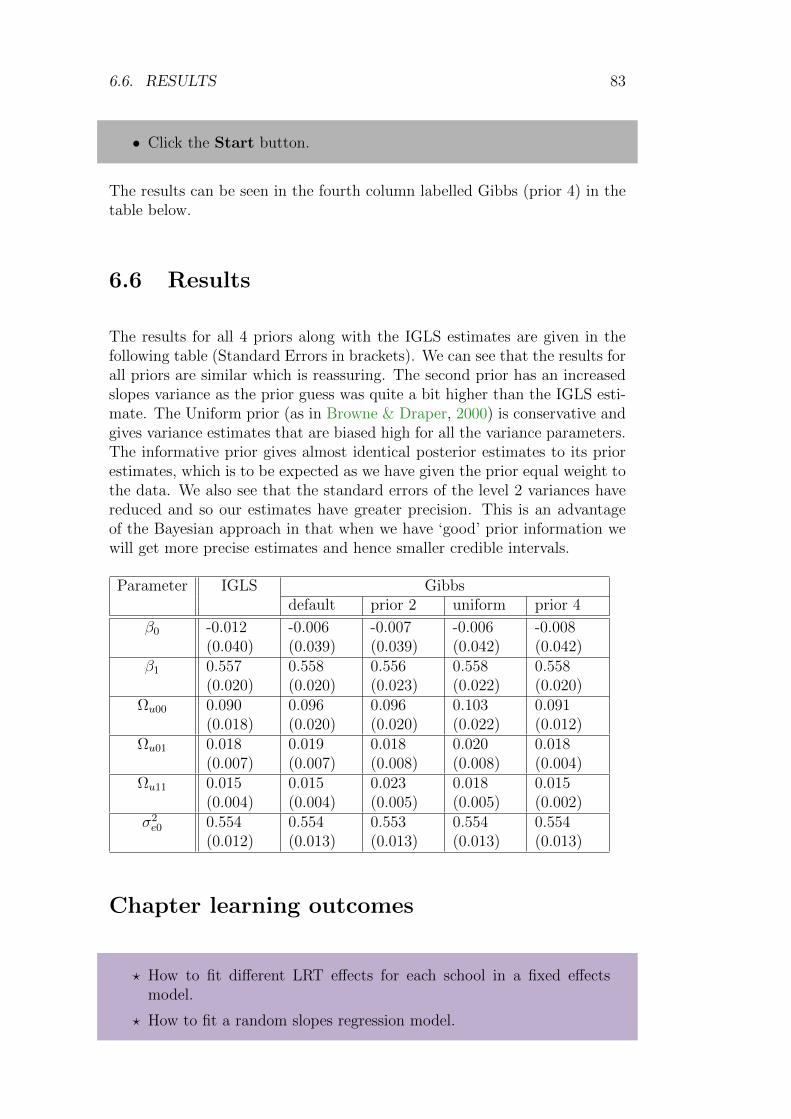
6.6. RESULTS 83
• Click the Start button.
The results can be seen in the fourth column labelled Gibbs (prior 4) in thetable below.
6.6 Results
The results for all 4 priors along with the IGLS estimates are given in thefollowing table (Standard Errors in brackets). We can see that the results forall priors are similar which is reassuring. The second prior has an increasedslopes variance as the prior guess was quite a bit higher than the IGLS esti-mate. The Uniform prior (as in Browne & Draper, 2000) is conservative andgives variance estimates that are biased high for all the variance parameters.The informative prior gives almost identical posterior estimates to its priorestimates, which is to be expected as we have given the prior equal weight tothe data. We also see that the standard errors of the level 2 variances havereduced and so our estimates have greater precision. This is an advantageof the Bayesian approach in that when we have ‘good’ prior information wewill get more precise estimates and hence smaller credible intervals.
Parameter IGLS Gibbsdefault prior 2 uniform prior 4
β0 -0.012(0.040)
-0.006(0.039)
-0.007(0.039)
-0.006(0.042)
-0.008(0.042)
β1 0.557(0.020)
0.558(0.020)
0.556(0.023)
0.558(0.022)
0.558(0.020)
Ωu00 0.090(0.018)
0.096(0.020)
0.096(0.020)
0.103(0.022)
0.091(0.012)
Ωu01 0.018(0.007)
0.019(0.007)
0.018(0.008)
0.020(0.008)
0.018(0.004)
Ωu11 0.015(0.004)
0.015(0.004)
0.023(0.005)
0.018(0.005)
0.015(0.002)
σ2e0 0.554
(0.012)0.554(0.013)
0.553(0.013)
0.554(0.013)
0.554(0.013)
Chapter learning outcomes
? How to fit different LRT effects for each school in a fixed effectsmodel.
? How to fit a random slopes regression model.

84 CHAPTER 6.
? How to compare models via the DIC diagnostic.
? How to create prediction intervals for a model using MCMC.
? A greater understanding of prior distributions.

Chapter 7
Using the WinBUGS Interfacein MLwiN
We have so far looked at fitting Normal response models to continuous uni-variate data in MLwiN. We could consider fitting further models with ad-ditional fixed or random terms and these would simply be extensions to themodels fitted thus far. There are, however, other extensions that we couldconsider; for example, heteroskedasticity of the response variable, which weconsider in Chapter 9 and alternative distributions for the random effectsthat we will consider later in this chapter.
The MCMC features in MLwiN are fairly new and we currently fit onlymodels of particular types although we are constantly extending the numberof models that can be fitted. If, however, a user wishes to fit a model thatcannot be currently fitted, for example fitting an alternative distribution forthe school level random effects, there are three main options. Firstly waitfor a later version of MLwiN that will fit their model; secondly write theirown code to fit their model; or thirdly try an alternative software package,for example WinBUGS.
WinBUGS (Spiegelhalter et al., 2000a, freely available from http://www.
mrc-bsu.cam.ac.uk/bugs) in its earlier guise of BUGS was one of the firstBayesian software packages and is a more general purpose Bayesian estima-tion engine than the MCMC engine in MLwiN. It works on a different phi-losophy of fitting models that can be represented by directed acyclic graphs(DAGs). BUGS has a compiled language which allows the user to specifytheir model through statements of two types—logical and distributional—which between them describe the structure of the DAG and hence the model.Then BUGS compiles this user code and constructs an MCMC estimationengine for the user’s model that can be run to give chains of estimates in asimilar way to the MLwiN engine.
In this chapter we will firstly consider once again the variance components
85

86 CHAPTER 7.
model and show how to fit this model in WinBUGS. We then go on toconsider a model that MLwiN cannot fit which has t-distributed residuals atthe school level. It should be noted at this point that most multilevel modelsare large and so cannot be run using the educational version of WinBUGSand so you will need to have the release version of WinBUGS.
7.1 Variance components models in WinBUGS
We will consider the tutorial dataset once again. Set up and run the variancecomponents model with one explanatory variable (standlrt) using the IGLSmethod by
• Pressing the Start button
On IGLS convergence we get the following estimates:
In Chapter 3 we then considered fitting this model using MCMC in MLwiNbut here we will consider instead using WinBUGS. To get to the BUGSoptions in MLwiN we need to do the following:
• Click on the Estimation Control button.
• Select the MCMC tab.
• Select MCMC/WinBUGS Options from the Model menu.
This will bring up the WinBUGS Options screen that looks as follows:

7.1. VARIANCE COMPONENTS MODELS IN WINBUGS 87
From this screen we can save the BUGS code for the currently set up modelor read in the output files that contain parameter traces from BUGS for usein MLwiN (see later). For now we will save our current model in BUGSformat:
• Select the WinBUGS 1.4 button.
• Click on the large button at the top of the window.
This will bring up a file save window similar to those for inputting andsaving worksheets. For now we will save the file in the default directoryas tutorial.bug. This will create a file that contains the BUGS modeldefinition, initial values and data. For users of classic BUGS who are usedto having three separate files, in WinBUGS the file tutorial.bug containsthe information from these three files with comment lines dividing them. Inwhat follows we use WinBUGS version 1.4.3 and so it is possible that resultswill change with other versions.
For background information on using WinBUGS it is strongly suggested thatthe user reads some of the user manual and examples documentation thatcomes with the package, in particular to become familiar with the WinBUGSnotation. For now to fit our model in WinBUGS, we must start the Win-BUGS program and read in the file tutorial.bug (from the directory it wassaved in) as a text file. Note that you will have to change the Files of typebox to All files (*.*) to see the file tutorial.bug. Having read in the file awindow headed tutorial.bug will appear containing the information neededby BUGS for this model.
As mentioned earlier the WinBUGS code is split into 3 sections and we willconsider these here in turn. Firstly a model definition is required and thisconsists of a description of the structure of the current problem. The codefor our simple variance components problem is as follows:
# WINBUGS 1.4 code generated from MLwiN program

88 CHAPTER 7.
#----MODEL Definition----------------
model
# Level 1 definition
for(i in 1:N) normexam[i] ∼ dnorm(mu[i],tau)
mu[i]<- beta[1] * cons[i]
+ beta[2] * standlrt[i]
+ u2[school[i]] * cons[i]
# Higher level definitions
for (j in 1:n2) u2[j] ∼ dnorm(0,tau.u2)
# Priors for fixed effects
for (k in 1:2) beta[k] ∼ dflat() # Priors for random terms
tau ∼ dgamma(0.001000,0.001000)
sigma2 <- 1/tau
tau.u2 ∼ dgamma(0.001000,0.001000)
sigma2.u2 <- 1/tau.u2
WinBUGS is a more general modelling package and so there is no standardorder to the model description although when the code is generated fromMLwiN it will generally have a similar structure. We firstly define the rela-tionship between the response (in this example normexam) and the fixedand random predictor variables.
Note that the column names from MLwiN are used as the variable namesin WinBUGS. WinBUGS does have some differences in what it allows as avariable name so if the WinBUGS code will not work it may be that some ofyour variable names are illegal, for example a column name like 1995 will beinterpreted as a number in WinBUGS so it is worth renaming such columnsin MLwiN.
So we see here that our response is normally distributed and that we havetwo fixed effects, beta[1] and beta[2] (always defined as beta by the codegenerator) and one set of random effects, u2 (always defined as u# where# is the level/classification indicator). Note that in WinBUGS the fixedeffects, beta, and all other vectors always start with index 1 and not 0 so thatthere will probably not be direct correspondence between the MLwiN andWinBUGS indexing. Next the code defines the random effects u2 as beingNormally distributed before finally giving the priors for the fixed effects andthe variances.
WinBUGS has two types of relationship: distributional relationships that

7.1. VARIANCE COMPONENTS MODELS IN WINBUGS 89
are described by the ∼ symbol and deterministic relationships that are de-scribed by the <- symbol which is also used in the S-plus package. Note thatthe normal distribution definition in WinBUGS, dnorm, has two parametersthat are the mean and the precision (NOT the variance), hence the deter-ministic relationship used to calculate the variance. The prior distributionsare identical to those used in the MCMC options in MLwiN.
Before running a model in WinBUGS we first need to read in the particularelements of the model using the Specification window available from theModel menu. After selecting the window containing the model by clickingon it, clicking on the check model button should give the message ‘modelis syntactically correct’ at the bottom of the screen. Next we need to load inthe data for the model. Due to the fact that the data is generally the largestpart of the file generated by MLwiN it is included after the initial values.For the tutorial.bug example the data section begins as follows:
#----Data File----------------------------------
list(N= 4059, n2 = 65,
school = c(1,1,1,1,1,1,1,1,1,1,1,1,1,1,1,1,1,1,1,1,1,1,1,1,1,1,1,1,1,
1,1,1,1,1,1,1,1,1,1,1,1,1,1,1,1,1,1,1,1,1,1,1,1,1,1,1,1,1,1,1,1,1,1,1,
1,1,1,1,1,1,1,1,1,2,2,2,2,2,2,2,2,2,2,2,2,2,2,2,2,2,2,2,2,2,2,2,2,2,2,
2,2,2,2,2,2,2,2,2,2,2,2,2,2,2,2,2,2,2,2,2,2,2,2,2,2,2,2,2,3,3,3,3,3,3,
3,3,3,3,3,3,3,3,3,3,3,3,3,3,3,3,3,3,3,3,3,3,3,3,3,3,3,3,3,3,3,3,3,3,3,
3,3,3,3,3,3,3,3,3,3,3,4,4,4,4,4,4,4,4,4,4,4,4,4,4,4,4,4,4,4,4, ...
Again BUGS borrows its notation from S-plus using the convention c(. . . )to represent a vector of observations. Here we see the first two constants,N and n2 that define the number of level 1 units and level 2 units, followedby a list of the school identifier for each observation. To load the data intoBUGS we need to highlight the list identifier at the start of the data listand click on the load data button in the specification window. If this issuccessful the message ‘data loaded’ will appear at the bottom of the screen.Next we have to combine the data and model definition by clicking on thecompile button. Again if this operation is successful a message appears atthe bottom of the screen, this time stating that ‘model compiled’.
Finally as BUGS uses MCMC methods all unknown parameters will needstarting values. These are included in the initial values part of the file thatfor our example is as follows:
#----Initial values file----------------------------
list(beta= c(0.002391,0.563371),
u2 = c( 0.373760,0.502043,0.503889,0.018131,0.240431,0.541395,
0.379002,-0.026173,-0.135181,-0.337021,0.179300,-0.061863,-0.149648,
-0.165592,-0.182922,-0.409984,-0.172780,-0.084464,-0.011510,0.214462,

90 CHAPTER 7.
0.244016,-0.435732,-0.489244,0.209408,-0.230472,-0.023543,0.023121,
-0.610002,0.240626,0.158475,0.033280,-0.006457,0.029590,-0.137882,
0.128634,-0.181341,-0.189077,-0.153068,0.130317,-0.234439,0.211543,
0.092820,-0.089927,-0.247556,-0.109729,-0.352727,-0.042628,-0.045058,
0.042845,-0.302412,-0.051373,0.381929,0.723314,-0.547252,0.503474,
0.009972,0.031894,0.138115,-0.658368,0.225656,-0.039551,-0.054029,
0.535641,0.087692,-0.165764),
tau= 1.767625,
tau.u2= 10.854523)
This gives the estimates from the IGLS run for the fixed effects and preci-sions, and an MLwiN RESI command for the initial values for u2 that areexactly what the MCMC routine in MLwiN uses as starting values. To usethese values in WinBUGS we need to highlight the list identifier at the startof the initial values and click on the load inits button on the specificationwindow. This will then give the final message ‘initial values loaded; modelinitialized’. Note that WinBUGS will generate starting values for any pa-rameters that have not explicitly been given starting values but here we havegiven all parameters starting values.
We are now ready to run the Gibbs sampler in the WinBUGS package. Beforewe start the estimation engine we have to tell WinBUGS which parameterswe wish to monitor. We will choose the same parameters as MLwiN uses.From the Inference menu select the Samples options and a window willappear that allows the user to specify which parameters to monitor. In thiswindow we will firstly select the fixed effects by typing beta in the nodebox. Note that when a correctly typed parameter is input the set buttonwill become enabled. We will also want to use a burn-in of 500 iterationsso we will also modify the beg value from 1 to 501. After this press the setbutton and the parameter will be set for monitoring. We now need to repeatthis procedure with the two variance parameters sigma2 and sigma2.u2.
It should be noted that it is possible in WinBUGS to get dynamic tracesof the parameters like those in the Trajectories window in MLwiN via thesample window. If we either type beta again in the node box or use thescroll button at the side of the box to select beta you will see that now allthe buttons become enabled. Clicking the trace button will give 2 emptytrace plots for beta[1] and beta[2] (as shown below), which will becomedynamic when we start updating. Similar traces can be brought up for thetwo variance parameters.

7.1. VARIANCE COMPONENTS MODELS IN WINBUGS 91
We are now ready to set the estimation engine running and this is done viathe Update window found in the Model menu. We need to specify thenumber of updates (including the burn-in) and so we will replace the 1000here with 5500 as is used in MLwiN. As in MLwiN you can also specify howoften to refresh the screen, whether to use thinning and, if WinBUGS needsto use Metropolis Hastings sampling, whether to adapt. There is also theoption to use a technique called over-relaxation that improves the mixingof the MCMC chains but takes longer per iteration. The current version ofWinBUGS (1.3) will choose the MCMC routines it uses for you dependingon the form of the conditional distribution (see section 1.3 of the WinBUGSmanual for details).
Now that we have set the number of iterations press the update buttonto start the sampler. After a few minutes (depending on the speed of yourprocessor and how many traces you are viewing) the update counter willreach 5500 and the sampling will be finished. WinBUGS has the nice featurethat it will give you a message at the bottom of the screen, for example‘updates took 88s’, stating how long the sampling took which is useful forcomparing model run times etc. Generally WinBUGS is slower for modelsthat can also be run in MLwiN but as we will see later it has greater flexibilityin the models it can fit and sometimes the MCMC methods it uses are moreefficient than the Metropolis Hastings methods used in MLwiN for binomialand Poisson response models.
Once the sampling has finished we can now look at the estimates, plots andother information again via the sample window. To get summary informa-tion, select beta in the node box and click on the stats button. A nodestatistics window will appear giving the following
node mean sd MC error 2.5% median 97.5% start samplebeta[1] 0.002979 0.03995 0.002516 -0.07465 0.004435 0.07912 501 5000beta[2] 0.5634 0.01264 1.997E-4 0.5388 0.5636 0.5882 501 5000
These results are similar to those obtained from MLwiN, and we can also getsimilar results for the other parameters as shown below.
node mean sd MC error 2.5% median 97.5% start samplesigma2 0.5661 0.0127 1.653E-4 0.5416 0.5662 0.5905 501 5000sigma2.u2 0.09662 0.02019 3.256E-4 0.06415 0.09446 0.1426 501 5000
We can also get trace plots and kernel density plots via the history anddensity buttons respectively. Below we see the trace plot for the parameterbeta[2]

92 CHAPTER 7.
and the kernel plot.
Currently WinBUGS does not allow the smoothing parameter to be changedfor the kernel plots so that they look rather crude but this will be changedin later versions. Note here that we could have typed * in the node box toget statistics or plots for all monitored nodes.
WinBUGS currently produces limited summary statistics and plots itself.Historically the plots and MCMC diagnostics were provided via a suite ofS-plus functions called CODA (Best et al., 1995), and WinBUGS also hasthe option to produce the input files that CODA requires. MLwiN can alsouse these files to input the parameter chains from WinBUGS into columnsin MLwiN.
Here we will consider all parameters by using the * option so select this inthe node box and press the coda button on the sample window. This willproduce two windows that are labelled CODA index which contains thevariable names and CODA for chain 1 which contains the values for theparameter chains. We will now save these files as text files by clicking on therespective windows and then choosing Save As from the File menu. We willneed to save the files in plain text (*.txt) format. We will store the CODAindex file as tutorial.ind and the CODA for chain 1 file as tutorial.outin the same directory as tutorial.bug. Note that these are the extensionsthat the classic BUGS used for these files but, as we have selected the plaintext format, WinBUGS will add an additional .txt to the index filename andso the files are actually saved as tutorial.ind.txt and tutorial.out.txt.
Now back in MLwiN if you want to input the traces return to the BUGSoptions window that we used earlier (available from the Model menu).
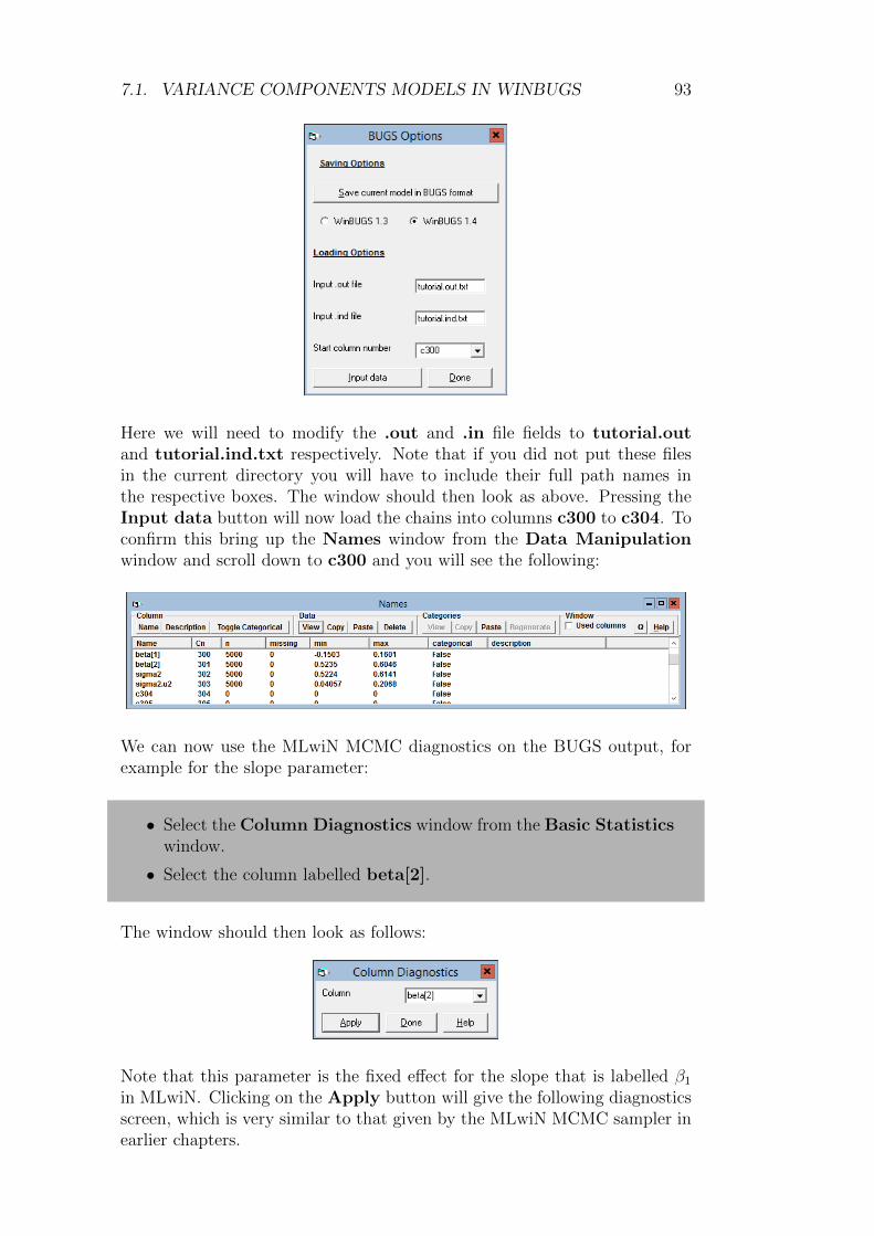
7.1. VARIANCE COMPONENTS MODELS IN WINBUGS 93
Here we will need to modify the .out and .in file fields to tutorial.outand tutorial.ind.txt respectively. Note that if you did not put these filesin the current directory you will have to include their full path names inthe respective boxes. The window should then look as above. Pressing theInput data button will now load the chains into columns c300 to c304. Toconfirm this bring up the Names window from the Data Manipulationwindow and scroll down to c300 and you will see the following:
We can now use the MLwiN MCMC diagnostics on the BUGS output, forexample for the slope parameter:
• Select the Column Diagnostics window from the Basic Statisticswindow.
• Select the column labelled beta[2].
The window should then look as follows:
Note that this parameter is the fixed effect for the slope that is labelled β1
in MLwiN. Clicking on the Apply button will give the following diagnosticsscreen, which is very similar to that given by the MLwiN MCMC sampler inearlier chapters.

94 CHAPTER 7.
We can repeat all of the above procedures for the intercept parameter andthe two variances and we will see that we get similar results for all fourparameters with both MLwiN and WinBUGS.
7.2 So why have a WinBUGS interface ?
The example we have just gone through will give similar results using bothsoftware packages and to use WinBUGS we have to move back and forth be-tween the two packages. Also the estimation engine in WinBUGS is slower,so you may be asking yourself the above question. The interface was writ-ten originally as a testing tool to confirm that when new types of modelsare programmed into MLwiN we get the same answers as WinBUGS. Werecommend that you check that both packages give similar answers.
7.3 t distributed school residuals
The main advantage of having a WinBUGS interface however, is to allowmodels that have not yet been developed in MLwiN to be fitted using Win-BUGS. We will illustrate this by considering alternative distributions for theschool level residuals in the tutorial example we considered earlier. In theUser’s Guide to MLwiN we look at plots of residuals against normal scores toconfirm that the normal distributional assumption is a good fit to the data.
The normal distribution is a member of the t distribution family. The t dis-tribution family has an additional degrees of freedom (df ) parameter and thenormal distribution is the limiting case when this parameter reaches infinity.We will here consider replacing the normal distribution at level 2 with a tdistribution where the df parameter has itself got a prior distribution. Forthis we will use a uniform prior and allow the df parameter to take values

7.3. T DISTRIBUTED SCHOOL RESIDUALS 95
in the range 1 to 200. This allows both small values, where the distributionhas very long tails, and large values, which are indistinguishable from thenormal distribution.
To include this prior we will need to edit the model definition in the filetutorial.bug. The new version is as follows (edits in blue):
#----MODEL Definition----------------
model
# Level 1 definition
for(i in 1:N) normexam[i] ∼ dnorm(mu[i],tau)
mu[i]<- beta[1] * cons[i]
+ beta[2] * standlrt[i]
+ u2[school[i]] * cons[i]
# Higher level definitions
for (j in 1:n2) u2[j] ∼ dt(0,tau.u2,df)
# Priors for fixed effects
for (k in 1:2) beta[k] ∼ dflat() # Priors for random terms
tau ∼ dgamma(0.001,0.001)
sigma2 <- 1/tau
tau.u2 ∼ dgamma(0.001,0.001)
sigma2.u2 <- 1/tau.u2
df ∼ dunif(2,200)
We will also need to give a starting value for df in the initial values file andso we will choose (arbitrarily) df = 10. Our initial values file then looks asfollows:
#----Initial values file----------------------------
list(beta= c(0.002391,0.563371),
u2 = c( 0.373760,0.502043,0.503889,0.018131,0.240431,0.541395,
0.379002,-0.026173,-0.135181,-0.337021,0.179300,-0.061863,-0.149648,
-0.165592,-0.182922,-0.409984,-0.172780,-0.084464,-0.011510,0.214462,
0.244016,-0.435732,-0.489244,0.209408,-0.230472,-0.023543,0.023121,
-0.610002,0.240626,0.158475,0.033280,-0.006457,0.029590,-0.137882,
0.128634,-0.181341,-0.189077,-0.153068,0.130317,-0.234439,0.211543,
0.092820,-0.089927,-0.247556,-0.109729,-0.352727,-0.042628,-0.045058,
0.042845,-0.302412,-0.051373,0.381929,0.723314,-0.547252,0.503474,
0.009972,0.031894,0.138115,-0.658368,0.225656,-0.039551,-0.054029,

96 CHAPTER 7.
0.535641,0.087692,-0.165764),
tau= 1.767625,
tau.u2= 10.854523,
df = 10)
This time we will monitor the same four parameters as before plus the dfparameter which we will set in the sample window. Note that the adaptingbox on the update window is ticked because for this model, WinBUGS1.4 uses a method called slice sampling to update the df parameter. Notethat the tick disappears when adapting has finished. We again run for 5000iterations after a burn-in of 500 iterations and get the following trace for df:
Here we see reasonably good mixing. Earlier versions of WinBUGS (1.3)didn’t use the slice sampler and then this parameter did not mix but the slicesampler has improved on this. We can see from the summary statistics belowthat on this small sample of 5000 iterations we cannot reject the possibilityof a heavy-tailed distribution.
node mean sd MC error 2.5% median 97.5% start sampledf 97.83 57.75 4.409 8.13 94.96 194.5 501 5000
In order to investigate the potential of starting value dependence we startedthree chains with identical parameter starting values except for df, which wasset to 2, 10 and 200 respectively for the 3 runs. To do this in WinBUGS isfairly easy as on the specification window there is a num of chains box thatwe edit to 3 (immediately after checking the model is syntactically correct).Then load the data and compile before loading the 3 sets of initial values.This simply involves editing the df=10 line of the initial value file beforeloading each set. We will increase the burn-in to 2000 by changing the begbox to 2001 on the sample window when we input the parameters we wishto monitor. We will also increase the updates to 12000 so that we have amonitoring run of 10000 iterations after the burn-in. Pressing update, thethree sets of chains will be run concurrently and so this will take longer.
If we look at plots of the 3 sets we see that, all 3 chains are mixing well

7.3. T DISTRIBUTED SCHOOL RESIDUALS 97
and there is strong overlap suggesting that sensitivity to the starting valueis not a problem. If we look at the summary statistics for the three chainscombined we get:
node mean sd MC error 2.5% median 97.5% start sampledf 101.5 56.12 1.832 9.671 101.2 195.1 2001 30000
This summary information suggests that a very small degrees of freedom (df)parameter and hence an extremely heavy tailed distribution is not likely butthat a value of df of less than 10 is not out of the question.
As a sensitivity analysis we will instead try fitting a model where the degreesof freedom is assumed known and has value 8 which suggests a slightly long-tailed distribution at level 2. Seltzer (1993) gives Gibbs sampling algorithmsfor exactly this scenario of a known df parameter. We will need to simplifyour model definition as follows:
# WINBUGS 1.4 code generated from MLwiN program
#----MODEL Definition----------------
model
# Level 1 definition
for(i in 1:N) normexam[i] ∼ dnorm(mu[i],tau)
mu[i]<- beta[1] * cons[i]
+ beta[2] * standlrt[i]
+ u2[school[i]] * cons[i]
# Higher level definitions
for (j in 1:n2) u2[j] ∼ dt(0,tau.u2,df)
# Priors for fixed effects
for (k in 1:2) beta[k] ∼ dflat() # Priors for random terms
tau ∼ dgamma(0.001,0.001)
sigma2 <- 1/tau
tau.u2 ∼ dgamma(0.001,0.001)
sigma2.u2 <- 1/tau.u2
df <- 8
and we will also need to remove the initial values for parameter df as itis now a constant. Again we will monitor beta, sigma2 and sigma2.u2.After running for 5000 iterations after a burn-in of 500 we get the followingestimates:

98 CHAPTER 7.
node mean sd MC error 2.5% median 97.5% start samplebeta[1] -0.001065 0.04125 0.002364 -0.08322 -7.715E-4 0.07792 501 5000beta[2] 0.5633 0.0124 1.979E-4 0.5391 0.5636 0.5872 501 5000sigma2.u2 0.07657 0.01805 4.247E-4 0.04746 0.0745 0.1171 501 5000sigma2 0.5662 0.01279 1.787E-4 0.5421 0.5659 0.5916 501 5000
Here we see that the fixed effects and level 1 variance are little changedin terms of point estimate and standard errors, suggesting the analysis isrobust to different level 2 distributions. The level 2 variance parameter isnot directly comparable as the variance of the t distribution is a function ofboth the sigma2.u2 and df parameters.
In fact the variance is 8/6 × 0.07657 = 0.102, which is slightly higher thanfor the Normal case.
We will investigate the WinBUGS interface further when we consider binaryresponse models in Chapter 10 and for several examples in later chapters.Here we will look at how the different procedures used in WinBUGS for thesemodels compare with the methods used in MLwiN.
Chapter learning outcomes
? How to create WinBUGS code from the MLwiN package.
? How to run models in WinBUGS.
? How to output chains from WinBUGS back into MLwiN.
? How to fit t distributed residuals in WinBUGS.
? How to check the sensitivity of the Gaussian assumption at level 2of the model.

Chapter 8
Running a Simulation Study inMLwiN
This book describes how to fit various statistical models using the MCMCmethodology available in MLwiN. One of the main questions people havewhen faced with a new methodology is what is its advantage over the currentmethod I am using? An alternative question that is often faced when usingMCMC methods is ‘Which prior should I use for my model?’ When we wishto compare which method or which ‘default’ priors are ‘best’ for our particularmodel and dataset we are faced by the problem of not knowing what thecorrect estimates should be. There are also issues about in what sense is amethod ‘better’ than another method and depending on your criterion youmay get different conclusions.
One of the best ways to compare different estimation methods is to run asimulation study. Here we generate simulated datasets where the true valuesof the parameters are known and so we have a ‘gold standard’ to compare ourestimates with. MLwiN is especially suited for running simulation studiesas the macro language underlying the package can be used both to generatesimulated datasets and fit models via several estimation methods. In thischapter we demonstrate how to perform one particular simulation study,and give macro code that can then be altered by the reader to fit alternativesimulation studies.
8.1 JSP dataset simulation study
Browne (1998) performed several simulation studies to compare likelihood-based methods with Bayesian MCMC methods with several alternative ‘de-fault’ prior distributions. These simulations were extended in Browne &Draper (2000, 2006). Browne used as the basis for his simulations a smalleducational dataset from the Junior School Project (JSP) (Mortimore et al.,
99

100 CHAPTER 8.
1988) and created many datasets with the same or similar structure to thisactual dataset. We will here consider one of the smallest models that Brownelooked at which contained 108 pupils spread evenly over 6 schools. In ourexample we will simply compare the IGLS maximum likelihood method withthe MCMC method with default (Γ(ε, ε)) priors.
To run a simulation study consists of four basic steps, two of which arerepeated:
1. Set up the structure of the dataset
Repeat the next 2 steps N times.
2. Generate a simulated dataset based on the true parameter values
3. Fit the model to the simulated dataset using all the methods to becompared.
4. Analyse the results of the N simulations.
We will now deal with the four steps in turn.
8.2 Setting up the structure of the dataset
For the purposes of our simulation we are going to fit a variance componentsmodel with no predictors to a dataset with 108 pupils in 6 schools. Conse-quently before we start we need to create 3 columns: a pupil id, a school idand a constant vector for the intercept term. We will also need to create aresponse variable although this will be generated for each simulated datasetso, for now, we will create a dummy constant response.
All of these columns can be created by the Generate Vector window butas we wish to run our simulations in batch mode we will need to write macrocommands instead. Fortunately virtually all the window buttons that per-form an action in MLwiN have an associated command in the commandlanguage. For more details on the command language see the Commandmanual or the online help where information on a particular command canbe found in the index under ‘Command XXXX’ where XXXX is the nameof the command.
So to start our macro we will do the following:

8.2. SETTING UP THE STRUCTURE OF THE DATASET 101
• Start up MLwiN.
• Select the Generate vector window from the Data Manipulationmenu.
• Select Sequence.
• Select Output column c1.
• Select Start number 1.
• Select End number 108.
• Select Step value 1.
The window should now look as follows:
Now click on Generate and column c1 will contain the numbers 1–108 torepresent the pupil identifiers. If we now look at the Command interfacewindow:
• Select the Command Interface window from the Data Manipu-lation menu.
• Remove the tick by the user box by clicking on it.
You should now see a lot of commands that MLwiN has performed whenstarting up, and the window should look something like the following:
The important command here is the GENErate command that creates thevector of level 1 identifiers. We now also need to create level 2 identifiers anda constant vector for both the intercept and the response. This can be doneusing the Generate Vector window as follows:

102 CHAPTER 8.
• Select Repeated Sequence.
• Select Output column c2.
• Select Maximum Number 6.
• Select Number of Repeats per Block 18.
• Select Number of Blocks 1.
• Select Generate.
• Select Constant Vector.
• Select Output Column c3.
• Select Number of Copies 108.
• Select Value 1.
• Select Generate.
• Select Output Column c4.
• Select Generate.
This will set up the four columns c1–c4 and we can then name these columnsusing the Names window. We will name the columns pupil, school, consand resp. After naming these four columns the Command interface win-dow will look as follows:
So here we see that setting up the four columns and naming them uses8 commands. (We can ignore the WSET commands). We could copy thesecommands into a macro so that rather than typing these commands we couldinstead just execute the macro. To do this:
• Select New Macro from the File Menu.
• Copy the 8 lines into this new macro window (highlight them usingthe mouse then press Ctrl+C, move to the Macro window and pressCtrl+V).
• Select Save Macro As from the File Menu.

8.2. SETTING UP THE STRUCTURE OF THE DATASET 103
• Browse to find the folder where the sample worksheets are located(somewhere like ‘C:\Program Files (x86)\MLwiN v2.31\samples’ )
• Type the file name simu into the Save window.
• Click on the Save button.
The macro window should now look as follows (note the directory name maybe different on your machine):
Note that any commands the macro window recognizes as valid macro com-mands it will colour blue. We now need to set up the variance componentsmodel as usual. Former users of MLN will know that there are also commandsthat can be used to set up models rather than the Equations window. Fornow set up a model in the Equations window that has resp as the response,2 levels with school as level 2 and pupil as level 1 and one predictor conswhich is a fixed effect and random at both levels 1 and 2. If you are not surehow to do this then you should re-read Chapter 2. Viewing the Commandinterface window we now see the following:
So here we have 6 commands that have set up the model. We can now addthese 6 commands to our macro so that we now have:

104 CHAPTER 8.
We have not yet saved our macro, which we can tell from the ‘[Modified]’that appears on the top bar of the window, so now save the macro again byselecting Save Macro from the File menu. We can now exit MLwiN andrestart. To get back to our position we simply need to:
• Select Open Macro from the File menu.
• Select simu.
• Click on Open.
• On the macro window that appears click on Execute.
(Note that in this case a quicker way to open the macro is to select it fromthe list of recently used macros at the bottom of the File menu.) So we havea macro that will set up the basic model structure. Now we will extend thismacro so that it generates simulated datasets.
8.3 Generating simulated datasets based on
true values
In order to perform repeated actions we now need to use several macrocommands that are not commonly used when running MLwiN in interac-tive mode. These commands are LOOP, ENDLOOP, OBEY, PAUSE,SEED and JOIN. We will have already seen most of these commands inthe macros we looked at in Chapter 1. The LOOP and ENDLOOP com-mands allow us to repeat a series of actions several times and the JOINcommand will allow us to join the results of each action onto the end of acolumn so that later we can store the results of all our simulations in onecolumn. The PAUSE 1 command as mentioned in Chapter 1 is an escapecommand in that it momentarily stops the macro at a point and updates allthe windows. We can illustrate these commands in action by modifying ourmacro to include the following extra commands:

8.3. STEP 2: GENERATING SIMULATED DATASETS 105
Before clicking on the Execute button you should now do the following:
• Select View/Edit Data from the Data Manipulation menu.
• Click on the View button.
• Select c5.
• Click on OK.
• On the Macro window click on the Execute button.
This macro, as should be evident when you click on Execute, simply writesthe loop number (stored in box b1) to the end of the column c5 and refreshesthe screen after each number. Interesting as this is, we would actually preferto do something more useful, at each iteration, than simply write out theiteration number. As we can see our macro has now become quite long. Inmacro writing as with other forms of programming it is useful to introducestructure into the code to aid readability. Although the current version ofthe Macro language does not include the concept of a function (that takesarguments) we can use the OBEY command to redirect a macro to anothermacro which can be thought of as a function with no arguments.
Here we will firstly write a short macro that will generate a simulated re-sponse based on the true settings for all the parameters. For brevity for therest of this chapter we will simply list commands rather than go through thewhole process of describing exactly how to perform the same actions via themenus and windows. To aid in your understanding you may want to try andperform the same actions using the windows to confirm you get the sameanswers.
Note that MLwiN reserves the columns c1096 and c1098 for storing theparameter estimates for the current model. To generate a response we there-

106 CHAPTER 8.
fore need to set the three values in c1096 and c1098 to the true answersfor the variance parameters and the fixed effects respectively. By defaultMLwiN will generate a warning if these are protected to prevent them frombeing accidently overwritten, so before we can change them we need to usethe MARK command to turn off this warning prior to editing and turn itback on afterwards. For example the command
MARK 0
will turn off column overwrite warnings and the command
MARK
will turn them back on.
Once this is done we can enter the desired values via the EDIT command,which is equivalent to editing the numbers in the Data window. For examplethe command
EDIT 1 c1096 10
will put the value 10 in the first position of c1096 which corresponds to thelevel 2 variance estimate. For the level 1 variance we use the true value 40and for the intercept we use the value 30.
Now given the true values we need to generate a random response from therandom part of the model and add this to the fixed part of the model. Herewe use the following command
SIMU 'resp'
This is a special command that takes the fixed effects and variance estimates,generates residuals at each level and by adding these to the fixed effectsconstructs a random response vector.
So to include these four commands in a macro do the following:
• Select New Macro from the File menu.
• Type the six commands into the macro.
• Save the macro as genresp.

8.3. STEP 2: GENERATING SIMULATED DATASETS 107
The macro should look as follows:
We can now execute this macro and then run the model.
• Click on the Execute button on the macro window.
• Click on the Start button.
As we have not changed the estimation settings MLwiN will have run themodel using our generated response using the IGLS method. If we look atthe estimates in the Equations window we should have something like thefollowing:
Note that we have not yet added a SEED command so you may get differentestimates due to having a different random response vector. We now need tolink up our macro for generating random responses via the OBEY command.You now need to alter the simu macro so that it looks as follows:

108 CHAPTER 8.
Here we have added two commands: SEED 1 that sets the random numberseed before the simulations begin and BATCH 1 that tells MLwiN we arerunning the macro in batch mode and so when we run the IGLS method (seelater) the macro will run to convergence rather than just for 1 iteration. Notethat the OBEY command includes the path name and so you may need tomodify this on your machine.
So we now have a macro that when run will generate 100 response vectors,we now need to add a macro that will run the methods and store the resultsin columns. This macro we will call runmodel and all results will be outputto columns c11–c15 so we will erase these columns before we start. Wetherefore need to make the following final modifications to macro simu:

8.4. STEP 3: FITTING THE MODEL 109
8.4 Fitting the model to the simulated datasets
We now need to write a macro that will run both the IGLS method and theMCMC method. To discover the commands that IGLS and MCMC uses youcan run both methods and look at the commands output although there willbe many commands, in particular for MCMC. This is because the MCMCcommand is called each time the screen is refreshed and also the software usesthe IGLS estimates and the RESI command to set up good starting valuesfor the residuals. To save you typing the commands yourself the macro canbe loaded:
• Select Open Macro from the File menu.
• Select runmodel from the list of files and click on Open.
The macro opened should look as follows:

110 CHAPTER 8.
Here we first run the IGLS method and store the estimates in c11 and theirvariances in c12. Then we run the MCMC method using the residuals andestimates from IGLS as starting values and run for 10,001 iterations after aburnin of 500. Note in their simulations Browne & Draper ran for 50,000iterations, and so it is easy to change the macro to do this, although herefor speed we use a shorter main run. We store the estimates in c13 andtheir variances in c14. For the Bayesian 95% credible intervals we need tocalculate the quantiles of the posterior distributions from the chains of valuesand for this we have another short macro as shown below:
To calculate the 2.5% percentile point we need to find the value where 2.5%

8.4. STEP 3: FITTING THE MODEL 111
of the other values in the chain are lower and 97.5% are higher hence we usea chain of 10,001 iterations rather than 10,000 for ease of calculation. Wefirstly separate the three chains using the SPLIt command and then sorteach of them and pick out the correct values storing them stacked in columnc15.
We can now run our first macro simu.txt to perform our simulation. In orderto watch the progress it will be worth opening the Data window and viewingthe columns where the output will appear. Note that we have used the JOINcommand in such a way that the estimates for each dataset will appear atthe top of each column. Note also that if you wish to view the output it isimportant to ensure that the Macro window is not above the Data window.Finally, note that because we have used commands like ‘OBEY genresp.txt’we will need to change the current directory to the directory where these filesare located. (We could alternatively have used the full pathname instead ofjust genresp etc. and then we would not have needed to change directory).
• Select View/Edit Data from the Data Manipulation menu.
• Select columns c11–c15 from the view option of this window.
• Stretch the Data window so all five columns are shown (they will becurrently empty).
• Select dIrectories from the Options menu.
• Click the Browse button next to the current directory box, locatethe folder where you saved the macros and click OK.
• Click Done.
• Click on the Execute button on the simu.txt macro window.
Running the 100 simulations may take a little time. For each simulation thecolumn c11 will have three estimates added to it and so as an indicator ofprogress this column will be of length 300 when the simulations are complete.Upon the macro finishing the window should look as follows:
All five output columns contain information for the 100 simulations stackedup.
Here c11 and c13 have the three sets of estimates stored for the IGLS and

112 CHAPTER 8.
MCMC methods respectively. Columns c12 and c14 contain the variances ofthe three estimates plus the covariances between the two variance estimates.Column c15 contains the MCMC 95% credible interval end points for the 3parameters. We now need to transform these five columns into some sensiblesummary measures.
8.5 Analysing the simulation results
In order to summarise the results of 100 simulations we will follow the exam-ple of Browne & Draper (2006) and consider the bias and interval coverageproperties of the two methods. For this we have written another macro anal-yse.txt. This macro, which is shown in part below, involves finding, as pointestimates, the average of the 100 simulations for each method. For intervalestimates, for the IGLS method we need to calculate the endpoints of 95%confidence intervals, and for this we use central Gaussian (mean ± 1.96×sd)intervals. See Browne & Draper (2006) for information on alternative inter-vals to be used with the IGLS method. The MCMC credible intervals havealready been calculated. Next we have the simple task of counting the num-ber of simulations where the true value is between the interval end points foreach interval.
The above macro involves separating the output columns via the SPLIt com-mand, and then calculating the required summary statistics via the CALCand AVER commands. The results are put in c40 for IGLS and c41 for theMCMC method as shown below:

8.5. STEP 4: ANALYSING THE SIMULATION RESULTS 113
These results show the point estimates with standard errors for the threeparameters and the percentage of intervals that cover the true parametervalue for each parameter.
These results are similar to those in Browne & Draper (2006). Both methodsshow very little bias for the intercept (true value = 30) and the MCMCprocedure only has a slight bias for the level 1 variance (true value = 40,MCMC mean estimate = 41.78). The level 2 variance however has bothmethods giving biased estimates. The true value is 10 and IGLS gives anaverage estimate of 8.25 (a 17.5% negative bias) whilst MCMC gives anaverage estimate of 16.91 (a 69.1% positive bias). As Browne & Draper showthe median estimate using the Γ(ε, ε) prior has much better bias properties(a 0.6% negative bias in their simulations) and this macro could be easilymodified to also calculate the medians for each simulation.
In terms of interval coverage the MCMC method gives much better coveragefor both the intercept and the level 2 variance. The level 1 variance has goodcoverage under both methods. Note however that if we were to look at theinterval widths we will find, like Browne & Draper, that the MCMC methodshave much larger intervals. Of course running only 100 simulations is notreally enough to compare the methods properly and more simulations wouldbe preferred. It would be easy to alter the above macros to run for 1000simulations with the MCMC method main run length increased to 50,000like Browne & Draper but this will take longer to run. It would also be easyto monitor the median for the MCMC method and the interval widths forboth methods.
The simulations in Browne & Draper originally took a few months to runbut given the advances in speed of processors running ALL the simulationsin their paper would today be much quicker.
Chapter learning outcomes
? How to run simulation experiments in MLwiN.

114 CHAPTER 8.
? How to use many new Macro commands.
? How to compare estimation methods for a particular model.

Chapter 9
Modelling Complex Variance atLevel 1 / Heteroscedasticity
One level normal response models assume that all responses are (conditionalon predictor values) independent observations from a Gaussian distributionwith an unknown mean structure and constant variance. The interest infitting one level models such as regressions and other linear models lies inimproving the description (in terms of fit to existing data and predictivepower) of the unknown mean function. In this book so far we have extendedthese one level models to the multilevel modelling framework while main-taining a constant level 1 variance.
The primary goal of multilevel modelling is to adjust inferences on parameterestimates to account for non-independence between observations. The vari-ance components models described in Chapters 3–5 do this by adjusting forcorrelation between responses taken from the same ‘higher level unit’. Thismeans that we assume that two responses taken from the same ‘higher levelunit’, for example school, are more likely to be similar than two responseschosen at random.
Although variance components models adjust for correlation between re-sponses in a cluster they still assume a constant variance across responses,which they split into components at the various levels of the model. This con-stant variance assumption may not be true and the variance of the responsesmay, like the mean of the responses, be a function of predictor variables.When the variance is treated as a function of the predictor variables this isknown as ‘heteroscedasticity’ or complex variation. In this chapter we willlook at fitting models that account for this complex variation using MCMCmethods. Browne et al. (2002) consider exactly this problem and give furtherdetails about the exact algorithms that we use later.
To illustrate ‘heteroscedasticity’ we can consider the tutorial dataset again.Before fitting any models to the dataset we could consider the values of the
115

116 CHAPTER 9.
response for different subsets (partitions) of the dataset. This partitioningof the dataset may then suggest predictors to fit in the model. To look atpartitions of the dataset we can use the Tabulate window in MLwiN:
• Select Tabulate from the Basic Statistics menu.
• Select Means as the Output Mode.
• Select normexam for the Variate column from the pull down list.
• Select girl from the pull down list to the right of Columns.
The screen should then look as follows:
• Press the Tabulate button.
0 1 TOTALSN 1623 2436 4059MEANS -0.140 0.0933 -0.000114SDs 1.03 0.970 0.992
Here we have split the dataset into boys (0) and girls (1). It is noticeablethat the two subsets differ both in terms of mean and standard deviationand hence variance (although the difference in standard deviation is prettysmall). We saw in Chapter 2 that girls did significantly better than boysbut there we assumed a constant variance for the two groups. In Chapter2 our main predictor of interest is the intake score, standlrt (c5). Thisvariable is continuous so in order to tabulate the response we will need tocreate partitions of the dataset based on ranges of intake variable. Here weaim to split the dataset into seven roughly equal partitions. To do this wecreate a column, named intakecat, which labels the partitions 0 (lowestintake scores) to 6 (highest intake scores). Enter the following commands atthe Command Interface window:

9.1. MCMC ALGORITHM 117
Calc c11 = (c5>(-1)) + (c5>(-0.5)) + (c5>(-0.1)) +
(c5>0.3) + (c5>0.7) + (c5>1.1)
Name c11 'intakecat'
Now if we return to the Tabulate window we can display the means for theseseven partitions as follows:
• Select intakecat from the pulldown list to the right of Columns.
• Select Means as the Output Mode.
• Press the Tabulate button.
The output for this tabulate command is as follows:
0 1 2 3 4 5 6 TOTALSN 612 594 619 710 547 428 549 4059MEANS -0.887 -0.499 -0.191 0.0439 0.278 0.571 0.963 -0.000114SDs 0.855 0.774 0.806 0.811 0.812 0.824 0.838 0.817
Here, as in Browne et al. (2002), the partitions 0 to 6 refer to intake scoresin the ranges less than −1, −1 to −0.5, −0.5 to −0.1, −0.1 to 0.3, 0.3to 0.7, 0.7 to 1.1, and greater than 1.1 respectively. We can see that themeans for the partitions increase with intake score and this corresponds tothe positive coefficient found for the intake fixed effect in Chapter 1. We can,however, also see that the standard deviation (and therefore the variance)of the partitions is not constant and is also, with the exception of the firstcategory, increasing. This pattern with larger variances at both extremecategories suggests that perhaps assuming a quadratic relationship betweenintake score and the variance would be sensible. We will next explain themodifications required to the MCMC algorithms to fit non-constant variancefunctions before returning to the tutorial example. Readers not interestedin the algorithmic details can skip the next section whilst those who wish toknow more can read Browne et al. (2002).
9.1 MCMC algorithm for a 1 level Normal
model with complex variation
We will here consider fitting the linear regression model from Chapters 1and 3 but with the additional assumption that the variance is a quadratic

118 CHAPTER 9.
function of the reading test predictor. The model can be written
yi = β0 + β1x1i + ei
ei ∼ N(0, σ2ei) where σ2
ei = XTeiΩeXei = Ωe0,0 + 2x1iΩe0,1 + x2
1iΩe1,1
Here although we think of the variance as a quadratic function, we maintainthe matrix formulation Ωe used by the IGLS method. The vector Xei containsthe predictors used in the level 1 variance for individual i, in this case theconstant predictor (x0 = 1 for all individuals) and the intake score (x1). Notethat if we wish to fit a simpler linear variance function we can constrain Ωe1,1
to equal zero.
To fit the model in a Bayesian framework we need to add prior distributionsfor the unknown parameters, β0, β1, and Ωe. We will use the default priorsfrom MLwiN, p(β0) ∝ 1, p(β1) ∝ 1 and p(Ωej,k) ∝ 1 for all j, k subject to theconstraint that σ2
ei > 0 for all i. This prior is equivalent to a uniform prioron all matrices Ωe that satisfy the constraint and is the only prior availablefor these parameters in MLwiN.
The algorithm now consists of two steps. Firstly the fixed effects vectorβ = (β0, β1)T is updated using Gibbs sampling from its bi-variate Normalconditional posterior distribution:
p(β|y, σ2ei) ∼ N2(β, D), where
β = D
[∑i
XTeiyiσ2ei
], and D =
∑i
σ2ei
XTi Xi
The second step then involves updating the three parameters that make upthe level 1 variance matrix Ωe. We cannot update these terms using Gibbssampling and so instead we will use Metropolis Hastings sampling. We willupdate each parameter in turn and will describe here the step to updateΩe0,1 as the other steps are similar. As in the Metropolis macro in Chapter 1we need to use a proposal distribution but this time we will use a truncatedNormal proposal in order to satisfy the constraints that the variance functionmust be positive for all observations.
We can write for every observation i,
σ2ei = 2x1iΩe0,1 − δi0,1, where δi0,1 = −Ωe0,0 − x2
1iΩe1,1
Now for the condition σ2ei > 0 ∀i to hold after we update Ωe0,1 we need
to calculate the truncation points where the condition ceases to hold. Thiswill result, in this case, in two sets of constraints that produce the twotruncation points for our proposal distribution (note that there will be onlyone truncation point for the other two parameters as they are multiplied byterms that are strictly positive). The constraints can be written as follows:

9.2. SETTING UP THE MODEL IN MLWIN 119
mu = mini
(δi0,12x1i
∀i, x1i < 0
)> Ωe0,1 > max
i
(δi0,12x1i
∀i, x1i > 0
)
So the Metropolis Hastings step at iteration t generates a proposed value Ω∗e0,1from a Normal distribution with mean Ω
(t)e0,1 and proposal variance s2
e0,1, thatsatisfies the above constraints and so hence we effectively are drawing froma truncated Normal distribution. Note that, as described in Browne et al.(2002), the value s2
e0,1 can be set by the MLwiN adaptive scheme. Then theupdate step is as follows:
Ω(t+1)e0,1 = Ω∗e0,1, with probability min
[1, R
p(Ω∗e0,1|y, β)
p(Ω(t)e0,1|y, β)
],
Ω(t+1)e0,1 = Ω
(t)e0,1, otherwise.
Here R =Φ(mu−Ω∗
e0,1
s2e0,1
)− Φ
(ml−Ω∗
e0,1
s2e0,1
)Φ
(mu−Ω
(t)e0,1
s2e0,1
)− Φ
(ml−Ω
(t)e0,1
s2e0,1
) which is the Hastings ratio.
The steps for the other two parameters, Ωe0,0 and Ωe1,1 have similar forms tothe above. Now that we have described the two steps the MCMC algorithmas usual consists of repeated application of the steps in turn. We will nowexplain how to set up this model in MLwiN using the tutorial dataset.
9.2 Setting up the model in MLwiN
We will start by setting up the first model from Chapter 2, which has fixedeffects defined for cons and standlrt and cons defined as random at level1. If you are unsure of how to set up this model refer to Chapter 2. Next weneed to include the complex variation terms at level 1.
• Select the standlrt predictor in the Equations window.
• From the X variable window that appears click on (i)student.
• Click on the Done button.
The Equations window should now look as follows:
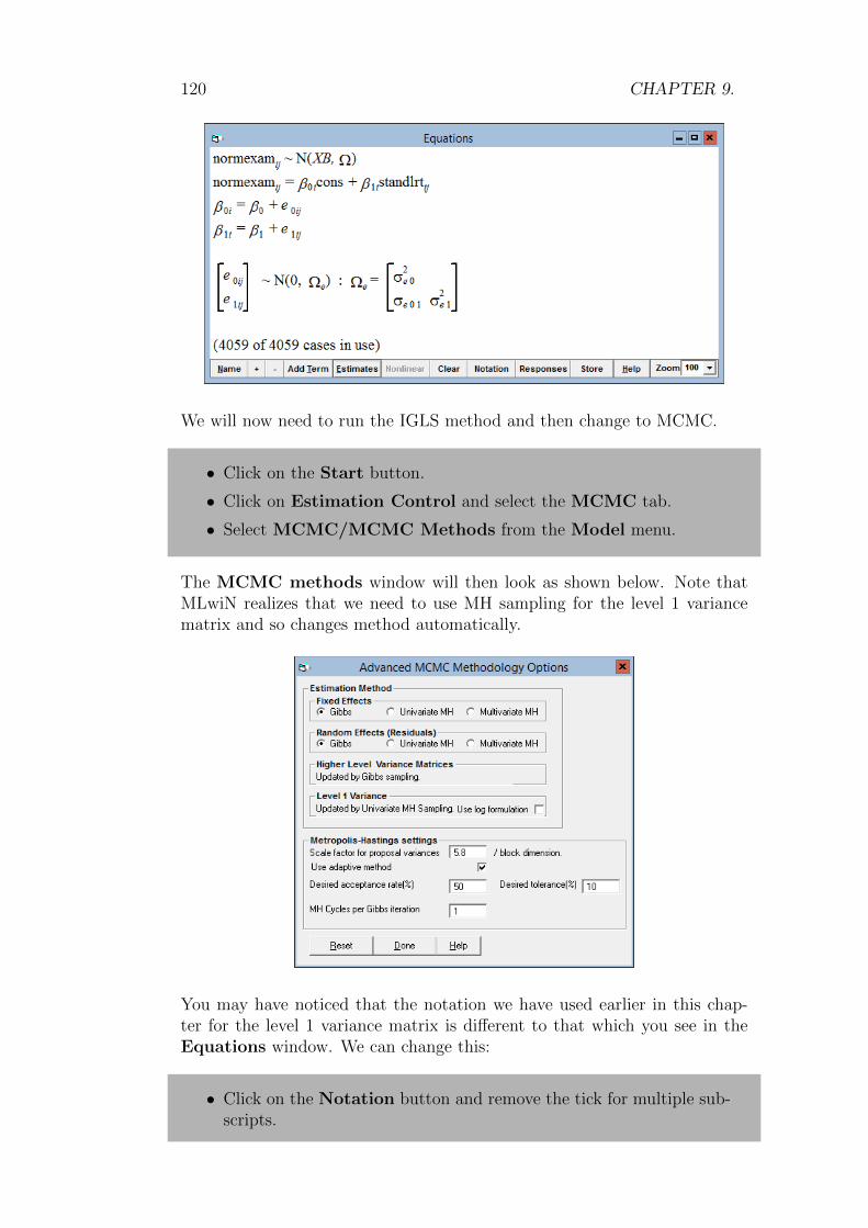
120 CHAPTER 9.
We will now need to run the IGLS method and then change to MCMC.
• Click on the Start button.
• Click on Estimation Control and select the MCMC tab.
• Select MCMC/MCMC Methods from the Model menu.
The MCMC methods window will then look as shown below. Note thatMLwiN realizes that we need to use MH sampling for the level 1 variancematrix and so changes method automatically.
You may have noticed that the notation we have used earlier in this chap-ter for the level 1 variance matrix is different to that which you see in theEquations window. We can change this:
• Click on the Notation button and remove the tick for multiple sub-scripts.

9.2. SETTING UP THE MODEL IN MLWIN 121
• Click on the Done button.
and we will get the following :
Now we need to run our model with complex variation.
• Click the Start button.
Note that the greater complexity in fitting a complex variance function atlevel 1 tends to slow computation down and so it will take longer to runthis model. Upon running for 5,000 iterations if we open the Trajectorieswindow we see the following:
Here we can tell that the variance parameters are being updated by Metropo-lis Hastings sampling by the fact that their chains have a more block-likeappearance. Also we can see that the chain for parameter Ωe1,1 goes nega-tive so it is more appropriate to use this alternative notation as this term

122 CHAPTER 9.
is clearly NOT a variance. We can compare the fit of this model with thesimple variance model via the DIC diagnostic:
• Select MCMC/DIC diagnostic from the Model menu.
The diagnostic is given below and compared with the diagnostic for the modelwith a constant variance fitted in Chapter 2.
Dbar D(thetabar) pD DIC9764.55 9759.62 4.93 9769.499763.54 9760.51 3.02 9766.56
Here we see that the DIC correctly estimates the 5 parameters in the modeland gives a very marginal improvement in fit (9759.6 versus 9760.5). Howeverdue to the two additional parameters the DIC value for this model is higherthan for the simpler model, suggesting in this case that there is no advantagein fitting the more complex variance function. This is backed up by both thelinear and quadratic variance terms being similar to or smaller than theirstandard errors.
The variance function can still however be calculated by using the Variancefunction window.
• Select Variance function from the Model menu.
• Select c12 from the variance output to list.
• Press the calc button.
Note that the variance function screen should look as follows:
Now we can plot the function we have calculated:
• Select Customised Graph(s) from the Graphs menu.

9.3. COMPLEX VARIATION IN MULTILEVEL MODELS 123
• Select column c12 as the Y variable.
• Select column standlrt as the X variable.
• Select plot type line.
• Click on the Apply button.
The graph of the function will appear as follows:
Here we see that this graph mimics the variances of the partitions of thedataset by the categorical intake score that we calculated earlier.
9.3 Complex variance functions in multilevel
models
We have in fact already considered a multilevel model that contains complexvariation. When we considered the random slopes regression model in Chap-ter 6 we interpreted this model graphically in terms of non-parallel regressionlines for each school. We could however also look at this model in terms ofthe (total) variance at the school and pupil level depending on the intakescore.
If we set up the random slopes model and run it using the default MCMCsettings (see Chapter 6 for details on setting up this model) we should getthe following:

124 CHAPTER 9.
Note that as we have clicked on the Notation button earlier some of theother terms will have a different notational form. This notation was designedfor cross-classified models that will be described later in Chapter 15. Clickon Notation again and tick the box for multiple subscripts to see standardnotation for a 2-level model. Now we can calculate and plot both the level 1and level 2 variance functions against the intake score by using the Variancefunction window as follows:
• Select Variance function from the Model menu.
• Select column c12 from the variance output to list.
• Click on the calc button.
• Select 2:school from the level list.
• Select column c13 from the variance output to list.
• Click on the calc button.
This will set up the level 1 function in column c12 and the level 2 functionin column c13. If you have been following this chapter from the start thenthe level 1 variance function will already be plotted and the Customisedgraph window should be as follows:

9.3. COMPLEX VARIATION IN MULTILEVEL MODELS 125
We now need to specify the level 2 variance function so the following isrequired:
• Select ds#2 by clicking in the white box below Y next to 2 on theleft of the window.
• Select c13 as the y variable.
• Select standlrt as the x variable.
• Select plot type line.
• Click on the Apply button.
The graph window will now have two lines in it as shown below:
Here the level 1 variance function is the flat (constant) line at 0.554 while thelevel 2 variance exhibits a quadratic relationship with intake score. Althoughwe did not find any significant evidence of heteroscedasticity in the one levelmodel earlier we can now test if there is any in our two level model. Toinclude the quadratic variance relationship again we need to do the following(after setting estimation method to IGLS):

126 CHAPTER 9.
• Select the standlrt predictor in the Equations window.
• From the X variable window that appears click on (i)student.
• Click on the Done button.
We can now run this model using MCMC by performing the following:
• Click on the Start button.
• Select MCMC from the Estimation menu then click the Donebutton.
• Click on the Start button.
After a short while the model will run and the Equations window (afterzooming to factor 75 to ensure window all fits on screen) will look as follows:
Here we see that the linear variance coefficient at level 1 (2×−0.014) is nega-tive whilst the quadratic coefficient (0.003) is positive but very small. We cancompare the DIC diagnostic for this model with that of the simple randomslopes regression model fitted in Chapter 6 by selecting the MCMC/DICdiagnostic option on the Model window.

9.4. RELATIONSHIP WITH GENDER 127
Dbar D(thetabar) pD DIC9120.64 9028.19 92.44 9213.08 (quadratic variance function at level 1)9122.99 9031.32 91.67 9214.65 (constant variance at level 1)
Here we see that fitting the model with the complex variance function resultsin a slight improvement in DIC. The quadratic term here is very small andif the variance function is plotted it looks approximately linear. Thereforeit would be interesting to see the effect of explicitly fitting just a linearrelationship.
• Change estimation mode to IGLS.
• Click on the quadratic term (0.003) at level 1 in the Equationswindow.
• Reply Yes to the question ‘Remove term standlrt/standlrt from thelevel 1 covariance matrix?’.
The blue 0.003 will be replaced by a grey 0 to indicate a structural zero inthe equations window. We now need to run this reduced model.
• Click on the Start button.
• Select MCMC from the Estimation menu.
• Click on the Start button.
• After the model has finished running select MCMC/DIC diagnosticfrom the Model menu.
If we now compare the DIC for this model we see
Dbar D(thetabar) pD DIC9119.41 9027.74 91.66 9211.07 (linear variance function at level 1)9120.64 9028.19 92.44 9213.08 (quadratic variance function at level 1)
So the simpler linear variance function is prefered to the quadratic function.
9.4 Relationship with gender
At the start of this chapter we considered partitioning the dataset into boysand girls and saw that gender seems to affect both the mean response andthe variance of the response. If we continue from the current model whichhas a linear variance function we can now add gender as a fixed effect andallow the level 1 variance to have terms for gender and gender by intake score.This can be interpreted as fitting two different linear relationships at level 1,one for boys and one for girls. Note that, although we are going to add all

128 CHAPTER 9.
the terms at once, generally you would want to add each in turn testing asyou go. To set up the model we need to do the following:
• Change Estimation mode to IGLS.
• Click on the Add term button on the Equations window.
• Select girl from the variable list and click on the Done button.
• Click on the girl variable in the Equations window and tick thelevel 1 box.
• Click on the bottom right 0.000 in the level 1 variance matrix. Amessage asking if you want to remove girl/girl should appear.
• Choose Yes to remove this term.
• Click on the Start button.
This will have set up the model and run it using IGLS and the Equationswindow should be as below:
We will now run the model using MCMC.
• Change Estimation method to MCMC.
• Click on the Start button.
After running the model we can once more check the DIC diagnostic value(via the Model menu).
Dbar D(thetabar) pD DIC9083.92 8990.26 93.66 9177.57

9.4. RELATIONSHIP WITH GENDER 129
Here we see that the DIC diagnostic has reduced significantly. If we hadadded terms in stages we would have seen that the majority of the reductionwas due to adding in gender as a fixed effect but there is also a significantreduction due to the more complex variance structure.
The variance at level 1 is now
σ2ei = Ωe0,0 + 2standlrtiΩe0,1 + 2girliΩe0,2 + 2standlrtigirliΩe1,2
So we have two separate linear relationships for boys and girls, which can becalculated by the Variance function window (along with the updated level 2variance function)
• Select Variance function from the Model menu.
• Select 1:student from the level list.
• Select column c12 from the variance output to list.
• Click on the calc button.
• Select 2:school from the level list.
• Select column c13 from the variance output to list.
• Click on the calc button.
The graph window will still be displaying the correct columns for the vari-ances but as we need to separate out the girls’ and boys’ lines at level 1 weneed to update the Customized graph window as follows:
• Select ds#1 by clicking in the white box below Y next to 1 on theleft of the window.
• Select girl as the group column.
• Click on the Apply button.
The graph will then appear as follows:

130 CHAPTER 9.
Note that you could label or colour the various lines and rescale the graph toinclude the origin but this is left as an exercise for the reader. The top twographs are the level 1 variance functions with the boys having the steepernegative slope. This graph is showing that the choice of school (level 2variance) is more important for the higher intake pupils than for the lowerintake pupils, and that intake score has a much greater effect on the varianceof responses for boys than girls. Note that in these complex variance functionmodels the simple intra-school correlation measure described in Chapter 4does not exist. However for a given gender and intake score we can calculatean equivalent measure, and as in Chapter 4 we can calculate the chain andhence confidence intervals for this measure.
9.5 Alternative log precision formulation
Spiegelhalter et al. (2000b) consider the problem of heteroscedasticity in mul-tilevel models in their schools example. One of the problems of the approachwe have described in this chapter is the restrictions on prior distributions forfitting this model. Spiegelhalter et al. (2000b) get around fitting the varianceat level 1 as a function of predictors, by instead fitting the log of the precisionat level 1 as a function of predictors. This means that, as the log of the pre-cision can take values anywhere on the real line, there are no constraints toworry about. We can consider fitting the above model using this formulationand so we will have
log(1/σ2ei) = Ωe0,0 + 2standlrtiΩe0,1 + 2girliΩe0,2 + 2standlrtigirliΩe1,2
To fit such a model in MLwiN we need only tell the software that we wantto fit this formulation via the MCMC Methods window.
• Change estimation to IGLS.
• Click on the Start button to run the model.
• Change estimation to MCMC.
• Select MCMC/MCMC Methods window from the Model menu.
• Click on the Use log formulation tickbox under Level 1 variance.
It should be noted at this point that currently the Equations window doesnot show this change in the model. For prior distributions MLwiN onlyallows uniform priors for all elements of Ωe, although now that the parameterconstraints have been removed it is possible to use informative Normal priorsvia WinBUGS and the WinBUGS interface.
We will now run the model by clicking on the Start button. Note that thelog formulation is slower to run. Upon completion we will get the followingestimates:

9.5. ALTERNATIVE LOG PRECISION FORMULATION 131
We can once again construct the graphs for these variance functions via thevariance functions window. We will however have to convert these valuesfrom inverse precisions to variances.
• Select Variance functions from the Model menu.
• Select 1:student from the level list
• Select column c12 from the variance output to list.
• Click on the calc button.
• Select 2:school from the level list.
• Select column c13 from the variance output to list.
• Click on the calc button.
• Select the Command interface window.
• Enter the command
CALC C12=1.0/EXPO(C12)

132 CHAPTER 9.
The Graph display window will now have changed to show the variancesin this new model as follows:
Here the relationship at level 1 is still nearly linear. If we look at the DICdiagnostic we see that there is no advantage in using the log-precision formu-lation and in this case the standard variance function formulation has lowerDIC value.
Dbar D(thetabar) pD DIC9085.01 8991.09 93.92 9178.93 (log-precision formulation)9083.92 8990.26 93.66 9177.57 (variance formulation)
Although the log formulation has the advantage of the ability to specifyinformative priors for level 1 variance terms (note this is available in Win-BUGS only) it suffers from the disadvantage that individual coefficients of thevariance function do not have a simple interpretation and the real variancerelationship is only accessible via a graph as shown above.
Chapter learning outcomes
? How to account for heteroscedasticity in Normal response models.
? How to graphically interpret variance functions.
? How to compare the fit of models via the DIC diagnostic.
? How to fit alternative log-precision functions.

Chapter 10
Modelling Binary Responses
In this book we have so far considered fitting models where our response is acontinuous variable. Of course there are many other possible response types,for example interest often lies in binary, proportion or count data. In thischapter we consider binary data. There are many possible scenarios wherebinary or 0/1 data occur: in education, exam score responses may often bein the form of a pass or fail; in health care, responses are often whether atreatment is successful or not; in political data, whether people vote for aparticular party or not.
In this chapter we will consider an example dataset from the 1988 BangladeshFertility Survey. This dataset consists of 1934 women who are grouped in60 districts and the response of interest is whether these women were us-ing contraception at the time of the survey. As predictor variables we willconsider effects for the age of the women, the number of children they haveand the district they come from. We will also be interested in whether thebetween-district variation differs for urban and rural areas.
The dataset can be found in the file bang1.ws. The reader unfamiliar withthe IGLS methods for fitting binary response models is referred to the User’sGuide to MLwiN.
• Select Open Sample Worksheet from the File menu.
• Select bang1.ws from the list of worksheets.
• Select Open.
The Names window will then look as follows:
133

134 CHAPTER 10.
Here woman identifies the individual women, district the district they livein and use whether they use contraception (1) or not (0). The predictorswe will consider are age which is the woman’s age in years centred aroundthe average age, lc which is the number of living children and urban whichcategorises the area (which is a sub-area of the districts) in which they liveas either urban (1) or rural (0). The other possible predictors that canbe investigated by the reader are educ which categorises education level ofthe women from none (1) to at least secondary education (4), hindu whichcategorises religion into Hindu or Muslim (other religions were excluded), andtwo district level predictors d illit and d pray which give the proportion ofilliterate women and the proportion of women who pray every day, for eachdistrict.
10.1 Simple logistic regression model
We will start by considering a simple logistic regression model accounting forthe age of the women only. Logistic regression models are more complicatedto fit than Normal models using the IGLS estimation method in MLwiN asthe methods use Taylor series expansions to approximate the model at eachiteration. This means that the estimates they produce are quasi-likelihoodestimates rather than maximum likelihood. For users familiar with earlierversions of MLwiN the use of two constant columns here labeled cons andbcons to allow for the transformations performed by the approximation indiscrete response modelling is now automated. Binomial response modelsalso need a special (denominator) column that contains the counts of thenumber of trials each Binomial is based on. For 0/1 data this will be anothercolumns of ones but for proportion data this will contain the number of unitson which each proportion is based.
To set up the basic logistic regression model we need to do the following:
• Select Equations from the Model menu.
• Click on the Clear button to remove any existing model in the work-sheet

10.1. SIMPLE LOGISTIC REGRESSION MODEL 135
• Click on the red y.
• Select use for the y variable.
• Select 2-ij for the number (N) of levels.
• Select district as level 2(j).
• Select woman as level 1(i).
• Click on the Done button.
• Click on the N and instead choose Binomial from the list.
This will set up the response variable and its type, and the hierarchicalstructure of the dataset. The window will look as follows:
We now need to set up the denominator column and our predictor variables:
• Click on the red nij.
• Select denomb and click on the Done button.
• Click on the red x0.
• Select cons and click on the Done button.
• Note the level 1 variance is Binomial and so doesn’t need adding.
• Click on the Add Term button.
• Select age from the variable list and click on the Done button.
The window now looks as follows:
There are several possible quasi-likelihood methods available in MLwiN but,as we are only using them for starting values and to set up the model, we

136 CHAPTER 10.
will use the default methods:
• Click on the Nonlinear button on the Equations window.
• On the window that appears click on Use Defaults.
• Click on the Done button.
• Click on the Start button.
The model should now run in 3 iterations. We now want to run the samemodel using MCMC.
• Select MCMC from the Estimation menu.
• Select MCMC/MCMC Methods from the Model menu.
The window will then appear as shown below. Here we see that for non-Normal responses MLwiN will not allow Gibbs sampling. We will discussthis at the end of the chapter when we compare MLwiN with WinBUGS onbinary response models.
If we now run the model using MCMC:
• Click the Start button.
we will get the following results (after clicking twice on the Estimates but-ton):

10.1. SIMPLE LOGISTIC REGRESSION MODEL 137
Here we see that the intercept term is −0.437, which, as age is centred,corresponds to the average woman. In order to convert this into a probabilitywe need to transform it onto the probability scale. This can be achieved bythe anti-logit operation in the Command interface window. Typing thecommand CALC B1=ALOG (-0.437) produces a probability of usingcontraception of 0.392. Note you may have to click the Output button tosee this in the Output window. The age coefficient is small and of the samemagnitude as its standard error, suggesting that there is no real effect of age.It should be noted that unlike the quasi-likelihood methods, we can now finda deviance for our models and use the DIC diagnostic.
The deviance formula for a Binomial model is :
D = −2∑i
[yi log(pi) + (1− yi) log(1− pi)]
where pi is the predicted value for observation i. To calculate pi we willneed to use the inverse distribution function that corresponds to the linkfunction, so for the logit we will need to calculate the antilogit for each fittedvalue as described above for the average woman. This is all performed in thebackground when the DIC diagnostic is calculated.
• Select MCMC/DIC diagnostic from the Model menu.
The output can be seen below along with that for the simpler model (whichwe will not fit) with just a constant probability of usage.
Dbar D(thetabar) pD DIC2591.28 2589.29 1.99 2593.27 (Model with age)2591.90 2590.91 0.99 2592.88 (Model without age)
We can see here that, as with the Normal case, the DIC diagnostic picksup almost exactly the correct degrees of freedom. The DIC diagnostic alsoconfirms that the model without age is only marginally better as we sus-pected from the coefficients and standard errors. Note that for Binomial

138 CHAPTER 10.
models there are two possible parameterisations for D(thetabar), the meanparameterization which uses the average value of pi from the chain, and thecanonical parameterization which uses the average values of the individual βithat form pi. In MLwiN we always use the canonical parameterisation but itshould be noted that the different parameterizations will often give differentDIC values.
In all the models fitted thus far we have been using the default monitoringrun length of 5,000 iterations. This is not to be encouraged and we shouldalways check we have run the MCMC algorithm for long enough particularlyfor non-Normal models where Metropolis sampling is the default for someparameters.
• Select Trajectories from the Model menu.
• Click on the chain for β1.
• Select Yes to calculate diagnostics.
The diagnostics for the age effect will then appear as follows:
Here we can see that the kernel plot shows a large probability of a valueless than zero. The Raftery-Lewis diagnostic suggests that we should runfor roughly three times our current run length. Note that as we are moreinterested in whether this effect is zero or not than quoting this parameterto two significant figures we will ignore the Brooks-Draper diagnostic.
We can now run this model for 15,000 iterations to see if this changes ourestimates:
• Select the Estimation Control window.
• Change Monitoring Chain length to 15000.
• Click on the More button.

10.1. SIMPLE LOGISTIC REGRESSION MODEL 139
If you now look at the DIC diagnostic and the MCMC diagnostics windowwe see that neither of them have changed much at all. This confirms theresults from the shorter run of 5,000 iterations.
Although we have found that age is not significant we will, for now, leaveit in the model while adding our next predictor, number of living children(lc). We will add this into the model via the Add Term button. This canbe done (after changing estimation method to IGLS) as follows:
• Change Estimation mode to IGLS.
• Click on the Add Term button on the Equations window.
• Select lc from the variable pull-down list.
• Click on the Done button.
Now we need to run the model using MCMC after using the IGLS method:
• Click on the Start button.
• Change Estimation mode to MCMC.
• Change Monitoring Run Length back to 5000.
• Click on the Done button.
• Click on the Start button.
After estimation has finished the Equations window will (after pressing the+ button) look as follows:
Interestingly when the number of children a woman has is added to the model,

140 CHAPTER 10.
the age coefficient now becomes significant, and of opposite sign. This is dueto the fact that the number of children is correlated with age.
The DIC diagnostic as shown below is greatly reduced in this model with 5parameters.
Dbar D(thetabar) pD DIC2519.98 2515.10 4.88 2524.852591.28 2589.29 1.99 2593.28 (without number of children)
10.2 Random effects logistic regression model
So far we have concentrated on the fixed effects simple logistic regressionmodels analogous to, for the Normal responses, the linear regression modelsin Chapter 1. As with Normal responses we can also add random effects toour model to account for different probabilities of contraception use for thedifferent districts in which the women live.
To add random effects we use the same procedure as with the Normal models.
• Change Estimation method to IGLS.
• Click on cons in the Equations window.
• Click on the (j)district box in the X variable window.
• Click on the Done button.
• Click on the Start button.
Here we have run this model using the IGLS method and the results shouldlook as follows:

10.2. RANDOM EFFECTS LOGISTIC REGRESSION MODEL 141
To now run this model using MCMC:
• Change Estimation mode to MCMC.
• Click on the Start button.
After 5,000 iterations we get the following estimates
We can see here that both the fixed effects and the level 2 variance estimatefrom MCMC are bigger (in magnitude) than the quasi-likelihood estimates.The 1st order MQL method, which is the default method that we have used,is known to give estimates that are biased downwards. We can investigatethe level 2 variance in more detail by viewing its MCMC diagnostics.
• Select Trajectories from the Model menu.
• Click in the trace graph for σ2u0.
• Select Yes to the question ‘Calculate MCMC diagnostics?’
This will bring up the MCMC diagnostics for the level 2 variance parameteras shown below. Here we see that the kernel plot has a long right-hand tail asexpected and consequently the mode, which is the equivalent to the estimateobtained using quasi-likelihood methods, is smaller than the mean. It hasan estimated value 0.279, which compares with the value 0.246 from the 1storder MQL method.
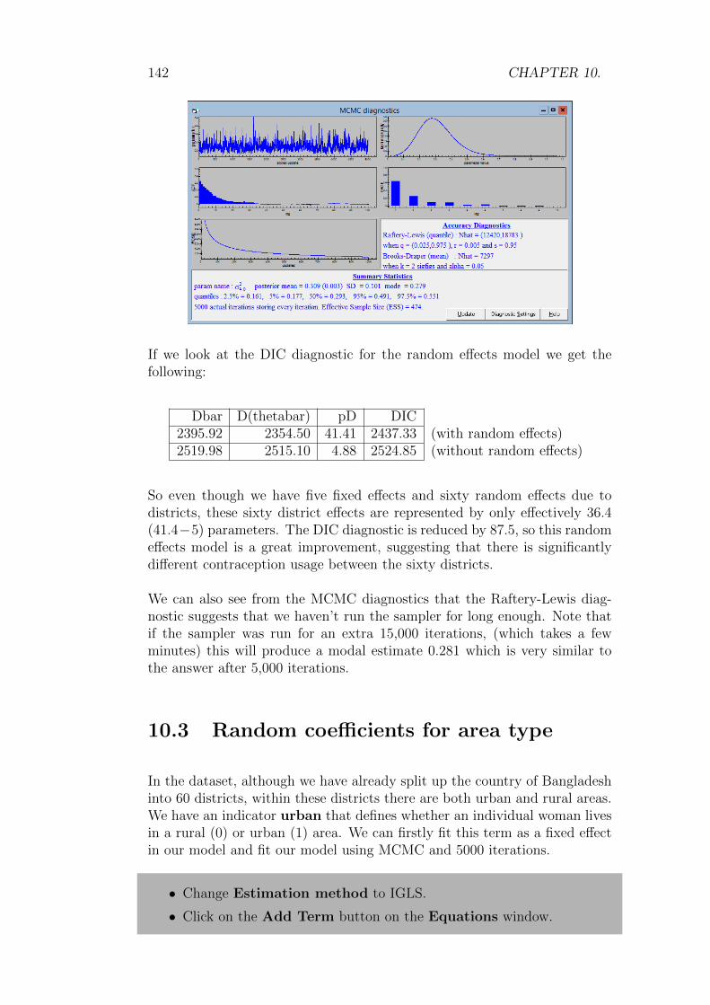
142 CHAPTER 10.
If we look at the DIC diagnostic for the random effects model we get thefollowing:
Dbar D(thetabar) pD DIC2395.92 2354.50 41.41 2437.33 (with random effects)2519.98 2515.10 4.88 2524.85 (without random effects)
So even though we have five fixed effects and sixty random effects due todistricts, these sixty district effects are represented by only effectively 36.4(41.4−5) parameters. The DIC diagnostic is reduced by 87.5, so this randomeffects model is a great improvement, suggesting that there is significantlydifferent contraception usage between the sixty districts.
We can also see from the MCMC diagnostics that the Raftery-Lewis diag-nostic suggests that we haven’t run the sampler for long enough. Note thatif the sampler was run for an extra 15,000 iterations, (which takes a fewminutes) this will produce a modal estimate 0.281 which is very similar tothe answer after 5,000 iterations.
10.3 Random coefficients for area type
In the dataset, although we have already split up the country of Bangladeshinto 60 districts, within these districts there are both urban and rural areas.We have an indicator urban that defines whether an individual woman livesin a rural (0) or urban (1) area. We can firstly fit this term as a fixed effectin our model and fit our model using MCMC and 5000 iterations.
• Change Estimation method to IGLS.
• Click on the Add Term button on the Equations window.

10.3. RANDOM COEFFICIENTS FOR AREA TYPE 143
• Choose urban from the Variable list.
• Click on the Done button.
Now run the model:
• Click on the Start button.
• Change Estimation Method to MCMC.
• Click on the Start button.
We can now see that urban has a fixed coefficient of 0.736 (0.123), whichsuggests that this is a strong predictor and that women in urban areas aremore likely to use contraception than women in rural areas. This is backed upby the reduction in DIC diagnostic to 2408.15 (a drop of 29), which suggeststhat this is a better model.
Just like fitting random coefficients in a Normal response model, we can nowsee if the effect of being in an urban area is different for the various districts.
• Change Estimation method to IGLS.
• Click on the urban predictor.
• From the X variable window click in the j(district) tickbox.
• Click on the Done button.
• Click on the Start button.
• Change Estimation Method to MCMC.
• Click on the Start button.
The model we have now fitted will upon convergence be as follows:

144 CHAPTER 10.
Here we see that the variance between districts is different for urban areasand rural areas with the rural areas having a variance of 0.418 and the urbanareas having a reduced variance of 0.418 − 2 × 0.432 + 0.738 = 0.292. Interms of model fit we are now fitting 6 fixed effects and 2×60 random effectsand so if we look at the DIC diagnostic for this model we get:
Dbar D(thetabar) pD DIC2328.93 2272.31 56.62 2385.56 (with urban random effects)2369.36 2330.58 38.79 2408.15 (without urban random effects)
Here once again we see that adding the extra terms increases the effectivenumber of parameters but reduces the DIC diagnostic suggesting that this isa better model.
10.4 Probit regression
The logit link function is only one of the possible link functions that we canuse with Binomial data. It is commonly used in medical applications as ithas a log-odds interpretation. By this we mean that the exponential of anycoefficient of a variable with a fixed effect (x) may be interpreted as an oddsratio, representing the multiplicative effect of a one unit increase in x onthe odds of the outcome (if x is continuous) or the odds relative to thosefor the reference category (if x is a dummy variable). For example the oddsof using contraception for a woman with one child (using our last model)are e1.157 = 3.18 times the odds of using contraception for women with no

10.4. PROBIT REGRESSION 145
children assuming all other factors are constant. This is particularly used inmedical applications where the response is mortality or infection, and so wecan then work out the relative odds of death or infection for two differentsubsets of the data.
Another popular link function is the probit link, which is the inverse cumu-lative density function of the Normal distribution. This link is often used foreconomics applications although, as with the logit, it can be used in manyapplication areas. One important advantage of the probit both in terms ofMCMC algorithms and interpretation is that we can think of our response asa threshold from an underlying (unknown) continuous response. This inter-pretation of a binary response can be used with any link function, but whenused with the probit link the unknown continuous response is then Normallydistributed.
To illustrate this threshold idea, consider an exam that is marked out of 100.(Note that marks out of 100 are not continuous data but are often treatedas Normally distributed and are a better approximation to continuity thana pass/fail response.) Then a pass mark may be set at 50 and our responsewill be whether an individual student passes (gets 50 or above) or fails (getsbelow 50). So our observed response is the pass/fail indicator but this isreally a surrogate for the more informative (unknown) response, which is theactual mark. The hope is that predictors related to the mark out of 100will also have a similar relationship to the pass/fail response. Of course incertain situations, for example mortality, it is difficult to think of a continuouspredictor which is underlying the 0/1 response (it is hard to rate people asbeing more dead than each other) but we can still use the threshold idea.
The threshold idea goes back a long way in the statistics literature but hasbeen used recently in conjunction with the Gibbs Sampler by Albert & Chib(1993) using a data augmentation algorithm (Tanner & Wong, 1987).
The idea then proceeds as follows: Let us assume we have a binary vari-able yi collected for several individuals i, that is a thresholded version ofan (unknown) continuous Normally distributed variable y∗i . Now if we knewthe value of y∗i then we could fit the standard Gibbs sampling algorithm forNormal response models. So we add an extra step into the Gibbs samplingalgorithm and generate y∗i at each iteration from its conditional posterior dis-tribution which is a truncated Normal distribution with mean (in the singlelevel case) XB and variance 1. The truncation point is zero and if yi is 0, y∗ihas to be negative and if yi is 1, y∗i has to be positive.
Then with the augmented dataset of y∗i generated, the other parameters canbe updated as in the Normal models discussed in earlier chapters. It shouldbe noted that this model can also be updated using Metropolis sampling aswith the logistic regression model but the Gibbs sampling algorithm is fasterand produces less correlated chains (as shown later). Albert & Chib (1993)also give an approximate Gibbs algorithm for the logistic regression model

146 CHAPTER 10.
that uses a t distribution with 8 degrees of freedom as an approximation tothe logistic distribution but this has not been implemented in MLwiN.
10.5 Running a probit regression in MLwiN
We will now fit the last model with random coefficients for urban using aprobit link rather than a logit link. To do this we need to do the following:
• Change Estimation method to IGLS.
• Click on the word logit in the Equations window.
• Choose probit from the link function list and click on the Donebutton.
• Click on the Start button.
• Change Estimation method to MCMC.
By default MLwiN picks univariate Metropolis Hastings for all non-Normalresponse models. We will therefore need to change estimation method toGibbs Sampling.
• Select MCMC/MCMC Methods from the Model menu.
The window will then look as shown below. Note that MLwiN has realisedthat it is possible to use Gibbs sampling for this model.
If we now click on the Reset button then MLwiN will choose Gibbs sampling(alternatively simply click on the two Gibbs buttons).

10.6. COMPARISON WITH WINBUGS 147
If we now run the model by clicking on the Start button, you will noticethat we get the message ‘Burning In. . . ’. This is because we are runningGibbs sampling and there is therefore no need to run an adapting period.The following table gives point estimates and effective sample sizes for runsof 5,000 iterations using both Gibbs and Metropolis sampling for this model.
Parameter Gibbs ESS (Gibbs) Metropolis ESS(MH)β0 -1.039 (0.099) 683 -1.048 (0.099) 60β1 -0.016 (0.005) 1888 -0.016 (0.005) 275β2 0.683 (0.097) 1770 0.692 (0.100) 199β3 0.823 (0.106) 1734 0.830 (0.108) 176β4 0.819 (0.111) 1584 0.829 (0.108) 93β5 0.501 (0.109) 580 0.505 (0.109) 96Ωu00 0.155 (0.050) 769 0.159 (0.051) 182Ωu05 -0.160 (0.067) 518 -0.171 (0.066) 141Ωu55 0.267 (0.118) 414 0.281 (0.111) 124Time 52s 107s
From the table we can see that the Gibbs sampler is not only faster butalso produces larger effective samples due to less correlation in the chains itproduces. We have however roughly the same estimates for both methods.
If we look at the DIC diagnostic for the probit model we see the following:
Dbar D(thetabar) pD DIC2328.19 2271.86 56.33 2384.53 (probit)2328.93 2272.31 56.62 2385.56 (logit)
Here there is very little to choose between the two link functions. It isalso possible to use a third link function, the complementary log-log link,with Bernoulli models but this will not be considered here. Note that theGibbs sampler cannot be used with the probit link when the response is aproportion.
10.6 Comparison with WinBUGS
Binomial response models can be fitted by other MCMC samplers, for exam-ple In earlier versions WinBUGS used the Adaptive Rejection (AR) samplingalgorithm (Gilks & Wild, 1992). It is often interesting to compare the perfor-mance of the various samplers, both in terms of their speed and the autocor-relation in the chains they produce. In the above probit regression example

148 CHAPTER 10.
we saw that the data augmentation Gibbs sampler approach was better bothin terms of run length and chain correlation than the Metropolis algorithm.This is not however the case when we compare the Metropolis algorithm withthe AR algorithm for logistic regression models, as the Metropolis algorithmis usually quicker and so we have to balance greater speed against higherautocorrelation.
We will illustrate this on a simple random slopes logistic regression model.We will clear the current probit regression and set up a model with just anintercept, age as a fixed effect and random effects for the districts.
• Change Estimation method to IGLS
• Click on the Clear button.
• Click on the red y.
• Select use for the y variable.
• Select 2-ij for the number of levels.
• Select district as level 2(j).
• Select woman as level 1(i).
• Click on Done.
• Click on the N and instead choose Binomial from the list.
• Select logit from the link function list and click on the Donebutton.
• Click on the red nij.
• Select denomb and click on the Done button.
• Click on the red x0.
• Select cons and select the j(district) tick box and click on the Donebutton.
• Click on the Add Term button.
• Select age from the variable list and click on the Done button.
The model when set up will look as follows:

10.6. COMPARISON WITH WINBUGS 149
We will firstly run IGLS and set up the model for WinBUGS.
• Click on the Start button
• Select MCMC from the Estimation menu.
• Select MCMC/WinBugs Options from the Model menu.
• Select WinBugs 1.4 radio button.
• Click on the Save Current Model in Bugs format button.
• Change Save as type to .bug files (*.bug).
• Save the file as bang.bug.
We will assume that you have read Chapter 7 and so are familiar with thebasic functionality of WinBUGS. We now need to start the WinBUGS pro-gram and load the file bang.bug as a text file from the directory it has beensaved. Note that again we will need to change the Files of type box toAll files (*.*) to see the file bang.bug. When the file is loaded the modeldefinition will look as follows:
#WINBUGS 1.4 code generated from MLwiN program
#----MODEL Definition----------------
model
# Level 1 definition
for(i in 1:N) use[i] ∼ dbin(p[i],denom[i])
logit(p[i]) <- beta[1] * cons[i]
+ beta[2] * age[i]
+ u2[district[i]] * cons[i]

150 CHAPTER 10.
# Higher level definitions
for (j in 1:n2) u2[j] ∼ dnorm(0,tau.u2)
# Priors for fixed effects
for (k in 1:2) beta[k] ∼ dflat() # Priors for random terms
tau.u2 ∼ dgamma(0.001000,0.001000)
sigma2.u2 <- 1/tau.u2
Here we see that our response variable use is defined as Binomially dis-tributed and is related to the predictor variables via the logit link function.We will need to repeat the set up procedure that we used in Chapter 7 forthe Normal response model:
• Select the Specification window from the Model menu.
• Click on the Check Model button.
• Highlight the list identifier at the start of the data list.
• Click on the Load Data button.
• Click on the Compile button.
• Highlight the list identifier at the start of the initial values list.
• Click on the Load Inits button.
This will have set up our model and we can now pick our parameters to store.Before we do this we will introduce an interesting feature of WinBUGS notmentioned in Chapter 7. If we wish to find out which methods WinBUGS isusing to fit the various components of the model we have defined we can usethe Node Info tool available from the Info menu.
If we then type our node name, for example beta, into the node box on thiswindow we can then hit the method button and get the method used in thelog window, depending on your defaults you may get:
beta[1] UpdaterGLM.LogitUpdater
This can be translated to mean that both the fixed effects are being up-dated using a multivariate Metropolis update using the method developedby Gamerman (Gamerman, 1997). As an aside and in case you do not see theabove method WinBUGS currently offers an alternative rejection samplingmethod. In what follows we will use the Gamerman method but to changeto single site you would need to do the following (if you do these instruc-tions you will need to switch back to the Gamerman method to get the sameestimates later) :

10.6. COMPARISON WITH WINBUGS 151
• Select the Specification window from the Model menu.
• Click on the Check Model button.
• Select the Blocking options window from the Options menu.
• Remove the Fixed effects tick in tick box.
• Highlight the list identifier at the start of the data list.
• Click on the Load Data button.
• Click on the Compile button.
• Highlight the list identifier at the start of the initial values list.
• Click on the Load Inits button.
Upon asking for methods for beta you would then see
beta[1] UpdaterRejection.Logit
beta[2] UpdaterRejection.Logit
Finally in version 1.3 of WinBUGS the default estimation method was dif-ferent again and you would see:
beta[1] UpdaterDFreeARS.StdUpdater
beta[2] UpdaterDFreeARS.StdUpdater
This can be translated to mean that both the fixed effects are being updatedby the standard Adaptive Rejection sampler (Gilks & Wild, 1992).
If on the other hand we type the node name tau.u2 into the node box andhit the method button we will get in either version:
tau.u2 UpdaterGamma.Updater
This is because the precision parameter, tau.u2, is being updated usingGibbs sampling from a Gamma full conditional distribution.
We now need to tell WinBUGS which parameters we wish to store.
• Select the Samples window from the Inference menu.
• Change the beg value to 501.
• Type beta in the node box.
• Click on the Set button.
• Type sigma2.u2 in the node box.
• Click on the Set button.
We have now set up the burn-in of 500 iterations to give a similar burn-in

152 CHAPTER 10.
to MLwiN. We have also stated the parameters we wish to store. To run theupdates we need to use the update window:
• Select the Update window from the Model menu.
• Change the updates value to 5500.
• Click on the update button.
We now need to wait a few minutes for WinBUGS to run. On a Pentium1.8GHz machine the updates take 79 seconds. In order to measure the effi-ciency of the sampler we will import the chains back into MLwiN and lookat the effective sample size (ESS) measure. To do this we need to do thefollowing:
• Select the Samples window from the Inference menu.
• Select beta from the node pull-down list.
• Click on the Coda button.
• Click on the window labelled Coda Index.
• Choose Save As from the File menu and choose plain text (*.txt)format.
• Save file as beta.ind.
• Click on the window labelled Coda for chain 1.
• Choose Save As from the File menu and choose plain text (*.txt)format.
• Save file as beta.out.
Having saved the two files for the fixed effects we can return to MLwiN anduse the BUGS Options window (available from the Model menu) we usedearlier to input the data.
• Change Input .out file to beta.out.txt
• Change Input .ind file to beta.ind.txt
• Click on Input Data button.
This will store beta[1] in column c300 and beta[2] in column c301 andrename the columns accordingly. We can now look at the diagnostics for thetwo parameters via the Column diagnostics window:

10.6. COMPARISON WITH WINBUGS 153
• Select the Column diagnostics window from the Basic Statisticsmenu.
• Select beta[1] from the Column pull-down list.
• Click on the Apply button.
The diagnostics will then appear as shown below. Here we see that theeffective sample size for β1 is 1099 for this sample of size 5,000 due to theautocorrelation in the chain. We can repeat this procedure for β2 and also wecan save the chains for σ2
u and find its effective sample size. The informationfor all these parameters will be summarized in the table at the end of thissection. Note here that the subscript numbering starts from 1 whilst inMLwiN it starts from zero.
We can now run the same model using Metropolis sampling in MLwiN. Themodel should currently be set up and MCMC should already be selected andso all we need to do is start the estimation. MLwiN does not by default givea timing estimate so you will need to time estimation via a stopwatch. It isbest to close all windows to optimise the speed of execution
• Select Close All Windows from the Windows menu.
• Click on the Start button.
For this example the estimation took 12 seconds on a 1.8GHz Pentium. Wecan now get effective sample sizes and other information from the MCMCdiagnostics window.
• Select Trajectories from the Model Menu.
• Click in the β0 trace graph box.
• Select Yes in the Calculate MCMC Diagnostics? box.

154 CHAPTER 10.
The diagnostics for β0 using Metropolis sampling will then be displayed asshown below. Here we have higher autocorrelation and so we see that theeffective sample size is only 185.
The results from the two methods can be seen in the following table. Theworst mixing parameter is the intercept (β0) and to get an effective samplesize of 5000 will take 8 + (5000/1099)× 71 seconds = 5 minutes 31 secondsusing the Gamerman algorithm while Metropolis will take 3 + (5000/185)×9 = 4 minutes 6 seconds. This means that even though the Gamermanalgorithm produces a less correlated chain, Metropolis is sufficiently quickerto give an effective sample of 5,000 in less time.
Parameter Gamerman ESS Metropolis ESS(MH)β0 -0.542 (0.084) 1099 -0.540 (0.089) 185β1 0.009 (0.005) 4929 0.009 (0.005) 1209σ2u 0.265 (0.084) 1221 0.273 (0.092) 433
TimeAdaptationand burn-in
8s 3s
Chain 71s 9sTotal 79s 12s
So we see that here it appears that Metropolis sampling in MLwiN is betterfor this random effects logistic regression model. Browne & Draper (2000)showed similar results for a couple of random effects logistic regression mod-els. It is however not guaranteed that this will be true for all models. ThePoisson models discussed in the next chapter seem to give highly correlatedchains using Metropolis or rejection sampling and they may be models thatit makes more sense to fit using the Gamerman algorithm in WinBUGS.
You may want to test the other models fitted in this chapter using WinBUGS,and so we have one word of warning regarding variable names. MLwiN allowsvirtually any string to represent a column and hence a variable name, for

10.6. COMPARISON WITH WINBUGS 155
example we have a variable in this chapter called three+kids. WinBUGShowever would interpret this literally as two variables called three and kidsand would therefore give an error as these variables are not defined in thedata section of the code. The WinBUGS interface code therefore strips outsuch characters so it is worth checking exactly what the variables have beencalled in your code. It is also therefore sensible to avoid variables that includeany of the following symbols: +,-,*,/,ˆ,(,),[ and ].
Chapter learning outcomes
? How to fit models to binary responses.
? How to fit multilevel random effects linear models.
? How to fit multiple random effects in a logistic model.
? How to fit probit regression models using the Gibbs sampler.
? How to fit binary response models in WinBUGS.
? How to compare estimation methods.
? How to time an estimation run in MLwiN.

156 CHAPTER 10.

Chapter 11
Poisson Response Modelling
In the last chapter we considered the modelling of binary outcome data. Inthat case for every individual our response is coded either as a zero or aone, where the meaning of the two states is dependent on the application.For example we may have pass or fail in education applications or presenceor absence of a disease in medical applications. Often when large datasetsare collected, the response variable (zero or one) may be available at thelowest (individual) level but all other information is collected at a higherlevel for example at an area level. Then rather than fit a Bernoulli model forthe individual responses we may instead either fit a Binomial model for theproportions in each area or a Poisson model for the counts in each area.
In this chapter we will consider fitting models to count data and we willlook at a particular example from the public health literature of counts ofmalignant melanoma mortality in the European community from 1971 to1980 relating them to exposure to ultra-violet radiation (UVB). This datasethas been investigated more thoroughly in Langford et al. (1998).
The dataset can be found in the MLwiN directory and is called mmmec.ws.
• Select Open Sample Worksheet from the File menu.
• Select mmmec.ws and click on Open.
The summary of the data will then be displayed as follows:
157

158 CHAPTER 11.
The data have been collected at a county level and the response variable, obs,consists of the observed count of male deaths from malignant melanoma overthe ten-year period. There are 354 counties from which the counts havebeen taken and these counties are taken from 78 regions in 9 countries in theEuropean Community giving us a 3-level structure. We have one predictoralso recorded at the county level and this is uvbi, which is the (centred)measure of UVB dose that reaches the earth’s surface in each county.
Although the data collected are counts of the number of deaths in eachcounty, counties vary in terms of size and number of years in which thedata were collected. Therefore if we do not account for these differences insome way any effects we see in our model may actually be picking up thedifferences in person-years of exposure between the different counties ratherthan the effects of interest. Commonly therefore in Poisson modelling, theexpected counts (exp in our worksheet) for each region are calculated. Theseassume that every individual has the same underlying mortality rate and sothe values of exp are directly proportional to the person-years of exposure.
As with the Binomial model we need to include a link function to translatethe count data to the whole real line. As count data is not restricted to therange 0–1 we do not use the logit link but instead use the log link which willtranslate the positive counts to values on the whole real line. As we wish toconsider (relative) rates rather than counts we need to use a function of theform:
log(πi/ expi) = f(predictors) where yi ∼ Poisson(πi)
Here yi is the observed count, which is assumed to be Poisson distributedwith mean parameter πi. Note that we can rewrite this equation as:
log(πi) = log(expi) + f(predictors)
The first term on the right is an offset, a known quantity which is to beincluded in the equation, and so in MLwiN we can now create the log of theexpected counts by doing the following:
• Open the Command interface window from the Data Manipu-lation menu and enter the following commands:
calc c9 = loge('exp') name c9 'logexp'

11.1. SIMPLE POISSON REGRESSION MODEL 159
11.1 Simple Poisson regression model
Now that we have created our offset term we are ready to fit our first Poissonmodel. We will first fit a single level model that accounts for our mainpredictor of interest, UV exposure. The model can be set up as follows:
• Select Equations from the Model Menu.
• Click on the red y.
• Select obs as the y variable.
• Select 3-ijk as the number of levels.
• Select nation as level 3(k).
• Select region as level 2(j).
• Select county as level 1(i).
• Click on the Done button.
• Click on the N and select Poisson from the popup list and click onthe Done button.
The above commands have set up the response variable, its distribution andthe hierarchical structure of the dataset. Note that even though we willfirstly fit a single level model we still define the whole three level structure.We now need to set up the offset and predictor variables:
• Click on the πijk and from the offset window that appears selectlogexp.
• Click on the Done button.
• Click on the red x0 and select cons and click on the Done button.
• Click on the Add Term button.
• Select uvbi from the variable list and click on the Done button.
• Click on the Nonlinear button.
• Click on the Use Defaults button on the Nonlinear Estimationwindow.
• Click on the Done button.
Note that the last three commands set up the default quasi-likelihood methodthat we will use to get starting values. We can now run the model usingMCMC after, as usual, first running IGLS.
• Click on the Start button.
• Click on the Estimation Control button.

160 CHAPTER 11.
• Click on the MCMC tab.
• Change the Monitoring chain length to 50,000.
• Change the refresh rate to 500.
• Click on the Done button.
• Click on the Start button.
After running the adapting period the 50,000 iterations should run in a coupleof minutes. We have increased the monitoring length here because, as we willsee later, the models we fit to this dataset produce parameter chains withhigh autocorrelations. We will talk briefly at the end of this chapter aboutother MCMC methods that aim to avoid this problem and we will return tothis issue in chapters 23 and 25.
After the 50,000 iterations have completed the Equations window shouldlook as follows (Note that you may have to press the Estimates and +buttons on the Equations window to get exactly this display):
Rather surprisingly we see that increased UV exposure is associated with areduction of incidence of melanoma. We will try to explain this by account-ing for the hierarchical structure in the data later. The DIC diagnostic isavailable for Poisson models. Here the deviance takes the following form:
D = 2∑i
(yi logyieθi− yi+eθi), where θi = log(expi) + f(predictors)
If we were to look at the DIC diagnostic available from the MCMC entryin the Model menu we will then see:
Dbar D(thetabar) pD DIC3449.50 3447.55 1.95 3451.453953.36 3952.35 1.01 3954.37 (Without UVBI for comparison)
Here we see that the diagnostic picks up the fact that there are 2 parametersin the model. We also see that adding UV exposure greatly reduces theDIC value suggesting this is a much better model than assuming a commonmortality.

11.2. ADDING IN REGION LEVEL RANDOM EFFECTS 161
We can also look at the diagnostics for the UV effect:
• Select Trajectories from the Model menu.
• Click on the trace for β1.
• Click on Yes to ‘Calculate MCMC diagnostics?’
The diagnostics will then appear as follows:
We can see that in this simple model the autocorrelations are fairly small andwe did not really need to run for 50,000, although we will for later models. Wewill now look at including some of the geographical structure in the model.
11.2 Adding in region level random effects
The single-level Poisson regression model assumes that the mortality rate isonly dependent on the UV exposure of the county and that this relationshipis the same for all regions. We can extend a Poisson model to a randomeffects Poisson model in the same way as for Normal and Binomial responsemodels, by allowing a random effect for each higher level unit, in this caseregion:
• Change Estimation method to IGLS.
• In the Equations window click on β0 (cons).
• Click in the (j)region tick box.
• Click on the Done button.
• Click on the Start button to obtain the IGLS estimates.
• Change Estimation method to MCMC.
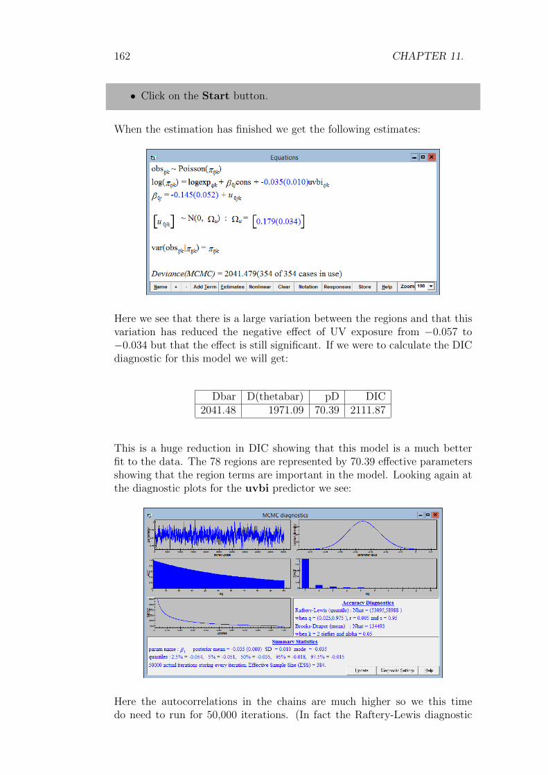
162 CHAPTER 11.
• Click on the Start button.
When the estimation has finished we get the following estimates:
Here we see that there is a large variation between the regions and that thisvariation has reduced the negative effect of UV exposure from −0.057 to−0.034 but that the effect is still significant. If we were to calculate the DICdiagnostic for this model we will get:
Dbar D(thetabar) pD DIC2041.48 1971.09 70.39 2111.87
This is a huge reduction in DIC showing that this model is a much betterfit to the data. The 78 regions are represented by 70.39 effective parametersshowing that the region terms are important in the model. Looking again atthe diagnostic plots for the uvbi predictor we see:
Here the autocorrelations in the chains are much higher so we this timedo need to run for 50,000 iterations. (In fact the Raftery-Lewis diagnostic

11.3. INCLUDING NATION EFFECTS IN THE MODEL 163
suggests running for slightly longer.) This is, however, not a problem as50,000 iterations only takes a couple of minutes to run.
Of course our data structure has an additional level of stratification in thateach region is in one of nine countries. We will next consider how to fit thesein the model.
11.3 Including nation effects in the model
We will consider two ways of fitting the effects for the nine EU nations intoour model. Firstly we will consider fitting nation as random effects in ourmodel. This will mean that our predicted mortality rates will be comprisedof a fixed effect for UV exposure and random effects for both the region andnation in which the county lies.
• Change Estimation method to IGLS.
• In the Equations window click on β0 (cons).
• Click in the (k)nation tick box.
• Click on the Done button.
• Click on the Start button to obtain the IGLS estimates.
• Change Estimation method to MCMC.
• Click on the Start button.
After estimation, if we firstly look at the DIC diagnostic for this new modelwe get:
Dbar D(thetabar) pD DIC2039.98 1978.83 61.15 2101.132041.48 1971.09 70.39 2111.87 (without nation effects)
So at first glance our new model has a reduction of DIC diagnostic of about10 points so is a better model. However if we look at the constituent partswe see that the new model has a worse fit (measured by D(thetabar)) eventhough it has more parameters! You may be wondering then why the DICdiagnostic thinks that we have a better model. This is because although wehave nominally more parameters, the random effects associated with regionare less important when the nation effects are taken into account and so theeffective number of parameters (pD) drops.
Looking at the Equations window we see that the variance between coun-tries is four times the magnitude of the variance between regions but has a

164 CHAPTER 11.
large standard error. This may be due to the fact that we only have ninecountries in our dataset. It may therefore be more sensible to fit the nationeffects as fixed rather than random effects. To do this we will use the Addterm button on the Equations window:
• Change Estimation method to IGLS.
• In the Equations window click on β0 (cons).
• Remove the ticks in the (k)nation and Fixed parameter tickboxes.
• Click on the Done button.
• Click on the Add Term button on the Equations window.
• Select nation from the variable dropdown list.
• Select [none] from the reference category dropdown list.
• Click on the Done button.
Generally we add dummy variables and use one category, for example Bel-gium, as a baseline. Here however we have removed the intercept and so canestimate effects for all nine countries. The two model formulations are justreparameterisations of each other and it happens that the parameterisationwith no intercept gives less correlated MCMC chains. We now need to fitthis model so:
• Click on the Start button to obtain the IGLS estimates.
• Change Estimation method to MCMC.
• Click on the Start button.
After 50,000 iterations the Equations window will look as follows:
Here we see that West Germany and Denmark have the highest melanomamortality rates whilst Ireland and France have the lowest. A comparison ofthe DIC diagnostic between the fixed and random effects models gives:

11.4. INTERACTION WITH UV EXPOSURE 165
Dbar D(thetabar) pD DIC2039.49 1977.81 61.68 2101.17 (fixed)2039.98 1978.83 61.15 2101.13 (random)
This shows that there is no advantage in treating the nine countries as ran-dom effects as opposed to fixed. Note that although we have run for 50,000iterations some of the parameter chains suggest, through the Raftery-Lewisdiagnostic, that we need to run for longer.
11.4 Interaction with UV exposure
We can extend our model further by removing the restriction that the effectof UV exposure is constant across countries after accounting for country andregion differences. We can remove the UV term and instead fit separate UVterms for each country. To do this we need to do the following:
• Change Estimation method to IGLS.
• In the Equations window click on the β1 term (uvbi).
• Click on the Delete Term button.
• Click on the Add Term button on the Equations window.
• Select 1 in the order box.
• Select nation from the first variable dropdown list.
• Select uvbi from the second variable dropdown list.
• Select [none] from the first ref cat dropdown list.
The window should now look as follows:
• Click on the Done button.
• Click on the Start button.
• Change Estimation method to MCMC.
• Click on the Start button.

166 CHAPTER 11.
After 50,000 iterations we will get the following point estimates:
So we now see that France still has a significantly lower mortality rate thanaverage, and Germany a significantly higher mortality rate (at average UVBexposure for the dataset). Both the UK and Italy have significantly higherrates than average (at average UVB exposure for the dataset) when the effectof UV exposure is allowed to vary between countries. The UK has a signifi-cant positive effect of UV exposure while Italy has a significant negative effectof UV exposure. There may be many reasons for these findings, for exampleItaly only has values of UV exposure greater than 2 and so this will implythat for the majority of Italians melanoma mortality is lower than average,and the significant interaction will suggest higher rates of melanoma in thenorth of Italy than the south. The UK by contrast always has negative valuesof exposure (remember this variable has been centred) and so the positivecoefficient of the exposure in the UK suggests higher rates of melanoma inthe south of the UK. One (of many) possible reason for this may be that thesouth is more affluent and so people there can afford more holidays in sunnyplaces. This is of course speculative and would require matching this datasetwith some economic data to back up this hypothesis. It is worth noting herethat these interpretations rely on the fact that our offsets are the logs of theexpected counts for each region and other forms of offset for example the logsof population size at risk will result in different interpretations.
We can compare this model with the last model via the DIC diagnostic.
Dbar D(thetabar) pD DIC2026.42 1964.58 61.84 2088.262039.49 1977.81 61.68 2101.17 (no interaction)
Here we see that the DIC diagnostic is again reduced, showing that fittingseparate UV effects for each country was a good idea.

11.5. METROPOLIS MIXING PROBLEMS 167
11.5 Problems with univariate updating Metropo-
lis procedures
One note of caution should be made here. If we look at the diagnostic tracesfor the parameters, for example β1, the effect for Belgium, (do this via theTrajectories window) we will get the following:
As we can see from the ACF graph this trace is very highly correlated andthere is no way that we can be confident of the estimates that the MCMCmethod has produced. All the Poisson models in this chapter can also be fit-ted in WinBUGS, which will use the Gamerman method described in the lastchapter instead of the Metropolis sampler used here. Although generally theGamerman method produces less correlated chains, for this model the chainsproduced are also highly correlated. For brevity we omit the WinBUGSanalysis here.
A reason for the high autocorrelations is that the parameters in the modelare themselves highly correlated. We will revisit this example in chapter 23to see if we can reparameterise the model to improve the mixing.
We ran the same model for 500,000 iterations using a thinning factor of 10and got the following estimates:

168 CHAPTER 11.
These estimates are fairly similar to those found in the User’s Guide toMLwiN using quasi-likelihood methods, which is reassuring. If we look inparticular at the parameter trace for β1 we see:
which is a great improvement. The DIC diagnostic is also affected by runningthe chain for longer here we see:
Dbar D(thetabar) pD DIC2027.91 1964.83 63.07 2090.98 (after 500,000)2026.42 1964.58 61.84 2088.26 (after 50,000)
so our model with interactions is marginally worse than we thought after50,000 iterations.

11.5. METROPOLIS MIXING PROBLEMS 169
Chapter learning outcomes
? How to fit Poisson response models.
? How to fit an offset term in MLwiN.
? How to fit main effects and interactions in Poisson models.

170 CHAPTER 11.

Chapter 12
Unordered CategoricalResponses
In Chapter 10, we considered fitting models to datasets where the responsevariable took two possible states, which were classed numerically as 0 and 1.In the example we looked at the two states were whether or not a womanuses contraception in a dataset of Bangladeshi women who took part in the1988 Fertility survey. The case of binary responses is in fact the simplestcase of two possible families of models that we can use when we have 2 ormore possible states or categories for a variable.
In this chapter we will consider the case of unordered categories and in Chap-ter 13 we will look at the alternative extension of binary responses to orderedcategorical models. Generally whether a response should be fitted as orderedor unordered is obvious from its definition, however there are some grey areas.For example in voting datasets where there are more than 2 possible partiesthat voters can vote for we would typically treat the parties as unorderedcategories. However an alternative in the UK would be to consider three(ordered) categories: Conservative, Labour and Other where Other isassumed to lie between the first two.
In this chapter we are going to consider another subset of the BangladeshiFertility survey of 1988 where we know not only whether the individualwomen used contraception but for the women who did we know the methodthey used. This subset of the dataset is found in the worksheet bang.ws.This dataset has also been investigated in the latest version of the User’sGuide to MLwiN and here we will generally consider using MCMC for thesame models.
• Select Open Sample Worksheet from the File menu.
• Select bang.ws from the list of worksheets.
• Select Open.
171

172 CHAPTER 12.
The Names window will then look as follows:
In this subset of the dataset we have in the column use whether or not awoman uses contraception and then in the column use4 a categorisation ofthe type of contraception used. The categories for the variable are
1. Sterilization of the woman or her partner.
2. Modern reversible methods.
3. Traditional methods.
4. Not using contraception.
We will be treating the four categories as unordered although there is avague ordering in terms of effectiveness of preventing pregnancy of the fourcategories. This subset of the Bangladeshi dataset shares the majority of itspredictor variables with the subset used in Chapter 10 and we will here onlyconsider a few of these variables in our modelling.
To motivate multinomial modelling we will firstly look at the distribution ofthe use4 variable via the Tabulate window.
• Select Tabulate from the Basic Statistics menu.
• Click on the Percentage of column totals tick box.
• Select use4 from the list next to Columns.
• Click on the Tabulate button.
This will run the TABUlate command and give the following results:
1 2 3 4 TOTALSN 302 555 282 1728 2867% 10.5 19.4 9.8 60.3 100.0

12.1. FITTING A FIRST SINGLE-LEVEL MULTINOMIAL MODEL 173
Here we see that 60.3% of the women do not use contraception, whilst ofthose that do roughly half use modern reversible methods.
12.1 Fitting a first single-level multinomial
model
The simplest multinomial model we can fit would simply encapsulate theinformation in the above tabulation. If we let the probability of an individuali having response r be π
(r)i = Pr(yi = r), then following on from the binary
response case we assume that one of the categories is the reference category(0 in the binary model). Then in the multinomial logistic model we constructa model that compares each of the categories with the baseline category. Forexample with t categories and category t as the baseline:
log
(π
(r)i
π(t)i
)= (XiB)(r), r = 1, . . . , t− 1
We therefore have t − 1 equations each of which is equivalent to a binaryresponse model comparing the probabilities of each category with the basecategory. Here X(r) is a set of predictor variables that may be common foreach equation or may be different. The corresponding coefficients β(r) areunique coefficients for the rth equation. Although the β(r) are themselves notparticularly meaningful to interpret, it is often preferable to calculate (forgiven predictor values, Xi) the predicted probabilities for the t categories.These are constructed as follows:
π(r)i =
exp((XiB)(r))
1 +t−1∑k=1
exp((XiB)(k))
, r = 1, ..., t− 1, π(t)i = 1−
t−1∑k=1
π(k)i
We will now construct a simple model that will recover the probabilities thatthe TABUlate command gave us.
We will firstly need to set up the category names for the use4 variable.
• Select Names from the Data Manipulation menu.
• Click on use4 from the list and then the View button in the cate-gories section.
• For the categories 1 through to 4 type in turn ster, mod, trad andnone.
The window should look as follows:

174 CHAPTER 12.
We will next click on the OK button and then set up the model in theEquations window as follows:
• Select Equations from the Model menu.
• Click on the red y and select use4 as the y variable.
• Select 1-i for the number (N) of levels.
• Select woman as the Level 1(i) identifier.
• Click on the Done button.
• Click on the N and from the list of distributions that appears scrolldown and select Multinomial.
• Change the reference category from ster to none and click on theDone button.
Next we need to define the denominator and the intercepts for each category:
• Click on the red nj to set the denominator.
• Select cons from the list that appears and click on the Done button.
• Click on the Add Term button.
• Select cons from the variable list.
• Click on the add Separate coefficients button.
The Equations window should now look (after pressing the + button twice)as follows:
Here we see the three equations that relate the four categories. When se-lecting multinomial modelling, MLwiN performs many data manipulation

12.1. FITTING A FIRST SINGLE-LEVEL MULTINOMIAL MODEL 175
operations behind the scenes to construct an expanded response variableand to expand the predictors accordingly. This is a similar process to theexpansion in multivariate models that we will describe in Chapter 18.
• Select View or Edit Data from the Data Manipulation menu.
• Click on the View button.
• Select the following 6 columns: resp, resp indicator,woman long, cons.ster, cons.mod, cons.trad.
• Click on the OK button.
The Data window looks as follows:
Here we see that for each observation in the original dataset we have 3 recordsin the new dataset, one for each category (excluding the base category). Theresp column transforms the response from a number between 1 and 4 tothree binary indicators. The resp indicator column simply identifies eachindicator with a category. The woman long column identifies the individualwoman for each record and the remaining 3 columns give the three interceptterms.
If we now wish to fit this first model using MCMC we need to do the following:
• Select Equations from the Model menu.
• Click on the Nonlinear button.
• On the window that appears click on the Use Defaults and Donebuttons.
• Click on the Start button (to run using IGLS 1st order MQL).
• Select MCMC from the Estimation menu.
• Click on the Start button.
The model will now be run using MCMC and after a few minutes we shouldget the following estimates (after pressing the estimates button twice):
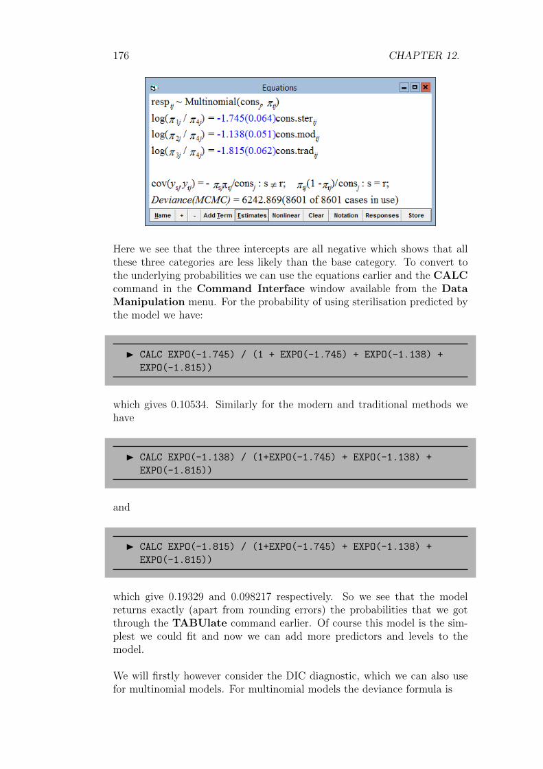
176 CHAPTER 12.
Here we see that the three intercepts are all negative which shows that allthese three categories are less likely than the base category. To convert tothe underlying probabilities we can use the equations earlier and the CALCcommand in the Command Interface window available from the DataManipulation menu. For the probability of using sterilisation predicted bythe model we have:
CALC EXPO(-1.745) / (1 + EXPO(-1.745) + EXPO(-1.138) +
EXPO(-1.815))
which gives 0.10534. Similarly for the modern and traditional methods wehave
CALC EXPO(-1.138) / (1+EXPO(-1.745) + EXPO(-1.138) +
EXPO(-1.815))
and
CALC EXPO(-1.815) / (1+EXPO(-1.745) + EXPO(-1.138) +
EXPO(-1.815))
which give 0.19329 and 0.098217 respectively. So we see that the modelreturns exactly (apart from rounding errors) the probabilities that we gotthrough the TABUlate command earlier. Of course this model is the sim-plest we could fit and now we can add more predictors and levels to themodel.
We will firstly however consider the DIC diagnostic, which we can also usefor multinomial models. For multinomial models the deviance formula is

12.2. ADDING PREDICTOR VARIABLES 177
D = −2∑i
t∑j=1
[I(yi = j)π(j)i ]
where I() is an indicator function which returns 1 if the condition is satisfied
i.e. if individual i uses method j. π(j)i is the estimated probability of being
in category j for individual i. This means that the MCMC engine in MLwiNcalculates the estimated probabilities as part of the DIC diagnostic command.
• Select MCMC/DIC diagnostic from the Model menu.
The output can be seen below:
Dbar D(thetabar) pD DIC6242.87 6239.80 3.07 6245.94
Here we can again see that the DIC picks up the correct degrees of freedom.We can now consider adding in predictor variables and see if they produce abetter model via the DIC diagnostic.
12.2 Adding predictor variables
In Chapter 10 we discovered that, for the subset of the Bangladeshi datasetused there, the number of living children a woman had increased her chancesof using contraception. If we now consider this predictor in the multinomialexample, we can look at the effect of the number of children on each of thethree types of contraceptive use.
• Change Estimation method to IGLS.
• Click on the Add Term button on the Equations window.
• Select lc in the variable list and keep lc0 as the reference category.
• Click on the add Separate coefficients button.
As there are four categories of number of living children and four categoriesof contraceptive use, the above commands will add (4−1)× (4−1) = 9 fixedeffect parameters. To run the model using MCMC we now need to do thefollowing:

178 CHAPTER 12.
• Click on the Start button (to run using IGLS 1st order MQL).
• Select MCMC from the Estimation menu.
• Click on the Start button.
After a few minutes the model runs and gives the following estimates:
Here we see that for all three types of contraception there is greater proba-bility of usage if the woman has had some children although the pattern isnot the same for all methods. For the modern (reversible) method there isgreater probability of usage (as opposed to non-usage) in women with 1 or2 living children and less probability for women with 3 or more children andthe least probability in women with no children. In contrast the probabilityof using traditional methods increases with the number of living children.
The User’s Guide to MLwiN gives a macro for calculating the probabilitiesfor this particular model which essentially involves using a similar formulathat we used for the last model, so for example to calculate the conditionalprobability of a woman with no living children using traditional methods wehave the following calculation
CALC EXPO(-2.584) / (1+EXPO(-3.972) + EXPO(-1.477) +
EXPO(-2.584))
which gives a probability of 0.0571. In contrast for a woman with 2 childrenthe calculation is as follows:
CALC EXPO(-2.584+1.052) / (1+EXPO(-3.972+2.741) +
EXPO(-1.477+0.695) + EXPO(-2.584+1.052))
which gives a probability of 0.110.

12.3. INTERVAL ESTIMATES: CONDITIONAL PROBABILITIES 179
As shown in the User’s Guide to MLwiN the TABUlate command can beused to construct the counts and probabilities of each of the 16 categories ina 2 way table of contraceptive use and number of living children. Then byconsidering the particular row corresponding to the number of living childrenwe can construct the probabilities given by the model.
12.3 Interval estimates for conditional prob-
abilities
One of the advantages of MCMC methods is that as they are simulation-basedapproaches we can construct interval estimates from the chains of values. Wecan also, as we saw in Chapter 4, calculate interval estimates for any derivedparameters as well, for example the above conditional probabilities. MLwiNstores the chains of parameter estimates stacked in column c1090 and so wefirstly need to split this column into 13 columns, 1 for each of the 12 fixedeffects plus one which contains a level 1 random effect that is constrainedto 1 at each iteration. Then the above calculations are carried out on thecolumns rather than the point estimates. The following commands can betyped in the Command interface window:
code 13 1 5000 c300
split c1090 c300 c301-c313
calc c314 = expo(c303) / (1+expo(c301) + expo(c302) +
expo(c303))
calc c315 = expo(c303+c311)/ (1 + expo(c301+c305) +
expo(c302+c308) + expo(c303+c311))
name c314 'prob1' c315 'prob2'
This will put chains of values for the two probabilities in columns c314 andc315 and we can look at them using the Column Diagnostics windowavailable from the Basic Statistics menu as follows for the first probability(of using traditional methods given the woman has no children):

180 CHAPTER 12.
So here we have a 95% credible interval for the probability of between 0.043and 0.072. Similarly for the probability of using traditional methods giventhe woman has 2 children we get an interval of (0.084,0.140) as shown below:
Finally if we now look at the DIC diagnostic we get the following:
Dbar D(thetabar) pD DIC6039.56 6027.92 11.64 6051.20 (current model)6242.87 6239.80 3.07 6245.94 (without living children predictors)
Here we see that the DIC diagnostic picks up (approximately) that we haveadded 9 parameters (11.64− 3.07) and the DIC value has reduced by nearly200 suggesting this is a much better model. We could of course now considersome of the other predictors as we did in Chapter 10 but here we will moveon to consider adding random effects.

12.4. ADDING DISTRICT LEVEL RANDOM EFFECTS 181
12.4 Adding district level random effects
The Bangladeshi dataset contains two levels with women nested within dis-tricts and so far we have assumed that the probability of using the varioustypes of contraception will be constant across districts. As we have 60 dis-tricts we will treat the differences between districts as random effects. Asthere are 3 contraceptive methods this will result in 3 sets of random effects.
• Change Estimation method to IGLS.
• Select Equations from the Model menu.
• Click on the response variable to bring up the Y variable window.
• Select 3-ijk for the N levels indicator.
• Select district as the level 3(k) identifiers.
• Click on the Done button.
• Click on cons.ster and select the k(district long) tickbox.
• Click on the Done button.
• Click on cons.mod and select the k(district long) tickbox.
• Click on the Done button.
• Click on cons.trad and select the k(district long) tickbox.
• Click on the Done button.
In the User’s Guide to MLwiN it was pointed out that the estimates from 1storder MQL estimation were often severely biased for multilevel multinomialmodels so here we will move straight to 2nd order PQL estimation to getstarting values for MCMC.
• Click on the Nonlinear button on the Equations window.
• Select 2nd Order and PQL from the options that appear.
• Click on the Done button.
• Click on the Start button.
After 11 iterations the model will converge to give the following estimates:

182 CHAPTER 12.
If we now change estimation method to MCMC and press the Start buttonwe can compare methods:
Here we see that as is often the case the MCMC estimation method giveslarger (in magnitude) estimates. If we now look at the chain for the firstvariance, σ2
v0, we can investigate this further.
• Select Trajectories from the Model menu.
• Click on the Select button and highlight district long :cons.ster/cons.ster
• Click on the Done button.
• Click on the trajectory plot and the Yes box that appears.
The MCMC diagnostics appear as follows:

12.4. ADDING DISTRICT LEVEL RANDOM EFFECTS 183
Here we see that in fact the posterior mode estimate of 0.607 agrees favourablywith the 2nd order PQL estimate of 0.544 suggesting that the differenceshere are mainly due to the fact that we were originally comparing mean withmode (ML) estimates. It is also noticeable that we should in fact have runfor longer than the 5,000 iterations. In fact some of the fixed effect tracessuggest a much longer run.
Considering the model we have fitted in more detail we can firstly use theDIC diagnostic to compare this model with the last model. To do this weselect MCMC/DIC diagnostic from the Model menu, which gives:
Dbar D(thetabar) pD DIC5729.62 5624.77 104.85 5834.47 (Model with random effects)6039.56 6027.92 11.64 6051.20 (Model without random effects)
Here we see that the DIC diagnostic has again been reduced, this time by over200 suggesting that the random effects model is significantly better. The 180random effects that we have added have contributed 106.41− 11.95 = 94.46effective parameters.
Looking at the parameter estimates we see that the three covariances arepositive and we can look at the correlations between the sets of randomeffects as follows:
• Select Estimate Tables from the Model menu.
• Select Level 3: district long from the drop-down list.
• Select C and unselect S, E, S and P at the top right of the window.
You should now have the following correlation matrix.

184 CHAPTER 12.
Here we see that there are fairly strong correlations between the three setsof random effects. This means that generally in districts with higher steril-isation probabilities, there are also higher probabilities of modern and tra-ditional methods as well. More succinctly the main differentiation betweendistricts is that there are some districts with high contraceptive use and oth-ers with low contraceptive use. However, the type of use does not exhibita particularly strong pattern such as, for example, higher probabilities oftraditional methods in districts with lower rates of usage of the other twomethods.
Care must be taken when interpreting these correlations as the numbers inthe base category will affect all three random effects simultaneously and soit is to be expected that there will be some positive correlation.
In the User’s Guide to MLwiN the residuals produced by this model alongwith plots are considered. Similar plots can be produced for the residualestimates produced by the MCMC methods and we will leave these as anexercise for the user.
Chapter learning outcomes
? How to fit models to unordered categorical responses
? How to extend such models to include random effects
? How to calculate point and interval estimates of conditional proba-bilities
? How to compare MCMC estimates with IGLS estimates

Chapter 13
Ordered Categorical Responses
In the last chapter we considered datasets where the response is one of a selec-tion of possible alternatives, where the alternatives do not have a particularordering. In this chapter we will consider the case where the alternatives dohave a natural ordering and so we can build this ordering into our model.It is of course possible to use the models in the last chapter with ordereddata as in some way they can be considered a special case of categorical dataand the general multinomial models in the last chapter will fit any types ofcategorical data.
Ordered categorical responses occur in many fields. In education, exammarks are often graded on a scale, for example A, B, C, D, E, and U with Arepresenting the best marks and U representing the worst marks (failures).Other examples are survey questionnaires where individuals have to givetheir level of agreement with a statement, typically ranging from ‘StronglyAgree’ through to ‘Strongly disagree’ and finally in health where a person’sillness/fitness may be classified on a scale.
Another possibility for fitting ordered categorical data is to treat the responsevariable as continuous and fit Normal response models. This will make moresense the greater the number of categories we have and in fact in educationsuch modelling is often performed on exam marks or grade scores. In theexample we will consider in this chapter our response is the mark in an Alevel (taken at age 18) chemistry exam and we will compare and contrastthe approaches of treating this response as continuous and as an orderedresponse.
13.1 A level chemistry dataset
The data that we analyse is taken from a larger dataset that contains allthe A level exam results taken in England for the period 1994–1997 (Yang &
185

186 CHAPTER 13.
Woodhouse, 2001) . The subset of the dataset used here is all the chemistryexam results for one examinations board in the year 1997.
• Select Open sample worksheet from the File menu.
• Select alevchem.ws from the list of worksheets.
• Select Open.
The Names window will then appear as we see below:
Here we see that there are in fact three levels to the data with 2166 pupils(pupil) nested within 219 schools (estab) nested within 70 LEAs (lea) al-though we will only consider the first two levels here. The response variableis a-point which ranges from 1 (grade F) to 6 (grade A). There are threepredictor variables, gcse-tot and gcse-no give the total points and numberof GCSE exams sat at age 16 and finally the sex, gender, of each child witha value of 1 representing a girl and 0 a boy. It should be noted that theGCSE system has 8 grades rather than 6 and these range from A∗ worth 8points then A worth 7 points through to G worth 1 point. The extra gradeA∗ was introduced for the first time in 1994.
Perhaps one of the first things we can do with the dataset is to construct theaverage GCSE scores as these would be preferable to the two predictors, totalGCSE score and total number of GCSEs. This can be achieved by typingthe following commands in the Command interface window (available fromthe Data Manipulation menu):
CALC c9=c5/c6
Here unlike in the User’s Guide to MLwiN we do not Normalise our responseor predictor variables. The A level score response can only take 6 possible val-ues and so the Normalising transform will only have limited effect. As shownbelow (by selecting histogram from the Customised graph window) al-though the GCSE scores are slightly skewed to the left for interpretation wemaintain the raw scores.

13.2. NORMAL RESPONSE MODELS 187
We will however centre the predictor around a GCSE average score of 6(note the actual average score is 6.15). This will make the intercept moremeaningful as it will now represent the prediction for a child with an averageGCSE score of 6. We will also consider quadratic and cubic coefficients ofthe predictor by typing the following commands in the Command interfacewindow.
CALC c9=c9-6
CALC c10=c9^2
CALC c11=c9^3
NAME c9 'gcseav' c10 'gcse^2' c11 'gcse^3'
For our response variable we are simply assuming that an F is worth 1 point,and an A is worth 6 points. This would seem rather arbitrary but will lead onto ordered response models which essentially remove this linear incrementalapproach. The alternative approach of using Normalised scores basicallygives an alternative mark to each grade from F to A based on their frequencyof occurring and an underlying Normal distribution assumption. Here thescores would be −1.287 for an F, −0.629 for an E, −0.245 for a D, 0.150 fora C, 0.639 for a B and 1.38 for an A. We can see that the gaps between theextremes (A/B and E/F) are larger. We will come back to this when we fitthe ordered response models.
13.2 Normal response models
To firstly set up a Normal response model we need to do the following:

188 CHAPTER 13.
• Select Equations from the Model menu.
• Click on the red y.
• Select a-point for the y variable.
• Select 1-i for the number (N) of levels.
• Select pupil as level 1(i) and click on the Done button.
• Click on the red x0 and select cons from the list.
• Select the i-pupil tick box keeping the Fixed Parameter box se-lected.
• Click on the Done button.
• Click on the Start button.
• Change Estimation method to MCMC.
• Click on the Start button.
After running for 5,000 iterations the Equations window will look as follows:
Here we see that on average students get 3.519 (somewhere between a GradeC and D) in their A level chemistry exam but there is a large variability inscores (3.092). If we look at the DIC diagnostic (available via the MCMCsubmenu of the Model menu) we get the following value which we will usefor comparison later:
Dbar D(thetabar) pD DIC8589.83 8587.82 2.01 8591.84
We will now add in the three powers of the GCSE predictor and the genderpredictor.
• Change Estimation method to IGLS.
• Select Add Term from the Equations window.

13.2. NORMAL RESPONSE MODELS 189
• Select gcseav from the variable list and click on the Done button.
• Repeat this procedure 3 times adding in gcseˆ2, gcseˆ3 and gen-der.
• Click on the Start button.
• Change Estimation method to MCMC.
• Click on the Start button.
The Equations window will then look as follows:
We firstly see that all these predictors are significant and that in combinationthey have reduced the unexplained variation from 3.092 to 1.469 that isover half the unknown variation has been explained. The DIC diagnostic asexpected gives a much improved DIC value:
Dbar D(thetabar) pD DIC6977.85 6971.86 5.99 6983.848589.83 8587.82 2.01 8591.84 (intercept only model)
We can plot the relationship by calculating predictions via the predictionswindow and the Customised graph window as follows:
• Select Predictions from the Model menu.
• Click on the word fixed towards the bottom of the window and selectInclude all fixed coefficients.
• Select c13 from the output from prediction to list.
• Click on the Calc button and close the window.
• Select Customised Graph(s) from the Graphs menu.
• Select c13 as the y variable and gcseav as the x variable.
• Select gender as the group indicator and line as the plot type.
• Click on the Apply button.

190 CHAPTER 13.
The predictions graph will look as follows:
Here we have two parallel curves with the girls doing on average about halfa grade worse than the boys (−0.483). The tail behaviour is rather unusualwith the average predicted A level grade increasing once the average GCSEgoes below 4 (−2 on the graph). This is due to four individuals who hadlow GCSE averages but achieved good A level chemistry grades (2 C’s and2 D’s). If we however consider the range of GCSE averages greater than4.5 (−1.5 on the graph and 95% of the pupils) we see a linear relationship.We will now look at treating the response variable as an ordered categoricalresponse rather than as a continuous measure.
13.3 Ordered multinomial modelling
In the last chapter we considered unordered categorical models and saw howeffectively such a model is a direct extension of the binary response modelwhere we look at the relative probability of each category as compared toone base category and ensure that the probabilities of being in each categorywill sum to 1 for each individual. To exploit the ordering of the categorieswe do not model the probabilities of the individual categories but insteadmodel the cumulative probabilities, for example the probability of getting aC grade or better, or as in our example the alternative probability of gettinga D grade or worse.
To fit such a model we will therefore have to construct a set of indicatorvariables for each response. So if yi is the response for individual i then wewill define y
(s)i to be an indicator that takes value 1 if yi is less than or equal
to category s and 0 otherwise.

13.3. ORDERED MULTINOMIAL MODELLING 191
Then we will fit separate equations for each y(s)i as follows:
E(y(s)i ) = γ
(s)i =
s∑h=1
π(h)i , s = 1, . . . , t− 1
Here we assume there are t categories and that category t is the base category.In the example that follows we will assume that A is the base category andthat we consider the less than a chosen category relationship but in practicewe could have alternatively chosen F as the base category and used a greaterthan relationship.
Now we need to define a link function to relate the probabilities γ(s)i to the
predictor variables. A common choice of model is the proportional oddsmodel which corresponds to fitting a logit link. We can write this as
logit(γ(s)i ) = α(s) + (Xβ)i
Here we see that we allow an additive effect for each category but assumea common effect for all other predictor variables. This is one major dif-ference between the ordered and unordered models but does make sense.In unordered models predictors might influence selecting different categoriesbut in the ordered case the predictors can only have an effect of increas-ing/decreasing the chance of achieving a higher category.
We will now consider setting up a basic multinomial model. We firstly needto create the categorical response variable.
• Select Names from the Data Manipulation menu.
• Click on a-point in the list of names and then click on the Viewbutton in the categories section.
• Check that the Categories window is as shown below.
• Click on the OK button.
We will now set up the first categorical model in the Equations window.
• Select Equations from the Model menu.
• Change Estimation mode back to IGLS.
• Click on the Clear button to remove the Normal response model.

192 CHAPTER 13.
• Click on the red y and again select a-point as the y variable.
• Select 1-i as the number of models and pupil as level 1(i) identifier.
• Click on the Done button.
• Click on the N and from the list of distributions that appears scrolldown and select multinomial.
• In the Multinomial options box select Ordered proportionalodds and A as the reference category.
• Click on the Done button.
The Equations window will now look as follows (after pressing the + buttontwice):
You will notice in the above window that the model now has two levels anda new response has been created in column resp. We can finish setting upthe first model as follows:
• Click on the nj in the window and select cons as the denominator.
• Click on the Done button.
• Click on the Add Term button and select cons from the variablelist.
• Click on the add Separate coefficients button.
The Equations window will now look as follows:

13.3. ORDERED MULTINOMIAL MODELLING 193
We can examine the new columns created via the Data window.
• Select View or Edit Data from the Data Manipulation menu.
• Click on the view button.
• Select the columns resp, resp indicator, pupil long, cons.(<=F)and cons.(<=E) using the CTRL keyto select multiple columns.
• Click on the OK button.
The Data window will then appear as follows. Here we can see that theoriginal response for each individual has been converted into 5 indicatorvariables stacked in the column resp. Here for example the first pupil (pupil1650) achieved a D and this is converted into the pattern of 5 indicators(0, 0, 1, 1, 1). The resp indicator column gives information on what eachindicator indicates and is used as the level 1 identifier. The original pupilcolumn has been replicated to produce the level 2 indicators, pupil long.The 5 indicators each have an associated intercept, which are picked up bythe 5 new constant columns.
We will now run the model using MCMC estimation.

194 CHAPTER 13.
• Select Equations from the Model menu.
• Click on the Nonlinear button.
• On the screen that appears click on the Use Defaults and Donebuttons.
• Click on the Start button.
• Change Estimation method to MCMC.
• Click on the Start button.
Upon finishing the 5,000 iterations the Equations window will appear asfollows (after pressing the Estimates button twice):
We can use these coefficients to calculate the probabilities of achieving eachof the 6 grades. For example the estimated probability of getting a grade F isthe anti-logit of −1.403, which equals 0.197. Similarly the probability of get-ting a grade E is the anti-logit of −0.703 minus the probability of getting anF, i.e. 0.331− 0.197 = 0.134. For this simple model we could of course havecalculated these probabilities by simply working out empirically the propor-tion of pupils in the dataset who got each grade. The modelling approachcomes into its own when we add predictors. However firstly we will calcu-late the DIC diagnostic for this first model for comparison later. SelectingMCMC/DIC diagnostic from the Model menu gives the following:
Dbar D(thetabar) pD DIC7726.39 7721.42 4.97 7731.36

13.4. ADDING PREDICTOR VARIABLES 195
13.4 Adding predictor variables
In the Normal response modelling section our next step was to include pre-dictors into the model. To do this we do the following:
• Change Estimation method back to IGLS.
• Select Equations from the Model menu.
• Click on the Add Term button.
• Select gcseav from the variable list.
• Click on the add Common coefficient button.
• Click on the Include all and Done buttons.
• Repeat this procedure for the variables gcseˆ2, gcseˆ3 and gender.
• Click on the Start button
• Change Estimation method to MCMC.
• Click on the Start button.
After 5,000 iterations we get the following results:
Here we see that all the predictors have negative coefficients. This is becausewe are predicting the probability of getting less than or equal to particulargrades and so as the ability of the pupil increases they are less likely to getbelow a particular threshold. The coefficients suggest that we do not needto fit a cubic term here and if we remove it and compare the DIC diagnosticwe see the following:

196 CHAPTER 13.
Dbar D(thetabar) pD DIC6100.01 6090.94 9.07 6109.09 (with cubic term)6100.97 6092.71 8.26 6109.23 (without cubic term)
It should be noted, as shown in the User’s Guide to MLwiN, that we couldin fact fit separate effects of each predictor for each grade boundary but asshown there fitting a single common predictor effect is acceptable. We willnow consider fitting a multilevel multinomial model, where the probabilitiesof getting the different grades depend on the school the students belong to.
13.5 Multilevel ordered response modelling
As with all the other response types that we have considered in this book itis perfectly plausible for there to be random variation between higher levelunits and ordered response models are no exception.
We will need to define the column that contains the higher level units butfirstly we need to remove the cubic term from the model (if we have notalready done so)
• Change Estimation method to IGLS.
• Select Equations from the Model menu.
• Click on the term gcseˆ3.12345 and click on the Delete Termbutton.
• Click on the term resp to bring up the Y variable window.
• Change the number of levels indicator to 3-ijk.
• Select estab as the level 3(k) identifier and click on the Donebutton.
We now need to decide how to add in the effect of the different schools.If we were to add random effects for each grade boundary then we wouldeffectively be ignoring the ordering and would have an equivalent model tothe unordered responses. We therefore wish to have one effect for each schoolthat changes each grade boundary. To obtain this we do the following:
• Click on the Add Term button.
• Select cons from the variable list.
• Click on the add Common coefficient button.
• Click on the Include all and Done buttons.

13.5. MULTILEVEL ORDERED RESPONSE MODELLING 197
This will have created a variable cons.12345 which is a common interceptterm. We do not want to fit this as a fixed effect but instead want to fit it asrandom at the establishment (school) level. To do this we do the following:
• Click on the cons.12345 term.
• In the X variable window that appears tick the k(estab long)tickbox.
• Remove the tick in the Fixed Parameter tickbox.
• Click on the Done button.
• Click on the Start button.
• Change Estimation method to MCMC.
• Click on the Start button.
Upon completion of the iterations we get the following estimates:
Here we see that there is some variability between the various establishmentsand fitting this model accounts for this variability. Looking at the DICdiagnostic we see that adding the 219 random effects has given rise to 110additional ‘effective’ parameters. The DIC has also reduced by over 150suggesting a much better fit to the data.
Dbar D(thetabar) pD DIC5825.96 5707.91 118.05 5944.01 (with random effects)6100.97 6092.71 8.26 6109.23 (without random effects)

198 CHAPTER 13.
We can continue to fit more complex models for example we may think thatthe effect of GCSE score is different for each school, which would result in arandom slopes model. To fit such a model we do the following:
• Change Estimation method to IGLS.
• Click on the term gcseav.12345 in the Equations window.
• In the X variable window that appears tick the k(estab long)tickbox.
• Click on the Done button.
• Click on the Start button.
• Change Estimation method to MCMC.
• Click on the Start button.
After running for 5,000 iterations we get the following estimates:
If we compare this model with the model that does not include random effectsfor GCSE score via the DIC diagnostic we get the following:

13.5. MULTILEVEL ORDERED RESPONSE MODELLING 199
Dbar D(thetabar) pD DIC5794.82 5649.08 145.74 5940.56 (with random slopes)5825.69 5707.91 118.05 5944.01 (without random slopes)
So the addition of random GCSE effects only makes a marginal improvement.It should be noted that throughout this chapter we have only been runningfor 5,000 monitoring iterations for each model. If we look at the chain forthe variance of the random GCSE effects via the Trajectories window wewill see the following:
Here we see that clearly more iterations are required. We will therefore runfor 50,000 iterations instead.
• Click on the Estimation Control button.
• Change the Monitoring chain length to 50000.
• Press the More button.
The MCMC diagnostics after 50,000 iterations (which will take several min-utes) are as follows:

200 CHAPTER 13.
Here we see that we have now run for sufficiently long enough to satisfy thediagnostics and in fact the parameter estimate has changed very little. If welook at the DIC diagnostic we see the following:
Dbar D(thetabar) pD DIC5799.36 5658.88 140.48 5939.83 (after 50,000 iterations)5794.82 5649.08 145.74 5940.56 (after 5,000 iterations)
Here the additional run length has confirmed a reasonably similar value forthe DIC diagnostic.
We could now extend our modelling as in the User’s Guide to MLwiN andconsider the effect of making gender random at the establishment level butwe leave this to the reader. As described in the last chapter an advantageof using a simulation based technique like MCMC is that we can createchains for derived parameters and this can also be done in ordered responsemodels to create interval estimates for conditional probabilities of achievingparticular grades. Again we leave this as an exercise for the interested reader.
Chapter learning outcomes
? How to fit models to ordered categorical responses
? How to extend such models to include random effects
? The differences between ordered and unordered categorical responsemodels

Chapter 14
Adjusting for MeasurementErrors in Predictor Variables
Statistical modelling attempts to fit models that describe the relationship be-tween an observed response variable and several observed predictor variables.We have so far considered how to fit models where the response variable iscontinuous, a binary indicator or a count. All these models assume that thereis variation between the observed data and a predicted model, and that thisvariation is due to additional unobserved predictor variables. When choosingstatistical models we try to find a balance between the fit and complexity of amodel. If we were to continue adding in predictors we could achieve a perfectfit to the dataset, but adding in ‘non-significant’ predictors will reduce thepredictive power of our model for observations outside of the dataset.
Apart from variation due to unknown predictors, there may also be variationor errors in the predictors that we fit in our model. For example if weconsider the tutorial dataset that was first introduced in Chapter 1 and focuson the London Reading Test (LRT) predictor that was used as a proxy forintake ability, then errors could occur in this predictor in many ways. Firstlyobvious measurement errors could occur, for example the teacher could marka paper wrongly or the researcher who created the dataset could type thedata incorrectly into the computer. Secondly, less obvious errors could occurif we consider the variable as a proxy for intake ability, for example a childmay do better on the test, as his favourite types of questions occur, whileanother child may be ill on the day of the test and hence do worse.
Measurement errors can occur in many forms. If the predictor is (pseudo)continuous like LRT score then we can assume that the measurement error isalso continuous and these types of measurement error can currently be fittedin MLwiN. If however the predictor was a categorical variable for examplean exam grade or the sex of the pupil then errors in these variables can bethought of as misclassifications, for example a boy is misclassified as a girl,and currently methods for dealing with these types of error have not been
201

202 CHAPTER 14.
implemented in MLwiN.
14.1 Effects of measurement error on predic-
tors
To illustrate the effect of measurement error on a predictor we will look atfitting a simple linear regression model to the tutorial dataset and thenintroducing errors into the LRT predictor.
• Select Open Sample Worksheet from the File menu.
• Select tutorial.ws from the list and click on Open.
• Set up the OLS linear regression model in the Equations windowas in Chapter 2.
You should now have set normexam as the response, school as the level 2identifier, student as the level 1 identifier, cons as a fixed effect and randomat level 1 and finally standlrt as a fixed effect (see Chapter 1 if you needmore details). For speed we will here use the IGLS method so run the modelby pressing the Start button. Upon convergence the model will look asfollows:
Here (as normexam has variance 1) the predictor standlrt has explained100 – 64.8 = 35.2% of the variation in the response variable normexam.We will assume that the standlrt we have fitted is the ‘true’ predictor andnow we will generate some random (Normal) errors. This we can do viathe Generate random number window although below we will use theCommand interface window. Firstly however we wish to look at howmuch variation there is in the ‘true’ predictor.
• Select Averages and Correlation from the Basic Statisticsmenu.

14.1. EFFECTS OF MEASUREMENT ERROR ON PREDICTORS 203
• Select standlrt from the drop down list and click on Calculate.
This will give the following output:
N Missing Mean s.d.standlrt 4059 0 0.0018103 0.99322
So here we see that the (standardized) variable has a variance of approxi-mately 1. We will now consider adding a measurement error to this variablethat has variance 0.2. Note that in the measurement error literature theterm reliability is often used with respect to measurement errors (see Wood-house et al., 1996) and here we will have a reliability of (1/(1+0.2))×100%= 83.3%.
To generate the errors we will type the following commands in the Com-mand interface window:
Seed 1
Nran 4059 c11
Calc c11=c11*sqrt(0.2)
Name c11 'errors'
Calc c12 = 'errors' + 'standlrt'
Name c12 'obslrt'
Here we set the random number seed to 1 so that you get the same set ofsimulated errors as the book. We then store the errors in column c11 and theresulting observed predictor values in column c12. It will be firstly of interestto fit a linear regression of the errors against the normexam variable.
• In the Equations window click on β1 (standlrt).
• Replace standlrt with errors from the pull down list.
• Click on the Done button.
• Click on the Start button.
Upon convergence the estimates will be as follows:

204 CHAPTER 14.
So here we see a non-significant positive relationship between the errors andthe exam score, which explains 0.3% of the variation. Of course the errorsare random and so a different set of random errors may produce a negativerelationship. We now look at the relationship between normexam and theobserved (i.e. with errors) LRT scores:
• In the Equations window click on β1 (errors).
• Replace errors with obslrt from the pull down list.
• Click on the Done button.
• Click on the Start button.
Upon convergence we will get the following:
So in adding the measurement errors to the predictor we have reduced itspredictive power and hence its coefficient is smaller and the residual variancehas increased. We could think of this regression as a weighted average ofthe earlier regressions between the exam score with true LRT score and theexam score with errors. Here the weights will be approximately equal to theprecisions (1/variance) of the estimates, although due to the intercepts beingestimated and not fixed at zero this will not hold exactly.
In order now to adjust for the measurement errors we need to add some extrastatements to the model. The MCMC methods used in MLwiN to adjust formeasurement error involve extra steps in which we generate the true values

14.1. EFFECTS OF MEASUREMENT ERROR ON PREDICTORS 205
at each iteration. To set up the MCMC measurement error model we do thefollowing.
• Click on the Estimation Control button.
• Click on the MCMC tab.
• Select MCMC/Measurement Errors from the Model menu.
• Click on the tick box for obslrt on the Measurement errors win-dow and input 0.2 as the error variance.
The window should then look as follows:
If we now look at the Equations window (and press + to get the priorinformation) we will get a window as follows:
Here we are fitting what is known as a ‘classical’ Bayesian measurement error

206 CHAPTER 14.
model. Basically this includes two additional model statements: firstly thatthe observed values are Normally distributed around the true values, andsecondly that the true values have a Normal distribution with an unknownmean and variance. The first statement by itself would simply have the effectof introducing more random measurement errors to the model, and thereforeit is the second statement of a distribution for the true values that fullyspecifies the measurement error model.
If we now click on the Start button to run the model we will see after 5,000iterations the following results:
We can see that the measurement error model has had the desired effectsin that the coefficient for the LRT variable has increased and the residualvariance has reduced. As this is a simulated dataset (and the errors had apositive relationship with the response) it should be noted that we will notobtain exactly the estimates from fitting the true predictor. However if werun many simulations then, on average, we will get the same predictor values(see Browne et al., 2001b, for a multilevel example of this). It should alsobe noted that the standard error of our coefficient is bigger than when we fitthe true predictor and this is due to the measurement error variance. Thismeans that measurement error models will remove the bias in the parametersand allow valid inferences. Measurement error modelling is therefore usefulin the main as a tool for sensitivity analysis.
To consider the effect of various measurement errors and hence reliabilitieswe generated several more sets of errors (all from seed 1). The table belowgives the estimates before and after adjusting for measurement error.

14.2. MEASUREMENT ERRORS IN MULTILEVEL MODELS 207
M.Errorvariance
Reliability β1
with errorσ2e
with errorβ1 afteradjustment
σ2e after
adjustment0.1 90.9% 0.549(0.012) 0.673(0.015) 0.605(0.014) 0.641(0.015)0.2 83.3% 0.505(0.013) 0.699(0.016) 0.608(0.015) 0.638(0.015)0.5 66.7% 0.404(0.011) 0.757(0.017) 0.612(0.018) 0.633(0.018)0.7 58.8% 0.357(0.011) 0.784(0.017) 0.614(0.021) 0.632(0.019)1.0 50.0% 0.303(0.010) 0.816(0.018) 0.614(0.025) 0.630(0.022)
Interestingly the bias induced (for this dataset) in the point estimates in-creases as the errors increase, and this is due to the slight positive correlationbetween the errors and the response. The standard errors for the parametersalso increase as we are less sure of our estimates the more measurement errorwe have.
14.2 Measurement error modelling in multi-
level models
Browne et al. (2001b) consider the effects of measurement errors in a Normalresponse random slopes regression model. We will now consider this modeland firstly set up the model with the true predictor standlrt.
• Change Estimation method to IGLS.
• In the Equations window click on β1 (obslrt).
• Change obslrt to standlrt from the pull down list.
• Click on the j(school) tickbox and click on the Done button.
• Click on the β0 (cons) predictor in the Equations window.
• Click on the j(school) tickbox and click on the Done button.
• Click on the Start button.
• Change Estimation method to MCMC.
• At this point you may have to remove the measurement errors andthis is done by removing the tick in the Measurement Error win-dow available from the Model menu.
• Click on the Start button.
You should now have fitted (using MCMC) the random slopes regressionmodel that we fitted in Chapter 6 and the estimates should be as shownbelow:

208 CHAPTER 14.
Now if we want to instead use the predictor with measurement error variance= 0.2 (note if you tried out the other measurement error specifications youwill need to recreate the errors column and the obslrt columns) we need todo the following:
• Change Estimation method to IGLS.
• Click on β1 (standlrt) and change standlrt to obslrt in the pulldown list.
• Untick and retick the j(school) box to make sure the random slopeis kept in the model.
• Click on the Done button.
• Click on the Start button.
• Change Estimation method to MCMC.
• Click on the Start button.
Upon running for 5,000 iterations the estimates (ignoring measurement er-rors) are as follows:
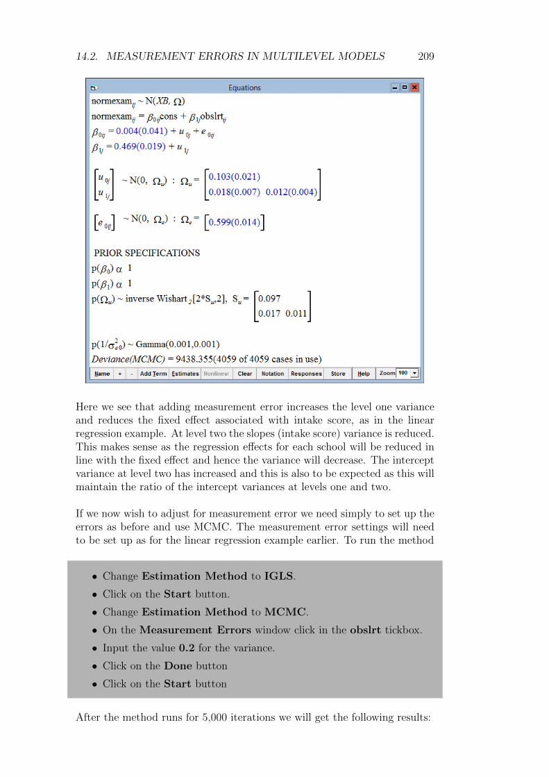
14.2. MEASUREMENT ERRORS IN MULTILEVEL MODELS 209
Here we see that adding measurement error increases the level one varianceand reduces the fixed effect associated with intake score, as in the linearregression example. At level two the slopes (intake score) variance is reduced.This makes sense as the regression effects for each school will be reduced inline with the fixed effect and hence the variance will decrease. The interceptvariance at level two has increased and this is also to be expected as this willmaintain the ratio of the intercept variances at levels one and two.
If we now wish to adjust for measurement error we need simply to set up theerrors as before and use MCMC. The measurement error settings will needto be set up as for the linear regression example earlier. To run the method
• Change Estimation Method to IGLS.
• Click on the Start button.
• Change Estimation Method to MCMC.
• On the Measurement Errors window click in the obslrt tickbox.
• Input the value 0.2 for the variance.
• Click on the Done button
• Click on the Start button
After the method runs for 5,000 iterations we will get the following results:
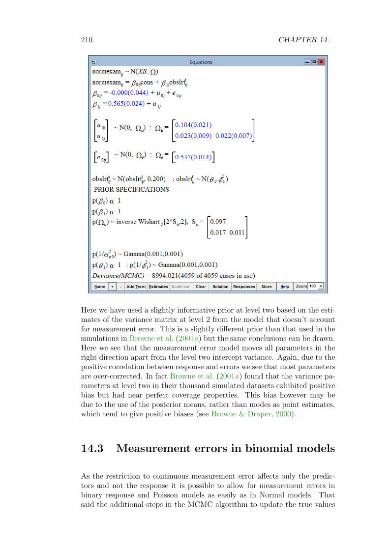
210 CHAPTER 14.
Here we have used a slightly informative prior at level two based on the esti-mates of the variance matrix at level 2 from the model that doesn’t accountfor measurement error. This is a slightly different prior than that used in thesimulations in Browne et al. (2001a) but the same conclusions can be drawn.Here we see that the measurement error model moves all parameters in theright direction apart from the level two intercept variance. Again, due to thepositive correlation between response and errors we see that most parametersare over-corrected. In fact Browne et al. (2001a) found that the variance pa-rameters at level two in their thousand simulated datasets exhibited positivebias but had near perfect coverage properties. This bias however may bedue to the use of the posterior means, rather than modes as point estimates,which tend to give positive biases (see Browne & Draper, 2000).
14.3 Measurement errors in binomial models
As the restriction to continuous measurement error affects only the predic-tors and not the response it is possible to allow for measurement errors inbinary response and Poisson models as easily as in Normal models. Thatsaid the additional steps in the MCMC algorithm to update the true values

14.3. MEASUREMENT ERRORS IN BINOMIAL MODELS 211
of the predictor will now need to be done using Metropolis rather than Gibbssampling although this happens automatically and so the user does not needto worry about this.
We will consider the first simple example from Chapter 10:
• Select Open Sample Worksheet from the File menu.
• Select bang1.ws from the list and click on Open.
We will now set up the simple single level logistic model with age as apredictor for contraceptive use.
• Select Equations from the Model menu.
• Click on the red y.
• Select use for the y variable.
• Select 2-ij for the number of levels.
• Select district as level 2(j).
• Select woman as level 1(i).
• Click on the Done button.
• Click on the N and instead choose Binomial from the list.
• Click on the Done button.
• Click on the red x0.
• Select cons and click on the Done button.
• Click on the Add Term button.
• Select age from the variable list and click on the Done button.
• Click on the red nij and select denomb from the list.
• Click on the Done button.
• Click on the Start button.
The estimates (from IGLS) are as follows:

212 CHAPTER 14.
The predictor to which we will add measurement error is age. If we usethe Average and Correlations window we will get the following summarystatistics for age:
N Missing Mean s.d.age 1934 0 0.0020481 9.0134
We will add measurement errors to age with a variance of 25 (s.d. of 5)which will correspond to a reliability of 81.25/(81.25+25) = 76.4%.
To create the measurement errors we need to type the following commandsin the Command Interface window:
Seed 3
Nran 1934 c16
Calc c16 = c16 * 5
Name c16 'errors'
Calc c17 = 'age' + 'errors'
Name c17 'obsage'
Here we have chosen random number seed 3 and this gives simulated errorsthat have an average of slightly less than zero. Now to see the effect of theerrors we need to change the predictor in the regression from age to obsage.
• Click on the β1 (age) in the Equations window.
• Replace age with obsage from the pull down list.
• Click on the Done button.
• Click on the Start button.
Upon convergence we get the following results:
So the errors have reduced the coefficient from 0.007 to 0.004. If we now

14.3. MEASUREMENT ERRORS IN BINOMIAL MODELS 213
wish to use MCMC and adjust for the measurement errors we need to do thefollowing:
• Change Estimation method to MCMC.
• Select MCMC/Measurement Errors from the Model menu.
• Click on the tick box for obsage on the Measurement Error win-dow and input 25 as the error variance.
The window should then look as follows:
Now click on the Done and Start buttons and after a few minutes we willget the following results:
So we see that the method moves the coefficient for age in the right direction,although the estimate is still slightly lower than the estimate with the true

214 CHAPTER 14.
predictor. This is because the errors had a slight negative bias and, giventhe coefficient for age is small and non-significant to start with, this smallbias becomes more important.
14.4 Measurement errors in more than one
variable and misclassifications
To finish this chapter we will consider other aspects of measurement errormodelling that are available in MLwiN or currently being researched. Firstlyif we have many predictors in our model we may have measurement errorson any or all of these predictors. We can account for these errors by addingindependent error assumptions for each predictor via the MeasurementError window. It is, however, plausible that measurement errors in twopredictors could be correlated, although accounting for correlated errors isnot currently available in MLwiN. Here the user would have to input bothmeasurement error variances for the predictors and correlations between themand a multivariate Normal distribution would be assumed for the errors.
As we mentioned earlier we are restricted to specifying continuous measure-ment errors. If however we had a predictor that was a binary outcome, forexample a pass/fail intake examination mark, we could theoretically use acontinuous error for this predictor. Although this seems rather unusual, asimilar argument to that used for the probit modelling in Chapter 10 couldbe used here.
More generally for binary predictors and categorical predictors we would haveto use a misclassification model rather than a measurement error model. Forexample, consider a predictor variable that has three categories and was fittedinto our model as two dummy variable predictors. Then we could considergenerating a prior distribution for the probability of observing category Awhen the true category is category B. We could work out probabilities forall nine combinations of observed and true category where the three proba-bilities for each true category would sum to 1. We would then have to invertthe table of probabilities to produce probabilities of an observation actuallybeing category B when category A is observed. Here the three probabilitiesassociated with category A being observed would need to sum to 1. Usingthis as a prior distribution we could combine this with the observed data tocreate a set of posterior probabilities for the true category for each observa-tion, at each iteration. This is harder to program as the dummy variableswill have to be modified simultaneously.
Finally we should reiterate that we recommend that measurement error mod-elling is used primarily as a sensitivity analysis tool. Once measurement er-rors have been added to a predictor we cannot expect to recover the truepredictor but given an estimate of the variance of the errors we can hope to

14.4. MORE VARIABLES AND MISCLASSIFICATIONS 215
gain a handle on the magnitude of the true predictor coefficients. It shouldbe noted that currently measurement errors cannot be used in MLwiN on pa-rameters that are involved in complex level 1 variance functions (see Chapter9) or in multivariate models (see Chapters 18–20).
Chapter learning outcomes
? What the effects of measurement errors are on predictors.
? How to account for measurement errors using MCMC.
? How to account for measurement errors in various multilevel models.
? How one would in theory account for misclassifications in categoricalpredictors.

216 CHAPTER 14.

Chapter 15
Cross Classified Models
One of the main uses of multilevel modelling is to account for the underlyingstructure in a dataset, whether it be pupils nested within schools or womennested within communities as seen in the examples so far. In accounting forthe structure we are removing the independence assumption between levelone units from the same level two units and instead partitioning the varianceinto variances between the units at the various levels in the dataset. Theexamples we have looked at so far have mainly concentrated on two-levelstructures but we have considered one three level structure (counties withinregions within nations) in Chapter 11.
Historically most multilevel modelling has assumed a hierarchical or nestedstructure for two reasons. Firstly many applications naturally have a nestedstructure, for example pupils within classes within schools, or patients withinwards within hospitals. Secondly the maximum likelihood based methods,for example IGLS, have been designed to work well for nested structures,as fast inversion routines are available for the block diagonal matrices thatnested structures produce. However, as we will see in the next three chapters,often the structure of the dataset is not strictly nested. In this chapter wewill consider cross-classified models before considering multiple membershipmodels (Chapter 16) and spatial models (Chapter 17).
When cross-classified and multiple membership effects are combined we canproduce multiple membership multiple classification (MMMC) models whichare described in detail in Browne, Goldstein & Rasbash (2001a). Detaileddescriptions of likelihood-based methods for both cross-classified models andmultiple membership models are given in Rasbash & Goldstein (1994) andRasbash & Browne (2001), while Rasbash & Browne (2002) compare the like-lihood approaches with the MCMC approach that we use here. In this chap-ter we will describe what we mean by a classification and a cross-classifiedmodel before considering an education-based example from Fife, Scotlandthat is considered in Rasbash et al. (2008, chap. 18).
217

218 CHAPTER 15.
15.1 Classifications and levels
We have so far concentrated on different ‘levels’ in a dataset where the defi-nition of a level has not been explicitly given, but we have been assuming anested relationship between levels. For example in education we may have athree ‘level’ dataset with our three levels being pupil, class and school. Herepupils are nested within classes and classes are nested within schools. Thisimplies that all pupils in the same class are also in the same school due tothe nesting of the levels. The response variable will be at the lowest level inthe dataset although predictors may be at the higher levels, for example theeffect of class size on individual pupil scores.
Note that if the response was at a higher level than some of the predictorsthen these predictors could only be fitted in the model as aggregates. Forexample we may have several previous tests scores for each pupil, whichwould imply a lower level of time/test below pupil. If our response was examscore at 16 then we would either fit each previous test as a separate predictoror fit an average previous test mark, and so for the model the lowest level ispupil and not test.
In this chapter we will consider the more general definition of a classification.Having defined our lowest level in the data as the level at which the responsevariable is collected then we can define a classification mathematically as afunction, c, that maps from the set θ of N lowest level units to a set Φ ofsize M where M ≤ N , and we define the resulting set Φ of M objects as theclassification units. In this chapter we will only consider single membershipclassifications, c(ni) = mj, ∀ni ∈ θ where mj ∈ Φ.
In words, if we consider the educational example earlier then our lowestlevel was pupil and the lowest level units are the individual pupils. Bothschool and class will then be classifications (functions) that given an in-dividual pupil will return their respective school and class, and so the setsof all schools and all classes will be the classification units associated withthe classifications school and class respectively. Note that as these classi-fications map directly from the lowest level there is no guarantee that theclassifications will be nested, and in fact nested classifications are a specialcase of the general ‘cross-classified’ classifications that we consider in thischapter.
MCMC methods treat each set of classification units (residuals in the model)as an additive term in the model and hence it is no more complicated (oncethe classifications have been calculated) to fit a cross-classified model thana nested model using MCMC. However there is one restriction and that isthat we need unique classification identifiers. For example if we truly havea three-level nested model with class 1 in school 1 and class 1 in school 2,then these two classes will need unique identifiers if this model is fitted as across-classified model to differentiate between the two class 1s.

15.2. NOTATION 219
15.2 Notation
Browne, Goldstein & Rasbash (2001a) introduce notation for fitting cross-classified and more complex models based upon the definition of a classifica-tion. Rather than trying to introduce more complex indices that take accountof the crossings and nestings (as in Rasbash & Browne, 2001) they insteadsimply give the response variable subscript i to index lowest level units, andthen use the classification names for the subscripts of random effects. Forexample consider the variance components model described first in Chapter3. This was written there as:
normexamij ∼ N(XB,Ω)
normexamij = β0ijcons + β1standlrtij
β0ij = β0 + u0j + e0ij
In the classification notation we would rewrite this as:
normexami ∼ N(XB,Ω)
normexami = β0iconsi + β1standlrti
β0i = β0 + u(2)0,school(i) + e0i
As there may be many classifications, rather than using different letters foreach, we give a superscript to represent the classification number (note thisstarts at 2 as we consider the lowest level as classification 1). To change be-tween notations we can use the Notation button on the Equations windowthat we earlier used for the alternative complex level 1 notation. We willnow consider a cross-classified example from the educational literature.
15.3 The Fife educational dataset
We will consider here an educational example from Fife in Scotland that isalso considered in the User’s Guide to MLwiN (Chapter 18). The data consistof pupils’ overall exam attainment at age 16 (as with the tutorial.ws datasetstudied earlier) and several predictor variables, including a verbal reasoningtest taken at age 11 and information on social class and parent’s occupation.The added complexity in the dataset is that we have information on both thesecondary school (ages 12 through to 16) in which the children studied andthe primary school (ages 5 through to 12) they attended prior to secondaryschool. Not all the children from a particular primary school will attend thesame secondary school so we have two classifications that are crossed ratherthan nested. The data consists of records for 3,435 children from 148 primaryschools and 19 secondary schools.
First we will load the dataset and look at the variable names:

220 CHAPTER 15.
• Select Open Sample Worksheet from the File menu.
• Select xc1.ws from the list and click on the Open button.
The Names window will appear as follows:
We here see that our response variable (attain) is a score from 1 to 10 thatrepresents the pupils score on a school leaving exam. The intake abilityis measured by a score in a verbal reasoning test, (vrq) and we also havepredictors that represent gender (sex), social class (sc), father’s education(fed), mother’s education (med) and the choice of secondary school thatthey attend (choice where 1 is first choice and so on).
We can look at the dataset more closely by:
• Select View or Edit Data from the Data Manipulation menu.
• Select to view columns attain, pid, sid and pupil.
The data have been sorted on primary school within secondary school. Wecan see here that 8 of the pupils who attended primary school 1 then attendedsecondary school 1. If we were to scan down the columns we would find thatthe rest of primary school 1 went to two other secondary schools, 45 tosecondary school 9 and 1 to secondary school 18 (to see this quickly type1355 or 3068 into the goto line box and this will take you to these groupsof pupils). So we can see that school 9 is the ‘main’ secondary school for

15.3. THE FIFE EDUCATIONAL DATASET 221
primary school 1 with 83% of pupils attending it. In the entire dataset 59of the 148 primary schools had all their pupils attend the same secondaryschool after leaving primary school and only 288 pupils did not attend their‘main’ secondary school. So although the dataset structure is not nested itis close to nested and this helps the likelihood-based methods in the User’sGuide to MLwiN (see Rasbash & Goldstein, 1994, for details). The degreeof ‘nestedness’ does not matter so much to the MCMC methods and in factit is probably easier to distinguish between two classifications if they are lessnested!
As the data are sorted on secondary schools and their effects will have hap-pened closer (in time) to the exam response of interest we will first con-sider fitting a two-level model of children within secondary school. We willhowever use the classification notation from the start and define the three-classification structure of the data.
• Select Equations from the Model menu.
• Click on the Notation button and remove the tick for multiple sub-scripts and an i subscript will appear on the red y.
• Click on the Done button.
• Click on the red y and select ATTAIN from the y pull down list.
• Select 3 from the N classifications box.
• Select sid as classification 3, PID as classification 2 and PUPIL asclassification 1.
• Click on the Done button.
• Click on the red x0 and select CONS from the pull down list.
• Select cons as a fixed effect and random at classifications pupil(1)and sid(3).
• Click on the Done button.
• Click on the Start button.
• Change Estimation method to MCMC.
• Click on the Start button.
This will have set up the 2 level variance components model and run it usingMCMC. The estimates in the Equations window will be as follows:

222 CHAPTER 15.
Here we see that there is significant variation between the secondary schoolsand this accounts for 0.489/(0.489+8.989)×100% = 5.1% of the total varia-tion in exam marks.
We can compare the DIC for this model with a simpler model with no schooleffects, and we see a reduction in DIC of 120 showing this is a much bettermodel. Also the 19 secondary school effects account for 18.2−2 = 16.2 effec-tive parameters so there are distinct differences between secondary schools.
Dbar D(thetabar) pD DIC17291.80 17273.61 18.19 17309.9917429.27 17427.26 2.01 17431.28 (no school effect)
15.4 A Cross-classified model
If we now consider adding in the effects of primary schools this can be donesimply via the Equations window.
• Change Estimation method to IGLS.
• Click on x0 (cons) and tick the PID(2) box.
• Click on the Start button.
What you have actually just done is fitted a ‘nested’ model of primary schoolnested within secondary school using IGLS. This can be confirmed by lookingat the Hierarchy viewer available via the Model menu.

15.4. A CROSS-CLASSIFIED MODEL 223
Here you can see that MLwiN has treated the individual groups of pupilsthat are from the same primary school and secondary school as separateprimary schools, for example the pupils in primary school 1 are treated asthree separate primary schools nested within secondary schools 1, 9 and 18respectively. This results in 303 rather than 148 primary schools. To fit across-classified model in IGLS instead involves following the procedures givenin Chapter 18 of the User’s Guide to MLwiN.
To fit the model (as cross-classified) using MCMC is however fairly simple.
• Change Estimation method to MCMC.
• Select MCMC/Classifications from the Model menu.
The window will appear as follows:
Here we now simply have to click in the Treat levels as cross-classifiedbox and click on the Done button. If we now select the Hierarchy Viewer

224 CHAPTER 15.
from the Model menu we get the alternative classifications viewer as shownbelow.
Here we see that this viewer shows we have only 148 primary schools as weare now taking account of the cross-classifications. After running the modelby clicking on the Start button we will get the following estimates:
The estimates are fairly similar to those achieved using IGLS in the User’sGuide to MLwiN although the variances for primary school (1.15 versus 1.12)and particularly secondary school (0.41 versus 0.35) are higher. This is dueto the difference between mean estimates and mode (ML) estimates for theskewed variance parameter posterior distributions. The trajectory plots con-firm this for the secondary school variance:

15.5. RESIDUALS 225
We can also see that primary school is actually more important in predictingthe attainment score than secondary school. One possible reason for thisis that secondary schools are generally larger (see Goldstein, 2003). Hereprimary school explains 1.15/(0.41+1.15+8.12)×100% = 11.9% of variationwhile secondary school only explains 0.41/(0.41+1.15+8.12)×100% = 4.2%.The DIC diagnostic again shows that this model is an improvement with areduction in DIC of over 250.
Dbar D(thetabar) pD DIC16940.56 16833.40 107.16 17047.73 (with primary school)17291.80 17273.61 18.19 17309.99 (without primary school)
15.5 Residuals
As with nested models we can work out residuals for the various levels ofour model. This may be done via the Residuals window available from theModel menu. We will look firstly at secondary school residuals:
• On the Residuals window, change the level box to 3:SID.
• Click on the Calc button.
• Click on the Plots tab, and if not selected, select residual x rank.
• Click on the Apply button.
The plot will then appear as follows:

226 CHAPTER 15.
Here we see the lowest ranked secondary school has a very low residual andmay be an outlier. Clicking on the graph on this point we get:
showing that this is secondary school 19. We will revisit this plot after addingin other variables. If we now look instead at the primary schools:
• On the Residuals window, click on the Settings tab.
• Change the level box to 2:PID.
• Click on the Calc button.
• Click on the Plots tab, and if not selected select residual x rank.
• Click on the Apply button.

15.6. ADDING PREDICTORS TO THE MODEL 227
Here we see the 148 primary school residuals. Here there is no evidence ofoutliers. If we click on the lowest residual (rank 1) we get the following:
So we see here that the lowest ranked primary school is school number 139and that even though the data are not nested the residuals screen can identifycorrectly the primary school. Note however that unlike nested models we donot get a level 3 identifier as primary school is not nested within secondaryschool.
15.6 Adding predictors to the model
We have so far not considered any of the available predictors in our model.We will firstly consider the effect of intake score (VRQ) in our model.

228 CHAPTER 15.
• Change Estimation method to IGLS.
• Click on the Add Term button and select VRQ from the variablelist.
• Click on the Done button.
• Click on the Start button.
• Change Estimation method to MCMC.
• Click on the Start button.
The estimates produced are as follows:
The predictor, vrq, explains not only a large amount of the residual variationbut also a large amount of the differences between secondary schools andbetween primary schools. Of the remaining variation, 6% is explained byprimary schools and less than 0.4% by secondary schools. The DIC diagnosticgives:
Dbar D(thetabar) pD DIC14724.86 14644.21 80.66 14805.52 (with vrq)16940.56 16833.40 107.16 17047.73 (without vrq)
which shows a reduction in DIC of over 2000! It is also interesting that theeffective number of parameters is reduced and this is clearly because VRQ isexplaining many of the differences between secondary schools and betweenprimary schools.

15.6. ADDING PREDICTORS TO THE MODEL 229
We can continue adding in the other predictor variables and retaining signif-icant predictors. In this case all predictors tested apart from gender (SEX)are significant. The model with all significant predictors can be obtained by:
• Change Estimation method to IGLS.
• Add the variables SC, FED, MED and CHOICE as fixed effectsto the model.
• Click on the Start button.
• Change Estimation method to MCMC.
• Click on the Start button.
When the 5,000 iterations have been run we get the following estimates:
Here we see that on average a pupil’s attainment is higher if they come froma higher social class, if their parents are better educated or if the school theyattend is their first choice. Adding the additional predictors has the effect ofreducing the DIC diagnostic by 80 and again reducing the effective number ofparameters slightly, suggesting more of the differences between schools havebeen explained by the additional predictors.
Dbar D(thetabar) pD DIC14651.56 14575.02 76.54 14728.1014724.86 14644.21 80.66 14805.52 (without additional predictors)
The secondary school variance is very small and if we now look at the resid-uals plot of the school residuals against rank (see instructions earlier on howto produce this) we see that the residual for school 19 is still lowest and lookslike an outlier. (Note that a number of error messages may crop up duringthe estimation here. It is safe to ignore them by clicking the OK button.)

230 CHAPTER 15.
We will therefore consider fitting a dummy variable for school 19 and remov-ing secondary school from the model.
• Select Command Interface from the Data Manipulation menuand enter the following commands:
calc c12 = 'sid' == 19
name c12 'school19'
• Change Estimation method to IGLS.
• Click on the β0 (cons) and remove the tick for sid(3).
• Click on the Add Term button and select school19 from the list.
• Click on the Done button.
• Click on the Start button.
• Change Estimation method to MCMC.
• Click on the Start button.
After the 5,000 iterations have completed our estimates are as follows:

15.7. CURRENT RESTRICTIONS 231
We can see that school 19 has a significant negative effect on attainment andif we look at the DIC diagnostic we see an improvement in DIC diagnosticof 3.4.
Dbar D(thetabar) pD DIC14649.39 14574.03 75.36 14724.74 (with secondary school 19 only)14651.56 14575.02 76.54 14728.10 (with all secondary school effects)
So in adding the predictors to our model we have explained all the secondaryschool variation down to a difference between school 19 and the rest of thesecondary schools. This of course means that, for the Fife dataset, we nowno longer need to fit a cross-classified model. Therefore if we were to re-sort the data on primary school we could have fitted the final model directlyusing IGLS or MCMC. Some people may think this is disappointing but withonly 19 secondary schools to start with it is unlikely that we will find muchvariation and in fact we now have a more parsimonious model. It may beinteresting for the researchers to now go and investigate why school 19 wasa potential outlier.
15.7 Current restrictions for cross-classified
models
As has been shown in this chapter it is now possible to quite easily fit cross-classified models in MLwiN using MCMC, although not all features havebeen updated to account for these models. For example currently the Pre-dictions window does not account for cross-classified random effects and willtherefore give error messages if it is used. It should also be noted that the

232 CHAPTER 15.
starting values that MCMC gets for the residuals will be based on the valuesobtained from the nested model and so will often be meaningless. It is possi-ble by running the MCMC and other commands in the Command interfacewindow to fit the separate IGLS two-level models and store these residuals incolumns to be used as starting values, but generally the MCMC routines arerobust to the nested model starting values. Currently cross-classified modelscan be fitted using IGLS, but only via additional commands that transformthe cross-classified model into a constrained nested model.
Chapter learning outcomes
? What is meant by a classification and a cross-classified model.
? How to fit cross-classified models in MLwiN using MCMC.
? How to look at residuals in a cross-classified model.
? Some of the current restrictions in fitting cross-classified models inMLwiN.

Chapter 16
Multiple Membership Models
In the last chapter we considered cross-classified models and introduced theconcept of a classification. All the classifications we considered were what wewould describe as ‘single membership’ classifications. This means that everylowest level unit is a member of one and only one classification unit. Forexample each pupil in the tutorial.ws dataset belongs to one and only oneschool and each woman in the bang1.ws dataset belongs to one and onlyone district.
It is however possible that we cannot (or do not want to) assign each lowestlevel unit to exactly one classification unit. This may be due to movementsbetween units over the time period for which the data were collected. Forexample if our response is exam scores at 16 then some pupils will have beeneducated in more than one school and thus we may want to account for theeffects of all schools. Alternatively our response may have been produced bythe aggregation of units. For example in veterinary epidemiology the unit ofmeasurement may be flocks of chickens and each flock may be produced fromindividual parent birds from several parent flocks, each of which has an effecton the child flock (see Browne, Goldstein & Rasbash, 2001a, for details).Both of these scenarios are examples of ‘multiple membership’ classifications.
Formally we can define a multiple membership classification as a map c fromthe set Θ of N lowest level units to the set Φ of M classification units suchthat each individual, ni ∈ Θ is mapped to a subset (possibly of size 1) Φi of Φ.So the single membership classifications are a special case where every Φi isof size 1. We will firstly consider in this chapter a (simulated) example fromemployment statistics that has a multiple membership classification, andfinish the chapter with a look at the combination of multiple membershipmodels and cross-classified models known as multiple membership multipleclassification (MMMC) models (Browne et al., 2001a).
233

234 CHAPTER 16.
16.1 Notation and weightings
In the last chapter we introduced a new notation for use with classifications.We can extend this classification to deal with multiple membership classifi-cations. When we have a multiple membership classification, a single lowestlevel unit will have a random effect for each ‘classification unit’ they belongto. Generally, to avoid lowest level units that belong to many classificationunits being given too much influence in the model, we assign weights foreach pairing of lowest level unit and classification unit. These weights typi-cally sum to 1 for each lowest level unit and we can write a simple multiplemembership model of pupils nested in multiple schools as:
yi ∼ N(XB,Ω)
yi = β0ix0i
β0i = β0 +∑
j∈school(i)
w(2)i,j u
(2)0j + e0i
Here we have a classification school and the weight w(2)i,j is the weight assigned
to the random effect for school j in the equation for pupil i. What quantitiesto use as weights is an interesting question. If we have no information otherthan that each pupil went to a particular selection of schools over the periodof their education then equal weights would be logical. If however we knowhow long they spent in each school then we could use this information tocreate weights proportional to the times spent in each school.
Both of these methods are making an assumption that the effect of a schoolis some fraction of the amount of time spent in all schools by each pupil andhence the weights for each pupil sum to 1. An alternative approach wouldbe that schools have an instantaneous effect that is equal for all pupils nomatter how long they spend there. We could of course fit this instantaneouseffect by having weights of one for each pupil by school combination but thiswill make comparison of the between schools variance and residual variancedifficult.
16.2 Office workers salary dataset
We will consider as an example a simulated dataset meant to represent theyearly salaries of randomly sampled office workers.
• Select Open Sample Worksheet from the File menu.

16.2. OFFICE WORKERS SALARY DATASET 235
• Select wage1.ws from the list and click on the Open button.
The Names window will appear as follows:
Here we have as a response variable earnings, the amount (in thousands ofpounds) that 3,022 workers earned in the last financial year. Most individ-uals worked for one company although some individuals worked for more,either because they work part time or because they changed job in the timeperiod. For these individuals we have information on the names of all (upto 4) companies they worked for in columns labelled company, company2,company3 and company4. There are 141 companies in the dataset andwe also have the fraction of time the individuals worked for each companyand this is stored in columns weight1 to weight4. As predictors for salarywe have the individual’s age, sex, the number of jobs they worked on andwhether they worked full or part-time.
We can firstly plot a histogram of the earnings:
• Select Customised Graph(s) from the Graphs menu.
• Select earnings from the y pull down list.
• Select histogram from the plot type list.
• Click on the Apply button.
The graph will then appear as follows:

236 CHAPTER 16.
As is common with earnings data, the graph shows that the response is highlyskewed to the right with the majority of people earning less than £40,000while a few individuals earn over £100,000. Therefore it is probably betterto consider a log transformation of the response and instead fit a Normalmodel to loge(response).
The column logearn was created via the command CALC 'logearn' =LOGE ('earnings') and is the (natural) logarithm of earnings. If we nowplot a histogram of this variable instead (by changing the y column to lo-gearn) we will see the following:
Here we see a much more Gaussian shape to the histogram suggesting thatthis will be a better variable to use as a response in a Normal response model.

16.3. MODELS FOR THE EARNINGS DATA 237
16.3 Models for the earnings data
We will firstly consider fitting some simple regression models to the earningsdata. The two predictors we will consider first are age-40 and numjobswhich represent the age of the workers (roughly centred) and the number ofcompanies they have worked for in the last 12 months.
• Select Equations from the Model menu.
• Click on the Notation button and remove the tick for multiplesubscripts and an i subscript will appear on the red y.
• Click on the Done button.
• Click on the red yi and select logearn as the y variable.
• Select 2 as the number of classifications, company as classification2 and id as classification 1.
• Click on the red x0 and select cons from the list.
• Select this variable as a fixed parameter and random at level1(id).
• Click on the Add Term button.
• Select age-40 from the variable list and click on the Done button.
• Click on the Add Term button.
• Select numjobs from the variable list and click on the Done but-ton.
• Click on the Start button.
• Change Estimation method to MCMC.
• Click on the Start button.
Upon finishing the 5,000 iterations we get the following estimates:
So we see that older workers earn on average more whilst people who workfor more companies in a year earn on average less. For example the average40 year old with 1 job earns e3.08−0.13=19.1k whilst the average 40 year old

238 CHAPTER 16.
with 2 jobs earns e3.08−0.26=16.8k. Note that due to the log transformationthese estimates will be median earnings rather than means.
If we look at the DIC diagnostic we see that it confirms what we see fromthe significance of the predictors, that both predictors are important.
Dbar D(thetabar) pD DIC5199.68 5195.62 4.06 5203.74 (age + numjobs)5228.58 5225.56 3.03 5231.61 (age only)5361.67 5359.66 2.01 5363.69 (neither)
We can now consider our two other predictor variables, gender and whetherthe person works full or part-time:
• Change Estimation method to IGLS.
• Click on the Add Term button.
• Select sex from the variable list and click on the Done button.
• Click on the Add Term button.
• Select parttime from the variable list and click on the Done but-ton.
• Click on the Start button.
• Change Estimation method to MCMC.
• Click on the Start button.
Upon convergence we see the following estimates:
Here we see that both being female (sex = 1) and being a part time worker onaverage reduces your salary. It is interesting that putting these two variablesinto the model has reduced the negative effect of the number of jobs andit is now not significant. If we compare the DIC diagnostic for this modelwith the previous model, and a model with numjobs removed we see thefollowing:

16.4. FITTING MULTIPLE MEMBERSHIP MODELS 239
Dbar D(thetabar) pD DIC4989.96 4983.98 5.98 4995.94 (this model)5199.68 5195.62 4.06 5203.74 (age + numjobs only)4990.83 4985.82 5.01 4995.84 (numjobs removed)
So it seems that the numjobs predictor is not important. If we now look atthe correlations between the predictors:
• Select Averages and Correlations from the Basic Statisticsmenu.
• Select Correlations and the variables parttime, sex and numjobs.
• Select Calculate.
Correlations
parttime sex numjobsparttime 1.0000sex 0.0399 1.0000numjobs 0.2908 0.1014 1.0000
We can see here that there are (small) positive correlations between numjobsand both sex and parttime and so the significant effect for numjobs in theearlier model was a surrogate for the actual effects due to gender and part-time/full-time.
16.4 Fitting multiple membership models to
the dataset
We can now consider accounting for the effects of the various companies onthe earnings of the employees. If we look at the distribution of the numberof jobs variable:
• Select Tabulate from the Basic Statistics window.
• Choose numjobs from the Columns pull down list.
• Click on the Tabulate button.
1 2 3 4 TOTALSN 2496 472 52 2 3022
We can see that in our dataset changing company is not a common phe-nomenon and so we could firstly fit a simple 2-level model that accounts for

240 CHAPTER 16.
only one company per individual. This would be the type of model we wouldhave to fit if, for example, we only collected the current employer for eachindividual. For our dataset we will consider just fitting the company thatappears in the column company which will be the first in numerical orderof the companies each individual works for.
• Change Estimation method to IGLS.
• Click on the β2 (numjobs) and click on the Delete Term button.
• Click on the β0 (cons) and tick the company(2) tick box.
• Click on the Start button.
• Change Estimation method to MCMC.
• Click on the Start button.
After running for 5,000 iterations the results are as follows:
So here we see that the first company of each employee explains 0.052/(0.052+0.253)= 17% of the remaining variation. If we look at the DIC diagnostic:
Dbar D(thetabar) pD DIC4421.62 4311.72 109.90 4531.524990.83 4985.82 5.01 4995.84 (no random effects)
Here we see that the random effects have reduced the DIC by over 400 andso are very important. There are also 110 − 5 = 105 effective parametersfor the 141 actual random effects so there are many important and distinctcompany effects.
If we now want to fit the multiple membership model we need to use theclassifications window that we looked at in the last chapter:

16.4. FITTING MULTIPLE MEMBERSHIP MODELS 241
• Change Estimation method to IGLS (to use same starting values).
• Click on the Start button.
• Change Estimation method to MCMC.
• Select MCMC/Classifications from the Model menu.
• Tick the Multiple Classification Level 2 tickbox.
• Choose 4 for the Number of columns.
• Choose weight1 as the Weight start Column.
The window should look as follows:
We now need to click on the Done button to apply the settings. Note thatMLwiN assumes that the identifier columns are in sequential order, so in thisexample company (column c2) contains the first set of identifiers and theother three sets must be in the columns c3–c5 respectively. The same is truefor the weight columns with columns c13–c16 named weight1 to weight4.Note that if an observation is associated with less than 4 companies thenboth the identifier and weight for the extra companies should be set equal tozero. We have here used a system of filling in the end columns with zeroesalthough the order of the columns does not matter, as long as the ith weightcolumn matches up with the ith identifier column.
• Click the Start button.
After running for 5,000 iterations we get the following estimates:

242 CHAPTER 16.
So accounting for all the companies explains 0.059/(0.059+0.247) = 19.3%of the variation. More importantly if we look at the DIC diagnostic wesee that the DIC diagnostic has been reduced by over 60 and the numberof effective parameters has increased, suggesting again many important anddistinct company effects.
Dbar D(thetabar) pD DIC4354.60 4240.64 113.97 4468.574421.62 4311.72 109.90 4531.52 (no MM)
16.5 Residuals in multiple membership mod-
els
We can look at the individual company effects via the Residuals window.
• Select Residuals from the Model menu.
• Select 2:company from the level pull down list.
• Change the SD multiplier from 1.0 to 1.4.
• Click on the Calc button.
• Click on the Plots tab.
• Select residual +/- 1.4 sd x rank.
• Click on the Apply button.
The residual graphs will then appear as shown below. Interestingly a coupleof the companies with the highest residuals look like potential outliers.

16.5. RESIDUALS IN MULTIPLE MEMBERSHIP MODELS 243
Looking at a plot of the (raw) residuals against normalized scores also showssimilar behaviour:
We can consider fitting separate terms for these two companies and treatingthese as fixed effects. Clicking on their residuals identifies them as companies54 and 67. Normally we could use the graph window to create dummy vari-ables for these two companies, but we cannot currently do this for multiple-membership models as MLwiN would currently only select individuals whohave company = 54 (67) and ignore the other 3 potential companies. We canhowever currently create the two columns using the Command Interfacewindow.
• Open the Command Interface window from the Data Manipu-lation menu.

244 CHAPTER 16.
• Type the following four commands:
Calc c22 = ('company' == 54) + ('company2' == 54) +
('company3' == 54) + ('company4' == 54)
name c22 'companyno54' Calc c23 = ('company' == 67) + ('company2' == 67) +
('company3' == 67) + ('company4' == 67)
name c23 'companyno67'
• Change Estimation method to IGLS.
• Add the variables companyno54 and companyno67 as fixed ef-fects to the model.
• Click on the Start button.
• Change Estimation method to MCMC.
• Click on the Start button.
Upon running for 5,000 iterations we get the following estimates:
Here we see that the two companies both have large positive coefficients andthe company level variance has reduced from 0.059 to 0.045. If we look atthe DIC diagnostic for the new model we see that it has been reduced by afurther 4 suggesting this is a slightly improved model:
Dbar D(thetabar) pD DIC4356.70 4248.63 108.07 4464.77 (with 2 additional fixed effects)4354.60 4240.64 113.97 4468.57 (with all random effects)

16.6. ALTERNATIVEWEIGHTS FORMULTIPLEMEMBERSHIPMODELS245
16.6 Alternative weights for multiple mem-
bership models
We have so far used weights that are proportional to the time spent in eachjob and, as this is a simulated dataset, these were the weights that wereactually used to generate the response variable. It is possible however toconsider using other weightings, for example we could look at the effect ofusing equal weights so that each company you work for has an equal effecton your final salary.
• Change Estimation method to IGLS.
• Click on the Start button.
• Change Estimation method to MCMC.
• Select MCMC/Classifications from the Model menu.
• Change the Weights start column to ew1.
• Click on the Done button.
• Click on the Start button.
Upon running for 5,000 iterations we get the following estimates:
The estimates are not greatly different from those we got when using the pro-portional weights earlier. This is probably because few respondents changejob. However if we now look at the DIC diagnostic we see:
Dbar D(thetabar) pD DIC4369.36 4261.93 107.43 4476.80 (equal weights)4356.70 4248.63 108.07 4464.77 (proportional weights)

246 CHAPTER 16.
So we can see that the equal weights give a DIC that is 11 higher, whichsuggests that this is a worse model. This is not surprising given that we usedthe proportional weights to generate the response. However this shows thatthe DIC diagnostic is useful for choosing between possible weighting systems.
16.7 Multiple membership multiple classifi-
cation (MMMC) models
In the past two chapters we have considered both cross-classified and multiple-membership models. Of course we can think of models that combine boththese advancements in one model. For example in our above analysis we mayalso have information on what secondary school the workers attended anduse this as a classification that is crossed with the multiple-membership clas-sification for companies. We call such models multiple membership multipleclassification (MMMC) models and Browne, Goldstein & Rasbash (2001a)give general MCMC algorithms for fitting such models. In their paper youwill find two large examples from veterinary epidemiology and demography,which are too large to include in this manual. We will however consider thethird example on Scottish lip cancer in the next chapter where amongst othermodels we will fit an MMMC model.
One other innovation in Browne et al. (2001a) is the ‘classification diagram’.When fitting MMMC models using MCMC estimation, knowledge of nestingrelationships is not needed to implement the algorithms. For a simple sum-mary of the model, however, it is useful to see the nesting relationships andso we advocate the use of a ‘classification diagram’. A classification diagramconsists of boxes to represent each classification with arrows to representnesting between two classifications, single arrows for single membership re-lationships and double arrows for multiple membership relationships.
Below are classification diagrams for the two examples in the last two chap-ters.
Primary School Secondary School
Pupil Worker
Company

16.7. MMMC MODELS 247
Chapter learning outcomes
? What is meant by a multiple membership model.
? How to transform and fit earnings data.
? How to fit a multiple membership model in MLwiN.
? How to look at residuals in a multiple membership model.
? How to compare alternative weighting schemes.
? What is meant by an MMMC model and a classification diagram.

248 CHAPTER 16.

Chapter 17
Modelling Spatial Data
In this chapter we will consider one particular dataset that has a spatialstructure and discuss what models we can fit to such a dataset. The termspatial data will mean different things to different people. Here we will be asgeneral as possible and consider collecting data at a variety of sites and alsocollecting some measure of the location of the sites. Of course we can analysespatial data in the same way as any other dataset, for example in Chapter 11we considered counts of melanoma mortality for different areas (locations)and simply fitted variance components models. However generally when wehave spatial data we also wish to account for the effects of the locations.
How we adjust for location will depend on whether we have single obser-vations at particular locations or estimates for contiguous areas. We canaccount for the effect of location in the first case by simply fitting func-tions of position, for example fitting polynomials in orthogonal directions orby considering point-process modelling. In the second case we are usuallyinterested in fitting models that account for spatial correlation.
In earlier chapters we have considered fitting two level nested models andhere we are assuming a correlation between individual level one units in thesame level 2 unit. In a spatially correlated model we assume that the corre-lation between observations is some function of the spatial distance betweenthem. In this chapter we will consider an epidemiological dataset of lip cancerincidence in Scotland.
17.1 Scottish lip cancer dataset
The dataset consists of observed counts of male lip cancer for the 56 regions ofScotland over the period 1975-1980 and was analysed in Clayton & Kaldor(1987). Research has focused on the effect of sun exposure on lip cancerdeaths using the surrogate measure, percentage of the workforce working in
249

250 CHAPTER 17.
outdoor occupations. The data are stored in the worksheet lips1.ws. Firstwe will open up the worksheet and look at the variable names.
• Select Open sample worksheet from the File Menu.
• Select lips1.ws from the list and click on the Open button.
Here we see that for each of the 56 regions (area) we have observed casesof lip cancer (obs) and an expected count based on population size and mix(exp). As in the Melanoma example in Chapter 11 we have calculated thelog of the expected count and this can be found in the column offs. Thepredictor of interest is perc aff , which is the percentage of the region whowork in agriculture, fishing and forestry and which ranges from 0% to 24%.We also have the neighbourhood structure for the regions, which is storedin columns neigh1 to neigh11. Each region borders up to 11 other regionsand the region numbers are stored in these columns.
17.2 Fixed effects models
We will firstly fit a simple constant risk model, which assumes that there isan underlying risk of getting lip cancer which is constant across the wholepopulation and any deviations from this risk in particular regions are simplyrandom Poisson variation. Note that in this chapter we will again use thenotation introduced in Browne, Goldstein & Rasbash (2001a). We can setup this model as follows:
• Open the Equations window from the Model Menu.
• Click on the Notation button and remove the tick for multiplesubscripts and an i subscript will appear on the red y.
• Click on the Done button.
• Click on the red yi.
• Select obs as the y variable.
• Select 3 as the number of classifications.

17.2. FIXED EFFECTS MODELS 251
• Select neigh1 as classification 3.
• Select area as classification 2.
• Select area as classification 1.
• Click on the Done button.
• Click on the N and select Poisson from the list.
• Click on the Done button.
• Click on the log(πi) and select offs from the list.
• Click on the Done button.
Note that here we have set up the response and its Poisson distribution. Wehave also defined the (potential) full structure of the dataset, which is notimportant for this first model but will be used later. Both classifications 1and 2 are defined as area because there is only 1 observation per area andso classification 2 will be used to account for over-dispersion in later models.We have also defined the offset parameter to be offs. We now need to set upthe predictor variables. We will start with just an intercept term.
• Click on the red x0 and select cons
• Click on the Done button.
As always we will run the model using IGLS first for starting values.
• Click on the Start button.
• Change Estimation mode to MCMC.
• Click on the Start button.
When the 5,000 iterations are finished we get the following estimates:
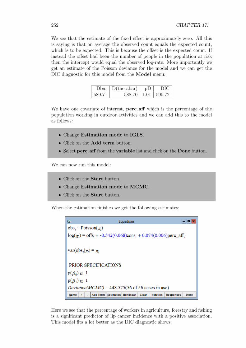
252 CHAPTER 17.
We see that the estimate of the fixed effect is approximately zero. All thisis saying is that on average the observed count equals the expected count,which is to be expected. This is because the offset is the expected count. Ifinstead the offset had been the number of people in the population at riskthen the intercept would equal the observed log-rate. More importantly weget an estimate of the Poisson deviance for the model and we can get theDIC diagnostic for this model from the Model menu:
Dbar D(thetabar) pD DIC589.71 588.70 1.01 590.72
We have one covariate of interest, perc aff which is the percentage of thepopulation working in outdoor activities and we can add this to the modelas follows:
• Change Estimation mode to IGLS.
• Click on the Add term button.
• Select perc aff from the variable list and click on the Done button.
We can now run this model:
• Click on the Start button.
• Change Estimation mode to MCMC.
• Click on the Start button.
When the estimation finishes we get the following estimates:
Here we see that the percentage of workers in agriculture, forestry and fishingis a significant predictor of lip cancer incidence with a positive association.This model fits a lot better as the DIC diagnostic shows:

17.3. RANDOM EFFECTS MODELS 253
Dbar D(thetabar) pD DIC448.58 446.60 1.98 450.55 (with predictor)589.71 588.70 1.01 590.72 (without predictor)
17.3 Random effects models
As with the melanoma example in Chapter 11 the next step is to considerfitting random effects to explain the remaining variation in the data. Thesimplest model here is to fit a variance components model where each region isgiven an (exchangeable) random effect, and these random effects are assumedto have a Normal distribution. This will now mean that for our 56 datapoints we are fitting 58 parameters (2 fixed effects and 56 random effects) butthis is allowed as the random effects are linked by their Normal distributionassumption, so in terms of effective parameters we are fitting less than 58parameters.
As we also saw in Chapter 11, Poisson models often produce highly auto-correlated chains and so for the rest of the models in this chapter we willincrease the lengths of the stored MCMC chains to 50,000. We will considermethods of improving mixing of chains for Poisson models in later chapters.To fit the variance components model we need to do the following:
• Change Estimation mode to IGLS.
• Click on the x0 (cons) and select the area(2) tick box .
• Click on the Done button.
• Click on the Start button.
• Change Estimation mode to MCMC.
• Change the monitoring chain length to 50,000 on the EstimationControl window.
• Change the refresh rate to 500 on the Estimation Control win-dow.
• Click on the Start button.
Upon completion of the 50,000 iterations we will get the following results:

254 CHAPTER 17.
Here we see the variance of the random effects appears to be quite large(0.384) and the deviance has been reduced considerably. To compare themodels we can look at the DIC diagnostic:
Dbar D(thetabar) pD DIC270.46 230.67 39.79 310.24 (with random effects)448.58 446.60 1.98 450.55 (with no random effects)
The DIC diagnostic is reduced by 140 suggesting a substantially improvedmodel, and we can also see that the 58 parameters translate to only 40effective parameters.
17.4 A spatial multiple-membership (MM) model
We have so far not taken account of the spatial relationships in the datasetapart from assuming the areas are separate entities. In the lip cancer datathe only spatial information we have is a list of which regions border eachother. In other words we have, for each region, its nearest neighbours. Wewill therefore consider two sets of random effects in our model. Firstly wewill consider the exchangeable area random effects that we have already fittedand then a multiple membership set of random effects for the neighbours ofeach region. This means that the rate of lip cancer in each region is affectedby both the region itself and its nearest neighbours.
This model can be set up as follows:

17.4. A SPATIAL MULTIPLE-MEMBERSHIP (MM) MODEL 255
• Change Estimation mode to IGLS.
• Click on the x0 (cons) and select the neigh1(3) tick box.
• Click on the Done button.
• Click on the Start button (Click yes on any numeric error messages).
• Change Estimation mode to MCMC.
• Select MCMC/Classifications from the Model menu.
• Tick the Multiple Classification level 3 tick box on the Classi-fication information window.
• Change the Number of Columns to 11.
• Change the Weights start column to weight1.
The Classification information window should now look as follows:
The weight columns contain equal weights for each neighbouring region thatsum to 1. This means that a region with four neighbours will have weightsof 0.25 for the four neighbouring regions (stored in columns weight1 toweight4 with zeroes in the columns weight5 to weight11). As in the lastchapter the neighbouring region identifiers are stored in sequential columnsstarting from neigh1 and there are at most 11 nearest neighbours for eachregion.
To run the model we now need to do the following:
• Click on the Done buttons on the Classification window.
• Click on the Start button.
After the 50,000 iterations have run the results will be as follows:

256 CHAPTER 17.
The deviance for this model is reduced slightly but we have added anotherset of 56 random effects making a total of 114 parameters for 56 data points!Interestingly, if we look at the DIC diagnostic, adding this second set ofparameters actually reduces the effective number of parameters:
Dbar D(thetabar) pD DIC269.47 236.20 33.27 302.74 (exchangeable + MM)270.46 230.67 39.79 310.24 (exchangeable random effects only)
The DIC diagnostic shows that this model is a large improvement on thelast model. To explain the reduction in effective parameters, comparing thelast models it can be seen that the variance associated with the exchangeablerandom effects is greatly reduced by the addition of the second set of effects.As the effective number of parameters for these random effects lies somewherebetween 0 and 56 and a variance of 0 would be equivalent to an effectivenumber of parameters equal to zero, then a reduction in the variance impliesa reduced effective number of parameters. Obviously this has to be balancedby the additional parameters due to the second set of random effects and sohere the reduction must be greater than the effective number of parametersintroduced by the additional set of random effects.
Langford et al. (1999) described the use of multiple membership models inspatial applications using pseudo-likelihood methods. They also extended

17.5. OTHER SPATIAL MODELS 257
the model to include a correlation between the two sets of random effects.This extension could also be done using MCMC but is currently not availablein MLwiN.
17.5 Other spatial models
There are more standard ways of fitting spatial models using MCMC toPoisson data and these are based on the conditional autoregressive (CAR)prior (Besag et al., 1992) that was originally used in image analysis. Thesepriors were used on the Scottish lip cancer dataset originally in Breslow &Clayton (1993).
The CAR prior is a spatial smoothing prior and CAR models differ fromthe multiple membership (MM) model we have just looked at because theindividual random effects are not independent. We can write a CAR modelas follows:
obsi ∼ Poisson(πi)
loge(πi) = loge(expi) +Xiβ2 + u(2)area[i]
u(2)area[i] ∼ N(u
(2)area[i], σ
2u(2)/rarea[i])
where u(2)area[i] =
∑j∈neighbour(area[i])
w(2)area[i],ju
(2)j /rarea[i]
This model has only one set of random effects, although it is also possibleto fit a model with an additional set of exchangeable random effects as wewill show later. The difference between the CAR model and the MM modelis that whilst the MM model has rarea[i] random effects for each observation,where rarea[i] is the number of neighbours for region i, the CAR model has onerandom effect for each observation. These random effects have as expectedvalue the average of the surrounding random effects. Note to make the CARmodel identifiable we either need to constrain the random effects to sum to0 or remove the intercept from the model (as shown above).
17.6 Fitting a CAR model in MLwiN
CAR models are not standard multilevel models and so have only been addedto MLwiN for the MCMC methods and haven’t been extensively tested. Wetherefore suggest you compare the results produced for any CAR model withthe results from the WinBUGS package. To set up the above CAR modelwe need to do the following:

258 CHAPTER 17.
• Change Estimation mode to IGLS.
• Click on the yi (obs) and change classification 3 to area.
• Click on the Done button.
• Click on the x0 (cons) and remove the ticks for fixed effect andarea(2).
• Click on the Done button.
• Click on the Start button.
• Change Estimation mode to MCMC.
• Select MCMC/Classifications from the Model menu.
• Remove the tick for Multiple Classification level 3.
• Tick the Spatial Classification (CAR) level 3 tick box.
• Select 11 for the number of columns.
• Select wcar1 for the Weights start Column.
• Select neigh1 for the ID start Column.
The Classifications window should now look as follows:
Note that previous versions of MLwiN only allowed one set of CAR residuals.In this version of MLwiN you can mean centre the random effects and inthis case more than one set of CAR residuals are permissable. Also for theCAR model (unlike the MM model) we must give the column for the firstset of neighbours on this screen as the classification given in the Equationswindow now gives the actual area codes for each observation. This is becausefor CAR residuals we need to know both the neighbouring regions and theactual region, whereas MM residuals are not always used for spatial modelsand hence do not always have an associated actual classification (see examplein Chapter 16). Also the CAR procedure typically uses weights of 1 for

17.6. FITTING A CAR MODEL IN MLWIN 259
all observations, as these weights will then be divided by the number ofneighbours in the model (ni).
We now need to run this model:
• Click on the Done buttons on the Classification information win-dow.
• Click on the Start button.
After the 50,000 updates have run we get the following results:
If we compare this model to the multiple membership model via the DICdiagnostic we get the following estimates:
Dbar D(thetabar) pD DIC268.83 240.47 28.36 297.19 (CAR model)269.47 236.20 33.27 302.74 (MM model)
Here we can see that the CAR model shows an improvement of 5 over themultiple-membership model. Browne, Goldstein & Rasbash (2001a) didsome other comparisons between the CAR and MM models on the lip cancerdataset and also found a slight improvement with the CAR model.
Here we see that we get an estimate for the effect of the outdoor activitypredictor and the variance of the CAR residuals but no estimate for theintercept. We can still get a point estimate for the intercept by calculatingthe residuals and finding their average.

260 CHAPTER 17.
• Select Residuals from the Model menu.
• Select 3:area for the level indicator.
• Click on the Calc button (ignore any error message here).
• Select Averages and Correlations from the Basic Statisticsmenu.
• Select column c300 from the pull down list and click on the Calcu-late button.
The following results will appear:
N Missing Mean s.d.c300 56 0 -0.21058 0.58506
So we see the intercept estimate is −0.211. (Note the s.d. here does notcorrespond to the standard error for this parameter).
We can now consider fitting this model in WinBUGS. To save the worksheetin WinBUGS format we need to do the following:
• Select MCMC/WinBugs Options from the Model menu.
• Select the WinBugs 1.4 button.
• Click on the Save Current Model in BUGS format button.
• Change Save as type to .bug files (*.bug)
• Enter the filename car.bug and click on the Save button.
If we now start up WinBUGS and read in the file car.bug as a text file (fromthe directory it was saved) we will see the following (note you will need tochange the Files of type box to All files (*.*) to see the file car.bug) :
#WINBUGS 1.4 code generated from MLwiN program
#----MODEL Definition----------------
model
# Level 1 definition
for(i in 1:N) obs[i] ∼ dpois(mu[i])
log(mu[i]) <- offs[i] + beta[1] * perc aff[i]
+ carmean + u3[area[i]] * cons[i]
# Higher level definitions
u3[1:n3] ∼ car.normal(adj[],weights[],num[],tau.u3)

17.7. INCLUDING EXCHANGEABLE RANDOM EFFECTS 261
# Priors for fixed effects
beta[1] ∼ dflat()
carmean ∼ dflat()
# Priors for random terms
tau.u3 ∼ dgamma(0.001000,0.001000)
sigma2.u3 <- 1/tau.u3
Here we see the model definition has the special function car.normal thatdefines the CAR residuals and accounts for the weights and neighbouring re-gions. The BUGS code also monitors the intercept, which is called carmeanin the above code.
Note that the BUGS examples volume II (Spiegelhalter et al., 2000b) alsocontains this lip cancer example dataset.
We can now set up the model and load in the data and initial values via theSpecification window available from the Model menu (see Chapter 7 fordetails). We will monitor the parameters beta, carmean and sigma2.u3by using the Samples window available from the Inference menu. Here youshould also change the beg box to 501 to allow a burnin of 500 iterations.
Now select the Update window from the Model menu and modify thenumber of updates to 50,500 (500 for the burnin) and click on the Updatebutton.
Once the updating has finished we can use the Samples window to getestimates. If we type * in the node box and click on stats we get thesummary statistics for all monitored parameters as shown below:
node mean sd MC error 2.5% median 97.5%beta[1] 0.03494 0.0131 2.802E-4 0.008248 0.03521 0.05976carmean -0.2036 0.1201 0.00249 -0.4365 -0.2037 0.03364sigma2.u3 0.5671 0.2001 0.002295 0.2702 0.5359 1.042
Here we see a reasonable agreement with the MLwiN estimates and we ad-ditionally get the standard error for the intercept term.
17.7 Including exchangeable random effects
As was mentioned earlier we can extend our model to include exchangeablerandom effects as we did for the multiple membership model. This model isoften described as a convolution model (Besag et al., 1992). To set up themodel in MLwiN we need to do the following:

262 CHAPTER 17.
• Change Estimation mode to IGLS.
• Click on x0 (cons) and tick the area(2) tickbox and then the Donebutton.
• Click on the Start button (Click yes on any numeric error messages).
• Change Estimation mode to MCMC.
• Click on the Start button.
Upon completion of the 50,000 iterations the estimates are as follows:
The deviance has been reduced slightly but if we look at the DIC diagnosticwe see that this model is slightly worse due to its added complexity, althoughthere is not much difference in DIC value.
Dbar D(thetabar) pD DIC268.00 238.38 29.63 297.63 (Convolution model)268.83 240.47 28.36 297.19 (CAR model)
17.8 Further reading on spatial modelling
There is a very large literature in spatial statistics and here we have onlymentioned a few of the possible spatial models. Mollie (1996) gives a goodoverview of spatial modelling of epidemiology data from a Bayesian perspec-tive. Lawson et al. (1999) and Elliott et al. (2000) are also good books on

17.8. FURTHER READING ON SPATIAL MODELLING 263
the subject of spatial epidemiology. WinBUGS has an add-on package calledGeoBUGS (Thomas et al., 2000), which includes further features in spatialmodelling including facilities to read in data from maps. Lawson et al. (2003)gives further details of fitting spatial models in both MLwiN and WinBUGS.
Both WinBUGS and MLwiN use univariate updating routines for Poissonmodels and CAR models are one class of models where the block-updatingMetropolis methods of Rue (2001) can be used efficiently (see Knorr-Held &Rue, 2002). We also consider other methods for improving mixing in Poissonmodels in chapters 23 and 25.
Chapter learning outcomes
? How to fit various spatial models to datasets.
? How to extend the multiple membership model to spatial applica-tions.
? What a CAR model and a convolution model are.
? How to fit CAR models in both MLwiN and WinBUGS.
? How to compare various spatial models using the DIC diagnostic.

264 CHAPTER 17.

Chapter 18
Multivariate Normal ResponseModels and Missing Data
We have so far concentrated on problems where we have one distinct ‘re-sponse’ variable that we are interested in and any other variables in ourdataset are treated as predictor variables for our response. Whether a vari-able is chosen as a predictor or a response in an analysis generally dependson the research questions that we have formed. Sometimes factors such ascollection time will govern our choice, for example in the tutorial dataset itwould not make much sense to treat the exam scores at 16 as predictors forthe London reading test scores which were taken five years earlier.
We may find however that our research questions result in us identifyingseveral variables as responses. We could then fit models to each responsevariable in turn using the techniques we have so far discussed. This will resultin separate analyses for each response variable, but we may also be interestedin correlations between the responses. To investigate these correlations wewould have to fit the responses as a multivariate response vector.
Another area where multivariate modelling is useful is the treatment of miss-ing data. Generally when we fit a univariate model with missing responses,the missing data have to be discarded unless we make some additional as-sumptions and impute values for them. In multivariate modelling we willoften have incomplete response vectors but we can still use such data byimputing the missing responses using the correlations that have been foundfrom the complete records (see later).
In this chapter we will firstly consider a dataset with two responses and com-plete records for every individual. This dataset is a subset of a larger dataset,which also includes individuals who have one or other response missing. Wewill then analyse the complete dataset. We finally look at a dataset withmore variables and show how we can use a multivariate multilevel model toperform multiple imputation (Rubin, 1987). In this chapter we will consider
265

266 CHAPTER 18.
continuous responses only but will consider how to deal with other responsetypes in Chapter 19.
18.1 GCSE science data with complete records
only
We will firstly consider a dataset of pupils’ marks from the General Certificateof Secondary Education (GCSE) exams taken in 1989. The examinationconsisted of two parts, the first being a traditional written question paper(marked out of 160 but rescaled to create a score out of 100) and the secondbeing coursework assignments (marked out of 108 but again rescaled to createa score out of 100). The dataset consists of data on 1905 students from 73schools in England although we only have complete records on 1523 students.First we will open up the worksheet and look at the variable names:
• Select Open Sample Worksheet from the File menu.
• Select gcsecomp1.ws from the list and click on the Open button.
The variables will then appear as follows:
Here we see the two response variables, written and csework, identifiersfor the student and the school for each observation and one gender-basedpredictor variable female. As with analysis of univariate responses we canstart by considering simple summary statistics and single level models.
We will first look at some summary statistics for the two responses:
• Select Average and Correlations from the Basic Statisticsmenu.
• Select the Correlation button (as this gives averages as well).
• Select both written and csework (you can use the mouse and theCtrl button).
The window should now look as follows:

18.2. FITTING SINGLE LEVEL MULTIVARIATE MODELS 267
If we now hit the Calculate button we will get the following estimates:
So here we see that the average coursework marks are higher than the writtenmarks, coursework marks are more variable than written marks and there isa fairly high positive correlation (0.475) between the pairs of marks.
18.2 Fitting single level multivariate models
To fit multivariate models in MLwiN the software needs to create the correctformat for the data. In earlier versions of MLwiN this was done via a specialMultivariate window but now can be done directly via the Equationswindow. Perhaps the simplest multivariate model we could fit would simplyreplicate the summary statistics above and we will now show how to construct

268 CHAPTER 18.
such a model.
• Select Equations from the Model menu.
• Click on the Responses button at the bottom of the window
• Click on written from the list that appears.
• Next click on csework from the list that appears.
The Responses window should now look as follows:
• Click on the Done button on the Responses window.
• On the Equations window click on the response names to bring upthe Y variable window.
The Y variable window will now appear and indicates that one level hasbeen set up with identifiers in a column labelled resp indicator. As ex-plained in the User’s Guide to MLwiN, the IGLS algorithm in MLwiN fitsmultivariate models by the clever trick of considering them as univariatemodels with no random variation at level 1 (an additional level which is cre-ated underneath the individual level). This can be achieved by transformingour original data by replication and pre-multiplication by indicator vectorsthat identify which variable is associated with each response. Note that thisis done automatically by the software if we set up more than one responsevariable.
For example if we have the two equations
Writteni = Cons× β1 + u1i
Cseworki = Cons× β2 + u2i
then we can stack the two response columns into one response column asfollows:
Respir = I(r = 1)×Cons×β1+I(r = 2)×Cons×β2+I(r = 1)×u1i+I(r = 2)×u2i

18.2. FITTING SINGLE LEVEL MULTIVARIATE MODELS 269
Here r is 1 for a written response and 2 for a coursework response and thefunction I(x) is equal to 1 if x is true and 0 otherwise.
To set up a single-level multivariate model we now need to specify the indi-vidual level identifiers and the intercept terms in the Equations window (aswe would for a univariate model):
• On the Y variable window change the number of levels to 2-ij.
• Select student for level 2(j).
• Click on the Done button.
• On the Equations window, click on the Add Term button.
• Choose cons from the variable list on the Add Term window.
The Specify term window will then look as follows:
As you can see there are two options for adding terms into the multivariatemodel. Firstly, as we will use here, we can add Separate coefficientswhich will add one term to each response equation. Alternatively we canuse the add Common coefficient option, which allows the user to specifywhich responses will share a common term. This is useful if we have severalresponses that we believe have the same relationship with a given predictor.
Click on the add Separate coefficients button and we will see the following:
We now need to specify the random part of the model:

270 CHAPTER 18.
• Click on the β0 (cons.written) and select the j(student long) tickbox (keeping fixed effect selected) and then click on the Done button.
• Click on the β1 (cons.csework) and select the j(student long)tick box (keeping fixed effect selected) and then click on the Donebutton.
• Note that student long is a column the software has created byrepeating the student identifiers twice, once for each response.
• Click on the Start button.
This will produce (after clicking on the + and Estimates buttons twice) thefollowing IGLS estimates:
Here if we compare our results with the earlier summary statistics we see thatthe means are represented in the model by the fixed effects. The variancematrix in the model at level 2 will give variances that are approximately equalto the square of the standard deviations quoted earlier. Note however thatIGLS is a maximum likelihood method and so the variances here are basedon a variance formula using a divisor of n whilst RIGLS and the standarddeviations earlier use a divisor of n− 1 (i.e. we get exactly the same resultsas before if we switch to RIGLS). The covariance here can also be used alongwith the variance to give approximately the same estimate for the correlationquoted earlier.
If we now want to fit this model using MCMC we need to do the following:
• Change Estimation method to MCMC.
• Click on the Start button.
After the 5,000 iterations have run we get (after pressing the + button onceagain) the following estimates:
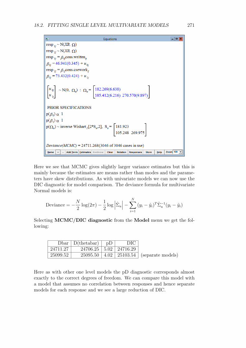
18.2. FITTING SINGLE LEVEL MULTIVARIATE MODELS 271
Here we see that MCMC gives slightly larger variance estimates but this ismainly because the estimates are means rather than modes and the parame-ters have skew distributions. As with univariate models we can now use theDIC diagnostic for model comparison. The deviance formula for multivariateNormal models is:
Deviance = −N2
log(2π)− 1
2log∣∣∣Σu
∣∣∣− N∑i=1
(yi − yi)T Σ−1u (yi − yi)
Selecting MCMC/DIC diagnostic from the Model menu we get the fol-lowing:
Dbar D(thetabar) pD DIC24711.27 24706.25 5.02 24716.2925099.52 25095.50 4.02 25103.54 (separate models)
Here as with other one level models the pD diagnostic corresponds almostexactly to the correct degrees of freedom. We can compare this model witha model that assumes no correlation between responses and hence separatemodels for each response and we see a large reduction of DIC.

272 CHAPTER 18.
18.3 Adding predictor variables
As with single response models we can now add predictor variables to ourmodel as fixed effects. In this dataset we only have one additional predictor,the sex of the individual students. To add new variables into a multivariatemodel we need to use the Add Term window.
• Change Estimation method to IGLS.
• Click on the Add Term button on the Equations window.
• Select female from the variable list.
• Click on the add Separate coefficients button.
This will add the additional two fixed effects, one to each of the responseequations. We can now run the model:
• Click on the Start button.
• Change Estimation method to MCMC.
• Click on the Start button.
After running for 5,000 iterations we get the following estimates:

18.4. A MULTILEVEL MULTIVARIATE MODEL 273
Here we see that girls do 6.3 points better on average at coursework but 3.3points worse on average at the written paper. If we compare our model withthe last model via the DIC diagnostic we see a significant reduction in DIC,which is to be expected given the two gender effects are both significantlylarger than their standard errors.
Dbar D(thetabar) pD DIC24566.19 24559.21 6.98 24573.16 (with gender effects)24711.27 24706.25 5.02 24716.29 (without gender effects)
18.4 A multilevel multivariate model
We can now consider the effect of school attended on the exam score. Asthere are 73 schools we will fit the school effects as random terms and thisresults in a two level multivariate response model which is treated in MLwiNas a three level model (with the responses treated as an additional lowerlevel). In the bivariate case the school attended can affect both responsesand so we will have two school level effects for each school and these couldbe correlated. This will result in a 2×2 school level variance matrix. To fitthis model we firstly need to return to the Equations window and defineour additional level.
• Change Estimation method to IGLS
• Select the Equations window from the Model menu.
• Click on the response names to bring up the Y variable window.
• Select 3-ijk as the number of levels.
• Select school from the level 3(k) pull down list.
• Click on the Done button.
We now need to add the two sets of random effects in the Equations windowand run the model using firstly IGLS and then MCMC.
• Select Equations from the Model menu.
• Click on the β0j (cons written) and click on the k(school long)tickbox.
• Click on the Done button.
• Click on the β1j (cons csework) and click on the k(school long)tickbox.
• Click on the Done button.
• Click on the Start button.

274 CHAPTER 18.
• Change Estimation method to MCMC.
• Click on the Start button.
After running for 5,000 iterations we get the following estimates:
If we were to compare the multilevel model to the single level model via theDIC diagnostic we will see the following:
Dbar D(thetabar) pD DIC23524.14 23397.53 126.61 23650.76 (multilevel model)24566.19 24559.21 6.98 24573.16 (single level model)

18.4. A MULTILEVEL MULTIVARIATE MODEL 275
Here we see that the multilevel specification reduces the DIC by roughly900 suggesting a much better model. The effective number of parameters(126.66) is slightly less than the 153 parameters in the model.
As with the univariate models in earlier chapters we have partitioned ourunexplained variation into that which is due to the schools and that whichis due to the students.
Here the school level explains 29.3% (52.197/(52.197+125.441)) of the re-maining variation in the written scores and 30.2% (79.696/(79.696+184.120))of the remaining variation in the coursework scores. There is also a fairlystrong positive correlation between responses at the school level (0.45) sug-gesting that schools with high average coursework scores also have high av-erage written scores.
We can investigate this further by looking at the school level residuals forthis model.
• Select Residuals from the Model menu.
• Select 3:school long from the level pull down list.
• Change the SD multiplier from 1.0 to 1.4.
• Click on the Calc button.
The school residuals have been stored in columns c300 and c301. We cannow look at ‘caterpillar’ plots of the residuals as we have seen in earlierchapters:
• Select the Plot tab on the Residuals window.
• Select Residual +/- 1.4 sd x rank.
• Click on the Apply button.
Two ‘caterpillar’ plots (minus the highlighting) will appear as shown below:

276 CHAPTER 18.
In the graphs we have highlighted (in various colours) the highest and lowestperforming school for each response, and two other schools that are interest-ing as we will see in the next plot. As we have two residuals we can also lookat pair-wise comparisons, which construct a 2 dimensional representation ofthe above caterpillar plots.
• Select the Residuals button in the pair-wise box.
• Click on the Apply button.
The following graph will then appear:
Here we see the school effects for both the written and coursework scoresand we see why the two additional schools have been highlighted. School22710 (highlighted yellow in the top left of the graph) has a below averagewritten test effect but an above average coursework effect whilst school 67105

18.5. GCSE SCIENCE DATA WITH MISSING RECORDS 277
(highlighted grey in the bottom right of the graph) has an above averagewritten score but a below average coursework. The reason these schools areinteresting is that the written test score was externally marked whilst thecoursework score was internally assessed but externally moderated. Thusit would be interesting to investigate these schools more closely to confirmwhether the difference in scores is due to actual disparities between pupils’practical and examination abilities or due to differences between external andinternal assessment.
18.5 GCSE science data with missing records
The analyses we have performed so far would be appropriate if we had com-plete records for all the data collected, but in our dataset we have otherpartial records that we have so far ignored. Ignoring missing data is dan-gerous because this can introduce biases into all the estimates in the model.We will now consider how to deal with missing data in a more sensible way.There are many techniques that deal with missing data and these can besplit into two families: First imputation-based techniques that attempt togenerate complete datasets before fitting models in the usual way to the im-puted data. Secondly model-based techniques that include the missing dataas a part of the model, and hence fit more complex models that account forthe missing data.
Imputation-based techniques are usually simpler but may perform worse ifthey fail to account for the uncertainty in the missing data whilst model-based techniques may become impractical for more complex problems. In thisexample we will consider a model based MCMC algorithm for multivariateNormal models with missing responses. Then for our second example we willconsider an imputation technique called ‘multiple imputation’ (Rubin, 1987)which gets around some of the lack of uncertainty in the missing data bygenerating several imputed datasets.
Firstly we will load up the complete data for the Science GCSE example:
• Select Open Sample Worksheet from the File menu.
• Select gcsemv1.ws from the list and click on the Open button.
The Names window will then appear as shown below. It should be notedhere that the missing data has been coded globally (you can use the Op-tions/Numbers window to do this with your own data) as missing ratherthan −1 as in the example in the User’s Guide to MLwiN.

278 CHAPTER 18.
We can now repeat the earlier analyses using this complete dataset. Wewill ignore the simpler model and consider firstly the single level model withgender effects that we fitted earlier. We can set up this model in an identicalway as described earlier so if you are unsure of how to do this refer back tothe earlier sections. In MLwiN the IGLS and MCMC methods fit this modelusing different approaches which are both equivalent to assuming a ‘missingat random’ or MAR assumption (Rubin, 1976). The IGLS method, due tothe clever trick of treating the multivariate problem as a special case of aunivariate problem, can simply remove the missing rows in the longer datavector, which contains one row for each response. (See the User’s Guide toMLwiN for more details).
The MCMC method considers the missing data as additional parameters inthe model and assumes an independent uniform prior for each missing re-sponse. Then the missing records have Normal posterior distributions (mul-tivariate Normal for individuals with more than one missing response) andthe Gibbs sampling algorithm is extended to include an additional step thatgenerates values for the missing data values at each iteration in the sampling.
To run the two approaches on our dataset we need to do the following:
• Set up the single level model with gender effects as described earlier.
• Click on the Start button.
• Change Estimation method to MCMC.
• Click on the Start button.
When the 5,000 iterations for the MCMC method have finished the Equationswindow will look as follows:

18.5. GCSE SCIENCE DATA WITH MISSING RECORDS 279
Notice that we now have 3428 responses observed and 382 responses missingout of our total of 3810 responses. The results we see here are fairly similarto those for the complete records only, although the female difference effectshave changed from 6.25 to 5.89 on coursework and −3.32 to −3.43 on writtenexamination. If we look at the DIC diagnostic for this model we get thefollowing:
Dbar D(thetabar) pD DIC30681.18 30292.23 388.95 31070.13
We cannot compare this diagnostic with other previous models as we noweffectively have a new dataset. However what is interesting is that the ef-fective number of parameters (pD) is approximately 389, which equals thenumber of missing responses (382) plus the number of parameters (7). So wecan see clearly that the MCMC algorithm treats missing data as additionalparameters in the model. Note that an alternative here would be to refor-mulate the deviance function to marginalize out the missing data and thiswould give different pD and DIC estimates.
We can now look again at the multilevel model considered earlier with thecomplete cases:

280 CHAPTER 18.
• Change Estimation method to IGLS.
• Select Equations from the Model menu and click on the responsenames to bring up the Y variable window.
• Select 3-ijk for the number of levels.
• Select school from the level 3(k) pull down list.
• Click on the Done button.
• Click on the β0j (cons written) and click on the k(school long)tickbox.
• Click on the β1j (cons csework) and click on the k(school long)tickbox.
• Click on the Start button.
• Change Estimation method to MCMC.
• Click on the Start button.
After running this model we get the following results, which are again similarto the estimates for the complete case data:

18.5. GCSE SCIENCE DATA WITH MISSING RECORDS 281
The DIC diagnostic again shows a great improvement in fitting a multilevelmodel:
Dbar D(thetabar) pD DIC29389.19 28878.14 511.05 29900.25 (multilevel model)30681.18 30292.23 388.95 31070.13 (single level model)
The MCMC method is generating values at each iteration for the missing dataand we may be interested in the values generated. Currently MLwiN doesnot allow the user to store the chains of these missing values but summarystatistics are available.
• Select MCMC/Missing data from the Model menu.
• Select the tickbox to store SDs (in c301).
The window should then look as follows:

282 CHAPTER 18.
Now click on the Calculate button and then the Done button to store theresults and close the window.
• Select View or Edit Data from the Data Manipulation menu.
• Click on the View button.
• Select columns resp indicator, resp, c300, and c301, which arelower down the list.
• Click on the OK button and resize the window to see all fourcolumns.
The window should look as follows:
Here we see that the first individual had a missing coursework response,which on average in the chain has estimate 51.2 with a standard deviationof 12.6. The second person has a missing written exam score which haspredicted value 36.8 with a standard deviation of 10.4. Currently MLwiNonly allows an MAR assumption for the response values although it is hopedthat in future releases we will include options that allow informative priordistributions for missing data. Note that there are other modelling techniquesfor handling non MAR data but we shall not discuss these here.
18.6 Imputation methods for missing data
As mentioned earlier there are two families of techniques that can be usedfor missing data; imputation and model based methods. The model-basedmethods as we saw in the last example make special provisions in the model

18.6. IMPUTATION METHODS FOR MISSING DATA 283
for the missing data. The imputation-based methods however are techniquesthat are used prior to modelling. We can think in fact of imputation tech-niques as being two stage techniques where the first stage involves imputing acomplete dataset and the second stage involves modelling using this completedataset.
The imputation step can be deterministic, for example simple imputationtechniques involve substituting missing data with a determined value. Asimple example of this determined value is the mean for the variable. Alter-natively a model can be created for the variables to be imputed, for examplea regression model and this model can then be used to generate predictedvalues to replace the missing values. Of course the model will give a pointestimate and a standard error for each missing observation and so we coulduse an alternative approach of generating a random draw from the predictivedistribution (under the imputation model) of the missing observation. Thiswill then produce a stochastic imputation procedure.
The disadvantage of imputation-based methods is that once the completedataset is generated all uncertainty about the missing values is lost. Mul-tiple imputation (Rubin, 1987) aims to bridge the gap between standardimputation-based methods and model-based methods by using a stochasticimputation procedure several times. Then we can perform our modellingon each of these N imputed complete datasets and use for each parameterestimate an average of the N estimates produced by the datasets, along witha standard error that is constructed from a combination of the variance foreach dataset and the variance between the datasets. So for a parameter θ wehave an estimate
θ =1
N
N∑i=1
θi, with variance V (θ) = V + (1 +N−1)B
where V =1
N
N∑i=1
V (θi) and B =1
N − 1
(θi − θ
)2
This approach would be equivalent to a model based approach if N was verylarge but even an N as small as 5 will give a reasonable approximation.
For more details on missing data and multiple imputation we recommendSchafer (1996). In this section we will simply show how to generate imputeddatasets using multivariate multilevel models in MLwiN. The effectiveness ofthe imputation procedure will depend on the imputation model used. Typi-cally single level multivariate normal models that take account of correlationbetween variables are used in multiple imputation. However it may be moreappropriate to use a multilevel multivariate model as an imputation model(note that such models have been used independently in Schafer, 1997).

284 CHAPTER 18.
18.7 Hungarian science exam dataset
This dataset was analysed in Goldstein (2003) and is part of the SecondInternational Science Survey carried out in 1984. The data we are using isthe component from Hungary and consists of marks from six tests taken by2,439 students in 99 schools. Of the six papers, three are core papers inearth sciences, biology and physics which were taken by all students whilstthe other three are optional papers, two in biology and one in physics ofwhich no student took all three. Although these tests were marked out ofdifferent totals ranging from 4 to 10, Goldstein (2003) converted each test tohave scores between 0 and 1. Here we will use instead scores between 0 and10 as these are closer to the original marks.
• Select Open Sample Worksheet from the File menu.
• Select hungary1.ws from the list and click on the Open button.
The variables in the dataset are as follows:
Here we see the two level identifiers, school and student, the six test scoresthat are stored in columns c3–c8 and one additional predictor female whichindicates the sex of each student. As with the earlier example we could tryand fit several different models to the dataset and compare the DIC diagnosticto find the ‘best’ model, here however we skip this stage and fit the modelthat Goldstein fits in his book.
To set up the model we first need to set up the model structure using themultivariate window.
• Select Equations from the Model menu.
• Click on the Responses button.
• On the list that appears click on es core, biol core, biol r3,biol r4, phys core and phys r2.
• Click on the Done button.
This will set up the responses and the Equations window should look asfollows:

18.7. HUNGARIAN SCIENCE EXAM DATASET 285
We now need to specify the level identifier variables and the predictor vari-ables:
• Click on the responses in the Equations window.
• On the Y variable window that appears select 3-ijk as the numberof levels.
• Select student from the level 2(j) pull down list.
• Select school from the level 3(k) pull down list.
• Click on the Done button.
• Click on the Add Term button.
• Select cons from the variable list and click on the add Separatecoefficients button.
• Click on the Add Term button.
• Select female from the variable list and click on the add Separatecoefficients button.
We have now added the fixed effects into the model and we now need to addthe random effects.
• Click on β0 (cons es core) and select the j(student long) andk(school long) tick boxes (keeping fixed effect selected).
• Click on the Done button.
• Repeat this for the other constants, β1, β2, β3, β4 and β5.
• Click on the Start button to run the model using IGLS.
After the IGLS model converges you should get fixed estimates as shownbelow. Note that due to the rescaling of the dataset these estimates are tentimes the estimates in Goldstein (2003).

286 CHAPTER 18.
We will now consider fitting this model using MCMC. Although this model isitself interesting we are using it purely as an imputation model and are moreinterested in the missing values imputed than the fixed effect and varianceestimates. To use multiple imputation it is desirable to have independentsamples from the posterior distributions of the missing data. Consequentlywe will run for a burn-in of 500 as usual and then store the values everythousand iterations. To get our first sample we will do the following:
• Change Estimation method to MCMC and open the EstimationControl window.
• Change the Monitoring Chain Length to 1,000.
• Click on the Start button.
After the estimation finishes (which may take a couple of minutes) we needto then do the following:
• Select MCMC/Missing Data from the Model menu.
• Select the Calculate 1 imputation button and change the outputcolumn to c31.
• Click on the Calculate button.
This will generate the first imputed dataset. It should be noted here thatthe values stored are the actual chain values after 1000 iterations and NOTthe means of the sets of 1000 values. We can now repeat the procedure fourmore times by in turn changing the Monitoring Chain Length to 2,000,3,000, 4,000 and 5,000 iterations and clicking on the More button. Theneach time we can change the Output column on the Missing Data screento c32, c33, c34 and c35 respectively and generate an imputed dataset.

18.7. HUNGARIAN SCIENCE EXAM DATASET 287
It should at this point be noted that we could have written a macro togenerate these datasets that would use the MCMC and DAMI commands(see the Command manual). After generating the 5 datasets we can view theresults in the data window:
• Select View or edit data from the Data Manipulation menu.
• Click on the view button.
• Select columns resp indicator, resp, c31, c32, c33, c34, and c35.
• Click on the OK button and resize the window.
The data will then look as follows:
Here we see the data for the first three individuals in the dataset. As canbe seen they each have one missing paper and the values for these papershave been generated from the respective posterior distribution. It should benoted at this point that in this model we are treating marks as continuousNormally distributed variables. This of course means that the imputed markswill follow these Normal distributions rather than the smaller set of valuespossible in the test. We are actively researching methods to impute orderedcategorical data, although Schafer (1996) considers this subject in a non-multilevel context in great detail. Recent work under the REALCOM projecthas extended the missing data capabilities of MLwiN but this is described inits own documentation.
We will return to this dataset in Chapter 20 when we consider multilevelfactor analysis modelling. In the next chapter we continue looking at multi-variate responses and consider mixed response models and correlated resid-uals/patterned variance matrices.

288 CHAPTER 18.
Chapter learning outcomes
? How to fit multivariate response models using MCMC in MLwiN.
? How MLwiN deals with missing data.
? How to fit multilevel multivariate models in MLwiN.
? How to compare multivariate models using the DIC diagnostic.
? How to generate datasets for multiple imputation in MLwiN.

Chapter 19
Mixed Response Models andCorrelated Residuals
In the last chapter we introduced modelling of multiple responses and con-centrated on responses that are all continuous variables. We assumed thatthese responses have a multivariate Normal distribution with unknown meanvector and variance matrix. In this chapter we will consider two extensionsto such a model. Firstly we will consider how to fit mixtures of Normaland Bernoulli distributed variables. We will consider an example from edu-cation where we have a continuous English exam mark and a dichotomousbehavioural measure. We will introduce some structure into the lowest levelvariance matrix to cater for the Bernoulli responses. Secondly we will con-sider more generally introducing specific structures into the variance matrixat the lowest level in particular for use with repeated measures. Here we con-sider an animal growth dataset and consider how to include auto-correlatedresiduals at the lowest level. The topic of MCMC modelling of constrainedvariance matrices is covered in Browne (2006).
19.1 Mixed response models
In the last chapter we concentrated on responses that are continuous vari-ables. However as we saw in Chapters 10–13 not all response variables havecontinuous distributions as some responses may be counts or dichotomousvariables. When we have mixtures of response types (as with models with allcontinuous responses) we wish to model correlation between the responsesin addition to adjusting for predictors. This is difficult as we have differentdistributional assumptions for our different responses. The iterative proce-dures used in MLwiN have to use quasi-likelihood methods when some ofthe responses are non-Normal and this involves linearizing the non-Normalresponses. This will result in estimates for covariances (correlations) at thelowest level, although what form the joint distribution of the responses at
289

290 CHAPTER 19.
this level has is not known.
If we use MCMC estimation we can currently only fit mixtures of Normaland Binomial responses, and then only with a probit link for the Binomial.This is because only this combination of responses results in an identifiabledistribution for the residuals at the lowest level. Other response combinationscan be handled by making the (often unrealistic) assumption of independenceat the bottom level, although not currently using the MCMC options inMLwiN.
The reason that the probit link Bernoulli and Normal combination can befitted stems again from the thresholding idea used in Albert & Chib (1993) asdiscussed in Chapter 10. This idea for the multivariate case is also discussedfor single level models in Chib & Hamilton (2000). Basically we can treat anyBernoulli responses as thresholded Normal responses with threshold 0 andvariance 1. Thus if the observed response is 0, then the underlying Normalresponse is negative and if the observed response is 1, the underlying Normalresponse is positive.
Given we can sample these unknown continuous responses as an additionalstep in a Gibbs sampling algorithm then combining these responses with theother observed continuous responses results in all responses being continuous.This means we can then make a multivariate Normal assumption for theresponses with the constraints that the variance for any of the unknownresponses equals 1. This means that although, as in Chapter 10 we can nowuse Gibbs sampling to update both the fixed effects and the residuals we nowhave to use Metropolis sampling to update the elements of the lowest levelvariance matrix.
For generality we use the technique used in Browne (2006) of univariateNormal Metropolis updates for the unconstrained elements of the variancematrix. This technique involves using random walk Normal proposals foreach parameter in turn and after producing a proposed new parameter valuechecking that it satisfies all constraints i.e. checking the variance matrixproduced is positive definite. If these conditions are not satisfied then thevalue is immediately rejected, otherwise we perform a standard Metropolisupdate and compare the log likelihoods with both the current and proposedvalues. As we are using Normal proposals rather than the truncated Normalproposals used in Chapter 9 we have symmetry and therefore do not need tocalculate a Hastings ratio.
We will now consider an example from the field of education.

19.2. THE JSP MIXED RESPONSE EXAMPLE 291
19.2 The JSP mixed response example
Our example dataset is a subset of the junior school project (JSP) dataset(Mortimore et al., 1988) and contains data on 1119 pupils from 47 schools.To view the data we need to load the worksheet and open the Names windowas shown below.
• Select Open Worksheet from the File menu.
• Select jspmix1.ws from the list of worksheets.
• Click on the Open button.
Our response variables are for each pupil an English test score (english)marked out of 100 and a behaviour rating (behaviour), which is coded 0if the pupil is rated in the bottom 25% and 1 otherwise. Note that thisresponse originally had three categories but we have combined the top 25%and middle 50% categories so that we can fit the response using a Binomialdistribution. Both these responses were measured at year 3 of the pupil’sschooling.
We are interested in if there is a correlation between badly behaved pupilsand poor exam marks, and we are also interested in the effect of predictorvariables on both the exam scores and the behaviour of the pupils. Ourpotential predictor variables are gender (sex with 0 for a girl and 1 fora boy), a fluency in English indicator taken at year 1 (fluent with 0 forbeginner, 1 for intermediate and 2 for fully fluent) and a test score at year 1(ravens score out of 40).
We could look first at a simple tabulation between the response variables.
• Select Tabulate from the Basic Statistics menu.
• Select Means as Output Mode.
• Select english as the Variate column.
• Select behaviour as the Columns indicator.
The window will look as follows:

292 CHAPTER 19.
Now if we click on the Tabulate button we get the following results.
0 1 TOTALSN 248 871 1119MEANS 28.9 45.1 41.5SD’S 18.5 21.0 20.5
So here we see that the badly behaved pupils have on average a 16.2 pointsworse performance in English. We can look at this relationship further byinvestigating correlations between the two responses and additionally thethree predictors:
• Select Averages and Correlation from the Basic Statisticsmenu.
• Click on Correlation in the Operation box.
• Select columns sex, fluent, ravens, english and behaviour (noteyou can use the Shift or Ctrl keys to do this).
• Click on the Calculate button.
This will execute the CORM command which gives means and sds for eachvariable along with the following correlation matrix:
Correlations
sex fluent ravens english behavioursex 1.0000fluent -0.0229 1.0000ravens 0.0341 0.1705 1.0000english -0.1479 0.2054 0.5042 1.0000behaviour -0.1272 -0.0038 0.2181 0.3122 1.0000
Here we see for english, positive correlations greater than 0.2 with bothfluency and ravens and a negative correlation of approximately −0.15 withgender. For behaviour we see a positive correlation of greater than 0.2 withravens and a negative correlation with gender but virtually no correlationwith fluency. There is also a strong positive correlation (0.31) between the

19.3. A SINGLE LEVEL MIXED RESPONSE MODEL 293
two responses. Based on this correlation matrix we can set up a single levelmodel with fixed effects for each of the large correlations.
19.3 Setting up a single level mixed response
model
We can start by setting up a multivariate Normal model via the Equationswindow as follows:
• Firstly we specify the responses by clicking on the Responses but-ton.
• Select english and behaviour from the list that appears and clickon the Done button.
• Click on the Add Term button and select cons from the variablelist.
• Click on the add Separate coefficients button.
• Click on the Add Term button and select sex from the variablelist.
• Click on the add Separate coefficients button.
• Click on the Add Term button and select ravens from the variablelist.
• Click on the add Separate coefficients button.
• Click on the Add Term button and select fluent from the variablelist.
• Click on the add Common coefficient button.
• On the screen that appears select english and click on the Donebutton.
Note that the variable fluent is not being fitted as a fixed effect for be-haviour as there was no correlation between these two variables. The Equa-tions window should now look as follows:

294 CHAPTER 19.
We now need to specify the level 2 identifiers and to let the software knowthat the behaviour response should be treated as a Binomial response. Todo this we need to specify the following in the Equations window:
• Click on the responses to bring up the Y variable window.
• Select 2-ij as the number of levels and id as the level 2 identifier.
• Click on the Done button.
• Click on the N for response 2 and on the window that appears selectBinomial for the distribution and probit for the link function.
• Click on the Done button.
• Click on the red n2j that appears and select denomb as the denom-inator variable. Click on the Done button.
• Click on β0 (cons.english) and select j(id long).
• Click on the Done button.
• Click on the Nonlinear button.
• On the Nonlinear window click on the Use defaults and the Donebuttons.
• Click on the Start button.
This will have now set up the mixed response model and run it using theIGLS 1st order MQL method and the results should be as follows:
Here we see that the individual level variance matrix contains some functionsand this is due to the Taylor series approximations that are involved in theIGLS methods used here. The IGLS methods do not use the (underlyingNormal) latent variable idea that is used by the MCMC method.

19.3. A SINGLE LEVEL MIXED RESPONSE MODEL 295
If we now want to run this model using MCMC we need to do the following:
• Change Estimation method to MCMC.
• Select MCMC/MCMC Methods from the Model menu.
• Click on Reset to select Gibbs sampling for fixed effects and resid-uals.
• Click on the Done button on the Advanced MCMC Methodol-ogy Options window.
• Click on the Start button.
After the 5,000 iterations have run we will get the following estimates:
Here we see reasonably similar estimates to the IGLS method. The covarianceparameter is however quite a bit larger (6.279 versus 4.209). This is becauseusing MCMC this parameter represents the covariance between the englishresponse and an unknown continuous behaviour response, which is positivewhen the observed dichotomous behaviour response equals one and negativewhen it equals zero. The IGLS method correlation is calculated differently.Here we see that the correlation between the pairs of residuals equals 0.345 =6.279/
√330.774 suggesting that there is a strong positive correlation between
English score and behaviour in the classroom even after accounting for otherpredictors.
We can also see the significant positive effects of fluency and Ravens testscore on English marks and Ravens test score on behaviour and the negativeeffect of gender suggesting that girls both do better at English and are betterbehaved at year 3. It should here be noted that we cannot currently use the

296 CHAPTER 19.
DIC diagnostic for these models as the deviance function is not worked outcorrectly.
19.4 Multilevel mixed response model
We can now extend our model to a multilevel model by adding in randomeffects for school for both responses as follows:
• Change Estimation method to IGLS.
• In the Equations window click on the response variables.
• Select 3-ijk from the N levels list and school from the level 3(k)pull down list.
• Click on β0j (cons.english) in the window and select thek(school long) tickbox.
• Click on the Done button.
• Click on β1 (cons.behaviour) in the window and select thek(school long) tickbox.
• Click on the Done button.
• Click on the Start button (to get starting values from IGLS).
• Change Estimation method to MCMC.
• Click on the Start button.
Upon running for 5,000 iterations we get the following estimates:

19.5. RATS DATASET 297
Here we see that the positive correlation between responses persists at theindividual level (0.363 = 6.198/
√291.510× 1.000) but is negligible at the
school level (0.035 = 0.058/√
40.837× 0.066), and so schools with more dis-ruptive children do not necessarily have worse average English attainment.All the fixed effects are little changed by adding in the school effects. Schooleffects explain 12.3% (40.837/(291.510+40.837)) of English attainment resid-ual variation and 6.2% (0.066/1.066) of behaviour score residual variation.Unfortunately due to the DIC diagnostic being unavailable for these modelswe cannot compare this model with the single level model, but the size ofthe coefficients appears to indicate a large improvement from introducingrandom effects.
19.5 Rats dataset
Our second example of a model with a constrained variance matrix comesfrom an animal growth dataset discussed in Gelfand et al. (1990). The dataconsists of the weights of 30 rats measured weekly over a five week period.We will firstly load up the dataset and look at the Names window:
• Select Open Sample Worksheet from the File menu.
• Select rats.ws from the list of worksheets.

298 CHAPTER 19.
• Click on the Open button.
The data will then appear as follows:
Here we see the five weights for each rat are recorded as five variables, y8,y15, y22, y29 and y36. Gelfand et al. (1990) considered fitting a singleresponse two level random slopes model with measurements nested withinrats. We could repeat their analysis by stacking the data for the five responsesinto one column as illustrated, for an example from education, in Chapter13 of the User’s Guide to MLwiN. However here we will consider the dataas five separate responses and fit a single level multivariate Normal responsemodel.
• Select Equations from the Model menu.
• Click on the Responses button to bring up the Responses window.
• Select y8, y15, y22, y29 and y36 as y variables.
• Click on the Done button.
• Click on the response names and select 2-ij as the number of levels.
• Select rat as the level 2(j) identifier and click on the Done button.
We have now set up the responses and the level identifiers and we next needto add the predictors.
• Click on the Add Term button and select cons from the variablelist.
• Click on the add Separate coefficients button on the Add Termwindow.
• Click on β0 (cons y8) and select the j(rat long) tick box and clickon the Done button.
• Click on β1 (cons y15) and select the j(rat long) tick box and clickon the Done button.
• Click on β2 (cons y22) and select the j(rat long) tick box and clickon the Done button.

19.5. RATS DATASET 299
• Click on β3 (cons y29) and select the j(rat long) tick box and clickon the Done button.
• Click on β4 (cons y36) and select the j(rat long) tick box and clickon the Done button.
• Click on the Start button.
• Change Estimation method to MCMC.
• Click on the Start button.
This will run the model using IGLS and then MCMC and the estimates after5,000 iterations will be as follows:
Interestingly with such a small dataset and a large number of parametersthere will be both a greater dependence on the prior distributions used,and the variance parameters will have skewed posterior distributions. Forexample if we look at the trace for the variance of the 8 day old measurements(σ2
u0):
• Select the Trajectories window from the Model menu.
• Click on the trace plot for σ2u0.
• Click on Yes to calculate diagnostics.
The diagnostics for this parameter will then appear as follows:

300 CHAPTER 19.
Here it is worth noting the differences between the mean, median and modefor this parameter due to the skewness. When we look at the DIC diagnosticavailable from the Model menu we get the following:
Dbar D(thetabar) pD DIC1008.87 993.29 15.58 1024.46
In fact this model has 20 parameters but the D(thetabar) statistic is sensitiveto which plug-in estimates we use.
19.6 Fitting an autoregressive structure to
the variance matrix
We could look at the variance in more detail and in particular look at thecorresponding correlation matrix using the Estimates window.
• Select the Estimate Tables window from the Model menu.
• Click on the pull down list and choose Level 2: rat long.
• Remove the tick from the P (past value) box.
• Add a tick to the C (correlations) box.
The window will then look as follows:

19.6. FITTING AN AUTOREGRESSIVE STRUCTURE 301
Here if we look at the correlations closely we see that the correlation is highbetween consecutive observations but decreases as observations get furtherapart. One possible method to account for this and reduce the number ofparameters used in the model is to impose a structure on these correlations.Given the observed values a natural candidate would be to fit an AR(1)correlation structure. Here the correlation between any two observations isequal to ρ to the power of the distance between the observations.
This can be done in MLwiN as follows:
• Change Estimation method to IGLS.
• Click on the Start button.
• Change Estimation method to MCMC.
• Select MCMC/Correlated Residuals from the Model menu.
• Choose AR1 structure/independent variances as CurrentCorrelation structure.
• Click on the Done button.
The options to change the structure of the variance matrix are fairly limited.They only work on the bottom level variance matrix of a multivariate modeland there are currently four special cases that are dealt with. These consistof either all equal correlations or AR1 correlation structures combined witheither independent or all equal variances.

302 CHAPTER 19.
For all these four combinations we use univariate Metropolis sampling forthe variance elements of the lowest level variance matrix and the correlationparameter ρ and then check that the variance matrix formed is positive defi-nite. All other steps of the algorithm are unchanged and use Gibbs sampling.As the dataset is small and we are running Metropolis steps we will run for50,000 iterations.
• Select the Estimation Control window.
• Change the Monitoring Chain Length to 50,000.
• Change the refresh rate to every 500 iterations.
• Click on the Start button.
After the iterations have finished the Estimates window should now look asfollows: (Note if you closed this window you will have to reopen it and selectthe options described earlier in the chapter.)
It should be noted here that when constraints are imposed on a variancematrix we are forced to use uniform priors on the individual elements of thevariance matrix. In this case we have used uniform priors on the 5 vari-ances and the correlation parameter ρ whereas previously we used an inverseWishart prior. As can be seen the variance estimates under a Uniform priorare much larger. The interested reader should look at Browne & Draper(2000, 2006) for more information on choosing “uninformative” prior distri-butions.

19.6. FITTING AN AUTOREGRESSIVE STRUCTURE 303
If we look at the DIC diagnostic for this model we get:
Dbar D(thetabar) pD DIC1015.65 1003.30 9.35 1025.00 (with constraint)1008.87 993.29 15.58 1024.46 (without constraint)
Again the pD estimate is an underestimate of the true number of parameterswhich in this model is 11. As we can see from comparing DIC values, thereduction in parameters is balanced by an increase in the deviance fromthe full covariance model. This may partly be due to the different priordistributions but could also be due to the fact that the correlations declinemore quickly than an AR1 process.
Chapter learning outcomes
? How to fit models to mixtures of binary and continuous outcomes.
? How to extend such models to the multilevel case.
? How to fit patterned variance matrices in repeated measures mod-elling.

304 CHAPTER 19.

Chapter 20
Multilevel Factor AnalysisModelling
In the last two chapters we have looked at datasets where there is morethan one response variable of interest. There are many common techniquesused to model and summarise multivariate datasets (see Chatfield & Collins,1980; Krzanowski & Marriott, 1994, 1995, for reviews). When we considera multivariate response vector we are typically interested in explaining boththe variation in the individual responses (as in single response modelling)and the correlation between the responses for individuals. As the number ofresponses increases so the number of correlations increases and we are ofteninterested in looking at methods of describing these correlations with fewerparameters, for example by assuming an autocorrelation pattern as shown inthe last chapter.
Often however even though we collect many responses on an individual, in-terest lies in finding differences between individuals (or groups of individuals)along a small number of summary dimensions rather than explaining differ-ences in particular responses. Variable reduction techniques are used to finda smaller set of derived responses, which capture the majority of the variationin the dataset. Factor analysis is an example of a technique that attemptsto do this.
20.1 Factor analysis modelling
In factor analysis modelling we aim to reduce the dimensionality of our re-sponse vector by creating ‘common factors’ as follows for a single level model:
yir =J∑j=1
λrjηij + eir
305

306 CHAPTER 20.
Here yir is the rth response for the ith individual, ηij is the jth factor for theith individual and λrj is the coefficient (known as the factor loading) for therth response for factor j. The eir is the residual (sometimes called specificfactor or uniqueness) for the rth response for the ith individual. To completethe model we give distributional assumptions for both the residuals and thefactors as follows:
eir ∼ N(0, σ2er), ηi ∼MVN(0,Ση)
Often the factors will be assumed independent and Ση will be diagonal withelements σ2
ηj but we can allow correlated factors (see later). To make thismodel identifiable we need to either fix/constrain some of the factor loadingsor the factor variances. If we wish to fit such a factor model in a Bayesianframework (as we will here) we also need to incorporate prior distributionsfor the factor loadings and all variances into the model. As for the multilevelmodels we have dealt with earlier we will assume ‘improper’ uniform priorsfor all loadings that are not fixed and Γ−1(10−3, 10−3) priors (by default) forall variances.
20.2 MCMC algorithm
The MCMC algorithm for the factor model is very similar to the algorithmfor a simple two level multilevel model. If we consider the factors as knownvalues then the problem becomes several one-level regression models withthe factor loadings as fixed effects in the regressions, which we can easilyfit. If on the other hand we consider the loadings as fixed then the factorsbecome level 2 residuals in a two level model, which we also know how tofit. Therefore we see that all parameters have simple known forms and so wecan use a Gibbs sampling algorithm to fit the model.
The great advantage of the Gibbs sampling algorithm is that we can of coursenow consider incorporating the factor analysis structure as a part of a moregeneral multivariate multilevel model. This allows us to include fixed effectsand higher-level structures in our model. Goldstein & Browne (2002) givegeneral MCMC algorithms for this and we will see how this works later.Firstly however we will return to our Hungarian exam results example thatwe discussed in Chapter 18.
20.3 Hungarian science exam dataset
The dataset as described in Chapter 18 consists of exam results from sixtests taken by 2,439 students in 1984. Of the tests all students took thethree core papers and then one or two of the optional papers. In Chapter 18we considered this dataset from a missing data viewpoint and used MCMC

20.3. HUNGARIAN SCIENCE EXAM DATASET 307
algorithms to impute the missing data. Here we will simply incorporate themissing data steps along with the factor analysis steps in our general MCMCalgorithm.
• Select Open Sample Worksheet from the File menu.
• Select hungary1.ws from the list and click on the Open button.
The variables in the dataset are as follows:
Here as before we have two level identifiers, school and student, and the sixtest scores are stored in columns c3–c8. We will firstly look at the correlationmatrix for the six responses.
• Select Averages and Correlations from the Basic Statisticsmenu.
• Click on the Correlation button.
• Select es core, biol core, and phys core from the pull-down list(you can use the mouse and the Ctrl button to do this).
If we now click on the Calculate button we will see the following estimates:

308 CHAPTER 20.
Here we see that the correlations between the three core scores are all reason-ably large, in particular between biology and physics scores. The Correla-tions option in MLwiN gives correlations based on complete responses only,and so as no individual has taken all six tests we cannot directly calculate a6×6 correlation matrix. Instead we can set up a simple multivariate modelthat consists of only an intercept for each response and a full covariancematrix between the 6 responses.
• Select Equations from the Model menu.
• Click on the Responses button.
• Select es core, biol core, biol r3, biol r4, phys core andphys r2 from the response list.
• Click on the Done button.
• Click on the responses and the Y variable window will appear.
• Select 2-ij for the number of levels.
• Select student from the level 2(j) pull down list.
• Click on the Done button.
We have now defined both the response and level identifiers. We now needto add the predictors and random effects to the model.

20.3. HUNGARIAN SCIENCE EXAM DATASET 309
• Click on the Add Term button.
• Select cons from the variable list on the Add Term window.
• Click on the add Separate coefficients button.
• Click on β0 (cons.es core) in the Equations window and select thej(student long) tick box keeping Fixed Parameter selected.
• Click on the Done button
• Repeat this for the other 5 variables, β1, β2, β3, β4, and β5.
• Click on the Start button to run the model using IGLS.
After the IGLS model converges we can look at the correlation matrix viathe Estimate Tables window:
• Select Estimate Tables from the Model menu.
• Replace Fixed Part with Level 2: student long in the pull downlist.
• Remove the tick under S, E, S and P by clicking in the boxes andadd a tick under the C.
The correlation matrix appears as follows:
Here we see that the correlations between the core subjects are almost iden-tical to the values obtained from the Averages and Correlations window.In fact if we were to select the responses in pairs via the Averages andCorrelations window we will get similar estimates to those obtained herefor each correlation (using all the individuals that have both responses). Ifwe look at this matrix in more detail we see that all correlations are posi-tive suggesting that students that do well in one paper will also generally dowell in the other papers. The correlations range from 0.161 between earthsciences core and the optional r3 paper in biology to a correlation of 0.525between the core papers in biology and physics. We will now try to explainthese 15 correlations by using factor analysis.

310 CHAPTER 20.
20.4 A single factor Bayesian model
We will firstly consider fitting a single factor model. To do this we first needto remove all the covariances from the model to have independence betweenthe responses. This is because these covariances will be explained by thefactor variables that we add to the model.
• Select Equations from the Model menu.
• In the Equations window click on the Estimates button until theestimates appear as green numbers.
• Scroll down until Ωu is visible.
• Click on the Ωu and select set diagonal matrix.
• When finished click on the Start button.
We will have now run a model that consists of 6 intercepts with independentrandom effects, one for each response. The Equations window should lookas follows:
We now need to define the factor model.

20.4. A SINGLE FACTOR BAYESIAN MODEL 311
• Change Estimation method to MCMC.
• Select MCMC/Factor Analysis from the Model menu.
• Click on the + button to increase the number of factors to 1.
The Factor Analysis screen will now appear as follows:
In factor analysis modelling we must be careful that we include enough con-straints to ensure a unique identifiable solution. This is even more importantwhen we use MCMC, as we have to avoid allowing the chains to move be-tween rotational solutions. For example if a factor is multiplied by −1, andthe respective loadings are also multiplied by −1 this will give an alternativesolution that also fits the data. Such solutions are equivalent and a maximis-ing algorithm will find just one of them whilst a simulation based methodmay move between the two and never converge.
Consequently in this chapter we will constrain the ith factor loading of theith factor to equal 1 and constrain the jth factor loading of the ith factor toequal 0 ∀j < i. Geweke & Zhou (1996) give a similar (but not identical andslightly less rigid) system of constraints.
To use this set of constraints we need to do the following:
• Change the Loading 1 value to 1 and click in the constraint boxfor loading 1.
• Click in the constraint box for the Variance value to remove thisconstraint.

312 CHAPTER 20.
• Click on the Set factors button to set the factors.
• Click on the Done button.
This will add the factor to the model. We can now run this model by clickingon the Start button. It should be noted at this point that factor analysismodels contain larger numbers of parameters than most of the models wehave dealt with so far and so this first model will take several minutes torun.
After the estimation finishes we will get the following estimates:
We see that the fixed effect parameters are roughly the same estimates asthe model without a factor. Our interest lies in the estimates of the factorloadings and the factor values or ‘scores’ themselves.
• Select MCMC/Factor Analysis from the Model menu.
• Click on the Output Options button.
• The Factor Analysis Output Options window will appear.
• On this window click on the three tick boxes to output factor values,loadings and variances respectively.

20.4. A SINGLE FACTOR BAYESIAN MODEL 313
• This will put estimates and standard errors in the default columns,c300-c305.
• Click on the Calculate button.
• Click on the Done buttons on both the Factor output and Factorwindows.
By default for factor analysis models, estimates and standard errors are cal-culated by the MCMC engine (as with residuals in other models). As we willsee later we can also store all or any of the chains for the parameters. Wewill now look at the estimates from the model.
• Select View/Edit Data from the Data Manipulation menu.
• Click on the view button and select columns c302, c303, c304 andc305 (note that you can use the Ctrl key to select multiple columns).
• Click on the OK button.
The data will look as follows:
Here we see the factor loadings in column c302 and the factor variance inc304. Note that these estimates are now also shown in the Equationswindow. The loadings are all positive and given that we saw all positivecorrelations between the responses we can think of this first factor as repre-senting a measure of overall exam success. In fact if the factor variance was1 then the loadings would represent the correlations between the factor andthe responses. All these loadings are much greater than their standard errors(given in c303), which also gives our interpretation more support.
The actual factor scores for this model can be seen in column c300. We canrank these and plot them against their ranks as follows:
• Select Command Interface from the Data Manipulation menuand enter the command:
RANK c300 c299

314 CHAPTER 20.
• Select Customised Graphs from the Graphs menu.
• Select c300 as the y variable.
• Select c299 as the x variable.
• Click on the Apply button.
The graph of the factor values will then be plotted as follows:
If we now click on the extreme points in the graph, for example the first(smallest) point, we will get the following window:
Here we see that the individual with the lowest factor value is student 664.Examining the data we see that this student got marks of 0 in both physicsand biology core papers, 1.6667 in the earth sciences core paper and 5.7143in the physics r2 additional paper. Similarly the individual with the highestfactor value is student 2132. Examining their responses we see that they got

20.5. ADDING A SECOND FACTOR TO THE MODEL 315
full marks (10) in all the 5 papers they took. This backs up our inference thatthis factor is giving a measure of overall performance. The non-symmetry ofthe graph is due to the average marks in all papers being high and conse-quently there being greater ceiling effects than floor effects in the responses.
20.5 Adding a second factor to the model
The last model attempted to reduce the six response multivariate Normalmodel to a model with the dependence between the responses explained byone factor, which we interpreted as a general exam ability indicator. We willnext consider adding a second factor to the model. To do this we firstly rerunIGLS to get the same starting values and then add in the factor as follows:
• Change Estimation method to IGLS.
• Click on the Start button.
• Change Estimation method to MCMC.
• Select MCMC/Factor Analysis from the Model menu.
• Click on the + button to increase the Number of factors to 2.
• Click on the lower + button to Show Factor 2.
• Change Loading 2 value from 0 to 1.
• Click on the constraint boxes for both Loadings 1 and 2.
• Click on the constraint box for Variance value to remove thisconstraint.
The Factor Analysis window should now look as follows:

316 CHAPTER 20.
• Click on the Set factors button.
• Click on the Store Values button.
• The Store Factor Chains window now appears.
• Click on the Store Factor Loadings tick box.
• Change column number to c21.
• Click on the Done buttons on both the Store Factor Chains andFactor Analysis windows.
We have now added the second factor to the model and told MLwiN to storethe factor loadings stacked in column c21. Note that we have not set anycorrelation between the factors i.e. the correlation is constrained to equalzero. We now need to click on the Start button and wait for several minutesfor the MCMC method to run.
We can now see in the Equations window that again the fixed effect esti-mates simply capture the means of the 6 responses and are unaffected by theaddition of the second factor. We can now output the factors and loadingsand look at the estimates (noting that the loadings are available also in theEquations window).
• Select MCMC/Factor Analysis from the Model menu.
• Click on the Output Options button.
• The Factor Analysis Output Options window will appear.
• On this window click on the three tick boxes to output factor values,loadings and variances respectively.

20.5. ADDING A SECOND FACTOR TO THE MODEL 317
• Click on the Calculate button.
• Click on the Done buttons on both the Factor output and Factorwindows.
• Select View/Edit Data from the Data Manipulation menu.
• Click on the view button and select columns c302, c303, c304 andc305 (note you can use the Ctrl key to select multiple columns).
• Click on the OK button.
The Data window will look as follows:
Here we have the loadings for the two factors stacked above each other. Thefirst factor still has very similar loadings and can be thought of once again asan indicator of overall test performance. The second factor has some muchgreater loadings but a much smaller variance (0.021 versus 0.514) and sois explaining a small proportion of the remaining uncertainty. The secondfactor seems to be picking out students who do comparatively better in theadditional tests r4 in biology and r2 in physics. The actual factor values or‘scores’ are stored stacked in column c300 and so we can plot these factorsafter first splitting the factors into separate columns:
• Select Generate vector from the Data Manipulation menu.
• Select Repeated Sequence.
• Change Output column to c306.
• Change Maximum number to 2.
• Change Number of repeats per block to 2439.
• Change Number of blocks to 1.
• Click on the Generate button.
• Select Split Column from the Data Manipulation menu.
• Select Split data in column to be c300.

318 CHAPTER 20.
• Select On Codes column to be c306.
• Select Output columns c307 and c308.
• Click on the Add to action list button.
The screen should look as follows:
If we now click on the Execute button the two sets of factor values willbe generated in columns c307 and c308. We can now plot these factors asfollows:
• Select Customised Graph(s) from the Graphs menu.
• Select c307 as the y variable.
• Select c308 as the x variable.
• Click on the Apply button.
The graph will appear as follows (note that the labels need to be addedmanually):

20.6. EXAMINING THE CHAINS OF THE LOADING ESTIMATES 319
Here we see that again pupil 664 is an obvious outlier from the main cloudof points. They have a large positive score for factor 2 due to the fact thatthey did OK on the physics r2 paper. Another interesting observation is thepupil with the lowest factor 2 value (pupil 1572) who has a factor 1 value ofaround 0. A close inspection of their scores shows that they did well in thecore tests (scores of 10,8 and 8) and OK in the biology r3 test (5) but gotzero in the physics r2 test and didn’t take the biology r4 test.
20.6 Examining the chains of the loading es-
timates
We can see that the second factor is much smaller than the first and is lessinterpretable. It is important to check convergence of the MCMC chainsfor all parameters when fitting a factor analysis model to check that ourestimates can be trusted. It is also useful to confirm that we have constrainedour problem sufficiently to make it identifiable although this is not alwaysobvious from viewing the chains. We have stored the chains of the loadingsstacked in column c21 and so we need to split up the chains and name them.This can be done through the windows in the Data Manipulation menubut to save time we will use the Command Interface window.
• Select Command Interface from the Data Ma-nipulation menu. Enter the following commands:
CODE 12 1 5000 c29
SPLIT c21 c29 c31-c42
NAME c32 'load1.2' NAME c39 'load2.3'
We can now view the chains for the two named loadings via the ColumnDiagnostics window available from the Basic Statistics menu.
Firstly if we choose column load1.2 we get the following diagnostics:

320 CHAPTER 20.
Here we see that we really need to run for longer to get accurate estimatesbut the chain does at least appear to have converged. If however we looknow at the diagnostics for load2.3 we see the following:
This chain does not seem to have converged yet and the loadings seem to beincreasing over time suggesting that perhaps we have not run a long enoughburnin for this problem. If we repeat fitting the model (after running IGLS)this time with a burnin of 5000 and a main run of 10,000 and look at thechain (after waiting a long time for the estimation to complete) we see thefollowing:

20.7. CORRELATED FACTORS 321
This chain looks a bit better behaved and now due to the longer burnin wehave loading estimates that are larger for the second factor thus reducing theimportance of the second factor and bringing it into question whether thefactor should be included. Note that now the factor variance of the secondfactor is only about a thousandth of that for the first factor. More research iscurrently being done to extend the DIC diagnostic to compare factor analysismodels.
20.7 Correlated factors
When we fitted the above two factor model we made the assumption thatthe factors were independent. We can however fit a model where the factorsare correlated. To do this in the above model we need to do the following:
• Select MCMC/Factor Analysis from the Model menu.
• Click on the Correlate Factors button.
• On the Factor Correlations window tick in the Covariance be-tween factors 1 and 2 tick box.
The Factor Correlations window will look as follows:
As with the other parameters we can constrain this covariance to a particularvalue. Here we will leave it unconstrained and click on the Done button

322 CHAPTER 20.
followed by the Set factors and Done buttons on the Factor Analysiswindow. Given that it appears that the second factor is not needed in thisdataset there is probably little point in testing out correlated factors on thismodel. However for the interested reader if you fit the above model withcorrelated factors (after running IGLS) and run for 10,000 iterations aftera burnin of 5,000 we get an estimate of 0.132 (0.126) for the covarianceparameter. The factors appear more balanced with variances of 0.621 and0.248 respectively. Note here that we have not tested whether the chainshave converged or even if the model is identifiable.
An alternative constraint system (that is often used in conventional factoranalysis) is to unconstrain the loadings that we have constrained to 1 andinstead constrain the factor variances to equal 1. Care has to be taken whenusing MCMC and such a constraint system, as there is the possibility for thechains to move between the equivalent rotational solutions and hence notconverge (see Goldstein & Browne, 2002).
20.8 Multilevel factor analysis
The Hungary Science dataset, as we saw in Chapter 18 has additional struc-ture in that the students are nested within schools. We can clear our currentmodels and set up a multivariate response model with both student andschool levels as follows:
• Change Estimation method to IGLS.
• Select Equations from the Model menu and click on the responsenames.
• On the Y variable window change number of levels to 3-ijk.
• Select school for the level 3(k) identifier.
• Click on the Done button.
• Click on the β0j (cons es core) and select the k(school long) box.
• Click on the Done button.
• Repeat the above for β1j, β2j, β3j, β4j and β5j.
• Click on Ωu and select set full matrix to put back the covariances.
• Click on the Start button to run the model.
After the IGLS model converges we can look at the correlation matrices atboth levels via the Estimate Tables window:
• Select Estimate Tables from the Model menu.

20.9. TWO LEVEL FACTOR MODEL 323
• Replace Fixed Part with Level 2: student long in the pull downlist.
• Remove the tick under S, E, S and P by clicking in the boxes andadd a tick under the C.
• Click on the + button and replace Level 2: student long withLevel 3: school long.
The correlation matrices will now be displayed (individual level on top) asfollows:
Here we see that the correlations at the individual level now range from0.123 to 0.432 and have generally been reduced slightly by the introductionof school effects. At the school level the correlations are greater rangingfrom 0.457 to 0.893. We will now try and explain these correlations with twofactors, one at each level.
20.9 Two level factor model
To fit the two level factor model we firstly need to remove all the covariancesfrom the model:
• Select Equations from the Model menu.
• In the Equations window click on the Estimates button until theestimates appear as green numbers.
• Scroll down until Ωv is visible.
• Click on the Ωv and select set diagonal matrix.
• Scroll down until Ωu is visible.

324 CHAPTER 20.
• Click on the Ωu and select set diagonal matrix.
• When finished click on the Start button.
We have effectively run (using IGLS) 6 separate variance components models,one for each response. We now need to change to MCMC and add the factors.
• Change Estimation method to MCMC.
• Select MCMC/Factor Analysis from the Model menu.
• Click on the Reset button to remove the existing factors.
• Click on the + button twice to set Number of factors to 2.
• Set up the first factor as before i.e. have the first loading constrainedto equal 1 and no other constraints.
• Click on the Show Factor + button to view factor 2.
• Change Random level for factor to 3 (school level)
• Change Loading 1 value to 1 and constrain it while removing anyother constraints
The Factor Analysis window for the second factor will look as shown belowand we now need to click on the Set factors and Done buttons to finish.
We now need to run the model using MCMC which we will run for the defaultsettings of a burn-in of 500 iterations and main run of 5,000 iterations so youmay have to reset these values on the Estimation Control window. Clickon the Start button to run the model. After a few minutes the estimationwill complete and we can output the estimates for the factors:

20.9. TWO LEVEL FACTOR MODEL 325
• Select MCMC/Factor Analysis from the Model menu.
• Click on the Output Options button.
• The Factor Analysis Output Options window will appear.
• On this window click on the three tick boxes to output factor values,loadings and variances respectively.
• Click on the Calculate button.
• Click on the Done buttons on both the Factor Output and Factorwindows.
• Select View/Edit Data from the Data Manipulation menu.
• Click on the view button and select columns c302, c303, c304 andc305.
• Note you can use the Ctrl key to select multiple columns.
• Click on the OK button.
The Data window will appear as follows:
Here the first 6 elements in column c302 are the loadings for the factor at thestudent level. These are very similar to the first factor model. The second sixnumbers are the loadings for the factor at the school level. Here we see againthat all six loadings are positive and so we can think of these as producinga factor that represents overall exam achievement at the school level. Thevariance of this factor is half the size of the variance for the factor at thestudent level.
The factor scores themselves are stacked in c300 by default and to avoidconfusion are enlarged to be the length of the observation (student) level(2439) i.e. there are 2439 scores for the level 1 factor, 99 for the level 2factor followed by 2340 zeroes. To capture the factors for the 99 schools wetherefore need to get hold of the 2440th to 2538th elements of c300 and thenrank them. We can do this and plot them as follows:

326 CHAPTER 20.
• Select Command interface from the Data Manipulation menu.Enter the following command:
PICK 2440 2538 c300 c30
RANK c30 c31
• Select Customised Graph(s) from the Graphs menu.
• Select c30 as the y variable.
• Select c31 as the x variable.
• Click on the Apply button.
The graph of the 99 school factor values is then as follows:
Here school number 8033 has the highest value of the factor while schoolnumber 2089 has the lowest and so the interested reader can look at themarks for the children in these schools to confirm that this can be used asan indicator of school achievement.
20.10 Extensions and some warnings
We could of course now extend the last model to include a second factorat the school level and interpret this factor. We also have not consideredfitting more terms in the fixed part of the model. We could consider fittingthe gender variable as a fixed effect for some or all of our responses. Thereare some restrictions in the models that can be fitted in MLwiN for examplethe variance matrix at the level which factors are included must be diagonaland have only one random term per response. The software will (hopefully)

20.10. EXTENSIONS AND SOME WARNINGS 327
check if a model is valid.
We will end this chapter by reiterating a warning. Unlike many of the mul-tilevel models that we discussed in earlier chapters multilevel factor anal-ysis models should be used with caution. The user should take care thatfirstly their model is identifiable and secondly that their interpretation isunique and/or appropriate. As these models are an area that we have notresearched deeply there is a certain amount of using these models at yourown risk and we will emphasize the importance of looking at the parameterchains to confirm convergence in these models.
Chapter learning outcomes
? What is meant by a factor analysis model.
? How to fit simple Bayesian factor analysis models in MLwiN.
? How to interpret factor loadings and values.
? How to fit more than one factor.
? How to fit multilevel factor analysis models.

328 CHAPTER 20.

Chapter 21
Using Structured MCMC
In this chapter we consider alternative MCMC methods for fitting Normalresponse multilevel models that will aim to reduce the correlations in thechains produced for the fixed effects and residuals. One reason for ‘poormixing’ of chains is correlation between parameters that are updated in dif-ferent blocks in the standard Gibbs sampling algorithm. Structured MCMCmethods circumvent this problem by updating certain groups of parameterstogether in bigger blocks. The methods that have been implemented in thenew version of MLwiN are limited to Normal response models and in fact tothe subset of 2-level nested Normal response models with no complex vari-ation at level 1. Thus one should consider these methods as illustrative ofalternative methodology rather than of huge benefit to the user base. We willconsider three models in this chapter, firstly a variance components modelwith no predictors, second a random intercepts model and finally a randomslopes model. We will cover slightly more of the technical details than inearlier chapters so some readers might prefer to skip some of the detailedmathematics in the next section and move on to the later practical sections.
21.1 SMCMC Theory
We will in this chapter consider the tutorial example considered earlierwhere we have exam marks of pupils clustered as they are taught in groupsin a set of schools.
Let yij be the mark for pupil i in school j, then perhaps the simplest modelwe could fit is
yij = β0 + uj + eij, uj ∼ N(0, σ2u), eij ∼ N(0, σ2
e)
Here we have an estimated average mark β0, school level residuals uj withvariance σ2
u and pupil level residuals eij with variance σ2e . We will assume
329

330 CHAPTER 21.
that we have J schools and that school j has nj pupils with the total numberof pupils being N .
For a Bayesian model we will use ‘diffuse’ priors as follows:
p(β0) ∝ 1, p(1/σ2u) ∼ Γ(ε, ε), p(1/σ2
e) ∼ Γ(ε, ε)
In this example with conjugate priors we have full conditionals that can beeasily evaluated and hence used in a Gibbs sampling algorithm as follows:
Step 1: β0 ∼ N(β0, D0) where D0 = σ2e
Nand β0 =
∑i,j(yij−uj)
N
Step 2: uj ∼ N(uj, Dj) where Dj = (nj
σ2e
+ 1σ2u)−1 and uj =
Dj
σ2e
nj∑i=1
(yij − β0)
Step 3: 1/σ2u ∼ Γ(cu, du) gives cu = J/2 + ε and du =
J∑j=1
u2j2
+ ε
Step 4: 1/σ2e ∼ Γ(ce, de) gives ce = N/2 + ε and de =
∑i,j
e2ij2
+ ε, where
eij = yij − β0 − uj
One source of ‘poor mixing’ occurs due to posterior correlation between theresiduals uj and the intercept β0. Basically the intercept for any specificschool j is the sum of the overall intercept β0 and the school residual uj andso if the value of the overall intercept increases then the school residuals tendto decrease to still fit the data and so there is a negative correlation betweenthe two parameters.
To counter this problem the technique of structured MCMC sampling wasdeveloped by Sargent et al. (2000). They describe SMCMC as a ‘generalmethod for Bayesian computing in richly-parameterized models, based on ablocked hybrid of the Gibbs sampling and Metropolis Hastings algorithms’.Basically they formulated an algorithm that treats all fixed effects and residu-als as one large vector that will be updated in one step as it has a multivariateNormal conditional posterior distribution as detailed below:
We write the model as a single vector response multivariate Normal modelbut the y vector is augmented by rearranging the terms for the level 2 effectsto give
y∗ ∼ MVN(X∗β∗, V ∗)
where we effectively rearrange uj ∼ MVN(0,Ωu) as 0 ∼ MVN(−uj,Ωu) andthen add these zeroes to create y∗.

21.1. SMCMC THEORY 331
Note that β∗ is a vector containing β0 and all elements of uj.
This model is just a rearrangement of the multilevel model and so has theconstraints built in.
The basic premise for Normal response models is to be able to write themodel in multivariate Normal form:
Y = Xθ + E, cov(E) = Λ
Then
p(θ|Y,X,Λ) ∼ MVN((XTΛ−1X)−1XTΛ−1Y, (XTΛ−1X)−1
)The method updates all fixed and random effects in one step and henceimproves mixing of the MCMC algorithm but relies on ‘nice’ forms for thelarge matrices that need inverting.
We will now return to the tutorial example that consists of data on 4059(N) students in 65 (J) schools, the response of interest is (Normalised) examscore at 16.
We start by reparameterising the model into a centred formulation (as willbe described in more detail in later chapters) by letting u∗j = β0 + uj and sowe have:
yij = u∗j + eij, u∗j ∼ N(β0, σ2u), eij ∼ N(0, σ2
e)
Then reconstructing the random effects statement as 0 ∼ N(β0 − u∗j , σ2u) we
can construct our model in the form
Y = Xθ + E, cov(E) = Λ
Here we have
Y =
(y0J
)=
1n1 0n1 . . . 0n1
0n2 1n2 . . . 0n2
......
. . .... 0N
0nJ0nJ
. . . 1nJ
−IJ 1J
u∗1...u∗Jβ0
+
(eδ
)
with
Λ =
(σ2eIN 0
0 σ2uIJ
)
Here we define 0m and 1n to be column vectors of m 0s and n 1s respectively.

332 CHAPTER 21.
Recall we now have:
p(θ|Y,X,Λ) ∼ MVN((XTΛ−1X)−1XTΛ−1Y, (XTΛ−1X)−1
)where
XTΛ−1X =
1/σ2
u + n1/σ2e 0 0 −1/σ2
u
0. . . 0
...0 0 1/σ2
u + nJ/σ2e −1/σ2
u
−1/σ2u · · · −1/σ2
u J/σ2u
Note that we could simply invert this 66 × 66 matrix by standard matrixinversion, however we can use the form of the matrix and some results frommatrix algebra to speed up the inversion. The following matrix inversionresult can be used when inverting XTΛ−1X:[
A BBT C
]−1
=
[A−1 00 0
]+
[−A−1B
I
] [C −BTA−1B
]−1 [ −BTA−1 I]
In our example the submatrix A is diagonal and so is very easy to invert andthis reduces the algorithm time.
The update steps for σ2u and σ2
e are as in the standard Gibbs sampling algo-rithm.
21.2 Fitting the model using MLwiN
We will first set up the above model in MLwiN and fit it using the standardMCMC methods used in previous chapters. Firstly we need to retrieve theworksheet:
• Select Open sample worksheet from the File menu.
• Select tutorial.ws.
This will open the Names window and we now need to bring up the Equa-tions window and set up the model.

21.2. FITTING THE MODEL USING MLWIN 333
• Select Equations from the Model menu.
• Click on y (either of the y symbols shown will do).
• In the y list, select normexam.
• In the N levels list, select 2-ij.
• In the level 2(j): list, select school.
• In the level 1(i): list, select student.
• Click on the Done button.
• Click on the red x0.
• In the drop-down list, select cons.
• Check the box labelled i(student).
• Check the box labelled j(school).
• Click on the Done button.
These commands will set up the model which we now need to fit usingMCMC, although firstly as usual we will fit it using IGLS to get startingvalues.
• Click Start.
• Click on the Estimation Control button
• Select the tab labelled MCMC
• Click Start.
Upon running the model the Equations window should look as follows:
We are interested in this chapter in looking at how well the chains producedby the MCMC methods mix and so for this we would like to look at theoutput for the intercept parameter β0. For this we need to get diagnosticsvia the Trajectories window.

334 CHAPTER 21.
• Select Trajectories from the Model menu.
• Click on the chain for β0 in the Trajectories window.
• On the window that appears click on the Yes button.
The MCMC diagnostics window will appear as follows:
Looking at this window we see that the mixing of the chain is poor with anACF plot showing high autocorrelations and an effective sample size of only191.
We will next compare the results produced when using the SMCMC codethat has been added to MLwiN. For this we will need to rerun IGLS andchoose SMCMC from the new MCMC Options window
• Click on the IGLS/RIGLS tab on the Estimation control win-dow.
• Click Start.
• Click on the Estimation Control button.
• Select the tab labelled MCMC on the Estimation control window.
• Select MCMC/MCMC options from the Model menu.
• Click on Structured MCMC.
The MCMC options window should then look as follows:

21.2. FITTING THE MODEL USING MLWIN 335
We will now run the model using SMCMC by doing the following:
• Click on the Done button on the MCMC options window.
• Click Start.
After the estimation finishes we need to view the chain for β0.
• Click on the chain for β0 in the Trajectories window.
• On the window that appears click on the Yes button.
We then get the following window:
Here we see a much better mixing chain, in fact we are getting effectivelyindependent samples for the parameter and an effective sample size (ESS) ofslightly more than our actual sample size! This is due to a slight negative

336 CHAPTER 21.
autocorrelation in the chain. It is clear therefore with this example thatSMCMC has a great benefit in terms of chain mixing, however this has tobe balanced with a computational cost in terms of computation time.
With all windows closed the standard algorithm takes just over 3 secondsto run this model, whilst the SMCMC method takes 4.5 seconds. For thissimple model the computational overhead is small but as we see this willincrease with later models.
21.3 A random intercepts model
In Chapter 3 of this manual we first looked at a random intercepts modelthat also contained the predictor standlrt. We can compare how SMCMCdoes when we add in this predictor to the model. Firstly we need to set upthe model:
• Click on the IGLS/RIGLS tab on the Estimation control win-dow.
• Click the Add Term button on the Equations window tool bar.
• Select standlrt from the variable list.
• Click on the Done button.
• Click Start.
• Select the tab labelled MCMC on the Estimation control window.
• Click Start.
After the model runs the Trajectories window will look as follows:

21.4. EXAMINING THE RESIDUAL CHAINS 337
If we compare this window with the equivalent window in chapter 3 we see thechains are mixing better, in particular the β0 chain. In fact if we investigatethe ESS for the parameters we see that for β0 this rises from 216 to 5209 andfor β1 from 4413 to 5332. So once again we observe essentially independentsampling for the parameters with a slight computational cost of a run timeof 5 seconds as opposed to 3.5 seconds.
21.4 Examining the residual chains
The SMCMC method is updating the level 2 residuals as well as the fixedeffects in the same step and so there should also be a benefit to the mixingof these chains. The residual chains are not normally stored by default byMLwiN but a method to store them is shown in section 4.6.
We will here make use of the Store residuals window as described in chapter4.
• Click on the IGLS/RIGLS tab on the Estimation control win-dow.
• Click Start.
• Click on the MCMC tab on the Estimation control window.
• Select MCMC/Store Residuals from the Model menu.
• Click on the Store Level 2 residuals tickbox.
The window should now look as follows:
• Click on the Done button on the Store Residuals window.
• Select the tab labelled MCMC on the Estimation control window.
• Change the length of monitoring chain to 5001.
• Click Start.
The estimation procedure will now store residuals as it proceeds throughthe iterations using SMCMC. Chapter 4 gives instructions on how to extract

338 CHAPTER 21.
individual residual chains. For brevity we do not repeat the instructions here.If however you follow the instructions and then view the chain for school 1’sresidual you will see the following:
Here we see that the ESS for this residual is 4659 as opposed to 1879 fromthe standard method showing once again the benefit of Structured MCMC.
21.5 Random slopes model theory
Adding additional predictors as fixed effects to a model, as we did in the lastmodel, only increases the size of the multivariate vector used in SMCMC by1 per predictor. Allowing that predictor to be random at the school leveland thus have different effects for each school will add lots of predictors tothe vector, 65 in the tutorial example.
In the last section we introduced one predictor, standlrt, a reading test atage 11 (x) and here we allow its coefficient to vary across schools as follows:
yij = β0 + β1xij + u0j + u1jxij + eij
uj ∼ MVN(0,Ωu), eij ∼ N(0, σ2e)
where uj = (u0j, u1j)T and Ωu is the variance/covariance matrix at the school
level which consists of the following terms: var(u0j) = σ2u0, var(u1j) = σ2
u1
and cov(u0j, u1j) = σu01.
For a Bayesian model we will use ‘diffuse’ priors as follows:
p(β0) ∝ 1, p(β1) ∝ 1, p(Ωu) ∼ IWishart(νp, Sp), p(1/σ2e) ∼ Γ(ε, ε)
In this example with conjugate priors we have full conditionals that can beeasily evaluated and hence used in a Gibbs sampling algorithm as follows:

21.5. RANDOM SLOPES MODEL THEORY 339
Step 1: β ∼ MVN(β, Σβ) gives Σβ = σ2e(X
TX)−1 and β = (XTX)−1XTdwhere dij = yij −XT
ijuj.
Step 2: uj ∼ MVN(uj, Σj) where Σj =
[nj∑i=1
XTijXij
σ2e
+ Ω−1u
]−1
and uj =
Σj
σ2e
nj∑i=1
XTij(yij −XT
ijβ).
Step 3: Ω−1u ∼ Wishart2(νu, Su) gives νu = J + νp and Su = (
J∑j=1
ujuTj +
S−1p )−1.
Step 4: 1/σ2e ∼ Γ(ce, de) gives ce = N/2 + ae and de =
∑i,j
e2ij2
+ be where
eij = yij −XTijβ −XT
ijuj.
This is the standard algorithm used in MLwiN for this model. For SMCMCsteps 3 and 4 are as for the standard algorithm and we will have one step toreplace steps 1 and 2 with a 132 dimensional Normal update.
We start by reparameterising the model into a centred formulation by lettingu∗0j = β0 + u0j and u∗1j = β1 + u1j so we have:
yij = u∗0j + xiju∗1j + eij, u∗j ∼ MVN(β,Ωu), eij ∼ N(0, σ2
e)
Then reconstructing the random effects statements as previously we can con-struct our model in the form
Y = Xθ + E, cov(E) = Λ
Here we have
Y =
(y
02J
)=
1n1 x.1 0 0 0
0 0. . . 0 0 0N 0N
0 0 0 1nJ x.J
−I2 0 0 0 I2
0 0. . . 0 0
...0 0 0 −I2 I2
u∗01
u∗11...u∗0Ju∗1Jβ0
β1
+
(e
δ
)
with
Λ =
(σ2eIN 0
0 diagJ(Ωu)
)
Recall we now have:
p(θ|Y,X,Λ) ∼ MVN((XTΛ−1X)−1XTΛ−1Y, (XTΛ−1X)−1
)

340 CHAPTER 21.
where
XTΛ−1X =
A1 0 0 −Ω−1
u
0. . . 0
...0 0 AJ −Ω−1
u
−Ω−1u · · · −Ω−1
u JΩ−1u
where Ai = Ω−1u +
XTi Xi
σ2e. Note that this makes the top left partition block
diagonal and hence the technique to speed up matrix inversions discussedearlier can again be used. We will now look at how this works in practice.
21.6 Random Slopes model practice
Following on from the random intercepts model (after perhaps unselectingthe store residuals option if you wish) we will now specify the randomslopes model:
• Click on the IGLS/RIGLS tab on the Estimation control win-dow.
• Click on standlrt in the Equations window.
• Click on the j(school) checkbox in the window that appears.
• Click on the Done button.
• Click Start.
• Select the tab labelled MCMC on the Estimation control window.
• Change the length of monitoring chain to 5000.
• Click Start.
After running the random slopes model we can view the chains for the param-eters by selecting the appropriate parameters from the Trajectories window.If we firstly look at the intercept parameter, β0 we see the following:

21.6. RANDOM SLOPES MODEL PRACTICE 341
Here we have almost independent sampling once again with an effective sam-ple size of 4445 iterations which compares with 281 for the standard algo-rithm. Similarly if we look at the average standlrt effect, β1, we see thefollowing:
Here we again have good mixing and the ESS of 4589 compares with 806 forthe standard algorithm. Note here that fitting random slopes tends to worsenthe mixing for the specific fixed effect in the standard algorithm. So we seethat once again SMCMC is much better than the standard Gibbs samplingalgorithm. As always there is a computational overhead, in this case it takes15.5 seconds to run SMCMC as opposed to 5.5 seconds using the standardalgorithm. It is worth considering that the tutorial dataset has only a smallnumber of level 2 units (65) and the cost in terms of speed of SMCMC willincrease with larger numbers of level 2 units. So although on the evidenceof this chapter, SMCMC looks to be a great advance, we will demonstratein later chapters other methods that also improve on the standard algorithmbut without the computational overhead.

342 CHAPTER 21.
Chapter learning outcomes
? How to use structured MCMC methods for Normal data
? How SMCMC improves both fixed effect and residual chains
? How to use SMCMC with random slopes
? The advantages and disadvantages of SMCMC

Chapter 22
Using the Structured MVNframework for models
In this chapter, as with the last chapter, we introduce some new MCMCmethods that are limited to a subset of the models that can be fitted inMLwiN. The methods described in this chapter are described in more detailin Browne et al. (2009a) where several models are considered using stand-alone code. We have however only implemented 2-level variance componentsmodels in MLwiN following the findings in Browne et al. (2009a).
We will firstly give some theoretical background in the next section to theideas behind the Structured MVN framework of models. For the reader whois less interested in the theory, as long as they consider the methods simplyas another alternative fast method for fitting variance components models inMCMC then they can skip forward to the practical sections that follow.
22.1 MCMC theory for Structured MVN mod-
els
When fitting multilevel models we are assuming some structure exists inthe data and often this amounts to clustering in the dataset where certainobservations are collected from the same level 2 unit and it is believed thatsuch observations should be more similar than observations collected fromdifferent level 2 units.
There are (at least) two ways of describing a multilevel model and we il-lustrate this here for a Normal response variance components model withresponse vector y, predictor variables X and data collected on J level 2 unitswith nj observations in the jth level 2 unit.
343

344 CHAPTER 22.
Firstly the random effect (latent variable) model, which is the form we haveconsidered in earlier chapters, describes the structure by adding random (un-observed) effects, uj to a standard linear model so that we have the following:
yij = Xijβ + uj + eijuj ∼ N(0, σ2
u), i = 1, . . . , nj,eij ∼ N(0, σ2
e), i = 1, . . . , nj, j = 1, . . . , J(22.1)
Here i indexes the observations in level 2 unit j and so yij is the ith responseon the jth level 2 unit, β is the fixed effects vector associated with thepredictors X and uj are the random effects, one for each level 2 unit.
As we have seen in earlier chapters, assuming conjugate priors are used thenthis model can be fitted using a four step Gibbs sampling algorithm.
An alternative formulation is to consider the whole response vector y asfollowing a multivariate Normal distribution as follows:
y ∼ MVN(Xβ, V )
The clustering can now be accounted for by choosing the form given to V . Wewill describe such a model formulation as a structured multivariate Normal(SMVN) model. A simple linear model can be described in this frameworkby letting V = σ2
eIN and in the random intercepts case given above we canwrite
yj ∼ MVN(Xjβ, Vj)Vj = σ2
eInj+ σ2
uJnj
(22.2)
where yj is the response vector for the jth level 2 unit, Xj is the matrixof p predictor variables for the jth level 2 unit, Inj
is the nj × nj identitymatrix and Jnj
is an nj × nj matrix of 1s. This formulation is the basis ofthe IGLS algorithm that is the default estimation method used in MLwiN.It is a straightforward exercise to verify that the two formulations result inthe same model.
We will in this chapter consider how to construct an MCMC algorithm for thesecond formulation of the multilevel model. One feature of this formulationis the lack of the random effects, uj, and consequently we have 3 sets ofunknown parameters, the fixed effects β, the level 2 variance σ2
u, and thelevel 1 variance σ2
e . All these parameters require prior distributions and sofor generality we will assume generic priors p(β), p(σ2
u) and p(σ2e).
We then combine these with the likelihood to form the posterior distribution.The likelihood is as follows:

22.1. MCMC THEORY FOR STRUCTURED MVN MODELS 345
L(y | β, σ2u, σ
2e) =
∏Jj=1(2π)−nj/2|Vj| exp
[−1
2(yj −Xjβ)TV −1
j (yj −Xjβ)]
where Vj = σ2eInj
+ σ2uJnj
.
This likelihood (and loglikelihood) can be simplified for special cases (asillustrated in McCulloch & Searle, 2001), for example, for a general randomintercept model the loglikelihood is
log(L(y | β, σ2u, σ
2e)) = −1
2N log 2π − 1
2
∑j log(σ2
e + njσ2u)− 1
2(N − J) log(σ2
e)
− 12σ2
e
∑i,j(yij −Xijβ)2 + σ2
u
2σ2e
∑j
(∑
i(yij−Xijβ))2
σ2e+njσ2
u.
Given the above we can construct a three step Metropolis Hastings algorithm(using suitable starting values):
Step 1: Update the fixed effects β using univariate random walk Metropolisat iteration t+ 1 as follows, for j = 1, . . . , p and with β(−j) signifying the βvector without component j:
βj(t+ 1) = βj(∗) with probability min
[1,
p(βj(∗)|y,σ2u,σ
2e ,β(−j))
p(βj(t)|y,σ2u,σ
2e ,β(−j))
]= βj(t) otherwise,
where βj(∗) ∼ N(βj(t), s2βj) and p(βj | y, σ2
u, σ2e ,β(−j)) ∝ L(y | β, σ2
u, σ2e)p(βj).
Step 2: Update σ2u using univariate random walk Metropolis at iteration t+1
as follows :
σ2u(t+ 1) = σ2
u(∗) with probability min[1,
p(σ2u(∗)|y,β,σ2
e)
p(σ2u(t)|y,β,σ2
e)
]= σ2
u(t) otherwise,
where σ2u(∗) ∼ N(σ2
u(t), s2pu) and p(σ2
u | y,β, σ2e) ∝ L(y | β, σ2
u, σ2e)p(σ
2u).
Here as described previously in Browne (2006) we use a Normal proposal dis-tribution and assume that inadmissible values for σ2
u will have zero likelihoodor a prior of zero.
Step 3: Update σ2e using univariate random walk Metropolis at iteration t+1
as follows :
σ2e(t+ 1) = σ2
e(∗) with probability min[1,
p(σ2e(∗)|y,β,σ2
u)
p(σ2e(t)|y,β,σ2
u)
]= σ2
e(t) otherwise,

346 CHAPTER 22.
where σ2e(∗) ∼ N(σ2
e(t), s2pe) and p(σ2
e | y,β, σ2u) ∝ L(y | β, σ2
u, σ2e)p(σ
2e).
To choose the values of the proposal standard deviations, sβj, spu and spewe use the adapting procedure from Browne & Draper (2000) described inearlier chapters.
To speed up the algorithm it is useful to consider how most efficiently toevaluate the likelihood. In fact it is easier to work with the log-likelihoodthan the likelihood. For the general variance components model we have
log(L(y | β, σ2u, σ
2e)) = −1
2N log 2π − 1
2
∑j log(σ2
e + njσ2u)− 1
2(N − J) log(σ2
e)
− 12σ2
e
∑i,j(yij −Xijβ)2 + σ2
u
2σ2e
∑j
(∑
i(yij−Xijβ))2
σ2e+njσ2
u.
Here the majority of the computation lies in the last two terms with theirsummations of squared terms over the length of the dataset. We can speedup evaluation by considering summary statistics of the data that are constantthrough iterations.
If we write y for the vector of responses yij and X for the matrix of predictorvariables then we can write the penultimate term,
∑i,j(yij−Xijβ)2 = yTy−
2yTXβ+βTXTXβ. If we were to store the sums of squares and cross productobjects yTy, yTX and XTX then we would need to do far fewer numericaloperations at each iteration. We could also construct the same objects foreach cluster and the operations for the inner i summation in the final termcan also be reduced. These efficiency gains rely on the fact that the numberof observations in the dataset N (and the size of each cluster nj) is far greaterthan the number of fixed effects p which is true in most cases.
We will next look at how we run this algorithm in practice.
22.2 Using the SMVN framework in practice
As with the last chapter we will investigate the tutorial dataset for compar-ison with the standard methods used in the earlier chapters. Firstly we needto retrieve the worksheet:
• Select Open sample worksheet from the File menu.
• Select tutorial.ws.
This will open the Names window and we now need once again to bring upthe Equations window and set up the model. Here again we will set up amodel with no predictor variables

22.2. USING THE SMVN FRAMEWORK IN PRACTICE 347
• Select Equations from the Model menu.
• Click on y (either of the y symbols shown will do).
• In the y list, select normexam.
• In the N levels list, select 2-ij.
• In the level 2(j): list, select school.
• In the level 1(i): list, select student.
• Click on the done button.
• Click on the red x0.
• In the drop-down list, select cons.
• Check the box labelled i(student).
• Check the box labelled j(school).
• Click on the Done button.
These commands will set up the model which we now need to fit usingMCMC, although firstly as usual we will fit it using IGLS to get startingvalues.
• Click Start.
The Equations should now look as follows:
Here we see the deviance calculated by IGLS is 11010.648. We will firstlyrun this model using the standard MCMC algorithm that assumes a randomeffect formulation.
• Click on the Estimation Control button
• Select the tab labelled MCMC
• Click Start.

348 CHAPTER 22.
Upon running the model the Equations window should look as follows:
Here we see that the Deviance is 10850.046 which is very different fromthat given by IGLS. This is because IGLS is using a multivariate Normalmodel likelihood whilst the MCMC method is using the product of univariateNormal likelihoods conditional on the random effects.
To calculate the DIC diagnostic for our model:
• Select MCMC/DIC diagnostic from the Model menu.
This will bring up the Output window with the following information:
Dbar D(thetabar) pD DIC10850.05 10790.01 60.03 10910.08
Here as described earlier we have 60 ‘effective’ parameters as the randomeffects are shrunk due to sharing a prior distribution and so do not contributewhole parameters to the parameter count.
We have previously looked at the diagnostics for the various parameters inthis model and in particular via the Trajectories window we can get theeffective sample size for each parameter in the model. These are 191, 3305and 4812 for β0, σ
2u0 and σ2
e0 respectively.
We will now consider how to run this model using the structured MVNformulation.
• Click on the IGLS/RIGLS tab on the Estimation control win-dow.
• Click Start.

22.2. USING THE SMVN FRAMEWORK IN PRACTICE 349
• Click on the Estimation Control button
• Select the tab labelled MCMC on the Estimation control window.
• Select MCMC/MCMC options from the Model menu.
• Click on Structured MVN
The MCMC options window should then look as follows:
We will next run the model using the SMVN formulation by doing the fol-lowing:
• Click on the Done button on the MCMC options window.
• Click Start.
This method is far quicker than the standard MCMC algorithm and if youclose all the windows while running the algorithm it will finish in less than asecond.
The Equations window should now look as follows:

350 CHAPTER 22.
One first thing to note is that the level 2 variance estimate σ2u0 here is larger
than seen for the random effects model. This is because the SMVN coding inMLwiN has only been done for uniform priors and so any priors displayed onthe Equations window should be ignored. A uniform prior for the variancewill give a larger posterior mean estimate than a Γ−1(ε, ε) prior as has beendiscussed in earlier chapters.
Here we see the deviance calculated by MCMC is 11013.908 which is muchcloser to that from IGLS (11010.648). Calculating the DIC diagnostic forour model we now get
Dbar D(thetabar) pD DIC11013.91 11010.92 2.98 11016.89
The main thing to note here is that the deviance given in the Equationswindow is the mean deviance (11013.91) rather than the deviance at themean (11010.92) which is closely related to the IGLS deviance (11010.65)which is effectively the deviance at the mode. The other thing to note is thatpD is given as 2.98, effectively 3 which corresponds to the number of actualparameters in the model as we no longer have random effects.
If we again look at diagnostics for the various parameters in the model and inparticular via the Trajectories window we look at the ESS for each param-eter in the model we get 1182, 974 and 1201 for β0, σ
2u0 and σ2
e0 respectively.Here we see an improvement for β0 as we no longer have the problem ofcorrelation between it and the residuals. All 3 parameters have reasonablysimilar ESS and these are smaller than the actual run-length primarily due tousing Metropolis sampling. However the methods are incredibly fast and sothe time to get a specific ESS will be competitive if not better than standardmethods for all parameters.
We next look at how we can perform model comparison with other predictorvariables before considering how to check if clustering is required.

22.3. MODEL COMPARISON AND STRUCTURED MVN MODELS 351
22.3 Model Comparison and structured MVN
models
We will next investigate how in this framework we can choose between modelsby adding the predictor variable standlrt to the model. We can also comparehow the SMVN framework compares with both the standard method andSMCMC when we add in this predictor to the model. Firstly we need to setup the model:
• Click on the IGLS/RIGLS tab on the Estimation control win-dow.
• Click the Add Term button on the Equations window tool bar.
• Select standlrt from the variable list.
• Click on the Done button.
• Click Start.
• Select the tab labelled MCMC on the Estimation control window.
• Click Start.
After the model runs the Trajectories window will look as follows:
Once again the estimation is almost instantaneous with most of the timetaken in refreshing windows. The effective sample sizes can be comparedwith the standard Gibbs sampler and structured MCMC in the table below.Here again we see that the method produces smaller ESS scores in general,however these should be balanced by the faster computations.

352 CHAPTER 22.
Parameter Gibbs SMCMC SMVNβ0 216 5209 1125β1 4413 5332 1219σ2u0 2821 3108 1015σ2e0 4712 4707 1276
If we look at the DIC diagnostic for this model via the Model menu we see
Dbar D(thetabar) pD DIC9361.30 9357.45 3.86 9365.16
Here again pD gives roughly the actual number of parameters in the modeland as seen for the standard Gibbs sampling algorithm we have a greatlyimproved model. Again the deviance at the mean (9357.45) is close to theIGLS deviance (9357.242) and hence the change in deviance is also similar(1653.47 versus 1653.41) although this does not mean we should use it in alikelihood ratio test.
22.4 Assessing the need for the level 2 vari-
ance
One problem when fitting models using MCMC is assessing whether a setof random effects should be included in the model. When testing a fixedeffect we have a myriad of options ranging from looking at the change inDIC between models to examining the credible interval for the additionalparameter for the presence of zero in the interval. We cannot do the samething with a variance parameter for the set of random effects as we arerestricted by the fact that a variance is typically assumed positive and so theprior used generally has no support for negative values. In the structuredMVN framework, however, the level 2 variance parameter σ2
u simply has arole as a parameter in the global variance matrix V . It is in this frameworkperfectly plausible for the parameter to take negative values to represent lesscorrelation within a cluster than is seen from a randomly selected group fromthe population at large and a small negative correlation will still result in apositive definite V matrix.
Such negative correlations are seen in practice: for example, in clusters ofanimal litters where competition for a shared resource tends to produce largevariation within a cluster. For the tutorial example we see, via the MCMCdiagnostics window, that there is no support for a negative value for σ2
u:

22.4. ASSESSING THE NEED FOR THE LEVEL 2 VARIANCE 353
We can however consider a model where we know that there is no real level 2variation. To do this we will simulate a response variable using the randomnumber generator in MLwiN.
• Select Generate Random Numbers from the Basic Statisticsmenu.
• Click the Normal Random Number button on the GenerateRandom Numbers window.
• Select column C11 from the output column list.
• Input 4059 into the Number of repeats box.
The window should now look as follows:
We will next generate this column and use it as a response in an IGLS runof the model
• Click the Generate button on the Generate Random Numberswindow.

354 CHAPTER 22.
• Click on the IGLS/RIGLS tab on the Estimation control win-dow.
• Click on the response name (normexamij) in the Equations win-dow.
• Select C11 from the y variable list.
• Click on the Done button.
• Click Start.
This will fit the previously considered variance components model but withour simulated response using IGLS. The results can be seen below:
The IGLS algorithm gives a zero estimate for the level 2 variance - basicallya check is included in the algorithm so that any negative estimates are resetto zero. This resetting can be removed via the Estimation control windowalthough we do not demonstrate this here.
We will next run the model using MCMC in the structured MVN framework:
• Select the tab labelled MCMC on the Estimation control window.
• Click Start.
We could now look at the chain for the level 2 variance via the Trajectorieswindow however this window will give a Kernel density plot restricted topositive values as the parameter is assumed to be positive. Instead we cantake the data solely for the level 2 variance parameter and use the ColumnDiagnostics window. This is a slightly involved procedure as detailed below:
• Select Generate Vector from the Data Manipulation menu.
• Click the Repeated Sequence button on the Generate Vectorwindow.

22.4. ASSESSING THE NEED FOR THE LEVEL 2 VARIANCE 355
• Select column C12 from the output column list.
• Input 4 into the Maximum number box.
• Input 1 into the Number of repeats per blocks box.
• Input 5000 into the Number of blocks box.
We are here creating an indicator vector which will match up the chains forthe four stored parameters that are currently stacked in column c1090. TheGenerate Vector window should look as follows:
We next need to use this vector to split up the various chains using the Splitcolumn window.
• Click the Generate button on the Generate Vector window.
• Select Split column from the Data Manipulation menu.
• Select column C1090 from the Split data in list.
• Select column C12 from the On codes list.
• Select columns C13-C16 from the Output Columns list.
• Click the Add to action list button.
The Split column window will then look as follows:

356 CHAPTER 22.
We next need to perform the splitting operation and view the column (c15)that contains the level 2 variance chain.
• Click the Execute button on the Split column window.
• Select Column Diagnostics from the Basic Statistics menu.
• Select column C15 from the column list.
• Click the Apply button.
The MCMC Diagnostics window will then look as follows:
Here we see that the parameter σ2u represented by column 15 has a chain
that contains both negative and positive estimates. We can now use theconfidence interval constructed from the chain to see that there is no needto account for school effects in the model.
As a verification we can also look at the DIC diagnostic. The table belowshows the DIC from this model fitted using the structured MVN framework

22.4. ASSESSING THE NEED FOR THE LEVEL 2 VARIANCE 357
and a simpler model with no random effects. Note to fit the simpler modelusing MCMC you have to switch off the Structured MVN option.
σ2u Dbar D(thetabar) pD DIC
With 11605.11 11601.44 3.67 11608.79Without 11604.61 11601.59 3.02 11607.63
We see quite clearly that the DIC estimate is actually lower for the modelwithout the random effect variance parameter included which backs up ourearlier findings.
In this chapter we have introduced another MCMC method for fitting Normalresponse variance components models that links with the IGLS algorithm.The advantage with this method is its computational speed which more thancompensates for the slightly smaller ESS values the method often produces.However the speed has to also be set against the scope of the method. Browneet al. (2009a) also investigated using the method for random slopes modelsand here the speed advantage disappears and so consequently the methodhas only been implemented in MLwiN for variance components methods.
Chapter learning outcomes
? How to use the structured MVN framework with variance compo-nents models
? How the DIC diagnostic works with these models
? How to allow negative variances at level 2

358 CHAPTER 22.

Chapter 23
Using Orthogonal fixed effectvectors
In this chapter we will introduce the first of three reparameterisation meth-ods that have been implemented in MLwiN. Basically a reparameterisationmethod involves reformulating a statistical model by replacing certain pa-rameters with other parameters. This reparameterisation has to be done insuch a way that it is possible to recover the original parameters in the model.
The first of these methods replaces a set of fixed effect predictors in a modelwith an alternative group of predictors that span the same parameter spacebut are orthogonal. We will give more details of what we mean by orthogonalvectors in the next section.
These methods have been implemented for all models in MLwiN and areuniversally useful, although in practice they are more useful for non-Normalresponse models. This is because the methods are best at removing theinfluence of correlation between chains for different fixed effects, and forNormal models all fixed effects are generally updated in a block.
In this chapter we revisit one model from each of three previous chapters andshow the improvements that using orthogonal predictors produce. We wouldrecommend ALWAYS using orthogonal predictors where possible for non-Normal models although we have not updated the material in earlier chapters.We will also investigate how the implementation of the methods has beenincluded in the MLwiN to WinBUGS interface at the end of the chapter. Forfurther details of the use of these methods and the other reparameterisationmethods used in later chapters see Browne et al. (2009b). We now give somefurther details of how these methods work in practice.
359

360 CHAPTER 23.
23.1 A simple example
We will start here by considering a very simple example with some responsevariable y. Let us suppose we believe the value of y depends on the genderof the individual and so we have a regression model
yi = β0 + β1genderi + ei, ei ∼ N(0, σ2e)
that contains just an intercept (β0) and a gender vector which takes values1 for girls and 0 for boys with associated coefficient β1. Then β0 wouldrepresent the average value of y for boys in the dataset and β1 the differencebetween the averages for boys and girls. Now we could reparameterise thismodel as follows:
yi = β0(1− genderi) + β∗1genderi + ei, ei ∼ N(0, σ2e)
Here we have replaced the intercept with a vector that takes values 1 forboys and 0 for girls and now β0 still represents the average value of y forboys but β∗1 represents the average value of y for girls. We are able to recoverthe original β1 as β1 = β∗1 − β0 and so this reparameterisation is simply adifferent way of expressing the same model and we would expect the sameestimates for ei and σ2
e no matter which parameterisation is used.
The second parameterisation has the additional property of containing or-thogonal predictor variables. For a set of predictor variables to be orthogonal,the product of any pair of predictor vectors must be 0 i.e.
∑Ni=1 xjixki = 0
would mean predictors xj and xk are orthogonal.
In our example we have xji = genderi and xki = 1− genderi which meansthat for every i either xji = 0 or xki = 0 and so their product is always zeroand as a consequence the sum of all terms is 0. Note that this is a specialcase and the only property needed for orthogonality is that the product is0. For the original formulation we had xji = genderi and xki = 1 ∀i (theintercept) and so the product of the two vectors will equal the number ofgirls in the data which will never equal zero unless there are no girls in thedataset in which case we cannot identify a gender effect.
This example gives a good motivation of why orthogonal vectors are useful asclearly in this rather special case we could almost in fact, using the orthogonalparameterisation, split the data into two subsets (boys and girls) and thenfit the models separately with the value of each parameter having no impacton the other. The only problem here is that both subsets would still sharethe same variance parameter whilst fitting the models separately would givetwo different estimates for σ2
e so it is not quite that simple. Clearly witha model that has the boys average and the difference between genders as

23.2. CONSTRUCTING ORTHOGONAL VECTORS 361
parameters, changing one parameter will change the other i.e. if the boys’average increases then the difference between the two genders will decreaseetc.
This is a special case but a similar property holds for orthogonal parametersin general: that the effect of each parameter should be independent of theothers and so we should see better mixing of MCMC algorithms where theparameters are updated separately if an orthogonal parameterisation is used.Orthogonal parameterisations should also have benefits for likelihood basedestimation procedures in improving convergence. We will next discuss howone constructs orthogonal vectors in general.
23.2 Constructing orthogonal vectors
Our general aim is given a set of predictor variable vectors X = (x1,x2, . . . ,xN)to replace these vectors with an orthogonal set that spans the same predictorspace. There are many such sets of orthogonal vectors and we will outline analgorithm that produces a unique set subject to the ordering of the predictors.The algorithm is as follows:
Step 1 : Number the predictors in some ordering 1, . . . , N .
Step 2 : Take each predictor in turn and replace it with a predictor that isorthogonal to all the (orthogonal) predictors already considered as describedbelow:
For predictor xk create x∗k = w1,kx1 + w2,kx2 + . . . wk−1,kxk−1 + xk so that(x∗i )
Tx∗k = 0 ∀i < k. Note that this results in solving k − 1 equations ink − 1 unknown w coefficients.
By performing this step for all predictors in turn we will end up with∑N
k=1 k−1 = (N−1)N/2 coefficients. Once we have performed step 2 for all predictorswe have a lower diagonal matrix W = [wi,j] such that X∗ = WX and so wecan run the model using the X∗ predictors.
This will result in chains for parameters β∗ which can be transformed intochains for the original parameters β by pre-multiplying β∗ by WT . Eachunique ordering of the predictors will give a unique set of orthogonal pre-dictors. The algorithm will generally work provided the predictors are notco-linear.
From a Bayesian modelling point of view it is worth pointing out here thatwe would normally need to calculate the Jacobian of the transformationfrom β to β∗ to ensure that we maintain the same prior distributions afterreparameterisation. In all of our examples however we use improper uniform

362 CHAPTER 23.
priors and so this is not a problem. It should however be noted that MLwiNwill ignore any informative priors when orthogonalisation is switched on.
As we will see in the sections that follow, although it is useful to know how thealgorithm works, the algorithm will simply run seamlessly in MLwiN withoutthe user ever seeing the orthogonal vectors that are used but simply gettingthe output for the original parameterisation. We will now go through four ex-amples showing specific models from earlier chapters. We will then comparethe mixing of the chains between the standard and orthogonal methods.
23.3 A Binomial response example
We will start by revisiting the Bangladeshi contraceptive use dataset whichwe studied in Chapter 10. In particular we will focus on the rather compli-cated example involving random coefficients for area type. We will now giveinstructions how to set up this model in MLwiN.
• Select Open sample worksheet from the File menu.
• Select bang1.ws from the list of worksheets.
• Select Open.
• Select Equations from the Model menu.
• Click on the Clear button to remove any existing model in the work-sheet
• Click on the red y.
• Select use for the y variable.
• Select 2-ij for the number (N) of levels.
• Select district as level 2(j).
• Select woman as level 1(i).
• Click on the Done button.
• Click on the N and instead choose Binomial from the list.
• Click on the Done button.
• Click on the red nij.
• Select denomb and click on the Done button.
• Click on the red x0.
• Select cons and click on the Done button.
• Click on cons in the Equations window.
• Click on the (j)district box in the X variable window.

23.3. A BINOMIAL RESPONSE EXAMPLE 363
• Click on the Done button. (Note the level 1 variance is Binomialand so doesn’t need adding).
• Click on the Add Term button.
• Select age from the variable list and click on the Done button.
• Click on the Add Term button on the Equations window.
• Select lc from the variable pull-down list.
• Click on the Done button.
• Click on the Add Term button on the Equations window.
• Choose urban from the Variable list.
• Click on the Done button.
• Click on the urban predictor.
• From the X variable window click in the j(district) tickbox.
• Click on the Done button.
• Click on the Start button.
• Change Estimation Method to MCMC.
• Click on the Start button.
After this rather long set of instructions the model will be run using thestandard MCMC algorithm of Metropolis Sampling for the fixed effects andresiduals and Gibbs sampling for the level 2 variance matrix. The Equationswindow will look as follows:
We will need to look at the Trajectories window to examine the mixing ofthe parameters:
• Select Trajectories from the Model menu.

364 CHAPTER 23.
• Modify the view last box to 5000.
• Click on the select button.
• In the pull down list choose 3 graphs per row.
• Click on the Done button.
The Trajectories window will look as follows:
Here we see that the mixing is not too bad overall however some parameters,for example β0 display worse mixing than the rest. For each parameter wecan click on the trace plot and get further diagnostics including effectivesample sizes. We will tabulate and compare ESS values later.
We now need to rerun IGLS and choose to use the orthogonal option inMCMC.
• Click on the IGLS/RIGLS tab on the Estimation control win-dow.
• Click Start.
• Click on the Estimation Control button
• Select the tab labelled MCMC on the Estimation control window.
• Select MCMC/MCMC options from the Model menu.
• Click on Use orthogonal parameterisation
The MCMC options window should then look as follows:

23.3. A BINOMIAL RESPONSE EXAMPLE 365
We will next run the model using the orthogonal parameterisation by doingthe following:
• Click on the Done button on the MCMC options window.
• Click Start.
Note the method should not normally take any longer to run than the stan-dard algorithm although with the Trajectories window in view and showingthe last 5000 iterations this will slow estimation down. If you prefer you canclose the Trajectories window and reopen it and reformat it as describedearlier when estimation has completed.
Upon completing 5000 iterations the Trajectories window will look as fol-lows:
Even at first glance the improvement in mixing of the chains for all the fixedeffects is impressive. In the table below we summarise the different ESSvalues for the two parameterisations.

366 CHAPTER 23.
Parameter Non-orthogonal Orthogonalβ0 73 301β1 190 1154β2 183 978β3 143 1024β4 75 924β5 60 124σ2u0 229 250
σu50 148 167σ2u5 130 129
Here we see that the improvement for those fixed effects not also associatedwith a set of random effects is of the order 5-10 times larger an ESS. Thetwo fixed effects β0 and β5 that are associated with sets of random effectsshow less (if any) improvement partly because their chains are also correlatedwith the chains for the sets of random effects. We will revisit this examplein Chapter 25 when we investigate hierarchical centring to see if we canalso improve the chains for these variables. The variance parameters shouldnot be affected greatly by the orthogonal transformation and if anythingfor these parameters the situation is worse after the fixed effects have beenorthogonalised.
Although some of the chains for this model mix poorly when orthogonalparameterisation is not used, we saw a Poisson model in Chapter 11 whichexhibited far worse mixing and we investigate it next.
23.4 A Poisson example
In Chapter 11 we investigated using Poisson response models for a datasetthat concerned Melanoma mortality in Europe. In section 11.4 we considereda model with fixed effects and interactions for nation and UV exposure andwe will revisit this model again here. First we need to set up the model inMLwiN and hence we need to follow the following instructions.
• Select Open sample worksheet from the File menu.
• Select mmmec.ws and click on Open.
• Open the Command interface window from the Data Manipu-lation menu and enter the following commands:
calc c9 = loge('exp') name c9 'logexp'

23.4. A POISSON EXAMPLE 367
• Select Equations from the Model Menu.
• Click on the red y.
• Select obs as the y variable.
• Select 2-ij as the number of levels.
• Select region as level 2(j).
• Select county as level 1(i).
• Click on the Done button.
• Click on the N and select Poisson from the popup list and click onthe Done button.
• Click on the πij and from the offset window that appears selectlogexp.
• Click on the Done button.
• Click on the red x0 and select cons and click on the Done button.
• In the Equations window click on β0 (cons).
• Click in the (j)region tick box.
• Remove the tick in the Fixed parameter tick box.
• Click on the Done button.
• Click on the Add Term button on the Equations window.
• Select nation from the variable dropdown list.
• Select [none] from the reference category dropdown list.
• Click on the Done button.
• Click on the Add Term button on the Equations window.
• Select 1 in the order box.
• Select nation from the first variable dropdown list.
• Select uvbi from the second variable dropdown list.
• Select [none] from the first ref cat dropdown list.
• Click on the Done button.
• Click on the Start button.
The above list of instructions should result in setting up the model structurefor the model in section 11.4 and fitting the model in IGLS. We next needto change estimation method to MCMC and repeat the model fitting of thatsection. We will also need to increase the run length because of the poormixing of the chains for this model. This we do as follows:
• Click on the Estimation Control button.
• Click on the MCMC tab.

368 CHAPTER 23.
• Change the Monitoring chain length to 50,000.
• Change the refresh rate to 500.
• Click on the Done button.
• Click on the Start button.
Upon running the model we will get the following estimates:
and if we investigate for example the chain for the Belgium effect, β1, (viathe Trajectories window) we see the following:
Here we have an ESS of 40 after in reality running for 50,000 iterations. Wewill again try and improve matters by using an orthogonal parameterisationas follows:
• Click on the IGLS/RIGLS tab on the Estimation control win-dow.
• Click Start.
• Click on the Estimation Control button
• Select the tab labelled MCMC on the Estimation control window.

23.4. A POISSON EXAMPLE 369
• Select MCMC/MCMC options from the Model menu.
• Click on Use orthogonal parameterisation
• Click on the Done button on the MCMC options window.
• Click Start.
If we now look at the β1 diagnostics we see the following:
Here the effective sample size increases from 40 to 4905, a factor of over a100! If we look at the table below we see universal improvement with theorthognal parameterisation.
Parameter Non-orthogonal Orthogonalβ1 40 4905β2 178 650β3 38 5315β4 1697 1764β5 73 1005β6 410 1640β7 88 6770β8 27 2220β9 29 2360β10 40 5104β11 211 1052β12 38 5307β13 1769 1964β14 77 1106β15 464 1764β16 87 6643β17 27 2190β18 29 2352σ2u0 4132 4248
The improvement varies from less than twice as big an ESS to over 150 times

370 CHAPTER 23.
as big however the important statistic is probably the value of the smallestESS and this rises from 27 to 650 which is a great improvement. For thismodel at least we can actually interpret the orthogonal parameterisation.The first 9 predictors are already orthogonal and so will remain the samein the orthogonal parameterisation. The other nine (interaction) terms areorthogonal to all predictors apart from the corresponding intercepts and soto make them orthogonal they will be centred around the nation mean forUVB. This also explains in part the great differences between the ESS valuesin the original parameterisation as each nation has a different mean UVBscore and for example France (nation 4) has the closest to 0.
We will next show how orthogonalisation helps with an ordered multinomialmodel.
23.5 An Ordered multinomial example
In Chapter 13 we looked at fitting ordered response multinomial models toa dataset of A level (chemistry) exam results. These responses are gradesfrom A - F on an exam taken at age 18 in the UK. We will here look at theeffect of using orthogonal fixed effects on the multilevel model described insection 20.5. Once again we need to load up the worksheet and set up themodel before we can compare methods. This can be done as follows:
• Select Open sample worksheet from the File menu.
• Select alevchem.ws from the list of worksheets.
• Select Open.
• Select the Command interface option from the Data Manipula-tion menu.
• Type the following commands into the Command interface win-dow.
CALC c9=c5/c6
CALC c9=c9-6
CALC c10=c9^2
NAME c9 'gcseav' c10 'gcse^2'
• Select Equations from the Model menu.
• Click on the red y and again select a-point as the y variable.
• Select 2-ij as the number of models, estab as level 2(j) and pupilas level 1(i) identifier.
• Click on the Done button.

23.5. AN ORDERED MULTINOMIAL EXAMPLE 371
• Click on the N and from the list of distributions that appears scrolldown and select multinomial.
• In the Multinomial options box select Ordered proportionalodds and A as the reference category.
• Click on the Done button.
• Click on the njk in the window and select cons as the denominator.
• Click on the Done button.
• Click on the Add Term button and select cons from the variablelist.
• Click on the add Separate coefficients button.
• Click on the Add Term button.
• Select gcseav from the variable list.
• Click on the add Common coefficient button.
• Click on the Include all and Done buttons.
• Repeat this procedure for the variables gcseˆ2, and gender.
• Click on the Add Term button.
• Select cons from the variable list.
• Click on the add Common coefficient button.
• Click on the Include all and Done buttons.
• Click on the cons.12345 term.
• In the X variable window that appears tick the k(estab long)tickbox.
• Remove the tick in the Fixed Parameter tickbox.
• Click on the Done button.
• Click on the Start button.
• Change Estimation method to MCMC.
• Click on the Start button.
Upon completion of the iterations we get the following estimates:

372 CHAPTER 23.
If we take a look at the Trajectories by doing the following:
• Select Trajectories from the Model menu.
• Click on Select on the Trajectories and on the window that appearschoose 3 graphs per row.
• Click on the Done button.
• Change view last to 5000.
we see that the chains’ mixing is not too bad:
We will next use the orthogonal predictor option:

23.5. AN ORDERED MULTINOMIAL EXAMPLE 373
• Click on the IGLS/RIGLS tab on the Estimation control win-dow.
• Click Start.
• Click on the Estimation Control button
• Select the tab labelled MCMC on the Estimation control window.
• Select MCMC/MCMC options from the Model menu.
• Click on Use orthogonal parameterisation
• Click on the Done button on the MCMC options window.
• Click Start.
Having run the model using the orthogonal parameterisation we can lookagain at the Trajectories window and see that things have improved al-though not by as huge an amount as we observed with the Poisson example.
We can look closely at each parameter chain and pick out the ESS and theseare given in the following table:
Parameter Non-orthogonal Orthogonalβ0 102 227β1 80 158β2 72 129β3 67 124β4 71 155β5 431 282β6 191 754β7 209 795σ2v8 239 193
Here we see that in general the method has improved the mixing (with theexception of β5); the improvement is of the order of a factor of around 2 in

374 CHAPTER 23.
terms of increased sample size which is far less than for the Poisson models.Note, although we do not give an example of it here, it is also possible to useorthogonal parameterisations with unordered multinomial examples.
23.6 The WinBUGS interface
The MLwiN to WinBUGS interface produces for the user WinBUGS codefor the same model that they are planning to fit in MLwiN. As we sawin Chapter 7 this then allows the user to modify their code further to usefeatures unavailable in MLwiN.
The new MCMC methods that are described in these chapters will also trans-late (in part) via the WinBUGS interface. The previous two chapter meth-ods (SMCMC and SMVN) are not available in WinBUGS and so are notincluded; however orthogonal parameterisations are as we describe here forthe Bangladeshi example.
To begin this section we need to once again set up the Bangladeshi model asdetailed in section 23.3. If you follow the instructions for loading the work-sheet and setting up the model and then run just with IGLS the Equationswindow should then look as follows:
In Chapter 7 we described WinBUGS in some details and will assume thereader has already read this chapter. We will now need to ensure we haveorthogonal predictors set up and then get to the BUGS options in MLwiN:we need to do the following:

23.6. THE WINBUGS INTERFACE 375
• Click on the Estimation Control button.
• Select the MCMC tab.
• Select MCMC/MCMC options from the Model menu.
• Click on Use orthogonal parameterisation.
• Click on the Done button on the MCMC options window.
• Select MCMC/WinBUGS Options from the Model menu.
This will bring up the WinBUGS Options screen that looks as follows:
From this screen we can save the BUGS code for the currently set up modelor read in the output files that contain parameter traces from BUGS for usein MLwiN (see later). For now we will save our current model in BUGSformat:
• Select the WinBUGS 1.4 button.
• Click on the large button at the top of the window.
This will bring up a file save window similar to those for inputting andsaving worksheets. For now we will save the file in the default directoryas bangort.bug. This will create a file that contains the BUGS modeldefinition, initial values and data.
To now fit our model in WinBUGS, we must start the WinBUGS programand read in the file bangort.bug (from the directory it was saved in) as atext file. Note that you will have to change the Files of type box to All files(*.*) to see the file bangort.bug. Having read in the file, a window headedbangort.bug will appear containing the information needed by BUGS forthis model.
We will here detail the model code created for WinBUGS in chunks. The

376 CHAPTER 23.
first section detailed below specifies the distribution for the variable use interms of a set of orthogonal predictors (orthog) with associated coefficients(betaort)
# WINBUGS 1.4 code generated from MLwiN program
#----MODEL Definition----------------
model
# Level 1 definition
for(i in 1:N) use[i] ∼ dbin(p[i],denom[i])
logit(p[i]) <- betaort[1] * orthog1[i]
+ betaort[2] * orthog2[i]
+ betaort[3] * orthog3[i]
+ betaort[4] * orthog4[i]
+ betaort[5] * orthog5[i]
+ betaort[6] * orthog6[i]
+ u2[district[i],1] * cons[i]
+ u2[district[i],2] * urban[i]
In the next section of code we need to specify the orthogonal predictors interms of the original predictors as follows:
for(i in 1:N)
orthog1[i] <- 1.000000 * cons[i]
+ 0 * age[i]
+ 0 * onekid[i]
+ 0 * twokids[i]
+ 0 * three kids[i]
+ 0 * urban[i]
orthog2[i] <- -0.002048 * cons[i]
+ 1 * age[i]
+ 0 * onekid[i]
+ 0 * twokids[i]
+ 0 * three kids[i]
+ 0 * urban[i]
orthog3[i] <- -0.183058 * cons[i]
+ 0.00883829 * age[i]
+ 1 * onekid[i]
+ 0 * twokids[i]
+ 0 * three kids[i]
+ 0 * urban[i]
orthog4[i] <- -0.195383 * cons[i]
+ 0.00122514 * age[i]

23.6. THE WINBUGS INTERFACE 377
+ 0.200184 * onekid[i]
+ 1 * twokids[i]
+ 0 * three kids[i]
+ 0 * urban[i]
orthog5[i] <- -0.552304 * cons[i]
+ -0.0305852 * age[i]
+ 0.432448 * onekid[i]
+ 0.56088 * twokids[i]
+ 1 * three kids[i]
+ 0 * urban[i]
orthog6[i] <- -0.337310 * cons[i]
+ -0.00216548 * age[i]
+ 0.00678972 * onekid[i]
+ 0.0708158 * twokids[i]
+ 0.089127 * three kids[i]
+ 1 * urban[i]
Here we see how the algorithm proceeds by adding in an additional predictorinto the construction of each orthogonal predictor in turn and so the firstpredictor simply is the intercept whilst the second is a linear function ofthe intercept and age and so on. Formulating the model in this way meansthat in the data section later the original data rather than the orthogonalpredictors can be given. The next section of the code relates the coefficientsfor the original predictors to those for the orthogonal predictors:
beta[1] <- 1.000000 * betaort[1]
+ -0.0020481 * betaort[2]
+ -0.183058 * betaort[3]
+ -0.195383 * betaort[4]
+ -0.552304 * betaort[5]
+ -0.33731 * betaort[6]
beta[2] <- 0.000000 * betaort[1]
+ 1 * betaort[2]
+ 0.00883829 * betaort[3]
+ 0.00122514 * betaort[4]
+ -0.0305852 * betaort[5]
+ -0.00216548 * betaort[6]
beta[3] <- 0.000000 * betaort[1]
+ 0 * betaort[2]
+ 1 * betaort[3]
+ 0.200184 * betaort[4]
+ 0.432448 * betaort[5]
+ 0.00678972 * betaort[6]
beta[4] <- 0.000000 * betaort[1]
+ 0 * betaort[2]
+ 0 * betaort[3]
+ 1 * betaort[4]

378 CHAPTER 23.
+ 0.56088 * betaort[5]
+ 0.0708158 * betaort[6]
beta[5] <- 0.000000 * betaort[1]
+ 0 * betaort[2]
+ 0 * betaort[3]
+ 0 * betaort[4]
+ 1 * betaort[5]
+ 0.089127 * betaort[6]
beta[6] <- 0.000000 * betaort[1]
+ 0 * betaort[2]
+ 0 * betaort[3]
+ 0 * betaort[4]
+ 0 * betaort[5]
+ 1 * betaort[6]
Here we see that, as the calculation of the coefficients involves a matrix mul-tiplication with the transpose of the matrix for the predictors, the numberof non-zero terms involved in each coefficient reduces by one with each coef-ficient in turn. Finally we have some code to define the rest of the model.
# Higher level definitions
for (j in 1:n2) u2[j,1:2] ∼ dmnorm(zero2[1:2],tau.u2[1:2,1:2])
# Priors for fixed effects
for (k in 1:6) betaort[k] ∼ dflat() # Priors for random terms
for (i in 1:2) zero2[i] <- 0tau.u2[1:2,1:2] ∼ dwish(R2[1:2, 1:2],2)
sigma2.u2[1:2,1:2] <- inverse(tau.u2[,])
This code specifies the prior distributions for the random effects, the fixedeffects and the level 2 variance. There then follows, as is customary, code forthe initial values and the data.
Before running a model in WinBUGS we first need to read in the particularelements of the model using the Specification window available from theModel menu. After selecting the window containing the model by clickingon it, clicking on the check model button should give the message ‘modelis syntactically correct’ at the bottom of the screen. As we saw earlier, Win-BUGS by default will use a block updating algorithm developed by Gamer-man (Gamerman, 1997) for the fixed effects which will not be improved bychanging the parameterisation. We will therefore force WinBUGS not touse this method. To do this we need to select Blocking Options from theOptions menu and remove the tick that appears there before closing thewindow.

23.6. THE WINBUGS INTERFACE 379
Next we need to load in the data for the model. Due to the fact that thedata is generally the largest part of the file generated by MLwiN it is includedafter the initial values. The data section always begins as follows:
#----Data File----------------------------------
list(
To load the data into BUGS we need to highlight the list identifier at thestart of the data list and click on the load data button in the specificationwindow. If this is successful the message ‘data loaded’ will appear at thebottom of the screen. Next we have to combine the data and model definitionby clicking on the compile button. Again if this operation is successfula message appears at the bottom of the screen, this time stating ‘modelcompiled’. Finally as BUGS uses MCMC methods all unknown parameterswill need starting values. These are included in the initial values part of thefile that starts as follows:
#----Initial values file----------------------------
list
To use these values in WinBUGS we need to highlight the list identifierat the start of the initial values and click on the load inits button on thespecification window. This will then give the final message ‘initial valuesloaded; model initialized’.
Before we start we have to tell WinBUGS which parameters we wish tomonitor. We will choose the same parameters as MLwiN uses. From theInference menu select the Samples options and a window will appear thatallows the user to specify which parameters to monitor. In this window wewill firstly select the fixed effects by typing beta in the node box. Notethat when a correctly typed parameter is input the set button will becomeenabled. We will also want to use a burn-in of some iterations. We will alsomodify the beg value from 1 to 501 to allow a burn-in of 500 iterations.After this press the set button and the parameter will be set for monitoring.We now need to repeat this procedure with the variance matrix sigma2.u2.
We are now ready to set the estimation engine running and this is done viathe Update window found in the Model menu. We need to specify thenumber of updates (including the burn-in) and so we will replace the 1000here with 5500 to give 5000 iterations after a burn-in of 500 iterations. Wethen press the update button to start the sampler. Note this updating willtake some time in WinBUGS (235s on my machine).
As described in chapter 7 WinBUGS has some facilities to allow the user toget summary statistics and plots of the chains and the reader is welcome toinvestigate these here as well. For now however we will bring the WinBUGSchains back into MLwiN for further analysis. WinBUGS also has the option

380 CHAPTER 23.
to produce input files in a format originally for a package called CODA.MLwiN can also use these files to input the parameter chains from WinBUGSinto columns in MLwiN. Here we will consider all parameters by using the* option so select this in the node box and press the coda button on thesample window. This will produce two windows that are labelled CODAindex, which contains the variable names, and CODA for chain 1, whichcontains the values for the parameter chains. We will now save these files astext files by clicking on the respective windows and then choosing Save Asfrom the File menu. We will need to save the files in plain text (*.txt) format.We will store the CODA index file as bangort.ind and the CODA forchain 1 file as bangort.out in the same directory as bangort.bug. Notethat these are the extensions that the classic BUGS used for these files but, aswe have selected the plain text format, WinBUGS will add an additional ‘.txt’to the first filename and so the files are actually saved as bangort.ind.txtand bangort.out.txt.
Now back in MLwiN if you want to input the traces return to the BUGSoptions window that we used earlier (available from the Model menu).Here we will need to modify the .out and .in file fields to bangort.out andbangort.ind.txt respectively. Note that if you did not put these files inthe current directory you will have to include their full path names in therespective boxes. Pressing the Input data button will now load the chainsinto columns c300 to c309. We can now use the MLwiN MCMC diagnosticson the BUGS output, for example for the intercept:
• Select the Column Diagnostics window from the Basic Statisticswindow.
• Select the column labelled beta[1].
• Click on the Apply button.
Note that this parameter is the intercept that is labelled β0 in MLwiN. Youshould now see the following diagnostics screen:

23.6. THE WINBUGS INTERFACE 381
Here we see a somewhat better ESS when compared with MLwiN. In thetable below we give a list of estimates and ESS for both the MLwiN andWinBUGS software packages using the orthogonal parameterisation:
Parameter MLwiN MLwiN WinBUGS WinBUGSEstimate ESS Estimate ESS
β0 -1.702 (0.167) 301 -1.724 (0.168) 1024β1 -0.026 (0.008) 1154 -0.027 (0.008) 4189β2 1.126 (0.162) 977 1.134 (0.161) 3718β3 1.349 (0.177) 1024 1.360 (0.176) 4224β4 1.346 (0.185) 924 1.360 (0.181) 3649β5 0.811 (0.192) 124 0.825 (0.179) 702σ2u0 0.417 (0.135) 250 0.426 (0.138) 639
σu50 -0.419 (0.172) 167 -0.441 (0.187) 410σ2u5 0.700 (0.300) 129 0.740 (0.338) 316
Here we see that WinBUGS gives somewhat better performance than MLwiNbut it takes much longer: 235s as opposed to 25s. The orthogonalised codedoes run slower in WinBUGS than the standard code which takes 142s so theimprovements, (not shown here) which consist of an ESS that has increaseby a factor of between 2 and 6, have to be balanced with a slower run time.For this model one can also choose to run the default blocking option inWinBUGS. With this option in place and not orthogonalizing the predictorsgives similar mixing and computation time (135s) to the standard code.
The WinBUGS program can be used with the other two examples here andwe anticipate that there will be an advantage from using an orthogonal pa-rameterisation for these as we have observed using MLwiN.
Chapter learning outcomes
? How using orthogonal vectors improves mixing
? The use of orthogonal vectors in binomial, Poisson and multinomialmodels
? How to use orthogonal vectors and the WinBUGS interface

382 CHAPTER 23.

Chapter 24
Parameter expansion
In this chapter we introduce another reparameterisation method that can beused to improve the mixing of MCMC algorithms. One of the main causes ofpoor mixing in MCMC algorithms is correlation between model parameters.We have thus far seen two methods that remove the correlation between thefixed effects and residuals by (i) updating them together and (ii) integratingout the residuals from the model. We have then seen a reparameterisationmethod that accounts for correlations between fixed effects when they areupdated individually. In this chapter we focus on another between parame-ters correlation, namely the correlation between a set of random effects andtheir variance. Generally the correlation between a set of random effects andtheir variance does not have a big impact on MCMC algorithms except in thesituation when the variance has support near zero. In this case the algorithmcan get stuck with chains close to zero for both the variance and the randomeffects for many iterations.
We will start by describing the method we will use to account for this problembefore showing the method in action on both (i) a Normal response modelwith a large random effects variance and (ii) a binomial response model witha small random effects variance. We will also look at the effect of the priorfor the variance, the WinBUGS interface and the extension of parameterexpansion to random slopes models.
24.1 What is Parameter Expansion?
Parameter expansion is a method that was originally developed by Liu et al.(1998) to speed up the EM algorithm. This method was then consideredin relation to the Gibbs sampler by Liu & Wu (1999) and has been con-sidered particularly for random effect models by van Dyk & Meng (2001),Browne (2004) and Gelman et al. (2008). The method is called “parameterexpansion” as the model we wish to fit is expanded by augmenting it with
383

384 CHAPTER 24.
additional parameters to form an expanded model. These additional param-eters make the model not identifiable but there exists within the model an‘embedded model’ which is identifiable and is the model that we wish to fit.This means that the original parameters can be constructed from the newaugmented parameter set.
Let us consider as a simple example a 2-level variance components modelfor the tutorial dataset. Here we have the exam marks of pupils clusteredas they are taught in groups in a set of schools. Let yij be the mark forpupil i in school j, then let us assume we have one predictor variable, the(standardised) mark obtained in a reading test taken at age 11, xij. A twolevel variance components model can then be described as follows:
yij = β0 + β1xij + uj + eij, uj ∼ N(0, σ2u), eij ∼ N(0, σ2
e)
Here we have an average intercept β0, and slope with reading test β1; schoollevel residuals uj with variance σ2
u; and pupil level residuals eij with varianceσ2e .
For a Bayesian model we will here use ‘diffuse’ priors as follows:
p(β0) ∝ 1, p(β1) ∝ 1, p(1/σ2u) ∼ Γ(ε, ε), p(1/σ2
e) ∼ Γ(ε, ε)
In fact in the tutorial example we have significant large school effects and sothe mixing of the school level variance parameter is good. We will howeverstill illustrate the parameter expansion technique.
To reparameterize the above model we will introduce an additional parameterα as follows:
yij = β0 + β1xij + αuj + eij, uj ∼ N(0, σ2u), eij ∼ N(0, σ2
e)
We give α a flat Uniform prior although other alternatives here might beNormal priors with large variances. As mentioned in Browne et al. (2009b)constraining the term σ2
u to the value 1 would see |α| playing the role of thestandard deviation of the random effects and we would then effectively havea prior that was uniform on the standard deviation scale. This option ishowever not offered in MLwiN.
The MCMC algorithm is not greatly changed by the addition of α as theonly existing update steps that change are the steps for the uj. uj will stillhave a Normal conditional posterior distribution but this will additionallydepend on the value of α. There will also need to be a Gibbs sampling stepfor α which will also have a Normal conditional posterior distribution.

24.2. THE TUTORIAL EXAMPLE 385
As we will see more clearly in the WinBUGS section at the end of the chapterthe parameters α, uj and σ2
u will not be identifiable and their chains willappear to wander fairly randomly. We can however form u∗j = αuj and σ2
u∗ =α2σ2
u which represent the original parameters and these will be identifiableparameters.
These two equations really sum up why parameter expansion improves mix-ing. Basically if there is support near zero for the level 2 variance then thechains can get stuck for long periods with both the variance and the resid-uals being close to zero. The chains can escape to explore the rest of theparameter space but when they return close to zero they will get stuck againas it is difficult to move one parameter without also moving the others awayfrom zero and each parameter is updated separately. The parameter α cir-cumvents this problem as an increase in α will in fact move both the varianceand the residuals together.
It should be noted that the prior distribution for σ2u∗ will not now be Γ−1(ε, ε)
as we used in previous chapters as σ2u has this prior. As discussed in Gelman
(2006) the prior is one of the folded-noncentral-t distributions although fornow we will simply think of it as an alternative non-informative prior. Wewill now consider using parameter expansion in MLwiN.
24.2 The tutorial example
We will first load up the tutorial worksheet in MLwiN and fit a variancecomponents model as described above to the data. Firstly we need to retrievethe worksheet:
• Select Open sample worksheet from the File menu.
• Select tutorial.ws.
This will open the Names window and we now need to bring up the Equa-tions window and set up the model.
• Select Equations from the Model menu.
• Click on y (either of the y symbols shown will do).
• In the y list, select normexam.
• In the N levels list, select 2-ij.
• In the level 2(j): list, select school.
• In the level 1(i): list, select student.
• Click on the Done button.

386 CHAPTER 24.
• Click on the red x0.
• In the drop-down list, select cons.
• Check the box labelled i(student).
• Check the box labelled j(school).
• Click on the Done button.
• Click the Add Term button on the Equations window tool bar.
• Select standlrt from the variable list.
• Click on the Done button.
These commands will set up the model which we now need to fit usingMCMC, although firstly as usual we will fit it using IGLS to get startingvalues.
• Click Start.
• Click on the Estimation Control button
• Select the tab labelled MCMC
• Click Start.
• Select Trajectories from the Model menu.
If we now look at the chain for the level 2 variance σ2u0 we see the following:
Here the posterior mean estimate is 0.097 with posterior mode 0.092 whichis the same as the IGLS estimate. We also see an effective sample size of2,821 which is reasonably large.
We will next use parameter expansion on this model.

24.2. THE TUTORIAL EXAMPLE 387
• Click on the IGLS/RIGLS tab on the Estimation control win-dow.
• Click Start.
• Click on the Estimation Control button.
• Select the tab labelled MCMC on the Estimation control window.
• Select MCMC/MCMC options from the Model menu.
• Click on the level 2 tick box under Parameter expansion at level:.
The MCMC options window should then look as follows:
We will now run the model using parameter expansion by doing the following:
• Click on the Done button on the MCMC options window.
• Click Start.
If we again look at the diagnostics for σ2u0 (via the Trajectories window)
we will see the following:
Here we see that the estimates have increased slightly with a posterior meanestimate of 0.099 and posterior mode 0.094. This is expected as the prior has

388 CHAPTER 24.
changed and the new prior does not pull the variance towards zero as muchas the Γ−1(ε, ε) prior. We also see a slightly larger effective sample size of3,182. As the posterior has little mass near zero the benefits of parameterexpansion are in this example fairly minimal.
What should be made clear here is that in MLwiN the Equations window isnot changed to reflect the parameter expansion option and the transformationfrom the non-identified parameters to the identified parameters is done in thebackground. It does however show the correct estimates. We will next lookat an example where parameter expansion has more of an impact.
24.3 Binary responses - Voting example
Historically the MLwiN documentation used as its binary response examplea dataset on voting intentions in the UK. This example was replaced as theclustering in the data was quite small and hence the Bangladeshi datasetwas used instead. An example with small amounts of clustering is however agood illustration for parameter expansion. Parameter expansion in a randomeffects logistic regression works in a very similar way to the Normal responsemodel in the last section. Basically an α parameter is introduced into themodel that multiplies the random effects in the linear predictor. This pa-rameter then is involved in both the random effects and their variance andhence avoids the sticking near zero problem described previously. In terms ofan MCMC algorithm, in MLwiN the uj are updated via Metropolis samplingin logistic regression models and this will be true of the parameter expandedformulation also. There will also be an additional Metropolis step to updatethe α parameter.
We will firstly describe briefly the background of the BES83 dataset beforegiving instructions on how to set up the model of interest. The data wewill consider come from the longitudinal component of the British ElectionStudy and consists of voting intentions in the 1983 UK general elections of 800voters who were grouped within 110 constituencies . The response variable iswhether or not the voter intended to vote Conservative (the party in powerat the time). The two level structure of voters nested within constituenciessuggested fitting a random effects logistic regression model.
There are also several interesting attitudinal predictors that relate the voters’opinions on four topical issues of the 1980s. The four such predictors werethe voters’ attitudes on nuclear weapons, unemployment, tax cuts and pri-vatisation of public services. Each of these were measured on a 21-point scaledesigned so that higher scores were expected to be related to more right-wingviews.
Firstly we need to retrieve the worksheet and set up the model:

24.3. BINARY RESPONSES - VOTING EXAMPLE 389
• Select Open sample worksheet from the File menu.
• Select bes83.ws.
• Select the Open button.
• Select Equations from the Model menu.
• Click on the red y.
• Select votecons for the y variable.
• Select 2-ij for the number (N) of levels.
• Select area as level 2(j).
• Select voter as level 1(i).
• Click on the done button.
• Click on the N and instead choose Binomial from the list.
• Click on the Done button.
• Click on the red nij.
• Select cons and click on the Done button.
• Click on the red x0.
• Select cons.
• Click on the (j)area box in the X variable window.
• Click on the Done button. (Note the level 1 variance is Binomialand so doesn’t need adding).
• Click on the Add Term button.
• Select defence from the variable list and click on the Done button.
• Click on the Add Term button on the Equations window.
• Select unemp from the variable pull-down list.
• Click on the Done button.
• Click on the Add Term button on the Equations window.
• Choose taxes from the Variable list.
• Click on the Done button.
• Click on the Add Term button on the Equations window.
• Choose privat from the Variable list.
• Click on the Done button.
• Click on the Start button.
The above will have set up the model and run it using IGLS (1st order MQL)estimation. The Equations window will then look as follows:

390 CHAPTER 24.
Here we see positive coefficients for each of the 4 predictors as we wereexpecting given that a higher score suggests more right-wing views. We canalso see that the level 2 variance is not huge with a standard error nearly asbig as the point estimate.
We will next fit the model using the standard MCMC algorithm
• Change Estimation Method to MCMC.
• Click on the Start button.
• Select Trajectories from the Model menu.
• Select the chain for σ2u0 from the Trajectories window.
If we look at the MCMC diagnostics window we see the following:
Here we see that the mode of the kernel plot is 0 and there is not muchevidence to in fact suggest a level 2 variance is needed. We also howeversee very poor mixing of the chain which results in an ESS of only 13! Theestimate for σ2
u0 is also actually smaller than the estimate from IGLS.

24.3. BINARY RESPONSES - VOTING EXAMPLE 391
We will next look at what happens when we choose to use parameter expan-sion with this example.
• Click on the IGLS/RIGLS tab on the Estimation control win-dow.
• Click Start.
• Click on the Estimation Control button.
• Select the tab labelled MCMC on the Estimation control window.
• Select MCMC/MCMC options from the Model menu.
• Click on the level 2 tick box under Parameter expansion atlevel:.
• Click on the Done button on the MCMC options window.
• Click Start.
After running the model using parameter expansion we can once again lookat the diagnostics for σ2
u0 as shown below:
It is immediately clear here that this chain is mixing better and the ESS hasincreased to 124 from 13. The other thing to note is the dramatic changein posterior mean estimate. The variance was estimated as 0.132 by IGLS,0.067 by MCMC originally and now is estimated as 0.182! It should of coursebe noted that the estimates are based on low ESS and so in the particular theoriginal MCMC estimate could change a lot if the method was run for longer.If we run both parameterisations for 50,000 iterations we see an estimate of0.123 for the original parameterisation with an ESS of 85 and an estimate of0.195 for the parameter expanded model with an ESS of 855. What is moretelling is that both parameterisations give a mode of 0. This explains in partone of the main issues with parameter expansion. Parameter expansion isclearly beneficial in models with small cluster variances but there remains thequestion of whether in such situations we should simply ignore the clustering.

392 CHAPTER 24.
Another issue here is the question of whether the poor mixing is in fact simplydue to the choice of prior distribution (given parameter expansion changesthis). We will investigate this further in the next section.
24.4 The choice of prior distribution
MLwiN offers several choices of priors for the model parameters and in par-ticular for variance parameters two sets of ‘diffuse’ priors are offered. Thedefault is the inverse gamma priors but a uniform prior for σ2
u0 is also offered.To change to these priors we need to do the following:
• Click on the IGLS/RIGLS tab on the Estimation control win-dow.
• Click Start.
• Click on the Estimation Control button.
• Select the tab labelled MCMC on the Estimation control window.
• Select MCMC/MCMC options from the Model menu.
• Remove the tick in the level 2 tick box under Parameter expan-sion at level:.
• Click on the Done button on the MCMC options window.
• Select MCMC/Priors from the Model menu.
• Click on the Uniform on the Variance Scale button.
The Priors window should then look as follows:
• Click on the Done button on the Priors window.
• Click Start.
MLwiN will now run the model with a uniform prior for σ2u0 which tends to
offer more support for larger values. The results of using this prior can beseen in the Diagnostics window as follows:

24.5. PARAMETER EXPANSION AND WINBUGS 393
Here we see that the Uniform prior does indeed increase the posterior meanestimate, here to 0.216. The mixing is also improved by the fact that themode is no longer zero and the ESS is 77. This is better than with the inverseGamma prior but not as good as with parameter expansion suggesting thatthe use of the parameter expansion algorithm has more benefit than simplychanging the prior distribution would have to the mixing of the chains. If werun with this prior for 50,000 iterations the estimate increases to 0.255 withan ESS of 383.
We will not attempt to influence the reader here on which is the ‘best’ priorto use for the variance parameters in these models but instead refer them toBrowne & Draper (2006) and Gelman (2006) for more on this subject.
24.5 Parameter expansion and WinBUGS
As we stated earlier MLwiN does not give the user any information via itsEquations window as to whether parameter expansion is being used or not.We can however also use the interface to WinBUGS to create code that usesparameter expansion. For this we need to change our model so that we returnto using inverse-Gamma priors and parameter expansion.
• Click on the IGLS/RIGLS tab on the Estimation control win-dow.
• Click Start.
• Click on the Estimation Control button.
• Select the tab labelled MCMC on the Estimation control window.
• Select MCMC/MCMC options from the Model menu.
• Check the level 2 tick box under Parameter expansion at level:.
• Click on the Done button on the MCMC options window.

394 CHAPTER 24.
• Select MCMC/Priors from the Model menu.
• Click on the Gamma priors button.
• Click on the Done button.
• Select MCMC/WinBUGS options from the Model menu.
• Click on the WinBUGS 1.4 button.
• Click on the big button at the top of the WinBUGS options win-dow.
• Save the file as votecons.bug in the window that appears
We will then start up WinBUGS and look at the code that appears. We willneed to read in the file votecons.bug (from the directory it was saved in) asa text file. To do this we will have to change the Files of type box to All files(*.*) to see the file votecons.bug. Having read in the file, a window headedvotecons.bug will appear containing the information needed by BUGS forthis model.
The model code for this model is fairly short and is detailed below:
# WINBUGS 1.4 code generated from MLwiN program
#----MODEL Definition----------------
model
# Level 1 definition
for(i in 1:N) VOTECONS[i] ∼ dbin(p[i],denom[i])
logit(p[i]) <- beta[1] * cons[i]
+ beta[2] * defence[i]
+ beta[3] * unemp[i]
+ beta[4] * taxes[i]
+ beta[5] * privat[i]
+ alpha2 * u2[ares[i]] * cons[i]
# Higher level definitions
for (j in 1:n2) u2[j] ∼ dnorm(0,tau.u2)
v2[j] <- u2[j]*alpha2
# Priors for fixed effects
for (k in 1:5) beta[k] ∼ dflat() alpha2 ∼ dflat()
# Priors for random terms

24.5. PARAMETER EXPANSION AND WINBUGS 395
tau.u2 ∼ dgamma(0.001000,0.001000)
sigma2.u2 <- 1/tau.u2
sigma2.v2 <- sigma2.u2*alpha2*alpha2
Here we see initially the Binomial distribution for VOTECONS describedand the linear predictor given for p[i]. Note here the parameter alpha2plays the role of α described in the earlier text. Basically with further levels/classifications in a model we may have parameter expansion at further levelsin which case we would have several α parameters and so the 2 indexes theclassification. The WinBUGS code then gives prior distributions for u2,beta, alpha2 and tau.u2. The lines to recover the original parameterswhich in WinBUGS are named v2 and sigma2.v2 are also given.
We will run this model in WinBUGS and then read the output files intoMLwiN. Before running a model in WinBUGS we first need to read in theparticular elements of the model using the Specification window availablefrom the Model menu. After selecting the window containing the model byclicking on it, clicking on the check model button should give the message‘model is syntactically correct’ at the bottom of the screen. As we haveseen earlier we have options as to which MCMC methods WinBUGS uses forlogistic regression models via the blocking options window available fromthe Options menu. As WinBUGS remembers the last used state of thisoption it is worth checking that the tick is present for fixed effects in thiswindow to get the same estimates as are shown here.
Next we need to load in the data for the model. Due to the fact that thedata is generally the largest part of the file generated by MLwiN it is includedafter the initial values. The data section always begins as follows:
#----Data File----------------------------------
list(
To load the data into BUGS we need to highlight the list identifier at thestart of the data list and click on the load data button in the specificationwindow. If this is successful the message ‘data loaded’ will appear at thebottom of the screen. Next we have to combine the data and model definitionby clicking on the compile button. Again if this operation is successfula message appears at the bottom of the screen, this time stating ‘modelcompiled’. Finally as BUGS uses MCMC methods all unknown parameterswill need starting values. These are included in the initial values part of thefile that starts as follows:
#----Initial values file----------------------------
list

396 CHAPTER 24.
To use these values in WinBUGS we need to highlight the list identifier atthe start of the initial values and click on the load inits button on the spec-ification window. This will then give the final message ‘model is initialized’.
Before we start we have to tell WinBUGS which parameters we wish tomonitor. We will here choose several parameters. From the Inference menuselect the Samples options and a window will appear that allows the userto specify which parameters to monitor. In this window we will firstly selectthe fixed effects by typing beta in the node box. Note that when a correctlytyped parameter is input the set button will become enabled. We will alsowant to use a burn-in of some iterations. We will modify the beg value from1 to 501 to use a burn-in of 500. After this press the set button and theparameter will be set for monitoring. We now need to repeat this procedurewith the level 2 variance sigma2.v2. We will also for illustration repeat theprocedure with the unidentified parameters sigma2.u2 and alpha2.
We are now ready to set the estimation engine running and this is done viathe Update window found in the Model menu. We need to specify thenumber of updates (including the burn-in) and so we will replace the 1000here with 5500 to give 5000 iterations after the burn-in as is used in MLwiN.We then press the update button to start the sampler.
After running the model in WinBUGS we will bring the chains back intoMLwiN for further analysis. WinBUGS also has the option to produce inputfiles in a format originally for a package called CODA. MLwiN can also usethese files to input the parameter chains from WinBUGS into columns inMLwiN. Here we will consider all parameters stored by using the * optionso select this in the node box and press the coda button on the samplewindow. This will produce two windows that are labelled CODA indexwhich contains the variable names and CODA for chain 1 which containsthe values for the parameter chains. We will now save these files as text filesby clicking on the respective windows and then choosing Save As from theFile menu. We will need to save the files in plain text (*.txt) format. We willstore the CODA index file as votecons.ind and the CODA for chain1 file as votecons.out in the same directory as votecons.bug. Note thatthese are the extensions that the classic BUGS used for these files but, as wehave selected the plain text format, WinBUGS will add an additional ‘.txt’to the first filename and so the files are actually saved as votecons.ind.txtand votecons.out.txt.
Now back in MLwiN if you want to input the traces return to the BUGSoptions window that we used earlier (available from the Model menu). Herewe will need to modify the .out and .in file fields to votecons.out.txt andvotecons.ind.txt respectively. Note that if you did not put these files inthe current directory you will have to include their full path names in therespective boxes. Pressing the Input data button will now load the chainsinto columns c300 to c307.

24.5. PARAMETER EXPANSION AND WINBUGS 397
We can now use the MLwiN MCMC diagnostics on the BUGS output, forexample if we want to look at the α2 chain:
• Select the Column Diagnostics window from the Basic Statisticswindow.
• Select the column labelled alpha2.
• Click on the Apply button.
The following diagnostics will then appear:
Here we can clearly see that this parameter is not identified as the chainjust wanders rather aimlessly. The chain for sigma2.u2 which is also notidentified similarly wanders aimlessly; however if we look at the chain forsigma2.v2:
• Select the Column Diagnostics window from the Basic Statisticsmenu.
• Select the column labelled sigma2.v2.
• Click on the Apply button.
We see the following diagnostics which show a reasonably well behaved chain:

398 CHAPTER 24.
Here the estimate of 0.189 is broadly similar to the estimate of 0.182 seen inMLwiN while the ESS of 881 is somewhat larger than the ESS of 124 . As westated earlier not only do we have access to the chains for the non-identifiedparameters in WinBUGS but we can also change the model code, for examplewe could constrain sigma2.u2 to be 1 and then look at |α2|. This we willleave as an exercise for the reader.
24.6 Parameter expansion and random slopes
We finish this chapter by considering extensions of the parameter expansionmethod described to other models. Browne (2004) looked at the use of pa-rameter expansion with cross-classified models and here each set of randomeffects could be expanded via the addition of an α parameter. Parameterexpansion could also be used in conjunction with other reparameterisations,for example the orthogonal methods in the last chapter as illustrated inBrowne et al. (2009b). Care has to be taken when considering the use ofthese methods with the hierarchical centring methods to be discussed in thenext chapter and we would caution the reader not to use the methods to-gether on the same classification, although as described in Browne (2004)they could be used together in the same model on different classifications.
The other extension that we can see for parameter expansion is to modelswith more than one set of random terms per classification, namely randomslopes models. This case we believe has not been heavily studied althoughthere are several possible ways that parameter expansion could be extendedto random slopes models. We consider perhaps the simplest where we stillhave one α parameter that is introduced as a multiplier to all sets of randomeffects. Returning to the Normal model discussed earlier we would have
yij = β0 + β1xij + αu0j + αxiju1j + eij, uj ∼ N(0,Ωu), eij ∼ N(0, σ2e)

24.6. PARAMETER EXPANSION AND RANDOM SLOPES 399
Here a random slope u1j is introduced for each school and both the slopesand intercepts are multiplied by the same α in the linear predictor. Here toobtain the desired random effects and variance we simply have u∗0j = αu0j,u∗1j = αu1j and Ω∗u = α2Ωu. Typically in MLwiN we use a slightly informativeWishart prior for Ωu so again we will have a change of prior for Ω∗u but thiswill still be a slightly informative prior.
To demonstrate this in practice we need to fit the model in MLwiN. Ratherthan repeating the instructions at the start of the chapter here, the readershould follow the instructions given earlier to load up the tutorial worksheetand set up (but not estimate) the variance components model. When thismodel has been set up to modify it to the random slopes you will need to dothe following:
• Click on the standlrt predictor.
• From the X variable window click in the j(school) tickbox.
• Click on the Done button.
• Click on the Start button.
• Change Estimation Method to MCMC.
• Click on the Start button.
This will run the model using the standard Gibbs sampling algorithm andproduces the following estimates in the Equations window:
If we now want to use parameter expansion we need to do the following:
• Click on the IGLS/RIGLS tab on the Estimation control win-dow.
• Click Start.

400 CHAPTER 24.
• Click on the Estimation Control button.
• Select the tab labelled MCMC on the Estimation control window.
• Select MCMC/MCMC options from the Model menu.
• Click on the level 2 tick box under Parameter expansion at level:.
• Click on the Done button on the MCMC options window.
• Click Start.
This will give the following output in the Equations window:
Here we see that the level 2 variance matrix estimates have all increasedslightly with the new prior induced by parameter expansion. In the tablebelow we compare ESS values for the two approaches:
Parameter Normal Normal P.E. P.E.Estimate ESS Estimate ESS
β0 -0.006 (0.039) 281 -0.011 (0.044) 215β1 0.558 (0.020) 806 0.557 (0.021) 697σ2u0 0.096 (0.020) 2937 0.099 (0.021) 2768
σu01 0.019 (0.007) 1811 0.020 (0.008) 1771σ2u1 0.015 (0.004) 1170 0.016 (0.005) 978σ2e 0.554 (0.013) 5250 0.554 (0.013) 4594
Interestingly here all the ESS values are slightly worse for the parameterexpanded formulation although not particularly different. This may just bebecause, as we saw for the variance components model, parameter expansiondoesn’t have much impact for models with significant cluster variability. Itmay also be interesting to investigate fitting different α terms for the randomintercepts and slopes. This would be possible (and could be easily done inWinBUGS) and again the original parameters will be recoverable but weleave this for future research.

24.6. PARAMETER EXPANSION AND RANDOM SLOPES 401
Chapter learning outcomes
? How and when to use parameter expansion to improve mixing.
? The use of parameter expansion in Normal and binomial models.
? The use of parameter expansion with random slopes.
? How to use parameter expansion and the WinBUGS interface.

402 CHAPTER 24.

Chapter 25
Hierarchical Centring
In this chapter we consider another technique that aims to improve themixing of MCMC algorithms via reparameterisation. Hierarchical centring(Gelfand et al., 1995) is the third technique that focuses on the correlationbetween fixed effects and residuals. While SMCMC updates the parameterstogether in one block and the structured MVN approach integrates out theresiduals, hierarchical centring reparameterises the model by replacing theresiduals by other terms. The advantage hierarchical centring has over theother two approaches (as implemented in MLwiN) is that it can be usedfor non-Normal responses. In the sections that follow we will introduce themethod in more detail and go through examples of its use with several re-sponse types. We will show how it can be used for Normal responses viathe WinBUGS interface and how we have implemented a version for non-Normal responses directly in MLwiN. We finish by describing an approachfor Normal responses that follows on from the non-Normal implementationbut which we have not verified as a true MCMC algorithm.
25.1 What is hierarchical centering?
Let us begin once again with our favourite 2-level tutorial example whichhas as a response exam marks of pupils clustered as they are taught in groupsin a set of schools.
Let yij be the mark for pupil i in school j; then perhaps the simplest multilevelmodel we could fit is
yij = β0 + uj + eij, uj ∼ N(0, σ2u), eij ∼ N(0, σ2
e)
Here we have an estimated average mark, β0, school level residuals, uj, withvariance σ2
u, and pupil level residuals, eij, with variance σ2e .
403

404 CHAPTER 25.
For a Bayesian model we will use ‘diffuse’ priors as follows:
p(β0) ∝ 1, p(1/σ2u) ∼ Γ(ε, ε), p(1/σ2
e) ∼ Γ(ε, ε)
As described in Chapter 21 a four step Gibbs sampling algorithm can beused for this model and is the default in MLwiN. This formulation is oftendescribed as the ‘uncentred’ formulation as the random effects are centredaround (have mean) 0 rather than around a function of the fixed effects.
In the case of the above model a natural alternative parameterisation wouldbe to centre the random effects around the overall mean β0. This is known ashierarchical centering and can be achieved by replacing uj with u∗j = β0 + ujand then the model is written:
yij = u∗j + eij, u∗j ∼ N(β0, σ2u), eij ∼ N(0, σ2
e)
To fit this parameterisation we still have a four step Gibbs sampling algo-rithm, however we now have a new step for β0 conditioning on u∗j and a stepfor u∗j that replaces the current step for uj. The fixed effect β0 will haveexactly the same meaning and the original uj can be retrieved by calculat-ing uj = u∗j − β0. This algorithm will work better than the original if thecorrelation between u∗j and β0 is of smaller magnitude than the correlationbetween uj and β0 which is usually the case provided the cluster variance σ2
u
is an appreciable part of the total variance.
Centring is not limited to simply centring around an overall mean or interceptas any higher level predictors can be moved up the hierarchy. It is alsopossible with random slopes to move the corresponding fixed effects up thehierarchy so for example the following model
yij = β0 + β1x1ij + β2x2j + β3x3ij + u0j + u1jx1ij + eij,
uj ∼ N(0,Ωu), eij ∼ N(0, σ2e)
could be reparameterised as follows:
yij = β3x3ij + u∗0j + u∗1jx1ij + eij,(u∗0ju∗1j
)∼ N
((β0 + β2x2j
β1
),
(σ2u0 σu01
σu01 σ2u1
)), eij ∼ N(0, σ2
e)
This example illustrates how complicated the reparameterisation can be.Here we have moved three of the fixed effects up the hierarchy but obviouslyother possible parameterisations exist where for example any permutation of

25.2. CENTRING NORMAL MODELS USING WINBUGS 405
the three fixed effects are moved. If we have a three level nested structurethings get even more complex as it is feasible as is done in Gelfand et al.(1995) to centre the level 2 residuals around the level 3 residuals and thelevel 3 residuals around the fixed effects.
For the implementation of hierarchical centering in MLwiN we only allowcentring for one chosen classification (whether the model is nested or crossed)and the random effects for this classification will be centred (where possible)around the fixed effects. The implementation will also perform all feasiblecentring operations as described in the second example above without givingthe user options with regard what to centre.
For the Gibbs sampling algorithm used by default for Normal models inMLwiN we have not implemented the hierarchical centering algorithm di-rectly and so as we see in the next section we rely on the WinBUGS inter-face for these models. Note that the hierarchical centering algorithm withMetropolis steps for the fixed and random effects is available for Normal mod-els as described for non-Normal models and an alternative algorithm will bedescribed later.
25.2 Centring Normal models using WinBUGS
We will first set up a variance components model using the tutorial dataset.Note we already looked at this model using WinBUGS in chapter 7.
• Select Open sample worksheet from the File menu.
• Select tutorial.ws.
• Select Equations from the Model menu.
• Click on y (either of the y symbols shown will do).
• In the y list, select normexam.
• In the N levels list, select 2-ij.
• In the level 2(j): list, select school.
• In the level 1(i): list, select student.
• Click on the Done button.
• Click on the red x0.
• In the drop-down list, select cons.
• Check the box labelled i(student).
• Check the box labelled j(school).
• Click on the Done button.
• Click the Add Term button on the Equations window tool bar.

406 CHAPTER 25.
• Select standlrt from the variable list.
• Click on the Done button.
• Click Start.
The above instructions will run the model using IGLS. We next need tochange to MCMC and set up the hierarchical centering options.
• Select the tab labelled MCMC on the Estimation control window.
• Select MCMC/MCMC options from the Model menu.
• Click on the Hierarchical centering tick box.
• Select 2 from the Centre at level list.
The MCMC options window will then look as follows:
We next need to confirm these settings and write out the model to WinBUGS:
• Click on the Done button.
• Select MCMC/WinBUGS options from the Model menu.
• Click on the WinBUGS 1.4 button.
• Click on the big button at the top of the WinBUGS options win-dow.
• Save the file as hc1.bug in the window that appears.
We will then start up WinBUGS and look at the code that appears. We willneed to read in the file hc1.bug (from the directory it was saved in) as a

25.2. CENTRING NORMAL MODELS USING WINBUGS 407
text file. To do this we will have to change the Files of type box to Allfiles (*.*) to see the file hc1.bug. Having read in the file, a window headedhc1.bug will appear containing the information needed by BUGS for thismodel.
The model code for this model is fairly short and is detailed below:
# WINBUGS 1.4 code generated from MLwiN program
#----MODEL Definition----------------
model
# Level 1 definition
for(i in 1:N) normexam[i] ∼ dnorm(mu[i],tau)
mu[i]<- beta[2] * standlrt[i]
+ u2[school[i]] * cons[i]
# Higher level definitions
for (j in 1:n2) u2[j] ∼ dnorm(mu.u2[j],tau.u2)
# Priors for fixed effects
for (k in 1:2) beta[k] ∼ dflat() # Priors for random terms
tau ∼ dgamma(0.001000,0.001000)
sigma2 <- 1/tau
for (i in 1:n2)
mu.u2[i]<-beta[1] * hccons[i]
tau.u2 ∼ dgamma(0.001000,0.001000)
sigma2.u2 <- 1/tau.u2
Here we see that centring has been performed in the code with mu.u2[j]defining the mean of school residual j and mu.u2[i] being defined as beta[1]×hccons[i] lower down in the code. Basically hccons is a constant vector oflength 65 (the number of schools).
We will now run the model and store the results in WinBUGS and then readin the output files into MLwiN. Before running a model in WinBUGS wefirst need to read in the particular elements of the model using the Specifi-cation window available from the Model menu. After selecting the window

408 CHAPTER 25.
containing the model by clicking on it, clicking on the check model buttonshould give the message ‘model is syntactically correct’ at the bottom of thescreen. Next we need to load in the data for the model. Due to the fact thatthe data is generally the largest part of the file generated by MLwiN it isincluded after the initial values. The data section always begins as follows:
#----Data File----------------------------------
list(
To load the data into BUGS we need to highlight the list identifier at thestart of the data list and click on the load data button in the specificationwindow. If this is successful the message ‘data loaded’ will appear at thebottom of the screen. Next we have to combine the data and model definitionby clicking on the compile button. Again if this operation is successfula message appears at the bottom of the screen, this time stating ‘modelcompiled’. Finally as BUGS uses MCMC methods all unknown parameterswill need starting values. These are included in the initial values part of thefile that starts as follows:
#----Initial values file----------------------------
list
To use these values in WinBUGS we need to highlight the list identifier atthe start of the initial values and click on the load inits button on the spec-ification window. This will then give the final message ‘model is initialized’.
Before we start we have to tell WinBUGS which parameters we wish tomonitor. We will here choose several parameters. From the Inference menuselect the Samples options and a window will appear that allows the userto specify which parameters to monitor. In this window we will firstly selectthe fixed effects by typing beta in the node box. Note that when a correctlytyped parameter is input the set button will become enabled. We will alsowant to use a burn-in of some iterations. For this we will use 500 iterationsas is used in MLwiN so we will also modify the beg value from 1 to 501.After this press the set button and the parameter will be set for monitoring.We now need to repeat this procedure with the two variance parameterssigma2.u2 and sigma2.
We are now ready to set the estimation engine running and this is done viathe Update window found in the Model menu. We need to specify thenumber of updates (including the burn-in) and so we will replace the 1000here with 5500 to give 5000 iterations after the burn-in as is used in MLwiN.We then press the update button to start the sampler.
After running the model in WinBUGS we will bring the chains back intoMLwiN for further analysis. WinBUGS also has the option to produce inputfiles in a format originally for a package called CODA. MLwiN can also use

25.2. CENTRING NORMAL MODELS USING WINBUGS 409
these files to input the parameter chains from WinBUGS into columns inMLwiN. Here we will consider all parameters stored by using the * optionso select this in the node box and press the coda button on the samplewindow. This will produce two windows that are labelled CODA indexwhich contains the variable names and CODA for chain 1 which containsthe values for the parameter chains. We will now save these files as text filesby clicking on the respective windows and then choosing Save As from theFile menu. We will need to save the files in plain text (*.txt) format. Wewill store the CODA index file as hc1.ind and the CODA for chain 1file as hc1.out in the same directory as hc1.bug. Note that these are theextensions that the classic BUGS used for these files but, as we have selectedthe plain text format, WinBUGS will add an additional ‘.txt’ to the firstfilename and so the files are actually saved as hc1.ind.txt and hc1.out.txt.
Now back in MLwiN if you want to input the traces return to the BUGSoptions window that we used earlier (available from the Model menu).Here we will need to modify the .out and .in file fields to hc1.out andhc1.ind.txt respectively. Note that if you did not put these files in thecurrent directory you will have to include their full path names in the re-spective boxes. Pressing the Input data button will now load the chainsinto columns c300 to c303.
We can now use the MLwiN MCMC diagnostics on the BUGS output, forexample if we want to look at the β0 chain labelled as beta[1] in the columnlist we see the following:
Here we see a reasonable ESS and in the table below we compare hierarchicalcentering with the other previously considered techniques for this model.
Parameter Gibbs SMCMC SMVN HCβ0 216 5209 1125 3753β1 4413 5332 1219 4207σ2u0 2821 3108 1015 2873σ2e0 4712 4707 1276 4810

410 CHAPTER 25.
As we might expect the only parameter that changes ESS greatly when com-pared with the standard (uncentred) Gibbs algorithm is the intercept β0 asthis is the only parameter of the four directly affected by centring. The HCmethod doesn’t do quite as well as SMCMC but is more generalisable toother models as we see next.
25.3 Binomial hierarchical centering algorithm
The technique of hierarchical centering can also be used in any model whichcontains a linear predictor with random effects. This class of models includesall the other types of multilevel models, for example binomial, Poisson andmultinomial models in MLwiN. The idea in these models is as with theNormal response models pushing the fixed effects that are constant acrossclusters up the hierarchy.
We will see, as described in Browne et al. (2009b), that for these modelswhere a random walk Metropolis algorithm is used the changes required tothe algorithm for hierarchical centering are very small. We will consider againthe dataset taken from the 1988 Bangladesh Fertility Survey which contains1934 women nested within 60 districts. The response variable yij is a binaryindicator of whether or not woman i in district j was using contraceptivesat the time of the survey. We begin by considering the simple model withonly an intercept term and district-level random effects. A two-level variancecomponents model for πij = Pr(yij = 1) can be written
yij ∼ Bernoulli(πij)logit(πij) = β0 + uj, uj ∼ N(0, σ2
u)p(β0) ∝ 1, p(σ2
u) ∼ Γ−1(ε, ε)
where β0 is the fixed intercept, and uj are random district effects with vari-ance σ2
u. We assume diffuse priors and use an improper uniform prior for β0
and a commonly used (and conjugate) inverse Gamma prior for σ2u. To fit
this model the standard algorithm used in MLwiN consists of the following:
Step 1: Update β0 using random walk Metropolis sampling.
Step 2: Update uj, j = 1, . . . , 60 using random walk Metropolis sampling.
Step 3: Update σ2u from its inverse Gamma full conditional using Gibbs
sampling.
We can reparameterise the above model by replacing the residuals uj by therandom effects u∗j = β0 + uj which leads to the following model formulation:

25.3. BINOMIAL HIERARCHICAL CENTERING ALGORITHM 411
yij ∼ Bernoulli(πij)logit(πij) = u∗j , u∗j ∼ N(β0, σ
2u)
p(β0) ∝ 1, p(σ2u) ∼ Γ−1(ε, ε)
Here the u∗j are (hierarchically) centred around β0. Using this parameterisa-tion we have different conditional distributions as we have replaced uj with u∗jand now we can construct an MCMC algorithm with conjugate Gibbs sam-pler steps for both β0 and σ2
u while keeping random walk Metropolis stepsfor the 60 u∗j .
The step for updating β0 from its full conditional distribution is as follows:
p(β0 | y, u∗, σ2u) ∼ N(β0, D), where
β0 =∑60
j=1
u∗j60
and D = σ2u
60,
Here we see that the update step now only involves the 60 random effectsand not the full 1934 data points. Interestingly we can consider this step (atiteration t+ 1) in terms of the original parameters as follows:
p(β0 | y, u∗, σ2u) ∼ N(β0, D), where
β0 = β(t)0 +
∑60j=1
uj60
and D = σ2u
60,
where β(t)0 is the current value of β0 (at iteration t).
If we are considering the original parameterisation then we must respect thatthe above is still conditional on u∗j and not uj and so after updating β0 wehave
uj = u(t)j + β
(t)0 − β
(t+1)0 ∀j = 1, . . . , J
to ensure that u∗j is kept fixed, where u(t)j is the value of uj prior to updating
β0.
The new random walk Metropolis step for u∗j when considered as a step foruj is identical to the Metropolis step in the original algorithm — we areconditioning on β0 and as uj = u∗j − β0, proposing an additive jump for u∗jinduces the same additive jump in uj.
This means that, from an algorithm programming point of view, to transformthe standard algorithm for the first model we simply need to modify the stepfor β0 to a Gibbs sampling step with an additional correction to the uj andleave the other two steps alone.

412 CHAPTER 25.
This has been implemented in MLwiN and we show this in practice in the nextsection. What should be noted for non-Normal models is that hierarchicalcentering not only benefits from potentially having less correlated parametersbut also the fact that some Metropolis steps are replaced by quicker Gibbssampling steps that often themselves result in better mixing.
25.4 Binomial example in practice
We will here consider the model that we looked at in Chapter 23. We willnow repeat the instructions on how to set up this model in MLwiN.
• Select Open sample worksheet from the File menu.
• Select bang1.ws from the list of worksheets.
• Select Open.
• Select Equations from the Model menu.
• Click on the Clear button to remove any existing model in the work-sheet
• Click on the red y.
• Select use for the y variable.
• Select 2-ij for the number (N) of levels.
• Select district as level 2(j).
• Select woman as level 1(i).
• Click on the Done button.
• Click on the N and instead choose Binomial from the list.
• Click on the Done button.
• Click on the red nij.
• Select denomb and click on the Done button.
• Click on the red x0.
• Select cons and click on the Done button.
• Click on cons in the Equations window.
• Click on the (j)district box in the X variable window.
• Click on the Done button. (Note the level 1 variance is Binomialand so doesn’t need adding).
• Click on the Add Term button.
• Select age from the variable list and click on the Done button.
• Click on the Add Term button on the Equations window.
• Select lc from the variable pull-down list.

25.4. BINOMIAL EXAMPLE IN PRACTICE 413
• Click on the Done button.
• Click on the Add Term button on the Equations window.
• Choose urban from the Variable list.
• Click on the Done button.
• Click on the urban predictor.
• In the X variable window click in the j(district) tickbox.
• Click on the Done button.
• Click on the Start button.
In chapter 23 we compared the reparameterisation with the standard method.Here we will move straight to using hierarchical centering
• Select the tab labelled MCMC on the Estimation control window.
• Select MCMC/MCMC options from the Model menu.
• Click on the Hierarchical Centring tick box.
• Select 2 from the Centre at level list.
• Click on the Done button.
• Click on the Start button.
The Equations window will look as follows:
We will need to look at the Trajectories window to examine the mixing ofthe parameters:
• Select Trajectories from the Model menu.

414 CHAPTER 25.
• Modify the view last box to 5000.
• Click on the select button.
• In the pull down list choose 3 graphs per row.
• Click on the Done button.
The Trajectories window will look as follows:
Here we see that mixing is generally similar to that seen for the standardalgorithm, although the mixing for the β5 parameter has improved (we giveESS values in the table later). The hierarchical centring steps will affect themixing of parameters β0 and β5 only due to the random intercepts and slopesand the fact that no other predictors in this model are constant at the higherlevel.
We can also look at combining the two reparameterisation methods, orthog-onal predictors and hierarchical centring, as is considered in Browne et al.(2009b). Here the order of predictors matters as the fixed predictors will betransformed. In the current order only the intercept parameter will be cen-tred (as it is first it will be replaced by itself in the orthogonal set created)as the urban vector will be replaced by an orthogonal vector which can thennot be centred around the slope residuals.
To use both methods we need to do the following:
• Click on the IGLS/RIGLS tab on the Estimation control win-dow.
• Click Start.
• Click on the Estimation Control button
• Select the tab labelled MCMC on the Estimation control window.
• Select MCMC/MCMC options from the Model menu.

25.4. BINOMIAL EXAMPLE IN PRACTICE 415
• Click on Use orthogonal parameterisation.
The MCMC options window should then look as follows:
To next run the model using both the orthogonal parameterisation and hi-erarchical centring we do the following:
• Click on the Done button on the MCMC options window.
• Click Start.
After running the Trajectories window will look as follows:
Here we see in fact the best trace for β0 of all the methods considered. Thetable below shows ESS values for all four methods considered in this chapterand the orthogonal chapter.

416 CHAPTER 25.
Parameter Standard Orthogonal HC HC + Ortβ0 73 301 53 507β1 190 1154 165 1124β2 183 977 100 1111β3 143 1024 67 1037β4 75 924 52 1048β5 60 124 435 257σ2u0 229 228 193 259
σu50 148 136 105 138σ2u5 130 116 93 92
Here we see that changing to an orthogonal parameterisation has greaterimpact for this model than hierarchical centring. If we altered the order ofpredictors and put urban first then we would get hierarchical centring ofslopes but not intercepts which gives a better ESS for β5 but worse for β0.
This model is simply one example and we can look at simpler exampleswhere hierarchical centring has more of an impact. For example if we wereto instead look at a variance components model with no predictors exceptthe intercept (this can be set up by deleting the other predictors via theEquations window) then we can compare the effect of centring against notcentring. Note for this model there is only one fixed effect so there is nodifference between the standard and orthogonal parameterisations.
The results of running this model using both the centred and uncentredparameterisations are given in the following table:
Parameter Standard HCβ0 221 1194σ2u0 430 522
Here we see a 5-fold increase in ESS for β0 showing the benefit of centringfor this model. We will next move on to reconsider a Poisson model that wealso considered in the orthogonal parameterisation chapter.
25.5 The Melanoma example
In chapter 23 we revisited a Poisson response model for a dataset that con-cerned Melanoma mortality in Europe. The model we considered had fixedeffects and interactions for nation and UV exposure and we will revisit thismodel again here while using hierarchical centring. First we need to set upthe model in MLwiN and hence we need to follow the following instructionsas in Chapter 23.

25.5. THE MELANOMA EXAMPLE 417
• Select Open sample worksheet from the File menu.
• Select mmmec.ws and click on Open.
• Open the Command interface window from the Data Manipu-lation menu and enter the following commands:
calc c9 = loge('exp') name c9 'logexp'
• Select Equations from the Model menu.
• Click on the red y.
• Select obs as the y variable.
• Select 2-ij as the number of levels.
• Select region as level 2(j).
• Select county as level 1(i).
• Click on the Done button.
• Click on the N and select Poisson from the popup list and click onthe Done button.
• Click on the πij and from the offset window that appears selectlogexp.
• Click on the Done button.
• Click on the red x0 and select cons and click on the Done button.
• In the Equations window click on β0 (cons).
• Click in the (j)region tick box.
• Remove the tick in the Fixed parameter tick box.
• Click on the Done button.
• Click on the Add Term button on the Equations window.
• Select nation from the variable dropdown list.
• Select [none] from the reference category dropdown list.
• Click on the Done button.
• Click on the Add Term button on the Equations window.
• Select 1 in the order box.
• Select nation from the first variable dropdown list.
• Select uvbi from the second variable dropdown list.
• Select [none] from the first ref cat dropdown list.
• Click on the Done button.
• Click on the Start button.

418 CHAPTER 25.
The above list of instructions should result in setting up the model structurefor the model originally introduced in section 11.4 and fitting the model inIGLS. We next need to change estimation method to MCMC and ask forhierarchical centring before fitting the model. As in chapter 23 we will alsoneed to increase the run length because of the potential poor mixing of thechains for this model. This we do as follows:
• Click on the Estimation Control button.
• Click on the MCMC tab.
• Change the Monitoring chain length to 50,000.
• Change the refresh rate to 500.
• Click on the Done button.
• Select MCMC/MCMC options from the Model menu.
• Click on the Hierarchical Centring tick box.
• Select 2 from the centre at level list.
• Click on the Done button.
• Click on the Start button.
If you look closely at the Equations window you will see that all the nationpredictors have simply a j subscript. This is because regions are nestedwithin nations and consequently the nation variables will be a constant atthe region level. This means that when we choose hierarchical centring wewill push all 9 nation effects up the hierarchy. After running for 50,000iterations we can, as in Chapter 23, look at the chain for the Belgium effect,β1 (via the Trajectories) window; we see the following:
Here we see that there is very little improvement from using hierarchicalcentring, as the main cause of the poor mixing is the correlation betweenthe pairs of predictor and interaction for each nation. We can, as we did forthe last example, look at using both hierarchical centring and an orthogonal

25.5. THE MELANOMA EXAMPLE 419
parameterisation. This will still centre the first 9 nation effects as they arealready orthogonal but will replace the interactions with orthogonal terms.This can be achieved as follows:
• Click on the IGLS/RIGLS tab on the Estimation control win-dow.
• Click Start.
• Click on the Estimation Control button
• Select the tab labelled MCMC on the Estimation control window.
• Select MCMC/MCMC options from the Model menu.
• Click on Use orthogonal parameterisation.
• Click on the Done button on the MCMC options window.
• Click Start.
Again if we look at the trace for β1 as shown below
we see as we saw in Chapter 23 that for this parameter the chain mixes muchbetter. To give a fair comparison of the whole model we give ESS for allparameters in the following table:

420 CHAPTER 25.
Parameter Standard Orthogonal HC HC + Orthβ1 40 4905 34 5202β2 178 650 254 1386β3 38 5315 33 5653β4 1697 1764 7891 12101β5 73 1005 150 1224β6 410 1640 475 2402β7 88 6770 44 6858β8 27 2220 26 1581β9 29 2360 32 2487β10 40 5104 33 5155β11 211 1052 181 1057β12 38 5307 33 5582β13 1769 1964 1767 1896β14 77 1106 131 1084β15 464 1764 388 1781β16 87 6643 44 6266β17 27 2190 26 1560β18 29 2352 31 2410σ2u0 4132 4248 6953 6766
Here we see that, although it is slight, there does seem to be some additionalbenefit of using hierarchical centring on top of the orthogonal parameterisa-tion as for the ESS increases for the worst mixing parameters. It should alsobe noted that both the non-Normal models were chosen as they illustratedimprovements when using orthogonal parameterisations. If for example weconsider the simpler model with only nation effects and no interactions thenthe original parameters are already orthogonal and so we can only comparethe standard formulation and a centred formulation. Here the improvementof using hierarchical centring is very impressive as shown in the table below:
Parameter Non-centred Centredβ1 627 29864β2 345 31700β3 413 34555β4 1206 21562β5 468 30527β6 1196 17241β7 3493 7002β8 3221 11419β9 589 27128σ2u0 7262 11818
We have here seen that generally hierarchical centring results in a betterMCMC algorithm for non-Normal response models. One note of caution as

25.6. NORMAL RESPONSE MODELS IN MLWIN 421
demonstrated in Browne et al. (2009b) in one example is that if the clustervariance is small, once again hierarchical centring can result in worse chains.
25.6 Normal response models in MLwiN
We alluded to the fact earlier that for Gibbs sampling in MLwiN we have notprogrammed up the full hierarchical centring algorithm. As was mentioned insection 25.3 when used with non-Normal responses, as MLwiN uses randomwalk Metropolis sampling for both level 2 residuals and fixed effects, the onlychange to the algorithm is a new Gibbs step for fixed effects that are centredand an adjustment to the residuals that results in correct conditioning in thestep.
This can also be used in MLwiN with Normal responses and random walkMetropolis sampling as detailed below. Firstly return to the beginning ofthis chapter for instructions on setting up the model for the tutorial datasetand setting up hierarchical centring prior to generating WinBUGS code. Wethen need to change estimation methods used:
• Select MCMC/MCMC methods from the Model menu.
• Click on the Univariate MH buttons for both Fixed Effects andRandom effects.
The Advanced MCMC Methodology window should look as follows:
• Click on the Done button on the Advanced MCMC Methodol-ogy window
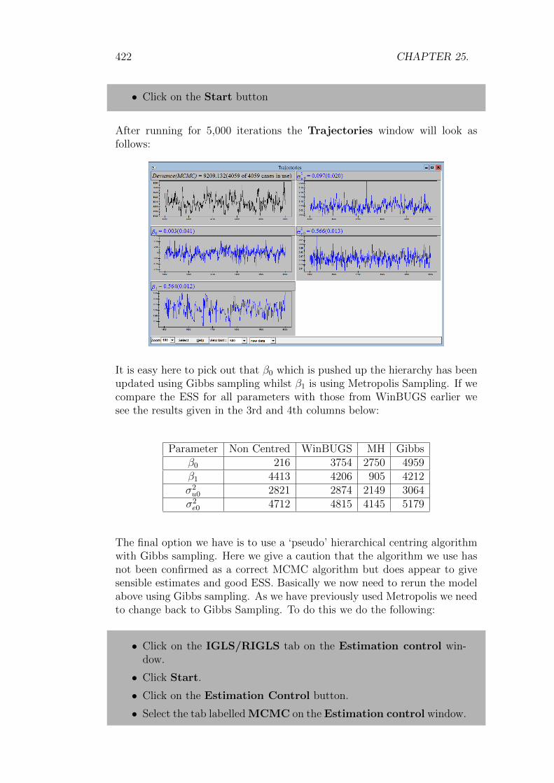
422 CHAPTER 25.
• Click on the Start button
After running for 5,000 iterations the Trajectories window will look asfollows:
It is easy here to pick out that β0 which is pushed up the hierarchy has beenupdated using Gibbs sampling whilst β1 is using Metropolis Sampling. If wecompare the ESS for all parameters with those from WinBUGS earlier wesee the results given in the 3rd and 4th columns below:
Parameter Non Centred WinBUGS MH Gibbsβ0 216 3754 2750 4959β1 4413 4206 905 4212σ2u0 2821 2874 2149 3064σ2e0 4712 4815 4145 5179
The final option we have is to use a ‘pseudo’ hierarchical centring algorithmwith Gibbs sampling. Here we give a caution that the algorithm we use hasnot been confirmed as a correct MCMC algorithm but does appear to givesensible estimates and good ESS. Basically we now need to rerun the modelabove using Gibbs sampling. As we have previously used Metropolis we needto change back to Gibbs Sampling. To do this we do the following:
• Click on the IGLS/RIGLS tab on the Estimation control win-dow.
• Click Start.
• Click on the Estimation Control button.
• Select the tab labelled MCMC on the Estimation control window.

25.6. NORMAL RESPONSE MODELS IN MLWIN 423
• Select MCMC/MCMC methods from the Model menu.
• Click on the Reset button and then the Done button on the Ad-vanced MCMC Methodology window.
• Click on the Start button.
After running we get the following chains in the Trajectories window:
Here we see all parameters appear to mix well and be using Gibbs samplingsteps. The ESS values are given in the last column of the earlier table and areas good if not better than those for the true hierarchical centring algorithmused by WinBUGS. So the question is what algorithm is MLwiN using?
If we consider the standard (uncentred) Gibbs sampling algorithm we havefour sets of steps to update β, u, σ2
u and σ2e respectively. We can also split
β into two parts, βC which can be centred and βU which can’t. Now theMetropolis sampling algorithm used earlier would have updated βU usingunivariate updating steps and simply replaced the equivalent univariate stepsfor βC with a Gibbs step with an adjustment to uj so that in reality u∗j =uj − (XCβC)j, the parameter from a centred formulation, is held constantand hence conditioned on.
So what we have done for the Gibbs algorithm is supplemented the four stepsfor the non-centred formulation with the Gibbs step for βC conditioningon the u∗j . This means that in each iteration βC is updated in two stepsand uj is updated in one step and adjusted in another. This may explainthe better mixing even than the standard Gibbs algorithm we demonstratedusing WinBUGS. Of course it is not clear that this algorithm is an acceptableGibbs sampling algorithm and we hope any MCMC theory researchers outthere can let us know either way. Until we have confirmation we thereforeurge caution while using this option and hence have left it to the end of thechapter.

424 CHAPTER 25.
Chapter learning outcomes
? How and when to use hierarchical centring to improve mixing.
? How to use hierarchical centring and the WinBUGS interface.
? Hierarchical centring for non-Normal response models.
? The use of a psuedo hierarchical centring algorithm in MLwiN forNormal responses.

Bibliography
Albert, J.H. & Chib, S. (1993). Bayesian analysis of Binary and Polychoto-mous Response Data. Journal of the American Statistical Association,88:669–679.
Besag, J., York, J. & Mollie, A. (1992). Bayesian image restoration with twoapplications in spacial statistics (with discussion). Annals of the Instituteof Statistical Mathematics, 43:1–59.
Best, N., Cowles, M.K. & Vines, K. (1995). Coda: Convergence diagnosis andoutput analysis software for Gibbs sampling output, Version 0.3. Technicalreport, Medical Research Council Biostatistics Unit, Cambridge.
Breslow, N.E. & Clayton, D.G. (1993). Approximate inference in general-ized linear mixed models. Journal of the American Statistical Association,88:9–25.
Browne, W.J. (1998). Applying MCMC methods to multilevel models. Ph.D.thesis, University of Bath.
Browne, W.J. (2004). An illustration of the use of reparameterisation meth-ods for improving MCMC efficiency in crossed random effects models. Mul-tilevel Modelling Newsletter, 16(1):13–25.
Browne, W.J. (2006). MCMC algorithms for constrained variance matrices.Computational Statistics & Data Analysis, 50(7):1655–1677.
Browne, W.J. & Draper, D. (2000). Implementation and performance issuesin the Bayesian and likelihood fitting of multilevel models. ComputationalStatistics, 15:391–420.
Browne, W.J. & Draper, D. (2006). A comparison of Bayesian and likelihood-based methods for fitting multilevel models. Bayesian Analysis, 1:473–550.
Browne, W.J., Goldstein, H. & Rasbash, J. (2001a). Multiple MembershipMultiple Classification (MMMC) models. Statistical Modelling, 1:103–124.
Browne, W.J., Goldstein, H., Woodhouse, G. & Yang, M. (2001b). AnMCMC algorithm for adjusting for errors in variables in random slopesmodels. Multilevel Modelling Newsletter, 13(1):4–10.
425

426 BIBLIOGRAPHY
Browne, W.J., Akkol, S. & Goldstein, H. (2009a). MCMC algorithms forstructured multivariate normal models. Technical report, submitted forpublication.
Browne, W.J., Steele, F., Golalizadeh, M. & Green, M. (2009b). The use ofsimple reparameterisations to improve the efficiency of MCMC estimationfor multilevel models with applications to discrete-time survival models.Journal of the Royal Statistical Society, Series A, 172:1–2.
Browne, W.J., Draper, D., Goldstein, H. & Rasbash, J. (2002). Bayesianand likelihood methods for fitting multilevel models with complex level-1variation. Computational Statistics and Data Analysis, 39(2):203–225.
Chatfield, C. & Collins, A.J. (1980). Introduction to Multivariate Analysis.London: Chapman & Hall.
Chib, S. & Carlin, B.P. (1999). On MCMC sampling in hierarchical longitu-dinal models. Statistics and Computing, 9:17–26.
Chib, S. & Hamilton, B.H. (2000). Bayesian analysis of cross-section andclustered data selection models. Journal of Econometrics, 97(1):25–50.
Clayton, D.G. & Kaldor, J. (1987). Empirical Bayes estimates of age-standardized relative risks for use in disease mapping. Biometrics, 43:671–681.
Elliott, P., Wakefield, J.C., Best, N.G. & Briggs, D.J. (2000). Spatial Epi-demiology: Methods and Applications. Oxford: Oxford University Press.
Gamerman, D. (1997). Sampling from the posterior distribution in general-ized linear mixed models. Statistics and Computing, 7:57–68.
Gelfand, A.E., Hills, S.E., Racine-Poon, A. & Smith, A.F.M. (1990). Illustra-tion of Bayesian inference in Normal data models using Gibbs Sampling.Journal of the American Statistical Association, 85:972–985.
Gelfand, A.E., Sahu, S.K. & Carlin, B.P. (1995). Efficient parameterisationsfor normal linear mixed models. Biometrika, 82:479–488.
Gelman, A. (2006). Prior distributions for variance parameters in hierarchicalmodels. Bayesian Analysis, 1:515–533.
Gelman, A., Roberts, G.O. & Gilks, W.R. (1995). Efficient Metropolis jump-ing rules. In J.M. Bernado, J.O. Berfer, A.P. Dawid & A.F.M. Smith, eds.,Bayesian Statistics 5, pages 559–607. Oxford: Oxford University Press.
Gelman, A., van Dyk, D.A., Huang, Z.Y. & Boscardin, W.J. (2008). Usingredundant parameterizations to fit hierarchical models. Journal of Com-putational and Graphical Statistics, 17:95–122.
Geweke, J. & Zhou, G. (1996). Measuring the pricing of the arbitrage pricingtheory. The Review of Financial Studies, 9:557–587.

BIBLIOGRAPHY 427
Gilks, W.R. & Wild, P. (1992). Adaptive rejection sampling for Gibbs sam-pling. Journal of the Royal Statistical Society, Series C, 41:337–348.
Gilks, W.R., Richardson, S. & Spiegelhalter, D.J. (1996). Markov ChainMonte Carlo in practice. London: Chapman & Hall.
Goldstein, H. (2003). Multilevel statistical models. London: Arnold, 3rdedition.
Goldstein, H. & Browne, W.J. (2002). Multilevel factor analysis modellingusing Markov Chain Monte Carlo (MCMC) estimation. In Marcoulides,G. A. & Moustaki, I., eds., Latent Variable and Latent Structure Models,pages 225–243. New Jersey: Lawrence Erlbaum.
Goldstein, H. & Speigelhalter, D.J. (1996). League tables and their limita-tions: statistical issues in comparisons of institutional performance. Jour-nal of the Royal Statistical Society, Series A, 159:385–443.
Kass, R.E., Carlin, B.P., Gelman, A. & Neal, R. (1998). Markov ChainMonte Carlo in practice: a roundtable discussion. American Statistican,52:93–100.
Knorr-Held, L. & Rue, H. (2002). On block updating in Markov random fieldmodels for disease mapping. Scandinavian Journal of Statistics, 29:597–614.
Krzanowski, W.J. & Marriott, F.H.C. (1994). Multivariate Analysis: Part 1:Distributions, Ordination and Inference. London: Edward Arnold.
Krzanowski, W.J. & Marriott, F.H.C. (1995). Multivariate Analysis: Part 2:Classification, Covariance Structures and Repeated Measurements. Lon-don: Edward Arnold.
Langford, I.H., Bentham, G. & McDonald, A. (1998). Multilevel mod-elling of geographically aggregated health data: A case study on malig-nant melanoma mortality and UV exposure in the European Community.Statistics in Medicine, 17:41–58.
Langford, I.H., Leyland, A.H., Rasbash, J., Goldstein, H., Day, R.J. & Mac-donald, A.L. (1999). Multilevel modelling of area-based health data. InA.B. Lawson, A. Biggeri, D. Boehning, E. Lessafre, J. Viel & R. Bertollini,eds., Disease Mapping and Risk Assesment for Public Health. Chichester:Wiley.
Lawson, A.B., Biggeri, A., Boehning, D., Lessafre, E., Viel, J. & Bertollini,R. (1999). Disease Mapping and Risk Assesment for Public Health. Chich-ester: Wiley.
Lawson, A.B., Browne, W.J. & Roderio, C.L.V. (2003). Disease Mappingwith WinBUGS and MLwiN. Chichester: Wiley.
Liu, C., Rubin, D.B. & Wu, Y.N. (1998). Parameter expansion to accelerateEM: The PX-EM algorithm. Biometrika, 85:755–770.

428 BIBLIOGRAPHY
Liu, J.S. & Wu, Y.N. (1999). Parameter expansion for data augmentation.Journal Of The American Statistical Association, 94:1264–1274.
McCulloch, C.E. & Searle, S.R. (2001). Generalized, Linear and Mixed Mod-els. New York: Wiley.
Mollie, A. (1996). Bayesian mapping of disease. In W.R. Gilks, S. Richardson& D.J. Spiegelhalter, eds., Markov Chain Monte Carlo in Practice. London:Chapman and Hall.
Mortimore, P., Sammons, P., Stoll, L., Lewis, D. & Ecob, R. (1988). SchoolMatters. Wells: Open Books.
Raftery, A.E. & Lewis, S.M. (1992). How many iterations in the Gibbssampler? In J.M. Bernado, J.O. Berfer, A.P. Dawid & A.F.M. Smith, eds.,Bayesian Statistics 4, pages 765–76. Oxford: Oxford University Press.
Rasbash, J. & Browne, W.J. (2001). Modelling non-hierarchical structures.In A.H. Leyland & H. Goldstein, eds., Multilevel Modelling of Health Statis-tics, pages 93–105. Chichester: Wiley.
Rasbash, J. & Browne, W.J. (2002). Non-hierarchical multilevel models. InJ.D. Leeuw & E. Meijer, eds., Handbook of Multilevel Analysis. Springer.
Rasbash, J. & Goldstein, H. (1994). Efficient analysis of mixed hierarchicaland cross-classified random structures using a multilevel model. Journalof Educational and Behavioural Statistics, 19:337–50.
Rasbash, J., Goldstein, H., Browne, W.J., Yang, M. & Woodhouse, G. (2000).The MLwiN Command Interface version 1.3. Institute of Education, Uni-versity of London, London.
Rasbash, J., Steele, F., Browne, W.J. & Goldstein, H. (2008). A User’sGuide to MLwiN Version 2.10. Centre for Multilevel Modelling, Universityof Bristol, Bristol.
Rubin, D.B. (1976). Inference and missing data. Biometrika, 63:581–592.
Rubin, D.B. (1987). Multiple Imputation for Nonresponse in Surveys. NewYork: J. Wiley and Sons.
Rue, H. (2001). Fast sampling of Gaussian Markov Fields. Journal of theRoyal Statistical Society, Series B, 63:325–338.
Sargent, D.J., Hodges, J.S. & Carlin, B.P. (2000). Structured Markov chainMonte Carlo. Journal Of Computational And Graphical Statistics, 9:217–234.
Schafer, J.L. (1996). Analysis of Incomplete Multivariate Data. London:Chapman & Hall.
Schafer, J.L. (1997). Imputation of missing covariates under a multivariatelinear mixed model. Technical report, unpublished.

BIBLIOGRAPHY 429
Seltzer, M.H. (1993). Sensitivity analysis for fixed effects in the hierarchicalmodel: A Gibbs sampling approach. Journal of Educational Statistics,18:207–235.
Spiegelhalter, D.J., Thomas, A. & Best, N.G. (2000a). WinBUGS version1.3: user manual. Medical Research Council Biostatistics Unit, Cam-bridge.
Spiegelhalter, D.J., Thomas, A. & Best, N.G. (2000b). WinBUGS version1.3: Examples volume II. Medical Research Council Biostatistics Unit,Cambridge.
Spiegelhalter, D.J., Best, N.G., Carlin, B.P. & van der Linde, A. (2002).Bayesian measures of model complexity and fit (with discussion). Journalof the Royal Statistical Society, Series B, 64:191–232.
Tanner, M. & Wong, W. (1987). The calculation of posterior distributions bydata augmentation (with discussion). Journal of the American StatisticalAssociation, 82:528–550.
Thomas, A., Best, N.G. & Spiegelhalter, D.J. (2000). GeoBUGS User Man-ual, Demonstration Version 1.0. Imperial College and MRC BiostatisticsUnit, Cambridge.
van Dyk, D.A. & Meng, X.L. (2001). The art of data augmentation. Journalof Computational and Graphical Statistics, 10:1–50.
Woodhouse, G., Yang, M., Goldstein, H. & Rasbash, J. (1996). Adjusting formeasurement errors in multilevel analysis. Journal of the Royal StatisticalSociety, Series A, 159:201–212.
Yang, M. & Woodhouse, G. (2001). Progress from GCSE to A and AS level:Simple measures and complex relationships. British Educational ResearchJournal, 27:245–268.