/V/) 4; .2- __ _._

Putting Time into Proof Outlines*

Fred B. Schneider** ,W ---d/---_'

Bard Bloom*Keith Marzullo****

TR 93-1333March 1993

Department of Computer ScienceCornell UniversityIthaca, NY 14853-7501

*A preliminary version of this work appeared in Real-time: Theory and Practice,Proceedings of REX workshop, June 1991, Springer-Verlag Lecture Notes inComputer Science, volume 600.**Supported in part by the Office of Naval Research under contract N00014-91-J-1219, the National Science Foundation under Grant No. CCR-8701103, DARPA/NSFGrant No. CCR-9014363, and a grant from IBM Endicott Programming Laboratory.***Supported in part by NSF grant CCR-9003441.****Supported in part by Defense Advanced Research Projects Agency (DoD) underNASA Ames grant number NAG 2-593 and by grants from IBM and Siemens.

https://ntrs.nasa.gov/search.jsp?R=19930015963 2019-10-13T01:11:11+00:00Z

_r

,41"

II

_ 27_Z_i

Putting Time into Proof Outlines*

Fred B. Schneider t

Cornell Universityfbs@cs, cornell, edu

Bard Bloom $

Cornell University

bard_cs, cornell, edu

Keith Marzulio §

Cornell University

marzullo_cs, cornell, edu

March 10, 1993

Abstract

A logic for reasoning about timing properties of concurrent programs is presented. The logic

is based on Hoare-style proof outlines and can handle maximal parallelism as well as certain

resource-constrained execution environments. The correctness proof for a mutual exclusion

protocol that uses execution timings in a subtle way illustrates the logic in action. A soundness

proof using structural operational semantics is outlined in the appendix.

Key words: concurrent program verification, timing properties, safety properties, real-time

programming, real-time actions, proof outlines.

1 Introduction

A safety property [9] of a program asserts that some proscribed "bad thing" does not occur during

execution. To prove that a program satisfies a safety property, one typically employs an invariant, a

characterization of current (and possibly past) program states that is not invalidated by execution.

If an invariant I holds in the initial state of the program and I =_ Q is valid for some Q, then

-_Q cannot occur during execution. Thus, to establish that a program satisfies the safety property

asserting that -,Q does not occur, it suffices to find such an invariant I.

Timing properties are safety properties where the "bad thing" involves the time and programstate at the instants that various specified control points in a program become active. 1 Timing

properties can concern externally visible events, llke inputs and outputs, as well as events and data

that are internal to a program, like the value of a variable or the time that a particular command

starts or finishes. For example, in process control applications, the elapsed time between a stimulus

and response may have to be bounded. This is a timing property where the "bad thing" is defined

in terms of the time that elapses after one control point becomes active until some other control

point does. Timing properties concerning internal events are useful in reasoning about ordinary

"A preliminary version of this work appeared in Real-time: Theory and Practice, Proceedings of REX workshop,

June 1991, Springer-Verlag Lecture Notes in Computer Science, volume 600.

?Supported in part by the Office of Naval Research under contract N00014-91-J-1219, the National Science Foun-

dation under Grant No. CCR-8701103, DARPA/NSF Grant No. CCR-9014363, and a grant from IBM Endicott

Programming Laboratory.

$Supported in part by NSF grant CCR-9003441.

iSupported in part by Defense Advanced Research Projects Agency (DoD) under NASA Ames grant number NAG

2-593, and by grants from IBM and Siemens.1Informally, the active control points at any instant are determined by the values of the program counters at that

instant. See [15] for a more formal definition.

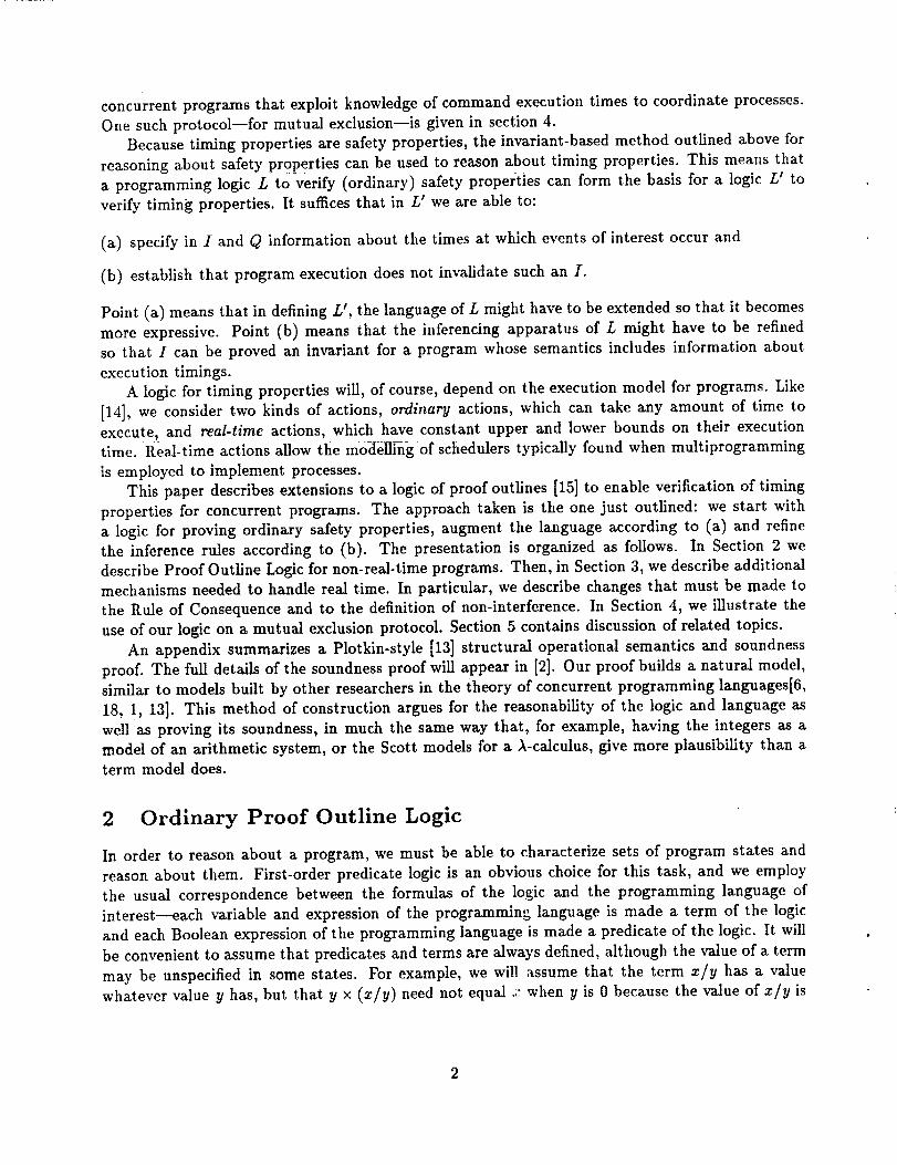
concurrent programs that exploit knowledge of command execution times to coordinate processes.

One such protocol--for mutual exclusion--is given in section 4.

Because timing properties are safety properties, the invariant-based method outlined above for

reasoning about safety properties can be used to reason about timing properties. This means that

a programming logic L to verify (ordinary) safety properties can form the basis for a logic L' to

verify timing properties. It suffices that in L' we are able to:

(a) specify in I and Q information about the times at which events of interest occur and

(b) establish that program execution does not invalidate such an I.

Point (a) means that in defining L _, the language of L might have to be extended so that it becomes

more expressive. Point (b) means that the inferencing apparatus of L might have to be refined

so that I can be proved an invariant for a program whose semantics includes information about

execution timings.

A logic for timing properties will, of course, depend on the execution model for programs. Like

[14], we consider two kinds of actions, ordinary actions, which can take any amount of time to

execute, and real-time actions, which have constant upper and lower bounds on their execution

time. Real-time actions allow the modeling of schedulers typically found when multiprogramming

is employed to implement processes.

This paper describes extensions to a logic of proof outlines [15] to enable verification of timing

properties for concurrent programs. The approach taken is the one just outlined: we start with

a logic for proving ordinary safety properties, augment the language according to (a) and refine

the inference rules according to (b). The presentation is organized as follows. In Section 2 we

describe Proof Outline Logic for non-real-time programs. Then, in Section 3, we describe additional

mechanisms needed to handle real time. In particular, we describe changes that must be made to

the Rule of Consequence and to the definition of non-interference. In Section 4_ we illustrate the

use of our logic on a mutual exclusion protocol. Section 5 contains discussion of related topics.

An appendix summarizes a Plotkin-style [13] structural operational semantics and soundnessproof. The full details of the soundness proof will appear in [2]. Our proof builds a natural model,

similar to models built by other researchers in the theory of concurrent programming languages[6,

18, 1, 13]. This method of construction argues for the reasonability of the logic and language as

well as proving its soundness, in much the same way that, for example, having the integers as a

model of an arithmetic system, or the Scott models for a ),-calculus, give more plausibility than aterm model does.

2 Ordinary Proof Outline Logic

In order to reason about a program, we must be able to characterize sets of program states and

reason about them. First-order predicate logic is an obvious choice for this task, and we employ

the usual correspondence between the formulas of the logic and the programming language of

interest--each variable and expression of the programmin_ language is made a term of the logic

and each Boolean expression of the programming language is made a predicate of the logic. It will

be convenient to assume that predicates and terms are always defined, although the value of a term

may be unspecified in some states. For example, we will ._ssume that the term x/y has a value

whatever value y has, but that y × (x/y) need not equal : when y is 0 because the value of x/y is

unspecified in such states. 2 ....

Predicates and function symbols for the programming language's data types provide a way to

express facts about program variables and expressions. Type declarations in the program induce

axioms concerning the values that may be assumed by the variables they declare. For simplicity,

we take these as given.

The state of a program also includes information that tells what atomic actions might be

executed next. For representing this control information, we fix some predicate symbols, called

control predicates, and give axioms to ensure that, as execution proceeds, changes in the values of

the control predicates correspond to changes in program counters. (An alternative representation

would have been to define a "program counter" variable and a data type for the values it can

assume.)

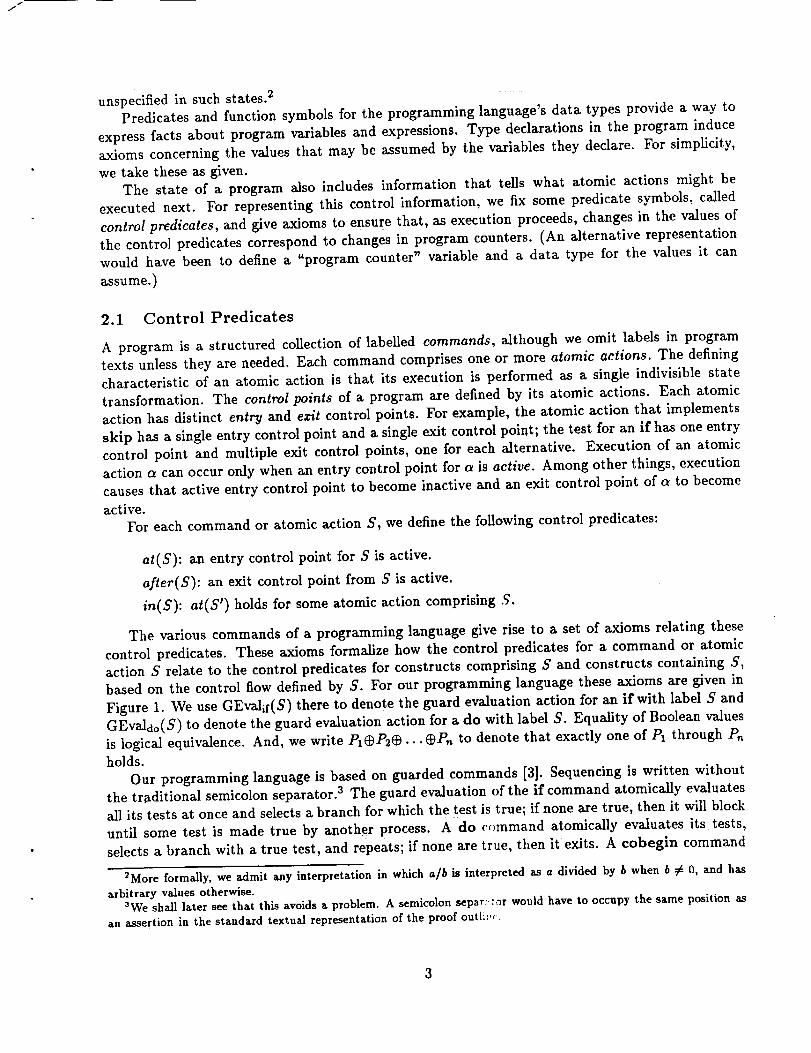
2.1 Control Predicates

A program is a structured collection of labelled commands, although we omit labels in program

texts unless they are needed. Each command comprises one or more atomic actions. The defining

characteristic of an atomic action is that its execution is performed as a single indivisible state

transformation. The control points of a program are defined by its atomic actions. Each atomic

action has distinct entry and ezit control points. For example, the atomic action that implements

skip has a single entry control point and a single exit control point; the test for an if has one entry

control point and multiple exit control points, one for each alternative. Execution of an atomic

action ex can occur only when an entry control point for a is active. Among other things, execution

causes that active entry control point to become inactive and an exit control point of a to becomeactive.

For each command or atomic action S, we define the following control predicates:

at(S): an entry control point for S is active.

after(S): an exit control point from S is active.

in(S): at(S') holds for some atomic action comprising S.

The various commands of a programming language give rise to a set of axioms relating these

control predicates. These axioms formalize how the control predicates for a command or atomic

action S relate to the control predicates for constructs comprising S and constructs containing S,

based on the control flow defined by S. For our programming language these axioms are given in

Figure 1. We use GEvaIif(S) there to denote the guard evaluation action for an if with label S and

GEvaldo(S) to denote the guard evaluation action for a do with label S. Equality of Boolean values

is logical equivalence. And, we write PI(_P2_... _P,_ to denote that exactly one of P1 through P,_holds.

Our programming language is based on guarded commands [3]. Sequencing is written without

the traditional semicolon separator. 3 The guard evaluation of the if command atomically evaluates

all its tests at once and selects a branch for which the test is true; if none are true, then it will block

until some test is made true by another process. A do _'ommand atomically evaluates its tests,

selects a branch with a true test, and repeats; if none are true, then it exits. A cobegin command

_More formally, we admit any interpretation in which a/b is interpreted as a divided by b when b _ O, and has

arbitrary values otherwise.

_We shall later see that this avoids a problem. A semicolon separ'_or wol_ld have to occupy the same position as

an asse_'tion in the standard textual representation of the proof outli:,,.

starts all of its component processes simultaneously, executing them concurrently. When they all

finish, the cobegin finishes as well.

Construct Axioms

c_ atomic --,(at(a) A after(a))

in(s) = at(s)

S : &S2

at(S) = at(&)after(S) = .fter(S=)

after(&) = .t(S=)in(S) = in(S,)@ in(S2)

S : ifBl'"*Sl"'" at(S)

OB_--.&... after(S)Bn-"_ Sn after( GEvalif( S) )

fi in(S)

= at(GEvallf(S))= (after(S,)$ayte_(S=)e...@afteK&))= (at(S1)_at(S2)@..._at(&))= in(GEvalif(S)) _) in(S1) D... • in(Sn)

S : do B1--S1 • • • at(GEvaldo(S))

OB_--.S,... after(CEV_o(S))UB.--.S. in(s)od at(S)

(after(GEvaldo(S)) V Vi"=, after(&))

= (at(S)@after(S1)_after(S2)@...@after(S,,))

= (at(S,)mat(S=)¢...eat(S.)eafter(S))= in(GEvaho(S))ein(&)_...ein(&)

=_ at(CEvaldo(S))

= (after(S,) _9"" _ after(S,,) @ after(GEvaldo(S)))

S : cobegin at(S) = (at(S,)A...Aat(Sn))

&//... //s. after(S) = (after(S,) ^... ^ after(S.))coend

Figure 1: Control Predicate Axioms

2.2 Syntax and Meaning of Proof Outlines

A proof outline PO(S) for a program or atomic action S is a mapping from the control predicatesof S to assertions. Each assertion is a Predicate Logic formula in which _.... :_ :

! -- -- =

• the free variables are program variables (typeset in italics) or rigid variables, (typeset in

uppercase roman), and

• the predicate symbols are control predicates or the predicates of the programming language's

expression language.

Assertions in which all terms are constructed from program variables, rigid variables, and predicates

--]n-v-o-l\'ing those va}]ab_ are called primitive assertions_ _- ::_ : ..... _::_+ ........... > : ....

If T is a subprogram of S and some PO(S) is fixed, then we write pre(T) (resp. post(T)) for the

assertion(s) that PO(S) associates with at(T) (resp.= aficrtT)); these are called the precondition

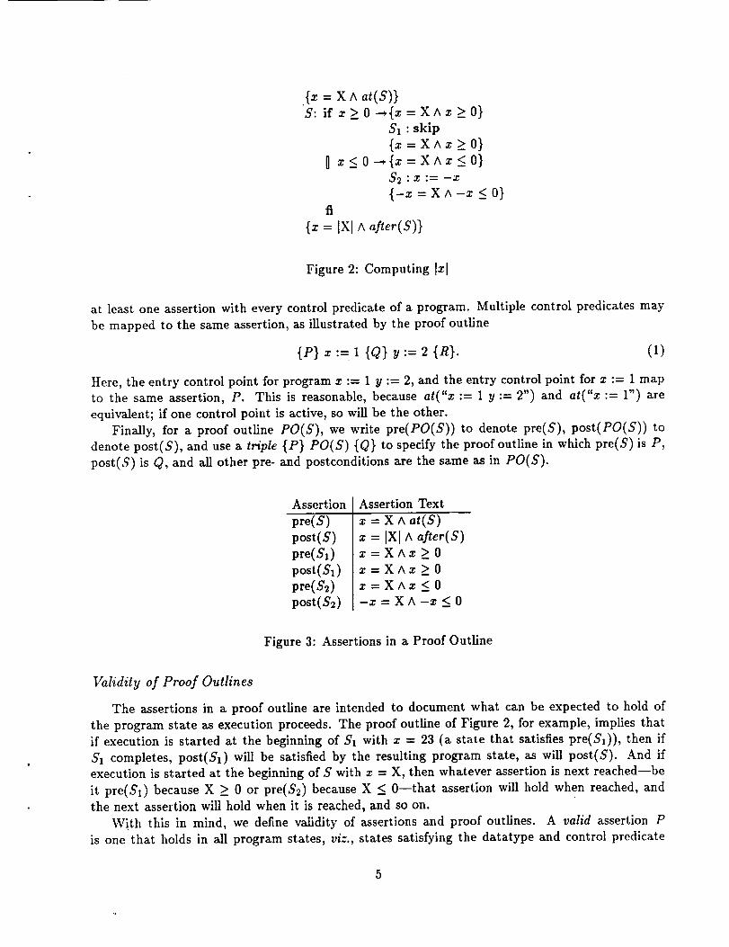
and postcondition of T. For the proof outline in Figure 2, this correspondence is summarized in

Figure 3. In it, x is a program variable and X is a rigid variable. All assertions except pre(S) and

post(S) are primitive.

Proof outlines are generally represented as texts containing the program S and an assertion in

braces before and after every subprogram of S. For our programming language, this will associate

{z = X A at(5,)}S: ifz>_O_{z=X^z>O}

5'1 : skip

{z = X^z__. 0}U z<O--,{z=XAz<O}

5'2 : X := --X

{-z = x ^ -x _ 0)fl

{x --IXl A after(5,)}

Figure 2: Computing Ix[

at least one assertion with every control predicate of a program. Multiple control predicates may

be mapped to the same assertion, as illustrated by the proof outline

{P} x := 1 {Q) y := 2 {R}. (1)

Here, the entry control point for program x := 1 y := 2, and the entry control point for z := 1 map

to the same assertion, P. This is reasonable, because at("x := 1 y := 2") and at("x := 1") are

equivalent; if one control point is active, so will be the other.

Finally, for a proof outline PO(5,), we write pre(PO(5')) to denote pre(5,), post(PO(5,)) to

denote post(5,), and use a triple {P} PO(5") {Q} to specify the proof outline in which pre(5,)is P,

post(5,) is Q, and all other pre- and postconditions are the same as in PO(5,).

Assertion

pre(5,)

post(S)

pre(5,1)

post(5,1)

pre(5'2)

post(S2)

Assertion Text

z = X ^ at(5,)

z = IXl A a#er(5,)x=XAx>0

z=XAx>0

z=XAz<0

-z = X A -z < 0

Figure 3: Assertions in a Proof Outline

Validity of Proof Outlines

The assertions in a proof outline are intended to document what can be expected to hold of

the program state as execution proceeds. The proof outline of Figure 2, for example, implies that

if execution is started at the beginning of 5'1 with z = 23 (a state that satisfies pre(5'l)), then if

5'1 completes, post(S1) will be satisfied by the resulting program state, as will post(S). And if

execution is started at the beginning of 5, with z = X, then whatever assertion is next reached--be

it pre(5'x) because X > 0 or pre(5'2) because X < 0--that assertion will hold when reached, andthe next assertion will hold when it is reached, and so on.

With this in mind, we define validity of assertions and proof outlines. A valid assertion P

is one that holds in all program states, viz., states satisfying the datatype and control predicate

5

{true}a : eobeg|n

{_=1}b: skip

{...}//

{...}c: skip

{...}eoend

{...}

Figure 4: Multiple Active Control Points (Partial proof outline)

axioms. A valid proof outline PO(S) will be one that describes a relationship among the program

variables and control predicates of S that is invariant and, therefore, not falsified by execution of

S. The invariant defined by a proof outline PO(S) is "if a control predicate cp is true, then so is

every assertion that PO(S) associates with cp" and is formalized as the proof outline invariant for

PO(S):

Ieo(s) : A ((at(T)::¢, pre(T))A (after(T):_ post(T)))T

where T ranges over the subprograms of S. For example, the proof outline invariant defined by

PO(S) of Figure 2 is:

at(S) :* (_ = X ^ at(S))A at(S1) _ (z = X Az >__O)A at(S2) :_ (z = X Az <_O)

^ after(S) _ (_ = IXl^ after(S))A after(Sl) _ (z = X Az > O)A after(S2) _ (--z = X A --_ <_O)

Notice that proof outline validity is with respect to executions starting in any state, even a

state in the middle of the program. For example, the proof outline

S: a:

b:

{z=0Ay=l}z := x+2

{_=2}y:=y+2

{_=2^y=s}

is not valid. This is because a state where at(b), z = 2, and y = 20 hold satisfies _Ipo(s), but

starting execution in this state leads to one that does not satisfy Ipo(s).In order to make the inference rules of our logic as easy to use as possible, we have designed

them so that hypotheses concerning proof outlines do not delve too deeply into the structure of

those proof outlines. Allowing multiple control predicates to be true simultaneously - as we do -

complicates the realization of this goal. Consider the concurrent program of Figure 4. There, at(a)

is true iff both at(b) and at(c) are true. Thus, in Figure 4. if at(a) and Ipo(s ) are both true, then

z = 1 holds. However, pre(a) gives no warning of this requirement; it is the trivial assertion "true".

6

ORlf_NAL PAL-_ IS

OF POOR QUALITY

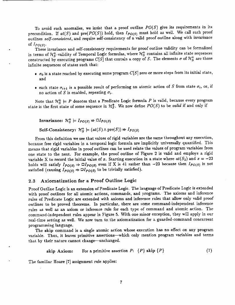
To avoid such anomalies, we insist that a proof outline PO(S) give its requirements in its

precondition. If at(S) and pre(PO(S)) hold, then IPo(s) must hold as well. We call such proof

outlines self-consistent, and require self-consistency of a valid proof outline along with invariance

of Ipo(s).These invariance and self-consistency requirements for proof outline validity can he formalized

in terms of "/-/+-validity of Temporal Logic formulas, where 7-/+ contains all infinite state sequences

constructed by executing programs C[S] that contain a copy of S. The elements a of 7-I+ are those

infinite sequences of states such that:

• a0 is a state reached by executing some program C[S] zero or more steps from its initial state,

and

• each state ai+x is a possible result of performing an atomic action of S from state ai, or, if

no action of S is enabled, repeating ai.

Note that 7_+ _ P denotes that a Predicate Logic formula P is valid, because every program

state is the first state of some sequence in _+. We now define PO(S) to be valid if and only if

Invariance: 7-/+ _= Ipo(s) =_ rllpo(s)

Self-Conslstency: "H+ # (at(S) A pre(S)) =_ Ipo(s)

From this definition we see that values of rigid variables are the same throughout any execution,

because free rigid variables in a temporal logic formula are implicitly universally quantified. This

means that rigid variables in proof outlines can be used relate the values of program variables from

one state to the next. For example, the proof outline of Figure 2 is valid and employs a rigid

variable X to record the initial value of x. Starting execution in a state where at(S2) and x = -23

holds will satisfy Ipo(s) =_ OIpo(s) even if X is 41 rather than -23 because then Ipo(s) is not

satisfied (causing Ipo(s ) =_ mIpo(s ) to be trivially satisfied).

2.3 Axiomatization for a Proof Outline Logic

Proof Outline Logic is an extension of Predicate Logic. The language of Predicate Logic is extended

with proof outlines for all atomic actions, commands, and programs. The axioms and inference

rules of Predicate Logic are extended with axioms and inference rules that allow only valid proof

outlines to be proved theorems. In particular, there are some command-independent inference

rules as well as an axiom or inference rule for each type of command and atomic action. The

command-independent rules appear in Figure 5. With one minor exception, they will apply in our

real-time setting as well. We now turn to the axiomatization for a guarded-command concurrent

programming language.

The skip command is a single atomic action whose execution has no effect on any program

variable. Thus, it leaves primitive assertions--which only mention program variables and terms

that by their nature cannot change---unchanged.

skip Axiom: For a primitive assertion P: {P} skip {P} (7)

The familiar Hoare [7] assignment rule applies:

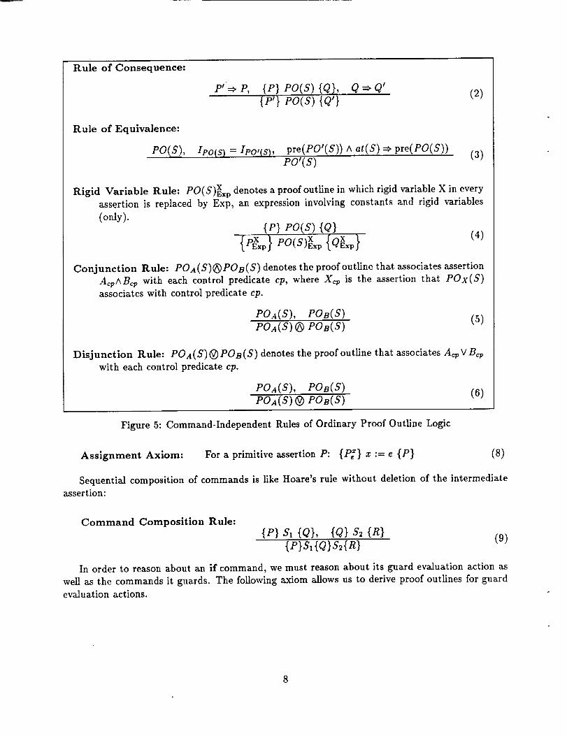
Rule of Consequence:

P":_ P, {P} PO(S) {Q}, Q _ Q'

{P'} PO(S) {Q'}(2)

Rule of Equivalence:

PO(S), Ipo(s) = Ipo,(s), pre(PO'(S)) A at(S) _ pre(PO(S))PO'(S)

(3)

Rigid Variable Rule: PO(S)Xxp denotes a proof outline in which rigid variable X in every

assertion is replaced by Exp, an expression involving constants and rigid variables

(only).{P} PO(S) {Q}

{pxo}Po(s)' x {ox,.}

Conjunction Rule: POA(S)_POB(S) denotes the proof outline that associates assertion

AcpABcp with each control predicate cp, where Xcp is the assertion that POx(S)

associates with control predicate cp.

POA(S), POB(S)

POA(S) @ POB(S)(2)

Disjunction Rule: POA(S) @ POB(S) denotes the proof outline that associates A_ v B_

with each control predicate cp.

POA(S), POB(S)

POA(S) (_ P08(S)(6)

Figure 5: Command-Independent Rules of Ordinary Proof Outline Logic

Assignment Axiom: For a primitive assertion P: {P/} x := e {P} (8)

Sequential composition of commands is like Hoare's rule without deletion of the intermediate

assertion:

Command Composition Rule:{P} S, {Q}, {Q} $2 {R}

{P}SI{O}S2{R}(9)

In order to reason about an if command, we must reason about its guard evaluation action as

well as the commands it guards. The following axiom allows us to derive proof outlines for guard

evaluation actions.

8

GEvalif(S)Axiom: For an if command

S : if BI _ SI _ ... _ B,_ _ S,_ fl

and a primitive assertion P,

{P} GEvallf(S) {P A (Ai at(Si) =_ Bi)} (10)

A proof outline for an if is then constructed by combining a proof outline for its guard evaluation

action with a proof outline for each alternative.

if rule:

(a) {P} GEvalif(S) {R}

(b) (n A at(S1)) :0 P1,

(c) {P1} PO(S,) {Q},

..., (R ^ at(S,,)) =_P,,..., {P,_}PO(S,.,) {Q}

{P}

S: if BI---*{P1}PO(SI){Q} (11)

_B,.,_{P,-,}PO(Sn){Q}fi

{Q}

The guard evaluation action for do selects a command Si for which corresponding guard Bi

holds. If no guard is true, then the control point following the do becomes active.

GEvaldo(S) Axiom: For a do command

S : do BI--*SI _ "" _ Bn-*S,, od

and a primitive assertion P,

{P} GEvaldo(S) {P h (Ai at(Si) =_ Bi) h (after(S) =_ (-,B1 ^"" ^ -,B,_))} (12)

The inference rule for do is based on a loop invariant, an assertion I that holds before and after

every iteration of a loop and, therefore, is guaranteed to hold when do terminates--no matter how

many iterations occur.

do rule:

(a) {I} CEvaldo(S) {a}(b) (R^ at(S1)) =vP1, ..., (RA at(S,,)) _ P,_(c) {P1} PO(Sa) {I}, ':., {P,_}PO(S,_) {I}(d) (R Aafter(S)) _ (XA-,B1 A..- _ _B, )

{i}S: doB1---*{PI}PO(Sx){I}

,.,

_B,_---.{P,_}PO(S,_){I}od

{I A-_Bx A...A -,B.}

(13)

9

The inferencerule for a cobegln combines proof outlines for its component processes. An

interference-freedom test [12] ensures that execution of an atomic action in one process does not

invalidate the proof outline invariant for another. This interference-freedom test is formulated in

terms of triples,YI(a,A): {pre(a) A A} a {A}

that are valid if and only if & does not invalidate assertion A. If no assertion in PO(Si) is invalidated

by an atomic action a then, by definition, Ipo(&) also cannot be inva_dated by a. Therefore, we can

prove that a collection of proof outlines PO(S1), ..., PO(Sn) are interference free by establishing:

Interference Freedom

For all i,j, 1 < i < n,1 < j < n,i _ j:For all atomic actions a in Si :

For all assertions A in PO(Sj) :

NI(a, A) is valid.

(14)

The following inference rule characterizes when a valid proof outline for a cobegin will result

from combining valid proof outlines for its component processes:

cobegin rule:(a) PO(S1), ..., PO(Sn)

(b) P =_ (Aipre(PO(Si)))

(Ai post( PO( Si) )) =_ O (15)(c)(el) PO(SI),..., PO(Sn) are interference free

% F

{P) cobegin PO(St)//...ffPO(Sn)eoend {Q)

Since execution of an atomic action a in one process never interferes with a control predicate

cp in another, certain interference-freedom triples follow axiomatically.

Process Independence Axiom: For a control predicate cp in one process and an atomic

action a in another,{ep = X} a {cV= X} (16)

Notice that NI(a, cp) follows directly from this axiom when a and cp are from different processes.

2.4 From Proof Outlines to Safety Properties

Theorems of Proof Outline Logic can be used in verifying safety properties because of the way that

proof outline validity is defined. If a proof outline PO(S) is walid then Ivo(s) must be an invariant.

Suppose that IRo(s) is an invariant. Then according to the method of Section 1 for proving safetyproperties, we can prove that executions of S starting with pre(PO(S)) true will satisfy the safety

property proscribing -_Q by proving (at(S) ^ pre(PO(S))) _ IRO(S) and Ipo(s ) ::_ -_Q. The proof

of (at(S) ^ prePO(S)) _ Ieo(s) follows trivially from th, -,ray fRO(S) is defined. And, to prove

Ipo(s) ::¢""Q, we simply prove

(cp ^ Ao, ) =_ Q (17)

for every assertion Acv in PO(S), where Acv is the asserlion that PO(S) associates with control

predicate cp. For example, we prove as follows that for ihe absolute value program in Figure 2

10

after(S) =_ (x = ]Xl) holds during executions started in a state satisfying z = X A at(S): For the

case where cp does not imply after(S), (17) is trivially valid. The remaining cases are when cp is

after(S1), after(S2) and after(S). Here, we must show

after(S1) A post(S1)

after(S2) A post(S2)

after(S) A post(S)

=, (after(S) a (. = Ixl))(after(S) (x --lxl))

=, (after(S) a = t 1))

All are valid.

3 Real-time Logic

3.1 A View of Real Time

In taking into account real-time, our universe of discourse comprises processes executing parts of

some program along with an external world. We thus are forced to consider three kinds of actions:

Ordinary actions: Atomic actions without timing constraints are called ordinary actions. They

may execute whenever they are enabled, or wait arbitrarily long.

Real-time actions: A real-time action is an atomic action whose execution time is constrained.

Idles: Execution time may pass without the program doing anything. Such a passage of time can

be attributed to the external world, and we model this by an idle.

Ordinary actions are familiar, and the Proof Outline Logic of Section 2 works fine for them.

Real-time actions cause no logical difficulties, as they have the same effects on variables and program

state as ordinary actions, but their execution is more constrained. Adding axioms to Proof Outline

Logic suffices for reasoning about the execution time of real-time actions. Idles, strangely enough,

are more troublesome because their presence causes some matters of logical concern (viz., the time)

to change without program execution. For example, Rule of Consequence (2) is unsound when idles

are present.

In defining our logic, we consider an extremely powerful real-time language, allowing constructs

that may be impractical or impossible to implement. Programmers using actual languages will

not necessarily have access to all the features we allow. However, we believe that most actual

programs in our intended domain can be translated into our language. Thus, expressive power is

an advantage: the more powerful our language, the greater the number of real programs that can

be expressed in it.

Our programming language is the one of Section 2 with additional real-time actions. In particu-

lar, for each unconditional atomic action 4 a, we define corresponding real-time action (_)[s,d where

8 and e are real-valued, non-negative constants. Execution of (a)[6, d causes the same indivisiblestate transformation as a does, but constrains it to occur at some instant between e and e + _ time

units after the entry control point for (a)[s,c] becomes active.We have elected to characterize the execution time for a real-time action in terms of two parame-

ters (/5 and e), following [14], in order to gain flexibility in modelling various execution environments.

4An atomic action is unconditional if it is executable whenever its entry control point becomes active. In the

programming notation of Section 2, skip, assignment, and the guard evaluation action for do are unconditional. The

guard evaluation for if is not unconditional.

11

Parametere describes the fixed execution time of the action on a bare machine; _ models execu-

tion delays attributable to multiprogramming and other resource contention. A system where each

process is assigned its own processor is modeled by choosing 0 for _; a system where processors are

shared is modeled by choosing a value for 6 based on the length of time that a runnable process

might have to wait for a processor to become available.

As an illustration, suppose we know that assignment commands take one time-unit, and that

there is a single processor. If three assignment commands are started concurrently, they will be

executed in some order. The first one to run will be started immediately and take one time-unit;

the last one will be started two units after it was issued, and it also takes one time-unit. Thus we

could model this with real-time actions having an execution time of 1 and a possible delay of 2.

cobegin (xl := 1)[2,1]//(x2 := 2)[2,1]//(x3 := 3)[2,t] coend

We do not allow a in a real-time action (a)[_,e] to be a conditional atomic action, such as anif guard evaluation action, because it is not clear what such a construct would mean. The delay

in a conditional atomic action is already dependent on something else - changes to the program

state. Lower bounds on conditional atomic actions (e.g., an if command that requires at least one

time-unit to evaluate its condition) can be implemented with a real-time skip command followed by

an ordinary if. Timeouts on conditional atomic actions can be implemented by parallel processesand shared variables.

When writing a real-time program, it is sometimes necessary to program a loop whose iterations

have fixed or bounded execution time. All of the atomic actions in such a loop must be real-time

actions. We therefore introduce the following syntax to specify that (GEvaldo(S))[6,¢ ] be used asthe guard evaluation action in a do command:

do [s,,]BI-*S1 _ "" _ Bn_Sn od (18)

3.2 Reasoning About Real-time Actions

To reason about timing properties, terms are added to the assertion language and additional in-

formation is included in the program state. This is because the method of Section 2 for reasoning

about safety properties can only be used to prove safety properties for which the negation of the

proscribed -,Q is implied by each of a proof outline's assertions. Timing properties, by definition,

concern the instants at which control predicates become active, so we define a term Tcp for each

control predicate cp:

f t t is the time that cp last became trueTen

-co cp has never been true(19)

We also define a new real-valued term 7" to be equal to the current time.

Only certain assignments of values to these terms axe sensible in a program state. In particular,

if two control points become active as part of the same event, then they must be assigned the same

time. For example, since S is the first subcommand of S T, we require that Tat(S) = Tat(S T).

Similarly, the subcommands $1 and S_ in S: cobegin $1//$2 coend start at the same time, so

we require Tat(S1) = Tat(S2) = Tat(S).

Notice what effect adding these terms to the state has on the definition of proof outline validity.

Recall that a proof outline PO(S) is valid if execution starting in any state that satisfies Ipo(s)

leaves Ieo(s) invariant. Now, a state includes a time, and so we must consider starting states witharbitrary times as well as arbitrary values for program variables and control.

12

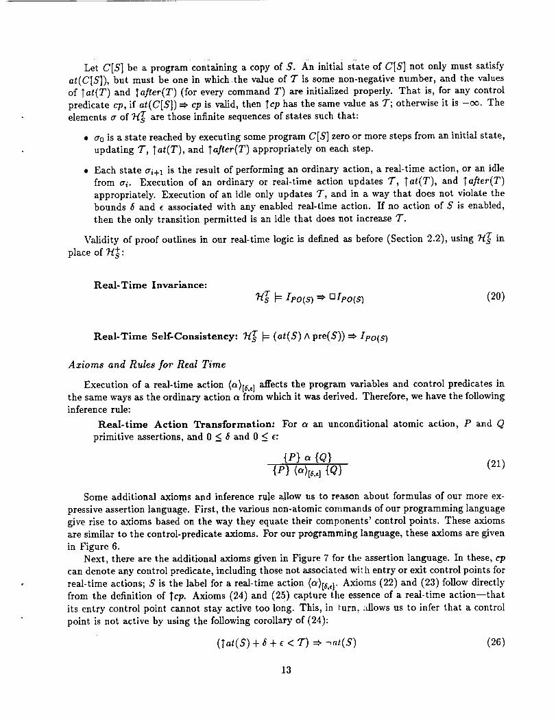
Let C[S] be a program containing a copy of S. An initial state of C[S] not only must satisfy

at(C[S]), but must be one in which the value of T is some non-negative number, and the values

of Tat(T) and Tafler(T) (for every command T) are initialized properly. That is, for any control

predicate cp, if at(C[S]) _ cp is valid, then Tcp has the same value as T; otherwise it is -_. The

elements a of 7-/s7 are those infinite sequences of states such that:

• a0 is a state reached by executing some program C[S] zero or more steps from an initial state,

updating T, Tat(T), and Tafler(T) appropriately on each step.

• Each state ai+l is the result of performing an ordinary action, a real-time action, or an idle

from a_. Execution of an ordinary or real-time action updates T, Tat(T), and Tarter(T)

appropriately. Execution of an idle only updates T, and in a way that does not violate the

bounds $ and _ associated with any enabled real-time action. If no action of S is enabled,

then the only transition permitted is an idle that does not increase T.

Validity of proof outlines in our real-time logic is defined as before (Section 2.2), using 7"/_ in

place of 7/+:

Real-Time Invariance:

Ipo(s) []I,,,o(s) (20)

Real-Time Self-Consistency: 7/_ _ (at(S) A pre(S)) =_ Ipo(s)

Axioms and Rules for Real Time

Execution of a real-time action (a)[6,,l affects the program variables and control predicates inthe same ways as the ordinary action a from which it was derived. Therefore, we have the following

inference rule:

Real-time Action Transformation:

primitive assertions, and 0 _< g and 0 _< E:

For a an unconditional atomic action, P and Q

{P} a {Q}

{P} {_)[6,,] {Q}(21)

Some additional axioms and inference rule allow us to reason about formulas of our more ex-

pressive assertion language. First, the various non-atomic commands of our programming language

give rise to axioms based on the way they equate their components' control points. These axioms

are similar to the control-predicate axioms. For our programming language, these axioms are given

in Figure 6.

Next, there are the additional axioms given in Figure 7 for the assertion language. In these, cp

can denote any control predicate, including those not associated wi'.h entry or exit control points for

real-time actions; S is the label for a real-time action (a)[&d. Axioms (22) and (23) follow directly

from the definition of Tcp. Axioms (24) and (25) capture the essence of a real-time action--that

its entry control point cannot stay active too long. This, in _urn, allows us to infer that a control

point is not active by using the following corollary of (24):

(tat(S) + + < 7) -.,.t(s) (26)

13

For S the sequentialcompositionS1S2Tat(S) =. Tat(Sx)

Tafter(S1) = Tat(S2)For an if command:

S: if BI"-*S1 0

Tat(S) =Tafter( S) =

T@_(¢Eval_f(S)) =

•.. DB,--,S,/tTat(GEvalif(S) )max(Tafier(S1), ... , Tafter(Sn))m_Lx(Tat(S1), ... , Tat(S,))

For a do command:

S: do BI_S1

Tat(CEV_o(S)) =Tafter(GEvalao(S)) =

-,in(s) =,at(S) :*in( Si ) :_

after(S) :_

"'" BB,_---.S. od

max (Tat(S), Tafter(S,),..., Tafter(Sn))

max(Tafter(S), Tat(S1),..., Tat(S,_))

Tarter(S)- Tafter( GEvalao( S) )

Tat(S)- Tat(GEvaldo(S))

Tat( Si) = Tafter( GEvaldo( S) )

lafter(Si) = Tat (GEvaldo(S))

For a cobegin command:S:

Tat(S)

Tafter( S)

cobegin $1 ff'"ffSn coend

= Tat(S1) = Tat(S2) =."= Tat(Sn)

= max (Tafler(S1), ... , tafter(S,_))

Figure 6: Control Time Axioms

The way these new terms change value when atomic actions execute is captured by new axioms.

For any ordinary or real-time atomic action a and control predicate cp, we have:

cp Invariance {cp = C ATcp = V} a {(cp =,. C) =_ (Tcp= V)} (27)

The antecedent in the postcondition is necessary for the case where cp could become true when a

finishes, e.g., cp = after(a).

Next, for any ordinary action, we have:Action Time Axioms:

{K < Tat(S)} S: a {K < Tafter(S)} (28)

{K _< T} S: a {K _< Tarter(S)} (29)

Action Time Axiom (28) asserts that the exit control point for S becomes active after the entry

control point for S last became active. Action-time Axiom (29) makes the subtly different assertion

tcp <_ 7- (22)

(Tcp=-o¢) =_ ",ep (23)

at(S) _ Tat(S)_<7"<Tot(S)+_+• (24)

Tat(S) # -_ _ Tafier(S)<TatCS)+,5+e (25)

Figure 7: General Real-Time Axioms

14

that theexit controlpoint for S becomes active after every time that the entry control point for S

was active.

For a real-time action (a}[_,c], the following axiom characterizes how execution changes the

Tcp-terms.

Real-time Action Axiom {K _< Tat(S)} S: (a)[_,c] {K + _ <_ Tafler(S)} (30)

This axiom is analogous to Action-time Axiom (28), except that now the postcondition has been

strengthened to give a tighter lower-bound on when the exit control point for S first becomes active.

Two things that the Real-time Action Axiom (30) does not say are worthy of note. First, thisaxiom does not bound the interval during which the entry control point for S is active; Axiom (24)

serves that role. Second, one might expect the following triple to be valid--its precondition being

similar to that of (29).

{K _< 7"} S: <a)[6,_] {K + e < 7"} (invalid) (31)

Unfortunately, (31)is not sound. Execution of S started in a state such that Tat(a) < K < 7" would

satisfy the precondition but might terminate before K + e. For example, consider an execution of

(a)[o,2] that is started at time 0. Thus, at time 7" = 1 the state satisfies K < 7" if we choose K = 1,and so precondition K < 7" is satisfied by that state. When execution of (a)[o,2] terminates--2units after it is started--at time 7" = 2, the postcondition K + _ < 7- is 1 + 2 < 2, which is false.

Finally, the following rule allows rigid variables to be instantiated with expressions involving

[cp-terms. (Rigid Variable Rule (4) only allows rigid variables to be instantiated by constants,

rigid variables, or expressions constructed from these.)

Tcp-Instantiation {Tcp= V} a {Tep = V}, {P} a {Q} (32)

This rule is typically used along with cp Invariance (27). For the case where real-time action

a and control predicate cp are in different processes, the first hypothesis of l"ep-Instantiation is

automatically satisfied due to Process Independence Axioms (16). Thus, we obtain a derived rule

of inference:

Derived Tcp-Instantiation

a and cp are in different processes,

{P} a {Q} (33)

3.3 Rule of Consequence Revisited

Most of the axioms and proof rules of Proof Outline Logic are sound in our real-time setting.

However, the Rule of Consequence (2) is unsound and needs revision. We also need to revisethe notion of interference freedom. While the Owicki-Gries cobegin rule [12] is sound, when the

assertion language concerns real time, the rule is is no longer complete and, in particular, not

powerful enough for even simple examples of concurrent real-time programs.Rule of Consequence (2) is invalid in any setting where some aspect of the state is not under

program control. Recall, the rule is:

15

MaxIdle(a)MaxIdle((a)[_,d)MaxIdle(S1$2)

MaxIdle(if • • -fi)

MaxIdte(do... od)

MaxIdle(do[_,,]... od)MaxIdle(cobeginS1//I...//S_ coend)

= oo a ordinary

= $+e

= MaxIdle(S1)

---- OO

"-- OO

= _+e

= min{MaxIdle(Si)[i = 1,...,n}

Figure 8: Definition of Maxldle(S), the maximum idle of S

P'_ P, {P} PO(S) {Q}, Q ::¢.Q'

{P'} PO(S) {Q'}

The difficulty is illustrated by the following example. Consider the following proof outline, which

is valid in our model:

{7" > 4) S: skip {true} (34)

Furthermore, note that(7" = 4) =} (7" _> 4) (35)

is valid. However, if we apply the Rule of Consequence to (34) and (35), we obtain the following

proof outline:{T = 4} S: skip {true} (36)

It is invalid because an idle by the environment invalidates its precondition, T = 4. In particular,

let 7 be a state in which at(S) A 7" = 4 is true. Therefore, the precondition of (36) is satisfied by

7, and so is Ipo(s). An idle can lead to a state 7' in which at(S) ^ 7- = 4.01, invalidating Ipo(s)-Thus the proof outline does not satisfy Real-Time Invariance (20), and hence is not valid.

We eliminate problems of this sort by modifying Rule of Consequence (2) so that idles cannot

invalidate a strengthened precondition P_. In light of (36), an obvious approach is to rule out any

strengthening of preconditions achieved by placing an upper bound on T. However, that restriction

would prevent us from deriving the valid triple

{Tat(S) = 4 ^ 4 < T <_ 6} S: sklp[0,2 ] {true}. (37)

We therefore characterize the interval over which a strengthened precondition P' must not be

invalidated by an idle. For any program S, define MaxIdle(:;) (ma_mum idle time for S) to be the

longest real time interval that can elapse after at(S) becomes true but before some program action

of S must be executed. If S may idle arbitrarily tong, then MaxIdle(S) = c¢. Figure 8 gives a way

to calculate MaxIdle(S) by induction on the structure of S.

For example,

MaxIdle(skip) =

as skip can walt arbitrarily long before taking a step, and

Maxldle(cobegin skip//(sklp)[0,2 ] coend) = 2

16

as that program will necessarily take a step at or before time 2. In order for Rule of Consequence

(2) to be sound, not only must P'=c,P hold but P' must remain true until time Tat(5,)+MaxIdle(5").

We say that an assertion P is patient for 5, if

(P ^ (Va.CT< d <_Tat(5')+ M Idle(5,)) (38)

Thus, if P' is patient for 5,, then P' can be a precondition for 5, and no idle by 5' can invalidate

P'. For example, 4 < T < 6 is patient for <skip)[0a 1, but 4 < T < 5 is not. A corollary of the way

_ is constructed is that the precondition of any valid proof outline P0(5,) is patient for 5'.Note that under some circumstances P' is easily demonstrated to be patient for 5':

• If P' does not mention 7".

• If P' only gives lower bounds on 7".

However, even assertions involving upper bounds on 7" can be patient. For example,

Tat(5') = 4 ^ 4 < 7" _<6

is patient for S : skip[0,21.A sound Rule of Consequence for our real-time logic can be formulated in terms of patient

assertions:

Rule of Consequence:

P' =_ P, P' is patient for 5,, {P} PO(5,) {Q}, Q =_Q'

{P'} PO(5,) {Q'}(39)

So, because 7" = 4 is not patient for skip, it is not possible to deduce (36) from (34) and (35)

using this new Rule of Consequence. On the other hand, because

(Tat(5")=4 A 4 < 7" <_ 6 )=_ 7" =2_4 (40)

is valid and Tat(S) = 4 A 4 < T < 6 is patient for skip[0al, we can use the Rule of Consequence

(39) to infer

{Tat(5") = 4 A 4 <_ 7- <_ 6} skip[0,2 ] {true} (41)

Note that we do not need to place similar restrictions on Q'. The interpretation of {P} PO(5,) {Q}

is that, when S finishes, Q remains true indefinitely. If Q =_ Q' in predicate logic, and Q remains

true forever, then Q' will also remain true forever.

The following derived rule, the Simple Rule of Consequence, handles most of the bookkeeping

uses of the Rule of Consequence (39):

Simple Rule of ConsequenceP'=P, {P} PO(5,){Q}, Q=_Q'

{P'} PO(5,){Q'} (42)

17

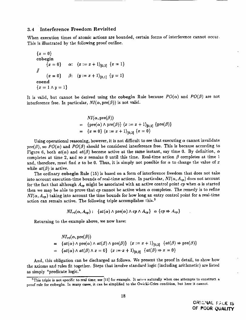
3.4 Interference Freedom Revisited

When execution times of atomic actions are bounded, certain forms of interference cannot occur.

This is illustrated by the following proof outline.

{x = O}cobegin

{x = 0} a://

{z=O}coend

{z= l^y= 1}

(x := x +1)[0,2] {x= 1}

(y:--x+l)[o,1] {y-- 1)

It is valid, but cannot be derived using the eobegin Rule because PO(a) and PO(_) are not

interference free. In particular, NI(a, pre(_)) is not valid.

NI(a, pre(_))

= {pre(a) ^ pre(_)} (x := z + 1)[0,2] {pre(f_)}

= = o} :=x+ i>[o, i{x= o}

Using operational reasoning, however, it is not difficult to see that executing a cannot invalidate

pre(f_), so PO(a) and PO(fl) should be considered interference free. This is because according to

Figure 6, both at(a) and at(fl) become active at the same instant, say time 0. By definition, a

completes at time 2, and so x remains 0 until this time. Real-time action fl completes at time 1

and, therefore, must find x to be 0. Thus, it is simply not possible for a to change the value of x

while at(fl) is active.The ordinary eobegin Rule (15) is based on a form of interference freedom that does not take

into account execution-time bounds of real-time actions. In particular, NI(a, An, ) does not account

for the fact that although A n, might be associated with an active control point cp when a is started

then we may be able to prove that cp cannot be active when a completes. The remedy is to refine

NI(a, Ao, ) taking into account the time bounds for how long an entry control point for a real-timeaction can remain active. The following triple accomplishes this)

NI,t(a,A_): {at(a)Apre(a)AcpAA_} a {ep_ Ao,}

Returning to the example above, we now have:

NIr,(a,pre(fl))

= {at(a)^ pre(a)^ at(_) ^ pre(fl)} (z := z + 1)[o.2]{at(fl)=_ pre(_)}

= {at(a) Aat(13)hx=O) (x:-----x+l)[o,2] {at(_)=_x=O}

And, this obligation can be discharged as follows. We present the proof in detail, to show how

the axioms and rules fit together. Steps that involve standard logic (including arithmetic) are listed

as simply "predicate logic."

5This triple is not specific to real time; see [11] for example. It atis(,s naturally when one attempts to construct a

proof rule for cobegln. In many cases, it can be simplified to the Owicki-Gries condition, but here it cannot.

18

OR._,"_Yi,-LF;._E I,.'.'.S

OF POOR QUALITY

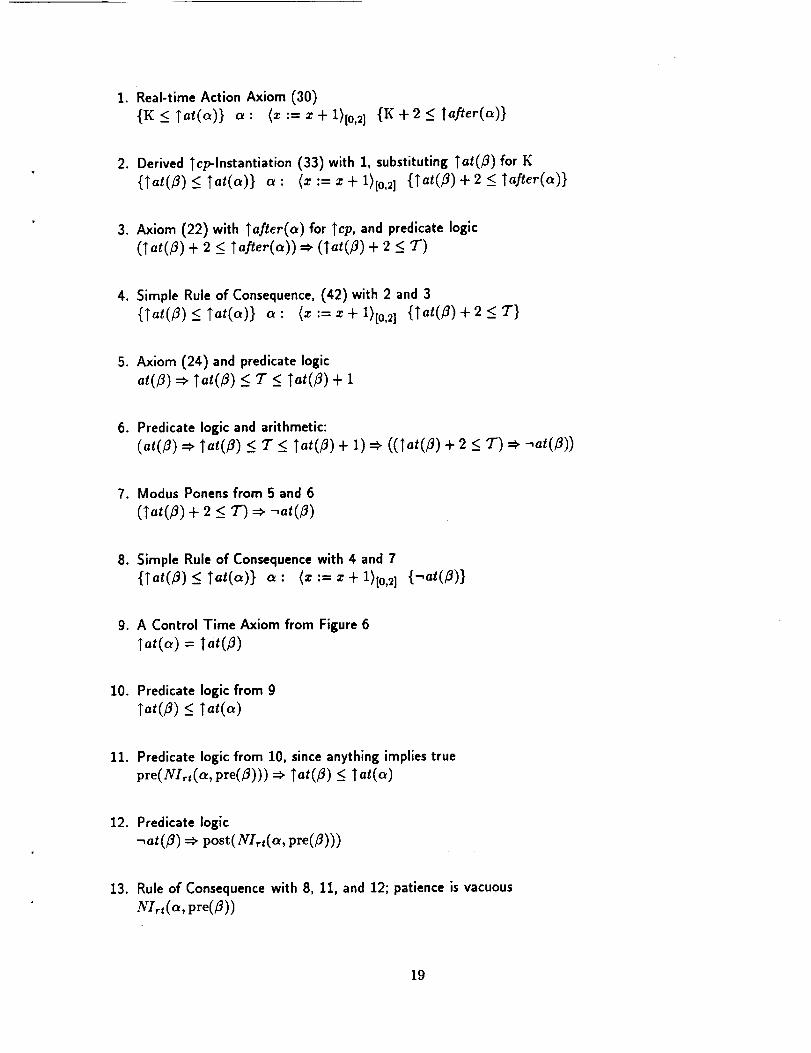
1. Real-time Action Axiom (30)

{K _<Tat(a)} a: {_ := x + 1)[0,2]{I_ + 2 _<Tafter(a)}

2. Derived TepInstantiation (33) with 1, substituting Tat(E) for K

{Tat(_) _< Tat(a)} a : <z := z + 1)[o,21 {Tat(E) + 2 _< Tafter(a)}

3. Axiom (22) with Wafter(a) for Tcp, and predicate logic

(Tat(E) + 2 < Tafter(a)) =_ (Tat(E) + 2 _<7")

4. Simple Rule of Consequence, (42) with 2 and 3

{Tat(/3) _< Tat(a)} a : (x := z + 1)[o,_] {Tat(/_) + 2 _<7-].

5. Axiom (24) and predicate logic

at(E) :* Tat(E) < 7" <. Tat(E) + 1

6. Predicate logic and arithmetic:

(at(#)_ Tat(�9) <_ T <_ Tat(E)+ 1)_ ((Tat(_) + 2 _< T)=_-,at(_))

7. Modus Ponens from 5 and 6

(Tat(_) + 2 _ 7")=_-_at(_)

8. Simple Rule of Consequence with 4 and 7

{Tat(E) < Tat(a)) a : (a: := z + 1)[o,21 {-,at(E)}

9. A Control Time Axiom from Figure 6

lat(a) = Tat(E)

10. Predicate logic from g

Tat(/3) _< Tat(a)

11. Predicate logic from 10, since anything implies true

pre(NI_t(a, pre(/3))) =_ Tat(fl) <_ Tat(a)

12. Predicate logic

-,at(E) ::*"post( NIrt(a, pre(/3)))

13. Rule of Consequence with 8, 11, and 12; patience is vacuous

NIrt(a, pre(fl))

19

Noticethat information about the time after a is accumulated in steps 4 and 5, and used in

step 6 to reach the same conclusion that operational reasoning gave: that, once a finishes,/_ hasalso finished.

4 Example: A Mutual Exclusion Protocol

cobeginb:ifx =0--+ c:

d: (skip/[8(d),c(d) ]

e : ifx = 1 -. f:

//b_ : ifx = 0 --+ d:

d' : (skip) [_(d,),c(d,)]e':ifz=2_f':

coend

(z := 1)[s(c),,(c)] fl

Critical Section fi

(z := 2)[6(e),,(e)] fl

Critical Section fi

Figure 9: Core of Fischer's Mutex Protocol

Knowledge of execution times can be exploited to synchronize processes. A mutual exclusion

protocol attributed in [10] to Mike Fischer [4] illustrates this point. The core of this protocol

appears in Figure 9. There, c, d, c_ and d _ are real-time actions. Provided the parameters defining

these real-time actions satisfy

$(c') + ¢(c') < E(d) (43)

and

6(c) + E(e) < e(d') (44)

this protocol implements mutual exclusion of the marked critical sections, as we now show.

Mutual exclusion of at(f) and at(f') is a safety property. It can be proved by constructing a

valid proof outline in which pre(f) _ -,at(f') and pre(f') =_ -at(f). g standard approach for this

is to construct a valid proof outline in which -(pre(f) A pre(f')) is valid. It is thus impossible for

at(f) A at(f') to hold, because that would imply pre(f) A pre(f').

A proof outline for the first process is given in Figure 10; the proof outline for the other process is

symmetric, with "1" everywhere replaced by "2" and the primed labels interchanged with unprimed

ones. Notice that pre(f)=_x = 1 and pre(fl)=_x = 2. Thus, the proof outlines satisfy the conditions

just outlined for ensuring that states satisfying at(f) A at(f) cannot occur.

It is not difficult to derive the proof outline of Figure 10 using the axiomatization of real-

time actions given above. The proofs of {pre(c)} c {post(c)) and {pre(d)} d {post(d)) are the

most enlightening, as they expose the role of assumptions (43) and (44) in the correctness of the

protocol. Here is the proof of {pre(c)) c {post(c)}:Let

M = t3(c') + e(c') - e(d)

1. Axiom (29)

(K _<T) c: := {K _<

20

true}

b: ifx=O --* {Tat(c') <_ T}

c: (z := 1)[6(c),,(c)l

{= # OA(atte)=_,Tat(e)+ M < Tat(d))}fl

{= # oA(at(e)=. Tat(e)+ M < Tat(d))}d: (skip)[_(d),,(d)l

{= # oA-_at(c')}e: ifz = 1 -- {z = 1A--,at(c')}

f: Critical Section 1

{true}fi

{true}

Figure 10: Proof Outline for Fischer's Algorithm

2. Derived Tcp-Instantiation, (33), on step 1, to substitute Tat(c') for K

{Tat(cO < 7"} c: (= := 1)[_(=),4_)] {Tat(cO < fafter(c)}

3. Control Time Axiom (Figure 6) for if and sequencing

Tatter(c) = Tat(d)

4. Predicate logic on step 3, and M < 0 by (43)

(tat(c') < tafler(c)) =¢, (tat(c 0 + M < Tat(d))

5. Predicate logic on step 4

Tat(c') < Tatter(c) =_, (at(cO_ (Tat(c') + M < Tat(d)))

6. Simple Rule of Consequence (39) on steps 2 and 5

{Tat(c') < 7"} c: (= := t)[6(c),,(_)] {at(c') =_ (Tat(cO+ M < Tat(d))}

7. Assignment Axiom (8)

8. Predicate logictrue =_ (1 = 1)

9. Predicate logic

x=l=_z#0

21

10. Rule of Consequence, (39) on steps 7, 8, and 9, since true is patient for c.

{true}c: (x :- 1)[6(c),,(c)]{x _ 0}

11. Conjunction Rule (5) on steps 10 and 6, plus a trivial use of the Rule of Equivalence (3).

{Tat(c')< T} c: (x:=i)v(c),_(c)]{x# 0^(at(c')_ Tat(_')+ M < Tat(d))}

And, here is the proof of {pre(d)} d {post(d)}.

I. Real-time Action Axiom (30)

{K < Tat(d)} d: (skip)t_(a),,(d) ] {K + e(d) _< Tafler(d)}

2. skip Axiom (7)

{L < K} d: (skip)[6(a),,(d)]{L < K}

3. Conjunction rule (5) on steps 1 and 2

{L < K A K _<Tat(d)}d: (skiP)t6(d):(d)]{L < K ^ K + e(d)_<Tafler(d)}

4. Predicate logic

(L < K A (K + e(d) _< TaS%r(d))) _ (L + e(d) < Tas%r(d))

5. Rule of Consequence (39) on 3 and 4, noting that the precondition does not mention time and is

thus patient.

{L < K < Tat(d)} d: (skip)[6(d),,(d) ] {L + ((d) < Tafler(d)}

6. cp Invariance axiom, (27)

{at(d)= C ^ Tat(d)= V} d: (skip)[_(d):(d)] {(at(d)=> C) _ (Tat(d)= V)}

7. RigidVariableRule (4)on 6, replacingC by true

{at(d) = true A Tat(d)= V} d: (skiP)t_(d),e(d)] {(at(d):_ true)=_ (Tat(d)= V)}

8. Rule of Equivalence (3) on 7

{Tat(d)= V} d: (skip)[6(d),,(d)] {Tat(d)= V}

9. Tcp-Instantiation (32) using 8 and 5 to substitute Tat(d) for K.

{L < Tat(d) <_ Tat(d)} d: (skip)[6(d),c(d)] {L + e(d) < Tarter(d)}

10. Rule of Equivalence (3) on 9

{L < Tat(d)} d: (skip)[6(d),((d)] {L + e(d)< Tarter(d)}

22

11. Derived Tcp-lnstantiation (33), and Rigid Variable Rule (4), to substitute Tat(c') + M for L in 10

{Tat(d) + M < Tat(d)} d: (sklp)[_(d),,(d) ] {Tat(d) + M + ,(d) < Taftev(d)}

12. Process Independence Axiom (16), Rigid Variable Rule (4), and Rule of Equivalence (3)

{-,at(c')} d: (sklp)[6(d),_(d) ] {-,at(c')}

13. Disjunction rule (6) on steps 11 and 12

{-_at(c') v (Tat(d)+ M < Tat(d))} d: (skip)[6(a),,(d) ] {--,at(d)V (tat(d)+ M + <(d) < Tafler(d)) }

14. Rule of Equivalence (3) on 13

{at(c') =:, (Tat(c') + M < Tat(d))} d: (skip}[8(d),,(d) ] {--,at(c') v (Tat(c') + M + E(d) < Tarter(d))}

15. Axiom (22)

Taper(d) < T

16.

--,at(d) v Tat(c') + E(c') + ,5(c') < Tafler(d)

Predicate Logic from step 15

--,at(c') V (Tat(d) + e(c') + _5(c') < T)

=_ Equation (26)

--,at(d) V--,at(d)

=_ Predicate Logic

-at(c')

17. Simple Rule of Consequence (42) on steps 14 and 16

{at(c') :_ (Tat(d)+ M < Tat(d))} d: (skiP)ts(d),,(a) 1 {-,at(d)}

18. skip Axiom (7)

{x # O} d: (skip)[6(d),,(d) ] {x # O}

19. Conjunction Rule (5) on steps 18 and 17

{x #0 A (at(c')=_ (Tat(c')+ M < Tat(d)))} d: (skip)[,(d),{(a) ] {x #0 A _at(c')}

Notice how timing information is used in step 16 to infer that a particular control point cannotbe active.

5 Related Work

It is instructive to compare our logic with that of [17], another Hoare-style logic [7] for reasoning

about execution of real-time programs. In [17], the passage of time is modeled by augmenting each

atomic action with an assignment to an interval-valued variable RT, so that RT contains lower and

23

upperboundsfor the program's elapsed execution time. The equivalent of our Command Composi-

tion Rule (9) and the Assignment Axiom (8) would then be used to derive rules for reasoning about

these augmented atomic actions. 6 In contrast, our logic is obtained by augmenting the assertion

language (of an underlying logic of proof outlines) with additional terms (Tcp and T) and devising

new axioms for reasoning about these terms. We cannot derive rules for real-time actions simply

by using the original logic, because we do not employ assignment commands to model the passageof time.

Although our logic is more complex, by augmenting the axioms rather than the atomic actions

we are led to a more powerful logic. First, having the Tcp-terms allows the logic to be more expres-

sive. These terms permit the definition of properties involving historical information--information

that is not part of the current state of the program. Timing properties that constrain the elapsed

time between events can only be formulated in terms of such historical information. The logic of

[17] has no way to express historical information and, consequently, can be employed to reason

about only certain timing properties.

Second, our axiomatization allows reasoning about programs whose timing behavior is data-

dependent. The logic of [17] does not permit such reasoning. For example, because of the way

command composition is handled in [17], the logic produces overly-conservative intervals for time

bounds. This is illustrated by the following sequential program, which takes at least 10 time units

to execute.ifB _ skip[0,9 ] _--B _ skip[0,1lfi

if-B _ skip[0,9] _ B ---*skip[0,1lfi

This fact can be proved in our logic; the logic of [17] can prove only that execution requires at

least 18 time units.

A Hoare-style programming logic for reasoning about real-time is also discussed in [8]. That

work is incomparable to ours. First, the programming language axiomatized in [8] is different,

having synchronous message-passing and no shared variables. This is symptomatic of a fundamental

difference in the two approaches. The emphasis in [8] is on the design of compositional proof

systems. Shared variables could not be handled compositionally and so they are excluded from

programs. In contrast, we do not require that our proof system be compositional, and we dohandle shared variablesJ Moreover, it would not be difficult to extend our logic for reasoning (non-

compositionally) about programs that employ synchronous message-passing or any of the other

communication/synchronization mechanisms for which Hoare-style axioms have been proposed.

The set of properties handled in [8] is also incomparable to what can be proved using our

logic. Our timing properties make visible the times at which control points become active (through

l"cp-terms). A compositional proof system cannot include information about control points in its

formulas, because they betray the internal structure of a component. The logic of [8], therefore, may

only be concerned with times at which externally visible events occur: the time of communications

events and the time that program execution starts and terminates. This turns out to allow proofs

of certain liveness properties as well as certain safety properties. Our logic cannot be used to prove

any liveness properties other than those implied by the progress of time.

eThe idea of augmenting actions with assignment commands in order to reason about the passage of time is alsodiscussed in [5], where it is used to extend Dijkstra's wp [3] for reasoning about elapsed execution time. A morerecent effort to augment a wp calculus for real time is reported in [16].

7The cobegin Rule of Proof Outline Logic (15) is not compositional because its interference-freedom test dependson the internal structure of the processes being composed.

24

6 Concerns

A concern when designing a logic isexpressive completeness. Our timing properties include many,

but not all, safety properties of interest for reasoning about the behavior of real-time programs.

This is because the historical information in a timing property is limited to times that control points

become active. One might also be concerned with the elapsed time since the program variables last

satisfied a given predicate or with satisfying constraints about how the program variables change

over time. These are safety properties, but neither is a timing property (according to our definition).

In general, safety properties can be partitioned into invariance properties and history properties

[15]. The invariant used in proving an invariance property need only refer to the current state; the

invariant used in proving a history property may need to refer to the sequence of states up to the

current state. Timing properties are a type of history property.

A version of Proof Outline Logic does exist for reasoning about history properties [15]. It

extends ordinary Proof Outline Logic by augmenting the assertion language with a "past state"

operator and a function-definition facility. In this logic, our l_cp-terms can be constructed explicitly;

they need not be primitive. And, the more general class of safety properties involving times--be it

times that predicates hold or times that control predicates hold--can be handled.

A Outline of the Soundness Proof

A.1 Scheme of the Proof

Our soundness proof has a straightforward structure. First we build a model, using structural

operational semantics (SOS) [13, 18, 6]. We then show how to interpret expressions and formulae

of the logic in this model. Using the model, we define the set of execution sequences _ used to

define validity in Section 3.2. We prove a series of "sanity lemmas," showing that the intuitive

definitions presented earlier match the formal definitions. Finally, we check each of the axioms and

proof rules against the model.

The most subtle part of the construction is in building the model. Checking the axioms and

proof rules is long but straightforward. In our model, we give a structural operational semantics

for our programming language. States 7 include all of the information necessary to interpret Proof

Outline Logic assertions. And, the operational semantics define the relation 7 "* 7', stating that a

program in state 7 can perform a single atomic action, or can idle, and enter state 7'.

Using ,--_, we construct a linear-time temporal-logic model of a program S; that is, a set of

infinite sequences F of states. We define a notion of "7 is a suitable initial state for S'. We get an

arbitrary consistent state 7o by running an arbitrary suitable initial state 7 for 5' arbitrarily long,

7 "_" 7o. _ is then the set of executions of S started in arbitrary consistent states 70.

Having defined _s7, we have have enough information to use the definition of Section 3.2 that

PO(S) when 7/_ _= Ipo(s) _ nIpo(s). Tiffs puts us in a position to check the soundness of thelogic, which is tedious but not difficult.

A.2 Defining the transition relation

Defining relation _ is nontrivial. The values of control predicates, especially at the beginning

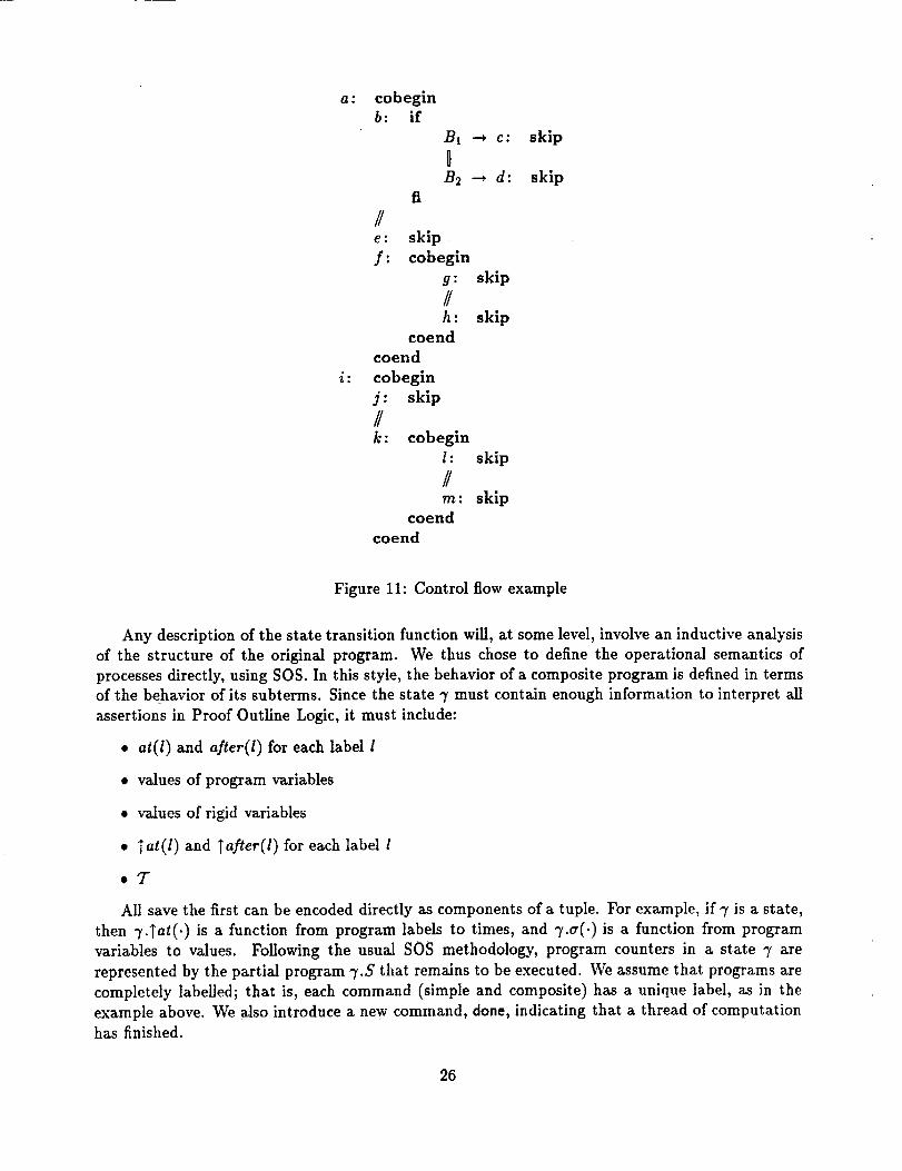
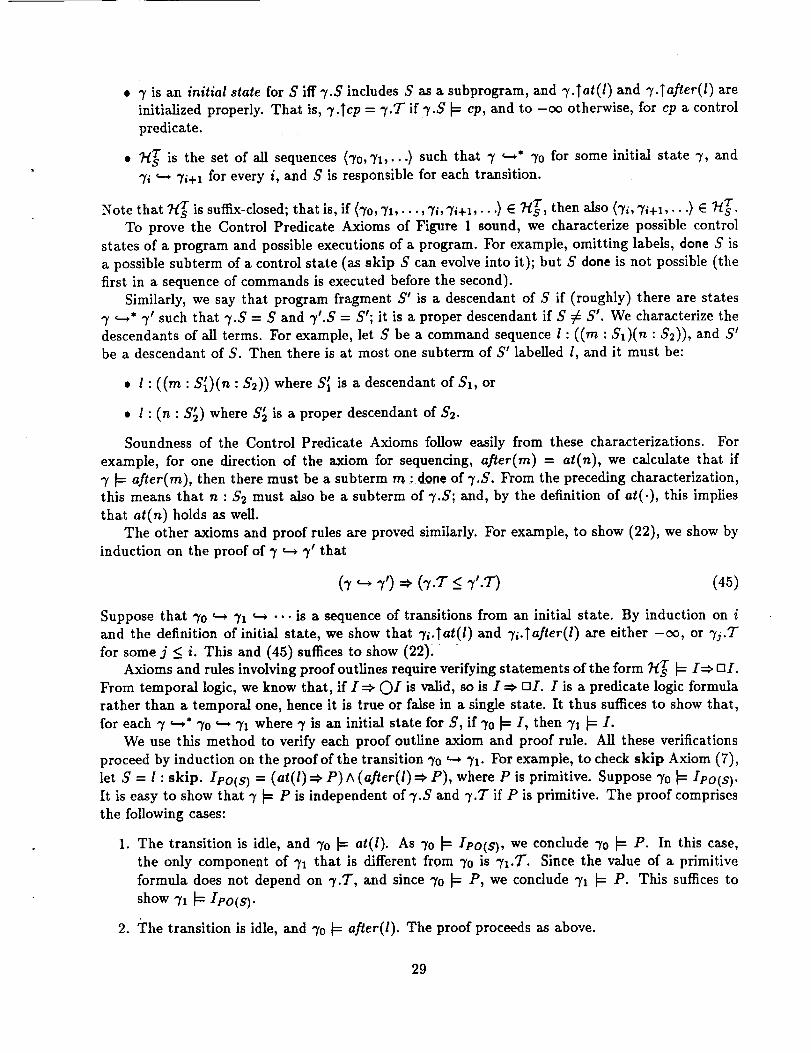
and end of concurrent segments, change in fairly complicated ways. Consider the program of

Figure 11. When the cobegln labelled a finishes, after(c) or after(d) will hold as well as after(g)

and after(h); and at(j), at(l), and at(m). A single atomic action m say, g finishing -- may cause

other actions at faraway points in the program to start. Or it may not.

25

a: cobeginb: if

B1 _ ¢:

DB2 --* d:

fl

//e : skip

f : eobegin

g : skip

//h : skip

coend

coend

i : cobegin

j : skip

//k : cobegin

l : skip

//m : skip

coend

coend

skip

skip

Figure 11: Control flow example

Any description of the state transition function will, at some level, involve an inductive analysis

of the structure of the original program. We thus chose to define the operational semantics of

processes directly, using SOS. In this style, the behavior of a composite program is defined in termsof the behavior of its subterms. Since the state 7 must contain enough information to interpret all

assertions in Proof Outline Logic, it must include:

• at(1) and after(1) for each label I

• values of program variables

• values of rigid variables

• Tat(l) and Tafter(1) for each label 1

•7"

All save the first can be encoded directly as components of a tuple. For example, if 7 is a state,

then 7.Tat(') is a function from program labels to times, and 7.a(-) is a function from program

variables to values. Following the usual SOS methodology, program counters in a state 7 are

represented by the partial program 7.S that remains to be executed. We assume that programs are

completely labelled; that is, each command (simple and composite) has a unique label, as in the

example above. We also introduce a new command, done, indicating that a thread of computation

has finished.

26

We now define the relation 7 _ 7' by induction on 7.S. By in large, if 7 _ 3", then 7 and 7'

are almost the same; e.g., most variables won't change values. We therefore present the SOS rules

by explaining the differences between 7 and 7'. s For example, if 7.S is the program I : skip, then

the operational rule which applies to 7 is:

If

7.5" = l : skip

3".S = l : done

7 '.7- > 7.7-

7 _ is otherwise the same as 7

Then 7 _-_ 7'

The behavior of a composite process is determined inductively by the behavior of its snbpro-

cesses. For example, cobegin $1//'"//Sn coend can act if one of the Si's can act without exceeding

the time bounds of the other Sj's. This happens if there is a state 7o in which the program is simply

the Si that performs the the transition. Thus, the rule for cobegin is roughly:

If

7.5" = cobegin $1//'"//Sift"'//Sn coend,

3'.S' = cobegin $1//" .//S_//...//Sn coend,

where 33'0, 7_ such that:

7o.S = Si

3'0 is otherwise the same as 3'

3'0 _ 3'_

No other component of 3'.S is required to act before 3'_.7-

s' = 3' .s3" is otherwise the same as 3'_

Then 3' '--+ 3"

Of course, the English antecedents are made formal.

Idle actions axe described by:

If

3".7" >_ 3".7"

3'.S is not required to act before 3".T

7' is otherwise the same as 7

Then 7 '-* 3'_

One important consequence of using a structural operational semantics is that 3' _ 3" iff there

is a proof of 3' '-* 7' from the operational rules. These proofs can be regarded as formal objects,

and, in particular, we can do induction on the proof that 3' '--+ 3". Many of the basic lemmas used

for soundness proceed by such inductions.This discussion omits subtleties that are essential to the proof. For the model construction, the

actual proof rules assign responsibility for the transition, so that when we define 7_ we can ensure

that S takes all the transitions in 7_. Roughly, a subterm S' of the program 3'.S is responsible for

the transition 7 "-+ 3" if S' appears as 70.S in the proof of 3' '-_ 7' or if the transition is idle. The

determination of which processes are finished requires some care. For example, done is a finished

atomic process, but there are also others, such as eobegin done//done eoend. While the intuition

is reasonably stra_ghtforwaxd, the details axe delicate.

Sin the full proof, we use a more standard SOS notation, which makes the structural induction clearer but requires

extra notation.

27

A.3 Interpreting Expressions and Formulae

The meanings of most expressions and formulae can be read directly from the state 3'. For example,

the value of the expression x + y in state 3' is the sum of 3'.a(x) and 3'.a(y). However, the values of

control predicates at(l) and after(l) depend on the control state 3'.S of the program. In this section,

we sketch the interpretations of these predicates for the case when I is the label of an atomic action.

Let 3' be a state in an element of 7_s_. Interpreting after(l) where 1 is the label of an atomic

action is straightforward; 3'.S includes a subterm of the form l : done if and only if the atomic

action labelled t in 3'.S is finished.We define the set of active atomic actions of a program S inductively; e.g., if S is atomic,

act(s) = (s}, e.0.

act(cobeginS1 ft...//Sneoend)

if $1 is not finished, act(SIS2)

if $1 is finished, act(SIS2)

= Ui act(SO= act(S1)= act(S )

Then 3, _ at(1) if I is the label of an atomic action in act(3'.S). In the actual proof, we allow at(l)when l is the label of any program, not just the label of an atomic action. This complicates the

definition of act somewhat and requires use of an extra set of markers in the operational semantics.

However, it allows us to verify the Proof Outline Logic control predicate axioms without having

built them directly into the definition of 3' _ at(1).

A.4 Sanity Checking

We demonstrate that the operational semantics and notion of interpreting processes are reasonable

by proving a series of sanity lemmas. These are lemmas that are not necessarily used in the

soundness proof proper but show that the formal definitions derived from the operational semantics

agree with the less formal ones used in the body of this paper. The following sanity lemma, for

example, shows that the intuitive definition of Tat(l) as the last time that at(1) became true agrees

with the formal definition of Tat(l) as it appears in the operational semantics:

Let 3'o be a suitable initial state, and 7o _ 71 '--* "" ". Then, for any index i and

label l, 7i.Tat(l) is:

• -c_ if (V0 < j < i : 3'./_ at(l))

• 3'./.7" if j is the largest 0 < j < i such that (3'./-1 _ at(l) and 7./_ at(1)).

• 3'o.T, if neither of the preceding conditions obtains; that is, if 3'0 _ at(1) but

(/3j : 7./I¢: at(l) ^ 7./+_ _ at(l)).

That is, the time that the bookkeeping mechanism gives for Tat(l) is in fact the value of the clock

on the most recent instant that at(l) became true.

A.5 Soundness

Once the SOS rules have been constructed and their sanity checked, it is a routine matter to show

soundness of all the Real-Time Proof Outline Logic axioms and proof rules. We define the model

7-/s7 in the following way. We consider executions starting with S in an arbitrary state of control

and memory. We allow other processes in this initial state as well. We thus consider executions

that start with some program that includes S; we run this program for a time (which gives an

arbitrary state, perhaps with S partially executed). However, in the sequences in 7-/s7, only S is

allowed to take steps, so S must be responsible for each transition.

28

• 7 is an initial state for S iff 7.S includes S as a subprogram, and 7.Tat(l) and 7. Tafter(1) are

initialized properly. That is, 7.Tcp = 7.7" if 7.,5" _ ep, and to -co otherwise, for cp a control

predicate.

• _ is the set of all sequences (70,71,...) such that 7 '--'* 7o for some initial state 7, and

71 _ 7/+1 for every i, and S is responsible for each transition.

Note that 7_ is suffix-closed; that is, if (7o, 71,..., 7, 71+1,...) E 7_, then also (7i, 71+1,...) E _.

To prove the Control Predicate Axioms of Figure 1 sound, we characterize possible control

states of a program and possible executions of a program. For example, omitting labels, done S is

a possible subterm of a control state (as skip S can evolve into it); but S done is not possible (the

first in a sequence of commands is executed before the second).

Similarly, we say that program fragment S' is a descendant of S if (roughly) there are states

7 '--'* 7 _ such that 7.S = S and 7'.S = S'; it is a proper descendant if S _ S'. We characterize the

descendants of all terms. For example, let S be a command sequence l : ((m : St)(n : $2)), and S'

be a descendant of S. Then there is at most one subterm of S' labelled l, and it must be:

• I: ((rn: S'l)(n : S2)) where SI is a descendant of $1, or

• I : (n : S_) where 81 is a proper descendant of $2.

Soundness of the Control Predicate Axioms follow easily from these characterizations. For

example, for one direction of the axiom for sequencing, after(m) = at(n), we calculate that if

7 _ after(m), then there must be a subterm m : done of 7.S. From the preceding characterization,

this means that n : $2 must also be a subterm of 7.S; and, by the definition of at(.), this implies

that at(n) holds as well.

The other axioms and proof rules are proved similarly. For example, to show (22), we show by

induction on the proof of 7 _-* 7 _ that

(7 _-" 70 _ (7.7" -< 7'.7") (45)

Suppose that 70 _ 71 "-' "'" is a sequence of transitions from an initial state. By induction on i

and the definition of initial state, we show that 7i.Tat(1) and 7i.Tafter(l) are either -oo, or 7j.7"

for some j _< i. This and (45) suffices to show (22):Axioms and rules involving proof outlines require verifying statements of the form 7_s_ _ I_ hi.

From temporal logic, we know that, if I _ C)I is valid, so is 1:0 rnI. I is a predicate logic formula

rather than a temporal one, hence it is true or false in a single state. It thus suffices to show that,

for each 7 "-'* 70 _ 71 where 7 is an initial state for S, if 70 _ I, then 71 _ I.

We use this method to verify each proof outline axiom and proof rule. All these verifications

proceed by induction on the proof of the transition 7o _ 71- For example, to check skip Axiom (7),

let S = l : skip. Ipo(s) = (at(l) =* P) ^ (after(l) _ P), where P is primitive. Suppose 7o _ Ieo(s).It is easy to show that 7 _ P is independent of 7.S and 7.7" if P is primitive. The proof comprises

the following cases:

1. The transition is idle, and 7o _ at(l). As 7o _ Ipo(s), we conclude 7o _ P. In this case,

the only component of 71 that is different from 7o is 71.T. Since the value of a primitive

formula does not depend on 7.7", and since 7o _ P, we conclude 71 _ P. This suffices to

show 71 _ Ieo(s).

2. The transitionisidle,and 7o _ after(1).The proof proceeds as above.

29

3. The transition is not idle, in which case it proceeds by SOS rule for skip above. That is,

70.S - l : skip, 71.S = l : done, and 70 and 71 are otherwise identical except possibly for

7i.T. Note that 70 _ P, because 7o _ at(I) and 70 _ Ipo(s). Primitive formulas do not

depend on the changed components. Hence 71 _ P and, thus, 7x _ Ieo(s) as desired.

4. 70 _ -_(at(1) A after(l)). In this case, S cannot be responslb]e for any non-idle transitions,

and all transitions are thus idle. In particular, 71 _ -(at(l)Aafter(l)), and hence 71 _ Ipo(s)

vacuously.

Each of the other axioms and rules of Real-Time Proof Outline Logic is handled in a similar

manner, and thus we establish soundness. The subtle part of the proof is not checking these rules,

so those details are omitted here. The subtle part is the definition of the real-time execution model

that is explained above.

Acknowledgements

We are grateful to Limor Fix for extensive comments, and Georges Lauri for preliminary work

on the soundness proof.

References

[1]

[2]

[3]

[4]

K. Apt a_d G. Plotkin. Countable nondeterminism and random assignment. J. A CM,

33(4):724-767, 1986.

B. Bloom and F. B. Schneider. Soundness of a real-time proof outline logic. In preparation.

E. W. Dijkstra. Guarded commands, nondeterminacy, and formal derivation of programs.

CA CM, 18(8):453-457, Aug 1975.

M. Fischer. Re: _raero are you? Arpanet [electronic mail system], June 1985. Message to:

Leslie Lamport. Message No.: 8506252257.AA07636@YALE-BULLDOG.YALE.ARPA.

[5] V. Haase. Specification and compositional verification of real-time systems. IEEE Transactions

on software engineering, 12(10):494-501, Oct 1981.

[6] M. Hennessy. The Semantics of Programming Languages: An elementary introduction using

structured operational semantics. Wiley, 1990.

[7] C. A. R. Hoare. An axiomatic basis for computer programming. Comm. ACM, 12(10):576-580,1969.

[8]

[9]

J. Hooman. Specification and Compositional Verification of Real-Time Systems. PhD thesis,

Eindhoven University of Technology, May 1991.

L. Lamport. Proving the correctness of multiprocess programs. IEEE Trans. on Software

Engineering, 3(2):125-143, 1977.

[10] L, Lamport. A fast mutual exclusion algorithm. ACM TOCS, 5(1):1-11, Feb 1987.

3O

[11] L. Lamport and F. B. Schneider. The "Hoare logic" of CSP and all that. ACM Trans. on

Programming Languages and Systems, 6(2):281-296, 1984.

[12] S. Owicki and D. Gries. An axiomatic proof technique for parallel programs I. Acta Informatica,

6(4):319-340, 1981.

[13] G. Plotkin. A structural approach to operational semantics. Technical Report DAIMI FN-19,

Aarhus University, Computer Science Department, Denmark, 1981.

[14] A. Pnueli and E. Harel. Applications of temporal logic to the specification of real-time systems

(extended abstract). In M. Joseph, editor, Formal Techniques in Real-time and Fault-tolerant

Systems, pages 84-98. Springer-Verlag, New York, 1988. LNCS Volume 331.

[15] F. B. Schneider. On concurrent programming. (in progress), Jan 1993.

[16] D. Scholefield and H. S. M. Zedan. Weakest precondition semantics for time and concurrency.

Information Processing Letters, 42:301-308, 1992.

[17] A. Shaw. Reasoning about time in higher-level language software. IEEE Trans. on Software

Engineering, 7:875-889, 1989.

[18] S. Weber, B. Bloom, and G. Brown. Compiling Joy to silicon: A verified silicon compilationscheme. In T. Knight and J. Savage, editors, Proceedings of the Advanced Research in VLSI

and Parallel Systems Conference, pages 79-98. 1992.

31