r package rodeo: basic use and sample applications · 2018-03-07 · r package rodeo: basic use and...
TRANSCRIPT
R package rodeo: Basic Use and Sample Applicationsdavid.kneis @ tu-dresden.de
2018-03-07
Contents
1 Main features of rodeo 2
2 Basic use 22.1 Example ODE system . . . . . . . . . . . . . . . . . . . . . . . . . . . . . . . . . . . . . . . . 22.2 Creating a rodeo model object . . . . . . . . . . . . . . . . . . . . . . . . . . . . . . . . . . . 42.3 Defining functions and assigning data . . . . . . . . . . . . . . . . . . . . . . . . . . . . . . . 52.4 Computing the stoichiometry matrix . . . . . . . . . . . . . . . . . . . . . . . . . . . . . . . . 52.5 Generating source code for numerical solvers . . . . . . . . . . . . . . . . . . . . . . . . . . . 52.6 Numerical integration . . . . . . . . . . . . . . . . . . . . . . . . . . . . . . . . . . . . . . . . 6
3 Advanced topics 63.1 Multi-box models . . . . . . . . . . . . . . . . . . . . . . . . . . . . . . . . . . . . . . . . . . . 6
3.1.1 Characteristics and use of multi-box models . . . . . . . . . . . . . . . . . . . . . . . . 63.1.2 Non-interacting boxes . . . . . . . . . . . . . . . . . . . . . . . . . . . . . . . . . . . . 73.1.3 Interacting boxes . . . . . . . . . . . . . . . . . . . . . . . . . . . . . . . . . . . . . . . 8
3.2 Maximizing performance through Fortran . . . . . . . . . . . . . . . . . . . . . . . . . . . . . 103.3 Forcing functions (time-varying parameters) . . . . . . . . . . . . . . . . . . . . . . . . . . . . 123.4 Generating model documentation . . . . . . . . . . . . . . . . . . . . . . . . . . . . . . . . . . 14
3.4.1 Exporting formatted tables . . . . . . . . . . . . . . . . . . . . . . . . . . . . . . . . . 143.4.2 Visualizing the stoichiometry matrix . . . . . . . . . . . . . . . . . . . . . . . . . . . . 15
4 Practical issues 174.1 Managing tabular input data . . . . . . . . . . . . . . . . . . . . . . . . . . . . . . . . . . . . 174.2 Stoichiometric matrices . . . . . . . . . . . . . . . . . . . . . . . . . . . . . . . . . . . . . . . 17
4.2.1 What should go in the matrix? . . . . . . . . . . . . . . . . . . . . . . . . . . . . . . . 174.2.2 Automatic creation . . . . . . . . . . . . . . . . . . . . . . . . . . . . . . . . . . . . . . 174.2.3 Model verification based on row sums . . . . . . . . . . . . . . . . . . . . . . . . . . . 18
4.3 Writing rodeo-compatible Fortran functions . . . . . . . . . . . . . . . . . . . . . . . . . . . . 194.3.1 Reference example . . . . . . . . . . . . . . . . . . . . . . . . . . . . . . . . . . . . . . 194.3.2 Common Fortran pitfalls . . . . . . . . . . . . . . . . . . . . . . . . . . . . . . . . . . . 204.3.3 More information on Fortran . . . . . . . . . . . . . . . . . . . . . . . . . . . . . . . . 20
4.4 Multi-object models . . . . . . . . . . . . . . . . . . . . . . . . . . . . . . . . . . . . . . . . . 20
5 Further examples 215.1 Single-box models . . . . . . . . . . . . . . . . . . . . . . . . . . . . . . . . . . . . . . . . . . 21
5.1.1 Streeter-Phelps like model . . . . . . . . . . . . . . . . . . . . . . . . . . . . . . . . . . 215.1.2 Bacteria in a 2-zones stirred tank . . . . . . . . . . . . . . . . . . . . . . . . . . . . . . 24
5.2 One-dimensional models . . . . . . . . . . . . . . . . . . . . . . . . . . . . . . . . . . . . . . . 295.2.1 Diffusion . . . . . . . . . . . . . . . . . . . . . . . . . . . . . . . . . . . . . . . . . . . 295.2.2 Advective-dispersive transport . . . . . . . . . . . . . . . . . . . . . . . . . . . . . . . 325.2.3 Ground water flow . . . . . . . . . . . . . . . . . . . . . . . . . . . . . . . . . . . . . . 365.2.4 Antibiotic resistant bacteria in a river . . . . . . . . . . . . . . . . . . . . . . . . . . . 40
5.3 Multi-object models . . . . . . . . . . . . . . . . . . . . . . . . . . . . . . . . . . . . . . . . . 525.3.1 Water-sediment interaction . . . . . . . . . . . . . . . . . . . . . . . . . . . . . . . . . 52
1
References 62
1 Main features of rodeo
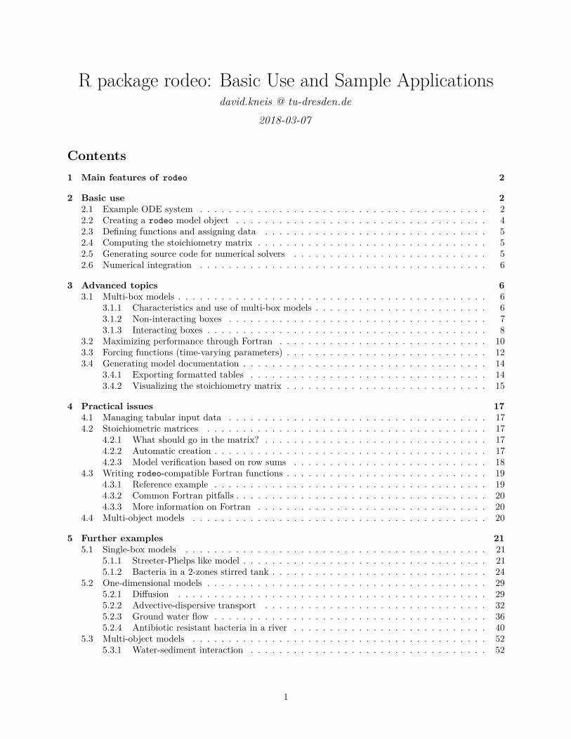
The rodeo package facilitates the implementation of ODE-based models in R. Such models describe thedynamics of a system with a set simultaneously differential equations. The package is particularly usefulin conjunction with the R packages deSolve and rootSolve providing numerical solvers for initial-valueproblems and steady-state estimation. The functionality of rodeo is summarized in the following figure.
1: Instantiation of a rodeo object from a table-based model specification. 2: Assignment of numeric datathrough the object’s set methods. 3: Automatic code generation and compilation / interpretation. 4: Accessto numeric data through the object’s get methods. 5: Access to functions.
The specific advantages from using rodeo are:
• The model is formulated independent from source code to facilitate portability, re-usability, anddocumentation. Specifically, the model has to be set-up using the well-established Peterson matrixnotation. All ingredients of a model (i. e. the ODE’s right hand sides, declarations, and documentation)are in tabular form and they can be imported from delimited text files or spreadsheets.
• Owing to the matrix notation, redundant terms are largely eliminated from the differential equations.This contributes to comprehensibility and increases computational efficiency. The stoichiometry matrixcan also be visualized to better communicate the model to other modelers or end users.
• rodeo provides a code generator which supports R and Fortran as target languages. Using compiledFortran can speed up numerical integration by 1 or 2 orders of magnitude (compared to plain R).
• Code can be generated for an arbitrary number of computational boxes (e. g. control volumes in aspatially discretized model). This allows even partial differential equations (e. g. reactive transportproblems) to be tackled after appropriate semi-discretization. The latter strategy is known as themethod-of-lines.
2 Basic use
2.1 Example ODE system
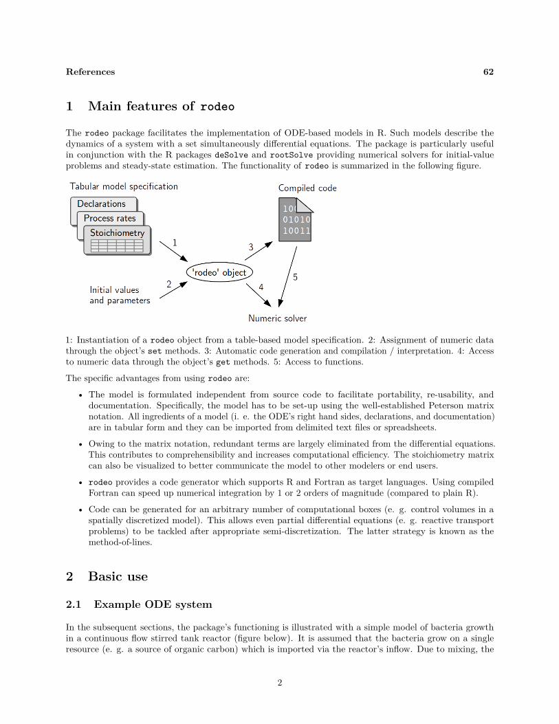
In the subsequent sections, the package’s functioning is illustrated with a simple model of bacteria growthin a continuous flow stirred tank reactor (figure below). It is assumed that the bacteria grow on a singleresource (e. g. a source of organic carbon) which is imported via the reactor’s inflow. Due to mixing, the
2
reactors contents is spatially homogeneous, hence the density of bacteria as well as the concentration of thesubstrate are scalars.
Changes in bacteria density are due to (1) resource-limited growth and (2) wash-out from the reactor (inflowis assumed to be sterile). The substrate concentration is controlled by (1) the inflow as well as (2) theconsumption by bacteria. A classical Monod term was used to model the resource dependency of bacteriagrowth. For the sake of simplicity, the external forcings (i. e. flow rate and substrate load) are held constantand the reactor’s volume is a parameter rather than a state variable.
The governing differential equations are
d
dtbac = mu ·
sub
sub + half· bac +
flow
vol· (0 − bac)
d
dtsub = −
1
yield· mu ·
sub
sub + half· bac +
flow
vol· (subin − sub)
where redundant terms are displayed in identical colors (all identifiers are explained in tables below). For usewith rodeo, the equations must be split up into a vector of process rates (r) and a matrix of stoichiometricfactors (S) so that the product of the two yields the vector of the state variables’ derivatives with respect totime (y). Note that
y = r · S
is the same as
y = ST· r
In the first form, y and r are row vectors. In the second form which involves the transpose of S, y and r arecolumn vectors. Adopting the first form, the above set of ODE can be written as
[
d
dtbac
d
dtsub
]
=
[
mu ·sub
sub + half· bac
flow
vol
]
·
1 −bac
−1
yieldsubin − sub
The vector r and the matrix S, together with a declaration of all identifiers appearing in the expressions, canconveniently be stored in tables, i.e. R data frames. Appropriate data frames are shipped with the packageand can be loaded with the R function data. Their contents is displayed below:
Table 1: Data set vars: Declaration of state variables.
name unit description
bac mg/ml bacteria densitysub mg/ml substrate concentration
3

Table 2: Data set pars: Declaration of parameters.
name unit description
mu 1/hour intrinsic bacteria growth ratehalf mg/ml half saturation concentration of substrateyield mg/mg biomass produced per amount of substratevol ml volume of reactorflow ml/hour rate of through-flowsub_in mg/ml substrate concentration in inflow
Table 3: Data set funs: Declaration of functions referenced at theODE’s right hand sides.
name unit description
monod - monod expression for resource limitation
Table 4: Data set pros: Definition of process rates.
name unit description expression
growth mg/ml/hour bacteria growth mu * monod(sub, half) * bacinout 1/hour water in-/outflow flow/vol
Table: Data set stoi: Definition of stoichiometric factors providing the relation between processes and statevariables. Note the (optional) use of a tabular layout instead of the more common matrix layout.
variable process expression——— ——– ————— bac growth 1bac inout -bacsub growth -1 / yieldsub inout (sub_in - sub)
2.2 Creating a rodeo model object
We start by loading packages and the example data tables whose contents was shown in the above tables.
rm(list=ls()) # Initial clean-up
library(deSolve)
library(rodeo)
data(vars, pars, pros, funs, stoi)
Then, a new object is created with the new method of the R6 class system. This requires us to supply thename of the class, data frames for initialization, as well as the spatial dimensions. Here, we create a single-boxmodel (one dimension with no subdivision).
model <- rodeo$new(vars=vars, pars=pars, funs=funs,
pros=pros, stoi=stoi, dim=c(1))
To inspect the object’s contents, we can use the following:
4

print(model) # Displays object members (output not shown)
print(model$stoichiometry()) # Shows stoichiometry as a matrix
2.3 Defining functions and assigning data
In order to work with the object, we need to define functions that are referenced in the process rate expressionsor stoichiometric factors (i. e. the ODEs’ right hand sides). For non-autonomous models, this includes thedefinition of forcings which are functions of a special argument with the reserved name ‘time’ (details followin a separate section on forcings).
For the bacteria growth example, we only need to implement a simple Monod function.
monod <- function(c, h) { c / (c + h) }
We also need to assign values to parameters and state variables (initial values) using the dedicated classmethods setPars and setVars. Since we deal with a single-box model, parameters and initial values can bestored in ordinary named vectors.
model$setVars(c(bac=0.01, sub=0))
model$setPars(c(mu=0.8, half=0.1, yield= 0.1, vol=1000, flow=50, sub_in=1))
2.4 Computing the stoichiometry matrix
Having defined all functions and having set the values of variables and parameters, one can compute thestoichiometric factors. In general, explicitly computing these factors is not necessary, it may be helpful indebugging however. To do so, the stoichiometry class method needs to be supplied with the index of thespatial box (only relevant for multi-box models) as well as the time of interest (in the case of non-autonomousmodels).
m <- model$stoichiometry(box=1, time=0)
print(signif(m, 3))
## bac sub
## growth 1.00 -10
## inout -0.01 1
The stoichiometry matrix is also a good means to communicate a model because it shows the interactionsbetween processes and variables in a concise way. How the stoichiometry matrix can be visualized graphicallyis demonstrated in a dedicated section below.
2.5 Generating source code for numerical solvers
In order to use the model for simulation, we need to generate source code to be passed to numerical solvers.Specifically, the generated function code shall return the derivatives of the state variables with respect totime plus additional diagnostic information (here: the process rates).
In this example, R code is generated (Fortran code generation is described elsewhere). The R code is not‘compiled’ in a strict sense but it is made executable through a combination of the functions eval and parse.
model$compile(fortran=FALSE)
5
2.6 Numerical integration
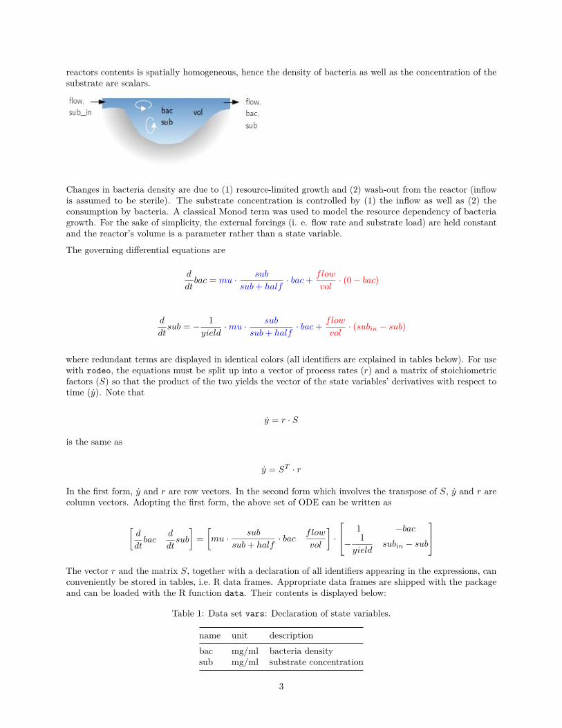
We are now ready to compute the evolution of the state variables over time by means of numerical integration.The call below employs the ode function from package deSolve.
out <- model$dynamics(times=0:96, fortran=FALSE)
plot(out) # plot method for 'deSolve' objects
The graphical output of the above code is displayed below (top row: state variables, bottom row: processrates).
0 20 40 60 80
0.0
20.0
8
bac
time
0 20 40 60 80
0.0
00.0
4
sub
time
0 20 40 60 80
0.0
00
0.0
05
growth
time
0 20 40 60 80
0.0
30.0
6
inout
time
3 Advanced topics
3.1 Multi-box models
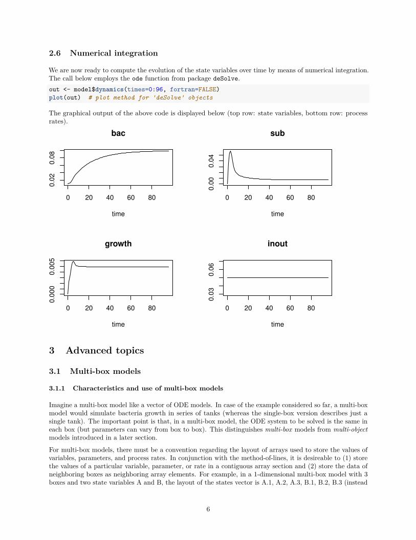
3.1.1 Characteristics and use of multi-box models
Imagine a multi-box model like a vector of ODE models. In case of the example considered so far, a multi-boxmodel would simulate bacteria growth in series of tanks (whereas the single-box version describes just asingle tank). The important point is that, in a multi-box model, the ODE system to be solved is the same ineach box (but parameters can vary from box to box). This distinguishes multi-box models from multi-objectmodels introduced in a later section.
For multi-box models, there must be a convention regarding the layout of arrays used to store the values ofvariables, parameters, and process rates. In conjunction with the method-of-lines, it is desireable to (1) storethe values of a particular variable, parameter, or rate in a contiguous array section and (2) store the data ofneighboring boxes as neighboring array elements. For example, in a 1-dimensional multi-box model with 3boxes and two state variables A and B, the layout of the states vector is A.1, A.2, A.3, B.1, B.2, B.3 (instead
6

of A.1, B.1, A.2, . . . ). Thus, the index of the box varies faster than the index of the variable. Note that thesame convention automatically applies to the output of the numerical solvers, i. e. the columns of the outputmatrix returned from the deSolve methods are ordered as just described.
There are two main areas of use for multi-box models:
1. They can be used, for example, to model an array of experiments, where the individual experimentsdifferent in parameters or initial values. In such a case the boxes do not interact, i.e. the dynamics ina particular box is from the dynamics in the other boxes.
2. Multi-box models can also be used to represent ODE systems originating from semi-discretization ofpartial differential equations. This approach, better known as the method-of-lines (MOL), is applicableto reactive transport problems, for example. In such a case, neighboring boxes do interact with eachother.
Examples for these two cases are provided below.
3.1.2 Non-interacting boxes
This example applies the bacteria growth model to two tanks, the latter being independent of each other. Westart from a clean environment.
rm(list=ls()) # Initial clean-up
library(deSolve)
library(rodeo)
data(vars, pars, pros, funs, stoi)
First of all, we need to create a model object with the appropriate number of dimensions and the desirednumber of boxes in each dimension. These values are specified in the dim argument of rodeo’s initializationmethod. Here, we request the creation of two boxes in the first and only dimension.
nBox <- 2
model <- rodeo$new(vars=vars, pars=pars, funs=funs,
pros=pros, stoi=stoi, dim=c(nBox))
Second, the function returning the state variables’ derivatives needs to be re-generated to reflect the alterednumber of boxes.
model$compile(fortran=FALSE)
monod <- function(c, h) { c / (c + h) }
Third, initial values and parameters need to be specified as arrays now (instead of vectors) because the valuescan vary from box to box. For a multi-box model with a single spatial dimension, we must use matrices (beingtwo-dimensional arrays) whose column names represent the names of variables or parameters, respectively.The matrix row with index i provides the respective values for the model’s i-th box.
In this example, the two reactors only differ in their storage capacity (parameter vol). All other parametersand the initial concentrations of substrate and bacteria are kept identical.
rp <- function (x) {rep(x, nBox)} # For convenient replication
v <- cbind(bac=rp(0.01), sub=rp(0))
model$setVars(v)
p <- cbind(mu=rp(0.8), half=rp(0.1), yield= rp(0.1),
vol=c(300, 1000), flow=rp(50), sub_in=rp(1))
model$setPars(p)
Finally, the integration method is called as usual.
7

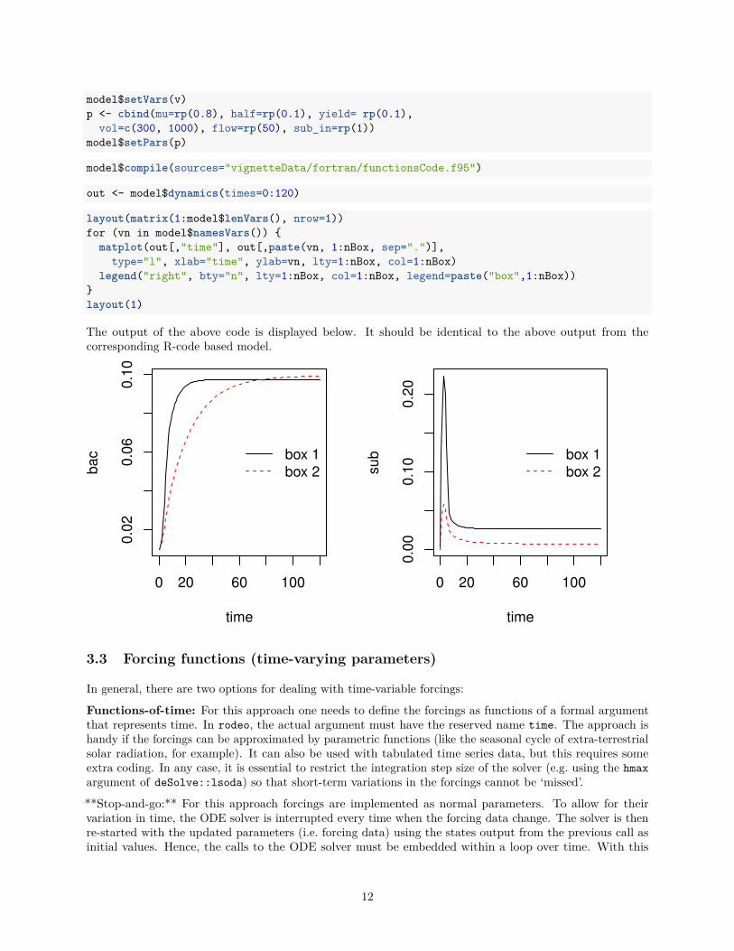
out <- model$dynamics(times=0:120, fortran=FALSE)
The dynamics of the state variables in all boxes are conveniently plotted with matplot. Note that the boxindex is appended to the state variables’ names and the two parts are separated by a period. For example,the bacteria density in the first box is found in column ‘bac.1’ of the matrix out.
layout(matrix(1:model$lenVars(), nrow=1))
for (vn in model$namesVars()) {
matplot(out[,"time"], out[,paste(vn, 1:nBox, sep=".")],
type="l", xlab="time", ylab=vn, lty=1:nBox, col=1:nBox)
legend("right", bty="n", lty=1:nBox, col=1:nBox, legend=paste("box",1:nBox))
}
layout(1)
0 20 60 100
0.0
20.0
60.1
0
time
bac box 1
box 2
0 20 60 100
0.0
00.1
00.2
0
time
sub box 1
box 2
3.1.3 Interacting boxes
In this context, interaction means that the state variables’ derivatives in a box i depend on the state ofanother box k. This is typically the case if advection or diffusion-like processes are simulated because fluxesbetween boxes (e.g. of mass or heat) are driven by spatial gradients.
rodeo’s support for interactions between boxes is currently limited to models with a single dimension (1Dmodels). Also, interaction is possible between adjacent boxes only (but not between, e.g., boxes i and i + 2).
The key to the simulation of interactions is that each box can query the values of state variables (or parameters)in the adjacent boxes. This functionality is implemented through the pseudo-functions ‘left’ and ‘right’. Thesecan be used in the mathematical expressions forming the ODE’s right hand sides. The functions do whattheir names say. For example, if ‘x’ is a state variable, the expression x - left(x) yields the differencebetween the value in the current box (index i) and the value in adjacent box i − 1. Likewise, x - right(x)
is used to calculate the difference between the current box (index i) and box i + 1.
The two pseudo-functions must behave specially at the model’s boundaries. In other words, it has to bedefined what left(x) returns for the leftmost box (index 1) and what right(x) returns for the box withthe highest index. The convention is simple: If the index would go out of bounds, the functions return therespective value for the current cell. See the table below for clarification.
8

Box index left(x) returns right(x) returns
1 x.1 x.22 x.1 x.33 x.2 x.44 x.3 x.55 (highest index) x.4 x.5
This behaviour of ‘left’ and ‘right’ at the models boundaries is often convenient. Consider, for example, amodel of advective transport using the backward finite-difference approximation u/dx * (left(c) - c) (‘u’:velocity, ‘c’: concentration, ‘dx’: box width). For the leftmost box, the whole term equates to zero since bothc and left(c) point to the concentration in box 1.
Imposing boundary conditions on the leftmost box (index 1) and the righmost box (highest index) is fairlysimple. First, the required term(s) are simply added to the process rate expressions. Second, the term(s) aremultiplied with a mask parameters that take a value of 1 at the desired boundary and 0 elsewhere. In thejust mentioned advection example, a resonable formulation could be
u/dx * (left(c) - c) + leftmost(2 * u/dx * (cUp - c))
where cUp is the concentration just upstream of the model domain, and leftmost is the mask parameterbeing set to one for the leftmost box and zero for all other boxes.
Interaction between boxes is demonstrated with a minimum example. It extends the above ‘no-interaction’example case by introduction of a diffusive flux of substrate between the two tanks.
The original model is first loaded and then extended for the new process.
rm(list=ls()) # Initial clean-up
library(deSolve)
library(rodeo)
data(vars, pars, pros, funs, stoi)
pars <- rbind(pars,
c(name="d", unit="1/hour", description="diffusion parameter")
)
pros <- rbind(pros,
c(name="diffSub", unit="mg/ml/hour", description="diffusion of substrate",
expression="d * ((left(sub)-sub) + (right(sub)-sub))")
)
stoi <- rbind(stoi,
c(variable="sub", process="diffSub", expression="1")
)
The following code sections are the same as for the ‘no-interaction’ case.
nBox <- 2
model <- rodeo$new(vars=vars, pars=pars, funs=funs,
pros=pros, stoi=stoi, dim=c(nBox))
model$compile(fortran=FALSE)
monod <- function(c, h) { c / (c + h) }
A value must be assigned to the newly introduced diffusion parameter d as well.
rp <- function (x) {rep(x, nBox)} # For convenient replication
v <- cbind(bac=rp(0.01), sub=rp(0))
model$setVars(v)
9

p <- cbind(mu=rp(0.8), half=rp(0.1), yield= rp(0.1),
vol=c(300, 1000), flow=rp(50), sub_in=rp(1),
d=rp(.75)) # Added diffusion parameter
model$setPars(p)
The code for integration and plotting is the same as for the ‘no-interaction’ case.
out <- model$dynamics(times=0:120, fortran=FALSE)
layout(matrix(1:model$lenVars(), nrow=1))
for (vn in model$namesVars()) {
matplot(out[,"time"], out[,paste(vn, 1:nBox, sep=".")],
type="l", xlab="time", ylab=vn, lty=1:nBox, col=1:nBox)
legend("right", bty="n", lty=1:nBox, col=1:nBox, legend=paste("box",1:nBox))
}
layout(1)
The output of the above code is displayed below. The effect of substrate diffusion is cleary visible in theoutput.
0 20 60 100
0.0
20.0
60.1
0
time
bac box 1
box 2
0 20 60 100
0.0
00.0
50.1
00.1
5
time
sub box 1
box 2
3.2 Maximizing performance through Fortran
As the number of simultaneous ODE increases and the right hand sides become more complex, computationtimes begin to matter. This is especially so in case of stiff systems of equations. In those time-critical cases,it is recommended to generate source code for a compilable language. The language supported by rodeo isFortran. Fortran was chosen because of its superior array support (compared to C) and for compatibilitywith existing numerical libraries.
One could use the low-level method
code <- model$generate(name="derivs",lang="f95") # not required for typical uses
to generate a function that computes the state variables’ derivatives in Fortran. However, the interface ofthe generated function is optimized for universality. In order to use the generated code with the numericalsolvers from deSolve or rootSolve, a specialized wrapper is required.
10

To make the use of Fortran as simple as possible, rodeo provides a high-level class method compile whichcombines
1. generation of the basic Fortran code via the generate method (see above),
2. generation of the required wrapper for compatibility with deSolve and rootSolve,
3. compilation of all Fortran sources into a shared library (based on the command R CMD SHLIB),
4. loading of the library
model$compile(sources="vignetteData/fortran/functionsCode.f95")
The compile method takes as argument the name of a file holding the Fortran implementation of functionsbeing referenced in the particular model’s mathematical expressions. This argument can actually be a vectorif the source code is split across several files. Consult the section on Fortran functions for coding guidelinesand take a look at the collection of examples.
The created library is automatically loaded with dyn.load and unloaded with dyn.unload when the objectis garbage collected. The name of the created library and the name of the derivatives function containedtherein are stored in the rodeo object internally. These names can be queried with the method libName()
and libFunc(), respectively.
A suitable Fortran implementation of the functions used in the example (contents of file ‘for-tran/functionsCode.f95’) is shown below. Note that all the functions are collected in a single Fortran modulewith implicit typing turned off. The name of this module must be 'functions' and it cannot be changed.Note that a Fortran module can import other modules which helps to structure more complex source codes.Also note that the user-supplied source files need to reside in directories with write-access to allow thecreation of intermediate files during compilation.
! This is file 'functionsCode.f95'
module functions
implicit none
contains
double precision function monod(c, h)
double precision, intent(in):: c, h
monod= c / (c + h)
end function
end module
The complete code to run the ‘no-interactions’ model from a previous section using Fortran-based code isgiven below. Note the additional arguments dllname and nout being passed to the numerical solver (fordetails consult the deSolve help page for method lsoda). It is especially important to pass the correct valueto nout: In case of rodeo-based models, this must be the number of processes multiplied with the totalnumber of boxes. Disregard of this may trigger segmentation faults that make R crash.
rm(list=ls()) # Initial clean-up
library(deSolve)
library(rodeo)
data(vars, pars, pros, funs, stoi)
nBox <- 2
model <- rodeo$new(vars=vars, pars=pars, funs=funs,
pros=pros, stoi=stoi, dim=c(nBox))
rp <- function (x) {rep(x, nBox)} # For convenient replication
v <- cbind(bac=rp(0.01), sub=rp(0))
11
model$setVars(v)
p <- cbind(mu=rp(0.8), half=rp(0.1), yield= rp(0.1),
vol=c(300, 1000), flow=rp(50), sub_in=rp(1))
model$setPars(p)
model$compile(sources="vignetteData/fortran/functionsCode.f95")
out <- model$dynamics(times=0:120)
layout(matrix(1:model$lenVars(), nrow=1))
for (vn in model$namesVars()) {
matplot(out[,"time"], out[,paste(vn, 1:nBox, sep=".")],
type="l", xlab="time", ylab=vn, lty=1:nBox, col=1:nBox)
legend("right", bty="n", lty=1:nBox, col=1:nBox, legend=paste("box",1:nBox))
}
layout(1)
The output of the above code is displayed below. It should be identical to the above output from thecorresponding R-code based model.
0 20 60 100
0.0
20.0
60.1
0
time
bac box 1
box 2
0 20 60 100
0.0
00.1
00.2
0
time
sub box 1
box 2
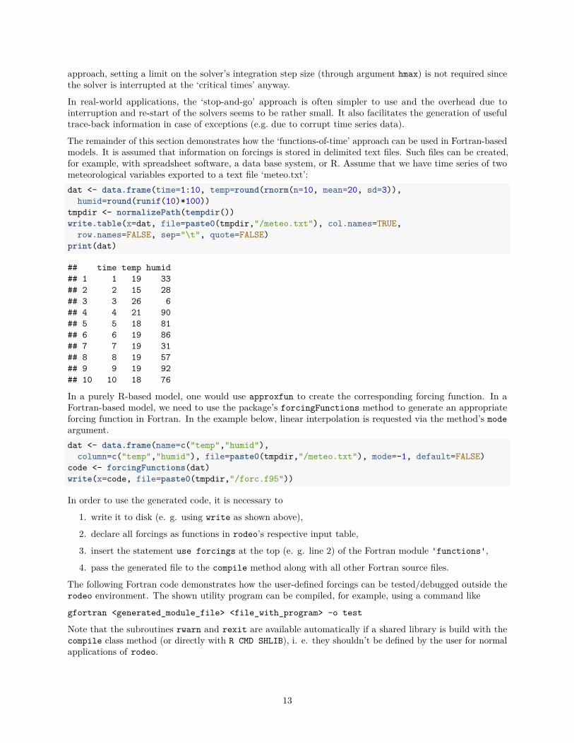
3.3 Forcing functions (time-varying parameters)
In general, there are two options for dealing with time-variable forcings:
Functions-of-time: For this approach one needs to define the forcings as functions of a formal argumentthat represents time. In rodeo, the actual argument must have the reserved name time. The approach ishandy if the forcings can be approximated by parametric functions (like the seasonal cycle of extra-terrestrialsolar radiation, for example). It can also be used with tabulated time series data, but this requires someextra coding. In any case, it is essential to restrict the integration step size of the solver (e.g. using the hmax
argument of deSolve::lsoda) so that short-term variations in the forcings cannot be ‘missed’.
**Stop-and-go:** For this approach forcings are implemented as normal parameters. To allow for theirvariation in time, the ODE solver is interrupted every time when the forcing data change. The solver is thenre-started with the updated parameters (i.e. forcing data) using the states output from the previous call asinitial values. Hence, the calls to the ODE solver must be embedded within a loop over time. With this
12
approach, setting a limit on the solver’s integration step size (through argument hmax) is not required sincethe solver is interrupted at the ‘critical times’ anyway.
In real-world applications, the ‘stop-and-go’ approach is often simpler to use and the overhead due tointerruption and re-start of the solvers seems to be rather small. It also facilitates the generation of usefultrace-back information in case of exceptions (e.g. due to corrupt time series data).
The remainder of this section demonstrates how the ‘functions-of-time’ approach can be used in Fortran-basedmodels. It is assumed that information on forcings is stored in delimited text files. Such files can be created,for example, with spreadsheet software, a data base system, or R. Assume that we have time series of twometeorological variables exported to a text file ‘meteo.txt’:
dat <- data.frame(time=1:10, temp=round(rnorm(n=10, mean=20, sd=3)),
humid=round(runif(10)*100))
tmpdir <- normalizePath(tempdir())
write.table(x=dat, file=paste0(tmpdir,"/meteo.txt"), col.names=TRUE,
row.names=FALSE, sep="\t", quote=FALSE)
print(dat)
## time temp humid
## 1 1 19 33
## 2 2 15 28
## 3 3 26 6
## 4 4 21 90
## 5 5 18 81
## 6 6 19 86
## 7 7 19 31
## 8 8 19 57
## 9 9 19 92
## 10 10 18 76
In a purely R-based model, one would use approxfun to create the corresponding forcing function. In aFortran-based model, we need to use the package’s forcingFunctions method to generate an appropriateforcing function in Fortran. In the example below, linear interpolation is requested via the method’s mode
argument.
dat <- data.frame(name=c("temp","humid"),
column=c("temp","humid"), file=paste0(tmpdir,"/meteo.txt"), mode=-1, default=FALSE)
code <- forcingFunctions(dat)
write(x=code, file=paste0(tmpdir,"/forc.f95"))
In order to use the generated code, it is necessary to
1. write it to disk (e. g. using write as shown above),
2. declare all forcings as functions in rodeo’s respective input table,
3. insert the statement use forcings at the top (e. g. line 2) of the Fortran module 'functions',
4. pass the generated file to the compile method along with all other Fortran source files.
The following Fortran code demonstrates how the user-defined forcings can be tested/debugged outside therodeo environment. The shown utility program can be compiled, for example, using a command like
gfortran <generated_module_file> <file_with_program> -o test
Note that the subroutines rwarn and rexit are available automatically if a shared library is build with thecompile class method (or directly with R CMD SHLIB), i. e. they shouldn’t be defined by the user for normalapplications of rodeo.
13
! auxiliary routines for testing outside R
subroutine rwarn(x)
character(len=*),intent(in):: x
write(*,*)x
end subroutine
subroutine rexit(x)
character(len=*),intent(in):: x
write(*,*)x
stop
end subroutine
! test program
program test
use forcings ! imports generated module with forcing functions
implicit none
integer:: i
double precision, dimension(5):: times= &
dble((/ 1., 1.5, 2., 2.5, 3. /))
do i=1, size(times)
write(*,*) times(i), temp(times(i)), humid(times(i))
end do
end program
3.4 Generating model documentation
3.4.1 Exporting formatted tables
One can use e. g. the package’s exportDF to export the object’s basic information in a format which issuitable for inclusion in HTML or LaTeX documents. The code section
# Select columns to export
df <- model$getVarsTable()[,c("tex","unit","description")]
# Define formatting functions
bold <- function(x){paste0("\\textbf{",x,"}")}
mathmode <- function(x) {paste0("$",x,"$")}
# Export
tex <- exportDF(x=df, tex=TRUE,
colnames=c(tex="symbol"),
funHead=setNames(replicate(ncol(df),bold),names(df)),
funCell=list(tex=mathmode)
)
cat(tex)
generates the following LaTeX code
\begin{tabular}{lll}\hline
\textbf{symbol} & \textbf{unit} & \textbf{description} \\ \hline
$bac$ & mg/ml & bacteria density \\
$sub$ & mg/ml & substrate concentration \\ \hline
14
\end{tabular}
holding tabular information on the model’s state variables. To include the result in a document one needs towrite the generated LaTeX code to a file for import with either the input or include directive. Things areeven simpler if the Sweave pre-processor is used which allows the above R code to be embedded in LaTeXdirectly between the special markers <<echo=FALSE, results=tex>>= and @.
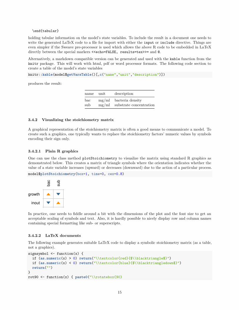
Alternatively, a markdown compatible version can be generated and used with the kable function from theknitr package. This will work with html, pdf or word processor formats. The following code section tocreate a table of the model’s state variables
knitr::kable(model$getVarsTable()[,c("name","unit","description")])
produces the result:
name unit description
bac mg/ml bacteria densitysub mg/ml substrate concentration
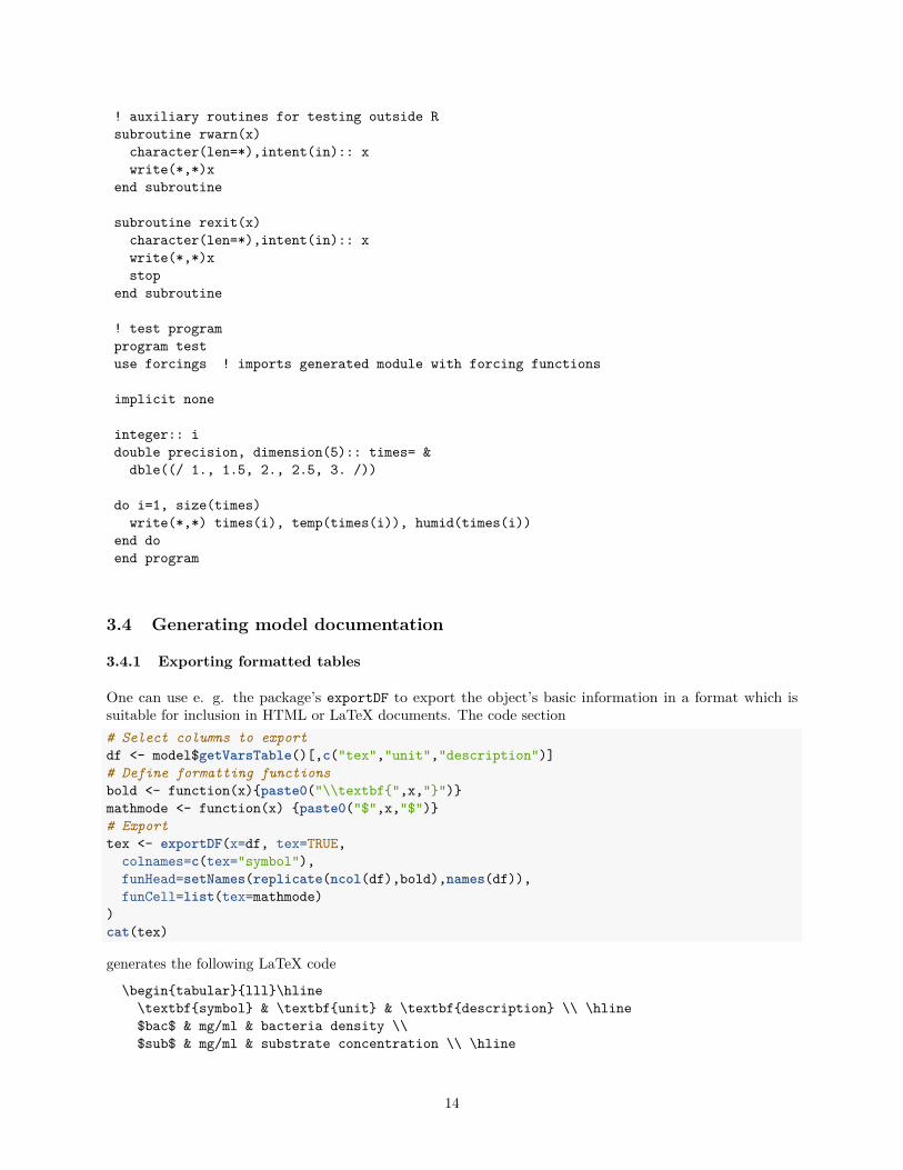
3.4.2 Visualizing the stoichiometry matrix
A graphical representation of the stoichiometry matrix is often a good means to communicate a model. Tocreate such a graphics, one typically wants to replace the stoichiometry factors’ numeric values by symbolsencoding their sign only.
3.4.2.1 Plain R graphics
One can use the class method plotStoichiometry to visualize the matrix using standard R graphics asdemonstrated below. This creates a matrix of triangle symbols where the orientation indicates whether thevalue of a state variable increases (upward) or decreases (downward) due to the action of a particular process.
model$plotStoichiometry(box=1, time=0, cex=0.8)
bac
sub
growth
inout
In practice, one needs to fiddle around a bit with the dimensions of the plot and the font size to get anacceptable scaling of symbols and text. Also, it is hardly possible to nicely display row and column namescontaining special formatting like sub- or superscripts.
3.4.2.2 LaTeX documents
The following example generates suitable LaTeX code to display a symbolic stoichiometry matrix (as a table,not a graphics).
signsymbol <- function(x) {
if (as.numeric(x) > 0) return("\\textcolor{red}{$\\blacktriangle$}")
if (as.numeric(x) < 0) return("\\textcolor{blue}{$\\blacktriangledown$}")
return("")
}
rot90 <- function(x) { paste0("\\rotatebox{90}
15
{$",gsub(pattern="*", replacement="\\cdot ", x=x, fixed=TRUE),"$}") }
m <- model$stoichiometry(box=1, time=0)
tbl <- cbind(data.frame(process=rownames(m), stringsAsFactors=FALSE),
as.data.frame(m))
tex <- exportDF(x=tbl, tex=TRUE,
colnames= setNames(c("",model$getVarsTable()$tex[match(colnames(m),
model$getVarsTable()$name)]), names(tbl)),
funHead= setNames(replicate(ncol(m),rot90), colnames(m)),
funCell= setNames(replicate(ncol(m),signsymbol), colnames(m)),
lines=TRUE
)
tex <- paste0("%\n% THIS IS A GENERATED FILE\n%\n", tex)
# write(tex, file="stoichiometry.tex")
The contents of the variable tex must be written to a text file and this file can then be imported in LaTeXwith the input directive.
3.4.2.3 HTML documents
The following example generates suitable code for inclusion in HTML documents.
signsymbol <- function(x) {
if (as.numeric(x) > 0) return("△")
if (as.numeric(x) < 0) return("▽")
return("")
}
m <- model$stoichiometry(box=1, time=0)
tbl <- cbind(data.frame(process=rownames(m), stringsAsFactors=FALSE),
as.data.frame(m))
html <- exportDF(x=tbl, tex=FALSE,
colnames= setNames(c("Process",model$getVarsTable()$html[match(colnames(m),
model$getVarsTable()$name)]), names(tbl)),
funCell= setNames(replicate(ncol(m),signsymbol), colnames(m))
)
html <- paste("<html>", html, "</html>", sep="\n")
# write(html, file="stoichiometry.html")
To test this, one needs to write the contents of the variable html to a text file and open that file in a webbrowser. In some cases, automatic conversion of the generated HTML into true graphics formats may bepossible, e. g. using auxiliary (Linux) tools like ‘html2ps’ and ‘convert’.
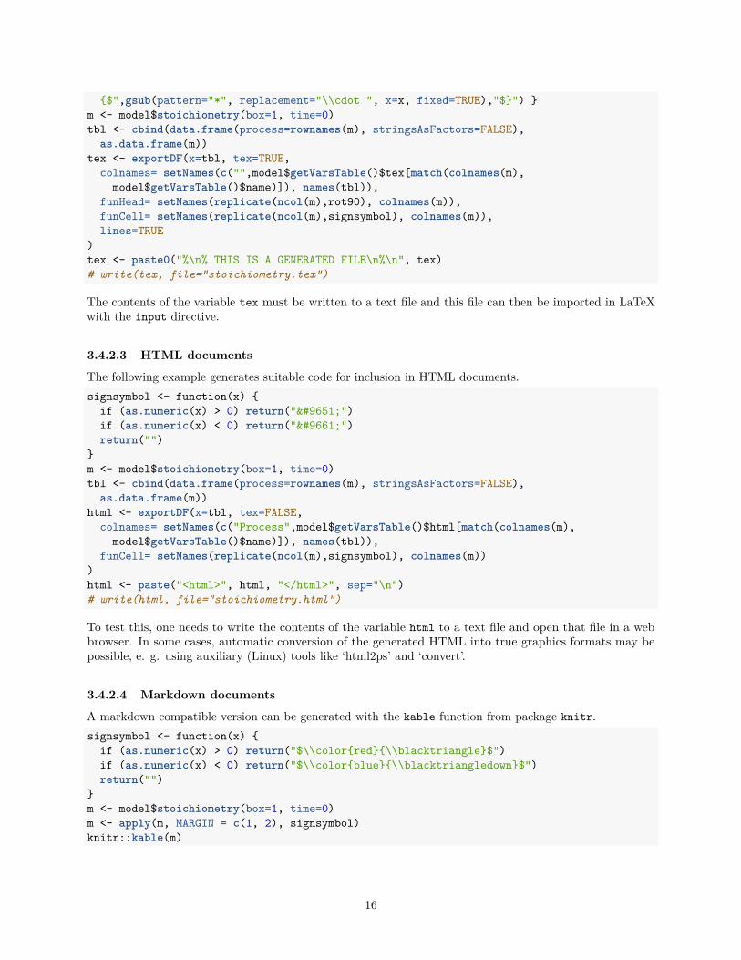
3.4.2.4 Markdown documents
A markdown compatible version can be generated with the kable function from package knitr.
signsymbol <- function(x) {
if (as.numeric(x) > 0) return("$\\color{red}{\\blacktriangle}$")
if (as.numeric(x) < 0) return("$\\color{blue}{\\blacktriangledown}$")
return("")
}
m <- model$stoichiometry(box=1, time=0)
m <- apply(m, MARGIN = c(1, 2), signsymbol)
knitr::kable(m)
16
bac sub
growth N H
inout H N
4 Practical issues
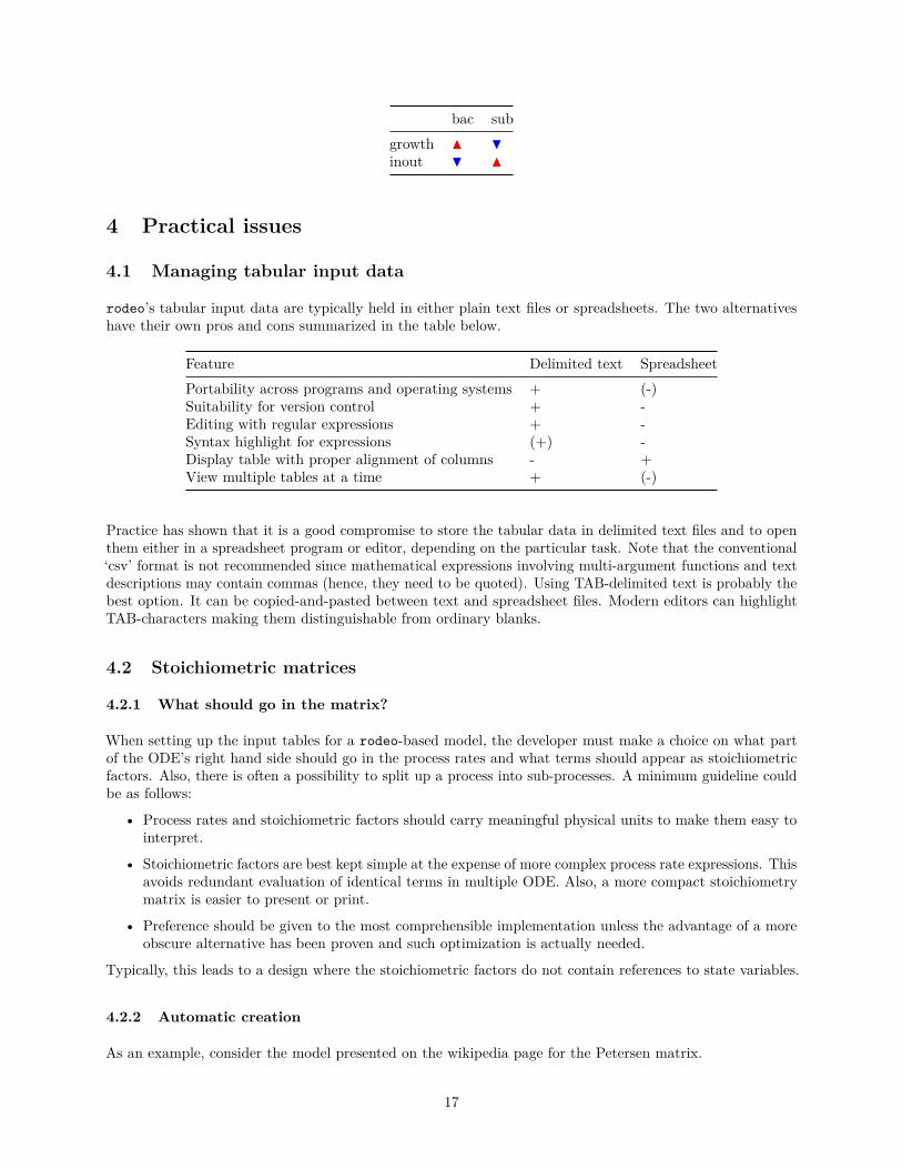
4.1 Managing tabular input data
rodeo’s tabular input data are typically held in either plain text files or spreadsheets. The two alternativeshave their own pros and cons summarized in the table below.
Feature Delimited text Spreadsheet
Portability across programs and operating systems + (-)Suitability for version control + -Editing with regular expressions + -Syntax highlight for expressions (+) -Display table with proper alignment of columns - +View multiple tables at a time + (-)
Practice has shown that it is a good compromise to store the tabular data in delimited text files and to openthem either in a spreadsheet program or editor, depending on the particular task. Note that the conventional‘csv’ format is not recommended since mathematical expressions involving multi-argument functions and textdescriptions may contain commas (hence, they need to be quoted). Using TAB-delimited text is probably thebest option. It can be copied-and-pasted between text and spreadsheet files. Modern editors can highlightTAB-characters making them distinguishable from ordinary blanks.
4.2 Stoichiometric matrices
4.2.1 What should go in the matrix?
When setting up the input tables for a rodeo-based model, the developer must make a choice on what partof the ODE’s right hand side should go in the process rates and what terms should appear as stoichiometricfactors. Also, there is often a possibility to split up a process into sub-processes. A minimum guideline couldbe as follows:
• Process rates and stoichiometric factors should carry meaningful physical units to make them easy tointerpret.
• Stoichiometric factors are best kept simple at the expense of more complex process rate expressions. Thisavoids redundant evaluation of identical terms in multiple ODE. Also, a more compact stoichiometrymatrix is easier to present or print.
• Preference should be given to the most comprehensible implementation unless the advantage of a moreobscure alternative has been proven and such optimization is actually needed.
Typically, this leads to a design where the stoichiometric factors do not contain references to state variables.
4.2.2 Automatic creation
As an example, consider the model presented on the wikipedia page for the Petersen matrix.
17
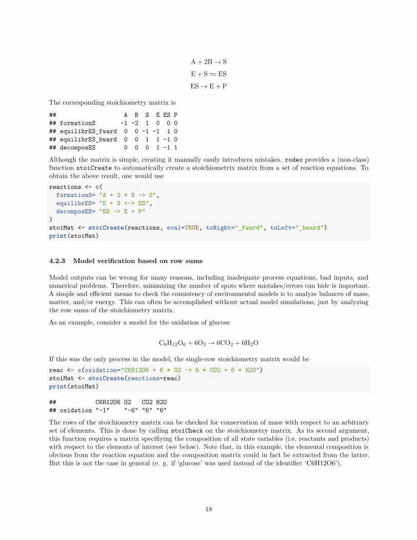
A + 2B → S
E + S ⇌ ES
ES → E + P
The corresponding stoichiometry matrix is
## A B S E ES P
## formationS -1 -2 1 0 0 0
## equilibrES_fward 0 0 -1 -1 1 0
## equilibrES_bward 0 0 1 1 -1 0
## decomposES 0 0 0 1 -1 1
Although the matrix is simple, creating it manually easily introduces mistakes. rodeo provides a (non-class)function stoiCreate to automatically create a stoichiometrix matrix from a set of reaction equations. Toobtain the above result, one would use
reactions <- c(
formationS= "A + 2 * B -> S",
equilibrES= "E + S <-> ES",
decomposES= "ES -> E + P"
)
stoiMat <- stoiCreate(reactions, eval=TRUE, toRight="_fward", toLeft="_bward")
print(stoiMat)
4.2.3 Model verification based on row sums
Model outputs can be wrong for many reasons, including inadequate process equations, bad inputs, andnumerical problems. Therefore, minimizing the number of spots where mistakes/errors can hide is important.A simple and efficient means to check the consistency of environmental models is to analyze balances of mass,matter, and/or energy. This can often be accomplished without actual model simulations, just by analyzingthe row sums of the stoichiometry matrix.
As an example, consider a model for the oxidation of glucose
C6H12O6 + 6O2 → 6CO2 + 6H2O
If this was the only process in the model, the single-row stoichiometry matrix would be
reac <- c(oxidation="C6H12O6 + 6 * O2 -> 6 * CO2 + 6 * H2O")
stoiMat <- stoiCreate(reactions=reac)
print(stoiMat)
## C6H12O6 O2 CO2 H2O
## oxidation "-1" "-6" "6" "6"
The rows of the stoichiometry matrix can be checked for conservation of mass with respect to an arbitraryset of elements. This is done by calling stoiCheck on the stoichiometry matrix. As its second argument,this function requires a matrix specifiying the composition of all state variables (i.e. reactants and products)with respect to the elements of interest (see below). Note that, in this example, the elemental composition isobvious from the reaction equation and the composition matrix could in fact be extracted from the latter.But this is not the case in general (e. g. if ‘glucose’ was used instead of the identifier ‘C6H12O6’).
18
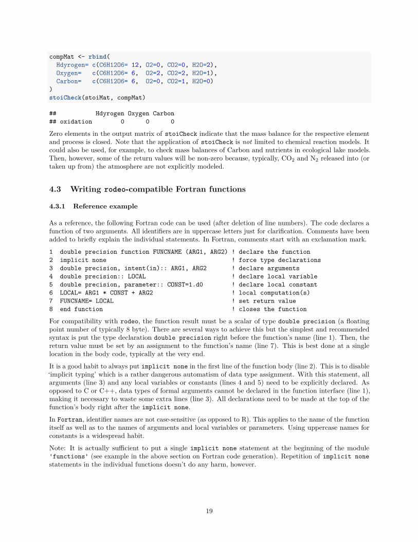
compMat <- rbind(
Hdyrogen= c(C6H12O6= 12, O2=0, CO2=0, H2O=2),
Oxygen= c(C6H12O6= 6, O2=2, CO2=2, H2O=1),
Carbon= c(C6H12O6= 6, O2=0, CO2=1, H2O=0)
)
stoiCheck(stoiMat, compMat)
## Hdyrogen Oxygen Carbon
## oxidation 0 0 0
Zero elements in the output matrix of stoiCheck indicate that the mass balance for the respective elementand process is closed. Note that the application of stoiCheck is not limited to chemical reaction models. Itcould also be used, for example, to check mass balances of Carbon and nutrients in ecological lake models.Then, however, some of the return values will be non-zero because, typically, CO2 and N2 released into (ortaken up from) the atmosphere are not explicitly modeled.
4.3 Writing rodeo-compatible Fortran functions
4.3.1 Reference example
As a reference, the following Fortran code can be used (after deletion of line numbers). The code declares afunction of two arguments. All identifiers are in uppercase letters just for clarification. Comments have beenadded to briefly explain the individual statements. In Fortran, comments start with an exclamation mark.
1 double precision function FUNCNAME (ARG1, ARG2) ! declare the function
2 implicit none ! force type declarations
3 double precision, intent(in):: ARG1, ARG2 ! declare arguments
4 double precision:: LOCAL ! declare local variable
5 double precision, parameter:: CONST=1.d0 ! declare local constant
6 LOCAL= ARG1 * CONST + ARG2 ! local computation(s)
7 FUNCNAME= LOCAL ! set return value
8 end function ! closes the function
For compatibility with rodeo, the function result must be a scalar of type double precision (a floatingpoint number of typically 8 byte). There are several ways to achieve this but the simplest and recommendedsyntax is put the type declaration double precision right before the function’s name (line 1). Then, thereturn value must be set by an assignment to the function’s name (line 7). This is best done at a singlelocation in the body code, typically at the very end.
It is a good habit to always put implicit none in the first line of the function body (line 2). This is to disable‘implicit typing’ which is a rather dangerous automatism of data type assignment. With this statement, allarguments (line 3) and any local variables or constants (lines 4 and 5) need to be explicitly declared. Asopposed to C or C++, data types of formal arguments cannot be declared in the function interface (line 1),making it necessary to waste some extra lines (line 3). All declarations need to be made at the top of thefunction’s body right after the implicit none.
In Fortran, identifier names are not case-sensitive (as opposed to R). This applies to the name of the functionitself as well as to the names of arguments and local variables or parameters. Using uppercase names forconstants is a widespread habit.
Note: It is actually sufficient to put a single implicit none statement at the beginning of the module'functions' (see example in the above section on Fortran code generation). Repetition of implicit none
statements in the individual functions doesn’t do any harm, however.
19

4.3.2 Common Fortran pitfalls
4.3.2.1 Double precision constants
Fortran has several types to represent floating point numbers that vary in precision but rodeo generally usesthe type double precision. Thus, any local variables and parameters should also be declared as double
precision. To declare a constant of this type, e. g. ‘pi’, one needs to use the special syntax 3.1415d0,i.e. the conventional ‘e’ in scientific notation must be replaced by ‘d’. Do not use the alternative syntax3.1415_8 as it is not portable. Some further examples are shown below. Note the use of the parameter
keyword informing the compiler that the declared items are constants rather than variables.
double precision, parameter:: pi= 3.1415d0, e= 2.7183d0 ! math constants
double precision, parameter:: kilograms_per_gram = 1.d-3 ! 1/1000
double precision, parameter:: distance_to_moon = 3.844d+5 ! 384400 km
4.3.2.2 Integers in numeric expressions
It is recommended to avoid integers in arithmetic expressions as the result may be unexpected. Use double
precision constants instead of integer constants or, alternatively, explicitly convert types by means of thedble intrinsic function.
average= (value1 + value2) / 2d0 ! does not use an integer at all
average= (value1 + value2) / dble(2) ! explicit type conversion
It is often even better not to use any literal constants, leading to a code like
double precision, parameter:: TWO= 2.d0
! ... possibly other statements ...
average= (value1 + value2) / TWO
4.3.2.3 Long Fortran statements (continuation lines)
Source code lines should not exceed 80 characters (though some Fortran compilers support longer lines). Ifan expression does not fit on a single line, the ampersand (&) must be used to indicate continuation lines.Missing & characters are a frequent cause of compile time errors and the respective diagnostic messages aresometimes rather obscure. It is recommended to put the & at the end of any unfinished line as in the followingexample:
a = term1 + term2 + &
term3 + term4 + &
term5
4.3.3 More information on Fortran
The code contained in the section on Fortran code generation or the gallery of examples may serve as astarting point. The Fortran wiki is a good source of additional information, also providing links to standarddocuments, books, etc.
4.4 Multi-object models
Real-world applications often require the simulation of multiple interacting compartments. In some casesit may still be possible to handle those systems with a single set of ODE and to properly set up theJacobian matrix. In many cases, however, it will be easier to work with separate ODE models (one for eachcompartment) and to allow for inter-model communication at an adequate frequency. The concept of ‘linked
20
sub-models’ can be used with rodeo and it is also promoted by the OpenMI initiative (Gregersen, Gijsbers,and Westen 2007). The downsides of the approach are
• a loss of computational efficiency, mainly because the ODE solver needs to re-start frequently,
• a potential loss in accuracy owing to time-step wise decoupling of the equations.
The second aspect is particularly important and, for serious applications, the impact of the chosen frequencyof inter-model communication needs to be understood. In general, a more accurate solution can be expectedif the frequency of communication is increased.
In spite of the mentioned drawbacks, the concept of linked sub-models remains attractive because
• a modular system is easier to develop, debug, document, and re-use,
• one can link rodeo-objects with any ‘foreign’ model objects, which opens the possibility to couple ODEand non-ODE models.
A simple test case demonstrating the linkage of two rodeo-objects can be found in a dedicated examplesection. Note that those parts of rodeo targeted at model coupling (e. g. the class method step) are underdevelopment and details of the implementation may change in the future.
5 Further examples
5.1 Single-box models
5.1.1 Streeter-Phelps like model
5.1.1.1 Problem description
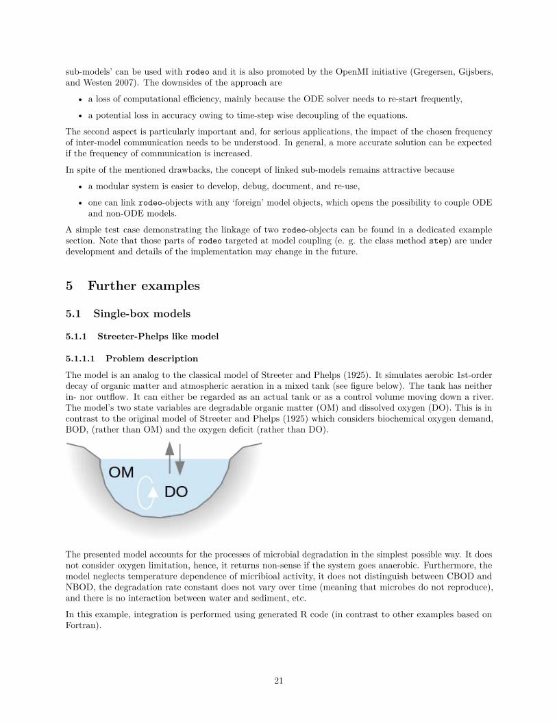
The model is an analog to the classical model of Streeter and Phelps (1925). It simulates aerobic 1st-orderdecay of organic matter and atmospheric aeration in a mixed tank (see figure below). The tank has neitherin- nor outflow. It can either be regarded as an actual tank or as a control volume moving down a river.The model’s two state variables are degradable organic matter (OM) and dissolved oxygen (DO). This is incontrast to the original model of Streeter and Phelps (1925) which considers biochemical oxygen demand,BOD, (rather than OM) and the oxygen deficit (rather than DO).
The presented model accounts for the processes of microbial degradation in the simplest possible way. It doesnot consider oxygen limitation, hence, it returns non-sense if the system goes anaerobic. Furthermore, themodel neglects temperature dependence of micribioal activity, it does not distinguish between CBOD andNBOD, the degradation rate constant does not vary over time (meaning that microbes do not reproduce),and there is no interaction between water and sediment, etc.
In this example, integration is performed using generated R code (in contrast to other examples based onFortran).
21

5.1.1.2 Tabular model definition
The model’s state variables, parameters, and functions are declared below, followed by the speficition ofprocess rates and stoichiometric factors.
Table 9: Declaration of state variables (file ‘vars.txt’).
name unit description
OM mg/l Organic matter (as carbon)DO mg/l Dissolved oxygen
Table 10: Declaration of parameters (file ‘pars.txt’).
name unit description
kd 1/day Degradation rate constantka 1/day Re-aeration rate constants mass ratio g DO consumed per g OMtemp celsius Temperature
Table 11: Declaration of functions (file ‘funs.txt’).
name unit description
DOsat mg/l Oxygen saturation as a function of temperature
Table 12: Definition of process rates (file ‘pros.txt’).
name unit description expression
degradation mg/l/d Decay rate kd * OMreaeration mg/l/d Re-aeration rate ka * (DOsat(temp)-DO)
Table: Definition of stoichiometric factors (file ‘stoi.txt’).
process OM DO ———— — — degradation -1 -s reaeration 0 1
5.1.1.3 Implementation of functions
Since the model is run in pure R, the required function is implemented directly in the R below.
5.1.1.4 R code to run the model
A rodeo-based implementation and application of the model is demonstrated by the following R code. Itmakes use of the tables displayed above.
rm(list=ls())
# Adjustable settings ##########################################################
pars <- c(kd=1, ka=0.5, s=2.76, temp=20) # parameters
vars <- c(OM=1, DO=9.02) # initial values
22
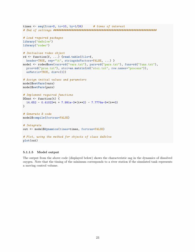
times <- seq(from=0, to=10, by=1/24) # times of interest
# End of settings ##############################################################
# Load required packages
library("deSolve")
library("rodeo")
# Initialize rodeo object
rd <- function(f, ...) {read.table(file=f,
header=TRUE, sep="\t", stringsAsFactors=FALSE, ...) }
model <- rodeo$new(vars=rd("vars.txt"), pars=rd("pars.txt"), funs=rd("funs.txt"),
pros=rd("pros.txt"), stoi=as.matrix(rd("stoi.txt", row.names="process")),
asMatrix=TRUE, dim=c(1))
# Assign initial values and parameters
model$setVars(vars)
model$setPars(pars)
# Implement required functions
DOsat <- function(t) {
14.652 - 0.41022*t + 7.991e-3*(t**2) - 7.7774e-5*(t**3)
}
# Generate R code
model$compile(fortran=FALSE)
# Integrate
out <- model$dynamics(times=times, fortran=FALSE)
# Plot, using the method for objects of class deSolve
plot(out)
5.1.1.5 Model output
The output from the above code (displayed below) shows the characteristic sag in the dynamics of dissolvedoxygen. Note that the timing of the minimum corresponds to a river station if the simulated tank representsa moving control volume.
23

0 2 4 6 8 10
0.0
0.4
0.8
OM
time
0 2 4 6 8 10
7.6
8.0
8.4
8.8
DO
time
0 2 4 6 8 10
0.0
0.4
0.8
degradation
time
0 2 4 6 8 10
0.0
0.2
0.4
0.6
reaeration
time
5.1.2 Bacteria in a 2-zones stirred tank
5.1.2.1 Problem description
The model simulates the dynamics of bacteria in a continuous-flow system which is subdivided into two tanks.The main tank is directly connected with the system’s in- and outflow. The second tank is connected to themain tank but it does not receive external inflow (see figure below and subsequent tables for a declaration ofsymbols). Both tanks are assumed to be perfectly mixed. The model accounts for import/export of bacteriaand substrate into/from the two tanks. Growth of bacteria in the two tanks is limited by substrate availabilityaccording to a Monod function.
24

Instead of simulating the system’s dynamics, we analyze steady-state concentrations of bacteria for differentchoices of the model’s parameters. The parameters whose (combined) effect is examined are:
1. the relative volume of the sub-tank in relation to the system’s total volume (parameter fS),
2. the intensity of exchange between the two tanks (parameter qS),
3. the growth rate of bacteria (controlled by parameter mu).
This kind of sensitivity analysis can be used to gain insight into the fundamental impact of transient storageon bacteria densities. A corresponding real-world systems would be a river section (main tank) that exchangeswater with either a lateral pond or the pore water of the hyporheic zone (sub-tanks). Note that, in thismodel, the sub-tank allocates a fraction of the system’s total volume. This is (at least partly) in contrast tothe mentioned real systems, where the total volume increases with increasing thickness of the hyporheic zoneor the size of a lateral pond.
The runsteady method from the rootSolve package is employed for steady-state computation. Thus, wejust perform integration over a time period a sufficient length. While this is not the most efficient strategy itcomes with the advantage of guaranteed convergence independent of the assumed initial state.
5.1.2.2 Tabular model definition
The model’s state variables, parameters, and functions are declared below, followed by the speficition ofprocess rates and stoichiometric factors.
Table 13: Declaration of state variables (file ‘vars.txt’).
name unit description
bM mg/ml Bacteria concentration in main tankbS mg/ml Bacteria concentration in sub-tanksM mg/ml Substrate concentration in main tanksS mg/ml Substrate concentration in sub-tank
Table 14: Declaration of parameters (file ‘pars.txt’).
name unit description
vol ml Total volume (main tank + sub-tank)fS - Fraction of total volume assigned to sub-tankqM ml/hour External in-/outflow to/from main tankqS ml/hour Flow rate in sub-tank branchbX mg/ml Concentration of bacteria in external inflow to main tanksX mg/ml Concentration of substrate in external inflow to main tank
25
name unit description
mu 1/hour Growth rate constant of bacteriayield mg/mg Yield coef. (bacteria produced per amount of substrate)half mg/ml Half saturation conc. of sustrate for bacteria growth
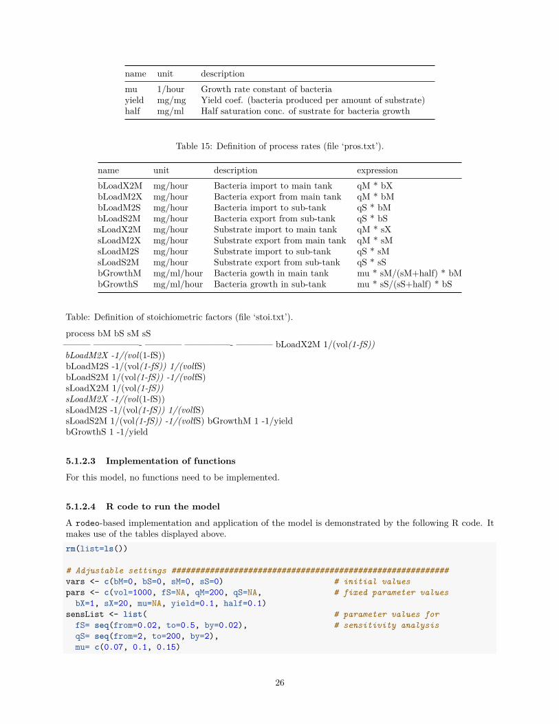
Table 15: Definition of process rates (file ‘pros.txt’).
name unit description expression
bLoadX2M mg/hour Bacteria import to main tank qM * bXbLoadM2X mg/hour Bacteria export from main tank qM * bMbLoadM2S mg/hour Bacteria import to sub-tank qS * bMbLoadS2M mg/hour Bacteria export from sub-tank qS * bSsLoadX2M mg/hour Substrate import to main tank qM * sXsLoadM2X mg/hour Substrate export from main tank qM * sMsLoadM2S mg/hour Substrate import to sub-tank qS * sMsLoadS2M mg/hour Substrate export from sub-tank qS * sSbGrowthM mg/ml/hour Bacteria gowth in main tank mu * sM/(sM+half) * bMbGrowthS mg/ml/hour Bacteria growth in sub-tank mu * sS/(sS+half) * bS
Table: Definition of stoichiometric factors (file ‘stoi.txt’).
process bM bS sM sS——— —————- ———— —————- ———— bLoadX2M 1/(vol(1-fS))bLoadM2X -1/(vol(1-fS))bLoadM2S -1/(vol(1-fS)) 1/(volfS)bLoadS2M 1/(vol(1-fS)) -1/(volfS)sLoadX2M 1/(vol(1-fS))sLoadM2X -1/(vol(1-fS))sLoadM2S -1/(vol(1-fS)) 1/(volfS)sLoadS2M 1/(vol(1-fS)) -1/(volfS) bGrowthM 1 -1/yieldbGrowthS 1 -1/yield
5.1.2.3 Implementation of functions
For this model, no functions need to be implemented.
5.1.2.4 R code to run the model
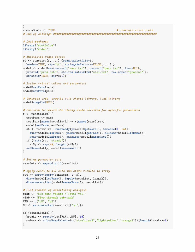
A rodeo-based implementation and application of the model is demonstrated by the following R code. Itmakes use of the tables displayed above.
rm(list=ls())
# Adjustable settings ##########################################################
vars <- c(bM=0, bS=0, sM=0, sS=0) # initial values
pars <- c(vol=1000, fS=NA, qM=200, qS=NA, # fixed parameter values
bX=1, sX=20, mu=NA, yield=0.1, half=0.1)
sensList <- list( # parameter values for
fS= seq(from=0.02, to=0.5, by=0.02), # sensitivity analysis
qS= seq(from=2, to=200, by=2),
mu= c(0.07, 0.1, 0.15)
26
)
commonScale <- TRUE # controls color scale
# End of settings ##############################################################
# Load packages
library("rootSolve")
library("rodeo")
# Initialize rodeo object
rd <- function(f, ...) {read.table(file=f,
header=TRUE, sep="\t", stringsAsFactors=FALSE, ...) }
model <- rodeo$new(vars=rd("vars.txt"), pars=rd("pars.txt"), funs=NULL,
pros=rd("pros.txt"), stoi=as.matrix(rd("stoi.txt", row.names="process")),
asMatrix=TRUE, dim=c(1))
# Assign initial values and parameters
model$setVars(vars)
model$setPars(pars)
# Generate code, compile into shared library, load library
model$compile(NULL)
# Function to return the steady-state solution for specific parameters
f <- function(x) {
testPars <- pars
testPars[names(sensList)] <- x[names(sensList)]
model$setPars(testPars)
st <- rootSolve::runsteady(y=model$getVars(), times=c(0, Inf),
func=model$libFunc(), parms=model$getPars(), dllname=model$libName(),
nout=model$lenPros(), outnames=model$namesPros())
if (!attr(st, "steady"))
st$y <- rep(NA, length(st$y))
setNames(st$y, model$namesVars())
}
# Set up parameter sets
sensSets <- expand.grid(sensList)
# Apply model to all sets and store results as array
out <- array(apply(sensSets, 1, f),
dim=c(model$lenVars(), lapply(sensList, length)),
dimnames=c(list(model$namesVars()), sensList))
# Plot results of sensitivity analysis
xlab <- "Sub-tank volume / Total vol."
ylab <- "Flow through sub-tank"
VAR <- c("bM", "bS")
MU <- as.character(sensList[["mu"]])
if (commonScale) {
breaks <- pretty(out[VAR,,,MU], 15)
colors <- colorRampPalette(c("steelblue2","lightyellow","orange2"))(length(breaks)-1)
}
27
layout(matrix(1:((length(VAR)+1)*length(MU)), ncol=length(VAR)+1,
nrow=length(MU), byrow=TRUE))
for (mu in MU) {
if (!commonScale) {
breaks <- pretty(out[VAR,,,mu], 15)
colors <- colorRampPalette(c("steelblue2","lightyellow","orange2"))(length(breaks)-1)
}
for (var in VAR) {
image(x=as.numeric(rownames(out[var,,,mu])),
y=as.numeric(colnames(out[var,,,mu])), z=out[var,,,mu],
breaks=breaks, col=colors, xlab=xlab, ylab=ylab)
mtext(side=3, var, cex=par("cex"))
legend("topright", bty="n", legend=paste("mu=",mu))
}
plot.new()
br <- round(breaks, 1)
legend("topleft", bty="n", ncol= 2, fill=colors,
legend=paste(br[-length(br)],br[-1],sep="-"))
}
layout(1)
5.1.2.5 Model output
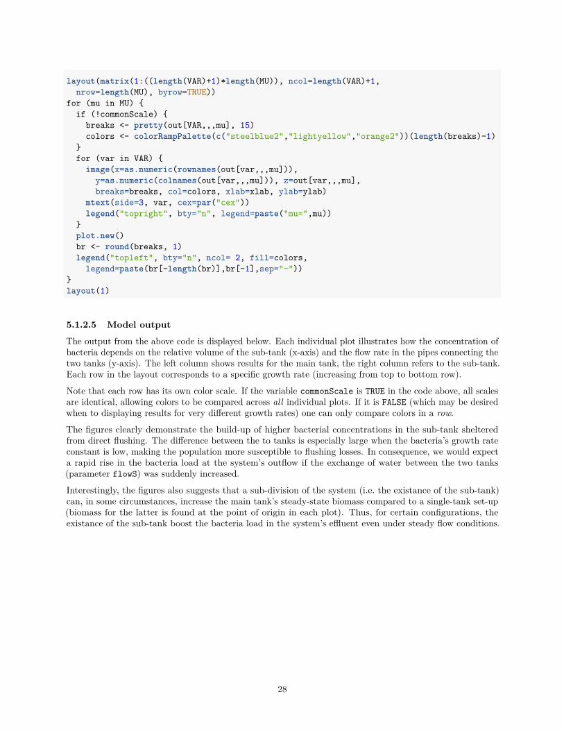
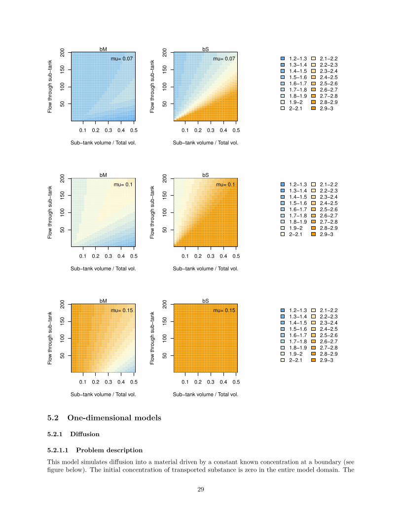
The output from the above code is displayed below. Each individual plot illustrates how the concentration ofbacteria depends on the relative volume of the sub-tank (x-axis) and the flow rate in the pipes connecting thetwo tanks (y-axis). The left column shows results for the main tank, the right column refers to the sub-tank.Each row in the layout corresponds to a specific growth rate (increasing from top to bottom row).
Note that each row has its own color scale. If the variable commonScale is TRUE in the code above, all scalesare identical, allowing colors to be compared across all individual plots. If it is FALSE (which may be desiredwhen to displaying results for very different growth rates) one can only compare colors in a row.
The figures clearly demonstrate the build-up of higher bacterial concentrations in the sub-tank shelteredfrom direct flushing. The difference between the to tanks is especially large when the bacteria’s growth rateconstant is low, making the population more susceptible to flushing losses. In consequence, we would expecta rapid rise in the bacteria load at the system’s outflow if the exchange of water between the two tanks(parameter flowS) was suddenly increased.
Interestingly, the figures also suggests that a sub-division of the system (i.e. the existance of the sub-tank)can, in some circumstances, increase the main tank’s steady-state biomass compared to a single-tank set-up(biomass for the latter is found at the point of origin in each plot). Thus, for certain configurations, theexistance of the sub-tank boost the bacteria load in the system’s effluent even under steady flow conditions.
28
0.1 0.2 0.3 0.4 0.5
50
100
150
200
Sub−tank volume / Total vol.
Flo
w thro
ugh s
ub−
tank
bM
mu= 0.07
0.1 0.2 0.3 0.4 0.5
50
100
150
200
Sub−tank volume / Total vol.
Flo
w thro
ugh s
ub−
tank
bS
mu= 0.07 1.2−1.31.3−1.41.4−1.51.5−1.61.6−1.71.7−1.81.8−1.91.9−22−2.1
2.1−2.22.2−2.32.3−2.42.4−2.52.5−2.62.6−2.72.7−2.82.8−2.92.9−3
0.1 0.2 0.3 0.4 0.5
50
100
150
200
Sub−tank volume / Total vol.
Flo
w thro
ugh s
ub−
tank
bM
mu= 0.1
0.1 0.2 0.3 0.4 0.5
50
100
150
200
Sub−tank volume / Total vol.
Flo
w thro
ugh s
ub−
tank
bS
mu= 0.1 1.2−1.31.3−1.41.4−1.51.5−1.61.6−1.71.7−1.81.8−1.91.9−22−2.1
2.1−2.22.2−2.32.3−2.42.4−2.52.5−2.62.6−2.72.7−2.82.8−2.92.9−3
0.1 0.2 0.3 0.4 0.5
50
100
150
200
Sub−tank volume / Total vol.
Flo
w t
hro
ugh s
ub−
tank
bM
mu= 0.15
0.1 0.2 0.3 0.4 0.5
50
100
150
200
Sub−tank volume / Total vol.
Flo
w t
hro
ugh s
ub−
tank
bS
mu= 0.15 1.2−1.31.3−1.41.4−1.51.5−1.61.6−1.71.7−1.81.8−1.91.9−22−2.1
2.1−2.22.2−2.32.3−2.42.4−2.52.5−2.62.6−2.72.7−2.82.8−2.92.9−3
5.2 One-dimensional models
5.2.1 Diffusion
5.2.1.1 Problem description
This model simulates diffusion into a material driven by a constant known concentration at a boundary (seefigure below). The initial concentration of transported substance is zero in the entire model domain. The
29
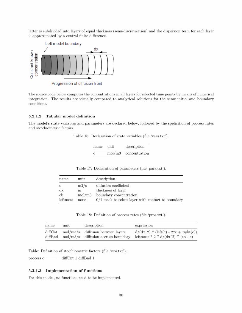
latter is subdivided into layers of equal thickness (semi-discretization) and the dispersion term for each layeris approximated by a central finite difference.
The source code below computes the concentrations in all layers for selected time points by means of numericalintegration. The results are visually compared to analytical solutions for the same initial and boundaryconditions.
5.2.1.2 Tabular model definition
The model’s state variables and parameters are declared below, followed by the speficition of process ratesand stoichiometric factors.
Table 16: Declaration of state variables (file ‘vars.txt’).
name unit description
c mol/m3 concentration
Table 17: Declaration of parameters (file ‘pars.txt’).
name unit description
d m2/s diffusion coefficientdx m thickness of layercb mol/m3 boundary concentrationleftmost none 0/1 mask to select layer with contact to boundary
Table 18: Definition of process rates (file ‘pros.txt’).
name unit description expression
diffCnt mol/m3/s diffusion between layers d/(dxˆ2) * (left(c) - 2*c + right(c))diffBnd mol/m3/s diffusion accross boundary leftmost * 2 * d/(dxˆ2) * (cb - c)
Table: Definition of stoichiometric factors (file ‘stoi.txt’).
process c ——– — diffCnt 1 diffBnd 1
5.2.1.3 Implementation of functions
For this model, no functions need to be implemented.
30
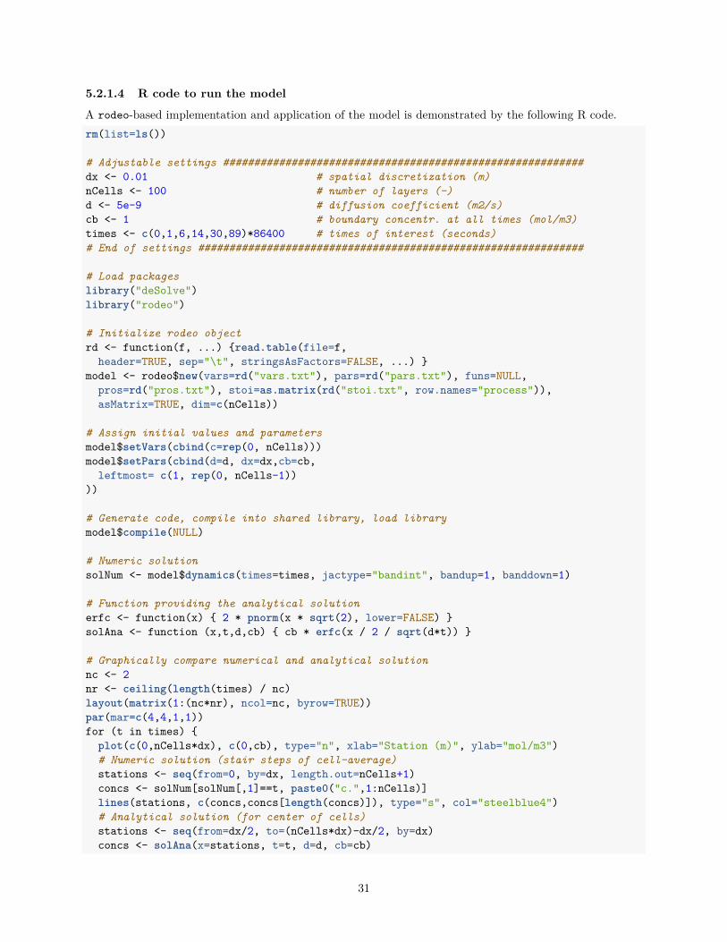
5.2.1.4 R code to run the model
A rodeo-based implementation and application of the model is demonstrated by the following R code.
rm(list=ls())
# Adjustable settings ##########################################################
dx <- 0.01 # spatial discretization (m)
nCells <- 100 # number of layers (-)
d <- 5e-9 # diffusion coefficient (m2/s)
cb <- 1 # boundary concentr. at all times (mol/m3)
times <- c(0,1,6,14,30,89)*86400 # times of interest (seconds)
# End of settings ##############################################################
# Load packages
library("deSolve")
library("rodeo")
# Initialize rodeo object
rd <- function(f, ...) {read.table(file=f,
header=TRUE, sep="\t", stringsAsFactors=FALSE, ...) }
model <- rodeo$new(vars=rd("vars.txt"), pars=rd("pars.txt"), funs=NULL,
pros=rd("pros.txt"), stoi=as.matrix(rd("stoi.txt", row.names="process")),
asMatrix=TRUE, dim=c(nCells))
# Assign initial values and parameters
model$setVars(cbind(c=rep(0, nCells)))
model$setPars(cbind(d=d, dx=dx,cb=cb,
leftmost= c(1, rep(0, nCells-1))
))
# Generate code, compile into shared library, load library
model$compile(NULL)
# Numeric solution
solNum <- model$dynamics(times=times, jactype="bandint", bandup=1, banddown=1)
# Function providing the analytical solution
erfc <- function(x) { 2 * pnorm(x * sqrt(2), lower=FALSE) }
solAna <- function (x,t,d,cb) { cb * erfc(x / 2 / sqrt(d*t)) }
# Graphically compare numerical and analytical solution
nc <- 2
nr <- ceiling(length(times) / nc)
layout(matrix(1:(nc*nr), ncol=nc, byrow=TRUE))
par(mar=c(4,4,1,1))
for (t in times) {
plot(c(0,nCells*dx), c(0,cb), type="n", xlab="Station (m)", ylab="mol/m3")
# Numeric solution (stair steps of cell-average)
stations <- seq(from=0, by=dx, length.out=nCells+1)
concs <- solNum[solNum[,1]==t, paste0("c.",1:nCells)]
lines(stations, c(concs,concs[length(concs)]), type="s", col="steelblue4")
# Analytical solution (for center of cells)
stations <- seq(from=dx/2, to=(nCells*dx)-dx/2, by=dx)
concs <- solAna(x=stations, t=t, d=d, cb=cb)
31
lines(stations, concs, col="red", lty=2)
# Extras
legend("topright", bty="n", paste("After",t/86400,"days"))
if (t == times[1]) legend("right",lty=1:2,
col=c("steelblue4","red"),legend=c("Numeric", "Exact"),bty="n")
abline(v=0)
}
layout(1)
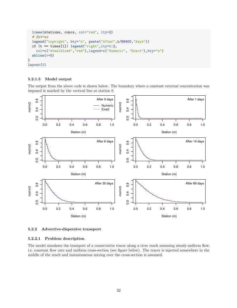
5.2.1.5 Model output
The output from the above code is shown below. The boundary where a constant external concentration wasimposed is marked by the vertical line at station 0.
0.0 0.2 0.4 0.6 0.8 1.0
0.0
0.4
0.8
Station (m)
mo
l/m
3
After 0 days
NumericExact
0.0 0.2 0.4 0.6 0.8 1.00
.00
.40
.8
Station (m)
mo
l/m
3
After 1 days
0.0 0.2 0.4 0.6 0.8 1.0
0.0
0.4
0.8
Station (m)
mo
l/m
3
After 6 days
0.0 0.2 0.4 0.6 0.8 1.0
0.0
0.4
0.8
Station (m)
mo
l/m
3
After 14 days
0.0 0.2 0.4 0.6 0.8 1.0
0.0
0.4
0.8
Station (m)
mo
l/m
3
After 30 days
0.0 0.2 0.4 0.6 0.8 1.0
0.0
0.4
0.8
Station (m)
mo
l/m
3
After 89 days
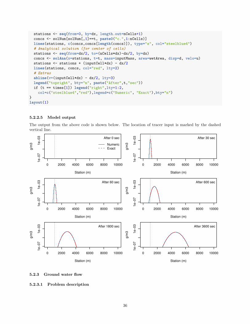
5.2.2 Advective-dispersive transport
5.2.2.1 Problem description
The model simulates the transport of a conservative tracer along a river reach assuming steady-uniform flow,i.e. constant flow rate and uniform cross-section (see figure below). The tracer is injected somewhere in themiddle of the reach and instantaneous mixing over the cross-section is assumed.
32
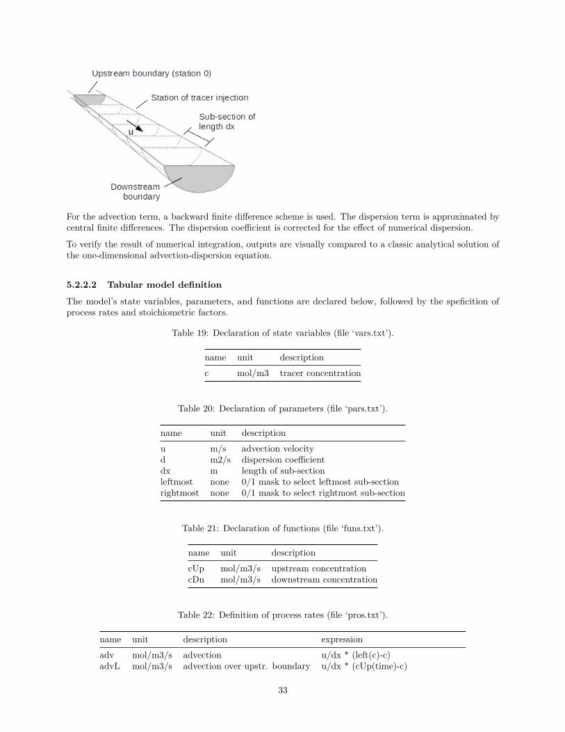
For the advection term, a backward finite difference scheme is used. The dispersion term is approximated bycentral finite differences. The dispersion coefficient is corrected for the effect of numerical dispersion.
To verify the result of numerical integration, outputs are visually compared to a classic analytical solution ofthe one-dimensional advection-dispersion equation.
5.2.2.2 Tabular model definition
The model’s state variables, parameters, and functions are declared below, followed by the speficition ofprocess rates and stoichiometric factors.
Table 19: Declaration of state variables (file ‘vars.txt’).
name unit description
c mol/m3 tracer concentration
Table 20: Declaration of parameters (file ‘pars.txt’).
name unit description
u m/s advection velocityd m2/s dispersion coefficientdx m length of sub-sectionleftmost none 0/1 mask to select leftmost sub-sectionrightmost none 0/1 mask to select rightmost sub-section
Table 21: Declaration of functions (file ‘funs.txt’).
name unit description
cUp mol/m3/s upstream concentrationcDn mol/m3/s downstream concentration
Table 22: Definition of process rates (file ‘pros.txt’).
name unit description expression
adv mol/m3/s advection u/dx * (left(c)-c)advL mol/m3/s advection over upstr. boundary u/dx * (cUp(time)-c)
33
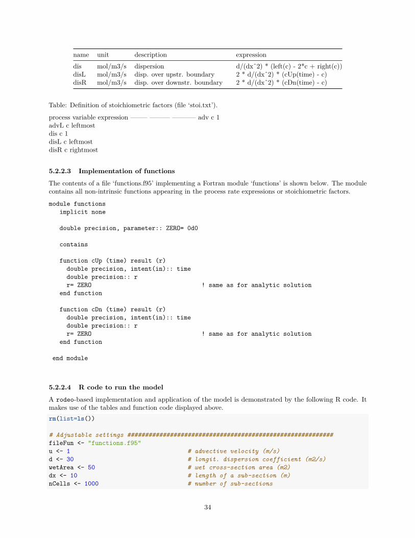
name unit description expression
dis mol/m3/s dispersion d/(dxˆ2) * (left(c) - 2*c + right(c))disL mol/m3/s disp. over upstr. boundary 2 * d/(dxˆ2) * (cUp(time) - c)disR mol/m3/s disp. over downstr. boundary 2 * d/(dxˆ2) * (cDn(time) - c)
Table: Definition of stoichiometric factors (file ‘stoi.txt’).
process variable expression ——– ——— ———– adv c 1advL c leftmostdis c 1disL c leftmostdisR c rightmost
5.2.2.3 Implementation of functions
The contents of a file ‘functions.f95’ implementing a Fortran module ‘functions’ is shown below. The modulecontains all non-intrinsic functions appearing in the process rate expressions or stoichiometric factors.
module functions
implicit none
double precision, parameter:: ZERO= 0d0
contains
function cUp (time) result (r)
double precision, intent(in):: time
double precision:: r
r= ZERO ! same as for analytic solution
end function
function cDn (time) result (r)
double precision, intent(in):: time
double precision:: r
r= ZERO ! same as for analytic solution
end function
end module
5.2.2.4 R code to run the model
A rodeo-based implementation and application of the model is demonstrated by the following R code. Itmakes use of the tables and function code displayed above.
rm(list=ls())
# Adjustable settings ##########################################################
fileFun <- "functions.f95"
u <- 1 # advective velocity (m/s)
d <- 30 # longit. dispersion coefficient (m2/s)
wetArea <- 50 # wet cross-section area (m2)
dx <- 10 # length of a sub-section (m)
nCells <- 1000 # number of sub-sections
34
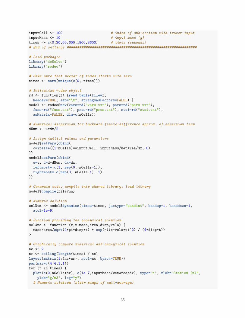
inputCell <- 100 # index of sub-section with tracer input
inputMass <- 10 # input mass (g)
times <- c(0,30,60,600,1800,3600) # times (seconds)
# End of settings ##############################################################
# Load packages
library("deSolve")
library("rodeo")
# Make sure that vector of times starts with zero
times <- sort(unique(c(0, times)))
# Initialize rodeo object
rd <- function(f) {read.table(file=f,
header=TRUE, sep="\t", stringsAsFactors=FALSE) }
model <- rodeo$new(vars=rd("vars.txt"), pars=rd("pars.txt"),
funs=rd("funs.txt"), pros=rd("pros.txt"), stoi=rd("stoi.txt"),
asMatrix=FALSE, dim=c(nCells))
# Numerical dispersion for backward finite-difference approx. of advection term
dNum <- u*dx/2
# Assign initial values and parameters
model$setVars(cbind(
c=ifelse((1:nCells)==inputCell, inputMass/wetArea/dx, 0)
))
model$setPars(cbind(
u=u, d=d-dNum, dx=dx,
leftmost= c(1, rep(0, nCells-1)),
rightmost= c(rep(0, nCells-1), 1)
))
# Generate code, compile into shared library, load library
model$compile(fileFun)
# Numeric solution
solNum <- model$dynamics(times=times, jactype="bandint", bandup=1, banddown=1,
atol=1e-9)
# Function providing the analytical solution
solAna <- function (x,t,mass,area,disp,velo) {
mass/area/sqrt(4*pi*disp*t) * exp(-((x-velo*t)^2) / (4*disp*t))
}
# Graphically compare numerical and analytical solution
nc <- 2
nr <- ceiling(length(times) / nc)
layout(matrix(1:(nc*nr), ncol=nc, byrow=TRUE))
par(mar=c(4,4,1,1))
for (t in times) {
plot(c(0,nCells*dx), c(1e-7,inputMass/wetArea/dx), type="n", xlab="Station (m)",
ylab="g/m3", log="y")
# Numeric solution (stair steps of cell-average)
35
stations <- seq(from=0, by=dx, length.out=nCells+1)
concs <- solNum[solNum[,1]==t, paste0("c.",1:nCells)]
lines(stations, c(concs,concs[length(concs)]), type="s", col="steelblue4")
# Analytical solution (for center of cells)
stations <- seq(from=dx/2, to=(nCells*dx)-dx/2, by=dx)
concs <- solAna(x=stations, t=t, mass=inputMass, area=wetArea, disp=d, velo=u)
stations <- stations + (inputCell*dx) - dx/2
lines(stations, concs, col="red", lty=2)
# Extras
abline(v=(inputCell*dx) - dx/2, lty=3)
legend("topright", bty="n", paste("After",t,"sec"))
if (t == times[1]) legend("right",lty=1:2,
col=c("steelblue4","red"),legend=c("Numeric", "Exact"),bty="n")
}
layout(1)
5.2.2.5 Model output
The output from the above code is shown below. The location of tracer input is marked by the dashedvertical line.
0 2000 4000 6000 8000 10000
1e
−0
71
e−
03
Station (m)
g/m
3
After 0 sec
NumericExact
0 2000 4000 6000 8000 10000
1e
−0
71
e−
03
Station (m)
g/m
3
After 30 sec
0 2000 4000 6000 8000 10000
1e
−0
71
e−
03
Station (m)
g/m
3
After 60 sec
0 2000 4000 6000 8000 10000
1e
−0
71
e−
03
Station (m)
g/m
3
After 600 sec
0 2000 4000 6000 8000 10000
1e
−0
71
e−
03
Station (m)
g/m
3
After 1800 sec
0 2000 4000 6000 8000 10000
1e
−0
71
e−
03
Station (m)
g/m
3
After 3600 sec
5.2.3 Ground water flow
5.2.3.1 Problem description
36

The model solves the partial differential equation describing one-dimensional (lateral) ground water flow underthe Dupuit-Forchheimer assumption. Flow is simulated along a transect between the watershed boundaryand a river (see Figure below).
The model has several boundary conditions:
• Zero lateral flow at left margin (boundary of watershed)
• Exchange with river at right margin (leaky aquifer approach, river water level can vary over time)
• No lateral flow accross right boundary (assuming symmetry, i.e. an identical watershed at the otherside of the river ).
• Time-variable recharge via percolation through unsaturated zone.
The governing equations can be found in Bronstert et al. (1991). Details on the leakage approach arepresented in Rauch (1993), Kinzelbach (1986), as well as Kinzelbach and Rausch (1995).
5.2.3.2 Tabular model definition
The model’s state variables, parameters, and functions are declared below, followed by the speficition ofprocess rates and stoichiometric factors.
Table 23: Declaration of state variables (file ‘vars.txt’).
name unit description
h m elevation of ground water surface
Table 24: Declaration of parameters (file ‘pars.txt’).
name unit description
dx m lateral discretizatonkf m/day hydraulic conductivityne - effective porosityh0 m elevation of aquifer basehBed m river bottom elevationwBed m width of river (rectangular x-section)kfBed m/day hydraulic conductivity of river bottom layertBed m thickness of river bottom layerleaky - 1 for leaky and 0 for normal cells
37
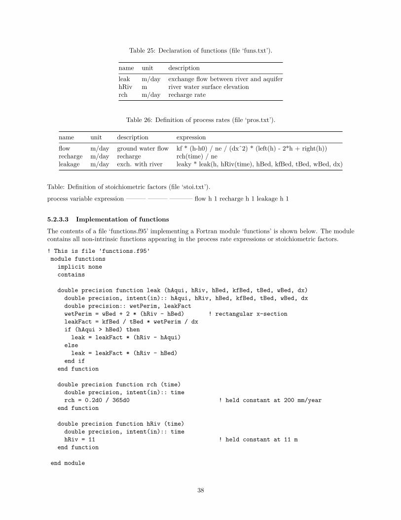
Table 25: Declaration of functions (file ‘funs.txt’).
name unit description
leak m/day exchange flow between river and aquiferhRiv m river water surface elevationrch m/day recharge rate
Table 26: Definition of process rates (file ‘pros.txt’).
name unit description expression
flow m/day ground water flow kf * (h-h0) / ne / (dxˆ2) * (left(h) - 2*h + right(h))recharge m/day recharge rch(time) / neleakage m/day exch. with river leaky * leak(h, hRiv(time), hBed, kfBed, tBed, wBed, dx)
Table: Definition of stoichiometric factors (file ‘stoi.txt’).
process variable expression ——— ——— ———– flow h 1 recharge h 1 leakage h 1
5.2.3.3 Implementation of functions
The contents of a file ‘functions.f95’ implementing a Fortran module ‘functions’ is shown below. The modulecontains all non-intrinsic functions appearing in the process rate expressions or stoichiometric factors.
! This is file 'functions.f95'
module functions
implicit none
contains
double precision function leak (hAqui, hRiv, hBed, kfBed, tBed, wBed, dx)
double precision, intent(in):: hAqui, hRiv, hBed, kfBed, tBed, wBed, dx
double precision:: wetPerim, leakFact
wetPerim = wBed + 2 * (hRiv - hBed) ! rectangular x-section
leakFact = kfBed / tBed * wetPerim / dx
if (hAqui > hBed) then
leak = leakFact * (hRiv - hAqui)
else
leak = leakFact * (hRiv - hBed)
end if
end function
double precision function rch (time)
double precision, intent(in):: time
rch = 0.2d0 / 365d0 ! held constant at 200 mm/year
end function
double precision function hRiv (time)
double precision, intent(in):: time
hRiv = 11 ! held constant at 11 m
end function
end module
38
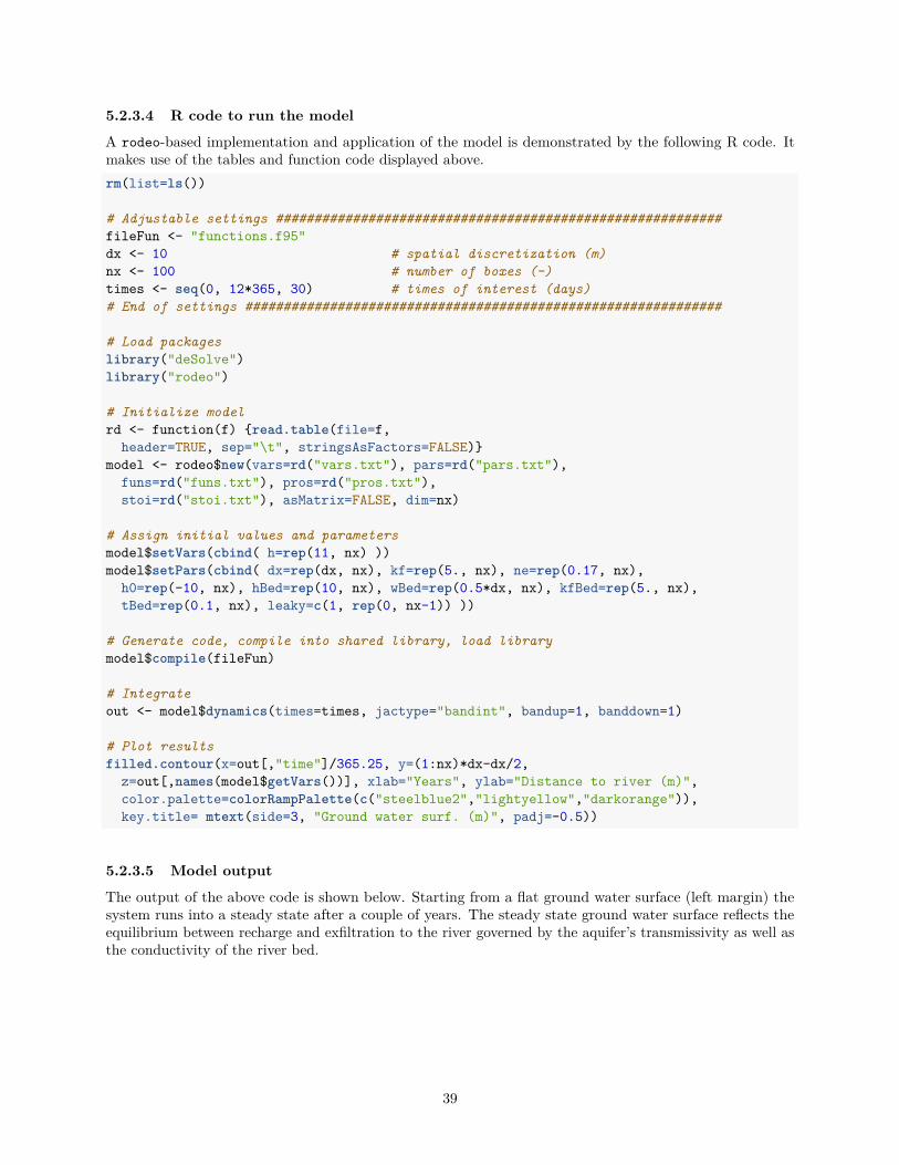
5.2.3.4 R code to run the model
A rodeo-based implementation and application of the model is demonstrated by the following R code. Itmakes use of the tables and function code displayed above.
rm(list=ls())
# Adjustable settings ##########################################################
fileFun <- "functions.f95"
dx <- 10 # spatial discretization (m)
nx <- 100 # number of boxes (-)
times <- seq(0, 12*365, 30) # times of interest (days)
# End of settings ##############################################################
# Load packages
library("deSolve")
library("rodeo")
# Initialize model
rd <- function(f) {read.table(file=f,
header=TRUE, sep="\t", stringsAsFactors=FALSE)}
model <- rodeo$new(vars=rd("vars.txt"), pars=rd("pars.txt"),
funs=rd("funs.txt"), pros=rd("pros.txt"),
stoi=rd("stoi.txt"), asMatrix=FALSE, dim=nx)
# Assign initial values and parameters
model$setVars(cbind( h=rep(11, nx) ))
model$setPars(cbind( dx=rep(dx, nx), kf=rep(5., nx), ne=rep(0.17, nx),
h0=rep(-10, nx), hBed=rep(10, nx), wBed=rep(0.5*dx, nx), kfBed=rep(5., nx),
tBed=rep(0.1, nx), leaky=c(1, rep(0, nx-1)) ))
# Generate code, compile into shared library, load library
model$compile(fileFun)
# Integrate
out <- model$dynamics(times=times, jactype="bandint", bandup=1, banddown=1)
# Plot results
filled.contour(x=out[,"time"]/365.25, y=(1:nx)*dx-dx/2,
z=out[,names(model$getVars())], xlab="Years", ylab="Distance to river (m)",
color.palette=colorRampPalette(c("steelblue2","lightyellow","darkorange")),
key.title= mtext(side=3, "Ground water surf. (m)", padj=-0.5))
5.2.3.5 Model output
The output of the above code is shown below. Starting from a flat ground water surface (left margin) thesystem runs into a steady state after a couple of years. The steady state ground water surface reflects theequilibrium between recharge and exfiltration to the river governed by the aquifer’s transmissivity as well asthe conductivity of the river bed.
39
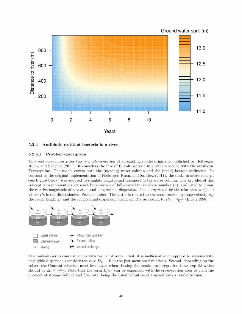
11.0
11.5
12.0
12.5
13.0
Ground water surf. (m)
0 2 4 6 8 10
200
400
600
800
Years
Dis
tan
ce
to
riv
er
(m)
5.2.4 Antibiotic resistant bacteria in a river
5.2.4.1 Problem description
This section demonstrates the re-implementation of an existing model originally published by Hellweger,Ruan, and Sanchez (2011). It considers the fate of E. coli bacteria in a stream loaded with the antibioticTetracycline. The model covers both the (moving) water column and the (fixed) bottom sediments. Incontrast to the original implementation of Hellweger, Ruan, and Sanchez (2011), the tanks-in-series concept(see Figure below) was adopted to simulate longitudinal transport in the water column. The key idea of thisconcept is to represent a river reach by a cascade of fully-mixed tanks whose number (n) is adjusted to mimicthe relative magnitude of advection and longitudinal dispersion. This is expressed by the relation n = P e
2+ 1
where Pe is the dimensionless Peclet number. The latter is related to the cross-section average velocity uL,the reach length L, and the longitudinal dispersion coefficient DL according to Pe = uL·L
DL
(Elgeti 1996).
The tanks-in-series concept comes with two constraints: First, it is inefficient when applied to systems withnegligible dispersion (consider the case DL → 0 in the just mentioned relation). Second, depending on thesolver, the Courant criterion must be obeyed when chosing the maximum integration time step ∆t whichshould be ∆t ≤
L
n·uL
. Note that the term L/uL can be expanded with the cross-section area to yield thequotient of storage volume and flow rate, being the usual definition of a mixed tank’s residence time.
40
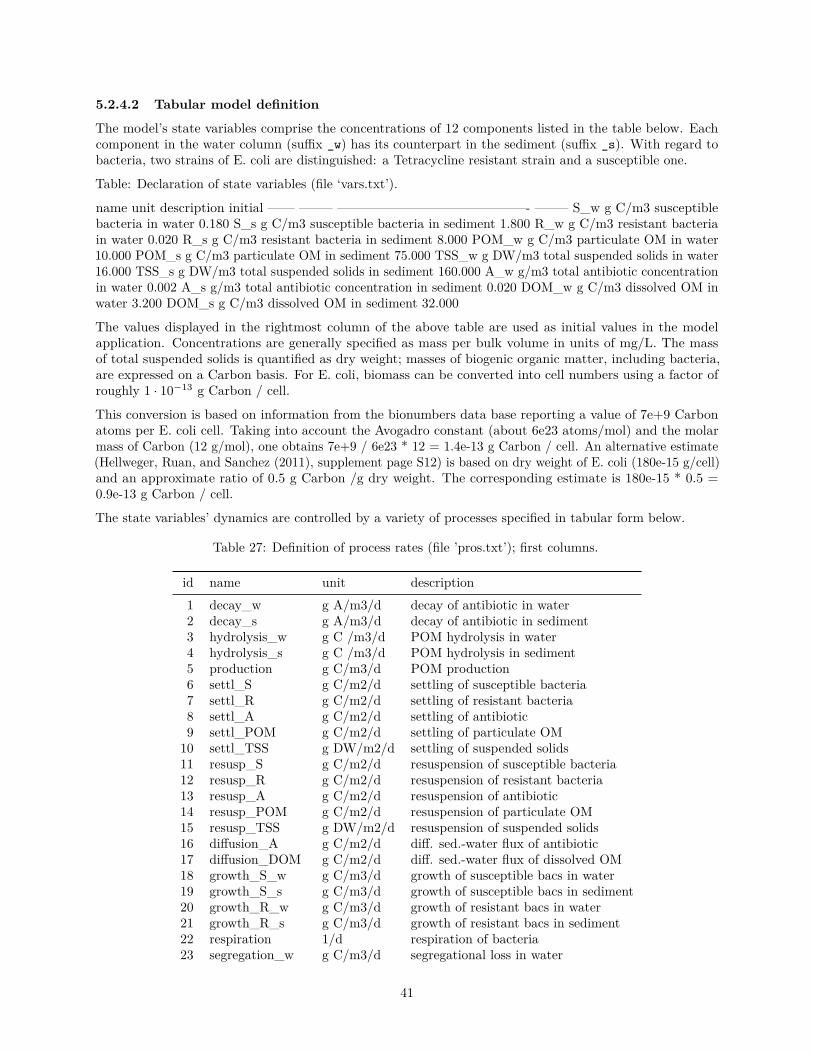
5.2.4.2 Tabular model definition
The model’s state variables comprise the concentrations of 12 components listed in the table below. Eachcomponent in the water column (suffix _w) has its counterpart in the sediment (suffix _s). With regard tobacteria, two strains of E. coli are distinguished: a Tetracycline resistant strain and a susceptible one.
Table: Declaration of state variables (file ‘vars.txt’).
name unit description initial —— ——– ——————————————- ——– S_w g C/m3 susceptiblebacteria in water 0.180 S_s g C/m3 susceptible bacteria in sediment 1.800 R_w g C/m3 resistant bacteriain water 0.020 R_s g C/m3 resistant bacteria in sediment 8.000 POM_w g C/m3 particulate OM in water10.000 POM_s g C/m3 particulate OM in sediment 75.000 TSS_w g DW/m3 total suspended solids in water16.000 TSS_s g DW/m3 total suspended solids in sediment 160.000 A_w g/m3 total antibiotic concentrationin water 0.002 A_s g/m3 total antibiotic concentration in sediment 0.020 DOM_w g C/m3 dissolved OM inwater 3.200 DOM_s g C/m3 dissolved OM in sediment 32.000
The values displayed in the rightmost column of the above table are used as initial values in the modelapplication. Concentrations are generally specified as mass per bulk volume in units of mg/L. The massof total suspended solids is quantified as dry weight; masses of biogenic organic matter, including bacteria,are expressed on a Carbon basis. For E. coli, biomass can be converted into cell numbers using a factor ofroughly 1 · 10−13 g Carbon / cell.
This conversion is based on information from the bionumbers data base reporting a value of 7e+9 Carbonatoms per E. coli cell. Taking into account the Avogadro constant (about 6e23 atoms/mol) and the molarmass of Carbon (12 g/mol), one obtains 7e+9 / 6e23 * 12 = 1.4e-13 g Carbon / cell. An alternative estimate(Hellweger, Ruan, and Sanchez (2011), supplement page S12) is based on dry weight of E. coli (180e-15 g/cell)and an approximate ratio of 0.5 g Carbon /g dry weight. The corresponding estimate is 180e-15 * 0.5 =0.9e-13 g Carbon / cell.
The state variables’ dynamics are controlled by a variety of processes specified in tabular form below.
Table 27: Definition of process rates (file ’pros.txt’); first columns.
id name unit description
1 decay_w g A/m3/d decay of antibiotic in water2 decay_s g A/m3/d decay of antibiotic in sediment3 hydrolysis_w g C /m3/d POM hydrolysis in water4 hydrolysis_s g C /m3/d POM hydrolysis in sediment5 production g C/m3/d POM production6 settl_S g C/m2/d settling of susceptible bacteria7 settl_R g C/m2/d settling of resistant bacteria8 settl_A g C/m2/d settling of antibiotic9 settl_POM g C/m2/d settling of particulate OM
10 settl_TSS g DW/m2/d settling of suspended solids11 resusp_S g C/m2/d resuspension of susceptible bacteria12 resusp_R g C/m2/d resuspension of resistant bacteria13 resusp_A g C/m2/d resuspension of antibiotic14 resusp_POM g C/m2/d resuspension of particulate OM15 resusp_TSS g DW/m2/d resuspension of suspended solids16 diffusion_A g C/m2/d diff. sed.-water flux of antibiotic17 diffusion_DOM g C/m2/d diff. sed.-water flux of dissolved OM18 growth_S_w g C/m3/d growth of susceptible bacs in water19 growth_S_s g C/m3/d growth of susceptible bacs in sediment20 growth_R_w g C/m3/d growth of resistant bacs in water21 growth_R_s g C/m3/d growth of resistant bacs in sediment22 respiration 1/d respiration of bacteria23 segregation_w g C/m3/d segregational loss in water
41

24 segregation_s g C/m3/d segregational loss in sediment25 conjugation_w g C/m3/d conjugation in water26 conjugation_s g C/m3/d conjugation in sediment27 transport_S g C/m3/d transport of susceptible bacteria28 transport_R g C/m3/d transport of resistant bacteria29 transport_A g C/m3/d transport of antibiotic30 transport_DOM g C/m3/d transport of dissolved OM31 transport_POM g C/m3/d transport of particulate OM32 transport_TSS g DW/m3/d transport of suspended solids
Table 28: Definition of process rates (file ’pros.txt’); further columns.
id expression
1 ka_w * A_w2 ka_s * A_s3 kh_w * POM_w4 kh_s * POM_s5 P / dw6 us * fp * S_w7 us * fp * R_w8 us * A_part(A_w, kd_DOM, kd_TSS, DOM_w, TSS_w)9 us * POM_w10 us * TSS_w11 ur * S_s12 ur * R_s13 ur * A_part(A_s, kd_DOM, kd_TSS, DOM_s, TSS_s)14 ur * POM_s15 ur * TSS_s16 ud * (A_diss(A_w, kd_DOM, kd_TSS, DOM_w, TSS_w) - por * A_diss(A_s, kd_DOM,
kd_TSS, DOM_s, TSS_s))17 ud * (DOM_w - por * DOM_s)18 kg * S_w * DOM_w / (DOM_w + h_DOM) * max(0, 1 - A_free(A_w, kd_DOM, kd_TSS,
DOM_w, TSS_w) / Amic)19 kg * S_s * DOM_s / (DOM_s + h_DOM) * max(0, 1 - A_free(A_s, kd_DOM, kd_TSS, DOM_s,
TSS_s) / Amic)20 kg * R_w * DOM_w / (DOM_w + h_DOM) * (1 - alpha)21 kg * R_s * DOM_s / (DOM_s + h_DOM) * (1 - alpha)22 kr23 ks * R_w24 ks * R_s25 kc * S_w * R_w26 kc * S_s * R_s27 1 / V * (Q_in * (S_in - S_w) + Q * (left(S_w) - S_w))28 1 / V * (Q_in * (R_in - R_w) + Q * (left(R_w) - R_w))29 1 / V * (Q_in * (A_in - A_w) + Q * (left(A_w) - A_w))30 1 / V * (Q_in * (DOM_in - DOM_w) + Q * (left(DOM_w) - DOM_w))31 1 / V * (Q_in * (POM_in - POM_w) + Q * (left(POM_w) - POM_w))32 1 / V * (Q_in * (TSS_in - TSS_w) + Q * (left(TSS_w) - TSS_w))
Besides the physical phenomena of advection and dispersion, the list of processes includes growth andrespiration losses of bacteria, as well as gene transfer between the two strains of E. coli. Particularly,the model describes the horizontal transfer of Tetracycline resistance through the exchange of plasmids
42

(conjugation) as well as the potential loss of the plasmid during cell division (segregational loss). Whilecarriage of the resistance genes is clearly advantageous under exposure to the antibiotic, the synthesis ofplasmids also has side effects to the cell, e. g. in the form of physiological costs. This phenomenon is describedas a reduction of the growth rate of the Tetracycline-resistant E. coli strain but evolutionary reduction ofplasmid costs (Lenski 1998) is neglected.
Tetracycline undergoes photolytic decay (Wammer et al. 2011) which is modeled as a first-order process.The antibiotic is also known to bind to organic and inorganic matter in relevant percentages (Tolls 2001).Hence, sorption effects must be included in the model to obtain realistic estimates of the freely availableTetracycline concentration to which the bacteriostatic effect is attributed (Chen et al. 2015). As in manybio-geo-chemical codes, it is assumed that sorption equilibria arise instantaneously. As this leads to a set ofalgebraic equations rather than ODE, sorption is not explicitly listed in the above table of processes.
The stoichiometric factors linking the processes with the state variables’ derivatives are provided in matrixformat below.
Table 29: Stoichiometric factors (file ’stoi.txt’); first columns.
process S_w S_s R_w R_s POM_w POM_s
decay_wdecay_ssettl_S -1/dw 1/dssettl_R -1/dw 1/dssettl_POM -1/dw 1/dssettl_TSSsettl_Aresusp_S 1/dw -1/dsresusp_R 1/dw -1/dsresusp_POM 1/dw -1/dsresusp_TSSresusp_Adiffusion_Adiffusion_DOMhydrolysis_w -1hydrolysis_s -1production 1growth_S_w 1growth_S_s 1growth_R_w 1growth_R_s 1respiration -S_w -S_s -R_w -R_ssegregation_w 1 -1segregation_s 1 -1conjugation_w -1 1conjugation_s -1 1transport_S 1transport_R 1transport_POM 1transport_TSStransport_Atransport_DOM
Table 30: Stoichiometric factors (file ’stoi.txt’); further columns.
43
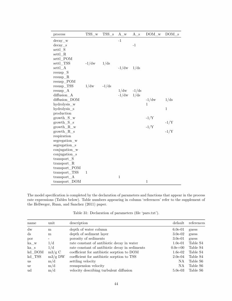
process TSS_w TSS_s A_w A_s DOM_w DOM_s
decay_w -1decay_s -1settl_Ssettl_Rsettl_POMsettl_TSS -1/dw 1/dssettl_A -1/dw 1/dsresusp_Sresusp_Rresusp_POMresusp_TSS 1/dw -1/dsresusp_A 1/dw -1/dsdiffusion_A -1/dw 1/dsdiffusion_DOM -1/dw 1/dshydrolysis_w 1hydrolysis_s 1productiongrowth_S_w -1/Ygrowth_S_s -1/Ygrowth_R_w -1/Ygrowth_R_s -1/Yrespirationsegregation_wsegregation_sconjugation_wconjugation_stransport_Stransport_Rtransport_POMtransport_TSS 1transport_A 1transport_DOM 1
The model specification is completed by the declaration of parameters and functions that appear in the processrate expressions (Tables below). Table numbers appearing in column ‘references’ refer to the supplement ofthe Hellweger, Ruan, and Sanchez (2011) paper.
Table 31: Declaration of parameters (file ‘pars.txt’).
name unit description default references
dw m depth of water column 6.0e-01 guessds m depth of sediment layer 3.0e-02 guesspor - porosity of sediments 3.0e-01 guesska_w 1/d rate constant of antibiotic decay in water 1.0e-01 Table S4ka_s 1/d rate constant of antibiotic decay in sediments 0.0e+00 Table S4kd_DOM m3/g C coefficient for antibiotic sorption to DOM 1.6e-02 Table S4kd_TSS m3/g DW coefficient for antibiotic sorption to TSS 2.0e-04 Table S4us m/d settling velocity NA Table S6ur m/d resuspension velocity NA Table S6ud m/d velocity describing turbulent diffusion 5.0e-03 Table S6
44

name unit description default references
P g C/m2/d rate of POM production 2.3e+00 Table S6kh_w 1/d rate constant of POM hydrolysis in water 5.0e-02 Table S6kh_s 1/d rate constant of POM hydrolysis in sediments 5.0e-02 Table S6fp - fraction of water-column bacteria being bound to particles 1.0e-01 Table S6kr 1/d bacteria respiration rate constant 1.1e-01 Table S4kg 1/d max. growth rate of sensitive bacteria 2.6e+00 Table S4h_DOM g C/m3 half saturation concentration of DOM for bacteria growth 9.1e+00 Table S6Y - yield; bacterial carbon / DOM carbon 3.6e-01 Table S7Amic g A/m3 minimum inhibiting conc. of freely dissolved antibiotic 1.3e-02 Table S6ks 1/d rate constant of segregational loss 4.0e-02 Table S6kc m3/g C/d constant to control conjugation 1.0e-05 Table S6alpha - reduction of growth rate due to resistance (plasmid cost) 1.0e-01 Table S6S_in g C/m3 concentrations in inflow 1.8e-02 Table S7R_in g C/m3 concentrations in inflow 2.0e-03 Table S7A_in g C/m3 concentrations in inflow 2.0e-03 guessDOM_in g C/m3 concentrations in inflow 3.2e+00 Table S7POM_in g C/m3 concentrations in inflow 4.0e-01 Table S7TSS_in g TSS/m3 concentrations in inflow 1.6e+01 Table S6V m3 reactor volume NA -Q_in m3/d external inflow (not from upstream reactor) NA -Q m3/d inflow from upstream reactor NA -
Table: Declaration of functions (file ‘funs.txt’).
name unit description——- ——- —————————————————————————– A_part mol/m3 concentration of an-tibiotic; particulate fractionA_diss mol/m3 concentration of antibiotic; freely dissolved and sorbed to dissolved matter A_free mol/m3concentration of antibiotic; freely dissolvedmax - maximum of arguments
5.2.4.3 Implementation of functions
For computational efficiency, the source code is generated in Fortran, hence, the functions need to beimplemented in Fortran as well (source code shown below). They return the different fractions of theantibiotic (particulate, dissolved, and freely dissolved) in the presence of two sorbents (DOM, TSS) assuminglinear sorption isothermes. The underlying equations can be found in the supplement of Hellweger, Ruan,and Sanchez (2011), number S2-S4.
module functions
implicit none
contains
! Consult the functions' declaration table to see what these functions do
double precision function A_part(A_tot, kd_DOM, kd_TSS, DOM, TSS) result (r)
double precision, intent(in):: A_tot, kd_DOM, kd_TSS, DOM, TSS
r= A_tot * kd_TSS * TSS / (1d0 + kd_DOM * DOM + kd_TSS * TSS)
end function
double precision function A_diss(A_tot, kd_DOM, kd_TSS, DOM, TSS) result (r)
double precision, intent(in):: A_tot, kd_DOM, kd_TSS, DOM, TSS
45
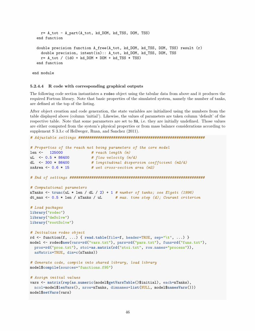
r= A_tot - A_part(A_tot, kd_DOM, kd_TSS, DOM, TSS)
end function
double precision function A_free(A_tot, kd_DOM, kd_TSS, DOM, TSS) result (r)
double precision, intent(in):: A_tot, kd_DOM, kd_TSS, DOM, TSS
r= A_tot / (1d0 + kd_DOM * DOM + kd_TSS * TSS)
end function
end module
5.2.4.4 R code with corresponding graphical outputs
The following code section instantiates a rodeo object using the tabular data from above and it produces therequired Fortran library. Note that basic properties of the simulated system, namely the number of tanks,are defined at the top of the listing.
After object creation and code generation, the state variables are initialized using the numbers from thetable displayed above (column ‘initial’). Likewise, the values of parameters are taken column ‘default’ of therespective table. Note that some parameters are set to NA, i.e. they are initially undefined. Those valuesare either computed from the system’s physical properties or from mass balance considerations according tosupplement S 3.3.c of Hellweger, Ruan, and Sanchez (2011).
# Adjustable settings ##########################################################
# Properties of the reach not being parameters of the core model
len <- 125000 # reach length (m)
uL <- 0.5 * 86400 # flow velocity (m/d)
dL <- 300 * 86400 # longitudinal dispersion coefficient (m2/d)
xsArea <- 0.6 * 15 # wet cross-section area (m2)
# End of settings ##############################################################
# Computational parameters
nTanks <- trunc(uL * len / dL / 2) + 1 # number of tanks; see Elgeti (1996)
dt_max <- 0.5 * len / nTanks / uL # max. time step (d); Courant criterion
# Load packages
library("rodeo")
library("deSolve")
library("rootSolve")
# Initialize rodeo object
rd <- function(f, ...) { read.table(file=f, header=TRUE, sep="\t", ...) }
model <- rodeo$new(vars=rd("vars.txt"), pars=rd("pars.txt"), funs=rd("funs.txt"),
pros=rd("pros.txt"), stoi=as.matrix(rd("stoi.txt", row.names="process")),
asMatrix=TRUE, dim=c(nTanks))
# Generate code, compile into shared library, load library
model$compile(sources="functions.f95")
# Assign initial values
vars <- matrix(rep(as.numeric(model$getVarsTable()$initial), each=nTanks),
ncol=model$lenVars(), nrow=nTanks, dimnames=list(NULL, model$namesVars()))
model$setVars(vars)
46
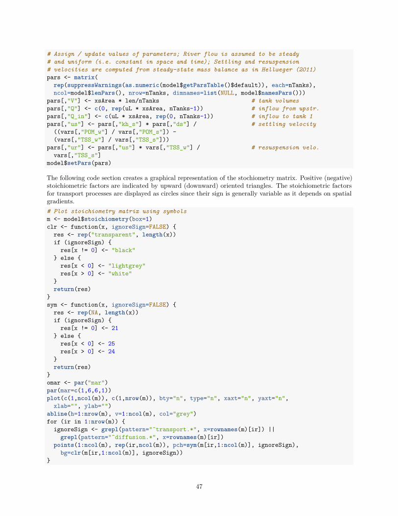
# Assign / update values of parameters; River flow is assumed to be steady
# and uniform (i.e. constant in space and time); Settling and resuspension
# velocities are computed from steady-state mass balance as in Hellweger (2011)
pars <- matrix(
rep(suppressWarnings(as.numeric(model$getParsTable()$default)), each=nTanks),
ncol=model$lenPars(), nrow=nTanks, dimnames=list(NULL, model$namesPars()))
pars[,"V"] <- xsArea * len/nTanks # tank volumes
pars[,"Q"] <- c(0, rep(uL * xsArea, nTanks-1)) # inflow from upstr.
pars[,"Q_in"] <- c(uL * xsArea, rep(0, nTanks-1)) # inflow to tank 1
pars[,"us"] <- pars[,"kh_s"] * pars[,"ds"] / # settling velocity
((vars[,"POM_w"] / vars[,"POM_s"]) -
(vars[,"TSS_w"] / vars[,"TSS_s"]))
pars[,"ur"] <- pars[,"us"] * vars[,"TSS_w"] / # resuspension velo.
vars[,"TSS_s"]
model$setPars(pars)
The following code section creates a graphical representation of the stochiometry matrix. Positive (negative)stoichiometric factors are indicated by upward (downward) oriented triangles. The stoichiometric factorsfor transport processes are displayed as circles since their sign is generally variable as it depends on spatialgradients.
# Plot stoichiometry matrix using symbols
m <- model$stoichiometry(box=1)
clr <- function(x, ignoreSign=FALSE) {
res <- rep("transparent", length(x))
if (ignoreSign) {
res[x != 0] <- "black"
} else {
res[x < 0] <- "lightgrey"
res[x > 0] <- "white"
}
return(res)
}
sym <- function(x, ignoreSign=FALSE) {
res <- rep(NA, length(x))
if (ignoreSign) {
res[x != 0] <- 21
} else {
res[x < 0] <- 25
res[x > 0] <- 24
}
return(res)
}
omar <- par("mar")
par(mar=c(1,6,6,1))
plot(c(1,ncol(m)), c(1,nrow(m)), bty="n", type="n", xaxt="n", yaxt="n",
xlab="", ylab="")
abline(h=1:nrow(m), v=1:ncol(m), col="grey")
for (ir in 1:nrow(m)) {
ignoreSign <- grepl(pattern="^transport.*", x=rownames(m)[ir]) ||
grepl(pattern="^diffusion.*", x=rownames(m)[ir])
points(1:ncol(m), rep(ir,ncol(m)), pch=sym(m[ir,1:ncol(m)], ignoreSign),
bg=clr(m[ir,1:ncol(m)], ignoreSign))
}
47

mtext(side=2, at=1:nrow(m), rownames(m), las=2, line=0.5, cex=0.8)
mtext(side=3, at=1:ncol(m), colnames(m), las=2, line=0.5, cex=0.8)
par(mar=omar)
rm(m)
decay_w
decay_s
hydrolysis_w
hydrolysis_s
production
settl_S
settl_R
settl_A
settl_POM
settl_TSS
resusp_S
resusp_R
resusp_A
resusp_POM
resusp_TSS
diffusion_A
diffusion_DOM
growth_S_w
growth_S_s
growth_R_w
growth_R_s
respiration
segregation_w
segregation_s
conjugation_w
conjugation_s
transport_S
transport_R
transport_A
transport_DOM
transport_POM
transport_TSS
S_
w
S_
s
R_
w
R_
s
PO
M_
w
PO
M_
s
TS
S_
w
TS
S_
s
A_
w
A_
s
DO
M_
w
DO
M_
s
The next code section demonstrates how a steady-state solution can be obtained by a call to methodsteady.1D from package rootSolve. This specific solver accounts for the banded structure of the Jacobianmatrix resulting from the tanks-in-series approach taking into account the layout of the vector of statevariables (explained in the section on multi-box models). Plotting was restricted to the bacteria concentrationsin the water column and sediment, respectively.
# Estimate steady-state
std <- rootSolve::steady.1D(y=model$getVars(), time=NULL, func=model$libFunc(),
parms=model$getPars(), nspec=model$lenVars(), dimens=nTanks, positive=TRUE,
dllname=model$libName(), nout=model$lenPros()*nTanks)
if (!attr(std, which="steady", exact=TRUE))
48
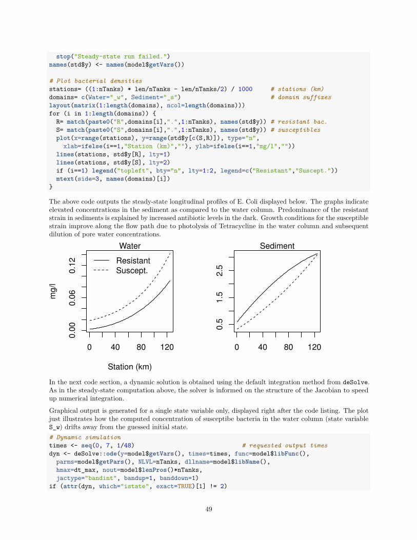
stop("Steady-state run failed.")
names(std$y) <- names(model$getVars())
# Plot bacterial densities
stations= ((1:nTanks) * len/nTanks - len/nTanks/2) / 1000 # stations (km)
domains= c(Water="_w", Sediment="_s") # domain suffixes
layout(matrix(1:length(domains), ncol=length(domains)))
for (i in 1:length(domains)) {
R= match(paste0("R",domains[i],".",1:nTanks), names(std$y)) # resistant bac.
S= match(paste0("S",domains[i],".",1:nTanks), names(std$y)) # susceptibles
plot(x=range(stations), y=range(std$y[c(S,R)]), type="n",
xlab=ifelse(i==1,"Station (km)",""), ylab=ifelse(i==1,"mg/l",""))
lines(stations, std$y[R], lty=1)
lines(stations, std$y[S], lty=2)
if (i==1) legend("topleft", bty="n", lty=1:2, legend=c("Resistant","Suscept."))
mtext(side=3, names(domains)[i])
}
The above code outputs the steady-state longitudinal profiles of E. Coli displayed below. The graphs indicateelevated concentrations in the sediment as compared to the water column. Predominance of the resistantstrain in sediments is explained by increased antibiotic levels in the dark. Growth conditions for the susceptiblestrain improve along the flow path due to photolysis of Tetracycline in the water column and subsequentdilution of pore water concentrations.
0 40 80 120
0.0
00
.06
0.1
2
Station (km)
mg
/l
Resistant
Suscept.
Water
0 40 80 120
0.5
1.5
2.5
Sediment
In the next code section, a dynamic solution is obtained using the default integration method from deSolve.As in the steady-state computation above, the solver is informed on the structure of the Jacobian to speedup numerical integration.
Graphical output is generated for a single state variable only, displayed right after the code listing. The plotjust illustrates how the computed concentration of susceptibe bacteria in the water column (state variableS_w) drifts away from the guessed initial state.
# Dynamic simulation
times <- seq(0, 7, 1/48) # requested output times
dyn <- deSolve::ode(y=model$getVars(), times=times, func=model$libFunc(),
parms=model$getPars(), NLVL=nTanks, dllname=model$libName(),
hmax=dt_max, nout=model$lenPros()*nTanks,
jactype="bandint", bandup=1, banddown=1)
if (attr(dyn, which="istate", exact=TRUE)[1] != 2)
49
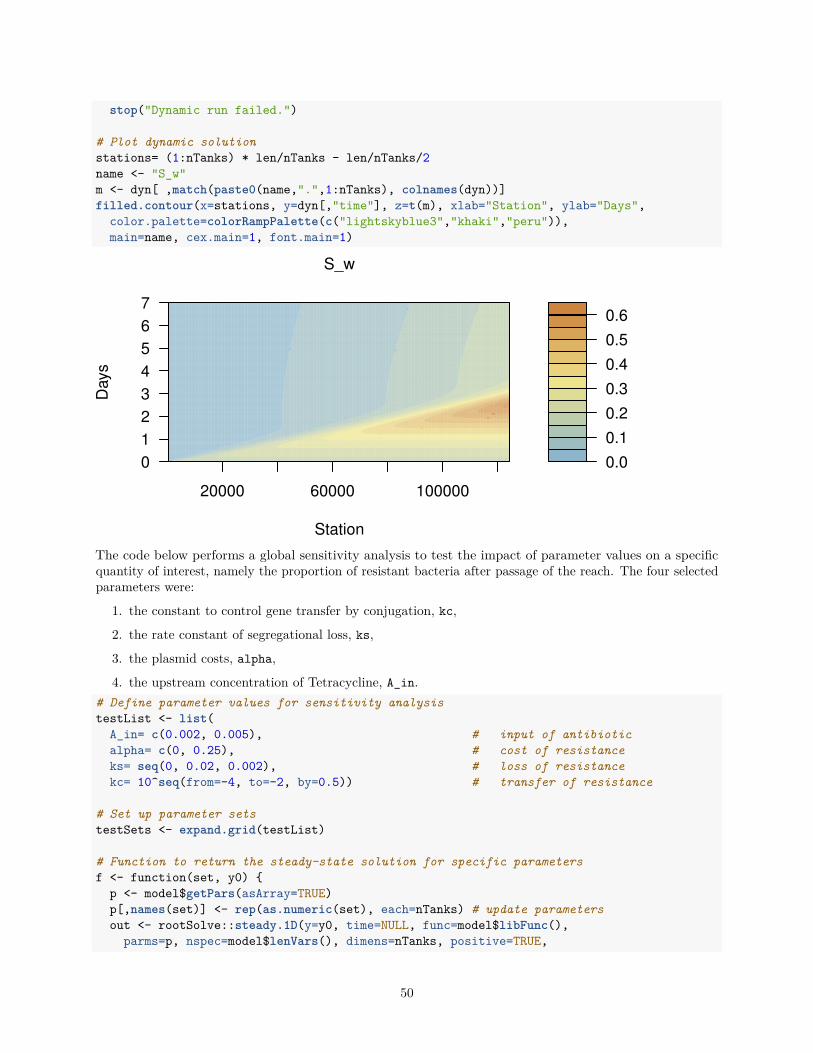
stop("Dynamic run failed.")
# Plot dynamic solution
stations= (1:nTanks) * len/nTanks - len/nTanks/2
name <- "S_w"
m <- dyn[ ,match(paste0(name,".",1:nTanks), colnames(dyn))]
filled.contour(x=stations, y=dyn[,"time"], z=t(m), xlab="Station", ylab="Days",
color.palette=colorRampPalette(c("lightskyblue3","khaki","peru")),
main=name, cex.main=1, font.main=1)
0.0
0.1
0.2
0.3
0.4
0.5
0.6
20000 60000 100000
0
1
2
3
4
5
6
7
S_w
Station
Days
The code below performs a global sensitivity analysis to test the impact of parameter values on a specificquantity of interest, namely the proportion of resistant bacteria after passage of the reach. The four selectedparameters were:
1. the constant to control gene transfer by conjugation, kc,
2. the rate constant of segregational loss, ks,
3. the plasmid costs, alpha,
4. the upstream concentration of Tetracycline, A_in.
# Define parameter values for sensitivity analysis
testList <- list(
A_in= c(0.002, 0.005), # input of antibiotic
alpha= c(0, 0.25), # cost of resistance
ks= seq(0, 0.02, 0.002), # loss of resistance
kc= 10^seq(from=-4, to=-2, by=0.5)) # transfer of resistance
# Set up parameter sets
testSets <- expand.grid(testList)
# Function to return the steady-state solution for specific parameters
f <- function(set, y0) {
p <- model$getPars(asArray=TRUE)
p[,names(set)] <- rep(as.numeric(set), each=nTanks) # update parameters
out <- rootSolve::steady.1D(y=y0, time=NULL, func=model$libFunc(),
parms=p, nspec=model$lenVars(), dimens=nTanks, positive=TRUE,
50
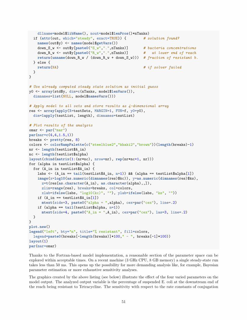
dllname=model$libName(), nout=model$lenPros()*nTanks)
if (attr(out, which="steady", exact=TRUE)) { # solution found?
names(out$y) <- names(model$getVars())
down_S_w <- out$y[paste0("S_w",".",nTanks)] # bacteria concentrations
down_R_w <- out$y[paste0("R_w",".",nTanks)] # at lower end of reach
return(unname(down_R_w / (down_R_w + down_S_w))) # fraction of resistant b.
} else {
return(NA) # if solver failed
}
}
# Use already computed steady state solution as initial guess
y0 <- array(std$y, dim=c(nTanks, model$lenVars()),
dimnames=list(NULL, model$namesVars()))
# Apply model to all sets and store results as 4-dimensional array
res <- array(apply(X=testSets, MARGIN=1, FUN=f, y0=y0),
dim=lapply(testList, length), dimnames=testList)
# Plot results of the analysis
omar <- par("mar")
par(mar=c(4,4,1.5,1))
breaks <- pretty(res, 8)
colors <- colorRampPalette(c("steelblue2","khaki2","brown"))(length(breaks)-1)
nr <- length(testList$A_in)
nc <- length(testList$alpha)
layout(cbind(matrix(1:(nr*nc), nrow=nr), rep(nr*nc+1, nr)))
for (alpha in testList$alpha) {
for (A_in in testList$A_in) {
labs <- (A_in == tail(testList$A_in, n=1)) && (alpha == testList$alpha[1])
image(x=log10(as.numeric(dimnames(res)$kc)), y=as.numeric(dimnames(res)$ks),
z=t(res[as.character(A_in), as.character(alpha),,]),
zlim=range(res), breaks=breaks, col=colors,
xlab=ifelse(labs, "log10(kc)", ""), ylab=ifelse(labs, "ks", ""))
if (A_in == testList$A_in[1])
mtext(side=3, paste0("alpha = ",alpha), cex=par("cex"), line=.2)
if (alpha == tail(testList$alpha, n=1))
mtext(side=4, paste0("A_in = ",A_in), cex=par("cex"), las=3, line=.2)
}
}
plot.new()
legend("left", bty="n", title="% resistant", fill=colors,
legend=paste0(breaks[-length(breaks)]*100," - ", breaks[-1]*100))
layout(1)
par(mar=omar)
Thanks to the Fortran-based model implementation, a reasonable section of the parameter space can beexplored within acceptable times. On a recent machine (3 GHz CPU, 8 GB memory) a single steady-state runtakes less than 50 ms. This opens up the possibility for more demanding analysis like, for example, Bayesianparameter estimation or more exhaustive sensitivity analyses.
The graphics created by the above listing (see below) illustrate the effect of the four varied parameters on themodel output. The analyzed output variable is the percentage of suspended E. coli at the downstream end ofthe reach being resistant to Tetracycline. The sensitivity with respect to the rate constants of conjugation
51
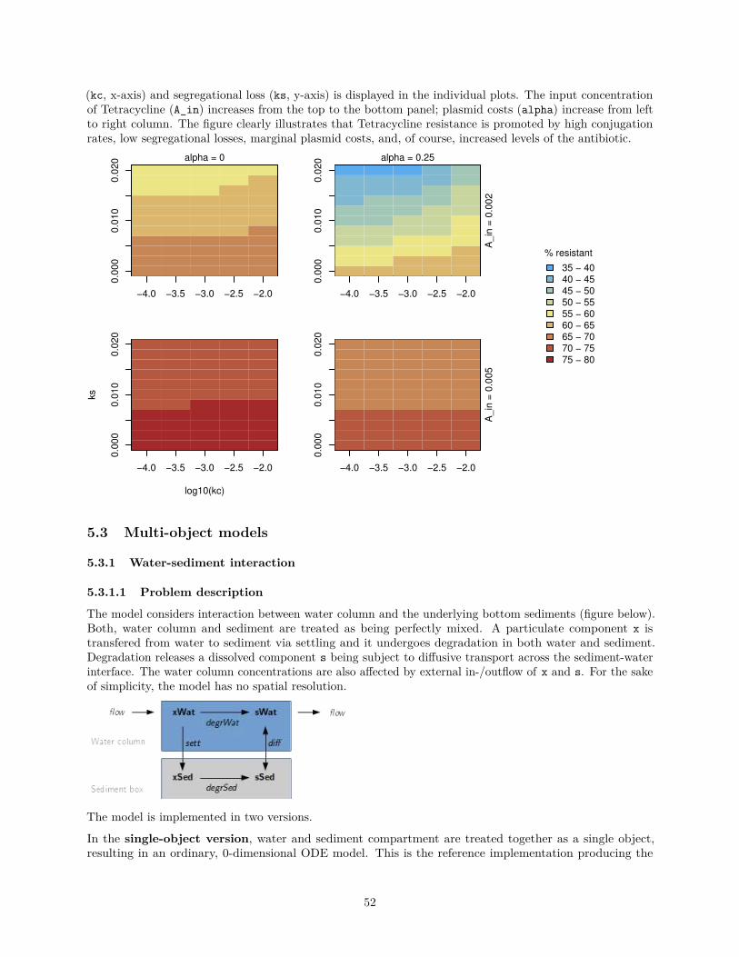
(kc, x-axis) and segregational loss (ks, y-axis) is displayed in the individual plots. The input concentrationof Tetracycline (A_in) increases from the top to the bottom panel; plasmid costs (alpha) increase from leftto right column. The figure clearly illustrates that Tetracycline resistance is promoted by high conjugationrates, low segregational losses, marginal plasmid costs, and, of course, increased levels of the antibiotic.
−4.0 −3.5 −3.0 −2.5 −2.0
0.0
00
0.0
10
0.0
20 alpha = 0
−4.0 −3.5 −3.0 −2.5 −2.0
0.0
00
0.0
10
0.0
20
log10(kc)
ks
−4.0 −3.5 −3.0 −2.5 −2.0
0.0
00
0.0
10
0.0
20 alpha = 0.25
A_in
= 0
.002
−4.0 −3.5 −3.0 −2.5 −2.0
0.0
00
0.0
10
0.0
20
A_in
= 0
.005
% resistant
35 − 4040 − 4545 − 5050 − 5555 − 6060 − 6565 − 7070 − 7575 − 80
5.3 Multi-object models
5.3.1 Water-sediment interaction
5.3.1.1 Problem description
The model considers interaction between water column and the underlying bottom sediments (figure below).Both, water column and sediment are treated as being perfectly mixed. A particulate component x istransfered from water to sediment via settling and it undergoes degradation in both water and sediment.Degradation releases a dissolved component s being subject to diffusive transport across the sediment-waterinterface. The water column concentrations are also affected by external in-/outflow of x and s. For the sakeof simplicity, the model has no spatial resolution.
The model is implemented in two versions.
In the single-object version, water and sediment compartment are treated together as a single object,resulting in an ordinary, 0-dimensional ODE model. This is the reference implementation producing the
52
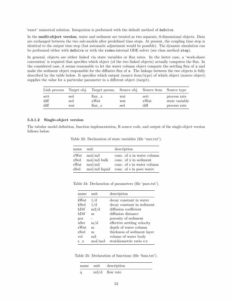
‘exact’ numerical solution. Integration is performed with the default method of deSolve.
In the multi-object version, water and sediment are treated as two separate, 0-dimensional objects. Dataare exchanged between the two sub-models after predefined time steps. At present, the coupling time step isidentical to the output time step (but automatic adjustment would be possible). The dynamic simulation canbe performed either with deSolve or with the rodeo-internal ODE solver (see class method step).
In general, objects are either linked via state variables or flux rates. In the latter case, a ‘work-shareconvention’ is required that specifies which object (of the two linked objects) actually computes the flux. Inthe considered case, it seems reasonable to let the water column object compute the settling flux of x andmake the sediment object responsible for the diffusive flux of s. The linkage between the two objects is fullydescribed by the table below. It specifies which output (source item/type) of which object (source object)supplies the value for a particular parameter in a different object (target).
Link process Target obj. Target param. Source obj. Source item Source type
sett sed flux_x wat sett process ratediff sed xWat wat xWat state variablediff wat flux_s sed diff process rate
5.3.1.2 Single-object version
The tabular model definition, function implementation, R source code, and output of the single-object versionfollows below.
Table 33: Declaration of state variables (file ‘vars.txt’).
name unit description
xWat mol/m3 conc. of x in water columnxSed mol/m3 bulk conc. of x in sedimentsWat mol/m3 conc. of s in water columnsSed mol/m3 liquid conc. of s in pore water
Table 34: Declaration of parameters (file ‘pars.txt’).
name unit description
kWat 1/d decay constant in waterkSed 1/d decay constant in sedimentkDif m2/d diffusion coefficienthDif m diffusion distancepor - porosity of sedimentuSet m/d effective settling velocityzWat m depth of water columnzSed m thickness of sediment layervol m3 volume of water bodys_x mol/mol stoichiometric ratio s:x
Table 35: Declaration of functions (file ‘funs.txt’).
name unit description
q m3/d flow rate
53
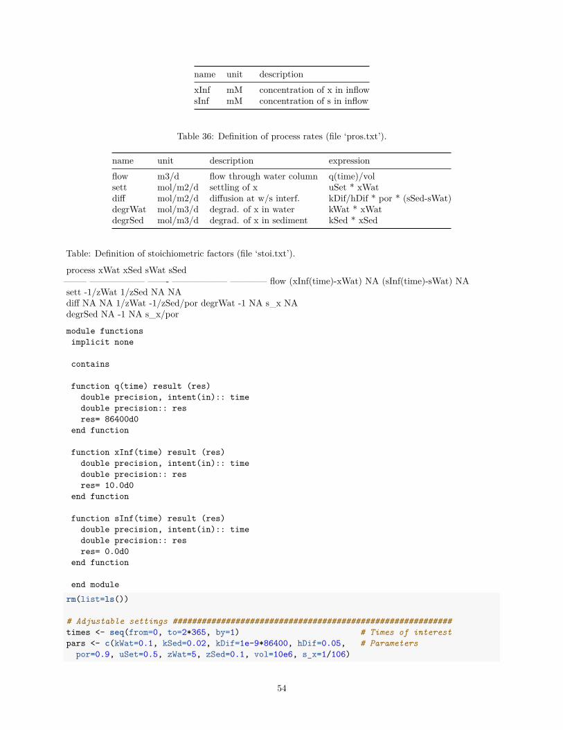
name unit description
xInf mM concentration of x in inflowsInf mM concentration of s in inflow
Table 36: Definition of process rates (file ‘pros.txt’).
name unit description expression
flow m3/d flow through water column q(time)/volsett mol/m2/d settling of x uSet * xWatdiff mol/m2/d diffusion at w/s interf. kDif/hDif * por * (sSed-sWat)degrWat mol/m3/d degrad. of x in water kWat * xWatdegrSed mol/m3/d degrad. of x in sediment kSed * xSed
Table: Definition of stoichiometric factors (file ‘stoi.txt’).
process xWat xSed sWat sSed——– —————— ——- —————— ———— flow (xInf(time)-xWat) NA (sInf(time)-sWat) NAsett -1/zWat 1/zSed NA NAdiff NA NA 1/zWat -1/zSed/por degrWat -1 NA s_x NAdegrSed NA -1 NA s_x/por
module functions
implicit none
contains
function q(time) result (res)
double precision, intent(in):: time
double precision:: res
res= 86400d0
end function
function xInf(time) result (res)
double precision, intent(in):: time
double precision:: res
res= 10.0d0
end function
function sInf(time) result (res)
double precision, intent(in):: time
double precision:: res
res= 0.0d0
end function
end module
rm(list=ls())
# Adjustable settings ##########################################################
times <- seq(from=0, to=2*365, by=1) # Times of interest
pars <- c(kWat=0.1, kSed=0.02, kDif=1e-9*86400, hDif=0.05, # Parameters
por=0.9, uSet=0.5, zWat=5, zSed=0.1, vol=10e6, s_x=1/106)
54
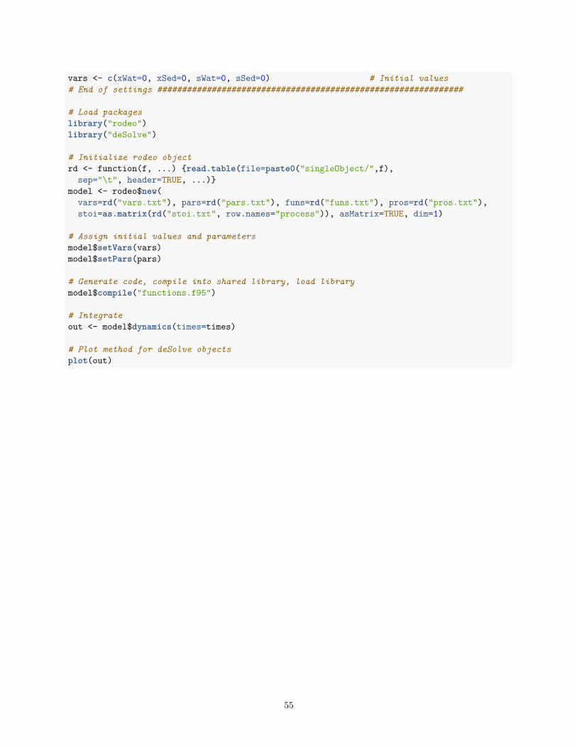
vars <- c(xWat=0, xSed=0, sWat=0, sSed=0) # Initial values
# End of settings ##############################################################
# Load packages
library("rodeo")
library("deSolve")
# Initialize rodeo object
rd <- function(f, ...) {read.table(file=paste0("singleObject/",f),
sep="\t", header=TRUE, ...)}
model <- rodeo$new(
vars=rd("vars.txt"), pars=rd("pars.txt"), funs=rd("funs.txt"), pros=rd("pros.txt"),
stoi=as.matrix(rd("stoi.txt", row.names="process")), asMatrix=TRUE, dim=1)
# Assign initial values and parameters
model$setVars(vars)
model$setPars(pars)
# Generate code, compile into shared library, load library
model$compile("functions.f95")
# Integrate
out <- model$dynamics(times=times)
# Plot method for deSolve objects
plot(out)
55
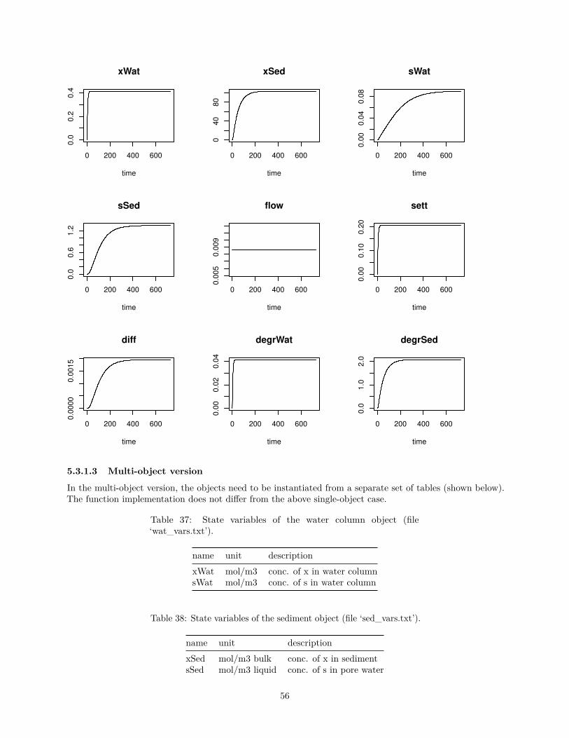
0 200 400 600
0.0
0.2
0.4
xWat
time
0 200 400 600
04
08
0
xSed
time
0 200 400 600
0.0
00
.04
0.0
8
sWat
time
0 200 400 600
0.0
0.6
1.2
sSed
time
0 200 400 600
0.0
05
0.0
09
flow
time
0 200 400 600
0.0
00
.10
0.2
0
sett
time
0 200 400 600
0.0
00
00
.00
15
diff
time
0 200 400 600
0.0
00
.02
0.0
4
degrWat
time
0 200 400 600
0.0
1.0
2.0
degrSed
time
5.3.1.3 Multi-object version
In the multi-object version, the objects need to be instantiated from a separate set of tables (shown below).The function implementation does not differ from the above single-object case.
Table 37: State variables of the water column object (file‘wat_vars.txt’).
name unit description
xWat mol/m3 conc. of x in water columnsWat mol/m3 conc. of s in water column
Table 38: State variables of the sediment object (file ‘sed_vars.txt’).
name unit description
xSed mol/m3 bulk conc. of x in sedimentsSed mol/m3 liquid conc. of s in pore water
56
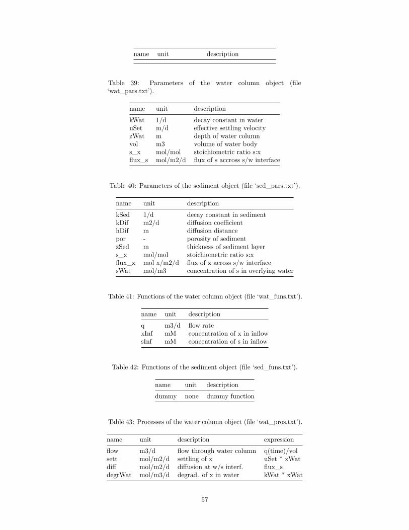
name unit description
Table 39: Parameters of the water column object (file‘wat_pars.txt’).
name unit description
kWat 1/d decay constant in wateruSet m/d effective settling velocityzWat m depth of water columnvol m3 volume of water bodys_x mol/mol stoichiometric ratio s:xflux_s mol/m2/d flux of s accross s/w interface
Table 40: Parameters of the sediment object (file ‘sed_pars.txt’).
name unit description
kSed 1/d decay constant in sedimentkDif m2/d diffusion coefficienthDif m diffusion distancepor - porosity of sedimentzSed m thickness of sediment layers_x mol/mol stoichiometric ratio s:xflux_x mol x/m2/d flux of x across s/w interfacesWat mol/m3 concentration of s in overlying water
Table 41: Functions of the water column object (file ‘wat_funs.txt’).
name unit description
q m3/d flow ratexInf mM concentration of x in inflowsInf mM concentration of s in inflow
Table 42: Functions of the sediment object (file ‘sed_funs.txt’).
name unit description
dummy none dummy function
Table 43: Processes of the water column object (file ‘wat_pros.txt’).
name unit description expression
flow m3/d flow through water column q(time)/volsett mol/m2/d settling of x uSet * xWatdiff mol/m2/d diffusion at w/s interf. flux_sdegrWat mol/m3/d degrad. of x in water kWat * xWat
57
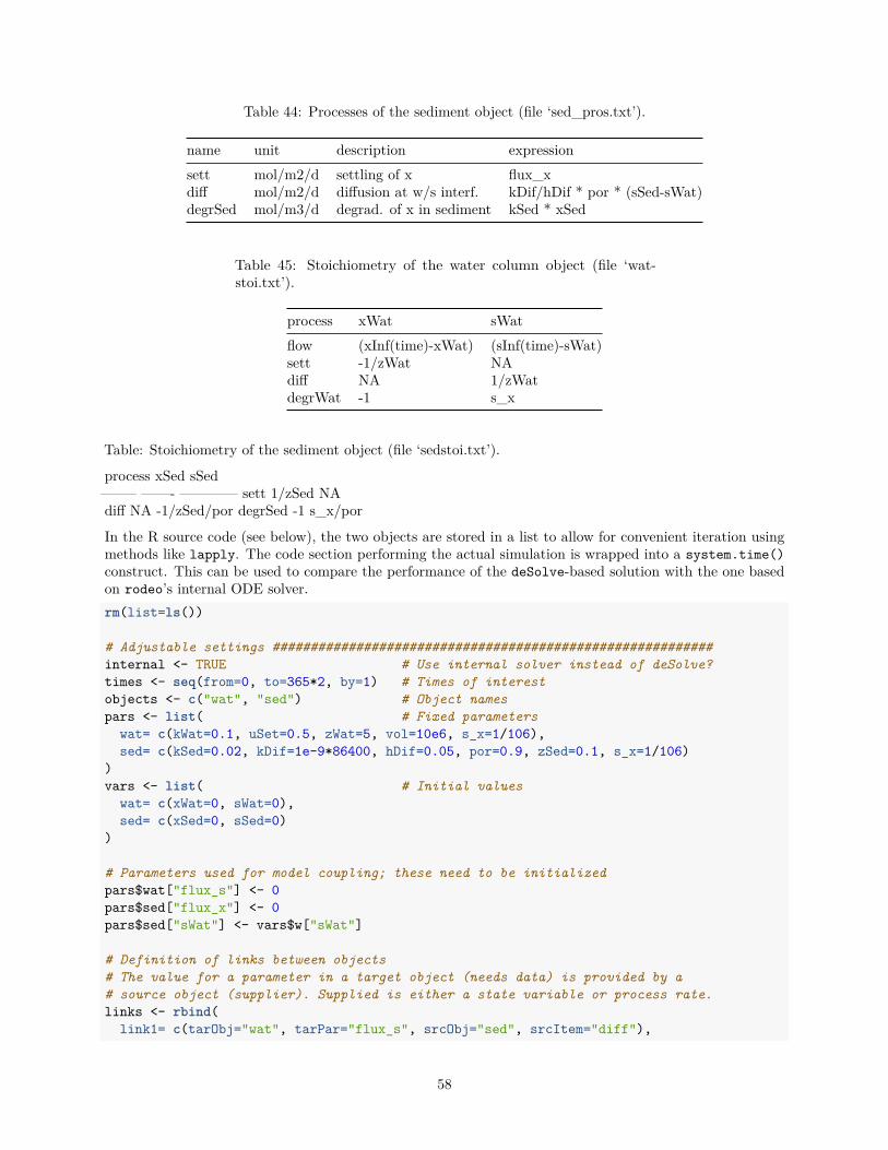
Table 44: Processes of the sediment object (file ‘sed_pros.txt’).
name unit description expression
sett mol/m2/d settling of x flux_xdiff mol/m2/d diffusion at w/s interf. kDif/hDif * por * (sSed-sWat)degrSed mol/m3/d degrad. of x in sediment kSed * xSed
Table 45: Stoichiometry of the water column object (file ‘wat-stoi.txt’).
process xWat sWat
flow (xInf(time)-xWat) (sInf(time)-sWat)sett -1/zWat NAdiff NA 1/zWatdegrWat -1 s_x
Table: Stoichiometry of the sediment object (file ‘sedstoi.txt’).
process xSed sSed——– ——- ———— sett 1/zSed NAdiff NA -1/zSed/por degrSed -1 s_x/por
In the R source code (see below), the two objects are stored in a list to allow for convenient iteration usingmethods like lapply. The code section performing the actual simulation is wrapped into a system.time()
construct. This can be used to compare the performance of the deSolve-based solution with the one basedon rodeo’s internal ODE solver.
rm(list=ls())
# Adjustable settings ##########################################################
internal <- TRUE # Use internal solver instead of deSolve?
times <- seq(from=0, to=365*2, by=1) # Times of interest
objects <- c("wat", "sed") # Object names
pars <- list( # Fixed parameters
wat= c(kWat=0.1, uSet=0.5, zWat=5, vol=10e6, s_x=1/106),
sed= c(kSed=0.02, kDif=1e-9*86400, hDif=0.05, por=0.9, zSed=0.1, s_x=1/106)
)
vars <- list( # Initial values
wat= c(xWat=0, sWat=0),
sed= c(xSed=0, sSed=0)
)
# Parameters used for model coupling; these need to be initialized
pars$wat["flux_s"] <- 0
pars$sed["flux_x"] <- 0
pars$sed["sWat"] <- vars$w["sWat"]
# Definition of links between objects
# The value for a parameter in a target object (needs data) is provided by a
# source object (supplier). Supplied is either a state variable or process rate.
links <- rbind(
link1= c(tarObj="wat", tarPar="flux_s", srcObj="sed", srcItem="diff"),
58
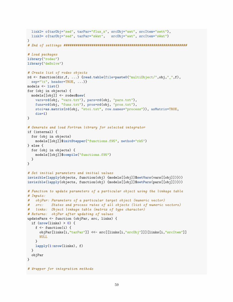
link2= c(tarObj="sed", tarPar="flux_x", srcObj="wat", srcItem="sett"),
link3= c(tarObj="sed", tarPar="sWat", srcObj="wat", srcItem="sWat")
)
# End of settings ##############################################################
# Load packages
library("rodeo")
library("deSolve")
# Create list of rodeo objects
rd <- function(dir,f, ...) {read.table(file=paste0("multiObject/",obj,"_",f),
sep="\t", header=TRUE, ...)}
models <- list()
for (obj in objects) {
models[[obj]] <- rodeo$new(
vars=rd(obj, "vars.txt"), pars=rd(obj, "pars.txt"),
funs=rd(obj, "funs.txt"), pros=rd(obj, "pros.txt"),
stoi=as.matrix(rd(obj, "stoi.txt", row.names="process")), asMatrix=TRUE,
dim=1)
}
# Generate and load Fortran library for selected integrator
if (internal) {
for (obj in objects)
models[[obj]]$initStepper("functions.f95", method="rk5")
} else {
for (obj in objects) {
models[[obj]]$compile("functions.f95")
}
}
# Set initial parameters and initial values
invisible(lapply(objects, function(obj) {models[[obj]]$setVars(vars[[obj]])}))
invisible(lapply(objects, function(obj) {models[[obj]]$setPars(pars[[obj]])}))
# Function to update parameters of a particular object using the linkage table
# Inputs:
# objPar: Parameters of a particular target object (numeric vector)
# src: States and process rates of all objects (list of numeric vectors)
# links: Object linkage table (matrix of type character)
# Returns: objPar after updating of values
updatePars <- function (objPar, src, links) {
if (nrow(links) > 0) {
f <- function(i) {
objPar[links[i,"tarPar"]] <<- src[[links[i,"srcObj"]]][links[i,"srcItem"]]
NULL
}
lapply(1:nrow(links), f)
}
objPar
}
# Wrapper for integration methods
59
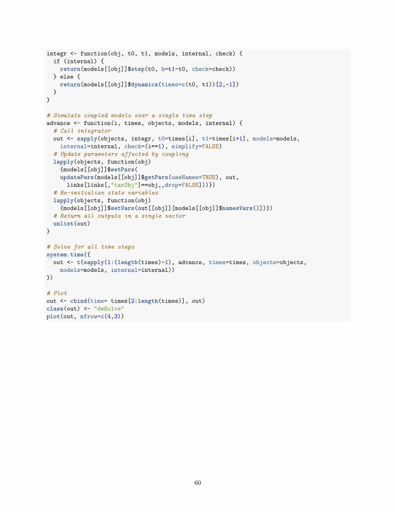
integr <- function(obj, t0, t1, models, internal, check) {
if (internal) {
return(models[[obj]]$step(t0, h=t1-t0, check=check))
} else {
return(models[[obj]]$dynamics(times=c(t0, t1))[2,-1])
}
}
# Simulate coupled models over a single time step
advance <- function(i, times, objects, models, internal) {
# Call integrator
out <- sapply(objects, integr, t0=times[i], t1=times[i+1], models=models,
internal=internal, check=(i==1), simplify=FALSE)
# Update parameters affected by coupling
lapply(objects, function(obj)
{models[[obj]]$setPars(
updatePars(models[[obj]]$getPars(useNames=TRUE), out,
links[links[,"tarObj"]==obj,,drop=FALSE]))})
# Re-initialize state variables
lapply(objects, function(obj)
{models[[obj]]$setVars(out[[obj]][models[[obj]]$namesVars()])})
# Return all outputs in a single vector
unlist(out)
}
# Solve for all time steps
system.time({
out <- t(sapply(1:(length(times)-1), advance, times=times, objects=objects,
models=models, internal=internal))
})
# Plot
out <- cbind(time= times[2:length(times)], out)
class(out) <- "deSolve"
plot(out, mfrow=c(4,3))
60
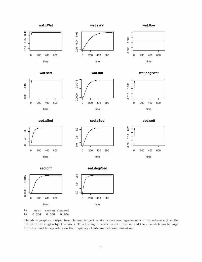
0 200 400 600
0.1
00
.25
0.4
0wat.xWat
time
0 200 400 600
0.0
00
.04
0.0
8
wat.sWat
time
0 200 400 600
0.0
05
0.0
09
wat.flow
time
0 200 400 600
0.0
50
.15
wat.sett
time
0 200 400 600
0.0
00
00
.00
15
wat.diff
time
0 200 400 600
0.0
10
0.0
30
wat.degrWat
time
0 200 400 600
04
08
0
sed.xSed
time
0 200 400 600
0.0
0.6
1.2
sed.sSed
time
0 200 400 600
0.0
00
.10
0.2
0
sed.sett
time
0 200 400 600
0.0
00
00
.00
15
sed.diff
time
0 200 400 600
0.0
1.0
2.0
sed.degrSed
time
## user system elapsed
## 0.204 0.000 0.204
The above graphical output from the multi-object version shows good agreement with the reference (i. e. theoutput of the single-object version). This finding, however, is not universal and the mismatch can be largefor other models depending on the frequency of inter-model communication.
61

References
Bronstert, A., P. Schmitt, E. J. Plate, and J. Wald. 1991. “A Physically Based Distributed WatershedModel to Simulate Floods and Flood Protection Measures in a Flat Area with Shallow Ground Water Table.”International Association for Hydraulic Research, XXIV Congress, Madrid, Spain.
Chen, Z., Y. Zhang, Y. Gao, S. A. Boyd, D. Zhu, and H. Li. 2015. “Influence of Dissolved Organic Matter onTetracycline Bioavailability to an Antibiotic-Resistant Bacterium.” Environmental Science and Technology49: 10903–10.
Elgeti, K. 1996. “A New Equation for Correlating a Pipe Flow Reactor with a Cascade of Mixed Reactors.”Chemical Engineering Science 51 (23): 5077–80.
Gregersen, J. B., P. J. A. Gijsbers, and S. J. P. Westen. 2007. “OpenMI: Open Modelling Interface.” Journalof Hydroinformatics 9 (3): 175–91.
Hellweger, F. L., X. Ruan, and S. Sanchez. 2011. “A Simple Model of Tetracycline Antibiotic Resistance inthe Aquatic Environment (with Application to the Poudre River).” Int. J. Environ. Res. Public Health 8 (2):480–97.
Kinzelbach, W. 1986. “Groundwater Modelling - an Introduction with Sample Programs in Basic.” InDevelopments in Water Science. Vol. 25. Elsevier.
Kinzelbach, W., and R. Rausch. 1995. Grundwassermodellierung. Gebrüder Bornträger, Stuttgart.
Lenski, R. E. 1998. “Bacterial Evolution and the Cost of Antibiotic Resistance.” International Microbiology1: 265–70.
Rauch, W. 1993. “Über Die Hydraulische Wechselwirkung von Oberflächengewässern Und Grundwasserkör-pern.” Wasserwirtschaft 83: 14–18.
Streeter, W. H., and W. B. Phelps. 1925. “A Study of the Pollution and Natural Purification of the OhioRiver.” Public Health Bull. 146, US Public Health Service, Washington DC.
Tolls, J. 2001. “Sorption of Veterinary Pharmaceuticals in Soils: A Review.” Environmental Science andTechnology 35 (17): 3397–3406.
Wammer, K.H., M.T. Slattery, A.M. Stemig, and J.L. Ditty. 2011. “Tetracycline Photolysis in NaturalWaters: Loss of Antibacterial Activity.” Chemosphere 85 (9): 1505–10.
62