quotation from it or information derived from it is to be ... · application of differential...
TRANSCRIPT

The copyright of this thesis vests in the author. No quotation from it or information derived from it is to be published without full acknowledgement of the source. The thesis is to be used for private study or non-commercial research purposes only.
Published by the University of Cape Town (UCT) in terms of the non-exclusive license granted to UCT by the author.
Univers
ity of
Cap
e Tow
n
Application of Differential Evolution to
Power System Stabilizer Design
PREPARED BY: TSHINA FA MULUMBA
This thesis is submitted to the University of Cape Town in full fulfilment of the academic
requirements for the Master of Science degree in Electrical Engineering
SUPERVISOR: PROF. K.A FOLLY
DEPARTMENT OF ELECTRICAL ENGINEERING UNIVERSITY OF CAPE TOWN
CAPE TOWN
Date: November 2012

Application of Differential Evolution to Power System Stabilizer design
i
Declaration
I hereby declare that this is my own work. All alternative sources used have been
identified and referenced. This thesis has not been submitted before for any degree at this
or any other institution for any degree or examination.
Signature:
Mr. Tshina Fa Mulumba
Signed at the University of Cape Town
Date: 21st of November 2012

Application of Differential Evolution to Power System Stabilizer design
ii
Acknowledgements
First and foremost, I am grateful to God for he is my shepherd who makes me lie down in
green pastures and leads me beside the still waters. He has given me purpose and
renewed my strengths to persevere until the end. To him I dedicate my thesis.
Special thanks to my supervisor Prof K.A Folly, for his continuous support both
spiritually and financially over the course of my research. Thank you for being very
understanding and approachable. You have been a great inspiration who has taught me
good work ethics and to always challenge myself to search for the truth. I couldn’t have
done it without you.
I am also thankful to my friends and fellow colleagues from the Power Research Group
who have been supportive and helpful in both academic and non-academic matters.
To my parents, Bernard Mulumba Tshina and Bibomba Kayiba Mulumba, without whom
I wouldn’t be here. I am thankful for all your supports and endless prayers. It has not
been an easy road yet, you’ve never stopped believing in me and encouraging me to
pursue my endeavours. Thank you for your patience and I am honoured to have parents
like you.
To my brothers (Dilan, Glory and Christian) and my sisters (Sophie, Nadine, Sarah and
Esther), thank you for your support and encouragements throughout my studies, I
couldn’t have done it without each and every one of you.
Last but not least, special appreciation goes to my beloved fiancée, Lebogang Motaung,
whose support and encouragements have kept me going during tough times. Thank you
for your patience whilst being away, for the love and prayers. You have never ceased to
believe in me.

Application of Differential Evolution to Power System Stabilizer design
iii
Synopsis
Low frequency oscillations in the range of 0.2 to 3 Hz are inherent to power systems.
They appear when there are power exchanges between large areas of interconnected
power systems or when power is transferred over long distances under medium to heavy
conditions. The use of fast acting high gain Automatic Voltage Regulator (AVR),
although improves the transient stability, has a detrimental effect on the small-signal
stability. For the last four decades, low frequency oscillations arising from the lack of
sufficient damping in the system have been frequently encountered in power systems.
The recent introduction of the deregulation and the unbundling of generation,
transmission and distribution as well as the large amount of Distributed Generation
connected to the power system have exacerbated the problem of low-frequency
oscillations.
For many years, Power System Stabilizers (PSSs) have been used to add damping to
electromechanical oscillations. Conventional Power System Stabilizers (CPSSs) have
been widely accepted by the power utilities due to their simplicity, moreover they are the
most cost effective damping control. Traditionally, CPSSs were designed using classical
control techniques such as root-locus, phase compensation, eigenvalue analysis, etc.
These stabilizers are mainly designed around the nominal operating condition. However,
the main disadvantage with CPSSs is that they cannot guarantee the stability of power
systems due to their nonlinear nature and varying operating conditions.
Over the past 30 years, there have been increasing interests in the optimization of the
parameters of Power System Stabilizers (PSSs) to provide adequate performance of the
PSS over varying operating conditions. Several approaches such as adaptive control,
robust optimal control, etc., have been proposed. However, adaptive controllers are
difficult to design and susceptible to problems like non-convergence of parameters and
numerical instability. Robust controllers based on H∞ optimal control theory have their
drawbacks as well. These include the selection of appropriate weighting functions, and
issues related to practical implementation due to the high dimension of the controllers.

Application of Differential Evolution to Power System Stabilizer design
iv
In recent years, many Evolutionary Algorithms (EAs) such as Genetic Algorithms (GAs)
have been proposed to optimally tune the parameters of the PSS. GAs are population
based search methods inspired by the mechanism of evolution and natural genetic.
Despite the fact that GAs are robust and have given promising results in many
applications, they still have some drawbacks. Some of these drawbacks are related to the
problem of genetic drift in GA which restricts the diversity in the population. As a result,
GAs may converge to suboptimal solutions. In addition, GAs are computationally time
consuming and require large computer storage when dealing with difficult problems that
have many variables. To cope with the above mentioned drawbacks, many variants of
GAs have been proposed often tailored to a particular problem. Recently, several simpler
and yet effective heuristic algorithms such as Population Based Incremental Learning
(PBIL) and Differential Evolution (DE), etc., have received increasing attention.
PBIL is a method that combines genetic algorithms and competitive learning for function
optimization. PBIL is an extension to the Evolutionary Genetic Algorithm (EGA). PBIL’s
algorithm is achieved through the re-examination of the performance of the EGA in terms
of competitive learning. However, PBIL drawbacks reside in the slow convergence due to
the learning process involved.
DE is a stochastic optimizer based on the differential mutation technique, used as a search
mechanism, and applies the greedy selection to direct the search toward the prospective
solutions in the search space. DE employs a “one-to-one” survivor selection which
consists of comparing each trial vector to its corresponding target vector. This process
ensures that the best vector at each index is retained. Furthermore, this also guarantees
that the very best-so-far solution is kept. In the last few years, DE has grown in reputation
among researchers due to its simplicity, efficiency, and robustness in function
optimization. Recently, DE has been used in various real-world problem solving
applications, especially in engineering.
Differential Evolution has been shown to be simple yet powerful algorithm especially for
optimally tuning Power System Stabilizers. However like other EAs, DE’s performance
is closely dependent on its intrinsic control parameters such as the mutation factor, the

Application of Differential Evolution to Power System Stabilizer design
v
crossover probability and population size. Inappropriate choice of these control parameter
values may result in significant deterioration of the algorithm performance and reliability
to effectively explore the search space for the global maximum or minimum. Very often,
these parameters are selected by means of trial-and-error. Once selected, these parameters
remain fixed throughout the search which may present limitations in DE’s performance.
Recently, the self- updating of the control parameters based on the feedback from the
search has been developed to overcome DE’s drawback and therefore enhancing the
robustness of the algorithm. The self-adaptive DE, often referred to as jDE because of the
adaptive scheme used, is similar to the DE scheme. During the optimization, jDE has a
fixed number of population whilst adapting the control parameters Fi and CRi associated
with each individual. Better values of the parameters lead to better individuals hence
better solutions.
In this thesis, first DE is used to optimally tune the parameters of the PSS to provide
adequate damping over a wide range of operating conditions. Then the self-adaptive DE
is applied. The PSS parameters optimization is achieved by maximizing an eigenvalue
based objective function. This consists of maximizing the lowest damping ratio of the
electromechanical modes of the system.
The resulting PSS was assessed using modal analysis and validated with time domain
simulations. For the small signal simulations, the system was subject to a 10 percent
disturbance in the voltage reference whereas for the transient analysis, the system was
subjected to 5-cycle three phase fault applied on the line.
The performances of DE-PSS were compared to those of PBIL-PSS, and to those of the
CPSS. The three PSSs were designed and tested on two power system models, namely,
the Single Machine Infinite bus (SMIB) and the Two-Area Multimachine system.
In the SMIB, both DE and PBIL PSSs were designed using five operating conditions. The
fitness curve revealed that DE was able to maximize the lowest damping from 2.7% to
26.59%, whereas PBIL was able to maximize the lowest damping to 23.25%. The modal

Application of Differential Evolution to Power System Stabilizer design
vi
analysis showed that DE-PSS performed better than PBIL-PSS for all the cases. As
expected, CPSS yielded good performance for the nominal case but its performance
degraded when the operating conditions changed. The time domain simulation results
validated the modal analysis results. It is shown that DE-PSS settled faster than PBIL-
PSS whereas CPSS was the slowest to settle down. The transient stability analysis, both
DE-PSS and PBIL-PSSs had similar performances. However DE-PSS showed slightly
higher overshoots and undershoots than PBIL.
In the Two-Area system, similar trends to SMIB were observed whereby DE-PSS
displayed better performance than PBIL and CPSS. The frequency domain findings were
validated using the time domain simulation for both small and large disturbances.
Furthermore, Self-Adaptive DE algorithm was also tested by applying it to tune the PSS
implemented in SMIB system. Its performance was evaluated by means of comparison to
the performance obtained with DE. Results showed that the Self-Adaptive algorithm
performed better than DE both in frequency domain and time domain.
Further investigations were conducted with regards to the effect of the population size in
the DE’s performance when applied to Two-Area Multimachine system. Results revealed
that larger population increased diversity hence explored better the search space.
However, there is a trade-off between efficiency and robustness. In PSSs, despite the
considerable improvement of the lowest damping ratio, larger populations tend to
converge slowly to the optimum value; whereas a relatively small population converges
quickly possibly to a local optimum.

Application of Differential Evolution to Power System Stabilizer design
vii
Table of Contents
Declaration .......................................................................................................................... i�
Acknowledgements ........................................................................................................... ii�
Synopsis ............................................................................................................................. iii�
Table of Contents ............................................................................................................ vii�
List of Figures ................................................................................................................... xi�
List of Tables ................................................................................................................... xv�
Nomenclature ................................................................................................................. xvi�
Chapter 1 ........................................................................................................................... 1�
1� Introduction ............................................................................................................... 1�
1.1� Power System Stabilizer ......................................................................................... 5�
1.1.1� Power System Stabilizer Structure ...................................................................... 6�
1.1.2� Conventional Power System Stabilizer design method ...................................... 7�
1.2� Modern Control Design Methods ........................................................................... 8�
1.2.1� Adaptive Control ................................................................................................. 9�
1.2.2� H� Controller ..................................................................................................... 9�
1.2.3� State-Feedback Optimal PSS ............................................................................ 10�
1.3� Optimization Based Power System Stabilizers ..................................................... 11�
1.3.1� Gradient based optimization ............................................................................. 11�
1.3.2� Evolution Algorithms ........................................................................................ 11�
1.4� Objectives of the Thesis ........................................................................................ 14�
1.5� Scope of the research ............................................................................................ 15�
1.6� Research Contribution .......................................................................................... 15�
1.7� Thesis Outline ....................................................................................................... 16�
Chapter 2 ......................................................................................................................... 18�
2� Small Signal Stability Analysis .............................................................................. 18�
2.1� Introduction ........................................................................................................... 18�
2.2� State-Space Representation ................................................................................... 18�
2.3� Linearization ......................................................................................................... 19�

Application of Differential Evolution to Power System Stabilizer design
viii
2.4� Modal Analysis ..................................................................................................... 21�
2.4.1� Eigenvalues ....................................................................................................... 21�
2.4.2� Eigenvectors ...................................................................................................... 22�
2.4.3� Eigenvalue sensitivity ....................................................................................... 24�
2.4.4� Participation factors .......................................................................................... 24�
2.5� Summary ............................................................................................................... 25�
Chapter 3 ......................................................................................................................... 26�
3� Differential Evolution Algorithm .......................................................................... 26�
3.1� Overview ............................................................................................................... 26�
3.2� Population Structure .............................................................................................. 27�
3.3� Initialization .......................................................................................................... 28�
3.4� Mutation ................................................................................................................ 28�
3.4.1� Strategy DE/rand/1 ............................................................................................ 30�
3.4.2� Strategy DE/best/1 ............................................................................................ 31�
3.4.3� Strategy DE/best/2 ............................................................................................ 31�
3.4.4� Strategy DE/local-to-best/2 ............................................................................... 31�
3.4.5� Strategy DE/rand/2 ............................................................................................ 31�
3.5� Crossover .............................................................................................................. 32�
3.5.1� Exponential crossover ....................................................................................... 33�
3.5.2� Uniform crossover ............................................................................................ 33�
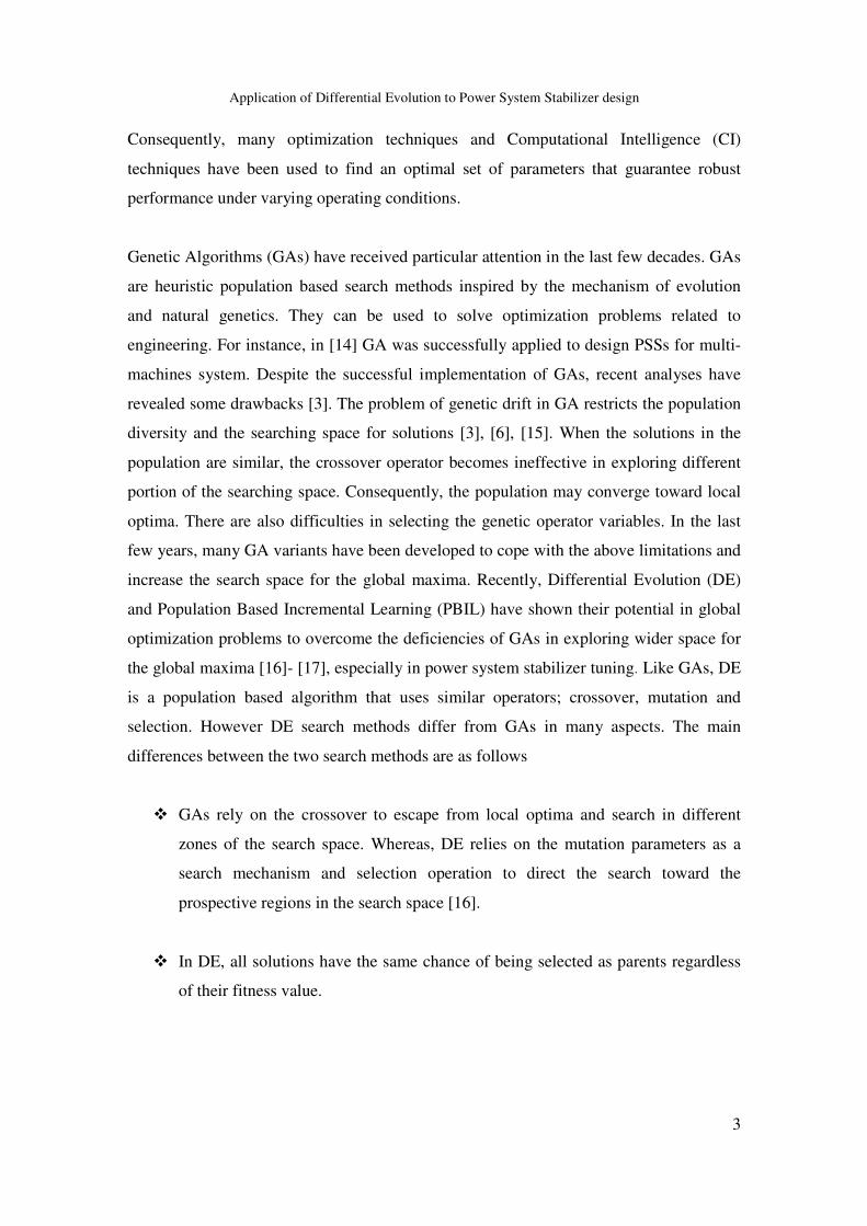
3.6� Selection ................................................................................................................ 34�
3.7� Termination ........................................................................................................... 35�
3.7.1� Objective met .................................................................................................... 35�
3.7.2� Maximum generation ........................................................................................ 35�
3.7.3� Population statistics .......................................................................................... 35�
3.7.4� Limited time ...................................................................................................... 36�
3.8� Summary ............................................................................................................... 36�
Chapter 4 ......................................................................................................................... 37�
4� Population Based Incremental Learning (PBIL) ................................................. 37�
4.1� Overview ............................................................................................................... 37�
4.2� Probability Vector (PV) and Population in PBIL ................................................. 38�
4.3� Competitive Learning ........................................................................................... 39�

Application of Differential Evolution to Power System Stabilizer design
ix
4.4� Mutation ................................................................................................................ 39�
4.5� Learning rate ......................................................................................................... 40�
4.6� Termination ........................................................................................................... 40�
4.7� Summary ............................................................................................................... 41�
Chapter 5 ......................................................................................................................... 42�
5� Power System Stabilizer Design ............................................................................ 42�
5.1� Introduction ........................................................................................................... 42�
5.2� Conventional PSS design ...................................................................................... 42�
5.3� Objective function ................................................................................................. 45�
5.4� Application of DE & PBIL to PSS design ............................................................ 46�
5.5� System configurations ........................................................................................... 50�
5.5.1� Single Machine to Infinite Bus system ............................................................. 50�
5.5.2� Two Area Multi-machine System ..................................................................... 52�
5.6� Summary ............................................................................................................... 54�
Chapter 6 ......................................................................................................................... 55�
6� Single Machine Infinite Bus System (SMIB): Simulation Results...................... 55�
6.1� Introduction ........................................................................................................... 55�
6.2� Optimized PSS ...................................................................................................... 55�
6.3� Modal Analysis ..................................................................................................... 57�
6.4� Time Domain Simulation ...................................................................................... 58�
6.4.1� Small Disturbance Simulation .......................................................................... 58�
6.4.2� Large disturbance simulation ............................................................................ 62�
6.4.2.1� Case 1: nominal operating condition ( P=1.0pu; Q= 0.32pu; Xe=0.5pu) ................. 62�
6.4.2.2� Case 2: System operating at P=0.5pu; Q= 0.17pu; Xe=0.7pu .................................. 66�
6.4.2.3� Case 3: System condition, P=1.0pu; Q= 0.34pu; Xe=0.7pu .................................... 69�
6.4.2.4� Case 4: System condition, P=0.5pu; Q=0.16pu; Xe=0.9pu ..................................... 72�
6.5� Summary ............................................................................................................... 75�
Chapter 7 ......................................................................................................................... 76�
7� Simulation Results for the Two-Area Multi-machine Systems ........................... 76�
7.1� Introduction ........................................................................................................... 76�
7.2� PSS Parameters optimization ................................................................................ 76�

Application of Differential Evolution to Power System Stabilizer design
x
7.3� Modal Analysis ..................................................................................................... 78�
7.4� Time domain Simulations ..................................................................................... 81�
7.4.1� Small disturbance .............................................................................................. 81�
7.4.2� Large disturbance simulation ............................................................................ 95�
7.4.2.1� Case 1: nominal condition where 100MW are transmitted over the tie-lines; .......... 96�
7.4.2.2� Case 2: 3-phase fault applied when 200MW are transmitted from area 1 to 2 ........ 98�
7.4.2.3� Case 3: 3-phase fault applied when 300MW are transmitted from area 1 to 2 ...... 101�
7.4.2.4� Case 4: 3-phase fault applied when 400MW are transmitted ................................. 103�
7.5� Summary ............................................................................................................. 106�
Chapter 8 ....................................................................................................................... 107�
8� Application of Self-Adaptive Differential Evolution to Power System Stabilizer
Design ............................................................................................................................. 107�
8.1� Introduction ......................................................................................................... 107�
8.2� Effects of Mutation F and Crossover Probability Cr on PSS Tuning ................. 108�
8.3� Effect of population size on PSS tuning ............................................................. 110�
8.4� Self-Adaptive Differential Evolution .................................................................. 114�
8.4.1� Application to PSS tuning: Modal analysis .................................................... 117�
8.4.2� Time Domain Step Response Analysis ........................................................... 118�
8.4.3� Large disturbances .......................................................................................... 122�
8.5� Summary ............................................................................................................. 132�
Chapter 9 ....................................................................................................................... 133�
9� Conclusions and Recommendations for Further Works ................................... 133�
References ...................................................................................................................... 137�
Research Publications ................................................................................................... 144�
Appendix ........................................................................................................................... A�

Application of Differential Evolution to Power System Stabilizer design
xi
List of Figures
Figure 1.1: Block Diagram of typical PSS .......................................................................... 6�
Figure 3.1: Population and Candidate structure ................................................................ 27�
Figure 3.2: Differential mutation ...................................................................................... 29�
Figure 3.3: Traditional Roulette wheel spun Np – times with fraction of allotted space
dependent on vector objective function value .................................................................. 30�
Figure 3.4: DE Stochastic universal sampling with equal Np spaced pointers and equal
slots size. The wheel is spun only once. ........................................................................... 30�
Figure 3.5: Exponential Crossover ................................................................................... 33�
Figure 3.6: Uniform crossover .......................................................................................... 34�
Figure 4.1: Probability vectors representation of 2 small population of 4 ........................ 38�
Figure 4.2; Probability vectors representation after update .............................................. 39�
Figure 5.1: Phase Lag in an SMIB system ........................................................................ 43�
Figure 5.2: Phase lag in a Two Area Multi Machine system ............................................ 44�
Figure 5.3: DE and PBIL parameters ................................................................................ 47�
Figure 5.4: chart for the PSS design using DE ................................................................. 48�
Figure 5.5: chart for the PSS design using PBIL .............................................................. 49�
Figure 5.6: Single machine to infinite bus system ............................................................ 50�
Figure 5.7: Two Area multi-machine system line diagram .............................................. 52�
Figure 6.1: DE fitness curve ............................................................................................. 56�
Figure 6.2: PBIL fitness curve .......................................................................................... 56�
Figure 6.3: Rotor speed responses for Case 1 ................................................................... 59�
Figure 6.4: Rotor speed responses for Case 2 ................................................................... 60�
Figure 6.5: Rotor speed responses for Case 3 ................................................................... 60�
Figure 6.6: Speed response for Case 4 .............................................................................. 61�
Figure 6.7: Speed responses for Case 5 ............................................................................ 62�
Figure 6.8: Rotor angle responses following 3-phase fault for case 1 .............................. 63�
Figure 6.9: Rotor speed responses following 3-phase fault for case 1 ............................. 64�
Figure 6.10: Terminal Voltage following 3-phase fault for case 1 ................................... 64�

Application of Differential Evolution to Power System Stabilizer design
xii
Figure 6.11: Electric field voltage following 3-phase fault for case 1 .............................. 65�
Figure 6.12: field voltage following 3-phase fault for case 1 ........................................... 65�
Figure 6.13: Rotor angle response following 3-phase fault for Case ............................... 66�
Figure 6.14: Speed response following a 3-phase fault for Case 2 ................................... 67�
Figure 6.15: Terminal voltage response following 3-phase fault for Case 2 .................... 67�
Figure 6.16: Electric field response for Case 2 ................................................................. 68�
Figure 6.17: Power output for Case 2 ............................................................................... 68�
Figure 6.18: Rotor angle responses for Case 3 ................................................................. 69�
Figure 6.19: Rotor speed responses for Case 3 ................................................................. 70�
Figure 6.20: Terminal voltage responses at bus 1 for Case 3 ........................................... 70�
Figure 6.21: Electric field voltage for Case 3 ................................................................... 71�
Figure 6.22: Active Power output responses for Case 3 ................................................... 71�
Figure 6.23: Rotor angle response following 3-phase fault for Case 4 ............................ 72�
Figure 6.24: Rotor speed response following 3-phase fault for Case 4 ............................ 73�
Figure 6.25: Terminal voltage response following 3-phase for Case 4 ............................ 73�
Figure 6.26: Electric field following a 3-phase fault for Case 4 ....................................... 74�
Figure 6.27: Active power output following 3-phase fault for Case 4 ............................. 74�
Figure 7.1: DE fitness curve ............................................................................................. 77�
Figure 7.2: PBIL fitness curve .......................................................................................... 77�
Figure 7.3: Active power response of G1 for Case 1 ........................................................ 82�
Figure 7.4: Active power response of G1 for Case 2 ........................................................ 82�
Figure 7.5: Active power response of G1 for Case 3 ........................................................ 83�
Figure 7.6: Active power response of G1 for Case 4 ........................................................ 83�
Figure 7.7: Active power response of G1 for Case 5 ........................................................ 84�
Figure 7.8: Active power response of G1 for Case 5 ........................................................ 84�
Figure 7.9: Active power response of G2 for Case 1 ........................................................ 85�
Figure 7.10: Active power response of G2 for Case 2 ...................................................... 86�
Figure 7.11: Active power response of G2 for Case 3 ...................................................... 86�
Figure 7.12: Active power response of G2 for Case 4 ...................................................... 87�
Figure 7.13: Active power response of G2 for Case 5 ...................................................... 87�
Figure 7.14: Active power response of G2 for Case 6 ...................................................... 88�
Figure 7.15: Active power response of G3 for Case 1 ...................................................... 89�

Application of Differential Evolution to Power System Stabilizer design
xiii
Figure 7.16: Active power response of G3 for Case 2 ...................................................... 89�
Figure 7.17: Active power response of G3 for Case 3 ...................................................... 90�
Figure 7.18: Active power response of G3 for Case 4 ...................................................... 90�
Figure 7.19: Active power response of G3 for Case 5 ...................................................... 91�
Figure 7.20: Active power response of G3 for Case 6 ...................................................... 91�
Figure 7.21: Active power response of G4 for Case 1 ...................................................... 92�
Figure 7.22: Active power response of G4 for Case 2 ...................................................... 93�
Figure 7.23: Active power response of G4 for Case 3 ...................................................... 93�
Figure 7.24: Active power response of G4 for Case 4 ...................................................... 94�
Figure 7.25: Active power response of G4 for Case 5 ...................................................... 94�
Figure 7.26: Active power response of G4 for Case 6 ...................................................... 95�
Figure 7.27: Terminal voltage response following a 3-phase fault for Case 1 ................. 96�
Figure 7.28: Rotor speed response following a 3-phase fault for Case 1 ......................... 97�
Figure 7.29: Electric field following a 3-phase fault for Case 1 ....................................... 97�
Figure 7.30: Active power output following 3-phase fault for Case 1 ............................. 98�
Figure 7.31: Terminal voltage response following a 3-phase fault for Case 2 ................. 99�
Figure 7.32: Rotor speed response following a 3-phase fault for Case 2 ......................... 99�
Figure 7.33: Electric field following a 3-phase fault for Case 2 ..................................... 100�
Figure 7.34: Active power output following 3-phase fault for Case 2 ........................... 100�
Figure 7.35: Terminal voltage response following a 3-phase fault for Case 3 ............... 101�
Figure 7.36: Rotor speed response following a 3-phase fault for Case 3 ....................... 102�
Figure 7.37: Electric field following a 3-phase fault for Case 3 ..................................... 102�
Figure 7.38: Active power output following 3-phase fault for Case 3 ........................... 103�
Figure 7.39: Terminal voltage response following a 3-phase fault for Case 4 ............... 104�
Figure 7.40: Rotor speed response following a 3-phase fault for Case 4 ....................... 104�
Figure 7.41: Electric field following a 3-phase fault for Case 4 ..................................... 105�
Figure 7.42: Active power output following 3-phase fault for Case 4 ........................... 105�
Figure 8.1: Effect of CR probability on DE performance .............................................. 109�
Figure 8.2: Effect of CR probability on DE performance .............................................. 110�
Figure 8.3: Fitness curve for different population size ................................................... 113�
Figure 8.4: Self-Adapting encoding aspect ..................................................................... 115�
Figure 8.5: Self-adaptive encoding aspect based on DE/rand/2 ..................................... 116�

Application of Differential Evolution to Power System Stabilizer design
xiv
Figure 8.6: Control Parameter settings ........................................................................... 117�
Figure 8.7: Step-response for Case 1 .............................................................................. 119�
Figure 8.8: Step-response for Case 2 .............................................................................. 120�
Figure 8.9: Step-response for Case 3 .............................................................................. 120�
Figure 8.10: Step-response for Case 4 ............................................................................ 121�
Figure 8.11: Rotor angle following 3-phase fault for Case 1 ......................................... 123�
Figure 8.12: Terminal voltage following 3-phase fault for Case 1 ................................. 123�
Figure 8.13: Speed response following 3-phase fault for Case 1 ................................... 124�
Figure 8.14: Electric field voltage following 3-phase fault for Case 1 ........................... 124�
Figure 8.15: Active power output following 3-phase fault for Case 1 ........................... 125�
Figure 8.16: Rotor angle following 3-phase fault for Case 2 ......................................... 126�
Figure 8.17: Terminal following 3-phase fault for Case 2 .............................................. 126�
Figure 8.18: Speed response following 3-phase fault for Case 2 ................................... 127�
Figure 8.19: Electric field voltage following 3-phase fault for Case 2 ........................... 127�
Figure 8.20: Active power output following 3-phase fault for Case 2 ........................... 128�
Figure 8.21: Rotor angle following 3-phase fault for Case 3 ......................................... 129�
Figure 8.22: Terminal voltage following 3-phase fault for Case 3 ................................. 130�
Figure 8.23: Speed response following 3-phase fault for Case 3 ................................... 130�
Figure 8.24: Electric field voltage following 3-phase fault for Case 3 ........................... 131�
Figure 8.25: Active power output following 3-phase fault for Case 3 ........................... 131�

Application of Differential Evolution to Power System Stabilizer design
xv
List of Tables
Table 5.1: SMIB Open Loop operating conditions used in the PSS design ..................... 51�
Table 5.2: Two-Area Open loop poles for the selected design operating conditions ....... 54�
Table 6.1: SMIB PSS parameters ..................................................................................... 57�
Table 6.2: SMIB electromechanical modes of the system with different PSSs Designs .. 58�
Table 7.1: Two-area PSS parameters ................................................................................ 78�
Table 7.2: Inter-area modes for Two-Area Multi-machine system .................................. 79�
Table 7.3: Local Area mode 1 ........................................................................................... 80�
Table 7.4: Local Area mode 2 ........................................................................................... 81�
Table 8.1: Experimental results of DE when varying the population ............................. 112�
Table 8.2: PSS parameters .............................................................................................. 118�
Table 8.3: System Open-loop and Closed-loop eigenvalues .......................................... 118�

Application of Differential Evolution to Power System Stabilizer design
xvi
Nomenclature
A State matrix
Pe Electrical power
Pm Mechanical power
Te Electrical torque
Tm Mechanical torque
� Small perturbation
T´do, T´qo d-axis, q-axis transient open circuit time constants
T´´do, T´´qo d-axis, q-axis sub-transient open circuit time constants
ed, eq d-axis, q-axis terminal voltage component
id, iq d-axis, q-axis terminal current component
H Inertia constant
KD Damping torque coefficient
Lfd Field winding leakage inductance
Ll Stator leakage inductance
Lad, Laq d-axis, q-axis stator to rotor mutual inductance
Ld, Lq d-axis, q axis synchronous inductance
L´d, L´q d-axis, q axis transient inductance
L´´d, L´´q d-axis, q axis subtransient inductance
Rfd Field resistance
λ Eigenvalue
ς Damping ratio
� Rotor angle
� Rotor angular velocity
�0 Base angular velocity
�d, �q d-axis, q axis stator flux linkage
�fd Field flux linkage
pu per unit
AVR Automatic Voltage Regulator

Application of Differential Evolution to Power System Stabilizer design
xvii
SMIB Single machine infinite bus
PSS Power System Stabilizer
CPSS Conventional Power System Stabilizer
DE-PSS Differential Evolution Power System Stabilizer
jDE -PSS Self-Adaptive Differential Evolution Power System Stabilizer
PBIL-PSS Population Based Incremental Learning Power System Stabilizer
CL Competitive Learning
PV Probability Vector
F Mutation Factor
CR Crossover Probability
Np Population number
EA Evolutionary Algorithm
AI Artificial Intelligence
SVC Static Var Compensator
STATCOM Static Compensators
FACTS Flexible Alternating Current Transmission Systems
Remarks: when any of the abbreviations is used in plural, then an (s) is added at the end
of the listed abbreviations. Also pu and per unit have been used interchangeably within
the thesis, but they are the same.
The notation for the complex numbers used in this thesis is j and not i.

Application of Differential Evolution to Power System Stabilizer design
1
Chapter 1
1 Introduction
This chapter introduces the concept of small signal stability problems with emphasis on
low frequency oscillations. Emphasis is given to techniques applied to limit and mitigate
these oscillations. Furthermore, a proposed method, which is the main focus of this
research, is briefly discussed. The chapter ends with the objectives and the scope of the
research.
Small signal stability is defined in [1] as “the ability of a power system to maintain
synchronism under small disturbances”. These disturbances are mainly due to external
faults and the constant change of operating conditions. As a result, low frequency
oscillations in the range of 0.2 – 3 Hz are often observed in the system. For the purpose
of analysis, these oscillations are often categorized into 5 groups: interplant mode, local
mode, inter-area mode, control mode, and torsional mode [2]. This thesis will however
focus on only the inter-area and local modes because the system models that have been
considered only exhibit these oscillations.
Inter-area oscillations characterized by frequencies ranging from 0.2 to 0.8 Hz. They
occur as a result of a group of generators in one area of a network oscillating against a
group of generators in another area. This is typical of an interconnected network with
many groups of generators [1], [3].
Local area oscillations on the other hand, have frequencies ranging from 0.8 to 2.0 Hz.
They are mostly associated with a single generator oscillating against the rest of the
network [1].
Over the years, these inherent oscillations have received a great deal of attention. Since
the development of interconnection between synchronous generators and the introduction
of deregulation of power systems, these oscillations have become apparent especially

Application of Differential Evolution to Power System Stabilizer design
2
during and after small and large disturbances, [2], [4], [5]. Several factors contribute to
the rise of these oscillations, commonly known as electromechanical modes. The use of
automatic controls, necessary to maintain the stability during transient faults have adverse
effects on the system damping due to their negative feedback nature [4]. For instance, the
rapid Automatic Voltage Regulator (AVR) and fast acting excitation system tend to
reduce the damping torque component on the rotor which is necessary to damp
oscillations [1], [5]. Moreover, the recent exponential increase in power demand which
has led to bulk power transfer over weak transmission lines was also found to cause
oscillations that limit the transfer capability of the system. If no adequate damping is
provided, these oscillations might grow in magnitude with time to create system
separation [1], [4] [5]. To mitigate these oscillations, various controllers have been
developed and implemented over the years. Power Systems Stabilizers (PSS) have been
extensively used as supplementary excitation controllers that provide additional damping
to eliminate electromechanical oscillations and enhance the overall system stability. To
achieve this, the PSS is often designed at a particular operating condition using
conventional methods such as phase compensation, root locus, etc. However, due to the
nonlinearity characteristics of power systems and the varying operating conditions, the
resulting Conventional PSS (CPSS) performance deteriorates as the operating conditions
change and therefore require re-tuning [6], [7].
Recently, new controllers that can provide adequate damping over a wide range of
operating conditions have been investigated to compensate for the shortcoming of the
CPSS. Modern control theory have been applied to design robust PSSs such as Adaptive
Control [8], [9], H� [10]- [11], and variable structure control [12] have been successfully
applied and tested in laboratory and online. However, power utilities still remain cautious
over their implementation [13].
In the recent years, increasing interests have been focused on the optimization of
stabilizers parameters to provide adequate performance for a wide range of operating
conditions.
Application of Differential Evolution to Power System Stabilizer design
3
Consequently, many optimization techniques and Computational Intelligence (CI)
techniques have been used to find an optimal set of parameters that guarantee robust
performance under varying operating conditions.
Genetic Algorithms (GAs) have received particular attention in the last few decades. GAs
are heuristic population based search methods inspired by the mechanism of evolution
and natural genetics. They can be used to solve optimization problems related to
engineering. For instance, in [14] GA was successfully applied to design PSSs for multi-
machines system. Despite the successful implementation of GAs, recent analyses have
revealed some drawbacks [3]. The problem of genetic drift in GA restricts the population
diversity and the searching space for solutions [3], [6], [15]. When the solutions in the
population are similar, the crossover operator becomes ineffective in exploring different
portion of the searching space. Consequently, the population may converge toward local
optima. There are also difficulties in selecting the genetic operator variables. In the last
few years, many GA variants have been developed to cope with the above limitations and
increase the search space for the global maxima. Recently, Differential Evolution (DE)
and Population Based Incremental Learning (PBIL) have shown their potential in global
optimization problems to overcome the deficiencies of GAs in exploring wider space for
the global maxima [16]- [17], especially in power system stabilizer tuning. Like GAs, DE
is a population based algorithm that uses similar operators; crossover, mutation and
selection. However DE search methods differ from GAs in many aspects. The main
differences between the two search methods are as follows
� GAs rely on the crossover to escape from local optima and search in different
zones of the search space. Whereas, DE relies on the mutation parameters as a
search mechanism and selection operation to direct the search toward the
prospective regions in the search space [16].
� In DE, all solutions have the same chance of being selected as parents regardless
of their fitness value.

Application of Differential Evolution to Power System Stabilizer design
4
� DE encodes parameters in floating – point regardless of their type, whereas GA
encoding is mainly binary although floating, gray, etc. Real-value encoding for
GA has also been proposed recently.
Some of the features of DE are [16], [16], [18] :
� Low computational complexity, and efficient in memory utilization due to its one-
to-one selection method.
� DE has a faster convergence, and greater freedom in designing mutation
distribution than GAs.
� Because DE only has three control parameters, mutation factor, crossover
probability, and population size, it makes it fairly easy to use.
Tuning these intrinsic control parameters often presents a challenge. Some guidelines
have been provided in [16] to help choose appropriate mutation factor and crossover
probability. Because these parameters are dependent on the nature of problem being
analysed, the guidelines may not guarantee good performance of DE. Hence a trial-and-
error approach is often used. In this thesis, the impact of the population size on the
performance of DE is also investigated. Recently, self-adaptive DE has been used to
address this drawback [19].
PBIL, on the other hand, is an extension to the Evolutionary Genetic Algorithm (EGA)
achieved through the re-examination of the performance of the EGA in terms of
competitive learning [20], [17]. PBIL has the following features [20]:
� It has no crossover and fitness proportional operators.
� It works with probability vector (number in range 0-1). This probability vector
controls the random bitstrings generated by PBIL and is used to create other
individuals through learning.

Application of Differential Evolution to Power System Stabilizer design
5
� Unlike GAs and DE, in PBIL, there is no need to store all solutions in the
population. Only the current best solution and the solution being evaluated are
stored. Hence, the “best” individual is used to update the probability vector so as
to produce solutions similar to the current best individuals.
� PBIL only has two intrinsic parameters, namely population size and the learning
rate factor.
As a result, PBIL is simpler, faster and more effective than the standard GA. However,
PBIL requires a large number of generations to converge toward the optimal solution.
Following the prominence of DE in the global optimization scene, this thesis aims to
present a extensive analysis of DE in PSS tuning. The results are compared to those of
PBIL, an equally renowned optimizer, to assess the performance of DE. The comparison
also includes the CPSS which has been designed for different system configurations.
1.1 Power System Stabilizer
For many years PSSs have been used to add damping to electromechanical oscillations.
They were first introduced in the late 1960s to compensate for the AVRs adverse effect
on the damping torque by means of positive feedback loop to provide additional damping
in the system [4].
PSSs essentially use the power amplification capability of the generators to generate a
damping torque in phase with the speed change of the generator rotor. This is achieved by
injecting a stabilizing signal into the excitation system voltage reference in such a way
that a component of electrical torque proportional to the rotor speed deviation is produced
[21], [22]. This stabilizing signal is, in most cases, the deviations in generator rotor speed
which fed through a compensation circuit to compensate for the phase lag between the
exciter voltage reference and generator electrical torque [1], [21].

Application of Differential Evolution to Power System Stabilizer design
6
1.1.1 Power System Stabilizer Structure
The basic objective of power system stabilizer is to modulate the generator’s excitation in
order to produce an electrical torque at the generator proportional to the rotor speed [1],
[21]. In order to achieve that, the PSS uses a simple lead-lag compensator circuit to adjust
the input signal and correct the phase lag between the exciter input and the electrical
torque. The PSS can use various inputs, such as the speed deviation of the generator
shaft, the change in electrical power or accelerating power, or even the terminal bus
frequency. However in many instances the preferred signal input to the PSS is the speed
deviation.
Figure 1.1 below illustrates the block diagram of a typical PSS. The PSS structure
generally consists of a washout, lead-lag networks, a gain and a limiter stages. . Each
stage performs a specific function.
2
1
11
sTsT
++
4
3
11
sTsT
++
w
w
sTsT+1
PSSK
min_PSSV
max_PSSV
ω∆ PSSV
Figure 1.1: Block Diagram of typical PSS
The washout stage is a high pass filter whose purpose is to filter out undesirable signals
and let through signals with frequencies in the range of 0.2 – 2 Hz. This stage prevents
any change in the terminal voltage. The value associated with the time constant �� is not
critical and may be in the range of 1 to 20 seconds. However it must be long enough to
pass stabilizing signals at the frequencies of interest relatively unchanged, but not so long
that it leads to undesirable generator voltage excursions. For local mode oscillations, a
washout of 1 to 2 s is satisfactory. Whereas for the inter-area oscillations a washout time
constant of 10 s or higher may be required in order to reduce phase lead at low
frequencies [23], [24].

Application of Differential Evolution to Power System Stabilizer design
7
The compensation stage consists of a combination of lead and lag circuits that produce an
appropriate phase lead characteristic to compensate for the phase lag between the exciter
input and the generator’s electrical torque. However the phase lag changes with the
operating condition. Therefore, a compromise must be made when determining the phase
lead. Hence a characteristic that is satisfactory for both the range of frequencies between
0.1 to 2.0 Hz and for different system conditions must be selected. This may result in less
than optimum damping at any one frequency. Generally, slight under-compensation is
preferable to over-compensation so that both damping and synchronizing torque
components are increased [1], [4], [23],
The gain stage determines the amount of damping introduced by the stabilizer. Hence,
increasing the gain can move unstable oscillatory modes into the left – hand complex s-
plane. Ideally, the gain should be set to a value corresponding to a maximum damping.
However, in practice the gain KPSS is set to a value satisfactory to damp the critical mode
without compromising the stability of other modes [4], [23], [24].
The limiter prevents conflicts with AVR actions during transient fault. The positive and
negative limits should be set around the AVR set point to avoid any counteraction. The
positive limit of the PSS contributes to improve the transient stability in the first swing
during a fault whereas the negative limit acts during the back swing of the rotor.
Designing a power system stabilizer is a complex task, particularly in a multimachine
system environment where several machines are involved. Parameters of the stabilizer
need to be appropriately tuned so that the damping of the electromechanical modes is
increased without adversely affecting the other oscillatory modes. Several design
methods have been investigated however the most common one is the Conventional
Power System Stabilizer (CPSS).
1.1.2 Conventional Power System Stabilizer design method
For many years conventional control methods have been applied to design PSSs. These
approaches consist of first linearizing the system at the nominal operating condition to be
able to extract the dynamic characteristics of the power system and its frequency
response. Once the phase lag is identified, the phase lead can be obtained by tuning the

Application of Differential Evolution to Power System Stabilizer design
8
time constants of the lead-lag circuit. Ideally a phase lead, equal and opposite to the phase
lag, is required to produce an electrical torque with a component proportional to the
speed. However in practice this cannot be achieved but can be closely matched over the
frequency range [4].
The gain on the other hand is obtained by applying the root locus method. The gain must
be carefully selected to stabilize the electromechanical mode without adversely affecting
the other modes such as the exciter mode [4], [24].
It is important to choose an appropriate value for the washout Tw. It would be adequate to
choose the time constant between 1 and 2 seconds if the damping of the local mode is the
only concern. However a Tw of 10 seconds or higher when inter – area is considered [1],
[24], [25].
Generally, determining the stabilizer’s parameters in systems with both local and inter –
area modes has a more complex approach. For the most case this situation is encountered
in a multimachine system. Therefore PSSs must be tuned one at a time through off-line
analysis, and tuned further during commissioning. The validity of the model used in the
off-line studies should be checked on commissioning. Setting power system stabilizers to
typical values is particularly dangerous for systems in which inter – area modes are of
concern. It is very easy for the stabilizer to have a destabilizing effect at low frequencies
that cannot be observed during on-line commissioning test [23], [26].
The performance of the CPSS often deteriorates over time due to nonlinearity and
changes of operating conditions. Over the years, several approaches of controllers design
have been investigated and implemented to overcome the shortcomings of the CPSSs.
Some of these methods are reviewed in the next section.
1.2 Modern Control Design Methods
In the last few decades, new stabilizers able to provide adequate damping across a wide
range of system operating conditions have been developed and successfully tested. These

Application of Differential Evolution to Power System Stabilizer design
9
designs are based on modern control theories which cater for the nonlinearity
characteristic of power systems.
1.2.1 Adaptive Control
Adaptive control can be described as the changing of controller parameters based on the
changes in system operating conditions [8]. The idea is to constantly update the controller
parameters according to recent measurement [3]. Power systems are inherently nonlinear
with varying operating conditions, hence adaptive control technique is well suited to track
the operating conditions and changes in the system. The resulting adaptive stabilizer uses
an identification algorithm that tracks the actual system operating condition, which then
adjusts its parameters on-line according to the environment in which it works. This
method can provide good damping over a wide range of operating condition [9], [27]-
[28].
Despite the good performance of the stabilizer, adaptive controllers are difficult to design
and susceptible to problems like non-convergence of parameters and numerical
instability. The response time of the controller is the key factor to a good closed-loop
performance. The adaptive power system stabilizer (APSS) employs complicated
algorithms for parameter identification and optimization which require significant amount
of computing time. The higher the order of the discrete model of the controlled system
used in identification, the more computing time is needed. To develop a quick response
PSS, it is necessary to investigate alternative techniques such as neural network and
Fuzzy logic based adaptive [22], [27], [29]
1.2.2 H� Controller
H� is a control technique that addresses the issue of the worst – case controller design for
systems subject to unknown disturbances, including problems of disturbance attenuation,
model matching, and tracking. The objective is to minimize the maximum norm of an
input-output operator, where the maximum is often taken over the unknowns such as
disturbances [30]. Following the nonlinearity characteristic of power systems and
unpredictable change of operating conditions, H� theory has been applied to overcome
the CPSS shortcomings. The method provides a theoretical mechanism to deal with

Application of Differential Evolution to Power System Stabilizer design
10
uncertainty in a system control design problem. The resulting controller minimizes the
effect of external disturbances on system output in terms of a H� norm which can easily
put the various types of disturbances into a single framework by using a frequency
weighting function to emphasise the interesting noise band. The mismatch between the
physical system and its mathematical description has been taken into account in the
control design process to cope with the stability problem in the presence of system
uncertainty [10]. H� has been successfully applied the designing PSSs [10], [31], [32],
[33]. However these controllers have drawbacks. Which includes the selection of
appropriate weighting functions, and issues related to practical implementation due to the
high dimension of the controllers [32]. In addition, the mixed sensitivity approach
produces closed loop poles whose damping is directly dependent on the open loop
system. This effect is caused by the pole-zero cancellation phenomena associated with
such an approach. This problem was solved in [34] using Bilinear approach. However the
H� based PSS tends to have the same order as the plant, therefore resulting in highly
complex stabilizers [3].
1.2.3 State-Feedback Optimal PSS
This method is based on eigenvalue shifting technique used to determine the weighing
matrix in the performance index. The dominant eigenvalue is shifted to the left side of
the s-plane until satisfactory shift is achieved or the controller’s practical limit is reached.
Computational programs are used to shift the poles in the complex s-plane. It allows for
the shaping of the dynamic response of the system. This method works properly, but
tends to have some problems, especially as the state matrix of the system grows. It makes
the process to be complex and computationally intensive [3], [35], [36].
Several compensations devices, such as Static Var Compensators (SVC), Thyristor
Controlled Series Capacitors (TCSC), and other Flexible AC Transmission System
(FACTS) have also been implemented to damp electromechanical modes [4], [37], [38].
However power utilities still prefer the conventional lead-lag PSS because they are the
most cost-effective oscillation damping controllers. This has led researchers to focus on
the optimization of the PSS parameters to effectively damp electromechanical oscillations
over a wide range of operating conditions.

Application of Differential Evolution to Power System Stabilizer design
11
1.3 Optimization Based Power System Stabilizers
Optimization is defined in [18] as the attempt to maximize a system’s desirable properties
whilst simultaneously minimizing its undesirable characteristic. In the recent years, there
has been increasing interests in applying optimization techniques to design power system
stabilizers. The approach consists of converting the problem of selecting PSS parameters
into a simple optimization problem. Thereafter finds the optimal set of PSS’ parameters
that will guarantee adequate damping across the entire range of operating conditions.
Over the years, several optimization algorithms have been investigated and few are
reviewed below.
1.3.1 Gradient based optimization
Gradient methods are classic optimization techniques that are based on a single point
derivative and iterative procedures. They use quadratic approximation of the function of
interest around one initial point. Then, the value of the point is then adjusted to a new
approximation or increased by a small step of the gradient until optimum value is
reached. These methods often require the existence of first derivative of the objective
function or even higher order in order to work properly [39]. Several gradient based
methods have been used for optimization such as Newton-Raphson, Quasi-Newton and
Gradient descent. However these methods are complex and computationally demanding.
They require excessive restrictions on parameters, objective functions, and constraint
functions. Convexity, continuity, and differentiability of objective functions are necessary
for these algorithms. The key disadvantage is their convergence to local minima. Most
real-world applications, such as PSS tuning, are represented as nonlinear and
discontinued functions. Therefore, the gradient techniques are not appropriate for the PSS
tuning. Hence, people have increasingly turned their attention to stochastic optimization
algorithms, especially evolution algorithms.
1.3.2 Evolution Algorithms
Evolution Algorithms (EAs) are population-based optimizer inspired by the mechanism
of evolution and natural selection. They attack the starting point problem by sampling the
objective function at multiple random initial points and explore the search space by
iteratively generating new point that are perturbation of the existing ones [16]. This

Application of Differential Evolution to Power System Stabilizer design
12
approach is convenient in locating the global maximum/minimum instead of local. EAs
are simple, robust, efficient, and versatile algorithms that can be applied to any types of
problems irrespective the function type, such as nonlinearity, or discontinuity or even the
complex.
In the last few years, increasing number of researches have proposed EAs to optimally
tune the parameters of the PSS to guarantee a robust performance over a wide range of
system conditions. Genetic Algorithms (GAs) have received particular attention in the
last few decades. GAs are heuristic population based search methods inspired by the
mechanism of evolution and natural genetic. They can be used to solve optimization
problems related to Engineering. For instance, in [14] GA was successfully applied to
design PSSs for multi-machines system. Despite GAs’ performance and promising results
in numerous applications, recent analyses have revealed some drawbacks [40]. The
problem of genetic drift in GA restricts the population diversity and the searching space
for solutions. As a result, GAs may converge to suboptimal solutions [6], [7], [40]. In
addition, GA is computationally time consuming and require large computer storage
when dealing with difficult problems such as tuning PSSs in a multi-machine
environment [41], [42].
To cope with the above drawbacks, many variants of GAs have been proposed often
tailored to a particular problem. Recently, several simpler and yet effective heuristic
algorithms have received increasing attention. They have shown their potential in global
optimization problems to overcome the deficiencies of GAs in exploring wider space for
the global maxima [16], [43], [44] especially in power system stabilizer tuning. Some of
these algorithms have been reviewed in the subsequent paragraphs.
Breeder Genetic Algorithm (BGA): was first introduced by Mühlenbein [44]. BGA
uses the concept of artificial breeding, whereby the top T% (say 15%) best solutions are
saved as “breeding pool” and the rest discarded. This is a similar concept used in animal
breeding. This algorithm use real-valued encoding. In [3], both BGA and PBIL were
applied to the design of PSS. They all displayed similar performance with each other and

Application of Differential Evolution to Power System Stabilizer design
13
outperformed GA. However BGA major disadvantage is its tendency quickly converge to
a solution that may be local due to the quick loss of diversity.
Population Based Incremental Learning (PBIL): is a method that combines genetic
algorithms and competitive learning for function optimization. PBIL is an extension to
the Evolutionary Genetic Algorithm (EGA) algorithm achieved through the re-
examination of the performance of the EGA in terms of competitive learning [20]. In [3],
[7] and [41], PBIL was used to tune the PSS’ parameters. The results showed
considerable enhancement in the PSS performance as opposed to those of GA. However,
PBIL drawbacks reside in the slow convergence due to the learning process involved.
This drawback can be solved by optimally tuning the learning rate (LR) parameter by
trial-and-error. Despite the tuning the LR, PBIL still requires a large number of
generation to obtain a solution.
Differential Evolution: is a stochastic optimizer based on the differential mutation
technique, used as a search mechanism, and applies the greedy selection to direct the
search toward the prospective solution in the search space [16], [45], [46]. DE employs a
“one-to-one survivor selection” which consists on comparing each trial vector to its
corresponding target vector. This process ensures that both the best vector at each index
is retained. Furthermore this also guarantees that the very best-so-far solution is kept. In
DE, all candidates have the same probability of being accepted. This algorithm is very
simple yet very powerful and robust optimizer.
DE has been the subject of intensive performance evaluation since its inception. Many
comparisons have been carried out with other optimization algorithms on benchmark
functions and several other applications. Most often DE outperforms its counterparts in
efficiency and robustness [45]. DE has thus earned its reputation and recognition among
researchers for its simplicity, efficiency, and robustness for function optimization.
Recently, DE has been implicitly used in a variety of problems, especially in engineering
[45]. As a result, in this thesis DE’ ability will be examined in optimally tune the PSS in
different system configurations. A systematic approach is used to test DE’s performance.
This approach consists of investigating the effect of the intrinsic control parameters on

Application of Differential Evolution to Power System Stabilizer design
14
the DE ability to tune the PSS. To address the drawbacks of DE, this investigation further
extends to the application of a self-adaptive scheme to PSS tuning whereby the mutation
and crossover parameters are changing during the optimization.
Several researches have applied DE in tuning the PSS. In [47], DE was successfully
applied in designing PSS. The resulting PSS was then compared to the CPSS through a
series of tests whereby DE based PSS outperformed the CPSS. In [46], DE is compared
to GA when used to simultaneously tune PSSs. The results have proven that DE out
performed GA.
Several other PSS design methods Particle Swarm Optimization (PSO) [48], and
Simulated Annealing (SA) [49] that have been successfully applied over the years, but
have not been discussed in this thesis.
1.4 Objectives of the Thesis
The objective of this thesis is to design a power system stabilizer based on Differential
Evolution (DE). The purpose of the applied optimization algorithm is to solve the problem of
conventional power system stabilizer design in the context of nonlinear plant and varying
operating conditions. With the versatility and effectiveness of DE in the global optimization
arena, it is hoped that this work will make a contribution to the development and application
of DE.
In order to develop a robust DE based PSS, the following topics are addressed in this
thesis:
� Find the optimal set of PSS’ parameters that ensures robust performance and
stability of the system over a wide range of operating conditions.
� Assess the performance of DE’s optimization ability in comparison to that of
Population-Based Incremental Learning (PBIL), a prominent optimization
technique.
� Simultaneously tune the power system stabilizers using DE and PBIL for
different system configurations such as SMIB and the Two-Area
Multimachine.

Application of Differential Evolution to Power System Stabilizer design
15
� Evaluate the resulting PSSs (DE & PBIL) by comparing their performances
including those of the CPSS by means of modal analysis which are validated
using time domain simulation.
� Investigate the effect of the intrinsic control parameters of DE in the PSS
tuning. Address the resulting drawbacks and propose alternatives.
� Draw conclusions and recommendations on the DE’s performance.
1.5 Scope of the research
This research investigates the application of Differential Evolution (DE) to design Power
System Stabilizers over a wide range of operating conditions. This approach consists of
determining a set of PSS’ parameters that ensures optimal performance, stability and
robustness across all operating conditions. The PSS tuning is achieved by maximizing the
system minimum damping ratio. This process is also known as the objective function
which is presented in Chapter 5.
The scope of the research also includes the design of PSSs using conventional methods
and Population Based Incremental Learning, a prominent optimization algorithm. A
comparison analysis is carried out to assess the performances DE based PSS. The
resulting PSSs are applied to different power system models such as Single Machine
Infinite Bus (SMIB) and Two-area multimachine. The investigations in this thesis are
limited to the analysis of the electromechanical modes which were conducted by means
of modal analysis. The results of the modal analysis were validated with time domain
simulations using both small and large disturbances. Further investigation is carried out to
assess the effect of DE’s control parameters on the performance of the DE based PSS.
This has led to the investigation of Self-Adaptive DE which was implemented, tested and
compared with the DE on an SMIB system. Conclusions and recommendations based on
the results obtained are presented.
1.6 Research Contribution
This research addresses the performance of DE in comparison with PBIL and CPSS when
applied Power System Stabilizers tuning. The performance is determined by the

Application of Differential Evolution to Power System Stabilizer design
16
convergence rate, frequency and time domains analysis. The major contribution are
summarized as follows
First, experimental analysis has been conducted to investigate DE’s convergence
behaviour for a PSS by understanding the effect of mutation factor and crossover
probability on the dynamic of the algorithm. This underlines the necessity to use self-
adaptive control parameters to tune PSSs.
Second, a self-adaptive algorithm is implemented to tune the PSS. This process prevents
the users’ manual tuning of the control parameters suitable to the characteristics of the
optimization problems. The resulting controller is tested and compared with the classic
DE from a performance point of view.
Third, the effects of the population size on the algorithm performance to tune the PSS
have been investigated.
1.7 Thesis Outline
The thesis report is organized as follows:
Chapter 1 Gives a background theory on small signal stability concept with emphasis
on the low frequency oscillation, its causes and mitigation techniques. A
review of the relevant work in the area of PSS tuning is presented which
lays down the motivation and the objectives of this work. Differential
Evolution is also briefly discussed.
Chapter 2 Reviews the mathematical concept of linearization applied to small signal
stability. The state space representation is also discussed.
Chapter 3 Presents DE and its optimization algorithm. Emphasis is put on the
differential mutation which is a process used to guide DE’s search toward
the global optimum. The crossover and selection criteria are also
discussed.
Chapter 4 Presents an overview of Population Based Incremental Learning (PBIL),
which is also an Evolutionary Algorithm. PBIL is based on a concept of
learning that update a probability vector (PV) to direct the search to the
optimum solution.

Application of Differential Evolution to Power System Stabilizer design
17
Chapter 5 Discusses the design procedure of a Power System Stabilizer (PSS). The
following consists of using the conventional method and the application
of the Differential Evolution (DE) and Population-Based Incremental
Learning (PBIL) to find the optimum set of parameters that guarantees the
robustness over a wide range of operating conditions. In addition, test
cases for various system configurations such as SMIB and multimachine
are also discussed in this section.
Chapter 6 Presents the optimized power System Stabilizers parameters. It also
discusses the results obtained for the SMIB. The eigenvalues analysis is
conducted as well as the time domain simulations are discussion thereof.
Chapter 7 Presents the application of DE and PBIL to simultaneously tune PSSs in a
Two-Area Multimachine system. Results are discussed by conducting a
modal analysis and time domain simulations which compares DE-PSS,
PBIL-PSS to CPSS.
Chapter 8 Tests the effects of DE control parameters on the optimization.
Preliminary work on Self-Adaptive Differential Evolution applied to
power system tuning, and the effect of population size in the optimization
are discussed.
Chapter 9 Concludes the thesis and give recommendations as well as giving
suggestions for future work.

Application of Differential Evolution to Power System Stabilizer design
18
Chapter 2
2 Small Signal Stability Analysis
2.1 Introduction
As defined in Chapter 1, small signal stability is the ability of a power system to maintain
stability when subject to small disturbances [1]. The disturbances are considered small
only if linearization of the system is possible. Hence, this chapter reviews linear
techniques used to analyse small signal oscillations and extract information about the
system dynamic characteristic. Techniques such as modal analysis, eigenvectors,
eigenvalues’ sensitivity and participation factors are elaborated in subsequent sections.
2.2 State-Space Representation
The State-Space representation is often used to describe the behaviour of a dynamic
system. Hence, to model this particular behaviour, a set of n first order nonlinear
differential equations are used. The notations are borrowed from [1] and are as follows
�� � � � ���� ��� ��� �� ��� ��� ������ � � ������� � (2.1)
Where n is the order of the system and r is the number of inputs. That can be written in
vector representation form:
�� � ���� �� �� (2.2)
Where:
� � � ����� � � �����
� � �����
��: the state vector containing the state variables
�� : contains the derivative of the state variables

Application of Differential Evolution to Power System Stabilizer design
19
� : the vector of the non-linear functions
� : the vector of the inputs
� : the time
� : the order of the system
! : the number of inputs
If the derivatives of the states variables are not explicit functions of time, the system is
referred to as autonomous systems of the form:
�� � ���� �� (2.3)
The equation relating the outputs to the inputs and state variables can be written as
" � �#�� �� (2.4)
Where
" � � �$�$� # � �%�%�
" : is the vector of outputs
# : is the vector of non-linear equations relating the state and inputs variables to the
outputs variables.
2.3 Linearization
The linearization process consists of initializing the state vector �&� and ��& the input
vector around the equilibrium point. Therefore, the following equation should be true.
��& � ��&� �&� � ' (2.5)
Following a small perturbation, (� and (�� in the system state and input variables, we get
�� � �&� ) (�� �������������������� � �& ) (� (2.6)

Application of Differential Evolution to Power System Stabilizer design
20
The above must satisfy equation 6.3 as follows
�� � ��& ) (�� � ��& ) (�� �& ) (�� (2.7)
If the perturbations in the system are assumed to be small, the system equations ��� ��
can be expressed in Taylor’s series expansion terms as in [1]. With few simplification, by
neglecting the terms associated with the second and higher order of powers of (� and (�,
equations (2.3) and (2.4) are as follows.
(�� � � *+,*-. (� ) /) *+,*-0 (�� ) *+,*1. (� ) /) *+,*12 (�� (2.8)
Where i = 1, 2, 3…n and
($� � *34*-. (� ) /) *34*-0 (�� ) *34*1. (� ) /) *34*12 (�� (2.9)
Where j = 1, 2, 3…m
For the general state space system, the linearization of (2.3) and (2.4) around the
operating point �&� and ��& are [1]:
(�� � 5(� ) 6(� (2.10)
(" � 7(� ) 8(� (2.11)
where:
5 �9::;*+.*-. *+.*-0� < �*+0*-. *+0*-0=>
>? 6 �9::;*+.*1. *+.*12� < �*+0*1. *+0*12=>
>? (2.12)
7 �9::;*3.*-. *3.*-0� < �*3@*-. *3@*-0 =>
>? 8 �9::;*3.*1. *3.*12� < �*3@*1. *3@*12 =>
>?

Application of Differential Evolution to Power System Stabilizer design
21
(� is the linearized state vector of dimension n
(" is the linearized output vector of dimension m
(� is the linearized input vector of dimension r
A is the state matrix of size (nxn)
B is the input matrix, size (nxr)
C is the output matrix, size (mxn)
D is the feed forward matrix, size (mxr)
After linearization, the system stability can be analysed using the modal analysis as
follows.
2.4 Modal Analysis
Once the state space has been established, the stability of the system can be extracted and
analysed by means of eigenvalues, eigenvector properties and participation factor.
2.4.1 Eigenvalues
The eigenvalues are the non-trivial solutions of a the matrix A, obtained by solving the
following equation
AB � CB������������������� (2.13)
Where D is nxl vector and A is nxn state matrix.
By rearranging equation (2.11), E value can be obtained by solving the following
equation
FG�A H CI� � ' (2.14)
Where I is the identity matrix
The n solutions of the above equation are the eigenvalues�C� C�� CJ� � C�� of the nxn
matrix A. These eigenvalues can be real or complex of the form�E � K L MN.
For a real A matrix, the complex eigenvalues occurs in conjugate pairs.

Application of Differential Evolution to Power System Stabilizer design
22
The stability of the system at an operating point (OP� QP) can be determined by analysing
the eigenvalues. Therefore, a system is said to be stable at a particular operating point if
all the eigenvalues are on the left-hand side of imaginary axis of the complex plane, and
unstable otherwise. A real eigenvalue corresponds to a non-oscillatory mode, whilst a
complex eigenvalue corresponds to an oscillatory mode. If the real eigenvalue is
negative, the mode decays over time; and if positive, the mode is said to have an
aperiodic instability. Whilst, for the conjugate complex eigenvalues (K L MN), the real
component K determines whether the mode is oscillatory stable or unstable by either
being positive or negative, whereas the imaginary component� N, gives the oscillatory
frequency in rad/s. The frequency of oscillation in Hertz is calculated as follows
� � R�S (2.15)
where the damping ratio �, which determines the rate of decay of the amplitude of the
oscillations and is given by the following equation:
T � UVWVXYZX (2.16)
For power systems, a damping ratio of 5% and above is considered adequate, but a
damping ratio of 20% and above is often preferred, especially for electromechanical
oscillations [4], [3].
2.4.2 Eigenvectors
Despite the fact that the accurate evaluation of the frequency and damping of oscillations
provide useful information about the stability, further information regarding the nature of
oscillations can be extracted by using eigenvectors. The contribution of each mode to a
particular state can be determined.
Hence, there is one and only one eigenvector associated with each eigenvalue. Such that
for the �[\ eigenvalue, the eigenvector �� satisfies the equation
A]^ � C�]^� ���������� � ����� _�� (2.17)

Application of Differential Evolution to Power System Stabilizer design
23
The eigenvector has the form
`� � �`����
Where ]^ is a column vector also known as the right eigenvector of dimension equal to
the number of state variables. Eigenvectors are not unique and each remains a valid
eigenvector when scaled by a constant. The right eigenvector describes how each mode
of oscillation is distributed among the system states [4].
Whereas, left eigenvectors are row vectors �ab that satisfy;
abA � C�ab� ��������������c � ������ _������ (2.18)
The left eigenvector describes the contribution of the activity of a state variable in a
mode.
The left and right eigenvectors are orthogonal, therefore;
ab]b � � (2.19)
To express the eigenproperties of the matrix A, modal matrices are introduced as follows
B � d]e ]fg h � daei afigj
k � diagonal matrix of eigenvalues as elements (�C� C�� CJ� � C��
Such that;
AB � Bk (2.20)
hB � ��������������lG�mG�h � BUe

Application of Differential Evolution to Power System Stabilizer design
24
Equation 2.17 can be re-written as follows
BUeAB � k
hAB � k (2.21)
2.4.3 Eigenvalue sensitivity
Eigenvalue sensitivity is a property useful for control analysis which helps determine the
sensitivity to changes in the elements of the state matrix. To achieve that, equation 2.17
which defines the cno�eigenvalue and cno eigenvectors are differentiate with respect to the
element ars of the state matrix in the pno row and qno column. The following is obtained
*r*s2t`� ) A *u,*s2t � *v,*s2t`� ) C� *u,*s2t (2.22)
Multiplying both sides with the ith left eigenvector w�
w� *r*s2t`� ) w�A H C�x� *u,*s2t � w� *v,*s2t`� (2.23)
Using the definition of left eigenvector above, wy`y � � and�w�A H C�x� � ', the
equation will simplify to
z{y�z|}~ � �, ����2tu,
�,u, � w� *r*s2t`� (2.24)
Thus the sensitivity of the eigenvalue Ey to the element ars of the state matrix is equal to
the product of the left eigenvector element �y and the right eigenvector element �y.
2.4.4 Participation factors
Despite the fact that eigenvectors are a good indication of the relative activity of the
states within a mode, it is not a good indicator of the importance of states to the mode
from a control aspect. To overcome this shortcoming, a matrix containing the measures of

Application of Differential Evolution to Power System Stabilizer design
25
the association between the state variables and the modes is formed by combining the
right and left eigenvectors. This matrix is known as participation matrix P [1], [4].
� � d� ��g with �� � ������� � �`��
��w��w��
(2.25)
Let a certain element pki, also known as the participation factor be defined as the measure
of the relative participation of the kth state variable in the ith mode and given as follows
��y � z{�z|�� (2.22)
In power system, participation factors give good indications for power system stabilizers
placement [4]. As previously mentioned, PSS is a device use to provide supplementary
signal to add damping at the generator shaft. Hence, the participation factor is use to
identify the states that correspond have the highest participation in the mode (in general
rotor speed and rotor angle). If the corresponding rotor angle and/or rotor speed
participation factor of a generator in a mode is zero, then that particular generator state
does not contribute to the damping of the mode. However if the participation factor is real
positive, adding damping at the generator will increase the damping of the mode whereas
if negative, it will have adverse effects [4].
2.5 Summary
This Chapter reviews the mathematical modelling of the small signal stability. The
linearization and the modal analysis have been discussed. The relationship between the
eigenvalues and the system states were also established.

Application of Differential Evolution to Power System Stabilizer design
26
Chapter 3
3 Differential Evolution Algorithm
This chapter provides a background theory to the Differential Evolution technique.
Furthermore, an in-depth analysis on its searching mechanism, used to find the optimum
value of a function, is presented.
3.1 Overview
DE was originally developed by Price and Storn in 1995 in an effort to overcome Genetic
Annealing shortcomings in solving the Chebyshev polynomial fitting problem [16], [18].
This algorithm is also a stochastic technique classified as an Evolutionary Algorithm
(EA). DE is more accurately defined as a parallel direct search method that uses a
population of points to search for a global minimum or maximum of a function over a
wide search space [16], [50]. Similar to most EAs, DE simulates the Darwinian evolution
theory to direct its search toward prospective areas. However, unlike Genetic Annealing
and traditional Genetic Algorithm (GA) which uses “bit-string” encoding, DE encodes all
parameters as floating-point regardless of their type. The floating-point representation
offers efficient memory utilization and its one-to-one selection strategy lowers
computational complexity which subsequently increases the speed of convergence.
Whereas, GAs are slower at converging to an optimum value and difficult to effectively
choose the control parameters [16].
DE is designed to efficiently solve non-differentiable and nonlinear functions and yet
retains its simplicity and good convergence to a global optimum [50]. The algorithm
starts by sampling the search space at various initial points randomly chosen, and then
generates new points that are perturbations (or mutations) of existing points. The
perturbation is achieved by adding the scaled difference between two randomly selected
vectors to a third. The resultant mutation vector is crossed over with the corresponding
parent to generate a trial or offspring vector [16], [50], [51]. Finally, the offspring
competes against its parent in a one-to-one selection process based on their fitness value.

Application of Differential Evolution to Power System Stabilizer design
27
The one with the better fitness value survives and enters the next generation. The
procedure is repeated for each point (or vector) in the search space to form the new
generation in the evolutionary cycle. The search stops when either the solution converges
to the true optimum or following a termination criterion such as maximum generation
number is reached [16].
3.2 Population Structure
In DE, the population, Px , is composed of Np candidates solution or points denoted as
Xi,g. Each candidate is D dimensional real – valued vector and ‘D’ is the number of
parameters to be optimized [16].
���� � ��y����������c � '��� ��� H �� � � '��� � ��|��� (3.1)
�y�� � �O��y��������� � '��� � � H �
The index, � � '��� � ��|� indicates the generation to which the vector belongs.
Whereas c � '��� ��� H �� indicates the individual within the population. The
parameters to be optimised are indexed by��. Figure 3.1 best illustrates the population and the vector candidates.
Figure 3.1 shows the population within the generation constituted of Np individuals. Each
individual is encoded with D parameters to be optimized.
.
.
.
1,0X 2,0X . . . NpX ,0
.
.
.. . .1,gX NpgX ,
x�������%G�G!���������=0P
=maxgP ����� �� �%G�G!������
1,1,0x
.
.
.Dx ,1,0
=1,0X
Figure 3.1: Population and Candidate structure

Application of Differential Evolution to Power System Stabilizer design
28
3.3 Initialization
DE starts the optimization process by generating an initial population Po of Np points or
vectors Xi,g encoded with D parameters xj,i,D. Every vector’s parameter is initialized
within the specified upper and lower bound of each parameter [16], [18], [50].
������������������������������������������������������������O�� � O��y�� � O�� (3.2)
For example, the initial value, at generation (g=0), of the j-th parameter of the i-th vector
is as follows
O��y�P ��p _¡�'���¢ �O�� H O��� ) O�� (3.3)
Randj is a random number generated within the ' £ p _¡� � �. The index j refers to the
vector’s parameter being generated [16], [50].
In order for DE to efficiently optimize, the initial population must be distributed
throughout the search space. Consequently, either a uniform or non-uniform distribution
may be used depending on how much is known about the optimum location. However,
non-uniform distribution or Gaussian distribution increases the chances of premature
convergence [16]. Therefore, uniform distribution is preferred since they best reflect the
lack of knowledge of the optimum location [16]. Hence, the uniform distribution is used
for the purpose of this research.
After initialization, the population is mutated. This process is further discussed in the next
section.
3.4 Mutation
Mutation is defined in [52] as a change in an organism’s gene which results in an altered
effect of it expression. This gene’s alteration allows the organism to better adapt to its
environment. In DE context, ‘Mutation’ is defined as a process of sampling four random
vectors from the current population and manipulating them with simple arithmetic
operations such as subtraction, addition and multiplication to form mutant vectors [51].

Application of Differential Evolution to Power System Stabilizer design
29
Equation 3.4 shows how the operation is done to obtain the mutant vector ¤y��. This
process is also known as “differential mutation”.
�������������������������¤y�� � �}P�� ) ¥¢ ��}�� H �}���������p' ¦ p� ¦ p� (3.4)
The mutation scale factor F is a positive real number, § d'��g, that controls the rate at
which the population evolves [16], [18], [50]. As mentioned before, to form one mutant
vector, DE randomly selects four vectors from the current population. One of which is the
parent, also known as “target vector”. This vector is used in the crossover and selection
stages, and will be discussed in section 3.5 and 3.6. As for the remaining three vectors,
namely the “base vector”, indexed with p', and the “difference vectors”, indexed with
p��& p�, they are combined using equation 3.4 to create one vector mutation, as
illustrated in Figure 3.2.
Figure 3.2: Differential mutation
The mutant vector, ¤y�� , is obtained by adding the weighted differential, ¥¢ �}�� H�}���� , to the base vector �}P��.
The above process is repeated Np-times to constitute a mutant population [16].
In order for DE to be effective, the following restrictions must be enforced:
� All selected vectors must be distinct from one another, p' ¦ p� ¦ p�;

Application of Differential Evolution to Power System Stabilizer design
30
Figure 3.3: Traditional Roulette wheel
spun Np – times with fraction of allotted
space dependent on vector objective
function value
�
���
��
�
���
�
����
���
���
� The base vector, , must only serve once per generation to avoid repetitive pick
and omission of other vectors which might lead the algorithm to converge to a
local optimum and lack of diversity in the population.
To ensure that the selected “base vector” only serves once, DE uses “stochastic universal
sampling” [16]. This method replaces the traditional roulette wheel, see Figure 3.3, used
in GA with a stationary pointer and slots size based on the objective function value. This
wheel is spun Np –times. Whereas the stochastic universal sampling consists of Np
equally spaced pointers and the roulette wheel only spins once [53]. Furthermore, in DE,
all candidates have the same probability of being accepted. Hence, slots on the wheel, as
in Figure 3.4, are equal size [16].
Several mutation strategies are used in literature to improve the global optimum search
[16], [51], [54], [55] These strategies consist of:
3.4.1 Strategy DE/rand/1
This strategy is the classical version of DE, aforementioned. It is summarized in equation
3.4. Despite the fact of being widely use, this approach is particularly slow in converging
to the optimum value [16], [56].
Figure 3.4: DE Stochastic universal
sampling with equal Np spaced pointers
and equal slots size. The wheel is spun
only once.
�
��
�
��
�
��
�
��
��
�
��

Application of Differential Evolution to Power System Stabilizer design
31
3.4.2 Strategy DE/best/1
This strategy is similar to DE/rand/1 with exception that the mutant vector is obtained as
follows
���������������������������������������������¤y�� � �¨©~n�� ) ¥¢ �}�� H �}���� (3.5)
The best individual, �¨©~n��, is perturbed to find the mutant vector. This approach has a
fast convergence and often to the local optimum [56].
3.4.3 Strategy DE/best/2
This strategy uses two mutation differences to create a mutant vector as shown in
equation 3.6.
��������������������������������¤y�� � �¨©~n�� ) ¥¢ ��}�� H �}���� ) ¥¢ �}J�� H �}ª��� (3.6)
where �}� �}�� �}J� �}ª are random mutually different vectors and��¨©~n��, the best
individual of the current population. This approach attempts to balance between
convergence speed and robustness [16]. However, it might converge to local optimum
due to the fact that��¨©~n�� pulls the population toward its direction very quickly.
3.4.4 Strategy DE/local-to-best/2
Similar to DE/best/2, this approach uses two mutation differences in the mutation process
as follows
��������������������������������¤y�� � �}«�� ) ¥¢ ��¨©~n�� H �}��� ) ¥¢ �}��� H �}J��� (3.7)
Here, the mutant vector is obtained by randomly sampling the base vector to be perturbed
by the scaled difference between the current best �¨©~n���¬��} and the scaled difference
of 2 randomly sampled vectors. This approach often misses some of the best values due
to the effect of the current best which influences the search direction [16].
3.4.5 Strategy DE/rand/2
This strategy is similar to both DE/local-to-best/2 and DE/best/2. However, all vectors
are randomly selected and mutually different from each other.

Application of Differential Evolution to Power System Stabilizer design
32
��������������������������������¤y�� � �}«�� ) ¥¢ ��}�� H �}���� ) ¥¢ �}J�� H �}ª��� (3.8)
Where,�p' ¦ p� ¦ p� ¦ p� ¦ p�. This approach is a little slower convergence. However,
it is very robust [16], [56].
In this thesis, DE/rand/2 is used due to the aim set to appropriately tune the PSS with
optimum time constants values for a robust performance. However, six vectors are
randomly selected as opposed to four vectors previously mentioned.
3.5 Crossover
In biology, crossover is defined as the process of forming offsprings by genetically
combining two different parents [57].Whereas in DE, crossover refers to the process of
combining a mutant vector with its ‘target vector” to create a “trial vector” [16], [50]. As
described in section 3.4, each vector �y���of the current population has a corresponding
mutant vector�¤y���. Hence, by applying equation 3.9, a D-dimensional trial vector
y�� � dQ�y�� � Q��y�� � Q®�y��g, is obtained.
Q��y�� � ¯°��y¢���c±�p _¡�'��� £ ²³ � p�� � �}|µ¶������� � ���� � �O��y���� ·¸¹pºcq¹����������������������������������������������������������������������� » (3.9)
where ²³� § d'��g is the crossover probability that controls the fraction of the parameter
values that are copied from both mutant and trial vector [16]. To determine whether the
parameter to be copied is from the mutant or trial vector, a random number, p _¡�
between [0, 1] is generated and compared to the predefined value of��²³�. If the generated
number is less than or equal to��²³� , the parameter will be copied from�¤y��; else, the
parameter is inherited from��y��. Whereas, �}|µ¶ is the random mutant parameter selected
to be copied first to ensure that the trial vector is not a duplicate of target vector.
DE employs two forms of crossover, namely exponential crossover and uniform
(binomial) crossover.

Application of Differential Evolution to Power System Stabilizer design
33
3.5.1 Exponential crossover
The exponential crossover consists of initially choosing a parameter from the mutant
vector at random, to be copied to the corresponding trial vector. Thereafter, a random
number p _¡� is generated and compared to the user defined crossover probability ��²³� to determine the source of the subsequent parameter. i.e., if p _¡�'��� £ ²³,
parameters will be copied from the mutant vector. However, the first time
that�p _¡�'��� ¼ ²³ , the current and all the remaining parameters are copied from the
target vector [16]. Figure 3.5 illustrates the exponential crossover.
Figure 3.5: Exponential Crossover
The initial random parameter index, �½}|µ¶ � �, of the mutant vector which is copied to
the corresponding location of the trial vector. As long as p _¡�'��� £ ²³ , parameters
are copied from the mutant (½}|µ¶ � ��¾). However, when �p _¡�'��� ¼ ²³, the
remaining parameters are copied from the target vector, ½}|µ¶ � ¿�À�'��� _¡��.
This method presents some drawbacks. The trial vector has a greater probability of
resembling the target vector. Hence, reduces the diversity of population [16]. To
overcome this shortcoming, uniform crossover is used.
3.5.2 Uniform crossover
Similar to the exponential crossover, the initial random parameter index, ½}|µ¶, is copied
from the mutant vector to the corresponding trial vector location to limit the risk of
duplicating the target vector. However, in uniform crossover, all remaining parameters
from both mutant and target vectors have an equal probability to be selected and copied
[16]. Expressly, the trial parameter source is determined by whether p _¡�'��� £ ²³ or

Application of Differential Evolution to Power System Stabilizer design
34
�p _¡�'��� ¼ ²³, to come from the mutant or target vector respectively. The uniform
crossover is illustrated in Figure 3.6
Figure 3.6: Uniform crossover
The uniform crossover has been used in this research due to the fact that it yield better
results and maintain the population diversity [18].
3.6 Selection
This process consists of choosing individuals that will enter the next generation. In most
EAs, selection pressure is applied when either choosing the vectors to recombine or when
choosing survivors [16].
Traditionally, GAs employed parent selection based on the fitness values, whereby
individuals with the highest fitness value are kept to undergo recombination or breeding
to produce offsprings with superior characteristics [58].
GAs bias selection in favour of better individuals whereas DE employs selection pressure
when picking the survivor to enter the next generation [16], [18], [50]. This type of
selection can cause the search to prematurely converge to a local optimum [16]. To
overcome this drawback, DE employs a “one-to-one survivor selection” which consists of
comparing each trial vector to its corresponding target vector. This process ensures that
the best vector at each index is retained. Furthermore, this also guarantees that the very
best-so-far solution is kept. Even so, a trial vector that is better than most individuals in
the current population will be rejected if its target is better, hence preserving the best
solution [16]. However trial vectors that have the worst fitness are never accepted.
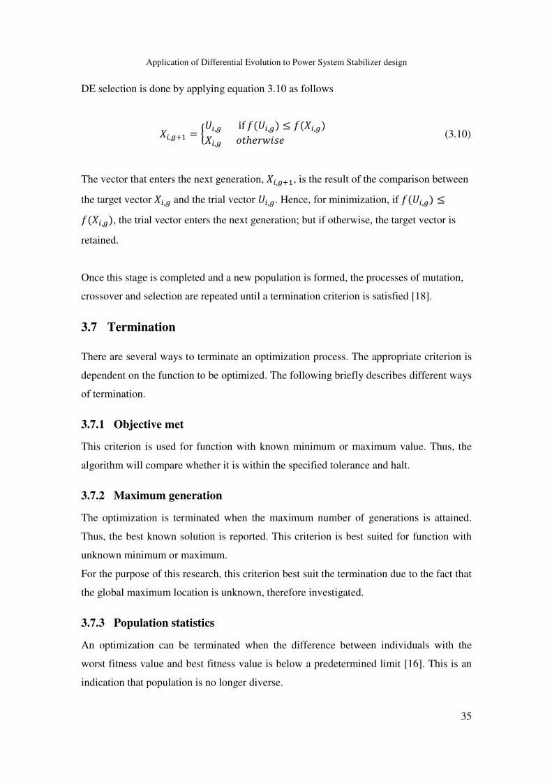
Application of Differential Evolution to Power System Stabilizer design
35
DE selection is done by applying equation 3.10 as follows
�y��Y � Áy������������±y��� £ ±�y����y�������� ·¸¹pºcq¹�����������������» (3.10)
The vector that enters the next generation, �y��Y, is the result of the comparison between
the target vector �y�� and the trial vector y��. Hence, for minimization, if ±y��� £±�y���, the trial vector enters the next generation; but if otherwise, the target vector is
retained.
Once this stage is completed and a new population is formed, the processes of mutation,
crossover and selection are repeated until a termination criterion is satisfied [18].
3.7 Termination
There are several ways to terminate an optimization process. The appropriate criterion is
dependent on the function to be optimized. The following briefly describes different ways
of termination.
3.7.1 Objective met
This criterion is used for function with known minimum or maximum value. Thus, the
algorithm will compare whether it is within the specified tolerance and halt.
3.7.2 Maximum generation
The optimization is terminated when the maximum number of generations is attained.
Thus, the best known solution is reported. This criterion is best suited for function with
unknown minimum or maximum.
For the purpose of this research, this criterion best suit the termination due to the fact that
the global maximum location is unknown, therefore investigated.
3.7.3 Population statistics
An optimization can be terminated when the difference between individuals with the
worst fitness value and best fitness value is below a predetermined limit [16]. This is an
indication that population is no longer diverse.

Application of Differential Evolution to Power System Stabilizer design
36
3.7.4 Limited time
Some applications are constrained by the time. In such case, manual intervention is
required regardless of the number of generation.
3.8 Summary
The theory behind the Differential Evolution (DE) technique is presented in this chapter.
DE is a parallel direct method that stochastically searches for the global optimum. DE
relies on the differential mutation and the crossover operations to guide its search toward
the prospect region.

Application of Differential Evolution to Power System Stabilizer design
37
Chapter 4
4 Population Based Incremental Learning (PBIL)
This chapter provides a background theory to Population-Based Incremental Learning
(PBIL). An analysis on PBIL optimization approach is also provided.
4.1 Overview
Like most EAs, PBIL is an optimization technique that stochastically searches for the
optimum value of a function by utilising some aspects of GAs combined with competitive
learning to guide its search toward prospective areas [3], [7], [15], [17], [20], [59], [60].
Developed by Shumeet Baluja in 1994 [20], PBIL borrows its competitive learning
concept from Artificial Neural Networks, and applies it to re-exanimate the performance
and update the population of prospect solutions [3], [15], [20]. Furthermore, PBIL
combines the aforementioned concept to that of GAs, such as initialization, mutation and
binary encoded representation [20]. However, the crossover operator has been subtracted
by redefining the role of the population [3], [7]. Hence, PBIL uses real-valued Probability
Vectors (PV) to control the random generated bit strings and create other vectors through
learning. PBIL then uses the current probability distribution to create �� individuals
which in turns, are evaluated with an objective function [3], [7], [15]. Using the best
individuals of the current population, the probability vector is updated by shifting the
likelihood of producing solutions corresponding to the best [3], [61]. There are other
variants of PBIL such as using the best and the worst elements to update the probability
vector (towards the best element and away from the worst element).One could also use
more than one element to update the PV. However in this thesis only the best individual
is used to update the probability vector.

Application of Differential Evolution to Power System Stabilizer design
38
4.2 Probability Vector (PV) and Population in PBIL
As mentioned in section 4.1, the Probability Vector (PV) is constituted of real-valued
probabilities that are used to generate individuals of a population [17]. The probability
vector size corresponds to the number of parameters, “_”, of an individual multiplied by
the parameter binary encoding-length “”. As given by equation 4.1.
����������������������������������������¤ � �� ��� � ���� º¸¹p¹�à � _ Ä Â (4.1)
For example, if an individual E has 4 parameters encoded and each parameter is 2-bits
representation in binary, PV will be constituted of 8 probability values, �¤ ��� ��� � �Å�� where each entry represents a bit string.
To start off, the probability vector is initialized to 0.5 which is the equal probability to
generate 1-or-0, bit string of given individual. This is illustrated in Figure 4.1.
Figure 4.1: Probability vectors representation of 2 small population of 4
Notice that both PVs are similar, however the individuals are entirely different.
Therefore, sampling from this vector will generate �� random individuals. The
population is a fundamental aspect in EAs; it provides the optimization with the ability to
explore the search space in parallel from multiple points [3], [7], [15], [20]. However as
the search progresses, the values in the probability vector will shift toward either 0.0 or
1.0, to represent the best individuals or solutions of a given problem [17], [20]. Hence,
through the aforementioned process, PV has redefined the role of the population and the
crossover operator [7]. In Figure 4.2, PV has been updated. The current probability of
generating a “1” for the first element of individuals in the population is 1.0 whereas the
second element is 0.75.

Application of Differential Evolution to Power System Stabilizer design
39
Figure 4.2; Probability vectors representation after update
4.3 Competitive Learning
Competitive learning is a concept borrowed from Artificial Neural Network (ANN). It
consists of grouping points based on their similarities with respect to the characteristics of
the study. This process of clustering is achieved without prior knowledge of the number
of groups or their features. Hence, Competitive Learning is given freedom to determine
the most relevant features for each group and cluster each point to their respective groups
based on these features [20].
Furthermore competitive learning applies the winner-take-all rule used by neurons that
are competing within a layer to stay active and the rest are shut down [20]. In the same
manner, PBIL only keeps the best solution to update the probability vector in order to
represent individuals with similar characteristics [17], [20].
4.4 Mutation
Similar to most EAs, PBIL apply mutation on the updated probability vector with small
perturbations on the position in the probability to maintain the diversity and prevent the
probability vector from converging quickly to an extreme value (either 0.0 or 1.0), hence
preventing premature convergence to a local optimum [20].
The mutation can be applied to the population or to the PV. In [20], the mutation operator
was applied to the PV whereby the vector is shifted by a value in a randomly chosen

Application of Differential Evolution to Power System Stabilizer design
40
direction. However in this research, a forgetting factor has been included to relax the
probability vector toward a neutral value of 0.5, [3], [62].
The mutation process is applied as follows.
For each locus�c � Æ�� � ÂÇ, if a random number p � p _¡'��� � �� (where ��is the
mutation probability), then mutate �y as follows.
�yÈ � �y H �� Ä �y H '¢¾� (4.2)
where ��is the mutation shift that controls the amount by which a mutation can alter the
value in each bit position. Following this operation, the cycle is repeated until
���individual is reached.
4.5 Learning rate
During the probability vector (PV) update, the learning rate (LR) determines the distance
by which PV is pushed for each iteration. In other words, LR determines how fast or slow
PV is shifted towards the best individuals [3]. Equation 4.3 shows how LR is applied.
������������������������������y· ) �� � �HÉ� Ä �y·�)ÉÄ Êy·������c � Æ�� � ÂÇ (4.3)
where É is the learning rate that defines the amount by which PV is pushed. Êy�is the best
solution in generation ·.
The magnitude of the learning rate plays a major role and its significance cannot be
undermined. A larger rate speeds up convergence, but it reduces the function space to be
searched, while a smaller rate will slow down the convergence, even though it increases
the exploration of a bigger search space, thereby increasing the likelihood of better
optimal solutions [3], [20].
4.6 Termination
Due to the fact that PBIL only stores the current best solution and the current solution
being evaluated, and therefore it runs as long as the current best solution keeps being

Application of Differential Evolution to Power System Stabilizer design
41
updated [3]. For that reason, the program is terminated when the number of iterations
reaches a specified maximum number.
4.7 Summary
The theory behind PBIL techniques has been presented in this chapter. In PBIL, the roles
of the population and the crossover operator have been substituted with a probability
vector (PV). This vector controls the random generated bit strings to create individuals.
PBIL uses PV to guide its search toward prospective solution by updating the vector
through a competitive learning process which in turn, is used to produce individuals with
the same likelihood as the best individual or solution.

Application of Differential Evolution to Power System Stabilizer design
42
Chapter 5
5 Power System Stabilizer Design
This chapter discusses the design procedure of a Power System Stabilizer (PSS). The
following consists of using the conventional method and the application of the two
aforementioned optimization techniques, namely Differential Evolution (DE) and
Population-Based Incremental Learning (PBIL). In addition, test cases for various system
configurations are also discussed in this section.
5.1 Introduction
As mentioned in chapter 1, PSS is a device that aids in subsiding low frequency
oscillations observed in a system by providing supplementary signal. Generally,
conventional control methods are used to tune the PSS’ parameters by linearizing the
system at a particular operating condition. However, its response becomes inadequate
when operating conditions change. As a result, the PSS requires constant re-tuning.
Alternatively, find parameters that will guarantee adequate performance of the PSS over a
wide range of operating conditions. Hence, the problem of selecting the PSS’ parameters
which simultaneously stabilizes a set of plants was converted to an optimization problem
solved by Differential Evolution (DE) and Population-Based Incremental Learning
(PBIL) using an eigenvalue based objective function [3], [6]. These computational
methods are used to find the optimum parameters. The resulting PSSs are tested under
various conditions for robust performance. However several factors affecting the overall
system performance, such as the objective function and controller parameters, must be
considered to achieve the desired performance. The CPSS design and the objective
function are discussed in subsequent sections.
5.2 Conventional PSS design
The conventional PSS consists of a washout block, a phase compensator block (lead/lag)
as well as the gain. These parameters, as described in equation 5.1, determine the

Application of Differential Evolution to Power System Stabilizer design
43
performance of the PSS. The block diagram of the equation 5.1 was shown in chapter 1
and reproduced here for easy reference.
������������������������������Ë�ÌÌÌ� � ÍÎÏÏ ÏÐÑYÏÐÑYÏÐ.YÏÐX
YÏÐÒYÏÐÓ (NÌ� (5.1)
Kpss is the gain of the PSS, T1 to T4 are lead/lag time constants, Tw is the washout time
constant. ¤�~~�is the output signal of the PSS in volts, whereas (N, the speed deviation, is
the input signal.
Conventionally, phase compensation and root locus are used to tune the PSS’ parameters.
These methods consist of identifying the system phase lag between the reference voltage
and the electrical torque, which is due to the automatic voltage regulators (AVRs) and
fast acting exciters [25], [4] as shown in Figure 5.1 to 5.2. Then determine the PSS phase
lead by fine tuning the lead/lag parameters,�� H �ª, needed to compensate the lag angle.
Once the time constants have been determined, the system root locus must be plotted.
The PSS gain is chosen such that the rotor mode eigenvalues is maximized without
adversely affecting other modes.
Figure 5.1: Phase Lag in an SMIB system
0 0.2 0.4 0.6 0.8 1 1.2 1.4 1.6 1.8 2-40
-35
-30
-25
-20
-15
-10
-5
0
Frequency(Hz)
Ang
le (d
egre
e)
System phase lag

Application of Differential Evolution to Power System Stabilizer design
44
Figure 5.2: Phase lag in a Two Area Multi Machine system
Figure 5.1 and5.2 show the different phase lags in a single machine infinite bus (SMIB)
and a two-area multi machine (2AMM). In the SMIB, the phase lag is found to be 100 at a
frequency of 0.7 Hz whereas the two area multimachine has phase lag of 200 at a
frequency of 0.65 Hz for the inter-area mode and 400 at a frequency of 1.15Hz for the
local modes. These phase lags are corrected with the application of PSSs. However
tuning these parameters is not an easy task, especially in a multi machine system. The
selection of PSS parameters and the location of the PSS in the system are very critical.
There are many modes of consideration in multi-machine as previously discussed. The
PSS might improve the damping of one electromechanical mode, but may have adverse
effect on other modes, such as the control modes. Whereas in single machine to infinite
bus (SMIB), the process is relatively simpler since the focus is to find optimal values of
the PSS that will help improve the stability of local modes only. Hence, EAs are applied
to simultaneously find optimum sets of parameters for different system setups. However
EAs, (PBIL and DE), both require an evaluation function, also known as objective
function, to find these optimum parameters.
0 0.2 0.4 0.6 0.8 1 1.2 1.4 1.6 1.8 2-80
-70
-60
-50
-40
-30
-20
-10
0Phase lag for Two Area Multi :achine system
Frequency(Hz)
Ang
le (d
egre
e)

Application of Differential Evolution to Power System Stabilizer design
45
5.3 Objective function
To get a better understanding of an objective function, let define the term optimization. In
simple terms, an optimization can be defined as an attempt to maximize a system’s
desirable properties whilst simultaneously minimizing its undesirable characteristics [16].
These properties and their effectiveness are dependent on the problem. Often, the
problem is represented as a function. For example, in this thesis, tuning the PSS’
parameters in order to add maximum damping ratio to the least damped mode is the
optimization goal. Mathematically, this can be represented by equation 5.2, also known
as objective function. In EA, the objective function can be defined as a performance
measure of individuals within a population. Moreover, it gives the proximity of a point to
the global maximum/minimum.
In this instance, the problem of finding the optimum set of PSS’ parameters to stabilize
the system over a wide range of operating conditions have been converted to an
optimization problem with the objective of improving the system lowest damping ratio.
Subsequently, this will ensure that all closed-loop poles remain on the negative side of
the s-plane despite the changes in operating condition [3], [6].
Therefore the objective function is formulated as follows [3]:
¤  � à O�Ãc _�Ty���� � º¸¹p¹�c � ���� _��¬�� � ���� �à (5.2)
Where T�is the lowest damping ratio. The index ‘c’ represents eigenvalue of the ‘�no’
operating conditions.
Ty � UV�V�XYZ�X is the damping ratio of the ith eigenvalue
Ôy � Õy are the real part and imaginary part (frequency of oscillation) of the ith eigenvalue
respectively.
The objective function can be stated as:
Maximize the lowest damping ratio
Subject to:

Application of Differential Evolution to Power System Stabilizer design
46
Ö��yµ £ Ö� £ Ö��|������º¸¹p¹�� � ���� �Ã
�y���yµ £ �y�� £ �y���|�����º¸¹p¹�c � ���� � _�¬�� � �� �à (5.3)
K and Ti denote the optimized controller gain and the lead lag time constants respectively
within their respective boundaries. The index ‘i’ denotes the lead lag parameter number
whereas ‘j’ is the machine number. In this thesis the following values were used:
Ö��|� � �'; �y���|� � ¾�seconds
Ö��yµ � �; �y���yµ � '¢''��seconds.
The objective function was applied to various system configurations, such as SMIB and
two-area multi machine systems. These systems are described in section 5.5.
5.4 Application of DE & PBIL to PSS design
In this section, DE & PBIL are applied to design the PSS based on the mathematical
model aforementioned. Once the parameters are obtained, they are tested for the
robustness in the following chapter. However, the method of tuning essentially involves
the following steps for all system configurations.
Step 1. Define the range of operating conditions.
Step 2. Test them by running the load flow. Eliminate those conditions for which the load
flow does not converge.
Step 3. Linearize the system at each operating condition and store the state-space A, B, C,
D matrices for each condition.
Step 4. Design the PSSs by solving the constrained optimization problem given by
equation 5.2 using DE and PBIL. This is applied to all operating conditions
Step 5. Once the optimum parameters are found, they are tested for robustness.
Step 6. In the case where the resulting PSSs performances are not good, go to step1.
These steps are summarized by the flow charts in Figure 5.4 and 5.5 representing the
application of DE and PBIL respectively.
Following the obtainment of PSSs’ parameters based on DE and PBIL, their
performances are evaluated by conducting a modal analysis. The results are then
validated through time domain simulations. Furthermore, a comparison analysis is carried
out for different designs and CPSS.

Application of Differential Evolution to Power System Stabilizer design
47
However, to obtain the optimum PSSs’ parameters, both algorithms had to be configured.
DE requires user-define parameters inputs such as the mutation factor ‘F’, the crossover
probability ‘²³ ’, the population number ‘��’ and the maximum number of generations
‘�’. These parameters greatly influence DE’s ability to find the global
minimum/maximum. Despite the recommendations provided by the authors in [16],
¥�¬�²³ values were determined by trial-and-errors. The population also affects the
optimization [16], [63], [64]. In [16], it is recommended that the population should be 10
times the dimensionality (or parameters to be optimized), 10D, however in this thesis 50,
was found to give best results. Some preliminary work with regards to PSS tuning are
presented in chapter 8 together with self-adaptive mutation and crossover parameters.
Whereas PBIL has fewer user-define inputs such as Learning rate (LR), forgetting factor
(FF) and population. Similar to [3], LR was set to 0.1 and FF to 0.005 within a population
of 50 for comparison sake. The generation however, was set to 500 to allow for enough
learning within the optimization [3], [6], [15]. Figure 5.3 summarizes the parameters used
for both algorithms.
Figure 5.3: DE and PBIL parameters

Application of Differential Evolution to Power System Stabilizer design
48
Figure 5.4: chart for the PSS design using DE

Application of Differential Evolution to Power System Stabilizer design
49
Figure 5.5: chart for the PSS design using PBIL

Application of Differential Evolution to Power System Stabilizer design
50
5.5 System configurations
In this thesis, three system configurations were considered for the PSS design. The Single
Machine to Infinite Bus (SMIB), the Two-area Multi-Machine and the New England 10-
Machines systems. These set-ups are further discussed in subsequent sections.
5.5.1 Single Machine to Infinite Bus system
This system consists of a synchronous generator connected to the infinite bus through a
double transmission line as illustrated by Figure 5.6. The generator was modelled using a
detailed 6th order differential equations and is equipped with a simple exciter which was
modelled using a first order equation and a turbine governor. The parameters are given in
Appendix B. The operating conditions of this system have been obtained by simulating
variations of generator output and transmission line reactance. Hence, by varying the
generated power from 0.5pu to 1.0 pu, it simulates a lightly loaded system to a heavily
loaded one whereas the variation of the line reactance, from 0.5pu to 1.0pu, simulates the
behaviour of a system with a strong tie-lines to weak tie-lines. The operating conditions
used in the design of the PSS are given in Table 5.1 together with the eigenvalues and
damping ratios.
Figure 5.6: Single machine to infinite bus system

Application of Differential Evolution to Power System Stabilizer design
51
The operating condition range consists of five cases used to tune the PSS. Table 5.1 lists
the open-loop system (or without PSS). Case 1 corresponds to the nominal operating
condition with an active power of 1.0pu and line reactance of 0.5pu. In this case, the
system is poorly damped with 4.7% which is below the power system acceptable margin
of 5% [4]. The system oscillates at a frequency of 0.59 Hz and decay away in about 23
seconds.
As the line reactance was increased by 50% to 0.7 and active power decreased by 50% to
0.5 pu for Case 2, the damping ratio reduced to 4.4%, oscillating at a frequency of 0.52
Hz which decay after 27 seconds. In Cases 3 and the line reactance was kept constant at
0.7 pu whereas the active power was increased to a maximum loading of 1.0pu. The
frequency of oscillation for the electromechanical modes is 0.51 Hz with damping ratio
of 3.7 %. In case 4, the power was reduced by 50% whereas the line reactance was
increased by 100% from the nominal condition to 0.5pu and 1.0pu respectively. The
system oscillates at a frequency of 0.47 Hz with a damping of 3.6% with a settling time
of 37 seconds. In Cases 5, the line reactance was kept constant at 1.0pu and the power
was set to maximum loading of 1.0pu. This case simulates the maximum power transfer
on weak tie-line. The frequency of oscillation for case 5 was 0.44 Hz with damping ratio
of 2.7%. These oscillations settled after 53 seconds.
Table 5.1: SMIB Open Loop operating conditions used in the PSS design
Case Active Power (pu)
Reactive Power (pu)
Line reactance (pu) Eigenvalues Damping ratio
Case 1 1.0 0.32 0.5 -0.177 ± j3.764 0.047
Case 2 0.5 0.17 0.7 -0.151 ± j3.395 0.044
Case 3 1.0 0.39 0.7 -0.119 ± j3.245 0.037
Case 4 0.5 0.16 0.9 -0.108 ± j2.94 0.036
Case 5 1.0 0.47 0.9 -0.076 ± j2.781 0.027

Application of Differential Evolution to Power System Stabilizer design
52
5.5.2 Two Area Multi-machine System
The system shown in Figure 5.7 consists of two areas, each with identical generating
units and similar ratings [1], [3]. All the generators are equipped with simple exciters (see
Appendix C) and similar turbine governors. The system’ parameters are given in
Appendix C. All the generators are 6th order whereas the AVRs are first order differential
equations. In addition, the system has two loads connected to bus 4 and 14 as illustrated
in Figure 5.7. The two areas are connected by two tie-lines.
The operating conditions were obtained by varying the loads’ demand which
subsequently varied the power transferred over the tie-lines. Hence, six cases (or
operating conditions), given in Table 5.2, were used to design and test the PSSs.
Furthermore, eigenvalues and damping ratio related to both inter area mode and local
modes are listed on the same table.
Figure 5.7: Two Area multi-machine system line diagram
Case 1 is the nominal operating condition. The load at bus 4 was set at 1167MW,
whereas the one at bus 14 was set to 1467MW. The total generation in Area 1 was 1330
MW whereas 1230MW was generated by Area 2. As a result, the power transferred from
Area1 to Area 2 was 100 MW. The inter-area mode oscillates at a frequency of 0.78 Hz
and a damping ratio of 0.1%. Hence, theses oscillations sustain for a long period. Both
local modes are marginally damped with 8.3% and 6.5 % where generators oscillate

Application of Differential Evolution to Power System Stabilizer design
53
against each other at frequencies of 1.15 Hz and 1.18Hz for Area 1 and Area 2
respectively. For case 2, load 1 and 2 were set to 1167MW and 1567MW respectively.
The total generation in Area 1 was 1405MW whilst 1400MW in Area 2. The power
transmitted from Area 1 to Area 2 was observed to be 200MW. The inter-area mode was
found to be unstable characterized by a negative damping ratio of -0.9% hence growing
oscillation of frequency of 0.77 Hz. Furthermore, the local modes oscillate at a frequency
of 1.16Hz and 1.18Hz. They have similar damping ratios of 6.7% and settle in 9 seconds.
In case 3, 300 MW was flowing through the tie-lines. The loads were set to 1067MW and
1667MW. Consequently, the eigenvalue corresponding to inter-area mode was further
destabilized as the corresponding poles were moving further into the right hand side of
the s-plane.
In case 4 & 5, the power transmitted was 400MW and 500MW respectively, from Area 1
to Area 2. Both cases are unstable, indicated by the negative damping of -1.68% and -
1.64%. Their frequency of oscillation has been further reduced from nominal case to
0.76Hz and 0.74Hz respectively. The local mode in Area 1 is relatively well damped with
7.07% in both cases. However, the local mode in Area 2 is poorly damped with 5.0% and
4.8% for case 4 and 5. Table 5.2 shows that the variation of the power transmitted
between the two areas negatively affect the electromechanical modes, both inter-area and
local modes, by reducing their relative damping ratios. Hence it can be observed that the
damping ratio related to the inter-area is poorly damped and in some cases negatively
damped. Whereas the damping related to the local modes have low damping but still
enough for the modes to be classified stable and in a good state [4]. In Case 6, the power
transmitted was 500MW over one-tie line from Area 1 to Area 2. It can be observed that
the inter-area frequency of oscillation has reduced to 0.544Hz and the damping ratio
slightly decreased to -1.7%.

Application of Differential Evolution to Power System Stabilizer design
54
Table 5.2: Two-Area Open loop poles for the selected design operating conditions
Case Active
Power Tie-lines Inter-area mode
Local area mode
1
Local area mode
2
1 100MW 2 -0.006 ± j4.962
(0.0012)
-0.606 ± j7.28
(0.0829)
-0.488 ± j7.42
(0.0656)
2 200MW 2 0.0461 ± j4.937
(-0.0093)
-0.4916 ± j7.290
(0.0735)
-0.4990 ± j7.420
(0.0670)
3 300MW 2 0.0428 ± j4.894
(-0.0087)
-0.4955 ± j07.280
(0.0707)
-0.5069 ± j7.405
(0.0683)
4 400MW 2 0.0806 ± j4.792
(-0.0168)
-0.5178 ± j07.300
(0.0678)
-0.3721 ± j7.344
(0.0506)
5 500MW 2 0.0771 ± j4.697
(-0.0168)
-0.5357 ± j7.269
(0.0673)
-0.3591 ± j7.335
(0.0488)
6 500MW 1 0.0589 ± j3.419
(-0.0170)
-0.4550 ± j7.330
(0.0617)
-0.3375 ± j7.224
(0.0460)
5.6 Summary
This chapter presented the different procedures used to design and tune the conventional
PSS, the PBIL-PSS and the DE-PSS optimization tuning approaches. The two EAs
procedures use an objective function based on maximizing the lowest damping ratio to
find the optimum PSS parameters. These methods were applied to two different system
models. On the SMIB, the PSS was designed over 5 operating conditions to improve the
open-loop eigenvalues. In the two-area multi machine system, the PSS was design over
six operating conditions to improve the dynamic of the inter-area mode.

Application of Differential Evolution to Power System Stabilizer design
55
Chapter 6
6 Single Machine Infinite Bus System (SMIB):
Simulation Results
6.1 Introduction
This chapter presents the simulation results for the single machine connected to the
infinite bus system. The PSS’ parameters are tuned based on the system minimum
damping ratio using DE and PBIL. The performance of the PSSs is assessed via the
modal analysis and validated using time domain simulations. The effectiveness of the
resulting PSSs to damp the low frequency oscillations is tested under various operating
conditions. The results are validated through simulations of the system’s response for five
different operating conditions. The comparison is carried out between the system
equipped with CPSS, DE-PSS and PBIL-PSS.
6.2 Optimized PSS
Following the application of DE and PBIL to tune the PSS, Figures 6.1 and 6.2 show the
optimization fitness curves of both algorithms. The optimization consisted of finding a set
of parameters that would give the best damping for the most dominant poles of the
system. Figure 6.1 shows DE converging to an optimum damping ratio value of 0.2659
corresponding to the electromechanical damping ratio of case 5. On the other hand,
Figure 6.2 shows that PBIL converged to an optimum damping ratio value of 0.2325.
These results indicate that DE performs slightly better than PBIL in finding the optimum
value.
It is deduced from Figure 6.1 that DE is able to explore the search space to only converge
after 100 generations for a maximum of 200 generations. PBIL, on the other hand,
explores the search space in a parallelized manner and starts settling after 150 for a
maximum of 300 generations. The difference in the maximum number of generations is
to allow PBIL to settle since its algorithm is based on learning.

Application of Differential Evolution to Power System Stabilizer design
56
Figure 6.1: DE fitness curve
Figure 6.2: PBIL fitness curve
0 20 40 60 80 100 120 140 160 180 2000.23
0.235
0.24
0.245
0.25
0.255
0.26
0.265
0.27
0.275DE best fitness over generations
Generations
Fitn
ess
0 50 100 150 200 250 3000.205
0.21
0.215
0.22
0.225
0.23
0.235
0.24Fitness value for PBIL optimization
Generations
Fitn
ess

Application of Differential Evolution to Power System Stabilizer design
57
Table 6.1 shows the DE, PBIL and CPSS parameters obtained after optimization.
Table 6.1: SMIB PSS parameters
K T1 T2 T3 T4
CPSS 13.868 3.7440 0.8778 3.7440 0.8778
DE-PSS 19.985 4.9376 0.4339 0.0103 0.1290
PBIL 16.361 1.7217 1.8110 4.9435 0.5568
6.3 Modal Analysis
Table 6.2 shows the eigenvalues corresponding to the electromechanical modes of the
closed-loop and the open loop system and the respective damping ratio in brackets. As
expected, the implementation of all PSS has significantly improved the system. In Case 1,
the nominal condition, DE has a slightly higher damping ratio of 52.1% whereas PBIL
has 45.15% and CPSS, 34.73%. It can be deduced that, DE based PSS provides 6.92%
more damping than PBIL and 17.37% more damping than CPSS. PBIL on the other hand
provides 10.42% more damping than CPSS. From the analysis of the eigenvalues, it can
be deduced that DE-PSS has transients that decay to within the ±2 % band in less than 2.5
seconds whilst PBIL-PSS and CPSS have transients that decay in 3 and 3.5 seconds,
respectively. In Case 2, as the transmission lines are increased by 50% and the loading
decreased, the damping ratio provided by all PSSs slightly drops. DE-PSS damping ratio
is reduced by 6% to a value of 45.37% whilst that of PBIL is reduced to 38.96% and that
of CPSS to 30.49%. With this, it is deduced that the PSSs will damp the oscillations to ±
2% of their final values in 3, 4 and 4.5 seconds for DE, PBIL and CPSS, respectively. As
the power transmitted is increased to 1.0 p.u for case 3, the damping is further reduced for
all PSSs to 39.11%, 30.14% and 23.31% for DE-PSS, PBIL-PSS and CPSS, respectively.
DE-PSS has a damping ratio of 37.98%, PBIL and CPSS damping ratios of 33.63% and
26.02%, respectively. However, when the system is heavily loaded combined with weak
transmission lines (case 5), DE-PSS has a damping of 26.59 % whilst PBIL has a
damping ratio 23.25% and the CPSS has the lowest damping ratio of 18.55%. However it
is noticeable that the addition of PSSs has slightly reduced the frequency of oscillation of
the electromechanical mode for all cases.

Application of Differential Evolution to Power System Stabilizer design
58
Table 6.2: SMIB electromechanical modes of the system with different PSSs Designs
Cases DE-PSS PBIL-PSS CPSS No PSS
1 -1.6950 ±j2.7780
(0.521)
-1.3296±2.6279i
0.4515
-1.1033±j 2.9792
0.3473 -0.177 ± j3.764
(0.047)
2 -1.2323±j2.4201
(0.4537)
-0.9570±j2.2621
(0.3896)
-0.8089±j2.5271
(0.3049) -0.1512±j3.3950
(0.0445)
3 -1.1576±j2.7233
(0.3917)
-0.8936±j2.8265
(0.3014)
-0.7281±j3.0379
(0.2331) -0.119 ± j3.245
(0.037)
4 -0.9102±j2.2167
(0.3798)
-0.7160±j2.0048
(0.3363)
-0.5957±j2.2107
(0.2602) -0.108 ± j2.94
(0.036)
5 -0.7065±j2.5401
(0.2659)
-0.6520±j2.6040
(0.2325)
-0.5114±j2.7087
(0.1855) -0.076 ± j2.781
(0.027)
6.4 Time Domain Simulation
The time domain simulations were performed to validate the results of modal analysis.
The effectiveness of the PSSs is assessed by their ability to damp low frequency
oscillations under various operating conditions. Furthermore, the PSS must be able to
stabilize the system under transient conditions. Therefore, two types of time domain
simulations are performed; small signal and transient simulations.
6.4.1 Small Disturbance Simulation
The small disturbance simulations have been performed for all five cases previously
mentioned by applying 10% step change in the reference voltage. The speed deviation
responses of the generator under the step change in the reference voltage are presented in
Figure 6.3 to Figure 6.7.
Figure 6.3 illustrates the step response of all PSSs for the nominal operating condition
(Case 1). The results show that all PSSs are able to adequately damp the oscillations;
hence improving the system dynamic stability. Both DE-PSS and PBIL-PSS settled
within 3 seconds whilst CPSS settled in about 3.5 seconds. However DE-PSS has the
least overshoot and CPSS the highest overshoot whereas PBIL has the least undershoot.

Application of Differential Evolution to Power System Stabilizer design
59
Figure 6.3: Rotor speed responses for Case 1
Figure 6.4 shows the responses of the rotor speed deviations for case 2. It is observed
that DE-PSS displays better performance with a settling time of about 3 seconds as
compared to a settling time of 4 and 5 seconds, respectively for both PBIL-PSS and
CPSS. Moreover, DE-PSS has the lowest overshoot and similar undershoot with that of
PBIL-PSS. CPSS on the other hand, has more oscillations and higher overshoots and
undershoots as compared to the other PSSs. The performance of the CPSS is degrading
with changes of operating conditions as expected.
Figure 6.5 shows the generator speed responses for case 3. Although the system remains
stable under all the PSSs, PBIL-PSS and DE-PSS improve the system dynamics
significantly. However, DE-PSS displays remarkable performance with settling time of
about 4 seconds. Furthermore, DE-PSS is better in terms of overshoots and undershoots.
PBIL-PSS settles within 5 seconds and the CPSS within 6 seconds.
0 1 2 3 4 5 6 7 8 9 10-5
-4
-3
-2
-1
0
1
2
3x 10
-4 Step response for Case:1
time(s)
spee
d de
viat
ion
CPSSPBIL-PSSDE-PSS

Application of Differential Evolution to Power System Stabilizer design
60
Figure 6.4: Rotor speed responses for Case 2
Figure 6.5: Rotor speed responses for Case 3
0 1 2 3 4 5 6 7 8 9 10-3
-2
-1
0
1
2
3x 10
-4 Step response for Case:2
time(s)
spee
d de
viat
ion
(p.u
)
CPSSPBIL-PSSDE-PSS
0 1 2 3 4 5 6 7 8 9 10-5
-4
-3
-2
-1
0
1
2
3x 10
-4 Step response for Case:3
time(s)
spee
d de
viat
ion
(p.u
)
CPSSPBIL-PSSDE-PSS

Application of Differential Evolution to Power System Stabilizer design
61
Figure 6.6 shows the step responses for case 4. Both DE-PSS and PBIL-PSS exhibit
better performances than the CPSS. However, DE-PSS has once more outperformed both
PBIL-PSS and CPSS with a settling time of 4.5 seconds. Whereas CPSS only settles after
6 seconds with higher overshoots and undershoots of 2.0*10-4pu and -4.9*10-4pu,
respectively. PBIL-PSS settles after 5 seconds.
Figure 6.7 shows the speed responses of the system for cases 5. In this particular case, the
system is heavily loaded with weak tie-line. In this scenario, the CPSS has a faster
response but oscillatory, hence a longer settling time of about 8 seconds. Whereas DE-
PSS has a slower response but exhibits the lowest overshoots and undershoots with a
settling time of about 5 seconds. Similarly, PBIL-PSS responds reasonably fast with more
oscillation than the DE and higher overshoots. PBIL-PSS settles in about 5.5 seconds.
Figure 6.6: Speed response for Case 4
0 1 2 3 4 5 6 7 8 9 10-4
-3
-2
-1
0
1
2x 10
-4 Step response for Case:4
time(s)
spee
d de
viat
ion
(p.u
)
CPSSPBIL-PSSDE-PSS

Application of Differential Evolution to Power System Stabilizer design
62
Figure 6.7: Speed responses for Case 5
6.4.2 Large disturbance simulation
For the large disturbance simulation, also known as transient stability, a more severe fault
is considered to further evaluate the PSSs robustness. The fault consists of subjecting the
system to a 5-cycles 3-phase fault. The fault is applied after 1 second on line 1 (Figure
5.6). The fault was cleared by disconnecting the line.
Transient Stability was performed for Case 1 to 4. Case 5 was not considered for these
simulations because of the inability of the system to regain stability after the fault was
cleared. This is mainly due to high value of the rotor pre-fault angle.
6.4.2.1 Case 1: nominal operating condition ( P=1.0pu; Q= 0.32pu; Xe=0.5pu)
Figure 6.8 to Figure 6.12 show the responses of the rotor speed, rotor angle, voltage
terminal, field voltage and active power following a three – phase short circuit fault on
line 1. Observations of the system responses show that all PSSs perform adequately.
From Fig, 6.8, it can be seen that the rotor angle increases when the fault is applied and
settles to a new value when the fault was cleared. The system equipped with DE-PSS
0 1 2 3 4 5 6 7 8 9 10-6
-5
-4
-3
-2
-1
0
1
2
3
4x 10
-4 Step response for Case:5
time(s)
spee
d de
viat
ion
(p.u
)
CPSSPBIL-PSSDE-PSS

Application of Differential Evolution to Power System Stabilizer design
63
displays a slightly better performance in terms of rotor angle and PBIL-PSS shows a
slight overshoot whereas the CPSS response is slightly slower to settle down. The pre-
fault angle was about 22.50 and increased to about 300 at post-fault Similar trends are
observed for the rotor speed responses (see Fig. 6.9) whereby the speed increases during
the fault and returns to initial speed when the fault is cleared. DE-PSS settles slightly
faster whilst PBIL-PSS has a slightly higher undershoot. However, the CPSS has the least
undershoot. Figure 6.10 shows for the responses of the terminal voltage. The voltage dips
to 0.8pu during the fault and returns to the initial value of 1.05p.u after the fault was
cleared. All controllers perform similarly with slight undershoot and overshoot. The
electric field responses are shown in Figure 6.11. It can be seen that it first increases to
the upper limit of voltage regulator, then decreases to lower limit before returning to
steady state when the fault is cleared. All the PSSs have similar responses; however, DE-
PSS has a higher overshoot. This may be attributed to the high gain of DEPSS in
comparison to PBIL-PSS and CPSS. Figure 6.12 shows the output power response of all
PSSs. It can be observed that all controllers perform similarly.
Figure 6.8: Rotor angle responses following 3-phase fault for case 1
0 1 2 3 4 5 6 7 822
24
26
28
30
32
34Rotor angle response for Case study:1
time(s)
Rot
or a
ngle
(deg
ree)
CPSSPBIL-PSSDE-PSS

Application of Differential Evolution to Power System Stabilizer design
64
Figure 6.9: Rotor speed responses following 3-phase fault for case 1
Figure 6.10: Terminal Voltage following 3-phase fault for case 1
0 1 2 3 4 5 6 7 80.9996
0.9998
1
1.0002
1.0004
1.0006
1.0008
1.001
1.0012
1.0014
1.0016Speed response for Case study:1
time(s)
Spe
ed (p
.u)
CPSSPBIL-PSSDE-PSS
0 1 2 3 4 5 6 7 80.75
0.8
0.85
0.9
0.95
1
1.05
1.1
1.15
1.2
1.25Terminal voltage for Case Study:1
time(s)
Vol
tage
(p.u
)
CPSSPBIL-PSSDE-PSS

Application of Differential Evolution to Power System Stabilizer design
65
Figure 6.11: Electric field voltage following 3-phase fault for case 1
Figure 6.12: field voltage following 3-phase fault for case 1
0 1 2 3 4 5 6 7 8-5
-4
-3
-2
-1
0
1
2
3
4
5Electric field for Case study:1
time(s)
E fi
eld(
p.u)
CPSSPBIL-PSSDE-PSS
0 1 2 3 4 5 6 7 8-0.2
0
0.2
0.4
0.6
0.8
1
1.2
1.4Power Output for Case 1
time(s)
Pow
er (p
.u)
CPSSPBIL-PSSDE-PSS

Application of Differential Evolution to Power System Stabilizer design
66
6.4.2.2 Case 2: System operating at P=0.5pu; Q= 0.17pu; Xe=0.7pu
Figure 6.13 to Figure 6.17 illustrate the rotor angle, the rotor speed, the terminal voltage
at bus 1, the electric field voltage and the power output response, respectively, following
a 3-phase fault on line 1. The different PSS responses followed a similar trend to Case 1.
Figure 6.13 shows the initial angle was 25.50 before fault and 360 at post-fault. Moreover,
DE-PSS settles within 3.5 seconds with the least overshoot and undershoot, faster than its
counterparts, PBIL-PSS and CPSS which settle in 4 and 4.5 seconds, respectively. In
Figure 6.14, the speed response yields similar settling times to those of the rotor angle.
The terminal voltage is shown in Figure 6.15. It can be observed that DE-PSS exhibits
slightly higher overshoot whilst PBIL-PSS has the lowest overshoot. However DE-PSS
settles slightly faster (in 3.5 seconds) than PBIL-PSS and CPSS, which settled in 4 and 5
seconds, respectively. Figure 6.16 shows the systems electric field responses during and
after the fault. The difference in performance between all the different PSSs is minimal.
For the power response shown in Figure 6.17, all PSSs perform similarly.
Figure 6.13: Rotor angle response following 3-phase fault for Case
0 1 2 3 4 5 6 7 824
26
28
30
32
34
36
38
40
42Rotor angle response for Case 2
time(s)
Rot
or a
ngle
(deg
ree)
CPSSPBIL-PSSDE-PSS

Application of Differential Evolution to Power System Stabilizer design
67
Figure 6.14: Speed response following a 3-phase fault for Case 2
Figure 6.15: Terminal voltage response following 3-phase fault for Case 2
0 1 2 3 4 5 6 7 80.999
0.9995
1
1.0005
1.001
1.0015Speed response for Case 2
time(s)
Spe
ed (p
.u)
CPSSPBIL-PSSDE-PSS
0 1 2 3 4 5 6 7 80.8
0.85
0.9
0.95
1
1.05
1.1
1.15
1.2
1.25Terminal voltage for Case 2
time(s)
Vol
tage
(p.u
)
CPSSPBIL-PSSDE-PSS

Application of Differential Evolution to Power System Stabilizer design
68
Figure 6.16: Electric field response for Case 2
Figure 6.17: Power output for Case 2
0 1 2 3 4 5 6 7 8-5
-4
-3
-2
-1
0
1
2
3
4
5Electric field for Case 2
time(s)
E fi
eld(
p.u)
CPSSPBIL-PSSDE-PSS
0 1 2 3 4 5 6 7 8-0.1
0
0.1
0.2
0.3
0.4
0.5
0.6Power Output for Case 2
time(s)
Pow
er (p
.u)
CPSSPBIL-PSSDE-PSS

Application of Differential Evolution to Power System Stabilizer design
69
6.4.2.3 Case 3: System condition, P=1.0pu; Q= 0.34pu; Xe=0.7pu
In this case, the fault was applied when the system was heavily loaded with a relatively
weak tie-line. Figure 6.18 to Figure 6.20 show that the performance of the CPSS has
deteriorated. It has more oscillations and a settling time of over 8 seconds for the rotor
angle, the rotor speed and the terminal voltage whereas DE and PBIL subside in about 5
and 6 seconds, respectively. Furthermore, DE displays the least overshoots and
undershoots. For the electric field, both DE and PBIL have similar performance as
opposed to the CPSS which is slightly slower in settling time. As for the active power
output in Figure 6.22, all PSSs show similar performances.
Figure 6.18: Rotor angle responses for Case 3
0 1 2 3 4 5 6 7 845
50
55
60
65
70
75
80
85Rotor angle response for Case 3
time(s)
Rot
or a
ngle
(deg
ree)
CPSSPBIL-PSSDE-PSS

Application of Differential Evolution to Power System Stabilizer design
70
Figure 6.19: Rotor speed responses for Case 3
Figure 6.20: Terminal voltage responses at bus 1 for Case 3
0 1 2 3 4 5 6 7 80.998
0.9985
0.999
0.9995
1
1.0005
1.001
1.0015
1.002
1.0025
1.003Speed response for Case 3
time(s)
Spe
ed (p
.u)
CPSSPBIL-PSSDE-PSS
0 1 2 3 4 5 6 7 80.85
0.9
0.95
1
1.05
1.1
1.15
1.2
1.25
1.3Terminal voltage for Case 3
time(s)
Vol
tage
(p.u
)
CPSSPBIL-PSSDE-PSS

Application of Differential Evolution to Power System Stabilizer design
71
Figure 6.21: Electric field voltage for Case 3
Figure 6.22: Active Power output responses for Case 3
0 1 2 3 4 5 6 7 8-5
-4
-3
-2
-1
0
1
2
3
4
5Electric field for Case 3
time(s)
E fi
eld(
p.u)
CPSSPBIL-PSSDE-PSS
0 1 2 3 4 5 6 7 8-0.2
0
0.2
0.4
0.6
0.8
1
1.2Power Output for Case 3
time(s)
Pow
er (p
.u)
CPSSPBIL-PSSDE-PSS

Application of Differential Evolution to Power System Stabilizer design
72
6.4.2.4 Case 4: System condition, P=0.5pu; Q=0.16pu; Xe=0.9pu
Fig 6.23 to Figure 6.27 show the system responses of the rotor angle, the rotor speed, the
terminal voltage, the field voltage and the active power, respectively. Under this large
disturbance, DE-PSS slightly outperforms both PBIL-PSS and CPSS with less overshoots
and undershoots with a settling time of about 4.5 seconds for the rotor angle and rotor
speed whereas PBIL-PSS shows slightly high overshoots and undershoots for the rotor
angle and speed with a faster response and settling time than that of CPSS (see Figures
6.23-24). However, for both the terminal voltage responses (Figure 6. 25) and electric
field voltage (Figure 6.26), DE has higher overshoots and undershoots following the fault
clearance but still regain the stability faster than both CPSS and PBIL.
Under the aforementioned operating condition, the CPSS showcase adequate
performance with a settling time of around 4 seconds for the active power responses
shown in Figure 6.27.All PSSs perform similarly with slight differences for the active
power.
Figure 6.23: Rotor angle response following 3-phase fault for Case 4
0 1 2 3 4 5 6 7 825
30
35
40
45
50Rotor angle response for Case 4
time(s)
Rot
or a
ngle
(deg
ree)
CPSSPBIL-PSSDE-PSS
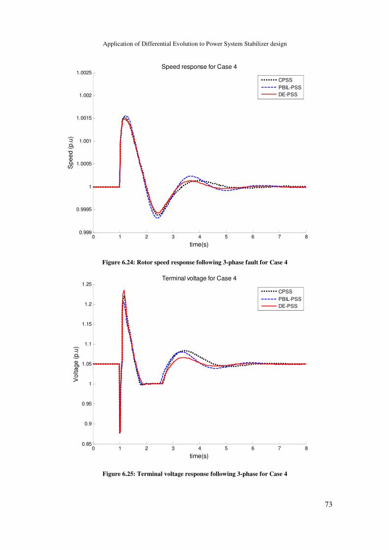
Application of Differential Evolution to Power System Stabilizer design
73
Figure 6.24: Rotor speed response following 3-phase fault for Case 4
Figure 6.25: Terminal voltage response following 3-phase for Case 4
0 1 2 3 4 5 6 7 80.999
0.9995
1
1.0005
1.001
1.0015
1.002
1.0025Speed response for Case 4
time(s)
Spe
ed (p
.u)
CPSSPBIL-PSSDE-PSS
0 1 2 3 4 5 6 7 80.85
0.9
0.95
1
1.05
1.1
1.15
1.2
1.25Terminal voltage for Case 4
time(s)
Vol
tage
(p.u
)
CPSSPBIL-PSSDE-PSS

Application of Differential Evolution to Power System Stabilizer design
74
Figure 6.26: Electric field following a 3-phase fault for Case 4
Figure 6.27: Active power output following 3-phase fault for Case 4
0 1 2 3 4 5 6 7 8-5
-4
-3
-2
-1
0
1
2
3
4
5Electric field for Case 4
time(s)
E fi
eld(
p.u)
CPSSPBIL-PSSDE-PSS
0 1 2 3 4 5 6 7 8-0.1
0
0.1
0.2
0.3
0.4
0.5
0.6Power Output for Case 4
time(s)
Pow
er (p
.u)
CPSSPBIL-PSSDE-PSS

Application of Differential Evolution to Power System Stabilizer design
75
6.5 Summary
In this chapter, the application of two proposed Evolution Algorithms (DE and PBIL) for
tuning the parameters of PSS has been tested for an SMIB system. The resulting PSSs
were compared with those of the CPSS. The modal analysis shows that all the PSSs are
capable of improving the dynamic stability of the system. In particular, DE-PSS performs
better than PBIL-PSS and CPSS for all cases that have been discussed. These results have
been validated in time domain simulations where DE-PSS outperformed both PBIL-PSS
and CPSS with faster settling times and less overshoots and undershoots in some cases.
As expected, the CPSS performs well for the nominal condition however degrades when
the operating conditions change for both small and large disturbances.

Application of Differential Evolution to Power System Stabilizer design
76
Chapter 7
7 Simulation Results for the Two-Area Multi-machine
Systems
7.1 Introduction
This chapter presents the simulation results for the Two-Area Multi Machine system. The
performances of the PSSs are assessed via the modal analysis and validated using time
domain simulations. The effectiveness of the resulting PSSs to damp the low frequency
oscillations is tested under various operating conditions (case 1 to case 6) using small and
large disturbances. The comparison is carried out between the system equipped with
CPSS, DE-PSS and PBIL-PSS. First, the final value obtained from the optimization
process of both DE and PBIL are presented. Next, the performances of PSSs are
evaluated and compared with modal analysis.
7.2 PSS Parameters optimization
Following the application of DE and PBIL to tune the PSS, Figure 7.1 and 7.2 show the
optimization fitness curve of both algorithms. The optimization consisted of finding a set
of parameters that would give the best damping for the dominant poles of the system.
Figure 7.1 shows DE converging to the optimum damping ratio value of 0.2263
corresponding to the electromechanical damping ratio of Case 6. Whereas PBIL, as
illustrated in Figure 7.2, reached the optimum value of damping ratio 0.2095. These
results indicate that DE performs slightly better than PBIL in finding the optimum value.
It is deduced from Figure 7.1 that DE is able to explore the search space to only converge
after 100 generations for a maximum of 180 generations. PBIL, on the other hand,
explores the search space in a parallelized manner and starts settling after 200 for a
maximum of 500 generations. The difference in the maximum number of generations is
to allow PBIL to settle since this approach is based on learning which takes some time.

Application of Differential Evolution to Power System Stabilizer design
77
However, the speed of convergence can be improved by changing the learning rate which
may affect the ability of the algorithm to find the optimum value.
Figure 7.1: DE fitness curve
Figure 7.2: PBIL fitness curve
0 20 40 60 80 100 120 140 160 180
0.15
0.16
0.17
0.18
0.19
0.2
0.21
0.22
0.23
Generation
Fitn
ess
DE best fitness over generation
0 50 100 150 200 250 300 350 400 450 5000.12
0.13
0.14
0.15
0.16
0.17
0.18
0.19
0.2
0.21Fitness value for PBIL optimization
Generations
Fitn
ess

Application of Differential Evolution to Power System Stabilizer design
78
Table 7.1 shows the PSSs’ parameters obtained after optimization along with the CPSS’
parameters. The system is constituted of four identical generators in two-different areas
as discussed in section 5 [3]. Hence, the PSSs in each area are identical such that
generator 1 and 2 have similar PSSs. The washout time constant used in the Multi-
machine system is 10seconds.
Table 7.1: Two-area PSS parameters
Kp T1 T2 T3 T4
PBIL-PSS
Gen 1&2 19.191 0.238 0.012 0.049 0.014
Gen 3&4 16.633 0.119 0.083 0.055 0.010
DE-PSS
Gen 1&2 19.992 0.051 0.019 0.053 0.015
Gen 3&4 19.997 0.116 0.015 0.111 0.016
CPSS
Gen 1&2 9.877 0.307 0.015 0.051 0.013
Gen 3&4 13.685 0.126 0.085 0.062 0.010
7.3 Modal Analysis
Table 7.2 shows the eigenvalues corresponding to the inter-area mode of the closed loop
and the open loop system and the respective damping ratios in brackets. As expected, the
implementation of all PSS has significantly improved the system’s stability. In Case 1,
the nominal condition, DE has a slightly higher damping ratio of 27.07% whereas PBIL
has a damping ratio of 23.62% and CPSS a damping ratio of 17.61%. Hence, the damping
provided by DE-PSS is 3.45% higher than that of PBIL and 9.46% better than that CPSS.
PBIL on the other hand is 6.42% higher than CPSS. From the analysis of the
eigenvalues, it can be deduced that DE-PSS has transient that decay to within the ±2 %
band in less than 3.2 seconds whilst PBIL-PSS and CPSS have transient that decay in 3.5
and 5 seconds, respectively. In Case 2, as the system loading is increased to 200MW, the
damping ratio provided by all PSSs slightly drops. DE-PSS’ damping ratio is reduced to a
value of 26.12% whilst PBIL and CPSS are reduced to 22.65% and 16.56%, respectively.
Hence, from the real part of the eigenvalue corresponding to the electromechanical mode,
it is deduced that there are transient that decay to within the ±2 % band in less than 3.3, 4
and 5.3 seconds for DE, PBIL and CPSS, respectively. As the power transmitted is

Application of Differential Evolution to Power System Stabilizer design
79
gradually increased to 300MW, 400MW and 500MW for Case 3, 4 and 5, the damping is
further reduced for all PSSs. DE-PSS provides damping ratio of 24.92%, 23.84% and
22.63%, with transient that decay in 3.5 to 4 seconds. Whereas PBIL-PSS provides
damping ratios of 22.45%, 22.18% and 20.95%, respectively with a settling time of 4 to 6
seconds. CPSS, as expected, provides the lowest damping of 16.42%, 16.23% and
15.06% for case 3, 4 and 5, respectively. Similar trends are observed in Case 6 whereby
the PSSs’ damping ratios are slightly reduced to 22.59% for DE-PSS, 20.94% for PBIL-
PSS and 15.02% for the CPSS. The modal analysis also reveals that CPSS takes longer to
subside low frequency oscillations. This is characterized by eigenvalues corresponding to
the inter-area mode being closest to the imaginary axis on the s-plan. DE-PSS has the
fastest settling time, subsequently the furthest eigenvalues in the left-hand side of the s-
plan. PBIL-PSS displays better performance than that of the CPSS and slightly less than
that of DE-PSS.
Table 7.2: Inter-area modes for Two-Area Multi-machine system
Case DE-PSS PBIL-PSS CPSS No-PSS
1 -1.273± j4.528
(0.2707)
-1.115± j4.589
(0.2362)
-0.807± j4.509
(0.1761)
-0.006 ± j4.962
(0.0012)
2 -1.219± j4.507
(0.2612)
-1.062± j4.566
(0.2265)
-0.753± j4.484
(0.1656)
0.0461 ± j4.937
(-0.0093)
3 -1.154± j4.477
(0.2492)
-1.044± j4.534
(0.2245)
-0.741± j4.453
(0.1642)
0.0428 ± j4.894
(-0.0087)
4 -1.089± j4.436
(0.2384)
-1.022± j4.491
(0.2218)
-0.725± j4.412
(0.1623)
0.0806 ± j4.792
(-0.0165)
5 -1.015± j4.404
(0.2263)
-0.950± j4.42
(0.2098)
-0.648± j4.384
(0.1506)
0.0771±j4.697
(-0.0168)
6 -0.806± j3.477
(0.2259)
-0.748± j3.496
(0.2094)
-0.518± j4.411
(0.1502)
0.0589 ± j3.419
(-0.0170)

Application of Differential Evolution to Power System Stabilizer design
80
Table 7.3 shows the local modes for Area 1. The addition of PSSs improved the mode’s
damping ratio from poorly damped to adequately damped. The CPSS provides 37.23%,
35.13%, 34.72%, 34.52%, 33.28% and 30.95%, for Case 1 to 6, respectively,. The
optimized PSS using PBIL provides 38.96% for Case 1, 37.46% for Case 2, 37.22% for
Case 3, 36.85% for Case 4, 35.17% for Case 5 and 33.44% for Case 6 whereas DE
provides 40.10% for Case 1, 38.62% for Case 2, 38.37% for Case 3, 38.01% for Case 4,
36.67% for Case 5 and 34.62% for Case 6. It can be observed that DE has a slightly
higher damping than those of PBIL-PSS and CPSS.
Table 7.3: Local Area mode 1
Case DE-PSS PBIL-PSS CPSS No-PSS
1 -2.384± j5.446
(0.4010)
-2.372± j5.607
(0.3896)
-2.098± j5.229
(0.3723)
-0.606 ± j7.28
(0.0829)
2 -2.304± j5.503
(0.3862)
-2.288± j5.663
(0.3746)
-2.010± j5.308
(0.3513)
-0.4916 ± j7.290
(0.0735)
3 -2.291± j5.513
(0.3837)
-2.274± j5.673
(0.3721)
-1.997± j5.322
(0.3472)
-0.4955 ± j7.280
(0.0707)
4 -2.271± j5.525
(0.3801)
-2.253± 5.685
(0.3685)
-1.978± j5.340
(0.3452)
-0.5178 ± j7.300
(0.0678)
5 -2.195± j5.570
(0.3667)
-2.160±j 5.709
(0.3517)
-1.907± j5.404
(0.3328)
-0.5357 ± j7.269
(0.0673)
6 -2.075± j5.623
(0.3462)
-2.049±j 5.774
(0.3344)
-1.783± j5.477
(0.3095)
-0.4550±j7.33
(0.0617)
Table 7.4 shows the local modes for Area 2. Again, the addition of PSSs significantly
improved the mode’s damping ratio. The CPSS provides the lowest damping ratio of
67.23%, 65.41%, 63.95%, 62.09%, 58.82% and 53.96% for Case 1 to 6, respectively.
PBIL-PSS, on the other hand, provides the highest damping of 77.25% for Case 1,
75.67% for Case 2, 74.34% for Case 3, 72.64% for Case 4, 68.21% for Case 5 and
65.53% for Case 6. DE- PSS provides slightly lower damping than those of PBIL with
74.76% for Case 1, 73.23% for Case 2, 71.94% for Case 3, 70.31% for Case 4, 67.66%
for Case 5 and 63.39% for Case 6.

Application of Differential Evolution to Power System Stabilizer design
81
Table 7.4: Local Area mode 2
Case DE-PSS PBIL-PSS CPSS No-PSS
1 -5.966± j5.299
(0.7476)
-6.460± j5.310
(0.7725)
-5.191± j5.726
(0.6723)
-0.488 ± j7.42
(0.0656)
2 -5.812± j5.405
(0.7323)
-6.302± j5.444
(0.7567)
-5.047± j5.835
(0.6541)
-0.4990 ± j7.420
(0.0670)
3 -5.685± j5.488
(0.7194)
-6.170± 5.550
(0.7434)
-4.925± j5.920
(0.6395)
-0.5069 ± j7.405
(0.0683)
4 -5.526± j5.589
(0.7031)
-6.004± j5.679
(0.7264)
-4.771± j6.022
(0.6209)
-0.3721 ± j7.344
(0.0506)
5 -5.298± j5.765
(0.6766)
-5.601± j6.007
(0.6821)
-4.538± j6.239
(0.5882)
-0.3591 ± j7.335
(0.0488)
6 -4.901± j5.978
(0.6339)
-5.353± j6.16
(0.6553)
-4.130± j6.444
(0.5396)
-0.3875±j7.224
(0.0526)
7.4 Time domain Simulations
The time domain simulation is divided into two sections namely small and large
disturbances.
7.4.1 Small disturbance
In this section, the time domain simulations were performed to validate the results of
modal analysis. The PSSs are assessed by their ability to damp low frequency oscillations
following a 10% step change in the reference voltage of the generator that has the largest
participation on the inter-area mode, which is generator 2. The disturbance is performed
for all 6 operating conditions. The step responses of active power deviation on all
generators are presented in Figure 7.3 to Figure 7.26.
Figure 7.3 to Figure 7.8 illustrate the active power deviation response of generator 1 to
the a 10% step change in reference voltage applied on generator 2 for Cases 1 to Case 6,
respectively. The results show that DE-PSS has the least undershoot in all cases and a
settling time varying between 3 and 4 seconds. Similarly to DE, PBIL-PSS settles within
that same range of time with the least overshoot whilst CPSS is slower, settling between
4.5 to 6 seconds. In Case 6, DE settles slightly faster than PBIL whereas the system
equipped with CPSS has slightly longer settling time.

Application of Differential Evolution to Power System Stabilizer design
82
Figure 7.3: Active power response of G1 for Case 1
Figure 7.4: Active power response of G1 for Case 2
0 1 2 3 4 5 6 7-0.06
-0.04
-0.02
0
0.02
0.04
0.06
0.08
0.1
0.12
0.14Step response of Generator 1 for Case 1
time(s)
chan
ge in
gen
erat
or a
ctiv
e po
wer
(p.u
)
DE-PSSPBIL-PSSCPSS
0 1 2 3 4 5 6 7-0.05
0
0.05
0.1
0.15Step response of Generator 1 for Case 2
time(s)
chan
ge in
gen
erat
or a
ctiv
e po
wer
(p.u
)
DE-PSSPBIL-PSSCPSS

Application of Differential Evolution to Power System Stabilizer design
83
Figure 7.5: Active power response of G1 for Case 3
Figure 7.6: Active power response of G1 for Case 4
0 1 2 3 4 5 6 7-0.05
0
0.05
0.1
0.15Step response of Generator 1 for Case 3
time(s)
chan
ge in
gen
erat
or a
ctiv
e po
wer
(p.u
)
DE-PSSPBIL-PSSCPSS
0 1 2 3 4 5 6 7-0.05
0
0.05
0.1
0.15Step response of Generator 1 for Case 4
time(s)
chan
ge in
gen
erat
or a
ctiv
e po
wer
(p.u
)
DE-PSSPBIL-PSSCPSS

Application of Differential Evolution to Power System Stabilizer design
84
Figure 7.7: Active power response of G1 for Case 5
Figure 7.8: Active power response of G1 for Case 5
0 1 2 3 4 5 6 7-0.05
0
0.05
0.1
0.15Step response of Generator 1 for Case 5
time(s)
chan
ge in
gen
erat
or a
ctiv
e po
wer
(p.u
)
DE-PSSPBIL-PSSCPSS
0 1 2 3 4 5 6 7-0.04
-0.02
0
0.02
0.04
0.06
0.08
0.1
0.12
0.14Step response of Generator 1 for Case 6
time(s)
chan
ge in
gen
erat
or a
ctiv
e po
wer
(p.u
)
DE-PSSPBIL-PSSCPSS

Application of Differential Evolution to Power System Stabilizer design
85
Figure 7.9 to Figure 7.14 illustrate the active power response of generator 2 when 10%
step change in reference voltage is applied on the same generator. Despite the fact that
both PSSs installed on generator 1 and 2 are identical, the results are different due to the
fact that generator 2 has the highest participation on the inter-area mode. Hence, unlike
generator 1, DE-PSS performs better than both PBIL-PSS and CPSS for all cases. It can
be observed that DE-PSS displays the least overshoots and undershoots. Moreover, its
transient decay within the ±2% band between 3 and 4 seconds deduced from the real part
of the eigenvalue analysed. PBIL-PSS, however, is slightly more oscillatory and only
settles after 4 seconds. Similarly to generator 1, the oscillations on the system equipped
with CPSS are sustained longer with a settling time of 5 to 6 seconds.
Figure 7.9: Active power response of G2 for Case 1
0 1 2 3 4 5 6 7-0.04
-0.03
-0.02
-0.01
0
0.01
0.02
0.03
0.04
0.05Step response of Generator 2 for Case 1
time(s)
chan
ge in
gen
erat
or a
ctiv
e po
wer
(p.u
)
DE-PSSPBIL-PSSCPSS

Application of Differential Evolution to Power System Stabilizer design
86
Figure 7.10: Active power response of G2 for Case 2
Figure 7.11: Active power response of G2 for Case 3
0 1 2 3 4 5 6 7-0.06
-0.04
-0.02
0
0.02
0.04
0.06Step response of Generator 2 for Case 2
time(s)
chan
ge in
gen
erat
or a
ctiv
e po
wer
(p.u
)
DE-PSSPBIL-PSSCPSS
0 1 2 3 4 5 6 7-0.06
-0.04
-0.02
0
0.02
0.04
0.06Step response of Generator 2 for Case 3
time(s)
chan
ge in
gen
erat
or a
ctiv
e po
wer
(p.u
)
DE-PSSPBIL-PSSCPSS

Application of Differential Evolution to Power System Stabilizer design
87
Figure 7.12: Active power response of G2 for Case 4
Figure 7.13: Active power response of G2 for Case 5
0 1 2 3 4 5 6 7-0.06
-0.04
-0.02
0
0.02
0.04
0.06Step response of Generator 2 for Case 4
time(s)
chan
ge in
gen
erat
or a
ctiv
e po
wer
(p.u
)
DE-PSSPBIL-PSSCPSS
0 1 2 3 4 5 6 7-0.06
-0.04
-0.02
0
0.02
0.04
0.06Step response of Generator 2 for Case 5
time(s)
chan
ge in
gen
erat
or a
ctiv
e po
wer
(p.u
)
DE-PSSPBIL-PSSCPSS

Application of Differential Evolution to Power System Stabilizer design
88
Figure 7.14: Active power response of G2 for Case 6
The step responses of generator 3 are illustrated in Figure 7.15 to Figure 7.20. Similar
trends to generator 2 are observed with generator 3. The CPSS displays the least
performance characterized by the largest overshoots and undershoots and slower settling
times of 7 seconds across all operating conditions. As expected, both EA-PSSs perform
better than the CPSS. However PBIL-PSS has larger undershoots than DE-PSS, reaching
-0.013pu and a settling time of just over 4 seconds for the first three cases and over 5
seconds for the remaining cases (4, 5 and 6). Furthermore, the system equipped with
PBIL-PSS stabilises slightly below those of DE-PSS and CPSS. It is observed that DE-
PSS has the best performance with the least overshoots and undershoots. This system
settles within 3.5 seconds for Case 1, 2 and 3 and a little over 4 seconds for Case 4, 5 and
6.
0 1 2 3 4 5 6 7-0.06
-0.04
-0.02
0
0.02
0.04
0.06
0.08Step response for Generator:2 for Case Study:6
time(s)
chan
ge in
gen
erat
or a
ctiv
e po
wer
(p.u
)
DE-PSSPBIL-PSSCPSS

Application of Differential Evolution to Power System Stabilizer design
89
Figure 7.15: Active power response of G3 for Case 1
Figure 7.16: Active power response of G3 for Case 2
0 1 2 3 4 5 6 7-0.015
-0.01
-0.005
0
0.005
0.01
0.015
0.02
0.025
0.03Step response for Generator:3 for Case:1
time(s)
chan
ge in
gen
erat
or a
ctiv
e po
wer
(p.u
)
DE-PSSPBIL-PSSCPSS
0 1 2 3 4 5 6 7-0.02
-0.015
-0.01
-0.005
0
0.005
0.01
0.015
0.02
0.025
0.03Step response for Generator:3 for Case:2
time(s)
chan
ge in
gen
erat
or a
ctiv
e po
wer
(p.u
)
DE-PSSPBIL-PSSCPSS

Application of Differential Evolution to Power System Stabilizer design
90
Figure 7.17: Active power response of G3 for Case 3
Figure 7.18: Active power response of G3 for Case 4
0 1 2 3 4 5 6 7-0.02
-0.01
0
0.01
0.02
0.03
0.04Step response for Generator:3 for Case:3
time(s)
chan
ge in
gen
erat
or a
ctiv
e po
wer
(p.u
)
DE-PSSPBIL-PSSCPSS
0 1 2 3 4 5 6 7-0.02
-0.01
0
0.01
0.02
0.03
0.04Step response for Generator:3 for Case:4
time(s)
chan
ge in
gen
erat
or a
ctiv
e po
wer
(p.u
)
DE-PSSPBIL-PSSCPSS

Application of Differential Evolution to Power System Stabilizer design
91
Figure 7.19: Active power response of G3 for Case 5
Figure 7.20: Active power response of G3 for Case 6
0 1 2 3 4 5 6 7-0.03
-0.02
-0.01
0
0.01
0.02
0.03
0.04Step response for Generator:3 for Case:5
time(s)
chan
ge in
gen
erat
or a
ctiv
e po
wer
(p.u
)
DE-PSSPBIL-PSSCPSS
0 1 2 3 4 5 6 7-0.02
-0.01
0
0.01
0.02
0.03
0.04Step response for Generator:3 for Case:6
time(s)
chan
ge in
gen
erat
or a
ctiv
e po
wer
(p.u
)
DE-PSSPBIL-PSSCPSS

Application of Differential Evolution to Power System Stabilizer design
92
Figure 7.21 to Figure 7.26 show the step responses of generator 4. Similar to generator 3,
the system equipped with CPSS performs the least. In Case 1, the system settles after 5
seconds. However as the system loading increases so does the settling time. Thus, CPSS
settles in 6 and after 7 seconds for Case 2 to 6. PBIL-PSS settles slightly faster, in 4 to
4.5 seconds for Case 1 to 5 whilst in Case 6, the system settles in 5.5 seconds. DE-PSS
settles around 3 seconds for Case 1, 2, 3 and 4 whilst for Case 5 and 6, the system settles
around 4 seconds. Moreover, it can be observed that DE-PSS exhibits smaller overshoots
and undershoots. This indicates that the DE-PSS performs better than PBIL-PSS and of
course CPSS.
Figure 7.21: Active power response of G4 for Case 1
0 1 2 3 4 5 6 7-0.015
-0.01
-0.005
0
0.005
0.01
0.015
0.02
0.025
0.03
0.035Step response for Generator:4 for Case:1
time(s)
chan
ge in
gen
erat
or a
ctiv
e po
wer
(p.u
)
DE-PSSPBIL-PSSCPSS

Application of Differential Evolution to Power System Stabilizer design
93
Figure 7.22: Active power response of G4 for Case 2
Figure 7.23: Active power response of G4 for Case 3
0 1 2 3 4 5 6 7-0.015
-0.01
-0.005
0
0.005
0.01
0.015
0.02
0.025
0.03
0.035Step response for Generator:4 for Case:2
time(s)
chan
ge in
gen
erat
or a
ctiv
e po
wer
(p.u
)
DE-PSSPBIL-PSSCPSS
0 1 2 3 4 5 6 7-0.015
-0.01
-0.005
0
0.005
0.01
0.015
0.02
0.025
0.03
0.035Step response for Generator:4 for Case:3
time(s)
chan
ge in
gen
erat
or a
ctiv
e po
wer
(p.u
)
DE-PSSPBIL-PSSCPSS

Application of Differential Evolution to Power System Stabilizer design
94
Figure 7.24: Active power response of G4 for Case 4
Figure 7.25: Active power response of G4 for Case 5
0 1 2 3 4 5 6 7-0.02
-0.01
0
0.01
0.02
0.03
0.04Step response for Generator:4 for Case:4
time(s)
chan
ge in
gen
erat
or a
ctiv
e po
wer
(p.u
)
DE-PSSPBIL-PSSCPSS
0 1 2 3 4 5 6 7-0.02
-0.01
0
0.01
0.02
0.03
0.04Step response for Generator:4 for Case:5
time(s)
chan
ge in
gen
erat
or a
ctiv
e po
wer
(p.u
)
DE-PSSPBIL-PSSCPSS

Application of Differential Evolution to Power System Stabilizer design
95
Figure 7.26: Active power response of G4 for Case 6
7.4.2 Large disturbance simulation
For the transient stability, a more severe fault was considered to further evaluate the PSSs
robustness. The fault consists of submitting the system to a 5-cycles 3-phase fault applied
after 1 second on line 1 (Figure 5.8). The fault is cleared by disconnecting the line
(between bus 5 and 9).
Transient stability was performed for Case 1 to 4. Case 5 and 6 were not considered for
the transient stability analysis because in Case 5, the system is unable to sustain the
severity of the fault due to the high power angle. As for Case 6, the system is operating
with one tie-line.
Since generator 2 has the highest participation on the inter-area mode, the results
presented below are those observed from G2.
0 1 2 3 4 5 6 7-0.02
-0.015
-0.01
-0.005
0
0.005
0.01
0.015
0.02
0.025
0.03Step response for Generator:4 for Case:6
time(s)
chan
ge in
gen
erat
or a
ctiv
e po
wer
(p.u
)
DE-PSSPBIL-PSSCPSS

Application of Differential Evolution to Power System Stabilizer design
96
7.4.2.1 Case 1: nominal condition where 100MW are transmitted over the tie-lines;
Figure 7.27 to Figure 7.30 illustrate the responses of the terminal voltage at bus 3, the
rotor speed, the field voltage and active power following a three phase short circuit fault
on line 1 (bus 5 to bus 6) at nominal operating condition. All PSSs perform adequately
and rapidly return to steady state operation after the fault is cleared. The three PSSs have
similar settling times for the terminal voltage, electric field and active power. Whilst for
the speed response, the CPSS is slightly slower, settling after 5 seconds. However, in
some instances the CPSS displays larger overshoots and undershoots. Both DE and PBIL
PSSs perform similarly despite the slight overshoots observed on the system equipped
with DE-PSS that are due to its high PSS gain.
Figure 7.27: Terminal voltage response following a 3-phase fault for Case 1
0 1 2 3 4 5 6 7
0.96
0.98
1
1.02
1.04
1.06
Voltage at the terminal of bus 3. for Case:1
time(s)
Vter
min
al (
p.u)
DE-PSSPBIL-PSSCPSS

Application of Differential Evolution to Power System Stabilizer design
97
Figure 7.28: Rotor speed response following a 3-phase fault for Case 1
Figure 7.29: Electric field following a 3-phase fault for Case 1
0 1 2 3 4 5 6 70.999
0.9995
1
1.0005
1.001
1.0015
1.002
1.0025
1.003speed deviation response. for Case:1
time(s)
spe
ed d
evia
tion
(p.u
)
DE PSSPBIL PSSCPSS
0 1 2 3 4 5 6 7-2
-1
0
1
2
3
4
5Electric field response response for Case:1
time(s)
Efie
ld (
p.u)
DE-PSSPBIL-PSSCPSS

Application of Differential Evolution to Power System Stabilizer design
98
Figure 7.30: Active power output following 3-phase fault for Case 1
7.4.2.2 Case 2: 3-phase fault applied when 200MW are transmitted from area 1 to
2
Figure 7.31 to Figure 7.34 illustrate the responses of the terminal voltage at bus 3, the
rotor speed, the field voltage and active power, respectively. It can be observed that the
CPSS is slightly more oscillatory than the previous case. In Figure 7.31 the CPSS settles
after 7 seconds whereas in Figure 7.32 to 7.34 it settles in 6 seconds. Despite the slightly
higher overshoots observed in Figure 7.31, 7.33 and 7.34, DE-PSS performs similarly to
PBIL-PSS with a settling time of about 4 seconds for the terminal voltage and active
power, whilst settling in 3 seconds for rotor speed and electric field. Hence the PBIL and
DE based PSSs perform better than the CPSS.
0 1 2 3 4 5 6 7
6.6
6.8
7
7.2
7.4
7.6
7.8
8
8.2
8.4Power output for Case:1
time(s)
pow
er (
p.u)
DE-PSSPBIL-PSSCPSS

Application of Differential Evolution to Power System Stabilizer design
99
Figure 7.31: Terminal voltage response following a 3-phase fault for Case 2
Figure 7.32: Rotor speed response following a 3-phase fault for Case 2
0 1 2 3 4 5 6 70.95
0.96
0.97
0.98
0.99
1
1.01
1.02Voltage at the terminal of bus 3. for Case:2
time(s)
Vter
min
al (
p.u)
DE-PSSPBIL-PSSCPSS
0 1 2 3 4 5 6 70.9995
1
1.0005
1.001
1.0015
1.002
1.0025
1.003
1.0035
1.004speed deviation response. for Case:2
time(s)
spe
ed d
evia
tion
(p.u
)
DE PSSPBIL PSSCPSS

Application of Differential Evolution to Power System Stabilizer design
100
Figure 7.33: Electric field following a 3-phase fault for Case 2
Figure 7.34: Active power output following 3-phase fault for Case 2
0 1 2 3 4 5 6 7-1
0
1
2
3
4
5Electric field response response for Case:2
time(s)
Efie
ld (
p.u)
DE-PSSPBIL-PSSCPSS
0 1 2 3 4 5 6 7
6.6
6.8
7
7.2
7.4
7.6
Power output for Case:2
time(s)
pow
er (
p.u)
DE-PSSPBIL-PSSCPSS

Application of Differential Evolution to Power System Stabilizer design
101
7.4.2.3 Case 3: 3-phase fault applied when 300MW are transmitted from area 1 to
2
The responses of the terminal voltage at bus 3, the rotor speed, the field voltage and
active power are shown in Figure 7.35 to Figure 7.38, respectively. In a similar trend to
the previous cases, both DE-PSS and PBIL-PSS perform similarly with settling times of
4.5 seconds for the terminal voltage and 4 seconds for the speed, electric field and power.
As expected, the CPSS is slower, settling after 7 seconds with slight overshoots.
Figure 7.35: Terminal voltage response following a 3-phase fault for Case 3
0 1 2 3 4 5 6 70.92
0.94
0.96
0.98
1
1.02
1.04
Voltage at the terminal of bus 3. for Case:3
time(s)
Vter
min
al (
p.u)
DE-PSSPBIL-PSSCPSS
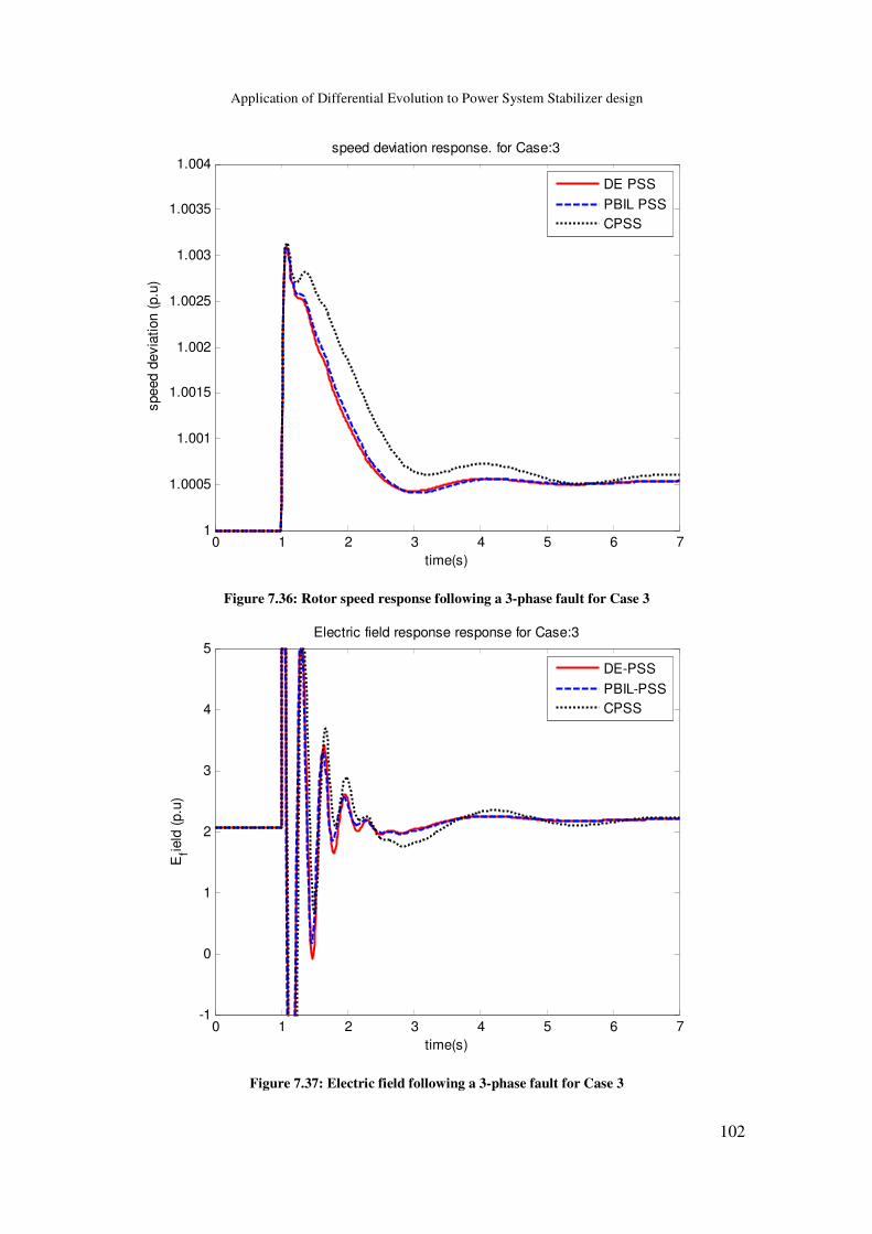
Application of Differential Evolution to Power System Stabilizer design
102
Figure 7.36: Rotor speed response following a 3-phase fault for Case 3
Figure 7.37: Electric field following a 3-phase fault for Case 3
0 1 2 3 4 5 6 71
1.0005
1.001
1.0015
1.002
1.0025
1.003
1.0035
1.004speed deviation response. for Case:3
time(s)
spe
ed d
evia
tion
(p.u
)
DE PSSPBIL PSSCPSS
0 1 2 3 4 5 6 7-1
0
1
2
3
4
5Electric field response response for Case:3
time(s)
Efie
ld (
p.u)
DE-PSSPBIL-PSSCPSS

Application of Differential Evolution to Power System Stabilizer design
103
Figure 7.38: Active power output following 3-phase fault for Case 3
7.4.2.4 Case 4: 3-phase fault applied when 400MW are transmitted
As the system loading increases, the performance of the CPSS deteriorates as it can be
observed in Figure 7.39 to Figure 7.42. The CPSS is increasingly slower to recover from
the fault taking over 7 seconds to damp the oscillations. Both DE and PBIL based PSSs,
on the other hand, display adequate and similar performance. Both systems settled just
over 4 seconds for the rotor speed responses in Figure 7.40, the electric field in Figure
7.41 and the active power in Figure 7.42, whilst settling in just over 5 seconds for the
terminal voltage in Figure 7.39.
0 1 2 3 4 5 6 7
6.6
6.8
7
7.2
7.4
7.6
Power output for Case:3
time(s)
pow
er (
p.u)
DE-PSSPBIL-PSSCPSS

Application of Differential Evolution to Power System Stabilizer design
104
Figure 7.39: Terminal voltage response following a 3-phase fault for Case 4
Figure 7.40: Rotor speed response following a 3-phase fault for Case 4
0 1 2 3 4 5 6 70.92
0.94
0.96
0.98
1
1.02
1.04
Voltage at the terminal of bus 3. for Case:4
time(s)
Vter
min
al (
p.u)
DE-PSSPBIL-PSSCPSS
0 1 2 3 4 5 6 71
1.0005
1.001
1.0015
1.002
1.0025
1.003
1.0035
1.004speed deviation response. for Case:4
time(s)
spe
ed d
evia
tion
(p.u
)
DE PSSPBIL PSSCPSS

Application of Differential Evolution to Power System Stabilizer design
105
Figure 7.41: Electric field following a 3-phase fault for Case 4
Figure 7.42: Active power output following 3-phase fault for Case 4
0 1 2 3 4 5 6 7-1
0
1
2
3
4
5Electric field response response for Case:4
time(s)
Efie
ld (
p.u)
DE-PSSPBIL-PSSCPSS
0 1 2 3 4 5 6 7
6.6
6.8
7
7.2
7.4
7.6
Power output for Case:4
time(s)
pow
er (
p.u)
DE-PSSPBIL-PSSCPSS

Application of Differential Evolution to Power System Stabilizer design
106
7.5 Summary
The application of two proposed Evolution Algorithms (DE and PBIL) for tuning the
parameters of PSS has been tested for a Two-Area Multimachine system. The resulting
PSSs were compared with those of the CPSS. The modal analysis shows that all the PSSs
are capable of improving the dynamic stability of the system. In particular, DE-PSS
performs better than PBIL-PSS and CPSS for all cases that have been discussed. These
results have been validated in time domain simulations under small disturbance where
DE-PSS outperformed both PBIL-PSS and CPSS with faster settling times and less
overshoots and undershoots in some cases. As expected, the CPSS performs well for the
nominal condition however degrades when the operating conditions change for both
small and large disturbances. In transient stability, it was observed that DE displayed
slightly higher overshoots than PBIL, which can be attributed to the slight higher gain.

Application of Differential Evolution to Power System Stabilizer design
107
Chapter 8
8 Application of Self-Adaptive Differential Evolution
to Power System Stabilizer Design
In this chapter, a systematic analysis of DE’s control parameters is conducted. The effects
of the mutation factor, crossover probability, and population size on DE’s performance in
tuning PSSs are presented. The chapter is therefore divided into three sections. The first
section investigates the inherence of the mutation factor and crossover probability on DE.
In the second section, the population size is also investigated. The effects of increasing
the population size are presented. As a result, the Self-Adaptive Differential Evolution is
used to tune a power system stabilizer in SMIB and compared to the Differential
Evolution (DE) in the third section.
.
8.1 Introduction
Differential Evolution has been shown to be a simple yet powerful algorithm especially
for optimally tuning Power System Stabilizers as in this thesis and real-world problems.
However like other EAs, DE’s performance is closely dependent on its intrinsic control
parameters such as the mutation factor, the crossover probability and population size.
Inappropriate choice of control parameter values may result in significant deterioration of
the algorithm performance and reliability to effectively explore the search space for the
global maximum or minimum. DE works generally well for many practical problems
when the control parameters are set appropriately [51]. The authors in [18] and [65] have
proposed some simple guidelines for the control parameter settings that ensure DE’s
optimal performance. These guidelines are mainly based on experimental studies and
their applicability to other problems may not always yield satisfactory results because the
control parameters of DE are dependent on problem characteristics and objective
functions. Consequently, they must be adjusted. Very often, these parameters are
obtained by trial-and-errors.

Application of Differential Evolution to Power System Stabilizer design
108
In the next section, the effect of the mutation factor ‘F’ and the crossover probability
‘CR’ on the PSS tuning are presented. An empirical rule for choosing these parameters is
established based on the results obtained in this research. Then, a self-adaptive scheme is
applied to the PSS tuning to solve the tedious process of finding the optimal control
parameters. For this section, since we want to evaluate the performance of the self-
adaptive DE to the conventional DE, CPSS and PBIL are not included. Only DE and self-
adaptive DE are compared.
8.2 Effects of Mutation F and Crossover Probability Cr on PSS Tuning
The sensitivity of differential evolution to its intrinsic control parameters has been a
challenge to practitioners since its inception. Quantifying the sensitivity of differential
evolution to its control parameters and subsequently extracting empirical rules for
choosing optimal intrinsic control parameters for future applications is of great
importance [45].
DE’s ability to find the global maximum is mainly dependent on the mutation and
crossover processes. As mentioned in chapter 3, the differential mutation allows DE to
explore the search space for the global maximum or minimum. This process is controlled
by the mutation scale factor F, a positive real number in the range of '�· ��. ‘F’ controls
the rate at which the population evolves. Whereas the crossover ensures that the diversity
of population is kept to avoid premature convergence to local optima. Hence this process
is directly dependent on the value of ‘CR’.
Figure 8.1 and 8.2 below show the effect of F and CR on the algorithm ability to
maximize the lowest damping ratio of an SMIB system. In order to determine the optimal
F & CR, one parameter is kept constant whilst varying the other, alternatively. In Figure
8.1, CR was kept constant to 0.9 whilst F was varied. DE converges to lowest damping
ratios of about 12%, 14%, 16%, 21%, 22% and 20% when F is set to 0.1, 0.3, 0.5, 0.75,
0.9 and 1.0, respectively. It can be observed that at lower value of F, DE’s performance
is restricted and unable to explore the search space adequately causing the algorithm to
converge fast to a poor solution (possibly local optima). Hence increasing F guarantees a

Application of Differential Evolution to Power System Stabilizer design
109
good search. However as it can be seen in Figure 8.1, DE performance is negatively
affected when F = 1.0 (but it’s still better than F=0.1 to 0.5). It can therefore be deduced
that values of F close to 0.9 are suitable for PSS tuning. It allows the algorithm to search
for the global maximum.
In Figure 8.2 above, F is kept constant at 0.9 and CR is varied. Results show that lower
values of CR, for example 0.1, cause the search to converge to local minima despite the
diversity. Hence increasing CR increases the diversity of the population which
subsequently increases the chance of finding the global maxima. Therefore, it is deduced
that for PSS tuning, CR works best with values ranging between [0.9 - 0.95]. Hence, it is
not recommended to set CR = 1.0 due to the fact that it negatively affects the
performance of DE by reducing its convergence rate when applied to PSS tuning.
This has led to the development of self-adaptive DE discussed in the section 8.4. The next
section investigates the impact of population size on the optimization.
Figure 8.1: Effect of CR probability on DE performance
0 5 10 15 20 25 30 35 40 45 500.06
0.08
0.1
0.12
0.14
0.16
0.18
0.2
0.22
0.24Crossover probability variation
Generation
Fitn
ess
valu
e
F=0.1 & CR=0.9F=0.3 & CR=0.9F=0.5 & CR=0.9F=0.75 & CR=0.9F=0.9 & CR=0.9F=1.0 & CR=0.9

Application of Differential Evolution to Power System Stabilizer design
110
Figure 8.2: Effect of CR probability on DE performance
8.3 Effect of population size on PSS tuning
The effect of population size parameter on the performance of DE has not been given
much importance and is often chosen as a constant value. Therefore, in this section,
investigations on its effects when tuning PSSs are conducted.
A population is constituted of Np individuals that represent possible solutions to a
problem domain. For many years, the question as to how to choose an adequate
population size for a particular domain has puzzled practitioners. If the population size is
small, the algorithm may converge fast; but the probability of premature convergence and
stagnation may be higher. Stagnation can be defined as a phenomenon whereby the
population remains diverse and unconverged, whilst the optimization process no longer
progresses [66]. Stagnation may occur virtually without any obvious reasons, whereas in
premature convergence the population loses its diversity [63], [66]. To overcome this
0 5 10 15 20 25 30 35 40 45 500.06
0.08
0.1
0.12
0.14
0.16
0.18
0.2
0.22
0.24Crossover probability variation
Generation
Fitn
ess
valu
e
F=0.9 & CR=0.1F=0.9 & CR=0.3F=0.9 & CR=0.5F=0.9 & CR=0.75F=0.9 & CR=0.95F=0.9 & CR=1.0

Application of Differential Evolution to Power System Stabilizer design
111
drawback, larger population may be used. However large population may require more
computational effort.
The author in [16] recommended that a population between 7.D and 10.D be used for a
good and efficient performance. D is the dimensionality of the problem also known as
parameters to be optimized. However, like the other control parameters, the population
size is problem dependent. With small dimensional problems, the population size bares
slight effects; however when the dimension is increased the effect of the population size
is more noticeable [16]. In that regards, the authors in [63] conducted an empirical study
of population size on DE algorithm. The results showed significant influence on the
performance of DE.
The investigations in this research are carried out in a Two-Area Multi Machine system
whereby the dimensionality of the problem is 10 parameters. Different population sizes
(D, 3.D, 5.D, 7.D, 10.D, 15.D and 20.D) are considered in this study. Because the
optimization is a random based operation, each set of population was run 10 times,
independently. The number of generation is set to 200. The analysis is based on the
maximum damping obtained from the 10 runs, the ‘Mean’ which indicate the average of
the maximized best damping ratios, the standard deviation, and time domain analysis.
Table 8.1 below summarizes the results obtained from the simulations (Best damping,
mean and standard deviation) for different population sizes. It is observed that when the
population is increased, the converged value also increases. This is due to a better
exploration capability. With a population of 15.D (150), DE converges to the best overall
damping ratio and has the highest average value. DE’s worst performance is recorded
when the population is set to D (10). This is expected since there is not much diversity
within the population which leads to a premature convergence and possibly stagnation.
Hence, this suggests that DE is caught into a local optimum. When DE is set to 10D
(100), it is observed that the standard deviation is at its highest. Hence a wider variation
in the maximum converged values is noticed. When the population is set to 50, DE
converged to a best damping of 26.94 %, and an average of 23%. It is also observed that
the standard deviation is the smallest. This suggests that the results obtained over the 10

Application of Differential Evolution to Power System Stabilizer design
112
runs are close with each other, therefore consistent. DE (50) converged to the second
highest average value.
Table 8.1: Experimental results of DE when varying the population
Population size Best damping Mean Std. Dev
10 0.178 0.161 0.0163
30 0.24390 0.22677 0.022362
50 0.26940 0.230126 0.0110
70 0.259877 0.2214 0.023452
100 0.26714 0.22537 0.032241
150 0.27400 0.24582 0.028197
200 0.26030 0.22307 0.026662
Figure 8.3 below shows the fitness curve of different population sizes. It is observed that
when the population size is small (10 & 30), the diversity is lost early, and DE
prematurely converges, possibly to a local optimum. However, as the population is
increased (50 to 100), DE is able to further explore the search space and converge to
better damping ratios. When the population is further increased (150 & 200), the diversity
within the population also increases, hence the convergence becomes slower. In this case,
one of the solutions would be to increase the number of generation to allow the algorithm
to converge to an optimum value.
Population size is often cited as a source of increased diversity [67], [71], [72], but it
would be expected to have different impacts on searches with low versus high values of
CR given the differing ways in which they explore solution space. It was shown in [73]
that the performance of DE improves whilst increasing CR settings and decreasing the
population size. This is due to the fact that the acceptance rate of new solutions is always

Application of Differential Evolution to Power System Stabilizer design
113
inversely related when CR = 0.9, yet on several problems is positively related when CR=
0.5. This suggests that a larger population can promote improved exploration when CR is
low, however, it means that the resulting gradual search has fewer opportunities to
improve each member of the population. In other words, when CR is high, a large
population works against convergence and prolongs the time during which large
difference vectors are produced. This results in a greater number of inappropriately large
moves due to the differential mutation F being used to try to improve result.
Consequently, reducing the value of F may also allow large populations to converge.
Figure 8.3: Fitness curve for different population size
In [64], the author developed a self-adaptive population algorithm to address the
drawbacks observed. However this method was not investigated in this thesis. In the next
section, the population was kept constant whereas CR and F where self-adapted when
applied to the tuning of the PSS.
0 20 40 60 80 100 120 140 160 180 200-0.05
0
0.05
0.1
0.15
0.2
0.25
0.3
Generation
Dam
ping
rat
io
DE (10)
DE (30)
DE (50)
DE (70)
DE (100)
DE (150)
DE (200)

Application of Differential Evolution to Power System Stabilizer design
114
8.4 Self-Adaptive Differential Evolution
The performance of DE is affected by its control parameters which are subsequently
dependent on the characteristics of the objective function. Hence, inadequate parameter
settings may degrade the convergence of the algorithm. Often, a tedious trial-and-error
approach is use to determine these parameters [51].
Recently, adaptive or self-adaptive mechanisms have been introduced in [19], [67]-[69],
to dynamically and automatically update the parameters to fit the objective function of
the optimization problem without user interaction or trial-and-error. The self-adaptive
algorithms have shown faster and more reliable convergence performance than the
Classic DE for many problems [19], [51], [67]-[69].
Most adaptive algorithms have been developed based on the Classic DE with strategy
DE/rand/1, [19], mentioned in Chapter 3 which is known to be robust but less efficient in
terms of convergence rate. However not many methods have been developed based on
the DE/current-to-best strategy due to the fact that they are usually less reliable and may
lead to premature convergence.
Some adaptive strategies have been briefly reviewed in the subsequent paragraphs.
FADE: The Fuzzy Adaptive Differential Evolution (FADE), introduced by Liu and
Lampinen in [67], is a fuzzy logic based controllers to adapt DE parameters Fi and CRi
for the mutation and crossover operations whereas the population is kept fixed.
SaDE: The Self-Adaptive DE (SaDE) was proposed in [69]. Two mutation strategies,
‘DE/rand/1’ (strategy 1) and ‘DE/current-to-best/2’ (strategy 2), may be used in this
algorithm. The self-adaptive strategy consists of applying a probability pi to first
determine the mutation strategy (1 or 2) to be used to generate a mutation vector. This
probability is updated after 50 generations. In this strategy, Fi is independently generated
for each generation according to a normal distribution with a mean of 0.5 and standard
deviation 0.3, defined as follows
¥y � p _¡_'¢¾�'¢�� (8.1)

Application of Differential Evolution to Power System Stabilizer design
115
The crossover probabilities CRi are independently generated according to a normal
distribution with mean CRm and standard deviation 0.1, defined as follows,
²³y � p _¡_²³�� '¢�� (8.2)
where ²³� is the mean of every 25 successful CR values in the last 25 generations.
jDE: Proposed by Brest et al. [19], this strategy is based on DE/rand/1. Similar to other
schemes, jDE fixes the population size during the optimization whilst adapting the
control parameters Fi and CRi associated with each individual. In other words, these
control parameters are adjusted by means of evolution (see Figure 8.4). Both of them are
encoded in the individual levels. The better values of these (encoded) control parameters
lead to better individuals which, in turn, are more likely to survive and produce offspring
and, hence, propagate these better parameter values [68], [70], [74].
Figure 8.4: Self-Adapting encoding aspect
The initialization process sets Fi =0.5 and CRi = 0.9 for each individual. jDE regenerates
(with probabilities × = ×� = 0.1 at each generation) new values for Fi and CRi according to
uniform distributions on [0.1,1] and [0,1], respectively.
������¥y��Y � Á ¥Ø ) p _¡ Ä ¥Ù��������������p _¡� � ×��������������y������������������������������� ·¸¹pºcq¹�����������������» (8.3)

Application of Differential Evolution to Power System Stabilizer design
116
������²³y��Y � Á p _¡J��������������p _¡ª � ×����������²³y��������������� ·¸¹pºcq¹�����������������» (8.4)
where randj, j = 1, 2, 3, 4, are uniform random values on [0, 1], and × = ×� = 0.1
represent the probabilities to adjust the control parameters. The newly generated
parameter values are used in the mutation and crossover operations to create the
corresponding offspring vectors and will replace the previous parameter values if the
offspring survive in the selection. It is believed that better parameter values tend to
generate individuals which are more likely to survive, and able to go into the next
generation.
In this work, the adaptive scheme used is based on the mutation strategy DE/rand/2 which
is as follows
��������������������������������¤y�� � �}«�� ) ¥¢ ��}�� H �}���� ) ¥¢ �}J�� H �}ª��� (8.5)
Hence, each individual is encoded with two values of Fi and CRi parameters as illustrated
in Figure 8.5. These control parameters are generated based on (8.3) and (8.4). This
approach allows robustness and good convergence. This self-adaptive strategy is applied
to tune the PSS and compared with DE in the subsequent sections.
Figure 8.5: Self-adaptive encoding aspect based on DE/rand/2

Application of Differential Evolution to Power System Stabilizer design
117
8.4.1 Application to PSS tuning: Modal analysis
In this section, jDE has been applied to tune PSS in an SMIB system described in chapter
5. The resulting PSS is compared to the classical DE (CDE) which is based on DE/rand/1
mutation strategy.
Because DE search engine is based on the mutation process, a relatively small population
is often used to ensure an optimal performance. Thus, DE control parameters were
configured as follows (Figure 8.6 below)
Figure 8.6: Control Parameter settings
The PSSs were designed over 5 operating conditions. Table 8.2 shows the PSSs’
parameters obtained after optimization using jDE and CDE whereas Table 8.3 shows the
case considered for the design and testing of the PSSs, with the open-loop and closed-
loop eigenvalues and the respective damping ratio in brackets.
The results show that the open-loop system is poorly damped for all cases whereas both
PSSs perform adequately. However, in Case 1, jDE has a slightly higher damping ratio of
43.4% whereas CDE has 40.8%. Furthermore there is a noticeable decrease in the
frequency of oscillation on the electromechanical modes associated with CDE-PSS. In
case 2, a slight drop in damping ratio is observed on the system equipped with CDE-PSS
whereas jDE-PSS damping remains constant at 43%. As the tie-lines are further
weakened in case 3, CDE-PSS has a damping of 33%. jDE on the other hand has 44.6%.
In case 4, when the system is heavily loaded combined with weak transmission lines,
jDE-PSS has a damping of 45 % whilst CDE-PSS has 27%. This agrees with the
expected performances of CDE with regards to the algorithm performance.

Application of Differential Evolution to Power System Stabilizer design
118
Table 8.2: PSS parameters
K T1 T2 T3 T4
CDE-PSS 17.2 0.0102 0.154 4.839 0.272
jDE-PSS 18.9 4.64 1.67 3.21 1.50
Table 8.3: System Open-loop and Closed-loop eigenvalues
Case Active Power (pu)
Line reactance (pu)
Open-Loop Eigenvalues CDE-PSS jDE-PSS
Case 1 1.0 0.3 -0.268±j4.457
(0.060) -1.521±j3.405
(0.408) -1.920±j3.979
(0.434)
Case 2 1.0 0.5 -0.118±j3.781
(0.0483) -1.134±j2.735
(0.383) -1.566±j3.232
(0.436)
Case 3 1.0 0.7 -0.133±j3.311
(0.0402) -0.832±j2.319
(0.330) -1.341±j2.689
(0.446)
Case 4 1.0 0.9 -0.0997±j2.947
(0.0338) -0.487±j1.694
(0.276) -1.161±j2.249
(0.458)
8.4.2 Time Domain Step Response Analysis
The small disturbance simulations have been performed for all four cases previously
mentioned by applying 10% step change in the reference voltage. The step response for
speed deviation of the generator is presented from Figure 8.7 to Figure 8.10.
Figure 8.7 shows the responses of the rotor speed deviations for Case 1. It can be seen
that all controllers are able to damp the oscillations and improve the system dynamic
stability; jDE-PSS settles within 2.5 seconds whereas CDE-PSS settles around 3 seconds.
In Figure 8.8, it is observed that the speed deviations jDE-PSS displays better
performance than that of CDE-PSS with settling time of 3 seconds and 5 seconds,
respectively.
Figure 8.9 shows the responses of the rotor speed deviations for case 3 whereby CDE-
PSS performance is deteriorating whereas jDE-PSS outperforms its counterpart. Despite
the faster settling time, jDE has slightly bigger undershoots which can be attributed to the
overcompensation of the stabilizer.

Application of Differential Evolution to Power System Stabilizer design
119
Figure 8.10 shows the speed response of the system for case 4. In this particular case, the
system is heavily loaded with weak tie-line. In this scenario, as expected, jDE has the
fastest response with settling time of about 4 seconds; whereas CDE-PSS has slower
decaying oscillations with a long settling time of about 10 seconds. It is also observed
that CDE has the largest overshoots whereas jDE has the biggest undershoots.
Figure 8.7: Step-response for Case 1
0 1 2 3 4 5 6 7 8 9 10-5
-4
-3
-2
-1
0
1
2x 10
-4 Step response for Case study:1
time(s)
spee
d de
viat
ion
CDE-PSSjDE-PSS
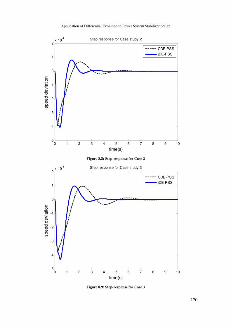
Application of Differential Evolution to Power System Stabilizer design
120
Figure 8.8: Step-response for Case 2
Figure 8.9: Step-response for Case 3
0 1 2 3 4 5 6 7 8 9 10-5
-4
-3
-2
-1
0
1
2x 10
-4 Step response for Case study:2
time(s)
spee
d de
viat
ion
CDE-PSSjDE-PSS
0 1 2 3 4 5 6 7 8 9 10-5
-4
-3
-2
-1
0
1
2x 10
-4 Step response for Case study:3
time(s)
spee
d de
viat
ion
CDE-PSSjDE-PSS

Application of Differential Evolution to Power System Stabilizer design
121
Figure 8.10: Step-response for Case 4
0 1 2 3 4 5 6 7 8 9 10-5
-4
-3
-2
-1
0
1
2
3x 10
-4 Step response for Case study:4
time(s)
spee
d de
viat
ion
CDE-PSSjDE-PSS

Application of Differential Evolution to Power System Stabilizer design
122
8.4.3 Large disturbances
The robustness of the PSS is further assessed when subjected to severe faults. The fault
consists of submitting the system to a 5-cycles 3-phase fault applied after 1 second on
line 1 (Figure 5.6). The fault was cleared by disconnecting the line.
Transient Stability was performed for Case 1 to 3. Case 4 was not considered because of
the inability of the system to regain stability after clearing the fault. This may be
attributed the high angle associated with the power (more than 90o).
8.4.3.1 Case 1: Three-phase fault applied the nominal system
Figure 8.11 to Figure 8.15 are the responses of the rotor speed, terminal voltage, the field
voltage and active power following a three-phase short circuit fault on line 1 for the
nominal operating condition. Both PSSs perform adequately and rapidly returned the
system to steady state operation after the fault is cleared. Despite the rapid response of
jDE-PSS, the system exhibits slightly larger overshoots and undershoots for the rotor
angle and speed response whereas for the terminal voltage, electric field and power
output, CDE-PSS has slightly high overshoots. In terms of settling time, both systems
settle around 5 seconds, however jDE is observed to be slightly faster.

Application of Differential Evolution to Power System Stabilizer design
123
Figure 8.11: Rotor angle following 3-phase fault for Case 1
Figure 8.12: Terminal voltage following 3-phase fault for Case 1
0 5 10 1520
22
24
26
28
30
32
34Rotor angle response for Case study:1
time(s)
Rot
or a
ngle
(deg
ree)
CDE-PSSjDE-PSS
0 5 10 150.85
0.9
0.95
1
1.05
1.1
1.15
1.2
1.25Terminal voltage for Case Study:1
time(s)
Vol
tage
(p.u
)
CDE-PSSjDE-PSS

Application of Differential Evolution to Power System Stabilizer design
124
Figure 8.13: Speed response following 3-phase fault for Case 1
Figure 8.14: Electric field voltage following 3-phase fault for Case 1
0 5 10 150.999
0.9995
1
1.0005
1.001
Speed response for Case study:1
time(s)
Spe
ed (p
.u)
CDE-PSSjDE-PSS
0 5 10 15-8
-6
-4
-2
0
2
4
6
8Electric field for Case study:1
time(s)
E fi
eld(
p.u)
CDE-PSSjDE-PSS

Application of Differential Evolution to Power System Stabilizer design
125
Figure 8.15: Active power output following 3-phase fault for Case 1
8.4.3.2 Case 2: 3-phase fault applied to case 2
The responses of the rotor angle, the terminal voltage at bus 3, the rotor speed, the field
voltage and active power are shown in Figure 8.16 to Figure 8.20, respectively. In this
case the difference in performance between the two systems is evident. jDE-PSS has a
faster response with less overshoots and undershoots for the rotor angle, terminal voltage,
speed, field voltage and power. Furthermore, the system has a settling time of around 5
seconds, whereas CDE-PSS settled around 7 seconds for the electric field and power, and
9 seconds for the rotor angle, speed and terminal voltage. The overshoots observed in
CDE-PSS may be attributed to under compensation which in turn is a result of inadequate
tuning of the intrinsic control parameters.
0 5 10 150.6
0.7
0.8
0.9
1
1.1
1.2
Power Output for Case study:1
time(s)
Pow
er (p
.u)
CDE-PSSjDE-PSS

Application of Differential Evolution to Power System Stabilizer design
126
Figure 8.16: Rotor angle following 3-phase fault for Case 2
Figure 8.17: Terminal following 3-phase fault for Case 2
0 5 10 1525
30
35
40
45
50Rotor angle response for Case study:2
time(s)
Rot
or a
ngle
(deg
ree)
CDE-PSSjDE-PSS
0 5 10 150.85
0.9
0.95
1
1.05
1.1
1.15
1.2
1.25Terminal voltage for Case Study:2
time(s)
Vol
tage
(p.u
)
CDE-PSSjDE-PSS

Application of Differential Evolution to Power System Stabilizer design
127
Figure 8.18: Speed response following 3-phase fault for Case 2
Figure 8.19: Electric field voltage following 3-phase fault for Case 2
0 5 10 150.999
0.9995
1
1.0005
1.001
1.0015
1.002Speed response for Case study:2
time(s)
Spe
ed (p
.u)
CDE-PSSjDE-PSS
0 5 10 15-8
-6
-4
-2
0
2
4
6
8Electric field for Case study:2
time(s)
E fi
eld(
p.u)
CDE-PSSjDE-PSS

Application of Differential Evolution to Power System Stabilizer design
128
Figure 8.20: Active power output following 3-phase fault for Case 2
0 5 10 150.6
0.7
0.8
0.9
1
1.1
1.2
Power Output for Case study:2
time(s)
Pow
er (p
.u)
CDE-PSSjDE-PSS

Application of Differential Evolution to Power System Stabilizer design
129
8.4.3.3 Case 3: 3-phase fault applied for case 3
The Transient responses of the terminal voltage at bus 3, the rotor speed, the field voltage
and active power are shown in Figure 8.21 to Figure 8.25, respectively. In a similar trend
to the previous case, CDE-PSS is more oscillatory with larger overshoots and
undershoots. The resulting system settles around 13 seconds whereas jDE-PSS in around
7 seconds.
Figure 8.21: Rotor angle following 3-phase fault for Case 3
0 5 10 1530
35
40
45
50
55
60
65
70Rotor angle response for Case study:3
time(s)
Rot
or a
ngle
(deg
ree)
CDE-PSSjDE-PSS

Application of Differential Evolution to Power System Stabilizer design
130
Figure 8.22: Terminal voltage following 3-phase fault for Case 3
Figure 8.23: Speed response following 3-phase fault for Case 3
0 5 10 150.85
0.9
0.95
1
1.05
1.1
1.15
1.2
1.25Terminal voltage for Case Study:3
time(s)
Vol
tage
(p.u
)
CDE-PSSjDE-PSS
0 5 10 150.9985
0.999
0.9995
1
1.0005
1.001
1.0015
1.002
1.0025Speed response for Case study:3
time(s)
Spe
ed (p
.u)
CDE-PSSjDE-PSS

Application of Differential Evolution to Power System Stabilizer design
131
Figure 8.24: Electric field voltage following 3-phase fault for Case 3
Figure 8.25: Active power output following 3-phase fault for Case 3
0 5 10 15-8
-6
-4
-2
0
2
4
6
8Electric field for Case study:3
time(s)
E fi
eld(
p.u)
CDE-PSSjDE-PSS
0 5 10 150.6
0.7
0.8
0.9
1
1.1
1.2
Power Output for Case study:3
time(s)
Pow
er (p
.u)
CDE-PSSjDE-PSS

Application of Differential Evolution to Power System Stabilizer design
132
8.5 Summary
The effects of DE’ intrinsic parameters (mutation factor, crossover probability and
population size) have been investigated when applied to PSS tuning. The performance of
DE is in fact dependent of the settings of these parameters. Low values of F cause DE to
prematurely converge to local optimum whereas values between [0.9, 0.95] ensures good
performance of the algorithm.
The crossover probability (CR) is responsible for the diversity within a given population.
It is observed that low values of CR restrain DE from exploring the entire search space
despite the diversity. This may cause stagnation. However when CR is set between [0.9-
0.95], the algorithm is able to both remain diverse and escape stagnation, which
subsequently search better for the global optimum. CR should not be set to 1 because it
may cause a quick loss of diversity.
The population size is also responsible for the diversity. Small population sizes have
revealed that DE prematurely converges to an optimum value whereas large populations
have slower convergence rates although yield better results.
The Self-Adaptive DE whereby F and CR are changing and Np is fixed, was
implemented to tune the PSS in SMIB. The results are compared with those of the DE.
The modal analysis shows that the self-adaptive outperformed DE-PSS for all the cases
considered. These results have been validated in time domain simulations under small
disturbance where self-adaptive outperformed DE-PSS with faster settling times and
slightly more overshoots and undershoots in some cases. In transient stability, it was
observed that self-adaptive displayed slightly less overshoots than DE.

Application of Differential Evolution to Power System Stabilizer design
133
Chapter 9
9 Conclusions and Recommendations for Further
Works
The problem of optimally tuning the power system stabilizer has been addressed in this
thesis. Optimization techniques based on Computational Intelligence have been used to
find the optimal set of the PSS’ parameters that provides adequate damping for a wide
range of operating conditions. Thus, in the first part, DE was developed and implemented
to tune the PSS. The algorithm performances were evaluated by comparing it to PBIL,
and CPSS. An empirical rule was formulated with regard to DE intrinsic parameters that
ensured optimal performance of the algorithm. To substitute the trial-and-error tuning
approach, an adaptive scheme was applied to DE’ control parameters and compared to
the Classic version of DE (CDE).
An eigenvalue based objective function was considered and implemented to optimally
tune the PSS. The optimization consisted of maximizing the lowest damping ratio that
corresponded to the electromechanical modes across all the operating conditions. The
tests were carried out on a Single Machine Infinite Bus and Two-Area Multimachine
systems.
Some of the primary requirements of good optimization algorithms are based on their
efficiency, robustness and simplicity. And when applied to PSS tuning, the resulting PSS
must be robust enough to wide variations in the system’ operating conditions. Hence,
investigations revealed that the CPSS does provide satisfactory performances for the
operating conditions around the nominal conditions. But the performance deteriorated as
the system loading was increased. Both DE and PBIL, on the other hand ensured stability
over the operating conditions considered in this work. Especially, DE-PSS which yielded
better results than PBIL-PSS. The modal analysis showed that DE had better damping,
and the step-response validated the findings by settling faster than PBIL-PSS and CPSS
in both SMIB and Two-Area systems. The PSSs were further tested for transient

Application of Differential Evolution to Power System Stabilizer design
134
disturbance to ensured robustness of the stabilizers when subjected to a three-phase fault.
The time domain simulations revealed that all PSSs performed satisfactory. However,
CPSS least performed whereas DE and PBIL had similar performance.
Based on the simulations results obtained in this thesis, the follow conclusions were
drawn:
� PBIL is a simpler algorithm with two control parameters to be set, population and
learning rate.
� PBIL is most efficient in terms of memory utilisation since it only keeps two
solutions, the best one and the one being evaluated. However PBIL requires more
generations to find the optimal solution. Because PBIL need to re-populate at
every generation based on the probability vector, it also requires more time.
Whereas DE is faster due to the floating point representation of the population
which facilitate arithmetic operations such differential mutation. The speed is also
attributed to the one-to-on selection type.
� DE performed better than PBIL in converging to highest minimum damping
hence better explored the search space for optimal set of PSS’ parameters.
� The time domain simulation validated the modal analysis whereby DE-PSS
settled faster than PBIL-PSS and CPSS when subjected to set-change input in the
reference voltage. Both DE and PBIL based PSSs proved to be more robust than
the CPSS with similar performances when the systems were subjected to transient
fault.
� Whereas DE has 3, mutation factor, the crossover probability and the population
number. It was established that the performance of DE is closely dependent on its
control parameters namely, mutation factor (F), crossover probability (CR), and
population size. These parameters are susceptible to change according to the
problem being optimized. Hence, an empirical rule for choosing DE intrinsic

Application of Differential Evolution to Power System Stabilizer design
135
control parameters fro PSS tuning was developed. F and CR effects were first
investigated by individually testing varying them and keeping the population
constant. The investigations showed that DE performed best when F and CR is
between 0.9 and 1. In this thesis, F= CR =0.95 was found to be satisfactory for
both SMIB and Two-Area. Despite the guidelines provided in literature, these
parameters are problem-based and must be carefully chosen. Trial-and-error
tuning is often used. This approach is very intricate and time consuming. Hence,
self-adaptive was implemented to address that issue.
� The results in this thesis showed, that jDE-PSS yielded better performance than
CDE-PSS in small signal analysis whereas transient analysis revealed much close
performance.
The effect of population size on DE’s performance was also investigated. Increasing the
population size has significant impact on DE. The convergence rate of DE suggests that
larger population improves the performance by achieving higher best minimum damping
ratios as opposed to small population. However, large population groups are highly
diverse and slow in convergence. This might require and increase in number of function
evaluations (generations) or readjustment of the mutation F and the crossover CR.
Based on the conclusions drawn from the work, the following recommendations can be
made
� Further investigation need to be carried out in simultaneously tuning the PSS in
New-England, 10-machine or even larger system to determine with certitude the
robustness of DE.
� Validate DE-PSS’ simulation results by implementing it into a physical system.
� Investigate the online application of DE in tuning the PSS.
� It would be desirable to further evaluate the Self-Adaptive DE (jDE), by
considering larger systems. Moreover, investigate different types of adaptive
schemes applied to DE.

Application of Differential Evolution to Power System Stabilizer design
136
� A fixed population size was considered in this work whilst adapting the control
parameters F and CR which were associated with each individual. Other adaptive
techniques that include the population size must be explored.

Application of Differential Evolution to Power System Stabilizer design
137
References
[1] P. Kundur, Power System Stability and Control.: Prentice-Hall, 1994.
[2] Pal Bikash and Chaudhuri Balarko, Robust Control in Power Systems.: Springer
Science, 2005.
[3] S.P.N Sheetekela, "Design of Power System Stabilizers using Evolutionary
Algorithms," Electrical, University of Cape Town, Cape Town, Thesis 2010.
[4] Graham Rogers, Power System Oscillations. Boston: Kluwer Academic, 1999.
[5] PM Anderson and Fouad AA, Power System Control and stability. Iowa, USA: The
Iowa State University Press, 1994.
[6] K.A. Folly, "Multimachine Power System Stabilizer design based on a simplified
version of genetic algorithms combined with learning," in Proceeding of the 13th
International conference on Itelligent Systems Application to Power Systems, 2005.
[7] KA Folly, "Small-signal stability enhancement of Power Systems using PBIL based
power system stabilizer ," in Artificial Intelligence in Energy Systems and Power,
2006.
[8] A. Ghosh, G. Ledwich, O. P. Malik, and G. S. Hope, "Power System Stabilizer
Based on Adaptive Control Techniques," IEEE Transaction on Power Apparatus
and Systems, , vol. Vol. PAS-103, no. 8, pp. 1983-1989, August 1984.
[9] Shaoru Zhang and Fang Lin Luo, "An Improved Simple Adaptive Control Applied
to Power System Stabilizer," IEEE TRANSACTIONS ON POWER ELECTRONICS,
vol. 24, no. 2, FEBRUARY 2009.
[10] S Chen and OP Malik, "H-infinity optimisation-based power system stabiliser," IEE
Proc.Gener. Transm. Distrib., vol. 142, no. 2, pp. 179-184, March 1995.
[11] T.C Yang, "Applying optimisation method to power system stabiliser design Part 1:
single-machine infinite-bus systems," Electrical Power & Energy Systems, vol. 19,
no. 1, pp. 29-35, 1997.
[12] S.S. Lee, Y. T. Yoon, J.K Park, S.Y. Li, "Non-linear Adaptive Decentralised
Stabilization Control for Multimachine Power Systems," International Journal of

Application of Differential Evolution to Power System Stabilizer design
138
Control , Automation and Systems, vol. 7, no. 3, pp. 389-397, 2009.
[13] O.P. Malik, G.S. Hope, Y.H. Qin and G.Y. Xu, G.P. Chen, "An adaptive Power
System Stabilizer based on the self – optimizing pole shifting control strategy,"
IEEE Transaction on Energy Conversion, vol. 8, no. 4, pp. 639 – 645, December
1993.
[14] A. Abido, and H. Mantaurym Y. L. Abdel – Magid, "Simultaneous stabilization
ofMultimachine Power System via genetic algorithm," IEEE Trans. Power Sys., vol.
14, no. 4, pp. 1428 – 1438, November 1999.
[15] KA Folly and GK Venayagamoorthy, "Optimal tuning of system stabilizer
parameters using PBIL with adaptive learning rate," in Power and Energy Society
General Meeting, 2010, pp. 1-6.
[16] K. Price, R. Storn, and J. Lampinem, Differential Evolution: A practical approach to
global optimization. Berlin Heldelberg: Springer-Verlag, 2005.
[17] R. Curuana S. Baluja, "Removing the genetic from the standard genetic algorithm,"
in Proceedings of the twelfth international conference on machine learning, Lake
Tahoe, Jula 1995.
[18] R. Storn and K. Price, "Differential Evolution- a simple and efficient adaptive
scheme for global optimization over continuous space," 1995.
[19] J. Brest, S. Greiner, B. Boskovic, M. Mernik, and V. Zumer, "Self-adapting control
parameters in differential evolution: a comparative study on numerical benchmark
problems," IEEE Trans. on Evolutionary Computation , pp. 646-657, 2006.
[20] S. Baluja, "Population-based incremental learning: A method for integrating genetic
search based function optimization and competitive learning," Carnigie Mellon
University, Technical report CMU-CS-94-163 1994.
[21] G. Rogers, "Demystifying power system oscillations," IEEE Computer Applications
in Power, vol. 9, no. 3, pp. 30 - 35, 1996.
[22] Antal Soos, "An Optimal Adaptive Power System Stabilizer," Department of
Electrical and Computer Engineering, University of Calgary, Calgary, Thesis 1997.
[23] P. Kundur, M. Klein, G.J. Rogers, and M.S. Zywno, "Application of Power System
Stabilizers for enhancement of overall system stability," IEEE Transactions on

Application of Differential Evolution to Power System Stabilizer design
139
Power Systems, vol. 4, no. 2, pp. 614-626, May 1989.
[24] K.R. Padiyar, Power System Dynamics Stability and Control. Banga lore: Wiley, ,
1996.
[25] E.V. Larsen and D.A. Swann, "Applying Power System Stabilizers, Part I; General
concepts, Part II; Performance objectives and Tuning concepts, Part III; Practical
considerations," IEEE Trans. on Power Apparatus and Systems, vol. PAS-100, pp.
3017-3046, 1981.
[26] Antal Soós and O.P Malik, "An H2 Optimal Adaptive Power System Stabilizer,"
IEEE TRANSACTIONS ON ENERGY CONVERSION, vol. 17, no. 1, pp. 143-149,
March 2002.
[27] A. Hariri and O.P. Malik, "Adaptive-Network-Based Fuzzy Logic Power System
Stabilizer," in IEEE WESCANEX PROCEEDINGS, 1995, pp. 111-116.
[28] Zhang S and Fang Lin Luo, "An Improved Simple Adaptive Control Applied to
Power System Stabilizer," IEEE TRANSACTIONS ON POWER ELECTRONICS,
vol. 24, no. 2, pp. 369-375, FEBRUARY 2009.
[29] A. Hariri and O.P. Malik, "A Fuzzy Logic Based Power System Stabilizer with
Learning Ability," IEEE Transactions on Energy Conversion, vol. 11, no. 4, pp. 721-
727, December 1996.
[30] T. Basar and P. Bernhard, H-Infinity Optimal Control and Related Minimax Design
Problems. Boston: Birkhäuser Boston, 1995.
[31] KA Folly, "Robust Controller Design for Small-Signal Stability Enhancement of
Power Systems," in IEEE AFRICON, 2004, pp. 631-636.
[32] K.A. Folly, N. Yorino, and H. Sasaki, "Improving the Robustness of H-Infinity PSSs
Using the Polynomial Approach," IEEE Trans. on Power Systems, vol. 13, no. 4, pp.
1359-1364, 1998.
[33] J Reddy and J.K Mendiratta, "H-Infinity Loop Shaping Based Robust Power System
Stabilizer for Dynamic Equivalent Multi-machine Power System," in IEEE
International Energy Conference, 2010, pp. 582-587.
[34] KA Folly, "On the prevention of Pole-zero cancellations in H infinity Power System
Controller Design: A comparison," SAIEE Africa Research Journal, vol. 99, no. 4,

Application of Differential Evolution to Power System Stabilizer design
140
December 2008.
[35] Y.N. Yu and C. Siggers, "Stabilization and Optimal Control Signals for a Power
System," IEEE Transactions on Power Apparatus and Systems, vol. 90 , no. 4, pp.
1469 - 1481, 1971.
[36] Y.N. YU, KHIEN VONGSURIY, and L.N. WEDMAN, "Application of Optimal
theory to Power System," IEEE TRANSACTIONS ON POWER APPARATUS AND
SYSTEMS, vol. 89, no. 1 , pp. 55-62, 1970.
[37] L.J. Cai and I. Erlich, "Simultaneous Coordinated Tuning of PSS and FACTS
Controller for Damping Power System Oscillation in Multi-Machine Systems," in
IEEE Proceedings: Power Tech Conference, vol. 2, 2003.
[38] N. Mithulananthan, C.A Canizares, J Reeve, and G. J Rogers, "Comparison of PSS,
SVC, and STATCOM controllers for damping power system oscillations," IEEE
trans on power systems, vol. 18, no. 2, pp. 786-792, May 2003.
[39] J. Nocedal and S.J. Wright, Numerical Optimization. New York: Springer-Verlag,
1999.
[40] Z. Michalewicz, Genetic Algorithms+Data Structure=Evolution Programs.: 3rd ed.
Springer-Velag; , 1996.
[41] K.A. Folly, "Multimachine power system stabilizer design based on a simplified
version of Genetic Algorithm combined with Learning," in International Conference
on Intelligent Systems Application to Power Systems (ISAP) , 2005.
[42] Pinaki Mitra and et.al, "Comparative of Population based Techniques for Power
System Stabilizer Design," in 15th International Conference on Intelligent System
Applications to Power Systems ISAP '09, 2009.
[43] H. Mühlenbein and D. Schlierkamp-Voosen, "The science of breeding and its
application to the breeder genetic algorithm BGA," IEEE Trans on Evolutionary
Computation, vol. 1, no. 4, pp. 335-360, 1994.
[44] H. Mühlenbein and D. Schlierkamp-Voosen, "Predictive models for the Breeder
Genetic Algorithm, I.: continuous parameter optimization," Evolutionary
Computation, vol. 1, no. 1, pp. 25-49, spring 1993.
[45] A. Qing, Differential Evolution: Fundamental and applications in Electrical

Application of Differential Evolution to Power System Stabilizer design
141
Engineering.: John Wiley & Sons, 2009.
[46] T. Mulumba and K.A. Folly, "Design and comparison of Multi-machine Power
System Stabilizer base on Evolution Algorithms," in Universities' Power
Engineering Conference (UPEC), Proceedings of 2011 46th International , Soest,
2011, pp. 1 - 6.
[47] Z. Wang, C.Y Chung, K.P. Wong, and C.T. Tse, "Robust power system stabilizer
design under multi-operating conditions using differential evolution," IET Gener.
TransmDistrib., vol. 2, no. 5, pp. 690 – 700, 2008.
[48] H. Shayeghi, A. Safari, and H.A. Shayanfa, "Multimachine Power System
Stabilizers Design Using PSO Algorithm," International Journal of Electrical and
Electronics Engineering, vol. 4, no. 4, pp. 226-233, 2009.
[49] M.A. Abido, "Robust Design of Multimachine Power System Stabilizers Using
Simulated Annealing," IEEE Trans on Energy Conversion, vol. 15, no. 3, 2000.
[50] R. Storn and K. Price, "Differential Evolution: a simple and efficient heuristic for
global optimization over continuous spaces," Journal of Global Oprimization, vol.
11, pp. 341-359, 1997.
[51] J. Zhang and A.C. Sanderson, Adaptive Differential Evolution: A robust approach to
multimodal problem optimization. Berlin Heidelberg: Springer, 2009.
[52] Considine G.D. and P.H. Kulik, Eds., Van Nostrand's Scientific Encyclopedia, 9th
ed. New York, USA: John Wiley & Sons Inc., 2002.
[53] J.E. Smith A.E. Eiben, Introduction to evolutionary computing.: Springer, 2003.
[54] R. Storn, "On the usage of Differential Evolution for function optimization," in
Fuzzy Information Processing Society, 1996, pp. 519-523.
[55] S. Rahnamayan and et. al, "Opposition-Based differential evolution," IEEE Trans.
on Evolutionary computation, vol. 12, pp. 64-79, 2008.
[56] H. Chi Y. Ao, "Experimental Study on Differential Evolution Strategies," in Global
Congress on Intelligent Systems, 2009.
[57] Science daily. (2012, June) Science daily. [Online].
http://www.sciencedaily.com/articles/c/chromosomal_crossover.htm
[58] DE Goldberg, Genetic algorithms in search, optimization and machine learning.

Application of Differential Evolution to Power System Stabilizer design
142
Reading, MA: Addison-Wesley, 1989.
[59] S. Yang and X. Yao, "Population-Based Incremental Learning with Associative for
Dynamic Environments," IEEE Trans. on Evolutionary computation, vol. 12, no. 5,
pp. 542-561, October 2008.
[60] S.L. Ho and S. Yang, "A population-Based Incremetal Learning Method for robust
optimal Solution," IEEE Trans. on Magnetics, vol. 46, no. 8, pp. 3189-3192, August
2010.
[61] S.Y. Yang and et. all, "A new implemetation of population based incremental
learning method for optimizations in Electromagnetics," IEEE Trans. on magnetics,
vol. 43, no. 4, pp. 1601-1604, April 2007.
[62] KA Folly, "Robust Controller Design Based on a Combination of genetic
Algorithms and Competitve Learning," in Proceedings of International Joint
Conference on Neural Networks, Orlando, Florida, USA, August 2007.
[63] R. Mallipeddi and P. N. Suganthan, "Empirical Study on the Effect of Population
Size on Differential," IEEE Congress on Evolutionary Computation, pp. 3663 -
3670, 2008.
[64] Jason Teo, "Exploring dynamic self-adaptive populations in differential evolution,"
Soft Comput, pp. 673–686, August 2005.
[65] J. Vesterstroem and R. Thomsen, "A comparativestudy of differential evolution,
particle swarm optimization, and evolutionary algorithms on numerical benchmark
problems," IEEE congress on Evolutionary Compution, pp. 1980-1987, June 2004.
[66] Lampinen J and Zelinka I., "On Stagnation of Differential Evolution Algorithm," in
Proc. of MENDEL, 6th Int. Mendel Conf. on Soft Computing, Brno, Czech Republic,
2000.
[67] J. Lui and J. Lampinen, "A Fuzzy adaptive differential evolution algorithm.," Soft
Computation: Fusion Found Method Appl., pp. 448-462, 2005.
[68] J. Brest, Borko Boskovic, and Viljem Zumer, "An improved self-adaptive
Differential Evolution Algorithm in Single objective constrained real-parameter
optimization," in Congress on evolutionary computation, 2010, pp. 1-8.
[69] P.N. Suganthan A.K. Quin, "Self-Adaptive Differential Evolution Algorithm for

Application of Differential Evolution to Power System Stabilizer design
143
numerical optimization," in Congres on Evolutionary Computation, 2005, pp. 1785-
1791.
[70] U.K. Chakraborty, Advances in Differential Evolution.: Springer-Verlag, 2008.
[71] E. Mezura-Montes, J. Vel´azquez-Reyes, and C. A. and Coello, "A comparative
study of differential evolution variants for global optimization," in in GECCO,
Seattle, Washington, USA, 2006, pp. 485–492.
[72] J. Brest and M. S. Maucec, "Population size reduction for the differential evolution
algorithm," Applied Intelligence, vol. 29, no. 3, pp. 228–247, 2008.
[73] J. Montgomery, "Crossover and the different faces of differential evolution
searches,”," in IEEE Congress on Evolutionary Computation (CEC), 2010.
[74] S. M. Islam, "An adaptive differential Evolution algorithm with novel mutation and
crossover strategies for global numerical optimization," IEEE Trans. on systems,
man, and cubernetics, vol. 42, no. 2, pp. 482-500, 2012.

Application of Differential Evolution to Power System Stabilizer design
144
Research Publications
1. T. Mulumba, K. A. Folly, O.P. Malik “Tuning of PSS parameters using
Differential Evolution”, 20th Southern African Universities’ Power Engineering
Conference (SAUPEC 2011, July 13-15, 2011, Cape Town, South Africa
2. T. Mulumba, K.A Folly, “Power System Stabilizer design: Comparison analysis
between Differential Evolution and Population based Incremental Learning”, 20th
Southern African Universities’ Power Engineering Conference (SAUPEC 2011),
July 13-15, 2011, Cape Town, South Africa
3. T. Mulumba, K. A. Folly, “Design and comparison of Multi-machine Power
System Stabilizer base on Evolution Algorithms”, The 46th international
Universities’ Power Engineering Conference (UPEC 2011), September 5- 8,
2011, Soest, Germany
4. T. Mulumba, K. A. Folly, “Application Evolution Algorithms to Power System
Stabilizers design: Impact of the Population size in Differential Evolution and
Population Based Incremental Learning”, 10th IEEE Africon 2011, September 13-
15, 2011, Victoria Falls, Livingstone, Zambia.
5. T. Mulumba, K. A. Folly, “Application of self-adaptive Differential Evolution to
tuning PSS parameters”, IEEE-PES Power Africa 2011, July 9-13, 2011,
Johannesburg, South Africa

Application of Differential Evolution to Power System Stabilizer design
A
Appendix
Appendix A: This section contains higher oscillations modes of DE-PSS, CPSS and
PBIL-PSS. Further simulation results (modal analysis and step responses)
of DE with different population sizes in chapter 8 have also been included.
Appendix B: This section gives the data for the SMIB system presented with results in
Chapter 5, section 5.1. The generator parameters, transmission line data as
well as the controller (AVR) are given under this section. Also presented
under this section are equations that model the generator used in the
simulations.
Appendix C: This section presents the data used in the Multi-machine simulations of
Chapter 5, section 5.2. The models used for the generators, the AVR and
the speed governor are given in this section.

Application of Differential Evolution to Power System Stabilizer design
B
Appendix A A.1 SMIB High Frequency modes of oscillations
Table A.1 : AVR mode for SMIB
Case No PSS CPSS PBIL-PSS DE-PSS
1 -6.7205±j19.969
(0.3190)
5.0169±j22.845
(0.2145)
-4.5783±j22.762
(0.1972)
-6.1665±j22.512
(0.2642)
2 -6.6572±j20.191
(0.3131)
-5.5135±j23.226
(0.2310)
-5.2960±j23.1643
(0.2229)
-6.0897±j23.0875
(0.2550)
3 -6.6728±j20.110
(0.3149)
-5.0693±j23.026
(0.21500
-4.6721±j22.9456
(0.1995)
-6.1079±j22.7322
(0.2595)
4 -6.6263±j20.282
(0.3105)
-5.5142±j23.337
(0.2300)
-5.3099±j23.2782
(0.2224)
-6.0548±j23.2072
(0.2525)
5 -6.6416±j20.202
(0.3123)
-5.1037±j23.144
(0.2153)
-4.7334±j23.0658
(0.2010)
-6.0706±j22.8744
(0.2565)
A.2 Self-Adaptive and DE High frequency modes of oscillation for SMIB
Table A.2 : AVR modes for Self-Adaptive DE (SMIB)
Case DE-PSS jDE-PSS
1 -5.54±j22.6
0.238
-4.60±j22.4
0.201
2 -5.55±j22.9
0.236
-4.75±j22.7
0.205
3 -5.56e±j23.1
0.234
-4.83±j22.9
0.206
4 -5.56±j23.2
0.233
-4.88±j23.0
0.207

Application of Differential Evolution to Power System Stabilizer design
C
A.3 Modal Analysis of population sizes
Table A.3 : Inter-area mode eigenvalues for different population sizes
Population size Case 1 Case 2 Case 3
DE-PSS (10) -0.959 + j4.91
(0.192)
-0.871 + j4.81
(0.178)
-0.684 + j3.86
(0.174)
DE-PSS (30) -1.19 + j4.72
(0.244)
-1.09 + j4.63
(0.229)
-0.815 + j3.75
(0.212)
DE-PSS (50) -1.17 + j4.57
(0.248)
-1.06 + j4.48
(0.231)
-0.820 + j3.53
(0.2263)
DE-PSS (70) -1.16 + j4.63
(0.242)
-1.06 + j4.55
(0.227)
-0.788 + j3.67
(0.210)
DE-PSS (100) -1.03 + j4.84
(0.207)
-9.31e-001 + j4.75
(0.192)
-0.755 + j3.84
(0.193)
DE-PSS (150) -1.15 + j4.63
(0.241)
-1.06 + j4.54
(0.226)
-0.784 + j3.67
(0.209)
DE-PSS (200) -1.16 + j4.56
(0.247)
-1.06 + j4.47
(0.231)
-0.770 + j3.53
(0.213)
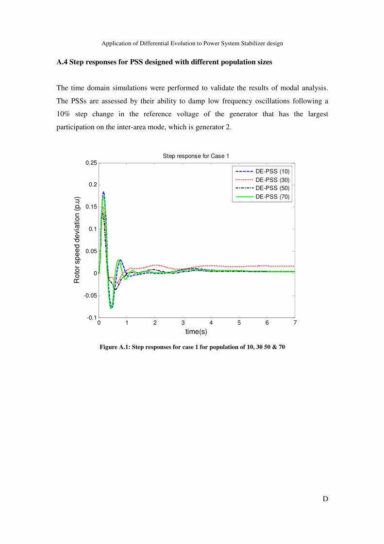
Application of Differential Evolution to Power System Stabilizer design
D
A.4 Step responses for PSS designed with different population sizes
The time domain simulations were performed to validate the results of modal analysis.
The PSSs are assessed by their ability to damp low frequency oscillations following a
10% step change in the reference voltage of the generator that has the largest
participation on the inter-area mode, which is generator 2.
Figure A.1: Step responses for case 1 for population of 10, 30 50 & 70
0 1 2 3 4 5 6 7-0.1
-0.05
0
0.05
0.1
0.15
0.2
0.25
time(s)
Rot
or s
peed
dev
iatio
n (p
.u)
Step response for Case 1
DE-PSS (10)DE-PSS (30)DE-PSS (50)DE-PSS (70)

Application of Differential Evolution to Power System Stabilizer design
E
Figure A.2: Step responses for case 2 for population of 10, 30 50 & 70
Figure A.3: Step responses for case 3 for population of 10, 30 50 & 70
0 1 2 3 4 5 6 7-0.15
-0.1
-0.05
0
0.05
0.1
0.15
0.2
0.25
time(s)
Rot
or s
peed
dev
iatio
n (p
.u)
Step response for case 2
DE-PSS (10)DE-PSS (30)DE-PSS (50)DE-PSS (70)
0 1 2 3 4 5 6 7-0.15
-0.1
-0.05
0
0.05
0.1
0.15
0.2
0.25
time(s)
Rot
or s
peed
dev
iatio
n (p
.u)
Step response for case 3
DE-PSS (10)DE-PSS (30)DE-PSS (50)DE-PSS (70)

Application of Differential Evolution to Power System Stabilizer design
F
Figure A.4: Step responses for case 1 for population of 100, 150 & 200
Figure A.5: Step responses for case 2 for population of 100, 150 & 200
0 1 2 3 4 5 6 7-0.06
-0.04
-0.02
0
0.02
0.04
0.06
0.08
0.1
0.12
0.14
time(s)
Rot
or s
peed
dev
iatio
n (p
.u)
Step response for case 1
DE-PSS (100)DE-PSS (150)DE-PSS (200)
0 1 2 3 4 5 6 7-0.1
-0.05
0
0.05
0.1
0.15
time(s)
Rot
or s
peed
dev
iatio
n (p
.u)
Step response for case 2
DE-PSS (100)DE-PSS (150)DE-PSS (200)

Application of Differential Evolution to Power System Stabilizer design
G
Figure A.6: Step responses for case 3 for population of 100, 150 & 200
0 1 2 3 4 5 6 7-0.1
-0.05
0
0.05
0.1
0.15
0.2
0.25
time(s)
Rot
or s
peed
dev
iatio
n (p
.u)
Step response for case 3
DE-PSS (100)DE-PSS (150)DE-PSS (200)

Application of Differential Evolution to Power System Stabilizer design
H
Appendix B
SMIB System B.1 Model Equations
Simple AVR structure
Figure B.1: AVR block diagram used in the SMIB system
Where:
Úr is the regulator time constant
Ír is the exciter gain
ËÐ is the terminal voltage
ËÛ is the PSS control signal
ËÜÝÞ is the reference voltage
VRMAX is the maximum limit of the AVR signal
VRMIN is the minimum limit of the AVR signal
EFD is the electric field signal
For the Single machine to infinite bus system, the following generator model was used;
it’s a 6th order sub-transient model.

Application of Differential Evolution to Power System Stabilizer design
I
The generator equations are:
F(Nß�F� � ��à Úßá H Úßâ H Íã(Nß�� FäF� � Nå(Nß�
The rotor circuit equations are represented as follows:
Fw+æF� � Nåç+æèsæ1 é+æ H Nåç+æ�+æ
FwæF� � HNåçæ�æ
FwêF� � HNåçê�ê
Fw�êF� � HNåç�ê��ê
The rotor currents are expressed by the following:
�+æ � �è+æ w+æ H wsæ� �æ � �èæ wæ H wsæ� �ê � �èê �wê H wsê�
��ê � �è�ê �w�ê H wsê�
The electrical torque is expressed by the following:
Úâ � wsæ�ê H wsê�æ

Application of Differential Evolution to Power System Stabilizer design
J
B.2 SMIB System Data
For the Single machine to infinite bus system, a 6th order sub-transient generator model
was used with a simple exciter with the following data
Generator data
Rating: 991MVA, 22kv, 50Hz
ëì � '¢�¾���!s � '¢'���ëæ � �¢'���ëæ� � '¢��¾� ëæ�� � '¢����Úæå� � ¾¢'��Úæå�� � '¢'��� ëê � �¢í����ëê� � '¢�����ëê�� � '¢��
Úêå� � '¢¿¿���Úêå�� � '¢'¿�� �à � �¢îÀ¾
Automatic Voltage Regulator parameters
Ís � �''���F�Ús � '¢'�
Transmission Line parameters
! � '
ïð � '
Power system stabilizer structure
The parameters Ks, T1- T4 were designed using conventional method and evolutionary
algorithms.
TW of 2.5s was used.
Figure B.2 : PSS block diagram used in SMIB

Application of Differential Evolution to Power System Stabilizer design
K
Appendix C
Multi- Machine System C.1 System Model Equations
F(Nß�F� � ��à Úßá H Úßâ H Íã(Nß�� FäF� � Nå(Nß�
The rotor circuit equations are represented as follows:
Fw+æF� � Nåç+æèsæ1 é+æ H Nåç+æ�+æ
FwæF� � HNåçæ�æ
FwêF� � HNåçê�ê
Fw�êF� � HNåç�ê��ê
The rotor currents are expressed by the following:
�+æ � �è+æ w+æ H wsæ� �æ � �èæ wæ H wsæ� �ê � �èê �wê H wsê�
��ê � �è�ê �w�ê H wsê�
The electrical torque is expressed by the following:
Úâ � wsæ�ê H wsê�æ

Application of Differential Evolution to Power System Stabilizer design
L
C.2 System Data
Generator data
All the generators used in the system are identical with the following parameters:
Rating: 900MVA, 22kV, 60Hz
ëì � '¢����������������!s � '¢'�����������ëæ � �¢î�������������������ëæÈ � '¢�� �ëæÈÈ � '¢�¾���������ÚæåÈ � î¢'���������ÚæåÈÈ � '¢'������������������ëê � �¢À�
��ëêÈ � '¢¾¾��������������ëêÈÈ � '¢���������������ÚêåÈ � '¢�������������� �ÚêåÈÈ � '¢'¾�� à � ¿¢¾����������������Íã � '����������AÏs[� '¢'¿¾����������������ñÏs[� '¢¾À���
All the reactances are in per unit, while the time constants are in seconds
Automatic Voltage Regulator (AVR) Parameters
Ís � �''���F�Ús � '¢'¾��Ú� � '¢'�
Turbine Governor block diagram and Parameters
Figure C.1: Speed governor block diagram used in the simulations for multi-machine
ÌG��������N+� � �������ò���� ó�çô � �¾�����Úás- � �������ÚÏ � '¢����Úð � '¢¾� ��ÚJ � '¢'���Úª � �¢�¾����Úõ � ¾¢'

Application of Differential Evolution to Power System Stabilizer design
M
Power System stabilizer Structure
The following PSS structure was used, the parameters Ks, T1 T2 T3 and T4 were designed
using the evolutionary algorithms, while the washout time constant TW of 10s was used.
Figure C.2: Block diagram for the PSS used in the Multi-machine system
All the reactances are in per unit, while the time constants are in seconds. The generators
active power output and line reactance were varied to simulate different operating
conditions.