quettra design problem solution - joanna lankester
TRANSCRIPT

Quettra Design Problem
Joanna Lankester1/30/15

Google location history

“Caltrain has seen 40 consecutive months of increased ridership.” - SF Examiner, March 2014
Census: 16% of commutes via public transit in the Bay Area

• Deduce train location history• Predict delays, high volume

30
2423
18
12
7
2

Person ID 8:00 location 8:05 location 8:10 location 8:15 location
1 30 24 23 18
2 30 23
3 24
4 5 10 23
Location ID 8:00 count 8:05 count 8:10 count 8:15 count
5 1 0 0 0
10 0 1 0 0
18 0 0 0 1
23 0 0 3 0
24 0 2 0 0
30 2 0 0 0

Location ID
8:00 count 8:05 count 8:10 count 8:15 count 8:20 count
5 1 0 0 0 0
10 0 1 0 0 0
18 0 0 0 0 1
23 0 0 1 2 0
24 0 0 2 0 0
30 0 2 0 0 0
Location ID 8:00 count 8:05 count 8:10 count 8:15 count
5 1 0 0 0
10 0 1 0 0
18 0 0 0 1
23 0 0 3 0
24 0 2 0 0
30 2 0 0 0
On time
Late
Schedule:• Loc. 30,
8:00• Loc. 24,
8:05• Loc. 23,
8:10• Loc. 18,
8:15
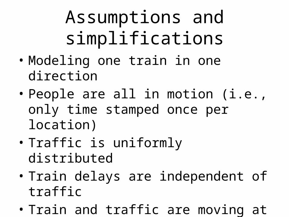
Assumptions and simplifications
• Modeling one train in one direction• People are all in motion (i.e., only time
stamped once per location)• Traffic is uniformly distributed• Train delays are independent of traffic• Train and traffic are moving at uniform speeds,
respectively
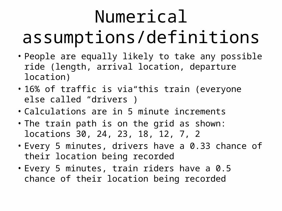
Numerical assumptions/definitions
• People are equally likely to take any possible ride (length, arrival location, departure location)
• 16% of traffic is via this train (everyone else called “drivers”)
• Calculations are in 5 minute increments• The train path is on the grid as shown: locations 30, 24, 23,
18, 12, 7, 2• Every 5 minutes, drivers have a 0.33 chance of their
location being recorded• Every 5 minutes, train riders have a 0.5 chance of their
location being recorded

Drivers - check
> sum(locationsBinned[2:30,2])[1] 263> 840*.33[1] 277.2

Drivers - check

Riders: path options
1 2 3 4 5 6 7Path length
Count options
1 6
2 5
3 4
4 3
5 2
6 1
Total 21

Riders - checkSum number of riders at each location to check that there are more riders in the middle than on the ends: colSums(riderPaths)[1] 35 81 110 133 111 88 44

Add riders and drivers time vs. location matrices
Location numbers on gridded map
Time of morning


Run simulation with data
• Assume there’s a 50% chance the train will be 10 min late Mondays and a 25% chance the train will be 5 min late Tuesdays
• Iterate for 100 Mondays and 100 Tuesdays, producing a new 1,000 person population for each
• Obtain 200 pairs of day of week and amount of time late

Simulation - check(1 time period = 5 minutes)
Mondays: E[late] = 0.5(2 time periods) + 0.5(0) = 1Tuesdays: E[late] = 0.25(1 time period) + 0.75(0) = 0.25
> table(lateness)lateness 0 1 2 127 23 50

Linear modelCall:lm(formula = lateness ~ dayOfWeek, data = data)
Residuals: Min 1Q Median 3Q Max -1.0000 -0.4225 -0.2300 0.8275 1.0000
Coefficients: Estimate Std. Error t value Pr(>|t|) (Intercept) 1.0000 0.0771 12.970 < 2e-16 ***dayOfWeekTuesday -0.7700 0.1090 -7.062 2.73e-11 ***---Signif. codes: 0 ‘***’ 0.001 ‘**’ 0.01 ‘*’ 0.05 ‘.’ 0.1 ‘ ’ 1
Residual standard error: 0.771 on 198 degrees of freedomMultiple R-squared: 0.2012, Adjusted R-squared: 0.1971
Lateness is on average 1 time period (5 minutes) unless it’s a Tuesday, when it is instead 1-0.77=0.25 time periods late on average

Endless possibilities!
• Predict number of people on the train• By holidays• By Giants game days• By weather
Goal: Adapt number of train cars according to predicted need