Query-able Kafka: An agile data analytics pipeline formobile wireless networks

Eric FalkUniversity of Luxembourg

eric.falk@uni.lu

Vijay K. GurbaniBell Laboratories, Nokia

Networksvijay.gurbani@nokia-bell-

labs.com

Radu StateUniversity of Luxembourg

radu.state@uni.lu

ABSTRACTDue to their promise of delivering real-time network insights,today’s streaming analytics platforms are increasingly be-ing used in the communications networks where the impactof the insights go beyond sentiment and trend analysis toinclude real-time detection of security attacks and predic-tion of network state (i.e., is the network transitioning to-wards an outage). Current streaming analytics platformsoperate under the assumption that arriving traffic is to theorder of kilobytes produced at very high frequencies. How-ever, communications networks, especially the telecommu-nication networks, challenge this assumption because someof the arriving traffic in these networks is to the order ofgigabytes, but produced at medium to low velocities. Fur-thermore, these large datasets may need to be ingested intheir entirety to render network insights in real-time. Ourinterest is to subject today’s streaming analytics platforms— constructed from state-of-the art software components(Kafka, Spark, HDFS, ElasticSearch) — to traffic densitiesobserved in such communications networks. We find thatfiltering on such large datasets is best done in a commonupstream point instead of being pushed to, and repeated, indownstream components. To demonstrate the advantagesof such an approach, we modify Apache Kafka to performlimited native data transformation and filtering, relievingthe downstream Spark application from doing this. Ourapproach outperforms four prevalent analytics pipeline ar-chitectures with negligible overhead compared to standardKafka. (Our modifications to Apache Kafka are publiclyavailable at https://github.com/Esquive/queryable-kafka.git)

1. INTRODUCTIONStreaming analytics platforms, generally composed of tiered

architectures as epitomized by the Lambda Architecture [26],promise to deliver (near) real-time decisions on large, contin-uous data streams. Such streams arise naturally in commu-nications networks, especially large networks like Twitter,

This work is licensed under the Creative Commons Attribution-NonCommercial-NoDerivatives 4.0 International License. To view a copyof this license, visit http://creativecommons.org/licenses/by-nc-nd/4.0/. Forany use beyond those covered by this license, obtain permission by emailinginfo@vldb.org.Proceedings of the VLDB Endowment, Vol. 10, No. 12Copyright 2017 VLDB Endowment 2150-8097/17/08.

Facebook, and packet-based public telecommunication sys-tem like the existing 4G networks. Architectures inspiredby the Lambda Architecture are organized in three layers:batch, streaming and serving layer. Incoming data streamsare distributed simultaneously to the batch and streaminglayers, with the assumption that there is a sizeable time lagbetween fitting the arriving data to models in the streamingand batch layers. The streaming layer operates on a dataonly once, in the order that it arrives, to deliver results innear real time. The batch layer has the luxury of iteratingover the entire dataset to produce results, at the cost of time.The batch and streaming layers forward computational out-put to the serving layer, which aggregates and merges theresults for presentation and allows ad-hoc queries.

While the streaming analytics architectures used todaysuffice for large networks like Twitter and Facebook, thispaper shows that they are not designed to handle the vol-ume of packet-based telecommunications systems like 4G orits successor, the 5G network [6]. Global mobile devices andconnections in 2015 grew to 7.9 billion; every server, mobiledevice (phone, tablet, vehicles), and network element in 4Ggenerates a steady stream of data that needs to be siftedthrough and processed with real-time requirements to pre-dict anomalies in the network state or foreshadow attacks onthe network. To characterize the inability of existing stream-ing analytics architectures to handle the volumes observedin the telecommunication traffic, we briefly describe an im-portant server in 4G and contextualize it’s traffic volume tothat of other large networks like Twitter and Facebook.

In the 4G network, a server called the Mobility Manage-ment Entity (MME) is a key control node for the access (ra-dio) network. It tracks the mobiles (or more generally calleda UE, User Equipment) as they move across cell boundaries,pages the UEs when messages arrive for them, authenti-cates the UE with the network, and is responsible for as-signing and maintaining the set of network parameters thatdefine specific treatment accorded to packets from that UE.In short, the MME is involved in all decisions that allow theUE to interface with the network. The MME produces alogfile record of every interaction between the UE and othernetwork elements; the logfile record contains over 230 fields,and each logfile record is about 850-1000+ bytes long. Thelogfile is maintained in a CSV format in UTF-8 encoding.

MMEs are configured for redundancy and reliability anddeployed in a pool to serve a metropolitan area. In a largemetropolitan area of 10 million people, under the conser-vative estimate that 20% of the UEs are interacting withthe network (establishing Internet sessions, moving around,

1646

making phone calls, etc.) the MME pool serving this areawill generate data at a rate of about 40 MB/s, or 3.5 TB/-day. (In a large metro area, a mean of 50,000 records/swill be generated by the MME with each record weighingin at 850 bytes for a rate of 42.5 MB/s.) By contrast,the WhatsApp instant messaging service, with a mean of347,222 messages/s [1], at an average message size of 66bytes (with metadata), generates about 22.9 MB/s1. TheTwitter network generates 11.4 MB/s2, and finally, Zhao etal. [41] state that Facebook generates log data at the rate of289.35 MB/s. To ensure our comparison is uniform acrossthe MME logfile data and other networks, we restrict ouranalysis to textual data from the Twitter, Facebook, andWhatsApp networks. Our metric does not include mediaattachments — video or pictures — of any kind.

Table 1: Ranking of message traffic in terms of MB/sec.(Only considering textual data)

Rank Use Case Traffic in MB/sec.1. Facebook 289.352. Pool of 5 active MMEs 200.003. Single MME 40.004. WhatsApp 22.905. Twitter 11.40

It is clear from the above table that datasets in telecom-munication networks are in the upper end of the data vol-umes generated by other networks. The provided measuresquantify the data generated by a MME of a 4G network en-tity, and it is expected that the 5G network with its supportfor Internet of Things, programmable networks, autonomiccomputing, and further thrusts into vehicular ad hoc net-works will push the need for even larger datasets for predic-tion and analytics.

1.1 Problem statement and contributionsA detailed description of our application in §3, here we

motivate the problem statement and contributions.The MME collects the logfiles in increments of a minute,

i.e., each minute, all the data is written out to the log file.While it is possible to obtain the data on finer timescales,the 1-minute batching mode suffices for our particular ap-plication on predicting a network outage because the logfilecontained enough observations to allow the data to fit ourstatistical models. At the rate of 40 MB/s, the MME logfilecan grow to 2.4 GB/min. Ingesting such a large file in areal-time data pipeline imposes latency penalties driven bythe fact that the entire 2.4 GB file must be processed be-fore the next batch arrives. Our models create a distributionfrom the arriving data, requiring access to the entire minute.Sampling was eschewed because it may not catch aberrantdatapoints, which may be outliers of interest. The modelsare discussed in Gurbani et al. [17] and Falk et al. [14].Here, we don’t discuss the models themselves but presentthe systemic challenges faced and mitigated while construct-ing the agile data analytics pipeline. Without such an agilestreaming analytics pipeline we had an unstable system thatcould not render timely predictive decisions.

1Numbers are based on Vergara et. al [37]. The averagemessage size is 26 bytes plus 40 bytes of metadata for atotal of 66 bytes.2According to Twitter blogs [28], the network observes amean of 5,700 tweets/s at about 2 KB/tweet, includingmetadata. This results in 11.4 MB/s.

As mentioned above, the entire 2.4 GB file must be pro-cessed before the next batch arrives. Furthermore, the na-ture of the streaming analytics data platforms in use today(i.e., the Lambda Architecture) is to perform data transfor-mation in the speed or batch layers; consequently, if thereare multiple speed layers (as there are in our application),the large dataset has to be transmitted to the order of thenumber of speed layers. Each speed layer will only need asubset of the columnstores in the dataset, however, due tothe paucity of transformation tools at the ingestion point,the large dataset must be transmitted in its entirety to eachlayer. While streaming analytics platforms are horizontallyscalable, their distributed data storages cannot deliver with-out some latency, which keeps growing as the size of datasetsincreases. Mining such big data within computable timebounds is an active area of research [15].

This work contributes to data management research thr-ough the following three contributions:

• We construct and evaluate a telecommunications-centricreal-time streaming data pipeline using state-of-the-art open source software components (Apache Hadoop[3], Spark [39] and Kafka [23]). During our evaluation,we subject the analytics pipeline to workloads not typ-ically seen in the canonical use of such platforms inglobal networks like Facebook and Twitter. Our find-ings are: (A) traditional analytics platforms are unableto handle the volume of data in the workloads typicalof a telecommunication network (large datasets pro-duced at medium to low velocities). The primary rea-son for this is the inability of the speed layer to dealwith extreme message sizes (2.4 GB/min). Aggregat-ing, summarizing or projecting relevant columns at thesource (MME) is not appropriate in our applicationdue to stringent constraints that monitor production-grade MME resources to keep them under engineeredthresholds (discussed in more detail in §4.4). (B) Itbecame increasingly clear that the batch layer wasnot needed in our application. The speed layers ex-peditiously compare arriving target distributions toknown distributions that were created a-priori. Ourapplication is not driven by ad-hoc queries — Whatis trending now? How many queries arriving from thesouthern hemisphere? — as much as it is by instanta-neous and temporal decisions — Is a network outagein progress? Is the network slice overloaded?

• To overcome limitations of prevalent streaming analyt-ics platforms, we propose to move extract-transform-load (ETL) tasks further upstream in the processingpipeline. This alleviates our finding (A) above andallows the analytics platform to process typical work-loads in a telecommunication network. A novel, simpleon-demand query mechanism was implemented on topof Apache Kafka, the ingestion point in our frame-work. This mechanism is located close to persistentstorage to leverage capabilities of disk backed linearsearch, alleviating each speed layer to deal with theETL overhead. We call our approach the query-ableKafka solution.

• We present an extensive evaluations of four streaminganalytics frameworks and compare these to our pro-posed framework implementing our novel on-demand

1647

query mechanism. We evaluate the results of these ar-chitectures on a cluster of 8 hosts as well as on AmazonAWS cluster. For each cluster, we measure three met-rics: CPU consumption of the hosts in the streaminganalytics platform, memory consumption and time-to-completion (TTC), defined as the time difference be-tween the message emission from the MME to the in-sertion of model output from the speed layer into theserving layer.

The rest of the paper is organized as follows: §2 overviewsrelated work, §3 outlines our target application used in thestreaming analytics pipeline, and §4 outlines four prevalentstreaming analytics architectures and introduces our query-able Kafka solution. §5 evaluates our solution against preva-lent architectures and discusses the advantages of our ap-proach; we conclude in §6.

2. RELATED WORKBy the late 90’s databases for telecommunications use

cases were an active area of research [19]. To maintain qual-ity of service and enable fault recovery, massive amounts oflog data generated by networking was analyzed close to real-time. Two notable works emerging from the telco domain,addressing this challenges in the pre-Hadoop era are: Gigas-cope [11] from AT&T research labs, and Datablitz from BellLaboratories [7]. Gigascope is a data store built to analyzestreaming network data to facilitate real-time reactiveness.Datablitz is a storage manager empowering highly concur-rent access to in-memory databases. Both solutions weredesigned to serve time critical applications in the context ofmassive streaming data.

Hadoop [3] and MapReduce [12] revolutionized large scaledata analytics, and for a long time appeared as the all-purpose answers to any big data assignment. Hadoop cannotbe used in the cases where Gigascope and Datablitz are de-ployed because the out-of-the-box Hadoop is not suited forreal-time needs; nonetheless, Facebook and Twitter have at-tempted to use it as a real-time processing platform [10][27].Further approaches have been made to port MapReduce op-erations on data streams [24] and proper stream processingframeworks have emerged [35][39][2].

When it comes to big data, the missing capacity if com-pared to traditional RDBM systems, is the time to availabil-ity once data is ingested. For a RDBMS, data is instanta-neously available whereas with big data stores a batch taskusually has to run in order to extract the information andmake the data eligible for ad-hoc queries. Although beinghorizontally scalable, distributed data storages cannot de-liver without noticeable latency. Moreover this latency keepsincreasing in front of the sheer amount of data to process.The issue is not solved yet [15], among the proposed solu-tions two protrude: the commonly called Lambda architec-ture [26] and the Kappa architecture [22]. The Lambda ar-chitecture capitalizes on the facts that models issued by longterm batch processes are strongly consistent because the fulldataset can be examined, whereas models from stream pro-cessors are fast to generate but only eventually consistentsince only small data portions are inspected [26]. The ar-chitecture consists of three layers: the batch, speed and thequery layer. The batch layer is typically build on top ofHadoop, and the speed layer employs distributed streamprocessors as Apache Storm [35], Spark [39] or Flink [2].

The Lambda architecture assumes that eventually consis-tent models, from the speed layer, are tolerable to bridgethe time required for two consecutive batch layer runs toexecute. The batch layer is the entity generating the con-sistent models, replacing the stream layer model once com-pleted. Examples of implemented Lambda architectures arein [26][38]. Analytics in the telecommunication domain ismore concerned with the currently arriving dataset insteadof the archived ones; it is crucial to employ the incomingstream data to contextualize the network state. Leverag-ing a full fledged Hadoop cluster as a batch layer is of mi-nor importance for real-time analytics of 4G MME data.An alternative to the Lambda architecture is the Kappaarchitecture [22]. The Kappa architecture employs the dis-tributed log aggregator and message broker Kafka [23] aspersistent store, instead of a relational database or a dis-tributed storage. Data is appended to an immutable logfile,from where it is streamed rapidly to consumers for computa-tional tasks. The totality of the data stored in the Kafka logcan be re-consumed at will, while replicated stream proces-sors are synchronized to ensure an uninterrupted successionof consistent models. Works such as [8] and [25] investigatebig data architectures for use with machine learning and net-work security monitoring, respectively. In the same mannera recent showcase of the Kappa architecture deployed for atelecommunication use case is given by [33]. In the Kappaarchitecture implemented in [33], the stream processor con-sumes raw data from Kafka, transforms it and writes it backto Kafka for later consumption by the model evaluation job.We demonstrate in this paper that this pattern is not effi-cient with large MME logfiles.

Literature on streaming data transformation is found inthe data-warehousing community. For instance Gobblin [31]from LinkedIn unifies data ingestion into Hadoop’s HDFSthrough an extensible interface and in-memory ETL capa-bilitites. Karakasidis et al. [21] investigate dedicated ETLqueues as an alternative to bulk ETL on the persistent store.Their experiments show that isolated ETL tasks only addminimal overhead but enable superior performance and dataflow orchestration. They also establish a taxonomy of trans-formations, categorizing operations in 3 classes:

• Filters: incoming tuples have to satisfy a conditionin order to be forwarded. In relational algebra thiscorresponds to select [16]: σC(R) operator. C is thecondition, and R the relation, in other words: the dataunit the selection is applied to.

• Transformers: the data structure of the results is al-ternated, in analogy to a projection: πA1,A2,...,An(R).A1, A2, ..., An are the attributes to be contained in theresults, and R the relation. Other transformers in thesense of [21] are per row aggregations, based on at-tributes of the relation.

• Binary operators: multiple sources, streams in thiscase, are combined to a single result. The equivalentin relational algebra terminology is the join: R1 1 R2,where R1 and R2 are two relations joined to a singleresultset.

Babu et al. [5] survey continuous queries over data streamsare surveyed in the context of STREAM, a database forstreaming data. A constantly updated view on the query

1648

results is kept, which implies deletion of entries that be-come obsolete. Similar to the query layer of a Lambda ar-chitecture, an up-to-date view on the data is maintainedin a summary table. With respect to our target applica-tion, the continuous queries could be applied to each MMElogfile as it transits the data through the pipeline. Oneconsideration in that direction was Apache NiFi [4], whichsupports transformations on CSV files through regular ex-pressions [30]. Treating CSV files without proper semanticsis a risky undertaking because not every boundary case canbe foreseen. Furthermore, in it’s current state, Apache NiFiis not appropriate for bulk processing [29], which is what weneed in our on-demand queryable Kafka solution. Finally,In JetStream [32], a system designed for near real-time dataanalysis across wide areas, employs continuous queries fordata aggregation at the locations of the data source. Thecondensed data is transmitted to a central point for thefinal analysis. However, JetStream exceeds the time con-straints imposed by our underlying task even when dealingwith smaller datasets that we use in our work.

3. TARGET APPLICATIONOur analytics platform supports a predictive model of the

network state, i.e., using the logfile records produced by theMME (c.f. §1), the application utilizes the analytics pipelineto predict the state of the network in near real-time. Thisnear real-time information provided the network operatoran authoritative insight of the network, which would nototherwise be possible. Network operators monitor these logmessages on a best-effort basis as real-time monitoring is notalways possible, leading operators to be in a reactive modewhen an outage occurs.

The MME produces a logfile record of every interactionbetween the UE and other network elements, each such in-teraction is called a procedure and the record contains aunique ProcedureID for each procedure; there are about70 procedures defined. Besides the ProcedureID, the log-file record contains over 230 fields, and each logfile recordis about 850-1000+ bytes long. The log file is written everyminute and weighs in at 2.4 GBytes composed of about 2.8million events (we consider a single record to be an event).We extract features from the events and create a distribu-tion to fit a model that predicts whether the network is ap-proaching an outage, and subsequently, when the networkis transitioning back to a stable state after an outage. Ourpredictive model needs an entire minute’s worth of eventsto characterize their distribution and compare it against theexpected distribution. This imposes a hard constraint of 60s(seconds), by which time the analytics platform must ingestthe data, perform ETL, fit it to a model and extract theresults.

In this paper, we describe our analytics platform at a sys-tems level that addresses our contributions; other details likethe evaluation of our predictive models, while important, areonly briefly mentioned where appropriate.

4. ARCHITECTURAL APPROACHESOur analytics spipeline is constructed from the widely

used Apache open-source ecosystem; we used the followingindividual components in our pipeline:

• Apache Hadoop [3], version 2.7.0 with YARN [36] as aresource manager;

• Apache Spark [39], version 1.6.0. Spark was chosenover Apache Storm [35] for three reasons: (1) SparkStreaming outperformed Storm on the word count bench-mark [40]; (2) default Spark libraries have native YARNsupport; (3) with proper code re-factoring, parts of theSpark code can be re-utilized for an eventual batchprocessing if the need arises;

• Apache Kafka [23], version 0.10.0.1 as the message bus,including the recently released Kafka Stream API [20];

• ElasticSearch [13] as a rich visualization engine to dis-play results of prediction.

We experiment with the analytics pipeline on five dis-tinct architectures (described below), each of which is im-plemented on a local cluster and on an Amazon Web Services(AWS) cloud to harness more resources than those availableon the local cluster. The configuration of the local clusterwas as follows: eight identical Mac Mini computers wereused as compute blades, each with a 3.1 GHz dual-core (vir-tual quad-core) Intel i5 processor and 16 GB of RAM. Allthe hosts were rack mounted and directly connected by acommodity network switch. Each host ran Ubuntu 14.04operating system. The virtual machines on the AWS cloudwere configured as follows: 6 m4.xlarge VM instances (4CPUs each, with 16GB RAM/CPU) and 5 m4.2xlarge VMinstances (8 CPUs each, with 32GB RAM/CPU). Each VMinstance used Ubuntu 14.04 operating system. Because ourinterest is in analyzing large datasets, we ran our experi-ments on the local cluster over a 100Mbps network as wellas 1Gbps network to characterize the effect of network la-tency. On the AWS cloud, we used only 1Gbps links.

Of the five distinct architectures, one (query-able Kafka,c.f., §4.4) is our contribution that is compared against fourothers. These four are grouped into two divisions: DivisonI architectures consider sending the logfile as a single largemessage from the Kafka consumer to the Kafka brokers whileDivision II architectures use variations of the well-knownpattern of time window events with Spark Streaming.

4.1 Division I Architectures: Aks and Ahdfs

The first setup is a classical stream analysis pipeline con-sisting of Apache Kafka and Spark Streaming; we refer tothis architecture in the rest of the paper as Aks. Figure1 shows the arrangement of the 8 hosts in the local clus-

Figure 1: The Aks architecture for local cluster

ter for classical stream analysis. In this arrangement, fivenodes: N[2:6] serve as Hadoop master (1 Node) and slaves (4Nodes). NodesN7 andN8 host a Kafka cluster, each runningtwo message brokers. The Kafka brokers run with 7GB of

1649

dedicated memory each. Each Hadoop slave node dedicates12GB of RAM to YARN, along with 8 YARN vcores (twoYARN vcores are equivalent to one physical hardware core).A Spark application receives a total of 32GB of RAM and 28YARN vcores, and the disk swap functionality is activated.A Spark executor, the actual message consumer, gets 7GBof RAM and 6 vcores. The Spark application driver has4GB of memory and 4 vcores, which is sufficient becausethe application’s code does not include operations leadingto the accumulation of the total message on the driver task.All operations are kept distributed on the Spark executors.N1 hosts an MME, which produces the messages. These

messages are retrieved by a Kafka producer executing on thesame node and sent out to a dedicated Kafka topic hostedon a Kafka cluster. The cluster has 4 partitions, distributedamong the brokers. A partition has a replication factor of3. The Kafka producer alternates writes on the partitionsto unburden the single brokers. The Kafka broker sendsthe messages of interest to Kafka consumers, which executeon the slaves and are responsible for fitting the model (theanalytics task) and inserting the results in ElasticSearch.

The machines in the AWS cloud are similarly arranged asin Figure 1 with the following exceptions: the Kafka clusterin the middle of the figure contains two more hosts, but wekept the number of brokers to be four as shown in the figure.In addition, there is an extra slave, for a total of 5 slaves.These extra resources, and more powerful machines on theAWS cloud allow us to push the streaming capabilities of ourpipeline further than we are able to do on the local cluster.

A literature review of streaming analytics frameworks [35,40, 9] did not consider messages comparable to the size of themessages seen in our application (2.4 GBytes). Given thesize of the messages, we were interested in testing whetherstoring them on the HDFS distributed file system couldspeed up analysis compared to sending them through Kafka.To do so, we evaluate our workload on the second pipelinearchitecture, Ahdfs. The architecture for Ahdfs is identi-cal to Figure 1 with the exception that the Kafka layer iscompletely absent, and the log messages from the MME areimmediately written to HDFS upon arrival. The stored filesare evaluated by a Spark task monitoring a predefined HDFSfolder for new files. The hardware and software are identi-cal to Aks (Figure 1) with the only difference being that theKafka layer (N7 and N8) is missing. The machines in theAWS cluster are similarly arranged with the exception of anextra slave for processing.

In both architectures, Kafka producer resides at the MMEand each minute gets the 2.4 GB logfile, marshals it as aKafka message and sends it to the Kafka broker. Kafka com-presses messages sent on the network; even though the com-pression ratio for the logfile is 10x, nearly 205 MBytes/minuteof data is sent over the network from each Kafka producer.Each minute is transmitted as a single compressed messagein the Kafka message set. Normally, Kafka batches smallmessages and transmits them in single message set; we mod-ify this behaviour as described in §4.4 since our message sizeis already large.

4.2 Division II Architectures: Aev and Akev

We now turn our attention to the canonical pattern inwhich Spark and Kafka frameworks are deployed: window-ing small messages at high arrival frequencies within a spe-cific time period [35, 40, 9]. We study two architectures that

are representative of this pattern. As in Division I architec-tures, nodes N7 and N8 host a Kafka cluster, each runningtwo message brokers; node N1 hosts the MME and Elastic-Search. Nodes N[2:6] in Division II architectures, however,run two Spark master applications. In the first architecture,Aev, one application is for the ETL workload and the secondone for model fitting. In the second architecture, Akev, theSpark ETL is replaced by an equivalent application builton the newly released Kafka KStreams API [20]. Figure 2shows the workflow of the two architectures.

The Spark ETL application for Aev (alternatively, theKStreams ETL application for Akev) consumes the messagesarriving from MME (panels 1, 2, 3). Recall that our targetapplication requires a large number of messages to studytheir distribution for model fitting (c.f., §3). Unlike the ar-chitectures of Division I, Aev and Akev receive a message-at-a-time from the MME Kafka producer. As these messagesarrive to the Spark (or KStream) application (panel 3), theyare curated and presented back to the Kafka cluster under adifferent topic (panel 4). Spark buffers the messages undera windowing regiment and reassembles the data from micro-batches until an entire minute’s results have been gathered.At that time, the gathered data is presented to the Sparkmodel fitting master application (panel 5). The model re-sults are inserted in ElasticSearch (panel 6).

We parameterize the number of messages needed to con-stitute enough messages corresponding to a minute; this be-comes a parameter to the Spark model evaluation task todecide whether it should start computations or wait for anadditional batch of data. All parameters that were required— Kafka message batch size, Spark batch size, Spark win-dow size and window shift size — were determined throughrigorous experimentation. Kafka consumers are also con-figured to ensure the highest possible parallelization, as inDivision I: one consumer thread (panel 5) is dedicated to asingle Kafka partition.

The Spark application (alternatively, the KStream appli-cation) gets 7 GB RAM and 6 vcores, each application mas-ter receives 4 GB RAM and 4 vcores. A total of 36 GBRAM and 32 YARN vcores are allocated, 4 GB RAM and4 more vcore compared to Division I architectures becauseof the additional application master. The machines in theAWS cloud for Division II architectures are configured inthe same manner as Division I.

4.3 Preliminary results and discussion on Di-vision I and II architectures

Before presenting our novel on-demand query architec-ture, it is instructive to look at the results obtained fromrunning our workload across the pipelines in Division I andII architectures, for both the local cluster and in the AWScloud. The primary task performed by the Spark execu-tors is one of prediction. The large log files arriving intothe system represent data collected on the MME in minuteintervals. The code executing on the Spark executors mustrender a prediction decision based on analyzing the contentsof the log message. Specifically, for the ProcedureIDs of in-terest, over 230 fields (features) are parsed, a few extractedand a distribution of these features is fitted to a model. Con-servatively, the Spark application is dedicated to monitoringa single ProcedureID.

All four architectures proved unsuccessful at real-time mon-itoring of mobile network. The failure stemmed primarily

1650

Figure 2: The Aev and Akev architectures on the local cluster. Panels 1,2,3: MME sends messages to the ETL tasks runningon YARN (Aev: Spark ETL; Akev: KStreams ETL). Panels 4,5: Curated data is sent to the Spark analytics tasks via thesame Kafka broker cluster under a different topic. Panel 6: The results are inserted to ElasticSearch.

from dealing with large messages and being dominated by acomputational time > 60s to execute the prediction model.Cumulatively, this had the effect of queuing up large mes-sages and delaying the prediction decision. Furthermore, weobserved that pushing large messages from Kafka to the restof the pipeline components resulted in Spark dropping datapartitions such that the data was unavailable for computa-tion when needed. Because of this, we were forced to scaledown the size of the messages simply to get a stable system.We found out empirically that a message size of 50 MBytes(uncompressed) was the common denominator between Aks

and Ahdfs, while a message size of 200 MBytes (uncom-pressed) was common to Aev and Akev. (For the remainderof the paper, when we mention file sizes we imply uncom-pressed files. While Kafka compresses these messages whiletransporting them, Spark executors perform computationson uncompressed files.)

We stress that network bandwidth is not the issue here;we ran all architectures locally on a 100 Mbps network andagain on a 1 Gbps network but did not see any measurabledifference in results. Computations related to our pipelineare not I/O bound, rather they are is CPU-bound. We willrevisit this in greater detail in §5 where we compare resultsfrom the four architectures against our novel on-demandquery mechanism. With this background, we present ournovel on-demand query mechanism.

4.4 Our contribution: Novel, on-demandquery-able Kafka for continuous queries

One of the strengths of query compilers in modern rela-tional databases is their awareness of the data model and thecosts for the multiple ways to access the information. Rela-tional database managers take into account a variety of met-rics to decide whether satisfying the query through indexingwill be faster, or whether the result set can be gathered op-timally through a linear scan [16]. Such complex decisionsare absent in streaming pipelines; the no-SQL nature of suchpipelines implies that the data is not even indexed. In fact,in our application the discrepancy is obvious: applying datafiltering on a distributed in-memory framework implies ashuffle operation, data partitioning, network transfers, taskscheduling, all as a prelude to subsequent work on fitting thedata against a model. However, it would be an advantageif we could perform some filtering given that the data weare dealing with is columnar to begin with. The questionis where should this filtering be done? Performing it in theSpark executors (the consumers) does not solve the prob-lem because the executors would need access to the entiredata in order to do the filtering. Performing this filtering

on the MME is one option, however, this is not an attrac-tive solution for the following reasons. One, network oper-ators typically are shy on running extraneous processes onproduction-grade MMEs; the CPU and memory consump-tion of the MMEs is budgeted precisely for its normal work-load. Thus executing extraneous processes that may causetransient spikes in CPU and memory at the MMEs is notacceptable. Second, the data produced by the MME is valu-able for purposes beyond network stability. It can be used toperform other functions like endpoint identification (an Ap-ple device versus a Samsung), monitoring subscriber qualityof experience, etc. Thus it seems reasonable to move thisdata, as large as it is, from the MME to a data center whereit could be used for various purposes. Given this discussion,the Kafka message broker provides the best location to allowfiltering of the kind we envision.

Architecturally, the query-able Kafka architecture, Aqk,is a replica of Aks (Figure 1), with the Kafka nodes N{7,8}running instances modified as described below for transportand query efficiency. Source code for modifications is avail-able at (https://github.com/Esquive/queryable-kafka.git).

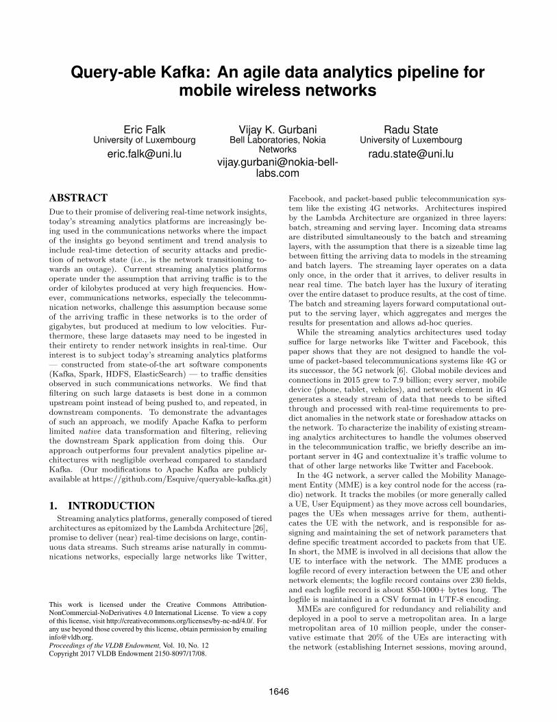
Modifications for Kafka transport efficiency: Aswith theAks architecture, one Spark application is dedicatedto the monitoring of a ProcedureID. The Kafka producersmarshals the entire 2.4 GByte logfile as a single messageand transmit it (compressed) to the Kafka broker efficiently.To transport the messages to Kafka in an efficient way, themessage format had to undergo minor modifications in re-gards to compression. In Kafka, messages consists of a fixedsize header followed by a variable length byte array repre-senting the key and a variable length byte array representingthe value (the first 4-bytes of the key and value array con-tain their lengths, respectively). Figure 3-A shows a Kafkamessage. Messages are further aggregated into a structurecalled a message set. Figure 3-B shows individual mes-sages, M1,M2, ...Mn, concatenated in a message set, eachmessage Mi consisting of the message layout shown in Fig-ure 3-A. The concatenated messages are compressed usinga codec, which is specified in the attribute element of Fig-ure 3-B. The resulting compressed blob becomes the “outer

Table 2: File sizes and number records/fileRaw file size Gzip size No. records

Log file 2.4 GBytes 214 MBytes 2,834,242Pid1 448 KBytes 105 KBytes 58,133Pid2 150 KBytes 6 KBytes 29,729Pid3 9 MBytes 1 MBytes 1,078,977Pid4 7 MBytes 1 MBytes 861,080

1651

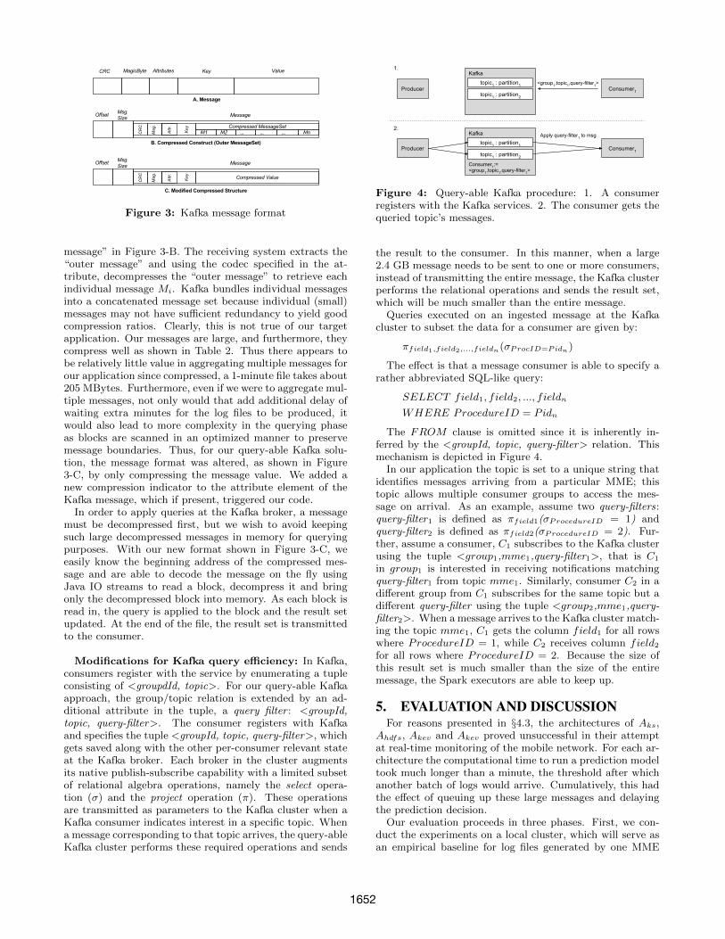
Figure 3: Kafka message format

message” in Figure 3-B. The receiving system extracts the“outer message” and using the codec specified in the at-tribute, decompresses the “outer message” to retrieve eachindividual message Mi. Kafka bundles individual messagesinto a concatenated message set because individual (small)messages may not have sufficient redundancy to yield goodcompression ratios. Clearly, this is not true of our targetapplication. Our messages are large, and furthermore, theycompress well as shown in Table 2. Thus there appears tobe relatively little value in aggregating multiple messages forour application since compressed, a 1-minute file takes about205 MBytes. Furthermore, even if we were to aggregate mul-tiple messages, not only would that add additional delay ofwaiting extra minutes for the log files to be produced, itwould also lead to more complexity in the querying phaseas blocks are scanned in an optimized manner to preservemessage boundaries. Thus, for our query-able Kafka solu-tion, the message format was altered, as shown in Figure3-C, by only compressing the message value. We added anew compression indicator to the attribute element of theKafka message, which if present, triggered our code.

In order to apply queries at the Kafka broker, a messagemust be decompressed first, but we wish to avoid keepingsuch large decompressed messages in memory for queryingpurposes. With our new format shown in Figure 3-C, weeasily know the beginning address of the compressed mes-sage and are able to decode the message on the fly usingJava IO streams to read a block, decompress it and bringonly the decompressed block into memory. As each block isread in, the query is applied to the block and the result setupdated. At the end of the file, the result set is transmittedto the consumer.

Modifications for Kafka query efficiency: In Kafka,consumers register with the service by enumerating a tupleconsisting of <groupdId, topic>. For our query-able Kafkaapproach, the group/topic relation is extended by an ad-ditional attribute in the tuple, a query filter : <groupId,topic, query-filter>. The consumer registers with Kafkaand specifies the tuple <groupId, topic, query-filter>, whichgets saved along with the other per-consumer relevant stateat the Kafka broker. Each broker in the cluster augmentsits native publish-subscribe capability with a limited subsetof relational algebra operations, namely the select opera-tion (σ) and the project operation (π). These operationsare transmitted as parameters to the Kafka cluster when aKafka consumer indicates interest in a specific topic. Whena message corresponding to that topic arrives, the query-ableKafka cluster performs these required operations and sends

Figure 4: Query-able Kafka procedure: 1. A consumerregisters with the Kafka services. 2. The consumer gets thequeried topic’s messages.

the result to the consumer. In this manner, when a large2.4 GB message needs to be sent to one or more consumers,instead of transmitting the entire message, the Kafka clusterperforms the relational operations and sends the result set,which will be much smaller than the entire message.

Queries executed on an ingested message at the Kafkacluster to subset the data for a consumer are given by:

πfield1,field2,...,fieldn(σProcID=Pidn)

The effect is that a message consumer is able to specify arather abbreviated SQL-like query:

SELECT field1, field2, ..., fieldn

WHERE ProcedureID = Pidn

The FROM clause is omitted since it is inherently in-ferred by the <groupId, topic, query-filter> relation. Thismechanism is depicted in Figure 4.

In our application the topic is set to a unique string thatidentifies messages arriving from a particular MME; thistopic allows multiple consumer groups to access the mes-sage on arrival. As an example, assume two query-filters:query-filter1 is defined as πfield1(σProcedureID = 1) andquery-filter2 is defined as πfield2(σProcedureID = 2). Fur-ther, assume a consumer, C1 subscribes to the Kafka clusterusing the tuple <group1,mme1,query-filter1>, that is C1

in group1 is interested in receiving notifications matchingquery-filter1 from topic mme1. Similarly, consumer C2 in adifferent group from C1 subscribes for the same topic but adifferent query-filter using the tuple <group2,mme1,query-filter2>. When a message arrives to the Kafka cluster match-ing the topic mme1, C1 gets the column field1 for all rowswhere ProcedureID = 1, while C2 receives column field2for all rows where ProcedureID = 2. Because the size ofthis result set is much smaller than the size of the entiremessage, the Spark executors are able to keep up.

5. EVALUATION AND DISCUSSIONFor reasons presented in §4.3, the architectures of Aks,

Ahdfs, Akev and Akev proved unsuccessful in their attemptat real-time monitoring of the mobile network. For each ar-chitecture the computational time to run a prediction modeltook much longer than a minute, the threshold after whichanother batch of logs would arrive. Cumulatively, this hadthe effect of queuing up these large messages and delayingthe prediction decision.

Our evaluation proceeds in three phases. First, we con-duct the experiments on a local cluster, which will serve asan empirical baseline for log files generated by one MME

1652

and executing prediction models for one ProcedureID. Thisphase reveals the inadequacy of the first two architectures,Aks and Ahdfs, to process files larger than 100 MBytes, andfiles larger than 200 MBytes for Aev and Akev. In the secondphase, we increase the size of the MME log files on the localcluster to demonstrate the scalability of our Aqk solution.Finally, using the AWS cloud to provide more compute re-sources, we study the scalability of our system as we scaleboth the number of MMEs (more logfiles) and ProcedureIDs(more computation).

We use the following metrics for evaluation:

• Time To Completion (TTC): The difference of time(in seconds) between the message emitted by the vir-tual MME, and the insertion of the results into elastic-Search. TTC includes latency and measures the timeneeded for end-to-end handling of a logfile.• Time from Producer to Kafka cluster (TPK): For ar-

chitectures using Kafka, the time required (in seconds)to send a logfile from the MME and ingest it intoKafka. TPK is an integral part of TTC but shownseparately to better estimate computational time ofthe Spark application.• Main Memory Consumption (MEM): The memory al-

located (in MBytes) by a process at a given time T .Throughout the evaluation, a cumulative MEM is used,which corresponds to MEM consumption on all con-cerned nodes that execute any Spark- or Kafka-relatedprocesses.• CPU usage (CPU): Cumulative percentage of the CPU

used by a process at a time T .

A custom Java Management Extension (JMX) [18] wasdeveloped for system resource monitoring, which writes MEMand CPU allocated to each JVM process to a logfile everysecond. To avoid impacting performance with excessive diskI/O, all machines on the local cluster are equipped with flashdrives. On AWS a unique data store is used for logging. AllKafka and Spark related processes are monitored on everynode in the cluster.

5.1 Phase I: Comparing ArchitecturesComparing Aks, Ahdfs and Aqk on the local cluster:

The Aks and Ahdfs architectures were unable to completecomputations within the time constraints for our target ap-plication; Aks could process logfiles that were < 100 MBytesin a timely manner, while Ahdfs saw a bottleneck for files> 150 MBytes. Our query-able Kafka solution (Akq) canprocess files as large as 2.4 GBytes, but to uniformly studythe behaviour of the three architectures we were forced touse the lowest common denominator size of 50 MBytes. Thelocal cluster has sufficient resources to run a single MME asa producer and a single Spark application as a consumerperforming computations for monitoring one ProcedureID.We chose ProcedureID 3 since it had the most observations(c.f. Table 2).

The observed results, discussed below, are similar on thelocal cluster as well as on the AWS cloud, despite the in-creased resources AWS provides to the Spark application.Network bandwidth does not appear to play any role: out-come of the experiments is identical on a 100 Mbps and 1Gbps networks with a savings of 2-3s on the faster network,a difference not enough to tip the balance in favour of thefaster network. This strongly implies that computations are

not network I/O bound but CPU bound, which is in linewith the findings in Shi et al. [34].

Figure 5-A compares TTC for the three architectures pro-cessing 50 MByte files. Aks and Ahdfs performances arealmost equal but are by far outperformed by our solution,Aqk: Ahdfs has a mean TTC of 34.97s, Aks 30.41s, and Aqk

4.66s. Our solution is about 7x (7 times) faster. Figure 5-Bdemonstrates the PDF for the CPU metric. Our solution,Aqk, is uni-modal with density concentrated around 0–10%of CPU usage, with an average usage of 6.02%. The bi-modality of Aks and Ahdfs, also observed by others [34], re-flects the processing in the Spark application: one mode forfiltering and the other for model evaluation. In our solution,filtering is performed by the Kafka cluster, thus the Sparkapplication only incurs model evaluation leading to the lonepeak for the Aqk curve. The Ahdfs architecture is the mostdemanding; CPU mean usage is 39.8%. Its curve is flattercompared to the other two because it is dominated by diskI/O, which interrupts the CPU. The cumulative CPU usageis greater than 100% because multiple cores were involved inHDFS servicing. The Aks architecture is also bi-modal witha mean CPU usage of 20.35%. Our solution outperforms theother two between 3.5x to 6.5x. Figure 5-C shows the PDFfor the MEM metric. Aks is the most resource hungry, withusage ranging from 5 GBytes – 15 GBytes with an averageof 10.3 GBytes. The range of memory required by the Ahdfs

architecture and our solution, Aqk, is almost similar — 2.5GBytes to 9 GBytes — although the peak of Ahdfs is higher.Our solution consumes less RAM (4.5 GBytes) than Ahdfs

(5.2 GBytes).The impact of our solution on system resources is in Fig-

ures 5-D and 5-E. (We do not present results for the Ahdfs

since it does not use Kafka.) Importantly, Figure 5-D showsthat adding our query-able Kafka extension has negligibleimpact on CPU consumption when compared to Aks. TheX-axis measures time, with a log file of 50 MBytes arriv-ing every minute, for the duration of the hour that we ranthe test. Our query-able Kafka solution does, however, im-pact memory. Figure 5-E shows that our solution consumes3.5 GBytes of RAM versus 669 MBytes of RAM used inAks. Memory usage for Aks is cyclic, constantly raising upto 1 GByte before garbage collection is triggered. By con-trast, in our solution memory slowly increases up to 8G Bbefore it starts to decrease; small fluctuations are frequentand accentuated, indicating a more recurrent garbage collec-tion. Overall, the gradual variation of memory allocation ofqueryable Kafka is suggesting the system is not overloaded.

Figure 5-F shows the outcome for the Spark applicationon the Aks architecture as we push it beyond its capabilityto deal with log files of 100 MBytes. For Aks, it is appar-ent that the TTC grows linearly over the hour that we ranthe system. The mean time to process a 100 MByte file inAks is 1,683.62s (28 minutes). Clearly, this does not sufficefor our application! Interestingly, the TPK stays constant,which strongly suggests that the time to send a log file fromthe MME to Kafka is not adding to the processing delay,rather, latency is being added by the Spark application asit deals with the large log files. The curve for query-ableKafka, Aqk, tells a different story altogether. The meantime it takes Aqk to process the 100 MByte file is very low— 6.30s, suggesting that performing the filtering upstreamallows the Spark application to concentrate on computationacross a much smaller result set. There isn’t any curve for

1653

0 10 20 30 40 50 60

010

20

30

40

50

60

Minute

TT

C (

s)

Ahdfs µ = 34.97 s

Aks µ = 30.41 s

Aqk µ = 4.66 s

(a) TTC (50 MByte log file)

0 50 100 150

0.0

00.1

00.2

00.3

0

Cumul. Spark CPU (%)

Density

Ahdfs µ = 39.8 %

Aks µ = 20.35 %

Aqk µ = 6.02 %

Model Evaluation

Model EvaluationFiltering

(b) Spark CPU (50 MByte log file)

0 5000 10000 15000

01.5

e−

43e−

4

Cumul. Spark MEM (MB)

Density

Ahdfs µ = 5220.71 MB

Aks µ = 10378.43 MB

Aqk µ = 4567.4 MB

(c) Spark MEM (50 MByte log file)

26

10

µ = 3.19 %

Ass

0 10 20 30 40 50 60

24

68

µ = 2.94 %

Aqk

PCMD file for minute

Cum

ula

ted K

afk

a C

PU

usage in %

(d) Kafka CPU (50 MByte log file)

200

800

µ = 633.5 MB

Ass

0 10 20 30 40 50 60

500

2000

µ = 1209.07 MB

Aqk

PCMD file for minute

Cum

ula

ted K

afk

a M

em

ory

usage in M

B

(e) Kafka MEM (50 MByte log file)

0 10 20 30 40 50 60

Minute

TT

C (

s)

[in logscale

]

03

10

70 TTC Aks µ = 1683.62 s

TTC Aqk µ = 6.3 s

TPK µ = 5.09 s

(f) TTC Aks (100 MByte log file)

Figure 5: Comparing Division I architectures during Phase I

Ahdfs because there is no easy way to determine in HDFSwhen a file has been completely written to the distributedstore.

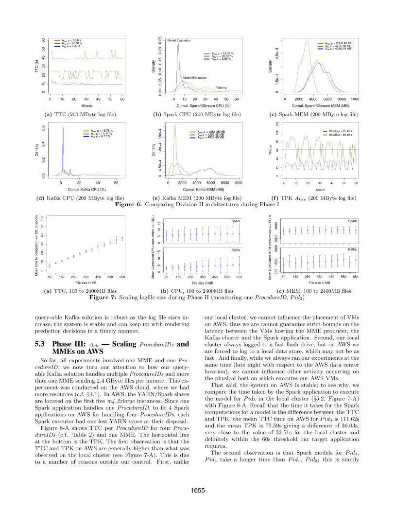
Comparing Aev, Akev and Aqk on the local cluster:The architectures in Division II proved to be more stable andbetter behaved than their Division I counterparts; they areable handle file sizes > 50 MBytes. Figure 6-F demonstratesthat with 200 MByte files, the TPK for Akev is below 60s butbecomes larger when file size increases. Pushing files > 200MBytes when using the Kafka KStreams ETL application inAkev leads to unstable behaviour. The unstable behaviour ischaracterized by a larger standard deviation; with an unpre-dictable TPK, the sliding window is unable to gather enoughrecords to constitute a stable distribution that would allowus to start the predictive task. We, therefore, use a file sizeof 200 MBytes for Division II architectures when comparingthem against our query-able Kafka solution.

Figure 6-A shows our solution with a 2x and almost 4xadvantage over Aev and Akev, respectively. On AWS, TTCsaw minimal improvement, although this was expected on acluster hosted on more powerful machines where each eachKafka broker had its own hard drive. We recognize, how-ever, that allocation of hardware resources on AWS cannotbe guaranteed. Figure 6-B shows the same uni-modal be-haviour of the CPU metric for our solution when comparedto the bi-modal behaviour of other two (for the same rea-sons). Aqk, our solution, uses the least amount of CPU.The difference in Spark MEM consumption (Figure 6-C) be-tween Division I and II is more stark. While in Division I,our solution proved better, here Akev is better (2.9 GByte).The reason is that KStreams, used by Akev, contributes tolow memory consumption. Regarding Kafka’s resource con-sumption,our solution, Aqk, outperforms Aev and Akev by

about 3x and 4x, respectively (Figure 6-D). This contrastswell with Division I architecture (Figure 5-D) where KafkaCPU metrics were about the same. In the Kafka MEM met-ric, Akev performs better due to KStreams (Figure 6-E).

5.2 Phase II: Aqk — Scaling file size on localcluster

Among all architectures, our query-able Kafka solution isthe only one that can scale to log file size of 2.4 GBytes.Therefore, we focus on its behaviour as we increase the filesize with one MME and one Spark application monitoringPid3.

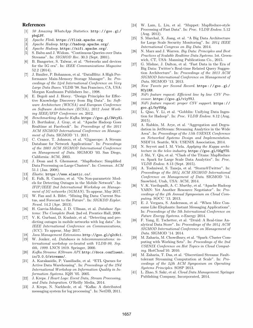
Figure 7-A shows that when the ETL filtering occurrs up-stream, as in our query-able Kafka solution, Spark can han-dle computations fast enough to guarantee a stable system.File size is increased in 100 MByte increments starting from100 MBytes and going to 2.4 GBytes. The time it takes forSpark computations is the difference in time between theTTC and the TPK. For a 2.4 GByte file, TTC is 77.84s andTPK is 44.33s, thus the time it takes for Spark to run themodel is 33.51s, which is well within the 60s threshold ourtarget application needs. Figure 7-B plots the CPU usageof the Kafka cluster and Spark application. For 2.4 GBytelog files, Kafka shows an average CPU consumption of 17%(σ = 17%) and Spark utilizes 15% (σ = 12.7%). Figure7-C shows the MEM metric. Spark memory remains con-stant at an average of 5.2 GBytes (σ = 1.1 GByte), evenas the log file size increases to 2.4 GBytes. Kafka memoryshows some variations. For a 2.4 GByte log file, Kafka uses,on the average, 7.3 GBytes (σ = 1.5 GBytes) memory. Asthe file sizes increase, Kafka memory converges to about 9GBytes distributed across 4 brokers, or 2.3 GByte RAM perbroker. This is a reasonable outcome, especially consideringthat the TPK is well bounded below 60s. In summary, our

1654

0 10 20 30 40 50 60

010

20

30

40

50

60

Minute

TT

C (

s)

Akev µ = 39.6 sAev µ = 20.91 sAqk µ = 9.37 s

(a) TTC (200 MByte log file)

0 10 20 30 40 50 60

0.0

00.0

50.1

00.1

50.2

00.2

5

Cumul. Spark/KStream CPU (%)

Density

Akev µ = 19.38 %Aev µ = 20.98 %Aqk µ = 6.88 %

Model Evaluation

Model Evaluation

Filtering

(b) Spark CPU (200 MByte log file)

0 2000 4000 6000 8000 10000

01.5

e−

44.5

e−

4

Cumul. Spark/KStream MEM (MB)

Density

Akev µ = 2908.43 MBAev µ = 4705.88 MBAqk µ = 4936.15 MB

(c) Spark MEM (200 MByte log file)

0 20 40 60

0.0

0.2

0.4

0.6

Cumul. Kafka CPU (%)

Density

Akev µ = 18.76 %Aev µ = 11.41 %Aqk µ = 4.17 %

(d) Kafka CPU (200 MByte log file)

0 2000 4000 6000 8000 10000

04.5

e−

412e−

418e−

4

Cumul. Kafka MEM (MB)

Density

Akev µ = 1051.35 MBAev µ = 1292.45 MBAqk µ = 4933.49 MB

(e) Kafka MEM (200 MByte log file)

0 10 20 30 40 50 60

02

04

06

08

01

00

12

0

Minute

TP

K (

s)

200MB µ = 25.45 s

300MB µ = 60.89 s

(f) TPK Akev (200 MByte log file)

Figure 6: Comparing Division II architectures during Phase I

010

20

30

40

50

60

50 150 250 350 450 550 650

File size in MB

Mean tim

e to c

om

ple

tion +

/− S

D, in

seconds

(a) TTC, 100 to 2400MB files

05

10

15 Spark

05

10

15

50 150 250 350 450 550 650

Kafka

File size in MB

Mean C

um

ula

ted C

PU

consum

tion +

/− S

D, in

%

(b) CPU, 100 to 2400MB files

2000

6000

Spark

500

1500

3000

50 150 250 350 450 550 650

Kafka

File size in MB

Mean C

um

ula

ted M

EM

consum

tion +

/− S

D, in

MB

(c) MEM, 100 to 2400MB files

Figure 7: Scaling logfile size during Phase II (monitoring one ProcedureID, Pid3)

query-able Kafka solution is robust as the log file sizes in-crease, the system is stable and can keep up with renderingprediction decisions in a timely manner.

5.3 Phase III: Aqk — Scaling ProcedureIDs andMMEs on AWS

So far, all experiments involved one MME and one Pro-cedureID ; we now turn our attention to how our query-able Kafka solution handles multiple ProcedureIDs and morethan one MME sending 2.4 GByte files per minute. This ex-periment was conducted on the AWS cloud, where we hadmore resources (c.f. §4.1). In AWS, the YARN/Spark slavesare located on the first five m4.2xlarge instances. Since oneSpark application handles one ProcedureID, to fit 4 Sparkapplications on AWS for handling four ProcedureIDs, eachSpark executor had one less YARN vcore at their disposal.

Figure 8-A shows TTC per ProcedureID for four Proce-dureIDs (c.f. Table 2) and one MME. The horizontal lineat the bottom is the TPK. The first observation is that theTTC and TPK on AWS are generally higher than what wasobserved on the local cluster (see Figure 7-A). This is dueto a number of reasons outside our control. First, unlike

our local cluster, we cannot influence the placement of VMson AWS, thus we are cannot guarantee strict bounds on thelatency between the VMs hosting the MME producer, theKafka cluster and the Spark application. Second, our localcluster always logged to a fast flash drive, but on AWS weare forced to log to a local data store, which may not be asfast. And finally, while we always ran our experiments at thesame time (late night with respect to the AWS data centerlocation), we cannot influence other activity occurring onthe physical host on which executes our AWS VMs.

That said, the system on AWS is stable; to see why, wecompare the time taken by the Spark application to executethe model for Pid3 in the local cluster (§5.2, Figure 7-A)with Figure 8-A. Recall that the time it takes for the Sparkcomputations for a model is the difference between the TTCand TPK; the mean TTC time on AWS for Pid3 is 111.62sand the mean TPK is 75.59s giving a difference of 36.03s,very close to the value of 33.51s for the local cluster anddefinitely within the 60s threshold our target applicationrequires.

The second observation is that Spark models for Pid3,Pid4 take a longer time than Pid1, Pid2; this is simply

1655

80

10

01

20

14

01

60

18

0

Pid1 Pid2 Pid3 Pid4

Pid1 µ = 92 s

Pid2 µ = 91.36 s

Pid3 µ = 111.62 s

Pid4 µ = 115.03 s

TPK µ = 75.59 s

Pid1 Pid2 Pid3 Pid4

Pid1 µ = 91.45 s

Pid2 µ = 90.48 s

Pid3 µ = 107.95 s

Pid4 µ = 117.62 s

TPK µ = 72.91 s

(a) 1 MME (b) 2 MMEs

Tim

e (

s)

Figure 8: Scaling ProcedureIDs and MMEs on AWS duringPhase III on 2.4 GByte logfiles

due to the fact that the former pair of ProcedureIDs havemore observations compared to the latter pair (c.f. Table 2),consequently it takes longer to run the models. However,all models complete within the 60s time required by ourtarget application. Finally, note that AWS offers us enoughresources that we are running four Spark applications, onefor each ProcedureID and are able to handle the load for 1MME without any problems. We could not do this on ourlocal cluster due to resource limitations.

Figure 8-B shows that even as we add another MME thatgenerates an additional 2.4 GBytes log files per minute, thesystem is able to sustain the load in stable state. With twoMMEs, the Kafka brokers are serving four consumer groupsnow subscribing to two topics, one for each MME. Addinga second MME has virtually no effect on the TTCs and theTPK even though twice as many log files are being pro-cessed. The boxplots of the ProcedureIDs between Figures8-A and -B are similar with minor variations in the medianvalues of Pid4. Bolstering our argument that adding a sec-ond MME does not impact processing is Table 3; for CPUand MEM metrics on Spark and Kafka, there is very littleappreciable difference between the system processing loadfrom one MME versus two MMEs. The impact on CPU andMEM is not the number of MMEs, but rather the numberof ProcedureIDs monitored as the analysis next shows.

Table 4 summarizes the results of Spark and Kafka ana-lyzing 2.4 GByte files for 1 and 4 ProcedureIDs. For SparkMEM, there is a linear relation for moving from one Proce-

Table 3: MEM and CPU with 4 monitored Proce-dureIDs and two MMEs

1 MME 2 MME

CPU (%)Spark

mean 13.68 15.11σ 9.77 9.27

Kafka mean 69.53 67.35σ 69.601 67.881

MEM (GB)Spark

mean 20 19.7σ 2.9 2.9

Kafka mean 20 20σ 7.6 7.7

1 σ is larger than mean because the data is dis-persed.

Table 4: Scalability for ProcedureIDs1 ProcedureID 4 ProcedureIDs

SparkMEMCPU

5.2 GBytes15%

20 GBytes13.68%

KafkaMEMCPU

9 GBytes17%

20 GBytes69.53%

dureID to four; for n ProcedureIDs, Spark will use n ∗ 5.2GBytes RAM. Spark CPU, on the other hand, remains ap-proximately constant as number of ProcedureIDs increasesto four. However, we expect it to increase if tens of Proce-dureIDs are monitored. Looking at Kafka resources, KafkaMEM exhibits a linear relation as well, although by a smallermultiplier (0.5n∗9 GBytes RAM for n ProcedureIDs). KafkaCPU uses n ∗ 17% for monitoring n ProcedureIDs. Clearly,the number of ProcedureIDs dictates resources usage; it isour expectation that while there are over 70 ProcedureIDs,practical and domain considerations limit analysis to a few.

Our investigations reveal that two MMEs is the limit thatour cluster on AWS can handle. This limitation is imposedby Spark, not by our query-able Kafka solution, which is ableto scale to more MMEs under the assumption that a hand-ful of ProcedureIDs are monitored. As per the discussion onFigure 8-A, the Spark application renders a prediction deci-sion in 36.03s. With two MMEs producing log files, it willtake the Spark application about a minute to execute themodels. Anything beyond two MMEs will lead to queuedmessages, making real-time prediction impossible. To scaleout to > 2 MMEs, the Spark application can be replicatedon a cluster subscribing to the Kafka topics reserved forthe new MMEs. We have shown that assuming a reasonablenumber of monitored ProcedureIDs, our system scales out byallocating additional YARN/Spark clusters. This is not anunrealistic assumption; service providers are more interestedin scaling the number of MMEs to cover large geographic ar-eas than they are in monitoring more ProcedureIDs/MME.

6. CONCLUSION AND FUTURE WORKTo address the real-time nature of the prediction decisions

required while handling GByte sized messages, we proposemoving ETL upstream, specifically, in an analytics pipeline,to move the ETL to messaging layer (Kafka) thus allowingmultiple speed layers (Spark application) to perform purecomputational tasks. We have further demonstrated the vi-ability of this approach through our query-able Kafka solu-tion, which scales with the workload.

In future work, we will examine the impact on the Kafkawith evolving query changes, with special emphasis on resultset size and the nature of query operations vs. predicate con-ditions. Current supported operations are projection, selec-tion and simple comparison predicates; we will explore thepossibility of expanding the operations and predicates withthe understanding that we do not want to turn Kafka intoa full SQL engine, but provide it enough relational powerwhile keeping it agile. Our query-able Kafka solution inte-grates querying in the internal load balancing scheme in arudimentary fashion. In future work we will take in accountoptimal querying for partition placement and partition I/O.

The code for query-able Kafka modifications described in§4.4 is available in a GIT repository athttps://github.com/Esquive/queryable-kafka.git.

1656

References[1] 50 Amazing WhatsApp Statistics. http://goo.gl/

pbqL9Y.[2] Apache Flink. https://flink.apache.org.[3] Apache Hadoop. http://hadoop.apache.org/.[4] Apache Hadoop. https://nifi.apache.org/.[5] S. Babu and J. Widom. “Continuous Queries over Data

Streams”. In: SIGMOD Rec. 30.3 (Sept. 2001).[6] B. Bangerter, S. Talwar, et al. “Networks and devices

for the 5G era”. In: IEEE Communications Magazine52.2 (2014).

[7] J. Baulier, P. Bohannon, et al. “DataBlitz: A High Per-formance Main-Memory Storage Manager”. In: Pro-ceedings of the 24rd International Conference on VeryLarge Data Bases. VLDB ’98. San Francisco, CA, USA:Morgan Kaufmann Publishers Inc., 1998.

[8] E. Begoli and J. Horey. “Design Principles for Effec-tive Knowledge Discovery from Big Data”. In: Soft-ware Architecture (WICSA) and European Conferenceon Software Architecture (ECSA), 2012 Joint Work-ing IEEE/IFIP Conference on. 2012.

[9] Benchmarking Apache Kafka. https://goo.gl/3WtyXl.[10] D. Borthakur, J. Gray, et al. “Apache Hadoop Goes

Realtime at Facebook”. In: Proceedings of the 2011ACM SIGMOD International Conference on Manage-ment of Data. SIGMOD ’11. 2011.

[11] C. Cranor, T. Johnson, et al. “Gigascope: A StreamDatabase for Network Applications”. In: Proceedingsof the 2003 ACM SIGMOD International Conferenceon Management of Data. SIGMOD ’03. San Diego,California: ACM, 2003.

[12] J. Dean and S. Ghemawat. “MapReduce: SimplifiedData Processing on Large Clusters”. In: Commun. ACM51.1 (Jan. 2008).

[13] Elastic. https://www.elastic.co/.[14] E. Falk, R. Camino, et al. “On Non-parametric Mod-

els for Detecting Outages in the Mobile Network”. In:IFIP/IEEE 2nd International Workshop on Manage-ment of 5G networks (5GMAN). To appear, May 2017.

[15] W. Fan and A. Bifet. “Mining Big Data: Current Sta-tus, and Forecast to the Future”. In: SIGKDD Explor.Newsl. 14.2 (Apr. 2013).

[16] H. Garcia-Molina, J. D. Ullman, et al. Database Sys-tems: The Complete Book. 2nd ed. Prentice Hall, 2008.

[17] V. K. Gurbani, D. Kushnir, et al. “Detecting and pre-dicting outages in mobile networks with log data”. In:IEEE International Conference on Communications,(ICC). To appear, May 2017.

[18] Java Management Extensions. http://goo.gl/q2cNc1.[19] W. Jonker, ed. Databases in telecommunications: in-

ternational workshop co-located with VLDB-99, Sep.6th, 1999. LNCS 1819. Springer, 2000.

[20] Kafka Streams: KStream API. http://docs.confluent.io/3.0.0/streams/.

[21] A. Karakasidis, P. Vassiliadis, et al. “ETL Queues forActive Data Warehousing”. In: Proceedings of the 2NdInternational Workshop on Information Quality in In-formation Systems. IQIS ’05. 2005.

[22] J. Kreps. I Heart Logs: Event Data, Stream Processing,and Data Integration. O’Reilly Media, 2014.

[23] J. Kreps, N. Narkhede, et al. “Kafka: A distributedmessaging system for log processing”. In: NetDB, 2011.

[24] W. Lam, L. Liu, et al. “Muppet: MapReduce-styleProcessing of Fast Data”. In: Proc. VLDB Endow. 5.12(Aug. 2012).

[25] S. Marchal, X. Jiang, et al. “A Big Data Architecturefor Large Scale Security Monitoring”. In: 2014 IEEEInternational Congress on Big Data. 2014.

[26] N. Marz and J. Warren. Big Data: Principles and BestPractices of Scalable Realtime Data Systems. 1st. Green-wich, CT, USA: Manning Publications Co., 2015.

[27] G. Mishne, J. Dalton, et al. “Fast Data in the Era ofBig Data: Twitter’s Real-time Related Query Sugges-tion Architecture”. In: Proceedings of the 2013 ACMSIGMOD International Conference on Management ofData. SIGMOD ’13. 2013.

[28] New Tweets per Second Record. https://goo.gl/

NCylRN.[29] NiFi feature request: Efficient line by line CSV Pro-

cessor. https://goo.gl/v1yYVJ.[30] NiFi feature request: proper CSV support. https://

goo.gl/hyV5Kg.[31] L. Qiao, Y. Li, et al. “Gobblin: Unifying Data Inges-

tion for Hadoop”. In: Proc. VLDB Endow. 8.12 (Aug.2015).

[32] A. Rabkin, M. Arye, et al. “Aggregation and Degra-dation in JetStream: Streaming Analytics in the WideArea”. In: Proceedings of the 11th USENIX Conferenceon Networked Systems Design and Implementation.NSDI’14. Seattle, WA: USENIX Association, 2014.

[33] N. Seyvet and I. M. Viela. Applying the Kappa archi-tecture in the telco industry. https://goo.gl/0OgYTO.

[34] J. Shi, Y. Qiu, et al. “Clash of the Titans: MapReducevs. Spark for Large Scale Data Analytics”. In: Proc.VLDB Endow. 8.13 (Sept. 2015).

[35] A. Toshniwal, S. Taneja, et al. “Storm@Twitter”. In:Proceedings of the 2014 ACM SIGMOD InternationalConference on Management of Data. SIGMOD ’14.Snowbird, Utah, USA: ACM, 2014.

[36] V. K. Vavilapalli, A. C. Murthy, et al. “Apache HadoopYARN: Yet Another Resource Negotiator”. In: Pro-ceedings of the 4th Annual Symposium on Cloud Com-puting. SOCC ’13. 2013.

[37] E. J. Vergara, S. Andersson, et al. “When Mice Con-sume Like Elephants: Instant Messaging Applications”.In: Proceedings of the 5th International Conference onFuture Energy Systems. e-Energy 2014.

[38] F. Yang, E. Tschetter, et al. “Druid: A Real-time An-alytical Data Store”. In: Proceedings of the 2014 ACMSIGMOD International Conference on Management ofData. SIGMOD ’14. 2014.

[39] M. Zaharia, M. Chowdhury, et al. “Spark: Cluster Com-puting with Working Sets”. In: Proceedings of the 2ndUSENIX Conference on Hot Topics in Cloud Comput-ing. HotCloud’10. 2010.

[40] M. Zaharia, T. Das, et al. “Discretized Streams: Fault-tolerant Streaming Computation at Scale”. In: Pro-ceedings of the 24th ACM Symposium on OperatingSystems Principles. SOSP 2013.

[41] L. Zhao, S. Sakr, et al. Cloud Data Management. SpringerPublishing Company, Incorporated, 2014.

1657