Quantum Random WalksQuantum Random Walks

Combinatorial and Computational Aspects of Statistical Physics/Random Graphs and Structures Cambridge, September 5, 2002

Julia Kempe

Computer Science Division and Department of Chemistry,

University of California, Berkeley&

CNRS & LRI, Université de Paris-Sud, France

Towards nanotechnology

Size of the components

Number of components

Speed

Gordon Moore 1965

prevent or use quantum effects ?

Theoretical limitations reached in 2020 !!!

Apparition of quantum phenomena

Information is physical!

Use the laws of quantum mechanics for the basic components of an

information processing machine!Quantum computingQuantum cryptographyQuantum information …

Main applications

Cryptography Protocol of unconditionally secure secret key distribution

[Bennett, Brassard 84]Implementation : ~ 100 km

Quantum information Teleportation [B, B, Crépeau, Jozsa, Peres, Wooters 93] Implementation [Bouwmeester, Pan, Mattle, Eibl, Weinfurter,

Zeilinger 97]

Algorithms Factoring, discrete logarithm, ... [Shor 94] Database search [Grover 96]Num. of qubits ? 1995 : 2, 1998 : 3, 2002 : 8 [Chuang (IBM)] - 10 [Los

Alamos]

The qubit

Classical bit: b{0,1}Probabilistic bit: probability distribution dR+

{0,1} such that ||d||1 =1. d=(p,1-p) with p [0,1]

Quantum bit: | C{0,1} such that || | ||2=1.

| = |0 + |1 with | | 2+ | | 2=1

(Dirac notation)

β

α ,

1

0 1 ,

0

1 0 ψ

* * *0 1,0 , 1 0,1 , ,t

0| , = 1|

Qubit evolution

Measure: reads and modifies

Measure| | 2

| | 2

|0 + |1|0

|1

Superposition Probability distribution

Unitary transformation: U C22 such that UU†=Id

| U |’ = U |

unitary reversible:

U| U† |

2( ) |

| |

p i i

i i

Example

Superposition:

Measure:

13

20

3

1

Measure1/3

2/3

|0

|1|

11

3 2

13d

23

Example

Superposition:

Measure:

Unitary transformations:

NOT: |0 |1

Hadamard:

13

20

3

1

Measure1/3

2/3

|0

|1|

| U |’ = U |

01

10

x

11

11

2

1H

13

10

3

2ψ x

16

210

6

21

2

10

3

2

2

10

3

1ψ

H

H

Quantum computer: n qubits n qubits tensor product | C{0,1}n such that || | ||

2=1.

| = x{0,1}n x |x with x |x |2 =1 Measure

Partial Measure

Measure|x | 2

x{0,1}n x |x |x

Measure

Second bit = 0 (||2 + | |2 )

|00+ |01+ |10+ |11 22

1000

γα

γα

Quantum computer: n qubits n qubits tensor product | C{0,1}n such that || | ||

2=1.

| = x{0,1}n x |x with x |x |2 =1 Measure

Partial Measure

Unitary transformation | U| with U U(2n)

ex: XOR=

Measure|x | 2

x{0,1}n x |x |x

Measure

Second bit = 0 (||2 + | |2 )

|00+ |01+ |10+ |11 22

1000

γα

γα

0100

1000

0010

0001|00 |01 |10 |11

+

|i|j

|i |XOR(i,j)

Quantum computing a function

Let f: {0,1}n {0,1}m

x f(x)

Reversible: Rf :{0,1}n+m {0,1}n+m

(x,y) (x,yf(x))

Quantum:Uf U(2n+m): Cn+m Cn+m

|x|y |x|yf(x)

Simplest Quantum Algorithm:Deutsch’s Problem

Input: function f:{0,1}{0,1} (in black box) Question: f constant (f(0)=f(1)) or balanced (f(0)f(1)) ?

Quantum black box (reversible):

Algorithm: one query only!!!

f|x|y

|x|yf(x)

fHH

H|0|1

Measure|0 -constant|1 -balanced

Simplest Quantum Algorithm:Deutsch’s Problem

Input: function f:{0,1}{0,1} (in black box) Question: f constant (f(0)=f(1)) or balanced (f(0)f(1)) ?

Quantum black box (reversible):

Algorithm: one query only!!!

f|x|y

|x|yf(x)

fHH

H|0|1

Measure|0 -constant|1 -balanced

12

110

2

11101101

2

1

)1()1(1)0()0(02

11010

2

110

)1()0()1()0()1()0(

ffffHff

fHH ffff

=0 if f balanced =0 if f constant

Universal computation

Classical circuit model:

Quantum circuit model:

• evaluates boolean functions• can be constructed from universal local gates (ex.: NAND, COPY)

010…1

bits

0

0

• unitary transformations U

qubits

|0

|0

|1

|1

|0

|0

Measure

U

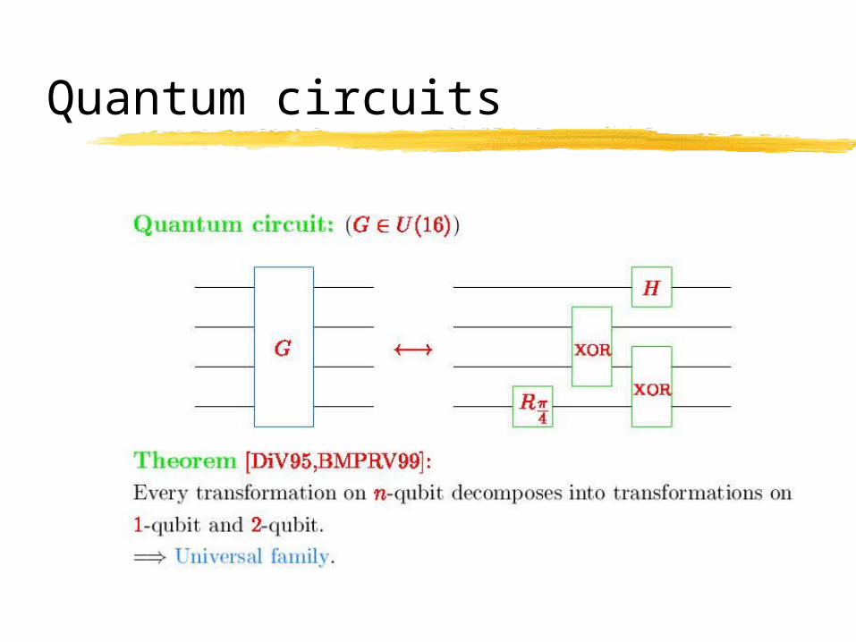
Quantum circuits

Quantum CircuitsQuantum circuits can simulate classical

circuits efficiently (with polynomial overhead)

Classical circuits can be efficiently simulated by classical reversible circuits; universal reversible gate – e.g. Toffoli-gate

Toffoli-gate can be generated with local unitary gates on a quantum computer

-> Classical circuits Quantum circuits

Quantum algorithms

Deutsch-Jozsa algorithm (’92): determines if a function (black box) is constant or 2-1 with only one query

Simon ’s algorithm (’94): period finding

Quantum algorithms

Deutsch-Jozsa algorithm (’92): determines if a function (black box) is constant or 2-1 with only one query

Simon ’s algorithm (’94): period finding Shor (’95): efficient factoring general problem (factoring, discrete log) = hidden

subgroup: Input: function f: G G s.t. f(x)=f(x+H) where H G Output: H (generators) efficient quantum algorithm if G - Abelian or « special »

Quantum algorithms

Deutsch-Jozsa algorithm (’92): determines if a function (black box) is constant or 2-1 with only one query

Simon ’s algorithm (’94): period finding Shor (’95): efficient factoring general problem (factoring, discrete log) = hidden

subgroup: Input: function f: G G s.t. f(x)=f(x+H) where H G Output: H (generators) efficient quantum algorithm if G - Abelian or « special »

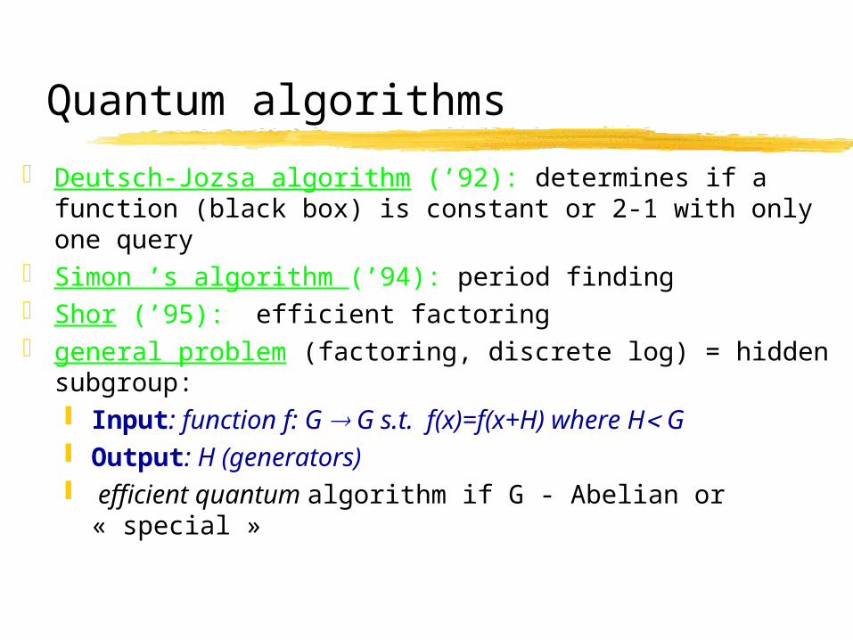
Grover (’96): Search of one entry in a database of size N with queries (Classical lower bound is (N))

(quantum lower bound)

( )N( )N

Discrete Quantum Walks

Discrete-time walks on finite graphs (Mixing Time) *:

Dorit Aharonov (Hebrew University) Andris Ambainis (IAS, Princeton) J. K. (LRI, Orsay&UC Berkeley) Umesh Vazirani (UC Berkeley)

(*STOC’01)

Mixing on the Hypercube:

C. Moore and A. Russel (quant-ph’01)

Polynomial hitting time on the Hypercube:

J. K. ( ’02+)

hitting time on other graphs (numerical & Analytical studies):

Neil Shenvi and J. K. (in preparation ‘02)

Markov chains

Markov chains for algorithms:

IdeaIdea: construct a Markov chain (simple, local transitions only, efficiently implementable) (1) whose stationary distribution gives the

solution to the problem Mixing timeMixing time or (2) which hits the desired solution

Hitting timeHitting time

« Quantum » Markov chains ?« Quantum » Markov chains ?

Example: Random walk for 2SAT

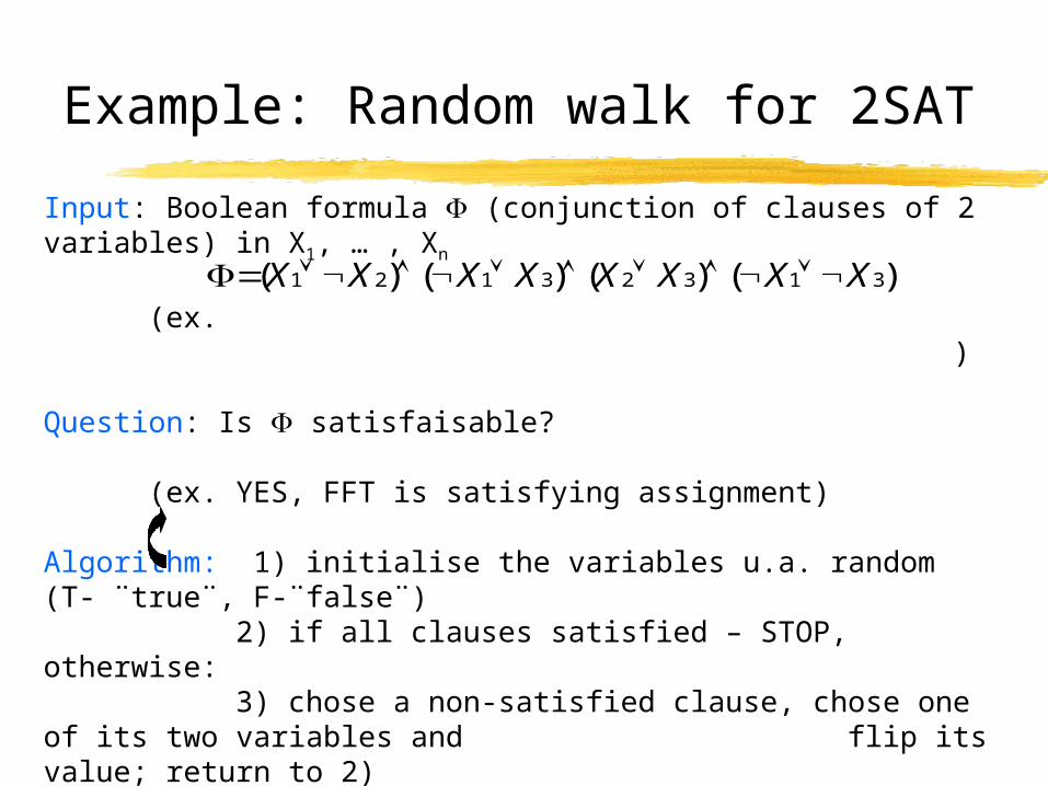
Input: Boolean formula (conjunction of clauses of 2 variables) in X1, … , Xn

(ex. )

Question: Is satisfaisable?

(ex. YES, FFT is satisfying assignment)

Algorithm: 1) initialise the variables u.a. random (T- ¨true¨, F-¨false¨) 2) if all clauses satisfied – STOP, otherwise: 3) chose a non-satisfied clause, chose one of its two variables and flip its value; return to 2)

)()()()( 31323121 XXXXXXXX

Example: Random walk for 2SAT

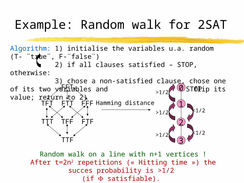
Algorithm: 1) initialise the variables u.a. random (T- ¨true¨, F-¨false¨) 2) if all clauses satisfied – STOP, otherwise: 3) chose a non-satisfied clause, chose one of its two variables and flip its value; return to 2)

FFT

TFT FFFFTT

FTFTFFTTT

TTF

0

1

2

3

STOP>1/2

>1/2

>1/2 <1/2

<1/2Hamming distance

Random walk on a line with n+1 vertices !After t=2n2 repetitions (« Hitting time ») the succes probability is >1/2

(if satisfiable).

Random Walks...3SAT - “biased” random walk with

exponential hitting time

in general : local, simple Markov chain on exponential domain

0 1

>1/3

<2/3

2

>1/3

<2/3<2/3

>1/3

3 4

>1/3

<2/3

5

<2/3

>1/3

STOP

(fastest known 3-SAT algorithm based on random walk [Schöning’99, Hofmeister, Schöning & Watanabe’02])

Random Walks... Random walk on the line: Mixing time=Hitting

time =O(n2) stationary dist.=uniform

Questions: Stationary distribution? (ergodic –>

independent of initial state?) Mixing time? Hitting time?

Methods: spectral gap, conductance, Log Sobolev, coupling, ………

1/21/2

O(n2)

Classical/quantum random walksClassical

Transition matrix:

translationally invariant

Dt(i)-distribution after time t

stationary distribution

measure of “closeness”: total variation distance

mixing time - time until <const.

1/21/2

O(n2)

)( jiprobM ij

πDlim tt

t

i

t π(i)(i)D2

1πD t

Classical/quantum random walksClassical Quantum

Transition matrix:

translationally invariant

Dt(i)-distribution after time t

stationary distribution

measure of “closeness”: total variation distance

mixing time - time until <const.

1/21/2

O(n2)

21 +

21

?

)( jiprobM ij

πDlim tt

t

i

t π(i)(i)D2

1πD t

unitary?reversible?

localtranslationally invariant

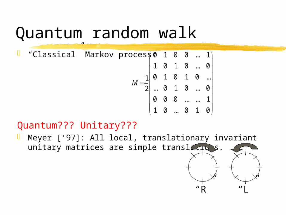
Quantum random walk “Classical” Markov process:

Quantum??? Unitary??? Meyer [‘97]: All local, translationary invariant unitary

matrices are simple translations.

“R” “L”

0 1 0 0 ... 1

1 0 1 0 ... 0

0 1 0 1 0 ...1... 0 1 0 ... 020 0 0 ... ... 1

1 0 ... 0 1 0

M

Classical random walk Incorporate “coin-flip” into walk!

Classical walk in two steps:{,} ={(,0),(,0),(,1),…,(,n-1),(,n-1)}

flip direction coin C=

perform controlled shift S: “R”   

“L”    M=S•C Trace out (ignore, average over) the direction-

space

“R” “L”

1 1 1 01 " "= " "=

1 1 0 12

Classical random walk

{,} ={(,0),(,0),(,1),…,(,n-1),(,n-1)}

  M=S•C Trace out (ignore, average over) the direction-space

1 1

1 1

1 11

1 1C 2

...

1 1

1 1

flip direction coin perform controlled shift : “R”   

“L”   

S =

1 0

0 0

0 0

0 1

……

…

Quantum random walk Meyer [‘97]: All local, translationary invariant unitary

matrices are simple translations.

“coined” walk in two steps:

{|,|}

”flip” direction coin ( )

perform controlled shift : | “R”   

| “L”   

1 1

2 2

“R” “L”

unitary “walk” U

U “collapses” to the classical random walk if we measure directions or positions at every step!

HH

1 11

1 -12

Quantum random walk

{,} ={(,0),(,0),(,1),…,(,n-1),(,n-1)}

  M=S•C After t steps measure Trace out (ignore, average over) the direction-space

“R” “L”

1 1

1 1

1 11

1 1C 2

...

1 1

1 1

flip direction coin perform controlled shift : “R”   

“L”   

S =

1 0

0 0

0 0

0 1

……

Quantum random walksExample: start in

induces probability-dist. Pt(i) on the sites (after measurement)

Convergence?Convergence?

NO! U is unitary reversible! (no stationary distrib.)

Def. “averaged distribution” Qt (Cesaro limit):

Theorem: QTheorem: Qtt converges to a stationary distribution. converges to a stationary distribution.

|0|1

|2

|n-1

0

1 1 2 0 0 2H shift 0 1 1H shift

2 0 2 ...2 H shift

U 0 t

t

t ss 0

1Q (v) P

t( )v

1 1

2 2

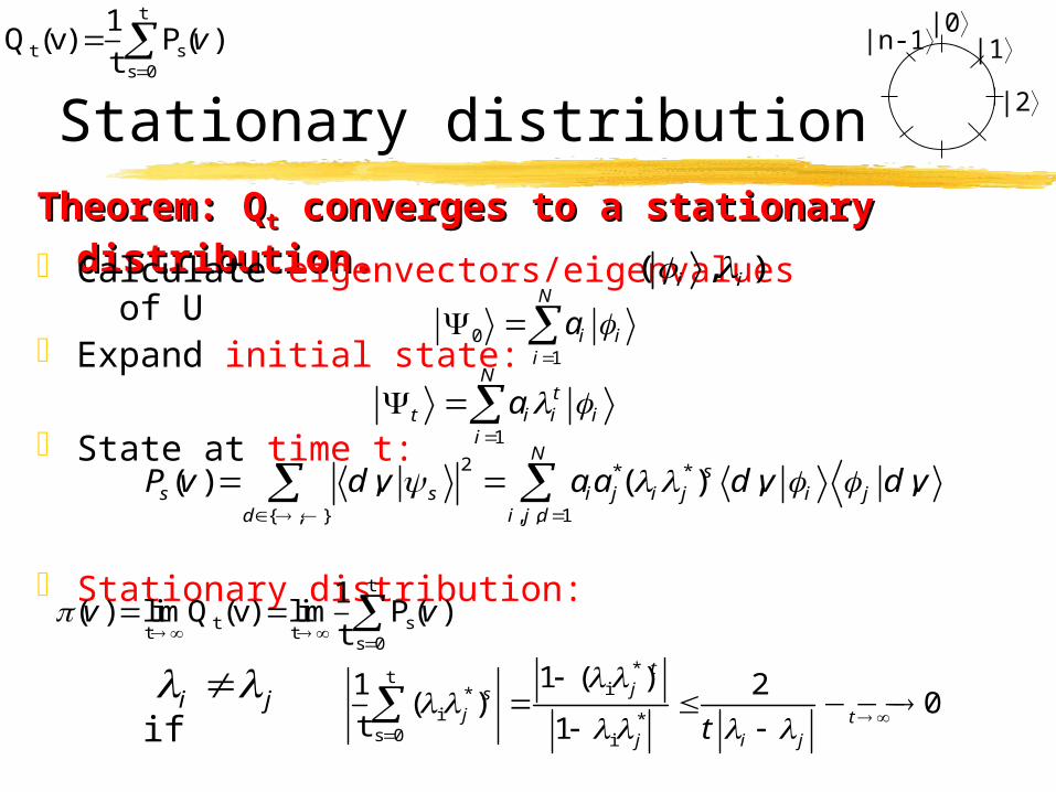
Stationary distributionTheorem: QTheorem: Qtt converges to a stationary converges to a stationary

distribution.distribution.

|0|1

|2

|n-1t

t ss 0

1Q (v) P

t( )v

Calculate eigenvectors/eigenvalues of U Expand initial state:

State at time t:

Stationary distribution:

if

( , )i i

01

N

i ii

a

1

Nt

t i i ii

a

2 * *

{ , } , , 1

( ) , ( ) , ,N

ss s i j i j i j

d i j d

P v d v aa d v d v

t

t st t

s 0

1limQ (v) lim P

t( ) ( )v v

t

i

is 0 i

(1 (t

*

*

*

1 ) 2) 0

1

tjs

j tj i jt

i j

Stationary distributionTheorem: QTheorem: Qtt converges to a stationary converges to a stationary

distribution.distribution.

|0|1

|2

|n-1t

t ss 0

1Q (v) P

t( )v

Stationary distribution:

uniform if G non-degenerate ( ):

If G also abelian -> stationary distribution uniform:

characters of the abelian group (unit norm)

2 * *

{ , } , , 1

( ) , ( ) , ,N

ss s i j i j i j

d i j d

P v d v aa d v d v

i

tt

d,i, j:

limQ (v) = *( ) , | | ,

j

i j i jv aa d v d v

i j

d,i

22( ) , |i iv a d v

i i iw 1( )i i

v

v vn

Observations

Classically: real eigenvalues Quantum: complex eigenvalues

Classically: “behavior” depends ( ) on second largest eigenvalue

Quantum: all eigenvalues equally important

Ex: mixing time determined by convergence of

i.e. by

1 21 ... 1N 2 * 1i i i

2

ti

is 0 i

(1 (t

*

*

*

1 ) 2)

1

tjs

j

j i jt

, :mini j

i ji j

(minimum gap)

Results on mixing time*Cycle:

quantum walk converges towards uniform distribution

Mixing time:classical: = (N2 log(1/))quantum: =O(N log N / 3)

Total variation distance:

Similar results in higher dimensions, for Cayley graphs, graphs on abelian groups, walks with different coins,…

ε t ετ s.t. ε t τ 0 ,d v

ττ

*D. Aharonov,A. Ambainis, J.K., U.Vazirani-STOC’01

2

, :

1(.) (.) 2

i j

T ii j i j

Q aT

(ln( /2) 1)(.) (.)T

ndQ

T

|0|1

|2

|n-1

Results on mixing time*Cycle:

quantum: =O(N log N / 3) 

« Warmstart » to get logarithmic -dependence: Initialize in Run quantum walk for steps -> measure (node v) Restart new walk in (d-random) Repeat k-times

Resulting distribution is -close to the stationary distribution

(works if stationary distribution is independent of initial state)

τ

*D. Aharonov,A. Ambainis, J.K., U.Vazirani-STOC’01

|0|1

|2

|n-1

0

,d v

k

1( log log( ))M On n

Results on mixing time*

Conductance-type lower bound for mixing time of any quantum walk on bounded degree graph:

capacitance flow

conductance:

Theorem (Jerrum,Sinclair’89):

1( )d

21 O1

Classical:

Quantum: d-max.degree

*D. Aharonov,A. Ambainis, J.K., U.Vazirani-STOC’01

X uu X

C

,,

X uv uu X v X

F p

X G

012

min

X

X

X GXC

FC

2

2(1 ) 22

ConductanceQuantum: d-max.degree

Cut (X,X) of G, boundary

Idea: start with state concentrated in X and show that at each time step “leakage” into X is bounded by .

Then after steps

And hence

1( )d

{ : v X}XB v X edge

12

' min ' dX

X G

B

X

XB

X

(1 )XB XVX

1'

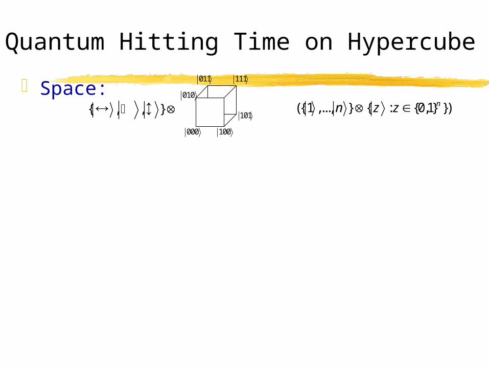
Quantum Hitting Time on Hypercube

Space:

000

010

100

101

111011

{ , , } ({1,..., } { : {0,1} })nn z z

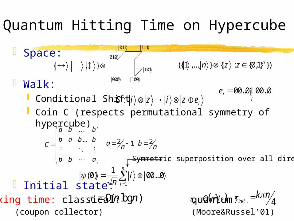
Quantum Hitting Time on Hypercube

Space:

Walk: Conditional Shift Coin C (respects permutational symmetry of

hypercube)

000

010

100

101

111011

{ , , } ({1,..., } { : {0,1} })nn z z

: iS i z i z e 00..01 00..0ii

e

...

a b b

b a b bC

b b a

2 21 a bn n

Quantum Hitting Time on Hypercube

Space:

Walk: Conditional Shift Coin C (respects permutational symmetry of

hypercube)

Initial state:

000

010

100

101

111011

{ , , } ({1,..., } { : {0,1} })nn z z

: iS i z i z e 00..01 00..0ii

e

...

a b b

b a b bC

b b a

2 21 a bn n

1

1(0) 00...0

n

i

in

Symmetric superposition over all directions

Mixing time: classical: quantum: (coupon collector) (Moore&Russel’01)

O( log )n n . 4instk n 3O n

Hitting time?Dilemma: constant measurement of position will

collapse U to the classical walk…

Two options:One-shot q-hitting-time (T,p):

Measure only at time T “Hits” desired target-state x with probability >p

Concurrent q-hitting-time (T,p): Partial measurement (“Am I at x/Am I not at x?”) at

all times Stop walk if x is hit. Probability >p to hit x before

time T

Results on hitting time*

Classical: from v to opposite v’ hitting-time

Quantum: One-shot hitting-time from v to v’ (T,p)

*J.K.’02

O(exp( )) 1 vn

T ( ), ( )2 2

n On n On 1-2

log n p=1-O

n

12 (T-n) even,

000

010

100

101

111011

and3log

T= n p=1-O2

nn

Results on hitting time*

Classical: from v to opposite v’ hitting-time

Quantum: One-shot hitting-time from v to v’ (T,p)

Need to know with accuracy when to measure, success 1 in linear time!

Concurrent hitting-time from v to v’ (T,p)

No information on when to measure needed, with amplification success 1 in T=O(n2)!

*J.K.’02

O(exp( )) 1 vn

T ( ), ( )2 2

n On n On 1-2

log n p=1-O

n

12 (T-n) even,

000

010

100

101

111011

O n

and3log

T= n p=1-O2

nn

1T= n p=2 n

“Details” Use symmetry to calculate eigenvalues/eigenvectors

of unmeasured walk U “Assymptotics” to calculate hitting probability at T

one-shot hitting time (T,p)

For concurrent hitting time give a lower bound on hitting probability in terms of unmeasured walk U:

Lemma:

2t(hit at t| not stopped before t)=p

2t(hit v' if measured at t)=p

2 3n2 1 (log )O n n

1t t t

22 2T T T

2

1t=0 t=0 t=0

1 1(hit before T)= 1T

t t t tp O nT T T

Robustness of initial condition

Polynomial hitting time to opposite corner, how long from other sites (or to sites close to corner)?

“close” initialstates give similar polynomial behavior

Upper bound:Region around v of polynomial hitting time to v’ at

most(otherwise we could find search

algorithm that beats the lower bound for quantum searching (Grover))

000

010

100

101

111011

2nO

2n

Open graphs

nG

… …

n-level binary tree

Example*:

*A.Childs, E.Farhi, S. Gutman, quant-ph/01…

starthit

1

1/3

2/3

2

2/3

1/3

n

1/3

2/3

n+1

2/3

2/3

…

1/3

2/3

1/3

2/3

Reduces to assymetric walk on the line (classically and quantum).

Open graphs

nG

… …

n-level binary tree

Example*:

*A.Childs, E.Farhi, S. Gutman, quant-ph/01…

starthit

1

1/3

2/3

2

2/3

1/3

n

1/3

2/3

n+1

2/3

2/3

…

1/3

2/3

1/3

2/3

Reduces to assymetric walk on the line (classically and quantum).

Classical: O(exp(n)) hitting time

Quantum: (numeric) poly(n) hitting time(N.Shenvi & J.K.’02)

Outlook/Open questions

In general which graphs have exponential quantum/classical gaps in hitting times ?

How robust is this gap w.r.t. initial position/distribution?

Mixing times for non-abelian walks ?Mixing times for walks on non-bounded

degree graphs?For degenrate or non-abelian groups

stationary distribution depends on initial state -algorithmic use?

Algorithmic use?

Outlook/Open questions

General THEORY???!!!

Connection to classicalMarkov chains?

Collaborators and related work

Discrete-time walks (Mixing Time) *: (On the Line)**:

Dorit Aharonov (Hebrew University) A. Ambainis, E. Bach, A. Nayak,Andris Ambainis (IAS, Princeton) A. Vishwanath, J. WatrousJ. K. (LRI, Orsay&UC Berkeley) (**STOC’01)Umesh Vazirani (UC Berkeley)

(*STOC’01)

Mixing on the Hypercube:

C. Moore and A. Russel (quant-ph’01)

Polynomial hitting time on the Hypercube:

J. K. (submitted ‘02)

hitting time on other graphs (numerical & Analytical studies):

Neil Shenvi and J. K. (in preparation ‘02)