quantum field theory i ii - thphys.uni-heidelberg.deweigand/qft2-14/skriptqft2.pdf · if x =...
TRANSCRIPT

Quantum Field Theory I + II
Institute for Theoretical Physics, Heidelberg University
Timo Weigand


Literature
This is a writeup of my Master programme course on Quantum Field Theory I (Chapters 1-6) andQuantum Field Theory II. The primary source for this course has been
• Peskin, Schröder: An introduction to Quantum Field Theory, ABP 1995,
• Itzykson, Zuber: Quantum Field Theory, Dover 1980,
• Kugo: Eichtheorie, Springer 1997,
which I urgently recommend for more details and for the many topics which time constraints haveforced me to abbreviate or even to omit. Among the many other excellent textbooks on QuantumField Theory I particularly recommend
• Weinberg: Quantum Field Theory I + II, Cambridge 1995,
• Srednicki: Quantum Field Theory, Cambridge 2007,
• Banks: Modern Quantum Field Theory, Cambridge 2008
as further reading. All three of them oftentimes take an approach different to the one of this course.Excellent lecture notes available online include
• A. Hebecker: Quantum Field Theory,
• D. Tong: Quantum Field Theory.
Special thanks to Robert Reischke1 for his fantastic work in typing these notes.
1For corrections and improvement suggestions please send a mail to [email protected].

4

Contents
1 The free scalar field 91.1 Why Quantum Field Theory? . . . . . . . . . . . . . . . . . . . . . . . . . . . . . . 91.2 Classical scalar field: Lagrangian formulation . . . . . . . . . . . . . . . . . . . . . 111.3 Noether’s Theorem . . . . . . . . . . . . . . . . . . . . . . . . . . . . . . . . . . . 141.4 Quantisation in the Schrödinger Picture . . . . . . . . . . . . . . . . . . . . . . . . 171.5 Mode expansion . . . . . . . . . . . . . . . . . . . . . . . . . . . . . . . . . . . . . 181.6 The Fock space . . . . . . . . . . . . . . . . . . . . . . . . . . . . . . . . . . . . . 211.7 Some important technicalities . . . . . . . . . . . . . . . . . . . . . . . . . . . . . . 23
1.7.1 Normalisation . . . . . . . . . . . . . . . . . . . . . . . . . . . . . . . . . . 231.7.2 The identity . . . . . . . . . . . . . . . . . . . . . . . . . . . . . . . . . . . 241.7.3 Position-space representation . . . . . . . . . . . . . . . . . . . . . . . . . . 24
1.8 On the vacuum energy . . . . . . . . . . . . . . . . . . . . . . . . . . . . . . . . . 251.9 The complex scalar field . . . . . . . . . . . . . . . . . . . . . . . . . . . . . . . . 281.10 Quantisation in the Heisenberg picture . . . . . . . . . . . . . . . . . . . . . . . . . 301.11 Causality and Propagators . . . . . . . . . . . . . . . . . . . . . . . . . . . . . . . 33
1.11.1 Commutators . . . . . . . . . . . . . . . . . . . . . . . . . . . . . . . . . . 331.11.2 Propagators . . . . . . . . . . . . . . . . . . . . . . . . . . . . . . . . . . . 351.11.3 The Feynman-propagator . . . . . . . . . . . . . . . . . . . . . . . . . . . . 361.11.4 Propagators as Green’s functions . . . . . . . . . . . . . . . . . . . . . . . . 39
2 Interacting scalar theory 412.1 Introduction . . . . . . . . . . . . . . . . . . . . . . . . . . . . . . . . . . . . . . . 412.2 Källén-Lehmann spectral representation . . . . . . . . . . . . . . . . . . . . . . . . 422.3 S-matrix and asymptotic in/out-states . . . . . . . . . . . . . . . . . . . . . . . . . 462.4 The LSZ reduction formula . . . . . . . . . . . . . . . . . . . . . . . . . . . . . . . 482.5 Correlators in the interaction picture . . . . . . . . . . . . . . . . . . . . . . . . . . 53
2.5.1 Time evolution . . . . . . . . . . . . . . . . . . . . . . . . . . . . . . . . . 552.5.2 From the interacting to the free vacuum . . . . . . . . . . . . . . . . . . . . 56
2.6 Wick’s theorem . . . . . . . . . . . . . . . . . . . . . . . . . . . . . . . . . . . . . 592.7 Feynman diagrams . . . . . . . . . . . . . . . . . . . . . . . . . . . . . . . . . . . 61
5
6 CONTENTS
2.7.1 Position space Feynman-rules . . . . . . . . . . . . . . . . . . . . . . . . . 632.7.2 Momentum space Feynman-rules . . . . . . . . . . . . . . . . . . . . . . . 63
2.8 Disconnected diagrams . . . . . . . . . . . . . . . . . . . . . . . . . . . . . . . . . 652.8.1 Vacuum bubbles . . . . . . . . . . . . . . . . . . . . . . . . . . . . . . . . 67
2.9 1-particle-irreducible diagrams . . . . . . . . . . . . . . . . . . . . . . . . . . . . . 672.10 Scattering amplitudes . . . . . . . . . . . . . . . . . . . . . . . . . . . . . . . . . . 70
2.10.1 Feynman-rules for the S -matrix . . . . . . . . . . . . . . . . . . . . . . . . 722.11 Cross-sections . . . . . . . . . . . . . . . . . . . . . . . . . . . . . . . . . . . . . . 73
3 Quantising spin 12 -fields 77
3.1 The Lorentz algebra so(1, 3) . . . . . . . . . . . . . . . . . . . . . . . . . . . . . . 773.2 The Dirac spinor representation . . . . . . . . . . . . . . . . . . . . . . . . . . . . . 813.3 The Dirac action . . . . . . . . . . . . . . . . . . . . . . . . . . . . . . . . . . . . 843.4 Chirality and Weyl spinors . . . . . . . . . . . . . . . . . . . . . . . . . . . . . . . 863.5 Classical plane-wave solutions . . . . . . . . . . . . . . . . . . . . . . . . . . . . . 893.6 Quantisation of the Dirac field . . . . . . . . . . . . . . . . . . . . . . . . . . . . . 91
3.6.1 Using the commutator . . . . . . . . . . . . . . . . . . . . . . . . . . . . . 913.6.2 Using the anti-commutator . . . . . . . . . . . . . . . . . . . . . . . . . . . 94
3.7 Propagators . . . . . . . . . . . . . . . . . . . . . . . . . . . . . . . . . . . . . . . 973.8 Wick’s theorem and Feynman diagrams . . . . . . . . . . . . . . . . . . . . . . . . 993.9 LSZ and Feynman rules . . . . . . . . . . . . . . . . . . . . . . . . . . . . . . . . . 100
4 Quantising spin 1-fields 1034.1 Classical Maxwell-theory . . . . . . . . . . . . . . . . . . . . . . . . . . . . . . . . 1034.2 Canonical quantisation of the free field . . . . . . . . . . . . . . . . . . . . . . . . . 1054.3 Gupta-Bleuler quantisation . . . . . . . . . . . . . . . . . . . . . . . . . . . . . . . 1084.4 Massive vector fields . . . . . . . . . . . . . . . . . . . . . . . . . . . . . . . . . . 1124.5 Coupling vector fields to matter . . . . . . . . . . . . . . . . . . . . . . . . . . . . 113
4.5.1 Coupling to Dirac fermions . . . . . . . . . . . . . . . . . . . . . . . . . . 1144.5.2 Coupling to scalars . . . . . . . . . . . . . . . . . . . . . . . . . . . . . . . 116
4.6 Feynman rules for QED . . . . . . . . . . . . . . . . . . . . . . . . . . . . . . . . . 1174.7 Recovering Coulomb’s potential . . . . . . . . . . . . . . . . . . . . . . . . . . . . 121
4.7.1 Massless and massive vector fields . . . . . . . . . . . . . . . . . . . . . . . 124
5 Quantum Electrodynamics 1275.1 QED process at tree-level . . . . . . . . . . . . . . . . . . . . . . . . . . . . . . . . 127
5.1.1 Feynman rules for in/out-states of definite polarisation . . . . . . . . . . . . 1275.1.2 Sum over all spin and polarisation states . . . . . . . . . . . . . . . . . . . . 1285.1.3 Trace identities . . . . . . . . . . . . . . . . . . . . . . . . . . . . . . . . . 1295.1.4 Centre-of-mass frame . . . . . . . . . . . . . . . . . . . . . . . . . . . . . . 130

CONTENTS 7
5.1.5 Cross-section . . . . . . . . . . . . . . . . . . . . . . . . . . . . . . . . . . 1305.2 The Ward-Takahashi identity . . . . . . . . . . . . . . . . . . . . . . . . . . . . . . 132
5.2.1 Relation between current conservation and gauge invariance . . . . . . . . . 1355.2.2 Photon polarisation sums in QED . . . . . . . . . . . . . . . . . . . . . . . 1365.2.3 Decoupling of potential ghosts . . . . . . . . . . . . . . . . . . . . . . . . . 136
5.3 Radiative corrections in QED - Overview . . . . . . . . . . . . . . . . . . . . . . . 1375.4 Self-energy of the electron at 1-loop . . . . . . . . . . . . . . . . . . . . . . . . . . 138
5.4.1 Feynman parameters . . . . . . . . . . . . . . . . . . . . . . . . . . . . . . 1395.4.2 Wick rotation . . . . . . . . . . . . . . . . . . . . . . . . . . . . . . . . . . 1405.4.3 Regularisation of the integral . . . . . . . . . . . . . . . . . . . . . . . . . . 141
5.5 Bare mass m0 versus physical mass m . . . . . . . . . . . . . . . . . . . . . . . . . 1445.5.1 Mass renormalisation . . . . . . . . . . . . . . . . . . . . . . . . . . . . . . 146
5.6 The photon propagator . . . . . . . . . . . . . . . . . . . . . . . . . . . . . . . . . 1465.7 The running coupling . . . . . . . . . . . . . . . . . . . . . . . . . . . . . . . . . . 1495.8 The resummed QED vertex . . . . . . . . . . . . . . . . . . . . . . . . . . . . . . . 150
5.8.1 Physical charge revisited . . . . . . . . . . . . . . . . . . . . . . . . . . . . 1535.8.2 Anomalous magnetic moment . . . . . . . . . . . . . . . . . . . . . . . . . 153
5.9 Renormalised perturbation theory of QED . . . . . . . . . . . . . . . . . . . . . . . 1545.9.1 Bare perturbation theory . . . . . . . . . . . . . . . . . . . . . . . . . . . . 1555.9.2 Renormalised Perturbation theory . . . . . . . . . . . . . . . . . . . . . . . 158
5.10 Infrared divergences . . . . . . . . . . . . . . . . . . . . . . . . . . . . . . . . . . . 164
6 Classical non-abelian gauge theory 1656.1 Geometric perspective on abelian gauge theory . . . . . . . . . . . . . . . . . . . . 1656.2 Non-abelian gauge symmetry . . . . . . . . . . . . . . . . . . . . . . . . . . . . . . 1676.3 The Standard Model . . . . . . . . . . . . . . . . . . . . . . . . . . . . . . . . . . 171
7 Path integral quantisation 1737.1 Path integral in Quantum Mechanics . . . . . . . . . . . . . . . . . . . . . . . . . . 173
7.1.1 Transition amplitudes . . . . . . . . . . . . . . . . . . . . . . . . . . . . . . 1737.1.2 Correlation functions . . . . . . . . . . . . . . . . . . . . . . . . . . . . . . 178
7.2 The path integral for scalar fields . . . . . . . . . . . . . . . . . . . . . . . . . . . . 1797.3 Generating functional for correlation functions . . . . . . . . . . . . . . . . . . . . 183
7.3.1 Functional calculus . . . . . . . . . . . . . . . . . . . . . . . . . . . . . . . 1837.4 Free scalar field theory . . . . . . . . . . . . . . . . . . . . . . . . . . . . . . . . . 1857.5 Perturbative expansion in interacting theory . . . . . . . . . . . . . . . . . . . . . . 1887.6 The Schwinger-Dyson equation . . . . . . . . . . . . . . . . . . . . . . . . . . . . 1917.7 Connected diagrams . . . . . . . . . . . . . . . . . . . . . . . . . . . . . . . . . . . 1957.8 The 1PI effective action . . . . . . . . . . . . . . . . . . . . . . . . . . . . . . . . . 1967.9 Γ(ϕ) as a quantum effective action and background field method . . . . . . . . . . . 200

8 CONTENTS
7.10 Euclidean QFT and statistical field theory . . . . . . . . . . . . . . . . . . . . . . . 2037.11 Grassman algebra calculus . . . . . . . . . . . . . . . . . . . . . . . . . . . . . . . 2067.12 The fermionic path integral . . . . . . . . . . . . . . . . . . . . . . . . . . . . . . . 211
8 Renormalisation of Quantum Field Theory 2178.1 Superficial divergence and power counting . . . . . . . . . . . . . . . . . . . . . . . 2178.2 Renormalisability and BPHZ theorem . . . . . . . . . . . . . . . . . . . . . . . . . 2208.3 Renormalisation of φ4 theory up to 2-loops . . . . . . . . . . . . . . . . . . . . . . 222
8.3.1 1-loop renormalisation . . . . . . . . . . . . . . . . . . . . . . . . . . . . . 2248.3.2 Renormalisation at 2-loop . . . . . . . . . . . . . . . . . . . . . . . . . . . 226
8.4 Renormalisation of QED revisited . . . . . . . . . . . . . . . . . . . . . . . . . . . 2318.5 The renormalisation scale . . . . . . . . . . . . . . . . . . . . . . . . . . . . . . . . 2338.6 The Callan-Symanzyk (CS) equation . . . . . . . . . . . . . . . . . . . . . . . . . . 2348.7 Computation of β-functions in massless theories . . . . . . . . . . . . . . . . . . . . 2378.8 The running coupling . . . . . . . . . . . . . . . . . . . . . . . . . . . . . . . . . . 2398.9 RG flow of dimensionful operators . . . . . . . . . . . . . . . . . . . . . . . . . . . 2438.10 Wilsonian effective action & Renormalisation Semi-Group . . . . . . . . . . . . . . 245
9 Quantisation of Yang-Mills-Theory 2539.1 Recap of classical YM-Theory . . . . . . . . . . . . . . . . . . . . . . . . . . . . . 2539.2 Gauge fixing the path integral . . . . . . . . . . . . . . . . . . . . . . . . . . . . . . 2559.3 Faddeev-Popov ghosts . . . . . . . . . . . . . . . . . . . . . . . . . . . . . . . . . 2599.4 Canonical quantisation and asymptotic Fock space . . . . . . . . . . . . . . . . . . 2629.5 BRST symmetry and the physical Hilbert space . . . . . . . . . . . . . . . . . . . . 264

Chapter 1
The free scalar field
1.1 Why Quantum Field Theory?
In (non-relativistic) Quantum Mechanics, the dynamics of a particle is described by the time-evolutionof its associated wave-function ψ(t, ~x) with respect to the non-relativistic Schrödinger equation
ih∂
∂tψ(t, ~x) = Hψ(t, ~x), (1.1)
with the Hamilitonian given by H = ~p2
2m + V(x). In order to achieve a Lorentz invariant framework, anaive approach would start by replacing this non-relativistic form of the Hamiltonian by a relativisticexpression such as
H =
√c2 ~p2 + m2c4 (1.2)
or, even better, by modifying the Schrödinger equation altogether such as to make it symmetric in∂∂t and the spatial derivative ~∇. However, the central insight underlying the formulation of QuantumField Theory is that this is not sufficient. Rather, combining the principles of Lorentz invariance andQuantum Theory requires abandoning the single-particle approach of Quantum Mechanics.
• In any relativistic Quantum Theory, particle number need not be conserved, since the relativisticdispersion relation E2 = c2~p2 + m2c4 implies that energy can be converted into particles andvice versa. This requires a multi-particle framework.
• Unitarity and causality cannot be combined in a single-particle approach: In Quantum Me-chanics, the probability amplitude for a particle to propagate from position ~x to ~y is
G(~x,~y) = 〈~y| e−ih Ht |~x〉 . (1.3)
One can show that e.g. for the free non-relativistic Hamiltonian H = p2
2m this is non-zero evenif xµ = (x0, ~x) and yµ = (y0,~y) are at a spacelike distance. The problem persists if we replaceH by a relativistic expression such as (1.2).
Quantum Field Theory (QFT) solves both these problems by a radical change of perspective:
9

10 CHAPTER 1. THE FREE SCALAR FIELD
• The fundamental entities are not the particles, but the field, an abstract object that penetratesspacetime.
• Particles are the excitations of the field.
Before developing the notion of an abstract field let us try to gain some intuition in terms of a mechan-ical model of a field. To this end we consider a mechanical string of length L and tension T along thex-axis and excite this string in the transverse direction. Let φ(x, t) denote the transverse excitation ofthe string. In this simple picture φ(x, t) is our model for the field. This system arises as the continuumlimit of N mass points of mass m coupled by a mechanical spring to each other. Let the distance ofthe mass points from each other projected to the x-axis be ∆ and introduce the transverse coordinatesqr(t), r = 1, . . . , N of the mass points. In the limit ∆ → 0 with L fixed, the profile qr(t) asymptotesto the field φ(x, t). In this sense the field variable x is the continuous label for infinitely many degreesof freedom.We can now linearise the force between the mass points due to the spring. As a result of a simpleexercise in classical mechanics the energy at leading order is found to be
E =N∑
r=0
(12
m(dqr(t)
dt
)2
+ k(q2r − qrqr−1)
)+O(q3), k =
TL
. (1.4)
In the continuum limit this becomes
E =
L∫0
12ρ
(∂φ(x, t)∂t
)2
+12ρc2
(∂φ(x, t)∂x
)2 dx (1.5)
in terms of the mass density ρ of the string and a suitably defined characteristic velocity c. Note thatthe second term indeed includes the nearest neighbour interaction because(
∂φ(x, t)∂x
)2
'
(limδx→0
φ(x + δx, t) − φ(x, t))δx
)2
(1.6)
contains the off-diagonal terms φ(x + δx, t)φ(x, t).The nearest-neighbour interaction implies that the equation of motion for the mass points qi obey cou-pled linear differential equations. This feature persists in the continuum limit. To solve the dynamicsit is essential that we are able to diagonalise the interaction in terms of the Fourier modes,
φ(x, t) =∞∑
k=1
Ak(t) sin(kπxL
),
E =L2
∞∑k=1
(12ρA2
k +12ρω2
k A2)
,
(1.7)
where ωk = kπc/L. We are now dealing with a collection of infinitely many, decoupled harmonicoscillators Ak(t).

1.2. CLASSICAL SCALAR FIELD: LAGRANGIAN FORMULATION 11
In a final step, we quantise this collection of harmonic oscillators. According to Quantum Mechanics,each mode Ak(t) can take energy values
Ek = hωk(nk + 1/2) nk = 0, 1, 2, ...,∞. (1.8)
The total energy is given by summing over the energy associated with all the modes, E =∑
Ek. Astate of definite energy E corresponds to mode numbers (n1, n2, ..., n∞), where we think of nr as anexcitation of the string or of the field φ, i.e. as a quantum. In condensed matter physics, these quan-tised excitations in terms of harmonic modes are called quasi-particles, e.g. phonons for mechanicalvibrations of a solid. Note that the above decoupling of the degrees of freedom rested on the quadraticform of the potential. Including higher terms will destroy this and induce interactions between modes.
The idea of Quantum Field Theory is to adapt this logic to particle physics and to describe a particleas the quantum of oscillation of an abstract field - just like in solid state physics we think of aquasi-particle as the vibrational excitation of a solid. The only difference is that the fields are nowmore abstract objects defined all over spacetime as opposed to concrete mechanical fields of the typeabove.As a familiar example for a field we can think of the Maxwell field Aµ(x, t) in classical electrody-namics. A photon is the quantum excitation of this. It has spin 1. Similarly we assign one field toeach particle species, e.g. an electron is the elementary excitation of the electron field (Spin 1/2). Wewill interpret the sum over harmonic oscillator energies as an integral over possible energies for givenmomentum,
E =∞∑
k=1
hωk(nk + 1/2)→∫
dp hωp(np + 1/2). (1.9)
A single particle with momentum p corresponds to np = 1 while all others vanish, but this is just aspecial example of a more multi-particle state with several npi , 0. In particular, in agreement withthe requirements of a multi-particle framework, at fixed E transitions between various multi-particlestates are in principle possible. Such transitions are induced by interactions corresponding to thehigher order terms in the Hamiltonian that we have discarded so far. As a triumph this formalism alsosolves the problem of causality, as we will see.
1.2 Classical scalar field: Lagrangian formulation
We now formalise the outlined transition from a classical system with a finite number of degreesof freedom qi(t) to a classical field theory in terms of a scalar field φ(t, ~x) ≡ φ(xµ). In classicalmechanics we start from an action
S =
t2∫t1
dt L(qi(t), qi(t)) with L =12
∑i
(qi(t))2 − V(q1, , qN), (1.10)

12 CHAPTER 1. THE FREE SCALAR FIELD
where we have included the mass m in the definition of qi(t). In a first step replace
qi → φ(xµ) ≡ φ(x), (1.11)
qi(t) →∂φ(x)∂t
, (1.12)
thereby substituting the label i = 1, ...N by a continous coordinate ~x ≡ xi with i = 1, 2, 3. For themoment we consider a real scalar field i.e. φ(x) = φ∗(x) which takes values in R, i.e.
φ : xµ → φ(xµ) ∈ R. (1.13)
We will see that such a field describes spin-zero particles. Examples of scalar particles in nature arethe Higgs boson or the inflaton, which cosmologists believe to be responsible for the exponential ex-pansion of the universe during in inflation.
To set up the Lagrange function we first note that in a relativistic theory the partial time derivative canonly appear as part of
∂µφ(x) ≡∂
∂xµφ(x). (1.14)
Thus the Lagrange function can be written as
L =
∫d3xL(φ(x), ∂µφ(x)), (1.15)
where L is the Lagrange density. The action therefore is
S =
∫d4xL(φ(x), ∂µφ(x)). (1.16)
While, especially in condensed matter physics, also non-relativistic field theories are relevant, we fo-cus on relativistic theories in this course.
Note furthermore that throughout this course we use conventions where
h = c = 1. (1.17)
Then L has the dimension mass4, i.e. [L] = 4, since [S ] = 0 and [d4x] = −4.
The next goal is to find the Lagrangian: In a relativistic setting L can contain powers of φ and1
∂µφ∂µφ ≡ ηµν∂µφ∂νφ, which is the simplest scalar which can be built from ∂µφ. The action in this
case is
S =
∫d4x
[12∂µφ∂
µφ − V(φ) +O(φn(∂φ)m)
], (1.18)
where12∂µφ∂
µφ =12φ2 −
12(∇φ)2 (1.19)
1Note that the only remaining option ∂µ∂µφ is a total derivative and will therefore not alter the equations of motion underthe usual assumptions on the boundary terms.

1.2. CLASSICAL SCALAR FIELD: LAGRANGIAN FORMULATION 13
and the last type of terms consists of higher derivative terms with m ≥ 2 or mixed terms with n ≥ 1.Notice that
• the signature for the metric is, in our conventions, (+,−,−,−), such that the sign in the actionis indeed chosen correctly such that the kinetic term appears with a positive prefactor;
• φ has dimension 1 (mass1).
The potential V(φ(x)) is in general a power series of the form
V(φ(x)) = a + bφ(x) + cφ2(x) + dφ3(x) + . . . . (1.20)
We assume that the potential has a global minimum at φ(x) = φ0(x) such that
∂V(φ)∂φ
|φ=φ0 = 0, V(φ0) = V0 (1.21)
By a field redefinition we ensure that the minimum is at φ0(x) ≡ 0 and expand V(φ(x)) around thisminimum as
V(φ(x)) = V0 +12
m2φ2(x) +O(φ3(x)). (1.22)
Here we used that the linear terms vanish at the extremum and the assumption that we are expandingaround a minimum implies m2 > 0. The constant V0 is the classical contribution to the ground state orvacuum energy. Since in a theory without gravity absolute energies are not measurable, we set V0 = 0for the time being, but keep in mind that in principle V0 is arbitrary. We will have considerably moreto say about V0 in the quantum theory in section (1.8).Therefore the action becomes
S =
∫d4x
[12(∂φ)2 −
12
m2φ2 + ...]
. (1.23)
We will find that m2, the prefactor of the quadratic term, is related to the mass of the particles and thatthe omitted higher powers of φ as well as the terms O(φn(∂φ)m) will give rise to interactions betweenthese particles.As an aside note that a negative value of m2 signals that the extremum around which we are expandingthe potential is a maximum rather than a minimum. Therefore m2 < 0 signals a tachyonic instability:quantum fluctuations will destabilise the vacuum and cause the system to roll down its potential untilit has settled in its true vacuum.We will start by ignoring interaction terms and studying the action of the free real scalar field theory
S =
∫d4x
[12(∂φ)2 −
12
m2φ2]
, φ = φ∗. (1.24)
The equations of motion are given by the Euler-Lagrange equations. As in classical mechanics wederive them by varying S with respect to φ and ∂µφ subject to δφ|boundary = δ∂µφ|boundary = 0. This

14 CHAPTER 1. THE FREE SCALAR FIELD
yields
0 != δS =
∫d4x
[∂L(φ(x), ∂µφ(x))
∂φ(x)δφ(x) +
∂L(φ(x), ∂µφ(x))∂(∂µφ(x))
δ∂µφ(x)]
=
∫d4x
[∂L(φ(x), ∂µφ(x))
∂φ(x)δφ(x) +
∂L(φ(x), ∂µφ(x))∂(∂µφ(x))
∂µδφ(x)]
.(1.25)
Integrating by parts gives∫d4x
[∂L(φ(x), ∂µφ(x))
∂φ(x)− ∂µ
∂L(φ(x), ∂µφ(x))∂(∂µφ(x))
]δφ(x) + boundary terms. (1.26)
Since the boundary terms vanish by assumption, therefore the integrand has to vanish for all variationsδφ(x). This yields the Euler-Lagrange equations
∂L(φ(x), ∂µφ(x))∂φ(x)
= ∂µ∂L(φ(x), ∂µφ(x))
∂(∂µφ(x)). (1.27)
By inserting (1.24) into (1.27) we find the equations of motion for the free scalar field
∂µ∂L
∂(∂µφ)= ∂µ∂
µφ =∂L
∂φ= −m2φ, (1.28)
i.e. the Klein-Gordon equation(∂2 + m2)φ(x) = 0. (1.29)
Note that (1.29) is a relativistic wave equation and that it is solved by
e±ipx with p ≡ pµ = (p0, ~p) (1.30)
subject to the dispersion relation −p2 + m2 = 0, i.e. p0 = ±√~p2 + m2. We now set
E~p :=√~p2 + m2 ≡ Ep (1.31)
and write the general solution of (1.29) in the form
φ(x) =∫
d3 p(2π)3
1√2Ep
(f (~p)e−ipx + g(~p)eipx
), (1.32)
where p := (Ep, ~p) and f ∗(~p) = g(~p) for real φ and px = p · x = pµxµ .
1.3 Noether’s Theorem
A key role in Quantum Field Theory is played by symmetries. We consider a field theory with La-grangian L(φ, ∂µφ). A symmetry of the theory is then defined to be a field transformation by whichL changes at most by a total derivative such that the action stays invariant. This ensures that theequations of motion are also invariant. Symmetries and conservation laws are related by Noether’sTheorem2:
2Emmy Noether, 1882-1935.

1.3. NOETHER’S THEOREM 15
Every continuous symmetry in the above sense gives rise to a Noether current jµ(x) suchthat
∂µ jµ(x) = 0 (1.33)
upon use of the equations of motion (≡ "on-shell").
This can be proven as follows:
For a continuous symmetry we can write infinitesimally:
φ→ φ+ εδφ+O(ε2) with δφ = X(φ, ∂µφ). (1.34)
Off-shell (i.e. without use of the equations of motion) we know that
L → L+ εδL+O(ε2) with δL = ∂µFµ (1.35)
for some Fµ. Now, under an arbitrary transformation φ → φ+ εδφ, which is not neces-sarily a symmetry, δL is given by
δL =∂L
∂φδφ+
∂L
∂(∂µφ)δ(∂µφ)
= ∂µ
[∂L
∂(∂µφ)δφ
]+
[∂L
∂φ− ∂µ
∂L
∂(∂µφ)
]δφ.
(1.36)
If δφ = X is a symmetry, then δL = ∂µFµ. Setting
jµ =∂L
∂(∂µφ)X − Fµ (1.37)
we therefore have
∂µ jµ = −(∂L
∂φ− ∂µ
∂L
∂(∂µφ)
)X (1.38)
off-shell. Note that the terms in brackets are just the Euler-Lagrange equation. Thus, ifwe use the equations of motion, i.e. on-shell, ∂µ jµ = 0.
This immediately yields the following Lemma:
Every continuous symmetry whose associated Noether current satisfies ji(t, ~x)→ 0 suffi-ciently fast for |~x| → ∞ gives rise to a conserved charge Q with
Q = 0. (1.39)
Indeed if we takeQ =
∫R3
d3x j0(t, ~x), (1.40)

16 CHAPTER 1. THE FREE SCALAR FIELD
then the total time derivative of Q is given by
Q =
∫R3
d3x∂
∂tj0
= −
∫R3
d3x ∂i ji(t, ~x) = 0(1.41)
by assumption of sufficiently fast fall-off of ji(t, ~x). We used that ∂µ jµ = 0 in the firststep.
The technical assumption ji(t, ~x)→ 0 for |~x| → ∞ is really an assumption of ’sufficiently fast fall-off’of the fields at spatial infinity, which is typically satisfied. Note that in a finite volume V = const., thequantity QV =
∫V
dV j0(t, ~x) satisfies local charge conservation,
QV = −
∫V
dV ∇~j = −∫∂V
~j · d~s. (1.42)
We now apply Noether’s theorem to deduce the canonical energy-momentum tensor: Under a globalspacetime transformation xµ → xµ + εµ a scalar field φ(xµ) transforms like
φ(xµ)→ φ(xµ − εµ) = φ(xµ) − εν ∂νφ(xµ)︸ ︷︷ ︸≡Xν(φ)
+O(ε2). (1.43)
Because L is a local function of x it transforms as
L → L− εν∂νL = L− ηµνεν∂µL
= L− εν∂µηµνL.
(1.44)
For each component ν we therefore have a conserved current ( jµ)ν given by
( jµ)ν =∂L
∂(∂µφ)∂νφ︸︷︷︸≡Xν
− ηµνL︸︷︷︸
≡(Fµ)ν
. (1.45)
With both indices up, we arrive at the canonical energy-momentum tensor
T µν =∂L
∂(∂µφ)∂νφ − ηµνL with ∂µT µν = 0 on-shell. (1.46)
The conserved charges are the energy E =∫
d3x T 00 associated with time translation invariance andthe spatial momentum Pi =
∫d3x T 0i associated with spatial translation invariance. We can combine
them into the conserved 4-momentum
Pν =∫
d3x T 0ν (1.47)
with the property Pν = 0.Two comments are in order:

1.4. QUANTISATION IN THE SCHRÖDINGER PICTURE 17
• In general, T µν may not be symmetric - especially in theories with spin. In such cases it canbe useful to modify the energy-momentum tensor without affecting its conservedness or theassociated conserved charges. Indeed we state as a fact that the Belinfante-Rosenfeld tensor
ΘµνBR := T µν + ∂ρS ρµν (1.48)
can be defined in terms of a suitable S ρµν = −S µρν such that ΘµνBR is symmetric and obeys
∂µΘµνBR = 0.
• In General Relativity (GR), there exists yet another definition of the energy-momentum tensor:With the metric ηµν replaced by gµν and
S =
∫d4x√−gLmatter(gµν, φ, ∂φ), (1.49)
where g ≡ detg, one defines the Hilbert energy-momentum tensor:
(ΘH)µν = −
2√−g
∂(√−gLmatter)
∂gµν, (1.50)
which is obviously symmetric and it the object that appears in the Einstein equations
Rµν +12
Rgµν = 8πG(ΘH)µν. (1.51)
In fact one can choose the Belinfante-Rosenfeld tensor such that it is equal to the Hilbert energy-momentum tensor.
1.4 Quantisation in the Schrödinger Picture
Before quantising field theory let us briefly recap the transition from classical to quantum mechanics.We first switch from the Lagrange formulation to the canonical formalism of the classical theory. Inclassical mechanics the canonical momentum conjugate to qi(t) is
pi(t) =∂L
∂qi(t). (1.52)
The Hamiltonian is the Legendre transformation of the Lagrange function L
H =∑
i
pi(t)qi(t) − L. (1.53)
To quantise in the Schrödinger picture we drop the time dependence of qi and pi and promote them toself-adjoint operators without any time dependence such that the fundamental commutation relation
[qi, p j] = iδi j (1.54)

18 CHAPTER 1. THE FREE SCALAR FIELD
holds. Then all time dependence lies in the states.
This procedure is mimicked in a field theory by first defining clasically
Π(t, ~x) :=∂L
∂φ(t, ~x)(1.55)
to be the conjugate momentum density. The Hamiltonian is
H =
∫d3xH =
∫d3x[Π(t, ~x)φ(t, ~x) −L], (1.56)
whereH is the Hamiltonian density. For the scalar field action (1.24) one finds
Π(t, ~x) = φ(t, ~x) (1.57)
and therefore
H =
∫d3x
[φ2(t, ~x) −
12(∂µφ)(∂
µφ) +12
m2φ2(t, ~x)]
=
∫d3x
[12φ2(t, ~x)︸ ︷︷ ︸
= 12 Π2(t,~x)
+12(∇φ(t, ~x))2 +
12
m2φ2(t, ~x)].
(1.58)
Note that as in classical mechanics one can define a Poisson bracket which induces a natural sym-pletic structure on phase space. In this formalism the Noether charges Q are the generators of theirunderlying symmetries with the respect to the Poisson bracket (see Assignment 1 for details).
We now quantise in the Schrödinger picture. Therefore we drop the time-dependence of φ and Πand promote them to Schrödinger-Picture operators φ(s)(~x) and Π(s)(~x). For real scalar fields we getself-adjoint operators φ(s)(~x) = (φ(s)(~x))† with the canonical commutation relations (dropping (s)
from now on)
[φ(~x), Π(~y)] = iδ(3)(~x −~y) , [φ(~x), φ(~y)] = 0 = [Π(~x), Π(~y)]. (1.59)
1.5 Mode expansion
Our Hamiltonian (1.58) resembles the Hamiltonian describing a collection of harmonic oscillators,one at each point ~x, but the term
(∇φ)2 ≈
(φ(~x + δ~x) − φ(~x)
|δ~x|
)2
(1.60)
couples the degrees of freedom at ~x and ~x + δ~x. To arrive at a description in which the harmonicoscillators are decoupled, we must diagonalise the potential. Now, a basis of eigenfunctions with

1.5. MODE EXPANSION 19
respect to ∇ is ei~p·~x. Thus the interaction will be diagonal in momentum space. With this motivationwe Fourier-transform the fields as
φ(~x) =∫
d3 p(2π)3 φ(~p)e
i~p·~x,
Π(~x) =∫
d3 p(2π)3 Π(~p)ei~p·~x,
(1.61)
where φ†(~p) = φ(−~p) ensures that φ(~x) is self-adjoint. To compute H in Fourier space we mustinsert these expressions into (1.58). First note that
12
∫d3x(∇φ(~x))2 =
12
∫d3x
(∫d3 p(2π)3∇ei~p·~xφ(~p)
)2
=12
∫d3x
∫d3 pd3q(2π)6 (−~p · ~q)ei(~p+~q)·~xφ(~p)φ(~q).
(1.62)
Thanks to the important equality∫d3x ei(~p+~q)·~x = (2π)3δ(3)(~p + ~q), (1.63)
the latter equation yields
12
∫d3x(∇φ(~x))2 =
12
∫d3 p(2π)3 ~p
2 φ(~p)φ(−~p)︸ ︷︷ ︸≡|φ(~p)|2
, (1.64)
and therefore with (1.58) altogether
H =
∫d3 p(2π)3
[12|Π(~p)|2 +
12ω2
p|φ(~p)|2]
, (1.65)
where ωp =√~p2 + m2. This is a collection of decoupled harmonic oscillators of frequency ωp - and
indeed the Hamiltonian is diagonal in momentum space.
The next step is to solve these oscillators in close analogy with the quantum mechanical treatment ofa harmonic oscillator of frequency ω with Hamiltonian
H =12
Π2 +ω2q2. (1.66)
The quantum mechanical definition of ladder operators a, a† such that
q =1√
2ω(a + a†) , Π = −
√ω
2i(a − a†) (1.67)
and with commutation relation [a, a†] = 1 can be generalised to field theory as follows: By takinginto account that
φ(~p) = φ†(−~p) , Π(~p) = Π†(−~p), (1.68)

20 CHAPTER 1. THE FREE SCALAR FIELD
we define the operators
a(~p) =12
√2ωp φ(~p) + i
√2ωp
Π(~p)
,
a†(~p) =12
√2ωp φ(−~p) − i
√2ωp
Π(−~p)
.
(1.69)
Solving for φ(~p) and Π(~p) and plugging into (1.61) yields
φ(~x) =∫
d3 p(2π)3
1√2ωp
(a(~p)ei~p·~x + a†(~p)e−i~p·~x
),
Π(~x) =∫
d3 p(2π)3 (−i)
√ωp
2
(a(~p)ei~p·~x − a†(~p)e−i~p·~x
).
(1.70)
From (1.61) and (1.59) we furthermore deduce the commutation relations
[φ(~p), Π(~q)] =∫
d3xd3ye−i~p·~xe−i~q·~y [φ(~x), Π(~y)]︸ ︷︷ ︸=iδ(3)(~x−~y)
= (2π)3iδ(3)(~p + ~q), (1.71)
where again (1.63) was used, and
[φ(~p), φ(~q)] = 0 = [Π(~p), Π(~q)]. (1.72)
The ladder operators therefore obey the commutation relation
[a(~p), a†(~q)] = (2π)3δ(3)(~p − ~q),
[a†(~p), a†(~q)] = 0 = [a(~p), a(~q)].(1.73)
The Hamiltonian (1.65) in mode expansion is
H =
∫d3 p(2π)3
[12
i √ωp
2
2 (a(~p) − a†(−~p)
) (a(−~p) − a†(~p)
)+ω2
p
21
2ωp
(a(~p) + a†(−~p)
) (a(−~p) + a†(~p)
) ].
(1.74)
Only cross-terms survive due to the commutation relations:
H =
∫d3 p(2π)3
ωp
4
[a(~p)a†(~p) + a†(−~p)a(−~p)
]· 2
=
∫d3 p(2π)3
ωp
2
[a(~p)a†(~p) + a†(−~p)a(−~p)
]=
∫d3 p(2π)3
ωp
2
[a†(~p)a(~p) + (2π)3δ(3)(~p − ~p) + a†(−~p)a(−~p)
].
(1.75)

1.6. THE FOCK SPACE 21
Therefore H in its final form is given by
H =
∫d3 p(2π)3ωp a†(~p)a(~p) + ∆H , (1.76)
where we renamed −~p→ ~p in the second term. The additional constant ∆H is
∆H =12
∫d3 pωp δ
(3)(0), (1.77)
which is clearly divergent. An interpretation will be given momentarily. By explicit computation onefinds that H obeys the commutation relations
[H, a(~p)] = −ωp a(~p),
[H, a†(~p)] = ωp a†(~p).(1.78)
Similarly one computes the spatial momentum operator
Pi =
∫d3x φ(~x)∂iφ(~x), (1.79)
to be
Pi =
∫d3 p(2π)3 pia†(~p)a(~p) + ∆pi , (1.80)
with∆pi =
12
∫d3 p pi δ(3)(0) ≡ 0. (1.81)
We combine H and P into the 4-momentum operator
Pµ =∫
d3 p(2π)3 pµa†(~p)a(~p) + ∆pµ , (1.82)
with pµ = (p0, ~p) = (ωp, ~p). It obeys the commutation relations
[Pµ, a†(~p)] = pµa†(~p),
[Pµ, a(~p)] = −pµa(~p).(1.83)
1.6 The Fock space
We now find the Hilbert space on which the 4-moment operator Pµ acts. The logic is analogous to theconsiderations leading to the representation theory of the harmonic oscillator in Quantum Mechanics:
• Since Pµ is self-adjoint it has eigenstates with real eigenvalues. Let |kµ〉 be such an eigenstatewith
Pµ |kµ〉 = kµ |kµ〉 . (1.84)

22 CHAPTER 1. THE FREE SCALAR FIELD
Then as a result of (1.83)
Pµa†(~q) |kµ〉 = a†(~q)Pµ |kµ〉+ qµa†(~q) |kµ〉
= (kµ + qµ)a†(~q) |kµ〉(1.85)
and similarly
Pµa(~q) |kµ〉 = (kµ − qµ)a(~q) |kµ〉 . (1.86)
This means that a(~q) and a†(~q) are indeed ladder operators which respectively subtract and add4-momentum qµ to or from |kµ〉.
• Next we observe that the Hamiltonian H = P0 given by (1.76) is non-negative, i.e. 〈ψ|H|ψ〉 ≥0 ∀ states |ψ〉 because
〈ψ|H|ψ〉 =∫
d3 p(2π)3ωp〈ψ|a†(~p)a(~p)|ψ〉+ ∆H〈ψ|ψ〉 ≥ 0. (1.87)
Thus there exists a state |0〉 such that
a(~q) |0〉 = 0 ∀ ~q. (1.88)
Otherwise successive action of a(~q) would lead to negative eigenvalues of H. |0〉 is called thevacuum of the theory. It has 4-momentum
Pµ |0〉 = ∆pµ |0〉 =
∆H , µ = 00 , µ = i
. (1.89)
• We interpret the divergent constant ∆H given in (1.77) as the vacuum energy. A more thoroughdiscussion of the significance of the divergence will be given later. For now we should note thatin a theory without gravity absolute energy has no meaning. We can hus discard the additiveconstant ∆pµ by defining
Pµ := Pµ − ∆pµ =
∫d3 p(2π)3 pµa†(~p)a(~p), (1.90)
with Pµ |0〉 = 0. From now on we only work with Pµ and drop the tilde.
• The state a†(~p) |0〉 then has 4-momentum pµ,
Pµa†(~p) |0〉 = pµa†(~p) |0〉 , (1.91)
with pµ = (Ep, ~p) and Ep =√~p2 + m2. Since this is the relativistic dispersion relation for
a single particle with mass m we interpret a†(~p) |0〉 as a 1-particle state with energy Ep andmomentum ~p.

1.7. SOME IMPORTANT TECHNICALITIES 23
• More generally an N-particle state with energy E = Ep1 + ... + EpN and momentum ~p =
~p1 + ...~pN is given bya†(~p1)a†( ~p2)...a†(~pN) |0〉 . (1.92)
So much about the formalism. To get a better feeling for the objects we have introduced, let us recapwhat we have done: We have started with the assertion that spacetime - in our case R1,3 - is filled withthe real scalar field φ(~x), which we have taken to be a free field with LagrangianL = 1
2 (∂φ)2− 1
2 m2φ2.This field is interpreted as a field operator, i.e. in the Schrödinger picture at every space point ~x theobject φ(~x) represents a self-adjoint operator that acts on a Hilbert space. This Hilbert space possessesa state of lowest energy, the vacuum |0〉. The vacuum corresponds to the absence of any excitations ofthe field φ (at least on-shell). If one pumps energy Ep and momentum ~p into some region of spacetimesuch that the relativistic dispersion relation Ep =
√~p2 + m2 holds, a particle a†(~p) |0〉 is created as
an excitation of φ(~x). In particular, for the free theory the parameter m in L is interpreted as the massof such a particle. Since the underlying field φ(x) is a scalar field, the associated particle is calledscalar particle. This realizes the shift of paradigm advertised at the very beginning of this course thatthe fundamental entity in Quantum Field Theory is not the particle, but rather the field:
The field φ(~x) is the property of spacetime that in the presence of energy and momentum(Ep, ~p) a particle of energy (Ep, ~p) can be created.
In particular, this naturally gives rise to a multi-particle theory. The particles are just the excitationsof the field and transitions with varying particle number can occur as long as the kinematics allows it.A first new, non-trivial conclusion we can draw from the formalism developed so far is the followingspecial case of the spin-statistics theorem:
Scalar particles obey Bose statistics.
All we have to show that the N-particle wavefunction is symmetric under permutations. This followsimmediately from the commutation relations, specifically the second line in (1.73):
|~p1, ..., ~pi, ..., ~p j, ..., ~pn〉 ' a†(~p1)...a†(~pi)...a†(~p j)...a†(~pN) |0〉
= a†(~p1)...a†(~p j)...a†(~pi)...a†(~pN) |0〉
' |~p1, ..., ~p j, ..., ~pi, ..., ~pn〉,
(1.93)
where we have not fixed the normalization of the Fock state yet.
1.7 Some important technicalities
1.7.1 Normalisation
For reasons that will become clear momentarily, we choose to normalise the 1-particle momentumeigenstates as |~p〉 :=
√2Epa†(~p) |0〉 and, more generally,
|~p1, ..., ~pn〉 :=√
2Ep1 · ... · 2EpN a†(~p1)...a†(~pN) |0〉 . (1.94)

24 CHAPTER 1. THE FREE SCALAR FIELD
Then〈~q|~p〉 =
√2Ep
√2Eq 〈0| a(~q)a†(~p) |0〉 . (1.95)
To compute the inner product of two such states we use an important trick: Move all a’s to the rightand all a† to the left with the help of
a(~q)a†(~p) = a†(~q)a(~p) + (2π)3δ(3)(~p − ~q). (1.96)
This gives rise to terms of the form a(~q) |0〉 = 0 = 〈0| a†(~p). Therefore
〈~q|~p〉 = (2π)32Epδ(3)(~p − ~q). (1.97)
Note that, as in Quantum Mechanics, momentum eigenstates are not strictly normalisable due to theappearance of the delta-distribution, but we can form normalisable states as wavepackets
| f 〉 =∫
d3 p f (~p) |~p〉 . (1.98)
1.7.2 The identity
With the above normalisation the identity operator on the 1-particle Hilbert space is
11−particle =
∫d3 p(2π)3
12Ep|~p〉 〈~p| . (1.99)
One should notice that∫ d3 p
(2π)31
2Epis a Lorentz-invariant measure. This, in turn, is part of the motiva-
tion for the normalisation of the 1-particle momentum eigentstates. To see this we rewrite the measureas ∫
d3 p(2π)3
12Ep
=
∫d3 p(2π)4
2π2Ep
=
∫d4 p(2π)4 2πδ(p2 −m2)Θ(p0),
(1.100)
where we used that δ(ax) = 1aδ(x) and that
δ(p2 −m2) = δ((p0 − Ep)(p0 + Ep)
)(1.101)
in the last step. (1.100) is manifestly Lorentz-invariant: First, d4 p → det(Λ)d4 p under a Lorentz-transformation, and since the determinat of a Lorentz-transformation is 1, it follows that d4 p isLorentz-invariant. Moreover the sign of p0 is unchanged under a Lorentz transformation.
1.7.3 Position-space representation
In Quantum Mechanics, the position eigenstate is related by a Fourier transformation to the momen-tum eigenstates, |x〉 =
∫ dp2πe−ipx |p〉 with 〈x|p〉 = eipx. Due to our normalisation
|~p〉 =√
2Epa†(~p) |0〉 , (1.102)

1.8. ON THE VACUUM ENERGY 25
the correct expression for |~x〉 in QFT is
|~x〉 =∫
d3 p(2π)3
12Ep
e−i~p·~x |~p〉 (1.103)
because then
〈~x|~p〉 =∫
d3q(2π)3
12Eq
ei~q·~x〈~q|~p〉 = ei~p·~x, (1.104)
where we used (1.97). Note that
|~x〉 =∫
d3 p(2π)3
1√2Ep
(e−i~p·~xa†(~p) + ei~p·~xa(~p)
)|0〉 = φ(~x) |0〉 . (1.105)
In other words, the field operator φ(x) acting on the vacuum |0〉 creates a 1-particle position eigenstate.
1.8 On the vacuum energy
We had seen that originally
H =
∫d3 p(2π)3ωpa†(~p)a(~p) + ∆H , ∆H =
12
∫d3 p(2π)3ωp (2π)3δ(0), (1.106)
where ∆H is the vacuum energy E0 such that H |0〉 = ∆H |0〉 ≡ E0 |0〉. E0 is the first example of adivergent quantity in QFT. In fact, it realises the two characteristic sources of a possible divergence inQFT:
• The divergent factor (2π)3δ(3)(0) is interpreted as follows: We know that∫R3
d3x ei~p·~x = (2π)3δ(3)(~p), (1.107)
so formally the volume of R3 is given by
VR3 =
∫R3
d3x = (2π)3δ(3)(0). (1.108)
The divergence of δ(3)(0) is rooted in the fact that the volume of R3 is infinite, and the cor-responding divergent factor in E0 arises because we are computing an energy in an infinitevolume. This divergent factor thus results from the long-distance (i.e. small energy) behaviourof the theory and is an example of an infra-red (IR) divergence. Generally in QFT, IR diver-gences signal that we are either making a mistake or ask an unphysical question. In our case,the mistake is to consider the theory in a strictly infinite volume, which is of course unphysical.One can regularise the IR divergence by instead considering the theory in a given, but finitevolume. What is free of the IR divergence is in particular the vacuum energy density
ε0 =E0
VR3=
12
∫d3 p(2π)3ωp. (1.109)

26 CHAPTER 1. THE FREE SCALAR FIELD
• Nonetheless, even ε0 remains divergent because
ε0 =E0
VR3=
∫d3 p
2(2π)3
√~p2 + m2 =
12
4π(2π)3
∞∫0
dpp2√
p2 + m2, (1.110)
which goes to infinity due to the integration over all momenta up to p → ∞. This is an ultra-violet (UV) divergence. The underlying reason for this (and all other UV divergences in QFT)is the breakdown of the theory at high energies (equivalently at short distances) - or at least abreakdown of our treatment of the theory.
To understand this last point it is beneficial to revisit the mechanical model of the field φ(t, x) as anexcitation of a mechanical string as introduced in section 1.1. Recall that the field φ(t, x) describes thetransverse position of the string in the continuum limit of vanishing distance ∆ between the individualmass points at position qi(t) which were thought of as connected by an elastic spring. However,in reality the string is made of atoms of finite, typical size R. A continuous string profile φ(t, x) istherefore not an adequate description at distances ∆ ≤ R or equivalently at energies E ≥ Λ ' 1/Rresolving such small distances. Rather, if we want to describe processes at energies E ≥ Λ, thecontinuous field theory φ(t, x) is to be replaced by the more fundamental, microscopic theory ofatoms in a lattice. In this sense the field φ(t, x) gives merely an effective description of the string validat energies E ≤ Λ. Extrapolation of the theory beyond such energies is doubtful and can give rise toinfinities - the UV divergences.In a modern approach to QFT, this reasoning is believed to hold also for the more abstract relativisticfields we are considering in this course. According to this logic, QFT is really an effective theorythat eventually must be replaced at high energies by a more fundamental theory. A necessarycondition for such a fundamental theory to describe the microscopic degrees of freedom correctlyis that it must be free of pathologies of all sort and in particular be UV finite.3 At the very least,gravitational degrees of freedom become important in the UV region and are expected to change thequalitative behaviour of the theory at energies around the Planck scale MP ' 1019GeV .Despite these limitations, in a ’good’ QFT the UV divergences can be removed - for all practicalpurposes - by the powerful machinery of regularisation and renormalisation. We will study thisprocedure in great detail later in the course, but let us take this opportunity to very briefly sketch thelogic for the example of the vacuum energy density:
• The first key observation is that in the classical Lagrangian we can have a constant term V0 ofdimension mass4,
L =12(∂φ)2 −
12
m2 φ2 − V0 , V0 = V |min, (1.111)
corresponding to the value of the classical potential at the minimum around which we expand.We had set V0 ≡ 0 in our analysis because we had argued that such an overall energy offsetis not measurable in a theory without gravity. However, as we have seen the vacuum energy
3To date, the only known fundamental theory that meets this requirement including gravity is string theory.

1.8. ON THE VACUUM ENERGY 27
density really consists of two pieces - the classical offset V0 and the quantum piece ∆H . Thus,let us keep V0 for the moment and derive the Hamiltonian
H =
∫d3x
(12
Π2 +12
m2 φ2 +12(∇φ)2
)+
∫d3x V0. (1.112)
• Next, we regularise the theory: Introduce a cutoff-scale Λ and for the time being only allow forenergies E ≤ Λ. If we quantise the theory with such a cutoff at play, the overall vacuum energyis now
H |0〉 = VR3(ε0(Λ) + V0) |0〉 (1.113)
with
ε0(Λ) =1
(2π)2
Λ∫0
dp p2√
p2 + m2. (1.114)
Note that the momentum integral only runs up to the cutoff Λ in the regularised theory.
• Since V0 is just a parameter, we can set
V0 = V0(Λ) = −ε0(Λ) + χ, χ finite as Λ → ∞. (1.115)
With this choice
H |0〉 = VR3 χ |0〉 (1.116)
independently of Λ!This way we absorb the divergence into a cutoff-dependent countertermV0(Λ) in the action such that the total vacuum energy density is finite. This step is calledrenormalisation. Crucially, note that the finite piece χ is completely arbitrary a priori. It must bedetermined experimentally by measuring a certain observable - in this case the vacuum energy(which is a meaningful observable only in the presence of gravity - see below).
• Finally, we can remove the cutoff by taking Λ → ∞.
To summarize, we define the quantum theory as the result of quantising the classical LagrangianL = 1
2 (∂φ)2 − 1
2 m2 φ2 − V0(Λ) with V0(Λ) = −ε0(Λ) + χ and taking the limit Λ → ∞ at the veryend. Since Λ appears only in the classical - or bare - Lagrangian, but in no observable, physicalquantity at any of the intermediate stages, we can safely remove it at the end. In this sense, the theoryis practically defined up to all energies.This way to deal with UV divergences comes at a prize: We lose the prediction of one observable pertype of UV divergence as a result of the inherent arbitrariness of the renormalisation step. In fact,above we have chosen V0(Λ) such that H |0〉 = VR3 χ |0〉. It is only in the absence of gravity thatthe vacuum energy is unobservable and thus χ is irrelevant. More generally, the value of the vacuumenergy must now be taken from experiment - χ is an input parameter of the theory rather than a predic-tion. While we have succeeded in removing the divergence by renormalising the original Lagrangian,

28 CHAPTER 1. THE FREE SCALAR FIELD
the actual value of the physical observable associated with the divergence - here the vacuum energydensity - must be taken as an input parameter from experiment or from other considerations. In arenormalisable QFT it is sufficient to do this for a finite number of terms in the Lagrangian so thatonce the associated observables are specified, predictive power is maintained for the computation ofall subsequent observables.
The Cosmological Constant in gravityIn gravity, the vacuum energy density is observable because it gravitates and we have to carry thevacuum energy with the field equations
Rµν −12
Rgµν = −8πGTµν + (ε0 + V0)gµν. (1.117)
This form of the Einstein field equations leads to accelerated expansion of the Universe. Indeed,observations indicate that the universe expands in an accelerated fashion, and the simplest - albeit notthe only possible - explanation would be to identify the underlying ’Dark energy’ with the vacuumenergy. Observationally, this would then point to ε0 + V0 = χ = (10−3eV)4. Of course in ourQFT approach it is impossible to explain such a value of the vacuum energy because as a side-effectof renormalisation we gave up on predicting it. In this respect, Quantum Field Theory remains aneffective description. In a fundamental, UV finite theory this would be different: There the net vacuumenergy would be the difference of a finite piece V0 and a finite quantum contribution ε0, both of whichwould be computable from first principles (if the theory is truly fundamental). Thus the two quantitiesshould almost cancel each other. There is a problem, though: On dimensional grounds one expectsboth V0 and ε0 to be of the order of the fundamental scale in the theory, which in a theory of quantumgravity is the Planck scale MP = 1019 GeV. The expected value for the vacuum energy density isthus M4
P, which differs by the observed value by about 122 orders of magnitude difference. Thus, thedifference of V0 and ε0 must be by 122 orders of magnitude smaller than both individual numbers.Such a behaviour is considered immense fine-tuning and thus unnatural. The famous CosmologicalConstant Problem is therefore the puzzle of why the observed value is so small.4
1.9 The complex scalar field
We now extend the formalism developed so far to the theory of a complex scalar field, which classi-cally no longer satisfies φ(x) = φ∗(x). A convenient way to describe a complex scalar field of massm is to note that its real and imaginary part can be viewed as independent real scalar fields φ1 and φ2
of mass m, i.e. we can write
φ(x) =1√
2(φ1(x) + iφ2(x)) . (1.118)
The real fields φ1 and φ2 are canonically normalised if we take as Lagrangian for the complex field
L = ∂µφ†(x)∂µφ(x) −m2φ†(x)φ(x). (1.119)
4In fact, the problem is even more severe as becomes apparent in the Wilsonian approach to be discussed in QFT2. Formore information see e.g. the review arXiv:1309.4133 by Cliff Burgess.

1.9. THE COMPLEX SCALAR FIELD 29
It is then a simple matter to repeat the programme of quantisation, e.g. by quantizing φ1 and φ2 asbefore and rewriting everything in terms of the complex field φ(x). At the end of this rewriting we canforget about φ1 and φ2 and simply describe the theory in terms of the complex field φ(x). The detailsof this exercise will be provided in the tutorials so that we can be brief here and merely summarise themain formulae.
• The fields φ(x) and φ†(x) describe independent degrees of freedom with respective conjugatemomenta
Π(t, ~x) =∂L
∂φ(t, ~x)= φ†(t, ~x),
Π†(t, ~x) =∂L
∂φ†(t, ~x)= φ(t, ~x).
(1.120)
The Hamiltonian H is
H =
∫d3x
(Π†(~x)φ†(~x) + Π(~x)φ(~x) −L
)=
∫d3x
(Π†(~x)Π(~x) + ∇φ†(~x)∇φ(~x) + m2φ†(~x)φ(~x)
).
(1.121)
• These fields are promoted to Schrödinger picture operators with non-vanishing commutators
[φ(~x), Π(~y)] = iδ(3)(~x −~y) =[φ†(~x), Π†(~y)
](1.122)
and all other commutators vanishing.
• The mode expansion is conveniently written as
φ(~x) =∫
d3 p(2π)3
1√2Ep
(a(~p)ei~p·~x + b†(~p)e−i~p·~x
)φ†(~x) =
∫d3 p(2π)3
1√2Ep
(b(~p)ei~p·~x + a†(~p)e−i~p·~x
),
(1.123)
where the mode operators a(~p) and b(~p) are independent and a†(~p) and b†(~p) describe therespective conjugate operators. A quick way to arrive at this form of the expansion is to plugthe mode expansion of the real fields φ1 and φ2 into (1.118). This identifies
a =1√
2(a1 + ia2),
b† =1√
2(a†1 + ia†2).
(1.124)
In particular this implies that
[a(~p), a†(~q)] = (2π)3δ(3)(~p − ~q) = [b(~p), b†(~q)], (1.125)
while all other commutators vanish.

30 CHAPTER 1. THE FREE SCALAR FIELD
• The mode expansion of the 4-momentum operator is
Pµ =∫
d3 p(2π)3 pµ
(a†(~p)a(~p) + b†(~p)b(~p)
). (1.126)
Crucially, one can establish that it has 2 types of momentum eigenstates
a†(~p) |0〉 and b†(~p) |0〉 , (1.127)
both of energy Ep =√~p2 + m2. I.e. both states have mass m, but they differ in their U(1)
charge as we will see now:
• The Lagrange density is invariant under the global continuous U(1) symmetry
φ(x)→ eiαφ(x), (1.128)
where α is a constant in R. Recall that the unitary group U(N) is the group of complex N × Nmatrices A satisfying A† = A−1. The dimension of this group is N2. In particular eiα ∈ U(1).According to Noether’s theorem there exists a conserved current (see Ass. 3)
jµ = −i(φ†∂µφ − ∂µφ†φ) (1.129)
and charge
Q =
∫d3x j0 = −
∫d3 p(2π)3
(a†(~p)a(~p) − b†(~p)b(~p).
)(1.130)
This Noether charge acts on a particle with momentum ~p as follows:
Qa†(~p) |0〉 = − a†(~p) |0〉 : charge − 1,
Qb†(~p) |0〉 =+ b†(~p) |0〉 : charge + 1.(1.131)
We interpret a†(~p) |0〉 as a particle of mass m and charge −1 and b†(~p) |0〉 as a particle withthe same mass, but positive charge, i.e. as its anti-particle. For the real field the particle isits own anti-particle. Note that the term ’charge ±1’ so far refers simply to the eigenvalue ofthe Noether charge operator Q associated with the global U(1) symmetry of the theory. Thatthis abstract charge really coincides with what we usually call charge in physics - i.e. that itdescribes the coupling to a Maxwell type field - will be confirmed later when we study QuantumElectrodynamics.
1.10 Quantisation in the Heisenberg picture
So far all field operators have been defined in the Schrödinger picture, in which the time-dependenceis carried entirely by the states on which these operators act. From Quantum Mechanics we recall

1.10. QUANTISATION IN THE HEISENBERG PICTURE 31
that alternatively quantum operators can be described in Heisenberg picture (HP), where the time-dependence is carried by the operators A(H)(t) and not the states. The HP operator A(H)(t) is definedas
A(H)(t) = eiH(S )(t−t0)A(S )e−iH(S )(t−t0), (1.132)
where A(S ) is the corresponding Schrödinger picture operator and H(S ) is the Schrödinger pictureHamilton operator. At the time t0 the Heisenberg operator and the Schrödinger operator coincide,i.e. A(H)(t0) = A(S ). We will set t0 ≡ 0 from now on. The definition (1.132) has the followingimplications:
• H(H)(t) = H(S ) ∀t.
• The time evolution of the Heisenberg picture operators is governed by the equation of motion
ddt
A(H)(t) = i[H, A(H)(t)]. (1.133)
• The Schrödinger picture commutators translate into equal time commutators, e.g.
[q(H)i (t), p(H)
j (t)] = i δi j. (1.134)
In field theory we similarly define the Heisenberg fields via
φ(H)(t, ~x) ≡φ(x) = eiH(S )tφ(S )(~x)e−iH(S )t,
Π(H)(t, ~x) ≡Π(x) = eiH(S )tΠ(S )(~x)e−iH(S )t,
H (H)(t, ~x) ≡H(x) = eiH(S )tH (S )(~x)e−iH(S )t.
(1.135)
These obey equal-time canonical commutation relations
[φ(t, ~x), Π(t,~y)] = iδ(3)(~x −~y)
[φ(t, ~x), φ(t,~y)] = 0 = [Π(t, ~x), Π(t,~y)].(1.136)
The Heisenberg equation of motion for φ(x) reads
∂
∂tφ(t, ~x) = i[H, φ(t, ~x)] = i
∫d3y[H(t,~y), φ(t, ~x)], (1.137)
with
H(t,~y) =12
Π2(t,~y) +12(∇φ(t,~y))2 +
12
m2φ2(t,~y) (1.138)
for a real scalar field. In the latter equation we used that H is time-independent, i.e. we can evaluatethe commutator at arbitrary times and thus choose equal time with φ(t, ~x) so that we can exploit theequal-time commutation relations.In evaluating (1.137) we observe that the only non-zero term comes from
12[Π2(t,~y), φ(t, ~x)] = (−i)Π(t,~y)δ(3)(~x −~y), (1.139)

32 CHAPTER 1. THE FREE SCALAR FIELD
where used the standard relation [A, BC] = [A, B]C + B[A, C] together with (1.136). This gives
∂
∂tφ(t, ~x) = Π(t, ~x) (1.140)
as expected. One can similarly show that
∂
∂tΠ(t, ~x) = i[H, Π(t,~y)]
= ∇2φ(t, ~x) −m2φ(t, ~x).(1.141)
Therefore altogether we can establish that the Klein-Gordon equation
(∂2 + m2)φ(x) = 0 (1.142)
holds as an operator equation at the quantum level.The covariantisation of (1.137) is
∂µφ(x) = i[Pµ, φ(x)] (1.143)
with Pi =∫
d3y Π(y) ∂iφ(y). Indeed this equation can be explicitly confirmed by evaluating thecommutator [Pi, φ(x)]. As a consequence we will check, on sheet 3, that
φ(xµ + aµ) = eiaµPµφ(x)e−iaµPµ . (1.144)
This, in fact, is simply the transformation property of the quantum field φ(x) under translation.Let us now compute the mode expansion for the Heisenberg field. From the mode expansion for theSchrödinger picture operator we find
φ(H)(t, ~x) =∫
d3 p(2π)3
1√2Ep
(eiHta(~p)e−iHtei~p·~x + eiHta†(~p)e−iHte−i~p·~x
). (1.145)
To simplify this we would like to commute eiHt through a(~p) and a†(~p). Since [H, a(~p)] = −a(~p)Ep,we can infer that
Ha(~p) = a(~p)(H − Ep) (1.146)
and by induction thatHna(~p) = a(~p)(H − Ep)
n. (1.147)
ThuseiHta(~p) = a(~p)ei(H−Ep)t, (1.148)
which gives the mode expansion in the Heisenberg picture
φ(H)(t, ~x) ≡ φ(x) =∫
d3 p(2π)3
1√2Ep
(a(~p)e−ip·x + a†(~p)eip·x
), (1.149)
with
p · x = p0x0 − ~p · ~x, (p0, ~p) = (Ep, ~p). (1.150)

1.11. CAUSALITY AND PROPAGATORS 33
In other words, the coefficient of e−ip·x in the mode expansion of the Heisenberg field corresponds tothe annihilator and the coefficient of eip·x to the creator. Note that indeed this mode expansion solvesthe operator equation of motion (1.142).For later purposes we also give the inverted expression
a(~q) =i√2Eq
∫d3x eiq·x
↔
∂0φ(x),
a†(~q) =−i√2Eq
∫d3x e−iq·x
↔
∂0φ(x),(1.151)
where
• u(x)↔
∂0 v(x) := u(x)∂0v(x) − (∂0u(x))v(x),
• the integrals∫
d3x are evaluated at arbitrary times t = x0.
You will check these expressions in the tutorial.
1.11 Causality and Propagators
We are finally in a position to come back to the question of causality in a relativistic quantum theory,which in section 1.1 served as one of our two prime motivations to study Quantum Field Theory. Wewill investigate the problem from two related points of view - via commutators and propagators.
1.11.1 Commutators
For causality to hold we need two measurements at spacelike distance not to affect each other. This isguaranteed if any two local observables O1(x) and O2(y) at spacelike separation commute, i.e.
[O1(x),O2(y)]!= 0 for (x − y)2 < 0. (1.152)
By a local observable we mean an observable in the sense of quantum mechanics (i.e. a hermitianoperator) that is defined locally at a spacetime point x, i.e. it depends only on x and at most on alocal neighborhood of x. Any such local observable is represented by a local (hermitian) operator, bywhich we mean any local (hermitian) expression of the fundamental operators φ(x) and ∂µφ(x) suchas products or powers series (e.g. exponentials) of the operators. Indeed such operators are local inthe sense that they depend only on a local neighborhood of the spacetime point x.To check for (1.152) we thus need to compute the commutator
∆(x − y) := [φ(x), φ(y)] (1.153)
not just at equal times x0 = y0, but for general times. In Fourier modes we have
∆(x − y) =∫
d3 p(2π)3
1√2Ep
∫d3q(2π)3
1√2Eq
×[a(~p)e−ip·x + a†(~p)eip·x, a(~q)e−iq·y + a†(~q)eiq·y
].
(1.154)

34 CHAPTER 1. THE FREE SCALAR FIELD
Using the commutation relations for the modes yields
∆(x − y) =∫
d3 p(2π)3
12Ep
(e−ip·(x−y) − e−ip·(y−x)
). (1.155)
Now assume (x − y)2 < 0. Since∫ d3 p
(2π)31
2Epis Lorentz invariant (see the discussion in section 1.7.2)
we can apply a Lorentz transformation such that (x0 − y0) = 0. Indeed this can be always be achievedif two points are at spacelike distance. This gives
∆(x − y)∣∣∣∣∣(x−y)2<0
=
∫d3 p(2π)3
12Ep
(ei~p·(~x−~y) − e−i~p·(~x−~y)
), (1.156)
which is evidently zero because we can change the integration variable from ~p to −~p in the secondterm. Consequently, also commutators of the form [∂xµφ(x), φ(y)] = ∂xµ [φ(x), φ(y)] vanish for x andy at spacelike distance. Therefore for all local operators we have
[Oi(x),O j(y)] = 0 if (x − y)2 < 0. (1.157)
This establishes that causality is maintained at the operational level.
Remark:In the above we have been able to derive (1.157) because we are working with a free theory, for whichthe free mode expansion implies [φ(x), φ(y)] = 0 for (x − y)2 < 0. In an interacting theory, such aderivation may not be possible since in this case a free mode expansion is no longer available. Moregenerally, therefore, one must postulate [φ(x), φ(y)] = 0 for (x− y)2 < 0 in form of an axiom of QFT.
A note on Quantum Entanglement
As we have seen, locality in Quantum Field Theory refers to the fact (or requirement) that localoperators commute at spacelike distances. By contrast, the states on which these operators act, i.e.the elements of the Hilbert space, do exhibit non-local behaviour just as in non-relativistic QuantumMechanics. Indeed the fact that in QFT local operators commute is not at odds with the existence ofentangled states, known from Quantum Mechanics. Consider e.g. an entangled 2-spin state |12 ,− 1
2 〉 −
|−12 , 1
2 〉. Even though the state is entangled, the spin operator S 1 for measurement of the spin of particle1 at x and S 2 for measurement of the spin of particle 2 at y commute. In particular the expectationvalue of S 2 is not changed by measuring S 1. Therefore by measuring the expectation value of S 2 wecannot determine if S 1 was measured and vice versa and the two measurements ’do not affect eachother’ in this sense. More generally, the states of the Quantum Field Theory are non-local objects. Wewill understand this better when discussing the Schrödinger Representation of states in the context ofpath integral quantization in QFT 2. The states are represented as functionals of the field configurationand are necessarily dependent on non-local information.

1.11. CAUSALITY AND PROPAGATORS 35
1.11.2 Propagators
Consider now the probability amplitude for a particle emitted at y to propagate to x (where it can bemeasured). This is given by the propagator
D(x − y) := 〈0| φ(x)φ(y) |0〉 , (1.158)
because |x〉 = φ(x) |0〉 is a position eigenstate. In particular, unlike in the non-relativistic expression(1.3), the time-evolution operator need not be inserted by hand because |x〉 contains information aboutthe time variable x0. By a mode expansion we find
D(x − y) ="
d3 p(2π)3
1√2Ep
d3q(2π)3
1√2Eq〈0|
(a(~q)e−iq·x + a†(~q)eiq·x
)×
(a(~p)e−ip·y + a†(~p)eip·y
)|0〉 .
(1.159)
Using a(~p) |0〉 = 0 = 〈0| a†(~q) we find that the only contribution is due to the term
e−iq·xeip·x 〈0| a(~q)a†(~p) |0〉 = e−iq·xeip·x(2π)3δ(3)(~q − ~p). (1.160)
This yields
D(x − y) = 〈0| φ(x)φ(y) |0〉 =∫
d3 p(2π)3
12Ep
e−ip(x−y). (1.161)
We see that D(x − y) is non-zero even for x and y at spacelike distance. On the other hand, in viewof (1.156) this cannot affect causality. So how can this be consistent? What saves the day is theobservation that
[φ(x), φ(y)] = D(x − y) − D(y − x). (1.162)
We can therefore interpret the commutator as describing 2 physical processes, whose quantum prob-ability amplitude apparently cancel each other for (x − y)2 < 0:
• D(x − y) is the quantum amplitude for a particle to travel from y→ x,
• D(y − x) is the quantum amplitude for a particle to travel from y→ x.
Indeed if x and y are at spacelike distance from each other, there is no Lorentz invariant notion ofwhether (x0 − y0) is bigger or smaller than zero. Therefore both processes can occur. In the ex-pression for [φ(x), φ(y)] these two processes cancel each other in the sense of a destructive quantummechanical interference.Even more interestingly we can consider a complex scalar field, which contains the mode operatorsaccording to
φ(x) ∼ a(~p), b†(~p),
φ†(x) ∼ a†(~p), b(~p).(1.163)

36 CHAPTER 1. THE FREE SCALAR FIELD
For a complex scalar field [φ(x), φ(y)] = 0 for all x, y. More interesting is the commutator
[φ(x), φ†(y)] = 〈0| φ(x)φ†(y) |0〉 − 〈0| φ†(y)φ(x) |0〉 , (1.164)
which vanishes for (x− y)2 < 0 while being in general non-zero otherwise. The first term correspondsto a particle which travels from y to x, while the second term corresponds to an anti-particle travel-ling from x to y. Again both processes cancel each other in the expression for the commutator. Theimportant conclusion is that the field formalism saves causality in the QM sense even though the QMprobability for a propagation x → y itself is non-zero if (x − y)2 < 0. This is why a single-particleapproach must fail. The field commutators, on the other hand, know about processes of all possibleparticles and anti-particles. Thus it is the intrinsic nature of Quantum Field Theory as a multi-particleframework which is responsible for causality.
1.11.3 The Feynman-propagator
We will see in the next chapter that an object of crucial importance in QFT is the Feynman-propagator
DF(x − y) := 〈0|Tφ(x)φ(y) |0〉 , (1.165)
where
Tφ(x)φ(y) =
φ(x)φ(y) if x0 ≥ y0,φ(y)φ(x) if y0 > x0 (1.166)
is the time-ordered product. The Feynman-propagator can be written as
DF(x − y) = Θ(x0 − y0) 〈0| φ(x)φ(y) |0〉︸ ︷︷ ︸D(x−y)
+Θ(y0 − x0) 〈0| φ(y)φ(x) |0〉︸ ︷︷ ︸D(y−x)
= Θ(x0 − y0)
∫d3 p(2π)3
12Ep
e−ip·(x−y)
∣∣∣∣∣∣p0=+Ep
+ Θ(y0 − x0)
∫d3 p(2π)3
12Ep
eip·(x−y)
∣∣∣∣∣∣p0=+Ep
.
(1.167)
Relabeling ~p by −~p in the second term gives∫d3 p(2π)3 ei~p·(~x−~y)
[Θ(x0 − y0)
12Ep
e−iEp(x0−y0) + Θ(y0 − x0)1
2EpeiEp(x0−y0)
]. (1.168)
The term in brackets can be rewritten as a complex contour integral. As a preparation recall Cauchy’sintegral formula:
Let g : U → C be a holomorphic function defined in an open subset U of C and considera closed disk D with C = ∂D ⊂ U. Then for z0 in the interior of D we have
g(z0) =1
2πi
∮C
g(z)z − z0
dz. (1.169)

1.11. CAUSALITY AND PROPAGATORS 37
In this spirit the first term in DF(x − y) can be written as
Θ(x0 − y0)1
2Epe−iEp(x0−y0)
= −Θ(x0 − y0)1
2πi
∮C1
dp0 e−ip0(x0−y0)
(p0 − Ep)(p0 + Ep),
(1.170)
where
• the poles are avoided in ε-surroundings as drawn in the picture.
• we close the contour in the lower half-plane such as to pick up the residue at p0 = +Ep and
• the integral is clockwise, which explains the overall minus sign.
Figure 1.1: Contour C1.
It is important to note that this result holds for any contour that encloses the poles as drawn. Inparticular, since x0 − y0 > 0 the integral along the lower half-plane asymptotically vanishes if wechoose to deform the contour to infinity, corresponding to R→ ∞. For the second term in (1.168) wecan similarly write
Θ(y0 − x0)1
2EpeiEp(x0−y0)
= −Θ(y0 − x0)1
2πi
∮C2
dp0 e−ip0(x0−y0)
(p0 − Ep)(p0 + Ep).
(1.171)
This time C2 runs counter-clockwise, but picks up the pole at p0 = −Ep, which again yields an overallminus.Now, as stressed above both expressions hold for any R > Ep, but if R → ∞, then the integralin the lower-/upper halfplane each vanishes due to the appearance of Θ(x0 − y0) and Θ(y0 − x0),respectively. It is at this place that the time ordering becomes crucial.We can therefore evaluate both integrals for R → ∞, add them with the help of 1 = Θ(x0 − y0) +
Θ(y0 − x0) and arrive at
DF(x − y) =∮C
d4 p(2π)4
ip2 −m2 e−ip·(x−y), (1.172)

38 CHAPTER 1. THE FREE SCALAR FIELD
Figure 1.2: Contour C2.
Figure 1.3: Contour C of the Feynman propagator.
where (p0 − Ep)(p0 + Ep) = p2 −m2 was used. In this expression the contour integral in p0 must betaken along the path C shown above.Since this is a complex contour integral, all that matters is the relative position of the contour to thepoles. Therefore we can equivalently pick the contour C on top of the real axis but shift the poles e.g.by an amount ±iε/Ep in the limit ε → 0.
Figure 1.4: Shifted poles.
This modifies the denominators as
p0 = −Ep + iε/Ep and p0 = Ep − iεp/Ep. (1.173)

1.11. CAUSALITY AND PROPAGATORS 39
This must be combined with taking the limit ε → 0 after performing the integral. With this understoodand using furthermore (p0 − (Ep − iε/Ep))(p0 + (Ep − iε/Ep)) =
(p0
)2− E2
p + 2iε + ε2/E2p =
p2 −m2 + iε with ε = 2iε − iε/Ep, the Feynman propagator can be written as the integral
DF(x − y) =∫
d4 p(2π)4
ip2 −m2 + iε
e−ip·(x−y) (1.174)
with the p0 integration along the real axis and with the limit ε → 0 after performing the integral.
1.11.4 Propagators as Green’s functions
Direct computation reveals that DF(x − y) is a Green’s function for the Klein-Gordon equation
(∂2x + m2)DF(x − y) = −iδ(4)(x − y). (1.175)
The general solution to the equation
(∂2 + m2)∆(x) = −iδ(4)(x) (1.176)
is found by Fourier transforming both sides as
∆(x) =∫
d4 p(2π)4 ∆(p)e−ip·x, δ(4)(x) =
∫d4 p(2π)4 e−ip·x (1.177)
and noting that the Klein-Gordon equation becomes an algebraic equation for the Fourier transforms,
(−p2 + m2)∆(p) = −i ⇒ ∆(p) =i
p2 −m2 . (1.178)
Special care must now be applied in performing the Fourier backtransformation for this solution dueto the appearance of the two poles at p0 = ±
√E2~p. Any consistent prescription to avoid divergences
in performing the contour integral in p0 leads to a solution to the original equation (1.175).In fact, there are 2 × 2 different ways to evaluate the contour integral in p0 by avoiding the two polesin the upper and lower half-plane. As will be shown in the tutorials, if we avoid both poles along acontour in the upper half-plane, the solution is the retarded Green’s function
DR(x − y) = Θ(x0 − y0)[D(x − y) − D(y − x)]
≡ Θ(x0 − y0) 〈0| [φ(x), φ(y)] |0〉, (1.179)
while avoiding both poles in the lower half-plane yields the the advanced Green’s function
DA(x − y) = Θ(y0 − x0)[D(x − y) − D(y − x)]. (1.180)

40 CHAPTER 1. THE FREE SCALAR FIELD
Figure 1.5: The retarded contour. Figure 1.6: The advanced contour.
Note that DR and DA appear also in classical field theory in the context of constructing solutions tothe inhomogenous Klein-Gordon equation, where they propagate the inhomogeneity forward (DR)and backward (DA) in time. In particular the classical version of causality is the statement that DR andDA vanish if (x − y)2 < 0, which we proved from a different perspective before.By contrast DF(x− y) is the solution corresponding to the contour described previously in this section.It does not appear in classical field theory. The reason is that DF(x− y) propagates ’positive frequencymodes’ e−ipx forward and ’negative frequency modes’ eipx backward in time (see (1.168)). Rememberthat DF(x − y) is non-vanishing, even for x and y at spacelike distance. Finally there is a fourthprescription which has no particularly important interpretation in classical or quantum field theory.

Chapter 2
Interacting scalar theory
2.1 Introduction
So far we have considered a free scalar theory
L0 =12(∂φ)2 − V0(φ) (2.1)
with V0(φ) =12 m2
0 φ2.
• The theory is exactly solvable: The Hilbert space is completely known as the Fock space ofmulti-particle states created from the vacuum |0〉.
• There are no interactions between the particles.
Interactions are described in QFT by potentials V(φ) beyond quadratic order. We can think of V(φ)as a formal power series in φ,
V(φ) =12
m20 φ
2︸ ︷︷ ︸V0
+13!
g φ3 +14!λ φ4 + ...,︸ ︷︷ ︸
Vint
(2.2)
and decompose the full Langrangian as
L = L0 +Lint, Lint = −Vint. (2.3)
This yields the decomposition of the full Hamiltonian as H = H0 + Hint. Introducing interactionterms leads to a number of important changes in the theory:
• The Hilbert space is different from the Hamiltonian of the free theory.
– This is true already for the vacuum, i.e. the full Hamiltonian H has a ground state |Ω〉different from the ground state |0〉 of the free Hamiltonian H0:
|0〉 ↔ vacuum of H0 : H0 |0〉 = E0 |0〉 ,
|Ω〉 ↔ vacuum of H : H |Ω〉 = EΩ |Ω〉(2.4)
with |Ω〉 , |0〉.
41

42 CHAPTER 2. INTERACTING SCALAR THEORY
– The mass of the momentum eigenstates of H does no longer equal the parameter m0 thatappears in L0.
– Bound states may exist in the spectrum.
• The states interact.
The dream of Quantum Field Theorists is to find the exact solution of a non-free QFT, i.e. find theexact spectrum and compute all interactions exactly. This has only been possible so far for veryspecial theories with a lot of symmetry, e.g. certain 2-dimensional QFTs with conformal invariance(Conformal Field Theory), or certain 4-dimensional QFTs with enough supersymmetry.However, for small coupling parameters such as g and λ in V(φ) we can view the higher terms assmall perturbations and apply perturbation theory. Note that depending on the mass dimension ofthe couplings it must be specified in what sense these parameters must be small, but e.g. for thedimensionless parameter λ this would mean that λ 1 for perturbation theory to be applicable.Before dealing with interactions in such a perturbative approach, however, we will be able to establisha number of non-trivial important results on the structure of the spectrum and interactions in a non-perturbative fashion.
2.2 Källén-Lehmann spectral representation
We take a first look at the spectrum of an interacting real scalar field theory in a manner valid forall types of interactions and without relying on perturbation theory. As a consequence of Lorentzinvariance the Hamiltonian and the 3-momentum operator must of course still commute, [H, ~P] = 01,and can thus be diagonalised simultaneously. By |λ~p〉 we denote such an eigenstate of H and ~P in thefull theory such that
H |λ~p〉 = Ep(λ) |λ~p〉 ,
~P |λ~p〉 = ~p |λ~p〉 .(2.5)
Each |λ~p〉 is related via a Lorentz boost with the corresponding state at rest, called |λ0〉. We can havethe following types of |λ~p〉:
• 1-particle states |1~p〉 with Ep =√~p2 + m2 and rest mass m. Remember that m is no more
identical to m0 in L0.
• Bound states with no analogue in the free theory.
• 2- and N-particle states formed out of 1-particle and the bound states. In this case we take ~p tobe the centre-of-mass momentum of the multi-particle state.
1This is simply the statement that the momentum operator is conserved - cf. (1.137).

2.2. KÄLLÉN-LEHMANN SPECTRAL REPRESENTATION 43
All these states are created from the vacuum |Ω〉. The crucial difference to the free theory is, though,that φ(x) cannot simply be written as a superposition of its Fourier amplitudes a(~p) and a†(~p) becauseit does not obey the free equation of motion, i.e.
(∂2 + m2)φ , 0. (2.6)
Rather,(∂2 + m2)φ = j (2.7)
for a suitable current j. Thus, acting with φ on |Ω〉 does not simply create a 1-particle state as in thefree theory.We will make frequent use of the completeness relation of this Hilbert space,
1 = |Ω〉 〈Ω|+∑λ
∫d3 p(2π)3
12Ep(λ)
|λ~p〉 〈λ~p| . (2.8)
Here the formal sum over λ includes the sum over the 1-particle state, over all types of bound statesas well as over all multi-particle states, while the integral
∫ d3 p(2π)3
1Ep(λ)
refers to the centre-of-massmomentum of a state of species λ. In particular, since specifying a multi-particle state requires spec-ifying the relative momenta of the individual states (in addition to the centre-of-mass momentum ~p),the sum over λ is really a sum over a continuum of states.Our first goal is to compute the interacting Feynman-propagator
〈Ω|Tφ(x)φ(y) |Ω〉 (2.9)
and to establish a physical interpretation for it. Even though we cannot rely on the mode expansion ofthe field any more, we will be able to make a great deal of progress with the help of two tricks.
• First we insert 1 between φ(x) and φ(y)2. We first ignore time ordering. Then, without loss ofgenerality we can assume that
〈Ω| φ(x) |Ω〉 = 0, (2.10)
because sinceφ(x) = eixµPµφ(0)e−ixµPµ (2.11)
(cf. (1.144)) and Pµ |Ω〉 = 0 we have
〈Ω| φ(x) |Ω〉 = 〈Ω| φ(0) |Ω〉 ∀x. (2.12)
So if c ≡ 〈Ω| φ(0) |Ω〉 , 0 we simply redefine φ→ φ − c to achieve (2.10). Therefore
〈Ω| φ(x) 1 φ(y) |Ω〉 =∑λ
∫d3 p(2π)3
12Ep(λ)
〈Ω| φ(x) |λ~p〉 〈λ~p| φ(y) |Ω〉 . (2.13)
2Whenever we do not know what to do, and Fourier transformation is not the answer, we insert a 1.

44 CHAPTER 2. INTERACTING SCALAR THEORY
Now〈Ω| φ(x) |λ~p〉 = 〈Ω| eiP·xφ(0)e−iP·x |λ~p〉 , (2.14)
and with 〈Ω| eiP·x = 〈Ω| and e−iP·x |λ~p〉 = |λ~p〉 e−ip·x we find
〈Ω| φ(x) |λ~p〉 = 〈Ω| φ(0) |λ~p〉 e−ip·x. (2.15)
• The next trick is to relate |λ~p〉 to |λ0〉 by a Lorentz boost. To this end we investigate the trans-formation behaviour of a scalar field under a Lorentz transformation
x 7→ x′ = Λx. (2.16)
In the spirit of Quantum Mechanics the action of the Lorentz group is represented on the Hilbertspace in terms of a unitary operator U(Λ) such that all states transform like
|α〉 7→ |α′〉 = U(Λ) |α〉 . (2.17)
What is new to us is that also the transformation of the field is determined in terms of U(Λ).More precisely, the scalar field transforms as
φ(x) 7→ φ′(x′) = φ(x(x′)) (2.18)
with φ′(x′) = U−1(Λ)φ(x′)U(Λ), i.e.
U−1(Λ)φ(x′)U(Λ) = φ(x). (2.19)
To see this we start with the familiar transformation of a classical scalar field under a Lorentztransformation given by
φ 7→ φ′(x′) = φ(x). (2.20)
We now need to find the analogue of this equation for operator-valued fields. The analogueof the classical value of φ(x) is the matrix element 〈α| φ(x) |β〉 evaluated on a basis of theHilbert space. The transformed field φ′(x) then corresponds to transformed matrix elements〈α′| φ(x) |β′〉. Thus the classical relation (2.20) translates into
〈α′| φ(x′) |β′〉︸ ︷︷ ︸〈α|U−1φ(x′)U |β〉
= 〈α| φ(x) |β〉 , (2.21)
for all states |α〉 and |β〉.
Now, let U denote a Lorentz boost such that
|λ~p〉 = U−1 |λ0〉 . (2.22)
We can then further manipulate (2.15) by writing
〈Ω| φ(x) |λ~p〉 = 〈Ω|U−1︸ ︷︷ ︸〈Ω|
Uφ(0)U−1︸ ︷︷ ︸φ(0)
U |λ~p〉︸︷︷︸|λ0〉
e−ip·x. (2.23)

2.2. KÄLLÉN-LEHMANN SPECTRAL REPRESENTATION 45
Figure 2.1: Spectral function.
Thus the Feynman propagator without time ordering can be expressed as
〈Ω| φ(x)φ(y) |Ω〉 =∑λ
∫d3 p(2π)3
12Ep(λ)
e−ip·(x−y)∣∣∣ 〈Ω| φ(0) |λ0〉
∣∣∣2, (2.24)
which is to be compared with the free scalar result (1.161). Including time ordering, we can peformthe same manipulations for the integral as in the free theory and therefore conclude
〈Ω|Tφ(x)φ(y) |Ω〉 =∑λ
∫d4 p(2π)4
ip2 −m2
λ + iεe−ip·(x−y)
∣∣∣ 〈Ω| φ(0) |λ0〉∣∣∣2. (2.25)
One can define
DF(x − y; M2) :=∫
d4 p(2π)4
ip2 −M2 + iε
e−ip·(x−y) (2.26)
to write
〈Ω|Tφ(x)φ(y) |Ω〉 =
∞∫0
dM2
2πρ(M2)DF(x − y; M2) (2.27)
in terms of the spectral function
ρ(M2) =∑λ
2π δ(M2 −m2λ)
∣∣∣ 〈Ω| φ(0) |λ0〉∣∣∣2, (2.28)
which has a typical form like in Figure 2.1. It is crucial to appreciate that the 1-particle states leadsto an isolated δ-function peak around M2 = m2. Therefore below M2 (2m)2 or M2 m2
bound thespectral function takes the form
ρ(M2) = 2π δ(M2 −m2) Z. (2.29)
Here we have defined the field-strength or wavefunction renormalisation
Z =∣∣∣ 〈Ω| φ(0) |10〉
∣∣∣2, (2.30)

46 CHAPTER 2. INTERACTING SCALAR THEORY
where |10〉 is a 1-particle state at rest.
Consider now the Fourier-transformation∫d4x eip·(x−y) 〈Ω|Tφ(x)φ(y) |Ω〉 =
∞∫0
dM2
2πρ(M2)
ip2 −M2 + iε
(2.31)
=i Z
p2 −m2 + iε+
∫ ∞
m2bound
dM2
2πρ(M2)
ip2 −M2 + iε
.
This identifies the 1-particle state as the first analytic pole at m2. This is an important observation:
The mass-square m2 of the particle is the location of the lowest-lying pole of the Fouriertransformed propagator.
I.e. computation of the propagator gives us, among other things, a way to read off the mass of theparticle. Note furthermore that
• bound states appear at higher isolated poles and
• N-particle states give rise to a branch cut beginning at p2 = 4m2.
The field-strength renormalisation Z was 1 in free theory because φ(0) just creates the free particlefrom vacuum. In an interacting theory∣∣∣ 〈Ω| φ(0) |10〉
∣∣∣ = √Z < 1 (2.32)
because φ creates not only 1-particle states and thus the overlap with the 1-particle states is smaller.In fact, by exploiting the properties of the spectral function one can prove formally that
Z = 1 if and only if the theory is free.
We give a guided tour through this proof in the tutorials.
2.3 S-matrix and asymptotic in/out-states
We now consider scattering of incoming states |i〉 to outgoing states | f 〉 with the aim of computingthe QM transition amplitude, i.e. the probability amplitude for scattering of |i〉 to | f 〉. The process isformulated in terms of the theory of asymptotic in- and out-states.
• In the asymptotic past, t → −∞, the in-states |i, in〉 are described as distinct wave-packetscorresponding to well-separated single particle states. Being far apart for t → −∞, they travelfreely as individual states. This is a consequence of locality of the interactions, which weassume in the sequel.
• As these states approach each other, they start to "feel each other", interact and scatter into thefinal states | f 〉.

2.3. S-MATRIX AND ASYMPTOTIC IN/OUT-STATES 47
• For t → ∞ these final states are again asymptotically free and well-separated 1-particle states.
The concept of free asymptotic in/out states is formalised by the so-called in- and out-fields φin andφout with the following properties:
• The in-state |i, in〉 is created from the asymptotic vaccum |vac, in〉 by action of φin as t → −∞.We will see that
|vac, in〉 = |Ω〉 , (2.33)
the vacuum of the interacting theory.
• |i, in〉 has E =√
p2 + m2 with m the value of the 1-particle pole in the Feynman propagator ofthe full interacting theory. In particular m , m0. Therefore, φin is a free field obeying the freeKlein-Gordon-equation, but with the full mass m , m0,
(∂2 + m2)φin = 0. (2.34)
It is thus possible to expand φin in terms of ain(~p) and a†in(~p) so that
φin(x) =∫
d3 p(2π)3
1√2Ep
(ain(~p)e−ip·x + a†in(~p)e
ip·x)
, (2.35)
where p0 =√~p2 + m2.
• φin satisfies the following relation to the interacting field φ: Asymptotically for t → −∞ theabove logic suggests identifying φin(x) with φ(x), at least in weak sense that their their matrixelements with a basis of the Hilbert space must agree in a suitable manner. We therefore makethe ansatz
φ→ C φin (2.36)
in the weak sense only, i.e.〈α| φ |β〉 → C 〈α| φin |β〉 (2.37)
for all |α〉 and |β〉 as t → −∞. With this input one can show (see Examples Sheet 5 for the proof)that
〈1~p| φ(0) |Ω〉 = C 〈1~p| φin(0) |Ω〉 . (2.38)
Since by construction 〈1~p| φin(0) |Ω〉 = 1 this identifies C =√
Z with Z the wavefunctionrenormalisation of the full theory as defined in (2.30). Thus
〈α| φ |β〉 →√
Z 〈α| φin |β〉 (2.39)
as t → −∞. Note that this is really true only in this weak sense. What does not hold in aninteracting field theory is that operator products (i.e. powers of φ(x)) approach correspondingproducts of φin(x).3
3If this were to hold, then the field theory would be free: Indeed the assumption that φ(x)φ(y) → Z φin(x)φin(y) andsimilarly for φ(y)φ(x) implies that Z = 1 by exploiting the commutation relations for the fields.

48 CHAPTER 2. INTERACTING SCALAR THEORY
• φout has of course analogous properties as t → +∞.
Our considerations can be summarised as follows: φin/out are free fields with single particle states ofenergy Ep =
√p2 + m2, with the mass m of the full theory. We can think of switching off all inter-
actions of the theory as t → ∓∞ except for self-interactions of the field. This leads to mass m , m0
and Z , 1. We will be able to understand what is meant by these self-interactions very soon whendiscussing the resummed propagator, and it will become clear then that indeed it is imperative to takeinto account m , m0 and Z , 1 for φin/out.
The Hilbert spaces of asymptotic in- and out-states are isomorphic Fock spaces. Thus there existsan operator S which maps the out-states onto the in-states, i.e.
|i, in〉 = S |i, out〉 . (2.40)
On Examples Sheet 5 we prove the following properties of S :
• S is unitary, i.e S † = S −1,
• φin(x) = Sφout(x)S −1,
• |vac,in〉 = |vac,out〉 = |Ω〉 and S |Ω〉 = |Ω〉.
Our aim is to compute the transition amplitude
〈 f , out| i, in〉 = 〈 f , in| S |i, in〉︸ ︷︷ ︸S -matrix element
, (2.41)
so that | 〈 f , in| S |i, in〉 |2 it the probability for scattering from the initial states to the final states.
2.4 The LSZ reduction formula
Let us now compute the S -matrix element
〈p1, ..., pn, out| q1, ..., qr, in〉 (2.42)
for scattering of asymptotic in- and out-states of definite momenta. One can think of this as the build-ing block to describe scattering of asymptotically localised wave-packets | fin〉 =
∫d3 p f (~p) |pin〉.
• We first use the definition of |qi, in〉 in terms of the creation operator of the in-field
φin(x) =∫
d3k(2π)3
1√
2Ek
(ain(~k)e−ik·x + a†in(
~k)eik·x)
(2.43)
given by
|qi, in〉 =√
2Eqia†
in(qi) |Ω〉 . (2.44)

2.4. THE LSZ REDUCTION FORMULA 49
We will use that
ain(~q) =i√2Eq
∫d3x eiq·x
↔
∂0 φin(x)∣∣∣x0=t ,
a†in(~q) =−i√2Eq
∫d3x e−iq·x
↔
∂0 φin(x)∣∣∣x0=t ,
(2.45)
(cf. (1.151)), where the integral can be evaluated at arbitrary time t. This allows us to trade |qi〉
by φin(x) as follows:
〈p1, ..., pn, out|q1, ..., qr, in〉 =√
2Eq1 〈p1, ..., pn, out| a†in( ~q1) |q2, ..., qr, in〉
=1i
∫d3x e−iq1·x
↔
∂0 〈p1, ..., pn, out| φin(t, ~x) |q2, ..., qr, in〉∣∣∣x0=t.
(2.46)
• Since t is arbitrary, we can take t → −∞ because in that limit we can make use of the relation
limt→−∞
〈1~p| φin(t, ~x) |Ω〉 = limt→−∞
Z−1/2 〈1~p| φ(t, ~x) |Ω〉 , (2.47)
or more generally
limt→−∞
〈p1, ..., pn, out| φin(t, ~x) |q2, ..., qr, in〉 = limt→−∞
Z−1/2 〈p1, ..., pn, out| φ(x) |q2, ..., qr, in〉 .(2.48)
This leads to
〈p1, ..., pn, out| q1, ..., qr, in〉
= limt→−∞
Z−1/2 1i
∫d3x e−iq1·x
↔
∂0 〈p1, ..., pn, out| φ(x) |q2, ..., qr, in〉︸ ︷︷ ︸≡∫
d3 x f (t,~x)
. (2.49)
• Our next aim is to let φ(x) act from the right on the out-states in order to annihilate one of thestates. To this end we need to relate the above matrix element with t → −∞ to a matrix elementin the limit t → ∞, where we can re-express φ(x) by φout(x). We can do so by exploiting thatfor all functions f (t, ~x)
( limt→∞− lim
t→−∞)
∫d3x f (t, ~x) = lim
t f→∞
ti→−∞
t f∫ti
dt∂
∂t
∫d3x f (t, ~x)
︸ ︷︷ ︸≡∫
d4 x ∂0 f (x)
, (2.50)
i.e.
limt→−∞
∫d3x f (t, ~x) = lim
t→+∞
∫d3x f (t, ~x) −
∫d4x ∂0 f (x). (2.51)
Therefore we can write the overlap of the in- and out-states as
〈p1, ..., pn, out| q1, ..., qr, in〉 = A − B (2.52)

50 CHAPTER 2. INTERACTING SCALAR THEORY
with
B =
∫d4x Z−1/2 ∂0
[e−iq1·x 1
i
↔
∂0 〈p1, ..., pn, out| φ(x) |q2, ..., qr, in〉]
(2.53)
and
A = limt→∞
∫d3x
1i
e−iq1·x↔
∂0 Z−1/2 〈p1, ..., pn, out| φ(x) |q2, ..., qr, in〉︸ ︷︷ ︸for t→∞: 〈p1,...,pn,out|φout(x)|q2,...,qr ,in〉
= 〈p1, ..., pn, out| a†out(~q1) |q2, ..., qr, in〉√
2Eq1 . (2.54)
Altogether
〈p1, ..., pn, out| q1, ..., qr, in〉 = 〈p1, ..., pn, out| a†out(~q1) |q2, ..., qr, in〉√
2Eq1 (2.55)
+i∫
d4x Z−1/2 ∂0
[e−iq1·x
↔
∂0 〈p1, ..., pn, out| φ(x) |q2, ..., qr, in〉]
.
• The first term gives
〈p1, ..., pn, out| a†out(~q1) |q2, ..., qr, in〉√
2Eq1 =
=n∑
k=1
2Epk(2π)3δ(3)(~pk − ~q1) 〈p1, ..., pk, ..., pn, out| q2, ..., qr, in〉,
(2.56)
where pk has to be taken out. This describes a process where one of the in- and outgoingstates are identical and do not participate in scattering. Such an amplitude corresponds to adisconnected diagram and its computation reduces to computing an S-matrix element involvingonly (r − 1) in- and (n − 1) out-states (since one in- and out-state factor out). The second termin (2.55) gives
i∫
d4x Z−1/2∂0[e−iq1·x∂0〈...〉 −
(∂0e−iq1·x
)〈...〉
]= i
∫d4x Z−1/2
[e−iq1·x∂2
0〈...〉 −(∂2
0e−iq1·x)〈...〉
],
(2.57)
because the cross-terms cancel each other. Now consider that
−∂20e−iq1·x =
(q0
1
)2e−iq1·x =
(q2
1 + ~q21
)e−iq1·x =
(m2 −∇2
)e−iq1·x. (2.58)
With respect to the spatial variable we can integrate two times by parts,∫d4x
(m2 −∇2
)e−iq1·x〈...〉 =
∫d4x e−iq1·x
(m2 −∇2
)〈...〉, (2.59)
since boundary terms at spatial infinity vanish. To justify this recall that the momentum eigen-states are to be thought of as convoluted with a wavefunction profile as in | fin〉 =
∫d3 p f (~p) |pin〉
so that the full states are really localised in space. Altogether this gives
〈p1, ..., pn, out| q1, ..., qr, in〉 =n∑
k=1
2Epk(2π)3δ(3)(~pk − ~q1) 〈p1, ..., pk, ..., pn, out| q2, ..., qr, in〉
+ i Z−1/2∫
d4x1 e−iq1·x1(1 + m2
)〈p1, ..., pn, out| φ(x1) |q2, ..., qr, in〉 .
(2.60)

2.4. THE LSZ REDUCTION FORMULA 51
• Now we repeat this for all remaining states. First consider replacing 〈p1| by φout as follows:
〈p1, ..., pn, out| φ(x1)|q2, ..., qr, in〉
=√
2Ep1 〈p2, ..., pn, out| aout(p1)φ(x1)|q2, ..., qr, in〉
= limy0
1→∞i Z−1/2
∫d3y1 eip1·y1
↔
∂y01〈p2, ..., pn, out| φ(y1)φ(x1) |q2, ..., qr, in〉 .
(2.61)
We would like to repeat the previous logic and transform this into a sum of two terms, oneof which being the disconnected term 〈p2, ..., pn, out| φ(x1)ain(~p1) |q2, ..., qr, in〉. However, weneed to be careful with the ordering of operators as we cannot simply commute ain(~p1) throughφ(x1). This is where the the time-ordering symbol T comes in. Namely, observe that for finitevalues of x0
1
limt f→∞
ti→−∞
t f∫ti
dy01
∂
∂y01
i Z−1/2∫
d3y1 eip1·y1↔
∂y01〈p2, ..., pn, out|Tφ(y1)φ(x1) |q2, ..., qr, in〉
= lim
y01→∞
[i Z−1/2
∫d3y1 eip1·y1
↔
∂y01〈p2, ..., pn, out| φ(y1)φ(x1) |q2, ..., qr, in〉
]− lim
y01→−∞
[i Z−1/2
∫d3y1 eip1·y1
↔
∂y01〈p2, ..., pn, out| φ(x1)φ(y1) |q2, ..., qr, in〉
]︸ ︷︷ ︸
≡〈p2,...,out|φ(x1)ain(~p1)|q2,...,in〉√
2Ep1 → disconnected term
.
(2.62)
Note the different ordering of φ(y1)φ(x1) in both terms. Indeed since the limit x01 → ±∞
appears outside of the correlator in eq. (2.60), the time-ordering symbol precisely yields theseorderings as y0
1 → ±∞. The term on the lefthand-side of (2.62) is, as before,
i Z−1/2∫
d4y1 eip1·y1(y1 + m2
)〈p2, ..., pn, out|Tφ(y1)φ(x1) |q2, ..., qr, in〉 . (2.63)
• This can be repeated for all in- and out states to get the Lehmann-Symanzik-Zimmermannreduction formula
〈p1, ..., pn, out| q1, ..., qr, in〉 ≡ 〈p1, ..., pn, in| S |q1, ..., qr, in〉
= (Σ disconnected terms)+
+(i Z−1/2
)n+r∫
d4y1...d4yn
∫d4x1...d4xr
× ei(∑n
k=1 pk ·yk−∑r
l=1 ql·xl)
×(y1 + m2
)...
(x1 + m2
)... 〈Ω|Tφ(y1)...φ(yn)φ(x1)...φ(xr) |Ω〉 .
(2.64)
This formula reduces the computation of the S -matrix to the computation of time-orderedcorrelation functions of the full interacting theory.

52 CHAPTER 2. INTERACTING SCALAR THEORY
• In terms of the Fourier transformed quantities it reads as follows. First note that(y + m2
)φ(y) =
∫d4 p(2π)4
(−p2 + m2
)e−ip·yφ( p). (2.65)
We can plug this into (2.64), perform the integrals∫
d4yk ei(pk− pk)yk = (2π)4δ(4)(pk − pk) (and
similarly for xl, where we define accordingly(y + m2
)φ(x) =
∫ d4q(2π)4
(−q2 + m2
)eiq·xφ(q))
and arrive at
〈p1, ...pn| S |q1, ..., qr〉∣∣∣connected =
(iZ−1/2
)n+rn∏
k=1
(−p2
k + m2) r∏
l=1
(−q2
l + m2)
× 〈Ω|T φ(p1)...φ(pn)φ(q1)...φ(qr) |Ω〉 .
(2.66)
Note that the p1, . . . , pn and q1, . . . qr which appear on both sides of this equation are on-shellsince these correspond to the physical 4-momenta of the out- and incoming 1-particles states.Therefore p2
k −m2 = 0 = q2l −m2. In order for 〈p1, ...pn| S |q1, ..., qr〉
∣∣∣connected to be non-zero,
the correlation function appearing on the right must therefore have a suitable pole structure suchas to cancel precisely the kinematic factors
∏nk=1
(−p2
k + m2)∏r
l=1
(−q2
l + m2).
In fact, as will be confirmed by explicit computation, 〈Ω|T φ(p1)...φ(pn)φ(q1)...φ(qr) |Ω〉 willin general be a sum of terms with different poles in the momenta. Only the term with thepole structure given precisely by
∏nk=1
1p2
k−m2
∏nl=1
1q2
l −m2 contributes to the connected S-matrix
element 〈p1, ...pn| S |q1, ..., qr〉∣∣∣connected. The terms with fewer poles will contribute at best to
disconnected scattering processes. On the other hand, since the S -matrix, being a QM prob-ability amplitude, is non-singular, the correlation functions cannot have more poles than whatis cancelled by the kinematic factors on the right, and this prediction of the LSZ-formula willindeed be confirmed in explicit computations.
Thusn∏
k=1
∫d4yk eipk ·yk
r∏l=1
∫d4xl e−iql·xl 〈Ω|T
∏k
φ(yk)∏
l
φ(xl) |Ω〉
=
n∏k=1
i√
Zp2
k −m2
r∏
l=1
i√
Zq2
l −m2
〈p1, ...pn| S |q1, ..., qr〉
∣∣∣∣∣connected
.
(2.67)
We have arrived at a very precise prescription to compute the connected piece of the S-matrix element
〈p1, ...pn| S |q1, ..., qr〉
∣∣∣∣∣connected
:
• Compute the Fourier transformation of the corresponding time-ordered (n + r)-correlation
function and take all momenta pk and ql on-shell, i.e. p0k =
√~p2
k + m2 and q0l =
√~p2
l + m2.
• The result will be a sum of terms each a function of the momenta, which are distinguished bythe structure of their poles.
• The connected S -matrix element (times (i√
Z)n+r)) is the residue with respect to∏nk=1
1p2
k−m2
∏rl=1
1q2
l −m2 .

2.5. CORRELATORS IN THE INTERACTION PICTURE 53
2.5 Correlators in the interaction picture
To further evaluate the LSZ formula we need to compute the (n+r)-correlation function
〈Ω|Tφ(y1)...φ(yn)φ(x1)...φ(xr) |Ω〉 (2.68)
of the full interacting theory with Hamiltonian
H = H0 + Hint. (2.69)
There are two ways how to do this, either by performing a path-integral computation, or by computingin the Interaction Picture. The path-integral formalism is reserved for the course QFT II. In the sequelwe consider the latter approach. Our strategy is to reduce the computation of the full correlator to acalculation in terms of
• free-field creation/annihilation operators and
• the free-field vacuum |0〉.
This is achieved in the Interaction Picture (≡ Dirac picture). Let φ(t, ~x) denote the Heisenberg Picturefield of the full interacting theory and fix some reference time t0. Then we define the InteractionPicture operators
ΦI(t, ~x) =eiH0(t−t0)φ(t0, ~x)e−iH0(t−t0)
ΠI(t, ~x) =eiH0(t−t0)Π(t0, ~x)e−iH0(t−t0).(2.70)
The motivation behind this definition is that ΦI(t, ~x) satisfies the free Klein-Gordon-equation
(∂2 + m20)ΦI(t, ~x) = 0 (2.71)
with mass m0 as in H0. One can see this as follows: The defintion (2.70) implies that
∂tΦI(t, ~x) = i[H0, ΦI(t, ~x)]
= eiH0(t−t0) i[H0, φ(t0, ~x)]︸ ︷︷ ︸Π(t0,~x)
e−iH0(t−t0). (2.72)
Here we are using that Π(t0, ~x) = i[H, φ(t0, ~x)] = i[H0, φ(t0, ~x)] because H and H0 differ only bypowers in φ(t, ~x).4
Therefore∂tΦI(t, ~x) = ΠI(t, ~x) (2.73)
and likewise
∂2t ΦI(t, ~x) = eiH0(t−t0) i[H0, Π(t0, ~x)]︸ ︷︷ ︸
(∇2−m20)φ(t0,~x)
e−iH0(t−t0) (2.74)
= (∇2 −m20)ΦI(t, ~x). (2.75)
4If we allow also for time derivative terms in the interactions, we should be writing here and in the sequeli[H0, φ(t0, ~x)] = Π0(t0, ~x) with Π0(t0, ~x) , Π(t, ~x). It can be checked that this does not alter the conclusions.

54 CHAPTER 2. INTERACTING SCALAR THEORY
Here it is crucial to appreciate that m0 appears because the commutator involves only H0 and thecomputation of i[H0, Π(t0, ~x)] proceeds as in the free theory.
Equ. (2.71) implies that ΦI(t, ~x) enjoys a free mode expansion of the form
ΦI(x) =∫
d3 p(2π)3
1√2Ep
(aI(~p)e−ip·x + a†I (~p)e
ip·x)
, p0 = E~p = ~p2 + m20. (2.76)
Furthermore it is easy to see that the interaction picture fields and, as a result of (2.73), also the modessatisfy the free-field commutation relations
[ΦI(t, ~x), ΠI(t,~y)] = iδ(3)(~x −~y), [aI(~p), a†I (~q)] = (2π)3δ(3)(~p − ~q). (2.77)
One then verifies that
[H0, aI(~p)] = −EpaI(~p), [H0, a†I (~p)] = +Epa†I (~p) (2.78)
as in the free theory. This can be seen e.g. by noting that H0 = eiH0(t−t0)H0e−iH0(t−t0) ≡ (H0)I
and therefore we can replace in H0 all fields φ(x) by φI(x) so that all free field results carry over.Consequently by the same arguments as in the free theory there must exist a vacuum state annihilatedby all aI(~p) and by H0. This identifies this state as the unique vacuum of the free theory, H0 |0〉 = 0,and therefore
aI(~p) |0〉 = 0. (2.79)
At t , t0, the Heisenberg Picture φ(t, ~x) and the Interaction Picture ΦI(t, ~x) relate as
φ(t, ~x) = eiH(t−t0)φ(t0, ~x)e−iH(t−t0)
= eiH(t−t0)e−iH0(t−t0)ΦI(t, ~x)eiH0(t−t0)e−iH(t−t0),(2.80)
which yields
φ(t, ~x) = U†(t, t0)ΦI(t, ~x)U(t, t0), (2.81)
where
U(t, t0) = eiH0(t−t0)e−iH(t−t0) (2.82)
is the time-evolution operator. Note that, since H and H0 do not commute, this is not just e−iHint(t−t0).
The logic is now to replace the Heisenberg Picture operators φ(x) in the correlator (2.68) by theInteraction Picture operators ΦI(x) because these obey a free-mode expansion. To further evaluatethe resulting expression, we first derive a useful expression for U(t, t0) and second establish a relationbetween the vacuum |Ω〉 of the interacting theory as appearing in (2.68) and the free vacuum |0〉 onwhich the interaction picture modes act.

2.5. CORRELATORS IN THE INTERACTION PICTURE 55
2.5.1 Time evolution
To compute U(t, t0) we note that the time-evolution operator satisfies
i∂
∂tU(t, t0) = HI(t)U(t, t0) (2.83)
with HI(t) = eiH0(t−t0)Hinte−iH0(t−t0) because
i∂teiH0(t−t0)e−iH(t−t0) = i[iH0eiH0(t−t0)e−iH(t−t0) + eiH0(t−t0)(−iH)e−iH(t−t0)
]= eiH0(t−t0)(H − H0)e−iH(t−t0)
= eiH0(t−t0)Hinte−iH0(t−t0)eiH0(t−t0)e−iH(t−t0)
= HI(t)U(t, t0).
(2.84)
As in Quantum Mechanics we solve the differential equation (2.83)by rewriting it as an integral equa-tion,
U(t, t0) =1i
t∫t0
HI(t′)U(t′, t0)dt′ + U(t0, t0). (2.85)
The latter can be solved iteratively with initial value U(0)(t, t0) = 1,
U(1)(t, t0) =1 +1i
t∫t0
dt1 HI(t1)U(0)(t1, t0)︸ ︷︷ ︸=1
,
U(2)(t, t0) =1 +1i
t∫t0
dt2 HI(t2)U(1)(t2, t0),
(2.86)
and so on at each iteration. The exact solution is given by the n-th iteration for n→ ∞,
limn→∞
U(n)(t, t0) ≡ U(t, t0). (2.87)
Indeed it is easy to check that this expression, which is just
U(t, t0) = 1 +∞∑
n=1
(1i
)n t∫t0
dt1
t1∫t0
dt2...
tn−1∫t0
dtnHI(t1)HI(t2)...HI(tn), (2.88)
solves equ. (2.83). Note that the HI(ti) under the integral are time-ordered.The solution can be simplified further. Consider e.g. the second term and observe that it can berewritten as
t∫t0
dt1
t1∫t0
dt2HI(t1)HI(t2) =12
t∫t0
dt1
t∫t0
dt2T (HI(t1)HI(t2)) . (2.89)

56 CHAPTER 2. INTERACTING SCALAR THEORY
Indeed the right-hand side is
12
t∫t0
dt1
t1∫t0
dt2HI(t1)HI(t2)
︸ ︷︷ ︸a) t1>t2
+12
t∫t0
dt1
t∫t1
dt2HI(t2)HI(t1)
︸ ︷︷ ︸b) t2>t1
(2.90)
and intgral b) is in fact the same as integral a). To see this rotate the square in the t1 − t2 plane overwhich we integrating by 90, which gives
b) =12
t∫t0
dt2
t2∫t0
dt1HI(t2)HI(t1) ≡ a) . (2.91)
With this reasoning the time-evolution operator is
U(t, t0) =∞∑
n=0
(−i)n
n!
t∫t0
dt1
t∫t0
dt2...
t∫t0
dtn T HI(t1)HI(tn). (2.92)
For the latter infinite series one introduces the notation
U(t, t0) = Te−i
t∫t0
dt′HI(t′). (2.93)
From the series expression one can verify that the time-evolution operator has the following properties:
• U†(t1, t2) = U−1(t1, t2) = U(t2, t1),
• U(t1, t2)U(t2, t3) = U(t1, t3) for t1 ≥ t2 ≥ t3.
2.5.2 From the interacting to the free vacuum
Having understood how to relate the full Heisenberg fields to the free interaction picture fields, wenow try to set up a relation between the free vacuum |0〉 and the interacting vacuum |Ω〉. Let |n〉 be aneigenstate of the full Hamiltonian, i.e.
H |n〉 = En |n〉 with H = H0 + Hint. (2.94)
Then the time-evolution of the free vacuum |0〉 is5
e−iHT |0〉 = e−iHT∑
n
|n〉 〈n| 0〉
=∑
n
e−iEnT |n〉 〈n| 0〉
= e−iEΩT |Ω〉 〈Ω| 0〉+∑|n〉,|Ω〉
e−iEnT |n〉 〈n| 0〉.
(2.95)
5You must not confuse time ordering T and time T over the next pages.

2.5. CORRELATORS IN THE INTERACTION PICTURE 57
If H0 |0〉 = 0, then H |Ω〉 = EΩ |Ω〉 with EΩ , 0, because we now compare the vacuum energy of 2theories or, put differently, the counter-term V0 in the Lagrangian has already been used to set E0 = 0so that we are stuck with EΩ, whatever it is. Be that as it may, we have En > EΩ ∀ |n〉 , |Ω〉. Soif we formally take the limit T → ∞(1 − iε), then e−iEnT is stronger suppressed and only the vacuum|Ω〉 survives in6
limT→∞(1−iε)
e−iHT |0〉 = limT→∞(1−iε)
e−iEΩT 〈Ω| 0〉 |Ω〉 . (2.96)
Solving this for |Ω〉 yields
|Ω〉 = limT→∞(1−iε)
e−iHT |0〉e−iEΩT 〈Ω| 0〉
. (2.97)
Note that we are assuming here that 〈Ω| |0〉 , 0, which is guaranteed at least for small perturbationsHint in H.To bring this to a form involving the time-evolution operator we shift T → T + t0 = t0 − (−T )) andwrite for e−iH(T+t0) |0〉
e−iH(t0−(−T )) e−iH0(−T−t0) |0〉︸ ︷︷ ︸=|0〉 since H0 |0〉= 0
= U(t0,−T ) |0〉 , (2.98)
because
U(t0,−T ) = U(−T , t0)−1 =[eiH0(−T−t0)e−iH(−T−t0)
]−1
= e−iH(T+t0)e−iH0(−T−t0).(2.99)
So the vacuum is
|Ω〉 = limT→∞(1−iε)
(e−iEΩ(t0−(−T )) 〈Ω| 0〉
)−1U(t0,−T ) |0〉 . (2.100)
Likewise, starting from limT→∞(1−iε) 〈0| e−iHT one gets
〈Ω| = limT→∞(1−iε)
〈0|U(T , t0)(e−iEΩ(T−t0) 〈0|Ω〉
)−1. (2.101)
Finally we can compute 〈Ω|Tφ(x)φ(y) |Ω〉. Suppose first that x0 ≥ y0 ≥ t0: Then 〈Ω|Tφ(x)φ(y) |Ω〉becomes
〈Ω| φ(x)φ(y) |Ω〉 = limT→∞(1−iε)
(e−iEΩ(T−t0) 〈0|Ω〉)−1
× 〈0|U(T , t0)U(x0, t0)†ΦI(x)U(x0, t0)︸ ︷︷ ︸φ(x)
×U(y0, t0)†ΦI(x)U(y0, t0)︸ ︷︷ ︸φ(y)
U(t0,−T ) |0〉(e−iEΩ(t0−(−T )) 〈Ω| 0〉
)−1
= limT→∞(1−iε)
(| 〈0|Ω〉|2e−iEΩ2T
)−1
× 〈0|U(T , x0)ΦI(x)U(x0, y0)ΦI(y)U(y0,−T ) |0〉 .
(2.102)
6Alternatively, the argument can be phrased as follows: Renormalise your theory such that EΩ = 0, but E0 , 0. Then itis clear that only the term involving |Ω〉 survives unsupressed. The following equations must then be adjusted, but the finalresult is the same.

58 CHAPTER 2. INTERACTING SCALAR THEORY
Note that the contraction U(x0, t0)U(t0, y0) = U(x0, y0) only works because of time-ordering. Wecan eliminate the constant prefactor by noting that
1 = 〈Ω|Ω〉 = limT→∞(1−iε)
(| 〈0|Ω〉|2e−iEΩ(2T )
)−1〈0|U(T , t0)U(t0,−T ) |0〉 . (2.103)
For x0 ≥ y0 ≥ t0 we arrive at
〈Ω| φ(x)φ(y) |Ω〉 = limT→∞(1−iε)
〈0|U(T , x0)ΦI(x)U(x0, y0)ΦI(y)U(y0,−T ) |0〉〈0|U(T ,−T ) |0〉
. (2.104)
The nominator is〈0|T ΦI(x)ΦI(y)U(T , x0)U(x0, y0)U(y0,−T )︸ ︷︷ ︸
U(T ,−T )
|0〉 , (2.105)
where the time-ordering symbol takes care of order. Similar conclusions are obtained for x0 ≤ y0.Therefore altogether
〈Ω|Tφ(x)φ(y) |Ω〉 = limT→∞(1−iε)
〈0|T(ΦI(x)ΦI(y)e−i
∫ T−T dtHI(t)
)|0〉
〈0|Te−i∫ T−T dtHI(t) |0〉
. (2.106)
This same reasoning goes through for higher n-point correlators. Our master formula for computingcorrelation function becomes
〈Ω|T∏
i
φ(xi) |Ω〉 = limT→∞(1−iε)
〈0|T∏
i ΦI(xi)e−i∫ T−T dtHI(t) |0〉
〈0|Te−i∫ T−T dtHI(t) |0〉
. (2.107)
This formula can be applied to concrete interactions, i.e.
L = L0 +Lint, e.g. Lint = −λ
4!φ4(x), (2.108)
where λ has mass-dimension 0. The interaction picture Hamiltonian is then
HI =
∫d3x
λ
4!ΦI(t, ~x)4 (2.109)
and we can expand the time-evolution perturbatively order by order in λ if λ 1 by expanding theexponential
limT→∞(1−iε)
e−i∫ T−T dtHI(t) = lim
T→∞(1−iε)e−i
∫d4 x λ
4! Φ4I (x). (2.110)
As we will see the (1 − iε) prescription for the boundaries of the integral will pose no problems (cf.discussion after (2.133)).There are basically two remaining problems:
• Perform a systematic evaluation of 〈0|T∏
i ΦI(xi) |0〉 and
• deal with the denominator.
We will solve these problems by exploiting the action of the creation and annihilation operators onthe vacuum.

2.6. WICK’S THEOREM 59
2.6 Wick’s theorem
To compute an expression of the form 〈0|T∏
i ΦI(xi) |0〉 we decompose ΦI into free modes,
ΦI =
∫d3 p(2π)3
1√2Ep
aI(~p)e−ip·x
︸ ︷︷ ︸=: Φ+
I (x)
+
∫d3 p(2π)3
1√2Ep
a†I (~p)eip·x
︸ ︷︷ ︸=: Φ−I (x)
. (2.111)
Now we want to commute all Φ−I (x) to the left of all Φ+I (x) to use
Φ+I (x) |0〉 = 0 = 〈0|Φ−I (x). (2.112)
To do so we definie normal-ordering:
An operator O is normal-ordered if all creation/annihilation operators appear on theleft/right. For such O we write : O :
Consider for example the operator:
: a†(~p1)a(~p2)a†(~p3) : = a†(~p1)a†(~p3)a(~p2) = a†(~p3)a†(~p1)a(~p2). (2.113)
It is obvious that〈0| : O : |0〉 = 0 (2.114)
for every non-trivial operator O , c1 for c ∈ C. We begin with 〈0|T ΦI(x)ΦI(y) |0〉 and drop thesubscript "I" from now on. There are two cases to consider, either x0 ≥ y0 or y0 ≥ x0. If x0 ≥ y0, thenT Φ(x)Φ(y) = Φ(x)Φ(y) and
Φ(x)Φ(y) = Φ−(x)Φ−(y) + Φ−(x)Φ+(y) + Φ+(x)Φ+(y) + Φ+(x)Φ−(y) (2.115)
The first three terms are already normal-ordered and the last term can be put in normal-ordered formby commuting the fields through each other,
Φ(x)Φ(y) = : Φ(x)Φ(y) : + [Φ+(x), Φ−(y)]. (2.116)
Similar expressions follow for x0 ≤ y0, so altogether
T (Φ(x)Φ(y)) = : Φ(x)Φ(y) : + Θ(x0 − y0)[Φ+(x), Φ−(y)]
+ Θ(y0 − x0)[Φ+(y), Φ−(x)].(2.117)
We notice that the last two terms are a C-number c and with
〈0|T Φ(x)Φ(y) |0〉 = 〈0| : Φ(x)Φ(y) : |0〉︸ ︷︷ ︸≡0
+ 〈0| c |0〉 = c ≡ D(0)F (x − y) (2.118)

60 CHAPTER 2. INTERACTING SCALAR THEORY
we find that
T (Φ(x)Φ(y)) = : Φ(x)Φ(y) : +D(0)F (x − y). (2.119)
We use the notation D(0)F (x − y) for the free Feynman propagator in the sequel to emphasize that this
object is defined in terms of the free mass parameter m0 appearing in the Lagrangian. If we define thecontraction
Φ(x)Φ(y) = D(0)F (x − y) = D(0)
F (y − x), (2.120)
we can write this as
T (Φ(x)Φ(y)) = : Φ(x)Φ(y) + Φ(x)Φ(y) : . (2.121)
Note that by definition : c := c for a C-number, which explains the notation : Φ(x)Φ(y) :.7 Thisgeneralises to higher products. E.g. one can show by direct computation that
T (Φ(x1)Φ(x2)Φ(x3)) ≡ T (Φ1Φ2Φ3)
= : Φ1Φ2Φ3 : + : Φ1 Φ2Φ3 : + : Φ1Φ2 Φ3 : + : Φ1Φ2Φ3 :
= : Φ1 : D(0)F (x2 − x3)+ : Φ3 : D(0)
F (x1 − x2)+ : Φ2 : D(0)F (x1 − x3).
(2.122)
Wick’s theorem generalises this for N fields,
T (Φ1...ΦN) = : Φ1...ΦN :
+∑
1≤i< j≤N
: Φ1... Φi...Φ j ...ΦN :
+∑
1≤i<k< j<l≤N
(: Φ1... Φi...Φk ... Φ j...Φl ...ΦN :
+ 2 more contractions)
+ ...
(2.123)
Indeed one can prove this by induction and summarize Wick’s theorem as
T (Φ1...ΦN) = : Φ1...ΦN : + : all contractions of distinct pairs : . (2.124)
The proof is reserved to Examples Sheet 6.Wick’s theorem together with (2.114) has two important consequences:
• 〈0|T Φ1...Φ2N+1 |0〉 = 0, because there is always an odd number of normal-ordered fields re-maining and
• 〈0|T Φ1...Φ2N |0〉 = D(0)F (x1− x2)D
(0)F (x3− x4)...D
(0)F (x2N−1− x2N)+
∑(all other contractions).
7See also the remark right after equ. (2.114).
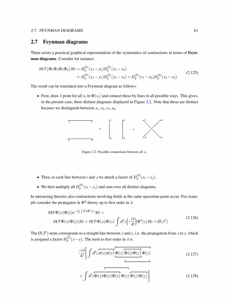
2.7. FEYNMAN DIAGRAMS 61
2.7 Feynman diagrams
There exists a practical graphical representation of the systematics of contractions in terms of Feyn-man diagrams. Consider for instance
〈0|T (Φ1Φ2Φ3Φ4) |0〉 = D(0)F (x1 − x2)D
(0)F (x3 − x4)
+ D(0)F (x1 − x3)D
(0)F (x2 − x4) + D(0)
F (x1 − x4)D(0)F (x2 − x3).
(2.125)
The result can be translated into a Feynman diagram as follows:
• First, draw 1 point for all xi in Φ(xi) and connect these by lines in all possible ways. This gives,in the present case, three distinct diagrams displayed in Figure 2.2. Note that these are distinctbecause we distinguish between x1, x2, x3, x4.
Figure 2.2: Possible connections between all xi.
• Then, to each line between i and j we attach a factor of D(0)F (xi − x j).
• We then multiply all D(0)F (xi − x j) and sum over all distinct diagrams.
In interacting theories also contractions involving fields at the same spacetime point occur. For exam-ple consider the propagator in Φ4-theory up to first order in λ:
〈0|T Φ(x)Φ(y)e−i λ4!
∫d4zΦ4(z) |0〉 =
〈0|T Φ(x)Φ(y) |0〉+ 〈0|T Φ(x)Φ(x)∫
d4z(−
iλ4!
)Φ4(z) |0〉+O(λ2).
(2.126)
The O(λ0)-term corresponds to a straight line between x and y, i.e. the propagation from x to y, whichis assigned a factor D(0)
F (x − y). The term to first order in λ is
−iλ4!
∫ d4z φ(x)φ(y)Φ(z)Φ(z)Φ(z)Φ(z)alalalaaaaaaaaaaaaaaaaaaaa
(2.127)
+
∫d4z
alalalaaaaaaaaaaaaaaaaaaa
Φ(x)Φ(y)Φ(z)Φ(z)Φ(z)Φ(z)
. (2.128)

62 CHAPTER 2. INTERACTING SCALAR THEORY
This can be written as ∫d4zD(0)
F (x − y)(42
)12
D(0)F (z − z)D(0)
F (z − z)
+
∫d4z D(0)
F (x − z)D(0)F (y − z)D(0)
F (z − z) · 4 · 3.(2.129)
The graphical representation of these two different contributions is given in Figure 2.3. Note theappearance of the point z, which is integrated over. The first term is proportional −iλ1
8 , while thesecond term has a factor of −iλ1
2 .
Figure 2.3: First and second term of O(λ1).
To give an interpretation of these combinatorial factors of 1/8 and 1/2, we observe that they coincidewith 1 over the order (≡ number of elements) of the symmetry group of the diagrams. These are calledthe symmetry factors. The symmetry factors are given by the number of ways one can exchangecomponents of the diagram without changing the diagram, where by components we mean either thetwo ends of a line starting and ending on the same point, entire lines between points or internal points(vertices - see below).For the two diagrams these are in turn:
• The single loop at z is symmetric under the exchange of the out- and in-going end of the loop, butthe direction must be consistent (i.e. one out- and one ingoing arrow). Therefore the symmetrygroup is G = Z2 and its order is |G| = 2.
• The double loop is separately symmetric under exchange of the out- and in-going end of bothloops, which gives a Z2 ×Z2 as well as under exchange of the two loops as a whole. Thereforethe symmetry group is G = Z2 ×Z2 ×Z2 and its order is |G| = 8.
One can show in general that if a Feynman diagram with symmetry group G always carries a combi-natorial factor 1
|G| . This is because if some symmetry remains the factor of 1n! in the interaction term
− λn!φ
n is only partially cancelled by counting the various contractions that yield the same diagram. Inthe above examples the symmetry group was due to the ambiguity in assigning arrows to the lines at avertex. In addition, if k vertices are identical, the symmetry group includes the group of permutationsof these k vertices of order |S k| = k!.
Let us introduce some jargon:
• The points x, y associated to Φ(x)Φ(y) in the correlator, which are not integrated over, arecalled external points.

2.7. FEYNMAN DIAGRAMS 63
• All other points - here z - over which is integrated over are internal points.
• For a Φn interaction, at an internal point n lines meet. Such points are called vertices.
2.7.1 Position space Feynman-rules
The translation of Wick’s theorem into Feynman-graphs as exemplified above can be proven to holdgenerally (the only non-trivial aspect being the symmetry factors). We summarize this in terms of theposition space Feynman-rules for the computation of
〈0|Tm∏
i=1
Φ(xi)e−i λn!
∫d4z φn(z) |0〉 (2.130)
at order λk, where we are assuming that all xi are distinct:
• Draw one external point for all xi and k internal points z j.
• Connect the points by lines such that
– to each external point xi 1 line is attached,
– to each internal point z j n lines are attached.
• To each line between points yi and y j (both external and internal) we associate a free propagator
D(0)F (yi − y j) = D(0)
F (y j − yi), (2.131)
where we stress again that the superscript reminds us to take the Feynman propagator of thefree theory.
• To each vertex associate a factor −iλ∫
d4 z j.
• To each external point associate a 1.
• Multiply all factors, Feynman propagators etc. and divide by the symmetry factor of the dia-gram.
• Then sum up all distinct such Feynman diagrams.
2.7.2 Momentum space Feynman-rules
More practical are the momentum space Feynman-rules: To each free propagator
D(0)F (x − y) =
∫d4 p(2π)4
ip2 −m2
0 + iεe−ip·(x−y) (2.132)
associate an arrow and momentum p in that direction. This means an arrow from x to y correspondsto the propagator D(0)
F (x− y). Obviously the direction is arbitrary because D(0)F (x− y) = D(0)
F (y− x),

64 CHAPTER 2. INTERACTING SCALAR THEORY
but let us make one such choice for each line. We can then perform the integral∫
d4z at each vertexexplicitly. E.g. for the Φ4-theory 4 lines meet at a vertex, and if, say, the momenta p1 and p2 pointinto that vertex and p3, p4 point out of it, this integral yields∫
d4z eip1·zeip2·ze−ip3·ze−ip4·z = (2π)4δ(4)(p1 + p2 − p3 − p4). (2.133)
This implements momentum conservation at each vertex. The delta-function will effectively eliminateone integral
∫d4 pi per vertex.8
Note at this point that the formal prescription that we integrate limT→∞(1−iε)
∫ T−T in (2.107) translates
into a corresponding prescription for∫
d4z. We should therefore view this integral as a complexcontour integral. From the fact that such integrals can be deformed in the complex plane as long as nopoles are hit it follows that the (1 − iε) prescription does not affect the result.The momentum-space Feynman rules9 for the computation of the n-point function
〈0|Tm∏
i=1
Φ(xi)e−i λn!
∫d4z φn(z) |0〉 (2.134)
at order λk are:
• Draw one external point for all xi and k internal points z j.
• Connect the points by lines such that
– to each external point xi 1 line is attached,
– to each internal point z j n lines are attached.
• To each line between points yi and y j (both external and internal) we associate a free propagator
D(0)F (yi − y j) (2.135)
with one choice of direction and to each such D(0)F (yi − y j) we associate directed momentum p
from yi to y j and a factori
p2 −m20 + iε
. (2.136)
• For each vertex we multiply a factor of (2π)4δ(4)(∑
ingoing pi −∑
outgoing pk) × (−iλ).
• For each external point we multiply a factor of e−ip·x for momentum pointing out of the externalpoint, or eip·x for momentum pointing into the point.
8The elimination of the zi-integration works this way only if the vertex is connected to at least one other point, eitherinternal or external. This is, for example, not the case for the second diagram in Fig. 2.3. More generally, one overall factorof
∫d4zi = VolR1,3 = (2π)4δ(4)(0) remains for diagrams not connected to any of the external points. We will see in the
next subsection how to deal with such ’disconnected diagrams’.9Careful: By momentum space Feynman rules we do not mean that we compute the Fourier transform of the correlator,
but rather that we give an equivalent set of rules for the computation of the correlator where the integral over the vertexpositions has been performed explicitly.

2.8. DISCONNECTED DIAGRAMS 65
• Integrate over each momentum∫ d4 p
(2π)4 and divide by the symmetry factor.
• Then sum up all distinct such Feynman diagrams.
For example, consider again the Φ4 theory to order λ, i.e.
〈0|T4∏
k=1
Φke−i λ4!
∫d4 xΦ4
|0〉 . (2.137)
λ0 corresponds to the diagrams in Figure 2.2. For λ1 we can have
Figure 2.4: Diagrams for λ1.
Consider the first diagram at order λ, make a consistent choice of momenta and assign eik·x for in-goingarrows at external points, e−ik·x for out-going arrows and −iλδ(4)(k1 + k2 − k3 − k4) at the vertex dueto momentum consvervation. We end up with
〈0|T4∏
k=1
Φ(xk)
(−
iλ4!
∫d4z Φ4(z)
)|0〉
∣∣∣∣∣Diagram ×
=4∏
j=1
∫d4k j
(2π)4 e−ik1·x1e−ik2·x2eik3·x3eik4·x4
× (−iλ)(2π)4δ(4)(k1 + k2 − k3 − k4)4∏
j=1
ik2
j −m20 + iε
.
(2.138)
As we will see soon, in the context of the LSZ formalism we actually need not the correlation function,but rather its Fourier transform. E.g. we will need expressions of the form∫
d4x1 eip1·x1
∫d4x2 eip2·x2
∫d4x3 e−ip3·x3
∫d4x4 e−ip4·x4 〈0| ... |0〉
∣∣∣∣∣Diagram ×
= (2π)4δ(4)(p1 + p2 − q3 − q4)(−iλ) × (2.139)i
p21 −m2
0 + iεi
p22 −m2
0 + iεi
p23 −m0 + iε
ip2
4 −m0 + iε.
2.8 Disconnected diagrams
A typical diagram contains disconnected pieces, i.e. subdiagrams which are not connected to any ofthe external points. For example consider the second diagram in Figure 2.4: The double loop in this

66 CHAPTER 2. INTERACTING SCALAR THEORY
case is not connected to any external point and therefore called ’disconnected piece’ (or disconnecteddiagram). A disconnected piece contains only internal points. By contrast, the part of the diagramwhich is connected to at least one external point is called ’partially connected diagram’.According to the Feynman rules disconnected pieces appear as overall factors of the Feynman dia-gram. If we sum up all Feynman diagrams that contribute to
〈0|T Φ(x1)...Φ(xk)e−i λN!
∫ΦNd4 x |0〉 (2.140)
the result factorises into the sum of all ’partially connected diagrams’ in the above sense multipliedby the sum of all disconnected diagrams. If you don’t believe this, just draw a few pages of Feynmandiagrams relevant for, say, the 4-point function in φ4-theory and convince yourself that the infinitesum over all relevant diagrams can be organized this way.Let V j denote the set of all individual disconnected pieces (i.e. Vi is a Feynman diagram containingonly internal points which itself is connected as a diagram). Then the sum over all diagrams notconnected to any of the external points can be organized as a sum over all Vi, where each Vi appearsni-times with ni = 0, 1, ...,∞. If some Vi appears ni-times we must divide its contribution by ni!to account for the symmetry factor from interchanging identical Vi. For instance, the sum over alldisconnected diagrams contains
1 + 8+ 12!88 + 1
3! 888 + ... + arbitrary products and number of loops.
Denoting by Vi also the value of the corresponding diagram, we have that the sum over all discon-nected diagrams is ∏
i
∞∑ni=0
(Vi)ni
1ni!
=∏
i
eVi = e∑
i Vi . (2.141)
This is called exponentiation of disconnected pieces. The final result for (2.140) is therefore of theform ∑
( at least partially connected pieces) × e∑
i Vi . (2.142)
Now consider the full correlator
〈Ω|T∏
i
φi |Ω〉 =〈0|T
∏i φie−i
∫HIdt |0〉
〈0|Te−i∫
HIdt |0〉. (2.143)
The denominator contains no external points and thus yields precisely
〈0|Te−i∫
HIdt |0〉 = e∑
i Vi ≡ the partition function. (2.144)
This cancels the factor from the nominator and thus
〈Ω|Tn∏i
φi |Ω〉 =∑
(all partially connected diagrams with n external points). (2.145)
Note that the partition function plays an important role also in Statistical Mechanics. In computingthe partition function in that context you will encounter many times the same reasoning that organizesthe sum over all its contributions in a form similar to the one above. In fact, when discussing the pathintegral approach to Quantum Field Theory in QFT II we will see that this is no coincidence.
2.9. 1-PARTICLE-IRREDUCIBLE DIAGRAMS 67
2.8.1 Vacuum bubbles
The disconnected diagrams contributing to the partition function are called vacuum bubbles and theyhave a remarkable physical interpretation: From eq. (2.103) we recall that
e∑
i Vi = 〈0|Te−i∫
dtHI |0〉 = limT→∞(1−iε)
∣∣∣ 〈Ω| 0〉∣∣∣2e−iEΩ2T (2.146)
so− iEΩ2T
∣∣∣T→∞(1−iε) =
∑Vi − log
(| 〈Ω| 0〉|2
)︸ ︷︷ ︸finite number
(2.147)
and thereforeEΩ = lim
T→∞(1−iε)
i∑
Vi
2T(2.148)
because the finite term plays no role in the limit we are taking. EΩ is the vacuum energy of theinteracting theory in the scheme where E0 - the vacuum energy of the free theory - has been set to0 by renormalisation of the original Lagrangian after adding a term − E0
VolR3
to L. In terms of thecorresponding energy density this means
EΩ
VolR3= lim
T→∞(1−iε)
i∑
j V j
2TVolR3= i
∑j V j
(2π)4δ(4)(0). (2.149)
Note that the factor of (2π)4δ(4)(0) in the denominator cancels a corresponding factor appearing inthe computation of each of the Vi from an uncancelled overall
∫d4z - see footnote 8. This factor
represents the familiar IR divergence of the vacuum energy from integration over spacetime. Aswe will see later when actually computing loops of this type, EΩ
VolR3
is also UV divergent because
of divergent momentum integration for the vacuum loops. This is no surprise as already E0Vol
R3was
divergent. We organise these divergences order by order in perturbation theory and can renormalisethem away by counter-terms, i.e. by adding to the classical Lagrangian terms of form10
L → L− λ1V(1)0 − λ2V(2)
0 − ..., (2.150)
just like we did for E0 (i.e. at order λ0) in the free theory.
2.9 1-particle-irreducible diagrams
As a first application of our formula for the computation of n-point functions in an interacting theorywe consider perturbative corrections to the propagator in Φ4-theory,
DF(x − y) = 〈Ω|T Φ(x)Φ(y) |Ω〉 =∑
i
O(λi). (2.151)
Some of the first few Feynman diagrams are shown in Figure 2.5.
10In fact, due to renormalisation of the other operators order by order in λ this is a bit of an oversimplification, but wewill come to this in more detail later in the course.

68 CHAPTER 2. INTERACTING SCALAR THEORY
Figure 2.5: Perturbative corrections.
To organise the sum over Feynman diagrams it is useful to define the concept of 1− particle-irreducible(1PI) Feynman diagrams. These are diagrams out of which one cannot produce 2 separate non-trivialdiagrams (diagrams containing more than just one line) by cutting a single line. E.g. in Figure 2.5only the 4th diagram is not 1PI (one can cut it in 2 by cutting the line between the two loops). It isstandard to introduce the notation
1PI =
∑(all non-trivial 1PI diagrams), (2.152)
where it is understood that we do not attach external points to both ends (i.e. no factors e−ip·x ori/(p2 −m2
0 + iε) from the left or right of 1PI.
We now define −iM2(p2) to be the value of 1PI, where p2 denotes the in- and outgoing momentum.
Clearly computing −iM2(p2) can be a hard task, and the result will be a complicated function of p2.In particular this quantity may be divergent (again due to integration over internal momenta). We willcompute −iM2(p2) explicitly for an electron in Quantum Electrodynamics, in which case it is calledself-energy, later in the course and find ways to deal with its divergence systematically. Irrespectiveof the outcome for −iM2(p2), the sum over all diagrams contributing to 〈Ω|T Φ(x)Φ(y) |Ω〉 canbe organised as a geometric series in 1 PI diagrams. Let us compute the Fourier transform DF(p2)
defined such that
DF(x − y) =∫
d4 p(2π)4 e−ip(x−y)DF(p2). (2.153)
DF(p2) can be expanded as
DF(p2) =ffi
p2−m20+iε
+fi
p2−m20+iε
1PI f
ip2−m2
0+iε
+f 1PIf
1PIf+ ... (2.154)
The fact that we are not drawing points at the two ends of diagrams symbolizes that we are omittingthe factors of eipx or e−ipy as these are, by definition, not part of DF(p2). The Fourier transformed

2.9. 1-PARTICLE-IRREDUCIBLE DIAGRAMS 69
propagator is then
DF(p2) =i
p2 −m20 + iε
+i
p2 −m20 + iε
(−iM2(p2)
) ip2 −m2
0 + iε+ ...
=i
p2 −m20 + iε
1 +M2(p2)
p2 −m20 + iε︸ ︷︷ ︸≡q
+
M2(p2)
p2 −m20 + iε
2
+ ...
=
ip2 −m2
0 + iε1
1 − M2(p2)
p2−m20+iε
.
(2.155)
Here we assumed that q < 1 so that the geometric series∑∞
n=0 qn converges to 11−q . Once again, we
will deal with the explicit form of −iM2(p2) later in QED and justify this assumption. This procedureis called Dyson resummation and yields the resummed propagator
DF(p2) =i
p2 − (m20 + M2(p2)) + iε
≡fpf (2.156)
Now, −iM2(p2) is a complicated function of p2 that we compute order by order in λ. We can thenextract the first analytic pole in DF(p2) and call it m2. Then
DF(p2) =i Z
p2 −m2 + iε+ terms regular at m2 (2.157)
for some Z. I.e. Z is by definition the residue (in the above sense) of DF(p2) at its first analytical polem2. This way we can compute
• m2 - the physical 1-particle-mass ≡ pole mass,
• Z - the wavefunction renormalisation,
perturbatively to given order in λ. This is a beautiful result because we can now understand quantita-tively why the mass of the 1-particle momentum eigenstates in an interacting theory differs from m0:The reason are the self-interactions of the field, which are resummed as above to shift the pole of thefull propagator from m0 to m. In particular this picture justifies our assertion made in the context ofasymptotic in- and out-states that the asymptotic states behave as free particles, but with fully ’renor-malised mass’ m , m0: By sending the particles infinitely far apart from each other we effectively’switch off’ the interactions between the different particles, but we cannot switch off the interactionsof the asymptotic particles with themselves (or rather of the field with itself). These are precisely the1PI contributions to DF(p2) and thus the in-and out-states do have the fully resummed mass m2 , m2
0.

70 CHAPTER 2. INTERACTING SCALAR THEORY
2.10 Scattering amplitudes
Recall the LSZ-reduction formula for r in- and n out-states
n∏k=1
∫d4yk eipk ·yk
r∏l=1
∫d4xl e−iql·xl 〈Ω|T Φ(y1)...Φ(x1)... |Ω〉
=∏
k
i Z1/2
p2k −m2 + iε
∏l
i Z1/2
q2l −m2 + iε
〈p1...| S |q1...〉∣∣∣connected,
(2.158)
where all ql and pk are on-shell. Now, recall that 〈p1...| S |q1...〉∣∣∣connected itself cannot be proportional
to p2k − m2 or q2
l − m2 because otherwise it is zero on-shell and thus no scattering occurs; likewise〈p1...| S |q1...〉
∣∣∣connected cannot contain any factors of (p2
k −m2)−1 or (q2l −m2)−1 because then it would
be divergent on-shell, in contradiction with its definition as a quantum mechanical amplitude. As aresult only those Feynman diagrams are relevant with exactly (n + r) poles at m2 in the above sense.It is not hard to see that these are precisely the ones that contribute to the fully connected correlationfunction. A fully connected correlation function has the structure displayed in Figure 2.6.
Figure 2.6: Fully connected correlation function with r in and n out states.
Here xfpf denotes the fully resummed propagator from lines connected to external points.The fully resummed propagator would appear if we computed to all orders in perturbation theory.More realistically, to a given finite order in perturbation theory we should think of the propagator ascomputed to suitable order.
The big blop in the middle denotes the amputated correlator. By amputated correlator we mean theFeynman diagram after cutting off all external legs carrying xfpf or fpfx. Sinceeach external leg carries a factor of i Z
p2−m2+iε near m2 if p2 is on-shell, all (n + r) external legs yieldtogether yield the right singularity structure.By contrast, partially connected diagrams such as the one in Figure 2.7 carry fewer factors of i
p2−m2+iεand thus do not contribute to 〈p1...| S |q1...〉
∣∣∣connected. Therefore the final result for the computation

2.10. SCATTERING AMPLITUDES 71
of scattering amplitudes is
〈p1, ..., pn| S |q1, ..., qr〉∣∣∣connected =
(√Z)n+r× (2.159)(∏
k
∫d4ykeipk ·yk
∏l
∫d4xle−iql·xl 〈Ω|T Φ(y1)...Φ(x1)... |Ω〉 |fully connected
)|Amputated
Note that the wavefunction renormalisation factor Z itself is of the form 1 + O(λ) in perturbationtheory, so to leading order in the coupling constant λ the Z-factors play no role as only O(λ) diagramscan be fully connected.
x1 xfpfx y1
x2 xfpfx y2
Figure 2.7: Partially connected diagramm, i.e. (n − 2) and (r − 2).
As an example we consider again the Φ4-theory to leading order. The only fully connected diagramat O(λ) is the first diagram in Figure 2.4. We make a consistent choice of ingoing versus outgoingmomenta and recall the result
〈Ω|T Φ(x1)Φ(x2)Φ(y1)Φ(y2) |Ω〉∣∣∣×=
=4∏
j=1
∫d4k j
(2π)4 e−ik1·x1e−ik2·x2eik3·y1eik4·y2
× (−iλ)(2π)4δ(4)(k1 + k2 − k3 − k4)4∏
l=1
ik2
l −m20 + iε
.
(2.160)
To compute 〈p1, p2| S |q1, q2〉 |connected we take first the Fourier transform as∫d4x1e−iq1·x1
∫d4x2e−iq2·x2
∫d4y1eip1·y1
∫d4y2eip2·y2
× 〈Ω|T Φ(x1)Φ(x2)Φ(y1)Φ(y2) |Ω〉∣∣∣×
= (−iλ)(2π)4δ(4)(q1 + q2 − p1 − p2)2∏
j=1
iq2
j −m20 + iε
ip2
j −m20 + iε
(2.161)

72 CHAPTER 2. INTERACTING SCALAR THEORY
and then we amputate by discarding all propagators from external lines. The result is
〈p1, p2| S |q1, q2〉∣∣∣connected, O(λ) = (−iλ)(2π)4δ(4)(q1 + q2 − p1 − p2), (2.162)
where we have discarded the factor√
Z4 because, as discussed, it does not contribute to the leadingorder result.
2.10.1 Feynman-rules for the S -matrix
This procedure can be summarised in general in terms of the Feynman-rules for the computation of〈p1, ..., pn| S |q1, ..., qr〉
∣∣∣connected as follows:
• Draw the relevant fully connected Feynman diagrams with (n+ r) external points to given orderin λ.
• Assign ingoing momenta ql and outgoing momenta pk and label momenta of internal lines withk j.
• Each vertex carries (−iλ)(2π)4δ(4) (∑
ingoing momenta − outgoing momenta).
• Each internal line carries ik2
j−m20+iε
.
• Integrate over all internal momenta∏
j
∫ d4k j
(2π)4 and divide by the symmetry factor.
• Sum up all diagrams and multiply by(√
Z)n+r
to given order in λ.
Deeper interpretation of the Feynman rules
The connection between correlation functions and S -matrix elements gives Feynman diagrams anintuitive physical meaning: In Figure 2.8 two particles come in and interact at Z1 to form two so-called "virtual" particles, which in turn join again at Z2 and form two outgoing states. The obvious
Figure 2.8: Feynman graph with two virtual particles.
interpretation of the Feynman diagram elements is therefore:
• A linef corresponds to the worldline of a particle.

2.11. CROSS-SECTIONS 73
•F e−ip·x is the wavefunction for a momentum-eigenstate.
• A vertexP Z is a localised interaction at a spacetime point Z.
• Summing up diagrams and integrating over∫
d4z amounts to coherently summing up the QMprobability amplitudes for all possible processes - called "channels" - with the same macro-scopic result. In particular, this will lead to QM interference between the different channels.
Intermediate particles, e.g. those running in the loop as k1 and k2 in Figure 2.8, are called virtualbecause they are generally off-shell: This means that these particles do in general not satisfy therelation k2
i −m20 = 0. E.g. for the loop-diagram above we integrate over all internal momenta (where
the delta-functions at the vertices implies that some of these integrals become trivial). In the presentdiagram momentum conservation at the first vertex implies that
q1 + q2 = k1 + k2 ⇔ k2 = q1 + q2 − k1, (2.163)
where k1 is free and thus integrated over. For most values of k1 we have k21 − m2
0 , 0. We canthink of this as a quantum-mechanical violation of the energy-momentum relation because E2
j ,
~k j2+ m2
0 for virtual particles. In Quantum Mechanics this is allowed for sufficiently short times - infact this precisely what is meant by the energy-time uncertainty relation arising in quantum mechanicalperturbation theory. Note, however, that 4-momentum conservation is guaranteed at each vertex dueto the factors
(2π)4(∑
ingoing momenta − outgoing momenta)
. (2.164)
LSZ versus Interaction Picture Perturbation Theory
On assignment 7 will work out a detailed a comparison of the LSZ approach to scattering as com-pleted in this chapter and a more naive approach based on quantum mechanical Interaction Pictureperturbation theory.
2.11 Cross-sections
S -matrix elements are in general of the form
〈 f | S |i〉 = δ f i︸︷︷︸no scattering
+ i(2π)4δ(4)(p f − pi)︸ ︷︷ ︸momentum conservation
· M f i︸︷︷︸=:scattering amplitude
(2.165)
In particular, momentum conservation is a consequence of the insertion of delta-functions at eachvertex in the Feynman diagrams. The first summand δ f i accounts for the situation that the initial andfinal states are identical, in which case no scattering occurs. In the sequel we will usually exclude thispossibility and focus on non-trivial scattering events.The QM probability for scattering of a given initial state |i〉 into a range of final states | f 〉 is
P|i〉→| f 〉 =∑| f 〉∈| f 〉
∣∣∣ 〈 f | S |i〉 ∣∣∣2. (2.166)

74 CHAPTER 2. INTERACTING SCALAR THEORY
Assume now that |i〉 < | f 〉 (so that in particular the term δ f i is irrelevant), then
P|i〉→| f 〉 =∑| f 〉∈| f 〉
[(2π)4δ(4)(p f − pi)
]2︸ ︷︷ ︸=(2π)4δ(4)(p f−pi) (2π)4 δ(4)(0)︸ ︷︷ ︸
=VR1,3
∣∣∣M f i∣∣∣2. (2.167)
We define the transition rate as the probability normalised per spacetime volume,
ω f i =P|i〉→| f 〉
unit time × unit volume(2.168)
and therefore
ω f i =∑| f 〉∈| f 〉
(2π)4δ(4)(p f − pi)∣∣∣M f i
∣∣∣2. (2.169)
For scattering into N identical particles this is
ω f i =1
N!
N∏n=1
∫d3kn
(2π)3
12En
(2π)4δ(4)∑
i
pi −∑
n
kn
∣∣∣M f i∣∣∣2, (2.170)
where the symmetry factor 1N! accounts for the indistinguishability of the N identical particles.
Now, a typical scattering experiment is of the form
Incoming beam of density ρB and length lB F Target A of density ρA and length lA ,
where ρA,B denote the respective number densities (i.e. number of particles per volume). The number(#) of scattered particles is proportional11 to lA lB
∫d2x ρa(x) ρB(x). The factor of proportionality has
dimension [Area] and is called cross-section σ,
# of events =: σ lA lB
∫d2x ρA(x) ρB(x). (2.171)
If ρA and ρB are constant and both beams overlap over the areaA, then
σ =# of scattered particles
lA lB ρA ρBA. (2.172)
This suggests the following intuitively clear interpretation of the meaning of σ: The cross-section σis the effective area of the beam B that participates in the scattering.
Consider now a 2 → N scattering process such that all out-going states |k j〉 are momentum eigen-states. The initial states are the momentum eigenstates |pA〉 and |pB〉. Let us go to the rest frame of
11Here we are assuming that all particles of the beam hitting the target get to interact with the target particles with equalprobability. For simplicity we are also assuming that the particle density varies only in the directions x1, x2 transverse to thebeam.
2.11. CROSS-SECTIONS 75
the target A called lab frame. Suppose for simpilcity that the beam B hits the target A over its entireareaA and that the densities of beam and target do not vary much. Then
# of eventsVolume × Time
=σρA ρB lA lBA
Volume × Time= σρA ρB
∣∣∣~vLB
∣∣∣, (2.173)
where the relevant interaction volume is is just Volume = A lA and the relevant interaction time iswhat it takes for the beam to pass over a given slice in the target orthogonal to the beam direction, i.e.
lBTime =
∣∣∣~v(L)B
∣∣∣. Sometimes it is also useful to think in terms of the beam flux F defined as
ρB∣∣∣~vL
B
∣∣∣ =: F . (2.174)
Since E = γm and ~p = mγ~v we can use
∣∣∣~vLB
∣∣∣ = ∣∣∣~pLB
∣∣∣EB
(2.175)
to obtain# events
Volume × Time= σρA ρB
∣∣∣~pLB
∣∣∣EB
= σρA F . (2.176)
What we actually compute in evaluating the S-matrix elements are not absolute numbers of events,but rather QM probabilites. In order make the transition between both these concepts we replace theparticle number densities ρA and ρB by the quantum mechanical densities of the corresponding singleparticles states, i.e. the probabilities of finding a particle A or B per given volume. If 〈pA|pA〉 = 1 thisprobability would be 1/VR3 = 〈pA|pA〉/VR3 . With our normalisation of momentum states
〈pA|pA〉 = (2π)3 2EA δ(3)(~pA − ~pA) = 2EAVR3 , (2.177)
we must replace
ρA →〈pA|pA〉
VR3= 2EA and ρb → 2EB. (2.178)
Since we are in the rest frame of A we have 2EA = 2m. Therefore in the lab frame (~v(L)A = 0)
ω f i =QM probabilityVolume × Time
= 4σm p(L)B . (2.179)
Note that4mp(L)B = 4 EA EB|~v
(L)B | = 4EA EB|~v
(L)A −~v(L)B | (2.180)
in the lab frame. Finally, one can show that 4 EA EB|~v(L)A − ~v(L)B | is invariant under Lorentz boosts
in direction A → B. Therefore ω f i = 4 EA EB|~vA − ~vB|σ is the correct general expression for thetransition rate valid in any frame 12. To conclude, the differential cross-section is
dσ =(2π)4
4EA EB |~vA −~vB|dΠN δ
(4)
pa + pB −∑
i
ki
∣∣∣M f i∣∣∣2, (2.181)
12For a more formal, but also considerably more complicated proof see Peskin-Schröder p.102 − 108.

76 CHAPTER 2. INTERACTING SCALAR THEORY
where
dΠN ≡1
N!
N∏n=1
∫d3kn
(2π)3
12En
. (2.182)
For example consider 2 − 2 scattering as shown in Figure 2.9. On Assignment 7 we show that if all
Figure 2.9: 2 − 2 scattering.
four particles have the same mass, the differential cross-section is
dσdΩ3
=12!
164π2
1s|M|2, (2.183)
where the relativistically invariant Mandelstam variable
s = (p1 + p2)2 = (p3 + p4)
2 (2.184)
appears. Note that in Φ4-theory |M|2 = λ2 to first order in λ, i.e. for the maximally localised,pointlike interaction given by the first Feynman diagram in Figure 2.4. Therefore
dσdΩ∼
1s
(2.185)
to first order in λ. This is a famous result, which in fact holds more generally:
The differential cross-section for hard scattering off a pointlike target (i.e. a target withno substructure of length l ≥ 1/
√s) falls off as 1/s.
This characteristic behaviour as observed in deep inelastic scattering experiments with hardons was acrucial clue to the the parton structure of hadrons as you will surely recall from your particle physicscourse.

Chapter 3
Quantising spin 12-fields
3.1 The Lorentz algebra so(1, 3)
Relativistic fields as representations of the Lorentz algebra
Relativistic fields are classified by their behaviour under Lorentz transformations
xµ 7→ x′µ = Λµν xν , Λµ
ν ∈ S O(1, 3). (3.1)
Quite generally a field Φa(x) transforms as a representation1 of the Lorentz group S O(1, 3) - or, moreprecisely, as we will see momentarily, of its double cover Spin(1, 3). This means that the classicalfield Φa(x) is a map
Φa : R1,3 → V , (3.2)
x 7→ Φa(x), a = 1, . . . , dim(V) (3.3)
with V a vector space such that the specific transformation behaviour of the field Φa(x) under (3.1) isgiven by
Φa(x) 7→ R(Λ)abΦb(Λ−1x′) = R(Λ)a
bΦb(x). (3.4)
Here for every element Λ ∈ S O(1, 3) the object R(Λ) is an automorphism (an invertible linear map)acting on V in a manner compatible with the group action of S O(1, 3). Specifying the representationin which the field transforms amounts to assigning such an automorphism R to every element Λ ∈S O(1, 3), where compatibility with the group action of S O(1, 3) means that2
R(Λ2)ab R(Λ1)
bc =R(Λ2Λ1)
ac
R(Λ−1)ab =
(R(Λ)−1
)a
b.
(3.5)
1The concept of Lie groups, Lie algebras and their representations has been discussed in detail in the course on QuantumMechanics. A good book in the present context is: Urbantke, Sexl: Relativity, Groups, Particles. As a quick reminder of themain points see e.g. http://www.thphys.uni-heidelberg.de/$\sim$weigand/Skript-QM2011/skript.pdf.
2In short, a representation R of a group G is a group homomorphism from G to Aut(V) for some vector space V .
77

78 CHAPTER 3. QUANTISING SPIN 12 -FIELDS
The vector space V is also called representation space. Note that the index a refers to the componentsof the fields with respect to a basis of the vector space V - called the representation space -, while µ, νare spacetime indices. These two are in general completely different objects.
Consider the following examples:
• For a real (or complex) scalar field Φ(x) the representation space V is just R (or C) and
R(Λ) = 1 ∀Λ. (3.6)
The scalar field is said to transform in the trivial or scalar representation and describes parti-cles with spin 0.
• A vector field Aµ(x) (e.g. the gauge potential of electro-magnetism) transforms in the vectorrepresentation: The representation space V is identified with spacetime R1,3 itself (or ratherits tangent space) and
R(Λ)µν = Λµν ∀Λ. (3.7)
Since here V = R1,3, we have in this case that a, b = µ, ν. A field in the vector representationdescribes particles with spin 1 (as we will see later in this course when quantising such vectorfields).
An important concept in representation theory is that of an irreducible representation (irrep): AnIrreducible representation is one whose representation space does not split into a direct sum of twovector spaces in a manner respected by the group action, i.e. it is not possible to find a basis of therepresentation space in which
R(Λ) =
? 00 ?
∀Λ. (3.8)
Irreducible representations form the building blocks of which larger representations can be formed byconsidering direct sums of representation spaces.
Spin 1/2 particles are described by fields in the spinor representation. To find this representationour starting point will not be the irreducible representations of the Lorentz group S O(1, 3), but of
The Lorentz algebra so(1, 3)
This is the algebra of infinitesimal Lorentz transformations connected to the identity. This is analo-gous to the precedure applied in quantum mechanics to find spin 1
2 representations of the algebra ofspatial rotations so(3) ' su(2).
A Lorentz transformation can be written infinitesimally as
Λµν = δ
µν +ω
µν. (3.9)

3.1. THE LORENTZ ALGEBRA S O(1, 3) 79
Since the metric must be invariant under a Lorentz transformation in the sense that
Λµα Λν
β ηαβ = ηµν, (3.10)
the infinitesimal transformations satisfy ωµν = −ωνµ. We introduce a basis of antisymmetric 4 × 4matrices into which we would like to expand ωµν. This basis contains 6 elements. Let the basis be(
MA)µν
with A = 1, ..., 6. (3.11)
Thenωµν = −
i2
ΩA(MA
)µν(3.12)
for some ΩA with summation over A understood. We introduce the double-index notation A = ρσ
with ρ,σ = 0, 1, 2, 3 such that(Mρσ)µν = −(Mσρ)µν (3.13)
is antisymmetric in σρ. Therefore
ωµν = −i2
Ωρσ(Mρσ)µν. (3.14)
So an infinitesimal Lorentz transformation is
Λµν = δ
µν −
i2
Ωρσ(Mρσ)µν. (3.15)
A finite transformation is given by applying the infnitesimal version N times for N → ∞ in the sense
Λµν(Mρσ) = lim
N→∞
(δµν −
1N
i2
Ωρσ(Mρσ)µν
)N
=[e−
i2 Ωρσ(Mρσ)
]µν.
(3.16)
This is what is meant by saying that the Mρσ are the generators of the Lie group S O(1, 3), or equiva-lently form a basis of the Lie algebra so(1, 3).The structure of the Lie algebra so(1, 3) is encoded in the commutation relations of its basis elements.To find these one expands the defining relation of the underlying Lie algebra S O(1, 3)
Λµα Λν
β ηαβ = ηµν (3.17)
to second order in Ω to conclude that
[Mρσ, Mτν] = −i (ηρνMστ + ηστMρν − ηρτMσν − ησνMρτ) . (3.18)
This defines the structure constants of the Lie-algebra so(1, 3). Recall that in general a basis T A of aLie algebra satisfies
[T A, T B] =∑
C
i f ABCTC , (3.19)
where f ABC are the structure constants. They obey

80 CHAPTER 3. QUANTISING SPIN 12 -FIELDS
• f ABC = − f BA
C
• and the Jacobi identity
f ABD f CD
E + f CAD f BD
E + f BCD f AD
E = 0. (3.20)
We view the commutator (3.18) as the defining relation for abstract objects Mρσ. An n-dimensionalrepresentation of the Lie algebra so(1, 3) is an assignment that associates to each Mρσ an invertiblemap
(Rρσ)ab = R(Mρσ)a
b (3.21)
acting on an n-dimensional vector space V such that the same relation (3.18) holds for the represen-tation matrices (Rρσ)a
b. The indices a, b = 1, . . . , n refer to a basis ea of V in the sense that v ∈ V isexpanded as v = vaea. Note again that in general a and b are unrelated to µ and ν.Consider as a special case the vector representation by choosing V = R1,3 (viewed as the tangentspace to spacetime). In this case we do identify a, b ≡ µ, ν and set
(Jρσ)µν := i(ηρµησν − ηρνησµ). (3.22)
One can check that this indeed satisfies the so(1, 3) relations (3.18) and that
ωµν = −i2ωρσ(J
ρσ)µν. (3.23)
Therefore
Λµν =
[e−
i2ωρσJ
ρσ]µν. (3.24)
We can use this result to deduce the matrix representation of spatial rotations by an angle α around anaxis ~n. The corresponding ωµν can be written as
ωi j = αεi jk nk. (3.25)
E.g. for a rotation around the x1-axis we have
~n =
100
⇒ ωρσ =
0 0 0 00 0 0 00 0 0 α
0 0 −α 0
. (3.26)
The corresponding infinitesimal rotations are then of the form
Λµν = δ
µν +ω
µν =
1 0 0 00 1 0 00 0 1 −α
0 0 α 1
, (3.27)

3.2. THE DIRAC SPINOR REPRESENTATION 81
whose finite version is
Λµν =
1 0 0 00 1 0 00 0 cosα − sinα0 0 sinα cosα
. (3.28)
3.2 The Dirac spinor representation
To find the spinor representation of so(1, 3) we start from the Clifford algebra Cliff(1, 3) definedas the algebra spanned by n × n-matrices (γµ)A
B, µ = 0, 1, 2, 3 and A, B = 1, . . . , n such that theanti-commutator is
γµ, γν := γµγν + γνγµ = 2ηµν 1. (3.29)
Reinstating for clarity the indices A and B the defining relation is
(γµ)AB(γ
ν)BC + (γν)A
B(γµ)B
C = 2ηµν 1AC . (3.30)
This implies
γµγν =
ηµν if µ = ν
−γνγµ if µ , ν. (3.31)
Therefore
(γ0)2 = 1, (γi)2 = −1. (3.32)
The central point is that given (γµ)AB as above the objects
(S ρσ)AB :=
i4[γρ, γσ]AB (3.33)
form a representation of so(1, 3), i.e.[S ρσ, S τk
]= −i
(ηρkS στ + ηστS ρk − ηρτS σk − ησkS ρτ
), (3.34)
therefore (3.18) holds. Thus we have constructed a representation of so(1, 3) from the Clifford alge-bra:
Every representation of Cliff(1,3) induces a representation of so(1,3).

82 CHAPTER 3. QUANTISING SPIN 12 -FIELDS
One can prove this by direct computation. To this end note that
S µν =
0 if µ = νi2γ
µγν if µ , ν
=i2(γµγν − ηµν). (3.35)
The claim then follows with the help of the anti-commutation relations (3.29) after some algebra asworked out in the tutorial.
Now we want to find an explicit representation of the Clifford algebra. Since it is useful to knowthe result for an arbitrary number of spacetime dimensions let us give the general result valid forCliff(1, d − 1). The problem is therefore to find n × n-matrices
(γµ)AB with µ = 0, 1, 2, ..., d − 1 and A, B = 1, ..., n (3.36)
subject to (3.29). This will then also give a representation of the Lorentz algebra so(1, d − 1). In thetutorials we will prove the following famous theorem:
The irreducible representations of Cliff(1, d − 1) are of dimension
n = 2d2 if d is even
n = 212 (d−1) if d is odd
. (3.37)
Let us now specialise to d = 4 as is relevant for QFT in four spacetime dimensions. In this casen = 4. One choice of γµ called chiral or Dirac representation is
γ0 =
0 12
12 0
, γi =
0 σi
−σi 0
, (3.38)
where σi are the Pauli matrices
σ1 =
0 11 0
, σ2 =
0 −ii 0
, σ3 =
1 00 −1
(3.39)
withσi,σ j = 2δi j. (3.40)
Given an invertible matrix U, every other choice UγµU−1 is also a representation of Cliff(1, 3). Thecomplex vector space on which (γµ)A
B acts is called the space of Dirac spinors ψA, A = 1, ..., n withn = 4 for d = 4.Now, from the above it is clear that the ψA also form a representation of so(1, 3) because the γµ
induce a representation of so(1, 3). More precisely, a Dirac spinor ψA transforms under a Lorentztransformation
Λµν =
[e−
i2ωρσJ
ρσ]µν
(3.41)
asψA 7→
[e−
i2ωρσS ρσ
]A
BψB. (3.42)

3.2. THE DIRAC SPINOR REPRESENTATION 83
A Dirac spinor field ψA(x) transforms as
x 7→ x′ = Λx, (3.43)
ψA(x) 7→ [S (Λ)]AB ψB(Λ−1x′) = [S (Λ)]AB ψ
B(x) (3.44)
with[S (Λ)]AB =
[e−
i2ωρσS ρσ
]A
B. (3.45)
The indices A = 1, ..., n, with n = 4 for Cliff(1, 3) are called spinor indices. Even though in 4dimensions A happens to run from 1, . . . , 4, we must not cunfuse them at any time with spacetimeindices µ, ν.
Now that we found a new type of representation of the Lorentz algebra so(1, 3) we would like togive it a physical interpretation. The important claim is that
A Dirac spinor field ψA(x) behaves like a spin 12 -field.
To prove this we consider a spatial rotation around ~n with
ωi j = α εi jk nk (3.46)
andS [Λ] =
[e−
i2ωi jS i j
]A
B. (3.47)
Now,
S i j =i4[γi, γ j] =
− i2σ
iσ j 00 − i
2σiσ j
= 12σ
k 00 1
2σk
(3.48)
with (i jk) cyclic permutations of 123. The latter equations follows from the properties of the Paulimatrices. So
S [Λ] =
e−i α2 ~n ~σ 00 e−i α2 ~n ~σ
. (3.49)
What is crucial is the factor of 12 , which indeed indicates a transformation as a spin 1
2 under thesubalgebra so(3) ⊂ so(1, 3) of spatial rotations. In particular consider a rotation by α = 2π around~nT = (0, 0, 1),
S [Λ] = exp
−iπσ3 00 −iπσ3
= −1. (3.50)
ThereforeψA 7→ −ψA (3.51)
under a rotation by 2π.

84 CHAPTER 3. QUANTISING SPIN 12 -FIELDS
While we have found a representation of the Lorentz-algebra so(1, 3), this does not give a representa-tion of the Lorentz-group S O(1, 3), but rather of its double cover Spin(1, 3). The latter is isomorphicto S L(2, C), the group of complex 2× 2 matrices with determinant 1 (not to confuse with S U(2), thegroup of complex unitary such matrices). In the tutorial we will investigate this isomorphism and thecorresponding description of spinors.
A Dirac spinor forms a representation of Spin(1, 3) ' S L(2, C), not of S O(1, 3).
The reason is that S [Λ = 1] , 1, which is incompatible with the group law of S O(1, 3). In Spin(1, 3)by contrast, a rotation around 2π does not correspond to the 1 because it is defined as the double coverof S O(1, 3).3 This is the relativistic version of the statement familiar from Quantum Mechanicsthat the j = 1
2 spinor representation of the algebra of spatial rotations so(3) does not furnish arepresentation of the Lie group S O(3) but only of its double cover S U(2).
3.3 The Dirac action
We now want to construct Lorentz scalars and vectors out of ψA(x) in order to construct a covariantaction. To do so we define the conjugate spinor ψ† := (ψ∗)T , i.e.
ψ† =((ψ1)∗, (ψ2)∗, (ψ3)∗, (ψ4)∗
). (3.52)
We now would like to know how ψ†(x)ψ(x) behaves under a Lorentz transformation Λ, under which
x 7→ x′ = Λx, (3.53)
ψ(x) 7→ S (Λ)ψ(Λ−1x′), (3.54)
ψ†(x) 7→ ψ†(Λ−1x′) S †(Λ). (3.55)
In order for ψ†(x)ψ(x) to transform as a Lorentz scalar, we would need S (Λ)† = S −1(Λ). However,
S †(Λ) = e[−i2ωρσS ρσ]
†
= ei2ωρσ(S
ρσ)† (3.56)
and
(S ρσ)† =( i4[γρ, γσ]
)†= −
i4
[γσ†, γρ†
]=
i4
[γρ†, γσ†
]. (3.57)
It is not possible to pick all γµ hermitian at the same time since
(γ0)2 = 1 → real eigenvalues,
(γi)2 = −1 → imaginary eigenvalues.(3.58)
Therefore, (S ρσ)† , (S ρσ) and thus S (Λ)† , S −1(Λ).
3For further reading see e.g. Urbantke, Sexl: Relativity, Groups, Particles.

3.3. THE DIRAC ACTION 85
Rather, it is possible to pick γµ such that
(γ0)† = γ0, (γi)† = −γi, (3.59)
which is indeed satisfied by the Dirac representation above. In this case
(γµ)† = γ0γµγ0, (3.60)
because γ0γ0 = 1 and γ0γi = −γiγ0. Therefore
γ0(S ρσ)†γ0 =i4γ0
[γρ†, γσ†
]γ0 =
i4[γρ, γσ] = S ρσ (3.61)
and soγ0S [Λ]†γ0 = S [Λ]−1. (3.62)
Inspired by this result we define the Dirac conjugate spinor
ψ := ψ†γ0. (3.63)
It transforms as
ψ(x) 7→ ψ†(Λ−1x′)S †(Λ)γ0 = ψ†(Λ−1x′)γ0S −1(Λ) = ψ(Λ−1x′)S −1(Λ). (3.64)
Thus the spinor bilinear ψ(x)ψ(x) transforms as
ψ(x)ψ(x) 7→ ψ(Λ−1x′)S −1(Λ)S (Λ)ψ((Λ−1x′)) = ψ(Λ−1x′)ψ(Λ−1x′). (3.65)
So ψ(x)ψ(x) is a scalar quantity. Furthermore one can show that ψ(x)γµψ(x) transforms as a vectorbecause
ψ(x)γµψ(x) 7→ ψ(Λ−1x′)S −1(Λ)γµS (Λ)ψ(Λ−1x′) (3.66)
andS −1(Λ)γµS (Λ) = Λµ
νγν, (3.67)
as will be proven in the tutorials. This logic can be repeated for tensors of rank n.
We can now build an action for ψ(x), where we follow the principle of simplicity. The simplestLorentz scalars built from ψ(x) which include non-trivial dynamics (i.e. at least one derivative has toappear) are
ψ(x)γµ∂µψ(x), ψ(x)ψ(x). (3.68)
So we take as the action for the free classical Dirac spinor field
S =
∫d4x ψ(x) [iγµ∂µ −m]ψ(x), (3.69)
where

86 CHAPTER 3. QUANTISING SPIN 12 -FIELDS
• the factor i is required for the action to be real
• and |m| will be the mass of the Dirac spinor particle.
This is the simplest action we can build. Interestingly - unlike in for the scalar field - it is possible toconstruct a Lorentz invariant action with only one derivative. Furthermore note that ψ(x) has massdimension [mass]3/2.
Since ψ(x) is complex we treat ψ(x) and ψ†(x) as independent when deriving the equations of motion.Varying with respect to ψ†(x) yields the Dirac equation
(iγµ∂µ −m)ψ(x) = 0, (3.70)
which is linear in the derivatives. In order to see that this indeed describes a field with mass |m| wenote that
0 = (iγµ∂µ + m)(iγµ∂µ −m)ψ
= (−γµγν∂µ∂ν −m2)ψ
= −( 1
2γµ, γν︸ ︷︷ ︸=ηµν
∂µ∂ν + m2)ψ
(3.71)
and thus obtain the Klein-Gordon equation (1.29) for the spinor field ψ(x). Loosely speaking:
Dirac equation =√
Klein-Gordon equation. (3.72)
This is a consequence of the particular manner how we constructed a representation of the Lorentzalgebra from the Clifford algebra. Equ. (3.71) also justifies the relative factor of i in the Dirac action,for which we can take m to be real.
3.4 Chirality and Weyl spinors
The Dirac spinor representation of Cliff(1, 3) is not irreducible as a representation of Spin(1, 3).Indeed for our special choice of Dirac matrices
γ0 =
0 12
12 0
, γi =
0 σi
−σi 0
(3.73)
ψA transforms under a spatial rotation as
ψ 7→
e− i2α~n·~σ 00 e−
i2α~n·~σ
ψ (3.74)
and under a Lorentz boost with ω0 j = χ j as
ψ 7→
e− 12 ~χ·~σ 00 e+
12 ~χ·~σ
ψ. (3.75)

3.4. CHIRALITY AND WEYL SPINORS 87
Therefore the subspaces spanned by
ψT− = (ψ1,ψ2, 0, 0) and ψT
+ = (0, 0,ψ3,ψ4) (3.76)
transform separately. Irrespective of the concrete representation the reducibility of the Dirac spinorrepsentation as a representation of Spin(1,3) can be seen as follows: Define
γ5 = iγ0γ1γ2γ3 (3.77)
with the properties
(γ5)2 = 1, γ5, γµ = 0, [S ρσ, γ5] = 0 (3.78)
following from the properties of the Clifford-algebra. Now consider the orthogonal projection opera-tors
P± :=12(1 ± γ5) (3.79)
with the properties
(P±)2 = P±, P+P− = 0 = P−P+, 1 = P+ + P−. (3.80)
Defining
ψ± := P±ψ (3.81)
yields
P±ψ∓ = 0. (3.82)
Now, since [S ρσ, γ5] = 0 we have P∓S [Λ]ψ± = 0, i.e. the ± subspaces transform separately underSpin(1, 3). The ψ± are called positive/negative-chirality spinors.In the special representation
γ0 =
0 12
12 0
, γi =
0 σi
−σi 0
, γ5 =
−12 00 12
(3.83)
we find
ψ− =
u−0 , ψ+ =
0u+
. (3.84)
The 2-component objects u± are called Weyl-spinors. It is the Weyl spinors that form irreduciblerepresentations of Spin(1,3).
It is instructive to rewrite the Dirac action in this language. The Dirac action decomposes as fol-lows: Since γ0γ5 = −γ5γ0 we have
γ0P± = P∓γ0 (3.85)
and therefore
ψ± = (P±ψ)†γ0 = ψ†P±γ
0 = ψP∓. (3.86)

88 CHAPTER 3. QUANTISING SPIN 12 -FIELDS
This means
ψ±ψ± = ψP∓P±ψ = 0,
ψ±ψ∓ = ψP∓ψ , 0(3.87)
and similary (using in addition that γµP± = P∓γµ)
ψ±γµψ± = ψγµP±ψ , 0
ψ∓γµψ± = 0.
(3.88)
The Dirac action can then be written as
S =
∫d4x ψ(iγµ∂µ −m)ψ
=
∫d4x
[ψ+iγµ∂µψ+ + ψ−iγµ∂µψ− −m(ψ+ψ− + ψ−ψ+)
],
(3.89)
or in Weyl-spinor notation as
S =
∫d4x
[u†+ iσµ ∂µ u+ + u†− iσµ ∂µ u− −m(u†+u− + u†−u+)
]. (3.90)
Hereσµ ≡ (12,σi) and σµ = (12,−σi). (3.91)
From the decomposed Dirac equation we can draw the following important conclusions about theunderlying physics:
• If m = 0, u+ and u− decouple and describe independent degrees of freedom subject to the Weylequations
iσµ∂µu+(x) = 0, iσµ∂µu−(x) = 0. (3.92)
Both u+ and u− transform in the s = 12 representation of SU(2) ⊂ Spin(1, 3), in the sense that
under spatial rotations
x 7→ R x, (3.93)
u±(x) 7→ e−i2α~n·~σ u±(R−1x). (3.94)
We define the helicity
h = εi jk piS jk =12~p · ~σ, (3.95)
which is the projection of the spin onto the momentum direction ~p. To solve the Weyl equationsof momentum pµ one makes the ansatz (see the next chapter for details)
u±(x) = u±(p)e−ip·x (3.96)
and finds
h u±(p) = ±12
u±(p), (3.97)
where u+ corresponds to right-handed and u− to left-handed spinors.

3.5. CLASSICAL PLANE-WAVE SOLUTIONS 89
• If m , 0, u+ and u− do not decouple. In this sense the full 4-component Dirac spinor ψ isneeded to describe massive spin- 1
2 fields. Note for fields of mass m , 0 it is impossible todefine a Lorentz invariant notion of helicity because massive particles travel with a velocityv < c and it is always possible to find a Lorentz frame in which the particle moves into theopposite direction. This causes a change in the helicity.
3.5 Classical plane-wave solutions
To solve the classical equation of motion (3.70) we make the ansatz
ψ(x) = u(~p)e−ip·x (3.98)
with p = (Ep, ~p) and Ep =√~p2 + m2. Here we have used that the dispersion relation p2 −m2 = 0
is satisfied because ψ(x) obeys the Klein-Gordon equation (3.71). Plugging this ansatz into the Diracequation yields
(pµγµ −m)u(~p) = 0. (3.99)
For our choice of γµ this is −m pµσµ
pµσµ −m
u(~p) = 0. (3.100)
We make the ansatz
u(~p) =
u1
u2
, (3.101)
which leads to the relationspµ σµ u2 = m u1,pµ σµ u1 = m u2.
(3.102)
These are consistent because
(pµσµ)(pµσµ) = (p0)2 − pi p j σiσ j︸︷︷︸δi j
= m2. (3.103)
The general solution can be parametrised by introducing some 2-component Weyl spinor ξ′ and writ-ing
u(~p) =
1m p ·σξ′
ξ′
. (3.104)
We make a conventional choiceξ′ =
√p · σ ξ (3.105)
with ξ†ξ = 1. Here√
M denotes the matrix whose eigenvalues are the square root of those of M.With this choice we find the so-called positive frequency solution
ψ(x) = u(~p)e−ip·x, u(~p) =
√p ·σξ√p ·σξ
. (3.106)

90 CHAPTER 3. QUANTISING SPIN 12 -FIELDS
Likewise
ψ(x) = v(~p)eip·x (3.107)
is a solution if
(γ · p + m)v(~p) = 0. (3.108)
This yields the negative frequency solution
ψ(x) = v(~p)eip·x, v(~p) =
√p ·σξ−
√p ·σξ
. (3.109)
Let us introduce a basis of the space of 2-spinors by ξs with
ξ 12=
10 , ξ− 1
2=
01 (3.110)
and therefore
ξ†sξs′ = δss′ . (3.111)
Note that ξs, viewed as a Weyl spinor, transforms in the s = 12 representation of SU(2). In particular
12σ3 ξ± 1
2= ±
12ξ± 1
2. (3.112)
Correspondingly us and vs with s = ± 12 describe spinors with spin ± 1
2 in direction x3. In the tutorialwe will convince ourselves of the important identities
us(~p)us′(~p) = 2m δss′ , u†s(~p)us′(~p) = 2p0 δss′ ,
vs(~p)vs′(~p) = −2m δss′ , v†s(~p)vs′(~p) = 2p0 δss′ ,
us(~p)vs′(~p) = 0
(3.113)
and ∑s
us(~p)us(~p) = γ · p + m,∑s
vs(~p)vs(~p) = γ · p −m.(3.114)
Let us consider the following example: Suppose we have chosen coordinates such that pµ = (E, 0, 0, p3).According to the above, the Dirac spinor solution u 1
2(~p) with spin 1
2 along x3 is given by
u 12(~p) =
√σ · p ξ 12√
σ · p ξ 12
=√
E − p3 ξ 12√
E + p3 ξ 12
. (3.115)

3.6. QUANTISATION OF THE DIRAC FIELD 91
If m = 0, then E = p3 and
u 12(~p) =
√2E
0010
≡ u+(~p) (3.116)
since ξ 12=
10. The solution correspnding to ξ− 1
2=
01 is
u− 12(~p) =
√
E + p3 ξ− 12√
E − p3 ξ− 12
m=0−→√
2E
0100
≡ u−(~p). (3.117)
The helicity of the solutions is
h u+(~p) =12
u+(~p)⇒ right-handed,
h u−(~p) = −12
u−(~p)⇒ left-handed.(3.118)
3.6 Quantisation of the Dirac field
So far our analysis of spinors has been classical. To define the quantum theory of spinor fields wefollow the same procedure as in the scalar case, but we will encounter a problem if we just impose thesame commutation relation as in the scalar case. Its resolution will prove the fermionic nature of spin12 particles.
3.6.1 Using the commutator
Starting from the classical Lagrangian
S =
∫d4x ψ(iγµ∂µ −m)ψ (3.119)
we find the conjugate momentum density
ΠA =∂L
∂ψA= iψ†A. (3.120)
We promote ψ(x) and Π(x) to Schrödinger picture quantum operators and expand these as
ψ(~x) =∑
s
∫d3 p(2π)3
1√2Ep
[as(~p)us(~p)ei~p·~x + b†s(~p)vs(~p)e−i~p·~x
],
ψ†(~x) =∑
s
∫d3 p(2π)3
1√2Ep
[bs(~p)v†s(~p)e
i~p·~x + a†s(~p)u†s(~p)e
−i~p·~x]
,(3.121)

92 CHAPTER 3. QUANTISING SPIN 12 -FIELDS
where us and vs are the spinor-valued solutions to the classical equation (3.70) corresponding to theansatz (3.98). The quantum operators as and bs are independent because the field ψ is complex. Thisexpansion guarantees that the corresponding Heisenberg fields with e±i~p·~x 7→ e∓ip·x satisfy the Diracequation as an operator equation.
We are now careful with operator orderings and proceed without specifying the commutation rela-tions. The Hamiltonian density is
H = Πψ −L = ψ(−iγ j∂ j + m)ψ. (3.122)
Now,
(−iγ j∂ j + m)ψ =∑
s
∫d3 p(2π)3
1√2Ep
[(−γ j p j + m)us(~p)as(~p)ei~p·~x
+ (γ j p j + m)vs(~p)b†s(~p)e−i~p·~x
] (3.123)
because∂ j ei~p·~x = ∂ j e−ipk xk
= −ip j ei~p·~x. (3.124)
Now use that vs and us solve the classical equation of motion, i.e.
(γµpµ −m)us(~p) = 0 ⇒ (−γ j p j + m)us(~p) = γ0 p0 us(~p),
(γµpµ + m)vs(~p) = 0 ⇒ (γ j p j + m)vs(~p) = −γ0 p0 vs(~p),(3.125)
and therefore
(−iγ j∂ j + m)ψ =∑
s
∫d3 p(2π)3
√Ep
2γ0
[as(~p)us(~p)ei~p·~x − b†s(~p)vs(~p)e−i~p·~x
]. (3.126)
To compute the Hamiltonian
H =
∫d3xψ†γ0(−iγ j∂ j + m)ψ (3.127)
we furthermore exploit the spinor identities
v†r (~p)us(~p) = 0 , u†r (~p)vs(~p) = 0,
u†r (p)us(p) = 2p0δrs = v†r (p)vs(p),(3.128)
which eventually give
H =
∫d3 p(2π)3 Ep
∑s
[a†s(~p)as(~p) − bs(~p)b†s(~p)
]. (3.129)
So far no re-ordering of operators has been performed. Now, the naive guess would be to impose, atthe next step, canonical commutation relations as for the scalar field,[
ψA(~x), ΠB(~x′)] ?= i δA
B δ(3)(~x − ~x′),[
ψA(~x),ψ†B(~x′)] ?= δA
B δ(3)(~x − ~x′),[
ψA(~x),ψB(~x′)] ?= 0.
(3.130)

3.6. QUANTISATION OF THE DIRAC FIELD 93
We will now show why this is wrong. The commutation relations would imply for the modes[ar(~p), a†s(~q)
]= (2π)3, δrs, δ(3)(~p − ~q),[
br(~p), b†s(~q)]= − (2π)3, δrs, δ(3)(~p − ~q),[
ar(~p), b(†)s (~q)]= 0.
(3.131)
Indeed we have
[ψ(~x),ψ†(~y)] =∑r,s
∫d3 p(2π)3
d3q(2π)3
1√4EpEq
([ar(~p), a†s(~q)
]ur(~p)us(~q)†ei(~p·~x−~q·~y)
+[b†r (~p), bs(~q)
]vr(~p)v†s(~q)e
−i(~p·~x−~q·~y)).
(3.132)
Then, using∑
s us(~p)us(~p) = γ · p + m and∑
s vs(~p)vs(~p) = γ · p − m, the commutator relations(3.130) of the field ψ would follow from the commutator relations (3.131) of the modes. Note that
[ar(~p), a†s(~q)] and [b†r (~p), bs(~q)] (3.133)
appear on same footing in the commutator of the field. This ordering is the reason for the crucialrelative minus sign in (3.131). If this were correct, then we could reorder the Hamiltonian to find
H =
∫d3 p(2π)3 Ep
∑s
[a†s(~p)as(~p) − b†s(~p)bs(~p) + (2π)3δ(0)
]. (3.134)
To give the mode operators a physical interpretation we observe that
[H, as(~p)] = −Ep as(~p),
[H, a†s(~p)] = Ep a†s(~p)(3.135)
and also
[H, bs(~p)] = −Ep bs(~p),
[H, b†s(~p)] = Ep b†s(~p)(3.136)
because the minus sign in the Hamiltonian cancels with the sign we pick up in the commutator. So asin the scalar theory we would interpret
as(~p), bs(~p) ↔ annihilation operators (3.137)
a†s(~p), b†s(~p) ↔ creation operators (3.138)
and define |0〉 such that as(~p) |0〉 = bs(~p) |0〉. The creation operators give positive energy modes byconstruction.While at first sight everything looks fine, in actuality this whole construction is in deep conflict withunitarity. The reason is that due to the minus sign in the commutator[
br(~p), b†s(~q)]= −(2π)3 δrs δ
(3)(~p − ~q) (3.139)

94 CHAPTER 3. QUANTISING SPIN 12 -FIELDS
the b-mode excitations are negative norm states. To see this note that
〈0| [br(~p), b†s(~q)] |0〉 = −(2π)3 δrsδ
(3)(~p − ~q) 〈0| 0〉. (3.140)
Evaluated for r = s and ~p = ~q we conclude
0 > −(2π)3δ(3)(0) = 〈0| [br(~p), b†r (~p)] |0〉 = 〈0| br(~p)b†r (~p) |0〉 = ||b†r |0〉 ||
2. (3.141)
Therefore no positive norm Hilbert space interpretation is possible!One might hope to avoid this problem by switching the interpretation of creation versus annihilationoperators for the b-modes. But then the energy spectrum becomes arbitrarily negative by excitingmore and more such states from the vacuum because of the minus sign in H ∼ −b†b!We therefore conclude that this procedure results in
• either loss of unitarity due to appearance of negative-norm states
• or unboundness from below of H, i.e. instability of the vacuum.
The origin of this problem lies in the fact that the signs in the spinor theory conspire such that toestablish a commutation relation of the schematic form [ψ,ψ†] ∼ 1 we must impose
[a, a†] ∼ 1 and [b†, b] ∼ 1 → [b, b†] ∼ −1. (3.142)
If instead we impose a relation symmetric in ψ and ψ† this minus sign for the b-mode relation wouldnot occur. The task is therefore to promote the classical Poisson-bracket relations not to operatorcommutation relations, but to an analogous ’bracket’ which is symmetric in both entries. The simplestsuch bracket is the anti-commutator. It turns out that this procedure is successful.
3.6.2 Using the anti-commutator
The correct procedure for quantisation of spin- 12 fields is to impose the canonical anti-commutation
relationsψA(~x),ψ†B(~x
′) = δAB δ
(3)(~x − ~x′),
ψA(~x),ψB(~x′) = 0 = ψ†A(~x),ψ†
B(~x′),
(3.143)
where A, B = AB + BA = B, A. This induces the mode relationsar(~p), a†s(~q)
= (2π)3 δrs δ
(3)(~p − ~q),br(~p), b†s(~q)
= (2π)3 δrs δ
(3)(~p − ~q),ar(~p), b(†)s (~q)
= 0.
(3.144)
Starting from H ∼∑
a†a − bb† we now find
H =
∫d3 p(2π)3 Ep
∑s
[a†s(~p)as(~p) + b†s(~p)bs(~p) − (2π)3δ(0)
]. (3.145)

3.6. QUANTISATION OF THE DIRAC FIELD 95
The divergent vacuum energy has opposite sign compared to a scalar theory. In theories with scalarsand spin- 1
2 fields cancellations in the vacuum energy are indeed possible.4
Since for this Hamiltonian the anti-commutation relations still imply the commutation relations (3.135)and (3.136), the vacuum is again defined by as(~p) |0〉 = 0 = bs(~p) |0〉. From this vacuum we definethe Fock space of a- and b-mode excitations. Let us start with the a-modes, which we will call theparticle sector.
1-particle states
The state |~p, s〉 :=√
2Epa†s(~p) |0〉 is a 1-particle state with momentum ~p, energy Ep =√~p2 + m2
and spin s in the x3-direction, normalized such that
〈~p, s| ~q, r〉 = 2Ep(2π)3δ(3)(~p − ~q)δrs. (3.146)
N-particle states
The state
|p1, s1; ...; pN , sN〉 =N∏
i=1
√2Epia
†s1(~p1)...a†sN
(~pN) |0〉 (3.147)
is an N-particle momentum eigenstate. This allows us, in complete analogy to the scalar field, to statethe following theorem
The wavefunction of N-particle states of spin 12 particles is anti-symmetric under particle
exchange.
Indeed, if we exchange two particles, we pick up a minus sign due to the anti-commutation relations:
a†si(~pi)a†s j
(~p j) = −a†s j(~p j)a†si
(~pi). (3.148)
This leads to the following Corollary
Spin 12 particles obey Fermi-statistics, i.e. they are fermions.
In particular they obey the Pauli exclusion principle:
No two fermionic states of exactly the same quantum numbers are possible.
4More generally, scalars and spinors contribute with opposite signs in loops and theories with supersymmetry, i.e. withan equal number of bosonic and fermionic degrees of freedom, therefore have a chance to exhibit better UV properties.

96 CHAPTER 3. QUANTISING SPIN 12 -FIELDS
The Pauli exclusion principle is again a result of the anti-commutation relation because
a†s(~p)a†s(~p) |0〉 = 0. (3.149)
This exemplifies the much more general Spin-Statistics-Theorem5:
Lorentz invariance, positivity of energy, unitarity and causality imply that:
• Particles of half-integer spin are fermions and
• particles of integer spin are bosons.
Excitations b†s(~p) |0〉 describe the corresponding anti-particles. Indeed the Lagrangian
L = ψ(iγµ∂µ −m)ψ (3.150)
enjoys a global U(1) symmetry because it is invariant under
ψ 7→ e−iαψ, ψ 7→ ψeiα, α ∈ R. (3.151)
The associated conserved Noether current will be found in the tutorial to take the form
jµ = ψγµψ, (3.152)
with Noether charge
Q =
∫d3x j0 =
∫d3xψ†ψ =
∫d3 p(2π)3
∑s
(a†s(~p)as(~p) − b†s(~p)bs(~p)
), (3.153)
after dropping a normal ordering constant. The charge acts on the 1-particle state as follows:
Q a†s(~p) |0〉 = + a†s(~p) |0〉 , thus defining a fermion,
Q b†s(~p) |0〉 = − b†s(~p) |0〉 , thus defining an anti-fermion.(3.154)
Finally, a careful analysis of the angular momentum operator via Noether’s theorem reveals that
Jx3 a†s(~p = 0) |0〉 = s a†s(~p = 0) |0〉 , (3.155)
but
Jx3 b†s(~p = 0) |0〉 = −s b†s(~p = 0) |0〉 , (3.156)
with s = ± 12 , For details of the derivation see Peskin-Schröder, page 61. This shows that b†s(~p = 0) |0〉
has spin (in x3-direction) −s, while a†s(~p = 0) |0〉 has spin +s.
5For a general proof see Weinberg (1, 5.7).

3.7. PROPAGATORS 97
3.7 Propagators
As for the scalar fields, we now move to the Heisenberg picture by considering the time-dependentfree fields (with free mass denoted by m0 to avoid confusion)
ψ(x) =∑
s
∫d3 p(2π)3
1√2Ep
[as(~p)us(~p)e−ip·x + b†s(~p)vs(~p)eip·x
],
ψ†(x) =∑
s
∫d3 p(2π)3
1√2Ep
[bs(~p)v†s(~p)e
−ip·x + a†s(~p)u†s(~p)e
ip·x]
,(3.157)
which, as noted already, satisfy the free Dirac equation as an operator equation.
To examine causality of the theory we define the anti-commutator
S AB(x − y) := ψA(x), ψB(y) (3.158)
and compute
S (x − y) =∑s,r
∫d3 p(2π)3
1√Ep
∫d3q(2π)3
1√Eq
×
[as(~p), a†r (~q)︸ ︷︷ ︸δsr(2π)3δ(3)(~p−~q)
us(~p)ur(~q)e−ip·xeiq·y
+ b†s(~p), br(~q)vs(~p)vr(~q)eip·xe−iq·y].
(3.159)
The identities ∑s
us(~p)us(~p) = γ · p + m0 and∑
s
vs(~p)vs(~p) = γp −m0 (3.160)
imply that
S (x − y) =∫
d3 p(2π)3
12Ep
[(γ · p + m0)e−ip·(x−y) + (γ · p −m0)e−ip·(y−x)
](3.161)
or in a more compact form
S (x − y) = (iγµ∂xµ + m) [D(0)(x − y) − D(0)(y − x)]. (3.162)
Here
D(0)(x − y) =∫
d3 p(2π)3
12Ep
e−ip·(x−y) (3.163)
is the propagator from the scalar theory with mass m0. In particular this implies that S (x − y) = 0for (x − y)2 < 0. This in turn guarantees that [O1(x),O2(y)] = 0 for (x − y)2 < 0 for Oi(x) anylocal expression of fermion bilinears ψψ. Since all physical observables are bosonic this establishescausality of the Dirac theory.

98 CHAPTER 3. QUANTISING SPIN 12 -FIELDS
The time-ordering symbol in the fermionic theory is defined as
T (ψ(x)ψ(y)) =
ψ(x)ψ(y) if x0 ≥ y0,−ψ(y)ψ(x) if y0 > x0.
(3.164)
Note the crucial minus sign. It is required because if (x − y)2 < 0, we have
ψ(x)ψ(y) = −ψ(y)ψ(x), (3.165)
because S (x − y) = 0 for (x − y)2 < 0. Now, for (x − y)2 < 0 the question of whether x0 ≥ y0 orx0 < y0 depends on the Lorentz frame we have chosen. To arrive at a Lorentz frame independentdefinition of the time-ordering symbol T the expression for T (ψ(x)ψ(y)) for x0 ≥ y0 and y0 ≥ x0
must agree.The Feynman propagator is
S F(x − y) = 〈0|Tψ(x)ψ(y) |0〉 , (3.166)
while〈0|Tψ(x)ψ(y) |0〉 = 0 = 〈0|T ψ(x)ψ(y) |0〉 . (3.167)
Now by the usual tricks one evaluates
S F(x − y) = Θ(x0 − y0) 〈0|ψ(x)ψ(y) |0〉 −Θ(y0 − x0) 〈0| ψ(y)ψ(x) |0〉
= Θ(x0 − y0)
∫d3 p(2π)3
12Ep
(γ · p + m0)e−ip·(x−y)
− Θ(y0 − x0)
∫d3 p(2π)3
12Ep
(γ · p −m0)e+ip·(x−y)
= (iγ · ∂x + m) D(0)F (x − y)︸ ︷︷ ︸
free scalar theory
,
(3.168)
with
D(0)F (x − y) =
∫d4 p(2π)4
ip2 −m2
0 + iεe−ip·(x−y). (3.169)
This gives
S F(x − y) =∫
d4 p(2π)4
i(γ · p + m0)
p2 −m20 + iε
e−ip·(x−y). (3.170)
Due to (γ · p + m0)(γ · p −m0) = p2 −m20 it is convenient to write
(γ · p + m0)
p2 −m20
= (γ · p −m0)−1. (3.171)
The Feynman propagator S F(x − y) is a Green’s function in that it represents one of the 4 possiblesolutions to
(iγµ∂µ −m)G(x − y) = iδ(4)(x − y). (3.172)
The interpretation and closure procedure in the complex plane for these are as in the scalar theory.

3.8. WICK’S THEOREM AND FEYNMAN DIAGRAMS 99
3.8 Wick’s theorem and Feynman diagrams
The time ordering of several fields picks up a minus sign whenever 2 fermionic fields are exchanged,e.g.
T (ψ1ψ2ψ3) =
(−1)ψ1ψ3ψ2 if x0
1 > x03 > x0
2,(−1)2ψ3ψ1ψ2 if x0
3 > x01 > x0
2,(−1)3ψ3ψ2ψ1 if x0
3 > x02 > x0
1,...
(3.173)
We define normal-ordered products as expressions with all creation operators to the left of all anni-hilation operators, where, unlike in the scalar theory, each exchange of two operators induces a minussign, e.g.
: bs(~p)a†r (~q)b†v(~k) : = (−1)2a†r (~q)b
†v(~k)bs(~p) (3.174)
and so on. ThenT (ψ(x)ψ(y)) = : ψ(x)ψ(y) : +ψ(x)ψ(y), (3.175)
withψ(x)ψ(y) = 〈0|Tψ(x)ψ(y) |0〉 = S F(x − y) (3.176)
andψ(x)ψ(y) = 0 = ψ(x)ψ(y) . (3.177)
Direct computation confirms that Wick’s theorem goes through, with the understanding that we in-clude the minus signs from operator exchanges. For instance
T (ψ1ψ2ψ3) = : ψ1ψ2ψ3 : + : ψ1ψ2 ψ3 :
+ : ψ1ψ2ψ3 :︸ ︷︷ ︸−:ψ1ψ3 ψ2: =−S f (x1−x3):ψ2 :
. (3.178)
With this in mind Wick’s theorem becomes
T (ψ1ψ2ψ3...) = : ψ1ψ2ψ3... + all contractions with signs : (3.179)
In particular〈0|T
∏i
ψ(xi)∏
j
ψ(x j) |0〉 , 0 (3.180)
only for equal numbers of ψ and ψ fields. Physically this just reflects charge conservation.
To compute a 2n-point function of this type, we draw the corresponding Feynman diagrams, butnow
• label the points xi associated with ψ(xi) and x j associated with ψ(x j) separately,
• only connect xi with x j and

100 CHAPTER 3. QUANTISING SPIN 12 -FIELDS
• associate each directed line from x j to xi with a propagator S F(xi − x j).
Be sure to always draw the arrow from x j to xi in order to account for the correct sign in S F(xi − x j).Apart from an overall sign (which is typically unimportant because we will eventually take the squareof the amplitude), the relative signs between the diagrams (which are important due to interference)equal the number of crossing lines. For instance, for
〈0|Tψ(x1)ψ(x2)ψ(x3)ψ(x4) |0〉 (3.181)
this prescription gives (see Figure 3.1)
S F(x1 − x2)S (x3 − x4) + (−1)1S F(x1 − x4)S (x3 − x2). (3.182)
2
1
4
3
2
1
4
3
Figure 3.1: Possible Feynman diagrams
3.9 LSZ and Feynman rules
We will examine interacting spin 12 fields in great detail in the context of Quantum Electrodynamics.
Another example of an interesting interacting theory is Yukawa theory, which couples a spin 12 field
to a real boson via a cubic coupling. Its form is given in the tutorial.
In this section we only briefly summarise the logic behind the computation of scattering amplitudeswith spin 1
2 . As in the scalar theory, in the presence of interactions we define asymptotic in- andout-fields satisfying the free Dirac equation with mass m , m0, where m0 is the mass in the free Diracaction. We then express the creation and annihilation modes by the in- and out-fields, e.g. for the

3.9. LSZ AND FEYNMAN RULES 101
in-fields
ain,s(~q) =1√2Eq
∫d3x us(~q)eiq·xγ0ψin(x),
a†in,s(~q) =1√2Eq
∫d3x ψin(x)γ0e−iq·xus(~q),
bin,s(~q) =1√2Eq
∫d3x ψin(x)γ0eiq·xvs(~q),
b†in,s(~q) =1√2Eq
∫d3x vs(~q)e−iq·xγ0ψin(x).
(3.183)
Using these one can perform exactly the same LSZ reduction procedure as in the scalar field case toextract the S -matrix. In this process we make heavy use of the equations
(γ · p −m)u(~p) = 0, (γ · p + m)v(~p) = 0, (3.184)
where now m is the fully renormalized physical mass. Consider incoming fermions |q, s,+〉 and anti-fermions |q′s′,−〉 and outgoing fermions 〈p, r,+| and anti-fermions 〈q′, r′,−|. The final result for theS-matrix element is
〈...(p, r,+)...(p′r′,−)....| S |...(q, s,+)...(q′, s′,−)...〉∣∣∣connected
=((−iZ)−
12
)n ((iZ)−
12
)n′ ∫d4x...
∫d4x′...
∫d4y...
∫d4y′
× e−i(q·x+q′·x′−p·y−p′·y′+...)ur(~p)(iγ · ∂y −m)...vs′(~q′)(iγ · ∂x′ −m)...
× 〈Ω|T ...ψ(y′)...ψ(y)...ψ(x)...ψ(x′)... |Ω〉 (−iγ ·←
∂x −m)us(~q)...(−iγ ·←
∂y −m)vr′(~p′).
(3.185)
Thus to compute the S-matrix we compute the Fourier transform of the amputated fully connectedassociated Feynman diagram, where for each external particle we include
• us(~q) for an incoming particle of spin s,
• vs′(~q′) for an incoming anti-particle of spin −s′,
• ur(~p) for an outgoing particle of spin r,
• vr′(~p′) for an outgoing anti-particle of spin −r′.
Alternatively, the appearance of these spinor polarisations can also be deduced by the Interactionpicture procedure discussed in the tutorials. We will exemplify this for Yukawa theory in the tutorialand later in the course for Quantum Electrodynamics.

102 CHAPTER 3. QUANTISING SPIN 12 -FIELDS

Chapter 4
Quantising spin 1-fields
4.1 Classical Maxwell-theory
Let us first recall the main aspects of classical Maxwell theory.
• The classical Maxwell equations are
~∇ · ~E = ρ , ~∇× ~E = −∂~B∂t
,
~∇× ~B = ~j +∂~E∂t
, ~∇ · ~B = 0,
(4.1)
where the sources are subject to local charge conservation, i.e.
∂
∂tρ+ ~∇ · ~j = 0. (4.2)
• By virtue of the inhomogeneous Maxwell equations and Helmholtz’s theorem the fields ~E and~B can locally be expressed as
~E = −~∇φ −∂~A∂t
, ~B = ~∇× ~A. (4.3)
• This description in terms of the scalar potential φ and the vector potential ~A is redundant because~E and ~B are invariant under a gauge transformation, i.e. a transformation
φ(x)→ φ(x) +∂
∂tα(x),
~A(x)→ ~A(x) − ~∇α(x).(4.4)
• To establish a Lorentz invariant formulation we introduce the 4-vector gauge potential Aµ andthe 4-current jµ as
Aµ =
φ~A , jµ =
ρ~j . (4.5)
103

104 CHAPTER 4. QUANTISING SPIN 1-FIELDS
The fields ~E and ~B are really components of the field strength tensor Fµν,
Fµν = ∂µAν − ∂νAµ, (4.6)
which in matrix notation reads
Fµν =
0 E1 E2 E3
−E1 0 −B3 B2
−E2 B3 0 −B1
−E3 −B2 B1 0
. (4.7)
• Using the field strength tensor the inhomogenous Maxwell equations can be written as
∂µFµν = jν. (4.8)
The homogenous Maxwell equations are automatically satisfied because they were used to ex-press ~E and ~B in terms of the potentials. Indeed they correspond to the Bianchi identity
∂[µFνρ] = 0, (4.9)
where [ ] denotes all cyclic permutations. Note that ∂µ jµ = 0 follows as a consistency conditionbecause ∂ν∂µFµν = 0 since we contract the symmetric tensor ∂ν∂µ with the anti-symmetrictensor Fµν.
• We stress again that Fµν and thus ~E and ~B are invariant under a local gauge transformation
Aµ(x)→ Aµ(x) + ∂µα(x). (4.10)
Configurations related by gauge transformations are physically equivalent. Gauge symmetriesmerely denote a redundancy in the description of the system. To determine the true local physi-cal degrees of freedom we must be sure to divide out by this redundancy. This will be the maindifficulty in quantising the system.
• The Maxwell equations follow as the equation of motion of Aµ from the action
S =
∫d4x
(−
14
FµνFµν − Aµ(x) jµ(x))
. (4.11)
Note that S is gauge invariant if and only if ∂µ jµ = 0. The equation of motion can be rewrittenas
Aµ − ∂µ(∂νAν) = jµ. (4.12)
• Due to gauge invariance we can always pick Aµ such that
∂µAµ = 0. (4.13)

4.2. CANONICAL QUANTISATION OF THE FREE FIELD 105
This partially fixes the gauge in Lorenz gauge, but we are still free to perform a residual gaugetransformation
Aµ → Aµ + ∂µφ with φ = 0 (4.14)
without violating the Lorenz gauge condition. In Lorenz gauge the equation of motion is
Aµ = jµ. (4.15)
• Lorenz gauge can be implemented by adding a Lagrange multiplier term in the action:
S =
∫d4x
(−
14
FµνFµν −λ
2(∂ · A)2 − Aµ jµ
). (4.16)
Therefore we now have two equations of motion, namely for Aµ
Aµ − (1 − λ)∂µ(∂ · A) = jµ (4.17)
and for λ∂ · A = 0, (4.18)
where by equation of motion for λ we mean that the variation of S with respect to λ is propor-tional to ∂ · A.
4.2 Canonical quantisation of the free field
We now set the current jµ = 0 and consider the free gauge potential. The free non-gauge fixedLagrangian is
L = −14
FµνFµν = −14(∂µAν − ∂νAµ)(∂µAν − ∂νAµ). (4.19)
It is not suitable for quantisation because the momentum density canonically conjugate to Aµ is
Πµ =∂L
∂Aµ= Fµ0, (4.20)
and since
Π0 = 0, (4.21)
(Aµ, Πµ) are no good canonical variables. Instead quantisation starts from the gauge fixed Lagrangian
L = −14
FµνFµν −λ
2(∂ · A)2, (4.22)
withΠµ = Fµ0 − ληµ0(∂ · A). (4.23)
We could proceed for a general Lagrange multiplier λ, but for simplicity we set
λ = 1 corresponding to Feynman gauge. (4.24)

106 CHAPTER 4. QUANTISING SPIN 1-FIELDS
Explicitly the Lagrangian in Feynman gauge is
L = −12∂µAν∂µAν together with ∂ · A = 0. (4.25)
Since the Lagrangian multiplier λ has been integrated out by setting λ = 1, its equation of motion∂ · A = 0 must now be imposed by hand as a constraint.
Note two important facts about the gauge fixed Lagrangian:
• The Langrangian L = − 12∂µAν∂µAν is simply the Lagrangian of 3 free massless scalars Ai,
i=1,2,3, but for µ = 0 the sign of the kinetic terms is wrong. This will be important in thesequel.
• The extra constraint ∂ · A = 0 is a consequence of the underlying gauge symmetry of the systemand will ensure that a consistent quantization is possible despite the wrong sign for µ = 0.
The equation of motion for Aµ which follows from (4.25) is
Aµ = 0 together with ∂ · A = 0. (4.26)
With (4.25) as a starting point, the canonical momentum density is
Πµ = −Aµ. (4.27)
We quantise the system by promoting Aµ and Πν to Heisenberg picture fields with canonical equal-time commutators
[Aµ(t, ~x), Πν(t,~y)] = iδµνδ(3)(~x −~y) (4.28)
and therefore[Aµ(t, ~x), Aν(t,~y)] = − iηµνδ(3)(~x −~y),
[Aµ(t, ~x), Aν(t,~y)] = 0 = [Aµ(t, ~x), Aν(t,~y)].(4.29)
As observed above there is an odd minus sign for µ = ν = 0. Despite this issue we proceed andconsider the mode expansion
Aµ(x) =∫
d3 p(2π)3
1√2Ep
3∑λ=0
εµ(~p, λ)[aλ(~p)e−ip·x + a†λ(~p)e
ip·x]
, (4.30)
which is compatible with the equation of motion Aµ = 0 as an operator equation provided
p2 = 0 ⇒ Ep = |~p|. (4.31)
Furthermore the vectors εµ(~p, λ), λ = 0, 1, 2, 3 are the 4 linearly independent real polarisation vectorswhose definition depends on the value of the lightlike vector pµ (satisfying p2 = 0). Our conventionsto define these are as follows: Let nµ denote the time axis such that n2 = 1.

4.2. CANONICAL QUANTISATION OF THE FREE FIELD 107
• εµ(~p, 0) ≡ nµ is the timelike or scalar polarisation vector.
• εµ(~p, i) for i = 1, 2 are called transverse polarisation vectors. They are defined via ε(~p, i) · n =
0 = ε(~p, i) · p andε(~p, i) · ε(~p, j) = −δi j. (4.32)
• εµ(~p, 3) is called longitudinal polarisation and is defined via ε(~p, 3) · n = 0 = ε(~p, 3) · ε(~p, i)for i = 1, 2 and ε(~p, 3)2 = −1. Since p2 = 0 it can therefore be expressed as
ε(~p, 3) =p − n(p · n)
p + n. (4.33)
So altogetherε(~p, λ) · ε(~p, λ′) = ηλ,λ′ . (4.34)
We stress that this basis of polarisation vectors depends on the concrete momentum vector p withp2 = 0. Consider e.g. a momentum vector pµ = (1, 0, 0, 1)T , then
ε(~p, 0) =
1000
, εµ(~p, 1) =
0100
, εµ(~p, 2) =
0010
, εµ(~p, 3) =
0001
. (4.35)
The canonical commutation relations imply for the modes
[aλ(~p), a†λ′(~p′)] = −ηλλ′(2π)3δ(3)(~p − ~p′) (4.36)
and[aλ(~p), aλ′(~p′)] = 0 = [a†λ(~p), a†λ′(~p
′)]. (4.37)
Note again the minus sign for timelike modes λ = λ′ = 0.The Hamiltonian is
H =
∫d3x (−AµAµ −L) =
12
∫d3x
[−AµAµ + ∂iAµ∂iAµ
](4.38)
and in modes
H = −
∫d3 p(2π)3 |~p|
∑λ
a†λ(~p)aλ(~p)εµ(~p, λ)εν(~p, λ)ηµν
=
∫d3 p(2π)3 |~p|
∑i
a†i (~p)ai(~p) − a†0(~p)a0(~p)
(4.39)
after dropping the vacuum energy. This leads to the following commutation relations (valid ∀λ)
[H, a†λ(~p)] = + |~p| a†λ(~p),
[H, aλ(~p)] = − |~p| aλ(~p).(4.40)
108 CHAPTER 4. QUANTISING SPIN 1-FIELDS
We define again the vacuum |0〉 such that aλ(~p) |0〉 = 0 and the 1-particle states
|~p, λ〉 :=√
2Epa†λ(~p) |0〉 (4.41)
as the states of momentum ~p and polarisation λ. The corresponding particles are called photons.
Two crucial problems remain though:
• The previous analysis seems to suggest that the theory gives rise to 4 independent degreesof freedom per momentum eigenstate, but from classical electrodynamics we only expect 2transverse degrees of freedom.
• Timelike polarisation states have negative norm,
〈~p, 0| ~q, 0〉 ∝ 〈0| [a(~p, 0), a†(~q, 0)] |0〉 = −(2π)3δ(3)(~p − ~q). (4.42)
Such negative norm states are called ghosts and spoil unitarity.
4.3 Gupta-Bleuler quantisation
The two above problems arose because the quantisation procedure so far is incomplete: The pointis that the constraint ∂ · A = 0 has not been implemented yet. It is impossible to implement thisconstraint as an operator equation for Heisenberg fields because then we would conclude
0 != [∂µAµ(t, ~x), Aν(t,~y)] =
[A0(t, ~x), Aν(t,~y)
]= iη0νδ(3)(~x −~y). (4.43)
The idea of the Gupta-Bleuler formalism is to implement ∂ · A = 0 not at the level of operators, butdirectly on the Hilbert space, i.e. as a defining constraint on the so-called physical states. The naiveguess would be to require
∂ · A |φ〉 != 0 (4.44)
for |φ〉 to be a physical state. Let us decompose
A(x) = A+(x) + A−(x), (4.45)
with
A+(x) =∫
d3 p(2π)3
1√2|~p|
∑λ
ε(~p, λ)aλ(~p)e−ip·x,
A−(x) =∫
d3 p(2π)3
1√2|~p|
∑λ
ε(~p, λ)a†λ(~p)eip·x
(4.46)
so that the physical state condition would be
(∂ · A+ + ∂ · A−) |φ〉 != 0. (4.47)
4.3. GUPTA-BLEULER QUANTISATION 109
But this is still too strong because then not even the vacuum |0〉 would be such a physical state - afterall
∂ · A+ |0〉 = 0, but ∂ · A− |0〉 , 0. (4.48)
However, the milder constraint∂ · A+ |φ〉
!= 0 !
= 〈φ| ∂ · A− (4.49)
suffices to guarantee
〈φ| ∂ · A |φ〉 = 〈φ| (∂ · A+ |φ〉) + (〈φ| ∂ · A−) |φ〉 = 0. (4.50)
So in the spirit of Ehrenfest’s theorem the classical relation ∂ · A = 0 is realised as a statement aboutthe expectation value 〈φ| ∂ · A |φ〉 = 0 in the quantum theory.To summarise: Out of the naive Fock space we define the physical Hilbert space by
φ ∈ Hphys ↔ ∂ · A+ |φ〉 = 0. (4.51)
This is the Gupta-Bleuler condition.
It suffices to construct the physical 1-particle states of definite momentum since Hphys is spanned bythe tensor product of these. Consider a state |~p, ζ〉, i.e. 1 photon of polarisation ζµ, where we define ageneral polarisation 4-vector
ζµ =∑λ,λ′
αληλλ′εµ(~p, λ). (4.52)
The state |~p, ζ〉 is defined as
|~p, ζ〉 :=√
2|~p|∑λ
αλa†λ(~p) |0〉 . (4.53)
Therefore〈~q, ζ | ~p, ζ′〉 = −(2π)3 · 2|~p|δ(3)(~p − ~q)ζ · ζ′. (4.54)
The physical state condition ∂µA+µ |~p, ζ〉 != 0 implies that pµζµ = 0 because
∂µA+µ |~p, ζ〉 =∫
d3q(2π)3
√2|~p|√2|~q|
∑λ
(−iqµ)εµ(~q, λ)e−iq·x aλ(~q)∑γ
αγa†γ(~p) |0〉︸ ︷︷ ︸=−(2π)3 ∑
γ αγ ηλγδ(3)(~p−~q)|0〉
= ipµζµ |0〉 .
(4.55)
Therefore|~p, ζ〉 ∈ Hphys ↔ pµζµ = 0. (4.56)
Since p2 = 0 for a massless photon, such ζµ can be decomposed as
ζµ = ζµT + ζ
µS , (4.57)

110 CHAPTER 4. QUANTISING SPIN 1-FIELDS
with ζS = c · p, ζ2S = 0 and ~ζT · ~pT = 0, ζ2
T < 0,. So |~p, ζ〉 ∈ Hphys can be written as
|~p, ζ〉 = |~p, ζT 〉+ |~p, ζs〉 (4.58)
where
• |~p, ζT 〉 describes 2 transverse degrees of freedom of positive norm, ‖ |~p, ζT 〉 ‖ > 0,
• |~p, ζS 〉 describes 1 combined timelike and longitudinal degree of freedom of zero norm, ‖ |~p, ζS 〉 ‖ =
0.
For example consider
pµ =
1001
⇒ ζT =
0ζ1
ζ2
0
, ζs = c
1001
(4.59)
and |~p, ζS 〉 ∝ (a†0(~p) − a†3(~p)) |0〉. Up to now, the Gupta-Bleuler procedure has eliminated the neg-ative norm states and left us with 3 polarisation states, but in fact one can prove the following theorem:
The state |~p, ζS 〉 decouples from all physical processes.
Such a zero-norm state that decouples from all physical processes is called spurious, hence the sub-script S . The meaning of this decoupling of null states is as follows:
• For the free theory decoupling means that
〈~p, ζS | O |~p, ζS 〉 = 0 (4.60)
for all observables O. As an example it is easy to check that
〈~p, ζS |H |~p, ζS 〉 = 0. (4.61)
Without loss of generality we take pµ = (1, 0, 0, 1)T and |~p, ζS 〉 ∝ (a†0(~p) − a†3(~p)) |0〉 andconfirm 〈~p, ζS |H |~p, ζS 〉 = 0 by noting the structure of the Hamiltonian
H ∼∑
i
a†i ai − a†0a0 (4.62)
and the relative minus sign in the commutation relations for timelike and spacelike modes.
Furthermore the spurious states decouple in the sense that |~p, ζS 〉 has zero overlap with |~p, ζT 〉
because ζS · ζT = 0.
• The decoupling statement becomes actually non-trivial in the presence of interactions: As longas the interactions respect gauge invariance, a spurious state |~p, ζS 〉 decouples from the S -matrixas an external (in or out) state. This follows from the Ward identities as will be discussed later.

4.3. GUPTA-BLEULER QUANTISATION 111
The conclusion is that only the 2 transverse polarisations are physically relevant as external states.These have positive norm.This does not mean that spurious states play no role at all:
• Spurious states do appear as internal states in S -matrix processes and are important for consis-tency of the amplitudes.
• Spurious states are required to establish Lorentz-invariance of the theory because ζT may pickup a spurious component ζS by going to a different Lorentz frame.
Let |ψS 〉 denote any multi-photon state constructed entirely out of spurious photons with polarizationζS . Since it decouples in the above sense, we can add and substract it without affecting any physicalproperties of a state. This establishes an equivalence relation onHphys:
|φ1〉 ∼ |φ2〉 if ∃ |ψs〉 : |φ1〉 = |φ2〉+ |ψS 〉 . (4.63)
This is the analogue of the residual gauge symmetry in classical theory: Indeed, one can show that1
〈ψs| Aµ(x) |ψs〉 = ∂µΛ(x) (4.64)
for a function Λ(x) with
Λ(x) = 0. (4.65)
Therefore:
Adding |ψs〉 in |φ〉 → |φ〉+ |ψs〉 is the quantum version of the residual transformation
Aµ → Aµ + ∂µΛ with Λ = 0 (4.66)
in Lorenz gauge.
A more general perspective on massless Spin 1 fields
Our starting point was not an arbitrary massless vector field Aµ(x), but the very specific gauge po-tential that arises in Maxwell-theory. More generally we might ask: Given a general massless vectorfield Aµ(x), how can we quantise it?
The definitive treatment of this question can be found in Weinberg, Vol. I, Chapter 8.1, which weurgently recommend. Following this reference, the arguments are:
• By Lorentz invariance alone, any massless vector field Aµ(x) must describe precisely two he-licity or polarization states (the two transverse degrees of freedom we found above).
1See Itzykson/Zuber, p.132 for a proof.

112 CHAPTER 4. QUANTISING SPIN 1-FIELDS
• On general grounds one can show that Lorentz vector fields describing two polarization statestransform under a Lorentz transformation as
Aµ(x)→ ΛµνA
ν(Λ−1x) + ∂µε(x, Λ) (4.67)
for a spacetime-dependent function ε(x, Λ). Therefore Lorentz invariance requires invarianceof the action under gauge transformations.
• The LagrangianL = −14 FµνFµν is the unique Lorentz invariant and gauge invariant Lagrangian
for a massless free vector field (i.e. up to quadratic order).
This proves the general statement:
Massless vector field theories must be gauge theories.
4.4 Massive vector fields
Theories of massive vector bosons on the other hand are consistent despite the lack of gauge invari-ance: Consider the Lagrangian for "massive electrodynamics"
L = −14
FµνFµν +12µ2AµAµ (4.68)
with the classical equation of motion, the so-called Proca equation,
∂µFµν + µ2Aν = 0. (4.69)
One can show that this Lagrangian is the unique Lorentz invariant Lagrangian for a free massive spin-1 field (without any spin-0 components - see Weinberg I, 7.5 for a proof). The mass term explicitlybreaks gauge invariance. So it is not possible to arrange for ∂ · A = 0 by gauge-fixing. However, theProca equation implies
0 = ∂µ∂νFµν︸ ︷︷ ︸=0
+µ2∂νAν ⇒ ∂ · A = 0. (4.70)
Thus, if m , 0, the constraint ∂ · A = 0 arises classically as a consequence of the equations of motion,not of gauge invariance. In the quantum theory it can indeed be justified to impose ∂ · A = 0 asan operator equation.2 The physical Hilbert space now exhibits 3 positive-norm degrees of freedomcorresponding to the polarisations
|~k, ζ〉 with ζµkµ = 0 and k2 − µ2 = 0. (4.71)
Since no residual gauge transformation is available, there is no further decoupling of one degree offreedom. To summarise:
2See Weinberg I, 7.5 for details. The main difference to the massless theory is that Π0 ≡ 0 now poses no problemsbecause, unlike in the massless case, we can solve A0 for the spacelike degrees of freedom and simply proceed with thequantisation of (Ai, Πi). In more sophisticated terms, the system is amenable to quantisation with Dirac constraints, seeagain Weinberg.

4.5. COUPLING VECTOR FIELDS TO MATTER 113
Massive vector fields have 3 physical degrees of freedom.Massless vector fields have 2 physical degrees of freedom.
Some comments are in order:
• One might be irritated that the constraint ∂ · A = 0, which in this case rests on the equations ofmotion, is imposed as a constraint in the quantum theory - quantisation must hold off-shell. Forthe free theory this is not really a problem: We can take the classical on-shell relation ∂ · A = 0as a motivation to simply declare the physical Hilbert space to consist of the transverse polari-sations only, thereby defining the quantum theory. That this remains correct in the presence ofinteractions rests again on the Ward identities, which, for suitable interactions, still guaranteethat the - now negative norm - states with polarisation ζ ∼ k decouple from the S-matrix. Wewill discuss this in detail in the context of the Ward identities.
• The procedure for quantising the Proca action breaks down if we set µ → 0. A frameworkwhere a smooth limit m→ 0 is possible is provided by the Stückelberg Lagrangian3
L = −14
FµνFµν +12µ2AµAµ −
λ
2(∂A)2. (4.72)
4.5 Coupling vector fields to matter
We would now like to couple a vector field Aµ(x) to a matter sector, e.g. a Dirac fermion or a scalarfield. Let us collectively denote the matter fields by φ and the pure matter action (excluding any terminvolving the gauge fields) by S rest
matter[φ]. Then we would like to construct an action
S = S 0A[A] + S int[A, φ] + S rest
matter[φ] (4.73)
that describes the coupling of this matter sector to a vector field Aµ(x) with free action (prior tocoupling) S 0
A[A] and interaction terms S int[A, φ]. Naively, we would think that we can simply writedown all possible Lorentz invariant terms in S int[A, φ] involving Aµ and φ and then organize theseas a series in derivatives and powers of fields, as we have done when writing down the most generalinteraction for a scalar field. This time, however, S int[A, φ] is subject to an important constraint: Itmust be chosen such that the successful decoupling of negative norm states and zero norm states (inthe case of a massless vector) in the free vector theory is not spoiled by the interaction. More precisely,if we denote by
M = ζµ(k)Mµ (4.74)
the scattering amplitude involving an external photon of polarisation vector ζµ(k) and momentum k,then consistency of the interaction requires - at the very least - that
kµMµ = 0. (4.75)
3Cf. Itzykson, Zuber, p. 136 ff. for details. Note that a priori this action does include spin-0 components in agreementwith the above claim that the Proca action is the most general action describing spin-1 degrees of freedom only.

114 CHAPTER 4. QUANTISING SPIN 1-FIELDS
This is equivalent to the requirement that external photons of polarisation ζµ(k) = kµ decouple fromthe interactions. As we will see this is necessary and also sufficient to ensure that if we start witha physical photon state of positive norm, no negative or zero norm states (in the case of a masslessvector theory) are produced via the interaction.Now, one can (and we will somewhat later in this course) prove very generally the following twoimportant theorems:
1.) The decoupling of unphysical photon states with polarisation ζµ(k) = kµ, i.e. equ. (4.75), isequivalent to the statement that
δS int[A, φ]δAµ
= − jµ (4.76)
for jµ the conserved current associated with a global continuous U(1) symmetry of the full actionS under which
φ(x)→ φ(x) − eα δφ(x), α ∈ R (4.77)
infinitesimally. Here we have rescaled the symmetry parameter α by a coupling constant e to com-ply with later conventions. In particular, ∂µ jµ = 0 on-shell. This is the statement that the vectortheory must couple to a conserved current. That coupling to a conserved current is equivalent to(4.75) is ensured by the Ward identities to be discussed in detail later in this course.
2.) If the vector theory is massless, i.e. if S 0A[A] is invariant under the gauge symmetry
Aµ(x)→ Aµ(x) + ∂µα(x), (4.78)
then (4.76) is equivalent to the statement that the full action S is invariant under the combinedgauge transformation
φ(x)→ φ(x) − eα(x) δφ(x) Aµ(x)→ Aµ(x) + ∂µα(x), (4.79)
where in particular φ(x) now transforms under a local symmetry since we have promoted theconstant α appearing in (4.77) to a function α(x). This process of promoting the global continuoussymmetry (4.77) to a combined gauge symmetry as above is called gauging.
As indicated, for pedagogical reasons we postpone a proof of both these assertions and first exemplifythe consistent coupling of a massless vector theory to matter via gauging by discussing interactionswith a Dirac fermion and a complex scalar theory.
4.5.1 Coupling to Dirac fermions
Let us start with the free Dirac fermion action
S restmatter =
∫d4x ψ(iγµ∂µ −m0)ψ. (4.80)

4.5. COUPLING VECTOR FIELDS TO MATTER 115
The only available vector Noether current of this action is due to the a priori global U(1) symmetry
ψ(x)→ e−ieαψ(x), ψ(x)→ ψ(x)eieα α ∈ R, (4.81)
where α ∈ R is the symmetry parameter and as above we have introduced a dimensionless couplingconstant e.With the normalisation conventions of eq. (1.37), the corresponding Noether current is
jµ = e ψγµψ and ∂µ jµ = 0 (4.82)
on-shell for ψ(x). As prescribed by the above theorem we proceed by gauging this global U(1)symmetry. This means that we promote the global U(1) symmetry to a local one, i.e. we promote theconstant α ∈ R to a function α(x). Now the kinetic term is no longer invariant because
ψ(iγ · ∂ −m)ψ 7→ ψeieα(x)(iγ · ∂ −m0)e−ieα(x)ψ
= ψ (iγµ(∂µ − ie ∂µα(x)) −m0)ψ
= ψ(iγ · ∂ −m0)ψ+ [∂µα(x)] jµ(x).
(4.83)
However, we observe that the interaction term
ψ(iγµ∂µ −m0)ψ − Aµ jµ, jµ = eψγµψ (4.84)
is invariant under the combined gauge transformation
ψ(x)→ e−ieα(x)ψ(x), Aµ → Aµ + ∂µα(x). (4.85)
Thus the interaction is gauge invariant off-shell and fully consistent. One can rewrite the interactionin terms of the covariant derivative
Dµ := ∂µ + ieAµ. (4.86)
Under a combined gauge transformation
ψ(x)→ e−ieα(x)ψ(x), Aµ → Aµ + ∂µα(x) (4.87)
the covariant derivative transforms as
Dµψ(x)→ e−ieα(x)Dµψ(x). (4.88)
Thus the Lagrangian
L = −14
FµνFµν + ψ(iγµDµ −m0)ψ = −14
F2 + ψ(iγ · ∂ −m0)ψ − Aµ jµ, jµ = eψγµψ (4.89)
is manifestly gauge invariant off-shell. In QED we set e = −|e| equal to the elementary charge of oneelectron such that
Q a†s(~p) |0〉 = − |e| a†s(~p) |0〉 for an electron,
Q b†s(~p) |0〉 = + |e| b†s(~p) |0〉 for a positron,
.
(4.90)

116 CHAPTER 4. QUANTISING SPIN 1-FIELDS
where Q is the Noether charge associated with jµ.
Let us stress that global and gauge symmetries are really on very different footings:
• A gauge symmetry is a redundancy of the description of the system.
• A global symmetry is a true symmetry between different field configurations.
Note furthermore that, by construction, the gauge symmetry (4.87) reduces for α(x) = α = const. tothe global symmetry
ψ→ e−ieαψ, A→ A, (4.91)
from which, in turn, charge conservation follows. In particular the appearance of a combined U(1)gauge symmetry of the system matter plus gauge fields requires an underlying global U(1) symmetryof the matter system.
4.5.2 Coupling to scalars
Conserved vector currents are available only for complex scalars. Put differently, real scalars areuncharged. Let us therefore consider a complex scalar theory, whose action prior to coupling to theMaxwell field reads
S restmatter = ∂µφ
†(x)∂µφ(x) −m2φ†(x)φ(x). (4.92)
The Noether current of the free theory associated with the global U(1) symmetry φ → e−ieαφ withα ∈ R is jµfree = ie (φ†∂µφ − (∂µφ†)φ).The naive guess for the coupling to the gauge sector would therefore be
Lnaiveint = −Aµ jµfree. (4.93)
However - unlike in the fermionic case - this coupling does not exhibit off-shell gauge invarianceunder
φ→ e−ieα(x)φ, Aµ → Aµ + ∂µα(x). (4.94)
Let us instead follow the general route of replacing the usual derivative ∂µφ by the covariant derivative
Dµφ(x) = (∂µ + ieAµ)φ. (4.95)
and consider the action
S =
∫d4x
(−
14
F2 + (Dµφ)†Dµφ −m2φ†φ
). (4.96)
The interaction which follows by expanding Dµ = ∂µ + ieAµ is
S int[A, φ] = −∫
d4x(ie(φ†∂µφ − (∂µφ†)φ)Aµ − e2AµAµφ†φ
). (4.97)

4.6. FEYNMAN RULES FOR QED 117
The last term quadratic in Aµ is required for gauge invariance and was missed in the naive guess (4.93).
To see what had gone wrong in the naive guess (4.93) note that for constant gauge parameter α ∈ R
the combined gauge transformation (4.94) reduces to a U(1) global symmetry of the full action (4.96).One can check that the Noether current associated with this global U(1) symmetry of (4.96) is just
jµ = −2e2Aµφ†φ+ ie(φ†∂µφ − (∂µφ†)φ
)= ie(φ†Dµφ − (Dµφ)†φ) (4.98)
and this does agree with the formula
δS int.[A, φ]δAµ
= − jµ. (4.99)
The point is that in general the Noether current may itself depend on Aµ once the coupling to thegauge field is taken into account because S int.[A, φ] may depend not just linearly on A. Thereforemerely writing −Aµ jµfree with jµfree the conserved current associated with S rest
matter only is in general notthe right thing to do.We conclude that generally the correct way to define gauge invariant interactions is by replacing∂µ → Dµ. This is called minimal coupling. In section 5.2 we will show that gauge invariance ofthe combined matter and gauge sector is necessary and sufficient to define a consistent theory with inparticular consistent interactions.
4.6 Feynman rules for QED
We are finally in a position to study the interactions of Quantum Electrodynamics (QED), whoseLagrangian is given by
L = −14
FµνFµν −λ
2(∂ · A)2 + ψ(iγ · ∂ −m0)ψ − eAµψγµψ. (4.100)
This theory describes the coupling of the Maxwell U(1) gauge potential to electro-magneticallycharged spin 1
2 particles of free mass m0.The Feynman rules for the U(1) gauge field are simple to state:
• The Feynman propagator for the gauge field in Feynman gauge (λ = 1) can easily be computedas
〈0|T Aµ(x)Aν(y) |0〉 = −ηµνD(0)F (x − y)
∣∣∣∣∣∣m2
0=0=
∫d4 p(2π)4
−i ηµν
p2 + iεe−ip·(x−y) (4.101)
by plugging in the mode expansion for the quantised spin 1 field in the Heisenberg picture andproceeding as in the scalar field case.
• For completeness we note that for arbitrary λ the propagator is
〈0|T Aµ(x)Aν(y) |0〉 =∫
d4 p(2π)4
−i(ηµν + pµpν
p2 ( 1λ − 1)
)p2 + iε
e−ip·(x−y). (4.102)

118 CHAPTER 4. QUANTISING SPIN 1-FIELDS
This is proven most easily in path-integral quantisation as will be discussed in detail in thecourse QFT II.
• Graphically we represent the propagator of a gauge field as follows:
yggx≡ −ηµν D(0)
F (x − y).
• To determine the Feynman rules we must go through the LSZ analysis for gauge fields. Byarguments similar to the ones that lead to the appearance of the spinor polarisation in the spin1/2 case one finds that external photon states |~p, λ〉 come with polarisation factors
εµ(~p, λ) for ingoingε∗µ(~p, λ) for outgoing
|~p, λ〉 (4.103)
Here we allowed for complex polarisation vectors.4
This leads to the following Feynman rules of QED:To compute the scattering amplitude iM f i defined in equ. (2.165) of a given process we draw allrelevant fully connected, amputated Feynman diagrams to the given order in the coupling constant eand read off iM f i as follows:
• Each interaction vertex has the form
µ
(with the arrows denoting fermion number flow) and carries a factor −ieγµ,
• each internal photon line µgGg ν carries a factor − iηµν
p2+iε ,
• each internal fermion line faf with the arrow denoting fermion (as opposed to anti-fermion) number flow carries a factor i(γ·p+m0)
p2−m20+iε
,
• momentum conservation is imposed at each vertex,
• we integrate over each (undetermined) internal momentum with the usual measure∫ d4 p
(2π)4 ,
• each ingoing photon of polarisation λ carries a factor εµ(~p, λ)Z12A ,
each outgoing photon of polarisation λ carries a factor εµ∗(~p, λ)Z12A ,
• each ingoing fermion of spin s carries a factor us(~p)Z12e ,
each ingoing anti-fermion of spin s carries a factor v−s(~p)Z12e ,
4For instance, sometimes it is useful to consider ε±µ (p) = ± 1√2(εµ(p, 1)± i εµ(p, 2)) to describe photon states of circular
polarisation, which coincide with helicity ±1 states).

4.6. FEYNMAN RULES FOR QED 119
• each outgoing fermion of spin s carries a factor us(~p)Z12e ,
each outgoing anti-fermion of spin s carries a factor v−s(~p)Z12e .
• The overall sign of a given diagram is easiest determined directly in the interaction picture. If2 diagrams are related by the exchange of n fermion lines, then the relative sign is (−1)n. If weare only interested in |iM f i|
2 this is often enough to determine the cross-section.
We will now give some important examples of leading order QED processes:
Electron scattering
Electron-scattering corresponds to the process
e−e− → e−e−. (4.104)
To leading order in the coupling e this process receives contributions from the two following fullyconnected, amputated diagrams:
t
p, s
q, r
p′, s′
q′, r′
−ieγν
−ieγµ
t′
p, s
q, r
p′, s′
q′, r′
Figure 4.1: Leading order Feynman diagrams for electron scattering.
According to the Feynman rules
iM f i = (ie)2[ur′(q′)γµur(q)
−iηµνt2 + iε
us′(p′)γνus(p)
− us′(p′)γµur(q)−iηµν
t′2 + iεur′(q′)γνus(p)
],
(4.105)
whereq − t − q′ = 0 ⇒ t = q − q′ and t + p − p′ = 0 ⇒ p′ = p + q − q′ (4.106)
in the first diagram andt′ = q − p′ and q′ = q − p′ + p (4.107)
in the second diagram. Note the relative minus sign between both diagrams due to the crossing fermionline!

120 CHAPTER 4. QUANTISING SPIN 1-FIELDS
Electron-positron annihilation
Electron-positron annihilation is the process
e+e− → 2γ. (4.108)
The two leading-order diagrams are
t
q, r
p, s
q′, λ′
p′, λ
−ieγν
−ieγµ
t′
q, r
p, s
q′, λ′
p′, λ
Figure 4.2: Electron-positron annihilation leading-order diagrams.
Then the Feynman rules yield
iM f i =(ie)2[v−r(q)γν
i(γt −m0)
t2 −m20 + iε
γµus(p)ε∗ν (q′, λ′)ε∗µ(p′, λ)
+ v−r(q)γνi(γt′ + m0)
t′2 −m20 + iε
γµus(p)ε∗ν (p′, λ)ε∗µ(q′, λ′)
],
(4.109)
where momentum conservation implies
t = p − p′, t′ = p − q′, q′ = p − p′ + q, p′ = p − q′ + q. (4.110)
e+e−- scattering (Bhabha scattering)
The process
e+e− → e+e− (4.111)
is described by the leading order diagram 4.3.
Compton scattering
Compton scattering corresponds to
e− + γ → e− + γ (4.112)
with leading order diagram 4.4.
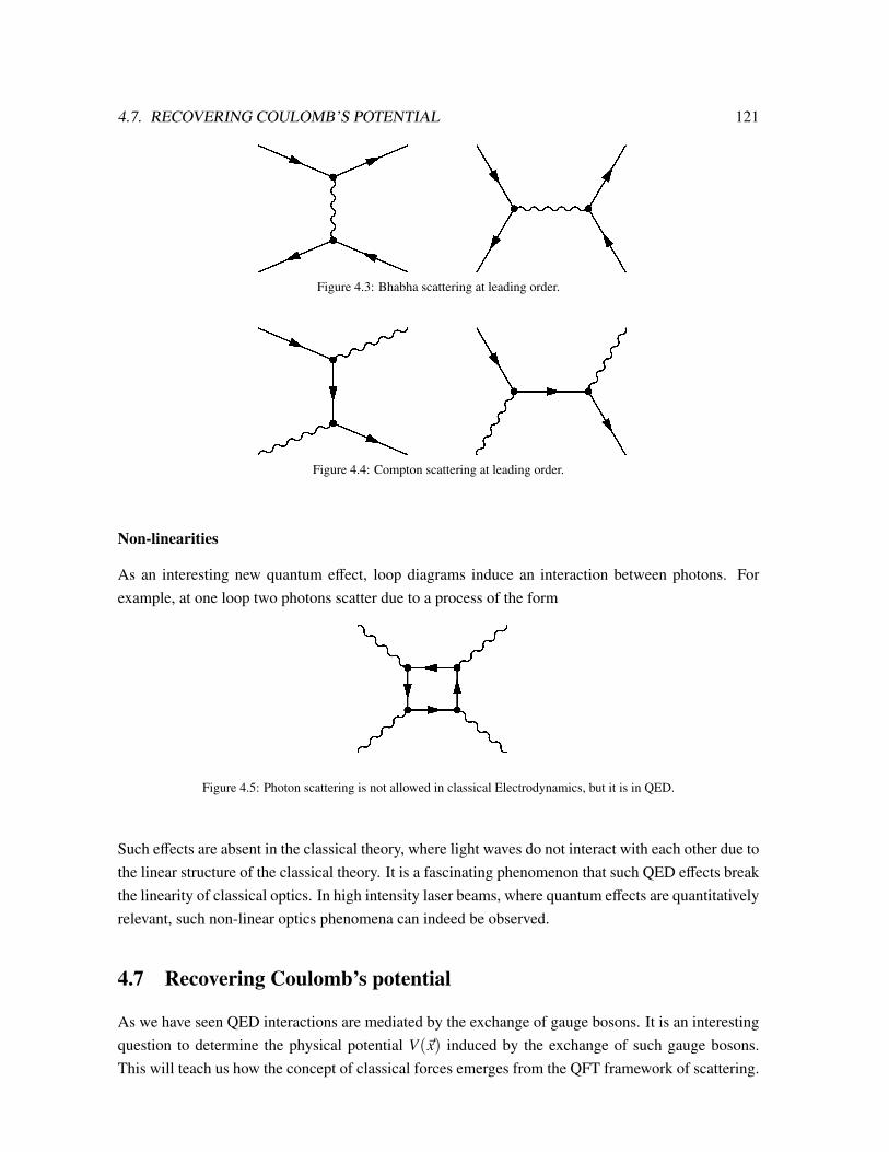
4.7. RECOVERING COULOMB’S POTENTIAL 121
Figure 4.3: Bhabha scattering at leading order.
Figure 4.4: Compton scattering at leading order.
Non-linearities
As an interesting new quantum effect, loop diagrams induce an interaction between photons. Forexample, at one loop two photons scatter due to a process of the form
Figure 4.5: Photon scattering is not allowed in classical Electrodynamics, but it is in QED.
Such effects are absent in the classical theory, where light waves do not interact with each other due tothe linear structure of the classical theory. It is a fascinating phenomenon that such QED effects breakthe linearity of classical optics. In high intensity laser beams, where quantum effects are quantitativelyrelevant, such non-linear optics phenomena can indeed be observed.
4.7 Recovering Coulomb’s potential
As we have seen QED interactions are mediated by the exchange of gauge bosons. It is an interestingquestion to determine the physical potential V(~x) induced by the exchange of such gauge bosons.This will teach us how the concept of classical forces emerges from the QFT framework of scattering.

122 CHAPTER 4. QUANTISING SPIN 1-FIELDS
To derive V(~x) the key idea is to consider the non-relativistic limit of the electron scattering process
e− + e− → e− + e− (4.113)
with distinguishable out-states corresponding to the Feynman diagram 4.6.
k
p
k′
p′
Figure 4.6: Electron scattering with distinguishable out-states.
This is then compared to the non-relativistic scattering process |~p〉 → |~p′〉 of two momentum eigen-states off a potential V(~x).
• In non-relativistic quantum mechanics, the scattering amplitudeA(|~p〉 → |~p′〉) for scattering ofan incoming momentum eigenstate |~p〉 to an outgoing momentum eigenstate |~p′〉 in the presenceof a scattering potential V is computed in the interaction picture as
A(|~p〉 → |~p′〉) − 1 = 〈~p′| e−i
∞∫−∞
dt′VI(t′)|~p〉 − 1 −i 〈~p′|
∞∫−∞
dt′VI(t′) |~p〉+ . . . ,
where we take the potential to be constant in time. As derived in standard textbooks on QuantumMechanics this equals to first order
A(|~p〉 → |~p′〉) − 1 = (2π)δ(Ep − Ep′)(−i) 〈~p′|V |~p〉 . (4.114)
This result goes by the name Born approximation and reads more explicitly in position space
A(|~p〉 → |~p′〉) − 1 = (2π)δ(Ep − Ep′)(−i)∫
d3r V(~r) e−i(~p−~p′)·~r. (4.115)
• This is to be compared with the non-relativistic limit of∫d3k(2π)3 ei~k·~r0 〈p′, k′| S |p, k〉
∣∣∣∣∣∣conn.
, (4.116)

4.7. RECOVERING COULOMB’S POTENTIAL 123
where 〈p′, k′| S |p, k〉
∣∣∣∣∣∣conn.
is the connected part of the S-matrix element of the scattering process
(4.113). Here the idea is to identify the electron with momentum p and p′ with the scatteringstates in the Quantum Mechanics picture and to view the other electron as a fixed target at ~r0 off
which |~p〉 scatters. The localisation of the fixed target at ~r0 in space is achieved by integratingover all Fourier modes, hence explaining the factor
∫d3k(2π)3 ei~k·~r0 . Without loss of generality we
will set ~r0 ≡ 0 in the sequel. Recalling the connection between the S-matrix element and thescattering amplitude iM, for which our Feynman rules are formulated, we find
〈p′, k′| S |p, k〉
∣∣∣∣∣∣conn.
= (2π)4δ(4)(p f − pi)(−ie)2
×
[ur′(p′)γµur(p)
−iηµν(p − p′)2 + iε
us′(k′)γνus(k)].
(4.117)
• In the the non-relativistic limit we have m0 |~p| and m0 |~k| and thus approximate p
(m0, ~p) +O(~p2). Then
ur(~p) =
√σµpµ ξr√σµpµ ξr
→ √σ0m0 ξr√σ0m0 ξr
= √m0
ξr
ξr
(4.118)
and
ur′(~p′)γµur(~p)→
2m0 δrr′ if µ = 0,0 otherwise.
(4.119)
Furthermore (p − p′)2 = −|~p − ~p′|2 +O(|~p|4) and therefore in the non-relativistic limit
〈p′, k′| S |p, k〉
∣∣∣∣∣∣conn.' −i
e2
|~p − ~p′|2 − iε(2m)2δ(E f − Ei)(2π)4δ(3)(~p f − ~pi). (4.120)
The factor (2m)2 is due to the different normalisation of momentum eigenstates in QFT and inQM and must therefore be neglected in comparing the respective expressions for the amplitude.
Putting all pieces together we can now identify∫d3r V(~r) e−i(~p−~p′)·~r =
e2
|~p − ~p′|2 − iε. (4.121)
Thus the Coulomb potential is
V(~r) =∫
d3q(2π)3
e2
~q2 − iεei
≡qr cos(θ)︷︸︸︷~q ·~r =
e2
4π2
∞∫0
dqq2
q2 − iεeiqr − e−iqr
iqr
=e2
4π2ir
∞∫−∞
dqq
(q +√
iε)(q −√
iε)eiqr.
(4.122)

124 CHAPTER 4. QUANTISING SPIN 1-FIELDS
Note that√
iε = eiπ/4 √ε lies in the upper complex half-plane. We interpret the integral as a complexcontour integral in the complex upper half-plane because we can close the contour in the upper half-plane as the contribution above the real axis vanishes in the limit |q| → ∞. We then pick up the residueat q =
√+iε and afterwards take the limit ε → 0. This leads to
V(~r) =e2
4π2ir2πi
√iε
2√
iεei√
iεr
∣∣∣∣∣∣ε=0
=e2
4πr. (4.123)
Since V is positive the potential for scattering of two electrons is repulsive as expected. If we replaceone e− by e+ and consider instead the process
e− + e+ → e− + e+, (4.124)
this amounts to replacing
ur′(p′)γµur(p) by vr′(p′)γµvr(p)→
2m0δrr′ if µ = 0,0 otherwise.
(4.125)
However, a careful analysis of the scattering amplitude in the interaction picture shows that one picksup one relative minus sign in the amplitude. Indeed, establishing the absolute sign of the amplitudewill be the task of Assignment 11. Thus we confirm the expected result that the potential mediatedby exchange of a spin-1 particle yields an attractive potential for oppositely charged particles and arepulsive potential for identically charged particles.
4.7.1 Massless and massive vector fields
It is instructive to compare the interaction of massless and massive vector fields:
• The Coulomb potential due to exchange of a massless spin-1 particle leads to a long-rangeforce as the potential dies off only like 1/r. If on the other hand the exchanged spin-1 particleis massive, the interaction is short-ranged. To see this suppose the photon has mass µ. All thatchanges is a mass term in the phton propagator. Thus
V(~r) =∫
d3q(2π)3
e2
~q2 + µ2 − iεei~q·~r =
e2
4πre−µr. (4.126)
Therefore massive vector bosons lead to short-range forces of range ∼ 1µ .
While the vector boson of QED is massless5, the weak nuclear forces in the Standard Modelare mediated by massive vector bosons (the three massive vector bosons W+, W− and Z ofspontaneously broken S U(2) gauge symmetry of mass of order 100 GeV). So this effect is
5A Yukawa-type deviation of the electromagnetic potential would be directly measurable and constrains the mass of thephoton to be below 10−14 eV, see E. R. Williams, J. E. Faller, and H. A. Hill, Phys. Rev. Lett. 26, 721-724 (1971). Inaddition, a variety of cosmological and astrophysical constraints imply that the photon mass is at best 10−18eV, as reviewede.g. in http://arxiv.org/pdf/0809.1003v5.pdf

4.7. RECOVERING COULOMB’S POTENTIAL 125
indeed highly relevant in particle physics and explains why in everyday physics at distancesbigger than (100 GeV)−1 only the electromagnetic force can be experienced.6
• The concept of forces mediated by exchange bosons is not restricted to spin-1 theories.
If we replace the vector boson of QED by a scalar boson φ of mass µ we arrive at Yukawatheory defined by
L =12∂φ2 −
12µ2φ2 + ψ(iγµ∂µ −m0)ψ − eφψψ︸︷︷︸
Yukawa int.
. (4.127)
The Feynman rules are very similar to those in QED except for two important changes: First, theinteraction vertex carries no γµ factor and second the scalar boson propagator must be modifiedfrom
−iηµνp2 − µ2 + iε
→i
p2 − µ2 + iε. (4.128)
This amounts to a crucial sign change in the non-relativistic limit because
−iη00
−|~p|2 − µ2 + iε→
i−|~p|2 − µ2 + iε
. (4.129)
Combining these two changes yields the universally attractive Yukawa potential
V(r) = −e2
4πre−µr. (4.130)
• Perturbative gravity can be understood at the level of field theory as a theory of massless spin-2particles, the gravitons, whose exchange likewise yields a universally attractive force. Since thegravitational potential is of the form 1/r (at least for conventional Einstein gravity), gravitonsmust be massless.7
To summarise the potential induced by the exchange of bosons of different spin acts on fermions ( f )and anti-fermions ( f ) as follows:
f f f f f f
Spin 0 (Yukawa theory) attractive attractive attractiveSpin 1 (Gauge theory) repulsive attractive repulsiveSpin 2 (Gravity) attractive attractive attractive
6The remaining Standard Model forces mediated by the eight massless gluons of S U(3) gauge theory is also short-ranged, but this is because of confinement.
7Current constraints imply that the graviton mass must be smaller than 10−20eV , seehttp://arxiv.org/pdf/0809.1003v5.pdf.

126 CHAPTER 4. QUANTISING SPIN 1-FIELDS

Chapter 5
Quantum Electrodynamics
5.1 QED process at tree-level
As an example for a typical tree-level QED process we compute the differential cross-section dσdΩ for
the scattering e+e− → µ+µ−. We describe both the electron/positron and the muon/anti-muon by aDirac spinor field of respective free mass me and mµ which we couple to the U(1) gauge field.
p
k′p′ q
k
e+
e−
µ+
µ−
Figure 5.1: e+e− → µ+µ− reaction.
In this protypical example and in many similar processes one proceeds as follows:
5.1.1 Feynman rules for in/out-states of definite polarisation
Apply the rules from the previous chapter and obtain:
iM(p, s; p′,−s′ → k, r; k′,−r′) = (ie)2vs′(p′)γµus(p)−iηµν
q2 + iεur(k)γνvr′(k′), (5.1)
where q = p + p′ = k + k′. Thus
iM =ie2
q2 vs′(p′)γµus(p)ur(k)γµvr′(k′). (5.2)
127

128 CHAPTER 5. QUANTUM ELECTRODYNAMICS
5.1.2 Sum over all spin and polarisation states
Often we do not keep track of the polarisation states of in and out states but are interested in theunpolarised amplitude-square
12
∑s
12
∑s′
∑r
∑r′
∣∣∣iM(p, s; p′,−s′ → k, r; k′,−r′)∣∣∣2, (5.3)
where 12∑
s12∑
s′ averages over the initial state polarisation as is appropriate if the incoming beam isnot prepared in a polarisation eigenstate. The sum
∑r∑
r′ over the final state polarisations is requiredin addition if the detector is blind to polarisation. With
(vs′γµus)
∗ = u†s 㵆γ0†︸ ︷︷ ︸=γ0γµ
vs′ = usγµvs′ (5.4)
one finds
14
∑Spins
|M|2 =14
e2
q4
∑s,s′,r,r′
(usγµvs′)(vs′γ
νus)(vr′γµur)(urγνvr′)
. (5.5)
Now we want to make use of the completeness relations∑s
us(~p)us(~p) = γ · p + me∑s
vs(~p)vs(~p) = γ · p −mµ.(5.6)
To do so it is first useful to make the spinor indices explicit1, e.g.
usγµvs′ =
∑A,B
(us)AγµA
Bv Bs′ , (5.7)
which shows that the expression can be reordered as
14
∑Spins
|M|2 =14
e2
q4
[ ∑s,s′,r,r′
us(p)Dus(p)AγµA
Bvs′(p′)Bvs′(p′)CγνC
D
× vr′(k′)H vr′(k′)EγE
µ Fur(k)F ur(k)GγG
ν H
]=
14
e2
q4
[tr((γ · p −me)γ
µ(γ · p + me)γν)
× tr((γ · k′ + mµ)γµ(γ · k −mµ)γν
)].
(5.8)
In order to proceed further we need to evaluate the traces over the γ matrices.
1Recall that the indices µ, ν are completely unrelated to the spinor indices, c.f. section 3.2.

5.1. QED PROCESS AT TREE-LEVEL 129
5.1.3 Trace identities
The following identities are very important to proceed further. We will prove them in general fashionon exercise sheet 10. The only thing to do is: insert a 1 cleverly, e.g. γ5γ5 and use the properties ofthe Clifford algebra as well as the cyclicity of the trace.
• trγµ = 0, because:
trγµ = tr γ5γ5︸︷︷︸≡1
γµ = −trγ5γµγ5 = −trγµγ5γ5 = −trγµ. (5.9)
• The trace of an odd number of γ-matrices vanishes, since
trγµ1 ...γµn = trγ5γ5γµ1 ...γµn = (−1)ntrγµ1 ...γµn . (5.10)
• trγµγν = 4ηµν, because
trγµγν = tr(2ηµν − γνγµ) = 2ηµνtr1 − tr(γνγµ)︸ ︷︷ ︸=trγµγν
. (5.11)
• Similarly one findstrγµγνγργσ = 4
[ηµνηρσ − ηµρηνσ + ηµσηνρ
]. (5.12)
• trγ5 = 0 sincetrγ5 = trγ0γ0γ5 = −trγ0γ5γ0 = −trγ5. (5.13)
• Likewise one can prove
trγ5γµ = trγ5γµγν = trγ5γµγνγσ = 0. (5.14)
• trγ5γαγβγγγδ = −4iεαβγδ, because the result must be antisymmetric in all indices and in partic-ular
trγ5γ0γ1γ2γ3 = −i tr γ5γ5 = −4i. (5.15)
• Further useful identities are
γµγνγµ = −2γν.
γµγνγργµ = 4ηνσ,
γµγνγργσγµ = −2γσγργν.
(5.16)
Applied to the present case these identities yield
tr[(γρpρ −me)γ
µ(γσp′σ + me)γν]
= 4pρp′σ(ηρµησν − ηρσηµν + ηρνηµσ
)−m2
e4ηµν + tr(odd number of γ’ s) ×me × ...
= 4[pµp′ν + pνp′µ − (p · p′ + m2
e)ηµν
] (5.17)

130 CHAPTER 5. QUANTUM ELECTRODYNAMICS
and similarly
tr[(γ · k′ + mµ)γµ(γ · k −mµ)γν
]= 4
[k′µkν + k′νkµ − (k · k
′ + m2µ)ηµν
]. (5.18)
Since the ratio of mµ and me is about 200 we can drop me. Then altogether after a few cancellations
14
∑Spins
|M|2 = 8e4
q4
[(p · k)(p′ · k′) + (p′ · k)(p · k′) + (p · p′)m2
µ
]. (5.19)
5.1.4 Centre-of-mass frame
Switch to the c.o.m. frame and rotate the coordinate frame such that p points in z-direction and p′ in−z-direction (see Figure 5.2).
p
p′
k′
k
Figure 5.2: Centre-of-mass frame, p in z-direction.
Introducing the angle θ between p′ and k and taking the relativistic limit, i.e. m2e |~p|
2, yields
p =
EEz
, p′ =
E−Ez
, k =
E~k
, ~k · z = |~k| cos θ. (5.20)
Therefore
q2 = (p + p′)2 = 2p · p′ = 4E2,
p · k = E2 − E|~k| cos θ = p′ · k′,
p · k′ = E2 + E|~k| cos θ = p′ · k.
(5.21)
Plugging this in and eliminating |~k|2 using |~k|2 = E2 −m2µ yields
14
∑Spins
|M|2 = e4
1 + m2µ
E2
+ 1 − m2µ
E2
cos2 θ
. (5.22)
5.1.5 Cross-section
To this end recall the general formula for a 2-2 scattering event. For this we had derived the expression
dσ =(2π)4
4EpEp′ |vp − vp′ |dΠ2δ
(4)(p + p′ − k − k′)|M f i|2 (5.23)

5.1. QED PROCESS AT TREE-LEVEL 131
with
dΠ2 =d3k(2π)3
d3k′
(2π)3
12Ek2Ek′
. (5.24)
Note that no factor of 12 is required here since µ+ and µ− are distinguishable. In the c.o.m. frame we
generally have
dΠ2(2π)4δ(4)(p + p′ − k − k′) =d|~k||~k|2dΩ
(2π)34EkEk′δ(Ecom − Ek − Ek′) (5.25)
with Ek =√|~k|2 + m2
k and Ek′ =√|~k|2 + m2
k′ and
d|~k|δ(Ecom − Ek − Ek′) =
|~k|Ek+|~k|Ek′
−1
. (5.26)
Then, altogether
dσdΩ
=1
4EpEp′ |vp − vp′ |
|~k|16π2Ecom
|M f i|2. (5.27)
Note that, if all 4 particles had equal masses and the outstates were indistinguishable, this wouldcorrectly reduce to the famous expression encountered earlier
dσdΩ
=12!
164π2
1s|M f i|
2 (5.28)
with s = E2com. Applied to the present case (5.27) yields, with
Ep = Ep′ = E =12
Ecom , |vp − vp′ | = 2, (5.29)
the differential cross-section
dσdΩ
=1
32π2
1E2
com
|~k|Ecom
14
∑Spins
|M f i|2. (5.30)
Introducing the fine-structure constant
α :=e2
4π∼
1137
(5.31)
leaves us with
dσdΩ
=α2
4E2com
√1 −
m2µ
E2
1 + m2µ
E2
+ 1 − m2µ
E2
cos2 θ
(5.32)
for the differential cross-section. Thus for the total cross-section
σ =4πα2
3Ecom
√1 +
mµ
E2
1 + 12
m2µ
E2
. (5.33)
The first term reflects the purely kinematic and thus universal energy dependence, while the secondterm represents the correction due to specifics of the QED interaction and is thus characteristic of theconcrete dynamics involved in this process.

132 CHAPTER 5. QUANTUM ELECTRODYNAMICS
5.2 The Ward-Takahashi identity
Consider a QED amplitude M(k) involving an external photon of momentum kµ with k2 = 0 andpolarisation ξµ(k). We thus can write the scattering amplitude as
M(k) = ξµ(k)Mµ(k). (5.34)
Then the Ward-Takahashi identity for QED is the statement that
kµMµ(k) = 0. (5.35)
To appreciate its significance recall from Gupta-Bleuler quantisation that the constraint
∂ · A+ |ψphys〉 = 0 (5.36)
implies ζµkµ = 0 for states |k, ζ〉 ∈ Hphys. This left 2 positive norm transverse polarisations ζT and 1zero norm polarisation ζs = k. (5.35) proves that the unphysical zero-norm polarization state |k, ζs〉
decouples from the S -matrix as an external state, as claimed.(5.35) follows from a more general from of the Ward identity. Consider a theory with arbitrary spinfields φa(x) with a global continuous symmetry
φa(x)→ φa(x) + εδφa(x), ε ∈ R, (5.37)
and a conserved Noether current jµ(x) such that classically
∂µ jµ = 0 (5.38)
holds on-shell. Then in the quantum theory the general Ward-Takahashi-identity is a statementabout current conservation inside a general n-point function:
0 = ∂µ 〈Ω|T jµ(x)φa1(x1)...φan(xn) |Ω〉
+ in∑
j=1
〈Ω| φa1 ...φa j(x j)δφa j(x j)δ(4)(x − x j)...φan(xn) |Ω〉 ,
(5.39)
where φa j(x j) is omitted. (5.39) can be proven as follows:
• For definiteness and simplicity consider a scalar theory. For the free theory, the classical equa-tion of motion is
δSδφ(x)
:=∂L
∂φ(x)− ∂µ
∂L∂(∂µφ(x))
= −(∂2 + m2)φ(x) = 0. (5.40)
This equation is satisfied by the Heisenberg quantum fields as an operator equation.

5.2. THE WARD-TAKAHASHI IDENTITY 133
• With the help of this operator equation, one finds that
(∂2x + m2)i 〈0|Tφ(x)φ(x1) |0〉 = δ(4)(x − x1) (5.41)
for a 2-point-function. The δ-distribution occurs due to the action of ∂x0 on Θ(x− x0) appearingin the time-ordering prescription symbolized by T . More generally one finds
(∂2x + m2)i 〈0|Tφ(x)φ(x1)...φ(xn) |0〉
=n∑
j=1
〈0|Tφ(x1)...φ(x j)δ(4)(x − x j)...φ(xn) |0〉 .
(5.42)
This can be written as the Schwinger-Dyson equation
〈0|TδS
δφ(x)φ(x1)...φ(xn) |0〉 = i
n∑j=1
〈0|Tφ(x1)...φ(x j)δ(4)(x − x j)...φ(xn) |0〉 . (5.43)
• By Noether’s theorem, if φ(x) → φ(x) + εδφ(x) is a global continuous symmetry, then theNoether current enjoys
∂µ jµ = −(∂L
∂φ(x)− ∂µ
∂L
∂(∂µφ(x))
)δφ(x) ≡ −
δSδφ(x)
δφ(x) (5.44)
off-shell. Plugging this into the Schwinger-Dyson equation yields:
∂µ 〈0|T jµ(x)φ(x1)...φ(xn) |0〉
+in∑
j=1
〈0|Tφ(x1)...φ(x j)δφ(x)δ(4)(x − x j)...φ(xn) |0〉 = 0.(5.45)
• In interacting theories the reasoning goes through - all that changes is that the equations ofmotion involve extra polynomial terms due to the interactions, which however do not alterthe conclusions. This yields the corresponding statements about the full correlation functions〈Ω| ... |Ω〉.
The Schwinger-Dyson equation and the Ward-identity show that the classical equation of motion andcurrent conservation hold inside the correlation functions only up to so-called contact terms, whichare precisely the extra terms we pick up if the insertion point x of the operator δS
δφ(x) or ∂µ jµ(x) coin-cides with the insertion point x j of one of the other fields inside the correlator.
Caveat:It is important to be aware that the n-point correlator 〈Ω| ... |Ω〉 involves in general divergent loop-diagrams to be discussed soon. The Ward identity only holds if the regularisation required to definethese divergent intergrals respects the classical symmetry. We will see that for QED such regulatorscan be found. On the other hand, if no regulator exists that respects the Ward-identity for a classical

134 CHAPTER 5. QUANTUM ELECTRODYNAMICS
symmetry, this symmetry is anomalous - it does not hold at the quantum level. Such anomalies willbe studied in great detail in QFT II.
It remains to deduce (5.35) from (5.39):
• Following LSZ, the scattering amplitudeM(k) involving an external photon |kµ, ξµ(k)〉 and nfurther particles is given by
〈 f | i〉 = iZ−1/2A ξµ(k)
∫d4x e−ik·x∂2
x... 〈Ω|T Aµ(x) ...︸︷︷︸(n other fields)
|Ω〉 (5.46)
In Feynman gauge the full interacting QED Lagrangian reads
L = −12∂µAν∂µAν − Aµ jµ + ψ(iγ · ∂ −m0)ψ, jµ = eψγµψ. (5.47)
The classical equation of motion for Aµ is
∂2Aµ = jµ (5.48)
and therefore∂2
x 〈Ω|T Aµ(x)... |Ω〉 = 〈Ω|T jµ(x)... |Ω〉+ contact terms, (5.49)
where the contact terms include (n−1) fields inside 〈Ω| ... |Ω〉. Being correlators only of (n−1)fields, these contact terms cannot have precisely n poles in the momenta of the n fields and thusdo not contribute to 〈 f | i〉 according to the LSZ formalism.
• Now we are left with
〈 f | i〉 = i Z−1/2A ξµ
∫d4xe−ik·x 〈Ω|T jµ(x)... |Ω〉 . (5.50)
For ξµ = kµ we find
kµ∫
d4x e−ik·x 〈Ω|T jµ(x)... |Ω〉 = i∫
d4x (∂µe−ik·x 〈Ω|T jµ(x)... |Ω〉
= − i∫
d4x e−ik·x∂µ 〈Ω|T jµ(x)... |Ω〉 ,(5.51)
where we used that surface terms vanish (because, as in LSZ, we are really having suitablewave-packets in mind). According to (5.39) this is
0 + contact terms. (5.52)
Also in this case the contact terms do not contribute to 〈 f | i〉 because we are essentially trad-ing one Aµ(x) field against one matter field δϕ(x) inside the correlator so that the resulting polestructure is not of the right form, in and (5.35) is proven.

5.2. THE WARD-TAKAHASHI IDENTITY 135
5.2.1 Relation between current conservation and gauge invariance
The proof of kµMµ(k) = 0 only requires that Aµ(x) couples to a conserved current in the sense that
S = S 0A[A] + S int[A, φ] + S rest
matter[φ] (5.53)
with
δS int[A, φ]δAµ
= − jµ (5.54)
the Noether current associated with a global continuous symmetry of the full interacting action S .
• For a massless vector theory, which, as a free theory, must always be gauge invariant, (5.54)is in fact equivalent to invariance of the theory under combined gauge transformations of thevector and the matter sector.
To prove that (5.54) implies gauge invariance, our point of departure is the existence of a globalcontinuous symmetry φ(x) → φ(x) + εδφ(x) with ε ∈ R constant, which leaves the full ac-tion S invariant. If we perform instead a local transformation φ(x) → φ(x) + ε(x)δφ(x) withvarying ε(x), then δS is in general no longer zero. Since it vanishes for constant ε, δS mustbe proportional (to first order) to ∂µε(x). In fact, Lorentz invariance implies that there ex-ists a 4-vector jµ(x) such that δS =
∫jµ∂µε(x) = −
∫(∂µ jµ)ε(x). This identifies jµ with
jµ, the conserved current (because for ε constant, the Noether current has the property that−
∫(∂µ jµ)ε =
∫( δSδφ δφε) ≡ δS - see equ. (5.44)). Now, since by assumption δS int
δAµ= − jµ we
have∫( δS intδAµ
+ jµ)∂µε(x) = 0. Writing S = S 0A[A] + S int[A, φ] + S rest
matter[φ], the fact that S 0A[A]
is gauge invariant for a massless vector theory implies that this is just the variation of S withrespect to the combined gauge transformation
Aµ → Aµ + ∂µε(x), φ(x)→ φ(x) + ε(x)δφ(x). (5.55)
The theory is thus gauge invariant.
To prove the other direction, suppose (5.55) leaves the action S 0A[A] + S int[A, φ] + S rest
matter[φ]
invariant (where again S 0A[A] is separately gauge invariant). Then there exists some conserved
jµ(x) such that∫( δS intδAµ
+ jµ)∂µε(x) = 0, and we conclude (5.54).
To conclude, massless vector theories are consistent if and only if the vector couples to aconserved current. This is the necessary and consistent condition for gauge invariance and forthe Ward identities.
• If we couple a massive vector, whose action is never gauge invariant, to a conserved current asin (5.54), then kµMµ = 0 still holds. The fact that in a massive vector theory the Ward identitiesare still satisfied provided that theory couples as in (5.54) is crucial for its consistency: Recallthat in a massive vector theory (k2 > 0), the negative norm states are the states
|kµ, ξµ〉 with ξµ = kµ. (5.56)

136 CHAPTER 5. QUANTUM ELECTRODYNAMICS
Restriction to ζµ with ζµkµ = 0 removes these. This is only justified in the interacting theoryas long as no dangerous states |kµ, ζµ = kµ〉 are produced, as is guaranteed thanks to kµMµ = 0for couplings to conserved currents.
5.2.2 Photon polarisation sums in QED
To evaluate the consequences of the Ward identities we can take, without loss of generality, the photon4-momentum to be
kµ = k
1001
(5.57)
and consider the corresponding basis of polarisation vectors
εµ(k, 0) =
1000
, εµ(k, 1) =
0100
, εµ(k, 2) =
0010
, εµ(k, 3) =
0001
. (5.58)
The Ward identity kµMµ(k) = 0 then implies M0(k) = M3(k). In physical applications we oftenneed to sum over the two transverse polarisation vectors λ = 1, 2 of an external photon involved in ascattering process. By the Ward identity this becomes
2∑λ=1
|εµ(k, λ)Mµ(k)|2 =2∑
λ=1
εµ(k, λ)ε∗ν (k, λ)Mµ(k)(Mν(k))∗ = |M1(k)|2 + |M2(k)|2
= |M1(k)|2 + |M2(k)|2 + |M3(k)|2 − |M0(k)|2
= −ηµνMµ(k)(Mν(k))∗. (5.59)
Thus in sums over polarisations of the above type we can replace∑2λ=1 εµ(k, λ)ε∗ν (k, λ) by −ηµν. This
will be used heavily in deriving the Klein-Nishina formula for Compton scattering in the tutorials.
5.2.3 Decoupling of potential ghosts
So far we have merely shown that the zero-norm states with polarization kµ decouple from the S-matrix and are thus not produced in scattering experiments. But what about the status of timelikepolarisation states, which correspond to the even more dangerous negative norm ghosts? Even if wedeclare Hphys not to contain them, we must prove that no such states are created as outgoing statesfrom physical in-states in scattering processes. Otherwise the interactions would render the theoryinconsistent.2
2Note that this is only a question for massless vector fields. For massive vector fields the negative norm states are justthe photons with polarization kµ (as k2 > 0) and these obviously decouple by the Ward identity.

5.3. RADIATIVE CORRECTIONS IN QED - OVERVIEW 137
In fact, it is again the Ward identity that guarantees that no ghosts are created as external states ininteractions. The argument relies on the relation
2∑λ=1
εµ(k, λ)ε∗ν (k, λ)Mµ(k)(Mν(k))∗ = −ηµνMµ(k)(Mν(k))∗ (5.60)
derived above and is sketched as follows: It suffices to show that the restriction of the S-matrix S tothe space of transverse polarisations is unitary. This means that we lose no information by consideringonly transverse in and out-states and thus guarantees that no unphysical states can be produced outof transverse incoming states. Let P denote the projector onto these states of transverse polarisations.The relation (5.60) amounts to the statement
S †PS = S †S . (5.61)
Since S †S = 1, this implies that (PS P)†(PS P) = P. This is precisely the statement that the restric-tion of S to the state of transverse polarisation is unitary.
5.3 Radiative corrections in QED - Overview
We now enter a quantitative discussion of radiative corrections in Quantum Field Theory as exempli-fied by loop corrections to QED. As we will see it is sufficient to study the following types of loopcorrections modifying the QED building blocks.
Corrections to the fermion propagator
We recall that the Feynman propagator of the free fermion field is
S F(x − y) =∫
d4 p(2π)4 e−ip(x−y) γ · p + m0
p2 −m20 + iε︸ ︷︷ ︸
≡ iγ·p−m0+iε
. (5.62)
Taking into account corrections due to QED interactions we have instead
〈Ω|Tψ(x)ψ(y) |Ω〉 = yfaf x +f|af+f|aff|af+ . . .
≡ yfpf x.(5.63)
Let
Af 1PIf B ≡ −iΣ(6 p)AB (5.64)
denote the amputated 1PI diagram. By Dyson resummation the full propagator then takes the form
yfpf x =
∫d4 p(2π)4 e−ip(x−y) i
γ · p −m0 −∑(6 p) + iε
, (5.65)
where∑(6 p) is called self-energy of the electron.

138 CHAPTER 5. QUANTUM ELECTRODYNAMICS
Corrections to the photon propagator
The Fourier transform of the photon propagator, denoted bygpg, derives by Dyson resum-mation from the 1-PI diagram
µg 1PIg ν ≡ iΠµν(q2) = self-energy of the photon or vacuum polarisation. (5.66)
Corrections to the interaction vertex
Loop corrections modifiy the cubic interaction vertex. We will find it useful to define an effectivevertex by summing up all loop-corrections. Schematically,
p p′
µ
+µ
+... =p p′
µ
' −ieΓµ(p, p′).
We will compute these corrections to 1-loop order. The diagrams will exhibit
• ultraviolet (UV) divergences from integrating the momenta of particles in the loop up to infinityand
• infra-red (IR) divergences if the diagram contains massless particles - i.e. photons - running inthe loop.
The general status of these singularities is as follows:
• IR divergences in loop-diagrams cancel against IR divergences from radiation of soft, i.e. low-energy photons and thus pose no conceptual problem.
• UV divergences require regularisation of the integral and can be absorbed in a clever definitionof the parameters via renormalisation.
5.4 Self-energy of the electron at 1-loop
At 1-loop order the electron propagator takes the form
〈Ω|Tψ(x)ψ(y) |Ω〉 = yfaf x + yf|af x︸ ︷︷ ︸=
∫ d4 p(2π)4
eip·(x−y)×(I)
(5.67)
where the integrand (I) is given by the diagram
(I) ≡ pfk|af p. (5.68)

5.4. SELF-ENERGY OF THE ELECTRON AT 1-LOOP 139
The photon in the loop carries momentum p − k. By means of the Feynman rules,
(I) =i(γ · p + m0)
p2 −m20 + iε
(−iΣ2(6 p))i(γ · p + m0)
p2 −m20 + iε
. (5.69)
The amputated 1-loop contribution corresponds to omitting the two outer fermion propagators andis thus given by
iΣ2(6 p) = (−ie)2∫
d4k(2π)4γ
µ i(6 k +mo)
k2 −m20 + iε
γν−iηµν
(p − k)2 + iε. (5.70)
It will turn out that the integral is divergent near k = 0 if p → 0. This is an IR divergence. Acareful analysis reveals that it will cancel in all amplitudes against similar such IR divergences fromother diagrams involving soft photons and thus poses no harm. For the present discussion we couldjust ignore it, but for completeness we introduce a ficticious small photon mass µ to regulate the IRdivergence:
iΣ2(6 p) = (−ie)2∫
d4k(2π)4γ
µ i(6 k +mo)
k2 −m20 + iε
γµ−i
(p − k)2 − µ2 + iε. (5.71)
The evaluation of such typical momentum integrals proceeds in 3 steps:
5.4.1 Feynman parameters
The integrand contains a fraction of the form 1AB with A = (p − k)2 − µ2 + iε and B = k2 −m2
0 + iε.It turns out useful to write this as 1
(...)2 and to complete the square in k. To this end we exploit theelementary identity
1AB
=
1∫0
dx1
(xA + (1 − x)B)2 . (5.72)
x is called a Feynman parameter. Applying this identity yields in the present case
1AB
=
1∫0
dx1
(x((p − k)2 − µ2 + iε) + (1 − x)(k2 −m20 + iε))2
=
1∫0
dx1
(k2 − 2xk · p + xp2 − xµ2 − (1 − x)m20 + iε + x2 p2 − x2 p2)2
=
1∫0
dx1
(l2 − ∆ + iε)2 ,
(5.73)
where l = k − xp and ∆ = −x(1 − x)p2 + xµ2 + (1 − x)m20. Then
− iΣ2(6 p) = −e2
1∫0
dx∫
d4l(2π)4
γµ(6 k +m0)γµ
(l2 − ∆ + iε)2 . (5.74)

140 CHAPTER 5. QUANTUM ELECTRODYNAMICS
The term in the numerator can be simplified with the help of the gamma-matrix identity
γµγνkνγµ = (2ηµν − γνγµ)kνγµ = kµγµ(2 − γνγν) (5.75)
and, in d-dimensions, γµγµ = d. Therefore altogether (keeping d arbitrary for later purposes)
γµ(6 k +m0)γµ = (2 − d)(6 l +x 6 p) + dm0. (5.76)
Now for symmetry reasons ∫d4l
(2π)4
lµ
(l2 − ∆)2 = 0 (5.77)
and thus, if d ≡ 4,
−iΣ2(6 p) = −e2
1∫0
dx∫
d4l(2π)4
−2x 6 p +4m0
(l2 − ∆ + iε)2 . (5.78)
Remark: For more general loop integrals one makes use of the identity
1A1...An
=
1∫0
dx1...dxnδ(∑
i
xi − l)(n − 1)!
(x1A1 + ... + xnAn)n , (5.79)
which can be proven by induction.
5.4.2 Wick rotation
As we have seen, we encounter loop-integrals of the typical form∫
d4l(2π)4
1(l2−∆+iε)n . This integral
would be relatively easy to perform if it were defined in Euclidean space. The Wick rotation relates itto such a Euclidean integral.Indeed, as the iε factors remind us, the l0 integral is in fact a complex contour integral along the realaxis. The value of this integral is unchanged if we deform the contour without hitting any pole. There-fore we can rotate the contour by 90 counter-clockwise to lie along the imaginary axis. Introducingthe Euclidean 4-momentum lE = (l0E ,~lE) as
l0 = il0E , ~l = ~lE (5.80)
such that l2 ≡ −l2E ≡ −∑
i(liE)2, we can write the integral as
∫d4l
(2π)4
1(l2 − ∆ + iε)m = i(−1)m
∫d4lE
(2π)4
1(l2E + ∆ − iε)m
. (5.81)
Since we won’t need the iε any longer we can omit it at this stage. We can now peform the integral asa spherical integral in R4.

5.4. SELF-ENERGY OF THE ELECTRON AT 1-LOOP 141
5.4.3 Regularisation of the integral
The integral
I4 =
∫d4lE
(2π)4
1(l2E + ∆)2
=
∞∫0
|lE |3d|lE |
(2π)4
∫dΩ4
1(|lE |
2 + ∆)2 (5.82)
is divergent due to integration over the UV region |lE | → ∞. To isolate the divergence we regularisethe integral. The 3 most common methods for regularisation are
• Momentum cutoff: Isolate the UV divergence as a divergence in the upper momentum limit Λby writing
∞∫0
. . . = limΛ→∞
Λ∫o
. . . . (5.83)
Following this procedure we can evaluate the integral in an elementary fashion as
I4 =
∫dΩ4 lim
Λ→∞
∞∫0
d|lE |
(2π)4
|lE |3
(|lE |2 + ∆)2
=
∫dΩ4 lim
Λ→∞
12
∞∫0
d|lE |2
(2π)4
|lE |2
(|lE |2 + ∆)2
=
∫dΩ4 lim
Λ→∞
12
1(2π)4
[∆
∆ + |lE |2 + log(|lE |
2 + ∆)]Λ2
l2=0
=
∫dΩ4 lim
Λ→∞
12
1(2π)4
[log
(Λ2
∆
)− 1
].
(5.84)
The loop leads to a log-divergence as Λ → ∞. The problem is that this regularisation procedureis not consistent with the Ward identities, as we will see when computing the photon propagator,and is therefore not a useful regularisation method in QED.
• Dimensional regularisation (dimReg) is probably the most common method. We first evaluatethe integral in d dimensions; writing d = 4 − ε then isolates the divergence as a pole in ε asε → 0.
Let us therefore consider
Id =ddlE
(2π)d
1(l2E + ∆)2
=
∫dΩd
(2π)3
∞∫0
d|lE ||lE |
d−1
(|lE |2 + ∆)2 . (5.85)
The volume of the unit sphere in d-dimensions is∫dΩd =
2πd/2
Γ( d2 )
(5.86)
where
Γ(z) =∫ ∞
0dy yz−1 e−y (5.87)

142 CHAPTER 5. QUANTUM ELECTRODYNAMICS
is the Euler Γ-function. This is because
(√π)d =
∞∫−∞
dxe−x2
d
=
∫dd xe−
∑di=1 x2
i
=
∫dΩd
∞∫0
d|x||x|d−1e−|x|2
=
∫dΩd
12
∞∫0
d(x2)(x2)d/2−1e−x2.
(5.88)
The Γ-function has the properties
– Γ(n) = (n − 1)! for n ∈N+ as can be shown by integration by parts.
– Γ(z) has analytic poles at z = 0,−1,−2,−3, ...; for a proof we refer to standard textbookson complex analysis.
Continuing with our integral we write
∞∫0
d|lE ||lE |
d−1
(|lE |2 + ∆)2 =
12
∞∫0
d|lE |2 (|lE |
2)d/2−1
(|lE |2 + ∆)2 (5.89)
and substitutex =
∆|lE |
2 + ∆⇒ |lE |
2 =∆x− ∆ (5.90)
withdx = −d|lE |
2 ∆(|lE |
2 + ∆)2 . (5.91)
Then the integral (5.89) becomes
=12
(1∆
)2−d/2 1∫0
dx x1−d/2(1 − x)d/2−1. (5.92)
As a last ingredient we need the Euler β-function
B(α, β) :=
1∫0
dx xα−1(1 − x)β−1 =Γ(α)Γ(β)Γ(α+ β)
, (5.93)
where the last identity is non-trivial and proven again in textbooks on complex analysis.
We can rewrite (5.92) in terms of B(α, β) with α = 2 − d/2 and β = d/2. Together withΓ(2) = 1 we arrive at
12
(1∆
)2−d/2 1∫0
dx x1−d/2(1 − x)d/2−1 =12
(1∆
)2−d/2
Γ(2 − d/2)Γ(d/2). (5.94)

5.4. SELF-ENERGY OF THE ELECTRON AT 1-LOOP 143
Therefore
Id =ddlE
(2π)d
1(l2E + ∆)2
=1
(4π)d/2Γ(2 − d/2)
(1∆
)2−d/2
. (5.95)
We now apply this to Id with d = 4 and note that we encounter a singularity from Γ(0). Toisolate the singularity we define
d = 4 − ε (5.96)
and would like to write I4 ∝ limε→0I4−ε . However I4 is dimensionless because
[lE ] = [mass], (5.97)
whereas I4−ε has dimension [mass]−ε . If we introduce a compensating mass scale M, we canwrite
I4 = limε→0
MεI4−ε = limε→∞
Mε 14π2−ε/2
Γ(ε/2)(
1∆
)ε/2
= limε→0
14π2 Γ(ε/2)
(4πM2
∆
)ε/2
.
(5.98)
Finally we use
– Γ(ε/2) = 2ε − γ+O(ε), where γ ≈ 0.5772 is the Euler-Mascheroni number and we refer
again to the complex analysis literature for a proof;
– xε/2 = 1 + ε2 log(x) +O(ε2), which is just a Taylor expansion in ε since xε/2 = e
ε2 log(x).
With this input
I4 = limε→0
1(4π)2
(2ε− γ+ log
(4πM2
∆
)+O(ε)
)(5.99)
and therefore
I4 = limε→0
1(4π)2
(2ε+ log
(M2
∆
)+O(ε)
), (5.100)
where M2 = 4πe−γM2.
The final result for the electron self-energy at 1-loop is
−iΣ2(6 p) = (−i)α
2π
1∫0
dx ((2 − ε/2)m0 − (1 − ε/2)x 6 p)(2ε+ log
M2
∆
) ∣∣∣∣∣∣∣ε→0
, (5.101)
where M is some as yet arbitrary mass-scale. We will understand its significance soon.
• Pauli-Villars (PV) regularisation: We subtract a diagram with a ficiticious massive particle inthe loop - here a photon - of mass Λ, i.e. we compute
pfk|af︸ ︷︷ ︸involves i
(p−k)2−µ2+iε
− pfk|af︸ ︷︷ ︸involves i
(p−k)2−Λ2+iε
. (5.102)

144 CHAPTER 5. QUANTUM ELECTRODYNAMICS
Subtracting the second diagram subtracts the divergence because for infinite momenta the massof the particle in the loop becomes irrelevant and both diagrams asymptote to the same divergentvalue. If Λ → ∞ the contribution of the subtracted vanishes and we recover the actual diagram.The divergence reappears therefore as a divergence in Λ as Λ → ∞.
Subtracting both diagrams yields
−iΣ2(6 p) = limΛ→∞
(computation with µ − computation with Λ)
= ...
−iΣ2(6 p) = limΛ→∞
(−i)α
2π
1∫0
dx(2m0 − x 6 p) log(
xΛ2
∆
),
(5.103)
where the omitted steps are elementary and similar to the integration performed in (5.84). Wecan rewrite this by introducing again an arbitrary mass scale M as
−iΣ2(6 p) = limΛ→∞
(−i)α
2π
1∫0
dx(2m0 − x 6 p)(log
(xΛ2
M2
)+ log
(M2
∆
)) ∣∣∣∣∣∣∣Λ→∞
(5.104)
Comparing (5.101) and (5.104) we note that the momentum-dependent terms are in both regu-larisation approaches the same, while the 1
ε -divergence in dimReg corresponds to a logarithmicdivergence in PV or in momentum cutoff regularisation.
5.5 Bare mass m0 versus physical mass m
Before dealing with the UV divergence of the electron-propagator, let us recall the non-perturbativeinformation encoded in the 2-point function. By the Källén-Lehmann spectral representation we have∫
d4x eip·x 〈Ω|Tψ(x)ψ(0) |Ω〉 =i
6 p −m0 − Σ(6 p)!=
iZ2
6 p −m+ terms analytic at m. (5.105)
The physical mass m is the location of the lowest-lying analytic pole and can thus be computed bysolving
6 p −m0 − Σ(6 p)∣∣∣6 p=m = 0, (5.106)
while the wavefunction renormalisation of the electron - called Z2 - is the residue of the propagator at6 p= m. To find this residue we perform a Taylor expansion of
f (6 p) :=6 p −m01 − Σ(6 p) (5.107)
around 6 p 0 = m · 1. Then
f (6 p) = f (6 p 0) + (6 p − 6 p 0)d fd 6 p
∣∣∣∣∣∣∣6 p0
+O((6 p − 6 p 0)
2)
= 0 + (6 p −m · 1)(1 −
dΣ(6 p)d 6 p
) ∣∣∣∣∣∣∣6 p=m·1
+O((6 p −m)2
).
(5.108)

5.5. BARE MASS M0 VERSUS PHYSICAL MASS M 145
Therefore
res[
16 p −m0 − Σ(6 p)
] ∣∣∣∣∣∣∣6 p=m
=
(1 −
dΣ(6 p)d 6 p
)−1∣∣∣∣∣∣∣6 p=m
=: Z2 (5.109)
and thus
Z−12 = 1 −
dΣ(6 p)d 6 p
∣∣∣∣∣∣∣6 p=m
. (5.110)
We can now compute m to order α, where
Σ(6 p) = Σ2(6 p) +O(α2). (5.111)
Then to order αm −m0 − Σ2(6 p= m) = 0 (5.112)
and thusδm := m −mo = Σ2(6 p= m) +O(α2). (5.113)
Note that if we trade m by m0 in Σ2(6 p= m), the error will be O(α2) and thus we can also write
δm := m −mo = Σ2(6 p= m0) +O(α2). (5.114)
In dimReg we find
m −m0 =α
2πm0
1∫0
dx((2 − x) +
ε
2(x − 1)
) 2ε+ log
M2
(1 − x)2m20 + xµ2
(5.115)
and in PV
m −m0 =α
2πm0
1∫0
dx(2 − x)
log(
xΛ2
M2
)+ log
M2
(1 − x)2m20 + xµ2
︸ ︷︷ ︸≡log
(xΛ2
(1−x)2m20+xµ2
). (5.116)
Note that m − m0 > 0: This is because what we are computing is literally the self-energy of theelectron, i.e. the mass shift due to the (positive!) energy stored in its own electric field. Recall fromclassical electrodynamics that also classically this quantity is divergent due to the pointlike structureof the electron. Not surprisingly, the divergence remains in QED.3
Likewise we can compute Z2 to order α by evaluating (5.110) at order α, the result being
Z2 = 1 +α
2π
1∫0
dx[−x log
(xΛ2
(1 − x)2m2 + xµ2
)+ 2(2 − x)
x(1 − x)m2
(1 − x)2m2 + xµ2
]+O(α2). (5.117)
3 Indeed, the fundamental reason for this divergence is because in QFT the fundamental objects are still pointlike, i.e.they have no substructure. In string theory, on the other hand, the fundamental objects do have an intrinsic substructure (as1-dimensional strings instead of points) and correspondingly this theory is free of UV divergences.

146 CHAPTER 5. QUANTUM ELECTRODYNAMICS
5.5.1 Mass renormalisation
We thus encounter an obvious problem: m −m0 is divergent due to the UV divergence of the propa-gator. What saves the day are the following crucial observations:
• Only m, the physical mass, is a physical observable. Namely m is the rest mass of an electronas measured in experiments.
• By contrast, m0, the so-called bare mass, is merely a parameter that appears in the Lagrangianand per se cannot be measured directly. Rather the Lagrangian produces for us, via the Feynmanrules, measurable quantities, the scattering amplitudes, which depend on m0.
This suggests the following solution to the divergence of δm: The divergence can be absorbed in thedefinition of m0 by interpreting the equation (5.113) for δm as an equation for m0 in terms of themeasured physical mass m and the cutoff Λ or ε. Concretely in PV regularisation (to be specific)
m0 = m
1 − α
2π
1∫0
dx(2 − x) log
xΛ2
(1 − x)2m20 + xµ2
+O(α2) = m0(Λ). (5.118)
This means that we take the parameter m0 in the Lagrangian to be divergent. We compute scatteringamplitudes etc. in terms of this divergent object m0(Λ) and at the end plug in the above equationfor m0(Λ) to express everything via m. If through this procedure all physical quantities in the endare independent of Λ, the theory is said to be renormalisable. Indeed QED is renormalisable.We willdiscuss how one can see this more systematically later.Rather than being systematic here, let us exemplify this in the following trivial example: Computethe mass m at 1-loop. Well, this means we take the equation for m in terms of m0 at 1-loop and plugin (5.118). Obviously we find m = m. This demonstrates that absorbing the divergence in the baremass comes at a price: We lose predicitivity for the physical mass. In other words, we must now takem directly from experiment. In a renormalisable theory we retain, however, predicitivity for all but afinite number of quantities.
5.6 The photon propagator
The building block to compute radiative corrections to the photon propagator is the 1PI amputateddiagram
νgq
1PIgq
µ := iΠµν(q). (5.119)
On general grounds we can make the following statements:
• By Lorentz invariance its tensorial structure can only depend on ηµν and qµqν.
• The Ward identity further implies transversality,
qµΠµν(q) = 0, (5.120)

5.6. THE PHOTON PROPAGATOR 147
because we can view Πµν as a 1 − 1 scattering amplitude.4 Thus
iΠµν(q) =(ηµν −
qµqν
q2
)f (q2). (5.121)
Note in particular that the Ward identity implies that no terms of the form qµqν
m20
or the alike ariseas these would destroy transversality.
• Finally, iΠµν(q) cannot have an analyic pole at q2 = 0,5 because this would require a single-particle massless intermediate state (whose propagator vanishes at zero momentum), but nosuch intermediate states occur for the 1 PI diagram relevant for the photon propagator.
Figure 5.3: Possible diagrams: The first loop carries only massive particles. In the second diagram the photon in the loop is
massless, but it does not arise as a single-particle due to the accompanying electron line.
Therefore,iΠµν(q) =
(q2ηµν − qµqν
)Π(q2), (5.122)
such that Π(q2) is regular at q2 = 0. It is useful to define the projection operator onto momentaorthogonal to qµ,
Pµν(q) = ηµν −qµqν
q2 (5.123)
withqµPµν(q) = 0 and Pµν(q)Pνρ(q) = Pµρ(q). (5.124)
By Dyson resummation the Fourier transform of the full propagator takes the form
gpg =gg +g 1PIg+g
1PIg 1PIg+ ...
=−i
q2(1 −Π(q2))
(ηµν −
qµqνq2
)+−iq2
qµqνq2 ,
(5.125)
where the final result follows with the help of (5.124) as will be discussed in the tutorial. Note thatthis holds in Feynman gauge ξ = 1. In general gauge we would get6
gpg =−i
q2(1 −Π(q2))
(ηµν −
qµqν
q2
)+ ξ−iq2
qµqν
q2 . (5.126)
4In fact, this argument applies to the fully resummed propagator rather than to Πµν(q). However, given the relationbetween both via Dyson resummation it is not hard to see that the Ward identity carries over to qµΠµν(q) = 0 because itmust hold order by order in the coupling constant.
5To avoid confusion, think of computing the diagram for finite cut-off Λ or ε > 0. The statement is that apart from theUV divergence as the cutoff is removed, iΠµν(q) exhibits no analytic pole at q2 = 0.
6We will see this via an easy path-integral proof in the course QFT 2.

148 CHAPTER 5. QUANTUM ELECTRODYNAMICS
This identifies the ξ-dependent term as pure gauge. We can omit it by going to Landau gauge ξ = 0,in which
gpg∣∣∣∣∣∣Landau
=−i
q2(1 −Π(q2))
(ηµν −
qµqνq2
). (5.127)
This result has two important consequences:
• Since Π(q2) is regular at q2 = 0 (again in the sense that for finite cutoff, there is no analyticpole) the pole at q2 = 0 is unaffected by the radiative corrections. Thus the photon remainsmassless as required by gauge invariance. This is a consequence of the Ward identity, whichhad lead to this form of iΠµν(q).
• The photon field strength renormalisation is simply
Z3 =1
1 −Π(0). (5.128)
To obtain the result at order α we procced in a similar manner as for Σ2(6 p). We denote by Π2(q2) the1-loop contribution to Π(q2) (just like Σ2(6 p) denotes the 1-loop contribution to Σ(6 p)). To computeΠ2(q2) we must consider the diagram
νgqcg
qµ (5.129)
and bring the result into the form (5.121) with Π2(q2) instead of Π(q2).This computation is most conveniently carried out in dimensional regularization. We merely quotethe final result
Π2(q2) = −2απ
1∫0
dx x(1 − x)(2ε+ log
M2
∆
) ∣∣∣∣∣∣∣ε→0
, (5.130)
where ∆ = m20 − x(1 − x)q2.
To conclude this section we state without proof that if we were to compute the 1-loop correctedpropagator with a naive momentum cutoff
∫ ∞0 dp →
∫ Λ0 dp, then we would find a divergent term of
the form
iΠµν2 (q) ∼ ηµνΛ2 + Pµν(...). (5.131)
This would violate qµΠµν(q) = 0 and thus the Ward identity. This shows, as claimed, that momen-tum cutoff regularisation breaks gauge invariance and is thus not useful in QED. Note that from ourderivation of the Ward identities, it may not be completely obvious why cutoff regularization leads toa breakdown of the Ward identities. Next term we will get to know a very simple derivation of theWard identities in the path integral quantization approach and interpret the breakdown of the Wardidentities as due to the fact that the cutoff-regularised measure of the path integral is not invariantunder the U(1) symmetry of the classical action.

5.7. THE RUNNING COUPLING 149
5.7 The running coupling
Radiative corrections to the photon propagator are responsible for an important phenomenon in QED,the running of the electric coupling. To see this we consider a scattering process with an intermediatephoton of the form
q q
Taking into account the appearance of e0 at each vertex, it is clear that the amplitude involves a factorof
(−ie0)2
1 −Π(q2)
−i(ηµν − qµqν/q2)
q2 . (5.132)
We can absorb the correction term (1 −Π(q2))−1 into the coupling and define an effective coupling
e(q2) :=e0√
1 −Π(q2). (5.133)
This obviously depends on q2, the energy transferred by the photon in the scattering process. Whenmeasuring the physical charge of an electron, we therefore need to specify the energy scale at whichthe measurement is performed. Let us define the physical coupling or renormalised charge as theeffective charge as measured at q2 = 0, i.e.
e := limq2→0
e(q2) =e0√
1 −Π(0)= e0
√Z3. (5.134)
Note that Π(0) is a divergent constant. E.g. at 1-loop in perturbation theory it takes the form indimensional regularisation
Π(0) = Π2(0) +O(α2) = −2απ
1∫0
dx x(1 − x)
2ε+ log
M2
m20
+O(α2). (5.135)
Note that at this order in α, m0 and m can be exchanged (because the difference is itself of O(α)).We proceed as we did when defining the physical electron mass and absorb the divergence into thedefinition of the bare coupling e0. This can be done because only e is a physical observable, whosefinite value we take from experiment. We define the bare coupling as
e0 = e√
1 −Π(0) ≡ e0(Λ) or e0(ε), (5.136)
depending on the regularisation method we used (Pauli-Villars or dimensional regularisation). Theeffective coupling at energy q2 is therefore
e2(q2) =e2
0
1 −Π(q2)=
e20
1 −Π2(q2)+O(α2) =
e2(1 −Π2(0))1 −Π2(q2)
+O(α2), (5.137)

150 CHAPTER 5. QUANTUM ELECTRODYNAMICS
where 1 −Π2(0) = 11+Π2(0)
+O(α2). Thus
e2(q2) =e2
1 − (Π2(q2) −Π2(0))+O(α2), (5.138)
where e2 ≡ e2(q2 = 0) is the physical charge at q2 = 0. We conclude that the effective coupling atq2 , 0 is
e2(q2) =e2
1 − Π2(q2)+O(α2), (5.139)
with Π2(q2) = Π2(q2) −Π2(0) finite and independent of Λ. Concretely,
Π2(q2) = −2απ
1∫0
dx x(1 − x) log(
m2
m2 − x(1 − x)q2
). (5.140)
The effective coupling of QED increases logarithmically with the energy scale at which the experimentis performed. The physical interpretation of this is that the charge of an electron is screened by virtuale+e− pairs so the effective charge decreases at long distance corresponding to small energy. Thus theQED vacuum appears like a polarisable medium. This explains the name vacuum polarisation forthe radiatively corrected photon propagator.
A comment on the Landau pole
Note that from this analysis, the effective coupling increases indefinitely as we increase the energy.This phenomenon is called the Landau pole of QED and casts doubt on the validity of the theory atarbitrarily high energies. We will find in QFT II that suitable non-abelian gauge theories such as QCDexhibit precisely the opposite phenomenon: they become asymptotically free and are thus perfectlywell-defined in the UV. One proposed solution to the Landau pole problem of QED is therefore thatthe electromagnetic gauge group, which is part of the Standard Model, might in fact emerge as part ofa unified non-abelian gauge group, whose dynamics takes over at high energies.
5.8 The resummed QED vertex
We define the amputated resummed cubic QED vertex as
p
qp′
µ ≡ −ieoΓµ(p′, p)
amputated
For later purposes we point out that in diagrams with external fermions this resummed vertex isdressed with suitable factors of Z2. For instance the amplitude associated with the diagram

5.8. THE RESUMMED QED VERTEX 151
p k
q
p′
q
k′
is of the form
iM ∼ u(p′) (−ie0 Z2 Γµ(p′, p)) u(p)−i(ηµν − qµqν/q2)
q2(1 −Π(q2)u(k′) (−ie0 Z2 Γν(k′, k)) u(k). (5.141)
Perturbatively the cubic vertex can be expanded as
p
qp′µ +p
qp′
pµ +O(α2)
By Lorentz invariance and the Ward identity, which implies that
qµu(p′)Γµ(p′, p)u(p) = 0, (5.142)
one can show that it must take the form
Γµ(p′, p) = γµF1(q2) + iS µνqν2m0
F2(q2), (5.143)
where F1(q2) and F2(q2) are called form factors and S µν = i4 [γ
µ, γν]. The form factors can becomputed perturbatively via loop-integrals. We merely quote the following results:
• F1(q2) is given by:
F1(q2) = 1 + δF1(q2) +O(α2), (5.144)
where δF1(q2) is a UV divergent function, which, e.g. in PV regularization, is given by
δF1(q2) =α
2π
1∫0
dx dy dz δ(x + y + z − 1)×
×
[log
zΛ2
∆+
1∆(1 − x)(1 − y)q2 + (1 − 4z + z2)m2
0
],
(5.145)
with ∆ = −xyq2 + (1 − z)2m20 + µ2z. Here µ shows up to regulate the IR divergences that will
cancel eventually.
152 CHAPTER 5. QUANTUM ELECTRODYNAMICS
• For F2(q2) = 0 + δF2(q2) +O(α2) one finds in PV regularisation
δF2(q2) =α
2π
1∫0
dx dy dz δ(x + y + z − 1)2m2
0z(1 − z)
∆, (5.146)
which is finite. This finiteness of F2(q2) persists to all orders in perturbation theory.
In the limit p′ → p, i.e. q → 0, we expect the loop corrections to vanish, i.e. as far as the vertexcorrections are concerned e.g.
p k
k′p′
→p k
k′
p′
Indeed one can show thatlimq→0
Z2Γµ(p + q, p) = γµ . (5.147)
Note the appearance of the factor Z2 due to the external fermion legs, as pointed out before. We canprove (5.147) in two ways:
• By direct inspection in perturbation theory one finds
Z2Γµ(p + q, p) = (1 + δZ2 +O(α2))
(γµ
(1 + δF1(q2 +O(α2)
)+ i
S µνqν2m0
F2(q2)
)= (1 + δZ2 + δF1(q2) +O(α2))γµ +
i2m0
S µνqνF2(q2),(5.148)
where δF1(q2) and δZ2 are related as
δF1(0) = −δZ2. (5.149)
This implies (5.147) because F2(q2) is finite.
• In fact one can prove (5.147) non-perturbatively via the Ward identities. One defines a quantityZ1 by
limq→0
Γµ(p + q, p) = Z−11 γµ. (5.150)
As we will prove on Assignment 12, the Ward identities imply that Z1 = Z2 and thus
limq→0
Z2Γµ(p + q, p) = γµ. (5.151)
In turn this proves that the relation (5.149) must hold order by order in perturbation theory.

5.8. THE RESUMMED QED VERTEX 153
5.8.1 Physical charge revisited
Since the cubic vertex contains information about the coupling strength, one might wonder whetherthe structure of radiative corrections included in Γµ(p′, p) is consistent with our previous definitionof the effective coupling given in section (5.7) based only on the photon propagator.To investigate this consider a typical fully resummed diagram of the form
q q∼−ie0Γµ(p′,p)Z2√
1−Π(q2)
1q2−ie0Γµ(k′,k)Z2√
1−Π(q2)
As q2 → 0 we find Γµ(p + q, p) → γµZ−11 (see eq. (5.150)) and thus as q2 → 0 the amplitude
reduces to (ignoring polarizations of external fields)
−ie0√1 −Π(0)
Z2
Z1γµ
1q2γµ
−ie0√1 −Π(0)
Z2
Z1. (5.152)
Since Z2/Z1 = 1 by the Ward identites, the physical charge at q2 = 0 is e0√
Z3 as we found before.
5.8.2 Anomalous magnetic moment
It is very instructive to study the the non-relativistic limit of the radiatively corrected vertex andcompare the interactions it induces with quantum mechanical scattering amplitudes in Born’s approx-imation. This analysis is performed in detail e.g. in Peskin-Schröder, p.187/188. The computationshows, amongst other things, that the coupling of an electron to an external ~B-field is described, in thenon-relatvistic limit, by a potential
V(~x) = −~µ · ~B(~x), ~µ = ge
2m~S , (5.153)
where ~µ represents the magnetic moment of the electron and ~S denotes the quantum mechanical spinoperator. The Landé factor comes out as
g = 2((F1(0) + Z2 − 1) + F2(0)) = 2 + 2F2(0)︸ ︷︷ ︸=O(α)
. (5.154)
The value g = 2 follows already from relativistic Quantum Mechanics, in which the Dirac equation isinterpreted as an equation for the wavefunction of the electron. Crucially, F2(0) yields QED loop cor-rections to g = 2. These can be computed order by order in perturbation theory and are in impressiveagreement with experiment.

154 CHAPTER 5. QUANTUM ELECTRODYNAMICS
5.9 Renormalised perturbation theory of QED
For a systematic treatment of UV divergent diagrams, it suffices to consider all amputated, 1PI UV-divergent diagrams. All divergent diagrams in a QFT are given either by these diagrams or possiblyby diagrams containing these as subdiagrams.In QFT II we will find a simple way to classify the divergent 1PI amputated diagrams in a given QFT.Applied to QED, this classification will prove that in QED the UV divergent 1PI amputated diagramsare precisely the three types of diagrams which we have studied in the previous sections:
g 1PIg, faf
1PIfaf,pp + q
q1PI (5.155)
Let us recap their properties.
• At 1-loop order we have found the following structure of UV divergences:
iΠµν(q2) = i(ηµν −
qµqν
q2
)Π2(q2). (5.156)
Expanding Π2(q2) as a Taylor series in q2 yields
Π2(q2) = c(1)0 logΛM
+ finite ×O(q2). (5.157)
That is, the UV divergence appears at order (q2)0 and is characterized by a constant coefficientc(1)0 independent of q2.
The remaining two diagrams at 1-loop order have the following structure:
pp−iΣ2(6 p) = a(1)o mo log Λ
M + a(1)1 6 p log ΛM + finite terms
and
p
qp′ µ − iΓµ2(p′, p) = b(1)0 γµ log Λ
M + finite
Therefore the UV divergences are specified, at 1-loop order, by altogether 4 divergent constants.
5.9. RENORMALISED PERTURBATION THEORY OF QED 155
• In QFT II we will argue that this structure persists to all orders in perturbation theory, i.e.
−iΣ(6 p) = a0m0 logΛM
+ a1 6 p logΛM
+ finite ×O(6 p 2)
a0 = a(1)0︸︷︷︸O(α)
+ a(2)0︸︷︷︸O(α2)
+... a1 = a(1)1 + a(2)1 + . . .
Π(q2) = c0 logΛM
+ finite ×O(q2) + ...
c0 = c(1)0 + c(2)0 + ...
iΓµ2(p′, p) =b0γµ log
ΛM
+ finite ×O((p′ − p)2)
b0 = b(1)0 + b(2)0 + ...
(5.158)
Thus at each order in perturbation theory, we encounter 4 constants that multiply UV divergent termsin the above 1PI diagrams. One can absorb these 4 divergent constants order by order in perturbationtheory by a procedure called renormalisation.There are two different, but equivalent ways to perform this procedure, which we now discuss in thecontext of QED.
5.9.1 Bare perturbation theory
So far we have worked in bare perturbation theory, which works as follows:
• We start with the bare LagrangianL = L0(e0, m0), (5.159)
where e0 and m0 are the so-called bare charge and mass.
• We compute the above three 1PI amputated UV divergent amplitudes to a given order in pertur-bation theory as functions of e0 and m0 and a cutoff Λ or ε. We keep the cutoff Λ finite (or εnon-zero) for the time being so that all computations are perfectly well-defined.
• From these amplitudes we deduce
m = m(m0, e0, Λ) as the physical electron mass,
e = e(m0, e0, Λ) as the physical coupling at q2 = 0(5.160)
and also
Z2 = Z2(m0, e0, Λ), the wavefunction renormalisation of the electron
Z3 = Z3(m0, e0, Λ), the wavefunction renormalisation of Aµ.(5.161)
• The renormalisation step amounts to interpreting (5.160) as an equation for the bare mass m0
and the bare coupling e0 in terms of the finite physical quantities m and e, i.e. we write
m0 = m0(e, m, Λ), e0 = e0(e, m, Λ). (5.162)

156 CHAPTER 5. QUANTUM ELECTRODYNAMICS
Thus 2 linear combinations of the 4 UV divergent constants are now contained in m0 and e0.We plug the expression for e0 and m0 back into L. The resulting renormalized Lagrangian isnow cuttoff dependent,
L = L(e0(m, e, Λ), m0(m, e, Λ)) (5.163)
and in particular divergent if we take Λ → ∞. This is not a problem because the Lagrangianper se has no physical meaning - only physical observables computed from L must be finite tomake sense.
The remaining 2 linear combinations of divergent constants which are not contained in m0 ande0 are contained in the expressions for Z2, Z3. Even though these do not appear in L in thepresent formulation, they enter the computation of scattering amplitudes via the Feynman rules.
• We now compute a given observable from L in perturbation theory to given order as functionsof e0 and m0, Z2, Z3 and Λ. The UV divergent terms in Λ cancel in all final expressions and allobservables are finite expressions of m and e plus terms in Λ which vanish as we take Λ → 0.For this to work it is crucial that we compute the observable to the same order in perturbationtheory to which we have computed (5.160) and (5.161). E.g. if we evaluate (5.160) and (5.161)at 1-loop order, then we must compute all remaining scattering amplitudes to 1-loop order aswell.
• At the very end we take Λ → ∞ or ε → 0. All observables remain finite.
The cancellation of Λ works because in all amplitudes we have just the correct numbers of Z2, Z3 etc.so that all divergences drop out. Rather than give a general proof we demonstrate this for one of thediagrams contributing to Compton scattering, including radiative corrections:
p p
Z1/23
Z1/22
Z1/23
Z1/22
Ignoring boring polarisation factors, we can organize the amplitude as follows:
(Z1/23 ie0ΓµZ2)
1Z2
i6 p −m0 − Σ(6 p)
(Z1/23 ie0ΓµZ2). (5.164)
We note the following crucial points:
• e0Z1/23 = e is finite.

5.9. RENORMALISED PERTURBATION THEORY OF QED 157
• Γµ(p + q, p)Z2 is also finite. To see this recall that divergence in Γµ(p + q, p) arises as theq2-independent term as parametrized in (5.158) and is thus already contained in limq2→0Γµ(p+q, p). Since Z2 is independent of q2 it thus surfices to consider limq2→0Γµ(p + q, p)Z2. But asdiscussed around equ. (5.151) this is finite to all orders in perturbation theory by means of theWard identities.
Explicitly, this can be confirmed perturbatively from
Γµ(p + q, p) = γµF1(q2) + iS µνqν2m0
F2(q2). (5.165)
Concerning the second term, F2(q2) is finite as function of m0 and e0. To a given order inperturbation theory we can replace e0 by e and m0 by m as the difference is relevant only at thenext order and thus the second term is finite, order by order in perturbation theory. Concerningthe first term,
F1(q2) = 1 + δF1(q2) +O(α2) (5.166)
with
δF1(q2) = δF1(0) + f (q2), (5.167)
where δF1(0) carries all UV divergences, while f (q2) is finite as a function of m0. Furthermorewe have
Z2 = 1 + δZ2 +O(α2) (5.168)
and
Z2Γµ(p + q, p) = γµ(1 + δZ2 + δF1(0)︸ ︷︷ ︸=0
+ f (q2) +O(α2) + ...finite). (5.169)
Therefore the divergence has cancelled out, because δF1(0) = −δZ2. This persists to all orders.
• What remains is the term
1Z2
i6 p −m0 − Σ(6 p)
=1Z2
(iZ2
6 p −m+ terms analytic at 6 p= m
). (5.170)
Crucially, the terms analytic at 6 p= m do not contain any divergence in the cutoff. This followsfrom the Taylor expansion (5.108), according to which these terms are given by the secondderivative of Σ(6 p), together with the fact that in −iΣ(6 p) all terms quadratic in 6 p and higher areUV finite. The Z2 factors in the first term cancel and the entire expression is finite.
Finally let us outline the generalization and consequences of this renormalisation procedure:
• Consider a general QFT. The theory is called renormalisable if only a finite number of re-summed amputated 1PI diagrams is UV divergent.

158 CHAPTER 5. QUANTUM ELECTRODYNAMICS
• Suppose the renormalisable QFT contains m different fields and suppose that the UV divergent1PI diagrams give rise to n divergent constants order by order in perturbation theory. Then (n−m) of these constants can be absorbed in the definition of (n −m) unphysical parameters, theso-called bare couplings. This procedure requires specifying the outcome of (n −m) physicalobservables as external input. The remaining m constants can be absorbed in the definition ofthe kinetic terms of the m fields without reducing the predictability of the theory further.
• Thus in a renormalisable theory only a finite number (n −m) of physical observables must bespecified order by order in perturbation theory, and predictive power is retained for all remainingobservables, which can be computed and are finite as we remove the cutoff.
• However, the price to pay for the appearance of the UV divergences in the first place is thatthe (n−m) observables cannot be computed by the theory even in principle!For instance, QEDcannot make any prediction whatsoever for the absolute value of the electron mass or the chargeat q2 = 0.7 As a result the renormalized QFT necessarily contains free parameters that must befitted to experiment. Another example for such an observable for which no prediction can bemade in a QFT with divergent partition function is the vacuum energy (cosmological constant).From a modern and widely accepted point of view (introduced by K. Wilson), a non-UV finite,but renormalisable QFT is an effective theory: The UV divergences hint at a breakdown ofthe theory at high energies, where it does not describe the microscopic degrees of freedomcorrectly. Renormalisation hides our ignorance about the true physics at high energies inthe (n −m) observables and we can fit the theory to experiment as one typically does witha phenomenological model.
If we want to go beyond this and describe a truly fundamental (as opposed to effective) theory,we need a theory that is UV finite even before renormalisation. As of this writing the onlyknown theory with this property which also includes gravity is string theory. It has indeed nofree parameters.
5.9.2 Renormalised Perturbation theory
An equivalent treatment is given by so-called renormalised perturbation theory. The aim is toorganise perturbation theory directly in the physical parameters m and e and without the need ofincluding Z2 and Z3 in the Feynman rules. This comes at the expense of certain divergent countertermsin the renormalised Lagrangian. The systematics is as follows:
• Start again with the bare Lagrangian
L = −14
F2 + ψ(i 6 ∂ −m0)ψ − e0ψγµψAµ. (5.171)
7However, once we take e(q2 = 0) from experiment, QED does predict the logarithmic running of the effective chargeas a function of q2.

5.9. RENORMALISED PERTURBATION THEORY OF QED 159
• Recall that the 2-point functions are normalised such that
gpg =−iZ3(ηµν + ...)
q2 + analytic terms,
fpf =iZ2
6 p −m+ analytic terms.
(5.172)
We can absorb Z2 and Z3 into the fields by renormalising the field strengths as
Aµ =: Z1/23 Aµr ,
ψ =: Z1/22 ψr
(5.173)
such that no factor Z2 and Z3 appears in the propagators of ψr and Aµr ,
〈Ω|T Aµr Aνr |Ω〉 ∼−iηµν + . . .
q2 + ..., 〈Ω|Tψrψr |Ω〉 ∼i
6 p −m+ . . . (5.174)
We can write the same Lagrangian in terms of the renormalised fields as
L = −14
Z3F2r + Z2ψr(i 6 ∂ −m0)ψr − Z2Z1/2
3 e0ψrγµψrAµ. (5.175)
To compute an amplitude, we apply the Feynman rules but with m0 replaced by Z2m0 and e0
replaced by Z2Z1/23 e0, and no factors of Z1/2
2 or Z1/23 for external particles in the S-matrix. It is
important to appreciate that
Renormalising the field strengths does not change any physics if we modify the Feyn-man rules accordingly.
• We can further rewrite this same Lagrangian as follows:
L =
(−
14
F2r + ψr(i 6 ∂ −m)ψr − eψrγ
µψrArµ
)+
(−
14δ3F2
r + ψr(iδ2 6 ∂ −δm)ψ − eδ1ψrγµψrArµ
)≡ L
(1)r +L
(2)r ,
(5.176)
where
δ3 = Z3 − 1, δ2 = Z2 − 1, δm = Z2m0 −m, δ1 =e0
eZ2Z1/2
3 − 1 =: Z1 − 1. (5.177)
This is only a rewriting of L in the form (5.175) by adding and subtracting L(1)r . L(2)
r containsthe so-called counterterms. Note that we have defined Z1 by Z1e = e0Z2Z1/2
3 . At this stage mand e are just arbitrary parameters to be fixed soon.
• The Feynman rules associated with the form (5.176) of the Lagrangian are now as follows:Associated with L(1)
r are the usual Feynman rules, but with the correct couplings as appearing

160 CHAPTER 5. QUANTUM ELECTRODYNAMICS
in L(1)r :
νgag µ =−iηµν
q2 + iε(in Feynman gauge),
faf =i
6 p −m + iεin terms of m, not m0, (5.178)
= −ieγµ, in terms of e, not e0.
The counterterms in L(2)r give rise to additional diagrams (counterterm diagrams). Their
structure becomes evident if we view the terms in L(2)r as extra couplings leading to amputated
diagrams. In deriving the Feynman rules note that a derivative ∂µ in position space will giverise to a factor of −ipµ in the momentum space Feynman rules.
– Thus the counterterm
ψr(iδ2 6 ∂ −δm)ψr (5.179)
gives rise to
fafxfaf ≡ i(6 p δ2 − δm). (5.180)
– The coupling of a photon to two fermions, i.e. −eδ1ψrγµψrArµ, gives rise to
− ieγµδ1. (5.181)
– The coupling of two photons
−14δ3FrµνF
µνr = −
12δ3Arµ(−η
µν∂2 + ∂µ∂ν)Arν (5.182)
gives rise to
− i(ηµνq2 − qµqν)δ3. (5.183)
We compute diagrams with the above rules and stress again that no factors of Z2 and Z3 appearfor external particles because these are already contained in the counterterms.
The above procedure is merely a reorganisation of perturbation theory. The result for an amplitude isthe same irrespective of whether the computation is performed
• either starting fromL as given in (5.171) with the original Feynman rules including all Z-factorsas before,
• or from L(1)r +L
(2)r in terms of Ar and ψr, including counterterm diagrams, and hence without
Z-factors for external particles.

5.9. RENORMALISED PERTURBATION THEORY OF QED 161
This reflects the ambiguity in setting up perturbation theory.As an example, let us compute the relevant 1-loop 1PI diagrams using the renormalized Feynmanrules.
• The fully resummed propagator of the renormalised electron field takes the form
fpfr =i
6 p −m − Σr(6 p). (5.184)
At 1-loop level, i.e. at order α in perturbation theory,
f 1PIf|1−loop = −iΣr(6 p)|1−loop = −iΣ(1)
2 (6 p) + i(6 p δ2 − δm)|α. (5.185)
Here −iΣ(1)2 (6 p) is computed from L(1)
r in terms of m and e, i.e. it has the form (5.101) with e0
and m0 replaced by e and m. The term i(6 p δ2 − δm) is due to the counterterm present in L(2)r .
As we will see momentarily, δm and δ2 depend on α (as do the remaining counterterms δ1 andδ3). At 1-loop level only terms up to and including order α are to be included.
• The photon propgator reads (in Landau gauge for simplicity)
νgpgr µ =−i
(ηµν +
qµqνq2
)q2(1 −Πr(q2))
. (5.186)
At 1-loop level, Πr(q2) is computed via
g 1PIgr |1−loop = iΠµν
r (q)|1−loop = i(q2ηµν − qµqν)(Π(1)2 (q2) − δ3|α) (5.187)
with Π(1)2 (q2) computed from L(1)
r and δ3|α) the counterterm expanded up to order α.
• The full vertex is pp + q
q
r
= −ieΓµr (p + q, p). (5.188)
Again at 1-loop level it takes the form
−ieΓµr (p + q, p)|1−loop = −ieΓ(1)µ(p + q, p) − ieγµδ1|α. (5.189)
Finally the 4 counterterm couplings are fixed by the renormalisation conditions as follows:
• Two conditions arise becausefpfr and νgpgr µ must not involve Z-factorsat the physical mass poles. This is because we had defined ψr and Ar by this condition, i.e. wehad declared that in the renormalised Feynman rules no factors of Z2 and Z3 appear.
• Two more conditions arise by specifying the meaning of e and m. This is arbitrary in principle.One possible choice (out of infinitely many) is that m represents the physical mass and e thephysical charge measured at q = 0.

162 CHAPTER 5. QUANTUM ELECTRODYNAMICS
Combining all of these four conditions translates into the following equations:(fpf
)r
!=
i6 p −m
+ terms analytic at m. (5.190)
Therefore we find
Σr(6 p)
∣∣∣∣∣∣6 pm
!= 0 ↔ m is the physical mass (5.191)
and
1 −d
d 6 pΣr(6 p)
∣∣∣∣∣∣6 p=m
= 1 ↔ residue is 1. (5.192)
Identifying e as the physical charge at q2 = 0 amounts to requiring thatpp + q
q
r
= −ieΓµr (p + q, p)!−→q→0−ieγµ. (5.193)
Therefore
−ieΓµr (p, p) != −ieγµ . (5.194)
Note that (5.192) has already been used. The last condition is(gpg
)r
!=−iηµν
q2 + terms analytic at q = 0 (5.195)
and thus
1 −Πr(0)!= 1. (5.196)
The conditions (5.191), (5.192), (5.194) and (5.196) are the 4 renormalisation conditions. We cansolve these perturbatively, order by order in perturbation theory. At 1-loop order we find for
• condition (5.191)Σ(1)
2 (m) − (m δ2 − δm)!= 0 (5.197)
and therefore
δm =m δ2 − Σ(1)2
= m δ2 −α
2π
1∫0
dx(2 −
ε
2
)m −
(1 −
ε
2
)x m
(2ε+ log
M2
∆
),
(5.198)
• conditon (5.192)
δ2 =d
d 6 pΣ(1)
2 (6 p)
∣∣∣∣∣∣m
, (5.199)
• condition (5.194)δ1 = −δF(1)
1 (0), (5.200)

5.9. RENORMALISED PERTURBATION THEORY OF QED 163
• condition (5.196)
δ3 = Π(1)2 (0) = −
2απ
1∫0
dx x(1 − x)(2ε+ log
M2
m2
). (5.201)
Thus indeed the counterms depend on α, as anticipated above.To conclude the 1-loop renormalised Lagrangian takes the form
L =
(−
14
F2 + ψ(i 6 ∂ −m)ψ − eψγµψAµ
)+
(−
14δ3F2 + ψ(iδ2 6 ∂ −δm)ψ − eδ1ψγ
µψAµ
),
(5.202)
where we have dropped the subscript r for the renormalised fields. We summarize:
• e and m are finite quantities to be taken from experiment - the physical coupling and mass.
• δ1, δ2, δ3 and δm are cutoff-dependent functions, δi = δi(e, m, Λ) in PV (or δi = δi(ε, e, m) indimReg), which are divergent for Λ → ∞ (or ε → 0). Since we have renormalised to 1-looporder, each δi so far is of O(α).
• When computing an amplitude, we take into account both the Feynman rules (5.178) and thecounterterms. Since we have computed the counterterms only to orderO(α) it is only consistentto compute all other diagrams to that same order, where we must take into account that the δi
are of order O(α). Thus, as in the computation of the 1PI diagrams, a loop diagram is alwaysaccompanied by a counterterm diagram, but to order α no counterterm diagrams appear insidea loop (as this would be order α2).
• The Feynman rules (5.178) give rise to a divergent expression in terms of m, e, Λ. The counterterm coefficients δi(m, e, Λ) will precisely cancel these divergences. All physical amplitudesare therefore independent of Λ in the end, so we can take Λ → ∞.
• If we wish to compute a quantity to order α2 we first need to compute the divergent 1PI termsto order α2, and impose again the renormalisation conditions. In this computation we must takeinto account, in addition to usual 2-loop diagrams from (5.178), also 1-loop diagrams on top ofO(α) counterterms, as well as diagrams involving only counterterms with coefficients expandedto order α2. We will discuss this more systematically in a 2-loop example in QFT II.
• The perturbative cancellation of divergences works only because the counterterms are of thesame form as the terms in the bare Lagrangian, i.e. they do not introduce any qualitatively newinteractions. This is guaranteed because at each order in perturbation theory, no qualitativelynew UV divergent 1PI diagrams arise, but the same 1PI diagrams merely receive higher-loopcontributions. This leads to a readjustment of the counterterm coefficients order by order suchas to absorb the new divergences.

164 CHAPTER 5. QUANTUM ELECTRODYNAMICS
The renormalisation scheme
• The renormalisation conditions (5.191) and (5.194) are arbitrary: We could define m and e to beany function of the physical mass m or e, thereby changing the δi accordingly. This ambiguitywill cancel in all final amplitudes.
• Conditions (5.192) and (5.196) are fixed by the Feynman rules, which do not contain any Z-factors. However, it is possible to change (5.192) and (5.196) if at the same time we modifythe Feynman rules accordingly. I.e. we can include arbitrary Z-factors for external states in theFeynman rules, provided we change (5.192) and (5.196). This reflects our freedom in normal-ising the fields in a manner consistent with the Feynman rules.
The concrete choice of renormalisation condition is called renormalisation scheme.
5.10 Infrared divergences
Loop diagrams with massless particles may exhibit infrared divergences from integration over loopmomenta k → 0.
• In QED at 1-loop order the IR divergent 1PI diagrams are
Indeed, we had introduced a small fictitious photon mass µ to regulate the IR divergences.
• These IR divergences cancel in all cross-sections against another source of IR divergences fromradiation of soft photons (Bremsstrahlung). Consider e.g.
k
kAs k → 0 these processes are divergent. This is the case already in classical electrodynamicsand called infrared catastrophe of electrodynamics. The reason why this divergence is notthat catastrophic after all is that no detector can measure a photon below a certain threshold.Thus we can include all possible Bremsstrahlung photons for k → 0 to a given process (becauseas k → 0 the soft photons cannot be measured. It now so happens that the resulting infrareddivergences precisely cancel the IR divergences from the above loop diagrams oder by order inα, in the cross-section σ. For details we refer to Peskin-Schröder 6.1, 6.4, 6.5.

Chapter 6
Classical non-abelian gauge theory
6.1 Geometric perspective on abelian gauge theory
We had approached U(1) gauge symmetry from the perspective of massless vector fields:
• A consistent Lorentz invariant quantum theory of free massless spin-1 field Aµ(x) must be agauge theory - see our discussion around equ. (4.67) based on Weinberg I, 8.1.
• At the level of interactions consistency requires that Aµ(x) couples to a conserved current jµ(x).This is equivalent to the gauging of a global symmetry in the matter sector - see our discussionaround (5.54) .
An alternative perspective on U(1) gauge symmetry is as follows:
• Start from a matter theory with a global U(1) symmetry, e.g.
L = ψ(i 6 ∂ −m)ψ, (6.1)
which is invariant under ψ(x) 7→ e−ieαψ(x) for constant α ∈ R.
• In a local QFT it is natural to consider local symmetries, i.e. to promote this to a local transfor-mation
ψ(x) 7→ e−ieα(x)ψ(x) =: U(x)ψ(x). (6.2)
The logic behind such a modification is that a symmetry transformation at spacetime point y faraway from x should not affect the field at x. Note that in QFT global symmetries, though, fromthis perspective, unnatural, are of course fully consistent. By contrast, it is conjectured that inpresence of gravity all symmetries must be local and that no global symmetries exist. In anycase we are motivated to consider the consequences of the transformation (6.2).
• There is an immediate problem: The ordinary derivative ∂µψ(x), defined via
nµ∂µψ(x) := limε→0
1ε[ψ(xµ + nµε) − ψ(x)] (6.3)
165

166 CHAPTER 6. CLASSICAL NON-ABELIAN GAUGE THEORY
is not a good object with respect to (6.2) because in (6.3) two objects with very different trans-formation behaviour under (6.2) appear, i.e.
ψ(x) 7→ U(x)ψ(x), but ψ(x + nε) 7→ U(x + nε)ψ(x + nε). (6.4)
• To define a better notion of derivative we introduce the object C(x, y) - the so-called comparatoror Wilson line - such that under (6.2)
C(y, x)ψ(x) 7→ U(y)C(y, x)ψ(x). (6.5)
Then we can define the covariant derivative Dµψ via
nµDµψ(x) := limε→0
1ε[ψ(x + nε) −C(x + nε, x)ψ(x)] . (6.6)
Its transformation under (6.2) is
Dµψ(x) 7→ U(x)Dµψ(x). (6.7)
• Let us now construct the Wilson line starting from the requirement (6.5), which implies thatunder (6.2)
C(y, x) 7→ U(y)C(y, x)U−1(x). (6.8)
Furthermore we impose C(y, y) = 1 for obvious reasons. Note that for the U(1) symmetryunder consideration U(x) is a pure phase, and it thus suffices to take C(y, x) as a pure phase.We will soon generalize this.
• Taylor expansion of C(y, x) yields
C(x + εn, x) = 1 − ieAµ(x)εnµ +O(ε2) (6.9)
for some vector field Aµ(x). Therefore
Dµψ = ∂µψ+ ieAµ(x)ψ(x). (6.10)
The transformation behaviour of the Wilson line is
C(x + εn, x) 7→ U(x + εn)C(x + εn, x)U−1(x) (6.11)
and to order ε therefore
1 − ieAµ(x)nµε 7→ (U(x) + εnµ∂µU(x)) (1 − ieAµ(x)nµε)U−1(x). (6.12)
Thus the vector field Aµ transforms as
Aµ(x) 7→ U(x)Aµ(x)U−1(x) +ie∂µU(x)U−1(x). (6.13)
For U(x) = e−ieα(x) we recover Aµ(x) 7→ Aµ(x) + ∂µα(x) as expected.

6.2. NON-ABELIAN GAUGE SYMMETRY 167
• The vector field Aµ(x) is therefore a direct consequence of the existence of a local symmetry. Itis called a connection. Aµ(x) is a local field and thus has dynamics in its own right.
• Consider [Dµ, Dν] interpreted as acting on ψ(x). Since
Dµψ(x) 7→ U(x)Dµψ(x) (6.14)
we have
[Dµ, Dν]ψ(x) 7→ U(x)[Dµ, Dν]ψ(x) = U(x)[Dµ, Dν]U−1(x)U(x)ψ(x) (6.15)
and thus[Dµ, Dν] 7→ U(x)[Dµ, Dν]U−1(x). (6.16)
• The term
[Dµ, Dν]ψ(x) = [∂µ + ieAµ(x), ∂ν + ieAν(x)]ψ(x)
= ie(∂µAν(x) − ∂νAµ(x) + ie[Aµ(x), Aν(x)]
)ψ(x)
(6.17)
leads to the definition of the field strength or curvature
Fµν :=1ie[Dµ, Dν] = ∂µAν − ∂νAµ + ie[Aµ, Aν]. (6.18)
For our U(1) theory with U(x) = e−ieα(x),
Fµν = ∂µAν − ∂νAµ (6.19)
and Fµν is invariant under U(1). Therefore
L = −14
FµνFµν + ψ(iγµDµ −m)ψ (6.20)
is invariant.
6.2 Non-abelian gauge symmetry
We now generalise all of this to a non-abelian symmetry group. Consider a Lie group H of dimensiondim(H). An element h ∈ H can be written as
H 3 h = exp
−igdim(H)∑
a=1
αa T a
, (6.21)
where g ∈ R takes the role of e, αa ∈ R and T a form a basis of the Lie algebra Lie(H), i.e. the algebraof infinitesimal group transformations. Viewed as an abstract Lie algebra, Lie(H) is determined bythe commutation relations
[T a, T b] = i f abcT c, (6.22)

168 CHAPTER 6. CLASSICAL NON-ABELIAN GAUGE THEORY
where a sum over c is understood. Without proof we state here that the structure constants f abc aretotally antisymmetric in the indices a, b, c and thus in particular invariant under cyclic permutationsof a, b, c.
For example:
• The Lie group H = U(1) has dim(H) = 1 and its generator is simply T a ≡ T ∈ R. Therefore[T , T ] = 0 and H is an abelian Lie algebra.
• The Lie group H = S U(N), viewed as an abstract group, is defined as the group of volume-element preserving linear transformations on CN which leave the sesqui-linear form
CN 3 u, v→ C : (u, v) 7→N∑
i=1
uivi (6.23)
invariant. We can identify H with the group of V ∈ CN,N such that
V† = V−1 and det V = 1 (6.24)
by assigning ∀h ∈ H a matrix V(h) as above. Lie(H) is then the algebra of T a ∈ CN,N such that
T a† = T a and trT a = 0. (6.25)
The dimension of Lie(H) is N2 − 1. For instance, the generators of H = S U(2) are typicallynormalised to be
T a =12σa (6.26)
with a = 1, 2, 3 and σa the Pauli matrices. The structure constants of S U(2) are then
f abc = εabc. (6.27)
• Other Lie groups of relevance in physics include O(N), S O(N), S p(2N), E6, E7, E8. For exam-ple, O(N) (S O(N)) is the group of (volume element preserving) linear transformations on RN
which leave the bilinear form uiδi jv j, i, j = 1, . . .N, invariant and can be identified with realorthogonal N ×N-matrices (of determinant one). S p(2N) is the group of linear transformationson R2N that leave the anti-symmetric symplectic form uiωi jv j, i, j = 1, . . . 2N invariant.
Consider now a matter Lagrangian with matter fields ψ(x) transforming in a unitary representation ofH such that L is invariant under global transformations
ψ(x) 7→ R(h) · ψ(x), R(h)† = R(h)−1 (6.28)
with h ∈ H. Two examples are the following:

6.2. NON-ABELIAN GAUGE SYMMETRY 169
• Take H = S U(N) and ψ(x) a Dirac spinor field in the fundamental representation, i.e. weconsider a CN-valued spinor field such that, suppressing spinor indices,
∀x : ψ(x) ≡ ψi(x) =
ψ1(x)
...ψN(x)
, R(h) · ψ(x) ≡ Vi j(h)ψ j(x). (6.29)
The Lagrangian
L = ψ(i 6 ∂ −m)ψ =N∑
i=1
ψi(i 6 ∂ −m)ψi (6.30)
is invariant under a global S U(N) transformation (6.28) because
ψ(i 6 ∂ −m)ψ 7→ ψR†(h)(i 6 ∂ −m)R(h)ψ = ψR†(h)R(h)︸ ︷︷ ︸=1
(i 6 ∂ −m)ψ. (6.31)
By the dimension of a representation we mean the dimension of the vector space in which thematter field takes its value. The (complex) dimension of the fundamental representation ofS U(N) is thus N.
• Take H = S U(N), but ψ(x) now in the adjoint representation, i.e. we consider now a spinorfield valued in the Lie algebra Lie(H) viewed as a vector space. This means that, with spinorindices suppressed,
∀x : ψ(x) ≡ ψi j(x) ∈CN,N
∣∣∣ψ†(x) = ψ(x), trψ(x) = 0
(6.32)
and the transformation behavior is given by the adjoint action of the Lie group H on its Liealgebra,
R(h) · ψ := V(h)ψV(h)−1 ≡ V(h)i jψ jk(V−1(k)
)kl
,
R†(h) · ψ := V†(h)ψ(V−1(h)
)†= V−1(h)ψV(h).
(6.33)
The real dimension of the adjoint representation coincides with dim(H).
Now consider
L = tr ψ(i 6 ∂ −m)ψ ≡ tr [ψi j(i 6 ∂ −m)ψ jl] ≡ ψi j(i 6 ∂ −m)ψ ji. (6.34)
This is invariant because
tr ψ(i 6 ∂ −m)ψ 7→ tr((VψV−1)†γ0(i 6 ∂ −m)VψV−1
)= tr
(VψV†(i 6 ∂ −m)VψV−1
)= tr
ψ V†V︸︷︷︸=1
(i 6 ∂ −m)ψV−1V︸︷︷︸=1
,
(6.35)
where cyclicity of the trace was used to go from the second to the third line.

170 CHAPTER 6. CLASSICAL NON-ABELIAN GAUGE THEORY
We can now repeat all the steps involved in the gauging of U(1) in this more general setting. Fordefiniteness we work with a Dirac spinor field in the fundamental representation of S U(N). Considerthe gauge transformation
ψ(x) 7→ U(x)ψ(x) (6.36)
with
U(x) = exp
−igdim(H)∑
a=1
αa(x) T a
≡ V(h(x)). (6.37)
Now it turns out that the compensator must take values in the representation of H. It can therefore beexpanded as
C(x + εn, x) = 1 − igdim(H)∑
a=1
Aaµ(x)T a ε nµ +O(ε2). (6.38)
This defines dimH vector fields Aaµ(x). The object
Aµ(x) ≡∑
a
Aaµ(x) T a (6.39)
is then an N × N matrix-valued vector field. The covariant derivative takes the form
Dµψ(x) = ∂µ(x) + ig∑
a
Aaµ(x)T a ψ(x), (6.40)
where T aψ(x) ≡ T ai jψ j(x). The gauge transformation on Aµ(x) is still
Aµ(x) 7→ U(x)Aµ(x)U−1(x) +ig∂µU(x)U−1(x), (6.41)
but now U(x) Aµ(x)U−1(x) , Aµ(x). Expanding
U(x) = 1 − ig∑
a
αa(x)T a +O(αa(x)2), (6.42)
one can read off that
Aµ(x) 7→ Aµ(x) + ∂µαa(x)T a − ig
∑a
αa(x) [T a, Aµ(x)], (6.43)
where [T a, Aµ(x)] = [T a, Abµ(x)T b] = Ab
µ(x) [T a, T b] = i f abc Abµ(x)T c. Therefore
Acµ(x) 7→ Ac
µ(x) + ∂µαc(x) + g f abc αa(x) Ab
µ(x). (6.44)
The field strength Fµν =1ig [Dµ, Dν] ≡ Fµν(x)aT a is
Fµν(x) = ∂µAν(x) − ∂νAµ(x) + ig[Aµ(x), Aν(x)],
Faµν(x) = ∂µAa
ν(x) − ∂νAaµ(x) − g f abc[Ab
µ(x), Acν(x)].
(6.45)

6.3. THE STANDARD MODEL 171
It transforms under a gauge transformation as
Fµν(x) 7→ U(x)Fµν(x)U−1(x) (6.46)
so Fµν(x) is not invariant. Rather Fµν(x) transforms in the adjoint representation. Thus
tr (FµνFµν) 7→ tr(UFµν U−1U︸︷︷︸
=1
FµνU−1)= tr
(FµνFµνU−1U) = tr(FµνFµν). (6.47)
Typically one normalises the generators T a such that
trT aT b =12δab. (6.48)
Then
L = −12
tr(FµνFµν) + ψ(iγµDµ −m)ψ
≡ −14
∑a
FaµνF
µνa + ψi(iγµ∂µ −m)ψi − gψiγµAa
µT ai jψ j
(6.49)
defines the so-called Yang-Mills Lagrangian. The crucial difference to U(1) gauge theory is that theYang-Mills gauge field exhibits cubic and quartic self-interactions which are contained in the term
−14
∑a
FaµνF
µνa. (6.50)
Diagrammatically, these interactions between the gauge bosons are of the form
,In QFT2 we will learn how to quantise such an intrinsically self-interacting theory.
6.3 The Standard Model
As a quick application let us briefly sketch that structure of the the Standard Model (SM) of ParticlePhysics, which is formulated as a Yang-Mills theory specified by the following data:
• The gauge group isG = S U(3) × S U(2) ×U(1)Y , (6.51)
where S U(3) represents QCD and its 8 gluons, S U(2) describes the weak interactions via W+,W− and Z and U(1)Y denotes hypercharge. S U(2) and U(1)Y are broken spontaneously toU(1)e.m, whose gauge field is the photon γ.
• The representations of fermionic matter are given as follows: The SM is a chiral theory, i.e.left- and righthanded fermion fields ψL ≡ PLψ and ψR ≡ PRψ transform in different representa-tions. The Standard Model comprises 3 families of

172 CHAPTER 6. CLASSICAL NON-ABELIAN GAUGE THEORY
S U(3) S U(2) U(1)Y
lefthanded QL ≡
ud
16
L · ≡
νl - 1
2
righthanded uR/dR · 23
/− 1
3
νR/lR · · 0/− 1
• In addition there is 1 complex scalar field φ(x) in representation
S U(3) S U(2) U(1)Y
· , , 12
The interactions are - apart from the Yang-Mills interactions that follow from the above representa-tions - given by
• the Higgs potentialV(φ) = µ2φ†φ − λ(φ†φ)2, (6.52)
with 〈φ〉 , 0, which leads to spontaneous breaking of S U(2) ×U(1)Y → U(1)e.m.,
• and the gauge invariant Yukawa interactions, very roughly of the form φψiψi, which yieldfermion masses if 〈φ〉 , 0.

Chapter 7
Path integral quantisation
7.1 Path integral in Quantum Mechanics
The path integral or functional integral formalism1 provides a formulation of Quantum Theory com-pletely equivalent to the canonical quantization method exploited to define Quantum Field Theory inthe first part of our course. Before turning to the application of this quantization scheme to field the-ories, we consider path integral methods in non-relativistic Quantum Mechanics. We will start with aquantum mechanical system in the canonical formulation and derive from this the path integral.
7.1.1 Transition amplitudes
Consider therefore a 1-particle system with a classical Hamilton function H(p, q). We denote thecorresponding quantum mechanical Hamilton operator by H( p, q). The Heisenberg picture positionoperator qH(t) has eigenvectors |q, t〉 with
qH(t) |q, t〉 = q |q, t〉 . (7.1)
In the Schrödinger picture we writeqS |q〉 = q |q〉 . (7.2)
The Heisenberg and Schrödinger picture eigenstates are related via
|q, t〉 = eiH( p,q)t |q〉 . (7.3)
In Quantum Mechanics we generally consider the transition amplitude
〈qF, tF| qI, tI〉 = 〈qF| e−iH(tF−tI) |qI〉 , (7.4)
for which we now derive a path integral representation as follows: The idea is to partition the transitiontime T := tF − tI into N + 1 intervals of length
δt =T
N + 1(7.5)
1Richard Feynman, 1948.
173

174 CHAPTER 7. PATH INTEGRAL QUANTISATION
and to factorise
e−iHT = e−iHδt . . . e−iHδt. (7.6)
Additionally we insert the unit-operator
1 =
∫dqk |qk〉 〈qk| (7.7)
between the factors of e−iHδt as follows:
〈qF, tF| qI, tI〉 = limN→∞
∫ N∏k=1
dqk 〈qF| e−iHδt |qN〉 〈qN | e−iHδt |qN−1〉 ... 〈q1| e−iHδt |qI〉 . (7.8)
Suppose first that H(p, q) = f (p) + V(q), e.g. with f (p) = p2
2m , and use the Baker-Campbell-Hausdorff formula
eA+B = eAeBe−12 [A,B]+.... (7.9)
Then we have
e−iHδt = e−i f ( p)δte−iV(q)δte12 [ f ( p),V(q)]δt2+O(δt3). (7.10)
The factor quadratic in δt is negligible in the limit of N → ∞, since then δt → 0. Therefore
〈qk+1| e−iHδt |qk〉 =
∫dpk 〈qk+1| e−i f ( p)δt |pk〉 〈pk| e−iV(q)δt |qk〉
=
∫dpke−i f (pk)δte−iV(qk)δt 〈qk+1| pk〉 〈pk| qk〉.
(7.11)
Recalling from Quantum Mechanics that
〈qk+1| pk〉 =1√
2πeipkqk+1 and 〈pk| qk〉 =
1√
2πe−ipkqk (7.12)
and taking the limit δt → 0 we obtain for 〈qk+1| e−iHδt |qk〉 the expression∫dpk
2πe−i( f (pk)+V(qk))δtei(qk+1−qk)pk . (7.13)
In the limit of infinitesimal intervals we can write this more symmetrically as∫dpk
2πe−iH(pk ,qk)δtei(qk+1−qk)pk , (7.14)
with
qk =12(qk + qk+1). (7.15)
Thus, altogether the transition amplitude is
〈qF, tF| qI, tI〉 = limN→∞
∫dp0
2π
N∏k=1
dpkdqk
2πei
∑Nk=0[pk
qk+1−qkδt −H(pk ,qk)]δt, (7.16)
7.1. PATH INTEGRAL IN QUANTUM MECHANICS 175
where q0 ≡ qI and qN+1 ≡ qF. Since
pkqk+1 − qk
δt→ pkqk for δt → 0 (7.17)
we end up with
〈qF, tF| qI, tI〉 =
q(tF)=qF∫q(tI)=qI
Dq(t)Dp(t)ei
tF∫tI
dt[pq−H(p,q)]. (7.18)
The measure∫Dq(t)Dp(t) is defined via the above discretisation with boundary conditions for q(t)
as given, whereas p(t) is free at the endpoints. We will say more about the mathematical aspects ofthis interpretation at the end of this section.
In the above expression it is implicit that we use the prescription (7.14). Indeed the underlying equa-tion
〈qk+1| H( p, q) |qk〉 =
∫dpk
2πei(qk+1−qk)pk H
(pk,
qk+1 + qk
2
)(7.19)
is certainly correct in the limit δt → 0 if, as assumed, H(p, q) = f (p) + V(q). More generally, theclassical Hamiltonian function may contain cross-terms pnqm. If H( p, q) contains such mixed terms,(7.19) will in general not hold. Note, however, that in the presence of terms pnqm in the classicalHamilton function the quantum mechanical Hamiltonian is not uniquely determined in the first placeby the classical one due to ordering issues. Rather, fixing a specific ordering of the mixed terms ofH( p, q) is part of defining what we mean by the quantum theory - and the process of quantization isnot always unique. An operator H( p, q) which satisfies equation (7.19), i.e.
H(p, q) =∫
dv eipv⟨q −
v2
∣∣∣∣∣∣H( p, q)
∣∣∣∣∣∣q + v2
⟩(7.20)
is called Weyl-ordered. Thus the above derivation of the path integral is, by definition, correct forquantum theories with Weyl-ordered Hamiltonian. As we have seen this trivially includes the caseH(p, q) = f (p) + V(q). On the other hand, if H( p, q) is not Weyl-ordered, then on the right handside of (7.18) extra terms appear. This is understood in the sequel - we take the right hand side of(7.18) as an abbreviation for the inclusion of these terms if necessary.
A note on rigorA much more detailed and very careful justification of the above procedure leading to equ. (7.18) canbe found e.g. in Chapter 1 of Brown, Quantum Field Theory.
We can write equation (7.18) as
〈qF, tF| qI, tI〉 =
q(tF)=qF∫q(tI)=qI
Dq(t)Dp(t)ei
tF∫tI
dtL(p,q)(7.21)

176 CHAPTER 7. PATH INTEGRAL QUANTISATION
with∫ tF
tIdtL(p, q) =: S [p, q] and L(p, q) ≡ pq − H(p, q). Note that here L(p, q) is really a function
of q and p, both of which we integrate over separately.
For the special case
H(p, q) =p2
2m+ V(q) (7.22)
one can evaluate the∫Dp integral explicitly. This is done rigorously in the above discretisation,
where we need to evaluate ∫dpk
2πe
i(pk(qk+1−qk)−δt
p2k
2m
). (7.23)
We almost recognize this as a Gaussian integral
∞∫−∞
dx e−12 ax2+bx =
√2πa
eb22a Re(a) > 0 (7.24)
except that the prefactor of the quadratic terms does not yet have a positive part. However, as will bediscussed in more detail below, it is mathematically justified to perform an analytic continuation of theintegrand by rotating δt to the lower complex half-plane. This means that δt is replaced by δt(1 − iε)with ε small and positive. We then evaluate the integral for δt(1 − iε) and take ε = 0 at the very endof all computations. With this in mind, (7.23) becomes
ei m2δt (q j+1−q j)2
√−im2πδt
≡ ei m2δt (q j+1−q j)2
C. (7.25)
Then m2 q2 − V(q) = L(q, q) remains and we obtain the Feynman-Kac-formula
〈qF, tF| qI, tI〉 = limN→∞
CN+1N∏
k=1
∫dqk e
itF∫tI
dtL(q,q)≡
q(tF)=qF∫q(tI)=qI
Dq(t)ei
tF∫tI
dtL(q,q). (7.26)
We can interpret this as follows: Reinstating h, the transition amplitude
〈qF, tF| qI, tI〉 =∫Dq(t)e
ih S [q(t),q(t)]
∣∣∣∣∣∣q(F)=qF
q(tI)=qI
(7.27)
counts all possible continuous paths from qI to qF weighted by exp[
ih S
]. This explains the name path
integral. In the classical limit S [q, q] h and due to the strongly oscillating phase of the integrand,the right-hand side is dominated by paths for which the action becomes stationary,
δSδq
= 0. (7.28)
This way one recovers the classical dynamics as the saddle-point approximation to the full quantumamplitude.

7.1. PATH INTEGRAL IN QUANTUM MECHANICS 177
On the well-definedness of the path integral in Quantum Mechanics:The above definition of the path integral as the limit N → ∞ in (7.16) is informal in the mathematicalsense due to at least two possible loopholes, which we now close:
• For N finite, we may wonder if each of the integrals (7.14) underlying (7.16) is convergent.For a typical Hamiltonian H(p, q) which is bounded from below, convergence of (7.14) followsby analytic continuation to ’Euclidean time’. Indeed we may view the parameter δt in (7.14)as along the (w.l.o.g. positive) real axis in the complex-plane. We can then rotate H(p, q)δtto the negative imaginary time-axis by a Wick rotation. Note that the dependence on p and qis unaffected. This Wick rotation is possible in Quantum Mechanics because for an analyticfunction H(p, q)δt we do not encounter any poles in the complex time-plane along the way.Wick rotation then effectively replaces
δt → −iδτ (7.29)
and (7.14) becomes ∫dpk
2πe−H(pk ,qk)δτei(qk+1−qk)pk . (7.30)
For instance for H = p2
2m +V(q), which is the form of H that will be of interest for the extensionto field theory, this integral is manifestly convergent as long as the potential V(q) is boundedbelow.
• The limit N → ∞ and the ensuing interpretation of (7.16) as an integral over all continuouspaths from qI to qF an be made mathematically rigorous - at least for H = p2
2m + V(q) - bydirectly passing to the Euclidean theory:
– First rotate δt → −iδτ already in the classical theory.
– Now compute the Euclidean transition amplitude 〈qF| e−Hτ |qI〉. At least for the physicallymost interesting theory H = p2
2m + V(q) one can rigorously prove that a mathematicallywell-defined measure exists on the space of continuous paths from qI to qF - the so-calledWiener measure. The existence of this measure for H = p2
2m + V(q) depends on theGaussian suppression factor in the Euclidean theory and furthermore on the crucial factor
C =√−im2πδt that appears in evaluating the momentum integral. 2
– In the end we rotate the Euclidean expression back to real time by making the replacementτ→ it in all formulae.
To conclude, the path-integral in Quantum mechanics is mathematically well-defined - at least forH = p2
2m + V(q), which is the form of the Hamiltonian that we will need for generalizations to fieldtheory. Note that despite the lack of rigour in the derivation of (7.16), for a number of interesting
2A careful treatment can be found e.g in Barry Simon, Functional integration and quantum physics, Chelsea Publishing2005.

178 CHAPTER 7. PATH INTEGRAL QUANTISATION
theories such as the harmonic oscillator the path integral in this form can be solved and convergentexpressions can be obtained in a very explicit manner. This will be demonstrated in the tutorials.Crucial in this context is again a suitable normalization of the position space path integral by carefully
taking into account the factor C =√−im2πδt in the measure in (7.26).
7.1.2 Correlation functions
Consider now the matrix element
〈qF, tF| qH(t1) |qI, tI〉 (7.31)
of the Heisenberg operator qH(t1) for tF > t1 > tI. We can transform this to the Schrödinger picture as
qH(t1) = eiHt1 qS e−iHt1 (7.32)
and obtain
〈qF| e−iH(tF−t1)qS e−iH(t1−tI) |qI〉 . (7.33)
We proceed as before in the computation of the transition amplitude by factorising the time evolutionoperator and inserting the identity multiple times. The operator qS now acts on |q〉K 〈q|K correspond-ing to the time t1,
qS |q〉K 〈q|K∣∣∣t1= q(t1) |q〉K 〈q|K
∣∣∣t1
. (7.34)
The matrix elements thus becomes
〈qF, tF| qH(t1) |qI, tI〉 =
q(tF)=qF∫q(tI)=qI
Dq(t)Dp(t) q(t1) eiS [q,p]. (7.35)
Likewise for tF > t1 > t2 > tI we find∫DqDp q(t1)q(t2)eiS [q,p] = 〈qF, tF| qH(t1)qH(t2) |qI, tI〉 , (7.36)
while for tF > t2 > t1 > tI we would get∫DqDp q(t1)q(t2)eiS [q,p] = 〈qF, tF| qH(t2)qH(t1) |qI, tI〉 . (7.37)
Thus time-ordering appears automatically:
〈qF, tF|TqH(t1)qH(t2) |qI, tI〉 =
q(tF)=qF∫q(tI)=qI
DqDp q(t1)q(t2)eiS [q,p]. (7.38)
We will need above expressions with initial and final states given by |Ω〉 - the vacuum of the interactingtheory. To compute this expression most simply we use the same trick employed in the context of
7.2. THE PATH INTEGRAL FOR SCALAR FIELDS 179
the interaction picture derivation of correlation functions in QFT I. Consider an eigenbasis of theHamiltonian with
H |n〉 = En |n〉 and H |Ω〉 = EΩ |Ω〉 (7.39)
and suppose without loss of generality that EΩ = 0 (otherwise we shift H by a constant). Then∀ |qI, tI〉 we can write
|qI, tI〉 = eiHtI |qI〉 =∑
n
eiHtI |n〉 〈n| qI〉 = |Ω〉 〈Ω| qI〉+∑|n〉,|Ω〉
eiEntI |n〉 〈n| qI〉. (7.40)
Let us now replace tI → tI(1 − iε) and take tI → −∞, with ε small and positive. In this limit all termswith |n〉 , |Ω〉 are exponentially suppressed. Thus
〈Ω|Ω〉 = (〈qF|Ω〉 〈Ω| qI〉)−1 lim
T→∞(1−iε)〈qF, T | qI,−T 〉, (7.41)
for all |qI〉 , |qF〉 with non-zero overlap with |Ω〉. Therefore
〈Ω|T∏
i
qH(ti) |Ω〉 = limT→∞(1−iε)
∫Dq(t)Dp(t)e
iT∫−T
dtL(p,q) ∏i q(ti)
∫Dq(t)Dp(t)e
iT∫−T
dtL(p,q)
. (7.42)
Note that
• the boundaries in∫Dq(t) are arbitrary as long as 〈Ω| qI〉 , 0 , 〈qF|Ω〉 and
• the denominator ensures that 〈Ω| 1 |Ω〉 = 1.
7.2 The path integral for scalar fields
We now apply the path integral approach to a field theory. Consider, to begin with, a classical realscalar field theory with classical Hamiltonian
H =
∫d3xH(φ(x), Π(x)), (7.43)
whereH(φ(x), Π(x)) =
12
Π2(x) +12(∇φ(x))2 + V(φ(x)). (7.44)
Note that all non-hatted quantities are classical fields. One defines the quantum fields φH(t, ~x) in theHeisenberg picture and its eigenstates via
φH(t, ~x) |φ(~x), t〉 = φ(t, ~x) |φ(~x), t〉 . (7.45)
Our task is thus to compute the transition amplitudes between two such states
〈φF(~x), tF| φI(~x), tI〉 ≡ 〈φF(~x)| eiH(tF−tI) |φI(~x)〉 . (7.46)
One proceeds by a careful regularization procedure as follows:

180 CHAPTER 7. PATH INTEGRAL QUANTISATION
• Introduce an infrared (IR) cutoff by considering the theory in a finite volume V as well as anultraviolet (UV) cutoff by discretizing V . I.e. we consider the theory on a finite 3-dimensionallattice L with lattice spacing a and parametrise the lattice sites by the discrete vectors
~x = a(n1, n2, n3), ni ∈ −N, . . . , N. (7.47)
The Hamiltonian of this discretized theory is
H =∑~x∈L
(12π2(~x) +
12
∑~j
φ(~x + ~j) − φ(~x)a
2
+ V(φ(~x))), (7.48)
where the sum over ~j is a suitable sum over nearest neighbors such as to reproduce the spatialderivative.
• The IR and UV regularized theory thus corresponds to a 3-dimensional Quantum Mechanicalsystem with a finite number of degrees of freedom. Thus we can use the path-integral formulafor the computation of the transition amplitude. By Wick rotation this is completely well-defined - including the transition to continuous time (but with space discrete).
• In the end we remove the IR and the UV cutoff in space. It is this continuum limit which in-troduces both IR and UV divergences. These must be taken care of by carefully implementingrenormalisation as we will see in more detail later. In a properly renormalized theory, all physi-cal quantities computed via the path integral (in particular correlation functions) are finite evenafter taking the continuum limit.
As an abbreviation of this procedure we can write the above transition amplitude as
〈φF(~x), tF| φI(~x), tI〉 ≡ 〈φF(~x)| eiH(tF−tI) |φI(~x)〉
=
φ(~x,tF)=φF(~x)∫φ(~x,tI)=φI(~x)
Dφ(x)DΠ(x)ei
tF∫tI
d4 x[Π(x)φ(x)−H(φ(x),Π(x))].
(7.49)
This is a formal expression meant in the above sense. Inserting the specific Hamiltonian (7.43) in theexponent shows that the Π integral is Gaussian, since φ ≡ Π. The Gaussian integral can be performedexplicitly as in the finite-dimensional case. A rigorous derivation can be given by discretizing the pathintegral and taking the continuum limit in the end. Altogether we have
〈φF(~x), tF| φI(~x), tI〉 =
φ(~x,tF)=φF(~x)∫φ(~x,tI)=φI(~x)
Dφ(x) ei
tF∫tI
d4 xL(φ(x)), (7.50)
where the extra factors picked up upon performing the Gaussian integral are, by definition, includedin the measure. Since we will normalize the relevant expressions in a suitable manner momentarily

7.2. THE PATH INTEGRAL FOR SCALAR FIELDS 181
this has no importance.Using again the trick from (7.41) yields, up to a factor of proportionality,
〈Ω|Ω〉 ∼ limT→∞(1−iε)
Dφ ei
T∫−T
d4 xL(φ(x))(7.51)
with arbitrary boundary conditions with non-zero overlap with |Ω〉. This yields the path-integralmaster formula for the computation of quantum correlation functions
G(x1, ..., xn) ≡ 〈Ω|T∏
i
φH(xi) |Ω〉
= limT→∞(1−iε)
∫Dφ(x)φ(x1)...φ(xn)ei
∫ T−T d4 xL(φ(x))∫
Dφ(x)ei∫ T−T d4 xL(φ(x))
,(7.52)
where the denominator ensures again correct normalisation. Note in particular that all universal con-stant prefactors from the Gaussian integral cancel as promised.
On Euclidean Field TheoryAs pointed out, the appearance of possible divergences in the path integral is related to the ultimateremoval of the spatial cutoff in the defining expression for the path-integral. In a perturbatively renor-malisable theory, the action can be renormalized order by order such that the perturbatively expandedcorrelation functions are finite in the continuum limit, order by order. Furthermore, as we will see, toset up perturbation theory it is sufficient to perform formal manipulations with the formal expressionof the path-integral without worrying about any convergence issues. More ambitiously, one mighthope to directly evaluate the path integral in an exact, non-perturbative manner. One way to do thisin practice is Lattice Field Theory, where one keeps, however, the spatial cutoff finite and computesthe integral numerically.In this approach, but also in more general contexts, if one is interested in explicit evaluations of thepath integral it is, as in Quantum Mechanics, useful to exploit the better convergence properties ofthe appearing integrals in the Euclidean theory. The idea is to compute the correlation functions asfunctions on R4 (as opposed to R1,3) with coordinates
xE = (x1, x2, x3, x4 = ix0). (7.53)
The Wick rotation x4 = ix0 implies that we should replace
ei∫
d4 xL(φ(x)) → e−∫
d4 xE L(φ(xE)) = e−S E . (7.54)
It is the suppression of the path integral by e−S E which is responsible for its improved convergenceproperties. The correlation functions in the Euclidean theory are called Schwinger functions, as op-posed to the correlation functions in Minkowski space, called Wightman functions. This way, one can

182 CHAPTER 7. PATH INTEGRAL QUANTISATION
compute a correlation function of a theory in R1,3 by first computing its associated Schwinger func-tion in the Euclidean theory and then Wick rotating back to R1,3 - provided one does not encounterany poles in the complex xE-plane as one undoes the Wick rotation.The Osterwalder-Schrader theorem gives conditions under which a mathematically precise defini-tion of a Lorentzian QFT (in the sense that it satisfies the so-called Wightman axions) via analyticcontinuation of the Euclidean path integral is possible. In particular, the Schwinger functions mustsatisfy a property known as reflection positivity. Unfortunately, to date the only interacting field the-ories for which the Osterwalder-Schrader conditions have been rigorously proven to be satisfied arecertain theories in 2 and 3 dimensions.3 These theories can be viewed as mathematically well-definedquantum field theories. Establishing such a definition of Quantum Yang-Mills theory in R1,3 is a 1-million-dollar problem.
On wave functionalsWe can conclude that there are two equivalent ways to define a quantum field theory starting from aclassical theory:
• Canonical formalism:
First promote the classical field φ(x) to a quantum operator φH(x). Then define the Hilbertspace of states and derive the correlators in the interaction picture as given by
〈Ω|T∏
i
φH(xi) |Ω〉 = limT→∞(1−iε)
〈0|T∏
i φI(xi)e−i∫ T−T dtHI(t) |0〉
〈0|Te−i∫ T−T dtHI(t) |0〉
. (7.55)
This is the Gell-Mann-Low formula, which we derived in section 2.5 in QFT I.
• Path integral formalism:
Alternatively we can begin not with the concept of a quantum operator, but with the conceptof a physical state as a wave functional of the classical fields. This is a generalization of thewell-familiar correspondence between states and wave functions (as functions on the space ofclassical observables) in Quantum Mechanics. Consider for instance the Schrödinger represen-tation in Quantum Mechanics, where the correspondence between a state localised at q0 and itswavefunction is
|q0, t〉 ↔ ψ(q(t)) = δ(q(t) − q0(t)). (7.56)
Similarly, in Quantum Field Theory we define a state |φ0(~x, t)〉 via a functional Ψ(φ(~x, t)) (asa map from the space of classical observables - the classical fields - to C) as
|φ0(~x, t)〉 ↔ Ψ[φ] = δ[φ(~x, t) − φ0(~x, t)]. (7.57)
3For an overview of some recent developments see e.g. the thesis by C. Anderson (www.math.harvard.edu/theses/senior/anderson/anderson.pdf) and references therein.

7.3. GENERATING FUNCTIONAL FOR CORRELATION FUNCTIONS 183
The next step is then to define the concept of a quantum operator φH(x) by specifying its matrixelements with a basis of states as
〈φ1(~x), t1| φH(x) |φ2(~x), t2〉 =
φ(~x,t2)=φ2(~x)∫φ(~x,t1)=φ1(~x)
Dφ(x)DΠ(x)ei∫ t2
t1d4 x[Πφ−H ] (7.58)
and more generally the correlators G(x1, ..., xn) via path integral of classical fields. In particularthe path integral is a convenient way to express the vacuum wave functional as the overlap
Ψ0[φ] = 〈φ(~x), t|Ω〉 = limtI→−∞(1−iε)
∫Dφ(~x, t′)DΠ(~x, t′)ei
∫ ttI
dt′d3 x[Πφ−H ], (7.59)
where φ(~x, t′)|t′=t = φ(~x, t), but φ(~x, tI) is arbitrary (with non-zero overlap with |Ω〉).4
7.3 Generating functional for correlation functions
A functional maps a function - e.g. the classical field φ(x) - to a C-number, e.g.
φ(x) 7→ S [φ(x)] =∫
d4xL(φ(x)). (7.60)
Consider the functional
Z[J] :=∫DφeiS [φ]+i
∫d4 xJ(x)φ(x) (7.61)
with some source-term J(x). Then we can rewrite this as
Z[J] =∫DφeiS [φ]
(1 + i
∫d4xφ(x)J(x) +
i2
2!
∫d4x1d4x2 φ(x1)φ(x2)J(x1)J(x2) + ...
)=
∫DφeiS [φ] + i
∫d4x J(x)
∫Dφ φ(x)eiS [φ]
+i2
2!
∫d4x1d4x2 J(x1)J(x2)
∫Dφ φ(x1)φ(x2)eiS [φ] + ...
(7.62)
and thusZ[J]Z[0]
=∞∑
n=0
in
n!
∫d4x1...
∫d4xn J(x1)...J(xn)G(x1, ..., xn). (7.63)
To solve this formula for G(x1, ..., xn) we need the tools of functional calculus.
7.3.1 Functional calculus
We can think of φ(x) as an element of an ∞-dimensional vector space and consider the followingformal analogies:
4For a detailed treatment of wave functionals we refer e.g. to Chapter 10 of Hatfield, QFT of Point Particles and Strings.

184 CHAPTER 7. PATH INTEGRAL QUANTISATION
• Finite-dimensional vector calculus
A vector is given as u ≡ ui. We can map two real vectors to R via the inner product
uivi ≡ uT v ≡ u · v. (7.64)
Linear operators are defined via
vi = Ai ju j ≡ (A · v)i. (7.65)
The identity operator isAi j = δi j (7.66)
such that the inverse of a linear operator satisfies
Ai jA−1jk = δik. (7.67)
• Infinite dimensional vector calculus (=functional calculus)
In this case the vector is the classical field φ(x), with the dependence on the continuous pa-rameter x formally representing the previous index i. The inner product becomes∫
dx φ(x)χ(x) ≡ φ · χ. (7.68)
A linear operator now acts as
χ(x) =∫
dyK(x, y)φ(y) ≡ (K · φ)(x), (7.69)
where K(x, y) is called the integral kernel. The identity operator is
K(x, y) = δ(x − y), (7.70)
such that the inverse operator obeys∫dyK(x, y)K−1(y, z) = δ(x − z). (7.71)
To set up a differential calculus we first consider a function of a finite-dimensional vector and performa Taylor expansion
f (ui + hi) = f (ui) +∂ f∂ui
hi +O(h2). (7.72)
This defines the derivative ∂ f∂ui
. Formally we can generalise this definition of a derivative to a functionalF[ϕ(x)] by expanding
F[ϕ(x) + h(x)] = F[ϕ(x)] +∫
dxδFδϕ(x)
h(x) +O(h2). (7.73)

7.4. FREE SCALAR FIELD THEORY 185
The quantity δFδϕ(x) is called functional derivative. It obeys the same rules as the finite-dimensional
derivatives. In particular it is useful to consider the analogies
∂
∂uiu j = δi j ↔
δ
δϕ(x)ϕ(y) = δ(x − y), (7.74)
∂
∂ui(u jk j) = δi jk j = ki ↔
δ
δϕ(x)
∫dyϕ(y)χ(y) ≡
δ
δϕ(x)(ϕ · χ) = χ(x). (7.75)
Further useful rules are
δ
δϕ(x)
∫dy(∂yϕ(y))χ(y) =
δ
δϕ(x)
[−
∫dyϕ(y) ∂yχ(y)
]= −∂xχ(x)
δ
δϕ(x)ei
∫dyϕ(y)χ(y) = iχ(x)ei
∫dyϕ(y)χ(y).
(7.76)
We will oftentimes leave the actual integrals implicit to save some writing. The last equation thenreads
δ
δϕ(x)eiϕ·χ = iχ(x)eiϕ·χ. (7.77)
Going back to (7.63) it is straightforward to see that
G(x1, ..., xn) =1
Z[0]
(δ
iδJ(x1)
)...
(δ
iδJ(xn)
)Z[J]
∣∣∣∣∣∣J=0
(7.78)
Z[J] is called generating functional for the Green’s functions.
7.4 Free scalar field theory
We consider the free scalar field action
S 0[φ] =
∫d4x
(12∂µφ∂
µφ −12
m20φ
2)
=
∫d4x
(−
12φ(x)(∂2
x + m20)φ(x)
).
(7.79)
In the path integral formula of Z[J] the contour is taken along t(1 − iε) in order to project the initialand final states to the vacuum state. For the free theory one can prove that alternatively one can shiftnot the time variable into the complex plane, but make the replacement
H → H − iεφ2(x), i.e. m20 → m2
0 − iε. (7.80)
Since this prescription works for the free theory, it does so also for perturbative interactions as longas the interaction does not deform the theory too far away from the free theory. Non-perturbatively,however, the replacement (7.80) cannot in general be proven to serve our purpose of projecting the

186 CHAPTER 7. PATH INTEGRAL QUANTISATION
initial and final states to the vacuum and one must stick with the prescription t → t(1 − iε).With (7.80) the partition function for the free theory takes the form
Z0[J] =∫Dφ e
i2
∫d4 x d4y φ(x)K(x,y)φ(y)+i
∫d4 x φ(x)J(x)
=
∫Dφ e
i2φ·(Kφ)+iφ·J ,
(7.81)
whereK(x, y) = −δ(4)(x − y)(∂2
x + m20 − iε). (7.82)
We will need the inverse K−1 of the linear operator K defined via∫d4y K(x, y)K−1(y, z) = δ(4)(x − z). (7.83)
Inserting K(x, y) yields(∂2
x + m20 − iε)K−1(x, z) = −δ(4)(x − z). (7.84)
Since the Feynman propagator is a Green’s function for the Klein-Gordon equation, we can just quoteour result from QFT I,
K−1(x, z) = −iDF(x − z) with DF(x) =∫
d4 p(2π)4
ip2 −m2
0 + iεe−ip·x. (7.85)
Note that in this approach the iε-term arises automatically as a consequence of (7.80). Thus,
Z0[J] =∫Dφ e−
12φ·D
−1F φ+iφ·J (7.86)
We can manipulate this further by completing the square as
i2φ · Kφ+ iφ · J =
i2(φ+ K−1J) · K(φ+ K−1J) −
i2
J · K−1J (7.87)
and shift the measureDφ = Dφ′ with φ′ = φ+ K−1 · J to find
Z0[J] =∫Dφ′e
i2φ′·Kφ′e−
12 J·DF J
= Z0[0]e12 (iJ)·DF(iJ)
≡ Z0[0]e12
∫d4 x d4y iJ(x)DF(x−y)iJ(y).
(7.88)
We notice thatZ0[0] =
∫Dφ′e−
12φ′·(−K)φ′ (7.89)
is a Gaussian integral. To compute it formally, we recall the finite dimensional formula (v ≡ vi, i =1, . . . , n) ∫
dn v e−12 vT Mv =
√(2π)n
detM, (7.90)

7.4. FREE SCALAR FIELD THEORY 187
for M symmetric and positive definite (or more generally for Re(µi) > 0, where µi are the eigenvaluesof M). Formally this generalizes to
Z0[0] =const.√det(−iK)
, (7.91)
where det(−iK) = det[δ(4)(x − y)(i∂2x + im2 + ε)] is called a functional determinant. Note that
Z0[0] is a divergent quantity, but as will be discussed in the tutorials it can be defined rigorously by aregularisation procedure, e.g. on a lattice with IR and UV cutoff. For finite cutoffs, Z0[0] is finite. Allphysical quantities are computed in the regularized theory and the expression Z0[0] cancels in all suchexpressions because the Green’s functions derive from Z[J]/Z[0]. In the end one takes the continuumlimit, and the formal divergence of det(−iK) poses no problems.
Our result (7.88) allows us to compute the n-point functions
G0(x1, ..., xn) =δ
iδJ(x1)...
δ
iδJ(xn)e
12 iJ·DF iJ︸ ︷︷ ︸≡
Z0 [J]Z0 [0]
∣∣∣J=0 (7.92)
of the free theory by differentiating the exponential with respect to J and setting J = 0. To computea 2n-point function one expands the exponential precisely to n-th order, while the 2n + 1-functionsvanish. In this spirit the 2-point function is computed as
G0(x1, x2) =δ
iδJ(x1)
δ
iδJ(x2)
12
∫d4x d4y iJ(x)DF(x − y)iJ(y) = DF(x1 − x2), (7.93)
confirming that the Green’s function of the D’Alembert operator gives the 2-point correlator in thefree theory. Feynman diagrams are a graphical way to organise the combinatorics of expanding theexponential and taking the functional derivatives. For example the result for
G0(x1, x2, x3, x4) =δ
iδJ(x1)
δ
iδJ(x2)
δ
iδJ(x3)
δ
iδJ(x4)
×12!
12
∫d4x d4y iJ(x)DF(x − y)iJ(y)
12
∫d4u d4v iJ(u)DF(u − v)iJ(v)
(7.94)
can be expressed graphically as
x3
x1
x4
x2
+x3
x1
x4
x2
+x4
x1
x3
x2
where a line between xi and x j denotes as always a factor of DF(xi − x j). Note that interactions onlyoccur if there is a dot on crossing lines, i.e. there is no interaction in the third diagram. As one canconvince oneself, the combinatorial factors work out correctly.

188 CHAPTER 7. PATH INTEGRAL QUANTISATION
7.5 Perturbative expansion in interacting theory
We now consider an action with extra interaction terms,
S [φ] = S 0[φ] +
∫d4xLint(φ). (7.95)
Then
Z[J] =∫Dφ eiS 0[φ]+i
∫d4 xLint(φ)+iJ·φ
=
∫Dφ ei
∫d4 xLint(φ)eiS 0[φ]+iJ·φ
=
∫Dφ ei
∫d4 xLint(−i δδJ )eiS 0[φ]+iJ·φ
= ei∫
d4 xLint(−i δδJ )∫Dφ eiS 0[φ]+iJ·φ.
(7.96)
In the third line we used (7.77), or more generally
F[φ]eiφ·J = F[δ
iδJ
]eiφ·J (7.97)
for any functional F[φ]. Inserting our previous result (7.88) for∫Dφ eiS 0[φ]+iJ·φ gives the important
result
Z[J] = ei∫
d4 xLint(−i δδJ )Z0[J] = Z0[0]ei∫
d4 xLint(−i δδJ )e12 (iJ)·DF(iJ). (7.98)
Equivalently one can write
Z[J] = Z0[0]e12δδφDF
δδφ ei
∫d4 xLint(φ)+iJ·φ
∣∣∣φ=0. (7.99)
To prove the equivalence of (7.98) and (7.99), we consider two functionals F and G and note that
F[δ
δφ
]G[φ]eiJ·φ = F
[δ
δφ
]G
[δ
iδJ
]eiJ·φ. (7.100)
Since the derivatives commute this is
G[δ
iδJ
]F
[δ
δφ
]eiJ·φ = G
[δ
iδJ
]F[iJ]eiJ·φ. (7.101)
In particular this implies that
G[δ
iδJ
]F[iJ] = G
[δ
iδJ
]F[iJ]eiJ·φ|φ=0 = F
[δ
δφ
]G[φ]eiJ·φ|φ=0. (7.102)
The equivalence of (7.98) and (7.99) follows from this if we identify
F[δ
δφ
]= e
12δδφDF
δδφ ,
G[φ] = ei∫
d4 xLint(φ).(7.103)

7.5. PERTURBATIVE EXPANSION IN INTERACTING THEORY 189
Perturbation theory can be set up from both expressions (7.98) or (7.99). Starting from (7.98) is closein spirit to our discussion of the free theory as will be demonstrated in the tutorials. In the sequel wetake the approach via (7.99) and make the following definition:
〈F[φ]〉0 B e12δδφDF
δδφ F[φ]
∣∣∣∣∣∣φ=0
. (7.104)
With this notation (7.99) becomes
Z[J]Z[0]
=〈ei
∫d4 xLint+iJ·φ〉0
〈ei∫
d4 xLint〉0
. (7.105)
G(x1, ..., xn) follows from (7.105) either by expanding eiJ·φ and using (7.63), or directly as
G(x1, ..., xn) =δ
iδJ(x1)...
δ
iδJ(xn)
Z[J]Z[0]
∣∣∣∣∣∣J=0
=
⟨δ
iδJ(x1)... δ
iδJ(xn)ei
∫d4 xLint+iJ·φ
⟩0⟨
ei∫
d4 xLint⟩
0
∣∣∣∣∣∣∣∣∣∣J=0
.(7.106)
We can perform the functional derivative in the nominator and arrive at the final expression
G(x1, ..., xn) =
⟨φ(x1)...φ(xn)ei
∫d4 xLint
⟩0⟨
ei∫
d4 xLint⟩
0
. (7.107)
To understand the meaning of this expression we must familiarize ourselves more with the operation(7.104). First, let us compute
〈φ(x1)φ(x2)〉0 B e12δδφDF
δδφφ(x1)φ(x2)
∣∣∣φ=0. (7.108)
Expanding the exponential and keeping precisely terms of quadratic order in δδφ yields
12
∫d4x d4y
δ
δφ(x)DF(x − y)
δ
δφ(y)φ(x1)φ(x2)
∣∣∣φ=0 = DF(x1 − x2) ≡ φ(x1)φ(x2) . (7.109)
Thus
〈φ(x1)φ(x2)〉0 = 〈0|T φ(x1)φ(x2) |0〉 , (7.110)
where |0〉 is the free vacuum. Generalising this reasoning gives a simple and very direct proof ofWick’s theorem, which will be presented in the exercises. We will end up with the result known fromQFT I:
• 〈φ1...φ2n〉0 = φ1φ2 φ3φ4 ... φ2n−1φ2n + all other contractions.
• 〈φ1...φ2n+1〉0 = 0.

190 CHAPTER 7. PATH INTEGRAL QUANTISATION
With Wick’s theorem at hand we go back to G(x1, ...xn) and expand exp[i∫
d4xLint] in (7.107) torecover exactly the same Feynman rules as in operator language from the Gell-Mann-Low formulain the interaction picture. We refer to QFT I for a precise statement of these rules in position and inmomentum space. The special case exp[i
∫d4xLint] = 1 gives the free theory.
Note that φ(xi) in (7.107) or δiδJ(xi)
in (7.106) corresponds to an external point xi in the Feynmandiagram. Thus Z[0] contains no external points and therefore represents the partition function since
Z[0] = e∑
i Vi . (7.111)
Here Vi is the value of a vacuum bubble labeled by i. Consequently Z[J]Z[0] , i.e. the generating functional
of the Green’s functions, contains no vacuum bubbles.
On the counting of loops and factors of h
Consider a fully connected Feynman diagram in momentum space with
• E = number of external lines,
• I = number of internal lines,
• V = number of vertices and
• L = number of loops.
L is the number of unfixed momentum integrals. From the momentum space Feynman rules we recallthat
• each internal propagator gives one momentum integral,
• each vertex gives one δ(4)(Σi pi), but
• one linear combination of these delta-functions merely corresponds to overall momentum con-servation.
This proves Euler’s formulaL = I − V + 1 . (7.112)
The perturbative expansion in loops corresponds to an expansion in h. To see this, we note that theexponent in the path integral is - reinstating h -
ih
S =ih
∫d4x φ
(−
12(∂2 + m2)φ
)+
ih
∫d4xLint. (7.113)
Each internal line carries a propagator, i.e. a factor of(∂2 + m2
h
)−1
∼ h, (7.114)

7.6. THE SCHWINGER-DYSON EQUATION 191
and each vertex carries a factor of h−1. For a given scattering process with fixed number E of externallines, expansion of a scattering amplitude in L therefore gives I −V = L− 1 extra powers of h (whichcome in addition to factors of h from the external particles, whose power is fixed for given E). Takinginto account these extra factors, in most field theories the classical scattering amplitude, i.e. O(h0),corresponds to the tree-level diagram, but exceptions to this rule of thumb exist.5
Note furthermore that for Lint =λn!φ
n, a loop expansion with fixed E is an expansion in λ, because
E + 2I = nV (7.115)
since both ends of each internal line and one end of each external line end in an n-point vertex. WithL = I − V + 1 this gives
(n − 2)V = 2L + (E − 2). (7.116)
So for E fixed, an expansion in L corresponds to an expansion in V .
7.6 The Schwinger-Dyson equation
One advantage of the path-integral quantisation method over the canonical formalism is that consider-ations of symmetry are more transparent. In particular it becomes very clear that classical symmetriescarry over to the quantum theory - but only provided the path integral measure is invariant.
To see this we consider a general theory with arbitrary fields collectively denoted by φ(x) defined by
Z[J] =∫Dφ ei(S [φ]+φ·J). (7.117)
Assume that a transformation
φ(x)→ φ′(x) = φ(x) + ε∆φ(x) +O(ε2) (7.118)
leaves the measureDφ invariant, i.e.Dφ = Dφ′. (7.119)
Note that this is really an assumption which may fail in general. Then
Z[J] =∫Dφ ei(S [φ]+φ·J)
=
∫Dφ′ ei(S [φ′]+φ′·J)
=
∫Dφ ei(S [φ′]+φ′·J)
=
∫Dφ ei(S [φ]+φ·J)
[1 + i
(δSδφ
+ J)ε∆φ+O(ε2)
].
(7.120)
5The most famous one is in fact the formulation of General Relativity as the quantum field theory of a spin-2 particle,where the classical potential is recovered from scattering amplitudes at 1-loop order in perturbation theory.

192 CHAPTER 7. PATH INTEGRAL QUANTISATION
In the second line we simply relabeled the integration variable and in the third we used invariance ofthe measure. Thus
0 =
∫Dφ ei(S [φ]+φ·J)
[δSδφ
∆φ+ J∆φ]
≡
∫Dφ ei(S [φ]+φ·J)
[∫d4y
(δSδφ(y)
+ J(y))
∆φ(y)]
.(7.121)
For the special transformation ∆φ(y) = δ(4)(y − x), our assumption (7.119) does indeed hold, andtherefore ∫
Dφ
(δS
δφ(x)+ J(x)
)ei(S [φ]+Jφ) = 0. (7.122)
Equ. (7.122) is the celebrated Schwinger-Dyson equation. It states that the classical equation ofmotion (here in presence of a source J),
0 =δSδφ
+ J, (7.123)
holds as an operator equation in the quantum theory, i.e. it holds inside the path integral (with nofurther field insertion at the same spacetime point).If we act on (7.122) with
∏ni=1
δiδJ(xi)
we arrive at
∫Dφ
( δSδφ(x)
+ J(x))φ(x1)...φ(xn) +
n∑i=1
φ(x1)...φ(xi−1)(−iδ(x − xi))φ(xi+1)...φ(xn)
× ei(S [φ]+Jφ) = 0. (7.124)
Taking J = 0 gives
〈Ω|TδS
δφ(x)
n∏i=1
φ(xi) |Ω〉 = in∑
i=1
〈Ω|Tφ(x1)φ(xi−1)δ(x − xi)φ(xi+1)...φ(xn) |Ω〉 . (7.125)
In this form the Schwinger-Dyson equation shows that the equations of motion hold inside a correla-tion function up to contact terms on the right-hand side.
As a simple corollary we derive the Ward-Takahashi identities: To this end start from (7.121) againand consider a transformation
φ→ φ+ ε∆φ (7.126)
with∆φ(y) = δ(4)(y − x)δφ(x) (7.127)
for a continuous global classical symmetry δφ such that
δSδφ(x)
δφ(x) = −∂µ jµ(x) (7.128)

7.6. THE SCHWINGER-DYSON EQUATION 193
(with no integration over the x-variable on the left) holds off-shell. Here jµ(x) is the Noether currentassociated with the global continuous symmetry. If this transformation leaves the measure invariant,then (7.121) yields
0 =
∫Dei(S [φ]+φJ) (−∂µ jµ(x) + J(x)δφ(x)) . (7.129)
Taking∏n
i=1δ
iδJ(xi)at J = 0 gives the Ward-Takahashi identity:
∂µ 〈Ω|T jµn∏
i=1
φ(xi) |Ω〉 = −in∑
i=1
〈Ω|Tφ(x1)...φ(xi−1)δφ(x)δ(4)(x − xi)φ(xi+1)...φ(xn) |Ω〉 .
(7.130)While we have seen this equation already in QFT1, the above path integral derivation indeed clarifies,as promised, that the Ward identities only hold for symmetries that leave the measure invariant. If thisis not the case, the symmetry is said to be anomalous and current conservation (up to contact terms)does not hold at the quantum level. We will learn more about anomalies later in this course.
To conclude this chapter we go back to the Schwinger-Dyson equation in its form (7.122) and use theidentity
F[φ]eiφ·J = F[δ
iδJ
]eiφ·J (7.131)
for F[φ] = δSδφ to rewrite (7.122) as δSδφ
∣∣∣∣∣∣φ= δ
iδJ
+ J
Z[J] = 0. (7.132)
The Schwinger-Dyson equation in this form is a fundamental identity for Z[J] that beautifully encodesthe structure of the correlation functions. To see this we introduce the abbreviations
φ(xi) ≡ φi, J(xi) ≡ Ji (7.133)
andS [φ] = −
12φiD −1
F i jφ j +∑m≥3
1m!
Y(m)in...im
φi1 ...φim (7.134)
as shorthand for−
12
∫d4xi d4x j φ(xi)δ
(4)(xi − x j)(∂2i + m2
0)φ(x j) (7.135)
and similarly for the interaction terms. To evaluate (7.132), i.e.
δSδφi
∣∣∣∣∣∣φi=
δiδJi
Z[J] = −Ji Z[J], (7.136)
we note thatδSδφi
∣∣∣∣∣∣φi=
δiδJi
= −D −1F i j
δ
iδJ j+
∑m
1(m − 1)!
Ymii1...im−1
δ
iδJi1...
δ
iδJim−1
. (7.137)

194 CHAPTER 7. PATH INTEGRAL QUANTISATION
Now multiply both sides by (DF)ki using (DF)ki
(D−1
F
)i j= δk j to find
−δ
iδJkZ[J] + (DF)ki
∑m≥3
1(m − 1)!
Y(m)ii1...im−1
δ
iδJi1...
δ
iδJim−1
Z[J] = −(DF)kiJiZ[J]. (7.138)
Thus the Schwinger-Dyson equation can be written as
δ
iδJkZ[J] = (DF)ki
Ji +∑
m
1(m − 1)!
Ymii1...im−1
δ
iδJi1...
δ
iδJim−1
Z[J]. (7.139)
Let us interpret this graphically by making the replacements
Z[J] ↔ Z
∏ni=1
δiδJi
Z[J] = Z
∣∣∣∣∣∣n
(n lines attached),
Ji ↔ xi, (DF)i j = if j, Yin...im = i1 i2
...
imThus the Schwinger-Dyson equation has the graphic representation
(7.140)
But this just states how the full 1-point function can be understood in terms of full higher n-point func-tions and bare interactions as encoded in S [φ]: The lefthand side gives the amplitude for a particlestarting at xk to couple to the vacuum via a full quantum process, represented by
Z . According tothe righthand-side, it can either be absorbed by a classical source J at xi, where we must sum over allpossible insertion locations xi, or it can decay first into two or more particles by a tree-level processbefore these in turn couple to the full quantum process. The numerical factors are the appropriatesymmetry factors.
In fact, this interpretation of the Schwinger-Dyson equation suggests a very elegant derivation of thekey concepts of Quantum Field Theory in a manner completely reverse to the approach we have takenin this course: Start with the concept of a free particle as an object that propagates freely in spacetime,and define the propagator DF i j as the quantum probability amplitude for a free particle to travel fromi to j. Next introduce the action S [φ] as in equ. (7.134) as nothing but a symbolic means to encodeall perturbative bare interactions Yi1...im , i.e. all the ways how an interacting particle can split up intoother particles along its way. Then the Schwinger-Dyson equation in its form (7.140) is an obviousproperty of quantum probability amplitudes in the sense described in the previous paragraph. Taking(7.140) as a starting point and going backwards leads to (7.132) as an equation for Z[J], which can besolved by making the Fourier ansatz Z[J] =
∫Dφ Z[φ] eiφ·J and solving the corresponding equation
for the Fourier transform Z[φ] with the result
Z[J] ∼∫Dφ ei(S [φ]+φ·J). (7.141)

7.7. CONNECTED DIAGRAMS 195
More details on this approach can be found in the QFT notes by Cvitanovic and the book by Banks.
7.7 Connected diagrams
As a consequence of the denominator in (7.107), a general Green’s function G(x1, . . . , xn) is computedonly from those Feynman diagrams which contain no vacuum bubbles, i.e. no diagrams not connectedto any of the external points. Nonetheless, G(x1, . . . , xn) does receive contributions from partiallyconnected Feynman diagrams. These are diagrams that factor into subdiagrams each of which isconnected only to some of the n external points x1, . . . , xn. As established by the LSZ formalism,what enters the computation of scattering amplitudes are only the fully connected Green’s functionsG(c)(x1, ..., xn) corresponding to fully connected Feynman graphs, i.e. to those Feynman diagramswhich do not factor into subdiagrams.Let us denote by the effective action iW[J] the generating functional for all fully connected Green’sfunctions G(c)(x1, , xn),6
iW[J] B∞∑
n=1
1n!
∫d4x1...
∫d4xn (iJ(x1))...(iJ(xn))G(c)(x1, . . . , xn), (7.142)
to be contrasted with the generating functional for all Green’s functions G(x1, , xn),
Z[J]Z[0]
=∞∑
n=0
1n!
∫d4x1...
∫d4xn (iJ(x1))(iJ(xn))G(x1, . . . , xn). (7.143)
One can convince oneself that
Z[J]Z[0]
= 1 + iW[J] +12(iW[J])2 +
13!(iW[J])3 + ... (7.144)
and thusZ[J]Z[0]
= eiW[J], i.e. iW[J] = lnZ[J]Z[0]
. (7.145)
To see (7.144) one observes that forming products of all fully connected Green’s functions indeedgives all (potentially partially connected) ones. The factor 1/n! prevents overcounting and is neces-sary to match the numerical factors in (7.143). For later purposes we define
τ(x1, ...xn) =δ
iδJ(x1)....
δ
iδJ(xn)iW[J] (7.146)
and thus
τ(x1, ...xn)∣∣∣J=0 = G(c)(x1, ..., xn). (7.147)
6Note that the sum starts at n = 1 so that W[0] = 0.
196 CHAPTER 7. PATH INTEGRAL QUANTISATION
7.8 The 1PI effective action
An important subclass of fully connected Feynman diagrams are the 1-particle-irreducible (1PI) dia-grams, which cannot be cut into two non-trivial diagrams by cutting a single internal line. We wouldlike to establish a generating functional for the 1PI connected diagrams, called 1PI effective actionΓ[ϕ]. Let us first define Γ[ϕ] and then discuss its relation to the 1PI diagrams.
• If φ(x) denotes the field in L(φ), define
ϕJ(x) BδW[J]δJ(x)
. (7.148)
By definition this is the 1-point function of φ(x) in the presence of the source J,
ϕJ(x) = 〈Ω| φ(x) |Ω〉J , (7.149)
as will be shown in the tutorials. The subscript in ϕJ(x) stresses the dependence on J. Then
ϕJ(x)∣∣∣J=0 = 〈Ω| φ(x) |Ω〉 . (7.150)
Without loss of generality we assume that ϕJ(x)|J=0 = 0: By Lorentz invariance 〈Ω| φ(x) |Ω〉 =〈Ω| φ(0) |Ω〉 = c∀x, and if c , 0 we redefine φ(x)→ φ(x) − c to ensure ϕJ(x)|J=0 = 0.
• Assume that the relation between ϕJ and J is invertible such that for a given function ϕ(x) thereexists a unique Jϕ(x) with the property
〈Ω| φ(x) |Ω〉J = ϕ(x). (7.151)
Then we define the 1PI effective action Γ[ϕ] to be the Legendre transform of W[J], i.e.
Γ[ϕ] B W[Jϕ] − ϕ · Jϕ ≡ W[Jϕ] −∫
d4x′ϕ(x′)Jϕ(x′). (7.152)
Γ[ϕ] is a functional of ϕ only, i.e.
δΓ[ϕ] =δΓδϕ· δϕ (7.153)
withδΓ
δϕ(x)=
δWδϕ(x)
−δϕ
δϕ(x)· Jϕ − ϕ ·
δJϕδϕ(x)
=
∫d4y
δWδJ(y)︸︷︷︸=ϕ
δJ(y)δϕ(x)
− Jϕ(x) − ϕ ·δJ
δϕ(x)(7.154)
and thusδΓ
δϕ(x)= −Jϕ(x). (7.155)
A note on the assumption of invertibilityIn the Euclidean theory (after Wick rotation) one can show that WE [J] is convex, which impliesthat Jϕ is well-defined as a function of ϕ.7 Thus ΓE [ϕ] is well-defined as the Legendre trans-
7For a proof we refer e.g. to Brown, Chapter 6.5.

7.8. THE 1PI EFFECTIVE ACTION 197
formation of WE [J] in the Euclidean theory. All computations can be performed there and thefinal results can be Wick rotated back in the end.
Our claim is now that Γ[ϕ] is the generating functional for the 1PI connected amputated Green’sfunctions Γn(x1, . . . , xn),
iΓ[ϕ] =∞∑
n=0
1n!
∫d4x1...d4xn ϕ(x1)ϕ(xn) Γn(x1, , xn). (7.156)
Put differently, if we define
Γn(x1, ..., xn) Bδ
δϕ(x1)...
δ
δϕ(xn)iΓ[ϕ], (7.157)
then the 1PI connected amputated Green’s functions Γn(x1, , xn) are
Γn(x1, ..., xn) = Γn(x1, ..., xn)∣∣∣ϕ=0. (7.158)
To prove this, we establish a relation between
τn(x1, ..., xn) =δ
iδJ(x1)...
δ
iδJ(xn)iW[J] (7.159)
and Γn(x1, ..., xn) that justifies this claim.
1) n=2:
We have
Γ2(x1, x2) =δ
δϕ(x1)
δ
δϕ(x2)iΓ[ϕ] =
δ
δϕ(x1)(−iJ(x2)),
τ2(x1, x2) =δ
iδJ(x1)
δ
iδJ(x2)iW[J] =
δ
iδJ(x1)ϕ(x2)
(7.160)
and thus using the chain rule∫dx2 τ2(x1, x2)Γ2(x2, x3) =
∫dx2
δϕ(x2)
iδJ(x1)
δ
δϕ(x2)(−iJ(x3))
= −δJ(x3)
iδJ(x1)= −δ(x1 − x3).
(7.161)
Thereforeτ2(x1, x2) = −Γ−1
2 (x1, x2). (7.162)
Evaluated at J = 0 and thus also ϕ = 0 (since ϕ|J=0 = 0) this gives
G(c)2 (x1, x2) = −Γ−1
2 (x1, x2). (7.163)
We will come back to the interpretation of this relation after the treating the case n = 3.

198 CHAPTER 7. PATH INTEGRAL QUANTISATION
2) n=3
To proceed further it is useful to systematise our computations as follows: First by means of the chainrule,
δ
iδJ(x)=
∫d4y
δϕ(y)iδJ(x)
δ
δϕ(y)=
∫d4y
δ2iWiδJ(x)iδJ(y)
δ
δϕ(y)
=
∫d4y τ2(x, y)
δ
δϕ(y).
(7.164)
Next, we introduce the graphical representation
Γ(x1, ..., xn) ≡ Γ
∣∣∣∣∣∣n, τn(x1, ..., xn) ≡
W
∣∣∣∣∣∣n
(7.165)
with n legs (denoted as |n) respectively. For example our result τ2(x, y) = −Γ2(x, y)−1 is graphicallyrepresented as
xf Wf y = −
(xf
Γ f y)−1
(7.166)
andδ
iδJ(x)≡ xf
W f yδ
δϕ(y)︸ ︷︷ ︸Integrate over y
. (7.167)
Finally, by definition δiδJ(x) adds a further line to τn(x1, ...xn) and δ
δϕ(x) adds another line to Γn(x1, ..., xn).Now we compute graphically
τ3(x, y, z) ≡δ
iδJ(x)yf
Wf z
= xf Wf ω
δ
δϕ(ω)yf
Wf z
= xf Wf ω
δ
δϕ(ω)
(− yf
Γ f z)−1
.
(7.168)
To compute δδφ(ω)
Γ2(x, z)−1 we generalize the identity(d
dλM(λ)−1
)AB
= −M−1AC
(d
dλM(λ)
)CD
M−1DB (7.169)
for matrices M(λ) to functional operators,
δ
δφ(ω)Γ−1
2 (y, z) = −∫
d4u d4v Γ−12 (y, u)︸ ︷︷ ︸=−τ2
δ
δφ(ω)Γ2(u, v)︸ ︷︷ ︸
=Γ3(ω,u,v)
Γ−12 (v, z)︸ ︷︷ ︸=−τ2
= −
∫d4u d4v τ2(y, u)Γ3(ω, u, v)τ2(v, z).
(7.170)
Thusδ
δϕ(ω)yf
Wf z = yf Wf
Γωf Wf z, (7.171)
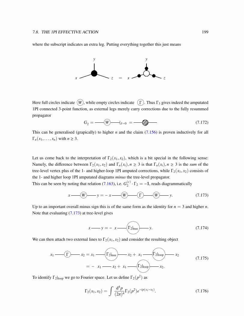
7.8. THE 1PI EFFECTIVE ACTION 199
where the subscript indicates an extra leg. Putting everything together this just means
x z =
y
x z
y
Here full circles indicate W , while empty circles indicate
Γ . Thus Γ3 gives indeed the amputated1PI connected 3-point function, as external legs merely carry corrections due to the fully resummedpropagator
G2 =f Wf|J=0 =fpf (7.172)
This can be generalised (grapically) to higher n and the claim (7.156) is proven inductively for allΓn(x1, . . . , xn) with n ≥ 3.
Let us come back to the interpretation of Γ2(x1, x2), which is a bit special in the following sense:Namely, the difference between Γ2(x1, x2) and Γn(xi), n ≥ 3 is that Γn(xi), n ≥ 3 is the sum of thetree-level vertex plus of the 1- and higher-loop 1PI amputed corrections, while Γ2(x1, x2) consists ofthe 1- and higher loop 1PI amputated diagrams minus the tree-level propagator.
This can be seen by noting that relation (7.163), i.e. G(c)2 · Γ2 = −1, reads diagrammatically
xf Wf y = − xf
Wf Γ f
Wf y. (7.173)
Up to an important overall minus sign this is of the same form as the identity for n = 3 and higher n.Note that evaluating (7.173) at tree-level gives
xf y = − xfΓ2|treef y. (7.174)
We can then attach two external lines to Γ2(x1, x2) and consider the resulting object
x1f Γ f x2 = x1f
Γ2|treef x2 + x1f
Γ2|loopf x2
= − x1f x2 + x1fΓ2|loopf x2.
(7.175)
To identify Γ2|loop we go to Fourier space. Let us define Γ2(p2) as
Γ2(x1, x2) =
∫d4 p(2π)4 Γ2(p2)e−ip(x1−x2). (7.176)

200 CHAPTER 7. PATH INTEGRAL QUANTISATION
In momentum space, by factoring out the external lines from the diagrams, we see that
− x1f x2 ⇔ −i
p2 −m20
p2 −m20
ii
p2 −m20
x1f−iM2f x2 ⇔
ip2 −m2
0
(−iΓ2(p2)|loop
) ip2 −m2
0
(7.177)
and thus
Γ2(p2) = −p2 −m2
0
i− iΓ2(p2)|loop. (7.178)
On the other hand, consider the Fourier transform of the fully resummed Feynman propagator G(c)2 (x1, x2)
via
G(c)2 (x1, x2) =fpf =
∫d4 p(2π)4 G(c)
2 (p2)e−ip(x1−x2), (7.179)
where G(c)2 (p2) is given by Dyson resummation as
G(c)2 (p2) =
ip2 −m2
0 −M2(p2). (7.180)
Here −iM2(p2) is the value of all amputated 1PI diagrams (i.e. without external legs) evaluated at1-loop and higher. Relation (7.163), i.e. G(c)
2 · Γ2 = −1, implies
Γ2(p2) = i(p2 −m20 −M2(p2)). (7.181)
In view of (7.178), we identify Γ2(p2)|loop = −iM2(p2). Together with (7.175) this justifies the aboveclaim that Γ2(x1, x2) consists of the 1- and higher loop 1PI amputated diagrams minus the tree-levelpropagator.
7.9 Γ(ϕ) as a quantum effective action and background field method
Diagrams like the ones above illustrate the following interpretation of Γ(ϕ): To compute a connectedn-point function in the full quantum theory, we use the tree-level Feynman rules but replace each k-vertex (with k ≥ 3) of the classical action S [φ] with the 1PI amputated k-vertex Γk as encoded in Γ[ϕ]and replace the free propagator with G2, the fully resummed propagator. This justifies the name 1PIeffective action of Γ[ϕ]:
Replacing S [φ] by Γ[ϕ] and computing at tree-level gives the full quantum theory.
This interpretation of Γ[ϕ] can also be seen in many different ways, one of them being the following:Define the object W[J, h] via 8
eiW[J,h] B
∫Dϕ e
ih (Γ[ϕ)+J·ϕ) (7.182)
8By contrast, we had eih W[J] = 1
Z[0]
∫Dφ e
ih (S [φ]+J·φ).

7.9. Γ(ϕ) AS A QUANTUM EFFECTIVE ACTION AND BACKGROUND FIELD METHOD 201
and expand
W[J, h] =∑
loops L
hL−1WL[J]. (7.183)
Now consider the formal limit h → 0, in which the righthand side becomes just W0/h. By thestationary phase argument, the right-hand side of (7.182) is given by the value of the integrand at thesaddle-point, i.e. by
eih (Γ[ϕ]+J·ϕ) (7.184)
with ϕ such thatδ
δϕ(Γ[ϕ] + J · ϕ])
∣∣∣ϕ=ϕ
= 0 i.e.δΓδϕ
∣∣∣∣∣∣ϕ
= −J. (7.185)
We omit the tilde from now. Thus
W0[J] = Γ[ϕ] + J · ϕ withδΓδϕ
= −J, (7.186)
where the righthand side is a functional of J only. But this is just the inverse Légendre transformationthat defined Γ[ϕ] = W[J] − J · ϕ with δΓ
δϕ = −J. Thus W0[J] = W[J]. Now, W[J] is the full quantumobject, and we thus find that
eih W[J] =
1Z[0]
∫Dφe
ih (S [φ]+J·φ) = e
ih (Γ[ϕ]+J·ϕ), (7.187)
where J and Γ[ϕ] are related via δΓδϕ = −J. We can interpret this result as follows:
• The integral 1Z[0]
∫Dφ is responsible for the quantum fluctuations.
• Replacing S [φ] by Γ[ϕ] (with ϕ such that δΓδϕ = −J) and working at tree-level (i.e. no
∫Dφ)
anymore) gives the full result.
In particular Γ and S are the same functionals at tree-level,
Γ[ϕ] = S [ϕ] + hK[ϕ] for some K[ϕ]. (7.188)
The equationδΓδϕ
= −J, i.e.δΓδϕ
= 0 for J = 0 (7.189)
is the quantum effective equation of motion replacing the classical δSδφ = 0 in the full quantum
theory.
Background field method
Consider again
eih W[J] =
∫Dφ e
ih (S [φ]+J·φ), (7.190)

202 CHAPTER 7. PATH INTEGRAL QUANTISATION
where∫Dφ ≡ 1
Z[0]
∫Dφ is the normalised measure such that∫
Dφeih (S [φ]+J·φ)
∣∣∣J=0 = 1. (7.191)
If we plug in the relation W[J] = Γ[ϕ] + J · ϕ and δΓδϕ = −J we arrive at
eih Γ[ϕ] =
∫Dφ e
ih (S [φ]− δΓ
δϕ (φ−ϕ)). (7.192)
Now define the fieldf (x) B φ(x) − ϕ(x), i.e. φ(x) = ϕ(x) + f (x). (7.193)
Since ϕ(x) is the vacuum expectation value of the quantum operator φ(x), we view f (x) as thequantum fluctuation around the background ϕ(x). The relation
eih Γ[ϕ] =
∫D f e
ih (S [ϕ+ f ]− δΓ
δϕ · f) (7.194)
shows that in order to determine Γ[ϕ] we must integrate out the quantum fluctuation f (x).To evaluate this integral we expand
S [ϕ+ f ] = S [ϕ] +δSδϕ· f +
12
f ·δ2Sδϕ2 · f + higher terms (7.195)
and with Γ = S + h · K and thus
−δΓδϕ· f = −
δSδϕ· f − h
δKδϕ· f (7.196)
we obtain
eih Γ[ϕ] =
∫D f e
ih
(S [ϕ]+ 1
2 f · δ2Sδϕ2 · f−h δK
δϕ · f+O( f 3)). (7.197)
Thus altogether
Γ[ϕ] = S [ϕ] − i h ln(∫D f e
ih
(12 f · δ
2Sδϕ2 · f−h δK
δϕ · f+O( f 3)))≡ S [ϕ] + hK[ϕ]. (7.198)
Since K[ϕ] appears on both sides, one has to solve this equation perturbatively. In particular the 1-loopcorrection to Γ is due to the lowest fluctuation terms in the integrand of
∫D f . Since K[ϕ] is by itself
already 1-loop, the relevant piece is only the quadratic one and
K(1-loop) = −i ln∫D f e
− 12 f ·
(− i
hδ2Sδϕ2
)· f
. (7.199)
At 2-loop order we then use the 1-loop result for K[ϕ] together with higher-order terms. As an exampleconsider φ4-theory with classical action
S =
∫d4x
[−
12φ(∂2 + m2)φ −
λ
4!φ4
](7.200)

7.10. EUCLIDEAN QFT AND STATISTICAL FIELD THEORY 203
and compute Γ[ϕ0] up to 1-loop order with ϕ0 =const. The computation will be done in the tutorials.If we define the effective potential V(ϕ0) via
Γ[φ0] = −VolR1,3 · V(ϕ0), (7.201)
and expandV(ϕ0) = V(0)(ϕ0) + V(1-loop)(ϕ0) + . . . , (7.202)
the result isV(0) =
12
m2ϕ20 +
λ
4!ϕ4
0 (7.203)
and V(1-loop)(ϕ0) is given by the Coleman-Weinberg-Potential
V(1-loop)(ϕ0) =12
∫d4k
(2π)4iln
m2 + λ2ϕ
20 − k2 − iε
m2 − k2 − iε
. (7.204)
The denominator is the contribution from the vacuum bubbles of the free theory, which must beremoved with our normalisation of the path-integral.
7.10 Euclidean QFT and statistical field theory
Let us briefly summarize our findings so far for the path integral in Minkowski space and collect thecorresponding expressions for the Euclidean theory. We then point out a beautiful formal analogybetween Euclidean Quantum Field Theory in 4 dimensions and Classical Statistical Field Theory in 3dimensions.In Lorentzian signature we have derived the following expressions (where we reinstate h): For thescalar field with classical action
S [φ] =∫
d4x(12(∂µφ)
2 −12
m2φ2 +Lint
)(7.205)
the generating functional for the correlation functions is defined as
Z[J] =∫Dφ e
ih (S [φ]+φ·J) (7.206)
so that ⟨T
∏i
φ(xi)
⟩=
1Z[0]
∏i
hδiδJ(xi)
Z[J]|J=0. (7.207)
Our conventions for the effective action are furthermore
eih W[J] =
Z[J]Z[0]
, Γ[ϕ] = W[Jϕ] − ϕ · Jϕ. (7.208)
As discussed, we can pass from Lorentzian to Euclidean signature via a Wick rotation replacingx0 → −ix4
E . In Euclidean space R4 with
(x1E , x2
E , x3E , x4
E) = (x2, x2, x3, ix0) (7.209)

204 CHAPTER 7. PATH INTEGRAL QUANTISATION
the analogous expressions are then
ZE [J] =∫Dφ e−
1h (S E [φ]−φ·J) (7.210)
with
S E [φ] B
∫d4xE
(12(∂Eφ)
2 +12
m2φ2 −Lint
)(7.211)
and
φ · J =
∫d4xEφ(xE)J(xE), (∂Eφ)
2 =4∑
i=1
∂
∂xiE
φ
2
. (7.212)
Furthermore ⟨T
∏i
φ(xE i)
⟩=
1ZE [0]
∏i
hδδJ(xE i)
ZE [J] (7.213)
and
e−1h WE [J] B
ZE [J]ZE [0]
, ΓE [ϕ] B WE [Jϕ] + ϕ · Jϕ,δΓE
δϕ= J. (7.214)
An executive summary of what Quantum Field Theory is about can be given as follows (workingin Euclidean signature):
• We start with a classical field φ(x) and associate to it the classical action S E [φ]. The field φ(x)arises as the continuum limit description of a system of N harmonic oscillators.
• In the classical limit, formally h→ 0, the field φ(x) takes a definite value given by the classicalequation of motion
δS E
δφ= 0. (7.215)
• For h finite, quantum fluctuations arise. These are encoded in ZE [J], where the path integraltakes into account all quantum fluctuations of the field.
• What we can compute in the quantum theory are quantum expectation values or correlationfunctions. In particular the quantum expectation value of the field in the presence of a source Jis
ϕ(x)J := 〈φ(x)〉J = 〈Ω| φ(x) |Ω〉J =1
Z[0]
∫Dφ φ(x)e−
1h (S E [φ]−φ·J). (7.216)
• With our definition of WE [J] we can compute this as
ϕ(x)J = −δWE
δJ(x). (7.217)
• In terms of the Légendre transform Γ[ϕ] we have
δΓE
δϕ= J. (7.218)
ΓE gives a quantum effective action after integrating out the quantum fluctuations in the sensethat
e−1h ΓE [ϕ] =
∫D f e
− 1h
(S E [ϕ+ f ]− δΓE
δϕ · f). (7.219)

7.10. EUCLIDEAN QFT AND STATISTICAL FIELD THEORY 205
Remarkably, this is formally exactly the same structure as in classical statistical mechanics or moreprecisely in its continuum limit, classical statistical field theory, in 3 spatial dimensions:
• Start with a classical field describing some classical observable, e.g. with s(~x) defined as themagnetisation density of a 3D ferromagnet with energy∫
d3xH(~x) =∫
d3x12(∇s(~x))2 . (7.220)
We can think of this as the continuum limit of a system of spins sn with nearest neighbourinteractions.
• At temperature T = 0, the system is in its ground state given by minimizing the energy (in thiscase given by s(~x) constant).
• For finite T there are thermal fluctuations of s(~x). These are encoded in the partition function
Z[H] =
∫Ds(~x)e−β
∫d3 x(H(s)−H(~x)s(~x)), (7.221)
where β = (kBT )−1 and H(~x) is an external source coupling to s(~x) (in the present case of aferromagnet this would be a magnetic field).
• The classical expectation value of s(~x) for an ensemble of systems is
〈s(~x)〉H =1
Z[H]
∫Ds(~x)s(~x)e−β
∫d3 x(H−Hs). (7.222)
• Define the free energy - the analogue of WE [J] - as
F[H] = −1β
lnZ, (7.223)
i.e.
e−βF[H] =
∫Ds(~x)e−β
∫d3 x(H−Hs). (7.224)
Then
M(~x) := 〈s(~x)〉H = −δF
δH(~x). (7.225)
• The Gibbs free energy is the Légendre transform of F[H],
G[M] = F[HM ] + M · HM, (7.226)
viewed as a functional of M. Then the average magnetisation is determined via the equation
δGδM
= H. (7.227)

206 CHAPTER 7. PATH INTEGRAL QUANTISATION
Due to this formal analogy, many problems in statistical field theory are solved in exactly the samemanner as in Euclidean QFT. In particular the structure of perturbation theory and important conceptsconcerning symmetry breaking and renormalisation agree.This can be summarized as follows:
4D QFT 3D statistical theoryφ(xE) s(~x)
quantum fluctuation thermal fluctuationh kBT
e−1h WE [J] e−βF[H]
ϕJ = −δWEδJ(~x) M = − δF
δH(~x)δΓEδϕ = J δG
δM = H
7.11 Grassman algebra calculus
We would now like to apply the path integral quantization method to systems with fermions. Considertherefore a Dirac fermion field operator ψA(t, ~x) with spin indices A = 1, 2, 3, 4 in the Heisenbergpicture and recall the anti-commutation relations
ψA(t, ~x), ψ†B(t,~y) = δAB δ
(3)(~x −~y) (7.228)
andψA(t, ~x), ψB(t,~y) = 0 = ψ†A(t, ~x), ψ
†
B(t,~y). (7.229)
We seek a path integral representation for the transition function 〈ψ(~xF), t f |ψ(~xI), tI〉 where the state|ψ(~x), t〉 is defined via
ψA(t, ~x) |ψ(~x), t〉 = ψA(t, ~x) |ψ(~x), t〉 . (7.230)
Here the non-hatted expression ψA(t, ~x) represents a classical field. We face the immediate problemthat consistency with (7.229) requires that the classical field ψA(t, ~x) satisfy
ψA(t, ~x)ψB(t,~y) = −ψB(t,~y)ψA(t, ~x). (7.231)
Thus ψA(t, ~x) cannot take values in C - rather we need the notion of anti-commuting numbers.
Consider first the case of a finite number of degrees of freedom by putting the theory, as usual, ona lattice of finite lattice spacing corresponding to a transition
ψA(t, ~x)→ ψAi (t) (7.232)
and let us omit the spinor indices for the time being. Then we search for classical objects ψi(t) withthe property
ψi(t)ψ j(t) = −ψ j(t)ψi(t). (7.233)
These ψi take values in a so-called Grassmann-algebra A defined as follows:

7.11. GRASSMAN ALGEBRA CALCULUS 207
• Let θi, i = 1, . . . , n, be a basis of an n-dimensional complex vector space V , i.e. we have thenotion of scalar multiplication aθi = θia, a ∈ C and vector addition aθi + bθ j ∈ V .
• Define then a bilinear anti-commutative multiplication
θiθ j = −θ jθi (7.234)
as a map from
V × V 7→ Λ2V , (7.235)
where Λ2V is the antisymmetric tensor product of V .
• Iteratively we can build higher rank anti-symmetric product spaces ΛkV up to ΛnV .
Then the Grassmann (or exterior) algebra is defined as the space
A =n⊕
k=0
ΛkV = C ⊕ V ⊕Λ2V ⊕ ... ⊕ΛnV . (7.236)
A typical element of A is of the form
a + aiθi +12
ai jθiθ j + ... +1n!
ai1...inθi1 ...θin (7.237)
with completely antisymmetrc coefficients ai j = −a ji etc. By abuse of notation, the θi are calledGrassmann numbers - though calling them ’numbers’ makes things look more exotic than theyare as the θi should really be viewed simply as elements of the abstract Grassmann algebra A. Inparticular they are nilpotent,
θ2i = 0. (7.238)
An important example of a Grassmann algebra is the space Ω of differential forms defined on ann-dimensional manifold endowed with the structure wedge (or exterior product).
A Grassmann algebra is a graded algebra:
An element of Λ2kV has grade (or degree) s = 0 (it is said to be even),an element of Λ2k+1V has grade (or degree) s = 1 (it is said be odd).
Note that a general element of A can always be written as the sum of an even and an odd element.Two elements A, B ∈A of definite degree sA and sB satisfy
A B = (−1)sA sB B A. (7.239)
Thus even elements are commuting and therefore sometimes called bosonic, whereas odd elementsare dubbed fermionic due to their anti-commuting nature.

208 CHAPTER 7. PATH INTEGRAL QUANTISATION
Differentiation and integration
To set up a notion of calculus on the space of functions
f : A → C, (7.240)
θ → f (θ) = a + aiθi + ... +1n!
ai1...inθi1in , (7.241)
one defines differentiation with respect to θi as follows:
• ∂∂θiθ j = δi j, ∂
∂θ ja = 0 ∀a ∈ C;
• ∂∂θi(a1 f1(θ) + a2 f2(θ)) = a1
∂∂θ1
f1(θ) + a2∂∂θ2
f2(θ) (linearity);
• If f1(θ) has definite grade s, then the graded Leibniz rule holds,
∂
∂θi
(f1(θ) f2(θ)
)=
(∂
∂θif1(θ)
)f2(θ) + (−1)s f1(θ)
∂
∂θif2(θ). (7.242)
For general f1(θ) we decompose f1(θ) into its even and odd part and then apply the gradedLeibniz rule by linearity.
For example∂
∂θi(θ jθk) = δi jθk − δikθ j. (7.243)
Next we define an integral I[ f (θ)] as a functional of f (θ). Our applications to the path integral willmake it evident that it is useful to define this functional such that it shares two key properties of thebosonic integral (in one variable for simplicity)
I[ f (x)] =
∞∫−∞
f (x)dx, (7.244)
namely
• I[a1 f1(x) + a2 f2(x)] = a1I[ f1(x)] + a2I[ f2(x)] and
• I[ f (x + a)] = I[ f (x)], i.e. translation invariance in the integration variable.
Consider first a Grassmann algebra with n = 1 such that
I[ f (θ] =∫
dθ f (θ) =∫
dθ(a + bθ). (7.245)
In this case translation invariance just means invariance under a shift of the integration variable θ →θ+ c and implies, together with linearity,∫
dθ c = 0 ∀c ∈ C. (7.246)

7.11. GRASSMAN ALGEBRA CALCULUS 209
We normalise∫
dθ θ = 1 such that∫dθ[a + bθ] = b =
∂
∂θ(a + bθ). (7.247)
For a Grassmann algebra based on Grassmann numbers θi, i = 1, . . . , n, generalized translation in-variance implies ∫
dθi θ j = δi j =∂
∂θiθ j. (7.248)
Then the Grassmann measure is defined as dnθ B dθndθn−1...dθ1. Because of
dθidθ j = −dθ jdθi (7.249)
we have to be aware of the order in dnθ. Thus∫
dnθ θ1θ2...θn = 1 and more generally∫dnθ θi1 ...θin = εi1...in (7.250)
with εi1...in the totally anti-symmetric ε-tensor normalised as ε1...n = 1. In particular for f (θ) =
a + aiθi + ... + 1n! ai1...inθi1...in we find∫
dnθ f (θ) =1n!
ai1...inεi1...in = a123...n. (7.251)
Only those terms contribute for which the Grassmann integral is ’saturated’ such that each dθi is pairedwith precisely one θi.Note that the above definitions ensure that upon integration by parts no boundary terms are picked up,∫
dnθ∂
∂θif (θ) = 0. (7.252)
As an application we compute the Jacobian that arises for a linear change of Grassmann integrationvariables. To begin with, if A is an (n × n)-matrix, then we can define θ′ = Aθ and find∫
dnθ f (θ′) =∫
dnθ f (Aθ) =
∫dnθ a12...nA1i1 ...Aninθi1 ...θin (7.253)
= a12...n A1i1 ...Aninεi1...in︸ ︷︷ ︸=detA
= det A∫
dnθ f (θ). (7.254)
In the first line we used (7.251). Thus∫dnθ f (θ′) = det A
∫dnθ f (θ) = det A
∫dnθ′ f (θ′) (7.255)
and consequently dnθ = detA dnθ′, i.e.
θ′ = A θ ⇒ dnθ′ = (det A)−1 dnθ. (7.256)
Compare this with the bosonic case dn(A · x) = ||det A|| dnx.

210 CHAPTER 7. PATH INTEGRAL QUANTISATION
Application: Fermionic Gauss integral
Consider θi, i = 1, ..., n, with n = 2m and let us compute
I =∫
dnθ e12 θiAi jθ j , Ai j = −A ji. (7.257)
To saturate the Grassmann measure we pick up the term to m−th order in the expansion of the expo-nential and find
I =1
2mm!
∫dnθ Ai1i2 ...Ain−1inθi1 ...θin−1θin
=1
2mm!εi1...in Ai1i2 ...Ain−1in B Pf(A),
(7.258)
where Pf(A) is the so-called Pfaffian. Note the difference in the definition of the Pfaffian and of thedeterminant,
det A =1n!εi1...inε j1... jn Ai1 j1 ...Ain jn . (7.259)
One can show with standard methods of linear algebra that (Pf(A))2 = det A and take the positivesign,
Pf(A) =√
det A. (7.260)
Complexification
So far the coefficients a ∈ C, but θi were treated as real, or equivalently as one anti-commuting degreeof freedom (which is the fermionic counterpart of 1 bosonic real number). One can also considercomplex θi and θ∗i , viewed as independent degrees of freedom. E.g. one can build such complexGrassmann variables θi, i = 1, . . . , n, out of real Grassmann variables ω j, j = 1, ..., 2n via
θi = ω2i−1 + iω2i, θ∗i = ω2i−1 − iω2i. (7.261)
Alternatively, we simply declare θi and θ∗i to denote independent objects and define the complexconjugate of a product via
(θi θ j)∗ = θ∗j θ
∗i . (7.262)
We furthermore define the measure
dnθ dnθ∗ Bn∏
i=1
dθi dθ∗i = dθ1dθ∗1...dθndθ∗n = dθndθ∗n...dθ1dθ∗1. (7.263)
The complex Gaussian integral then reads∫dθ dθ∗ eθ
∗i Bi jθ j =
1n!
∫dθndθ∗n...dθ1dθ∗1Bi1 j1 ...Bin jn θ
∗i1θ j1 ...θ∗inθ jn
=1n!εi1...in ε j1... jn Bi1 j1 . . . Bin jn = det B.
(7.264)
Let us compare our results for bosonic and fermionic Gaussian integrals:

7.12. THE FERMIONIC PATH INTEGRAL 211
• Real case: ∫dnx e−
12 xiAi j x j =
√(2π)n
det A(bosonic integration),∫
dnθ e12 θiAi jθ j =
√det A (fermionic integration).
(7.265)
• Complex case: ∫dnz dnz∗ e−z∗i Bi jz j =
(2π)n
det B(bosonic),∫
dnθ∗ dnθ e−θ∗i Bi jθ j = det B (fermionic).
(7.266)
Note the change in the order of dnθ∗ and dnθ in the last term in order to accomodate for the (−1)sign in the exponent.
7.12 The fermionic path integral
We are now ready to come back to physics and to address the transition amplitude between twofermionic states. We first consider the quantum mechanics of a single fermion by making the transition
ψA(t, ~x)→ ψi(t) (7.267)
ignoring the spinor components A and taking i = 1. We then seek the states |ψ, t〉 such that
ψ(t) |ψ, t〉 = ψ(t) |ψ, t〉 (7.268)
with ψ(t) a complex Grassmann number. Working at fixed time t and suppressing the t-dependencewe must find the Hilbert space acted upon by ψ and ψ† with anti-commutation relations
ψ, ψ = 0 = ψ†, ψ†, ψ, ψ† = 1. (7.269)
In analogy with the analogous bosonic relations [a, a†] = 1, [a, a] = 0 = [a†, a†] this system is calleda fermionic harmonic oscillator. We assume (or alternatively show by exploiting boundedness ofthe Hamiltonian) the existence of a ground state
|0〉 such that ψ |0〉 = 0 (7.270)
and define the state |1〉 as ψ† |0〉 = |1〉. By means of the anti-commutation relations
ψ† |1〉 = ψ†ψ† |0〉 = 0,
ψ |1〉 = ψψ† |0〉 = (1 − ψ†ψ) |0〉 = |0〉 .(7.271)
We now claim that the sought-after eigenstate |ψ〉 with ψ |ψ〉 = ψ |ψ〉 takes the form
|ψ〉 = |0〉 − ψ |1〉 . (7.272)

212 CHAPTER 7. PATH INTEGRAL QUANTISATION
To avoid confusion note that the unhatted ψ is a complex Grassmann number, while the hatted ψ, ψ†
are annihilation and creation operators.Indeed,
ψ(|0〉 − ψ |1〉) = 0 − ψψ |1〉 . (7.273)
Since |1〉 = ψ† |0〉 is a Grassmann odd object, we have ψ |1〉 = − |1〉ψ. Equivalently, this follows fromthe relation ψ†ψ = −ψψ†. Either way we find
ψ |ψ〉 = ψψ |1〉 = ψ |0〉 = ψ |0〉 − ψ2 |1〉 = ψ(|0〉 − ψ |1〉) = ψ |ψ〉 . (7.274)
We can rewrite the eigenstate as
e−ψψ†
|0〉 = (1 − ψψ†) |0〉 = |0〉 − ψ |1〉 . (7.275)
Thus the eigenstate of the fermionic annihilation operator
ψ |ψ〉 = ψ |ψ〉 (7.276)
is given by
|ψ〉 = |0〉 − ψ |1〉 = e−ψψ†
|0〉 (7.277)
The state |ψ〉 is the fermionic analogue of a bosonic coherent state |µ〉 defined as the eigenstate of theannihilator,
a |µ〉 = µ |µ〉 with |µ〉 = eµa† |0〉 . (7.278)
The complex conjugate state 〈ψ| defined via 〈ψ| ψ† = 〈ψ|ψ∗ is simply
〈ψ| = 〈0| − 〈1|ψ∗ = 〈0| e−ψψ∗
. (7.279)
We will also need the inner product of two fermionic coherent states
〈ψ|ψ′〉 = 〈0| 0〉+ 〈1|ψ∗ψ′ |1〉 = 1 + ψ∗ψ′ (7.280)
and thus〈ψ|ψ′〉 = eψ
∗ψ′. (7.281)
Finallly the completeness relation in terms of the coherent states is given by∫dψ∗dψ |ψ〉 e−ψ
∗ψ 〈ψ| = 1 (7.282)
since the left-hand side is ∫dψ∗dψ (|0〉 − ψ |1〉) (1 − ψ∗ψ)(〈0| − 〈1|ψ∗)
=
∫dψ∗dψ (− |0〉ψ∗ψ 〈0|+ ψ |1〉 〈1|ψ∗)︸ ︷︷ ︸
−ψ∗ψ|0〉〈0|+ψψ∗ |1〉〈1|)
= |0〉 〈0|+ |1〉 〈1| = 1,
(7.283)

7.12. THE FERMIONIC PATH INTEGRAL 213
where we used that only terms ∼ ψ∗ψ saturate the Grassmann measure.
Let us now compute the quantum mechanical transition amplitude
〈ψF , tF |ψI , tI〉 = 〈ψF | e−iH(t f−tI) |ψI〉 (7.284)
between two fermionic coherent states. We assume that the structure of the Hamiltonian is
H = ψ†Mψ ≡ H(ψ†, ψ) (7.285)
for some bosonic, i.e. Grassmann even, M. In fact this will be sufficient to treat the field theoreticDirac fermion system we are interested in. As in the derivation of the bosonic path integral we partitionthe time evolution operator according to
e−iH(tF−tI) = limN→∞
(e−iHδt
)N, δt =
tF − tI
N(7.286)
and insert suitable factors of the identity, this time given by
1 j =
∫dψ∗jdψ j |ψ j〉 e
−ψ∗jψ j 〈ψ j| . (7.287)
Thus
〈ψF , tF |ψI , tI〉 = limN→∞
∫ N∏j=1
dψ∗jdψ j 〈ψN+1| e−iHδt |ψN〉 e−ψ∗NψN 〈ψN | ... |ψ1〉 e−ψ
∗1ψ1 〈ψ1| e−iHδt |ψ0〉
(7.288)with |ψ0〉 ≡ |ψI〉 and |ψN+1〉 ≡ |ψF〉. Now
〈ψ j+1| e−iHδt |ψ j〉 = 〈ψ j+1| e−iψ†Mψδt |ψ j〉
= 〈ψ j+1| (1 − iψ†Mψδt) |ψ j〉
= 〈ψ j+1|ψ j〉 − i 〈ψ j+1| ψ†Mψδt |ψ j〉
= (1 − iψ∗j+1Mψ jδt) 〈ψ j+1|ψ j〉
= eψ∗j+1ψ je−iψ∗j+1 Mψ jδt
= eψ∗j+1ψ j+1eψ
∗j+1(ψ j−ψ j+1)e−iψ∗j+1 Mψ jδt.
(7.289)
The factor eψ∗j+1ψ j+1 cancels with a corresponding factor e−ψ
∗j+1ψ j+1 from the insertion of the identity,
except for one remaining factor eψ∗N+1ψN+1 . Thus
〈ψF , tF |ψI , tI〉 = limN→∞
∫ N∏j=1
dψ∗j dψ j eψ∗N+1ψN+1 e
∑Nj=0(−ψ∗j+1(ψ j+1−ψ j)−iδtH(ψ∗j+1,ψ j)). (7.290)
As N → ∞ the exponential becomes
ei∫
dt(ψ∗ i ∂∂tψ−H) (7.291)
214 CHAPTER 7. PATH INTEGRAL QUANTISATION
and eψ∗N+1ψN+1 can be absorbed into the measure to arrive at the fermionic path integral for the Quantum
Mechanics of a single complex fermion,
〈ψF , tF |ψI , tI〉 =
∫Dψ∗Dψ ei
∫ tFtI
dt (ψ∗i ∂ψ∂t −H). (7.292)
To generalise this result to the Quantum Field Theory of a Dirac fermion we consider the classicalaction
S =
∫d4x ψ(x) (iγµ∂µ −m0)ψ(x) +Lint ≡
∫d4xL (7.293)
withL = ψ(x)iγ0∂0ψ(x) + ψ(x)
(iγi∂i −m0
)ψ(x) +Lint (7.294)
and ψ ≡ ψA, ψ ≡ ψ†Aγ0, (γ0)2 = 1. Note that the Hamiltonian is
H = −ψ(x)(iγi∂i −m0)ψ(x) −Lint. (7.295)
Thus we immediately generalise the above result to field theory as
〈ψF(~xF), tF |ψI(~xI), tI〉 =
∫Dψ(t, ~x)Dψ(t, ~x)ei
∫ tFtI
d4 xL(ψ,ψ). (7.296)
Note that we can integrate over ψ as opposed to ψ∗ without cost. To project initial and final states tothe vacuum |Ω〉, the same trick of replacing
m0 → m0 − iε (7.297)
works with tI → −∞ and tF → ∞. With this understanding we define the generating functional forfermionic correlation functions as
Z[η, η] = 〈Ω|Tei∫
d4 x[L(ψ,ψ)+η(x)ψ(x)+ψ(x)η(x)] |Ω〉
=
∫DψDψeiS [ψ,ψ]+iη·ψ+iψ·η,
(7.298)
where the external sources η, η are Grassmann-valued classical fields. Then for instance
〈Ω|Tψ(x1)ψ(x2) |Ω〉 =1
Z[0, 0]δ
iδη(x1)
−δ
iδη(x2)Z[η, η]|η=0=η, (7.299)
where special attention must be paid to the various minus signs.The same methods as in the bosonic theory can be applied to deduce from this the fermionic Feynmanrules. For example, as will be derived in the tutorials, in the free theory completing the square yields
Z0[η, η] = Z0[0, 0]e−ηS Fη (7.300)
where the fermionic Feynman propagator
S F(x − y) =∫
d4 p(2π)4
i(γ · p + m0 − iε)
p2 −m20 + iε
e−ip(x−y) (7.301)
7.12. THE FERMIONIC PATH INTEGRAL 215
is a solution to
(iγ · ∂x −m0 + iε)(−iS F(x − y)) = δ(x − y), i.e. (iγ · ∂ −m0 + iε) = iS −1F . (7.302)
Thus〈0|Tψ(x)ψ(y) |0〉 = S F(x − y). (7.303)
Similarly one confirms the fermionic Feynman rules as stated in QFT I.

216 CHAPTER 7. PATH INTEGRAL QUANTISATION

Chapter 8
Renormalisation of Quantum FieldTheory
In QFT I we claimed without proof the following properties of Quantum Electrodynamics (QED):
• The structure of UV divergences is encoded in the following three types of diagrams:
f 1PIf, g
1PIg,
• The four constants multiplying the divergences in these diagrams can be absorbed order by
order in perturbation theory in the counterterms of the renormalized Lagrangian such that allphysical amplitudes are finite. For this recall chapter 5.9 of QFT I.
While we demonstrated the second point at 1-loop order in QED, a number of open questions remain:
1. Why are only the above diagrams relevant as far as the structure of UV divergences is concerned,and how do these diagrams generalise to other QFTs?
2. How does one prove finiteness of the renormalised theory beyond 1-loop order in perturbationtheory?
3. What is the physics behind the renormalisation procedure?
8.1 Superficial divergence and power counting
In this section we address the question which diagrams are the relevant ones concerning the structureof UV divergences in QFT. We will do so for definiteness in the context of a scalar theory in d
217
218 CHAPTER 8. RENORMALISATION OF QUANTUM FIELD THEORY
dimensions with bare Lagrangian
L0 =12(∂µφ)
2 −12
m20φ
2 −λ(n)0
n!φn. (8.1)
Consider a connected diagram with E external lines, L loops, V vertices and I internal propagators.We had seen that for such diagrams
L = I − V + 1. (8.2)
Since each external line ends with 1 end at a vertex and each internal line with 2 ends, we have
nV = 2I + E. (8.3)
Now, naively the structure of momentum integrals in the UV for such a diagram is∫ddk1...
∫ddkL
k21...k2
I
(8.4)
since each loop gives a momentum integral∫
ddk and each internal line contributes a propagatorscaling like (k2 − m2)−1. Let us define D to be the difference of the power of the momentum innominator and denominator. In the above theory
D = d L − 2 I. (8.5)
If we introduce a momentum cutoff in the UV by replacing∫ ∞
dk →∫ Λ
dk, (8.6)
then according to this naive analysis the amplitudeM for the process associated with a diagram scalesas follows with Λ:
D > 0 : M ∼ ΛD (superfically divergent),
D < 0 : M ∼ Λ−|D| (superficially finite),
D = 0 : M ∼ log(Λ) (superficially log-divergent).
According to this reasoning, as Λ → ∞ only diagrams with D ≥ 0 are divergent. Therefore D iscalled superficial degree of divergence. The term superficial indicates that D does not always reflectthe actual divergence or finiteness properties of a diagram, due to one of the three possible exceptions:
• If D ≥ 0, then a diagram may still be actually finite if a sufficient amount of symmetry constrainsthe form of the amplitude or leads to cancellations among infinite terms. For example, super-symmetry leads to such cancellations, and the theory with maximal supersymmetry, N = 4Super-Yang-Mills theory in 4D, is even finite to all orders.
• If D < 0, a diagram may be actually divergent if the divergence is due to a simpler divergentsubdiagram.

8.1. SUPERFICIAL DIVERGENCE AND POWER COUNTING 219
• Tree-level diagrams have D = 0, but are finite.
To illustrate this consider φ4 theory in d = 4.
1. The following diagram has D = 0 and is superficially and actually logarithmically divergent,as we will see later.
2. The following diagram has D = −2 and is superficially and actually finite.
3. The following diagram still has D = −2, but is actually divergent. However, a closer look
reveals that the divergence is due to diagram 1, which appears as a divergent subdiagram withD = 0.
Conclusions: Except for the issue of divergent sudiagrams, all divergences come at most from thesuperficially divergent diagrams.
Given its importance, it is useful to derive an explicit expression for D. In the theory under consider-ation (φn in d dimensions) we have
D = d L − 2 I = d(I − V + 1) − 2I (8.7)
with I = 12 (nV − E) and thus
D = d −(d − n
d − 22
)V −
d − 22
E . (8.8)
Equation (8.8) can also be obtained by dimensional analysis: The action
S =
∫dd x
−12φ(∂2 + m2
0)φ −λ(n)0
n!φn
. (8.9)

220 CHAPTER 8. RENORMALISATION OF QUANTUM FIELD THEORY
has mass dimension zero (in natural units with h = 1 = c) and therefore
[φ] =d − 2
2, [λ
(n)0 ] = −n
d − 22
+ d. (8.10)
Consider a diagram with E external lines. To determine the mass dimension of the associated am-plitude, we note that it would receive a tree-level contribution M(E) = −iλ(E) if there were a termλ(E)φE in L. Thus
[M(E)] = [λ(E)] = d − Ed − 2
2. (8.11)
Furthermore, ifM(E) has superficial degree D, then
M(E) ∼ (λ(n)o )V ΛD (8.12)
unless one of the 3 exceptions is at work, where V is the number of n-point vertices. Therefore
V [λ(n)0 ] + D = d − Ed − 2
2(8.13)
and thus
D = d −(d − n
d − 22
)V −
d − 22
E = d − [λ(n)0 ]V −d − 2
2E. (8.14)
The appearance of the mass dimension of the coupling constant is very important as we will see in asecond.
8.2 Renormalisability and BPHZ theorem
The UV properties of a theory depend crucially on the sign of the coefficient of V in the expression(8.8) for D. To see this consider the following examples:
1. For φ4 theory in 4 dimensions (d = 4, n = 4) we find D = 4 − E, i.e. D depends only on E,not on V or L. There exists only a finite number of superficially divergent amplitudes. Since theaction is invariant under φ → −φ, any diagram with an odd number of external lines vanishes,and the only superficially divergent amplitudes are the following:
E = 0:
pE = 2:
fpfE = 4:

8.2. RENORMALISABILITY AND BPHZ THEOREM 221
Since D is independet of L, superficial divergences appear for these amplitudes at every orderin perturbation theory.
2. In φ3 theory in 4 dimensions (d = 4, n = 3), we have D = 4−V − E. Now only a finite numberof superficially divergent Feynman diagrams exist since V appears directly and with a negativesign.
3. In φ5 theory in 4 dimensions (d = 4, n = 5), we have D = 4 + V − E. There exists an infinitenumber of superficially divergent amplitudes since for every value of E diagrams with highenough V diverge.
Definition: A theory is called
• (power-counting) renormalisable if the number of superficially divergent amplitudes is finite,but superficial divergences appear at every order in perturbation theory.
• (power-counting) super-renormalisable if the number of superficially divergent Feynmandiagrams is finite.
• (power-counting) non-renormalisable if the number of superficially divergent amplitudes isinfinite.
From D = d − [λ(n)]V − d−22 E (and analogous formulae for other theories) we draw the following
important conclusion:A theory is
• renormalisable if its coupling has vanishing mass dimension.
• super-renormalisable if its coupling has positive mass dimension.
• non-renormalisable if its coupling has negative mass dimension.
The significance of the concept of (power-counting) renormalisablity is summarised in the BPHZtheorem1
• Ignore the issue of divergent subgraphs for a moment. Then if a theory is (power-counting)renormalisable, at each order in perturbation theory only a finite number of divergent dia-grams, parametrized by a finite number of divergent constants, appear. One can absorb thesedivergences order by order in the counterterms of the renormalized Lagrangian such that allphysical amplitudes are finite.
• The counterterms create new Feynman diagrams relevant at the next order. These will cancelthe divergences of the divergent subdiagrams (if present) at the next order.
1Due to Bogoliubov, Parasiuk, Hepp, Zimmermann.
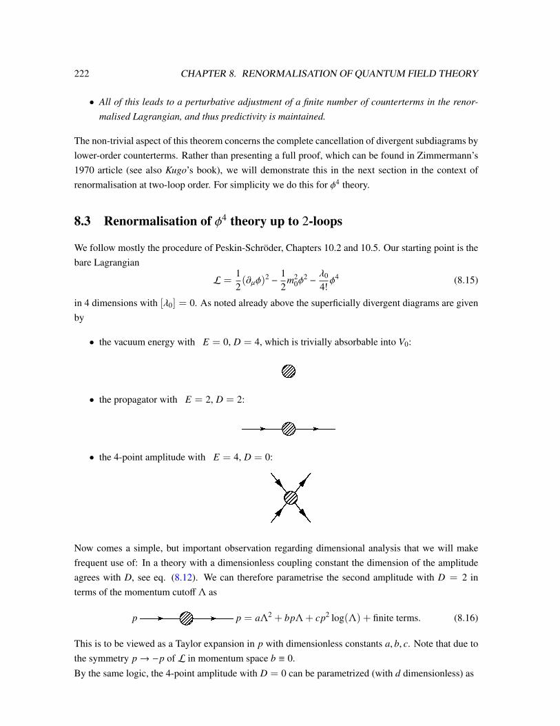
222 CHAPTER 8. RENORMALISATION OF QUANTUM FIELD THEORY
• All of this leads to a perturbative adjustment of a finite number of counterterms in the renor-malised Lagrangian, and thus predictivity is maintained.
The non-trivial aspect of this theorem concerns the complete cancellation of divergent subdiagrams bylower-order counterterms. Rather than presenting a full proof, which can be found in Zimmermann’s1970 article (see also Kugo’s book), we will demonstrate this in the next section in the context ofrenormalisation at two-loop order. For simplicity we do this for φ4 theory.
8.3 Renormalisation of φ4 theory up to 2-loops
We follow mostly the procedure of Peskin-Schröder, Chapters 10.2 and 10.5. Our starting point is thebare Lagrangian
L =12(∂µφ)
2 −12
m20φ
2 −λ0
4!φ4 (8.15)
in 4 dimensions with [λ0] = 0. As noted already above the superficially divergent diagrams are givenby
• the vacuum energy with E = 0, D = 4, which is trivially absorbable into V0:
p• the propagator with E = 2, D = 2:
fafpfaf• the 4-point amplitude with E = 4, D = 0:
Now comes a simple, but important observation regarding dimensional analysis that we will makefrequent use of: In a theory with a dimensionless coupling constant the dimension of the amplitudeagrees with D, see eq. (8.12). We can therefore parametrise the second amplitude with D = 2 interms of the momentum cutoff Λ as
pfafpfaf p = aΛ2 + bpΛ + cp2 log(Λ) + finite terms. (8.16)
This is to be viewed as a Taylor expansion in p with dimensionless constants a, b, c. Note that due tothe symmetry p→ −p of L in momentum space b ≡ 0.By the same logic, the 4-point amplitude with D = 0 can be parametrized (with d dimensionless) as

8.3. RENORMALISATION OF φ4 THEORY UP TO 2-LOOPS 223
= d log(Λ) + finite terms
Definition: If the divergence is multiplied by a simple monomial in p as above, it is called localdivergence. In the presence of divergent subgraphs more complicated expressions of p will appear.The BPHZ theorem states that it is possible to absorb the 3 divergent constants a, c, d into 3 countert-erms in the renormalised Lagrangian, order by order in renormalized perturbation theory. As discussedin the context of QED in QFT1 we define the renormalised field
φr = Z−12φ (8.17)
with Z the wavefunction renormalisation and rewrite L as
L =12(∂µφr)
2 −12
m2φ2r −
λ
4!φ4
r +12δZ(∂µφr)
2 −12δmφ
2r −
δλ4!φ4
r (8.18)
where δZ = Z − 1, δm = m20Z −m2 and δλ = λ0Z2 − λ. We henceforth compute with the renormalised
Feynman rulespF ∼ i
p2−m2+iε ,pFx pF ∼ i(p2δZ − δm)
∼ −iλ,∼ −iδλ
and no factors of√
Z for in- and out-going states in the computation of scattering amplitudes. Todefine the meaning of m and λ we impose the following renormalisation conditions:
pFp pF != i
p2−m2 + terms regular at p2 = m2
p2
p1
p3
p4amp.
= −iλ at s = 4m2, t = u = 0
Here s, t, u are the Mandelstam variables, which read with the above convention for the arrow of themomenta,
s = (p1 + p2)2, t = (p1 − p3)
2, u = (p1 − p4)2. (8.19)
Now
fpf =i
p2 −m2 −M2(p2), (8.20)
where −iM2(p2) is the amplitude of the 1PI amputated diagrams. Thus the first renormalisationcondition implies:
M2(p2)∣∣∣p2=m2
!= 0,
ddp2 M2(p2)
∣∣∣p2=m2
!= 0. (8.21)
Note that the renormalisation conditions are arbitrary and define the renormalisation scheme.

224 CHAPTER 8. RENORMALISATION OF QUANTUM FIELD THEORY
8.3.1 1-loop renormalisation
At 1-loop order
f
1PIf = +fxf
and thus2
f 1PIf = (−iλ)
12
∫d4k(2π)4
ik2 −m2 + iε
+ i(p2δ(1)Z − δ
(1)m ) ≡ −iM2(p2)
∣∣∣1-loop. (8.22)
We compute the integral by dimensional regularisation. The result (see exercise sheet 5 for a deriva-tion) is
∫ddk(2π)d
ik2 −m2 =
1(4π)d/2
Γ(1 − d
2
)(m2)1−d/2
. (8.23)
For d = 4 − ε and with the help of
Γ(−1 +
ε
2
)= −
2ε
e−12γ·ε
(1 +
ε
2
)+O(ε3) (8.24)
we get
= iλ2
(1 + 2
ε
)(m2)1−ε/2
(4π)2−ε/2 e−12γε = i
2λ
16π2 m2(
2ε + 1 − log(m2)
)(e−γ4π)
12 ε ,
where we used
(m2)−ε/2 = e−ε2 m2
= 1 −ε
2log(m2) +O(ε3). (8.25)
Note that the expected quadratic divergence aΛ2 corresponds, in dimensional regularization, to thedivergent term
iλ16π2 m2 1
ε. (8.26)
More precisely, for the integral with a UV momentum cutoff, the divergence would be proportional to
Λ2 −m2log(m2 + Λ2
m2
). (8.27)
As a rule of thumb, in a theory with dimensionless coupling constant, the order in Λ correspondingto a 1
ε -pole in dimensional regularization agrees with the mass dimension of the prefactor: Here[λm2] = 2 and thus the divergence is expected to scale as Λ2.
2The factor of 12 in front of the integral is a symmetry factor.

8.3. RENORMALISATION OF φ4 THEORY UP TO 2-LOOPS 225
Altogether
− iM2(p2) = −iλ2
14πd/2
Γ(1 − d
2
)(m2)1−d/2
+ i(p2δ
(1)Z − δ
(1)m
)(8.28)
and the renormalisation conditions imply
ddp2 M2(p2)
∣∣∣∣∣∣p2=m2
!= 0 ⇒ δ
(1)Z
!= 0 (8.29)
and
M2(p2)
∣∣∣∣∣∣p2=m2
!= 0⇒ δ
(1)m
!= −
λ
2(4π)d/2
Γ(1 − d
2
)(m2)1−d/2
∣∣∣∣∣∣d→4
. (8.30)
Note that at 1-loop M2(p2) ≡ 0 ∀p2 and the first non-trivial corrections to the propagator appear atthe 2-loop level. This, however, is a specialty of φ4 theory in four dimensions.
The computation of the 4-point amplitude at 1-loop level involves the following diagrams,
p2
p1
p3
p4
=p2
p1
p3
p4
−iλ +p3p4
p2
p1
+ + +p1p2
p3
p4 p2
p1 p3
p4
p2p1
p3
p4
(1) + O(λ3)
The first loop amplitude corresponds to the s-channel,
p2
p1 p3
p4
= 12 (−iλ)2
∫d4k(2π)4
ik2−m2
i(k+p)2−m2 B (−iλ)2iV(p2)
where p = p1 + p2. Then
iM(p1 p2 → p3 p4) = −iλ+ (−iλ)2 [iV(s) + iV(t) + iV(u)] − iδ(1)λ +O(λ3). (8.31)
The renormalisation condition implies
iM|s=4m2,t=u=0 = −iλ ⇒ (−iλ)2[iV(4m2) + 2iV(0)
]− iδ(1)λ
!= 0. (8.32)
Therefore
δ(1)λ
!= −λ2
(V(4m2) + 2V(0)
)≡ δ
(1)λ (s) + δ
(1)λ (u + t). (8.33)

226 CHAPTER 8. RENORMALISATION OF QUANTUM FIELD THEORY
The computation of V(p2) proceeds again via dimensional regularisation and is performed on exercisesheet 5, with the result
V(p2) = −12
Γ(ε(4π)2−ε/2
∫ 1
0dx
1[m2 − x(1 − x)p2]ε
= −1
32π2
∫ 1
0dx
[2ε− γ+ log(4π) − log(m2 − x(1 − x)p2
].
(8.34)
Then
δ(1)λ =
λ2
32π2
∫ 1
0dx
[6ε− 3γ+ 3 log(4π) − log(m2(1 − 4x(1 − x))) − 2 log(m2)
]. (8.35)
Computing iM(p1 p2 → p3 p4) up to O(λ2) gives:
iM(p1 p2 → p3 p4) = − iλ −iλ2
32π2
1∫0
dx[
log(
m2 − x(1 − x)sm2 − x(1 − x)4m2
)
+ log(m2 − x(1 − x)t
m2
)+ log
(m2 − x(1 − x)u
m2
) ].
(8.36)
This is manifestly finite and depends on two measurable input parameters m and λ.
8.3.2 Renormalisation at 2-loop
We now move on to 2-loop order and demonstrate that all divergences can be absorbed in 2-loop coun-terterms. In particular we need to show that divergences due to divergent subdiagrams are cancelledby the 1-loop counterterms that we have already included.
To exemplify this aspect of the BPHZ theorem we consider
at 2-loop-level.
1. In diagrams of the type
+(1)
the 1-loop counterterm to the propagator in the second diagram cancels the extra divergence inthe first diagram. In fact, as a speciality of φ4-theory, we have seen that, at 1-loop level,

8.3. RENORMALISATION OF φ4 THEORY UP TO 2-LOOPS 227
+
= 0
So the above diagrams give no contribution at order λ3.
2. There are 5 × 3 + 1 diagrams of the form
+plus the corresponding t-channel diagrams
+...
plus the u-channel diagrams
+...
as well as the 2-loop counterterm, which we split as
(2) =s
(2) +t + u
(2)
We consider only the s-channel, since t-and u-channel work completely analogously. The im-portant point to notice is that all momentum independent divergences can be absorbed into

228 CHAPTER 8. RENORMALISATION OF QUANTUM FIELD THEORY
s
(2)
One must therefore show that the momentum dependent divergences cancel among the five s-channel diagrams. Following Peskin-Schröder, they can be grouped into
group 1:
p2
p1p3
p4
+p2
p1 p3
p4
(1), s +p2
p1 p3
p4
(1), s
group 2:
and group 3:
Note that group 1 contains only the s-channel 1-loop counter terms, while in group 2 and 3 thecombined (t + u)-channel counter terms appear. The divergences of the diagrams of group 1are very easy to deal with: In terms of our previous definition
p2
p1 p3
p4
= (−iλ)2iV(p2)

8.3. RENORMALISATION OF φ4 THEORY UP TO 2-LOOPS 229
with p = p1 + p2 = p3 + p4 we have
p2
p1p3
p4
= (−iλ)3(iV(p2)
)2
and
p2
p1 p3
p4
(1), s =p2
p1 p3
p4
(1), s = (−iλ)iV(p2)λ2(iV(4m2)
)
For the counter term diagram we used our result that −iδ(1)λ (s) = λ2(iV(4m2)
). Adding both
contributions up and completing the square leads to
(−iλ)3(−
(V(p2) − V(4m2)
)2+
(V(4m2)
)2)
(8.37)
for group 1. From the explicit expression of V(p2) we deduce that
V(p2) − V(4m2) = finite, (8.38)
while(V(4m2)
)2has merely a momentum-independent divergence, which can be absorbed by
the 2-loop counter term
s
(2)
Note that ∼(
2ε
)2contains a divergence of the form 2
ε . More generally, higher loop-order diver-gences give higher powers in 1/ε.
Now consider the diagram from group 2, given by

230 CHAPTER 8. RENORMALISATION OF QUANTUM FIELD THEORY
= (−iλ)3∫
d4k(2π)4
ik2 −m2
i(k + p)2 −m2 iV
((p3 + k)2
)(8.39)
with p = p1 + p2 = p3 + p4. This diagram exemplifies the appearance of a nested singu-larity, which appears when 2 divergent subdiagrams share a common propagator. In this case,so-called non-local divergences appear, for which the prefactor of the singularity is not a sim-ple polynomial in p, but a more complicated function in p.
Integrals of this kind would keep us from the street for a while. We do not explicitly performthe computation, which is straightforward, but a little lengthy, and merely quote the result fromPeskin-Schröder, Chapter 10: When the dust has settled, the amplitude can be written as thesum of 2 terms:
• Term 1 has only a momentum independent singularity, which can be absorbed into the2-loop counter-term.
• Term 2 is given by
−iλ3
2(4π)4
2ε
1∫0
dy[1ε− γ+ log(4π) − log(m2 − y(1 − y)p2)
](8.40)
and exhibits 2 types of singularities:The double pole 2
ε1ε indicates the higher-loop nature of the singularity, as before. It is due
to the region in momentum space where both loops diverge. By contrast, the term
2ε
log(m2 − y(1 − y)p2) (8.41)
is the non-local singularity advertised above. The factor of 2/ε is due to the regime inmomentum space where only 1 of the subdiagrams diverges, and the log(p2) representsthe finite QFT process around this from the other subdiagram.
Explicit computation confirms that these singularities are cancelled by the counter-termdiagram
(1), t + u
This completes the proof that at 2-loop order, all divergences, including those of divergent subdia-grams, can be absorbed into the counter-terms. A formalization of this procedure leads to the BPHZtheorem. More on the ideas behind its proof can be found e.g. in Kugo.
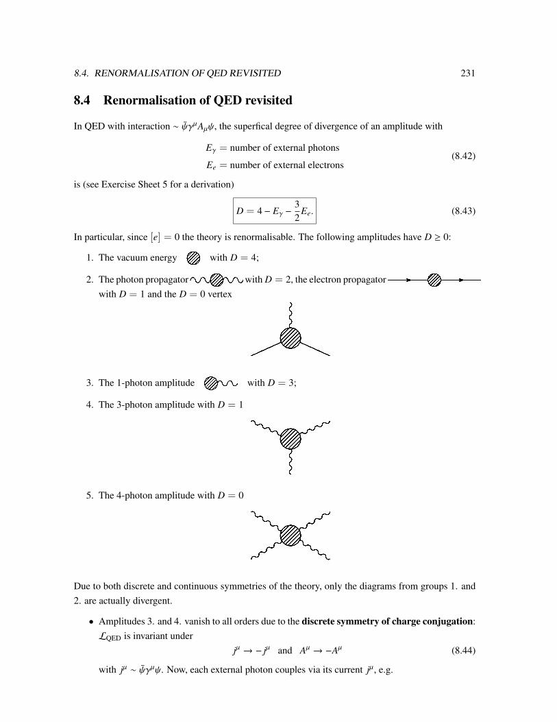
8.4. RENORMALISATION OF QED REVISITED 231
8.4 Renormalisation of QED revisited
In QED with interaction ∼ ψγµAµψ, the superfical degree of divergence of an amplitude with
Eγ = number of external photons
Ee = number of external electrons(8.42)
is (see Exercise Sheet 5 for a derivation)
D = 4 − Eγ −32
Ee. (8.43)
In particular, since [e] = 0 the theory is renormalisable. The following amplitudes have D ≥ 0:
1. The vacuum energy p with D = 4;
2. The photon propagatorgpgwith D = 2, the electron propagatorfafpfafwith D = 1 and the D = 0 vertex
3. The 1-photon amplitude pg with D = 3;
4. The 3-photon amplitude with D = 1
5. The 4-photon amplitude with D = 0
Due to both discrete and continuous symmetries of the theory, only the diagrams from groups 1. and2. are actually divergent.
• Amplitudes 3. and 4. vanish to all orders due to the discrete symmetry of charge conjugation:LQED is invariant under
jµ → − jµ and Aµ → −Aµ (8.44)
with jµ ∼ ψγµψ. Now, each external photon couples via its current jµ, e.g.

232 CHAPTER 8. RENORMALISATION OF QUANTUM FIELD THEORY
Thus a diagram with only an odd number of external photons vanishes.
• Diagram 5. is non-zero, but actually finite as a consequence of gauge symmetry. This can beshown by exploiting the Ward identities.Note that diagram 5. is responsible for the non-linearity of QED due to the scattering of photonswith each other induced by loop effects.
Thus as claimed in QFT I, as far as the UV divergences are concerned it suffices to consider thediagrams 2. (the contribution of 1. is easily absorbed into the vacuum energy term). But againsymmetry lowers the actual degree of divergence for the first two diagrams of 2. to logarithmic ones:
• By dimensional analysis, the fermion propagator, having D = 1, can be Taylor-expanded aspFfpfaf = A0 + A1 6 p +A2 p2 + ... (8.45)
withA0 = a0Λ, A1 = a1 log Λ, A2 and higher: finite as Λ → ∞ (8.46)
and a0, a1 dimensionless. But then the mass shift of the electron would be proportional to Λ.Instead this shift must be proportional to the electron mass me itself. This is because if me ≡ 0,then the theory possesses chiral or axial symmetry, because the Lagrangian can be written as
L = ψLiγ · ∂ψL + ψRiγ · ∂ψR − e jµAµ (8.47)
and is invariant under independent rotations of the left- and right-chiral spinors
ψL → eiαψL, ψR → eiβψR. (8.48)
This symmetry, however, forbids a mass term, which must be of the form meψRψL. Thus A0
must contain an explicit power of me. By dimensional analysis there is no more room for afactor of Λ, and A0 can at worst be of the form
A0 = a0me log Λ, (8.49)
as is in fact confirmed by computation.
• The photon propagator is, by dimensional analysis, of the form
µqGgpg qG ν = B0 + Bµ1qµ + B2q2 + ... (8.50)
withB0 = b0Λ2, Bµ1 = bµ1Λ, B2 = b2 log Λ (8.51)
and bi dimensionless. But by the Ward identities we know that
µgpg ν =(ηµνq2 − qµqν
)Π(q2) (8.52)
and thus b0 = b1 = 0.

8.5. THE RENORMALISATION SCALE 233
Thus all diagrams of 2. are logarithmically divergent. Renormalisation proceeds as discussed, at1-loop level, in QFT I.
8.5 The renormalisation scale
Renormalisation automatically introduces a mass scale µ - the renormalisation scale - in the quantumtheory via the renormalisation conditions. In our renormalisation of φ4 theory we have so far chosento identify µ with the mass m of φ because our renormalisation conditions have been
M2(p2)∣∣∣p2=m2 = 0 =
ddp2 M2(p2)
∣∣∣p2=m2 (8.53)
and
= −iλ at scale s = 4m2, t = u = 0
More generally, the renormalisation scale µ can be an independent scale since the renormalisationconditions are arbitrary. Since this observation is so crucial for all that follows we would like toillustrate it very explicitly. To this end let us consider the massless theory
L =12(∂φ)2 −
λ0
4!φ4
0 (8.54)
in d= 4. Note that this theory has no classical scale since m0 = 0. However, as we will now see, thescale-invariance of the classical theory is broken in the quantum theory due to the appearance of therenormalisation scale. For instance, we can impose the renormalisation conditions
1. M2(p2) = 0 at p2 = −µ2, i.e. for spacelike momenta,
2. ddp2 M2(p2) = 0 at p2 = −µ2,
3. and for the vertex:
p2
p1
p4
p3
= −iλ at (p1 + p2)2 = (p1 + p3)2 = (p1 + p4)2 = −µ2
With φ = Z−1/2φ0 , conditions 1. and 2. imply∫d4x eip·x 〈Ω|Tφ(x)φ(0) |Ω〉
∣∣∣p2=−µ2 =
ip2
∣∣∣p2=−µ2 , (8.55)

234 CHAPTER 8. RENORMALISATION OF QUANTUM FIELD THEORY
i.e. ∫d4x eip·x 〈Ω|Tφ0(x)φ0(0) |Ω〉
∣∣∣p2=−µ2 =
i Zp2
∣∣∣p2=−µ2 . (8.56)
In particular, the wavefunction renormalisation factor Z used in φ = Z−1/2φ0 is not the residue of thepropagator at the physical mass p2 = 0, but has the meaning as given in the previous equation.Now, to fully appreciate the appearance of the renormalisation scale µ, consider the renormalisedconnected 4-correlator
G(4)(x1, .., x4) = 〈Ω|Tφ(x1)...φ(x4) |Ω〉∣∣∣connected. (8.57)
Its Fourier transformation is
G(4)(p1, .., p4) =[−iλ+ (−iλ)2(iV(s) + iV(t) + iV(u)) − iδλ +O(λ3)
] 4∏i=1
ip2
i
. (8.58)
Note the product∏4
i=1i
p2i
from the external legs because we are computing the 4-point correlator, not
the scattering amplitude iM(p1 p2 → p3 p4). Renormalisation condition 3. implies
δλ = (−iλ)2 · 3V(−µ2) =3λ2
2(4π)d/2
1∫0
dxΓ(2 − d
2
)(x(1 − x)µ2)2−d/2
=3λ2
2(4π)2
[2ε− log µ2 + finite terms
] (8.59)
in dimensional regularization, whereas in cutoff regularisation the term in brackets would be of theform
logΛ2
µ2 + finite. (8.60)
The crucial observation is that G(4)(p1, ..., p4) is finite, but
• explicitly depends on the renormalisation scale µ through the counterterm δλ and
• implicitly depends on µ, at 1-loop, via λ because λ is defined via renormalisation condition 3.at the scale µ.
(At higher loop, there will also be an implicit µ-dependence via Z as we will see below.)
8.6 The Callan-Symanzyk (CS) equation
The CS equation quantifies the dependence of various quantities on the renormalisation scale µ. Toderive it we be begin with the bare correlator (for definiteness in massive φ4 theory)
G(0)n (x1, ..., xn) = 〈Ω|T
∏i
φ0(xi) |Ω〉∣∣∣conn. (8.61)

8.6. THE CALLAN-SYMANZYK (CS) EQUATION 235
computed from the bare Feynman rules in terms of the parameters λ0, m0 appearing in the bare La-grangian L0 as well as the cutoff Λ (or ε). There is no explicit dependence of G(0)
n (x1, ..., xn) on therenormalisation scale µ, i.e.
G(0)n (x1, ..., xn) = G(0)
n (x; λ0, m0; Λ) (8.62)
and this quantity satisfies the equation
ddµ
G(0)n (x; λ0, m0)
∣∣∣λ0, m0 fixed = 0. (8.63)
Here it is important that we do not vary with respect to λ0 and m0, but only state that no explicitdependence on µ is given. The reason we stress this is that in bare perturbation theory, λ0 and m0 mustthemselves depend on the cutoff Λ in such a way as to cancel the divergences, and this definition of thebare parameters in turn involves a renormalisation scale (cf the discussion in section 5.9.1). However,this dependence on µ is only implicit via λ0 and m0, and as long as we do not include variation withrespect to these bare parameters, equation (8.63) is correct.Let us compare this with the renormalised correlator
Gn(x1, ..., xn) = 〈Ω|T∏
i
φ(xi) |Ω〉∣∣∣conn. (8.64)
with
φ(xi) = Z−1/2φ0(xi) (8.65)
computed via the renormalised Feynman rules including counter-terms. As demonstrated above,Gn(xi) depends on the renormalisation parameters λ, m and the renormalisation scale µ, but not onthe cutoff,
Gn(x1, ..., xn) = G(x; λ, m; µ). (8.66)
Now, going from the bare Lagrangian to the renormalised Lagrangian is only a reformulation of thesame theory. Thus the bare and the renormalized correlators must agree up to the rescaling of fieldsφ = Z−1/2φ0, i.e.
Gn(x1, ..., xn) = Z−n/2G(0)n (x1, , xn). (8.67)
To avoid confusion, we stress that if we compare scattering amplitudes iM, the amplitudes computedin bare and renormalised perturbation theory agree completely since we compensate for the rescalingof φ by omitting factors of Z1/2 for external states in LSZ. This is not so in the transition from Gn toG(0)
n , and thus the extra factor Z−n/2 appears.
Together with (8.63) we conclude that
µd
dµ
(Zn/2 Gn(x; λ, m; µ)
)∣∣∣λ0,m0 fixed = 0, (8.68)

236 CHAPTER 8. RENORMALISATION OF QUANTUM FIELD THEORY
where the extra factor of µ has been included for later convenience. This can be further evaluated withthe help of the chain rule. In terms of the quantities
βλ B µdλdµ
∣∣∣λ0,m0
,
βm2 B µd
dµm2
∣∣∣λ0,m0
,
γφ B12µ
ZdZdµ
∣∣∣λ0,m0
=µ
2d
dµlog Z
∣∣∣λ0,m0
(8.69)
we arrive at the celebrated Callan-Symanzik or renormalisation group equation(µ∂
∂µ+ βλ
∂
∂λ+ βm2
∂
∂m2 + n · γφ
)Gn(x; λ, m; µ) = 0. (8.70)
The physical interpretation of the functions (8.69) will be discussed in length in a subsequent section.Suffice it here to anticipate that, for instance,
βλ = µd
dµλ (8.71)
describes how the physical coupling λ changes as we change the energy scale at which we perform anexperiment3.The significance of the CS equation is that it allows us to compute βλ, βm2 , γφ explicitly in perturbationtheory by first computing Gn(x; λ, m; µ) and plugging it into the CS equation. This allows for aperturbative solution for βλ, βm2 , γφ, order by order in the coupling constant. Here it is important tocarefully compare only terms at the same perturbative order. Even before doing this, let us state twogeneral results:
• Since Gn(x; λ, m; µ) is independent of the cutoff, so must be βλ, βm2 , γφ.
• While the higher order terms in βλ, βm2 , γφ will depend on the renormalisation scheme, toleading order in the coupling constant the answer turns out to be universal.
Before embarking on a more systematic analysis, consider massless φ4 theory in the renormalisationscheme of section (8.5):
• The 2-point function satisfies [µ∂
∂µ+ βλ
∂
∂λ+ 2γφ
]G2(p) = 0. (8.72)
At 1-loop order, which for the 2-point function is O(λ), we have seen that as a speciality ofφ4-theory
M2(p2) = 0, (8.73)
i.e.∂
∂µG2
∣∣∣1−loop = 0 =
∂
∂λG2
∣∣∣1−loop. (8.74)
Thus γφ = O(λ2).3Cf. renormalisation condition 3. in the previous section, which defines λ at scale µ.
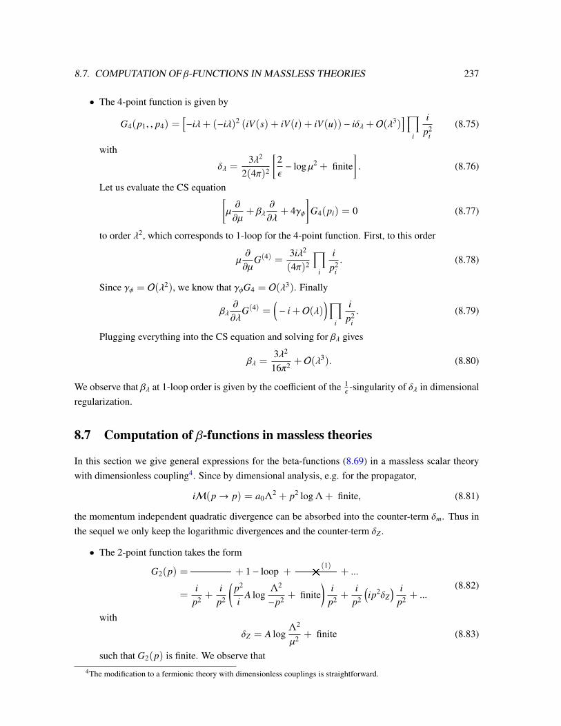
8.7. COMPUTATION OF β-FUNCTIONS IN MASSLESS THEORIES 237
• The 4-point function is given by
G4(p1, , p4) =[−iλ+ (−iλ)2 (iV(s) + iV(t) + iV(u)) − iδλ +O(λ3)
]∏i
ip2
i
(8.75)
with
δλ =3λ2
2(4π)2
[2ε− log µ2 + finite
]. (8.76)
Let us evaluate the CS equation[µ∂
∂µ+ βλ
∂
∂λ+ 4γφ
]G4(pi) = 0 (8.77)
to order λ2, which corresponds to 1-loop for the 4-point function. First, to this order
µ∂
∂µG(4) =
3iλ2
(4π)2
∏i
ip2
i
. (8.78)
Since γφ = O(λ2), we know that γφG4 = O(λ3). Finally
βλ∂
∂λG(4) =
(− i +O(λ)
)∏i
ip2
i
. (8.79)
Plugging everything into the CS equation and solving for βλ gives
βλ =3λ2
16π2 +O(λ3). (8.80)
We observe that βλ at 1-loop order is given by the coefficient of the 1ε -singularity of δλ in dimensional
regularization.
8.7 Computation of β-functions in massless theories
In this section we give general expressions for the beta-functions (8.69) in a massless scalar theorywith dimensionless coupling4. Since by dimensional analysis, e.g. for the propagator,
iM(p→ p) = a0Λ2 + p2 log Λ + finite, (8.81)
the momentum independent quadratic divergence can be absorbed into the counter-term δm. Thus inthe sequel we only keep the logarithmic divergences and the counter-term δZ .
• The 2-point function takes the form
G2(p) =ff + 1 − loop +fx (1)f + ...
=i
p2 +i
p2
(p2
iA log
Λ2
−p2 + finite)
ip2 +
ip2
(ip2δZ
) ip2 + ...
(8.82)
with
δZ = A logΛ2
µ2 + finite (8.83)
such that G2(p) is finite. We observe that4The modification to a fermionic theory with dimensionless couplings is straightforward.

238 CHAPTER 8. RENORMALISATION OF QUANTUM FIELD THEORY
– the only explicit µ dependence is due to δZ at 1-loop, and that
– δZ is O(λ).
As we will show below, β(λ) = O(λ2). Therefore at leading order the CS equation implies that
− µ∂
∂µδZ + 2γφ = 0 (8.84)
and thus
γφ =12µ∂
∂µδZ = −A. (8.85)
• More generally, the n-point function at 1-loop order is of the form
Gn = tree-level + 1-loop PI + vertex counter-term + external legs, (8.86)
where the external legs only contribute to G, not to the scattering amplitude. This can beparametrized as
Gn =∏
i
ip2
i
−iλ − iB logΛ2
−p2 − iδλ + (−iλ)∑
i
Ai logΛ2
−p2i
− δZi
, (8.87)
where∑
i extends over all n external legs. To solve the CS equationµ ∂∂µ + βλ∂
∂λ+
n∑i=1
γi
Gn = 0 (8.88)
we note that
– only δλ, δZi contribute to µ ∂∂µGn and that
– all terms except −iλ are of order λ2. So to leading order
∂
∂λGn = ((−i) +O(λ))
∏i
ip2
i
. (8.89)
To leading order in λ therefore
µ∂
∂µ
δλ − λ∑i
δZi
+ β(λ) + λ∑
i
12µ∂
∂µδZi︸ ︷︷ ︸
=γi
= 0. (8.90)
Since
δλ = −B logΛ2
µ2 + finite, δZi = Ai logΛ2
µ2 + finite (8.91)
the β-function becomes
β(λ) = µ∂
∂µ
−δλ + 12λ∑
i
δZi
= −2B− λ∑
i
Ai. (8.92)
To leading order the finite terms do not enter the expressions for β(λ) and γ(λ). Since the differentrenormalisation schemes only differ by the finite terms, the 1-loop results are independent of thescheme. At next-to-leading order, the β-functions are scheme-dependent.

8.8. THE RUNNING COUPLING 239
1-loop β-function of QED
As an application we compute the 1-loop β-function in QED. Recall our conventions for the counter-terms appearing in the renormalisation of QED as discussed in QFT 1:
δ3 = Z3 − 1 ↔ photon renormalisation
δ2 = Z2 − 1 ↔ fermion renormalisation(8.93)
and
= ieδ1γµ
To leading order in the coupling e, the γ-functions therefore are
γ3 =12µ∂
∂µδ3, γ2 =
12µ∂
∂µδ2 (8.94)
and from the Callan-Symanzyk equation of the 3-point function one concludes that to leading orderin e
βe = µ∂
∂µ(−eδ1 +
12
2eδ2 +12
eδ3). (8.95)
As will be discussed in more detail in the tutorials, the explicit expressions for δ1, δ2, δ3 obtained inQFT I ( with the renormalisation scale µ identified with the electron mass scale m) imply
γ2 = γ3 =e2
12π2 +O(e3), β =e3
12π2 +O(e4) (8.96)
in Feynman gauge.
8.8 The running coupling
Having computed the 1-loop β-functions, we are in a position to discuss the physics encoded in these.Let us repeat our mantra that it is the renormalisation conditions which define the meaning of thephysical coupling λ at the renormalisation scale µ. E.g. in massless φ4 theory we defined the dimen-sionless coupling λ by declaring that
iM(p1 p2 → p3 p4) = −iλ at s = t = u = −µ2. (8.97)
The so-defined coupling is therefore really a function of the renormalisation scale µ, λ = λ(µ), andthis λ(µ) is the effective coupling relevant for processes with typical momenta of order µ.To appreciate this latter point, recall that iM(p1 p2 → p3 p4) in the above theory is
iM = −iλ − iλ2
32π2
[log−sµ2 + log
−tµ2 + log
−uµ2
]+O(λ3) (8.98)
with λ = λ(µ) as in (8.97).

240 CHAPTER 8. RENORMALISATION OF QUANTUM FIELD THEORY
• For momenta s, t, u ∼ −µ2, the loop-corrections are small, and the tree-level result −iλ(µ) is agood approximation. In this sense, λ(µ) is a measure for the strength of the interaction. This iswhat we call the effective coupling for processes at momentum scale µ.
• At scales |s|, |t|, |u| µ2 (or µ2), the 1-loop correction becomes big due to the appearance ofa so-called large log. We see that perturbation theory is an expansion not only in λ, but also inlog −p2
µ2 with p a typical momentum/energy scale of the process.
Thus, at scales s, t, u ∼ −µ21, with µ1 µ or µ1 µ, the coupling λ(µ) defined at scale µ
is not what we would call the relevant coupling - it does not reflect the actual strength of theinteraction because the tree-level and the 1-loop contribution differ so much.
• At scales s, t, u ∼ −µ21 with µ1 µ (or µ1 µ) a better expansion parameter for perturbation
theory is λ(µ1) defined viaλ(µ1) = −M
∣∣∣s=t=u=−µ2
1. (8.99)
We therefore conclude that indeed
λ(µ) gives the strength of the interaction at energy scale µ.
Now, the evolution of this coupling λ(µ) as we vary µ is precisely what is encoded in the β-functionthrough
µd
dµλ(µ) =
dd log µ
λ(µ) = β(λ). (8.100)
The change in λ(µ) as we change µ is called renormalisation group (RG) flow for reasons that willbecome clear in section (8.10). The above RG flow equation describes the running of the coupling inthe above sense.Being a first-order differential equation, (8.100) uniquely specifies λ(µ) in terms of the value of λ at areferences scale µ∗. Suppose therefore that λ∗ = λ(µ)
∣∣∣µ=µ∗
as determined by one measurement at µ∗.Then (8.100) is solved by
λ(µ)∫λ∗
dλ′
β(λ′)=
µ∫µ∗
d log µ′ = logµ
µ∗. (8.101)
As an example consider the 1-loop β-function in QED,
β(e) =1
12π2 e3. (8.102)
The associated RG flow equation is easily integrated (see the tutorials) and gives for the fine-structureα ≡ e2
4π
α(µ) =α∗
1 − 23πα
∗ log µµ∗
with α∗ = α(µ)∣∣∣µ=µ∗
. (8.103)
Observe that according to this analysis, α(µ) increases as µ increases and even seems to diverge atµ = µ∗ exp
(3π2α∗
).

8.8. THE RUNNING COUPLING 241
Alternative RG bevaviours
Depending on the sign of the β-function there are 3 qualitatively different types of behavior for theRG flow of the coupling as well as hybrids thereof. Let us first turn to the extreme cases:
1. If β(λ) > 0, λ(µ) increases (decreases) as µ increases (decreases). If we start at a perturbativevalue λ∗ at µ∗ and follow the RG flow for increasing µ, then at some scale λ(µ) ceases to beperturbative and perturbation theory, in particular our perturbative evaluation of the β-function,is no more reliable. If by a non-perturbative analysis beyond that point one finds that β(λ) > 0∀λ, then λ(µ) increases indefinitely. This can happen either asymptotically, i.e. λ → ∞ asµ → ∞, or even for finite value of µ, λ → ∞ as µ → µ∗. The latter instance is referred toas a Landau pole. In presence of a Landau pole, the theory is not well-defined at all energyscales.5 As we will understand in section 8.10 we should think of the theory as to be replacedby a different theory at some high energy scale which resolves the Landau-pole.
On the other hand, the theory is perturbatively well-defined in the IR, where λ is small. Forinstance, if β(λ) → 0 as λ → 0 as would be the case e.g. for β(λ) = cλx with c > 0, thenλ(µ) → 0 as µ → 0. The coupling thus approaches an IR fixed point, and the theory becomesfree in the IR. The fixed point λ = 0 is therefore called Gaussian fixed point.Perturbatively β(λ) > 0 for φ4 theory in d = 4 and for U(1) gauge theory in d = 4, but thenon-perturbative status is less clear.6
2. If β(λ) < 0, λ(µ) decreases (increases) as µ increases (decreases). The theory is perturbative inthe UV, but ceases to be perturbative in the IR.If β(λ) → 0 as λ → 0 as would be the case e.g. for β(λ) = cλx with c < 0, we have thatλ→ 0 as µ→ ∞ in a controlled way (i.e. λ flows to a Gaussian UV fixed-point) and the theorybecomes free in the UV. This is called asymptotic freedom.In d = 4 the only known example for asymptotic freedom is Yang-Mills theory to be discussedin detail later.
3. If β ≡ 0 ∀µ, λ(µ) is independent of µ. The theory is thus scale-independent or conformal.Since the counter-terms do not induce any scale dependence, there cannot be any UV diver-gences altogether - the theory is finite. For example N = 4 Super-Yang-Mills theory is finitebecause all divergences cancel order by order in perturbation theory due to the large amount ofsupersymmetry.
Apart from these three extreme cases, it can happen that β(λ) interpolates between 1., 2., 3., i.e.changes sign and thus hits zero at some value.
5In the less severe case, where λ → ∞ as µ → ∞ one might consider it as a matter of taste whether or not one shouldcall the theory well-defined.
6A numerical analysis via lattice field theory seems to suggest that the Landau pole in both cases is physical and not justan artifact of perturbation theory.

242 CHAPTER 8. RENORMALISATION OF QUANTUM FIELD THEORY
• If β(λ) > 0 to lowest order in λ, but higher order terms, relevant for bigger λ and thus (since westarted with β(λ) > 0) for larger µ, have a negative sign, then β(λ) becomes 0 at λ = λ∗:
β(λ
)
λ
λ*
As µ→ ∞, λ→ λ∗ with β(λ∗) = 0. λ∗ is called non-trivial UV fixed point.
• Alternatively, β(λ) could start negative for small values of λ and hit 0 at λ∗:
β(λ
)
λ
λ*
Then λ → λ∗ as µ → 0 (non-trivial IR fixed point). Such behavior is known to occur e.g. inφ4 theory in d < 4. As will be discussed in the tutorials,
β(λ) = (d − 4)λ+3λ2
16π2 ⇒ β(λ∗) = 0 for λ∗ =16π2
3(4 − d), (8.104)
8.9. RG FLOW OF DIMENSIONFUL OPERATORS 243
where λ is here the suitably rescaled (dimensionless) quartic scalar coupling. Thus for d < 4the theory approaches the celebrated Wilson-Fisher fixed point λ∗ > 0 in the IR.
Anomalous dimension and power-law behavior near fixed points
Near a non-trivial fixed point λ∗, the 2-point function of a scalar theory in d = 4 behaves as
G2(p) = C(
1p2
)1−γφ(λ∗)
. (8.105)
This can be proven by integrating the Callan-Symanzyk equation and using approximate scale - inde-pendence near the fixed point. For a derivation we refer to the tutorials. The propagator (8.105) lookslike the propagator of the free theory,
G2(p)∣∣∣free ∼
1p2 , (8.106)
except for the different power (1 − γ∗). Consequently γφ is called anomalous dimension of φ sincenear λ∗ , the propagator G2(p) behaves like in a free theory with a field of mass dimension (1 −γφ(λ∗)). More generally, such power-law behaviour of the propagator is a sign of scale-invariance (asrealised near λ = λ∗ where β = 0).
8.9 RG flow of dimensionful operators
Our analysis of the running of the dimensionless coupling λ can be generalised to dimensionful cou-plings. To this end suppose that we add to a renormalisable action (containing only dimensionlesscouplings) in d dimensions a term ∫
dd x Ci Odi , (8.107)
where Odi is some local operator7 of mass dimension di, and treat it as a perturbation. Then define γi
via the generalised Callan-Symanzyk equation:
0 =
[µ∂
∂µ+ β
∂
∂λ+ nγφ + γi Ci
∂
∂Ci
]Gn(x; λ, Ci; µ). (8.108)
Compared to β ∂∂λ we have scaled out one power of Ci in γi Ci
∂∂Ci
so that γi is dimensionless. Clearlyγi → 0 as λ→ 0 and Ci → 0.Now, the coupling Ci has mass dimension
[Ci] = d − di, (8.109)
so we can define a dimensionless coupling gi via
Ci = gi µd−di . (8.110)
7By this we mean any product of the fundamental fields or their derivatives.

244 CHAPTER 8. RENORMALISATION OF QUANTUM FIELD THEORY
Rewriting Gn(x; λ, Ci; µ) as Gn(x; λ, gi; µ) introduces some extra explicit µ dependence, and theCallan-Symanczyk equation becomes (after omitting the tilde)
0 =
[µ∂
∂µ+ β(λ)
∂
∂λ+ nγφ + (γi + di − d)gi︸ ︷︷ ︸
=:βi
∂
∂gi
]Gn(x; λ, gi; µ), (8.111)
or, more symmetrically,
0 =
[µ∂
∂µ+ β(λ)
∂
∂λ+ nγφ + βi
∂
∂gi
]Gn(x; λ, gi; µ). (8.112)
By definition, the dimensionless gi satisfies the RG flow equation
dd logµ
gi = βi = (γi + di − d)gi. (8.113)
Suppose that λ 1 and gi 1. Then necessarily γi 1 and
βi → (di − d + ...)gi (8.114)
so that (8.113) is solved to first approximation by
gi(µ) = gi(µ∗)e(di−d)(ln µ
µ∗) = gi(µ
∗)
(µ
µ∗
)di−d
. (8.115)
Note that if di − d = 0, corresponding to a dimensionless coupling constant, this crude approximationgives no information about the behavior of the coupling and one has to compute the perturbative con-tributions to the beta-function even to determine the leading behaviour of the RG flow. We conclude:
• If [Ci] = d − di > 0, i.e. Ci is a super-renormalisable coupling, then
gi gi(µ∗) for µ µ∗ (8.116)
in a perturbative theory.
• If [Ci] = d − di < 0, i.e. Ci is a non-renormalisable coupling, then
gi(µ) gi(µ∗) (8.117)
in a perturbative theory.
Non-renormalisable couplings become irrelevant in the IR: Even if they are present at higherscales, they become small for smaller energy processes. On the other hand, super-renormalisablecouplings become relevant in the IR.
But it is important to keep in mind that if the coupling λ is big, then γi cannot be neglected in (8.113).In principle, this can change the qualitative behaviour of the flow.

8.10. WILSONIAN EFFECTIVE ACTION & RENORMALISATION SEMI-GROUP 245
For example, as already noted, in φ4 theory in d dimensions the rescaled dimensionless couplingλ behaves as
β(λ) = (d − 4)λ+λ2
16π2 . (8.118)
For d < 4 λ is super-renormalisable, but for big values of λ due to the second term β(λ) becomespositive and changes even the sign of the β-function.
8.10 Wilsonian effective action & Renormalisation Semi-Group
Our philosophy behind renormalisation has so far been this:
• The cutoff Λ is merely a way to regulate divergent integrals without any physical meaning.
• Renormalisation is a trick to remove the cutoff-dependence in physical amplitudes. This proce-dure allows us to take Λ → ∞ without encountering any divergences.
• This comes at the cost of losing predictability for a number of physical masses and coupling.
• In a renormalisable theory, only a finite number of such physical couplings must be taken asinput parameters from experiment, and we end up with a well-defined theory.
The so-called Wilsonian approach gives a rather different interpretation to renormalisation, inspiredby analogies with condensed matter and statistical physics:
• According to Wilson, we should think of a QFT as an effective description of physics which isaccurate only at energies below an intrinsic cutoff Λ0 (or at distances larger than some ∆xmin).At energies beyond Λ0 the field theory picture does not correctly reflect the microscopic degreesof freedom.
• For instance, consider as our field the magnetisation density s(~x) of a metal in 3D statisticalfield theory. This s(~x) is the continuum limit of the spin degrees of freedom si at lattice site i ofthe atomic lattice. There is an intrinsic cutoff given by the lattice spacing a:At distances smaller than the lattice spacing a, no concept of continuous magnetisation exists- the continuous field theory description is strictly speaking invalid. The appearance of diver-gences in bare perturbation theory as we take a → 0 reflects this mismatch of the field theorywith the microscopic degrees of freedom.Nonetheless, via renormalisation, one can take the continuum limit, but at the cost of having totake the couplings as input parameters. These parametrise our ignorance of the true physics atdistances ∼ a from the perspective of the field theory.
• Applied to relativistic QFT, one would similarly argue that beyond some high energy scale Λ0,QFT fails to capture the microscopic degrees of freedom. In particular, all matter gravitates,

246 CHAPTER 8. RENORMALISATION OF QUANTUM FIELD THEORY
and the effects of gravity become non-negligible at the (reduced) Planck scale
Mpl =1
√8πGN
= 2.43 × 10¹⁸GeV. (8.119)
The observed UV divergences in bare perturbation theory result from the breakdown of ourQFT beyond this scale. Still, in a renormalisable and asymptotically free (or at least UV safe)theory one can take the cutoff Λ0 → ∞, but at the cost of parametrising our ignorance of thetrue degrees of freedom in a finite number of parameters.
• In the modern Wilsonian interpretation of Quantum Field Theory, we should view the QFTas an effective theory. E.g. in a non UV-finite QFT it is impossible to predict the vacuumenergy V0 - this is one of the input parameters. To explain the mystery of Dark Energy, we needa more fundamental, UV finite theory. To date, the only known theory that is UV finite andasymptotes to a weakly coupled effective Quantum Field Theory in the IR is String Theory. InString Theory, the concept of pointlike particles is abandoned in the UV: All particles are in factexcitations of a 1-dimensional string of length `s. At distances above `s we can approximate thetheory by a point particle theory, i.e. a QFT as we have studied it. Thus the string length is theintrinsic cutoff of the low-energy effective QFT, and at distances smaller than `s the theory flowsto a rather different (in particular non-local) description without UV divergences and withoutfree dimensionless input parameters.
After this general outline we now demonstrate quantitatively how the high energy degrees of freedomare indeed captured in the effective coupling constants at lower energies. This will give a physicalmeaning to the running of the couplings. In view of the above motivation let us start with a bareLagrangian in d Euclidean dimensions, e.g.
L =12(∂φ)2 +
12
m2φ2 +λ
4!φ4 (8.120)
and impose a momentum cutoff Λ0: In path integral quantisation, this means we restrict the measure- written in Fourier space - to the Fourier modes φ(k) with 0 ≤ |k| ≤ Λ0, i.e. define the theory via
Z =
∫[Dφ]Λ0e−
∫dd xE(L+J·φ), (8.121)
where [Dφ]Λ0 ≡∏|k|≤Λ0 dφ(k). Note the specific combinations of minus signs and absence of factors
of i in the Euclidean theory. This partition function enables us to compute amplitudes up to a typicalenergy scale Λ0 of external particles. Suppose now that we are interested in processes at typicalenergy scales below
Λ = bΛ0 0 < b < 1. (8.122)
As we saw in the previous picture, loop computations will give rise to large log-corrections if Λ Λ0.To avoid these, we can integrate out the degrees of freedom between Λ and Λ0 once and for alland work with a path integral defined only in terms of the remaining degrees of freedom below Λ. Tocompute this new effective path integral we first split each Fourier mode as
φ(k) = φ(k) + φ(k), (8.123)

8.10. WILSONIAN EFFECTIVE ACTION & RENORMALISATION SEMI-GROUP 247
where
φ(k) =
0 if 0 ≤ |k| ≤ bΛ0
φ(k) if bΛ0 ≤ |k| ≤ Λ0(8.124)
and
φ(k) =
φ(k) if 0 ≤ |k| ≤ bΛ0
0 if bΛ0 ≤ |k| ≤ Λ0.(8.125)
Taking J = 0 for brevity, we get
Z =
∫DφDφ e−
∫dd x[ 1
2 (∂φ+∂φ)2+ 1
2 m2(φ+φ)2+ λ4! (φ+φ)
4]
=
∫Dφ e−
∫dd x( 1
2∂φ2+ 1
2 m2φ2+ λ4!φ
4)
×
∫Dφ e−
∫dd x[ 1
2∂φ2+ 1
2 m2φ2+ λ4! φ
4+ λ6φφ
3+ λ4φ
2φ2+ λ6 φφ
3],
(8.126)
where terms φφ are omitted due to orthogonality of different momentum modes. The partition functionis of the form
Z =
∫[Dφ]bΛ0e−S [φ]
∫[Dφ]bΛ0≤|k|≤Λ0e−S [φ,φ]. (8.127)
The key idea is that this can be rewritten as
Z =
∫[Dφ]bΛ0e−
∫dd xLeff . (8.128)
To this end we view all terms in S [φ, φ] except the kinetic term as a perturbation, which is justified for
λ 1 and m Λ = bΛ0. (8.129)
Then perturbatively∫Dφ e−S [φ,φ] =
∫Dφe−
∫dd x 1
2∂φ2[1 −
∫dd x
( 12
m2φ2 +λ
4!φ4 +
λ
6φφ3 +
λ
4φ2φ2 +
λ
6φφ3
)+ . . .
]≡ 〈[...]〉.
(8.130)
This is computed via Wick’s theorem in perturbation theory, where we contract only pairs of φ, andin the resulting propagator only momenta bΛ0 ≤ |k| ≤ Λ appear. Let us sketch how this works:
1. Consider for example the term⟨−
∫dd x
λ
4φ2φ2
⟩=
∫Dφe−
∫dd x 1
2∂φ2(−
∫dd x
λ
4φ2(x)φ2(x)
)= −
∫dd x
12φ2(x)
λ
2φ(x)φ(x)︸ ︷︷ ︸
=∫ dd p
(2π)de−ip(x−x) 1
p2
∣∣∣bΛ0≤|p|≤λ0
=
∫dd x
(−
12φ2(x)µ
)(8.131)

248 CHAPTER 8. RENORMALISATION OF QUANTUM FIELD THEORY
with
µ =λ
2
∫dd p(2π)d
1p2
∣∣∣∣∣∣bΛ0≤|p|≤Λ0
=λ
(4π)d/2Γ(d/2)1 − bd−2
d − 2Λd−2. (8.132)
Note that in the Euclidean theory no factor of i appears in the propagator. Graphically onerepresents the φ-propagator with two extra lines:
φ(x)φ(y) ≡ x y
φ(x) φ(x)
φ2(x)φ2(y) ≡
Together with n-fold powers of that same term (which arise from expanding the exponential ine−[S (φ,φ)]) this just gives a correction to the mass term present already in e−S [φ].
2. Next consider the square of this term:
14
⟨λ4φ
2φ2 λ4φ
2φ2⟩∼
2
+
The first diagram is just the square of the mass correction, as advocated. The second term isschematically of the form∫
dd x ddy φ2(x)φ2(y) '∫
dd x(φ4(x) + c φ2(x)(∂φ(x))2 + . . . (8.133)
The first summand provides a contribution to the φ4 coupling in S [φ], while the second gives anew, derivative interaction not present in our original action.
3. Likewise, also higher order interaction terms in φ appear, e.g. the contraction
14
⟨λ6φ
3φλ6φ3φ
⟩∼
provides a φ6 interaction in S eff .

8.10. WILSONIAN EFFECTIVE ACTION & RENORMALISATION SEMI-GROUP 249
This way, all possible interactions are created in S eff which are consistent with the symmetries of thebare Lagrangian (here just φ→ −φ), and we find
Z =
∫[Dφ]bΛ0e−S
bΛ0eff (8.134)
with ∫dd xLbΛ0
eff=
∫dd x
[12(1 + ∆Z) (∂φ)2 +
12(m2 + ∆m2) φ2 +
14!(λ+ ∆λ) φ4 (8.135)
+ ∆C (∂µφ)4 + ∆D φ6 + ...
]. (8.136)
The object S bΛ0eff
is called Wilsonian effective action. The coefficients ∆Z, ∆m, ∆λ, ∆C, ∆D can besystematically computed in perturbation theory. They receive contributions only from the momentumregime bΛ0 ≤ |k| ≤ Λ0. When we compute correlators at scales below Λ = bΛ0 via the Wilsonianeffective action (8.134), only momenta |k| ≤ Λ = bΛ0 appear in the loops since all effects of themodes with bΛ0 < |k| < Λ0 are already encoded in Leff.The Wilsonian effective action is not to be confused with the quantum effective action Γ[ϕ]. Asdiscussed in section 7.9, the latter includes all quantum effects, i.e. computation with Γ[ϕ] at tree-level (no loops!) gives the full quantum theory. By contrast, in the Wilsonian effective action S bΛ0
eff
only the quantum effects due to modes from bΛ0 < |k| < Λ0 are included, and in computations withS bΛ0
effloops with momenta 0 ≤ |k| ≤ Λ = bΛ0 must still be performed.
For better comparison of LbΛ0eff
with the original Lagrangian, which we denote now by LΛ0 , we bringthe kinetic term to standard form by rescaling
φ′ = φ(1 + ∆Z)1/2. (8.137)
Then the partition function Z is given by
Z =
∫[Dφ′]Λe−S ′Λeff with Λ = bΛ0 (8.138)
and
S ′Λeff =
∫dd x
[12(∂φ′)2 +
12
m′2φ′2 +λ′
4!φ′4 +C′(∂φ′)4 + D′φ′6 + ...
](8.139)
for
m′2 = (m2 + ∆m2)(1 + ∆Z)−1,
λ′ = (λ+ ∆λ)(1 + ∆Z)−2,
C′ = (C + ∆C)(1 + ∆Z)−2,
D′ = (D + ∆D)(1 + ∆Z)−3.
(8.140)
Note that in our case C = D = 0 in the original LΛ0 . Thus the effect of integrating out the degreesof freedom with bΛ0 < |k| < Λ0 amounts to renormalising the couplings in the Lagrangian as above.

250 CHAPTER 8. RENORMALISATION OF QUANTUM FIELD THEORY
The successive application of this operation gives rise to the renormalisation group. This is reallyonly a semi-group, since this procedure only allows us to lower the cutoff by integrating out degreesof freedom, i.e. there does not exist an inverse element.
The running of the couplings in the Wilsonian picture is to be interpreted as the evolution of thecutoff dependent couplings in the effective action as we change the cutoff. To make a connection toour previous picture we must identify the cutoff Λ with the renormalisation scale µ.I.e. the effective couplings λ(Λ) are defined by specifying observables computed from the effectiveaction with cutoff Λ. This replaces our previous renormalisation condition fixing λ(µ).With this identification, the fundamental form of the running couplings agree to leading order in per-turbation. This is all we can hope for, because, as always, beyond leading order the specific scaledependence of the coupling depends on the specific renormalisation scheme. E.g. for φ4 theory ind = 4 carrying out the Wilsonian renormalisation procedure as sketched above gives
∆Z∣∣∣1-loop = 0, ∆λ
∣∣∣1-loop = −
3λ2
16π2 log1b
. (8.141)
With b = Λ/Λ0 < 1 this gives for small |1 − b|
λ(Λ) = λ(Λ0) +3
16π2λ2(Λ0) log
ΛΛ0
, (8.142)
in agreement with our previous results for the β-function of φ4-theory. More generally, for a dimen-sionful coupling
∫dd x CdiOdi with
• Odi a local operator of mass dimension di and
• Cdi of mass dimension [Cdi ] = d − di
one finds in φ4-theory
Cdi(Λ) = Cdi(Λ0) + (number)λdi/2(Λ0)(Λd−di −Λd−di
0
)+ higher order. (8.143)
In fact, this is just as expected by dimensional analysis. As in our previous approach it is useful todefine a dimensionless coupling, but now in terms of Λ,
gi(Λ) = Ci(Λ)Λdi−d, (8.144)
which enjoys the RG flow
gi(Λ) =
gi(Λ0) + (number)λdi/2(Λ0)
(Λ0
Λ
)di−d
− 1
+ ...
(Λ0
Λ
)d−di
. (8.145)
Provided the theory is perturbative, the scaling due to(Λ0
Λ
)d−di
=
(Λ0
Λ
)[Ci]
(8.146)

8.10. WILSONIAN EFFECTIVE ACTION & RENORMALISATION SEMI-GROUP 251
dominates and thus if Ci is non-renormalisable ([Ci] < 0), the initial value of gi(Λ0) is irrelevant atscales Λ Λ0 and
Ci(Λ) = O(λdi/2
)Λ[Ci] Λ[Ci] (8.147)
for λ 1. This agrees with our conclusions from the Callan-Symanzik approach: Non-renormalisablecouplings become irrelevant in the IR: Even if they are present at higher scales, they become smallfor smaller energy processes. On the other hand, super-renormalisable couplings become relevantin the IR.
Conclusion
• In the modern Wilsonian interpretation, a QFT is defined via an intrinsic cutoff scale Λ0 beyondwhich it does not capture the microscopic degrees of freedom any more. For particle physicsone would assume that at the very least
Λ0 ∼ Mpl ∼ 2.43 × 10¹⁸ GeV, (8.148)
which is the scale where quantum gravity effects become non-negligibly strong such that it isno longer justified to ignore them.
• Let us define our theory at this intrinsic cutoff by a Lagrangian LΛ0 . We can think of thecouplings Ci(Λ0) as being computed by whatever more fundamental theory takes over at scalesabove Λ0. In the spirit of an effective description, we view these Ci(Λ0) as parametrising thephysics beyond Λ0. At scales Λ0, all possible non-renormalisable couplings are important,because the underlying microscopic degrees of freedom become important at Λ0 and it takes alot of parameters to describe these in QFT. I.e. all couplings consistent with the symmetries ofthe theory will appear in LΛ0 .
• For processes at our scales Λ Λ0 we compute with the effective action LΛeff
with couplingsCi(Λ) arising by RG flow starting from Ci(Λ0). Crucially, as long as the theory is weaklycoupled up to Λ0, the non-renormalisable couplings at Λ Λ0 are of order
Ci(Λ) ∼ λdi/2Λ[Ci] Λ[Ci], (8.149)
whatever they are originally at Λ0. Since the microscopic degrees of freedom become importantonly at high scales, it takes only a few parameters - the renormalisable and super-renormalisableones - to effectively approximate the physics at Λ Λ0. This explains why we only observerenormalisable couplings at scale Λ.
• Despite the physical meaning of Λ0 (the intrinsic cutoff) we can formally take Λ0 → ∞ pro-vided all couplings remain finite, i.e. no Landau poles arise. This was our original motivation indoing renormalisation, but from a Wilsonian perspective we now understand that our theory re-mains an effective theory to the extent that all couplings are really input parameters and cannotbe computed from first principles without knowing the underlying theory.

252 CHAPTER 8. RENORMALISATION OF QUANTUM FIELD THEORY
On the fine-tuning problem in scalar theories
For scalar theories, in particular φ4 in d = 4, there remains a problem because of the RG flow of thescalar mass:
m2(Λ) = m2(Λ0) + (number)λ(Λ0)(Λ2 −Λ20) + ..., (8.150)
which is the special case of (8.145) for d − di = 2. At scales Λ Λ0, the dominant term is givenby λΛ2
0, and thus m2(Λ) is of order λ(Λ0)Λ20. This is much bigger than we naturally expect in an
effective theory at scale Λ. To arrive at a value for m2(Λ) of order Λ2 instead, it would appear onemust carefully fine-tune the tree-level m2(Λ0) such as to almost precisely cancel the loop correctionsof order Λ2
0.For example, in the Standard Model of Particle Physics, the Higgs particle is a scalar field withmH ∼ 126 GeV. But if we take Λ0 ∼ 1019GeV, then
m2H
Λ20
10−32. (8.151)
The necessary fine-tuning to achieve this is considered ’technically unnatural’ and gives rise to theso-called hierarchy problem: What stabilises the mass of a scalar at hierachically smaller mass thanMpl?Basically there are 3 alternative types of solutions to the fine-tuning problem that are being discussedin the modern literature:
1. If the inherent cutoff for the Standard Model were not MPl., but at, say, 1 TeV, the fine-tuningwould be dramatically reduced. This would imply that new physics takes over at Λ0 ∼ 1 TeV.Candidates for such new dynamics are supersymmetry (SUSY) or large extra dimensions. Thisreasoning motivates the search for such new physics at LHC.
2. Alternatively we could consider accepting the fine-tuning, which is not logically impossible -for instance, but not necessarily, motivated by the so-called anthropic principle (which wouldstate that only values of mH ∼ 1 TeV could give rise to structure formation as we observe it andthus, by definition, only a universe in which mH is so fine-tuned can be observed). Clearly thisis hard to make precise, but it is a logical possibility in principle.
3. Yet another approach would be to completely revise our notion of naturalness, even though it isunclear at present what it should be replaced by.
It is important to appreciate that such a hierarchy problem does not arise for fermions and vectorsbecause their masses are stabilised by extra symmetry, namely gauge symmetry for vectors and chiralsymmetry for fermions. Small masses for these fields are technically natural in the sense that oncewe choose them small at tree-level, they remain small including loop-corrections. This is guaranteedwhenever setting the mass to zero implies an enhancement of symmetry - such as in the present casegauge symmetry for massless vector bosons and chiral symmetry for massless fermions.

Chapter 9
Quantisation of Yang-Mills-Theory
9.1 Recap of classical YM-Theory
Let us quickly recall the description of classical non-abelian gauge theory as introduced in QFT1.Our starting point is a Lie group H with Lie algebra Lie(H) such that every element h ∈ H can beexpressed as
h = e−igα with α ∈ Lie(H), g ∈ R. (9.1)
In terms of a basis T a of the Lie algebra, i.e. in terms of a complete set of generators of the Lie groupH, α can be written as
α =∑
a
αaT a ≡ αaT a. (9.2)
The T a satisfy the defining relations
[T a, T b] = i f abcT c = −[T b, T a] (9.3)
which fulfill the Jacobi identity
[[T a, T b], T c] + [[T c, T a], T b] + [[T b, T c], T a] = 0. (9.4)
A Lie algebra possesses a symmetric bilinear from, the so-called Killing form,
κab = T a T b = T b T a ∈ R (9.5)
which is invariant under the adjoint action of the Lie group H on its Lie algebra, i.e.
hT ah−1 hT bh−1 = T a T b ∀h. (9.6)
For an abstractly given Lie algebra, the Killing form is defined as
κab = tr[T a, [T b, ·]] ≡∑
c
(T ∗c )[Ta, [T b, T c]], (9.7)
where (T ∗c ) is an element of a basis of the dual vector space such that (T ∗c )Td = δd
c .
253

254 CHAPTER 9. QUANTISATION OF YANG-MILLS-THEORY
Expanding T a T b = hT ah−1 hT bh−1 with h = e−igTc to order g gives
[T a, T c] T b = −T a [T c, T b]. (9.8)
If H is compact as a manifold, then the invariant from can be shown to be positive definite, and onecan normalise it as
T a T b =12δab. (9.9)
The Killing form κab = T a T b and its inverse can be used to raise and lower Lie-algebra indices.Having said this, we will from now on put all Lie algebra indices upstairs with summation overrepeated indices understood. Then the structure constants f abc are totally antisymmetric (as will beshown in the exercises) and invariant under cyclic permutations.In the sequel we will typically think of T a as given in the defining matrix representation, i.e. as anN × N matrix acting on CN for some N. E.g. for H =SU(k), N = k and the T a are represented ashermitian traceless k × k matrices. In such a matrix representation we can identify
T a T b ≡ trT aT b. (9.10)
Consider now a Lie(H)-valued gauge potential, i.e. a connection
Aµ(x) ≡ Aaµ(x)T a (9.11)
transforming under a gauge transformation
U(x) = e−igα(x) (9.12)
as
Aµ(x) 7→ UAµU−1 +ig(∂µU)U−1. (9.13)
To linear order this is
Aµ(x) 7→ Aµ + Dµα(x) +O(α2), (9.14)
where the adjoint covariant derivative acts on Lie(H)-valued fields as
Dµα(x) B ∂µα(x) + ig[Aµ(x),α(x)]. (9.15)
In components this means that
Aaµ(x) 7→ Aa
µ(x) + ∂µαa(x) + g f abcαb(x)Ac
µ(x). (9.16)
The curvature associated with the connection Aµ(x) is
Fµν(x) =1ig[Dµ, Dν] ≡ Fa
µνTa, (9.17)

9.2. GAUGE FIXING THE PATH INTEGRAL 255
where we think of 1ig [Dµ, Dν] as acting on a Lie(H)-valued field. Plugging in the above definition of
the adjoint covariant derivative yields
Fµν(x) = ∂µAν − ∂νAµ + ig[Aµ, Aν] (9.18)
or in componentsFaµν(x) = ∂µAa
ν − ∂νAaµ − g f abcAb
µAcν. (9.19)
The field strength transforms in the adjoint representation of H as
Fµν 7→ UFµνU−1 (9.20)
and satisfies the Bianchi identity
DµFαβ + DβFµα + DαFβµ = 0. (9.21)
The pure Yang-Mills Lagrangian
L = −12
trFµνFµν = −14
∑a
FaµνF
µνa (9.22)
is gauge invariant. The equations of motion for Aµ read
DµFµν = 0 ≡ ∂µFµν + ig[Aµ, Fµν]. (9.23)
The commutator introduces cubic and quartic interactions which will be discussed in detail later on.
9.2 Gauge fixing the path integral
Gauge invariance complicates the quantisation of Yang-Mills theory:
• In canonical quantisation, we would start by defining the conjugate momenta to Aµ, but while
Πi =∂L
∂Ai∼ F0i (9.24)
one findsΠ0 =
∂L
∂A0= 0. (9.25)
This is a result of the fact that A0 appears without a time derivative in L - it is a non-dynamicalfield. Variation of the action with respect to A0 gives
DiF0i = 0, (9.26)
which is a non-dynamical constraint, and A0 is a Lagrange multiplier enforcing this constraint.Thus canonical quantisation requires the technology1 of quantisation of constrained, or singu-lar, systems. Quantisation of singular systems is a rich subject by itself. A variant of canonical
1For details of this technique see e.g. the book by Kugo.

256 CHAPTER 9. QUANTISATION OF YANG-MILLS-THEORY
quantization with constraints for the simple case of U(1) theory is in fact the Gupta-Bleulerquantisation method discussed in QFT1, but for non-abelian gauge theories things are morecomplicated due to the more involved form of the constraints. We will not start with canoni-cal quantization, but rather begin with path-integral quantization and return to the problem ofcanonical quantization afterwards.
• Alternatively in path integral quantisation we would write the action as
S =
∫d4x
(−
12
Aaν(K · Aa)ν +O(A3)
), (9.27)
where (K · A)ν = −∂2Aν+ ∂ν∂µAµ, find the propagator iDF = K−1 and perturbatively quantise
the interacting theory. However, the operator K is not invertible since it has a non-trivial kernel:
(K · ∂α)ν = 0 ∀α(x). (9.28)
In fact, this is a consequence of gauge invariance. Recall that an infinitesimal gauge transfor-mation acts as
Aµ 7→ Aµ + ∂µα+ ig[Aµ,α]. (9.29)
Since the coupling g enters only the interactions, the transformation Aµ 7→ Aµ + ∂µα+ O(g)must leave the kinetic term invariant, which is nothing other than the statement (9.28). Notethat this problem is therefore independent of whether we consider abelian or non-abelian gaugetheory.
We will now begin quantization of Yang-Mills theory in the path-integral approach. Apart from pro-viding a general method to compute correlation functions of gauge invariant operators, this will resultin a formalism in which we can also perform canonical quantization of the theory as required for thedefinition of the (physical) Hilbert space.The key idea is to cure the above problem of non-invertibility of the kinetic term by removing theredundancy in the space of gauge field configurations due to gauge invariance. Let
A B space of all gauge fields Aµ(x) (9.30)
and denote by
Ahµ(x) B hAµh−1 +
ig(∂µh)h−1 (9.31)
a gauge transformation on Ahµ with h ∈ H. Then fields related by a gauge transformation are physically
equivalent, Aµ(x) ∼ Ahµ(x). This is because Aµ satisfies the equation of motion if and only if so does
Ahµ.
Given Aµ(x), the gauge equivalent field configurations are said to lie in the same orbit under gaugetransformations h ∈ H, denoted
Ahµ(x) ∀h ∈ H. (9.32)

9.2. GAUGE FIXING THE PATH INTEGRAL 257
The physically inequivalent degrees of freedom are then counted by the quotient space
A/H BAµ ∼ Ah
µ : Aµ ∈ A, h ∈ H
, (9.33)
i.e. they are given by all Aµ-field configurations modulo gauge transformations. Our aim is now todefine the path integral not onA, but on the physical spaceA/H as∫
A/H
dµ[A]eiS [A]. (9.34)
To this end we must construct a suitable measure µ[A] onA/H such that∫A
DA =
∫H
dµ[h]∫A/H
dµ[A], (9.35)
with dµ[h] a measure on H. If we have found such a measure, we can factor out the integration overthe gauge orbit and only pick one representative per orbit as shown below.
To achieve (9.35) one introduces a gauge fixing condition
F(A) != 0 (9.36)
for some function F which maps the Lie(H)-valued connectionA to some other Lie(H)-valued field.For example we could take F(A) B ∂µAµ or generalisations thereof to be discussed later. Ideally, wewould like that given A ∈ A
F(Ah) = 0 for some unique h ∈ H (9.37)
such as to fix one representative per gauge orbit.2 Then on the lefthand side of (9.35) we can insert 1
given by
1 =
∫H
dµ[h]δ[F(Ah)
]M(Ah) (9.38)
2Indeed we will assume this here. In actuality, this condition is not satisfied because of a residual gauge symmetry.Consequently, there are several gauge equivalent field configurations that satisfy F(A) = 0. These are called Gribovcopies. One must restrict integration to a fundamental region where the gauge fixing is unique. This restriction indeed hasphysical consequences, e.g. it modifies the form of the propagator in the deep infra-red.
258 CHAPTER 9. QUANTISATION OF YANG-MILLS-THEORY
where the Jacobian factor
M(Ah) = det∂F(Ah)
∂h(9.39)
is needed in analogy with the formula
1 =
∫R
dx δ[ f (x)]
∣∣∣∣∣∣∂ f (x)∂x
∣∣∣∣∣∣ (9.40)
and will be evaluated momentarily. Then∫A
DA =
∫A
DA∫H
dµ[h]δ[F(Ah)
]M(Ah)
=
∫H
dµ[h]∫A
DA δ[F(Ah)
]M(Ah).
(9.41)
For all that follows we make the non-trivial assumption that we can find aDA that satisfies
DA = DAh. (9.42)
If no such measure exists, the gauge symmetry is said to be anomalous and no consistent quantizationprocedure can be found. We will discuss such anomalies later in this course. Given (9.42) we have∫
A
DA =
∫H
dµ[h]∫A
DAh δ[F(Ah)
]M(Ah). (9.43)
Relabelling Ah → A yields ∫A
DA =
∫H
dµ[h]∫A
DA δ [F(A)] M(A)
︸ ︷︷ ︸≡
∫A/H
dµ[A]
, (9.44)
which defines our desired measure onA/H. This procedure can be repeated with any gauge invariantintegrand. In particular, since S [A] = S [Ah] by classical gauge invariance, this results in∫
A
DA eiS [A] =
∫H
dµ[h]∫A
DA δ [F(A)] M(A) eiS [A]. (9.45)
The factor∫
H dµ[h] is just an overall factor Vol(H) that will cancel against the same factor in thedenominator in the expression of correlation functions and can thus be ignored. Thus we define thepartition function
Z =
∫A
DA δ [F(A)] M(A)eiS [A] ≡
∫A/H
dµ[A]eiS [A]. (9.46)
It remains to compute M(A): By assumption, there exists one h = h0 such that F[Ah0 ] = 0. Note thatthe measure dµ[h] on H satisfies∫
H
dµ[h] f (h) =∫H
dµ[h] f (gh) ∀g ∈ H (9.47)

9.3. FADDEEV-POPOV GHOSTS 259
for all functions f on H. Applying this to (9.38) with g = h0 gives
1 =
∫H
dµ[h]δ[F(Ah)
]M(Ah) with A = Ah0 . (9.48)
This receives contributions only near h = id. Thus we can express the integral as one over infinitesi-mal group elements by expanding h = eiα with α ∈ Lie(H),
1 =
∫H
dµ[h]δ[F(Ah)
]M(Ah) =
∫Lie(H)
dα δ [F(Aα)] M(Aα) (9.49)
for a suitably normalised measure dα. Here
M(Aα) = det∂F(Aα)∂α
(9.50)
with∂F(Aα)∂α
=∂F(Aα)∂Aα
∂
∂αAα. (9.51)
Given the form Aαµ = Aµ − Dµα of an infinitesimal gauge transformation, (9.51) results in
∂F(Aα)∂Aαµ
(−Dµ). (9.52)
Finally we can replace Aα → A as we did before because DA and S [A] are gauge invariant. Thus weend up with
Z '∫A
DA δ [F(A)] det∆FP eiS [A] (9.53)
with the Faddeev-Popov matrix
∆FP = −∂F(A)∂Aµ
Dµ. (9.54)
With the help of this gauge fixed expression of the path integral one can now compute expectationvalues of any gauge invariant operator O(A) as
〈Ω|TO(A) |Ω〉 = limT→∞(1−iε)
∫ADA δ[F(A)]det∆FP O(A) ei
∫ T−T d4 xL∫
ADA δ[F(A)] det∆FP ei
∫ T−T d4 xL
. (9.55)
Note that gauge invariance of O(A) is crucial as otherwise the replacement Ah → A at intermediatesteps is wrong.
9.3 Faddeev-Popov ghosts
For all further computations a couple of further technical steps are required which help us rewrite∫DA δ[F(A)] det∆FP eiS [A] : (9.56)

260 CHAPTER 9. QUANTISATION OF YANG-MILLS-THEORY
1. First, we can rewrite the delta-functional implementing the gauge-fixing constraint as
δ[F(A)] =∫DBa(x)ei
∫d4 x Ba(x) Fa(A), (9.57)
where F(A) is a Lie(H)-valued field, i.e. F(A) = Fa(A)T a and thus likewise B(x) = Ba(x)T a
is a Lie(H)-valued auxiliary field called Nakanishi-Lautrup field with suitably normalisedmeasureDB.
2. To rewrite det∆FP recall the general formula∫dnθ∗ dθ eθ
∗i Mi jθ j = detM (9.58)
for Mi j ∈ CN,N , θ∗i , θi complex Grassmann variables. The Faddeev-Popov matrix is an operatoracting on Lie(H)-valued fields. So we replace
θ∗i → c(x) = ca(x)T a, θi → c(x) = ca(x)T a, (9.59)
with c(x), c(x) Grassmann-valued, Lie(H)-valued fields, to write
det∆FP =
∫DcDc ei
∫d4 x ca(x)(∆FPc(x))a
(9.60)
with suitably normalised measuresDc,Dc.
Thus altogether∫DA δ[F(A)] det∆FP eiS [A] =
∫DA
∫DB
∫D c
∫Dc eiS [A,B,c,c], (9.61)
where
S [A, B, c, c] =∫
d4x(−
14
(Faµν
)2+ Ba(x)Fa(A) + ca(x)(∆FPc(x))a
). (9.62)
The Grassmann-valued fields ca(x) and ca(x) are called Faddeev-Popov ghosts and anti-ghosts re-spectively. They transform as scalar fields under SO(1, 3), but have fermionic statistics due to theirGrassmannian nature. Thus they violate the spin-statistics theorem. The underlying reason is that theyviolate unitarity since their Fock space does not have a positive definite norm, as will be discussed indetail later. This explains the name ’ghost’, which generally describes a state with non-positive norm.We shall think of the ghost fields as unphysical, ’negative’ degrees of freedom which, as we will alsosee explicitly later, cancel unphysical polarisations of the Yang-Mills field.
Instead of requiring that F(A) = 0 we could equally well require that
F(A(x)) = f (x) (9.63)

9.3. FADDEEV-POPOV GHOSTS 261
for some Lie(H)-valued field f (x). In fact, one can even average over all possible f (x) with anarbitrary measure - because all results are independent of how precisely we fix the gauge. A convenientway to do this is to replace
δ[F(A)] →∫D f δ[F(A) − f ] e−
i2ξ
∫d4 x f a(x) f a(x) (9.64)
for arbitrary ξ. Then (9.64) can alternatively be written as
e−i
2ξ
∫d4 x Fa(A(x)) Fa(A(x)) (9.65)
or, by introducing as before an auxiliary field B(x),∫DB
∫D f e−
i2ξ
∫d4 x f a(x) f a(x)+i
∫d4 x Ba(x)(Fa(x)− f a(x))
=
∫DB
∫D f e−
i2ξ
∫d4 x ( f a(x)+ξBa(x))2+ i
2 ξ∫
d4 x Ba(x)Ba(x)+i∫
d4 x Ba(x) Fa(x)
'
∫DB ei
∫d4 x ( ξ2 Ba(x)Ba(x)+Ba(x)Fa(x)),
(9.66)
where in the last step we are omitting an overall numerical factor from the Gaussian integral that willcancel in all correlation functions. Furthermore we abbreviate F(A(x))a ≡ Fa(x) (not to be confusedwith the Yang-Mills field strength Fa
µν(x)). Thus there are two alternative final results for the gaugefixed path integral:
• Using (9.65) we find
Z =
∫DA
∫Dc
∫Dc ei
∫d4 x(− 1
4 (Faµν)
2− 12ξ FaFa+ca(∆FPc)a]. (9.67)
• Using (9.66) yields
Z =
∫DA
∫DB
∫Dc
∫Dc eiS [A,B,c,c] (9.68)
with
S [A, B, c, c] =∫
d4x(−
14(Fa
µν)2 + BaFa +
ξ
2BaBa + ca(∆FPc)a
). (9.69)
Note that in (9.68) Ba(x) has no kinetic term (hence its name auxiliary field). Its equation of motionis
Ba(x) = −1ξ
Fa(A(x)). (9.70)
Integrating out Ba(x), i.e. replacing Ba by its equation of motion and omitting∫DB, gives (9.67)
from (9.68).
In the sequel we will often work with the gauge-fixing condition
F(A) = ∂µAµ (9.71)

262 CHAPTER 9. QUANTISATION OF YANG-MILLS-THEORY
and
∆FP = −∂F∂Aµ
Dµ = −∂µDµ. (9.72)
Then e.g. (9.67) becomes
Z =
∫DA
∫Dc
∫Dc eiS [A,c,c] (9.73)
with
S [A, c, c] =∫
d4x[−
14(Fa
µν)2 −
12ξ
(∂µAaµ)2 + ca(−∂µDµc)a]
. (9.74)
The value of the so-called gauge-fixing parameter ξ is arbitrary, and we will see that all physicalamplitudes are independent of this gauge choice.
9.4 Canonical quantisation and asymptotic Fock space
While the path-integral allows for the computation of 〈Ω|TO(A) |Ω〉 for any gauge-invariant operatorO(A) - we will provide the Feynman rules soon - canonical quantisation is required to establish theHilbert space of states. As stressed in section (9.2), naive canonical quantization of the gauge invariantYang-Mills Lagrangian
LYM = −14(Fa
µν)2 (9.75)
faces the problem that Aa0 has no canonically conjugate momentum. What saves the day is that the
Faddeev-Popov treatment of the path-integral has provided us with a gauge-fixed classical Lagrangian
L(A, B, c, c) = −14(Fa
µν)2 − ∂µBaAa
µ +ξ
2BaBa + ∂µcaDµca. (9.76)
Indeed our approach will be to view (9.76) as the proper Lagrangian that should serve as our startingpoint also for canonical quantization.Starting from (9.76) gives the canonically conjugate fields
ΠaµA =
∂L
∂Aaµ
= (Fa)µ0, Πac =
L
∂ca = − ˙ca, (9.77)
ΠaB =
∂L
∂Ba= −Aa
0, Πac =
∂L
∂ ˙ca = ca − g f abcAb0cc. (9.78)
At first sight it looks as if the original problem that Πa0A ≡ 0 in the non-gauge-fixed LYM still persists,
after all Fa00 still vanishes and it is only for Aai that we find non-zero commutation relations[
Aaj(t, ~x), Ab
k(t,~y)]= i δab δk j δ
(3)(~x −~y). (9.79)
These follow from[Aa
j(t, ~x), Πbk(t,~y)
]=
[Aa
j(t, ~x), ∂kAb0(t,~y) − Ab
k(t,~y)]= i η jk δ
ab δ(3)(~x −~y) (9.80)
together with[Aa
j(t, ~x), Aak(t,~y)
]= 0.
9.4. CANONICAL QUANTISATION AND ASYMPTOTIC FOCK SPACE 263
On the other hand (9.78) implies that
[Ba(t, ~x),−Aa0(t,~y)] = i δab δ(3)(~x −~y). (9.81)
Thus we can view this as the missing commutation relation for Aa0 by effectively treating Ba as the
momentum canonically conjugate to Aa0:[
Aa0(t, ~x), Bb(t,~y)
]= i δab δ(3)(~x −~y). (9.82)
By the Grassmanian nature of ghosts we furthermore impose the anti-commutation relationsca(t, ~x), Πb
c(t,~y)=
ca(t, ~x), Πb
c(t,~y)= iδabδ(3)(~x −~y). (9.83)
Note that withca† = ca, (ca)† = −ca (9.84)
we have L = L† as required for unitarity of the full S -matrix.In trying to determine the physical Hilbert space we face the problem that the theory is intrinsicallyinteracting and thus the Heisenberg operators have no free-field mode expansion. The full spectrumtherefore contains complicated bound states of gauge bosons, and, if present, of charged matter states.In fact, deriving the Hilbert space of Yang-Mills theory from first principles is one of the biggest openquestions of Quantum Field Theory.However, if we content ourselves with computing matrix elements for scattering experiments, it suf-fices to know the asymptotic in- and out-states. According to the general LSZ logic developed insection 2.3, these correspond to the Fock space of excitations created from the vacuum by the asymp-totic in- and out-fields. The asymptotic fields in turn are given by fully renormalized, but free fieldswhose dynamics is determined by the free Lagrangian (i.e. setting g = 0)
L0 = −14
(∂µAa
ν − ∂νAaµ
)2− ∂µBaAa
µ +ξ
2BaBa + ∂µ ˜ca∂µca, (9.85)
where the tilde stresses the nature as asymptotic fields. In the so-called Feynman gauge correspondingto ξ = 1 all fields enjoy a free mode expansion (see the tutorials for a proof). In particular we canexpand the asymptotic gauge field as
Aaµ(x) =
∫d3k(2π)3
1√
2Ek
3∑λ=0
εaµ(~k, λ)
[aaλ(~k)e−ik·x + aa†
λ (~k)eik·x]
, (9.86)
where the polarisation vectors satisfy
ε(~k, λ) · ε(~k, λ′) = ηλλ′ . (9.87)
Furthermore one can integrate out Ba by replacing it by its equation of motion Ba = −∂µAaµ (for
ξ = 1) and combine (9.79) and (9.82) into the commutation relations[Aaµ(t, ~x), Ab
ν(t,~y)]= −i δab ηµν δ
(3)(~x −~y), (9.88)

264 CHAPTER 9. QUANTISATION OF YANG-MILLS-THEORY
i.e. [aa†λ (~k), ab
λ′(~k′)
]= −δabηλλ′(2π)3δ(3)(~k −~k′). (9.89)
As in QED the resulting asymptotic Fock spaces contains negative norm states for time-like and andzero-norm states for longitudinal polarisations. Furthermore
ca(x) =∫
d3 p(2π)3
1√2Ep
(ca(~p)e−ip·x + ca†(~p)eip·x
)(9.90)
(with a similar expansion for c), and the anti-commutation relations for the asymptotic ghost modesread
ca(~p), cb†(~p′)
andca(~p), cb†(~p′)
∝ −δabδ(3)(~p − ~p′). (9.91)
This yields zero-norm excitations in the ghost sector (see again the tutorials for more details).In view of the appearance of negative and zero-norm states in the asymptotic Fock space - not tomention the problem that the ghost fields are non-physical degrees of freedom in the first place - thequestion arises: What is the physical Hilbert space?
9.5 BRST symmetry and the physical Hilbert space
The problem of determining the physical Hilbert spaceHphys comes in two parts:
1. Give a criterion forHphys which guarantees a positive-definite norm onHphys.
2. Show that time-evolution does not lead out ofHphys, i.e. show that the S -matrix acts as a unitaryoperator onHphys.
In principle we are free to choose any criterion forHphys as long as it leads to a positive-definite norm- after all this is part of the definition of the theory. However, in almost all cases the S-matrix will notrespect this criterion. On the other hand, if the criterion for Hphys is related to a symmetry of the fullinteracting theory, then invariance of the physical Hilbert space under time-evolution follows becausethe S -matrix respects that symmetry by assumption.As a preparation for our definition of Hphys we must therefore first determine the symmetries of thethe full interacting, gauge-fixed Lagrangian
L = −14
F aµν Fµνa +
ξ
2BaBa + Ba∂µAa
µ + ca (−∂µDµc)a . (9.92)
The first term is gauge invariant, but the gauge fixing term Ba∂µAaµ and the ghost Lagrangian ∼ ∂µcDµc
break gauge invariance as a result of the partial derivatives. This is of course as it must be - after allour desire to fix the gauge was what lead to the above Lagrangian.However (9.92) possesses a residual global fermionic symmetry - the BRST symmetry3 - acting asfollows: First define a Grassmann odd operator S such that
S Aµ = −Dµc = −(∂µc + ig[Aµ, c]), S c =i2
gc, c, S c = −B, S B = 0. (9.93)
3Due to Becchi, Rouet, Stora and Tyutin.

9.5. BRST SYMMETRY AND THE PHYSICAL HILBERT SPACE 265
Note that
• S Aµ is just an infinitesimal gauge transformation δA of Aµ, but with δAµ = −Dµα replaced by−Dµc;
• the assertion that S is Grassmann odd means that, by definition, S obeys a graded Leibniz rule,e.g.
S (cA) = (S c)A − c(S A), (9.94)
since the c is Grassmann odd.
The operator S has two decisive properties:
1. S is nilpotent,
S 2 = 0, (9.95)
i.e. S · S ·Φ = 0 with Φ any of the fields A, c, c, B.
2. The Lagrangian (9.92) can be written as
L = −14
F aµν Fµνa − Sψ(x) (9.96)
for ψ(x) = ca∂µAaµ +
ξ2 caBa.
Note that properties (9.95) and (9.96) immediately imply that the action (9.92) is invariant underapplication of S , i.e.
S · L = 0, (9.97)
because S ·(F aµν Fµνa
)= 0 since S acting on Aµ is just a gauge transformation with gauge parameter
c(x) and by (9.95) S 2 · ψ = 0.The proof of (9.95) is worked out on the exercise sheets and requires the Jacobi identity. Property(9.96) follows simply by noting that
S ·(ca∂µAa
µ
)= (S c)a(∂µAµ)a − ca∂µ(S Aµ)a = −Ba(∂µAµ)a + ca∂µ(Dµc)a, (9.98)
Sξ
2caBa =
ξ
2((S c)aBa − caS Ba) =
ξ
2(−BaBa − ca · 0) . (9.99)
Finally, the BRST symmetry transformation is defined as
δεΦ = ε S ·Φ (9.100)
with Φ any of the fields A, c, c, B. Here ε is a global (i.e. not spacetime-dependent) Grassmannvariable. Clearly δ2
ε = 0 because S 2 = 0 and
δεL = 0. (9.101)

266 CHAPTER 9. QUANTISATION OF YANG-MILLS-THEORY
By Noether’s theorem one can construct the associated classical Noether current JµBRST with
∂µJµBRST = 0 (9.102)
and its charge
QBRST =
∫d4x J0
BRST with QBRST = 0. (9.103)
The precise form of JµBRST and QBRST can easily be worked out, but is not essential for us here. If weperform canonical quantisation as sketched in the previous section, the classical Noether charge QBRST
is promoted to a quantum BRST operator QBRST which generates the BRST symmetry transformationin the sense that [
εQBRST, X]= iδε X. (9.104)
That a Noether charge generates the symmetry underlying its conservation in the quantum theory isa general fact. (9.104) can also be checked explicitly via the canonical commutation relations onceQBRS T is worked out.As a result of the nilpotence of S , also QBRST is nilpotent,
Q2BRST = 0. (9.105)
In order to see (9.104) we first consider X to be bosonic. Then[εQ, X
]= iδε X = iεS X (9.106)
implies [Q, X
]= iS X. (9.107)
If X is fermionic, then instead
iεS X =[εQ, X
]= εQX − XεQ = ε(QX + XQ), (9.108)
so Q, X = iS X. Let X be bosonic. Then S X = −i[Q, X
]is fermionic and
0 = S 2X =Q, [Q, X]
= Q(QX − XQ) + (QX − XQ)Q =
[Q2, X
]. (9.109)
A similar conclusion holds for X fermionic, and thus
0 =[Q2, X
]for all fields . (9.110)
So either Q2 ∼ 1 or Q2 = 0. But Q2 ∼ 1 is not possible because symmetry of the theory under BRSTtransformations implies that also the vacuum must be invariant,
Q |Ω〉 = 0, (9.111)
in contradiction with Q2 ∼ 1.
Conservation of the classical Noether charge, QBRST = 0, translates into the relation[H, QBRST
]= 0. (9.112)

9.5. BRST SYMMETRY AND THE PHYSICAL HILBERT SPACE 267
Finally we note thatQ†BRST = QBRST, (9.113)
as follows from the explicit expression for QBRST together with
A = A†, c = c†, ˆc = − ˆc†, B = B†, (9.114)
even though we will not derive this here.Before discussing the relation of QBRST with the physical Hilbert spaceHphys, we embark on a littlemathematical digression:LetH be a vector space and Q : H 7→ H a general nilpotent linear operator, i.e. Q2 = 0.
• An element |ψ〉 ∈ H with Q |ψ〉 = 0, i.e. |ψ〉 ∈ ker(Q) is called Q-closed.
• An element |ψ〉 ∈ H such that ∃χ ∈ H with |ψ〉 = Q |χ〉, i.e. |ψ〉 ∈ ImQ, is called Q-exact.
• Since Q2 = 0, we have thatIm(Q) ⊂ Ker(Q) (9.115)
because Q |ψ〉 = Q2 |χ〉 = 0.
• IfH has an inner product and if Q = Q† with respect to it, then
〈ψ|ψ〉 = 0 ∀ψ ∈ Im(Q) (9.116)
because〈ψ|ψ〉 = 〈χ| Q†Q |χ〉 = 〈χ| Q2 |χ〉 = 0. (9.117)
Furthermore〈ψ| φ〉 = 0 ∀ |ψ〉 ∈ Im(Q), |φ〉 ∈ Ker(Q). (9.118)
Thus Q-exact states are null and orthogonal to Q-closed states.
• As a result, Q-closed states differing only by Q-exact elements have the same norm. To see thislet |ψ1〉, |ψ2〉 ∈ Ker(Q) such that
|ψ1〉 − |ψ2〉 = Q |χ〉 . (9.119)
Then
〈ψ1|ψ1〉 = 〈ψ2 |ψ2〉+ 〈χ| Q†Q |χ〉+ 〈ψ2| Qχ〉+ 〈χ| Q† |ψ2〉 = 〈ψ2 |ψ2〉 . (9.120)
• This motivates defining an equivalence relation on Ker(Q) by identifying elements in Ker(Q)
which differ only by elements in Im(Q), i.e.
∀ψ1,ψ2 ∈ Ker(Q) : |ψ1〉 ∼ |ψ2〉 i f |ψ1〉 − |ψ2〉 ∈ Im(Q). (9.121)
One furthermore defines the Q-cohomology as the quotient space
Cohom(Q) BKer(Q)
Im(Q)≡closed |ψ〉exact |ψ〉
. (9.122)

268 CHAPTER 9. QUANTISATION OF YANG-MILLS-THEORY
• As an example of this structure consider H = Ω•(M) B space of differential forms onmanifold M and Q B d∧, i.e. the exterior derivative. A closed p-form ω satisfies dω = 0. Anexact p-form χ satisfies χ = dφ for some (p − 1)-form, and the p-th cohomology group is
Hp(M) Bclosed p-formsexact p-forms
. (9.123)
After this digression, we come back to our physical problem. In order to fully define quantum Yang-Mills-theory, we must define what we mean by the physical state spaceHphy, and then prove that thisdefinition is stable under time-evolution and implies a positive-norm Hilbert space.Our definition ofHphys is guided by the following two observations:
1. The space of states on which the time-evolution operator is independent of the specific choiceof gauge-fixing condition is given by Ker(QBRST), i.e. by |ψ〉 such that QBRST |ψ〉 = 0.We willprove this below.
2. Within this space, the BRST-exact states |χ〉 ∈ Im(QBRST), have zero overlap with all otherstates - as follows from previous discussion, in particular (9.118).
Now, invariance of time-evolution under changes of gauge fixing condition is obviously required forthe theory to make sense, so we require for sure
QBRST |ψphys〉!= 0 (9.124)
for physical states. Furthermore, states with zero overlap with all other states can never be measuredand are therefore unphysical. With this motivation we define
Hphys = Cohom(QBRST) ≡Ker(QBRST)
Im(QBRST). (9.125)
Before exploringHphys further, we prove 1. from above: The time-evolution operator is
U = Tei∫
Hdt = ei∫(Πφ−L)dt, (9.126)
where Πφ stands symbolically for all fields and their conjugates and L can be written as
L = −14
(Faµν
)2− S · ψ, (9.127)
with S generating the BRST transformations. Now, only ψ depends on the explicit choice of gaugefixing condition F(A) = 0. So a general transition amplitude 〈α| U |β〉 ' 〈α| (1 + i
∫(Πφ − L) |β〉
(infinitesimally) changes under a change of the gauge fixing condition F as
δF 〈α| U |β〉 = 〈α| (iδFSψ) |β〉 = 〈α| iS δFψ |β〉 . (9.128)
Since by definition iS X =[QBRST, X
], this is
= 〈α| (QδFψ − δFψQ) |β〉 . (9.129)

9.5. BRST SYMMETRY AND THE PHYSICAL HILBERT SPACE 269
For this to vanish for all δFψ, we need
QBRST |β〉 = 0 = 〈α| QBRST. (9.130)
It remains to evaluate the physical state condition explicitly and to check the existence of a positive-definitene norm onHphys, as well as to check unitarity of the S -matrix.
Evaluating the physical state condition
We can only do this explicitly for the asymptotic in/out-states, for which we now how they are createdby the action of the free asymptotic in/out-fields A, B, c, ˜c. Since B ∼ ∂A by its equation of motionit suffices to consider 1-particle excitations of Aµ, c, ˜c. Let us define the states
|Aaµ(~k)〉 B
3∑λ=0
εaµ(~k, λ)a†aλ (~k) |Ω〉 ,
|ca(~k)〉 B ca†(~k) |Ω〉
(9.131)
and similarly for |ca(~k)〉, with a†, c†, c† the creation operators for the asymptotic fields A, c, ˜c, asintroduced in section 9.4. Now, for these free asymptotic fields (for which essentially g ≡ 0), theBRST transformations take the simple form
S Aµ = − ∂µc,
S c = 0,
S ˜c = − B = −∂A,
S B = 0,
(9.132)
in Feynman gauge ξ = 1. Thus
QBRST |Aµa(~k)〉 = α kµ |ca(~k)〉 , (9.133)
QBRST |ca(~k)〉 = 0, (9.134)
QBRST | ˜ca(~k)〉 = β kµ |Aaµ(~k)〉 (9.135)
for some numerical factors α, β , 0. First, we note that nil potency Q2BRST = 0 implies that
0 = Q2BRST |c
a(k)〉 = αβ(kµkµ) |ca(~k)〉 (9.136)
and thus
k2 = 0. (9.137)
Properties of Cohom (QBRST):
• First evaluate the condition QBRST |ψ〉 = 0 if |ψ〉 ∈ Hphys: Applied to (9.135) this implies that aphysical state |ψ〉 (with non-vanishing kµ) cannot have any c-excitations. Furthermore, in viewof (9.133), a state |ξ〉 B ξµ |Aµ(~k)〉 with polarisation vector ξµ is physical only if
ξµkµ = 0. (9.138)

270 CHAPTER 9. QUANTISATION OF YANG-MILLS-THEORY
• Next analyse our identification |ψ〉 ∼ 0 if |ψ〉 = QBRST |χ〉: (9.133) implies |ca(~k)〉 is BRSTtrivial, while (9.135) implies that ξµ |Aµ(k)〉 is BRST trivial for ξµ = kµ.
To summarise:A physical state |ψ〉 ∈ Hphys = Cohom(QBRST) is of the form
|ψ〉 = ξµ |Aµ(~k)〉 (9.139)
with k2 = 0 for ξµkµ = 0. We furthermore identify states with polarisation vector ξµ ∼ ξµ + kµ, i.e.longitudinal null states are trivial.
Unitarity of S -matrix:
Since L = L†, we know that the S -matrix is unitary on the entire Fock space with basis |γ〉 ∈ HFock,i.e. ∑
|γ〉
〈α| S † |γ〉 〈γ| S |β〉 = 〈α| 1 |β〉 . (9.140)
However, we need unitarity to hold onHphys = Cohom(QBRST), i.e.4∑|χT 〉∈Hphys
〈φT | S † |χT 〉 〈χT | S |ψT 〉!= 〈φT | 1 |ψT 〉 (9.141)
for |φT 〉 , |ψT 〉 ∈ Hphys transversely polarised states. Since[H, QBRST
]= 0 we know that
QBRSTS |ψT 〉 = S QBRST |ψT 〉 = 0, (9.142)
so S does not lead out of Ker(Q). But S can and in fact does produce BRST exact states in Im(QBRST)- we will see this explicitly in examples. Still, these are null, i.e. have zero overlap with all otherstates in Ker(Q). Therefore using (9.140)
〈φT | 1 |ψT 〉 =∑|γ〉
〈φT | S † |γ〉 〈γ| S |ψT 〉
=∑
|χT 〉∈Hphys
〈φT | S † |χT 〉 〈χT | S |ψT 〉 .(9.143)
In the last line we first decomposed HFock into Ker(QBRST) and its orthogonal complement and sec-ond used that only the projection of |γ〉 to the transversely polarized physical space Cohom(QBRST) ⊂
Ker(QBRST) has non-trivial overlap with S |ψT 〉 because the latter lies inside Ker(QBRST), and stateswithin Im(QBRS T ) are null and orthogonal on each other. Thus the S -matrix is unitary.
All of the above applies also to the special case of U(1) gauge theory. There, the c − c system
4In the sequel S denotes the S-matrix, not the BRST transformation operator. We hope this causes no confusion.

9.5. BRST SYMMETRY AND THE PHYSICAL HILBERT SPACE 271
does not couple to Aµ since Dµc = ∂µc as the ghosts transform in the adjoint representation, whichfor gauge group U(1) is trivial. Also, the constraint
QBRST |ψ〉 = 0 (9.144)
reduces to the Gupta-Bleuler condition∂A+ |ψ〉 = 0. (9.145)
In YM theory, imposing (9.140) on the full Hilbert space is not adequate since unlike the full operatorQBRST it does not commute with the interacting Hamiltonian H and is thus not stable under time-evolution.