lecture notes on quantum field theory - new mexico...
TRANSCRIPT
Lecture Noteson Quantum Field Theory
Ivan AvramidiNew Mexico Institute of Mining and Technology
Socorro, NM 87801
January 25, 2016

Contents
I Effective Action Approach in Quantum Field Theory V
1 Introduction 11.1 Fundamental Physics . . . . . . . . . . . . . . . . . . . . . . . . 1
1.1.1 Relation of Physical Theories . . . . . . . . . . . . . . . 11.1.2 Problems of the Fundamental Physics . . . . . . . . . . . 51.1.3 Classical Mechanics . . . . . . . . . . . . . . . . . . . . 51.1.4 Classical Field Theory . . . . . . . . . . . . . . . . . . . 61.1.5 Special Relativity . . . . . . . . . . . . . . . . . . . . . . 71.1.6 Quantum Mechanics . . . . . . . . . . . . . . . . . . . . 71.1.7 Quantum Field Theory . . . . . . . . . . . . . . . . . . . 91.1.8 Classical Gravity and General Relativity . . . . . . . . . . 111.1.9 Quantum Gravity . . . . . . . . . . . . . . . . . . . . . . 12
1.2 Fields and Particles . . . . . . . . . . . . . . . . . . . . . . . . . 14
2 Relativistic Invariance 172.1 Spacetime. . . . . . . . . . . . . . . . . . . . . . . . . . . . . . . 172.2 Poincare and Lorentz Groups . . . . . . . . . . . . . . . . . . . . 18
2.2.1 Poincare Group . . . . . . . . . . . . . . . . . . . . . . . 182.2.2 Group of Translations . . . . . . . . . . . . . . . . . . . 192.2.3 Lorentz Group . . . . . . . . . . . . . . . . . . . . . . . 19
2.3 Poincare and Lorentz Algebras . . . . . . . . . . . . . . . . . . . 232.4 Tensor Fields . . . . . . . . . . . . . . . . . . . . . . . . . . . . 25
2.4.1 Representations of the Lorentz Group . . . . . . . . . . . 252.4.2 Tensor Representations . . . . . . . . . . . . . . . . . . . 282.4.3 Reflections and Pseudo-tensors . . . . . . . . . . . . . . . 29
2.5 Spinor Fields . . . . . . . . . . . . . . . . . . . . . . . . . . . . 302.5.1 Dirac Matrices . . . . . . . . . . . . . . . . . . . . . . . 312.5.2 Spinor Representation . . . . . . . . . . . . . . . . . . . 32
I

II CONTENTS
2.5.3 Covariant Spinor Representation . . . . . . . . . . . . . . 362.5.4 Reflections . . . . . . . . . . . . . . . . . . . . . . . . . 362.5.5 Spinors of Higher Rank . . . . . . . . . . . . . . . . . . 37
3 Action Functional 393.1 Action in Classical Mechanics . . . . . . . . . . . . . . . . . . . 393.2 Action in Field Theory . . . . . . . . . . . . . . . . . . . . . . . 393.3 Noether Theorem. . . . . . . . . . . . . . . . . . . . . . . . . . . 41
3.3.1 Energy and Momentum . . . . . . . . . . . . . . . . . . . 433.3.2 Angular Momentum and Spin . . . . . . . . . . . . . . . 433.3.3 Current and Charge . . . . . . . . . . . . . . . . . . . . . 44
3.4 Models in field theory . . . . . . . . . . . . . . . . . . . . . . . . 45
4 Path Integrals 494.1 Action in Quantum Mechanics . . . . . . . . . . . . . . . . . . . 494.2 Gaussian Path Integrals . . . . . . . . . . . . . . . . . . . . . . . 504.3 Functional Integration . . . . . . . . . . . . . . . . . . . . . . . . 544.4 Stationary Phase Method . . . . . . . . . . . . . . . . . . . . . . 594.5 Path Integrals with Fermions . . . . . . . . . . . . . . . . . . . . 61
5 Background Field Method 695.1 Scattering Matrix . . . . . . . . . . . . . . . . . . . . . . . . . . 695.2 Generating Functional . . . . . . . . . . . . . . . . . . . . . . . 725.3 Path Integral for Generating Functional . . . . . . . . . . . . . . 775.4 Chronological Mean Values . . . . . . . . . . . . . . . . . . . . . 785.5 Effective Action . . . . . . . . . . . . . . . . . . . . . . . . . . . 795.6 Feynmann Diagrams . . . . . . . . . . . . . . . . . . . . . . . . 835.7 Loop Expansion . . . . . . . . . . . . . . . . . . . . . . . . . . . 835.8 Effective Action in Scalar Field Theory . . . . . . . . . . . . . . 88
6 Gauge Theories 976.1 Dynamical Configuration Subspace . . . . . . . . . . . . . . . . 1016.2 Invariant Measure . . . . . . . . . . . . . . . . . . . . . . . . . . 1026.3 Ward Identities . . . . . . . . . . . . . . . . . . . . . . . . . . . 1026.4 Physical Field Variables . . . . . . . . . . . . . . . . . . . . . . . 1026.5 Propagators . . . . . . . . . . . . . . . . . . . . . . . . . . . . . 1036.6 De Witt Gauge Conditions . . . . . . . . . . . . . . . . . . . . . 1056.7 Effective Action in Gauge Theories . . . . . . . . . . . . . . . . . 106
Ivan G. Avramidi: Lectures on Quantum Field Theory (2016), NMT intro-qft2.tex; May 4, 2016; 18:30; p. 1

CONTENTS III
6.8 Yang-Mills Theory and Quantum Gravity . . . . . . . . . . . . . 1096.8.1 Yang-Mills Theory . . . . . . . . . . . . . . . . . . . . . 1096.8.2 General Relativity . . . . . . . . . . . . . . . . . . . . . 112
II Mathematical Supplement 117
7 Lie Groups and Lie Algebras 1197.1 Abstract Group . . . . . . . . . . . . . . . . . . . . . . . . . . . 1197.2 Continuous Groups . . . . . . . . . . . . . . . . . . . . . . . . . 1207.3 Invariant Subgroups . . . . . . . . . . . . . . . . . . . . . . . . . 1237.4 Homomorphisms . . . . . . . . . . . . . . . . . . . . . . . . . . 1257.5 Direct and Semi-direct Products . . . . . . . . . . . . . . . . . . 1267.6 Group Representations . . . . . . . . . . . . . . . . . . . . . . . 1277.7 Multiple-valued Representations. Universal Covering Group. . . . 1297.8 Matrix Lie Groups . . . . . . . . . . . . . . . . . . . . . . . . . 1307.9 The Structure Constants of a Lie Group. . . . . . . . . . . . . . . 1337.10 Exponential Mapping . . . . . . . . . . . . . . . . . . . . . . . . 1367.11 Algebra of S U(2) . . . . . . . . . . . . . . . . . . . . . . . . . . 1367.12 Algebra of S O(3) . . . . . . . . . . . . . . . . . . . . . . . . . . 1387.13 Representations of S U(2) and S O(3) . . . . . . . . . . . . . . . . 138
7.13.1 Algebra so(3) . . . . . . . . . . . . . . . . . . . . . . . . 1397.13.2 Representations of S O(3) . . . . . . . . . . . . . . . . . 141
7.14 Group S U(2) . . . . . . . . . . . . . . . . . . . . . . . . . . . . 1447.14.1 Algebra su(2) . . . . . . . . . . . . . . . . . . . . . . . . 1447.14.2 Representations of S U(2) . . . . . . . . . . . . . . . . . 1487.14.3 Double Covering Homomorphism S U(2)→ S O(3) . . . . 151
7.15 Heisenberg Algebra, Fock Space and Harmonic Oscillator . . . . 1527.16 Operators on Finite-Dimensional Inner Product Spaces . . . . . . 158
III Physical Supplement 163
8 Classical Field Theory 1658.1 Introduction . . . . . . . . . . . . . . . . . . . . . . . . . . . . . 165
8.1.1 Superclassical fields . . . . . . . . . . . . . . . . . . . . 1658.1.2 Field configurations . . . . . . . . . . . . . . . . . . . . 1688.1.3 Field functionals . . . . . . . . . . . . . . . . . . . . . . 169
Ivan G. Avramidi: Lectures on Quantum Field Theory (2016), NMT intro-qft2.tex; May 4, 2016; 18:30; p. 2

IV Contents
8.1.4 Dynamics . . . . . . . . . . . . . . . . . . . . . . . . . . 1768.2 Models in field theory . . . . . . . . . . . . . . . . . . . . . . . . 1788.3 Small disturbances and Green functions . . . . . . . . . . . . . . 1818.4 Wronskian . . . . . . . . . . . . . . . . . . . . . . . . . . . . . . 1828.5 Retarded and advanced Green functions . . . . . . . . . . . . . . 1848.6 Cauchy problem for Jacobi fields . . . . . . . . . . . . . . . . . . 1868.7 Feynman propagator . . . . . . . . . . . . . . . . . . . . . . . . 1878.8 Classical perturbation theory . . . . . . . . . . . . . . . . . . . . 189
9 Quantum Mechanics 1939.1 Mathematical Foundations of Quantum Mechanics . . . . . . . . 1939.2 Kinematics . . . . . . . . . . . . . . . . . . . . . . . . . . . . . 1939.3 Dynamics . . . . . . . . . . . . . . . . . . . . . . . . . . . . . . 1959.4 Classical Mechanics . . . . . . . . . . . . . . . . . . . . . . . . . 1969.5 Quantum Mechanics . . . . . . . . . . . . . . . . . . . . . . . . 2009.6 Semiclassical Approximation . . . . . . . . . . . . . . . . . . . . 2039.7 Path Integrals . . . . . . . . . . . . . . . . . . . . . . . . . . . . 206
10 Quantum Field Theory at Finite Temperature 209
Notation 215
Bibliography 217
Ivan G. Avramidi: Lectures on Quantum Field Theory (2016), NMT intro-qft2.tex; May 4, 2016; 18:30; p. 3

Part I
Effective Action Approach inQuantum Field Theory
V


Chapter 1
Introduction
These are the lecture notes for the Seminar in Quantum Field Theory (QFT). Theyare not supposed to replace a regular course on QFT but rather give a conceptualintroduction to the subject for motivated students of physics and mathematics. Fora more detailed exposition the reader is referred to the literature at the end of thesenotes, the books I recommend are [5, 20, 21, 23, 24, 26, 27, 28, 32, 33, 35, 37].The book [26] is the closest in the spirit and the methodology to these lectures.
1.1 Fundamental Physics
1.1.1 Relation of Physical Theories
Like any other physical theory Quantum Field Theory is a theory designed todescribe physical phenomena at a certain length scale. Contrary to mathematicsphysics does not know infinities. All observations are measured by some appara-tus that returns some finite values. That is why, physics does not really deal withthe infinite lengths and zero lengths. These are idealization of reality. In realityphysicists deal with the scales from the largest possible ones of about 1028cm,which is roughly equal to the size of the observable Universe, to 10−33cm, whichis believed to be the smallest theoretically possible scale.
The typical length scales of various physical objects are given in the table
1

2 CHAPTER 1. INTRODUCTION
Objects Scale (cm)observable Universe 1028
clusters of galaxies 1023
Solar system 1014
Earth 1010
molecules 10−6
atoms 10−8
nuclei 10−12
proton 10−13
LHC scale 10−16
GUT scale 10−28
Planck scale 10−33
Here the LHC stands for the Large Hadron Collider and GUT stands for theGrand Unification Theory.
The physics at length scales in the range 1013 − 10−13cm is well established.The cosmological and the astrophysical length scales are well described by Gen-eral Relativity with few problems like the dark energy (cosmological scale) andthe dark matter (galactical scale). The standard macroscopic scales are very welldescribed by the Newtonian Classical Mechanics. The molecular and the atomicscales are well described by the non-relativistic Quantum Mechanics.
The scales from the atomic ones to the LHC ones are the scales of the elemen-tary particle physics (or high energy physics). These are the scales that requirerelativistic Quantum Mechanics or Quantum Field Theory for the adequate de-scription. The current theory of the elementary particles is called the StandardModel. This model was finalized in the 1970’s and is still working pretty good.However, it starts to show some cracks in its foundation. One of the facts thatdoes not fit in the model are the non-zero masses of neutrino. Also, there aresome recent indications from the LHC that there is some new physics beyond theStandard Model.
The higher energy scales (or the smaller length scales) are not understood verywell and are not studied experimentally. These energy scales cannot be reach atthe particle accelerators and the only data come from astrophysics (cosmic raysetc). Quantum Field Theory is still applied at those energy scales but at this stagethese theories are speculative.
Finally, to understand the physics at the Planckian scales one requires a con-sistent theory of quantum gravity which is currently absent. The most popularcandidates for the theory of quantum gravity are String Theory, Loop Quantum
Ivan G. Avramidi: Lectures on Quantum Field Theory (2016), NMT intro-qft2.tex; May 4, 2016; 18:30; p. 4

1.1. FUNDAMENTAL PHYSICS 3
Gravity and some others. These theories should be able to describe physical phe-nomena in the early Universe (Big Bang singularity, the nature of time, quantumcosmology) as well as the physics of black holes (quantum explosion of blackholes, collisions of black holes, structure of the event horizon of black holes, in-formation paradox, firewall, entropy of black holes etc).
In 1832 Gauss realized that in fundamental physics one needs only three fun-damental units of length (cm), mass (g) and time (s), which led to the so-calledCGS unit system. Among many physical constants only three are really funda-mental. These are the speed of light, c, the Planck constant, ~, and the gravita-tional constant, G. they have the following dimensions
[c] = LT−1, [~] = L2MT−1, [G] = L3M−1T−2,
where L,T and M are units of length, time and mass.To put it in a prospective let us recall the history of fundamental physical
theories. The classical mechanics and gravity theory was created by Newton in1687. The theory of classical electrodynamics was finalized by Maxwell in 1865.The classical mechanics was superseded by Einstein’s Special Theory of Relativ-ity in 1905 and the Newtonian gravity theory was replaced by Einstein’s GeneralRelativity in 1915. Quantum Mechanics was created by Bohr, Schrodinger andHeisenberg in 1926. The first Quantum Field Theory, Quantum Electrodynamics,was put on a solid ground in 1949. The current theory of elementary particles,the Standard Model, which unified the electromagnetic, weak and strong interac-tions was finalized in 1974. The search for the theory of Quantum Gravity is stillongoing with various success, it is not completed yet.
The relations between different theories can be illustrated on Fig. 1.1.1. There-fore, the Quantum Field Theory and the Quantum Gravity can be viewed on asdeformations of the classical theories corresponding to the fundamental constantsc, ~, G.
In 1899 Planck proposed so called natural units by combining these three fun-damental physical constants. The Planck length, mass and time are defined by
Lp =
(~Gc3
)1/2
∼ 10−33cm, (1.1) ?
Mp =
(~cG
)1/2
∼ 10−5g, (1.2) ?
Tp =
(~Gc5
)1/2
∼ 10−43s, (1.3) ?
Ivan G. Avramidi: Lectures on Quantum Field Theory (2016), NMT intro-qft2.tex; May 4, 2016; 18:30; p. 5

4 CHAPTER 1. INTRODUCTION
〈fig1〉
Quantum Gravity
Quantum Field Theory
Quantum Mechanics
General Relativity
Special Relativity Newtonian Gravity
Classical Mechanics
?
? ?
?
U
U
N
~
=
G → 0
c→ ∞
~→ 0
~→ 0
~→ 0
G → 0
c→ ∞
c→ ∞
G → 0
Figure 1.1: Relations of physical theories
Therefore, one can set ~ = c = G = 1, which makes all quantities dimension-less, and measure everything in Planck units. This is the natural unit system inquantum gravity. In quantum field theory one usually sets ~ = c = 1, which leavesonly one unit, mass (or energy), and measure everything in that unit. I this systemthe unit of length and time is the same and is the reciprocal of the mass unit
L = T =1M,
that is,
[G] =1
M2 .
Ivan G. Avramidi: Lectures on Quantum Field Theory (2016), NMT intro-qft2.tex; May 4, 2016; 18:30; p. 6

1.1. FUNDAMENTAL PHYSICS 5
In the following we always put ~ = c = G = 1, except for some explicit expres-sions where they are left for convenience.
1.1.2 Problems of the Fundamental PhysicsFour of the most important problems of the fundamental physics, which are prob-ably related to each other, are
1. Quantization of gravity: find a way to combine the basic principles ofgeneral relativity with the basic principles of quantum mechanics.
2. Foundations of quantum mechanics: develop a consistent interpretationof quantum mechanics.
3. Unified field theory: combine all known interactions and particles in asingle theory.
4. Cosmology: explain the origin of the dark matter and the dark energy.
1.1.3 Classical MechanicsAny physical theory consists of two parts: kinematics and dynamics. Kinematicsdescribes the states of a system and dynamics predicts the evolution of the statein time, so given an initial state at an initial time we should be able to predict thestate of the system at any time in the future.
This is exactly what happens in classical mechanics. The configuration of amechanical system can be described by a finite number of independent parameterscalled the coordinates. Each such coordinate is called a degree of freedom and thetotal number of them is called the number of degrees of freedom. That is why,a classical mechanical system is a system with finitely many degrees of freedom.However, the knowledge of all coordinates at an initial time is not enough topredict the dynamical evolution of the system since prescribing the coordinatesonly does not describe the state of the system. Two systems could have the samecoordinates but be in completely different states since one system could be at restand the other could be moving. That is why, a complete description of the stateof a classical mechanical system requires prescribing not only the coordinates butalso the velocities (or momenta). Then, given the coordinates and momenta at aninitial time uniquely determines the evolution of the system in the future.
Ivan G. Avramidi: Lectures on Quantum Field Theory (2016), NMT intro-qft2.tex; May 4, 2016; 18:30; p. 7

6 CHAPTER 1. INTRODUCTION
To develop the mathematical formalism one introduces the set of all states ofa system called the phase space, which is a finite dimensional symplectic mani-fold. Then the state is a point in the phase space and the dynamics is a curve inthe phase space, which is governed by the Hamiltonian equations (a system offirst order ordinary differential equations). The equations of classical mechanicsare invariant under the Galilean transformations, which include translations oftime, translations of space, rotations of space and the uniform motions of space(Galilean boosts).
It is worth stressing one very important point here. Suppose that our systemconsists of two subsystems. If these subsystems interact then, strictly speaking,the whole system should be treated as a whole. In other words the equationsof motion above do not decouple. However, if the interaction of these subsys-tems becomes negligible, for example, they move apart at large distance, then theequations of motion decouple and we have two subsystems whose dynamics iscompletely independent. Then the knowledge of the evolution of each subsystemdetermines the dynamics of the whole system. This is an intuitively obvious prop-erty that holds for classical systems but does not hold in quantum systems (seebelow).
1.1.4 Classical Field Theory
Besides classical mechanical systems classical physics also deals with the clas-sical field theory, in particular, electromagnetic fields. A field can be viewed asa mechanical system with infinitely many degrees of freedom, one for each pointin space. That is why, the state of a classical field is described by specifyingthe field and its time derivative at each point in space. Thus, the phase space isnow the set of all smooth functions on space and the dynamical evolution is acurve in this space governed by the field equations (a system of partial differentialequations), in particular, Maxwell equations. Maxwell equations are experimen-tally verified with a very good precision and there is no doubt that they are validin all macroscopic phenomena including electromagnetism, in particular, lightpropagation. The problem is that they are not invariant under the Galilean trans-formations of classical mechanics but rather under the Lorentz transformations,which include translations of time, translations of space, rotations of space andthe pseudo-rotations of space-time (Lorentz boosts).
Ivan G. Avramidi: Lectures on Quantum Field Theory (2016), NMT intro-qft2.tex; May 4, 2016; 18:30; p. 8

1.1. FUNDAMENTAL PHYSICS 7
1.1.5 Special Relativity
It is an experimental fact that light propagates with the same speed c in all inertialreference frames. Einstein analyzed the physics of the classical mechanics andshowed that classical mechanics is inconsistent with the properties of the lightpropagation. He modified the laws of the classical mechanics and formulated anew theory called Special Relativity. In this theory all physical laws are the samein all inertial reference frames, that is, all equations of physics are invariant underthe Lorentz transformation of the space-time coordinates (ct, x, y, z). The parame-ter that measures the tendency of an object to stay at rest is called the inertial mass.According to special relativity when the speed of an object increases then the in-ertia increases and becomes infinite when the speed reaches the speed of light.That is why, nothing can travel faster than light and the new relativistic effectsbecome important for objects moving close to the speed of light. The only suchobjects are elementary particles. If the mass of an elementary particle is m then itis relativistic if its speed is large enough so that its kinetic energy is comparable tomc2. Of course, for massless particles this means that they are always relativistic,so they always travel with the speed of light. Beside the photon, there are someother massless particles like neutrino (according to recent data it may have a smallmass), graviton (not discovered yet) and others. There was a controversy recentlyabout new experimental data that neutrino could propagate faster than light, butnow almost everybody agrees that that was an experimental error. If that weretrue, then the whole body of modern physics should have been reevaluated andmodified somehow.
Mathematically, one could say that special relativity is a deformation of classi-cal mechanics, which is recovered in the limit c→ ∞. Note that classical Maxwellfield theory is already relativistic.
1.1.6 Quantum Mechanics
It is an experimental fact that microscopic objects exhibit wave phenomena (likediffraction and interference) that cannot be explained by the classical mechanics.
One of the most important features of a quantum system is that it cannot bereduced to its parts but should be treated as a whole; one says, that different partsof a quantum system are entangled. This is a very new feature that is absent inclassical mechanics. If a quantum system consists of two subsystems then evenif their interaction vanishes (let say, they move apart at large distance) they arestill not independent. The dynamics of the whole system is not determined by the
Ivan G. Avramidi: Lectures on Quantum Field Theory (2016), NMT intro-qft2.tex; May 4, 2016; 18:30; p. 9

8 CHAPTER 1. INTRODUCTION
dynamics of its (even non interacting) subsystems. Of course, one could say thatthis means that these subsystems do interact, but the interaction is not the usuallocal one but rather some kind of a non-local interaction. This is what is meantwhen one says that the subsystems are entangled.
This leads to a number of surprising apparent paradoxes, like the Schrodingercat paradox, which lead some authors to conclude that quantum mechanics isan incomplete theory with some deep foundational problems which need to beresolved before it can be united with gravity.
The state of a quantum system is described by specifying a complex-valuedfunction on the physical space called the wave function. The wave function isdetermined only up to a constant normalizing factor which can be chosen so thatit has a unit norm, and, additionally, up to a constant phase factor. Given aninitial state, that is, an initial wave function, at an initial time quantum mechanicspredicts the wave function at all future times.
The standard approach to quantum mechanics (called the Copenhagen inter-pretation) is somewhat minimalistic. It is assumed that the only way to know thestate of a quantum system is by providing a set of measurements. A measure-ment is an interaction of a quantum system with a classical system governed bythe classical mechanics. That is why, quantum mechanics requires classical me-chanics for its logical formulation. The main problem of quantum mechanics istherefore reduced to predicting the outcomes of measurements.
Another very important feature of quantum mechanics is that it cannot predictthe outcome of a measurement with complete certainty; the most it can do is topredict the probabilities of various outcomes of a measurement.
There two main physical principles in quantum mechanics: the superpositionprinciple and the uncertainty principle. The uncertainty principle says that ingeneral two physical observables cannot have specific values in a given state, thereis a limit at which they can be determined. The product of uncertainties in thesetwo physical variables is bounded from below, that is, if one approaches zero thenthe other must go to infinity.
Suppose that we have two initial states ψ1(0) and ψ2(0) of a system. Thenquantum mechanics determines the evolution of each of these states with time,say ψ1(t) and ψ2(t). The superposition principle says that the time evolution of theinitial state
ψ(0) = a1ψ1(0) + a2ψ(0), (1.4) ?
(where a1 and a2 are complex numbers such that |a1|2 + |a2|
2 = 1) is determined
Ivan G. Avramidi: Lectures on Quantum Field Theory (2016), NMT intro-qft2.tex; May 4, 2016; 18:30; p. 10

1.1. FUNDAMENTAL PHYSICS 9
by the same linear combination
ψ(t) = a1ψ1(t) + a2ψ(t). (1.5) ?
Moreover, if the measurement of a physical observable A in the state ψ1 alwaysreturns the value A1 and the measurement of A in the state ψ2 always returns thevalue A2, then the measurement of A in the state ψ = a1ψ1 + a2ψ can only giveeither A1 and A2 with probabilities |a1|
2 and |a2|2.
The mathematical formalism of quantum mechanics is provided by the the-ory of self-adjoint operators in a Hilbert space. The states of a quantum system(the wave function) are described by unit vectors in a Hilbert space. The physi-cal observables are described by self-adjoint operators in the Hilbert space. Thepossible values of a physical observable A are given by the eigenvalues An of theoperator A. The probability that a measurement of a physical quantity in a state ψreturns An is determined by
Pn = |(ψn, ψ)|2, (1.6) ?
where ψn are the eigenfunctions of the operator A corresponding to the eigenvalueAn, so that the expectation value of the observable A in a state ψ is given by
〈A〉 = (ψ, Aψ) =∑
n
PnAn. (1.7) ?
The dynamical evolution of a state of a quantum system is described by theSchrodinger equation, which is a linear partial differential equation.
One could say that quantum mechanics is a deformation of classical mechan-ics, which is recovered in the limit ~→ 0.
1.1.7 Quantum Field TheoryOf course, quantum mechanics is not a relativistic theory. It does not apply tophysical phenomena involving relativistic quantum objects like elementary par-ticles. The most important property of elementary particles is that the numberparticles is not conserved; the particles are being created and annihilated all thetime. This is what one usually sees in the experiments. There are certain waysto register an elementary particle and to measure its mass, its spin, its charge, itsmomentum and other characteristics. One collides say a beam of electrons witha beam of positrons (or something else) coming from large distances at certainangles. The states of the particles in both beams are measured in advance andknown, like their momentum, the polarization, etc. The interaction occurs in a
Ivan G. Avramidi: Lectures on Quantum Field Theory (2016), NMT intro-qft2.tex; May 4, 2016; 18:30; p. 11

10 CHAPTER 1. INTRODUCTION
compact space region in a very small amount of time. Then one registers theproducts of this collision going in all possible directions with all possible mo-menta. What one sees is not just the two particles that collided (such a collisionis called an elastic scattering; it happens usually at low energies) but a lot of newparticles that were created during the collision. The original particles may havedisappeared totally. One could get a pretty good visual picture of what is going onby drawing so called Feynman diagrams. Quite often the results of the collisionfurther decay in some other particles which are detected. So, if one knows in whatit could decay one can judge of the existence of some new particles. This is howusually the discoveries of new elementary particles are made.
The mathematical theory of the relativistic quantum mechanics is called Quan-tum Field Theory. The most common problems in quantum theory are scatteringproblems. One prepares particles in a certain specified states and collides themeither with each other or with a target and then observes the outcome, that is,registers the states of the outgoing particles. If ψin is the initial state and ψout isthe final state then (ψin, ψout) is called the amplitude of this process, its square|(ψin, ψout)|2 gives the probability of the initial state ψin becoming the final stateψout. The set of all such amplitudes is called the scattering matrix, or, simply,the S -matrix. The primary goal of quantum field theory is the calculation of thescattering matrix, that is, such amplitudes.
The quantum field theories that describe the interaction of elementary particlesare non-linear, and, therefore, cannot be solved exactly. The only reasonable wayto carry out calculations is the perturbation theory. In this approach one splits thefield in a free non-interacting part and small quantum perturbations that interactwith each other. Then one expands in powers of the perturbation and gets an infi-nite series in powers of a parameter called a coupling constant that describes thestrength of the interaction. Such a series can be represented graphically by thefamous Feynmann diagrams. It turns out that, roughly speaking, the order of theperturbation theory is related to the number of loops in Feynman diagrams. Thetree diagrams are purely classical, they do not take into account the quantum na-ture of the elementary particles. All loop diagrams represent quantum correctionsto the classical processes. And then one realizes that there are two main problemswith such an expansion. First, the whole series is only an asymptotic series and itdiverges. Second, each term in this series in all orders of the perturbation theory,if computed formally, also diverges. The reason for these divergences, called theultra-violet divergences, is the local nature of the interaction.
A reasonable thing to do is to regularize the integrals representing the Feyn-mann diagrams to make them finite and then to take off the regularization at the
Ivan G. Avramidi: Lectures on Quantum Field Theory (2016), NMT intro-qft2.tex; May 4, 2016; 18:30; p. 12

1.1. FUNDAMENTAL PHYSICS 11
end of the calculations. For example, one could just cut off the integrals at somelarge momenta (or small distances) or by introducing a smooth cutoff function. Itturns out that in some important cases of quantum field theories (quantum electro-dynamics, Yang-Mills theory, Dirac theory, Higgs theory, etc) only finitely manytypes of singularities occur, and, therefore, it is possible to isolate all singularitiesand then absorb them in the redefinition (or the renormalization) of the classicalparameters of the fields (like mass, coupling constant, the field itself etc.). Thismeans that one classifies all Feynmann diagrams according to their potential forthe divergences. The high-order diagrams will usually converge but all of themhave some diverging subdiagrams. The problem is complicated even further bythe overlapping of the divergences from one subdiagram with another. All this canbe done and has been done. It is not easy. People like Feynmann and Schwingergot Nobel prizes for doing that in quantum electrodynamics and t’Hooft got hisNobel prize for doing the same thing in Yang-Mills theory.
If this is possible, then the theory is called renormalizable. In such theoriesone can compute all quantities of interest and compare them with the experiments,which makes them consistent quantum field theories. The meaning of the renor-malizability is that the physics at low energies does not depend on the unknownphysics at high energies. All other theories are called non-renormalizable. In suchtheories the number of different types of divergences is infinite and it is impossi-ble to get rid of all of them by redefining only finitely many parameters of theclassical fields. Unfortunately, this is a generic case, and General Relativity is aperfect example of a non-renormalizable theory. In such theories the details of thephysics at high energies impact the physical phenomena at low energies.
Now, one could think of quantum field theory as a deformation of the quantummechanics by relativizing it or the deformation of special relativity by quantizingit. In either way, in the limits ~ → 0 and c → ∞ one should recover the classicalmechanics.
1.1.8 Classical Gravity and General RelativityClassical Newtonian Gravity is a theory of gravitational interaction of massiveobjects. In the classical theory the gravitational phenomena are described by ascalar gravitational field. Every massive body creates a gravitational field whosegradient determines the force exerted by the gravitational field on another massivebody. This interaction is instantaneous, in other words, it propagates with infinitespeed. The main equation of Newtonian gravity is an elliptic partial differentialequation, that is, there is no time, it is static.
Ivan G. Avramidi: Lectures on Quantum Field Theory (2016), NMT intro-qft2.tex; May 4, 2016; 18:30; p. 13

12 CHAPTER 1. INTRODUCTION
Einstein showed that the classical theory of gravitation contradicts special rel-ativity and found a way to modify the gravity theory so that it becomes relativistic.One of the most important physical principles of general relativity is the Equiv-alence Principle that asserts that locally the effects of the gravitational field isequivalent to the acceleration of the reference frame. That is why, he required thatthe equation of physics should be invariant not only under linear Lorentz transfor-mations but also under general coordinate transformations (or diffeomorphisms).This lead him to introduce the pseudo-Riemannian metric, the connection and thecurvature of the space-time. Therefore, according to Einstein gravity is describednot by a single scalar field but by a metric, which is a symmetric 2-tensor, andall gravitational phenomena are the manifestations of the curvature of the space-time. In particular, there is no instantaneous gravitational interaction; instead, allmassive bodies move along the geodesics of the curved space-time.
One could think of general relativity as a deformation of the special relativitysuch that the special relativity is recovered as G → 0 (no gravity). In the limit asc→ ∞ general relativity turns to a non-relativistic classical gravity theory.
1.1.9 Quantum GravityGeneral relativity is constructed by using the following fundamental objects andconcepts:
1. events,
2. spacetime,
3. topology of spacetime,
4. manifold structure of spacetime,
5. smooth differentiable structure of spacetime,
6. diffeomorphism group invariance,
7. causal structure (global hyperbolicity),
8. dimension of spacetime,
9. (pseudo)-Riemannian metric with the signature (− + · · ·+),
10. canonical connections on spin-tensor bundles over the spacetime.
Ivan G. Avramidi: Lectures on Quantum Field Theory (2016), NMT intro-qft2.tex; May 4, 2016; 18:30; p. 14

1.1. FUNDAMENTAL PHYSICS 13
Every attempt to quantize general relativity immediately encounters manyproblems such as:
1. what is the space-time?
2. how relevant are the space-time concepts of general relativity?
3. what exactly should be quantized (metric, connection, topology)?
4. should one consider connection an independent quantum object?
5. is it possible to use the standard interpretation of quantum mechanics?
6. is it possible to quantize gravity separately from all other interactions?
7. how much of the space-time structure should remain fixed: topology, smoothstructure, causal structure, etc?
8. are the continuum concepts of standard theory valid at ultra-small scales?
9. is space-time discrete?
10. does the continuum structure appear only in coarse-grained sense?
11. does the topology change?
12. what exactly is quantum (does fluctuate)?
13. what is the dimension of the space-time?
14. can the signature of the metric change?
There are many approaches to quantum gravity based on how they answer theabove questions. The very first one is the attempt to quantize general relativityin the same way as an ordinary quantum field theory. We fix the topology anddecompose the metric in the Minkowski metric and a fluctuation, which describesthe propagation of gravitons, massless particles of spin 2. This is the minimalisticapproach since we do not change anything else, including the interpretation ofquantum mechanics. The main problem with this approach is that general rela-tivity is non-renormalizable and, therefore, this approach in its simplest form justdoes not work. One of the reasons for non-renormalizability of general relativityis its non-polynomial behavior. There are infinitely many types of interaction of
Ivan G. Avramidi: Lectures on Quantum Field Theory (2016), NMT intro-qft2.tex; May 4, 2016; 18:30; p. 15

14 CHAPTER 1. INTRODUCTION
gravitons with each other. The simplest way to see why general relativity is non-renormalizable is to look at the dimension of its coupling constant (which is G,the Newton constant),
[G] =1
M2 , (1.8) ?
where M is the unit of energy (or mass). This means that the expansion in powersof G produces more and more divergent diagrams.
One can modify the theory by including some other fields and some extradimensions and require very specific interactions, eventually, this approach ledto the string theory. This is the approach of high-energy physicists to the grav-itational problem. Other approaches to quantum gravity include: loop quantumgravity, dynamical triangulations, non-commutative geometry and others.
1.2 Fields and ParticlesQuantum field theory (QFT) is a theory of relativistic fields for describing theproperties of elementary particles and their interaction.
Quantum fields enable to describe such physical phenomena as creation andannihilation of elementary particles, and their transformation in each other.
The relativistic field is, in fact, a typical example of a continuum system. How-ever, it can be described by a discrete mechanical system with infinite many de-grees of freedom, so called field oscillators. This enables one to quantize theclassical fields by associativing to the field some discrete quanta of energy, whichcorresponds to different energetic states of the field oscillators. The elementaryparticles have some specific spins, internal angular momentum, electric chargeand other characteristics. They are identified with the quanta of correspondingrelativistic fields.
The kinematic properties of elementary particles are described by quantumtheory of free (noninteracting) fields. The quantum theory of interacting fieldsis the theory of the interaction of elementary particles. The QFT is a quantumrelativistic theory. It contains two fundamental physical constants, reflecting theseproperties: the speed of light c and the Plank constant ~. The more ambitiousquantum gravity is a further generalization (not completed yet) and contains inaddition the Newton gravitational constant G.
• QFT is the theory of elementary particles
• Properties of elementary particles
Ivan G. Avramidi: Lectures on Quantum Field Theory (2016), NMT intro-qft2.tex; May 4, 2016; 18:30; p. 16

1.2. FIELDS AND PARTICLES 15
• Mass
• Spin
• Electric charge
• Lifetime, stable and unstable particles
• Transmutation of particles
• Electromagnetic, weak, strong, gravitational interactions
• Conservation laws and symmetries
• Noether theorem
• External conservation laws: energy, momentum, angular momentum
• Internal conservation laws: electric charge, barion charge, color charge, etc
• Particle-field dualism
• Fields have infinitely many degrees of freedom
• Dynamics and interactions of particles are described by relativistic quantumfields
• Quantum field enables one to describe all possible states of (infinitely) manyparticles by one object
• Quantum fields are obtained from classical fields by quantization
• Whereas a classical field is a function, a quantum field is an operator actingon a Hilbert space
• This allows to describe the transmutation of particles
• To each degree of freedom of a quantum field corresponds a harmonic os-cillator
• Quantum field is interpreted as an infinite collection of oscillators (quants,particles) corresponding to various energetic states of the oscillators.
Ivan G. Avramidi: Lectures on Quantum Field Theory (2016), NMT intro-qft2.tex; May 4, 2016; 18:30; p. 17

16 CHAPTER 1. INTRODUCTION
• Electromagnetic field is described by a real vector field. They have zeromass, do not electric charge and have spin 1.
• Particles with zero mass move with the speed of light
• Massive particles move with speeds less than the speed of light.
• Neutral particles are described by real fields
• Particles with electric charge are described by complex fields
• Particles without spin are described by scalar fields
• Particles with integer spin are described by vector and tensor fields
• Particles with half-integer spin are described by spinor and spin-tensor fields
• Free particles are described by linear wave equations
• Interacting particles are described by nonlinear wave equations.
• Lorentz transformations
• Lorentz group and its subgroups
• Poincare group
• Representations of groups
• Representations of Lorentz group
• Tensor and spinor representations
• Examples: scalars, vectors, covectors, spinors, 2-tensors
• Space reflections
• Pseudo-tensors: pseudo-scalars, pseudo-vectors,
• Parity
Ivan G. Avramidi: Lectures on Quantum Field Theory (2016), NMT intro-qft2.tex; May 4, 2016; 18:30; p. 18

Chapter 2
Relativistic Invariance
2.1 Spacetime.
Classical mechanical systems have finite degrees of freedom, i.e. they are de-scribed by a finite set of configuration variables (e.g. coordinates of the particlesin the space), qi(i = 1, · · · ,N), which are functions of time: qi = qi(t). The field, incontrary, is described by a finite set of functions over the space ϕA
x , (A = 1, · · · ,D),x denoting a point in the space, which are functions of time ϕA
x = ϕA(t, x). Thenumber of degrees of freedom of a field is, therefore, proportional to the numberof the points x of the space, which is, of course, infinite. Thus, the field has in-ifinitely many degrees of freedom and is an example of an infinitely-dimensionalsystem. It is helpful to treat the space argument of the field just as on a continuouslabel, i.e. to replace i = (A, x) and qi(t) = ϕA(t, x).
So, the fields are just functions of the time and space coordinates. The collec-tion of the time t together with space coordinates x = (x, y, z) define an event withcoordinates x = (x0, x1, x2, x3), where x0 = t, x1 = x, x2 = y, x3 = z. The set of allevents determines the spacetime M, one of the basic object of any physical theory.Although there are only three physical space coordinates, sometimes there is aneed to consider physical models in spaces of lower or higher dimension. That iswhy we will assume that there are d−1 space coordinates so that x = (x1, . . . , xd−1)and x = (x0, x1, . . . , xd−1). To enumerate the space coordinates we will always usethe small Latin index, xi, (i = 1, 2, . . . , d − 1) and for the spacetime coordinateswe use the small Greek one, xµ, (µ = 0, 1, 2, . . . , d − 1).
The spacetime should be endowed with a metric, i.e. a rule for calculating the
17

18 CHAPTER 2. RELATIVISTIC INVARIANCE
spacetime interval, i.e. the distance, between two close points x and x + dx,
ds2 = ηµνdxµdxν (2.1) 1.2
where η = (ηµν) is a symmetric d × d matrix. Here and everywhere below we usethe usual convention that one should perform a summation over repeated (dummy)indices. In the special theory of relativity it is postulated to be the Minkowskimetric. If the coordinates x are Cartesian, then it has the form
η =
−1 0 · · · 00 1 · · · 0...
.... . .
...0 0 · · · 1
(2.2) ?1.1?
or, in short, η = diag (−1, 1, · · · , 1). The metric of this kind is called pseudo-Euclidean metric. The spacetime interval can be positive, negative or zero. Thecorresponding vector dx = (dt, dx) is called space-like, time-like or light (alsonull or isotropic) vector. The light vectors form the light cone, so that the time-like vectors lie inside and the spacelike outside it.
2.2 Poincare and Lorentz GroupsThe principle of relativistic invariance states that all systems of coordinates arephysically equivalent. This means that all physical observables should be invariantunder the Poincare group.
2.2.1 Poincare GroupLet us remind the definition of the Poincare group. The set of inhomogeneouslinear transformations g of the coordinates
x′µ = Λµαxα + aµ (2.3) ?1.3?
or in matrix form
x′ = Λx + a (2.4) ?1.3a?
leaving the interval (2.1) invariant is called the general Poincare group (or thegeneral inhomogeneous Lorentz group) and will be denoted by P. The invarianceof the spacetime interval means
ΛµαηµνΛ
νβ = ηαβ or ΛTηΛ = η, (2.5) 1.5
Ivan G. Avramidi: Lectures on Quantum Field Theory (2016), NMT intro-qft2.tex; May 4, 2016; 18:30; p. 19

2.2. POINCARE AND LORENTZ GROUPS 19
where T denote the transposition.So, an element of the Poincare group g is determined by a matrix Λ = (Λµ
ν),satisfying the condition (2.5), and a vector a = (aµ)
g = (Λ, a). (2.6) ?1.47?
The identity transformation is given by
e = (I, 0), (2.7) ?1.48?
where I is the identity matrix. It is easy to compute the product of two transfor-mations
g1g2 = (Λ1Λ2, a1 + Λ1a2) (2.8) 1.49
and the inverse
g−1 = (Λ−1,−Λ−1a). (2.9) ?1.50?
2.2.2 Group of TranslationsIt is obvious that the transformations of the coordinates
x′ = x + a, (2.10) ?
i.e. the elements of the Poincare group of the form
τ = (I, a) (2.11) ?
form a subgroup of the Poincare group called the group of translations and de-noted by T . From (2.8) it is also clear that this group is commutative, or Abelian,
τ1τ2 = τ2τ1 = (1, a1 + a2). (2.12) ?
2.2.3 Lorentz GroupThe set of homogeneous linear transformations
x′ = Λx, (2.13) 1.6
Ivan G. Avramidi: Lectures on Quantum Field Theory (2016), NMT intro-qft2.tex; May 4, 2016; 18:30; p. 20

20 CHAPTER 2. RELATIVISTIC INVARIANCE
with Λ satisfying the condition (2.5), consists of the elements of the Poincaregroup of the form
l = (Λ, 0) (2.14) ?
and forms another subgroup of the Poincare group, called the general Lorentzgroup L. It is isomorphic to the group O(1, d − 1) of matrices satisfying thecondition (2.5): L ' O(1, d−1). This group is non-commutative (or non-Abelian).
From the condition (2.13) we have
( det Λ)2 = 1 (2.15) ?1.7?
and, therefore,
det Λ = ±1. (2.16) ?1.8?
Besides
−(Λ00)2 + δikΛ
i0Λ
k0 = −1. (2.17) ?1.9?
Hence
Λ00 = ±
√1 + δikΛi
0Λk0. (2.18) ?1.10?
An connected component of a Lie group is a subset (not necessarily a sub-group) such that all transformations from this subset can be transformed into eachother by a continuous transformation.
A connected component of a Lie group that contains the identity element is asubgroup called its proper subgroup.
The general Lorentz group has four connected components
L = LI,LII,LIII,LIV. (2.19) ?
I. Proper Lorentz group LI.
det Λ = +1, Λ00 > 0. (2.20) ?1.11?
It contains obviously the identity transformation
Λ = I (2.21) ?1.12?
and all the pseudo-orthogonal rotations.
Ivan G. Avramidi: Lectures on Quantum Field Theory (2016), NMT intro-qft2.tex; May 4, 2016; 18:30; p. 21

2.2. POINCARE AND LORENTZ GROUPS 21
II. Products of proper Lorentz transformations and the time reflection LII.
det Λ = −1, Λ00 < 0. (2.22) 1.18
This component contains the products of proper Lorentz transformationsand the reflection of the time coordinate
T : x0 → x′0 = −x0. (2.23) 1.19
given by the matrix
Λ(T ) =
−1 0 · · · 00 1 · · · 0...
.... . .
...0 0 · · · 1
. (2.24) 1.20
III. Products of the proper Lorentz transformations and the space reflectionLIII,
det Λ = −1, Λ00 > 0. (2.25) ?1.22?
These transformations are the products of the pseudoorthogonal rotationsfrom the proper Lorentz group and the reflection of one space coordinate,say x1,
P : x1 → x′1 = −x1 (2.26) ?
given by the matrix
Λ(P) =
1 0 0 · · · 00 −1 0 · · · 00 0 1 · · · 0...
......
. . ....
0 0 0 · · · 1
. (2.27) ?1.24?
IV. Products of the proper Lorentz transformations with the time reflection andthe space reflection LIV,
det Λ = +1, Λ00 < 0. (2.28) ?1.25?
Ivan G. Avramidi: Lectures on Quantum Field Theory (2016), NMT intro-qft2.tex; May 4, 2016; 18:30; p. 22

22 CHAPTER 2. RELATIVISTIC INVARIANCE
These are the products of the proper Lorentz transformations with the timereflection T and one reflection P of the space coordinate given by the matrix
Λ(TP) =
−1 0 0 · · · 00 −1 0 · · · 00 0 1 · · · 0...
......
. . ....
0 0 0 · · · 1
. (2.29) ?1.27?
The proper Lorentz subgroup L1 together with the component LIV form asubgroup of the general Lorentz group
S O(1, d − 1) = L1,LIV (2.30) ?1.26a?
with the propertydet Λ = 1. (2.31) ?
The proper Lorentz subgroup L1 together with the component LIII form an-other subgroup of the general Lorentz group
L+ = L1,LIII (2.32) ?1.26b?
with the propertyΛ0
0 > 0. (2.33) ?
This subgroup is called the full (complete) orthochronous Lorentz group.It is clear that the proper component of all subgroups of the Lorentz group is
the proper Lorentz group.The Lorenz group has also an Abelian discrete subgroup of all reflections
Γ = 1,T, P,T P ; (2.34) ?
obviously,T P = PT, T 2 = P2 = (T P)2 = I. (2.35) ?1.45?
The relation between different connected components of the Lorenz group is il-lustrated in Fig. 2.1
Ivan G. Avramidi: Lectures on Quantum Field Theory (2016), NMT intro-qft2.tex; May 4, 2016; 18:30; p. 23

2.3. POINCARE AND LORENTZ ALGEBRAS 23
L1
LIILIV
LIII
M
:
TT P
P
T P
-
Rq
P
T
Figure 2.1: General Lorentz group〈fig2b〉
2.3 Poincare and Lorentz AlgebrasThe infinitesimal Poincare transformations read
g = e + ω, (2.36) ?1.56?
where
ω = (ε, a), (2.37) ?1.57?
a is an infinitesimal vector and ε = (εµν) is an infinitesimal matrix satisfying thecondition
εµαηµβ + ηαµεµβ = 0, (2.38) ?1.14?
or
ετη + ηε = 0, (2.39) 1.58
meaning
εµν = −ενµ, (2.40) 1.16
where
εµν = ηµαεαν. (2.41) ?1.17?
Ivan G. Avramidi: Lectures on Quantum Field Theory (2016), NMT intro-qft2.tex; May 4, 2016; 18:30; p. 24

24 CHAPTER 2. RELATIVISTIC INVARIANCE
The number of independent components of an infitisemal vector a is, obvi-ously, equal d. Thus the dimension of the group of translation is equal to d
dimT = d. (2.42) ?
The Lorentz transformations are determined by the antisymmetric matrix εµν whichhas d(d − 1)/2 independent parameters. Therefore, the dimension of the Lorentzgroup is
dimL =d(d − 1)
2. (2.43) ?
Therefore, the dimension of the Poincare group is
dimP = d +d(d − 1)
2=
d(d + 1)2
. (2.44) ?
Any infinitesimal Poincare transformation can be presented, hence, in the form
ω =12εαβMαβ + aγPγ = λaXa, (2.45) ?1.59?
whereλa = (εαβ, aγ) (2.46) ?
are the infinitesimal parameters and
Xa = (Mαβ, Pγ) (2.47) ?1.61?
are the generators, which have the form
Mαβ = −Mβα = (Mµναβ, 0) (2.48) ?1.62?
with
Mµναβ = δµαηβν − δ
µβηαν = 2δµ[αηβ]ν. (2.49) ?1.63?
and
Pγ = (0, Pµγ) (2.50) ?1.64?
with
Pµγ = δµγ. (2.51) ?1.65?
Ivan G. Avramidi: Lectures on Quantum Field Theory (2016), NMT intro-qft2.tex; May 4, 2016; 18:30; p. 25

2.4. TENSOR FIELDS 25
The generators Mαβ and Pα of the Poincare group satisfy the commutationrelations
[Mαβ,Mγδ] = −ηαγMβδ − ηβδMαγ + ηαδMβγ + ηβγMαδ, (2.52) 1.66[Mαβ, Pµ] = ηµαPβ − ηµβPα, (2.53) ?1.67?
[Pα, Pβ] = 0, (2.54) 1.68
and form the Lie algebra of the Poincare group, called the Poincare algebra.It is immediately seen that the generators of translations Pα form an Abelian
subalgebra (2.54) and the generators of Lorentz transformations form the non-Abelian Lorentz algebra (2.52). The infinitesimal form of pure Lorentz transfor-mations is
Λ = I + ε = I +12εαβMαβ. (2.55) ?1.13?
Exercise. Obtain the structure constants of the Lorentz group.
[Mαβ,Mγδ] =12
CµναβγδMµν. (2.56) ?1.69?
Answer:
Cµναβγδ = 8δ[µ
[δδµ][αηβ]γ] = δνδδ
µαηβγ + · · · (2.57) ?1.70?
2.4 Tensor Fields
2.4.1 Representations of the Lorentz GroupLet us consider now a set of some smooth functions over the spacetime
ϕ(x) = ϕA(x) (2.58) ?1.71?
This set of functions defines a field if it transforms according to some specific ruleunder transformation of coordinates from the Poincare group
xµ → x′µ = Λµνxν + aµ. (2.59) 1.72x
Namely, to the transformation of the coordinates (2.59) it is assigned a homoge-neous linear transformation of the field components
ϕ(x)→ ϕ′(x′) = D(Λ)ϕ(x) (2.60) ?1.73?
where the operator D(Λ) is completely determined by the matrix Λ.
Ivan G. Avramidi: Lectures on Quantum Field Theory (2016), NMT intro-qft2.tex; May 4, 2016; 18:30; p. 26

26 CHAPTER 2. RELATIVISTIC INVARIANCE
1. Thus, to each Lorentz transformation Λ it is assigned a linear transformationD(Λ)
Λ 7→ D(Λ) (2.61) ?1.74?
2. Besides, the identity element of the Lorentz group corresponds to the iden-tity transformation
D(I) = I. (2.62) ?1.75?
3. The product of two elements of Lorentz group is represented by the productof corresponding transformations
D(Λ1Λ2) = D(Λ1)D(Λ2). (2.63) ?1.76?
A system of operators (matrices) with such properties is called the representa-tion of the group. The operators D(Λ) are the matrices with the rank equal to thenumber of the field components. If the number of the field components is finite, itis said that the transformations D(Λ) form a finite-dimensional representation ofthe Lorentz group. Otherwise we have infinite-dimensional representation of theLorentz group.
Usually one restricts oneself to the finite-dimensional representations. Thusone can treat D(Λ) as operators acting in finite-dimensional linear space VD offield components and take them as p × p square matrices
D(Λ) = (DAB(Λ)), A = 1, . . . , p, (2.64) ?1.77?
with p = dim VD being the number of the field component.Sometimes it is possible to divide the space of field components VD , where
the representation D acts, into subspaces VD(i) that are invariant under all transfor-mations of the representation, (i.e., into subspaces that are mapped onto oneselfunder D). Such representations are called reducible. Otherwise the representationis called irreducible.
Any reducible representation is a direct sum of irreducible ones,
D = D(1) ⊕ D(2) ⊕ · · · ⊕ D(r). (2.65) ?
Ivan G. Avramidi: Lectures on Quantum Field Theory (2016), NMT intro-qft2.tex; May 4, 2016; 18:30; p. 27

2.4. TENSOR FIELDS 27
The matrix of a reducible representation can be always put in block form by thelinear transformations of the basis in the space of the field components.
D =
D(1) 0 0 · · · 00 D(2) 0 · · · 00 0 D(3) · · · 0...
......
. . ....
0 0 0 · · · D(r)
(2.66) ?1.78?
where the blocks on the diagonal are given by the irreducible representations.Thus the study of any field is reduced to the study of finite-dimensional ir-
reducible representations of the Lorentz group. All such representations can beclassified. In general they can be single-valued and two-valued. This is related tothe fact that the assignment
Λ 7→ D(Λ) (2.67) ?1.79?
does not need to be single-valued, because the fields themselves are not directlyobservable variables in the experiments. The observables are, however, alwaysconstructed from the bilinear combinations of the fields. Thus the non-single-valued representations D(Λ) must lead to single-valued observables given by bi-linear combinations of the fields.
Besides, there is a need that the operators D(Λ) are continuous functions of theLorentz transformations parameters Λµ
ν, that is, an infinitesimal transformationof the coordinates causes an infinitesimal transformation of the field components.This means
D(I +
12εαβMαβ
)= I +
12εαβTαβ (2.68) ?1.81?
whereTαβ = D(Mαβ) (2.69) ?
are the generators of the Lorentz group in the representation D. Obviously theyform a representation of the Lie algebra of the Lorentz group
[Tαβ,Tγδ] = −ηαγTβδ − ηβδTαγ + ηαδTβγ + ηβγTαδ (2.70) ?1.82?
and form a basis of d(d − 1)/2 matrices of the same dimension as D(Λ).
Ivan G. Avramidi: Lectures on Quantum Field Theory (2016), NMT intro-qft2.tex; May 4, 2016; 18:30; p. 28

28 CHAPTER 2. RELATIVISTIC INVARIANCE
Thus the finite-dimensional representations of the Lorentz group are split-ted in two categoties. The first one is characterized by the single-valued rela-tion Λ 7→ D(Λ) and contains so called tensor (and pseudotensor) representations.The fields transforming with respect to the tensor (pseudotensor) representationsare called tensor (pseudotensor) fields. Sometimes they can be observed directly(electromagnetic field). The second category contains two-valued representations
Λ 7→ ±D(Λ). (2.71) ?1.83?
and describes the spinor and spin-tensor fields.
2.4.2 Tensor RepresentationsThe transformation law of a contravariant tensor of rank p under the properLorentz group reads
ϕ′µ1...µp(x′) =∂x′µ1
∂xα1· · ·
∂x′µp
∂xαpϕα1...αp(x) (2.72) ?1.84?
or, remembering that
∂x′µ1
∂xα= Λµ
α, (2.73) ?1.85?
ϕ′µ1...µp(x′) = Λµ1α1 · · ·Λ
µpαpϕ
α1...αp(x). (2.74) ?1.86?
The transformation law of covariant tensor of rank q under the proper Lorentzgroup is
ϕ′ν1...νq(x′) =
∂xβ1
∂x′ν1· · ·
∂xβq
∂x′νqϕβ1...βq(x) (2.75) ?
= Λν1β1 · · · Λνq
βqϕβ1...βq(x), (2.76) ?1.90?
where
Λ = Λ−1T = ηΛη−1; Λµν = ηµαΛ
αβη
βν. (2.77) ?1.91?
The general tensor field of rank (p, q) transforms according to a tensor productof contravariant and covariant representations
ϕ′µ1...µpν1...νq(x′) = Λµ1
α1 · · ·ΛµpαpΛν1
β1 · · · Λνqβqϕα1...αp
β1...βq(x). (2.78) ?1.95?
Ivan G. Avramidi: Lectures on Quantum Field Theory (2016), NMT intro-qft2.tex; May 4, 2016; 18:30; p. 29

2.4. TENSOR FIELDS 29
Examples
The simplest tensor fields are:
1. the scalar field is invariant under proper Lorentz transformations
ϕ′(x′) = ϕ(x), (2.79) ?
2. contravariant ϕµ and covariant ϕµ vector fields transform according to
ϕ′µ(x′) = Λµνϕ
ν(x), ϕ′µ(x′) = Λµνϕν(x), (2.80) ?
3. tensors of rank 2, ϕµν, ϕµν
ϕ′µν(x′) = ΛµαΛν
βϕαβ(x), ϕ′µν(x′) = ΛµαΛ
νβϕ
αβ(x). (2.81) ?
The metric itself ηµν, the inverse matrix η−1 = (ηµν), determined by
ηµνηνα = δµα, (2.82) ?
and the Kronecker symbol δµν, the unit matrix, are covariant, contravariant andmixed tensors of rank 2. The metric enables one to state a correspondence be-tween contravariant and covariant tensors by stifting the indices up and down, inparticular,
ϕµ = ηµνϕν, ϕµ = ηµνϕν. (2.83) ?
2.4.3 Reflections and Pseudo-tensorsSo far we considered only the transformation laws of tensor fields under the properLorentz group L1, which contains only continuous transformations of the space-time coordinates.
The general Lorentz group L contains in addition discrete transformations ofthe time and space coordinates. Thus, the fields can transform, in general, underthe discrete transformations (reflections) too. Since any reflection, say P, repeatedtwice is equal to the identical transformation
P2 = I (2.84) ?
and the tensor field representations are single-valued, i.e.
D(I) = I, (2.85) ?
Ivan G. Avramidi: Lectures on Quantum Field Theory (2016), NMT intro-qft2.tex; May 4, 2016; 18:30; p. 30

30 CHAPTER 2. RELATIVISTIC INVARIANCE
one hasD(P)D(P) = D(P2) = D(I) = I. (2.86) ?
Therefore, there are only two possibilities
D(P) = ±I. (2.87) ?
The tensor fields that are invariant under reflections are called simply tensorfields, whereas the fields that change sign are caled pseudo-tensors, pseudo-scalar,pseudo-vector, etc.).
The transformation law of the fields under the reflections determines a specificphysical property of the corresponding particles, called parity. It plays an essentialrole in determining the possible forms of interaction of various fields.
2.5 Spinor FieldsThe two-valued representations of the Lorentz group are caled spinor represen-tations. The properties of the spinor representation significantly depend on thedimension, in particular, whether the dimension is even or odd. Since the physicaldimension is equal to four, which is even, we limit ourselves to even dimensiononly, which is the most interesting case anyway.
The corresponding fields are called spinor fields, or simply spinors. The trans-formation law of the spinor fields is more complicated. A spinor field is given bya set of 2m, where m = d/2, complex, in general, functions
ψ(x) = (ψA(x)), A = 1, 2, . . . , 2m. (2.88) ?
Of course, in four dimensions this number is equal to four. So, spinors in fourdimensions can be represented by a column vector of four complex functions.Sometimes, they can be taken to be real functions, for example in four-dimensionalMinkowski spacetime. Real spinor fields are called Majorana spinors, the com-plex ones are caled Dirac spinors. The Dirac spinors are generic, they exist in anyspacetime, whereas the Majorana ones exist only in spacetimes of distinguisheddimension. Of course, any Dirac spinor can be presented also by 2 × 2m = 2m+1
real functions. The important fact is, however, that the Majorana spinor is such aspinor that can be presented by real functions, the number of which is one half ofthe number of real components of the Dirac spinor.
Under the Lorentz tranformations
x→ x′ = Λx (2.89) ?
Ivan G. Avramidi: Lectures on Quantum Field Theory (2016), NMT intro-qft2.tex; May 4, 2016; 18:30; p. 31

2.5. SPINOR FIELDS 31
the spinor fields transform also linearly and homogeneously
ψ(x)→ ψ′(x′) = D(Λ)ψ(x). (2.90) ?
However, now the relationΛ 7→ D(Λ) (2.91) ?
is more complicated.
2.5.1 Dirac MatricesTo describe this relation one has to introduce a set of d complex square 2m × 2m
matrices called the Dirac matrices,
γµ = (γABµ), A = 1, 2, . . . , 2m, µ = 0, 1, 2, . . . , d − 1, (2.92) ?
that satisfy the anticommutation relations
γµγν + γνγµ = 2ηµνI, (2.93) 1.187
where I is the identity matrix. A set of elements satisfying such anticommutationrelations is called also Clifford algebra.
We list some of the most important properties of the Dirac matrices.
1. Pauli Theorem. Any two systems of Dirac matrices γµ and γµ are equiva-lent, i.e., there exists non-degenerate matrices A and B such that
γµ = −A−1γµA, γµ = B−1γµB. (2.94) ?
2. The system of transposed matrices γTµ also satisfies the anticommutation
relations (2.93) and, therefore, there exists a unique (up to arbitrary complexfactor) non-degenerate matrix E = (EAB) such that
γTµ = −EγµE−1. (2.95) ?
3. The Hermitian conjugate matrices ㆵ also satisfy the anticommutation re-lations (2.93) and are equivalent to γµ, i.e., there exists a unique (up to acomplex number) non-degenerate matrix β such that
ㆵ = −βγµβ−1. (2.96) 1.231
The matrix β can be choosen, for example, to be Hermitian β† = β or anti-Hermitian β† = −β.
Ivan G. Avramidi: Lectures on Quantum Field Theory (2016), NMT intro-qft2.tex; May 4, 2016; 18:30; p. 32

32 CHAPTER 2. RELATIVISTIC INVARIANCE
2.5.2 Spinor RepresentationLet us consider a Lorentz transformation from the proper Lorentz group L1. It iseasy to see that the matrices
γ′µ = Λµνγ
ν, (2.97) ?
where Λ is the matrix of a Lorentz transformation satisfy the same anticommuta-tion relations
γ′µγ′ν + γ′νγ′µ = 2ηµνI (2.98) ?
and, therefore, should be equivalent to γµ. This means that there exists a nonde-generate matrix D(Λ) such that
Λµνγ
ν = D−1(Λ)γµD(Λ). (2.99) 1.210
The matrix D(Λ) is determined only up to an arbitrary complex number. Thisequation together with a normalization condition
DT (Λ)ED(Λ) = E (2.100) 1.201
defines the matrices D(Λ) for any proper Lorentz transformation Λ, which form aspinor representation of the proper Lorentz group L1.
For the general Lorentz group (including reflections) there are several spinorrepresentations which differ by the behavior of spinors under the reflections. Wewill not consider this subject here.
Let us instead calculate the form of the matrices D(Λ) for infinitesimal Lorentztransformations,
Λ = I +12εαβMαβ, (2.101) ?
i.e., we are going to find the generators of the Lorentz group in spinor representa-tion
Gαβ = D(Mαβ). (2.102) ?
As usual we have
D(I +
12εαβMαβ
)= I +
12εαβGαβ (2.103) 1.81a
To find the explicit form of Gµν we substitute (2.103) in (2.99). Taking intoaccount only linear terms we obtain
εµνγν =
12εαβ[γµ,Gαβ]. (2.104) ?
Ivan G. Avramidi: Lectures on Quantum Field Theory (2016), NMT intro-qft2.tex; May 4, 2016; 18:30; p. 33

2.5. SPINOR FIELDS 33
Therefore,[γµ,Gαβ] = δµαγβ − δ
µβγα. (2.105) ?
The solution of this equation with the condition
GTαβ = −EGαβE−1 (2.106) ?
which follows from the normalization condition (2.100) is
Gαβ =12γαβ =
14
[γα, γβ], (2.107) ?
whereγαβ = γ[αγβ] (2.108) ?
is the anti-symmetrized product of the Dirac matrices.One can show that for finite Lorentz transformations with the matrix Λ = exp ε
the matrix D(Λ) has the form
D(Λ) = exp(14εαβγαβ
). (2.109) 1.254
We give the proof below for an interested reader but it can be skipped withoutany loss.
Lemma. Let X be a matrix and AdX be an operator acting on matrices by
AdXY = [X,Y]. (2.110) ?
Thenexp(−AdX)Y = exp(−X)Y exp(X). (2.111) ?
Proof. We define the matrix
Y(t) = exp(tAdX)Y. (2.112) ?
It is easy to see that it satisfies the differential equation
dY(t)dt
= AdXY(t) = [X,Y(t)] (2.113) ?
with the initial conditionY(0) = Y. (2.114) ?
Ivan G. Avramidi: Lectures on Quantum Field Theory (2016), NMT intro-qft2.tex; May 4, 2016; 18:30; p. 34

34 CHAPTER 2. RELATIVISTIC INVARIANCE
The solution of this initial value problem is
Y(t) = exp(tX)Y exp(−tX). (2.115) ?
Thus we find finally
exp(−AdX)Y = exp(−X)Y exp(X). (2.116) ?
Now, let us define the matrix
X =14εαβγαβ. (2.117) ?
First, by using the algebra of Dirac matrices we obtain
γαγβγµ = γµγαγβ + 2δµβγα − 2δµαγβ. (2.118) ?
Therefore, by antisymmetrizing over α and β we get
[γαβ, γµ] = −4δµ[αγβ]. (2.119) ?
Now, by contracting this equation with εαβ we compute the commutator
[X, γα] = −εαβγβ. (2.120) ?
Therefore,Adk
X γα = [X, [· · · [X︸ ︷︷ ︸
k
, γα] = (−1)k(εk)αβγβ (2.121) ?
Therefore,
exp(−AdX )γα =
∞∑k=0
(−1)k
k!Adk
X γα
=
∞∑k=0
1k!
(εk)αβγβ
= [exp(ε)]αβγβ
= Λαβγ
β. (2.122) ?
Now, by using the lemma above we find
exp(−AdX)γα = exp(−X)γα exp(X), (2.123) ?
and, therefore,Λα
βγβ = exp(−X)γα exp(X). (2.124) ?
Finally, by using the definition of the matrices D(Λ), (2.99), we obtain
D(Λ) = exp X. (2.125) 1.254
Ivan G. Avramidi: Lectures on Quantum Field Theory (2016), NMT intro-qft2.tex; May 4, 2016; 18:30; p. 35

2.5. SPINOR FIELDS 35
Two-valuedness of Spinor Representation
As we already mentioned above the spinor representations are two-valued. Thiscan be demonstrated by sonsidering a finite space rotation in the plane (x1, x2) onthe angle θ. From (2.125) we get
D(θ) = exp(γ12
θ
2
). (2.126) ?
By using the fact that the square of the matrix γ12 is proportional to the identitymatrix
(γ12)2 = −I, (2.127) ?
we obtain(γ12)2k = i2kI, (2.128) ?
(γ12)2k+1 = i2kγ12. (2.129) ?
Therefore,
exp(γ12
θ
2
)= I cos
(θ
2
)+ γ12 sin
(θ
2
). (2.130) ?
Thus when we do a pure space rotation on the angle 2π, which is, of course,identical tranformation, we find
D(2π) = −I. (2.131) ?
But we also hadD(0) = I. (2.132) ?
Thus one can define D(θ) only up to the sign.This means that the spinor fields ψ(x) also change the sign under the space
rotation on 2πψ(x)→ ψ′(x′) = D(2π)ψ(x) = −ψ(x). (2.133) ?
Only after the rotation on the angle 4π one returns to the identity.Strictly speaking one can avoid using two-valued representations by going
from tthe Lorentz group to its universal covering group Spin(1, n), so that
L1 = Spin1(1, n)/Z2, (2.134) ?
where Z2 = +1,−1 is the cyclic group of order 2. The spin group has both thetensor and the spinor representations, which are all single-valued.
Ivan G. Avramidi: Lectures on Quantum Field Theory (2016), NMT intro-qft2.tex; May 4, 2016; 18:30; p. 36

36 CHAPTER 2. RELATIVISTIC INVARIANCE
2.5.3 Covariant Spinor Representation
In the same manner as for tensor fields (contravariant and covariant) there is an-other spinor representation ψ = (ψA), so called covariant spinor representation,which transforms under Lorentz transformations according to
ψ′(x′) = ψ(x)D−1(Λ). (2.135) ?
It is related with the spinor representation by
ψ = ψ†β, or ψA = ψ∗BβBA. (2.136) ?
where the matrix β = (βAB) is defined by (2.96). One can show that the bilinearcombinations of the spinor fields like
ϕµ1...µk = ψγµ1 · · · γµkψ (2.137) ?
transform according to single-valued tensor representations.
Excercise. Prove the above statement!
2.5.4 Reflections
The behavior of spinor fields under the reflection is a bit more complicated be-cause the square of a reflection can be represented by both the identical transfor-mation +I and −I. Thus for spinor representation one has
D(P)D(P) = D(P2) = ±I (2.138) ?
and, therefore, there are two possibilities
(D(P))2 = +I and (D(P))2 = −I. (2.139) ?
(This splits the spin group Spin in two inequivalent components: one for whichD2(P) = I, which is the component containing identity, Spin1, and another com-ponent, for which D2(P) = −I. We will not consider the precise form of the matrixD for the reflections. It can be found in the literature.
Ivan G. Avramidi: Lectures on Quantum Field Theory (2016), NMT intro-qft2.tex; May 4, 2016; 18:30; p. 37

2.5. SPINOR FIELDS 37
2.5.5 Spinors of Higher RankTaking the tensor product of spinor representations one can obtain spinor fields ofany rank
ψA1...ApB1...Bq (2.140) ?
which transform according to the rule
ψ′(x′)A1...ApB1...Bq = DA1
C1 . . .DAp
CpψC1...Cp
F1...Fq(x)D−1F1B1 . . .D
−1FpBq . (2.141) ?
One should note that many of these representations are equivalent to the tensorones, namely, those which have the equal number of contravariant and covariantspinor indices
ψA1...ApB1...Bp . (2.142) ?
Any such spinor field is converted in corresponding tensor field with the help ofDirac matrices. Besides, the spinor indices can be shifted (up and down) by thematrix E and the dot indices (of complex conjugate spinors) can be convertedinto the normal (undotted) indices by the matrix β. Therefore, all spinor repre-sentations with even number of spinor indices are equivalent to tensor representa-tions and the spinor field with odd number of spinor indices are equivalent to thespin-tensor representations having only one spinor index and a number of tensorindices
ψµ1...µpν1...νq(x) = (ψAµ1...µp
ν1...νq(x)) (2.143) ?
Such spin-tensor fields are transformed like the tensor product of tensor and spinorrepresentations
ψ′µ1...µpν1...νq(x′) = Λµ1
α1 . . .ΛµpαpΛν1
β1 . . . Λνqβq D(Λ)ψα1...αp
β1...βq(x), (2.144) ?
where D(Λ) are the matrices of spinor representation.The Dirac matrices γµ = (γA
Bµ) themselves are spin-tensors, more preciselythe product of a vector and spinor of second rank. According to general rule theytransform as follows
γ′ABµ = Λµ
νDACγ
CFνD−1F
B (2.145) ?
or in matrix formγ′µ = Λµ
νD(Λ)γνD−1(Λ). (2.146) ?
Therefore, from (2.99) we see that, similarly to the spacetime metric ηµν and theKronecker symbol δµν , the spintensors defined by the Dirac matrices are invariantunder the Lorentz transformation
γ′µ = γµ. (2.147) ?
Ivan G. Avramidi: Lectures on Quantum Field Theory (2016), NMT intro-qft2.tex; May 4, 2016; 18:30; p. 38

38 CHAPTER 2. RELATIVISTIC INVARIANCE
One can take this fact as the definition of the spinor representation.
Ivan G. Avramidi: Lectures on Quantum Field Theory (2016), NMT intro-qft2.tex; May 4, 2016; 18:30; p. 39

Chapter 3
Action Functional
3.1 Action in Classical Mechanics• Example: Pendulum.
• Functionals.
• Kinematics.
• Dynamics.
• Boundary (initial) conditions
• Action.
• Action for a single particle.
• Euler-Lagrange equations.
• Rotation invariant potentials.
• Conservation of angular momentum.
3.2 Action in Field Theory• Requirements for the action.
• Relativistic invariance.
39

40 CHAPTER 3. ACTION FUNCTIONAL
• Locality.
• Unitarity (no higher derivatives).
• Other symmetries.
• Lagrangian.
• Euler-Lagrange equations.
• Noether Theorem. Variation of the action under changes of coordinatesand fields that satisfy the equations of motion with variations that do notvanish at the boundary and depend on some constant (global) parameters
• Action
• Lagrangian
• Mechanics
• Hamiltonian
• Least action principle
• Euler-Lagrange equations
• Properties of the Lagrangian
• Locality
• Relativistic invariance
• Dependence of first derivatives only
• Problems with higher derivative theories
• Boundary terms and total derivatives
• Unitarity (Lagrangian is a real valued function)
• Relativistic invariance (Lagrangian is a scalar)
Notation. We will denote the partial derivatives of the fields with respect tothe space-time coordinates simply by the comma,
ϕ,µ = ∂µϕ =∂
∂xµϕ.
Ivan G. Avramidi: Lectures on Quantum Field Theory (2016), NMT intro-qft2.tex; May 4, 2016; 18:30; p. 40

3.3. NOETHER THEOREM. 41
3.3 Noether Theorem.
Let ϕA(x) be some fields, where A = 1, . . . ,N, defined in some region Ω =
[t1, t2] × Σ of the spacetime with the action
S (ϕ) =
∫Ω
dxL(ϕ, ϕ,µ).
The dynamics of the fields is determined by the principle of least action,that is, the dynamical fields are the extremals of the action functional: thevariation of the action functional with fixed boundary conditions shouldvanish. This leads to the Euler-Lagrange equations
∂
∂ϕAL − ∂µ∂
∂ϕA,µ
L = 0.
Let ωa, a = 1, . . . , s, be some s infinitesimal parameters and
xµ 7→ x′µ = xµ + δxµ, (3.1) ?ϕA(x) 7→ ϕ′A(x′) = ϕA(x) + δϕA(x), (3.2) 42xx
with
δxµ = Xµaω
a (3.3) ?δϕA = ΦA
a (ϕ)ωa, (3.4) ?
be some infinitesimal transformations of the coordinates and the fields. LetJµa , a = 1, . . . , s be s currents defined by
Jµa =(ϕA,νX
νa − ΦA
a
) ∂
∂ϕA,µ
L − XµaL.
Suppose that:
1. the fields satisfy the Euler-Lagrange equations,
2. the action is invariant under the transformations (3.2).
Then the currents Jµa are divergence free,
∂µJµa = 0,
Ivan G. Avramidi: Lectures on Quantum Field Theory (2016), NMT intro-qft2.tex; May 4, 2016; 18:30; p. 41

42 CHAPTER 3. ACTION FUNCTIONAL
and the corresponding charges
Qa =
∫Σ
dxJ0a(t, x) (3.5) ?
are conserved, that is,ddt
Qa = 0.
The charges Qa are dynamical invariants.
• Proof. We haveδdx = ∂µδxµ dx
and
δϕA(x) = ϕ′A(x′) − ϕA(x)= ϕ′A(x′) − ϕA(x′) + ϕA(x′) − ϕA(x)= δϕA(x) + δxµ∂µϕA(x) (3.6) ?
δL = δxµ∂µL +∂L
∂ϕA δϕA +
∂L
∂ϕA,µ
δϕA,µ
δϕA,µ = ∂µδϕ
A
δL = δxµ∂µL +
(∂L
∂ϕA − ∂µ∂L
∂ϕA,µ
)δϕA + ∂µ
(∂L
∂ϕA,µ
δϕA
)= δxµ∂µL + +∂µ
(∂L
∂ϕA,µ
δϕA
)(3.7) ?
δ(Ldx) = ∂µ
[Lδxµ +
∂L
∂ϕA,µ
δϕA
]dx (3.8) ?
= ∂µ
[(Lδµν −
∂L
∂ϕA,µ
ϕA,ν
)δxν +
∂L
∂ϕA,µ
δϕA
]dx (3.9) ?
= −∂µJµaωadx (3.10) ?
So,
δS =
∫Ω
dx∂µJµaωa
Therefore,∂µJµa = 0.
Ivan G. Avramidi: Lectures on Quantum Field Theory (2016), NMT intro-qft2.tex; May 4, 2016; 18:30; p. 42

3.3. NOETHER THEOREM. 43
3.3.1 Energy and Momentum
The translations
x′µ = xµ + ωµ, ϕ′A(x′) = ϕA(x)
lead to the continuity equation for the energy-momentum tensor
T µν = ϕA
,ν
∂
∂ϕA,µ
L − δµνL.
and the conservation of the momentum
Pν =
∫dxT 0
ν
3.3.2 Angular Momentum and Spin
The infinitesimal Lorenz transformations
x′µ = xµ +12
Mµναβω
αβxν, ϕ′A(x′) = ϕA(x) +12
T ABαβω
αβϕB(x)
whereMµ
ναβ = δµαηβν − δµβηαν (3.11) ?
lead to the continuity equation for the angular momentum tensor
Jµαβ = Lµαβ + S µαβ,
where
Lµαβ = ϕA,νM
νλαβxλ
∂
∂ϕA,µ
L − MµναβxνL (3.12) ?
S µαβ = −T A
BαβϕB ∂
∂ϕA,µ
L, (3.13) ?
It is easy to show that
Lµαβ = xβT µα − xαT µ
β, (3.14) ?
and, therefore, it is the ordinary orbital angular momentum. The tensor S µαβ
is then the spin of the field. It is important to realize that neither the orbital
Ivan G. Avramidi: Lectures on Quantum Field Theory (2016), NMT intro-qft2.tex; May 4, 2016; 18:30; p. 43

44 CHAPTER 3. ACTION FUNCTIONAL
momentum nor the spin are conserved separately, only the sum of these twotensors, which determines the total angular momentum, is conserved. Theconserved vector of the angular momentum is obtained from the dual of theanti-symmetric tensor
Aαβ =
∫dxJ0
αβ,
that is,
Ji =12εi jkA jk. (3.15) ?
3.3.3 Current and Charge
The phase transformations of scalar fields
x′µ = xµ, ϕ′A(x′) = ϕA(x) + DABaω
aϕB
lead to the continuity equation for the current
Jµa = −DABaϕ
B ∂
∂ϕA,µ
L, (3.16) ?
and the corresponding conserved charges
Qa =
∫dxJ0
a . (3.17) ?
In particular, consider a complex scalar field ϕ. Suppose that the action isinvariant under the phase transformations
ϕ′ = exp(iω)ϕ, ϕ′ = exp(−iω)ϕ,
with any constant ω. The infinitesimal form of this transformation is
ϕ′ = ϕ + iωϕ, ϕ′ = ϕ − iωϕ.
The conserved current in this case is nothing but the electric current
Jµ = i(ϕ
∂
∂ϕ,µL − ϕ
∂
∂ϕ,µL
)(3.18) ?
Ivan G. Avramidi: Lectures on Quantum Field Theory (2016), NMT intro-qft2.tex; May 4, 2016; 18:30; p. 44

3.4. MODELS IN FIELD THEORY 45
andQ =
∫dxJ0
is the electric charge. Of course, instead of a complex scalar
ϕ = u + iv
field one can consider a couple of real scalar fields, u and v with the corre-sponding transformation
u′ = cosωu − sinωv, (3.19) ?v′ = sinωu + cosωv, (3.20) ?
which in infinitesimal form reads
u′ = u − ωv, v′ = v + ωu.
3.4 Models in field theoryLet us list some simple field theoretical models.
Scalar fields. First of all, a system of real scalar fields ϕA, (A = 1, . . . ,D), in-teracting with gravitational and vector gauge fields is described by
S ϕ =
∫M
dx g1/2−
12
gµνδAB∇µϕA∇νϕ
B −12
(m2 + ξR)δABϕAϕB − V(ϕ)
, (3.21) ?
where gµν is the metric of the spacetime, g = detgµν,
∇µϕA =
(∂µδ
AB + Aa
µTA
a B
)ϕB (3.22) ?
is the covariant derivative, Aaµ, (a = 1, . . . , p) are the vector gauge fields, Ta =
(T Aa B) are the generators of the Lie algebra of the gauge group
[Ta,Tb] = CcabTc, (3.23) ?
Ccab are the structure constants, m2 is the mass parameter, ξ is the coupling con-
stant to gravity, R is the scalar curvature, and V(ϕ) is a potential for the scalarfields, that does not depend on the derivatives of the fields ϕ.
A more complicated system of scalar fields is the so called nonlinear σ-model
S σ = −12
∫M
dxg1/2gµνEAB(ϕ)∇µϕA∇νϕB, (3.24) ?
where EAB(ϕ) is a local function of the scalar fields.
Ivan G. Avramidi: Lectures on Quantum Field Theory (2016), NMT intro-qft2.tex; May 4, 2016; 18:30; p. 45
46 CHAPTER 3. ACTION FUNCTIONAL
Yang-Mills fields. The system of vector gauge fields Aaµ in curved spacetime is
described by the Yang-Mills Lagrangian
S Y M = −1
4e2
∫M
dx g1/2gµαgνβδabFaµνF
bαβ (3.25) ?
where e is the coupling constant
Faµν = ∂µAa
ν − ∂νAaµ + Ca
bcAbµAc
ν (3.26) ?
is the field strength of the gauge fields and Cabc are the structure constants of a
simple compact Lie group.
Gravity. The gravitational field is described by the metric tensor of the space-time gµν. The simplest Lagrangian is the Einstein-Hilbert one
S EH =1
16πG
∫M
dx g1/2(R − 2Λ), (3.27) ?
where G is the Newtonian gravitational constant and Λ is the cosmological con-stant. This is the only covariant action that leads to the equation of motion ofsecond order. One can, however, consider more complicated gravitational La-grangians
S R+R2 =
∫M
dx g1/2−
12 f 2 CµναβCµναβ +
16ν2 R2 +
116πG
(R − 2Λ), (3.28) ?
where Cµναβ is the Weyl tensor, f is the tensor coupling constant and ν — theconformal one. This Lagrangian leads to equations of motion of fourth order.That is why this model is also called the higher-derivative gravity. One of thecrucial difference between the sigma-model and gravity on the one side and othermodels on the other side is that the coefficient in front of the derivatives of thefields does depend on the fields, whereas for S ϕ, S Y M it does not. As we willsee in further lectures, this coefficient determines the Riemannian metric of theconfiguration manifoldM. That is for the scalar fields and Yang-Mills fields thismetric is constant, i.e., does not depend on the fields. Therefore, the correspondingRiemannian curvature vanishes, i.e., the configuration space is, in fact, flat. Forthe σ-model and gravity this is not the case. The configuration space metric isnot constant, and, hence, the configuration space is curved. This causes seriousdifficulties in quantizing these theories.
Ivan G. Avramidi: Lectures on Quantum Field Theory (2016), NMT intro-qft2.tex; May 4, 2016; 18:30; p. 46

3.4. MODELS IN FIELD THEORY 47
Spinor fields. All the previous models were bosonic. Let us also write down aLagrangian describing a system of spinor fields ψ = (ψAi), where A = 1, . . . , 2m; i =
1, . . . ,N, (which are fermionic) interacting with gravitational and Yang-Mills fields.First of all, we introduce the orthonormal Lorentz frame ea
µ by
gµν = ηabeaµe
bν. (3.29) ?
and its dual frame eµa by
eaµe
µb = δa
b, eµaeaν = δµν . (3.30) ?
This enables one to define the Dirac matrices in curved space by
γµ = eaµγa, (3.31) ?
so thatγµγν + γνγµ = 2gµνI. (3.32) ?
The covariant derivative of spinor fields is defined by
∇µψ =
(∂µ +
12ωab
µγab + AaµTa
)ψ, (3.33) ?
where ωabµ is the so called spinor connection
ωabµ =
12
gaceνc(ebν,µ − eb
µ,ν
)−
12
gbceνc(eaν,µ − ea
µ,ν
)+
12
gaegb f gcdeνeeσf ed
µ
(ecν,σ − ec
σ,ν
), (3.34) ?
Then the action of the collection of spinor fields has the form
S ψ =
∫M
dx g1/2ψ(γµ∇µ − m
)ψ. (3.35) ?
Ivan G. Avramidi: Lectures on Quantum Field Theory (2016), NMT intro-qft2.tex; May 4, 2016; 18:30; p. 47

48 CHAPTER 3. ACTION FUNCTIONAL
Ivan G. Avramidi: Lectures on Quantum Field Theory (2016), NMT intro-qft2.tex; May 4, 2016; 18:30; p. 48

Chapter 4
Path Integrals
4.1 Action in Quantum Mechanics• Action in classical mechanics
• Euler-Lagrange equations
• Hamilton equations
• Hamilton-Jacobi equation
• Schrodinger equation
• Semi-classical approximation of quantum mechanics
• Schrodinger kernel (transition amplitude)
• Transition amplitude for constant potential
• Transition amplitude for small times
• Discretizing the time interval
• Convolution of transition amplitudes
• Path integral representation of the transition amplitude
U(t, x; t′, x′) =
∫M
Dq exp( i~
S (q)), (4.1) ?
49

50 CHAPTER 4. PATH INTEGRALS
whereM is the space of all continuous paths q(τ) starting at the point x′ atthe time t′ and ending at the point x at the time t, and S (q) is the classicalaction functional.
4.2 Gaussian Path Integrals?〈section2.2〉? First of all, we remind the fundamental one-dimensional Gaussian integral
∞∫−∞
dx√π
e−x2= 1 . (4.2) ?
By scaling the variable x→√
a x with a positive constant a > 0 we also get
∞∫−∞
dx√π
e−ax2= a−1/2 . (4.3) ?
Next, by shifting the variable x → x − b/(2a), with b being an arbitrary constant,we get
∞∫−∞
dx√π
e−ax2+bx = a−1/2 exp(
b2
4a
). (4.4) 215cc
By differentiating this equation with respect to b one can compute integrals ofpolynomials,
∞∫−∞
dx√π
e−ax2+bxxk =12
a−3/2(∂
∂b
)k
exp(
b2
4a
), (4.5) ?
in particular,
∞∫−∞
dx√π
e−ax2+bxx =12
a−3/2b exp(
b2
4a
), (4.6) ?216cc?
∞∫−∞
dx√π
e−ax2+bxx2 =12
a−3/2(1 +
b2
2a
)exp
(b2
4a
). (4.7) ?216acc?
Ivan G. Avramidi: Lectures on Quantum Field Theory (2016), NMT intro-qft2.tex; May 4, 2016; 18:30; p. 49

4.2. GAUSSIAN PATH INTEGRALS 51
By expanding both sides of eq. (4.4) in a power series in b we finally obtainthe following Gaussian integrals for any non-negative integer k
∞∫−∞
dx√π
e−ax2x2k+1 = 0 , (4.8) ?
∞∫−∞
dx√π
e−ax2x2k =
(2k)!22kk!
a−k−1/2 . (4.9) ?217cc?
Higher-dimensional Gaussian integrals are computed similarly. We use thefollowing notation. For a vector x = (xi) = (x1, . . . , xn) and a covector p = (pi) =
(p1, . . . , pn) in Rn we define the standard pairing
〈p, x〉 = pixi . (4.10) ?
Also, if A = (Ai j) is a n × n matrix, then we denote
〈x, Ax〉 = xiAi jx j . (4.11) ?
Now, let A = (Ai j) be a real symmetric positive matrix, which means that〈x, Ax〉 > 0 for all x , 0 in Rn, and G = A−1 = (Gi j) be its inverse. We want tocompute the Gaussian integrals of polynomials
Gi1...ik =
∫Rn
dxπn/2 exp
(− 〈x, Ax〉
)xi1 · · · xik , (4.12) ?
where dx = dx1 · · · dxn. First, we prove that for any vector B = (Bi) there holds∫Rn
dxπn/2 exp
(− 〈x, Ax〉 + 〈B, x〉
)= ( det A)−1/2 exp
(14〈B,GB〉
). (4.13) 218cc
This formula can be proved by diagonalizing the matrix A and using the one-dimensional Gaussian integral (4.4).
By differentiating with respect to Bi one can compute the integrals of polyno-mials ∫
Rn
dxπn/2 exp
(− 〈x, Ax〉 + 〈B, x〉
)xi1 · · · xik
= ( det A)−1/2 ∂
∂Bi1· · ·
∂
∂Bikexp
(14〈B,GB〉
), (4.14) ?
Ivan G. Avramidi: Lectures on Quantum Field Theory (2016), NMT intro-qft2.tex; May 4, 2016; 18:30; p. 50

52 CHAPTER 4. PATH INTEGRALS
in particular, ∫Rn
dxπn/2 exp
(− 〈x, Ax〉 + 〈B, x〉
)xi
=12
( det A)−1/2 GikBk exp(14〈B,GB〉
), (4.15) ?221cc?
∫Rn
dxπn/2 exp
(− 〈x, Ax〉 + 〈B, x〉
)xix j (4.16) ?222cc?
=12
( det A)−1/2(Gi j +
12
GikBkBlGl j
)exp
(14〈B,GB〉
)By expanding both sides of eq. (4.13) in the Taylor series in Bi we now obtain
all Gaussian integrals of polynomials
Gi1...i2k+1 = 0 , (4.17) ?
Gi1...i2k = ( det A)−1/2 (2k)!22kk!
G(i1 i2 · · ·Gi2k−1 i2k) , (4.18) gauss1
where the parenthesis denote complete symmetrization over all indices included,in particular,
G = ( det A)−1/2 , (4.19) ?
Gi j =12
( det A)−1/2 Gi j , (4.20) ?
Gi jkl =14
( det A)−1/2(Gi jGkl + GikG jl + GilG jk
). (4.21) ?
The beauty of Gaussian integrals is that they can be easily generalized to anydimension, even infinite dimensions. A very important property of Gaussian in-tegrals is that the right-hand sides of the above equations do not depend on thedimension of the space Rn, which enables one to go to the limit n→ ∞ and definethe infinite-dimensional Gaussian path integrals.
In one dimension we replace the vector xi by a function q(τ), the symmetricmatrix Ai j by a self-adjoint operator A acting on these functions and the pairing〈p, q〉 by an inner product
(J, q) =
∫ t
t′dτ J(τ)q(τ), (4.22) ?
Ivan G. Avramidi: Lectures on Quantum Field Theory (2016), NMT intro-qft2.tex; May 4, 2016; 18:30; p. 51
4.2. GAUSSIAN PATH INTEGRALS 53
where J(τ) is an arbitrary function. Further, we replace the volume elementdx/π−n/2 by a formal measure Dq in the space M of all smooth functions q(τ)with the boundary conditions q(t′) = x′ and q(t) = x. Then the Gaussian pathintegrals in one dimension are
G(t1, . . . , tk) =
∫M
Dq exp −(q, Aq) q(t1) · · · q(tk) . (4.23) ?
Such integrals can be evaluated exactly in the same way as Gaussian integrals infinite dimensions. Formally, we would like to take the limit n→ ∞ in eq. (4.13).
All we need then is to define the inverse operator G = A−1 and its determinantDet A. The inverse of the operator A is nothing but its Green function G(τ, τ′)defined by
A(τ)G(τ, τ′) = δ(τ − τ′) , (4.24) ?
with the appropriate boundary conditions. The determinant of a self-adjoint oper-ator A can be defined as follows. Let (λ j)∞j=1 be the eigenvalues of the operator A(we suppose, for simplicity that the operator A is positive, that is, all eigenvaluesare positive, λ j > 0). Let ζ(s) be the function of a complex variable s defined by
ζ(s) =
∞∑j=1
λ−sj . (4.25) ?
One can show that this function is a meromorphic function of s analytic at s = 0.This enables one to define the so-called zeta-regularized determinant by
Det A = exp[−ζ′(0)
]. (4.26) ?
With all this in mind we define the basic Gaussian path integral by (comparewith (4.13))∫
M
Dq exp −(q, Aq) + (J, q) = ( Det A)−1/2 exp
14
(J,GJ), (4.27) ?
where J = J(τ) is an arbitrary function and
(J,GJ) =
∫ t
t′dτ
∫ t
t′dτ′J(τ)G(τ, τ′)J(τ′). (4.28) ?
Ivan G. Avramidi: Lectures on Quantum Field Theory (2016), NMT intro-qft2.tex; May 4, 2016; 18:30; p. 52

54 CHAPTER 4. PATH INTEGRALS
Now, by expanding both sides of this integral in a functional powers series inthe powers of J we obtain all Gaussian integrals. The integrals of odd monomialsvanish, as usual,
G(t1, . . . , t2k+1) = 0 , (4.29) ?
and the integrals of even monomials are (compare with (4.18))
G(t1, . . . , t2k) =(2k)!22kk!
( Det A)−1/2 Sym G(t1, t2) · · ·G(t2k−1, t2k) ; (4.30) ?
here the operator Sym denotes the complete symmetrization over the argumentsof the Green functions. In particular,
G = ( Det A)−1/2 , (4.31) ?
G(t1, t2) =12
( Det A)−1/2 G(t1, t2) (4.32) ?
G(t1, t2, t3, t4) =14
( Det A)−1/2G(t1, t2)G(t3, t4) + G(t1, t3)G(t2, t4)
+G(t1, t4)G(t2, t3). (4.33) ?
This definition of one-dimensional Gaussian path integrals can be straight-forwardly generalized to higher-dimensional path integrals over a collection offunctions qi(τ), where i = 1, 2, . . . , n and τ ∈ [t′, t]. In this case the Gaussianintegrals are
Gi1...i2k(t1, . . . , t2k) =(2k)!22kk!
( Det A)−1/2 Sym Gi1i2(t1, t2) · · ·Gi2k−1i2k(t2k−1, t2k) ,(4.34) ?
where Gi j(t, t′) is the Green function of the operator A defined by
Ai j(τ)G jk(τ, τ′) = δki δ(τ − τ
′) . (4.35) ?
4.3 Functional IntegrationWe are going now to introduce the notion of the functional integration, i.e., theintegration over the configuration space. It is also called path integral.
To do this let us consider first the finite dimensional approximation. That iswe substitute the spacetime manifold M with a finite subset of points MN ⊂ M.Consider first the boson fields. Then any field configuration ϕi becomes a finite-dimensional column-vector, i.e., i = 1, . . . ,D × N . Thus the configuration space
Ivan G. Avramidi: Lectures on Quantum Field Theory (2016), NMT intro-qft2.tex; May 4, 2016; 18:30; p. 53

4.3. FUNCTIONAL INTEGRATION 55
M becomes a finite dimensional manifold MN ⊂ M with local coordinates ϕi .We assume that the values of fields vary from −∞ to +∞ . So, in this approxima-tion, the configuration spaceMN is just RD×N
MN = RD×N . (4.36) ?(2.82)?
In some cases the values of the fields can be restricted by some constraints.The configuration space MN can be then a region of RD×N , or, more generally,can be some compact Riemannian space with some metric and so on. But we willnot consider such complications.
All such complications are related to the global structure of the configurationspace, a very complicated problem that is still open. In other words, our consid-eration is purely local in the configuration space. We consider actually the pointsof the configuration space that lie in the neighborhood of the dynamical subspaceM0. This is the typical approach of the perturbation theory — one has a classicalbackground and some small quantum fluctuations around this background. In thecase when the weight of large fluctuations is suppressed one can extend this smallneighborhood of the mass shell by the whole tangent space. The error of suchapproximation is asymptotically small in the semiclassical limit.
Any functional of the fields A(ϕ) is just a function of finite number of variablesϕi . Let us suppose that this function falls off sufficiently rapidly at the infinity, sothat
limϕ→±∞
∣∣∣∣∣ϕi1 · · ·ϕin ∂
∂ϕk1· · ·
∂
∂ϕkmA(ϕ)
∣∣∣∣∣→ 0 (4.37) ?(2.83)?
for any n and m. Let us consider the finite dimensional integral∫RD×N
DϕA(ϕ) (4.38) ?(2.84)?
with some measure
Dϕ ≡dϕ1
√2π· · ·
dϕD×N
√2π
. (4.39) ?(2.85)?
Such integrals have a number of crucial properties that do not depend muchon the dimension of the space RD×N .
1. First of all, there is the transformation rule of the measure under the changeof variables
Dϕ = Dϕ′ det∣∣∣∣∣ ∂ϕ∂ϕ′
∣∣∣∣∣ . (4.40) ?
Ivan G. Avramidi: Lectures on Quantum Field Theory (2016), NMT intro-qft2.tex; May 4, 2016; 18:30; p. 54

56 CHAPTER 4. PATH INTEGRALS
2. Second, there is the integration by parts without the off-integral terms∫DϕA(ϕ)
∂
∂ϕi B(ϕ) = −
∫Dϕ
(∂
∂ϕi A(ϕ))
B(ϕ) (4.41) ?(2.86)?
3. Third, there is the well defined Fourier transform
B(J) =
∫Dϕ exp(iJϕ)A(ϕ), (4.42) ?(2.87)?
A(ϕ) =
∫DJ exp(−iJϕ)B(J) (4.43) ?(2.88)?
where Jϕ = Jkϕk.
4. Fourth, the Fourier transform of the unity defines the delta-function
δ(J) =
∫Dϕ exp(iJϕ), (4.44) ?(2.89)?
so that ∫DJδ(J − J′)A(J) = A(J′). (4.45) ?(2.90)?
5. Finally, there is a particular but very important class of such integrals, socalled Gaussian integrals. With our normalization of the measure we have∫
Dϕ exp(−
12|ϕ|2
)= 1, (4.46) ?(2.91)?
where |ϕ|2 = ϕiδikϕk. More generally,∫Dϕ exp
(−
12ϕAϕ
)= (det A)−1/2, (4.47) (2.92)
where ϕAϕ ≡ ϕiAikϕk. The determinant, detA, appears actually as the Jaco-
bian of the change of variables ϕ→ A−1/2ϕ .
This formula is valid for any nondegenerate matrix A having eigenvalues withpositive real part:
Re A > 0. (4.48) ?(2.93)?
Ivan G. Avramidi: Lectures on Quantum Field Theory (2016), NMT intro-qft2.tex; May 4, 2016; 18:30; p. 55

4.3. FUNCTIONAL INTEGRATION 57
If λa(A) denote the eigenvalues of the matrix A with
|argλa(A)| <π
2, (4.49) ?
then the formula (4.47) can be also rewritten in the form∫Dϕ exp
(−
12ϕAϕ
)= |detA|−1/2 exp −i ind(A) , (4.50) ?(2.94)?
where
ind(A) =12
∑a
arg λa(A) (4.51) ?
is the index of the matrix A. By presenting the matrix A in the polar coordinates
A =√
AA∗ exp(i arg(A)), (4.52) ?(2.95)?
where
arg(A) =1i
logA√
AA∗, (4.53) ?(2.96)?
we find that the index is determined by the trace of the phase
ind(A) =12
tr arg(A). (4.54) ?(2.97)?
For a nondegenerate Hermitian matrix A having non-zero real eigenvalues onehas also ∫
Dϕ exp( i2ϕAϕ
)= (det (−iA))−1/2
= |det A|−1/2 exp[ iπ
4sign(A)
](4.55) (2.98)
wheresign (A) = N+(A) − N−(A) (4.56) (2.99)
is the signature of the matrix A and N+(A) and N−(A) are the numbers of the pos-itive and negative eigenvalues. Note that the formula (4.55) follows from (4.56)with account of
ind(−iA) = −π
4sign(A). (4.57) ?(2.100)?
Ivan G. Avramidi: Lectures on Quantum Field Theory (2016), NMT intro-qft2.tex; May 4, 2016; 18:30; p. 56

58 CHAPTER 4. PATH INTEGRALS
By shifting the integration variable ϕ → ϕ + const in Gaussian integrals weobtain more general formulas∫
Dϕ exp(−
12ϕAϕ + iJϕ
)= (det A)−1/2 exp
(−
12
JA−1J). (4.58) ?(2.101)?
∫Dϕ exp
( i2ϕAϕ + iJϕ
)= (det (−iA))−1/2 exp
(−
i2
JGJ)
(4.59) ?(2.102)?
where G = A−1.From these equation by expanding in power series in J we obtain a series of
integrals ∫Dϕ exp
( i2ϕAϕ
)ϕi1 · · ·ϕi2n+1 = 0. (4.60) ?(2.103)?
∫Dϕ exp
( i2ϕAϕ
)ϕi1 · · ·ϕi2n
= (det(−iA))−1/2 (2n)!n!
( i2
)n
G(i1i2 · · ·Gi2n−1i2n). (4.61) 2.104
By using these integrals one can calculate, at least formally, integrals of arbitraryanalytical functions with Gaussian measure∫
Dϕ exp( i2ϕAϕ + iJϕ
)B(ϕ) =
∫Dϕ exp
( i2ϕAϕ
)B
(1i∂
∂J
)exp(iJϕ)
= B(1i∂
∂J
)det (−iA)−1/2 exp
( i2
JGJ).
(4.62) (2.111)
The functional integral (called also path integral, or Feynman integral) is theintegral over the configuration space M. In field theory M is infinitely dimen-sional. Besides, it contains also fermion field configurations, i.e., it is a super-space.
Formally it can be defined by the continuous limit of the finite-dimensionalcaseMN →M when the number of the points N in the spacetime goes to infinity.
A very important property of the Gaussian integrals consists in the fact thattheir form does not depend much on the dimension of MN . In the continuumlimit N → ∞ the finite-dimensional matrix Aik becomes a differential operatorand the inverse G = −A−1 — its Green function. This Green function can be well
Ivan G. Avramidi: Lectures on Quantum Field Theory (2016), NMT intro-qft2.tex; May 4, 2016; 18:30; p. 57

4.4. STATIONARY PHASE METHOD 59
defined if one imposes some boundary conditions. This means that the boundaryconditions do actually enter the definition of the functional measure Dϕ — oneintegrates over some field configurations with some boundary conditions. Withoutthe boundary conditions the functional measure is not well defined. Further, thereis a determinant that enters the formula for the Gaussian integral. If we manageto generalize the notion of the determinant to the infinite-dimensional (functional)case, then we will have a well defined Gaussian functional integral.
Thus, formally all the formulas are the same as in the finite-dimensional caseand we are allowed to do the change of variables and the integration by parts.
One has to note that many (almost all) expressions are formally divergent —if one tries to evaluate the integrals, one encounters the meaningless divergentexpressions. These divergences are purely local and are due to the local nature ofthe quantum field theory. This difficulty can be overcome in the framework of therenormalization theory, that will be discussed a bit in next lectures.
4.4 Stationary Phase MethodLet us consider now integrals depending on a small parameter ~
Z(J) =
∫Dϕ exp
i~
[S (ϕ) + Jϕ]
(4.63) ?(2.106)?
where S (ϕ) is a real valued function. Our aim is to calculate this integral in thelimit ~→ 0.
It is clear that as ~→ 0 the integral oscillates very fast and gives an asymptot-ically small contribution. The main contribution comes from the critical point ϕi
0where the phase S (ϕ) + Jϕ is stationary. The critical points ϕ0 are the solutions ofthe equations
∂S∂ϕi = −Ji. (4.64) (2.113)
and are, of course, some functions of J, ϕ0 = ϕ0(J). We assume that there is onlya finite number of critical points ϕ0,α(J), (α = 1, . . . , p), all of them being isolatedpoints. Then one can divide the whole integration region in the non-overlappingneighborhoods of the critical pointsMα.
Then as ~ → 0 the integral becomes the sum of the integrals over the neigh-borhoods of the critical points
Z(J) ∼∑α
∫Mα
Dϕ exp i~
[S (ϕ) + Jϕ]. (4.65) ?
Ivan G. Avramidi: Lectures on Quantum Field Theory (2016), NMT intro-qft2.tex; May 4, 2016; 18:30; p. 58

60 CHAPTER 4. PATH INTEGRALS
In each Mα we change the integration variables ϕi = ϕi0,α + hi and expand the
exponent in power series in h
S (ϕ) + Jϕ = S (ϕ0,α) + Jiϕi0,α +
12
S ,ik(ϕ0,α)hkhi +
+
∞∑n=3
1n!
S ,i1...in(ϕ0,α)hin · · · hi1 , (4.66) ?
where commas denote partial derivatives, that is,
S i1...in(ϕ) =∂
∂ϕi1· · ·
∂
∂ϕinS (ϕ). (4.67) ?
Then with the same accuracy we extend each integration regionMα to the wholespace RD×N obtaining
Z(J) ∼p∑
α=1
exp[ i~
(S (ϕ0,α) + Jϕ0,α
)]×
∫Dh exp
i~
12
S ,ik(ϕ0,α)hkhi +
∞∑n=3
1n!
S ,i1...in(ϕ0,α)hin · · · hi1
.
(4.68) ?
This integral can be calculated by using the formula (4.62):
Z(J) ∼p∑
α=1
exp i~
(S (ϕ0,α) + Jϕ0,α)
det(−
i~
S ,ik(ϕ0,α))−1/2
× exp
i∞∑
n=3
~(n−1)/2
n!S ,i1...in(ϕ0,α)
∂
i∂pin· · ·
∂
i∂pi1
exp( i2
piGik0,αpk
)∣∣∣∣∣∣∣p=0
,
(4.69) 2.119
where Gik0,α is the inverse of the matrix S ,ik(ϕ0)
S ,ik(ϕ0,α)Gk j0,α = −δ
ji . (4.70) ?
Note that the critical points ϕα are determined from the equation (4.64) and do,therefore, depend on J.
Ivan G. Avramidi: Lectures on Quantum Field Theory (2016), NMT intro-qft2.tex; May 4, 2016; 18:30; p. 59

4.5. PATH INTEGRALS WITH FERMIONS 61
4.5 Path Integrals with FermionsIn the exposition above the variables ϕ were assumed to be boson. That is why theintegral overMN was just the usual Riemann (or Lebesgue) integral. Because ofthe Pauli exclusion principle the classical fermion fields must be anti-commutingrather than commuting. On the first glance it seems to be impossible to generalizethe concept of integration on the fermion anticommuting variables. However, itturns out to be possible to define the integral over anticommuting variables purelyformally, i.e., by demanding some properties of this object to be valid (postulates)and proving that the definition is consistent. The resulting object is still calledintegral although it has nothing to do with the Riemann (or Lebesgue) measure— these is no measure for anticommuting variables. The integral over fermionvariables was introduced mainly in the papers of F. Berezin.
Let us consider just one anticommuting variable θ. From the anticommutativ-ity with itself
θθ = −θθ (4.71) ?
it follows that it is nilpotentθ2 = 0. (4.72) ?
Therefore, any function of it is linear
f (θ) = a + θb. (4.73) ?
The derivative of this function is defined as usual
∂ f (θ)∂θ
= b. (4.74) ?
Consider a change of the variable θ
θ = θ(η) = e + ηc (4.75) ?
where e and c are some constants. Then, as usual
→
∂
∂η=
→
∂ θ
∂η
→
∂
∂θ. (4.76) ?
Let us now define a linear functional,
I( f ) =
∫dθ f (θ), (4.77) 2.143
Ivan G. Avramidi: Lectures on Quantum Field Theory (2016), NMT intro-qft2.tex; May 4, 2016; 18:30; p. 60

62 CHAPTER 4. PATH INTEGRALS
called formally integral, that satisfies the following rules:
I( f · c) = I( f ) · c, (4.78) ?2.144?
I( f1 + f2) = I( f1) + I( f2), (4.79) ?2.145?
I(1) =
∫dθ = 0, (4.80) ?2.146?
I(θ) =
∫dθ θ = 1. (4.81) 2.147
By linearity this sufficies to calculate the integral of any function
I(a + θb) = aI(1) + I(θ)b = b. (4.82) ?
In other words, this functional is nothing but the derivative.
I( f ) =
∫dθ f (θ) =
∂
∂θf (θ). (4.83) ?
One can prove that with such definition of the integral the following usualproperties remain valid in anticommuting case too
1. Integration by parts∫dθ f (θ)
→
∂
∂θg(θ)
= +
∫dθ
f (θ)←
∂
∂θ
g(θ). (4.84) ?
Note the ’wrong’ sign + here! Usually, for boson case, one has − in theright hand side.
2. Defining the Fourier transform by
f (ψ) =
∫Dθ exp(iθψ) f (θ), (4.85) ?
ψ being a fermion variable,
ψθ = −θψ, ψ2 = 0. (4.86) ?
andDθ =
dθ√
i= exp
(−iπ
4
)dθ, (4.87) ?
Ivan G. Avramidi: Lectures on Quantum Field Theory (2016), NMT intro-qft2.tex; May 4, 2016; 18:30; p. 61

4.5. PATH INTEGRALS WITH FERMIONS 63
we also have the usual property
f (θ) =
∫Dψ exp(+iψθ) f (ψ) =
∫Dψ exp(−iθψ) f (ψ). (4.88) ?
i.e.˜f = f . (4.89) ?
3. The Fourier transform of the unity defines a δ-functional
δ(ψ) =
∫Dθ exp(iθψ) (4.90) ?
which has the expected property∫dψ δ(ψ) f (ψ) = f (0). (4.91) ?
4. Using the definition we calculate formally∫dθ f (η(θ)) =
∂
∂θf (η(θ)) =
∂η(θ)∂θ
∂ f (η)∂η
=∂η(θ)∂θ
∫dη f (η). (4.92) ?
Therefore, formally we have an unusual behavior under the change of thevariables
dθ(η) =
(∂θ
∂η
)−1
dη. (4.93) ?
This is to compare with the usual rule
d f (x) =
(∂ f∂x
)dx (4.94) ?
for commuting variables and is the main difference between integration overcommuting and anticommuting variables.
Having defined the one-dimensional integral over anticommuting variable onecan define the integral for multiple anticommuting variables. Let us consider nowseveral anticommuting variables θi, (i = 1, . . . p), forming a Grassmanian algebraΛp
θiθk + θkθi = 0. (4.95) ?
Ivan G. Avramidi: Lectures on Quantum Field Theory (2016), NMT intro-qft2.tex; May 4, 2016; 18:30; p. 62

64 CHAPTER 4. PATH INTEGRALS
Let us take a function of θ and expand it in the power series in θ
f (θ) =
∞∑n=0
1n!θi1 · · · θinain...i1 . (4.96) ?
From the anticommutativity of θ it is easy to see that the coefficients of this seriesai1...in are completely antisymmetric tensors in all their indices (so called p-forms),i.e.,
ai1...in = a[i1...in], (4.97) ?
where square brackets mean the antisymmetrization.If the number of the anticommuting variables is finite, say p, then it is clear
that the rank of the p-forms is restricted from above (n ≤ p) — there are no anti-symmetric tensors of rank more than the dimension of the Grassmanian algebra.Therefore, any function of θ is actually a polynomial
f (θ) = a + θiai +12θiθkaki + · · · +
1p!θi1 · · · θipaip...i1 . (4.98) ?
The derivatives of such polynomials are defined as usual. And the integrals aredefined again pure formally as linear functionals using the rules (4.77)-(4.81) foreach variable θi: ∫
dθi f (θ) =∂
∂θi f (θ) (4.99) ?
Moreover, now one can also define the multiple integrals∫dθidθk f (θ) =
∫dθi ∂
∂θk f (θ) =∂2
∂θi∂θk f (θ) (4.100) ?∫dθip−1 · · · dθi1 =
∂p−1
∂θip−1 · · · ∂θi1f (θ), (4.101) ?∫
dθ f (θ) =∂p
∂θ1 · · · ∂θp f (θ). (4.102) 2.168
where dθ ≡ dθ1 · · · dθp. The last integral is called the integral over the wholeGrassmanian algebra Λp. Since any function f (θ) is, in fact, a polynomial, thisintegral does not depend on θ and is just the highest order coefficient∫
dθ f (θ) = a1...p. (4.103) ?
The integral over anticommuting variables in multidimensional case possessesall basic properties:
Ivan G. Avramidi: Lectures on Quantum Field Theory (2016), NMT intro-qft2.tex; May 4, 2016; 18:30; p. 63

4.5. PATH INTEGRALS WITH FERMIONS 65
1. integration by parts∫Dθ f (θ)
→
∂
∂θi g(θ)
= +
∫Dθ
f (θ)←
∂
∂θi
g(θ), (4.104) 2.170a
2. Fourier transformf (ψ) =
∫Dθ exp(iθψ) f (θ), (4.105) ?
f (θ) =
∫Dψ exp(iψθ) f (ψ), (4.106) ?
where ψi are anticommuting variables
ψiψk + ψkψi = 0, ψiθk + ψkθi = 0, (4.107) ?
and
Dθ =dθ1
√i· · ·
dθp
√i
= exp(−iπ
4p)
dθ. (4.108) ?
3. δ-functionδ(ψ) =
∫Dθ exp(iθψ) (4.109) ?∫
Dψδ(ψ) f (ψ) = f (0). (4.110) ?
4. Change of variablesθi = θi(η), (4.111) ?
Dθ = det
∣∣∣∣∣∣ ∂θi
∂ηk
∣∣∣∣∣∣−1
Dη. (4.112) 2.178
Note the inverse power of the Jacobian!
Let us prove eq. (4.112). This formula is easy to obtain from the definitionof the integral in term of the highest order derivative (4.102). Under the lineartransformations
θi = Aikη
k, (4.113) ?
with A being a matrix with boson elements, we have easily
θ1 · · · θp = A1[i1 · · · A
pip]η
i1 · · · ηip =
= det A η1 · · · ηp (4.114) ?
Ivan G. Avramidi: Lectures on Quantum Field Theory (2016), NMT intro-qft2.tex; May 4, 2016; 18:30; p. 64

66 CHAPTER 4. PATH INTEGRALS
Therefore,∂p
∂θ1 · · · ∂θp = ( det A)−1 ∂p
∂η1 · · · ∂ηp . (4.115) ?
andDθ = ( det A)−1Dη. (4.116) ?
For a general nonlinear change of variables it suffices to prove (4.112) forinfinitesimal form
θi = ηi + ξi(η). (4.117) ?
We have ∫dθ f (θ) =
∫dηJ(η) f (η) (4.118) ?
wheref (η) def
= f (θ(η)) = f (η + ξ(η)). (4.119) ?
and J is the fermionic generalization of the Jacobian.On the right hand side we can just replace the integration variable by θ∫
dθ f (θ) =
∫dθJ(θ) f (θ). (4.120) 2.186
To first order in η we have
f (θ) = f (θ + ξ(θ)) = f (θ) + ξi(θ)∂ f (θ)∂θ
(4.121) ?
By writingJ(θ) = 1 + ε(θ) (4.122) ?
we have from (4.120) ∫dθ
ε(θ) f (θ) + ξi∂ f (θ)
∂θi
= 0. (4.123) ?
Integrating by parts we rewrite this as∫dθ
ε(θ) f (θ) +
ξi
←
∂
∂θi
f (θ)
= 0 (4.124) ?
and, therefore, we have finally
ε(θ) = −ξi
←
∂
∂θi . (4.125) ?
Ivan G. Avramidi: Lectures on Quantum Field Theory (2016), NMT intro-qft2.tex; May 4, 2016; 18:30; p. 65

4.5. PATH INTEGRALS WITH FERMIONS 67
Note that the sign here is determined by the sign in the integration by parts for-mula. For boson variables this sign would be +1. Thus
J = 1 − ξi,i = exp
(1 − ξi
,i
)= exp
[− tr log
(δi
k + ξi,k
)]=
(det (1 + ξi
,i))−1
=(
det θi,k
)−1. (4.126) ?
So we convinced ourselves that, indeed, the fermionic Jacobian is just the inversebosonic one (4.112).
Thus we see that all the formulas of integration look almost the same in bosonand fermion case. The only difference is the sign in the formula of integration byparts (4.104) and the inverse power of the Jacobian in the formula of the changeof variables (4.112), which is actually the consequence of the integration by parts.
By using the definition of the integral over anticommuting variables one canshow that the formulas for the Gaussian integrals are still valid with the onlymodification: the power of the determinant is the opposite. This is so because theGaussian integrals are calculated , in fact, just by the change of coordinates.
If one normalizes the measure by∫Dϕ exp
−
12ϕiEikϕ
k
= 1 (4.127) ?
for some fixed anti-symmetric matrix E
Eik = −Eki, (4.128) ?
then any Gaussian integral is∫Dϕ exp
i2ϕAϕ + iJϕ
= det (−iA)+1/2 exp
i2
JGJ, (4.129) ?
where A = E−1A and G = −A−1. It can be calculated by the change of variables
ϕi →[(−iE−1A)−1/2
]ikhk − Jk(A−1)ki (4.130) ?
and taking into account the Jacobian (??). All other formulas (also for the station-ary phase method) are the consequences of this Gaussian integral and also remainvalid.
Ivan G. Avramidi: Lectures on Quantum Field Theory (2016), NMT intro-qft2.tex; May 4, 2016; 18:30; p. 66

68 CHAPTER 4. PATH INTEGRALS
Ivan G. Avramidi: Lectures on Quantum Field Theory (2016), NMT intro-qft2.tex; May 4, 2016; 18:30; p. 67

Chapter 5
Background Field Method
5.1 Scattering MatrixAny dynamical system, both classical and quantum, is described by the set ofstates and the dynamical evolution. The state of a classical dynamical system atsome time is characterized by the values of the fields and momentums (or veloc-ities), i.e., the first time derivatives at this time, more precisely, on a spacelikesurface. In other words, the state is a point in the phase space:
P = (ϕ(x), ϕ(x))|x ∈ Σt, t ∈ (tin, tout) . (5.1) ?
Given a state at an initial time one is able to determine from the dynamicalequation of motion the states at all other times, which defines the dynamical evo-lution of the classical dynamical system, so called dynamical trajectory. Thuseach dynamical trajectory is a solution of the classical equation of motion andas such defines a point in the configuration space M . The set of all dynamicaltrajectories defines the dynamical configuration subspace (or the mass shell),M0.In other words, the dynamical subspace is the set of all solutions of equations ofmotion with all possible initial conditions. Each solution, i.e., each point ofM0,is parametrized by the initial state. Therefore, one can also call each point in thedynamical configuration subspace a ‘state’ of the dynamical system.
Thus the values of the fields and their first time derivatives are independentdynamical variables that completely describe the system. Any physical observableA is some functional of the dynamical variables A(ϕ). The value of the physicalobservable in a given state is just the value of this functional on the dynamicaltrajectory
A(ϕ)|P = A(ϕP), (5.2) ?(2.2)?
69

70 CHAPTER 5. BACKGROUND FIELD METHOD
where ϕP is the solution of the dynamical equations of motion with given initialconditions P.
In QFT this classical picture is modified. In short, one has three postulates:
1. The phase space P is substituted by a Hilbert space H . The state of thesystem is described by a vector |ψ〉 in this Hilbert space.
2. The fields ϕ(x) and, therefore, the physical observables A = A(ϕ) becomeoperators (which do not commute any longer) acting on the vectors of thisHilbert space
A : H → H , (5.3) ?(2.3)?
A† = A. (5.4) ?(2.4)?
3. The mean value of an observable A in the state |ψ〉 is defined in terms of theinner product of the Hilbert space
〈A〉 = 〈ψ|A|ψ〉. (5.5) ?(2.5)?
Most of the problems of standard QFT deal with the scattering processes. Thismeans that in the remote past one has well defined measurable physical states.These can be, for example, two beams of free noninteracting particles that are faraway from each other in the space. These beams approach each other at somefinite time and do interact in some finite region Ω. After the interaction the beamsgo away again to infinity. The particles at the remote future infinity are again free,i.e., they do not interact with each other.
Free particles are described by the linearized equations of motion. Therefore,it is not difficult to construct the states of free particles. The essential nontriv-ial physical phenomena occur inside the dynamical region Ω. These processesare described by the nonlinear equations that are impossible to solve exactly, ingeneral.
To describe formally this kind of physics one introduces the so called scat-tering matrix, or, shortly, the S -matrix. Let A ⊂ H be the subspace of all initialstates and let |α; in〉 be an orthonormal complete set of initial state vectors with αbeing some labels. That means
〈α; in|α′; in〉 = δαα′ (5.6) ?(2.9)?
and any initial state |in〉 can be presented in form
|in〉 =∑α∈A
|α; in〉〈in;α|in〉. (5.7) ?(2.10)?
Ivan G. Avramidi: Lectures on Quantum Field Theory (2016), NMT intro-qft2.tex; May 4, 2016; 18:30; p. 68

5.1. SCATTERING MATRIX 71
Further, let B ⊂ H be the subspace of all final states and let |β; out〉 be an or-thonormal complete set of final state vectors with other labels β, i.e.,
〈β; out|β′; out〉 = δββ′ (5.8) ?(2.11)?
and|out〉 =
∑β∈B
|β; out〉〈out; β|out〉 (5.9) ?(2.12)?
for any final vector |out〉. Here the summation over the labels α and β is understoodto include as usual the integration over continuous variables.
The scattering processes are described by the transitions amplitudes
〈out|in〉. (5.10) ?(2.13)?
It is clear that such transition amplitudes would be known if one knows all thetransition amplitudes
S (β, α) = 〈out; β|α; in〉, α ∈ A, β ∈ B. (5.11) ?(2.14)?
The matrix with such elements is called the scattering matrix, or S -matrix. Notethat if A , B then the S -matrix is not a square matrix. This could happen, forexample, if in the out-region there are some exotic states, such as bound states, thatcannot be presented as a linear combination of the initial vectors |α; in〉. Moreover,the labels α and β may contain the continuous labels as well.
If A = B and both sets are complete then one can define an operator, called thescattering operator,
S =∑α∈A
|α; in〉〈out;α|. (5.12) ?(2.15)?
The S -matrix is then a square matrix with the entries determined by the matrixelements of this operator
S (β, α) = 〈out; β|S|α; out〉 = 〈in; β|S|α; in〉. (5.13) ?(2.16)?
The scattering operator must be unitary
S†S = I, (5.14) ?(2.17)?
and the sets |α; in〉 and |β; in〉 are said to be unitary equivalent. The unitarity simplymeans the conservation of probabilities. The scattering operator transforms theinitial vectors in the final ones and vice versa
|α; in〉 = S|α; out〉 (5.15) ?(2.18)?
〈out;α| = 〈in;α|S. (5.16) ?(2.19)?
Ivan G. Avramidi: Lectures on Quantum Field Theory (2016), NMT intro-qft2.tex; May 4, 2016; 18:30; p. 69

72 CHAPTER 5. BACKGROUND FIELD METHOD
5.2 Generating FunctionalAs we have seen the objects of main interest in QFT are the 〈out|in〉 transitionamplitudes. We are now going to describe a very elegant and general approach forcalculating such amplitudes. For simplicity we restrict ourselves to bosonic fieldsonly. Fermionic fields will be treated later. Also, we introduce a very useful DeWitt’s notation. Let us consider a field ϕA(x) with some discrete indices taking Nvalues, A = 1, . . . ,N. We combine both the discrete index A and the spacetimepoint x in one multi-index
i = (A, x), A = 1, . . . ,N; x ∈ M. (5.17) ?
Now, a combined summation-integration is assumed over all repeated indices, thatis,
Jiϕi =
∫M
dxN∑
A=1
JA(x)ϕA(x) . (5.18) ?
This notation simplifies the calculations significantly.Let |in〉 and |out〉 be some initial and final states of a quantum dynamical sys-
tem. Let us consider the transition amplitude
〈out|in〉 (5.19) ?(2.20)?
and ask the question: how does the amplitude 〈out|in〉 change under a variation ofthe action δS of the form
δS =
∫Ω
dx δL(x), (5.20) ?(2.21)?
where δL(x) has a compact support in Ω, i.e.,
tout > suppL > tin. (5.21) ?
We will often call below the support of a local functional (like the action) simplythe support of the integrand, i.e.,
supp δS = supp δL = x ∈ M | δL(x) , 0 . (5.22) ?(2.22)?
The answer to this question gives the Schwinger’s variational principle whichstates that
δ〈out|in〉 = i〈out|δS |in〉. (5.23) 2.23
Ivan G. Avramidi: Lectures on Quantum Field Theory (2016), NMT intro-qft2.tex; May 4, 2016; 18:30; p. 70

5.2. GENERATING FUNCTIONAL 73
This principle gives a very powerful tool to study the transition amplitudes. Onecan say that it is the quantization postulate, because the whole information aboutthe quantum fields will be derived from the single equation (5.23).
Let us change the external conditions by adding a linear interaction with ex-ternal classical sources in the dynamical region Ω to the action
S (ϕ)→ S (ϕ) + Jiϕi (5.24) ?(2.24)?
withtout > supp Ji > tin. (5.25) ?
The amplitude 〈out|in〉 becomes a functional of the sources Z(J):
Z(J) = 〈out| in〉∣∣∣∣S 7→S +Jϕ
. (5.26) ?(2.25)?
By using the Schwinger variational principle one can compute all variationalderivatives of the functional Z(J).
Consider a specific variation of the action of the form
δS = δJkϕk (5.27) 2.26
withtout > supp δJk > tin. (5.28) ?
From the Schwinger variational principle we have in this case
δ〈out | in〉 = iδJk〈out | ϕk |in〉 (5.29) ?(2.27)?
Hence1iδ
δJkZ = 〈out| ϕk |in〉. (5.30) ?
This can be written in the the form
1iδ
δJkZ = Zφk, (5.31) ?
where
φk = 〈ϕk〉 =〈out| ϕk |in〉〈out|in〉
. (5.32) ?(2.28)?
Now let us consider this amplitude and another variation of the form (5.27)with δJ j with support in the future with respect to the time tk
tout > supp δJ j > tk > tin. (5.33) ?(2.29)?
Ivan G. Avramidi: Lectures on Quantum Field Theory (2016), NMT intro-qft2.tex; May 4, 2016; 18:30; p. 71

74 CHAPTER 5. BACKGROUND FIELD METHOD
Then by defining a new initial state
ϕk| in〉 = |ϕk ; in〉 (5.34) ?(2.30)?
one can again apply the Schwinger principle to get
δ〈out |ϕk|in〉 = δ〈out|ϕk; in〉= iδJ j〈out|ϕ j|ϕk; in〉= iδJ j〈out|ϕ jϕk|in〉. (5.35) ?(2.31)?
Therefore, (1i
)2δ
δJ j
δ
δJkZ = 〈out|ϕ jϕk|in〉 (5.36) ?(2.32)?
fortout > t j > tk > tin. (5.37) ?
In the opposite casetout > tk > t j > tin, (5.38) ?(2.34)?
i.e., if the support of the second variation is in the past with respect to the time tk
we calculate
δ〈out|ϕk|in〉 = δ〈out;ϕk|in〉= i〈out;ϕk|δJ jϕ
j|in〉= i〈out|ϕkδJ jϕ
j|in〉= iδJ j〈out|ϕkϕ j|in〉. (5.39) ?(2.35)?
That is (1i
)2δ2
δJ jδJkZ = 〈out|ϕkϕ j|in〉 (5.40) ?(2.36)?
for tout > tk > t j > tin.One can combine both cases in one formula by writing(
1i
)2δ2
δJ jδJkZ = 〈out|T (ϕ jϕk)|in〉 (5.41) ?(2.37)?
where T is the operator of chronological ordering defined by
T(ϕ jϕk
)=
ϕ jϕk, t j > tk
ϕkϕ j, tk > t j
Ivan G. Avramidi: Lectures on Quantum Field Theory (2016), NMT intro-qft2.tex; May 4, 2016; 18:30; p. 72

5.2. GENERATING FUNCTIONAL 75
One can show that, in general, the variational derivatives of the functional Z(J)determined the chronological amplitudes,(
1i
)nδn
δJin · · · δJi1Z = 〈out|T
(ϕin · · · ϕi1
)|in〉. (5.42) ?(2.39)?
This can be written in another form(1i
)nδn
δJin · · · δJi1Z = Z〈ϕin · · · ϕi1〉, (5.43) ?(2.39x)?
where
〈ϕin · · · ϕi1〉 =〈out|T
(ϕin · · · ϕi1
)|in〉
〈out|in〉(5.44) ?(2.39)y?
are called the chronological mean values. In other words, the functional Z(J) isthe generating functional for chronological amplitudes
Z(J + η) = Z(J)∞∑
n=0
in
n!ηi1 · · · ηin〈ϕ
in · · · ϕi1〉. (5.45) ?(2.41)?
The chronological mean values of an arbitrary functional A(ϕ)
A(ϕ) =
∞∑n=0
1n!
Ai1...inϕin · · ·ϕi1 , (5.46) ?(2.42)?
is given by
〈A(ϕ)〉 =
∞∑n=0
1n!
Ai1...in〈ϕin · · · ϕi1〉
=1Z
∞∑n=0
1n!
Ai1...in1in
δn
δJin · · · δJi1Z
=1
Z(J)A
(1iδ
δJ
)Z(J). (5.47) ?(2.43)?
Let us now define another functional W(J) by
Z(J) = exp[iW(J)] (5.48) ?(2.44)?
Ivan G. Avramidi: Lectures on Quantum Field Theory (2016), NMT intro-qft2.tex; May 4, 2016; 18:30; p. 73

76 CHAPTER 5. BACKGROUND FIELD METHOD
and consider its Taylor expansion
W(J + η) =
∞∑n=0
1n!ηi1 · · · ηinG
in...i1(J) (5.49) ?(2.45)?
withGin...i1(J) =
δn
δJin · · · δJiW(J). (5.50) ?(2.46)?
First of all, it is easy to see that
Ginin−1...i1 =δ
δJinGin−1...i1 , (5.51) ?
in particular,
φi =δ
δJiW, (5.52) ?(2.47)?
G ji =δ
δJ jφi, (5.53) ?
etc.Further, we have
〈A(ϕ)〉 = exp(−iW)A(1iδ
δJ
)exp(iW)
= A(φ +
1iδ
δJ
)· 1. (5.54) 2.48
Therefore,
〈ϕin · · · ϕi1〉 =
(1i
)n
exp(−iW)δn
δJin · · · δJi1exp(iW)
=
(φin +
1iδ
δJin
)· · ·
(φi2 +
1iδ
δJi2
)φi1 . (5.55) ?(2.49)?
This enables one to compute
〈ϕi〉 = φi, (5.56) ?(2.50)?
〈ϕiϕk〉 = φiφk +1iGik, (5.57) ?(2.51)?
〈ϕiϕkϕ j〉 = φiφkφ j +3iφ(iGk j) +
1i2G
ik j, (5.58) ?(2.52)?
〈ϕiϕkϕ jϕl〉 = φiφkφ jφl +4iφ(iφ jGkl) +
4i2φ
(iG jkl) +3i2G
(i jGkl) +1i3G
ik jl,
(5.59) ?(2.52zz)?
Ivan G. Avramidi: Lectures on Quantum Field Theory (2016), NMT intro-qft2.tex; May 4, 2016; 18:30; p. 74

5.3. PATH INTEGRAL FOR GENERATING FUNCTIONAL 77
etc. Here the indices in the brackets are symmetrized, i.e., one has to sum over allpermutation of the indices, e.g.
φ(iGk j) =13
φiGk j + φkG ji + φ jGik
. (5.60) ?(2.53)?
Thus we see that φ is actually the mean field, Gik is called the one-point Greenfunction, or propagator, and Gii...in — the multi-point Green functions. They de-scribe the extent to which the mean values of products of field operators differform products of the mean values. That is why they are also called correlationfunctions.
Thus, whilst Z(J) is the generating functional for chronological amplitudes thefunctional W(J) is the generating functional for the Green functions. The Greenfunctions satisfy the boundary conditions which are determined by the states |in〉and |out〉 .
5.3 Path Integral for Generating FunctionalLet us now write the mean value of the operator equations of motion
〈S i(ϕ)〉 = −Ji. (5.61) ?
whereS i(ϕ) =
δ
δϕi S (ϕ) (5.62) ?
Using the formula for the mean values (5.54)
〈A(ϕ)〉 = A(1iδ
δJ
)Z(J) (5.63) ?
one can rewrite this equation in the formS i
(1iδ
δJ
)+ Ji
Z(J) = 0 (5.64) 2.217
This is a functional differential equation for Z(J). Let us try a functional Fouriertransform
Z(J) =
∫Dϕ f (ϕ) exp(iJϕ). (5.65) ?
Ivan G. Avramidi: Lectures on Quantum Field Theory (2016), NMT intro-qft2.tex; May 4, 2016; 18:30; p. 75

78 CHAPTER 5. BACKGROUND FIELD METHOD
Substituting this integral in the equation (5.64) we calculate
0 =
∫Dϕ f (ϕ)
(S ,i
(1iδ
δJ
)+ Ji
)exp(iJϕ)
=
∫Dϕ f (ϕ)
(S ,i(ϕ) + Ji
)exp(iJϕ)
=
∫Dϕ f (ϕ)
(S ,i(ϕ) +
1iδ
δϕi
)exp(iJϕ)
=
∫Dϕ exp(iJϕ)
(S ,i(ϕ) −
1iδ
δϕi
)f (ϕ) (5.66) ?
Thus we get a functional equation for the functional f (ϕ)
δ
δϕi f (ϕ) = i f (ϕ)S ,i(ϕ). (5.67) ?
The solution of this equation is obviously
f (ϕ) = N exp iS (ϕ) (5.68) ?
with some normalization ’constant’ N .Thus we obtained the generating functional in form of a functional integral
Z(J) = exp(iW(J)) = 〈out|in〉 = N
∫Dϕ exp i[S (ϕ) + Jϕ] . (5.69) 2.222
The chronological amplitudes and the mean values of any functional A(ϕ) are thendefined by
〈out|T (A(ϕ)) |in〉 = N
∫Dϕ exp i(S (ϕ) + Jϕ) A(ϕ) (5.70) ?
〈A(ϕ)〉 =
∫Dϕ exp i(S (ϕ) + Jϕ) A(ϕ)∫Dϕ exp i(S + Jϕ)
. (5.71) ?
5.4 Chronological Mean ValuesLet us now show how the chronological values of any functional can be calculatedin terms of the Green functions. Consider some analytic functional
A(ϕ) =
∞∑n=0
1n!
Ain...i1ϕi1...in . (5.72) ?(2.78)?
Ivan G. Avramidi: Lectures on Quantum Field Theory (2016), NMT intro-qft2.tex; May 4, 2016; 18:30; p. 76

5.5. EFFECTIVE ACTION 79
From the equation (5.54) we know that the chronological mean value of this func-tional can be presented in form
〈A(ϕ)〉 = exp[−iW(J)]A(1iδ
δJ
)exp[iW(J)]. (5.73) ?(2.79)?
We calculate
〈A(ϕ)〉 = A(1iδ
δη
)exp i[W(J + η) −W(J)]
∣∣∣∣∣∣η=0
= A(1iδ
δη
)exp
i
ηkφk +
∞∑n=2
1n!ηin · · · ηi1G
i1...in
∣∣∣∣∣∣∣η=0
= A(1iδ
δη
)exp
i∞∑
n=2
1n!
(1i
)n
Gi1...in δ
δhin· · ·
δ
δhi1
expiηk(φk + hk)
∣∣∣∣∣∣∣η=0h=0
= exp
i∞∑
n=2
1n!
(1i
)n
Gi1...in δ
δhin· · ·
δ
δhi1
∣∣∣∣∣∣∣h=0
A(φ + h). (5.74) ?(2.80)?
This result can be also rewritten in a slightly different form
〈A(ϕ)〉 = : exp
i∞∑
n=2
1n!
(1i
)n
Gi1...in δ
δφin· · ·
δ
δφi1
:A(φ) (5.75) ?2.85a?
where the colon denotes the normal ordering, i.e., in the expansion of the exponentall the functional derivatives should be moved to the right and act to the right. Inother words, although the Green functions Gi1...in are also functionals of φ, in theexpansion of the normal ordered exponent the functional derivatives are treatednot to act on the Green functions.
5.5 Effective ActionThe mean field itself is a functional of the sources, φ = φ(J), the derivative of themean field being the propagator
δφi
δJ j=
δ2WδJ jδJi
= G ji. (5.76) ?(2.54)?
In non-gauge field theories the matrix Gi j is non-degenerate. Therefore, one canchange the variables and consider φ as independent variable and J(φ) (as well as
Ivan G. Avramidi: Lectures on Quantum Field Theory (2016), NMT intro-qft2.tex; May 4, 2016; 18:30; p. 77

80 CHAPTER 5. BACKGROUND FIELD METHOD
all ofter functionals) as the functional of φ . The derivative with respect to J isthen
δ
δJi=δφk
δJi
δ
δφk = Gik δ
δφk . (5.77) (2.55)
In particular,
〈A(ϕ)〉 = A(φ j +
1iG jk δ
δφk
)· 1. (5.78) ?(2.56)?
AlsoGin...i1 = Ginkn
δ
δφkn· · · Gi3k3
δ
δφk3Gi2i1 . (5.79) (2.57)
Let us consider now the operator equations of motion
δ
δϕi S (ϕ) = −Ji. (5.80) ?(2.58)?
The mean value of these equations reads⟨δ
δϕi S (ϕ)⟩
= −Ji. (5.81) (2.59)
Differentiating this equation with respect to J j and using eq. (5.77) we have
G jk δ
δφk
⟨δ
δϕi S (ϕ)⟩
= δji . (5.82) (2.60)
Thus, the matrixδ
δφk
⟨δ
δϕi S (ϕ)⟩
(5.83) ?(2.62)?
is the equal to the inverse of the propagatorG jk. Since the propagator is symmetric
Gik = Gki, (5.84) ?(2.61)?
it must be symmetric too, that is,
δ
δφk
⟨δ
δϕi S (ϕ)⟩
=δ
δφi
⟨δ
δϕk S (ϕ)⟩
(5.85) ?(2.62)a?
This means that there exists a functional Γ(φ) such that⟨δ
δϕk S (ϕ)⟩
=δ
δφi Γ(φ) (5.86) ?
Ivan G. Avramidi: Lectures on Quantum Field Theory (2016), NMT intro-qft2.tex; May 4, 2016; 18:30; p. 78

5.5. EFFECTIVE ACTION 81
Then the equations (5.81) and (5.82) take the form
δ
δφi Γ(φ) = −Ji, (5.87) 2.66
DkiGi j = −δ
jk, (5.88) 2.67
where
Dki =δ2
δφkδφi Γ(φ). (5.89) ?2.67zx?
One can also express the generating functional W directly in terms of the func-tional Γ. We have
φi =δ
δJiW = Gi j δ
δφ jW. (5.90) 2.68
Using eq. (5.88) we obtain now
δ
δφ jW = −φi δ2
δφiδφ j Γ =δ
δφ j
(Γ − φi δ
δφi Γ
). (5.91) ?2.69?
Therefore,
W(J) = Γ(φ) − φi δ
δφi Γ(φ)
∣∣∣∣∣∣φ=φ(J)
(5.92) 2.70
up to some additive nonessential normalization constant. Using eqs. (5.87), (5.90)this can also be rewritten as
Γ(φ) = W(J) − Jiδ
δJiW(J)
∣∣∣∣∣∣J=J(φ)
. (5.93) 2.71
The equations (5.92) and (5.93) are nothing but the functional Legendre transform.Using the relation of the functional W to the effective action (5.92) one can
obtain from (5.69) a functional equation for the effective action
exp i~
Γ(φ)
=
∫Dϕ exp
i~
[S (ϕ) − Γ,i(ϕi − φi)], (5.94) ?
where the Planck constant ~ is introduced for convenience. This will be helpful tomake the semiclassical expansion.
The functional Γ(φ) is called the effective action. In principle, it containsall information about the quantum field. Its variational derivatives completelydetermine the dynamics of the quantum fields.
Ivan G. Avramidi: Lectures on Quantum Field Theory (2016), NMT intro-qft2.tex; May 4, 2016; 18:30; p. 79

82 CHAPTER 5. BACKGROUND FIELD METHOD
1. The first derivative gives the effective equation of motion (5.87) (where wecan now put J = 0)
δ
δφi Γ(φ) = 0 (5.95) ?
determining the dynamics of the background field φ; it fixes a classical so-lution φ = φ0.
2. The second variational derivative gives the operator Di j which determinesthe propagator of the quantum field via equation (5.88)
Dki(φ0)Gi j(φ0) = −δjk (5.96) ?
on the classical background φ0.
3. The higher order variational derivatives, n ≥ 3, determine the so-calledvertex functions
Γi1...in(φ0) =δn
δφi1 . . . δφinΓ(φ0), (5.97) ?
which determine all Green functions Gi1...in and, therefore, all chronologicalmean values and all S -matrix amplitudes.
The higher order Green functions, n ≥ 3, can be computed in terms of thepropagator and the vertex functions as follows. First, by differentiating the equa-tion (5.88) for the propagator with respect to φl we get
ΓklmGl j +Dkl
δ
δφmGl j = 0. (5.98) ?
Now, by multiplying this equation by Gki and using the eq. (5.88) we get a veryuseful identity
δ
δφmGi j = GikΓkmnG
n j. (5.99) ?(2.68)?
Finally, by using the equation (5.79) and the above identity we can compute allGreen functions. In particular, we obtain
Gki j = Gkm δ
δφmGi j = ΓpmnG
kmGipGn j. (5.100) ?(2.69)?
Glki j = Glr δ
δφrGki j = ΓpmnrG
lrGkmGipGn j + 3ΓamnGabΓbrsG
mlGnkGriGs j.
(5.101) ?
Ivan G. Avramidi: Lectures on Quantum Field Theory (2016), NMT intro-qft2.tex; May 4, 2016; 18:30; p. 80

5.6. FEYNMANN DIAGRAMS 83
5.6 Feynmann DiagramsThere is a very convenient graphical representation of the Green functions. Let usrepresent the propagator Gi j by a line labeled by two indices i and j, which canhave orientation in case Gi j is not symmetric, and the vertex functions by verticeshaving prongs equal in number to the number of functional differentiations Thenthe Green functions are represented by diagrams in which lines are joined togetherat vertices in the same ways as the propagators in the explicit expressions arecoupled to derivatives of the effective action by dummy indices. Such graphs arecalled Feynmann diagrams.
These diagrams are obtained by application of two rules:
1. The differentiation with respect to the source corresponds to the insertion ofan external line in all possible ways into a given diagram.
2. The differentiation with respect to the mean field corresponds to the inser-tion of a vertex prong in all possible ways into a given diagram.
Each Green function of a given order is expressible as the sum of all simplyconnected (or tree) diagrams having a fixed number of external lines. Notice thatin quantum theory the vertexes Γi1...in are nonlocal and, in general, do not vanishfor any n, also for polynomial theories.
Summarizing one can say that the knowledge of the effective action enablesone to compute all the scattering amplitudes, i.e., the S -matrix.
1. First of all, it determines the mean fields φ = 〈ϕ〉 via the eq. (5.87).
2. Second, it determines the propagator, i.e., the one-point Green function Gi j.
3. Further, it gives the vertex functions Γ,i1...in (n ≥ 3) that together with thepropagator determine the multi-point Green functions Gi1...in (n ≥ 3) bymeans of the tree diagrams.
4. Finally, the effective action determines the generating functional Z = exp(iW) =
〈out|in〉 that together with the multi-point Green functions determine all thechronological amplitudes 〈out|T(A(ϕ))|in〉 and, hence, the S -matrix.
5.7 Loop ExpansionObviously, the effective action is impossible to compute exactly. Therefore, oneshould develop some approximation schemes for the calculation of the effective
Ivan G. Avramidi: Lectures on Quantum Field Theory (2016), NMT intro-qft2.tex; May 4, 2016; 18:30; p. 81

84 CHAPTER 5. BACKGROUND FIELD METHOD
action. One such scheme is the semiclassical approximation as ~ → 0. This is anasymptotic expansion obtained by solving the functional equation (4.69) in formof a power series in the small parameter ~,
Γ(φ) = S (φ) + Σ(φ), (5.102) 2.228
where
Σ(φ) ∼∞∑
k=1
~kΓ(k)(φ) (5.103) 2.229
is called the self-energy functional. One should note from the beginning that thisexpansion is purely formal (or asymptotic). There is no guaranty at all that itconverges. Moreover, there are indications that it diverges, in general.
By substituting the expansion (5.103) into the equation (4.69), making thechange of variables
ϕ = φ +√~ h (5.104) ?
and expanding the action in Taylor series in h, we obtain
expiΓ(1)(φ)
exp
i ∞∑k=2
~k−1Γ(k)(φ)
=
∫Dh exp
i12
hiAik(φ)hk
× exp
i∞∑
k=3
~k/2−1S ,i1...in(φ)hin · · · hi1 − i∞∑
k=1
~k−1/2Γ(k),i(φ)hi
,(5.105) ?
where
Aik(φ) =δ2
δϕiϕk S (φ) (5.106) ?
By expanding both sides of this equation in the powers of ~ and equating thecoefficients we obtain an infinite set of equations that determine recursively allthe contributions Γ(n). All the functional integrals appearing in this expansionhave the form ∫
Dh exp i
2hAh
hi1 · · · hin . (5.107) ?
These integrals are Gaussian and can be calculated in terms of the bare propagatorG = −A−1 by using the formula (4.61).
It is this point that enables one to define the functional integration well — onedoes not need other integrals in perturbation theory. As a result we express theeffective action in terms of the bare propagator and the vertex functions only.
Ivan G. Avramidi: Lectures on Quantum Field Theory (2016), NMT intro-qft2.tex; May 4, 2016; 18:30; p. 82

5.7. LOOP EXPANSION 85
In particular,
Γ(1) = −i2
log det A, (5.108) ?
Γ(2) = −1
12S ,i jkG(k jGieGnm)S ,mne −
18
S ,i jkmG(i jGkm) (5.109) ?
etc.Using the graphical representation one can present the result in the form of
Feynman diagrams. We see immediately that each order in ~ is represented byloop diagrams the number of loops being equal to the order of perturbation theory.That is why the semiclassical expansion in the Planck constant is called also theloop expansion. We could, in principle, put ~ = 1 from the beginning. Theappearance of ~ in the eq. (5.102) is only to order the quantum corrections.
Thus, the self-energy functional Σ describes all quantum corrections to theclassical theory and gives rise to the nonlocality of the effective dynamical equa-tions
S ,i = −Ji − Σ,i. (5.110) ?
All the loop diagrams of the perturbation theory are actually divergent. There-fore, it must ultimately be dealt with the methods of renormalization theory.
Let us make finally some general remarks.
1. Quantum mechanics is basically a theory of small disturbances. The S -matrix may be regarded as a mathematical tool which goes beyond the sim-ple linear approximation and describes the interaction of the disturbances.
2. The entire quantum theory is summed up in the functional structure of theeffective action. The Green functions built from the effective action contain,in fact, more information than just the S -matrix amplitudes. Therefore,instead of asking separate questions about each distinct physical process wemay ask equivalent questions about the effective action Γ(φ). For this it isnecessary, however, that the background fields φ vary over all permissiblevalues.
3. Neither the classical action S nor the self-energy functional Σ have physicalsense separately. Only the effective action
Γ = S + Σ (5.111) ?
has physical meaning and describes real physics. If the self-energy func-tional contains terms similar to those in the classical action then only the
Ivan G. Avramidi: Lectures on Quantum Field Theory (2016), NMT intro-qft2.tex; May 4, 2016; 18:30; p. 83

86 CHAPTER 5. BACKGROUND FIELD METHOD
sums of their coefficients can be determined experimentally as observablecoupling constants.
4. If some terms in the self-energy functional have divergent coefficients thenthey can be compensated by the counterterms in the classical action. Inother words, if one decomposes
Σ = Σdiv + Σfin, (5.112) ?
where Σdiv and Σfin are the divergent and finite parts of the self-energy func-tional, then the effective action can be equivalently rewritten as
Γ = S + Σ = (S + Σdiv) + Σfin = S ren + Σfin (5.113) ?
whereS ren = S + Σdiv (5.114) ?
is the renormalized classical action. It is supposed that S is also divergentinitially, so that S ren is finite. This is the basis of the renormalization theory.
5. We stress once again that to construct the S -matrix with the help of theeffective action one needs only tree diagrams. No closed loops appear. Thevertices generated by the effective action are self-vertices (or full, exact ordressed). All the quantum corrections are already included in them. That is,one can say that the effective action describes the dynamics of the quantumfields of large amplitude with due regard to quantum corrections. This alsoremains true in the case when there is no well defined S -matrix at all.
To be more precise, let us write the classical action in the form
S (φ) =
r∑i=1
ciIi(φ), (5.115) ?
where Ii(φ), i = 1, 2, . . . , r, is a finite set of some functionals and ci are the cou-pling constants. To regularize the theory we deform the action by introducinga small dimensionless regularization parameter ε so that as ε → 0 we recoverthe non-regularized theory. To preserve dimensions one also needs to introduce arenormalization parameter µ with the dimension of mass (or energy). That is, weintroduce
S reg(ε, µ, φ) =
r∑i=1
cregi (ε, µ)Ii(φ), (5.116) ?
Ivan G. Avramidi: Lectures on Quantum Field Theory (2016), NMT intro-qft2.tex; May 4, 2016; 18:30; p. 84

5.7. LOOP EXPANSION 87
Now, we calculate the self-energy functional Σ(ε, µ) which should be finite forfinite ε and divergent for ε→ 0. We decompose it by separating the divergent part
Σ(ε, µ) = Σdiv(ε, µ) + Σfin(ε, µ), (5.117) ?
the divergent part has the same functional structure, i.e.,
Σdiv(ε, µ) =
r∑i=1
βi(ε, µ)Ii(φ), (5.118) ?
and there exists the limitlimε→0
Σfin(ε, µ). (5.119) ?
Then all divergences can be effectively canceled so that the renormalized couplingconstants
creni (µ) = lim
ε→0
creg
i (ε, µ) + βi(ε, µ)
(5.120) ?
are finite. Then the renormalized effective action takes the form
Γren = S ren(µ) + Γfin(µ), (5.121) ?
where
S ren(µ) =
r∑i=1
creni (µ)Ii(φ), (5.122) ?
Γfin(µ) = limε→0
Σfin(ε, µ). (5.123) ?
Such field theories are called renormalizable QFT. In non-renormalizable fieldtheories there appear infinitely many divergent terms of different functional type.Therefore, the effective action cannot be made finite within the renormalizationprocedure.
Notice that as an artifact of the renormalization there appears an arbitrary en-ergy scale µ. The study of the dependence of the renormalized coupling constantsci(µ) on the renormalization parameter µ is a very important problem. Since therenormalized effective action does not depend on the renormalization parameterthis gives a differential equation that determines the dependence of the renormal-ized self-energy functional on the energy
∂
∂µΓfin(µ) = −
r∑i=1
∂
∂µcren
i (µ)Ii(φ). (5.124) ?
Equations like this are called renormalization group equations.
Ivan G. Avramidi: Lectures on Quantum Field Theory (2016), NMT intro-qft2.tex; May 4, 2016; 18:30; p. 85
88 CHAPTER 5. BACKGROUND FIELD METHOD
5.8 Effective Action in Scalar Field TheoryWe illustrate the general theory described above on the example of a self-interactingreal scalar field in four-dimensional Minkowski spacetime. Before we proceed wemake a slight modification of the theory by rotating the time coordinate t = x0 byπ/2 counterclockwise in the complex plane, that is, we replace the real time t byan imaginary time t = iτ, where τ is real, which results in replacing the Minkowskimetric gµν = ηµν with signature (−,+,+,+) by the Euclidean metric gµν = δµν. TheEuclidean action of the model is
S =
∫dx
12ϕ(− + m2)ϕ +
λ
24ϕ4
(5.125) ?
where m is the mass parameter, λ is the coupling constant and
= gµν∂µ∂ν (5.126) ?
is the Laplacian.The variational derivatives of this functional are
δSδϕ
= (− + m2)ϕ +λ
6ϕ3 (5.127) ?
δ2Sδϕ(x1)δϕ(x2)
=
− + m2 +
λ
2ϕ2(x1)
δ(x1 − x2) (5.128) ?
δ3Sδϕ(x1)δϕ(x2)δϕ(x3)
= λϕ(x1)δ(x1 − x2)δ(x1 − x3) (5.129) ?
δ4Sδϕ(x1)δϕ(x2)δϕ(x3)δϕ(x4)
= λδ(x1 − x2)δ(x1 − x3)δ(x1 − x4) (5.130) ?
The propagator G(x, x′) is the Green function of the operator (L + m2),
L = − +λ
2ϕ2, (5.131) ?
defined by(L + m2)G(x, x′) = δ(x − x′). (5.132) ?
In the Euclidean formalism the effective action is defined by the equation
exp−
1~
Γ(φ)
=
∫Dϕ exp
−
1~
[S (ϕ) − Γ,i(ϕi − φi)
], (5.133) ?
Ivan G. Avramidi: Lectures on Quantum Field Theory (2016), NMT intro-qft2.tex; May 4, 2016; 18:30; p. 86

5.8. EFFECTIVE ACTION IN SCALAR FIELD THEORY 89
and has the following loop expansion
Γ = S + ~Γ1 + ~2Γ2 + O(~3), (5.134) ?
where
Γ(1) =12
log det (L + m2), (5.135) ?
Γ(2) =1
12S ,i jkG(k jGieGnm)S ,mne +
18
S ,i jkmG(i jGkm)
=1
12λ2
∫dx dy [G(x, y)]3ϕ(x)ϕ(y) +
18λ
∫dx [G(x, x)]2 (5.136) ?
It can be expressed in terms of the heat kernel U(t; x, x′) of the operator Ldefined by
(∂t + L)U(t; x, x′) = 0 (5.137) ?
with the initial condition
U(0; x, x′) = δ(x − x′). (5.138) ?
It is easy to check that
G(x, x′) =
∫ ∞
0dte−tm2
U(t; x, x′). (5.139) ?
It is worth stressing that one should not confuse the auxiliary parameter t with thephysical time; they have nothing to do with each other.
The advantage of using the heat kernel is that it is a smooth function near thediagonal x = x′, whereas the Green function is singular. In the free theory, whenλ = 0, the heat kernel has the well known form (in n dimensions)
U(t; x, x′) = (4π)−n/2 exp−
14t
(x − x′)2
(5.140) ?
In general, for λ , 0, one cannot compute it excactly. However, one can show thatas t → 0 the heat kernel in n dimensions has the following asymptotic expansion
U(t; x, x′) = (4π)−n/2 exp−
14t
(x − x′)2 ∞∑
k=0
(−1)k
k!tk−n/2ak(x, x′) (5.141) ?
Ivan G. Avramidi: Lectures on Quantum Field Theory (2016), NMT intro-qft2.tex; May 4, 2016; 18:30; p. 87
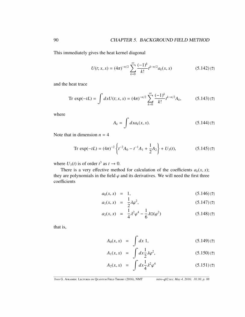
90 CHAPTER 5. BACKGROUND FIELD METHOD
This immediately gives the heat kernel diagonal
U(t; x, x) = (4π)−n/2∞∑
k=0
(−1)k
k!tk−n/2ak(x, x) (5.142) ?
and the heat trace
Tr exp(−tL) =
∫dxU(t; x, x) = (4π)−n/2
∞∑k=0
(−1)k
k!tk−n/2Ak, (5.143) ?
where
Ak =
∫dxak(x, x). (5.144) ?
Note that in dimension n = 4
Tr exp(−tL) = (4π)−2
t−2A0 − t−1A1 +12
A2
+ U3(t), (5.145) ?
where U3(t) is of order t3 as t → 0.There is a very effective method for calculation of the coefficients ak(x, x);
they are polynomials in the field ϕ and its derivatives. We will need the first threecoefficients
a0(x, x) = 1, (5.146) ?
a1(x, x) =12λϕ2, (5.147) ?
a2(x, x) =14λ2ϕ4 −
16λ(ϕ2) (5.148) ?
that is,
A0(x, x) =
∫dx 1, (5.149) ?
A1(x, x) =
∫dx
12λϕ2, (5.150) ?
A2(x, x) =
∫dx
14λ2ϕ4 (5.151) ?
Ivan G. Avramidi: Lectures on Quantum Field Theory (2016), NMT intro-qft2.tex; May 4, 2016; 18:30; p. 88

5.8. EFFECTIVE ACTION IN SCALAR FIELD THEORY 91
The diagonal of the Green function can be formally computed in terms of theheat kernel as
G(x, x) =
∫ ∞
0dt e−tm2
U(t; x, x)
= (4π)−n/2∞∑
k=0
(−1)k
k!
∫ ∞
0dt tk−n/2e−tm2
ak(x, x)
= (4π)−n/2∞∑
k=0
(−1)k
k!Γ(k + 1 − n/2)
1m2k+2−n ak(x, x) (5.152) ?
The one-loop effective action (that is, the the operator (L + m2), can also beexpressed in terms of the heat kernel as follows. First, for any matrix A
log det A = Tr log A (5.153) ?
Now, note that for any positive real number a there holds
1a
=
∫ ∞
0dt e−ta (5.154) ?
By integrating this equation over a we get
log a = −
∫ ∞
0
dtt
(e−ta − e−tC) + log C. (5.155) ?
with some constant C. Thus, applying this equation to all eigenvalues of the op-erator (L + m2) we get
Γ1 = −12
∫ ∞
0
dtt
Tr e−t(L+m2)
= −12
∫ ∞
0
dtt
e−tm2Tr e−tL
= −12
∫ ∞
0
dtt
e−tm2∫
dx U(t; x, x) (5.156) ?
Finally, by using the asymptotic expansion of the heat kernel we obtain
Γ1 = −12
(4π)−n/2∞∑
k=0
(−1)k
k!
∫ ∞
0dt tk−1−n/2e−tm2
Ak
= −12
(4π)−n/2∞∑
k=0
(−1)k
k!Γ(k − n/2)
1m2k−n Ak (5.157) ?
Ivan G. Avramidi: Lectures on Quantum Field Theory (2016), NMT intro-qft2.tex; May 4, 2016; 18:30; p. 89

92 CHAPTER 5. BACKGROUND FIELD METHOD
It is clear that in four-dimensional space-time (n = 4) the integrals over theproper time diverge at the lower limit. Therefore, they should be regularized.To do this one can introduce in the proper time integral a regularizing functionρ(tµ2; ε) that depends on the regularizing parameter ε and the renormalizationparameter µ. In the limit ε → 0 the regularizing function must tend to unity,and for ε , 0 it must ensure the convergence of the proper time integrals (i.e., itmust approach zero sufficiently rapidly at t → 0 and be bounded at t → ∞ bya polynomial). The concrete form of the function ρ does not matter. In practice,one uses the cut-off regularization, the Pauli–Villars one, the analytical one, thedimensional one, the ζ-function regularization and others.
The dimensional regularization is one of the most convenient for the practicalcalculations (especially in massless and gauge theories) as well as for general in-vestigations. The theory is formulated in the space of arbitrary dimension n whilethe topology and the metric of the additional n−4 dimensions can be arbitrary. Topreserve the physical dimension of all quantities in the n-dimensional space-timeit is necessary to introduce the dimensional parameter µ. All integrals are calcu-lated in that region of the complex plane of n where they converge. It is obviousthat for Re n < C, with some constant C, the integrals converge and define ana-lytic functions of the dimension n. The analytical continuation of these functionsto the neighborhood of the physical dimension leads to singularities at the pointn = 4. After subtracting these singularities we obtain analytical functions in thevicinity of the physical dimension, the value of this function at the point n = 4defines the finite value of the initial expression.
It is easy to see that for an integer value of n, say n = 4, this expressiondiverges since the Gamma function Γ(z) as a function of a complex variable z hassimple poles at negative integer points z = −k, k = 0, 1, 2, . . . . It is well knownthat as ε→ 0
Γ(−k + ε) =(−1)k
k!
1ε
+ ψ(k + 1) + O(ε), (5.158) ?
where
ψ(k + 1) =
k∑j=1
1j− C, (5.159) ?
where ψ(z) = Γ′(z)/Γ(z) and C = −ψ(1) ≈ 0.577 is the Euler constant. In particu-
Ivan G. Avramidi: Lectures on Quantum Field Theory (2016), NMT intro-qft2.tex; May 4, 2016; 18:30; p. 90

5.8. EFFECTIVE ACTION IN SCALAR FIELD THEORY 93
lar,
Γ(ε) =1ε
+ ψ(1) + O(ε), (5.160) ?
Γ(−1 + ε) = −1ε− ψ(2) + O(ε), (5.161) ?
Γ(−2 + ε) =12ε
+12ψ(3) + O(ε). (5.162) ?
Now, let us write the dimension in the form
n = 4 + ε (5.163) ?
and then try to take the limit as ε→ 0. The result for the diagonal Green functionis
G(x, x) = Gdiv(x, x) + Gfin(x, x) (5.164) ?
where
Gdiv(x, x) = (4π)−2(2ε
+ C + logm2
4πµ2
) [m2 − a1(x, x)
](5.165) ?
Gfin(x, x) = −(4π)−2m2 + Gren(x, x) , (5.166) ?
Gren(x, x) =1
(4π)2
∞∑k=2
1k(k − 1)
ak(x, x)m2(k−1) (5.167) ?
Here the renormalized Green function Gren is normalized so that as m→ ∞ it goesto zero. The result for the effective action is
Γ(1) = Γdiv1 + Γfin
1 (5.168) ?
where
Γdiv1 = −
14
(4π)−2(2ε
+ C + logm2
4πµ2
) [m4A0 − 2m2A1 + A2
](5.169) ?
Γfin1 =
12
(4π)−2(34
m4A0 − m2A1
)+ Γren
(1) (5.170) ?
Γren1 =
12
(4π)−2∞∑
k=3
1k(k − 1)(k − 2)
Ak
m2(k−2) (5.171) ?
Here the renormalized effective action is normalized so that it vanishes for fieldsof infinite mass as m→ ∞.
Ivan G. Avramidi: Lectures on Quantum Field Theory (2016), NMT intro-qft2.tex; May 4, 2016; 18:30; p. 91

94 CHAPTER 5. BACKGROUND FIELD METHOD
Now, by using the explicit form of the heat kernel coefficients we can computethe divergent part of the one-loop effective action
Γdiv1 = −
14
(4π)−2(2ε
+ C + logm2
4πµ2
) ∫dx
m4 − 2m2 1
2ϕ2 + 6λ2 1
24ϕ4
,
(5.172) ?The first term here is just an infinite constant and can be safely neglected. Theother two terms should be added to the classical action to define the renormalizedclassical action
S ren = S + ~Γdiv1 , (5.173) ?
which leads to the renormalized coupling constants
m2ren(µ) = m2 + ~
12
(4π)−2(2ε
+ C + logm2
4πµ2
)m2λ + O(~2) (5.174) ?
λren(µ) = λ − ~32
(4π)−2(2ε
+ C + logm2
4πµ2
)λ2 + O(~2) (5.175) ?
To be able to take the limit ε → 0 we need to assume that the parameters of theclassical action do depend on ε in exactly such a way to cancel the divergences.
This means that the renormalized constants depend on the renormalizationparameter µ in such a way that
µ∂
∂µm2 = −(4π)−2m2λ (5.176) ?
µ∂
∂µλ = 3(4π)−2λ2 (5.177) ?
These are the renormalization group (RG) equations. The solution of these equa-tions has the form
λ(µ) =λ0
1 − 3(4π)−2λ0 log (µ/µ0)(5.178) ?
m2(µ) =[1 − 3(4π)−2λ0 log (µ/µ0)
]1/3m2
0 (5.179) ?
Notice that the coupling constant λ(µ) becomes infinite and the mass m(µ) con-verges to zero at a finite energy scale
µ = exp[(4π)2
3λ0
]µ0. (5.180) ?
Ivan G. Avramidi: Lectures on Quantum Field Theory (2016), NMT intro-qft2.tex; May 4, 2016; 18:30; p. 92

5.8. EFFECTIVE ACTION IN SCALAR FIELD THEORY 95
This is the so-called Landau pole. The theory cannot be continued after that en-ergy. Alternatively, we can rewrite this equation in the form
λ0 =λ(µ)
1 + 3(4π)−2λ(µ) log (µ/µ0)(5.181) ?
If we require that λ(µ) remains finite as µ → ∞, then λ0 should be equal to zero,λ0 = 0. This is the so-called zero-charge problem. It basically means that thetheory is trivial. Of course, these equations are obtained in the perturbation theoryand for large λ cannot be trusted.
There are quantum field theories, such as Yang-Mills theory, in which thebehavior of the coupling constant g(µ) at high energies as µ → ∞ is exactlyopposite, that is,
g(µ) =g0
1 + βg0 log (µ/µ0), (5.182) ?
where β > 0 is a positive constant. Then, obviously, the coupling constant g(µ)approaches zero at high energies as µ→ ∞. This situation is called the asymptoticfreedom. In this case the results obtained in perturbation theory remain valid athigh energies since the coupling remains small.
Ivan G. Avramidi: Lectures on Quantum Field Theory (2016), NMT intro-qft2.tex; May 4, 2016; 18:30; p. 93

96 CHAPTER 5. BACKGROUND FIELD METHOD
Ivan G. Avramidi: Lectures on Quantum Field Theory (2016), NMT intro-qft2.tex; May 4, 2016; 18:30; p. 94

Chapter 6
Gauge Theories
In the previous lecture it has been shown how to quantize a non-gauge field theory.We defined the generating functionals Z(J) and W(J) and the effective action Γ(φ)and constructed the perturbation theory for these objects, i.e., the diagrammatictechnique. All the diagrams are constructed of two kinds of the constituent blocks— the propagator and the vertexes. If these objects turn out to be well definedthen all the diagrams are well defined (at least formally). Thus the effective action(and consequently the S -matrix) is well defined, at least perturbatively.
Of course, to do practical calculations, this is not enough and one has to em-ploy the apparatus of the renormalization theory. But on the formal level theconstruction in the previous lecture is consistent. It gives simply a raw frameworkthat should be filled with further details and methods.
The bare vertex functions S ,i1...in , n ≥ 3, are simple ultralocal objects — thereare no difficulties at all in defining them correctly. As far as the propagator Gik =
(S ,ik)−1 is concerned we simply assumed that there exists some propagator thatcan be well defined by fixing some appropriate boundary conditions.
It is this condition that determines the non-gauge field theory. However, it isnot always the case. Moreover, the most interesting field models (which are alsomost important from the physical point of view) belong to another class of fieldtheories, so called gauge field theories, where this condition is not fulfilled.
To formulate this more precisely let us consider a dynamical system that isdescribed by a set of (for simplicity boson) fields ϕi and an action functional S (ϕ).The classical dynamics of the system is described by the equations of motion
S ,i ≡δSδϕi = 0. (6.1) 3.1
97

98 CHAPTER 6. GAUGE THEORIES
All possible field configurations form the configuration space M = ϕi. Thesolutions of the classical equations of motion determine the dynamical subspace(mass-shell)M0 ⊂ M,
M0 =ϕi
0 : S ,i(ϕ0) = 0. (6.2) ?3.2?
Let ϕ0 be a point inM0, i.e., a solution of the equations of motion (6.1) withsome boundary conditions. It should be noted that the boundary conditions are,in general, not arbitrary. The equations of motion can impose some constraintson possible boundary conditions. Let us consider the neighbourhood of ϕ0 inM0,i.e., let us consider another solution of the form
ϕ0 = ϕ0 + δϕ (6.3) ?
with the same boundary conditions. The infinitesimal disturbance δϕ satisfiesobviously the homogeneous equation of small disturbances
S ,ik(ϕ0)δϕk = 0 (6.4) 3.3
and zero boundary conditions.If all the equations (6.1) are functionally independent, i.e., if there is a unique
solution for given boundary conditions, then the matrix S ,ik(ϕ0) (so called Hes-sian), is nondegenerate. Hence the homogeneous equation of small disturbanceswith zero boundary conditions has only trivial solution δϕ = 0, i.e., it does nothave any solutions of compact support.
In other words this means that all solutions of the equations of motion areisolated critical points of the action, i.e., in a sufficiently small neighbourhood ofany solution there is no other solution with the same boundary conditions. (In theEuclidean formulation of QFT this is exactly what happens). It might be useful tonote that in this case the equations of motion can be, in principle, rewritten in theform
ϕA = f A(ϕ, ϕ). (6.5) ?
In general, the equations (6.1) are not independent — there some linear iden-tities, called Noether identities, between them
S ,iRiα ≡ 0, (6.6) 3.5
where α = (a, x) is a condensed index that also includes the spacetime point anda = 1, . . . , p. This means that in the dynamical subspaceM0 the Hessian S ,ik(ϕ0)is degenerate
S ,ik(ϕ0)Riα(ϕ0) = 0, (6.7) ?
Ivan G. Avramidi: Lectures on Quantum Field Theory (2016), NMT intro-qft2.tex; May 4, 2016; 18:30; p. 95

99
i.e., there are nontrivial solutions of homogeneous equations of small disturbances(6.4). The number of dynamical degrees of freedom is equal to the number ofindependent equations and is less or equal to (D − p). It is clear that it should bep < D, otherwise the system would not have any dynamical degrees of freedomat all.
More generally, Riα is a set of vector fields on the configuration space M.
Defining
Rα = Riα(ϕ)
δ
δϕi (6.8) ?3.8?
one can rewrite eq. (6.6) in the form
RαS ≡ 0. (6.9) ?3.9?
The vector fields Rα define the invariant flows on M. This means that there aresome specific transformations of the fields
δξϕi = Ri
αξα (6.10) ?3.11?
that leave the action functional invariant:
δξS = S ,iδξϕi = S ,iRi
αξα = 0. (6.11) ?3.13?
Here ξα are some infinitesimal parameters
ξα = ξa(x), (6.12) ?3.12?
that are functions over spacetime with compact support. Such transformations arecalled invariance transformations and Rα are called the generators of invariancetransformations.
The generators Rα are not independent since the commutator of two invariantflows is an invariance flow again, that is,
(δξ1δξ2 − δξ2δξ1)S = 0. (6.13) ?3.14?
This means that[Rα,Rβ]S = (RαRβ − RβRα)S = 0, (6.14) ?3.15?
or in components (Riα,kR
kβ − Ri
β,kRkα
)S ,i = 0. (6.15) ?3.16?
This identity says that the commutator of invariance transformations is again avector field onM that is orthogonal to S ,i.
In most important case (that includes such important systems as electrody-namics, Yang-Mills theory and gravity) the invariance flows satisfy the followingconditions:
Ivan G. Avramidi: Lectures on Quantum Field Theory (2016), NMT intro-qft2.tex; May 4, 2016; 18:30; p. 96

100 CHAPTER 6. GAUGE THEORIES
1. The vector fields Rα(ϕ) are linearly independent. This means that
Riαξ
α = 0 if and only if ξ = 0. (6.16) 3.17
Put it in another way: there are no ξα , 0 of compact support such thatequation (6.16) holds.
2. The invariance flows Rα are complete, i.e., they generate all invariant flows.This means that the subspace of all vectors orthogonal to S ,i is covered bylinear combination of the vectors Ri
α.
3. The invariance flows form an infinite-dimensional Lie algebra (called thegauge algebra)
[Rα,Rβ] = CγαβRγ, (6.17) ?3.19?
or in componentsRi
β,kRkα − Ri
α,kRkβ = Cγ
αβRiγ, (6.18) ?3.20?
and satisfy the Jacobi identity[Rα[Rβ,Rγ]
]+
[Rβ, [Rγ,Rγ]
]+
[Rγ,[Rα,Rβ]
]≡ 0. (6.19) ?3.24?
Here Cγαβ are some constant functionals (independent of ϕ), called the struc-
ture constants of the Lie algebra, satisfying the condition
Cγαβ = −Cγ
βα (6.20) ?3.21?
andCγ
β[λCβµν] ≡ 0. (6.21) ?3.28?
This means that the gauge transformations form an infinite-dimensional Liegroup, called gauge group G. If the structure constants vanish, Cα
βγ = 0, thengauge group is Abelian and the field theory is called Abelian gauge theory (elec-trodynamics). The most interesting gauge field models are non-Abelian (Yang-Mills, gravity).
The flow vectors Rα decompose the configuration space into the gauge orbits.An orbit is a subspace of M consisting of the points that are connected by thegauge transformations. The space of orbits is then
M =M/G (6.22) ?
The linear independence of the vectors Rα at each point implies that each orbit isa copy of the group manifold.
Ivan G. Avramidi: Lectures on Quantum Field Theory (2016), NMT intro-qft2.tex; May 4, 2016; 18:30; p. 97

6.1. DYNAMICAL CONFIGURATION SUBSPACE 101
6.1 Dynamical Configuration SubspaceThe gauge field theories are characterized by the presence of some transformationsof the fields, gauge transformations, that leave the action invariant. Therefore,such transformations do not play any role in solving the equations of motion, i.e.,in determining the dynamical subspaceM0. Two field configurations that can beconnected by a gauge transformation, i.e., two points in an orbit, are physicallyequivalent. This means that physical dynamical variables are the classes of gaugeequivalent field configurations, i.e., the orbits. The physical configuration spaceis, hence, the space of orbits M =M/G. In other words the physicall observablesmust be the invariants of the gauge group.
Let us show that the invariance flows map the dynamical subspace M0 intoitself. Varying the identity
S ,iRiα ≡ 0 (6.23) ?3.32?
we haveS ,ikRi
α + S ,iRiα,k ≡ 0. (6.24) 3.33
Therefore, the gauge transformation of the left-hand side of the equations of mo-tion is
δξS ,k = S ,kiRiαξ
α = −S ,iRiα,kξ
α. (6.25) ?3.34?
This means that a point ϕ0 of the dynamical subspaceM0 is not lead out ofM0
by gauge transformations. In other words the orbits can not intersect M0, theycan either lie completely in M0 or not to have any common point with M0. Ifonly one point of an orbit lies inM0, then the whole orbit does. The vector fieldsRi
α(ϕ0) at the tangent space Tϕ0M at a point ϕ0 ∈ M0 do not have any orthogonalcomponent to this tangent space. They only cover a part of the tangent space, and,therefore, are all tangent vectors toM0, that is, Rα ∈ Tϕ0M0.
This becomes clear if we note thatM0 is defined by vanishing of the functionalS ,i(ϕ). Thus the normal vector toM0 is determined by the Hessian onM0
Nk(ϕ0) = S ,ik(ϕ0)Ai (6.26) ?3.35?
where ϕ0 is a point inM0 and Ai is an arbitrary constant functional. Indeed, it iseasily seen from above that if S ,i = 0 then
Riα(ϕ0)Ni(ϕ0) = 0. (6.27) ?
Therefore, the vectors Rα are tangent toM0. Thus the field transformations of theform
δϕi = Riαξ
α (6.28) ?3.36?
Ivan G. Avramidi: Lectures on Quantum Field Theory (2016), NMT intro-qft2.tex; May 4, 2016; 18:30; p. 98

102 CHAPTER 6. GAUGE THEORIES
are unphysical.
6.2 Invariant MeasureAs in the previous lecture, to quantize the gauge field theories, we will need tointegrate over the configuration space M. One needs, thus, a measure Dϕ µ(ϕ)onM. In the gauge field theories this measure should be gauge-invariant, at leastformally. The most natural way to introduce the measure is to construct a metricEi j on the configuration space that is gauge invariant; then
µ = ( det Ei j)1/2. (6.29) ?
In local field theories this is actually a differential operator. It is always assumedthat the metric Eik is ultralocal, i.e., it depends locally only on the fields but noton their derivatives,
Eik = EAB(ϕ(x))δ(x, x′). (6.30) ?3.76?
6.3 Ward IdentitiesBy differentiating the identity (6.6) one can get an infinite series of higher-orderidentities (called Ward identities) such as
S ,iRiα = 0, (6.31) ?3.47?
S ,ikRiα + S ,iRi
α,k = 0, (6.32) ?3.48?
S ,ik jRiα + 2S ,i(kRi
|α|, j) + S ,iRiα,k j = 0, (6.33) ?3.48?
These identities express the variation of the vertex functions S ,k1...kn in terms of S ,i
and S ,i j and the vertex functions of lower order.
6.4 Physical Field VariablesThus we have seen that the configuration spaceM is decomposed by the invari-ance flows into the orbits. To describe the local geometry of the configurationspace it is convencient to reparametrize it by introducing new local coordinatesIA(ϕ) and χα(ϕ), so that the variables IA enumerate the orbits and the variables
Ivan G. Avramidi: Lectures on Quantum Field Theory (2016), NMT intro-qft2.tex; May 4, 2016; 18:30; p. 99

6.5. PROPAGATORS 103
χα label the points in the orbits. The variables IA(ϕ) are obviously gauge invari-ants which are, in general, very complicated nonlocal functionals. The change ofvariables
ϕ j 7→ ϕ j = (IA(ϕ), χα(ϕ)) (6.34) ?
should be nondegenerate.Since IA are gauge invariants it is clear that the vector fields Rα are
Rα = Riα
δ
δϕi = Riαχ
β,iδ
δχβ+ Ri
αIA,iδ
δIA = Fβα
δ
δχβ(6.35) ?3.62?
whereFβ
α = χβ,iR
iα. (6.36) ?3.63?
Let us now define a matrix
Nαβ = EikRiαRk
β. (6.37) 3.75
In practical cases of interest the generators Riα are first order differential operators;
then Nαβ is the differential operator of second order. Since the vector fields Riα
are linearly independent and the metric Eik is nondegenerate, the matrix Nαβ isnondegenerate too. This means that there is an inverse operator N−1αβ. In fieldtheory this is a Green function of the operator Nαβ.
6.5 PropagatorsWe consider two close solutions, ϕ0 and ϕ = ϕ0 + δϕ, of the equations of motion.That is we have
S ,i(ϕ0) = 0 (6.38) ?3.99?
and to first order in δϕ a homogeneous equation of small disturbances
S ,ik(ϕ0)δϕk = 0. (6.39) ?3.100?
In the case of non-gauge theories the operator S ,ik is non-degenerate, i.e., fixingsome boundary conditions this equation has only trivial solution.
The main difference (and the problem) of the gauge theories is that the opera-tor S ,ik is degenerate on mass shell. That is even by fixing the boundary conditionsthe equation (??) has non-trivial solutions of the form
δξϕk = Rk
αξα, (6.40) ?3.106?
Ivan G. Avramidi: Lectures on Quantum Field Theory (2016), NMT intro-qft2.tex; May 4, 2016; 18:30; p. 100

104 CHAPTER 6. GAUGE THEORIES
with ξα being small functions of compact support. That is, δξϕk are the zero-modes of the operator S ,ik. Thus, the operator S ,ik does not have well definedGreen functions.
Thus instead of having a well defined unique solution for fixed boundary con-ditions we have a class of physically equivalent solutions, an orbit. To deal withsuch situations one has to choose a representative solution in each orbit. This canbe done by imposing some supplementary conditions, so called gauge conditions.We choose the supplementary conditions in the form
χαiδϕi = 0. (6.41) ?3.111?
The matrix χαi here must be chosen in such a way that guaranties that the matrix
Fαβ = χαiR
iβ (6.42) ?3.113?
is non-degenerate. We will see below that this is always possible. The Greenfunction of this operator F−1β
α is called the Faddeev-Popov ghost propagator.Further, let βαβ be a symmetric nondegenerate matrix and L be an operator
defined byLik = S ,ik + χαiβαβχ
βk. (6.43) ?3.116?
The operator L is a symmetric and non-degenerate. Indeed, from the Wardidentities eq. (6.24) on mass shell (when S i = 0) we have
LikRkα = χ
γiβγβF
βα (6.44) ?3.118?
RiαLik = Fγ
αβγβχβk (6.45) ?3.119?
Therefore, any zero-mode hi,Likhk = 0, (6.46) 3.123a
must satisfy the equation
0 = RiαLinhk
0 = Fγαβγβχ
βkh
k0. (6.47) ?3.120?
Thereforeχβkh
k = 0. (6.48) 3.121
Further,0 = Likhk = S ,ikhk. (6.49) ?3.122?
Ivan G. Avramidi: Lectures on Quantum Field Theory (2016), NMT intro-qft2.tex; May 4, 2016; 18:30; p. 101

6.6. DE WITT GAUGE CONDITIONS 105
Therefore, on mass shell the zero-modes of the operator L are the zero-modes ofthe operator S ,ik. But we know from the completeness condition that all zero-modes of S ,ik have the form
hk = Rkαξ
α. (6.50) ?3.123?
Substituting this into the equation (6.48) we get
0 = χβkR
kαξ
α = Fβαξ
α. (6.51) ?3.124?
The operator Fαβ is nonsingular by construction. Therefore, we find that
ξα = 0. (6.52) ?3.125?
This means that there are no functions of compact support that satisfy the equa-tion (6.46). This proves that the operator L is non-singular on mass-shell. Byanalyticity this means also that it is nonsingular in the neighbourhood of the massshell.
The Green function Gi j of the operator Li j is the propagator of the gauge fields.
6.6 De Witt Gauge ConditionsA natural and very convenient choice of the functional χαi due to De Witt is
χαi = βαβRkβEki (6.53) ?3.114?
where βαβ is the inverse of the matrix βαβ. The supplementary condition
χαiδϕi = βαβRk
βEkiδϕi = 0 (6.54) ?3.127?
means then that small disturbance δϕi is orthogonal to the orbit.In De Witt gauge conditions the operators F and L take especially simple form
Fαβ = βαγRi
γEikRkβ = βαγNγβ (6.55) ?3.115?
Lik = S ,ik + EimRmαβ
αβRnβEnk (6.56) ?3.117?
where the operator N is defined in (6.37). Both operators, N and L, are symmetricnon-degenerate operators.
Ivan G. Avramidi: Lectures on Quantum Field Theory (2016), NMT intro-qft2.tex; May 4, 2016; 18:30; p. 102

106 CHAPTER 6. GAUGE THEORIES
6.7 Effective Action in Gauge TheoriesNow we are going to quantize the gauge theories by means of the Feyman func-tional integral. In the same way as in non-gauge theories we consider the in– andout– regions, define some |in〉 and |out〉 states in these region and study the ampli-tude 〈out|in〉. In analogy with non-gauge theories we write the amplitude in formof a functional integral
〈out|in〉 =
∫Dϕ f (ϕ) exp iS (ϕ) , (6.57) ?3.141?
where S (ϕ) is the action and f (ϕ) is some unknown functional.The problem with this integral is that it is defined only formally even in the
non-gauge theories. In gauge theories there is an additional difficulty caused bythe gauge invariance of the action. The formal convergence of this integral wasguaranteed by the exponential exp(iS (ϕ)). The main contribution came from thecritical points, i.e., the solutions of the equations of motion.
The contributions of the field configurations that lie far away from the massshell were suppressed by the oscillations of the integrand. Therefore, the func-tional integral could be defined in perturbation theory, where it just takes intoaccount the small fluctuations around the mass shell. It turned out to be possibleto define this integral by means of the diagrammatic technique (see the previouslecture).
In gauge field theories the action S (ϕ) is invariant along the orbits. This meansthat the large fluctuations along the orbits are not suppressed because there is nofast oscillation of exp(iS (ϕ)) — it remains constant along the orbits. Thus theconvergence of the functional integral along the orbits must be guaranteed by thefunctional f (ϕ). As we have seen all field configurations on an orbit are physicallyequivalent. Therefore, we actually do not have to integrate along the orbits at all!We only have to integrate over the orbit space M =M/G.
To give a concrete meaning to these intuitive ideas let us consider a reparametriza-tion of the configuration spaceM by the coordinates ϕi = (IA, χα), where IA labelthe orbits and χα the points in the orbit. From the invariance of the action func-tional it follows that it depends only on I,
S (ϕ) = S (I). (6.58) ?3.142?
Therefore, it defines an action functional on the orbit space M. This functional isan usual non-gauge functional, however, extremely nonlocal. Therefore, we can
Ivan G. Avramidi: Lectures on Quantum Field Theory (2016), NMT intro-qft2.tex; May 4, 2016; 18:30; p. 103

6.7. EFFECTIVE ACTION IN GAUGE THEORIES 107
write
〈out|in〉 =
∫M
DI expiS (I)
(6.59) ?3.143?
where µ(I) is some measure. This integral can be obviously rewritten as an integraloverM by introducing a δ-functional
〈out|in〉 =
∫M
DIDχ δ(χ − ζ) expiS (I)
(6.60) ?3.144?
where ζα are some constants.The trick consists now in changing the integration variables and going back to
the initial field variables ϕ. We have
DIDχ = DϕJ(ϕ), (6.61) ?
where J(ϕ) is the Jacobian. One can show that the Jacobian J(ϕ) is expressed interms of the operator Fα
β,J(ϕ) = det F(ϕ) (6.62) ?3.155?
Therefore, we obtain
〈out|in〉 =
∫Dϕ det F(ϕ)δ(χ(ϕ) − ξ) exp iS (ϕ) (6.63) ?3.145?
One can transform the functional integral further by introducing some addi-tional field variables and functional integrations. First, one can use the Fourierintegral representation of the functional delta functional to get
〈out|in〉 =
∫DϕDλ det F(ϕ) exp i[S (ϕ) + λα(χα(ϕ) − ξα)] . (6.64) ?3.170?
The new field λα plays the role of a Lagrange multiplier. It is assumed to satisfythe appropriate boundary conditions in the in- and out- regions coherent to thoseof the fields ϕi. The total functional in the exponent
S (ϕ) + λ(χ(ϕ) − ζ) (6.65) ?3.171?
is not gauge invariant any longer. Therefore, its second derivative is a nondegen-erate operator and has well defined Green functions.
Ivan G. Avramidi: Lectures on Quantum Field Theory (2016), NMT intro-qft2.tex; May 4, 2016; 18:30; p. 104

108 CHAPTER 6. GAUGE THEORIES
Remembering that the constants ζα were arbitrary one can go a bit further andintegrate eq. (??) over ζ with a Gaussian measure∫
dζ( det β)1/2 exp( i2ζµβ µνζ
ν)
(6.66) ?3.172?
with a nondegenerate matrix β. As a result we get finally
〈out|in〉 =
∫Dϕ ( det β)1/2 det F(ϕ) exp
i[S (ϕ) +
12χµ(ϕ)βµνχν(ϕ)
]. (6.67) 3.173
The second term in the total functional in the exponent breaks down the gaugeinvariance. It is called the gauge-breaking term. Therefore, the exponential isnot gauge invariant and guaranties the convergence of the functional integral forlarge ϕ. Its second derivative determines a non-singular operator of small distur-bances. It has a well defined Green function (propagator) and gives a basis for theperturbation theory similar to that constructed in the previous lecture.
Often it is convenient to go further and to represent the determinants arisingin equation (6.67) in terms of functional integrals over auxillary anticommutingGrassmanian field variables, so called ghost fields. Remembering the formulas ofthe previous lecture one can write
det F(ϕ) =
∫DθDψ exp
iθαFα
βψβ, (6.68) ?3.174?
det β1/2 =
∫Dω exp
i2ωµβµνω
ν, (6.69) ?3.175?
where ψβθα, ωµ are the ghost fields satisfying appropriate boundary conditions inin– out– regions coherent with those of the fields ϕ.
Therefore, the 〈out|in〉 amplitude takes the form
〈out|in〉 =
∫DϕDψDθDω exp iS tot(ϕ, ψ, θ, ω) (6.70) ?3.176?
where
S tot(ϕ, ψ, θ, ω) = S (ϕ) +12χµ(ϕ)βµνχν(ϕ) + θαFα
βψβ +
12ωµβµνω
ν. (6.71) ?3.177?
Thus a system of gauge fields ϕi described by the action S (ϕ) is equivalent toan auxillary system of the fields ϕi, ψα, θ
β, ωµ described by the non-gauge action
Ivan G. Avramidi: Lectures on Quantum Field Theory (2016), NMT intro-qft2.tex; May 4, 2016; 18:30; p. 105

6.8. YANG-MILLS THEORY AND QUANTUM GRAVITY 109
S tot(ϕ, ψ, θ, ω). Therefore, by introducing the sources one can use now the wholeapparatus of the generating functionals and construct the effective action and theS - matrix. Since the total action S tot(ϕ, ψ, θ, ω) is not gauge invariant its secondderivative is a nonsingular operator and has a well defined propagator. All thematerial of previous lecture is applicable to the total action. The only difference isthat the ghost fields are purely formal and should not appear in the physical statesin in- and out- regions.
The effective action Γ(φ) (in Euclidean formulation) is now determined by theequation
exp−
1~
Γ(φ)
=
∫Dϕ det F(ϕ)( det β)1/2
× exp−
1~
[S (ϕ) +
12χµ(ϕ)βµνχν(ϕ) − (ϕi − φi)Γ,i(φ)
].(6.72) ?
Using this equation we find the one-loop effective action
Γ = S + ~Γ(1) + O(~2) (6.73) ?
Γ(1) =12
log det L − 2 log det F − log det β
(6.74) ?
where
Lik = S ,ik + χµ,iβµνχν,k , (6.75) ?
χµ,i = χµ,i(ϕ)∣∣∣∣ϕ=φ
, (6.76) ?
F = F(ϕ)∣∣∣∣ϕ=φ
(6.77) ?
This can now be computed by using the same methods as for non-gauge theories.
6.8 Yang-Mills Theory and Quantum Gravity
6.8.1 Yang-Mills TheoryYang-Mills theory is an example of a gauge theory with the configuration spaceM being the space of connections on a vector bundle over a spacetime M. Let Gbe a simple compact Lie group of dimension N with the structure constants Ca
bc.All Latin indices will run over 1, . . . ,N. Sor simplicity one could take the group
Ivan G. Avramidi: Lectures on Quantum Field Theory (2016), NMT intro-qft2.tex; May 4, 2016; 18:30; p. 106

110 CHAPTER 6. GAUGE THEORIES
G = S U(2); then N = 3. The Yang-Mills field can be parametrized by a set ofvector fields
ϕi = Aaµ(x) , i ≡ (aµ, x) . (6.78) ?
The infinitesimal gauge transformations have the form
δξAaµ = ∇µξ
a =(∂µδ
ab + Ac
µCa
cb
)ξb (6.79) ?
The parameters of gauge transformations are the components of the scalar fields,
ξµ = ξa(x) , µ ≡ (a, x) . (6.80) ?
The local generators of the gauge transformations in this parametrization are de-fined by their action as follows
Riαξ
α = ∇µξa , i ≡ (aµ, x) , (6.81) ?
Letγab = −
12
CcadCd
bc (6.82) ?
One can show that this matrix is positive and non-degenerate; it is called Cartan-Killing metric on the Lie algebra. For simple groups one can always make itEuclidean
γab = δab. (6.83) ?
An invariant fiber metric is defined by
Eµaν
b = gµνγab , (6.84) ?
The Yang-Mills action has the form
S Y M = −1
4e2
∫M
dx g1/2gµαgνβδabFaµνF
bαβ (6.85) ?
where e is the coupling constant
Faµν = ∂µAa
ν − ∂νAaµ + Ca
bcAbµAc
ν (6.86) ?
is the field strength of the gauge fields.The first variation of the action gives the classical equations of motion
∇νFµνa = 0 , (6.87) ?
Ivan G. Avramidi: Lectures on Quantum Field Theory (2016), NMT intro-qft2.tex; May 4, 2016; 18:30; p. 107

6.8. YANG-MILLS THEORY AND QUANTUM GRAVITY 111
which satisfy, of course, the Nother identities
∇µ∇νFµνa = 0 . (6.88) ?
The second variation of the action defines a second-order partial differentialoperator
Pabµν = −gµνδa
b∆ + ∇µ∇ν − 2FcµνC
acb + Rµνδ
ab (6.89) ?
Here, of course, ∆ = gµν∇µ∇ν denotes the Laplacian.Next, we choose the De Witt gauge condition
χa = ∇µhaµ . (6.90) ?
The ghost operator in this gauge is a second-order differential operator defined by
Fab = −δa
b∆ . (6.91) ?
For the gauge operator L to be non-degenerate it is necessary to choose theoperator γ as a zero order differential operator defined by
γab =λ
e2 δab , (6.92) ?
where λ , 0 is a real parameter. The Yang-Mills operator L now reads
Labµν = −gµνδa
b∆ + (1 − λ)∇µ∇ν − 2FcµνC
acb + Rµνδ
ab (6.93) ?
The most convenient choice is the so-called minimal gauge
λ = 1 . (6.94) ?
In this gauge the non-diagonal derivatives vanish
Labµν = −gµνδa
b∆ − 2FcµνC
acb + Rµνδ
ab (6.95) ?
Thus, with this choice of gauge parameters the one-loop effective action ofYang-Mills theory is given by
Γ(1) =12
log Det L − log Det F . (6.96) ?eaxxz?
Therefore, in order to compute the effective action we need to compute the deter-minants of Laplace type partial differential operators.
Ivan G. Avramidi: Lectures on Quantum Field Theory (2016), NMT intro-qft2.tex; May 4, 2016; 18:30; p. 108

112 CHAPTER 6. GAUGE THEORIES
One can now use the same technique to compute the divergent part of theeffective action
Γdiv =1ε
∫M
dx g1/2β1gµαgνβδabFa
µνFbαβ +β2RµναβRµναβ +β3RµνRµν +β4R2
(6.97) ?
with some constants βi; here, of course, ε = n − 4. This means that in flat spacethe Yang-Mills theory is renormalizable since the divergence can be absorbed inthe classical action. The high energy behavior off the coupling constant e canbe determined from the renormalization group equations. For the gauge groupS U(N) it has the form
e2(µ) =e2
0
1 + 1148π2 Ne2
0 log (µ/µ0)(6.98) ?
which shows that it is asymptotically free, that is, the coupling e(µ) vanishes asµ→ ∞.
It also shows that in order for Yang-Mills theory to be renormalizable in curvedspace the gravitational action should contain terms quadratic in curvature (in ad-dition to the Einstein term).
6.8.2 General RelativityEinstein’s theory of general relativity is an example of a gauge theory with thegauge group G being the group of all diffeomorphisms of the spacetime manifoldM and the configuration spaceM being the space of all pseudo-Riemannian met-rics on M. The physical configuration spaceM/G of all orbits of the gauge groupis then the space of all geometries on the spacetime.
The gravitational field can be parametrized by the metric tensor of the space-time
ϕi = gµν(x) , i ≡ (µν, x) . (6.99) ?
An invariant fiber metric is defined by
Eµναβ = gµ(αgβ)ν − κgµνgαβ , (6.100) ?
where κ , 1/n is a real parameter. The inverse metric is then
E−1µναβ = gµ(αgβ)ν −
κ
nκ − 1gµνgαβ . (6.101) ?
Ivan G. Avramidi: Lectures on Quantum Field Theory (2016), NMT intro-qft2.tex; May 4, 2016; 18:30; p. 109
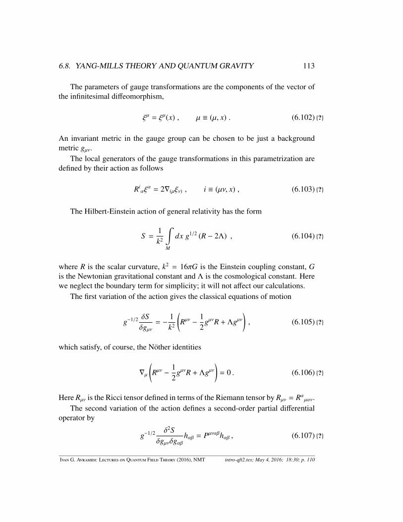
6.8. YANG-MILLS THEORY AND QUANTUM GRAVITY 113
The parameters of gauge transformations are the components of the vector ofthe infinitesimal diffeomorphism,
ξµ = ξµ(x) , µ ≡ (µ, x) . (6.102) ?
An invariant metric in the gauge group can be chosen to be just a backgroundmetric gµν.
The local generators of the gauge transformations in this parametrization aredefined by their action as follows
Riαξ
α = 2∇(µξν) , i ≡ (µν, x) , (6.103) ?
The Hilbert-Einstein action of general relativity has the form
S =1k2
∫M
dx g1/2 (R − 2Λ) , (6.104) ?
where R is the scalar curvature, k2 = 16πG is the Einstein coupling constant, Gis the Newtonian gravitational constant and Λ is the cosmological constant. Herewe neglect the boundary term for simplicity; it will not affect our calculations.
The first variation of the action gives the classical equations of motion
g−1/2 δSδgµν
= −1k2
(Rµν −
12
gµνR + Λgµν), (6.105) ?
which satisfy, of course, the Nother identities
∇µ
(Rµν −
12
gµνR + Λgµν)
= 0 . (6.106) ?
Here Rµν is the Ricci tensor defined in terms of the Riemann tensor by Rµν = Rαµαν.
The second variation of the action defines a second-order partial differentialoperator by
g−1/2 δ2Sδgµνδgαβ
hαβ = Pµναβhαβ , (6.107) ?
Ivan G. Avramidi: Lectures on Quantum Field Theory (2016), NMT intro-qft2.tex; May 4, 2016; 18:30; p. 110

114 CHAPTER 6. GAUGE THEORIES
where
Pµν,αβ = −1
2k2
−
(gα(µgν)β − gαβgµν
)∆
−gµν∇(α∇β) − gαβ∇(µ∇ν) + 2∇(µgν)(α∇β)
−2R(µ|α|ν)β − gα(µRν)β − gβ(µRν)α + Rµνgαβ + Rαβgµν
+
(gµ(αgβ)ν −
12
gµνgαβ)
(R − 2Λ)
(6.108) ?
Here, of course, ∆ = gµν∇µ∇ν denotes the Laplacian.Next, we choose the De Witt gauge condition
χα = −Eαβµν∇βhµν = −(gα(ν∇µ) − κgµν∇α
)hµν . (6.109) ?
The ghost operator in this gauge is a second-order differential operator defined by
Fµν = −2Eµαβ
ν∇α∇β = −δµν∆ + (2κ − 1)∇µ∇ν − Rµν . (6.110) ?
For this operator to be non-singular, the gauge parameter should satisfy the con-dition κ , 1.
For the graviton operator L to be non-degenerate it is necessary to choose theoperator γ as a zero order differential operator defined by
γµν =α
k2 gµν , (6.111) ?
where α , 0 is a real parameter. Thus we obtain a two-parameter class of gaugesinvolving two arbitrary parameters, κ and α.
The graviton operator L now reads
Lµν,αβ =1
2k2
−
(gα(µgν)β − (1 + 2ακ2)gαβgµν
)∆
−(1 + 2ακ)gµν∇(α∇β) − (1 + 2ακ)gαβ∇(µ∇ν) + 2(1 + α)∇(µgν)(α∇β)
−2R(µ|α|ν)β − gα(µRν)β − gβ(µRν)α) + Rµνgαβ + gµνRαβ
+
(gµ(αgβ)ν −
12
gµνgαβ)
(R − 2Λ)
(6.112) ?
Ivan G. Avramidi: Lectures on Quantum Field Theory (2016), NMT intro-qft2.tex; May 4, 2016; 18:30; p. 111

6.8. YANG-MILLS THEORY AND QUANTUM GRAVITY 115
The most convenient choice is the so-called minimal gauge
κ =12, α = −1 . (6.113) ?
In this gauge the non-diagonal derivatives in both the graviton operator and theghost operator vanish
Lµν,αβ =1
2k2
(gα(µgν)β −
12
gαβgµν)
(−∆ + R − 2Λ)
−2R(µ|α|ν)β − gα(µRν)β − gβ(µRν)α) + Rµνgαβ + gµνRαβ
, (6.114) ?
Fµν = −δµν∆ − Rµ
ν . (6.115) ?
Finally, we define the graviton operator in the canonical Laplace-type form, L,by factoring out the configuration space metric (in the minimal gauge κ = 1/2)
Lµναβ = 2k2E−1µνρσLρσαβ . (6.116) ?
We obtainLµναβ = −δα(µδ
βν)∆ + Qµν
αβ , (6.117) ?
where
Qµναβ = −2Rµ
(ανβ) − 2δ(α
(µRβ)ν) + Rµνgαβ +
2n − 2
gµνRαβ
+
(δα(µδ
βν) −
1(n − 2)
gµνgαβ)
R − 2Λδα(µδβν) . (6.118) ?
Thus, with this choice of gauge parameters the one-loop effective action ofquantum general relativity is given by
Γ(1) =12
log Det L − log Det F . (6.119) ?eaxxz?
Therefore, in order to compute the effective action we need to compute the de-terminants of Laplace type partial differential operators acting on symmetric two-tensors and vectors.
One can now use the same technique to compute the divergent part of theeffective action
Γdiv =1ε
∫M
dx g1/2β5RµναβRµναβ + β6RµνRµν + β7R2 + β8RΛ + β9Λ
2,
(6.120) ?
Ivan G. Avramidi: Lectures on Quantum Field Theory (2016), NMT intro-qft2.tex; May 4, 2016; 18:30; p. 112

116 CHAPTER 6. GAUGE THEORIES
with some constants βi; here, of course, ε = n − 4. This means that in Einsteingeneral relativity is non-renormalizable since the divergence cannot be absorbedin the classical action. In order for quantum gravity to be renormalizable thegravitational action should contain terms quadratic in curvature (in addition to theEinstein term).
Ivan G. Avramidi: Lectures on Quantum Field Theory (2016), NMT intro-qft2.tex; May 4, 2016; 18:30; p. 113
Part II
Mathematical Supplement
117


Chapter 7
Lie Groups and Lie Algebras
7.1 Abstract Group
An abstract group G is a set of elements g for which
i. an associative composition law, called the multiplication, is given so thatfor each ordered pair of elements (g1, g2) another element g1g2, called theirproduct, is associated
(g1, g2)→ g1g2, (7.1) ?
andg1(g2g3) = (g1g2)g3, (7.2) ?
ii. there exists an element e, called the unit element (or identity element), suchthat for any g
ge = eg = g, (7.3) ?
iii. an operation, called the inversion is given, i.e., with each element g its in-verse g−1 is associated,
g→ g−1, (7.4) ?
such thatg−1g = gg−1 = e. (7.5) ?
Basic Notions
119

120 CHAPTER 7. LIE GROUPS AND LIE ALGEBRAS
1. If for any elements g1 and g2 of the group G
g1g2 = g2g1, (7.6) ?
then the group is called Abelian or commutative. Otherwise it is non-Abelian.
2. The number of elements of the group G is called the order of G and denotedby |G|.
3. The group of finite order is called the finite group. Otherwise it is infinite.
4. Infinite group can be discrete and continuous. If the elements g of a groupG can be enumerated with the help of a discrete index, gi, (i = 1, 2, . . . ),the group G is called discrete. Otherwise it is continuous. Finite groups areobviously always discrete.
5. A subset H of elements of the group G is called a subgroup if it itself is agroup with the same composition law. This means that the identity elemente of G, the products of any elements of H as well as their inverses belongto H. One says that H is closed under the multiplication and the inversionlaws.
6. A subgroup H is called proper subgroup if it consists of more than just theunit element but does not coincide with the whole group itself.
7.2 Continuous Groups1. The elements of a general continuous group can be parametrized by a set of
continuous real parameters
g = g(λ), (λ = (λa), a = 1, 2, . . . ). (7.7) ?
If the set of continuous parameters is finite, i.e., a = 1, 2, . . . , p, the group iscalled finite dimensional, the number of the parameters being the dimensionof the group dim G = p. Otherwise, the group is infinitely-dimensional.
2. If the parameters f a(λ, µ) of the product of two elements
g(λ)g(µ) = g( f (λ, µ) (7.8) ?
Ivan G. Avramidi: Lectures on Quantum Field Theory (2016), NMT intro-qft2.tex; May 4, 2016; 18:30; p. 114

7.2. CONTINUOUS GROUPS 121
are analytic functions of the parameters of the factors, i.e. the functionsf a(λ, µ) possess derivatives of all orders with respect to all arguments, and,similarly, the parameters λa(λ) of the inverse element g(λ) = g−1(λ) areanalytic functions of the parameters λ then the continuous group is calledLie group.
3. The continuous parameters λa are called coordinates on the Lie group. Fora finite-dimensional Lie group G the coordinates λa vary in some region ofthe Euclidean space Rp, p being the dimension of the group. If the domainof variation of the coordinates is finite, or compact, i.e. |λa| < ∞, the groupis said to be compact (for more precise definition see the bibliography).
4. A curve (or path ) g = g(τ), 0 ≤ τ ≤ 1, on a Lie group G is a mapping
τ ∈ [0, 1]→ g(τ) ∈ G, (7.9) ?
where τ is a real parameter. The one-parameter subset g(τ) of the group Gitself is called the curve too. A curve g(τ) is continuous if the coordinatesλa(τ) of the element g(τ) are continuous functions of the parameter τ. Wewill call the continuous curves just curves.
5. One says that two elements g0 and g1 are connected by a curve g(τ) if
g(0) = g0, g(1) = g1. (7.10) ?
6. If g(0) = g(1) = g the curve is called closed curve, or the loop, goingthfough the element g. The loop consisting only from one element g iscalled the null loop at g.
7. A subset H of the group G is called arcwise connected (or connected) ifevery two elements of H can be connected by a continuous curve.
8. A component of an element g of a Lie group G is the union of all connectedsubsets of G containing the element g.
9. The component G1 of the identity element of the group G is called theproper connected component of the group G.
10. A general Lie group G consists of many connected components Gi, whichare disconnected from each other. Each conected component Gi is obtainedfrom the proper subgroup G1 by applying some discrete transformation γi
Ivan G. Avramidi: Lectures on Quantum Field Theory (2016), NMT intro-qft2.tex; May 4, 2016; 18:30; p. 115

122 CHAPTER 7. LIE GROUPS AND LIE ALGEBRAS
-
e
g(τ) g1
G1
Figure 7.1: Proper connected component of the group
of a discrete subgroup Γ. Thus a Lie group is a direct product of the propersubgroup and some discrete subgroup
G = G1 × Γ, (7.11) ?1.43?
where G1 is the proper group and Γ the discrete subgroup.
G1
G2 G3
GN+1
M
:
γ1γ2
γN
. . .
Figure 7.2: General continuous group
Lorentz Group as Example The general Lorentz group L ' O(1, d − 1)has four connected components. The role of the component of the identityG1 plays the proper orthochronous Lorentz group L1 ' S O1(1, d − 1). Thediscrete subgroup Γ is the finite group of reflections of the time and onespace coordinate
Γ = 1,T, P,T P T P = PT. (7.12) ?1.44?
T 2 = P2 = (T P)2 = 1. (7.13) ?1.45?
Ivan G. Avramidi: Lectures on Quantum Field Theory (2016), NMT intro-qft2.tex; May 4, 2016; 18:30; p. 116

7.3. INVARIANT SUBGROUPS 123
L1
LIILIV
LIII
M
:
TT P
P
T P
-
Rq
P
T
Figure 7.3: General Lorentz group
11. Two curves g(τ) and g′(τ) connecting the elements g0 and g1 are said tobe homotopic if there exists a continuous deformation of one curve intoanother, which leaves the end points g0 and g1 unaltered, i.e., there exist acontinuous function h(τ, s) of two parameters τ and s such that
h(0, s) = g0, h(1, s) = g1 (7.14) ?
h(τ, 0) = g(τ), h(τ, 1) = g′(τ). (7.15) ?
12. A Lie group is said to be simply connected if every loop is homotopic to thenull loop, i.e., every loop is contractable to one point.
13. All loops at an element g are classified into the so called homotopy classes.
14. A Lie group is said to be n-connected if it has n homotopy classes at eachelement.
7.3 Invariant Subgroups1. A parametrized curve g = g(τ), (a ≤ τ ≤ b), on the Lie group G is called
the one-parameter subgroup of the Lie group G if
g(0) = e, (7.16) ?g(τ1 + τ2) = g(τ1)g(τ2), (7.17) ?g(−τ) = (g(τ))−1. (7.18) ?
Ivan G. Avramidi: Lectures on Quantum Field Theory (2016), NMT intro-qft2.tex; May 4, 2016; 18:30; p. 117

124 CHAPTER 7. LIE GROUPS AND LIE ALGEBRAS
2. Let H be a subgroup of G. The orbit gH of H through an element g in G isthe set of all elements gh with h in H
gH = gh : h ∈ H. (7.19) ?
3. If H is a proper subgroup, the orbits of H in G are called the left cosets of Hin G. The set of all left cosets is denoted by G/H. Analogously it is definedthe set H \G of all right cosets
Hg = hg : h ∈ H. (7.20) ?
4. A subgroup H of a group G is said to be normal or invariant subgroup ofG if for any g in G and any h in H the element ghg−1, called the conjugateelement, is again in H
gH = Hg, or gHg−1 ⊂ H. (7.21) ?
In other words the normal subgroup is closed under the conjugation and theleft and right cosets of H in G coincide with each other.
5. Theorem. The set of left cosets G/H of a subgroup H in G is itself a groupif H is normal subgroup.
6. Theorem. The component G1 of the identity e of a Lie group G, i.e. theconnected component containing the identity element, is a closed invariantsubgroup of G.
7. A set C(G) of all elements of a group G which commute with all elementsof G is called the center of the group
C(G) = g ∈ G : g′g = gg′ ∀g′ ∈ G. (7.22) ?
8. Theorem. The center C(G) is an Abelian normal subgroup of G. ThusG/C(G) is itself a group.
9. Theorem. If G is a connected Lie group and H is an invariant discretesubgroup, then H is central, i.e. it is a subgroup of the center.
10. A Lie group is said to be simple if it has no proper, connected invariant Liesubgroup. It might, however, contain a discrete invariant subgroup.
11. A Lie group is said to be semisimple if it contains no proper invariant con-nected Abelian Lie subgroup.
Ivan G. Avramidi: Lectures on Quantum Field Theory (2016), NMT intro-qft2.tex; May 4, 2016; 18:30; p. 118

7.4. HOMOMORPHISMS 125
7.4 Homomorphisms1. A mapping
ϕ : G → G′ (7.23) ?
which preserves the group multiplication, i.e.
ϕ(gg′) = ϕ(g)ϕ(g′) (7.24) ?
is called homomorphism.
2. Note that several elements of G may have the same image in G′! The set ofall elements of G which are mapped to the identity element of G′ is calledthe kernel of the homomorphism ϕ:
Kerϕ = g ∈ G : ϕ(g) = e′ ∈ G′. (7.25) ?
3. Theorem. The kernel of a homomorphism ϕ is a normal subgroup of G,i.e. for any g in G and any h in Kerϕ the element ghg−1 is again in Kerϕ; inother words
g(Kerϕ)g−1 = Kerϕ. (7.26) ?
4. Theorem. Thus G/Kerϕ is a group.
5. Two groups G and G′ are said to be isomorphic
G ' G′ (7.27) ?
if their elements can be put into one-to-one correspondence which is pre-served under multiplication.
6. An isomorphism ϕ : G → G′ is simply a one-to-one homomorphism, i.e.Kerϕ = e, so that the inverse map ϕ−1 : G′ → G is also a homomorphism.
7. An isomorphism ϕ : G → G of a group with itself is called automorphismof the group.
8. Theorem. The set Aut (G) of all automorphisms of a group G is itself agroup.
Ivan G. Avramidi: Lectures on Quantum Field Theory (2016), NMT intro-qft2.tex; May 4, 2016; 18:30; p. 119

126 CHAPTER 7. LIE GROUPS AND LIE ALGEBRAS
9. A homomorphismϕ : G′ → G (7.28) ?
is called surjective mapping onto G if for any g in G there exists at least oneelement g′ in G′ such that ϕ(g′) = g.
10. Theorem. If homomorphism ϕ : G → G is a surjective mapping onto G,then the group G is isomorphic to G/Kerϕ
G ' G/Kerϕ. (7.29) ?
The group G is called the universal covering group of G.
7.5 Direct and Semi-direct Products1. The set of all ordered pairs
(g, g′), (7.30) ?1.47?
where g is an element of a group G and g′ an element of another one G′,with the product rule
(g1, g′1)(g2, g′2) = (g1g2, g′1g′2) (7.31) ?
is called the direct product (or Cartesian product, or outer product, or sim-ply product) G ×G′ of the groups G and G′. The unit element of G ×G′ is(e, e′) and the inverse of (g, g′) is (g, g′)−1 = (g−1, g′−1).
2. Let G = g be a subgroup of the group of automorphisms Aut (H) of an-other group H = h, i.e., the group G acts isomorphically on the groupH
g : h ∈ H → g(h) ∈ H. (7.32) ?
The set of all ordered pairs (g, h) with the product rule
(g1, h1)(g2, h2) = (g1g2, h1g1(h2)) (7.33) ?1.65a?
defines the semi-direct product G n H of the groups G and H. The unitelement of G n H is (e, 1) and the inverse of (g, h) is
(g, h)−1 = (g−1, g−1(h−1)). (7.34) ?
Ivan G. Avramidi: Lectures on Quantum Field Theory (2016), NMT intro-qft2.tex; May 4, 2016; 18:30; p. 120

7.6. GROUP REPRESENTATIONS 127
3. If the group T = a is Abelian with the group multiplication denoted by+ and the group L = Λ acts linearly on T , then the semidirect productL n T has the multiplication rule
(Λ1, a1)(Λ2, a2) = (Λ1Λ2, a1 + Λ1a2). (7.35) ?1.65b?
4. Theorem. The semidirect product G n H has the following properties:
(a) H is a normal subgroup of G n H,
(b) G n H/H is isomorphic to G.
7.6 Group Representations1. If for each element g of a group G it is given an invertible operator D(g) in
a vector space VD(g) : V → V (7.36) ?
and for all g1 and g2 in G
D(g1g2) = D(g1)D(g2) (7.37) ?
then the set of the operators D(g) is said to form a linear representation ofthe group G on a vector space V .
2. Note that for any element g in G
D(g−1) = D−1(g) (7.38) ?
andD(e) = I, (7.39) ?
where I is the identical operator in V .
3. In general, there are several elements in G which are mapped on I.
4. An invertible operator in the vector space is called automorphism of thevector space V .
5. Theorem. The set of all automorphisms of a vector space forms a group,denoted by Aut (V).
Ivan G. Avramidi: Lectures on Quantum Field Theory (2016), NMT intro-qft2.tex; May 4, 2016; 18:30; p. 121

128 CHAPTER 7. LIE GROUPS AND LIE ALGEBRAS
6. Thus, a linear representation of a group G on a vector space V is a homo-morphism
D : G → Aut (V). (7.40) 1.55a
7. If D is isomorphism, i.e. the correspondence (7.40) is one-to-one, the rep-resentation D is said to be faithful (or exact).
8. If the dimension of the vector space p = dim V is finite then the operatorsD(g) are described by p × p matrices and we have a matrix representationof the group G, I being the unit matrix.
9. If Aut (V) = G then the representation D : G → Aut (V) is called thedefining representation (or fundamental representation.
10. Every Lie group has the adjoint representation such that dim V = dim G,which is determined by its structure constants (defined later).
11. For compact simple groups the adjoint representation is irreducible.
12. If the operators D(g) are unitary, i.e. D†(g)D(g) = I, then the representationD is called unitary.
13. Not every Lie group has a faithful finite-dimensional (matrix) representa-tion.
14. If two representations D1 and D2 of a group G on the vector space V arerelated by an invertible operator A on V , i.e. an automorphism of the vectorspace V ,
D1(g) = A−1D2(g)A (7.41) ?
then the representations D1 and D2 are said to be equivalent.
15. With any matrix representation D of a group G it is associated a map
χD : G → C, (7.42) ?
defined by the trace of the representation matrices
χD(g) = tr D(g), (7.43) ?
which is called the character of the representation D. The value χD(g) iscalled the character of the the element g in the representation D.
Ivan G. Avramidi: Lectures on Quantum Field Theory (2016), NMT intro-qft2.tex; May 4, 2016; 18:30; p. 122

7.7. MULTIPLE-VALUED REPRESENTATIONS. UNIVERSAL COVERING GROUP.129
16. The equivalent representations have the same characters.
17. A representation D of a Lie group G is called reducible if there is a properinvariant subspace V1 ⊂ V , i.e. D : V1 → V1, so V1 is closed under D.Otherwise the representation is called irreducible.
18. Every reducible unitary representation D of a Lie group G is a direct sumof irreducible ones, i.e. D = D1 ⊕ · · · ⊕ Dn.
19. For an Abelian Lie group all irreducible representations are one-dimensional.
7.7 Multiple-valued Representations. Universal Cov-ering Group.
1. The matrix elements D(g) of the representation D of a Lie group G arerequired to be continuous functions on the group G. Among continuousfunctions on the group G there may be some functions which are multi-valued. Thus the representation can be, in principle, multiple-valued.
2. We say that a representation D of G is m-valued representation if witheach element g of the group G there are associated m diferent operatorsD1(g), . . . ,Dm(g).
3. Let us consider a continuous function D(g) on the group G and let us lookat the values D(g(τ)) along a continuous closed curve (loop) g(τ) on G, sothat g(0) = g(1) = g. It could hapen, in principle, that
D(g(0)) , D(g(1)). (7.44) ?
Let us fix an initial value D0 = D(g(0)) and take all possible loops in Gstarting at g.
If the maximal number of different values D(g(1)) is m, then the functionD(g) is m-valued. This number is a property of the group and reflects theconnectedness of the group itself.
4. If the loop g(τ) on the group G can be varied continuously so that it contractsto the initial point g, i.e., it is homotopic to the null loop, the continuousfunction D(g) must return to its original value D0. If this is the case for allloops on the group, i.e., if all loops are homotopic to the null loop, the group
Ivan G. Avramidi: Lectures on Quantum Field Theory (2016), NMT intro-qft2.tex; May 4, 2016; 18:30; p. 123
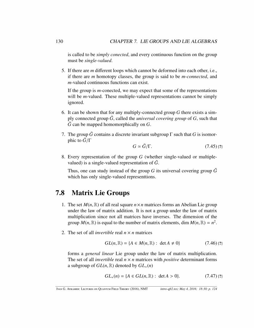
130 CHAPTER 7. LIE GROUPS AND LIE ALGEBRAS
is called to be simply conected, and every continuous function on the groupmust be single-valued.
5. If there are m different loops which cannot be deformed into each other, i.e.,if there are m homotopy classes, the group is said to be m-connected, andm-valued continuous functions can exist.
If the group is m-conected, we may expect that some of the representationswill be m-valued. These multiple-valued representations cannot be simplyignored.
6. It can be shown that for any multiply-connected group G there exists a sim-ply connected group G, called the universal covering group of G, such thatG can be mapped homomorphically on G.
7. The group G contains a discrete invariant subgroup Γ such that G is isomor-phic to G/Γ
G ' G/Γ. (7.45) ?
8. Every representation of the group G (whether single-valued or multiple-valued) is a single-valued representation of G.
Thus, one can study instead of the group G its universal covering group Gwhich has only single-valued representtions.
7.8 Matrix Lie Groups1. The set M(n,R) of all real square n×n matrices forms an Abelian Lie group
under the law of matrix addition. It is not a group under the law of matrixmultiplication since not all matrices have inverses. The dimension of thegroup M(n,R) is equal to the number of matrix elements, dim M(n,R) = n2.
2. The set of all invertible real n × n matrices
GL(n,R) = A ∈ M(n,R) : det A , 0 (7.46) ?
forms a general linear Lie group under the law of matrix multiplication.The set of all invertible real n × n matrices with positive determinant formsa subgroup of GL(n,R) denoted by GL+(n)
GL+(n) = A ∈ GL(n,R) : det A > 0. (7.47) ?
Ivan G. Avramidi: Lectures on Quantum Field Theory (2016), NMT intro-qft2.tex; May 4, 2016; 18:30; p. 124

7.8. MATRIX LIE GROUPS 131
The dimension of both this groups is also equal to the number of the matrixelements: dim GL+(n) = dim GL(n,R) = n2.
3. The special linear group S L(n,R) is a subgroup of GL(n,R) which is formedby all invertible matrices of order n with unit determinant
S L(n,R) = A ∈ GL(n,R) : det A = 1. (7.48) ?
S L(n,R) is a Lie group of dimension n2 − 1.
4. The real orthogonal group O(n) is the subgroup of GL(n,R) of all real or-thogonal matrices of order n
O(n) = A ∈ GL(n,R) : AT A = 1. (7.49) ?
O(n) is a Lie group of dimension n(n − 1)/2.
5. The special orthogonal group S O(n) is a subgroup of O(n) of orthogonalmatrices with unit determinant
S O(n) = A ∈ O(n) : det A = 1, (7.50) ?
dim S O(n) = dim O(n) = n(n − 1)/2.
6. The pseudo-orthogonal group O(p, q), 0 < p ≤ q, is a subgroup of GL(n,R)of all pseudo-orthogonal matrices of type (p, q)
O(p, q) = A ∈ GL(n,R) : ATηA = η, (7.51) ?
where η is the diagonal matrix of the form
η = diag (−1, · · · ,−1︸ ︷︷ ︸p
,+1, · · · ,+1︸ ︷︷ ︸q
). (7.52) ?
dim O(p, q) = dim O(n) = n(n − 1)/2.
7. The special pseudo-orthogonal group S O(p, q), 0 < p ≤ q, is a subgroupof O(p, q) of all pseudo-orthogonal matrices of type (p, q) with unit deter-minant
S O(p, q) = A ∈ O(p, q) : det A = 1, (7.53) ?
dim S O(p, q) = dim S O(n) = n(n − 1)/2.
Ivan G. Avramidi: Lectures on Quantum Field Theory (2016), NMT intro-qft2.tex; May 4, 2016; 18:30; p. 125

132 CHAPTER 7. LIE GROUPS AND LIE ALGEBRAS
8. Similarly, one defines the groups of complex matrices M(n,C), GL(n,C)and S L(n,C). Obviously,
dim M(n,C) = 2 · dim M(n,R) = dim GL(n,C) = 2 · dim GL(n,R) = 2n2
(7.54) ?and
dim S L(n,C) = 2 · dim S L(n,R) = 2(n2 − 1). (7.55) ?
9. Analogously to the real orthogonal group O(n), the unitary group U(n) is asubgroup of GL(n,C) of unitary matrices
U(n) = A ∈ GL(n,C) : A†A = 1. (7.56) ?
where † means the Hermitian conjugate: A† = AT∗. U(n) is a Lie group ofdimension n2.
10. The special uitary group S U(n) is defined as a subgroup of U(n) of unitarymatrices with unit determinant
S U(n) = A ∈ U(n) : det A = 1. (7.57) ?
S U(n) is a Lie group of dimension n2 − 1.
Theorem.
i.) The groups GL(n,C), S L(n,C), S L(n,R), S O(n), S U(n) and U(n) are con-nected.
ii.) The groups S L(n,C) and S U(n) are simply connected.
iii.) The groups GL(n,R) and S O(p, q) (0 < p ≤ q) have two connected compo-nents.
For convenience of further references we present the information about thesematrix groups in form of a table
Ivan G. Avramidi: Lectures on Quantum Field Theory (2016), NMT intro-qft2.tex; May 4, 2016; 18:30; p. 126

7.9. THE STRUCTURE CONSTANTS OF A LIE GROUP. 133
group dimension connectedness compactnessM(n,C) 2n2 simply connected non-compactM(n,R) n2 simply connected non-compact
GL(n,C) 2n2 connected non-compactGL(n,R) n2 two connected components non-compactGL+(n) n2 connected non-compact
S L(n,C) 2(n2 − 1) simply connected compactS L(n,R) n2 − 1 connected compact
O(n) n(n − 1)/2 two connected components compactO(p, q) n(n − 1)/2 four connected components non-compactS O(n) n(n − 1)/2 connected compact
S O(p, q) n(n − 1)/2 two connected components non-compactU(n) n2 connected compact
S U(n) n2 − 1 simply conected compact
Figure 7.4: Matrix Groups
7.9 The Structure Constants of a Lie Group.Let us consider a finite-dimensional Lie group G of dimension p, i.e. the groupelements are parametrized by p real parameters (λ = (λa), a = 1, 2, . . . , p). Onecan always choose the coordinates λa so that the identity element e is at the origin,i.e. e = g(0). If it is not so we just multiply all the elements of the group by g−1(0).
Let f a(λ, µ), (a = 1, 2, . . . , p), be the coordinates of the product g(λ)g(µ) oftwo elements of a Lie group, g(λ) and g(µ), and λa(λ) be the coordinates of theinverse element (g(λ))−1 = g(λ). By definition of the Lie group the functionsf a(λ, µ) and λa(λ) are analytic functions. These functions are not arbitrary butsatisfy very important functional identities:
f (λ, 0) = f (0, λ) = λ, (7.58) ?f (λ, λ) = 0, (7.59) ?1.56?
f (λ, f (µ, ν)) = f ( f (λ, µ), ν). (7.60) 1.58
These are highly nontrivial identities that determine the functions f (λ, µ) and,hence, the group, up to a change of coordinates on the group. By differentiatingthese identities one can obtain a lot of other identities of higher order. Let usconsider the neighbourhood of the identity element. The functions f (λ, µ) can be
Ivan G. Avramidi: Lectures on Quantum Field Theory (2016), NMT intro-qft2.tex; May 4, 2016; 18:30; p. 127

134 CHAPTER 7. LIE GROUPS AND LIE ALGEBRAS
expanded then in the Taylor series in λ and µ:
f a(λ, µ) = λa + µa + Babcλ
bµc + O3(λ, µ) (7.61) ?1.38?
where
Babc =
∂2 f a(λ, µ)∂λb∂µc
∣∣∣∣∣∣λ=µ=0
(7.62) ?
and O3(λ, µ) denotes the terms of order higher than 3 in λ and µ. The numbers
Cabc = Ba
bc − Babc (7.63) ?
are called the structure constants of the Lie group. They can be also defined by
Cabc =
∂2
∂λb∂µc
[f a( f (λ, µ), f (λ, µ))
] ∣∣∣∣∣∣λ=µ=0
(7.64) ?
The structure constants are obviously antisymmetric in lower indices
Cabc = −Ca
cb (7.65) ?
and satisfy the Jacobi identities
CdeaC
ebc + Cd
ebCeca + Cd
ecCeab = 0, (7.66) 1.101
or, in short,Cd
e[aCebc] = 0. (7.67) ?1.39?
This identity, for example, can be obtained by differentiating the eq. (7.60)with respect to λa, µb and νc, putting λ = µ = ν = 0 and antisymmetrizing overa, b and c.
Let us consider a continuous curve g(τ) = g(λ(τ)) going through the unitelement, so that g(0) = e. The components
X =dg(τ)
dτ
∣∣∣∣∣∣τ=0
, (7.68) ?
define a vector X, called the tangent vector to the curve g(τ) at e. The set oftangent vectors to all curves going through identity element forms a linear vectorspace L, caled the tangent space, TeG, at e.
Note that if g(λ) is unitary, i.e. g† = g−1, then X is anti-Hermitian, i.e. X† =
−X.
Ivan G. Avramidi: Lectures on Quantum Field Theory (2016), NMT intro-qft2.tex; May 4, 2016; 18:30; p. 128

7.9. THE STRUCTURE CONSTANTS OF A LIE GROUP. 135
Let Xa be the basis vectors, called generators, in the tangent space L. Forexample, one can always define the generators by
Xa =∂g∂λa
∣∣∣∣λ=0
, (7.69) ?
so thatg(λ) = e + λaXa + O(λ2) . (7.70) ?
Then one can introduce the structure of a Lie algebra by defining for each or-dered pair (Xa, Xb) of tangent vectors Xa and Xb a composition rule, called the Liemultiplication (or Lie bracket, or simply comutator),
(Xa, Xb) ∈ L × L→ [Xa, Xb] ∈ L, (7.71) ?
so that[Xa, Xb] = Cc
abXc. (7.72) ?
This Lie algebra is called the Lie algebra of the Lie group G. The Jacobi identity(7.66) can be rewritten in terms of double commutators in form
[Xa[Xb, Xc]] + [Xb[Xc, Xa]] + [Xc[Xa, Xb]] = 0. (7.73) ?
For Abelian groups all structure constants vanish Cabc = 0 and we have so
called Abelian Lie algebra[Xa, Xb] = 0. (7.74) ?
If Cabc are the structure constants of a Lie group, then the matrices Ta defined
by (Ta)bc = Cb
ac form a representation of the Lie algebra called the adjoint repre-sentation under the standard matrix multiplication. The commutation relations
[Ta,Tb] = CcabTc (7.75) ?
are then nothing but the Jacobi identities.
Theorem. In the class Γ of all connected Lie groups having isomorphic Liealgebras there exists one and only one simply connected group G, called the uni-versal covering group of the class Γ. Any group of the class Γ is a factor groupG/N, where N is a discrete central invariant subgroup. Note that the membersof the class Γ, i.e. the groups having isomorphic Lie algebras, although locallyisomorphic, may be totally different globally.
Ivan G. Avramidi: Lectures on Quantum Field Theory (2016), NMT intro-qft2.tex; May 4, 2016; 18:30; p. 129

136 CHAPTER 7. LIE GROUPS AND LIE ALGEBRAS
Theorem. A compact connected Lie group G is a direct product of its connectedcenter G0 and of its simple compact connected Lie subgroups Gk, k = 1, 2, . . . , n,
G = G0 ×G1 × · · · ×Gn (7.76) ?
7.10 Exponential Mapping
The exponential map exp is a homomorphism of the Lie algebra L into the Liegroup G
exp : X ∈ L→ exp(X) ∈ G. (7.77) ?
Theorem. Let G be a Lie group and L its Lie algebra. Then for every tangentvector X ∈ L there exists a one-parameter subgroup exp(τX) of G, i.e. a uniqueanalytic homomorphism g(τ) = exp(τX) of R into G, such that
g(τ1)g(τ2) = g(τ1 + τ2), (7.78) ?dg(τ)
dτ
∣∣∣∣∣∣τ=0
= X, (7.79) ?
g(0) = e. (7.80) ?
In some cases, (but not generically!), the exponential map X → exp(X), X ∈L, covers the whole group G.
If Ta are the generators in the adjoint representation then g(λ) = exp(λaTa)forms the adjoint representation of the Lie group.
7.11 Algebra of S U(2)
Pauli matrices are defined by
σ1 =
(0 11 0
), σ2 =
(0 −ii 0
), σ3 =
(1 00 −1
). (7.81) ?
Ivan G. Avramidi: Lectures on Quantum Field Theory (2016), NMT intro-qft2.tex; May 4, 2016; 18:30; p. 130

7.11. ALGEBRA OF S U(2) 137
They have the following properties
σ+i = σi (7.82) ?σ2
i = I (7.83) ?detσi = −1 (7.84) ?
trσi = 0 , (7.85) ?σ1σ2 = iσ3 (7.86) ?σ2σ3 = iσ1 (7.87) ?σ3σ1 = iσ2 (7.88) ?
which can be written in the form
σiσ j = δi jI + iεi jkσk . (7.89) ?
They satisfy the following commutation relations
[σi, σ j] = 2iεi jkσk (7.90) ?
and the anti-commutation relations
σiσ j + σ jσi = 2δi jI (7.91) ?
Therefore, Pauli matrices form a representation of Clifford algebra in 2 dimen-sions and are, in fact, Dirac matrices in 2 dimensions.
The matricesXi =
i2σi (7.92) ?
are the generators of the Lie algebra su(2) with the commutation relations
[Xi, X j] = −εi jkXk (7.93) ?
An arbitrary element of the group S U(2) in canonical coordinates yi has the form
exp( i2σ jy j
)= I cos
y2
+ iσ jy j siny2, (7.94) ?
where
y =√
yiyi, yi =yi
y(7.95) ?
This can be written in the form
exp (X(y)) = I cos(y/2) + X(y)sin(y/2)
y/2. (7.96) ?
where X(y) = Xiyi.
Ivan G. Avramidi: Lectures on Quantum Field Theory (2016), NMT intro-qft2.tex; May 4, 2016; 18:30; p. 131

138 CHAPTER 7. LIE GROUPS AND LIE ALGEBRAS
7.12 Algebra of S O(3)
The generators Ji of the algebra so(3) defined by
J1 =
0 0 00 0 10 −1 0
, J2 =
0 0 −10 0 01 0 0
, J3 =
0 1 0−1 0 00 0 0
, (7.97) ?
or(Ji)k
j = −εki j = εik j (7.98) ?
satisfy the algebra[Ji, J j] = −εk
i jJk (7.99) ?
A general element of the group S O(3) in canonical coordinates yi has the form
exp (J(y)) = I cos y + P(1 − cos y) + J(y)sin y
y(7.100) ?
= P + Π cos y + J(y)sin y
y, (7.101) ?
where J(y) = Jiyi and the matrices Π and P are defined by
Pij = yiy j (7.102) ?
Πij = δi
j − yiy j (7.103) ?
7.13 Representations of S U(2) and S O(3)
Let ψA, A = 1, 2, be a two-component complex vector (called spinor) in C2. LetEAB be an anti-symmetric metric in this space
(EAB) =
(0 1−1 0
)(7.104) ?
defining the inner product
〈ψ, ϕ〉 = ψAEABϕB = ψ1ϕ2 − ψ2ϕ1 (7.105) ?
The metric determines the covariant vectors
ψA = EABψB = −ψBEBA (7.106) ?
Ivan G. Avramidi: Lectures on Quantum Field Theory (2016), NMT intro-qft2.tex; May 4, 2016; 18:30; p. 132

7.13. REPRESENTATIONS OF S U(2) AND S O(3) 139
Then〈ψ, ϕ〉 = ψAϕA = −ψBϕ
B (7.107) ?
We define the basis spinors by
e1 =
(10
), e2 =
(01
)(7.108) ?
We also define the symmetric spinors of rank n
ψA1...An (7.109) ?
The basis vectors in this space is
eA1 · · · (7.110) ?
7.13.1 Algebra so(3)
The generators Xi = Xi, i = 1, 2, 3, of the algebra so(3) are 3×3 real antisymmetricmatrices defined by
X1 =
0 0 00 0 10 −1 0
, X2 =
0 0 −10 0 01 0 0
, X3 =
0 1 0−1 0 00 0 0
, (7.111) ?
or(Xi)k
j = −εki j = εik j (7.112) ?
Raising and lowering a vector index does not change anything; it is done just forconvenience of notation. These matrices have a number of properties
XiX j = E ji − Iδi j , (7.113) ?
andεi jkXk = Ei j − E ji (7.114) ?
where(E ji)kl = δk
jδli (7.115) ?
Therefore, they satisfy the algebra
[Xi, X j] = −εki jXk (7.116) ?
Ivan G. Avramidi: Lectures on Quantum Field Theory (2016), NMT intro-qft2.tex; May 4, 2016; 18:30; p. 133

140 CHAPTER 7. LIE GROUPS AND LIE ALGEBRAS
The Casimir operator is defined by
X2 = XiXi (7.117) ?
It is equal toX2 = −2I (7.118) ?
and commutes with all generators
[Xi, X2] = 0 . (7.119) ?
A general element of the group S O(3) in canonical coordinates yi has the form
exp (X(y)) = I cos r + P(1 − cos r) + X(y)sin r
r(7.120) ?
= P + Π cos r + X(y)sin r
r, (7.121) ?
where
r =√
yiyi, θi =yi
r(7.122) ?
X(y) = Xiyi, and the matrices Π and P are defined by
Pij = θiθ j (7.123) ?
Πij = δi
j − θiθ j (7.124) ?
In particular, for r = π we have
exp (X(y)) = P − Π (7.125) ?
Notice thattr P = 1, tr Π = 2 (7.126) ?
and, therefore,
tr exp (X(y)) = 1 + 2 cos r . (7.127) ?
Also,
detsinh X(y)
X(y)=
(sin r
r
)2
(7.128) ?
Ivan G. Avramidi: Lectures on Quantum Field Theory (2016), NMT intro-qft2.tex; May 4, 2016; 18:30; p. 134

7.13. REPRESENTATIONS OF S U(2) AND S O(3) 141
7.13.2 Representations of S O(3)
Let Xi be the generators of S O(3) in a general irreducible representation satisfyingthe algebra
[Xi, X j] = −εi jkXk (7.129) ?
They are determined by symmetric traceless tensors of type ( j, j) (with j a positiveinteger)
(Xi)l1...l jk1...k j = − jε(l1
i(k1δl2k2· · · δ
l j)k j)
(7.130) ?
ThenX2 = − j( j + 1)I (7.131) ?
whereIl1...l j
k1...k j = δ(l1(k1· · · δ
l j)k j)
(7.132) ?
Another basis of generators is (J+, J−, J3), where
J+ = −iX1 + X2 (7.133) ?J− = −iX1 − X2 (7.134) ?J3 = −iX3 (7.135) ?
so thatJ†+ = J− , J†3 = J3. (7.136) ?
They satisfy the commutation relations
[J+, J−] = 2J3, [J3, J+] = J+, [J3, J−] = −J− . (7.137) ?
The Casimir operator in this basis is
X2 = −J+J− − J23 + J3 = −J−J+ − J2
3 − J3 (7.138) ?
From the commutation relations we have
J3J+ = J+(J3 + 1) (7.139) ?J3J− = J−(J3 − 1) (7.140) ?J−J+ = −X2 − J2
3 − J3 (7.141) ?J+J− = −X2 − J2
3 + J3 (7.142) ?
Since J3 commutes with X2 they can be diagonalized simultaneously. Sincethey are both Hermitian, they have real eigenvalues. Notice also that since Xi areanti-Hermitian, then
X2 ≤ 0 . (7.143) ?
Ivan G. Avramidi: Lectures on Quantum Field Theory (2016), NMT intro-qft2.tex; May 4, 2016; 18:30; p. 135

142 CHAPTER 7. LIE GROUPS AND LIE ALGEBRAS
Let |λ,m〉 be the basis in which both operators are diagonal, that is,
X2|λ,m〉 = −λ|λ,m〉 (7.144) ?J3|λ,m〉 = m|λ,m〉 (7.145) ?
There are many ways to show that the eigenvalues m of the operator J3 are integers.Now, since
X21 + X2
2 = X2 − X23 = X2 + J2
3 ≤ 0 (7.146) ?
then the eigenvalues of J3 are bounded by a maximal integer j,
|m| ≤ j (7.147) ?
that is, m takes (2 j + 1) values
− j,− j + 1, · · · ,−1, 0, 1, · · · , j − 1, j (7.148) ?
¿From the commutation relations above we have
J+|λ,m〉 = const |λ,m + 1〉 (7.149) ?J−|λ,m〉 = const |λ,m − 1〉 (7.150) ?
Let |λ, 0〉 be the eigenvector corresponding to the eigenvalue m = 0, that is
J3|λ, 0〉 = 0 . (7.151) ?
Then for positive m > 0
|λ,m〉 = aλmJm+ |λ, 0〉 (7.152) ?
|λ,−m〉 = aλ,−mJm− |λ,−m〉 (7.153) ?
Then
J+|λ, j〉 = 0 (7.154) ?J−|λ,− j〉 = 0 (7.155) ?
Therefore,
0 = J−J+|λ, j〉 =(−X2 − J2
3 − J3
)|λ, j〉 (7.156) ?
0 = J+J−|λ,− j〉 =(−X2 − J2
3 + J3
)|λ,− j〉 (7.157) ?
Ivan G. Avramidi: Lectures on Quantum Field Theory (2016), NMT intro-qft2.tex; May 4, 2016; 18:30; p. 136

7.13. REPRESENTATIONS OF S U(2) AND S O(3) 143
Thus, (λ2 − j2 − j
)|λ, j〉 = 0 (7.158) ?
So, the eigenvalues of the Casimir operator X2 are labeled by a non-negative inte-ger j ≥ 0,
λ j = j( j + 1) . (7.159) ?
These eigenvalues have the multiplicity
d j = 2 j + 1 . (7.160) ?
In particular, for j = 1 we get λ1 = 2 as expected before.From now on we will denote the basis in which the operators X2 and J3 are
diagonal by
|λ j,m〉 =
∣∣∣∣∣ jm
⟩. (7.161) ?
The matrix elements of the generators J± can be computed as follows. First of all,
⟨ jm
∣∣∣∣∣ J3
∣∣∣∣∣ jm′
⟩= δmm′m (7.162) ?
We have
j( j + 1) =
⟨ jm
∣∣∣∣∣ J+
∣∣∣∣∣ jm − 1
⟩ ⟨ jm − 1
∣∣∣∣∣ J−∣∣∣∣∣ jm
⟩+ m2 − m (7.163) ?
and ⟨ jm
∣∣∣∣∣ J+
∣∣∣∣∣ jm − 1
⟩=
⟨ jm − 1
∣∣∣∣∣ J−∣∣∣∣∣ jm
⟩(7.164) ?
This gives
⟨ jm
∣∣∣∣∣ J+
∣∣∣∣∣ jm′
⟩= δm′,m−1
√( j + m)( j − m + 1) (7.165) ?
⟨ jm
∣∣∣∣∣ J−∣∣∣∣∣ jm′
⟩= δm′,m+1
√( j − m)( j + m + 1) (7.166) ?
Ivan G. Avramidi: Lectures on Quantum Field Theory (2016), NMT intro-qft2.tex; May 4, 2016; 18:30; p. 137

144 CHAPTER 7. LIE GROUPS AND LIE ALGEBRAS
The matrix elements of the generators Xi are
⟨ jm
∣∣∣∣∣ X1
∣∣∣∣∣ jm′
⟩= δm′,m−1
i2
√( j + m)( j − m + 1)
+δm′,m+1i2
√( j − m)( j + m + 1) (7.167) ?⟨ j
m
∣∣∣∣∣ X2
∣∣∣∣∣ jm′
⟩= δm′,m−1
12
√( j + m)( j − m + 1)
−δm′,m+112
√( j − m)( j + m + 1) (7.168) ?⟨ j
m
∣∣∣∣∣ X3
∣∣∣∣∣ jm′
⟩= δmm′im (7.169) ?
Thus, irreducible representations of S O(3) are labeled by a non-negative inte-ger j ≥ 0. The matrices of the representation j in canonical coordinates yi will bedenoted by
D jmm′(y) =
⟨ jm
∣∣∣∣∣ exp[X(y)
] ∣∣∣∣∣ jm′
⟩(7.170) ?
where X(y) = Xiyi.The characters of the irreducible representations are
χ j(y) =
j∑m=− j
D jmm(y) =
j∑m=− j
eimr = 1 + 2j∑
m=1
cos(mr) (7.171) ?
7.14 Group S U(2)
7.14.1 Algebra su(2)
Pauli matrices σi = σi, i = 1, 2, 3, are defined by
σ1 =
(0 11 0
), σ2 =
(0 −ii 0
), σ3 =
(1 00 −1
). (7.1) ?
Ivan G. Avramidi: Lectures on Quantum Field Theory (2016), NMT intro-qft2.tex; May 4, 2016; 18:30; p. 138

7.14. GROUP S U(2) 145
They have the following properties
σ†i = σi (7.2) ?σ2
i = I (7.3) ?detσi = −1 (7.4) ?
trσi = 0 , (7.5) ?σ1σ2 = iσ3 (7.6) ?σ2σ3 = iσ1 (7.7) ?σ3σ1 = iσ2 (7.8) ?
σ1σ2σ3 = iI (7.9) ?(7.10) ?
which can be written in the form
σiσ j = δi jI + iεi jkσk . (7.11) ?
They satisfy the following commutation relations
[σi, σ j] = 2iεi jkσk (7.12) ?
The traces of products are
trσiσ j = 2δi j (7.13) ?trσiσ jσk = 2iεi jk (7.14) ?
Also, there holdsσiσi = 3I . (7.15) ?
The Pauli matrices satisfy the anti-commutation relations
σiσ j + σ jσi = 2δi jI (7.16) ?
Therefore, Pauli matrices form a representation of Clifford algebra in 3 dimen-sions and are, in fact, Dirac matrices σi = (σi
AB), where A, B = 1, 2, in 3 dimen-
sions. The spinor metric E = (EAB) is defined by
E =
(0 1−1 0
). (7.17) ?
Ivan G. Avramidi: Lectures on Quantum Field Theory (2016), NMT intro-qft2.tex; May 4, 2016; 18:30; p. 139

146 CHAPTER 7. LIE GROUPS AND LIE ALGEBRAS
Notice thatE = iσ2 (7.18) ?
and the inverse metric E−1 = (EAB) is
E−1 = −E (7.19) ?
ThenσT
i = −EσiE−1 (7.20) ?
This allows to define the matrices Eσi = (σi AB) with covariant indices
Eσ1 = σ3 =
(1 00 −1
), (7.21) ?
Eσ2 = iI =
(i 00 i
), (7.22) ?
Eσ3 = −σ1 =
(0 −1−1 0
). (7.23) ?
Notice that the matrices Eσi are all symmetric
(Eσi)T = Eσi (7.24) ?
Pauli matrices satisfy the following completeness relation
σiA
BσiC
D = 2δADδ
CB − δ
ABδ
CD (7.25) ?
which impliesσi
(A(Bσi
C)D) = δ(A
(BδC)
D) (7.26) ?
This givesσi ABσi CD = 2EADECB − EABECD (7.27) ?
In a more symmetric form
σi ABσi CD = EADECB + EBDECA (7.28) ?
A spinor is a two dimensional complex vector ψ = (ψA), A = 1, 2 in the spinorspace C2. We use the metric E to lower the index to get the covariant components
ψA = EABψB (7.29) ?
Ivan G. Avramidi: Lectures on Quantum Field Theory (2016), NMT intro-qft2.tex; May 4, 2016; 18:30; p. 140

7.14. GROUP S U(2) 147
which defines the cospinor ψ = (ψA)
ψ = Eψ (7.30) ?
We also define the conjugated spinor ψ = (ψA) by
ψA = ψA∗ (7.31) ?
On the complex spinor space there are two invariant bilinear forms
〈ψ, ϕ〉 = ψϕ = ψA∗ϕA (7.32) ?
andψϕ = ψAϕ
A = EABψBϕA = ψ1ϕ2 − ψ2ϕ1 (7.33) ?
Note that〈ψ, ψ〉 = ψψ = ψA∗ψA = |ψ1|2 + |ψ2|2 (7.34) ?
andψψ = ψAψ
A = 0 (7.35) ?
The matricesXi =
i2σi (7.36) ?
are the generators of the Lie algebra su(2) with the commutation relations
[Xi, X j] = −εi jkXk (7.37) ?
The Casimir operator isX2 = XiXi (7.38) ?
It commutes with all generators
[Xi, X2] = 0 . (7.39) ?
There holdsX2 = −
34
I (7.40) ?
tr XiX j = −12δi j (7.41) ?
Notice thatX2 = − j( j + 1)I (7.42) ?
Ivan G. Avramidi: Lectures on Quantum Field Theory (2016), NMT intro-qft2.tex; May 4, 2016; 18:30; p. 141

148 CHAPTER 7. LIE GROUPS AND LIE ALGEBRAS
with j = 12 , which determines the fundamental representation of S U(2).
An arbitrary element of the group S U(2) in canonical coordinates yi has theform
exp( i2σ jy j
)= I cos
r2
+ iσ jθj sin
r2, (7.43) ?
This can be written in the form
exp (X(y)) = I cos(r/2) + X(y)sin(r/2)
r/2. (7.44) ?
where X(y) = Xiyi. In particular, for r = 2π
exp (X(y)) = −I. (7.45) ?
Obviously,tr exp (X(y)) = 2 cos(r/2) (7.46) ?
7.14.2 Representations of S U(2)
We define symmetric contravariant spinors ψA1...A2 j of rank 2 j. Each index herecan be lowered by the metric EAB. The number of independent components ofsuch spinor is precisely
2 j∑i=0
1 = (2 j + 1) (7.47) ?
Let Xi be the generators of S U(2) in a general irreducible representation sat-isfying the algebra
[Xi, X j] = −εi jkXk (7.48) ?
They are determined by symmetric spinors of type (2 j, 2 j)
(Xk)A1...A2 jB1...B2 j = i jσk
(A1(B1δ
A2B2· · · δ
A2 j)B2 j)
(7.49) ?
ThenX2 = − j( j + 1)I (7.50) ?
whereIA1...A2 j
B1...B2 j= δ(A1
(B1· · · δ
A2 j)B2 j)
(7.51) ?
Ivan G. Avramidi: Lectures on Quantum Field Theory (2016), NMT intro-qft2.tex; May 4, 2016; 18:30; p. 142

7.14. GROUP S U(2) 149
Another basis of generators is
J+ = −iX1 + X2 (7.52) ?J− = −iX1 − X2 (7.53) ?J3 = −iX3 (7.54) ?
They have all the properties of the generators of S O(3) discussed above exceptthat the operator J3 has integer eigenvalues m. One can show that they can beeither integers or half-integers taking (2 j + 1) values
− j,− j + 1, . . . , j − 1, j , |m| ≤ j (7.55) ?
with j being a positive integer or half-integer. If j is integer, then all eigenvaluesm of J3 are integers including 0. If j is a half-integer, then all eigenvalues m arehalf-integers and 0 is excluded.
We choose a basis in which the operators X2 and J3 are diagonal. Let ψ =
ψA1...A2 j be a symmetric spinor of rank 2 j. Let e1 = (e1A) and e2 = (e2
A) be thebasis cospinors defined by
e1A = δA
1 , e2A = δA
2 . (7.56) ?
Let
e j,mA1...A j+mB1...B j−m = e1
(A1 · · · e1A j+me2
B1 · · · e2B j−m)
= δ(A11 · · · δ
A j+m
1 δB12 · · · δ
B j−m)2 (7.57) ?
Then this is an eigenspinor of the operator J3 with the eigenvalue m
J3e j,m = me j,m (7.58) ?
Then the spinors ∣∣∣∣∣ jm
⟩=
((2 j)!
( j + m)!( j − m)!
)1/2
e j,m (7.59) ?
form an orthonormal basis in the space of symmetric spinors of rank 2 j.
Ivan G. Avramidi: Lectures on Quantum Field Theory (2016), NMT intro-qft2.tex; May 4, 2016; 18:30; p. 143

150 CHAPTER 7. LIE GROUPS AND LIE ALGEBRAS
The matrix elements of the generators Xi are given by exactly the same formu-las ⟨ j
m
∣∣∣∣∣ X1
∣∣∣∣∣ jm′
⟩= δm′,m−1
i2
√( j + m)( j − m + 1)
+δm′,m+1i2
√( j − m)( j + m + 1) (7.60) ?⟨ j
m
∣∣∣∣∣ X2
∣∣∣∣∣ jm′
⟩= δm′,m−1
12
√( j + m)( j − m + 1)
−δm′,m+112
√( j − m)( j + m + 1) (7.61) ?⟨ j
m
∣∣∣∣∣ X3
∣∣∣∣∣ jm′
⟩= δmm′im (7.62) ?
but now j and m are either both integers or half-integers.Thus, irreducible representations of S U(2) are labeled by a non-negative half-
integer j ≥ 0. The matrices of the representation j in canonical coordinates yi
areD j
mm′(y) =
⟨ jm
∣∣∣∣∣ exp[X(y)
] ∣∣∣∣∣ jm′
⟩(7.63) ?
where X(y) = Xiyi. The representations of S U(2) with integer j are at the sametime representations of S O(3). However, representations with half-integer j donot give representations of S O(3), since for r = 2π
D jmm′(y) = −δmm′ . (7.64) ?
The characters of the irreducible representations are: for integer j
χ j(y) =
j∑m=− j
D jmm(y) =
j∑m=− j
eimr = 1 + 2j∑
m=1
cos(mr) (7.65) ?
and for half-integer j
χ j(y) =
− 12 + j∑
k=− 12− j
D j12 +k, 1
2 +k(y) =
− 12 + j∑
k=− 12− j
exp[i(12
+ k)
r]
= 2j∑
k=1
cos[(
12
+ k)
r]
(7.66) ?Now, let Xi and Y j be the generators of two representations and let
Gi = Xi ⊗ IY + IX ⊗ Yi (7.67) ?
Ivan G. Avramidi: Lectures on Quantum Field Theory (2016), NMT intro-qft2.tex; May 4, 2016; 18:30; p. 144

7.14. GROUP S U(2) 151
Then Gi generate the product representation X ⊗ Y and
exp[G(y)] = exp[X(y)] exp[Y(y)] (7.68) ?
Therefore, the character of the product representation factorizes
χG(y) = χX(y)χY(y) (7.69) ?
7.14.3 Double Covering Homomorphism S U(2)→ S O(3)
Recall that the matrices Eσi = (σi AB) are symmetric and the matrix E = (EAB) isanti-symmetric. Let ψAB be a symmetric spinor. Then one can form a vector
Ai = σi BAψAB = tr (Eσiψ) . (7.70) ?
Conversely, given a vector Ai we get a symmetric spinor of rank 2 by
ψAB =12
Aiσi AB (7.71) ?
orψ =
12
AiσiE−1 (7.72) ?
More generally, given a symmetric spinor of rank 2 j we can associate to it asymmetric tensor of rank j by
Ai1...i j = σi1 A1B1 · · ·σi j A jB jψA1...A jB1...B j (7.73) ?
One can show that this tensor is traceless. Indeed by using the eq. (??) and thefact that the spinor is symmetric we see that the tensor A is traceless. The inversetransformation is defined by
ψA1...A jB1...B j =12 j A
i1...i jσi1 A1B1 · · ·σi j A jB j (7.74) ?
The double covering homomorphism
Λ : S U(2)→ S O(3) (7.75) ?
is defined as follows. Let U ∈ S U(2). Then the matrices UσiU−1 satisfy all theproperties of the Pauli matrices and are therefore in the algebra su(2). Therefore,
UσiU−1 = Λ ji(U)σ j . (7.76) ?
Ivan G. Avramidi: Lectures on Quantum Field Theory (2016), NMT intro-qft2.tex; May 4, 2016; 18:30; p. 145
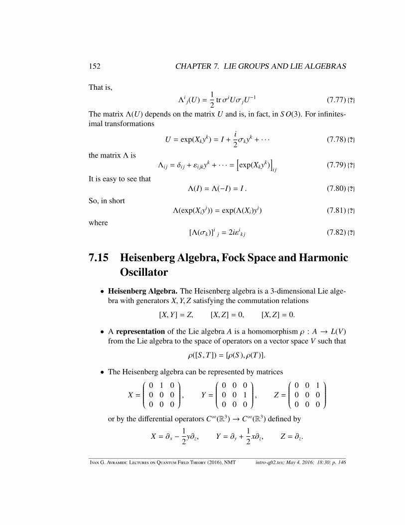
152 CHAPTER 7. LIE GROUPS AND LIE ALGEBRAS
That is,
Λij(U) =
12
trσiUσ jU−1 (7.77) ?
The matrix Λ(U) depends on the matrix U and is, in fact, in S O(3). For infinites-imal transformations
U = exp(Xkyk) = I +i2σkyk + · · · (7.78) ?
the matrix Λ isΛi j = δi j + εi jkyk + · · · =
[exp(Xkyk)
]i j
(7.79) ?
It is easy to see thatΛ(I) = Λ(−I) = I . (7.80) ?
So, in shortΛ(exp(Xiyi)) = exp(Λ(Xi)yi) (7.81) ?
where[Λ(σk)]i
j = 2iεik j (7.82) ?
7.15 Heisenberg Algebra, Fock Space and HarmonicOscillator
• Heisenberg Algebra. The Heisenberg algebra is a 3-dimensional Lie alge-bra with generators X,Y,Z satisfying the commutation relations
[X,Y] = Z, [X,Z] = 0, [X,Z] = 0.
• A representation of the Lie algebra A is a homomorphism ρ : A → L(V)from the Lie algebra to the space of operators on a vector space V such that
ρ([S ,T ]) = [ρ(S ), ρ(T )].
• The Heisenberg algebra can be represented by matrices
X =
0 1 00 0 00 0 0
, Y =
0 0 00 0 10 0 0
, Z =
0 0 10 0 00 0 0
or by the differential operators C∞(R3)→ C∞(R3) defined by
X = ∂x −12
y∂z, Y = ∂y +12
x∂z, Z = ∂z.
Ivan G. Avramidi: Lectures on Quantum Field Theory (2016), NMT intro-qft2.tex; May 4, 2016; 18:30; p. 146

7.15. HEISENBERG ALGEBRA, FOCK SPACE AND HARMONIC OSCILLATOR153
• Properties of the Heisenberg algebra
[X,Yn] = nZYn−1
[X, exp(bY)] = bZ exp(bY)
X exp (bY) = exp (bY) (X + bZ)
exp(−bY)X exp(bY) = X + bZ
X exp(−
12
Y2)
= exp(−
12
Y2)
(X − ZY)
[Y, Xn] = nZXn−1
[Y, exp(aX)] = −aZ exp(aX)
exp(aX)Y = (Y + aZ) exp(aX)
exp(aX)Y exp(−aX) = Y + aZ
exp(aX) exp(bY) = exp(abZ) exp(bY) exp(aX)
exp(−bY) exp(aX) exp(bY) = exp(abZ) exp(aX)
exp(aX) exp(bY) exp(−aX) = exp(abZ) exp(bY)
• Campbell-Hausdorff formula
exp(aX + bY) = exp(−
ab2
Z)
exp(aX) exp(bY)
= exp(ab2
Z)
exp(bY) exp(aX)
• Heisenberg group. The Heisenberg group is a 3-dimensional Lie groupwith the generators X,Y,Z.
• An arbitrary element of the Heisenberg group is parametrized by canonicalcoordinates (a, b, c) as
g(a, b, c) = exp(aX + bY + cZ)
Obviously,g(0, 0, 0) = I
and the inverse is defined by
[g(a, b, c)]−1 = g (−a,−b,−c)
Ivan G. Avramidi: Lectures on Quantum Field Theory (2016), NMT intro-qft2.tex; May 4, 2016; 18:30; p. 147

154 CHAPTER 7. LIE GROUPS AND LIE ALGEBRAS
• The group multiplication law in the Heisenberg group takes the form
g(a, b, c)g(a′, b′, c′) = g(a + a′, b + b′, c + c′ +
12
(ab′ − a′b))
• Notice that
g(a, b, c) = g(0, 0, c +
ab2
)g(0, b, 0)g(a, 0, 0)
• A representation of a Lie group G is a homomorphism ρ : G → Aut (V)from the group G to the space of invertible operators on a vector space Vsuch that for any g, h ∈ G
ρ(gh) = ρ(g)ρ(h)
andρ(g−1) = [ρ(g)]−1, ρ(e) = I
• Representations of the Heisenberg group.
• The elements of the Heisenberg group could be represented by the upper-triangular matrices. Notice that
X2 = Y2 = Z2 = XZ = YZ = 0
andXY = YX = Z
or 0 a c0 0 b0 0 0
2
=
0 0 ab0 0 00 0 0
, 1 a c
0 1 b0 0 1
3
= 0.
Therefore,
g(a, b, c) =
1 a c + ab0 1 b0 0 1
,Ivan G. Avramidi: Lectures on Quantum Field Theory (2016), NMT intro-qft2.tex; May 4, 2016; 18:30; p. 148

7.15. HEISENBERG ALGEBRA, FOCK SPACE AND HARMONIC OSCILLATOR155
• Another representation is defined by the action on functions in R3. Noticethat
exp(aX) f (x, y, z) = f(x + a, y, z −
a2
y)
exp(bY) f (x, y, z) = f(a, y + b, z +
a2
x)
exp(cZ) f (x, y, z) = f (x, y, z + c)
• Therefore,
g(a, b, c) f (x, y, z) = f(x + a, y + b, z + c +
b2
x −a2
y)
• Fock space.
• Let us define the operatorN = YX
• It is easy to see that
[N,Y] = ZY, [N, X] = −ZX.
• Suppose that there exists a unit vector v0 called the vacuum state such that
Xv0 = 0
• Let us define a sequence of vectors
vn =1√
n!Ynv0
• By using the properties of the Heisenberg algebra it is easy to show that
Yvn =√
n + 1 vn+1, n ≥ 0,Xvn =
√n Zvn−1, n ≥ 1
ThereforeNvn = n Zvn, n ≥ 0
Ivan G. Avramidi: Lectures on Quantum Field Theory (2016), NMT intro-qft2.tex; May 4, 2016; 18:30; p. 149

156 CHAPTER 7. LIE GROUPS AND LIE ALGEBRAS
• Let us define vectors
w(b) = exp(bY)v0 =
∞∑n=0
bn
√n!
vn
called the coherent states.
• Then by using the properties of the Heisenberg algebra we get
Xw(b) = bZw(b)
• Now, suppose thatY = X∗
andZ = I
• Then, the vectors vn are orthonormal
(vn, vm) = δnm
and are the eigenvectors of the self-adjoint operator
N = X∗X
with integer eigenvalues n ≥ 0.
• Then the spacespanvn | n ≥ 0
is called the Fock space and the operators X and X∗ are called the annihi-lation and creation operators and the operator N is called the operator ofthe number of particles.
• Note, also that the coherent states are not orthonormal
(w(a),w(b)) = eab
• Finally, we compute the trace of the heat semigroup operator
Tr exp(−tX∗X) =
∞∑n=0
e−tn =1
1 − e−t
Ivan G. Avramidi: Lectures on Quantum Field Theory (2016), NMT intro-qft2.tex; May 4, 2016; 18:30; p. 150

7.15. HEISENBERG ALGEBRA, FOCK SPACE AND HARMONIC OSCILLATOR157
• Harmonic oscillator. Let D be an anti-self-adjoint operator and Q be aself-adjoint operator satisfying the commutation relations
[D,Q] = I
• The harmonic oscillator is a quantum system with the (self-adjoint posi-tive) Hamiltonian
H = −12
D2 +12
Q2
• Then the operators
X =1√
2(D + Q), X∗ =
1√
2(−D + Q).
are the creation and annihilation operators.
• The operator of the number of particles is
N = X∗X = −12
D2 +12
Q2 −12
and, therefore, the Hamiltonian is
H = N +12
• The eigenvalues of the Hamiltonian are
λn = n +12
with the eigenvectors vn
• It is clear that the vectors
ψn(t) = e−itλnvn = exp[−it
(n +
12
)]1
2n/2√
n!(−D + Q)nv0
satisfy the equation(i∂t − H)ψn = 0
which is called the Schrodinger equation.
Ivan G. Avramidi: Lectures on Quantum Field Theory (2016), NMT intro-qft2.tex; May 4, 2016; 18:30; p. 151

158 CHAPTER 7. LIE GROUPS AND LIE ALGEBRAS
• The vacuum state is determined from the equation
(D + Q)v0 = 0
and has the form
v0 = exp(−
12
Q2)ψ0
with ψ0 satisfyingDψ0 = 0 .
• The heat trace (also called the partition function) for the harmonic oscilla-tor is
Tr exp(−tH) =1
2 sinh (t/2)
7.16 Operators on Finite-Dimensional Inner Prod-uct Spaces
• Let H be a finite-dimensional Hilbert space. Let n = dim H.
• Let ek, (k = 1, . . . , n), be a basis in H.
• Define the metric G = (gi j) by
gi j = (ei, e j)
• Then for any x =∑n
j=1 x je j and y =∑n
k=1 ykek
(x, y) = g jkx jyk ∗.
• The matrix G is non-degenerate, i.e.
det G , 0 .
• The metric is symmetric, i.e.
gi j = g ji, (or GT = G),
Ivan G. Avramidi: Lectures on Quantum Field Theory (2016), NMT intro-qft2.tex; May 4, 2016; 18:30; p. 152

7.16. OPERATORS ON FINITE-DIMENSIONAL INNER PRODUCT SPACES159
if the inner product is symmetric, that is ∀x, y ∈ H, (x, y) = (y, x), andHermitian, i.e.
gi j = g∗ji, (or GT = G∗, or G† = G),
where G† = GT∗, if the inner product is Hermitian, i.e. satisfies (x, y) =
(y, x)∗. In the latter case the inner product is linear in the first argument andanti-linear in the second argument.
• Define the inverse matrix G−1 = (gi j) by
n∑k=1
gikgk j = δij,
n∑k=1
gikgk j = δji .
or in matrix formGG−1 = I, G−1G = I,
where I = (δij) is the identity matrix.
• Consider a linear transformation of the basis
e′j =
n∑k=1
αkjek
where A = (αkj) is a nondegenerate matrix. In the matrix form this becomes
E′ = AT E,
where E = (e j) and E′ = (e′k) are column vectors and AT is the transposematrix.
The inverse transformation is given by
e j =
n∑k=1
βkje′k, E = A−1 T E′,
where A−1 = (βkj) is the inverse matrix.
Ivan G. Avramidi: Lectures on Quantum Field Theory (2016), NMT intro-qft2.tex; May 4, 2016; 18:30; p. 153

160 CHAPTER 7. LIE GROUPS AND LIE ALGEBRAS
• Then the metric G transforms according to
g′i j =
n∑k=1
n∑m=1
αkigkmα
mj
or in the matrix formG′ = ATGA.
The inverse metric G−1 transforms according to
g′i j =
n∑k=1
n∑m=1
βikgkmβ j
m
or in the matrix formG′−1 = A−1G−1A−1 T .
• The determinant of the metric transforms according to
det G′ = ( det A)2 det G.
• Let L : H → H be a linear operator. Then
Le j =
n∑k=1
Lkjek
with some Lkj. Multiplying by em we get
(Le j, em) =
n∑k=1
gkmLkj.
Thus,
Lkj =
n∑m=1
gmk(Le j, em)
• Let x ∈ H be a vector. Then
x =
n∑k=1
x je j
Ivan G. Avramidi: Lectures on Quantum Field Theory (2016), NMT intro-qft2.tex; May 4, 2016; 18:30; p. 154

7.16. OPERATORS ON FINITE-DIMENSIONAL INNER PRODUCT SPACES161
and
Lx =
n∑j=1
n∑k=1
(Lkjx j)ek
So, the operator L is completely described by the matrix L = (Lkj). If
X = (x j) is the column vector, then the action of the operator L on X is thecolumn vector LX.
• Under the transformation of the basis E′ = AT E, the matrix L of the operatorL transforms according to
L′k j =
n∑m=1
n∑i=1
βkiα
mjLi
m
or in the matrix formL′ = A−1LA.
• There is a one-to-one correspondence between the operators on H and then × n complex matrices.
• The trace of the operator L is defined by the trace of the matrix L,
tr L =
n∑k=1
Lkk .
• The determinant of the operator L is defined by the determinant of thematrix L,
det L = det (Lkj) .
• Since the trace is cyclic, tr (ABC) = tr (BCA) = tr (CAB), and the de-terminant is multiplicative, det (AB) = det (A) det (B), the trace and thedeterminant of the operator L do not depend on the basis,
tr L′ = tr L and det L′ = det L.
• The adjoint L† of the operator L is defined by
(L†x, y) = (x, Ly) ∀x, y ∈ H .
Ivan G. Avramidi: Lectures on Quantum Field Theory (2016), NMT intro-qft2.tex; May 4, 2016; 18:30; p. 155

162 CHAPTER 7. LIE GROUPS AND LIE ALGEBRAS
• An operator O : H → H is orthogonal if the inner product is symmetricand ∀x, y ∈ H
(Ox,Oy) = (x, y),
• An operator U : H → H is unitary if the inner product is Hermitian and∀x, y ∈ H
(Ux,Uy) = (x, y),
• The set of all operators on a vector space E is a vector space.
• The product AB of the operators A and B is the composition of A and B.
• Operators form an algebra.
Ivan G. Avramidi: Lectures on Quantum Field Theory (2016), NMT intro-qft2.tex; May 4, 2016; 18:30; p. 156

Part III
Physical Supplement
163


Chapter 8
Classical Field Theory
8.1 IntroductionIn these lectures we will use mostly the covariant spacetime approach to the fieldtheory developed mainly by De Witt [?, ?].
The basic object of any physical theory is the spacetime. We will denote it byM and assume that it is a d-dimensional manifold with the topological structure
M = I × Σ, (8.1) ?
where I is an open interval of the real line and Σ is some (d − 1)-dimensionalmanifold. Σ can be compact or noncompact. More precisely, we assume thespacetime to be a Riemannian manifold with a hyperbolic metric g of the signature(− + · · ·+) which admits a foliation of spacetime into spacelike sections identicalto Σ.
The points of the spacetime are denoted by x and local coordinates by xµ (µ =
0, 1, . . . , d − 1), x0 will be often denoted by t as well.
8.1.1 Superclassical fieldsLet us consider a set of some say real smooth differentiable functions over thespacetime
ϕA(x), A = 1, 2, . . . , p. (8.2) ?
If these functions transform according to some special rules under the transforma-tion of the coordinates, i.e., if they form a representation of the diffeomorphismgroup they are said to be a classical field.
165

166 CHAPTER 8. CLASSICAL FIELD THEORY
This can be formulated in a more mathematical language. Let us consider avector bundle Vc(M) over the spacetime M each fiber of which is a vector spaceVc, on which the Lorentz group O1(1, d − 1), subscript 1 denoting the componentof O(1, d − 1) containing the identity, acts. The sections of this vector bundle arecalled classical tensor fields. They do not need to be irreducible representationsof the Lorentz group. In general, the bundle Vc(M) is the direct sum of all bundleswith sections being irreducible tensor representations of Lorentz group.
These tensor fields are represented by their components, which form a set ofsmooth differentiable functions on the spacetime manifold
ϕ : M → Rp, (8.3) ?
p = dim Vc being the dimension of the corresponding vector space.The label A denotes the collection of all possible discrete indices that label the
tensor product of irreducible representations.We will always suppose that there exists also spin structure on the spacetime
manifold M, i.e., that the second Stiefel-Whitney class of M vanishes, and thereis an associated vector bundle Va(M), each fibre of which is a complex vectorspace Va, on which the spin group S pin1(1, d − 1), i.e. the covering group ofLorentz group, acts. The sections of this bundle are called spinor fields. Thebundle Va(M) we consider is, in general, the direct sum of all spin-tensor bundles,having the sections as spin-tensor fields.
One of the most important theorems in quantum field theory is the theo-rem about the connection of the spin and statistics. It states that there is a cru-cial difference between the tensor fields and spin-tensor fields. All tensor fieldshave bosonic statistics and are called boson fields and the spin-tensor fields havefermionic statistics and are called fermion fields.
In QFT the classical fields become Hermitian operators on a Hilbert space.The boson fields satisfy some commutation relations and the fermion ones – theanticommutation relations
[B1, B2] = ~ · · · , [F1, F2]+ = ~ · · · , [B, F] = 0. (8.4) ?
where B and F denote some boson and fermion fields, [, ] and [, ]+ are the com-mutator and the anticommutator.
That is why in the classical limit ~ → 0 of QFT the boson fields are assumedto commute with each other and with the fermion fields
B1B2 = B2B1, (8.5) 1.16
Ivan G. Avramidi: Lectures on Quantum Field Theory (2016), NMT intro-qft2.tex; May 4, 2016; 18:30; p. 157

8.1. INTRODUCTION 167
BF = FB, (8.6) ?1.17?
However, the fermion fields in the classical limit should be taken to anticommutewith each other
F1F2 = −F2F1. (8.7) 1.18
It is clear that the product of two (and, hence, of any even number) of fermionfields is a boson field.
We do not restrict ourselves only to boson or fermion fields. The set ϕA con-tains both boson and fermion fields. Such sets of the boson and fermion fields arecalled super fields.
To deal with the collection of the boson and fermion fields we define the parityε(ϕA) of the field component ϕA by
ε(A) ≡ ε(ϕA) =
0, if ϕA is bosonic1, if ϕA is fermionic. (8.8) ?
Then commutation relations (8.5) — (8.7) can be written in a closed form
ϕAϕB = (−1)ε(A)ε(B)ϕBϕA (8.9) 1.19
or[ϕA, ϕB]s = ϕAϕB − (−1)ε(A)ε(B)ϕBϕA = 0. (8.10) 1.20
This is called supercommutator. To simplity the notation one can adopt the con-vention that an index or symbol appearing in an exponent of (−1) is to be un-derstood as assuming the value 0 or 1 according as the associated quantity isfermionic or bosonic and replace ε(A)→ A .
The variables ϕA satisfying the conditions (8.9) are called the Grassmanianvariables or supernumbers. They are said to form a Grassmanian algebra ΛD
of dimension D. Thus the fields ϕA(x) at a fixed point x ∈ M generate a finitedimensional Grassmanian algebra, ΛD, the fermion fields being the odd elementsof it and the boson fields the even ones. If we include the values of the fields at allthe points x ∈ M, then we have infinitely dimensional Grassmanian algebra Λ∞.Therefore
ϕ : M → Λ∞. (8.11) ?
The classical fields satisfying the commutation (8.10) relations are called super-classical fields. That is why the starting point of QFT is not just the classical fieldtheory but rather the superclassical field theory.
Ivan G. Avramidi: Lectures on Quantum Field Theory (2016), NMT intro-qft2.tex; May 4, 2016; 18:30; p. 158

168 CHAPTER 8. CLASSICAL FIELD THEORY
8.1.2 Field configurations
A field configuration is defined to be the set of all ϕA(x) for all x
ϕ = ϕA(x) : x ∈ M, A = 1, . . . ,D. (8.12) ?
To present this idea in a more visual way we will use the condensed notationof De Witt. In this notation the discrete index A and the spacetime point x arecombined in one lable i ≡ (A, x)
ϕi ≡ ϕA(x). (8.13) ?
The field ϕi becomes then an infinite-dimensional (continuous) column , i.e., acontravariant vector, the product of two fields, ϕiϕk, and, in general, any quantitywith two upper indices like Gik becomes infinite-dimensional matrix (tensor)
Gik = GAB(x, y), i ≡ (A, x); k ≡ (B, y) (8.14) ?
and so on. Intuitively one can use a finite-dimensional analogy. Let MN be alattice (a finite subset of points) in M
MN = xa, a = 1, . . . ,N; xa ∈ M ⊂ M. (8.15) ?
Then i = 1, . . . ,D×N and ϕi becomes a D×N finite-dimensional column (vector)
ϕi =
ϕ1(x1)...
ϕ1(xN)...
ϕD(x1)...
ϕD(xN)
. (8.16) ?
Thus the field configuration is just the set of the values of the field in all pointsof the manifold. The matrix Gik should be viewed on as a (D × N) × (D × N) -
Ivan G. Avramidi: Lectures on Quantum Field Theory (2016), NMT intro-qft2.tex; May 4, 2016; 18:30; p. 159

8.1. INTRODUCTION 169
dimensional matrix
G11(x1, x1) . . . G11(x1, xN) . . . G1D(x1, x1) . . . G1D(x1, xN)...
......
...G11(xN , x1) . . . G11(xN , xN) . . . G1D(xN , x1) . . . G1D(xN , xN)
......
. . ....
...
GD1(x1, x1) . . . GD1(x1, xN) . . . GDD(x1, x1) . . . GDD(x1, xN)...
......
...GD1(xN , x1) . . . GD1(xN , xN) . . . GDD(xN , x1) . . . GDD(xN , xN)
(8.17) ?
Further, as usual it will be always assumed that a summation over repeatedindices is performed. That is in condensed notation — a combined summation-integration, i.e.
Jϕ ≡ Jiϕi ≡
∫M
dx JA(x)ϕA(x) (8.18) ?
Thus one can formally consider such objects, as the traces and the determinantsof the infinite-dimensional matrices.
The next object that is used extensively in QFT is the configuration spaceM.Configuration space is the set of all possible field configurations
M =ϕi
. (8.19) ?
One can show that the configuration space in an infinite-dimensional supermani-fold.
8.1.3 Field functionalsA supernumber-valued function S (ϕ) on the configuration space with
S (ϕ) :M→ Λ∞ (8.20) ?
is called a field functional. Functions on supermanifolds are defined by the formalpower series in fermion fields. Denoting the boson fields by χ and the fermionfields by ψ, i.e.
ϕ =
(χψ
), (8.21) ?
one can write
Ivan G. Avramidi: Lectures on Quantum Field Theory (2016), NMT intro-qft2.tex; May 4, 2016; 18:30; p. 160

170 CHAPTER 8. CLASSICAL FIELD THEORY
S (ϕ) =∑n≥0
fa1...an(χ)ψan · · ·ψa1
≡∑n≥0
∫dx1 · · · dxn fA1···An(χ; x1 . . . xn)ψAn(xn) · · ·ψA1(x1),
(8.22) ?
where ai ≡ (Ai, xi), with the spinor index Ai running over Ai = 1, . . . , q for someq < D. From the anticommutativity of the fermion fields it is clear that fa1...an(χ)are antisymmetric in all their indices. These are infinite-dimensional p-forms onsupermanifoldM.
The functional derivatives of the field functionals are defined as follows. Letus consider an infinitesimal variation
δϕi ≡ δϕA(x) ∈ C∞(M). (8.23) ?
The set of all points of spacetime where δϕi is not equal to zero is called thesupport of δϕi
Ω ≡ supp δϕi =x ∈ M, δϕA(x) , 0
, (8.24) ?
δϕA = 0 for x < Ω. (8.25) ?
We assume that δϕi has a compact support
Ω ⊂ M. (8.26) ?
Let δS (ϕ) denote the corresponding change in S (ϕ). If for all ϕ ∈ M and allδϕ ∈ C∞(M) with compact support, δS (ϕ) can be written in the form
δS (ϕ) = δϕii,S (ϕ) = S ,i(ϕ)δϕ
=
∫M
dx δϕA(x)
→
δ
δϕA(x)S (ϕ)
=
∫M
dx
S (ϕ)←
δ
δϕA(x)
δϕA(x),
(8.27) ?
where the coefficients
i,S ≡→
δ
δϕi S ≡→
δ
δϕA(x)S , (8.28) ?
Ivan G. Avramidi: Lectures on Quantum Field Theory (2016), NMT intro-qft2.tex; May 4, 2016; 18:30; p. 161

8.1. INTRODUCTION 171
S ,i ≡ S←
δ
δϕi ≡ S←
δ
δϕA(x)(8.29) ?
are independent on the δϕi, then the S (ϕ) is called differentiable functional on Mand i,S and S ,i are called the left and the right functional derivatives.
Now consider some finite variation hi and the value of the functional S (ϕ) atthe point ϕ + h. At a regular point ϕ it can be expanded in the functional Taylorseries
S (ϕ + h) def= S (ϕ) + S ,i(ϕ)hi +
12
S ,ik(ϕ)hkhi + · · ·
=∑n≥0
1n!
S ,i1...in(ϕ)hin · · · hi1 , (8.30) ?
where all variations are moved to the right.The coefficients of this series are called the higher right functional derivatives
S ,i1...in = S←
δn
δϕi1 · · · δϕin. (8.31) ?
Since the superfields ϕi do not commute, the order of variation in Taylor seriesis important. By rewriting it in the form
S (ϕ + h) =∑n≥0
1n!
hi1 · · · hinin...i1,
S (ϕ), (8.32) ?
we define the higher left functional derivatives
in...i1,S ≡
→
δn
δϕin · · · δϕi1S . (8.33) ?
In the usual notation the term of second order in this series looks more complicated
S ,ikhkhi ≡
∫dx dy
S (ϕ)
←
δ2
δϕA(x)δϕB(y)
hB(y)hA(x). (8.34) ?
Changing the order of variations it is easy to find the relation between the left andright derivatives. If the functional S itself is even (bosonic), i.e., ε(S ) = 0, then
S ,i = (−1)ii,S (8.35) ?
Ivan G. Avramidi: Lectures on Quantum Field Theory (2016), NMT intro-qft2.tex; May 4, 2016; 18:30; p. 162

172 CHAPTER 8. CLASSICAL FIELD THEORY
In general
S←
δ
δϕi = (−1)i(1+ε(S ))
→
δ
δϕi S , (8.36) ?
where ε(S ) is the parity of functional S . Besides
···ik··· ,S = (−1)ik···ki··· ,S (8.37) ?
S , ···ik··· = (−1)ikS , ···ki··· (8.38) ?
In other words one has→
δ
δϕi
→
δ
δϕk = (−1)ik
→
δ
δϕk
→
δ
δϕi , (8.39) ?
←
δ
δϕi
←
δ
δϕk = (−1)ik
←
δ
δϕk
←
δ
δϕi . (8.40) ?
From these equations it follows, that the mixed left-right second derivative of aneven functional possesses the following symmetry relation
i,S ,k = (−1)i+k+ikk,S ,i. (8.41) ?
A matrix with down indices satisfying such a relation will be called supersymmet-ric. This name is because the bilinear form
ηEh ≡ ηiEikhk, (8.42) ?
where Eik is a supersymmetric matrix with parity determined only by its indices,ε(Eik) = ε(i) + ε(k), is symmetric.
If we write a supersymmetric matrix E in the block form
(Eik) =
(A BC D
), (8.43) ?
where A and D are bose-bose and fermi-fermi sectors (and, therefore, even) andB and C are the mixed bose-fermi and fermi-bose ones (and, hence, odd), thenthe supersymmetry means that the matrices A and D are symmetric and B and Csatisfy the relations
AT = A, DT = D, (8.44) ?
BT = −C. (8.45) ?
Ivan G. Avramidi: Lectures on Quantum Field Theory (2016), NMT intro-qft2.tex; May 4, 2016; 18:30; p. 163

8.1. INTRODUCTION 173
Example 1. The simplest functional is the field itself. The derivative of it isdefined by
δϕi = ϕi,kδϕ
k = δϕkk,ϕ
i, (8.46) ?
or
δϕA(x) =
∫dy
ϕA(x)←
δ
δϕB(y)
δϕB(y) =
∫dyδϕB(y)
→
δ
δϕB(y)ϕA(x)
(8.47) ?
Thereforeϕi,k = δi
k, k,ϕi = δi
k, (8.48) ?
whereδi
k = δABδ(x, y) (8.49) ?
is infinite-dimensional Kronecker symbol (continuous identity matrix). We alsohave obviously the super commutation rule
→
δ
δϕi ϕk = (−1)ikϕk
→
δ
δϕi + δki . (8.50) ?
Similary, for any linear functional
S = Jiϕi (8.51) ?
we getS ,i = Ji. (8.52) ?
Example 2. Consider now a quadratic functional.
S =12ϕiEikϕ
k (8.53) ?
where E is a supersymmetric matrix
Eik = (−1)k+i+ikEki. (8.54) ?
We calculateδS =
12ϕiEikδϕ
k +12δϕiEikϕ
k = ϕiEikδϕk. (8.55) ?
ThereforeS ,k = ϕiEik. (8.56) ?
Ivan G. Avramidi: Lectures on Quantum Field Theory (2016), NMT intro-qft2.tex; May 4, 2016; 18:30; p. 164

174 CHAPTER 8. CLASSICAL FIELD THEORY
FurtherδS ,k = δϕiEik = (−1)kEkiδϕ
i. (8.57) ?
HenceS ,ki = (−1)kEki, (8.58) ?
i,S ,k = Eik. (8.59) ?
Thus using the functional differentiation one can define the concept of tangentspaces and generalize, at least formally, almost the whole structure of differentialgeometry to the infinite-dimensional supermanifold. In particular, introducing asupersymmetric nondegenerate matrix Eik(ϕ) that depends only on the values ofthe fields but not on their derivatives and is diagonal in the continuous part,
Eik(ϕ) = EAB(ϕ(x))δ(x, y), (8.60) ?
one can define the ultra-local Riemannian metric on the supermanifoldM by
E = dϕiEik(ϕ)dϕk
=
∫M
dxdϕA(x)EAB(ϕ(x))dϕB(x). (8.61) ?
This gives the interval between two field configurations ϕ and ϕ + dϕ. Then onecan define formally the connections, geodesics, curvature etc.
Example 3. Now, let us consider a special class of functionals, namely, localfunctionals. These are functionals which depend on the values of the fields andfinite number of their derivatives.
The local functionals have the following form
S (ϕ) =
∫M
dxL(ϕ, ϕ,µ, . . . , ϕ,µ1...µN ) (8.62) ?
whereϕ,µ ≡ ∂µϕ, (8.63) ?
ϕ,µ1...µN ≡ ∂µ1 · · · ∂µNϕ, (8.64) ?
Ivan G. Avramidi: Lectures on Quantum Field Theory (2016), NMT intro-qft2.tex; May 4, 2016; 18:30; p. 165

8.1. INTRODUCTION 175
and L is some function of the fields derivatives on one spacetime point. It is notdifficult to calculate the functional derivative of local functionals. We calculate
S (ϕ + δϕ) = S (ϕ) +
∫dx
δϕA
→
∂L
∂ϕA + δϕA,µ
→
∂L
∂ϕA,µ
+ · · ·
=
= S (ϕ) +
∫dxδϕA
→
∂L
∂ϕA − ∂µ
→
∂ L
∂ϕA
+ · · ·
(8.65) ?
where the dots contain the similar terms with higher derivatives of ϕ. Thus weobtain the Euler-Lagrange formula
i,S ≡
→
δSδϕA(x)
=
→
∂ L
∂ϕA(x)− ∂µ
→
∂ L
∂ϕA,µ
+ · · ·
=
→
∂L
∂ϕA(x)+
N∑n=1
(−1)n∂µ1 · · · ∂µn
→
∂ L
∂ϕA,µ1...µn
(8.66) ?
Thus, the functional derivative of any local functional is given by
i,S ≡→
δ
δϕA(x)S ≡
→
D
DϕA(x)L(x), (8.67) ?
where→
D
DϕA =
→
∂
∂ϕA +∑n≥1
(−1)n∂µ1 · · · ∂µn
→
∂
∂ϕA,µ1...µn
(8.68) ?
Similarly,
S ,i ≡ S←
δ
δϕA(x)≡ L(x)
←
D
DϕA(x). (8.69) ?
The functional derivative of a local functional is obviously again a local functional
i,S ≡→
δ SδϕA(x)
=
→
D
DϕA(x)L(x) =
∫dy δ(x, y)
→
DL(y)DϕA(y)
. (8.70) ?
Thus the second derivative is simply given by
i,S ,k ≡
→
δ
δϕA(x)S
←
δ
δϕB(y)=
→
D
DϕA(y)(L(y)δ(x, y))
←
D
DϕB(y). (8.71) ?
Ivan G. Avramidi: Lectures on Quantum Field Theory (2016), NMT intro-qft2.tex; May 4, 2016; 18:30; p. 166

176 CHAPTER 8. CLASSICAL FIELD THEORY
Therefore, the first derivative is a usual function on M but the second derivative isa distribution. It is easy to see that the second derivative is actually the kernel ofa differential operator of order 2N. For the functionals that include only the firstderivatives of the fields the second functional derivative looks like
∆ik ≡ i,S ,k =
(−∂µAµν
AB∂ν +12
(Bµ
AB∂µ + ∂µBµAB
)−CAB
)δ(x, y), (8.72) ?1.71?
where
AµνAB ≡
12
→
∂
∂ϕA,µ
L
←
∂
∂ϕB,ν
+
→
∂
∂ϕA,ν
L
←
∂
∂ϕB,µ
, (8.73) ?1.72?
BµAB ≡
→
∂
∂ϕAL
←
∂
∂ϕB,µ
−
→
∂
∂ϕA,µ
L
←
∂
∂ϕB
+12∂ν
→
∂
∂ϕA,µ
L
←
∂
∂ϕB,ν
−
→
∂
∂ϕA,ν
L
←
∂
∂ϕB,µ
, (8.74) ?
CAB ≡ −
→
∂
∂ϕAL
←
∂
∂ϕB +12∂µ
→
∂
∂ϕAL
←
∂
∂ϕB,µ
+
→
∂
∂ϕA,µ
L
←
∂
∂ϕB
. (8.75) ?
For real functional S (ϕ) and real ϕi the matrices A and C are supersymmetricand the matrix B is antisupersymmetric, and possess the following reality (super-Hermitian) relations
AµνAB = Aνµ
AB = (−1)A+B+ABAµνBA = (−1)A+B+ABAµν ∗
AB , (8.76) ?
BµAB = −(−1)A+B+ABBµ
BA = (−1)A+B+ABBµ ∗AB, (8.77) ?
CAB = (−1)A+B+ABCAB = (−1)A+B+ABC ∗AB. (8.78) ?
Recalling that ∂+µ = −∂µ it follows from these properties that the operator ∆ is self-
adjont ∆+ = ∆. This is the consequence of the symmetry and reality properties ofthe functional differentiation.
8.1.4 DynamicsThe fundamental assumption of the field theory is that any dynamical system canbe described by an action functional. This means that the nature and dynamical
Ivan G. Avramidi: Lectures on Quantum Field Theory (2016), NMT intro-qft2.tex; May 4, 2016; 18:30; p. 167

8.1. INTRODUCTION 177
properties of the system are completely determined by the action functional. Theaction functional is a differentiable real-valued even supernumber-valued scalarfield on the configuration space
S :M→ Rc, (8.79) ?
where Rc is the set of all real even supernumbers. The choice of dynamical vari-ables, i.e., the fields ϕi, used to describe the system is not unique. Consequently,the configuration spaceM, i.e., the set of all possible field configurations, is alsonot unique. It depends on the choice of the dynamical variables ϕi (i.e., on theparametrization of the dynamical system) and on the boundary conditions im-posed at the time limits (and at spatial infinity if
∑is noncompact). Analogously,
the choice of the action functional is not unique.However, for a given dynamical system all action functionals describe the
same physics, i.e., they must give physically equivalent sets of the dynamical fieldconfigurations. The dynamical field configurations are defined as the field config-urations satisfying the stationary action principle: physically admissible valuesfor dynamical variables are those for which the action is stationary under smalldisturbances with given boundary conditions
δS = 0. (8.80) ?
In other words, the dynamical field configurations must satisfy the dynamicalequations of motion
δSδϕi = 0 (8.81) ?
with given boundary conditions. The set of all dynamical field configurationsM0
is a subspace of the configuration spaceM0 ⊂ M which is called the dynamicalsubspace. In QFT it is often called the mass shell.
In the local field theory the dynamical equations are local partial differentialequations. This means that the action is a local functional
S (ϕ) =
∫Ω
dxL(ϕ, ∂ϕ, . . .), (8.82) ?
where Ω ⊂ M is the region of spacetime which we are interested in from thedynamical point of view and L called the Langrangian is a scalar density of unitweight. The whole setting of the problem is illustrated on the Fig. 8.1.
Ivan G. Avramidi: Lectures on Quantum Field Theory (2016), NMT intro-qft2.tex; May 4, 2016; 18:30; p. 168

178 CHAPTER 8. CLASSICAL FIELD THEORY
6
Past
tin
tout
Future
Bin(ϕ) = 0
in-region
Bout(ϕ) = 0
out-region
δSδϕ
= 0
Ω
Σin
Σout
Σ∞
B∞(ϕ) = 0
Figure 8.1: Dynamics〈dynamics〉
In simple cases the region Ω is just
Ω = (tin, tout) × Σ (8.83) ?
and∂Ω = Σin ∪ Σout ∪ Σ∞, (8.84) ?
where Σ∞ = (tin, tout) × ∂Σ. Besides, in the usual scattering problems of QFT onetakes tin and tout first finite but at the very end of calculations let them go to infinity
t inout→ ∓∞. (8.85) ?
8.2 Models in field theoryLet us list some simple field theoretical models.
Ivan G. Avramidi: Lectures on Quantum Field Theory (2016), NMT intro-qft2.tex; May 4, 2016; 18:30; p. 169

8.2. MODELS IN FIELD THEORY 179
Scalar fields. First of all, a system of scalar fields ϕA, (A = 1, . . . ,D), interact-ing with gravitational and vector gauge fields is described by
S ϕ =
∫M
dx g1/2−
12
gµνδAB∇µϕA∇νϕ
B −12
(m2 + ξR)δABϕAϕB − V(ϕ)
, (8.86) ?
where gµν is the metric of the spacetime, g = detgµν,
∇µϕA =
(∂µδ
AB + Aa
µTA
a B
)ϕB (8.87) ?
is the covariant derivative, Aaµ, (a = 1, . . . , p) are the vector gauge fields, Ta =
(T Aa B) are the generators of the Lie algebra of the gauge group
[Ta,Tb] = CcabTc, (8.88) ?
Ccab are the structure constants, m2 is the mass parameter, ξ is the coupling con-
stant to gravity, R is the scalar curvature, and V(ϕ) is a potential for the scalarfields, that does not depend on the derivatives of the fields ϕ.
A more complicated system of scalar fields is the so called nonlinear σ-model
S σ = −12
∫M
dxg1/2gµνEAB(ϕ)∇µϕA∇νϕB, (8.89) ?
where EAB(ϕ) is a local function of the scalar fields.
Yang-Mills fields. The system of vector gauge fields Aaµ in curved spacetime is
described by the Yang-Mills Lagrangian
S Y M = −1
4e2
∫M
dx g1/2gµαgνβδabFaµνF
bαβ (8.90) ?
where e is the coupling constant
Faµν = ∂µAa
ν − ∂νAaµ + Ca
bcAbµAc
ν (8.91) ?
is the field strength of the gauge fields and Cabc are the structure constants of a
simple compact Lie group.
Ivan G. Avramidi: Lectures on Quantum Field Theory (2016), NMT intro-qft2.tex; May 4, 2016; 18:30; p. 170

180 CHAPTER 8. CLASSICAL FIELD THEORY
Gravity. The gravitational field is described by the metric tensor of the space-time gµν. The simplest Lagrangian is the Einstein-Hilbert one
S EH =1
16πG
∫M
dx g1/2(R − 2Λ), (8.92) ?
where G is the Newtonian gravitational constant and Λ is the cosmological con-stant. This is the only covariant action that leads to the equation of motion ofsecond order. One can, however, consider more complicated gravitational La-grangians
S R+R2 =
∫M
dx g1/2−
12 f 2 CµναβCµναβ +
16ν2 R2 +
116πG
(R − 2Λ), (8.93) ?
where Cµναβ is the Weyl tensor, f is the tensor coupling constant and ν — theconformal one. This Lagrangian leads to equations of motion of fourth order.That is why this model is also called the higher-derivative gravity. One of thecrucial difference between the sigma-model and gravity on the one side and othermodels on the other side is that the coefficient in front of the derivatives of thefields does depend on the fields, whereas for S ϕ, S Y M it does not. As we willsee in further lectures, this coefficient determines the Riemannian metric of theconfiguration manifoldM. That is for the scalar fields and Yang-Mills fields thismetric is constant, i.e., does not depend on the fields. Therefore, the correspondingRiemannian curvature vanishes, i.e., the configuration space is, in fact, flat. Forthe σ-model and gravity this is not the case. The configuration space metric isnot constant, and, hence, the configuration space is curved. This causes seriousdifficulties in quantizing these theories.
Spinor fields. All the previous models were bosonic. Let us also write down aLagrangian describing a system of spinor fields ψA (which are fermionic) interact-ing with gravitational and Yang-Mills fields
S ψ =
∫M
dx g1/2ψAδAB
(iγµ∇µ − m
)ψB. (8.94) ?
Hereγµ = ea
µγa, (8.95) ?
Ivan G. Avramidi: Lectures on Quantum Field Theory (2016), NMT intro-qft2.tex; May 4, 2016; 18:30; p. 171

8.3. SMALL DISTURBANCES AND GREEN FUNCTIONS 181
γa are the Dirac 2[d/2] × 2[d/2] matrices, satisfying the anticommutation relations
γaγb + γbγa = 2gab, (8.96) ?
with gab = diag (−1, 1, . . . , 1), and eaµ are the 1-forms of the local Lorentz frame
satisfying the relationsgµν = gabea
µebν, (8.97) ?
ψ is the Dirac conjugate spinorψ = ψ+η, (8.98) ?
where η is the matrix of charge conjugation defined by
γ+µ = −ηγµη
−1. (8.99) ?
The covariant derivative of spinor fields is defined by
∇µψA =
(∂µδ
AB +
12ωab
µγabδAB + Aa
µTAa B
)ψB, (8.100) ?
where γab = γ[aγb], ωabµ is the so called spinor connection
ωabµ =
12
gaceνc(ebν,µ − eb
µ,ν
)−
12
gbceνc(eaν,µ − ea
µ,ν
)+
12
gaegb f gcdeνeeσf ed
µ
(ecν,σ − ec
σ,ν
), (8.101) ?
and eµa is the dual basis of contravariant vectors
eaµe
µb = δa
b, eµaeaν = δµν . (8.102) ?
8.3 Small disturbances and Green functionsLet us consider the equations of motion
i,S =δSδϕi = 0. (8.103) ?
They are, in general, complicated nonlinear partial differential equations. Letϕi be a solution of equations of motion and let us look for another solution in
Ivan G. Avramidi: Lectures on Quantum Field Theory (2016), NMT intro-qft2.tex; May 4, 2016; 18:30; p. 172

182 CHAPTER 8. CLASSICAL FIELD THEORY
the neighborhood of ϕ, of the form ϕ + δϕ, where δϕi is an infinitesimal field.Substifing ϕ + δϕ in the equations of motion
i,S (ϕ + δϕ) = i,S (ϕ) + i,S , j(ϕ)δϕ j + · · · = 0 (8.104) ?
and limiting ourselves to the quantities of the first order we get
∆i jδϕj = 0, (8.105) ?
where∆i j = i,S , j (8.106) ?
This is the homogeneous equation of small disturbances. Its solutions are knownas Jacobi fields. In practice it is convenient to introduce infinitesimal externalsources δJi which cause the small disturbances. Let the action suffer the followingchange
S (ϕ)→ S (ϕ) + δJiϕi. (8.107) ?
Then the equations of motion for the disturbed system becomes
i,S (ϕ) = −δJi. (8.108) ?
In the first order, the solution of these equation of motion is
ϕi + δϕi, (8.109) ?
where ϕ is the solution ofi,S (ϕ) = 0 (8.110) ?
and δϕi is the solution of the equation
∆i j(ϕ)δϕ j = −δJi. (8.111) ?
This is called the inhomogeneous equation of small disturbances. Its general so-lution is the sum of a particular solution and an arbitrary Jacobi field.
8.4 WronskianAs we have seen for the local theory without higher derivatives the operator ofsmall disturbances is a differential operator of second order and has the form
∆ik = ∆AB(x, ∂)δ(x, y) (8.112) ?
Ivan G. Avramidi: Lectures on Quantum Field Theory (2016), NMT intro-qft2.tex; May 4, 2016; 18:30; p. 173

8.4. WRONSKIAN 183
∆AB(x, ∂) =
−∂µAµν
AB∂ν +12
(Bµ
AB∂µ + ∂µBµAB
)−CAB
. (8.113) ?
and is formally self-adjoint, i.e., the matrices Aµν and C are supersymmetric
AµνAB = (−1)A+B+ABAµν
AB, AµνAB = Aνµ
AB, (8.114) ?
CµAB = (−1)A+B+ABCµ
BA (8.115) ?
and Bµ is antisupersymmetric
BµAB = −(−1)A+B+ABBµ
BA. (8.116) ?
Besides, for real fields the matrices are super-Hermitian
AµνAB = (−1)A+B+BAAµν ∗
AB etc. (8.117) ?
The operator ∆ acts on the fields according to
∆ikhk =
∫dy∆AB(x, ∂)δ(x, y)hB(y) = ∆AB(x, ∂)hB(x). (8.118) ?
hi∆ik =
∫dyhA(y)∆AB(y, ∂)δ(y, x) = hA(x)∆AB
(x,−
←
∂
). (8.119) ?
On the other hand
hi∆ik = (−1)k∆kihi = (−1)B∆BA(y, ∂)hA(y), (8.120) ?
∆BA(y, ∂)hA = (−1)BhA∆AB
(y,−
←
∂
). (8.121) ?
The formally adjoint operator is
∆+AB(x, ∂) = ∆∗BA(x,−∂) = −∂µAµν ∗
BA ∂ν −12
(Bµ∗
BA∂µ + ∂µBµ∗BA
)−C∗BA (8.122) ?
Let us consider a bilinear form
I(g, h) ≡ gi(∆ikhk
)−
(gi∆ik
)hk
=
∫Ω
dx gA(∆AB
(x,→
∂
)− ∆AB
(x,−
←
∂
))hB, (8.123) ?
where Ω is a compact region of spacetime M with smooth boundary ∂Ω.
Ivan G. Avramidi: Lectures on Quantum Field Theory (2016), NMT intro-qft2.tex; May 4, 2016; 18:30; p. 174

184 CHAPTER 8. CLASSICAL FIELD THEORY
For the second order operators this can be shown to be
I(g, h) =
∫Ω
dx ∂µ(gA
↔
WµAB hB
)=
∫∂Ω
dΣµgA↔
WµAB hB (8.124) ?
where↔
WµAB= −Aµν
AB
→
∂ν +←
∂ν AµνAB + Bµ
AB (8.125) ?
is called Wronskian operator associated with ∆.For the operator ∆ to be self-adjoint this antisymmetric bilinear form must
vanish. This means that formally self-adjoint operator is self-adjoint indeed onthe fields satisfying such boundary conditions that this surface integral vanishes.(For example Dirichlet).
8.5 Retarded and advanced Green functionsLet us consider now the inhomogeneous equation of small disturbances
∆ikδϕk = −δJi. (8.126) 1.132
Suppose that ∆ is a nonsingular differential operator, i.e., with some boundaryconditions the solution of this equation exists and is unique.
This is not the case in the field theories with local gauge symmetries, such asYang-Mills theory and gravity. We will deal with such theories in the further lec-tures. Anyway after imposing the corresponding supplementary gauge conditionsthe operator ∆ becomes non-singular in these theories too.
The solution of the equation (8.126) can be expressed then in terms of Greenfunctions
δϕi = Gi jδJ j =
∫Ω
dy GAB(x, y)δJB(y), (8.127) ?
where Gi j is the Green function, i.e., the solution of the equation
∆ikGk j = −δji (8.128) ?
with some boundary conditions.In classical field theory one considers the retarded and advanced boundary
conditions, i.e.,δϕ+|Σout = 0, (8.129) ?
Ivan G. Avramidi: Lectures on Quantum Field Theory (2016), NMT intro-qft2.tex; May 4, 2016; 18:30; p. 175

8.5. RETARDED AND ADVANCED GREEN FUNCTIONS 185
δϕ−|Σin = 0. (8.130) ?
That is the retarded G−i j and advanced G+i j Green functions satisfy the followingboundary conditions
G−i j = 0 if i < j,G+i j = 0 if i > j. (8.131) ?
Here i < j (i > j) means that the time ti associated with the index i lies to the past(future) of the time t j associated with the index j.
Consequently, G−i j(G+i j) is nonvanishing only when the spacetime point xi
associated with i lies on or inside the future (past) light cone emanating from thespacetime point x j associated with j.
Future light cone
Past light coneThe self-adjointness of ∆ gives rise to simple relations between the retarded
and the advanced Green functions. One can show that
G±i j = (−1)i jG∓ ji. (8.132) ?
This is called reciprocity relations. The derivation is
0 = (−1)ikG−ik[∆ke − (−1)k+e+ke∆ek
]G+e j
= −(−1)i jG− ji − (−1)e(i+1)∆ekG−kiG+e j
= −(−1)i jG− ji + G+i j. (8.133) ?
Using the advanced and retarded Green functions one can define other Greenfunctions. First one can define a specific solution of the homogeneous equation ofsmall disturbances
Gi j def= G+i j −G−i j. (8.134) ?
Ivan G. Avramidi: Lectures on Quantum Field Theory (2016), NMT intro-qft2.tex; May 4, 2016; 18:30; p. 176

186 CHAPTER 8. CLASSICAL FIELD THEORY
By definition it is antisupersymmetric
Gi j = −(−1)i jG ji. (8.135) ?
This function satisfies obviously
∆ikGk j = 0 (8.136) ?
and is called Pauli-Jordan (sometimes also Schwinger) supercommutator function.It will give the supercommutator of linear field operators in quantum theory[
ϕi, ϕ j]
s= i~Gi j (8.137) ?
It is clear that G(x, y) is nonvanishing only inside the light cone emanating fromthe point y.
This means that for two spacetime points x and y which are separated by aspacelike interval the field operators (super) commute. That is there are no physi-cal correlations between the fields in such points. This must be so in any reason-able field theory because of the causality principle — the information cannot betransferred faster than light.
8.6 Cauchy problem for Jacobi fieldsThe supercommutator function gives the solution of the Cauchy problem for theJacobi fields:
∆ikδϕk = 0 (8.138) ?
δϕAJ (x) =
∫Σin
dΣµGAB(x, y)↔
WBC
µ
(y, ∂)δϕCJ (y), (8.139) ?
where Σin is an arbitrary spacelike surface. Thus the Jacobi fields are completelydetermined by the values of δϕ on Σin and its first derivatives induced by the Wron-skian operator.
Ivan G. Avramidi: Lectures on Quantum Field Theory (2016), NMT intro-qft2.tex; May 4, 2016; 18:30; p. 177

8.7. FEYNMAN PROPAGATOR 187
8.7 Feynman propagatorThe most important boundary condition used in QFT are the causal (Feynman)ones, which lead to the Feynman propagator. They can be described as follows.The Feynman propagator G(x, y) is defined by the requirement that it should beexpanded in negative frequency modes in the in-region and in positive frequencymodes in the out-region, i.e., roughly speaking
G(x, y) =
∑n
e−iωntun , t → −∞∑n
e+iωntvn , t → +∞t = x0 (8.140) ?
In other words, the Feynman propagator is defined by the requirement that itshould be finite when
t → ±i∞ (8.141) ?
This becomes formally correct by the following procedure. Let us consider thecomplexified spacetime when the time coordinate can take complex values. Letus go in this complexified spacetime to the so called Euclidean section, when thetime is purely imaginary
t = iτ. (8.142) ?
This is called the Wick rotation.The spacetime metric of the Euclidean section becomes Riemannian with the
positive signatureg→ gE (8.143) ?
sign gEµν = (+ · · ·+). (8.144) ?
Further, we also define the Euclidean Lagrangian and the action functional
L → −LE (8.145) ?
S → iS E. (8.146) ?
The operator of small disturbances becomes elliptic differential operator
∆→ ∆E. (8.147) ?
If , additionally, the Euclidean action S E is a bounded functional, that is the casein most ’normal’ field theories, then the operator ∆E is positive elliptic operator.Such an operator has a unique Euclidean Green function defined by the equation
∆EGE = 1. (8.148) ?
Ivan G. Avramidi: Lectures on Quantum Field Theory (2016), NMT intro-qft2.tex; May 4, 2016; 18:30; p. 178

188 CHAPTER 8. CLASSICAL FIELD THEORY
The corresponding boundary condition is the regularity of GE at Euclidean infin-ity xE → ±∞, i.e., for τ → ±∞ too. But these are exactly the Feynman boundaryconditions. Therefore, the Feynman propagator is obtained by the analytical con-tinuation back to the Lorentzian spacetime
GEτ−→−it−→ G. (8.149) ?
If the Euclidean action is not bounded from below then the operator ∆E isnot positive any longer — it can have zero modes as well as negative modes.The Euclidean Green function as well as the Feynman propagator are not welldefined then. This causes difficulties in quantizing such models and could breakthe stability and the unitarity of the theory.
There are many other Green functions obtained by linear combinations fromthe advanced, retarded and Feynman ones.
For example, there is a symmetric Green function
G =12
(G+ + G−
), (8.150) ?
∆G = −1, (8.151) ?
Gi j = (−1)i jG ji. (8.152) ?
Further one defines the Hadamard Green function G(1) by
G = G +i2
G(1), (8.153) ?
which is a symmetric solution of the homogeneous equation
∆G(1) = 0, (8.154) ?
G(1)i j = (−1)i jG(1) ji (8.155) ?
The Wightman functions G(±) are defined by
G(±) = G − iG±. (8.156) ?
All these Green function define in QFT the vacuum averages of the form< out| ϕiϕ j |in >for different boundary conditions.
Ivan G. Avramidi: Lectures on Quantum Field Theory (2016), NMT intro-qft2.tex; May 4, 2016; 18:30; p. 179

8.8. CLASSICAL PERTURBATION THEORY 189
8.8 Classical perturbation theoryLet Ji be some finite external functions and the action functional suffer the change
S (ϕ)→ S (ϕ) + Jiϕi. (8.157) ?
The equations of motion for this system are
S ,i(ϕ) = −Ji. (8.158) ?
Let φ be the solution of this equation:
S ,i(φ) = −Ji. (8.159) ?
This means that φ is a functional of the sources J. The field φ is called the back-ground field.
Let us look for another solution
ϕ = φ + h (8.160) ?
where h is a finite disturbance.Expanding the action in h
S (φ + h) =∑n≥0
1n!
S ,i1...in(φ)hin · · · hi1
= S (φ) + S ,i(φ)hi +12
hii,S ,k(φ)hk +
+∑n≥3
1n!
S ,i1...in(φ)hin · · · hi1 (8.161) ?
and differentiating with respect to h we obtain
δ
δhi S (φ + h) =∑n≥0
1n! i,S ,i1...inh
in · · · hi1
= i,S + i,S ,khk +∑n≥2
1n! i,S ,i1...inh
in · · · hii . (8.162) ?
Therefore, defining ∆ik = i,S ,k and recalling that i,S = (−1)iS ,i = −(−1)iJi weobtain
∆ikhk = (−1)iJi −∑n≥2
1n! i,S ,i1...inh
in · · · hi1 . (8.163) ?
Ivan G. Avramidi: Lectures on Quantum Field Theory (2016), NMT intro-qft2.tex; May 4, 2016; 18:30; p. 180

190 CHAPTER 8. CLASSICAL FIELD THEORY
If ∆ is a nonsingular operator this nonlinear differential equation may be rewrittenas an integro-differential one
hk = hkJ + Gki
∑n≥2
1n! i,S ,i1...inh
in · · · hi1
, (8.164) 1.170
where hJ is the solution of the linear inhomogeneous equation,
hkJ = hk
0 − (−1)iGkiJi, (8.165) ?
h0 being a Jacobi field and Gki some Green function of the operator ∆ with appro-priate boundary conditions.
This integro-differential equation may be solved formally by iteration. Theresult is a power series in hJ
hk = hkJ + Gki
∑n≥2
1n! iTi1...inh
inJ · · · h
i1J . (8.166) 1.172
The coefficients iTi1...in are called the tree functions. It is not difficult to calcu-late some first tree functions substituting the expansion (8.166) into the equation(8.164).
iTkm = i,S ,km, (8.167) ?
iTkmn = i,S kmn + i,S ,kpGpqS ,qmn. (8.168) ?
Each tree function iTi1...in can be presented as the sum of all tree graphs having onetrunk and n ≥ 2 terminal branches.
Each internal line represents a Green function (propagator)
Gik ⇐⇒ ...... (8.169) ?
and each verfex represents a vertex function
S ,i1...in ⇐⇒ .... n ≥ 3 (8.170) ?
Indices of the Green functions and vertex functions are paired together as the com-binatorics of the graph indicate, and summation-integrations are performed overall pairs. If Gik is not supersymmetric each internal line may have an orienta-tion (e.g. for complex, i.e., charged, fields). Along each path from the trunk to aterminal branch the orientation are all required to be the same.
Ivan G. Avramidi: Lectures on Quantum Field Theory (2016), NMT intro-qft2.tex; May 4, 2016; 18:30; p. 181

8.8. CLASSICAL PERTURBATION THEORY 191
Finally, a summation is carried out over all distinct permutations of the freeindices borne by the terminal branches with a factor (−1) included for each inter-change of a pair of fermionic indices.
1T2 = (8.171) ?
1T3 = (8.172) ?
1T4 = (8.173) ?
1T5 = (8.174) trees
The graphs for some low-order tree functions are given on the Fig (8.174)If we multiply the tree functions by Green function for each index we obtain
the tree multi-point Green functions
Gk1...kn = (−1)PTi1...inGinknGin−1kn−1 · · ·Gi1k1 (8.175) ?
The diagram for the multi-point Green functions are the same except for now notonly the internal lines but also the external ones represent Green function.
The multi-point Green functions appear for example, if h0 = 0 and, hence,h k
J = −(−1)kGkiJi and the solution is expanded in the external sources
hk = −(−1)iGkiJi +∑n≥2
(−1)n+i1+···+in 1n!
Gki1...in Jin · · · Ji1 . (8.176) ?
This solution is non-vanishing only when the sources are present.In quantum scattering theory one encounters structures having the same gen-
eral form as hiJ iTi1...inh
inJ · · · h
i1J . These terms are called tree amplitudes. In the
scattering theory they become physical quantities that yield transition probabili-ties and transition rates.
From the structure of tree amplitudes it is clear that the whole scattering pro-cess is divided in some elementary processes, namely the propagation of smalldisturbances h in a given background φ from one spacetime point x to another y.This process is described by the propagator G(x, y). Another elementary processis the local interaction of the disturbances h (in the background φ) between them-selves at a fixed spacetime point. These processes are described by the tree vertexfunctions
S ,i1...in . (8.177) ?
Ivan G. Avramidi: Lectures on Quantum Field Theory (2016), NMT intro-qft2.tex; May 4, 2016; 18:30; p. 182

192 CHAPTER 8. CLASSICAL FIELD THEORY
In local theories the vertex functions S ,i1...in are ultra-local, i.e., they contain (n−1)δ-functions, i.e., the terms like
i,S ,i1...inhin · · · hi1 = fA (h, ∂h, . . . , ∂mh) (8.178) ?
are local functionals.In polynomial field theories there are only finite number of different types of
interaction, sinceS ,i1...in = 0 for n ≥ N + 1, (8.179) ?
N being the highest degree of the nonlinear terms in the action. However, in non-polynomial theories like gravity there are infinite-many types of interactions. Thisalso causes difficulties in QFT by renormalizing such theories.
Ivan G. Avramidi: Lectures on Quantum Field Theory (2016), NMT intro-qft2.tex; May 4, 2016; 18:30; p. 183

Chapter 9
Quantum Mechanics
9.1 Mathematical Foundations of Quantum Mechan-ics
9.2 Kinematics• The physical reality is described in terms of two sets of objects: observ-
ables and states. The set of observables will be denoted by A and the setof states will be denoted by Ω.
• The set of observables A is a real algebra, that is, a real vector spaceequipped with a bilinear product.
• The algebra of observables is not necessarily commutative. The product ofobservables is defined by
A B =14
[(A + B)2 − (A − B)2
].
• The set of states Ω is a convex subset of a vector space.
• A state that cannot be decomposed as a linear combination of two differentstates is called a pure state; all other states are called mixed states.
• Each state ω ∈ Ω assigns to each observable A ∈ A a probability distribu-tion ωA(λ) on the real line R.
193

194 CHAPTER 9. QUANTUM MECHANICS
• The expectation (or mean) value of the observable A in the state ω is de-fined by
〈ω, A〉 =
∫R
λ dωA(λ)
• That is, each state can be identified with a positive linear functional on thealgebraA,
〈ω, · 〉 : A → R .
that satisfies the following properties. For any ω ∈ Ω, A, B ∈ A, a, b ∈ R:
〈ω, aA + bB〉 = a 〈ω, A〉 + b 〈ω, B〉〈ω, A〉 = 〈ω, A〉〈ω, 1〉 = 1,⟨ω, A2
⟩≥ 0 .
It defines the duality between the algebraA and the set Ω (the observablesand states).
• This can be described alternatively as follows. We suppose that there is alinear functional called the trace on a subset A tr of the algebra of observ-ables
Tr : A′ → R.
Such observables are called trace-class.
• Then a state ω ∈ Ω is described by a trace-class observable ρω ∈ A′ suchthat ρωA is also trace-class and
〈ω, A〉 = Tr (ρωA).
• Of course, for any state ω and any observable A it has to satisfy
Tr ρω = 1,
Tr ρωA ≥ 0.
• The set of states Ω is complete if any two observables have the same ex-pectation values for all states if and only if they are equal, that is, if for anyA, B ∈ A, 〈ω, A〉 = 〈ω, B〉 for any state ω ∈ Ω if and only if A = B. Itis naturally to assume that the set Ω is complete; if it is not, then we cancomplete it by adding more states.
Ivan G. Avramidi: Lectures on Quantum Field Theory (2016), NMT intro-qft2.tex; May 4, 2016; 18:30; p. 184

9.3. DYNAMICS 195
• The variance of the observable A in the state ω is defined by
(∆ωA)2 =⟨ω, A2
⟩− 〈ω, A〉2
• Let f : R→ R be a real valued function and A ∈ A be an observable. Thenf (A) is an observable such that for any state ω ∈ Ω
〈ω, f (A)〉 =
∫R
f (λ) dωA(λ)
• It is easy to see that the probability distribution of an observable A can becomputed by
ωA(λ) = 〈ω, θ(λ − A)〉 ,
where θ(x) is the step function.
9.3 Dynamics• A Lie bracket on the algebraA is a bi-linear map
, : A×A → A
satisfying the conditions: for any F,G,H ∈ A,
F,G = −G, F, anti-symmetry,
F, G,H + G, H, F + H, F,G = 0, Jacobi identity,
and
F,G H = F,G H + G F,H, derivation property .
• A vector space with a Lie bracket is called Lie algebra.
• A flow (or a motion) of a space X is a one-parameter group of automor-phisms
Ut : X → X
such that
UtUs = UsUt = Ut+s, U−t = (Ut)−1, U0 = Id .
Ivan G. Avramidi: Lectures on Quantum Field Theory (2016), NMT intro-qft2.tex; May 4, 2016; 18:30; p. 185

196 CHAPTER 9. QUANTUM MECHANICS
• Each observable H ∈ A generates a flow (or a motion) of the algebra ofobservablesA by the differential equation
dAdt
= H, A.
• The flow of observables naturally induces a flow in the space of states
Gt : Ω→ Ω
by the pairing〈ω,UtA〉 = 〈Gtω, A〉 .
9.4 Classical Mechanics
• The most important feature of classical mechanics is that the algebra ofobservablesA is commutative.
• Such an algebra can be realized as an algebra of functions on a symplecticmanifold called the phase space M.
• Thus the product of observables is simply the product of real valued func-tions
A B = AB .
• A configuration space is a smooth manifold X of a finite dimension n.
• The phase space is the cotangent bundle M = T ∗X of the configurationspace.
• An observable is a real smooth function on the cotangent bundle.
• The observables form the algebra of observablesA = C∞(M).
• Let qi be the local coordinates on X and (xµ) = (qi, p j) be the local coor-dinates on M. Here the latin indices range from 1 to n and Greek indicesrange from 1 to 2n.
Ivan G. Avramidi: Lectures on Quantum Field Theory (2016), NMT intro-qft2.tex; May 4, 2016; 18:30; p. 186

9.4. CLASSICAL MECHANICS 197
• Locally a Poisson bracket is described by an anti-symmetric contravariant2-tensor
F,G = P(dF, dG) = Pαβ∂αF∂βG,
such thatPµν = −Pνµ
andPµ[α∂µPβγ] = 0
• A canonical Poisson bracket is defined by
(Pµν) =
(0 −II 0
),
and has the formF,G =
∂F∂pi
∂G∂qi −
∂F∂qi
∂G∂pi
.
• Note that in this casepi, q j = δ
ji .
• A symplectic form is a non-degenerate closed 2-form on M.
• In local coordinates it has the form
ω =12ωµνdxµ ∧ dxν
and is described by a non-degenerate anti-symmetric 2n × 2n matrix
(ωµν) =
(A BC D
),
where A, B,C,D are n × n matrices. It satisfies
ωµν = −ωνµ, detωµν , 0
anddω = 0,
that is,∂[µωνλ] = 0 .
Ivan G. Avramidi: Lectures on Quantum Field Theory (2016), NMT intro-qft2.tex; May 4, 2016; 18:30; p. 187

198 CHAPTER 9. QUANTUM MECHANICS
• The canonical symplectic form is constant and has the form
ω = dqi ∧ dpi,
that is,
(ωµν) =
(0 I−I 0
).
• Every symplectic form defines a Poisson bracket by
(Pµν) = (ωµν)−1
• The Lie bracket is the Poisson bracket defined by the symplectic structure.
• The trace functional is just the integral over the phase space
Tr A =
∫M
A(x) dx
• States are normalized measures µω on the phase space, that is,
〈ω, A〉 = Tr ρωA =
∫M
A(q, p)dµω(q, p)
wheredµω(q, p) = ρω(q, p) dqdp ,
and ρω(q, p) is the corresponding probability distribution.
• Probability distribution is positive and is normalized by
〈ω, 1〉 = Tr ρω =
∫Mρω(q, p)dqdp = 1.
• Thus, the states in classical mechanics are described by probability distri-butions on the phase space.
• The probability distribution of an observable A in a state ω is defined by
ωA(λ) =
∫Mθ(λ − A(q, p))dµω
Ivan G. Avramidi: Lectures on Quantum Field Theory (2016), NMT intro-qft2.tex; May 4, 2016; 18:30; p. 188

9.4. CLASSICAL MECHANICS 199
• Pure states are identified with points (q0, p0) ∈ M in phase space and aredescribed by the distribution functions
ρ(q0,p0)(q, p) = δ(q − q0)δ(p − p0).
All other probability distributions define mixed states.
• The expectation value of a variable A(q, p) in a pure state (q0, p0) is equalto the value of the function A at this point⟨
ω(q0,p0), A⟩
= A(q0, p0) .
• Pure states are studied in classical mechanics and mixed states are studiedin statistical physics.
• For pure states the variance of any observable is zero.
• A Hamiltonian H is an observable.
• The Hamiltonian defines a Hamiltonian flow
x 7→ xt = Utx
on the phase space bydxdt
= H, x
• This generates the flow on the algebra of the observables
A(x) 7→ At(x) = A(Utx)
and a flow on the space of states
ω 7→ ωt = Gtω
byρGtω(x) = ρ(G−tx)
so that〈ω, At〉 = 〈ωt, A〉
This equality uses the Liouville theorem∣∣∣∣∣∂Gtx∂x
∣∣∣∣∣ = 1,
which means that the phase volume is invariant under the flow.
Ivan G. Avramidi: Lectures on Quantum Field Theory (2016), NMT intro-qft2.tex; May 4, 2016; 18:30; p. 189

200 CHAPTER 9. QUANTUM MECHANICS
• This leads to two possible descriptions of the same physical reality: theHamiltonian picture in which the observables depend on time and the prob-ability density does not
dAdt
= H, A,dρdt
= 0
and the Liouville picture in which
dAdt
= 0,dρdt
= −H, ρ.
9.5 Quantum Mechanics• In the case of quantum mechanics the algebra of observables consists of
real elements of a complex associative algebra with involution, which isnon-commutative.
• Such an algebra can be realized as an algebra of linear self-adjoint opera-tors in a complex Hilbert spaceH
A = A ∈ L(H) | A∗ = A
• In this case the product of observables is the symmetrized product of oper-ators
A B =12
(AB + BA)
• Then the product of two observables is an observable, that is, if A and B areself-adjoint then A B is self-adjoint.
• The trace functional is the trace of a trace-class operator in the Hilbert space.
• The states are described by the positive trace class operators with unittrace
Ω = ρ ∈ L(H) | ρ ≥ 0, ρ∗ = ρ, Tr ρ = 1
Such an operator is called a density matrix.
• The expectation value of A in the state ω is defined by
〈ω, A〉 = Tr (ρωA)
Ivan G. Avramidi: Lectures on Quantum Field Theory (2016), NMT intro-qft2.tex; May 4, 2016; 18:30; p. 190

9.5. QUANTUM MECHANICS 201
• The probability distribution ωA(λ) is given by
ωA(λ) = Tr (ρωPA(λ)) ,
where PA(λ) = θ(λ − A) is the spectral projection of the operator A.
• Let ψi be an orthonormal basis of the eigenvectors of the operator A withthe eigenvalues λi,
Aψi = λiψi;
assume that they are simple.
• Then the spectral projection of the operator A is
PA(λ) = θ(λ − A) =∑λi≤λ
Pi,
where Pi are projections to the eigenspaces.
• Then the distribution function ωA(λ) is
ωA(λ) =∑λi≤λ
Tr ρωPi .
• There is an orthonormal basis fi in which the density matrix is diagonal
ρ =
∞∑i=1
ρiPi,
where Pi are the projections to the vectors fi and ρi is a sequence of non-negative real numbers such that
0 ≤ ρi ≤ 1
∞∑i=1
ρi = 1
• The pure states are given by one-dimensional projections Pi.
• That is, a state is pure if and only if Tr ρ2 = 1, and mixed if Tr ρ2 < 1.
• A pure state is described not by a vector but by a one-dimensional subspace(a line).
Ivan G. Avramidi: Lectures on Quantum Field Theory (2016), NMT intro-qft2.tex; May 4, 2016; 18:30; p. 191

202 CHAPTER 9. QUANTUM MECHANICS
• For a pure state ω described by a vector ψ and the projector Pψ
ρω = Pψ
〈ω, A〉 = Tr PψA
ωA(λ) = Tr PψPA(λ) = (ψ, PA(λ)ψ).
• The Lie bracket is defined by the commutator (quantum Poisson bracket)
A, B~ =i~
(AB − BA).
• Note that for bracket of two self-adjoint operators is self-adjoint.
• One can show that the algebras A with different values of ~ are not iso-morphic. In classical mechanics the Poisson bracket with different factorsdefine isomorphic algebras by a change of variables.
• The derivation property is valid for both the symmetrized product A B andthe non-symmetrized product AB.
• There is the Heisenberg uncertainty principle
∆ωA∆ωB ≥~
2|〈ω, A, B~〉|
This is the main distinction between classical and quantum mechanics.
• The Heisenberg picture is the quantum analog of the Hamiltonian picturein the classical mechanics. The dynamics is described by the evolution ofobservables (the states are constant)
dAdt
= H, A~,dρdt
= 0
• The solution of this equation can be written as
A(t) = U(−t)A(0)U(t)
whereU(t) = exp
(−
i~
Ht)
is the unitary evolution operator.
Ivan G. Avramidi: Lectures on Quantum Field Theory (2016), NMT intro-qft2.tex; May 4, 2016; 18:30; p. 192

9.6. SEMICLASSICAL APPROXIMATION 203
• The Schrodinger picture is the quantum analog of the Liouville picture.the dynamics is described by the time evolution of states and the observablesare constant
dAdt
= 0,dρdt
= −H, ρ~ .
The solution of this equation is
ρ(t) = U(t)ρ(0)U(−t).
• For pure states ψ this equation is equivalent to the Schrodinger equation
i~dψρdt
= Hψ .
The solution of this equation is
ψ(t) = U(t)ψ(0) .
9.6 Semiclassical Approximation• We consider a n-dimensional system so that phase space M = R2n and the
space of states is the Hilbert spaceH = L2(Rn).
• The algebra of observables is the algebra of self-adjoint operators A =
L(H) onH .
• In quantum mechanics we replace the canonical coordinates (qi, p j) by theoperators (Qi, P j) ∈ L(H) defined by
(Qiψ)(q) = qiψ(q), (P jψ)(q) = −i~∂
∂q jψ(q)
• Obviously, they do not commute
[P j,Qk] = −i~δ jk
orP j,Qk~ = δ
jk .
Ivan G. Avramidi: Lectures on Quantum Field Theory (2016), NMT intro-qft2.tex; May 4, 2016; 18:30; p. 193

204 CHAPTER 9. QUANTUM MECHANICS
• An observable A ∈ A is an operator described by its integral kernel A(q, q′),
(Aψ)(q) =
∫Rn
dq′ A(q, q′)ψ(q′).
• The product of the operators A and B is defined by the convolution of kernels
(AB)(q, q′) =
∫Rn
dq′′ A(q, q′′)B(q′′, q′) .
• The main question of the quantization is: How do you associate a quan-tum observable (an operator) A to a classical observable (a function on thephase space) F(q, p)?
• In other words, the quantization is a map
C∞(M) = Aclassical → Aquantum = L(H) .
• The simple answer is: Just replace the canonical variables q and p by theoperators Q and P so that
A = F(Q, P).
• There is no unique way to quantize a classical system because of the order-ing of operators.
• Since the operators Q and P do not commute there is a ordering problem
qp 7→ QP or PQ = QP + 1?
• There are three canonical ways to do this for polynomial operators:
1. normal (Wick) ordering: all Q are placed to the left of all P,
2. anti-normal ordering: all P are place to the left of all Q,
3. Weyl ordering: all products are symmetrized.
• One can also describe an operator A by its symbol F(q, p), which is a func-tion on the phase space,
AF(q, q′) =
∫Rn
dp(2π~)n exp
(1~
ip(q − q′))
F(q + q′
2, p
).
Ivan G. Avramidi: Lectures on Quantum Field Theory (2016), NMT intro-qft2.tex; May 4, 2016; 18:30; p. 194

9.6. SEMICLASSICAL APPROXIMATION 205
• This correspondence is called Weyl quantization. It maps a function to anoperator F 7→ AF .
• The inverse map is given by
F(q, p) =
∫Rn
du exp(−
1~
ipu)
AF
(q +
u2, q −
u2
).
This maps an operator to a function AF 7→ F.
• The Weyl quantization corresponds to complete symmetrization of the prod-uct of operators.
• Notice that as ~→ 0
AF(q, q′) = F(q, 0)δ(q − q′) .
• The Weyl quantization is not a homomorphism from the algebra of functionson the phase space (the classical algebra of observables) to the algebra ofoperators (the quantum algebra of observables).
• Note that it is linear, that is, ffor any a, b ∈ C and any functions F,G
AaF+bG = aAF + bAG
• Let AF be an operator with the symbol F and AG be an operator with thesymbol G. Then the kernel of the product of the operators AF AG is definedby some symbol F ?G, that is,
AF AG = AF?G.
• This defines a new product ?, called the Moyal product, on the algebra offunctions such that as ~→ 0
F ?G = FG +i2~F,G + O(~).
• The Moyal product is non-commutative (and non-local).
Ivan G. Avramidi: Lectures on Quantum Field Theory (2016), NMT intro-qft2.tex; May 4, 2016; 18:30; p. 195

206 CHAPTER 9. QUANTUM MECHANICS
• We can define a quantum Poisson bracket (or Moyal bracket) on thealgebra of functions by
F,G? =i~
(F ?G −G ? F)
One can show that
F,G? =2~
F(q, p) exp
i~2
←−−∂∂q j
−−→∂
∂p j−
←−−∂
∂p j
−−→∂
∂q j
G(q, p)
so that as ~→ 0F,G? = F,G + O(~)
• That is,AF , AG~ = AF,G?
• Thus, both the classical mechanics and the quantum mechanics can be re-alized in terms of the same objects (functions on the phase space) but thestructure constants of the product and the Lie bracket are defined as seriesin positive powers of ~, the zero order term being the classical one.
• Therefore, the quantum mechanics is a deformation of classical mechanics,with the Planck constant being the deformation parameter.
• One can show that the classical mechanics is unstable and the quantum me-chanics is its unique deformation into a stable structure.
• The instability of the classical mechanics has to do wit the exactness of purestates.
9.7 Path Integrals• To determine the quantum dynamics we need to compute the evolution op-
eratorU(t, t′) = exp
[−iH(t − t′)
]We set ~ = 1 for simplicity.
• We consider a one-dimensional system as an example.
Ivan G. Avramidi: Lectures on Quantum Field Theory (2016), NMT intro-qft2.tex; May 4, 2016; 18:30; p. 196

9.7. PATH INTEGRALS 207
• We have
U(t, t′) =
(exp
[−iH
(t − t′)N
])N
• When N is large
exp[−iH
(t − t′)N
]∼ 1 − iH
(t − t′)N
+ · · ·
• Let h(q, p) be the Weyl symbol of the Hamiltonian H.
• The using the kernel of this operator and computing the kernel of the com-position we get
U(q, t; q′, t′) ≈∫R2N
N∏j=1
dq j dp j
2πexp
iN∑
j=1
[p j(q j − q j−1) − h
(q j + q j−1
2, p j
)]• As N → ∞ we get the path integral
U(q, t; q′, t′) =
∫M
Dq Dp exp iS (q, p) ,
whereDq Dp =
∏t′≤t≤t′′
dq(t) dp(t)2π
is the path integral “measure”,
S (q, p) =
∫ t′′
t′dt
[p(t)q(t) − h (q(t), p(t))
]is the action and the integral is taken over all paths q(t), p(t) in the phasespace with fixed initial and final points, that is,
q(t′) = q′, q(t′′) = q′′ ,
and the values p(t′) and p(t′′) are unrestricted.
• In a particular case
h(q, p) =p2
2m+ V(q)
Ivan G. Avramidi: Lectures on Quantum Field Theory (2016), NMT intro-qft2.tex; May 4, 2016; 18:30; p. 197

208 CHAPTER 9. QUANTUM MECHANICS
by changing the variables
p 7→ p′ = p + mq, q 7→ q
we get
pq − h 7→ −p2
2m+ L(q, q)
whereL(q, q) =
m2
q2 − V(q)
is the Lagrangian.
• Then we get the integral
U(q, t; q′, t′) =
∫M
Dq exp iS (q) ,
where the action is now
S (q) =
∫ t′′
t′dt L(q, q).
Ivan G. Avramidi: Lectures on Quantum Field Theory (2016), NMT intro-qft2.tex; May 4, 2016; 18:30; p. 198

Chapter 10
Quantum Field Theory at FiniteTemperature
Let E be the internal energy, T be the temperature, S the entropy, P the pressure,V the volume, N the number of particles and µ the chemical potential.
For a canonical statistical ensemble with the Hamiltonian E and fixed T,V andN the free energy F = E − TS is a function of T,V,N defined by
F = −T log Tr exp(−
ET
). (10.1) ?
Then the differentialdF = −S dT − PdV + µdN (10.2) ?
defines the entropy, the pressure and the chemical potential.For a grand canonical ensemble with the Hamiltonian E and the operator of
number of particles N and fixed T,V, µ the thermodynamic potential Ω = E−TS −µN is a function of T,V, µ defined by
Ω = −T log Tr exp(−
E − µNT
). (10.3) ?
Then the differentialdΩ = −S dT + PdV − Ndµ (10.4) ?
defines the entropy, the pressure and the number of particles.The heat capacity at constant volume is defined by
Cv =∂
∂TE = T
∂
∂TS , (10.5) ?
209

210CHAPTER 10. QUANTUM FIELD THEORY AT FINITE TEMPERATURE
therefore,
Cv = −T∂2
∂T 2 F = −T∂2
∂T 2 Ω . (10.6) ?
Let S 1 be a circle of radius a, Σ be a compact manifold and M = S 1 × Σ. Let
I(φ) =
∫S 1
dτ∫
Σ
dxL(φ, ∂φ) , (10.7) ?
be a (positive definite) Euclidean action functional of a field φ on M. Then tem-perature is related to the radius of the circle by
T =1
2πa, (10.8) ?
the volume isV = vol (Σ), (10.9) ?
the Hamiltonian isE = T I(φ) , (10.10) ?
and the trace is taken as the path integral over all field configurations
Tr exp(−
ET
)=
∫Dφ exp
[−I(φ)
]. (10.11) ?
To deal with the chemical potential and the thermodynamic potential Ω, onehas to define the operator of number of particles N. This can be any conservedcharge of the field system. Suppose that there is a continuous one-parameter trans-formation of the fields
φi 7→ φ′i = Φi(φ, ω) = φi + Ri(φ)ω + O(ω2), (10.12) ?
where
Ri(φ) =∂
∂ωΦi(φ, ω)
∣∣∣∣∣∣ω=0
(10.13) ?
that leaves the acion I(φ) invariant. Then there is a conserved charge∫Σ
dxq(φ) , (10.14) ?
where q(φ) is the charge density defined by
q(φ) = Ri(φ)∂
∂φiL(φ, ∂φ) , (10.15) ?
Ivan G. Avramidi: Lectures on Quantum Field Theory (2016), NMT intro-qft2.tex; May 4, 2016; 18:30; p. 199

211
where φi = ∂τφi. Let
Q =
∫S 1
dτ∫
Σ
dx q(φ) . (10.16) ?
Then the operator N can be taken to be
N = T Q (10.17) ?
so that the partition function for the grand canonical ensemble is
Tr exp(−
E − µNT
)=
∫Dφ exp
[−I(φ) + µQ(φ)
]. (10.18) ?
Note thatI(φ) − µQ(φ) =
∫S 1
dτ∫
Σ
dx[L(φ) − µq(φ)
]. (10.19) ?
Thus, it just amounts to adding the charge density to the Lagrangian.
Ivan G. Avramidi: Lectures on Quantum Field Theory (2016), NMT intro-qft2.tex; May 4, 2016; 18:30; p. 200

212CHAPTER 10. QUANTUM FIELD THEORY AT FINITE TEMPERATURE
Ivan G. Avramidi: Lectures on Quantum Field Theory (2016), NMT intro-qft2.tex; May 4, 2016; 18:30; p. 201

Physical Constants
213
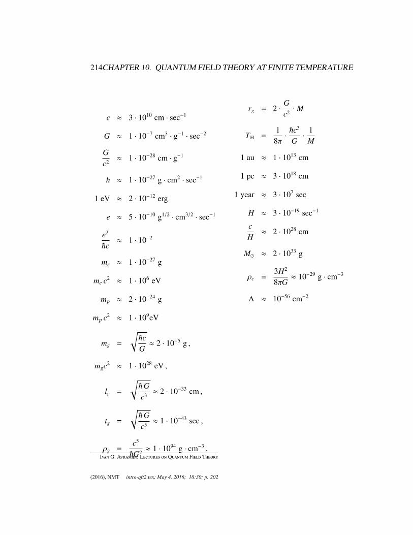
214CHAPTER 10. QUANTUM FIELD THEORY AT FINITE TEMPERATURE
c ≈ 3 · 1010 cm · sec−1
G ≈ 1 · 10−7 cm3 · g−1 · sec−2
Gc2 ≈ 1 · 10−28 cm · g−1
~ ≈ 1 · 10−27 g · cm2 · sec−1
1 eV ≈ 2 · 10−12 erg
e ≈ 5 · 10−10 g1/2 · cm3/2 · sec−1
e2
~c≈ 1 · 10−2
me ≈ 1 · 10−27 g
me c2 ≈ 1 · 106 eV
mp ≈ 2 · 10−24 g
mp c2 ≈ 1 · 109eV
mg =
√~cG≈ 2 · 10−5 g ,
mgc2 ≈ 1 · 1028 eV ,
lg =
√~Gc3 ≈ 2 · 10−33 cm ,
tg =
√~Gc5 ≈ 1 · 10−43 sec ,
ρg =c5
~G2 ≈ 1 · 1094 g · cm−3 ,
rg = 2 ·Gc2 · M
TH =1
8π·~c3
G·
1M
1 au ≈ 1 · 1013 cm
1 pc ≈ 3 · 1018 cm
1 year ≈ 3 · 107 sec
H ≈ 3 · 10−19 sec−1
cH≈ 2 · 1028 cm
M ≈ 2 · 1033 g
ρc =3H2
8πG≈ 10−29 g · cm−3
Λ ≈ 10−56 cm−2
Ivan G. Avramidi: Lectures on Quantum Field Theory
(2016), NMT intro-qft2.tex; May 4, 2016; 18:30; p. 202

Notation
xxx meaning
215

216 Notation
Ivan G. Avramidi: Lectures on Quantum Field Theory (2016), NMT intro-qft2.tex; May 4, 2016; 18:30; p. 203

Bibliography
?avramidi00? [1] I. G. Avramidi, Heat Kernel and Quantum Gravity, (Berlin: Springer, 2000)
?barut77? [2] A. O. Barut and R. Raczka, Theory of Group Representations and Applica-tions, (PWN — Polish Scientific Publishers, Warszawa, 1977)
?birrel82? [3] N. D. Birrel and P. C. W. Davies, Quantum Fields in Curved Spacetime,(Cambridge University Press, Cambridge, 1982)
?bjorken65? [4] J. D. Bjorken and S. D. Drell, Relativistic Quantum Fields, (McGraw-Hill,New York, 1965)
bogolyubov80 [5] N. N. Bogolyubov and D. V. Shirkov, Introduction to the Theory of Quan-tized Fields, (Wiley, New York, 1980)
?bogolyubov80a? [6] N. N. Bogolyubov and D. V. Shirkov, Quantum Fields, (Nauka, Moskow,1980)
?brown92? [7] L. S. Brown, Quantum Field Theory, Cambridge University Press, 1992
?dewitt65? [8] B. S. De Witt, Dynamical Theory of Groups and Fields, (Gordon & Breach,New York, 1965).
?dewitt84? [9] B. S. De Witt, The Spacetime Approach to Quantum Field Theory, Rela-tivity, Groups & Topology II, ed. by B. S. De Witt and R. Stora, (North-Holland, Amsterdam, 1984) pp. 381-738
?dubrovin92? [10] B. A. Dubrovin, A. T. Fomenko and S. P. Novikov, Modern Geometry —Methods and Applications, (Springer, New York, 1989)
?faddeev80? [11] L. D. Faddeev and A. A. Slavnov, Gauge Fields, Benjamin/Cummings,1980.
217

218 Bibliography
?faddeev09? [12] L. D. Faddeev and O. A. Yakuboski, Lectures on Quantum Mechanics forMathematics Students, (AMS, 2009)
?folland08? [13] G. B. Folland, Quantum Field Theory, American Mathematical Society,2008
?fulling89? [14] S. Fulling, Aspects of Quantum Field Theory in Curved Space-time, (Cam-bridge University Press, Cambridge, 1989)
?glimm81? [15] J. Glimm and A. Jaffe, Quantum Physics: a Functional Integral Point ofView, (Springer, New York, 1981)
?grib80? [16] A. A. Grib, S. G. Mamaev, V. M. Mostepanenko, Quantum Effects in StrongExternal Fields, (Atomizdat, Moskow, 1980)
?hamermesh89? [17] M. Hamermesh, Group Theory and its Applications to Physical Problems,(Dover Publications, New York, 1989)
?isham89a? [18] C. J. Isham, Lectures on Groups and Vector Spaces for physicists, (WorldScientific, Singapore, 1989)
?isham89b? [19] C. J. Isham, Modern Differential Geometry for physicists, (World Scientific,Singapore, 1989)
itzukson80 [20] C. Itzukson and J.-B. Zuber, Quantum Field Theory, (McGraw-Hill, NewYork, 1980)
lancaster14 [21] T. Lancaster and S. J. Blundell, Quantum Field Theory for the Gifted Ama-teur, Oxford University Press, 2014
?maggiore05? [22] M. Maggiore, A Modern Introduction to Quantum Field Theory, OxfordUniversity Press, 2005
peskin95 [23] M. E. Peskin and D. V. Schroeder, An Introduction to Quantum Field The-ory, Westview Press, 1995.
rabin95 [24] J. M. Rabin, Introduction to Quantum Field Theory for Mathematicians, inGeometry and Quantum Field Theory, Eds. D. Freed and K. Uhlenbeck,American Mathematical Society, 1995.
?rajaraman82? [25] R. Rajaraman, Solitons and Instantons: Introduction to Solitons and In-stantons in Quantum Field Theory, (North-Holland, Amsterdam, 1982)
Ivan G. Avramidi: Lectures on Quantum Field Theory (2016), NMT intro-qft2.tex; May 4, 2016; 18:30; p. 204

Bibliography 219
ramond81 [26] P. Ramond, Field Theory: a Modern Primer, (Benjamin, Reading, 1981)
ryder96 [27] L. H. Ryder, Quantum Field Theory, Cambridge University Press, 1996
schwartz13 [28] M. D. Schwartz, Quantum Field Theory and the Standard Model, Cam-bridge University Press, 2013
?schwinger73? [29] J. Schwinger, Particles, Sources and Fields, (Addison-Wesley, Reading,1973)
?siegel? [30] W. Siegel, Fields, State University of New York at Stony Brook,http://insti.physics.sunysb.edu/ siegel/Fields4temp.pdf
?slavnov78? [31] A. A. Slavnov and L. D. Faddeev, Introduction to the Quantum Theory ofGauge Fields, (Nauka, Moskow, 1978)
srednicki07 [32] M. Srednicki, Quantum Field Theory, Cambridge University Press, 2007
sterman93 [33] G. Sterman, An Introduction to Quantum Field Theory, Cambridge Univer-sity Press, 1993
?takhtajan08? [34] L. Takhtajan, Quantum Mechanics for Mathematicians, (AMS, 2008)
tong [35] D. Tong, Lectures on Quantum Field Theory, University of Cambridge,http://www.damtp.cam.ac.uk/user/dt281/qft/qft.pdf
?vasiliev76? [36] A. N. Vasiliev, Functional Methods in Quantum Field Theory and Statistics,(Leningrad University, Leningrad, 1976)
weinberg95 [37] S. Weinberg, The Quantum Theory of Fields, Vol I, Foundations, (Cam-bridge University Press, Cambridge, 1995)
?zee03? [38] A. Zee, Quantum Field Theory in a Nutshell, Princeton University Press,2003
?zhelnorovich82? [39] V. A. Zhelnorovich, Spinor Theory and its Application in Physics and Me-chanics, (Nauka, Moscow, 1982)
Ivan G. Avramidi: Lectures on Quantum Field Theory (2016), NMT intro-qft2.tex; May 4, 2016; 18:30; p. 205