QUANTITY SURVEYS

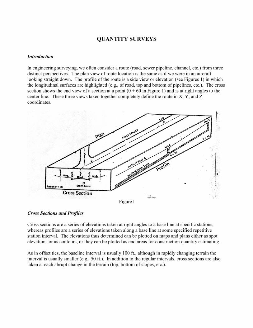
Introduction In engineering surveying, we often consider a route (road, sewer pipeline, channel, etc.) from three distinct perspectives. The plan view of route location is the same as if we were in an aircraft looking straight down. The profile of the route is a side view or elevation (see Figures 1) in which the longitudinal surfaces are highlighted (e.g., of road, top and bottom of pipelines, etc.). The cross section shows the end view of a section at a point (0 + 60 in Figure 1) and is at right angles to the center line. These three views taken together completely define the route in X, Y, and Z coordinates.

Figure1

Cross Sections and Profiles Cross sections are a series of elevations taken at right angles to a base line at specific stations, whereas profiles are a series of elevations taken along a base line at some specified repetitive station interval. The elevations thus determined can be plotted on maps and plans either as spot elevations or as contours, or they can be plotted as end areas for construction quantity estimating. As in offset ties, the baseline interval is usually 100 ft., although in rapidly changing terrain the interval is usually smaller (e.g., 50 ft.). In addition to the regular intervals, cross sections are also taken at each abrupt change in the terrain (top, bottom of slopes, etc.).

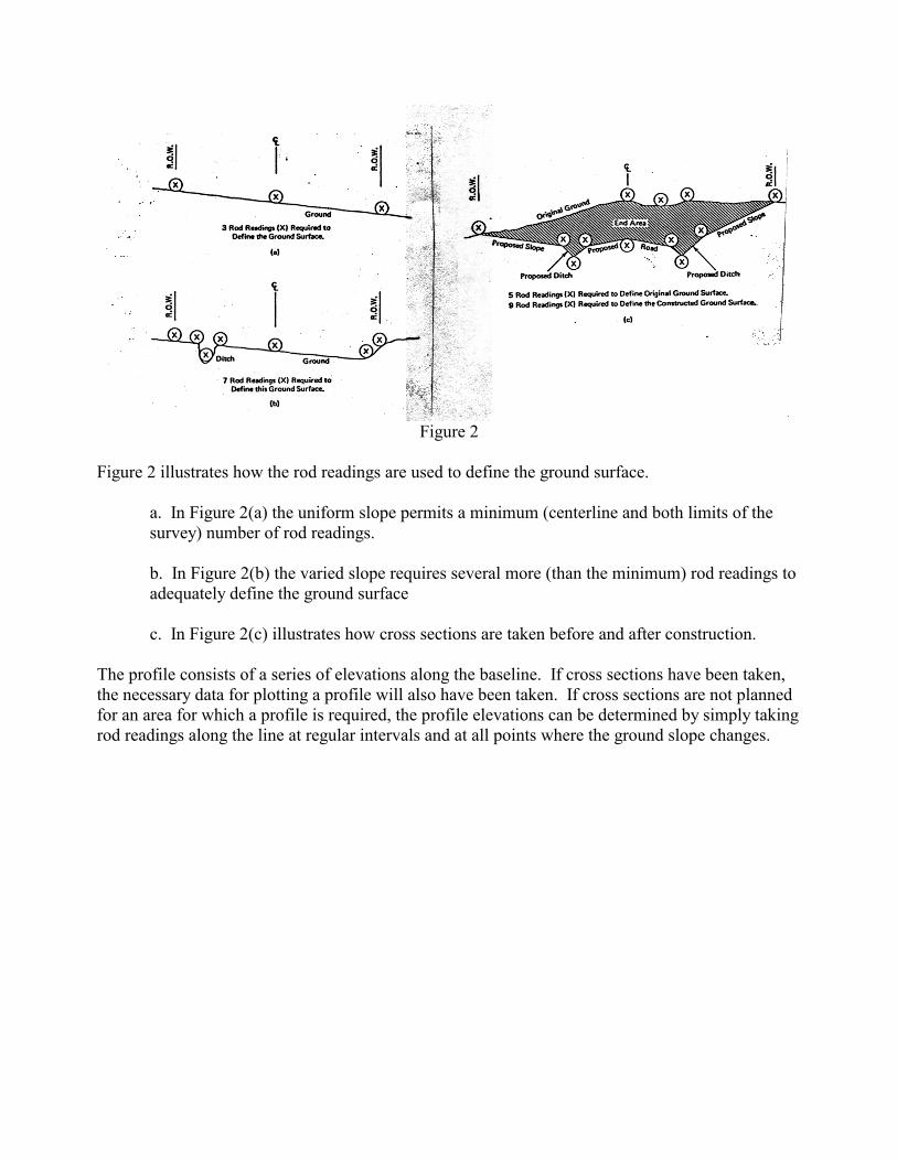
Figure 2

Figure 2 illustrates how the rod readings are used to define the ground surface.

a. In Figure 2(a) the uniform slope permits a minimum (centerline and both limits of the survey) number of rod readings. b. In Figure 2(b) the varied slope requires several more (than the minimum) rod readings to adequately define the ground surface c. In Figure 2(c) illustrates how cross sections are taken before and after construction.

The profile consists of a series of elevations along the baseline. If cross sections have been taken, the necessary data for plotting a profile will also have been taken. If cross sections are not planned for an area for which a profile is required, the profile elevations can be determined by simply taking rod readings along the line at regular intervals and at all points where the ground slope changes.

Figure 3

Typical field notes for profile leveling are shown in Figure 3. Cross sections are booked in different formats.

Figure 4

Figure 4 shows cross sections booked in standard level note format. All the rod readings for one station (that can be "seen" from the HI) are booked together.

Figure 5

Figure 5 shows the positions of the rod readings at station 2 + 60. In cases where the terrain is very rugged, making the level and rod work very time-consuming (many instrument setups). Electronic tacheometer instruments (ETI), also known as total station, can very quickly measure distances and differences in elevation; the rod man holds a reflecting prism mounted on a range pole instead of holding a rod. Many of these instruments have the distance and elevation data recorded automatically for future computer processing, while others require that the data be manually entered into the data recorder. This method can be used to advantage on a multitude of surveying projects, including right-angle offset and cross sections. Road and highway construction often requires the location of granular (sand, gravel) deposits for use in the highway road beds. These borrow pits (gravel pits) are surveyed to determine the volume of material "borrowed" and transported to the site. Before any excavation takes place, one or more reference baselines are established and two bench marks (at minimum) are located in convenient locations. The reference lines are located in secure locations where neither the stripping and stockpiling of top soil or the actual excavation of the granular material will endanger the stakes. Cross sections are taken over (and beyond) the area of proposed excavation. These original cross sections will be used as a datum against which interim and final excavations will be measured. The volumes calculated from the cross sections are often converted to tons for payment purposes. In many locations, weigh scales are located at the pit to aid in converting the volumes and as a check on the calculated quantities. The original cross sections are taken over a grid at 50 ft. (20 m) intervals. As the excavation proceeds, additional rod readings (in addition to 50 ft. grid readings) for top and bottom of excavation are required. Permanent targets can be established to assist in the alignment of the cross section lines running perpendicular to the base line at each 50 ft. station. If permanent targets have not been erected, a surveyor on the base line can keep the rodman on line by using a prism or by estimated right angles.

Construction Volumes In highway construction, for economic reasons, the designers try to optimally balance cut and fill volumes. Cut and fill cannot be precisely balanced because of geometric and esthetic design considerations, and because of the unpredictable effects of shrinkage and swell. Shrinkage occurs when a cubic yard is excavated and then placed while being compacted. The same material formerly occupying 1 yd. volume now occupies a smaller volume. Shrinkage reflects an increase in density of the material and is obviously greater for silts, clays, and loams than it is for granular materials such as sand and gravel. Swell is a term used to describe the placing of shattered (blasted) rock. Obviously 1 yd. of solid rock will expand significantly when shattered. Swell is usually in the 15 percent to 20 percent range, whereas shrinkage is in the 10 percent to 15 percent range, although values as high as 40 percent are possible with organic material in wet areas. To keep track of cumulative cuts and fills as the profile design proceeds, the cumulative cuts (plus) and fills (minus) are shown graphically in a mass diagram. The total cut-minus-fill is plotted at each station directly below the profile plot. The mass diagram is an excellent method of determining waste or borrow volumes and can be adapted to show haul (transportation) considerations Figure 6.

Figure 6

Large fills require borrow material usually taken from a nearby borrow pit. The borrow pit in Figure H1-7 was laid out on a 50 ft. grid. The volume of a grid square is the average height (a + b + c + d )/4 times the area of the base (50 ). The partial grid volumes (along the perimeter of the borrow pit) can be computed by forcing the perimeter volumes into regular geometric shapes (wedge shapes or quarter-cones). Cross Sections and Volumes Cross sections are useful in determining quantities of cut and fill in construction design. If the original ground cross section is plotted, and then the as constructed cross section is also plotted, the end area at that particular station can be computed.

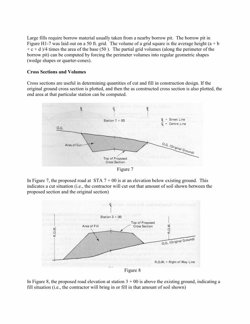
Figure 7

In Figure 7, the proposed road at STA 7 + 00 is at an elevation below existing ground. This indicates a cut situation (i.e., the contractor will cut out that amount of soil shown between the proposed section and the original section)

Figure 8

In Figure 8, the proposed road elevation at station 3 + 00 is above the existing ground, indicating a fill situation (i.e., the contractor will bring in or fill in that amount of soil shown)

Figure 9

Figure 9 shows a transition section between cut and fill sections End Areas When the end areas of cut or fill have been computed for adjacent stations, the volume of cut or fill between those stations can be computed by simply averaging the end areas and multiplying the average end area by the distance between the end area stations. Figure 10 illustrates this concept.

Figure 10

V = {(A1 + A2 )/2} L

The above formula gives the general case for volume computation, where A and A are the end areas of two adjacent stations, and L is the distance (feet) between the stations. The answer in cubic feet is divided by 27 to give the answer in cubic yards. The average end area method of computing volumes is entirely valid only when the area of the midsection is, in fact, the average of the two end areas. This is seldom the case in actual earthwork computations; however, the error in volume resulting from this assumption is insignificant for the usual earthwork quantities of cut and fill. For special earthwork quantities (e.g., expensive structures excavation) or for higher-priced materials (e.g., concrete in place), a more precise method of volume computation, the prismoidal formula, must be used. Prismoidal Formula If values more precise than end area volumes are required, the prismoidal formula can be used. A prismoid is a solid with parallel ends joined by plane or continuously warped surfaces. The prismoidal formula is: V = L {A1 + 4Am + A2 )/6} ft2 or m2 Where A1 and A2 are the two end areas, Am is the area of a section midway between A1 and A2, and L is the distance from A1 to A2. Am is not the average of A1 and A2 , but Am is derived from distances that are the average of corresponding distances required for A1 and A2 computations. This formula is also used for other geometric solids (e.g., truncated prisms, cylinders, and cones). To justify its use, the surveyor must refine the field measurements to reflect the increase in precision being sought. A typical application of the prismoidal formula would be the computation of in place volumes of concrete. The difference in cost between a cubic yard or meter of concrete and a cubic yard or meter of earth cut or fill is sufficient reason for the increased precision.