ce 220 laboratory manualhturner/ce220/220_lab.pdf · civil engineering department ce 220 advanced...
TRANSCRIPT
CE 220 Laboratory Notes, Fall 2002
CE 220 LABORATORY
MANUAL 2002
InRoads 8.3
INSTRUCTOR DR. HOWARD TURNER P.L.S.
MAPPING SCIENCES CENTER OF EXCELLENCE CALIFORNIA STATE POLYTECHNIC UNIVERSITY, POMONA
3801 W. TEMPLE AVENUE POMONA CA 91768
Copyright Howard Turner 2002 Page 1

CE 220 Laboratory Notes, Fall 2002
INTRODUCTION TO LAB PROCEDURES 1 FORMAT
A. GENERAL
Laboratory notes are to be neatly and professionally performed and written. The use of proper English grammar, correct spelling, as well as overall good appearance, is expected. All laboratory notes shall be written in an ELAN (E64-8X4W) field book or equivalent (available at the bookstore or at survey supply stores). All notes shall be printed legibly in pencil using 2H or harder lead. Laboratory notes written in cursive or written with soft lead (which smears) will have points deducted. All calculations are to be shown in general equation form, as well as at least one specific example employing the actual measurements made during the course of the field work. The procedures for the individual labs and some examples of note taking styles are provided in the following pages of this manual.
B. NOTE TAKING ELEMENTS
1. Complete all data as required by the instructor and/or by the
outline of each individual lab. 2. The title of each lab shall be clearly written on the first page of the
lab notes.
3. All pages shall be numbered in the upper or lower corners.
4. A complete sketch of the survey must be included. The sketch should include bearings and distances (where applicable), call outs, north arrow and scale, label angles, label buildings, sidewalks, trees, significant physical feature and any other notes as necessary.
5. List the date, weather, temperature, equipment used that day. 6. Note the job that each party member performed (i.e. chainman,
rodman, party chief, note taker, etc.).
7. Sign your name on the last page of the notes and label as "original" or label "copy" if duplicated.
8. Show general equations along with at least one specific numerical example for each new calculation for clarity and verification.
Copyright Howard Turner 2002 Page 2

CE 220 Laboratory Notes, Fall 2002
9. Include anything else specified by the instructor during the lecture.
C. THE REQUIREMENTS OF PROPER NOTE TAKING
1. Integrity - Measurements that are forgotten or not written down could negate the effectiveness of the notes for plotting or for further calculations. This could result in having to return to the field in order to complete the survey. NOTE: Field notes may later be used as evidence of work performed in a court case or litigation.
2. Accuracy - The most important requirement. Care must be taken
not only when taking the measurement, but also when writing the measurement down. Transposed numbers could mean having to survey a site twice.
3. Organization - Notes that are arranged properly (orderly) for the
type of survey performed helps contribute to accuracy and integrity.
4. Clarity - Notes which are clearly written help make errors and omissions more apparent thus reducing the chance of future problems .
5. Forms - Examples of the various forms of note taking are included
in this manual.
II. LABORATORY RULES
A. There shall be absolutely NO HORSEPLAY. B. All equipment is to be treated with the utmost respect using diligent care.
C. The field instruments should be carried in their cases and placed on
the tripod only after the tripod has been set up and checked for sturdiness.
D. A crew will be assigned - generally consisting of four people. The crew will appoint a new leader (party chief) for each day of surveying. The party chief will be responsible for the proper performance of the survey, proper handling of the equipment, and in general make decisions in the field. The party chief will also
Copyright Howard Turner 2002 Page 3

CE 220 Laboratory Notes, Fall 2002
inventory the locker after each lab session and sign and date the inventory list indicating all equipment has been returned and is in proper working order.
E. Any equipment that is not working properly should be reported to
the instructor as soon as it is noticed.
Copyright Howard Turner 2002 Page 4

CE 220 Laboratory Notes, Fall 2002
CALIFORNIA STATE POLYTECHNIC UNIVERSITY, POMONA Civil Engineering Department
CE 220 ADVANCED SURVEYING
CE 220L ADVANCED SURVEYING LABORATORY
INSTRUCTOR Turner Grade Evaluation Lecture* Grade Evaluation Lab* OFFICE HOURS
M/W 4:15-6:00 P.M.. 3-One hour exams Lab Exercises 60% T 2:00-3:00 P.M., Th 5:00-6:00 P.M. Best two count 50% each Mapping Project 40%
TEXT TOTAL 100% TOTAL 100% 1) ELEMEMARY SURVEYING, LABORATORY MANUAL Wolf & Brinker, 9th ed. ADVANCED SURVEYING 2) ROUTE SURVEYING AND DESIGN, Meyer & Gibson, 5th ed.
Available at ASK ,
WEEK CLASS TOPIC ASSIGNED CHAPTERS Read before lecture listed
1 Lect. #1 Introduction Lect. #2 Precise Leveling, Theodolites and E.D.M Chapters 5&6 (B&W) Lab. #1 Precise Leveling
2 Lect. #3 Route Surveying Chapter 1 (M&G) Lect. #4 Circular Curves Chapter 2 (M&G) Lab. #2 Measuements with E.D.M
3 Lect. #5 Circular Curves Chapter 3 (M&G) Lect. #6 Compound, Reverse & Spiral Curves Chapter 5 (M&G) Lab. #3 Measuring Polygon EDM
4 Lect. #7 Vertical Curves Chapter 4 (M&G) Lect. #8 Vertical Curves Lab. #4 Measuring Polygon EDM
5 Lect. #9 Surveying Astronomy Chapter 18, 20 (B&W) Lect. #10 Test #1 Lab. #5 Simple Curve Layout
6 Lect. #11 Global Positioning Systems Lect. #12 Global Positioning Systems Lab. #6 Measure Polygon GPS
7 Lect. #13 Earthworks Chapter 8 (M&G) Lect. # 14 Construction Methods Lab. #7 Introduction to Go-Cart Project
8 Lect. #15 Computer Techniques in Route Surveying Lect. # 16 Test #2 Lab. #8 Go-Cart Project
9 Lect. #17 Computer Techniques in Route Surveying Lect. # 18 Public Lands System Chapter 23 (B&W) Lab. #9 Go-Cart Project
10 Lect. #19 State Plane Coordinates Chapter 21 (B&W) Lect. # 20 Course Review Lab. #10 Go-Cart Project Due
FALL 2000
Copyright Howard Turner 2002 Page 5

CE 220 Laboratory Notes, Fall 2002
CE 220
LABORATORY 1
OBJECTIVE
To perform three-wire leveling REQUIRED MATERIAL Automatic Level Level Rod Level Rod Bubble Cloth Tape Stakes and Hammer PROCEDURE 1) Find the bench mark in the sidewalk southwest of the Engineering Building. Read the bench mark number and elevation. 2) Setup the level so the rod can be read on the bench mark. 3) Hold the rod vertical on the bench mark with the level rod bubble attached. 4) Read all three wires on the backsight and record the readings in your field book. 5) Measure the distance to the backsight position. 6) Move the rod to the foresight position and ensure that the distance to the foresight position is equal to the backsight position. 7) Read all three wires on the foresight position. 8) Run levels from the bench mark to point A on the polygon using the methods described above. Use stakes as turning points. 9) Record the data in your field book.
Copyright Howard Turner 2002 Page 6

CE 220 Laboratory Notes, Fall 2002
CE 220
LABORATORY 2 OBJECTIVE TO GIVE THE STUDENT INSTRUCTION IN THE OPERATION OF E.D.M AND THEODOLITES. REQUIRED MATERIAL
Total Station Battery Tripod Prism with tribrach Tripod Nails Flagging
PROCEDURE 1. Each group will be assigned a Total Station. 2. Each group will occupy arbitrary points along the line AB. 3. Tripods with tribrachs and prisms will be set-up on points C and G. 4. Distances will be measured to points C and G. The distance should be measured
10 times and the mean of the measurements taken should be calculated. 5. Angles between the points C and G will be measured. 4 sets of angles will be
measured.
Copyright Howard Turner 2002 Page 7

CE 220 Laboratory Notes, Fall 2002
Copyright Howard Turner 2002 Page 8
CE220
LABORATORY 3 AND 4 OBJECTIVE To measure the seven sides of the polygon and the angles contained in the polygon by precise methods. REQUIRED MATERIAL
Total Station Tripod Prism. Prism pole
PROCEDURE 1. Setup and level the total station over a point. 2. Setup and level the prism on the previous station (BS). 3. Setup and level the prism on the foresight station (FS). 4. Set zero on the backsight prism and measure the direction and distance to the
foresight prism. 5. Record all the measurements as they are made in the field book. 6. Move to the next station and continue until all angles and all distances have been
measured on the polygon. 7. Adjust the polygon by the compass rule and obtain the adjusted values of the
points.

CE 220 Laboratory Notes, Fall 2002
CE220
LABORATORY 5 OBJECTIVE To stakeout a simple curve. REQUIRED MATERIAL
Total Station. Rod and Prism. Tape. Plumb-bobs. Stakes. Hammer. Nails.
PROCEDURE
1. Using the calculated data on polygon, calculate delta. 2. Given a radius of 50 to 200 feet, calculate the tangent. Set the BC, EC, and Radius
point. 3. Use stationing of 0+20 feet and calculate the deflection angles 4. Stake the right offset line on a 15 ft. offset. 5. Calculate the short chords and use them to stake out the curve. 6. Calculate the long chord and measure the distance as a check on BC and EC.
Copyright Howard Turner 2002 Page 9

CE 220 Laboratory Notes, Fall 2002
220 PROJECT
OBJECTIVE: To design a GO-CART around the polygon by The Old Stable.
PARAMETERS The finished grade of the track will be as follows: Point A 2 foot above existing ground Point B 2 foot below existing ground Point C 2 foot above existing ground Point D 2 foot below existing ground Point E 2 foot above existing ground Point G 2 foot below existing ground The cut side slopes on the track will be 2:1, and the fill side slopes will be 1.5:1. The cross grade on the track will be 1% from the outside to the inside. The Right-of-Way for the track will be 25 feet. The width of the pavement will be 6 feet and the pavement will be in the center of the R-
of-W. Station 2+00 will be a point half way “on-line” between point A and point B. A minimum of 25 foot radius curves will be set on the track.
Copyright Howard Turner 2002 Page 10


CE 220 Laboratory Notes, Fall 2002
PART 3 –GETTING STARTED AND DATA REDUCTION
This course teaches the basic steps required completing a typical road relocation and site design project. Everyone does not work the same way. Therefore, the steps you choose to take in your own workflow may differ slightly from the steps presented here. A series of laboratories in CE 134, CE220 and CE222 will give you a working knowledge of how to use InRoads and how to apply the commands to your projects. When you complete this series, you will have created a model imilar to the following: s
US_old
New Resort
Retention Pond
New Road
A: Getting Started In this laboratory, you will: Review how to get into MicroStation Learn how to start the InRoads program Learn how to exit InRoads and MicroStation
Copyright Howard Turner 2002 Page 12
CE 220 Laboratory Notes, Fall 2002
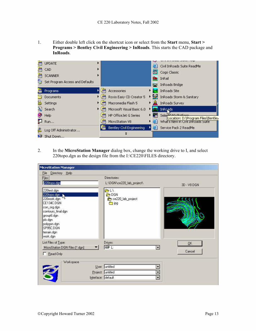
1. Either double left click on the shortcut icon or select from the Start menu, Start >
Programs > Bentley Civil Engineering > InRoads. This starts the CAD package and InRoads.
2. In the MicroStation Manager dialog box, change the working drive to I, and select
220topo.dgn as the design file from the I:\CE220\FILES directory.
Copyright Howard Turner 2002 Page 13

CE 220 Laboratory Notes, Fall 2002
3. Once MicroStation and InRoads starts, the inroads command window appears.
4. Select from the MicroStation pull down menus, Utilities > Key-in. Dock the dialog
either to the bottom or top of the screen. Only the key-in field will be displayed.
Copyright Howard Turner 2002 Page 14

CE 220 Laboratory Notes, Fall 2002
5. Select the Fit View command and select the view to fit the design file graphics. The
existing graphics in the design file will be fitted to the active view. .
6. This is a good time to set the display depth of this 3D-design file. Key in DP=100,2000
and select the view. This sets the display of the design file so that all elements between the elevation of 100 and 2000 are shown. The elevations used during these exercises are between 700 and 1000 feet.
Copyright Howard Turner 2002 Page 15

CE 220 Laboratory Notes, Fall 2002
7. Choose File > Save Settings from the MicroStation Command Window. The graphic settings of the design file are saved. NOTE: You can also save these settings by keying in file design.
8. From the InRoads menu, choose File > Exit. InRoads is exited. 9. Now exit MicroStation by choosing File > Exit or by simply keying in exit
Copyright Howard Turner 2002 Page 16

CE 220 Laboratory Notes, Fall 2002
•
•
Summary Start InRoads by selecting Programs > Bentley Civil Engineering > InRoads SelectCAD or by double-clicking the InRoads SelectCAD icon.
InRoads can be quit out of and the CAD software will remain open, by selecting File > Exit from the InRoads command window or both the CAD software and InRoads can be exited by selecting File > Exit from the CAD software’s menu.
Copyright Howard Turner 2002 Page 17

CE 220 Laboratory Notes, Fall 2002
Digital Terrain Models A digital terrain model (DTM) is composed of points, triangles and perimeters. The DTM doesn't limit itself to the earth's surface. It can represent any type of spatial data. It's important to note that Civil Engineer’s site modeling software allows only one Z coordinate for each X-Y coordinate.
Copyright Howard Turner 2002 Page 18
CE 220 Laboratory Notes, Fall 2002
Before a surface can be defined, surface data is needed first. A wide variety of surface point information can be loaded into surfaces. To load these point types, any of the available import commands can be used. The only exception is inferred points, which must be generated separately with the Generate Inferred Breaklines command.
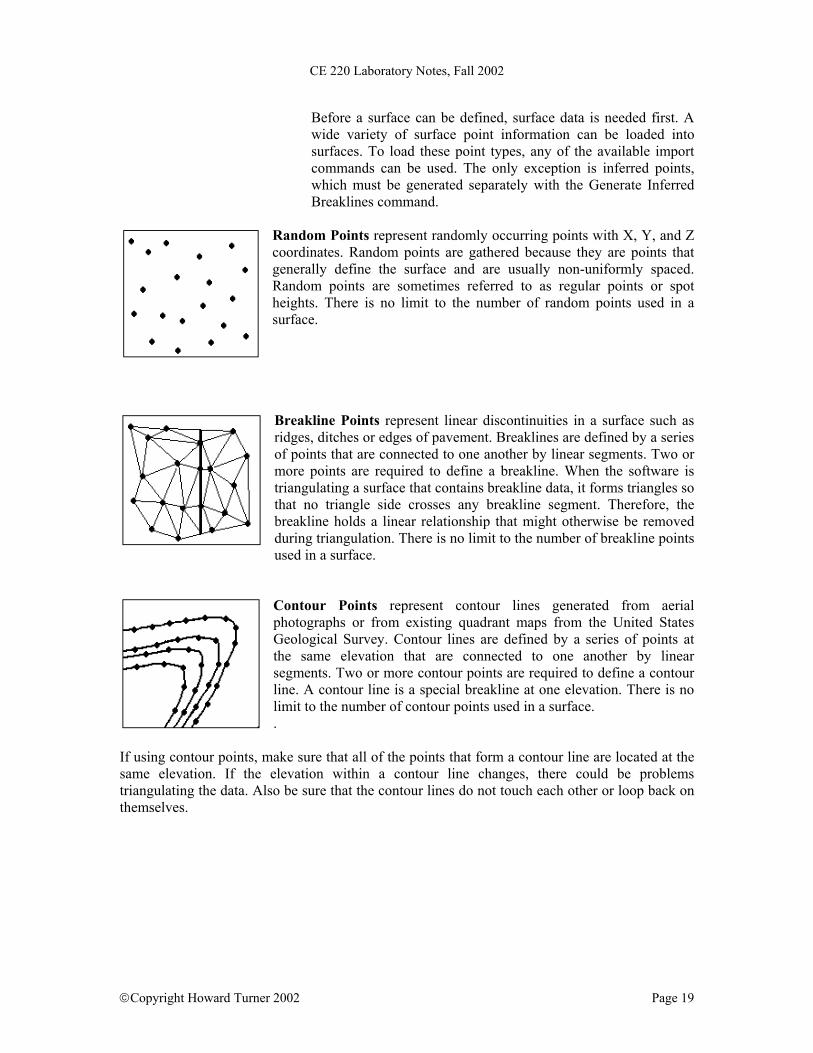
Random Points represent randomly occurring points with X, Y, and Z coordinates. Random points are gathered because they are points that generally define the surface and are usually non-uniformly spaced. Random points are sometimes referred to as regular points or spot heights. There is no limit to the number of random points used in a surface.
Breakline Points represent linear discontinuities in a surface such as ridges, ditches or edges of pavement. Breaklines are defined by a series of points that are connected to one another by linear segments. Two or more points are required to define a breakline. When the software is triangulating a surface that contains breakline data, it forms triangles so that no triangle side crosses any breakline segment. Therefore, the breakline holds a linear relationship that might otherwise be removed during triangulation. There is no limit to the number of breakline points used in a surface.
Contour Points represent contour lines generated from aerial photographs or from existing quadrant maps from the United States Geological Survey. Contour lines are defined by a series of points at the same elevation that are connected to one another by linear segments. Two or more contour points are required to define a contour line. A contour line is a special breakline at one elevation. There is no limit to the number of contour points used in a surface. .
If using contour points, make sure that all of the points that form a contour line are located at the same elevation. If the elevation within a contour line changes, there could be problems triangulating the data. Also be sure that the contour lines do not touch each other or loop back on themselves.
Copyright Howard Turner 2002 Page 19

CE 220 Laboratory Notes, Fall 2002
Interior Boundary Points represent undefined areas in a model, such as footprints of buildings, edges of lakes or areas with no available data. Interior boundaries are also referred to as obscure areas. This point type can be used to define void areas, or areas where no valid point data exists within a terrain model. Interior boundaries are defined by a series of points that form a closed polygon. At least three non-collinear points are required to define an interior boundary. Several interior boundaries in a model can be had, but they should not overlap
one another. To triangulate models containing interior boundaries, the software uses the same algorithm as breaklines. Additionally, it marks all triangles formed inside the boundary as deleted. Once a triangle is marked as deleted, the software does not use it in any subsequent command. However, deleted triangles are still stored in memory. This is because every triangle stores information about the triangle's three neighboring triangles, which allows the software to easily evaluate the surface. Removing the interior boundary makes the points previously marked as deleted available again.
Exterior Boundary Points represent the outer extent of the model. Exterior boundaries may also be called edges. Exterior boundaries are similar to interior boundaries as they are also composed of a series of points that form a closed polygon. At least three non-collinear points are required to define an exterior boundary. To triangulate models containing exterior boundaries, the software uses the same algorithm as for breaklines. In addition, it marks all triangles formed outside the boundary as deleted. Once a triangle is marked as deleted, the software
does not use it in any subsequent command. Just one exterior boundary in each surface is allowed. If the exterior boundary is deleted, any points previously outside are available again to the surface.
Inferred Points represent breakline points that the software generates to force contour lines to form correct relationships in the DTM. These points are generally used when digitized contours are the basis for the terrain model data. Digitized contour input can result in poor definition of points that have the same elevation and of the terrain surface where ridges, valleys or hill peaks appear. Instead of following the real contours, contour points are sometimes connected incorrectly, resulting in an inaccurate representation of the model. To force the contour points to be connected correctly, inferred points are placed along ridges, valleys or other problem areas. The points are connected to form a breakline, which forces the contour lines to fall in the correct location. Inferring points should be done prior to final display due to an increase in the number of points. Inferring not only improves the surface, but also improves the display of the contours. Inferred points can not be imported. To generate them in the model, use the Generate Inferred Breaklines
command. This type of point can be exported into an ASCII file or viewed in the drawing.
Copyright Howard Turner 2002 Page 20

CE 220 Laboratory Notes, Fall 2002
Collecting DTM Data
Several rules must be kept in mind while collecting surface data. Accurate data collection is essential for producing accurate models. First, the correct spacing of random points and the correct placement of breaklines are critical to accurately modeling physical sites. Random points should be colleted at all local minima and maxima within a site. A local minimum or maximum is a location within the modeled site that is at a low or high elevation relative to neighboring points. Additionally, random points should be collected throughout the site so that the distance from one random point to another is about equal. Breakline data should be added to force the model to accurately represent areas where there are discontinuities in the terrain surface. Such features include the top and bottom of ditches and the edges of roadway pavement. Additionally, in certain circumstances where modeling areas include ridge or valley lines, breaklines that follow these features will want to be added. In general, breaklines should not cross one another, although the software allows this condition. If breaklines cross, problems may be experienced when triangulating the surface. Crossing breaklines should have the same elevation at their intersection since a surface cannot contain two points at the same X, Y and have a different Z.
Field Survey Data
When collecting terrain model data through field surveys, survey crews typically collect random points in a regular, grid-like fashion. Although the distances between these points varies from site to site, it normally ranges from 5 to 50 meters, depending on the topography. To fine-tune the accuracy of the model, topographic measurements along lines where there is an obvious break in the terrain slope are also collected. This second set of points is added as breaklines. Finally, if there are certain areas on the site that need to be excluded from the model, such as the footprints of large buildings, the survey crew collects data points defining the perimeter of the area and adds these to the model as interior boundary points.
Photogrammetric or Digitized Data
If surface data is collected with photogrammetric or digitized data, two different techniques to input the data may be used. The first method is very similar to that used by field survey crews. Collect random points in a fairly equal-spaced, grid-like pattern, and then supplement them with more detailed breakline and
Copyright Howard Turner 2002 Page 21

CE 220 Laboratory Notes, Fall 2002
interior boundary data. This method takes a little more time, but is more accurate. The second technique generally results in less accurate models. It digitizes existing contour information directly and uses that information as the basis for the terrain model. It is best not to stream digitize contours because it creates too many unnecessary points in your model. Even so, this very dense data can still be managed with the InRoads family of products.
When using photogrammetric or digitized data, different point types should be separated on different drawing file levels. For example, place random points on level 11 and contour points on level 12. This makes it easier to work with the model. No matter how the data is collected, remember to collect the right amount of information. Too little information causes a coarse, inaccurate model. Too much information can slow processing.
After the Data is Loaded After the point data is loaded to the surface, the software is used to triangulate the data, associating the points and defining the surface by drawing lines between the points.
Select which surface to triangulate and the maximum triangle length. For example, a zero length indicates infinity. After the surface is triangulated, save it. Define the location and the name of the surface file. After saving the surface, it can be reloaded or opened later. For more information about saving, naming, and opening existing surfaces, refer to the Help files. Next, review the surface to see the minimum and maximum coordinate range. Reviewing the surface shows whether any points are out of range. After reviewing the surface, the software
Copyright Howard Turner 2002 Page 22

CE 220 Laboratory Notes, Fall 2002
can be used to edit it. The Help files have more information about the surface editing commands. Display surface information such as contours and triangles and color-code the elevation ranges. When using contours, the command to establish the parameter settings for the display is selected, such as contour spacing and the number of minor contours between each major contour.
If Write Lock is off when contours are displayed, the graphics will disappear when the view is updated. If Write Lock is on when the contours are displayed, the contours display permanently. There are many ways to add, change, and store surface information. The on-line Help files include many additional details.
What Is a Feature?
Copyright Howard Turner 2002 Page 23

CE 220 Laboratory Notes, Fall 2002
What is a Feature? A feature is a unique instance of a 3D surface item or entity in a DTM. A feature can be one of five types, corresponding to the different types of DTM points: random, breakline, exterior boundary, interior boundary or contour. Although features are a new and powerful concept, they are essentially one or more items contained in a digital terrain model. Any one item or group is given a name and assigned a feature style. Feature Styles controls everything about how a feature gets displayed. The ability to identify different features by name, to select and edit them using filters, and to independently control their display characteristics are benefits of organizing the DTM into features.
Random Features versus Breakline Features
The purpose of this section is to explain some key differences between random features and breakline features. Remember that all features, regardless of type (breakline, random, interior, …) are basically defined as a 3D entity. Features are groups (or single), points or elements. This discussion attempts to explain the significance between the two most common types: breakline features and random features. Breakline Features Breakline features represent groups of DTM points with an important linear relationship. A few examples of breaklines are the edge of a roadway lane, the bottom of a ditch, the edge of a curb, and so on. When a DTM is triangulated, breakline features are honored in such a way that no triangle edge (triangle leg) will cross the path defined by connecting the points in the breakline feature. Breaklines, thus, promote accuracy in the triangulated model. The breakline designation implies significance to the linear path between each point in the feature. As a result, breakline features can appear in cross sections, whereas random features cannot. This is a critical difference. Also, with the software, a point density interval can be applied to your breakline features, ensuring that numerous triangle vertices will appear along each feature leg. However, the point density interval cannot be applied to random features. Random Features Random features represent distinct points with no significant linear relationship. Random points typically represent general terrain elevations. Because there is no important linear relationship among the points in the random feature, random
Copyright Howard Turner 2002 Page 24

CE 220 Laboratory Notes, Fall 2002
features cannot be displayed in cross sections. A point density interval cannot be applied to a random feature. Displaying Linear versus Point Data With the software, the points that define a feature can be displayed, as well as the connecting line segments between those points. This is true for all feature types-- even random features. In fact, the connecting line segments and not the actual 3D feature points can be chosen to be displayed. The settings that control what gets displayed are in the feature style. On the other hand, just the points from a breakline feature can be chosen to be displayed, even though the linear relationship is what is very important about these points. The key point to remember is the control one has on how features are displayed (points, line segments or both) regardless of the feature type. Symbology for Displaying Features All of the display characteristics of features are controlled by feature styles. For more information on feature styles, see the Help topic on the Feature Style Manager, which is located on the Tools menu, and was done in the last lab.
Locks – Part 1
Copyright Howard Turner 2002 Page 25

CE 220 Laboratory Notes, Fall 2002
The following is an introduction to only some of the Locks that the InRoads family of products uses. Other locks will be introduced where they are used.
Write: The Write lock generates graphics in one of two modes: display and write, or display-only. In the display and write mode, the graphics created by each command display in the view port and are written to the active drawing file. This is traditionally the manner in which CAD packages and add-on applications have functioned. Using this mode, any of the windowing functions to access a different view of the data or the element manipulation commands to modify the data can be used. The display and write mode is enabled by toggling the Write lock on. With the Write lock toggled off, all graphics are generated in the display-only mode. That is, the generated graphics display in one or more view ports, but are not written to the active drawing file. Using any of the windowing commands when the graphics are in display-only mode removes the graphics from the view port. This is because the elements have not been written to the drawing file. Additionally, because the elements do not actually exist in the active drawing file, any element manipulation commands to modify display-only graphics cannot be used. Suppose there is a line placed in the drawing file. If the [Redraw] or View Update command were selected with the Write lock toggled on, the line redisplays in the drawing file. If the Write lock is toggled off and the command is selected, the line is removed from the screen. The display-only mode is extremely useful when needing to view large amounts of terrain model data and then quickly removing that data from the screen. Since the display-only mode does not write graphics to the active drawing file, it can decrease drawing file size and increase the speed in which all graphics display in views by using this mode. The Write lock can be enabled or disabled at any time, even when about to click the Apply button in one of the View commands.
Pencil/Pen: Pencil Pen Note: The Pencil/Pen lock is applicable only when the Write lock is on. Also, the Pencil/Pen lock applies to 3D display-only. It does not apply to cross sections or profiles. This command toggles the Pencil/Pen lock between Pencil mode and Pen mode. This lock affects the display of virtually every piece of 3D graphics representing surfaces or geometry.
Copyright Howard Turner 2002 Page 26

CE 220 Laboratory Notes, Fall 2002
The Pencil/Pen lock controls what happens when a piece of graphics is redisplayed. Two actions may occur: one, the new graphics will display in addition to the old ones (Pen mode) or two, the new graphics will replace the old ones (Pencil mode). To keep previous work displayed and not lose it when modifying and redisplaying the surface or geometry, the Pen mode would be used. Pencil mode, on the other hand, is a convenience because it automatically cleans up the graphics from the previous work as it is modified in the design and redisplayed. The following two points summarize the basic notion of each mode: • Pen mode graphics are permanent and allow duplicates (see
the Delete Ink lock). • Pencil mode graphics persist only until an item is
redisplayed; there are no duplicates.
The effect of the Delete Ink Lock: Although the previous explanation refers to graphics drawn in Pen mode as “permanent,” this is not completely accurate. The graphics are permanent as far as Pen mode is concerned. However, if the Delete Ink lock is on at the time of redisplay, even graphics previously drawn in “ink” will be replaced by the new instance of the graphics. Please note that graphics drawn using Pen mode are said to be drawn in ink. The Delete Ink lock allows redisplayed graphics to replace even graphics that were drawn in ink. For example, a use for this might occur if work were done in Pen mode for a while comparing different designs and before finally settling on a design (assume we are talking about an alignment). If the alignment were displayed several times in ink, the Delete Ink lock can be turned on and the alignment can be displayed one more time. All the previous instances of the alignment will be removed when the alignment is redisplayed. The Delete Ink lock will probably remain off most of the time. One Thing To Remember: It is critical to understand that the current setting of the Pencil/Pen lock is irrelevant in determining what will happen when a piece of graphics is redisplayed. What is relevant is whether the existing graphics are displayed in Pencil mode or in Pen mode. Style: The main concept behind the Style lock is data-driven symbology. The Style locks affects two groups of commands: · all the View Surface commands, and · the Annotate Cross Section command.
Copyright Howard Turner 2002 Page 27

CE 220 Laboratory Notes, Fall 2002
Style Lock and the View Surface Commands The effect of the Style lock is this: When the Style lock is on and you activate a View Surface command, the dialog box for the command will not be displayed, but rather your surface data will be displayed in the graphics file without any further input from you. The Style lock bypasses the dialog box and displays the active surface, automatically determining what symbology to use. How is the symbology determined? When you run a View Surface command with Style lock on, the symbology is chosen according to the following procedure: 1) If a preference is associated with the active surface (see Surface Properties), the software reads this preference name and looks for a saved preference with a matching name in the command that you are running. If the command contains a saved preference by the same name as the preference that is specified in the active surface, then the issue of symbology is settled – the command is executed using that saved preference. 2) If there is no preference associated with the active surface or if there is no saved preference with a matching name, the software looks to the Preferred Preference. The Preferred Preference is defined under Tools > Options, on the General tab when the Category is set to Settings. If the View Surface command contains a saved preference by the same name as the Preferred Preference, the command is executed using that saved preference. 3) Finally, if the preference is still unresolved, the software just uses the Default preference. Every command has a Default preference – Default cannot be deleted. When the Style lock is off, activating the View Surface command displays a dialog box, as usual, and the settings on the dialog box are used to control symbology. Style Lock and the Annotate Cross Section Command The effect of the Style lock on Cross Section commands is limited to only one command: Annotate Cross Section. Before considering exactly what the Style lock does for this command, you should understand that, in addition to specifying a preference name (see the previous discussion), a surface specifies a named symbology. To verify this, look at the Symbology field in the Cross Sections group box on the Advanced tab of the Surface Properties dialog box. The named
Copyright Howard Turner 2002 Page 28

CE 220 Laboratory Notes, Fall 2002
symbology specified in this field is defined expressly for using the Style lock with the Annotate Cross Section command. Note For more information on named symbology, see the help topic on the Symbology Manager command. In the Create Cross Section command, the Style lock affects the symbology for the surface data line and for features, which are displayed as points in cross section. The other graphics displayed by this command (the title, legend, axes, and grid) are not affected by the Style lock. The symbology for these other pieces of graphics is controlled by the dialog box settings, which are stored in the preference file (CIVIL.INI). In the Annotate Cross Section command, the Style lock affects the symbology of point and segment annotation as well as feature annotation. Other graphics, such as the frame, ticks, and titles, are not affected by the Style lock. The symbology for these other pieces of graphics is controlled by the dialog box settings, which are stored in the preference file (CIVIL.INI). When the Style lock is on, the symbology for the point and segment annotation comes from the named symbology associated with the surface by the Symbology parameter on the Surface Properties dialog box. When the Style lock is off, the symbology comes from the feature style associated with each feature. Because each feature can have a unique feature style, it is possible for the annotation for each feature to be displayed with different symbology. Note Style Lock does not affect the profile commands. Locate: The Locate lock determines whether to snap to graphics displayed in the graphics file or to snap to the position occupied by a feature in the active surface. If the lock is set to graphics (the icon shows a single, red line), locate actions will seek the nearest displayed graphics. If the lock is set to features (the icon shows an image of a surface), locate actions will seek the position of the nearest feature in the active surface whether or not the feature is actually displayed. You can use the locate lock to locate features that are not even displayed. If they exist in the DTM, the locate will find them Point Snap: When turned on, this lock enables the cursor to snap or lock onto the closest point defined in the geometry project. Element: When turned on, this lock enables the cursor to snap or lock onto the closest geometry element in the active geometry project. This can be used to extract distances and directions
Copyright Howard Turner 2002 Page 29

CE 220 Laboratory Notes, Fall 2002
from that element to design new elements or points. Point Snap Lock and Element Lock cannot be turned on at the same time. Station: This lock is applicable only when the first station specified on the horizontal alignment is an odd-numbered station (for example, 2+39) and you are generating cross sections, executing the Roadway Modeler, or generating station-type reports. When this lock is turned on, the software applies a given command action to the first station, and forces all subsequent actions to even-numbered stations. For example, if the first station is 2+39, and the station interval is defined as 50, the software performs the command action at stations 2+39, 2+50, 3+00. and so on. When Station Lock is turned off and the first station is odd-numbered, the software applies the command action to odd-numbered stations only (for example 2+39, 2+89, 3+39).
Report: The Report lock is used by several commands to control whether or not the command displays output in a dialog box as the command calculations are performed. If this lock is off, the command processes and stores results without displaying them in an output dialog box.
Copyright Howard Turner 2002 Page 30

CE 220 Laboratory Notes, Fall 2002
SURFACE CREATION
NOTE: From this point on, unless stated differently, all commands will be chosen from
the InRoads menu.
1. Create a surface by choosing File > New. The New dialog box displays.
2. In the Name field, key in ce220, then use
the TAB key to move to the next field. This is a Description field that allows you to key in any description you like.
3. In the Description field, key in ce220, then
use the TAB key to move to the Max. Length field. This is the maximum length of a triangle vertex. Leave it set to 0 (zero). The 0 (zero) value indicates that the length can be as long as necessary.
4. TAB to Material, and key in TopSoil, then
choose Apply. This creates a surface named ce220, and it also makes ce220 the active surface
5. Dismiss the dialog box by choosing Close.
If the Surface tab is selected at the bottom of the InRoads Workspace Bar, then Surface and lab are selected. Notice that on the right is the data relative to that surface. At this point there is none. The box around the surface symbol indicates which surface is active. Click on the minus sign to collapse the tree. This works like the Microsoft Windows Explorer.
Copyright Howard Turner 2002 Page 31
CE 220 Laboratory Notes, Fall 2002
Loading Graphic Data in to a Surface
Now that the surface has been created, data can be entered into the surface.
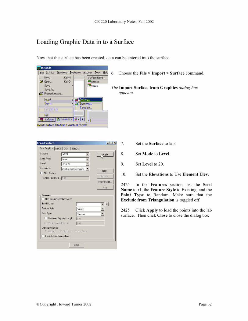
6. Choose the File > Import > Surface command. The Import Surface from Graphics dialog box
appears.
7. Set the Surface to lab. 8. Set Mode to Level. 9. Set Level to 20. 10. Set the Elevations to Use Element Elev. 2424 In the Features section, set the Seed Name to r1, the Feature Style to Existing, and the Point Type to Random. Make sure that the Exclude from Triangulation is toggled off. 2425 Click Apply to load the points into the lab surface. Then click Close to close the dialog box
Copyright Howard Turner 2002 Page 32
CE 220 Laboratory Notes, Fall 2002
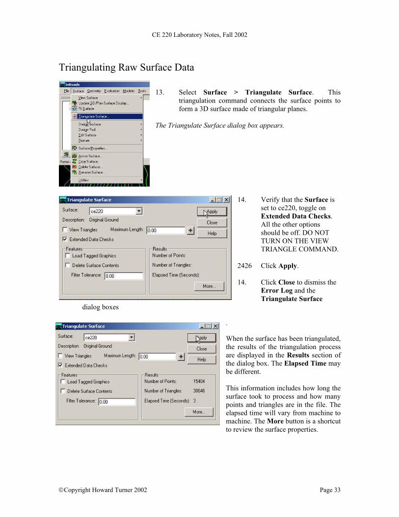
Triangulating Raw Surface Data 13. Select Surface > Triangulate Surface. This
triangulation command connects the surface points to form a 3D surface made of triangular planes.
The Triangulate Surface dialog box appears.
14. Verify that the Surface is
set to ce220, toggle on Extended Data Checks. All the other options should be off. DO NOT TURN ON THE VIEW TRIANGLE COMMAND.
2426 Click Apply. 14. Click Close to dismiss the
Error Log and the Triangulate Surface
dialog boxes
. When the surface has been triangulated, the results of the triangulation process are displayed in the Results section of the dialog box. The Elapsed Time may be different. This information includes how long the surface took to process and how many points and triangles are in the file. The elapsed time will vary from machine to machine. The More button is a shortcut to review the surface properties.
Copyright Howard Turner 2002 Page 33

CE 220 Laboratory Notes, Fall 2002
Reviewing a Surface
2427 To see another way of reviewing the results of the triangulation process, select Surface > Surface Properties. This is where the More button displays from the Triangulate Surface dialog box. The Surface Properties dialog box lists the number of points for each surface point type, the coordinate range of the entire surface model or the individual point types and the number of triangles in the surface. It also lists the name, description, maximum length and material type of the surface.
The name, description, maximum triangle length, the display preference, the display settings for cross sections and the material type can be edited or changed in the appropriate fields. Saving a Surface
15. This is a good time to save the surface file. Select File > Save As. 16. Set the Save as type to Surface (*.dtm) and make sure the Active is set to ce220. 17. Change to the home directory, if it is not the active directory. 18. In the File name field, key in ce220.dtm, if it is not already listed, and click Save then Cancel. This command will
automatically place a .dtm extension on the name of the file if a file extension is not specified.
NOTE: Now the ce220 surface has been created, loaded, and saved. The next time the surface file needs to be loaded, all that has to be done is select the File > Open command (DO NOT DO THIS NOW!), set the Files of Type to Surface (*.dtm), and select the ce220.dtm file.
Copyright Howard Turner 2002 Page 34

CE 220 Laboratory Notes, Fall 2002
Set up to Display Contours
19 Verify that the Write lock is turned on, the Pencil/Pen toggle is set to Pencil, and the Style lock is off. (A lock that is on looks like a pushed in button).
When the Write lock is off, any graphics displayed by InRoads are temporary. In other words, if any view manipulation commands are used, such as Window Area [Zoom Window], Zoom In or Zoom Out, the graphics will disappear. When the Pencil/Pen mode is set to Pen, the graphics that are displayed are written to drawing/design file just like using ink on Mylar. If the mode is set to Pencil, then it is like using a pencil on Mylar and the graphic can be updated. So, if it were set to pencil and contours are displayed, if the contours of the same surface are displayed again, the pencil lines are erased and the new contour lines are displayed. A Style lock is used with surface displays. When the Style lock is on and a View Surface command is activated, the dialog box for the command will not be displayed, but rather the surface data will be displayed in the graphics file without any further input. The Style lock bypasses the dialog box and displays the active surface, automatically determining what symbology to use based on the preference set with the surface. MAKE SURE STYLE LOCK IS OFF.
Displaying the Contours
20 Select Surface > View Surface > Contours. The View Contours dialog box appears. 21. Click the Main tab. Verify that Surface is set to ce220. 22. Set the contour Interval to 1.0 and the Minors per Major ratio to 4. This displays 4 minor contours to every major contour. 23. In the Symbology area, toggle off Major Depression and Minor Depression contours. 24. Set the symbology according to the following section.
Copyright Howard Turner 2002 Page 35

CE 220 Laboratory Notes, Fall 2002
MicroStation Symbology
25. In the Symbology dialog box, highlight major contours and click the Edit button. The line symbology dialog box appears.
26. The Color, Line Style, Weight are automatically set when a Symbology Name is
selected, based on the way that name was previously set up. Click OK. 27. Leave Symbology Name blank. Set Level to Level 35. Set Color to 6 and Line Style to 0. Click OK. The Line Symbology dialog sets the display preferences of the major contours when the surface ce220 is displayed. The color, line style and weight can be controlled by either selecting the entry field and entering the number or by selecting the icon to the right of the entry field, graphically selecting the entry. The
Symbology Names are choices that can be created using the Symbology Manager, which is located in the Tools pull-down menu.
Copyright Howard Turner 2002 Page 36
CE 220 Laboratory Notes, Fall 2002
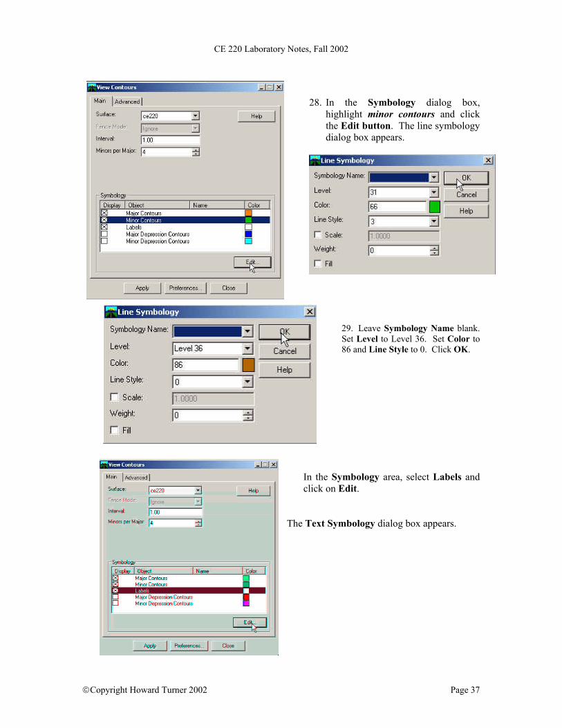
28. In the Symbology dialog box, highlight minor contours and click the Edit button. The line symbology dialog box appears.
29. Leave Symbology Name blank. Set Level to Level 36. Set Color to 86 and Line Style to 0. Click OK.
In the Symbology area, select Labels and click on Edit.
The Text Symbology dialog box appears.
Copyright Howard Turner 2002 Page 37
CE 220 Laboratory Notes, Fall 2002
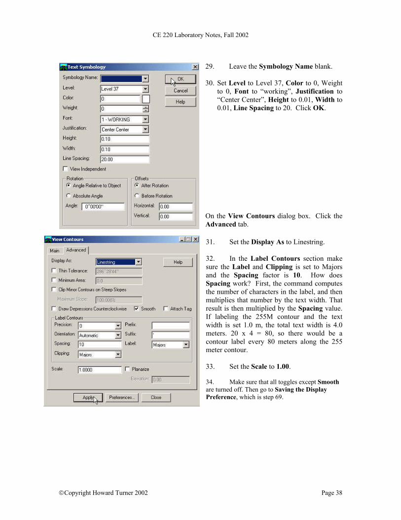
29. Leave the Symbology Name blank. 30. Set Level to Level 37, Color to 0, Weight
to 0, Font to “working”, Justification to “Center Center”, Height to 0.01, Width to 0.01, Line Spacing to 20. Click OK.
On the View Contours dialog box. Click the Advanced tab. 31. Set the Display As to Linestring. 32. In the Label Contours section make sure the Label and Clipping is set to Majors and the Spacing factor is 10. How does Spacing work? First, the command computes the number of characters in the label, and then multiplies that number by the text width. That result is then multiplied by the Spacing value. If labeling the 255M contour and the text width is set 1.0 m, the total text width is 4.0 meters. 20 x 4 = 80, so there would be a contour label every 80 meters along the 255 meter contour. 33. Set the Scale to 1.00. 34. Make sure that all toggles except Smooth are turned off. Then go to Saving the Display Preference, which is step 69.
Copyright Howard Turner 2002 Page 38

CE 220 Laboratory Notes, Fall 2002
Saving the Display Preference
35. Click Preferences.
36. On the Preferences dialog box make sure that default is highlighted and click Save Preference As. The Save As dialog box appears.
37. Click OK on the Save Preferences As dialog box and click Close on the Preferences dialog box.. 38. Click Apply in the View Contours dialog box to display the contours. The new contours are displayed.
Copyright Howard Turner 2002 Page 39

CE 220 Laboratory Notes, Fall 2002
Summary • A DTM can represent any type of spatial data. • Using the File > Import > Surface command is one of the
ways to load data into a surface.
• After the point data is loaded to the surface, the software is used to triangulate the data.
• After the surface is triangulated, save it. Define the location
and name of the surface. • Before displaying the surface terrain contours, it is a good
idea to consider the Write lock and set the Pencil/Pen settings. When the Write lock is turned off, any graphics displayed by InRoads are temporary. However, when the Write lock is on and in Pencil mode, displayed graphics can be zoomed into. If some settings were changed and redisplayed, the old graphics are deleted and replaced by the new graphics.
Copyright Howard Turner 2002 Page 40
CE 220 Laboratory Notes, Fall 2002
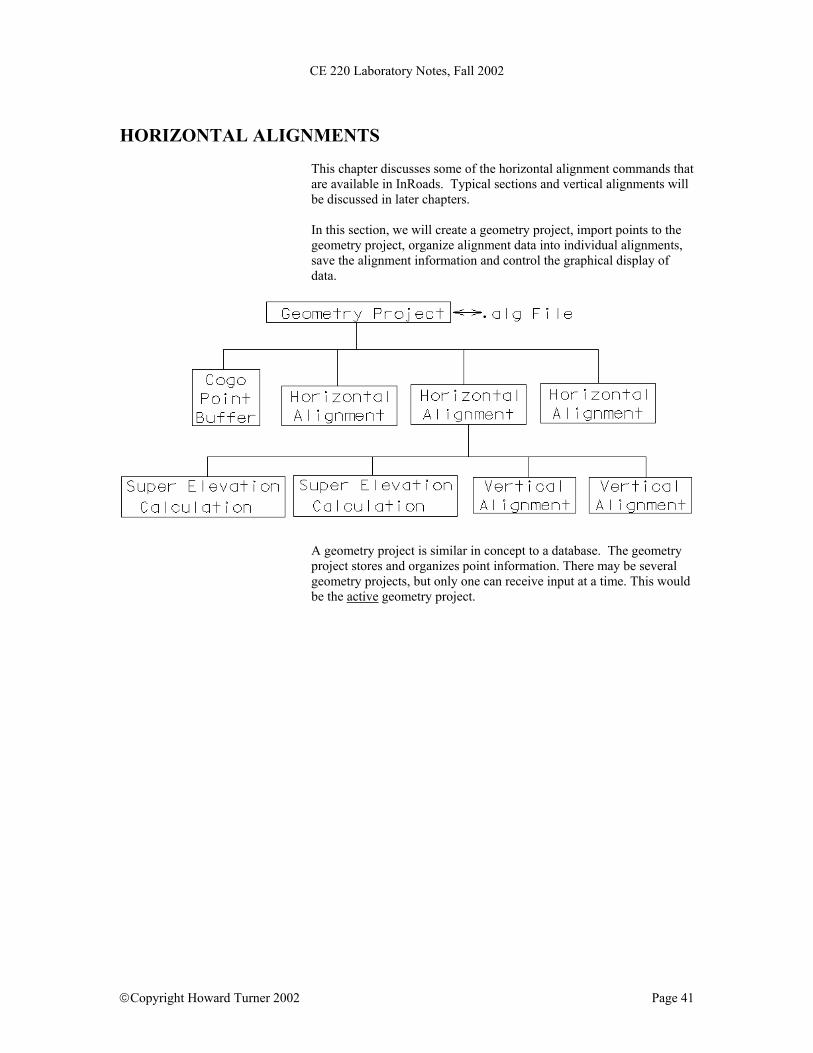
HORIZONTAL ALIGNMENTS
This chapter discusses some of the horizontal alignment commands that are available in InRoads. Typical sections and vertical alignments will be discussed in later chapters. In this section, we will create a geometry project, import points to the geometry project, organize alignment data into individual alignments, save the alignment information and control the graphical display of data.
A geometry project is similar in concept to a database. The geometry project stores and organizes point information. There may be several geometry projects, but only one can receive input at a time. This would be the active geometry project.
Copyright Howard Turner 2002 Page 41

CE 220 Laboratory Notes, Fall 2002
Data can be imported or copied from other sources to the active geometry project. The points, along with their x, y and z coordinates, are stored in the COGO random point buffer. The alignment data must be organized into individual alignments. The software uses horizontal and vertical alignments. Only one alignment can be manipulated within a project at a time. This is the active alignment. Each horizontal alignment can reference superelevation calculation data and vertical alignments. It is often helpful to display and manipulate specific design elements in the software. For instance, a traverse may reflect points a surveyor occupied, and the true boundary may reflect points on which surveying instruments could not be set. Rocks or trees may mark the actual boundary. In such cases, the surveyed traverse may be displayed without the property boundary, and the property boundary without the surveyed traverse. To do this, store the points that make up separate design elements as alignments. These are groups of points saved as units. Alignment data can be organized into individual horizontal alignments. It is necessary to save each traverse, street, curve return and lot as a separate alignment by assigning alignment names. Alignments can be stored by graphically choosing points or by keying in the point numbers.
When keying in the points names, the point numbers are enclosed in parentheses, individual points are separated by spaces, and a range of points are separated by a hyphen. When describing a closed alignment, the first and last points must be the same. After storing a closed alignment, calculate the area and produce direction and distance reports. To verify the contents of the alignment project, display alignments or list the point coordinates. Points of Intersection (PIs) can be deleted or moved as necessary. When the tangent lines are set, curves can be set or revised. There are tools to help in the design of the curves like the curve calculator. It is important to remember, the graphics display the information in the project and that deleting the graphics does not delete the project information. As alignment design is performed, the display color, line thickness, design file level or text size can be changed. Remember preferences are used to control how graphic elements display. When changing the way graphics display, turn Write lock off or set the Pencil/Pen mode to pencil before placing graphics. This allows the design to be experimented with before graphics are written permanently to the design file.
Copyright Howard Turner 2002 Page 42

CE 220 Laboratory Notes, Fall 2002
Use Report lock to control the display of information when working with Coordinate Geometry commands. If Report lock is off, the commands are processed, but the results of the processing do not display. If Report lock is on, the commands are processed and the results display automatically. The Station lock is used to force anything that involves stationing to the nearest whole station.
Copyright Howard Turner 2002 Page 43

CE 220 Laboratory Notes, Fall 2002
Horizontal Alignments
1. Start MicroStation and InRoads using the design file lab.dgn. To review how to start MicroStation, see Chapter 1.
2. Create a new geometry project File > New.
3. The new geometry dialog box opens. Select the Geometry Tab. Make Type Geometry Project .. Enter Lab in the Name dialog box. Enter CE220 Lab in the Description field. Press apply.
Copyright Howard Turner 2002 Page 44
CE 220 Laboratory Notes, Fall 2002
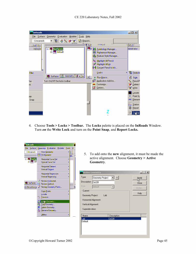
4. Choose Tools > Locks > Toolbar. The Locks palette is placed on the InRoads Window.
Turn on the Write Lock and turn on the Point Snap, and Report Locks.
5. To add onto the new alignment, it must be made the active alignment. Choose Geometry > Active Geometry.
Copyright Howard Turner 2002 Page 45

CE 220 Laboratory Notes, Fall 2002
6. Create a new horizontal geometry project File > New The new geometry dialog box opens. Select the Geometry Tab. Make Type Horizontal Alignment .. Enter h1 in the Name dialog box. Enter CE220 in the Description field. Press apply. . 7. Choose Close.
Adding Horizontal Points of Intersection 8. Choose Palettes > Horizontal Curve Set>AddPI.
Copyright Howard Turner 2002 Page 46

CE 220 Laboratory Notes, Fall 2002
9. For the first PI, we know the exact coordinates. Point B is N5000; E2000. The first PI is added by key-in. In the MicroStation command window, key-in
ne=5000,5000 Press enter. The point is placed and a dynamic line attaches to the point
The message Identify Point/Backup displays. This
means that you should identify the location of the next PI. You can identify this location with key in or by placing a data point.
10. For the second PI on our alignment, we know the
bearing and distance. So, key in di=207.85,s01^47’08”w
This will place the next PI. A line is now drawn from Point B to Point C The message Identify Point/Backup displays. This means that you should identify the location of the next PI. You can identify this location with key in or by placing a data point.
11. Now we know the distance and direction to the third PI. Key in di=150.66,s15^45’49”w to place the next point.
Your screen should look something like the picture to the left.
Remember that if the Write Lock is off, when you try to manipulate the view, the graphics will disappear.
12. For the fourth PI, we have the distance and bearing where the
new road is to be placed. Key in di=98.91,n42^05’46”w to place the fourth PI. Your screen should look similar to the picture to the left.
Copyright Howard Turner 2002 Page 47

CE 220 Laboratory Notes, Fall 2002
13. For the fifth PI, point F, we have the distance and bearing where the new road is to be
placed. Key in di=192.23,n28^51’27”e to place the fifth PI.
14. For the sixth PI, point G, we have the distance and bearing where the new road is to be placed. Key in
di=168.84,s75^24’00”w to place the sixth PI.
15. For the seventh PI, point A, we have the distance and bearing where the new road is to be placed. Key in
di=222.33,n71^23’59”w to place the seventh PI.
16. For the closing course, from A to B, with the dynamic line attached to point A, snap onto point B, and accept the point the a data button.
19. Reset (right mouse click) out of the Add Horizontal PI command. 20. Fit the design view. The completed polygon should look like the diagram below.
Copyright Howard Turner 2002 Page 48

CE 220 Laboratory Notes, Fall 2002
21. Delete the graphics from the MicroStation window. To check if the graphics is stored correctly in the database, redisplay the alignment, choose Geometry > Review Horizontal. Remember that Pen Lock controls whether or not the graphics are written into the design file.
Saving the Geometry Project to a File
22. Save the edited geometry by choosing File > Save > Geometry Project. Save the file on the class drive on the server. The file should be given the name Lab.alg.
Copyright Howard Turner 2002 Page 49

CE 220 Laboratory Notes, Fall 2002
23. The alignment you have drawn will not allow curves between the first and last course of the alignment. You should draw a second alignment. Start the new alignment on a tangent, midway between two PI points. Snap on to the existing PIs.
Revising Curve Sets
With the PIs in place, the curves sets that are attached to the PIs can be modified. You might be asking, "What curve sets?" A curve set is defined as being a spiral-arc-spiral, spiral-arc-spiral-spiral-arc-spiral or no curve between two elements. The elements can be either straight or curved. When a PI is placed, there is no curve associated with it, just a straight element. To place a curve set between two straight elements, the Revise Curve Set command can used.
24. Choose Geometry>Horizontal Curve
Set>Define Curve.
The Horizontal Curve Set Editor dialog box appears. 25. Set Define By as Known PI Coordinates 26. Select Curve Set Type as SCS. 27. Select Radius 1 and key in 25.00. 28. Select Clothoid by Length and key in 0.00. This is the first (incoming) spiral length. 29. Select Clothoid by Length and key in 0.00. This is the outgoing spiral length. The dialog box on your screen should resemble that shown here. 30. Choose Apply. .
Copyright Howard Turner 2002 Page 50

CE 220 Laboratory Notes, Fall 2002
31. Press <Next > to accept the curve set. The alignment is updated with the new curve
set definition.
32. This identifies the second curve set. Select Radius 1 and key in 200.00. Choose Apply and
press <Next> to accept the results.
The curve set now looks like the picture to the left.
33. Select the Radius1 entry field. Key in an appropriate radius value, e.g. 25.00. Choose Apply and accept the results by pressing <Next>.
34. Add curve sets to all the remaining PIs by using your
knowledge gained from the curve layout exercise. Press Close to exit the form.
35. Save the geometry file,
by choosing File > Save>Geometry Project.
Displaying the Active Alignment
43. Delete the graphics related to the alignment from the
MicroStation file. Toggle the Pen Lock and Station Lock on and then choose Geometry > Review Horizontal to display the horizontal alignment and write the graphics to the design file.
The final horizontal alignment should look similar to the drawing at the top of the next page.
Copyright Howard Turner 2002 Page 51

CE 220 Laboratory Notes, Fall 2002
CE 220 Laboratory Notes, Fall 2002
Copyright Howard Turner 2002 Page 52
Copyright Howard Turner 2002 Page 52
CE 220 Laboratory Notes, Fall 2002
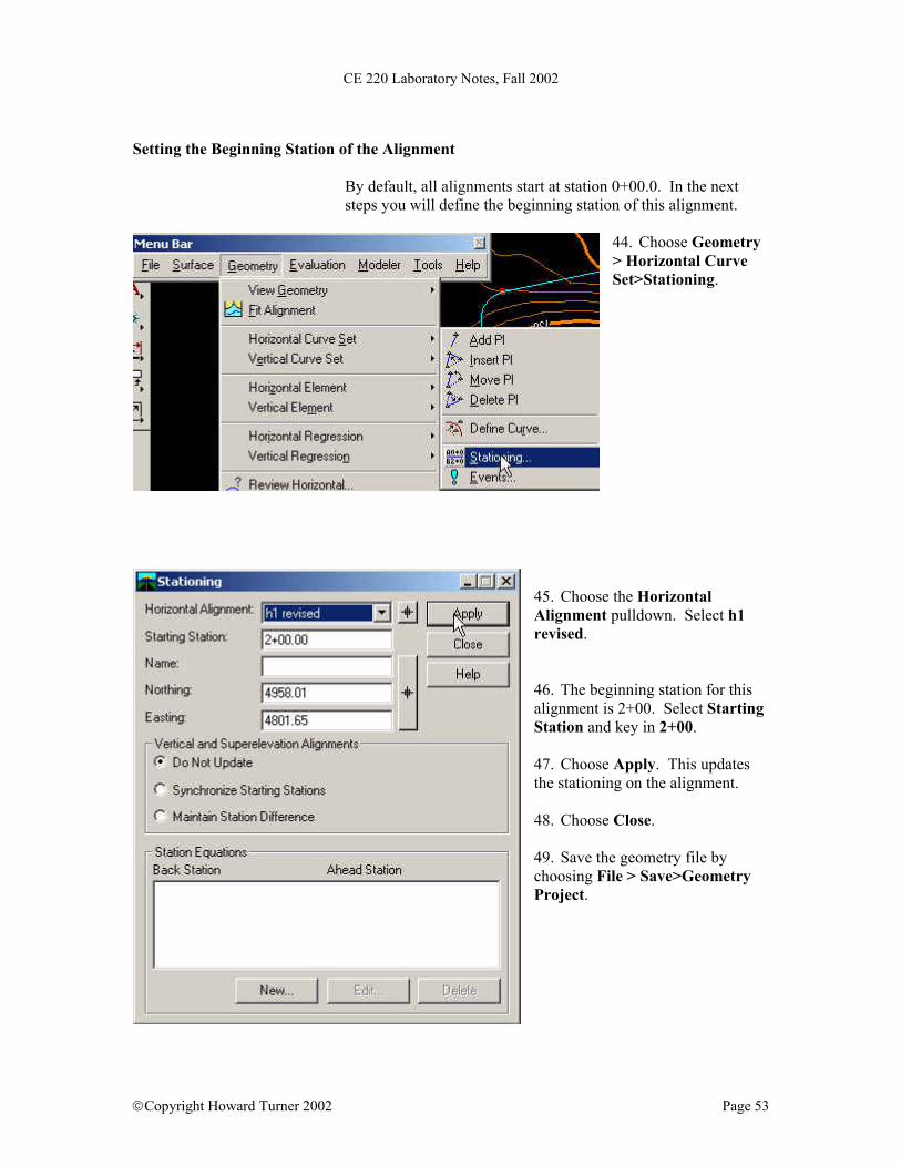
Setting the Beginning Station of the Alignment
By default, all alignments start at station 0+00.0. In the next steps you will define the beginning station of this alignment.
44. Choose Geometry > Horizontal Curve Set>Stationing.
45. Choose the Horizontal Alignment pulldown. Select h1 revised. 46. The beginning station for this alignment is 2+00. Select Starting Station and key in 2+00. 47. Choose Apply. This updates the stationing on the alignment. 48. Choose Close. 49. Save the geometry file by choosing File > Save>Geometry Project.
Copyright Howard Turner 2002 Page 53

CE 220 Laboratory Notes, Fall 2002
Displaying the Alignment Stationing 50. Choose Geometry>View Geometry > Stationing. The View Station Dialog Box appears.
51. Toggle the Method to Automatic, select the horizontal Alignment as h1 revised, and set the Interval to 100.00. Toggle on Major Ticks, Major Stations, Minor Ticks and Minor Stations. All other toggles should be off.
52. Choose Regular Stations tab from the top of the dialog box.
Copyright Howard Turner 2002 Page 54
CE 220 Laboratory Notes, Fall 2002
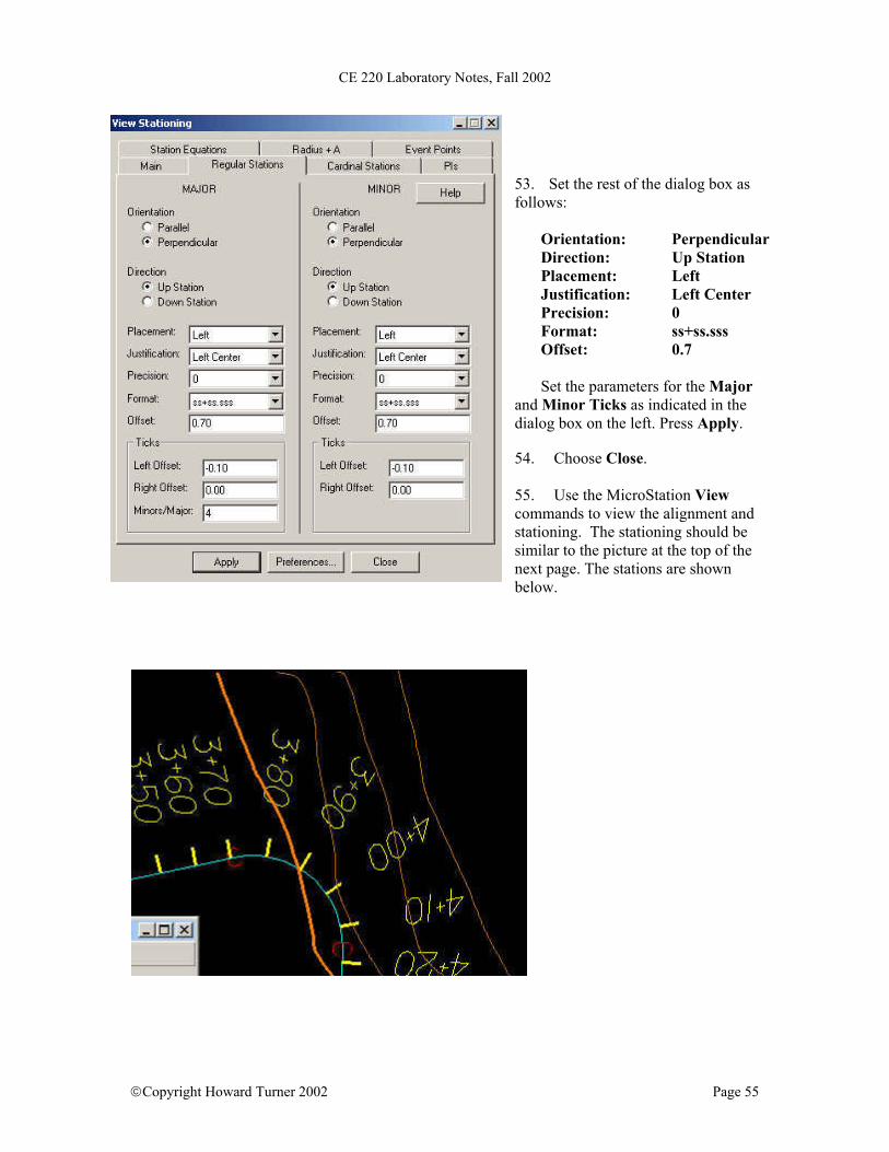
53. Set the rest of the dialog box as follows: Orientation: Perpendicular Direction: Up Station Placement: Left Justification: Left Center Precision: 0 Format: ss+ss.sss Offset: 0.7 Set the parameters for the Major and Minor Ticks as indicated in the dialog box on the left. Press Apply. 54. Choose Close. 55. Use the MicroStation View commands to view the alignment and stationing. The stationing should be similar to the picture at the top of the next page. The stations are shown below.
Copyright Howard Turner 2002 Page 55

CE 220 Laboratory Notes, Fall 2002
Summary • A geometry project is similar in concept to a database.
• You can have several geometry projects but only the active geometry can receive input at one time.
• You can import or copy data from other sources to the active geometry project.
• You'll want to save each traverse, street, curve return, and lot as a separate alignment.
• Points of Intersection can be deleted or moved as necessary.
• Tools like the curve calculator help you to design curves.
Copyright Howard Turner 2002 Page 56

CE 220 Laboratory Notes, Fall 2002
Profiles This chapter discusses how to display surface information along a horizontal alignment. This display is better known as a profile. In subsequent chapters, a profile will be used to create a vertical alignment for the horizontal alignment. Later the alignments will be used to model the proposed roadway. In this section on creating profiles, a profile will be displayed to extract the terrain model elevation information. If multiple surfaces were displayed, then that information could be extracted at the same time. A profile is a cross section view of the surface terrain along a linear element. That element can be between multiple defined points, a graphics element or an alignment.
A profile does not need ground terrain displayed, nor does a surface model need to be created to display a ground terrain on a profile grid. The use of the multi-point profile option is productive when working in a building site with other projects that are more site design oriented. After choosing the Multi-Point option, the software prompts for the points that are to be connected for a profile to be identified graphically. This is similar to placing a linestring or polyline. The profile grid and surface displays are controlled by using the tabs on the dialog box. The Symbology section is used to set the colors, level, weight, font and text heights and widths. The first surface selected will have that color, and
Copyright Howard Turner 2002 Page 57

CE 220 Laboratory Notes, Fall 2002
the next surface will have the next color in the color table. In a future release, the Symbology Manager will control the color of the surface display.
A vertical exaggeration can also be set. For example, a vertical exaggeration of five means that for every one-foot of vertical elevation change, the profile will plot a five-foot vertical elevation change in the design file. A vertical exaggeration of ten will plot ten feet in the design file for every foot of elevation change.
When using the profile command, the surface (or surfaces) to profile will be selected, then the location for displaying the lower corner of the profile will be selected. When using the Profile command, select the active horizontal alignment, multiple points or a graphic element and set station limits and elevation limits can be selected. Note that if the elevation limits are set too small, the ground line can fall off the profile. Remember that if the Write Lock is off when the view is updated, the graphics will disappear. If the Write Lock is on when the profile is displayed, the profile displays permanently. Note that before a vertical alignment can be designed interactively, a profile of the horizontal alignment must be created and displayed with the Write Lock on.
Remember the .alg file contains the geometry project. The coordinate geometry points and the horizontal alignments are owned by the project. The horizontal alignment owns the superelevation calculations and the vertical alignments.
Copyright Howard Turner 2002 Page 58

CE 220 Laboratory Notes, Fall 2002
Creating a Profile
1. Select Evaluation > Profile>
Create Profile.
2. Off of the Main tab, in the Source section, click Alignment and make sure that h1 revised is the alignment listed.
3. The Create data field should
be set to Window and Data.
4. The Set Name data field should be set to h1 revised. For an explanation of the Set Name, click the on-line Help.
5. In the Symbology section, make sure the Surface ce220 display is on.
(NOTE: More than one surface can be profiled at a time. In the Symbology section, click in the Display column the surfaces to
be displayed.
6. Click the Features tab. Notice that some of the Features are highlighted (selected) and others are not highlighted (not selected). The reason for this is that the Features not highlighted (not selected) do not have Feature Styles that may be displayed in profile. In other words, for a feature to be displayed, the Feature Style MUST be appropriately turned on. To be able to see features that are not selected, using the cursor, select the feature and press the Edit Style button. In the Edit Feature Style dialog box that will appear, it is possible to turn on Projected Line Segments, Projected
Points, Crossing Points and Annotation. For more information concerning the use of these program features, press the Help button.
7. Be sure that the Crossing Features and the Projected Features check boxes are turned off.
Copyright Howard Turner 2002 Page 59

CE 220 Laboratory Notes, Fall 2002
8. Click the Controls tab.
9. In the Exaggeration area,
set the Vertical exaggeration to 10.000 and the Horizontal Exaggeration to 1.000.
10. Make sure the Limits are
toggled off and the plotting Direction is set to Left to Right.
11. In the Window Clearance
section, toggle on Apply and set the Top to 5.000 and the Bottom to 10.000.
The Top and Bottom clearance is new in Version 8.3. This allows an area to be reserved at the top and at the bottom of a profile for annotation. In this case, the profile is set a little larger on the top (5 meters) and a little larger on the bottom (10 meters) so that the areas can be annotated without having the text go outside of the profile window.
12. Click the Grid tab.
13. In the Symbology section under
Display, turn on the Major Horizontal and the Major Vertical objects, and make sure everything else is turned off.
Copyright Howard Turner 2002 Page 60

CE 220 Laboratory Notes, Fall 2002
14. Click the Axes tab.
15. Set the Axis selection field to Left. Toggle the Annotation field to Ticks. In the Major Ticks section, set the Length to 0.2, the Position to Both Sides, and the Spacing to 10.000. In the Minor Ticks section, set the Length to 0.1, the Position to Inside, and the Minors/Major to 4.
16. Under the Title tab, in the Text entry field enter Elevation. In the Placement section, toggle on Automatic. In the Symbology section, toggle on Box and Text.
Copyright Howard Turner 2002 Page 61

CE 220 Laboratory Notes, Fall 2002
17. Click Apply and then datapoint to locate the lower left-hand corner of the profile. Identify a place to the right of the site. Click Close.
25.
Copyright Howard Turner 2002 Page 62

CE 220 Laboratory Notes, Fall 2002
Vertical Alignments
This chapter discusses how to create a vertical alignment on a profile that was created using a horizontal alignment. As a review, the vertical alignment is owned by the horizontal alignment. The horizontal alignment is owned by the geometry project.
Cogo Point Buffer
Horizontal Alignment
Horizontal Alignment
Superelevation Calculations
Vertical Alignment
Horizontal Element Buffer
Vertical Element Buffer
Geometry Project.alg file
There are three ways to create a vertical alignment. One way involves using a surface, another is to use the ASCII Geometry command and the third is to interactively create the vertical alignment using a profile window.
Cop
Begin by making sure the correct horizontal alignment is active. Then create a new vertical alignment, assign a name to the vertical alignment, provide a description, establish the display preferences and set the vertical arc definition. This will create the alignment.
yright Howard Turner 2002 Page 63
CE 220 Laboratory Notes, Fall 2002
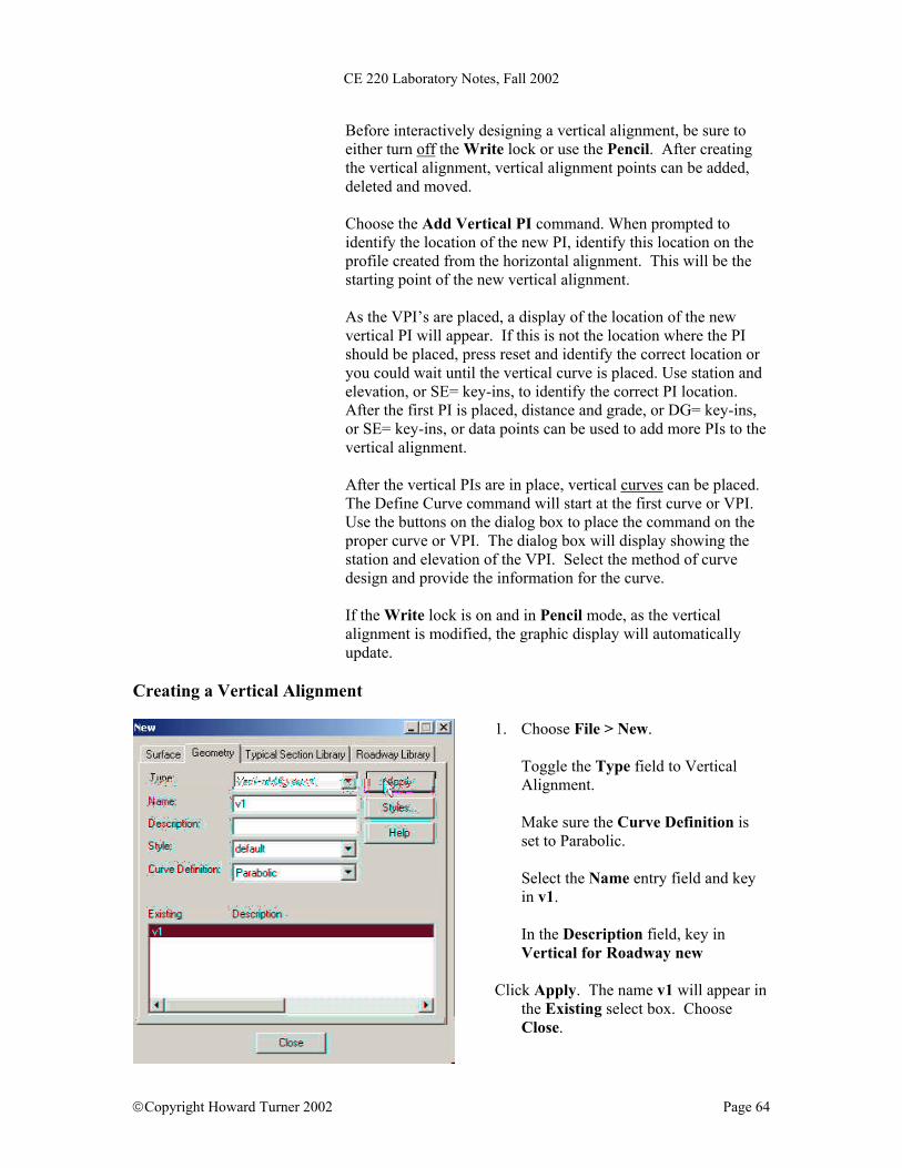
Before interactively designing a vertical alignment, be sure to either turn off the Write lock or use the Pencil. After creating the vertical alignment, vertical alignment points can be added, deleted and moved. Choose the Add Vertical PI command. When prompted to identify the location of the new PI, identify this location on the profile created from the horizontal alignment. This will be the starting point of the new vertical alignment. As the VPI’s are placed, a display of the location of the new vertical PI will appear. If this is not the location where the PI should be placed, press reset and identify the correct location or you could wait until the vertical curve is placed. Use station and elevation, or SE= key-ins, to identify the correct PI location. After the first PI is placed, distance and grade, or DG= key-ins, or SE= key-ins, or data points can be used to add more PIs to the vertical alignment. After the vertical PIs are in place, vertical curves can be placed. The Define Curve command will start at the first curve or VPI. Use the buttons on the dialog box to place the command on the proper curve or VPI. The dialog box will display showing the station and elevation of the VPI. Select the method of curve design and provide the information for the curve. If the Write lock is on and in Pencil mode, as the vertical alignment is modified, the graphic display will automatically update.
Creating a Vertical Alignment
1. Choose File > New.
Toggle the Type field to Vertical
Alignment.
Make sure the Curve Definition is set to Parabolic.
Select the Name entry field and key
in v1.
In the Description field, key in Vertical for Roadway new
Click Apply. The name v1 will appear in
the Existing select box. Choose Close.
Copyright Howard Turner 2002 Page 64
CE 220 Laboratory Notes, Fall 2002
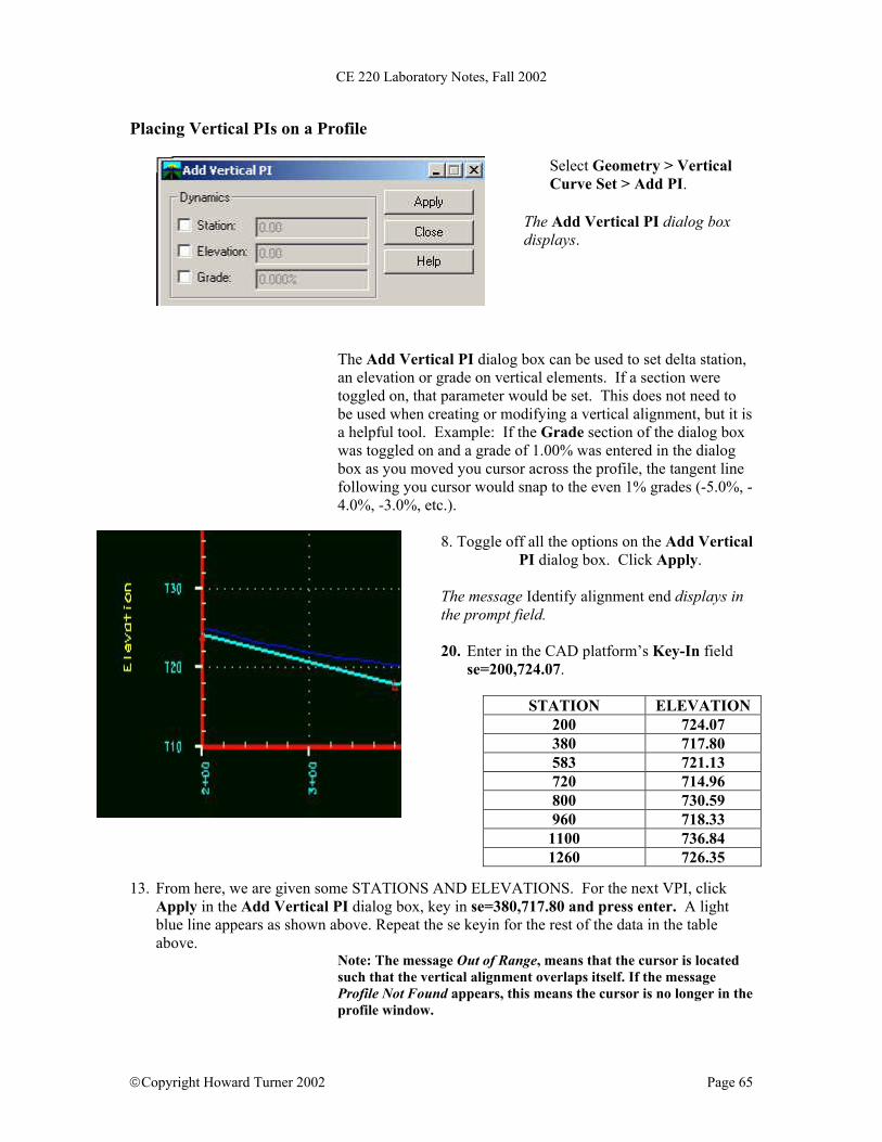
Placing Vertical PIs on a Profile
Select Geometry > Vertical Curve Set > Add PI.
The Add Vertical PI dialog box displays.
The Add Vertical PI dialog box can be used to set delta station, an elevation or grade on vertical elements. If a section were toggled on, that parameter would be set. This does not need to be used when creating or modifying a vertical alignment, but it is a helpful tool. Example: If the Grade section of the dialog box was toggled on and a grade of 1.00% was entered in the dialog box as you moved you cursor across the profile, the tangent line following you cursor would snap to the even 1% grades (-5.0%, -4.0%, -3.0%, etc.).
8. Toggle off all the options on the Add Vertical
PI dialog box. Click Apply. The message Identify alignment end displays in
the prompt field.
20. Enter in the CAD platform’s Key-In field se=200,724.07.
STATION ELEVATION 200 724.07 380 717.80 583 721.13 720 714.96 800 730.59 960 718.33
1100 736.84 1260 726.35
13. From here, we are given some STATIONS AND ELEVATIONS. For the next VPI, click
Apply in the Add Vertical PI dialog box, key in se=380,717.80 and press enter. A light blue line appears as shown above. Repeat the se keyin for the rest of the data in the table above.
Note: The message Out of Range, means that the cursor is located such that the vertical alignment overlaps itself. If the message Profile Not Found appears, this means the cursor is no longer in the profile window.
Copyright Howard Turner 2002 Page 65

CE 220 Laboratory Notes, Fall 2002
14. Choose File > Save>Geometry Project. Revising Vertical Curves
Now the vertical curves can be set. The Vertical Define Curve command works just like the Horizontal Define Curve.
15 Select Geometry > Vertical Curve Set > Define Curve.
16 Just like the horizontal curves,
the Define Vertical Curve command finds the first VPI or curve set on an alignment.
17 In the Define Vertical Curve
dialog box, in the Vertical Curve section, set the Calculate By to Length of Curve and for Length enter 150.00. Click Apply.
The vertical alignment display is updated with the vertical curve definition.
18 Click Next.
19 The curve Length should be set to 95.000. Click Apply.
19. Apply curve lengths of 50, 50, 50 and 120 to the following curves respectively.
The vertical alignment display is updated with the vertical curve definition as shown below.
Copyright Howard Turner 2002 Page 66

CE 220 Laboratory Notes, Fall 2002
Annotation of the Vertical Alignment 20. Select Geometry > View Geometry > Vertical Annotation. Select h1 revised as the Horizontal Alignment and v1 for the Vertical Alignment.
21. Select the Profile Set: h1 revised.
22. Do not turn on any of the Limits.
Copyright Howard Turner 2002 Page 67
CE 220 Laboratory Notes, Fall 2002
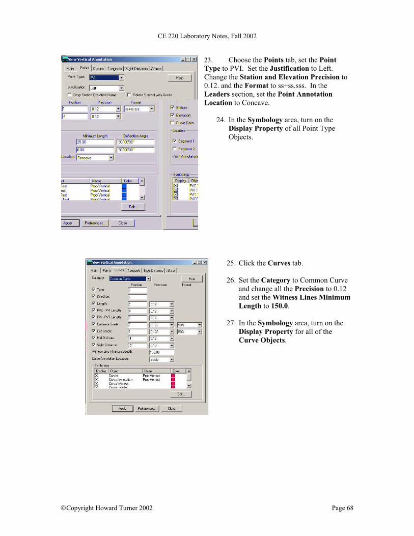
23. Choose the Points tab, set the Point Type to PVI. Set the Justification to Left. Change the Station and Elevation Precision to 0.12. and the Format to ss+ss.sss. In the Leaders section, set the Point Annotation Location to Concave.
24. In the Symbology area, turn on the Display Property of all Point Type Objects.
25. Click the Curves tab.
26. Set the Category to Common Curve and change all the Precision to 0.12 and set the Witness Lines Minimum Length to 150.0.
27. In the Symbology area, turn on the
Display Property for all of the Curve Objects.
Copyright Howard Turner 2002 Page 68
CE 220 Laboratory Notes, Fall 2002
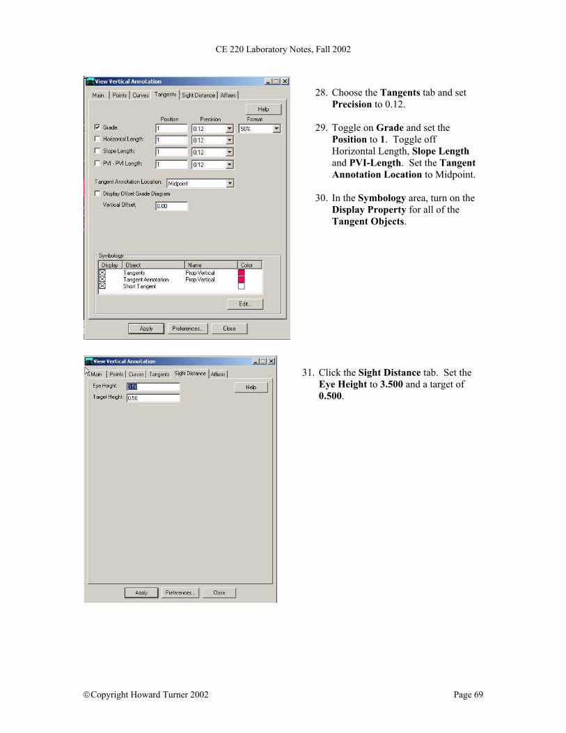
28. Choose the Tangents tab and set
Precision to 0.12.
29. Toggle on Grade and set the Position to 1. Toggle off Horizontal Length, Slope Length and PVI-Length. Set the Tangent Annotation Location to Midpoint.
30. In the Symbology area, turn on the
Display Property for all of the Tangent Objects.
31. Click the Sight Distance tab. Set the Eye Height to 3.500 and a target of 0.500.
Copyright Howard Turner 2002 Page 69

CE 220 Laboratory Notes, Fall 2002
•
•
•
32. Click on the Affixes tab. Set the
Category to Tangents.
33. Change any of the Suffix that has a FT or m to ‘.
34. Inspect the other Categories and
change any entry that has a Suffix of a m or FT to ‘.
35. Click Apply. The vertical alignment is annotated.
36. On the View Vertical Annotation dialog box, click Close.
Summary
The vertical alignment is owned by the horizontal alignment. The horizontal alignment is owned by the geometry project. After creating the vertical alignment, vertical alignment points can be added, deleted, inserted and moved. Curves can be placed after the vertical PIs are in place.
Copyright Howard Turner 2002 Page 70

CE 220 Laboratory Notes, Fall 2002
Templates This chapter discusses how to create a library of typical sections, also known as a typical section library. A typical section is used in road design and it is sometimes known as a template. The top of grade and any sublayers are shown along with the side slope conditions. The side slope conditions depict which slope would be used if in cut or fill. The side slope conditions also depict whether that condition is on the right side or the left side of the travel lanes. In this section, some of the terms used when creating a typical section (template) will be defined, how to create and load a typical section library, how to create a typical section, how to add and edit segments in a typical section and how to save the typical section library will be looked at. A typical section defines how a road will be built. It also shows what sublayers, if any, are used and what happens if the proposed road is below the existing ground or above it. To understand what a typical section is, a few terms will be defined. A backbone is the center section of the typical section. Normally, the slopes and lengths of the backbone segments will not change throughout the model.
The exterior portion of the typical section is the section in which the cut slope or the fill slopes are defined. Other points on the typical section include superelevation range points, superelevation pivot points, and transition control points.
Because superelevation assigns raised outside edges to the curve, superelevation range points establish which segments of the typical section will be raised, and the superelevation pivot point establishes the point the segments will turn about.
Copyright Howard Turner 2002 Page 71

CE 220 Laboratory Notes, Fall 2002
When modeling, there is a point on the typical section that establishes whether the typical section is in a cut or fills condition, which is called a hinge point. A typical section has two hinge points, one on each end of the backbone. All cut or fill slopes are attached to the hinge. A typical section point's horizontal and vertical positions are controlled by the transition control points.. Check Help for more information. Typical sections are stored in a typical section library along with cut and fill tables, material tables and decision tables. To create a typical section, select the Define Typical Sections command found in the Modeler pull down menu. A list of typical sections is displayed in the dialog box. An existing typical section can be selected to be edited, or a new typical section can be added.
When adding a typical section, establish a name and a description, and then select whether this is a typical section, a cut and fill table, a material table or a decision table. Once the typical section is added to the list, edit it to add segments to it. Display the dialog box and set an active layer to edit. Since this is a new typical section, a layer will be added by giving the layer a name to be used when a model is created. The name of the surface which is created will also be the name of the layer. After a layer is created, segments can be added to the typical section. First, check what is being added to and how the segments are going to be added. To add a segment, establish the slope and length for that segment to have. All slopes are based from the center going outward. A negative slope is downward and a positive upward. All lengths are positive. Two other parameters are set when the segment is created--the segment's transition control point and its fixity. The transition control point is added to the end of the segment. It is used to control exactly how that point is modeled. The fixity allows the segment to vary either in length, slope or both. Once finished with one side of the backbone, enter the cut slope for that side and the fill slope. Remember a cut slope is a slope going upward, so it would have a positive value.
Copyright Howard Turner 2002 Page 72

CE 220 Laboratory Notes, Fall 2002
When one side of the typical section is finished, either enter the remaining sides or use one of the tools that mirror or copy one side of the typical section to the other. When mirroring is complete, the typical section segments can be edited. There are also tools for setting the superelevation range and pivot points. First, set the superelevation range then set the pivot point. The Typical Section View gives confirmation on where points are set. Remember that if the sublayers are going to be super-elevated, a range for the Superelevation must be established. Also, remember to save the typical section library after the typical section has been edited or created.
Copyright Howard Turner 2002 Page 73

CE 220 Laboratory Notes, Fall 2002
Templates
1. Choose File > New>Typical Section Library, the New Template Library dialog box appears. Type CE220 in the Name Field. Type lab for ce220 in the Description field, and choose Apply to create the template library. This will create a slot in memory for the template library. Loading a Template Library 2. If a template library already exists, choose File > Open > Typical Section Library, select lab.tml and choose OK.
Creating a Template
3. Select Modeler >
Define Typical Sections.
4. Click the Templates
tab.
5. Click the New button.
Copyright Howard Turner 2002 Page 74

CE 220 Laboratory Notes, Fall 2002
6. On the New Template dialog box, in the Name field, key in Two Lane and in the Description field, key in Two Lane Section.
7. Click Apply, then Close to
dismiss the dialog box.
8. Notice that the
name Go-Cart is now entered into the list of typical sections.
9. Select Go-Cart
from the list of typical sections. Now click Edit.
Copyright Howard Turner 2002 Page 75

CE 220 Laboratory Notes, Fall 2002
Creating Typical Section Segments
10. Look at the Layer section of the Edit Template dialog box. This allows the user to create multiple layers in the typical section like sub-base, select fill or binder course. Each typical section layer will create a surface with the name of the layer when the typical section is modeled. Layer names are case sensitive.
Be careful with how you type in the layer name is typed. The layer name will become a surface name. If possibly using this typical section with other templates, be aware that the layer name is CASE SENSITIVE. A surface named Top is not the same as a surface named top!
11. In the Name section, key in
top, and as a Description, key in finished grade. This will create a typical section layer and it will be the active layer.
12. Click New to add the layer. The typical section of this road is two 3-foot lanes with no shoulders on each side. The cut slope is 2:1 {50%}(2feet horizontal for each vertical foot) and the fill slopes will be 1.5:1 {66.66%}. The cross grade on the pavement is 1% from outside to inside. The pavement is 6 feet wide.
Copyright Howard Turner 2002 Page 76

CE 220 Laboratory Notes, Fall 2002
13. Click the Segment tab.
14. The View section should
have both Left Side and Right Side toggled on. Zone should be set to Left Backbone and the Edit Mode should be set to Add After. Press New.
15. Key in, in the Input section of the dialog box, the first template section that is a Slope of 1.0% and a Width of 3.0. Make sure that you press TAB after each key-in. In the Transition Control list select uncontrolled and select it. Make sure that the Fixity is set to Fixed. Once the sections are filled in, click New. Notice that the typical section display area shows a line. This is the line that was just added. As the typical section is built or modified, the display will change. This is a visual confirmation of the typical section.
Copyright Howard Turner 2002 Page 77
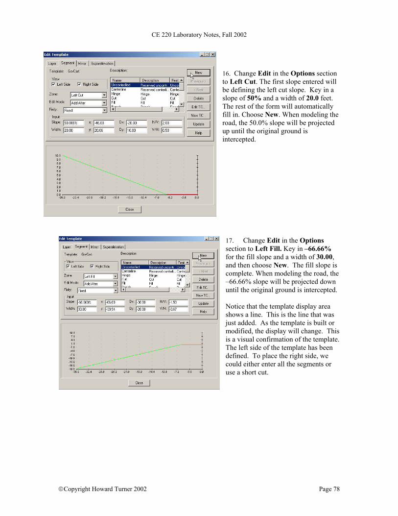
CE 220 Laboratory Notes, Fall 2002
16. Change Edit in the Options section to Left Cut. The first slope entered will be defining the left cut slope. Key in a slope of 50% and a width of 20.0 feet. The rest of the form will automatically fill in. Choose New. When modeling the road, the 50.0% slope will be projected up until the original ground is intercepted.
17. Change Edit in the Options section to Left Fill. Key in –66.66% for the fill slope and a width of 30.00, and then choose New. The fill slope is complete. When modeling the road, the –66.66% slope will be projected down until the original ground is intercepted. Notice that the template display area shows a line. This is the line that was just added. As the template is built or modified, the display will change. This is a visual confirmation of the template. The left side of the template has been defined. To place the right side, we could either enter all the segments or use a short cut.
Copyright Howard Turner 2002 Page 78

CE 220 Laboratory Notes, Fall 2002
18. The short cut would mirror the left side of the template to the right. Select the Mirror tab and complete the form as shown. Click Close until you reach the Typical Sections Dialog Box
Copyright Howard Turner 2002 Page 79
14. Notice that the typical section is displayed in the Define Typical Sections dialog box. Click Close to exit the dialog box.
Saving a Typical Section Library
15. Select File > Save > Typical Section Library.
The new typical section is saved in the typical section library on disk.
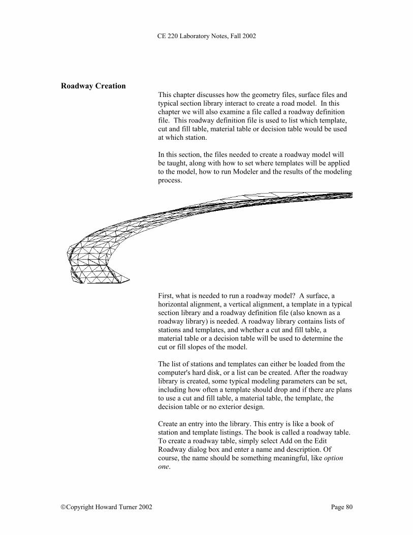
CE 220 Laboratory Notes, Fall 2002
Roadway Creation
This chapter discusses how the geometry files, surface files and typical section library interact to create a road model. In this chapter we will also examine a file called a roadway definition file. This roadway definition file is used to list which template, cut and fill table, material table or decision table would be used at which station. In this section, the files needed to create a roadway model will be taught, along with how to set where templates will be applied to the model, how to run Modeler and the results of the modeling process.
First, what is needed to run a roadway model? A surface, a horizontal alignment, a vertical alignment, a template in a typical section library and a roadway definition file (also known as a roadway library) is needed. A roadway library contains lists of stations and templates, and whether a cut and fill table, a material table or a decision table will be used to determine the cut or fill slopes of the model. The list of stations and templates can either be loaded from the computer's hard disk, or a list can be created. After the roadway library is created, some typical modeling parameters can be set, including how often a template should drop and if there are plans to use a cut and fill table, a material table, the template, the decision table or no exterior design. Create an entry into the library. This entry is like a book of station and template listings. The book is called a roadway table. To create a roadway table, simply select Add on the Edit Roadway dialog box and enter a name and description. Of course, the name should be something meaningful, like option one.
Copyright Howard Turner 2002 Page 80

CE 220 Laboratory Notes, Fall 2002
After the table is created, it becomes the active table for editing. A new table has no listing of stations and templates. When adding a listing, specify a starting station and a template. Also set how the catch will be designed and if the interval is different than the one set with the default settings. The following is an example of how to transition from a two-lane road section to a four-lane. The alignment starts at station 0+00 and will be modeled using a two lane template to station 20+00. At 30+00 a four lane road will begin. The template and station list will look like this.
With this table, this is how the road would be modeled. The road starts at station 0 with a two lane section and is modeled until station 20, which will start the transition section to a four lane typical section. At station 30, the model will use the four-lane typical section.
After setting the station and template list, save the roadway definition file. After selecting the command, set the parameters, and indicate if a report is wanted. Now to model. Select which roadway definition and surface will be used and modeled. A surface will be created for each template layer that is in the typical section. After modeling, save the surfaces that were created.
Copyright Howard Turner 2002 Page 81
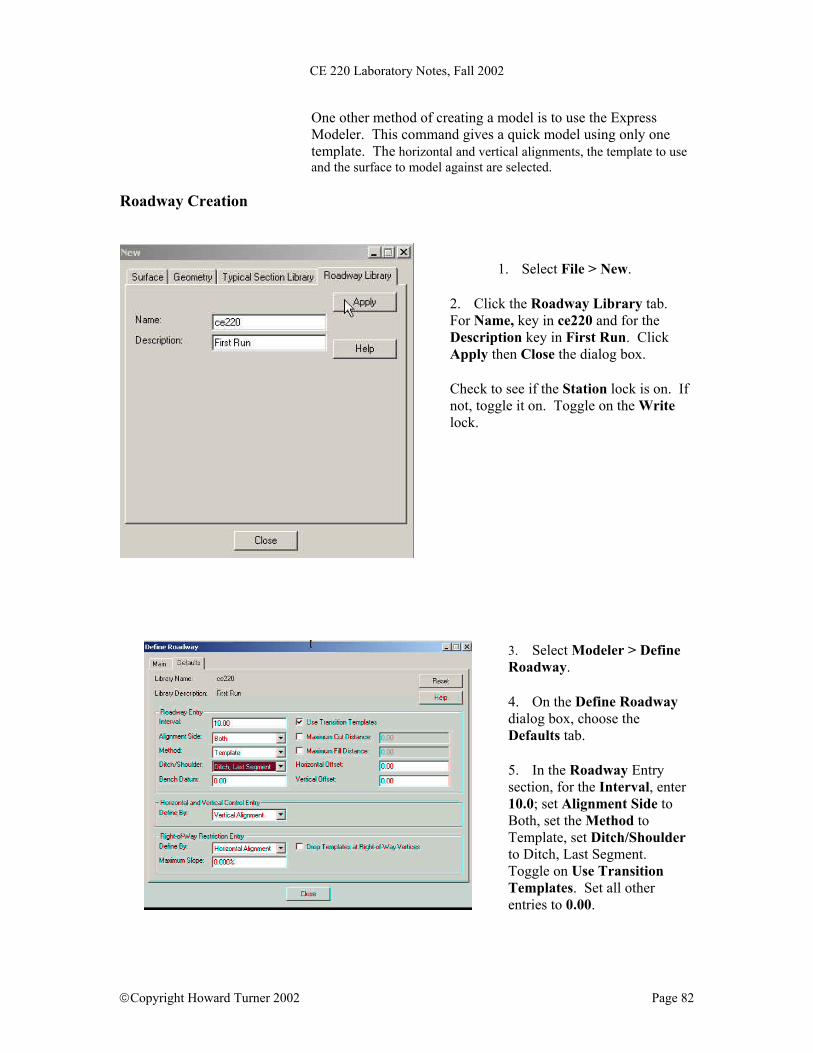
CE 220 Laboratory Notes, Fall 2002
One other method of creating a model is to use the Express Modeler. This command gives a quick model using only one template. The horizontal and vertical alignments, the template to use and the surface to model against are selected.
Roadway Creation
1. Select File > New. 2. Click the Roadway Library tab.
For Name, key in ce220 and for the Description key in First Run. Click Apply then Close the dialog box.
Check to see if the Station lock is on. If
not, toggle it on. Toggle on the Write lock.
3. Select Modeler > Define
Roadway. 4. On the Define Roadway
dialog box, choose the Defaults tab.
5. In the Roadway Entry
section, for the Interval, enter 10.0; set Alignment Side to Both, set the Method to Template, set Ditch/Shoulder to Ditch, Last Segment. Toggle on Use Transition Templates. Set all other entries to 0.00.
Copyright Howard Turner 2002 Page 82

CE 220 Laboratory Notes, Fall 2002
6. Click the Main tab
and click New. In the Name field, key in Run1 (for the first roadway to be defined). In the Description field, key in Two Lane Road Only. Click Apply, then Close.
Select the Roadway
definition name that was just created, then click Edit.
Creating the Station and Template Entries
The Edit Roadway dialog box appears.
Notice there are no stations or
templates listed in the Station Template list. To add information to the list, click New.
Copyright Howard Turner 2002 Page 83

CE 220 Laboratory Notes, Fall 2002
8. Key in 200.00 in the Station entry field. This is where we are going to start to apply the template. Set the Interval to 50.0. Select the entry field Template under the Both heading. Select G0-Cart from the templates listed on the far right. The Template field is now filled in. Set Catch Point to Template. Choose OK.
9. Notice that the
Edit Roadway dialog box now has an entry. Click Close.
10. Close the
Define Roadway dialog box.
11. Select File >
Save As. Toggle the Save as type to Roadway Libraries (*.rwl).
Check the directory where the file will be saved. It should be h:\yourdirectory. Enter lab
as the name of the file, then click Save to save lab.rwl. Cancel out of the dialog box.
What is currently loaded into InRoads? A. A horizontal and vertical alignment (lab.alg) B. A ground surface (newsite.dtm) C. A typical section library (lab.tml) D. A roadway definition library (lab.rwl) Now a road can be modeled using the Roadway Modeler command.
Copyright Howard Turner 2002 Page 84

CE 220 Laboratory Notes, Fall 2002
Page 85
Modeling the Roadway
12 Select Modeler > Roadway Modeler.
13 Click the Advanced tab.
14 Check to see that the Mode is
toggled to As Defined. In the Sides section, both Left and Right are toggled on.
15 Toggle onthe Superelevation
Apply To. In the Transition Control Lines section, toggle on the Display – First Layer. The Subgrade Intercept can be toggled to anything because there are no sub-layers.
16 Toggle on Empty Design
Surfaces and Add Exterior Boundary. In the Critical Sections area, toggle on all check boxes.
17 All other toggles should be
toggled off.
yright Howard Turner 2002
18. Click the Report tab. Toggle on Generate Binary Report and Generate Error Log. Make sure the File Name for each is the same as shown in the picture. Simply place an appropriate file name in the data field, use the browse button to select the location and click Save followed by Cancel.
Cop

CE 220 Laboratory Notes, Fall 2002
Page 86
19 Click on the Layer Controls tab and toggle off Use Layer Controls. What are layer controls? Click on the Help button and find out.
20 Click Preferences and Save the
default preference.
Copyright Howard Turner 2002
16. Select the Main tab. The Roadway Modeler dialog box lists the active horizontal and vertical alignments.
17. From the list of Roadway Definitions,
select run1 and select ce220 as the Original Surface. Turn off the Station Limit and the Create Cut and Fill Features then click Apply.
A status bar appears at the bottom of the InRoads explore showing the percent complete and then a surface will be created called top.

CE 220 Laboratory Notes, Fall 2002
23. Note that the surface top appears in the Original Surface list in the Roadway Modeler dialog box, because it is now DTM.
24 Once the processing is done, click Close.
25 Select File > Save As. Toggle the Save as type to Surfaces (*.dtm). Save the surface top as top.dtm in the training directory. (Check the Active surface first!)
Summary
• To run a roadway model, a surface, a horizontal alignment, a vertical alignment, a template in a typical section library and a roadway definition file are needed. This is also known as a roadway library.
• A roadway library contains lists of stations and templates,
and whether a cut and fill table, material table or a decision table will be used for the exterior design portion of the model.
• After modeling, save the surfaces created. • One other method of creating a model is to use the Express
Modeler. This command gives a quick model using only one template. The user selects the horizontal and vertical alignments, the template to use and the surface that will be modeled against.
Copyright Howard Turner 2002 Page 87

CE 220 Laboratory Notes, Fall 2002
Evaluation
This section will discuss how to evaluate the results of using the Roadway Modeler. You'll learn how to evaluate results by generating cross sections and calculating earthwork quantities using the end-area volume report. Two-point cross sections are cross sections that are extracted perpendicular to a user-defined line. You define the interval between consecutive cross sections and the left and right offsets of each cross section. A cross section is always extracted at the beginning and ending of user-defined line endpoints.
You can also use the software to extract and display cross sections along an alignment. Any alignment can be used as the basis for computing the cross section positions. To extract cross sections along a portion of the alignment, use the Station Limits parameter and set the Start point or station and the Stop point or station. You can also cut a cross section of a single station. Survey crews sometimes collect cross-sectional data along alignments. This data is usually collected on a station-by-station
Copyright Howard Turner 2002 Page 88

CE 220 Laboratory Notes, Fall 2002
basis. That is, at each station, the surveyor typically moves perpendicularly to the alignment. Elevation measurements are recorded at critical breaks in grade. The software can display this information as a set of cross-sections. When this method is used it is not necessary to create a digital terrain model. No alignment is needed; simply define the data in an ASCII file. The four-column format for each elevation record is station offset elevation and pen-up/pen-down. The cross-sections should be stored in ascending station order. And, within each cross section, the offset values should be in ascending order. Remember that negative offsets are to the left of the centerline and positive offsets are to the right.
The first pen-up/pen-down value for each station will have a value of one. The last pen-up/pen-down value for each station will have a value of two. All intermediate records will use a value of zero.
Copyright Howard Turner 2002 Page 89

CE 220 Laboratory Notes, Fall 2002
You can also compute end-area volumes using the cross-sectional data stored in the design file. You must first extract multiple cross sections and write them to the design file. The cross sections must contain data from at least two surfaces. When using the end-area command, you will select which cross-section set to use. The volumes will be based on the surfaces that were displayed with the cross-section set. If the graphics move indicating a change in cross-section to surface you must recalculate the volumes. You can also use the cross section information to create the surface. For more information, consult the reference guide. Use the fill factor parameter to control the factor at which fill volumes are scaled and use the cut factor parameter to control the factor at which the cut volumes are scaled. These parameters can be any positive number. When creating earthwork quantity reports, control the output units of the cut, fill, and net volumes using the software parameters. Triangle volume, grid volume and end-area volume ASCII reports are available. You can also compute the true surface area and the planar area for any surface.
Copyright Howard Turner 2002 Page 90

CE 220 Laboratory Notes, Fall 2002
Creating Cross Sections
. 1. Select Evaluation > Cross Section > Create Cross Section.
2. Click the Main tab. Set the Set Name data field to new. Set the Interval to 20.000, Left Offset to -30.000, and Right Offset to 30.000. 3. Set the Create field to Window and Data (this is the cross section grid and the ground lines). In the Source section, toggle on Alignment and set it to new. In the Symbology area, toggle on both surfaces ce220 and top. Notice that both surfaces have already been selected to display via the “existing ground” and the “New Design” symbologies. To display these surfaces using these specifications, nothing else has to be done.
4 In the Symbology area, Edit ce220. The Edit Named Symbology dialog box will appear.
5 The color of the Cross Section Line
shown here is also the same color that appears in the Symbology area in the Create Cross Section dialog box. Changes to level [layer], color, weight or line style can be made here. When these are complete, click Apply, then Close.
Copyright Howard Turner 2002 Page 91

CE 220 Laboratory Notes, Fall 2002
6 Click Apply.
7 Take the cursor and identify, in the design [drawing] file, where the first cross section (lower left) is to be plotted.
8 The placed data point will
define the lower left corner of the set of cross sections to be plotted.
9 Click Close when the command has completed processing. Fit View [Zoom Extents].
Generating Volumes
10 Select Evaluation > Volumes > End-Area Volume.
11 Select the name of the Cross Section
Set that was just created. A rectangle is displayed around the cross section set in the design file (It may be necessary to zoom out to see it).
12 For the Original Surface, select
ce220.
13 For the Design Surface, select top.
14 In the End-Area Volume dialog box, click Apply.
After processing, the results of the
calculations are displayed in the dialog box. Because a report was toggled on, both an ASCII and binary file was generated. The numbers may differ.
Copyright Howard Turner 2002 Page 92

CE 220 Laboratory Notes, Fall 2002
Copyright Howard Turner 2002 Page 93
15 Start Notepad and Open the file endvol.rpt and print it.
Summary
• Multi-point cross sections are cross sections that are extracted perpendicular to a user-defined line. The interval between consecutive cross sections and the left and right offsets of each cross section are defined.
• A cross section is always extracted at the beginning and
ending of user-defined line endpoints. • End-area volumes can be computed using the cross sectional
data stored in the design file. Multiple cross sections must first be extracted and written to the design file. The cross sections must contain data from at least two surfaces.
• Cross sections do not have to be placed in the same drawing
or design file as plan graphics. All the InRoads product suite needs are the surfaces and the alignment that is the basis of the cross sections.