quantitative applications in the social sciences · pdf filequantitative applications in the...
TRANSCRIPT


Quantitative Applications in the Social Sciences
A S AG E P U B L I C AT I O N S S E R I E S
1. Analysis of Variance, 2nd Edition Iversen/Norpoth
2. Operations Research Methods Nagel/Neef3. Causal Modeling, 2nd Edition Asher4. Tests of Significance Henkel5. Cohort Analysis, 2nd Edition Glenn6. Canonical Analysis and Factor
Comparison Levine7. Analysis of Nominal Data, 2nd Edition
Reynolds 8. Analysis of Ordinal Data
Hildebrand/Laing/Rosenthal 9. Time Series Analysis, 2nd Edition Ostrom
10. Ecological Inference Langbein/Lichtman 11. Multidimensional Scaling Kruskal/Wish 12. Analysis of Covariance Wildt/Ahtola 13. Introduction to Factor Analysis
Kim/Mueller 14. Factor Analysis Kim/Mueller 15. Multiple Indicators Sullivan/Feldman 16. Exploratory Data Analysis Hartwig/Dearing 17. Reliability and Validity Assessment
Carmines/Zeller 18. Analyzing Panel Data Markus 19. Discriminant Analysis Klecka 20. Log-Linear Models Knoke/Burke21. Interrupted Time Series Analysis
McDowall/McCleary/Meidinger/Hay22. Applied Regression Lewis-Beck 23. Research Designs Spector 24. Unidimensional Scaling McIver/Carmines 25. Magnitude Scaling Lodge26. Multiattribute Evaluation
Edwards/Newman27. Dynamic Modeling
Huckfeldt/Kohfeld/Likens 28. Network Analysis Knoke/Kuklinski 29. Interpreting and Using Regression Achen 30. Test Item Bias Osterlind31. Mobility Tables Hout 32. Measures of Association Liebetrau33. Confirmatory Factor Analysis Long 34. Covariance Structure Models Long 35. Introduction to Survey Sampling Kalton36. Achievement Testing Bejar 37. Nonrecursive Causal Models Berry38. Matrix Algebra Namboodiri 39. Introduction to Applied Demography
Rives/Serow 40. Microcomputer Methods for Social
Scientists, 2nd Edition Schrodt41. Game Theory Zagare 42. Using Published Data Jacob 43. Bayesian Statistical Inference Iversen 44. Cluster Analysis Aldenderfer/Blashfield45. Linear Probability, Logit, and Probit Models
Aldrich/Nelson
46. Event History Analysis Allison 47. Canonical Correlation Analysis Thompson 48. Models for Innovation Diffusion Mahajan/
Peterson 49. Basic Content Analysis, 2nd Edition
Weber 50. Multiple Regression in Practice Berry/
Feldman 51. Stochastic Parameter Regression Models
Newbold/Bos 52. Using Microcomputers in Research
Madron/Tate/Brookshire 53. Secondary Analysis of Survey Data
Kiecolt/Nathan 54. Multivariate Analysis of Variance
Bray/Maxwell 55. The Logic of Causal Order Davis 56. Introduction to Linear Goal Programming
Ignizio 57. Understanding Regression Analysis
Schroeder/Sjoquist/Stephan 58. Randomized Response Fox/Tracy59. Meta-Analysis Wolf 60. Linear Programming Feiring 61. Multiple Comparisons Klockars/Sax62. Information Theory Krippendorff 63. Survey Questions Converse/Presser 64. Latent Class Analysis McCutcheon 65. Three-Way Scaling and Clustering
Arabie/Carroll/DeSarbo66. Q Methodology McKeown/Thomas 67. Analyzing Decision Making Louviere 68. Rasch Models for Measurement Andrich 69. Principal Components Analysis Dunteman 70. Pooled Time Series Analysis Sayrs 71. Analyzing Complex Survey Data,
2nd Edition Lee/Forthofer72. Interaction Effects in Multiple Regression,
2nd Edition Jaccard/Turrisi73. Understanding Significance Testing Mohr 74. Experimental Design and Analysis Brown/
Melamed 75. Metric Scaling Weller/Romney 76. Longitudinal Research, 2nd Edition
Menard 77. Expert Systems Benfer/Brent/Furbee 78. Data Theory and Dimensional Analysis
Jacoby 79. Regression Diagnostics Fox 80. Computer-Assisted Interviewing Saris 81. Contextual Analysis Iversen 82. Summated Rating Scale Construction
Spector 83. Central Tendency and Variability Weisberg 84. ANOVA: Repeated Measures Girden 85. Processing Data Bourque/Clark 86. Logit Modeling DeMaris
FM-Hao.qxd 3/13/2007 11:20 AM Page i

87. Analytic Mapping and GeographicDatabases Garson/Biggs
88. Working With Archival DataElder/Pavalko/Clipp
89. Multiple Comparison ProceduresToothaker
90. Nonparametric Statistics Gibbons 91. Nonparametric Measures of Association
Gibbons 92. Understanding Regression Assumptions
Berry 93. Regression With Dummy Variables Hardy 94. Loglinear Models With Latent Variables
Hagenaars95. Bootstrapping Mooney/Duval 96. Maximum Likelihood Estimation Eliason 97. Ordinal Log-Linear Models Ishii-Kuntz 98. Random Factors in ANOVA Jackson/
Brashers 99. Univariate Tests for Time Series Models
Cromwell/Labys/Terraza 100. Multivariate Tests for Time Series Models
Cromwell/Hannan/Labys/Terraza 101. Interpreting Probability Models: Logit,
Probit, and Other Generalized LinearModels Liao
102. Typologies and Taxonomies Bailey103. Data Analysis: An Introduction
Lewis-Beck104. Multiple Attribute Decision Making
Yoon/Hwang105. Causal Analysis With Panel Data Finkel106. Applied Logistic Regression Analysis,
2nd Edition Menard107. Chaos and Catastrophe Theories Brown108. Basic Math for Social Scientists:
Concepts Hagle 109. Basic Math for Social Scientists:
Problems and Solutions Hagle110. Calculus Iversen111. Regression Models: Censored, Sample
Selected, or Truncated Data Breen112. Tree Models of Similarity and Association
James E. Corter113. Computational Modeling Taber/Timpone114. LISREL Approaches to Interaction Effects
in Multiple Regression Jaccard/Wan115. Analyzing Repeated Surveys Firebaugh116. Monte Carlo Simulation Mooney117. Statistical Graphics for Univariate and
Bivariate Data Jacoby118. Interaction Effects in Factorial Analysis
of Variance Jaccard
119. Odds Ratios in the Analysis ofContingency Tables Rudas
120. Statistical Graphics for VisualizingMultivariate Data Jacoby
121. Applied Correspondence AnalysisClausen
122. Game Theory Topics Fink/Gates/Humes123. Social Choice: Theory and Research
Johnson124. Neural Networks Abdi/Valentin/Edelman 125. Relating Statistics and Experimental
Design: An Introduction Levin 126. Latent Class Scaling Analysis Dayton 127. Sorting Data: Collection and Analysis
Coxon 128. Analyzing Documentary Accounts
Hodson 129. Effect Size for ANOVA Designs
Cortina/Nouri 130. Nonparametric Simple Regression:
Smoothing Scatterplots Fox 131. Multiple and Generalized Nonparametric
Regression Fox 132. Logistic Regression: A Primer Pampel 133. Translating Questionnaires and Other
Research Instruments: Problems andSolutions Behling/Law
134. Generalized Linear Models: A UnitedApproach Gill
135. Interaction Effects in Logistic RegressionJaccard
136. Missing Data Allison 137. Spline Regression Models Marsh/Cormier 138. Logit and Probit: Ordered and
Multinomial Models Borooah 139. Correlation: Parametric and
Nonparametric MeasuresChen/Popovich
140. Confidence Intervals Smithson 141. Internet Data Collection Best/Krueger142. Probability Theory Rudas 143. Multilevel Modeling Luke 144. Polytomous Item Response Theory
Models Ostini/Nering 145. An Introduction to Generalized Linear
Models Dunteman/Ho 146. Logistic Regression Models for Ordinal
Response Variables O’Connell 147. Fuzzy Set Theory: Applications in the
Social Sciences Smithson/Verkuilen 148. Multiple Time Series Models
Brandt/Williams149. Quantile Regression Hao/Naiman
Quantitative Applications in the Social Sciences
A S AG E P U B L I C AT I O N S S E R I E S
FM-Hao.qxd 3/13/2007 11:20 AM Page ii

Series/Number 07–149
QUANTILE REGRESSION
LINGXIN HAOThe Johns Hopkins University
DANIEL Q. NAIMANThe Johns Hopkins University
FM-Hao.qxd 3/13/2007 11:20 AM Page iii

Copyright © 2007 by Sage Publications, Inc.
All rights reserved. No part of this book may be reproduced or utilized in any form or by anymeans, electronic or mechanical, including photocopying, recording, or by any informationstorage and retrieval system, without permission in writing from the publisher.
For information:
Sage Publications, Inc.2455 Teller RoadThousand Oaks, California 91320E-mail: [email protected]
Sage Publications Ltd.1 Oliver’s Yard55 City RoadLondon EC1Y 1SPUnited Kingdom
Sage Publications India Pvt. Ltd.B 1/l 1 Mohan Cooperative Industrial AreaMathura Road, New Delhi 110 044India
Sage Publications Asia-Pacific Pte. Ltd.33 Pekin Street #02-01Far East SquareSingapore 048763
Printed in the United States of America.
Library of Congress Cataloging-in-Publication Data
Hao, Lingxin, 1949–Quantile regression / Lingxin Hao, Daniel Q. Naiman.
p. cm.—(Quantitative applications in the social sciences; 149)Includes bibliographical references and index.ISBN 978-1-4129-2628-7 (pbk.)
1. Social sciences—Statistical methods. 2. Regression analysis.I. Naiman, Daniel Q. II. Title.HA31.3.H36 2007519.5′36—dc22
2006035964
This book is printed on acid-free paper.
07 08 09 10 11 10 9 8 7 6 5 4 3 2 1
Acquisitions Editor: Lisa Cuevas ShawAssociate Editor: Sean ConnellyEditorial Assistant: Karen GreeneProduction Editor: Melanie BirdsallCopy Editor: Kevin BeckTypesetter: C&M Digitals (P) Ltd.Proofreader: Cheryl RivardIndexer: Sheila BodellCover Designer: Candice HarmanMarketing Manager: Stephanie Adams
FM-Hao.qxd 3/13/2007 11:20 AM Page iv

CONTENTS
Series Editor’s Introduction vii
Acknowledgments ix
1. Introduction 1
2. Quantiles and Quantile Functions 7
CDFs, Quantiles, and Quantile Functions 7Sampling Distribution of a Sample Quantile 11Quantile-Based Measures of Location and Shape 12Quantile as a Solution to a Certain Minimization Problem 14Properties of Quantiles 19Summary 20Note 20Chapter 2 Appendix: A Proof: Median and Quantiles
as Solutions to a Minimization Problem 21
3. Quantile-Regression Model and Estimation 22
Linear-Regression Modeling and Its Shortcomings 22Conditional-Median and Quantile-Regression Models 29QR Estimation 33Transformation and Equivariance 38Summary 42Notes 42
4. Quantile-Regression Inference 43
Standard Errors and Confidence Intervals for the LRM 43Standard Errors and Confidence Intervals for the QRM 44The Bootstrap Method for the QRM 47Goodness of Fit of the QRM 51Summary 54Note 55
FM-Hao.qxd 3/13/2007 11:20 AM Page v
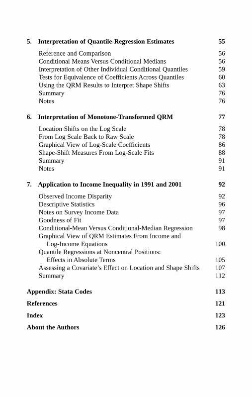
5. Interpretation of Quantile-Regression Estimates 55
Reference and Comparison 56Conditional Means Versus Conditional Medians 56Interpretation of Other Individual Conditional Quantiles 59Tests for Equivalence of Coefficients Across Quantiles 60Using the QRM Results to Interpret Shape Shifts 63Summary 76Notes 76
6. Interpretation of Monotone-Transformed QRM 77
Location Shifts on the Log Scale 78From Log Scale Back to Raw Scale 78Graphical View of Log-Scale Coefficients 86Shape-Shift Measures From Log-Scale Fits 88Summary 91Notes 91
7. Application to Income Inequality in 1991 and 2001 92
Observed Income Disparity 92Descriptive Statistics 96Notes on Survey Income Data 97Goodness of Fit 97Conditional-Mean Versus Conditional-Median Regression 98Graphical View of QRM Estimates From Income and
Log-Income Equations 100Quantile Regressions at Noncentral Positions:
Effects in Absolute Terms 105Assessing a Covariate’s Effect on Location and Shape Shifts 107Summary 112
Appendix: Stata Codes 113
References 121
Index 123
About the Authors 126
FM-Hao.qxd 3/13/2007 11:20 AM Page vi

vii
SERIES EDITOR’S INTRODUCTION
The classical linear-regression model has been part and parcel of aquantitative social scientist’s methodology for at least four decades. TheQuantitative Applications in the Social Sciences series has covered the topicwell, with at least the following numbers focused centrally on the classicallinear regression: Nos. 22, 29, 50, 57, 79, 92, and 93. There are manymore treatments in the series of various extensions of the linear regression,such as logit, probit, event history, generalized linear, and generalized non-parametric models as well as linear-regression models of censored, sample-selected, truncated, and missing data, as well as many other related methods,including analysis of variance, analysis of covariance, causal modeling,log-linear modeling, multiple comparisons, and time-series analysis.
The central aim of the classical regression is to estimate the meansof a response variable conditional on the values of the explanatory vari-ables. This works well when regression assumptions are met, but notwhen conditions are nonstandard. (For a thorough discussion of linear-regression assumptions, see No. 92, Understanding Regression Assump-tions, by William Berry.) Two of them are the normality assumption and thehomoscedasticity assumption. These two crucial assumptions may not besatisfied by some common social-science data. For example, (conditional)income distributions are seldom normal, and the dispersion of the annualcompensations of chief executive officers tends to increase with firm size,an indication of heteroscedasticity. This is where quantile regression canhelp because it relaxes these assumptions. In addition, quantile regressionoffers the researcher a view—unobtainable through the classical regression—of the effect of explanatory variables on the (central and noncentral) loca-tion, scale, and shape of the distribution of the response variable.
The idea of quantile regression is not new, and in fact goes back to 1760,when the itinerant Croatian Jesuit Rudjer Josip Boscovich—a man whowore many hats including those of a physicist, an astronomer, a diplomat, aphilosopher, a poet, and a mathematician—went to London for computa-tional advice for his nascent method of median regression. However, thecomputational difficulty for such regression analysis posed a huge chal-lenge until recent years. With today’s fast computers and wide availability ofstatistical software packages such as R, SAS, and Stata that implementthe quantile-regression procedure, fitting a quantile-regression model todata has become easy. However, we have so far had no introduction inthe series to the method to explain what quantile regression is all about.
FM-Hao.qxd 3/13/2007 11:20 AM Page vii

Hao and Naiman’s Quantile Regression is a truly welcome addition tothe series. They present the concept of quantiles and quantile functions,specify the quantile-regression model, discuss its estimation and infer-ence, and demonstrate the interpretation of quantile-regression estimates—transformed and not—with clear examples. They also provide a completeexample of applying quantile regression to the analysis of income inequal-ity in the United States in 1991 and 2001, to help fix the ideas and proce-dures. This book, then, fills a gap in the series and will help make quantileregression more accessible to many social scientists.
—Tim F. LiaoSeries Editor
viii
FM-Hao.qxd 3/13/2007 11:20 AM Page viii

ACKNOWLEDGMENTS
Lingxin first became interested in using quantile regression to study race,immigration, and wealth stratification after learning of Buchinsky’s work(1994), which applied quantile regression to wage inequality. This interestled to frequent discussions about methodological and mathematical issuesrelated to quantile regression with Dan, who had first learned about the sub-ject as a graduate student under Steve Portnoy at the University of Illinois.In the course of our conversations, we agreed that an empirically orientedintroduction to quantile regression would be vital to the social-scienceresearch community. Particularly, it would provide easier access to neces-sary tools for social scientists who seek to uncover the impact of socialfactors on not only the mean but also the shape of a response distribution.
We gratefully acknowledge our colleagues in the Departments of Sociologyand Applied Mathematics and Statistics at The Johns Hopkins Universityfor their enthusiastic encouragement and support. In addition, we are grate-ful for the aid that we received from the Acheson J. Duncan Fund for theAdvancement of Research in Statistics. Our gratitude further extends toadditional support from the attendees of seminars at various universitiesand from the Sage QASS editor, Dr. Tim F. Liao. Upon the completion ofthe book, we wish to acknowledge the excellent research and editorialassistance from Xue Mary Lin, Sahan Savas Karatasli, Julie J. H. Kim, andCaitlin Cross-Barnet. The two anonymous reviewers of the manuscript alsoprovided us with extremely helpful comments and beneficial suggestions,which led to a much-improved version of this book. Finally, we dedicatethis book to our respective parents, who continue to inspire us.
ix
FM-Hao.qxd 3/13/2007 11:20 AM Page ix

FM-Hao.qxd 3/13/2007 11:20 AM Page x

QUANTILE REGRESSION
Lingxin HaoThe Johns Hopkins University
Daniel Q. NaimanThe Johns Hopkins University
1. INTRODUCTION
The purpose of regression analysis is to expose the relationship between aresponse variable and predictor variables. In real applications, the responsevariable cannot be predicted exactly from the predictor variables. Instead,the response for a fixed value of each predictor variable is a random vari-able. For this reason, we often summarize the behavior of the response forfixed values of the predictors using measures of central tendency. Typicalmeasures of central tendency are the average value (mean), the middle value(median), or the most likely value (mode).
Traditional regression analysis is focused on the mean; that is, wesummarize the relationship between the response variable and predictorvariables by describing the mean of the response for each fixed value ofthe predictors, using a function we refer to as the conditional mean of theresponse. The idea of modeling and fitting the conditional-mean function isat the core of a broad family of regression-modeling approaches, includingthe familiar simple linear-regression model, multiple regression, modelswith heteroscedastic errors using weighted least squares, and nonlinear-regression models.
Conditional-mean models have certain attractive properties. Under idealconditions, they are capable of providing a complete and parsimoniousdescription of the relationship between the covariates and the response dis-tribution. In addition, using conditional-mean models leads to estimators(least squares and maximum likelihood) that possess attractive statisticalproperties, are easy to calculate, and are straightforward to interpret. Such
1
01-Hao.qxd 3/13/2007 3:28 PM Page 1

models have been generalized in various ways to allow for heteroscedasticerrors so that given the predictors, modeling of the conditional mean andconditional scale of the response can be carried out simultaneously.
Conditional-mean modeling has been applied widely in the social sci-ences, particularly in the past half century, and regression modeling of therelationship between a continuous response and covariates via least squaresand its generalization is now seen as an essential tool. More recently, mod-els for binary response data, such as logistic and probit models and Poissonregression models for count data, have become increasingly popular in social-science research. These approaches fit naturally within the conditional-mean modeling framework. While quantitative social-science researchershave applied advanced methods to relax some basic modeling assumptionsunder the conditional-mean framework, this framework itself is seldomquestioned.
The conditional-mean framework has inherent limitations. First, whensummarizing the response for fixed values of predictor variables, theconditional-mean model cannot be readily extended to noncentral locations,which is precisely where the interests of social-science research oftenreside. For instance, studies of economic inequality and mobility haveintrinsic interest in the poor (lower tail) and the rich (upper tail). Educationalresearchers seek to understand and reduce group gaps at preestablishedachievement levels (e.g., the three criterion-referenced levels: basic, pro-ficient, and advanced). Thus, the focus on the central location has longdistracted researchers from using appropriate and relevant techniques toaddress research questions regarding noncentral locations on the responsedistribution. Using conditional-mean models to address these questions maybe inefficient or even miss the point of the research altogether.
Second, the model assumptions are not always met in the real world.In particular, the homoscedasticity assumption frequently fails, andfocusing exclusively on central tendencies can fail to capture informa-tive trends in the response distribution. Also, heavy-tailed distributionscommonly occur in social phenomena, leading to a preponderance ofoutliers. The conditional mean can then become an inappropriate andmisleading measure of central location because it is heavily influencedby outliers.
Third, the focal point of central location has long steered researchers’attention away from the properties of the whole distribution. It is quite natural to go beyond location and scale effects of predictor variables on theresponse and ask how changes in the predictor variables affect the underlyingshape of the distribution of the response. For example, much social-scienceresearch focuses on social stratification and inequality, areas that require
2
01-Hao.qxd 3/13/2007 3:28 PM Page 2

close examination of the properties of a distribution. The central location,the scale, the skewness, and other higher-order properties—not central loca-tion alone—characterize a distribution. Thus, conditional-mean models are inherently ill equipped to characterize the relationship between a responsedistribution and predictor variables. Examples of inequality topics include economic inequality in wages, income, and wealth; educational inequality inacademic achievement; health inequality in height, weight, incidence of dis-ease, drug addiction, treatment, and life expectancy; and inequality in well-being induced by social policies. These topics have often been studied underthe conditional-mean framework, while other, more relevant distributionalproperties have been ignored.
An alternative to conditional-mean modeling has roots that can be tracedto the mid-18th century. This approach can be referred to as conditional-median modeling, or simply median regression. It addresses some of theissues mentioned above regarding the choice of a measure of central ten-dency. The method replaces least-squares estimation with least-absolute-distance estimation. While the least-squares method is simple to implementwithout high-powered computing capabilities, least-absolute-distance esti-mation demands significantly greater computing power. It was not until thelate 1970s, when computing technology was combined with algorithmicdevelopments such as linear programming, that median-regression model-ing via least-absolute-distance estimation became practical.
The median-regression model can be used to achieve the same goal as conditional-mean-regression modeling: to represent the relationshipbetween the central location of the response and a set of covariates. However,when the distribution is highly skewed, the mean can be challenging tointerpret while the median remains highly informative. As a consequence,conditional-median modeling has the potential to be more useful.
The median is a special quantile, one that describes the central loca-tion of a distribution. Conditional-median regression is a special case ofquantile regression in which the conditional .5th quantile is modeledas a function of covariates. More generally, other quantiles can be usedto describe noncentral positions of a distribution. The quantile notiongeneralizes specific terms like quartile, quintile, decile, and percentile.The pth quantile denotes that value of the response below which theproportion of the population is p. Thus, quantiles can specify any positionof a distribution. For example, 2.5% of the population lies below the.025th quantile.
Koenker and Bassett (1978) introduced quantile regression, which mod-els conditional quantiles as functions of predictors. The quantile-regressionmodel is a natural extension of the linear-regression model. While the
3
01-Hao.qxd 3/13/2007 3:28 PM Page 3

linear-regression model specifies the change in the conditional mean of thedependent variable associated with a change in the covariates, the quantile-regression model specifies changes in the conditional quantile. Since anyquantile can be used, it is possible to model any predetermined position ofthe distribution. Thus, researchers can choose positions that are tailored totheir specific inquiries. Poverty studies concern the low-income population;for example, the bottom 11.3% of the population lived in poverty in 2000(U.S. Census Bureau, 2001). Tax-policy studies concern the rich, forexample, the top 4% of the population (Shapiro & Friedman, 2001).Conditional-quantile models offer the flexibility to focus on these popula-tion segments whereas conditional-mean models do not.
Since multiple quantiles can be modeled, it is possible to achieve amore complete understanding of how the response distribution is affectedby predictors, including information about shape change. A set of equallyspaced conditional quantiles (e.g., every 5% or 1% of the population) cancharacterize the shape of the conditional distribution in addition to itscentral location. The ability to model shape change provides a significantmethodological leap forward in social research on inequality. Traditionally,inequality studies are non-model based; approaches include the Lorenzcurve, the Gini coefficient, Theil’s measure of entropy, the coefficient ofvariation, and the standard deviation of the log-transformed distribution. Inanother book for the Sage QASS series, we will develop conditional Lorenzand Gini coefficients, as well as other inequality measures based on quantile-regression models.
Quantile-regression models can be easily fit by minimizing a generalizedmeasure of distance using algorithms based on linear programming. As aresult, quantile regression is now a practical tool for researchers. Softwarepackages familiar to social scientists offer readily accessed commands forfitting quantile-regression models.
A decade and a half after Koenker and Bassett first introduced quantileregression, empirical applications of quantile regression started to growrapidly. Empirical researchers took advantage of quantile regression’sability to examine the impact of predictor variables on the response dis-tribution. Two of the earliest empirical papers by economists (Buchinsky,1994; Chamberlain, 1994) provided practical examples of how to applyquantile regression to the study of wages. Quantile regression allowedthem to examine the entire conditional distribution of wages and deter-mine if the returns to schooling, and experience and the effects of unionmembership differed across wage quantiles. The use of quantile regres-sion to analyze wages increased and expanded to address additional top-ics such as changes in wage distribution (Machado & Mata, 2005; Melly,
4
01-Hao.qxd 3/13/2007 3:28 PM Page 4

2005), wage distributions within specific industries (Budd & McCall,2001), wage gaps between whites and minorities (Chay & Honore, 1998)and between men and women (Fortin & Lemieux, 1998), educationalattainment and wage inequality (Lemieux, 2006), and the intergenerationaltransfer of earnings (Eide & Showalter, 1999). The use of quantile regres-sion also expanded to address the quality of schooling (Bedi & Edwards,2002; Eide, Showalter, & Sims, 2002) and demographics’ impact oninfant birth weight (Abreveya, 2001). Quantile regression also spread toother fields, notably sociology (Hao, 2005, 2006a, 2006b), ecology andenvironmental sciences (Cade, Terrell, & Schroeder, 1999; Scharf,Juanes, & Sutherland, 1989), and medicine and public health (Austin et al., 2005; Wei et al., 2006).
This book aims to introduce the quantile-regression model to a broadaudience of social scientists who are interested in modeling both the loca-tion and shape of the distribution they wish to study. It is also written forreaders who are concerned about the sensitivity of linear-regression modelsto skewed distributions and outliers. The book builds on the basic literatureof Koenker and his colleagues (e.g., Koenker, 1994; Koenker, 2005;Koenker & Bassett, 1978; Koenker & d’Orey, 1987; Koenker & Hallock,2001; Koenker & Machado, 1999) and makes two further contributions. Wedevelop conditional-quantile-based shape-shift measures based on quantile-regression estimates. These measures provide direct answers to researchquestions about a covariate’s impact on the shape of the response distribu-tion. In addition, inequality research often uses log transformation of right-skewed responses to create a better model fit even though “inequality” inthis case refers to raw-scale distributions. Therefore, we develop methods toobtain a covariate’s effect on the location and shape of conditional-quantilefunctions in absolute terms from log-scale coefficients.
Drawn from our own research experience, this book is oriented towardthose involved with empirical research. We take a didactic approach, usinglanguage and procedures familiar to social scientists. These include clearlydefined terms, simplified equations, illustrative graphs, tables and graphsbased on empirical data, and computational codes using statistical softwarepopular among social scientists. Throughout the book, we draw examplesfrom our own research on household income distribution. In order to pro-vide a gentle introduction to quantile regression, we use simplified modelspecifications wherein the conditional-quantile functions for the raw or logresponses are linear and additive in the covariates. As in linear regression,the methodology we present is easily adapted to more complex model spec-ifications, including, for example, interaction terms and polynomial or splinefunctions of covariates.
5
01-Hao.qxd 3/13/2007 3:28 PM Page 5

Quantile-regression modeling provides a natural complement to model-ing approaches dealt with extensively in the QASS series: UnderstandingRegression Assumptions (Berry, 1993), Understanding Regression Analysis(Schroeder, 1986), and Multiple Regression in Practice (Berry & Feldman,1985). Other books in the series can be used as references to some of thetechniques discussed in this book, e.g., Bootstrapping (Mooney, 1993) andLinear Programming (Feiring, 1986).
The book is organized as follows. Chapter 2 defines quantiles and quantilefunctions in two ways—using the cumulative distribution function and solv-ing a minimization problem. It also develops quantile-based measures oflocation and shape of a distribution in comparison with distributional moments(e.g., mean, standard deviation). Chapter 3 introduces the basics of thequantile-regression model (QRM) in comparison with the linearregres-sion model, including the model setup, the estimator, and properties. Thenumerous quantile-regression equations with quantile-specific parametersare a unique feature of the quantile-regression model. We describe howquantile-regression fits are obtained by making use of the minimum dis-tance principle. The QRM possesses properties such as monotonic equivari-ance and robustness to distributional assumptions, which produce flexible,nonsensitive estimates, properties that are absent in the linear-regressionmodel. Chapter 4 discusses inferences for the quantile-regression model. Inaddition to introducing the asymptotic inference for quantile-regressioncoefficients, the chapter emphasizes the utility and feasibility of the boot-strap method. In addition, this chapter briefly discusses goodness of fit forquantile-regression models, analogous to that for linear-regression models.Chapter 5 develops various ways to interpret estimates from the quantile-regression model. Going beyond the traditional examination of the effectof a covariate on specific conditional quantiles, such as the median or off-central quantiles, Chapter 5 focuses on a distributional interpretation. Itillustrates graphical interpretations of quantile-regression estimates andquantitative measures of shape changes from quantile-regression estimates,including location shifts, scale shifts, and skewness shifts. Chapter 6 con-siders issues related to monotonically transformed response variables. Wedevelop two ways to obtain a covariate’s effect on the location and shapeof conditional-quantile functions in absolute terms from log-scale coeffi-cients. Chapter 7 presents a systematic application of the techniques intro-duced and developed in the book. This chapter analyzes the sources of thepersistent and widening income inequality in the United States between1991 and 2001. Finally, the Appendix provides Stata codes for performingthe analytic tasks described in Chapter 7.
6
01-Hao.qxd 3/13/2007 3:28 PM Page 6

2. QUANTILES AND QUANTILE FUNCTIONS
Describing and comparing the distributional attributes of populations isessential to social science. The simplest and most familiar measures used todescribe a distribution are the mean for the central location and the standarddeviation for the dispersion. However, restricting attention to the mean andstandard deviation alone leads us to ignore other important properties thatoffer more insight into the distribution. For many researchers, attributes ofinterest often have skewed distributions, for which the mean and standarddeviation are not necessarily the best measures of location and shape. To characterize the location and shape of asymmetric distributions, thischapter introduces quantiles, quantile functions, and their properties byway of the cumulative distribution function (cdf). It also develops quantile-based measures of location and shape of a distribution and, finally, rede-fines a quantile as a solution to a certain minimization problem.
CDFs, Quantiles, and Quantile Functions
To describe the distribution of a random variable Y, we can use its cumulativedistribution function (cdf). The cdf is the function FY that gives, for eachvalue of y, the proportion of the population for which Y ≤ y. Figure 2.1 showsthe cdf for the standard normal distribution. The cdf can be used to calculatethe proportion of the population for any range of values of y. We see in Figure2.1 that FY(0) = .5 and FY (1.28) = .9. The cdf can be used to calculate all otherprobabilities involving Y. In particular: P[Y > y] = 1 − Fy (y) (e.g., in Figure 2.1,P[Y > 1.28] = 1 − Fy (1.28) = 1 − 0.9 = 0.1) and P[a < Y ≤ b] = FY (b) − FY (a)(e.g., in Figure 2.1, P[0 ≤ Y ≤ 1.28] = FY (1.28) − FY (0) = 0.40)). The twomost important properties of a cdf are monotonicity (i.e., F ( y1) ≤ F(y2 )whenever y1 ≤ y2) and its behavior at infinity limy→−∞ F(y) = 0 andlimy→+∞ F (y) = 1. For a continuous random variable Y, we can also representits distribution using a probability density function fy defined as the functionwith the property that P[a ≤ Y ≤ b] = ∫b
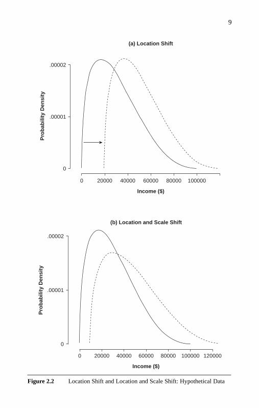
y = a fY dy for all choices of a and b.Returning to the issue of the inadequacy of location and spread for fully
describing a distribution, suppose we are told that the mean householdincome for whites (W) exceeds that of blacks (B) by $20,500. This could bedescribed simply by a shift in the location of the distribution while retain-ing the shape (see the corresponding density functions in Figure 2.2a),so that the relationship between the distributions is expressed byFB(y) = F W(y − 20,500). The difference in distributions may consist of achange in both location and scale (see the corresponding density functionsin Figure 2.2b), so that the relationship between the distributions takes thegeneral form FB(y) = F W(ay − c) for constants a and c (a > 0). This is the
7
02-Hao.qxd 3/13/2007 4:29 PM Page 7

case when both the mean and the variance of y differ between populationsW and B. Knowledge of measures of location and scale, for example, themean and standard deviation, or alternatively the median and interquartilerange, enables us to compare the attribute Y between the two distributions.
As distributions become less symmetrical, more complex summarymeasures are needed. Consideration of quantiles and quantile functionsleads to a rich collection of summary measures. Continuing the discussionof a cdf, F, for some population attribute, the pth quantile of this distribu-tion, denoted by Q (p)(F) (or simply Q (p) when it is clear what distribution isbeing discussed), is the value of the inverse of the cdf at p, that is, a valueof y such that F (y) = p. Thus, the proportion of the population with anattribute below Q (p) is p. For example, in the standard normal case (seeFigure 2.1), F(1.28) = .9, so Q(.9) = 1.28, that is, the proportion of the pop-ulation with the attribute below 1.28 is .9 or 90%.
Analogous to the population cdf, we consider the empirical or sample cdfassociated with a sample. For a sample consisting of values y1, y2, . . . , yn,the empirical cdf gives the proportion of the sample values that is less thanor equal to any given y. More formally, the empirical cdf F is defined by
F(y) = the proportion of sample values less than or equal to y.
As an example, consider a sample consisting of 20 households withincomes of $3,000, $3,500, $4,000, $4,300, $4,600, $5,000, $5,000, $5,000,$8,000, $9,000, $10,000, $11,000, $12,000, $15,000, $17,000, $20,000,
8
.0−3 −2 −1 0 1 2 3
.2
.4
.6
.8
.9
1
.5F(y
)
Y
Q(.9)
Figure 2.1 The CDF for the Standard Normal Distribution
02-Hao.qxd 3/13/2007 4:29 PM Page 8
9
Pro
bab
ility
Den
sity
Income ($)
(a) Location Shift
.00001
.00002
0
0 20000 40000 60000 80000 100000
Figure 2.2 Location Shift and Location and Scale Shift: Hypothetical Data
Pro
bab
ility
Den
sity
Income ($)
.00001
.00002
0
0 20000 40000 60000 80000 100000 120000
(b) Location and Scale Shift
02-Hao.qxd 3/13/2007 4:29 PM Page 9

$32,000, $38,000, $56,000, and $84,000. Since there are eight householdswith incomes at or below $5,000, we have F(5,000) = 8/20. A plot of theempirical cdf is shown in Figure 2.3, which consists of one jump and severalflat parts. For example, there is a jump of size 3/20 at 5,000, indicating thatthe value of 5,000 appears three times in the sample. There are also flat partssuch as the portion between 56,000 and 84,000, indicating that there are nosample values in the interior of this interval. Since the empirical cdf can beflat, there are values having multiple inverses. For example, in Figure 2.3there appears to be a continuum of choices for Q (.975) between 56,000 and84,000. Thus, we need to exercise some care when we introduce quantilesand quantile functions for a general distribution with the following definition:
Definition. The pth quantile Q (p) of a cdf F is the minimum of the setof values y such that F (y) ≥ p. The function Q (p) (as a function of p) isreferred to as the quantile function of F.
Figure 2.4 shows an example of a quantile function and the correspond-ing cdf. Observe that the quantile function is a monotonic nondecreasingfunction that is continuous from below.
As a special case we can talk about sample quantiles, which can be usedto estimate quantiles of a sampled distribution.
10
flat for incomes between$56,000 and $84,000
jump of size3/20 at $5,000
20000 40000 60000 80000 1000000
0.2
0.4
0.6
0.8
1.0
Fre
qu
ency
Income ($)
Figure 2.3 CDF With Jumps and Flat Parts
02-Hao.qxd 3/13/2007 4:29 PM Page 10
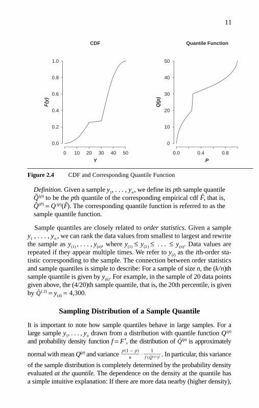
Definition. Given a sample y1, . . . , yn, we define its pth sample quantileQ (p) to be the pth quantile of the corresponding empirical cdf F, that is,Q(P) = Q (p)(F). The corresponding quantile function is referred to as thesample quantile function.
Sample quantiles are closely related to order statistics. Given a sampley1 , . . . , yn , we can rank the data values from smallest to largest and rewritethe sample as y(1) , . . . , y(n), where y(1) ≤ y(2) ≤ . . . ≤ y(n). Data values arerepeated if they appear multiple times. We refer to y(i) as the ith-order sta-tistic corresponding to the sample. The connection between order statisticsand sample quantiles is simple to describe: For a sample of size n, the (k/n)thsample quantile is given by y(k). For example, in the sample of 20 data pointsgiven above, the (4/20)th sample quantile, that is, the 20th percentile, is givenby Q (.2) = y(4) = 4,300.
Sampling Distribution of a Sample Quantile
It is important to note how sample quantiles behave in large samples. For alarge sample y1, . . . , yn drawn from a distribution with quantile function Q (p)
and probability density function f = F′, the distribution of Q(p) is approximately
normal with mean Q(p) and variance . In particular, this variance
of the sample distribution is completely determined by the probability densityevaluated at the quantile. The dependence on the density at the quantile hasa simple intuitive explanation: If there are more data nearby (higher density),
p(1 − p)
n· 1
f (Q(p))2
11
0 10 20 30 40 50
Y
0.0
0.2
0.4
0.6
0.8
1.0
F(y
)
PQ
(p)
0.0 0.4 0.8
0
10
20
30
40
50
CDF Quantile Function
Figure 2.4 CDF and Corresponding Quantile Function
02-Hao.qxd 3/13/2007 4:29 PM Page 11

the sample quantile is less variable; conversely, if there are fewer data nearby(low density), the sample quantile is more variable.
To estimate the quantile sampling variability, we make use of the varianceapproximation above, which requires a way of estimating the unknownprobability density function. A standard approach to this estimation is illus-trated in Figure 2.5, where the slope of the tangent line to the function Q(p)
at the point p is the derivative of the quantile function with respect to p, or
equivalently, the inverse density function: = 1/f(Q(p)). This term can be
approximated by the difference quotient , which is the slope
of the secant line through the points (p − h, Q(p − h)) and (p + h, Q(p + h)) forsome small value of h.
Quantile-Based Measures of Location and Shape
Social scientists are familiar with the quantile-based measure of centrallocation; namely, instead of the mean (the first moment of a density func-tion), the median (i.e., the .5th quantile) has been used to indicate the
1
2h(Q(p+h) − Q(p−h))
d
dpQ(p)
12
Q(p0+h)
Q(p0+h) − Q(p0−h)
Q(p0−h)
p0−h p0+hp0
Q(p0)
secantline tangent
line
Q(p)
P
2h
Figure 2.5 Illustrating How to Estimate the Slope of a Quantile Function
NOTE: The derivative of the function Q(p) at the point p0 (the slope of the tangent line) is approximated bythe slope of the secant line, which is (Q(p
0+ h) − Q(p
0− h))/2h.
02-Hao.qxd 3/13/2007 4:29 PM Page 12

center of a skewed distribution. Using quantile-based location allows oneto investigate more general notions of location beyond just the center of adistribution. Specifically, we can examine a location at the lower tail (e.g.,the .1th quantile) or a location at the upper tail (e.g., the .9th quantile) forresearch questions regarding specific subpopulations.
Two basic properties describe the shape of a distribution: scale and skew-ness. Traditionally, scale is measured by the standard deviation, which is basedon the second moment of a distribution involving a quadratic function of thedeviations of data points from the mean. This measure is easy to interpret fora symmetric distribution, but when the distribution becomes highly asymmet-ric, its interpretation tends to break down. It is also misleading for heavy-taileddistributions. Since many of the distributions used to describe social phenom-ena are skewed or heavy-tailed, using the standard deviation to characterizetheir scales becomes problematic. To capture the spread of a distribution with-out relying on the standard deviation, we measure spread using the followingquantile-based scale measure (QSC) at a selected p:
QSC (p) = Q(1 − p) − Q(p) for p < .5. [2.1]
We can obtain the spread for the middle 95% of the population betweenQ (.025) and Q (.975), or the middle 50% of the population between Q (.25) andQ (.75) (the conventional interquartile range), or the spread of any desirablemiddle 100(1 − 2p)% of the population.
The QSC measure not only offers a direct and straightforward measure ofscale but also facilitates the development of a rich class of model-based scale-shift measures (developed in Chapter 5). In contrast, a model-based approachthat separates out a predictor’s effect in terms of a change in scale as measuredby the standard deviation limits the possible patterns that could be discovered.
A second measure of a distributional shape is skewness. This property isthe focus of much inequality research. Skewness is measured using a cubicfunction of data points’ deviations from the mean. When the data are sym-metrically distributed about the sample mean, the value of skewness is zero.A negative value indicates left skewness and a positive value indicates rightskewness. Skewness can be interpreted as saying that there is an imbalancebetween the spread below and above the median.
Although skewness has long been used to describe the nonnormality of adistribution, the fact that it is based on higher moments of the distributionis confining. We seek more flexible methods for linking properties likeskewness to covariates. In contrast to moment-based measures, samplequantiles can be used to describe the nonnormality of a distribution in ahost of ways. The simple connection between quantiles and the shape of adistribution enables further development of methods for modeling shapechanges (this method is developed in Chapter 5).
13
02-Hao.qxd 3/13/2007 4:29 PM Page 13

Uneven upper and lower spreads can be expressed using the quantilefunction. Figure 2.6 describes two quantile functions for a normal distribu-tion and a right-skewed distribution. The quantile function for the normaldistribution is symmetric around the .5th quantile (the median). For exam-ple, Figure 2.6a shows that the slope of the quantile function at the .1thquantile is the same as the slope at the .9th quantile. This is true for all othercorresponding lower and upper quantiles. By contrast, the quantile functionfor a skewed distribution is asymmetric around the median. For instance,Figure 2.6b shows that the slope of the quantile function at the .1th quan-tile is very different from the slope at the .9th quantile.
Let the upper spread refer to the spread above the median and the lowerspread refer to the spread below the median. The upper spread and thelower spread are equal for a symmetric distribution. On the other hand, thelower spread is much shorter than the upper spread in a right-skewed dis-tribution. We quantify the measure of quantile-based skewness (QSK) as aratio of the upper spread to the lower spread minus one:
QSK(p) = (Q (1−p) − Q (.5))/(Q (.5) − Q (p) ) − 1 for p < 0.5. [2.2]
The quantity QSK (p) is recentered using subtraction of one, so that it takesthe value zero for a symmetric distribution. A value greater than zero indi-cates right-skewness and a value less than 0 indicates left-skewness.
Table 2.1 shows 9 quantiles of the symmetric and right-skewed distributionin Figure 2.6b, their upper and lower spreads, and the QSK (p) at four differentvalues of p. The QSK (p)s are 0 for the symmetric example, while they rangefrom 0.3 to 1.1 for the right-skewed distribution. This definition of QSK (p) issimple and straightforward and has the potential to be extended to measurethe skewness shift caused by a covariate (see Chapter 5).
So far we have defined quantiles in terms of the cdf and have developedquantile-based shape measures. Readers interested in an alternative defini-tion of quantiles that will facilitate the understanding of the quantile-regression estimator (in the next chapter) are advised to continue on to thenext section. Others may wish to skip to the Summary Section.
Quantile as a Solution to a Certain Minimization Problem
A quantile can also be considered as a solution to a certain minimizationproblem. We introduce this redefinition because of its implication for thequantile-regression estimator to be discussed in the next chapter. We startwith the median, the .5th quantile.
To motivate the minimization problem, we first consider the familiar mean,µ, of the y distribution. We can measure how far a given data point of Y is fromthe value µ using the squared deviation (Y − µ)2, and then how far Y is from µ,
14
02-Hao.qxd 3/13/2007 4:29 PM Page 14

15
P
0 .1 .2 .3 .4 .5 .6 .7 .8 .9 1
Q
6
5
4
5.5
4.5
(a) Normal
6
5.5
5
4.5
4
Q
P
0 .1 .2 .3 .4 .5 .6 .7 .8 .9 1
(b) Right-Skewed
Figure 2.6 Normal Versus Skewed Quantile Functions
02-Hao.qxd 3/13/2007 4:29 PM Page 15

on average, by the mean squared deviation E[(Y − µ)2]. One way to think abouthow to define the center of a distribution is to ask for the point µ at which theaverage squared deviation from Y is minimized. Therefore, we can write
E [(Y − µ)2] = E [Y2] − 2E [Y]µ + µ2
= (µ − E [Y])2 + (E [Y2] − (E [Y])2).= (µ − E [Y])2 + Var (Y) [2.3]
Because the second term Var(Y) is constant, we minimize Equation 2.3by minimizing the first term (µ − Ε[Y])2. Taking µ = Ε[Y] makes the firstterm zero and minimizes Equation 2.3 because any other values of µ makethe first term positive and cause Equation 2.3 to depart from the minimum.
Similarly, the sample mean for a sample of size n can also be viewed asthe solution to a minimization problem. We seek the point µ that minimizes
the average squared distance
[2.4]
where y− denotes the sample mean, and s2y the sample variance. The solution
to this minimization problem is to take the value of µ that makes the firstterm as small as possible, that is, we take µ = y− .
For concreteness, consider a sample of the following nine values: 0.23,0.87, 1.36, 1.49, 1.89, 2.69, 3.10, 3.82, and 5.25. A plot of the mean squared
1
n
n∑i=1
(yi − µ)2 = 1
n
n∑i=1
(µ − y---)2 + 1
n
n∑i=1
(yi − y---)2 = (µ − y---)2 + s2y,
1
n
n∑i=1
(yi − µ)2 :
16
TABLE 2.1Quantile-Based Skewness Measure
Symmetric Right-Skewed
Lower or Lower or Proportion of Upper Upper Population Quantile Spread QSK Quantile Spread QSK
0.1 100 110 0 130 60 1.70.2 150 60 0 150 40 1.30.3 180 30 0 165 25 1.00.4 200 10 0 175 15 0.30.5 210 — — 190 — —0.6 220 10 — 210 20 —0.7 240 30 — 240 50 —0.8 270 60 — 280 90 —0.9 320 110 — 350 160 —
02-Hao.qxd 3/13/2007 4:29 PM Page 16

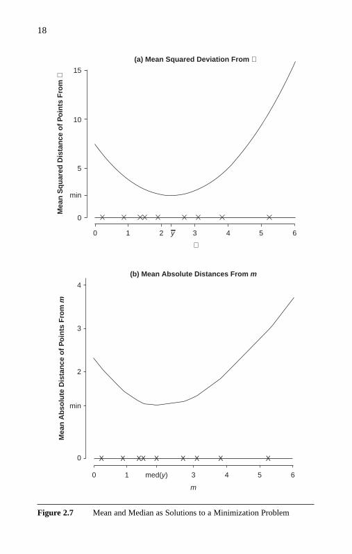
distance of sample points from a given point µ is shown in Figure 2.7a.Note that the function to minimize is convex, with a smooth parabolic form.
The median m has a similar minimizing property. Instead of using squareddistance, we can measure how far Y is from m by the absolute distance|Y − m|and measure the average distance in the population from m by the meanabsolute distance E|Y − m|. Again we can solve for the value m by minimizingE|Y − m|. As we shall see, the function of |Y − m| is convex, so that the mini-mization solution is to find a point where the derivative with respect to m is zeroor where the two directional derivatives disagree in sign. The solution is themedian of the distribution. (A proof appears in the Appendix of this chapter.)
Similarly, we can work on the sample level. We define the mean absolute
distance from m to the sample points by . A plot of this function
is given in Figure 2.7b for the same sample of nine points above. Comparedwith the function plotted in Figure 2.7a (the mean squared deviation), Figure2.7b remains convex and parabolic in appearance. However, rather than beingsmooth, the function in Figure 2.7b is piecewise linear, with the slope changingprecisely at each sample point. The minimum value of the function shownin this figure coincides with the median sample value of 1.89. This is a specialcase of a more general phenomenon. For any sample, the function defined
by f (m) is the sum of V-shaped functions fi(m) = |yi − m|/n
(see Figure 2.8 for the function fi corresponding to the data point withyi = 1.49). The function fi takes a minimum value of zero when m = yi has aderivative of −1/n for m < yi and 1/n for m > yi . While the function is not dif-ferentiable at m = yi, it does have a directional derivative there of −1/n in thenegative direction and 1/n in the positive direction. Being the sum of thesefunctions, the directional derivative of f at m is (r − s)/n in the negative direc-tion and (s − r) /n in the positive direction, where s is the number of datapoints to the right of m and r is the number of data points to the left of m. Itfollows that the minimum of f occurs when m has the same number of datapoints to its left and right, that is, when m is a sample median.
This representation of the median generalizes to the other quantiles as fol-lows. For any p∈(0,1), the distance from Y to a given q is measured by theabsolute distance, but we apply a different weight depending on whether Y is tothe left or to the right of q. Thus, we define the distance from Y to a given q as:
[2.5]
We look for the value q that minimizes the mean distance from Y:E [dp(Y,q)]. The minimum occurs when q is the pth quantile (see Appendix
dp(Y, q) ={(1 − p)|Y − q| Y < q
p|Y − q| Y ≥ q.
= 1
n
n∑i=1
|yi − m|
1
n
n∑i=1
|yi − m|
17
{
02-Hao.qxd 3/13/2007 4:29 PM Page 17
18
15
(a) Mean Squared Deviation From µ
10
5
0
min
0 1 2 3 4 5 6
Mea
n S
qu
ared
Dis
tan
ce o
f P
oin
ts F
rom
µ
µ
y
4
3
2
0
min
0 1 3
m
4 5 6med(y)
Mea
n A
bso
lute
Dis
tan
ce o
f P
oin
ts F
rom
m
X X XX X X X X X
(b) Mean Absolute Distances From m
Figure 2.7 Mean and Median as Solutions to a Minimization Problem
02-Hao.qxd 3/13/2007 4:29 PM Page 18

of this chapter). Similarly, the pth sample quantile is the value of q that min-imizes the average (weighted) distance:
Properties of Quantiles
One basic property of quantiles is monotone equivariance property. It statesthat if we apply a monotone transformation h (for example, the exponentialor logarithmic function) to a random variable, the quantiles are obtained byapplying the same transformation to the quantile function. In other words,if q is the pth quantile of Y, then h(q) is the pth quantile of h(Y). An analogousstatement can be made for sample quantiles. For example, for the sampledata, since we know that the 20th percentile is 4,300, if we make a log
1
n
n∑i=1
dp(yi, q) = 1 − p
n
∑yi<q
|yi − q| + p
n
∑yi>q
|yi − q|.
19
0.4
0.3
0.2
0.1
0.0
0 1 2 3 4 5yi
µ
Fi(
m)
Figure 2.8 V-Shaped Function Used to Describe the Median as the Solutionto a Minimization Problem
02-Hao.qxd 3/13/2007 4:29 PM Page 19
transformation of the data, the 20th percentile for the resulting data will belog (4,300) = 8.37.
Another basic property of sample quantiles relates to their insensitivityto the influence of outliers. This feature, which has an analog in quantileregression, helps make quantiles and quantile-based procedures useful inmany contexts. Given a sample of data x1, . . . , xn with sample median m,we can modify the sample by changing a data value xi that is above themedian to some other value above the median. Similarly, we can change adata value that is below the median to some other value below the median.Such modifications to the sample have no effect on the sample median.1 Ananalogous property holds for the pth sample quantile as well.
We contrast this with the situation for the sample mean: Changing anysample value xi to some other value xi + ∆ changes the sample mean by ∆/n.Thus, the influence of individual data points is bounded for sample quan-tiles and is unbounded for the sample mean.
Summary
This chapter introduces the notions of quantile and quantile function. Wedefine quantiles and quantile functions by way of the cumulative distribu-tion function. We develop quantile-based measures of location and shape ofa distribution and highlight their utility by comparing them with conven-tional distribution moments. We also redefine quantiles as a solution to aminimization problem, preparing the reader for a better understanding ofthe quantile regression estimator. With these preparations, we proceed tothe next chapter on the quantile-regression model and its estimator.
Note
1. To be precise, this assumes that the sample size is odd. If the samplesize is even, then the sample median is defined as the average of the (n/2)thand (n/2 + 1)th order statistics, and the statement holds if we modify a datavalue above (or below) the (n/2 + 1)th (or (n/2)th) order statistic, keepingit above (or below) that value.
20
02-Hao.qxd 3/13/2007 4:29 PM Page 20
Chapter 2 Appendix
A Proof: Median and Quantiles as Solutions to a Minimization Problem
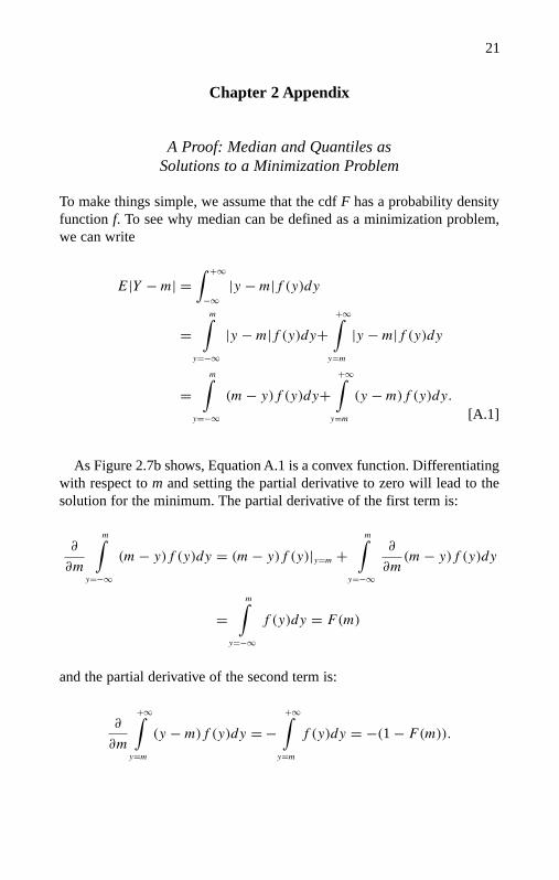
To make things simple, we assume that the cdf F has a probability densityfunction f. To see why median can be defined as a minimization problem,we can write
[A.1]
As Figure 2.7b shows, Equation A.1 is a convex function. Differentiatingwith respect to m and setting the partial derivative to zero will lead to thesolution for the minimum. The partial derivative of the first term is:
and the partial derivative of the second term is:
∂
∂m
+∞∫y=m
(y − m)f (y)dy = −+∞∫
y=m
f (y)dy = −(1 − F(m)).
∂
∂m
m∫y=−∞
(m − y)f (y)dy = (m − y)f (y)|y=m +m∫
y=−∞
∂
∂m(m − y)f (y)dy
=m∫
y=−∞
f (y)dy = F(m)
E|Y − m| =∫ +∞
−∞|y − m|f (y)dy
=m∫
y=−∞
|y − m|f (y)dy++∞∫
y=m
|y − m|f (y)dy
=m∫
y=−∞
(m − y)f (y)dy++∞∫
y=m
(y − m)f (y)dy.
21
03-Hao.qxd 3/13/2007 5:24 PM Page 21
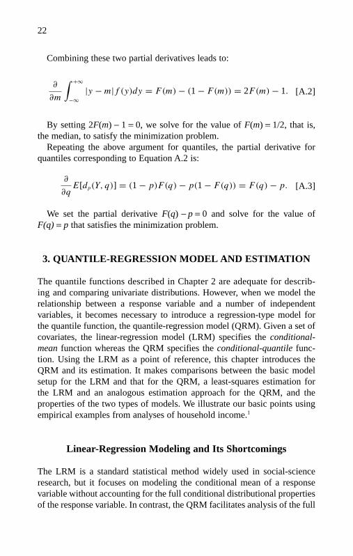
Combining these two partial derivatives leads to:
[A.2]
By setting 2F(m) − 1 = 0, we solve for the value of F(m) = 1/2, that is,the median, to satisfy the minimization problem.
Repeating the above argument for quantiles, the partial derivative forquantiles corresponding to Equation A.2 is:
[A.3]
We set the partial derivative F(q) − p = 0 and solve for the value ofF(q) = p that satisfies the minimization problem.
3. QUANTILE-REGRESSION MODEL AND ESTIMATION
The quantile functions described in Chapter 2 are adequate for describ-ing and comparing univariate distributions. However, when we model therelationship between a response variable and a number of independentvariables, it becomes necessary to introduce a regression-type model for the quantile function, the quantile-regression model (QRM). Given a set ofcovariates, the linear-regression model (LRM) specifies the conditional-mean function whereas the QRM specifies the conditional-quantile func-tion. Using the LRM as a point of reference, this chapter introduces theQRM and its estimation. It makes comparisons between the basic modelsetup for the LRM and that for the QRM, a least-squares estimation forthe LRM and an analogous estimation approach for the QRM, and theproperties of the two types of models. We illustrate our basic points usingempirical examples from analyses of household income.1
Linear-Regression Modeling and Its Shortcomings
The LRM is a standard statistical method widely used in social-scienceresearch, but it focuses on modeling the conditional mean of a responsevariable without accounting for the full conditional distributional propertiesof the response variable. In contrast, the QRM facilitates analysis of the full
∂
∂qE[dp(Y, q)] = (1 − p)F(q) − p(1 − F(q)) = F(q) − p.
∂
∂m
∫ +∞
−∞|y − m|f (y)dy = F(m) − (1 − F(m)) = 2F(m) − 1.
22
03-Hao.qxd 3/13/2007 5:24 PM Page 22
23
conditional distributional properties of the response variable. The QRM andLRM are similar in certain respects, as both models deal with a continuousresponse variable that is linear in unknown parameters, but the QRM andLRM model different quantities and rely on different assumptions abouterror terms. To better understand these similarities and differences, we layout the LRM as a starting point, and then introduce the QRM. To aid theexplication, we focus on the single covariate case. While extending to morethan one covariate necessarily introduces additional complexity, the ideasremain essentially the same.
Let y be a continuous response variable depending on x. In our empiricalexample, the dependent variable is household income. For x, we use aninterval variable, ED (the household head’s years of schooling), or alterna-tively a dummy variable, BLACK (the head’s race, 1 for black and 0 forwhite). We consider data consisting of pairs (xi ,yi) for i = 1, . . . , n basedon a sample of micro units (households in our example).
By LRM, we mean the standard linear-regression model
yi = β0 + β1x i + ε i , [3.1]
where εi is identically, independently, and normally distributed with meanzero and unknown variance σ 2. As a consequence of the mean zeroassumption, we see that the function β 0 + β 1x being fitted to the data corre-sponds to the conditional mean of y given x (denoted by E [ y ⎢x]), which isinterpreted as the average in the population of y values corresponding to afixed value of the covariate x.
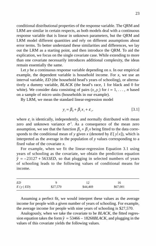
For example, when we fit the linear-regression Equation 3.1 usingyears of schooling as the covariate, we obtain the prediction equationy = –23127 + 5633ED, so that plugging in selected numbers of years of schooling leads to the following values of conditional means forincome.
ED 9 12 16E ( y | ED) $27,570 $44,469 $67,001
Assuming a perfect fit, we would interpret these values as the averageincome for people with a given number of years of schooling. For example,the average income for people with nine years of schooling is $27,570.
Analogously, when we take the covariate to be BLACK, the fitted regres-sion equation takes the form y = 53466 – 18268BLACK, and plugging in thevalues of this covariate yields the following values.
03-Hao.qxd 3/13/2007 5:24 PM Page 23

Again assuming the fitted model to be a reflection of what happens at thepopulation level, we would interpret these values as averages in subpopulations,for example, the average income is $53,466 for whites and $35,198 for blacks.
Thus, we see that a fundamental aspect of linear-regression models isthat they attempt to describe how the location of the conditional distribu-tion behaves by utilizing the mean of a distribution to represent its centraltendency. Another key feature of the LRM is that it invokes a homoscedas-ticity assumption; that is, the conditional variance, Var (y|x ), is assumed tobe a constant σ 2 for all values of the covariate. When homoscedasticityfails, it is possible to modify LRM by allowing for simultaneous modelingof the conditional mean and the conditional scale. For example, one canmodify the model in Equation 3.1 to allow for modeling the conditionalscale: yi = β0 + β1x i + e γε i, where γ is an additional unknown parameterand we can write Var (y|x) = σ 2e γ.
Thus, utilizing LRM reveals important aspects of the relationshipbetween covariates and a response variable, and can be adapted to performthe task of modeling what is arguably the most important form of shapechange for a conditional distribution: scale change. However, the estimationof conditional scale is not always readily available in statistical software.In addition, linear-regression models impose significant constraints on themodeler, and it is challenging to use LRM to model more complex condi-tional shape shifts.
To illustrate the kind of shape shift that is difficult to model using LRM,imagine a somewhat extreme situation in which, for some population ofinterest, we have a response variable y and a covariate x with the propertythat the conditional distribution of y has the probability density of the formshown in Figure 3.1 for each given value of x = 1,2,3. The three probabil-ity density functions in this figure have the same mean and standard devia-tion. Since the conditional mean and scale for the response variable y donot vary with x, there is no information to be gleaned by fitting a linear-regression model to samples from these populations. In order to understandhow the covariate affects the response variable, a new tool is required.Quantile regression is an appropriate tool for accomplishing this task.
A third distinctive feature of the LRM is its normality assumption.Because the LRM ensures that the ordinary least squares provide the bestpossible fit for the data, we use the LRM without making the normalityassumption for purely descriptive purposes. However, in social-scienceresearch, the LRM is used primarily to test whether an explanatory variable
24
BLACK 0 1E ( y | BLACK) $53,466 $35,198
03-Hao.qxd 3/13/2007 5:24 PM Page 24

significantly affects the dependent variable. Hypothesis testing goes beyondparameter estimation and requires determination of the sampling variabil-ity of estimators. Calculated p-values rely on the normality assumption oron large-sample approximation. Violation of these conditions may causebiases in p-values, thus leading to invalid hypothesis testing.
A related assumption made in the LRM is that the regression model usedis appropriate for all data, which we call the one-model assumption.Outliers (cases that do not follow the relationship for the majority of thedata) in the LRM tend to have undue influence on the fitted regression line.The usual practice used in the LRM is to identify outliers and eliminatethem. Both the notion of outliers and the practice of eliminating outliersundermine much social-science research, particularly studies on socialstratification and inequality, as outliers and their relative positions to thoseof the majority are important aspects of inquiry. In terms of modeling, onewould simultaneously need to model the relationship for the majority casesand for the outlier cases, a task the LRM cannot accomplish.
25
0.5 1.0 1.5
1.5
1.0
0.5
0.0
2.0 2.5
Y
x = 3
x = 1x = 2
Figure 3.1 Conditional Distributions With the Same Mean and StandardDeviation but Different Skewness
03-Hao.qxd 3/13/2007 8:28 PM Page 25

All of the features just mentioned are exemplified in our householdincome data: the inadequacy of the conditional mean from a distributionalpoint of view and violations of the homoscedasticity assumption, the nor-mality assumption, and the one-model assumption. Figure 3.2 shows thedistributions of income by education groups and racial groups. The locationshifts among the three education groups and between blacks and whites areobvious, and their shape shifts are substantial. Therefore, the conditionalmean from the LRM fails to capture the shape shifts caused by changes inthe covariate (education or race). In addition, since the spreads differ sub-stantially among the education groups and between the two racial groups,the homoscedasticity assumption is violated, and the standard errors arenot estimated precisely. All box graphs in Figure 3.2 are right-skewed.Conditional-mean and conditional-scale models are not able to detect thesekinds of shape changes.
By examining residual plots, we have identified seven outliers, includingthree cases with 18 years of schooling having an income of more than$505,215 and four cases with 20 years of schooling having an income ofmore than $471,572. When we add a dummy variable indicating member-ship in this outlier class to the regression model of income on education, wefind that these cases contribute an additional $483,544 to the intercept.
These results show that the LRM approach can be inadequate for a vari-ety of reasons, including heteroscedasticity and outlier assumptions and thefailure to detect multiple forms of shape shifts. These inadequacies are notrestricted to the study of household income but also appear when othermeasures are considered. Therefore, it is desirable to have an alternativeapproach that is built to handle heteroscedasticity and outliers and detectvarious forms of shape changes.
As pointed out above, the conditional mean fails to identify shape shifts.The conditional-mean models also do not always correctly model centrallocation shifts if the response distribution is asymmetric. For a symmetricdistribution, the mean and median coincide, but the mean of a skewed dis-tribution is no longer the same as the median (the .5th quantile). Table 3.1shows a set of brief statistics describing the household income distribution.The right-skewness of the distribution makes the mean considerably largerthan the median for both the total sample and for education and racialgroups (see the first two rows of Table 3.1). When the mean and the medianof a distribution do not coincide, the median may be more appropriate tocapture the central tendency of the distribution. The location shifts amongthe three education groups and between blacks and whites are considerablysmaller when we examine the median rather than the mean. This differenceraises concerns about using the conditional mean as an appropriate measurefor modeling the location shift of asymmetric distributions.
26
03-Hao.qxd 3/13/2007 5:24 PM Page 26

27
600
(a) Education Groups
500
400
300
200
100
0
$100
0
9 years of schooling 12 years of schooling 16 years of schooling
600
500
400
300
200
100
0
$100
0
White Black
(b) Race Groups
Figure 3.2 Box Graphs of Household Income
03-Hao.qxd 3/13/2007 5:24 PM Page 27

28
TAB
LE
3.1
Hou
seho
ld I
ncom
e D
istr
ibut
ion:
Tota
l,E
duca
tion
Gro
ups,
and
Rac
ial G
roup
s
Tota
lE
D =
9E
D =
12E
D =
16W
HIT
EB
LA
CK
Mea
n50
,334
27,8
4140
,233
71,8
3353
,466
35,1
98
Qua
ntil
eM
edia
n (.
50th
Qua
ntile
)39
,165
22,1
4632
,803
60,5
4541
,997
26,7
63.1
0th
Qua
ntile
11,0
228,
001
10,5
1021
,654
12,4
866,
837
.25t
h Q
uant
ile20
,940
12,3
2918
,730
36,8
0223
,198
13,4
12.7
5th
Qua
ntile
65,7
9336
,850
53,0
7590
,448
69,6
8047
,798
.90t
h Q
uant
ile98
,313
54,3
7077
,506
130,
981
102,
981
73,0
30
Qua
ntil
e-B
ased
Sca
le(Q
.75−
Q.2
5)44
,853
24,5
2134
,344
53,6
4646
,482
34,3
86(Q
.90−
Q.1
0)87
,291
46,3
6966
,996
109,
327
90,4
9566
,193
Qua
ntil
e-B
ased
Ske
wne
ss(Q
.75−
Q.5
0) −1
(Q.5
0−Q
.25)
.46
.50
.44
.26
.47
.58
(Q.9
0−Q
.50)
−1(Q
.50−
Q.1
0)1.
101.
281.
01.8
11.
071.
32
03-Hao.qxd 3/13/2007 5:24 PM Page 28

Conditional-Median and Quantile-Regression Models
With a skewed distribution, the median may become the more appropriatemeasure of central tendency; therefore, conditional-median regression,rather than conditional-mean regression, should be considered for thepurpose of modeling location shifts. Conditional-median regression wasproposed by Boscovich in the mid-18th century and was subsequentlyinvestigated by Laplace and Edgeworth. The median-regression modeladdresses the problematic conditional-mean estimates of the LRM. Medianregression estimates the effect of a covariate on the conditional median, soit represents the central location even when the distribution is skewed.
To model both location shifts and shape shifts, Koenker and Bassett (1978)proposed a more general form than the median-regression model, the quan-tile-regression model (QRM). The QRM estimates the potential differentialeffect of a covariate on various quantiles in the conditional distribution, forexample, a sequence of 19 equally distanced quantiles from the .05th quan-tile to the .95th quantile. With the median and the off-median quantiles, these19 fitted regression lines capture the location shift (the line for the median),as well as scale and more complex shape shifts (the lines for off-medianquantiles). In this way, the QRM estimates the differential effect of a covari-ate on the full distribution and accommodates heteroscedasticity.
Following Koenker and Bassett (1978), the QRM corresponding to theLRM in Equation 3.1 can be expressed as:
yi = β (p)0 + β (p)
1 xi + ε (p)i , [3.2]
where 0 < p < 1 indicates the proportion of the population havingscores below the quantile at p. Recall that for LRM, the conditional meanof yi given x i is E (yi|xi ) = β0 + β 1x i, and this is equivalent to requiringthat the error term ε i have zero expectation. In contrast, for the corre-sponding QRM, we specify that the pth conditional quantile given xi isQ (p)( yi|xi) = β (p)
0 + β (p)1 xi. Thus, the conditional pth quantile is determined
by the quantile-specific parameters, β (p)0 and β (p)
1 , and a specific value of thecovariate xi. As for the LRM, the QRM can be formulated equivalently witha statement about the error terms εi. Since the term β (p)
0 +β (p)1 x i is a constant,
we have Q (p)( yi|xi) = β (p)0 + β (p)
1 xi + Q(p)(εi ) = β (p)0 + β (p)
1 xi, so an equivalentformulation of QRM requires that the pth quantile of the error termbe zero.
It is important to note that for different values of the quantile p ofinterest, the error terms ε ( p)
i for fixed i are related. In fact, replacingp by q in Equation 3.2 gives yi = β (q)
0 + β (q)1 x i + ε (q)
i , which leads toε (p)
i – ε (q)i = (β (q)
0 – β (p)0 ) + xi( β (q)
1 – β (p)1 ), so that the two error terms differ by
29
03-Hao.qxd 3/13/2007 5:24 PM Page 29

a constant given x i. In other words, the distributions of ε (p)i and ε (q)
i are shiftsof one another. An important special case of QRM to consider is one inwhich the ε (p)
i for i = 1, . . . , n are independent and identically distributed;we refer to this as the i.i.d. case. In this situation, the qth quantile of ε (p)
i isa constant cp,q depending on p and q and not on i. Using Equation 3.2, wecan express the qth conditional-quantile function as Q(q)( yi|xi ) =Q(p)( yi|xi ) + cp,q.
2 We conclude that in the i.i.d. case, the conditional-quan-tile functions are simple shifts of one another, with the slopes β 1
(p) taking acommon value β1. In other words, the i.i.d. assumption says that there areno shape shifts in the response variable.
Equation 3.2 dictates that unlike the LRM in Equation 3.1, whichhas only one conditional mean expressed by one equation, the QRM canhave numerous conditional quantiles. Thus, numerous equations can beexpressed in the form of Equation 3.2.3 For example, if the QRM specifies19 quantiles, the 19 equations yield 19 coefficients for x i , one at each of the19 conditional quantiles ( β 1
.05, β 1.10, . . . , β 1
.95). The quantiles do not have tobe equidistant, but in practice, having them at equal intervals makes themeasier to interpret.
Fitting Equation 3.2 in our example yields estimates for the 19 condi-tional quantiles of income given education or race (see Tables 3.2 and 3.3).The coefficient for education grows monotonically from $1,019 at the .05thquantile to $8,385 at the .95th quantile. Similarly, the black effect is weakerat the lower quantiles than at the higher quantiles.
The selected conditional quantiles on 12 years of schooling are:
30
p .05 .50 .95E ( yi | EDi = 12) $7,976 $36,727 $111,268
and the selected conditional quantiles on blacks are:
p .05 .50 .95E ( yi | BLACKi = 1) $5,432 $26,764 $91,761
These results are very different from the conditional mean of the LRM.The conditional quantiles describe a conditional distribution, which can beused to summarize the location and shape shifts. Interpreting QRM esti-mates is a topic of Chapters 5 and 6.
Using a random sample of 1,000 households from the total sample andthe fitted line based on the LRM, the left panel of Figure 3.3 presentsthe scatterplot of household income against the head of household’s yearsof schooling. The single regression line indicates mean shifts, for example,a mean shift of $ 22,532 from 12 years of schooling to 16 years of schooling
03-Hao.qxd 3/13/2007 5:24 PM Page 30

31
TAB
LE
3.2
Qua
ntile
-Reg
ress
ion
Est
imat
es f
or H
ouse
hold
Inc
ome
on E
duca
tion
(1)
(2)
(3)
(4)
(5)
(6)
(7)
(8)
(9)
(10)
(11)
(12)
(13)
(14)
(15)
(16)
(17)
(18)
(19)
ED
1,01
91,
617
2,02
32,
434
2,75
03,
107
3,39
73,
657
3,94
84,
208
4,41
84,
676
4,90
55,
214
5,55
75,
870
6,37
36,
885
8,38
5(2
8)(3
1)(4
0)(3
9)(4
4)(5
1)(5
7)(6
4)(6
6)(7
2)(8
1)(9
2)(8
8)(1
02)
(127
)(1
38)
(195
)(2
74)
(463
)
Con
stan
t−
4,25
2−7
,648
−9,1
70−1
1,16
0−1
2,05
6−1
3,30
8−1
3,78
3−1
3,72
6−1
4,02
6−1
3,76
9−1
2,54
6−1
1,55
7−9
,914
−8,7
60−7
,371
−4,2
27−1
,748
4,75
510
,648
(380
)(4
24)
(547
)(5
27)
(593
)(6
93)
(764
)(8
66)
(884
)(9
69)
(1,0
84)
(1,2
26)
(1,1
69)
(1,3
58)
(1,6
90)
(1,8
28)
(2,5
82)
(3,6
19)
(6,1
01)
NO
TE
:Sta
ndar
d er
rors
in p
aren
thes
es.
TAB
LE
3.3
Qua
ntile
-Reg
ress
ion
Est
imat
es f
or H
ouse
hold
Inc
ome
on R
ace
(1)
(2)
(3)
(4)
(5)
(6)
(7)
(8)
(9)
(10)
(11)
(12)
(13)
(14)
(15)
(16)
(17)
(18)
(19)
BL
AC
K−3
,124
−5,6
49−7
,376
−8,8
48−9
,767
−11,
232
−12,
344
−13,
349
−14,
655
−15,
233
−16,
459
−17,
417
−19,
053
−20,
314
−21,
879
−22,
914
−26,
063
−29,
951
−40,
639
(304
)(3
06)
(421
)(4
85)
(584
)(5
36)
(609
)(7
08)
(781
)(7
65)
(847
)(8
87)
(1,0
50)
(1,0
38)
(1,1
91)
(1,2
21)
(1,4
35)
(1,9
93)
(3,5
73)
Con
stan
t8,
556
12,4
8616
,088
19,7
1823
,198
26,8
3230
,354
34,0
2438
,047
41,9
9746
,635
51,5
1556
,613
62,7
3869
,680
77,8
7087
,996
102,
981
132,
400
(115
)(1
16)
(159
)(1
83)
(220
)(2
02)
(230
)(2
68)
(295
)(2
89)
(320
)(3
35)
(397
)(3
92)
(450
)(4
61)
(542
)(7
53)
(1,3
50)
NO
TE
:Sta
ndar
d er
rors
in p
aren
thes
es.
03-Hao.qxd 3/13/2007 5:24 PM Page 31

32
Quantile Regression
80000
60000
40000
20000
0
Ho
use
ho
ld In
com
e
Linear Regression
0 5 10 15 20
80000
60000
40000
20000
0
Ho
use
ho
ld In
com
e
0 5 10 15 20
Figure 3.3 Effects of Education on the Conditional Mean and ConditionalQuantiles of Household Income: A Random Sample of 1,000Households
(5633 · (16 – 12)). However, this regression line does not capture shapeshifts.
The right panel of Figure 3.3 shows the same scatterplot as in the leftpanel and the 19 quantile-regression lines. The .5th quantile (the median)fit captures the central location shifts, indicating a positive relationshipbetween conditional-median income and education. The slope is $ 4,208,shifting $16,832 from 12 years of schooling to 16 years of schooling(4208 · (16 – 12)). This shift is lower than the LRM mean shift.
In addition to the estimated location shifts, the other 18 quantile-regressionlines provide information about shape shifts. These regression lines arepositive, but with different slopes. The regression lines cluster tightly atlow levels of education (e.g., 0–5 years of schooling) but deviate from eachother more widely at higher levels of education (e.g., 16–20 years of
03-Hao.qxd 3/13/2007 5:24 PM Page 32

schooling). A shape shift is described by the tight cluster of the slopes atlower levels of education and the scattering of slopes at higher levels ofeducation. For instance, the spread of the conditional income on 16 yearsof schooling (from $12,052 for the .05th conditional quantile to $144,808for the .95th conditional quantile) is much wider than that on 12 years ofschooling (from $7,976 for the .05th conditional quantile to $111,268 forthe .95th conditional quantile). Thus, the off-median conditional quantilesisolate the location shift from the shape shift. This feature is crucial fordetermining the impact of a covariate on the location and shape shifts of theconditional distribution of the response, a topic discussed in Chapter 5 withthe interpretation of the QRM results.
QR Estimation
We review least-squares estimation so as to place QR estimation in a famil-iar context. The least-squares estimator solves for the parameter estimatesβ 0 and β 1 by taking those values of the parameters that minimize the sumof squared residuals:
min ∑i(yi – ( β0+β 1 xi ) )2. [3.3]
If the LRM assumptions are correct, the fitted response functionβ 0 + β 1 approaches the population conditional mean E ( y⏐x) as the samplesize goes to infinity. In Equation 3.3, the expression minimized is the sumof squared vertical distances between data points ( x i , y i ) and the fitted liney = β 0 + β 1x.
A closed-form solution to the minimization problem is obtained by(a) taking partial derivatives of Equation 3.3 with respect to β0 and β1,respectively; (b) setting each partial derivative equal to zero; and (c) solv-ing the resulting system of two equations with two unknowns. We thenarrive at the two estimators:
A significant departure of the QR estimator from the LR estimator is thatin the QR, the distance of points from a line is measured using a weightedsum of vertical distances (without squaring), where the weight is 1 – p forpoints below the fitted line and p for points above the line. Each choice
β1 =
n∑i
(xi − x)(yi − y---)
n∑i
(xi − x)2
, β0 = y--- − β1x.
33
03-Hao.qxd 3/13/2007 5:24 PM Page 33

for this proportion p, for example, p = .10, .25, .50, gives rise to a differentfitted conditional-quantile function. The task is to find an estimator with thedesired property for each possible p. The reader is reminded of the discus-sion in Chapter 2 where it was indicated that the mean of a distribution canbe viewed as the point that minimizes the average squared distance over thepopulation, whereas a quantile q can be viewed as the point that minimizesan average weighted distance, with weights depending on whether the pointis above or below the value q.
For concreteness, we first consider the estimator for the median-regressionmodel. In Chapter 2, we described how the median (m) of y can be viewed as the minimizing value of E|y – m|. For an analogous prescription in themedian-regression case, we choose to minimize the sum of absolute residu-als. In other words, we find the coefficients that minimize the sum of absoluteresiduals (the absolute distance from an observed value to its fitted value).The estimator solves for the βs by minimizing Equation 3.4:
∑i ⎢yi – β0 – β1xi ⎢. [3.4]
Under appropriate model assumptions, as the sample size goes to infin-ity, we obtain the conditional median of y given x at the population level.
When expression Equation 3.4 is minimized, the resulting solution,which we refer to as the median-regression line, must pass through a pairof data points with half of the remaining data lying above the regressionline and the other half falling below. That is, roughly half of the residualsare positive and half are negative. There are typically multiple lines withthis property, and among these lines, the one that minimizes Equation 3.4is the solution.
Algorithmic Details
In this subsection, we describe how the structure of the function Equation3.4 makes it amenable to finding an algorithm for its minimization. Readerswho are not interested in this topic can skip this section.
The left panel of Figure 3.4 shows eight hypothetical pairs of data points(xi, yi) and the 28 lines (8(8 − 1)/2 = 28) connecting a pair of these pointsis plotted. The dashed line is the fitted median-regression line, that is, theline that minimizes the sum of absolute vertical distance from all datapoints. Observe that of the six points not falling on the median-regressionline, half of the points are below it and the other half are above it. Everyline in the (x, y) plane takes the form y = β0 + β1x for some choice ofintercept-slope pair ( β0 , β 1), so that we have a correspondence betweenlines in the (x, y) plane and points in the ( β0 , β 1) plane. The right panel
34
03-Hao.qxd 3/13/2007 5:24 PM Page 34
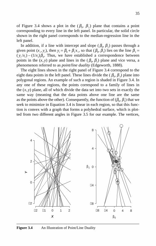
of Figure 3.4 shows a plot in the ( β0, β 1) plane that contains a pointcorresponding to every line in the left panel. In particular, the solid circleshown in the right panel corresponds to the median-regression line in theleft panel.
In addition, if a line with intercept and slope ( β0, β1) passes through agiven point (x i , yi), then yi = β0 + β1x i, so that (β0, β1) lies on the line β1 =( yi /xi) – (1/xi)β0. Thus, we have established a correspondence betweenpoints in the (x, y) plane and lines in the ( β0, β1) plane and vice versa, aphenomenon referred to as point/line duality (Edgeworth, 1888).
The eight lines shown in the right panel of Figure 3.4 correspond to theeight data points in the left panel. These lines divide the ( β0, β 1) plane intopolygonal regions. An example of such a region is shaded in Figure 3.4. Inany one of these regions, the points correspond to a family of lines in the (x, y) plane, all of which divide the data set into two sets in exactly thesame way (meaning that the data points above one line are the sameas the points above the other). Consequently, the function of (β0, β1) that weseek to minimize in Equation 3.4 is linear in each region, so that this func-tion is convex with a graph that forms a polyhedral surface, which is plot-ted from two different angles in Figure 3.5 for our example. The vertices,
35
4
2
−2
−2 −1 0 1 2 −8 −4 0 4 8
0
X
0
−4
4
8
−8
β1
β0
Y
Figure 3.4 An Illustration of Point/Line Duality
03-Hao.qxd 3/13/2007 5:24 PM Page 35

edges, and facets of the surface project to points, line segments, and regions,respectively, in the (β0, β1) plane shown in the right-hand panel of Figure 3.4.Using the point/line duality correspondence, each vertex corresponds to a lineconnecting a pair of data points. An edge connecting two vertices in the sur-face corresponds to a pair of such lines, where one of the data points definingthe first line is replaced by another data point, and the remaining points main-tain their position (above or below) relative to both lines.
An algorithm for minimization of the sum of absolute distances inEquation 3.4, one thus leading to the median-regression coefficients (β 0, β 1 ) ,can be based on exterior-point algorithms for solving linear-programmingproblems. Starting at any one of the points (β0, β1) corresponding to a vertex, the minimization is achieved by iteratively moving from vertex to
36
Figure 3.5 Polyhedral Surface and Its Projection
ββ1
ββ1
ββ0
ββ0
03-Hao.qxd 3/13/2007 5:24 PM Page 36

vertex along the edges of the polyhedral surface, choosing at each vertexthe path of the steepest descent until arriving at the minimum. Using thecorrespondence described in the previous paragraph, we iteratively movefrom line to line defined by pairs of data points, at each step deciding whichnew data point to swap with one of the two current ones by picking the onethat leads to the smallest value in Equation 3.4. The minimum sum ofabsolute errors is attained at the point in the ( β0, β1 ) plane below the lowestvertex of the surface. A simple argument involving the directional derivativewith respect to β0 (similar to the one in Chapter 2 showing that the median isthe solution to a minimization problem) leads to the conclusion that the samenumber of data points lie above the median-regression line as lie below it.
The median-regression estimator can be generalized to allow for pthquantile-regression estimators (Koenker & d’Orey, 1987). Recall from thediscussion in Chapter 2 that the pth quantile of a univariate sample y1, . . . , yn
distribution is the value q that minimizes the sum of weighted distances fromthe sample points, where points below q receive a weight of 1 – p and pointsabove q receive a weight of p. In a similar manner, we define the pth quantile-regression estimators β 0
(p) and β 1(p) as the values that minimize the weighted
sum of distances between fitted values yi = β 0(p) + β 1
(p)xi and the yi, where weuse a weight of 1 – p if the fitted value underpredicts the observed value yi
and a weight of p otherwise. In other words, we seek to minimize a weightedsum of residuals yi – yi where positive residuals receive a weight of p andnegative residuals receive a weight of 1 – p. Formally, the pth quantile-regression estimators β 0
(p) and β 1(p) are chosen to minimize
[3.5]
where dp is the distance introduced in Chapter 2. Thus, unlike Equation 3.4,which states that the negative residuals are given the same importance asthe positive residuals, Equation 3.5 assigns different weights to positive andnegative residuals. Observe that in Equation 3.5, the first sum is the sum ofvertical distances of data points from the line y = β 0
(p) + β 1(p) x, for points
lying above the line. The second is a similar sum over all data points lyingbelow the line.
Observe that, contrary to a common misconception, the estimation ofcoefficients for each quantile regression is based on the weighted dataof the whole sample, not just the portion of the sample at that quantile.
n∑i=1
dp(yi, yi) = p∑
yi≥β(p)0 +β
(p)1 xi
|yi − β(p)
0 − β(p)
1 xi | + (1 − p)
∑yi<β
(p)0 +β
(p)1 xi
|yi − β(p)
0 − β(p)
1 xi |,
37
03-Hao.qxd 3/13/2007 5:24 PM Page 37
An algorithm for computing the quantile-regression coefficients β 0( p) and
β 1(p) can be developed along lines similar to those outlined for the median-
regression coefficients. The pth quantile-regression estimator has a similarproperty to one stated for the median-regression estimator: The proportionof data points lying below the fitted line y = β 0
(p)+β 1(p)x is p, and the pro-
portion lying above is 1 – p.For example, when we estimate the coefficients for the .10th quantile-
regression line, the observations below the line are given a weight of .90and the ones above the line receive a smaller weight of .10. As a result, 90%of the data points (xi,yi) lie above the fitted line leading to positive residuals,and 10% lie below the line and thus have negative residuals. Conversely, toestimate the coefficients for the .90th quantile regression, points below theline are given a weight of .10, and the rest have a weight of .90; as a result,90% of observations have negative residuals and the remaining 10% havepositive residuals.
Transformation and Equivariance
In analyzing a response variable, researchers often transform the scale toaid interpretation or to attain a better model fit. Equivariance properties ofmodels and estimates refer to situations when, if the data are transformed,the models or estimates undergo the same transformation. Knowledge ofequivariance properties helps us to reinterpret fitted models when we trans-form the response variable.
For any linear transformation of the response variable, that is, the additionof a constant to y or the multiplication of y by a constant, the conditionalmean of the LRM can be exactly transformed. The basis for this statementis the fact that for any choice of constants a and c, we can write
E (c + ay |x) = c + aE(y |x). [3.6]
For example, if every household in the population received $500 fromthe government, the conditional mean would also be increased by $500 (thenew intercept would be increased by $500). When the $1 unit of income istransformed to the $1,000 unit, the conditional mean in the $1 unit isincreased by 1,000 times as well (the intercept and the slope are both mul-tiplied by 1,000 to be on the dollar scale). Similarly, if the dollar unit forwage rate is transformed to the cent unit, the conditional mean (the inter-cept and the slope) is divided by 100 to be on the dollar scale again. Thisproperty is termed linear equivariance because the linear transformation is
38
03-Hao.qxd 3/13/2007 5:24 PM Page 38

the same for the dependent variable and the conditional mean. The QRMalso has this property:
Q(p)(c + ay |x) = c + a (Q(p)[y | x] ), [3.7]
provided that a is a positive constant. If a is negative, we haveQ(p) (c + ay | x) = c + a(Q (1− p)[ y|x]) because the order is reversed.
Situations often arise in which nonlinear transformation is desired.Log transformations are frequently used to address the right-skewness ofa distribution. Other transformations are considered in order to make adistribution appear more normal or to achieve a better model fit.
Log transformations are also introduced in order to model a covariate’seffect in relative terms (e.g., percentage changes). In other words, the effect ofa covariate is viewed on a multiplicative scale rather than on an additive one.In our example, the effects of education or race were previously expressed inadditive terms (the dollar unit), and it may be desirable to measure an effect inmultiplicative terms, for example, in terms of percentage changes. For exam-ple, we can ask: What is the percentage change in conditional-mean incomebrought about by one more year of schooling? The coefficient for education ina log income equation (multiplied by 100) approximates the percentagechange in conditional-mean income brought about by one more year ofschooling. However, under the LRM, the conditional mean of log income isnot the same as the log of conditional-mean income. Estimating two LRMsusing income and log income yields two fitted models:
y = –23,127 + 5,633ED, log y = 8.982 + .115ED.
The result from the log income model suggests that one more year ofeducation increases the conditional-mean income by about 11.5%.4 Theconditional mean of the income model at 10 years of schooling is $33,203,the log of which becomes 8.108. The conditional mean of the log incomemodel at the same schooling level is 10.062, a much larger figure than thelog of the conditional mean of income (8.108). While the log transforma-tion of a response in the LRM allows an interpretation of LRM estimates asa percentage change, the conditional mean of the response in absolute termsis impossible to obtain from the conditional mean on the log scale:
E(log y ⎢x ) ≠ log [E( y ⎢x )] and E (yi ⎢xi) ≠ eE[log yi ⎢xi ]. [3.8]
Specifically, if our aim is to estimate the education effect in absoluteterms, we use the income model, whereas for the impact of education in
39
03-Hao.qxd 3/13/2007 5:24 PM Page 39

relative terms, we use the log income model. Although the two objectivesare related to each other, the conditional means of the two models are notrelated through any simple transformation.5 Thus, it would be a mistake touse the log income results to make conclusions about the distribution ofincome (though this is a widely used practice).
The log transformation is one member of the family of monotone trans-formations, that is, transformations that preserve order. Formally, a trans-formation h is a monotone if h(y) < h(y′) whenever y < y′. For variablestaking positive values, the power transformation h (y) = yφ is monotone fora fixed positive value of the constant φ. As a result of nonlinearity, when weapply a monotone transformation, the degree to which the transformationchanges the value of y can differ from one value of y to the next. While theproperty in Equation 3.6 holds for linear functions, it is not the case forgeneral monotone functions, that is, E (h (y)|x) ≠ h (E(yi|xi)). Generallyspeaking, the “monotone equivariance” property fails to hold for condi-tional means, so that LRMs do not possess monotone equivariance.
By contrast, the conditional quantiles do possess monotone equivariance;that is, for a monotone function h, we have
Q(p)(h (y) ⎢x) = h (Q(p)[y|x]). [3.9]
This property follows immediately from the version of monotone equi-variance stated for univariate quantiles in Chapter 2. In particular, a condi-tional quantile of log y is the log of the conditional quantile of y:
Q(p)(log(y) ⎢x) = log (Q(p)[y|x]), [3.10]
and equivalently,
Q(p)(y ⎢x) = eQ(p)[log(y) ⎢x], [3.11]
so that we are able to reinterpret fitted quantile-regression modelsfor untransformed variables to quantile-regression models for trans-formed variables. In other words, assuming a perfect fit for the pth quantilefunction of the form Q(p)(y|x) = β0 + β1x, we have Q(p)(log y|x) =log(β0 + β1x), so that we can use the impact of a covariate expressed inabsolute terms to describe the impact of a covariate in relative terms andvice versa.
Take the conditional median as an example:
Q(.50)( yi ⎢EDi) = –13769 + 4208EDi, Q(.50) (log(yi) ⎢EDi ) = 8.966 + .123EDi .
40
03-Hao.qxd 3/13/2007 5:24 PM Page 40

The conditional median of income at 10 years of schooling is $28,311.The log of this conditional median, 10.251, is similar to the conditionalmedian of the log income equation at the same education level, 10.196.Correspondingly, when moving from log to raw scale, in absolute terms, theconditional median at 10 years of schooling from the log income equationis e10.916 = 28,481.
The QRM’s monotone equivariance is particularly important for researchinvolving skewed distributions. While the original distribution is distortedby the reverse transformation of log-scale estimates if the LRM is used, theoriginal distribution is preserved if the QRM is used. A covariate’s effecton the response variable in terms of percentage change is often used ininequality research. Hence, the monotone equivariance property allowsresearchers to achieve both goals: measuring percentage change caused bya unit change in the covariate and measuring the impact of this change onthe location and shape of the raw-scale conditional distribution.
Robustness
Robustness refers to insensitivity to outliers and to the violation of modelassumptions concerning the data y. Outliers are defined as some values ofy that do not follow the relationship for the majority values. Under theLRM, estimates can be sensitive to outliers. Earlier in the first section ofthis chapter, we presented an example showing how outliers of income dis-tribution distort the mean and the conditional mean. The high sensitivity ofthe LRM to outliers has been widely recognized. However, the practice ofeliminating outliers does not satisfy the objective of much social-scienceresearch, particularly inequality research.
In contrast, the QRM estimates are not sensitive to outliers.6 This robust-ness arises because of the nature of the distance function in Equation 3.5that is minimized, and we can state a property of quantile-regression esti-mates that is similar to a statement made in Chapter 2 about univariatequantiles. If we modify the value of the response variable for a data pointlying above (or below) the fitted quantile-regression line, as long as thatdata point remains above (or below) the line, the fitted quantile-regressionline remains unchanged. Stated another way, if we modify values of theresponse variable without changing the sign of the residual, the fitted lineremains the same. In this way, as for univariate quantiles, the influence ofoutliers is quite limited.
In addition, since the covariance matrix of the estimates is calculatedunder the normality assumption, the LRM’s normality assumption is neces-sary for obtaining the inferential statistics of the LRM. Violation of thenormality assumption can cause inaccuracy in standard errors. The QRM is
41
03-Hao.qxd 3/13/2007 5:24 PM Page 41

robust to distributional assumptions because the estimator weighs the localbehavior of the distribution near the specific quantile more than the remotebehavior of the distribution. The QRM’s inferential statistics can be distri-bution free (a topic discussed in Chapter 4). This robustness is important instudying phenomena of highly skewed distributions such as income, wealth,educational, and health outcomes.
Summary
This chapter introduces the basics of the quantile-regression model incomparison with the linear-regression model, including the model setup,the estimation, and the properties of estimates. The QRM inherits many ofthe properties of sample quantiles introduced in Chapter 2. We explain howLRM is inadequate for revealing certain types of effects of covariates on thedistribution of a response variable. We also highlight some of the key featuresof QRM. We present many of the important differences between the QRMand the LRM, namely, (a) multiple-quantile-regression fits versus single-linear-regression fits to data; (b) quantile-regression estimation that minimizesa weighted sum of absolute values of residuals as opposed to minimizing thesum of squares in least-squares estimation; and (c) the monotone equivari-ance and robustness to distributional assumptions in conditional quantilesversus the lack of these properties in the conditional mean. With these basics,we are now ready to move on to the topic of QRM inference.
Notes
1. The data are drawn from the 2001 panel of the Survey of Income andProgram Participation (SIPP). Household income is the annual income in2001. The analytic sample for Chapters 3 through 5 includes 19,390 whitehouseholds and 3,243 black households.
2. Q (q)(y i ⎢x i) = Q (q)(β 0( p) + x i β 1
( p) + ε i( p)) = β 0
( p) + x i β 1( p) + Q (q)
(εi(p)) = Q(p) (yi ⎢xi) + cp,q.3. The number of distinct quantile solutions, however, is bounded by the
finite sample size.4. Precisely, the percentage change is 100(e.115–1) = 12.2%.5. The conditional mean is proportional to the exponential of the linear
predictor (Manning, 1998). For example, if the errors are normally distrib-uted N(0, σε
2), then E(yi ⎢xi) = eβ0 + β1xi+ 0.5σ ε
2
. The term e0.5σ ε2
is sometimescalled the smearing factor.
6. Note that this robustness does not apply to outliers of covariates.
42
03-Hao.qxd 3/13/2007 5:24 PM Page 42

4. QUANTILE-REGRESSION INFERENCE
Chapter 3 covered the topic of parameter estimation. We now turn to thetopic of inferential statistics, specifically standard errors and confidenceintervals for coefficient estimates from the QRM. We begin with an overviewof inference in the LRM, discussing the exact finite sample and asymptoticdistributions of quantities used in the construction of confidence intervalsand hypothesis tests. Then, we introduce the corresponding asymptotic pro-cedure for the QRM. Next, we introduce the bootstrap procedure for theQRM, which allows for inference about QRM coefficients. The bootstrapprocedure is preferable to the asymptotic because the assumptions for theasymptotic procedure usually do not hold, and even if these assumptionsare satisfied, it is complicated to solve for the standard error of the con-structed scale and skewness shifts. The bootstrap procedure offers the flex-ibility to obtain the standard error and confidence interval for any estimatesand combinations of estimates. The last section of this chapter discusses thetopics of goodness of fit and model checking.
Standard Errors and Confidence Intervals for the LRM
We begin with an overview of inference for coefficients in the LRM
expressed in the form yi = under ideal modeling assumptions, which
state that errors εi are independently and identically (i.i.d.) normally distrib-uted with mean 0 and a constant variance σ 2, so that exact distributions can bederived. The expression x(i)
j is used to denote the value of the jth covariate forthe ith sampled individual. It will be helpful below to think of x(i), the vectorof covariate values for the ith individual, as a (row) k-vector.
The usual estimator of the error variance is given by σ 2 = RSS/(n − k),where RSS denotes the residual sum of squares and k is the number of pre-dictor variables (including the intercept term) used in the fitted model.Letting the n × k matrix of predictor variable values be denoted by X (sothat the ith row is x(i), the covariate values for the ith individual), the jointdistribution of the least-squares estimator β of the vector of regressioncoefficients is multivariate normal, with the mean being the true β and thecovariance matrix given by σ 2(X tX)–1. As a consequence, an individualcoefficient estimator β j has a normal distribution, with the mean being thetrue βj, and a variance of δjσ 2, where δj denotes the jth diagonal entry of thematrix (Xt X)–1. Thus, we estimate the variance of β j using δjσ 2.
Naturally, we estimate the standard deviation of the estimator by thesquare root of this estimator and refer to this as the standard error of β j
(denoted by sβ j). As a consequence of the assumptions about the error
k∑j=1
βjx(i)
j + εi
43
04-Hao.qxd 3/13/2007 5:43 PM Page 43
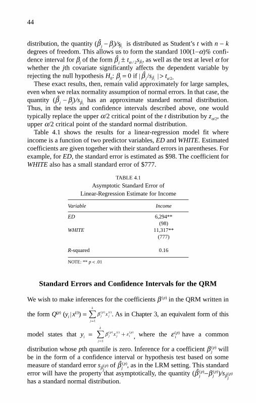
distribution, the quantity (β j − βj)/sβ jis distributed as Student’s t with n − k
degrees of freedom. This allows us to form the standard 100(1−α)% confi-dence interval for βj of the form β j ± tα / 2sβ j
, as well as the test at level α forwhether the jth covariate significantly affects the dependent variable byrejecting the null hypothesis H0: βj = 0 if|β j /sβ j
|> ta/2.These exact results, then, remain valid approximately for large samples,
even when we relax normality assumption of normal errors. In that case, thequantity (β j − βj)/sβ j
has an approximate standard normal distribution.Thus, in the tests and confidence intervals described above, one wouldtypically replace the upper α/2 critical point of the t distribution by zα/2, theupper α/2 critical point of the standard normal distribution.
Table 4.1 shows the results for a linear-regression model fit whereincome is a function of two predictor variables, ED and WHITE. Estimatedcoefficients are given together with their standard errors in parentheses. Forexample, for ED, the standard error is estimated as $98. The coefficient forWHITE also has a small standard error of $777.
44
TABLE 4.1
Asymptotic Standard Error ofLinear-Regression Estimate for Income
Variable Income
ED 6,294**(98)
WHITE 11,317**(777)
R-squared 0.16
NOTE: ** p < .01
Standard Errors and Confidence Intervals for the QRM
We wish to make inferences for the coefficients β (p) in the QRM written in
the form Q(p) (yi|x(i)) = . As in Chapter 3, an equivalent form of this
model states that yi = , where the ε i(p) have a common
distribution whose pth quantile is zero. Inference for a coefficient β (p)j will
be in the form of a confidence interval or hypothesis test based on somemeasure of standard error sβ (p)
jof β (p)
j , as in the LRM setting. This standarderror will have the property that asymptotically, the quantity (β (p)
j −β (p)j )/sβ (p)
jhas a standard normal distribution.
k∑j=1
β(p)
j x(i)
j + ε(p)
i
k∑j=1
β(p)
j x(i)
j
04-Hao.qxd 3/13/2007 5:43 PM Page 44

Standard errors for the QRM are considerably simpler and easier to describeunder the i.i.d. model presented in Chapter 3. In this case, the asymptoticcovariance matrix for β (p) takes the form
[4.1]
The term fε(p)(0) appearing in Equation 4.1 is the probability density ofthe error term ε (p) evaluated at the pth quantile of the error distribution.1 Asin the LRM, the covariance matrix is a scalar multiple of the (Xt X)–1 matrix.However, in the QRM, the multiplier is the asymptotic
variance of a sample quantile based on a (univariate) sample ε 1(p), . . . , ε (p)
n . Thedensity term appearing in this expression is unknown and needs to be estimatedjust as in the univariate case, and the procedure described in Chapter 2 for esti-mation of the corresponding term is easily adapted to the present situation.The quantity can be estimated using a difference quotient
, where the sample quantiles Q(p ± h) are based on
the residuals ε i(p) = yi i = 1, . . . , n for the fitted QRM model. The
choice of h to use is a delicate one, and Koenker (2005) describes a coupleof approaches to choosing h.
It is more complex to deal with the non-i.i.d. case. In this case, the ε i(p) no
longer have a common distribution, but all of these distributions still have apth quantile of zero. To handle this noncommon distribution, it becomesnecessary to introduce a weighted version (D1 below) of the Xt X matrix.
All of the analytic methods for obtaining approximate standard errors in theQRM are derived from a general result described in Koenker (2005) giving amultivariate normal approximation to the joint distribution of the coefficientestimates β (p)
j . This distribution has a mean with components that are the truecoefficients and a covariance matrix of the form: Σβ (p) = , where
[4.2]
where x(i) is the ith row of X with dimension of 1 × k. Here the terms D0 andD1 are k × k matrices. The weight wi = fεi
(p) (0), with the probability densityfunction ε (p)
i evaluated at 0 (which is the pth conditional quantile of ε (p)i ).
Thus, we can think of the sum in the expression for D1 as being Xt X, whereX is obtained from X by multiplying the ith row by . Mild conditionscan be given under which convergence in Equation 4.1 is to positive defi-nite matrices Di. As in the i.i.d. case, we see the asymptotic distribution of
√wi
D0 = limn→∞1
n
n∑i=1
x(i)tx(i), and D1 = limn→∞1
n
n∑i=1
wix(i)tx(i),
p(1 − p)
nD−1
1 D0D−11
k∑j=1
β(p)
j x(i)
j ,
1
2h(Q(p)(p + h) − Q(p)(p − h))
1
fε(p)
= d
dpQ(p)(ε(p))
p(1 − p)
n· 1
fε(p) (0)2
�β(p) = p(1 − p)
n· 1
fε(p) (0)2(XtX)−1.
45
04-Hao.qxd 3/13/2007 5:43 PM Page 45

β (p) on the conditional-density function evaluated at the quantile of inter-est. However, since the ε (p)
i are not identically distributed, these terms differwith i, leading to different weights. Since the density function is unknown,it becomes necessary to estimate the weights wi appearing in Equation 4.2.Two methods for producing estimates wi of the weights are described inKoenker (2005). Whatever method is employed, the covariance matrix forβ (p) is estimated as ∑ = D1
−1D0D1−1, where
[4.3]
An estimated standard error for an individual coefficient estimator β (p)j is
obtained by taking the square root of the corresponding diagonal element ofthe estimated covariance matrix Σ. As in the i.i.d. case, we are now able totest hypotheses about the effects of the covariates on the dependent variable,and to obtain confidence intervals for the quantile-regression coefficients.
Table 4.2 shows the asymptotic and bootstrap standard error of estimatesin a two-covariate QRM for the .05th and .95th income quantiles, respec-tively. The asymptotic and bootstrap errors differ moderately but lead to thesame conclusion about the effect of ED and WHITE. The point estimate forED is $1,130, and the standard error is $36 at the .05th quantile. The cor-responding numbers at the .95th quantile are $9,575 and $605, respectively.The coefficient for WHITE is $3,197 with a standard error of $359 atthe .05th quantile, and $17,484 with a standard error of $2,895 at the .95thquantile. Confidence intervals can be obtained using the standard errors.
D0 = 1
n
n∑i=1
x(i)tx(i), and D1 = 1
n
n∑i=1
wix(i)tx(i).
p(1 − p)
n
46
TABLE 4.2
Quantile-Regression Model of Income WithAsymptotic and 500 Resample Bootstrap Standard Errors
P
Variable .05 .95
ED 1,130 9,575(36) (605)[80] [268]
WHITE 3,197 17,484(359) (2,895)[265] [2,280]
NOTE: Asymptotic standard errors are in parentheses and bootstrap standard errorsare in brackets.
04-Hao.qxd 3/13/2007 5:43 PM Page 46

Table 4.2 shows that the positive effects of ED and WHITE are statisti-cally significant for the two extreme quantiles. However, whether the effectof a covariate differs significantly across quantiles needs to be tested. Thesetests require a covariance matrix of the coefficients across quantiles. As wediscussed above, estimating the variance of the error in the QRM is morecomplicated than in the LRM; therefore, the covariance of coefficients frommultiple QRMs would be even more complicated, making a closed-formsolution practically impossible. Thus, we need an alternative method to esti-mate the covariance of coefficients across quantiles, which will be discussedin the next section.
The more important concern about the asymptotic standard error is that thei.i.d. assumption of errors is unlikely to hold. The often-observed skewnessand outliers make the error distribution depart from i.i.d. Standard large-sample approximations have been found to be highly sensitive to minor devi-ations from the i.i.d. error assumption. Thus, asymptotic procedures based onstrong parametric assumptions may be inappropriate for performing hypothe-sis testing and for estimating the confidence intervals (Koenker, 1994).Alternative methods that do not make the i.i.d. assumption are more robust andpractical (e.g., Kocherginsky, He, & Mu, 2005). In order to obtain robustresults, a statistical technique that is applicable regardless of the form of theprobability density function for the response variable and the error is desirable.In other words, this alternative method should make no assumption about thedistribution of the response. A good candidate is the bootstrap method.
The Bootstrap Method for the QRM
An alternative to the asymptotic method described in the previous sectionis to apply the bootstrap approach. The bootstrap method is a Monte-Carlomethod for estimating the sampling distribution of a parameter estimatethat is calculated from a sample of size n from some population. When ordi-nary Monte-Carlo simulation is used to approximate the sampling distribu-tion, the population distribution is assumed to be known, samples of size nare drawn from that distribution, and each sample is used to calculate aparameter estimate. The empirical distribution of these calculated parame-ter estimates is then used as an approximation to the desired sampling dis-tribution. In particular, the standard error of the estimate can be estimatedusing standard deviation of the sample of parameter estimates.
The bootstrap approach, introduced by Efron (1979), differs from ordi-nary Monte-Carlo simulation. Instead of drawing samples from a hypo-thetical distribution, we draw samples of size n with replacement from theactual observed data set. The number of resamples, denoted by M, is
47
04-Hao.qxd 3/13/2007 5:43 PM Page 47

usually between 50 and 200 for estimating a standard deviation andbetween 500 and 2,000 for a confidence interval. Although each resamplewill have the same number of elements as the original sample, it couldinclude some of the original data points more than once while excludingothers. Therefore, each of these resamples will randomly depart from theoriginal sample.
To illustrate the bootstrap with a concrete example, consider theestimation of the 25th percentile Q(.25) of a population based on sample 25thpercentile Q(.25) for a sample y1, . . . , yn. We would like to estimate the standard error of this estimate. One approach to this is to use the large-sample approximation to the variance of Q(p) given in Chapter 2. This gives
as an approximation to the standard
deviation of Q(.25), where f denotes the population-density function. Since thedensity is unknown, it becomes necessary to estimate it, and as in the begin-ning of this chapter, we can estimate the term 1/f (Q(.25)) using (Q(.25+h) −Q(.25−h))/(2h) for some appropriate choice of the constant h.
The bootstrap approach to this problem is somewhat more direct: Wedraw a large number of samples of size n with replacement from the origi-nal data set. Each of these samples is referred to as a bootstrap sample.For the mth bootstrap sample y (m)
1 , . . . , y (m)n , we compute a value Q (
m.25)
Repeating this large number M(50 to 200) times leads to a sampleQ m
(.25),m = 1, . . . , M, which we treat as drawn from the sampling distributionof Q (.25). We then use the standard deviation sbootof the Q (.25)
m , m = 1, . . . , Mto estimate the desired standard deviation.
The bootstrap estimates can also be used to form an approximate confi-dence interval for the desired population 25th percentile. A variety ofapproaches are available for this. One is to make use of the original estimateQ(.25) from the sample, its estimated standard error sboot, and normal approx-imation to give a 100(1 − α)% confidence interval of the form Q(.25) ± zα/2sboot.
Another alternative is to make use of the empirical quantiles of thesample of bootstrap estimates. For a bootstrap 95% confidence interval, wetake the endpoints of the interval to be the empirical .025th and .975thquantiles of the sample bootstrap estimates. To be more specific, if weorder the bootstrap estimates Q1
(.25), . . . , Q1000(.25) from smallest to largest to
give order statistics Q(1)(.25), . . . , Q(1000)
(.25) , we take the confidence interval to be[Q
(.25)
(50), Q (.25)
(951)
]. A similar construction is possible for a confidence interval
with any desired coverage probability.Extending this idea to the QRM, we wish to estimate standard errors
of quantile-regression parameter estimates β (p) = (β (p)1 , . . . , β (p)
k ), which are
√p(1 − p)
nf (Q(p))2=
√(1/4)(3/4)
nf (Q(p))2=
√3
4√
nf (Q(.25))
48
04-Hao.qxd 3/13/2007 5:43 PM Page 48

estimated based on data consisting of sample covariate-response pairs(xi, yi), i = 1, . . . , n. The (x, y)-pair bootstrap refers to the approach inwhich bootstrap samples of size n are obtained by sampling with replace-ment from these pairs, that is, the micro units (individuals with their x, ydata). Identical copies of a data pair in the sample are counted according totheir multiplicity, so that a copy appearing k times would be k times morelikely to be sampled.
Each bootstrap sample gives rise to a parameter estimate, and we esti-mate the standard error sboot of a particular coefficient estimate β (p)
i by tak-ing the standard deviation of the M bootstrap estimates. The bootstrapestimates can be used to produce a confidence interval for an individualquantile regression parameter β (p)
i in various ways. One method is tomake use of the standard error estimate and normal approximation:β (p)
i ± zα / 2sboot. Alternatively, we can base a confidence interval on samplequantiles. For example, a 95% confidence interval of β (p)
i is from the2.5th percentile to the 97.5th percentile of the sample consisting of Mbootstrap estimates β p
m .Multiple QRMs based, for instance, on 19 equispaced quantiles (p =
.05, . . . , .95) can be considered collectively. We can estimate the covariancebetween all possible quantile-regression coefficients over the 19 models. Forexample, when the model being fitted contains an intercept parameter β (p)
1 andcoefficients corresponding to two covariates β (p)
2 and β (p)3 , we have
3 × 19 = 57 estimated coefficients, yielding a 57 × 57 covariance matrix. Thismatrix provides not only the variance for the coefficient of each covariate ateach quantile (e.g., Var(β (.05)
1 ) and Var(β (.50)1 )) but also the covariance of esti-
mates at different quantiles for the same covariate (e.g., Cov(β (.05)1 , β (.50)
1 )).With both variance and covariance estimated, we can perform hypothe-
ses testing on the equivalence of a pair of coefficients β (p)i and β (q)
i corre-sponding to the same covariate but across distinct quantiles p and q using aWald statistic:
[4.4]
The term σ 2β(p)
j − β (q)j
in the denominator is the estimated variance of the
difference β (p)j − β (q)
j , which is obtained by using the following equality andsubstituting the estimated variances and covariances on the right-hand side:
Var(β (p)j − β (q)
j ) = Var(β (p)j ) + Var(β (q)
j ) − 2Cov(β (p)j , β (q)
j ). [4.5]
Wald statistic = (β(p)
j − β(q)
j )2
σ 2
β(p)j
− β(q)j
.
49
04-Hao.qxd 3/13/2007 5:43 PM Page 49

Under the null hypothesis, the Wald statistic has an approximate χ 2
distribution with one degree of freedom.More generally, we can test equality of multiple coefficients across
quantiles. For example, assuming we have two covariates in addition to theintercept term in the models, we may wish to test whether the conditionalpth and qth quantile functions are shifts of one another; that is,
H0: β (p)2 = β (q)
2 and β (p)3 = β (q)
3 versus Ha: β (p)2 ≠ β (q)
2 or β (p)3 ≠ β (q)
3 ,
with the intercept term left out. A Wald statistic for performing this testcan be described as follows. First, we use the estimated covariances toobtain an estimated covariance matrix Σβ (p) − β (q) for β (p) − β (q) of the
form Σβ (p) − β (q) = , where the entries are obtained by substituting
estimated variances and covariances into the following expressions:
σ11 = Var(β (p)1 − β (q)
1 ) = Var(β (p)1 ) + Var (β (q)
1 ) − Cov(β (p)1 , β (q)
1 )
σ12 = σ21 = Cov(β (p)1 , β (p)
2 ) + Cov(β (q)1 , β (q)
2 ) − Cov(β (p)1 , β (q)
2 )
− Cov(β (q)1 , β (p)
2 )
σ22 = Var(β (p)2 − β (q)
2 ) = Var(β (p)2 ) + Var (β (q)
2 ) − Cov(β (p)2 , β (q)
2 )
Next we calculate the test statistic as
which under the null hypothesis is approximately distributed as χ2 with twodegrees of freedom.
Stata performs the bootstrap procedure for a single QRM using thebsqreg command and for multiple QRMs using the sqreg command.The estimates from the sqreg command are the same as those from theseparate estimates using bsqreg, but the sqreg command will provide theentire covariance matrix. The utility of sqreg is that it allows researchersto test for equivalence of coefficients across quantiles. With the advance-ment of computing technology, the bootstrap method can be used by mostresearchers. For example, Stata (version 9.2) using a computer with a64-bit, 1.6-GHz processor takes about eight minutes to complete the esti-mation of covariances for a two-covariate QRM at the median based on
W =[β
(p)
1 − β(q)
1
β(p)
2 − β(q)
2
]t
�−1β(p)−β(q)
[β
(p)
1 − β(q)
1
β(p)
2 − β(q)
2
],
[σ11 σ12
σ21 σ22
]
50
04-Hao.qxd 3/13/2007 5:43 PM Page 50
500 resamples of our income data of over 20,000 households. The corre-sponding estimation of 19 quantiles with 500 replicates takes two hours.
Goodness of Fit of the QRM
In linear-regression models, the goodness of fit is measured by the R-squared(the coefficient of determination) method:
[4.6]
The numerator in the second expression is the sum of squared distancesbetween the observed yi and the corresponding values yi fitted by the model.On the other hand, the denominator is the sum of squared distancesbetween the observed yi and the fitted values that we would obtain if weincluded only the intercept term in the model. Thus, we interpret R2 as theproportion of variation in the dependent variable explained by the predictorvariables in the model. This quantity ranges from 0 to 1, with a larger valueof R2 indicating a better model fit.
An analog of the R2 statistic can be readily developed for quantile-regression models. Since linear-regression-model fits are based on theleast-squares criterion and quantile-regression models are based on minimiz-ing a sum of weighted distances Σn
i = 1dp(yi , yi) as in (3 − 5)⎯with dif-ferent weights used depending on whether yi > yi or yi < yi ⎯we need tomeasure goodness of fit in a manner that is consistent with this crite-rion. Koenker and Machado (1999) suggest measuring goodness of fitby comparing the sum of weighted distances for the model of interestwith the sum in which only the intercept parameter appears. Let V1(p)be the sum of weighted distances for the full pth quantile-regressionmodel, and let V 0(p) be the sum of weighted distance for the model thatincludes only a constant term. For example, using the one-covariatemodel, we have
V 1(p) =n∑
i=1
dp(yi, yi)
=∑
yi≥β(p)0 +β
(p)1 xi
p|yi − β(p)
0 − β(p)
1 xi | +∑
yi<β(p)0 +β
(p)1 xi
(1 − p)|yi − β(p)
0 − β(p)
1 xi |
R2 =∑
i
(yi − y---)2
∑i
(yi − y---)2= 1 −
∑i
(yi − y)2
∑i
(yi − y---)2
51
04-Hao.qxd 3/13/2007 5:43 PM Page 51

and
For the model that only includes a constant term, the fitted constant is thesample pth quantile Q(p) for the sample y1 , . . . , yn. The goodness of fit isthen defined as
[4.7]
Since the V 0(p) and V1(p) are nonnegative, R(p) is at most 1. Also,because the sum of weighted distances is minimized for the full-fittedmodel, V1(p) is never greater than V 0(p), so R(p) is greater than or equal tozero. Thus, R(p) is within the range of [0, 1], with a larger R(p) indicatinga better model fit. Equation 4.7 is a local measure of the goodness of fit ofQRM at p. The global assessment of a QRM for the whole distributionrequires an examination of the R(p) collectively.
The R(p) defined above allows for comparison of a fitted model with anynumber of covariates beyond the intercept term to the model in which onlythe intercept term is present. This is a restricted form of a goodness-of-fitcomparison introduced by Koenker and Machado (1999) for nested models.By obvious extension, the improvement in fit for a given model can be mea-sured relative to a more restricted form of the model. The resulting quantityis referred to as the relative R(p) value. Let V 2(p) be the sum of weighteddistances for the less restricted pth quantile-regression model, and let V 1(p)be the sum of weighted distance for the more restricted pth quantile-regression model. The relative R(p) can be expressed as:
[4.8]
We turn to our income example for illustration. We fit a two-covariate QRM(education and race) and a one-covariate QRM (education only) for income at19 equispaced quantiles. The values in Table 4.3 represent the measures ofgoodness of fit for the full model relative to the constant model (see Figure4.1). Stata provides the measure of goodness of fit using Equation 4.7 andrefers to it as “pseudo-R2” to distinguish it from the ordinary R2 from LRM.
Relative R(p) = 1 − V 2(p)
V 1(p).
R(p) = 1 − V 1(p)
V 0(p).
V 0(p) =n∑
i=1
dp(yi, Q(p)) =
∑yi≥y
p|yi − Q(p)| +∑yi<y
(1 − p)|yi − Q(p)|.
52
04-Hao.qxd 3/13/2007 5:43 PM Page 52

53
TAB
LE
4.3
Goo
dnes
s of
Fit
for
QR
M o
f In
com
e
Mod
el0.
050.
100.
150.
200.
250.
300.
350.
400.
450.
500.
550.
600.
650.
700.
750.
800.
850.
900.
95M
ean
Two-
Cov
aria
teIn
com
e.0
254
.044
1.0
557
.065
2.0
726
.079
3.0
847
.089
7.0
943
.098
5.1
025
.105
9.1
092
.112
0.1
141
.116
2.1
179
.120
8.1
271
.091
3
One
-C
ovar
iate
Inco
me
.020
4.0
381
.049
6.0
591
.066
6.0
732
.078
4.0
834
.088
1.0
922
.096
3.0
998
.103
3.1
064
.109
2.1
112
.113
1.1
169
.123
0.0
857
NO
TE
:The
two-
cova
riat
e m
odel
incl
udes
edu
catio
n an
d ra
ce a
nd th
e on
e-co
vari
ate
mod
el in
clud
es e
duca
tion.
The
ent
ries
are
R,t
he g
oodn
ess-
of-f
it m
easu
re f
or th
e Q
RM
.
04-Hao.qxd 3/13/2007 5:43 PM Page 53
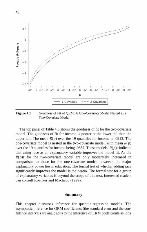
The top panel of Table 4.3 shows the goodness of fit for the two-covariatemodel. The goodness of fit for income is poorer at the lower tail than theupper tail. The mean R(p) over the 19 quantiles for income is .0913. Theone-covariate model is nested in the two-covariate model, with mean R(p)over the 19 quantiles for income being .0857. These models’ R(p)s indicatethat using race as an explanatory variable improves the model fit. As theR(p)s for the two-covariate model are only moderately increased incomparison to those for the one-covariate model, however, the majorexplanatory power lies in education. The formal test of whether adding racesignificantly improves the model is the t-ratio. The formal test for a groupof explanatory variables is beyond the scope of this text. Interested readerscan consult Koenker and Machado (1999).
Summary
This chapter discusses inference for quantile-regression models. Theasymptotic inference for QRM coefficients (the standard error and the con-fidence interval) are analogous to the inference of LRM coefficients as long
54
.05 .1 .15 .2 .25 .3 .35 .4 .45 .5 .55 .6 .65 .7 .75 .8 .85
P
Pse
ud
o R
-Sq
uar
e
.95.9
1-Covariate 2-Covariate
.12
.1
.08
.06
.04
.02
Figure 4.1 Goodness of Fit of QRM: A One-Covariate Model Nested in aTwo-Covariate Model
04-Hao.qxd 3/13/2007 5:43 PM Page 54

as necessary modifications are made to properly estimate the variance ofthe error. Given the often-skewed distribution of the dependent variables insocial-science studies, the assumptions underlying the asymptotic inferencecan be questionable and an alternative approach to inference is desirable.The bootstrap method offers an excellent solution. This chapter introducesthe bootstrap procedure for QRM coefficients. The idea of bootstrapping isrelatively straightforward and, with the advancement of computing tech-nology, quite practical.
In addition, this chapter briefly discusses the goodness of fit of the QRManalogous to that for the LRM. The measure of goodness of fit for theQRM, the R(p), accounts for the appropriate weight each observation takesfor a specific quantile equation. The R(p) is easy to comprehend and itsinterpretation follows the familiar R-squared for the LRM.
Note
1. Recall that the pth quantile of ε (p) is assumed to be zero in the QRM.
5. INTERPRETATION OF QUANTILE-REGRESSION ESTIMATES
In this chapter, we discuss the interpretation of quantile-regression esti-mates. We first interpret quantile-regression fits for specific quantiles. Themedian-regression quantile can be used to track location changes. Otherspecific regression quantiles, for example, the .05th and .95th quantiles, canbe used to assess how a covariate predicts the conditional off-central loca-tions as well as shape shifts of the response. We also consider the more gen-eral case of sequences of regression quantiles, which can reveal more subtlechanges in the shape of the response variable’s distribution.
We use the interpretation of LRM estimates as a starting point and inter-pret the QRM estimates in the context of income inequality. In this way,we demonstrate two key advantages of the QRM approach over LRM: Itenables us to model off-central conditional quantiles as well as shape shiftsin the distribution of a response variable. Various methods are illustratedusing the same income example as in Chapter 3 but now considering edu-cation and race simultaneously. Throughout the chapter, we focus on analy-ses of the raw-scale response. Interpreting estimates for a monotonicallytransformed response variable and understanding the implications for theraw scale of the response are discussed in Chapter 6.
55
04-Hao.qxd 3/13/2007 5:43 PM Page 55

Reference and Comparison
To facilitate the interpretation of quantile-regression estimates, we use thenotions of reference and comparison as well as some general ideas related toquantification of effects. The reference is a conventional regression term andthe comparison is the effect of a unit increase of a covariate in regression.1
In many instances, our interest will be on comparing one group toanother. For example, we might wish to compare individuals with 11 yearsof education to those with 12 years of education. Alternatively, we might beinterested in comparing blacks to whites. In any case, we start with one possible setting of the covariates, for example, all blacks with 11 years ofeducation, and refer to the subpopulation with these attributes as a referencegroup. Then, we modify one of the covariates in a specific way, for exam-ple, changing 11 years to 12 years of education, or change being black tobeing white. We then refer to the subpopulation corresponding to thechanged covariate settings as a comparison group. A key feature of thesetwo group comparisons is that a single covariate is modified, leaving theremaining covariates fixed.
Examining how the response distribution is altered when we switch from a reference group to a comparison group helps quantify the effect of achange in a single covariate on the distribution of the response. For the LRM,fitted coefficients can be interpreted as estimated effects, that is, estimates ofthe change in the mean of the response distribution that results from a one-unit increase in a continuous covariate or the change of the value from 0 to 1of a dummy covariate. Each of these changes can be interpreted as an esti-mated difference in means between a reference group and a comparisongroup. The analog for the QRM is an estimated difference in a particularquantile between a reference group and a comparison group, resulting from aone-unit increase in a continuous covariate or the change of the value from 0to 1 of a dummy covariate, with other covariates held constant.
Conditional Means Versus Conditional Medians
By far, the simplest QRM to understand is the median-regression model (the.5th QRM), which expresses the conditional median of a response variablegiven predictor variables, and provides a natural alternative to LRM, whichfits the conditional mean. These are natural to compare in that they bothattempt to model the central location of a response-variable distribution.
The income LRM estimate is $6,314 for ED and $11,452 for WHITE.One more year of schooling is associated with a $6,314 increase in meanincome at any fixed level of education. Because of the linearity assumption,
56
05-Hao.qxd 3/13/2007 4:29 PM Page 56
the same amount of increase in the conditional mean would occur forhouseholds at any fixed level of schooling. For example, one more year ofeducation is associated with a same amount of increase in the mean incomefor households whose head has 9 or 16 years of schooling. In addition, theeffect of an additional year of education is the same for blacks as it is for whites: No interaction between race and education is specified in themodel. In terms of reference and comparison groups, we can say that whilethere are many different reference-group/comparison-group combinations,there are only two possible effects: a single race effect and a single educa-tion effect.2
The LRM includes a rigid assumption: From one group to the next, theincome distribution undergoes a shift without an alteration in its scale andshape. In particular, the positive coefficient for education reveals the degreeto which the distribution shifts to the right as a result of a one-year changein the level of education, and this is the only way in which distributionchange is manifested. Similarly, the coefficient for WHITE in the LRM ofincome on race indicates the rightward location shift from blacks’ incomedistribution to whites’ income distribution, again without altering its shape:The mean income of blacks is $11,452 lower than that of whites.
In passing from the LRM to the QRM and focusing on the special caseof median regression, the key modification to keep in mind is that we modelthe conditional median rather than the conditional mean. As discussed inChapter 3, the median might be a more suitable measure of central locationfor a distribution for a variety of reasons that carry over when we attemptto model the behavior of a collection of conditional distributions. Forinstance, these conditional distributions might be right-skewed, makingtheir means more a reflection of what is happening in the upper tail of thedistributions than a reflection of what is happening in the middle. As a con-crete example, families in the top-income percentile may profoundly influ-ence any analysis meant to investigate the effect of education on medianincome. Consequently, the analysis may reveal education effects for theconditional mean, which is much higher than the conditional median.
The interpretation of a median-regression coefficient is analogous to thatof an LRM coefficient. Table 5.1 gives the estimated coefficients for vari-ous quantile-regression models, including the median (.5th quantile) regres-sion. In the case of a continuous covariate, the coefficient estimate isinterpreted as the change in the median of the response variable corre-sponding to a unit change in the predictor. The consequences of linearityand no interactions in the LRM apply for the median-regression model. Inparticular, the effect on the median response of a one-year increase in edu-cation is the same for all races and education levels, and the effect of achange in race is the same for all education levels.
57
05-Hao.qxd 3/13/2007 4:29 PM Page 57

58
TAB
LE
5.1
Qua
ntile
-Reg
ress
ion
Est
imat
es a
nd T
heir
Asy
mpt
otic
Sta
ndar
d E
rror
for
Inc
ome
.05
.10
.15
.20
.25
.30
.35
.40
.45
.50
.55
.60
.65
.70
.75
.80
.85
.90
.95
ED
1,13
01,
782
2,31
52,
757
3,17
23,
571
3,90
04,
266
4,54
94,
794
5,18
25,
571
5,84
16,
224
6,59
86,
954
7,50
58,
279
9,57
5(3
6)(4
1)(5
1)(5
1)(6
0)(6
1)(6
6)(7
3)(8
2)(9
2)(8
6)(1
02)
(107
)(1
29)
(154
)(1
50)
(209
)(3
16)
(605
)
WH
ITE
3,19
74,
689
5,64
26,
557
6,72
47,
541
8,16
88,
744
9,08
79,
792
10,4
7511
,091
11,4
0711
,739
12,1
4212
,972
13,2
4914
,049
17,4
84(3
59)
(397
)(4
75)
(455
)(5
27)
(528
)(5
61)
(600
)(6
62)
(727
)(6
64)
(776
)(7
93)
(926
)(1
,065
)(9
88)
(1,2
99)
(1,7
90)
(2,8
95)
NO
TE
:Asy
mpt
otic
sta
ndar
d er
rors
are
in p
aren
thes
es.
05-Hao.qxd 3/13/2007 4:29 PM Page 58

The coefficient for ED in the conditional-median model is $4,794, whichis lower than the coefficient in the conditional-mean model. This suggeststhat while an increase of one year of education gives rise to an averageincrease of $6,314 in income, the increase would not be as substantial formost of the population. Similarly, the coefficient for WHITE in the conditional-median model is $9,792, lower than the corresponding coeffi-cient in the conditional-mean model.
The asymptotic standard errors of estimates under the assumption ofi.i.d. are shown in parentheses. If the i.i.d. assumption holds, the standarderror of the education effect on the median of income is $92, the t-ratio is52.1, and the p-value is less than .001, providing evidence to reject the nullhypothesis that education has no effect on the median income. The coeffi-cient for WHITE has a standard error of $727 and is statistically significantat the .001 level.
Interpretation of Other Individual Conditional Quantiles
Sometimes, researchers are more interested in the lower or upper tails of adistribution than in the central location. Education policy concerning equal-ity focuses on elevating the test scores of underachieving students. In 2000,39% of 8th graders were below the basic achievement level of science.Thus, the .39th quantile is more relevant than the mean or median for edu-cational researchers. Welfare policy targets the lower-income population. Ifthe national poverty rate is 11%, the .11th income quantile and quantilesbelow that level become more relevant than the median or the mean for welfare researchers. Researchers find that union membership yields agreater return at the lower end of the income distribution than at the mean(Chamberlain, 1994). On the other hand, for the top 10% of income earn-ers in the population, education at prestigious private universities tends tobe more common. Studies of the benefits of prestigious higher educationmay focus on the 90th income quantile and above.
The coefficients of QRM fits for 19 quantiles in Table 5.1 can be used to examine effects of education and race on various income quantiles.3 Toinform welfare policymakers, we examine the education and race coefficientsat the .10th and .05th quantiles of the conditional-income models. We see thatone more year of education can increase income by $1,782 at the .10th quan-tile and $1,130 at the .05th quantile, and the black-white gap is $4,689 at the.10th quantile and $3,197 at the .05th quantile. For researchers interested inreturn to education at the right tail, we look at the estimates of educationat the .90th and .95th quantiles. The coefficient for the .95th quantile is$9,575, much larger than that at the .90th quantile ($8,279), suggesting the
59
05-Hao.qxd 3/13/2007 4:29 PM Page 59

contribution of prestigious higher education to income disparity. Under thei.i.d. assumption, the asymptotic standard errors indicate that the educationeffect and the racial effect are significant at the off-central quantiles as well.
Because the i.i.d. is a very restrictive assumption that assumes no shapeshift of the response, more flexible approaches to estimation of standarderrors, such as bootstrapping, should be used. Table 5.2 presents the pointestimate and standard error of parameters for the two covariates based on a500-resample bootstrap procedure. The bootstrapped point estimates aresimilar to the asymptotic estimates, but they tend to vary to a lesser degreeacross quantiles than do the asymptotic standard errors, particularly for ED(see Figures 5.1 and 5.2).
Tests for Equivalence of Coefficients Across Quantiles
When multiple quantile regressions are estimated, we need to test whetherapparent differences are statistically significant. To perform such a test,the covariance matrix of cross-quantile estimates must be estimated. Thiscovariance matrix is estimated numerically via bootstrapping to allow flex-ible errors and provide a numerical solution to the very complex asymptoticformulae.
Table 5.3 presents the point estimates, bootstrap standard errors, and p-values for tests of equivalence of the estimates at the pth quantile againstthose at the median, those at the (1 − p)th quantile, and those at the (p + .05)thquantile for p ≤ .5. Depending on the circumstances, the bootstrap methodcan give smaller or larger standard errors than using asymptotic methods.For example, at the median income, the asymptotic method gives a pointestimate of $4,794 and a standard error of $92 for education. The corre-sponding numbers using bootstrap are $4,794 and $103. However, at the.05th quantile, the bootstrap reports a lower level of precision of the esti-mate for education than the asymptotic method: The bootstrap standarderror is $80, larger than the asymptotic standard error ($36).
The p-values for Wald tests of equivalence of estimates across quantilesshow that the effect of education differs across quantiles in all of our selectedtests. These tests compare the current estimate (say, at the .05th quantile)against three estimates: those at the median, those at the correspondingposition in the opposite tail (at the .95th quantile), and those at the adjacenthigher quantile (at the .10th quantile). In contrast, the race effect does notstatistically differ in a substantial number of our selected tests. For example,the white effect at the .20th quantile is not significantly different from thatat the .25th quantile. In particular, the race effect on income quantiles abovethe median does not differ statistically from the corresponding effect on the
60
05-Hao.qxd 3/13/2007 4:29 PM Page 60
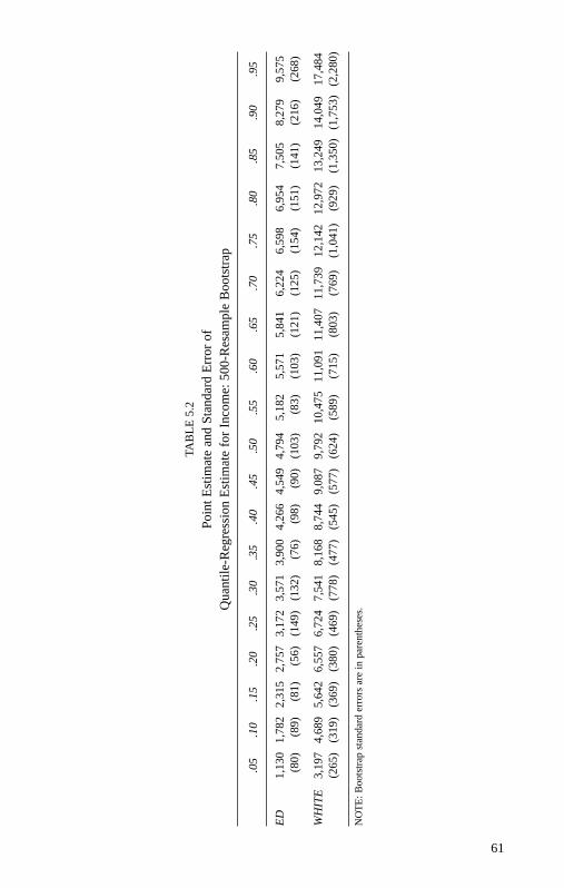
61
TAB
LE
5.2
Poin
t Est
imat
e an
d St
anda
rd E
rror
of
Qua
ntile
-Reg
ress
ion
Est
imat
e fo
r In
com
e:50
0-R
esam
ple
Boo
tstr
ap
.05
.10
.15
.20
.25
.30
.35
.40
.45
.50
.55
.60
.65
.70
.75
.80
.85
.90
.95
ED
1,13
01,
782
2,31
52,
757
3,17
23,
571
3,90
04,
266
4,54
94,
794
5,18
25,
571
5,84
16,
224
6,59
86,
954
7,50
58,
279
9,57
5(8
0)(8
9)(8
1)(5
6)(1
49)
(132
)(7
6)(9
8)(9
0)(1
03)
(83)
(103
)(1
21)
(125
)(1
54)
(151
)(1
41)
(216
)(2
68)
WH
ITE
3,19
74,
689
5,64
26,
557
6,72
47,
541
8,16
88,
744
9,08
79,
792
10,4
7511
,091
11,4
0711
,739
12,1
4212
,972
13,2
4914
,049
17,4
84(2
65)
(319
)(3
69)
(380
)(4
69)
(778
)(4
77)
(545
)(5
77)
(624
)(5
89)
(715
)(8
03)
(769
)(1
,041
)(9
29)
(1,3
50)
(1,7
53)
(2,2
80)
NO
TE
:Boo
tstr
ap s
tand
ard
erro
rs a
re in
par
enth
eses
.
05-Hao.qxd 3/13/2007 4:29 PM Page 61

TABLE 5.3
Equivalence of Coefficients AcrossQuantiles of Income: 500-Resample Bootstrap
P-Value
Different Different Different From From Coeff. From Coeff. 4 Coeff.
Quantile/ Coeff. at at (1 − p)th at (p + .05)th Jointly Variable Coefficient Median? Quantile? Quantile? Different?
.05th QuantileED 1130** 0.0000 0.0000 0.0000 0.0000
(80)WHITE 3197** 0.0000 0.0000 0.0000 0.0000
(265)
.10th QuantileED 1782** 0.0000 0.0000 0.0000 0.0000
(89)WHITE 4689** 0.0000 0.0000 0.0000 0.0000
(319)
.15th QuantileED 2315** 0.0000 0.0000 0.0000 0.0000
(81)WHITE 5642** 0.0000 0.0000 0.0018 0.0000
(369)
.20th QuantileED 2757** 0.0000 0.0000 0.0000 0.0000
(56)WHITE 6557** 0.0000 0.0000 0.4784 0.0000
(380)
.25th QuantileED 3172** 0.0000 0.0000 0.0000 0.0000
(149)WHITE 6724** 0.0000 0.0000 0.0012 0.0000
(469)
.30th QuantileED 3571** 0.0000 0.0000 0.0000 0.0000
(132)WHITE 7541** 0.0000 0.0000 0.0142 0.0000
(778)
.35th QuantileED 3900** 0.0000 0.0000 0.0000 0.0000
(76)WHITE 8168** 0.0000 0.0000 0.0035 0.0000
(477)
62
05-Hao.qxd 3/13/2007 4:29 PM Page 62
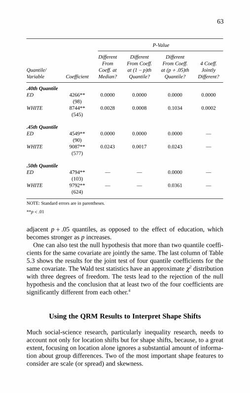
63
adjacent p + .05 quantiles, as opposed to the effect of education, whichbecomes stronger as p increases.
One can also test the null hypothesis that more than two quantile coeffi-cients for the same covariate are jointly the same. The last column of Table5.3 shows the results for the joint test of four quantile coefficients for thesame covariate. The Wald test statistics have an approximate χ2 distributionwith three degrees of freedom. The tests lead to the rejection of the nullhypothesis and the conclusion that at least two of the four coefficients aresignificantly different from each other.4
Using the QRM Results to Interpret Shape Shifts
Much social-science research, particularly inequality research, needs toaccount not only for location shifts but for shape shifts, because, to a greatextent, focusing on location alone ignores a substantial amount of informa-tion about group differences. Two of the most important shape features toconsider are scale (or spread) and skewness.
P-Value
Different Different Different From From Coeff. From Coeff. 4 Coeff.
Quantile/ Coeff. at at (1 − p)th at (p + .05)th Jointly Variable Coefficient Median? Quantile? Quantile? Different?
.40th QuantileED 4266** 0.0000 0.0000 0.0000 0.0000
(98)WHITE 8744** 0.0028 0.0008 0.1034 0.0002
(545)
.45th QuantileED 4549** 0.0000 0.0000 0.0000 —
(90)WHITE 9087** 0.0243 0.0017 0.0243 —
(577)
.50th QuantileED 4794** — — 0.0000 —
(103)WHITE 9792** — — 0.0361 —
(624)
NOTE: Standard errors are in parentheses.
**p < .01
05-Hao.qxd 3/13/2007 4:29 PM Page 63

64
A Graphical View
Because we are interested in how predictor variables change the shape ofthe response distribution, we use the QRM to produce estimates at multiplequantiles. The analysis of shape effects can be considerably more complexthan the analysis of location, and we see an important trade-off. On the onehand, shape analysis, which can be carried out by making use of multiplesets of QRM estimates at various quantiles, has the potential to reveal moreinformation than the analysis of location effects alone. On the other hand,describing this additional information can be cumbersome and requiresadditional effort. In particular, examination of quantile-regression coeffi-cients for a long sequence of quantile values (for example, .05, .10, . . . ,.90, .95) is unwieldy, and a graphical view of QRM estimates becomes anecessary step in interpreting QRM results.
The QRM coefficients for a particular covariate reveal the effectof a unit change in the covariate on quantiles of the response distribu-tion. Consequently, arrays of these coefficients for a range of quantilescan be used to determine how a one-unit increase in the covariate affectsthe shape of the response distribution. We highlight this shape-shifteffect by a graphical view examining coefficients. For a particular covari-ate, we plot the coefficients and the confidence envelope, where thepredictor variable effect β (p) is on the y-axis and the value of p is onthe x-axis.
Figure 5.1 provides a graphical view for the income quantiles as a func-tion of education and race (both centered at their respective means). Usingthe estimated coefficients (see Table 5.1), we draw a graph of the effect ofED (WHITE) and the 95% confidence envelope. We also draw the graph for the fitted CONSTANT. Because the covariates have been centered abouttheir means, CONSTANT gives the fitted quantile function at the covariatemean, which is referred to as the typical setting. This conditional-quantilefunction at the typical setting is right-skewed given the flat slopes below themedian and the steep slopes above the median.
The effect of ED can be described as the change in a conditional-incomequantile brought about by one additional year of education, at any level of education, fixing race. The education effect is significantly positive,because the confidence envelope does not cross the zero line (see the thickhorizontal line). Figure 5.1a shows an upward-sloping curve for the effectsof education: The effect of one more year of schooling is positive for allvalues of p and steadily increasing with p. This increase accelerates afterthe .80th quantile.
The effect of WHITE can be described as the change in the conditional-income quantile brought about by changing the race from black to white,
05-Hao.qxd 3/13/2007 8:21 PM Page 64

65
0
0
.1 .2 .3 .4 .5 .6 .7 .8 .9 1
2000
4000
6000
8000
10000
Qu
anti
le C
oef
fici
ents
fo
r In
com
e ($
)
P
(a) ED
Figure 5.1 Asymptotic 95% Confidence Interval of Quantile-RegressionEstimates: Income
0
0
.1 .2 .3 .4 .5 .6 .7 .8 .9 1
P
5000
10000
15000
20000
25000
Qu
anti
le C
oef
fici
ents
fo
r In
com
e ($
)
(b) WHITE
(Continued)
05-Hao.qxd 3/13/2007 4:29 PM Page 65

(c) Constant (“Typical Setting”)
120000
90000
60000
30000
0
0 .1 .2 .3 .4 .5 .6 .7 .8 .9 1
P
Qu
anti
le C
oef
fici
ents
fo
r In
com
e ($
)
Figure 5.1 (Continued)
66
fixing the education level. The effect of being white is significantly positive,as the zero line is far below the confidence envelope. Figure 5.1b depictsanother upward-sloping curve for the effect of being white as compared withbeing black. The slopes below the .15th quantile and above the .90th quan-tile are steeper than those at the middle quantiles.
Figure 5.2 is the graph corresponding to Figure 5.1 except that theconfidence envelope is based on bootstrap estimates. We observe that thebootstrapping confidence envelope in Figure 5.2 is more balanced thanthe asymptotic confidence envelope in Figure 5.1. We draw a similar shape-shift pattern from Figures 5.1 and 5.2.
These graphs convey additional patterns related to the effects of educa-tion and race. First, education and race are responsible for location shifts aswell as shape shifts. If there were only location shifts, increasing educationby a single year or changing race from black to white would cause everyquantile to increase by the same amount, leading to a graph of β (p) versusp resembling a horizontal line. Instead, we see that β (p) is monotonically
05-Hao.qxd 3/13/2007 4:29 PM Page 66

67
0 .1 .2 .3 .4 .5 .6 .7 .8 .9 1
10000
8000
6000
4000
2000
0
Qu
anti
le C
oef
fici
ents
fo
r In
com
e ($
)
P
(a) ED
Figure 5.2 Bootstrap 95% Confidence Interval of Quantile-RegressionEstimates: Income
0
0 .1 .2 .3 .4 .5 .6 .7 .8 .9 1
5000
10000
15000
20000
25000
Qu
anti
le C
oef
fici
ents
fo
r In
com
e ($
)
P
(b) WHITE
(Continued)
05-Hao.qxd 3/13/2007 4:29 PM Page 67
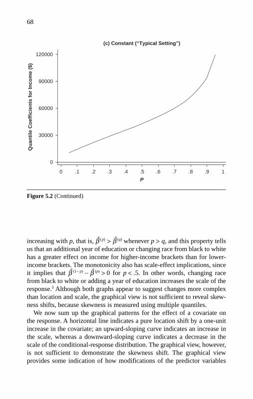
120000
90000
60000
30000
0
0 .1 .2 .3 .4 .5 .6 .7 .8 .9 1
P
Qu
anti
le C
oef
fici
ents
fo
r In
com
e ($
)
(c) Constant (“Typical Setting”)
68
Figure 5.2 (Continued)
increasing with p, that is, β (p) > β (q) whenever p > q, and this property tellsus that an additional year of education or changing race from black to whitehas a greater effect on income for higher-income brackets than for lower-income brackets. The monotonicity also has scale-effect implications, sinceit implies that β (1− p) − β (p) > 0 for p < .5. In other words, changing racefrom black to white or adding a year of education increases the scale of theresponse.5 Although both graphs appear to suggest changes more complexthan location and scale, the graphical view is not sufficient to reveal skew-ness shifts, because skewness is measured using multiple quantiles.
We now sum up the graphical patterns for the effect of a covariate on the response. A horizontal line indicates a pure location shift by a one-unitincrease in the covariate; an upward-sloping curve indicates an increase inthe scale, whereas a downward-sloping curve indicates a decrease in thescale of the conditional-response distribution. The graphical view, however,is not sufficient to demonstrate the skewness shift. The graphical viewprovides some indication of how modifications of the predictor variables
05-Hao.qxd 3/13/2007 4:29 PM Page 68

69
produce shape shifts. We are also interested in how large the shift is andwhether the shift is significant. Our next task is to develop quantitativemeasures for two types of shape shifts from the QRM estimates.
Scale Shifts
The standard deviation is a commonly employed measure of the scale orspread for a symmetric distribution. For skewed distributions, however, dis-tances between selected quantiles provide a more informed description ofthe spread than the standard deviation. For a value of p between 0 and .5,we identify two sample quantiles: Q (1− p) (the [1− p]th quantile) and Q (p)
(the pth quantile). The pth interquantile range, IQR(p) = Q (1− p) − Q (p), is ameasure of spread. This quantity describes the range of the middle (1 − 2p)proportion of the distribution. When p = .25, the interquantile range becomesthe interquartile range IQR (.25) = Q (.75) − Q(.25), giving the range of the mid-dle 50% of the distribution. Other values of p, for example, .10, .05, .025,can be used as well to capture spread further out in two tails of a distribu-tion. For example, using p = .10, the pth interquantile range gives the rangeof the middle 80% of the distribution.
Figure 5.3 compares a reference group and a comparison group,which have the same median M. Fixing some choice of p, we can mea-sure an interquantile range IQRR = UR − LR for the reference group, andIQRC = UC − LC for the comparison group. We then use the difference-in-differences IQRC − IQRR as a measure of scale shift. In the figure, thecomparison group’s scale is larger than that of the reference group, whichresults in a positive scale shift.
Turning to our application example, Table 5.4 shows the scale changes ofthe household income distribution for different educational groups usingtwo methods; one approach uses sample quantiles, that is, quantiles calcu-lated directly from the two group samples, and the second approach makesuse of fitted coefficients for covariates from the income QRM. The samplequantiles lead to an interquartile range of $26,426 for the group with11 years of schooling and $34,426 for the group with twelve years ofschooling. The sample spread for the 12-year-education group is $8,000higher than for the 11-year-education group. This scale shift can beobtained by computing the difference between the interquartile rangesQ(.75) − Q(.25) for the two groups. We see that from 11 to 12 years, theinterquartile range increased by $34,426 − $26,426 = $8,000. Using thesame approach for other interquantile ranges, we find that the scale increaseis $15,422 for the middle 80% of the sample, $19,736 for the middle 90%,and $28,052 for the middle 95%.
05-Hao.qxd 3/13/2007 4:29 PM Page 69

70
The QRM fits provide an alternative approach to estimating scale-shifteffects. Here, we use the notation β (p) to refer to the fitted coefficient corre-sponding to some covariate in a pth quantile-regression model. Such a coef-ficient indicates the increase or decrease in any particular quantile broughtabout by a unit increase in the covariate. Thus, when we increase the covari-ate by one unit, the corresponding pth interquantile range changes by theamount β (1− p) − β (p), which is the pth scale-shift effect denoted by SCS(p).
SCS(p) = IQR(p)C − IQR(p)
R = (Q(1− p)C − Q(p)
C ) − (Q(1− p)R − Q(p)
R )
= (Q(1− p)C − Q(1− p)
R ) − (Q(p)C − Q(p)
R )
= β (1− p) − β (p) for p < .5. [5.1]
If we fit a linear QRM with no interaction terms between covariates, thescale effect does not depend on the particular covariate setting (the refer-ence group). When SCS(p) is zero, there is apparently no evidence of scalechange. A negative value indicates that increasing the covariate results in adecrease in scale, while a positive value indicates the opposite effect.
Using Equation 5.1 and estimates from Table 5.2, the scale shift broughtabout by one more year of schooling for the middle 50% of the populationis $3,426 (subtracting the coefficient at the .25th quantile from that at the.75th quantile: $6,598 − $3,172 = $3,426). There are two reasons why thisscale shift is smaller than the observed scale shift of $8,000. The model-based measure is a partial measure, controlling for other covariates (here,race). Also, the scale shift based on sample quantiles is specific for two
LC LR UR UC
Reference Comparison
M
Figure 5.3 Scale Shifts
05-Hao.qxd 3/13/2007 4:29 PM Page 70

71
education groups, whereas the model-based measure considers all educa-tion groups. With Equation 5.1, we interpret the QRM coefficients for edu-cation as increases in scale by $6,497 for the middle 80% of the population,$8,445 for the middle 90% of the population, and $10,902 for the middle95% of the population (see the last column of Table 5.4).
We can interpret the racial effect in terms of scale shifts in the same fash-ion. Using Table 5.2, controlling for education, whites’ income spread ishigher than blacks’ income spread: $12,142 − $6,724 = $5,418 for the mid-dle 50% of the population, $14,049 − $4,689 = $9,360 for the middle 80%,and $17,484 − $3,197 = $14,287 for the middle 90%.
A scale change can proportionally stretch or contract the segments aboveand below the median, while keeping the original skewness intact. It canalso disproportionately stretch or contract the segments above and belowthe median, while changing the skewness. Equation 5.1 is unable to distin-guish between proportional and disproportional scale shifts.
TABLE 5.4
Scale Shifts of Income DistributionFrom 11-Year to 12-Year Education
Sample-Based
Quantile and Education = 11 Education = 12 Difference Model-Quantile Range (1) (2) (2) − (1) Based
Q.025 3387 5229 1842 665
Q.05 5352 7195 1843 1130
Q.10 6792 10460 3668 1782
Q.25 12098 18694 6596 3172
Q.75 38524 53120 14596 6598
Q.90 58332 77422 19090 8279
Q.95 74225 95804 21579 9575
Q.975 87996 117890 29894 11567
Q.75 − Q.25 26426 34426 8000
β *.75 − β *
.25 3426
Q.90 − Q.10 51540 66962 15422
β *.90 − β *
.10 6497
Q.95 − Q.05 68873 88609 19736
β *.95 − β *
.05 8445
Q.975 − Q.025 84609 112661 28052
β *.975 − β *
.025 10902
05-Hao.qxd 3/13/2007 4:29 PM Page 71
72
Skewness Shifts
A disproportional scale shift that relates to greater skewness indicates anadditional effect on the shape of the response distribution. Chapter 2 devel-oped a direct measure of quantile-based skewness, QSK, defined as the ratioof the upper spread to the lower spread minus 1 (recall Equation 2.2). IfQSK is greater than 0, the distribution is right-skewed, and vice versa.Recall Figure 3.2, where the box graphs for education groups and racialgroups show this imbalance of upper and lower spreads. Columns 1 and 2of the middle panel (quantile range) in Table 5.5 present the upper andlower spreads for two education groups with 11 and 12 years of schooling,respectively. We can see that both groups have a right-skewed income dis-tribution for the middle 50%, 80%, 90%, and 95% of the sample.
When we examine whether the skewness of a comparison group differsfrom that of a reference group, we look for disproportional scale shifts.Figure 5.4 illustrates such a disproportional scale shift for right-skewed dis-tributions in a hypothetical situation. Let MR and MC indicate the median ofthe reference and the comparison, respectively. The upper spread is UR − MR
for the reference and UC − MC for the comparison. The lower spread isMR − LR for the reference and MC − LC for the comparison. The disproportioncan be measured by taking the ratio of (UC − MC)/(UR − MR) to (MC − LC)/(MR − LR). If this “ratio-of-ratios” equals 1, then there is no skewness shift. Ifthe ratio-of-ratios is less than 1, the right-skewness is reduced. If the ratio-of-ratios is greater than 1, the right-skewness is increased. The shift in terms ofpercentage change can be obtained by this quantity minus 1. We call thisquantity skewness shift, or SKS.
Let’s look at the sample-based SKS in Table 5.5, the skewness shift of thegroup with 12 years of schooling from the group with 11 years of schooling.Although we learned from the last section that the scale of the more-educated group is larger than that of the less-educated group, the right-skewness is considerably lower in the more-educated group, as the SKSis –.282 for the middle 50% of the sample, –.248 for the middle 80%, –.283for the middle 95%, and –.195 for the middle 95%. The skewness reductionis between −19.5% and −28.3% over a variety of quantile ranges.
Our task is to use the QRM coefficients to obtain model-based SKS,which involves the conditional quantiles of the reference group. We specifythe typical covariate setting as the reference (the estimated constant α ). TheSKS for the middle 100(1 − 2p)% of the population is:
SKS(p) = [(Q(1− p)C − Q(.5)
C ) /(Q(1 − p)R − Q(.5)
R )]/[(Q(.5)C − Q(p)
C )]/(Q(.5)R − Q(p)
R )] − 1
= [(β (1− p) + α (1− p) − β (.5) − α (.5))/(α (1− p) − α(.5))]/[(β (.5) + α(.5) − β (p) − α (p))/(α (.5) − α (p))] − 1. [5.2]
05-Hao.qxd 3/13/2007 4:29 PM Page 72

73
TABLE 5.5
Skewness Shifts of IncomeDistribution Due to One More Year of Schooling
Sample-Based Model-Based
Quantile Quantile QRM QRMp (ED = 11) (ED = 12) SKS (p) β α SKS (p)
.025 3387 5229 −.195 665 6900 −.049
.05 5352 7195 −.283 1130 9850 −.047
.10 6792 10460 −.248 1782 14168 −.037
.25 12098 18694 −.282 3172 24932 −.016
.50 20985 32943 4794 42176
.75 38524 53120 6598 65745
.90 58332 77422 8279 94496
.95 74225 95804 9575 120104
.975 87996 117890 11567 150463
Quantile RangeQ.75 − Q.50 17539 20177Q.50 − Q.25 8887 14249Q.90 − Q.50 37347 44479Q.50 − Q.10 14193 22483Q.95 − Q.50 53240 62861Q.50 − Q.05 15633 25748Q.975 − Q.50 67011 84947Q.50 − Q.025 17598 27714
NOTE: The sample-based SKS(p) = [(QC
(1–p)− QC
(.5)) /(Q
R
(1–p)− Q R
(.5)) ]/[(Q
C
(.5)− QC
( p)) /(Q
R
(.5)− Q R
( p)) ] − 1.
For the middle 50% population, we have:
SKS (.25) = [(QC
(.75)− QC
(5)) /(Q
R
(.75)− Q R
(.5)) ]/[(Q
C
(.5)− Q C
(.25)) /(Q
R
(.5)− Q R
(.25)) ] − 1
= [20177/17539]/[14249/8887] − 1
= [1.150/1.603]
= −.283
The model-based skewness shift is
SKS (p) = [(β (1 − p)− α (1 − p)
− β (.5)− α (.5)
)/(α (1 − p)− α (.5)
)]/[(β (.5)+ α (.5)
− β ( p)− α ( p)
) /(α (.5)− α ( p)
)] − 1
For the middle 50% population, we have:
SKS (.25) = [(β (.75)+ α (.75)
− β (.5)− α (.5)
)/(α (.75))− α (.5)
)]/[(β (.5)+ α (.5)
− β ( .25)− α ( .25)
) /(α (.5)− α ( .25)
)] − 1
= [(6598 + 65745 − 4794 − 42176)/(65745 − 42176)]/[(4794 + 42176 − 3172 − 24932)/(42176 − 24932)] − 1
= [25373/23569]/[18866/17244]
= [1.077/1.094]
= −.016
05-Hao.qxd 3/13/2007 4:29 PM Page 73

74
Note that because we take the ratio of two ratios, SKS effectively elimi-nates the influence of a proportional scale shift. When SKS = 0, it indicateseither no scale shift or a proportional scale shift. Thus, SKS is a measure ofskewness above and beyond proportional scale shifts. SKS < 0 indicates areduction of right-skewness due to the effect of the explanatory variablewhereas SKS > 0 indicates an exacerbation of right-skewness.
The right panel (the model-based panel) of Table 5.5 presents the estimatedcoefficient for education (β ), the estimated constant for the typical covariatesetting (α ), and the model-based SKS. One more year of schooling slightlydecreases right-skewness for all four selected SKSs. The percentage decreasesrange from −1.6% to −4.9%. These model-based estimates are much smallerthan the sample-based SKS, because the model-based partial effect of educa-tion is a shift from the typical covariate setting, controlling for race.
The impact of being white is a less-skewed conditional income (seeTable 5.6): −6.6% for the middle 50% of the population, −8.5% for the mid-dle 80% of the population, −8.7% for the middle 90% of the population,and −7.6% for the middle 95% of the population. It appears that the reduc-tion is greater for the middle 80% and 90% of the population than for themiddle 50% of the population. This finding indicates a greater expansion ofthe white upper middle class than the black upper middle class.
We have developed an overall evaluation of a covariate’s impact on theinequality of the response, which examines the alignment of the signs of loca-tion, scale, and skewness shifts when these shifts are statistically significant.A positive, significant location shift indicates that the comparison group’smedian is higher than that of the reference group. A positive, significantscale shift indicates the comparison group’s spread is greater than that of thereference group. Furthermore, a positive, significant skewness shift indicates
LC MCLR MR UC UR
Reference Comparison
Figure 5.4 Skewness Shifts
05-Hao.qxd 3/13/2007 4:29 PM Page 74

75
that the comparison group is more right-skewed than the reference group. Ifwe reverse-code the reference as the comparison and the comparison as thereference, we have three negative shifts. Thus, the sign alignment of shifts,which we call in-sync shifts, makes the total distribution more unequal andthe disadvantaged more concentrated. When the three shifts induced by apredictor are in sync, this predictor exacerbates inequality through bothlocation and shape changes. Inconsistent signs of shifts indicate that the pre-dictor variable changes the location and shape of the response in an oppositedirection, and the predictor’s total effect on the response inequality is com-promised. We refer to this pattern as out of sync.
Table 5.7 summarizes this overall evaluation for our income example.Bootstrap confidence intervals are also presented. If the confidence intervalbounds include zero, at the 95% significance level, we are not certainwhether the shift is positive or negative. Only one shift statistic is insignifi-cant in Table 5.7 (the SKS of WHITE for the middle 50% of the population).
Table 5.7 shows that one more year of education induces a positive loca-tion and scale shift but a negative skewness shift. The pattern is out of sync.Similarly, being white induces a positive location and scale shift with a negative skewness shift, exhibiting an out-of-sync pattern. Therefore, oursimple model suggests that while higher education and being white areassociated with a higher median income and a wider income spread, theincome distributions for the less educated and for blacks are more skewed.If this simple model is correct, neither education nor race exacerbatesincome inequality. This example demonstrates the value of categorizingvariables as having in-sync or out-of-sync effects in summarizing manyestimates from the QRM. Once we determine a variable’s effect regardingsync, as for education or race above, we can easily determine whether ornot it makes a contribution to inequality.
TABLE 5.6
Skewness Shifts of IncomeDistribution From Black to White: Model-Based
P QRM β QRM α SKS(p)
.025 2576 6900 –0.076
.05 3197 9850 –0.087
.10 4689 14168 –0.085
.25 6724 24932 –0.066
.50 9792 42176
.75 12142 65745
.90 14049 94496
.95 17484 120104
.975 22092 150463
05-Hao.qxd 3/13/2007 4:29 PM Page 75

TABLE 5.7
Point Estimate and 95% ConfidenceInterval of Shape Shifts: 500-Resample Bootstrap
SCS SKS SKS SKS SKSLocation (.025 to (.025 to (.05 to (.10 to (.25 to
Variable (.50) .975) .975) .95) .90) .75)
IncomeED 4794 10920 −.049 −.046 −.037 −.017Lower bound 4592 10162 −.056 −.053 −.044 −.028Upper bound 4966 11794 −.041 −.038 −.029 −.005
WHITE 9792 19027 −.079 −.090 −.088 −.067Lower bound 9474 10602 −.151 −.147 −.152 −.136Upper bound 10110 26712 −.023 −.037 −.024 .005
76
Summary
This chapter develops various ways to interpret estimates from the quantile-regression model (QRM). Beyond the traditional examination of covariates’effects on specific conditional quantiles, such as the median or positions atthe lower or upper quantiles, we expand to the distributional interpretation.We illustrate graphical interpretations of QRM estimates and quantitativemeasures of shape changes from QRM estimates, including location shifts,scale shifts, and skewness shifts. Our household income example illustratesthe direct utility of the QRM estimates in analyzing the contribution ofcovariates on income inequality.
This chapter focuses on interpretations of the QRM based on raw-scaleresponse variables. These interpretations are directly applied to linearlytransformed response variables. However, for a better model fit, skewedresponse variables are often transformed monotonically. For example,log transformation is the most popular one for right-skewed distributions.Estimates of effects have differing interpretations depending on whether theresponse variable is represented on a raw scale or on a log scale. In addi-tion, the choice of a modeling approach is important in that the conclusionsreached from the analysis of one model may not have valid analogs for theother. For this reason, we devote Chapter 6 to the specific issues arisingfrom monotone transformation of the response variable.
Notes
1. The reference/comparison terminology is used in Handcock andMorris (1999).
05-Hao.qxd 3/13/2007 4:29 PM Page 76
77
2. One can speak of the effect of an additional year of education,and this will be the same for all races and for all education levels. Similarly,there is an effect of switching from being black to being white, which is thesame for all education levels. There is also a white-to-black effect, which is opposite of the black-to-white effect. The analysis of location effects forLRM with no interactions is quite simple. The analysis becomes consider-ably more complicated when we introduce interactions into the model.
3. Note that we can specify any quantiles, such as the .39th quantile,rather than equal-distance quantiles.
4. There are many different and potentially less conservative approachesto multiple testing than the one presented here. For example, a form of stu-dentized range test (Scheffé, 1959) can be used.
5. The effect on scale of a unit change in the covariate is given by
SCALE(y|x + 1) − SCALE(y|x) =
[(Q(1− p)(y|x + 1) − Q(p)(y|x + 1)] − [(Q(1− p)(y|x) − Q(p)(y|x)] =
[(β (1− p)(x + 1) − (β (p)(x + 1))] − [(β (1− p)x − β (p)x)] = β (1− p) − β (p) for p < .5.
6. INTERPRETATION OF MONOTONE-TRANSFORMED QRM
When fitting regression models, it is usually appropriate to apply a log trans-formation to right-skewed response variables in order to ensure that themodel assumptions are at least close to being satisfied. Log transformationsare also practical, since they allow interpretation of predictor variable effectsin relative terms. Similarly, taking the square (or some other power greaterthan one) of left-skewed response variables can make the new distributionmore symmetric. These nonlinear, monotonic transformations, while capa-ble of improving the model fit, no longer preserve the original distribution.When modeling location and shape shifts associated with a change in a par-ticular covariate, it makes much more sense to analyze these shifts on a rawscale than on the monotonically transformed scale. Thus, to aid a substan-tively sensible interpretation of QRM for monotonically transformedresponse variables, we need to obtain effects of covariates on the raw scalefrom transformed-scale coefficients. This chapter uses the log-transformationcase to discuss two methods that fulfill the goal. These methods can beapplied to any monotone transformation of the response variable.
05-Hao.qxd 3/13/2007 4:29 PM Page 77

78
Location Shifts on the Log Scale
We start from location shifts. One way to model the central location of theresponse variable is to consider the conditional-mean model relating edu-cation to log income. Table 6.1 shows that each additional year of educa-tion increases the conditional-mean income by a factor of e.128 = 1.137,which indicates a 13.7% increase.1 The corresponding fitted-median modelin Table 6.2 (middle column p = .5) gives a coefficient of .131, which indi-cates that one more year of education increases the conditional-medianincome by e.131 = 1.140, or 14.0%. In relative terms, the education effect hasa slightly stronger effect on the conditional median, whereas in absoluteterms, the education effect is stronger on the conditional mean, as shown inChapter 5.
Because the concept of a percent increase requires the specification of a reference group, when a predictor variable is categorical, that is, indicat-ing group membership, some care has to be taken to choose an appropriatereference category to facilitate interpretation. For example, suppose wefit a model in which log income is expressed as a function of race(BLACK/WHITE), using 0 to indicate black and 1 to indicate white. Our fit-ted LRM (Table 6.1) says that the coefficient is .332, indicating that whites’income is greater than blacks’ by a factor of e.332 = 1.393, a 39.3% increasein income. On the other hand, if we adopt the reverse code, using 0 toindicate white and 1 to indicate black, the linear equivariance property ofthe LRM tells us that the coefficient for BLACK should be –.332. Here the interpretation of the negative coefficient for BLACK does notcorrespond to a 39.3% decrease in income. Instead, the factor would be e−.332 = 0.717, that is, a 28.3% decrease in income. This point becomes clearerfor larger values of the coefficient. For example, a coefficient of 2 in the firstmodel would indicate that whites experience an increase of income of 639%over that of blacks, but in the second model, the coefficient would be –2, andthis would correspond to blacks’ income being lower than whites’ by 86.5%.One must keep in mind that when the response variable is log transformed,changing the reference category of a dummy variable leads to two outcomes:The coefficient changes its sign and the percent change is transformed intoits reciprocal (1/e2 = 1/7.389 = 0.135 and 0.135 −1 = −0.865).
From Log Scale Back to Raw Scale
Log transformation of the response variable provides a technical analyticmeans by which to obtain a better fit to the data and an interpretation of the
06-Hao.qxd 3/13/2007 12:23 PM Page 78

79
estimates in relative terms. Multiplication on a raw scale becomes additionon a log scale. However, a linear function of a log-transformed responsevariable specifies the error term as additive rather than multiplicative,thereby altering the distribution of the original error term. In addition, theuse of the log transformation has clear disadvantages in that it dramati-cally distorts the measurement scale. In inequality studies, making a logtransformation has the effect of artificially diminishing the appearanceof inequality, as it dramatically contracts the right-hand tail of the distri-bution. Typically, we are more interested in modeling effects on thecentral location of the raw-scale response variable, rather than on its logtransformation.
What do shifts in location of the log-transformed response variable tellus about what happens on the raw-scale response-variable distribution?The answer depends on the choice of location estimate. For the case of the conditional mean, estimates on a log scale provide limited informationabout what happens on a raw scale, and vice versa. Only linear transfor-mations have the equivariance property, enabling the use of the mean of arandom variable to determine the mean of its transformation. Because thelog transformation is nonlinear, the conditional-mean income is not theexponential function of the conditional mean of log income, as we detailedin Chapter 3. In effect, there is no easy, simple, or closed-form expressionto calculate the effect of a covariate in absolute terms from the coefficientof the log-income model. Thus, it is difficult to use the LRM for the log ofthe response variable to understand the mean shift on the raw scale. In con-trast, the median-regression model is more accommodating. When amonotone transformation is applied to the response variable, the condi-tional median transforms accordingly.
TABLE 6.1
Classical Regression Estimates forLog Income: Effects of Education and Race
Variable Coefficient
ED 0.128**(0.0020)
WHITE 0.332**(0.0160)
Constant 10.497**(0.0050)
NOTE: Asymptotic standard errors are in parentheses.
**p < .01
06-Hao.qxd 3/13/2007 12:23 PM Page 79
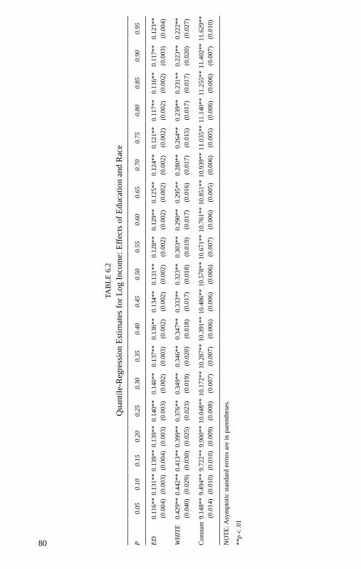
80
TAB
LE
6.2
Qua
ntile
-Reg
ress
ion
Est
imat
es f
or L
og I
ncom
e:E
ffec
ts o
f E
duca
tion
and
Rac
e
P0.
05
0.10
0.
15
0.20
0.
25
0.30
0.
35
0.40
0.
45
0.50
0.
55
0.60
0.
65
0.70
0.
75
0.80
0.
85
0.90
0.
95
ED
0.11
6**
0.13
1**
0.13
9**
0.13
9**
0.14
0**
0.14
0**
0.13
7**
0.13
6**
0.13
4**
0.13
1**
0.12
8**
0.12
9**
0.12
5**
0.12
4**
0.12
1**
0.11
7**
0.11
6**
0.11
7**
0.12
3**
(0.0
04)
(0.0
03)
(0.0
04)
(0.0
03)
(0.0
03)
(0.0
02)
(0.0
03)
(0.0
02)
(0.0
02)
(0.0
02)
(0.0
02)
(0.0
02)
(0.0
02)
(0.0
02)
(0.0
02)
(0.0
02)
(0.0
02)
(0.0
03)
(0.0
04)
WH
ITE
0.42
9**
0.44
2**
0.41
3**
0.39
9**
0.37
6**
0.34
9**
0.34
6**
0.34
7**
0.33
3**
0.32
3**
0.30
3**
0.29
0**
0.29
5**
0.28
0**
0.26
4**
0.23
9**
0.23
1**
0.22
3**
0.22
2**
(0.0
40)
(0.0
29)
(0.0
30)
(0.0
25)
(0.0
23)
(0.0
19)
(0.0
20)
(0.0
18)
(0.0
17)
(0.0
18)
(0.0
19)
(0.0
17)
(0.0
16)
(0.0
17)
(0.0
15)
(0.0
17)
(0.0
17)
(0.0
20)
(0.0
27)
Con
stan
t9.
148*
*9.
494*
*9.
722*
*9.
900*
*10
.048
**10
.172
**10
.287
**10
.391
**10
.486
**10
.578
**10
.671
**10
.761
**10
.851
**10
.939
**11
.035
**11
.140
**11
.255
**11
.402
**11
.629
**(0
.014
)(0
.010
)(0
.010
)(0
.009
)(0
.008
)(0
.007
)(0
.007
)(0
.006
)(0
.006
)(0
.006
)(0
.007
)(0
.006
)(0
.005
)(0
.006
)(0
.005
)(0
.006
)(0
.006
)(0
.007
)(0
.010
)
NO
TE
:Asy
mpt
otic
sta
ndar
d er
rors
are
in p
aren
thes
es.
**p
<.0
1
06-Hao.qxd 3/13/2007 12:23 PM Page 80
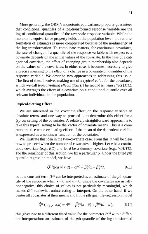
More generally, the QRM’s monotonic equivariance property guaranteesthat conditional quantiles of a log-transformed response variable are the log of conditional quantiles of the raw-scale response variable. While themonotonic equivariance property holds at the population level, the retrans-formation of estimates is more complicated because of the nonlinearity ofthe log transformation. To complicate matters, for continuous covariates,the rate of change of a quantile of the response variable with respect to acovariate depends on the actual values of the covariate. In the case of a cat-egorical covariate, the effect of changing group membership also dependson the values of the covariates. In either case, it becomes necessary to givea precise meaning to the effect of a change in a covariate on quantiles of theresponse variable. We describe two approaches to addressing this issue. The first of these involves making use of a typical value for the covariates,which we call typical-setting effects (TSE). The second is mean effect (ME),which averages the effect of a covariate on a conditional quantile over allrelevant individuals in the population.
Typical-Setting Effect
We are interested in the covariate effect on the response variable inabsolute terms, and one way to proceed is to determine this effect for a typical setting of the covariates. A relatively straightforward approach is totake this typical setting to be the vector of covariate means. This is a com-mon practice when evaluating effects if the mean of the dependent variableis expressed as a nonlinear function of the covariates.2
We illustrate this idea in the two-covariate case. From this, it will be clearhow to proceed when the number of covariates is higher. Let x be a contin-uous covariate (e.g., ED) and let d be a dummy covariate (e.g., WHITE).For the remainder of this section, we fix a particular p. Under the fitted pthquantile-regression model, we have
Q(p)(log y⎪x,d) = α (p) + β x(p)x + β d
(p)d, [6.1]
but the constant term α(p) can be interpreted as an estimate of the pth quan-tile of the response when x = 0 and d = 0. Since the covariates are usuallynonnegative, this choice of values is not particularly meaningful, whichmakes α(p) somewhat uninteresting to interpret. On the other hand, if wecenter all covariates at their means and fit the pth quantile-regression model
Q(p)(log y⎪x,d) = α(p) + β x(p)(x − x–) + β d
(p)(d − d–), [6.1´]
this gives rise to a different fitted value for the parameter α(p) with a differ-ent interpretation: an estimate of the pth quantile of the log-transformed
81
06-Hao.qxd 3/13/2007 12:23 PM Page 81
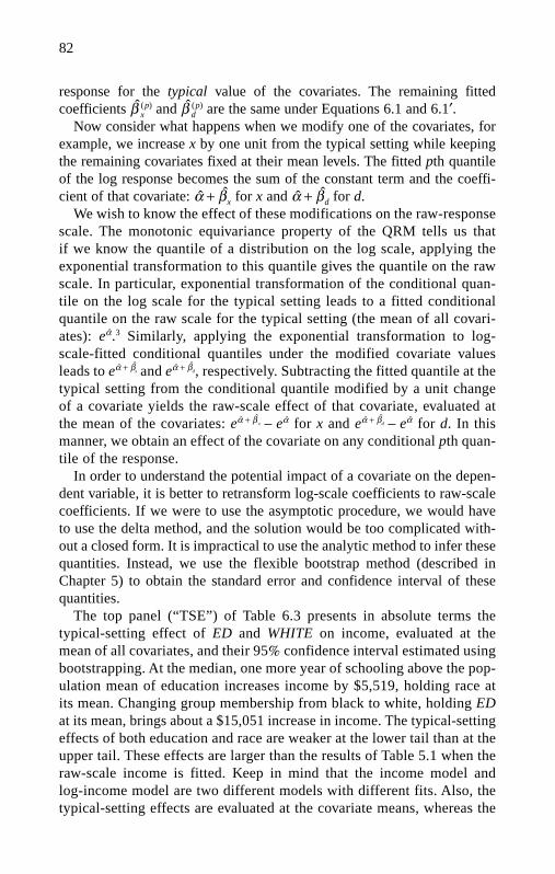
82
response for the typical value of the covariates. The remaining fitted coefficients β x
(p) and β d(p) are the same under Equations 6.1 and 6.1′.
Now consider what happens when we modify one of the covariates, forexample, we increase x by one unit from the typical setting while keepingthe remaining covariates fixed at their mean levels. The fitted pth quantileof the log response becomes the sum of the constant term and the coeffi-cient of that covariate: α + βx for x and α + βd for d.
We wish to know the effect of these modifications on the raw-responsescale. The monotonic equivariance property of the QRM tells us that if we know the quantile of a distribution on the log scale, applying theexponential transformation to this quantile gives the quantile on the rawscale. In particular, exponential transformation of the conditional quan-tile on the log scale for the typical setting leads to a fitted conditionalquantile on the raw scale for the typical setting (the mean of all covari-ates): eα.3 Similarly, applying the exponential transformation to log-scale-fitted conditional quantiles under the modified covariate valuesleads to eα + βx and eα + βd, respectively. Subtracting the fitted quantile at thetypical setting from the conditional quantile modified by a unit changeof a covariate yields the raw-scale effect of that covariate, evaluated atthe mean of the covariates: eα + β x − eα for x and eα + βd − eα for d. In thismanner, we obtain an effect of the covariate on any conditional pth quan-tile of the response.
In order to understand the potential impact of a covariate on the depen-dent variable, it is better to retransform log-scale coefficients to raw-scalecoefficients. If we were to use the asymptotic procedure, we would haveto use the delta method, and the solution would be too complicated with-out a closed form. It is impractical to use the analytic method to infer thesequantities. Instead, we use the flexible bootstrap method (described inChapter 5) to obtain the standard error and confidence interval of thesequantities.
The top panel (“TSE”) of Table 6.3 presents in absolute terms the typical-setting effect of ED and WHITE on income, evaluated at themean of all covariates, and their 95% confidence interval estimated usingbootstrapping. At the median, one more year of schooling above the pop-ulation mean of education increases income by $5,519, holding race atits mean. Changing group membership from black to white, holding EDat its mean, brings about a $15,051 increase in income. The typical-settingeffects of both education and race are weaker at the lower tail than at theupper tail. These effects are larger than the results of Table 5.1 when theraw-scale income is fitted. Keep in mind that the income model and log-income model are two different models with different fits. Also, thetypical-setting effects are evaluated at the covariate means, whereas the
06-Hao.qxd 3/13/2007 12:23 PM Page 82

coefficients from fitting the raw-scale income apply to any covariate settings.
Mean Effect
The typical-setting approach is simple to implement and provides some information about the effect of a unit change in a covariate on theresponse. However, it only accounts for the effect of this change at themean of the covariates. Since this effect can vary over the range of covari-ate values, it is plausible that the use of typical values leads to a distortedpicture. We introduce another possibility, which is to average in the oppo-site order: First compute the effect of a unit change in the covariate for
83
TABLE 6.3
Point Estimate and 95% Confidence Interval of Typical-Setting Effects and MeanEffects From Log-Income QRM: 500-Resample Bootstrap
ED WHITE
CI CILower Upper Lower Upper
Effect Bound Bound Effect Bound Bound
TSE.025 660 530 821 4457 3405 6536.05 1157 1015 1291 4978 4208 6400.10 1866 1747 1977 7417 6062 8533.15 2486 2317 2634 8476 7210 9951.25 3477 3323 3648 10609 8839 12378.50 5519 5314 5722 15051 12823 17075.75 7992 7655 8277 18788 15669 21647.85 9519 9076 9910 19891 16801 22938.90 11108 10593 11676 22733 18468 27444.95 14765 13677 15662 28131 21181 34294.975 18535 16973 19706 41714 33344 51297
ME.025 697 554 887 2719 2243 3424.05 1241 1073 1396 3276 2875 3868.10 2028 1887 2163 4792 4148 5284.15 2717 2514 2903 5613 5007 6282.25 3799 3620 4008 7228 6343 8098.50 5965 5716 6203 10746 9528 11832.75 8524 8114 8865 14141 12162 15828.85 10082 9581 10559 15429 13362 17329.90 11772 11157 12478 17664 14900 20491.95 15754 14476 16810 21875 17207 25839.975 19836 18007 21235 31419 26192 37014
06-Hao.qxd 3/13/2007 12:23 PM Page 83

84
every possible setting of the covariates, and then average this effect overthe covariate settings in the data. We propose to use this idea when thequantile function of the response depends in a nonlinear way on the covari-ates, for example, in Equations 6.1 and 6.1′ when log(y) is expressed as alinear function of the covariates. If, instead, the quantile function is a lin-ear function of the covariates, then these two methods of averaging lead tothe same result.
Proceeding formally, for a continuous covariate x and for any p, we ask:How much does a (random) individual’s pth conditional quantile change ifhis or her x increases by one unit, with other covariates held constant? We then average this change over individuals in a reference population.Continuing with the two-covariate model, we can determine the quantiledifference due to a one-unit increase in x as:
∆Qx(p) = Q (p)(y|x + 1, d) − Q (p)(y|x,d). [6.2]
And the average quantile difference becomes the mean effect of a unitchange in x on y at p, denoted by MEx
(p):
[6.3]
In our model, where log income is a function of education and race, edu-cation is an interval variable. Implementing Equation 6.3 requires:
1. obtaining each individual’s estimated pth conditional quantile, using
Q(p)(yi|xi,di) = eα (p) + βx(p) xi + β d
(p)di;
2. obtaining the corresponding pth conditional quantile if his or hereducation increases by one year using Q(p)(yi|xi + 1,di) =eα (p) + β
x(p) (xi + 1) + β d
(p)di;
3. taking the difference between the two terms; and
4. averaging the difference.
For a dichotomous covariate, we wish to know the change in the condi-tional quantile if a person changes his or her group membership from d = 0to d = 1, while keeping other covariates constant. In this case, only the subgroup of d = 0 is relevant because an inclusion of the other group willmake other covariates change at the same time. Thus, for dichotomous d,the quantile difference becomes:
∆Qd,0,1(p) = Q(p)(y⎪x, 1) − Q(p)(y⎪x, 0). [6.4]
ME(p)
x = 1
n
n∑i=1
[Q(p)(yi | xi + 1, di) − Q(p)(yi | xi, di)
].
06-Hao.qxd 3/13/2007 12:23 PM Page 84

And the mean effect of d, denoted by ME(p)d,0,1, is:
[6.5]
where n0 denotes the number of sampled individuals with di = 0.In our example, WHITE is a dummy variable. The calculation will be con-
fined to sampled blacks only (WHITE = 0). The steps are:
1. obtaining each black’s pth conditional quantile, using
2. obtaining the corresponding pth conditional quantile if a black becomes
a white using
3. taking the difference between the two terms; and
4. averaging the difference.
The bottom panel (“ME”) of Table 6.3 presents the mean effect of edu-cation and race and their 95% confidence interval. The effects of both EDand WHITE increase with p. The magnitudes of the education effects aresimilar to the typical-setting effects. However, the mean effects of WHITEchange more widely with p than the typical-setting effects.
Infinitesimal Effects
For both the typical-setting and mean-effect methods described above, thecovariate of interest is changed by a single unit in order to quantify its effecton the response variable. Since both methods are designed so as to addresssituations when the quantile function of the response is a nonlinear functionof the covariates, the calculated effect is generally not proportional to thesize of the unit. For example, the unit of education could be half a year ratherthan a whole year, and the effect of an increase in half a year of schoolingneed not be equal to half of the effect of an additional year of schooling. Inaddition, some covariates may be viewed as truly continuous. For example,in a study of health outcomes, we might use income as a covariate.
An alternative approach is to consider the infinitesimal rate of change inthe quantile with respect to a covariate, that is, replace a finite difference bya derivative. For example, assuming we fit a model of Equation 6.1 to give
, we have
d
dxQ(p)(y | x, d) = β(p)
x eα(p) + β(p)x (x−x--- ) + β
(p)
d (d−d--- ),
Q(p)(y | x, d) = eα(p)+β(p)x (x−x--- )+β
(p)
d (d−d--- )
Q(p)(yi | xi, di = 1) = eα(p)+β(p)x xi+β
(p)
d ;
Q(p)(yi | xi, di = 0) = eα(p)+β(p)x xi ;
ME(p)
d,0,1 = 1
n0
∑i:di=0
[Q(p)(yi | xi, 1) − Q(p)(yi | xi, 0)
],
85
06-Hao.qxd 3/13/2007 12:23 PM Page 85

15
12
09
06
03
0
0 .1 .2 .3 .4 .5 .6 .7 .8 .9 1
P
Qu
anti
le C
oef
fici
ents
fo
r L
og
Inco
me
(a) ED
Figure 6.1 Graphical View of Log-Scale Estimates From Log-Income QRM
so that, substituting x = x– and d = d–, the analog of the typical-settingeffect becomes . Similarly, the analog of the meaneffect takes the form
Graphical View of Log-Scale Coefficients
The graphs of log-scale coefficients are shown in Figure 6.1, which showsthe curve for ED, WHITE, and the constant from the log-income QRM. Theconditional-quantile function of log income at the typical setting in Figure6.1c has a somewhat normal appearance, given its similar slopes below andabove the median. This finding shows that the log transformation of incomecontracts the right tail so that the posttransformed distribution is closer tonormal. Since a log coefficient can be interpreted as a percentage change, astraight horizontal line should indicate a pure scale shift without a skewnessshift. Any curves departing from the horizontal pattern can indicate eitherskewness shifts or pure location shifts, but it is very difficult to tell which
ME(p)
x = 1
n
n∑i=1
d
dxQ(p)(y | xi, di) = 1
n
n∑i=1
β(p)
x eα + β(p)x (xi−x--- ) + β
(p)
d (di−d--- ).
d
dxQ(p)(y | x, d) = β(p)
x eα(p)
86
06-Hao.qxd 3/13/2007 12:23 PM Page 86

87
0
.05
.1
.15
.2
.25
.3
.35
.4
.45Q
uan
tile
Co
effi
cien
ts f
or
Lo
g In
com
e
0 .1 .2 .3 .4 .5 .6 .7 .8 .9 1
(b) WHITE
Figure 6.1 (Continued)
12
11.5
11
10.5
10
9.5
9
1.9.8.7.6.5.4.3.2.10
P
Qu
anti
le C
oef
fici
ents
fo
r L
og
Inco
me
(c) Constant (“Typical Setting”)
06-Hao.qxd 3/13/2007 12:23 PM Page 87
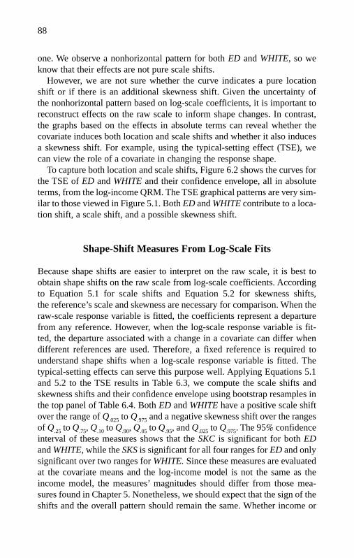
88
one. We observe a nonhorizontal pattern for both ED and WHITE, so weknow that their effects are not pure scale shifts.
However, we are not sure whether the curve indicates a pure locationshift or if there is an additional skewness shift. Given the uncertainty of the nonhorizontal pattern based on log-scale coefficients, it is important toreconstruct effects on the raw scale to inform shape changes. In contrast,the graphs based on the effects in absolute terms can reveal whether thecovariate induces both location and scale shifts and whether it also inducesa skewness shift. For example, using the typical-setting effect (TSE), wecan view the role of a covariate in changing the response shape.
To capture both location and scale shifts, Figure 6.2 shows the curves forthe TSE of ED and WHITE and their confidence envelope, all in absoluteterms, from the log-income QRM. The TSE graphical patterns are very sim-ilar to those viewed in Figure 5.1. Both ED and WHITE contribute to a loca-tion shift, a scale shift, and a possible skewness shift.
Shape-Shift Measures From Log-Scale Fits
Because shape shifts are easier to interpret on the raw scale, it is best toobtain shape shifts on the raw scale from log-scale coefficients. Accordingto Equation 5.1 for scale shifts and Equation 5.2 for skewness shifts,the reference’s scale and skewness are necessary for comparison. When theraw-scale response variable is fitted, the coefficients represent a departurefrom any reference. However, when the log-scale response variable is fit-ted, the departure associated with a change in a covariate can differ whendifferent references are used. Therefore, a fixed reference is required tounderstand shape shifts when a log-scale response variable is fitted. Thetypical-setting effects can serve this purpose well. Applying Equations 5.1and 5.2 to the TSE results in Table 6.3, we compute the scale shifts andskewness shifts and their confidence envelope using bootstrap resamples inthe top panel of Table 6.4. Both ED and WHITE have a positive scale shiftover the range of Q.025 to Q.975 and a negative skewness shift over the rangesof Q.25 to Q.75, Q.10 to Q.90, Q.05 to Q.95, and Q.025 to Q.975. The 95% confidenceinterval of these measures shows that the SKC is significant for both EDand WHITE, while the SKS is significant for all four ranges for ED and onlysignificant over two ranges for WHITE. Since these measures are evaluatedat the covariate means and the log-income model is not the same as theincome model, the measures’ magnitudes should differ from those mea-sures found in Chapter 5. Nonetheless, we should expect that the sign of theshifts and the overall pattern should remain the same. Whether income or
06-Hao.qxd 3/13/2007 12:23 PM Page 88

89
20000
15000
10000
5000
0
Qu
anti
le C
oef
fici
ents
fo
r L
og
Inco
me,
Ret
ran
sfo
rmed
($)
0 .1 .2 .3 .4 .5 .6 .7 .8 .9 1
P
(a) ED
50000
40000
30000
20000
10000
0
Qu
anti
le C
oef
fici
ents
fo
r L
og
Inco
me,
Ret
ran
sfo
rmed
($)
0 .1 .2 .3 .4 .5 .6 .7 .8 .9 1
(b) WHITE
P
Figure 6.2 Graphical View of TSE (in Absolute Terms) From Log-IncomeQRM
06-Hao.qxd 3/13/2007 12:23 PM Page 89
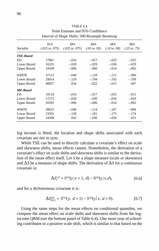
log income is fitted, the location and shape shifts associated with eachcovariate are not in sync.
While TSE can be used to directly calculate a covariate’s effect on scaleand skewness shifts, mean effects cannot. Nonetheless, the derivation of acovariate’s effect on scale shifts and skewness shifts is similar to the deriva-tion of the mean effect itself. Let S be a shape measure (scale or skewness)and ∆S be a measure of shape shifts. The derivation of ∆S for a continuouscovariate is:
∆Sx(p) = S(p)(y|x + 1, d) − S(p)(y|x,d), [6.6]
and for a dichotomous covariate it is:
∆Sd,0,1(p) = S(p)(y, d = 1) − S(p)(y⎪x, d = 0). [6.7]
Using the same steps for the mean effects on conditional quantiles, wecompute the mean effect on scale shifts and skewness shifts from the log-income QRM (see the bottom panel of Table 6.4). One more year of school-ing contributes to a positive scale shift, which is similar to that based on the
90
TABLE 6.4
Point Estimate and 95% ConfidenceInterval of Shape Shifts: 500-Resample Bootstrap
SCS SKS SKS SKS SKSVariable (.025 to .975) (.025 to .975) (.05 to .95) (.10 to .90) (.25 to .75)
TSE-BasedED 17861 –.016 –.017 –.025 –.015Lower Bound 16325 –.028 –.029 –.036 –.029Upper Bound 19108 –.006 –.006 –.014 –.002
WHITE 37113 –.040 –.118 –.111 –.090Lower Bound 29014 –.129 –.194 –.193 –.199Upper Bound 46837 .054 –.022 –.015 .047
ME-BasedED 19118 –.016 –.017 –.025 –.015Lower Bound 17272 –.028 –.030 –.036 –.029Upper Bound 20592 –.006 –.006 –.014 –.002
WHITE 28653 –.046 –.114 –.107 –.084Lower Bound 23501 –.128 –.181 –.175 –.174Upper Bound 34348 .042 –.030 –.026 .031
06-Hao.qxd 3/13/2007 12:23 PM Page 90

TSE. WHITE has a positive effect on scale shifts, and the magnitude islarger than that based on the TSE. The effects of education and race onskewness shifts are remarkably similar between ME and TSE. The overallpattern given by the ME is also not in sync, supporting the same conclusionas when using the TSE.
Summary
This chapter discusses interpretation issues arising from nonlinear, mono-tone transformation of the response variable in the QRM. Thanks to themonotone equivariance of the QRM, we are able to reconstruct the effectsof a covariate on the raw scale of the response distribution, which isunachievable with the LRM. Nonetheless, the reconstruction requires specific methods. This chapter develops two approaches. The typical-setting method is computationally simple, while the mean-effect method isslightly more involved. Both approaches involve averaging over the covari-ate values, but in different orders. Both typical-setting effects and meaneffects refer to the whole sample or a subsample. Researchers shouldchoose a method that best addresses a specific research question.
The next chapter provides an overall summary of the techniques intro-duced in this book by applying them to a real research question. In theapplication, we compare the sources of U.S. income inequality in 1991 and2001, illustrating what motivates a QR analysis and how to proceed step bystep, with the complete Stata codes.
Notes
1. If the estimate coefficient is β , then a unit increase in the predictorvariable results in an increase of (100(eβ − 1))%. For small values of theestimated coefficient β , this is approximately 100β %.
2. These practices include the effect on probability from logit-, probit-,and tobit-model estimates.
3. For linear-regression models, the fitted intercept can be interpreted asthe geometric mean of the response y. The geometric mean is defined as
, which is equivalent to . The geometric mean is always less
than or equal to the arithmetic mean. But this interpretation is no longervalid in quantile regression.
e1n
(n∑i
log yi
)(n∏i
yi
)1n
91
06-Hao.qxd 3/13/2007 12:23 PM Page 91

92
7. APPLICATION TO INCOME INEQUALITY IN 1991 AND 2001
The empirical illustrations in previous chapters used oversimplifiedspecifications with one or two covariates. This chapter applies the tech-niques in the book to a particular topic: the persistence and wideningof household income inequality from 1991 to 2001. Our goal is to system-atically summarize the techniques developed in this book via a concreteempirical application. Drawing from the U.S. Survey of Income andProgram Participation (SIPP), we add the 1991 data to the previously used2001 data. Household income is adjusted to the 2001 constant dollar. Wespecify a parsimonious model for household income as a function of fivefactors (13 covariates): life cycle (age and age-squared), race-ethnicity(white, black, Hispanic, and Asian), education (college graduate, some col-lege, high school graduate, and without high-school education), householdtypes (married couple with children, married couple without children,female head with children, single person, and other), and rural residence.This is the specification used throughout the chapter. Models for both raw-scale income and log-transformed income are fitted. The analyses include(a) assessing the goodness of fit for raw-scale and log-scale income mod-els, (b) comparing ordinary-least-squares (OLS) and median-regressionestimates, (c) examining coefficients at the two tails, (d) graphically view-ing 19 sets of coefficient estimates and their confidence intervals, and(e) attaining location and shape shifts of conditional quantiles for eachcovariate in each year and examining the trend over the decade.
Observed Income Disparity
Figure 7.1 shows 99 empirical quantiles for race-ethnicity groups and edu-cation groups in 1991 and 2001. One of the most interesting features is thegreater spread for the middle 98% of the members in each group in 2001 ascompared to 1991.
More detailed comparisons require the actual values of the quantiles.Table 7.1 compares the .025th-quantile, median, and .975th-quantile house-hold incomes (in 2001 constant dollars) for 1991 and 2001. The numbersare weighted to reflect population patterns. A common characteristic isobserved for the total and each subgroup: The stretch (QSC.025) for themiddle 95% households is much wider for 2001 than for 1991, indicatinggrowing total and within-group disparities in income over the decade.
The racial disparity between whites and others in the lower half of theincome distribution declined in the last decade. This decline can be seen as
07-Hao.qxd 3/13/2007 4:30 PM Page 92

93
White Black Hispanic Asian
Inco
me
$100
0
350
300
250
200
150
100
50
0
0 .1 .2 .3 .4 .5 .6 .7 .8 .9 1
P
1991
College Some College
High School No High School
Inco
me
$100
0
350
300
250
200
150
100
50
0
0 .1 .2 .3 .4 .5 .6 .7 .8 .9 1
P
Figure 7.1 Empirical Quantile Functions by Race-Ethnicity and EducationGroups
(Continued)
07-Hao.qxd 3/13/2007 4:30 PM Page 93
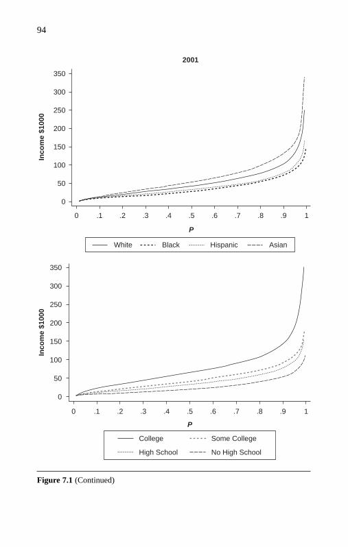
94
2001
0 .1 .2 .3 .4 .5 .6 .7 .8 .9 1
Inco
me
$100
0
350
300
250
200
150
100
50
0
White Black Hispanic Asian
P
0 .1 .2 .3 .4 .5 .6 .7 .8 .9 1
P
350
300
250
200
150
100
50
0
Inco
me
$100
0
College Some College
High School No High School
Figure 7.1 (Continued)
07-Hao.qxd 3/13/2007 4:30 PM Page 94

95
the fall in the .025th-quantile income of white households in contrast witha moderate gain for the black and Hispanic counterparts. Asians madegreater headway than whites at the median and at the .975th quantile, butthe lowest 2.5% of Asian households were left behind.
An important change in income inequality is the change in returns toeducation for the top tail. While most college graduates gained an ampleamount of income over the decade, more than half of the people with abelow-college education saw their income actually decline. In particular,more than 97.5% of high school dropouts in 2001 had a notably lowerincome than their 1991 counterparts.
Consideration of household type, defined by marriage and presence ofchildren, leads us to another arena where social stratification reshapesthe income distribution. Progress is seen for married couples with children,whereas the income of single-mother families and single-person house-holds is stagnant. Inequality between urban and rural areas and inequalitywithin both urban and rural areas intensified over the decade studied.
TABLE 7.1
Household Income Distribution by Groups: 1991 and 2001
Quantile
1991 2001
Group .025 .500 .975 .025 .500 .975
Total 6256 38324 131352 6000 40212 164323
Race-EthnicityWhite 6765 40949 135443 6600 42878 172784Black 3773 23624 101160 3788 27858 113124Hispanic 5342 28851 114138 5600 33144 119454Asian 5241 49354 149357 4800 55286 211112
EducationCollege graduate 11196 64688 168912 10910 65298 263796Some college 8059 42082 120316 6364 41901 134796High school grad. 6392 35723 104102 5347 33246 118162No high school 4918 20827 80603 4408 20319 79515
Household TypeMarried w/ children 12896 55653 143343 14193 61636 204608Married w/o children 11621 43473 146580 10860 47665 176375Female head 3666 23420 94114 3653 27690 96650Single person 4884 20906 83213 3977 21369 91551Other household type 7301 37896 115069 6600 41580 150123
ResidenceUrban 6330 40732 137574 6199 42504 174733Rural 6122 32874 111891 5419 33505 118079
07-Hao.qxd 3/13/2007 4:30 PM Page 95

96
Descriptive Statistics
Table 7.2 presents the weighted mean and standard deviation for variablesused in the analyses. We see that mean income increased by nearly $5,000from 1991 to 2001, a much higher figure than the growth in median incomeobserved in the previous table. The small increase in log income reminds usthat the log transformation contracts the right tail of the distribution. Weobserve greater diversity in the race-ethnicity structure and considerableimprovement in the population’s education. However, the number of house-holds of married couples with children decreased, whereas “other” typesand single-person households were on the rise. The United States continuedthe urbanization and suburbanization seen in previous decades.
TABLE 7.2
Descriptive Statistics of Variables Used in Analysis
1991 2001
Variable Mean SD Mean SD
ResponseIncome ($) 46168 33858 51460 46111Log income 10.451 0.843 10.506 0.909Age 49 17 49 17Age-squared 2652 1798 2700 1786
CovariateRace-EthnicityWhite .795 .404 .755 .430Black .101 .301 .118 .322Hispanic .079 .269 .094 .292Asian .025 .157 .033 .177
EducationCollege graduate .230 .421 .261 .439Some college .210 .407 .296 .457High school grad. .341 .474 .302 .459No high school .219 .414 .141 .348
Household TypeMarried w/ children .330 .470 .287 .452Married w/o children .224 .417 .233 .423Female head .108 .310 .104 .305Single person .257 .437 .267 .442Other household type .082 .274 .110 .313
ResidenceUrban .732 .443 .773 .419Rural .268 .443 .227 .419
Sample Size 10111 25891
07-Hao.qxd 3/13/2007 4:30 PM Page 96

Notes on Survey Income Data
Two characteristics of survey income data make the QRM approach a betterstrategy for analysis than the LRM. First, only 0.2% of the households haveincomes over a million dollars, whereas for over 96% of the population,income is less than $100,000. Thus, data for the very rich profoundly influ-ence the OLS coefficient estimates. Second, survey income is often top-coded for each income source; thus, it is not straightforward to assess atwhich level a household’s total income is trimmed. In addition, surveys indifferent years may use different top-coding criteria, resulting in a tediousprocess to make the data from different years comparable. These problemsare not concerns in quantile-regression modeling owing to the robustnessproperty of the QRM described in Chapter 3. In this example, we choose thetwo extremes to be the .025th and .975th quantiles, thus focusing on model-ing the middle 95% of the population. Since data points that have been top-coded tend to be associated with positive residuals for the fitted .975th QRM,the effect on the QRM estimates of replacing the (unknown) income valueswith top-coded values tends to be minimal. This simplifies data managementsince we can include in the analysis all survey data points, top-coded or not.
Throughout this example, each covariate is centered at its mean. Conse-quently, the constant term from the income OLS regression represents themean income of the population, whereas the constant term from the log-income OLS regression represents the mean log income. For the fitted QRMmodels based on centered covariates, the constant term for the incomequantile regression represents the conditional quantile for income at thetypical setting, and the constant term for the log income represents theconditional quantile for log income at the typical setting.
Goodness of Fit
Because the QRM no longer makes linear-regression assumptions, raw-scale income can be used without transformation. Nevertheless, we wouldlike to choose a better-fitting model if log transformation can achieve it. Wethus perform comparisons of goodness of fit between the income equationand the log-income equation. We fit separate QRMs at the 19 equallyspaced quantiles (a total of 2 × 19 = 38 fits), using Stata’s “qreg” com-mand. Although the qreg command produces the asymptotic standard errors(which can be biased), we are only interested in the goodness-of-fit statis-tics, the QRM Rs. Table 7.3 shows the QRM’s Rs (defined in Chapter 5) forthe raw- and log-scale response.
In general, log transformation yields a better fit of the model to the datathan the raw scale. For the 1991 data, the R of log income is higher for
97
07-Hao.qxd 3/13/2007 4:30 PM Page 97

98
0 < p < .65—nearly two thirds of the 19 quantiles examined gain a better fit.For the 2001 data, the R of log income is higher for 0 < p < .85, presentinga stronger case for using log transformation for the 2001 data than for the1991 data. However, the log scale does not fit as well at the top tail. If the top-tail behavior and stratification are the major concern, the raw-scale incomeshould be used. For this reason, we will illustrate analyses of both scales.
Conditional-Mean Versus Conditional-Median Regression
We model the conditional median to represent the relationship betweenthe central location of income and the covariates. By contrast, conditional-mean models, such as the OLS, estimate the conditional mean, whichtends to capture the upper tail of the (right-skewed) income distribution. Themedian regression was estimated using the Stata “qreg” command. Thiscommand was also used on 500 bootstrap samples of the original sample so
TABLE 7.3
Goodness of Fit: Raw-Scale Versus Log-Scale Income QRM
1991 2001
Income Log Income Difference Income Log Income Difference
Quantile (1) (2) (2) – (1) (1) (2) (2) − (1)
.05 .110 .218 .109 .093 .194 .101
.10 .155 .264 .109 .130 .237 .107
.15 .181 .281 .099 .154 .255 .101
.20 .198 .286 .088 .173 .265 .091
.25 .212 .290 .078 .188 .270 .083
.30 .224 .290 .067 .200 .274 .074
.35 .233 .290 .057 .209 .276 .066
.40 .242 .289 .048 .218 .277 .059
.45 .249 .288 .039 .225 .276 .051
.50 .256 .286 .029 .231 .275 .044
.55 .264 .282 .019 .236 .273 .037
.60 .270 .279 .009 .240 .270 .030
.65 .275 .275 −.001 .243 .266 .023
.70 .280 .270 −.010 .246 .262 .015
.75 .285 .264 −.021 .249 .256 .008
.80 .291 .258 −.032 .249 .250 .000
.85 .296 .250 −.047 .250 .242 −.008
.90 .298 .237 −.061 .252 .233 −.019
.95 .293 .213 −.080 .258 .222 −.036
NOTE: Presented are R-squared of QRM.
07-Hao.qxd 3/13/2007 4:30 PM Page 98
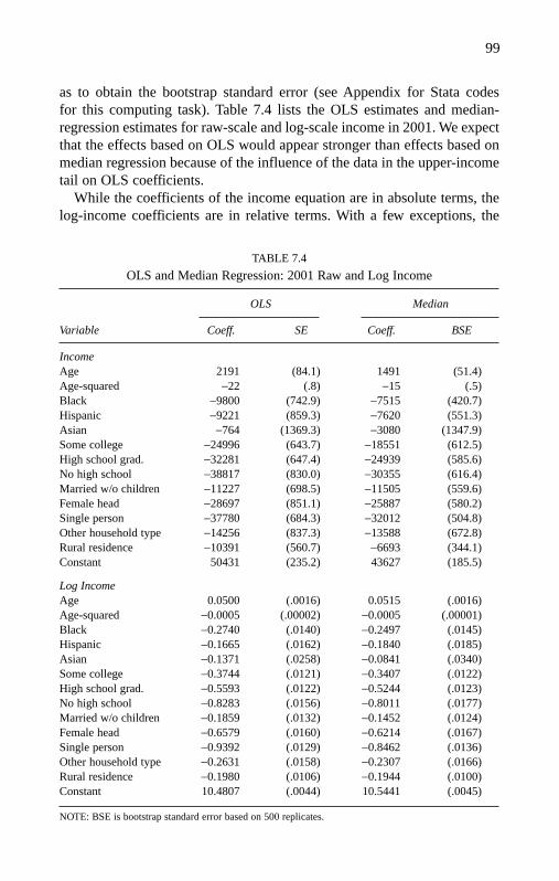
as to obtain the bootstrap standard error (see Appendix for Stata codesfor this computing task). Table 7.4 lists the OLS estimates and median-regression estimates for raw-scale and log-scale income in 2001. We expectthat the effects based on OLS would appear stronger than effects based onmedian regression because of the influence of the data in the upper-incometail on OLS coefficients.
While the coefficients of the income equation are in absolute terms, thelog-income coefficients are in relative terms. With a few exceptions, the
99
TABLE 7.4
OLS and Median Regression: 2001 Raw and Log Income
OLS Median
Variable Coeff. SE Coeff. BSE
IncomeAge 2191 (84.1) 1491 (51.4)Age-squared −22 (.8) −15 (.5)Black −9800 (742.9) −7515 (420.7)Hispanic −9221 (859.3) −7620 (551.3)Asian −764 (1369.3) −3080 (1347.9)Some college −24996 (643.7) −18551 (612.5)High school grad. −32281 (647.4) −24939 (585.6)No high school −38817 (830.0) −30355 (616.4)Married w/o children −11227 (698.5) −11505 (559.6)Female head −28697 (851.1) −25887 (580.2)Single person −37780 (684.3) −32012 (504.8)Other household type −14256 (837.3) −13588 (672.8)Rural residence −10391 (560.7) −6693 (344.1)Constant 50431 (235.2) 43627 (185.5)
Log IncomeAge 0.0500 (.0016) 0.0515 (.0016)Age-squared −0.0005 (.00002) −0.0005 (.00001)Black −0.2740 (.0140) −0.2497 (.0145)Hispanic −0.1665 (.0162) −0.1840 (.0185)Asian −0.1371 (.0258) −0.0841 (.0340)Some college −0.3744 (.0121) −0.3407 (.0122)High school grad. −0.5593 (.0122) −0.5244 (.0123)No high school −0.8283 (.0156) −0.8011 (.0177)Married w/o children −0.1859 (.0132) −0.1452 (.0124)Female head −0.6579 (.0160) −0.6214 (.0167)Single person −0.9392 (.0129) −0.8462 (.0136)Other household type −0.2631 (.0158) −0.2307 (.0166)Rural residence −0.1980 (.0106) −0.1944 (.0100)Constant 10.4807 (.0044) 10.5441 (.0045)
NOTE: BSE is bootstrap standard error based on 500 replicates.
07-Hao.qxd 3/13/2007 4:30 PM Page 99
100
OLS coefficients for log income are larger in magnitude than for medianregression. For example, compared with being white, being black decreasesthe conditional-median income by 100(e−.274 −1) = −24% according to the OLSresults, but by 100(e−.2497 − 1) = −22% according to the median-regressionresults. In other words, mean income for blacks is 24% lower than it is forwhites, and blacks’ median income is 22% lower than whites’, all else beingequal. We note that while we can determine the effect of being black inabsolute terms on the conditional median because of the monotonic equi-variance property of the QRM, we cannot do so with the conditional-meanlog-scale estimates because the LRM does not have the monotonic equi-variance property. We will later return to attaining effects in absolute termsfrom log-income-equation estimates.
Graphical View of QRM Estimates From Income and Log-Income Equations
An important departure of the QRM from the LRM is that there are num-erous sets of quantile coefficients being estimated. We use Stata’s “sqreg”command for fitting the QRM with 19 equally spaced quantiles (.05th, . . . ,.95th) simultaneously. The sqreg command uses the bootstrap method toestimate the standard errors of these coefficients. We specified 500 repli-cates to ensure a large enough number of bootstrap samples for stableestimates of the standard errors and 95% confidence intervals. The sqregcommand does not save estimates from each bootstrap but only presentsa summary of the results. We perform this bootstrapping for raw-scaleincome and log-transformed income. Results from the sqreg are used tomake graphical presentations of coefficients.
Using such a large number of estimates results in a trade-off betweencomplexity and parsimony. On the one hand, the large numbers of parame-ter estimates are capable of capturing complex and subtle changes in thedistribution shape, which is exactly the advantage of using the QRM.On the other hand, this complexity is not without costs, as we may be con-fronted with an unwieldy collection of coefficient estimates to interpret.Thus, a graphical view of QRM estimates, previously optional, becomes anecessary step in interpreting QRM results.
We are particularly interested in how the effect of a covariate varies withthe quantiles of interest. The graphical view in which we plot how the esti-mated QRM coefficients vary with p is valuable for highlighting trends inthese coefficients. For raw-scale coefficients, a horizontal line indicates thatthe coefficient does not vary with p, so that the effect of a constant changein the covariate on the quantile of the response is the same for all quantiles.
07-Hao.qxd 3/13/2007 4:30 PM Page 100
In other words, with all the other covariates fixed, the covariate changeproduces a pure location shift: a positive shift if the line is above the hori-zontal zero line and a negative shift if the line is below the zero line. On theother hand, a straight nonhorizontal line indicates both location and scaleshifts. In this case, the location shift is determined by the quantile coeffi-cient at the median: A positive median coefficient indicates a rightwardlocation shift and a negative median coefficient indicates a leftward loca-tion shift. An upward-sloping straight line indicates a positive scale shift(the scale becomes wider). By contrast, a downward-sloping straight lineindicates a negative scale shift (the scale becomes narrower). Any nonlin-ear appearance in the curve implies the presence of a more complex shapeshift, for example, in the form of a skewness shift. These graphs, however,provide neither exact quantities of shape shifts nor their statistical signifi-cance. We will examine their significance later using shape-shift quantities.
To illustrate how to identify the location and shape shifts using a graph-ical view, we examine closely the age effect on raw-scale income in Figure7.2. As the coefficients and the confidence envelope are above 0 (the thickhorizontal line), the age effects on various quantiles of raw-scale incomeare all positive and significant. The age coefficients form an upward-sloping, generally straight line, indicating that an increase in age shifts thelocation of the income distribution rightward and expands the scale of theincome distribution.
The plots in Figure 7.3 show results for raw-scale income. Coefficientpoint estimates and 95% confidence intervals based on bootstrap standarderrors are plotted against p ∈(0,1). The shaded area indicates that the effectof a covariate is significant for particular quantiles if the area does not crosszero. For example, the Asian effect is insignificant beyond p > .45 becausethe confidence envelope crosses 0 beyond that point. Chapter 4 summarizessome basic patterns that provide hints as to location shifts and scale shiftsfor raw- and log-scale coefficients. Below we discuss patterns emerging fromour example.
The graph for the constant coefficient is a predicted quantile function forincome for the typical household (i.e., the income of a fictional householdbased on the mean of all covariates) and serves as the baseline. This quantilefunction indicates that for the typical household, income has a right-skeweddistribution. This skewness is less pronounced than the skewness observedfor the income data without taking into account the effects of the covariates.Among the 13 covariates, only “age” has positive effects. The middle 70% ofthe population is estimated to have a proportional increase in income withage. The bottom-tail rates of the age effect are disproportionately lower,whereas the upper-tail rates are disproportionately higher. However, this non-proportionality is not sufficient to allow conclusions about skewness, because
101
07-Hao.qxd 3/13/2007 4:30 PM Page 101

102
the baseline skewness (represented by the constant term) must be taken intoaccount. All other covariates have negative effects. As mentioned earlier, theAsian effect is significant for the lower tail of the conditional distribution.This segment of the curves is quite flat, suggesting a pure location shiftfor the lower half. A few covariates have close-to-flat curves; for example,compared with whites, Hispanics’ income is lower by a similar amount atalmost all quantiles, making the curve flat. However, most covariates appearto produce not only location shifts but also substantial shape shifts.
The graphs for log coefficients are presented in Figure 7.4. We note thatlog transformation contracts the right-skewed distribution to give approxi-mate normality. Thus, the graph of the constant coefficients resembles thequantile function of a normal distribution. As discussed in Chapter 4,the log coefficient approximates proportional change in relative terms;straight flat lines indicate location shifts and scale shifts without changingthe skewness. Any departure from the straight flat line becomes difficult tointerpret as it tends to indicate combinations of location, scale, and skew-ness shifts. In addition, because on the log scale a tiny amount of logincome above or below a straight flat line at the upper quantiles translatesto a large amount of income, we should be cautious in claiming a close-to-flat curve. For example, the curves for the three lowest categories of educa-tion appear quite flat, but we do not claim them as close-to-flat because
3000
2000
1000
0
Qu
anti
le C
oef
fici
ents
fo
r In
com
e ($
)
P
0 .1 .2 .3 .4 .5 .6 .7 .8 .9 1
Figure 7.2 Age Effect: Raw-Scale QRM Coefficient and BootstrapConfidence Envelope, 2001
07-Hao.qxd 3/13/2007 4:30 PM Page 102

103
0.1
.2.3
.4.5
.6.7
.8.9
1
020406080100
120
P
Co
nst
ant
0
0 −5 −10
−15
−20
.1.2
.3.4
.5.6
.7.8
.91
PR
ura
l
0
0 −5 −10
−15
−20
−25
.1.2
.3.4
.5.6
.7.8
.91
PO
ther
Ho
use
ho
lds
0
−20
−40
−60
−80
0.1
.2.3
.4.5
.6.7
.8.9
1P
Sin
gle
Per
son
0.1
.2.3
.4.5
.6.7
.8.9
1
0
−10
−20
−30
−40
−50
P
Fem
ale
Hea
d
0.1
.2.3
.4.5
.6.7
.8.9
1
0 −5 −10
−15
−20
−25
−30
P
Mar
ried
w/o
Ch
ildre
n
1.9
.8.7
.6.5
.4.3
.2.1
0
−100−80
−60
−40
−200
P
No
Hig
h S
cho
ol
1.9
.8.7
.6.5
.4.3
.2.1
0
−80
−60
−40
−200
P
So
me
Co
lleg
e
1.9
.8.7
.6.5
.4.3
.2.1
0
−80
−60
−40
−200
P
Hig
h S
cho
ol G
rad
uat
e
1.9
.8.7
.6.5
.4.3
.2.1
0
0123
P
Ag
e
1.9
.8.7
.6.5
.4.3
.2.1
0
0
−.01
−.02
−.03
P
Ag
e-S
qu
ared
0 −5 −10
−15
0.1
.2.3
.4.5
.6.7
.8.9
1P
Bla
ck
0 −5 −10
−15
0.1
.2.3
.4.5
.6.7
.8.9
1P
His
pan
ic
30 20 10 0
−10
1.9
.8.7
.6.5
.4.3
.2.1
0P
Asi
an
Fig
ure
7.3
Raw
-Sca
le Q
RM
Coe
ffic
ient
s an
d B
oots
trap
Con
fide
nce
Env
elop
es:2
001
07-Hao.qxd 3/13/2007 4:30 PM Page 103

104
Ag
e
.06
.04
.02 0
0.1
.2.3
.4.5
.6.7
.8.9
1P
0.1
.2.3
.4.5
.6.7
.8.9
1
0
−.00
02
−.00
04
−.00
06
P
Ag
e-S
qu
ared
0.1
.2.3
.4.5
.6.7
.8.9
1P
Bla
ck
−4−3−2−10
0.1
.2.3
.4.5
.6.7
.8.9
1P
His
pan
ic
0 −1 −2 −3
.1
.2.3
.4.5
.6.7
.8.9
01
−202 −4 −6
P
Asi
an
0 −1 −2 −3 −4 −5 −6
0.1
.2.3
.4.5
.6.7
.8.9
1
So
me
Co
lleg
e
P
0.1
.2.3
.4.5
.6.7
.8.9
1
0−.
1−.
2−.
3−.
4−.
5−.
6−.
7
Hig
h S
cho
ol G
adu
ate
P0
.1.2
.3.4
.5.6
.7.8
.91
−.2
−.4
−.6
−.8 −10
No
Hig
h S
cho
ol
P
0.1
.2.3
.4.5
.6.7
.8.9
1
−.1
−.2
−.3
−.4
−.50
P
Mar
ried
w/o
Ch
ildre
n
1
0.1
.2.3
.4.5
.6.7
.8.9
−.2
−1.5−1−.50
P
Fem
ale
Hea
d
1.9
.8.7
.6.5
.4.3
.2.1
0
11
10.5 10 9.5
P
Co
nst
ant
11.5
1.9
.8.7
.6.5
.4.3
.2.1
0
0−.
05 −.1
−.15 −.2
−.25 −.
3
Ru
ral
P
0.1
.2.3
.4.5
.6.7
.8.9
1
Oth
er H
ou
seh
old
s
P
0
−.2
−.4
−.6
−.8
1.9
.8.7
.6.5
.4.3
.2.1
0
Sin
gle
Per
son
P
−.2
−.4
−.6
−.8
−.1
−1.2
−1.40
Fig
ure
7.4
Log
-Sca
le Q
RM
Coe
ffic
ient
s an
d B
oots
trap
Con
fide
nce
Env
elop
es:2
001
07-Hao.qxd 3/13/2007 4:30 PM Page 104

105
their upper tail above the .8th quantile drops discernibly. In short, graphs oflog coefficients are less telling and require greater caution in interpretationthan graphs of raw-scale coefficients.
Quantile Regressions at Noncentral Positions: Effects in Absolute Terms
Graphical views offer an overview of the covariates’ impact on the shapeof the conditional-income distribution. We now complement the graphicalview with a closer look at some of the off-central positions. We choose twoextremes that fall outside of the graphs we just examined: the .025th and.975th quantiles. In order to obtain coefficient standard errors for theseadditional .025th- and .975th-quantile regressions of raw-scale income, wecan either use “sqreg” with 500 replicates or manually perform the boot-strap method for 500 replicates, saving all 500 sets of resulting coefficientestimates. The conditional shape-shift quantities require programmingbased on each of the bootstrap replicates of these two quantile estimates, sowe present the manual bootstrap results here. With the 500 sets of coeffi-cient estimates, we use the median as the point estimate and the middle95% as the confidence interval. If the confidence interval does not cross 0,the coefficient is significant at the p = .05 level. These results are almostidentical to the sqreq outputs.
Estimates for the log-income equations are not in absolute terms.Because effects in absolute terms are essential to understanding the impactof a covariate on the shape of the distribution, we need to find the effect inabsolute terms, evaluated at the typical setting (the mean of all covariates).As for the raw income, we save 500 sets of log-scale coefficients from boot-strap samples. For each covariate in the estimation based on a bootstrapsample, we
• Obtain the log-conditional quantile of one unit increase from the mean of thecovariate by adding the coefficient to the constant term.
• Take the exponential of this log-conditional quantile and the exponential ofthe constant term to yield two raw-scale conditional quantiles.
• Take the difference between these two raw-scale-conditional quantiles, whichbecomes the effect of the covariate in absolute terms, evaluated at the typicalsetting, the TSE.
Table 7.5 shows the effects in absolute terms from income and log-income equations at the .025th and .975th quantiles. The top panel is fromthe income equation. The constant term represents the estimated value of
07-Hao.qxd 3/13/2007 4:30 PM Page 105

the .025th and .975th quantiles, respectively, when all covariates are at theirmean values: about $10,000 at the bottom and about $137,000 at the top.The most striking pattern is the huge difference in the effect of a covariateon the two ends. For example, being black reduces income by $1,991 atthe .025th quantile and by $17,380 at the .975th quantile. In addition,Hispanics and Asians have significantly lower income than whites at the.025th quantile but not at the .975th percentile.
TABLE 7.5
Effects in Absolute Terms on Tail Quantiles:2001 Raw and Log Income
0.025th Quantile 0.975th Quantile
Variable Coeff. Coeff.
Income ModelAge 248** 3103**Age-squared −2** −29**Black −1991** −17380**Hispanic −2495** −7418Asian −4221** 16235Some college −2607** −105858**High school grad. −4332** −119924**No high school −6211** −129464**Married w/o children −4761** −18878**Female head −10193** −50465**Single person −12257** −78570**Other household type −7734** −16876**Rural residence −943** −18654**Constant 10156** 137561**
Log-Income ModelAge 396** 5409**Age-squared −3** −53**Black −2341** −28867**Hispanic −1835** −8032Asian −3259** 8636Some college −1916** −49898**High school grad. −2932** −57557**No high school −4095** −70006**Married w/o children −3149** −12471**Female head −5875** −33219**Single person −6409** −63176**Other household type −4382** −5282**Rural residence −938** −26742**Constant 8457** 115804**
NOTE: Significance (** p < .05) is determined by 95% confidence interval based on 500 bootstrap replicates.
106
07-Hao.qxd 3/13/2007 4:30 PM Page 106

107
The lower panel shows the TSEs based on the log-income equation. Theconstant term represents the .025th and .975th conditional quantiles atthe typical setting. The TSEs are quite similar to those estimated from theincome equation. They are not exactly the same, because the log-incomemodel fits better than the income model and because the log-income equa-tion estimates are evaluated at the typical setting.
Assessing a Covariate’s Effect on Location and Shape Shifts
QRM estimates can be used to calculate precisely how a covariate shiftsthe location and shape of the conditional distribution. To do such an assess-ment, we compare two groups: a reference group and a comparison group.In the case of a continuous covariate, the reference group is defined byequating the covariate to some value, and the comparison group is definedby increasing the covariate by one unit, holding other covariates constant.For a dichotomous covariate, we change its value from 0 to 1, holding othercovariates constant. All comparisons are made in absolute terms to revealthe raw-scale distribution. Thus, if log-income regression is used to fit thedata, the coefficient in absolute terms for a covariate is obtained first (as inthe previous section). Location shifts are captured by the coefficients at themedian. Shape (scale and skewness) shifts are based on a combination of anumber of coefficients. Their significance levels are determined using thebootstrap method.
Table 7.6 shows the results from the income model for 1991 and 2001,with location shifts in the top panel, scale shifts in the middle, and skewnessshifts in the bottom. In 1991, all covariates except Asian significantly shiftthe comparison group’s location from the reference group. Some of theseeffects change noticeably from 1991 to 2001. The Asian location shift,insignificant in 1991, becomes significantly negative in 2001, suggestingthe absolute advantage of whites over minorities. Other racial and ethnicgroups’ location shifts, however, appear to become weaker. Age’s locationshift is less important in 2001 than in 1991. The same is true for having lesseducation. However, the negative location shifts for household types that arenot “married with children” become stronger, as does rural residence.
Location shifts capture between-group differences. As previously dis-cussed for Table 7.4, median-regression coefficients are weaker than OLS coef-ficients. For the highly right-skewed income distribution, median-regressioncoefficients capture the central location shift, whereas the OLS coeffi-cients are influenced more heavily by the right tail. Using location shifts(median regression), our findings regarding education groups suggest that the
07-Hao.qxd 3/13/2007 4:30 PM Page 107
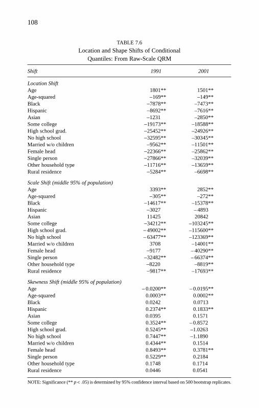
TABLE 7.6
Location and Shape Shifts of ConditionalQuantiles: From Raw-Scale QRM
Shift 1991 2001
Location ShiftAge 1801** 1501**Age-squared −169** –149**Black −7878** –7473**Hispanic −8692** –7616**Asian −1231 –2850**Some college −19173** –18588**High school grad. −25452** –24926**No high school −32595** –30345**Married w/o children −9562** –11501**Female head −22366** –25862**Single person −27866** –32039**Other household type −11716** –13659**Rural residence −5284** –6698**
Scale Shift (middle 95% of population)Age 3393** 2852**Age-squared −305** –272**Black −14617** –15378**Hispanic −3027 – 4893Asian 11425 20842Some college −34212** –103245**High school grad. − 49002** –115600**No high school − 63477** –123369**Married w/o children 3708 –14001**Female head −9177 – 40290**Single person −32482** – 66374**Other household type −8220 –8819**Rural residence −9817** –17693**
Skewness Shift (middle 95% of population)Age − 0.0200** – 0.0195**Age-squared 0.0003** 0.0002**Black 0.0242 0.0713Hispanic 0.2374** 0.1833**Asian 0.0395 0.1571Some college 0.3524** – 0.8572High school grad. 0.5245** –1.0263No high school 0.7447** –1.1890Married w/o children 0.4344** 0.1514Female head 0.8493** 0.3781**Single person 0.5229** 0.2184Other household type 0.1748 0.1714Rural residence 0.0446 0.0541
NOTE: Significance (** p < .05) is determined by 95% confidence interval based on 500 bootstrap replicates.
108
07-Hao.qxd 3/13/2007 4:30 PM Page 108

109
education effect in terms of location shifts is not as strong as indicated in theliterature. The change in location shift, or between-group difference, is onlyone part of the story about how inequality changed over the decade; the otheris the shape change, or relative within-group differences. The advantage of theQRM is that they disentangle the between- and within-group differences,advancing our understanding of changes in inequality.
Scale shifts are one type of shape changes. Among the three racial andethnic minority groups, only blacks have a shorter conditional-income dis-tribution scale than do whites. The scale for the income of the middle 95%of blacks is much narrower than it is for whites, suggesting greater homo-geneity among blacks than whites and the significance of race in determin-ing income. This scale shift becomes stronger in 2001. The same is seen inthe three less-educated groups. The education scale shift offers a consistentand refined finding about the increasing importance of education in deter-mining income: It is the shape shift, rather than the location shift, that indi-cates the rising importance of education.
Skewness shifts are another type of shape change. An increase in theskewness of a conditional quantile indicates uneven within-group differen-tiation that favors the top-tail members. The 1991 results show that manydisadvantaged groups experience this uneven within-group differentiation,including Hispanics, the three less-educated groups, and disadvantagedhousehold types (single-mother, single-person, and “other” households).Some of these shifts disappear in 2001, particularly those of the educationgroups. This finding further reveals the mechanism by which society rewardscollege graduates and limits upward mobility for the most able among theless educated.
Results on the raw scale from the log-income model are shown inTable 7.7. These results capture the same trends for life cycle, racial andethnic groups, education groups, household types, and rural residence. Thelocation shifts and scale shifts in each year, as well as their decade trends,are similar whether income or log income is fitted. Discrepancies are foundfor skewness shifts. In particular, skewness is reduced significantly for less-educated groups in 2001; this finding is significant based on the log-incomemodel but insignificant based on the income model. It is not surprising thatsuch discrepancies should appear when examining the two model fits(income and log income). They represent fundamentally distinct models,with one of them (log income) providing a better fit. On the other hand, ifqualitative conclusions differ, it may indicate that the results are sensitive.We determine whether this is the case by looking at the overall evaluationof a covariate’s role in inequality.
We develop an overall evaluation of a covariate’s impact on inequality,which examines the alignment of the signs of location and shape shifts.
07-Hao.qxd 3/13/2007 4:30 PM Page 109

TABLE 7.7
Location and Shape Shifts ofConditional Quantiles: From Log-Scale QRM
Shift 1991 2001
Location ShiftAge 2456** 1994**Age-squared −24** −20**Black −9759** −8386**Hispanic −7645** − 6300**Asian −1419 −3146**Some college −10635** −11012**High school grad. −14476** −15485**No high school −20891** −20892**Married w/o children −3879** −5103**Female head −15815** −17506**Single person −19599** −21658**Other household type − 6509** −7734**Rural residence − 4931** − 6725**
Scale Shift (middle 95% of population)Age 4595** 5008**Age-squared − 41** −50**Black −17244** −26509**Hispanic −2503 − 6017Asian 4290 12705Some college −22809** − 47992**High school grad. −32675** −54434**No high school − 44457** − 65956**Married w/o children 77 −9264**Female head −10269 −27272**Single person −32576** −56791**Other household type −7535 −906Rural residence −12218** −25760**
Skewness Shift (middle 95% of population)Age − 0.0417** − 0.0100Age-squared 0.0005** 0.0002Black 0.1127 − 0.0682Hispanic 0.2745** 0.1565**Asian − 0.0383 0.1469Some college 0.0655 − 0.2775**High school grad. 0.0934 − 0.2027**No high school 0.2742** − 0.1456**Married w/o children 0.0890 − 0.0272Female head 0.5404** 0.3193**Single person 0.2805** − 0.0331Other household type 0.0164 0.1640**Rural residence 0.0012 − 0.0740
NOTE: Significance (** p < .05) is determined by 95% confidence interval based on 500 bootstrap replicates.
110
07-Hao.qxd 3/13/2007 4:30 PM Page 110

111
Only significant shifts are counted. For a covariate, in-sync signs in thethree shifts indicate that the covariate exacerbates inequality; the larger thenumber of significant signs, the stronger the exacerbating effect becomes.Out-of-sync signs indicate that the covariate may increase between-groupinequality while decreasing within-group inequality, or vice versa. Theleft panel of Table 7.8 for the income model shows that none of the covari-ates have in-sync effects on inequality in 1991, but many do in 2001. Thesein-sync covariates are education groups, household types (except femaleheads), and rural residence. The right panel shows the corresponding resultsfrom the log-income model. We see little contradiction in the overall eval-uation. For example, for education groups, the pattern changes from out ofsync in 1991 to in sync in 2001 in both models. Thus, American society in2001 was more unequal and its social stratification more salient by educa-tion, marriage, presence of children, and rural residence than was the casea decade earlier.
In this example, we use the middle 95% population to calculate theshape-shift quantities. Researchers can design their own shape-shift defini-tions according to their research questions. It is possible to design corre-sponding shape shifts for the middle 99%, 98%, 90%, 80%, or 50% of thepopulation. We leave this to our readers to undertake.
TABLE 7.8
Overall Evaluation of Covariates’ Role in Inequality:Synchronicity Patterns in Coefficients
Income Equation Log-Income Equation
Variable 1991 2001 1991 2001
Age + + − + + − + + − + + 0Age-squared − − + − − + − − + − − 0Black − − 0 − − 0 − − 0 − − 0Hispanic − 0 + − 0 + − 0 + − 0 +Asian 0 0 0 − 0 0 0 0 0 − 0 0Some college − − + − − 0 − − 0 − − −High school grad. − − + − − 0 − − 0 − − −No high school − − + − − 0 − − + − − −Married w/o children − 0 + − − 0 − 0 0 − − 0Female head − 0 + − − + − 0 + − − +Single person − − + − − 0 − − + − − 0Other household type − 0 0 − − 0 − 0 0 − 0 +Rural residence − − 0 − − 0 − − 0 − − 0
07-Hao.qxd 3/13/2007 4:30 PM Page 111

Summary
What are the sources of the persistent and widening income inequality inthe recent decade? To address this research question, we apply the tech-niques developed in this book. We start with a descriptive analysis usingthe notion of quantiles introduced in Chapter 2. For income data, we dis-cuss the issues of right-skewed distributions and top-coding and explainwhy and how the QRM can accommodate these features. The analyses fol-low the steps discussed in Chapters 3 through 6: defining and fitting mod-els, assessing the goodness of fit, estimating the inference of parameters,making graphs of coefficients and their confidence intervals, and calculat-ing location and shape shifts and their inferences. We describe the incomeand log-income models, paying special attention to the reconstructed raw-scale coefficients. Along with our description of the steps, we demonstratethe utility of the QRM techniques in addressing the research questionthrough interpretations of the results. It is our hope that this systematicsummarization of the application procedures will provide clear guidancefor empirical research.
112
07-Hao.qxd 3/13/2007 4:30 PM Page 112

APPENDIX: STATA CODES
Data: d0.dta is a Stata system file prepared for the analysis.
I. Stata Codes for Analysis of Raw-Scale Income
Step 1: Goodness of Fit
113
* q0.do * a full model * raw-scale income in $1000 * OLS * 19 quantiles tempfile t use d0 global X age age2 blk hsp asn scl hsg nhs mh fh sg ot rural * centering covariates sum $X tokenize $X while "`1'"~="" { egen m=mean(`1') replace `1'=`1'-m drop m macro shift } sum $X forvalues k=1/2 { reg cinc $X if year==`k' } forvalues i=1/19 { local j=`i'/20 qreg cinc $X if year==1, q(`j') nolog } forvalues i=1/19 { local j=`i'/20 qreg cinc $X if year==2, q(`j') nolog }
EM-Hao.qxd 3/13/2007 12:25 PM Page 113

Step 2: Simultaneous Quantile Regressions With 500 Replicates
114
* s0.do * full model * sreq 19 quaniles * raw-scale income in $1000 * analysis for 2001 tempfile t set matsize 400 global X age age2 blk hsp asn scl hsg nhs mh fh sg ot rural use cinc $X year if year==2 using d0, clear drop year * centering covariates sum $X tokenize $X while "`1'"~="" { egen m=mean(`1') replace `1'=`1'-m drop m macro shift } sum $X sqreg cinc $X, reps(500) q(.05 .10 .15 .20 .25 .30 .35 .40 .45 .50 .55 .60 .65 .70 .75 .80 .85 .90 .95) mstore b, from(e(b)) mstore v, from(e(V)) keep age keep if _n<11 save s0, replace
* s_m0.do * matrix operation * 13 covariates + cons * graphs for beta's (19 QR) * 500 bootstrap se * analysis for 2001 * for black-white graphs set scheme s2mono set matsize 400 * 13 covariate + cons local k=14 * k parameters for each of the 19 quantiles local k1=`k'*19 use s0, clear qui mstore b qui mstore v * 95%ci * dimension `k' x 1 mat vv=vecdiag(v) mat vv=vv'
Step 3: Use Results From s0.do to Create Tables and Graphs
EM-Hao.qxd 3/13/2007 12:25 PM Page 114

115
svmat vv mat drop vv qui replace vv1=sqrt(vv1) mkmat vv1 if _n<=`k1', mat(v) drop vv1 mat b=b' mat l=b-1.96*v mat u=b+1.96*v * 19 quantiles mat q=(.05\.10\.15\.20\.25\.30\.35\.40\.45\.50\.55\.60\.65\.70\.75\.80\.85\.90\.95) * reorganize matrix by variable forvalues j=1/`k' { forvalues i=1/19 { local l=`k'*(`i'-1)+`j' mat x`j'q`i'=q[`i',1],b[`l',1],l[`l',1],u[`l',1],v[`l',1] } } forvalues j=1/`k' { mat x`j'=x`j'q1 forvalues i=2/19 { mat x`j'=x`j'\x`j'q`i' } * q b l u v mat list x`j', format(%8.3f) svmat x`j' mat a1=x`j'[1...,2] mat a2=x`j'[1...,5] mat xx`j'=q,a1,a2 * q b v
mat list xx`j', format(%8.3f) mat drop a1 a2 xx`j' } * graphs using the same scale for categorical covariates * use age, age-squared and constant as examples * age twoway rarea x13 x14 x11, color(gs14) || line x12 x11, lpattern(solid) yline(0, lpattern(solid) lwidth(medthick)) ylabel(0 "0" 1 "1000" 2 "2000" 3 "3000") ytitle(quantile coefficients for income ($)) xtitle(p) xlabel(0(.1)1) legend(off) graph export g0.ps, as(ps) logo(off) replace * age2 twoway rarea x23 x24 x21, color(gs14) || line x22 x21, lpattern(solid) yline(0, lstyle(foreground) lpattern(solid) lwidth(medthick)) xtitle(p) xlabel(0(.1)1) legend(off) graph export g2.ps, as(ps) logo(off) replace * constant (the typical setting) twoway rarea x143 x144 x141, color(gs14) || line x142 x141, lpattern(solid) yline(0, lstyle(foreground) lpattern(solid) lwidth(medthick)) ylabel(0(20)120) xlabel(0(.1)1) xtitle(p) legend(off) graph export g14.ps, as(ps) logo(off) replace drop x* matrix drop _all
EM-Hao.qxd 3/13/2007 12:25 PM Page 115

116
* bs0.do * location and shape shift quantities * bootstrap confidence interval * 3 quantiles (.025, .5, .975) set matsize 800 * k= # of covariates + cons local k=14 local k1=`k'-1 * initial forvalues j=0/2 { use e`j'1, clear qui mstore e mat ren e e`j' } forvalues j=0/2 { forvalues i=2/500 { use e`j'`i', clear qui mstore e
* e0.do * full model * raw-scale income in $1000 * bootstrap * analysis for 2001 tempfile t global X age age2 blk hsp asn scl hsg nhs mh fh sg ot rural use cinc $X year if year==2 using d0, clear drop year * centering covariates sum $X tokenize $X while "`1'"~="" { egen m=mean(`1') replace `1'=`1'-m drop m macro shift } sum $X save `t' forvalues i=1/500 { use `t', clear bsample qreg cinc $X, q(.025) nolog mstore e, from(e(b)) keep if _n<11 keep age save e0`i', replace }
Step 4: Calculating Location and Shape Shifts
[Modify the codes of e0.do to make e1.do for the .5th quantile and e2.dofor the .975th quantile]
EM-Hao.qxd 3/13/2007 12:25 PM Page 116

117
mat e`j'=e`j'\e mat drop e } } forvalues j=0/2 { qui svmat e`j' } * mean of estimate (point estimate) * percentile-method (95% ci) forvalues j=0/2 { forvalues i=1/`k' { pctile x=e`j'`i', nq(40) sort x qui gen x0=x if _n==20 qui gen x1=x if _n==1 qui gen x2=x if _n==39 egen em`j'`i'=max(x0) egen el`j'`i'=max(x1) egen eu`j'`i'=max(x2) drop x x0 x1 x2 sum em`j'`i' el`j'`i' eu`j'`i' } } * SCS scale shift forvalues i=1/`k1' { gen sc1s`i'=e2`i'-e0`i' pctile x=sc1s`i', nq(40) sort x qui gen x0=x if _n==20 qui gen x1=x if _n==1 qui gen x2=x if _n==39 egen sc1sm`i'=max(x0) egen sc1sl`i'=max(x1) egen sc1su`i'=max(x2) drop x x0 x1 x2 sum sc1sm`i' sc1sl`i' sc1su`i' }
* SKS skewedness shift * SKS e2(.975) - e1(.5) and e1(.5) - e0(.025) * i for covariate, k for constant forvalues i=1/`k1' { gen nu=(e2`i'+e2`k'-e1`i'-e1`k')/(e2`k'-e1`k') gen de=(e1`i'+e1`k'-e0`i'-e0`k')/(e1`k'-e0`k') gen sk1s`i'=nu/de drop nu de pctile x=sk1s`i', nq(40) sort x qui gen x0=x if _n==20 qui gen x1=x if _n==1 qui gen x2=x if _n==39 egen sk1sm`i'=max(x0) egen sk1sl`i'=max(x1) egen sk1su`i'=max(x2) drop x x0 x1 x2 sum sk1sm`i' sk1sl`i' sk1su`i' }
EM-Hao.qxd 3/13/2007 12:25 PM Page 117

118
set matsize 800 * k= # of covariates + cons local k=14 local k1=`k'-1 * parameter matrix (e0 e1 e2) * initial forvalues j=0/2 { use e`j'1, clear qui mstore e mat ren e e`j' } * 500 reps forvalues j=0/2 { forvalues i=2/500 { use e`j'`i', clear qui mstore e mat e`j'=e`j'\e mat drop e } } * get log conditional quantile forvalues j=0/2 { * dimensions 500 x 14 * c`j'1 to c`j'13 are covariates * c`j'14 constant forvalues m=1/`k' { mat c`j'`m'=e`j'[1...,`m'] } forvalues m=1/`k1' { mat c`j'`m'=c`j'`m'+c`j'`k' } mat c`j'=c`j'1 mat drop c`j'1 forvalues m=2/`k' { mat c`j'=c`j',c`j'`m' mat drop c`j'`m' } * transform log-scale conditional quantile to raw-scale conditinal quantile * matrix to var svmat c`j' mat drop c`j' forvalues m=1/`k' { qui replace c`j'`m'=exp(c`j'`m') }
II. Stata Codes for Analysis of Log Income
[Substitute raw-scale income with log-scale income, following Steps 1–3 onpages 113 to 115]
Step 4: Calculating Raw-Scale Locationand Shape Shifts Based on Log-Income QRM
[Substitute raw-scale income with log-scale income in e0.do, e1.do, and e2.do]
EM-Hao.qxd 3/13/2007 12:25 PM Page 118

119
} mat e`j'=e`j'1 mat drop e`j'1 forvalues m=2/`k' { mat e`j'=e`j',e`j'`m' mat drop e`j'`m' } mstore e`j', from(e`j') replace } mat dir keep age keep if _n<11 save l-r, replace **** * bs1.do * bootstrap method * location and shape shift quantities * based on log-to-raw coeff set matsize 800 * k= # of covariates + cons local k=14 local k1=`k'-1 use l-r forvalues j=0/2 { qui mstore e`j' qui svmat e`j' } * mean of estimate (point estimate) * sd of estimates (se) * percentile-method (95% ci) forvalues j=0/2 { forvalues i=1/`k' { pctile x=e`j'`i', nq(40) sort x qui gen x0=x if _n==20 qui gen x1=x if _n==1 qui gen x2=x if _n==39 egen em`j'`i'=max(x0) egen el`j'`i'=max(x1) egen eu`j'`i'=max(x2) drop x x0 x1 x2 sum em`j'`i' el`j'`i' eu`j'`i' } } * SCS scale shift forvalues i=1/`k1' {
forvalues m=1/`k1' { qui replace c`j'`m'=c`j'`m'-c`j'`k' } * var to matrix forvalues m=1/`k' { mkmat c`j'`m', mat(e`j'`m')
EM-Hao.qxd 3/13/2007 12:25 PM Page 119

120
egen sc1sl`i'=max(x1) egen sc1su`i'=max(x2) drop x x0 x1 x2 sum sc1sm`i' sc1sl`i' sc1su`i' } * SKS skewedness shift * SKS e2(.975) - e1(.5) and e1(.5) - e0(.025) * i for covariate, k for constant forvalues i=1/`k1' { gen nu=(e2`i'+e2`k'-e1`i'-e1`k')/(e2`k'-e1`k') gen de=(e1`i'+e1`k'-e0`i'-e0`k')/(e1`k'-e0`k') gen sk1s`i'=nu/de drop nu de pctile x=sk1s`i', nq(40) sort x qui gen x0=x if _n==20 qui gen x1=x if _n==1 qui gen x2=x if _n==39 egen sk1sm`i'=max(x0) egen sk1sl`i'=max(x1) egen sk1su`i'=max(x2) drop x x0 x1 x2 sum sk1sm`i' sk1sl`i' sk1su`i' }
gen sc1s`i'=e2`i'-e0`i' pctile x=sc1s`i', nq(40) sort x qui gen x0=x if _n==20 qui gen x1=x if _n==1 qui gen x2=x if _n==39 egen sc1sm`i'=max(x0)
EM-Hao.qxd 3/13/2007 12:25 PM Page 120

121
REFERENCES
Abreveya, J. (2001). The effects of demographics and maternal behavior on the distribution ofbirth oucomes. Empirical Economics, 26, 247–257.
Austin, P., Tu, J., Daly, P., & Alter, D. (2005). The use of quantile regression in health careresearch: A case study examining gender differences in the timeliness of thrombolytictherapy. Statistics in Medicine, 24, 791–816.
Bedi, A., & Edwards, J. (2002). The impact of school quality on earnings and educationalreturns—evidence from a low-income country. Journal of Development Economics, 68,157–185.
Berry, W. D. (1993). Understanding regression assumptions. Newbury Park, CA: SagePublications.
Berry, W. D., & Feldman, S. (1985). Multiple regression in practice. Beverly Hills, CA: SagePublications.
Buchinsky, M. (1994). Changes in the U.S. wage structure 1963–1987: Application of quan-tile regression. Econometrica, 62, 405–458.
Budd, J. W., & McCall, B. P. (2001). The grocery stores wage distribution: A semi-parametricanalysis of the role of retailing and labor market institutions. Industrial and LaborRelations Review, 54, Extra Issue: Industry Studies of Wage Inequality, 484–501.
Cade, B. S., Terrell, J. W., & Schroeder, R. L. (1999). Estimating effects of limiting factorswith regression quantiles. Ecology, 80, 311–323.
Chamberlain, G. (1994). Quantile regression, censoring and the structure of wages. InC. Skins (Ed.), Advances in Econometrics (pp. 171–209). Cambridge, UK: CambridgeUniversity Press.
Chay, K. Y., & Honore, B. E. (1998). Estimation of semiparametric censored regressionmodels: An application to changes in black-white earnings inequality during the 1960s. TheJournal of Human Resources, 33, 4–38.
Edgeworth, F. (1888). On a new method of reducing observations relating to several quantiles.Philosophical Magazine, 25, 184–191.
Efron, B. (1979). Bootstrap methods: Another look at the jackknife. Annals of Statistics, 7, 1–26.Eide, E. R., & Showalter, M. H. (1999). Factors affecting the transmission of earnings
across generations: A quantile regression approach. The Journal of Human Resources, 34,253–267.
Eide, E. R, Showalter, M., & Sims, D. (2002). The effects of secondary school quality on thedistribution of earnings. Contemporary Economic Policy, 20, 160–170.
Feiring, B. R. (1986). Linear programming. Beverly Hills, CA: Sage Publications.Fortin, N. M., & Lemieux, T. (1998). Rank regressions, wage distributions, and the gender
gap. The Journal of Human Resources, 33, 610–643.Handcock, M. S., & Morris, M. (1999). Relative distribution methods in the social sciences.
New York: Springer.Hao, L. (2005, April). Immigration and wealth inequality: A distributional approach. Invited
seminar at The Center for the Study of Wealth and Inequality, Columbia University.Hao, L. (2006a, January). Sources of wealth inequality: Analyzing conditional distribution.
Invited seminar at The Center for Advanced Social Science Research, New York University.Hao, L. (2006b, May). Sources of wealth inequality: Analyzing conditional location and shape
shifts. Paper presented at the Research Committee on Social Stratification and Mobility
EM-Hao.qxd 3/13/2007 12:25 PM Page 121

122
(RC28) of the International Sociological Association (ISA) Spring meeting 2006 inNijmegen, the Netherlands.
Kocherginsky, M., He, X., & Mu, Y. (2005). Practical confidence intervals for regression quan-tiles. Journal of Computational and Graphical Statistics, 14, 41–55.
Koenker, R. (1994). Confidence intervals for regression quantiles. In Proceedings of the 5thPrague symposium on asymptotic statistics (pp. 349–359). New York: Springer-Verlag.
Koenker, R. (2005). Quantile regression. Cambridge, UK: Cambridge University Press.Koenker, R., & Bassett, Jr., G. (1978). Regression quantiles. Econometrica, 46, 33–50.Koenker, R., & d’Orey, V. (1987). Computing regression quantiles. Applied Statistics, 36,
383–393.Koenker, R., & Hallock, K. F. (2001). Quantile regression: An introduction. Journal of Economic
Perspectives, 15, 143–156.Koenker, R., & Machado, J. A. F. (1999). Goodness of fit and related inference processes for
quantile regression. Journal of Econometrics, 93, 327–344.Lemieux, T. (2006). Post-secondary education and increasing wage inequality. Working Paper
No. 12077. Cambridge, MA: National Bureau of Economic Research.Machado, J., & Mata, J. (2005). Counterfactual decomposition of changes in wage distribu-
tions using quantile regression. Journal of Applied Econometrics, 20, 445–465.Manning, W. G. (1998). The logged dependent variable, heteroscedasticity, and the retrans-
formation problem. Journal of Health Economics, 17, 283–295.Melly, B. (2005). Decomposition of differences in distribution using quantile regression.
Labour Economics,12, 577–590.Mooney, C. Z. (1993). Bootstrapping: A nonparametric approach to statistical inference.
Newbury Park, CA: Sage PublicationsScharf, F. S., Juanes, F., & Sutherland, M. (1989). Inferring ecological relationships from the
edges of scatter diagrams: Comparison of regression techniques. Ecology, 79, 448–460.Scheffé, H. (1959). Analysis of variance. New York: Wiley.Schroeder, L. D. (1986). Understanding regression analysis: An introductory guide. Beverly
Hills, CA: Sage Publications.Shapiro, I., & Friedman, J. (2001). Income tax rates and high-income taxpayers: How strong
is the case for major rate reduction? Washington, DC: Center for Budget and PolicyPriorities.
U.S. Census Bureau. (2001). U.S. Department of Commerce News. (CB01–158). Washington,DC.
Wei, Y., Pere, A., Koenker, R., & He, X. (2006). Quantile regression methods for referencegrowth charts. Statistics in Medicine, 25, 1369–1382.
EM-Hao.qxd 3/13/2007 12:25 PM Page 122

INDEX
123
Absolute terms, covariate effects in,105–107
Algorithmic details, QR estimation,34–38
Asymptotic standard error, 59, 60
Bassett, Jr., G., 3, 4, 29Bootstrap method for quantile regression
modeling, 47–50, 99confidence envelope, 66tests for equivalence, 60–63
Central tendency of distributions, 26Coefficients
equivalence tests, 60–63estimation, 37–38income disparity regression, 99–100log-scale, 86–88of determination, 51of linear regression modeling, 57–59of quantile regression modeling,
59–60, 72Comparison and reference, quantile
regression estimates, 56Conditional mean regression,
1–3, 24, 26income disparity, 98–100transformation and, 39–41versus conditional medians, 56–59,
98–100Conditional median regression, 29–33
income disparity, 98–100versus conditional means, 56–59,
98–100Confidence intervals and standard
errorsbootstrap method, 47–49for linear regression modeling,
43–44for quantile regression modeling,
44–47Covariates
effect on location and shape shifts,107–111
effects in absolute terms, 105–107infinitesimal effects, 85–86mean effect, 83–85
QRM estimates from income andlog-income equations, 100–105
typical-setting effect, 81–83Cumulative distribution function
(cdf), 7–11, 14
Descriptive statistics and incomedisparity, 96
Determination, coefficient of, 51Distribution
central tendency of, 26cumulative distribution function
(cdf) and, 7–11mean, 14–19sample quantiles, 10–12sampling variability, 11–12scale
and skewness, 13–14, 15fshifts, 69–71
shape, 64–69skewness, 13–14, 15f, 72–75
Duality, point/line, 35
Efron, B., 47Equivalence of coefficients across
quintiles, 60–63Equivariance and transformation, 38–41Errors, standard
asymptotic, 59, 60linear regression modeling, 43–44quantile regression modeling,
44–47, 59Estimation, quantile regression, 33–38
graphical view, 100–105income and log-income equations,
100–105reference and comparison, 56
Goodness of fitincome disparity analysis, 97–98of quantile regression modeling,
51–54Stata codes, 113
Graphical viewQRM estimates from income and
log-income equations, 100–105shape shifts, 64–69
Index-Hao.qxd 3/7/2007 12:56 PM Page 123

Income disparityconditional mean versus conditional
median regression, 98–100covariate effects on location and
shape shifts, 107–111descriptive statistics, 96goodness of fit and, 97–98graphical view of QRM estimates,
100–105observed, 92–95quantile regressions at noncentral
positions, 105–107survey data, 97
Infinitesimal effects, 85–86Insensitivity to influence of outliers,
quantile, 20, 41–42
Koenker, R., 3, 4, 5, 29, 45, 51–52, 54
Linear equivariance, 38–39Linear regression modeling (LRM)
conditional means versus conditionalmedians in, 56–59
conditional-mean and, 29–33goodness of fit, 51–52quantile regression modeling
compared to, 22–28robustness and, 41–42standard errors and confidence
intervals, 43–44Linear transformation, 38–41Location
covariate effects on, 107–111quantile-based measures of shape and,
12–14, 32–33shifts on log scale, 78Stata codes, 116–117
Log scalecoefficients graphical view,
86–88location shifts on, 78, 109–111raw scale and, 78–86shape shift measures from, 88–91Stata codes, 118–120typical-setting effect, 81–83
Machado, J. A. F., 51–52, 54Mean
as solution to minimization problem,16–19
conditional, 1–3, 24, 26, 39–41,56–59
distribution, 14–19
effect, covariate, 83–85squared deviation, 16
Median-regression
lines, 34–38modeling, 3, 34–38
as solution to minimization problem,17–19, 21–22
conditional-, 29–33, 56–59Minimization problem, quantile as a
solution to, 14–19,21–22, 33–34
Monotone equivariance property,19–20, 40–41, 81
Monotone transformation,19–20, 40
infinitesimal effects, 85–86interpretation, 77–91location shifts on log scale, 78log scale back to raw scale, 78–86mean effect, 83–85typical-setting, 81–83
Monte-Carlo simulation, 47–48
Noncentral positions, quantileregressions at, 105–107
Nonlinear transformation, 39Normality assumption of linear
regression modeling, 24–25Null hypothesis, 49–50, 63
Off-central positions, quantileregressions at, 105–107
One-model assumption, 25–26Outliers
in linear regression modeling, 25–26quantile insensitivity to influence
of, 20robustness, 41–42
Point/line duality, 35Polyhedral surfaces, 36–37Properties of quantiles, 19–20
Quantile regression modeling(QRM), 3–6
at noncentral positions, 105–107bootstrap method for, 47–50, 99coefficients estimation, 37–38conditional means and, 56–59conditional median and,
29–33, 56–59estimation, 33–38
124
Index-Hao.qxd 3/7/2007 12:56 PM Page 124

income and log-income equations,100–105
reference and comparison, 56goodness of fit of, 51–54income disparity, 97–111inference, 43–55interpretation shape shifts using,
63–76linear regression modeling compared
to, 22–28monotone transformed, 77–91robustness and, 41–42shape shifts, 64–69Stata codes, 114transformation and equivariance,
39–41Quantiles
-based measures of location andshape, 12–14, 32–33, 64–69
-based scale measure (QSC),13, 69–71
-based skewness (QSK),14, 15f, 72–75
as a solution to a certain minimizationproblem, 14–19, 21–22, 33–34
functions, 7–11income disparity, 92–95insensitivity to influence of outliers,
20, 41–42interpretation of individual, 59–60monotone equivariance property,
19–20properties, 19–20tests for equivalence of coefficients
across, 60–63
Raw scaleincome equations, 101–105log scale to, 78–81shape shift measures, 88Stata codes, 118–120typical-setting effect, 81–83
Reference and comparison, quantileregression estimates, 56
Regression analysisconditional mean in, 1–3median-regression modeling in, 3purpose of, 1quantile regression modeling in, 3–6
Robustness, 41–42
Sampling variabilty, quantile,11–12, 69
Scale shifts, 69–71, 88, 90–91,101–102, 109–111
and skewness of distribution, 13–14Scatterplots, 32Shape shifts
covariate effects on, 107–111linear regression modeling, 24, 26,
32–33, 60measures from log-scale fits, 88–91quantile-based measures of location
and, 12–14Stata codes, 116–117using quantile regression results to
interpret, 63–76Shifts, shape. See ShapeSkewness
and scale of distribution, 13–14, 15fshifts, 72–75, 88, 90–91, 101–102
Standard errors and confidence intervalsasymptotic, 59, 60for linear regression modeling,
43–44for quantile regression modeling,
44–47, 59Stata codes, 50
goodness of fit, 113location and shape shifts calculation,
116–117raw-scale location and shape shifts
based on log-income QRM,118–120
simultaneous quantile regressions,114
tables and graphs creation, 114–115Surface, polyhedral, 36–37Survey data, income disparity, 97
Tables and graphs Stata codes,114–115
Tests for equivalence of coefficientsacross quantiles, 60–63
Transformationequivariance and, 38–41log income, 97–98monotone, 19–20, 40, 77–91
Wage distributions, 4–5Wald statistic, 49–50, 60
125
Index-Hao.qxd 3/7/2007 12:56 PM Page 125
126
ABOUT THE AUTHORS
Lingxin Hao (PhD, Sociology, 1990, University of Chicago) is a professorof sociology at The Johns Hopkins University. She was a 2002–2003 VisitingScholar at the Russell Sage Foundation. Her areas of specialization includethe family and public policy, social inequality, immigration, quantitativemethods, and advanced statistics. The focus of her research is on theAmerican family, emphasizing the effects of structural, institutional, andcontextual forces in addition to individual and family factors. Her researchtests hypotheses derived from sociological and economic theories usingadvanced statistical methods and large national survey data sets. Her articleshave appeared in various journals, including Sociological Methodology,Sociological Methods and Research, Quality and Quantity, AmericanJournal of Sociology, Social Forces, Sociology of Education, Social ScienceResearch, and International Migration Review.
Daniel Q. Naiman (PhD, Mathematics, 1982, University of Illinois atUrbana-Champaign) is a professor in, and chair of, the Department ofApplied Mathematics and Statistics at The Johns Hopkins University. Hewas elected as a Fellow of the Institute of Mathematical Statistics in 1997,and was an Erskine Fellow at the University of Canterbury in 2005. Muchof his mathematical research has focused on geometric and computationalmethods for multiple testing. He has collaborated on papers applying sta-tistics in a variety of areas: bioinformatics, econometrics, environmentalhealth, genetics, hydrology, and microbiology. His articles have appeared invarious journals, including Annals of Statistics, Bioinformatics, Biometrika,Human Heredity, Journal of Multivariate Analysis, Journal of the AmericanStatistical Association, and Science.
ATA-Hao.qxd 3/13/2007 12:24 PM Page 126