quantitative analysis of distributed energy resources in future distribution networks
TRANSCRIPT

Degree project in
Quantitative analysis of DistributedEnergy Resources in Future Distribution
Networks
Xue Han
Stockholm Sweden 2012
XR-EE-ICS 2012004
ICSMaster Thesis
Abstract
There has been a large body of statements claiming that the large scale
deployment of Distributed Energy Resources (DERs) will eventually reshape
the future distribution grid operation in numerous ways However there is
a lack of evidence specifying to what extent the power system operation will
be alternated In this project quantitative results in terms of how the future
distribution grid will be changed by the deployment of distributed genera-
tion active demand and electric vehicles are presented The quantitative
analysis is based on the conditions for both a radial and a meshed distri-
bution network The input parameters are on the basis of the current and
envisioned DER deployment scenarios proposed for Sweden
The simulation results indicate that the deployment of DERs can signif-
icantly reduce the power losses and voltage drops by compensating power
from the local energy resources and limiting the power transmitted from the
external grid However it is notable that the opposite results (eg severe
voltage fluctuations larger power losses) can be obtained due to the inter-
mittent characteristics of DERs and the irrational management of different
types of DERs in the DNs Subsequently this will lead to challenges for the
Distribution System Operator (DSO)
Keywords Distribution Network Distributed Generation Electric Vehi-
cle Active Demand Power Losses Voltage Profile
Acknowledgements
The thesis has been implemented in cooperation with Vattenfall Research
and Development and was approved by the Department of Industrial Infor-
mation and Control Systems at KTH - Royal Institute of Technology This
project would have not been completed without all those who helped me
with difficulties and problems
First and foremost I would like to show my gratitude to my supervisor
Claes Sandels who provides the basic idea of this thesis and offers me the
opportunity to work on it I am also grateful for the support and fruitful
discussion from my co-supervisor Kun Zhu All their contributions of time
ideas and important feedback throughout the whole period of thesis work
make me accumulate the experience and knowledge in a stimulating envi-
ronment
I am especially grateful for the encouragement and suggestions on future
plans from Prof Lars Nordstrom
I would like to thank Arshad Saleem Nicholas Honeth Yiming Wu
Davood Babazadeh for their kind help on modelling of DERs and designing
of DNs I also want to show my appreciation to Aquil Amir Jalia Quentin
Lambert and Ying He for their help when collecting data and their valuable
advice
Thanks to all the people at Vattenfall who share their insightful ideas
with me and all my friends in ICS who always support me
In the end I do hope my thesis could help Claes and Kun with their PhD
study in ICS and could give some interesting ideas to Vattenfall for their
research
Xue Han
Stockholm March
Contents
List of Figures iv
List of Tables vi
Abbreviation vii
1 Introduction 1
11 Background 1
12 Goals and Delimitations 3
121 Goals and Objective 3
122 Research Questions 4
123 Delimitation 4
124 Definitions and Nomenclature 5
13 Outline of the Report 7
2 Method 8
21 Study Approach 8
22 Mathematical Method 9
3 Theory 11
31 Basic Power System Theory 11
311 DN 11
312 Components 12
313 Calculations in Power System 13
32 Comparison of Network Topologies 15
321 Description of Several Networks 16
322 Comparison of Key Parameters 17
33 Wind Power as DGs 19
331 Operation Mechanism 19
332 Historical Data 20
34 EV Fleets and Behaviours of Customers 21
35 Load Profiles in the MV Level DNs 23
i
CONTENTS
351 Conventional Residential Load 25
352 Other Types of Loads 25
353 Actions Applied in AD Dimension 26
36 Estimation of the Development of DERs and the Changes of Activities in
DNs 30
4 Construction of the Simulation Toolbox 31
41 Network Model 31
42 DG Model 32
421 Wind Power 32
43 EV Model 33
431 Algorithm of Modelling 33
432 Parameter Sets for Simulations 35
433 Individual Results 36
44 AD Model 36
441 Price Sensitivity 37
442 Energy Efficiency Actions 38
443 Small Scale Productions 39
444 Individual Results 40
45 Summary of the Parameters 42
5 Results and Analyses 43
51 Simulation Process 44
52 Phase 1 ndash Simulation of Individual Dimensions 45
53 Phase 2 ndash Estimated Use Cases 47
531 Results of Cases in the Radial Network 47
532 Results of Cases in the Meshed Network 51
533 Analysis 53
54 Phase 3 ndash Sensitive Analysis and Extreme Cases 57
541 DG Dimension 57
542 EV Dimension 58
543 AD Dimension 59
6 Discussion and Future Work 61
61 Discussion 61
62 Future Work 62
7 Conclusion 63
References 64
ii
CONTENTS
A Topologies and Description of Test Networks 69
B Flow charts of models 76
C Load Profile of AD 79
D Pre-study on impacts of DERs 81
E Matlab GUI 83
iii
List of Figures
11 Background of the thesis project 1
12 The scenario space 7
21 The Project Procedure 8
31 Typical network topologies 12
32 π-equivalent circuit of lines 12
33 Equivalent circuit of transformer 13
34 General Structure in WindTurbine Block 19
35 Typical power curve of wind turbine 20
36 Total production of wind turbines on Gotland in 2010 21
37 Starting time for different types trips in 24-hour period 22
38 Typical charging curve 23
39 Structure of the hourly load curve of apartments 24
310 Structure of the hourly load curve of houses 24
311 Aggregated load profiles on a random bus of other types of loads 26
312 The acceptance of customers on different appliances 27
313 The Equivalent Circuit Diagram of Photovoltaic Cell 28
314 V-I Feature Curve of a PV cell 29
315 Historical data of Clearness Index on Gotland 30
41 Wind power production on 24-hour base 32
42 Characteristics of EVs 33
43 Individual Results of the model of EVs 37
44 Typical structure of a house as a flexible demand 37
45 Appliances investigated in the strategy 38
46 Structure of the difference between original and reshaped hourly load curve 41
51 The organization of scenarios 43
52 The study procedure of simulations 44
iv
LIST OF FIGURES
53 The simulation process 44
54 Allocation of different load profiles 45
55 Total wind production in the radial network 46
56 Total consumption of EVs in the network 46
57 Electricity price 47
58 Total consumption of residential customers (radial network) 47
59 Voltage condition in Radial Network 48
510 Voltage on Bus5 49
511 Total power losses in the network 49
512 Voltage condition in Meshed Network 50
513 Voltage on Bus SS10 51
514 Total power losses in the network 52
515 Total wind production in the network 57
516 Voltage on Bus5 57
517 Equivalent load curve of EVs in the network 58
518 The Voltage on Bus5 and power losses in the network 58
519 Total consumption of the ADs in the network 59
520 Consumption of all kinds of loads in the network 59
521 Voltage on Bus5 and power losses in the network 60
A1 Topology of the Rural Bornholm MV Feeder 69
A2 Topology of the IEEE Test Feeder 70
A3 Topology of the Rural network from the Swedish reliability report 71
A4 Topology of the Urban network from the Swedish reliability report 72
A5 Topology of radial network 73
A6 Topology of meshed network 73
A7 Network Description of the Radial Network 74
A8 Network Description of the Mesh Network 75
B1 Detailed description of blocks in the flowchart 76
B2 Flowchart of EVrsquos algorithm 77
B3 Flowchart of load generation procedure 78
C1 Load profiles of apartments and houses 80
D1 Impacts of DGs and EVs on DNs 81
D2 Impacts of DGs and EVs on DNs 82
E1 GUI application 83
v
List of Tables
31 Different voltage levels in DNs 11
32 Comparison of demonstrative parameters of test network 17
33 Swedish fleet in traffic in 2010 22
34 Average Commuting distances and time 22
35 Comparison of capacities of different types of EV 22
36 Different types of charing 23
37 Seasonal Coefficients of Appliances 25
38 Estimation of evolution of DERs 30
41 Comparison of demonstrative parameters of DN topologies 31
42 Location and the penetration level of wind power 32
43 Allocation of characteristics of the EV fleet 35
44 Capacity of Battery of each PHEVBEV[kWh] 35
45 Trip Types for different types of EV 36
46 Price sensitivity strategy for appliances 39
47 Modelling Parameters 42
51 Simulation Scenarios 45
52 Summary of Voltage Fluctuation 53
53 The Extent of Voltage Fluctuations in Radial Network 55
54 Summary of Average Power Losses 56
vi
Abbreviations
AD Active DemandAVR Automatic Voltage RegulatorBEV Pure Battery Electric VehicleCHP Combined Heat and Power (plant)CV Commercial VehicleDER Distributed Energy ResourceDG Distributed GenerationDN Distribution NetworkDSM Demand Side ManagementDSO Distribution System OperatorEV Electric VehicleHV High Voltage (level)LV Low Voltage (level)MV Medium Voltage (level)PHEV Plug-in Hybrid Electric VehiclePSS Power System Stabilizerpu per unitPrV Private VehiclePV Photovoltaic panel (cells)RES Renewable Energy SourceSOC State of Charge
vii
Chapter 1
Introduction
In this chapter the scopes and aims of the project are described The preliminary
study on both the characteristics of DNs and the potential problems of DERs are pre-
sented as well Furthermore the outline of the thesis report is given in the last section
11 Background
Figure 11 Background of the thesis project - [1]
A series of environmental goals such as [2][3][4] are proposed worldwide which will
lead to the changes of policies and legislations in different countries [5][6] These adjust-
ments result in a dramatically increased penetration of DERs in the conventional DNs
The continuously growing DG especially powered by intermittent energy resources
poses a potential risk on the power system operation (especially in the situations of the
mismatches between the generation and the demand of customers in the DNs [7]) EVs
as the stars in the future transportation sector are expected to reduce the dependency
in fossil fuels The introduction of EVs does not only cast a burdens on the electricity
grid but also imply a new load pattern which is consumer driving behaviour dependent
Meanwhile the widely use of advanced metering technology gives the opportunity for
customers especially households to respond on price signals from the electricity mar-
1
11 Background
ket These modifications result in challenges and problems in terms of the operation
and planning of the DNs for the DSOs [8][9][10][11] Fig 11 illustrates the discussion
above [1]
Some related concepts such as rdquoDERrdquo rdquoSmart Gridrdquo and rdquoEVrdquo have been drawn
a lot of attention among engineers academic researchers and energy companies A lot
of projects are organized to study DERs[12] However most of the projects focused
on reliability issues of the operation [13][14] and analysing the features of one specific
category of DERs [8][15][16] Therefore it is hard to see a global view on interpreting
the changes in a quantitative way[17] So in this project we try to use the concrete and
quantitative results to indicate the impacts of DERs in DNs and to consult the DSO
into further research domains
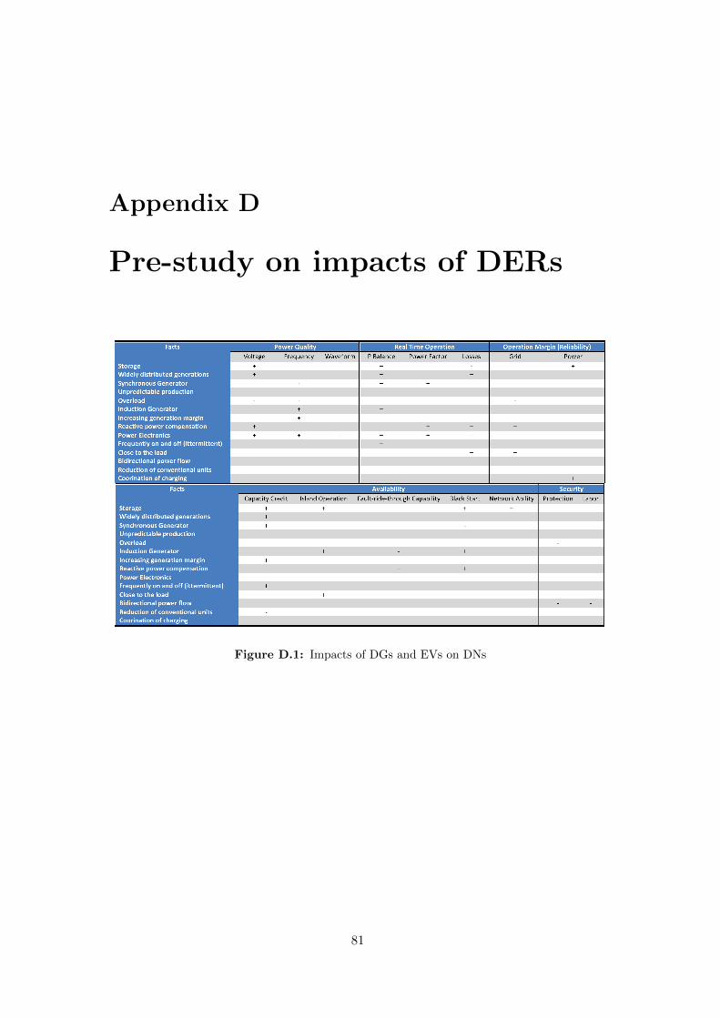
The introduction of DERs will significantly influence the operation of the whole
network (see Fig D1 and Fig D2 in Appendix) The impacts are classified below
bull Power Flow and Power Losses DERs at the terminal of feeders can change the
original power flow even result in a bidirectional power flow to some extent [8][18]
The capacity of transmission lines is released by DGs and the peak load may be
reduced by Demand Side Management (DSM) ie strategically managing the
active demand [11][19] However renewable energy production is hard to predict
and control comparing to the conventional generation sources In some conditions
power losses may be larger
bull Power Quality Power quality includes the following aspects voltage fluctuations
and harmonics [8][20] Large deviations of the production or consumption of DERs
in each hour such as the removal of a certain load or generator cause voltage sag
or swell [8][18] Power electronics configured in the DNs inject some high frequency
harmonics into the DNs as well [8][18]
bull Reliability and Availability The integration of DGs reduces power transmis-
sion and improves the availability of grid and power supply in general It also
benefits to the island operation and black-out start when a large disturbance oc-
curs [13] Some DGs equipped with Automatic Voltage Regulators (AVR) and
Power System Stabilizers (PSS) can help to stabilize the power system frequency
and voltage which improve the reliability of the DNs [11] However large pene-
tration of DGs may trigger the instability of the whole system and give rise to a
poor power factor a poor frequency stability and a strong chance of short-circuit
[18]
Thus some critical problems may occur in the power system especially in DNs
2
12 Goals and Delimitations
Some immediate questions can be addressed such as
bull What happens if a large-scale wind production is introduced in a given DN
bull How big are the consequences
bull Will it affect the voltage profile in the DNs
bull How much power is saved in the DNs by applying energy efficiency actions
bull How large load profile will a given EV fleet introduce to the DN
For Vattenfall the assessment of theses questions is urgently needed to be answered
to maintain a strong grid operation At the same time by analysing different energy
resources available in terms of all the roles in DNs (including DSO) some business
cases (eg Aggregators [15][21]) appear very interesting which could provide economical
profits and strengthened electricity supply facing the changes in DNs For example the
isolated grid of Gotland (connected to mainland Sweden with a HVDC line) with a high
penetration of wind energy requires an extensive upgrade (eg the implementation of
advanced grid management system according to smart grid concept) to enhance the
security of the present grid and the quality of power supply It is therefore interesting
from the DSO point of view to look upon the most possible critical problems in the DNs
of Gotland For more information about Gotland see [22] and [23]
12 Goals and Delimitations
It is obvious that all the DER components own their unique and very complicated sys-
tems and can be modelled in different ways for various purposes Considering the size of
this project all components are simplified and integrated as loads or generators in MV-
DNs The dynamic behaviour is neglected during the modelling In the static analysis
of power system power losses and voltage profiles are the two primary concerns on the
grid operation and planning The reason is that they are directly relevant to the opera-
tional investments and are sensitive to changes in the network [8][15][16][19][24][25][26]
Thus the main task of the thesis project is to interpret changes in the power system
onto different scenarios in the future environment of the Swedish DNs The quantita-
tive results with regard to the voltage profiles and power losses are expected from the
simulations Subsequently the analysis on the challenges caused by the changes can be
assessed based on these simulation results
121 Goals and Objective
The master thesis project has three goals
1 The first goal is to design and implement two reference DNs a meshed and a radial
network see Section41) in Simulink
3
12 Goals and Delimitations
2 The second goal is to construct a toolbox that consists of different DER models
This is done in order to make it possible for simulating and analysing different
scenarios A scenario is further defined in Section 124
3 The third and final goal is to analyse different technical problems arising from the
scenarios ie voltage problems and power losses in the DNs
122 Research Questions
After the thesis work the following questions should be answered
bull Which technical problems are observed in the worst case And in which condition
bull How does different factors (eg season network penetration level etc) affect the
DN Are the impacts beneficial or harmful
And some more questions could be discussed
bull Is it necessary to apply some aggregators to improve the behaviour of DNs
bull What type of aggregators are needed
123 Delimitation
Initial delimitations are summed up below
bull Data sets are based on the real conditions of Sweden (specifically solar irradiation
and historical wind production data from Gotland)
bull Only two specific networks (ie radial and meshed) are modelled for the simula-
tions and are designed to represent the condition in Sweden especially in Gotland
to some extent
bull Only two interesting factors are selected as targets of simulations and analyses
ie voltage fluctuations and power losses in the network
bull Dynamic behaviour and protection issues are not considered in the thesis
bull All the models are integrated at a medium voltage (MV) DN ie 10kV
bull Only consider customersrsquo behaviour in a random weekday
bull Wind power is the only component in the DG dimension
bull Two types of vehicles ie private vehicles (PVs) and commercial vehicles (CVs)
with certain behaviour are simulated
bull Two types of electric vehicles ie pure battery vehicles (BEVs) and plug-in hybrid
electric vehicles (PHEVs) are taken into account
bull Charging infrastructure is only available at home and at work
bull The regulating actions of the DSO is out of the scope of this study The price
sensitivity is only concerning the day ahead prices (not any time of use tariffs etc)
4
12 Goals and Delimitations
124 Definitions and Nomenclature
To clarify the contribution and delimitation of the thesis some important definitions
in the whole thesis work are presented
1241 Distributed Energy Resources
The concept of rdquoDistributed Energy Resourcesrdquo is not clearly defined either by an
authoritative organization nor by an academic project team Yet it is widely used in a
lot of papers reports and books In our project the definition of DER is given as
Definition 1 DERs are regarded as the electric equipment installed in DNs which pro-vide energy or participate in the operation of the power system regardless of producingor consuming power The deployment of DERs in the grid reflects a paradigm shiftregarding how electricity power is in a power system [11][17]
1242 Scenario
A scenario is composed by different DERs in a certain DN during a certain period
(eg a random weekday in the winter) The integration of DERs are influenced by some
external forces such as opinions of policy makers and consumers and the parameters of
the DN ie the peak load of the specific DN DERs are grouped into three dimensions
DGs EVs and ADs To some extent if the integration levels of DERs hit the threshold
values the DSO will have no choice but to either (i) refurbish the network (eg
replace wires install bigger transformers etc) orand (ii) contract ancillary services
from generators and loads to secure the network operation (i) - (ii) will require some
kind of investments from the DSO and how he should act towards this issue is part of
an optimal decision policy problem The DSO is supposed to minimize the overall cost
with respect of keeping the system operation safe reliable and efficient To simplify
the model we assume that the dimensions are independent from one another Hence a
scenario is defined as follows
Definition 2 A scenario is a specific future plan in terms of amount of DERs in acertain DN DERs are defined by three dimensions (DG AD and EV viz the scenariospace) and their potential success is only dependent on external factors such as opinionsfrom policy makers and consumers Furthermore the scenario space is variable iethe dimension can be assigned different numbers Meanwhile the properties of the DNis fixed In the end the scenario should reflect some kind of technical issue of theoperation that the DSO should solve from an optimal decision making policy in networkinvestments
1243 Electric Vehicle
Continuous improvements of storage technologies and a dedicated support from policy
makers promise a bright future for EVs From the power systemrsquos perspective EVs are
5
12 Goals and Delimitations
batteries embedded in transportation facilities charged and discharged in some cases
when connected to the grid
How much when and where EVs are charged are mostly depending on (i) driving
patterns (eg the behaviour of commuters) (ii) the type of EVs (eg PHEVs) (iii)
charging availability (eg at home) For example a private car runs two or three trips
per day within the time periods around 900 - 1700 respectively The length of each
trip is about 20 km in cities The locations available for charging are at home and at
work If the car is a BEV the possible driving range is very limited (typically 20 - 25
km before a recharge is needed [27][28])
Definition 3 EVs are modelled as portable batteries whose behaviour and properties aredetermined by the vehicle types driving patterns and availability of charging facilities
1244 Active Demand
The improved technologies such as dispatched smart-metering system enable the
customers to track the price and consumption in households The trends of of market
deregulation provide much more opportunities of their participation in the system At
the same time new feed-in tariffs and plans to increase energy efficiency lead to a
strong will of advanced activities on the demand side (eg installation of solar panels
new appliances with an energystar label etc) Three segments are set to define AD
regardless of the effects of DSOs (eg cutting off the peak load compensating power to
the grid when isolated) AD dimension is consequently defined as
Definition 4 Active Demand is residential consumers who change their load by either(i) shifting consumption with respect to the electricity price on the day-ahead market(ii) producing their own energy by installing PV panels on their roofs or (iii) updatinghousewares with the purpose of improving energy efficiency In the end these changeswill reshape the load profiles of the households
1245 Dimension 3 ndash Distributed Generation
The installed capacity of DGs is growing stably especially powered by renewable
energy such as wind solar biomass etc Reasons to introduce them are listed in
the book [8] such as the trends of deregulation of Electricity Market environmental
concerns and enhancing the margin between peak load and available production etc
According to [24] the definition of DG is given as
Definition 5 Distributed generation is an electric power source directly connected tothe MV-DNs within the scale of 15 MW Specifically in this project the wind powergeneration is studied due to its popularity and notable intermittent nature
Obviously the operations of different kinds of DGs are independent on their primal
drivings and the interfaces with the electricity grids which will be detailed described in
6
13 Outline of the Report
latter part of this section In view of the development of DG technologies in Sweden
wind power is considered as the only resource in the DG dimension to reduce the contents
of the models Some micro or small size production (eg solar panels) are regarded
as part of AD dimension due to the reason that they are directly connected to the
consumers ie on the customer side of the meters
DG
AD EV
Figure 12 The scenario space - DERs are defined by three dimensions (DG AD andEV viz the scenario space)
13 Outline of the Report
In chapter 2 common methods used in the thesis work are listed and explained
Furthermore some general knowledge of power system theory which is the basis of sim-
ulation is introduced
In chapter 3 introduction and explanations of different components in the DN are
given (eg mechanism of regulation of power production of DGs load profiles of con-
ventional residential loads state of art of the EV technology etc) Different network
topologies are compared two of which are selected as the networks for simulation
In chapter 4 models of different components participating in the networks are de-
scribed with their mathematical algorithms on the basis of their behaviour Models in
the three dimensions are illustrated independently with the rational level of integration
of individual components
In chapter 5 some results of the performed simulations are presented and analysed
A short summary of conclusions obtained in the thesis work is presented in chapter 6
In Chapter 7 an outlook of potential future work can be found
7
Chapter 2
Method
In the first section the study approach of the thesis work is presented followed by
some basic mathematical methods
21 Study Approach
The procedure of the thesis is presented as follows in Fig 21
In the pre-study phase some potential problems in the DNs are studied based on
the fundamental power system theory (eg power flow calculation mathematical mod-
els of the DERs and the DN components in power system) Two target factors ie
power losses and voltage are studied by simulating the scenarios based on the under-
lying models and theoretical algorithms The parameter inputs are from the empirical
observations and the statistics in the related materials such as [29][28] The models
are improved by detecting the difference between expectation and simulation results
eg the availability of vehicles in the network at a certain time The parameters and
algorithms are adjusted until the simulation results meet the real condition based on
historical data The problems revealed from the simulations could further be studied
and solved by for instance aggregators
Figure 21 The Project Procedure - The process of simulation repeats until the perfor-mances of models are close to the results in pre-study literatures and outputs of simulationsare sufficient for the analyses
8
22 Mathematical Method
Other than the method used in the thesis project ie rdquomodelling and simulationrdquo
some other applied procedures can be found in other studies In the book [8] the author
collected a large amount of reliable data of different DERs analysed the data by using
statistic methods and in the end got the conclusions based on the observations In the
large project rdquoMicrogridrdquo[13] some real cases are studied for example a low voltage
level (LV) network study in Portugal Electricity prices line characteristics and their
reliability are studied on the basis of comparison of different countries In the report
[30] the author modelled a fleet of EVs in Monte Carlo simulation models and drew
some conclusions regarding their impact on eg the peak load
To help the DSO to make decisions in network investments the quantified results are
necessary These results could only be accessed by either simulations or study on real
cases Since the pilot network is costly and is absent of existence the only way is to do
the simulations based on the real conditions and available data
22 Mathematical Method
In this section some methods based on probability theory and used in specific algo-
rithms of DERs are described These mathematical methods are carried out to construct
models with specific random factors following certain distributions [31]
Random variable A variable X is a random variable when X is a numerical function
on a probability space Ω function X Ω rarr R ie X is measurable The distribution
of X is described by giving its probability function F (x) = P (X le x) When the
probability function F (x) has the form of F (x) =int xminusinfin f(y)dy X has the density function
f
Normal distribution Normal distribution describes the empirical measurements of
experiments are normally and continuously distributed The density function is given
as following
f(x) =1
σradic
2πeminus (xminusmicro)2
(2σ2) (21)
micro is the mean value and σ is the standard deviation
Lognormal distribution If the random variable χ is normally distributed X =
exp(χ) follows the lognormal distribution The estimation of X EX = emicro+σ2
2
9
22 Mathematical Method
Uniform distribution f(x) = 1 in a certain range (a b) and 0 otherwise
F (x) =
0 x le ax a le x le b1 x gt 1
(22)
Binomial Distribution If the random variable X is said following a Binomial (n p)
distribution if
P (X = m) =
(nm
)pm(1minus p)nminusm (23)
Weibull distribution The density function of a Weibull random variable X is
f(xλ κ) =
0 x lt 0κλ(xλ)κminus1eminus( x
λ)κ x ge 0
(24)
where κ gt 0 is the shape parameter and λ gt 0 is the scale parameter κ = 1 indicates
the exponential distribution while κ = 2 indicates the Rayleigh distribution
Monte Carlo method Some mathematical results could not be strictly proved but
could be derived or estimated when facilitated Monte Carlo methods Applications are
utilized in a lot of fields from decisionsrsquo making to simulations of complicated systems
Monte Carlo methods are those methods which use random samples in a calculation
that has a structure of a stochastic process (ie a sequence of states whose evolution
is determined by random events) [32] If there are an amount of variables (ie system
inputs) and the function of these inputs are complicated Monte Carlo methods can be
used to get a good estimation of the observation (ie system output) It is formulated
as
E(Y ) =1
N
Nsumi
Yi (25)
where Y is the observation and implemented in Monte Carlo methods for N times
Each observation Yi is independent and determined by functions and constrains of vari-
ables x12M
10
Chapter 3
Theory
The basic knowledge in power system analysis is introduced in this chapter For the
simulation purpose the underlying foundation of models are presented in the following
sections Data sets used to model elements in the toolbox are proposed
31 Basic Power System Theory
This section is a brief digest from some power system analysis books
311 DN
Voltage level DN is the last stage in electricity delivery path which carries electricity
from transmission networks to the end users The whole DN can be split up into three
voltage levels corresponding to the nominal value of the voltage (see Table 31) [33]
As mentioned in Chapter 1 MV is selected as the voltage level for simulation and
modelling Usually customers in the low voltage levels are connected to MVs with
step-down transformers in substations Some consumers with large consumptions are
directly connected to MVs Common voltages in MV-DNs in Sweden are 10 kV and 20
kV There are voltage level 3 6 and 33 kV but these are rare [34]
Network topology The simulation approach requires the first step that typical DN
topologies should be identified Usually the MV-DNs in urban area are with loop or
mesh topologies while in rural area with mesh or radial topologies (see Fig 31)
System Nominal Voltage [kV]
LV le 1MV 1minus 35HV ge 35
Table 31 Different voltage levels in DNs[33]
11
31 Basic Power System Theory
However considering the breakers in networks are normally open most networks are
operating as radial ones [13]
(a) Loop (b) Mesh (c) Radial
Figure 31 Typical network topologies[13]
312 Components
3121 Transmission lines
A considerable share of power in MV-DNs are consumed by the transmission lines
instead of loads due to lower voltage and higher current In MV-DNs both overhead
lines and underground cables are commonly used [13] In Sweden the ratio between
these two types of transmission lines is 31 [34] Overhead lines are less expensive than
underground cables but more space consuming [34][35]
Transmission lines are commonly characterized as π model by their resistance Rs
Rs Xs
Bsh
2
Bsh
2
Figure 32 π-equivalent circuit of lines - π-equivalent of transmission line with RsXs and Bsh
series inductance Ls and shunt capacitance Csh as shown in Fig 32 Reactance Xs
is obtained by ωLs while subceptance Bsh is obtained by ωCsh Thus the equivalent
model of the transmission line is derived as
Zs = Rs + jXs (31)
Ysh = jBsh (32)
where
ω is the angular frequency of power system
12
31 Basic Power System Theory
Zs is the series impedance of the line
Ysh is the shunt admittance of the line
The fact that underground cables have larger capacitance and smaller inductance
compared with overhead lines may lead to novel phenomena of voltage and power losses
in feeders [35]
3122 Transformer
Transformers as the interface between MV-DNs and HV-DNs or between LV-DNs
and MV-DNs bring the voltage levels down eg from 60 kV to 10 kV Usually on-load
tap-changers are only utilized on HVMV transformers to keep the voltage constant
without disconnecting any loads while manually tap-changers are utilized on MVLV
transformers and adjusted only once during installation [36]
The equivalent circuit (referring to the primary side) of a transformer as shown in Fig
33 consists of in-series resistance Rp and Rs representing power losses on each side in-
series reactance Xp and Xs resulted from flux leakage as well as the magnetizing branch
reactance Xm in parallel with the iron losses component Rc (see Fig 33)
Figure 33 Equivalent circuit of transformer - Secondary impedance is referred tothe primary side [36]
313 Calculations in Power System
3131 Power flow
Power flow calculations in general enable a certain power system to indicate voltage
magnitude and angle in each bus active and reactive power flow between each bus The
identified known and unknown quantities in the system determine types of buses (ie
PQ bus PV bus slack bus) Then calculations could be implemented by power balance
equations
0 = minusPi +Nsumk=1
| Vi || Vk | (Gik cos θik +Bik sin θik) (33)
13
31 Basic Power System Theory
0 = minusQi +
Nsumk=1
| Vi || Vk | (Gik sin θik minusBik cos θik) (34)
where Gik and Bik can be obtained from the admittance matrix YBUS
3132 Power losses
The reason to choose which voltage level of the grid much depends on power losses
which are transformed into heat When power losses decrease the maximal capacity on
lines mainly due to the limit of thermal capacity could increase Power losses on the
level of 10 kV are about 3 times of those on the level of 20 kV [34] Other than the
technical factors the design of system operation could also affect the total losses in the
system Power losses Ploss in power system follow such formulas
Ploss = I2R (35)
I =S
U(36)
where
R is the resistance of the transmission line [Ω]
I is the current flowing through the line [A]
U is the voltage difference between two ends of the line [V]
S is the absolute value of complex power given byradicP 2 +Q2 [VA]
3133 Power factor
In power flow calculation two components are obtained as active power [W] P which
transfer energy and reactive power [Var] Q which move no energy to the loads Hence
power factor is defined as
powerfactor =| cosϕ |= P
S=
PradicP 2 +Q2
(37)
When powerfactor = 0 the power flow is purely reactive When powerfactor = 1
only active power generated by the source is consumed Power factors are expressed as
rdquoleadingrdquo or rdquolaggingrdquo to show the phase angle ϕ
3134 Voltage variation and weakest point
For safety concerns there are limits of network voltage to protect equipments con-
nected to the system According to the European Standard EN50160 [20] the voltage
magnitude variation should not exceed plusmn10 for 95 of one week measured as mean
10 minutes root-mean-square (RMS) values The consumption will result in a voltage
drop on the feeder The further away from the substation bus the lower the voltage
14
32 Comparison of Network Topologies
will be On the contrary the connection of generations will lead to a voltage rise on
the feeder The interaction of consumption and generation in MV-DNs therefore causes
voltage variations
The voltage variation in steady state is approximately equal to
∆U
Usim=RlinePG +XlineQG
U2middot 100 (38)
With a given limit on the variation of the voltage ∆Umax the maximum allowed
produced active power from a connected generator can be derived as
Assume that the power factor is constant Then Qmax = α lowast Pmax
According to the equation (38)
∆Umax =(R+ α middotX)PGmax
U(39)
rArr
PGmax =∆Umax
(R+ α middotX)U(310)
From Equation 39 we can derive that when the nominal voltage value and feed-in
power are constant larger equivalent impedance leads to larger variation in voltage In a
power system the weakest point is the load point where the equivalent impedance is the
largest Usually the most critical voltage problem appears in the weakest point The
equivalent impedance is called Thevenin equivalent impedance which is usually decided
by the distance from the slack bus material of transmission line and the topology of
the network
3135 Penetration levels
The penetration levels of DER components indicates the share of them in the whole
network The penetration level is expressed as the ratio between the installed capacity
of DER components and the peak load value
micropen = 100
(sumPnomG
P peakL
)(311)
32 Comparison of Network Topologies
The DNs directly connect to the end users Their topologies and sizes are different
among areas depending on the operation concepts utilized devices and the load profiles
Thus voltage quality reliability and power losses in this stage are interesting aspects to
study in DNs Several electrical network models are developed as test systems to analyse
one or more specific characteristics (eg voltage regulation unbalanced load reliability
15
32 Comparison of Network Topologies
of system etc) However a majority are developed to study power system reliability
which indicates that they are not of sufficient details to the level upon which our research
questions could be addressed Additionally there are some network models for power
flow analysis but their sizes are too large to be implemented in Simulink Matlab For the
purpose of investigating the integration of DERs in a future DN reasonable test networks
are required for a sufficient analysis of the simulation results and a correct direction for
further network studies The DNs are studied at a medium voltage level ie 10 kV
From literature review study several typical existing test networks are acknowledged
described and compared [13][37][38][39] Their topologies can be found in the Appendix
321 Description of Several Networks
bull IEEE Test Feeder ndash IEEE Comprehensive distribution test feeder developed by
IEEE Working Group is presented on the IEEE website It consists of 55 buses
two voltage levels and 25 loads which represent a wide variety of components
in one circuit [40] It is a large radial network It is possible to connect some
switches in the network to form a small loop Some other types of modules (eg
identical feeders connected to the same bus radial structure with loads distributed
on feeders) are presented in the network Examples of all the components in the
network are provided in the work document The network allows all the standard
components of a distribution system to be tested (See Fig A2 in appendix for
the topology)
bull Bornholm Test Network ndash The Bornholm Test Network is modelled based on
the real distribution network in Bornholm an island of Denmark with 2 voltage
levels 11 buses 9 transmission lines 7 loads and 3 distributed generations The
detailed parameters of the network are not available However the general network
data can be found in [37] (refer to the topology in Fig A1 in the appendix)
bull Swedish Test Systems ndash The Swedish Test Systems are developed by Elforsk
a Swedish industry research association to analyse the reliability of Swedish net-
works and the electricity market in Sweden The test systems include two distri-
bution systems one for the urban area (ie SURTS) and the other one for the
rural area (ie SRRTS) Loads component data are well represented by these test
systems due to the support from and involvement of Swedish power distribution
companies SURTS is a 10 kV system with 10 identical feeders in cable-loop de-
sign while SRRTS consists of two modules both of which are radial structure
Reliabilities load data and outage costs are specified in the model [34] (refer to
the topologies in Fig A3 and Fig A4 in the appendix)
16
32 Comparison of Network Topologies
bull The Gotland Network - An isolated mixed network ie both urban and rural
networks with a big share of wind power generation [41] A typical feeder in
the network consists at least 20 load points Shunt capacitors are installed in
the network at the MV level Wind power is directly and particularly connected
to the substation bus with a transformer Load data and parameters of network
components are available It is accessible for the simulation in future work The
edge of the feeder could be regarded as a normally open switch or a big load Some
typical structures of feeders could be selected to represent the whole MV network
after analyse both topologies and load characteristics of the network
bull The German Network - The German test network is provided for the EU project
More Microgrids The description is in the work package G deliverable 1 of More
Microgirds The test system consists of two MV networks (ie urban and rural)
and a detailed LV network for study Line parameters and load profiles are well
presented in the document The MV networks are taken from existing networks
considered to be typical The LV network is an artificial network with different
structure for different load segments The structure of urban MV network is similar
to the Swedish one but the loop circuit is closed by two paralleled feeders with a
normally open switch in between The rural MV network is a 20kV mesh system
with 2 external connection points and 14 buses 15 loads (with static state values
in the figure) and 2 generations are involved in the network Initial power-flow
calculation is described in the figure for different lines and loads Compared with
Swedish rural one the topology is more complicated but with less components in
the network [13]
322 Comparison of Key Parameters
A discussion on the listed test networks is conducted by comparing their complexity
and representativeness Table 32 shows some key parameters of these networks
Table 32 Comparison of demonstrative parameters of test network
Network Voltage Level Buses Loads GenerationsTopology
IEEE NA 55 25 5 meshBornholm 60 kV10 kV 11 7 3 radialSURT 130 kV10 kV 62 60 0 loopSRRT 40 kV10 kV 19 many 0 radialGerman urban kV20 kV 83 81 NA loopGerman rural kV20 kV 14 15 2 meshGotland 70 kV11 kV hundreds mesh
17
32 Comparison of Network Topologies
Complexity From the description part it is shown that Bornholm test network
and German rural network are much simpler than the other ones The Bornholm net-
work does only consist of 11 buses and German one of 14 buses which simplifies the
quantities of parameters and the analysis of phenomena in simulations Part of the Ger-
man network is selected as mesh network for simulation with 11 buses 8 load points
and two locations for generations The other part of the network is connected with
another substation bus and is isolated to the selected part during normal conditions
Seven or eight load points in the network are sufficient to implement different consumer
categories (ie residential commercial industrial) and to assign EVs together with
loads randomly Some large scale distributed generation such as wind power can be
directly connected to the 10 kV level or a even higher voltage level Those generations
in small scales such as Photovoltaic (PV) panels can be connected in parallel with the
residential load denoting that connecting points are in lower voltage level
Some other simple test systems developed by IEEE [40] are proposed to study unbal-
anced systems and voltage regulators in a very long feeder which do not fit the condition
in this project and the characteristics of real Swedish DNs
Representativeness The network condition in Gotland is similar to that in Born-
holm The restructured German rural network and the DNs in Gotland have some
mutual features To obtain a better representation typical parameters are chosen ac-
cording to the real condition in Gotland (eg the proportions of cables and overhead
lines the distance between buses the voltage levels) The radial network could repre-
sent a typical radial feeder and the first part of a loop feeder with normally open switch
Besides some features of it are set for comparison Feeder B2 is quite short while feeder
B3 is longer which means that buses in B2 can be regarded as rdquostrong gridrdquo compared
with those in B3 In addition B4 and B5 are compared to show the difference between
cables and overhead lines Thus most of technical effects due to the topology of the
network are considered in the test system Since the meshed network is well presented
in the report [13] all properties and characteristics of the cables are modelled based on
the real condition
The IEEE test system SURT and SRRT are all intended for reliability analysis which
indicates that there is no detailed parameters within the documentation In addition
the size of these test systems is a way to large and is not appropriate for the simulation
in Simulink
18
33 Wind Power as DGs
33 Wind Power as DGs
Wind energy is one of the major growing renewable energy technologies in the recent
years Wind power is intermittent and hard to manage which may lead to the voltage
sag or swell usually in a short period The deviation between the real wind production
and and the predicted production may result in grid outages For those wind turbines
equipped with induction generators reactive power is absorbed by them which bring
about a poor power factor and less active power capacity of the transmission line From
an economic perspective additional reactive power compensating devices are costly and
mostly installed in HV networks (to secure the reliable system operation) Wind speed
always reaches the peak value in the winter However for safety concerns a strict
temperature limit (eg minus40C) and speed limit (eg 25 ms) will force the turbines
to cut off their whole production The extracted power curve fits the demand curve in
Sweden because the peak load in Sweden also appears in the winter time Aggregation
of a large geographically spread wind power can reduce the impact of meteorological
influence and improve the accuracy of the prediction significantly [26]
Figure 34 General Structure in WindTurbine Block
331 Operation Mechanism
The wind turbine is the device that extract mechanical power from wind power going
through its swept area and then to transfer energy to electricity (see Fig 34) The
power output of the turbine is given by the following equation [42]
Pm = Cp(λ β)ρA
2v3w (312)
Tm =Pmωel
(313)
19
33 Wind Power as DGs
where
Cp is coefficient of extracted wind power
λ is tip speed ratio of rotor blade tip speed and wind speed
β is blade pitch angle
ρ is air density (kgm3)
A is the tip swept area (m2)
vw is wind speed ms
ωel is the rotation speed of generator (rads)
A generic equation is used to model Cp [43]
Cp(λ β) = c1
(c2
λiminus c3β minus c4
)e
minusc5λi + c6λ (314)
in which1
λi=
1
λ+ 008βminus 0035
β3 + 1 (315)
Power curves of different type of turbines are unique due to different control methods
different blade lengths different tower heights etc in which rdquocut-in speedrdquo rdquocut-off
speedrdquo rdquorated speedrdquo and rdquorated powerrdquo are the main features of the power curve A
typical power curve is shown in Fig 35 [44]
Figure 35 Typical power curve of wind turbine - Power curves and other technicaldata of wind turbines are given in the product brochures[44]
332 Historical Data
The occurrence of wind speed follows a Weibull distribution and there is little corre-
lation of wind speeds in neighbouring hours Meanwhile the direction and turbulence
of wind are other two main factors which affect the production of electricity Except for
these factors the turbine structures regulation strategies location of the wind farm
and the distribution of wind turbines have a large impact on the production Hence
as a static model the aggregated wind power is depicted as the generation changing on
20
34 EV Fleets and Behaviours of Customers
an hourly basis in a MV-DN at the generation point in the network Fig 36 shows the
variation of total wind production on Gotland throughout the whole year 2010 [41]
0 30 60 90 120 150 180 210 240 270 300 330 3600
10
20
30
40
50
60
70
80
90
Day
Tota
l W
ind P
roduction [M
W]
Figure 36 Total production of wind turbines on Gotland in 2010 - The datarecords production in each hour in the whole year [41]
34 EV Fleets and Behaviours of Customers
EVs are vehicles that at least are partly powered by electricity or use electric motors
as the direct propulsion Transport sector is one of the most important and largest part
of energy consumption and the energy use in transport sector is dominated entirely by
oil products (eg petrol diesel etc) in Sweden[45] For the purpose of reducing the
emission of CO2 and improving energy efficiency the deployment of a large amount of
EVs can be envisioned in a near future
On-board batteries the core of the EV technology introduce a large amount of
possibilities to the power system to interact with them via charging facilities (eg
plug-in electric outlets) Without considering the effects of management and control
the charging behaviour is mainly dependent on three factors
I Driving patterns In our case only Private Cars (PrV) and Commercial Vehi-
cles (CV) are considered The statistics of travelling behaviour in Sweden (eg
numbers of trips per day the distance covered by on e trip hours of the trips
etc) are collected based on [28] and [29] Table 33 implies that each household in
Sweden own one car in average and EVs are not commonly deployed until now
Table 34 presents the general trip length in different areas and the time consumed
in each trip In Fig 37 the blue curve and the black one illustrate two types
of driving patterns in a day It gives the primary understanding on how vehicles
behave in Sweden
II Types of EVs Among various types of EVs we took Plug-in Hybrid Electric
Vehicles (PHEVs) and Pure Battery Electric Vehicles (BEVs) into our considera-
21
34 EV Fleets and Behaviours of Customers
Table 33 Swedish fleet in traffic in 2010 [29]
Type of Vehicles Private Cars Commercial Cars Heavy Vehicles Others
No of Vehicles 3 446 517 1 376 358 526 441 1 869 683
Type of fuel Petrol Diesel Electricity Other
No of Cars 3 479 607 606 570 190 248 815
Table 34 Average Commuting distances and time[28]
Municipality Groupings Distance [km] Time [mins]
Urban Area 20plusmn 1 42plusmn 3Suburban Area 25plusmn 2 40plusmn 2Rural Area 28plusmn 2 41plusmn 1Total 23 41
Figure 37 Starting time for different types trips in 24-hour period (times103) [28]
Table 35 Comparison of capacities of different types of EV[27] - shown in differentcoloured curves
Type of Vehicles Battery Capcity [kWh]
BEV 25 sim 35City-BEV 10 sim 16PHEV90 12 sim 18PHEV30 6 sim 12
tion Compared to PHEVs (with internal combustion system) BEVs (with pure
electricity propulsion) need a larger battery capacity According to the report [27]
typical capacities are shown in Table35
III Charging patterns Charging facilities for different purpose in different area are
assumed planned well to fulfil the basic requirements of EV charging Depending
22
35 Load Profiles in the MV Level DNs
on the preferences of car owners three possible charging approaches1 are proposed
as listed in Table 36 [27]
In reality the charging curve is not a straight line but with some variations
Table 36 Different types of charging [27]
Type of Charge Load Charging time
Slow le 5 kW ge 4 hoursStandard 5 kW - 20 kW 1 hour - 4 hoursFast ge 40 kW le 1 hour
of the slope along the charging process Fig 38 shows one typical real charging
curve For simplicity we assume that the charging current is constant (ie the
curve is a straight line)
Three stages of charging places are stated in [27] as (1) at home (2) at home
and at work (3) everywhere Different charging approaches correspond to different
charging places
Figure 38 Typical charging curve - This is a charging curve of Li-Ion batteries whichcould be idealized or linearised[27]
35 Load Profiles in the MV Level DNs
Flexible residential loads is an important part of our scope The conventional load
profile is reshaped by modifying actions Loads of other sectors are excluded which are
assumed that they have already made their own optimized modifications on their loads
1Charging time depends on the size of battery
23
35 Load Profiles in the MV Level DNs
Figure 39 Structure of the hourly load curve of apartments - Apartment withtwo people (25-65 years old) Workdays
Figure 310 Structure of the hourly load curve of houses - House with two people(25-65 years old) Workdays)[46]
24
35 Load Profiles in the MV Level DNs
351 Conventional Residential Load
According to the report Statistics Sweden 2011 [29] the distribution of houses and
apartments are quite even especially in cities According to [46] the most representa-
tive pattern is a two persons apartment or house Thus the load profiles on an hourly
basis of these patterns are collected as the original residential load profiles in our study
To perform price sensitive strategies different type of household appliances are classified
(eg Dish washer heating white goods etc) Usually heating and water heating in
apartment buildings are not accounted into the consumption of electricity while direct
electric heating is (eg from heat pumps) Subsequently the profiles are presented in
Fig 39 and Fig 310 with different appliances in different colors
As described in [34] the density of residential customers at the LV-DNs are 20(km
of line) in the urban area and less than 10(km of line) in the rural area respectively
Thus the numbers of customers in each load points in the network model are set to
be around 500 for the urban area and 200 for the rural area The load curve of an
apartment is based on the data set in [47] with 120 units aggregated (ie a whole
building) The load curve of a house is based on the data set for a two person (25-65
years old) household (with direct electric heating) measured and presented in the report
[46] In general rdquoone appliancerdquo of the data set refers to an average value of a group of
appliances in the households
Temperature is an important factor influencing the consumptions of different ap-
pliances of which the seasonality effects coefficients are assigned in the report [46] as
well To simplify the model coefficients of four seasons are selected to represent the
temperature factors (see Table 37)
Table 37 Seasonal Coefficients of Appliances[46]
Appliances Spring Summer Autumn Winter
White goods 09 10 09 07Lighting 14 10 22 16Audio and TV 13 10 15 19Cooking 13 10 13 17Heating 10 03 10 25
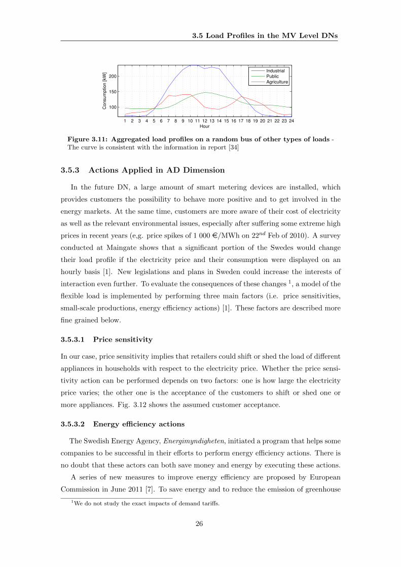
352 Other Types of Loads
In [34] some real load profiles of different load types are given Since only the
residential loads are interesting the combination of other types are distributed in the
network As an example Fig 311 shows different loads profiles (industrial public and
agricultural)
25
35 Load Profiles in the MV Level DNs
1 2 3 4 5 6 7 8 9 10 11 12 13 14 15 16 17 18 19 20 21 22 23 24
100
150
200
Hour
Consum
ption [kW
]
Industrial
Public
Agriculture
Figure 311 Aggregated load profiles on a random bus of other types of loads -The curve is consistent with the information in report [34]
353 Actions Applied in AD Dimension
In the future DN a large amount of smart metering devices are installed which
provides customers the possibility to behave more positive and to get involved in the
energy markets At the same time customers are more aware of their cost of electricity
as well as the relevant environmental issues especially after suffering some extreme high
prices in recent years (eg price spikes of 1 000 eMWh on 22nd Feb of 2010) A survey
conducted at Maingate shows that a significant portion of the Swedes would change
their load profile if the electricity price and their consumption were displayed on an
hourly basis [1] New legislations and plans in Sweden could increase the interests of
interaction even further To evaluate the consequences of these changes 1 a model of the
flexible load is implemented by performing three main factors (ie price sensitivities
small-scale productions energy efficiency actions) [1] These factors are described more
fine grained below
3531 Price sensitivity
In our case price sensitivity implies that retailers could shift or shed the load of different
appliances in households with respect to the electricity price Whether the price sensi-
tivity action can be performed depends on two factors one is how large the electricity
price varies the other one is the acceptance of the customers to shift or shed one or
more appliances Fig 312 shows the assumed customer acceptance
3532 Energy efficiency actions
The Swedish Energy Agency Energimyndigheten initiated a program that helps some
companies to be successful in their efforts to perform energy efficiency actions There is
no doubt that these actors can both save money and energy by executing these actions
A series of new measures to improve energy efficiency are proposed by European
Commission in June 2011 [7] To save energy and to reduce the emission of greenhouse
1We do not study the exact impacts of demand tariffs
26
35 Load Profiles in the MV Level DNs
Figure 312 The acceptance of customers on different appliances - [19]
gases some products and actions are recommended to improve the efficiency of energy
consumption For example to replace light bulbs with Compact Fluorescent Lamps
(CFLs) at home or in public areas to use energy-efficient housewares to enhance the
insulation of buildings Subsequently the reduction of consumption can be ob-
tained However different actions (like the change of lamps) may lead to other negative
results (eg change of power factor harmonics introduced in the network etc) When
considering an individual household the change is tiny which can be ignored compared
with consumption on the bus
3533 Small scale production ndash PV panels
Small scal production is considered as the production units that have a power output
of typically a couple of kWrsquos and are connected directly to the loads (like PV panels
micro CHPs)
A few decades ago limited by high cost solar photovoltaic is not that prevalent as
nowadays The price of PV cells has significantly been reduced while the efficiency is
increased due to the new technology advancements and the manufacturing process [48]
According to [45] the electricity production of solar in Sweden is about 200 MWh in
2009 And a variety of forms of grants and subsidies for solar cells in Sweden promise
a blooming trend of their development To interpret this trend into the thesis work
the PV model is created as the small scale production to indicate its influence on the
residential load profile Data are collected from [49] where the sizes of PV panels on the
roofs are determined as 20 m2 for each house and 3 m2 for each apartment respectively
A PV cell can produce current under its exposure to the sun Thus it is reasonable
to model it as a diode together with an equivalent current source depending on the
27
35 Load Profiles in the MV Level DNs
Figure 313 The Equivalent Circuit Diagram of Photovoltaic Cell
environment temperature and irradiation of the sun (see Fig 313) In some papers
instead of a current source the author modelled the PV cell as a voltage source of which
the output voltage is stablized around the system voltage and the output current are
influenced by the environmental temperature and the irradiation of the sun [48]
VC = CV
(AkTref
eln
(Iph + Io minus IC
Io
)minusRsIC
)(316)
Iph = CI middot Isc (317)
IPV = IC middotNS (318)
VPV = VC middotNP (319)
where
NS is the amount of series cells in a panel
NP is the amount of paralleled cells in a panel
VC is the output voltage of a PV cell
IC is the output current of a PV cell
Iph is the photocurrent produced by the semiconductor in the PV cell
Isc is the short-circuit current of the equivalent circuit
Io is the reverse satiation current of the diode (00002A)
RS is the series resistor in the equivalent circuit to reshape the I V curve according to
the open circuit voltage
A is a curve adjusting factor to fit the model curve to the real one
k is the Bolzmann constant as 138times 1023 JK
Tref is the reference operation temperature given by the manufacturer
e is the quantity of a single electron as 1602times 10minus19 C
28
35 Load Profiles in the MV Level DNs
CV is the coefficient of voltage caused by the temperature and the irradiation
CI is the coefficient of current caused by the temperature and the irradiation
From [50] the coefficients of the voltage and the current CV and CI can be described
by two decoupled part temperature dependent coefficients and irradiation dependent
coefficients as
CTV = 1 + βT (Tref minus Tx) (320)
CTI = 1minus γTSref
(Tref minus Tx) (321)
CSV = 1minus βTαS(Sref minus Sx) (322)
CSV = 1minus 1
Sref(Sref minus Sx) (323)
where
Sref is the reference operation irradiation given by the manufacturer
βT is the PV cell output voltage versus the temperature coefficient
αS is the slope of the change in the temperature due to a change of the solar irradiation
level
γT is the module efficiency
The V-I characteristics curve is shown in Fig 314
Figure 314 V-I Feature Curve of a PV cell
It is obvious that the PV production is mostly affected by the solar irradiation
and temperature The production in the winter is very low compared to the sum-
mer conditions Some seasonal factors are introduced in the simulation to reflect these
effects The PV panel production is estimated by applying historical irradiation data
from NASA as shown in Fig 315 [51]
29
36 Estimation of the Development of DERs and the Changes of Activitiesin DNs
1983 1987 1991 1995 1999 20030
01
02
03
04
05
06
07
Day (19830701 ~ 20050630)
Cle
arn
ess I
nd
ex
Figure 315 Historical data of Clearness Index on Gotland - Clearness Index isproportional to the production of PV cells [kWm2d]
36 Estimation of the Development of DERs and the Changesof Activities in DNs
As mentioned a lot of targets related to energy and environment are set The most
important target is the EU 202020 targets (see [2]) The targets as the short-term
plan are applied and need to be met in 2020 while the long-term planning can be ex-
tended to 2050 Thus it is necessary to estimate how the electricity market and the
future DNs look like
In the annual report Energy in Sweden in 2010 [45] the new climate and energy
policies are presented These are (i) The proportion of energy supplied by RES should
be 50 larger than the annual energy consumption in Sweden by 2020 (ii) Vehicles in
Sweden should be independent of fossil fuels by 2030 (iii) The efficiency of energy use is
required to be improved to reduce 20 in energy consumption between the years 2008
to 2020 (iv) 40 reduction in greenhouse gas emissions needs to be met by 2020 in
comparison with 1990 while the target no greenhouse gas emission by 2050 is set for
a longer vision
Aiming at these targets the changes in the future DNs are implemented in accor-
dance with the three dimensions in scenarios Table 38 gives a first idea of these future
developments
Table 38 Estimation of evolution of DERs
DER Short-term Long-term
DG 30 of the peak load ge50 of the peak loadEV 20 of total vehicles 50 of total vehiclesAD 20 of total customers 50 of total customersADenergyefficiency ndash 20 reduction of load
30
Chapter 4
Construction of the SimulationToolbox
This chapter focuses on the modelling of DNs and DERs based on the theory stated in
the previous chapter The radial and meshed network models are presented in the first
section where some important parameters are listed in table form The algorithms and
parameters for the DER models are given in the following sections
41 Network Model
In Simulink two different network models are constructed To capture their static
characteristics both generation and loads are constituted as Load blocks in Simulink
ie generation is indicated as the negative input and the consumption as the positive
one To detect the voltage and power flow on each bus Scopes are added with some
sufficient Transformation blocks Other components (eg switches) and functions can
be joined into the model for further study The network parameters are based on the
report [13] (see Chapter 3) and summarized in Section 45 The topologies of these
networks are shown in Fig A5 and Fig A6 respectively In these two networks
the number of individual residential loads are about 3800 (radial) and 1800 (meshed) 1
Detailed data concerning these two networks can be found in Table 41 Fig A7 and
Fig A8 in Appendix
Table 41 Comparison of demonstrative parameters of DN topologies
Topology Voltage Level Buses Loads Generators Referring Network Peak Load
Radial 60 kV10 kV 11 7 3 Bornholm [37] 15MWMeshed 60 kV10 kV 11 8 2 German rural [13] 20MW
1Numbers of loads are defined according to the report [13] corresponding to the real conditions indifferent types of Swedish areas in which about 400 residential loads are connected to each load point
31
42 DG Model
42 DG Model
421 Wind Power
0 1 2 3 4 5 6 7 8 9 1011121314151617181920212223240
20
40
60
80
Sprin
g
0 1 2 3 4 5 6 7 8 9 1011121314151617181920212223240
20
40
60
80
Sum
mer
0 1 2 3 4 5 6 7 8 9 1011121314151617181920212223240
20
40
60
80
Autu
mn
Time [Hr]
0 1 2 3 4 5 6 7 8 9 1011121314151617181920212223240
20
40
60
80
Win
ter
Time [Hr]
Figure 41 Wind power production on 24-hour base
A cluster of wind power plants from one wind wind park is modelled as an aggre-
gated generation unit connected to the MV-DNs at the production points Their pro-
duction profiles are depicted on an hourly basis and their volumes are collected from
[41] (source wind production data of Gotland in year 2010) To capture the features
of wind generation the mean values and deviations are calculated and it is assumed
to follow a normal distribution with high deviations [52] An example of production
profiles in four different seasons are shown in Fig 41 The potential production of
wind power is determined by the penetration level of DG microDGpen ie the ratio between
the installed DG capacity and the peak load The aggregated wind generation and their
sizes are presented in Table 42 with respect to the peak load The unit names can be
found in the topologies of network models (See Fig A6 and Fig A5)
Table 42 Location and the penetration level of wind power
Network Radial network Meshed network
Unit Name G1 G2 G3 G1 G2Penetration 2
7microDGpen
37micro
DGpen
27micro
DGpen
13micro
DGpen
23micro
DGpen
32
43 EV Model
43 EV Model
431 Algorithm of Modelling
EV Fleet
Urban Rural
Private Vehicles
Commercial Vehicles
Private Vehicles
Commercial Vehicles
BEV PHEV
SOCTrip Type
Battery Size
70 30 90 10
50 50
1
1
Figure 42 Characteristics of EVs - Assign characteristics by different classes
There are two types of EVs studied in this paper ie Pure Battery Electric Vehi-
cles (BEVs) and Plug-in Hybrid Electric Vehicles (PHEVs) The total number of EVs
is in proportion to the number of households in the studied area defined by microEVpen It
is assumed that if one EV leaves the geographic area reflecting the studied distribution
networks an EV with the same features will enter
The EV fleet is defined by driving patterns type of vehicles and the availability of
charging facilities of which the statistics of the parameters are described in the section
34 The EV fleet is randomly split into different classes as shown in Fig 42 With the
categorized properties the EVs are performed on the state transitions
Three states for EVs are set rdquoRunning (0)rdquo rdquoCharging (1)rdquo and rdquoParking (2)rdquo
The initial states of all EVs are assumed to be at home and charging In each time
step according to the last state of the EVs different transition procedures are applied
The State of Charge (SOC) power consumption duo to charge remaining trip length
and numbers of completed trips are updated at the beginning of each iteration The
33
43 EV Model
algorithm is described by the flowchart in Fig B2
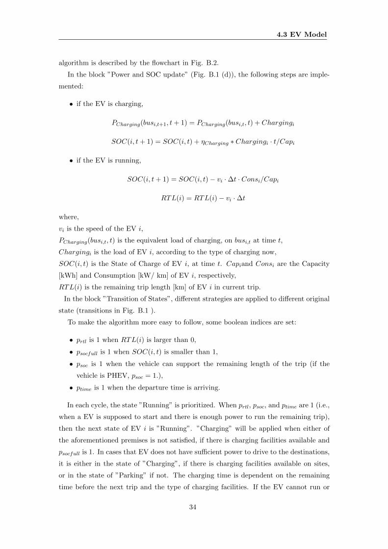
In the block rdquoPower and SOC updaterdquo (Fig B1 (d)) the following steps are imple-
mented
bull if the EV is charging
PCharging(busit+1 t+ 1) = PCharging(busit t) + Chargingi
SOC(i t+ 1) = SOC(i t) + ηCharging lowast Chargingi middot tCapi
bull if the EV is running
SOC(i t+ 1) = SOC(i t)minus vi middot∆t middot ConsiCapi
RTL(i) = RTL(i)minus vi middot∆t
where
vi is the speed of the EV i
PCharging(busit t) is the equivalent load of charging on busit at time t
Chargingi is the load of EV i according to the type of charging now
SOC(i t) is the State of Charge of EV i at time t Capiand Consi are the Capacity
[kWh] and Consumption [kW km] of EV i respectively
RTL(i) is the remaining trip length [km] of EV i in current trip
In the block rdquoTransition of Statesrdquo different strategies are applied to different original
state (transitions in Fig B1 )
To make the algorithm more easy to follow some boolean indices are set
bull prtl is 1 when RTL(i) is larger than 0
bull psocfull is 1 when SOC(i t) is smaller than 1
bull psoc is 1 when the vehicle can support the remaining length of the trip (if the
vehicle is PHEV psoc = 1)
bull ptime is 1 when the departure time is arriving
In each cycle the state rdquoRunningrdquo is prioritized When prtl psoc and ptime are 1 (ie
when a EV is supposed to start and there is enough power to run the remaining trip)
then the next state of EV i is rdquoRunningrdquo rdquoChargingrdquo will be applied when either of
the aforementioned premises is not satisfied if there is charging facilities available and
psocfull is 1 In cases that EV does not have sufficient power to drive to the destinations
it is either in the state of rdquoChargingrdquo if there is charging facilities available on sites
or in the state of rdquoParkingrdquo if not The charging time is dependent on the remaining
time before the next trip and the type of charging facilities If the EV cannot run or
34
43 EV Model
get charged then the state of EV i will be set as rdquoParkingrdquo For observations states
location and SOC in each time instant for every EV are recorded in matrices together
with the equivalent load matrix
432 Parameter Sets for Simulations
Table 43 Allocation of characteristics of the EV fleet
Network PrVCVSpeed Consumption Trip Length Trip Type[kmh] [kWkm] [km] 1 2 3 4
Urban
PrV40 012
20(std)02 03 04 01
(70) plusmn1CV
25 018100 (std)
05 045 005(30) plusmn5
Rural
PrV60 018
28(std)02 03 04 01
(90) plusmn15CV
30 022100 (std)
05 045 005(10) plusmn10
Allocation of parameters for different types of EVs
The percentage of PrVCV and PHEVBEV are random numbers following a normal
distribution so as departure time of each trip and the capacity of battery in each vehicle
Trip lengths of all trips follow a log-normal distribution Table 43 and Table 44 shows
characteristics of the EV fleet
Due to the effect of temperature the consumption of the EVs vary Hence the
common seasonal factor is introduced to reflect the effect of temperature to some extent
Possibility of charging and charging type
The availability of the charging facilities determine the possibilities to be charged in
Table 44 Capacity of Battery of each PHEVBEV[kWh]
Type Cap Mean Cap Dev
PHEV 9 3BEV 25 5
the model If the available charging duration is less than 1 hour there is no chance for
charging (ie no fast charging utility) if the available charging duration is less than 4
hours and more than 1 hour the possibility of charging is 03 and the charging type is
standard charging if the available charging duration is even longer or the EV is at home
( the initial place) the charging possibility is 1 and the charging type is slow charging
Commuting patterns and corresponding probabilities (see Table 45)
After studying the customersrsquo behaviour a number of trip types are designed with
different possibilities as shown in Table 43
35
44 AD Model
For PrVs four possibilities are considered
bull Two trips a day One is in the morning and the other one is in the afternoon (go
to work and go back home)
bull Three trips a day Except for those two trips there is one extra trip for leisure
after work
bull Four trips a day Except for those two trips there are two extra trips for leisure
at noon
bull No trip in the whole day
For CVs three possibilities are considered
bull One trip a day running since morning
bull Two trips a day One is in the morning the other one is in the afternoon
bull No trip in the whole day
Table 45 Trip Types of different types of EV[27]
Type of Vehicles Type of trips Departure time Possibility
PrV
1 9 12 13 17 022 9 17 24 24 033 9 17 19 24 044 24 24 24 24 01
CV
1 9 24 24 24 052 9 13 24 24 0453 24 24 24 24 005
433 Individual Results
By applying the algorithm stated above the simulation result can be derived as shown
in Fig 43 In Fig 43 (b) we can observe that the critical situation appears in the
evening around 8 pm when most of the vehicles drive back home and start to charge
There are two dips of the equivalent load curve at noon since some vehicles drive off
for lunch and cannot connect to the grid
44 AD Model
To evaluate the consequences of the changes on the demand side a general model of
the flexible loads is developed according to the discussion in Chapter 3 [1] with the con-
sequence as a reshaped load profile (see Fig 44) Smart meters control the operation
of the appliances by reading the electricity price on an hourly basis DCAD converters
transmit the power production of PV panels to supply consumption of appliances and
36
44 AD Model
0 1 2 3 4 5 6 7 8 9 10 11 12 13 14 15 16 17 18 19 20 21 22 23 241
2
3
4
5
6
7
8B
us
0 1 2 3 4 5 6 7 8 9 10 11 12 13 14 15 16 17 18 19 20 21 22 23 240
010203040506070809
1
SO
C [
]
0 1 2 3 4 5 6 7 8 9 10 11 12 13 14 15 16 17 18 19 20 21 22 23 240
1
2
run(0)charge(1)park(2)
Sta
te
(a) The state of a certain EV in the simulation
0 1 2 3 4 5 6 7 8 9 10 11 12 13 14 15 16 17 18 19 20 21 22 23 240
10
20
30
40
50
60
70
80
Eq
uiv
ale
nt
loa
d p
rofile
of
EV
s [
kW
]
Time [Hr]
(b) Equivalent load curve of EVs in Bus4
Figure 43 Individual Results of the model of EVs
Figure 44 Typical structure of a house as a flexible demand - residential applianceswith smart meters PV panels and DCAC Converters [49]
to feed power back to the grid to some extent
The original residential load profiles are given by [12] The structure of the mathe-
matical model of AD is given in Fig B3 Properties such as location (at which bus)
type (apartment or house) are assumed to be random The original load profiles are
reshaped if and only if the three independent factors affect the customersrsquo behaviour
441 Price Sensitivity
AD will change the electricity consumption (eg from heat pumps) with respect
to the electricity price from the day-ahead market with a purpose to reduce energy
bills We assume that consumers are price sensitive and proper metering technology
and market contracts are available The electricity price changes on an hourly basis
which can be read by the metering system The price sensitivity strategy is defined as a
37
44 AD Model
piecewise function that shifts or sheds consumption of prioritized residential appliances
based on customersrsquo preferences
Stochastic hourly prices are generated based on the electricity price data from Nordic
energy market (Nordpool) for the time period 012009 to 102011 [53] The random
coefficient is set to 001 The electricity price is modelled as a normal distribution and
is dependent on the price of the previous hour These two factors are assumed to have
an equal effect on the price setting
Figure 45 Appliances investigated in the strategy
Different groups of appliances should be shifted or shed when the electricity price
crosses a certain value based on the designed strategy For example when the electricity
price reaches 10 above the average price the tasks of tumble dryers supposed to start
at this particular instant will be postponed for 6 hour when a lower electricity price
can be expected Thus the cost of electricity is reduced A summary of the patterns
of different house appliances is presented in Table 46 Fig 45 illustrate the size of
different appliances
442 Energy Efficiency Actions
Energy efficiency actions aim to save energy by implementing solutions to reduce the
consumption of the households (eg improving the insulation of the house updating
house appliances etc) The efforts of energy efficiency actions can significantly reduce
38
44 AD Model
Table 46 Price sensitivity strategy for appliances [19][54]
AppliancesStrategy
priority control price limit
Dish Washer 1 postpone for 6h 105 ndashTumble Dryer 2 postpone for 6h 110 ndash
Washing Machine 3 postpone for 6h 115 ndashHeating 4 postpone for 1h amp cut 30 off 120 - 500 1h
Kitchen Appliance 5 postpone for 1h 500 1h
the total consumption in households An optimistic study shows that the consumption
can be reduced by 80 [55])
The consumption in the future will increase due to the gain of appliances in house-
holds On the contrary the energy efficient actions will lead to the reduction of con-
sumption Hence in general it is reasonable to eliminate these two factors during the
modelling for the short-term case In the long-term vision by applying a lot of actions
we assume that the size of load is lowered (see Table 38) Additional effects is open for
discussion at the present stage ηeff denotes the improved energy efficiency as defined
as
ηeff =Loadnewres minus PPV
Loadorigres
(41)
where
Loadnewres is the new residential load [kW]
PPV is the PV production [kW]
Loadorigres is the original residential load [kW]
In the project rdquoOne Tonne Liferdquo [55] a family lives in a house with all environmental-
friendly and energy-efficient appliances foods building materials EVs smart tempera-
ture management system and PV panels The footprints of their CO2 emission as well
as energy consumption shows that the efforts of energy efficiency actions decrease the
total consumption by 80 Hence we will simulate this extreme situation to find out
interesting points compared with other cases (eg when the house is almost isolated
from external grid is it still interesting to apply price sensitivy actions)
443 Small Scale Productions
Consumers have their own small production unit at their premises in our case PV
panels It is important to mention that these generators are connected to the low voltage
network (eg 400 V) and are modelled as load reduction rather than as pure production
(as in the case of DG) We assume that all the customers who are price sensitive own
a PV panel as well The main purpose is to decrease the energy cost of the households
39
44 AD Model
The interest in small scale production is increased due to environmental awareness and
potential cost reduction ie (price times reduced load + income from sold energy)minus invest-
ment and running costgt 0 PV energy production is estimated by applying historical
irradiation data from NASA [51] In order to eliminate the fluctuation of PV we as-
sume that a low-pass filter is connected with PV to smooth the wave The production
of electricity is proportional to the area of PV panels in each bus
444 Individual Results
By applying the strategies stated above three actions are applied on the conventional
residential loads Stochastic result of the loads (one is apartment and the other one is
house) are obtained and the difference between old curves and new ones is shown in
Fig 46 In the figure we can find that different groups of loads are shifted or shed
from day-time to night A portion of the consumption is kept constant due to the fact
that the electricity price does not hit a sufficiently high value or the appliances does not
participate in the strategy
40
44 AD Model
1 2 3 4 5 6 7 8 9 10 11 12 13 14 15 16 17 18 19 20 21 22 23 24minus04
minus03
minus02
minus01
0
01
02
03
Hour
Consum
ption o
f diffe
rent applia
nces [kW
hh
]
Fixed (Lighting Audio amp TV Computer Cooking Other)
Dish washer
Tumble dryer
Washing machine
Heating amp water heating
White goods
Total
(a) Difference in hourly load curve (Apartment with two people Workdays)
1 2 3 4 5 6 7 8 9 10 11 12 13 14 15 16 17 18 19 20 21 22 23 24minus3
minus2
minus1
0
1
2
3
4
5
Hour
Consum
ption o
f diffe
rent applia
nces [kW
hh
]
Fixed (Lighting Audio amp TV Computer Cooking Other)
Dish washer
Tumble dryer
Washing machine
White goods
Total
(b) Difference in hourly load curve (House with two people Workdays)
Figure 46 Structure of the difference between original and reshaped hourly load curve
41
45 Summary of the Parameters
45 Summary of the Parameters
The most important modelling parameters are listed in Table 47
Table 47 Modelling Parameters
Parameter Numerical value Description
microDGpen 10 - 80 the penetration level of DGs (ratio between ratedproduction and peak load)
microEVpen 0 - 70 the penetration level of EVs (ratio between numberof EVs and total numbers of vehicles)
microADpen 0 - 100 the penetration level of ADs (ratio between num-ber of flexible loads and total number of residentialloads)
ηeff 0- 80 the proportion of size of load by applying energyefficiency actions
timeh 1 24 hour [h]
n3800 (radial) numbers of residential loads and private vehicles
in the network1800 (meshed)Pwind historical data wind production
P ratewind7 (radial)
rated wind production (installed capacity) [MW]15 (meshed)
Speed Table43 speed of electric vehicles [kmh]Cons Table43 consumption of electric vehicles [kWhh]TripL Table43 the length of one trip [km]TripT Table45 and 43 trip typepPrV 0 1 the index marking CV (0) and PrV (1)pEV 0 1 the index marking BEV (1) and PHEV (0)
TempEV Table 37 temperature coefficientCapEV Table44 the capacity of battery in EVs [kWh]SOC 99 (SOC0) State of Charge of EVs []LoadEV equivalent load of EVs [kW]priceav average price [SEKWh]price historical data hourly market price [SEKWh]phs 0 1 the index marking house (1) and apartment (0)pps 0 1 the index marking price sensitivity (1) and not (0)
Tempap Table 37 temperature coefficient of different appliancesLoadres historical data [46] residential load [kW]Loadind historical data [34] industrial load [MW]Loadpub historical data [34] public and agricultural load [MW]
Loadorigres original residential loadLoadnewres new residential loadPPV historical data PV production
Power factor 09
42
Chapter 5
Results and Analyses
In this chapter the simulations are performed based on the set up of scenarios and
algorithms introduced in the previous chapters In the beginning the whole simulation
process is explained Subsequently the simulation results are presented and discussed
in three phases separately
Generally three key variables are organized for different scenarios as shown in Fig
DG
EV
AD
+ +
point in DER space season network
Figure 51 The organization of scenarios - Different scenarios in different seasonssimulated in different networks
51 The foundation of the Simulink model is a collection of several historical data sets
eg day-ahead Swedish electricity prices typical load profiles in Sweden typical driv-
ing behaviour of vehicle owners in Sweden recorded solar irradiation data in Gotland
and historical wind production in Gotland etc Each scenarios have 8 sub use cases
performed in two different network models and in four different seasons Subsequently
the targets of the simulations the voltage and power losses are obtained and discussed
to forecast the problems in the system operation (see Fig 52) For each scenario the
time horizon is set to 24 hours The time step of EVs is 10 minutes while that of other
dimensions is 1 hour For synchronizing the time step shrinks into 10 minutes for DGs
and ADs in Simulink
43
51 Simulation Process
$amp()+)-(
(01($)+0
2345(amp1)6731
8 9 8lt+(
=34
gt61(
gtamp31
amp0amp
A(031
lt3B313$3
gt410C031
DC031
80)30E33010()
6$3F30G1H)06-
gt3
03 EG31)D3
Figure 52 The study procedure of simulations - Bottom layer ndash major variables indifferent cases
51 Simulation Process
$amp()$+
-0-(1
$amp(23$amp-(()
4014amp5(367((8(9-01
0amp(30lt=+$gt-(301
-0amp(3-$8$amp$1
-gt-$8((amp1
A-3(amp-(1
8amp3--ampB3-
C($3(D801
EF3(amp-(1
G-gt$8amp8($()F+$39-91
0amp-$amp$001
H)3$01
I+(3ampJamp3$01
C(9Jamp3$01
I0-amp-gtI-8$amp-(1
K-0-(1
L-0-(1
F-0-(1
20
Figure 53 The simulation process - Results are drawn in each phases
The whole simulation process is constituted by three different phases as shown in
Fig 53 Data of three dimensions is executed in advance as the basis of simulations
in the network In the second phase three scenarios are implemented consisting of 8
cases within 2 DNs and 4 seasons The reference scenario indicates the condition of the
present DN (ie no AD no EV and limited DGs) Two scenarios with combination
of different penetration levels on 3 dimensions are created on the basis of envision of
the DN structure in the future These cases are quantified as a short-term vision (eg
year 2020) with more penetration of DERs and a long-term vision (eg year 2050) with
much more DER participants In the third phase the effects of an individual dimension
are obtained by sensitivity simulations to indicate the weight of the influential factors
of each dimension To avoid the effect of the other factors the cases are conducted in
the radial network long-term case spring (see Table 51)
44
52 Phase 1 ndash Simulation of Individual Dimensions
Table 51 Simulation Scenarios
Basic Cases Scenario Points in scenario space
4 Seasons2 Networks
Reference microDGpen = 10 microEVpen = microADpen = 0
Short-termmicroDGpen = 30 microEVpen = 20
microADpen = 20
Long-termmicroDGpen = 50 microEVpen = 50
microADpen = 50 ηeff = 20
Sensitive Simulation Dimension Case ID Points in scenario space
SpringRadialLong-term
DG1 microDGpen = 0
2 microDGpen = 80
3 microDGpen = 80 amp Pwind = P ratedwind
EV4 microEVpen = 20
5 microEVpen = 70
6 Average SOC0 = 50
AD
7 microADpen = 0
8 microADpen = 100
9 ηeff = 010 ηeff = 80
52 Phase 1 ndash Simulation of Individual Dimensions
During the simulations all components are modelled as consumption or generation
that changes over time The size and the shape of the power curve change via altering
parameters Since these curves representing the DER components in the toolbox de-
termine the operation condition in the DNs it is important to look upon the results of
individual dimension to discover the underlying causes of the phenomena Fig54 is
an example of the consumption and DG production on an hourly basis In this case the
installed capacity of DG is about half of the peak load in the network and the actual
generation is just around 30 due to the variation of the wind speed The consumption
1 2 3 4 5 6 7 8 9 10 11 12 13 14 15 16 17 18 19 20 21 22 23 240
1
2
3
4
5
6
Hour
Pow
er
Cu
rve [M
W]
ADs
plus EVs
plus Other loads
Wind Production
Figure 54 Allocation of different load profiles - in radial network long term spring
45
52 Phase 1 ndash Simulation of Individual Dimensions
peak occurs at around 1300 when the contribution from the EVs is comparably large
The injected power of every bus can be derived from the difference between the DG
production and the consumption as shown in the example Given the injected power in
the system we can calculate the power flow afterwards
Spring Summer Autumn Winter0
1
2
3
4
5
Tota
l w
ind p
roduction [M
W]
Reference
Longminusterm
Shortminusterm
Figure 55 Total wind production in the radial network - Hourly production infour seasons
DG dimension Due to different penetration levels between the cases the wind pro-
duction curves are different in size From Fig 55 we can see that wind production
is largest in the winter time The hourly production is independent from neighbouring
hours In a short period (eg one day) the wind production varies dramatically
Spring Summer Autumn Winter0
500
1000
1500
2000
Time
To
tal L
oa
d C
urv
e o
f E
Vs [
kW
]
Short Term (Radial) Long Term (Radial) Short Term (Mesh) Long Term (Mesh)
Figure 56 Total consumption of EVs in the network - daily curve in four seasons
EV dimension The equivalent load curve of an random EV fleet in the short-term
cases and the long-term cases are shown in Fig 56 The stress of the EV load on the
power system increases when the numbers of EVs in the studied area increase The
peak load occurs at around 1800 ndash2200
46
53 Phase 2 ndash Estimated Use Cases
AD dimension Based on the historical data of the electricity market prices price
curves for four seasons are produced Electricity prices in the winter are highest through-
out the whole year due to the large demand of heat and less hydro production
As for the EV fleet the total residential load curves in the radial DN are plotted in
Fig 58 It shows that the negative consumption appears in the long-term case due to
the PV energy production The power flow is reversed at noon
1 2 3 4 5 6 7 8 9 10 11 12 13 14 15 16 17 18 19 20 21 22 23 240
100
200
300
400
500
600
Time [Hr]
Ele
ctr
icity p
rice [S
EK
MW
h]
Spring Summer Autumn Winter
Figure 57 Electricity price - Electricity price in Sweden from Nordpool [53]
Spring Summer Autumn Winter
minus4000
minus2000
0
2000
4000
6000
Time
Tota
l R
esid
ential Load [kW
]
Original
Short Term
Long Term
Figure 58 Total consumption of residential customers (radial network) - byshifting load and installing PV panels on the roof
53 Phase 2 ndash Estimated Use Cases
531 Results of Cases in the Radial Network
By running simulations in Simulink the operation of the whole network is obtained
Fig 59 is an example showing the voltage changes over time in each bus It is observed
that the voltage profile in Bus2 (the radial network) has insignificant voltage drops and
variations while those on Bus5 and Bus32 are of worse condition The reason to this is
a long electrical distance to these points from the external grid The comparison of the
47
53 Phase 2 ndash Estimated Use Cases
81
82
83
84
85
86
87
88
89
9
Bus2 Bus21 Bus22 Bus3 Bus31 Bus32 Bus4 Bus41 Bus42 Bus5
Voltage flu
ctu
ation [kV
]
(a) Voltage distribution [kV] (in radial network long term spring)
(b) Topology
Figure 59 Voltage condition in Radial Network
48
53 Phase 2 ndash Estimated Use Cases
voltage profiles on Bus5 is summed up in Fig 510 Another noticeable phenomenon
is that in the radial network Bus42 has small voltage drops It is because Bus42 is
connected to Bus3 with a cable where the voltage drop can be compensated by reactive
power The nominal values are the mean voltage in the reference cases Power losses in
the network are also obtained from the simulations (see Fig 511)
In Fig 510 the voltage varies more actively when the integration of DERs increase
whereas significant fluctuations appear in the long-term cases There is a notable voltage
drop by 7 in the winter time compared to in other seasons Power losses share the
same trends as the voltage profiles as shown in Fig 511
09
092
094
096
098
1
102
104
106
108
Ref Short Long Ref Short Long Ref Short Long Ref Short Long
Spring Summer Autumn Winter
Figure 510 Voltage on Bus5 - in radial network different scenarios
0
01
02
03
04
05
06
07
08
09
Ref Short Long Ref Short Long Ref Short Long Ref Short Long
Pow
er
Losses in R
adia
l N
etw
ork
[M
W]
Spring Summer Autumn Winter
Figure 511 Total power losses in the network - in radial network different scenarios
49
53 Phase 2 ndash Estimated Use Cases
86
87
88
89
9
91
SS1 SS2 SS3 SS4 SS5 SS6 SS7 SS8 SS9 SS10
Voltage flu
ctu
ation [kV
]
(a) Voltage distribution [kV] (in meshed network long term spring)
(b) Topology
Figure 512 Voltage condition in Meshed Network
50
53 Phase 2 ndash Estimated Use Cases
532 Results of Cases in the Meshed Network
In the meshed network the voltage profiles tends to be more heterogeneous due to
the fact that there are more connections among buses comparing with the topology of
the radial network Fig 512 shows the voltage curve of the meshed network during
spring in the long-term case From the figure we can see that Bus SS10 is the most
distant point in the network and sharing the worst experiences of voltage profiles in the
network Thus we choose this bus for the further observation as shown in Fig 513
Power losses in the meshed network are also obtained from the simulations (see Fig
514)
Still the most serious voltage drop appears in the winter time and more DER
components introduce more variations on the voltage profiles However the range is
comparably smaller than in the radial network The value of the power loss in the
meshed network is about 90 higher than in the radial network
097
098
099
1
101
102
103
104
105
Ref Short Long Ref Short Long Ref Short Long Ref Short Long
Spring Summer Autumn Winter
Figure 513 Voltage on Bus SS10 - (pu) in the meshed network different scenarios
51
53 Phase 2 ndash Estimated Use Cases
045
05
055
06
065
07
075
08
Ref Short Long Ref Short Long Ref Short Long Ref Short Long
Pow
er
Losses in M
esh N
etw
ork
[M
W]
Spring Summer Autumn Winter
Figure 514 Total power losses in the network - in the meshed network differentscenarios
52
53 Phase 2 ndash Estimated Use Cases
533 Analysis
5331 Impacts on voltage fluctuations
In Standard EN50610[20] it is defined that 95 of the 10-minutes average values of
the voltage measured should be within the range of 10 of the nominal voltage under
normal operation The largest voltage fluctuations on Bus5 or Bus SS10 are summarised
in Table 52 below
Scenario SeasonRadial Network Meshed Network
Voltage [pu] Time [Hr] Voltage [pu] Time [Hr]
Reference
Spring 1017 5 0989 18Summer 1040 3 1015 1Autumn 0982 20 0988 17Winter 0912 8 0975 16
Short-term
Spring 1034 5 1024 24Summer 1046 3 1019 3Autumn 1041 5 1028 5Winter 0906 2010 0980 1610
Long-term
Spring 1062 5 1038 5Summer 1055 3 1032 1110Autumn 1073 5 1047 5Winter 0904 20 0973 1610
Table 52 Summary of Voltage Fluctuation
Influence of the DN Topology Comparing the results in the meshed network with
those in the radial network we can find that the conditions in different points in the
meshed network are much more homogeneous than in the radial network And the
fluctuations of voltages of all points in Meshed Network are lower than those in Radial
Network The meshed network can provide better voltage quality and power supply
However when observing the power flow in the meshed one the direction changes with
time to balance the consumption and production in every location All the points of the
network are affected by each other The fact makes the network operation and planning
more complicated
In our case more attention should be paid on the radial network as noticed in Table
52 In Long-term and Spring and Short-term and Spring cases the voltage is close to
the limit in a short period of time which may damage operating equipment connected
to Bus32 or Bus5 In the radial network load points are more independent compared to
the loads in the meshed network and usually there is only one way to supply the power
Further large transmitted power and long transmission lines will do harm to the voltage
quality
53
53 Phase 2 ndash Estimated Use Cases
Apart from the network topologies comparing Bus32 with Bus22 in the radial network
the voltage profile in Bus32 is much severe than in Bus22 caused by the different length
of transmission lines to the strong point in the network However the condition of
Bus42 is better than the one of Bus32 since cables instead of overhead lines are installed
along the trace from Bus3 to Bus42 Underground cables have tremendous advantages to
improve appearance and to maintain qualified voltages because in all tests the power
factor of generators and loads is about 09 and all components are inductive which
require reactive power to compensate If cables and overhead lines are managed well
the voltage profiles everywhere in the network are improved
Influence of Season In the project the only concerned parameters of time is season
Four seasons in a year are represented by their typical months (ie April for spring July
for summer October for autumn and January for winter) In Table 37 the seasonal
coefficients of residential loads are defined So are those of DGs and EVs For different
loads in the networks consumption is higher in the winter and lower in the summer
linked to high value of voltage in winter and low in summer In Fig 510 and Fig
513 it is easily found that the lowest voltage occurs in winter and the lowest voltage
will be close to the lower voltage limit during some short periods (ie in 9 am and 8
pm) While the generation is large and consumption is comparably low the voltage
may hit the highest value (ie in Autumn 5 am) From Table 52we can conclude that
special attention must be paid to the period when the mismatch between consumption
and generation is most significant In addition attention must be paid to Spring and
Autumn since the production or consumption of DERs varies a lot compared in Summer
and Winter Large deviations are illustrated from the results If the participation of
DERs increases there might be some critical situations
Since the meshed network is much more robust than the radial network the variation
of voltage is not that serious So the frequency of extreme value situations are not fixed
for the different cases In the radial network the lowest voltage occurs at 8 am in
Case 4 (reference scenario during the winter) and meanwhile at around 8 pm in the
other cases during the winter It is because that the EVs change the shape of total load
and shift the maximal load to 8 pm
Influence of Penetration Levels In our vision of development of future DNs the
penetration levels of three dimensions are increasing and referred as the scenarios rdquoref-
erencerdquo rdquoshort-termrdquo and rdquolong-termrdquo We use the mean values of voltage in reference
cases as the nominal values Comparing subgroups of different scenarios in Fig 510
and Fig 513 it can be seen that the voltage sags in the reference cases are reduced
54
53 Phase 2 ndash Estimated Use Cases
in general by increasing penetration levels of DERs while the fluctuations increase as
well The worst situations in long-term cases are even more severe (see Table 52) since
high penetration levels introduce large variation of power input and output Thus the
voltage curves in long-term looks sharper and hit the worst value comparing to refer-
ence and short-term cases However in the winter the worst case in hour 20 has been
improved in long-term case due to the reason that the consumptions are decreased by
energy efficiency actions
Potential threat to the normal operation To secure the voltage quality invest-
ments must be made in additional regulating devices approximately related to how
frequently the problem occurs Hence the frequency of voltage beyond the range of
5 is accumulated to imply the potential threat of voltage variation (see Table 53)
and how serious it is The winter time is always the hash time when there is a large
possibility that the voltage goes out of the range of 5 It is observed that in long-term
scenarios the stability of voltage is the worst indicating that advanced management of
DERs is necessary Moreover the quality of the voltage profile in winter is most critical
compared with in other seasons even though DERs help bring the voltage up away from
the limit
Scenario Reference Short-term Long-term
Season SP SU FA WI SP SU FA WI SP SU FA WI
Frequency 0 0 0 82 0 0 0 77 8 8 1 36
Table 53 The Extent of Voltage Fluctuations in Radial Network
5332 Impacts on power losses in DNs
The largest power losses in the both networks in different seasons and cases are
summarised in Table 54
Influence of Season From Table 54 Fig 511 and Fig 514 it is easily observed
that seasonal effects are very large and causes high losses in the winter and low losses
in the summer The average losses in the summer is reduced by up to around 50 of
spring and 70 of winter (radial network)
Influence of the DN Topology Power losses in the radial network are lower than
in the meshed network because the larger amount sizes of production and consumption
capacities (see Fig A7 and Fig A8) and the most effective factor on power losses is
the current in the transmission lines Hence the larger capacities cause larger current
55
53 Phase 2 ndash Estimated Use Cases
Scenario SeasonPav [kW] Total Energy Lost [MWh]
Radial Meshed Radial Meshed
Reference
Spring 217 543
2942 5486Summer 118 514Autumn 232 549Winter 658 678
Short-term
Spring 202 512
2919 5232Summer 125 504Autumn 218 520Winter 671 645
Long-term
Spring 161 493
2299 4984Summer 120 492Autumn 175 509Winter 502 582
Table 54 Summary of Average Power Losses
which leads to larger losses in the network If we can reduce the current or heat over
the lines the loss is efficiently reduced Comparing the results between the networks it
is observed that the seasonal effects has a small significance since the network topology
can help to reduce the heat on each transmission line
Influence of Penetration Levels From Table 54 Fig 511 and Fig 514 we can
see that the average values of power losses in long-term cases are reduced in comparison
to the reference cases It is because that in the long-term scenario penetration levels of
DGs and ADs are increased Thus the total equivalent load in the network is reduced
However since the introduction of DERs leads to larger variation of power input and
output in the network the variation of power loss in different hours become larger and
the worst situations always appear in long-term cases In Table 54 the red numbers
show that power losses increase while DERs increase (for the radial network in the
summer) Identical results for the winter time (green figures) The reason is that during
summer wind power produces less energy than in the other seasons With the growing
consumption of EVs the difference between production and consumption become higher
which cannot be covered by the increased penetration of wind power
After summarizing all the results we can conclude that the worst condition is the case
of Short-term winter in the radial network In that case the shortage of wind power
and the increased numbers of EVs lead to a larger power loss in the network than in
other cases which is very interesting The noticeable reverse of the trend verified in the
simulation gives the preliminary idea concerning the planning of integration of DERs
56
54 Phase 3 ndash Sensitive Analysis and Extreme Cases
54 Phase 3 ndash Sensitive Analysis and Extreme Cases
541 DG Dimension
0
2
4
6
8
10
12
pen = 50 pen = 0 pen = 80 pen = 80 Rated P
Win
d p
ow
er
pro
du
ctio
n in
Ra
dia
l N
etw
ork
[M
W]
0 1 2 3 4 5 6 7 8 9 10 11 12 13 14 15 16 17 18 19 20 21 22 23 240
2
4
6
8
10
12
Hour
pen = 50
pen = 0
pen = 80
pen = 80 Rated P
Figure 515 Total wind production in the network - in the radial network Long-term spring
096
098
1
102
104
106
108
11
112
114
pen = 50 pen = 0 pen = 80 pen = 80 Rated P
Vo
lta
ge
on
Bu
s5
in
diffe
ren
t ca
se
s [
pu
]
005
01
015
02
025
03
035
04
pen = 50 pen = 0 pen = 80 pen = 80 Rated P
Po
we
r L
osse
s in
Ra
dia
l N
etw
ork
[M
W]
Figure 516 Voltage on Bus5 - in the radial network Long-term spring
The first three cases with changes of parameter values in the DG dimension show
the effects of penetration of wind production in the network The last two cases indicate
the impacts of wind speed ie two extreme cases as no wind production and the
production of wind power keep producing at its maximal capacity Fig 515 shows
the wind production of these cases Fig 516 indicates the results in Simulink The
voltage drop is very serious when little wind power is produced in the network In case
2 and the normal case of long-term the introduction of wind power improve the voltage
levels in most of the hours but also increase the fluctuation of the voltage The light
green curve shows the extreme situation (referred as Case 3) We can find the voltage
rises significantly with about 10 of that in the normal case of long-term It hits the
higher feasible limit of the voltage value in almost all hours with small fluctuation Power
losses of this case are lower due to the large power production Since wind production
is kept constant at its maximal value there is very litter variation of voltage and power
losses caused by DG dimension in Case 3
57
54 Phase 3 ndash Sensitive Analysis and Extreme Cases
542 EV Dimension
0 1 2 3 4 5 6 7 8 9 10 11 12 13 14 15 16 17 18 19 20 21 22 23 240
1
2
3
4
5
Hour
Lo
ad
Cu
rve
of
EV
s in
Ra
dia
l N
etw
ork
[M
W]
pen = 50
pen = 0pen = 50 amp SOC
0 = 50
pen = 70
Figure 517 Equivalent load curve of EVs in the network - in the radial networkLong-term spring
094
096
098
1
102
104
106
pen = 50 pen = 0 pen = 50 amp SOC_0 = 50pen = 70
Voltage o
n B
us5 in d
iffe
rent cases [pu
]
01
02
03
04
05
06
pen = 50 pen = 0 pen = 50 amp SOC_0 = 50 pen = 70
Pow
er
Losses in R
adia
l N
etw
ork
[M
W]
Figure 518 The Voltage on Bus5 and power losses in the network - in the radialnetwork Long-term spring
Cases No4 to No6 imply changes in the EV dimension which will lead to al-
ternation of the EV behaviour Case 6 is an example showing the impacts of different
charging patterns Since the size of power of EVs are smaller comparing the size of wind
production the changes of voltage and power flow are comparably smaller than in cases
1 to 3 Fig 517 Fig 518 show the results of these cases
In Fig 517 we can indicate that the equivalent load of EVs are increasing with the
growing numbers of EVs in the network From the light green curve we can find that
the initial SOC is an important parameter which can alter the shape of curve dramat-
ically especially in the early hours of a day However Case 6 does minor harm to the
general system operation because there is not much consumption in the early morning
In Fig 518 it is observed that the penetration level of EVs is correlated with the
equivalent load of EV dimension to some extent The trend of growing numbers of EVs
in the network lead to larger voltage sags larger voltage fluctuations and larger power
losses in the network Subsequently to keep a healthy operation of the power system
especially in the evening some corresponding solutions are necessary
58
54 Phase 3 ndash Sensitive Analysis and Extreme Cases
543 AD Dimension
0 1 2 3 4 5 6 7 8 9 10 11 12 13 14 15 16 17 18 19 20 21 22 23 24
0
1000
2000
3000
4000
5000
Time [hr]
Lo
ad
Cu
rve
of
AD
s in
Ra
dia
l N
etw
ork
(L
on
gminus
term
) [k
W]
penAD
= 0 penEV
= 100 Eff = 0 Eff = 80 penEV
= 50
Figure 519 Total consumption of the ADs in the network - in the radial networkLong-term spring
05
1
15
2
25
3
35
pen = 50 pen = 0 pen = 100 pen = 50 eff = 0 pen = 50 eff = 80
Fle
xib
le R
esid
en
tia
l L
oa
d [
MW
]
Figure 520 Consumption of all kinds of loads in the network - in the radialnetwork Long-term spring
The impact of parameters in AD dimension are simulated by introducing cases
No7 to No 10 In Fig 519 the alternated power curves of the ADs are obtained From
Fig 519 we can find that in some situations the direction of power flow is reversed as
in case No10 By shifting and shedding according to the electricity price the profits of
the retailer increases but might amplify the stress on the transmission lines especially
in low-price hours The problems connected to the demand side actions occur especially
in the Hr20 - Hr21 In Fig 520 and Fig 521 we can illustrate that in Case 7 8 and 9
there is little influence on the network of the variation of parameters due to the reason
that shifted residential loads in the network are not large enough compared to DGs and
EVs However the flexible changes are enough to be applied to smooth the peak and
reduce the stress on the transmission lines The energy efficiency actions if successfully
obtained can obviously affect both the mean and deviation of voltage levels and power
59
54 Phase 3 ndash Sensitive Analysis and Extreme Cases
095
0965
098
0995
101
1025
104
1055
107
1085
pen=
0 e
ff=20
pen=
50 e
ff=20
pen=
100
eff=
20
pen=
50 e
ff=0
pen=
50 e
ff=80
0
005
01
015
02
025
03
035
04
045
05
pen=
0 e
ff=20
pen=
50 e
ff=20
pen=
100
eff=
20
pen=
50 e
ff=0
pen=
50 e
ff=80
Figure 521 Voltage on Bus5 and power losses in the network - in radial networkLong-term spring
lossesWhen the prices are set 10 higher the red crosses show the impacts by AD
actions are larger The reduction of losses is dependent on the numbers of households
involved in AD actions However energy efficiency actions decrease the impacts since
they will reduce the size of residential loads directly
60
Chapter 6
Discussion and Future Work
61 Discussion
The simulation results presented in Chapter 5 show the potential changes brought by
large scale deployment of DERs in the DN models However the models are adapted
to a simplified and essential condition and are based on the assumptions that only
external factors will affect the deployment of DERs eg no risk of customersrsquo attitude
no improper subsidy Meanwhile the whole DNs including existing DERs are totally
without advanced management Some difficulties during the study are drawn in this
chapter The potential barriers to introduce DERs in a large scale are presented here
as well
Lack of sources for data When constructing models the most serious problems are
to find proper sources to support modelling and to provide reliable data sets Until now
there are few research studies concerning all kinds of DERs in the project So it is hard
to find the validated data from a single source More time is spent on looking for proper
sources and deciding the parameters based on the data and description Moreover due
to the multiple sources it is meaningless to indicate the exact threshold values for when
and where the critical phenomena occur
Barriers on simulation software Simulink Matlab is a good software tool for sim-
ulations in different areas However it cannot handle simulations of a normal sized DN
(ie with 40-100 buses) since the pre-defined models in the library are complicated and
call more calculations on variables which are not that interesting Meanwhile some
unnecessary parameters in the models need to be set to keep the simulation running in
a normal condition
Cost on investment One of the prompts to develop DERs is to reduce the power
transmission in the DNs and consequently reduce the cost for power losses building
new transmission lines install additional shunt capacitors ancillary services etc How-
ever the results present a not that optimistic vision on developing DERs Thus the
61
62 Future Work
investment on metering devices contracts with customers advanced management may
be even higher than that on conventional DNs These messages will definitely influence
on the decision of both the DSO and the customers in the DNs The information about
this part is not considered in the thesis work
Technical problems Since all DERs are integrated at MV-level detailed information
of the DERs is hard to be interpreted such as the reliability of production the dynamic
behaviours and some parameters concerning the regulation (eg power factor power
reserve etc)
62 Future Work
In the master thesis project most of the questions in Section 121 are answered
by conducting DER toolbox simulations and analyses Some potential operation prob-
lems are extrapolated from the results (eg the worst case of short-term scenario in
radial winter condition) To solve these problems and to ensure the quality and safety
of power supply some study of aggregation approaches (such as [21][56][23]) could be
accomplished based on the analyses in future studies
Wind production as the main DER sharing a large response of the operation is
intermittent and introduces large voltage fluctuations As the development of communi-
cation technology in the power system as well as the increasing interest of rdquoAggregatorrdquo
concept the contribution of DERs could be larger by applying proper aggregation ap-
proaches Flexible demand-side management to cover the mismatch between power
production and consumption in the DN could contribute to the steady operation of
power system Another interesting aggregator could be executed in the EV dimension
by managing the charging behaviours of EVs to change the shape of load curve when
there is a large penetration of EVs in the DN
These aggregators can be modelled in the program as well afterwards Results will
subsequently feedback to the study of aggregators Thus business concepts and techni-
cal issues will not be isolated any more
Another aspect of efforts based on the thesis work could be connecting the whole
program with advanced communication system eg real-time simulator to get more
accurate results And dynamic performance of DNs might provide more interesting
problems to study In the toolbox although at the first time some dynamic models of
generators are implemented DERs are simplified as changeable inputs or outputs in the
end Dynamic models and more functions could be added into the existing program
Finally in the thesis work almost no historical data is from the same source There-
fore some large error may appear in the results A pilot network is necessary to get
more adequate results Some parameters in the program are considered independently
however in fact there might be some underlying correlations which could be found
when data come from the same source
62
Chapter 7
Conclusion
This paper presents quantitative analysis of the potential changes brought by large
scale deployment of DERs in European distribution networks The contribution are
two folded First of all we created models for DG EV and AD for the condition and
prerequisites of Sweden Secondly we performed quantitative simulations of different
DER deployment in two different network models The output of the simulations re-
flected the voltage variations and power losses incurred by the DERs In general the
introduction of DER could reduce the power losses and voltage drop by limiting power
transferred from the centralized and remote sites However it must be noted that the
opposite results can happen due to the uncertain characteristics of the DERs The im-
pacts of the influential parameters in the models are evaluated in the sensitive analysis
It is tempting to apply our models and methodology to study other DER development
scenarios in the future The research output could potentially be used to foresee the
potential benefits and challenges for the upcoming smart grid business cases (eg the
Aggregator role [21][56]) related to the deployment of DERs
63
References
[1] C Sandels ldquoWork document Generating scenarios for the future distribution net-
worksrdquo 2011 1 2 26 36
[2] ldquoThe EU rdquo20-20-20rdquo targetsrdquo httpeceuropaeuclimapoliciespackage
index_enhtm 1 30
[3] ldquoDatabase of State Incentives for Renewables amp Efficiencyrdquo httpwww
dsireusaorg 1
[4] ldquoThe Energy Status And Policy of Chinardquo httpwwwgovcnzwgk2007-12
26content_844159htm 1
[5] ldquoUk government feed-in-tariffsrdquo httpwwwdeccgovukencontentcms
meeting_energyRenewable_enerfeedin_tarifffeedin_tariffaspx 2012
1
[6] ldquoEnergy roadmap 2050rdquo tech rep European Commision 2011 1
[7] C of the European Communities ldquoAction plan for energy efficiency Real-
ising the potentialrdquo httpeur-lexeuropaeuLexUriServLexUriServdo
url=COM20060545FINENPDF 2006 1 26
[8] Integration of Distributed Generation in the Power System Wiley-IEEE Press
2011 httpeuwileycomWileyCDAWileyTitleproductCd-0470643374
html 2 3 6 9
[9] P S Georgilakis ldquoTechnical challenges associated with the integration of wind
power into power systemsrdquo Renewable and Sustainable Energy Reviews vol 12
pp 852ndash863 2008 2
[10] K Clement-Nyns and e a E Haesen ldquoThe impact of charging plug-in hybrid elec-
tric vehicles on a residential distribution gridrdquo Power Systems IEEE Transactions
vol 25 pp 371ndash380 2010 2
[11] M Braun ldquoTechnological control capability of der to provide future ancillary ser-
vicesrdquo International Journal of Distributed Energy Resources vol 3 no 3 2007
2 5
64
REFERENCES
[12] ldquoEuropean distributed energy resources projectsrdquo tech rep European Communi-
ties - Directorate-General for Research Unit J2 2004 httpwwwfp7orgtr
tubitak_content_files271docsProje_Kataloglaridis_energy_enpdf
2
[13] e Christine Schwaegerl ldquoDevelopment of future scenarios and eu network data
collectionrdquo tech rep More Microgrid Group 2008 httpwwwmicrogridseu
indexphppage=presentationsamplimit=9999 2 9 12 16 17 18 31
[14] H Zareipour K Bhattacharya and C Canizares ldquoDistributed generation Current
status and challengesrdquo in Proc 36th Annual North American Power Symposium
(NAPS) pp 9ndash10 2004 2
[15] e Regine BELHOMME Ramon CERERO REAL DE ASUA ldquoADDRESS AC-
TIVE DEMAND FOR THE SMART GRIDS OF THE FUTURE booktitle
= CIRED Seminar 2008 SmartGrids for Distribution year = 2008 number
= 80 note = httpieeexploreieeeorgstampstampjsptp=amparnumber=
4591822rdquo 2 3
[16] Renewable and efficient electric power systems NY USA Wiley Online Library
2004 2 3
[17] K Schneider et al ldquoDistribution system analysis to support the smart gridrdquo in
Power and Energy Society General Meeting pp 1ndash8 2010 2 5
[18] J Driesen and R Belmans ldquoDistributed generation challenges and possible so-
lutionsrdquo in Power Engineering Society General Meeting 2006 IEEE pp 8ndashpp
IEEE 2006 2
[19] T N Emilia Bierlestam ldquoPeak management final reportrdquo tech rep Vattenfall
2011 2 3 27 39
[20] ldquoStandard en 50160 -voltage characteristics in public distribution sys-
temsrdquo httpwwwcopperinfocoukpower-qualitydownloadspqug
542-standard-en-50160-voltage-characteristics-inpdf 2 14 53
[21] C Sandels and U Franke ldquoVehicle to grid monte carlo simulations for optimal
aggregator strategiesrdquo in International Conference on Power System Technology
IEEE 3 62 63
[22] ldquoEnergy plan for the municipality of gotland year 2007 ndash 2010rdquo tech rep Munic-
ipality of Gotland Executive office 2006 3
[23] Q Lambert ldquoBusiness models for an aggregator Is an aggregator economically
sustainable on gotlandrdquo Masterrsquos thesis KTH - Royal Institute of Technology
2012 3 62
65
REFERENCES
[24] T Ackermann G Andersson and L Soder ldquoDistributed generation a def-
initionrdquo Electric Power Systems Research vol 57 no 3 pp 195ndash204 2001
httppdnsciencedirectcomscience_ob=MiamiImageURLamp_cid=271091amp_
user=4478132amp_pii=S0378779601001018amp_check=yamp_origin=articleamp_
zone=toolbaramp_coverDate=20-Apr-2001ampview=camporiginContentFamily=
serialampwchp=dGLbVlV-zSkzSampmd5=31179d05fabaad1d8589524657ac84c81-s2
0-S0378779601001018-mainpdf 3 6
[25] S Yee J Milanovic and F Hughes ldquoOverview and comparative analysis of gas
turbine models for system stability studiesrdquo Power Systems IEEE Transactions
on Power System vol 23 pp 108ndash118 Feb 2008 httpieeexploreieeeorg
stampstampjsptp=amparnumber=4374139 3
[26] P Georgilakis ldquoTechnical challenges associated with the integration of wind power
into power systemsrdquo Renewable and Sustainable Energy Reviews vol 12 no 3
pp 852ndash863 2008 httpusersntuagrpgeorgilFilesJ23pdf 3 19
[27] Grid for Vehicles Parameter Manual httpwwwg4veudatasParameter_
Manual_WP1_3_RWTH_101216pdf 6 22 23 36
[28] ldquoRes 2005-2006 the national travel surveyrdquo tech rep SwedishInstitiute for Trans-
port and Communications Analysis SIKA 2007 6 8 21 22
[29] S S centralbyra ldquoStatistical yearbook of sweden 2011rdquo tech rep
Sveriges Statistiska centralbyra 2011 httpwwwscbsePages
PublishingCalendarViewInfo____259924aspxpublobjid=17399 8 21
22 25
[30] M Rousselle ldquoImpact of the electric vehicle on the electric systemrdquo Masterrsquos the-
sis Kungliga Tekniska Hogskolan 2009 httpseeweb01eekthseupload
publicationsreports2009XR-EE-ES_2009_018pdf 9
[31] B W Lennart Rade Beta Mathematics Handbook CRC-Press 1997 9
[32] M H Kalos and P A Whitlock Monte Carlo Methods WILEY-VCH 2 ed
2009 httpeuwileycomWileyCDAWileyTitleproductCd-3527626220
descCd-descriptionhtml 10
[33] Electrical Power Engineering Reference amp Applications India Taylor amp Francis
Group 2007 httpwwwelectricalengineering-bookcom 11
[34] M U Oskar Engblom ldquoRepresentativa testnat for svenska eldistri-
butionsnatrdquo tech rep ELFORSK AB 2008 httpwwwelforsk
seProgramomradenAnvandningMarketDesignPublications2008
0842-Representativa-testnat-for-svenska-eldistributionsnat 11
12 14 16 25 26 42
66
REFERENCES
[35] R Brown ldquoUnderground vs overhead distribution wires Issues to considerrdquo tech
rep InfraSource Technology 2007 httpwarringtonufledupurcdocs
initiatives_UndergroundingAssessmentpdf 12 13
[36] G McPherson and R Laramore An introduction to electrical machines and
transformers Wiley 1990 httpeuwileycomWileyCDAWileyTitle
productCd-0471635294html 13
[37] J Nielsen and J Oslashstergaard ldquoThe bornholm power system-an overviewrdquo
Centre for Electric Technology Technical University of Denmark 2008
httpwwwpowerlabdkuploadsitespowerlabdkmediathe_bornholm_
power_system_an_overview_v2pdf 16 31
[38] S Babaei D Steen O Carlson L Bertling et al ldquoEffects of plug-in electric
vehicles on distribution systems A real case of gothenburgrdquo in Innovative Smart
Grid Technologies Conference Europe (ISGT Europe) 2010 IEEE PES pp 1ndash8
IEEE 2010 16
[39] J Cardell and M Ilic ldquoMaintaining stability with distributed generation in a re-
structured industryrdquo in Power Engineering Society General Meeting 2004 IEEE
pp 2142ndash2149 IEEE 2004 16
[40] ldquoIEEE testfeederrdquo httpewhieeeorgsocpesdsacomtestfeeders
indexhtml 16 18
[41] ldquoGEABrdquo httpwwwgotlandsenergise 17 21 32
[42] N W Miller W W Price and J J Sanchez-gasca ldquoDynamic modeling of ge 15
and 36 wind turbine-generatorsrdquo tech rep GE-power Systems Energy Consulting
2003 19
[43] T M Inc ldquoSimulink help in matlab 2010ardquo httpwwwmathworkssehelp
toolboxsimulink 20
[44] ldquoVastas product brochuresrdquo httpwwwvestascomenmediabrochures
aspx 20
[45] Energimyndigheten ldquoEnergy in sweden 2010rdquo Tech Rep 167 Energimyn-
digheten 2010 httpwebbshopcmseSystemDownloadResource
ashxp=Energimyndighetenamprl=defaultResourcesPermanentStatic
e0a2619a83294099a16519a0b5edd26fET2010_46pdf 21 27 30
[46] E Swedish Energy Agency ldquoEnd-use metering campaign in 400 households
in sweden and assessment of the potential electricity savingsrdquo tech rep
Swedish Energy Agency Enertech 2009 httpwwwenergimyndighetenseen
Facts-and-figures1Improved-energy-statistics-in-buildings 24 25 42
67
REFERENCES
[47] A A Jalia ldquoOrganization and control of a local market based concept towards
onsite distributed energy resources based electricity supply in urban swedish res-
idential buildingsrdquo Masterrsquos thesis KTH - Royal Institute of Technology 2011
25
[48] M Buresch Photovoltaic Energy Systems Design and Installation New York
McGraw-Hill Book Co 1983 httpadsabsharvardeduabs1983mgh
bookB 27 28
[49] E S Trust ldquoSolar calculator sizingrdquo httpwwwsolarenergynetArticles
solar-calculatoraspx 27 37
[50] I H Altas and aM Sharaf ldquoA photovoltaic array simulation model for matlab-
simulink gui environmentrdquo 2007 International Conference on Clean Electri-
cal Power pp 341ndash345 May 2007 httpwwwihaltascomdownloads
publicationspapers_eng082_ICCEP_07_Capri_Italy_altas_sharafpdf 29
[51] ldquoRETScreen atmospheric science data centerrdquo httpeosweblarcnasagov
sseRETScreen 29 40
[52] J S Rohatgi and V Nelson Wind Characteristics An Analysis for the Generation
of Wind Power Alternate Energy Institute West Texas Aamp M University 1994
32
[53] ldquoNordpoolrdquo httpwwwnordpoolspotcom 38 47
[54] J Paatero and P Lund ldquoA model for generating household electricity load profilesrdquo
International journal of energy research vol 30 no 5 pp 273ndash290 2006 39
[55] ldquoOne tonne life projectrdquo httponetonnelifecom 2011 39
[56] E Peeters R Belhomme C Batlle F Bouffard S Karkkainen D Six and
M Hommelberg ldquoAddress scenarios and architecture for active demand devel-
opment in the smart grids of the futurerdquo in Electricity Distribution-Part 1 2009
CIRED 2009 20th International Conference and Exhibition on pp 1ndash4 IET 2009
62 63
68
Appendix A
Topologies and Description ofTest Networks
Figure A1 Topology of the Rural Bornholm MV Feeder
69
Figure A2 Topology of the IEEE Test Feeder
70
Figure A3 Topology of the Rural network from the Swedish reliability report
71
Figure A4 Topology of the Urban network from the Swedish reliability report
72
B3
B31B32 B4
B41B42 B5
Line4
B1
B2
Transformer60 kV11 kV
External grid
Line1
Line2
Line6
Line7
Line8
Line9 Line3
L3L4
L5
L6
B21B22
L1L2
Line5G1
G2
G3
L7
Figure A5 Topology of radial network
B1
SS1
Transformer60 kV11 kV
External grid
Line9
Line3
SS8
G1
Line5L1
Line1SS3
SS2
Line2
L2
Line6
L3
SS4
Line4
Line8Line7
L4
SS5
L5
SS6
L6
SS7
G2
SS10
L8
Line10
Line11 Line12
L7
SS9
Figure A6 Topology of meshed network
73
$amp()(+-( 0( $amp()
)1( 220(
3(4-(5$140(6(474-($($8(
9568(5$140(amp5((3468-(
lt=gt(8(5$140(566$6(A(
$1($amp(6B(22(C66B(D(
$456=665(56B(E(-6(5-(F(
-6$4C$-(amp54G56gt(8(
H4=$46(5-(-$6(A($8(
5$140(6(-$4=5-(H4$(
4H465G5amp(5(A-4(5(=--(
$amp((A($8(C45(amp4-(5(
lt1-5gt(
IJ$45(K4-(
LHgt( 2+3( (( ((
M=gt($gt( 0(
NOP(PG( 2(
)5(( H( )5amp$8( lt$4$( I5-(
2( Q48-( R( SR( SF(
R( L( R( SF( ST(
F( Q48-( T( ST( SU(
T( Q48-( gtU( SR( SR2(
U( Q48-( gtV( SR2( SRR(
( Q48-( 2gtU( SF( SF2(
E( Q48-( 2gtR( SF2( SFR(
V( L( 2gtU( ST( ST2(
D( L( 2gtR( ST2( STR(
$gt()5amp$8( Q48-( L( 34amp( ((
2TgtE( 2( TgtE(
2gtFFFFFF
FF(((
9IP6( W(X+YZ( [(X+YZ( H14(A$4( Slt(
)2( Rgt( 2gtR(
gtVDDVDT
FV( SR2(
)R( gt( gtRD(
gtDFTVD
UF( SRR(
)F( gt( gtF(
gtVDTTRE2
D2( SF2(
)T( 2gtV( gtD2(
gtVDRTFUR
E( SFR(
)U( gt( gtRD(
gtDFTVD
UF( ST2(
)( 2( gtTV(
gtD2URF
UE( STR(
)E( 2( gtTV(
gtD2URF
UE( SU(
K2( R( 2( SR(
KR( F( 2( SF(
KF( R((( 2( ST(
$gt()-( VgtR( Tgt2(
gtVDVFFF
RU(
W4=$46( P]Q8=6O0=^( )]_O0=^( L]`O0=^( ((
Q48-(a( gtF( 2gtFIbF( 2gtIbV(
Q48-(( gtER( Ugt2IbF( 2gtIbE(
L(a( gt2( FgtRIbF( FgtIb(
L(( gt2( RgtVEIbF( UgtIb( `c( M$140(964HG5(
456A4=4( Hc(dampbb922( (0( 20e2gt2( =c( 22b2b2(
P$-(W14( P6(]HgtCgt^( fA(]HgtCgt^( Wg66( Ng6(]HgtCgt^( I-$4c( _5B(NC(
U+3( gt2( gtR(RU(0Y( gt((( 465( (
Figure A7 Network Description of the Radial Network
74
$amp()(+-( 0( $amp()
)1( 220(
3(456(7$180(5(898-($($6(847(
7$180(7(88$(48(4lt8amp8-5=(gt6(
7$180(lt755$5(($1($amp(5(22(
AB55(2C($8754557(75(D(-5((7-(C(
-5$8AB$-(amp78E75=(gt6(84$85(
7-(-$5(($6(7$180(5(-$847-(
8$F(8857E7amp($6(8B8(amp8-(lt7-E7(
7(G1-7=(
HI$87(8-(
J=( 2+3( (( ((
K4=($=( 0(
LMN(NE( 2(
)7(( gtF( )7amp$6( G$8$( H7-(
2( O86-( =2( GG2( GGC(
C( O86-( =2( GG2( GGP(
P( O86-( C=2( GGC( GGD(
Q( O86-( =D( GGC( GGQ(
R( O86-( 2=Q( GGP( GGS(
( O86-( =P( GGQ( GGR(
S( O86-( =R( GGR( GG(
D( O86-( =P( GGS( GG(
T( O86-( 2( GGD( GG(
2( O86-( 2( GGT( GGS(
22( O86-( C=Q( GGD( GG2(
2C( O86-( 2=T( GG2( GGT(
gt$=()7amp$6( O86-( JA( 38amp( ((
22=T( 22=T( (
2=PCCCCC
CCC(
UHN5( V(W+XY( Z(W+XY( 18(lt$8( [G(
)2( Q=D( C=P(
=DTTRQT
SC2( GGC(
)C( P=Q( 2=QS(
=TCS2
RD( GGP(
)P( =Q( =2T(
=TPCSS
RQ( GGQ(
)Q( =P( =2R(
=DTQQCS
2T2( GGR(
)R( Q=C( C=(
=TC
2PS( GG(
)( C=TT( 2=QR(
=DTTSSD
P( GGS(
)S( =Q( =2T(
=TPCSS
RQ( GGT(
)D( C=C( 2=(
=TDDP
SR( GG2(
2( 2( GGD(
C( R( GG(
gt$=()-( 2D=QR( D=TP(
=T2T
DDP(
V84$85( N]O645M04^()]_M04^( J]`M04^( ((
O86-(a( =P( 2=PHbP( 2=HbD(
O86-(( =SC( R=2HbP( 2=HbS(
JA(a( =2( P=CHbP( P=Hb(
JA(( =2( C=DSHbP( R=Hb( `c( K$180(U5lt8E7(
gt875848( gtFc(dampbbU22( (0( 20e2=2( gt4c( 22b22bCP(
N$-(V18( N5(]=B=^( f(]=B=^( Vg55( Lg5lt(]=B=^( H-$8c( _7(LB(
R+3( =2( =C(CR(0X( =(((857( (
Figure A8 Network Description of the Mesh Network
75
Appendix B
Flow charts of models
Running Parking
Charging
remaining trip lengthgt0SOCgt0
(p_r)
Update
Running Parking
Charging
if SOCgt=1p_p=1
initial State=
Running
highest priority
if SOClt1p_c=1
initial State=
Charging
Running Parking
Charging
initial State=
Parking
SOClt1 ampt_availabe --gt
chance to charge (p_c)
t_availabe --gt fail to charge (p_p=1-p_c)
Remaining trips-1
Remainning trips-1Update
Update
Update
Update
Update
remaining trip lengthgt0SOCgt0
(p_r)
remaining trip lengthgt0SOCgt0
(p_r)
SOClt1 ampt_availabe --gt
chance to charge (p_c)
SOCgt=1 or t_availabe --gt fail to charge
(p_p=(1-p_c)(1-p_r))
$amp()$amp()+-0123456()3456(78)+-01292-62lt-=gt
$((20=
lt
3(0(68AltB
amp((2-016lt1345C8DDE
$amp()$amp()
amp((20ltlt6lt1
3456()3456(78)7(06F9-GltampHF(6Gltgt$((20=
I2H6lt6lt1(06FJ2lt1(6()I2H6lt6lt1(06FJ2lt1(6(78)7(06F
No
Yes
Yes
No
(a)
(b)
(c)
(d)
Figure B1 Detailed description of blocks in the flowchart - (a) rdquoRunningrdquo (b)rdquoChargingrdquo (c) rdquoParkingrdquo (d) rdquoflowchart of Update blockrdquo pp pr and pc represent theprobability of parking running and charging
76
$
$amp($)+$-(amp01(2$23(421(
54$6768)(amp01(2$23(421(
8$8)(amp01(2$23(421(
9(7($amp($)amp(2401(2$23(421(
$(($amp01(2$23(421(
lt71=amp7gtgt
7112(gt4amp(71(gt$A762amp1((B$gtC
$(776$1(764gt$1(764
07B
54$6765D$E(7(24
FD
ampG($HI5DB(
8$7amp7amp(
gtJKLgt7M03N
Yes
NogtJKLgt8N
Yes
No
Figure B2 Flowchart of EVrsquos algorithm
77
$
amp()amp+
-amp01$1$2
1 hellip n_AD
31$040560(406171$3amp0$0892
9$(60(401$(
lt11(60$amp430=gt$2
+A+ampBlt-C
Damp$E60=gtampgt60gtamp2
F$gt02amp2G6
3((02gt(01$49gtamp
Damp4
9$(60D(H1$gt
9$(601$49gtamp
No
Yes
Figure B3 Flowchart of load generation procedure
78
Appendix C
Load Profile of AD
79
$
amp
(
)
+
-
amp
ampamp
amp
amp(
amp)
amp
amp+
amp
amp-
amp
amp
(
)
$amp()+amp
012234567
ampampampampampampampampampampampampampampampampampampampampampampampamp
896lt
+
(
)
(
(
(+
-
+
+(
+
++
ampampampamp-()()amp((
=29gt
A-+AA++A+Aamp+A((A(A-))A(
))(-A)(A+()A(A)(A-
(-)(AA++A-(A+AA+A)A-
03BC4$
ampA)amp)A
amp)amp(Aamp(Aamp)Aamp)A
ampAampA-
(
(A+)A+A(-A(A(()A(Aamp)Aamp)A())A()A)A(
0D9lt
+
+
-
amp
(
(
)
)(
((
(
ampampamp-ampamp-
+)
(
amp
ampamp
EC4$5
amp+-amp+amp+amp+amp+amp((amp(amp(-ampamp+amp+amp+ampamp+amp+(amp++ampampamp-amp)amp-amp
F95GH54$
amp)A
)A
A
A
A
Aamp
AampampA+ampA-ampA-amp+AampampA)ampAampAamp)Aamp
amp
ampamp-A+)ampAA-)ampA)A(
+
+
3I142$J4$
AAampampA
+A+
(Aamp
(AampAA+A-)Aampamp+A)ampAampA(ampA-AampampA(A)(A+)(A+)AA+A(A)A+
KH59lt3
H79lt4
A
A(
A(
A(
A+
ampAamp
A(ampAA(-Aamp(ampA--A))A+A)Aampamp)A+amp-A
amp)A-Aampamp(AampA(
-A)
)A+
4H6lt
amp(ampamp)-+amp)amp)-ampamp)amp-(amp+-ampamp)-amp(amp(ampampamp-ampampamp+-ampamp-+amp()(amp((amp(ampamp)amp)+amp+)amp+-
-01231amp()+amp
012234567
ampampampampampampampampampampampampampampampampampampampampampampampamp
896lt
ampAA+ampampAamp+A(ampampAA+-+AA+--A+)A+-
A+amp(A))ampAamp)A+)A++A--+Aamp)A--)+A-ampAamp
=29gt
ampA
A)
)(ampA+A)amp+A-amp)A)amp(Aamp)A)
-A)A-(A)))A)-A-A)ampA)amp-A)amp-A+amp(A)A-
03BC4$
amp
amp
)
)
)
)
(+
(+
+
-)
(+
-)
(+
+
-)
)-
(+
0D9lt
+
(+
-)amp
+
amp-
amp
+
)
)-
amp
)amp(++
)-
+
amp
A)
(A+
EC4$5
)A-
+ampA+A-
amp-
ampampA+
(A+amp(A
)A-
amp-A-
A
A+
A+
-A)
F95GH54$
+
+
ampA
A+AAampA
A
)A-
+
-A)ampAA+(A++A)ampA
amp
A
A
3I142$J4$
ampA+
)A-
amp+A-+-A)A)
-
-ampA+
)
)
-A+
)ampamp-A)amp-amp)A)
KH59lt3
H79lt4
amp
)A-
)A-amp)A)A+((A+
(((A+((A+(ampA(A)((A+
((A)
+
-)
)
(+
)
Figure C1 Load profiles of apartments and houses
80
Appendix D
Pre-study on impacts of DERs
Figure D1 Impacts of DGs and EVs on DNs
81
Figure D2 Impacts of DGs and EVs on DNs
82
Appendix E
Matlab GUI
Figure E1 GUI application
83
- xue fron pagepdf
- Final Report_lastversion
-
- List of Figures
- List of Tables
- Abbreviation
- 1 Introduction
-
- 11 Background
- 12 Goals and Delimitations
-
- 121 Goals and Objective
- 122 Research Questions
- 123 Delimitation
- 124 Definitions and Nomenclature
-
- 13 Outline of the Report
-
- 2 Method
-
- 21 Study Approach
- 22 Mathematical Method
-
- 3 Theory
-
- 31 Basic Power System Theory
-
- 311 DN
- 312 Components
- 313 Calculations in Power System
-
- 32 Comparison of Network Topologies
-
- 321 Description of Several Networks
- 322 Comparison of Key Parameters
-
- 33 Wind Power as DGs
-
- 331 Operation Mechanism
- 332 Historical Data
-
- 34 EV Fleets and Behaviours of Customers
- 35 Load Profiles in the MV Level DNs
-
- 351 Conventional Residential Load
- 352 Other Types of Loads
- 353 Actions Applied in AD Dimension
-
- 36 Estimation of the Development of DERs and the Changes of Activities in DNs
-
- 4 Construction of the Simulation Toolbox
-
- 41 Network Model
- 42 DG Model
-
- 421 Wind Power
-
- 43 EV Model
-
- 431 Algorithm of Modelling
- 432 Parameter Sets for Simulations
- 433 Individual Results
-
- 44 AD Model
-
- 441 Price Sensitivity
- 442 Energy Efficiency Actions
- 443 Small Scale Productions
- 444 Individual Results
-
- 45 Summary of the Parameters
-
- 5 Results and Analyses
-
- 51 Simulation Process
- 52 Phase 1 ndash Simulation of Individual Dimensions
- 53 Phase 2 ndash Estimated Use Cases
-
- 531 Results of Cases in the Radial Network
- 532 Results of Cases in the Meshed Network
- 533 Analysis
-
- 54 Phase 3 ndash Sensitive Analysis and Extreme Cases
-
- 541 DG Dimension
- 542 EV Dimension
- 543 AD Dimension
-
- 6 Discussion and Future Work
-
- 61 Discussion
- 62 Future Work
-
- 7 Conclusion
- References
- A Topologies and Description of Test Networks
- B Flow charts of models
- C Load Profile of AD
- D Pre-study on impacts of DERs
- E Matlab GUI
-

Abstract
There has been a large body of statements claiming that the large scale
deployment of Distributed Energy Resources (DERs) will eventually reshape
the future distribution grid operation in numerous ways However there is
a lack of evidence specifying to what extent the power system operation will
be alternated In this project quantitative results in terms of how the future
distribution grid will be changed by the deployment of distributed genera-
tion active demand and electric vehicles are presented The quantitative
analysis is based on the conditions for both a radial and a meshed distri-
bution network The input parameters are on the basis of the current and
envisioned DER deployment scenarios proposed for Sweden
The simulation results indicate that the deployment of DERs can signif-
icantly reduce the power losses and voltage drops by compensating power
from the local energy resources and limiting the power transmitted from the
external grid However it is notable that the opposite results (eg severe
voltage fluctuations larger power losses) can be obtained due to the inter-
mittent characteristics of DERs and the irrational management of different
types of DERs in the DNs Subsequently this will lead to challenges for the
Distribution System Operator (DSO)
Keywords Distribution Network Distributed Generation Electric Vehi-
cle Active Demand Power Losses Voltage Profile
Acknowledgements
The thesis has been implemented in cooperation with Vattenfall Research
and Development and was approved by the Department of Industrial Infor-
mation and Control Systems at KTH - Royal Institute of Technology This
project would have not been completed without all those who helped me
with difficulties and problems
First and foremost I would like to show my gratitude to my supervisor
Claes Sandels who provides the basic idea of this thesis and offers me the
opportunity to work on it I am also grateful for the support and fruitful
discussion from my co-supervisor Kun Zhu All their contributions of time
ideas and important feedback throughout the whole period of thesis work
make me accumulate the experience and knowledge in a stimulating envi-
ronment
I am especially grateful for the encouragement and suggestions on future
plans from Prof Lars Nordstrom
I would like to thank Arshad Saleem Nicholas Honeth Yiming Wu
Davood Babazadeh for their kind help on modelling of DERs and designing
of DNs I also want to show my appreciation to Aquil Amir Jalia Quentin
Lambert and Ying He for their help when collecting data and their valuable
advice
Thanks to all the people at Vattenfall who share their insightful ideas
with me and all my friends in ICS who always support me
In the end I do hope my thesis could help Claes and Kun with their PhD
study in ICS and could give some interesting ideas to Vattenfall for their
research
Xue Han
Stockholm March
Contents
List of Figures iv
List of Tables vi
Abbreviation vii
1 Introduction 1
11 Background 1
12 Goals and Delimitations 3
121 Goals and Objective 3
122 Research Questions 4
123 Delimitation 4
124 Definitions and Nomenclature 5
13 Outline of the Report 7
2 Method 8
21 Study Approach 8
22 Mathematical Method 9
3 Theory 11
31 Basic Power System Theory 11
311 DN 11
312 Components 12
313 Calculations in Power System 13
32 Comparison of Network Topologies 15
321 Description of Several Networks 16
322 Comparison of Key Parameters 17
33 Wind Power as DGs 19
331 Operation Mechanism 19
332 Historical Data 20
34 EV Fleets and Behaviours of Customers 21
35 Load Profiles in the MV Level DNs 23
i
CONTENTS
351 Conventional Residential Load 25
352 Other Types of Loads 25
353 Actions Applied in AD Dimension 26
36 Estimation of the Development of DERs and the Changes of Activities in
DNs 30
4 Construction of the Simulation Toolbox 31
41 Network Model 31
42 DG Model 32
421 Wind Power 32
43 EV Model 33
431 Algorithm of Modelling 33
432 Parameter Sets for Simulations 35
433 Individual Results 36
44 AD Model 36
441 Price Sensitivity 37
442 Energy Efficiency Actions 38
443 Small Scale Productions 39
444 Individual Results 40
45 Summary of the Parameters 42
5 Results and Analyses 43
51 Simulation Process 44
52 Phase 1 ndash Simulation of Individual Dimensions 45
53 Phase 2 ndash Estimated Use Cases 47
531 Results of Cases in the Radial Network 47
532 Results of Cases in the Meshed Network 51
533 Analysis 53
54 Phase 3 ndash Sensitive Analysis and Extreme Cases 57
541 DG Dimension 57
542 EV Dimension 58
543 AD Dimension 59
6 Discussion and Future Work 61
61 Discussion 61
62 Future Work 62
7 Conclusion 63
References 64
ii
CONTENTS
A Topologies and Description of Test Networks 69
B Flow charts of models 76
C Load Profile of AD 79
D Pre-study on impacts of DERs 81
E Matlab GUI 83
iii
List of Figures
11 Background of the thesis project 1
12 The scenario space 7
21 The Project Procedure 8
31 Typical network topologies 12
32 π-equivalent circuit of lines 12
33 Equivalent circuit of transformer 13
34 General Structure in WindTurbine Block 19
35 Typical power curve of wind turbine 20
36 Total production of wind turbines on Gotland in 2010 21
37 Starting time for different types trips in 24-hour period 22
38 Typical charging curve 23
39 Structure of the hourly load curve of apartments 24
310 Structure of the hourly load curve of houses 24
311 Aggregated load profiles on a random bus of other types of loads 26
312 The acceptance of customers on different appliances 27
313 The Equivalent Circuit Diagram of Photovoltaic Cell 28
314 V-I Feature Curve of a PV cell 29
315 Historical data of Clearness Index on Gotland 30
41 Wind power production on 24-hour base 32
42 Characteristics of EVs 33
43 Individual Results of the model of EVs 37
44 Typical structure of a house as a flexible demand 37
45 Appliances investigated in the strategy 38
46 Structure of the difference between original and reshaped hourly load curve 41
51 The organization of scenarios 43
52 The study procedure of simulations 44
iv
LIST OF FIGURES
53 The simulation process 44
54 Allocation of different load profiles 45
55 Total wind production in the radial network 46
56 Total consumption of EVs in the network 46
57 Electricity price 47
58 Total consumption of residential customers (radial network) 47
59 Voltage condition in Radial Network 48
510 Voltage on Bus5 49
511 Total power losses in the network 49
512 Voltage condition in Meshed Network 50
513 Voltage on Bus SS10 51
514 Total power losses in the network 52
515 Total wind production in the network 57
516 Voltage on Bus5 57
517 Equivalent load curve of EVs in the network 58
518 The Voltage on Bus5 and power losses in the network 58
519 Total consumption of the ADs in the network 59
520 Consumption of all kinds of loads in the network 59
521 Voltage on Bus5 and power losses in the network 60
A1 Topology of the Rural Bornholm MV Feeder 69
A2 Topology of the IEEE Test Feeder 70
A3 Topology of the Rural network from the Swedish reliability report 71
A4 Topology of the Urban network from the Swedish reliability report 72
A5 Topology of radial network 73
A6 Topology of meshed network 73
A7 Network Description of the Radial Network 74
A8 Network Description of the Mesh Network 75
B1 Detailed description of blocks in the flowchart 76
B2 Flowchart of EVrsquos algorithm 77
B3 Flowchart of load generation procedure 78
C1 Load profiles of apartments and houses 80
D1 Impacts of DGs and EVs on DNs 81
D2 Impacts of DGs and EVs on DNs 82
E1 GUI application 83
v
List of Tables
31 Different voltage levels in DNs 11
32 Comparison of demonstrative parameters of test network 17
33 Swedish fleet in traffic in 2010 22
34 Average Commuting distances and time 22
35 Comparison of capacities of different types of EV 22
36 Different types of charing 23
37 Seasonal Coefficients of Appliances 25
38 Estimation of evolution of DERs 30
41 Comparison of demonstrative parameters of DN topologies 31
42 Location and the penetration level of wind power 32
43 Allocation of characteristics of the EV fleet 35
44 Capacity of Battery of each PHEVBEV[kWh] 35
45 Trip Types for different types of EV 36
46 Price sensitivity strategy for appliances 39
47 Modelling Parameters 42
51 Simulation Scenarios 45
52 Summary of Voltage Fluctuation 53
53 The Extent of Voltage Fluctuations in Radial Network 55
54 Summary of Average Power Losses 56
vi
Abbreviations
AD Active DemandAVR Automatic Voltage RegulatorBEV Pure Battery Electric VehicleCHP Combined Heat and Power (plant)CV Commercial VehicleDER Distributed Energy ResourceDG Distributed GenerationDN Distribution NetworkDSM Demand Side ManagementDSO Distribution System OperatorEV Electric VehicleHV High Voltage (level)LV Low Voltage (level)MV Medium Voltage (level)PHEV Plug-in Hybrid Electric VehiclePSS Power System Stabilizerpu per unitPrV Private VehiclePV Photovoltaic panel (cells)RES Renewable Energy SourceSOC State of Charge
vii
Chapter 1
Introduction
In this chapter the scopes and aims of the project are described The preliminary
study on both the characteristics of DNs and the potential problems of DERs are pre-
sented as well Furthermore the outline of the thesis report is given in the last section
11 Background
Figure 11 Background of the thesis project - [1]
A series of environmental goals such as [2][3][4] are proposed worldwide which will
lead to the changes of policies and legislations in different countries [5][6] These adjust-
ments result in a dramatically increased penetration of DERs in the conventional DNs
The continuously growing DG especially powered by intermittent energy resources
poses a potential risk on the power system operation (especially in the situations of the
mismatches between the generation and the demand of customers in the DNs [7]) EVs
as the stars in the future transportation sector are expected to reduce the dependency
in fossil fuels The introduction of EVs does not only cast a burdens on the electricity
grid but also imply a new load pattern which is consumer driving behaviour dependent
Meanwhile the widely use of advanced metering technology gives the opportunity for
customers especially households to respond on price signals from the electricity mar-
1
11 Background
ket These modifications result in challenges and problems in terms of the operation
and planning of the DNs for the DSOs [8][9][10][11] Fig 11 illustrates the discussion
above [1]
Some related concepts such as rdquoDERrdquo rdquoSmart Gridrdquo and rdquoEVrdquo have been drawn
a lot of attention among engineers academic researchers and energy companies A lot
of projects are organized to study DERs[12] However most of the projects focused
on reliability issues of the operation [13][14] and analysing the features of one specific
category of DERs [8][15][16] Therefore it is hard to see a global view on interpreting
the changes in a quantitative way[17] So in this project we try to use the concrete and
quantitative results to indicate the impacts of DERs in DNs and to consult the DSO
into further research domains
The introduction of DERs will significantly influence the operation of the whole
network (see Fig D1 and Fig D2 in Appendix) The impacts are classified below
bull Power Flow and Power Losses DERs at the terminal of feeders can change the
original power flow even result in a bidirectional power flow to some extent [8][18]
The capacity of transmission lines is released by DGs and the peak load may be
reduced by Demand Side Management (DSM) ie strategically managing the
active demand [11][19] However renewable energy production is hard to predict
and control comparing to the conventional generation sources In some conditions
power losses may be larger
bull Power Quality Power quality includes the following aspects voltage fluctuations
and harmonics [8][20] Large deviations of the production or consumption of DERs
in each hour such as the removal of a certain load or generator cause voltage sag
or swell [8][18] Power electronics configured in the DNs inject some high frequency
harmonics into the DNs as well [8][18]
bull Reliability and Availability The integration of DGs reduces power transmis-
sion and improves the availability of grid and power supply in general It also
benefits to the island operation and black-out start when a large disturbance oc-
curs [13] Some DGs equipped with Automatic Voltage Regulators (AVR) and
Power System Stabilizers (PSS) can help to stabilize the power system frequency
and voltage which improve the reliability of the DNs [11] However large pene-
tration of DGs may trigger the instability of the whole system and give rise to a
poor power factor a poor frequency stability and a strong chance of short-circuit
[18]
Thus some critical problems may occur in the power system especially in DNs
2
12 Goals and Delimitations
Some immediate questions can be addressed such as
bull What happens if a large-scale wind production is introduced in a given DN
bull How big are the consequences
bull Will it affect the voltage profile in the DNs
bull How much power is saved in the DNs by applying energy efficiency actions
bull How large load profile will a given EV fleet introduce to the DN
For Vattenfall the assessment of theses questions is urgently needed to be answered
to maintain a strong grid operation At the same time by analysing different energy
resources available in terms of all the roles in DNs (including DSO) some business
cases (eg Aggregators [15][21]) appear very interesting which could provide economical
profits and strengthened electricity supply facing the changes in DNs For example the
isolated grid of Gotland (connected to mainland Sweden with a HVDC line) with a high
penetration of wind energy requires an extensive upgrade (eg the implementation of
advanced grid management system according to smart grid concept) to enhance the
security of the present grid and the quality of power supply It is therefore interesting
from the DSO point of view to look upon the most possible critical problems in the DNs
of Gotland For more information about Gotland see [22] and [23]
12 Goals and Delimitations
It is obvious that all the DER components own their unique and very complicated sys-
tems and can be modelled in different ways for various purposes Considering the size of
this project all components are simplified and integrated as loads or generators in MV-
DNs The dynamic behaviour is neglected during the modelling In the static analysis
of power system power losses and voltage profiles are the two primary concerns on the
grid operation and planning The reason is that they are directly relevant to the opera-
tional investments and are sensitive to changes in the network [8][15][16][19][24][25][26]
Thus the main task of the thesis project is to interpret changes in the power system
onto different scenarios in the future environment of the Swedish DNs The quantita-
tive results with regard to the voltage profiles and power losses are expected from the
simulations Subsequently the analysis on the challenges caused by the changes can be
assessed based on these simulation results
121 Goals and Objective
The master thesis project has three goals
1 The first goal is to design and implement two reference DNs a meshed and a radial
network see Section41) in Simulink
3
12 Goals and Delimitations
2 The second goal is to construct a toolbox that consists of different DER models
This is done in order to make it possible for simulating and analysing different
scenarios A scenario is further defined in Section 124
3 The third and final goal is to analyse different technical problems arising from the
scenarios ie voltage problems and power losses in the DNs
122 Research Questions
After the thesis work the following questions should be answered
bull Which technical problems are observed in the worst case And in which condition
bull How does different factors (eg season network penetration level etc) affect the
DN Are the impacts beneficial or harmful
And some more questions could be discussed
bull Is it necessary to apply some aggregators to improve the behaviour of DNs
bull What type of aggregators are needed
123 Delimitation
Initial delimitations are summed up below
bull Data sets are based on the real conditions of Sweden (specifically solar irradiation
and historical wind production data from Gotland)
bull Only two specific networks (ie radial and meshed) are modelled for the simula-
tions and are designed to represent the condition in Sweden especially in Gotland
to some extent
bull Only two interesting factors are selected as targets of simulations and analyses
ie voltage fluctuations and power losses in the network
bull Dynamic behaviour and protection issues are not considered in the thesis
bull All the models are integrated at a medium voltage (MV) DN ie 10kV
bull Only consider customersrsquo behaviour in a random weekday
bull Wind power is the only component in the DG dimension
bull Two types of vehicles ie private vehicles (PVs) and commercial vehicles (CVs)
with certain behaviour are simulated
bull Two types of electric vehicles ie pure battery vehicles (BEVs) and plug-in hybrid
electric vehicles (PHEVs) are taken into account
bull Charging infrastructure is only available at home and at work
bull The regulating actions of the DSO is out of the scope of this study The price
sensitivity is only concerning the day ahead prices (not any time of use tariffs etc)
4
12 Goals and Delimitations
124 Definitions and Nomenclature
To clarify the contribution and delimitation of the thesis some important definitions
in the whole thesis work are presented
1241 Distributed Energy Resources
The concept of rdquoDistributed Energy Resourcesrdquo is not clearly defined either by an
authoritative organization nor by an academic project team Yet it is widely used in a
lot of papers reports and books In our project the definition of DER is given as
Definition 1 DERs are regarded as the electric equipment installed in DNs which pro-vide energy or participate in the operation of the power system regardless of producingor consuming power The deployment of DERs in the grid reflects a paradigm shiftregarding how electricity power is in a power system [11][17]
1242 Scenario
A scenario is composed by different DERs in a certain DN during a certain period
(eg a random weekday in the winter) The integration of DERs are influenced by some
external forces such as opinions of policy makers and consumers and the parameters of
the DN ie the peak load of the specific DN DERs are grouped into three dimensions
DGs EVs and ADs To some extent if the integration levels of DERs hit the threshold
values the DSO will have no choice but to either (i) refurbish the network (eg
replace wires install bigger transformers etc) orand (ii) contract ancillary services
from generators and loads to secure the network operation (i) - (ii) will require some
kind of investments from the DSO and how he should act towards this issue is part of
an optimal decision policy problem The DSO is supposed to minimize the overall cost
with respect of keeping the system operation safe reliable and efficient To simplify
the model we assume that the dimensions are independent from one another Hence a
scenario is defined as follows
Definition 2 A scenario is a specific future plan in terms of amount of DERs in acertain DN DERs are defined by three dimensions (DG AD and EV viz the scenariospace) and their potential success is only dependent on external factors such as opinionsfrom policy makers and consumers Furthermore the scenario space is variable iethe dimension can be assigned different numbers Meanwhile the properties of the DNis fixed In the end the scenario should reflect some kind of technical issue of theoperation that the DSO should solve from an optimal decision making policy in networkinvestments
1243 Electric Vehicle
Continuous improvements of storage technologies and a dedicated support from policy
makers promise a bright future for EVs From the power systemrsquos perspective EVs are
5
12 Goals and Delimitations
batteries embedded in transportation facilities charged and discharged in some cases
when connected to the grid
How much when and where EVs are charged are mostly depending on (i) driving
patterns (eg the behaviour of commuters) (ii) the type of EVs (eg PHEVs) (iii)
charging availability (eg at home) For example a private car runs two or three trips
per day within the time periods around 900 - 1700 respectively The length of each
trip is about 20 km in cities The locations available for charging are at home and at
work If the car is a BEV the possible driving range is very limited (typically 20 - 25
km before a recharge is needed [27][28])
Definition 3 EVs are modelled as portable batteries whose behaviour and properties aredetermined by the vehicle types driving patterns and availability of charging facilities
1244 Active Demand
The improved technologies such as dispatched smart-metering system enable the
customers to track the price and consumption in households The trends of of market
deregulation provide much more opportunities of their participation in the system At
the same time new feed-in tariffs and plans to increase energy efficiency lead to a
strong will of advanced activities on the demand side (eg installation of solar panels
new appliances with an energystar label etc) Three segments are set to define AD
regardless of the effects of DSOs (eg cutting off the peak load compensating power to
the grid when isolated) AD dimension is consequently defined as
Definition 4 Active Demand is residential consumers who change their load by either(i) shifting consumption with respect to the electricity price on the day-ahead market(ii) producing their own energy by installing PV panels on their roofs or (iii) updatinghousewares with the purpose of improving energy efficiency In the end these changeswill reshape the load profiles of the households
1245 Dimension 3 ndash Distributed Generation
The installed capacity of DGs is growing stably especially powered by renewable
energy such as wind solar biomass etc Reasons to introduce them are listed in
the book [8] such as the trends of deregulation of Electricity Market environmental
concerns and enhancing the margin between peak load and available production etc
According to [24] the definition of DG is given as
Definition 5 Distributed generation is an electric power source directly connected tothe MV-DNs within the scale of 15 MW Specifically in this project the wind powergeneration is studied due to its popularity and notable intermittent nature
Obviously the operations of different kinds of DGs are independent on their primal
drivings and the interfaces with the electricity grids which will be detailed described in
6
13 Outline of the Report
latter part of this section In view of the development of DG technologies in Sweden
wind power is considered as the only resource in the DG dimension to reduce the contents
of the models Some micro or small size production (eg solar panels) are regarded
as part of AD dimension due to the reason that they are directly connected to the
consumers ie on the customer side of the meters
DG
AD EV
Figure 12 The scenario space - DERs are defined by three dimensions (DG AD andEV viz the scenario space)
13 Outline of the Report
In chapter 2 common methods used in the thesis work are listed and explained
Furthermore some general knowledge of power system theory which is the basis of sim-
ulation is introduced
In chapter 3 introduction and explanations of different components in the DN are
given (eg mechanism of regulation of power production of DGs load profiles of con-
ventional residential loads state of art of the EV technology etc) Different network
topologies are compared two of which are selected as the networks for simulation
In chapter 4 models of different components participating in the networks are de-
scribed with their mathematical algorithms on the basis of their behaviour Models in
the three dimensions are illustrated independently with the rational level of integration
of individual components
In chapter 5 some results of the performed simulations are presented and analysed
A short summary of conclusions obtained in the thesis work is presented in chapter 6
In Chapter 7 an outlook of potential future work can be found
7
Chapter 2
Method
In the first section the study approach of the thesis work is presented followed by
some basic mathematical methods
21 Study Approach
The procedure of the thesis is presented as follows in Fig 21
In the pre-study phase some potential problems in the DNs are studied based on
the fundamental power system theory (eg power flow calculation mathematical mod-
els of the DERs and the DN components in power system) Two target factors ie
power losses and voltage are studied by simulating the scenarios based on the under-
lying models and theoretical algorithms The parameter inputs are from the empirical
observations and the statistics in the related materials such as [29][28] The models
are improved by detecting the difference between expectation and simulation results
eg the availability of vehicles in the network at a certain time The parameters and
algorithms are adjusted until the simulation results meet the real condition based on
historical data The problems revealed from the simulations could further be studied
and solved by for instance aggregators
Figure 21 The Project Procedure - The process of simulation repeats until the perfor-mances of models are close to the results in pre-study literatures and outputs of simulationsare sufficient for the analyses
8
22 Mathematical Method
Other than the method used in the thesis project ie rdquomodelling and simulationrdquo
some other applied procedures can be found in other studies In the book [8] the author
collected a large amount of reliable data of different DERs analysed the data by using
statistic methods and in the end got the conclusions based on the observations In the
large project rdquoMicrogridrdquo[13] some real cases are studied for example a low voltage
level (LV) network study in Portugal Electricity prices line characteristics and their
reliability are studied on the basis of comparison of different countries In the report
[30] the author modelled a fleet of EVs in Monte Carlo simulation models and drew
some conclusions regarding their impact on eg the peak load
To help the DSO to make decisions in network investments the quantified results are
necessary These results could only be accessed by either simulations or study on real
cases Since the pilot network is costly and is absent of existence the only way is to do
the simulations based on the real conditions and available data
22 Mathematical Method
In this section some methods based on probability theory and used in specific algo-
rithms of DERs are described These mathematical methods are carried out to construct
models with specific random factors following certain distributions [31]
Random variable A variable X is a random variable when X is a numerical function
on a probability space Ω function X Ω rarr R ie X is measurable The distribution
of X is described by giving its probability function F (x) = P (X le x) When the
probability function F (x) has the form of F (x) =int xminusinfin f(y)dy X has the density function
f
Normal distribution Normal distribution describes the empirical measurements of
experiments are normally and continuously distributed The density function is given
as following
f(x) =1
σradic
2πeminus (xminusmicro)2
(2σ2) (21)
micro is the mean value and σ is the standard deviation
Lognormal distribution If the random variable χ is normally distributed X =
exp(χ) follows the lognormal distribution The estimation of X EX = emicro+σ2
2
9
22 Mathematical Method
Uniform distribution f(x) = 1 in a certain range (a b) and 0 otherwise
F (x) =
0 x le ax a le x le b1 x gt 1
(22)
Binomial Distribution If the random variable X is said following a Binomial (n p)
distribution if
P (X = m) =
(nm
)pm(1minus p)nminusm (23)
Weibull distribution The density function of a Weibull random variable X is
f(xλ κ) =
0 x lt 0κλ(xλ)κminus1eminus( x
λ)κ x ge 0
(24)
where κ gt 0 is the shape parameter and λ gt 0 is the scale parameter κ = 1 indicates
the exponential distribution while κ = 2 indicates the Rayleigh distribution
Monte Carlo method Some mathematical results could not be strictly proved but
could be derived or estimated when facilitated Monte Carlo methods Applications are
utilized in a lot of fields from decisionsrsquo making to simulations of complicated systems
Monte Carlo methods are those methods which use random samples in a calculation
that has a structure of a stochastic process (ie a sequence of states whose evolution
is determined by random events) [32] If there are an amount of variables (ie system
inputs) and the function of these inputs are complicated Monte Carlo methods can be
used to get a good estimation of the observation (ie system output) It is formulated
as
E(Y ) =1
N
Nsumi
Yi (25)
where Y is the observation and implemented in Monte Carlo methods for N times
Each observation Yi is independent and determined by functions and constrains of vari-
ables x12M
10
Chapter 3
Theory
The basic knowledge in power system analysis is introduced in this chapter For the
simulation purpose the underlying foundation of models are presented in the following
sections Data sets used to model elements in the toolbox are proposed
31 Basic Power System Theory
This section is a brief digest from some power system analysis books
311 DN
Voltage level DN is the last stage in electricity delivery path which carries electricity
from transmission networks to the end users The whole DN can be split up into three
voltage levels corresponding to the nominal value of the voltage (see Table 31) [33]
As mentioned in Chapter 1 MV is selected as the voltage level for simulation and
modelling Usually customers in the low voltage levels are connected to MVs with
step-down transformers in substations Some consumers with large consumptions are
directly connected to MVs Common voltages in MV-DNs in Sweden are 10 kV and 20
kV There are voltage level 3 6 and 33 kV but these are rare [34]
Network topology The simulation approach requires the first step that typical DN
topologies should be identified Usually the MV-DNs in urban area are with loop or
mesh topologies while in rural area with mesh or radial topologies (see Fig 31)
System Nominal Voltage [kV]
LV le 1MV 1minus 35HV ge 35
Table 31 Different voltage levels in DNs[33]
11
31 Basic Power System Theory
However considering the breakers in networks are normally open most networks are
operating as radial ones [13]
(a) Loop (b) Mesh (c) Radial
Figure 31 Typical network topologies[13]
312 Components
3121 Transmission lines
A considerable share of power in MV-DNs are consumed by the transmission lines
instead of loads due to lower voltage and higher current In MV-DNs both overhead
lines and underground cables are commonly used [13] In Sweden the ratio between
these two types of transmission lines is 31 [34] Overhead lines are less expensive than
underground cables but more space consuming [34][35]
Transmission lines are commonly characterized as π model by their resistance Rs
Rs Xs
Bsh
2
Bsh
2
Figure 32 π-equivalent circuit of lines - π-equivalent of transmission line with RsXs and Bsh
series inductance Ls and shunt capacitance Csh as shown in Fig 32 Reactance Xs
is obtained by ωLs while subceptance Bsh is obtained by ωCsh Thus the equivalent
model of the transmission line is derived as
Zs = Rs + jXs (31)
Ysh = jBsh (32)
where
ω is the angular frequency of power system
12
31 Basic Power System Theory
Zs is the series impedance of the line
Ysh is the shunt admittance of the line
The fact that underground cables have larger capacitance and smaller inductance
compared with overhead lines may lead to novel phenomena of voltage and power losses
in feeders [35]
3122 Transformer
Transformers as the interface between MV-DNs and HV-DNs or between LV-DNs
and MV-DNs bring the voltage levels down eg from 60 kV to 10 kV Usually on-load
tap-changers are only utilized on HVMV transformers to keep the voltage constant
without disconnecting any loads while manually tap-changers are utilized on MVLV
transformers and adjusted only once during installation [36]
The equivalent circuit (referring to the primary side) of a transformer as shown in Fig
33 consists of in-series resistance Rp and Rs representing power losses on each side in-
series reactance Xp and Xs resulted from flux leakage as well as the magnetizing branch
reactance Xm in parallel with the iron losses component Rc (see Fig 33)
Figure 33 Equivalent circuit of transformer - Secondary impedance is referred tothe primary side [36]
313 Calculations in Power System
3131 Power flow
Power flow calculations in general enable a certain power system to indicate voltage
magnitude and angle in each bus active and reactive power flow between each bus The
identified known and unknown quantities in the system determine types of buses (ie
PQ bus PV bus slack bus) Then calculations could be implemented by power balance
equations
0 = minusPi +Nsumk=1
| Vi || Vk | (Gik cos θik +Bik sin θik) (33)
13
31 Basic Power System Theory
0 = minusQi +
Nsumk=1
| Vi || Vk | (Gik sin θik minusBik cos θik) (34)
where Gik and Bik can be obtained from the admittance matrix YBUS
3132 Power losses
The reason to choose which voltage level of the grid much depends on power losses
which are transformed into heat When power losses decrease the maximal capacity on
lines mainly due to the limit of thermal capacity could increase Power losses on the
level of 10 kV are about 3 times of those on the level of 20 kV [34] Other than the
technical factors the design of system operation could also affect the total losses in the
system Power losses Ploss in power system follow such formulas
Ploss = I2R (35)
I =S
U(36)
where
R is the resistance of the transmission line [Ω]
I is the current flowing through the line [A]
U is the voltage difference between two ends of the line [V]
S is the absolute value of complex power given byradicP 2 +Q2 [VA]
3133 Power factor
In power flow calculation two components are obtained as active power [W] P which
transfer energy and reactive power [Var] Q which move no energy to the loads Hence
power factor is defined as
powerfactor =| cosϕ |= P
S=
PradicP 2 +Q2
(37)
When powerfactor = 0 the power flow is purely reactive When powerfactor = 1
only active power generated by the source is consumed Power factors are expressed as
rdquoleadingrdquo or rdquolaggingrdquo to show the phase angle ϕ
3134 Voltage variation and weakest point
For safety concerns there are limits of network voltage to protect equipments con-
nected to the system According to the European Standard EN50160 [20] the voltage
magnitude variation should not exceed plusmn10 for 95 of one week measured as mean
10 minutes root-mean-square (RMS) values The consumption will result in a voltage
drop on the feeder The further away from the substation bus the lower the voltage
14
32 Comparison of Network Topologies
will be On the contrary the connection of generations will lead to a voltage rise on
the feeder The interaction of consumption and generation in MV-DNs therefore causes
voltage variations
The voltage variation in steady state is approximately equal to
∆U
Usim=RlinePG +XlineQG
U2middot 100 (38)
With a given limit on the variation of the voltage ∆Umax the maximum allowed
produced active power from a connected generator can be derived as
Assume that the power factor is constant Then Qmax = α lowast Pmax
According to the equation (38)
∆Umax =(R+ α middotX)PGmax
U(39)
rArr
PGmax =∆Umax
(R+ α middotX)U(310)
From Equation 39 we can derive that when the nominal voltage value and feed-in
power are constant larger equivalent impedance leads to larger variation in voltage In a
power system the weakest point is the load point where the equivalent impedance is the
largest Usually the most critical voltage problem appears in the weakest point The
equivalent impedance is called Thevenin equivalent impedance which is usually decided
by the distance from the slack bus material of transmission line and the topology of
the network
3135 Penetration levels
The penetration levels of DER components indicates the share of them in the whole
network The penetration level is expressed as the ratio between the installed capacity
of DER components and the peak load value
micropen = 100
(sumPnomG
P peakL
)(311)
32 Comparison of Network Topologies
The DNs directly connect to the end users Their topologies and sizes are different
among areas depending on the operation concepts utilized devices and the load profiles
Thus voltage quality reliability and power losses in this stage are interesting aspects to
study in DNs Several electrical network models are developed as test systems to analyse
one or more specific characteristics (eg voltage regulation unbalanced load reliability
15
32 Comparison of Network Topologies
of system etc) However a majority are developed to study power system reliability
which indicates that they are not of sufficient details to the level upon which our research
questions could be addressed Additionally there are some network models for power
flow analysis but their sizes are too large to be implemented in Simulink Matlab For the
purpose of investigating the integration of DERs in a future DN reasonable test networks
are required for a sufficient analysis of the simulation results and a correct direction for
further network studies The DNs are studied at a medium voltage level ie 10 kV
From literature review study several typical existing test networks are acknowledged
described and compared [13][37][38][39] Their topologies can be found in the Appendix
321 Description of Several Networks
bull IEEE Test Feeder ndash IEEE Comprehensive distribution test feeder developed by
IEEE Working Group is presented on the IEEE website It consists of 55 buses
two voltage levels and 25 loads which represent a wide variety of components
in one circuit [40] It is a large radial network It is possible to connect some
switches in the network to form a small loop Some other types of modules (eg
identical feeders connected to the same bus radial structure with loads distributed
on feeders) are presented in the network Examples of all the components in the
network are provided in the work document The network allows all the standard
components of a distribution system to be tested (See Fig A2 in appendix for
the topology)
bull Bornholm Test Network ndash The Bornholm Test Network is modelled based on
the real distribution network in Bornholm an island of Denmark with 2 voltage
levels 11 buses 9 transmission lines 7 loads and 3 distributed generations The
detailed parameters of the network are not available However the general network
data can be found in [37] (refer to the topology in Fig A1 in the appendix)
bull Swedish Test Systems ndash The Swedish Test Systems are developed by Elforsk
a Swedish industry research association to analyse the reliability of Swedish net-
works and the electricity market in Sweden The test systems include two distri-
bution systems one for the urban area (ie SURTS) and the other one for the
rural area (ie SRRTS) Loads component data are well represented by these test
systems due to the support from and involvement of Swedish power distribution
companies SURTS is a 10 kV system with 10 identical feeders in cable-loop de-
sign while SRRTS consists of two modules both of which are radial structure
Reliabilities load data and outage costs are specified in the model [34] (refer to
the topologies in Fig A3 and Fig A4 in the appendix)
16
32 Comparison of Network Topologies
bull The Gotland Network - An isolated mixed network ie both urban and rural
networks with a big share of wind power generation [41] A typical feeder in
the network consists at least 20 load points Shunt capacitors are installed in
the network at the MV level Wind power is directly and particularly connected
to the substation bus with a transformer Load data and parameters of network
components are available It is accessible for the simulation in future work The
edge of the feeder could be regarded as a normally open switch or a big load Some
typical structures of feeders could be selected to represent the whole MV network
after analyse both topologies and load characteristics of the network
bull The German Network - The German test network is provided for the EU project
More Microgrids The description is in the work package G deliverable 1 of More
Microgirds The test system consists of two MV networks (ie urban and rural)
and a detailed LV network for study Line parameters and load profiles are well
presented in the document The MV networks are taken from existing networks
considered to be typical The LV network is an artificial network with different
structure for different load segments The structure of urban MV network is similar
to the Swedish one but the loop circuit is closed by two paralleled feeders with a
normally open switch in between The rural MV network is a 20kV mesh system
with 2 external connection points and 14 buses 15 loads (with static state values
in the figure) and 2 generations are involved in the network Initial power-flow
calculation is described in the figure for different lines and loads Compared with
Swedish rural one the topology is more complicated but with less components in
the network [13]
322 Comparison of Key Parameters
A discussion on the listed test networks is conducted by comparing their complexity
and representativeness Table 32 shows some key parameters of these networks
Table 32 Comparison of demonstrative parameters of test network
Network Voltage Level Buses Loads GenerationsTopology
IEEE NA 55 25 5 meshBornholm 60 kV10 kV 11 7 3 radialSURT 130 kV10 kV 62 60 0 loopSRRT 40 kV10 kV 19 many 0 radialGerman urban kV20 kV 83 81 NA loopGerman rural kV20 kV 14 15 2 meshGotland 70 kV11 kV hundreds mesh
17
32 Comparison of Network Topologies
Complexity From the description part it is shown that Bornholm test network
and German rural network are much simpler than the other ones The Bornholm net-
work does only consist of 11 buses and German one of 14 buses which simplifies the
quantities of parameters and the analysis of phenomena in simulations Part of the Ger-
man network is selected as mesh network for simulation with 11 buses 8 load points
and two locations for generations The other part of the network is connected with
another substation bus and is isolated to the selected part during normal conditions
Seven or eight load points in the network are sufficient to implement different consumer
categories (ie residential commercial industrial) and to assign EVs together with
loads randomly Some large scale distributed generation such as wind power can be
directly connected to the 10 kV level or a even higher voltage level Those generations
in small scales such as Photovoltaic (PV) panels can be connected in parallel with the
residential load denoting that connecting points are in lower voltage level
Some other simple test systems developed by IEEE [40] are proposed to study unbal-
anced systems and voltage regulators in a very long feeder which do not fit the condition
in this project and the characteristics of real Swedish DNs
Representativeness The network condition in Gotland is similar to that in Born-
holm The restructured German rural network and the DNs in Gotland have some
mutual features To obtain a better representation typical parameters are chosen ac-
cording to the real condition in Gotland (eg the proportions of cables and overhead
lines the distance between buses the voltage levels) The radial network could repre-
sent a typical radial feeder and the first part of a loop feeder with normally open switch
Besides some features of it are set for comparison Feeder B2 is quite short while feeder
B3 is longer which means that buses in B2 can be regarded as rdquostrong gridrdquo compared
with those in B3 In addition B4 and B5 are compared to show the difference between
cables and overhead lines Thus most of technical effects due to the topology of the
network are considered in the test system Since the meshed network is well presented
in the report [13] all properties and characteristics of the cables are modelled based on
the real condition
The IEEE test system SURT and SRRT are all intended for reliability analysis which
indicates that there is no detailed parameters within the documentation In addition
the size of these test systems is a way to large and is not appropriate for the simulation
in Simulink
18
33 Wind Power as DGs
33 Wind Power as DGs
Wind energy is one of the major growing renewable energy technologies in the recent
years Wind power is intermittent and hard to manage which may lead to the voltage
sag or swell usually in a short period The deviation between the real wind production
and and the predicted production may result in grid outages For those wind turbines
equipped with induction generators reactive power is absorbed by them which bring
about a poor power factor and less active power capacity of the transmission line From
an economic perspective additional reactive power compensating devices are costly and
mostly installed in HV networks (to secure the reliable system operation) Wind speed
always reaches the peak value in the winter However for safety concerns a strict
temperature limit (eg minus40C) and speed limit (eg 25 ms) will force the turbines
to cut off their whole production The extracted power curve fits the demand curve in
Sweden because the peak load in Sweden also appears in the winter time Aggregation
of a large geographically spread wind power can reduce the impact of meteorological
influence and improve the accuracy of the prediction significantly [26]
Figure 34 General Structure in WindTurbine Block
331 Operation Mechanism
The wind turbine is the device that extract mechanical power from wind power going
through its swept area and then to transfer energy to electricity (see Fig 34) The
power output of the turbine is given by the following equation [42]
Pm = Cp(λ β)ρA
2v3w (312)
Tm =Pmωel
(313)
19
33 Wind Power as DGs
where
Cp is coefficient of extracted wind power
λ is tip speed ratio of rotor blade tip speed and wind speed
β is blade pitch angle
ρ is air density (kgm3)
A is the tip swept area (m2)
vw is wind speed ms
ωel is the rotation speed of generator (rads)
A generic equation is used to model Cp [43]
Cp(λ β) = c1
(c2
λiminus c3β minus c4
)e
minusc5λi + c6λ (314)
in which1
λi=
1
λ+ 008βminus 0035
β3 + 1 (315)
Power curves of different type of turbines are unique due to different control methods
different blade lengths different tower heights etc in which rdquocut-in speedrdquo rdquocut-off
speedrdquo rdquorated speedrdquo and rdquorated powerrdquo are the main features of the power curve A
typical power curve is shown in Fig 35 [44]
Figure 35 Typical power curve of wind turbine - Power curves and other technicaldata of wind turbines are given in the product brochures[44]
332 Historical Data
The occurrence of wind speed follows a Weibull distribution and there is little corre-
lation of wind speeds in neighbouring hours Meanwhile the direction and turbulence
of wind are other two main factors which affect the production of electricity Except for
these factors the turbine structures regulation strategies location of the wind farm
and the distribution of wind turbines have a large impact on the production Hence
as a static model the aggregated wind power is depicted as the generation changing on
20
34 EV Fleets and Behaviours of Customers
an hourly basis in a MV-DN at the generation point in the network Fig 36 shows the
variation of total wind production on Gotland throughout the whole year 2010 [41]
0 30 60 90 120 150 180 210 240 270 300 330 3600
10
20
30
40
50
60
70
80
90
Day
Tota
l W
ind P
roduction [M
W]
Figure 36 Total production of wind turbines on Gotland in 2010 - The datarecords production in each hour in the whole year [41]
34 EV Fleets and Behaviours of Customers
EVs are vehicles that at least are partly powered by electricity or use electric motors
as the direct propulsion Transport sector is one of the most important and largest part
of energy consumption and the energy use in transport sector is dominated entirely by
oil products (eg petrol diesel etc) in Sweden[45] For the purpose of reducing the
emission of CO2 and improving energy efficiency the deployment of a large amount of
EVs can be envisioned in a near future
On-board batteries the core of the EV technology introduce a large amount of
possibilities to the power system to interact with them via charging facilities (eg
plug-in electric outlets) Without considering the effects of management and control
the charging behaviour is mainly dependent on three factors
I Driving patterns In our case only Private Cars (PrV) and Commercial Vehi-
cles (CV) are considered The statistics of travelling behaviour in Sweden (eg
numbers of trips per day the distance covered by on e trip hours of the trips
etc) are collected based on [28] and [29] Table 33 implies that each household in
Sweden own one car in average and EVs are not commonly deployed until now
Table 34 presents the general trip length in different areas and the time consumed
in each trip In Fig 37 the blue curve and the black one illustrate two types
of driving patterns in a day It gives the primary understanding on how vehicles
behave in Sweden
II Types of EVs Among various types of EVs we took Plug-in Hybrid Electric
Vehicles (PHEVs) and Pure Battery Electric Vehicles (BEVs) into our considera-
21
34 EV Fleets and Behaviours of Customers
Table 33 Swedish fleet in traffic in 2010 [29]
Type of Vehicles Private Cars Commercial Cars Heavy Vehicles Others
No of Vehicles 3 446 517 1 376 358 526 441 1 869 683
Type of fuel Petrol Diesel Electricity Other
No of Cars 3 479 607 606 570 190 248 815
Table 34 Average Commuting distances and time[28]
Municipality Groupings Distance [km] Time [mins]
Urban Area 20plusmn 1 42plusmn 3Suburban Area 25plusmn 2 40plusmn 2Rural Area 28plusmn 2 41plusmn 1Total 23 41
Figure 37 Starting time for different types trips in 24-hour period (times103) [28]
Table 35 Comparison of capacities of different types of EV[27] - shown in differentcoloured curves
Type of Vehicles Battery Capcity [kWh]
BEV 25 sim 35City-BEV 10 sim 16PHEV90 12 sim 18PHEV30 6 sim 12
tion Compared to PHEVs (with internal combustion system) BEVs (with pure
electricity propulsion) need a larger battery capacity According to the report [27]
typical capacities are shown in Table35
III Charging patterns Charging facilities for different purpose in different area are
assumed planned well to fulfil the basic requirements of EV charging Depending
22
35 Load Profiles in the MV Level DNs
on the preferences of car owners three possible charging approaches1 are proposed
as listed in Table 36 [27]
In reality the charging curve is not a straight line but with some variations
Table 36 Different types of charging [27]
Type of Charge Load Charging time
Slow le 5 kW ge 4 hoursStandard 5 kW - 20 kW 1 hour - 4 hoursFast ge 40 kW le 1 hour
of the slope along the charging process Fig 38 shows one typical real charging
curve For simplicity we assume that the charging current is constant (ie the
curve is a straight line)
Three stages of charging places are stated in [27] as (1) at home (2) at home
and at work (3) everywhere Different charging approaches correspond to different
charging places
Figure 38 Typical charging curve - This is a charging curve of Li-Ion batteries whichcould be idealized or linearised[27]
35 Load Profiles in the MV Level DNs
Flexible residential loads is an important part of our scope The conventional load
profile is reshaped by modifying actions Loads of other sectors are excluded which are
assumed that they have already made their own optimized modifications on their loads
1Charging time depends on the size of battery
23
35 Load Profiles in the MV Level DNs
Figure 39 Structure of the hourly load curve of apartments - Apartment withtwo people (25-65 years old) Workdays
Figure 310 Structure of the hourly load curve of houses - House with two people(25-65 years old) Workdays)[46]
24
35 Load Profiles in the MV Level DNs
351 Conventional Residential Load
According to the report Statistics Sweden 2011 [29] the distribution of houses and
apartments are quite even especially in cities According to [46] the most representa-
tive pattern is a two persons apartment or house Thus the load profiles on an hourly
basis of these patterns are collected as the original residential load profiles in our study
To perform price sensitive strategies different type of household appliances are classified
(eg Dish washer heating white goods etc) Usually heating and water heating in
apartment buildings are not accounted into the consumption of electricity while direct
electric heating is (eg from heat pumps) Subsequently the profiles are presented in
Fig 39 and Fig 310 with different appliances in different colors
As described in [34] the density of residential customers at the LV-DNs are 20(km
of line) in the urban area and less than 10(km of line) in the rural area respectively
Thus the numbers of customers in each load points in the network model are set to
be around 500 for the urban area and 200 for the rural area The load curve of an
apartment is based on the data set in [47] with 120 units aggregated (ie a whole
building) The load curve of a house is based on the data set for a two person (25-65
years old) household (with direct electric heating) measured and presented in the report
[46] In general rdquoone appliancerdquo of the data set refers to an average value of a group of
appliances in the households
Temperature is an important factor influencing the consumptions of different ap-
pliances of which the seasonality effects coefficients are assigned in the report [46] as
well To simplify the model coefficients of four seasons are selected to represent the
temperature factors (see Table 37)
Table 37 Seasonal Coefficients of Appliances[46]
Appliances Spring Summer Autumn Winter
White goods 09 10 09 07Lighting 14 10 22 16Audio and TV 13 10 15 19Cooking 13 10 13 17Heating 10 03 10 25
352 Other Types of Loads
In [34] some real load profiles of different load types are given Since only the
residential loads are interesting the combination of other types are distributed in the
network As an example Fig 311 shows different loads profiles (industrial public and
agricultural)
25
35 Load Profiles in the MV Level DNs
1 2 3 4 5 6 7 8 9 10 11 12 13 14 15 16 17 18 19 20 21 22 23 24
100
150
200
Hour
Consum
ption [kW
]
Industrial
Public
Agriculture
Figure 311 Aggregated load profiles on a random bus of other types of loads -The curve is consistent with the information in report [34]
353 Actions Applied in AD Dimension
In the future DN a large amount of smart metering devices are installed which
provides customers the possibility to behave more positive and to get involved in the
energy markets At the same time customers are more aware of their cost of electricity
as well as the relevant environmental issues especially after suffering some extreme high
prices in recent years (eg price spikes of 1 000 eMWh on 22nd Feb of 2010) A survey
conducted at Maingate shows that a significant portion of the Swedes would change
their load profile if the electricity price and their consumption were displayed on an
hourly basis [1] New legislations and plans in Sweden could increase the interests of
interaction even further To evaluate the consequences of these changes 1 a model of the
flexible load is implemented by performing three main factors (ie price sensitivities
small-scale productions energy efficiency actions) [1] These factors are described more
fine grained below
3531 Price sensitivity
In our case price sensitivity implies that retailers could shift or shed the load of different
appliances in households with respect to the electricity price Whether the price sensi-
tivity action can be performed depends on two factors one is how large the electricity
price varies the other one is the acceptance of the customers to shift or shed one or
more appliances Fig 312 shows the assumed customer acceptance
3532 Energy efficiency actions
The Swedish Energy Agency Energimyndigheten initiated a program that helps some
companies to be successful in their efforts to perform energy efficiency actions There is
no doubt that these actors can both save money and energy by executing these actions
A series of new measures to improve energy efficiency are proposed by European
Commission in June 2011 [7] To save energy and to reduce the emission of greenhouse
1We do not study the exact impacts of demand tariffs
26
35 Load Profiles in the MV Level DNs
Figure 312 The acceptance of customers on different appliances - [19]
gases some products and actions are recommended to improve the efficiency of energy
consumption For example to replace light bulbs with Compact Fluorescent Lamps
(CFLs) at home or in public areas to use energy-efficient housewares to enhance the
insulation of buildings Subsequently the reduction of consumption can be ob-
tained However different actions (like the change of lamps) may lead to other negative
results (eg change of power factor harmonics introduced in the network etc) When
considering an individual household the change is tiny which can be ignored compared
with consumption on the bus
3533 Small scale production ndash PV panels
Small scal production is considered as the production units that have a power output
of typically a couple of kWrsquos and are connected directly to the loads (like PV panels
micro CHPs)
A few decades ago limited by high cost solar photovoltaic is not that prevalent as
nowadays The price of PV cells has significantly been reduced while the efficiency is
increased due to the new technology advancements and the manufacturing process [48]
According to [45] the electricity production of solar in Sweden is about 200 MWh in
2009 And a variety of forms of grants and subsidies for solar cells in Sweden promise
a blooming trend of their development To interpret this trend into the thesis work
the PV model is created as the small scale production to indicate its influence on the
residential load profile Data are collected from [49] where the sizes of PV panels on the
roofs are determined as 20 m2 for each house and 3 m2 for each apartment respectively
A PV cell can produce current under its exposure to the sun Thus it is reasonable
to model it as a diode together with an equivalent current source depending on the
27
35 Load Profiles in the MV Level DNs
Figure 313 The Equivalent Circuit Diagram of Photovoltaic Cell
environment temperature and irradiation of the sun (see Fig 313) In some papers
instead of a current source the author modelled the PV cell as a voltage source of which
the output voltage is stablized around the system voltage and the output current are
influenced by the environmental temperature and the irradiation of the sun [48]
VC = CV
(AkTref
eln
(Iph + Io minus IC
Io
)minusRsIC
)(316)
Iph = CI middot Isc (317)
IPV = IC middotNS (318)
VPV = VC middotNP (319)
where
NS is the amount of series cells in a panel
NP is the amount of paralleled cells in a panel
VC is the output voltage of a PV cell
IC is the output current of a PV cell
Iph is the photocurrent produced by the semiconductor in the PV cell
Isc is the short-circuit current of the equivalent circuit
Io is the reverse satiation current of the diode (00002A)
RS is the series resistor in the equivalent circuit to reshape the I V curve according to
the open circuit voltage
A is a curve adjusting factor to fit the model curve to the real one
k is the Bolzmann constant as 138times 1023 JK
Tref is the reference operation temperature given by the manufacturer
e is the quantity of a single electron as 1602times 10minus19 C
28
35 Load Profiles in the MV Level DNs
CV is the coefficient of voltage caused by the temperature and the irradiation
CI is the coefficient of current caused by the temperature and the irradiation
From [50] the coefficients of the voltage and the current CV and CI can be described
by two decoupled part temperature dependent coefficients and irradiation dependent
coefficients as
CTV = 1 + βT (Tref minus Tx) (320)
CTI = 1minus γTSref
(Tref minus Tx) (321)
CSV = 1minus βTαS(Sref minus Sx) (322)
CSV = 1minus 1
Sref(Sref minus Sx) (323)
where
Sref is the reference operation irradiation given by the manufacturer
βT is the PV cell output voltage versus the temperature coefficient
αS is the slope of the change in the temperature due to a change of the solar irradiation
level
γT is the module efficiency
The V-I characteristics curve is shown in Fig 314
Figure 314 V-I Feature Curve of a PV cell
It is obvious that the PV production is mostly affected by the solar irradiation
and temperature The production in the winter is very low compared to the sum-
mer conditions Some seasonal factors are introduced in the simulation to reflect these
effects The PV panel production is estimated by applying historical irradiation data
from NASA as shown in Fig 315 [51]
29
36 Estimation of the Development of DERs and the Changes of Activitiesin DNs
1983 1987 1991 1995 1999 20030
01
02
03
04
05
06
07
Day (19830701 ~ 20050630)
Cle
arn
ess I
nd
ex
Figure 315 Historical data of Clearness Index on Gotland - Clearness Index isproportional to the production of PV cells [kWm2d]
36 Estimation of the Development of DERs and the Changesof Activities in DNs
As mentioned a lot of targets related to energy and environment are set The most
important target is the EU 202020 targets (see [2]) The targets as the short-term
plan are applied and need to be met in 2020 while the long-term planning can be ex-
tended to 2050 Thus it is necessary to estimate how the electricity market and the
future DNs look like
In the annual report Energy in Sweden in 2010 [45] the new climate and energy
policies are presented These are (i) The proportion of energy supplied by RES should
be 50 larger than the annual energy consumption in Sweden by 2020 (ii) Vehicles in
Sweden should be independent of fossil fuels by 2030 (iii) The efficiency of energy use is
required to be improved to reduce 20 in energy consumption between the years 2008
to 2020 (iv) 40 reduction in greenhouse gas emissions needs to be met by 2020 in
comparison with 1990 while the target no greenhouse gas emission by 2050 is set for
a longer vision
Aiming at these targets the changes in the future DNs are implemented in accor-
dance with the three dimensions in scenarios Table 38 gives a first idea of these future
developments
Table 38 Estimation of evolution of DERs
DER Short-term Long-term
DG 30 of the peak load ge50 of the peak loadEV 20 of total vehicles 50 of total vehiclesAD 20 of total customers 50 of total customersADenergyefficiency ndash 20 reduction of load
30
Chapter 4
Construction of the SimulationToolbox
This chapter focuses on the modelling of DNs and DERs based on the theory stated in
the previous chapter The radial and meshed network models are presented in the first
section where some important parameters are listed in table form The algorithms and
parameters for the DER models are given in the following sections
41 Network Model
In Simulink two different network models are constructed To capture their static
characteristics both generation and loads are constituted as Load blocks in Simulink
ie generation is indicated as the negative input and the consumption as the positive
one To detect the voltage and power flow on each bus Scopes are added with some
sufficient Transformation blocks Other components (eg switches) and functions can
be joined into the model for further study The network parameters are based on the
report [13] (see Chapter 3) and summarized in Section 45 The topologies of these
networks are shown in Fig A5 and Fig A6 respectively In these two networks
the number of individual residential loads are about 3800 (radial) and 1800 (meshed) 1
Detailed data concerning these two networks can be found in Table 41 Fig A7 and
Fig A8 in Appendix
Table 41 Comparison of demonstrative parameters of DN topologies
Topology Voltage Level Buses Loads Generators Referring Network Peak Load
Radial 60 kV10 kV 11 7 3 Bornholm [37] 15MWMeshed 60 kV10 kV 11 8 2 German rural [13] 20MW
1Numbers of loads are defined according to the report [13] corresponding to the real conditions indifferent types of Swedish areas in which about 400 residential loads are connected to each load point
31
42 DG Model
42 DG Model
421 Wind Power
0 1 2 3 4 5 6 7 8 9 1011121314151617181920212223240
20
40
60
80
Sprin
g
0 1 2 3 4 5 6 7 8 9 1011121314151617181920212223240
20
40
60
80
Sum
mer
0 1 2 3 4 5 6 7 8 9 1011121314151617181920212223240
20
40
60
80
Autu
mn
Time [Hr]
0 1 2 3 4 5 6 7 8 9 1011121314151617181920212223240
20
40
60
80
Win
ter
Time [Hr]
Figure 41 Wind power production on 24-hour base
A cluster of wind power plants from one wind wind park is modelled as an aggre-
gated generation unit connected to the MV-DNs at the production points Their pro-
duction profiles are depicted on an hourly basis and their volumes are collected from
[41] (source wind production data of Gotland in year 2010) To capture the features
of wind generation the mean values and deviations are calculated and it is assumed
to follow a normal distribution with high deviations [52] An example of production
profiles in four different seasons are shown in Fig 41 The potential production of
wind power is determined by the penetration level of DG microDGpen ie the ratio between
the installed DG capacity and the peak load The aggregated wind generation and their
sizes are presented in Table 42 with respect to the peak load The unit names can be
found in the topologies of network models (See Fig A6 and Fig A5)
Table 42 Location and the penetration level of wind power
Network Radial network Meshed network
Unit Name G1 G2 G3 G1 G2Penetration 2
7microDGpen
37micro
DGpen
27micro
DGpen
13micro
DGpen
23micro
DGpen
32
43 EV Model
43 EV Model
431 Algorithm of Modelling
EV Fleet
Urban Rural
Private Vehicles
Commercial Vehicles
Private Vehicles
Commercial Vehicles
BEV PHEV
SOCTrip Type
Battery Size
70 30 90 10
50 50
1
1
Figure 42 Characteristics of EVs - Assign characteristics by different classes
There are two types of EVs studied in this paper ie Pure Battery Electric Vehi-
cles (BEVs) and Plug-in Hybrid Electric Vehicles (PHEVs) The total number of EVs
is in proportion to the number of households in the studied area defined by microEVpen It
is assumed that if one EV leaves the geographic area reflecting the studied distribution
networks an EV with the same features will enter
The EV fleet is defined by driving patterns type of vehicles and the availability of
charging facilities of which the statistics of the parameters are described in the section
34 The EV fleet is randomly split into different classes as shown in Fig 42 With the
categorized properties the EVs are performed on the state transitions
Three states for EVs are set rdquoRunning (0)rdquo rdquoCharging (1)rdquo and rdquoParking (2)rdquo
The initial states of all EVs are assumed to be at home and charging In each time
step according to the last state of the EVs different transition procedures are applied
The State of Charge (SOC) power consumption duo to charge remaining trip length
and numbers of completed trips are updated at the beginning of each iteration The
33
43 EV Model
algorithm is described by the flowchart in Fig B2
In the block rdquoPower and SOC updaterdquo (Fig B1 (d)) the following steps are imple-
mented
bull if the EV is charging
PCharging(busit+1 t+ 1) = PCharging(busit t) + Chargingi
SOC(i t+ 1) = SOC(i t) + ηCharging lowast Chargingi middot tCapi
bull if the EV is running
SOC(i t+ 1) = SOC(i t)minus vi middot∆t middot ConsiCapi
RTL(i) = RTL(i)minus vi middot∆t
where
vi is the speed of the EV i
PCharging(busit t) is the equivalent load of charging on busit at time t
Chargingi is the load of EV i according to the type of charging now
SOC(i t) is the State of Charge of EV i at time t Capiand Consi are the Capacity
[kWh] and Consumption [kW km] of EV i respectively
RTL(i) is the remaining trip length [km] of EV i in current trip
In the block rdquoTransition of Statesrdquo different strategies are applied to different original
state (transitions in Fig B1 )
To make the algorithm more easy to follow some boolean indices are set
bull prtl is 1 when RTL(i) is larger than 0
bull psocfull is 1 when SOC(i t) is smaller than 1
bull psoc is 1 when the vehicle can support the remaining length of the trip (if the
vehicle is PHEV psoc = 1)
bull ptime is 1 when the departure time is arriving
In each cycle the state rdquoRunningrdquo is prioritized When prtl psoc and ptime are 1 (ie
when a EV is supposed to start and there is enough power to run the remaining trip)
then the next state of EV i is rdquoRunningrdquo rdquoChargingrdquo will be applied when either of
the aforementioned premises is not satisfied if there is charging facilities available and
psocfull is 1 In cases that EV does not have sufficient power to drive to the destinations
it is either in the state of rdquoChargingrdquo if there is charging facilities available on sites
or in the state of rdquoParkingrdquo if not The charging time is dependent on the remaining
time before the next trip and the type of charging facilities If the EV cannot run or
34
43 EV Model
get charged then the state of EV i will be set as rdquoParkingrdquo For observations states
location and SOC in each time instant for every EV are recorded in matrices together
with the equivalent load matrix
432 Parameter Sets for Simulations
Table 43 Allocation of characteristics of the EV fleet
Network PrVCVSpeed Consumption Trip Length Trip Type[kmh] [kWkm] [km] 1 2 3 4
Urban
PrV40 012
20(std)02 03 04 01
(70) plusmn1CV
25 018100 (std)
05 045 005(30) plusmn5
Rural
PrV60 018
28(std)02 03 04 01
(90) plusmn15CV
30 022100 (std)
05 045 005(10) plusmn10
Allocation of parameters for different types of EVs
The percentage of PrVCV and PHEVBEV are random numbers following a normal
distribution so as departure time of each trip and the capacity of battery in each vehicle
Trip lengths of all trips follow a log-normal distribution Table 43 and Table 44 shows
characteristics of the EV fleet
Due to the effect of temperature the consumption of the EVs vary Hence the
common seasonal factor is introduced to reflect the effect of temperature to some extent
Possibility of charging and charging type
The availability of the charging facilities determine the possibilities to be charged in
Table 44 Capacity of Battery of each PHEVBEV[kWh]
Type Cap Mean Cap Dev
PHEV 9 3BEV 25 5
the model If the available charging duration is less than 1 hour there is no chance for
charging (ie no fast charging utility) if the available charging duration is less than 4
hours and more than 1 hour the possibility of charging is 03 and the charging type is
standard charging if the available charging duration is even longer or the EV is at home
( the initial place) the charging possibility is 1 and the charging type is slow charging
Commuting patterns and corresponding probabilities (see Table 45)
After studying the customersrsquo behaviour a number of trip types are designed with
different possibilities as shown in Table 43
35
44 AD Model
For PrVs four possibilities are considered
bull Two trips a day One is in the morning and the other one is in the afternoon (go
to work and go back home)
bull Three trips a day Except for those two trips there is one extra trip for leisure
after work
bull Four trips a day Except for those two trips there are two extra trips for leisure
at noon
bull No trip in the whole day
For CVs three possibilities are considered
bull One trip a day running since morning
bull Two trips a day One is in the morning the other one is in the afternoon
bull No trip in the whole day
Table 45 Trip Types of different types of EV[27]
Type of Vehicles Type of trips Departure time Possibility
PrV
1 9 12 13 17 022 9 17 24 24 033 9 17 19 24 044 24 24 24 24 01
CV
1 9 24 24 24 052 9 13 24 24 0453 24 24 24 24 005
433 Individual Results
By applying the algorithm stated above the simulation result can be derived as shown
in Fig 43 In Fig 43 (b) we can observe that the critical situation appears in the
evening around 8 pm when most of the vehicles drive back home and start to charge
There are two dips of the equivalent load curve at noon since some vehicles drive off
for lunch and cannot connect to the grid
44 AD Model
To evaluate the consequences of the changes on the demand side a general model of
the flexible loads is developed according to the discussion in Chapter 3 [1] with the con-
sequence as a reshaped load profile (see Fig 44) Smart meters control the operation
of the appliances by reading the electricity price on an hourly basis DCAD converters
transmit the power production of PV panels to supply consumption of appliances and
36
44 AD Model
0 1 2 3 4 5 6 7 8 9 10 11 12 13 14 15 16 17 18 19 20 21 22 23 241
2
3
4
5
6
7
8B
us
0 1 2 3 4 5 6 7 8 9 10 11 12 13 14 15 16 17 18 19 20 21 22 23 240
010203040506070809
1
SO
C [
]
0 1 2 3 4 5 6 7 8 9 10 11 12 13 14 15 16 17 18 19 20 21 22 23 240
1
2
run(0)charge(1)park(2)
Sta
te
(a) The state of a certain EV in the simulation
0 1 2 3 4 5 6 7 8 9 10 11 12 13 14 15 16 17 18 19 20 21 22 23 240
10
20
30
40
50
60
70
80
Eq
uiv
ale
nt
loa
d p
rofile
of
EV
s [
kW
]
Time [Hr]
(b) Equivalent load curve of EVs in Bus4
Figure 43 Individual Results of the model of EVs
Figure 44 Typical structure of a house as a flexible demand - residential applianceswith smart meters PV panels and DCAC Converters [49]
to feed power back to the grid to some extent
The original residential load profiles are given by [12] The structure of the mathe-
matical model of AD is given in Fig B3 Properties such as location (at which bus)
type (apartment or house) are assumed to be random The original load profiles are
reshaped if and only if the three independent factors affect the customersrsquo behaviour
441 Price Sensitivity
AD will change the electricity consumption (eg from heat pumps) with respect
to the electricity price from the day-ahead market with a purpose to reduce energy
bills We assume that consumers are price sensitive and proper metering technology
and market contracts are available The electricity price changes on an hourly basis
which can be read by the metering system The price sensitivity strategy is defined as a
37
44 AD Model
piecewise function that shifts or sheds consumption of prioritized residential appliances
based on customersrsquo preferences
Stochastic hourly prices are generated based on the electricity price data from Nordic
energy market (Nordpool) for the time period 012009 to 102011 [53] The random
coefficient is set to 001 The electricity price is modelled as a normal distribution and
is dependent on the price of the previous hour These two factors are assumed to have
an equal effect on the price setting
Figure 45 Appliances investigated in the strategy
Different groups of appliances should be shifted or shed when the electricity price
crosses a certain value based on the designed strategy For example when the electricity
price reaches 10 above the average price the tasks of tumble dryers supposed to start
at this particular instant will be postponed for 6 hour when a lower electricity price
can be expected Thus the cost of electricity is reduced A summary of the patterns
of different house appliances is presented in Table 46 Fig 45 illustrate the size of
different appliances
442 Energy Efficiency Actions
Energy efficiency actions aim to save energy by implementing solutions to reduce the
consumption of the households (eg improving the insulation of the house updating
house appliances etc) The efforts of energy efficiency actions can significantly reduce
38
44 AD Model
Table 46 Price sensitivity strategy for appliances [19][54]
AppliancesStrategy
priority control price limit
Dish Washer 1 postpone for 6h 105 ndashTumble Dryer 2 postpone for 6h 110 ndash
Washing Machine 3 postpone for 6h 115 ndashHeating 4 postpone for 1h amp cut 30 off 120 - 500 1h
Kitchen Appliance 5 postpone for 1h 500 1h
the total consumption in households An optimistic study shows that the consumption
can be reduced by 80 [55])
The consumption in the future will increase due to the gain of appliances in house-
holds On the contrary the energy efficient actions will lead to the reduction of con-
sumption Hence in general it is reasonable to eliminate these two factors during the
modelling for the short-term case In the long-term vision by applying a lot of actions
we assume that the size of load is lowered (see Table 38) Additional effects is open for
discussion at the present stage ηeff denotes the improved energy efficiency as defined
as
ηeff =Loadnewres minus PPV
Loadorigres
(41)
where
Loadnewres is the new residential load [kW]
PPV is the PV production [kW]
Loadorigres is the original residential load [kW]
In the project rdquoOne Tonne Liferdquo [55] a family lives in a house with all environmental-
friendly and energy-efficient appliances foods building materials EVs smart tempera-
ture management system and PV panels The footprints of their CO2 emission as well
as energy consumption shows that the efforts of energy efficiency actions decrease the
total consumption by 80 Hence we will simulate this extreme situation to find out
interesting points compared with other cases (eg when the house is almost isolated
from external grid is it still interesting to apply price sensitivy actions)
443 Small Scale Productions
Consumers have their own small production unit at their premises in our case PV
panels It is important to mention that these generators are connected to the low voltage
network (eg 400 V) and are modelled as load reduction rather than as pure production
(as in the case of DG) We assume that all the customers who are price sensitive own
a PV panel as well The main purpose is to decrease the energy cost of the households
39
44 AD Model
The interest in small scale production is increased due to environmental awareness and
potential cost reduction ie (price times reduced load + income from sold energy)minus invest-
ment and running costgt 0 PV energy production is estimated by applying historical
irradiation data from NASA [51] In order to eliminate the fluctuation of PV we as-
sume that a low-pass filter is connected with PV to smooth the wave The production
of electricity is proportional to the area of PV panels in each bus
444 Individual Results
By applying the strategies stated above three actions are applied on the conventional
residential loads Stochastic result of the loads (one is apartment and the other one is
house) are obtained and the difference between old curves and new ones is shown in
Fig 46 In the figure we can find that different groups of loads are shifted or shed
from day-time to night A portion of the consumption is kept constant due to the fact
that the electricity price does not hit a sufficiently high value or the appliances does not
participate in the strategy
40
44 AD Model
1 2 3 4 5 6 7 8 9 10 11 12 13 14 15 16 17 18 19 20 21 22 23 24minus04
minus03
minus02
minus01
0
01
02
03
Hour
Consum
ption o
f diffe
rent applia
nces [kW
hh
]
Fixed (Lighting Audio amp TV Computer Cooking Other)
Dish washer
Tumble dryer
Washing machine
Heating amp water heating
White goods
Total
(a) Difference in hourly load curve (Apartment with two people Workdays)
1 2 3 4 5 6 7 8 9 10 11 12 13 14 15 16 17 18 19 20 21 22 23 24minus3
minus2
minus1
0
1
2
3
4
5
Hour
Consum
ption o
f diffe
rent applia
nces [kW
hh
]
Fixed (Lighting Audio amp TV Computer Cooking Other)
Dish washer
Tumble dryer
Washing machine
White goods
Total
(b) Difference in hourly load curve (House with two people Workdays)
Figure 46 Structure of the difference between original and reshaped hourly load curve
41
45 Summary of the Parameters
45 Summary of the Parameters
The most important modelling parameters are listed in Table 47
Table 47 Modelling Parameters
Parameter Numerical value Description
microDGpen 10 - 80 the penetration level of DGs (ratio between ratedproduction and peak load)
microEVpen 0 - 70 the penetration level of EVs (ratio between numberof EVs and total numbers of vehicles)
microADpen 0 - 100 the penetration level of ADs (ratio between num-ber of flexible loads and total number of residentialloads)
ηeff 0- 80 the proportion of size of load by applying energyefficiency actions
timeh 1 24 hour [h]
n3800 (radial) numbers of residential loads and private vehicles
in the network1800 (meshed)Pwind historical data wind production
P ratewind7 (radial)
rated wind production (installed capacity) [MW]15 (meshed)
Speed Table43 speed of electric vehicles [kmh]Cons Table43 consumption of electric vehicles [kWhh]TripL Table43 the length of one trip [km]TripT Table45 and 43 trip typepPrV 0 1 the index marking CV (0) and PrV (1)pEV 0 1 the index marking BEV (1) and PHEV (0)
TempEV Table 37 temperature coefficientCapEV Table44 the capacity of battery in EVs [kWh]SOC 99 (SOC0) State of Charge of EVs []LoadEV equivalent load of EVs [kW]priceav average price [SEKWh]price historical data hourly market price [SEKWh]phs 0 1 the index marking house (1) and apartment (0)pps 0 1 the index marking price sensitivity (1) and not (0)
Tempap Table 37 temperature coefficient of different appliancesLoadres historical data [46] residential load [kW]Loadind historical data [34] industrial load [MW]Loadpub historical data [34] public and agricultural load [MW]
Loadorigres original residential loadLoadnewres new residential loadPPV historical data PV production
Power factor 09
42
Chapter 5
Results and Analyses
In this chapter the simulations are performed based on the set up of scenarios and
algorithms introduced in the previous chapters In the beginning the whole simulation
process is explained Subsequently the simulation results are presented and discussed
in three phases separately
Generally three key variables are organized for different scenarios as shown in Fig
DG
EV
AD
+ +
point in DER space season network
Figure 51 The organization of scenarios - Different scenarios in different seasonssimulated in different networks
51 The foundation of the Simulink model is a collection of several historical data sets
eg day-ahead Swedish electricity prices typical load profiles in Sweden typical driv-
ing behaviour of vehicle owners in Sweden recorded solar irradiation data in Gotland
and historical wind production in Gotland etc Each scenarios have 8 sub use cases
performed in two different network models and in four different seasons Subsequently
the targets of the simulations the voltage and power losses are obtained and discussed
to forecast the problems in the system operation (see Fig 52) For each scenario the
time horizon is set to 24 hours The time step of EVs is 10 minutes while that of other
dimensions is 1 hour For synchronizing the time step shrinks into 10 minutes for DGs
and ADs in Simulink
43
51 Simulation Process
$amp()+)-(
(01($)+0
2345(amp1)6731
8 9 8lt+(
=34
gt61(
gtamp31
amp0amp
A(031
lt3B313$3
gt410C031
DC031
80)30E33010()
6$3F30G1H)06-
gt3
03 EG31)D3
Figure 52 The study procedure of simulations - Bottom layer ndash major variables indifferent cases
51 Simulation Process
$amp()$+
-0-(1
$amp(23$amp-(()
4014amp5(367((8(9-01
0amp(30lt=+$gt-(301
-0amp(3-$8$amp$1
-gt-$8((amp1
A-3(amp-(1
8amp3--ampB3-
C($3(D801
EF3(amp-(1
G-gt$8amp8($()F+$39-91
0amp-$amp$001
H)3$01
I+(3ampJamp3$01
C(9Jamp3$01
I0-amp-gtI-8$amp-(1
K-0-(1
L-0-(1
F-0-(1
20
Figure 53 The simulation process - Results are drawn in each phases
The whole simulation process is constituted by three different phases as shown in
Fig 53 Data of three dimensions is executed in advance as the basis of simulations
in the network In the second phase three scenarios are implemented consisting of 8
cases within 2 DNs and 4 seasons The reference scenario indicates the condition of the
present DN (ie no AD no EV and limited DGs) Two scenarios with combination
of different penetration levels on 3 dimensions are created on the basis of envision of
the DN structure in the future These cases are quantified as a short-term vision (eg
year 2020) with more penetration of DERs and a long-term vision (eg year 2050) with
much more DER participants In the third phase the effects of an individual dimension
are obtained by sensitivity simulations to indicate the weight of the influential factors
of each dimension To avoid the effect of the other factors the cases are conducted in
the radial network long-term case spring (see Table 51)
44
52 Phase 1 ndash Simulation of Individual Dimensions
Table 51 Simulation Scenarios
Basic Cases Scenario Points in scenario space
4 Seasons2 Networks
Reference microDGpen = 10 microEVpen = microADpen = 0
Short-termmicroDGpen = 30 microEVpen = 20
microADpen = 20
Long-termmicroDGpen = 50 microEVpen = 50
microADpen = 50 ηeff = 20
Sensitive Simulation Dimension Case ID Points in scenario space
SpringRadialLong-term
DG1 microDGpen = 0
2 microDGpen = 80
3 microDGpen = 80 amp Pwind = P ratedwind
EV4 microEVpen = 20
5 microEVpen = 70
6 Average SOC0 = 50
AD
7 microADpen = 0
8 microADpen = 100
9 ηeff = 010 ηeff = 80
52 Phase 1 ndash Simulation of Individual Dimensions
During the simulations all components are modelled as consumption or generation
that changes over time The size and the shape of the power curve change via altering
parameters Since these curves representing the DER components in the toolbox de-
termine the operation condition in the DNs it is important to look upon the results of
individual dimension to discover the underlying causes of the phenomena Fig54 is
an example of the consumption and DG production on an hourly basis In this case the
installed capacity of DG is about half of the peak load in the network and the actual
generation is just around 30 due to the variation of the wind speed The consumption
1 2 3 4 5 6 7 8 9 10 11 12 13 14 15 16 17 18 19 20 21 22 23 240
1
2
3
4
5
6
Hour
Pow
er
Cu
rve [M
W]
ADs
plus EVs
plus Other loads
Wind Production
Figure 54 Allocation of different load profiles - in radial network long term spring
45
52 Phase 1 ndash Simulation of Individual Dimensions
peak occurs at around 1300 when the contribution from the EVs is comparably large
The injected power of every bus can be derived from the difference between the DG
production and the consumption as shown in the example Given the injected power in
the system we can calculate the power flow afterwards
Spring Summer Autumn Winter0
1
2
3
4
5
Tota
l w
ind p
roduction [M
W]
Reference
Longminusterm
Shortminusterm
Figure 55 Total wind production in the radial network - Hourly production infour seasons
DG dimension Due to different penetration levels between the cases the wind pro-
duction curves are different in size From Fig 55 we can see that wind production
is largest in the winter time The hourly production is independent from neighbouring
hours In a short period (eg one day) the wind production varies dramatically
Spring Summer Autumn Winter0
500
1000
1500
2000
Time
To
tal L
oa
d C
urv
e o
f E
Vs [
kW
]
Short Term (Radial) Long Term (Radial) Short Term (Mesh) Long Term (Mesh)
Figure 56 Total consumption of EVs in the network - daily curve in four seasons
EV dimension The equivalent load curve of an random EV fleet in the short-term
cases and the long-term cases are shown in Fig 56 The stress of the EV load on the
power system increases when the numbers of EVs in the studied area increase The
peak load occurs at around 1800 ndash2200
46
53 Phase 2 ndash Estimated Use Cases
AD dimension Based on the historical data of the electricity market prices price
curves for four seasons are produced Electricity prices in the winter are highest through-
out the whole year due to the large demand of heat and less hydro production
As for the EV fleet the total residential load curves in the radial DN are plotted in
Fig 58 It shows that the negative consumption appears in the long-term case due to
the PV energy production The power flow is reversed at noon
1 2 3 4 5 6 7 8 9 10 11 12 13 14 15 16 17 18 19 20 21 22 23 240
100
200
300
400
500
600
Time [Hr]
Ele
ctr
icity p
rice [S
EK
MW
h]
Spring Summer Autumn Winter
Figure 57 Electricity price - Electricity price in Sweden from Nordpool [53]
Spring Summer Autumn Winter
minus4000
minus2000
0
2000
4000
6000
Time
Tota
l R
esid
ential Load [kW
]
Original
Short Term
Long Term
Figure 58 Total consumption of residential customers (radial network) - byshifting load and installing PV panels on the roof
53 Phase 2 ndash Estimated Use Cases
531 Results of Cases in the Radial Network
By running simulations in Simulink the operation of the whole network is obtained
Fig 59 is an example showing the voltage changes over time in each bus It is observed
that the voltage profile in Bus2 (the radial network) has insignificant voltage drops and
variations while those on Bus5 and Bus32 are of worse condition The reason to this is
a long electrical distance to these points from the external grid The comparison of the
47
53 Phase 2 ndash Estimated Use Cases
81
82
83
84
85
86
87
88
89
9
Bus2 Bus21 Bus22 Bus3 Bus31 Bus32 Bus4 Bus41 Bus42 Bus5
Voltage flu
ctu
ation [kV
]
(a) Voltage distribution [kV] (in radial network long term spring)
(b) Topology
Figure 59 Voltage condition in Radial Network
48
53 Phase 2 ndash Estimated Use Cases
voltage profiles on Bus5 is summed up in Fig 510 Another noticeable phenomenon
is that in the radial network Bus42 has small voltage drops It is because Bus42 is
connected to Bus3 with a cable where the voltage drop can be compensated by reactive
power The nominal values are the mean voltage in the reference cases Power losses in
the network are also obtained from the simulations (see Fig 511)
In Fig 510 the voltage varies more actively when the integration of DERs increase
whereas significant fluctuations appear in the long-term cases There is a notable voltage
drop by 7 in the winter time compared to in other seasons Power losses share the
same trends as the voltage profiles as shown in Fig 511
09
092
094
096
098
1
102
104
106
108
Ref Short Long Ref Short Long Ref Short Long Ref Short Long
Spring Summer Autumn Winter
Figure 510 Voltage on Bus5 - in radial network different scenarios
0
01
02
03
04
05
06
07
08
09
Ref Short Long Ref Short Long Ref Short Long Ref Short Long
Pow
er
Losses in R
adia
l N
etw
ork
[M
W]
Spring Summer Autumn Winter
Figure 511 Total power losses in the network - in radial network different scenarios
49
53 Phase 2 ndash Estimated Use Cases
86
87
88
89
9
91
SS1 SS2 SS3 SS4 SS5 SS6 SS7 SS8 SS9 SS10
Voltage flu
ctu
ation [kV
]
(a) Voltage distribution [kV] (in meshed network long term spring)
(b) Topology
Figure 512 Voltage condition in Meshed Network
50
53 Phase 2 ndash Estimated Use Cases
532 Results of Cases in the Meshed Network
In the meshed network the voltage profiles tends to be more heterogeneous due to
the fact that there are more connections among buses comparing with the topology of
the radial network Fig 512 shows the voltage curve of the meshed network during
spring in the long-term case From the figure we can see that Bus SS10 is the most
distant point in the network and sharing the worst experiences of voltage profiles in the
network Thus we choose this bus for the further observation as shown in Fig 513
Power losses in the meshed network are also obtained from the simulations (see Fig
514)
Still the most serious voltage drop appears in the winter time and more DER
components introduce more variations on the voltage profiles However the range is
comparably smaller than in the radial network The value of the power loss in the
meshed network is about 90 higher than in the radial network
097
098
099
1
101
102
103
104
105
Ref Short Long Ref Short Long Ref Short Long Ref Short Long
Spring Summer Autumn Winter
Figure 513 Voltage on Bus SS10 - (pu) in the meshed network different scenarios
51
53 Phase 2 ndash Estimated Use Cases
045
05
055
06
065
07
075
08
Ref Short Long Ref Short Long Ref Short Long Ref Short Long
Pow
er
Losses in M
esh N
etw
ork
[M
W]
Spring Summer Autumn Winter
Figure 514 Total power losses in the network - in the meshed network differentscenarios
52
53 Phase 2 ndash Estimated Use Cases
533 Analysis
5331 Impacts on voltage fluctuations
In Standard EN50610[20] it is defined that 95 of the 10-minutes average values of
the voltage measured should be within the range of 10 of the nominal voltage under
normal operation The largest voltage fluctuations on Bus5 or Bus SS10 are summarised
in Table 52 below
Scenario SeasonRadial Network Meshed Network
Voltage [pu] Time [Hr] Voltage [pu] Time [Hr]
Reference
Spring 1017 5 0989 18Summer 1040 3 1015 1Autumn 0982 20 0988 17Winter 0912 8 0975 16
Short-term
Spring 1034 5 1024 24Summer 1046 3 1019 3Autumn 1041 5 1028 5Winter 0906 2010 0980 1610
Long-term
Spring 1062 5 1038 5Summer 1055 3 1032 1110Autumn 1073 5 1047 5Winter 0904 20 0973 1610
Table 52 Summary of Voltage Fluctuation
Influence of the DN Topology Comparing the results in the meshed network with
those in the radial network we can find that the conditions in different points in the
meshed network are much more homogeneous than in the radial network And the
fluctuations of voltages of all points in Meshed Network are lower than those in Radial
Network The meshed network can provide better voltage quality and power supply
However when observing the power flow in the meshed one the direction changes with
time to balance the consumption and production in every location All the points of the
network are affected by each other The fact makes the network operation and planning
more complicated
In our case more attention should be paid on the radial network as noticed in Table
52 In Long-term and Spring and Short-term and Spring cases the voltage is close to
the limit in a short period of time which may damage operating equipment connected
to Bus32 or Bus5 In the radial network load points are more independent compared to
the loads in the meshed network and usually there is only one way to supply the power
Further large transmitted power and long transmission lines will do harm to the voltage
quality
53
53 Phase 2 ndash Estimated Use Cases
Apart from the network topologies comparing Bus32 with Bus22 in the radial network
the voltage profile in Bus32 is much severe than in Bus22 caused by the different length
of transmission lines to the strong point in the network However the condition of
Bus42 is better than the one of Bus32 since cables instead of overhead lines are installed
along the trace from Bus3 to Bus42 Underground cables have tremendous advantages to
improve appearance and to maintain qualified voltages because in all tests the power
factor of generators and loads is about 09 and all components are inductive which
require reactive power to compensate If cables and overhead lines are managed well
the voltage profiles everywhere in the network are improved
Influence of Season In the project the only concerned parameters of time is season
Four seasons in a year are represented by their typical months (ie April for spring July
for summer October for autumn and January for winter) In Table 37 the seasonal
coefficients of residential loads are defined So are those of DGs and EVs For different
loads in the networks consumption is higher in the winter and lower in the summer
linked to high value of voltage in winter and low in summer In Fig 510 and Fig
513 it is easily found that the lowest voltage occurs in winter and the lowest voltage
will be close to the lower voltage limit during some short periods (ie in 9 am and 8
pm) While the generation is large and consumption is comparably low the voltage
may hit the highest value (ie in Autumn 5 am) From Table 52we can conclude that
special attention must be paid to the period when the mismatch between consumption
and generation is most significant In addition attention must be paid to Spring and
Autumn since the production or consumption of DERs varies a lot compared in Summer
and Winter Large deviations are illustrated from the results If the participation of
DERs increases there might be some critical situations
Since the meshed network is much more robust than the radial network the variation
of voltage is not that serious So the frequency of extreme value situations are not fixed
for the different cases In the radial network the lowest voltage occurs at 8 am in
Case 4 (reference scenario during the winter) and meanwhile at around 8 pm in the
other cases during the winter It is because that the EVs change the shape of total load
and shift the maximal load to 8 pm
Influence of Penetration Levels In our vision of development of future DNs the
penetration levels of three dimensions are increasing and referred as the scenarios rdquoref-
erencerdquo rdquoshort-termrdquo and rdquolong-termrdquo We use the mean values of voltage in reference
cases as the nominal values Comparing subgroups of different scenarios in Fig 510
and Fig 513 it can be seen that the voltage sags in the reference cases are reduced
54
53 Phase 2 ndash Estimated Use Cases
in general by increasing penetration levels of DERs while the fluctuations increase as
well The worst situations in long-term cases are even more severe (see Table 52) since
high penetration levels introduce large variation of power input and output Thus the
voltage curves in long-term looks sharper and hit the worst value comparing to refer-
ence and short-term cases However in the winter the worst case in hour 20 has been
improved in long-term case due to the reason that the consumptions are decreased by
energy efficiency actions
Potential threat to the normal operation To secure the voltage quality invest-
ments must be made in additional regulating devices approximately related to how
frequently the problem occurs Hence the frequency of voltage beyond the range of
5 is accumulated to imply the potential threat of voltage variation (see Table 53)
and how serious it is The winter time is always the hash time when there is a large
possibility that the voltage goes out of the range of 5 It is observed that in long-term
scenarios the stability of voltage is the worst indicating that advanced management of
DERs is necessary Moreover the quality of the voltage profile in winter is most critical
compared with in other seasons even though DERs help bring the voltage up away from
the limit
Scenario Reference Short-term Long-term
Season SP SU FA WI SP SU FA WI SP SU FA WI
Frequency 0 0 0 82 0 0 0 77 8 8 1 36
Table 53 The Extent of Voltage Fluctuations in Radial Network
5332 Impacts on power losses in DNs
The largest power losses in the both networks in different seasons and cases are
summarised in Table 54
Influence of Season From Table 54 Fig 511 and Fig 514 it is easily observed
that seasonal effects are very large and causes high losses in the winter and low losses
in the summer The average losses in the summer is reduced by up to around 50 of
spring and 70 of winter (radial network)
Influence of the DN Topology Power losses in the radial network are lower than
in the meshed network because the larger amount sizes of production and consumption
capacities (see Fig A7 and Fig A8) and the most effective factor on power losses is
the current in the transmission lines Hence the larger capacities cause larger current
55
53 Phase 2 ndash Estimated Use Cases
Scenario SeasonPav [kW] Total Energy Lost [MWh]
Radial Meshed Radial Meshed
Reference
Spring 217 543
2942 5486Summer 118 514Autumn 232 549Winter 658 678
Short-term
Spring 202 512
2919 5232Summer 125 504Autumn 218 520Winter 671 645
Long-term
Spring 161 493
2299 4984Summer 120 492Autumn 175 509Winter 502 582
Table 54 Summary of Average Power Losses
which leads to larger losses in the network If we can reduce the current or heat over
the lines the loss is efficiently reduced Comparing the results between the networks it
is observed that the seasonal effects has a small significance since the network topology
can help to reduce the heat on each transmission line
Influence of Penetration Levels From Table 54 Fig 511 and Fig 514 we can
see that the average values of power losses in long-term cases are reduced in comparison
to the reference cases It is because that in the long-term scenario penetration levels of
DGs and ADs are increased Thus the total equivalent load in the network is reduced
However since the introduction of DERs leads to larger variation of power input and
output in the network the variation of power loss in different hours become larger and
the worst situations always appear in long-term cases In Table 54 the red numbers
show that power losses increase while DERs increase (for the radial network in the
summer) Identical results for the winter time (green figures) The reason is that during
summer wind power produces less energy than in the other seasons With the growing
consumption of EVs the difference between production and consumption become higher
which cannot be covered by the increased penetration of wind power
After summarizing all the results we can conclude that the worst condition is the case
of Short-term winter in the radial network In that case the shortage of wind power
and the increased numbers of EVs lead to a larger power loss in the network than in
other cases which is very interesting The noticeable reverse of the trend verified in the
simulation gives the preliminary idea concerning the planning of integration of DERs
56
54 Phase 3 ndash Sensitive Analysis and Extreme Cases
54 Phase 3 ndash Sensitive Analysis and Extreme Cases
541 DG Dimension
0
2
4
6
8
10
12
pen = 50 pen = 0 pen = 80 pen = 80 Rated P
Win
d p
ow
er
pro
du
ctio
n in
Ra
dia
l N
etw
ork
[M
W]
0 1 2 3 4 5 6 7 8 9 10 11 12 13 14 15 16 17 18 19 20 21 22 23 240
2
4
6
8
10
12
Hour
pen = 50
pen = 0
pen = 80
pen = 80 Rated P
Figure 515 Total wind production in the network - in the radial network Long-term spring
096
098
1
102
104
106
108
11
112
114
pen = 50 pen = 0 pen = 80 pen = 80 Rated P
Vo
lta
ge
on
Bu
s5
in
diffe
ren
t ca
se
s [
pu
]
005
01
015
02
025
03
035
04
pen = 50 pen = 0 pen = 80 pen = 80 Rated P
Po
we
r L
osse
s in
Ra
dia
l N
etw
ork
[M
W]
Figure 516 Voltage on Bus5 - in the radial network Long-term spring
The first three cases with changes of parameter values in the DG dimension show
the effects of penetration of wind production in the network The last two cases indicate
the impacts of wind speed ie two extreme cases as no wind production and the
production of wind power keep producing at its maximal capacity Fig 515 shows
the wind production of these cases Fig 516 indicates the results in Simulink The
voltage drop is very serious when little wind power is produced in the network In case
2 and the normal case of long-term the introduction of wind power improve the voltage
levels in most of the hours but also increase the fluctuation of the voltage The light
green curve shows the extreme situation (referred as Case 3) We can find the voltage
rises significantly with about 10 of that in the normal case of long-term It hits the
higher feasible limit of the voltage value in almost all hours with small fluctuation Power
losses of this case are lower due to the large power production Since wind production
is kept constant at its maximal value there is very litter variation of voltage and power
losses caused by DG dimension in Case 3
57
54 Phase 3 ndash Sensitive Analysis and Extreme Cases
542 EV Dimension
0 1 2 3 4 5 6 7 8 9 10 11 12 13 14 15 16 17 18 19 20 21 22 23 240
1
2
3
4
5
Hour
Lo
ad
Cu
rve
of
EV
s in
Ra
dia
l N
etw
ork
[M
W]
pen = 50
pen = 0pen = 50 amp SOC
0 = 50
pen = 70
Figure 517 Equivalent load curve of EVs in the network - in the radial networkLong-term spring
094
096
098
1
102
104
106
pen = 50 pen = 0 pen = 50 amp SOC_0 = 50pen = 70
Voltage o
n B
us5 in d
iffe
rent cases [pu
]
01
02
03
04
05
06
pen = 50 pen = 0 pen = 50 amp SOC_0 = 50 pen = 70
Pow
er
Losses in R
adia
l N
etw
ork
[M
W]
Figure 518 The Voltage on Bus5 and power losses in the network - in the radialnetwork Long-term spring
Cases No4 to No6 imply changes in the EV dimension which will lead to al-
ternation of the EV behaviour Case 6 is an example showing the impacts of different
charging patterns Since the size of power of EVs are smaller comparing the size of wind
production the changes of voltage and power flow are comparably smaller than in cases
1 to 3 Fig 517 Fig 518 show the results of these cases
In Fig 517 we can indicate that the equivalent load of EVs are increasing with the
growing numbers of EVs in the network From the light green curve we can find that
the initial SOC is an important parameter which can alter the shape of curve dramat-
ically especially in the early hours of a day However Case 6 does minor harm to the
general system operation because there is not much consumption in the early morning
In Fig 518 it is observed that the penetration level of EVs is correlated with the
equivalent load of EV dimension to some extent The trend of growing numbers of EVs
in the network lead to larger voltage sags larger voltage fluctuations and larger power
losses in the network Subsequently to keep a healthy operation of the power system
especially in the evening some corresponding solutions are necessary
58
54 Phase 3 ndash Sensitive Analysis and Extreme Cases
543 AD Dimension
0 1 2 3 4 5 6 7 8 9 10 11 12 13 14 15 16 17 18 19 20 21 22 23 24
0
1000
2000
3000
4000
5000
Time [hr]
Lo
ad
Cu
rve
of
AD
s in
Ra
dia
l N
etw
ork
(L
on
gminus
term
) [k
W]
penAD
= 0 penEV
= 100 Eff = 0 Eff = 80 penEV
= 50
Figure 519 Total consumption of the ADs in the network - in the radial networkLong-term spring
05
1
15
2
25
3
35
pen = 50 pen = 0 pen = 100 pen = 50 eff = 0 pen = 50 eff = 80
Fle
xib
le R
esid
en
tia
l L
oa
d [
MW
]
Figure 520 Consumption of all kinds of loads in the network - in the radialnetwork Long-term spring
The impact of parameters in AD dimension are simulated by introducing cases
No7 to No 10 In Fig 519 the alternated power curves of the ADs are obtained From
Fig 519 we can find that in some situations the direction of power flow is reversed as
in case No10 By shifting and shedding according to the electricity price the profits of
the retailer increases but might amplify the stress on the transmission lines especially
in low-price hours The problems connected to the demand side actions occur especially
in the Hr20 - Hr21 In Fig 520 and Fig 521 we can illustrate that in Case 7 8 and 9
there is little influence on the network of the variation of parameters due to the reason
that shifted residential loads in the network are not large enough compared to DGs and
EVs However the flexible changes are enough to be applied to smooth the peak and
reduce the stress on the transmission lines The energy efficiency actions if successfully
obtained can obviously affect both the mean and deviation of voltage levels and power
59
54 Phase 3 ndash Sensitive Analysis and Extreme Cases
095
0965
098
0995
101
1025
104
1055
107
1085
pen=
0 e
ff=20
pen=
50 e
ff=20
pen=
100
eff=
20
pen=
50 e
ff=0
pen=
50 e
ff=80
0
005
01
015
02
025
03
035
04
045
05
pen=
0 e
ff=20
pen=
50 e
ff=20
pen=
100
eff=
20
pen=
50 e
ff=0
pen=
50 e
ff=80
Figure 521 Voltage on Bus5 and power losses in the network - in radial networkLong-term spring
lossesWhen the prices are set 10 higher the red crosses show the impacts by AD
actions are larger The reduction of losses is dependent on the numbers of households
involved in AD actions However energy efficiency actions decrease the impacts since
they will reduce the size of residential loads directly
60
Chapter 6
Discussion and Future Work
61 Discussion
The simulation results presented in Chapter 5 show the potential changes brought by
large scale deployment of DERs in the DN models However the models are adapted
to a simplified and essential condition and are based on the assumptions that only
external factors will affect the deployment of DERs eg no risk of customersrsquo attitude
no improper subsidy Meanwhile the whole DNs including existing DERs are totally
without advanced management Some difficulties during the study are drawn in this
chapter The potential barriers to introduce DERs in a large scale are presented here
as well
Lack of sources for data When constructing models the most serious problems are
to find proper sources to support modelling and to provide reliable data sets Until now
there are few research studies concerning all kinds of DERs in the project So it is hard
to find the validated data from a single source More time is spent on looking for proper
sources and deciding the parameters based on the data and description Moreover due
to the multiple sources it is meaningless to indicate the exact threshold values for when
and where the critical phenomena occur
Barriers on simulation software Simulink Matlab is a good software tool for sim-
ulations in different areas However it cannot handle simulations of a normal sized DN
(ie with 40-100 buses) since the pre-defined models in the library are complicated and
call more calculations on variables which are not that interesting Meanwhile some
unnecessary parameters in the models need to be set to keep the simulation running in
a normal condition
Cost on investment One of the prompts to develop DERs is to reduce the power
transmission in the DNs and consequently reduce the cost for power losses building
new transmission lines install additional shunt capacitors ancillary services etc How-
ever the results present a not that optimistic vision on developing DERs Thus the
61
62 Future Work
investment on metering devices contracts with customers advanced management may
be even higher than that on conventional DNs These messages will definitely influence
on the decision of both the DSO and the customers in the DNs The information about
this part is not considered in the thesis work
Technical problems Since all DERs are integrated at MV-level detailed information
of the DERs is hard to be interpreted such as the reliability of production the dynamic
behaviours and some parameters concerning the regulation (eg power factor power
reserve etc)
62 Future Work
In the master thesis project most of the questions in Section 121 are answered
by conducting DER toolbox simulations and analyses Some potential operation prob-
lems are extrapolated from the results (eg the worst case of short-term scenario in
radial winter condition) To solve these problems and to ensure the quality and safety
of power supply some study of aggregation approaches (such as [21][56][23]) could be
accomplished based on the analyses in future studies
Wind production as the main DER sharing a large response of the operation is
intermittent and introduces large voltage fluctuations As the development of communi-
cation technology in the power system as well as the increasing interest of rdquoAggregatorrdquo
concept the contribution of DERs could be larger by applying proper aggregation ap-
proaches Flexible demand-side management to cover the mismatch between power
production and consumption in the DN could contribute to the steady operation of
power system Another interesting aggregator could be executed in the EV dimension
by managing the charging behaviours of EVs to change the shape of load curve when
there is a large penetration of EVs in the DN
These aggregators can be modelled in the program as well afterwards Results will
subsequently feedback to the study of aggregators Thus business concepts and techni-
cal issues will not be isolated any more
Another aspect of efforts based on the thesis work could be connecting the whole
program with advanced communication system eg real-time simulator to get more
accurate results And dynamic performance of DNs might provide more interesting
problems to study In the toolbox although at the first time some dynamic models of
generators are implemented DERs are simplified as changeable inputs or outputs in the
end Dynamic models and more functions could be added into the existing program
Finally in the thesis work almost no historical data is from the same source There-
fore some large error may appear in the results A pilot network is necessary to get
more adequate results Some parameters in the program are considered independently
however in fact there might be some underlying correlations which could be found
when data come from the same source
62
Chapter 7
Conclusion
This paper presents quantitative analysis of the potential changes brought by large
scale deployment of DERs in European distribution networks The contribution are
two folded First of all we created models for DG EV and AD for the condition and
prerequisites of Sweden Secondly we performed quantitative simulations of different
DER deployment in two different network models The output of the simulations re-
flected the voltage variations and power losses incurred by the DERs In general the
introduction of DER could reduce the power losses and voltage drop by limiting power
transferred from the centralized and remote sites However it must be noted that the
opposite results can happen due to the uncertain characteristics of the DERs The im-
pacts of the influential parameters in the models are evaluated in the sensitive analysis
It is tempting to apply our models and methodology to study other DER development
scenarios in the future The research output could potentially be used to foresee the
potential benefits and challenges for the upcoming smart grid business cases (eg the
Aggregator role [21][56]) related to the deployment of DERs
63
References
[1] C Sandels ldquoWork document Generating scenarios for the future distribution net-
worksrdquo 2011 1 2 26 36
[2] ldquoThe EU rdquo20-20-20rdquo targetsrdquo httpeceuropaeuclimapoliciespackage
index_enhtm 1 30
[3] ldquoDatabase of State Incentives for Renewables amp Efficiencyrdquo httpwww
dsireusaorg 1
[4] ldquoThe Energy Status And Policy of Chinardquo httpwwwgovcnzwgk2007-12
26content_844159htm 1
[5] ldquoUk government feed-in-tariffsrdquo httpwwwdeccgovukencontentcms
meeting_energyRenewable_enerfeedin_tarifffeedin_tariffaspx 2012
1
[6] ldquoEnergy roadmap 2050rdquo tech rep European Commision 2011 1
[7] C of the European Communities ldquoAction plan for energy efficiency Real-
ising the potentialrdquo httpeur-lexeuropaeuLexUriServLexUriServdo
url=COM20060545FINENPDF 2006 1 26
[8] Integration of Distributed Generation in the Power System Wiley-IEEE Press
2011 httpeuwileycomWileyCDAWileyTitleproductCd-0470643374
html 2 3 6 9
[9] P S Georgilakis ldquoTechnical challenges associated with the integration of wind
power into power systemsrdquo Renewable and Sustainable Energy Reviews vol 12
pp 852ndash863 2008 2
[10] K Clement-Nyns and e a E Haesen ldquoThe impact of charging plug-in hybrid elec-
tric vehicles on a residential distribution gridrdquo Power Systems IEEE Transactions
vol 25 pp 371ndash380 2010 2
[11] M Braun ldquoTechnological control capability of der to provide future ancillary ser-
vicesrdquo International Journal of Distributed Energy Resources vol 3 no 3 2007
2 5
64
REFERENCES
[12] ldquoEuropean distributed energy resources projectsrdquo tech rep European Communi-
ties - Directorate-General for Research Unit J2 2004 httpwwwfp7orgtr
tubitak_content_files271docsProje_Kataloglaridis_energy_enpdf
2
[13] e Christine Schwaegerl ldquoDevelopment of future scenarios and eu network data
collectionrdquo tech rep More Microgrid Group 2008 httpwwwmicrogridseu
indexphppage=presentationsamplimit=9999 2 9 12 16 17 18 31
[14] H Zareipour K Bhattacharya and C Canizares ldquoDistributed generation Current
status and challengesrdquo in Proc 36th Annual North American Power Symposium
(NAPS) pp 9ndash10 2004 2
[15] e Regine BELHOMME Ramon CERERO REAL DE ASUA ldquoADDRESS AC-
TIVE DEMAND FOR THE SMART GRIDS OF THE FUTURE booktitle
= CIRED Seminar 2008 SmartGrids for Distribution year = 2008 number
= 80 note = httpieeexploreieeeorgstampstampjsptp=amparnumber=
4591822rdquo 2 3
[16] Renewable and efficient electric power systems NY USA Wiley Online Library
2004 2 3
[17] K Schneider et al ldquoDistribution system analysis to support the smart gridrdquo in
Power and Energy Society General Meeting pp 1ndash8 2010 2 5
[18] J Driesen and R Belmans ldquoDistributed generation challenges and possible so-
lutionsrdquo in Power Engineering Society General Meeting 2006 IEEE pp 8ndashpp
IEEE 2006 2
[19] T N Emilia Bierlestam ldquoPeak management final reportrdquo tech rep Vattenfall
2011 2 3 27 39
[20] ldquoStandard en 50160 -voltage characteristics in public distribution sys-
temsrdquo httpwwwcopperinfocoukpower-qualitydownloadspqug
542-standard-en-50160-voltage-characteristics-inpdf 2 14 53
[21] C Sandels and U Franke ldquoVehicle to grid monte carlo simulations for optimal
aggregator strategiesrdquo in International Conference on Power System Technology
IEEE 3 62 63
[22] ldquoEnergy plan for the municipality of gotland year 2007 ndash 2010rdquo tech rep Munic-
ipality of Gotland Executive office 2006 3
[23] Q Lambert ldquoBusiness models for an aggregator Is an aggregator economically
sustainable on gotlandrdquo Masterrsquos thesis KTH - Royal Institute of Technology
2012 3 62
65
REFERENCES
[24] T Ackermann G Andersson and L Soder ldquoDistributed generation a def-
initionrdquo Electric Power Systems Research vol 57 no 3 pp 195ndash204 2001
httppdnsciencedirectcomscience_ob=MiamiImageURLamp_cid=271091amp_
user=4478132amp_pii=S0378779601001018amp_check=yamp_origin=articleamp_
zone=toolbaramp_coverDate=20-Apr-2001ampview=camporiginContentFamily=
serialampwchp=dGLbVlV-zSkzSampmd5=31179d05fabaad1d8589524657ac84c81-s2
0-S0378779601001018-mainpdf 3 6
[25] S Yee J Milanovic and F Hughes ldquoOverview and comparative analysis of gas
turbine models for system stability studiesrdquo Power Systems IEEE Transactions
on Power System vol 23 pp 108ndash118 Feb 2008 httpieeexploreieeeorg
stampstampjsptp=amparnumber=4374139 3
[26] P Georgilakis ldquoTechnical challenges associated with the integration of wind power
into power systemsrdquo Renewable and Sustainable Energy Reviews vol 12 no 3
pp 852ndash863 2008 httpusersntuagrpgeorgilFilesJ23pdf 3 19
[27] Grid for Vehicles Parameter Manual httpwwwg4veudatasParameter_
Manual_WP1_3_RWTH_101216pdf 6 22 23 36
[28] ldquoRes 2005-2006 the national travel surveyrdquo tech rep SwedishInstitiute for Trans-
port and Communications Analysis SIKA 2007 6 8 21 22
[29] S S centralbyra ldquoStatistical yearbook of sweden 2011rdquo tech rep
Sveriges Statistiska centralbyra 2011 httpwwwscbsePages
PublishingCalendarViewInfo____259924aspxpublobjid=17399 8 21
22 25
[30] M Rousselle ldquoImpact of the electric vehicle on the electric systemrdquo Masterrsquos the-
sis Kungliga Tekniska Hogskolan 2009 httpseeweb01eekthseupload
publicationsreports2009XR-EE-ES_2009_018pdf 9
[31] B W Lennart Rade Beta Mathematics Handbook CRC-Press 1997 9
[32] M H Kalos and P A Whitlock Monte Carlo Methods WILEY-VCH 2 ed
2009 httpeuwileycomWileyCDAWileyTitleproductCd-3527626220
descCd-descriptionhtml 10
[33] Electrical Power Engineering Reference amp Applications India Taylor amp Francis
Group 2007 httpwwwelectricalengineering-bookcom 11
[34] M U Oskar Engblom ldquoRepresentativa testnat for svenska eldistri-
butionsnatrdquo tech rep ELFORSK AB 2008 httpwwwelforsk
seProgramomradenAnvandningMarketDesignPublications2008
0842-Representativa-testnat-for-svenska-eldistributionsnat 11
12 14 16 25 26 42
66
REFERENCES
[35] R Brown ldquoUnderground vs overhead distribution wires Issues to considerrdquo tech
rep InfraSource Technology 2007 httpwarringtonufledupurcdocs
initiatives_UndergroundingAssessmentpdf 12 13
[36] G McPherson and R Laramore An introduction to electrical machines and
transformers Wiley 1990 httpeuwileycomWileyCDAWileyTitle
productCd-0471635294html 13
[37] J Nielsen and J Oslashstergaard ldquoThe bornholm power system-an overviewrdquo
Centre for Electric Technology Technical University of Denmark 2008
httpwwwpowerlabdkuploadsitespowerlabdkmediathe_bornholm_
power_system_an_overview_v2pdf 16 31
[38] S Babaei D Steen O Carlson L Bertling et al ldquoEffects of plug-in electric
vehicles on distribution systems A real case of gothenburgrdquo in Innovative Smart
Grid Technologies Conference Europe (ISGT Europe) 2010 IEEE PES pp 1ndash8
IEEE 2010 16
[39] J Cardell and M Ilic ldquoMaintaining stability with distributed generation in a re-
structured industryrdquo in Power Engineering Society General Meeting 2004 IEEE
pp 2142ndash2149 IEEE 2004 16
[40] ldquoIEEE testfeederrdquo httpewhieeeorgsocpesdsacomtestfeeders
indexhtml 16 18
[41] ldquoGEABrdquo httpwwwgotlandsenergise 17 21 32
[42] N W Miller W W Price and J J Sanchez-gasca ldquoDynamic modeling of ge 15
and 36 wind turbine-generatorsrdquo tech rep GE-power Systems Energy Consulting
2003 19
[43] T M Inc ldquoSimulink help in matlab 2010ardquo httpwwwmathworkssehelp
toolboxsimulink 20
[44] ldquoVastas product brochuresrdquo httpwwwvestascomenmediabrochures
aspx 20
[45] Energimyndigheten ldquoEnergy in sweden 2010rdquo Tech Rep 167 Energimyn-
digheten 2010 httpwebbshopcmseSystemDownloadResource
ashxp=Energimyndighetenamprl=defaultResourcesPermanentStatic
e0a2619a83294099a16519a0b5edd26fET2010_46pdf 21 27 30
[46] E Swedish Energy Agency ldquoEnd-use metering campaign in 400 households
in sweden and assessment of the potential electricity savingsrdquo tech rep
Swedish Energy Agency Enertech 2009 httpwwwenergimyndighetenseen
Facts-and-figures1Improved-energy-statistics-in-buildings 24 25 42
67
REFERENCES
[47] A A Jalia ldquoOrganization and control of a local market based concept towards
onsite distributed energy resources based electricity supply in urban swedish res-
idential buildingsrdquo Masterrsquos thesis KTH - Royal Institute of Technology 2011
25
[48] M Buresch Photovoltaic Energy Systems Design and Installation New York
McGraw-Hill Book Co 1983 httpadsabsharvardeduabs1983mgh
bookB 27 28
[49] E S Trust ldquoSolar calculator sizingrdquo httpwwwsolarenergynetArticles
solar-calculatoraspx 27 37
[50] I H Altas and aM Sharaf ldquoA photovoltaic array simulation model for matlab-
simulink gui environmentrdquo 2007 International Conference on Clean Electri-
cal Power pp 341ndash345 May 2007 httpwwwihaltascomdownloads
publicationspapers_eng082_ICCEP_07_Capri_Italy_altas_sharafpdf 29
[51] ldquoRETScreen atmospheric science data centerrdquo httpeosweblarcnasagov
sseRETScreen 29 40
[52] J S Rohatgi and V Nelson Wind Characteristics An Analysis for the Generation
of Wind Power Alternate Energy Institute West Texas Aamp M University 1994
32
[53] ldquoNordpoolrdquo httpwwwnordpoolspotcom 38 47
[54] J Paatero and P Lund ldquoA model for generating household electricity load profilesrdquo
International journal of energy research vol 30 no 5 pp 273ndash290 2006 39
[55] ldquoOne tonne life projectrdquo httponetonnelifecom 2011 39
[56] E Peeters R Belhomme C Batlle F Bouffard S Karkkainen D Six and
M Hommelberg ldquoAddress scenarios and architecture for active demand devel-
opment in the smart grids of the futurerdquo in Electricity Distribution-Part 1 2009
CIRED 2009 20th International Conference and Exhibition on pp 1ndash4 IET 2009
62 63
68
Appendix A
Topologies and Description ofTest Networks
Figure A1 Topology of the Rural Bornholm MV Feeder
69
Figure A2 Topology of the IEEE Test Feeder
70
Figure A3 Topology of the Rural network from the Swedish reliability report
71
Figure A4 Topology of the Urban network from the Swedish reliability report
72
B3
B31B32 B4
B41B42 B5
Line4
B1
B2
Transformer60 kV11 kV
External grid
Line1
Line2
Line6
Line7
Line8
Line9 Line3
L3L4
L5
L6
B21B22
L1L2
Line5G1
G2
G3
L7
Figure A5 Topology of radial network
B1
SS1
Transformer60 kV11 kV
External grid
Line9
Line3
SS8
G1
Line5L1
Line1SS3
SS2
Line2
L2
Line6
L3
SS4
Line4
Line8Line7
L4
SS5
L5
SS6
L6
SS7
G2
SS10
L8
Line10
Line11 Line12
L7
SS9
Figure A6 Topology of meshed network
73
$amp()(+-( 0( $amp()
)1( 220(
3(4-(5$140(6(474-($($8(
9568(5$140(amp5((3468-(
lt=gt(8(5$140(566$6(A(
$1($amp(6B(22(C66B(D(
$456=665(56B(E(-6(5-(F(
-6$4C$-(amp54G56gt(8(
H4=$46(5-(-$6(A($8(
5$140(6(-$4=5-(H4$(
4H465G5amp(5(A-4(5(=--(
$amp((A($8(C45(amp4-(5(
lt1-5gt(
IJ$45(K4-(
LHgt( 2+3( (( ((
M=gt($gt( 0(
NOP(PG( 2(
)5(( H( )5amp$8( lt$4$( I5-(
2( Q48-( R( SR( SF(
R( L( R( SF( ST(
F( Q48-( T( ST( SU(
T( Q48-( gtU( SR( SR2(
U( Q48-( gtV( SR2( SRR(
( Q48-( 2gtU( SF( SF2(
E( Q48-( 2gtR( SF2( SFR(
V( L( 2gtU( ST( ST2(
D( L( 2gtR( ST2( STR(
$gt()5amp$8( Q48-( L( 34amp( ((
2TgtE( 2( TgtE(
2gtFFFFFF
FF(((
9IP6( W(X+YZ( [(X+YZ( H14(A$4( Slt(
)2( Rgt( 2gtR(
gtVDDVDT
FV( SR2(
)R( gt( gtRD(
gtDFTVD
UF( SRR(
)F( gt( gtF(
gtVDTTRE2
D2( SF2(
)T( 2gtV( gtD2(
gtVDRTFUR
E( SFR(
)U( gt( gtRD(
gtDFTVD
UF( ST2(
)( 2( gtTV(
gtD2URF
UE( STR(
)E( 2( gtTV(
gtD2URF
UE( SU(
K2( R( 2( SR(
KR( F( 2( SF(
KF( R((( 2( ST(
$gt()-( VgtR( Tgt2(
gtVDVFFF
RU(
W4=$46( P]Q8=6O0=^( )]_O0=^( L]`O0=^( ((
Q48-(a( gtF( 2gtFIbF( 2gtIbV(
Q48-(( gtER( Ugt2IbF( 2gtIbE(
L(a( gt2( FgtRIbF( FgtIb(
L(( gt2( RgtVEIbF( UgtIb( `c( M$140(964HG5(
456A4=4( Hc(dampbb922( (0( 20e2gt2( =c( 22b2b2(
P$-(W14( P6(]HgtCgt^( fA(]HgtCgt^( Wg66( Ng6(]HgtCgt^( I-$4c( _5B(NC(
U+3( gt2( gtR(RU(0Y( gt((( 465( (
Figure A7 Network Description of the Radial Network
74
$amp()(+-( 0( $amp()
)1( 220(
3(456(7$180(5(898-($($6(847(
7$180(7(88$(48(4lt8amp8-5=(gt6(
7$180(lt755$5(($1($amp(5(22(
AB55(2C($8754557(75(D(-5((7-(C(
-5$8AB$-(amp78E75=(gt6(84$85(
7-(-$5(($6(7$180(5(-$847-(
8$F(8857E7amp($6(8B8(amp8-(lt7-E7(
7(G1-7=(
HI$87(8-(
J=( 2+3( (( ((
K4=($=( 0(
LMN(NE( 2(
)7(( gtF( )7amp$6( G$8$( H7-(
2( O86-( =2( GG2( GGC(
C( O86-( =2( GG2( GGP(
P( O86-( C=2( GGC( GGD(
Q( O86-( =D( GGC( GGQ(
R( O86-( 2=Q( GGP( GGS(
( O86-( =P( GGQ( GGR(
S( O86-( =R( GGR( GG(
D( O86-( =P( GGS( GG(
T( O86-( 2( GGD( GG(
2( O86-( 2( GGT( GGS(
22( O86-( C=Q( GGD( GG2(
2C( O86-( 2=T( GG2( GGT(
gt$=()7amp$6( O86-( JA( 38amp( ((
22=T( 22=T( (
2=PCCCCC
CCC(
UHN5( V(W+XY( Z(W+XY( 18(lt$8( [G(
)2( Q=D( C=P(
=DTTRQT
SC2( GGC(
)C( P=Q( 2=QS(
=TCS2
RD( GGP(
)P( =Q( =2T(
=TPCSS
RQ( GGQ(
)Q( =P( =2R(
=DTQQCS
2T2( GGR(
)R( Q=C( C=(
=TC
2PS( GG(
)( C=TT( 2=QR(
=DTTSSD
P( GGS(
)S( =Q( =2T(
=TPCSS
RQ( GGT(
)D( C=C( 2=(
=TDDP
SR( GG2(
2( 2( GGD(
C( R( GG(
gt$=()-( 2D=QR( D=TP(
=T2T
DDP(
V84$85( N]O645M04^()]_M04^( J]`M04^( ((
O86-(a( =P( 2=PHbP( 2=HbD(
O86-(( =SC( R=2HbP( 2=HbS(
JA(a( =2( P=CHbP( P=Hb(
JA(( =2( C=DSHbP( R=Hb( `c( K$180(U5lt8E7(
gt875848( gtFc(dampbbU22( (0( 20e2=2( gt4c( 22b22bCP(
N$-(V18( N5(]=B=^( f(]=B=^( Vg55( Lg5lt(]=B=^( H-$8c( _7(LB(
R+3( =2( =C(CR(0X( =(((857( (
Figure A8 Network Description of the Mesh Network
75
Appendix B
Flow charts of models
Running Parking
Charging
remaining trip lengthgt0SOCgt0
(p_r)
Update
Running Parking
Charging
if SOCgt=1p_p=1
initial State=
Running
highest priority
if SOClt1p_c=1
initial State=
Charging
Running Parking
Charging
initial State=
Parking
SOClt1 ampt_availabe --gt
chance to charge (p_c)
t_availabe --gt fail to charge (p_p=1-p_c)
Remaining trips-1
Remainning trips-1Update
Update
Update
Update
Update
remaining trip lengthgt0SOCgt0
(p_r)
remaining trip lengthgt0SOCgt0
(p_r)
SOClt1 ampt_availabe --gt
chance to charge (p_c)
SOCgt=1 or t_availabe --gt fail to charge
(p_p=(1-p_c)(1-p_r))
$amp()$amp()+-0123456()3456(78)+-01292-62lt-=gt
$((20=
lt
3(0(68AltB
amp((2-016lt1345C8DDE
$amp()$amp()
amp((20ltlt6lt1
3456()3456(78)7(06F9-GltampHF(6Gltgt$((20=
I2H6lt6lt1(06FJ2lt1(6()I2H6lt6lt1(06FJ2lt1(6(78)7(06F
No
Yes
Yes
No
(a)
(b)
(c)
(d)
Figure B1 Detailed description of blocks in the flowchart - (a) rdquoRunningrdquo (b)rdquoChargingrdquo (c) rdquoParkingrdquo (d) rdquoflowchart of Update blockrdquo pp pr and pc represent theprobability of parking running and charging
76
$
$amp($)+$-(amp01(2$23(421(
54$6768)(amp01(2$23(421(
8$8)(amp01(2$23(421(
9(7($amp($)amp(2401(2$23(421(
$(($amp01(2$23(421(
lt71=amp7gtgt
7112(gt4amp(71(gt$A762amp1((B$gtC
$(776$1(764gt$1(764
07B
54$6765D$E(7(24
FD
ampG($HI5DB(
8$7amp7amp(
gtJKLgt7M03N
Yes
NogtJKLgt8N
Yes
No
Figure B2 Flowchart of EVrsquos algorithm
77
$
amp()amp+
-amp01$1$2
1 hellip n_AD
31$040560(406171$3amp0$0892
9$(60(401$(
lt11(60$amp430=gt$2
+A+ampBlt-C
Damp$E60=gtampgt60gtamp2
F$gt02amp2G6
3((02gt(01$49gtamp
Damp4
9$(60D(H1$gt
9$(601$49gtamp
No
Yes
Figure B3 Flowchart of load generation procedure
78
Appendix C
Load Profile of AD
79
$
amp
(
)
+
-
amp
ampamp
amp
amp(
amp)
amp
amp+
amp
amp-
amp
amp
(
)
$amp()+amp
012234567
ampampampampampampampampampampampampampampampampampampampampampampampamp
896lt
+
(
)
(
(
(+
-
+
+(
+
++
ampampampamp-()()amp((
=29gt
A-+AA++A+Aamp+A((A(A-))A(
))(-A)(A+()A(A)(A-
(-)(AA++A-(A+AA+A)A-
03BC4$
ampA)amp)A
amp)amp(Aamp(Aamp)Aamp)A
ampAampA-
(
(A+)A+A(-A(A(()A(Aamp)Aamp)A())A()A)A(
0D9lt
+
+
-
amp
(
(
)
)(
((
(
ampampamp-ampamp-
+)
(
amp
ampamp
EC4$5
amp+-amp+amp+amp+amp+amp((amp(amp(-ampamp+amp+amp+ampamp+amp+(amp++ampampamp-amp)amp-amp
F95GH54$
amp)A
)A
A
A
A
Aamp
AampampA+ampA-ampA-amp+AampampA)ampAampAamp)Aamp
amp
ampamp-A+)ampAA-)ampA)A(
+
+
3I142$J4$
AAampampA
+A+
(Aamp
(AampAA+A-)Aampamp+A)ampAampA(ampA-AampampA(A)(A+)(A+)AA+A(A)A+
KH59lt3
H79lt4
A
A(
A(
A(
A+
ampAamp
A(ampAA(-Aamp(ampA--A))A+A)Aampamp)A+amp-A
amp)A-Aampamp(AampA(
-A)
)A+
4H6lt
amp(ampamp)-+amp)amp)-ampamp)amp-(amp+-ampamp)-amp(amp(ampampamp-ampampamp+-ampamp-+amp()(amp((amp(ampamp)amp)+amp+)amp+-
-01231amp()+amp
012234567
ampampampampampampampampampampampampampampampampampampampampampampampamp
896lt
ampAA+ampampAamp+A(ampampAA+-+AA+--A+)A+-
A+amp(A))ampAamp)A+)A++A--+Aamp)A--)+A-ampAamp
=29gt
ampA
A)
)(ampA+A)amp+A-amp)A)amp(Aamp)A)
-A)A-(A)))A)-A-A)ampA)amp-A)amp-A+amp(A)A-
03BC4$
amp
amp
)
)
)
)
(+
(+
+
-)
(+
-)
(+
+
-)
)-
(+
0D9lt
+
(+
-)amp
+
amp-
amp
+
)
)-
amp
)amp(++
)-
+
amp
A)
(A+
EC4$5
)A-
+ampA+A-
amp-
ampampA+
(A+amp(A
)A-
amp-A-
A
A+
A+
-A)
F95GH54$
+
+
ampA
A+AAampA
A
)A-
+
-A)ampAA+(A++A)ampA
amp
A
A
3I142$J4$
ampA+
)A-
amp+A-+-A)A)
-
-ampA+
)
)
-A+
)ampamp-A)amp-amp)A)
KH59lt3
H79lt4
amp
)A-
)A-amp)A)A+((A+
(((A+((A+(ampA(A)((A+
((A)
+
-)
)
(+
)
Figure C1 Load profiles of apartments and houses
80
Appendix D
Pre-study on impacts of DERs
Figure D1 Impacts of DGs and EVs on DNs
81
Figure D2 Impacts of DGs and EVs on DNs
82
Appendix E
Matlab GUI
Figure E1 GUI application
83
- xue fron pagepdf
- Final Report_lastversion
-
- List of Figures
- List of Tables
- Abbreviation
- 1 Introduction
-
- 11 Background
- 12 Goals and Delimitations
-
- 121 Goals and Objective
- 122 Research Questions
- 123 Delimitation
- 124 Definitions and Nomenclature
-
- 13 Outline of the Report
-
- 2 Method
-
- 21 Study Approach
- 22 Mathematical Method
-
- 3 Theory
-
- 31 Basic Power System Theory
-
- 311 DN
- 312 Components
- 313 Calculations in Power System
-
- 32 Comparison of Network Topologies
-
- 321 Description of Several Networks
- 322 Comparison of Key Parameters
-
- 33 Wind Power as DGs
-
- 331 Operation Mechanism
- 332 Historical Data
-
- 34 EV Fleets and Behaviours of Customers
- 35 Load Profiles in the MV Level DNs
-
- 351 Conventional Residential Load
- 352 Other Types of Loads
- 353 Actions Applied in AD Dimension
-
- 36 Estimation of the Development of DERs and the Changes of Activities in DNs
-
- 4 Construction of the Simulation Toolbox
-
- 41 Network Model
- 42 DG Model
-
- 421 Wind Power
-
- 43 EV Model
-
- 431 Algorithm of Modelling
- 432 Parameter Sets for Simulations
- 433 Individual Results
-
- 44 AD Model
-
- 441 Price Sensitivity
- 442 Energy Efficiency Actions
- 443 Small Scale Productions
- 444 Individual Results
-
- 45 Summary of the Parameters
-
- 5 Results and Analyses
-
- 51 Simulation Process
- 52 Phase 1 ndash Simulation of Individual Dimensions
- 53 Phase 2 ndash Estimated Use Cases
-
- 531 Results of Cases in the Radial Network
- 532 Results of Cases in the Meshed Network
- 533 Analysis
-
- 54 Phase 3 ndash Sensitive Analysis and Extreme Cases
-
- 541 DG Dimension
- 542 EV Dimension
- 543 AD Dimension
-
- 6 Discussion and Future Work
-
- 61 Discussion
- 62 Future Work
-
- 7 Conclusion
- References
- A Topologies and Description of Test Networks
- B Flow charts of models
- C Load Profile of AD
- D Pre-study on impacts of DERs
- E Matlab GUI
-

CONTENTS
A Topologies and Description of Test Networks 69
B Flow charts of models 76
C Load Profile of AD 79
D Pre-study on impacts of DERs 81
E Matlab GUI 83
iii
List of Figures
11 Background of the thesis project 1
12 The scenario space 7
21 The Project Procedure 8
31 Typical network topologies 12
32 π-equivalent circuit of lines 12
33 Equivalent circuit of transformer 13
34 General Structure in WindTurbine Block 19
35 Typical power curve of wind turbine 20
36 Total production of wind turbines on Gotland in 2010 21
37 Starting time for different types trips in 24-hour period 22
38 Typical charging curve 23
39 Structure of the hourly load curve of apartments 24
310 Structure of the hourly load curve of houses 24
311 Aggregated load profiles on a random bus of other types of loads 26
312 The acceptance of customers on different appliances 27
313 The Equivalent Circuit Diagram of Photovoltaic Cell 28
314 V-I Feature Curve of a PV cell 29
315 Historical data of Clearness Index on Gotland 30
41 Wind power production on 24-hour base 32
42 Characteristics of EVs 33
43 Individual Results of the model of EVs 37
44 Typical structure of a house as a flexible demand 37
45 Appliances investigated in the strategy 38
46 Structure of the difference between original and reshaped hourly load curve 41
51 The organization of scenarios 43
52 The study procedure of simulations 44
iv
LIST OF FIGURES
53 The simulation process 44
54 Allocation of different load profiles 45
55 Total wind production in the radial network 46
56 Total consumption of EVs in the network 46
57 Electricity price 47
58 Total consumption of residential customers (radial network) 47
59 Voltage condition in Radial Network 48
510 Voltage on Bus5 49
511 Total power losses in the network 49
512 Voltage condition in Meshed Network 50
513 Voltage on Bus SS10 51
514 Total power losses in the network 52
515 Total wind production in the network 57
516 Voltage on Bus5 57
517 Equivalent load curve of EVs in the network 58
518 The Voltage on Bus5 and power losses in the network 58
519 Total consumption of the ADs in the network 59
520 Consumption of all kinds of loads in the network 59
521 Voltage on Bus5 and power losses in the network 60
A1 Topology of the Rural Bornholm MV Feeder 69
A2 Topology of the IEEE Test Feeder 70
A3 Topology of the Rural network from the Swedish reliability report 71
A4 Topology of the Urban network from the Swedish reliability report 72
A5 Topology of radial network 73
A6 Topology of meshed network 73
A7 Network Description of the Radial Network 74
A8 Network Description of the Mesh Network 75
B1 Detailed description of blocks in the flowchart 76
B2 Flowchart of EVrsquos algorithm 77
B3 Flowchart of load generation procedure 78
C1 Load profiles of apartments and houses 80
D1 Impacts of DGs and EVs on DNs 81
D2 Impacts of DGs and EVs on DNs 82
E1 GUI application 83
v
List of Tables
31 Different voltage levels in DNs 11
32 Comparison of demonstrative parameters of test network 17
33 Swedish fleet in traffic in 2010 22
34 Average Commuting distances and time 22
35 Comparison of capacities of different types of EV 22
36 Different types of charing 23
37 Seasonal Coefficients of Appliances 25
38 Estimation of evolution of DERs 30
41 Comparison of demonstrative parameters of DN topologies 31
42 Location and the penetration level of wind power 32
43 Allocation of characteristics of the EV fleet 35
44 Capacity of Battery of each PHEVBEV[kWh] 35
45 Trip Types for different types of EV 36
46 Price sensitivity strategy for appliances 39
47 Modelling Parameters 42
51 Simulation Scenarios 45
52 Summary of Voltage Fluctuation 53
53 The Extent of Voltage Fluctuations in Radial Network 55
54 Summary of Average Power Losses 56
vi
Abbreviations
AD Active DemandAVR Automatic Voltage RegulatorBEV Pure Battery Electric VehicleCHP Combined Heat and Power (plant)CV Commercial VehicleDER Distributed Energy ResourceDG Distributed GenerationDN Distribution NetworkDSM Demand Side ManagementDSO Distribution System OperatorEV Electric VehicleHV High Voltage (level)LV Low Voltage (level)MV Medium Voltage (level)PHEV Plug-in Hybrid Electric VehiclePSS Power System Stabilizerpu per unitPrV Private VehiclePV Photovoltaic panel (cells)RES Renewable Energy SourceSOC State of Charge
vii
Chapter 1
Introduction
In this chapter the scopes and aims of the project are described The preliminary
study on both the characteristics of DNs and the potential problems of DERs are pre-
sented as well Furthermore the outline of the thesis report is given in the last section
11 Background
Figure 11 Background of the thesis project - [1]
A series of environmental goals such as [2][3][4] are proposed worldwide which will
lead to the changes of policies and legislations in different countries [5][6] These adjust-
ments result in a dramatically increased penetration of DERs in the conventional DNs
The continuously growing DG especially powered by intermittent energy resources
poses a potential risk on the power system operation (especially in the situations of the
mismatches between the generation and the demand of customers in the DNs [7]) EVs
as the stars in the future transportation sector are expected to reduce the dependency
in fossil fuels The introduction of EVs does not only cast a burdens on the electricity
grid but also imply a new load pattern which is consumer driving behaviour dependent
Meanwhile the widely use of advanced metering technology gives the opportunity for
customers especially households to respond on price signals from the electricity mar-
1
11 Background
ket These modifications result in challenges and problems in terms of the operation
and planning of the DNs for the DSOs [8][9][10][11] Fig 11 illustrates the discussion
above [1]
Some related concepts such as rdquoDERrdquo rdquoSmart Gridrdquo and rdquoEVrdquo have been drawn
a lot of attention among engineers academic researchers and energy companies A lot
of projects are organized to study DERs[12] However most of the projects focused
on reliability issues of the operation [13][14] and analysing the features of one specific
category of DERs [8][15][16] Therefore it is hard to see a global view on interpreting
the changes in a quantitative way[17] So in this project we try to use the concrete and
quantitative results to indicate the impacts of DERs in DNs and to consult the DSO
into further research domains
The introduction of DERs will significantly influence the operation of the whole
network (see Fig D1 and Fig D2 in Appendix) The impacts are classified below
bull Power Flow and Power Losses DERs at the terminal of feeders can change the
original power flow even result in a bidirectional power flow to some extent [8][18]
The capacity of transmission lines is released by DGs and the peak load may be
reduced by Demand Side Management (DSM) ie strategically managing the
active demand [11][19] However renewable energy production is hard to predict
and control comparing to the conventional generation sources In some conditions
power losses may be larger
bull Power Quality Power quality includes the following aspects voltage fluctuations
and harmonics [8][20] Large deviations of the production or consumption of DERs
in each hour such as the removal of a certain load or generator cause voltage sag
or swell [8][18] Power electronics configured in the DNs inject some high frequency
harmonics into the DNs as well [8][18]
bull Reliability and Availability The integration of DGs reduces power transmis-
sion and improves the availability of grid and power supply in general It also
benefits to the island operation and black-out start when a large disturbance oc-
curs [13] Some DGs equipped with Automatic Voltage Regulators (AVR) and
Power System Stabilizers (PSS) can help to stabilize the power system frequency
and voltage which improve the reliability of the DNs [11] However large pene-
tration of DGs may trigger the instability of the whole system and give rise to a
poor power factor a poor frequency stability and a strong chance of short-circuit
[18]
Thus some critical problems may occur in the power system especially in DNs
2
12 Goals and Delimitations
Some immediate questions can be addressed such as
bull What happens if a large-scale wind production is introduced in a given DN
bull How big are the consequences
bull Will it affect the voltage profile in the DNs
bull How much power is saved in the DNs by applying energy efficiency actions
bull How large load profile will a given EV fleet introduce to the DN
For Vattenfall the assessment of theses questions is urgently needed to be answered
to maintain a strong grid operation At the same time by analysing different energy
resources available in terms of all the roles in DNs (including DSO) some business
cases (eg Aggregators [15][21]) appear very interesting which could provide economical
profits and strengthened electricity supply facing the changes in DNs For example the
isolated grid of Gotland (connected to mainland Sweden with a HVDC line) with a high
penetration of wind energy requires an extensive upgrade (eg the implementation of
advanced grid management system according to smart grid concept) to enhance the
security of the present grid and the quality of power supply It is therefore interesting
from the DSO point of view to look upon the most possible critical problems in the DNs
of Gotland For more information about Gotland see [22] and [23]
12 Goals and Delimitations
It is obvious that all the DER components own their unique and very complicated sys-
tems and can be modelled in different ways for various purposes Considering the size of
this project all components are simplified and integrated as loads or generators in MV-
DNs The dynamic behaviour is neglected during the modelling In the static analysis
of power system power losses and voltage profiles are the two primary concerns on the
grid operation and planning The reason is that they are directly relevant to the opera-
tional investments and are sensitive to changes in the network [8][15][16][19][24][25][26]
Thus the main task of the thesis project is to interpret changes in the power system
onto different scenarios in the future environment of the Swedish DNs The quantita-
tive results with regard to the voltage profiles and power losses are expected from the
simulations Subsequently the analysis on the challenges caused by the changes can be
assessed based on these simulation results
121 Goals and Objective
The master thesis project has three goals
1 The first goal is to design and implement two reference DNs a meshed and a radial
network see Section41) in Simulink
3
12 Goals and Delimitations
2 The second goal is to construct a toolbox that consists of different DER models
This is done in order to make it possible for simulating and analysing different
scenarios A scenario is further defined in Section 124
3 The third and final goal is to analyse different technical problems arising from the
scenarios ie voltage problems and power losses in the DNs
122 Research Questions
After the thesis work the following questions should be answered
bull Which technical problems are observed in the worst case And in which condition
bull How does different factors (eg season network penetration level etc) affect the
DN Are the impacts beneficial or harmful
And some more questions could be discussed
bull Is it necessary to apply some aggregators to improve the behaviour of DNs
bull What type of aggregators are needed
123 Delimitation
Initial delimitations are summed up below
bull Data sets are based on the real conditions of Sweden (specifically solar irradiation
and historical wind production data from Gotland)
bull Only two specific networks (ie radial and meshed) are modelled for the simula-
tions and are designed to represent the condition in Sweden especially in Gotland
to some extent
bull Only two interesting factors are selected as targets of simulations and analyses
ie voltage fluctuations and power losses in the network
bull Dynamic behaviour and protection issues are not considered in the thesis
bull All the models are integrated at a medium voltage (MV) DN ie 10kV
bull Only consider customersrsquo behaviour in a random weekday
bull Wind power is the only component in the DG dimension
bull Two types of vehicles ie private vehicles (PVs) and commercial vehicles (CVs)
with certain behaviour are simulated
bull Two types of electric vehicles ie pure battery vehicles (BEVs) and plug-in hybrid
electric vehicles (PHEVs) are taken into account
bull Charging infrastructure is only available at home and at work
bull The regulating actions of the DSO is out of the scope of this study The price
sensitivity is only concerning the day ahead prices (not any time of use tariffs etc)
4
12 Goals and Delimitations
124 Definitions and Nomenclature
To clarify the contribution and delimitation of the thesis some important definitions
in the whole thesis work are presented
1241 Distributed Energy Resources
The concept of rdquoDistributed Energy Resourcesrdquo is not clearly defined either by an
authoritative organization nor by an academic project team Yet it is widely used in a
lot of papers reports and books In our project the definition of DER is given as
Definition 1 DERs are regarded as the electric equipment installed in DNs which pro-vide energy or participate in the operation of the power system regardless of producingor consuming power The deployment of DERs in the grid reflects a paradigm shiftregarding how electricity power is in a power system [11][17]
1242 Scenario
A scenario is composed by different DERs in a certain DN during a certain period
(eg a random weekday in the winter) The integration of DERs are influenced by some
external forces such as opinions of policy makers and consumers and the parameters of
the DN ie the peak load of the specific DN DERs are grouped into three dimensions
DGs EVs and ADs To some extent if the integration levels of DERs hit the threshold
values the DSO will have no choice but to either (i) refurbish the network (eg
replace wires install bigger transformers etc) orand (ii) contract ancillary services
from generators and loads to secure the network operation (i) - (ii) will require some
kind of investments from the DSO and how he should act towards this issue is part of
an optimal decision policy problem The DSO is supposed to minimize the overall cost
with respect of keeping the system operation safe reliable and efficient To simplify
the model we assume that the dimensions are independent from one another Hence a
scenario is defined as follows
Definition 2 A scenario is a specific future plan in terms of amount of DERs in acertain DN DERs are defined by three dimensions (DG AD and EV viz the scenariospace) and their potential success is only dependent on external factors such as opinionsfrom policy makers and consumers Furthermore the scenario space is variable iethe dimension can be assigned different numbers Meanwhile the properties of the DNis fixed In the end the scenario should reflect some kind of technical issue of theoperation that the DSO should solve from an optimal decision making policy in networkinvestments
1243 Electric Vehicle
Continuous improvements of storage technologies and a dedicated support from policy
makers promise a bright future for EVs From the power systemrsquos perspective EVs are
5
12 Goals and Delimitations
batteries embedded in transportation facilities charged and discharged in some cases
when connected to the grid
How much when and where EVs are charged are mostly depending on (i) driving
patterns (eg the behaviour of commuters) (ii) the type of EVs (eg PHEVs) (iii)
charging availability (eg at home) For example a private car runs two or three trips
per day within the time periods around 900 - 1700 respectively The length of each
trip is about 20 km in cities The locations available for charging are at home and at
work If the car is a BEV the possible driving range is very limited (typically 20 - 25
km before a recharge is needed [27][28])
Definition 3 EVs are modelled as portable batteries whose behaviour and properties aredetermined by the vehicle types driving patterns and availability of charging facilities
1244 Active Demand
The improved technologies such as dispatched smart-metering system enable the
customers to track the price and consumption in households The trends of of market
deregulation provide much more opportunities of their participation in the system At
the same time new feed-in tariffs and plans to increase energy efficiency lead to a
strong will of advanced activities on the demand side (eg installation of solar panels
new appliances with an energystar label etc) Three segments are set to define AD
regardless of the effects of DSOs (eg cutting off the peak load compensating power to
the grid when isolated) AD dimension is consequently defined as
Definition 4 Active Demand is residential consumers who change their load by either(i) shifting consumption with respect to the electricity price on the day-ahead market(ii) producing their own energy by installing PV panels on their roofs or (iii) updatinghousewares with the purpose of improving energy efficiency In the end these changeswill reshape the load profiles of the households
1245 Dimension 3 ndash Distributed Generation
The installed capacity of DGs is growing stably especially powered by renewable
energy such as wind solar biomass etc Reasons to introduce them are listed in
the book [8] such as the trends of deregulation of Electricity Market environmental
concerns and enhancing the margin between peak load and available production etc
According to [24] the definition of DG is given as
Definition 5 Distributed generation is an electric power source directly connected tothe MV-DNs within the scale of 15 MW Specifically in this project the wind powergeneration is studied due to its popularity and notable intermittent nature
Obviously the operations of different kinds of DGs are independent on their primal
drivings and the interfaces with the electricity grids which will be detailed described in
6
13 Outline of the Report
latter part of this section In view of the development of DG technologies in Sweden
wind power is considered as the only resource in the DG dimension to reduce the contents
of the models Some micro or small size production (eg solar panels) are regarded
as part of AD dimension due to the reason that they are directly connected to the
consumers ie on the customer side of the meters
DG
AD EV
Figure 12 The scenario space - DERs are defined by three dimensions (DG AD andEV viz the scenario space)
13 Outline of the Report
In chapter 2 common methods used in the thesis work are listed and explained
Furthermore some general knowledge of power system theory which is the basis of sim-
ulation is introduced
In chapter 3 introduction and explanations of different components in the DN are
given (eg mechanism of regulation of power production of DGs load profiles of con-
ventional residential loads state of art of the EV technology etc) Different network
topologies are compared two of which are selected as the networks for simulation
In chapter 4 models of different components participating in the networks are de-
scribed with their mathematical algorithms on the basis of their behaviour Models in
the three dimensions are illustrated independently with the rational level of integration
of individual components
In chapter 5 some results of the performed simulations are presented and analysed
A short summary of conclusions obtained in the thesis work is presented in chapter 6
In Chapter 7 an outlook of potential future work can be found
7
Chapter 2
Method
In the first section the study approach of the thesis work is presented followed by
some basic mathematical methods
21 Study Approach
The procedure of the thesis is presented as follows in Fig 21
In the pre-study phase some potential problems in the DNs are studied based on
the fundamental power system theory (eg power flow calculation mathematical mod-
els of the DERs and the DN components in power system) Two target factors ie
power losses and voltage are studied by simulating the scenarios based on the under-
lying models and theoretical algorithms The parameter inputs are from the empirical
observations and the statistics in the related materials such as [29][28] The models
are improved by detecting the difference between expectation and simulation results
eg the availability of vehicles in the network at a certain time The parameters and
algorithms are adjusted until the simulation results meet the real condition based on
historical data The problems revealed from the simulations could further be studied
and solved by for instance aggregators
Figure 21 The Project Procedure - The process of simulation repeats until the perfor-mances of models are close to the results in pre-study literatures and outputs of simulationsare sufficient for the analyses
8
22 Mathematical Method
Other than the method used in the thesis project ie rdquomodelling and simulationrdquo
some other applied procedures can be found in other studies In the book [8] the author
collected a large amount of reliable data of different DERs analysed the data by using
statistic methods and in the end got the conclusions based on the observations In the
large project rdquoMicrogridrdquo[13] some real cases are studied for example a low voltage
level (LV) network study in Portugal Electricity prices line characteristics and their
reliability are studied on the basis of comparison of different countries In the report
[30] the author modelled a fleet of EVs in Monte Carlo simulation models and drew
some conclusions regarding their impact on eg the peak load
To help the DSO to make decisions in network investments the quantified results are
necessary These results could only be accessed by either simulations or study on real
cases Since the pilot network is costly and is absent of existence the only way is to do
the simulations based on the real conditions and available data
22 Mathematical Method
In this section some methods based on probability theory and used in specific algo-
rithms of DERs are described These mathematical methods are carried out to construct
models with specific random factors following certain distributions [31]
Random variable A variable X is a random variable when X is a numerical function
on a probability space Ω function X Ω rarr R ie X is measurable The distribution
of X is described by giving its probability function F (x) = P (X le x) When the
probability function F (x) has the form of F (x) =int xminusinfin f(y)dy X has the density function
f
Normal distribution Normal distribution describes the empirical measurements of
experiments are normally and continuously distributed The density function is given
as following
f(x) =1
σradic
2πeminus (xminusmicro)2
(2σ2) (21)
micro is the mean value and σ is the standard deviation
Lognormal distribution If the random variable χ is normally distributed X =
exp(χ) follows the lognormal distribution The estimation of X EX = emicro+σ2
2
9
22 Mathematical Method
Uniform distribution f(x) = 1 in a certain range (a b) and 0 otherwise
F (x) =
0 x le ax a le x le b1 x gt 1
(22)
Binomial Distribution If the random variable X is said following a Binomial (n p)
distribution if
P (X = m) =
(nm
)pm(1minus p)nminusm (23)
Weibull distribution The density function of a Weibull random variable X is
f(xλ κ) =
0 x lt 0κλ(xλ)κminus1eminus( x
λ)κ x ge 0
(24)
where κ gt 0 is the shape parameter and λ gt 0 is the scale parameter κ = 1 indicates
the exponential distribution while κ = 2 indicates the Rayleigh distribution
Monte Carlo method Some mathematical results could not be strictly proved but
could be derived or estimated when facilitated Monte Carlo methods Applications are
utilized in a lot of fields from decisionsrsquo making to simulations of complicated systems
Monte Carlo methods are those methods which use random samples in a calculation
that has a structure of a stochastic process (ie a sequence of states whose evolution
is determined by random events) [32] If there are an amount of variables (ie system
inputs) and the function of these inputs are complicated Monte Carlo methods can be
used to get a good estimation of the observation (ie system output) It is formulated
as
E(Y ) =1
N
Nsumi
Yi (25)
where Y is the observation and implemented in Monte Carlo methods for N times
Each observation Yi is independent and determined by functions and constrains of vari-
ables x12M
10
Chapter 3
Theory
The basic knowledge in power system analysis is introduced in this chapter For the
simulation purpose the underlying foundation of models are presented in the following
sections Data sets used to model elements in the toolbox are proposed
31 Basic Power System Theory
This section is a brief digest from some power system analysis books
311 DN
Voltage level DN is the last stage in electricity delivery path which carries electricity
from transmission networks to the end users The whole DN can be split up into three
voltage levels corresponding to the nominal value of the voltage (see Table 31) [33]
As mentioned in Chapter 1 MV is selected as the voltage level for simulation and
modelling Usually customers in the low voltage levels are connected to MVs with
step-down transformers in substations Some consumers with large consumptions are
directly connected to MVs Common voltages in MV-DNs in Sweden are 10 kV and 20
kV There are voltage level 3 6 and 33 kV but these are rare [34]
Network topology The simulation approach requires the first step that typical DN
topologies should be identified Usually the MV-DNs in urban area are with loop or
mesh topologies while in rural area with mesh or radial topologies (see Fig 31)
System Nominal Voltage [kV]
LV le 1MV 1minus 35HV ge 35
Table 31 Different voltage levels in DNs[33]
11
31 Basic Power System Theory
However considering the breakers in networks are normally open most networks are
operating as radial ones [13]
(a) Loop (b) Mesh (c) Radial
Figure 31 Typical network topologies[13]
312 Components
3121 Transmission lines
A considerable share of power in MV-DNs are consumed by the transmission lines
instead of loads due to lower voltage and higher current In MV-DNs both overhead
lines and underground cables are commonly used [13] In Sweden the ratio between
these two types of transmission lines is 31 [34] Overhead lines are less expensive than
underground cables but more space consuming [34][35]
Transmission lines are commonly characterized as π model by their resistance Rs
Rs Xs
Bsh
2
Bsh
2
Figure 32 π-equivalent circuit of lines - π-equivalent of transmission line with RsXs and Bsh
series inductance Ls and shunt capacitance Csh as shown in Fig 32 Reactance Xs
is obtained by ωLs while subceptance Bsh is obtained by ωCsh Thus the equivalent
model of the transmission line is derived as
Zs = Rs + jXs (31)
Ysh = jBsh (32)
where
ω is the angular frequency of power system
12
31 Basic Power System Theory
Zs is the series impedance of the line
Ysh is the shunt admittance of the line
The fact that underground cables have larger capacitance and smaller inductance
compared with overhead lines may lead to novel phenomena of voltage and power losses
in feeders [35]
3122 Transformer
Transformers as the interface between MV-DNs and HV-DNs or between LV-DNs
and MV-DNs bring the voltage levels down eg from 60 kV to 10 kV Usually on-load
tap-changers are only utilized on HVMV transformers to keep the voltage constant
without disconnecting any loads while manually tap-changers are utilized on MVLV
transformers and adjusted only once during installation [36]
The equivalent circuit (referring to the primary side) of a transformer as shown in Fig
33 consists of in-series resistance Rp and Rs representing power losses on each side in-
series reactance Xp and Xs resulted from flux leakage as well as the magnetizing branch
reactance Xm in parallel with the iron losses component Rc (see Fig 33)
Figure 33 Equivalent circuit of transformer - Secondary impedance is referred tothe primary side [36]
313 Calculations in Power System
3131 Power flow
Power flow calculations in general enable a certain power system to indicate voltage
magnitude and angle in each bus active and reactive power flow between each bus The
identified known and unknown quantities in the system determine types of buses (ie
PQ bus PV bus slack bus) Then calculations could be implemented by power balance
equations
0 = minusPi +Nsumk=1
| Vi || Vk | (Gik cos θik +Bik sin θik) (33)
13
31 Basic Power System Theory
0 = minusQi +
Nsumk=1
| Vi || Vk | (Gik sin θik minusBik cos θik) (34)
where Gik and Bik can be obtained from the admittance matrix YBUS
3132 Power losses
The reason to choose which voltage level of the grid much depends on power losses
which are transformed into heat When power losses decrease the maximal capacity on
lines mainly due to the limit of thermal capacity could increase Power losses on the
level of 10 kV are about 3 times of those on the level of 20 kV [34] Other than the
technical factors the design of system operation could also affect the total losses in the
system Power losses Ploss in power system follow such formulas
Ploss = I2R (35)
I =S
U(36)
where
R is the resistance of the transmission line [Ω]
I is the current flowing through the line [A]
U is the voltage difference between two ends of the line [V]
S is the absolute value of complex power given byradicP 2 +Q2 [VA]
3133 Power factor
In power flow calculation two components are obtained as active power [W] P which
transfer energy and reactive power [Var] Q which move no energy to the loads Hence
power factor is defined as
powerfactor =| cosϕ |= P
S=
PradicP 2 +Q2
(37)
When powerfactor = 0 the power flow is purely reactive When powerfactor = 1
only active power generated by the source is consumed Power factors are expressed as
rdquoleadingrdquo or rdquolaggingrdquo to show the phase angle ϕ
3134 Voltage variation and weakest point
For safety concerns there are limits of network voltage to protect equipments con-
nected to the system According to the European Standard EN50160 [20] the voltage
magnitude variation should not exceed plusmn10 for 95 of one week measured as mean
10 minutes root-mean-square (RMS) values The consumption will result in a voltage
drop on the feeder The further away from the substation bus the lower the voltage
14
32 Comparison of Network Topologies
will be On the contrary the connection of generations will lead to a voltage rise on
the feeder The interaction of consumption and generation in MV-DNs therefore causes
voltage variations
The voltage variation in steady state is approximately equal to
∆U
Usim=RlinePG +XlineQG
U2middot 100 (38)
With a given limit on the variation of the voltage ∆Umax the maximum allowed
produced active power from a connected generator can be derived as
Assume that the power factor is constant Then Qmax = α lowast Pmax
According to the equation (38)
∆Umax =(R+ α middotX)PGmax
U(39)
rArr
PGmax =∆Umax
(R+ α middotX)U(310)
From Equation 39 we can derive that when the nominal voltage value and feed-in
power are constant larger equivalent impedance leads to larger variation in voltage In a
power system the weakest point is the load point where the equivalent impedance is the
largest Usually the most critical voltage problem appears in the weakest point The
equivalent impedance is called Thevenin equivalent impedance which is usually decided
by the distance from the slack bus material of transmission line and the topology of
the network
3135 Penetration levels
The penetration levels of DER components indicates the share of them in the whole
network The penetration level is expressed as the ratio between the installed capacity
of DER components and the peak load value
micropen = 100
(sumPnomG
P peakL
)(311)
32 Comparison of Network Topologies
The DNs directly connect to the end users Their topologies and sizes are different
among areas depending on the operation concepts utilized devices and the load profiles
Thus voltage quality reliability and power losses in this stage are interesting aspects to
study in DNs Several electrical network models are developed as test systems to analyse
one or more specific characteristics (eg voltage regulation unbalanced load reliability
15
32 Comparison of Network Topologies
of system etc) However a majority are developed to study power system reliability
which indicates that they are not of sufficient details to the level upon which our research
questions could be addressed Additionally there are some network models for power
flow analysis but their sizes are too large to be implemented in Simulink Matlab For the
purpose of investigating the integration of DERs in a future DN reasonable test networks
are required for a sufficient analysis of the simulation results and a correct direction for
further network studies The DNs are studied at a medium voltage level ie 10 kV
From literature review study several typical existing test networks are acknowledged
described and compared [13][37][38][39] Their topologies can be found in the Appendix
321 Description of Several Networks
bull IEEE Test Feeder ndash IEEE Comprehensive distribution test feeder developed by
IEEE Working Group is presented on the IEEE website It consists of 55 buses
two voltage levels and 25 loads which represent a wide variety of components
in one circuit [40] It is a large radial network It is possible to connect some
switches in the network to form a small loop Some other types of modules (eg
identical feeders connected to the same bus radial structure with loads distributed
on feeders) are presented in the network Examples of all the components in the
network are provided in the work document The network allows all the standard
components of a distribution system to be tested (See Fig A2 in appendix for
the topology)
bull Bornholm Test Network ndash The Bornholm Test Network is modelled based on
the real distribution network in Bornholm an island of Denmark with 2 voltage
levels 11 buses 9 transmission lines 7 loads and 3 distributed generations The
detailed parameters of the network are not available However the general network
data can be found in [37] (refer to the topology in Fig A1 in the appendix)
bull Swedish Test Systems ndash The Swedish Test Systems are developed by Elforsk
a Swedish industry research association to analyse the reliability of Swedish net-
works and the electricity market in Sweden The test systems include two distri-
bution systems one for the urban area (ie SURTS) and the other one for the
rural area (ie SRRTS) Loads component data are well represented by these test
systems due to the support from and involvement of Swedish power distribution
companies SURTS is a 10 kV system with 10 identical feeders in cable-loop de-
sign while SRRTS consists of two modules both of which are radial structure
Reliabilities load data and outage costs are specified in the model [34] (refer to
the topologies in Fig A3 and Fig A4 in the appendix)
16
32 Comparison of Network Topologies
bull The Gotland Network - An isolated mixed network ie both urban and rural
networks with a big share of wind power generation [41] A typical feeder in
the network consists at least 20 load points Shunt capacitors are installed in
the network at the MV level Wind power is directly and particularly connected
to the substation bus with a transformer Load data and parameters of network
components are available It is accessible for the simulation in future work The
edge of the feeder could be regarded as a normally open switch or a big load Some
typical structures of feeders could be selected to represent the whole MV network
after analyse both topologies and load characteristics of the network
bull The German Network - The German test network is provided for the EU project
More Microgrids The description is in the work package G deliverable 1 of More
Microgirds The test system consists of two MV networks (ie urban and rural)
and a detailed LV network for study Line parameters and load profiles are well
presented in the document The MV networks are taken from existing networks
considered to be typical The LV network is an artificial network with different
structure for different load segments The structure of urban MV network is similar
to the Swedish one but the loop circuit is closed by two paralleled feeders with a
normally open switch in between The rural MV network is a 20kV mesh system
with 2 external connection points and 14 buses 15 loads (with static state values
in the figure) and 2 generations are involved in the network Initial power-flow
calculation is described in the figure for different lines and loads Compared with
Swedish rural one the topology is more complicated but with less components in
the network [13]
322 Comparison of Key Parameters
A discussion on the listed test networks is conducted by comparing their complexity
and representativeness Table 32 shows some key parameters of these networks
Table 32 Comparison of demonstrative parameters of test network
Network Voltage Level Buses Loads GenerationsTopology
IEEE NA 55 25 5 meshBornholm 60 kV10 kV 11 7 3 radialSURT 130 kV10 kV 62 60 0 loopSRRT 40 kV10 kV 19 many 0 radialGerman urban kV20 kV 83 81 NA loopGerman rural kV20 kV 14 15 2 meshGotland 70 kV11 kV hundreds mesh
17
32 Comparison of Network Topologies
Complexity From the description part it is shown that Bornholm test network
and German rural network are much simpler than the other ones The Bornholm net-
work does only consist of 11 buses and German one of 14 buses which simplifies the
quantities of parameters and the analysis of phenomena in simulations Part of the Ger-
man network is selected as mesh network for simulation with 11 buses 8 load points
and two locations for generations The other part of the network is connected with
another substation bus and is isolated to the selected part during normal conditions
Seven or eight load points in the network are sufficient to implement different consumer
categories (ie residential commercial industrial) and to assign EVs together with
loads randomly Some large scale distributed generation such as wind power can be
directly connected to the 10 kV level or a even higher voltage level Those generations
in small scales such as Photovoltaic (PV) panels can be connected in parallel with the
residential load denoting that connecting points are in lower voltage level
Some other simple test systems developed by IEEE [40] are proposed to study unbal-
anced systems and voltage regulators in a very long feeder which do not fit the condition
in this project and the characteristics of real Swedish DNs
Representativeness The network condition in Gotland is similar to that in Born-
holm The restructured German rural network and the DNs in Gotland have some
mutual features To obtain a better representation typical parameters are chosen ac-
cording to the real condition in Gotland (eg the proportions of cables and overhead
lines the distance between buses the voltage levels) The radial network could repre-
sent a typical radial feeder and the first part of a loop feeder with normally open switch
Besides some features of it are set for comparison Feeder B2 is quite short while feeder
B3 is longer which means that buses in B2 can be regarded as rdquostrong gridrdquo compared
with those in B3 In addition B4 and B5 are compared to show the difference between
cables and overhead lines Thus most of technical effects due to the topology of the
network are considered in the test system Since the meshed network is well presented
in the report [13] all properties and characteristics of the cables are modelled based on
the real condition
The IEEE test system SURT and SRRT are all intended for reliability analysis which
indicates that there is no detailed parameters within the documentation In addition
the size of these test systems is a way to large and is not appropriate for the simulation
in Simulink
18
33 Wind Power as DGs
33 Wind Power as DGs
Wind energy is one of the major growing renewable energy technologies in the recent
years Wind power is intermittent and hard to manage which may lead to the voltage
sag or swell usually in a short period The deviation between the real wind production
and and the predicted production may result in grid outages For those wind turbines
equipped with induction generators reactive power is absorbed by them which bring
about a poor power factor and less active power capacity of the transmission line From
an economic perspective additional reactive power compensating devices are costly and
mostly installed in HV networks (to secure the reliable system operation) Wind speed
always reaches the peak value in the winter However for safety concerns a strict
temperature limit (eg minus40C) and speed limit (eg 25 ms) will force the turbines
to cut off their whole production The extracted power curve fits the demand curve in
Sweden because the peak load in Sweden also appears in the winter time Aggregation
of a large geographically spread wind power can reduce the impact of meteorological
influence and improve the accuracy of the prediction significantly [26]
Figure 34 General Structure in WindTurbine Block
331 Operation Mechanism
The wind turbine is the device that extract mechanical power from wind power going
through its swept area and then to transfer energy to electricity (see Fig 34) The
power output of the turbine is given by the following equation [42]
Pm = Cp(λ β)ρA
2v3w (312)
Tm =Pmωel
(313)
19
33 Wind Power as DGs
where
Cp is coefficient of extracted wind power
λ is tip speed ratio of rotor blade tip speed and wind speed
β is blade pitch angle
ρ is air density (kgm3)
A is the tip swept area (m2)
vw is wind speed ms
ωel is the rotation speed of generator (rads)
A generic equation is used to model Cp [43]
Cp(λ β) = c1
(c2
λiminus c3β minus c4
)e
minusc5λi + c6λ (314)
in which1
λi=
1
λ+ 008βminus 0035
β3 + 1 (315)
Power curves of different type of turbines are unique due to different control methods
different blade lengths different tower heights etc in which rdquocut-in speedrdquo rdquocut-off
speedrdquo rdquorated speedrdquo and rdquorated powerrdquo are the main features of the power curve A
typical power curve is shown in Fig 35 [44]
Figure 35 Typical power curve of wind turbine - Power curves and other technicaldata of wind turbines are given in the product brochures[44]
332 Historical Data
The occurrence of wind speed follows a Weibull distribution and there is little corre-
lation of wind speeds in neighbouring hours Meanwhile the direction and turbulence
of wind are other two main factors which affect the production of electricity Except for
these factors the turbine structures regulation strategies location of the wind farm
and the distribution of wind turbines have a large impact on the production Hence
as a static model the aggregated wind power is depicted as the generation changing on
20
34 EV Fleets and Behaviours of Customers
an hourly basis in a MV-DN at the generation point in the network Fig 36 shows the
variation of total wind production on Gotland throughout the whole year 2010 [41]
0 30 60 90 120 150 180 210 240 270 300 330 3600
10
20
30
40
50
60
70
80
90
Day
Tota
l W
ind P
roduction [M
W]
Figure 36 Total production of wind turbines on Gotland in 2010 - The datarecords production in each hour in the whole year [41]
34 EV Fleets and Behaviours of Customers
EVs are vehicles that at least are partly powered by electricity or use electric motors
as the direct propulsion Transport sector is one of the most important and largest part
of energy consumption and the energy use in transport sector is dominated entirely by
oil products (eg petrol diesel etc) in Sweden[45] For the purpose of reducing the
emission of CO2 and improving energy efficiency the deployment of a large amount of
EVs can be envisioned in a near future
On-board batteries the core of the EV technology introduce a large amount of
possibilities to the power system to interact with them via charging facilities (eg
plug-in electric outlets) Without considering the effects of management and control
the charging behaviour is mainly dependent on three factors
I Driving patterns In our case only Private Cars (PrV) and Commercial Vehi-
cles (CV) are considered The statistics of travelling behaviour in Sweden (eg
numbers of trips per day the distance covered by on e trip hours of the trips
etc) are collected based on [28] and [29] Table 33 implies that each household in
Sweden own one car in average and EVs are not commonly deployed until now
Table 34 presents the general trip length in different areas and the time consumed
in each trip In Fig 37 the blue curve and the black one illustrate two types
of driving patterns in a day It gives the primary understanding on how vehicles
behave in Sweden
II Types of EVs Among various types of EVs we took Plug-in Hybrid Electric
Vehicles (PHEVs) and Pure Battery Electric Vehicles (BEVs) into our considera-
21
34 EV Fleets and Behaviours of Customers
Table 33 Swedish fleet in traffic in 2010 [29]
Type of Vehicles Private Cars Commercial Cars Heavy Vehicles Others
No of Vehicles 3 446 517 1 376 358 526 441 1 869 683
Type of fuel Petrol Diesel Electricity Other
No of Cars 3 479 607 606 570 190 248 815
Table 34 Average Commuting distances and time[28]
Municipality Groupings Distance [km] Time [mins]
Urban Area 20plusmn 1 42plusmn 3Suburban Area 25plusmn 2 40plusmn 2Rural Area 28plusmn 2 41plusmn 1Total 23 41
Figure 37 Starting time for different types trips in 24-hour period (times103) [28]
Table 35 Comparison of capacities of different types of EV[27] - shown in differentcoloured curves
Type of Vehicles Battery Capcity [kWh]
BEV 25 sim 35City-BEV 10 sim 16PHEV90 12 sim 18PHEV30 6 sim 12
tion Compared to PHEVs (with internal combustion system) BEVs (with pure
electricity propulsion) need a larger battery capacity According to the report [27]
typical capacities are shown in Table35
III Charging patterns Charging facilities for different purpose in different area are
assumed planned well to fulfil the basic requirements of EV charging Depending
22
35 Load Profiles in the MV Level DNs
on the preferences of car owners three possible charging approaches1 are proposed
as listed in Table 36 [27]
In reality the charging curve is not a straight line but with some variations
Table 36 Different types of charging [27]
Type of Charge Load Charging time
Slow le 5 kW ge 4 hoursStandard 5 kW - 20 kW 1 hour - 4 hoursFast ge 40 kW le 1 hour
of the slope along the charging process Fig 38 shows one typical real charging
curve For simplicity we assume that the charging current is constant (ie the
curve is a straight line)
Three stages of charging places are stated in [27] as (1) at home (2) at home
and at work (3) everywhere Different charging approaches correspond to different
charging places
Figure 38 Typical charging curve - This is a charging curve of Li-Ion batteries whichcould be idealized or linearised[27]
35 Load Profiles in the MV Level DNs
Flexible residential loads is an important part of our scope The conventional load
profile is reshaped by modifying actions Loads of other sectors are excluded which are
assumed that they have already made their own optimized modifications on their loads
1Charging time depends on the size of battery
23
35 Load Profiles in the MV Level DNs
Figure 39 Structure of the hourly load curve of apartments - Apartment withtwo people (25-65 years old) Workdays
Figure 310 Structure of the hourly load curve of houses - House with two people(25-65 years old) Workdays)[46]
24
35 Load Profiles in the MV Level DNs
351 Conventional Residential Load
According to the report Statistics Sweden 2011 [29] the distribution of houses and
apartments are quite even especially in cities According to [46] the most representa-
tive pattern is a two persons apartment or house Thus the load profiles on an hourly
basis of these patterns are collected as the original residential load profiles in our study
To perform price sensitive strategies different type of household appliances are classified
(eg Dish washer heating white goods etc) Usually heating and water heating in
apartment buildings are not accounted into the consumption of electricity while direct
electric heating is (eg from heat pumps) Subsequently the profiles are presented in
Fig 39 and Fig 310 with different appliances in different colors
As described in [34] the density of residential customers at the LV-DNs are 20(km
of line) in the urban area and less than 10(km of line) in the rural area respectively
Thus the numbers of customers in each load points in the network model are set to
be around 500 for the urban area and 200 for the rural area The load curve of an
apartment is based on the data set in [47] with 120 units aggregated (ie a whole
building) The load curve of a house is based on the data set for a two person (25-65
years old) household (with direct electric heating) measured and presented in the report
[46] In general rdquoone appliancerdquo of the data set refers to an average value of a group of
appliances in the households
Temperature is an important factor influencing the consumptions of different ap-
pliances of which the seasonality effects coefficients are assigned in the report [46] as
well To simplify the model coefficients of four seasons are selected to represent the
temperature factors (see Table 37)
Table 37 Seasonal Coefficients of Appliances[46]
Appliances Spring Summer Autumn Winter
White goods 09 10 09 07Lighting 14 10 22 16Audio and TV 13 10 15 19Cooking 13 10 13 17Heating 10 03 10 25
352 Other Types of Loads
In [34] some real load profiles of different load types are given Since only the
residential loads are interesting the combination of other types are distributed in the
network As an example Fig 311 shows different loads profiles (industrial public and
agricultural)
25
35 Load Profiles in the MV Level DNs
1 2 3 4 5 6 7 8 9 10 11 12 13 14 15 16 17 18 19 20 21 22 23 24
100
150
200
Hour
Consum
ption [kW
]
Industrial
Public
Agriculture
Figure 311 Aggregated load profiles on a random bus of other types of loads -The curve is consistent with the information in report [34]
353 Actions Applied in AD Dimension
In the future DN a large amount of smart metering devices are installed which
provides customers the possibility to behave more positive and to get involved in the
energy markets At the same time customers are more aware of their cost of electricity
as well as the relevant environmental issues especially after suffering some extreme high
prices in recent years (eg price spikes of 1 000 eMWh on 22nd Feb of 2010) A survey
conducted at Maingate shows that a significant portion of the Swedes would change
their load profile if the electricity price and their consumption were displayed on an
hourly basis [1] New legislations and plans in Sweden could increase the interests of
interaction even further To evaluate the consequences of these changes 1 a model of the
flexible load is implemented by performing three main factors (ie price sensitivities
small-scale productions energy efficiency actions) [1] These factors are described more
fine grained below
3531 Price sensitivity
In our case price sensitivity implies that retailers could shift or shed the load of different
appliances in households with respect to the electricity price Whether the price sensi-
tivity action can be performed depends on two factors one is how large the electricity
price varies the other one is the acceptance of the customers to shift or shed one or
more appliances Fig 312 shows the assumed customer acceptance
3532 Energy efficiency actions
The Swedish Energy Agency Energimyndigheten initiated a program that helps some
companies to be successful in their efforts to perform energy efficiency actions There is
no doubt that these actors can both save money and energy by executing these actions
A series of new measures to improve energy efficiency are proposed by European
Commission in June 2011 [7] To save energy and to reduce the emission of greenhouse
1We do not study the exact impacts of demand tariffs
26
35 Load Profiles in the MV Level DNs
Figure 312 The acceptance of customers on different appliances - [19]
gases some products and actions are recommended to improve the efficiency of energy
consumption For example to replace light bulbs with Compact Fluorescent Lamps
(CFLs) at home or in public areas to use energy-efficient housewares to enhance the
insulation of buildings Subsequently the reduction of consumption can be ob-
tained However different actions (like the change of lamps) may lead to other negative
results (eg change of power factor harmonics introduced in the network etc) When
considering an individual household the change is tiny which can be ignored compared
with consumption on the bus
3533 Small scale production ndash PV panels
Small scal production is considered as the production units that have a power output
of typically a couple of kWrsquos and are connected directly to the loads (like PV panels
micro CHPs)
A few decades ago limited by high cost solar photovoltaic is not that prevalent as
nowadays The price of PV cells has significantly been reduced while the efficiency is
increased due to the new technology advancements and the manufacturing process [48]
According to [45] the electricity production of solar in Sweden is about 200 MWh in
2009 And a variety of forms of grants and subsidies for solar cells in Sweden promise
a blooming trend of their development To interpret this trend into the thesis work
the PV model is created as the small scale production to indicate its influence on the
residential load profile Data are collected from [49] where the sizes of PV panels on the
roofs are determined as 20 m2 for each house and 3 m2 for each apartment respectively
A PV cell can produce current under its exposure to the sun Thus it is reasonable
to model it as a diode together with an equivalent current source depending on the
27
35 Load Profiles in the MV Level DNs
Figure 313 The Equivalent Circuit Diagram of Photovoltaic Cell
environment temperature and irradiation of the sun (see Fig 313) In some papers
instead of a current source the author modelled the PV cell as a voltage source of which
the output voltage is stablized around the system voltage and the output current are
influenced by the environmental temperature and the irradiation of the sun [48]
VC = CV
(AkTref
eln
(Iph + Io minus IC
Io
)minusRsIC
)(316)
Iph = CI middot Isc (317)
IPV = IC middotNS (318)
VPV = VC middotNP (319)
where
NS is the amount of series cells in a panel
NP is the amount of paralleled cells in a panel
VC is the output voltage of a PV cell
IC is the output current of a PV cell
Iph is the photocurrent produced by the semiconductor in the PV cell
Isc is the short-circuit current of the equivalent circuit
Io is the reverse satiation current of the diode (00002A)
RS is the series resistor in the equivalent circuit to reshape the I V curve according to
the open circuit voltage
A is a curve adjusting factor to fit the model curve to the real one
k is the Bolzmann constant as 138times 1023 JK
Tref is the reference operation temperature given by the manufacturer
e is the quantity of a single electron as 1602times 10minus19 C
28
35 Load Profiles in the MV Level DNs
CV is the coefficient of voltage caused by the temperature and the irradiation
CI is the coefficient of current caused by the temperature and the irradiation
From [50] the coefficients of the voltage and the current CV and CI can be described
by two decoupled part temperature dependent coefficients and irradiation dependent
coefficients as
CTV = 1 + βT (Tref minus Tx) (320)
CTI = 1minus γTSref
(Tref minus Tx) (321)
CSV = 1minus βTαS(Sref minus Sx) (322)
CSV = 1minus 1
Sref(Sref minus Sx) (323)
where
Sref is the reference operation irradiation given by the manufacturer
βT is the PV cell output voltage versus the temperature coefficient
αS is the slope of the change in the temperature due to a change of the solar irradiation
level
γT is the module efficiency
The V-I characteristics curve is shown in Fig 314
Figure 314 V-I Feature Curve of a PV cell
It is obvious that the PV production is mostly affected by the solar irradiation
and temperature The production in the winter is very low compared to the sum-
mer conditions Some seasonal factors are introduced in the simulation to reflect these
effects The PV panel production is estimated by applying historical irradiation data
from NASA as shown in Fig 315 [51]
29
36 Estimation of the Development of DERs and the Changes of Activitiesin DNs
1983 1987 1991 1995 1999 20030
01
02
03
04
05
06
07
Day (19830701 ~ 20050630)
Cle
arn
ess I
nd
ex
Figure 315 Historical data of Clearness Index on Gotland - Clearness Index isproportional to the production of PV cells [kWm2d]
36 Estimation of the Development of DERs and the Changesof Activities in DNs
As mentioned a lot of targets related to energy and environment are set The most
important target is the EU 202020 targets (see [2]) The targets as the short-term
plan are applied and need to be met in 2020 while the long-term planning can be ex-
tended to 2050 Thus it is necessary to estimate how the electricity market and the
future DNs look like
In the annual report Energy in Sweden in 2010 [45] the new climate and energy
policies are presented These are (i) The proportion of energy supplied by RES should
be 50 larger than the annual energy consumption in Sweden by 2020 (ii) Vehicles in
Sweden should be independent of fossil fuels by 2030 (iii) The efficiency of energy use is
required to be improved to reduce 20 in energy consumption between the years 2008
to 2020 (iv) 40 reduction in greenhouse gas emissions needs to be met by 2020 in
comparison with 1990 while the target no greenhouse gas emission by 2050 is set for
a longer vision
Aiming at these targets the changes in the future DNs are implemented in accor-
dance with the three dimensions in scenarios Table 38 gives a first idea of these future
developments
Table 38 Estimation of evolution of DERs
DER Short-term Long-term
DG 30 of the peak load ge50 of the peak loadEV 20 of total vehicles 50 of total vehiclesAD 20 of total customers 50 of total customersADenergyefficiency ndash 20 reduction of load
30
Chapter 4
Construction of the SimulationToolbox
This chapter focuses on the modelling of DNs and DERs based on the theory stated in
the previous chapter The radial and meshed network models are presented in the first
section where some important parameters are listed in table form The algorithms and
parameters for the DER models are given in the following sections
41 Network Model
In Simulink two different network models are constructed To capture their static
characteristics both generation and loads are constituted as Load blocks in Simulink
ie generation is indicated as the negative input and the consumption as the positive
one To detect the voltage and power flow on each bus Scopes are added with some
sufficient Transformation blocks Other components (eg switches) and functions can
be joined into the model for further study The network parameters are based on the
report [13] (see Chapter 3) and summarized in Section 45 The topologies of these
networks are shown in Fig A5 and Fig A6 respectively In these two networks
the number of individual residential loads are about 3800 (radial) and 1800 (meshed) 1
Detailed data concerning these two networks can be found in Table 41 Fig A7 and
Fig A8 in Appendix
Table 41 Comparison of demonstrative parameters of DN topologies
Topology Voltage Level Buses Loads Generators Referring Network Peak Load
Radial 60 kV10 kV 11 7 3 Bornholm [37] 15MWMeshed 60 kV10 kV 11 8 2 German rural [13] 20MW
1Numbers of loads are defined according to the report [13] corresponding to the real conditions indifferent types of Swedish areas in which about 400 residential loads are connected to each load point
31
42 DG Model
42 DG Model
421 Wind Power
0 1 2 3 4 5 6 7 8 9 1011121314151617181920212223240
20
40
60
80
Sprin
g
0 1 2 3 4 5 6 7 8 9 1011121314151617181920212223240
20
40
60
80
Sum
mer
0 1 2 3 4 5 6 7 8 9 1011121314151617181920212223240
20
40
60
80
Autu
mn
Time [Hr]
0 1 2 3 4 5 6 7 8 9 1011121314151617181920212223240
20
40
60
80
Win
ter
Time [Hr]
Figure 41 Wind power production on 24-hour base
A cluster of wind power plants from one wind wind park is modelled as an aggre-
gated generation unit connected to the MV-DNs at the production points Their pro-
duction profiles are depicted on an hourly basis and their volumes are collected from
[41] (source wind production data of Gotland in year 2010) To capture the features
of wind generation the mean values and deviations are calculated and it is assumed
to follow a normal distribution with high deviations [52] An example of production
profiles in four different seasons are shown in Fig 41 The potential production of
wind power is determined by the penetration level of DG microDGpen ie the ratio between
the installed DG capacity and the peak load The aggregated wind generation and their
sizes are presented in Table 42 with respect to the peak load The unit names can be
found in the topologies of network models (See Fig A6 and Fig A5)
Table 42 Location and the penetration level of wind power
Network Radial network Meshed network
Unit Name G1 G2 G3 G1 G2Penetration 2
7microDGpen
37micro
DGpen
27micro
DGpen
13micro
DGpen
23micro
DGpen
32
43 EV Model
43 EV Model
431 Algorithm of Modelling
EV Fleet
Urban Rural
Private Vehicles
Commercial Vehicles
Private Vehicles
Commercial Vehicles
BEV PHEV
SOCTrip Type
Battery Size
70 30 90 10
50 50
1
1
Figure 42 Characteristics of EVs - Assign characteristics by different classes
There are two types of EVs studied in this paper ie Pure Battery Electric Vehi-
cles (BEVs) and Plug-in Hybrid Electric Vehicles (PHEVs) The total number of EVs
is in proportion to the number of households in the studied area defined by microEVpen It
is assumed that if one EV leaves the geographic area reflecting the studied distribution
networks an EV with the same features will enter
The EV fleet is defined by driving patterns type of vehicles and the availability of
charging facilities of which the statistics of the parameters are described in the section
34 The EV fleet is randomly split into different classes as shown in Fig 42 With the
categorized properties the EVs are performed on the state transitions
Three states for EVs are set rdquoRunning (0)rdquo rdquoCharging (1)rdquo and rdquoParking (2)rdquo
The initial states of all EVs are assumed to be at home and charging In each time
step according to the last state of the EVs different transition procedures are applied
The State of Charge (SOC) power consumption duo to charge remaining trip length
and numbers of completed trips are updated at the beginning of each iteration The
33
43 EV Model
algorithm is described by the flowchart in Fig B2
In the block rdquoPower and SOC updaterdquo (Fig B1 (d)) the following steps are imple-
mented
bull if the EV is charging
PCharging(busit+1 t+ 1) = PCharging(busit t) + Chargingi
SOC(i t+ 1) = SOC(i t) + ηCharging lowast Chargingi middot tCapi
bull if the EV is running
SOC(i t+ 1) = SOC(i t)minus vi middot∆t middot ConsiCapi
RTL(i) = RTL(i)minus vi middot∆t
where
vi is the speed of the EV i
PCharging(busit t) is the equivalent load of charging on busit at time t
Chargingi is the load of EV i according to the type of charging now
SOC(i t) is the State of Charge of EV i at time t Capiand Consi are the Capacity
[kWh] and Consumption [kW km] of EV i respectively
RTL(i) is the remaining trip length [km] of EV i in current trip
In the block rdquoTransition of Statesrdquo different strategies are applied to different original
state (transitions in Fig B1 )
To make the algorithm more easy to follow some boolean indices are set
bull prtl is 1 when RTL(i) is larger than 0
bull psocfull is 1 when SOC(i t) is smaller than 1
bull psoc is 1 when the vehicle can support the remaining length of the trip (if the
vehicle is PHEV psoc = 1)
bull ptime is 1 when the departure time is arriving
In each cycle the state rdquoRunningrdquo is prioritized When prtl psoc and ptime are 1 (ie
when a EV is supposed to start and there is enough power to run the remaining trip)
then the next state of EV i is rdquoRunningrdquo rdquoChargingrdquo will be applied when either of
the aforementioned premises is not satisfied if there is charging facilities available and
psocfull is 1 In cases that EV does not have sufficient power to drive to the destinations
it is either in the state of rdquoChargingrdquo if there is charging facilities available on sites
or in the state of rdquoParkingrdquo if not The charging time is dependent on the remaining
time before the next trip and the type of charging facilities If the EV cannot run or
34
43 EV Model
get charged then the state of EV i will be set as rdquoParkingrdquo For observations states
location and SOC in each time instant for every EV are recorded in matrices together
with the equivalent load matrix
432 Parameter Sets for Simulations
Table 43 Allocation of characteristics of the EV fleet
Network PrVCVSpeed Consumption Trip Length Trip Type[kmh] [kWkm] [km] 1 2 3 4
Urban
PrV40 012
20(std)02 03 04 01
(70) plusmn1CV
25 018100 (std)
05 045 005(30) plusmn5
Rural
PrV60 018
28(std)02 03 04 01
(90) plusmn15CV
30 022100 (std)
05 045 005(10) plusmn10
Allocation of parameters for different types of EVs
The percentage of PrVCV and PHEVBEV are random numbers following a normal
distribution so as departure time of each trip and the capacity of battery in each vehicle
Trip lengths of all trips follow a log-normal distribution Table 43 and Table 44 shows
characteristics of the EV fleet
Due to the effect of temperature the consumption of the EVs vary Hence the
common seasonal factor is introduced to reflect the effect of temperature to some extent
Possibility of charging and charging type
The availability of the charging facilities determine the possibilities to be charged in
Table 44 Capacity of Battery of each PHEVBEV[kWh]
Type Cap Mean Cap Dev
PHEV 9 3BEV 25 5
the model If the available charging duration is less than 1 hour there is no chance for
charging (ie no fast charging utility) if the available charging duration is less than 4
hours and more than 1 hour the possibility of charging is 03 and the charging type is
standard charging if the available charging duration is even longer or the EV is at home
( the initial place) the charging possibility is 1 and the charging type is slow charging
Commuting patterns and corresponding probabilities (see Table 45)
After studying the customersrsquo behaviour a number of trip types are designed with
different possibilities as shown in Table 43
35
44 AD Model
For PrVs four possibilities are considered
bull Two trips a day One is in the morning and the other one is in the afternoon (go
to work and go back home)
bull Three trips a day Except for those two trips there is one extra trip for leisure
after work
bull Four trips a day Except for those two trips there are two extra trips for leisure
at noon
bull No trip in the whole day
For CVs three possibilities are considered
bull One trip a day running since morning
bull Two trips a day One is in the morning the other one is in the afternoon
bull No trip in the whole day
Table 45 Trip Types of different types of EV[27]
Type of Vehicles Type of trips Departure time Possibility
PrV
1 9 12 13 17 022 9 17 24 24 033 9 17 19 24 044 24 24 24 24 01
CV
1 9 24 24 24 052 9 13 24 24 0453 24 24 24 24 005
433 Individual Results
By applying the algorithm stated above the simulation result can be derived as shown
in Fig 43 In Fig 43 (b) we can observe that the critical situation appears in the
evening around 8 pm when most of the vehicles drive back home and start to charge
There are two dips of the equivalent load curve at noon since some vehicles drive off
for lunch and cannot connect to the grid
44 AD Model
To evaluate the consequences of the changes on the demand side a general model of
the flexible loads is developed according to the discussion in Chapter 3 [1] with the con-
sequence as a reshaped load profile (see Fig 44) Smart meters control the operation
of the appliances by reading the electricity price on an hourly basis DCAD converters
transmit the power production of PV panels to supply consumption of appliances and
36
44 AD Model
0 1 2 3 4 5 6 7 8 9 10 11 12 13 14 15 16 17 18 19 20 21 22 23 241
2
3
4
5
6
7
8B
us
0 1 2 3 4 5 6 7 8 9 10 11 12 13 14 15 16 17 18 19 20 21 22 23 240
010203040506070809
1
SO
C [
]
0 1 2 3 4 5 6 7 8 9 10 11 12 13 14 15 16 17 18 19 20 21 22 23 240
1
2
run(0)charge(1)park(2)
Sta
te
(a) The state of a certain EV in the simulation
0 1 2 3 4 5 6 7 8 9 10 11 12 13 14 15 16 17 18 19 20 21 22 23 240
10
20
30
40
50
60
70
80
Eq
uiv
ale
nt
loa
d p
rofile
of
EV
s [
kW
]
Time [Hr]
(b) Equivalent load curve of EVs in Bus4
Figure 43 Individual Results of the model of EVs
Figure 44 Typical structure of a house as a flexible demand - residential applianceswith smart meters PV panels and DCAC Converters [49]
to feed power back to the grid to some extent
The original residential load profiles are given by [12] The structure of the mathe-
matical model of AD is given in Fig B3 Properties such as location (at which bus)
type (apartment or house) are assumed to be random The original load profiles are
reshaped if and only if the three independent factors affect the customersrsquo behaviour
441 Price Sensitivity
AD will change the electricity consumption (eg from heat pumps) with respect
to the electricity price from the day-ahead market with a purpose to reduce energy
bills We assume that consumers are price sensitive and proper metering technology
and market contracts are available The electricity price changes on an hourly basis
which can be read by the metering system The price sensitivity strategy is defined as a
37
44 AD Model
piecewise function that shifts or sheds consumption of prioritized residential appliances
based on customersrsquo preferences
Stochastic hourly prices are generated based on the electricity price data from Nordic
energy market (Nordpool) for the time period 012009 to 102011 [53] The random
coefficient is set to 001 The electricity price is modelled as a normal distribution and
is dependent on the price of the previous hour These two factors are assumed to have
an equal effect on the price setting
Figure 45 Appliances investigated in the strategy
Different groups of appliances should be shifted or shed when the electricity price
crosses a certain value based on the designed strategy For example when the electricity
price reaches 10 above the average price the tasks of tumble dryers supposed to start
at this particular instant will be postponed for 6 hour when a lower electricity price
can be expected Thus the cost of electricity is reduced A summary of the patterns
of different house appliances is presented in Table 46 Fig 45 illustrate the size of
different appliances
442 Energy Efficiency Actions
Energy efficiency actions aim to save energy by implementing solutions to reduce the
consumption of the households (eg improving the insulation of the house updating
house appliances etc) The efforts of energy efficiency actions can significantly reduce
38
44 AD Model
Table 46 Price sensitivity strategy for appliances [19][54]
AppliancesStrategy
priority control price limit
Dish Washer 1 postpone for 6h 105 ndashTumble Dryer 2 postpone for 6h 110 ndash
Washing Machine 3 postpone for 6h 115 ndashHeating 4 postpone for 1h amp cut 30 off 120 - 500 1h
Kitchen Appliance 5 postpone for 1h 500 1h
the total consumption in households An optimistic study shows that the consumption
can be reduced by 80 [55])
The consumption in the future will increase due to the gain of appliances in house-
holds On the contrary the energy efficient actions will lead to the reduction of con-
sumption Hence in general it is reasonable to eliminate these two factors during the
modelling for the short-term case In the long-term vision by applying a lot of actions
we assume that the size of load is lowered (see Table 38) Additional effects is open for
discussion at the present stage ηeff denotes the improved energy efficiency as defined
as
ηeff =Loadnewres minus PPV
Loadorigres
(41)
where
Loadnewres is the new residential load [kW]
PPV is the PV production [kW]
Loadorigres is the original residential load [kW]
In the project rdquoOne Tonne Liferdquo [55] a family lives in a house with all environmental-
friendly and energy-efficient appliances foods building materials EVs smart tempera-
ture management system and PV panels The footprints of their CO2 emission as well
as energy consumption shows that the efforts of energy efficiency actions decrease the
total consumption by 80 Hence we will simulate this extreme situation to find out
interesting points compared with other cases (eg when the house is almost isolated
from external grid is it still interesting to apply price sensitivy actions)
443 Small Scale Productions
Consumers have their own small production unit at their premises in our case PV
panels It is important to mention that these generators are connected to the low voltage
network (eg 400 V) and are modelled as load reduction rather than as pure production
(as in the case of DG) We assume that all the customers who are price sensitive own
a PV panel as well The main purpose is to decrease the energy cost of the households
39
44 AD Model
The interest in small scale production is increased due to environmental awareness and
potential cost reduction ie (price times reduced load + income from sold energy)minus invest-
ment and running costgt 0 PV energy production is estimated by applying historical
irradiation data from NASA [51] In order to eliminate the fluctuation of PV we as-
sume that a low-pass filter is connected with PV to smooth the wave The production
of electricity is proportional to the area of PV panels in each bus
444 Individual Results
By applying the strategies stated above three actions are applied on the conventional
residential loads Stochastic result of the loads (one is apartment and the other one is
house) are obtained and the difference between old curves and new ones is shown in
Fig 46 In the figure we can find that different groups of loads are shifted or shed
from day-time to night A portion of the consumption is kept constant due to the fact
that the electricity price does not hit a sufficiently high value or the appliances does not
participate in the strategy
40
44 AD Model
1 2 3 4 5 6 7 8 9 10 11 12 13 14 15 16 17 18 19 20 21 22 23 24minus04
minus03
minus02
minus01
0
01
02
03
Hour
Consum
ption o
f diffe
rent applia
nces [kW
hh
]
Fixed (Lighting Audio amp TV Computer Cooking Other)
Dish washer
Tumble dryer
Washing machine
Heating amp water heating
White goods
Total
(a) Difference in hourly load curve (Apartment with two people Workdays)
1 2 3 4 5 6 7 8 9 10 11 12 13 14 15 16 17 18 19 20 21 22 23 24minus3
minus2
minus1
0
1
2
3
4
5
Hour
Consum
ption o
f diffe
rent applia
nces [kW
hh
]
Fixed (Lighting Audio amp TV Computer Cooking Other)
Dish washer
Tumble dryer
Washing machine
White goods
Total
(b) Difference in hourly load curve (House with two people Workdays)
Figure 46 Structure of the difference between original and reshaped hourly load curve
41
45 Summary of the Parameters
45 Summary of the Parameters
The most important modelling parameters are listed in Table 47
Table 47 Modelling Parameters
Parameter Numerical value Description
microDGpen 10 - 80 the penetration level of DGs (ratio between ratedproduction and peak load)
microEVpen 0 - 70 the penetration level of EVs (ratio between numberof EVs and total numbers of vehicles)
microADpen 0 - 100 the penetration level of ADs (ratio between num-ber of flexible loads and total number of residentialloads)
ηeff 0- 80 the proportion of size of load by applying energyefficiency actions
timeh 1 24 hour [h]
n3800 (radial) numbers of residential loads and private vehicles
in the network1800 (meshed)Pwind historical data wind production
P ratewind7 (radial)
rated wind production (installed capacity) [MW]15 (meshed)
Speed Table43 speed of electric vehicles [kmh]Cons Table43 consumption of electric vehicles [kWhh]TripL Table43 the length of one trip [km]TripT Table45 and 43 trip typepPrV 0 1 the index marking CV (0) and PrV (1)pEV 0 1 the index marking BEV (1) and PHEV (0)
TempEV Table 37 temperature coefficientCapEV Table44 the capacity of battery in EVs [kWh]SOC 99 (SOC0) State of Charge of EVs []LoadEV equivalent load of EVs [kW]priceav average price [SEKWh]price historical data hourly market price [SEKWh]phs 0 1 the index marking house (1) and apartment (0)pps 0 1 the index marking price sensitivity (1) and not (0)
Tempap Table 37 temperature coefficient of different appliancesLoadres historical data [46] residential load [kW]Loadind historical data [34] industrial load [MW]Loadpub historical data [34] public and agricultural load [MW]
Loadorigres original residential loadLoadnewres new residential loadPPV historical data PV production
Power factor 09
42
Chapter 5
Results and Analyses
In this chapter the simulations are performed based on the set up of scenarios and
algorithms introduced in the previous chapters In the beginning the whole simulation
process is explained Subsequently the simulation results are presented and discussed
in three phases separately
Generally three key variables are organized for different scenarios as shown in Fig
DG
EV
AD
+ +
point in DER space season network
Figure 51 The organization of scenarios - Different scenarios in different seasonssimulated in different networks
51 The foundation of the Simulink model is a collection of several historical data sets
eg day-ahead Swedish electricity prices typical load profiles in Sweden typical driv-
ing behaviour of vehicle owners in Sweden recorded solar irradiation data in Gotland
and historical wind production in Gotland etc Each scenarios have 8 sub use cases
performed in two different network models and in four different seasons Subsequently
the targets of the simulations the voltage and power losses are obtained and discussed
to forecast the problems in the system operation (see Fig 52) For each scenario the
time horizon is set to 24 hours The time step of EVs is 10 minutes while that of other
dimensions is 1 hour For synchronizing the time step shrinks into 10 minutes for DGs
and ADs in Simulink
43
51 Simulation Process
$amp()+)-(
(01($)+0
2345(amp1)6731
8 9 8lt+(
=34
gt61(
gtamp31
amp0amp
A(031
lt3B313$3
gt410C031
DC031
80)30E33010()
6$3F30G1H)06-
gt3
03 EG31)D3
Figure 52 The study procedure of simulations - Bottom layer ndash major variables indifferent cases
51 Simulation Process
$amp()$+
-0-(1
$amp(23$amp-(()
4014amp5(367((8(9-01
0amp(30lt=+$gt-(301
-0amp(3-$8$amp$1
-gt-$8((amp1
A-3(amp-(1
8amp3--ampB3-
C($3(D801
EF3(amp-(1
G-gt$8amp8($()F+$39-91
0amp-$amp$001
H)3$01
I+(3ampJamp3$01
C(9Jamp3$01
I0-amp-gtI-8$amp-(1
K-0-(1
L-0-(1
F-0-(1
20
Figure 53 The simulation process - Results are drawn in each phases
The whole simulation process is constituted by three different phases as shown in
Fig 53 Data of three dimensions is executed in advance as the basis of simulations
in the network In the second phase three scenarios are implemented consisting of 8
cases within 2 DNs and 4 seasons The reference scenario indicates the condition of the
present DN (ie no AD no EV and limited DGs) Two scenarios with combination
of different penetration levels on 3 dimensions are created on the basis of envision of
the DN structure in the future These cases are quantified as a short-term vision (eg
year 2020) with more penetration of DERs and a long-term vision (eg year 2050) with
much more DER participants In the third phase the effects of an individual dimension
are obtained by sensitivity simulations to indicate the weight of the influential factors
of each dimension To avoid the effect of the other factors the cases are conducted in
the radial network long-term case spring (see Table 51)
44
52 Phase 1 ndash Simulation of Individual Dimensions
Table 51 Simulation Scenarios
Basic Cases Scenario Points in scenario space
4 Seasons2 Networks
Reference microDGpen = 10 microEVpen = microADpen = 0
Short-termmicroDGpen = 30 microEVpen = 20
microADpen = 20
Long-termmicroDGpen = 50 microEVpen = 50
microADpen = 50 ηeff = 20
Sensitive Simulation Dimension Case ID Points in scenario space
SpringRadialLong-term
DG1 microDGpen = 0
2 microDGpen = 80
3 microDGpen = 80 amp Pwind = P ratedwind
EV4 microEVpen = 20
5 microEVpen = 70
6 Average SOC0 = 50
AD
7 microADpen = 0
8 microADpen = 100
9 ηeff = 010 ηeff = 80
52 Phase 1 ndash Simulation of Individual Dimensions
During the simulations all components are modelled as consumption or generation
that changes over time The size and the shape of the power curve change via altering
parameters Since these curves representing the DER components in the toolbox de-
termine the operation condition in the DNs it is important to look upon the results of
individual dimension to discover the underlying causes of the phenomena Fig54 is
an example of the consumption and DG production on an hourly basis In this case the
installed capacity of DG is about half of the peak load in the network and the actual
generation is just around 30 due to the variation of the wind speed The consumption
1 2 3 4 5 6 7 8 9 10 11 12 13 14 15 16 17 18 19 20 21 22 23 240
1
2
3
4
5
6
Hour
Pow
er
Cu
rve [M
W]
ADs
plus EVs
plus Other loads
Wind Production
Figure 54 Allocation of different load profiles - in radial network long term spring
45
52 Phase 1 ndash Simulation of Individual Dimensions
peak occurs at around 1300 when the contribution from the EVs is comparably large
The injected power of every bus can be derived from the difference between the DG
production and the consumption as shown in the example Given the injected power in
the system we can calculate the power flow afterwards
Spring Summer Autumn Winter0
1
2
3
4
5
Tota
l w
ind p
roduction [M
W]
Reference
Longminusterm
Shortminusterm
Figure 55 Total wind production in the radial network - Hourly production infour seasons
DG dimension Due to different penetration levels between the cases the wind pro-
duction curves are different in size From Fig 55 we can see that wind production
is largest in the winter time The hourly production is independent from neighbouring
hours In a short period (eg one day) the wind production varies dramatically
Spring Summer Autumn Winter0
500
1000
1500
2000
Time
To
tal L
oa
d C
urv
e o
f E
Vs [
kW
]
Short Term (Radial) Long Term (Radial) Short Term (Mesh) Long Term (Mesh)
Figure 56 Total consumption of EVs in the network - daily curve in four seasons
EV dimension The equivalent load curve of an random EV fleet in the short-term
cases and the long-term cases are shown in Fig 56 The stress of the EV load on the
power system increases when the numbers of EVs in the studied area increase The
peak load occurs at around 1800 ndash2200
46
53 Phase 2 ndash Estimated Use Cases
AD dimension Based on the historical data of the electricity market prices price
curves for four seasons are produced Electricity prices in the winter are highest through-
out the whole year due to the large demand of heat and less hydro production
As for the EV fleet the total residential load curves in the radial DN are plotted in
Fig 58 It shows that the negative consumption appears in the long-term case due to
the PV energy production The power flow is reversed at noon
1 2 3 4 5 6 7 8 9 10 11 12 13 14 15 16 17 18 19 20 21 22 23 240
100
200
300
400
500
600
Time [Hr]
Ele
ctr
icity p
rice [S
EK
MW
h]
Spring Summer Autumn Winter
Figure 57 Electricity price - Electricity price in Sweden from Nordpool [53]
Spring Summer Autumn Winter
minus4000
minus2000
0
2000
4000
6000
Time
Tota
l R
esid
ential Load [kW
]
Original
Short Term
Long Term
Figure 58 Total consumption of residential customers (radial network) - byshifting load and installing PV panels on the roof
53 Phase 2 ndash Estimated Use Cases
531 Results of Cases in the Radial Network
By running simulations in Simulink the operation of the whole network is obtained
Fig 59 is an example showing the voltage changes over time in each bus It is observed
that the voltage profile in Bus2 (the radial network) has insignificant voltage drops and
variations while those on Bus5 and Bus32 are of worse condition The reason to this is
a long electrical distance to these points from the external grid The comparison of the
47
53 Phase 2 ndash Estimated Use Cases
81
82
83
84
85
86
87
88
89
9
Bus2 Bus21 Bus22 Bus3 Bus31 Bus32 Bus4 Bus41 Bus42 Bus5
Voltage flu
ctu
ation [kV
]
(a) Voltage distribution [kV] (in radial network long term spring)
(b) Topology
Figure 59 Voltage condition in Radial Network
48
53 Phase 2 ndash Estimated Use Cases
voltage profiles on Bus5 is summed up in Fig 510 Another noticeable phenomenon
is that in the radial network Bus42 has small voltage drops It is because Bus42 is
connected to Bus3 with a cable where the voltage drop can be compensated by reactive
power The nominal values are the mean voltage in the reference cases Power losses in
the network are also obtained from the simulations (see Fig 511)
In Fig 510 the voltage varies more actively when the integration of DERs increase
whereas significant fluctuations appear in the long-term cases There is a notable voltage
drop by 7 in the winter time compared to in other seasons Power losses share the
same trends as the voltage profiles as shown in Fig 511
09
092
094
096
098
1
102
104
106
108
Ref Short Long Ref Short Long Ref Short Long Ref Short Long
Spring Summer Autumn Winter
Figure 510 Voltage on Bus5 - in radial network different scenarios
0
01
02
03
04
05
06
07
08
09
Ref Short Long Ref Short Long Ref Short Long Ref Short Long
Pow
er
Losses in R
adia
l N
etw
ork
[M
W]
Spring Summer Autumn Winter
Figure 511 Total power losses in the network - in radial network different scenarios
49
53 Phase 2 ndash Estimated Use Cases
86
87
88
89
9
91
SS1 SS2 SS3 SS4 SS5 SS6 SS7 SS8 SS9 SS10
Voltage flu
ctu
ation [kV
]
(a) Voltage distribution [kV] (in meshed network long term spring)
(b) Topology
Figure 512 Voltage condition in Meshed Network
50
53 Phase 2 ndash Estimated Use Cases
532 Results of Cases in the Meshed Network
In the meshed network the voltage profiles tends to be more heterogeneous due to
the fact that there are more connections among buses comparing with the topology of
the radial network Fig 512 shows the voltage curve of the meshed network during
spring in the long-term case From the figure we can see that Bus SS10 is the most
distant point in the network and sharing the worst experiences of voltage profiles in the
network Thus we choose this bus for the further observation as shown in Fig 513
Power losses in the meshed network are also obtained from the simulations (see Fig
514)
Still the most serious voltage drop appears in the winter time and more DER
components introduce more variations on the voltage profiles However the range is
comparably smaller than in the radial network The value of the power loss in the
meshed network is about 90 higher than in the radial network
097
098
099
1
101
102
103
104
105
Ref Short Long Ref Short Long Ref Short Long Ref Short Long
Spring Summer Autumn Winter
Figure 513 Voltage on Bus SS10 - (pu) in the meshed network different scenarios
51
53 Phase 2 ndash Estimated Use Cases
045
05
055
06
065
07
075
08
Ref Short Long Ref Short Long Ref Short Long Ref Short Long
Pow
er
Losses in M
esh N
etw
ork
[M
W]
Spring Summer Autumn Winter
Figure 514 Total power losses in the network - in the meshed network differentscenarios
52
53 Phase 2 ndash Estimated Use Cases
533 Analysis
5331 Impacts on voltage fluctuations
In Standard EN50610[20] it is defined that 95 of the 10-minutes average values of
the voltage measured should be within the range of 10 of the nominal voltage under
normal operation The largest voltage fluctuations on Bus5 or Bus SS10 are summarised
in Table 52 below
Scenario SeasonRadial Network Meshed Network
Voltage [pu] Time [Hr] Voltage [pu] Time [Hr]
Reference
Spring 1017 5 0989 18Summer 1040 3 1015 1Autumn 0982 20 0988 17Winter 0912 8 0975 16
Short-term
Spring 1034 5 1024 24Summer 1046 3 1019 3Autumn 1041 5 1028 5Winter 0906 2010 0980 1610
Long-term
Spring 1062 5 1038 5Summer 1055 3 1032 1110Autumn 1073 5 1047 5Winter 0904 20 0973 1610
Table 52 Summary of Voltage Fluctuation
Influence of the DN Topology Comparing the results in the meshed network with
those in the radial network we can find that the conditions in different points in the
meshed network are much more homogeneous than in the radial network And the
fluctuations of voltages of all points in Meshed Network are lower than those in Radial
Network The meshed network can provide better voltage quality and power supply
However when observing the power flow in the meshed one the direction changes with
time to balance the consumption and production in every location All the points of the
network are affected by each other The fact makes the network operation and planning
more complicated
In our case more attention should be paid on the radial network as noticed in Table
52 In Long-term and Spring and Short-term and Spring cases the voltage is close to
the limit in a short period of time which may damage operating equipment connected
to Bus32 or Bus5 In the radial network load points are more independent compared to
the loads in the meshed network and usually there is only one way to supply the power
Further large transmitted power and long transmission lines will do harm to the voltage
quality
53
53 Phase 2 ndash Estimated Use Cases
Apart from the network topologies comparing Bus32 with Bus22 in the radial network
the voltage profile in Bus32 is much severe than in Bus22 caused by the different length
of transmission lines to the strong point in the network However the condition of
Bus42 is better than the one of Bus32 since cables instead of overhead lines are installed
along the trace from Bus3 to Bus42 Underground cables have tremendous advantages to
improve appearance and to maintain qualified voltages because in all tests the power
factor of generators and loads is about 09 and all components are inductive which
require reactive power to compensate If cables and overhead lines are managed well
the voltage profiles everywhere in the network are improved
Influence of Season In the project the only concerned parameters of time is season
Four seasons in a year are represented by their typical months (ie April for spring July
for summer October for autumn and January for winter) In Table 37 the seasonal
coefficients of residential loads are defined So are those of DGs and EVs For different
loads in the networks consumption is higher in the winter and lower in the summer
linked to high value of voltage in winter and low in summer In Fig 510 and Fig
513 it is easily found that the lowest voltage occurs in winter and the lowest voltage
will be close to the lower voltage limit during some short periods (ie in 9 am and 8
pm) While the generation is large and consumption is comparably low the voltage
may hit the highest value (ie in Autumn 5 am) From Table 52we can conclude that
special attention must be paid to the period when the mismatch between consumption
and generation is most significant In addition attention must be paid to Spring and
Autumn since the production or consumption of DERs varies a lot compared in Summer
and Winter Large deviations are illustrated from the results If the participation of
DERs increases there might be some critical situations
Since the meshed network is much more robust than the radial network the variation
of voltage is not that serious So the frequency of extreme value situations are not fixed
for the different cases In the radial network the lowest voltage occurs at 8 am in
Case 4 (reference scenario during the winter) and meanwhile at around 8 pm in the
other cases during the winter It is because that the EVs change the shape of total load
and shift the maximal load to 8 pm
Influence of Penetration Levels In our vision of development of future DNs the
penetration levels of three dimensions are increasing and referred as the scenarios rdquoref-
erencerdquo rdquoshort-termrdquo and rdquolong-termrdquo We use the mean values of voltage in reference
cases as the nominal values Comparing subgroups of different scenarios in Fig 510
and Fig 513 it can be seen that the voltage sags in the reference cases are reduced
54
53 Phase 2 ndash Estimated Use Cases
in general by increasing penetration levels of DERs while the fluctuations increase as
well The worst situations in long-term cases are even more severe (see Table 52) since
high penetration levels introduce large variation of power input and output Thus the
voltage curves in long-term looks sharper and hit the worst value comparing to refer-
ence and short-term cases However in the winter the worst case in hour 20 has been
improved in long-term case due to the reason that the consumptions are decreased by
energy efficiency actions
Potential threat to the normal operation To secure the voltage quality invest-
ments must be made in additional regulating devices approximately related to how
frequently the problem occurs Hence the frequency of voltage beyond the range of
5 is accumulated to imply the potential threat of voltage variation (see Table 53)
and how serious it is The winter time is always the hash time when there is a large
possibility that the voltage goes out of the range of 5 It is observed that in long-term
scenarios the stability of voltage is the worst indicating that advanced management of
DERs is necessary Moreover the quality of the voltage profile in winter is most critical
compared with in other seasons even though DERs help bring the voltage up away from
the limit
Scenario Reference Short-term Long-term
Season SP SU FA WI SP SU FA WI SP SU FA WI
Frequency 0 0 0 82 0 0 0 77 8 8 1 36
Table 53 The Extent of Voltage Fluctuations in Radial Network
5332 Impacts on power losses in DNs
The largest power losses in the both networks in different seasons and cases are
summarised in Table 54
Influence of Season From Table 54 Fig 511 and Fig 514 it is easily observed
that seasonal effects are very large and causes high losses in the winter and low losses
in the summer The average losses in the summer is reduced by up to around 50 of
spring and 70 of winter (radial network)
Influence of the DN Topology Power losses in the radial network are lower than
in the meshed network because the larger amount sizes of production and consumption
capacities (see Fig A7 and Fig A8) and the most effective factor on power losses is
the current in the transmission lines Hence the larger capacities cause larger current
55
53 Phase 2 ndash Estimated Use Cases
Scenario SeasonPav [kW] Total Energy Lost [MWh]
Radial Meshed Radial Meshed
Reference
Spring 217 543
2942 5486Summer 118 514Autumn 232 549Winter 658 678
Short-term
Spring 202 512
2919 5232Summer 125 504Autumn 218 520Winter 671 645
Long-term
Spring 161 493
2299 4984Summer 120 492Autumn 175 509Winter 502 582
Table 54 Summary of Average Power Losses
which leads to larger losses in the network If we can reduce the current or heat over
the lines the loss is efficiently reduced Comparing the results between the networks it
is observed that the seasonal effects has a small significance since the network topology
can help to reduce the heat on each transmission line
Influence of Penetration Levels From Table 54 Fig 511 and Fig 514 we can
see that the average values of power losses in long-term cases are reduced in comparison
to the reference cases It is because that in the long-term scenario penetration levels of
DGs and ADs are increased Thus the total equivalent load in the network is reduced
However since the introduction of DERs leads to larger variation of power input and
output in the network the variation of power loss in different hours become larger and
the worst situations always appear in long-term cases In Table 54 the red numbers
show that power losses increase while DERs increase (for the radial network in the
summer) Identical results for the winter time (green figures) The reason is that during
summer wind power produces less energy than in the other seasons With the growing
consumption of EVs the difference between production and consumption become higher
which cannot be covered by the increased penetration of wind power
After summarizing all the results we can conclude that the worst condition is the case
of Short-term winter in the radial network In that case the shortage of wind power
and the increased numbers of EVs lead to a larger power loss in the network than in
other cases which is very interesting The noticeable reverse of the trend verified in the
simulation gives the preliminary idea concerning the planning of integration of DERs
56
54 Phase 3 ndash Sensitive Analysis and Extreme Cases
54 Phase 3 ndash Sensitive Analysis and Extreme Cases
541 DG Dimension
0
2
4
6
8
10
12
pen = 50 pen = 0 pen = 80 pen = 80 Rated P
Win
d p
ow
er
pro
du
ctio
n in
Ra
dia
l N
etw
ork
[M
W]
0 1 2 3 4 5 6 7 8 9 10 11 12 13 14 15 16 17 18 19 20 21 22 23 240
2
4
6
8
10
12
Hour
pen = 50
pen = 0
pen = 80
pen = 80 Rated P
Figure 515 Total wind production in the network - in the radial network Long-term spring
096
098
1
102
104
106
108
11
112
114
pen = 50 pen = 0 pen = 80 pen = 80 Rated P
Vo
lta
ge
on
Bu
s5
in
diffe
ren
t ca
se
s [
pu
]
005
01
015
02
025
03
035
04
pen = 50 pen = 0 pen = 80 pen = 80 Rated P
Po
we
r L
osse
s in
Ra
dia
l N
etw
ork
[M
W]
Figure 516 Voltage on Bus5 - in the radial network Long-term spring
The first three cases with changes of parameter values in the DG dimension show
the effects of penetration of wind production in the network The last two cases indicate
the impacts of wind speed ie two extreme cases as no wind production and the
production of wind power keep producing at its maximal capacity Fig 515 shows
the wind production of these cases Fig 516 indicates the results in Simulink The
voltage drop is very serious when little wind power is produced in the network In case
2 and the normal case of long-term the introduction of wind power improve the voltage
levels in most of the hours but also increase the fluctuation of the voltage The light
green curve shows the extreme situation (referred as Case 3) We can find the voltage
rises significantly with about 10 of that in the normal case of long-term It hits the
higher feasible limit of the voltage value in almost all hours with small fluctuation Power
losses of this case are lower due to the large power production Since wind production
is kept constant at its maximal value there is very litter variation of voltage and power
losses caused by DG dimension in Case 3
57
54 Phase 3 ndash Sensitive Analysis and Extreme Cases
542 EV Dimension
0 1 2 3 4 5 6 7 8 9 10 11 12 13 14 15 16 17 18 19 20 21 22 23 240
1
2
3
4
5
Hour
Lo
ad
Cu
rve
of
EV
s in
Ra
dia
l N
etw
ork
[M
W]
pen = 50
pen = 0pen = 50 amp SOC
0 = 50
pen = 70
Figure 517 Equivalent load curve of EVs in the network - in the radial networkLong-term spring
094
096
098
1
102
104
106
pen = 50 pen = 0 pen = 50 amp SOC_0 = 50pen = 70
Voltage o
n B
us5 in d
iffe
rent cases [pu
]
01
02
03
04
05
06
pen = 50 pen = 0 pen = 50 amp SOC_0 = 50 pen = 70
Pow
er
Losses in R
adia
l N
etw
ork
[M
W]
Figure 518 The Voltage on Bus5 and power losses in the network - in the radialnetwork Long-term spring
Cases No4 to No6 imply changes in the EV dimension which will lead to al-
ternation of the EV behaviour Case 6 is an example showing the impacts of different
charging patterns Since the size of power of EVs are smaller comparing the size of wind
production the changes of voltage and power flow are comparably smaller than in cases
1 to 3 Fig 517 Fig 518 show the results of these cases
In Fig 517 we can indicate that the equivalent load of EVs are increasing with the
growing numbers of EVs in the network From the light green curve we can find that
the initial SOC is an important parameter which can alter the shape of curve dramat-
ically especially in the early hours of a day However Case 6 does minor harm to the
general system operation because there is not much consumption in the early morning
In Fig 518 it is observed that the penetration level of EVs is correlated with the
equivalent load of EV dimension to some extent The trend of growing numbers of EVs
in the network lead to larger voltage sags larger voltage fluctuations and larger power
losses in the network Subsequently to keep a healthy operation of the power system
especially in the evening some corresponding solutions are necessary
58
54 Phase 3 ndash Sensitive Analysis and Extreme Cases
543 AD Dimension
0 1 2 3 4 5 6 7 8 9 10 11 12 13 14 15 16 17 18 19 20 21 22 23 24
0
1000
2000
3000
4000
5000
Time [hr]
Lo
ad
Cu
rve
of
AD
s in
Ra
dia
l N
etw
ork
(L
on
gminus
term
) [k
W]
penAD
= 0 penEV
= 100 Eff = 0 Eff = 80 penEV
= 50
Figure 519 Total consumption of the ADs in the network - in the radial networkLong-term spring
05
1
15
2
25
3
35
pen = 50 pen = 0 pen = 100 pen = 50 eff = 0 pen = 50 eff = 80
Fle
xib
le R
esid
en
tia
l L
oa
d [
MW
]
Figure 520 Consumption of all kinds of loads in the network - in the radialnetwork Long-term spring
The impact of parameters in AD dimension are simulated by introducing cases
No7 to No 10 In Fig 519 the alternated power curves of the ADs are obtained From
Fig 519 we can find that in some situations the direction of power flow is reversed as
in case No10 By shifting and shedding according to the electricity price the profits of
the retailer increases but might amplify the stress on the transmission lines especially
in low-price hours The problems connected to the demand side actions occur especially
in the Hr20 - Hr21 In Fig 520 and Fig 521 we can illustrate that in Case 7 8 and 9
there is little influence on the network of the variation of parameters due to the reason
that shifted residential loads in the network are not large enough compared to DGs and
EVs However the flexible changes are enough to be applied to smooth the peak and
reduce the stress on the transmission lines The energy efficiency actions if successfully
obtained can obviously affect both the mean and deviation of voltage levels and power
59
54 Phase 3 ndash Sensitive Analysis and Extreme Cases
095
0965
098
0995
101
1025
104
1055
107
1085
pen=
0 e
ff=20
pen=
50 e
ff=20
pen=
100
eff=
20
pen=
50 e
ff=0
pen=
50 e
ff=80
0
005
01
015
02
025
03
035
04
045
05
pen=
0 e
ff=20
pen=
50 e
ff=20
pen=
100
eff=
20
pen=
50 e
ff=0
pen=
50 e
ff=80
Figure 521 Voltage on Bus5 and power losses in the network - in radial networkLong-term spring
lossesWhen the prices are set 10 higher the red crosses show the impacts by AD
actions are larger The reduction of losses is dependent on the numbers of households
involved in AD actions However energy efficiency actions decrease the impacts since
they will reduce the size of residential loads directly
60
Chapter 6
Discussion and Future Work
61 Discussion
The simulation results presented in Chapter 5 show the potential changes brought by
large scale deployment of DERs in the DN models However the models are adapted
to a simplified and essential condition and are based on the assumptions that only
external factors will affect the deployment of DERs eg no risk of customersrsquo attitude
no improper subsidy Meanwhile the whole DNs including existing DERs are totally
without advanced management Some difficulties during the study are drawn in this
chapter The potential barriers to introduce DERs in a large scale are presented here
as well
Lack of sources for data When constructing models the most serious problems are
to find proper sources to support modelling and to provide reliable data sets Until now
there are few research studies concerning all kinds of DERs in the project So it is hard
to find the validated data from a single source More time is spent on looking for proper
sources and deciding the parameters based on the data and description Moreover due
to the multiple sources it is meaningless to indicate the exact threshold values for when
and where the critical phenomena occur
Barriers on simulation software Simulink Matlab is a good software tool for sim-
ulations in different areas However it cannot handle simulations of a normal sized DN
(ie with 40-100 buses) since the pre-defined models in the library are complicated and
call more calculations on variables which are not that interesting Meanwhile some
unnecessary parameters in the models need to be set to keep the simulation running in
a normal condition
Cost on investment One of the prompts to develop DERs is to reduce the power
transmission in the DNs and consequently reduce the cost for power losses building
new transmission lines install additional shunt capacitors ancillary services etc How-
ever the results present a not that optimistic vision on developing DERs Thus the
61
62 Future Work
investment on metering devices contracts with customers advanced management may
be even higher than that on conventional DNs These messages will definitely influence
on the decision of both the DSO and the customers in the DNs The information about
this part is not considered in the thesis work
Technical problems Since all DERs are integrated at MV-level detailed information
of the DERs is hard to be interpreted such as the reliability of production the dynamic
behaviours and some parameters concerning the regulation (eg power factor power
reserve etc)
62 Future Work
In the master thesis project most of the questions in Section 121 are answered
by conducting DER toolbox simulations and analyses Some potential operation prob-
lems are extrapolated from the results (eg the worst case of short-term scenario in
radial winter condition) To solve these problems and to ensure the quality and safety
of power supply some study of aggregation approaches (such as [21][56][23]) could be
accomplished based on the analyses in future studies
Wind production as the main DER sharing a large response of the operation is
intermittent and introduces large voltage fluctuations As the development of communi-
cation technology in the power system as well as the increasing interest of rdquoAggregatorrdquo
concept the contribution of DERs could be larger by applying proper aggregation ap-
proaches Flexible demand-side management to cover the mismatch between power
production and consumption in the DN could contribute to the steady operation of
power system Another interesting aggregator could be executed in the EV dimension
by managing the charging behaviours of EVs to change the shape of load curve when
there is a large penetration of EVs in the DN
These aggregators can be modelled in the program as well afterwards Results will
subsequently feedback to the study of aggregators Thus business concepts and techni-
cal issues will not be isolated any more
Another aspect of efforts based on the thesis work could be connecting the whole
program with advanced communication system eg real-time simulator to get more
accurate results And dynamic performance of DNs might provide more interesting
problems to study In the toolbox although at the first time some dynamic models of
generators are implemented DERs are simplified as changeable inputs or outputs in the
end Dynamic models and more functions could be added into the existing program
Finally in the thesis work almost no historical data is from the same source There-
fore some large error may appear in the results A pilot network is necessary to get
more adequate results Some parameters in the program are considered independently
however in fact there might be some underlying correlations which could be found
when data come from the same source
62
Chapter 7
Conclusion
This paper presents quantitative analysis of the potential changes brought by large
scale deployment of DERs in European distribution networks The contribution are
two folded First of all we created models for DG EV and AD for the condition and
prerequisites of Sweden Secondly we performed quantitative simulations of different
DER deployment in two different network models The output of the simulations re-
flected the voltage variations and power losses incurred by the DERs In general the
introduction of DER could reduce the power losses and voltage drop by limiting power
transferred from the centralized and remote sites However it must be noted that the
opposite results can happen due to the uncertain characteristics of the DERs The im-
pacts of the influential parameters in the models are evaluated in the sensitive analysis
It is tempting to apply our models and methodology to study other DER development
scenarios in the future The research output could potentially be used to foresee the
potential benefits and challenges for the upcoming smart grid business cases (eg the
Aggregator role [21][56]) related to the deployment of DERs
63
References
[1] C Sandels ldquoWork document Generating scenarios for the future distribution net-
worksrdquo 2011 1 2 26 36
[2] ldquoThe EU rdquo20-20-20rdquo targetsrdquo httpeceuropaeuclimapoliciespackage
index_enhtm 1 30
[3] ldquoDatabase of State Incentives for Renewables amp Efficiencyrdquo httpwww
dsireusaorg 1
[4] ldquoThe Energy Status And Policy of Chinardquo httpwwwgovcnzwgk2007-12
26content_844159htm 1
[5] ldquoUk government feed-in-tariffsrdquo httpwwwdeccgovukencontentcms
meeting_energyRenewable_enerfeedin_tarifffeedin_tariffaspx 2012
1
[6] ldquoEnergy roadmap 2050rdquo tech rep European Commision 2011 1
[7] C of the European Communities ldquoAction plan for energy efficiency Real-
ising the potentialrdquo httpeur-lexeuropaeuLexUriServLexUriServdo
url=COM20060545FINENPDF 2006 1 26
[8] Integration of Distributed Generation in the Power System Wiley-IEEE Press
2011 httpeuwileycomWileyCDAWileyTitleproductCd-0470643374
html 2 3 6 9
[9] P S Georgilakis ldquoTechnical challenges associated with the integration of wind
power into power systemsrdquo Renewable and Sustainable Energy Reviews vol 12
pp 852ndash863 2008 2
[10] K Clement-Nyns and e a E Haesen ldquoThe impact of charging plug-in hybrid elec-
tric vehicles on a residential distribution gridrdquo Power Systems IEEE Transactions
vol 25 pp 371ndash380 2010 2
[11] M Braun ldquoTechnological control capability of der to provide future ancillary ser-
vicesrdquo International Journal of Distributed Energy Resources vol 3 no 3 2007
2 5
64
REFERENCES
[12] ldquoEuropean distributed energy resources projectsrdquo tech rep European Communi-
ties - Directorate-General for Research Unit J2 2004 httpwwwfp7orgtr
tubitak_content_files271docsProje_Kataloglaridis_energy_enpdf
2
[13] e Christine Schwaegerl ldquoDevelopment of future scenarios and eu network data
collectionrdquo tech rep More Microgrid Group 2008 httpwwwmicrogridseu
indexphppage=presentationsamplimit=9999 2 9 12 16 17 18 31
[14] H Zareipour K Bhattacharya and C Canizares ldquoDistributed generation Current
status and challengesrdquo in Proc 36th Annual North American Power Symposium
(NAPS) pp 9ndash10 2004 2
[15] e Regine BELHOMME Ramon CERERO REAL DE ASUA ldquoADDRESS AC-
TIVE DEMAND FOR THE SMART GRIDS OF THE FUTURE booktitle
= CIRED Seminar 2008 SmartGrids for Distribution year = 2008 number
= 80 note = httpieeexploreieeeorgstampstampjsptp=amparnumber=
4591822rdquo 2 3
[16] Renewable and efficient electric power systems NY USA Wiley Online Library
2004 2 3
[17] K Schneider et al ldquoDistribution system analysis to support the smart gridrdquo in
Power and Energy Society General Meeting pp 1ndash8 2010 2 5
[18] J Driesen and R Belmans ldquoDistributed generation challenges and possible so-
lutionsrdquo in Power Engineering Society General Meeting 2006 IEEE pp 8ndashpp
IEEE 2006 2
[19] T N Emilia Bierlestam ldquoPeak management final reportrdquo tech rep Vattenfall
2011 2 3 27 39
[20] ldquoStandard en 50160 -voltage characteristics in public distribution sys-
temsrdquo httpwwwcopperinfocoukpower-qualitydownloadspqug
542-standard-en-50160-voltage-characteristics-inpdf 2 14 53
[21] C Sandels and U Franke ldquoVehicle to grid monte carlo simulations for optimal
aggregator strategiesrdquo in International Conference on Power System Technology
IEEE 3 62 63
[22] ldquoEnergy plan for the municipality of gotland year 2007 ndash 2010rdquo tech rep Munic-
ipality of Gotland Executive office 2006 3
[23] Q Lambert ldquoBusiness models for an aggregator Is an aggregator economically
sustainable on gotlandrdquo Masterrsquos thesis KTH - Royal Institute of Technology
2012 3 62
65
REFERENCES
[24] T Ackermann G Andersson and L Soder ldquoDistributed generation a def-
initionrdquo Electric Power Systems Research vol 57 no 3 pp 195ndash204 2001
httppdnsciencedirectcomscience_ob=MiamiImageURLamp_cid=271091amp_
user=4478132amp_pii=S0378779601001018amp_check=yamp_origin=articleamp_
zone=toolbaramp_coverDate=20-Apr-2001ampview=camporiginContentFamily=
serialampwchp=dGLbVlV-zSkzSampmd5=31179d05fabaad1d8589524657ac84c81-s2
0-S0378779601001018-mainpdf 3 6
[25] S Yee J Milanovic and F Hughes ldquoOverview and comparative analysis of gas
turbine models for system stability studiesrdquo Power Systems IEEE Transactions
on Power System vol 23 pp 108ndash118 Feb 2008 httpieeexploreieeeorg
stampstampjsptp=amparnumber=4374139 3
[26] P Georgilakis ldquoTechnical challenges associated with the integration of wind power
into power systemsrdquo Renewable and Sustainable Energy Reviews vol 12 no 3
pp 852ndash863 2008 httpusersntuagrpgeorgilFilesJ23pdf 3 19
[27] Grid for Vehicles Parameter Manual httpwwwg4veudatasParameter_
Manual_WP1_3_RWTH_101216pdf 6 22 23 36
[28] ldquoRes 2005-2006 the national travel surveyrdquo tech rep SwedishInstitiute for Trans-
port and Communications Analysis SIKA 2007 6 8 21 22
[29] S S centralbyra ldquoStatistical yearbook of sweden 2011rdquo tech rep
Sveriges Statistiska centralbyra 2011 httpwwwscbsePages
PublishingCalendarViewInfo____259924aspxpublobjid=17399 8 21
22 25
[30] M Rousselle ldquoImpact of the electric vehicle on the electric systemrdquo Masterrsquos the-
sis Kungliga Tekniska Hogskolan 2009 httpseeweb01eekthseupload
publicationsreports2009XR-EE-ES_2009_018pdf 9
[31] B W Lennart Rade Beta Mathematics Handbook CRC-Press 1997 9
[32] M H Kalos and P A Whitlock Monte Carlo Methods WILEY-VCH 2 ed
2009 httpeuwileycomWileyCDAWileyTitleproductCd-3527626220
descCd-descriptionhtml 10
[33] Electrical Power Engineering Reference amp Applications India Taylor amp Francis
Group 2007 httpwwwelectricalengineering-bookcom 11
[34] M U Oskar Engblom ldquoRepresentativa testnat for svenska eldistri-
butionsnatrdquo tech rep ELFORSK AB 2008 httpwwwelforsk
seProgramomradenAnvandningMarketDesignPublications2008
0842-Representativa-testnat-for-svenska-eldistributionsnat 11
12 14 16 25 26 42
66
REFERENCES
[35] R Brown ldquoUnderground vs overhead distribution wires Issues to considerrdquo tech
rep InfraSource Technology 2007 httpwarringtonufledupurcdocs
initiatives_UndergroundingAssessmentpdf 12 13
[36] G McPherson and R Laramore An introduction to electrical machines and
transformers Wiley 1990 httpeuwileycomWileyCDAWileyTitle
productCd-0471635294html 13
[37] J Nielsen and J Oslashstergaard ldquoThe bornholm power system-an overviewrdquo
Centre for Electric Technology Technical University of Denmark 2008
httpwwwpowerlabdkuploadsitespowerlabdkmediathe_bornholm_
power_system_an_overview_v2pdf 16 31
[38] S Babaei D Steen O Carlson L Bertling et al ldquoEffects of plug-in electric
vehicles on distribution systems A real case of gothenburgrdquo in Innovative Smart
Grid Technologies Conference Europe (ISGT Europe) 2010 IEEE PES pp 1ndash8
IEEE 2010 16
[39] J Cardell and M Ilic ldquoMaintaining stability with distributed generation in a re-
structured industryrdquo in Power Engineering Society General Meeting 2004 IEEE
pp 2142ndash2149 IEEE 2004 16
[40] ldquoIEEE testfeederrdquo httpewhieeeorgsocpesdsacomtestfeeders
indexhtml 16 18
[41] ldquoGEABrdquo httpwwwgotlandsenergise 17 21 32
[42] N W Miller W W Price and J J Sanchez-gasca ldquoDynamic modeling of ge 15
and 36 wind turbine-generatorsrdquo tech rep GE-power Systems Energy Consulting
2003 19
[43] T M Inc ldquoSimulink help in matlab 2010ardquo httpwwwmathworkssehelp
toolboxsimulink 20
[44] ldquoVastas product brochuresrdquo httpwwwvestascomenmediabrochures
aspx 20
[45] Energimyndigheten ldquoEnergy in sweden 2010rdquo Tech Rep 167 Energimyn-
digheten 2010 httpwebbshopcmseSystemDownloadResource
ashxp=Energimyndighetenamprl=defaultResourcesPermanentStatic
e0a2619a83294099a16519a0b5edd26fET2010_46pdf 21 27 30
[46] E Swedish Energy Agency ldquoEnd-use metering campaign in 400 households
in sweden and assessment of the potential electricity savingsrdquo tech rep
Swedish Energy Agency Enertech 2009 httpwwwenergimyndighetenseen
Facts-and-figures1Improved-energy-statistics-in-buildings 24 25 42
67
REFERENCES
[47] A A Jalia ldquoOrganization and control of a local market based concept towards
onsite distributed energy resources based electricity supply in urban swedish res-
idential buildingsrdquo Masterrsquos thesis KTH - Royal Institute of Technology 2011
25
[48] M Buresch Photovoltaic Energy Systems Design and Installation New York
McGraw-Hill Book Co 1983 httpadsabsharvardeduabs1983mgh
bookB 27 28
[49] E S Trust ldquoSolar calculator sizingrdquo httpwwwsolarenergynetArticles
solar-calculatoraspx 27 37
[50] I H Altas and aM Sharaf ldquoA photovoltaic array simulation model for matlab-
simulink gui environmentrdquo 2007 International Conference on Clean Electri-
cal Power pp 341ndash345 May 2007 httpwwwihaltascomdownloads
publicationspapers_eng082_ICCEP_07_Capri_Italy_altas_sharafpdf 29
[51] ldquoRETScreen atmospheric science data centerrdquo httpeosweblarcnasagov
sseRETScreen 29 40
[52] J S Rohatgi and V Nelson Wind Characteristics An Analysis for the Generation
of Wind Power Alternate Energy Institute West Texas Aamp M University 1994
32
[53] ldquoNordpoolrdquo httpwwwnordpoolspotcom 38 47
[54] J Paatero and P Lund ldquoA model for generating household electricity load profilesrdquo
International journal of energy research vol 30 no 5 pp 273ndash290 2006 39
[55] ldquoOne tonne life projectrdquo httponetonnelifecom 2011 39
[56] E Peeters R Belhomme C Batlle F Bouffard S Karkkainen D Six and
M Hommelberg ldquoAddress scenarios and architecture for active demand devel-
opment in the smart grids of the futurerdquo in Electricity Distribution-Part 1 2009
CIRED 2009 20th International Conference and Exhibition on pp 1ndash4 IET 2009
62 63
68
Appendix A
Topologies and Description ofTest Networks
Figure A1 Topology of the Rural Bornholm MV Feeder
69
Figure A2 Topology of the IEEE Test Feeder
70
Figure A3 Topology of the Rural network from the Swedish reliability report
71
Figure A4 Topology of the Urban network from the Swedish reliability report
72
B3
B31B32 B4
B41B42 B5
Line4
B1
B2
Transformer60 kV11 kV
External grid
Line1
Line2
Line6
Line7
Line8
Line9 Line3
L3L4
L5
L6
B21B22
L1L2
Line5G1
G2
G3
L7
Figure A5 Topology of radial network
B1
SS1
Transformer60 kV11 kV
External grid
Line9
Line3
SS8
G1
Line5L1
Line1SS3
SS2
Line2
L2
Line6
L3
SS4
Line4
Line8Line7
L4
SS5
L5
SS6
L6
SS7
G2
SS10
L8
Line10
Line11 Line12
L7
SS9
Figure A6 Topology of meshed network
73
$amp()(+-( 0( $amp()
)1( 220(
3(4-(5$140(6(474-($($8(
9568(5$140(amp5((3468-(
lt=gt(8(5$140(566$6(A(
$1($amp(6B(22(C66B(D(
$456=665(56B(E(-6(5-(F(
-6$4C$-(amp54G56gt(8(
H4=$46(5-(-$6(A($8(
5$140(6(-$4=5-(H4$(
4H465G5amp(5(A-4(5(=--(
$amp((A($8(C45(amp4-(5(
lt1-5gt(
IJ$45(K4-(
LHgt( 2+3( (( ((
M=gt($gt( 0(
NOP(PG( 2(
)5(( H( )5amp$8( lt$4$( I5-(
2( Q48-( R( SR( SF(
R( L( R( SF( ST(
F( Q48-( T( ST( SU(
T( Q48-( gtU( SR( SR2(
U( Q48-( gtV( SR2( SRR(
( Q48-( 2gtU( SF( SF2(
E( Q48-( 2gtR( SF2( SFR(
V( L( 2gtU( ST( ST2(
D( L( 2gtR( ST2( STR(
$gt()5amp$8( Q48-( L( 34amp( ((
2TgtE( 2( TgtE(
2gtFFFFFF
FF(((
9IP6( W(X+YZ( [(X+YZ( H14(A$4( Slt(
)2( Rgt( 2gtR(
gtVDDVDT
FV( SR2(
)R( gt( gtRD(
gtDFTVD
UF( SRR(
)F( gt( gtF(
gtVDTTRE2
D2( SF2(
)T( 2gtV( gtD2(
gtVDRTFUR
E( SFR(
)U( gt( gtRD(
gtDFTVD
UF( ST2(
)( 2( gtTV(
gtD2URF
UE( STR(
)E( 2( gtTV(
gtD2URF
UE( SU(
K2( R( 2( SR(
KR( F( 2( SF(
KF( R((( 2( ST(
$gt()-( VgtR( Tgt2(
gtVDVFFF
RU(
W4=$46( P]Q8=6O0=^( )]_O0=^( L]`O0=^( ((
Q48-(a( gtF( 2gtFIbF( 2gtIbV(
Q48-(( gtER( Ugt2IbF( 2gtIbE(
L(a( gt2( FgtRIbF( FgtIb(
L(( gt2( RgtVEIbF( UgtIb( `c( M$140(964HG5(
456A4=4( Hc(dampbb922( (0( 20e2gt2( =c( 22b2b2(
P$-(W14( P6(]HgtCgt^( fA(]HgtCgt^( Wg66( Ng6(]HgtCgt^( I-$4c( _5B(NC(
U+3( gt2( gtR(RU(0Y( gt((( 465( (
Figure A7 Network Description of the Radial Network
74
$amp()(+-( 0( $amp()
)1( 220(
3(456(7$180(5(898-($($6(847(
7$180(7(88$(48(4lt8amp8-5=(gt6(
7$180(lt755$5(($1($amp(5(22(
AB55(2C($8754557(75(D(-5((7-(C(
-5$8AB$-(amp78E75=(gt6(84$85(
7-(-$5(($6(7$180(5(-$847-(
8$F(8857E7amp($6(8B8(amp8-(lt7-E7(
7(G1-7=(
HI$87(8-(
J=( 2+3( (( ((
K4=($=( 0(
LMN(NE( 2(
)7(( gtF( )7amp$6( G$8$( H7-(
2( O86-( =2( GG2( GGC(
C( O86-( =2( GG2( GGP(
P( O86-( C=2( GGC( GGD(
Q( O86-( =D( GGC( GGQ(
R( O86-( 2=Q( GGP( GGS(
( O86-( =P( GGQ( GGR(
S( O86-( =R( GGR( GG(
D( O86-( =P( GGS( GG(
T( O86-( 2( GGD( GG(
2( O86-( 2( GGT( GGS(
22( O86-( C=Q( GGD( GG2(
2C( O86-( 2=T( GG2( GGT(
gt$=()7amp$6( O86-( JA( 38amp( ((
22=T( 22=T( (
2=PCCCCC
CCC(
UHN5( V(W+XY( Z(W+XY( 18(lt$8( [G(
)2( Q=D( C=P(
=DTTRQT
SC2( GGC(
)C( P=Q( 2=QS(
=TCS2
RD( GGP(
)P( =Q( =2T(
=TPCSS
RQ( GGQ(
)Q( =P( =2R(
=DTQQCS
2T2( GGR(
)R( Q=C( C=(
=TC
2PS( GG(
)( C=TT( 2=QR(
=DTTSSD
P( GGS(
)S( =Q( =2T(
=TPCSS
RQ( GGT(
)D( C=C( 2=(
=TDDP
SR( GG2(
2( 2( GGD(
C( R( GG(
gt$=()-( 2D=QR( D=TP(
=T2T
DDP(
V84$85( N]O645M04^()]_M04^( J]`M04^( ((
O86-(a( =P( 2=PHbP( 2=HbD(
O86-(( =SC( R=2HbP( 2=HbS(
JA(a( =2( P=CHbP( P=Hb(
JA(( =2( C=DSHbP( R=Hb( `c( K$180(U5lt8E7(
gt875848( gtFc(dampbbU22( (0( 20e2=2( gt4c( 22b22bCP(
N$-(V18( N5(]=B=^( f(]=B=^( Vg55( Lg5lt(]=B=^( H-$8c( _7(LB(
R+3( =2( =C(CR(0X( =(((857( (
Figure A8 Network Description of the Mesh Network
75
Appendix B
Flow charts of models
Running Parking
Charging
remaining trip lengthgt0SOCgt0
(p_r)
Update
Running Parking
Charging
if SOCgt=1p_p=1
initial State=
Running
highest priority
if SOClt1p_c=1
initial State=
Charging
Running Parking
Charging
initial State=
Parking
SOClt1 ampt_availabe --gt
chance to charge (p_c)
t_availabe --gt fail to charge (p_p=1-p_c)
Remaining trips-1
Remainning trips-1Update
Update
Update
Update
Update
remaining trip lengthgt0SOCgt0
(p_r)
remaining trip lengthgt0SOCgt0
(p_r)
SOClt1 ampt_availabe --gt
chance to charge (p_c)
SOCgt=1 or t_availabe --gt fail to charge
(p_p=(1-p_c)(1-p_r))
$amp()$amp()+-0123456()3456(78)+-01292-62lt-=gt
$((20=
lt
3(0(68AltB
amp((2-016lt1345C8DDE
$amp()$amp()
amp((20ltlt6lt1
3456()3456(78)7(06F9-GltampHF(6Gltgt$((20=
I2H6lt6lt1(06FJ2lt1(6()I2H6lt6lt1(06FJ2lt1(6(78)7(06F
No
Yes
Yes
No
(a)
(b)
(c)
(d)
Figure B1 Detailed description of blocks in the flowchart - (a) rdquoRunningrdquo (b)rdquoChargingrdquo (c) rdquoParkingrdquo (d) rdquoflowchart of Update blockrdquo pp pr and pc represent theprobability of parking running and charging
76
$
$amp($)+$-(amp01(2$23(421(
54$6768)(amp01(2$23(421(
8$8)(amp01(2$23(421(
9(7($amp($)amp(2401(2$23(421(
$(($amp01(2$23(421(
lt71=amp7gtgt
7112(gt4amp(71(gt$A762amp1((B$gtC
$(776$1(764gt$1(764
07B
54$6765D$E(7(24
FD
ampG($HI5DB(
8$7amp7amp(
gtJKLgt7M03N
Yes
NogtJKLgt8N
Yes
No
Figure B2 Flowchart of EVrsquos algorithm
77
$
amp()amp+
-amp01$1$2
1 hellip n_AD
31$040560(406171$3amp0$0892
9$(60(401$(
lt11(60$amp430=gt$2
+A+ampBlt-C
Damp$E60=gtampgt60gtamp2
F$gt02amp2G6
3((02gt(01$49gtamp
Damp4
9$(60D(H1$gt
9$(601$49gtamp
No
Yes
Figure B3 Flowchart of load generation procedure
78
Appendix C
Load Profile of AD
79
$
amp
(
)
+
-
amp
ampamp
amp
amp(
amp)
amp
amp+
amp
amp-
amp
amp
(
)
$amp()+amp
012234567
ampampampampampampampampampampampampampampampampampampampampampampampamp
896lt
+
(
)
(
(
(+
-
+
+(
+
++
ampampampamp-()()amp((
=29gt
A-+AA++A+Aamp+A((A(A-))A(
))(-A)(A+()A(A)(A-
(-)(AA++A-(A+AA+A)A-
03BC4$
ampA)amp)A
amp)amp(Aamp(Aamp)Aamp)A
ampAampA-
(
(A+)A+A(-A(A(()A(Aamp)Aamp)A())A()A)A(
0D9lt
+
+
-
amp
(
(
)
)(
((
(
ampampamp-ampamp-
+)
(
amp
ampamp
EC4$5
amp+-amp+amp+amp+amp+amp((amp(amp(-ampamp+amp+amp+ampamp+amp+(amp++ampampamp-amp)amp-amp
F95GH54$
amp)A
)A
A
A
A
Aamp
AampampA+ampA-ampA-amp+AampampA)ampAampAamp)Aamp
amp
ampamp-A+)ampAA-)ampA)A(
+
+
3I142$J4$
AAampampA
+A+
(Aamp
(AampAA+A-)Aampamp+A)ampAampA(ampA-AampampA(A)(A+)(A+)AA+A(A)A+
KH59lt3
H79lt4
A
A(
A(
A(
A+
ampAamp
A(ampAA(-Aamp(ampA--A))A+A)Aampamp)A+amp-A
amp)A-Aampamp(AampA(
-A)
)A+
4H6lt
amp(ampamp)-+amp)amp)-ampamp)amp-(amp+-ampamp)-amp(amp(ampampamp-ampampamp+-ampamp-+amp()(amp((amp(ampamp)amp)+amp+)amp+-
-01231amp()+amp
012234567
ampampampampampampampampampampampampampampampampampampampampampampampamp
896lt
ampAA+ampampAamp+A(ampampAA+-+AA+--A+)A+-
A+amp(A))ampAamp)A+)A++A--+Aamp)A--)+A-ampAamp
=29gt
ampA
A)
)(ampA+A)amp+A-amp)A)amp(Aamp)A)
-A)A-(A)))A)-A-A)ampA)amp-A)amp-A+amp(A)A-
03BC4$
amp
amp
)
)
)
)
(+
(+
+
-)
(+
-)
(+
+
-)
)-
(+
0D9lt
+
(+
-)amp
+
amp-
amp
+
)
)-
amp
)amp(++
)-
+
amp
A)
(A+
EC4$5
)A-
+ampA+A-
amp-
ampampA+
(A+amp(A
)A-
amp-A-
A
A+
A+
-A)
F95GH54$
+
+
ampA
A+AAampA
A
)A-
+
-A)ampAA+(A++A)ampA
amp
A
A
3I142$J4$
ampA+
)A-
amp+A-+-A)A)
-
-ampA+
)
)
-A+
)ampamp-A)amp-amp)A)
KH59lt3
H79lt4
amp
)A-
)A-amp)A)A+((A+
(((A+((A+(ampA(A)((A+
((A)
+
-)
)
(+
)
Figure C1 Load profiles of apartments and houses
80
Appendix D
Pre-study on impacts of DERs
Figure D1 Impacts of DGs and EVs on DNs
81
Figure D2 Impacts of DGs and EVs on DNs
82
Appendix E
Matlab GUI
Figure E1 GUI application
83
- xue fron pagepdf
- Final Report_lastversion
-
- List of Figures
- List of Tables
- Abbreviation
- 1 Introduction
-
- 11 Background
- 12 Goals and Delimitations
-
- 121 Goals and Objective
- 122 Research Questions
- 123 Delimitation
- 124 Definitions and Nomenclature
-
- 13 Outline of the Report
-
- 2 Method
-
- 21 Study Approach
- 22 Mathematical Method
-
- 3 Theory
-
- 31 Basic Power System Theory
-
- 311 DN
- 312 Components
- 313 Calculations in Power System
-
- 32 Comparison of Network Topologies
-
- 321 Description of Several Networks
- 322 Comparison of Key Parameters
-
- 33 Wind Power as DGs
-
- 331 Operation Mechanism
- 332 Historical Data
-
- 34 EV Fleets and Behaviours of Customers
- 35 Load Profiles in the MV Level DNs
-
- 351 Conventional Residential Load
- 352 Other Types of Loads
- 353 Actions Applied in AD Dimension
-
- 36 Estimation of the Development of DERs and the Changes of Activities in DNs
-
- 4 Construction of the Simulation Toolbox
-
- 41 Network Model
- 42 DG Model
-
- 421 Wind Power
-
- 43 EV Model
-
- 431 Algorithm of Modelling
- 432 Parameter Sets for Simulations
- 433 Individual Results
-
- 44 AD Model
-
- 441 Price Sensitivity
- 442 Energy Efficiency Actions
- 443 Small Scale Productions
- 444 Individual Results
-
- 45 Summary of the Parameters
-
- 5 Results and Analyses
-
- 51 Simulation Process
- 52 Phase 1 ndash Simulation of Individual Dimensions
- 53 Phase 2 ndash Estimated Use Cases
-
- 531 Results of Cases in the Radial Network
- 532 Results of Cases in the Meshed Network
- 533 Analysis
-
- 54 Phase 3 ndash Sensitive Analysis and Extreme Cases
-
- 541 DG Dimension
- 542 EV Dimension
- 543 AD Dimension
-
- 6 Discussion and Future Work
-
- 61 Discussion
- 62 Future Work
-
- 7 Conclusion
- References
- A Topologies and Description of Test Networks
- B Flow charts of models
- C Load Profile of AD
- D Pre-study on impacts of DERs
- E Matlab GUI
-
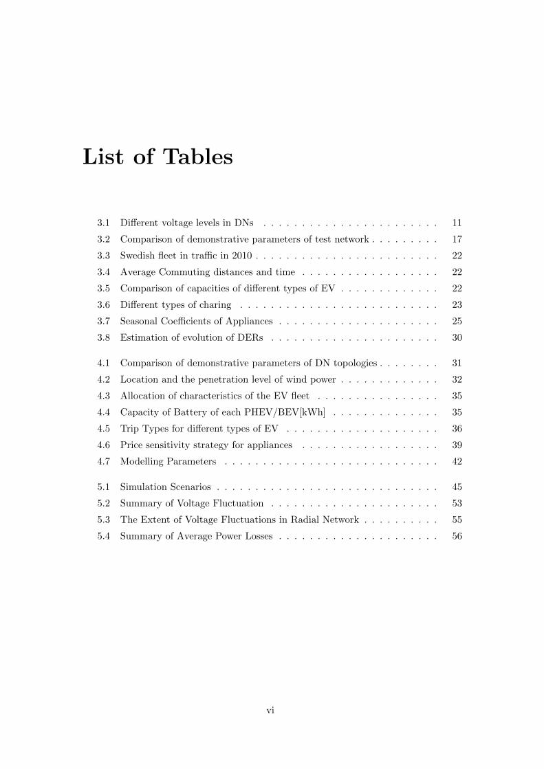

12 Goals and Delimitations
2 The second goal is to construct a toolbox that consists of different DER models
This is done in order to make it possible for simulating and analysing different
scenarios A scenario is further defined in Section 124
3 The third and final goal is to analyse different technical problems arising from the
scenarios ie voltage problems and power losses in the DNs
122 Research Questions
After the thesis work the following questions should be answered
bull Which technical problems are observed in the worst case And in which condition
bull How does different factors (eg season network penetration level etc) affect the
DN Are the impacts beneficial or harmful
And some more questions could be discussed
bull Is it necessary to apply some aggregators to improve the behaviour of DNs
bull What type of aggregators are needed
123 Delimitation
Initial delimitations are summed up below
bull Data sets are based on the real conditions of Sweden (specifically solar irradiation
and historical wind production data from Gotland)
bull Only two specific networks (ie radial and meshed) are modelled for the simula-
tions and are designed to represent the condition in Sweden especially in Gotland
to some extent
bull Only two interesting factors are selected as targets of simulations and analyses
ie voltage fluctuations and power losses in the network
bull Dynamic behaviour and protection issues are not considered in the thesis
bull All the models are integrated at a medium voltage (MV) DN ie 10kV
bull Only consider customersrsquo behaviour in a random weekday
bull Wind power is the only component in the DG dimension
bull Two types of vehicles ie private vehicles (PVs) and commercial vehicles (CVs)
with certain behaviour are simulated
bull Two types of electric vehicles ie pure battery vehicles (BEVs) and plug-in hybrid
electric vehicles (PHEVs) are taken into account
bull Charging infrastructure is only available at home and at work
bull The regulating actions of the DSO is out of the scope of this study The price
sensitivity is only concerning the day ahead prices (not any time of use tariffs etc)
4
12 Goals and Delimitations
124 Definitions and Nomenclature
To clarify the contribution and delimitation of the thesis some important definitions
in the whole thesis work are presented
1241 Distributed Energy Resources
The concept of rdquoDistributed Energy Resourcesrdquo is not clearly defined either by an
authoritative organization nor by an academic project team Yet it is widely used in a
lot of papers reports and books In our project the definition of DER is given as
Definition 1 DERs are regarded as the electric equipment installed in DNs which pro-vide energy or participate in the operation of the power system regardless of producingor consuming power The deployment of DERs in the grid reflects a paradigm shiftregarding how electricity power is in a power system [11][17]
1242 Scenario
A scenario is composed by different DERs in a certain DN during a certain period
(eg a random weekday in the winter) The integration of DERs are influenced by some
external forces such as opinions of policy makers and consumers and the parameters of
the DN ie the peak load of the specific DN DERs are grouped into three dimensions
DGs EVs and ADs To some extent if the integration levels of DERs hit the threshold
values the DSO will have no choice but to either (i) refurbish the network (eg
replace wires install bigger transformers etc) orand (ii) contract ancillary services
from generators and loads to secure the network operation (i) - (ii) will require some
kind of investments from the DSO and how he should act towards this issue is part of
an optimal decision policy problem The DSO is supposed to minimize the overall cost
with respect of keeping the system operation safe reliable and efficient To simplify
the model we assume that the dimensions are independent from one another Hence a
scenario is defined as follows
Definition 2 A scenario is a specific future plan in terms of amount of DERs in acertain DN DERs are defined by three dimensions (DG AD and EV viz the scenariospace) and their potential success is only dependent on external factors such as opinionsfrom policy makers and consumers Furthermore the scenario space is variable iethe dimension can be assigned different numbers Meanwhile the properties of the DNis fixed In the end the scenario should reflect some kind of technical issue of theoperation that the DSO should solve from an optimal decision making policy in networkinvestments
1243 Electric Vehicle
Continuous improvements of storage technologies and a dedicated support from policy
makers promise a bright future for EVs From the power systemrsquos perspective EVs are
5
12 Goals and Delimitations
batteries embedded in transportation facilities charged and discharged in some cases
when connected to the grid
How much when and where EVs are charged are mostly depending on (i) driving
patterns (eg the behaviour of commuters) (ii) the type of EVs (eg PHEVs) (iii)
charging availability (eg at home) For example a private car runs two or three trips
per day within the time periods around 900 - 1700 respectively The length of each
trip is about 20 km in cities The locations available for charging are at home and at
work If the car is a BEV the possible driving range is very limited (typically 20 - 25
km before a recharge is needed [27][28])
Definition 3 EVs are modelled as portable batteries whose behaviour and properties aredetermined by the vehicle types driving patterns and availability of charging facilities
1244 Active Demand
The improved technologies such as dispatched smart-metering system enable the
customers to track the price and consumption in households The trends of of market
deregulation provide much more opportunities of their participation in the system At
the same time new feed-in tariffs and plans to increase energy efficiency lead to a
strong will of advanced activities on the demand side (eg installation of solar panels
new appliances with an energystar label etc) Three segments are set to define AD
regardless of the effects of DSOs (eg cutting off the peak load compensating power to
the grid when isolated) AD dimension is consequently defined as
Definition 4 Active Demand is residential consumers who change their load by either(i) shifting consumption with respect to the electricity price on the day-ahead market(ii) producing their own energy by installing PV panels on their roofs or (iii) updatinghousewares with the purpose of improving energy efficiency In the end these changeswill reshape the load profiles of the households
1245 Dimension 3 ndash Distributed Generation
The installed capacity of DGs is growing stably especially powered by renewable
energy such as wind solar biomass etc Reasons to introduce them are listed in
the book [8] such as the trends of deregulation of Electricity Market environmental
concerns and enhancing the margin between peak load and available production etc
According to [24] the definition of DG is given as
Definition 5 Distributed generation is an electric power source directly connected tothe MV-DNs within the scale of 15 MW Specifically in this project the wind powergeneration is studied due to its popularity and notable intermittent nature
Obviously the operations of different kinds of DGs are independent on their primal
drivings and the interfaces with the electricity grids which will be detailed described in
6
13 Outline of the Report
latter part of this section In view of the development of DG technologies in Sweden
wind power is considered as the only resource in the DG dimension to reduce the contents
of the models Some micro or small size production (eg solar panels) are regarded
as part of AD dimension due to the reason that they are directly connected to the
consumers ie on the customer side of the meters
DG
AD EV
Figure 12 The scenario space - DERs are defined by three dimensions (DG AD andEV viz the scenario space)
13 Outline of the Report
In chapter 2 common methods used in the thesis work are listed and explained
Furthermore some general knowledge of power system theory which is the basis of sim-
ulation is introduced
In chapter 3 introduction and explanations of different components in the DN are
given (eg mechanism of regulation of power production of DGs load profiles of con-
ventional residential loads state of art of the EV technology etc) Different network
topologies are compared two of which are selected as the networks for simulation
In chapter 4 models of different components participating in the networks are de-
scribed with their mathematical algorithms on the basis of their behaviour Models in
the three dimensions are illustrated independently with the rational level of integration
of individual components
In chapter 5 some results of the performed simulations are presented and analysed
A short summary of conclusions obtained in the thesis work is presented in chapter 6
In Chapter 7 an outlook of potential future work can be found
7
Chapter 2
Method
In the first section the study approach of the thesis work is presented followed by
some basic mathematical methods
21 Study Approach
The procedure of the thesis is presented as follows in Fig 21
In the pre-study phase some potential problems in the DNs are studied based on
the fundamental power system theory (eg power flow calculation mathematical mod-
els of the DERs and the DN components in power system) Two target factors ie
power losses and voltage are studied by simulating the scenarios based on the under-
lying models and theoretical algorithms The parameter inputs are from the empirical
observations and the statistics in the related materials such as [29][28] The models
are improved by detecting the difference between expectation and simulation results
eg the availability of vehicles in the network at a certain time The parameters and
algorithms are adjusted until the simulation results meet the real condition based on
historical data The problems revealed from the simulations could further be studied
and solved by for instance aggregators
Figure 21 The Project Procedure - The process of simulation repeats until the perfor-mances of models are close to the results in pre-study literatures and outputs of simulationsare sufficient for the analyses
8
22 Mathematical Method
Other than the method used in the thesis project ie rdquomodelling and simulationrdquo
some other applied procedures can be found in other studies In the book [8] the author
collected a large amount of reliable data of different DERs analysed the data by using
statistic methods and in the end got the conclusions based on the observations In the
large project rdquoMicrogridrdquo[13] some real cases are studied for example a low voltage
level (LV) network study in Portugal Electricity prices line characteristics and their
reliability are studied on the basis of comparison of different countries In the report
[30] the author modelled a fleet of EVs in Monte Carlo simulation models and drew
some conclusions regarding their impact on eg the peak load
To help the DSO to make decisions in network investments the quantified results are
necessary These results could only be accessed by either simulations or study on real
cases Since the pilot network is costly and is absent of existence the only way is to do
the simulations based on the real conditions and available data
22 Mathematical Method
In this section some methods based on probability theory and used in specific algo-
rithms of DERs are described These mathematical methods are carried out to construct
models with specific random factors following certain distributions [31]
Random variable A variable X is a random variable when X is a numerical function
on a probability space Ω function X Ω rarr R ie X is measurable The distribution
of X is described by giving its probability function F (x) = P (X le x) When the
probability function F (x) has the form of F (x) =int xminusinfin f(y)dy X has the density function
f
Normal distribution Normal distribution describes the empirical measurements of
experiments are normally and continuously distributed The density function is given
as following
f(x) =1
σradic
2πeminus (xminusmicro)2
(2σ2) (21)
micro is the mean value and σ is the standard deviation
Lognormal distribution If the random variable χ is normally distributed X =
exp(χ) follows the lognormal distribution The estimation of X EX = emicro+σ2
2
9
22 Mathematical Method
Uniform distribution f(x) = 1 in a certain range (a b) and 0 otherwise
F (x) =
0 x le ax a le x le b1 x gt 1
(22)
Binomial Distribution If the random variable X is said following a Binomial (n p)
distribution if
P (X = m) =
(nm
)pm(1minus p)nminusm (23)
Weibull distribution The density function of a Weibull random variable X is
f(xλ κ) =
0 x lt 0κλ(xλ)κminus1eminus( x
λ)κ x ge 0
(24)
where κ gt 0 is the shape parameter and λ gt 0 is the scale parameter κ = 1 indicates
the exponential distribution while κ = 2 indicates the Rayleigh distribution
Monte Carlo method Some mathematical results could not be strictly proved but
could be derived or estimated when facilitated Monte Carlo methods Applications are
utilized in a lot of fields from decisionsrsquo making to simulations of complicated systems
Monte Carlo methods are those methods which use random samples in a calculation
that has a structure of a stochastic process (ie a sequence of states whose evolution
is determined by random events) [32] If there are an amount of variables (ie system
inputs) and the function of these inputs are complicated Monte Carlo methods can be
used to get a good estimation of the observation (ie system output) It is formulated
as
E(Y ) =1
N
Nsumi
Yi (25)
where Y is the observation and implemented in Monte Carlo methods for N times
Each observation Yi is independent and determined by functions and constrains of vari-
ables x12M
10
Chapter 3
Theory
The basic knowledge in power system analysis is introduced in this chapter For the
simulation purpose the underlying foundation of models are presented in the following
sections Data sets used to model elements in the toolbox are proposed
31 Basic Power System Theory
This section is a brief digest from some power system analysis books
311 DN
Voltage level DN is the last stage in electricity delivery path which carries electricity
from transmission networks to the end users The whole DN can be split up into three
voltage levels corresponding to the nominal value of the voltage (see Table 31) [33]
As mentioned in Chapter 1 MV is selected as the voltage level for simulation and
modelling Usually customers in the low voltage levels are connected to MVs with
step-down transformers in substations Some consumers with large consumptions are
directly connected to MVs Common voltages in MV-DNs in Sweden are 10 kV and 20
kV There are voltage level 3 6 and 33 kV but these are rare [34]
Network topology The simulation approach requires the first step that typical DN
topologies should be identified Usually the MV-DNs in urban area are with loop or
mesh topologies while in rural area with mesh or radial topologies (see Fig 31)
System Nominal Voltage [kV]
LV le 1MV 1minus 35HV ge 35
Table 31 Different voltage levels in DNs[33]
11
31 Basic Power System Theory
However considering the breakers in networks are normally open most networks are
operating as radial ones [13]
(a) Loop (b) Mesh (c) Radial
Figure 31 Typical network topologies[13]
312 Components
3121 Transmission lines
A considerable share of power in MV-DNs are consumed by the transmission lines
instead of loads due to lower voltage and higher current In MV-DNs both overhead
lines and underground cables are commonly used [13] In Sweden the ratio between
these two types of transmission lines is 31 [34] Overhead lines are less expensive than
underground cables but more space consuming [34][35]
Transmission lines are commonly characterized as π model by their resistance Rs
Rs Xs
Bsh
2
Bsh
2
Figure 32 π-equivalent circuit of lines - π-equivalent of transmission line with RsXs and Bsh
series inductance Ls and shunt capacitance Csh as shown in Fig 32 Reactance Xs
is obtained by ωLs while subceptance Bsh is obtained by ωCsh Thus the equivalent
model of the transmission line is derived as
Zs = Rs + jXs (31)
Ysh = jBsh (32)
where
ω is the angular frequency of power system
12
31 Basic Power System Theory
Zs is the series impedance of the line
Ysh is the shunt admittance of the line
The fact that underground cables have larger capacitance and smaller inductance
compared with overhead lines may lead to novel phenomena of voltage and power losses
in feeders [35]
3122 Transformer
Transformers as the interface between MV-DNs and HV-DNs or between LV-DNs
and MV-DNs bring the voltage levels down eg from 60 kV to 10 kV Usually on-load
tap-changers are only utilized on HVMV transformers to keep the voltage constant
without disconnecting any loads while manually tap-changers are utilized on MVLV
transformers and adjusted only once during installation [36]
The equivalent circuit (referring to the primary side) of a transformer as shown in Fig
33 consists of in-series resistance Rp and Rs representing power losses on each side in-
series reactance Xp and Xs resulted from flux leakage as well as the magnetizing branch
reactance Xm in parallel with the iron losses component Rc (see Fig 33)
Figure 33 Equivalent circuit of transformer - Secondary impedance is referred tothe primary side [36]
313 Calculations in Power System
3131 Power flow
Power flow calculations in general enable a certain power system to indicate voltage
magnitude and angle in each bus active and reactive power flow between each bus The
identified known and unknown quantities in the system determine types of buses (ie
PQ bus PV bus slack bus) Then calculations could be implemented by power balance
equations
0 = minusPi +Nsumk=1
| Vi || Vk | (Gik cos θik +Bik sin θik) (33)
13
31 Basic Power System Theory
0 = minusQi +
Nsumk=1
| Vi || Vk | (Gik sin θik minusBik cos θik) (34)
where Gik and Bik can be obtained from the admittance matrix YBUS
3132 Power losses
The reason to choose which voltage level of the grid much depends on power losses
which are transformed into heat When power losses decrease the maximal capacity on
lines mainly due to the limit of thermal capacity could increase Power losses on the
level of 10 kV are about 3 times of those on the level of 20 kV [34] Other than the
technical factors the design of system operation could also affect the total losses in the
system Power losses Ploss in power system follow such formulas
Ploss = I2R (35)
I =S
U(36)
where
R is the resistance of the transmission line [Ω]
I is the current flowing through the line [A]
U is the voltage difference between two ends of the line [V]
S is the absolute value of complex power given byradicP 2 +Q2 [VA]
3133 Power factor
In power flow calculation two components are obtained as active power [W] P which
transfer energy and reactive power [Var] Q which move no energy to the loads Hence
power factor is defined as
powerfactor =| cosϕ |= P
S=
PradicP 2 +Q2
(37)
When powerfactor = 0 the power flow is purely reactive When powerfactor = 1
only active power generated by the source is consumed Power factors are expressed as
rdquoleadingrdquo or rdquolaggingrdquo to show the phase angle ϕ
3134 Voltage variation and weakest point
For safety concerns there are limits of network voltage to protect equipments con-
nected to the system According to the European Standard EN50160 [20] the voltage
magnitude variation should not exceed plusmn10 for 95 of one week measured as mean
10 minutes root-mean-square (RMS) values The consumption will result in a voltage
drop on the feeder The further away from the substation bus the lower the voltage
14
32 Comparison of Network Topologies
will be On the contrary the connection of generations will lead to a voltage rise on
the feeder The interaction of consumption and generation in MV-DNs therefore causes
voltage variations
The voltage variation in steady state is approximately equal to
∆U
Usim=RlinePG +XlineQG
U2middot 100 (38)
With a given limit on the variation of the voltage ∆Umax the maximum allowed
produced active power from a connected generator can be derived as
Assume that the power factor is constant Then Qmax = α lowast Pmax
According to the equation (38)
∆Umax =(R+ α middotX)PGmax
U(39)
rArr
PGmax =∆Umax
(R+ α middotX)U(310)
From Equation 39 we can derive that when the nominal voltage value and feed-in
power are constant larger equivalent impedance leads to larger variation in voltage In a
power system the weakest point is the load point where the equivalent impedance is the
largest Usually the most critical voltage problem appears in the weakest point The
equivalent impedance is called Thevenin equivalent impedance which is usually decided
by the distance from the slack bus material of transmission line and the topology of
the network
3135 Penetration levels
The penetration levels of DER components indicates the share of them in the whole
network The penetration level is expressed as the ratio between the installed capacity
of DER components and the peak load value
micropen = 100
(sumPnomG
P peakL
)(311)
32 Comparison of Network Topologies
The DNs directly connect to the end users Their topologies and sizes are different
among areas depending on the operation concepts utilized devices and the load profiles
Thus voltage quality reliability and power losses in this stage are interesting aspects to
study in DNs Several electrical network models are developed as test systems to analyse
one or more specific characteristics (eg voltage regulation unbalanced load reliability
15
32 Comparison of Network Topologies
of system etc) However a majority are developed to study power system reliability
which indicates that they are not of sufficient details to the level upon which our research
questions could be addressed Additionally there are some network models for power
flow analysis but their sizes are too large to be implemented in Simulink Matlab For the
purpose of investigating the integration of DERs in a future DN reasonable test networks
are required for a sufficient analysis of the simulation results and a correct direction for
further network studies The DNs are studied at a medium voltage level ie 10 kV
From literature review study several typical existing test networks are acknowledged
described and compared [13][37][38][39] Their topologies can be found in the Appendix
321 Description of Several Networks
bull IEEE Test Feeder ndash IEEE Comprehensive distribution test feeder developed by
IEEE Working Group is presented on the IEEE website It consists of 55 buses
two voltage levels and 25 loads which represent a wide variety of components
in one circuit [40] It is a large radial network It is possible to connect some
switches in the network to form a small loop Some other types of modules (eg
identical feeders connected to the same bus radial structure with loads distributed
on feeders) are presented in the network Examples of all the components in the
network are provided in the work document The network allows all the standard
components of a distribution system to be tested (See Fig A2 in appendix for
the topology)
bull Bornholm Test Network ndash The Bornholm Test Network is modelled based on
the real distribution network in Bornholm an island of Denmark with 2 voltage
levels 11 buses 9 transmission lines 7 loads and 3 distributed generations The
detailed parameters of the network are not available However the general network
data can be found in [37] (refer to the topology in Fig A1 in the appendix)
bull Swedish Test Systems ndash The Swedish Test Systems are developed by Elforsk
a Swedish industry research association to analyse the reliability of Swedish net-
works and the electricity market in Sweden The test systems include two distri-
bution systems one for the urban area (ie SURTS) and the other one for the
rural area (ie SRRTS) Loads component data are well represented by these test
systems due to the support from and involvement of Swedish power distribution
companies SURTS is a 10 kV system with 10 identical feeders in cable-loop de-
sign while SRRTS consists of two modules both of which are radial structure
Reliabilities load data and outage costs are specified in the model [34] (refer to
the topologies in Fig A3 and Fig A4 in the appendix)
16
32 Comparison of Network Topologies
bull The Gotland Network - An isolated mixed network ie both urban and rural
networks with a big share of wind power generation [41] A typical feeder in
the network consists at least 20 load points Shunt capacitors are installed in
the network at the MV level Wind power is directly and particularly connected
to the substation bus with a transformer Load data and parameters of network
components are available It is accessible for the simulation in future work The
edge of the feeder could be regarded as a normally open switch or a big load Some
typical structures of feeders could be selected to represent the whole MV network
after analyse both topologies and load characteristics of the network
bull The German Network - The German test network is provided for the EU project
More Microgrids The description is in the work package G deliverable 1 of More
Microgirds The test system consists of two MV networks (ie urban and rural)
and a detailed LV network for study Line parameters and load profiles are well
presented in the document The MV networks are taken from existing networks
considered to be typical The LV network is an artificial network with different
structure for different load segments The structure of urban MV network is similar
to the Swedish one but the loop circuit is closed by two paralleled feeders with a
normally open switch in between The rural MV network is a 20kV mesh system
with 2 external connection points and 14 buses 15 loads (with static state values
in the figure) and 2 generations are involved in the network Initial power-flow
calculation is described in the figure for different lines and loads Compared with
Swedish rural one the topology is more complicated but with less components in
the network [13]
322 Comparison of Key Parameters
A discussion on the listed test networks is conducted by comparing their complexity
and representativeness Table 32 shows some key parameters of these networks
Table 32 Comparison of demonstrative parameters of test network
Network Voltage Level Buses Loads GenerationsTopology
IEEE NA 55 25 5 meshBornholm 60 kV10 kV 11 7 3 radialSURT 130 kV10 kV 62 60 0 loopSRRT 40 kV10 kV 19 many 0 radialGerman urban kV20 kV 83 81 NA loopGerman rural kV20 kV 14 15 2 meshGotland 70 kV11 kV hundreds mesh
17
32 Comparison of Network Topologies
Complexity From the description part it is shown that Bornholm test network
and German rural network are much simpler than the other ones The Bornholm net-
work does only consist of 11 buses and German one of 14 buses which simplifies the
quantities of parameters and the analysis of phenomena in simulations Part of the Ger-
man network is selected as mesh network for simulation with 11 buses 8 load points
and two locations for generations The other part of the network is connected with
another substation bus and is isolated to the selected part during normal conditions
Seven or eight load points in the network are sufficient to implement different consumer
categories (ie residential commercial industrial) and to assign EVs together with
loads randomly Some large scale distributed generation such as wind power can be
directly connected to the 10 kV level or a even higher voltage level Those generations
in small scales such as Photovoltaic (PV) panels can be connected in parallel with the
residential load denoting that connecting points are in lower voltage level
Some other simple test systems developed by IEEE [40] are proposed to study unbal-
anced systems and voltage regulators in a very long feeder which do not fit the condition
in this project and the characteristics of real Swedish DNs
Representativeness The network condition in Gotland is similar to that in Born-
holm The restructured German rural network and the DNs in Gotland have some
mutual features To obtain a better representation typical parameters are chosen ac-
cording to the real condition in Gotland (eg the proportions of cables and overhead
lines the distance between buses the voltage levels) The radial network could repre-
sent a typical radial feeder and the first part of a loop feeder with normally open switch
Besides some features of it are set for comparison Feeder B2 is quite short while feeder
B3 is longer which means that buses in B2 can be regarded as rdquostrong gridrdquo compared
with those in B3 In addition B4 and B5 are compared to show the difference between
cables and overhead lines Thus most of technical effects due to the topology of the
network are considered in the test system Since the meshed network is well presented
in the report [13] all properties and characteristics of the cables are modelled based on
the real condition
The IEEE test system SURT and SRRT are all intended for reliability analysis which
indicates that there is no detailed parameters within the documentation In addition
the size of these test systems is a way to large and is not appropriate for the simulation
in Simulink
18
33 Wind Power as DGs
33 Wind Power as DGs
Wind energy is one of the major growing renewable energy technologies in the recent
years Wind power is intermittent and hard to manage which may lead to the voltage
sag or swell usually in a short period The deviation between the real wind production
and and the predicted production may result in grid outages For those wind turbines
equipped with induction generators reactive power is absorbed by them which bring
about a poor power factor and less active power capacity of the transmission line From
an economic perspective additional reactive power compensating devices are costly and
mostly installed in HV networks (to secure the reliable system operation) Wind speed
always reaches the peak value in the winter However for safety concerns a strict
temperature limit (eg minus40C) and speed limit (eg 25 ms) will force the turbines
to cut off their whole production The extracted power curve fits the demand curve in
Sweden because the peak load in Sweden also appears in the winter time Aggregation
of a large geographically spread wind power can reduce the impact of meteorological
influence and improve the accuracy of the prediction significantly [26]
Figure 34 General Structure in WindTurbine Block
331 Operation Mechanism
The wind turbine is the device that extract mechanical power from wind power going
through its swept area and then to transfer energy to electricity (see Fig 34) The
power output of the turbine is given by the following equation [42]
Pm = Cp(λ β)ρA
2v3w (312)
Tm =Pmωel
(313)
19
33 Wind Power as DGs
where
Cp is coefficient of extracted wind power
λ is tip speed ratio of rotor blade tip speed and wind speed
β is blade pitch angle
ρ is air density (kgm3)
A is the tip swept area (m2)
vw is wind speed ms
ωel is the rotation speed of generator (rads)
A generic equation is used to model Cp [43]
Cp(λ β) = c1
(c2
λiminus c3β minus c4
)e
minusc5λi + c6λ (314)
in which1
λi=
1
λ+ 008βminus 0035
β3 + 1 (315)
Power curves of different type of turbines are unique due to different control methods
different blade lengths different tower heights etc in which rdquocut-in speedrdquo rdquocut-off
speedrdquo rdquorated speedrdquo and rdquorated powerrdquo are the main features of the power curve A
typical power curve is shown in Fig 35 [44]
Figure 35 Typical power curve of wind turbine - Power curves and other technicaldata of wind turbines are given in the product brochures[44]
332 Historical Data
The occurrence of wind speed follows a Weibull distribution and there is little corre-
lation of wind speeds in neighbouring hours Meanwhile the direction and turbulence
of wind are other two main factors which affect the production of electricity Except for
these factors the turbine structures regulation strategies location of the wind farm
and the distribution of wind turbines have a large impact on the production Hence
as a static model the aggregated wind power is depicted as the generation changing on
20
34 EV Fleets and Behaviours of Customers
an hourly basis in a MV-DN at the generation point in the network Fig 36 shows the
variation of total wind production on Gotland throughout the whole year 2010 [41]
0 30 60 90 120 150 180 210 240 270 300 330 3600
10
20
30
40
50
60
70
80
90
Day
Tota
l W
ind P
roduction [M
W]
Figure 36 Total production of wind turbines on Gotland in 2010 - The datarecords production in each hour in the whole year [41]
34 EV Fleets and Behaviours of Customers
EVs are vehicles that at least are partly powered by electricity or use electric motors
as the direct propulsion Transport sector is one of the most important and largest part
of energy consumption and the energy use in transport sector is dominated entirely by
oil products (eg petrol diesel etc) in Sweden[45] For the purpose of reducing the
emission of CO2 and improving energy efficiency the deployment of a large amount of
EVs can be envisioned in a near future
On-board batteries the core of the EV technology introduce a large amount of
possibilities to the power system to interact with them via charging facilities (eg
plug-in electric outlets) Without considering the effects of management and control
the charging behaviour is mainly dependent on three factors
I Driving patterns In our case only Private Cars (PrV) and Commercial Vehi-
cles (CV) are considered The statistics of travelling behaviour in Sweden (eg
numbers of trips per day the distance covered by on e trip hours of the trips
etc) are collected based on [28] and [29] Table 33 implies that each household in
Sweden own one car in average and EVs are not commonly deployed until now
Table 34 presents the general trip length in different areas and the time consumed
in each trip In Fig 37 the blue curve and the black one illustrate two types
of driving patterns in a day It gives the primary understanding on how vehicles
behave in Sweden
II Types of EVs Among various types of EVs we took Plug-in Hybrid Electric
Vehicles (PHEVs) and Pure Battery Electric Vehicles (BEVs) into our considera-
21
34 EV Fleets and Behaviours of Customers
Table 33 Swedish fleet in traffic in 2010 [29]
Type of Vehicles Private Cars Commercial Cars Heavy Vehicles Others
No of Vehicles 3 446 517 1 376 358 526 441 1 869 683
Type of fuel Petrol Diesel Electricity Other
No of Cars 3 479 607 606 570 190 248 815
Table 34 Average Commuting distances and time[28]
Municipality Groupings Distance [km] Time [mins]
Urban Area 20plusmn 1 42plusmn 3Suburban Area 25plusmn 2 40plusmn 2Rural Area 28plusmn 2 41plusmn 1Total 23 41
Figure 37 Starting time for different types trips in 24-hour period (times103) [28]
Table 35 Comparison of capacities of different types of EV[27] - shown in differentcoloured curves
Type of Vehicles Battery Capcity [kWh]
BEV 25 sim 35City-BEV 10 sim 16PHEV90 12 sim 18PHEV30 6 sim 12
tion Compared to PHEVs (with internal combustion system) BEVs (with pure
electricity propulsion) need a larger battery capacity According to the report [27]
typical capacities are shown in Table35
III Charging patterns Charging facilities for different purpose in different area are
assumed planned well to fulfil the basic requirements of EV charging Depending
22
35 Load Profiles in the MV Level DNs
on the preferences of car owners three possible charging approaches1 are proposed
as listed in Table 36 [27]
In reality the charging curve is not a straight line but with some variations
Table 36 Different types of charging [27]
Type of Charge Load Charging time
Slow le 5 kW ge 4 hoursStandard 5 kW - 20 kW 1 hour - 4 hoursFast ge 40 kW le 1 hour
of the slope along the charging process Fig 38 shows one typical real charging
curve For simplicity we assume that the charging current is constant (ie the
curve is a straight line)
Three stages of charging places are stated in [27] as (1) at home (2) at home
and at work (3) everywhere Different charging approaches correspond to different
charging places
Figure 38 Typical charging curve - This is a charging curve of Li-Ion batteries whichcould be idealized or linearised[27]
35 Load Profiles in the MV Level DNs
Flexible residential loads is an important part of our scope The conventional load
profile is reshaped by modifying actions Loads of other sectors are excluded which are
assumed that they have already made their own optimized modifications on their loads
1Charging time depends on the size of battery
23
35 Load Profiles in the MV Level DNs
Figure 39 Structure of the hourly load curve of apartments - Apartment withtwo people (25-65 years old) Workdays
Figure 310 Structure of the hourly load curve of houses - House with two people(25-65 years old) Workdays)[46]
24
35 Load Profiles in the MV Level DNs
351 Conventional Residential Load
According to the report Statistics Sweden 2011 [29] the distribution of houses and
apartments are quite even especially in cities According to [46] the most representa-
tive pattern is a two persons apartment or house Thus the load profiles on an hourly
basis of these patterns are collected as the original residential load profiles in our study
To perform price sensitive strategies different type of household appliances are classified
(eg Dish washer heating white goods etc) Usually heating and water heating in
apartment buildings are not accounted into the consumption of electricity while direct
electric heating is (eg from heat pumps) Subsequently the profiles are presented in
Fig 39 and Fig 310 with different appliances in different colors
As described in [34] the density of residential customers at the LV-DNs are 20(km
of line) in the urban area and less than 10(km of line) in the rural area respectively
Thus the numbers of customers in each load points in the network model are set to
be around 500 for the urban area and 200 for the rural area The load curve of an
apartment is based on the data set in [47] with 120 units aggregated (ie a whole
building) The load curve of a house is based on the data set for a two person (25-65
years old) household (with direct electric heating) measured and presented in the report
[46] In general rdquoone appliancerdquo of the data set refers to an average value of a group of
appliances in the households
Temperature is an important factor influencing the consumptions of different ap-
pliances of which the seasonality effects coefficients are assigned in the report [46] as
well To simplify the model coefficients of four seasons are selected to represent the
temperature factors (see Table 37)
Table 37 Seasonal Coefficients of Appliances[46]
Appliances Spring Summer Autumn Winter
White goods 09 10 09 07Lighting 14 10 22 16Audio and TV 13 10 15 19Cooking 13 10 13 17Heating 10 03 10 25
352 Other Types of Loads
In [34] some real load profiles of different load types are given Since only the
residential loads are interesting the combination of other types are distributed in the
network As an example Fig 311 shows different loads profiles (industrial public and
agricultural)
25
35 Load Profiles in the MV Level DNs
1 2 3 4 5 6 7 8 9 10 11 12 13 14 15 16 17 18 19 20 21 22 23 24
100
150
200
Hour
Consum
ption [kW
]
Industrial
Public
Agriculture
Figure 311 Aggregated load profiles on a random bus of other types of loads -The curve is consistent with the information in report [34]
353 Actions Applied in AD Dimension
In the future DN a large amount of smart metering devices are installed which
provides customers the possibility to behave more positive and to get involved in the
energy markets At the same time customers are more aware of their cost of electricity
as well as the relevant environmental issues especially after suffering some extreme high
prices in recent years (eg price spikes of 1 000 eMWh on 22nd Feb of 2010) A survey
conducted at Maingate shows that a significant portion of the Swedes would change
their load profile if the electricity price and their consumption were displayed on an
hourly basis [1] New legislations and plans in Sweden could increase the interests of
interaction even further To evaluate the consequences of these changes 1 a model of the
flexible load is implemented by performing three main factors (ie price sensitivities
small-scale productions energy efficiency actions) [1] These factors are described more
fine grained below
3531 Price sensitivity
In our case price sensitivity implies that retailers could shift or shed the load of different
appliances in households with respect to the electricity price Whether the price sensi-
tivity action can be performed depends on two factors one is how large the electricity
price varies the other one is the acceptance of the customers to shift or shed one or
more appliances Fig 312 shows the assumed customer acceptance
3532 Energy efficiency actions
The Swedish Energy Agency Energimyndigheten initiated a program that helps some
companies to be successful in their efforts to perform energy efficiency actions There is
no doubt that these actors can both save money and energy by executing these actions
A series of new measures to improve energy efficiency are proposed by European
Commission in June 2011 [7] To save energy and to reduce the emission of greenhouse
1We do not study the exact impacts of demand tariffs
26
35 Load Profiles in the MV Level DNs
Figure 312 The acceptance of customers on different appliances - [19]
gases some products and actions are recommended to improve the efficiency of energy
consumption For example to replace light bulbs with Compact Fluorescent Lamps
(CFLs) at home or in public areas to use energy-efficient housewares to enhance the
insulation of buildings Subsequently the reduction of consumption can be ob-
tained However different actions (like the change of lamps) may lead to other negative
results (eg change of power factor harmonics introduced in the network etc) When
considering an individual household the change is tiny which can be ignored compared
with consumption on the bus
3533 Small scale production ndash PV panels
Small scal production is considered as the production units that have a power output
of typically a couple of kWrsquos and are connected directly to the loads (like PV panels
micro CHPs)
A few decades ago limited by high cost solar photovoltaic is not that prevalent as
nowadays The price of PV cells has significantly been reduced while the efficiency is
increased due to the new technology advancements and the manufacturing process [48]
According to [45] the electricity production of solar in Sweden is about 200 MWh in
2009 And a variety of forms of grants and subsidies for solar cells in Sweden promise
a blooming trend of their development To interpret this trend into the thesis work
the PV model is created as the small scale production to indicate its influence on the
residential load profile Data are collected from [49] where the sizes of PV panels on the
roofs are determined as 20 m2 for each house and 3 m2 for each apartment respectively
A PV cell can produce current under its exposure to the sun Thus it is reasonable
to model it as a diode together with an equivalent current source depending on the
27
35 Load Profiles in the MV Level DNs
Figure 313 The Equivalent Circuit Diagram of Photovoltaic Cell
environment temperature and irradiation of the sun (see Fig 313) In some papers
instead of a current source the author modelled the PV cell as a voltage source of which
the output voltage is stablized around the system voltage and the output current are
influenced by the environmental temperature and the irradiation of the sun [48]
VC = CV
(AkTref
eln
(Iph + Io minus IC
Io
)minusRsIC
)(316)
Iph = CI middot Isc (317)
IPV = IC middotNS (318)
VPV = VC middotNP (319)
where
NS is the amount of series cells in a panel
NP is the amount of paralleled cells in a panel
VC is the output voltage of a PV cell
IC is the output current of a PV cell
Iph is the photocurrent produced by the semiconductor in the PV cell
Isc is the short-circuit current of the equivalent circuit
Io is the reverse satiation current of the diode (00002A)
RS is the series resistor in the equivalent circuit to reshape the I V curve according to
the open circuit voltage
A is a curve adjusting factor to fit the model curve to the real one
k is the Bolzmann constant as 138times 1023 JK
Tref is the reference operation temperature given by the manufacturer
e is the quantity of a single electron as 1602times 10minus19 C
28
35 Load Profiles in the MV Level DNs
CV is the coefficient of voltage caused by the temperature and the irradiation
CI is the coefficient of current caused by the temperature and the irradiation
From [50] the coefficients of the voltage and the current CV and CI can be described
by two decoupled part temperature dependent coefficients and irradiation dependent
coefficients as
CTV = 1 + βT (Tref minus Tx) (320)
CTI = 1minus γTSref
(Tref minus Tx) (321)
CSV = 1minus βTαS(Sref minus Sx) (322)
CSV = 1minus 1
Sref(Sref minus Sx) (323)
where
Sref is the reference operation irradiation given by the manufacturer
βT is the PV cell output voltage versus the temperature coefficient
αS is the slope of the change in the temperature due to a change of the solar irradiation
level
γT is the module efficiency
The V-I characteristics curve is shown in Fig 314
Figure 314 V-I Feature Curve of a PV cell
It is obvious that the PV production is mostly affected by the solar irradiation
and temperature The production in the winter is very low compared to the sum-
mer conditions Some seasonal factors are introduced in the simulation to reflect these
effects The PV panel production is estimated by applying historical irradiation data
from NASA as shown in Fig 315 [51]
29
36 Estimation of the Development of DERs and the Changes of Activitiesin DNs
1983 1987 1991 1995 1999 20030
01
02
03
04
05
06
07
Day (19830701 ~ 20050630)
Cle
arn
ess I
nd
ex
Figure 315 Historical data of Clearness Index on Gotland - Clearness Index isproportional to the production of PV cells [kWm2d]
36 Estimation of the Development of DERs and the Changesof Activities in DNs
As mentioned a lot of targets related to energy and environment are set The most
important target is the EU 202020 targets (see [2]) The targets as the short-term
plan are applied and need to be met in 2020 while the long-term planning can be ex-
tended to 2050 Thus it is necessary to estimate how the electricity market and the
future DNs look like
In the annual report Energy in Sweden in 2010 [45] the new climate and energy
policies are presented These are (i) The proportion of energy supplied by RES should
be 50 larger than the annual energy consumption in Sweden by 2020 (ii) Vehicles in
Sweden should be independent of fossil fuels by 2030 (iii) The efficiency of energy use is
required to be improved to reduce 20 in energy consumption between the years 2008
to 2020 (iv) 40 reduction in greenhouse gas emissions needs to be met by 2020 in
comparison with 1990 while the target no greenhouse gas emission by 2050 is set for
a longer vision
Aiming at these targets the changes in the future DNs are implemented in accor-
dance with the three dimensions in scenarios Table 38 gives a first idea of these future
developments
Table 38 Estimation of evolution of DERs
DER Short-term Long-term
DG 30 of the peak load ge50 of the peak loadEV 20 of total vehicles 50 of total vehiclesAD 20 of total customers 50 of total customersADenergyefficiency ndash 20 reduction of load
30
Chapter 4
Construction of the SimulationToolbox
This chapter focuses on the modelling of DNs and DERs based on the theory stated in
the previous chapter The radial and meshed network models are presented in the first
section where some important parameters are listed in table form The algorithms and
parameters for the DER models are given in the following sections
41 Network Model
In Simulink two different network models are constructed To capture their static
characteristics both generation and loads are constituted as Load blocks in Simulink
ie generation is indicated as the negative input and the consumption as the positive
one To detect the voltage and power flow on each bus Scopes are added with some
sufficient Transformation blocks Other components (eg switches) and functions can
be joined into the model for further study The network parameters are based on the
report [13] (see Chapter 3) and summarized in Section 45 The topologies of these
networks are shown in Fig A5 and Fig A6 respectively In these two networks
the number of individual residential loads are about 3800 (radial) and 1800 (meshed) 1
Detailed data concerning these two networks can be found in Table 41 Fig A7 and
Fig A8 in Appendix
Table 41 Comparison of demonstrative parameters of DN topologies
Topology Voltage Level Buses Loads Generators Referring Network Peak Load
Radial 60 kV10 kV 11 7 3 Bornholm [37] 15MWMeshed 60 kV10 kV 11 8 2 German rural [13] 20MW
1Numbers of loads are defined according to the report [13] corresponding to the real conditions indifferent types of Swedish areas in which about 400 residential loads are connected to each load point
31
42 DG Model
42 DG Model
421 Wind Power
0 1 2 3 4 5 6 7 8 9 1011121314151617181920212223240
20
40
60
80
Sprin
g
0 1 2 3 4 5 6 7 8 9 1011121314151617181920212223240
20
40
60
80
Sum
mer
0 1 2 3 4 5 6 7 8 9 1011121314151617181920212223240
20
40
60
80
Autu
mn
Time [Hr]
0 1 2 3 4 5 6 7 8 9 1011121314151617181920212223240
20
40
60
80
Win
ter
Time [Hr]
Figure 41 Wind power production on 24-hour base
A cluster of wind power plants from one wind wind park is modelled as an aggre-
gated generation unit connected to the MV-DNs at the production points Their pro-
duction profiles are depicted on an hourly basis and their volumes are collected from
[41] (source wind production data of Gotland in year 2010) To capture the features
of wind generation the mean values and deviations are calculated and it is assumed
to follow a normal distribution with high deviations [52] An example of production
profiles in four different seasons are shown in Fig 41 The potential production of
wind power is determined by the penetration level of DG microDGpen ie the ratio between
the installed DG capacity and the peak load The aggregated wind generation and their
sizes are presented in Table 42 with respect to the peak load The unit names can be
found in the topologies of network models (See Fig A6 and Fig A5)
Table 42 Location and the penetration level of wind power
Network Radial network Meshed network
Unit Name G1 G2 G3 G1 G2Penetration 2
7microDGpen
37micro
DGpen
27micro
DGpen
13micro
DGpen
23micro
DGpen
32
43 EV Model
43 EV Model
431 Algorithm of Modelling
EV Fleet
Urban Rural
Private Vehicles
Commercial Vehicles
Private Vehicles
Commercial Vehicles
BEV PHEV
SOCTrip Type
Battery Size
70 30 90 10
50 50
1
1
Figure 42 Characteristics of EVs - Assign characteristics by different classes
There are two types of EVs studied in this paper ie Pure Battery Electric Vehi-
cles (BEVs) and Plug-in Hybrid Electric Vehicles (PHEVs) The total number of EVs
is in proportion to the number of households in the studied area defined by microEVpen It
is assumed that if one EV leaves the geographic area reflecting the studied distribution
networks an EV with the same features will enter
The EV fleet is defined by driving patterns type of vehicles and the availability of
charging facilities of which the statistics of the parameters are described in the section
34 The EV fleet is randomly split into different classes as shown in Fig 42 With the
categorized properties the EVs are performed on the state transitions
Three states for EVs are set rdquoRunning (0)rdquo rdquoCharging (1)rdquo and rdquoParking (2)rdquo
The initial states of all EVs are assumed to be at home and charging In each time
step according to the last state of the EVs different transition procedures are applied
The State of Charge (SOC) power consumption duo to charge remaining trip length
and numbers of completed trips are updated at the beginning of each iteration The
33
43 EV Model
algorithm is described by the flowchart in Fig B2
In the block rdquoPower and SOC updaterdquo (Fig B1 (d)) the following steps are imple-
mented
bull if the EV is charging
PCharging(busit+1 t+ 1) = PCharging(busit t) + Chargingi
SOC(i t+ 1) = SOC(i t) + ηCharging lowast Chargingi middot tCapi
bull if the EV is running
SOC(i t+ 1) = SOC(i t)minus vi middot∆t middot ConsiCapi
RTL(i) = RTL(i)minus vi middot∆t
where
vi is the speed of the EV i
PCharging(busit t) is the equivalent load of charging on busit at time t
Chargingi is the load of EV i according to the type of charging now
SOC(i t) is the State of Charge of EV i at time t Capiand Consi are the Capacity
[kWh] and Consumption [kW km] of EV i respectively
RTL(i) is the remaining trip length [km] of EV i in current trip
In the block rdquoTransition of Statesrdquo different strategies are applied to different original
state (transitions in Fig B1 )
To make the algorithm more easy to follow some boolean indices are set
bull prtl is 1 when RTL(i) is larger than 0
bull psocfull is 1 when SOC(i t) is smaller than 1
bull psoc is 1 when the vehicle can support the remaining length of the trip (if the
vehicle is PHEV psoc = 1)
bull ptime is 1 when the departure time is arriving
In each cycle the state rdquoRunningrdquo is prioritized When prtl psoc and ptime are 1 (ie
when a EV is supposed to start and there is enough power to run the remaining trip)
then the next state of EV i is rdquoRunningrdquo rdquoChargingrdquo will be applied when either of
the aforementioned premises is not satisfied if there is charging facilities available and
psocfull is 1 In cases that EV does not have sufficient power to drive to the destinations
it is either in the state of rdquoChargingrdquo if there is charging facilities available on sites
or in the state of rdquoParkingrdquo if not The charging time is dependent on the remaining
time before the next trip and the type of charging facilities If the EV cannot run or
34
43 EV Model
get charged then the state of EV i will be set as rdquoParkingrdquo For observations states
location and SOC in each time instant for every EV are recorded in matrices together
with the equivalent load matrix
432 Parameter Sets for Simulations
Table 43 Allocation of characteristics of the EV fleet
Network PrVCVSpeed Consumption Trip Length Trip Type[kmh] [kWkm] [km] 1 2 3 4
Urban
PrV40 012
20(std)02 03 04 01
(70) plusmn1CV
25 018100 (std)
05 045 005(30) plusmn5
Rural
PrV60 018
28(std)02 03 04 01
(90) plusmn15CV
30 022100 (std)
05 045 005(10) plusmn10
Allocation of parameters for different types of EVs
The percentage of PrVCV and PHEVBEV are random numbers following a normal
distribution so as departure time of each trip and the capacity of battery in each vehicle
Trip lengths of all trips follow a log-normal distribution Table 43 and Table 44 shows
characteristics of the EV fleet
Due to the effect of temperature the consumption of the EVs vary Hence the
common seasonal factor is introduced to reflect the effect of temperature to some extent
Possibility of charging and charging type
The availability of the charging facilities determine the possibilities to be charged in
Table 44 Capacity of Battery of each PHEVBEV[kWh]
Type Cap Mean Cap Dev
PHEV 9 3BEV 25 5
the model If the available charging duration is less than 1 hour there is no chance for
charging (ie no fast charging utility) if the available charging duration is less than 4
hours and more than 1 hour the possibility of charging is 03 and the charging type is
standard charging if the available charging duration is even longer or the EV is at home
( the initial place) the charging possibility is 1 and the charging type is slow charging
Commuting patterns and corresponding probabilities (see Table 45)
After studying the customersrsquo behaviour a number of trip types are designed with
different possibilities as shown in Table 43
35
44 AD Model
For PrVs four possibilities are considered
bull Two trips a day One is in the morning and the other one is in the afternoon (go
to work and go back home)
bull Three trips a day Except for those two trips there is one extra trip for leisure
after work
bull Four trips a day Except for those two trips there are two extra trips for leisure
at noon
bull No trip in the whole day
For CVs three possibilities are considered
bull One trip a day running since morning
bull Two trips a day One is in the morning the other one is in the afternoon
bull No trip in the whole day
Table 45 Trip Types of different types of EV[27]
Type of Vehicles Type of trips Departure time Possibility
PrV
1 9 12 13 17 022 9 17 24 24 033 9 17 19 24 044 24 24 24 24 01
CV
1 9 24 24 24 052 9 13 24 24 0453 24 24 24 24 005
433 Individual Results
By applying the algorithm stated above the simulation result can be derived as shown
in Fig 43 In Fig 43 (b) we can observe that the critical situation appears in the
evening around 8 pm when most of the vehicles drive back home and start to charge
There are two dips of the equivalent load curve at noon since some vehicles drive off
for lunch and cannot connect to the grid
44 AD Model
To evaluate the consequences of the changes on the demand side a general model of
the flexible loads is developed according to the discussion in Chapter 3 [1] with the con-
sequence as a reshaped load profile (see Fig 44) Smart meters control the operation
of the appliances by reading the electricity price on an hourly basis DCAD converters
transmit the power production of PV panels to supply consumption of appliances and
36
44 AD Model
0 1 2 3 4 5 6 7 8 9 10 11 12 13 14 15 16 17 18 19 20 21 22 23 241
2
3
4
5
6
7
8B
us
0 1 2 3 4 5 6 7 8 9 10 11 12 13 14 15 16 17 18 19 20 21 22 23 240
010203040506070809
1
SO
C [
]
0 1 2 3 4 5 6 7 8 9 10 11 12 13 14 15 16 17 18 19 20 21 22 23 240
1
2
run(0)charge(1)park(2)
Sta
te
(a) The state of a certain EV in the simulation
0 1 2 3 4 5 6 7 8 9 10 11 12 13 14 15 16 17 18 19 20 21 22 23 240
10
20
30
40
50
60
70
80
Eq
uiv
ale
nt
loa
d p
rofile
of
EV
s [
kW
]
Time [Hr]
(b) Equivalent load curve of EVs in Bus4
Figure 43 Individual Results of the model of EVs
Figure 44 Typical structure of a house as a flexible demand - residential applianceswith smart meters PV panels and DCAC Converters [49]
to feed power back to the grid to some extent
The original residential load profiles are given by [12] The structure of the mathe-
matical model of AD is given in Fig B3 Properties such as location (at which bus)
type (apartment or house) are assumed to be random The original load profiles are
reshaped if and only if the three independent factors affect the customersrsquo behaviour
441 Price Sensitivity
AD will change the electricity consumption (eg from heat pumps) with respect
to the electricity price from the day-ahead market with a purpose to reduce energy
bills We assume that consumers are price sensitive and proper metering technology
and market contracts are available The electricity price changes on an hourly basis
which can be read by the metering system The price sensitivity strategy is defined as a
37
44 AD Model
piecewise function that shifts or sheds consumption of prioritized residential appliances
based on customersrsquo preferences
Stochastic hourly prices are generated based on the electricity price data from Nordic
energy market (Nordpool) for the time period 012009 to 102011 [53] The random
coefficient is set to 001 The electricity price is modelled as a normal distribution and
is dependent on the price of the previous hour These two factors are assumed to have
an equal effect on the price setting
Figure 45 Appliances investigated in the strategy
Different groups of appliances should be shifted or shed when the electricity price
crosses a certain value based on the designed strategy For example when the electricity
price reaches 10 above the average price the tasks of tumble dryers supposed to start
at this particular instant will be postponed for 6 hour when a lower electricity price
can be expected Thus the cost of electricity is reduced A summary of the patterns
of different house appliances is presented in Table 46 Fig 45 illustrate the size of
different appliances
442 Energy Efficiency Actions
Energy efficiency actions aim to save energy by implementing solutions to reduce the
consumption of the households (eg improving the insulation of the house updating
house appliances etc) The efforts of energy efficiency actions can significantly reduce
38
44 AD Model
Table 46 Price sensitivity strategy for appliances [19][54]
AppliancesStrategy
priority control price limit
Dish Washer 1 postpone for 6h 105 ndashTumble Dryer 2 postpone for 6h 110 ndash
Washing Machine 3 postpone for 6h 115 ndashHeating 4 postpone for 1h amp cut 30 off 120 - 500 1h
Kitchen Appliance 5 postpone for 1h 500 1h
the total consumption in households An optimistic study shows that the consumption
can be reduced by 80 [55])
The consumption in the future will increase due to the gain of appliances in house-
holds On the contrary the energy efficient actions will lead to the reduction of con-
sumption Hence in general it is reasonable to eliminate these two factors during the
modelling for the short-term case In the long-term vision by applying a lot of actions
we assume that the size of load is lowered (see Table 38) Additional effects is open for
discussion at the present stage ηeff denotes the improved energy efficiency as defined
as
ηeff =Loadnewres minus PPV
Loadorigres
(41)
where
Loadnewres is the new residential load [kW]
PPV is the PV production [kW]
Loadorigres is the original residential load [kW]
In the project rdquoOne Tonne Liferdquo [55] a family lives in a house with all environmental-
friendly and energy-efficient appliances foods building materials EVs smart tempera-
ture management system and PV panels The footprints of their CO2 emission as well
as energy consumption shows that the efforts of energy efficiency actions decrease the
total consumption by 80 Hence we will simulate this extreme situation to find out
interesting points compared with other cases (eg when the house is almost isolated
from external grid is it still interesting to apply price sensitivy actions)
443 Small Scale Productions
Consumers have their own small production unit at their premises in our case PV
panels It is important to mention that these generators are connected to the low voltage
network (eg 400 V) and are modelled as load reduction rather than as pure production
(as in the case of DG) We assume that all the customers who are price sensitive own
a PV panel as well The main purpose is to decrease the energy cost of the households
39
44 AD Model
The interest in small scale production is increased due to environmental awareness and
potential cost reduction ie (price times reduced load + income from sold energy)minus invest-
ment and running costgt 0 PV energy production is estimated by applying historical
irradiation data from NASA [51] In order to eliminate the fluctuation of PV we as-
sume that a low-pass filter is connected with PV to smooth the wave The production
of electricity is proportional to the area of PV panels in each bus
444 Individual Results
By applying the strategies stated above three actions are applied on the conventional
residential loads Stochastic result of the loads (one is apartment and the other one is
house) are obtained and the difference between old curves and new ones is shown in
Fig 46 In the figure we can find that different groups of loads are shifted or shed
from day-time to night A portion of the consumption is kept constant due to the fact
that the electricity price does not hit a sufficiently high value or the appliances does not
participate in the strategy
40
44 AD Model
1 2 3 4 5 6 7 8 9 10 11 12 13 14 15 16 17 18 19 20 21 22 23 24minus04
minus03
minus02
minus01
0
01
02
03
Hour
Consum
ption o
f diffe
rent applia
nces [kW
hh
]
Fixed (Lighting Audio amp TV Computer Cooking Other)
Dish washer
Tumble dryer
Washing machine
Heating amp water heating
White goods
Total
(a) Difference in hourly load curve (Apartment with two people Workdays)
1 2 3 4 5 6 7 8 9 10 11 12 13 14 15 16 17 18 19 20 21 22 23 24minus3
minus2
minus1
0
1
2
3
4
5
Hour
Consum
ption o
f diffe
rent applia
nces [kW
hh
]
Fixed (Lighting Audio amp TV Computer Cooking Other)
Dish washer
Tumble dryer
Washing machine
White goods
Total
(b) Difference in hourly load curve (House with two people Workdays)
Figure 46 Structure of the difference between original and reshaped hourly load curve
41
45 Summary of the Parameters
45 Summary of the Parameters
The most important modelling parameters are listed in Table 47
Table 47 Modelling Parameters
Parameter Numerical value Description
microDGpen 10 - 80 the penetration level of DGs (ratio between ratedproduction and peak load)
microEVpen 0 - 70 the penetration level of EVs (ratio between numberof EVs and total numbers of vehicles)
microADpen 0 - 100 the penetration level of ADs (ratio between num-ber of flexible loads and total number of residentialloads)
ηeff 0- 80 the proportion of size of load by applying energyefficiency actions
timeh 1 24 hour [h]
n3800 (radial) numbers of residential loads and private vehicles
in the network1800 (meshed)Pwind historical data wind production
P ratewind7 (radial)
rated wind production (installed capacity) [MW]15 (meshed)
Speed Table43 speed of electric vehicles [kmh]Cons Table43 consumption of electric vehicles [kWhh]TripL Table43 the length of one trip [km]TripT Table45 and 43 trip typepPrV 0 1 the index marking CV (0) and PrV (1)pEV 0 1 the index marking BEV (1) and PHEV (0)
TempEV Table 37 temperature coefficientCapEV Table44 the capacity of battery in EVs [kWh]SOC 99 (SOC0) State of Charge of EVs []LoadEV equivalent load of EVs [kW]priceav average price [SEKWh]price historical data hourly market price [SEKWh]phs 0 1 the index marking house (1) and apartment (0)pps 0 1 the index marking price sensitivity (1) and not (0)
Tempap Table 37 temperature coefficient of different appliancesLoadres historical data [46] residential load [kW]Loadind historical data [34] industrial load [MW]Loadpub historical data [34] public and agricultural load [MW]
Loadorigres original residential loadLoadnewres new residential loadPPV historical data PV production
Power factor 09
42
Chapter 5
Results and Analyses
In this chapter the simulations are performed based on the set up of scenarios and
algorithms introduced in the previous chapters In the beginning the whole simulation
process is explained Subsequently the simulation results are presented and discussed
in three phases separately
Generally three key variables are organized for different scenarios as shown in Fig
DG
EV
AD
+ +
point in DER space season network
Figure 51 The organization of scenarios - Different scenarios in different seasonssimulated in different networks
51 The foundation of the Simulink model is a collection of several historical data sets
eg day-ahead Swedish electricity prices typical load profiles in Sweden typical driv-
ing behaviour of vehicle owners in Sweden recorded solar irradiation data in Gotland
and historical wind production in Gotland etc Each scenarios have 8 sub use cases
performed in two different network models and in four different seasons Subsequently
the targets of the simulations the voltage and power losses are obtained and discussed
to forecast the problems in the system operation (see Fig 52) For each scenario the
time horizon is set to 24 hours The time step of EVs is 10 minutes while that of other
dimensions is 1 hour For synchronizing the time step shrinks into 10 minutes for DGs
and ADs in Simulink
43
51 Simulation Process
$amp()+)-(
(01($)+0
2345(amp1)6731
8 9 8lt+(
=34
gt61(
gtamp31
amp0amp
A(031
lt3B313$3
gt410C031
DC031
80)30E33010()
6$3F30G1H)06-
gt3
03 EG31)D3
Figure 52 The study procedure of simulations - Bottom layer ndash major variables indifferent cases
51 Simulation Process
$amp()$+
-0-(1
$amp(23$amp-(()
4014amp5(367((8(9-01
0amp(30lt=+$gt-(301
-0amp(3-$8$amp$1
-gt-$8((amp1
A-3(amp-(1
8amp3--ampB3-
C($3(D801
EF3(amp-(1
G-gt$8amp8($()F+$39-91
0amp-$amp$001
H)3$01
I+(3ampJamp3$01
C(9Jamp3$01
I0-amp-gtI-8$amp-(1
K-0-(1
L-0-(1
F-0-(1
20
Figure 53 The simulation process - Results are drawn in each phases
The whole simulation process is constituted by three different phases as shown in
Fig 53 Data of three dimensions is executed in advance as the basis of simulations
in the network In the second phase three scenarios are implemented consisting of 8
cases within 2 DNs and 4 seasons The reference scenario indicates the condition of the
present DN (ie no AD no EV and limited DGs) Two scenarios with combination
of different penetration levels on 3 dimensions are created on the basis of envision of
the DN structure in the future These cases are quantified as a short-term vision (eg
year 2020) with more penetration of DERs and a long-term vision (eg year 2050) with
much more DER participants In the third phase the effects of an individual dimension
are obtained by sensitivity simulations to indicate the weight of the influential factors
of each dimension To avoid the effect of the other factors the cases are conducted in
the radial network long-term case spring (see Table 51)
44
52 Phase 1 ndash Simulation of Individual Dimensions
Table 51 Simulation Scenarios
Basic Cases Scenario Points in scenario space
4 Seasons2 Networks
Reference microDGpen = 10 microEVpen = microADpen = 0
Short-termmicroDGpen = 30 microEVpen = 20
microADpen = 20
Long-termmicroDGpen = 50 microEVpen = 50
microADpen = 50 ηeff = 20
Sensitive Simulation Dimension Case ID Points in scenario space
SpringRadialLong-term
DG1 microDGpen = 0
2 microDGpen = 80
3 microDGpen = 80 amp Pwind = P ratedwind
EV4 microEVpen = 20
5 microEVpen = 70
6 Average SOC0 = 50
AD
7 microADpen = 0
8 microADpen = 100
9 ηeff = 010 ηeff = 80
52 Phase 1 ndash Simulation of Individual Dimensions
During the simulations all components are modelled as consumption or generation
that changes over time The size and the shape of the power curve change via altering
parameters Since these curves representing the DER components in the toolbox de-
termine the operation condition in the DNs it is important to look upon the results of
individual dimension to discover the underlying causes of the phenomena Fig54 is
an example of the consumption and DG production on an hourly basis In this case the
installed capacity of DG is about half of the peak load in the network and the actual
generation is just around 30 due to the variation of the wind speed The consumption
1 2 3 4 5 6 7 8 9 10 11 12 13 14 15 16 17 18 19 20 21 22 23 240
1
2
3
4
5
6
Hour
Pow
er
Cu
rve [M
W]
ADs
plus EVs
plus Other loads
Wind Production
Figure 54 Allocation of different load profiles - in radial network long term spring
45
52 Phase 1 ndash Simulation of Individual Dimensions
peak occurs at around 1300 when the contribution from the EVs is comparably large
The injected power of every bus can be derived from the difference between the DG
production and the consumption as shown in the example Given the injected power in
the system we can calculate the power flow afterwards
Spring Summer Autumn Winter0
1
2
3
4
5
Tota
l w
ind p
roduction [M
W]
Reference
Longminusterm
Shortminusterm
Figure 55 Total wind production in the radial network - Hourly production infour seasons
DG dimension Due to different penetration levels between the cases the wind pro-
duction curves are different in size From Fig 55 we can see that wind production
is largest in the winter time The hourly production is independent from neighbouring
hours In a short period (eg one day) the wind production varies dramatically
Spring Summer Autumn Winter0
500
1000
1500
2000
Time
To
tal L
oa
d C
urv
e o
f E
Vs [
kW
]
Short Term (Radial) Long Term (Radial) Short Term (Mesh) Long Term (Mesh)
Figure 56 Total consumption of EVs in the network - daily curve in four seasons
EV dimension The equivalent load curve of an random EV fleet in the short-term
cases and the long-term cases are shown in Fig 56 The stress of the EV load on the
power system increases when the numbers of EVs in the studied area increase The
peak load occurs at around 1800 ndash2200
46
53 Phase 2 ndash Estimated Use Cases
AD dimension Based on the historical data of the electricity market prices price
curves for four seasons are produced Electricity prices in the winter are highest through-
out the whole year due to the large demand of heat and less hydro production
As for the EV fleet the total residential load curves in the radial DN are plotted in
Fig 58 It shows that the negative consumption appears in the long-term case due to
the PV energy production The power flow is reversed at noon
1 2 3 4 5 6 7 8 9 10 11 12 13 14 15 16 17 18 19 20 21 22 23 240
100
200
300
400
500
600
Time [Hr]
Ele
ctr
icity p
rice [S
EK
MW
h]
Spring Summer Autumn Winter
Figure 57 Electricity price - Electricity price in Sweden from Nordpool [53]
Spring Summer Autumn Winter
minus4000
minus2000
0
2000
4000
6000
Time
Tota
l R
esid
ential Load [kW
]
Original
Short Term
Long Term
Figure 58 Total consumption of residential customers (radial network) - byshifting load and installing PV panels on the roof
53 Phase 2 ndash Estimated Use Cases
531 Results of Cases in the Radial Network
By running simulations in Simulink the operation of the whole network is obtained
Fig 59 is an example showing the voltage changes over time in each bus It is observed
that the voltage profile in Bus2 (the radial network) has insignificant voltage drops and
variations while those on Bus5 and Bus32 are of worse condition The reason to this is
a long electrical distance to these points from the external grid The comparison of the
47
53 Phase 2 ndash Estimated Use Cases
81
82
83
84
85
86
87
88
89
9
Bus2 Bus21 Bus22 Bus3 Bus31 Bus32 Bus4 Bus41 Bus42 Bus5
Voltage flu
ctu
ation [kV
]
(a) Voltage distribution [kV] (in radial network long term spring)
(b) Topology
Figure 59 Voltage condition in Radial Network
48
53 Phase 2 ndash Estimated Use Cases
voltage profiles on Bus5 is summed up in Fig 510 Another noticeable phenomenon
is that in the radial network Bus42 has small voltage drops It is because Bus42 is
connected to Bus3 with a cable where the voltage drop can be compensated by reactive
power The nominal values are the mean voltage in the reference cases Power losses in
the network are also obtained from the simulations (see Fig 511)
In Fig 510 the voltage varies more actively when the integration of DERs increase
whereas significant fluctuations appear in the long-term cases There is a notable voltage
drop by 7 in the winter time compared to in other seasons Power losses share the
same trends as the voltage profiles as shown in Fig 511
09
092
094
096
098
1
102
104
106
108
Ref Short Long Ref Short Long Ref Short Long Ref Short Long
Spring Summer Autumn Winter
Figure 510 Voltage on Bus5 - in radial network different scenarios
0
01
02
03
04
05
06
07
08
09
Ref Short Long Ref Short Long Ref Short Long Ref Short Long
Pow
er
Losses in R
adia
l N
etw
ork
[M
W]
Spring Summer Autumn Winter
Figure 511 Total power losses in the network - in radial network different scenarios
49
53 Phase 2 ndash Estimated Use Cases
86
87
88
89
9
91
SS1 SS2 SS3 SS4 SS5 SS6 SS7 SS8 SS9 SS10
Voltage flu
ctu
ation [kV
]
(a) Voltage distribution [kV] (in meshed network long term spring)
(b) Topology
Figure 512 Voltage condition in Meshed Network
50
53 Phase 2 ndash Estimated Use Cases
532 Results of Cases in the Meshed Network
In the meshed network the voltage profiles tends to be more heterogeneous due to
the fact that there are more connections among buses comparing with the topology of
the radial network Fig 512 shows the voltage curve of the meshed network during
spring in the long-term case From the figure we can see that Bus SS10 is the most
distant point in the network and sharing the worst experiences of voltage profiles in the
network Thus we choose this bus for the further observation as shown in Fig 513
Power losses in the meshed network are also obtained from the simulations (see Fig
514)
Still the most serious voltage drop appears in the winter time and more DER
components introduce more variations on the voltage profiles However the range is
comparably smaller than in the radial network The value of the power loss in the
meshed network is about 90 higher than in the radial network
097
098
099
1
101
102
103
104
105
Ref Short Long Ref Short Long Ref Short Long Ref Short Long
Spring Summer Autumn Winter
Figure 513 Voltage on Bus SS10 - (pu) in the meshed network different scenarios
51
53 Phase 2 ndash Estimated Use Cases
045
05
055
06
065
07
075
08
Ref Short Long Ref Short Long Ref Short Long Ref Short Long
Pow
er
Losses in M
esh N
etw
ork
[M
W]
Spring Summer Autumn Winter
Figure 514 Total power losses in the network - in the meshed network differentscenarios
52
53 Phase 2 ndash Estimated Use Cases
533 Analysis
5331 Impacts on voltage fluctuations
In Standard EN50610[20] it is defined that 95 of the 10-minutes average values of
the voltage measured should be within the range of 10 of the nominal voltage under
normal operation The largest voltage fluctuations on Bus5 or Bus SS10 are summarised
in Table 52 below
Scenario SeasonRadial Network Meshed Network
Voltage [pu] Time [Hr] Voltage [pu] Time [Hr]
Reference
Spring 1017 5 0989 18Summer 1040 3 1015 1Autumn 0982 20 0988 17Winter 0912 8 0975 16
Short-term
Spring 1034 5 1024 24Summer 1046 3 1019 3Autumn 1041 5 1028 5Winter 0906 2010 0980 1610
Long-term
Spring 1062 5 1038 5Summer 1055 3 1032 1110Autumn 1073 5 1047 5Winter 0904 20 0973 1610
Table 52 Summary of Voltage Fluctuation
Influence of the DN Topology Comparing the results in the meshed network with
those in the radial network we can find that the conditions in different points in the
meshed network are much more homogeneous than in the radial network And the
fluctuations of voltages of all points in Meshed Network are lower than those in Radial
Network The meshed network can provide better voltage quality and power supply
However when observing the power flow in the meshed one the direction changes with
time to balance the consumption and production in every location All the points of the
network are affected by each other The fact makes the network operation and planning
more complicated
In our case more attention should be paid on the radial network as noticed in Table
52 In Long-term and Spring and Short-term and Spring cases the voltage is close to
the limit in a short period of time which may damage operating equipment connected
to Bus32 or Bus5 In the radial network load points are more independent compared to
the loads in the meshed network and usually there is only one way to supply the power
Further large transmitted power and long transmission lines will do harm to the voltage
quality
53
53 Phase 2 ndash Estimated Use Cases
Apart from the network topologies comparing Bus32 with Bus22 in the radial network
the voltage profile in Bus32 is much severe than in Bus22 caused by the different length
of transmission lines to the strong point in the network However the condition of
Bus42 is better than the one of Bus32 since cables instead of overhead lines are installed
along the trace from Bus3 to Bus42 Underground cables have tremendous advantages to
improve appearance and to maintain qualified voltages because in all tests the power
factor of generators and loads is about 09 and all components are inductive which
require reactive power to compensate If cables and overhead lines are managed well
the voltage profiles everywhere in the network are improved
Influence of Season In the project the only concerned parameters of time is season
Four seasons in a year are represented by their typical months (ie April for spring July
for summer October for autumn and January for winter) In Table 37 the seasonal
coefficients of residential loads are defined So are those of DGs and EVs For different
loads in the networks consumption is higher in the winter and lower in the summer
linked to high value of voltage in winter and low in summer In Fig 510 and Fig
513 it is easily found that the lowest voltage occurs in winter and the lowest voltage
will be close to the lower voltage limit during some short periods (ie in 9 am and 8
pm) While the generation is large and consumption is comparably low the voltage
may hit the highest value (ie in Autumn 5 am) From Table 52we can conclude that
special attention must be paid to the period when the mismatch between consumption
and generation is most significant In addition attention must be paid to Spring and
Autumn since the production or consumption of DERs varies a lot compared in Summer
and Winter Large deviations are illustrated from the results If the participation of
DERs increases there might be some critical situations
Since the meshed network is much more robust than the radial network the variation
of voltage is not that serious So the frequency of extreme value situations are not fixed
for the different cases In the radial network the lowest voltage occurs at 8 am in
Case 4 (reference scenario during the winter) and meanwhile at around 8 pm in the
other cases during the winter It is because that the EVs change the shape of total load
and shift the maximal load to 8 pm
Influence of Penetration Levels In our vision of development of future DNs the
penetration levels of three dimensions are increasing and referred as the scenarios rdquoref-
erencerdquo rdquoshort-termrdquo and rdquolong-termrdquo We use the mean values of voltage in reference
cases as the nominal values Comparing subgroups of different scenarios in Fig 510
and Fig 513 it can be seen that the voltage sags in the reference cases are reduced
54
53 Phase 2 ndash Estimated Use Cases
in general by increasing penetration levels of DERs while the fluctuations increase as
well The worst situations in long-term cases are even more severe (see Table 52) since
high penetration levels introduce large variation of power input and output Thus the
voltage curves in long-term looks sharper and hit the worst value comparing to refer-
ence and short-term cases However in the winter the worst case in hour 20 has been
improved in long-term case due to the reason that the consumptions are decreased by
energy efficiency actions
Potential threat to the normal operation To secure the voltage quality invest-
ments must be made in additional regulating devices approximately related to how
frequently the problem occurs Hence the frequency of voltage beyond the range of
5 is accumulated to imply the potential threat of voltage variation (see Table 53)
and how serious it is The winter time is always the hash time when there is a large
possibility that the voltage goes out of the range of 5 It is observed that in long-term
scenarios the stability of voltage is the worst indicating that advanced management of
DERs is necessary Moreover the quality of the voltage profile in winter is most critical
compared with in other seasons even though DERs help bring the voltage up away from
the limit
Scenario Reference Short-term Long-term
Season SP SU FA WI SP SU FA WI SP SU FA WI
Frequency 0 0 0 82 0 0 0 77 8 8 1 36
Table 53 The Extent of Voltage Fluctuations in Radial Network
5332 Impacts on power losses in DNs
The largest power losses in the both networks in different seasons and cases are
summarised in Table 54
Influence of Season From Table 54 Fig 511 and Fig 514 it is easily observed
that seasonal effects are very large and causes high losses in the winter and low losses
in the summer The average losses in the summer is reduced by up to around 50 of
spring and 70 of winter (radial network)
Influence of the DN Topology Power losses in the radial network are lower than
in the meshed network because the larger amount sizes of production and consumption
capacities (see Fig A7 and Fig A8) and the most effective factor on power losses is
the current in the transmission lines Hence the larger capacities cause larger current
55
53 Phase 2 ndash Estimated Use Cases
Scenario SeasonPav [kW] Total Energy Lost [MWh]
Radial Meshed Radial Meshed
Reference
Spring 217 543
2942 5486Summer 118 514Autumn 232 549Winter 658 678
Short-term
Spring 202 512
2919 5232Summer 125 504Autumn 218 520Winter 671 645
Long-term
Spring 161 493
2299 4984Summer 120 492Autumn 175 509Winter 502 582
Table 54 Summary of Average Power Losses
which leads to larger losses in the network If we can reduce the current or heat over
the lines the loss is efficiently reduced Comparing the results between the networks it
is observed that the seasonal effects has a small significance since the network topology
can help to reduce the heat on each transmission line
Influence of Penetration Levels From Table 54 Fig 511 and Fig 514 we can
see that the average values of power losses in long-term cases are reduced in comparison
to the reference cases It is because that in the long-term scenario penetration levels of
DGs and ADs are increased Thus the total equivalent load in the network is reduced
However since the introduction of DERs leads to larger variation of power input and
output in the network the variation of power loss in different hours become larger and
the worst situations always appear in long-term cases In Table 54 the red numbers
show that power losses increase while DERs increase (for the radial network in the
summer) Identical results for the winter time (green figures) The reason is that during
summer wind power produces less energy than in the other seasons With the growing
consumption of EVs the difference between production and consumption become higher
which cannot be covered by the increased penetration of wind power
After summarizing all the results we can conclude that the worst condition is the case
of Short-term winter in the radial network In that case the shortage of wind power
and the increased numbers of EVs lead to a larger power loss in the network than in
other cases which is very interesting The noticeable reverse of the trend verified in the
simulation gives the preliminary idea concerning the planning of integration of DERs
56
54 Phase 3 ndash Sensitive Analysis and Extreme Cases
54 Phase 3 ndash Sensitive Analysis and Extreme Cases
541 DG Dimension
0
2
4
6
8
10
12
pen = 50 pen = 0 pen = 80 pen = 80 Rated P
Win
d p
ow
er
pro
du
ctio
n in
Ra
dia
l N
etw
ork
[M
W]
0 1 2 3 4 5 6 7 8 9 10 11 12 13 14 15 16 17 18 19 20 21 22 23 240
2
4
6
8
10
12
Hour
pen = 50
pen = 0
pen = 80
pen = 80 Rated P
Figure 515 Total wind production in the network - in the radial network Long-term spring
096
098
1
102
104
106
108
11
112
114
pen = 50 pen = 0 pen = 80 pen = 80 Rated P
Vo
lta
ge
on
Bu
s5
in
diffe
ren
t ca
se
s [
pu
]
005
01
015
02
025
03
035
04
pen = 50 pen = 0 pen = 80 pen = 80 Rated P
Po
we
r L
osse
s in
Ra
dia
l N
etw
ork
[M
W]
Figure 516 Voltage on Bus5 - in the radial network Long-term spring
The first three cases with changes of parameter values in the DG dimension show
the effects of penetration of wind production in the network The last two cases indicate
the impacts of wind speed ie two extreme cases as no wind production and the
production of wind power keep producing at its maximal capacity Fig 515 shows
the wind production of these cases Fig 516 indicates the results in Simulink The
voltage drop is very serious when little wind power is produced in the network In case
2 and the normal case of long-term the introduction of wind power improve the voltage
levels in most of the hours but also increase the fluctuation of the voltage The light
green curve shows the extreme situation (referred as Case 3) We can find the voltage
rises significantly with about 10 of that in the normal case of long-term It hits the
higher feasible limit of the voltage value in almost all hours with small fluctuation Power
losses of this case are lower due to the large power production Since wind production
is kept constant at its maximal value there is very litter variation of voltage and power
losses caused by DG dimension in Case 3
57
54 Phase 3 ndash Sensitive Analysis and Extreme Cases
542 EV Dimension
0 1 2 3 4 5 6 7 8 9 10 11 12 13 14 15 16 17 18 19 20 21 22 23 240
1
2
3
4
5
Hour
Lo
ad
Cu
rve
of
EV
s in
Ra
dia
l N
etw
ork
[M
W]
pen = 50
pen = 0pen = 50 amp SOC
0 = 50
pen = 70
Figure 517 Equivalent load curve of EVs in the network - in the radial networkLong-term spring
094
096
098
1
102
104
106
pen = 50 pen = 0 pen = 50 amp SOC_0 = 50pen = 70
Voltage o
n B
us5 in d
iffe
rent cases [pu
]
01
02
03
04
05
06
pen = 50 pen = 0 pen = 50 amp SOC_0 = 50 pen = 70
Pow
er
Losses in R
adia
l N
etw
ork
[M
W]
Figure 518 The Voltage on Bus5 and power losses in the network - in the radialnetwork Long-term spring
Cases No4 to No6 imply changes in the EV dimension which will lead to al-
ternation of the EV behaviour Case 6 is an example showing the impacts of different
charging patterns Since the size of power of EVs are smaller comparing the size of wind
production the changes of voltage and power flow are comparably smaller than in cases
1 to 3 Fig 517 Fig 518 show the results of these cases
In Fig 517 we can indicate that the equivalent load of EVs are increasing with the
growing numbers of EVs in the network From the light green curve we can find that
the initial SOC is an important parameter which can alter the shape of curve dramat-
ically especially in the early hours of a day However Case 6 does minor harm to the
general system operation because there is not much consumption in the early morning
In Fig 518 it is observed that the penetration level of EVs is correlated with the
equivalent load of EV dimension to some extent The trend of growing numbers of EVs
in the network lead to larger voltage sags larger voltage fluctuations and larger power
losses in the network Subsequently to keep a healthy operation of the power system
especially in the evening some corresponding solutions are necessary
58
54 Phase 3 ndash Sensitive Analysis and Extreme Cases
543 AD Dimension
0 1 2 3 4 5 6 7 8 9 10 11 12 13 14 15 16 17 18 19 20 21 22 23 24
0
1000
2000
3000
4000
5000
Time [hr]
Lo
ad
Cu
rve
of
AD
s in
Ra
dia
l N
etw
ork
(L
on
gminus
term
) [k
W]
penAD
= 0 penEV
= 100 Eff = 0 Eff = 80 penEV
= 50
Figure 519 Total consumption of the ADs in the network - in the radial networkLong-term spring
05
1
15
2
25
3
35
pen = 50 pen = 0 pen = 100 pen = 50 eff = 0 pen = 50 eff = 80
Fle
xib
le R
esid
en
tia
l L
oa
d [
MW
]
Figure 520 Consumption of all kinds of loads in the network - in the radialnetwork Long-term spring
The impact of parameters in AD dimension are simulated by introducing cases
No7 to No 10 In Fig 519 the alternated power curves of the ADs are obtained From
Fig 519 we can find that in some situations the direction of power flow is reversed as
in case No10 By shifting and shedding according to the electricity price the profits of
the retailer increases but might amplify the stress on the transmission lines especially
in low-price hours The problems connected to the demand side actions occur especially
in the Hr20 - Hr21 In Fig 520 and Fig 521 we can illustrate that in Case 7 8 and 9
there is little influence on the network of the variation of parameters due to the reason
that shifted residential loads in the network are not large enough compared to DGs and
EVs However the flexible changes are enough to be applied to smooth the peak and
reduce the stress on the transmission lines The energy efficiency actions if successfully
obtained can obviously affect both the mean and deviation of voltage levels and power
59
54 Phase 3 ndash Sensitive Analysis and Extreme Cases
095
0965
098
0995
101
1025
104
1055
107
1085
pen=
0 e
ff=20
pen=
50 e
ff=20
pen=
100
eff=
20
pen=
50 e
ff=0
pen=
50 e
ff=80
0
005
01
015
02
025
03
035
04
045
05
pen=
0 e
ff=20
pen=
50 e
ff=20
pen=
100
eff=
20
pen=
50 e
ff=0
pen=
50 e
ff=80
Figure 521 Voltage on Bus5 and power losses in the network - in radial networkLong-term spring
lossesWhen the prices are set 10 higher the red crosses show the impacts by AD
actions are larger The reduction of losses is dependent on the numbers of households
involved in AD actions However energy efficiency actions decrease the impacts since
they will reduce the size of residential loads directly
60
Chapter 6
Discussion and Future Work
61 Discussion
The simulation results presented in Chapter 5 show the potential changes brought by
large scale deployment of DERs in the DN models However the models are adapted
to a simplified and essential condition and are based on the assumptions that only
external factors will affect the deployment of DERs eg no risk of customersrsquo attitude
no improper subsidy Meanwhile the whole DNs including existing DERs are totally
without advanced management Some difficulties during the study are drawn in this
chapter The potential barriers to introduce DERs in a large scale are presented here
as well
Lack of sources for data When constructing models the most serious problems are
to find proper sources to support modelling and to provide reliable data sets Until now
there are few research studies concerning all kinds of DERs in the project So it is hard
to find the validated data from a single source More time is spent on looking for proper
sources and deciding the parameters based on the data and description Moreover due
to the multiple sources it is meaningless to indicate the exact threshold values for when
and where the critical phenomena occur
Barriers on simulation software Simulink Matlab is a good software tool for sim-
ulations in different areas However it cannot handle simulations of a normal sized DN
(ie with 40-100 buses) since the pre-defined models in the library are complicated and
call more calculations on variables which are not that interesting Meanwhile some
unnecessary parameters in the models need to be set to keep the simulation running in
a normal condition
Cost on investment One of the prompts to develop DERs is to reduce the power
transmission in the DNs and consequently reduce the cost for power losses building
new transmission lines install additional shunt capacitors ancillary services etc How-
ever the results present a not that optimistic vision on developing DERs Thus the
61
62 Future Work
investment on metering devices contracts with customers advanced management may
be even higher than that on conventional DNs These messages will definitely influence
on the decision of both the DSO and the customers in the DNs The information about
this part is not considered in the thesis work
Technical problems Since all DERs are integrated at MV-level detailed information
of the DERs is hard to be interpreted such as the reliability of production the dynamic
behaviours and some parameters concerning the regulation (eg power factor power
reserve etc)
62 Future Work
In the master thesis project most of the questions in Section 121 are answered
by conducting DER toolbox simulations and analyses Some potential operation prob-
lems are extrapolated from the results (eg the worst case of short-term scenario in
radial winter condition) To solve these problems and to ensure the quality and safety
of power supply some study of aggregation approaches (such as [21][56][23]) could be
accomplished based on the analyses in future studies
Wind production as the main DER sharing a large response of the operation is
intermittent and introduces large voltage fluctuations As the development of communi-
cation technology in the power system as well as the increasing interest of rdquoAggregatorrdquo
concept the contribution of DERs could be larger by applying proper aggregation ap-
proaches Flexible demand-side management to cover the mismatch between power
production and consumption in the DN could contribute to the steady operation of
power system Another interesting aggregator could be executed in the EV dimension
by managing the charging behaviours of EVs to change the shape of load curve when
there is a large penetration of EVs in the DN
These aggregators can be modelled in the program as well afterwards Results will
subsequently feedback to the study of aggregators Thus business concepts and techni-
cal issues will not be isolated any more
Another aspect of efforts based on the thesis work could be connecting the whole
program with advanced communication system eg real-time simulator to get more
accurate results And dynamic performance of DNs might provide more interesting
problems to study In the toolbox although at the first time some dynamic models of
generators are implemented DERs are simplified as changeable inputs or outputs in the
end Dynamic models and more functions could be added into the existing program
Finally in the thesis work almost no historical data is from the same source There-
fore some large error may appear in the results A pilot network is necessary to get
more adequate results Some parameters in the program are considered independently
however in fact there might be some underlying correlations which could be found
when data come from the same source
62
Chapter 7
Conclusion
This paper presents quantitative analysis of the potential changes brought by large
scale deployment of DERs in European distribution networks The contribution are
two folded First of all we created models for DG EV and AD for the condition and
prerequisites of Sweden Secondly we performed quantitative simulations of different
DER deployment in two different network models The output of the simulations re-
flected the voltage variations and power losses incurred by the DERs In general the
introduction of DER could reduce the power losses and voltage drop by limiting power
transferred from the centralized and remote sites However it must be noted that the
opposite results can happen due to the uncertain characteristics of the DERs The im-
pacts of the influential parameters in the models are evaluated in the sensitive analysis
It is tempting to apply our models and methodology to study other DER development
scenarios in the future The research output could potentially be used to foresee the
potential benefits and challenges for the upcoming smart grid business cases (eg the
Aggregator role [21][56]) related to the deployment of DERs
63
References
[1] C Sandels ldquoWork document Generating scenarios for the future distribution net-
worksrdquo 2011 1 2 26 36
[2] ldquoThe EU rdquo20-20-20rdquo targetsrdquo httpeceuropaeuclimapoliciespackage
index_enhtm 1 30
[3] ldquoDatabase of State Incentives for Renewables amp Efficiencyrdquo httpwww
dsireusaorg 1
[4] ldquoThe Energy Status And Policy of Chinardquo httpwwwgovcnzwgk2007-12
26content_844159htm 1
[5] ldquoUk government feed-in-tariffsrdquo httpwwwdeccgovukencontentcms
meeting_energyRenewable_enerfeedin_tarifffeedin_tariffaspx 2012
1
[6] ldquoEnergy roadmap 2050rdquo tech rep European Commision 2011 1
[7] C of the European Communities ldquoAction plan for energy efficiency Real-
ising the potentialrdquo httpeur-lexeuropaeuLexUriServLexUriServdo
url=COM20060545FINENPDF 2006 1 26
[8] Integration of Distributed Generation in the Power System Wiley-IEEE Press
2011 httpeuwileycomWileyCDAWileyTitleproductCd-0470643374
html 2 3 6 9
[9] P S Georgilakis ldquoTechnical challenges associated with the integration of wind
power into power systemsrdquo Renewable and Sustainable Energy Reviews vol 12
pp 852ndash863 2008 2
[10] K Clement-Nyns and e a E Haesen ldquoThe impact of charging plug-in hybrid elec-
tric vehicles on a residential distribution gridrdquo Power Systems IEEE Transactions
vol 25 pp 371ndash380 2010 2
[11] M Braun ldquoTechnological control capability of der to provide future ancillary ser-
vicesrdquo International Journal of Distributed Energy Resources vol 3 no 3 2007
2 5
64
REFERENCES
[12] ldquoEuropean distributed energy resources projectsrdquo tech rep European Communi-
ties - Directorate-General for Research Unit J2 2004 httpwwwfp7orgtr
tubitak_content_files271docsProje_Kataloglaridis_energy_enpdf
2
[13] e Christine Schwaegerl ldquoDevelopment of future scenarios and eu network data
collectionrdquo tech rep More Microgrid Group 2008 httpwwwmicrogridseu
indexphppage=presentationsamplimit=9999 2 9 12 16 17 18 31
[14] H Zareipour K Bhattacharya and C Canizares ldquoDistributed generation Current
status and challengesrdquo in Proc 36th Annual North American Power Symposium
(NAPS) pp 9ndash10 2004 2
[15] e Regine BELHOMME Ramon CERERO REAL DE ASUA ldquoADDRESS AC-
TIVE DEMAND FOR THE SMART GRIDS OF THE FUTURE booktitle
= CIRED Seminar 2008 SmartGrids for Distribution year = 2008 number
= 80 note = httpieeexploreieeeorgstampstampjsptp=amparnumber=
4591822rdquo 2 3
[16] Renewable and efficient electric power systems NY USA Wiley Online Library
2004 2 3
[17] K Schneider et al ldquoDistribution system analysis to support the smart gridrdquo in
Power and Energy Society General Meeting pp 1ndash8 2010 2 5
[18] J Driesen and R Belmans ldquoDistributed generation challenges and possible so-
lutionsrdquo in Power Engineering Society General Meeting 2006 IEEE pp 8ndashpp
IEEE 2006 2
[19] T N Emilia Bierlestam ldquoPeak management final reportrdquo tech rep Vattenfall
2011 2 3 27 39
[20] ldquoStandard en 50160 -voltage characteristics in public distribution sys-
temsrdquo httpwwwcopperinfocoukpower-qualitydownloadspqug
542-standard-en-50160-voltage-characteristics-inpdf 2 14 53
[21] C Sandels and U Franke ldquoVehicle to grid monte carlo simulations for optimal
aggregator strategiesrdquo in International Conference on Power System Technology
IEEE 3 62 63
[22] ldquoEnergy plan for the municipality of gotland year 2007 ndash 2010rdquo tech rep Munic-
ipality of Gotland Executive office 2006 3
[23] Q Lambert ldquoBusiness models for an aggregator Is an aggregator economically
sustainable on gotlandrdquo Masterrsquos thesis KTH - Royal Institute of Technology
2012 3 62
65
REFERENCES
[24] T Ackermann G Andersson and L Soder ldquoDistributed generation a def-
initionrdquo Electric Power Systems Research vol 57 no 3 pp 195ndash204 2001
httppdnsciencedirectcomscience_ob=MiamiImageURLamp_cid=271091amp_
user=4478132amp_pii=S0378779601001018amp_check=yamp_origin=articleamp_
zone=toolbaramp_coverDate=20-Apr-2001ampview=camporiginContentFamily=
serialampwchp=dGLbVlV-zSkzSampmd5=31179d05fabaad1d8589524657ac84c81-s2
0-S0378779601001018-mainpdf 3 6
[25] S Yee J Milanovic and F Hughes ldquoOverview and comparative analysis of gas
turbine models for system stability studiesrdquo Power Systems IEEE Transactions
on Power System vol 23 pp 108ndash118 Feb 2008 httpieeexploreieeeorg
stampstampjsptp=amparnumber=4374139 3
[26] P Georgilakis ldquoTechnical challenges associated with the integration of wind power
into power systemsrdquo Renewable and Sustainable Energy Reviews vol 12 no 3
pp 852ndash863 2008 httpusersntuagrpgeorgilFilesJ23pdf 3 19
[27] Grid for Vehicles Parameter Manual httpwwwg4veudatasParameter_
Manual_WP1_3_RWTH_101216pdf 6 22 23 36
[28] ldquoRes 2005-2006 the national travel surveyrdquo tech rep SwedishInstitiute for Trans-
port and Communications Analysis SIKA 2007 6 8 21 22
[29] S S centralbyra ldquoStatistical yearbook of sweden 2011rdquo tech rep
Sveriges Statistiska centralbyra 2011 httpwwwscbsePages
PublishingCalendarViewInfo____259924aspxpublobjid=17399 8 21
22 25
[30] M Rousselle ldquoImpact of the electric vehicle on the electric systemrdquo Masterrsquos the-
sis Kungliga Tekniska Hogskolan 2009 httpseeweb01eekthseupload
publicationsreports2009XR-EE-ES_2009_018pdf 9
[31] B W Lennart Rade Beta Mathematics Handbook CRC-Press 1997 9
[32] M H Kalos and P A Whitlock Monte Carlo Methods WILEY-VCH 2 ed
2009 httpeuwileycomWileyCDAWileyTitleproductCd-3527626220
descCd-descriptionhtml 10
[33] Electrical Power Engineering Reference amp Applications India Taylor amp Francis
Group 2007 httpwwwelectricalengineering-bookcom 11
[34] M U Oskar Engblom ldquoRepresentativa testnat for svenska eldistri-
butionsnatrdquo tech rep ELFORSK AB 2008 httpwwwelforsk
seProgramomradenAnvandningMarketDesignPublications2008
0842-Representativa-testnat-for-svenska-eldistributionsnat 11
12 14 16 25 26 42
66
REFERENCES
[35] R Brown ldquoUnderground vs overhead distribution wires Issues to considerrdquo tech
rep InfraSource Technology 2007 httpwarringtonufledupurcdocs
initiatives_UndergroundingAssessmentpdf 12 13
[36] G McPherson and R Laramore An introduction to electrical machines and
transformers Wiley 1990 httpeuwileycomWileyCDAWileyTitle
productCd-0471635294html 13
[37] J Nielsen and J Oslashstergaard ldquoThe bornholm power system-an overviewrdquo
Centre for Electric Technology Technical University of Denmark 2008
httpwwwpowerlabdkuploadsitespowerlabdkmediathe_bornholm_
power_system_an_overview_v2pdf 16 31
[38] S Babaei D Steen O Carlson L Bertling et al ldquoEffects of plug-in electric
vehicles on distribution systems A real case of gothenburgrdquo in Innovative Smart
Grid Technologies Conference Europe (ISGT Europe) 2010 IEEE PES pp 1ndash8
IEEE 2010 16
[39] J Cardell and M Ilic ldquoMaintaining stability with distributed generation in a re-
structured industryrdquo in Power Engineering Society General Meeting 2004 IEEE
pp 2142ndash2149 IEEE 2004 16
[40] ldquoIEEE testfeederrdquo httpewhieeeorgsocpesdsacomtestfeeders
indexhtml 16 18
[41] ldquoGEABrdquo httpwwwgotlandsenergise 17 21 32
[42] N W Miller W W Price and J J Sanchez-gasca ldquoDynamic modeling of ge 15
and 36 wind turbine-generatorsrdquo tech rep GE-power Systems Energy Consulting
2003 19
[43] T M Inc ldquoSimulink help in matlab 2010ardquo httpwwwmathworkssehelp
toolboxsimulink 20
[44] ldquoVastas product brochuresrdquo httpwwwvestascomenmediabrochures
aspx 20
[45] Energimyndigheten ldquoEnergy in sweden 2010rdquo Tech Rep 167 Energimyn-
digheten 2010 httpwebbshopcmseSystemDownloadResource
ashxp=Energimyndighetenamprl=defaultResourcesPermanentStatic
e0a2619a83294099a16519a0b5edd26fET2010_46pdf 21 27 30
[46] E Swedish Energy Agency ldquoEnd-use metering campaign in 400 households
in sweden and assessment of the potential electricity savingsrdquo tech rep
Swedish Energy Agency Enertech 2009 httpwwwenergimyndighetenseen
Facts-and-figures1Improved-energy-statistics-in-buildings 24 25 42
67
REFERENCES
[47] A A Jalia ldquoOrganization and control of a local market based concept towards
onsite distributed energy resources based electricity supply in urban swedish res-
idential buildingsrdquo Masterrsquos thesis KTH - Royal Institute of Technology 2011
25
[48] M Buresch Photovoltaic Energy Systems Design and Installation New York
McGraw-Hill Book Co 1983 httpadsabsharvardeduabs1983mgh
bookB 27 28
[49] E S Trust ldquoSolar calculator sizingrdquo httpwwwsolarenergynetArticles
solar-calculatoraspx 27 37
[50] I H Altas and aM Sharaf ldquoA photovoltaic array simulation model for matlab-
simulink gui environmentrdquo 2007 International Conference on Clean Electri-
cal Power pp 341ndash345 May 2007 httpwwwihaltascomdownloads
publicationspapers_eng082_ICCEP_07_Capri_Italy_altas_sharafpdf 29
[51] ldquoRETScreen atmospheric science data centerrdquo httpeosweblarcnasagov
sseRETScreen 29 40
[52] J S Rohatgi and V Nelson Wind Characteristics An Analysis for the Generation
of Wind Power Alternate Energy Institute West Texas Aamp M University 1994
32
[53] ldquoNordpoolrdquo httpwwwnordpoolspotcom 38 47
[54] J Paatero and P Lund ldquoA model for generating household electricity load profilesrdquo
International journal of energy research vol 30 no 5 pp 273ndash290 2006 39
[55] ldquoOne tonne life projectrdquo httponetonnelifecom 2011 39
[56] E Peeters R Belhomme C Batlle F Bouffard S Karkkainen D Six and
M Hommelberg ldquoAddress scenarios and architecture for active demand devel-
opment in the smart grids of the futurerdquo in Electricity Distribution-Part 1 2009
CIRED 2009 20th International Conference and Exhibition on pp 1ndash4 IET 2009
62 63
68
Appendix A
Topologies and Description ofTest Networks
Figure A1 Topology of the Rural Bornholm MV Feeder
69
Figure A2 Topology of the IEEE Test Feeder
70
Figure A3 Topology of the Rural network from the Swedish reliability report
71
Figure A4 Topology of the Urban network from the Swedish reliability report
72
B3
B31B32 B4
B41B42 B5
Line4
B1
B2
Transformer60 kV11 kV
External grid
Line1
Line2
Line6
Line7
Line8
Line9 Line3
L3L4
L5
L6
B21B22
L1L2
Line5G1
G2
G3
L7
Figure A5 Topology of radial network
B1
SS1
Transformer60 kV11 kV
External grid
Line9
Line3
SS8
G1
Line5L1
Line1SS3
SS2
Line2
L2
Line6
L3
SS4
Line4
Line8Line7
L4
SS5
L5
SS6
L6
SS7
G2
SS10
L8
Line10
Line11 Line12
L7
SS9
Figure A6 Topology of meshed network
73
$amp()(+-( 0( $amp()
)1( 220(
3(4-(5$140(6(474-($($8(
9568(5$140(amp5((3468-(
lt=gt(8(5$140(566$6(A(
$1($amp(6B(22(C66B(D(
$456=665(56B(E(-6(5-(F(
-6$4C$-(amp54G56gt(8(
H4=$46(5-(-$6(A($8(
5$140(6(-$4=5-(H4$(
4H465G5amp(5(A-4(5(=--(
$amp((A($8(C45(amp4-(5(
lt1-5gt(
IJ$45(K4-(
LHgt( 2+3( (( ((
M=gt($gt( 0(
NOP(PG( 2(
)5(( H( )5amp$8( lt$4$( I5-(
2( Q48-( R( SR( SF(
R( L( R( SF( ST(
F( Q48-( T( ST( SU(
T( Q48-( gtU( SR( SR2(
U( Q48-( gtV( SR2( SRR(
( Q48-( 2gtU( SF( SF2(
E( Q48-( 2gtR( SF2( SFR(
V( L( 2gtU( ST( ST2(
D( L( 2gtR( ST2( STR(
$gt()5amp$8( Q48-( L( 34amp( ((
2TgtE( 2( TgtE(
2gtFFFFFF
FF(((
9IP6( W(X+YZ( [(X+YZ( H14(A$4( Slt(
)2( Rgt( 2gtR(
gtVDDVDT
FV( SR2(
)R( gt( gtRD(
gtDFTVD
UF( SRR(
)F( gt( gtF(
gtVDTTRE2
D2( SF2(
)T( 2gtV( gtD2(
gtVDRTFUR
E( SFR(
)U( gt( gtRD(
gtDFTVD
UF( ST2(
)( 2( gtTV(
gtD2URF
UE( STR(
)E( 2( gtTV(
gtD2URF
UE( SU(
K2( R( 2( SR(
KR( F( 2( SF(
KF( R((( 2( ST(
$gt()-( VgtR( Tgt2(
gtVDVFFF
RU(
W4=$46( P]Q8=6O0=^( )]_O0=^( L]`O0=^( ((
Q48-(a( gtF( 2gtFIbF( 2gtIbV(
Q48-(( gtER( Ugt2IbF( 2gtIbE(
L(a( gt2( FgtRIbF( FgtIb(
L(( gt2( RgtVEIbF( UgtIb( `c( M$140(964HG5(
456A4=4( Hc(dampbb922( (0( 20e2gt2( =c( 22b2b2(
P$-(W14( P6(]HgtCgt^( fA(]HgtCgt^( Wg66( Ng6(]HgtCgt^( I-$4c( _5B(NC(
U+3( gt2( gtR(RU(0Y( gt((( 465( (
Figure A7 Network Description of the Radial Network
74
$amp()(+-( 0( $amp()
)1( 220(
3(456(7$180(5(898-($($6(847(
7$180(7(88$(48(4lt8amp8-5=(gt6(
7$180(lt755$5(($1($amp(5(22(
AB55(2C($8754557(75(D(-5((7-(C(
-5$8AB$-(amp78E75=(gt6(84$85(
7-(-$5(($6(7$180(5(-$847-(
8$F(8857E7amp($6(8B8(amp8-(lt7-E7(
7(G1-7=(
HI$87(8-(
J=( 2+3( (( ((
K4=($=( 0(
LMN(NE( 2(
)7(( gtF( )7amp$6( G$8$( H7-(
2( O86-( =2( GG2( GGC(
C( O86-( =2( GG2( GGP(
P( O86-( C=2( GGC( GGD(
Q( O86-( =D( GGC( GGQ(
R( O86-( 2=Q( GGP( GGS(
( O86-( =P( GGQ( GGR(
S( O86-( =R( GGR( GG(
D( O86-( =P( GGS( GG(
T( O86-( 2( GGD( GG(
2( O86-( 2( GGT( GGS(
22( O86-( C=Q( GGD( GG2(
2C( O86-( 2=T( GG2( GGT(
gt$=()7amp$6( O86-( JA( 38amp( ((
22=T( 22=T( (
2=PCCCCC
CCC(
UHN5( V(W+XY( Z(W+XY( 18(lt$8( [G(
)2( Q=D( C=P(
=DTTRQT
SC2( GGC(
)C( P=Q( 2=QS(
=TCS2
RD( GGP(
)P( =Q( =2T(
=TPCSS
RQ( GGQ(
)Q( =P( =2R(
=DTQQCS
2T2( GGR(
)R( Q=C( C=(
=TC
2PS( GG(
)( C=TT( 2=QR(
=DTTSSD
P( GGS(
)S( =Q( =2T(
=TPCSS
RQ( GGT(
)D( C=C( 2=(
=TDDP
SR( GG2(
2( 2( GGD(
C( R( GG(
gt$=()-( 2D=QR( D=TP(
=T2T
DDP(
V84$85( N]O645M04^()]_M04^( J]`M04^( ((
O86-(a( =P( 2=PHbP( 2=HbD(
O86-(( =SC( R=2HbP( 2=HbS(
JA(a( =2( P=CHbP( P=Hb(
JA(( =2( C=DSHbP( R=Hb( `c( K$180(U5lt8E7(
gt875848( gtFc(dampbbU22( (0( 20e2=2( gt4c( 22b22bCP(
N$-(V18( N5(]=B=^( f(]=B=^( Vg55( Lg5lt(]=B=^( H-$8c( _7(LB(
R+3( =2( =C(CR(0X( =(((857( (
Figure A8 Network Description of the Mesh Network
75
Appendix B
Flow charts of models
Running Parking
Charging
remaining trip lengthgt0SOCgt0
(p_r)
Update
Running Parking
Charging
if SOCgt=1p_p=1
initial State=
Running
highest priority
if SOClt1p_c=1
initial State=
Charging
Running Parking
Charging
initial State=
Parking
SOClt1 ampt_availabe --gt
chance to charge (p_c)
t_availabe --gt fail to charge (p_p=1-p_c)
Remaining trips-1
Remainning trips-1Update
Update
Update
Update
Update
remaining trip lengthgt0SOCgt0
(p_r)
remaining trip lengthgt0SOCgt0
(p_r)
SOClt1 ampt_availabe --gt
chance to charge (p_c)
SOCgt=1 or t_availabe --gt fail to charge
(p_p=(1-p_c)(1-p_r))
$amp()$amp()+-0123456()3456(78)+-01292-62lt-=gt
$((20=
lt
3(0(68AltB
amp((2-016lt1345C8DDE
$amp()$amp()
amp((20ltlt6lt1
3456()3456(78)7(06F9-GltampHF(6Gltgt$((20=
I2H6lt6lt1(06FJ2lt1(6()I2H6lt6lt1(06FJ2lt1(6(78)7(06F
No
Yes
Yes
No
(a)
(b)
(c)
(d)
Figure B1 Detailed description of blocks in the flowchart - (a) rdquoRunningrdquo (b)rdquoChargingrdquo (c) rdquoParkingrdquo (d) rdquoflowchart of Update blockrdquo pp pr and pc represent theprobability of parking running and charging
76
$
$amp($)+$-(amp01(2$23(421(
54$6768)(amp01(2$23(421(
8$8)(amp01(2$23(421(
9(7($amp($)amp(2401(2$23(421(
$(($amp01(2$23(421(
lt71=amp7gtgt
7112(gt4amp(71(gt$A762amp1((B$gtC
$(776$1(764gt$1(764
07B
54$6765D$E(7(24
FD
ampG($HI5DB(
8$7amp7amp(
gtJKLgt7M03N
Yes
NogtJKLgt8N
Yes
No
Figure B2 Flowchart of EVrsquos algorithm
77
$
amp()amp+
-amp01$1$2
1 hellip n_AD
31$040560(406171$3amp0$0892
9$(60(401$(
lt11(60$amp430=gt$2
+A+ampBlt-C
Damp$E60=gtampgt60gtamp2
F$gt02amp2G6
3((02gt(01$49gtamp
Damp4
9$(60D(H1$gt
9$(601$49gtamp
No
Yes
Figure B3 Flowchart of load generation procedure
78
Appendix C
Load Profile of AD
79
$
amp
(
)
+
-
amp
ampamp
amp
amp(
amp)
amp
amp+
amp
amp-
amp
amp
(
)
$amp()+amp
012234567
ampampampampampampampampampampampampampampampampampampampampampampampamp
896lt
+
(
)
(
(
(+
-
+
+(
+
++
ampampampamp-()()amp((
=29gt
A-+AA++A+Aamp+A((A(A-))A(
))(-A)(A+()A(A)(A-
(-)(AA++A-(A+AA+A)A-
03BC4$
ampA)amp)A
amp)amp(Aamp(Aamp)Aamp)A
ampAampA-
(
(A+)A+A(-A(A(()A(Aamp)Aamp)A())A()A)A(
0D9lt
+
+
-
amp
(
(
)
)(
((
(
ampampamp-ampamp-
+)
(
amp
ampamp
EC4$5
amp+-amp+amp+amp+amp+amp((amp(amp(-ampamp+amp+amp+ampamp+amp+(amp++ampampamp-amp)amp-amp
F95GH54$
amp)A
)A
A
A
A
Aamp
AampampA+ampA-ampA-amp+AampampA)ampAampAamp)Aamp
amp
ampamp-A+)ampAA-)ampA)A(
+
+
3I142$J4$
AAampampA
+A+
(Aamp
(AampAA+A-)Aampamp+A)ampAampA(ampA-AampampA(A)(A+)(A+)AA+A(A)A+
KH59lt3
H79lt4
A
A(
A(
A(
A+
ampAamp
A(ampAA(-Aamp(ampA--A))A+A)Aampamp)A+amp-A
amp)A-Aampamp(AampA(
-A)
)A+
4H6lt
amp(ampamp)-+amp)amp)-ampamp)amp-(amp+-ampamp)-amp(amp(ampampamp-ampampamp+-ampamp-+amp()(amp((amp(ampamp)amp)+amp+)amp+-
-01231amp()+amp
012234567
ampampampampampampampampampampampampampampampampampampampampampampampamp
896lt
ampAA+ampampAamp+A(ampampAA+-+AA+--A+)A+-
A+amp(A))ampAamp)A+)A++A--+Aamp)A--)+A-ampAamp
=29gt
ampA
A)
)(ampA+A)amp+A-amp)A)amp(Aamp)A)
-A)A-(A)))A)-A-A)ampA)amp-A)amp-A+amp(A)A-
03BC4$
amp
amp
)
)
)
)
(+
(+
+
-)
(+
-)
(+
+
-)
)-
(+
0D9lt
+
(+
-)amp
+
amp-
amp
+
)
)-
amp
)amp(++
)-
+
amp
A)
(A+
EC4$5
)A-
+ampA+A-
amp-
ampampA+
(A+amp(A
)A-
amp-A-
A
A+
A+
-A)
F95GH54$
+
+
ampA
A+AAampA
A
)A-
+
-A)ampAA+(A++A)ampA
amp
A
A
3I142$J4$
ampA+
)A-
amp+A-+-A)A)
-
-ampA+
)
)
-A+
)ampamp-A)amp-amp)A)
KH59lt3
H79lt4
amp
)A-
)A-amp)A)A+((A+
(((A+((A+(ampA(A)((A+
((A)
+
-)
)
(+
)
Figure C1 Load profiles of apartments and houses
80
Appendix D
Pre-study on impacts of DERs
Figure D1 Impacts of DGs and EVs on DNs
81
Figure D2 Impacts of DGs and EVs on DNs
82
Appendix E
Matlab GUI
Figure E1 GUI application
83
- xue fron pagepdf
- Final Report_lastversion
-
- List of Figures
- List of Tables
- Abbreviation
- 1 Introduction
-
- 11 Background
- 12 Goals and Delimitations
-
- 121 Goals and Objective
- 122 Research Questions
- 123 Delimitation
- 124 Definitions and Nomenclature
-
- 13 Outline of the Report
-
- 2 Method
-
- 21 Study Approach
- 22 Mathematical Method
-
- 3 Theory
-
- 31 Basic Power System Theory
-
- 311 DN
- 312 Components
- 313 Calculations in Power System
-
- 32 Comparison of Network Topologies
-
- 321 Description of Several Networks
- 322 Comparison of Key Parameters
-
- 33 Wind Power as DGs
-
- 331 Operation Mechanism
- 332 Historical Data
-
- 34 EV Fleets and Behaviours of Customers
- 35 Load Profiles in the MV Level DNs
-
- 351 Conventional Residential Load
- 352 Other Types of Loads
- 353 Actions Applied in AD Dimension
-
- 36 Estimation of the Development of DERs and the Changes of Activities in DNs
-
- 4 Construction of the Simulation Toolbox
-
- 41 Network Model
- 42 DG Model
-
- 421 Wind Power
-
- 43 EV Model
-
- 431 Algorithm of Modelling
- 432 Parameter Sets for Simulations
- 433 Individual Results
-
- 44 AD Model
-
- 441 Price Sensitivity
- 442 Energy Efficiency Actions
- 443 Small Scale Productions
- 444 Individual Results
-
- 45 Summary of the Parameters
-
- 5 Results and Analyses
-
- 51 Simulation Process
- 52 Phase 1 ndash Simulation of Individual Dimensions
- 53 Phase 2 ndash Estimated Use Cases
-
- 531 Results of Cases in the Radial Network
- 532 Results of Cases in the Meshed Network
- 533 Analysis
-
- 54 Phase 3 ndash Sensitive Analysis and Extreme Cases
-
- 541 DG Dimension
- 542 EV Dimension
- 543 AD Dimension
-
- 6 Discussion and Future Work
-
- 61 Discussion
- 62 Future Work
-
- 7 Conclusion
- References
- A Topologies and Description of Test Networks
- B Flow charts of models
- C Load Profile of AD
- D Pre-study on impacts of DERs
- E Matlab GUI
-