quantifying the laffer curve on the continued activity tax
TRANSCRIPT
HAL Id: halshs-00178465https://halshs.archives-ouvertes.fr/halshs-00178465
Submitted on 11 Oct 2007
HAL is a multi-disciplinary open accessarchive for the deposit and dissemination of sci-entific research documents, whether they are pub-lished or not. The documents may come fromteaching and research institutions in France orabroad, or from public or private research centers.
L’archive ouverte pluridisciplinaire HAL, estdestinée au dépôt et à la diffusion de documentsscientifiques de niveau recherche, publiés ou non,émanant des établissements d’enseignement et derecherche français ou étrangers, des laboratoirespublics ou privés.
Quantifying the Laffer Curve on the Continued ActivityTax in a Dynastic Framework
Jean-Olivier Hairault, François Langot, Thepthida Sopraseuth
To cite this version:Jean-Olivier Hairault, François Langot, Thepthida Sopraseuth. Quantifying the Laffer Curve on theContinued Activity Tax in a Dynastic Framework. International Economic Review, Wiley, 2008, 49(3), pp.755-797. �10.1111/j.1468-2354.2008.00497.x�. �halshs-00178465�

Quantifying the Laffer Curve on the Continued Activity Tax ina Dynastic Framework ∗†
By J���-O���� H����� , F������ L���� ��� T��� ���� S������ � 1
Paris School of Economics (PSE), IZA and University of Paris 1 Panthéon-Sorbonne, France,University of Maine, GAINS, PSE, France, University of Evry, EPEE, PSE, France
It is argued that the tax on continued activity should be removed by implementing actuarially-
fair schemes. However, these schemes cannot fund the expected Social Security deficit. This
paper proposes to give individuals a fraction of the actuarially-fair incentives in the case of post-
poned retirement. Social Security faces a trade-off between giving enough incentives to make
individuals delay retirement and giving little increase in pensions in order to help finance its
expected deficit. This trade-off is captured by a Laffer curve. Finally, when the Social Secu-
rity system aims to maximize welfare, the optimal tax on postponed retirement is still strictly
positive.
JEL Classification: H31, H55, J26
∗Manuscript received December 2004; revised May 2007
†Email: [email protected]; [email protected]; [email protected]
1 The authors acknowledge financial support from the Commissariat Général au Plan. We benefited from fruitful
discussions with L. Caussat, P. Y. Hénin, T. Japelli, M. Juillard, M. Pagano, P. Pestieau, B. Sédillot, E. Walraet
and T. Weitzenblum. We thank anonymous referees for helpful comments as well as seminar participants at
the EEA Congress (Stockholm, 2003), ESEM (Madrid, 2004) the Society for Computational Economics meeting
(Seattle, 2003), the CSEF (Naples, 2003), the SED meeting (Paris, 2003), the workshop on intergenerational
transfers (Paris, 2003), the Association Française des Sciences Economiques (Paris, 2003), the Scientific Workshop
of the Caisse des Dépôts et Consignations (Bordeaux, 2003), T2M (Orléans, 2004), Fourgeaud seminar (Paris,
2003) and Society of Labor Economics - European Association of Labor Economics (San Francisco, 2005). Errors
and omissions are ours.
1
Keywords: retirement behavior and wealth, actuarially-fair benefits.
1 Introduction
Ageing jeopardizes the sustainability of Pay-As-You-Go (PAYG) systems. Social Security (SS)
provisions exacerbate this financial fragility by providing huge incentives to leave the labor force
early. Gruber and Wise (1998, 2004) have extensively documented the existence of a substantial
tax on continued activity, especially in Europe. Faced with the changing demographic trend
of an ageing population, most developed countries have accordingly chosen to encourage the
elderly to delay retirement by rewarding a longer working life with an increased pension. It is
often argued that Social Security provisions should be actuarially neutral at the margin (see
for instance Lindbeck and Persson, 2003): contributions collected during additional working
years and the foregone pensions due to this delayed retirement should be exactly matched by
an increase in the value of the pension received over a shorter retirement period. However, by
definition, an actuarially-fair scheme cannot help finance the expected Social Security deficit
inherent in economies containing an ageing population. Drastic Social Security reforms such as
those in Sweden and Italy could be viewed as an attempt to implement a pension system with
an actuarially-fair flavor, while the recent French reform has introduced pension adjustments
which are far from being neutral. What is the suitable fraction of the actuarially-fair scheme
that individuals should be given? Actually, it is fairly intuitive that Social Security systems face
a trade-off between giving enough incentives to make individuals actually postpone retirement
and giving little increase in Social Security provisions in order to generate a financial surplus.
In this paper, we aim first at quantifying the size of this trade-off, which will be captured by a
Laffer curve.
If this view can receive some support on public finance grounds, it may be highly questionable
from a welfare point of view. Why should the tax imposed by the SS system not be fully removed?
The complete elimination of the tax distortion is beyond doubt welfare-improving, even if it does
not help ensure the sustainability of the PAYG system. However, it is not necessarily welfare-
optimizing in a second best world 2. In this paper, we show that it could be efficient, even when
2 Cremer et al. (2004) raise the same question. They show that the tax on postponed retirement can be used
for redistributive purposes when non-distortionary tools are not available.
2
adopting a welfare view, to maintain a strictly positive tax on continued activity. Transferring
the financial surplus generated by older workers who delay retirement to younger workers could
be welfare-increasing if the latter are liquidity constrained and face uninsurable risks during the
working life. This transfer could typically take the form of a decrease in the payroll tax. This
is not to say that this policy is necessarily the optimal way to deal with expected deficits but
that it may be welfare-improving relative to the status quo.
We propose in this paper to cope with the issue of retirement decisions in relation with SS
provision reforms. This question is at the heart of recent SS reforms in Europe, beyond the
question of the relative efficiency of funded versus PAYG systems, which has been extensively
analyzed in recent papers (see Imrohoroglu et al., 1999; Conesa and Krueger, 1999; Storesletten
et al., 1999; Fuster et al., 2003). These works develop overlapping generation models with
borrowing constraints and altruism along with several sources of uncertainty. Heterogenous agent
models can replicate the salient features of the wealth distribution and measure the consequences
of various retirement systems on the capital stock. However, these studies take retirement
behavior to be fixed. Conversely, studies of retirement (Rust, 1989; Stock and Wise, 1990;
Berkovec and Stern, 1991; Rust and Phelan, 1997) assume that capital markets are perfect, so
that saving and consumption decisions are made in the background and do not affect retirement
decisions. Our paper tries to merge both literatures by taking into account the interaction
between wealth and retirement decisions3. Incentive schemes could lead to boosting the role of
wealth and thereby to much more heterogeneity in the retirement age. Moreover, the originality
of our approach lies in the analysis of how altruism and earning risks across generations affect
retirement behavior when borrowing constraints exist. Along these lines, we extend Fuster
(1999) and Fuster et al. (2003)’s analysis of the role of altruism on Social Security reform to
encompass retirement decisions. We think that a dynastic framework is well-suited to quantify
the Laffer curve on the continued activity. Altruism running from parent to child is a necessary
feature to generate empirically realistic wealth heterogeneity (see Fuster, 1999; De Nardi, 2004).
This heterogeneity is likely to be linked with the distribution of retirement ages. Altruism may
also affect more directly the retirement decisions as the precautionary saving motive against the
3 Recent papers have also tackled this issue (see Diamond and Hausman, 1984; Kahn, 1988; Coile et al., 2002;
der Klaauw and Wolpin, 2002; Gustman and Steinmeir, 2002).
3
earning risks at birth could make agents willing to work longer4.
Our quantitative exercise relies on French data. Indeed, France is an extreme case of defined
pension plans: little freedom is left to individuals as far as retirement decisions are concerned. It
was only in 2003 that the SS reform has introduced a 3% pension adjustment for any additional
working years beyond the normal number of contributive years. This paper is an attempt to
assess the rationality of such a reform, which seems far from the actuarially-fair adjustment.
Before quantifying the Laffer curve on the continued activity tax, we show that the impact of
actuarially-fair adjustments on retirement decisions is significant. In addition, starting from the
current homogenous retirement behavior, introducing incentives leads to more heterogeneity in
the retirement age.
We show in a stationary regime that the implicit tax on continued work inherent in the
current Social Security scheme led the French economy to be located on the right-hand side of
the Laffer curve before 2003: from a public finance point of view, it may be efficient to reduce
this tax by allowing agents to delay retirement in order to receive additional pensions, but only a
fraction (45%) of the actuarially-fair scheme must be given to these agents in order to maximize
the budget surplus of the PAYG system. This result gives some support for the 3% pension
adjustments put in place very recently by the 2003 French SS reform, which appears very close
to the maximum of the Laffer curve.
However, maintaining a tax on continued activity may be also justified on welfare grounds.
Combining decreases in the marginal tax on continued activity and in the average payroll tax is
welfare-improving in terms of new-born generation expected utility. This policy yields a better
consumption smoothing over the life cycle for liquidity-constrained younger workers who then
benefit from a payroll tax decrease due to the surpluses generated by the delaying of retirement.
Beyond this intertemporal transfer, incentive schemes also lead to transfers across abilities. High-
skilled workers delay retirement more than low-skilled agents, thereby generating SS surplus.
This allows a decrease in the SS contribution rate that is particularly beneficial to low-skilled
workers. Indeed, these agents are the most liquidity-constrained in the economy. From a welfare
point of view, it is optimal to give individuals 85% of the actuarially-fair incentive versus 45%
for the maximum of the Laffer curve.4 Low (2005) proposes a comprehensive analysis of the role of self-insurance in a life-cycle model of labor supply
and savings, but in partial equilibrium and for the intensive margin of labor.
4

Finally, the sensitivity analysis reveals the importance of taking into account intergener-
ational linkages. It appears that altruism is crucial to the understanding of the elasticity of
retirement age to incentives. As altruistic older workers desire to insure their offspring against
earning risks at birth, they choose to postpone retirement in as far as they are eager to accu-
mulate large bequests. A precautionary saving motive at the end of the working life strongly
influences the retirement age. For instance, shutting off the effect of intergenerational linkages
leads to increase the dependency ratio by more than 3 percentage points when actuarially-fair
pensions adjustments are given. In this case, the trade-off inherent in the Laffer curve worsens.
More incentives must be given, and the SS budget surplus decreases by a third.
The paper is organized as follows. We present our benchmark model (Section 2), its calibra-
tion and its consistency with actual data (Section 3). We then assess the impact of incentive
schemes on retirement behavior (Section 4), thereby stressing the strong interaction between
wealth and retirement decisions. In Section 5, we quantify the Laffer curve on the continued
work tax and perform the welfare analysis before gauging the robustness of our results by
changing key parameters (Section 6). Section 7 concludes.
2 The model economy
The model analyzed in this section is a modified version of the stochastic neoclassical growth
model with uninsured idiosyncratic risk and no aggregate uncertainty. We consider a large
number of individuals with identical preferences. They go through the life cycle stages of working
age and retirement. One of the key features of our model is that the retirement age derives from
an endogenous decision as in Rust and Phelan (1997). Following Castañeda et al. (2003) here,
agents age stochastically. Upon death, individuals are replaced by other individuals of the same
dynasty and are imperfectly altruistic towards them.
In addition, individuals face two sources of capital market inefficiency. The first stems from
market incompleteness that prevents them from insuring against idiosyncratic risks: they can
only hold a risk-free asset in order to smooth consumption over time. The second relies on a
liquidity constraint: individuals are not allowed to run into debt. Agents cannot borrow against
the present value of the Social Security claims (in contrast to Fuster, 1999).
5

2.1 The French pension system
The French pension system consists of a wide range of pension schemes. Farmers, civil servants,
wage earners and self-employed people subscribe to different retirement plans. In this paper, we
focus on the pension plans of wage earners in private firms. Approximately 70% of the labor
force falls under this so-called “General Regime” (GR) which constitutes the first pillar of the
French SS system. This regime is based on defined pension plans and managed by a State agency
(CNAV). Its US counterpart is the Old Age and Survivors Insurance (OASI).
The French SS system also relies on a second pillar, which consists of mandatory comple-
mentary schemes, organized and managed on an occupational basis. Both retirement plans
are pay-as-you-go systems, but they are characterized by separate budgets. Depending on the
occupational group, 30 to 50% of the retirement pension is paid by complementary schemes.
These latter cannot be discarded when analyzing retirement decisions. However, policy debates
focus on how the computation of GR benefits could be modified in order to encourage people
to postpone retirement. Besides, the General Regime is directly managed by the government,
so it constitutes a policy tool, while complementary schemes are managed by trade unions and
representatives of employers. Moreover, these latter are already close to actuarially-fair adjust-
ments as they are more contributive, whereas the former is further away from such adjustments.
In this paper, we restrict ourselves to the study of the GR pillar and its reform, even if we
take into consideration both pillars in the benchmark economy calibration5. Hereafter, we refer
improperly to the SS system when presenting the GR pillar.
The pension in the French SS system can be claimed from the early retirement age (ERA,
60 years old) onwards and cannot be combined with a working activity. It depends on three
elements according to a complex non-linear formula: the reference wage wref , the pension rate
ρ and the number of contributing quarters d. The pension is based on the following formula:
ωGR = min
(1,
d
150
)×wref × ρ (1)
The pension rate ρ equals at most 50%. An individual is eligible to receive this “full rate”
(ρ = 0.5) once he has contributed a minimum number of quarters to the General Regime (dn)
or at the mandatory retirement age (MRA, 65 years old), whatever the number of quarters
of contribution. In this sense, and this is certainly the main difference from the US system,5 Appendix A summarizes the French complementary pension system.
6
there is no normal retirement age in France. Rather there is a normal number dn of contributing
quarters. If retirement occurs before one of these conditions is met, the individual faces a reduced
pension rate, equal to 50% minus 1.25% per quarter necessary to reach either the mandatory
retirement age or dn contributing quarters. No pension adjustments 6 are proposed for any
additional contributing quarters beyond dn. ρ can be written as, for people eligible for the SS
system:
ρ = 0.5− 0.0125×max {0,min [(MRA− z)× 4, dn − d)]}
with z the agent’s retirement age in years. If the normal retirement age is often considered in
France as being equal to the early retirement age, it is only because the normal number of
contributing years is such that most workers have reached their full rate at this age. In 1993,
the Balladur reform increased the normal number of contributing quarters from 150 quarters to
160 quarters without affecting the “proratization ”term d150 . The mandatory retirement age is
still 65.
The reference wage wref is defined as the average annual gross wage of the best N years
of one’s career. In the US, the Primary Insurance Amount is a fraction of average past wages
(AIME), as is the French SS pension. However, while AIME is computed over the quasi-totality
of one’s career (35 years), the French equivalent is based on the best 25 years. Wages are
truncated to the Social Security cap that prevailed each year such that the reference wage is
wref =1
N
N∑
n=1
Min(wn, CapSS)
where wn and CapSS denote the wage of the best N years and the Social Security cap respec-
tively.
The SS system provides a strong incentive to wait until the individual reaches the full rate
before claiming his benefits. Indeed, retiring before dn quarters of contribution implies not
only a reduced pension rate ρ but also a lower share of the reference wage included in the
pension (through the “proratization” term d150 in equation (1)). After the full rate, no pension
adjustments are proposed. As mentioned by Blanchet and Pelé (1997), retirement in France is
heavily taxed until the age at which the full rate is attained, and heavily subsidized after this
6 We calibrate our model before the introduction in 2003 of the 3% pension adjustment for any additional years
of contributions.
7

age. In contrast, the US system corresponds to quasi-actuarial neutrality on both sides of the
normal retirement age.
The General Regime is financed through a payroll tax on the worker’s wage, θ, that is
determined to balance the SS budget and is paid by workers and firms (θ = θw + θf ) according
to a given sharing rule.
2.2 Individual uncertainty
In this Section, we define the exogenous stochastic variables of the model, namely the intergen-
erational ability, the aging of individuals and their employment opportunities.
2.2.1 Labor ability
We assume the existence at birth of an idiosyncratic shock γ that permanently affects the lifetime
labor productivity of individuals. The labor ability process is a three-state, first-order Markov
chain. The labor ability γ can be High, Medium or Low: γ ∈ Γ = {H, M, L}. Labor abilities are
assumed to be correlated across generations as the result of the transmission of human capital
from parent to child (Becker and Tomes, 1979, 1986). It is assumed that, once born with a labor
ability, individuals keep the same ability during their working life.
The individual’s life expectancy, the wage level and the wage profile over the working life as
the return from seniority depend on the labor ability. Note that the unemployment risk at the
end of working life will also differ across labor abilities.
2.2.2 Life cycle
Each period, some individuals are born and some individuals die7. More precisely, when an
individual dies, he gives birth to a single child. Individuals belonging to the same dynasty do
not overlap. Unlike Fuster (1999), and Fuster et al. (2003), there are only dynasties and no
households in the model economy. We also assume that there is uncertainty about the ability
of the children. The bequest motive is driven by the distribution of the ability shocks, and not
by their realization8.
7 For empirical reasons, we assume that there is no demographic growth (Aglietta et al., 2002).
8 This might overstate the bequest motive for some parents and understate it for others. It is then not clear
how different the retirement distribution would have been if we had allowed parents to know the child ability.
8
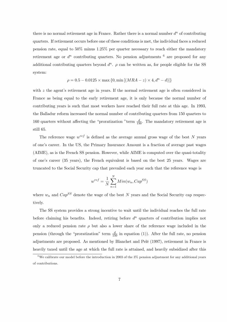
Figure 1: Life cycle model
Y E O
WERA
RERA Mπ−1
EEπ−1
EEπ
YYπ
YYπ−1
OOπ
OOπ−1 WERA+1
RERA+1 Mπ−1
Mπ−1 Mπ−1RMRA
Mπ
Mπ
Retirement decision Retirement decision
Mπ−1
Figure 1 summarizes the age structure. Following Castañeda et al. (2003) and Ljunqvist and
Sargent (2005), agents age stochastically and sequentially until the early retirement age (ERA).
Between this age and the mandatory retirement age (MRA), age and time evolve in parallel
in order to determine the retirement age very accurately: workers grow older of one year each
period9.
Before the early retirement age, we consider three classes of working age: the young, the
experienced and the old workers, respectively denoted Y , E and O. All agents are "born" as
young workers (Y ) at a given age which corresponds to end of education. Rather than assuming
deterministic aging, as in a traditional overlapping generation model, individuals face a given
probability to move to the next age group. The probability of remaining a young (experienced)
worker in the next period is πY Y (πEE) and, as aging occurs sequentially, the probability of
becoming an experienced (old) worker is 1 − πY Y (1 − πEE). As workers differ in terms of
age at end of education according to their ability, they do not experience the same number of
years before ERA. This translates into different probabilities π’s across ability. Until ERA, the
probability of dying is taken to be zero.
The existence of these three aging classes permits to take into account a typical wage life cycle
profile: as a worker accumulates experience during his life cycle, we assume that the efficiency of
9 This is the meaning of subscript "+1" in Figure 1.
9
the labor input grows with the agent’s age. Thus, when a young worker becomes an experienced
worker, his efficiency is multiplied by 1 + xY . An old worker’s efficiency is (1 + xE) times that
of a young agent, with xY < xE .
With a probability equal to 1−πOO, older workers reach the retirement eligibility age (ERA).
In this second life cycle stage, from the ERA onwards, individuals face a probability of dying
which is specific to their labor ability. For people still in activity and alive, until the mandatory
retirement age (MRA), workers grow older of one year each period. At the beginning of each
period (ERA for instance), conditional on being alive, they choose to retire (RERA) or not
(WERA). If they decide to postpone retirement, they remain in the labor force one additional
year with the same efficiency as the older workers. If they survive, they will face the same choice
at the beginning of the next period. Conditional on being alive and in activity, workers must
retire at the beginning of the mandatory retirement age (MRA).
We will denote by ξ the stochastic age variable which is assumed to follow a finite state
Markov process. ξ takes values in the set Ξ = {Y, E, O, ERA, ERA+ 1, ..., MRA− 1, MRA}.
Retirees must be defined by their retirement age z as their pension depends on z. Using age-
specific mortality rates would also have required to keep track of the age of retired workers. For
computational reasons, we consider a constant probability πM of dying. Retirees, conditional
on surviving, remain in the same age group (ξ′ = ξ) . A retiree is then characterized by a
given ξ which actually corresponds to its retirement age z. This allows us to have only one
state variable for retirees (retirement age) instead of two (retirement age and current age)10. In
addition, consistency requires that individuals who are still in the labor force also face a constant
probability of dying πM .
Our assumptions on the demographics are driven by the choice to make the retirement age
endogenous. Our model combines a detailed modelling in ages when retirement is possible with
a parsimonious life cycle prior to the ERA and posterior to the retirement age. All individuals
pass through the age stages Y , E and O. Their life-cycle differs after the early retirement age
depending on the retirement age. Some may retire early, at ERA. The set of stages describing
their life cycle is then {Y, E, O, ERA}. Others may retire later, at age ERA+ i. Their life cycle
is then {Y, E, O, ERA, ..., ERA + i}. The last element corresponds to the retirement age and
10 Even if it would have been more satisfying to consider age-specific mortality rates, constant ones significantly
reduce the scale of the dynamic programming, and then the computational burden.
10
they remain in this state until they die.
2.2.3 Unemployment shocks
We introduce an unemployment risk only for older workers (ξ = O). We discard unemployment
risks during the medium stages of working life (ξ = E): the exit rate from employment is
very low at medium ages, much less than in the US for instance (Aubert et al., 2005). Ignoring
unemployment risk for the younger workers (ξ = Y ) is more questionable as their unemployment
rate is high in France. However, unemployment risk at young ages do not alter retirement
decision at older ages. This is not the case for the observed decline in the employment rate of
workers aged 55-59. Introducing this idiosyncratic risk of being unemployed at these ages is then
essential to the understanding of retirement decisions and the implications of any policy aiming
at delaying retirement age. In France, based on the French Labor Survey (1990-2003), it appears
that the employment rate for the 55-59 years old decreased by more than 20%, relative to the
50-54 age group. The exit rate from employment is around 12% for the 55-59 years old workers,
fourfold the rate for these aged 30-49. Secondly, it is important to notice that the exit rate
from unemployment at these ages is very close to zero11. These workers have access to specific
arrangements of unemployment insurance12 (including an exemption from seeking employment).
However, it must be emphasized that only workers age 55-59 who have been laid-off are eligible
to these specific unemployment programs. Unemployed old workers exit employment as a result
of involuntary quits and have access to inactivity benefits until retirement13 (see Aubert et al.,
2005).
We then assume that old individuals face an (un)employment shock φ ∈ Φ = {e, u} which
is assumed to follow a two-state Markov process. The individual labor input is set to l(φ).
When unemployed (φ = u), the time endowment is devoted to leisure (l(u) = 0) and workers
receive an unemployment benefit until the age of full pension rate. When employed (φ = e),
they inelastically supply l units of labor input (l(e) = l) at a wage rate w. Consistently with
11 Only 2% of the 55-59 years old non-employed people find a new job annually, while this proportion is around
30% for the 39-49 age group.
12 The development of generous unemployment insurance for older workers has been viewed as an answer to the
propensity of firms to get rid of their older staff during downsizing.
13 Making actuarially-fair (early retirement) schemes available to individuals before 60 could be welfare-
improving. However, we will discard this question by maintaining the early retirement age at 60.
11

empirical evidence, we will consider that the unemployment state is an absorbing state until
retirement. Workers become retired as employed or unemployed. As their pension depends on
their work history, through the reference wage wref , φ is still a state variable for retirees.
2.3 Preferences
Individuals derive utility from their own consumption and leisure as well as from the well-being
of all their descendants (they belong to the same dynasty), but not of their predecessors.
We assume that the instantaneous utility function u is of a CRRA type:
u(C, 1− l) =(C1−ν(1− l)ν)1−σ̃
1− σ̃
with Ct consumption, σ̃ ∈ [0, 1[∪]1,∞[ the risk aversion and ν ∈ [0, 1] the share of leisure
in the instantaneous utility. Time endowment is normalized to one. The utility function is
Cobb-Douglas in consumption and leisure. The reasons for this choice are that this function
is compatible with a balanced growth path and the parameters needed for the calibration have
been extensively studied in the literature relying on calibration (Cooley and Prescott, 1995;
Hansen and Imrogoroglu, 1992; Rios Rull, 1996; Huggett and Ventura, 1999).
2.4 Firms and technology
Firms use capital and labor to produce a single good according to the following production
function: Y = Kα(XL)1−α, with α ∈ [0, 1] the output share of capital, K the aggregate capital
which depreciates at a constant rate δ and L the labor input obtained by aggregating the
efficiency labor units. X is a deterministic exogenous productivity trend growing at a rate of g.
Firms produce in a perfectly competitive environment and maximize profits by hiring labor
from workers and renting capital from individuals so that marginal products equal factor prices.
w(γ, ξ)(1 + Θf (w(γ, ξ)) = µ(γ, ξ)(1− α)Y
L(2)
r + δ = αY
K(3)
with r the interest rate and Θf is the contribution rate paid by the firm to finance the pay-
as-you-go pension system14. µ(γ, ξ) a global efficiency indicator combining labor ability and
14Θf splits in two components: θf the contribution rate of the General Regime and cMCSf the one of the
12
seniority.
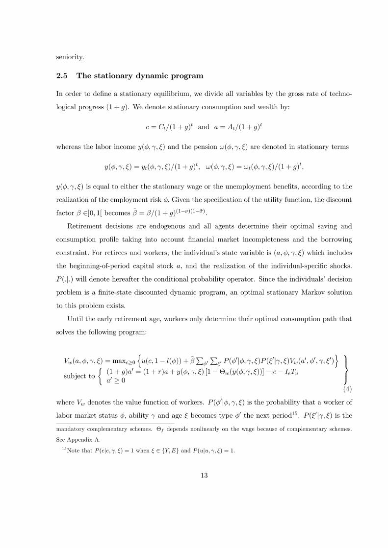
2.5 The stationary dynamic program
In order to define a stationary equilibrium, we divide all variables by the gross rate of techno-
logical progress (1 + g). We denote stationary consumption and wealth by:
c = Ct/(1 + g)t and a = At/(1 + g)t
whereas the labor income y(φ, γ, ξ) and the pension ω(φ, γ, ξ) are denoted in stationary terms
y(φ, γ, ξ) = yt(φ, γ, ξ)/(1 + g)t, ω(φ, γ, ξ) = ωt(φ, γ, ξ)/(1 + g)t,
y(φ, γ, ξ) is equal to either the stationary wage or the unemployment benefits, according to the
realization of the employment risk φ. Given the specification of the utility function, the discount
factor β ∈]0, 1[ becomes β̃ = β/(1 + g)(1−ν)(1−σ̃).
Retirement decisions are endogenous and all agents determine their optimal saving and
consumption profile taking into account financial market incompleteness and the borrowing
constraint. For retirees and workers, the individual’s state variable is (a, φ, γ, ξ) which includes
the beginning-of-period capital stock a, and the realization of the individual-specific shocks.
P (.|.) will denote hereafter the conditional probability operator. Since the individuals’ decision
problem is a finite-state discounted dynamic program, an optimal stationary Markov solution
to this problem exists.
Until the early retirement age, workers only determine their optimal consumption path that
solves the following program:
Vw(a, φ, γ, ξ) = maxc≥0
{u(c, 1− l(φ)) + β̃
∑φ′∑
ξ′ P (φ′|φ, γ, ξ)P (ξ′|γ, ξ)Vw(a
′, φ′, γ, ξ′)}
subject to{(1 + g)a′ = (1 + r)a+ y(φ, γ, ξ) [1−Θw(y(φ, γ, ξ))]− c− IeTu
a′ ≥ 0
(4)
where Vw denotes the value function of workers. P (φ′|φ, γ, ξ) is the probability that a worker of
labor market status φ, ability γ and age ξ becomes type φ′ the next period15. P (ξ′|γ, ξ) is the
mandatory complementary schemes. Θf depends nonlinearly on the wage because of complementary schemes.
See Appendix A.15 Note that P (e|e, γ, ξ) = 1 when ξ ∈ {Y,E} and P (u|u, γ, ξ) = 1.
13
probability that a worker of ability16 γ and age ξ becomes age ξ′ the next period.
Θw(y(φ, γ, ξ)) embodies the contribution rate paid by the worker (employed or unemployed)
to finance the pay-as-you-go pension system17. Unemployment benefits are financed through a
lump-sum tax Tu by workers when employed. Ie is the indicator function for φ = e. It is equal
to one if φ = e and zero otherwise.
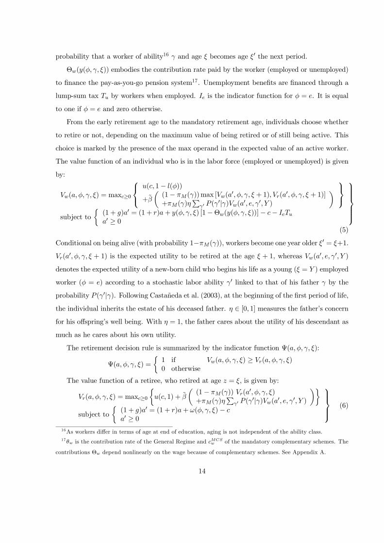
From the early retirement age to the mandatory retirement age, individuals choose whether
to retire or not, depending on the maximum value of being retired or of still being active. This
choice is marked by the presence of the max operand in the expected value of an active worker.
The value function of an individual who is in the labor force (employed or unemployed) is given
by:
Vw(a, φ, γ, ξ) = maxc≥0
u(c, 1− l(φ))
+β̃
((1− πM(γ))max [Vw(a
′, φ, γ, ξ + 1), Vr(a′, φ, γ, ξ + 1)]
+πM(γ)η∑
γ′ P (γ′|γ)Vw(a
′, e, γ′, Y )
)
subject to{(1 + g)a′ = (1 + r)a+ y(φ, γ, ξ) [1−Θw(y(φ, γ, ξ))]− c− IeTu
a′ ≥ 0
(5)
Conditional on being alive (with probability 1−πM(γ)), workers become one year older ξ′ = ξ+1.
Vr(a′, φ, γ, ξ + 1) is the expected utility to be retired at the age ξ + 1, whereas Vw(a
′, e, γ′, Y )
denotes the expected utility of a new-born child who begins his life as a young (ξ = Y ) employed
worker (φ = e) according to a stochastic labor ability γ′ linked to that of his father γ by the
probability P (γ′|γ). Following Castañeda et al. (2003), at the beginning of the first period of life,
the individual inherits the estate of his deceased father. η ∈ [0, 1] measures the father’s concern
for his offspring’s well being. With η = 1, the father cares about the utility of his descendant as
much as he cares about his own utility.
The retirement decision rule is summarized by the indicator function Ψ(a, φ, γ, ξ):
Ψ(a, φ, γ, ξ) =
{1 if Vw(a, φ, γ, ξ) ≥ Vr(a, φ, γ, ξ)0 otherwise
The value function of a retiree, who retired at age z = ξ, is given by:
Vr(a, φ, γ, ξ) = maxc≥0
{u(c, 1) + β̃
((1− πM(γ)) Vr(a
′, φ, γ, ξ)+πM(γ)η
∑γ′ P (γ
′|γ)Vw(a′, e, γ′, Y )
)}
subject to{(1 + g)a′ = (1 + r)a+ ω(φ, γ, ξ)− ca′ ≥ 0
(6)
16 As workers differ in terms of age at end of education, aging is not independent of the ability class.17θw is the contribution rate of the General Regime and cMCS
w of the mandatory complementary schemes. The
contributions Θw depend nonlinearly on the wage because of complementary schemes. See Appendix A.
14

Retirees receive a pension ω(φ, γ, ξ) that is the sum of the public Social Security pension and
benefits paid by mandatory complementary schemes. The only choice faced by a retiree is his
consumption profile and the optimal amount of financial assets he wants to give to his child,
according to the stochastic intergenerational expected changes in ability.
2.6 Definition of the equilibrium
Following Castañeda et al. (2003), we define the variable s ∈ S which denotes jointly the
employment shock, the random labor ability and the random age of individuals:
s : Φ× Γ× Ξ → S
(φ, γ, ξ) → s(φ, γ, ξ)
Its process is independent and identically distributed across individuals and follows a finite
state Markov chain. The conditional transition probability is defined as follows:
P (s′|s) = Pr{st+1 = s′|st = s}
The steady state equilibrium is characterized by worker and retiree choices for consump-
tion and savings {cw(a, s), cr(a, s), a′w(a, s), a′r(a, s)} and for retirement Ψ(a, s), value functions
Vw(a, s) and Vr(a, s), a vector of prices (r, w(s)), a SS policy (θ, ωGR(s)), a stationary distribu-
tion of individuals Λ(a, s) and a set of aggregate variables (K̃, L) which respectively denotes the
stationary capital stock and the efficient labor input. The stationary equilibrium is such that:
(i) Individuals’ decision rules are solutions to the lifetime maximization programs (4), (5) and
(6)
(ii) Factor prices are competitive, conditions (2) and (3) hold.
(iii) The endogenous probability distribution Λ(a, s) is the stationary distribution associated
with (A(a, s), P (s′|s)) such that:
Λ(a′, s′) =∑
s
∑
{a:a′=A(a,s)}
Λ(a, s)P (s′|s)
with a′ ≡ A(a, s) the individuals’ policy that encompasses retirement choices and saving
decisions. A(a, s) is such that:
A(a, s) = Ψ(a, s)a′w(a, s) + [1−Ψ(a, s)]a′r(a, s)
15

(iv) Factor inputs are aggregated over individuals.
L =∑
s
∑
a
Ψ(a, s)lµ(s)
K̃ =∑
s
∑
a
Λ(a, s)A(a, s)
(v) The payroll tax rate θ adjusts to balance the SS budget: 18
∑
s
∑
a
Ψ(a, s)θy(s) =∑
s
∑
a
(1−Ψ(a, s))ωGR(s)) (7)
Given the specification of preferences and the various constraints, it is not possible to solve
this equilibrium analytically. We implement numerical techniques based on a discretization
of state variables (see Ljungqvist and Sargent 2000 for a presentation of the methodology).
3 Calibration and quantitative evaluation
3.1 Calibration on French data
This section presents the calibration of the demographic structure, idiosyncratic risks, life cycle
profile of labor earnings, Social Security arrangements, preferences and technology parameters.
We choose to calibrate the pension system after the French 1993 Balladur reform.
3.1.1 Labor ability and employment risks
Labor abilities are calibrated on the basis of ability categories for which information on lifetime
wage profiles, intergenerational links, employment rates and death probabilities is available. The
high ability labor class (H) will correspond to executives, the medium one (M) to white-collars,
and the low one (L) to clerks and blue-collars.
There exists some degree of intergenerational transmission of human capital. The correlation
between the parent’s human capital and that of his offspring is given by the intergenerational
ability matrix computed from INSEE (1995) (Table 1). The risk for a H type agent to have a
child who belongs to a lower ability class is superior to 50%. This will provide a strong bequest
motive to insure his descendant against this risk.
18 The budgets of complementary schemes and unemployment insurance are balanced. We do not explicitly
present these budgets as they are not the primary focus of our paper.
16

Table 1: Intergenerational change in abilitySon’s Ability (t+ 1)
Father’s Ability (t)
H M L
H 0.4077 a 0.3187 0.2736
M 0.2191 0.3507 0.4302
L 0.0929 0.1952 0.7119
a: A H-ability worker faces a 40.77% probability
of giving birth to a H-ability son
Table 2: Unemployment replacement rate (ρu) and employment risk (πu)ρu πu
H 0.60 a 0.063 b
M 0.61 0.083
L 0.65 0.086
a: An unemployed H-ability agent receives 0.60 of his last annual net wage
b: Each year, an H-ability worker faces a 6.3% probability of becoming unemployed
As argued in Section 2.2.3, the employment risk occurs at the end of working life. It differs
across labor ability groups. We assume that the transition rate from non-employment to em-
ployment is null. The annual transition rate from employment to non-employment πu is set such
that the model replicates the employment rate of male individuals aged 55 - 59 for each ability
class (computed from the French Employment Survey). In particular, blue-collars and clerks (L)
face a higher risk of non-employment than white-collars (M) (Table 2). Non-employed workers
are either unemployed or entitled to programs specific to older workers named as pre-retirement
programs. As the replacement rates are not the same, we consider that workers in the non-
employed state receive an average benefit (ρu), weighted by the relative population entitled to
these two non-employed statuses.
3.1.2 Demographics and lifetime wage
We assume that individuals are born when they enter the labor market. As shown by Colin
et al. (2000), the age at end of education differs across labor abilities (Table 3). This age affects
retirement choices which are conditional on a minimum duration of contributions.
As workers differ in terms of age at birth, their expected length of working life until the
common early retirement age differs too. As they also experience a common decrease in the em-
17
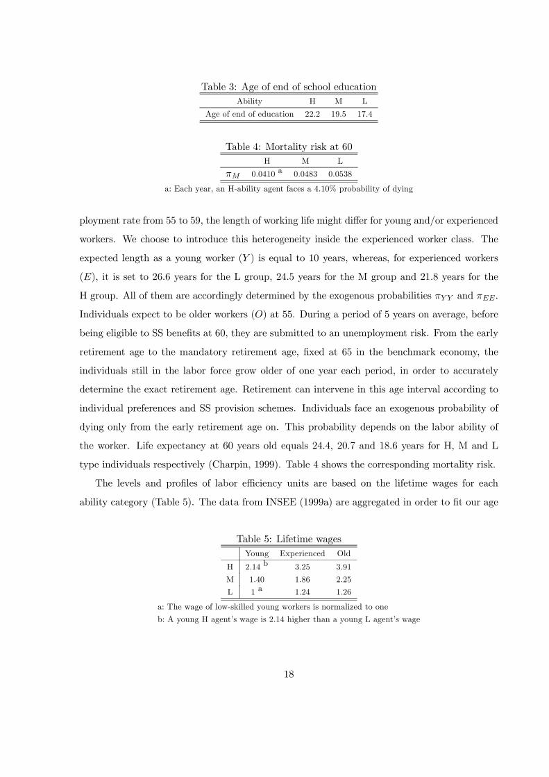
Table 3: Age of end of school educationAbility H M L
Age of end of education 22.2 19.5 17.4
Table 4: Mortality risk at 60H M L
πM 0.0410 a 0.0483 0.0538
a: Each year, an H-ability agent faces a 4.10% probability of dying
ployment rate from 55 to 59, the length of working life might differ for young and/or experienced
workers. We choose to introduce this heterogeneity inside the experienced worker class. The
expected length as a young worker (Y ) is equal to 10 years, whereas, for experienced workers
(E), it is set to 26.6 years for the L group, 24.5 years for the M group and 21.8 years for the
H group. All of them are accordingly determined by the exogenous probabilities πY Y and πEE.
Individuals expect to be older workers (O) at 55. During a period of 5 years on average, before
being eligible to SS benefits at 60, they are submitted to an unemployment risk. From the early
retirement age to the mandatory retirement age, fixed at 65 in the benchmark economy, the
individuals still in the labor force grow older of one year each period, in order to accurately
determine the exact retirement age. Retirement can intervene in this age interval according to
individual preferences and SS provision schemes. Individuals face an exogenous probability of
dying only from the early retirement age on. This probability depends on the labor ability of
the worker. Life expectancy at 60 years old equals 24.4, 20.7 and 18.6 years for H, M and L
type individuals respectively (Charpin, 1999). Table 4 shows the corresponding mortality risk.
The levels and profiles of labor efficiency units are based on the lifetime wages for each
ability category (Table 5). The data from INSEE (1999a) are aggregated in order to fit our age
Table 5: Lifetime wagesYoung Experienced Old
H 2.14 b 3.25 3.91
M 1.40 1.86 2.25
L 1 a 1.24 1.26
a: The wage of low-skilled young workers is normalized to one
b: A young H agent’s wage is 2.14 higher than a young L agent’s wage
18
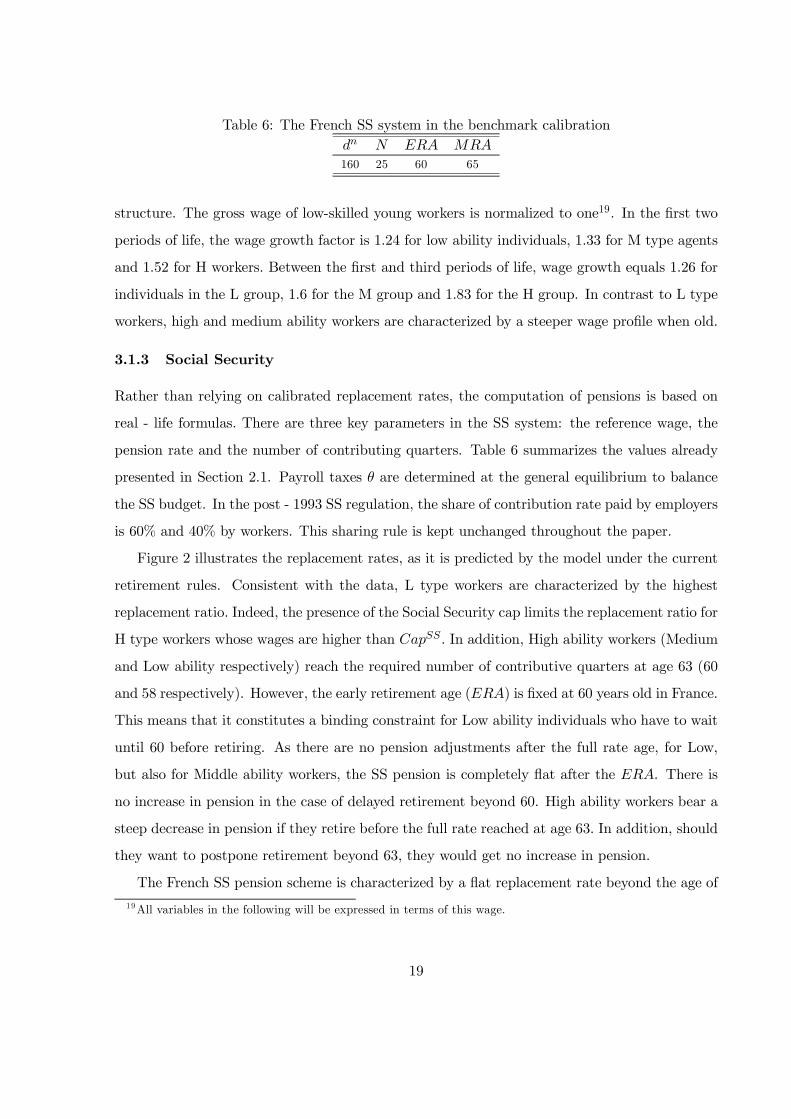
Table 6: The French SS system in the benchmark calibrationdn N ERA MRA
160 25 60 65
structure. The gross wage of low-skilled young workers is normalized to one19. In the first two
periods of life, the wage growth factor is 1.24 for low ability individuals, 1.33 for M type agents
and 1.52 for H workers. Between the first and third periods of life, wage growth equals 1.26 for
individuals in the L group, 1.6 for the M group and 1.83 for the H group. In contrast to L type
workers, high and medium ability workers are characterized by a steeper wage profile when old.
3.1.3 Social Security
Rather than relying on calibrated replacement rates, the computation of pensions is based on
real - life formulas. There are three key parameters in the SS system: the reference wage, the
pension rate and the number of contributing quarters. Table 6 summarizes the values already
presented in Section 2.1. Payroll taxes θ are determined at the general equilibrium to balance
the SS budget. In the post - 1993 SS regulation, the share of contribution rate paid by employers
is 60% and 40% by workers. This sharing rule is kept unchanged throughout the paper.
Figure 2 illustrates the replacement rates, as it is predicted by the model under the current
retirement rules. Consistent with the data, L type workers are characterized by the highest
replacement ratio. Indeed, the presence of the Social Security cap limits the replacement ratio for
H type workers whose wages are higher than CapSS . In addition, High ability workers (Medium
and Low ability respectively) reach the required number of contributive quarters at age 63 (60
and 58 respectively). However, the early retirement age (ERA) is fixed at 60 years old in France.
This means that it constitutes a binding constraint for Low ability individuals who have to wait
until 60 before retiring. As there are no pension adjustments after the full rate age, for Low,
but also for Middle ability workers, the SS pension is completely flat after the ERA. There is
no increase in pension in the case of delayed retirement beyond 60. High ability workers bear a
steep decrease in pension if they retire before the full rate reached at age 63. In addition, should
they want to postpone retirement beyond 63, they would get no increase in pension.
The French SS pension scheme is characterized by a flat replacement rate beyond the age of
19 All variables in the following will be expressed in terms of this wage.
19
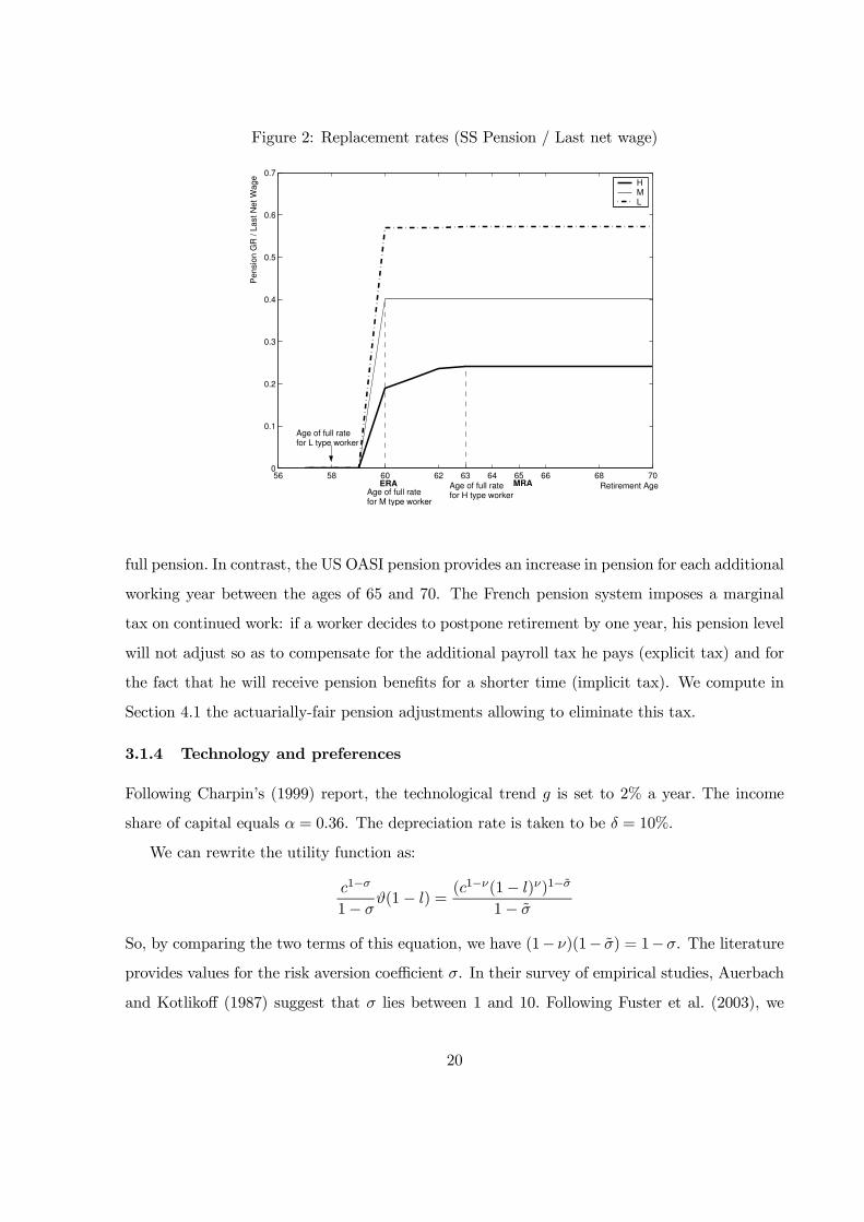
Figure 2: Replacement rates (SS Pension / Last net wage)
56 58 60 62 63 64 65 66 68 700
0.1
0.2
0.3
0.4
0.5
0.6
0.7
Pensio
n G
R / L
ast N
et W
age
Retirement Age
HML
ERA Age of full ratefor H type worker
MRA Age of full ratefor M type worker
Age of full ratefor L type worker
full pension. In contrast, the US OASI pension provides an increase in pension for each additional
working year between the ages of 65 and 70. The French pension system imposes a marginal
tax on continued work: if a worker decides to postpone retirement by one year, his pension level
will not adjust so as to compensate for the additional payroll tax he pays (explicit tax) and for
the fact that he will receive pension benefits for a shorter time (implicit tax). We compute in
Section 4.1 the actuarially-fair pension adjustments allowing to eliminate this tax.
3.1.4 Technology and preferences
Following Charpin’s (1999) report, the technological trend g is set to 2% a year. The income
share of capital equals α = 0.36. The depreciation rate is taken to be δ = 10%.
We can rewrite the utility function as:
c1−σ
1− σϑ(1− l) =
(c1−ν(1− l)ν)1−σ̃
1− σ̃
So, by comparing the two terms of this equation, we have (1− ν)(1− σ̃) = 1−σ. The literature
provides values for the risk aversion coefficient σ. In their survey of empirical studies, Auerbach
and Kotlikoff (1987) suggest that σ lies between 1 and 10. Following Fuster et al. (2003), we
20
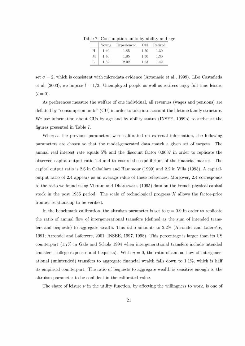
Table 7: Consumption units by ability and ageYoung Experienced Old Retired
H 1.40 1.85 1.50 1.30
M 1.40 1.85 1.50 1.30
L 1.52 2.02 1.63 1.42
set σ = 2, which is consistent with microdata evidence (Attanasio et al., 1999). Like Castañeda
et al. (2003), we impose l = 1/3. Unemployed people as well as retirees enjoy full time leisure
(l = 0).
As preferences measure the welfare of one individual, all revenues (wages and pensions) are
deflated by “consumption units” (CU) in order to take into account the lifetime family structure.
We use information about CUs by age and by ability status (INSEE, 1999b) to arrive at the
figures presented in Table 7.
Whereas the previous parameters were calibrated on external information, the following
parameters are chosen so that the model-generated data match a given set of targets. The
annual real interest rate equals 5% and the discount factor 0.9637 in order to replicate the
observed capital-output ratio 2.4 and to ensure the equilibrium of the financial market. The
capital output ratio is 2.6 in Caballaro and Hammour (1999) and 2.2 in Villa (1995). A capital-
output ratio of 2.4 appears as an average value of these references. Moreover, 2.4 corresponds
to the ratio we found using Vikram and Dhareswar’s (1995) data on the French physical capital
stock in the post 1955 period. The scale of technological progress X allows the factor-price
frontier relationship to be verified.
In the benchmark calibration, the altruism parameter is set to η = 0.9 in order to replicate
the ratio of annual flow of intergenerational transfers (defined as the sum of intended trans-
fers and bequests) to aggregate wealth. This ratio amounts to 2.2% (Arrondel and Laferrère,
1991; Arrondel and Laferrere, 2001; INSEE, 1997, 1998). This percentage is larger than its US
counterpart (1.7% in Gale and Scholz 1994 when intergenerational transfers include intended
transfers, college expenses and bequests). With η = 0, the ratio of annual flow of intergener-
ational (unintended) transfers to aggregate financial wealth falls down to 1.1%, which is half
its empirical counterpart. The ratio of bequests to aggregate wealth is sensitive enough to the
altruism parameter to be confident in the calibrated value.
The share of leisure ν in the utility function, by affecting the willingness to work, is one of
21
the key parameters in the model. However, the current pension system imposes such a huge
tax on continued activity after the full pension age that it hardly reveals leisure preferences at
the end of working life. Blanchet and Pelé (1997) provide the most comprehensive survey on
retirement decision in France. Based on data which do not include the 1993 Balladur reform,
the salient fact they stress is that the majority of individuals retire at 60. This first result is
quite ambiguous. Do people retire as soon as they can due to a strong preference for leisure
or because they are heavily taxed after the full rate? It is difficult to answer this question as,
before 1993, 60 was both the early retirement age and the full pension age for a vast majority
of workers. 20 Another interesting feature provides a first answer. Blanchet and Pelé (1997)
observe another peak in the retirement age distribution at 65. This smaller peak at age 65 stems
from retirement by people with incomplete careers, especially women. This indicates that some
people choose to work until they reach the full pension age.
These first empirical insights can be completed by more recent data including the 1993
reform. We verify that people actually retire at their full pension age. First, among male
individuals retiring at age 60, 95% had indeed accumulated dn contributive quarters (French
ministry of Labor, Drees 2003). Secondly, since the Balladur reform, more individuals have
reached the full rate between the ages of 60 and 65. The Balladur 1993 reform has lengthened
the duration of contributions from 150 quarters to 160 quarters to reach the full pension age.
The implementation has been phased in with one additional quarter per generation, from 1934
to 1943 (dn = 150 for generations born before 1933, dn = 151 for generations born in 1934,
etc.). Figure 3 represents the peak of the distribution of contributive quarters at retirement for
male individuals retiring between the ages of 60 and 65. The peak moves to 151 quarters for
the 1934 generation, 152 for the 1935 generation, to 157 for the 1940 generation. Finally, the
same pattern is present for every generation, following the way the reform is phased in 21: the
retirement age mainly coincides with the full pension age.
This emphasizes the importance of the tax on continued activity in retirement decisions. This
stylized fact makes the calibration of parameter ν difficult, as the importance of the tax does
not enable us to pin down precisely the relative preference for leisure. Conversely, preferences
20 Indeed, in the pre-1993 regime, dn = 150. H type workers (M and L respectively) accumulated the required
number of contributive quarters at age 60 (57 and 55 respectively).
21 We thank Antoine Bozio for providing us with the French Social Security data. See also Bozio (2005).
22

Figure 3: Evolution of the number of contributive quarters at retirement (Source: Social Securitydata)
146
148
150
152
154
156
158
1928
1929
1930
1931
1932
1933
1934
1935
1936
1937
1938
1939
1940
Birth Year
Nu
mb
er
of
co
ntr
ibu
tive q
uart
ers
at
reti
rem
en
t (m
od
e o
f d
istr
ibu
tio
n)
which would lead to anticipated or delayed retirement relative to the full pension age can be
confidently rejected. We identify an interval of admissible values for this parameter: under a
minimum value of preference for leisure, individuals would put off retirement beyond their full
rate age, while above a maximal admissible value, they would exit before the full rate. We
determine these interval bounds by simulations22. Admissible values for ν lie in the interval
[0.61; 0.65] and we consider 0.63 as the benchmark value23. For these values, the model predicts
that 100% of individuals will retire at their full rate age (Figure 4). Only High ability individuals
work beyond the early retirement age since they reach 160 quarters of contribution at the age
of 63. Medium and Low ability workers, who reach the required number of contributions to get
a full pension at the age of 58 and 60 respectively, stop working at the early retirement age.
22 Note that the upper bound has been determined on the sole basis of the behavior of H type workers (we assume
the same preference across labor abilities) since their full pension age (63) differs from the early retirement age
(60).
23 It is worth emphasizing that the value of ν is such that, at the steady state, a unit of good without work
is worth 1.99 times a unit of good gotten by working. The calibrated value is consistent with Stock and Wise’s
(1990) estimate. They found on US data that the ratio of a consumption unit with work to a consumption unit
without work equals 1.66.
23
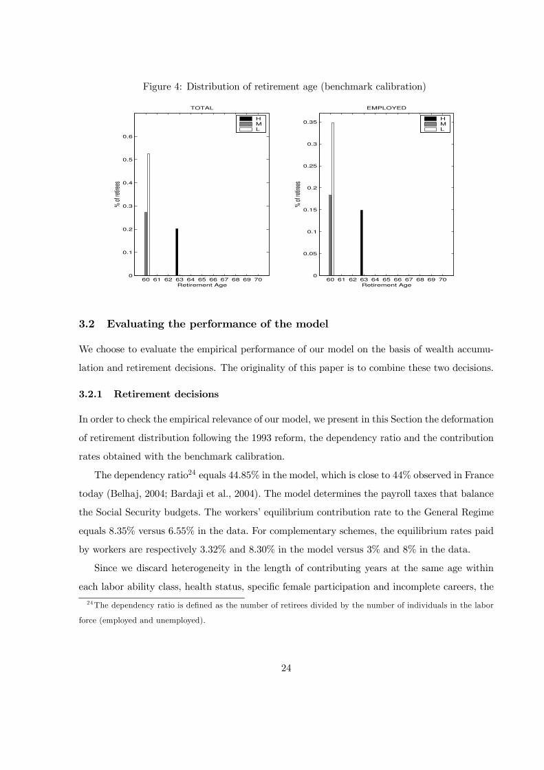
Figure 4: Distribution of retirement age (benchmark calibration)
60 61 62 63 64 65 66 67 68 69 700
0.1
0.2
0.3
0.4
0.5
0.6
TOTAL
% o
f ret
irees
Retirement Age
HML
60 61 62 63 64 65 66 67 68 69 700
0.05
0.1
0.15
0.2
0.25
0.3
0.35
EMPLOYED
% o
f ret
irees
Retirement Age
HML
3.2 Evaluating the performance of the model
We choose to evaluate the empirical performance of our model on the basis of wealth accumu-
lation and retirement decisions. The originality of this paper is to combine these two decisions.
3.2.1 Retirement decisions
In order to check the empirical relevance of our model, we present in this Section the deformation
of retirement distribution following the 1993 reform, the dependency ratio and the contribution
rates obtained with the benchmark calibration.
The dependency ratio24 equals 44.85% in the model, which is close to 44% observed in France
today (Belhaj, 2004; Bardaji et al., 2004). The model determines the payroll taxes that balance
the Social Security budgets. The workers’ equilibrium contribution rate to the General Regime
equals 8.35% versus 6.55% in the data. For complementary schemes, the equilibrium rates paid
by workers are respectively 3.32% and 8.30% in the model versus 3% and 8% in the data.
Since we discard heterogeneity in the length of contributing years at the same age within
each labor ability class, health status, specific female participation and incomplete careers, the
24 The dependency ratio is defined as the number of retirees divided by the number of individuals in the labor
force (employed and unemployed).
24

Figure 5: Impact of the 1993 Balladur reform on the distribution of retirement age (benchmarkcalibration)
60 61 62 63 64 65 66 67 68 69 700
0.2
0.4
0.6
0.8
1
TOTAL
% o
f re
tire
es
Retirement age
Before the 1993 Balladur reform − AllAfter the 1993 Balladur reform − H typeAfter the 1993 Balladur reform − M typeAfter the 1993 Balladur reform − L type
only H type agentsdelay retirement
model cannot capture the complete distribution of retirement age25. However, we replicate the
stylized fact that agents mostly retire as soon as the full rate is available. As noted above,
following the 1993 reform, the peak of the distribution of contributive quarters at retirement
for male individuals retiring between the ages of 60 and 65 has moved consistently with the
increase in the normal number of contributing years. We verify that our model can replicate
this deformation of retirement distribution following the 1993 reform. Notice that the full
pension age has increased for H type workers only, as the early retirement is still binding for
the L and M types. Their retirement age should have increased, consistently with the observed
rise in contributive quarters at retirement (Figure 3). We verify that High ability workers delay
their retirement age by the number of additional contributing years necessary to reach the full
rate (Figure 5). The elasticity of delayed retirement to the normal contribution years in the
model seems consistent with the observed behaviors depicted in Figure 3.
3.2.2 Wealth accumulation
Table 8 presents statistics on the wealth distribution as predicted by the model versus its em-
pirical counterpart based on the 1998 French Wealth Survey (Enquête Patrimoine). Table 8
25 Including additional sources of heterogeneity would have made the model hardly tractable.
25
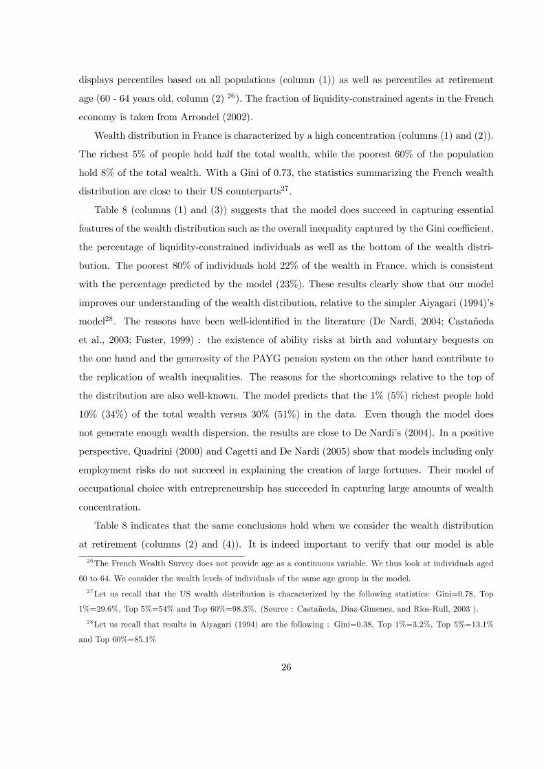
displays percentiles based on all populations (column (1)) as well as percentiles at retirement
age (60 - 64 years old, column (2) 26). The fraction of liquidity-constrained agents in the French
economy is taken from Arrondel (2002).
Wealth distribution in France is characterized by a high concentration (columns (1) and (2)).
The richest 5% of people hold half the total wealth, while the poorest 60% of the population
hold 8% of the total wealth. With a Gini of 0.73, the statistics summarizing the French wealth
distribution are close to their US counterparts27.
Table 8 (columns (1) and (3)) suggests that the model does succeed in capturing essential
features of the wealth distribution such as the overall inequality captured by the Gini coefficient,
the percentage of liquidity-constrained individuals as well as the bottom of the wealth distri-
bution. The poorest 80% of individuals hold 22% of the wealth in France, which is consistent
with the percentage predicted by the model (23%). These results clearly show that our model
improves our understanding of the wealth distribution, relative to the simpler Aiyagari (1994)’s
model28. The reasons have been well-identified in the literature (De Nardi, 2004; Castañeda
et al., 2003; Fuster, 1999) : the existence of ability risks at birth and voluntary bequests on
the one hand and the generosity of the PAYG pension system on the other hand contribute to
the replication of wealth inequalities. The reasons for the shortcomings relative to the top of
the distribution are also well-known. The model predicts that the 1% (5%) richest people hold
10% (34%) of the total wealth versus 30% (51%) in the data. Even though the model does
not generate enough wealth dispersion, the results are close to De Nardi’s (2004). In a positive
perspective, Quadrini (2000) and Cagetti and De Nardi (2005) show that models including only
employment risks do not succeed in explaining the creation of large fortunes. Their model of
occupational choice with entrepreneurship has succeeded in capturing large amounts of wealth
concentration.
Table 8 indicates that the same conclusions hold when we consider the wealth distribution
at retirement (columns (2) and (4)). It is indeed important to verify that our model is able
26 The French Wealth Survey does not provide age as a continuous variable. We thus look at individuals aged
60 to 64. We consider the wealth levels of individuals of the same age group in the model.
27 Let us recall that the US wealth distribution is characterized by the following statistics: Gini=0.78, Top
1%=29.6%, Top 5%=54% and Top 60%=98.3%. (Source : Castañeda, Diaz-Gimenez, and Rios-Rull, 2003 ).
28 Let us recall that results in Aiyagari (1994) are the following : Gini=0.38, Top 1%=3.2%, Top 5%=13.1%
and Top 60%=85.1%
26
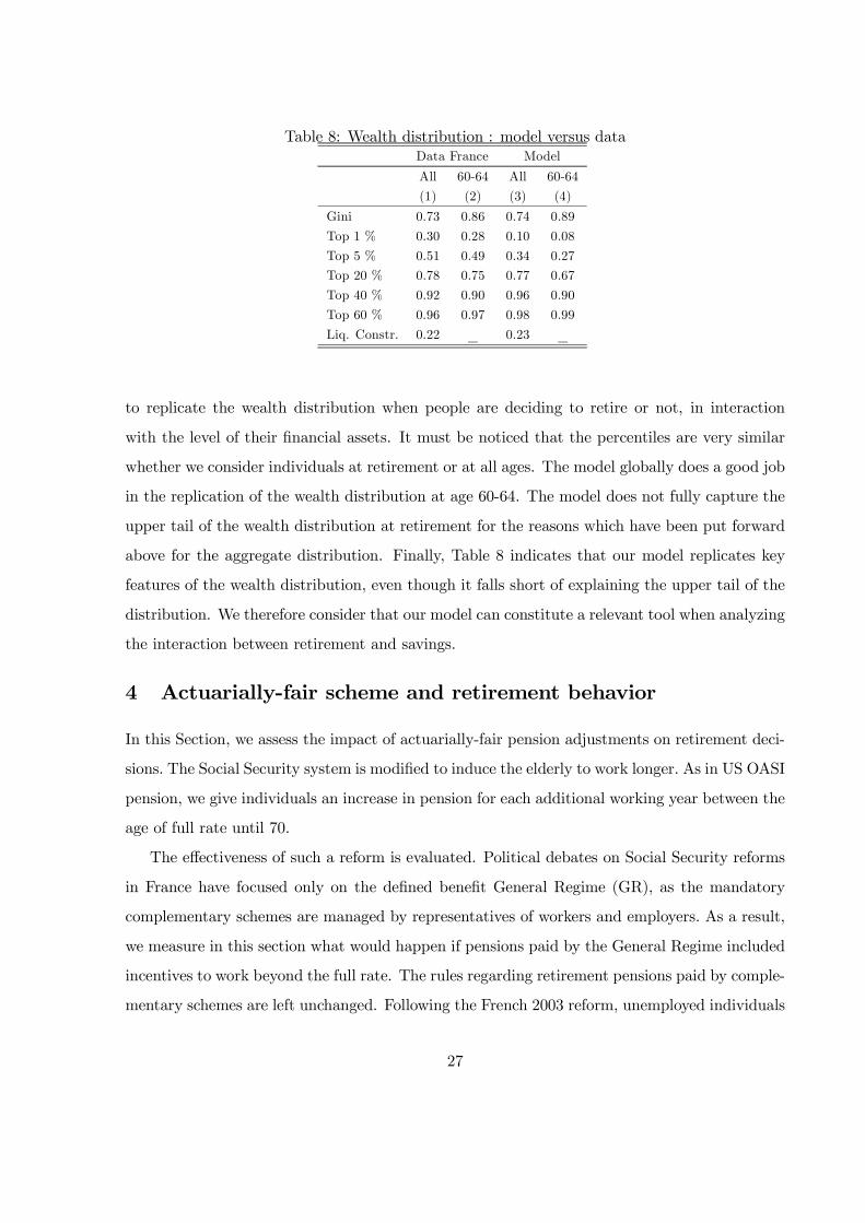
Table 8: Wealth distribution : model versus dataData France Model
All 60-64 All 60-64
(1) (2) (3) (4)
Gini 0.73 0.86 0.74 0.89
Top 1 % 0.30 0.28 0.10 0.08
Top 5 % 0.51 0.49 0.34 0.27
Top 20 % 0.78 0.75 0.77 0.67
Top 40 % 0.92 0.90 0.96 0.90
Top 60 % 0.96 0.97 0.98 0.99
Liq. Constr. 0.22 _ 0.23 _
to replicate the wealth distribution when people are deciding to retire or not, in interaction
with the level of their financial assets. It must be noticed that the percentiles are very similar
whether we consider individuals at retirement or at all ages. The model globally does a good job
in the replication of the wealth distribution at age 60-64. The model does not fully capture the
upper tail of the wealth distribution at retirement for the reasons which have been put forward
above for the aggregate distribution. Finally, Table 8 indicates that our model replicates key
features of the wealth distribution, even though it falls short of explaining the upper tail of the
distribution. We therefore consider that our model can constitute a relevant tool when analyzing
the interaction between retirement and savings.
4 Actuarially-fair scheme and retirement behavior
In this Section, we assess the impact of actuarially-fair pension adjustments on retirement deci-
sions. The Social Security system is modified to induce the elderly to work longer. As in US OASI
pension, we give individuals an increase in pension for each additional working year between the
age of full rate until 70.
The effectiveness of such a reform is evaluated. Political debates on Social Security reforms
in France have focused only on the defined benefit General Regime (GR), as the mandatory
complementary schemes are managed by representatives of workers and employers. As a result,
we measure in this section what would happen if pensions paid by the General Regime included
incentives to work beyond the full rate. The rules regarding retirement pensions paid by comple-
mentary schemes are left unchanged. Following the French 2003 reform, unemployed individuals
27
are not entitled to the incentive plans.
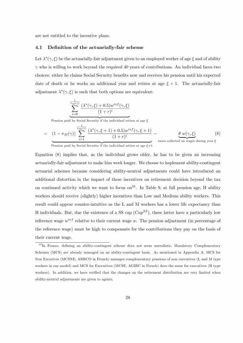
4.1 Definition of the actuarially-fair scheme
Let λ∗(γ, ξ) be the actuarially-fair adjustment given to an employed worker of age ξ and of ability
γ who is willing to work beyond the required 40 years of contributions. An individual faces two
choices: either he claims Social Security benefits now and receives his pension until his expected
date of death or he works an additional year and retires at age ξ + 1. The actuarially-fair
adjustment λ∗(γ, ξ) is such that both options are equivalent:
1πM (γ)∑
i=0
(λ∗(γ, ξ) + 0.5)wref (γ, ξ)
(1 + r)i
︸ ︷︷ ︸Pension paid by Social Security if the individual retires at age ξ
= (1− πM(γ))
1πM (γ)∑
i=1
(λ∗(γ, ξ + 1) + 0.5)wref (γ, ξ + 1)
(1 + r)i
︸ ︷︷ ︸Pension paid by Social Security if the individual retires at age ξ+1
− θ w(γ, ξ)︸ ︷︷ ︸
taxes collected on wages during year ξ
(8)
Equation (8) implies that, as the individual grows older, he has to be given an increasing
actuarially-fair adjustment to make him work longer. We choose to implement ability-contingent
actuarial schemes because considering ability-neutral adjustments could have introduced an
additional distortion in the impact of these incentives on retirement decision beyond the tax
on continued activity which we want to focus on29. In Table 9, at full pension age, H ability
workers should receive (slightly) higher incentives than Low and Medium ability workers. This
result could appear counter-intuitive as the L and M workers has a lower life expectancy than
H individuals. But, due the existence of a SS cap (CapSS), these latter have a particularly low
reference wage wref relative to their current wage w. The pension adjustment (in percentage of
the reference wage) must be high to compensate for the contributions they pay on the basis of
their current wage.
29 In France, defining an ability-contingent scheme does not seem unrealistic. Mandatory Complementary
Schemes (MCS) are already managed on an ability-contingent basis. As mentioned in Appendix A, MCS for
Non Excutives (MCSNE, ARRCO in French) manages complementary pensions of non executives (L and M type
workers in our model) and MCS for Executives (MCSE, AGIRC in French) does the same for executives (H type
workers). In addition, we have verified that the changes on the retirement distribution are very limited when
ability-neutral adjustments are given to agents.
28
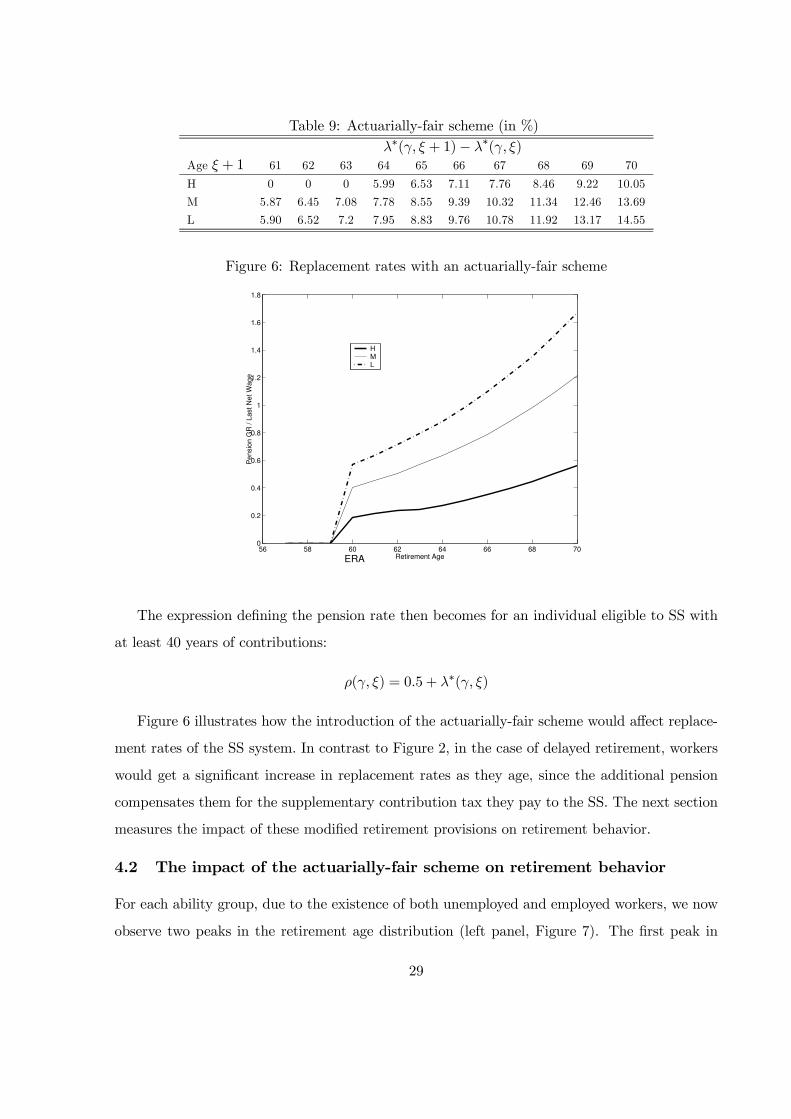
Table 9: Actuarially-fair scheme (in %)λ∗(γ, ξ + 1)− λ∗(γ, ξ)
Age ξ + 1 61 62 63 64 65 66 67 68 69 70
H 0 0 0 5.99 6.53 7.11 7.76 8.46 9.22 10.05
M 5.87 6.45 7.08 7.78 8.55 9.39 10.32 11.34 12.46 13.69
L 5.90 6.52 7.2 7.95 8.83 9.76 10.78 11.92 13.17 14.55
Figure 6: Replacement rates with an actuarially-fair scheme
56 58 60 62 64 66 68 700
0.2
0.4
0.6
0.8
1
1.2
1.4
1.6
1.8
Pe
nsio
n G
R /
La
st
Ne
t W
ag
e
Retirement Age
HML
ERA
The expression defining the pension rate then becomes for an individual eligible to SS with
at least 40 years of contributions:
ρ(γ, ξ) = 0.5 + λ∗(γ, ξ)
Figure 6 illustrates how the introduction of the actuarially-fair scheme would affect replace-
ment rates of the SS system. In contrast to Figure 2, in the case of delayed retirement, workers
would get a significant increase in replacement rates as they age, since the additional pension
compensates them for the supplementary contribution tax they pay to the SS. The next section
measures the impact of these modified retirement provisions on retirement behavior.
4.2 The impact of the actuarially-fair scheme on retirement behavior
For each ability group, due to the existence of both unemployed and employed workers, we now
observe two peaks in the retirement age distribution (left panel, Figure 7). The first peak in
29

Figure 7: Distribution of retirement age when individuals are given the actuarially-fair scheme
60 61 62 63 64 65 66 67 68 69 700
0.05
0.1
0.15
0.2
0.25
0.3
TOTAL
% o
f ret
irees
Retirement Age
HML
60 61 62 63 64 65 66 67 68 69 700
0.05
0.1
0.15
0.2
0.25
0.3
EMPLOYED
% o
f ret
irees
Retirement Age
HML
each ability group corresponds to retirement choices of unemployed individuals who still retire
at the age of full rate, as they are not eligible to the incentive schemes. By contrast, employed
workers take advantage of the actuarially fair scheme and delay retirement: the dependency
ratio declines from 44.85% to 37.85%. This exogenous source of between-employment status
variations now generates an important heterogeneity in retirement age.
It remains to present the retirement behavior of employed workers (right panel, Figure 7).
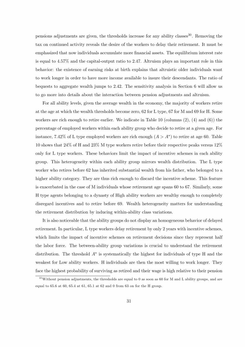
The inspection of the individual decision rules reveals the interaction between wealth accumu-
lation and retirement. Figure 8 illustrates the choice of a 64 year old H type agent. In order to
take his decision, he compares the value of being retired at age 64 to that of remaining active at
the same age. The value functions intersect when his financial holdings equals A∗ = 28.53. If his
current wealth is larger than A∗, the High ability agent would retire. If the High ability worker
is not rich enough (A < A∗), he chooses to keep on working. The model actually yields an array
of wealth thresholds above which individuals of each ability category decide to retire (Table 10).
For instance, a Low ability worker who considers retiring at 60 years old must have current
wealth greater than 9.27 in order to cease working. Given the normalization considered in our
model, this threshold corresponds to 8.3 years of his current net wage. When actuarially-fair
30
pensions adjustments are given, the thresholds increase for any ability classes30. Removing the
tax on continued activity reveals the desire of the workers to delay their retirement. It must be
emphasized that now individuals accumulate more financial assets. The equilibrium interest rate
is equal to 4.57% and the capital-output ratio to 2.47. Altruism plays an important role in this
behavior: the existence of earning risks at birth explains that altruistic older individuals want
to work longer in order to have more income available to insure their descendants. The ratio of
bequests to aggregate wealth jumps to 2.42. The sensitivity analysis in Section 6 will allow us
to go more into details about the interaction between pension adjustments and altruism.
For all ability levels, given the average wealth in the economy, the majority of workers retire
at the age at which the wealth thresholds become zero, 62 for L type, 67 for M and 69 for H. Some
workers are rich enough to retire earlier. We indicate in Table 10 (columns (2), (4) and (6)) the
percentage of employed workers within each ability group who decide to retire at a given age. For
instance, 7.42% of L type employed workers are rich enough (A > A∗) to retire at age 60. Table
10 shows that 24% of H and 23% M type workers retire before their respective peaks versus 12%
only for L type workers. These behaviors limit the impact of incentive schemes in each ability
group. This heterogeneity within each ability group mirrors wealth distribution. The L type
worker who retires before 62 has inherited substantial wealth from his father, who belonged to a
higher ability category. They are thus rich enough to discard the incentive scheme. This feature
is exacerbated in the case of M individuals whose retirement age spans 60 to 67. Similarly, some
H type agents belonging to a dynasty of High ability workers are wealthy enough to completely
disregard incentives and to retire before 69. Wealth heterogeneity matters for understanding
the retirement distribution by inducing within-ability class variations.
It is also noticeable that the ability groups do not display an homogeneous behavior of delayed
retirement. In particular, L type workers delay retirement by only 2 years with incentive schemes,
which limits the impact of incentive schemes on retirement decisions since they represent half
the labor force. The between-ability group variations is crucial to understand the retirement
distribution. The threshold A∗ is systematically the highest for individuals of type H and the
weakest for Low ability workers. H individuals are then the most willing to work longer. They
face the highest probability of surviving as retired and their wage is high relative to their pension
30 Without pension adjustments, the thresholds are equal to 0 as soon as 60 for M and L ability groups, and are
equal to 65.6 at 60, 65.4 at 61, 65.1 at 62 and 0 from 63 on for the H group.
31
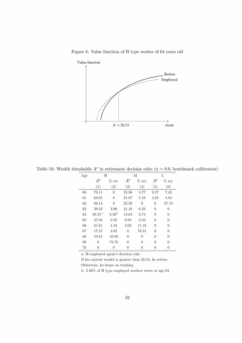
Figure 8: Value function of H type worker of 64 years old
Asset
Value function
Retiree
Employed
A* = 28.53
Table 10: Wealth thresholds A∗ in retirement decision rules (η = 0.9, benchmark calibration)Age H M L
A∗ % ret. A∗ % ret. A∗ % ret.
(1) (2) (3) (4) (5) (6)
60 79.11 0 25.36 3.77 9.27 7.42
61 68.05 0 21.87 1.19 4.25 4.84
62 66.14 0 22.39 0 0 87.74
63 38.23 2.06 21.10 0.10 0 0
64 28.53 a 2.56b 14.04 3.74 0 0
65 27.94 0.22 9.94 3.53 0 0
66 21.61 4.42 4.03 11.16 0 0
67 17.27 4.02 0 76.51 0 0
68 10.81 10.93 0 0 0 0
69 0 75.78 0 0 0 0
70 0 0 0 0 0 0
a: H employed agent’s decision rule:
If his current wealth is greater than 28.53, he retires
Otherwise, he keeps on working
b: 2.56% of H type employed workers retire at age 64
32
(their replacement ratio is the lowest).
5 Maintaining a tax on continued activity
The PAYG system faces two challenges: ensuring the financial sustainability of the system while
preserving the well-being of retirees and workers. We argue in this paper that more actuarially-
fair schemes could help meet these two objectives.
First (Section 5.1), we explore the financial implications of giving only a fraction of the
actuarially-fair scheme to agents willing to postpone retirement. This incentive program can
actually encourage individuals to work longer, thereby allowing the SS to collect additional
taxes. However, the SS has to carefully choose the fraction of the actuarially-fair scheme given
to individuals. On the one hand, incentives have to be large enough to entice people to delay
retirement. On the other hand, when incentives are high, pensions to be paid are increased. We
show that this trade - off is captured by a Laffer Curve on the continued activity. We determine
thereafter the fraction of the actuarially-fair scheme which should be given to individuals in
order to maximize the SS financial surplus. In this analysis, all equilibrium conditions defined
in Section 2.6 hold, except condition (v).
Secondly (Section 5.2), the actuarially-fair scheme could also be used as a tool to make
individuals postpone retirement while increasing their welfare. We then determine the fraction of
the actuarially-fair scheme which should be given to individuals in order to maximize the average
measure of the expected lifetime utility of newborns. In this welfare analysis, all equilibrium
conditions hold, including condition (v). The SS also faces a trade-off in terms of welfare. By
lowering the tax on continued activity, the SS improves the expected welfare for the end of the
life cycle when workers are free to choose their retirement age. However, the SS then collect fewer
contribution taxes on continued activity, which results in higher contribution rates during the
working life. This may decrease the expected welfare for these ages in case of binding liquidity
constraints.
5.1 A public finance perspective
Individuals now receive a fraction (1 − τ) of the actuarially-fair scheme. This Section aims at
assessing the incentive schemes that maximize the Social Security surplus. In order to measure
the magnitude of these financial gains, we express them in terms of percentage points of reduction
33
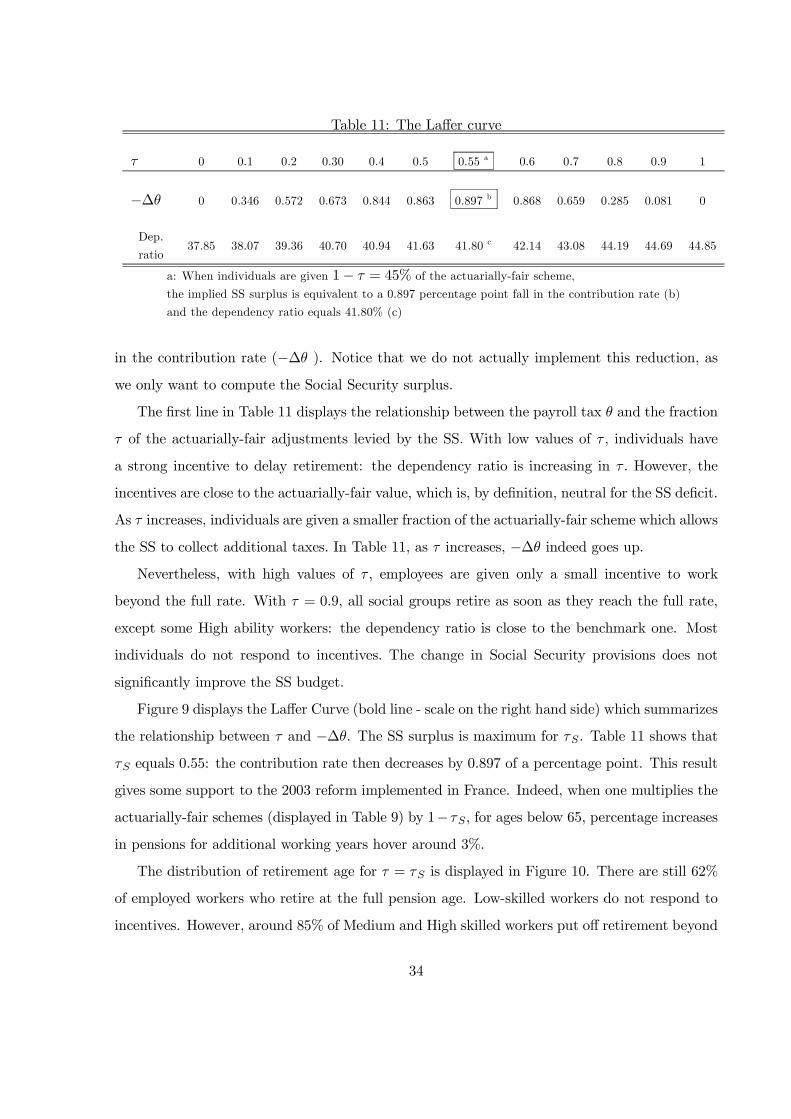
Table 11: The Laffer curve
τ 0 0.1 0.2 0.30 0.4 0.5 0.55 a 0.6 0.7 0.8 0.9 1
−∆θ 0 0.346 0.572 0.673 0.844 0.863 0.897 b 0.868 0.659 0.285 0.081 0
Dep.
ratio37.85 38.07 39.36 40.70 40.94 41.63 41.80 c 42.14 43.08 44.19 44.69 44.85
a: When individuals are given 1− τ = 45% of the actuarially-fair scheme,
the implied SS surplus is equivalent to a 0.897 percentage point fall in the contribution rate (b)
and the dependency ratio equals 41.80% (c)
in the contribution rate (−∆θ ). Notice that we do not actually implement this reduction, as
we only want to compute the Social Security surplus.
The first line in Table 11 displays the relationship between the payroll tax θ and the fraction
τ of the actuarially-fair adjustments levied by the SS. With low values of τ, individuals have
a strong incentive to delay retirement: the dependency ratio is increasing in τ . However, the
incentives are close to the actuarially-fair value, which is, by definition, neutral for the SS deficit.
As τ increases, individuals are given a smaller fraction of the actuarially-fair scheme which allows
the SS to collect additional taxes. In Table 11, as τ increases, −∆θ indeed goes up.
Nevertheless, with high values of τ, employees are given only a small incentive to work
beyond the full rate. With τ = 0.9, all social groups retire as soon as they reach the full rate,
except some High ability workers: the dependency ratio is close to the benchmark one. Most
individuals do not respond to incentives. The change in Social Security provisions does not
significantly improve the SS budget.
Figure 9 displays the Laffer Curve (bold line - scale on the right hand side) which summarizes
the relationship between τ and −∆θ. The SS surplus is maximum for τS . Table 11 shows that
τS equals 0.55: the contribution rate then decreases by 0.897 of a percentage point. This result
gives some support to the 2003 reform implemented in France. Indeed, when one multiplies the
actuarially-fair schemes (displayed in Table 9) by 1−τS, for ages below 65, percentage increases
in pensions for additional working years hover around 3%.
The distribution of retirement age for τ = τS is displayed in Figure 10. There are still 62%
of employed workers who retire at the full pension age. Low-skilled workers do not respond to
incentives. However, around 85% of Medium and High skilled workers put off retirement beyond
34
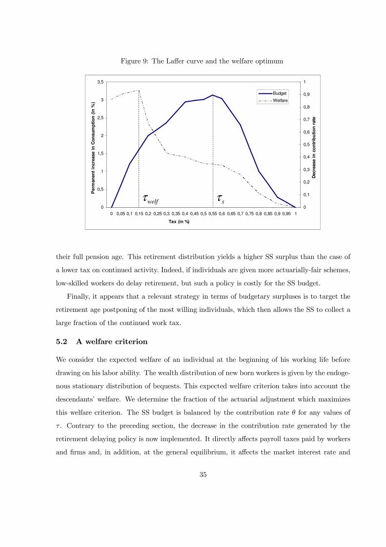
Figure 9: The Laffer curve and the welfare optimum
0
0,5
1
1,5
2
2,5
3
3,5
0 0,05 0,1 0,15 0,2 0,25 0,3 0,35 0,4 0,45 0,5 0,55 0,6 0,65 0,7 0,75 0,8 0,85 0,9 0,95 1
Tax (in %)
Perm
an
en
t in
cre
ase i
n C
on
su
mp
tio
n (
in %
)
0
0,1
0,2
0,3
0,4
0,5
0,6
0,7
0,8
0,9
1
Decre
ase i
n c
on
trib
uti
on
rate
Budget
Welfare
sτwelfτ
their full pension age. This retirement distribution yields a higher SS surplus than the case of
a lower tax on continued activity. Indeed, if individuals are given more actuarially-fair schemes,
low-skilled workers do delay retirement, but such a policy is costly for the SS budget.
Finally, it appears that a relevant strategy in terms of budgetary surpluses is to target the
retirement age postponing of the most willing individuals, which then allows the SS to collect a
large fraction of the continued work tax.
5.2 A welfare criterion
We consider the expected welfare of an individual at the beginning of his working life before
drawing on his labor ability. The wealth distribution of new born workers is given by the endoge-
nous stationary distribution of bequests. This expected welfare criterion takes into account the
descendants’ welfare. We determine the fraction of the actuarial adjustment which maximizes
this welfare criterion. The SS budget is balanced by the contribution rate θ for any values of
τ . Contrary to the preceding section, the decrease in the contribution rate generated by the
retirement delaying policy is now implemented. It directly affects payroll taxes paid by workers
and firms and, in addition, at the general equilibrium, it affects the market interest rate and
35
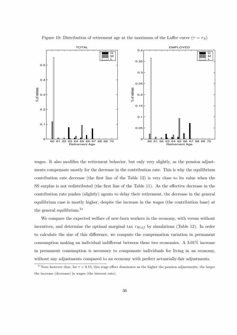
Figure 10: Distribution of retirement age at the maximum of the Laffer curve (τ = τS)
60 61 62 63 64 65 66 67 68 69 700
0.1
0.2
0.3
0.4
0.5
TOTAL
% o
f ret
irees
Retirement Age
HML
60 61 62 63 64 65 66 67 68 69 700
0.05
0.1
0.15
0.2
0.25
0.3
0.35
0.4EMPLOYED
% o
f ret
irees
Retirement Age
HML
wages. It also modifies the retirement behavior, but only very slightly, as the pension adjust-
ments compensate mostly for the decrease in the contribution rate. This is why the equilibrium
contribution rate decrease (the first line of the Table 12) is very close to its value when the
SS surplus is not redistributed (the first line of the Table 11). As the effective decrease in the
contribution rate pushes (slightly) agents to delay their retirement, the decrease in the general
equilibrium case is mostly higher, despite the increase in the wages (the contribution base) at
the general equilibrium.31
We compare the expected welfare of new-born workers in the economy, with versus without
incentives, and determine the optimal marginal tax τWelf by simulations (Table 12). In order
to calculate the size of this difference, we compute the compensation variation in permanent
consumption making an individual indifferent between these two economies. A 3.01% increase
in permanent consumption is necessary to compensate individuals for living in an economy,
without any adjustments compared to an economy with perfect actuarially-fair adjustments.
31 Note however that, for τ < 0.15, this wage effect dominates as the higher the pension adjustments, the larger
the increase (decrease) in wages (the interest rate).
36
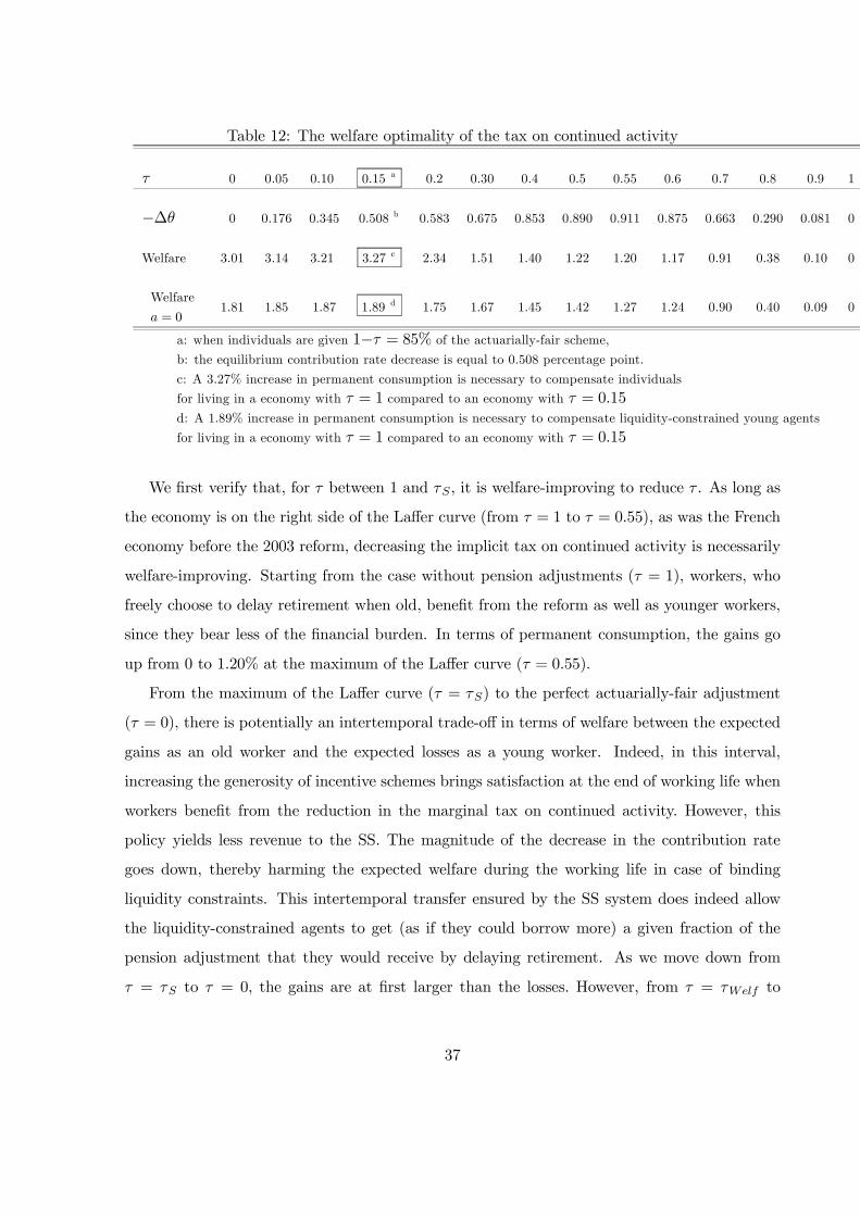
Table 12: The welfare optimality of the tax on continued activity
τ 0 0.05 0.10 0.15 a 0.2 0.30 0.4 0.5 0.55 0.6 0.7 0.8 0.9 1
−∆θ 0 0.176 0.345 0.508 b 0.583 0.675 0.853 0.890 0.911 0.875 0.663 0.290 0.081 0
Welfare 3.01 3.14 3.21 3.27 c 2.34 1.51 1.40 1.22 1.20 1.17 0.91 0.38 0.10 0
Welfare
a = 01.81 1.85 1.87 1.89 d 1.75 1.67 1.45 1.42 1.27 1.24 0.90 0.40 0.09 0
a: when individuals are given 1−τ = 85% of the actuarially-fair scheme,
b: the equilibrium contribution rate decrease is equal to 0.508 percentage point.
c: A 3.27% increase in permanent consumption is necessary to compensate individuals
for living in a economy with τ = 1 compared to an economy with τ = 0.15d: A 1.89% increase in permanent consumption is necessary to compensate liquidity-constrained young agents
for living in a economy with τ = 1 compared to an economy with τ = 0.15
We first verify that, for τ between 1 and τS , it is welfare-improving to reduce τ . As long as
the economy is on the right side of the Laffer curve (from τ = 1 to τ = 0.55), as was the French
economy before the 2003 reform, decreasing the implicit tax on continued activity is necessarily
welfare-improving. Starting from the case without pension adjustments (τ = 1), workers, who
freely choose to delay retirement when old, benefit from the reform as well as younger workers,
since they bear less of the financial burden. In terms of permanent consumption, the gains go
up from 0 to 1.20% at the maximum of the Laffer curve (τ = 0.55).
From the maximum of the Laffer curve (τ = τS) to the perfect actuarially-fair adjustment
(τ = 0), there is potentially an intertemporal trade-off in terms of welfare between the expected
gains as an old worker and the expected losses as a young worker. Indeed, in this interval,
increasing the generosity of incentive schemes brings satisfaction at the end of working life when
workers benefit from the reduction in the marginal tax on continued activity. However, this
policy yields less revenue to the SS. The magnitude of the decrease in the contribution rate
goes down, thereby harming the expected welfare during the working life in case of binding
liquidity constraints. This intertemporal transfer ensured by the SS system does indeed allow
the liquidity-constrained agents to get (as if they could borrow more) a given fraction of the
pension adjustment that they would receive by delaying retirement. As we move down from
τ = τS to τ = 0, the gains are at first larger than the losses. However, from τ = τWelf to
37

τ = 0, the losses during the liquidity-constrained periods of the working life dominates the
expected gains when old. Relative to the Laffer curve in terms of public finance, the maximum
is shifted leftward (Figure 9, broken line, left hand side) and reached when 1− τWelf = 85% of
the actuarially-fair pension adjustment is given to agents who delay retirement.
In the context of liquidity-constrained workers, the actuarially-fair adjustments are no longer
optimal, even if more must be given to workers than in the financial surplus case. Indeed, a
significant proportion of the population benefits from the decrease in the contribution rate. 34.7%
of workers before the early retirement age are liquidity-constrained. It must be emphasized that
focusing only on the welfare of new-born individuals who are liquidity-constrained (last line of
Table 12) would have led to recommend the same pension adjustments32 . The proportion of
liquidity-constrained young workers in the labor force is then a key determinant of the optimal
degree of fairness of the pension adjustments.
Beyond this intertemporal transfer, incentive schemes also lead to transfers across abilities.
Indeed, 58.5% of the liquidity-constrained agents belong to the L group, 26% to the M type and
15.5% to the H class. L type individuals are then the primary winners of the lower contribution
rate. With τ = τWelf , M and H type workers still benefit from incentive schemes. This can be
seen in Figure 11 that displays the retirement distribution for the optimal welfare taxation. 95%
of the H type workers delay retirement, 93% for the M-type and 86% for the L-type (figure 11).
The number of delayed years is lower for L-type workers. H and M workers then contribute
(freely) more to the financial surpluses of the SS. The redistribution of the financial surpluses
through an even decrease in the payroll tax is particularly favorable to Low-skilled workers.
Indeed, these agents are more liquidity-constrained and benefit from the transfers of some part
of the surpluses generated by the other two ability groups. The incentive policy then redistributes
income towards L type agents, thereby providing insurance against the ability risk at birth. This
feature contributes to maintaining a tax on continued activity at the social optimum. It also
explains why this policy could still be optimal in the cases where intervivos transfers would be
possible33 (Fuster et al. (2003)).
32 The decrease in the contribution rate per se would lead to recommend smaller pension adjustments, but
higher values of τ imply higher interest rates and then lower wages, harming the welfare of liquidity-constrained
agents.
33 We have not verified this conjecture.
38
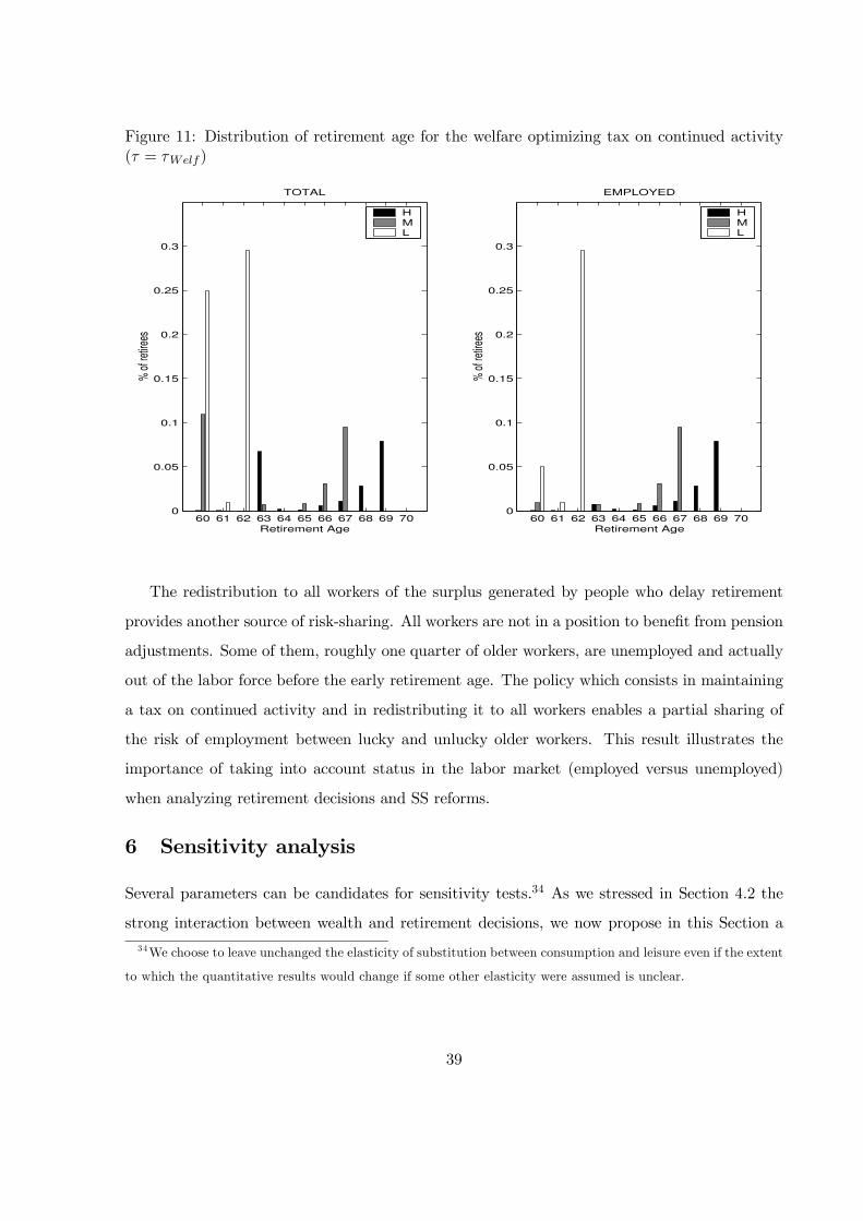
Figure 11: Distribution of retirement age for the welfare optimizing tax on continued activity(τ = τWelf )
60 61 62 63 64 65 66 67 68 69 700
0.05
0.1
0.15
0.2
0.25
0.3
TOTAL
% o
f ret
irees
Retirement Age
HML
60 61 62 63 64 65 66 67 68 69 700
0.05
0.1
0.15
0.2
0.25
0.3
EMPLOYED
% o
f ret
irees
Retirement Age
HML
The redistribution to all workers of the surplus generated by people who delay retirement
provides another source of risk-sharing. All workers are not in a position to benefit from pension
adjustments. Some of them, roughly one quarter of older workers, are unemployed and actually
out of the labor force before the early retirement age. The policy which consists in maintaining
a tax on continued activity and in redistributing it to all workers enables a partial sharing of
the risk of employment between lucky and unlucky older workers. This result illustrates the
importance of taking into account status in the labor market (employed versus unemployed)
when analyzing retirement decisions and SS reforms.
6 Sensitivity analysis
Several parameters can be candidates for sensitivity tests.34 As we stressed in Section 4.2 the
strong interaction between wealth and retirement decisions, we now propose in this Section a
34 We choose to leave unchanged the elasticity of substitution between consumption and leisure even if the extent
to which the quantitative results would change if some other elasticity were assumed is unclear.
39
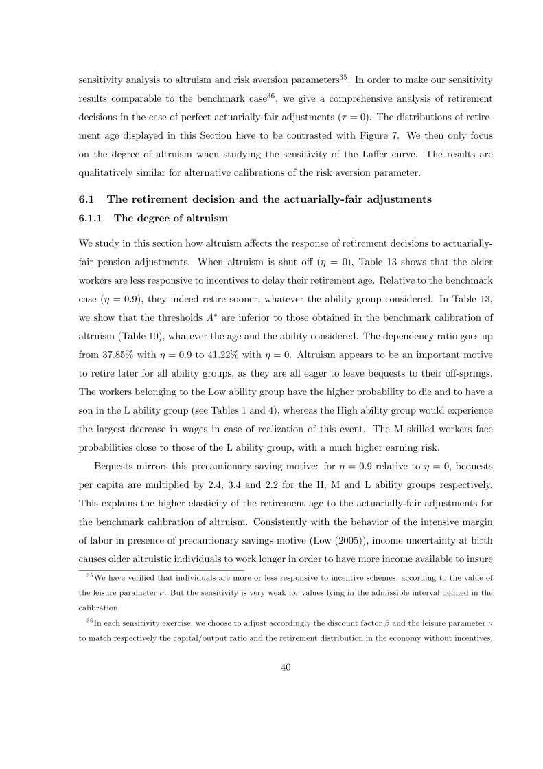
sensitivity analysis to altruism and risk aversion parameters35. In order to make our sensitivity
results comparable to the benchmark case36, we give a comprehensive analysis of retirement
decisions in the case of perfect actuarially-fair adjustments (τ = 0). The distributions of retire-
ment age displayed in this Section have to be contrasted with Figure 7. We then only focus
on the degree of altruism when studying the sensitivity of the Laffer curve. The results are
qualitatively similar for alternative calibrations of the risk aversion parameter.
6.1 The retirement decision and the actuarially-fair adjustments
6.1.1 The degree of altruism
We study in this section how altruism affects the response of retirement decisions to actuarially-
fair pension adjustments. When altruism is shut off (η = 0), Table 13 shows that the older
workers are less responsive to incentives to delay their retirement age. Relative to the benchmark
case (η = 0.9), they indeed retire sooner, whatever the ability group considered. In Table 13,
we show that the thresholds A∗ are inferior to those obtained in the benchmark calibration of
altruism (Table 10), whatever the age and the ability considered. The dependency ratio goes up
from 37.85% with η = 0.9 to 41.22% with η = 0. Altruism appears to be an important motive
to retire later for all ability groups, as they are all eager to leave bequests to their off-springs.
The workers belonging to the Low ability group have the higher probability to die and to have a
son in the L ability group (see Tables 1 and 4), whereas the High ability group would experience
the largest decrease in wages in case of realization of this event. The M skilled workers face
probabilities close to those of the L ability group, with a much higher earning risk.
Bequests mirrors this precautionary saving motive: for η = 0.9 relative to η = 0, bequests
per capita are multiplied by 2.4, 3.4 and 2.2 for the H, M and L ability groups respectively.
This explains the higher elasticity of the retirement age to the actuarially-fair adjustments for
the benchmark calibration of altruism. Consistently with the behavior of the intensive margin
of labor in presence of precautionary savings motive (Low (2005)), income uncertainty at birth
causes older altruistic individuals to work longer in order to have more income available to insure
35 We have verified that individuals are more or less responsive to incentive schemes, according to the value of
the leisure parameter ν. But the sensitivity is very weak for values lying in the admissible interval defined in the
calibration.
36 In each sensitivity exercise, we choose to adjust accordingly the discount factor β and the leisure parameter ν
to match respectively the capital/output ratio and the retirement distribution in the economy without incentives.
40
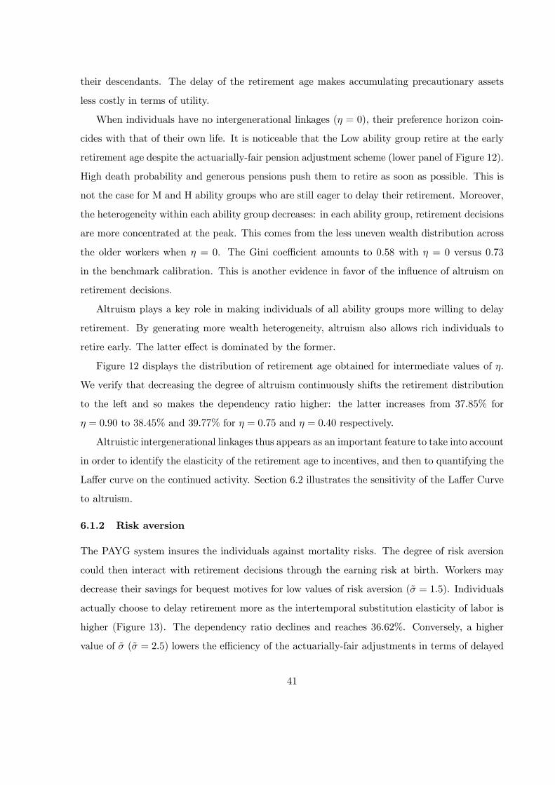
their descendants. The delay of the retirement age makes accumulating precautionary assets
less costly in terms of utility.
When individuals have no intergenerational linkages (η = 0), their preference horizon coin-
cides with that of their own life. It is noticeable that the Low ability group retire at the early
retirement age despite the actuarially-fair pension adjustment scheme (lower panel of Figure 12).
High death probability and generous pensions push them to retire as soon as possible. This is
not the case for M and H ability groups who are still eager to delay their retirement. Moreover,
the heterogeneity within each ability group decreases: in each ability group, retirement decisions
are more concentrated at the peak. This comes from the less uneven wealth distribution across
the older workers when η = 0. The Gini coefficient amounts to 0.58 with η = 0 versus 0.73
in the benchmark calibration. This is another evidence in favor of the influence of altruism on
retirement decisions.
Altruism plays a key role in making individuals of all ability groups more willing to delay
retirement. By generating more wealth heterogeneity, altruism also allows rich individuals to
retire early. The latter effect is dominated by the former.
Figure 12 displays the distribution of retirement age obtained for intermediate values of η.
We verify that decreasing the degree of altruism continuously shifts the retirement distribution
to the left and so makes the dependency ratio higher: the latter increases from 37.85% for
η = 0.90 to 38.45% and 39.77% for η = 0.75 and η = 0.40 respectively.
Altruistic intergenerational linkages thus appears as an important feature to take into account
in order to identify the elasticity of the retirement age to incentives, and then to quantifying the
Laffer curve on the continued activity. Section 6.2 illustrates the sensitivity of the Laffer Curve
to altruism.
6.1.2 Risk aversion
The PAYG system insures the individuals against mortality risks. The degree of risk aversion
could then interact with retirement decisions through the earning risk at birth. Workers may
decrease their savings for bequest motives for low values of risk aversion (σ̃ = 1.5). Individuals
actually choose to delay retirement more as the intertemporal substitution elasticity of labor is
higher (Figure 13). The dependency ratio declines and reaches 36.62%. Conversely, a higher
value of σ̃ (σ̃ = 2.5) lowers the efficiency of the actuarially-fair adjustments in terms of delayed
41
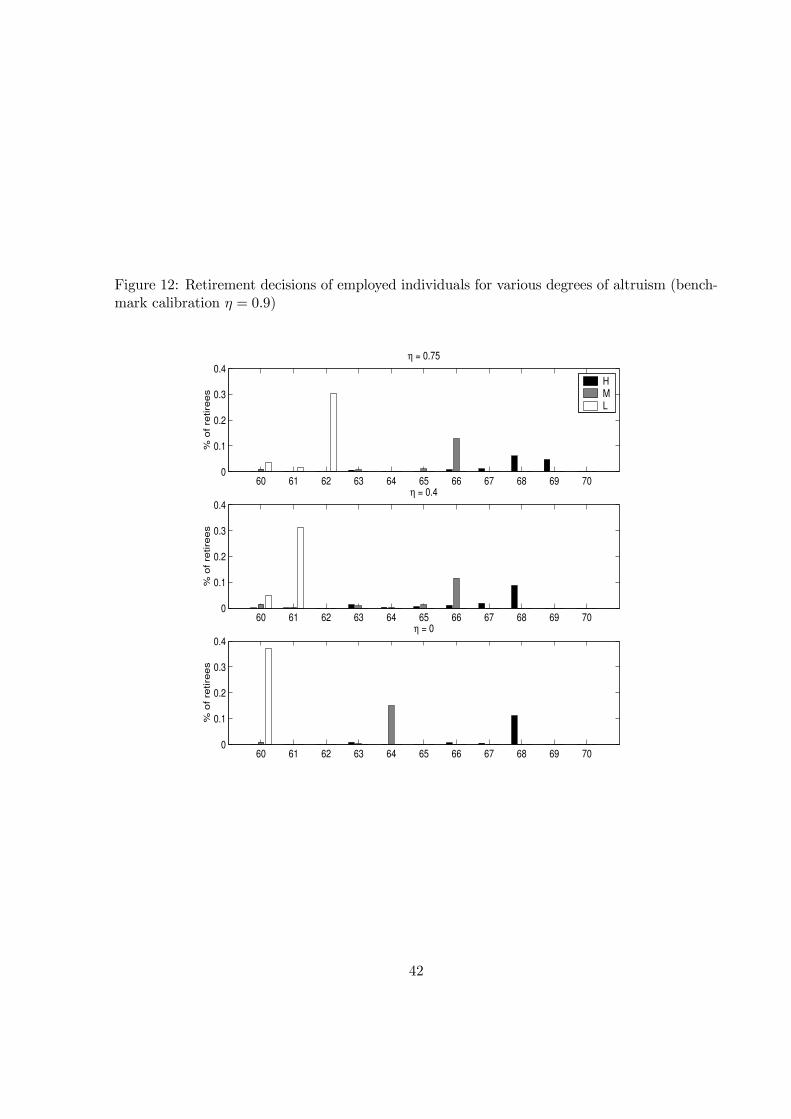
Figure 12: Retirement decisions of employed individuals for various degrees of altruism (bench-mark calibration η = 0.9)
60 61 62 63 64 65 66 67 68 69 700
0.1
0.2
0.3
0.4
% o
f re
tire
es
η = 0.75
HML
60 61 62 63 64 65 66 67 68 69 700
0.1
0.2
0.3
0.4
% o
f re
tire
es
η = 0.4
60 61 62 63 64 65 66 67 68 69 700
0.1
0.2
0.3
0.4
% o
f re
tire
es
η = 0
42

Table 13: Wealth thresholds A∗ in retirement decision rules and retirement decisions (η = 0)Age H M L
A∗ % ret. A∗ % ret. A∗ % ret.
(1) (2) (3) (4) (5) (6)
60 57.1 0 18.6 5.3 0 100
61 52.78 0 18.6 0 0 0
62 53.2 0 16.8 0 0 0
63 19.6 6.0 13.6 1.3 0 0
64 19.3 a 0 0 93.3 0 0
65 16.8 5.8 0 0 0 0
66 11.3 4.7 b 0 0 0 0
67 8.1 3.3 0 0 0 0
68 0 85.3 0 0 0 0
69 0 0 0 0 0 0
70 0 0 0 0 0 0
a: H employed agent’s decision rule:
If his current wealth is greater than 19.3, he retires
Otherwise, he keeps on working
b: 4.7% of H type workers retire at age 66
retirements.
6.2 The Laffer curve and the degree of altruism
Retirement decisions are sensitive to altruism and risk aversion. When individuals are less
responsive to the incentive policy, the trade-off between the tax on continued activity and the
SS surplus worsens. We illustrate this point for the degree of altruism.
A lower degree of altruism deteriorates the trade-off inherent in the Laffer curve37. Relative
to the benchmark calibration, the Laffer curve and its maximum are shifted to the left. As
workers choose to retire sooner, it is optimal in terms of public finance to reduce the tax on
continued activity more. Whereas 45% of the actuarially-fair adjustment must be given in the
benchmark calibration, this proportion increases as long the degree of altruism decreases: 55%
for η = 0.75, 60% for η = .40 and finally 70% for η = 0. As shown by Figure 14, lower
altruism yields less significant increases in the total Social Security surplus. The benchmark
case (η = 0.9) generates a decrease of 0.897 percentage point in the contribution rate. Only
one third of this decrease is reached for η = 0. This last point indicates that the benchmark
37 It is also the case for a higher degree of risk aversion.
43

Figure 13: Distribution of retirement age of employed individuals for various degrees of riskaversion σ̃ (benchmark calibration σ̃ = 2)
60 61 62 63 64 65 66 67 68 69 700
0.05
0.1
0.15
0.2
0.25
0.3
% o
f re
tire
es
σ = 2.5
HML
60 61 62 63 64 65 66 67 68 69 700
0.05
0.1
0.15
0.2
0.25
0.3
% o
f re
tire
es
σ = 1.5
44
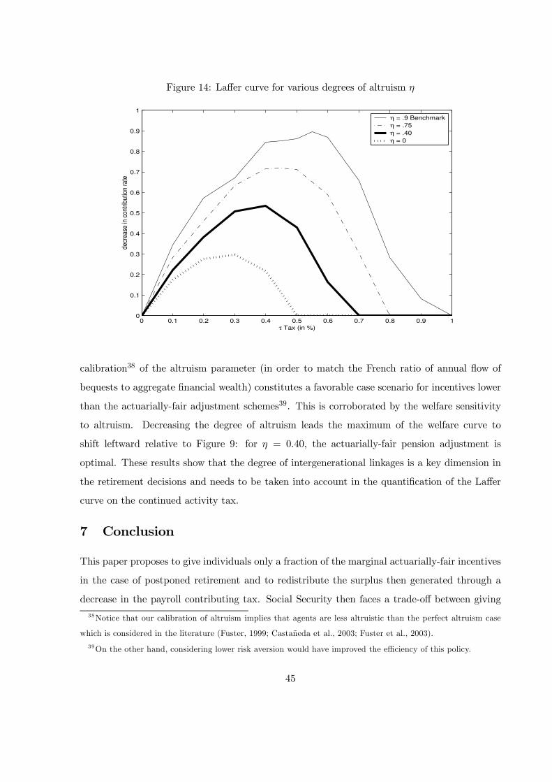
Figure 14: Laffer curve for various degrees of altruism η
0 0.1 0.2 0.3 0.4 0.5 0.6 0.7 0.8 0.9 10
0.1
0.2
0.3
0.4
0.5
0.6
0.7
0.8
0.9
1
τ Tax (in %)
decr
ease
in c
ontr
ibut
ion
rate
η = .9 Benchmark
η = .75
η = .40
η = 0
calibration38 of the altruism parameter (in order to match the French ratio of annual flow of
bequests to aggregate financial wealth) constitutes a favorable case scenario for incentives lower
than the actuarially-fair adjustment schemes39. This is corroborated by the welfare sensitivity
to altruism. Decreasing the degree of altruism leads the maximum of the welfare curve to
shift leftward relative to Figure 9: for η = 0.40, the actuarially-fair pension adjustment is
optimal. These results show that the degree of intergenerational linkages is a key dimension in
the retirement decisions and needs to be taken into account in the quantification of the Laffer
curve on the continued activity tax.
7 Conclusion
This paper proposes to give individuals only a fraction of the marginal actuarially-fair incentives
in the case of postponed retirement and to redistribute the surplus then generated through a
decrease in the payroll contributing tax. Social Security then faces a trade-off between giving
38 Notice that our calibration of altruism implies that agents are less altruistic than the perfect altruism case
which is considered in the literature (Fuster, 1999; Castañeda et al., 2003; Fuster et al., 2003).
39 On the other hand, considering lower risk aversion would have improved the efficiency of this policy.
45
enough incentives to make individuals actually delay retirement and giving little increase in
pensions in order to maximize the financial surpluses. This trade-off is captured by a Laffer
curve that we quantify on French data. The maximum of the Laffer curve is reached when 45%
of the actuarially-fair scheme is given to individuals willing to delay retirement, which is close
to the 3% increase in pensions proposed by the 2003 French reform.
When the Social Security aims at maximizing welfare, the optimal tax on postponed retire-
ment is lower than the one obtained from the Laffer curve but still strictly positive. With a
positive tax on postponed retirement, the redistribution of the contributions collected on the
additional working years are beneficial to liquidity-constrained and low ability workers and un-
employed people at the end of working life. Maintaining a tax on continued activity allows the
SS system to implement transfers across and within generations which are welfare-improving.
All these results are derived from a dynastic general equilibrium model where the endogenous
wealth distribution and intergenerational linkages play a key role in determining retirement
decisions, especially when incentive schemes are introduced in SS provisions.
This paper shows that countries whose SS system is still far from actuarially-fair pension
adjustments should urgently implement a reform partially closing the gap. Such a delayed
retirement age policy is incentive-compatible. Moreover, by lowering the payroll tax40 while
maintaining a tax on continued activity, the reform can spread the gains over all the population.
Decreasing the tax on continued activity, by putting off the end of career horizon, could also
encourage a more intensive job-search by older unemployed workers before the early retirement
age. In this paper, we have considered exogenous employment risks. This calls for a more general
approach to older workers participation rate. Hairault et al. (2006) propose a first investigation
toward this direction, but disregard wealth accumulation. It constitutes a promising avenue of
research.
40 One could also say that this policy will limit the necessary increase in the payroll tax to finance the expected
deficits in the coming years.
46
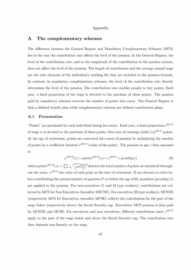
Appendix
A The complementary schemes
The difference between the General Regime and Mandatory Complementary Schemes (MCS)
lies in the way the contribution rate affects the level of the pension. In the General Regime, the
level of the contribution rate, and so the magnitude of the contribution to the pension system,
does not affect the level of the pension. The length of contribution and the average annual wage
are the only elements of the individual’s working life that are included in the pension formula.
In contrast, in mandatory complementary schemes, the level of the contribution rate directly
determines the level of the pension. The contribution rate enables people to buy points. Each
year, a fixed proportion of the wage is devoted to the purchase of these points. The pension
paid by mandatory schemes converts the number of points into euros. The General Regime is
thus a defined benefit plan while complementary schemes are defined contribution plans.
A.1 Presentation
“Points” are purchased by each individual during his career. Each year, a fixed proportion cMCS
of wage w is devoted to the purchase of these points. One euro of earnings yields 1/pMCS points.
At the age of retirement, points are converted into euros of pension by multiplying the number
of points by a coefficient denoted vMCS (value of the point). The pension at age z then amounts
to
ωMCS(z) = pointsMCS(z)× vMCS × penalty(z) (9)
where pointsMCS(z) =∑z
i=1cMCS(i)w(i)pMCS(i)
denotes the total number of points accumulated through-
out the years, vMCS the value of each point at the date of retirement. If one chooses to retire be-
fore contributing the normal number of quarters dn or before the age of 65, penalties (penalty(z))
are applied to the pension. For non-executives (L and M type workers), contributions are col-
lected by MCS for Non Executives (hereafter MSCNE). For executives (H type workers), MCSNE
(respectively MCS for Executives, hereafter MCSE) collects the contribution for the part of the
wage below (respectively above) the Social Security cap. Executives’ MCS pension is then paid
by MCSNE and MCSE. For executives and non executives, different contribution rates cMCS
apply to the part of the wage below and above the Social Security cap. The contribution rate
then depends non-linearly on the wage.
47
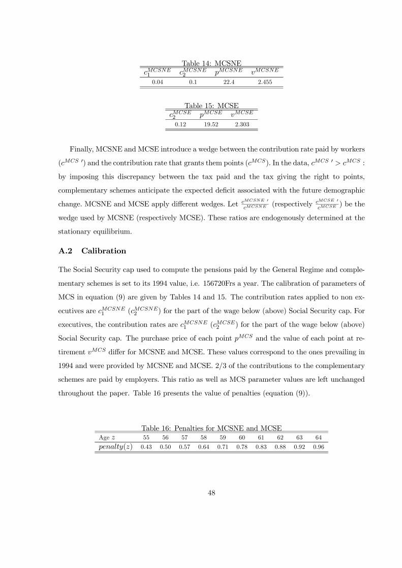
Table 14: MCSNEcMCSNE1 cMCSNE
2 pMCSNE vMCSNE
0.04 0.1 22.4 2.455
Table 15: MCSEcMCSE2 pMCSE vMCSE
0.12 19.52 2.303
Finally, MCSNE and MCSE introduce a wedge between the contribution rate paid by workers
(cMCS ′) and the contribution rate that grants them points (cMCS). In the data, cMCS ′ > cMCS :
by imposing this discrepancy between the tax paid and the tax giving the right to points,
complementary schemes anticipate the expected deficit associated with the future demographic
change. MCSNE and MCSE apply different wedges. Let cMCSNE ′
cMCSNE (respectively cMCSE ′
cMCSE ) be the
wedge used by MCSNE (respectively MCSE). These ratios are endogenously determined at the
stationary equilibrium.
A.2 Calibration
The Social Security cap used to compute the pensions paid by the General Regime and comple-
mentary schemes is set to its 1994 value, i.e. 156720Frs a year. The calibration of parameters of
MCS in equation (9) are given by Tables 14 and 15. The contribution rates applied to non ex-
ecutives are cMCSNE1 (cMCSNE
2 ) for the part of the wage below (above) Social Security cap. For
executives, the contribution rates are cMCSNE1 (cMCSE
2 ) for the part of the wage below (above)
Social Security cap. The purchase price of each point pMCS and the value of each point at re-
tirement vMCS differ for MCSNE and MCSE. These values correspond to the ones prevailing in
1994 and were provided by MCSNE and MCSE. 2/3 of the contributions to the complementary
schemes are paid by employers. This ratio as well as MCS parameter values are left unchanged
throughout the paper. Table 16 presents the value of penalties (equation (9)).
Table 16: Penalties for MCSNE and MCSEAge z 55 56 57 58 59 60 61 62 63 64
penalty(z) 0.43 0.50 0.57 0.64 0.71 0.78 0.83 0.88 0.92 0.96
48
References
Aglietta, M., D. Blanchet and F. Héran, Démographie et Économie, volume 35 of Rapport CAE
(Paris: Conseil d’Analyse Economique, 2002).
Aiyagari, S. R., “Uninsured Idiosyncratic Risk and Aggregate Saving,” The Quarterly Journal
of Economics 109 (August 1994), 659—684.
Arrondel, L., “Risk Management and Wealth Accumulation Behavior in France,” Economics
Letters 74 (January 2002), 187—194.
Arrondel, L. and A. Laferrere, “Taxation and Wealth Transmission in France,” Journal of Public
Economics 79 (2001), 3—33.
Arrondel, L. and F. Laferrère, “Sucessions et Héritiers À Travers Les Données Fiscales,”
Economie et Prévision 100-101 (1991), 137—175.
Attanasio, O. P., J. Banks, C. Meghir and G. Weber, “Humps and Bumps in Lifetime Consump-
tion,” Journal of Business and Economic Statistics 17 (1999).
Aubert, P., D. Blanchet and D. Blau, “The Labour Market After Age 50 : Some Elements of
a Franco - American Comparison,” INSEE Working Paper g2005 - 13, INSEE, November
2005.
Auerbach, A. and L. Kotlikoff, Dynamic Fiscal Policy (Cambridge Univ. Press, 1987).
Bardaji, J., B. Sédillot and E. Walraet, “Les Retraites Du Secteur Public : Projections À
L’horizon 2040 À L’aide Du Modèle de Microsimulation DESTINIE,” Technical Report G
2004 / 14, INSEE, 2004.
Becker, G. and N. Tomes, “An Equilibrium Theory of the Distribution of Income and Intergen-
erational Mobility,” Journal of Political Economy 87 (1979), 1153—1189.
Becker, G. and N. Tomes, “Human Capital and the Rise and Fall of Families,” Journal of Labor
Economics 4 (1986), s1—s39.
49
Belhaj, H., “Les Indicateurs de Suivi Des Pensions : L’annexe Statistique Présentée Par la
France Dans Le Rapport de Stratégie Nationale sur Les Pensions,” Solidarité et Santé 2
(Avril - Juin 2004), 29—52.
Berkovec, J. and S. Stern, “Job Exit of Older Men,” Econometrica 59 (1991), 189—210.
Blanchet, D. and G. Pelé, “Social Security and Retirement in France,” NBER Working Paper
6214, NBER, October 1997.
Bozio, A., “Does Increasing Contribution Length Lead to Higher Retirement Age ? Evidence
from the 1993 French Pension Reform,” Mimeo, PSE, 2005.
Caballaro, R. J. and M. Hammour, “The Limits of Special Interest: What Caused Three Decades
of High Unemployment in Europe?,” Mimeo, MIT, October 1999.
Cagetti, M. and M. De Nardi, “Entrepreneurship, Frictions, and Wealth,” Working Paper 2005-
9, Federal Reserve Bank of Chicago, 2005.
Castañeda, A., J. Diaz-Gimenez and V. Rios-Rull, “Accounting for the U.S. Earnings and Wealth
Inequality,” Journal of Political Economy 111 (2003), 818—857.
Charpin, J. M., Rapport Au Premier Ministre : L’avenir de Nos Retraites (Documentation
Française, 1999).
Coile, C., P. Diamond, J. Gruber and A. Jousten, “Delays in Claiming Social Security Benefits,”
Journal of Public Economics 84 (2002), 357—385.
Colin, C., V. Iéhlé and R. Mahieu, “Les Trajectoires de Fin de Carrière Des Salariés Du Secteur
Privé,” Solidarité-Santé (2000).
Conesa, J. and D. Krueger, “Social Security Reform with Heterogeneous Agents,” Review of
Economic Dynamics 2 (October 1999), 757—795.
Cooley, T. and E. Prescott, “Economic Growth and Business Cycles,” in T. Cooley, ed., Frontiers
of Business Cycle Researchchapter 1 (Princeton University Press, 1995).
Cremer, H., J. Lozachmeur and P. Pestieau, “Social Security, Retirement Age and Optimal
Income Taxation,” Journal of Public Economics 88 (2004), 2259—2281.
50

De Nardi, M., “Wealth Inequality and Intergenerational Links,” Review of Economic Studies 71
(July 2004), 743—768.
der Klaauw, H. V. and K. I. Wolpin, “Social Security, Pensions and the Savings and Retirement
Behavior of Households,” Mimeo, November 2002.
Diamond, P. and J. A. Hausman, “Individual Retirement and Savings Behavior,” Journal of
Public Economics 23 (1984), 81—114.
DREES, “L Âge de la Liquidation Des Droits À la Retraite de la Génération 1934,” Etudes et
Résultats 237 (Mai 2003), available at http://www.sante.gouv.fr/drees/etude-resultat/.
Fuster, L., “Is Altruism Important for Understanding the Long-Run Effects of Social Security?,”
Review of Economics Dynamics 2 (1999), 616—637.
Fuster, L., A. Imrohoroglu and S. Imrohoroglu, “A Welfare Analysis of Social Security in a
Dynastic Framework,” International Economic Review 44 (November 2003), 1247—1273.
Gale, W. and J. Scholz, “Intergenerational Transfers and the Accumulation of Wealth,” Journal
of Economic Perspectives 8 (Autumn 1994), 145—160.
Gruber, J. and D. Wise, “Social Security and Retirement: An International Comparison,” Amer-
ican Economic Review 88 (May 1998), 158—163.
Gruber, J. and D. Wise, Social Security Programs and Retirement Around the World: Micro-
Estimation (National Bureau of Economic Research Conference Report, 2004).
Gustman, A. L. and T. L. Steinmeir, “The Social Security Early Entitlement Age in a Structural
Model of Retirement and Wealth,” NBER Working Paper 9183, NBER, September 2002.
Hairault, J., F. Langot and T. Sopraseuth, “The Interaction Between Retirement and Job Search:
A Global Approach to Older Workers Employment,” IZA Discussion Paper DP 1984, IZA,
February 2006.
Hansen, G. and A. Imrogoroglu, “The Role of Unemplyment Insurance in an Economy with
Liquidity Constraints and Moral Hazard,” Journal of Political Economy 100 (1992), 118—
142.
51
Huggett, M. and G. Ventura, “On the Distributional Effects of Social Security Reform,” Review
of Economic Dynamics 2 (July 1999), 498—531.
Imrohoroglu, A., S. Imrohoroglu and D. H. Joines, “Computational Models of Social Security:
A Survey,” in R. Marimon and A. Scott, eds., Computational Methods for the Study of
Dynamic Economies (Oxford University Press, 1999), 221—237.
INSEE, Mobilité Sociale Tome Deux, volume 89-90-91 of Emploi et Revenus (1995).
INSEE, “Successions et Donations En 1994, De Plus En Plus de Successions Déclarées,” INSEE
première (June 1997).
INSEE, “Le Patrimoine National,” INSEE première (July 1998).
INSEE, La Structure Des Salaires En 1994, volume 146-147 of Emploi et Revenu (1999a).
INSEE, Revenu et Patrimoine Des Ménages, volume 28 of Synthèses (1999b).
Kahn, J. A., “Social Security, Liquidity and Early Retirement,” Journal of Public Economics
35 (1988), 97—117.
Lindbeck, A. and T. Persson, “The Gains from Pension Reform,” Journal of Economic Literature
41 (March 2003), 74—112.
Ljungqvist, L. and T. J. Sargent, Recursive Macroeconomic Theory (MIT Press, 2000).
Ljunqvist, L. and T. Sargent, “Obsolescence, Uncertainty and Heterogeneity : The European
Employment Experience,” Mimeo, November 2005.
Low, H. W., “Self-Insurance in a Life-Cycle Model of Labour Supply and Savings,” Review of
Economic Dynamics 8 (2005), 945—975.
Quadrini, V., “Entrepreneurship, Saving and Social Mobility,” Review of Economic Dynamics
3 (January 2000), 1—40.
Rios Rull, V., “Life-Cycle Economies and Aggregate Fluctuations,” Review of Economic Studies
63 (July 1996), 465—490.
52
Rust, J., “A Dynamic Programming Model of Retirement Behavior,” in D. Wise, ed., The
Economics of Aging (Chicago Press, 1989), 359—398.
Rust, J. and C. Phelan, “How Social Security and Medicare Affect Retirement Behavior in a
World of Incomplete Markets,” Econometrica 65 (1997), 781—831.
Stock, J. and D. Wise, “Pensions, the Option Value of Work, and Retirement,” Econometrica
58 (1990), 1151—1180.
Storesletten, K., C. I. Telmer and A. Yaron, “The Risk-Sharing Implications of Alternative
Social Security Arrangements,” Carnegie-Rochester Conference Series on Public Policy 50
(June 1999), 213—259.
Vikram, N. and A. Dhareshwar, “A New Database on Physical Capital Stock: Sources, Method-
ology and Results,” Technical Report, Wolrd Bank, 1995.
Villa, P., “Séries Longues Macroéconomiques,” Technical Report, CEPII, 1995, available on
CEPII website : http://www.cepii.fr/francgraph/bdd/villa/mode.htm.
53