how far are we from the slippery slope? the laffer curve revisited
TRANSCRIPT

Work ing PaPer Ser i e Sno 1174 / aPr i L 2010
HoW Far are We
From THe SLiPPery
SLoPe?
THe LaFFer Curve
reviSiTed
by Mathias Trabandt and Harald Uhlig

WORKING PAPER SER IESNO 1174 / APR I L 2010
In 2010 all ECB publications
feature a motif taken from the
€500 banknote.
HOW FAR ARE WE FROM THE
SLIPPERY SLOPE?
THE LAFFER CURVE REVISITED 1
by Mathias Trabandt 2
and Harald Uhlig 3
1 A number of people and seminar participants provided us with excellent comments, for which we are grateful, and a complete list would be rather
long. Explicitly, we would like to thank Wouter DenHaan, Robert Hall, John Cochrane, Rick van der Ploeg and Richard Rogerson. This
research was supported by the Deutsche Forschungsgemeinschaft through the SFB 649 ”Economic Risk”, by the RTN network
MAPMU (contract HPRNCT-2002-00237) and by the NSF grant SES-0922550. An early draft of this paper has been awarded
with the CESifo Prize in Public Economics 2005. The views expressed in this paper are solely the responsibility of the
authors and should not be interpreted as reflecting the views of the ECB or Sveriges Riksbank.
2 Fiscal Policies Division, European Central Bank, Kaiserstrasse 29, 60311 Frankfurt am Main, GERMANY and Sveriges Riksbank,
e-mail: [email protected]
3 Department of Economics, University of Chicago, 1126 East 59th Street, Chicago, IL 60637, USA, NBER and CEPR,
e-mail: [email protected]
This paper can be downloaded without charge from http://www.ecb.europa.eu or from the Social Science Research Network electronic library at http://ssrn.com/abstract_id=1533409.
NOTE: This Working Paper should not be reported as representing the views of the European Central Bank (ECB). The views expressed are those of the authors
and do not necessarily reflect those of the ECB.
© European Central Bank, 2010
AddressKaiserstrasse 2960311 Frankfurt am Main, Germany
Postal addressPostfach 16 03 1960066 Frankfurt am Main, Germany
Telephone+49 69 1344 0
Internethttp://www.ecb.europa.eu
Fax+49 69 1344 6000
All rights reserved.
Any reproduction, publication and reprint in the form of a different publication, whether printed or produced electronically, in whole or in part, is permitted only with the explicit written authorisation of the ECB or the authors.
Information on all of the papers published in the ECB Working Paper Series can be found on the ECB’s website, http://www.ecb.europa.eu/pub/scientific/wps/date/html/index.en.html
ISSN 1725-2806 (online)
3ECB
Working Paper Series No 1174April 2010
Abstract 4
Non-technical summary 5
1 Introduction 7
2 The model 9
2.1 The Constant Frisch Elasticity (CFE) preferences 12
2.2 Equilibrium 16
3 Calibration and parameterization 21
3.1 EU-14 model and individual EU countries 22
4 Results 24
4.1 Labor tax laffer curves 26
4.2 Capital tax laffer curves 28
5 Conclusion 31
References 32
Figures 37
Appendices 43
CONTENTS
4ECBWorking Paper Series No 1174April 2010
Abstract
We characterize the Laffer curves for labor taxation and capital income taxation quan-
titatively for the US, the EU-14 and individual European countries by comparing the
balanced growth paths of a neoclassical growth model featuring ”constant Frisch elastic-
ity” (CFE) preferences. We derive properties of CFE preferences. We provide new tax
rate data. For benchmark parameters, we find that the US can increase tax revenues by
30% by raising labor taxes and 6% by raising capital income taxes. For the EU-14 we
obtain 8% and 1%. Denmark and Sweden are on the wrong side of the Laffer curve for
capital income taxation.
Key words: Laffer curve, incentives, dynamic scoring, US and EU-14 economy
JEL Classification: E0, E60, H0

5ECB
Working Paper Series No 1174April 2010
Non-Technical Summary
How do tax revenues and production adjust, if labor taxes or capital income taxes are
changed? To answer this question, we characterize the Laffer curves for labor taxation
and capital income taxation quantitatively for the US, the EU-14 and individual European
countries by comparing the balanced growth paths of a neoclassical growth model, as
distortionary tax rates are varied.
We employ preferences which are consistent with long-run growth and which feature a
constant Frisch elasticity of labor supply, originally proposed by King and Rebelo (1999).
We call these CFE (“constant Frisch elasticity”) preferences and derive and calculate their
properties.
For the benchmark calibration with a Frisch elasticity of 1 and an intertemporal elas-
ticity of substitution of 0.5, the US can increase tax revenues by 30% by raising labor
taxes and 6% by raising capital income taxes, while the same numbers for the EU-14 are
8% and 1%.
To provide this analysis requires values for the tax rates on labor, capital and con-
sumption. Following Mendoza, Razin, and Tesar (1994), we calculate new data for these
tax rates in the US and individual EU-14 countries for 1995 to 2007.
Denmark and Sweden are on the “wrong” side of the Laffer curve for capital income
taxation. By contrast, e.g. Germany could raise 10% more tax revenues by raising labor
taxes but only 2% by raising capital taxes. The same numbers for e.g. France are 5% and
0%, for Italy 4% and 0% and for Spain 13% and 2%.
We show that the fiscal effect is indirect: by cutting capital income taxes, the biggest
contribution to total tax receipts comes from an increase in labor income taxation. We
show that lowering the capital income tax as well as raising the labor income tax results
in higher tax revenue in both the US and the EU-14, i.e. in terms of a “Laffer hill”, both
the US and the EU-14 are on the wrong side of the peak with respect to their capital tax
rates.

6ECBWorking Paper Series No 1174April 2010
Following Mankiw and Weinzierl (2005), we pursue a dynamic scoring exercise. That
is, we analyze by how much a tax cut is self-financing if we take incentive feedback effects
into account. We find that for the US model 32% of a labor tax cut and 51% of a capital
tax cut are self-financing in the steady state. In the EU-14 economy 54% of a labor tax
cut and 79% of a capital tax cut are self-financing.
February 2010, Mathias Trabandt
7ECB
Working Paper Series No 1174April 2010
1 Introduction
How do tax revenues and production adjust, if labor taxes or capital income taxes are
changed? To answer this question, we characterize the Laffer curves for labor taxation and
capital income taxation quantitatively for the US, the1 EU-14 and individual European
countries by comparing the balanced growth paths of a neoclassical growth model, as
tax rates are varied. The government collects distortionary taxes on labor, capital and
consumption and issues debt to finance government consumption, lump-sum transfers and
debt repayments.
We employ a preference specification which is consistent with long-run growth and
which features a constant Frisch elasticity of labor supply, originally proposed by King
and Rebelo (1999). We call these CFE (“constant Frisch elasticity”) preferences. We
calculate and discuss their properties as well as discuss the implications for the cross-
elasticity of consumption and labor as emphasized by Hall (2008), which should prove
useful beyond the question at hand. To our knowledge, this has not been done previously
in the literature and therefore provides an additional key contribution of this paper.
For the benchmark calibration with a Frisch elasticity of 1 and an intertemporal elas-
ticity of substitution of 0.5, the US can increase tax revenues by 30% by raising labor taxes
and 6% by raising capital income taxes, while the same numbers for the EU-14 are 8% and
1%. We furthermore calculate the the degree of self-financing of tax cuts and provide a
sensitivity analysis for the parameters. To provide this analysis requires values for the tax
rates on labor, capital and consumption. Following Mendoza, Razin, and Tesar (1994), we
calculate new data for these tax rates in the US and individual EU-14 countries for 1995
to 2007 and provide their values in appendix A: these too should be useful beyond the
question investigated in this paper.
In 1974 Arthur B. Laffer noted during a business dinner that “there are always two
tax rates that yield the same revenues”.2 Subsequently, the incentive effects of tax cuts
was given more prominence in political discussions and political practice. We find that
there is a Laffer curve in standard neoclassical growth models with respect to both capital
1For data availability reasons, we could not include Luxembourg in our analysis. Therefore, we refer to theEU-14 rather than the EU-15.
2see Wanniski (1978).

8ECBWorking Paper Series No 1174April 2010
taxation and labor income taxation. According to our quantitative results, Denmark and
Sweden indeed are on the “wrong” side of the Laffer curve for capital income taxation.
Following Mankiw and Weinzierl (2005), we pursue a dynamic scoring exercise. That
is, we analyze by how much a tax cut is self-financing if we take incentive feedback effects
into account. We find that for the US model 32% of a labor tax cut and 51% of a capital
tax cut are self-financing in the steady state. In the EU-14 economy 54% of a labor tax
cut and 79% of a capital tax cut are self-financing.
We show that the fiscal effect is indirect: by cutting capital income taxes, the biggest
contribution to total tax receipts comes from an increase in labor income taxation. We
show that lowering the capital income tax as well as raising the labor income tax results
in higher tax revenue in both the US and the EU-14, i.e. in terms of a “Laffer hill”, both
the US and the EU-14 are on the wrong side of the peak with respect to their capital tax
rates.
There is a considerable literature on this topic, but our contribution differs from the ex-
isting results in several dimensions. Baxter and King (1993) employ a neoclassical growth
model with productive government capital to analyze the effects of fiscal policy. Garcia-
Mila, Marcet, and Ventura (2001) use a neoclassical growth model with heterogeneous
agents to study the welfare impacts of alternative tax schemes on labor and capital.
Lindsey (1987) has measured the response of taxpayers to the US tax cuts from 1982 to
1984 empirically, and has calculated the degree of self-financing. Schmitt-Grohe and Uribe
(1997) show that there exists a Laffer curve in a neoclassical growth model, but focus on
endogenous labor taxes to balance the budget, in contrast to the analysis here. Ireland
(1994) shows that there exists a dynamic Laffer curve in an AK endogenous growth model
framework, with their results debated in Bruce and Turnovsky (1999), Novales and Ruiz
(2002) and Agell and Persson (2001). In an overlapping generations framework, Yanagawa
and Uhlig (1996) show that higher capital income taxes may lead to faster growth, in
contrast to the conventional economic wisdom. Floden and Linde (2001) contains a Laffer
curve analysis. Jonsson and Klein (2003) calculate the total welfare costs of distortionary
taxes including inflation. They find them to be five times higher in Sweden than the
US, and that Sweden is on the slippery slope side of the Laffer curve for several tax
instruments. Our results are in line with these findings, with a sharper focus on the
9ECB
Working Paper Series No 1174April 2010
location and quantitative importance of the Laffer curve with respect to labor and capital
income taxes.
Our paper is closely related to Prescott (2002, 2004), who raised the issue of the
incentive effects of taxes by comparing the effects of labor taxes on labor supply for the
US and European countries. We broaden that analysis here by including incentive effects
of labor and capital income taxes in a general equilibrium framework with endogenous
transfers. Their work has been discussed by e.g. Ljungqvist and Sargent (2006), Blanchard
(2004) as well as Alesina, Glaeser, and Sacerdote (2005). The dynamic scoring approach
of Mankiw and Weinzierl (2005) has been discussed by Leeper and Yang (2005).
Like Christiano and Eichenbaum (1992), Baxter and King (1993), McGrattan (1994),
Lansing (1998), Cassou and Lansing (2006), Klein, Krusell, and Rios-Rull (2004) as well
as Trabandt (2006), we assume that government spending may be valuable only insofar as
it provides utility separably from consumption and leisure.
The paper is organized as follows. We specify the model in section 2 and its param-
eterization in section 3. Section 4 discusses our results. Further details are contained in
the appendix as well as in a technical appendix.
2 The Model
Time is discrete, t = 0, 1, . . . ,∞. The representative household maximizes the discounted
sum of life-time utility subject to an intertemporal budget constraint and a capital flow
equation. Formally,
maxct,nt,kt,xt,btE0
∞∑t=0
βt [u(ct, nt) + v(gt)]
s.t.
(1 + τ ct )ct + xt + bt = (1− τn
t )wtnt + (1− τkt )(dt − δ)kt−1
+δkt−1 + Rbtbt−1 + st + Πt + mt
kt = (1− δ)kt−1 + xt
10ECBWorking Paper Series No 1174April 2010
where ct, nt, kt, xt, bt, mt denote consumption, hours worked, capital, investment, gov-
ernment bonds and an exogenous stream of payments. The household takes government
consumption gt, which provides utility, as given. Further, the household receives wages wt,
dividends dt, profits Πt from the firm and asset payments mt. Moreover, the household
obtains interest earnings Rbt and lump-sum transfers st from the government. The house-
hold has to pay consumption taxes τ ct , labor income taxes τn
t and capital income taxes τkt .
Note that capital income taxes are levied on dividends net-of-depreciation as in Prescott
(2002, 2004) and in line with Mendoza, Razin, and Tesar (1994).
Note further that we assume there to be an asset (“tree”), paying a constant stream of
payments mt, growing at the balanced growth rate of the economy. We allow the payments
to be negative and thereby allow the asset to be a liability. This feature captures a
permanently negative or positive trade balance, equating mt to net imports, and introduces
international trade in a minimalist way. As we shall concentrate on balanced growth path
equilibria, this model is therefore consistent with an open-economy interpretation with
source-based capital income taxation, where the rest of the world grows at the same rate
and features households with the same time preferences. Indeed, the trade balance plays
a role in the reaction of steady state labor to tax changes and therefore for the shape of
the Laffer curve. For transitional issues, additional details become relevant. Our model is
a closed economy. Labor immobility between the US and the EU-14 is probably a good
approximation. For capital, this may be justified with the Feldstein and Horioka (1980)
observation that domestic saving and investment are highly correlated or by interpreting
the model in the light of ownership-based taxation instead of source-based taxation. In
both cases changes in fiscal policy will have only minor cross border effects. For explicit
tax policy in open economies, see e.g Mendoza and Tesar (1998) or Kim and Kim (2004)
and the references therein.
The representative firm maximizes its profits subject to a Cobb-Douglas production
technology,
maxkt−1,ntyt − dtkt−1 − wtnt (1)
s.t.
yt = ξtkθt−1n
1−θt (2)
where ξt denotes the trend of total factor productivity.
11ECB
Working Paper Series No 1174April 2010
The government faces the budget constraint,
gt + st + Rbtbt−1 = bt + Tt (3)
where government tax revenues Tt are
Tt = τ ct ct + τn
t wtnt + τkt (dt − δ)kt−1. (4)
Our goal is to analyze how the equilibrium shifts, as tax rates are shifted. We focus
on the comparison of balanced growth paths. Assume that
mt = ψtm (5)
where ψ is the growth factor of aggregate output. Our key assumption is that government
debt as well as government spending do not deviate from their balanced growth pathes,
i.e.
bt−1 = ψtb (6)
and
gt = ψtg (7)
When tax rates are shifted, government transfers adjust according to the government
budget constraint (3), rewritten as
st = ψtb(ψ −Rbt) + Tt − ψtg. (8)
As an alternative, we shall also consider keeping transfers on the balanced growth path
and adjusting government spending instead.
More generally, the tax rates may be interpreted as wedges as in Chari, Kehoe, and
Mcgrattan (2007), and some of the results in this paper carry over to that more general
interpretation. What is special to the tax rate interpretation and crucial to the analysis
in this paper, however, is the link between tax receipts and transfers (or government
spending) via the government budget constraint.

12ECBWorking Paper Series No 1174April 2010
2.1 The Constant Frisch Elasticity (CFE) preferences
The intertemporal elasticity of substitution as well as the Frisch elasticity of labor supply
are key properties of the preferences for the analysis at hand.
As a benchmark, it is reasonable to assume that preferences are separable in consump-
tion and labor. Further, we do not wish to restrict ourselves to a unit intertemporal
elasticity of substitution. To avoid spurious wealth effects that are inconsistent with long-
run observations, we need to impose that the preferences are consistent with long-run
growth (i.e. consistent with a constant labor supply as wages and consumption grow at
the same rate). We furthermore wish to allow for variation in the supply elasticity for
labor. It is then natural to focus on preferences with a constant intertemporal elasticity
of substitution as well as a constant Frisch elasticity of labor supply,
ϕ =dn
dw
w
n|Uc
(9)
We shall call preferences with these features “constant Frisch elasticity” preferences
or CFE preferences. As this paper makes considerable use of these preferences, we shall
investigate their properties in some detail. The following result has essentially been stated
in King and Rebelo (1999), equation (6.7) as well Shimer (2008), but without a proof.
Proposition 1 Suppose preferences are separable across time with a twice continuously
differentiable felicity function u(c, n), which is strictly increasing and concave in c and
−n, discounted a constant rate β, consistent with long-run growth and feature a constant
Frisch elasticity of labor supply ϕ, and suppose that there is an interior solution to the
first-order condition. Then, the preferences feature a constant intertemporal elasticity of
substitution 1/η > 0 and are given by
u(c, n) = log(c) − κn1+ 1
ϕ (10)
if η = 1 and by
u(c, n) =1
1− η
(c1−η
(1− κ(1− η)n1+ 1
ϕ
)η
− 1)
(11)
if η > 0, η �= 1, where κ > 0, up to affine transformations. Conversely, this felicity
function has the properties stated above.

13ECB
Working Paper Series No 1174April 2010
Proof: It is well known that consistency with long run growth implies that the
preferences feature a constant intertemporal elasticity of substitution 1/η > 0 and are of
the form
u(c, n) = log(c)− v(n) (12)
if η = 1 and
u(c, n) =1
1− η
(c1−ηv(n)− 1
)(13)
where v(n) is increasing (decreasing) in n iff η > 1 (η < 1). We concentrate on the second
equation. Interpret w to be the net-of-the-tax-wedge wage, i.e. w = ((1− τn)/(1 + τ c))w,
where w is the gross wage and where τn and τ c are the (constant) tax rates on labor income
and consumption. Taking the first order conditions with respect to a budget constraint
c + . . . = wn + . . .
we obtain the two first order conditions
λ = c−ηv(n) (14)
−(1− η)λw = c1−ηv′(n) (15)
Use (14) to eliminate c1−η in (15), resulting in
−1− η
ηλ
1
η w =1
ηv′(n) (v(n))
1
η−1
=d
dn(v(n))
1
η (16)
The constant elasticity ϕ of labor with respect to wages implies that n is positively propor-
tional to wϕ, for λ constant3. Write this relationship and the constant of proportionality
conveniently as
w = ξ1ηλ−1
η
(1 +
1
ϕ
)n
1
ϕ (17)
for some ξ1 > 0, which may depend on λ. Substitute this equation into (16). With λ
constant, integrate the resulting equation to obtain
ξ0 − ξ1(1− η)n1
ϕ+1 = v(n)
1
η (18)
3The authors are grateful to Robert Shimer, who pointed out this simplification of the proof.
14ECBWorking Paper Series No 1174April 2010
for some integrating constant ξ0. Note that ξ0 > 0 in order to assure that the left-hand
side is positive for n = 0, as demanded by the right-hand side. Furthermore, as v(n)
cannot be a function of λ, the same must be true of ξ0 and ξ1. Up to a positive affine
transformation of the preferences, one can therefore choose ξ0 = 1 and ξ1 = κ for some
κ > 0 wlog. Extending the proof to the case η = 1 is straightforward. •
Hall (2008) has recently emphasized the importance of the Frisch demand for con-
sumption4 c = c(λ,w) and the Frisch labor supply n = n(λ,w), resulting from solving the
first-order conditions (14) and (15). His work has focussed attention in particular on the
cross-elasticity between consumption and wages. That elasticity is generally not constant
for CFE preferences, but depends on κ and the steady state level of labor supply. The
next proposition provides the elasticities of c(λ,w) and n(λ,w), which will be needed in
(23). In particular, it follows that
cross-Frisch-elasticity of consumption wrt wages =ϕ
ηνcn (19)
for some value νcn, given as an expression involving balanced growth labor supply and
the CFE parameters. In equation (38) below, we shall show that νcn can be calculated
from additional balanced growth observations as well as ϕ and η alone, without reference
to κ. Put differently, balanced growth observations as well as the Frisch elasticity of
labor supply and η imply a value for the cross elasticity of Frisch consumption demand.
Conversely, a value for the latter has implication for some of the other variables: it is not
a “free parameter”. When we calibrate our model, we will provide the implications for
the cross-elasticity in table 8, which one may wish to compare to the value of 0.3 given by
Hall (2008). As a start, the proposition below or, more explicitly, equation (38) further
below implies, that the νcn and therefore the cross elasticity is positive iff η > 1 (and is
zero, if η = 1).
The proposition more generally provides the equations necessary for calculating the
log-linearized dynamics of a model involving CFE preferences, or, alternatively, for solving
for the elasticity of the Frisch demand and Frisch supply. Given ϕ, η and νcn, all other
coefficients are easily calculated.
4Hall (2008) writes the Frisch consumption demand and Frisch labor supply as c = C(λ, λw) and n =N(λ, λw).
15ECB
Working Paper Series No 1174April 2010
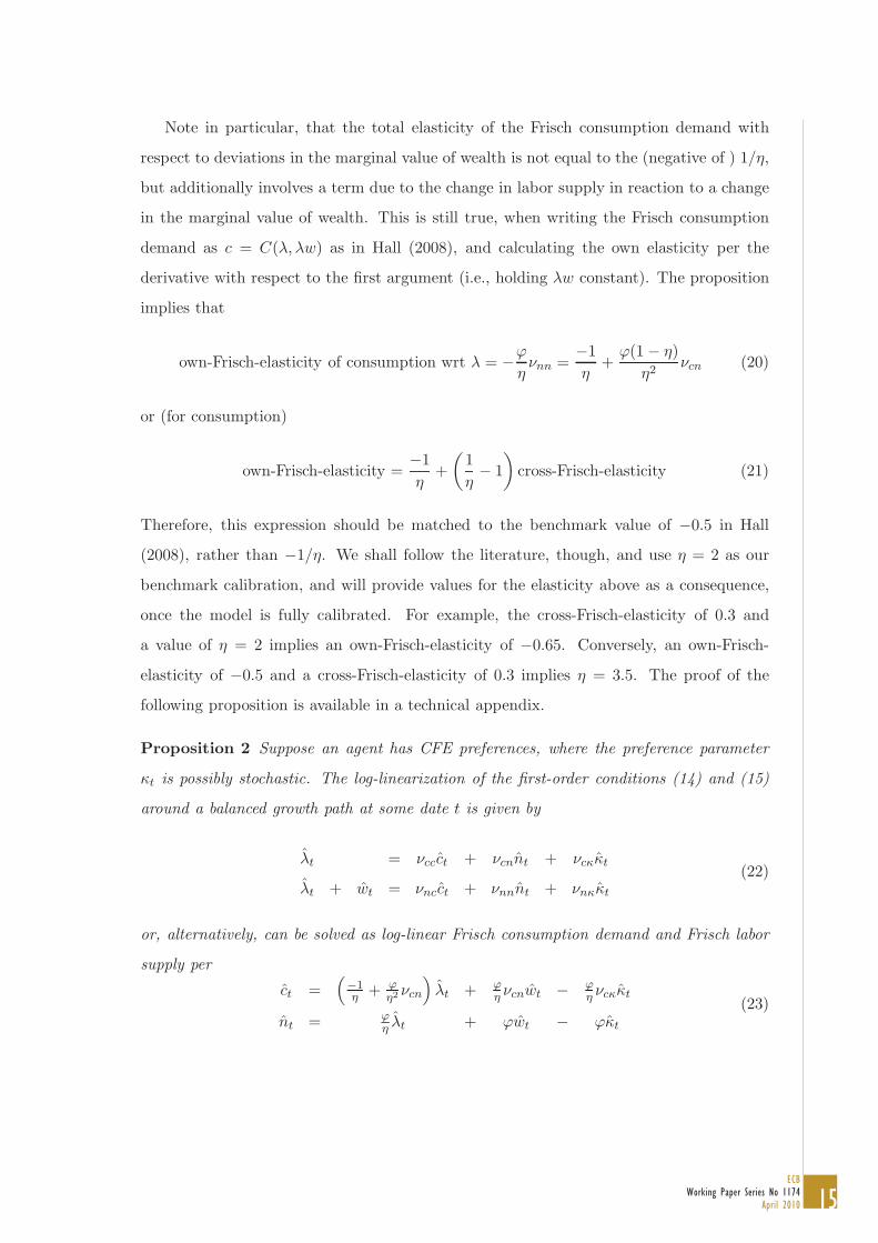
Note in particular, that the total elasticity of the Frisch consumption demand with
respect to deviations in the marginal value of wealth is not equal to the (negative of ) 1/η,
but additionally involves a term due to the change in labor supply in reaction to a change
in the marginal value of wealth. This is still true, when writing the Frisch consumption
demand as c = C(λ, λw) as in Hall (2008), and calculating the own elasticity per the
derivative with respect to the first argument (i.e., holding λw constant). The proposition
implies that
own-Frisch-elasticity of consumption wrt λ = −ϕ
ηνnn =
−1
η+
ϕ(1− η)
η2νcn (20)
or (for consumption)
own-Frisch-elasticity =−1
η+
(1
η− 1
)cross-Frisch-elasticity (21)
Therefore, this expression should be matched to the benchmark value of −0.5 in Hall
(2008), rather than −1/η. We shall follow the literature, though, and use η = 2 as our
benchmark calibration, and will provide values for the elasticity above as a consequence,
once the model is fully calibrated. For example, the cross-Frisch-elasticity of 0.3 and
a value of η = 2 implies an own-Frisch-elasticity of −0.65. Conversely, an own-Frisch-
elasticity of −0.5 and a cross-Frisch-elasticity of 0.3 implies η = 3.5. The proof of the
following proposition is available in a technical appendix.
Proposition 2 Suppose an agent has CFE preferences, where the preference parameter
κt is possibly stochastic. The log-linearization of the first-order conditions (14) and (15)
around a balanced growth path at some date t is given by
λt = νccct + νcnnt + νcκκt
λt + wt = νncct + νnnnt + νnκκt
(22)
or, alternatively, can be solved as log-linear Frisch consumption demand and Frisch labor
supply per
ct =(−1η
+ ϕη2 νcn
)λt + ϕ
ηνcnwt − ϕ
ηνcκκt
nt = ϕηλt + ϕwt − ϕκt
(23)

16ECBWorking Paper Series No 1174April 2010
where hat-variables denote log-deviations and where
νcc = −η
νcn = −
(1 +
1
ϕ
)(1− η)
((ηκn1+ 1
ϕ
)−1
+ 1−1
η
)−1
νcκ =ϕ
1 + ϕνcn
νnn =1
ϕ−
1− η
ηνcn
νnc = 1− η
νnκ = 1−1− η
ηνcκ
As an alternative, we also use the Cobb-Douglas preference specification
U(ct, nt) = α log(ct) + (1− α) log(1− nt) (24)
as it is an important and widely used benchmark, see e.g. Cooley and Prescott (1995),
Chari, Christiano, and Kehoe (1995) or Uhlig (2004).
2.2 Equilibrium
In equilibrium the household chooses plans to maximize its utility, the firm solves its
maximization problem and the government sets policies that satisfy its budget constraint.
Inspection of the balanced growth relationships provides some useful insights for the issue
at hand. Some of these results are more generally useful for examining the impact of
wedges on balanced growth allocations as in Chari, Kehoe, and Mcgrattan (2007).
Except for hours worked, interest rates and taxes all other variables grow at a constant
rate
ψ = ξ1
1−θ
For CFE preferences, the balanced growth after-tax return on any asset is
R = βψ−η , (25)
17ECB
Working Paper Series No 1174April 2010
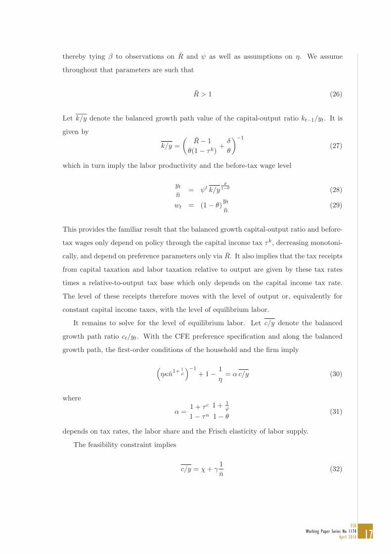
thereby tying β to observations on R and ψ as well as assumptions on η. We assume
throughout that parameters are such that
R > 1 (26)
Let k/y denote the balanced growth path value of the capital-output ratio kt−1/yt. It is
given by
k/y =
(R− 1
θ(1− τk)+
δ
θ
)−1
(27)
which in turn imply the labor productivity and the before-tax wage level
yt
n= ψt k/y
θ1−θ (28)
wt = (1− θ)yt
n(29)
This provides the familiar result that the balanced growth capital-output ratio and before-
tax wages only depend on policy through the capital income tax τk, decreasing monotoni-
cally, and depend on preference parameters only via R. It also implies that the tax receipts
from capital taxation and labor taxation relative to output are given by these tax rates
times a relative-to-output tax base which only depends on the capital income tax rate.
The level of these receipts therefore moves with the level of output or, equivalently for
constant capital income taxes, with the level of equilibrium labor.
It remains to solve for the level of equilibrium labor. Let c/y denote the balanced
growth path ratio ct/yt. With the CFE preference specification and along the balanced
growth path, the first-order conditions of the household and the firm imply
(ηκn1+ 1
ϕ
)−1
+ 1−1
η= α c/y (30)
where
α =1 + τ c
1− τn
1 + 1ϕ
1− θ(31)
depends on tax rates, the labor share and the Frisch elasticity of labor supply.
The feasibility constraint implies
c/y = χ + γ1
n(32)
18ECBWorking Paper Series No 1174April 2010
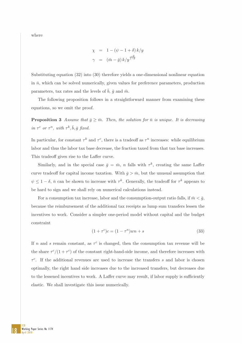
where
χ = 1− (ψ − 1 + δ) k/y
γ = (m− g) k/y−θ1−θ
Substituting equation (32) into (30) therefore yields a one-dimensional nonlinear equation
in n, which can be solved numerically, given values for preference parameters, production
parameters, tax rates and the levels of b, g and m.
The following proposition follows in a straightforward manner from examining these
equations, so we omit the proof.
Proposition 3 Assume that g ≥ m. Then, the solution for n is unique. It is decreasing
in τ c or τn, with τk, b, g fixed.
In particular, for constant τk and τ c, there is a tradeoff as τn increases: while equilibrium
labor and thus the labor tax base decrease, the fraction taxed from that tax base increases.
This tradeoff gives rise to the Laffer curve.
Similarly, and in the special case g = m, n falls with τk, creating the same Laffer
curve tradeoff for capital income taxation. With g > m, but the unusual assumption that
ψ ≤ 1 − δ, n can be shown to increase with τk. Generally, the tradeoff for τk appears to
be hard to sign and we shall rely on numerical calculations instead.
For a consumption tax increase, labor and the consumption-output ratio falls, if m < g,
because the reimbursement of the additional tax receipts as lump sum transfers lessen the
incentives to work. Consider a simpler one-period model without capital and the budget
constraint
(1 + τ c)c = (1− τn)wn + s (33)
If n and s remain constant, as τ c is changed, then the consumption tax revenue will be
the share τ c/(1 + τ c) of the constant right-hand-side income, and therefore increases with
τ c. If the additional revenues are used to increase the transfers s and labor is chosen
optimally, the right hand side increases due to the increased transfers, but decreases due
to the lessened incentives to work. A Laffer curve may result, if labor supply is sufficiently
elastic. We shall investigate this issue numerically.

19ECB
Working Paper Series No 1174April 2010
Alternatively, consider fixing s rather than g. Rewrite the budget constraint of the
household as
c/y = χ + γ1
n(34)
where
χ =1
1 + τ c
(1− (ψ − 1 + δ) k/y − τn(1− θ)− τk
(θ − δ k/y
))
γ =b(R − ψ) + s + m
1 + τ ck/y
−θ1−θ
can be calculated, given values for preference parameters, production parameters, tax rates
and the levels of b, s and m.
To see the difference to the case of fixing g, consider again the one-period model and
budget constraint (33). Maximizing growth-consistent preferences as in (13) subject to
this budget constraint, one obtains
(η − 1)v(n)
nv′(n)= 1 +
s
(1− τn)wn(35)
If transfers s do not change with τ c, then consumption taxes do not change labor supply.
Moreover, if transfers are zero, s = 0, labor taxes do not have an impact either. In both
cases, the substitution effect and the income effect exactly cancel just as they do for an
increase in total factor productivity. This insight generalizes to the model at hand, albeit
with some modification.
Proposition 4 Fix s, and instead adapt g, as the tax revenues change across balanced
growth equilibria.
• There is no impact of consumption tax rates τ c on equilibrium labor. As a conse-
quence, tax revenues always increase with increased consumption taxes.
• Suppose that
0 = b(R− ψ) + s + m (36)
Furthermore, suppose that labor taxes and capital taxes are jointly changed, so that
τn = τk
(1−
δ
θk/y
)(37)

20ECBWorking Paper Series No 1174April 2010
where the capital-income ratio depends on τk per (27). Equivalently, suppose that
all income from labor and capital is taxed at the rate τn without a deduction for
depreciation. Then there is no change of equilibrium labor.
Proof: For the claim regarding consumption taxes, note that the terms (1 + τc) for χ
and γ cancel with the corresponding term in α in equation (30). For the claim regarding
τk and τn, note that (37) together with (27) implies
R− 1 = (1− τk)
(θ
k/y− δ
)= (1− τn)
θ
k/y− δ
Then either by rewriting the budget constraint with an income tax τn and calculating the
consumption-output ratio or with
χ =1− τn
1 + τ c
(1− θ
Ψ− 1 + δ
R − 1 + δ
)
as well as γ = 0, one obtains that the right-hand side in equation (30) and therefore also
n remain constant, as tax rates are changed. •
This discussion highlights in particular the tax-unaffected income b(R−ψ) + s + m on
equilibrium labor. It also highlights an important reason for including the trade balance
in this analysis.
Given n, it is then straightforward to calculate total tax revenue as well as government
spending. Conversely, provided with an equilibrium value for n, one can use this equation
to find the value of the preference parameter κ, supporting this equilibrium. A similar
calculation obtains for the Cobb-Douglas preference specification.
While one could now use n and κ to calculate νcn for the coefficients in proposition 2,
there is a more direct and illuminating approach. Equation (30) can be rewritten as
νcn = −
(1 +
1
ϕ
)(1− η)
(α c/y
)−1
(38)
allowing the calculation of νcn from observing the consumption-output ratio, the parameter
α as well as ϕ and η, without reference to κ. Put differently, these values imply a value for
νcn and therefore for the cross-elasticity of the Frisch consumption demand with respect
to wages. The values implied by our calibration below are given in table 8.
21ECB
Working Paper Series No 1174April 2010
3 Calibration and Parameterization
We calibrate the model to annual post-war data of the US and EU-14 economy. Mendoza,
Razin, and Tesar (1994), calculate average effective tax rates from national product and
income accounts for the US. For this paper, we have followed their methodology to cal-
culate tax rates from 1995 to 2007 for the US and 14 of the EU-15 countries, excluding
Luxembourg for data availability reasons5. Appendix A provides some the details on the
required calculations and the data used, with further discussion of our approach and fur-
ther detail available in a technical appendix. Tables 13, 14 and 15 contain our calculated
panel of tax rates for labor, capital and consumption respectively.
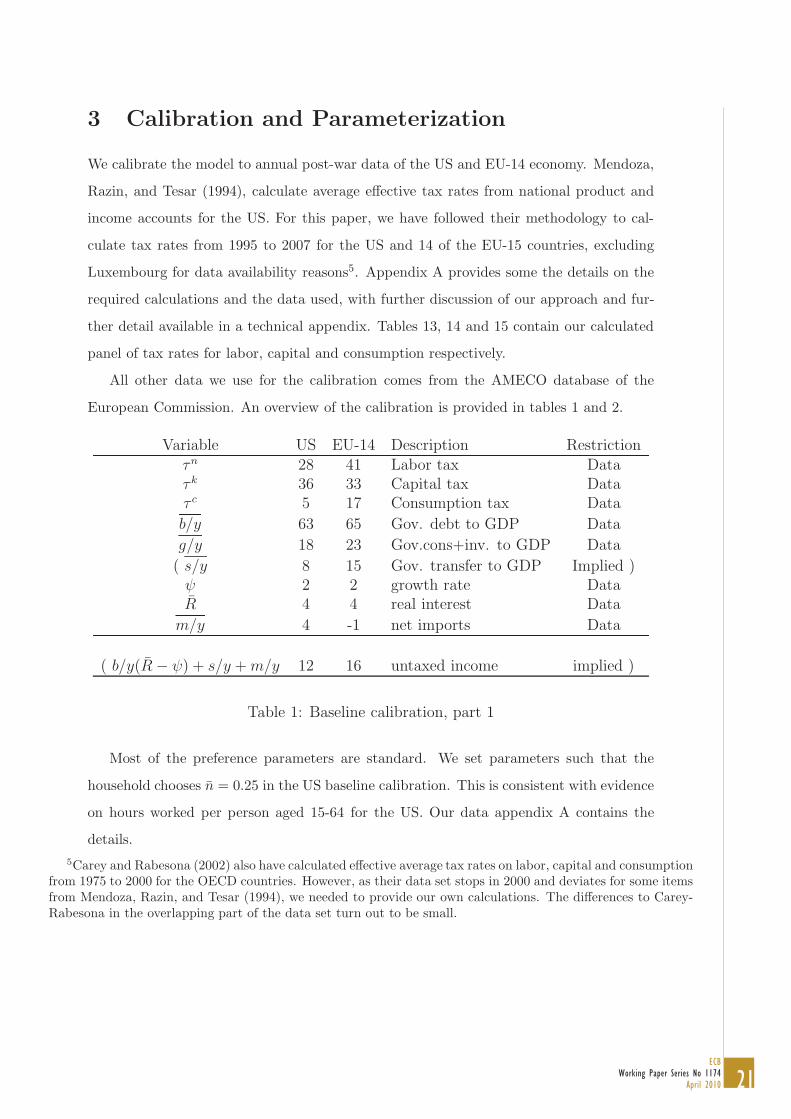
All other data we use for the calibration comes from the AMECO database of the
European Commission. An overview of the calibration is provided in tables 1 and 2.
Variable US EU-14 Description Restrictionτn 28 41 Labor tax Dataτk 36 33 Capital tax Dataτ c 5 17 Consumption tax Data
b/y 63 65 Gov. debt to GDP Data
g/y 18 23 Gov.cons+inv. to GDP Data
( s/y 8 15 Gov. transfer to GDP Implied )ψ 2 2 growth rate DataR 4 4 real interest Data
m/y 4 -1 net imports Data
( b/y(R− ψ) + s/y + m/y 12 16 untaxed income implied )
Table 1: Baseline calibration, part 1
Most of the preference parameters are standard. We set parameters such that the
household chooses n = 0.25 in the US baseline calibration. This is consistent with evidence
on hours worked per person aged 15-64 for the US. Our data appendix A contains the
details.
5Carey and Rabesona (2002) also have calculated effective average tax rates on labor, capital and consumptionfrom 1975 to 2000 for the OECD countries. However, as their data set stops in 2000 and deviates for some itemsfrom Mendoza, Razin, and Tesar (1994), we needed to provide our own calculations. The differences to Carey-Rabesona in the overlapping part of the data set turn out to be small.

22ECBWorking Paper Series No 1174April 2010
Var. US EU-14 Description Restrictionθ 0.38 0.38 Capital share on prod. Dataδ 0.07 0.07 Depr. rate of capital Dataη 2 2 inverse of IES benchmarkϕ 1 1 Frisch elasticity benchmarkκ 3.46 3.46 weight of labor nus = 0.25η 1 1 inverse of IES alternativeϕ 3 3 Frisch elasticity alternativeκ 3.38 3.38 weight of labor nus = 0.25α 0.319 0.321 Cons. weight in C-D nus = 0.25
Table 2: Baseline calibration, part 2
For the intertemporal elasticity of substitution, we follow a general consensus for it to
be close to 0.5 and therefore η = 2, as our benchmark choice. The specific value of the
Frisch labor supply elasticity is of central importance for the shape of the Laffer curve.
In the case of the alternative Cobb-Douglas preferences the Frisch elasticity is given by
1−nn
and equals 3 when n = 0.25. This value is in line with e.g. Kydland and Prescott
(1982), Cooley and Prescott (1995) and Prescott (2002, 2004), while a value close to 1 as
in Kimball and Shapiro (2003) may be closer to the current consensus view.
We therefore use η = 2 and ϕ = 1 as the benchmark calibration for the CFE preferences,
and use η = 1 and ϕ = 3 as alternative calibration and for comparison to a Cobb-Douglas
specification. A more detailed discussion is provided in subsection B.2 of the technical
appendix.
3.1 EU-14 Model and individual EU countries
As a benchmark, we keep all other parameters as in the US model, i.e. the parameters
characterizing the growth rate as well as production and preferences. As a result, we
calculate the differences between the US and the EU-14 as arising solely from differences
in fiscal policy. This corresponds to Prescott (2002, 2004) who argues that differences in
hours worked between the US and Europe are due to different level of labor income taxes.
In the subsection B.3 of the technical appendix, we provide a comparison of predicted
versus actual data for three key values: equilibrium labor, the capital-output ratio and
the consumption-output ratio. Discrepancies remain. While these are surely due to a
variety of reasons, in particular e.g. institutional differences in the implementation of
23ECB
Working Paper Series No 1174April 2010
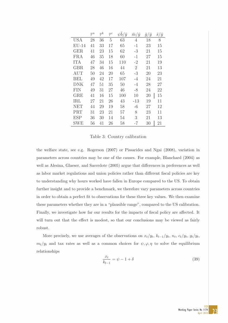
τn τk τ c ψb/y m/y g/y s/yUSA 28 36 5 63 4 18 8EU-14 41 33 17 65 -1 23 15GER 41 23 15 62 -3 21 15FRA 46 35 18 60 -1 27 15ITA 47 34 15 110 -2 21 19GBR 28 46 16 44 2 21 13AUT 50 24 20 65 -3 20 23BEL 49 42 17 107 -4 24 21DNK 47 51 35 50 -4 28 27FIN 49 31 27 46 -8 24 22GRE 41 16 15 100 10 20 15IRL 27 21 26 43 -13 19 11NET 44 29 19 58 -6 27 12PRT 31 23 21 57 8 23 11ESP 36 30 14 54 3 21 13SWE 56 41 26 58 -7 30 21
Table 3: Country calibration
the welfare state, see e.g. Rogerson (2007) or Pissarides and Ngai (2008), variation in
parameters across countries may be one of the causes. For example, Blanchard (2004) as
well as Alesina, Glaeser, and Sacerdote (2005) argue that differences in preferences as well
as labor market regulations and union policies rather than different fiscal policies are key
to understanding why hours worked have fallen in Europe compared to the US. To obtain
further insight and to provide a benchmark, we therefore vary parameters across countries
in order to obtain a perfect fit to observations for these three key values. We then examine
these parameters whether they are in a “plausible range”, compared to the US calibration.
Finally, we investigate how far our results for the impacts of fiscal policy are affected. It
will turn out that the effect is modest, so that our conclusions may be viewed as fairly
robust.
More precisely, we use averages of the observations on xt/yt, kt−1/yt, nt, ct/yt, gt/yt,
mt/yt and tax rates as well as a common choices for ψ,ϕ, η to solve the equilibrium
relationshipsxt
kt−1= ψ − 1 + δ (39)
24ECBWorking Paper Series No 1174April 2010
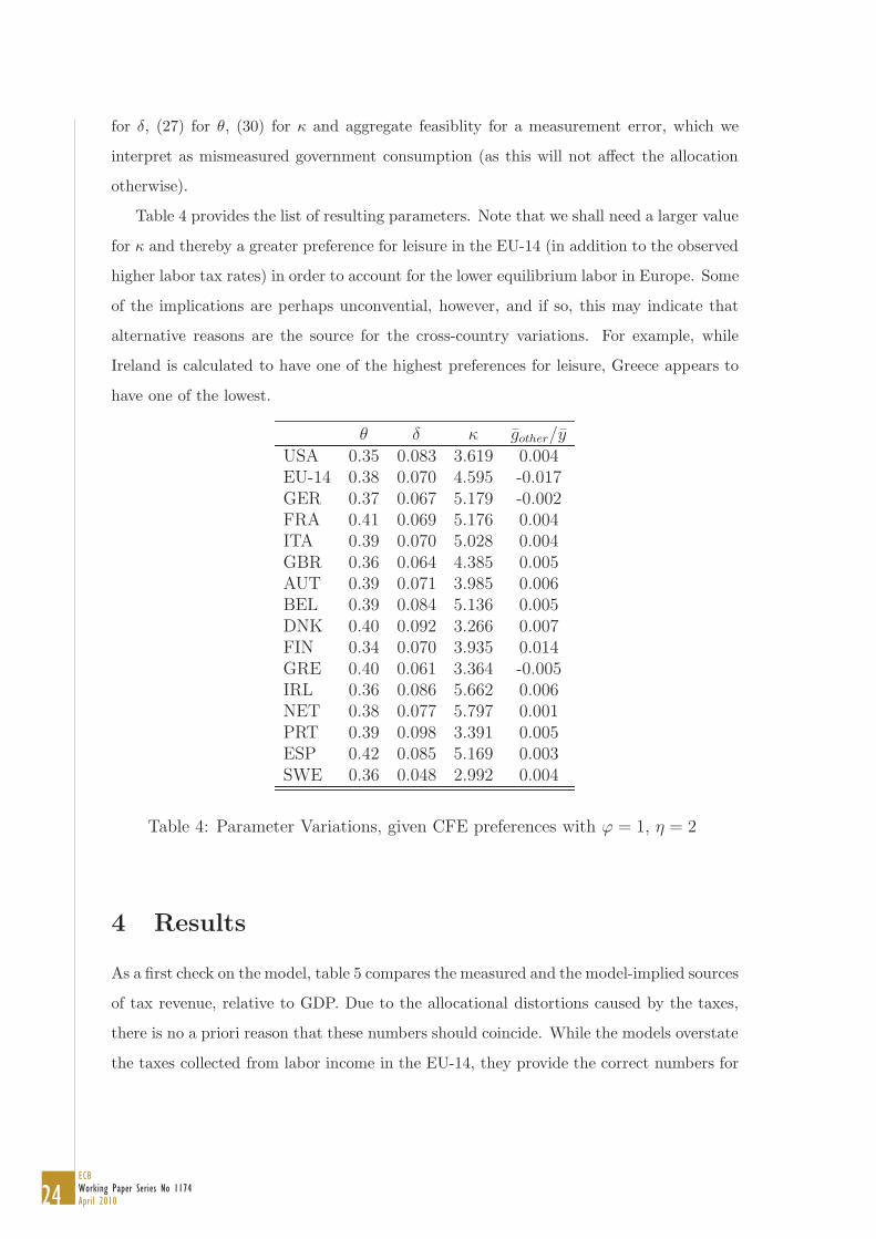
for δ, (27) for θ, (30) for κ and aggregate feasiblity for a measurement error, which we
interpret as mismeasured government consumption (as this will not affect the allocation
otherwise).
Table 4 provides the list of resulting parameters. Note that we shall need a larger value
for κ and thereby a greater preference for leisure in the EU-14 (in addition to the observed
higher labor tax rates) in order to account for the lower equilibrium labor in Europe. Some
of the implications are perhaps unconvential, however, and if so, this may indicate that
alternative reasons are the source for the cross-country variations. For example, while
Ireland is calculated to have one of the highest preferences for leisure, Greece appears to
have one of the lowest.
θ δ κ gother/yUSA 0.35 0.083 3.619 0.004EU-14 0.38 0.070 4.595 -0.017GER 0.37 0.067 5.179 -0.002FRA 0.41 0.069 5.176 0.004ITA 0.39 0.070 5.028 0.004GBR 0.36 0.064 4.385 0.005AUT 0.39 0.071 3.985 0.006BEL 0.39 0.084 5.136 0.005DNK 0.40 0.092 3.266 0.007FIN 0.34 0.070 3.935 0.014GRE 0.40 0.061 3.364 -0.005IRL 0.36 0.086 5.662 0.006NET 0.38 0.077 5.797 0.001PRT 0.39 0.098 3.391 0.005ESP 0.42 0.085 5.169 0.003SWE 0.36 0.048 2.992 0.004
Table 4: Parameter Variations, given CFE preferences with ϕ = 1, η = 2
4 Results
As a first check on the model, table 5 compares the measured and the model-implied sources
of tax revenue, relative to GDP. Due to the allocational distortions caused by the taxes,
there is no a priori reason that these numbers should coincide. While the models overstate
the taxes collected from labor income in the EU-14, they provide the correct numbers for
25ECB
Working Paper Series No 1174April 2010
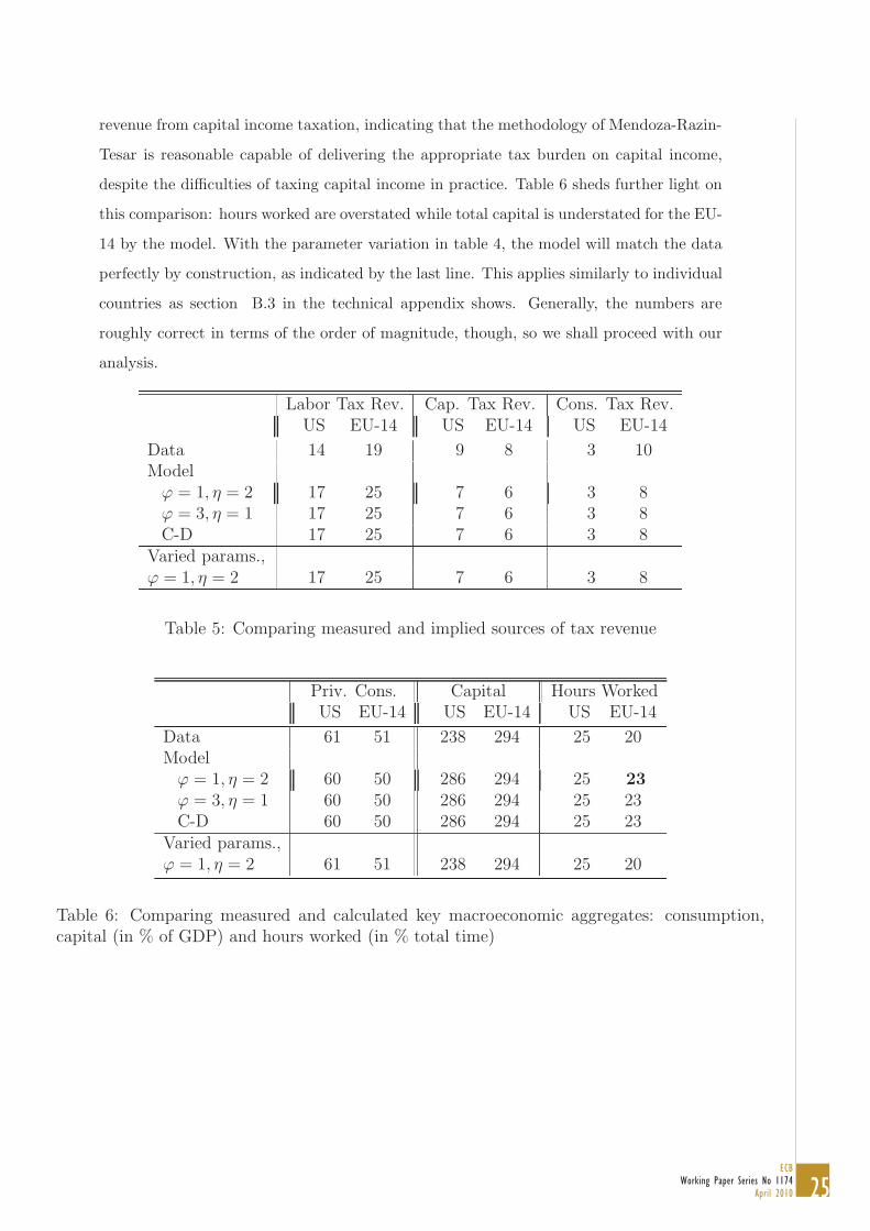
revenue from capital income taxation, indicating that the methodology of Mendoza-Razin-
Tesar is reasonable capable of delivering the appropriate tax burden on capital income,
despite the difficulties of taxing capital income in practice. Table 6 sheds further light on
this comparison: hours worked are overstated while total capital is understated for the EU-
14 by the model. With the parameter variation in table 4, the model will match the data
perfectly by construction, as indicated by the last line. This applies similarly to individual
countries as section B.3 in the technical appendix shows. Generally, the numbers are
roughly correct in terms of the order of magnitude, though, so we shall proceed with our
analysis.
Labor Tax Rev. Cap. Tax Rev. Cons. Tax Rev.US EU-14 US EU-14 US EU-14
Data 14 19 9 8 3 10Model
ϕ = 1, η = 2 17 25 7 6 3 8ϕ = 3, η = 1 17 25 7 6 3 8C-D 17 25 7 6 3 8
Varied params.,ϕ = 1, η = 2 17 25 7 6 3 8
Table 5: Comparing measured and implied sources of tax revenue
Priv. Cons. Capital Hours WorkedUS EU-14 US EU-14 US EU-14
Data 61 51 238 294 25 20Model
ϕ = 1, η = 2 60 50 286 294 25 23ϕ = 3, η = 1 60 50 286 294 25 23C-D 60 50 286 294 25 23
Varied params.,ϕ = 1, η = 2 61 51 238 294 25 20
Table 6: Comparing measured and calculated key macroeconomic aggregates: consumption,capital (in % of GDP) and hours worked (in % total time)

26ECBWorking Paper Series No 1174April 2010
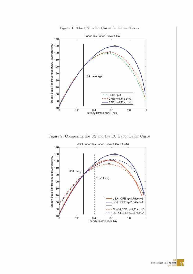
4.1 Labor Tax Laffer Curves
The Laffer curve for labor income taxation in the US is shown in figure 1. Note that
the CFE and Cobb-Douglas preferences coincide closely, if the intertemporal elasticity of
substitution 1/η and the Frisch elasticity of labor supply ϕ are the same at the bench-
mark steady state. Therefore, CFE preferences are close enough to the Cobb-Douglas
specification, if η = 1, and provide a growth-consistent generalization, if η �= 1.
For marginal rather than dramatic tax changes, the slope of the Laffer curve near the
current data calibration is of interest. The slope is related to the degree of self-financing
of a tax cut, defined as the ratio of additional tax revenues due to general equilibrium
incentive effects and the lost tax revenues at constant economic choices. More formally
and precisely, we calculate the degree of self-financing of a labor tax cut per
self-financing rate = 1−1
wtn
∂Tt(τn, τk)
∂τn≈ 1−
1
wtn
Tt(τn + ε, τk)− Tt(τn − ε, τk)
2ε
where T (τn, τk, τc; g, b) is the function of tax revenues across balanced growth equilbria
for different tax rates, and constant paths for government spending g and debt b. This
self-financing rate is a constant along the balanced growth path, i.e. does not depend on
t. Likewise, we calculate the degree of self-financing of a capital tax cut.
We calculate these self-financing rates numerically as indicated by the second expres-
sion, with ε set to 0.01 ( and tax rates expressed as fractions). If there were no endogenous
change of the allocation due to a tax change, the loss in tax revenue due to a one per-
centage point reduction in the tax rate would be wtn, and the self-financing rate would
calculate to 0. At the peak of the Laffer curve, the tax revenue would not change at all,
and the self-financing rate would be 100%. Indeed, the self-financing rate would become
larger than 100% beyond the peak of the Laffer curve.
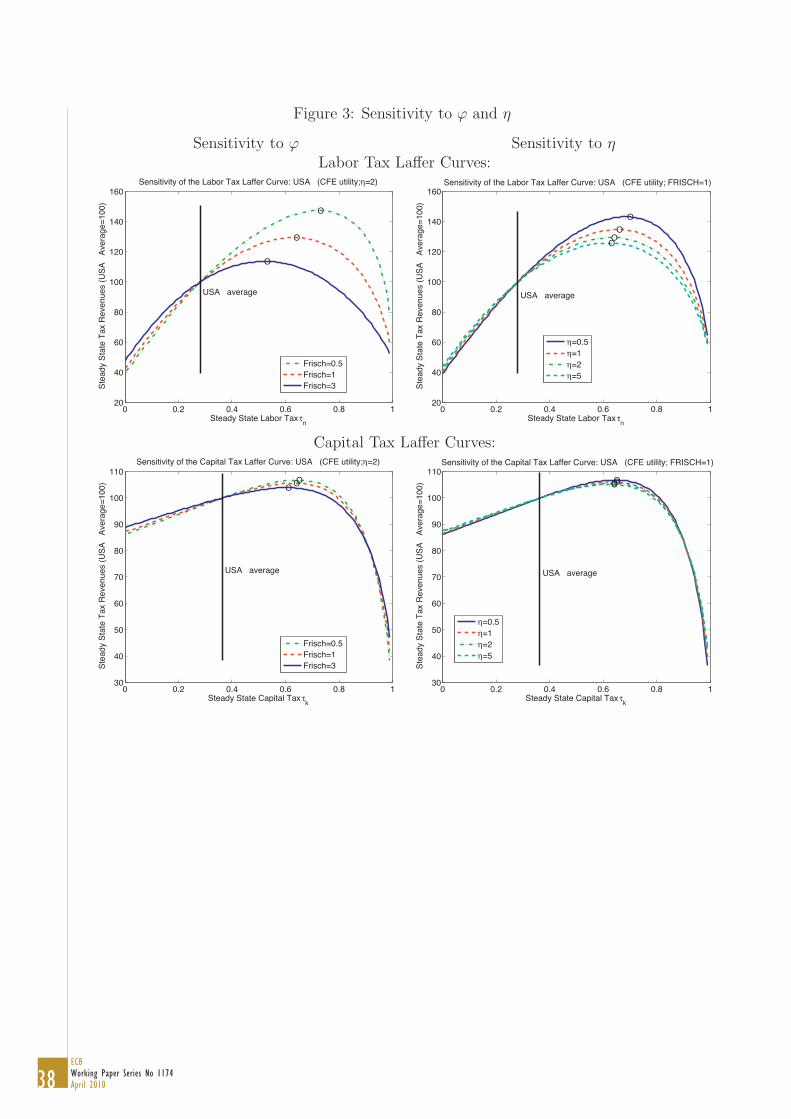
For labor taxes, table 7 provides results for the self-financing rate as well as for the
location of the peak of the Laffer curve for our benchmark calibration of the CFE preference
parameters, as well as a sensitivity analysis. Figure 3 likewise shows the sensitivity of the
Laffer curve to variations in ϕ and η. The peak of the Laffer curve shifts up and to the
right, as η and ϕ are decreased. The dependence on η arises due to the nonseparability
of preferences in consumption and leisure. Capital adjusts as labor adjusts across the
balanced growth paths.

27ECB
Working Paper Series No 1174April 2010
The table provides results for the US as well as the EU-14: there is considerably less
scope for additional financing of government revenue in Europe from raising labor taxes.
For our preferred benchmark calibration with a Frisch elasticity of 1 and an intertemporal
elasticity of substitution of 0.5, we find that the US and the EU-14 are located on the left
side of their Laffer curves, but while the US can increase tax revenues by 30% by raising
labor taxes, the EU-14 can raise only an additional 8%.
To gain further insight, figure 2 compares the US and the EU Laffer curve for our
benchmark calibration of ϕ = 1 and η = 2, benchmarking both Laffer curves to 100%
at the US labor tax rate. As the CFE parameters are changed, so are the cross-Frisch
elasticities and own-Frisch elasticities of consumption: the values are provided in table 8.
Parameter % self-fin. max. τn max. add. tax rev.Region: US EU-14 US EU-14 US EU-14ϕ = 1, η = 2 : 32 54 63 62 30 8ϕ = 3, η = 1 : 38 65 57 56 21 4
ϕ = 3, η = 2 : 49 78 52 51 14 2ϕ = 1, η = 2 : 32 54 63 62 30 8ϕ = 0.5, η = 2 : 21 37 72 71 47 17
ϕ = 1, η = 2 : 32 54 63 62 30 8ϕ = 1, η = 1 : 27 47 65 65 35 10ϕ = 1, η = 0.5 : 20 37 69 68 43 15
Table 7: Labor Tax Laffer curves: degree of self-financing, maximal tax rate, maximal additionaltax revenues. Shown are results for the US and the EU-14, and the sensitivity of the results tochanges in the CFE preference parameters.
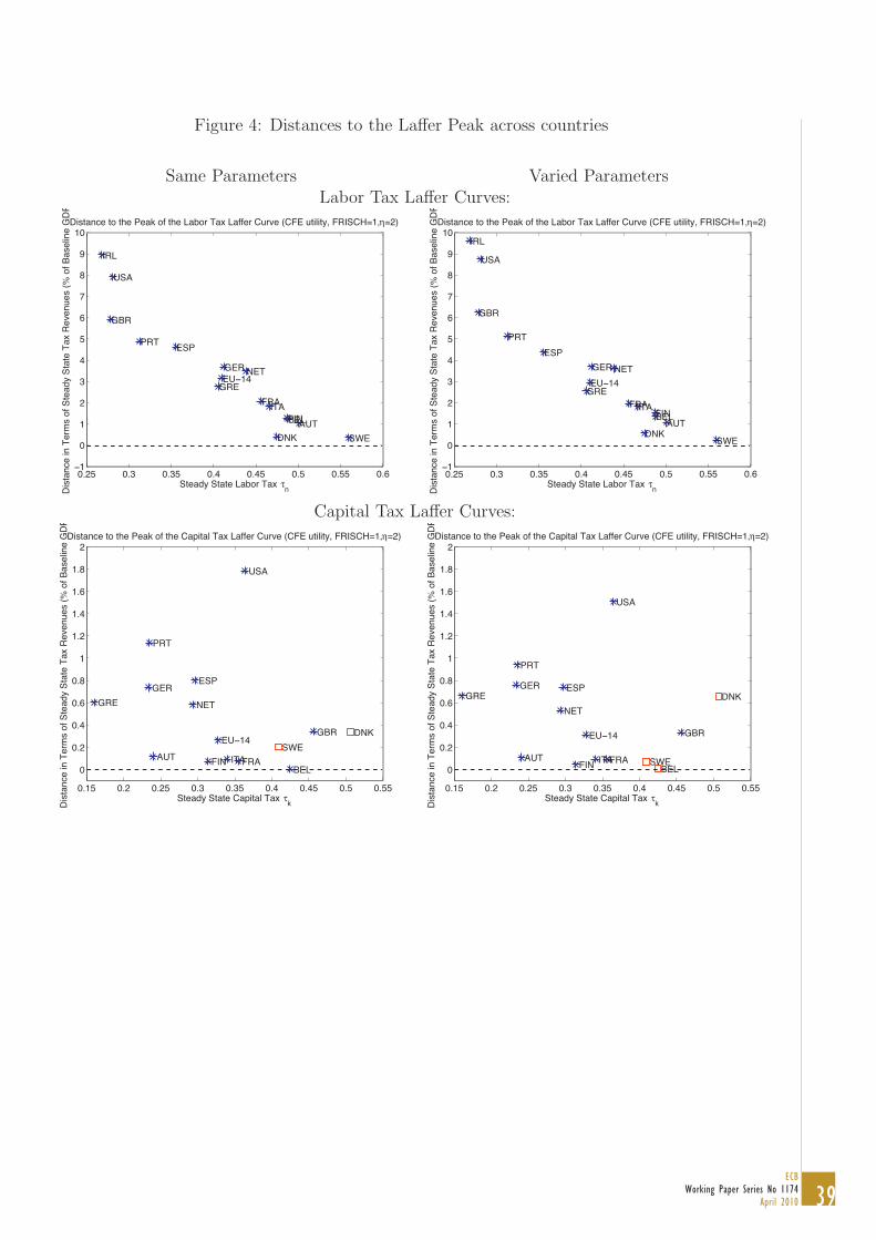
Table 9 as well as figure 4 provide insight into the degree of self-financing as well as
the location of the Laffer curve peak for individual countries, for both the case of keeping
the parameters the same across all countries as well as varying them according to table 4.
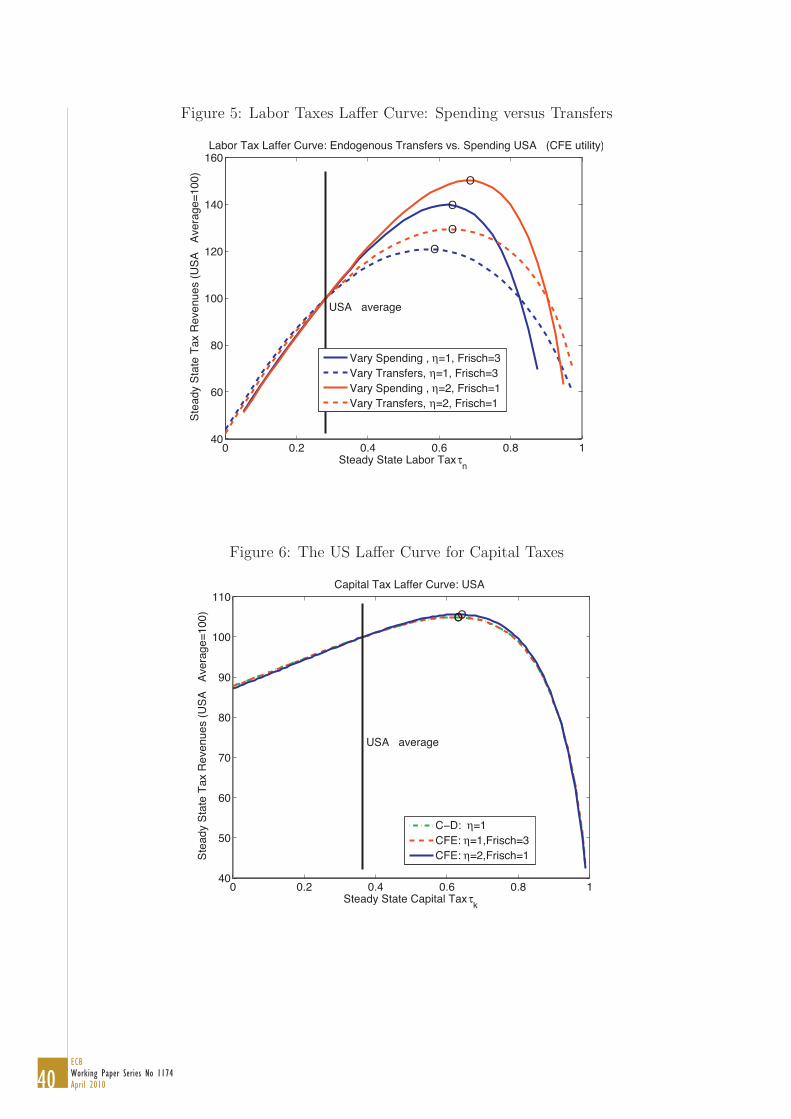
It matters for the thought experiment here, that the additional tax revenues are spent
on transfers, and not on other government spending. For the latter, the substitution effect
is mitigated by an income effect on labor: as a result the Laffer curve becomes steeper
with a peak to the right and above the peak coming from a “labor tax for transfer” Laffer
curve, see figure 5.
This matters even more for consumption taxes. As we have shown above, the consump-
tion tax revenue increase with increased consumption taxes, in the case the additional

28ECBWorking Paper Series No 1174April 2010
Parameter cross-Frisch-elast. own-Frisch-elast.Region: US EU-14 US EU-14ϕ = 1, η = 2 : 0.4 0.3 -0.7 -0.7ϕ = 3, η = 1 : -0.0 -0.0 -1.0 -1.0
ϕ = 3, η = 2 : 1.1 0.9 -1.0 -1.0ϕ = 1, η = 2 : 0.4 0.3 -0.7 -0.7ϕ = 0.5, η = 2 : 0.2 0.2 -0.6 -0.6
ϕ = 1, η = 2 : 0.4 0.3 -0.7 -0.7ϕ = 1, η = 1 : -0.0 -0.0 -1.0 -1.0ϕ = 1, η = 0.5 : -0.7 -0.6 -2.7 -2.6
Table 8: Cross-Frisch elasticities of consumption wrt wages and own-Frisch elasticities of con-sumption wrt to the Lagrange multiplier on wealth.
revenues are used for additional government spending, while there can be a Laffer curve,
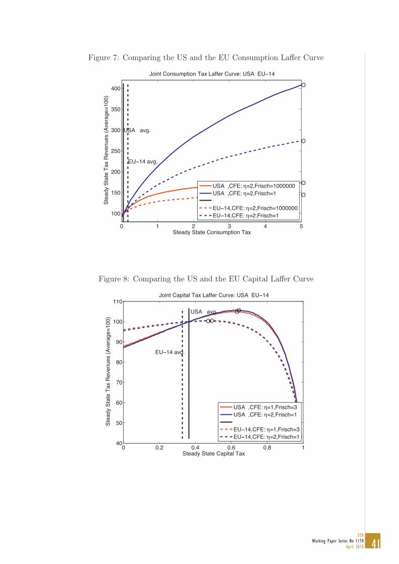
in case the additional revenues are used for transfers. Figure 7 shows the consumption
Laffer curve once for our benchmark parameterization and once for an extreme version of
an infinite Frisch elasticity, both for the US and for the EU-14 and benchmarking both
Laffer curves to 100% at the US consumption tax rate. The figure shows the Laffer curve in
consumption taxes to be increasing throughout, and the potential for additional revenues
to be dramatic. Whether it is possible in practice to raise consumption taxes amounting
to, say, 80% of the sales price (as would be the case for τc = 4) is a different matter,
though.
4.2 Capital Tax Laffer Curves
Figure 6 shows the Laffer curve for capital income taxation in the US. Benchmark results, a
comparison to the EU as well as the sensitivity analysis with respect to the CFE parameters
are given in table 10 as well as the right column of figure 3 and in figure 8, benchmarking
both Laffer curves to 100% at the US capital tax rate. For our preferred benchmark
calibration with a Frisch elasticity of 1 and an intertemporal elasticity of substitution of
0.5, we find that the US and the EU-14 are located on the left side of their Laffer curves,
but the scope for raising tax revenues by raising capital income taxes are small: they are
bound by 6% in the US and by 1% in the EU-14.
The cross-country comparison is in the right column of figure 4 and in table 11. Sev-
eral countries, e.g. Denmark and Sweden, show a negative self-financing fraction: these
29ECB
Working Paper Series No 1174April 2010
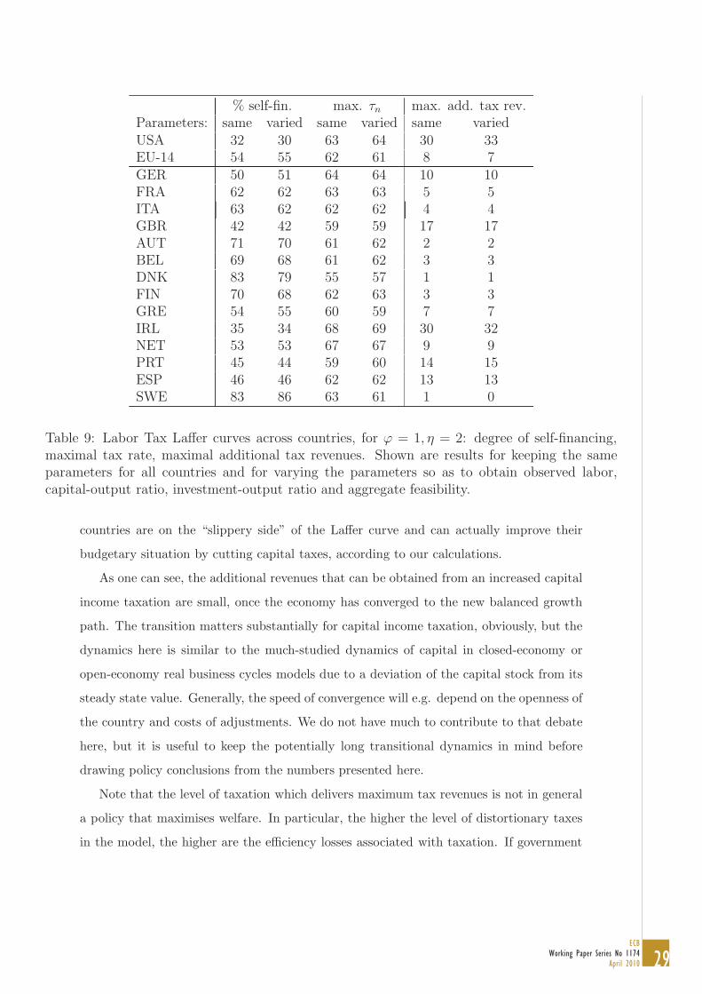
% self-fin. max. τn max. add. tax rev.Parameters: same varied same varied same variedUSA 32 30 63 64 30 33EU-14 54 55 62 61 8 7GER 50 51 64 64 10 10FRA 62 62 63 63 5 5ITA 63 62 62 62 4 4GBR 42 42 59 59 17 17AUT 71 70 61 62 2 2BEL 69 68 61 62 3 3DNK 83 79 55 57 1 1FIN 70 68 62 63 3 3GRE 54 55 60 59 7 7IRL 35 34 68 69 30 32NET 53 53 67 67 9 9PRT 45 44 59 60 14 15ESP 46 46 62 62 13 13SWE 83 86 63 61 1 0
Table 9: Labor Tax Laffer curves across countries, for ϕ = 1, η = 2: degree of self-financing,maximal tax rate, maximal additional tax revenues. Shown are results for keeping the sameparameters for all countries and for varying the parameters so as to obtain observed labor,capital-output ratio, investment-output ratio and aggregate feasibility.
countries are on the “slippery side” of the Laffer curve and can actually improve their
budgetary situation by cutting capital taxes, according to our calculations.
As one can see, the additional revenues that can be obtained from an increased capital
income taxation are small, once the economy has converged to the new balanced growth
path. The transition matters substantially for capital income taxation, obviously, but the
dynamics here is similar to the much-studied dynamics of capital in closed-economy or
open-economy real business cycles models due to a deviation of the capital stock from its
steady state value. Generally, the speed of convergence will e.g. depend on the openness of
the country and costs of adjustments. We do not have much to contribute to that debate
here, but it is useful to keep the potentially long transitional dynamics in mind before
drawing policy conclusions from the numbers presented here.
Note that the level of taxation which delivers maximum tax revenues is not in general
a policy that maximises welfare. In particular, the higher the level of distortionary taxes
in the model, the higher are the efficiency losses associated with taxation. If government
30ECBWorking Paper Series No 1174April 2010
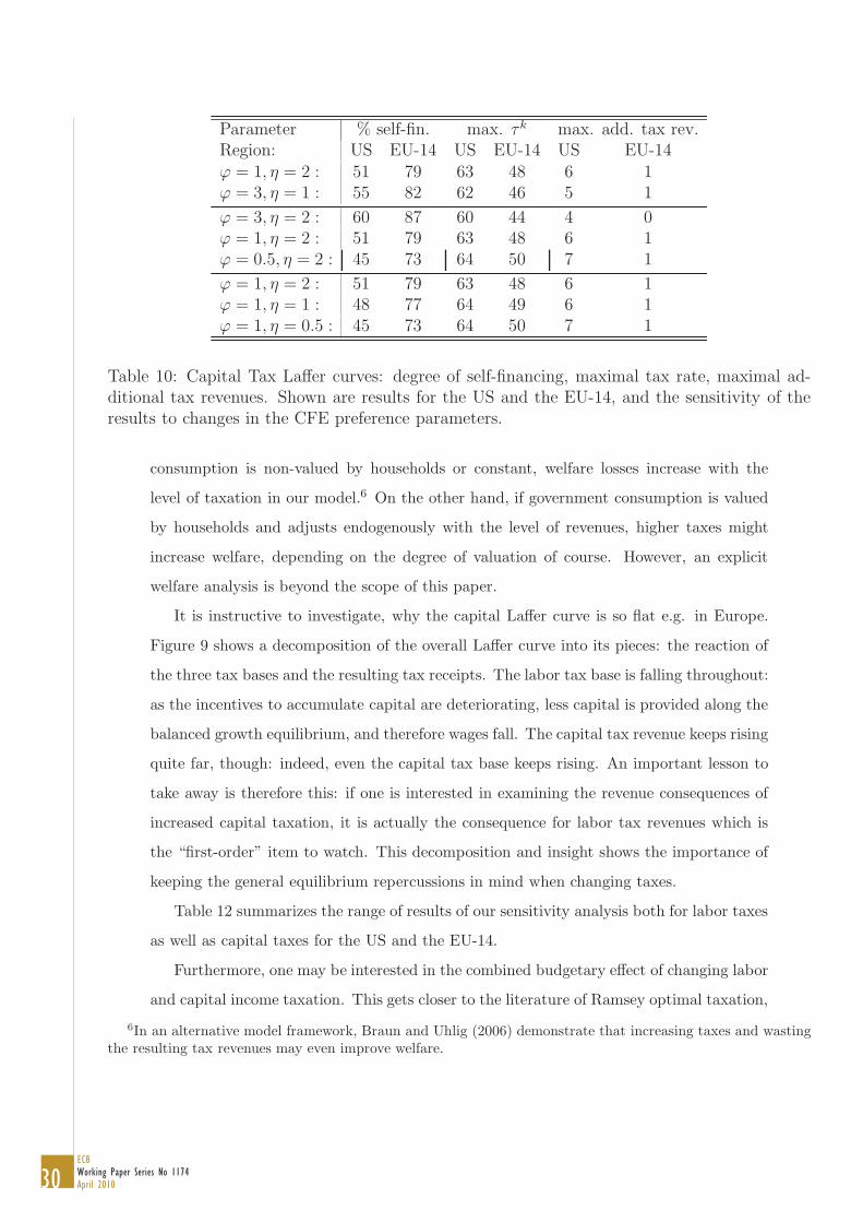
Parameter % self-fin. max. τk max. add. tax rev.Region: US EU-14 US EU-14 US EU-14ϕ = 1, η = 2 : 51 79 63 48 6 1ϕ = 3, η = 1 : 55 82 62 46 5 1
ϕ = 3, η = 2 : 60 87 60 44 4 0ϕ = 1, η = 2 : 51 79 63 48 6 1ϕ = 0.5, η = 2 : 45 73 64 50 7 1
ϕ = 1, η = 2 : 51 79 63 48 6 1ϕ = 1, η = 1 : 48 77 64 49 6 1ϕ = 1, η = 0.5 : 45 73 64 50 7 1
Table 10: Capital Tax Laffer curves: degree of self-financing, maximal tax rate, maximal ad-ditional tax revenues. Shown are results for the US and the EU-14, and the sensitivity of theresults to changes in the CFE preference parameters.
consumption is non-valued by households or constant, welfare losses increase with the
level of taxation in our model.6 On the other hand, if government consumption is valued
by households and adjusts endogenously with the level of revenues, higher taxes might
increase welfare, depending on the degree of valuation of course. However, an explicit
welfare analysis is beyond the scope of this paper.
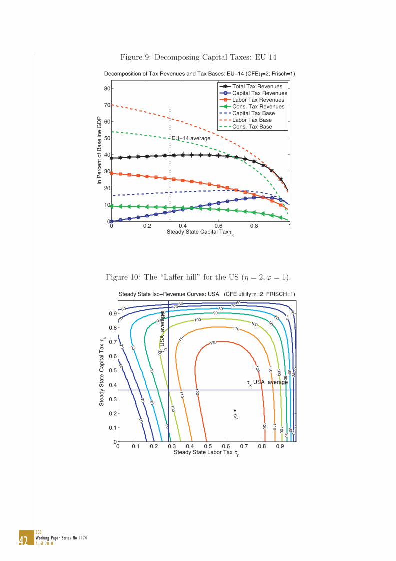
It is instructive to investigate, why the capital Laffer curve is so flat e.g. in Europe.
Figure 9 shows a decomposition of the overall Laffer curve into its pieces: the reaction of
the three tax bases and the resulting tax receipts. The labor tax base is falling throughout:
as the incentives to accumulate capital are deteriorating, less capital is provided along the
balanced growth equilibrium, and therefore wages fall. The capital tax revenue keeps rising
quite far, though: indeed, even the capital tax base keeps rising. An important lesson to
take away is therefore this: if one is interested in examining the revenue consequences of
increased capital taxation, it is actually the consequence for labor tax revenues which is
the “first-order” item to watch. This decomposition and insight shows the importance of
keeping the general equilibrium repercussions in mind when changing taxes.
Table 12 summarizes the range of results of our sensitivity analysis both for labor taxes
as well as capital taxes for the US and the EU-14.
Furthermore, one may be interested in the combined budgetary effect of changing labor
and capital income taxation. This gets closer to the literature of Ramsey optimal taxation,
6In an alternative model framework, Braun and Uhlig (2006) demonstrate that increasing taxes and wastingthe resulting tax revenues may even improve welfare.
31ECB
Working Paper Series No 1174April 2010
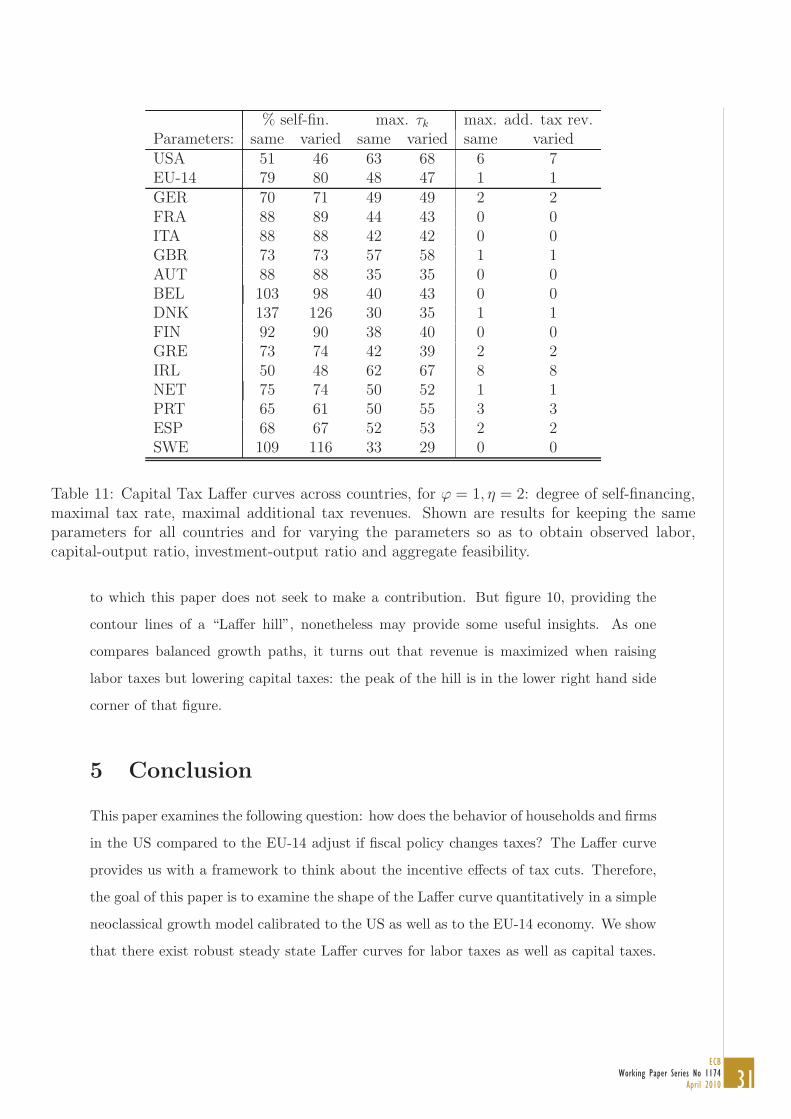
% self-fin. max. τk max. add. tax rev.Parameters: same varied same varied same variedUSA 51 46 63 68 6 7EU-14 79 80 48 47 1 1GER 70 71 49 49 2 2FRA 88 89 44 43 0 0ITA 88 88 42 42 0 0GBR 73 73 57 58 1 1AUT 88 88 35 35 0 0BEL 103 98 40 43 0 0DNK 137 126 30 35 1 1FIN 92 90 38 40 0 0GRE 73 74 42 39 2 2IRL 50 48 62 67 8 8NET 75 74 50 52 1 1PRT 65 61 50 55 3 3ESP 68 67 52 53 2 2SWE 109 116 33 29 0 0
Table 11: Capital Tax Laffer curves across countries, for ϕ = 1, η = 2: degree of self-financing,maximal tax rate, maximal additional tax revenues. Shown are results for keeping the sameparameters for all countries and for varying the parameters so as to obtain observed labor,capital-output ratio, investment-output ratio and aggregate feasibility.
to which this paper does not seek to make a contribution. But figure 10, providing the
contour lines of a “Laffer hill”, nonetheless may provide some useful insights. As one
compares balanced growth paths, it turns out that revenue is maximized when raising
labor taxes but lowering capital taxes: the peak of the hill is in the lower right hand side
corner of that figure.
5 Conclusion
This paper examines the following question: how does the behavior of households and firms
in the US compared to the EU-14 adjust if fiscal policy changes taxes? The Laffer curve
provides us with a framework to think about the incentive effects of tax cuts. Therefore,
the goal of this paper is to examine the shape of the Laffer curve quantitatively in a simple
neoclassical growth model calibrated to the US as well as to the EU-14 economy. We show
that there exist robust steady state Laffer curves for labor taxes as well as capital taxes.
32ECBWorking Paper Series No 1174April 2010
US EUPotential additional tax revenues (in % ):labor taxes 14% .. 47% 2% .. 17%
capital taxes 4% .. 7% 0% .. 1%Maximizing tax rate (in %) :
labor taxes 52% .. 72% 51% .. 71%capital taxes 60% .. 64% 44% .. 50%Percent self-financing of a tax cut (in % ):labor taxes 20% .. 49% 37% .. 78%
capital taxes 45% .. 60% 73% .. 87%
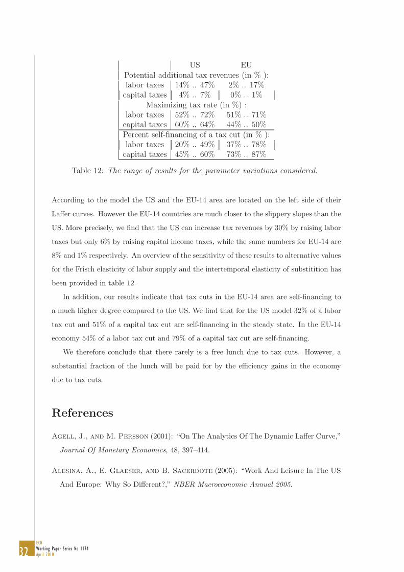
Table 12: The range of results for the parameter variations considered.
According to the model the US and the EU-14 area are located on the left side of their
Laffer curves. However the EU-14 countries are much closer to the slippery slopes than the
US. More precisely, we find that the US can increase tax revenues by 30% by raising labor
taxes but only 6% by raising capital income taxes, while the same numbers for EU-14 are
8% and 1% respectively. An overview of the sensitivity of these results to alternative values
for the Frisch elasticity of labor supply and the intertemporal elasticity of substitition has
been provided in table 12.
In addition, our results indicate that tax cuts in the EU-14 area are self-financing to
a much higher degree compared to the US. We find that for the US model 32% of a labor
tax cut and 51% of a capital tax cut are self-financing in the steady state. In the EU-14
economy 54% of a labor tax cut and 79% of a capital tax cut are self-financing.
We therefore conclude that there rarely is a free lunch due to tax cuts. However, a
substantial fraction of the lunch will be paid for by the efficiency gains in the economy
due to tax cuts.
References
Agell, J., and M. Persson (2001): “On The Analytics Of The Dynamic Laffer Curve,”
Journal Of Monetary Economics, 48, 397–414.
Alesina, A., E. Glaeser, and B. Sacerdote (2005): “Work And Leisure In The US
And Europe: Why So Different?,” NBER Macroeconomic Annual 2005.
33ECB
Working Paper Series No 1174April 2010
Baxter, M., and R. G. King (1993): “Fiscal Policy In General Equilibrium,” American
Economic Review, 82(3), 315–334.
Blanchard, O. (2004): “The Economic Future Of Europe,” Journal Of Economic Per-
spectives, 18(4), 3–26.
Braun, R. A., and H. Uhlig (2006): “The Welfare Enhancing Effects Of A Selfish
Government In The Presence Of Uninsurable, Idiosyncratic Risk,” Humboldt University
SFB 649 Discussion Paper, (2006-070).
Bruce, N., and S. J. Turnovsky (1999): “Budget Balance, Welfare, And The Growth
Rate: Dynamic Scoring Of The Long Run Government Budget,” Journal Of Money,
Credit And Banking, 31, 162–186.
Carey, D., and J. Rabesona (2002): “Tax Ratios On Labour And Capital Income And
On Consumption,” OECD Economic Studies, (35).
Cassou, S. P., and K. J. Lansing (2006): “Tax Reform With Useful Public Expendi-
tures,” Journal Of Public Economic Theory, 8(4), 631–676.
Chari, V. V., L. J. Christiano, and P. J. Kehoe (1995): “Policy Analysis In Busi-
ness Cycle Models,” Thomas F. Cooley, Ed., Frontiers Of Business Cycle Research,
Princeton, New Jersey: Princeton University Press, pp. 357–91.
Chari, V. V., P. J. Kehoe, and E. R. Mcgrattan (2007): “Business Ccyle Account-
ing,” Econometrica, 75(3), 781–836.
Christiano, L. J., and M. Eichenbaum (1992): “Current Real-Business-Cycle Theories
And Aggregate Labor-Market Fluctuations,” American Economic Review, 82, 430–50.
Cooley, T. F., and E. Prescott (1995): “Economic Growth And Business Cycles,”
Frontiers Of Business Cycle Research (Ed. Thomas F. Cooley), Princeton University
Press, pp. 1–38.
Domeij, D., and M. Floden (2006): “The Labor-Supply Elasticity And Borrowing
Constraints: Why Estimates Are Biased,” Review Of Economic Dynamics, 9, 242–262.
34ECBWorking Paper Series No 1174April 2010
Feldstein, M., and C. Horioka (1980): “Domestic Saving And International Capital
Flows,” The Economic Journal, 90, 314–329.
Floden, M., and J. Linde (2001): “Idiosyncratic Risk In The United States And
Sweden: Is There A Role For Government Insurance?,” Review Of Economic Dynamics,
4, 406–437.
Garcia-Mila, T., A. Marcet, and E. Ventura (2001): “Supply-Side Interventions
And Redistribution,” Manuscript.
Gruber, J. (2006): “A Tax-Based Estimate Of The Elasticity Of Intertemporal Substi-
tution,” NBER Working Paper.
Hall, R. E. (1988): “Intertemporal Substitution Of Consumption,” Journal Of Political
Economy, 96(2), 339–357.
(2008): “Sources and Mechanisms of Cyclical Fluctuations in the Labor Market,”
draft, Stanford University.
House, C. L., and M. D. Shapiro (2006): “Phased-In Tax Cuts And Economic Activ-
ity,” Forthcoming American Economic Review.
Ireland, P. N. (1994): “Supply-Side Economics And Endogenous Growth,” Journal Of
Monetary Economics, 33, 559–572.
Jonsson, M., and P. Klein (2003): “Tax Distortions In Sweden And The United
States,” European Economic Review, 47, 711–729.
Kim, J., and S. H. Kim (2004): “Welfare Effects Of Tax Policy In Open Economies:
Stabilization And Cooperation,” Manuscript.
Kimball, M. S., and M. D. Shapiro (2003): “Labor Supply: Are The Income And
Substitution Effects Both Large Or Small?,” Manuscript.
King, R. S., and S. T. Rebelo (1999): “Resuscitating Real Business Cycles,” Handbook
Of Macroeconomics, Edited By J. B. Taylor And M. Woodford, Amsterdam: Elsevier,
1B, 927–1007.

35ECB
Working Paper Series No 1174April 2010
Klein, P., P. Krusell, and J. V. Rios-Rull (2004): “Time-Consistent Public Ex-
penditures,” Manuscript.
Kniesner, T. J., and J. P. Ziliak (2005): “The Effect Of Income Taxation On Con-
sumption And Labor Supply,” Manuscript.
Kydland, F. E., and E. C. Prescott (1982): “Time To Build And Aggregate Fluc-
tuations,” Econometrica, 50, 1345–1370.
Lansing, K. (1998): “Optimal Fiscal Policy In A Business Cycle Model With Public
Capital,” The Canadian Journal Of Economics, 31(2), 337–364.
Leeper, E. M., and S.-C. S. Yang (2005): “Dynamic Scoring: Alternative Financing
Schemes,” NBER Working Paper.
Lindsey, L. B. (1987): “Individual taxpayer response to tax cuts: 1982-1984: With
implications for the revenue maximizing tax rate,” Journal of Public Economics, 33(2),
173–206.
Ljungqvist, L., and T. J. Sargent (2006): “Do Taxes Explain European Employ-
ment? Indivisible Labor, Human Capital, Lotteries, And Savings,” Manuscript.
Mankiw, G. N., and M. Weinzierl (2005): “Dynamic Scoring: A Back-Of-The-
Envelope Guide,” Forthcoming Journal Of Public Economics.
McGrattan, E. R. (1994): “The Macroeconomic Effects Of Distortionary Taxation,”
Journal Of Monetary Economics, 33(3), 573–601.
Mendoza, E. G., A. Razin, and L. L. Tesar (1994): “Effective Tax Rates In Macroe-
conomics: Cross-Country Estimates Of Tax Rates On Factor Incomes And Consump-
tion,” Journal Of Monetary Economics, 34, 297–323.
Mendoza, E. G., and L. L. Tesar (1998): “The International Ramifications Of Tax
Reforms: Supply-Side Economics In A Global Economy,” American Economic Review,
88, 402–417.
Novales, A., and J. Ruiz (2002): “Dynamic Laffer Curves,” Journal Of Economic
Dynamics And Control, 27, 181–206.
36ECBWorking Paper Series No 1174April 2010
Pissarides, C., and L. R. Ngai (2008): “Welfare Policy and the Sectoral Distribution
of Employment,” draft, London School of Economics.
Prescott, E. C. (2002): “Prosperity And Depression,” American Economic Review, 92,
1–15.
(2004): “Why Do Americans Work So Much More Than Europeans?,” Quarterly
Review, Federal Reserve Bank Of Minneapolis.
(2006): “Nobel Lecture: The Transformation Of Macroeconomic Policy And
Research,” Journal Of Political Economy, 114(2), 203–235.
Rogerson, R. (2007): “Taxation and Market Work: Is Scandinavia an Outlier?,” NBER
Working Paper 12890.
Schmitt-Grohe, S., and M. Uribe (1997): “Balanced-Budget Rules, Distortionary
Taxes, And Aggregate Instability,” Journal Of Political Economy, 105(5), 976–1000.
Shimer, R. (2008): “Convergence in Macroeconomics: The Labor Wedge,” Manuscript,
University of Chicago.
Trabandt, M. (2006): “Optimal Pre-Announced Tax Reforms Under Valuable And
Productive Government Spending,” Manuscript.
Uhlig, H. (2004): “Do Technology Shocks Lead To A Fall In Total Hours Worked?,”
Journal Of The European Economic Association, 2(2-3), 361–371.
Wanniski, J. (1978): “Taxes, Revenues, And The Laffer Curve,” The Public Interest.
Yanagawa, N., and H. Uhlig (1996): “Increasing The Capital Income Tax May Lead
To Faster Growth,” European Economic Review, 40, 1521–1540.
37ECB
Working Paper Series No 1174April 2010
Figure 1: The US Laffer Curve for Labor Taxes
0 0.2 0.4 0.6 0.8 140
50
60
70
80
90
100
110
120
130
140Labor Tax Laffer Curve: USA
Steady State Labor Tax τn
USA average
Stea
dy S
tate
Tax
Rev
enue
s (U
SA
Aver
age=
100)
O
OO
C−D: η=1CFE: η=1,Frisch=3CFE: η=2,Frisch=1
Figure 2: Comparing the US and the EU Labor Laffer Curve
0 0.2 0.4 0.6 0.8 140
50
60
70
80
90
100
110
120
130
140
USA avg.
O
O
EU−14 avg.
OO
Joint Labor Tax Laffer Curve: USA EU−14
Steady State Labor Tax
Stea
dy S
tate
Tax
Rev
enue
s (A
vera
ge=1
00)
USA ,CFE: η=1,Frisch=3USA ,CFE: η=2,Frisch=1
EU−14,CFE: η=1,Frisch=3EU−14,CFE: η=2,Frisch=1
38ECBWorking Paper Series No 1174April 2010
Figure 3: Sensitivity to ϕ and η
Sensitivity to ϕ Sensitivity to ηLabor Tax Laffer Curves:
0 0.2 0.4 0.6 0.8 120
40
60
80
100
120
140
160Sensitivity of the Labor Tax Laffer Curve: USA (CFE utility; η=2)
Steady State Labor Tax τn
USA average
Stea
dy S
tate
Tax
Rev
enue
s (U
SA
Aver
age=
100)
O
O
O
Frisch=0.5Frisch=1Frisch=3
0 0.2 0.4 0.6 0.8 120
40
60
80
100
120
140
160Sensitivity of the Labor Tax Laffer Curve: USA (CFE utility; FRISCH=1)
Steady State Labor Tax τn
USA average
Stea
dy S
tate
Tax
Rev
enue
s (U
SA
Aver
age=
100)
OOO
O
η=0.5η=1η=2η=5
Capital Tax Laffer Curves:
0 0.2 0.4 0.6 0.8 130
40
50
60
70
80
90
100
110Sensitivity of the Capital Tax Laffer Curve: USA (CFE utility; η=2)
Steady State Capital Tax τk
USA average
Stea
dy S
tate
Tax
Rev
enue
s (U
SA
Aver
age=
100) O OO
Frisch=0.5Frisch=1Frisch=3
0 0.2 0.4 0.6 0.8 130
40
50
60
70
80
90
100
110Sensitivity of the Capital Tax Laffer Curve: USA (CFE utility; FRISCH=1)
Steady State Capital Tax τk
USA average
Stea
dy S
tate
Tax
Rev
enue
s (U
SA
Aver
age=
100) OOOO
η=0.5η=1η=2η=5
39ECB
Working Paper Series No 1174April 2010
Figure 4: Distances to the Laffer Peak across countries
Same Parameters Varied ParametersLabor Tax Laffer Curves:
0.25 0.3 0.35 0.4 0.45 0.5 0.55 0.6−1
0
1
2
3
4
5
6
7
8
9
10
GER
FRAITA
GBR
AUTBEL
DNK
FIN
GRE
IRL
NET
PRT ESP
SWE
USA
EU−14
Distance to the Peak of the Labor Tax Laffer Curve (CFE utility, FRISCH=1, η=2)
Steady State Labor Tax τnDis
tanc
e in
Ter
ms
of S
tead
y St
ate
Tax
Rev
enue
s (%
of B
asel
ine
GDP
0.25 0.3 0.35 0.4 0.45 0.5 0.55 0.6−1
0
1
2
3
4
5
6
7
8
9
10
GER
FRAITA
GBR
AUTBEL
DNK
FIN
GRE
IRL
NET
PRTESP
SWE
USA
EU−14
Distance to the Peak of the Labor Tax Laffer Curve (CFE utility, FRISCH=1, η=2)
Steady State Labor Tax τnDis
tanc
e in
Ter
ms
of S
tead
y St
ate
Tax
Rev
enue
s (%
of B
asel
ine
GDP
Capital Tax Laffer Curves:
0.15 0.2 0.25 0.3 0.35 0.4 0.45 0.5 0.55
0
0.2
0.4
0.6
0.8
1
1.2
1.4
1.6
1.8
2
GER
FRAITA
GBR
AUTBEL
DNK
FIN
GRE NET
PRT
ESP
SWE
USA
EU−14
Distance to the Peak of the Capital Tax Laffer Curve (CFE utility, FRISCH=1, η=2)
Steady State Capital Tax τkDis
tanc
e in
Ter
ms
of S
tead
y St
ate
Tax
Rev
enue
s (%
of B
asel
ine
GDP
0.15 0.2 0.25 0.3 0.35 0.4 0.45 0.5 0.55
0
0.2
0.4
0.6
0.8
1
1.2
1.4
1.6
1.8
2
GER
FRAITA
GBR
AUTBEL
DNK
FIN
GRENET
PRT
ESP
SWE
USA
EU−14
Distance to the Peak of the Capital Tax Laffer Curve (CFE utility, FRISCH=1, η=2)
Steady State Capital Tax τkDis
tanc
e in
Ter
ms
of S
tead
y St
ate
Tax
Rev
enue
s (%
of B
asel
ine
GDP
40ECBWorking Paper Series No 1174April 2010
Figure 5: Labor Taxes Laffer Curve: Spending versus Transfers
0 0.2 0.4 0.6 0.8 140
60
80
100
120
140
160Labor Tax Laffer Curve: Endogenous Transfers vs. Spending USA (CFE utility)
Steady State Labor Tax τn
USA average
Stea
dy S
tate
Tax
Rev
enue
s (U
SA
Aver
age=
100)
O
O
O
O
Vary Spending , η=1, Frisch=3Vary Transfers, η=1, Frisch=3Vary Spending , η=2, Frisch=1Vary Transfers, η=2, Frisch=1
Figure 6: The US Laffer Curve for Capital Taxes
0 0.2 0.4 0.6 0.8 140
50
60
70
80
90
100
110Capital Tax Laffer Curve: USA
Steady State Capital Tax τk
USA average
Stea
dy S
tate
Tax
Rev
enue
s (U
SA
Aver
age=
100) OOO
C−D: η=1CFE: η=1,Frisch=3CFE: η=2,Frisch=1
41ECB
Working Paper Series No 1174April 2010
Figure 7: Comparing the US and the EU Consumption Laffer Curve
0 1 2 3 4 5
100
150
200
250
300
350
400
USA avg.
O
O
EU−14 avg.
O
O
Joint Consumption Tax Laffer Curve: USA EU−14
Steady State Consumption Tax
Stea
dy S
tate
Tax
Rev
enue
s (A
vera
ge=1
00)
USA ,CFE: η=2,Frisch=1000000USA ,CFE: η=2,Frisch=1
EU−14,CFE: η=2,Frisch=1000000EU−14,CFE: η=2,Frisch=1
Figure 8: Comparing the US and the EU Capital Laffer Curve
0 0.2 0.4 0.6 0.8 140
50
60
70
80
90
100
110
USA avg. OO
EU−14 avg.
OO
Joint Capital Tax Laffer Curve: USA EU−14
Steady State Capital Tax
Stea
dy S
tate
Tax
Rev
enue
s (A
vera
ge=1
00)
USA ,CFE: η=1,Frisch=3USA ,CFE: η=2,Frisch=1
EU−14,CFE: η=1,Frisch=3EU−14,CFE: η=2,Frisch=1
42ECBWorking Paper Series No 1174April 2010
Figure 9: Decomposing Capital Taxes: EU 14
0 0.2 0.4 0.6 0.8 10
10
20
30
40
50
60
70
80
Decomposition of Tax Revenues and Tax Bases: EU−14 (CFE; η=2; Frisch=1)
Steady State Capital Tax τk
In P
erce
nt o
f Bas
elin
e G
DP
EU−14 average
Total Tax RevenuesCapital Tax RevenuesLabor Tax RevenuesCons. Tax RevenuesCapital Tax BaseLabor Tax BaseCons. Tax Base
Figure 10: The “Laffer hill” for the US (η = 2, ϕ = 1).
60
60
60
6060
606060
70
70
7070
70
7070
70
80
80
8080
80
8080
90
90
90
90
90
9090
100
100
100100
100100
110
110
110
110110
120
120
120120
131τ n U
SA a
vera
ge
τk USA average
Steady State Iso−Revenue Curves: USA (CFE utility; η=2; FRISCH=1)
Stea
dy S
tate
Cap
ital T
axτ k
Steady State Labor Tax τn
0 0.1 0.2 0.3 0.4 0.5 0.6 0.7 0.8 0.90
0.1
0.2
0.3
0.4
0.5
0.6
0.7
0.8
0.9

43ECB
Working Paper Series No 1174April 2010
Appendix
A EU-14 Tax Rates and GDP Ratios
In order to obtain EU-14 tax rates and GDP ratios we proceed as follows. E.g., EU-14
consumption tax revenues can be expressed as:
τ cEU−14,tcEU−14,t =
∑j
τ cj,tcj,t (40)
where j denotes each individual EU-14 country. Rewriting equation (40) yields the con-
sumption weighted EU-14 consumption tax rate:
τ cEU−14,t =
∑j τ c
j,tcj,t
cEU−14,t
=
∑j τ c
j,tcj,t∑j cj,t
. (41)
The numerator of equation (41) consists of consumption tax revenues of each individual
country j whereas the denominator consists of consumption tax revenues divided by the
consumption tax rate of each individual country j. Formally,
τ cEU−14,t =
∑j TCons
j,t∑j
T Consj,t
τcj,t
. (42)
The methodology of Mendoza, Razin, and Tesar (1994) allows to calculate implicit
individual country consumption tax revenues so that we can easily calculate the EU-14
consumption tax rate τ cEU−14,t. Likewise, applying the same procedure we calculate EU-14
labor and capital tax rates. Taking averages over time yields the tax rates we report in
table 1.
In order to calculate EU-14 GDP ratios we proceed as follows. E.g., the GDP weighted
EU-14 debt to GDP ratio can be written as:
bEU−14,t
yEU−14,t=
∑j
bj,t
yj,tyj,t∑
j yj,t(43)

44ECBWorking Paper Series No 1174April 2010
where bj and yj are individual country government debt and GDP. Likewise, we apply the
same procedure for the EU-14 transfer to GDP ratio. Taking averages over time yields
the numbers used for the calibration of the model.
Tables 13, 14 and 15 contain our calculated panel of tax rates for labor, capital and
consumption respectively.
1995 1996 1997 1998 1999 2000 2001 2002 2003 2004 2005 2006 2007USA 27.6 28.2 28.6 28.9 29.2 29.6 29.4 27.2 26.3 26.1 27.4 27.9 28.4EU-14 42.3 42.2 42.0 41.3 41.5 40.5 40.2 39.7 40.1 40.1 40.5 41.0 41.3GER 42.0 40.9 41.4 41.9 41.7 41.4 41.7 40.8 40.6 40.0 40.2 41.2 41.5FRA 46.2 46.8 46.6 45.4 45.8 45.3 44.7 44.4 45.0 44.7 46.0 45.9 45.7ITA 46.4 48.5 49.7 45.9 46.3 45.7 45.5 45.6 45.9 46.2 46.1 46.2 47.8GBR 26.8 26.1 25.7 26.9 27.4 27.8 27.7 27.2 27.7 28.8 29.3 29.8 30.4AUT 47.5 48.7 50.0 50.1 50.3 49.4 50.8 50.7 50.7 50.8 50.3 50.3 50.3BEL 48.1 48.0 48.6 49.0 48.4 48.3 48.3 49.0 49.3 49.6 49.5 48.5 48.8DNK 46.4 46.8 47.4 46.6 48.6 48.8 48.7 47.5 47.7 46.6 47.0 46.7 47.9FIN 51.9 52.6 50.4 49.9 48.9 49.4 48.6 48.0 46.6 45.8 46.6 47.1 47.2GRE NaN NaN NaN NaN NaN 40.2 39.8 41.0 42.3 40.5 40.3 40.0 40.3IRL NaN NaN NaN NaN NaN NaN NaN 25.4 25.6 26.9 27.0 27.4 28.5NET 49.4 46.4 46.8 42.3 43.6 43.6 40.4 40.7 41.0 41.8 42.8 45.8 45.0PRT 29.4 29.8 30.1 29.9 30.1 30.8 31.2 31.4 32.0 31.9 32.5 32.7 34.4ESP NaN NaN NaN NaN NaN 34.1 34.8 35.1 35.1 35.1 35.9 36.6 37.4SWE 52.9 54.6 56.3 58.1 60.7 57.2 55.2 53.6 55.2 55.9 56.0 56.5 54.6
Table 13: Labor income taxes in percent across countries and time
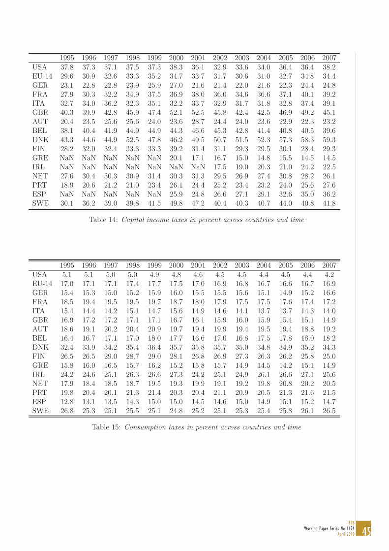
45ECB
Working Paper Series No 1174April 2010
1995 1996 1997 1998 1999 2000 2001 2002 2003 2004 2005 2006 2007USA 37.8 37.3 37.1 37.5 37.3 38.3 36.1 32.9 33.6 34.0 36.4 36.4 38.2EU-14 29.6 30.9 32.6 33.3 35.2 34.7 33.7 31.7 30.6 31.0 32.7 34.8 34.4GER 23.1 22.8 22.8 23.9 25.9 27.0 21.6 21.4 22.0 21.6 22.3 24.4 24.8FRA 27.9 30.3 32.2 34.9 37.5 36.9 38.0 36.0 34.6 36.6 37.1 40.1 39.2ITA 32.7 34.0 36.2 32.3 35.1 32.2 33.7 32.9 31.7 31.8 32.8 37.4 39.1GBR 40.3 39.9 42.8 45.9 47.4 52.1 52.5 45.8 42.4 42.5 46.9 49.2 45.1AUT 20.4 23.5 25.6 25.6 24.0 23.6 28.7 24.4 24.0 23.6 22.9 22.3 23.2BEL 38.1 40.4 41.9 44.9 44.9 44.3 46.6 45.3 42.8 41.4 40.8 40.5 39.6DNK 43.3 44.6 44.9 52.5 47.8 46.2 49.5 50.7 51.5 52.3 57.3 58.3 59.3FIN 28.2 32.0 32.4 33.3 33.3 39.2 31.4 31.1 29.3 29.5 30.1 28.4 29.3GRE NaN NaN NaN NaN NaN 20.1 17.1 16.7 15.0 14.8 15.5 14.5 14.5IRL NaN NaN NaN NaN NaN NaN NaN 17.5 19.0 20.3 21.0 24.2 22.5NET 27.6 30.4 30.3 30.9 31.4 30.3 31.3 29.5 26.9 27.4 30.8 28.2 26.1PRT 18.9 20.6 21.2 21.0 23.4 26.1 24.4 25.2 23.4 23.2 24.0 25.6 27.6ESP NaN NaN NaN NaN NaN 25.9 24.8 26.6 27.1 29.1 32.6 35.0 36.2SWE 30.1 36.2 39.0 39.8 41.5 49.8 47.2 40.4 40.3 40.7 44.0 40.8 41.8
Table 14: Capital income taxes in percent across countries and time
1995 1996 1997 1998 1999 2000 2001 2002 2003 2004 2005 2006 2007USA 5.1 5.1 5.0 5.0 4.9 4.8 4.6 4.5 4.5 4.4 4.5 4.4 4.2EU-14 17.0 17.1 17.1 17.4 17.7 17.5 17.0 16.9 16.8 16.7 16.6 16.7 16.9GER 15.4 15.3 15.0 15.2 15.9 16.0 15.5 15.5 15.6 15.1 14.9 15.2 16.6FRA 18.5 19.4 19.5 19.5 19.7 18.7 18.0 17.9 17.5 17.5 17.6 17.4 17.2ITA 15.4 14.4 14.2 15.1 14.7 15.6 14.9 14.6 14.1 13.7 13.7 14.3 14.0GBR 16.9 17.2 17.2 17.1 17.1 16.7 16.1 15.9 16.0 15.9 15.4 15.1 14.9AUT 18.6 19.1 20.2 20.4 20.9 19.7 19.4 19.9 19.4 19.5 19.4 18.8 19.2BEL 16.4 16.7 17.1 17.0 18.0 17.7 16.6 17.0 16.8 17.5 17.8 18.0 18.2DNK 32.4 33.9 34.2 35.4 36.4 35.7 35.8 35.7 35.0 34.8 34.9 35.2 34.3FIN 26.5 26.5 29.0 28.7 29.0 28.1 26.8 26.9 27.3 26.3 26.2 25.8 25.0GRE 15.8 16.0 16.5 15.7 16.2 15.2 15.8 15.7 14.9 14.5 14.2 15.1 14.9IRL 24.2 24.6 25.1 26.3 26.6 27.3 24.2 25.1 24.9 26.1 26.6 27.1 25.6NET 17.9 18.4 18.5 18.7 19.5 19.3 19.9 19.1 19.2 19.8 20.8 20.2 20.5PRT 19.8 20.4 20.1 21.3 21.4 20.3 20.4 21.1 20.9 20.5 21.3 21.6 21.5ESP 12.8 13.1 13.5 14.3 15.0 15.0 14.5 14.6 15.0 14.9 15.1 15.2 14.7SWE 26.8 25.3 25.1 25.5 25.1 24.8 25.2 25.1 25.3 25.4 25.8 26.1 26.5
Table 15: Consumption taxes in percent across countries and time

46ECBWorking Paper Series No 1174April 2010
TECHNICAL APPENDIX
B Additions to the main text
B.1 A proof
Proof: [Proof for Proposition 2.] Log-linearization generally leads to (22), where
νcc =uccc
uc
νcn =ucnn
uc
νcκ =ucκκ
uc
νnn =unnn
un
νnc =ucnc
un
νnκ =ucκκ
un
For the explicit expressions, calculate. For the Frisch demand and supply, use matrix
inversion for (22) together with the explicit expressions for the coefficients, and calculate.
•
B.2 Details on the Calibration Choices
Empirical estimates of the intertemporal elasticity vary considerably. Hall (1988) estimates
it to be close to zero. Recently, Gruber (2006) provides an excellent survey on estimates
in the literature. Further, he estimates the intertemporal elasticity to be two. Cooley and
Prescott (1995) and King and Rebelo (1999) use an intertemporal elasticity equal to one.
The general current consensus seems to be that the intertemporal elasticity of substitution
is closer to 0.5, which we shall use for our baseline calibration, but also investigating a
value equal to unity as an alternative, and impose it for the Cobb-Douglas preference
specification.
There is a large literature that estimates the Frisch labor supply elasticity from micro
data. Domeij and Floden (2006) argue that labor supply elasticity estimates are likely to

47ECB
Working Paper Series No 1174April 2010
be biased downwards by up to 50 percent. However, the authors survey the existing micro
Frisch labor supply elasticity estimates and conclude that many estimates range between
0 and 0.5. Further, Kniesner and Ziliak (2005) estimate a Frisch labor supply elasticity of
0.5 while and Kimball and Shapiro (2003) obtain a Frisch elasticity close to 1. Hence, this
literature suggests an elasticity in the range of 0 to 1 instead of a value of 3 as suggested
by Prescott (2006).
In the most closely related public-finance-in-macro literature, e.g. House and Shapiro
(2006), a value of 1 is often used. We shall follow that choice as our benchmark calibration,
and regard a value of 3 as the alternative specification.
We therefore use η = 2 and ϕ = 1 as the benchmark calibration for the CFE preferences,
and use η = 1 and ϕ = 3 as alternative calibration and for comparison to a Cobb-Douglas
specification for preferences with an intertemporal elasticity of substitution equal to unity
and imposing n = 0.25, implying a Frisch elasticity of 3.
B.3 Comparing the model to the data
Figure 11 shows the match between model prediction and data for equilibrium labor as well
as for the capital-output ratio: the discrepancies get resolved by construction in the right-
hand column, with the varied parameters as in table 4. Figure 12 shows the implications
for tax revenues relative to output: the predictions do not move much with the variation
in the parameters. Generally, though, the model overpredicts the amount of labor tax
revenues and underpredicts the amount of capital tax revenues collected, compared to the
data.
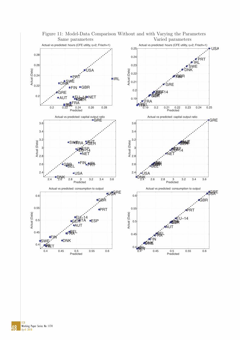
48ECBWorking Paper Series No 1174April 2010
Figure 11: Model-Data Comparison Without and with Varying the ParametersSame parameters Varied parameters
0.2 0.22 0.24 0.26 0.28
0.2
0.22
0.24
0.26
0.28
GERFRAITA
GBR
AUTBEL
DNKFIN
GRE
IRL
NET
PRT
ESP
SWE
USA
EU−14
Actu
al (D
ata)
Predicted
Actual vs predicted: hours (CFE utility, η=2; Frisch=1)
0.19 0.2 0.21 0.22 0.23 0.24 0.25
0.19
0.2
0.21
0.22
0.23
0.24
0.25
GERFRA
ITA
GBR
AUT
BEL
DNKFIN
GRE
IRL
NET
PRT
ESP
SWE
USA
EU−14
Actu
al (D
ata)
Predicted
Actual vs predicted: hours (CFE utility, η=2; Frisch=1)
2.4 2.6 2.8 3 3.2 3.4 3.6
2.4
2.6
2.8
3
3.2
3.4
3.6
GERFRAITA
GBR
AUT
BEL
DNK
FIN
GRE
IRL
NET
PRT
ESPSWE
USA
EU−14
Actu
al (D
ata)
Predicted
Actual vs predicted: capital output ratio
2.4 2.6 2.8 3 3.2 3.4 3.6
2.4
2.6
2.8
3
3.2
3.4
3.6
GERFRAITA
GBR
AUT
BEL
DNK
FIN
GRE
IRL
NET
PRT
ESPSWE
USA
EU−14
Actu
al (D
ata)
Predicted
Actual vs predicted: capital output ratio
0.4 0.45 0.5 0.55 0.6
0.4
0.45
0.5
0.55
0.6
GER
FRA
ITA
GBR
AUTBEL
DNKFIN
GRE
IRLNET
PRT
ESP
SWE
USA
EU−14
Actu
al (D
ata)
Predicted
Actual vs predicted: consumption to output
0.4 0.45 0.5 0.55 0.60.4
0.45
0.5
0.55
0.6
GER
FRA
ITA
GBR
AUTBEL
DNKFIN
GRE
IRLNET
PRT
ESP
SWE
USA
EU−14
Actu
al (D
ata)
Predicted
Actual vs predicted: consumption to output
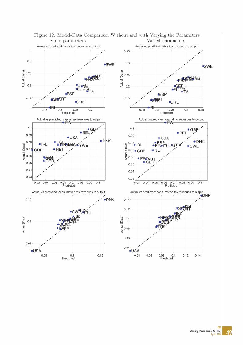
49ECB
Working Paper Series No 1174April 2010
Figure 12: Model-Data Comparison Without and with Varying the ParametersSame parameters Varied parameters
0.15 0.2 0.25 0.3
0.15
0.2
0.25
0.3
GERFRA
ITA
GBR
AUTBELDNKFIN
GREIRL
NET
PRTESP
SWE
USA
EU−14
Actu
al (D
ata)
Predicted
Actual vs predicted: labor tax revenues to output
0.15 0.2 0.25 0.3 0.35
0.15
0.2
0.25
0.3
0.35
GERFRA
ITA
GBR
AUTBELDNK FIN
GREIRL
NET
PRTESP
SWE
USA
EU−14
Actu
al (D
ata)
Predicted
Actual vs predicted: labor tax revenues to output
0.03 0.04 0.05 0.06 0.07 0.08 0.09 0.1
0.03
0.04
0.05
0.06
0.07
0.08
0.09
0.1
GER
FRA
ITAGBR
AUT
BEL
DNKFIN
GREIRL
NET
PRT
ESPSWE
USA
EU−14
Actu
al (D
ata)
Predicted
Actual vs predicted: capital tax revenues to output
0.03 0.04 0.05 0.06 0.07 0.08 0.09 0.10.03
0.04
0.05
0.06
0.07
0.08
0.09
0.1
GER
FRA
ITAGBR
AUT
BEL
DNKFIN
GREIRL
NET
PRT
ESPSWE
USA
EU−14
Actu
al (D
ata)
Predicted
Actual vs predicted: capital tax revenues to output
0.05 0.1 0.15
0.05
0.1
0.15
GERFRA
ITA
GBRAUTBEL
DNK
FIN
GREIRL
NET
PRT
ESP
SWE
USA
EU−14
Actu
al (D
ata)
Predicted
Actual vs predicted: consumption tax revenues to output
0.04 0.06 0.08 0.1 0.12 0.14
0.04
0.06
0.08
0.1
0.12
0.14
GERFRA
ITA
GBRAUTBEL
DNK
FIN
GREIRL
NET
PRT
ESP
SWE
USA
EU−14
Actu
al (D
ata)
Predicted
Actual vs predicted: consumption tax revenues to output

50ECBWorking Paper Series No 1174April 2010
C Data Discussion and Overview
Figure 13 shows the resulting time series for taxes as well as the macroeconomic series we
have used. For the calibration, we equate the values on the balanced growth path with
the averages of these time series over the period from 1995 to 2007.
Using this methodology necessarily fails to capture fully the detailed nuances and
features of the tax law and the inherent incentives. Nonetheless, several arguments may
be made for why we use effective average tax rates instead of marginal tax rates for the
calibration of the model. First, we are not aware of a comparable and coherent empirical
methodology that could be used to calculate marginal labor, capital and consumption tax
rates for the US and 15 European countries for a time span of, say, the last 12 years. By
contrast, our calculations along with Mendoza, Razin, and Tesar (1994) and Carey and
Rabesona (2002) calculate effective average tax rates for labor, capital and consumption
for our countries of interest. There is some data available from the NBER for marginal
tax rates on the federal and state level: however and at least for the US, the difference
between marginal and average tax rates are modest.
Second, if any we probably make an error on side of caution since effective average tax
rates can be seen as as representing a lower bound of statutory marginal tax rates. Third,
marginal tax rates differ all across income scales. In order to properly account for this, a
heterogenous agent economy is needed. This might be a useful next step but may fog up
key issues analyzed in this paper initially. Fourth, statutory marginal tax rates are often
different from realized marginal tax rates due to a variety of tax deductions etc. So that
potentially, the effective tax rates computed and used here may reflect realized marginal
tax rates more accurately than statutory marginal tax rates in legal tax codes. Fifth,
using effective tax rates following the methodology of Mendoza, Razin, and Tesar (1994)
facilitates comparison to previous studies that also use these tax rates as e.g. Mendoza
and Tesar (1998) and many others. Nonetheless, a further analysis taking these points
into account in detail is a useful next step on the research agenda.
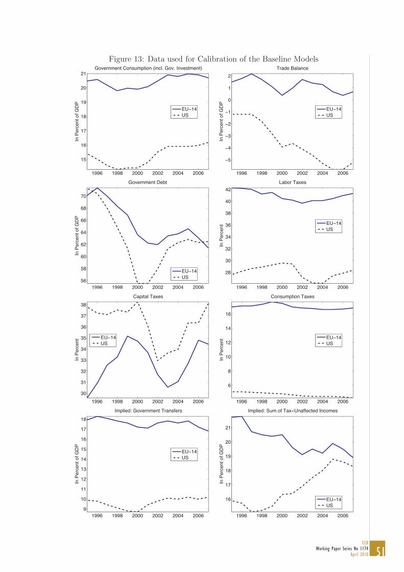
51ECB
Working Paper Series No 1174April 2010
Figure 13: Data used for Calibration of the Baseline Models
1996 1998 2000 2002 2004 2006
15
16
17
18
19
20
21Government Consumption (incl. Gov. Investment)
In P
erce
nt o
f GD
P
EU−14US
1996 1998 2000 2002 2004 2006
−5
−4
−3
−2
−1
0
1
2Trade Balance
In P
erce
nt o
f GD
P
EU−14US
1996 1998 2000 2002 2004 200656
58
60
62
64
66
68
70
Government Debt
In P
erce
nt o
f GD
P
EU−14US
1996 1998 2000 2002 2004 2006
28
30
32
34
36
38
40
42Labor Taxes
In P
erce
ntEU−14US
1996 1998 2000 2002 2004 200630
31
32
33
34
35
36
37
38Capital Taxes
In P
erce
nt
EU−14US
1996 1998 2000 2002 2004 2006
6
8
10
12
14
16
Consumption Taxes
In P
erce
nt
EU−14US
1996 1998 2000 2002 2004 20069
10
11
12
13
14
15
16
17
18Implied: Government Transfers
In P
erce
nt o
f GD
P
EU−14US
1996 1998 2000 2002 2004 2006
16
17
18
19
20
21
Implied: Sum of Tax−Unaffected Incomes
In P
erce
nt o
f GD
P
EU−14US

52ECBWorking Paper Series No 1174April 2010
D Data Details
This appendix describes the data used in the main part of the paper. We use annual data
from 1995 to 2007 for the following countries: USA, Germany (GER), France (FRA), Italy
(ITA), United Kingdom (UK), Austria (AUT), Belgium (B), Denmark (DEN), Finland
(FIN), Greece (GRE), Ireland (IRL), Netherlands (NET), Portugal (PRT), Spain (ESP)
and Sweden (SWE). Data from the sources listed below was downloaded in fall 2008.
D.1 Databases used
AMECO: Database of the European Commission available at:
http : //ec.europa.eu/economy finance/db indicators/db indicators8646 en.htm.
OECD: Databases for annual national accounts, labor force statistics and revenue statis-
tics of the OECD. Available at:
http : //stats.oecd.org/wbosdos/Default.aspx?usercontext = sourceoecd
GGDC: Groningen Growth and Development Centre and the Conference Board total
economy database, January 2008 available at: http : //www.ggdc.net or
http : //www.conference − board.org/economics/downloads/TED08I.xls
NIPA: National income and product accounts provided by the BEA. Available at: www.bea.gov.
D.2 Macro Data
D.2.1 Raw Data
All data below except for population and hours are in $, EUR or local currency for Den-
mark, Sweden and United Kingdom:
Nominal GDP: Gross domestic product at current market prices (AMECO, UVGD).
Nominal government consumption: Final consumption expenditure of general gov-
ernment at current prices (AMECO, UCTG).
53ECB
Working Paper Series No 1174April 2010
Nominal total government expenditures: Total current expenditure: general gov-
ernment; ESA 1995 (AMECO, UUCG).
Nominal total government expenditures excluding interest payments: Total cur-
rent expenditure excluding interest - general government - ESA 1995 (AMECO, UUCGI).
Nominal government debt: General government consolidated gross debt - Excessive
deficit procedure (based on ESA 1995) and former definition (linked series) (AMECO,
UDGGL).
Nominal total private consumption: Private final consumption expenditure at current
prices (AMECO, UCPH).
Nominal total private investment: Gross fixed capital formation at current prices:
private sector (AMECO, UIGP).
Real capital stock: Net capital stock at constant (2000) prices; total economy (AMECO,
OKND).
Real GDP: Gross domestic product at constant (2000) market prices (AMECO, OVGD).
Nominal exchange rate: ECU-EUR exchange rates - Units of national currency per
EUR/ECU (AMECO, XNE).
Net exports: Net exports of goods and services at current prices (National accounts)
(AMECO, UBGS).
Nominal government investment: Gross fixed capital formation at current prices:
general government; ESA 1995 (AMECO, UIGG0).
Total Hours Worked: Total annual hours worked (GGDC).
Nominal durable consumption: Final consumption expenditure of households, P311:
durable goods, old breakdown, national currency, current prices, national accounts database
(OECD).
Population: Population 15-64, labor force statistics (OECD).
D.2.2 Data Calculations
Consumption and Investment. Total consumption in the data consists of non-durable con-
sumption of goods and services and and durable consumption. In the model consumption
is meant to be non-durable consumption only. In order to align the data with the model
we therefore substract durable consumption from total consumption and add it to pri-
vate investment in the data. Unfortunately, durable consumption data is available only

54ECBWorking Paper Series No 1174April 2010
for FRA, IRE, NET, UK and US. The sample covered is somewhat different across these
countries. However, in order to proxy durable consumption data for the remaining coun-
tries we proceed as follows. We compute the ratio of durable consumption and total private
consumption per year for the available country data. Interestingly, the shares for FRA,
IRE and NET are twice as large as those for the UK and the US. We then calculate the
total average share per year of the average UK/US and average FRA/IRE/NET shares.
For the countries where there is no durable consumption data this total average share per
year is applied to the annual total private consumption data in order to obtain a measure
of durable consumption.
Government Interest Payments. Government interest payments are calculated as the
difference between total government expenditures and total government expenditures ex-
cluding interest payments.
Implied Government Transfers and Tax-Unaffected Income. Government transfers that
are consistent with the model are calculated by substracting government consumption,
government interest payments and government investment from total government expen-
ditures in the data.
Similarly, tax-unaffected income consistent with the model is calculated by adding
government interest payments, government transfers and net imports in the data.
GDP Growth. Per capita GDP growth is calculated by dividing real GDP by population
and then calculating annual percentage changes.
Hours Worked. In order to obtain a measure of annual hours worked per person we
divide total annual hours by population. Furthermore, we assume 14.55 hours per day to
be allocated between leisure and work in the US and EU-14 similar to Ragan (2005) who
assumes 14 hours. We obtain a normalized average US hours per person measure of 0.25
as used in the main part of the paper.
Ratios of Variables to GDP. Based on the above data we calculate the GDP ratios
for the countries. We also require the weighted EU-14 GDP ratios which are calculated
according to the description in appendix A.1.
Note that variables that describe the fiscal sector such as e.g. government debt etc.
are only available in nominal terms. Consistent with the model, we divide these nominal
variables by nominal GDP i.e. deflate nominal variables with the GDP deflator. We also
55ECB
Working Paper Series No 1174April 2010
deflate all other nominal variables with the GDP deflator. Since we are interested in GDP
ratios only we do not need to divide the time series by population since the division would
appear in the numerator as well as in the denominator and therefore would cancel out.
D.3 Tax Rates Data
We calculate effective tax rates on labor income, capital income and consumption following
the methodology of Mendoza, Razin and Tesar (1994) and used in Mendoza, Razin and
Tesar (1997).
D.3.1 Raw Data
All data below are nominal in $, EUR or local currency for Denmark, Sweden and United
Kingdom:
5110: General taxes, revenue statistics (OECD).
5121: Excise taxes, revenue statistics (OECD).
3000: Payroll taxes, revenue statistics (OECD).
4000: Property taxes, revenue statistics (OECD).
1000: Income, profit and capital gains taxes, revenue statistics (OECD).
2000: Social security contributions, revenue statistics (OECD).
2200: Social security contributions of employers, revenue statistics (OECD).
1100: Income, profit and capital gains taxes of individuals, revenue statistics (OECD).
1200: Income, profit and capital gains taxes of corporations, revenue statistics (OECD).
4100: Recurrent taxes on immovable property, revenue statistics (OECD).
4400: Taxes on financial and capital transactions, revenue statistics (OECD).
GW: Compensation of employees: general government - ESA 1995 (AMECO, UWCG).
OS: Net operating surplus: total economy (AMECO, UOND). This is net operating sur-
plus plus net mixed income or equivalently the gross operating surplus minus consumption
of fixed capital. For the USA OS is not available in AMECO. We obtained OS from NIPA
table 11000 line 11.

56ECBWorking Paper Series No 1174April 2010
W: Gross wages and salaries: households and NPISH (AMECO, UWSH). For the USA
W is not available in AMECO. We obtained W from NIPA table 11000 line 4.
PEI: Net property income: households and NPISH (AMECO, UYNH). Note that in con-
trast to the data available to Mendoza, Razin and Tesar (1994) the present PEI data
does not contain entrepreneurial income of households anymore. Instead household en-
trepreneurial income is contained in OSPUE defined below. For the USA PEI is not
available in AMECO. We calculate this from OECD property income received (SS14 S15:
Households and non-profit institutions serving households, SD4R: Property income; re-
ceived, national accounts) minus property income paid (SS14 S15: Households and non-
profit institutions serving households, SD4P: Property income; paid, national accounts).
OSPUE: Gross operating surplus and mixed income: households and NPISH (AMECO,
UOGH). OSPUE in Mendoza, Razin and Tesar (1994) is operating surplus of private un-
incorporated enterprises. This data is called mixed income now. Note that all we need
for the tax rate calculations below is the sum OSPUE+PEI. We miss data on household
entrepreneurial income in PEI above. Therefore, we use gross operating surplus and mixed
income of households in order to obtain a measure of household entrepreneurial and mixed
income. For the USA OSPUE is not available in AMECO. We calculate this from the
OECD (HH. Operating surplus and mixed income, gross, national accounts, detailed ag-
gregates). We substract consumption of fixed capital obtained from the OECD (SS14 S15:
Households and non-profit institutions serving households, national accounts) from gross
operating surplus and mixed income in order to obtain a measure of net operating surplus
and mixed income to be used for the tax rate calculations below.
For some European countries the above data starts at a later date than 1995. In ad-
dition, for a few country data time series observations for 2007 are missing. In order to
obtain estimates for 2007 we apply the average growth rates of the last 5 to 20 years to the
observation in 2006. Finally, we use all available individual country data for calculating
weighted averages for the period 1995-2007.
57ECB
Working Paper Series No 1174April 2010
D.3.2 Tax Rate Calculations
D.3.3 Effective Tax Rates
Following the methodology of Mendoza, Razin and Tesar (1994) we calculate the following
effective tax rates:
Consumption tax: τ c = 5110+5121C+G−GW−5110−5121
Personal income tax: τh = 1100OSPUE+PEI+W
Labor income tax: τn = τhW+2000+3000W+2200
Capital income tax: τk = τh(OSPUE+PEI)+1200+4100+4400OS
Where C, G and W denote nominal total private consumption, government consump-
tion and wages and salaries.
For the overlapping years 2000 to 2005, our effective tax rates on consumption and
labor income are close to those obtained by Carey and Rabesona’s (2002) recalculation of
the Mendoza, Razin and Tesar (1994). In particular, the average cross country difference
in consumption taxes from 2000 to 2005 is -0.3% percent and 0.7% for labor income taxes.
For capital income taxes the difference is somewhat larger i.e. -4.9%.
Sources of Tax Revenues to GDP Ratios. In the main part of the paper we require data
for sources of tax revenue to GDP ratios. According to the Mendoza, Razin and Tesar
(1994) methodology e.g. the capital tax is calculated as the ratio of capital tax revenues
and the capital tax base. With the above data at hand it is easy to calculate capital tax
revenues and divide them by nominal GDP to obtain the desired statistic. Labor and
consumption tax revenues to GDP ratios are calculated in a similar way.

Work ing PaPer Ser i e Sno 1118 / november 2009
DiScretionary FiScal PolicieS over the cycle
neW eviDence baSeD on the eScb DiSaggregateD aPProach
by Luca Agnello and Jacopo Cimadomo