quantifying the impact of global warming on saltwater...
TRANSCRIPT
i
Quantifying the Impact of Global Warming on Saltwater Intrusion at Shelter Island, New York Using a Groundwater Flow Model
A Final Report Presented
by
Daniel James Rozell
to
The Graduate School
in Partial fulfillment of the
Requirements
for the Degree of
Master of Science
in
Geosciences with concentration in Hydrogeology
Stony Brook University
December, 2007

ii
Stony Brook University
The Graduate School
Daniel James Rozell
We, the Final Report committee for the above candidate for the
Master of Science in Geosciences with concentration in Hydrogeology degree,
Hereby recommend acceptance of this Final Report.
Teng-fong Wong, Research Advisor, Professor, Department of Geosciences
Gilbert Hanson, Professor, Department of Geosciences
Henry Bokuniewicz, Professor, School of Marine and Atmospheric Sciences
iii
Abstract
In order to quantify the effects global warming may have on a small island, a
previously published single density steady-state groundwater flow model for Shelter
Island, NY was changed to a variable density transient groundwater flow model. The
original model code, created for MODFLOW, was adapted to SEAWAT-2000.
The 2007 IPCC report predictions for changes in precipitation and sea level rise
over the next century were applied to the calibrated model. A scenario most favorable to
groundwater retention consisting of a predicted precipitation increase of 15% and a sea
level rise of 0.6 ft was compared to the current long-term average. This resulted in a
seaward movement of the interface by an average of 76 ft and a maximum of 199 ft. The
water table rose by an average of 0.89 feet. A second scenario least favorable to
groundwater retention consisting of a predicted precipitation decrease of 2% and a sea
level rise of 2 ft was compared to the current long-term average. This resulted in a
landward movement of the interface by an average of 53 ft and a maximum of 121 ft.
The water table rose by an average of 1.94 feet.

iv
Table of Contents
LIST OF FIGURES .....................................................................................................................................V LIST OF TABLES ..................................................................................................................................... VI ACKNOWLEDGEMENTS......................................................................................................................VII INTRODUCTION AND OBJECTIVE .......................................................................................................1
INTRODUCTION............................................................................................................................................1 OBJECTIVE ..................................................................................................................................................3
BACKGROUND............................................................................................................................................4 THEORY.......................................................................................................................................................4 STUDY AREA.............................................................................................................................................10 PREVIOUS MODELS ...................................................................................................................................15
GROUNDWATER FLOW MODEL.........................................................................................................19 MODEL OVERVIEW....................................................................................................................................19
Model Geometry ..................................................................................................................................19 Boundary Conditions ...........................................................................................................................20 Seawater ..............................................................................................................................................24 Recharge..............................................................................................................................................25 Geologic Parameters ...........................................................................................................................26 Pumping...............................................................................................................................................27 Other Assumptions...............................................................................................................................28
CALIBRATION............................................................................................................................................29 SENSITIVITY ANALYSIS .............................................................................................................................36 VALIDATION..............................................................................................................................................37
RESULTS.....................................................................................................................................................39 DISCUSSION ..............................................................................................................................................46
CONCLUSION.............................................................................................................................................52 FUTURE WORK..........................................................................................................................................53
REFERENCES............................................................................................................................................55 APPENDIX 1 ..............................................................................................................................................60 APPENDIX 2 ...............................................................................................................................................61
v
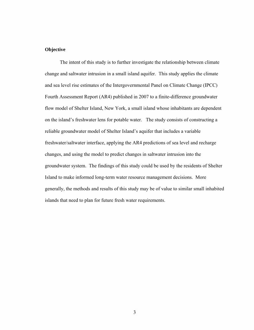
List of Figures Figure 1: A small island aquifer where the shaded area is the freshwater lens, h represents the water table height above sea level, and z represents the depth of the freshwater/saltwater interface below sea level (modified from Urbano, 2001).................. 4 Figure 2: A) Idealized freshwater/saltwater interface under hydrostatic conditions. ......... 6 Figure 3: Location of Shelter Island (Simmons, 1986)..................................................... 10 Figure 4: Shelter Island (NY GIS, 2007) .......................................................................... 11 Figure 5: North (A) to South (A’) hydrogeologic cross-section of Shelter Island (Simmons, 1986)............................................................................................................... 12 Figure 6: Diagram of Shelter Island hydrology where the freshwater lens is deformed by a confining clay layer (Simmons, 1986) ........................................................................... 13 Figure 7: Water table contour map of Shelter Island. The transect C-C' is used in the Schubert (1999) model and the model constructed for this study (modified from Shubert, 1999). ................................................................................................................................ 14 Figure 8: Cross section C-C’ shows geologic units, freshwater/saltwater interface, and boreholes during March 17-20, 1995 (modified from Schubert, 1999)............................ 16 Figure 9: Grid spacing for the finite-difference model created from cross-section C-C' (modified from Schubert, 1999) ....................................................................................... 20 Figure 10: Model boundary conditions from Schubert (1999) study .............................. 22 Figure 11: Boundary Conditions for initial model. Grey areas are no-flow cells. Blue cells are constant head boundaries.................................................................................... 23 Figure 12: Boundary conditions for SEAWAT-2000 model. Orange cells represent constant head boundaries. Grey cells represent saltwater concentrations of 2.18 lbs/ft3. 23 Figure 13: Boundary conditions for second SEAWAT-2000 model. Orange cells represent constant head. Light grey cells represent saltwater concentrations of 2.18 lbs/ft3. Dark grey cells represent the Pleistocene marine clay layer (inactive). ........................... 24 Figure 14: Head value scatter diagram from PEST forward run. ..................................... 33 Figure 15: Head-Time curve for the initial SEAWAT-2000 model showing head levels reach steady state in 350,000 days. Vertical axis units are feet and horizontal units are days. .................................................................................................................................. 34 Figure 16: Head-Time curve for the revised SEAWAT-2000 model showing head levels reach steady state in 10,000 days. Vertical axis units are feet and horizontal units are days. .................................................................................................................................. 35 Figure 17: Uniform horizontal grid spacing of 50 ft used in grid sensitivity analysis. .... 37 Figure 18: Reconstructed Schubert model run using PMWIN. Contours show head levels in feet. ............................................................................................................................... 39 Figure 19: Transient SEAWAT-2000 model run to steady-state. Contours show head levels in feet. ..................................................................................................................... 40 Figure 20: Transient SEAWAT-2000 model run to steady-state. Contours show salt concentration in 10% increments from freshwater to seawater. ....................................... 40 Figure 21: Revised SEAWAT-2000 model where the marine clay unit is treated as a no-flow boundary. Contours show head levels in feet. ......................................................... 40 Figure 22: Revised SEAWAT-2000 model where the marine clay unit is treated as a no-flow boundary. Contours show salt concentration in 10% increments from freshwater to seawater............................................................................................................................. 41

vi
Figure 23: Relative velocity vector field for revised SEAWAT-2000 model. The arrow size in each cell is proportional to the flow velocity and points in the direction of flow. 41 Figure 24: Flow path lines for revised SEAWAT-2000 model. ....................................... 41 Figure 25: Position of the Freshwater/Saltwater interface in West Neck Bay for three climate change scenarios. All distances are in feet. The interface is defined as an isochlor of 250 mg/L (0.0156 lb/ft3). MSL is the mean sea-level for 2007. The horizontal position of the shoreline is assumed to be stationary in all scenarios. ............ 44 Figure 26: Zone of diffusion for freshwater/saltwater interface for Scenario 1 (top), Scenario 2 (middle), and Scenario 3 (bottom). Axes are in feet and color coded salt concentrations are in lbs /cubic ft. Note that the horizontal axis is not linear. ................ 45
List of Tables Table 1: Contributing factors to sea level rise (modified from IPCC, Feb. 2007) ............. 1 Table 2: National Geodetic Vertical Datum (NGVD) and mean sea-level within Peconic Bay. All values are in feet (modified from Schubert, 1999)............................................ 24 Table 3: Defined geologic units and parameters used in O'Rourke(2000) model. ........... 26 Table 4: Defined geologic units and parameters used in Schubert (1999) model. Conductivities varied slightly at borders between hydrogeologic units. .......................... 27 Table 5: Measured and simulated water levels measured in feet above National Geodetic Vertical Datum of 1929 for Schubert (1999) model. (modified from Schubert, 1999)... 30 Table 6: Initial Head Conditions for first model run ........................................................ 30 Table 7: Parameters used for each geologic unit in revised SEAWAT-2000 model. Conductivities varied slightly at borders between hydrogeologic units. .......................... 35 Table 8: PEST Parameter Sensitivity Analysis................................................................. 36 Table 9: PEST Observation Sensitivity Analysis ............................................................. 36 Table 10: Comparison of the calibration and validation process results. Precipitation data comes from the Greenport station (see Appendix I). Well head data were taken from March of the following year for modeling consistency. ................................................... 38

vii
Acknowledgements
I would like to thank Prof. Teng-fong Wong, my advisor, for guiding me to
important resources, making helpful suggestions, and encouraging my progress.
Additionally, I owe my gratitude to Prof. Hanson and Prof. Bokuniewicz for their time
and efforts. I would also like to recognize Jonathan Wanlass of the Suffolk County
Department of Health and Margaret Phillips of the U.S. Geological Survey for providing
me with data essential to this project. Lastly, I would like to thank Loretta Budd, the
Department of Geosciences graduate program coordinator, who has helped me sail
smoothly through the sea of paperwork that unavoidably accompanies graduate school.

1
Introduction and Objective
Introduction
There is considerable public concern and scientific uncertainty regarding the
scope and magnitude of the climate change trend popularly called Global Warming. The
current general consensus in the scientific community is that anthropogenic sources are
causing the Earth to warm and this trend is likely to continue for at least several decades
regardless of any mitigating countermeasures taken by humans (IPCC, Feb. 2007).
Considerable effort has been expended to quantifiably predict what environmental effects
are to be expected over the next century from global warming.
Sea level rise is one of the most often cited effects of global warming. Rising
mean sea levels around the world have been documented over the last half century and
are hypothesized to be primarily caused by thermal expansion of warming water and
melting of glaciers and ice sheets (Table 1). As global warming continues over the next
century, mean sea levels will also continue to rise (IPCC, Feb. 2007).
Table 1: Contributing factors to sea level rise (modified from IPCC, Feb. 2007)
2
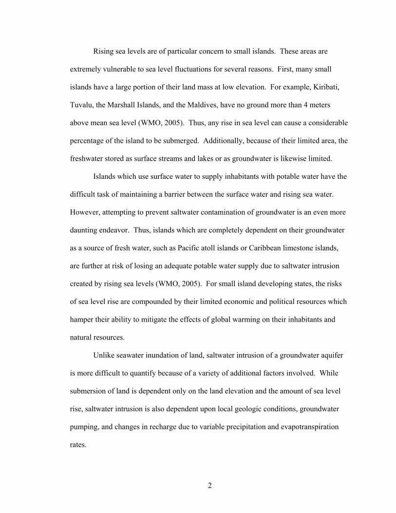
Rising sea levels are of particular concern to small islands. These areas are
extremely vulnerable to sea level fluctuations for several reasons. First, many small
islands have a large portion of their land mass at low elevation. For example, Kiribati,
Tuvalu, the Marshall Islands, and the Maldives, have no ground more than 4 meters
above mean sea level (WMO, 2005). Thus, any rise in sea level can cause a considerable
percentage of the island to be submerged. Additionally, because of their limited area, the
freshwater stored as surface streams and lakes or as groundwater is likewise limited.
Islands which use surface water to supply inhabitants with potable water have the
difficult task of maintaining a barrier between the surface water and rising sea water.
However, attempting to prevent saltwater contamination of groundwater is an even more
daunting endeavor. Thus, islands which are completely dependent on their groundwater
as a source of fresh water, such as Pacific atoll islands or Caribbean limestone islands,
are further at risk of losing an adequate potable water supply due to saltwater intrusion
created by rising sea levels (WMO, 2005). For small island developing states, the risks
of sea level rise are compounded by their limited economic and political resources which
hamper their ability to mitigate the effects of global warming on their inhabitants and
natural resources.
Unlike seawater inundation of land, saltwater intrusion of a groundwater aquifer
is more difficult to quantify because of a variety of additional factors involved. While
submersion of land is dependent only on the land elevation and the amount of sea level
rise, saltwater intrusion is also dependent upon local geologic conditions, groundwater
pumping, and changes in recharge due to variable precipitation and evapotranspiration
rates.
3
Objective
The intent of this study is to further investigate the relationship between climate
change and saltwater intrusion in a small island aquifer. This study applies the climate
and sea level rise estimates of the Intergovernmental Panel on Climate Change (IPCC)
Fourth Assessment Report (AR4) published in 2007 to a finite-difference groundwater
flow model of Shelter Island, New York, a small island whose inhabitants are dependent
on the island’s freshwater lens for potable water. The study consists of constructing a
reliable groundwater model of Shelter Island’s aquifer that includes a variable
freshwater/saltwater interface, applying the AR4 predictions of sea level and recharge
changes, and using the model to predict changes in saltwater intrusion into the
groundwater system. The findings of this study could be used by the residents of Shelter
Island to make informed long-term water resource management decisions. More
generally, the methods and results of this study may be of value to similar small inhabited
islands that need to plan for future fresh water requirements.
4
Background
Theory
Seawater’s high salinity results in a density approximately 2.5% greater than
freshwater. This density difference is large enough to prevent substantial mixing
between the freshwater and saltwater. Thus, a typical freshwater aquifer on a small
island resembles a lens floating on saltwater as seen in Figure 1. Although this interface
is often represented as sharp and impermeable, it actually exists as a zone of diffusion
with the freshwater boundary delineated by some defined chloride concentration, often a
potable water standard (Domenico and Schwartz, 1998).
Figure 1: A small island aquifer where the shaded area is the freshwater lens, h represents the water table height above sea level, and z represents the depth of the
freshwater/saltwater interface below sea level (modified from Urbano, 2001)
The depth of the interface between fresh and saline water near a shore was first
empirically determined independently by Baden-Ghyben (1889) and Herzberg (1901) to
be 40 times the height of the water table when referenced against mean sea level. The
analytic explanation of this phenomenon, referred to as the Ghyban-Herzberg formula, is
based on a hydrostatic water column of freshwater overlaying saltwater with an
impermeable interface (Domenico and Schwartz, 1998). The weight of the freshwater

5
column, (h + z)g ρf , is balanced by the weight of a saltwater column, zg ρs. Set equal to
each other and rearranged, the resulting equation is:
( )fs
fhzρρ
ρ−
= (1)
where h is the height of the freshwater column above sea level, z is the depth of the
interface below sea level, ρf is the density of freshwater, and ρs is the density of saltwater
Substituting in the average relative densities of fresh and salt water, 1 and 1.025, the
Ghyban-Herzberg formula simplifies to
hz 40= (2)
which corresponds to the original empirical data. However, this simple hydrostatic
analysis does not take groundwater discharge to sea into account so it only roughly
approximates the actual position of the freshwater/saltwater interface (Figure 2A).
Taking freshwater subsurface discharge into account, such as the Glover (1959) solution
for a confined aquifer or the Rumner Jr. and Shiau (1968) solution for an unconfined
aquifer, results in a more realistic saltwater interface as seen in Figure 2B.
The Rumner Jr. and Shiau (1968) analytical solution, which applies to the aquifer
in this study (Paulsen et al, 2004), defines the flow net near the interface between salt and
fresh water by a set of coordinates (X,Z) given by the following equations:
( ) ( ) ⎥⎦⎤
⎢⎣⎡ Ψ−Ψ−Φ
+= 22
21G
KK
KKQX
z
x
zx
(3a)
( )[ ]Φ+ΦΨ+= 1GKK
KKQZ
z
x
zx
(3b)
where X is the horizontal position of the interface measured inland from the shoreline, Z
is the depth of the interface measured from the intersection of the water table and land

6
surface, Q is the discharge per unit width of the aquifer, Kx and Kz are the horizontal and
vertical hydraulic conductivities of the aquifer, and the density contrast parameter, G, is
defined as:
( )fs
fGρρ
ρ−
= (3c)
Also, the potential function, Ф, is
QhK z−=Φ (3d)
and Ψ is the stream function such that Ψ = -1 represents the freshwater/saltwater
interface.
Figure 2: A) Idealized freshwater/saltwater interface under hydrostatic conditions. B) Freshwater/saltwater interface that includes discharge of groundwater to the sea
(modified from Freeze and Cherry, 1979)
If sea level rises due to climate change, the position of the freshwater/saltwater
interface, as defined by the Rumner Jr. and Shiau equations, will shift inland and upwards
as the origin, (X0, Z0) moves inland and to higher elevation. Likewise, assuming higher
7
evapotranspiration rates and lowered recharge, the depth of the freshwater/saltwater
interface, Z, should decrease as discharge, Q, decreases.
Although analytical solutions effectively model simple theoretical scenarios,
numerical methods allow for complex, irregular, and heterogeneous scenarios to be
modeled. The most widely used groundwater flow numerical modeling program is the
USGS program MODFLOW, originally documented by McDonald and Harbaugh (1984),
which uses finite-difference methods to simulate three-dimensional groundwater flows
(Harbaugh et al., 2000). Within a defined grid of cells, MODFLOW iteratively solves the
following partial differential equation for the node in each cell (McDonald and Harbaugh,
1988):
thSW
zhK
zyhK
yxhK
x szzyyxx ∂∂
=+⎟⎠⎞
⎜⎝⎛
∂∂
∂∂
+⎟⎟⎠
⎞⎜⎜⎝
⎛∂∂
∂∂
+⎟⎠⎞
⎜⎝⎛
∂∂
∂∂ (4)
where Kxx, Kyy, and Kzz are values of hydraulic conductivity along the x, y, and z
coordinate axes, which are assumed to be parallel to the major axes of hydraulic
conductivity; h is the potentiometric head; W is a volumetric flux per unit volume
representing sources and/or sinks of water, with W<0 for flow out of the ground-water
system, and W>0 for flow in; SS is the specific storage of the porous material; and t is
time.
Equation (4) assumes constant density fluid, so it cannot be used to model
saltwater intrusion. As a result, SEAWAT was developed to model variable-density
flows (Langevin et al., 2003). SEAWAT-2000, the version used in this study, is based on
MODFLOW-2000 (Harbaugh et al., 2000) and MT3DMS (Zheng and Wang, 1999), a
solute transport application. Within a defined grid of cells, SEAWAT iteratively solves

8
the following partial differential equation for the node in each cell (Guo and Langevin,
2002):
⎥⎥⎦
⎤
⎢⎢⎣
⎡⎟⎟⎠
⎞⎜⎜⎝
⎛
∂∂−
+∂
∂
∂∂
+⎥⎥⎦
⎤
⎢⎢⎣
⎡⎟⎟⎠
⎞⎜⎜⎝
⎛
∂∂−
+∂
∂
∂∂
βρρρ
βρ
βαρρρ
αρ
α βαZh
KZhK
f
fff
f
fff (5)
tC
Cth
SqZhK f
fssf
fff ∂
∂∂∂
+∂
∂=+
⎥⎥⎦
⎤
⎢⎢⎣
⎡⎟⎟⎠
⎞⎜⎜⎝
⎛
∂∂−
+∂
∂
∂∂
+ρθρρ
γρρρ
γρ
γ γ
where α, β, γ are orthogonal coordinate axes, aligned with the principal directions of
permeability; t is time; θ is effective porosity; C is solute concentration; ρ is the density
of the native aquifer water; ρf is the density of freshwater; Z is the elevation at the
measurement point; ρs is fluid density of source or sink water; and qs is the volumetric
flow rate of sources and sinks per unit volume of aquifer. Additionally, Kf is equivalent
freshwater hydraulic conductivity which is defined as:
f
ff
gkK
μρα
α = (6)
where kα is the measured hydraulic conductivity in the α direction, g is the acceleration
due to gravity, and µf is the viscosity of freshwater under standard conditions (Guo and
Langevin, 2002). Likewise, Sf is equivalent freshwater specific storage which is defined
as:
gSS ff ρ= (7)
where S is the aquifer specific storage.
Equation (5) is expressed in terms of equivalent freshwater head, i.e., the higher
head level that would occur in a piezometer if the saline water in the column were
replaced with fresh water. This is done solely for simplifying calculations and does not
9
necessarily represent a real measurement method. In the original SEAWAT program, the
user was required to manually convert all input head values measured in seawater to
equivalent freshwater heads and convert all output back from equivalent freshwater
heads. However, SEAWAT-2000 internally converts between actual head readings and
equivalent freshwater heads using (Langevin et al., 2003):
Zhhf
f
ff ρ
ρρρρ −
−= (8)
and
Zhhf
ff
f
ρρρ
ρρ −
+= (9)
Comparing Equations (4) and (5): the first three terms on the left-hand side of
each equation represent the net flux across the unit volume’s faces, the fourth left-hand
side term represents the flux from sources and sinks within the unit volume, and the first
term on the right-hand side of each equation represents the time rate of change of water
stored within the unit volume. The only important distinction is that Equation (4) uses
volumetric fluxes whereas Equation (5) uses mass fluxes in order to account for variable
density. The second right-hand term in Equation (5), which has no corresponding term in
Equation (4), represents the rate of fluid mass change caused by a solute concentration
change. If there is no solute change and density remains constant, this term equals zero
and Equations (4) and (5) become functionally equivalent.
In the case of saltwater intrusion simulations, variable-density flow is coupled
with solute transport and density changes are assumed to be wholly dependent on solute
concentration (i.e. temperature and pressure are ignored). This relationship is defined as:
10
CCf ∂∂
+=ρρρ (10)
and the user must supply values for ρf, the density of freshwater, and ∂ρ/∂C, typically set
to 0.7143 for standard freshwater/saltwater simulations (Langevin et al., 2003).
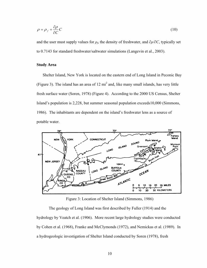
Study Area
Shelter Island, New York is located on the eastern end of Long Island in Peconic Bay
(Figure 3). The island has an area of 12 mi2 and, like many small islands, has very little
fresh surface water (Soren, 1978) (Figure 4). According to the 2000 US Census, Shelter
Island’s population is 2,228, but summer seasonal population exceeds10,000 (Simmons,
1986). The inhabitants are dependent on the island’s freshwater lens as a source of
potable water.
Figure 3: Location of Shelter Island (Simmons, 1986)
The geology of Long Island was first described by Fuller (1914) and the
hydrology by Veatch et al. (1906). More recent large hydrology studies were conducted
by Cohen et al. (1968), Franke and McClymonds (1972), and Nemickas et al. (1989). In
a hydrogeologic investigation of Shelter Island conducted by Soren (1978), fresh
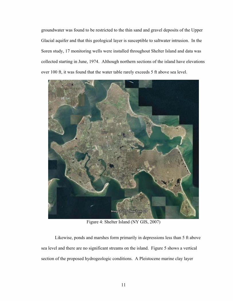
11
groundwater was found to be restricted to the thin sand and gravel deposits of the Upper
Glacial aquifer and that this geological layer is susceptible to saltwater intrusion. In the
Soren study, 17 monitoring wells were installed throughout Shelter Island and data was
collected starting in June, 1974. Although northern sections of the island have elevations
over 100 ft, it was found that the water table rarely exceeds 5 ft above sea level.
Figure 4: Shelter Island (NY GIS, 2007)
Likewise, ponds and marshes form primarily in depressions less than 5 ft above
sea level and there are no significant streams on the island. Figure 5 shows a vertical
section of the proposed hydrogeologic conditions. A Pleistocene marine clay layer
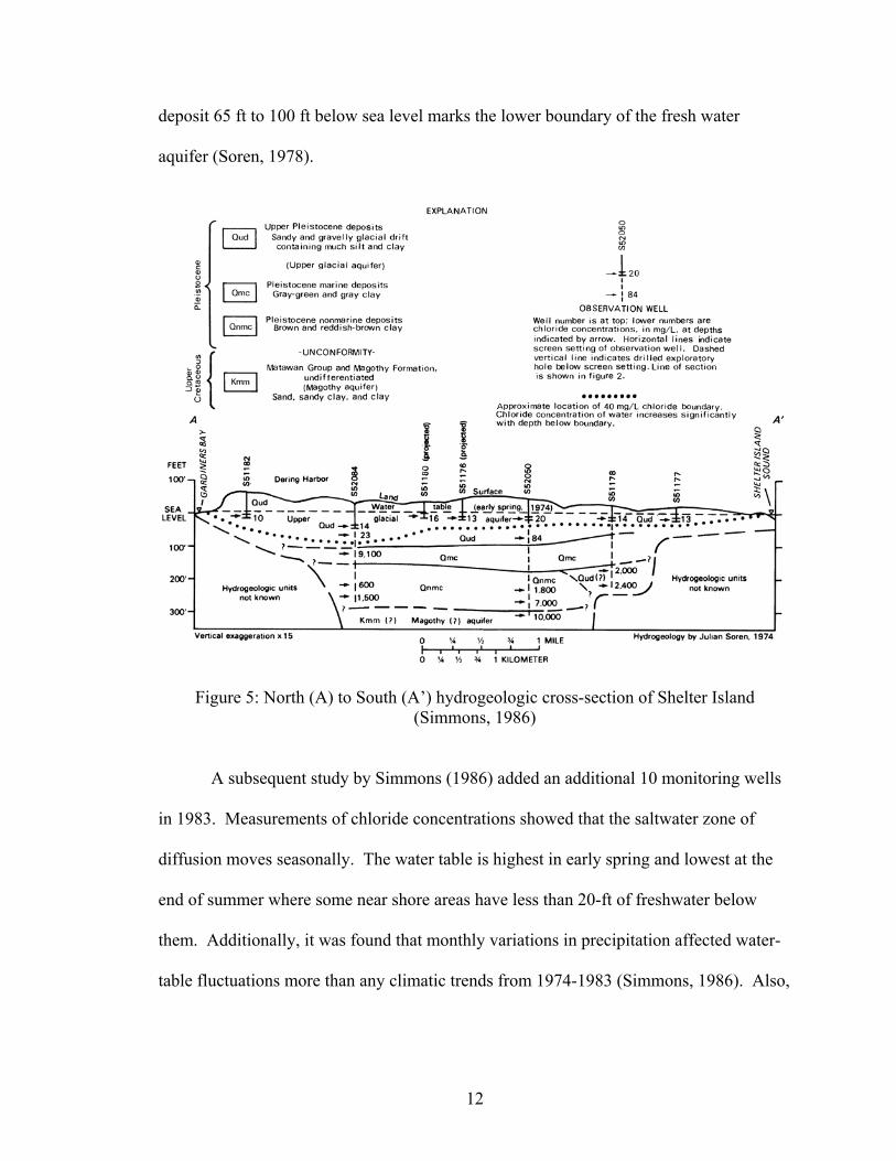
12
deposit 65 ft to 100 ft below sea level marks the lower boundary of the fresh water
aquifer (Soren, 1978).
Figure 5: North (A) to South (A’) hydrogeologic cross-section of Shelter Island (Simmons, 1986)
A subsequent study by Simmons (1986) added an additional 10 monitoring wells
in 1983. Measurements of chloride concentrations showed that the saltwater zone of
diffusion moves seasonally. The water table is highest in early spring and lowest at the
end of summer where some near shore areas have less than 20-ft of freshwater below
them. Additionally, it was found that monthly variations in precipitation affected water-
table fluctuations more than any climatic trends from 1974-1983 (Simmons, 1986). Also,
13
precipitation and evapotranspiration are the main components affecting aquifer recharge;
less than 1% of precipitation becomes overland runoff (Nemickas and Koszalka, 1982).
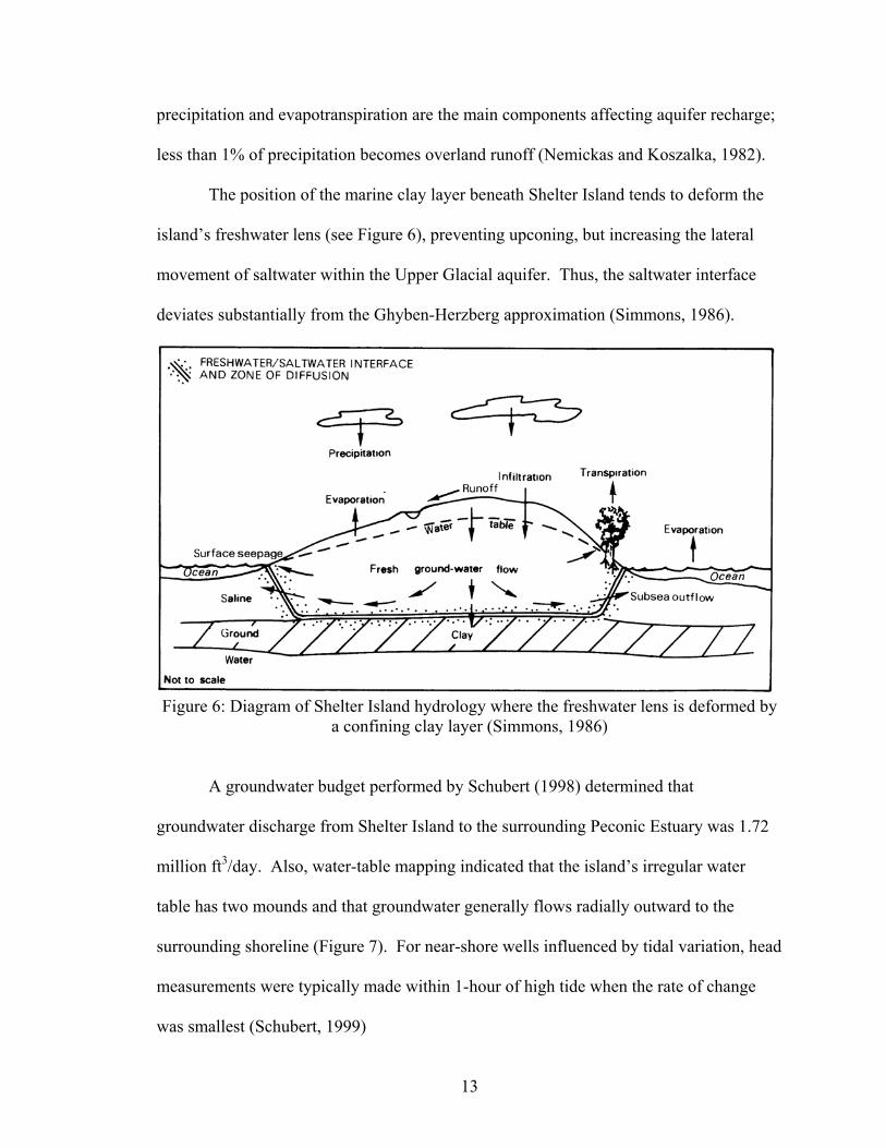
The position of the marine clay layer beneath Shelter Island tends to deform the
island’s freshwater lens (see Figure 6), preventing upconing, but increasing the lateral
movement of saltwater within the Upper Glacial aquifer. Thus, the saltwater interface
deviates substantially from the Ghyben-Herzberg approximation (Simmons, 1986).
Figure 6: Diagram of Shelter Island hydrology where the freshwater lens is deformed by
a confining clay layer (Simmons, 1986)
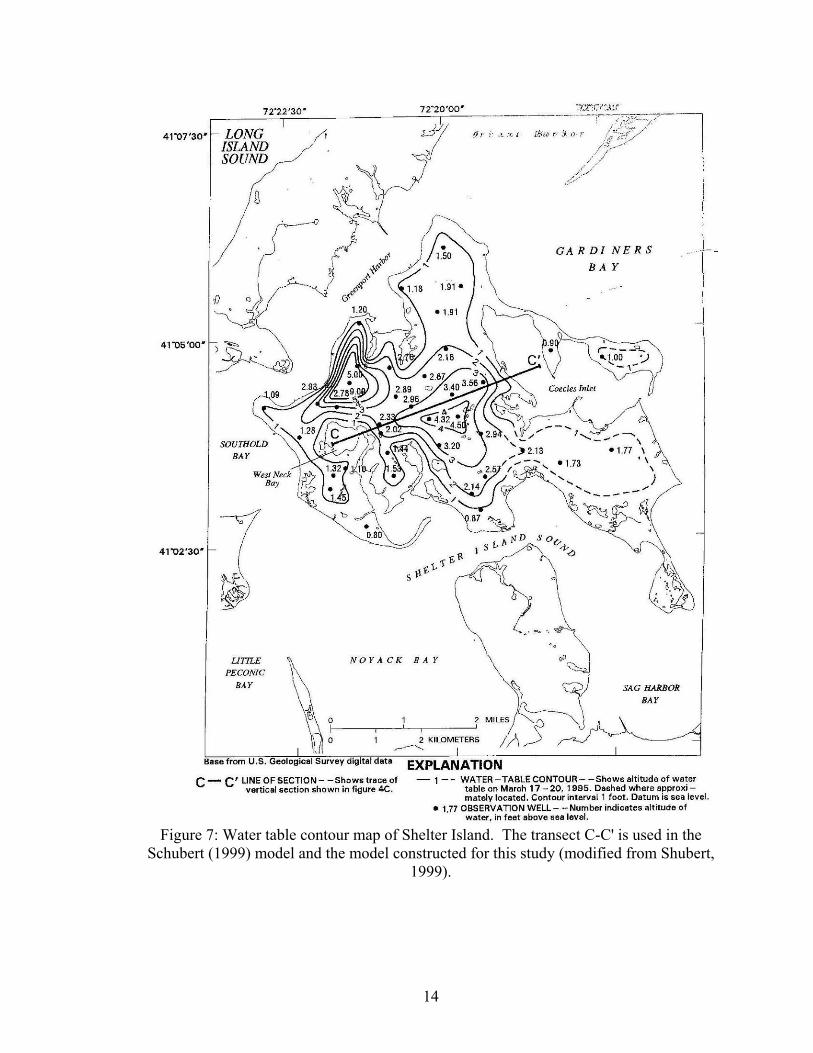
A groundwater budget performed by Schubert (1998) determined that
groundwater discharge from Shelter Island to the surrounding Peconic Estuary was 1.72
million ft3/day. Also, water-table mapping indicated that the island’s irregular water
table has two mounds and that groundwater generally flows radially outward to the
surrounding shoreline (Figure 7). For near-shore wells influenced by tidal variation, head
measurements were typically made within 1-hour of high tide when the rate of change
was smallest (Schubert, 1999)
14
Figure 7: Water table contour map of Shelter Island. The transect C-C' is used in the
Schubert (1999) model and the model constructed for this study (modified from Shubert, 1999).
15
Previous Models
Buxton and Modica (1992) created one of the first computer groundwater flow
models for Long Island. Schubert (1999) created a groundwater flow model for Shelter
Island simulating a two-dimensional vertical section across Shelter Island in order to
determine groundwater distribution, flow paths, and groundwater travel time (Figure 7).
Borehole data was used to map the hydrogeologic characteristics of the vertical section
(Figure 8). Schubert found that almost all recharge left the groundwater system as
shoreline underflow with an average flow age of less than 20 yrs. The small amount that
traveled through the Pleistocene marine clay layer and emerged as sub-sea underflow had
an average age of about 1,800 yrs.
A three-dimensional groundwater flow model of Shelter Island was created by
O’Rourke (2000) with the purpose of quantifying coastal groundwater discharge into
West Neck Bay of Shelter Island and comparing results to field data. The model
computed monthly average specific discharges into West Neck Bay ranging from 0.64
ft/day to 0.84 ft/day while field measurements yielded monthly average specific
discharges ranging from 0.44 ft/day to 1.49 ft/day.
In a closely related study by Paulsen et al. (2004), field measurements of
submarine groundwater discharge into West Neck Bay were taken at three sites, all
within close proximity to the western end of the Shelter Island cross-section modeled by
Schubert (1999). In that study, data from a borehole 295 ft inland indicated that the
freshwater/saltwater interface was at 68 ft below sea level with fine sand from surface to
97 ft below sea level and marine gray clay from 97 ft to 110 ft. Submarine groundwater
discharge was found to range from 0.07 to 7.4 ft/day depending on location and tide.

16
Figure 8: Cross section C-C’ shows geologic units, freshwater/saltwater interface, and
boreholes during March 17-20, 1995 (modified from Schubert, 1999)
Urbano (2001) modeled the effects of climate change on a freshwater aquifer
using a finite-difference model. The study area, Nantucket Island, Massachusetts, has
very similar geologic and climatic conditions to Shelter Island (Pearson et al., 1998). The
study used estimates from the US Global Change Research Program that predicted
groundwater recharge in the northeastern US would range from -30% to +20% in the year
2100 (NAST, 2000). Likewise, from the IPCC 2001 Third Assessment Report, mean sea
level in 2100 was predicted to rise between 20 and 90 cm at a rate of 5 mm/year (IPCC

17
WGII , 2001). The Urbano (2001) model predicted that a 5% reduction in recharge
created a 20% increase in the rate of saltwater intrusion. Similarly, a 5 mm/yr sea level
rise created an 8% increase in the rate of saltwater intrusion.
Tiruneh and Motz (2003) used SEAWAT to model the movement of the
freshwater/saltwater interface in a coastal aquifer that was influenced by global warming.
The study used six different climate change scenarios described in the 2001 IPCC Third
Assessment Report as inputs to a model that represented an idealized coastal aquifer with
inland pumping wells. After 100 years, compared to a scenario with no pumping or sea
level rise, a scenario with pumping showed a 2% salinity increase, a scenario with sea
level rise showed a 9% increase, and a scenario with both showed a 12% increase.
Misut et al. (2004) used the USGS quasi-three-dimensional finite-difference
program SHARP to simulate saltwater intrusion in the North Fork of Long Island due to
pumping and drought. One of the scenarios modeled was a 5-year drought that consisted
of a 20% recharge reduction below the average (1959-1999) recharge rate and a 20%
increase in agricultural pumping over 1999 rates. Simulation results found saltwater
intrusion risk at 6 out of 10 wells and an average upward movement of the
freshwater/saltwater interface of several feet.
The hydrogeologic conditions of the North Fork of Long Island are similar to
Cape Cod, Massachusetts (Schubert, 1999). Masterson (2004) used SEAWAT to model
the effects of pumping, decreases in recharge, and sea level rise on four freshwater lenses
in Lower Cape Cod, Massachusetts. A rising sea level in model simulations caused water
tables to rise, stream flows to increase, and a decrease in the depth of freshwater/saltwater
interfaces. Due to the increased stream flow, the simulated water table rose slower than

18
local sea-level. This resulted in the thinning of the aquifer. Neither field data nor model
simulations indicated that the freshwater/saltwater interface moved with seasonal changes
in recharge. Only multi-year changes caused substantial movement of the interface
within the model. Masterson and Garabedian (2007) used the same model to show that a
2.65 mm/yr sea level rise between 1929 and 2050 causes a freshwater lens thickness
decrease of 2% away from streams and 22% to 31% near streams.

19
Groundwater Flow Model
Model Overview
A finite-difference groundwater flow model was created using MODFLOW-2000
(Harbaugh et al., 2000) along with PMWIN Pro (Chiang, 2005) as the graphical user
interface pre-processor, and post-processor. The most recently published USGS Shelter
Island groundwater model, created by Schubert (1999), was used as a starting point for
this model. The USGS provided the original MODFLOW files, but due to formatting
differences in the raw data files, PMWIN Pro was unable to read the USGS files.
However, the original MODFLOW run output file provided enough information to enable
a reconstruction of the model as described in Schubert’s 1999 USGS report. Ultimately,
the model was run with SEAWAT-2000 in order to fully model the moving interface
between saltwater and freshwater, but because the variable density function of SEAWAT
is not compatible with the sensitivity and parameter estimation processes of
MODFLOW-2000, it was useful to run the model first using MODFLOW-2000 in order
to make use of those features (Langevin et al., 2003)
Model Geometry
The Schubert (1999) model of groundwater flow on Shelter Island consisted of a
cross-sectional area 187.5-ft deep and 16,000-ft wide cutting east-west across the island
(Figure 7). The model grid consisted of 25 vertical layers, each 7.5 feet thick, starting
from 5 feet above mean sea level to 182.5 feet below sea level. The range was originally
chosen to include the highest measured head elevation to a depth below the top of the
Pleistocene marine clay layer. Within this clay layer, the groundwater flow was believed
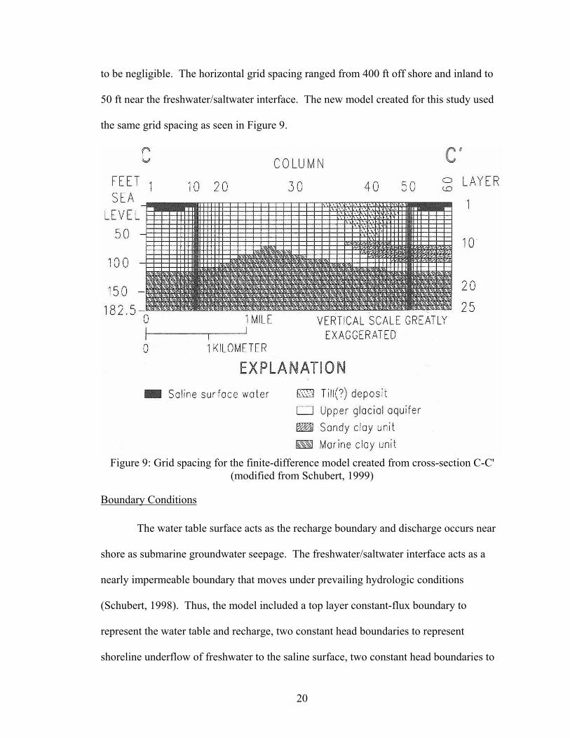
20
to be negligible. The horizontal grid spacing ranged from 400 ft off shore and inland to
50 ft near the freshwater/saltwater interface. The new model created for this study used
the same grid spacing as seen in Figure 9.
Figure 9: Grid spacing for the finite-difference model created from cross-section C-C'
(modified from Schubert, 1999)
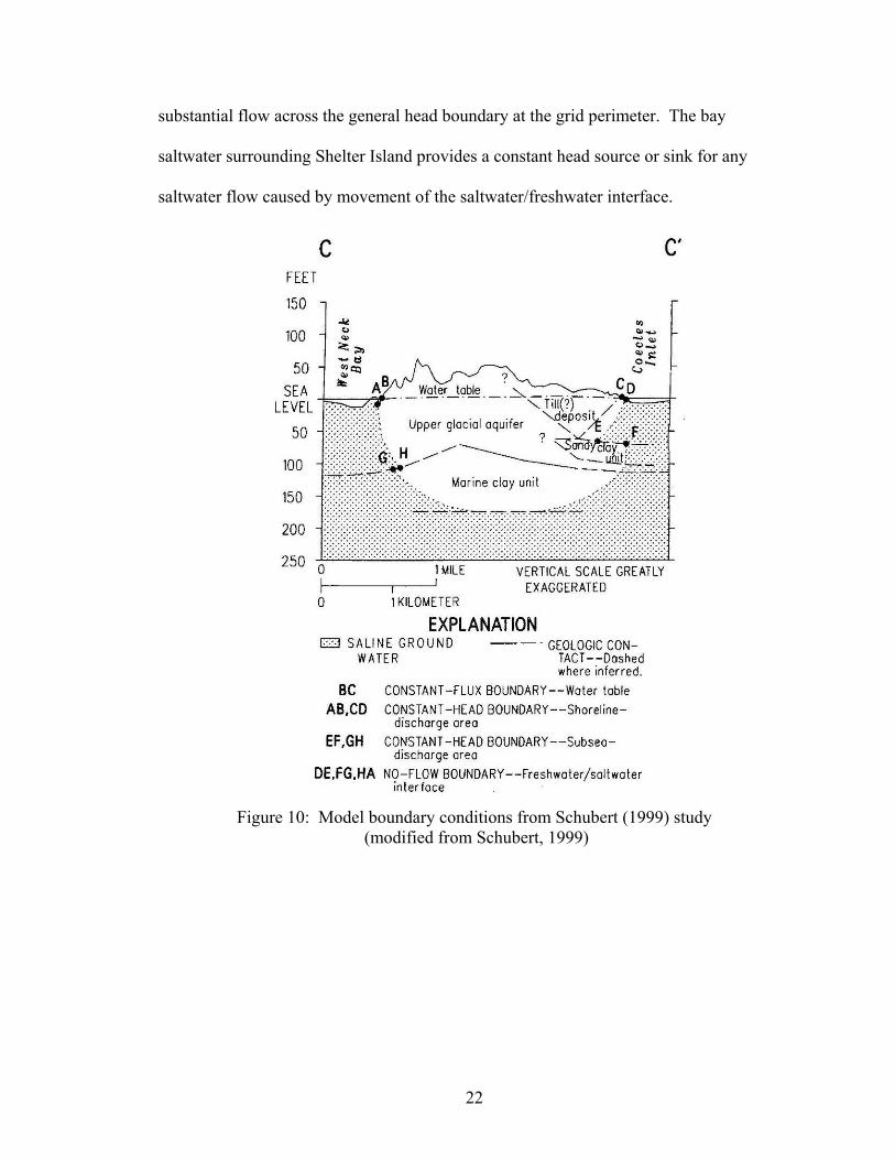
Boundary Conditions
The water table surface acts as the recharge boundary and discharge occurs near
shore as submarine groundwater seepage. The freshwater/saltwater interface acts as a
nearly impermeable boundary that moves under prevailing hydrologic conditions
(Schubert, 1998). Thus, the model included a top layer constant-flux boundary to
represent the water table and recharge, two constant head boundaries to represent
shoreline underflow of freshwater to the saline surface, two constant head boundaries to
21
represent sub-sea discharge near the clay layer, and three no-flow boundaries that
represent the freshwater/saltwater interface as shown in Figure 10.
For this study, the top model layer was defined as unconfined and the rest of the
layers were allowed to be fully convertible between confined and unconfined with
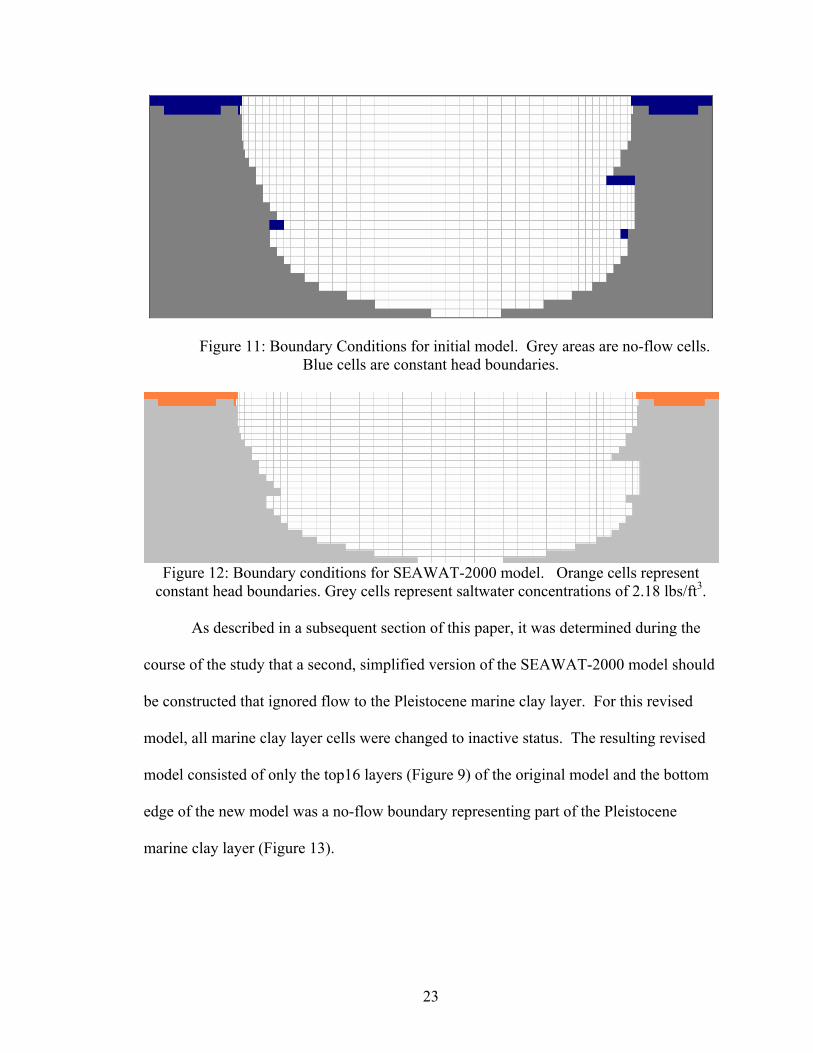
variable transmissivity during the simulation. The boundary conditions, as described in
Figure 10, are applied to the model as seen in Figure 11. It should be noted that the
sandy clay unit with the constant-head boundary E-F (Figure 10) was modeled with
another lower constant-head boundary between its base and the marine clay layer that is
not shown in Figure 10, but is shown in Figure 11.
For the SEAWAT-2000 model run in this study, the recharge interface and
constant head boundary representing the seawater surface surrounding the island did not
change. However, because SEAWAT can correctly model the freshwater/seawater
interface, it was unnecessary to create a series of no-flow boundaries to represent this
interface. Instead, the boundaries were removed and the edges of the freshwater lens
were delineated by the concentration of salt in each cell. Thus, all the grey no-flow cells
seen in Figure 12 were changed to active cells and the salt concentration for those cells
was increased to that of seawater. This created the initial freshwater/saltwater interface
which was then free to move during the simulation.
Additionally, for the SEAWAT-2000 model, a general head boundary condition
was initially used along the sides and bottom perimeter cells. Without a general head
boundary condition, the grid perimeter is interpreted as a no-flow boundary, a situation
that does not describe field conditions. However, it was determined during subsequent
simulations that the perimeter general head boundary was unnecessary since there was no
22
substantial flow across the general head boundary at the grid perimeter. The bay
saltwater surrounding Shelter Island provides a constant head source or sink for any
saltwater flow caused by movement of the saltwater/freshwater interface.
Figure 10: Model boundary conditions from Schubert (1999) study
(modified from Schubert, 1999)
23
Figure 11: Boundary Conditions for initial model. Grey areas are no-flow cells. Blue cells are constant head boundaries.
Figure 12: Boundary conditions for SEAWAT-2000 model. Orange cells represent
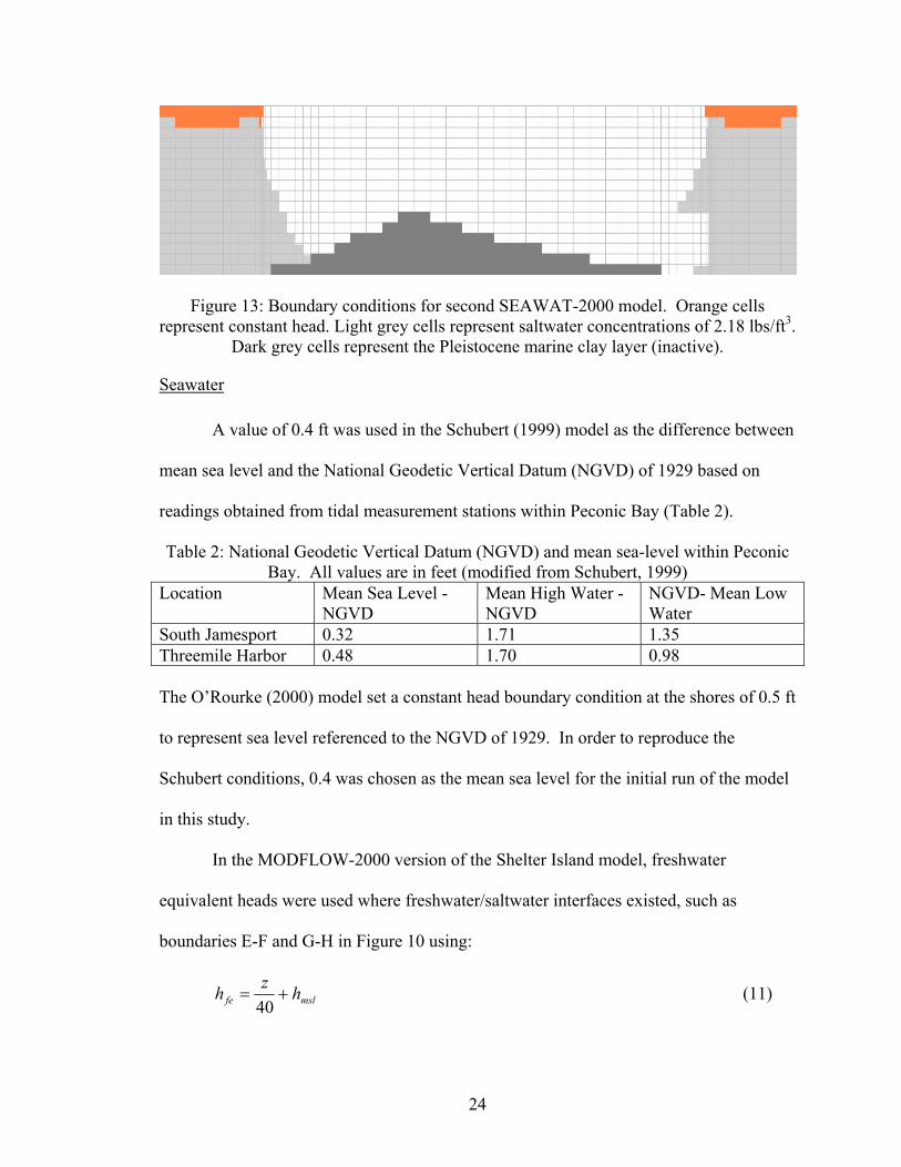
constant head boundaries. Grey cells represent saltwater concentrations of 2.18 lbs/ft3. As described in a subsequent section of this paper, it was determined during the
course of the study that a second, simplified version of the SEAWAT-2000 model should
be constructed that ignored flow to the Pleistocene marine clay layer. For this revised
model, all marine clay layer cells were changed to inactive status. The resulting revised
model consisted of only the top16 layers (Figure 9) of the original model and the bottom
edge of the new model was a no-flow boundary representing part of the Pleistocene
marine clay layer (Figure 13).
24
Figure 13: Boundary conditions for second SEAWAT-2000 model. Orange cells represent constant head. Light grey cells represent saltwater concentrations of 2.18 lbs/ft3.
Dark grey cells represent the Pleistocene marine clay layer (inactive).
Seawater
A value of 0.4 ft was used in the Schubert (1999) model as the difference between
mean sea level and the National Geodetic Vertical Datum (NGVD) of 1929 based on
readings obtained from tidal measurement stations within Peconic Bay (Table 2).
Table 2: National Geodetic Vertical Datum (NGVD) and mean sea-level within Peconic Bay. All values are in feet (modified from Schubert, 1999)
Location Mean Sea Level -NGVD
Mean High Water -NGVD
NGVD- Mean Low Water
South Jamesport 0.32 1.71 1.35 Threemile Harbor 0.48 1.70 0.98 The O’Rourke (2000) model set a constant head boundary condition at the shores of 0.5 ft
to represent sea level referenced to the NGVD of 1929. In order to reproduce the
Schubert conditions, 0.4 was chosen as the mean sea level for the initial run of the model
in this study.
In the MODFLOW-2000 version of the Shelter Island model, freshwater
equivalent heads were used where freshwater/saltwater interfaces existed, such as
boundaries E-F and G-H in Figure 10 using:
mslfe hzh +=40
(11)
25
where hfe is the freshwater equivalent head and hmsl is the mean sea level (Schubert,
1999). However, in the SEAWAT-2000 version of the Shelter Island model, the
freshwater/saltwater interface was denoted by the concentration differences of salt in
freshwater, approximately 0 lbs/ft3, and seawater, 2.18 lbs/ft3 (Masterson, 2004).
Recharge
Shelter Island has an area of 7,670 acres or approximately 12 square miles (Schubert,
1998). Because there are no significant streams on Shelter Island, precipitation that is not
lost to evapotranspiration becomes recharge to the aquifer (Soren, 1978). Miller and
Frederick (1969) determined that the mean annual precipitation for Long Island was
between 43 and 45 inches. For the years 1974 to 1983, Simmons (1986) computed a rate
of precipitation of 47 inches/yr. According to Nemickas and Koszalka (1982), the rate of
evapotranspiration on Long Island is 50%, and the rate of overland runoff is 1%.
Peterson (1987) also used a recharge rate of 50% as a good approximation. However,
Steenhuis et al. (1985) suggested an alternative method using a recharge rate between
75% and 90% from October 15 to May 15 and a recharge rate of 0% for the warmer
summer months when evapotranspiration equals or exceeds precipitation. See Appendix
I for an application of these recharge rates to the precipitation measured at the weather
stations surrounding Shelter Island. Because long-term steady-state conditions were of
primary concern in this study, the 50% recharge rate approximation was used for all
modeling.

26
Geologic Parameters
Soren (1978) determined that Shelter Island sand has a horizontal hydraulic
conductivity between 200 and 270 ft/day and a hydraulic gradient of 0.00115. According
to Smolensky et al. (1989), Long Island sand has a horizontal hydraulic conductivity of
270 ft/day with an anisotropy ratio of 10:1. The Pleistocene Smithtown Clay on central
Long Island has a vertical hydraulic conductivity of 0.035 to 0.07 ft/day (Misut and
Feldman, 1996). Porosity is estimated to be an average of 30% (Franke and
McClymonds,1972; Soren, 1978). A study of the North Fork of Long Island by Schubert
et al. (2004) used a horizontal hydraulic conductivity of 200 ft/day for upper glacial
outwash, a horizontal hydraulic conductivity of 80 ft/day for upper glacial moraine, an
anisotropy ratio of 10:1, and a vertical hydraulic conductivity for confining units of 0.4
ft/day.
The O’Rourke (2000) model used hydrogeologic parameters as described in Table
3. For transient model runs, specific storage was set at 1 x 10⁻⁶ ft-1 and specific yield was
set to 0.25.
Table 3: Defined geologic units and parameters used in O'Rourke(2000) model.
Sediment Type Horizontal
Conductivity (ft/day)
Vertical Conductivity
(ft/day) Porosity
Fine Sand 232 2.32 0.30 Medium Sand 232 23.2 0.30 Coarse Sand 300 30 0.25
Silt and Clay (till) 5 .5 0.40 Clay 1 0.05 0.45
Four hydrogeologic units are represented in this study’s model as shown in Figure
9: (1) a poorly sorted mixture of clay, silt, sand, and gravel referred to as till, (2) upper

27
glacial aquifer moraine and outwash, (3) a sand clay unit, and (4) the Pleistocene marine
clay unit (Schubert, 1999). The parameters used in the original Schubert (1999) model
after calibration are shown in Table 4.
Table 4: Defined geologic units and parameters used in Schubert (1999) model. Conductivities varied slightly at borders between hydrogeologic units.
Layer Horizontal Conductivity
(ft/day)
Vertical Conductivity
(ft/day) Till 30 0.30 Moraine and outwash 320 32 Sandy clay 10 0.10 Pleistocene marine clay 4 0.002 Porosity (all layers) 30%
Pumping
In 1983, by which time population had stabilized according to the 2000 US
Census, Shelter Island had three local water supply facilities serving 25% of the
population. It was estimated that the total annual pumpage for the island was 262 million
gallons (Simmons, 1986) or approximately 96,000 ft3/day.
According to Franke and McClymonds (1972), about 85% of public water
pumpage is returned to groundwater in non-sewered sections of Long Island. Only a
small portion of Shelter Island is sewered and most water returns through septic systems
relatively close to where it was pumped (Schubert, 1998). Assuming an 85% return rate,
only 14,400 ft3/day is lost to pumping. Likewise, agricultural withdrawal, the only
appreciable non-residential water use on Shelter Island, is estimated at 4,600 ft3/day
(Schubert, 1998). Together these pumping rates are less than 1% of the estimated 1.72
million ft3/day of submarine groundwater discharge for the island. Thus, pumping is
ignored in this study.
28
Other Assumptions
Because the vertical cross-section chosen for Shelter Island is not perpendicular to
all potentiometric contours (Figure 7), the model does not strictly represent two-
dimensional flow. However, the cross-section was chosen such that most water-table
contours, especially near-shore, are perpendicular to the model and will provide
reasonably good results (Schubert, 1999).
Also, the study did not take land subsidence from dewatering into account as
recommended by Titus and Narayan (1996). Because the water table on Shelter Island is
close to sea level, excessive freshwater pumping would create negligible amounts of
dewatered land subsidence (Davis, 1987). Additionally, since pumping is ignored in this
study, it is reasonable to also ignore subsidence caused by pumping.
Because regional tectonic subsidence rates were not taken into account in this
study, over the maximum timeframe of this study, the relative sea level rise is
underestimated. According to glacial isostatic adjustment theory, since the last glacial
maximum 21,000 years ago, the crust formerly depressed under the North American ice
sheet has been visco-elastically rebounding. Concurrently, a crustal bulge at the glacial
edge has been subsiding (Peltier, 1999). Because Long Island exists in the area of pro-
glacial forebulge collapse, the area has a rate of sea level rise in excess of eustatic sea
level rise. Subtracting an average absolute sea level rise rate for the eastern North
American coast of 1.3 mm/year (Gornitz, 2000) from the relative sea level rise for
Montauk, NY and Port Jefferson, NY of 2.27 and 2.20 mm/year respectively (Gornitz et
al., 2002), yields a regional subsidence rate of 0.90 to 0.97 mm/year. Over the course of
a century, this translates to 90 to 97 mm (3.5 to 3.8 inches) of subsidence. Since Shelter
29
Island is between Port Jefferson and Montauk, assuming a constant subsidence rate in the
future, by the end of the study, the local sea level should be an additional 3.5 to 3.8
inches higher than the eustatic averages given in the IPCC.
Calibration
In the Schubert (1999) model, hydraulic conductivity parameters,
freshwater/saltwater interface position, and precipitation data were all adjusted by trial
and error until reasonable matches with field monitoring well measurements were
obtained. Calibration was performed for March 1995 during which water levels were
approximately 24% below long-term averages due to low recharge in 1994 that was 26%
below average. Therefore, the model was calibrated using March 1995 well head levels
and a recharge of 50% of 1994 precipitation resulting in recharge of 0.00377 ft/day per
unit area which was arrived at from the 1994 Greenport annual rainfall datum listed in
Appendix I as follows:
dayftftdays
yryr
rain /00377.0%50"12
125.3651"07.33
=××× (12)
During two model runs, O’Rourke (2000) used the following recharge estimates:
0.009823 ft/day for a steady-state calibration March 1999 run, and 0.01081 ft/day for a
steady-state March 1994 validation run.
In the Schubert (1999) study, the freshwater/saltwater interface, modeled as a no-
flow boundary, was placed according to field measurements and calculations using the
modified Ghyban-Herzberg formula (equation 11). The resulting model head simulations
were compared to field observation in Table 5. The largest differences between the
simulated and measured water levels were found near the center of the island and were
30
likely due to the most substantial deviation from two-dimensional flow at that location
(Figure 7). Discrepancies near the shoreline were attributed to the effect of the tide on
near shore monitoring wells which was ignored in the Schubert model.
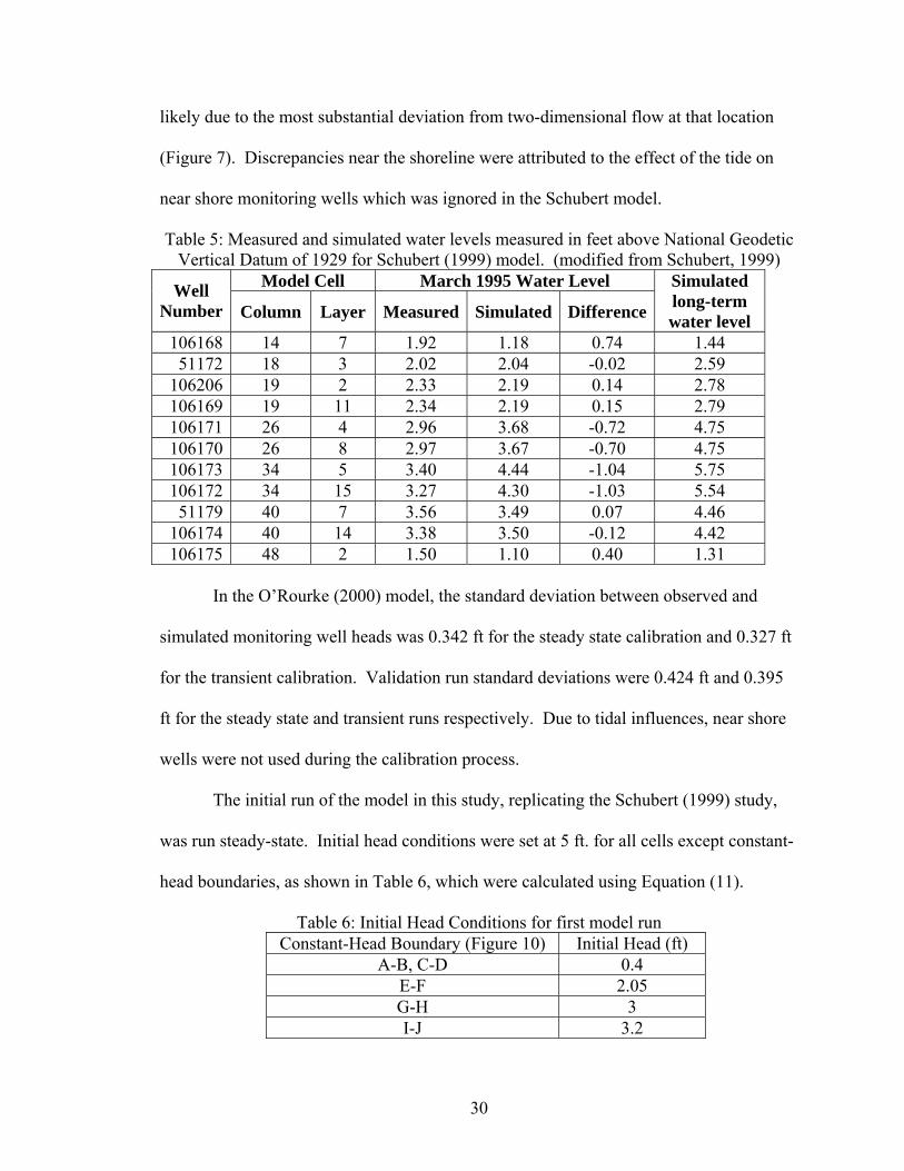
Table 5: Measured and simulated water levels measured in feet above National Geodetic Vertical Datum of 1929 for Schubert (1999) model. (modified from Schubert, 1999)
Model Cell March 1995 Water Level Well Number Column Layer Measured Simulated Difference
Simulated long-term water level
106168 14 7 1.92 1.18 0.74 1.44 51172 18 3 2.02 2.04 -0.02 2.59
106206 19 2 2.33 2.19 0.14 2.78 106169 19 11 2.34 2.19 0.15 2.79 106171 26 4 2.96 3.68 -0.72 4.75 106170 26 8 2.97 3.67 -0.70 4.75 106173 34 5 3.40 4.44 -1.04 5.75 106172 34 15 3.27 4.30 -1.03 5.54 51179 40 7 3.56 3.49 0.07 4.46
106174 40 14 3.38 3.50 -0.12 4.42 106175 48 2 1.50 1.10 0.40 1.31
In the O’Rourke (2000) model, the standard deviation between observed and
simulated monitoring well heads was 0.342 ft for the steady state calibration and 0.327 ft
for the transient calibration. Validation run standard deviations were 0.424 ft and 0.395
ft for the steady state and transient runs respectively. Due to tidal influences, near shore
wells were not used during the calibration process.
The initial run of the model in this study, replicating the Schubert (1999) study,
was run steady-state. Initial head conditions were set at 5 ft. for all cells except constant-
head boundaries, as shown in Table 6, which were calculated using Equation (11).
Table 6: Initial Head Conditions for first model run Constant-Head Boundary (Figure 10) Initial Head (ft)
A-B, C-D 0.4 E-F 2.05 G-H 3 I-J 3.2
31
After the original Schubert (1999) data was duplicated, the model was
recalibrated using two automated parameter estimation programs: PEST, which uses the
Gauss-Marquardt-Levenberg method (Doherty, 1994), and UCODE, which uses the
Gauss-Newton iterative method to find the weighted least squares objective function
(Hill, 1998).
In order to use either PEST or UCODE, the parameters to be estimated were first
selected and defined. For this model, either program had the capability to estimate the
horizontal and vertical hydraulic conductivity and recharge. The grid spacing, boundary
conditions, initial head values, and porosity were not adjusted in any of the parameter
estimation runs. An initial parameter estimation run was restricted to hydraulic
conductivity. This was accomplished by defining eight different hydraulic conductivity
regions, four vertical and four horizontal, within the model corresponding to the various
hydrogeological units. Next, the head observations listed in Table 5 were entered into
PEST and the program was run in the parameter estimation mode.
Parameter estimation using PEST proved unsuccessful. The inverse modeling
returned parameters outside of reasonably expected results. Even when restricted to
estimating only the horizontal hydraulic conductivities of the four geological units, PEST
did not give acceptable results. Specifically, the horizontal conductivity of the clay layer,
determined by Schubert to be 4 ft/day was estimated by PEST to be 400 ft/day, the upper
bound set within PEST for that parameter. Hill (1998) recommends rejecting inverse
modeling results that are obtained by an imposed upper or lower parameter limit because
it suggests potential inverse model instability. In those cases, it is recommended that
prior information be used to estimate the most probable parameter value. In this case, the
32
prior information of the Schubert model results and previously mentioned published
literature provided the best estimates. Thus, automated parameter estimation was
abandoned.
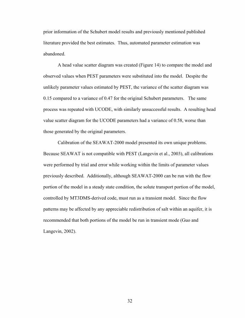
A head value scatter diagram was created (Figure 14) to compare the model and
observed values when PEST parameters were substituted into the model. Despite the
unlikely parameter values estimated by PEST, the variance of the scatter diagram was
0.15 compared to a variance of 0.47 for the original Schubert parameters. The same
process was repeated with UCODE, with similarly unsuccessful results. A resulting head
value scatter diagram for the UCODE parameters had a variance of 0.58, worse than
those generated by the original parameters.
Calibration of the SEAWAT-2000 model presented its own unique problems.
Because SEAWAT is not compatible with PEST (Langevin et al., 2003), all calibrations
were performed by trial and error while working within the limits of parameter values
previously described. Additionally, although SEAWAT-2000 can be run with the flow
portion of the model in a steady state condition, the solute transport portion of the model,
controlled by MT3DMS-derived code, must run as a transient model. Since the flow
patterns may be affected by any appreciable redistribution of salt within an aquifer, it is
recommended that both portions of the model be run in transient mode (Guo and
Langevin, 2002).
33
Figure 14: Head value scatter diagram from PEST forward run.
The variance is 0.15. The standard deviation is 0.39 ft. In order to run the model in transient mode, a specific storage and specific yield
were required. Based on the O’Rourke (2000) model and recommended specific storage
(Domenico, 1972) and recommended specific yield values (Domenico and Schwartz,
1998), a specific storage of 1 x 10⁻⁴ ft-1 and a specific yield of 0.25 were chosen.
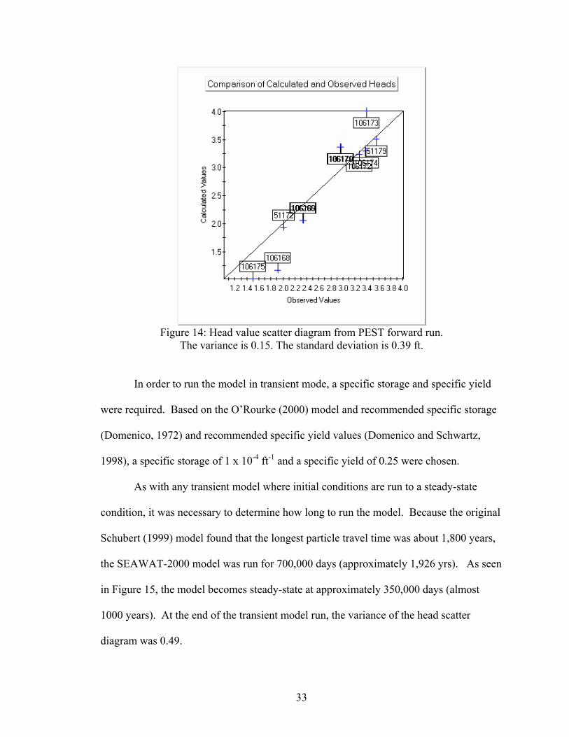
As with any transient model where initial conditions are run to a steady-state
condition, it was necessary to determine how long to run the model. Because the original
Schubert (1999) model found that the longest particle travel time was about 1,800 years,
the SEAWAT-2000 model was run for 700,000 days (approximately 1,926 yrs). As seen
in Figure 15, the model becomes steady-state at approximately 350,000 days (almost
1000 years). At the end of the transient model run, the variance of the head scatter
diagram was 0.49.

34
However, the concentrations and head contour diagrams showed a failure of the
model to correctly model the freshwater/saltwater interface within the marine clay layer.
According to the Schubert (1999) model, almost all flow occurred in the upper glacial
aquifer. Therefore, a model that excluded the flow within the marine clay unit still
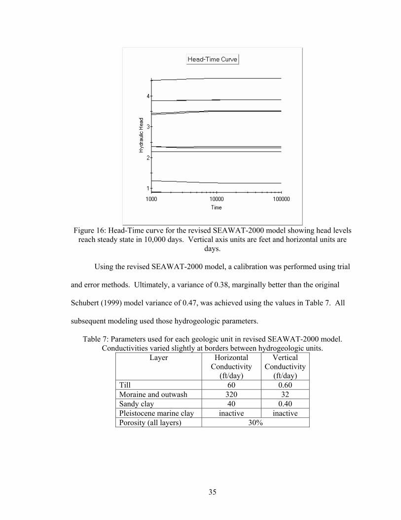
approximates the aquifer conditions. The second version of the SEAWAT-2000 model
that was created to model only the upper glacial flow (see Figure 13), reached steady-
state far faster than the original model. Figure 16 shows that the second model reaches
equilibrium within 10,000 days (approximately 27 years). Thus, for all subsequent model
runs, each simulation was run for 20,000 days in order to ensure that the transient model
had run to full steady-state conditions.
Figure 15: Head-Time curve for the initial SEAWAT-2000 model showing head levels reach steady state in 350,000 days. Vertical axis units are feet and horizontal units are
days.
35
Figure 16: Head-Time curve for the revised SEAWAT-2000 model showing head levels
reach steady state in 10,000 days. Vertical axis units are feet and horizontal units are days.
Using the revised SEAWAT-2000 model, a calibration was performed using trial
and error methods. Ultimately, a variance of 0.38, marginally better than the original
Schubert (1999) model variance of 0.47, was achieved using the values in Table 7. All
subsequent modeling used those hydrogeologic parameters.
Table 7: Parameters used for each geologic unit in revised SEAWAT-2000 model. Conductivities varied slightly at borders between hydrogeologic units.
Layer Horizontal Conductivity
(ft/day)
Vertical Conductivity
(ft/day) Till 60 0.60 Moraine and outwash 320 32 Sandy clay 40 0.40 Pleistocene marine clay inactive inactive Porosity (all layers) 30%
36
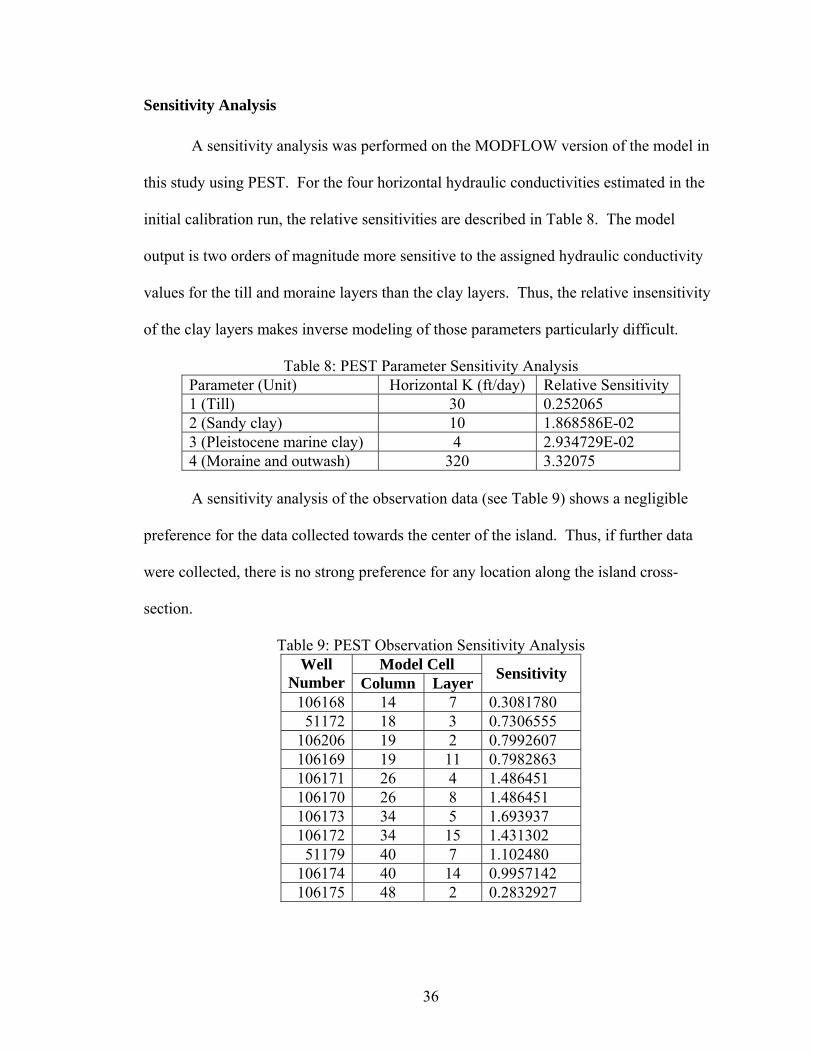
Sensitivity Analysis
A sensitivity analysis was performed on the MODFLOW version of the model in
this study using PEST. For the four horizontal hydraulic conductivities estimated in the
initial calibration run, the relative sensitivities are described in Table 8. The model
output is two orders of magnitude more sensitive to the assigned hydraulic conductivity
values for the till and moraine layers than the clay layers. Thus, the relative insensitivity
of the clay layers makes inverse modeling of those parameters particularly difficult.
Table 8: PEST Parameter Sensitivity Analysis Parameter (Unit) Horizontal K (ft/day) Relative Sensitivity 1 (Till) 30 0.252065 2 (Sandy clay) 10 1.868586E-02 3 (Pleistocene marine clay) 4 2.934729E-02 4 (Moraine and outwash) 320 3.32075
A sensitivity analysis of the observation data (see Table 9) shows a negligible
preference for the data collected towards the center of the island. Thus, if further data
were collected, there is no strong preference for any location along the island cross-
section.
Table 9: PEST Observation Sensitivity Analysis Model Cell Well
Number Column Layer Sensitivity
106168 14 7 0.3081780 51172 18 3 0.7306555
106206 19 2 0.7992607 106169 19 11 0.7982863 106171 26 4 1.486451 106170 26 8 1.486451 106173 34 5 1.693937 106172 34 15 1.431302 51179 40 7 1.102480
106174 40 14 0.9957142 106175 48 2 0.2832927
37
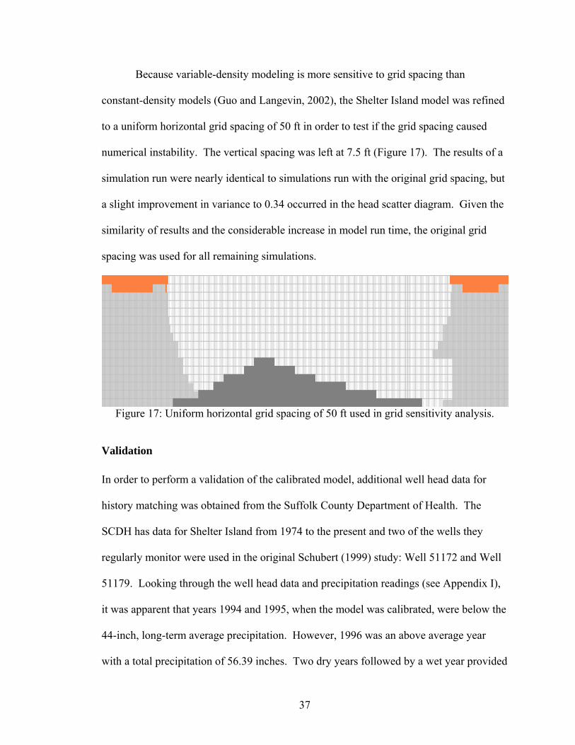
Because variable-density modeling is more sensitive to grid spacing than
constant-density models (Guo and Langevin, 2002), the Shelter Island model was refined
to a uniform horizontal grid spacing of 50 ft in order to test if the grid spacing caused
numerical instability. The vertical spacing was left at 7.5 ft (Figure 17). The results of a
simulation run were nearly identical to simulations run with the original grid spacing, but
a slight improvement in variance to 0.34 occurred in the head scatter diagram. Given the
similarity of results and the considerable increase in model run time, the original grid
spacing was used for all remaining simulations.
Figure 17: Uniform horizontal grid spacing of 50 ft used in grid sensitivity analysis.
Validation
In order to perform a validation of the calibrated model, additional well head data for
history matching was obtained from the Suffolk County Department of Health. The
SCDH has data for Shelter Island from 1974 to the present and two of the wells they
regularly monitor were used in the original Schubert (1999) study: Well 51172 and Well
51179. Looking through the well head data and precipitation readings (see Appendix I),
it was apparent that years 1994 and 1995, when the model was calibrated, were below the
44-inch, long-term average precipitation. However, 1996 was an above average year
with a total precipitation of 56.39 inches. Two dry years followed by a wet year provided
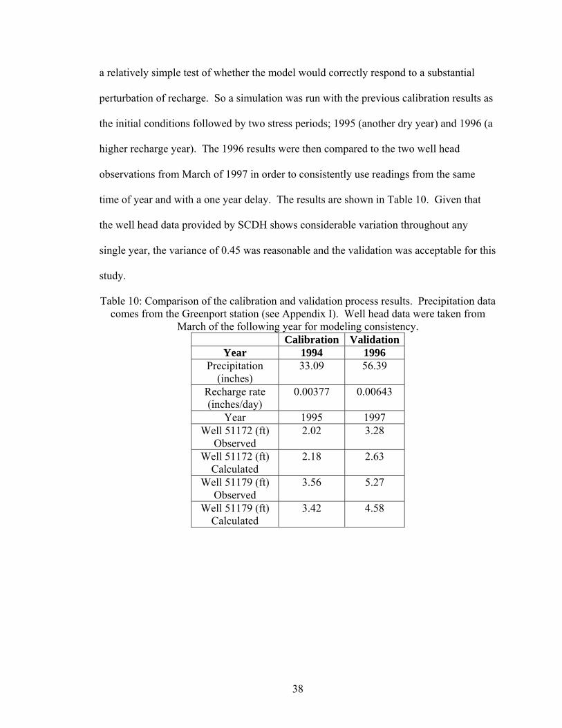
38
a relatively simple test of whether the model would correctly respond to a substantial
perturbation of recharge. So a simulation was run with the previous calibration results as
the initial conditions followed by two stress periods; 1995 (another dry year) and 1996 (a
higher recharge year). The 1996 results were then compared to the two well head
observations from March of 1997 in order to consistently use readings from the same
time of year and with a one year delay. The results are shown in Table 10. Given that
the well head data provided by SCDH shows considerable variation throughout any
single year, the variance of 0.45 was reasonable and the validation was acceptable for this
study.
Table 10: Comparison of the calibration and validation process results. Precipitation data comes from the Greenport station (see Appendix I). Well head data were taken from
March of the following year for modeling consistency. Calibration Validation
Year 1994 1996 Precipitation
(inches) 33.09 56.39
Recharge rate (inches/day)
0.00377 0.00643
Year 1995 1997 Well 51172 (ft)
Observed 2.02 3.28
Well 51172 (ft) Calculated
2.18 2.63
Well 51179 (ft) Observed
3.56 5.27
Well 51179 (ft) Calculated
3.42 4.58
39
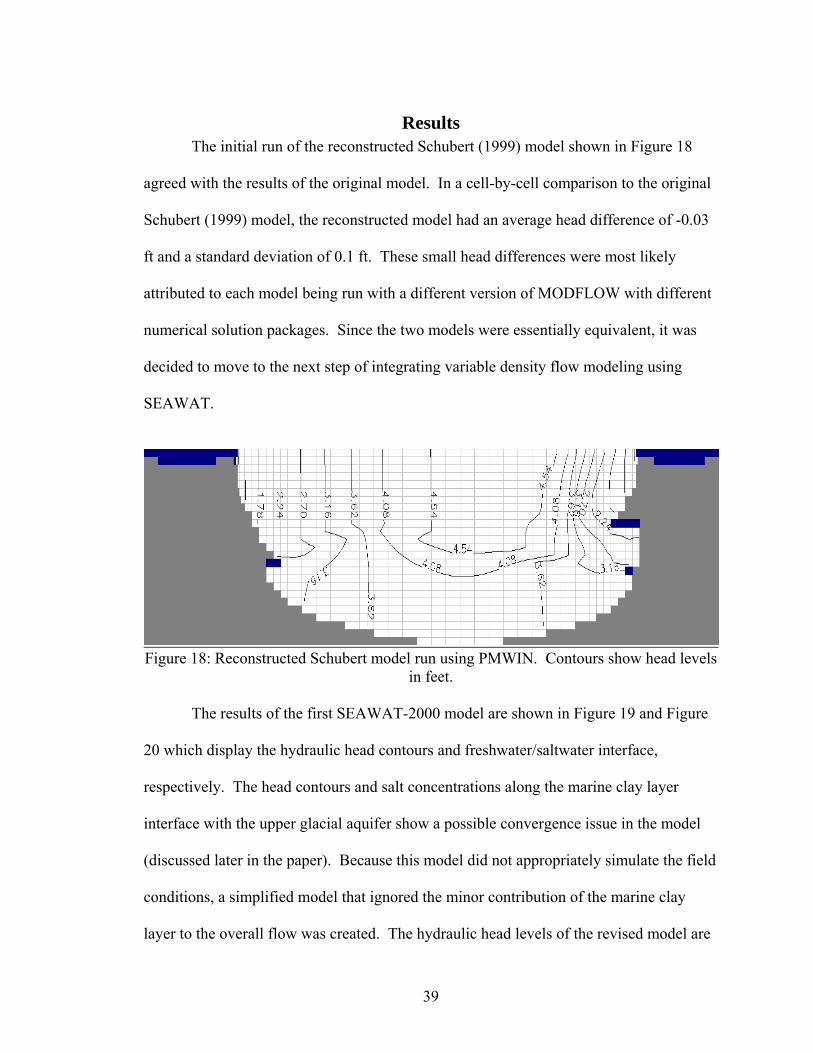
Results The initial run of the reconstructed Schubert (1999) model shown in Figure 18
agreed with the results of the original model. In a cell-by-cell comparison to the original
Schubert (1999) model, the reconstructed model had an average head difference of -0.03
ft and a standard deviation of 0.1 ft. These small head differences were most likely
attributed to each model being run with a different version of MODFLOW with different
numerical solution packages. Since the two models were essentially equivalent, it was
decided to move to the next step of integrating variable density flow modeling using
SEAWAT.
Figure 18: Reconstructed Schubert model run using PMWIN. Contours show head levels
in feet.
The results of the first SEAWAT-2000 model are shown in Figure 19 and Figure
20 which display the hydraulic head contours and freshwater/saltwater interface,
respectively. The head contours and salt concentrations along the marine clay layer
interface with the upper glacial aquifer show a possible convergence issue in the model
(discussed later in the paper). Because this model did not appropriately simulate the field
conditions, a simplified model that ignored the minor contribution of the marine clay
layer to the overall flow was created. The hydraulic head levels of the revised model are
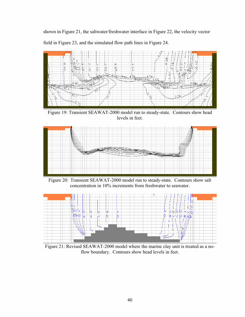
40
shown in Figure 21, the saltwater/freshwater interface in Figure 22, the velocity vector
field in Figure 23, and the simulated flow path lines in Figure 24.
Figure 19: Transient SEAWAT-2000 model run to steady-state. Contours show head
levels in feet.
Figure 20: Transient SEAWAT-2000 model run to steady-state. Contours show salt
concentration in 10% increments from freshwater to seawater.
Figure 21: Revised SEAWAT-2000 model where the marine clay unit is treated as a no-
flow boundary. Contours show head levels in feet.
41
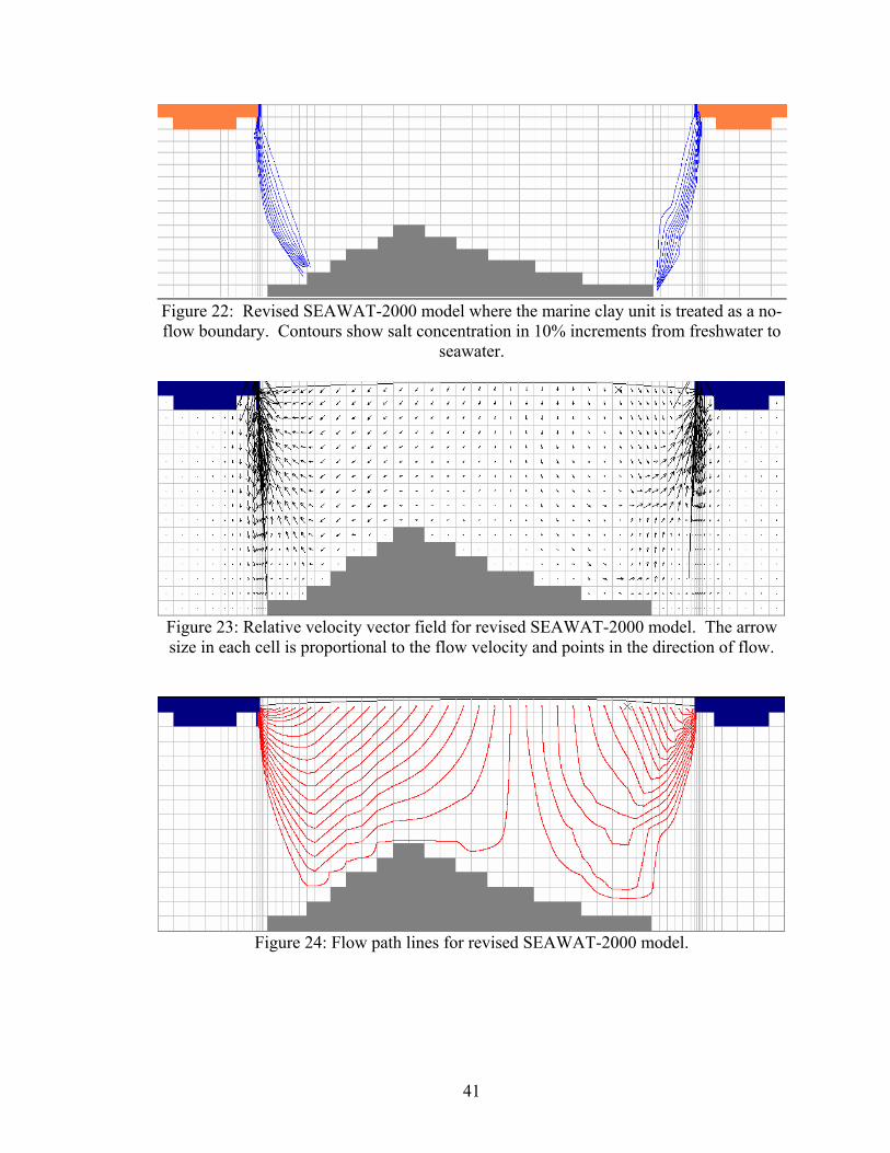
Figure 22: Revised SEAWAT-2000 model where the marine clay unit is treated as a no-flow boundary. Contours show salt concentration in 10% increments from freshwater to
seawater.
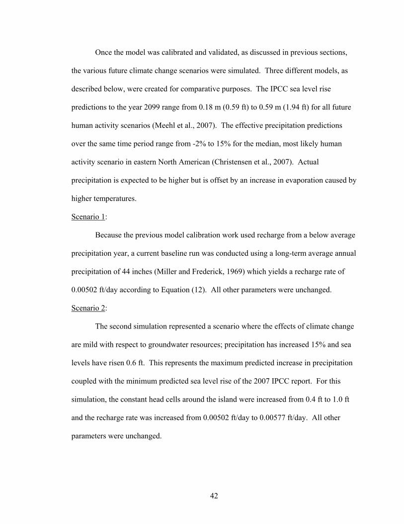
Figure 23: Relative velocity vector field for revised SEAWAT-2000 model. The arrow size in each cell is proportional to the flow velocity and points in the direction of flow.
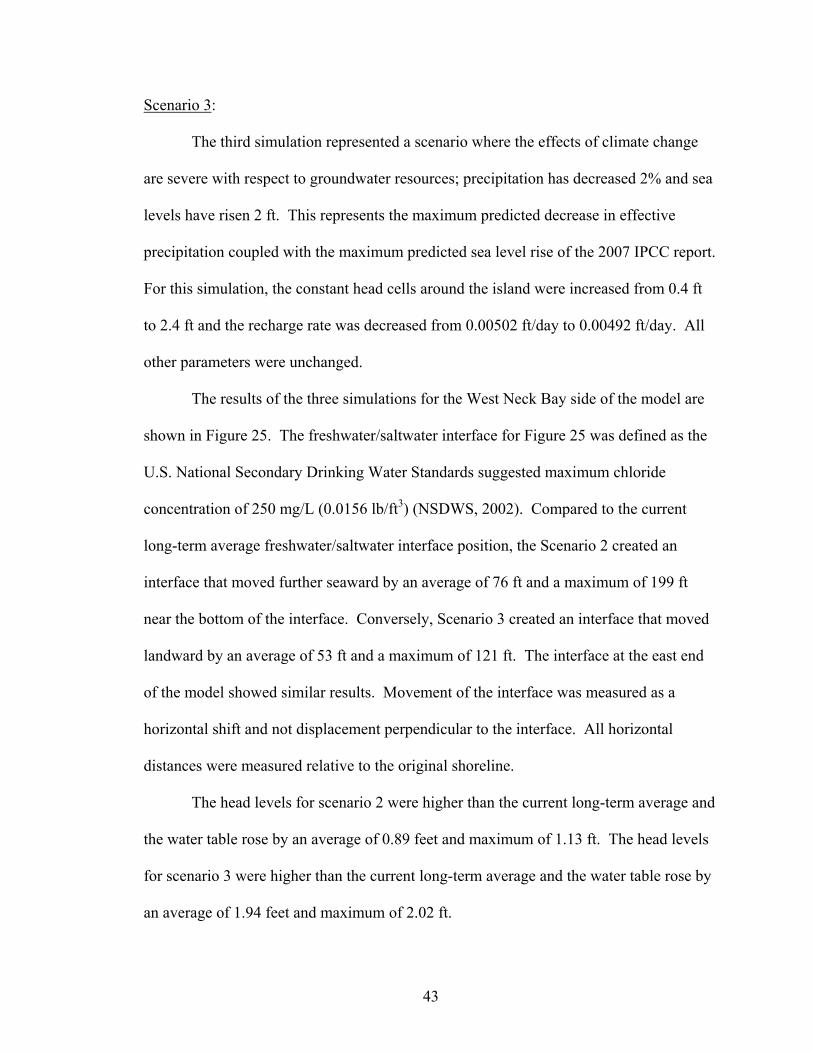
Figure 24: Flow path lines for revised SEAWAT-2000 model.
42
Once the model was calibrated and validated, as discussed in previous sections,
the various future climate change scenarios were simulated. Three different models, as
described below, were created for comparative purposes. The IPCC sea level rise
predictions to the year 2099 range from 0.18 m (0.59 ft) to 0.59 m (1.94 ft) for all future
human activity scenarios (Meehl et al., 2007). The effective precipitation predictions
over the same time period range from -2% to 15% for the median, most likely human
activity scenario in eastern North American (Christensen et al., 2007). Actual
precipitation is expected to be higher but is offset by an increase in evaporation caused by
higher temperatures.
Scenario 1:
Because the previous model calibration work used recharge from a below average
precipitation year, a current baseline run was conducted using a long-term average annual
precipitation of 44 inches (Miller and Frederick, 1969) which yields a recharge rate of
0.00502 ft/day according to Equation (12). All other parameters were unchanged.
Scenario 2:
The second simulation represented a scenario where the effects of climate change
are mild with respect to groundwater resources; precipitation has increased 15% and sea
levels have risen 0.6 ft. This represents the maximum predicted increase in precipitation
coupled with the minimum predicted sea level rise of the 2007 IPCC report. For this
simulation, the constant head cells around the island were increased from 0.4 ft to 1.0 ft
and the recharge rate was increased from 0.00502 ft/day to 0.00577 ft/day. All other
parameters were unchanged.
43
Scenario 3:
The third simulation represented a scenario where the effects of climate change
are severe with respect to groundwater resources; precipitation has decreased 2% and sea
levels have risen 2 ft. This represents the maximum predicted decrease in effective
precipitation coupled with the maximum predicted sea level rise of the 2007 IPCC report.
For this simulation, the constant head cells around the island were increased from 0.4 ft
to 2.4 ft and the recharge rate was decreased from 0.00502 ft/day to 0.00492 ft/day. All
other parameters were unchanged.
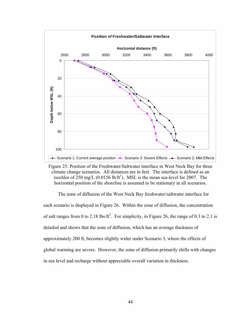
The results of the three simulations for the West Neck Bay side of the model are
shown in Figure 25. The freshwater/saltwater interface for Figure 25 was defined as the
U.S. National Secondary Drinking Water Standards suggested maximum chloride
concentration of 250 mg/L (0.0156 lb/ft3) (NSDWS, 2002). Compared to the current
long-term average freshwater/saltwater interface position, the Scenario 2 created an
interface that moved further seaward by an average of 76 ft and a maximum of 199 ft
near the bottom of the interface. Conversely, Scenario 3 created an interface that moved
landward by an average of 53 ft and a maximum of 121 ft. The interface at the east end
of the model showed similar results. Movement of the interface was measured as a
horizontal shift and not displacement perpendicular to the interface. All horizontal
distances were measured relative to the original shoreline.
The head levels for scenario 2 were higher than the current long-term average and
the water table rose by an average of 0.89 feet and maximum of 1.13 ft. The head levels
for scenario 3 were higher than the current long-term average and the water table rose by
an average of 1.94 feet and maximum of 2.02 ft.
44
Position of Freshwater/Saltwater Interface
0
20
40
60
80
100
2600 2800 3000 3200 3400 3600 3800 4000
Horizontal distance (ft)D
epth
bel
ow M
SL (f
t)
w
Scenario 1: Current average position Scenario 3: Severe Effects Scenario 2: Mild Effects
Figure 25: Position of the Freshwater/Saltwater interface in West Neck Bay for three climate change scenarios. All distances are in feet. The interface is defined as an isochlor of 250 mg/L (0.0156 lb/ft3). MSL is the mean sea-level for 2007. The horizontal position of the shoreline is assumed to be stationary in all scenarios.
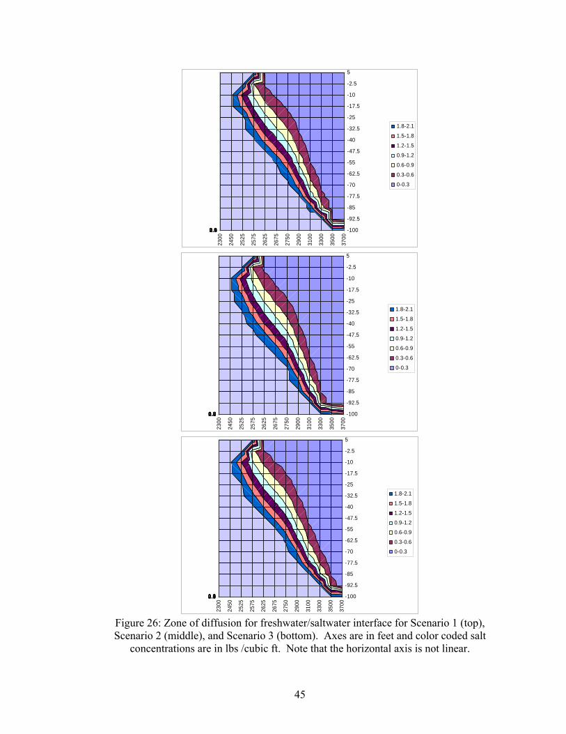
The zone of diffusion of the West Neck Bay freshwater/saltwater interface for
each scenario is displayed in Figure 26. Within the zone of diffusion, the concentration
of salt ranges from 0 to 2.18 lbs/ft3. For simplicity, in Figure 26, the range of 0.3 to 2.1 is
detailed and shows that the zone of diffusion, which has an average thickness of
approximately 200 ft, becomes slightly wider under Scenario 3, where the effects of
global warming are severe. However, the zone of diffusion primarily shifts with changes
in sea level and recharge without appreciable overall variation in thickness.
45
2300
2450
2525
2575
2625
2675
2750
2900
3100
3300
3500
3700
5
-2.5
-10
-17.5
-25
-32.5
-40
-47.5
-55
-62.5
-70
-77.5
-85
-92.5
-10000.30.60.91.21.51.82.1
1.8-2.1
1.5-1.8
1.2-1.5
0.9-1.2
0.6-0.9
0.3-0.6
0-0.3
2300
2450
2525
2575
2625
2675
2750
2900
3100
3300
3500
3700
5
-2.5
-10
-17.5
-25
-32.5
-40
-47.5
-55
-62.5
-70
-77.5
-85
-92.5
-10000.30.60.91.21.51.82.1
1.8-2.1
1.5-1.8
1.2-1.5
0.9-1.2
0.6-0.9
0.3-0.6
0-0.3
2300
2450
2525
2575
2625
2675
2750
2900
3100
3300
3500
3700
5
-2.5
-10
-17.5
-25
-32.5
-40
-47.5
-55
-62.5
-70
-77.5
-85
-92.5
-10000.30.60.91.21.51.82.1
1.8-2.1
1.5-1.8
1.2-1.5
0.9-1.2
0.6-0.9
0.3-0.6
0-0.3
Figure 26: Zone of diffusion for freshwater/saltwater interface for Scenario 1 (top), Scenario 2 (middle), and Scenario 3 (bottom). Axes are in feet and color coded salt
concentrations are in lbs /cubic ft. Note that the horizontal axis is not linear.
46
Discussion
The SEAWAT modeling was problematic because PMWIN is not directly
compatible with SEAWAT or SEAWAT-2000. However, because PMWIN is
compatible with MODFLOW-2000 and MT3DMS, it was possible to use SEAWAT-
2000 with PMWIN. The user need only separately create the MODFLOW-2000 and
MT3DMS input files using PMWIN as the pre-processor and then combine them to run
SEAWAT-2000. The SEAWAT-2000 documentation (Langevin et al., 2003) explains
how to create the additional files that allows SEAWAT-2000 to read and write to the
MODFLOW-2000 and MT3DMS files. Additionally, the extra data files, created with a
text editor, define the reference densities of the variable density fluid models. When the
simulation is complete, PMWIN can be used as the post-processor without additional file
manipulation.
The original SEAWAT-2000 model attempt appeared to have convergence
problems with regards to the Pleistocene marine clay unit. Guo and Langevin (2002)
outline several issues that cause problems with variable density flow models. With
respect to the finite difference grid, the need for cell volume uniformity and higher
resolution, particularly vertical resolution, are potential issues for constant-density
simulations that are converted to variable-density. In the case of the Schubert (1999)
model, the relatively small and uniform vertical resolution may have prevented some
numerical instability issues. Furthermore, using a higher resolution and uniform
horizontal grid spacing in the sensitivity analysis did not reveal any stability issues
related to grid size. However, an even finer vertical and horizontal grid spacing may
allow for an appropriate solution.
47
Other model design problems that can give rise to numerical instability include:
initial conditions that are very far from equilibrium, rapidly changing boundary
conditions, and large differences in hydrogeologic unit properties in adjacent cells.
Because the initial head conditions and general head boundary values were based on the
previous Schubert (1999) model, they are an unlikely source of instability. The large
change in hydraulic conductivities, a ratio of almost 100:1, between the upper glacial
sand unit and the marine clay unit interface, are a more likely cause of numerical
instability. Adding an intermediate layer to minimize the sharply differentiated units
might solve the model instability. However, it is important not to stray too far from the
actual known geologic conditions of the site merely to work around the mathematical
weaknesses of any particular modeling approach. In this case, excluding the contribution
of the marine clay layer from the simulation was deemed to be the best compromise.
The slow response time of the marine clay unit is an additional reason for
excluding it from the model. According to the particle-tracking performed by Schubert
(1999), the average travel time through the marine clay unit was 1,800 years. Travel time
for the upper glacial unit flow averaged about 20 years with almost all flow less than 50
years. The freshwater/saltwater interface in the upper glacial aquifer responds within
decades to changes in recharge and sea level, while the interface within the marine clay
unit responds over millennia. Because the simulation time of this study is less than a
century, it is reasonable to treat the marine clay unit as impermeable and a no-flow
boundary within that timeframe. Additionally, rapid climate change, as predicted by the
IPCC, should cause a distorted freshwater/saltwater interface that could be difficult to
model due to possible discontinuities near the interface of the two hydrogeologic units. It
48
is also possible that the current freshwater/saltwater interface in the marine clay layer
might not be in equilibrium with the current hydrologic conditions in the upper glacial,
but still responding to an equilibrium shift that occurred in the recent past.
It should be noted that the steady-state condition of the transient models was
determined using plots of the head levels over time; stable head levels implied steady-
state flow conditions. However, the transport portion of the model was in steady-state
only when concentrations did not change over time. For this study, it was assumed that
salt concentrations achieved steady-state in parallel with the flow portion of the model
because flow and transport were coupled within a single time-step lag. Assuming there
was no conceptual error in the model, this assumption should be appropriate. This is
important because, although the calibration process focused on head levels, in the
predictive modeling, the salt concentrations and position of the freshwater/saltwater
interface were of primary interest.
A closely related assumption in this study was to ignore any effects of nutrient
loading and transport within the model. Simmons (1986) found the various impurities in
Shelter Island groundwater to be small compared to the overall solute concentration of
seawater such that assuming the freshwater to have a concentration of zero introduced
minimal error. However, it is possible that localized groundwater pollution could create
a solute concentration high enough to noticeably effect the density relationship between
the freshwater and groundwater and thereby cause deviation from the modeled
simulations.
From Figure 24, which shows the flow lines within the freshwater lens, it appears
that most recharge to Shelter Island leaves the aquifer as submarine groundwater
49
discharge. The model results are in general agreement with previous work by O’Rourke
(2000) and Paulsen et al. (2004) that found below sea level seepage faces near the
shoreline, often visible at low tide, which were responsible for most of the discharge of
the aquifer. Although the region of discharge was confirmed in the SEAWAT-2000
model, it was more difficult to make any comparison of quantity of discharge with
previous studies. Because submarine groundwater discharge is highly dependent on
recharge, comparing discharge in different years or seasons is not meaningful.
The results shown in Figure 26 suggest that diffusion does not play a major role in
the long-term movement of the freshwater/saltwater interface. This is a reasonable
conclusion since molecular diffusion, as described by Fick’s Law, is proportional to the
concentration gradient and the velocity of the diffusive particles which is primarily
dependent on temperature, particle size, and fluid viscosity (Domenico and
Schwartz,1998). Since none of these characteristics change within the model, it is
assumed that diffusion is constant across all scenarios. However, because SEAWAT
assumes constant temperature, it is possible that, due to global warming, the amount of
diffusion at the freshwater/saltwater interface will increase over the next century because
of an increase in temperature of the seawater and groundwater. Thus, it is not possible to
make any realistic predictions regarding future diffusion without first estimating the
future dispersion coefficient.
Lateral mechanical dispersion was not used in the simulations in this study. The
model was two-dimensional and solute concentrations were assumed to be uniform
perpendicular to the cross-section of model. When simulations were run with lateral
50
dispersion, the output confirmed that simplifying the model to exclude lateral dispersion
was appropriate.
Tidal or seasonal mixing was not considered in this study. Paulson et al. (2004)
found a daily asymmetrical change in submarine groundwater discharge and salinity.
Thus, the range of brackish water is larger than that modeled when assuming a relatively
stationary interface with a zone of diffusion. However, because this study was concerned
with the long-term movement of the freshwater/saltwater interface, the daily and seasonal
movement of the interface and the additional mixing it causes was not considered. In an
October, 2007 Geological Society of America meeting, Motomu Ibaraki, of Ohio State
University presented unpublished research that suggested that shores with highly sorted
sandy layers may experience freshwater and saltwater mixing that causes saltwater
intrusion 10% to 50% further inland than simple sea level rise inundation. If peer-review
supports these findings, mixing may be an important component of future Shelter Island
modeling.
Once the revised SEAWAT-2000 model was created and the calibration process
began, it was clear that, although it was an improvement over the original Schubert
(1999) model, weaknesses in the original carried over to the new model. The highest
deviations from the field data occurred at the center of the island. This was attributed to
that section of the model having the largest deviation from purely two dimensional flow
(see Figure 7). Also, the observation closest to West Neck Bay, was substantially higher
than the simulation. This was attributed to hydraulic tidal loading in the Schubert (1999)
report. Schneider and Kruse (2003), in a study of a small sandy barrier island in Florida,
found that tidal forcing caused water table elevations to change by several tens of

51
centimeters daily. Likewise, individual precipitation events could cause similar changes
within days. Thus, estimating the freshwater/saltwater interface, which responds much
more slowly over time, directly from any single set of head levels, yields uncertain
results.
The predicted movement of the freshwater/saltwater interface agrees with the
conceptual model of Simmons (1986). Because the marine clay unit restricts the
movement of the bottom of the interface, the sides move substantially landward or
seaward in response to hydrological conditions (see Figure 6). Since Simmons (1986)
observed that the interface moves with the seasons and varying recharge, it is important
to note that the model predicted movements of the freshwater/saltwater interface are
long-term averages that would act as the new baseline from which regular season
variability would fluctuate.
Because the model simulations did not consider surface topology and the few
small near shore ponds on Shelter Island that intersect the water table, it is more difficult
to determine the impact of scenarios 2 and 3 on the volume of freshwater under Shelter
Island.. If the effect of outflow to surface water is substantial, the actual head levels may
be lower than simulated due to increased flow to ponds and subsequent higher
evaporation rates. Additionally, by not considering surface topology, it was not possible
to correctly model the horizontal movement of the shoreline that would occur as rising
sea level inundated coastal land. On the northern shores of Shelter Island, where there
are high bluffs rising from the shore, there should be minimal movement of the shoreline.
At the southern end of Shelter Island, the movement of the shoreline may be more
substantial and a source of error if not considered within the model. For the cross-section
52
modeled in this study (Figure 7), assuming a stationary shoreline simplified modeling
while introducing an acceptably small error.
Conclusion In order to quantify the effects that global warming may have on a small sandy
barrier island, a previously published single density steady-state groundwater flow model
for Shelter Island, NY was changed to a variable density transient groundwater flow
model. The original model code, created for MODFLOW, was adapted to SEAWAT-
2000 and run with PMWIN Pro as the graphical user interface. In order to obtain
simulations that were consistent with field observations, the marine clay layer was set as
a no-flow boundary in the SEAWAT-2000 model. The calibrated SEAWAT-2000 model
had a variance of 0.38 compared to the original Schubert (1999) model variance of 0.47.
The 2007 IPCC report predictions for changes in precipitation and sea level rise
over the next century were applied to the calibrated model. A scenario most favorable to
groundwater retention consisting of a predicted precipitation increase of 15% and a sea
level rise of 0.6 ft was compared to the current long-term average. This resulted in a
seaward movement of the interface by an average of 76 ft and a maximum of 199 ft. The
water table rose by an average of 0.89 feet. A second scenario least favorable to
groundwater retention consisting of a predicted precipitation decrease of 2% and a sea
level rise of 2 ft was compared to the current long-term average. This resulted in a
landward movement of the interface by an average of 53 ft and a maximum of 121 ft.
The water table rose by an average of 1.94 feet.
53
Future Work
Parameter estimation software usually fails due to either the insensitivity of the
head observations, non-uniqueness of solutions, or model instability (Hill, 1998). In the
case of this study, the limited head observations were a contributing factor to the failed
automated parameter estimation. With an increased number of observation data, the
chances of obtaining non-unique solutions would decrease significantly. Future
modeling work should include increasing the number of observations to aid the
calibration and validation process. Also, a redesigned model should use small uniform
cell sizes both vertically and horizontally to minimize numerical instability issues. A
model the island’s aquifer in warmer climate should consider the effects of increased
temperature on diffusion which presumably will increase the zone of diffusion at the
freshwater/saltwater interface and further decrease the volume of potable water.
Additionally, the effects of mixing on the brackish zone should be added to more
precisely ascertain the extent of potable water.
In order to properly estimate the actual volumetric loss or gain of potable water on
Shelter Island due to climate change over the next century, a full three-dimensional
variable density flow model should be created that also incorporates the additional
regional tectonic subsidence. Most importantly, the model should add surface
topological features and include the intersection of ponds with the water table in order to
model shoreline movement and to see what effects are caused by the increased
evaporation and outflow resulting from a rising water table. Incorporating a water quality
component to the model may also be necessary since one of the primary sources of
contamination on Shelter Island is effluent from septic tanks. Because these sources are

54
closer to the water table than surface contaminants, a rising water table may cause a
substantial increase in water pollution thereby further reducing the effective volume of
potable water available to the residents of Shelter Island.

55
References Buxton, H.T., and Modica, E., Patterns and Rates of Ground-Water Flow on Long Island,
New York, Ground Water , Vol. 30, No. 6, 857-866 Chiang, Wen-Hsing, 2005, 3D-Groundwater Modeling with PMWIN, 2nd Edition,
Heidelberg: Springer, 397 p. Christensen, J.H., B. Hewitson, A. Busuioc, A. Chen, X. Gao, I. Held, R. Jones, R.K.
Kolli, W.-T. Kwon, R. Laprise, V. Magaña Rueda, L. Mearns, C.G. Menéndez, J. Räisänen, A. Rinke, A. Sarr and P. Whetton, 2007: Regional Climate Projections. In: Climate Change 2007: The Physical Science Basis. Contribution of Working Group I to the Fourth Assessment Report of the Intergovernmental Panel on Climate Change [Solomon, S., D. Qin, M. Manning, Z. Chen, M. Marquis, K.B. Averyt, M. Tignor and H.L. Miller (eds.)]. Cambridge University Press, Cambridge, United Kingdom and New York, NY, USA.
Cohen, Philip, Franke, O.L., and Foxworthy, B.L., 1968, An atlas of Long Island’s water
resources: New York State Water Resources Commission Bulletin 62, 117 p. Davis, G.H., 1987, Land subsidence and sea level rise on the Atlantic Coastal Plain of the
United States, Environmental Geology, Vol. 10, No. 2, p. 67-80 Doherty, J. 1994, PEST: Corinda, Australia, Watermark Computing, 122 p. Domenico, P.A., 1972, Concepts and Models in Groundwater Hydrology, McGraw-Hill, New York, 405 p. Domenico, P.A. and Schwartz, F.W., 1998, Physical and Chemical Hydrogeology, 2nd
Edition , New York: John Wiley & Sons, 494 p. Freeze, R. A., and Cherry, J. A., 1979, Groundwater: Englewood Cliffs, N.J.,
Prentlce-Hall, 604 p. Fuller, M.L., 1914, The geology of Long Island, New York: U.S. Geological Survey
Professional Paper 82, 231 p. Franke, O.L., and McClymonds, N.E., 1972, Summary of the hydrologic situation on
Long Island, New York as a guide to water-management alternatives: U.S. Geological Survey Professional Paper 627-F, 59 p.
Ghyben, W.B., 1889, Notes in verband met Woorgenomen Put boring Nabji Amsterdam,
Tijdschr. Koninhitk, Inst. Ingrs., The Hague.
56
Guo, Weixing, and Langevin, C.D., 2002, User’s guide to SEAWAT: A computer program for simulation of three-dimensional variable-density ground-water flow: U.S. Geological Survey Techniques of Water-Resources Investigations, book 6, chap. A7, 77 p.
Glover, R.E., 1959, The pattern of fresh-water flow in a confined coastal aquifer, Journal
of Geophysical Research, Vol. 64, No.4, p.457-459 Gornitz, V., 2000, Climate change and the coast: impacts in the New York City
metropolitan region, EOS, Vol. 81, No.17, S73. Gornitz, V., Couch, S., and Hartig, E.K., Impacts of sea level rise in the New York City
metropolitan area, Global and Planetary Changes, Vol. 32, p. 61– 88 Herzberg, B., 1901, Die Wasserversovgung einiger Nordseebaser, J. Gasbeleucht and
wasserversov, v. 44, p. 815-819 Harbaugh AW, Banta ER, Hill MC and McDonald MG, 2000, MODFLOW-2000, The
U.S. Geological Survey modular ground-water model User guide to modularization concepts and the ground-water flow process, U.S. Geological Survey Open-file report 00-92.
Hill, M.C., 1998, Methods and guidelines for effective model calibration: U.S.
Geological Survey Water-Resources Investigations Report 98-4005, 90 p. IPCC, Feb. 2007, Climate Change 2007: The Physical Science Basis, Summary for
Policymakers, Contribution of Working Group I to the Fourth Assessment Report of the IPCC, Paris
IPCC WGI, 2001, Climate Change 2001: Scientific Basis, Cambridge University
Press, Cambridge Langevin, C.D., Shoemaker, W.B, and Guo, W., 2003, MODFLOW-2000, the U.S.
Geological Survey Modular Ground-Water Model—Documentation of the SEAWAT-2000 Version with the Variable-Density Flow Process (VDF) and the Integrated MT3DMS Transport Process (IMT), U.S. Geological Survey Open-File Report 03-426
Masterson, J.P., 2004, Simulated interaction between freshwater and saltwater and effects
of ground-water pumping and sea-level change, Lower Cape Cod aquifer system, Massachusetts: U.S. Geological Survey Scientific Investigations Report 2004-5014, 72 p.
Masterson, J.P. and Garabedian, S.P., Effects of Sea-Level Rise on Ground Water Flow
in a Coastal Aquifer System, Ground Water, Vol. 45, No. 2, p. 209-217
57
McDonald, M.G., and Harbaugh, A.W., 1984, A modular three-dimensional finite-difference ground-water flow model: U.S. Geological Survey Open-File Report 83-875, 528 p.
McDonald, M.G., and Harbaugh, A.W., 1988, A modular three-dimensional finite-
difference ground-water flow model: U.S. Geological Survey Techniques of Water-Resources Investigations, book 6, chap. A1, 586 p.
Meehl, G.A., T.F. Stocker, W.D. Collins, P. Friedlingstein, A.T. Gaye, J.M. Gregory, A.
Kitoh, R. Knutti, J.M. Murphy, A. Noda, S.C.B. Raper, I.G. Watterson, A.J. Weaver and Z.-C. Zhao, 2007: Global Climate Projections. In: Climate Change 2007: The Physical Science Basis. Contribution of Working Group I to the Fourth Assessment Report of the Intergovernmental Panel on Climate Change [Solomon, S., D. Qin, M. Manning, Z. Chen, M. Marquis, K.B. Averyt, M. Tignor and H.L. Miller (eds.)]. Cambridge University Press, Cambridge, United Kingdom and New York, NY, USA.
Miller, J.F., and Rederick, R.H., 1969, The precipitation regime of Long Island, New York: U.S. Geol. Survey Prof. Paper 627-A, 21 p. Misut, P.E., and Feldman, S.M., 1996, Delineation of areas contributing recharge to wells
in central Long Island, New York, by particle tracking: U.S. Geological Survey Open-Fiile Report 95-703, 47 p.
Misut, P.E., Schubert, C.E., Bova, R.G., and Colabufo, S.R., 2003, Simulated Effects of
Pumping and Drought on Ground-Water Levels and the Freshwater-Saltwater Interface on the North Fork, Long Island, New York, U.S. Geological Survey Water-Resources Investigations Report 03-4184
NAST, 2000, Climate change Impacts on the United States: The potential con-
sequences of climate variability and change, US Global Change Research Program, Washington, DC
Nemickas, B., and Koszalka, E. J., 1982, Geohydrologic appraisal of water resources of
the South Fork, Long Island, New York: U.S. Geological Survey Water-Supply Paper 2073, 55 p.
Nemickas, B., Mallard, G.E., and Reilly, T.E., 1989, Availability and historical
development of ground-water resources of Long Island, New York—an introduction: U.S. Geological Survey Water-Resources Investigations Report 88-4113, 43 p.
NSDWS, 2002, National Secondary Drinking Water Standards, Code of Federal
Regulations (CFR), Title 40, Ch I, Part 143, Section 143.3 NY GIS Clearinghouse, 2007, http://www.nysgis.state.ny.us/
58
O’Rourke, D.E., 2000, Quantifying Specific Discharge into West Neck Bay, Shelter Island, New York Using a Three-Dimensional Finite-Difference Groundwater Flow Model and Continuous measurements with an Ultrasonic Seepage Meter, Masters Thesis, Stony Brook University
Paulsen, R.J, O’Rouke, D, Smith, C.F and Wong, T.F., 2004, Tidal Load and Saltwater
Inflluences on Submarine Ground Water Discharge, Ground Water, Vol. 42, No. 7, p 990-999
Pearson, M., Taylor, J.Z., and Dingman, S.L., 1998, Sharp Interface models of Salt Water
Intrusion and Wellhead Delineation on Nantucket Island, Massachusetts, Ground Water, Vol. 36, No. 5, p. 731-742
Peltier, W.R., 1999, Global sea level rise and glacial isostatic adjustment, Global and
Planetary Change, Vol. 20, p. 93–123 Peterson, D.S., 1987, Ground-water recharge rates in Nassau and Suffolk Counties, New
York: U.S. Geological Survey Water-Resources Investigations Report 86-4181, 19 p. Rummer Jr., R.R. and Shiau, J.C, 1968, Salt water interface in a layered coastal aquifer,
Water Resources Research, Vol. 4, No. 6, p. 1235-1247 Schneider, J.C. and Kruse, S.E., 2003, A comparison of controls on freshwater lens
morphology of small carbonate and siliciclastic islands: examples from barrier islands in Florida, USA, Journal of Hydrology, Vol. 284, p. 253-269
Schubert, C.E., 1998, Areas Contributing Ground Water to the Peconic Estuary, and
Ground-water Budgets for the North and South Forks and Shelter Island, Eastern Suffolk County, New York, U.S. Geological Survey Water Resources Investigations Report 97-4136
Schubert, C.E., 1999, Ground-Water Flow Paths and Traveltime to Three Small
Embayments within the Peconic Estauary, Eastern Suffolk County, New York, USGS Water Resources Investigations Report 98-4181
Schubert, C.E., Bova, R.G., and Misut, P.E., 2004, Hydrogeologic framework of the
North Fork and surrounding areas, Long Island, New York: U.S. Geological Survey Water-Resources Investigations Report 02-4284, 4 sheets.
Simmons, Dale L., 1986, Geohydrology and Ground-Water Quality on Shelter Island,
Suffolk County, New York, 1983-84, U.S. Geological Survey Water-Resources Investigations Report 85-4165, 39 p.
Smolensky, D.A, Buxton, H.T., and Shernoff, P.K., 1989, Hydrologic framework of
Long Island, New York: U.S. Geological Survey Hydrologic Investigations Atlas HA-709, 3 sheets, scale 1:250,000.
59
Soren, Julian, 1978, Hydrogeologic Conditions in the Town of Shelter Island, Suffolk County, Long Island, New York, U.S. Geological Survey Water-Resources Investigations Report 77-77, 22 p.
Steenhius, T.S., Jackson, C.D., Kung, S.K.J., and Brutsaert, W., 1985, Measurement of
groundwater recharge on eastern Long Island, New York, USA: Journal of Hydrology, v. 79, p. 145-169.
Tiruneh, N.D. and Motz, L.H., 2003, Three Dimensional Modeling of Saltwater Intrusion
Coupled with the Impact of Climate Change and Pumping, World Water Environ. Resourc. Congr., ASCE, Philadelphia, p 1079-1087
Titus, J.G. and Narayanan, V.K., 1995, The Probability of Sea level Rise, EPA,
Washington D.C. Urbano, L.D, 2001, “The Impact of Climatic Change on Ground Water Systems.” Diss. U
of Minnesota Veatch, A.C., Slichter, C.S., Bowman, Isaiah, Crosby, W.O., and Horton, R.E., 1906,
Underground water resources of Long Island, New York: U.S. Geological Survey Professional Paper 44, 394 p.
World Meteorological Organization, 2005, Saving Paradise, Ensuring Sustainable
Development, Small Island Developing States, WMO-No. 973 Zheng, Chunmiao, and Wang, P.P., 1999, MT3DMS—A modular three-dimensional
multispecies transport model for simulation of advection, dispersion and chemical reactions of contaminants in ground-water systems; documentation and user’s guide: Jacksonville, Fla., U.S. Army Corps of Engineers Contract Report SERDP-99-1.
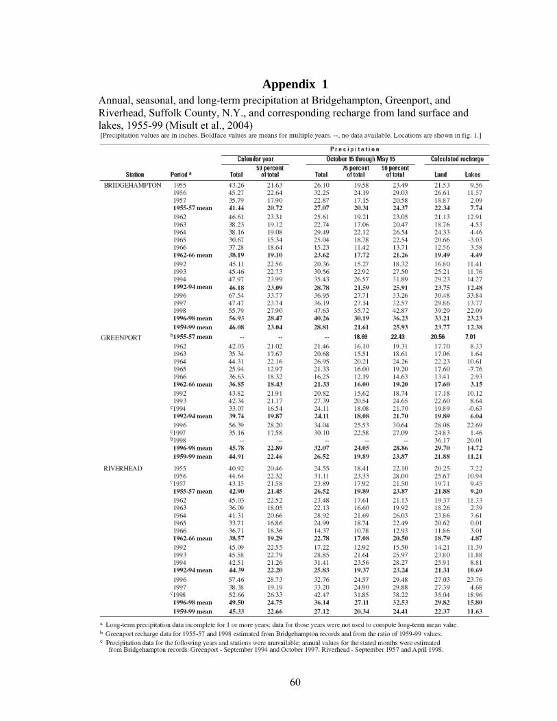
60
Appendix 1 Annual, seasonal, and long-term precipitation at Bridgehampton, Greenport, and Riverhead, Suffolk County, N.Y., and corresponding recharge from land surface and lakes, 1955-99 (Misult et al., 2004)

61
Appendix 2 Map of monitoring wells installed on Shelter Island installed for various studies (Soren, 1978) (Simmon, 1986) (Schubert, 1998) and data collected by the Suffolk County Department of Health for wells used to calibrate/validate the model in this study.
(modified from Schubert, 1998)